Embed Size (px)
Citation preview
IZA DP No. 2737
Comparing Subjective and Objective Measures ofHealth: Evidence from Hypertension for theIncome/Health Gradient
David W. JohnstonCarol PropperMichael A. Shields
DI
SC
US
SI
ON
PA
PE
R S
ER
IE
S
Forschungsinstitutzur Zukunft der ArbeitInstitute for the Studyof Labor
April 2007
Comparing Subjective and Objective Measures of Health:
Evidence from Hypertension for the Income/Health Gradient
David W. Johnston University of Melbourne
Carol Propper
CMPO, University of Bristol, CASE and CEPR
Michael A. Shields
University of Melbourne and IZA
Discussion Paper No. 2737 April 2007
IZA
P.O. Box 7240 53072 Bonn
Germany
Phone: +49-228-3894-0 Fax: +49-228-3894-180
E-mail: [email protected]
Any opinions expressed here are those of the author(s) and not those of the institute. Research disseminated by IZA may include views on policy, but the institute itself takes no institutional policy positions. The Institute for the Study of Labor (IZA) in Bonn is a local and virtual international research center and a place of communication between science, politics and business. IZA is an independent nonprofit company supported by Deutsche Post World Net. The center is associated with the University of Bonn and offers a stimulating research environment through its research networks, research support, and visitors and doctoral programs. IZA engages in (i) original and internationally competitive research in all fields of labor economics, (ii) development of policy concepts, and (iii) dissemination of research results and concepts to the interested public. IZA Discussion Papers often represent preliminary work and are circulated to encourage discussion. Citation of such a paper should account for its provisional character. A revised version may be available directly from the author.
IZA Discussion Paper No. 2737 April 2007
ABSTRACT
Comparing Subjective and Objective Measures of Health: Evidence from Hypertension for the Income/Health Gradient*
Economists rely heavily on self-reported measures of health status to examine the relationship between income and health. In this paper we directly compare survey responses to a self-reported measure of health that is commonly available in nationally-representative individual and household surveys, with objective measures of the same health condition. Our particular focus is on hypertension, which is the most prevalent health condition in Western countries. Using data from the Health Survey for England, we find that there is a substantial difference in the percentage of adult survey respondents reporting that they have hypertension as a chronic health condition compared to that from repeated measurements by a trained nurse. Around 85% of individuals measured as having hypertension do not report having it as a chronic illness. Importantly, we find no evidence of an income/health gradient using self-reported hypertension, but a large (about 14 times the size) gradient when using objectively measured hypertension. We also find that the probability of false negative reporting, that is an individual not reporting to have chronic hypertension when in fact they have it, is significantly higher for individuals living in low income households. Given the wide use of such self-reported chronic health conditions in applied research, and the asymptomatic nature of many major illnesses such as hypertension, diabetes, heart disease and cancer at moderate and sometimes very elevated levels, we show that using commonly available self-reported chronic health measures is likely to lead to an underestimate of true income-related inequalities in health. This has important implications for policy advice. JEL Classification: I10, I18, C42 Keywords: hypertension, objective health, self-reported health, reporting error, income Corresponding author: Carol Propper CMPO University of Bristol 2 Priory Road Bristol BS8 ITX United Kingdom E-mail: [email protected]
* We would like to thank Maarten Lindeboom, Eddy van Doorslaer and seminar participants at the Universities of Bristol, Bergen, Melbourne and Western Australia and Karen Ireland for their helpful comments.
3
1. Introduction The relationship between income and health, and any underlying causal mechanisms, is a hotly
debated topic (see, for example, Deaton and Paxson, 1998; Smith, 1999; Chase, 2002). In
examining this topic, economists have relied heavily on self-reported measures of general health
status and, to a lesser extent, self-reported chronic health conditions. One of the main factors used
to justify the use of such measures is that self-reported health is a significant predictor of future
functioning and mortality within countries (see, for example, Idler and Angel, 1990; Idler and Kasl,
1995; Idler and Benysmini, 1997; van Doorslaer and Gerdtham, 2003; Frijters et al., 2005b).
Recent studies using self-reported measures of general health status and panel data have found only
a weak role for increased income leading to improved health (see, for example, Adams et al., 2003;
Meer et al., 2003; Contoyannis et al., 2004; Frijters et al., 2005a; Lindahl, 2005). However, if such
self-reported measures suffer from some amount of reporting error, this has implications for the
literature and consequently also policy aimed at ameliorating income inequalities.
The extent to which there can be reporting error in self-reported health is thus an important
issue. Such error can occur for a number of reasons (see Murray and Chen, 1992). Survey
respondents may report their health differently depending on their socially driven conceptions of
what ‘health’ means, their expectations of their own health, their use of healthcare, and their
comprehension of the actual survey questions asked (Bago d’Uva et al., 2006). These factors are
problematic because they are likely to vary systematically with observed demographic and socio-
economic characteristics such as education and income and it is these same characteristics that are
most widely used to assess what the relationship between income and health is or whether
inequalities in health exist (see, for example, van Doorslaer et al., 1997). It is also widely
understood that individuals can (consciously) misreport their health given clear financial incentives
to do so. For example, where receipt of welfare payments is conditional on health status,
individuals have an incentive to report their health or extent of disability to be worse than it really
is. This poses problems for empirical studies of the relationship between health status and labour
market outcomes (see, for example, Stern, 1989; Bound, 1991; Currie and Madrian, 1999;
Lindeboom et al., 2006; Kapteyn et al., 2006)1.
There have been two main approaches used to tackle this potential measurement problem. One
is to ‘purge’ self-reported general health measures of reporting error using other measures of health
typically available in survey data that are still self-reported, but are seen to be more objective
(Baker et al., 2004). Most commonly, these are self-reported chronic health measures. These
studies then use the residual variation from a regression of self-reported general health on self-
1 For example, Kapteyn et al. (2006) found that much of the difference in self-reported work disability between the U.S. and the Netherlands is due to different reporting thresholds in the two countries.

4
reported chronic health conditions to examine the extent of any reporting heterogeneity.
Lindeboom and van Doorslaer (2004) found some evidence of reporting bias by age and gender,
but not income, using Canadian data and the constructed McMaster Health Utility Index as their
more objective measure. Hagan et al. (2006) undertake a similar exercise focusing on the effect of
self-reported health on mortality using British data.
It is not, however, clear that these more objective health measures are not also subject to
reporting error. A recent paper by Baker et al. (2004) sheds some light on this issue by matching a
wide range of self-reported chronic health conditions to records of public healthcare usage in
Canada. They found clear evidence that such conditions are subject to a large amount of systematic
reporting error, leading to large attenuation biases when used as explanatory variables. They also
found that false negative reporting, where individuals had used medical services but not reported a
matched health condition in the survey, were around 50% for most chronic conditions examined.2
A recent development has been to examine variation in the reporting of hypothetical health-
related ‘vignettes’ by survey respondents. These are intended to represent fixed levels of latent
health so that all variation can be attributed to reporting behaviour (Salomon et al., 2004). The
assumption underlying this method is that individuals rate the hypothetical vignettes relating to
someone else in exactly the same way as they would rate their own health. There is also the
concern that the vignettes may not represent fixed levels of health. Using this approach Bago
d’Uva et al. (2006) found evidence of reporting differences by income using data from China, India
and Indonesia. In fact, the hypothesis of homogenous reporting across all socio-demographic
characteristics was rejected for all countries and all health domains. This reporting error acted to
reduce the estimated income/health gradient using self-reported general health as the outcome
variable. One explanation proposed by the authors is that higher income groups may have higher
expectations about their health and therefore report their health as lower than it would be if viewed
by an individual with low income.
The extent and impact of reporting error, in particular with respect to the income/health
gradient, therefore remains contentious. In this paper, we attempt to contribute to this literature by
more directly investigating the differences between self-reported and actual health by matching
self-reports of an important health condition, namely hypertension (or high blood pressure), to
precise clinical measures of that same condition. We do this using detailed data drawn from the
2 Baker et al. (2006) match survey data for 1996/7 NPHS survey respondents living in Ontario to self-reported chronic illness diagnosed by a healthcare professional to public healthcare expenditure records recorded over the previous five years. Some 66% of survey respondents were able to be matched to the public healthcare records. Importantly, no matching to private healthcare was undertaken, and there exists a considerable possibility of mis-match due to the difficultly (discussed in their paper) in exactly matching a health condition to the actual health codes used by the public healthcare system in Ontario. Moreover, this form of matching is not able to shed any light on the issue of undiagnosed chronic health conditions, as individuals will not have sought medical advice if they had mild or no symptoms. This is particularly an issue for health conditions such as diabetes and hypertension.

5
Health Survey for England (HSE), which contains information from both survey respondents and
an interview by a trained nurse. Unlike Baker et al. (2004) our data does not have the possibility of
error arising from the need to match separately collected public healthcare records with survey
data, as our clinical measures of the condition are taken from individuals at the same time (within 2
weeks) as they are asked questions about their health. The limitation of our study is that we are
only able to focus on hypertension, as it is the only condition where we can exactly match self-
reported with objective measures.3 However, hypertension is the most prevalent chronic health
condition in Western countries and is a major risk factor for cardiovascular disease. Moreover,
hypertension is often called the ‘Silent Killer’, because it is typically asymptomatic at moderate and
even highly evaluated levels of blood pressure. This makes the issue of undiagnosed hypertension a
major public health concern. In addition, the asymptomatic nature of hypertension at moderate and
sometimes advanced levels is shared by many of the most prevalent chronic health conditions
including diabetes, cardiovascular disease and many types of cancer. This means that individuals
are simply not aware that they have such a condition (often until it is too late) and so self-reported
general health measures would not capture this aspect of poor health. However, the asymptomatic
nature of hypertension also means that our study will obtain estimates of reporting error towards
the upper-bound.
Using the matched information from individual questionnaires and nurse interviews, we
investigate if there are differences in the estimated relationship between socioeconomic
characteristics, with a particular focus on income, and the probability of having hypertension using
self-reported compared to objective measures. We then examine whether there are systematic
reporting differences by socio-economic characteristics, by estimating a model of false negative
reporting. In addition to standard demographic controls, we are also able to control, given the broad
topics covered by the HSE, for the use of hypertensive medication, the severity of the disease,
individual lifestyle choices and the availability and use of healthcare.
2. Key facts about hypertension
Hypertension or elevated blood pressure is an extremely prevalent health condition, with the
worldwide prevalence estimated to be as high as 1 billion individuals. In the US alone, it is 3 In principal we can also exactly match individuals self-reports of having diabetes as a chronic health condition with a clinical measure of diabetes (glucose) taken in the nurse interview. No other measures except hypertension and diabetes have a direct correspondence between what is asked in the individual questionnaire and what can be measured from the nurse interview (or later tests conducted on blood and saliva samples taken by the nurse). However, unlike blood pressure measurements that are simple to conduct, data on glucose is only collected from a small sub-sample of the HSE in only selected years. We do not use the diabetes information in this paper because of a major selection issue that results in a very low prevalence rate in the HSE. In particular, the problem is that individuals (in the selected sub-sample of the total sample) are required to fast for 24 hours before the nurse interview so that an accurate measure of insulin can be obtained. The problem is that individuals who already know that they have diabetes have no incentive to agree to the fast. Such a problem does not arise with measuring blood pressure.

6
estimated that some 50 million adults currently have high blood pressure (BP) that warrants some
form of medical treatment (JNC7, 2004). While hypertension can occur in childhood and
adolescence, the condition is mostly an adult concern, partly arising from the need for the heart to
pump harder as the body ages.
A salient aspect of the condition for our analysis is that moderate, and even high levels of
elevated BP, are typically asymptomatic. It is this aspect of the condition, as for mild diabetes or
cardiovascular disease, which makes it particularly problematic if individuals are simply unaware
that they have hypertension. Undiagnosed hypertension is therefore a major public health issue in
Western countries. It is only at a severely elevated level of BP that an individual may experience
some symptoms, which can include headaches, an increase in heart rate and a general feeling of ill
health. Importantly, the relationship between BP and the risk of coronary vascular disease is
continuous and independent of other risk factors. The higher the blood pressure, the higher the risk
of a heart attack, heart failure, stroke, and kidney disease. It is estimated that approximately 7.1
million deaths per year in the US may be attributable to hypertension including death from heart
disease, stroke, diabetes, chronic kidney disease and dementia (JNC7, 2004).
In addition to increasing with age, hypertension has a strong hereditary link (JNC7, 2004).
Moreover, a number of other important causal factors for hypertension have been identified in the
medical literature. These include excess body weight, excessive levels of dietary sodium intake,
excessive alcohol consumption, smoking, reduced physical activity and inadequate intake of fruits
and vegetables (JNC7, 2004). As we will see in our data, the prevalence of these lifestyle choices
is high in the English population. In the US about 30% of adults are either overweight or obese and
the figure for the UK is 25% (Flegal et al., 2002).
The positive aspect of hypertension is that it is treatable, and control of the condition is
associated with favourable trends in the morbidity and mortality associated with the disease.4
Primatesta and Poulter (2006) have estimated that at least 45,000 fatal and non-fatal cardiovascular
episodes could be prevented each year by treating all uncontrolled hypertensive adults in England
alone. Recommended treatments are drug therapy combined with lifestyle modification. Low levels
of hypertension can be controlled with one drug; higher levels require two (or more)
antihypertensive agents selected from different drug classes. Suggested lifestyle modifications
include weight loss programmes and changes in diet to reduce sodium intake. Lifestyle
modification has been estimated to provide substantial benefits. For example, weight loss of as little
as 4.5kg reduces BP and/or prevents hypertension in a large proportion of overweight persons.
Likewise, a low sodium eating plan has BP effects similar to a single drug therapy (JNC7 2004). 4 In the US, since 1972, age-adjusted death rates from stroke and coronary heart disease have declined by approximately 60 and 50 percent respectively and these benefits have occurred independent of gender, race or socio-economic status. JNC7 (2004) links these to higher treatment rates of BP.

7
Levels of hypertension are therefore related to age, hereditary predisposition, lifestyle choices
and medical treatment. Poor control of BP has been argued to be related to both physician and
patient attitudes. In the US, certain groups such as young men are particularly unlikely to adhere to
treatment regimes, while women are more likely than men to know they have hypertension, to have
it treated and to have it managed (Burt et al., 1995).
In clinical practice and hypertension research, blood pressure is typically calculated by
measuring the pressure of an inflated cuff placed around the upper arm. This test provides two
pieces of information: Systolic BP (SBP) measures blood pressure when the heart beats and
Diastolic BP (DBP) measures blood pressure between beats. Both are measured in millimetre of
mercury (mmHg). The combined use of these two measures is the most commonly used method to
diagnose hypertension. The recent medical literature on hypertension provides the following cut-
offs: ‘Normal’ BP is diagnosed when SBP is less than 120 and DBP is less than 80;
‘Prehypertension’ is having a SBP of 120-139 or a DBP of 80-89; ‘Stage 1 Hypertension’ is having
a SBP of 140-159 or a DBP of 90-99; and ‘Stage 2 Hypertension’ is having a SBP greater or equal
to 160 or a DBP greater or equal to 100 (JNC7, 2004).
3. Data, definitions, sample characteristics and simple bias calculations
3.1 The Health Survey for England
Our data source is the Health Survey for England (HSE), which was commissioned by the
Department of Health, and carried out by the Joint Health Surveys Unit of Social and Community
Planning Research, and the Department of Epidemiology and Public Health at University College
London. Beginning in 1992, the HSE is an annual survey and is designed to monitor trends in the
nation’s health. The unit of survey in the HSE is the household, and information is collected from
both adults and children living in England (children aged 12-15 complete a questionnaire, while a
parent provides information about younger children). Importantly, information is collected through
a combination of a face-to-face interview, a self-completion questionnaire and a medical
examination (including various measurements such as height and weight, and the taking of a blood
and saliva sample for clinical tests) conducted by a trained nurse. Using the Postcode Address File
as a sampling frame, the HSE is considered to be representative of England: additional details of
the sampling procedure can be found in Prescott-Clark and Primatesta (1998).
In this paper, we pool data from the 1998 and 2003 HSE’s. In both of these years, additional
information was collected from respondents relating to the risk factors for Cardiovascular Disease
(CVD). This provides us with additional information relating to hypertension that we utilise in our
empirical models. We focus on adults aged 25+ at the time of interview, which provides a total
sample of 27,000 adults. We exclude adults aged less than 25 because the incidence of

8
hypertension for this group is extremely low. When we focus on respondents for whom we have
observed valid blood pressure measurements, this gives a working sample of just over 18,600
adults (more details provided below). The size of the sample was larger in the 1998 than 2003 HSE,
so 55.9% of our working sample comes from 1998. The average age is 51.8 years, 44.7% are male,
65.2% are married or co-habiting, 14.6% hold a degree or equivalent level qualification, 58.5% are
employed either full or part-time, and 27% are retired. The average pre-tax household income is
£27,0075 and the sample is fairly evenly distributed across the English regions. In terms of health-
related characteristics, 23.1% are clinically obese as measured by the nurse (i.e. their BMI≥30),
22.1% are smokers, 16.3% report to drink alcohol on a daily basis, 22.3% report that they regularly
participate in vigorous exercise or sports, and 12.6% report eating fried food at least 3 times each
week.
3.2 Self-reported and objective measures of hypertension
The HSE provides contemporaneous and directly comparable, self-reported and objective measures
of the same health condition, namely hypertension. At the start of the HSE individual
questionnaire, respondents are asked:
“Do you have any long-standing illness, disability or infirmity? By long-standing I mean anything
that has troubled you over a period of time?”
Each respondent can report up to six such conditions, and these are grouped together by the
data organisers into 42 categories. Category number 17 is hypertension or high blood pressure,
which we use to create a binary self-reported measure of hypertension (SR1). We select this
measure because this type of question, asking respondents about their chronic health conditions, is
common in household surveys and it is widely used by researchers as a measure of health status.6
Further, we want to compare a commonly available measure of health with a clinical measure of
the same condition to assess the consequences of having to rely on such subjective health
5 The main measure of income that we use is current total pre-tax annual household income, which is provided in 31 bands in the HSE data, ranging from less than £520 to more than £150,000. To get a continuous measure of household income we took midpoints of these bands and deflated them (to 2000 prices) using the UK average earnings index according to the month in which the interview was conducted. Hence, we have a pseudo-continuous measure with over 700 potential values (31 bands * 12 months * 2 years) for total household income, which we then convert into natural logarithms for use in the statistical analyses. We also conduct some robustness tests later in the paper using alternative functional forms for household income. 6 Note that if there are individuals who are aware that they have hypertension but do not consider it a chronic illness, our measure will underestimate individual’s knowledge of their hypertensive status. However, the aim of this paper is to evaluate the reporting error that exists using a commonly available measure of health rather than establishing hypertension prevalence rates.
9
information to estimate the income/health gradient or to help ‘purge’ self-reported general health
status from reporting error (see, for example, Case et al., 2002).
The HSE also contains another self-reported hypertension measure, where the conditions of
‘long-standing disability or infirmity’ are not posed in the question. Respondents are asked “Have
you ever had your blood pressure measured by a doctor or nurse?” If the answer was “Yes”, they
were then asked, “Thinking about the last time your blood pressure was measured, were you told it
was.., (1) Normal, (2) higher than normal, (3) lower than normal, or (4) were you not told
anything?” While we provide some statistics for this alternative self-reported measure we do not
use it in our empirical models of the income/health gradient or false negative reporting because it is
not available in most surveys and so is not generally used in the literature on purging measures of
self-reported health or income-health gradients. In addition, there is also a clear timing issue. Only
64% of the sample reported having their BP tested sometime in the last 12 months, just below 10%
reported that it is longer then five years ago that they were last tested and 3.3% reported never to
have had their BP tested. Moreover, we want to compare having currently measured hypertension
by a nurse with contemporaneous self-reported hypertension (and contemporaneously measured
socioeconomic characteristics).7
At the end of the individual interview (e.g. on page 63 of the 2003 questionnaire), respondents
were asked if they agreed to a visit with a qualified nurse in order to “collect more medical
information and carry out some measurements”. Some 90.9% agreed to this visit. Of those who
agreed, 90.3% actually had the nurse interview (or 82.1% of total sample). Virtually all nurse
interviews were conducted within two weeks of the initial face-to-face interview.
A key component of the nurse interview was the taking of repeated blood pressure (BP)
measurements. A BP reading was taken three times in the interview, and of those who had the
nurse interview, valid BP measurements were collected from 84.9% of respondents (or 69.7% of
total sample). This gives us our working sample of 18,600, for whom we observe both self-reported
and nurse measured hypertension.8 Note that an ‘invalid’ BP measurement occurred if a respondent
7 Another question was used by Banks et al. (2006) as a measure of ‘lifetime’ hypertension prevalence in the 2003 HSE. Respondents are asked, “Do you now have, or have ever had, high blood pressure”. If the answer was “Yes”, respondents were then asked, ‘Were you told by a doctor or nurse that you had high blood pressure?” Just over 25% (25.8%) of our sample report a positive reply to this question, which corresponds to the 32% reported by Banks et al. (2006) for their sample of 40-70 year olds in the 2003 HSE. As with the SR2 measure, we do not use this lifetime prevalence measure in our empirical models because we are looking at the relationship between self-reported beliefs of currently having hypertension with currently measured hypertension by a nurse. For example, only 59% of individuals reporting positively to the above question were measured by the nurse to currently have 140/90 hypertension in our sample. Similarly, 26% of respondents reporting never to have been told by a doctor or nurse that they had high blood pressure are measured by the nurse to be hypertensive. Also, like SR2 this lifetime prevalence measure is not commonly available in individual or household surveys. For example, in the UK context, while self-reported chronic health conditions are reported in the British Household Panel Study, the UK’s Quarterly Labour Force Survey and the UK’s General Household Survey, no other measure of self-reported (not objectively measured) conditions is available. 8 There does not appear to be any selection on the main observable characteristics. For example, 44.7% of the total sample are male compared to 44.3% of the working sample; the average age of the total sample is 51.1 compared to
10
had eaten, smoked, drunk alcohol or undertaken vigorous exercise in the last 30 minutes, and that
the majority of the invalid cases arise arose because a respondent had recently eaten. Blood
pressure measurements were not taken from pregnant women. As is standard in the medical
literature, we use the average of the 2nd and 3rd blood pressure readings, which allows for the
possibility that the first measurement might be higher than usual (e.g. because of initial interview
nerves, or because of the initial physical exertion before the interview begins). It is likely that this
average BP reading will still contain some measurement error. For example, measurement error can
arise from inaccurate equipment, incorrect testing procedures, or the use of a wrongly sized cuff.9
There is no reason to think, however, that any error will be correlated with socio-demographic
characteristics, and so it will not invalidate any of our main conclusions.
Following standard medical practice (see Section 2), we define a survey respondent in this
paper as having at least Stage 1 hypertension if their SBP is greater than or equal to 140 or their
DBP is greater than or equal to 90 (≥140/90). However, we also estimate models where we use the
continuous SBP measure as our dependent variable. We also conduct a number of tests which show
that our main results, with respect to socio-economic differentials in hypertension, remain robust to
the exact measures used. In addition, in both the 1998 and 2003 HSE, respondents were also asked
in the individual questionnaire, before the nurse survey was conducted, whether they have ever had
their BP tested, and if so, how long ago. Only 3% reported that they had never had their BP tested.
Information was also collected on whether individuals reported currently taking BP medication. We
use this additional information as control variables in our empirical models.
3.3 The extent of hypertension and false reporting
Table 1 provides some descriptive statistics for hypertension in England from the HSE. The mean
level of SBP in the sample is 134.9 mmHg and the mean level of DBP is 74.6 mmHg. Most
importantly, only 7.1% of the sample reported that they currently had hypertension as a chronic
illness, while 34.7% had clinical hypertension (≥ 140/90) as measured by the nurse. The raw
correlation between our two measures is only 0.17. The level of false negatives in this context,
which is the percentage of individuals who have measured hypertension but do not report currently
having hypertension as a chronic condition, is extremely high at nearly 87%.
Alternatively using SR2, we see just over 11% of respondents reported that they were told by a
doctor or nurse that they had higher than normal BP when last tested. The raw correlation between
51.8 for the working sample; and the average annual pre-tax household income for the total sample is £27,128 compared to £27,007 for the working sample. 9 There were, however, three different size cuffs available for the nurse to use: small adult cuff (17-25cm), standard adult cuff (23-33cm) and large adult cuff (31-40cm).

11
SR2 and clinical hypertension (≥ 140/90) is only a little higher at 0.22, and the false negative rate
remains very high at 77%.10
Taken together, these results are suggestive of a substantial public health problem of
undiagnosed hypertension in England since there are well-established long-term health
consequences of hypertension and BP medication is very inexpensive and effective at reducing BP.
Note that our use of self-reported chronic hypertension will overstate the extent of
underdiagnosis.11
In contrast, the level of false positives (individuals who stated they had hypertension when in
fact their blood pressure was lower than 140/90) was only 4% (or 6% using SR2). Baker et al.
(2004) found similar low levels of false positives for hypertension using Canadian data, but lower
levels of false negatives. The level of false negatives in Baker et al. (2004) varies considerably
depending on the assumptions they make about the relevant time-period when matching data from
self-reports to public healthcare records. The HSE data requires no matching and so cannot suffer
from matching issues.
An alternative definition of hypertension sometimes used in the medical literature (see, for
example, Primatesta and Poulter, 2006) is when an individual has measured BP≥140/90 and/or
they are currently taking some form of BP medication. Some 13% of respondents in our sample
reported that they were taking BP medication at the time of the individual interview. Given that
only 7% report having hypertension, this suggests that many individuals who are taking BP
medication incorrectly believe that their BP is at normal levels. If we use this alternative definition,
the percentage with hypertension increases to 39.1% (from 34.7%) and the level of false negatives
falls by about 3% (83.7% from 86.9%). The level of false positives also falls from 4% to 1%. The
use of either of these two alternative measures of clinical hypertension does not, however, make
any difference to the substantive results that we present.
The next three figures show descriptive statistics with respect to age, household income and
region of residence, and the prevalence of hypertension in England. Figure 1 plots both self-
reported and objective hypertension by age. As expected, both increase, but measured hypertension
rises considerably faster with age than self-reported chronic hypertension. This is suggestive of
undiagnosed hypertension becoming more of a problem as individuals’ age. Importantly, the data
also clearly reveal (Figure 2) a very large hypertension differential by household income, with
10 If we restrict our attention to those reporting that they have had their BP tested within the last years, 14.5% of the sample report being told that they have higher than normal BP by a doctor or nurse. Even with this restriction, we still get a false negative rate of 75%. 11 Primatesta and Poulter (2006) report that about 62% of individuals who have measured hypertension are aware of the condition, using an awareness measure based on HSE respondents reporting that they have been told by a doctor or nurse at some point in their life that they had high blood pressure. However, it is not clear how this ‘lifetime’ measure relates to an individual’s current awareness of having hypertension. Also, this is the same measure that Banks et al. (2006) use as their lifetime hypertension prevalence measure.

12
individuals living in households in the lowest quartile of income having roughly double the
probability of being measured by the nurse as hypertensive. A much smaller differential is also
evident for self-reported chronic hypertension, and taken together with the objective measure,
suggests that undiagnosed hypertension might be more prevalent in poorer English households.
Finally, Figure 3 presents the percentage of individuals with self-reported and objective
hypertension by broad English region. There is some evidence of a general North-South divide with
the highest prevalence of objectively measured hypertension being in the North East (42.2%) and
Yorkshire (37.6%), and the lowest in London (28.5%). These are very large differences, especially
if thought of in terms of actual population numbers: the North East would have around 300,000 less
adults with hypertension if its prevalence was at the London level. No such regional differential,
however, is observed for self-reported chronic hypertension. Most importantly, it is also clear from
these figures that policy-makers could be easily mislead about inequalities in hypertension at the
population level if they were to rely solely on the results of studies that used only a self-reported
measure of chronic hypertension.
Amongst other hypotheses that we explore in our empirical models is whether or not these raw
income and regional differences still remain after we have controlled for a large set of factors
which could be driving this correlation including lifestyle choices, smoking, drinking, obesity;
access and choices regarding healthcare, including time since having a BP test, whether currently
on BP medication and the number of GPs per capita in the local area.
Finally, there is some positive news gained from looking at differences in self-reported and
objective hypertension between 1998 and 2003.12 If we looked at only self-reported hypertension
the picture would seem negative: in 1998 only 5.5% of respondents reported having hypertension
compared to 8.5% in 2003. If this was the only information we had available we might wrongly
conclude that the prevalence of hypertension had increased over this 5-year period. However, over
the same period objective hypertension fell from 37.1% to 31.1%, and the average measured
systolic BP fell from 135.9 to 133.5 (75.5 to 73.3 for diastolic BP). Combining both these sources
of information gives a more positive picture: awareness of hypertension has increased and the
management of hypertension also improved over this period (also see Primatesta and Poulter,
2006).
12 Note that in the 2003 HSE, the blood pressure equipment was changed from Dinamap to Omron. However, for consistency purposes, the 2003 HSE reports Dinamap equivalent measurements that are calculated using a well established calibration factor (see Primatesta and Poulter, 2006). In this paper, we use Dinamap measurements from 1998 and Dinamap equivalent measurements from 2003.
13
3.4 Simple bias calculations
Error in self-reported health measures will lead to biased coefficient estimates when the self-
reported measure is used either as an explanatory or dependent variable. While the primary focus of
this paper is the differential in the estimated income/health gradient when subjective compared to
objective hypertension measures are used, here we present some simple bias calculations when self-
reported hypertension is used as an explanatory and dependent variable. To do this, we use the
framework of Bound et al. (2001), which allows for a direct comparison with the results from
previous validation studies.
In the case where self-reported hypertension is used as the sole explanatory variable in a
regression model, the proportional bias (minus the ratio of the bias to the true coefficient value) is
equal to the coefficient from a regression of the error on self-reported health (denote this value as
θ).13 If self-reported hypertension is used as a dependent variable (for example, in a probit model)
and it is assumed that any measurement error is uncorrelated with the explanatory variables in the
model, then the proportional bias in the marginal effects equal the sum of the false negative and
false positive rates (denote this value as δ).
Our estimate of θ is 0.68. In other words, if self-reported hypertension is used as an
explanatory variable instead of objective hypertension, the estimated coefficient will be 68%
smaller than the true value. This estimate is much larger than the figure reported in Baker et al.
(2004), who calculated that the proportional bias due to self-reported hypertension is 0.36 using
Canadian data. Our estimate of δ is 0.91. Again, this is substantially larger than Baker et al.’s
estimate, which equals 0.46.14 The difference between our proportional bias estimates and those
reported in Baker et al. is a result of the much higher rate of false-negative reporting that we
observe. One possible reason for this difference is the reliance by Baker et al. (2004) on matching
subjective survey responses to past medical records and therefore a doctor’s particular diagnosis.
Our proportional bias estimates are also large compared with validation studies of other variables.
For example, Card et al. (2004) investigated the accuracy of reported Medicaid coverage in the
Survey of Income and Program Participation and found values of θ and δ equal to 0.20 and 0.18,
respectively.
13 We follow other validation studies and limit our analysis to the scenario where self-reported hypertension is the only regressor. When this is not the case, the proportional bias becomes the coefficient from a regression of the measurement error on all the explanatory variables. 14 Baker et al. (2004) do not provide an estimate of the bias when self-reported health is used as a dependent variable. However, the sum of the false negative and false positive rates given in their Table 1, under the column ‘Narrow Mapping’, equal 0.46.

14
4. Empirical results
4.1 The estimated health-income gradient
In this section we start by examining whether the lack of income gradient in self-reported chronic
hypertension and the large gradient in measured hypertension, as well as the clear regional
differentials, seen in the raw data are robust to controls for demographics, education, genetic
predisposition, measures of location, employment, health and lifestyle. We begin by estimating
simple probit and regression models that control for basic demographic characteristics and year of
survey. We then extend the models to control for education, location and genetic predisposition.
Finally, we add in employment status, obesity and measures of lifestyle. The estimates are
presented in Tables 2 and 3. The Pseudo R2 measure indicates a reasonable goodness-of-fit for each
model, in the range of 0.25 to 0.31.
This large set of controls allows us to examine the impact of income after allowing for
observables which are likely to be correlated with income and region. In addition, differences in
awareness and incidence of hypertension across different social groups are of interest in their own
right. For example, conditioning on employment status allows us to examine whether the
‘justification’ hypothesis, i.e. that reporting health problems is both a socially acceptable
rationalisation of lack of labour market participation and one which allow individuals to access
higher welfare payments (e.g. Kapteyn et al., 2006), may affect hypertension reporting.
Conditioning on obesity, genetics and lifestyle allows us to examine whether individuals who are at
greater risk are aware of their greater risk.
Table 2 presents the marginal effects of the estimated relationship between the self-reported
and two objective measures of hypertension and income, controlling for only basic demographic
variables. The two objective measures are the standard definition of hypertension and the level of
systolic blood pressure as a measure of severity. The Table shows no income gradient for self-
reported chronic hypertension but a clear negative gradient in both objective measures: individuals
living in low income households are significantly more likely to have hypertension and also to have
more severe hypertension. Its is important to note that the calculated marginal effect of a one-log
point increase in household income is around 14 times larger (-0.002 compared to -0.028) when
using objectively measured rather than self-reported hypertension. If we take the six log-point
variation in household income observed in the data, this would mean a 16.8 percentage point
difference in the probability of having recorded hypertension between the poorest and richest
individuals.15 If we estimate this model using SR2 as the binary dependant variable, that is the
individual reporting to have been told that they had higher than normal BP when last tested, the
15 We have also run the models using diastolic BP as our objective measure. In this case, the coefficient on log household income is again negative and statistically significant (i.e. -0.242, t-stat=-2.02).

15
coefficient on log household income is -0.017 (t-stat=-4.88).16 Therefore if we take SR2 to be to
some extent more objective than SR1, as expected the coefficient estimate on income gets closer to
that found using the clinical measure.
Note that we are treating income as exogenous in these models. We believe that this is a valid
assumption because hypertension has a unique set of properties: it is typically asymptomatic except
at extremely elevated levels, it is often undiagnosed and it can be treated very inexpensively. Given
these characteristics, hypertension is unlikely to affect labour market behaviour and as a result is
unlikely to affect an individual’s income.
Table 2 also shows demographic differences in the self-reported and objective measures. Men
do not report chronic hypertension, yet are considerably more likely to actually have measured
hypertension than women. In contrast, individuals from ethnic minorities are more likely to report
that they have hypertension, when in reality they have very similar actual rates to the rest of the
population. The reporting behaviour of the married and non-married is not significantly different,
although individuals who are married are less likely to have hypertension than those that are not
married. The final set of coefficients in this table shows the change between the two survey years.
As suggested by the raw data in Section 3, the prevalence of objective hypertension has fallen: for
example, systolic blood pressure has fallen by just over 3 points. However, reported hypertension
has actually risen.
Table 3 extends the set of controls. Extended Model 1 adds controls for education and genetic
predisposition to hypertension as captured by parental deaths from cardiovascular disease.
Importantly, the lack of income gradient in the self-reported measure and the gradient in objective
measures remain, although the magnitude of the coefficient on household income for the objective
measures is roughly halved. Conditional on income, education has no impact on self-reported
hypertension but is negatively associated with objective measures. As expected given the medical
literature, individuals with a family history of cardiovascular disease recognise their greater risk,
but the impact of parental history on reporting is less than on the risk of actually having
hypertension. The second three columns add controls for location, work status, obesity and life
style. The first row shows that the income gradient changes very little allowing for these additional
controls. Importantly, in terms of health inequalities in England, the coefficients on the controls
indicate that the differences in self-reported and objective health by region seen in the raw data
remain. While there are no significant differences in either self-reported or objective hypertension
by rural or urban residence, there are significant and large differences between regions. Individuals
outside the South East are less likely to report hypertension as a chronic illness, while in fact they
have significantly higher objective levels. 16 These additional results are available on request from the authors.
16
The work status estimates give limited support to the idea that individuals may report this
condition to justify non-participation in the labour market. Both non-participants and the disabled
report higher rates of hypertension, while neither actually have higher rates. Being obese is
associated with both reporting and actually having hypertension, but the estimated marginal effect
of obesity on the chance of self-reporting is considerably lower than the effect on the probability of
actually having the condition. Those who take vigorous exercise/sports and do not smoke are less
likely to report that they have hypertension, while those who drink alcohol daily are not. In fact,
alcohol consumption is positively associated with actual hypertension while the other behaviours
are not.
In summary, while controlling for education, work, lifestyle, area of residence and genetics,
approximately halves the estimated size of the association between income and hypertension, these
controls do not change the basic picture that self-reports, as commonly used by researchers, are not
income graded despite the fact that there is a strong negative relationship between income and
objective levels of hypertension. The findings of significant regional differences in hypertension
also remain after controlling for the extensive list of socio-economic variables.
4.2 Investigating false negatives reporting
The previous sections showed the difference in the prevalence of self-reported chronic hypertension
versus objectively measured hypertension. Individuals may misreport for a variety of reasons
including:
a. They had no symptoms and so have not sought medical advice;
b. They had symptoms and sought medical advice, but either the medical practitioner found no
evidence of hypertension or did not tell them they had hypertension;
c. They were tested and told that they had high blood pressure, but did not report it as a chronic
illness when asked in the individual questionnaire;
d. They were tested and prescribed BP medication, and so believe that they are no longer
hypertensive when in fact they still are.
The importance of each reason will depend on individual attitudes and knowledge about health, the
severity of hypertension, lifestyle and attempts to control hypertension, and the availability and
response of medical care. In this section, we attempt to better understand the extent and reasons for
reporting errors in self-reported chronic illnesses by explicitly modelling the role of observable
characteristics on the propensity for an individual to misreport. Here we define a misreport to have
taken place if SR = 0, but measured BP≥140/90 i.e. a false negative report. In using this definition,

17
we do not focus on the individuals who incorrectly reported hypertension (the false positives).
However, as Table 1 shows only 3.8 percent of individuals committed such an error.
The difficulty in modelling this reporting error is that false negative reporting can only occur
for individuals who have measured hypertension BP≥140/90. We do not observe whether a non-
hypertensive individual would misreport if they were hypertensive. To estimate the impact of
observables on an individual’s potential to misreport, we use the Censored Bivariate Probit model
introduced in Van de Ven and Van Praag (1981). This model consists of two latent equations, one
describing the propensity to misreport ( *1y ) and the other describing the propensity for an
individual to be measured as hypertensive ( *2y ):
* , 1, 2ji ji j jiy x jβ ε′= + =
where the realisation of the latent variable *1y is denoted by 1y and equals 1 if *
1 0y > and *2 0y > ,
and zero otherwise; xji are vectors of socio-demographic characteristics; and ε1i, ε2i are distributed
bivariate normal with variance equal to one and covariance equal to ρ. The model is estimated by
Maximum Likelihood. The non-zero covariance accounts for unobservable characteristics that
affect both the propensity to misreport and the propensity to be measured as hypertensive. For
example, this may arise if individuals with high discount rates are more likely to be hypertensive
and to misreport, and individuals’ discount rates are not directly observed.
For the model to be well identified, four dummy variables indicating whether the individual’s
mother and father died of cardiovascular disease before or after the age of 60 are excluded from the
misreport equation. These variables are valid exclusions if they influence the probability of having
hypertension but do not directly affect the probability of misreporting. Therefore we are using the
fact that there is a strong hereditary component in hypertension for identification purposes.
Statistical tests indicate that these instruments are highly significant in the hypertension equation
and so the first assumption is satisfied (see Chi-squared statistics in Table 4). The second
assumption cannot be directly tested; however, it may be violated if having a parent die of
cardiovascular disease alters an individual’s health-related behaviour (e.g. more frequent doctor
visits) or the treatment received by a doctor (e.g. higher propensity to receive medication). The
advantage given by the richness of the HSE data is that we are able to explicitly control for these
possibilities by including in the misreport equation variables that represent time since last blood
pressure test, whether the individual has been prescribed blood pressure medication and the severity
of hypertension (as measured by systolic and diastolic values).

18
The marginal effects from the bivariate censored probit models and the associated z-statistics
are presented in Table 4. Overall, the models appear to be well identified, the instruments included
in the hypertension equation are statistically significant and the estimated correlation between the
error terms of the two equations is positive and significant. The first column of the table examines
the association with household income, allowing for basic demographics and change over time. The
second allows for a more in-depth analysis of misreporting by adding controls for education, work
status, region of residence, lifestyle, measures of the availability of medical services, measures of
the use of medical services for hypertension, and the actual level of systolic blood pressure. Use of
this wide ranging set of controls allows us to test whether any income gradient in misreporting is
robust to behaviours of individuals or medical providers that are associated with income.
The first column of the Table 4 shows that the negative association between income and the
propensity to misreport is robust to basic demographic controls. The differences between men and
women seen in the previous section remains: in common with other studies we find men are
significantly less likely to recognise they have the disease than women. Perhaps more surprisingly,
those from ethnic minorities are less likely to report a false negative (though this is not robust to the
large set of controls in the second column of estimates). The results also show a clear fall in
misreporting over time. The time effect is robust to medical intervention. So it is not simply the
result of an increase in the testing of blood pressure or the prescription of BP medication by GPs.
The greater stress on primary care by the Labour administration post 1997, alongside general
attempts to increase public awareness of health (for example, the ‘5 a day campaign’ which seeks
to increase fruit and vegetable consumption), may account for the rise in awareness, and the fall in
actual prevalence, of hypertension17.
The next set of results allows for the other controls. For this condition, there is only weak
evidence of differences in false reporting by education (conditioning on income). Nor does the
justification hypothesis appear to have an effect on reporting behaviour. Both these results are
rather different from those found looking at the differences in reporting behaviour relative to
broader medical conditions (for example, the vignette analysis of Bago D’Uva et al. (2006) or the
literature on employment and reported health status). The lack of impact of education may be
because the HSE has better measures of income than other surveys and so the education parameter
does not pick up some of the income effect, or it may be that there are smaller differences across
education when we examine awareness of a specific condition rather than general health. The
nature of hypertension probably accounts for the lack of importance of work status. If moderate
hypertension is asymptomatic then it cannot limit ability to work, so will not be used to justify 17 In addition, in 2004, the UK government adopted a new performance framework for GPs intended to increase the extent of preventative care by linking payments to meeting targeting for preventative care. This post-dates the data used here.

19
being out of work. The final row of the first column shows the clear change in reporting behaviour
between the surveys. The marginal effect is large – of the same order as the well known difference
between males and females.
The results also show strong regional differences in awareness of hypertension that do not
appear to be explained by either the observed characteristics of the individuals who live in those
regions, their level of health, their lifestyles or the medical care they have received for
hypertension. Individuals in all regions outside Greater London are more likely to report false
negatives. Most of the regional differences are statistically significant and the effects not trivial.
Individuals in the South East region, which is contiguous with London, are around 6 percentage
points more likely to report a false negative, whilst those in the North East are 12 percentage points
more likely than those who live in London.
Individuals who are at risk of higher hypertension because of their obesity are nearly 10
percentage points less likely to recognise that they have hypertension, controlling for diet, lifestyle
and exercise (which themselves have no statistical impact on false reports). The general availability
of medical care does not appear to affect misreporting, but specific medical intervention for
hypertension does affect the propensity to misreport. The more recently an individual was tested for
hypertension the less likely they are to report a false negative. The effects of recent testing are
large: individuals who were last tested five years or more prior to the survey are nearly 20
percentage points more likely to false report compared to those tested in the last year. Those who
are taking blood pressure medication are also less likely to report a false negative. Finally, those
who have higher blood pressure are more likely to correctly report that they have hypertension.
In summary, our results show systematic differences across individuals in their awareness of
having hypertension. In particular, those with low income, males, the aged, those living outside
London (especially in the North East and Yorkshire), and individuals who are obese are less likely
to recognise that they have the condition. Medical intervention directed at the detection or
treatment of hypertension appears to significantly lower the risk of false reporting as does a rise in
the awareness of hypertension.
4.3 Robustness tests
We have conducted a number of robustness tests by including additional control variables in the
false negative selection model. Firstly, we have relaxed the functional form of household income
by using both decile and quartile dummies instead of log household income, as well as including
the actual income bands (grouped) as reported in the survey. Each of these more flexible forms
suggests that log household income provides a good approximation. If we use simply income
quartiles, for example, relative to being in the lowest quartile the estimated marginal reduction in

20
the probability of false negative reporting of being in income quartile 2 is -0.043 (t-stat=2.23),
quartile 3 is -0.0584 (t-stat=2.41) and quartile 4 is -0.068 (t-stat=2.56).
We have also investigated whether controlling for stress, anxiety, depression and sleeplessness
can explain away the income and region findings. It might be that low income is associated with
high levels of stress that then leads to hypertension, and that living in some areas of England is
more stressful than others. Including dummy variables for feeling unhappy, feeling under strain and
suffering from sleeplessness (using information collected as part of the General Heath
Questionnaire, GHQ12) in both the hypertension and false negative equations does not change at
all our income or regional results, which remain statistically significant and large in magnitude.
In terms of capturing area differences in healthcare supply (i.e. the availability of medical
personnel to measure blood pressure) we control in the model of false reporting for the number of
GPs per capita at the (100) District Health Authority. We also tried a number of hospital supply
measures including information on waiting times for elective surgery. As with GP per capita, we
found that the estimated role of hospital supply measures is never statistically significant.
We have also tested the robustness of our false negative results to two alternative definitions of
objective hypertension. If we follow Primatests and Poulter (2006) and define having hypertension
as having measured BP at 140/90 or/and reporting currently taking BP medication, then the
marginal effect for a one-log point change in household income (using Extended Model 3 controls)
is -0.022 (t-stat=-2.12), and the marginal effects for living in the North East is 0.113 (t-stat=3.49)
and Yorkshire is 0.070 (t-stat=2.51). Moreover, if we increase the required levels of measured BP
necessary to be diagnosed with hypertension to having SBP≥ 150 (instead of ≥ 140) or DBP≥95
(instead of ≥90), then the equivalent marginal effects are -0.018 (t-stat=1.85), 0.091 (t-stat=2.44)
and 0.074 (t-stat=2.19), respectively. Therefore, our main findings are robust to the exact definition
of objective hypertension used to define false negative reporting.
There is some discussion in the medical literature that males over 50 years of age should have
a higher cut-off of SBP and DBP to be considered hypertensive. Consequently, we have re-
estimated the selection model both dropping males in this age group from the sample and also
introducing a new cut-off of SBP≥160 and/or DBP ≥95 for them. Again these different cut-offs
make no substantive difference to our results. For example, when we drop males aged over 50 from
the sample, the marginal effect on log household income increases to -0.029 (t-stat=2.33).
Finally, we have controlled for the possibility that hypertension might be correlated with a
higher probability of having other health conditions. For example, it might be the case that
individuals with a serious health condition report that condition but do not report a lesser condition.
If this condition is hypertension this would lead to false negative levels that are too high. To test for
this we have re-estimated the selection model (Extended Model 3 specification) with controls for
21
all the other chronic health conditions that are recorded in the HSE. Interestingly, we find that only
those reporting having arthritis, respiratory problems and diabetes are significant less likely to false
negatively report. However, our estimates on all the main socio-economic variables of interest
remain virtually unchanged (e.g. the marginal effect on log household income is -0.028 (t-
stat=2.39) rather than -0024 (t-stat=2.31).18
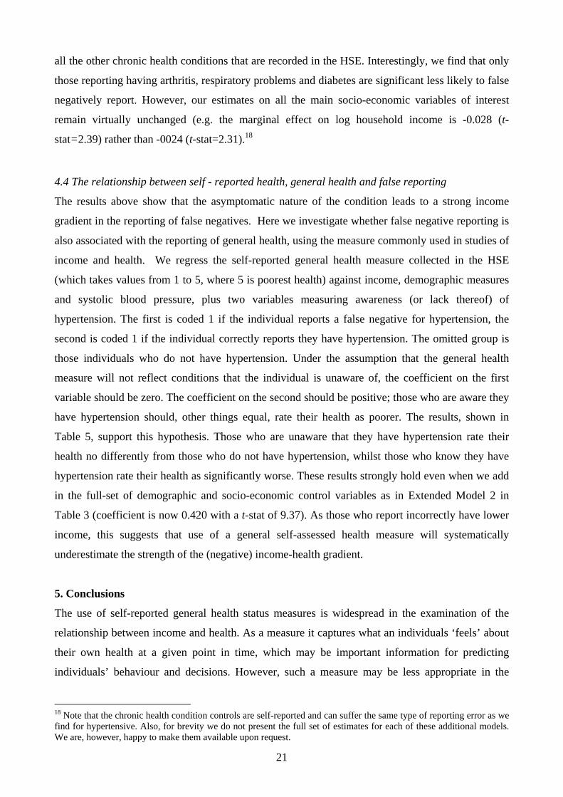
4.4 The relationship between self - reported health, general health and false reporting
The results above show that the asymptomatic nature of the condition leads to a strong income
gradient in the reporting of false negatives. Here we investigate whether false negative reporting is
also associated with the reporting of general health, using the measure commonly used in studies of
income and health. We regress the self-reported general health measure collected in the HSE
(which takes values from 1 to 5, where 5 is poorest health) against income, demographic measures
and systolic blood pressure, plus two variables measuring awareness (or lack thereof) of
hypertension. The first is coded 1 if the individual reports a false negative for hypertension, the
second is coded 1 if the individual correctly reports they have hypertension. The omitted group is
those individuals who do not have hypertension. Under the assumption that the general health
measure will not reflect conditions that the individual is unaware of, the coefficient on the first
variable should be zero. The coefficient on the second should be positive; those who are aware they
have hypertension should, other things equal, rate their health as poorer. The results, shown in
Table 5, support this hypothesis. Those who are unaware that they have hypertension rate their
health no differently from those who do not have hypertension, whilst those who know they have
hypertension rate their health as significantly worse. These results strongly hold even when we add
in the full-set of demographic and socio-economic control variables as in Extended Model 2 in
Table 3 (coefficient is now 0.420 with a t-stat of 9.37). As those who report incorrectly have lower
income, this suggests that use of a general self-assessed health measure will systematically
underestimate the strength of the (negative) income-health gradient.
5. Conclusions
The use of self-reported general health status measures is widespread in the examination of the
relationship between income and health. As a measure it captures what an individuals ‘feels’ about
their own health at a given point in time, which may be important information for predicting
individuals’ behaviour and decisions. However, such a measure may be less appropriate in the
18 Note that the chronic health condition controls are self-reported and can suffer the same type of reporting error as we find for hypertensive. Also, for brevity we do not present the full set of estimates for each of these additional models. We are, however, happy to make them available upon request.

22
context of identifying health inequalities that should be of concern to policy-makers. This is
because self-reported health measures can suffer from reporting error that is related to key socio-
economic characteristics including income. An additional aspect of health important in measuring
socio-economic inequalities is that many chronic health conditions that are partly socio-
economically determined are asymptomatic at moderate and often advanced stages. This means that
people may not know that they have such a condition, and consequently this is then not picked up
in self-reported measures even though there are serious long-term health consequences of such
illnesses. This applies to some of the most prevalent health conditions including diabetes,
hypertension, cardiovascular disease and many cancers. Baker et al. (2004) suggest that reporting
error occurs with respect to a wide-range of self-reported chronic health conditions.
The task then is to be able to establish the extent to which such errors are related to socio-
economic characteristics, particularly income. In this respect, recent studies are mixed in their
conclusions about whether using self-reported health leads to a good estimate of the ‘true’
income/health gradient, or whether there is a tendency to either under or over-estimate the
relationship.
Using two waves of data from the Health Survey for England, we provide direct evidence on
this issue by comparing survey responses to self-reported and objective measures of exactly the
same health condition, namely hypertension. Hypertension is an important condition as it is highly
prevalent in Western countries, and given its asymptomatic nature is often described as the ‘Silent
Killer’. The fact that hypertension is asymptomatic except at extremely elevated levels of blood
pressure, and that BP medication is cheap (GP access is free at the point of delivery in the British
NHS and pharmaceuticals are heavily subsidised for the poor) and effective, means that we are able
to treat income as largely exogenous, because the issue of reverse causality is not relevant. This
same aspect of the condition also means that we estimate the upper-bound in the extent of possible
reporting error.
We find a large difference in the percentage of the sample who report having hypertension as a
chronic illness (7.1%) relative to those who are measured to have the condition (34.7%), with the
raw correlation between the two measures being only 0.17. The percentage of individuals
committing a false negative report in this context, which is those reporting that they do not have
chronic hypertension but are in fact measured by the nurse as being hypertensive, is extremely high
at about 86%. Most importantly, we find no evidence of an income/health gradient in hypertension
when we use the self-reported measure but a large and statistically significant gradient using
objective measures. In fact, the size of the coefficient on log household income is around 14 times
bigger for the objective measure, even after extensively controlling for demographic and socio-
economic characteristics that might be expected to be correlated with income. This differential
23
cannot be explained by differences in obesity, lifestyle choices such as smoking, drinking, exercise
and eating fried food, nor can it be explained by differential stress rates or access to health services.
We also examine the characteristics of individuals most likely to false negatively report, that is
have measured hypertension but not report it when asked in the survey. Income is again an
important explanatory variable, with each additional log point increase in household income
reducing the probability of committing a false negative report by about 2.5 percentage points.
Again, these differentials cannot be explained by differences in usage or access to medical services,
nor differential usage of hypertension medication or differences in the severity of hypertension.
As reported in the recent literature using health ‘vignettes’, it is likely that studies that rely
only on self-reported measures of health will tend to under-estimate the true extent of the
income/health gradient. One reason is that health expectations are to some extent socially-driven
with high income groups having higher expectations about what constitutes ‘good’ health. This
means that they report their health as lower than it would be if the same level of health was viewed
by an individual from a low income background. Given the asymptomatic nature of hypertension,
we find the size of this under-estimate to be very large. Although it is towards the upper-bound of
the size of reporting error, the fact that there are many serious health conditions that are
asymptomatic at moderate and sometimes even advanced stages19 means the issue we examine is
not confined to hypertension alone. Our results therefore suggest that estimates of the
income/health gradient which use self-reported measures underestimate the extent of the gradient;
the importance of illnesses which are often asymptomatic in early stages suggests that the
discrepancy between actual and reported ill health is an important topic for future research.
19 To get a lower-bound we would need to compare self-reported and objective measures of conditions where the symptoms are immediate and more obvious to the individual such as problems with eyesight, hearing or musculoskeletal pain.

24
References
Adams, P., M.D. Hurd, D. McFadden, A. Merrill and T. Ribeiro (2003). Health, wealth, and wise? Tests for direct causal paths between health and socioeconomic status. Journal of Econometrics, 112, pp. 3-56.
Bago d’Uva, T., E. van Doorslaer, M. Lindeboom, O. O’Donnell and S. Chatterji (2006). Does reporting heterogeneity bias the measurement of health disparities? HEDG Working Paper no. 06/03, University of York.
Baker, M., M. Stabile and C. Deri (2004). What do self-reported objective measures of health measure? Journal of Human Resources, 39, pp. 1067-1093.
Banks, J, Marmot, M, Oldfield, Z and Smith, J P (2006) Disease and disadvantage in the United States and England. JAMA, 295(17): 2037-2045.
Bound, J. (1991). Self-reported versus objective measures of health in retirement models. Journal of Human Resources, 26, pp. 107-137.
Bound, J., C. Brown, and N. Mathiowetz (2001). Measurement Error in Survey Data. In Handbook of Econometrics, vol.5, ed. J. Heckman and E. Leamer, 3705-3843. New York: Elsevier Science.
Burt, V., P. Whelton, E. Rocella, C. Brown, J. Culter, M. Higgins, M. Horan and D. Labarthe (1995). Prevalence of hypertension in the US adult population: Results from the third National Health and Nutrition Examination Survey 1988-1991. Hypertension, 25, pp. 305-13.
Card, D., A. Hildreth and L. Shore-Sheppard (2004). The Measurement of Medicaid coverage in the SIPP: Evidence from a comparison of matched records. Journal of Business & Statistics, 22, pp. 410-420.
Case, A., Lubotsky, D. and Paxson, C. (2002). Economic Status and Health in Childhood: The Origins of the Gradient. American Economic Review, 92, pp. 1308-1334.
Chase, C. (2002). Income and health: Prologue. Health Affairs, 21, pp. 12. Chobanian AV, Bakris GL, Black HR, Cushman WC, Green LA, Izzo JL Jr., Jones DW, Materson
BJ, Oparil S, Wright JT Jr. and EJ. Roccella. National High Blood Pressure Education Program Coordinating Committee (2003). The Seventh Report of the Joint National Committee on Prevention, Detection, Evaluation, and Treatment of High Blood Pressure: The JNC 7 report. Hypertension, 42, pp. 1206–1252.
Contoyannis, P., A.M. Jones and N. Rice (2004). The dynamics of health in the British household panel survey. Journal of Applied Econometrics, 19, pp. 473-503.
Currie, J. and B. Madrian (1999). Health, health insurance and the labor market. In Handbook of Labor Economics, vol.3C, ed. O. Ashenfelter and D. Card, 3309-3416. New York: Elsevier Science.
Deaton, A. and C.H. Paxson (1998). Aging and inequality in income and health. American Economic Review, 99, pp. 248-253.
Flegal, K., M. Carrol, C. Ogden and C. Johnson (2002). Prevalence and trends in obesity amongst US adults 1999-2000. Journal of the American Medical Association, 288, pp. 1723-1727.
Frijters, P., J.P. Haisken-DeNew and M.A. Shields (2005a). The causal effect of income on health: Evidence from German reunification. Journal of Health Economics, 24, pp. 997-1017.
Frijters, P., J.P. Haisken-DeNew and M.A. Shields (2005b). Socio-Economic Status, Health Shocks, Life Satisfaction and Mortality: Evidence from an Increasing Mixed Proportional Hazard Model. IZA Discussion Paper no. 1488 (February 2005).
Hagan R., A.M. Jones and N. Rice. (2006). Health and retirement in Europe. HEDG Working Paper no. 06/10, University of York.
Idler, E.L. and R.J. Angel (1990). Self-rated health and mortality in the NHAMES-I epidemiologic follow-up-study. American Journal of Public Health, 80, pp. 446-452.
Idler, E.L. and Y. Benyamini (1997). Self-rated health and mortality: A review of twenty-seven community studies. Journal of Health and Social Behavior, 38, pp. 21-37.

25
Idler, E.L. and S.V. Kasl (1995). Self-ratings of health – so they also predict change in functional ability. Journals of Gerontology Series B – Psychological Sciences and Social Sciences, 50, pp. S344-S353.
Kapteyn, A., Smith, J.P. and van Soest, A. (2007). Vignettes and self-reports of work disability in the U.S. and the Netherlands. American Economic Review, forthcoming.
Lewington, S., R. Clarke, N. Qizilbash, R. Peto and R. Collins (2002). Age-specific relevance of usual blood pressure to vascular mortality: A meta-analysis of individual data for more than 1 million adults in 61 prospective studies. Lancet, 360, pp.1903-913.
Lindahl, M. (2005). Estimating the effect of income on health and mortality using lottery prizes as an exogenous source of variation in income. Journal of Human Resources, 40, pp. 144-168.
Lindeboom M and E. van Doorslaer (2004). Cut point shifts and index shift in self-reported health. Journal of Health Economics, 23, pp. 1083-1099.
Lindeboom, M., A. Llena-Nozal and B. van der Klaauw (2006). Disability and work: The role of health shocks and childhood circumstances. IZA Discussion paper, No. 2096.
Meer, J., D.L. Miller, H.S. Rosen (2003). Exploring the health-wealth nexus. Journal of health Economics, 22, pp. 713-730.
Murray, C and L. Chen (1992). Understanding morbidity change. Population and Development Review, 18, pp. 481-503.
Primatesta, P. and N. Poulter (2006). Improvement in hypertension management in England: Results from the Health Survey for England 2003. Journal of Hypertension, 24, pp. 1187-1192.
Salomon, J, A. Tandon, C. Murray and WHSPSC Group (2004). Comparability of self-rated health: Cross sectional multi-country survey using anchoring vignettes. British Medical Journal, 328, pp. 258-261.
Smith, J.P. (1999). Health bodies and thick wallets: The dual relation between health and economic status. Journal of Economic Perspectives, 13, pp. 145-166.
Stern, S. (1989). Measuring the effect of disability on labor force participation. Journal of Human Resources, 24, pp. 361-395.
Thomas, D. and E. Frankenberg (2002). The Measurement and Interpretation of Health in Social Surveys. In Summary Measures of Population Health: Concepts, Ethics, Measurement and Applications, edited by C.J.L. Murray, J.A. Salomon, C.D. Mathers, and A.D. Lopez, 387–420. Geneva: World Health Organization.
Van Doorslaer E., A. Wagstaff, H. Bleichrodt, S. Calonge, U. Gerdtham, M. Gerfin, J. Geurts, L. Gross, U. Hakkinen, R. Leu, O. O’Donnell, C. Propper, F. Puffer, M. Rodriguez, G. Sundberg, and O. Winkelhake (1997). Income-related inequalities in health: some international comparisons. Journal of Health Economics, 16, pp. 93-112.
Van Doorslaer, E. and U. Gertham (2003). Does inequality in self-assessed health predict inequality in survival by income? Evidence from Swedish data. Social Science and Medicine, 57, pp. 1621-1629.

26
Figure 1: Self-Reported Chronic Hypertension and Objective Hypertension by Age
Figure 2: Self-Reported Chronic Hypertension and Objective Hypertension by Household Income Quartile
0.1
.2.3
.4.5
Pro
porti
on H
yper
tens
ive
1st Quartile 2nd Quartile 3rd Quartile 4th Quartile
SR 140/90
0.2
.4.6
.8P
roba
bilit
y of
hyp
erte
nsio
n
30 40 50 60 70 80Age
140/90 SR
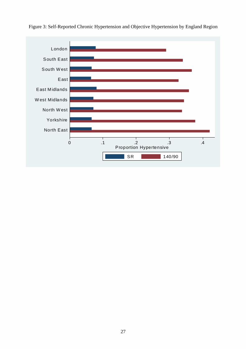
27
Figure 3: Self-Reported Chronic Hypertension and Objective Hypertension by England Region
0 .1 .2 .3 .4Proportion Hypertensive
North East
Yorkshire
North W est
W est Midlands
East M idlands
East
South W est
South East
London
SR 140/90
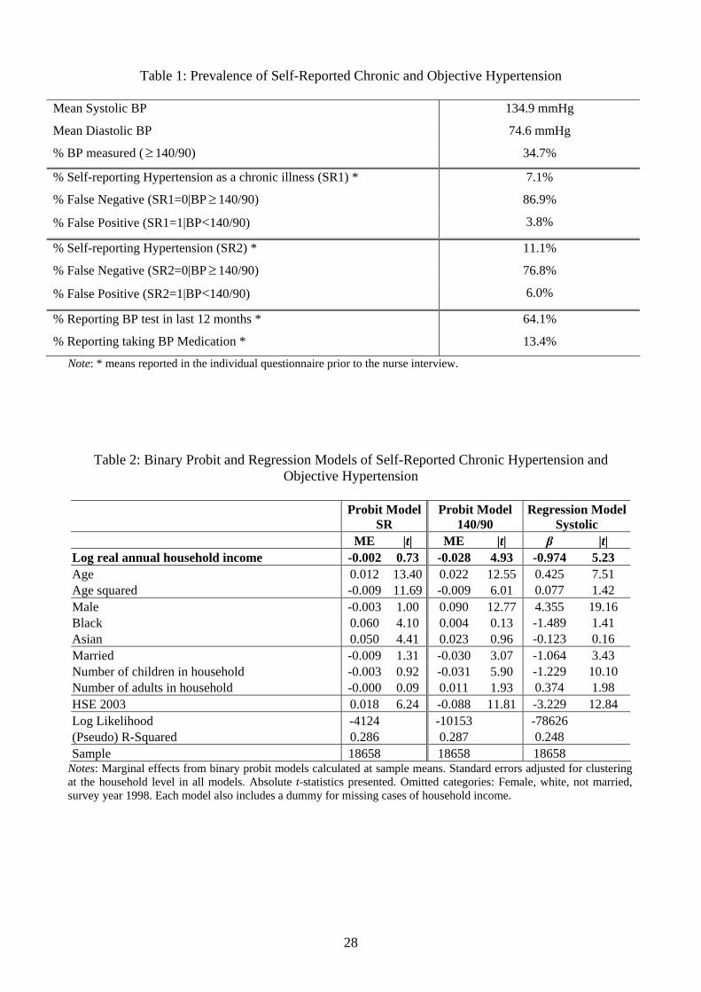
28
Table 1: Prevalence of Self-Reported Chronic and Objective Hypertension
Mean Systolic BP 134.9 mmHg
Mean Diastolic BP 74.6 mmHg
% BP measured (≥ 140/90) 34.7%
% Self-reporting Hypertension as a chronic illness (SR1) * 7.1%
% False Negative (SR1=0|BP≥ 140/90) 86.9%
% False Positive (SR1=1|BP<140/90) 3.8%
% Self-reporting Hypertension (SR2) * 11.1%
% False Negative (SR2=0|BP≥ 140/90) 76.8%
% False Positive (SR2=1|BP<140/90) 6.0%
% Reporting BP test in last 12 months * 64.1%
% Reporting taking BP Medication * 13.4%
Note: * means reported in the individual questionnaire prior to the nurse interview.
Table 2: Binary Probit and Regression Models of Self-Reported Chronic Hypertension and Objective Hypertension
Probit Model
SR Probit Model
140/90 Regression Model
Systolic ME |t| ME |t| β |t| Log real annual household income -0.002 0.73 -0.028 4.93 -0.974 5.23 Age 0.012 13.40 0.022 12.55 0.425 7.51 Age squared -0.009 11.69 -0.009 6.01 0.077 1.42 Male -0.003 1.00 0.090 12.77 4.355 19.16 Black 0.060 4.10 0.004 0.13 -1.489 1.41 Asian 0.050 4.41 0.023 0.96 -0.123 0.16 Married -0.009 1.31 -0.030 3.07 -1.064 3.43 Number of children in household -0.003 0.92 -0.031 5.90 -1.229 10.10 Number of adults in household -0.000 0.09 0.011 1.93 0.374 1.98 HSE 2003 0.018 6.24 -0.088 11.81 -3.229 12.84 Log Likelihood -4124 -10153 -78626 (Pseudo) R-Squared 0.286 0.287 0.248 Sample 18658 18658 18658
Notes: Marginal effects from binary probit models calculated at sample means. Standard errors adjusted for clustering at the household level in all models. Absolute t-statistics presented. Omitted categories: Female, white, not married, survey year 1998. Each model also includes a dummy for missing cases of household income.

29
Table 3: Extended Probit Models of Self-Reported Chronic Hypertension and Objective Hypertension Extended Model 1 Extended Model 2 SR 140/90 Systolic BP SR 140/90 Systolic BP ME |t| ME |t| ME |t| ME |t| ME |t| ME |t| Log real annual household income -0.002 0.91 -0.014 2.23 -0.426 2.09 0.001 0.55 -0.013 2.04 -0.415 1.98 Age 0.011 12.35 0.020 11.23 0.349 6.06 0.010 11.39 0.019 10.31 0.282 4.72 Age squared -0.008 10.77 -0.008 5.15 0.124 2.26 -0.007 9.87 -0.007 4.52 0.177 2.98 Male -0.002 0.78 0.093 13.08 4.460 19.53 -0.002 0.75 0.086 11.01 4.010 15.61 Black 0.059 3.97 0.037 1.14 -0.047 0.04 0.060 4.06 0.044 1.32 0.026 0.02 Asian 0.042 3.82 0.041 1.65 0.662 0.84 0.037 3.58 0.053 2.09 1.023 1.28 Married -0.005 1.32 -0.033 3.49 -1.266 4.09 -0.006 1.69 -0.036 3.73 -1.326 4.25 Number of children in household -0.002 0.76 -0.030 5.70 -1.233 9.96 -0.002 0.83 -0.030 5.63 -1.181 9.43 Number of adults in household 0.000 0.05 0.008 1.45 0.268 1.43 -0.000 0.44 0.007 1.22 0.185 0.99 HSE 2003 0.017 6.22 -0.087 11.43 -3.109 12.32 0.015 5.41 -0.092 11.80 -3.250 12.68 Degree 0.002 0.43 -0.050 4.00 -2.001 5.10 0.006 1.16 -0.042 3.31 -1.616 4.04 Other higher qualification 0.005 0.92 -0.036 2.89 -1.503 3.70 0.008 1.58 -0.032 2.43 -1.198 2.89 A Levels or equivalent -0.003 0.54 -0.022 1.49 -0.631 1.44 -0.001 0.16 -0.018 1.20 -0.401 0.92 O Levels or equivalent 0.003 0.84 -0.033 3.24 -0.915 2.77 0.006 1.43 -0.032 3.12 -0.813 2.45 Mother died of CVD aged less than 60 0.023 2.51 0.072 2.95 2.060 2.28 0.021 2.45 0.067 2.77 1.780 2.00 Mother died of CVD aged greater than 59 0.021 6.09 0.023 2.26 1.338 3.27 0.020 5.81 0.023 2.10 1.243 3.04 Father died of CVD aged less than 60 0.032 4.85 0.037 2.31 1.049 2.00 0.029 4.58 0.034 2.15 0.958 1.81 Father died of CVD aged greater than 59 0.010 3.19 0.022 2.46 0.832 2.42 0.010 3.29 0.023 2.47 0.846 2.48 North East -0.014 2.11 0.102 4.78 3.933 5.92 -0.014 2.25 0.103 4.80 3.897 5.94 North West -0.006 0.97 0.053 3.13 2.404 4.54 -0.006 1.05 0.052 3.07 2.335 4.47 Yorkshire -0.009 1.54 0.078 4.36 2.608 4.66 -0.009 1.71 0.076 4.26 2.550 4.60 West Midlands -0.006 1.05 0.048 2.62 1.980 3.41 -0.007 1.22 0.047 2.56 1.956 3.43 East Midlands -0.003 0.45 0.065 3.62 2.429 4.28 -0.003 0.60 0.062 3.47 2.330 4.16 East -0.010 1.66 0.032 1.80 1.108 2.03 -0.009 1.68 0.032 1.79 1.080 2.01 South East -0.006 1.03 0.047 2.92 1.833 3.67 -0.005 1.01 0.048 2.97 1.848 3.76 South West -0.010 1.84 0.053 2.99 2.110 3.70 -0.010 1.77 0.056 3.15 2.218 3.93 Reside suburbs 0.005 1.19 0.000 0.01 0.316 0.81 0.005 1.17 -0.001 0.08 0.244 0.63 Reside rurally -0.001 0.23 -0.001 0.04 0.462 1.03 -0.002 0.39 -0.004 0.27 0.355 0.80

30
Table 3: (Continued) Working part-time - - - - - - -0.006 1.38 -0.031 2.64 -1.322 3.80 Unemployed - - - - - - 0.011 0.95 -0.033 1.22 -1.777 1.94 Non participant - - - - - - 0.013 2.32 -0.005 0.35 -0.486 0.94 Disabled - - - - - - 0.015 2.09 -0.024 1.28 -0.604 0.85 Student - - - - - - 0.013 0.71 -0.095 2.15 -2.461 1.92 Retired - - - - - - 0.006 1.23 0.005 0.34 -0.192 0.36 Doctor or registered nurse - - - - - - -0.011 1.44 -0.025 1.06 -1.322 1.77 Obese (BMI≥ 30) - - - - - - 0.035 10.27 0.141 15.05 5.502 17.78 Smoker - - - - - - -0.008 2.20 -0.002 0.19 -0.059 0.19 Drink alcohol daily - - - - - - 0.004 1.23 0.041 3.95 1.281 3.60 Vigorous sports/exercise regularly - - - - - - -0.009 2.39 -0.015 1.56 -0.513 1.88 Eats fried food regularly - - - - - - -0.003 0.76 0.010 0.90 0.677 1.84 Log Likelihood -4080 -10103 -78521 -3988 -9914 -77929 (Pseudo) R-Squared 0.292 0.293 0.253 0.310 0.313 0.270 Sample 18658 18658 18658 18658 18658 18658
Notes: Marginal effects from binary probit models calculated at sample means. Standard errors adjusted for clustering at the household level in all models. Absolute t-statistics presented. Omitted categories: Female, white, not married, survey year 1998, less than ‘O’ level as highest qualification, mother did/had not died of CVD, father did/ has not dies of CVD, lives in Greater London, resides in city location, works full-time, not a doctor or registered nurse, is not obese, non-smoker, drinks less than every day, does not undertake regular vigorous sports/exercise and does not regularly east fried food. Each model also includes a dummy for missing cases of household income, and a dummy control for BMI missing.
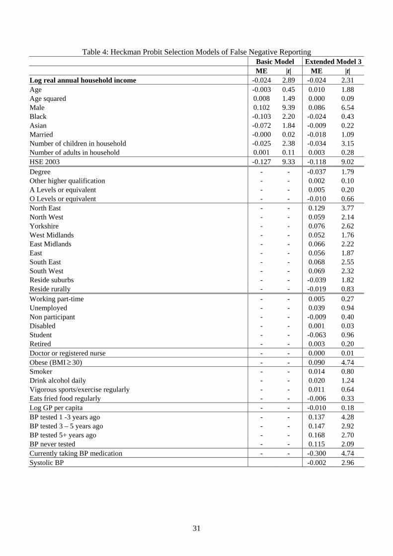
31
Table 4: Heckman Probit Selection Models of False Negative Reporting Basic Model Extended Model 3 ME |t| ME |t| Log real annual household income -0.024 2.89 -0.024 2.31 Age -0.003 0.45 0.010 1.88 Age squared 0.008 1.49 0.000 0.09 Male 0.102 9.39 0.086 6.54 Black -0.103 2.20 -0.024 0.43 Asian -0.072 1.84 -0.009 0.22 Married -0.000 0.02 -0.018 1.09 Number of children in household -0.025 2.38 -0.034 3.15 Number of adults in household 0.001 0.11 0.003 0.28 HSE 2003 -0.127 9.33 -0.118 9.02 Degree - - -0.037 1.79 Other higher qualification - - 0.002 0.10 A Levels or equivalent - - 0.005 0.20 O Levels or equivalent - - -0.010 0.66 North East - - 0.129 3.77 North West - - 0.059 2.14 Yorkshire - - 0.076 2.62 West Midlands - - 0.052 1.76 East Midlands - - 0.066 2.22 East - - 0.056 1.87 South East - - 0.068 2.55 South West - - 0.069 2.32 Reside suburbs - - -0.039 1.82 Reside rurally - - -0.019 0.83 Working part-time - - 0.005 0.27 Unemployed - - 0.039 0.94 Non participant - - -0.009 0.40 Disabled - - 0.001 0.03 Student - - -0.063 0.96 Retired - - 0.003 0.20 Doctor or registered nurse - - 0.000 0.01 Obese (BMI≥ 30) - - 0.090 4.74 Smoker - - 0.014 0.80 Drink alcohol daily - - 0.020 1.24 Vigorous sports/exercise regularly - - 0.011 0.64 Eats fried food regularly - - -0.006 0.33 Log GP per capita - - -0.010 0.18 BP tested 1 -3 years ago - - 0.137 4.28 BP tested 3 – 5 years ago - - 0.147 2.92 BP tested 5+ years ago - - 0.168 2.70 BP never tested - - 0.115 2.09 Currently taking BP medication - - -0.300 4.74 Systolic BP -0.002 2.96

32
Table 4: (Continued) Rho 0.896 0.943 Log Likelihood -12482 -11516 Wald Test (Rho=0) Chi-squares (1) 23.04 25.18 Test of 1st stage ‘instrument’ power Chi-squared (4) 39.87 21.28 Sample 18658 18658 Notes: Unconditional Marginal effects from Heckman Probit Selection models calculated at sample means. Standard errors adjusted for clustering at the household level in all models. Absolute t-statistics presented. Omitted categories: Female, white, not married, survey year 1998, less than ‘O’ level as highest qualification, mother did/had not died of CVD, father did/ has not dies of CVD, lives in Greater London, resides in city location, works full-time, not a doctor or registered nurse, is not obese, non-smoker, drinks less than every day, does not undertake regular vigorous sports/exercise and does not regularly east fried food, BP tested in last 12 months, and not currently taking any BP medication. Each model also includes a dummy for missing cases of household income, and a dummy control for BMI missing.

33
Table 5: Ordered Probit Model of Self-Reported General Health Status
Basic Model β |t| Log real annual household income -0.320 23.27 Age 0.192 5.17 Age squared -0.007 2.18 Male 0.007 0.49 Black 0.168 2.39 Asian 0.284 5.63 Married -0.064 2.93 Number of children in household -0.018 1.66 Number of adults in household 0.094 7.39 140/90 = 1, SR=1 (Individual reports having chronic hypertension) 0.449 10.25 140/90 = 1, SR=0 (Individual does not report having chronic hypertension) 0.021 0.77 Systolic BP -0.001 1.67 HSE 2003 -0.040 2.22 Log Likelihood -22638 (Pseudo) R-Squared 0.121 Sample 18658
Notes: Standard errors adjusted for clustering at the household level in all models. Omitted categories: Female, white, not married, does not have 140/90 hypertension and survey year 1998.