Embed Size (px)
Citation preview

1
Working Paper Series
Congressional Budget Office
Washington, D.C.
Comparing Wages in the
Federal Government and the Private Sector
Justin Falk
Microeconomic Studies Division
Congressional Budget Office
January 2012
Working Paper 2012-3
To enhance transparency and encourage external review of CBO’s work, the agency’s working paper series includes
papers that provide technical descriptions of CBO analyses as well as papers that present original, independent
research by CBO analysts. Working papers are not subject to CBO’s regular review and editing process. Papers in
this series are available at www.cbo.gov/publications (select Working Papers).
The author thanks Greg Acs, Andrew Biggs, McKinley Blackburn, Will Carrington, Molly Dahl, Matt Goldberg,
Larry Katz, Joseph Kile, Alan Krueger, Alex Mas, David Moore, Brooks Pierce, Jason Richwine, Stephanie Ruiz,
James Sherk, and Heidi Shierholz for their comments and suggestions.
2
Comparing Wages in the
Federal Government and the Private Sector
Abstract
This analysis used Current Population Survey data from 2005 through 2010 to compare the
hourly wages of federal employees and workers in the private sector who have certain similar
observable characteristics. In that comparison, we found that the arithmetic average of wages
was about 21 percent higher for federal employees than for their private-sector counterparts
among workers with no more than a high school education, was about the same in both sectors
among workers with a bachelor’s degree, and was 23 percent lower in the federal sector among
workers with a professional degree or Ph.D. Overall, federal wages were about 2 percent higher,
on average, than wages of similar private-sector workers.
We found that the wages of federal employees were much less dispersed than those of employees
with similar characteristics in the private sector—particularly among workers with more
education. That aspect of the data causes semilog regressions to generate inconsistent estimates
of percentage differences in arithmetic means. Consistent estimates of differences in arithmetic
means—obtained using a quasi-maximum likelihood estimator that is robust to distributional
misspecification—are substantially smaller than differences in geometric means estimated by
semilog regressions. The differences in arithmetic means are more relevant for answering
questions about how federal spending would change if federal workers were paid wages equal to
those of measurably similar workers in the private sector.
The estimates do not show precisely what federal workers would earn if they were employed in
the private sector. The difference between what federal employees earn and what they would
earn in the private sector could be larger or smaller depending on characteristics that were not
included in this analysis because such traits are not easy to measure. The results apply to the cost
of employing full-time full-year workers. The analysis focused on those workers—who
accounted for about 93 percent of the total hours worked by federal employees from 2005
through 2010—because higher-quality data were available for them than for other workers.
3
I. Introduction Numerous researchers have concluded that workers in the federal government are more highly
compensated, on average, than those in the private sector with similar education, experience, and
other characteristics. This study reexamined data from the Current Population Survey (CPS) to
estimate differences in hourly wages and used administrative data on federal pay to more
accurately impute high earnings that were top-coded in the CPS. Comparing federal workers
with workers in the private sector having certain similar observable characteristics, we estimated
that hourly wages were higher in the federal government than in the private sector for high
school graduates and lower for people with professional degrees.
What are the average differences in wages between federal and private-sector workers overall?
Because of differences in wage dispersion within the sectors for people with similar
characteristics, the answer depends critically on the definition of ―average.‖ Pooling results from
all education levels, we found that the arithmetic mean of hourly wages was about 2 percent
greater among federal workers than among similar workers in the private sector. Most of the
previous literature comparing federal and private-sector wages examined differences between the
mean log wages of those two sectors (and we also found larger differences in those geometric
means), but this study focused on differences in the arithmetic means of wages, for both practical
and theoretical reasons.
As a practical matter, lawmakers have asked what the implications would be for the federal
budget if federal workers were paid the same wages as similar workers in the private sector.
With the number of federal hours worked held constant, the answer to that question depends on
the difference in arithmetic means between the wages of such workers in the federal and private
sectors. Differences in mean log wages do not answer that question.
The basic theoretical model of wage determination derived by Mincer (1974) and others leads to
a form for wages (Y) as a function of worker characteristics (X) such that .
Although the empirical literature has almost exclusively focused on estimation of the semilog
regression model , consistent estimates of are generally not consistent
estimates of —as discussed by Blackburn (2007). In particular, differences in wage dispersion
between two groups of otherwise similar workers (that is, heteroscedasticity in the log-linear
regression models) cause to be an inconsistent estimate of , and we found that wages of
federal employees were substantially less dispersed than those of similar workers in the private
sector.
The differences in wages between federal and private-sector workers with similar characteristics
also depend on the analytical treatment of firm size. Our main specification compared federal
workers with private-sector workers in large firms, because we judged those private-sector
employees to be doing work more comparable to that done by federal workers. In particular, the
workforces of federal agencies and large private firms are both relatively specialized, educated,
and skilled compared with those of other employers. In supplemental analyses in which the
treatment of other worker characteristics was unchanged, we found that average private-sector
wages were lower when they were based on workers in all firms rather than on workers in large
firms.
4
In all of the comparisons, we measured differences between employees with similar observable
characteristics; we did not attempt to address other potential questions of interest, such as what
the wages of federal workers would have been if those particular workers had never been
employed by the federal government, or what their wages would be if they were laid off from the
federal government and moved to the private sector. Those types of questions involve various
issues (such as unobserved abilities, selection into and out of the federal sector, and impacts of
job loss) that we did not have sufficient data or a credible identification strategy to address.
The hourly wages that this paper focuses on are only one component of hourly compensation.
Analyzing differences in overall compensation would involve quantifying the value of the fringe
benefits—such as pensions or other employer contributions to retirement savings—provided in
each sector. That issue is addressed in Falk (2012).
The remainder of this paper consists of six sections. Section II reviews previous research and
discusses our interpretation of it. Section III describes the data used in this analysis, and section
IV describes the characteristics of the workers in those data. Section V analyzes the distribution
of wages for similar workers in the federal and private sectors, and section VI analyzes average
wages for those workers. Section VII offers conclusions.
II. Background and Context Wages of federal employees are determined by a system that emphasizes tenure with the federal
government (Belman and Heywood, 1996). Research has consistently found that wages in the
federal sector exceed the wages of similar workers in the private sector. Recent studies have used
log-linear regression analyses and have reported federal wage premiums of 14 percent to 19
percent. Other research has demonstrated that those methods produce inconsistent estimates of
the percentage differences in the arithmetic means of wages, whereas quasi-maximum likelihood
methods provide consistent estimates.
A. Previous Research
Two studies have focused on comparing federal and private-sector wages using recent cross-
sectional data from the CPS. Sherk (2010) concluded that federal wages were 18 percent higher,
on average, than wages in the private sector when controlling for education, age, sex, race,
occupation, part-time employment, marital status, immigration status, and location.1 Biggs and
Richwine (2011) concluded that federal wages exceeded private-sector wages by 14 percent
when controlling for those same characteristics of employees and including adjustments for firm
size. Biggs and Richwine also estimated the wage differential separately for workers at different
levels of educational attainment. They estimated that federal wages exceeded private-sector
wages by 22 percent among workers with only a high school education and by 4 percent among
workers with a graduate degree. Sherk (2010) and Biggs and Richwine (2011) both used
1 That research also concluded that the wage difference between the federal government and the private sector was
22 percent when the sample of federal employees was restricted to those who reported working in public
administration.
5
censored data on earnings, which can cause bias because the procedure for imputing
replacements for censored values does not account for federal employment.2
Earlier, Belman and Heywood (2004) used data from 1997–1999 cross sections of the CPS to
compare wages between sectors while controlling for workers’ education, age, sex, race, part-
time employment, marital status, location, union status, and broad occupational classification.
They found that federal wages exceeded private-sector wages by 19 percent.3
Using different data and a different approach, the Federal Salary Council (FSC) regularly
compares the salaries paid for federal jobs that are on the General Schedule with the salaries paid
for similar jobs in the private sector to inform the President’s recommendation for adjustments to
federal pay. The FSC found that the average of federal salaries trailed the average of private-
sector salaries by 26 percent in 2011 (Federal Salary Council, 2011). The council does not model
wages as a function of workers’ education, age, or other attributes measured in the CPS. Instead,
it compares salaries for federal and private-sector positions that require similar levels of
knowledge and entail similar degrees of complexity.4 However, Famulari (2002) found that by
matching detailed descriptions of positions, the FSC may have ended up comparing federal
workers with private-sector workers who have more experience.
Older research examined details of the differences between federal and private-sector pay that
may still be relevant. Borjas (2002) and Katz and Krueger (1991) used the CPS to study
intertemporal trends in the distributions of wages for the federal, state, and local government
sectors in the context of the rapidly increasing wage dispersion that occurred in the private sector
during the 1980s and 1990s. Borjas found that the dispersion of wages, as measured by the
difference in the logarithms of wages between the 90th and 10th percentiles of the distribution,
had grown more slowly in the federal sector than in the private sector. Katz and Krueger found
that the difference between the wages of college- and high-school-educated workers had grown
more slowly in the federal sector than in the private sector when adjusted for potential
experience, sex, race, part-time employment, and location. They also found that, after adjusting
for those characteristics, the dispersion of wages had remained roughly constant in the federal
2 If a worker reports earning over $200,000, the CPS provides an imputed value for earnings instead of the reported
value to protect the identity of the worker. The imputation procedure assigns those workers the average of earnings
across all workers with top-coded earnings who have the same sex, race/origin, and ―work experience‖ (full-time
and full-year or not). That procedure does not distinguish between the averages of earnings for federal and private-
sector workers. Consequently, using the imputed values will bias estimates of differences between federal and
private-sector wages when differences exist in the underlying averages of censored earnings that would not be
eliminated by controlling for measured attributes. In addition, Sherk (2010) excluded workers with wages below
$5 per hour or above $60 per hour from his sample, which could further bias estimates if the percentage of workers
excluded varied between the two sectors.
3 The 19 percent difference was based on a specification that controlled for broad occupational distinction. The
authors found a difference of 14 percent when comparing for a more detailed occupational distinction and a
difference of 23 percent when not controlling for occupation.
4 Specifically, the FSC matches positions on the basis of indices for ―knowledge,‖ ―job controls and complexity,‖
―contacts,‖ and ―physical environment,‖ although most of the weight is placed on the first two factors. The
methodology is described in more detail in the appendix of President’s Pay Agent (2002).
6
sector although it was growing in the private sector. Borjas and Katz and Krueger also found that
federal-private wage differentials were larger for women than for men.
B. Approaches to Estimating Differences Between Sectors
In the analyses discussed in the previous subsection (except those by the FSC), researchers
regressed the natural logarithm of wages on an additive function of workers’ measured attributes
to control for differences in those attributes. The coefficients in those log-linearized models were
estimated using least squares, and the difference in predicted values of log wages between the
federal and private sectors, measured in log points, was interpreted as the percentage difference
in wages between sectors—usually by exponentiating the difference in log points, implicitly
giving the percentage difference in the geometric means of wages for the sectors.
Those studies did not provide further detail about whether the intent was to measure the
percentage difference in the expected value of wages or some other characteristic of the wage
distributions. However, an older comparison of federal and private-sector wages by Smith (1977)
noted that the difference in log wages yields the percentage difference between the geometric
means, which generally does not equal the percentage difference in expected values—that is, in
arithmetic means. Moulton (1990) and Gyourko and Tracy (1988) explicitly constructed
estimates of the percentage difference in the arithmetic means of wages between the federal and
private sectors by accounting for differences in the conditional variances of the federal and
private-sector wage distributions. (Those estimates assumed that the error term in the log-
linearized model was normally distributed and that the expected value of wages therefore
equaled the exponential of the sum of the expected value of log wages and half the variance of
log wages.) However, those studies used data that are now over 20 years old.
Arithmetic and Geometric Means. To see why estimates of arithmetic and geometric means
might differ, consider an illustrative comparison of wages for two groups, each of which contains
two workers (see Table 1). When the wage dispersion within a group is small, as in group A—
where the two workers have wages 20 percent above and below the group’s arithmetic mean—
the arithmetic and geometric means for the group are similar. By contrast, in group B—where
the two workers have wages 60 percent above and below the group’s arithmetic mean, the wage
of worker 1 is twice the geometric mean, and the wage of worker 2 is half that mean—the
arithmetic and geometric means differ substantially. We constructed this comparison to illustrate
how the geometric mean of wages in group A could be higher than that of group B by 22 percent
(or 0.2 log points) even though the arithmetic means are identical.
Returning to our practical motivation for focusing on arithmetic means, if the federal government
had a set of workers paid like those in group A and changed their pay to resemble that of group B
to make them comparable with similar workers in the private sector, there would be no effect on
the federal budget—even though the mean log wage had been 0.2 log points higher in group A.
Thus, the difference in the mean log wage is not informative for the question of interest.
More generally, consider the difference in the mean log wage for any two groups (that is,
, where and are wages in groups A and B, respectively). That
difference can be decomposed (using a Taylor series evaluated at the expected values of wages)
7
into the difference in the logs of the arithmetic means of wages ( ) and a remainder that depends
on the variance ( ) and higher-order central moments as shown in equation (1):
(1)
The remainder is equal to zero if the shapes of the wage distributions in the two groups are the
same, such that all normalized higher-order central moments take on the same values for the two
groups (for example, ). In that case, the percentage difference in the geometric
means of the wages of the two groups is equal to the percentage difference in the arithmetic
means.
Methods for Estimating Differences in Arithmetic Means. Three studies have focused on
inaccuracies in estimating the percentage difference in arithmetic means when using a log-
linearized model. Manning and Mullahy (2001) studied the implications of using log-linearized
models for data with properties that are common in the field of health economics, such as
skewness and heteroscedasticity. Their Monte Carlo simulations showed that the log-linear
model resulted in inconsistent estimates of percentage differences in arithmetic means of
outcomes when the data were heteroscedastic—a circumstance that also has been found in wage
comparisons.5 Silva and Tenreyro (2006) used Monte Carlo simulation to examine the
consequences of using the log-linear model in the context of international trade flows. They
found that the log-linear model resulted in inconsistent estimates of the effects of both
continuous and categorical explanatory variables when the data were heteroscedastic. Lastly,
Blackburn (2007) concluded that using the log-linear model to compare union and nonunion
wages overstated the amount by which the arithmetic mean of union wages exceeded that of
nonunion wages.
All of those studies traced the inaccuracies in using the log-transformation to the fact that the
logarithm of an expected value is not equal to the expected value of logarithms—an instance of a
corollary to Jensen’s inequality. They suggested using quasi-maximum likelihood estimators
with the exponential form of the model, which leaves the dependent variable untransformed.
That modeling approach can generate a consistent estimate of the difference in the arithmetic
means of wages between two groups in the presence of heteroscedasticity.
III. Data In this study, we used the Current Population Survey to estimate differences in wages between
federal workers and private-sector workers with certain similar observable characteristics. We
analyzed federal and private-sector wages using data from the Social and Economic Supplement
to the CPS, which is administered each March. The March CPS is a nationally representative
survey of the civilian noninstitutionalized population, which is conducted annually by the Census
5 Borjas (2002) found that the distribution of residuals was less dispersed in the public sector than in the private
sector. Card (2001) found evidence suggesting that union wage distributions were less dispersed than nonunion
wage distributions.
8
Bureau. Respondents are asked about their earnings, sector of employment, and a variety of other
attributes of themselves and their employers.
For this analysis, we pooled the 2006–2011 cross sections of the March CPS. Because workers
report their earnings over the previous year in that survey, the cross sections cover 2005 through
2010. The cross sections were combined to increase the size of the sample and to allow a
comparison of wages that spanned periods of economic growth as well as decline. The number of
federal workers in the sample used for the analysis was 8,311 and the number of private-sector
workers was 211,504.
A. Composition of the Sample
To construct that analytical sample, we made a number of decisions. We opted to compare the
wages of federal civilian employees whose compensation is directly funded through
Congressional appropriations with the wages of private-sector workers. We did not analyze the
wages earned by members of the armed services or by employees of the Postal Service or the
Tennessee Valley Authority (TVA). (The Postal Service and the TVA do not receive specific
appropriations for compensation of their workers; their operations are primarily funded through
revenues from services provided.) To remove those workers from the analysis, we excluded CPS
respondents who reported working in the Postal Service or the electric power industry. We also
excluded employees of state and local governments, workers under age 16 or over age 64, and
self-employed people. The self-employed were omitted because their earnings not only reflect
the payments they earn for their labor but also can include the returns on their investments in
capital (such as purchasing computers, office space, machinery, etc.).
To improve the accuracy of the analysis, we also excluded part-time and part-year workers and
individuals who worked multiple jobs. Wages tend to be measured with more error for people
who worked less than 35 hours in a usual week or less than 50 weeks during the previous year,
because wages are calculated by dividing earnings by the number of hours worked. Thus, those
part-time and part-year workers have smaller denominators, which exacerbate errors in the
reporting of their earnings. Those workers accounted for only about 7 percent of the hours
worked by federal employees. For CPS respondents who worked multiple jobs, the sector of
employment is only reported for their longest job, and hours worked are only reported as a total
for all jobs.
Some respondents do not report their earnings, sector of employment, or other measured
attributes. The Census Bureau imputes values for those characteristics for many of those
respondents. We excluded workers who did not provide their earnings or sector of employment,
because the imputed values for those variables do not provide additional information about the
relationship between earnings and sector of employment.6 However, we included workers who
had imputed values only for other measured attributes, because their reports of earning and
sector provide additional information about the relationship between those variables.
6 About 16 percent of federal workers and 21 percent of private-sector workers were excluded from the sample
because they had imputed earnings.
9
B. Measuring Wages
We calculated hourly wages by dividing the earnings that workers reported for the previous year
by the product of the hours they worked in a usual week and the number of weeks they worked
in the previous year. Annual earnings include tips, overtime pay, commissions, and bonuses, as
well as salaries and are inflated to 2010 dollars based on the employment cost index for wages
and salary in private industry. Roemer (2002) found that the averages of annual earnings in the
March CPS were similar to averages calculated from the records of the Social Security
Administration. However, Lemeiux (2006) argues that for workers who are paid by the hour,
wages calculated from reports of annual earnings are less precise measures than the direct reports
of pay rates available for the outgoing rotation groups of the CPS. That argument is unlikely to
present an issue for our research as only a small portion of federal employees are paid by the
hour. Moreover, the March CPS has two advantages over the outgoing rotation groups: It
includes data on the size of the firms employing workers, and it provides more information on
the wages of high earners.
In order to accurately capture differences in high wages between the federal and private sectors,
we adjusted the values that the Census Bureau had imputed for the 0.7 percent of federal workers
and the 1.2 percent of private-sector workers who reported earnings over $200,000. The averages
that the Census Bureau provides in place of top-coded earnings do not distinguish between the
earnings of federal and private-sector workers.7,8
We used administrative data that cover most
federal employees to calculate the averages of earnings for federal workers making more than
$200,000.9 As with the CPS data, those earnings were averaged within groups of employees
having the same sex, race/origin, and full-time full-year status for each year. Those averages
were used in place of the values provided by the Census Bureau for federal employees and were
also used to adjust the averages that the Census Bureau provided for private-sector workers.10
The average of earnings across those groups was $238,220 for federal workers and $432,553 for
workers in the private sector.
C. Measuring Sector of Employment
The workforce tabulations in the national income and product accounts indicate that data from
the March CPS overstate the percentage of the population that works for the federal government,
which could bias a comparison of federal and private-sector wages. In the March CPS, federal
7 See footnote 2 for a more detailed description of the Census Bureau’s procedure.
8 For the 2011 March CPS, the Census Bureau changed its procedure for protecting the identity of high earners, but
we were able to follow the procedure for distinguishing between the average earnings of federal and private-sector
workers making over $200,000 that we had used for the older cross sections.
9 For a description of those administrative data, called the Central Personnel Data File, see Congressional Budget
Office, Characteristics and Pay of Federal Civilian Employees (March 2007), p. 2.
10 The average for the top-coded earnings of private-sector workers is calculated as a weighted difference between
the average of top-coded earnings for all workers and the average of top-coded earnings for federal workers, with
the weights based on the portion of top-coded earnings attributed to federal employees. That adjustment removes
federal earnings from the average wages used for private-sector workers but leaves the earnings of workers we
excluded from the sample. The data did not enable us to estimate the average for the top-coded earnings of workers
who were excluded from the sample. The majority of those workers were excluded because they were self-
employed.
10
employees accounted for 2.7 percent of weeks worked by federal and private-sector employees
from 2005 through 2010.11
But according to the national income and product accounts, federal
employees accounted for only 1.8 percent of weeks worked by federal and private-sector
employees during those years. That discrepancy suggests that some private-sector employees,
perhaps those who work for a federal contractor, misclassify themselves as federal employees in
the March CPS. However, the average of the earnings for people who report being federal
employees in the CPS is similar to the average of the earnings recorded for federal employees in
the administrative data.
IV. Characteristics of Workers The federal workforce tends to be more concentrated in professional occupations—and thus
more educated and older—than the private-sector workforce (see Table 2). About a third of
federal employees work in professional occupations, such as the sciences or engineering,
whereas a larger portion of private-sector employees work in blue-collar occupations or retail
sales. Professional occupations often require more formal training or experience than do the
occupations more common in the private sector. Partly because of that difference, the average
age of federal employees is 4 years higher than that of private-sector employees. The greater
concentration of federal workers in professional occupations also means that they are more likely
to have a bachelor’s degree: 51 percent of the federal workforce has at least that much education,
versus 31 percent of the private-sector workforce. Likewise, 21 percent of federal employees
have a master’s, professional, or doctoral degree, compared with 9 percent of private-sector
employees.
The characteristics of employers, as well as of workers, differ between the federal and private
sectors. Most federal employees work for large agencies; the biggest, the Department of Defense,
employs about 800,000 civilian workers. Nearly all federal employees work for entities that have
at least 1,000 workers. In contrast, only about 40 percent of private-sector employees work for
entities with at least 1,000 employees.
The federal government and private sector also differ in the extent to which their workers are
represented by unions, which can influence employees' compensation. About 21 percent of
federal employees are members of unions, whereas the portion of private-sector workers who
belong to unions has declined to 8 percent. However, union membership does not appear to
provide the same indication of workers' skills and characteristics in the two sectors, in part
because the occupations in which union membership is common differ.
Federal employees work in a wide variety of locations, because the services they deliver are
required across the nation. For example, nurses and doctors who work at hospitals run by the
Department of Veterans Affairs, security screeners at airports, and air traffic controllers are
spread throughout the United States. In total, about 14 percent of federal employees work in the
11
For comparability with the national income and product accounts, we calculated the percentage of hours worked
by federal employees from a broader sample than was used for the rest of the analysis. The broader sample only
excludes employees of state governments, local governments, government-sponsored enterprises, and the armed
forces.
11
Washington, D.C., metropolitan area; the other 86 percent (2 million people) are located
throughout the country in roughly similar proportions to workers in the private sector.
The attributes of the federal workforce are more like those of private-sector workers at large
firms than those of workers at small firms, because both large firms and federal agencies require
a workforce that is more specialized and educated than small firms do. Many federal employees
have expertise in specific roles, as over 95 percent of them work in agencies that divide tasks
among more than 100 occupations. That degree of specialization is not possible for small
employers. In addition, only 27 percent of workers at small firms have at least a bachelor's
degree; whereas the proportion of workers with that level of education is greater at large firms
(37 percent) and in the federal government (51 percent).
V. Distributions of Wages
To construct descriptive statistics of the wage distributions of federal workers and of private-
sector workers who have similar observable characteristics to federal workers, we estimated
weights that were used to reweight the private-sector sample, following an approach developed
by DiNardo, Fortin, and Lemieux (1996) and Fortin, Lemieux, and Firpo (2011, pp. 63–69).
Specifically, in equation (2) below, let D* be a latent variable such that a worker is employed in
the federal government if D* > 0 and in the private sector otherwise, and let X be a set of worker
characteristics.12
(2)
We estimated separate logit models based on equation (2) for each of five major categories of
educational attainment (s): high school diploma or less, some college, bachelor’s degree,
master’s degree, and professional degree or doctorate. We then multiplied the CPS weights of
private-sector workers by exp(X ) for each major education category and normalized those new
weights so that they summed to the share of federal workers within each of those categories.
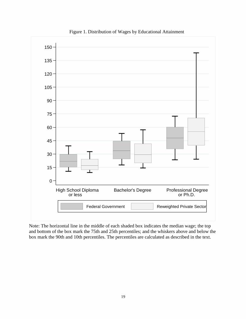
Using that approach to compare wages in the federal government at the 10th, 25th, 50th, 75th,
and 90th percentiles of the distribution with those in the private sector for people who have
similar observable characteristics, we found that federal wages were higher among workers with
no more than a high school education at all percentiles we examined (see Figure 1). For workers
with a bachelor’s degree, federal wages were higher from the 10th through 75th percentiles but
were lower at the 90th percentile. For workers with a professional degree or Ph.D., federal wages
were lower at each percentile and were about half as much at the 90th percentile. On a related
note, we found that the dispersion of federal wages, as measured by the ratio of the 90th to 10th
12
The worker characteristics included here were a fourth-order polynomial in potential experience and indicators for
more-detailed levels of educational attainment: 9th grade or less, 10th grade, 11th grade, 12th grade, high school
diploma, vocational associate’s degree, academic associate’s degree, bachelor's degree, master's degree, professional
degree, and doctorate. In addition, we included a set of 12 indicators representing all combinations of race/origin
(Hispanic, black, and white), sex (males and female), and marital status (married and single). Other characteristics
were indicators for being an immigrant; being a noncitizen; living outside a metropolitan area; 5 categories for firm
size, by number of employees (1–9, 10–99, 100–499, 500–999, and 1,000+); 24 occupational categories; 5 regions;
and 6 calendar years.
12
percentiles, was smaller than the dispersion of private-sector wages for workers with at least a
bachelor’s degree—especially for those with a professional degree or Ph.D.
VI. Average Wages As discussed in section II, the recent literature comparing federal and private-sector wages has
most commonly taken the approach of examining differences in log wages between the sectors
after controlling for covariates. In this section, we first show how that approach produces
inconsistent estimates of the percentage difference between the arithmetic means of wages in
those sectors. Second, we outline our method for providing consistent estimates of that
difference by directly modeling the conditional mean function. Third, we present the results from
implementing that method. And fourth, we assess the sensitivity of those results. Because
previous research indicated that the relationship between wages and education varied
substantially by level of educational attainment, we estimated differences for each major
education category and then constructed a weighted average of those differences for the overall
estimates reported throughout this section.
A. Inconsistent Estimation from the Semilog Model
Let D be an indicator for federal employment, X be the same set of worker characteristics as
defined for equation (2), and Y be the hourly wage. A typical estimate of the percentage
difference in the arithmetic means of wages between the federal and private sectors within a
major education category would be , where is the estimated parameter
based on equation (3).
(3)
As noted by Blackburn (2007), however, may depend on D and X even if
= 0 and therefore may enter into the calculation of as in equation (4).
(4)
The Taylor series for the expected value of the exponential of the error term when evaluated at
zero is . Using the second-order expansion of that
series, depends on the conditional variance of the error term as in equation (5).
(5)
We tested the equality of the expectations of the conditional variance for each sector within each
major education category using a linear approximation by estimating equation (6), employing the
squared residuals from equation (3) in our estimates of .
(6)
13
We rejected the null hypothesis that within each major education category. That
evidence of heteroscedasticity implies that under the assumptions used to
construct the approximations in equations (5) and (6).
B. Consistent Estimation of the Conditional Mean Function We estimated the percentage difference in the arithmetic averages of wages between the federal
and private sectors in four main steps. Our approach compared federal wages with the predicted
value of private-sector wages for a worker with the same observable characteristics. We
estimated a full interaction between sector of employment and worker characteristics—that is,
the differences between sectors were allowed to vary for each characteristic. Because we used a
nonlinear model, we then integrated over the distribution of worker characteristics to obtain our
estimates.
First, we directly modeled the conditional mean function within each major education category s.
In equation (7), let Y, D, and X be wages, sector, and worker characteristics as defined above,
and let .
(7)
In equation (7), the joint null hypothesis that is a test of whether worker characteristics
have a different association with wages in the federal and private sectors beyond the federal-
sector main effect for a worker with average characteristics for the federal sector. We
estimated the parameters of equation (7) using quasi-maximum likelihood estimation (QMLE)
methods that provide consistent parameter estimates when the underlying distribution of the data
differs from that assumed in the estimation (Gourieroux, Monfort, and Trogan, 1984).
Specifically, for our main specification, we used Poisson QMLE, which Silva and Tenreyro
(2006) found had a lower mean squared error than several other QMLE methods in simulations.
Second, let the average wages of workers in the private sector with characteristics similar to
federal workers be denoted as in equation (8). We estimated by integrating our
conditional mean function over the distribution of federal worker characteristics, denoted as
.
(8)
Third, let the average wages of workers in the federal sector be denoted as in equation (9).
We estimated in a manner analogous to that used in equation (8).
(9)
Fourth, for our overall estimate of wages in the private sector, we used a weighted average of the
estimates for each major education category for both the federal and private sectors
—where the weights were the share of federal workers in each major education
category, , as in equation (10).
14
(10)
Following the method described by Rao (1994), we calculated the standard errors for estimates
based on equations (8), (9), (10), and for the percentage difference between federal wages and
the wages of private-sector workers with similar characteristics, using replicate weights to
account for stratification and cluster sampling variability that occurred in calculating the post-
stratification weights used to make the CPS more representative of the U.S. population.
Specifically, we calculated each estimate 160 times using each of the 160 weights provided by
the Census Bureau; the reported standard errors are proportional to the standard deviation of
those estimates from the estimate based on the post-stratification weights.
C. Results
On average, compared with private-sector employers, the federal government paid higher wages
for workers with low educational attainment but paid lower wages for workers with high
educational attainment (see Table 3). The average wage for federal employees overall was about
$32 per hour, about 2 percent higher than the average wage for private-sector workers with the
same characteristics. Among workers with a high school diploma or less education, the average
wage was 21 percent higher for federal employees than for private-sector workers with the same
measured attributes. In contrast, among workers whose education culminated in a doctorate or
professional degree, the average wage was 23 percent lower for federal employees than for
similar private-sector workers. Between those levels of education, the averages of wages in the
two sectors were closer to each other. In particular, the average wage for federal employees with
a bachelor’s degree was about equal to the average wage for similar private-sector employees.
The federal government paid women higher wages, on average, than private-sector employers
did but paid men similar wages (see Table 4). Adjusted for the differences in the other measured
attributes, the average wage for female federal employees was 6 percent higher than the average
wage for women in the private sector, whereas the average wages for men were similar between
the two sectors. Nevertheless, men earned more than women in both sectors, on average, but the
difference was smaller for federal employees. If the lower average wages for women resulted
from discrimination, then the higher wages that women tended to earn in the federal sector could
have been the result of federal employers being less discriminatory. The tendency for women to
have earned less might also be explained by less investment in their careers in ways that were not
captured by the measured attributes or by a difference between men’s and women’s tastes for
certain careers and jobs.13
Researchers have had difficulty quantifying the importance of those
various hypotheses in explaining the lower earnings of women because the hypotheses are based
on attributes of workers and their employers that are difficult to measure and are not available in
the CPS or most other data sources.
13
Altonji and Blank (1999) summarize the research on the importance of discrimination and differences in human
capital accumulation in explaining the tendency for women to have lower wages. Bertrand (2011) summarizes the
research on the importance of differences in the psychology of male and female workers in explaining the tendency
for women to have lower wages.
15
D. Sensitivity of the Results
The comparisons of average wages are somewhat sensitive to whether adjustments are made for
the differences in the size of federal and private-sector employers. Including controls for
education, experience, occupation, and demographic traits is standard practice when analyzing
wages, but researchers are more divided on whether to control for firm size. (For additional
discussion, see Belman and Heywood, 1990.) On the one hand, jobs are likely to be more
specialized in the federal government and at large private firms than at smaller firms, so larger
private-sector employers might value the specialized skills of federal workers. On the other hand,
the higher wages paid by large private firms may not reflect pay for skills that are transferable
between the federal and private sectors.
When controls are not included for the size of employers, the average wage for federal workers
is 9 percent larger than the average wage for private-sector workers with similar measured
attributes (see Table A1). Conversely, average wages are similar in the two sectors if the sample
is limited to employers with more than 1,000 workers. In either case, the comparisons of average
wages by education level imply that private-sector employers pay a larger wage differential for
more-educated workers.
The accuracy of QMLE depends on the expected value of wages being correctly specified in
terms of the measured attributes. For example, assuming that the relationships of wages to
potential experience are the same in the federal and private sectors could lead to inaccurate
comparisons of wages if those relationships differ in the data. We rejected the hypothesis that
for each of the major education categories, indicating that the interactions between sector
and worker characteristics were jointly significant; we allowed for those interactions in our main
analyses.
Although we used the Poisson distribution in our main specification for QMLE, we also
examined estimates assuming a gamma distribution and a normal distribution. Because QMLE is
consistent even if the distribution is misspecified, when distributions differ, QMLE should in
principle give similar estimates if the expected value of wages is correctly specified. Using
QMLE with either Poisson, gamma, or normal distributions all resulted in intersector wage
differentials of about 2 percent (see Table A2). The reweighting approach used in section V to
analyze the distribution of wages also produced an estimate of the average intersector wage
differential similar to those of the three QMLE methods, as did a model of the level of wages in
which differences between the sectors were controlled for using linear regression.
In contrast, the more traditional approach of estimating the log-linear model yields wage
differentials that are substantially larger. For perspective, the percentage difference between the
average federal wage of about $32 per hour and the average private-sector wage of about $24 per
hour is 37 percent, which matches the estimates from the three QMLEs for the level-exponential
model when no controls are included for the measured attributes. By comparison, the estimate
from the log-linear approach is 52 percent, which is the percentage difference in geometric
averages. Once controls are included for the measured attributes, the log-linear approach gives a
percentage difference in the geometric averages of 13 percent, whereas the three QMLE methods
yield percentage differences in arithmetic averages of about 2 percent.
16
To test the sensitivity of the results to the choice of wage measures, we replicated the
comparison of averages using the wage measure from the outgoing rotation groups (ORGs) of
the CPS. Those wage comparisons are less precise because we limited the sample to workers
who were in the ORG during March so that we could control for firm size and adjust top-coded
wages. ORG wages are calculated from reports of weekly earnings. The Census Bureau imputes
weekly earnings of $2,885 ($150,000 per year divided by 52 weeks) for all workers reporting
earnings above that threshold. To more accurately measure the wages of high earners, we
assumed that those workers’ weekly earnings exceeded the top-coding threshold of $2,885 per
week by the same percentage that their annual earnings exceeded $150,000. With that adjustment
made, the variances of wages based on weekly and annual earnings are similar within both the
federal and private sectors. Moreover, the federal-private wage differential estimated for ORG
wages is not significantly different from the differential estimated for wages based on annual
earnings (see Table A3).
VII. Conclusions This analysis finds that the differences between federal and private-sector wages vary
substantially by educational attainment. Compared with workers in the private sector who have
certain similar observable characteristics, federal employees with lower educational attainment
have higher wages, those with bachelor’s degrees have about the same wages, and those with
more education have lower wages.
Wages are less dispersed among federal employees than among private-sector workers with
similar characteristics. That heteroscedasticity led us to model the conditional mean of wages
directly, rather than using a more common semilog regression, which produces inconsistent
estimates of differences in arithmetic means between the sectors in the presence of
heteroscedasticity. Our method provides a consistent estimate of the percentage difference in the
arithmetic means of wages between federal employees and workers in the private sector with
similar characteristics. That difference is more relevant than the difference in the geometric mean
for answering questions such as what the effect on total wages would be if federal workers were
paid wages equal to those of similar workers in the private sector. The finding that differences in
arithmetic means between federal and similar private-sector workers are smaller than differences
in geometric means was more prominently featured in older research on this topic than in recent
literature.
17
References
Altonji, Joseph G., and Rebecca M. Blank, ―Race and Gender in the Labor Market,‖
Handbook of Labor Economics, vol. 3, part C, edited by Orley Ashenfelter and David Card
(Amsterdam: Elsevier, 1999), pp. 3144–3259.
Belman, Dale, and John S. Heywood, ―The Effect of Establishment and Firm Size on Public
Wage Differentials,‖ Public Finance Quarterly, vol. 18, no. 2 (1990), pp. 221–235.
———, ―The Structure of Compensation in the Public Sector,‖ Public Sector Employment in
a Time of Transition, edited by Dale Belman, Morley Gunderson, and Douglas Hyatt (Madison,
Wisc.: Industrial Relations Research Association, 1996), pp. 127–161.
———, ―Public Wage Differentials and the Treatment of Occupational Differences,‖
Journal of Policy Analysis and Management, vol. 23, no. 1 (2004), pp. 135–152.
Bertrand, Marianne, ―New Perspectives on Gender,‖ Handbook of Labor Economics, vol. 4,
part B, edited by Orley Ashenfelter and David Card (Amsterdam: Elsevier, 2011), pp. 1546–
1592.
Biggs, Andrew, and Jason Richwine, Comparing Federal and Private Sector Compensation,
Economic Policy Working Paper 2011-02 (Washington, D.C.: American Enterprise Institute,
June 2011).
Blackburn, McKinley, ―Estimating Wage Differentials Without Logarithms,‖ Labour
Economics, vol. 14 (July 2007), pp. 73–99.
Borjas, George, The Wage Structure and the Sorting of Workers into the Public Sector,
Working Paper 9313 (Cambridge, Mass.: National Bureau of Economic Research, October
2002).
Card, David, ―The Effect of Unions on Wage Inequality in the U.S. Labor Market,‖
Industrial and Labor Relations Review, vol. 54, no. 2 (January 2001), pp. 296–315.
DiNardo, John, Nicole M. Fortin, and Thomas Lemieux, ―Labor Market Institutions and the
Distribution of Wages, 1973–1992: A Semiparametric Approach,‖ Econometrica, vol. 64, no. 5
(September 1996), pp. 1001–1044.
Falk, Justin, Comparing Benefits and Total Compensation in the Federal Government and
the Private Sector, Working Paper 2012-4 (Washington, D.C.: Congressional Budget Office,
January 2012).
Famulari, Melissa, ―What’s in a Name? Title Inflation in the Federal Government‖ (draft,
University of Texas at Austin, August 2002).
Federal Salary Council, Level of Comparability Payments for January 2013 (November 22,
2011).
Fortin, Nicole, Thomas Lemieux, and Sergio Firpo, ―Decomposition Methods in
Economics,‖ Handbook of Labor Economics, vol. 4, part A, edited by Orley Ashenfelter and
David Card (Amsterdam: Elsevier, 2011), pp. 1–101.
Gourieroux, Christian S., Alain Monfort, and Alain Trogan, ―Pseudo Maximum Likelihood
Methods: Theory,‖ Econometrica, vol. 52, no. 3 (May 1984), pp. 681–700.
Gyourko, Joseph, and Joseph Tracy, ―An Analysis of Public- and Private-Sector Wages
Allowing for Endogenous Choices of Both Government and Union Status,‖ Journal of Labor
Economics, vol. 6, no. 2 (April 1988), pp. 229–253.
Katz, Lawrence, and Alan Krueger, ―Changes in the Structure of Wages in the Public and
Private Sector,‖ Research in Labor Economics, vol. 12 (1991), pp. 137–172.
18
Lemieux, Thomas, ―Increasing Residual Wage Inequality: Composition Effects, Noisy Data,
Rising Demand for Skill?‖ American Economic Review, vol. 96, no. 3 (June 2006), pp. 461–498.
Manning, Willard, and John Mullahy, ―Estimating Log Models: To Transform or Not to
Transform?‖ Journal of Health Economics, vol. 20 (March 2001), pp. 461–494.
Mincer, Jacob, Schooling, Experience, and Earnings (New York: Columbia University Press,
1974).
Moulton, Brent, ―A Reexamination of the Federal-Private Wage Differential in the United
States,‖ Journal of Labor Economics, vol. 8, no. 2 (April 1990), pp. 270–283.
President’s Pay Agent, Report on Locality-Based Comparability Payments for the General
Schedule: Annual Report of the President’s Pay Agent (December 2002).
Rao, J.N.K., ―Resampling Methods for Complex Surveys,‖ Proceedings of the 1994 Joint
Statistical Meetings, Survey Research Methods Section, American Statistical Association, vol. 1
(1994), pp. 35–41.
Roemer, Marc, Using Administrative Earnings Records to Assess Wage Data Quality in the
March Current Population Survey and the Survey of Income and Program Participation,
Technical Paper TP-2002-22 (U.S. Census Bureau, Longitudinal Employer-Household
Dynamics, November 2002).
Sherk, James, Inflated Federal Pay: How Americans Are Overtaxed to Overpay the Civil
Service, Working Paper CDA 10-05 (Washington, D.C.: Heritage Foundation Center for Data
Analysis, July 2010).
Silva, Santos, and Silvana Tenreyro, ―The Log of Gravity,‖ Review of Economics and
Statistics, vol. 88, no 4 (November 2006), pp. 641–658.
Smith, Sharon, ―Government Wage Differential,‖ Journal of Urban Economics, vol. 4
(1977), pp. 248–271.
19
Figure 1. Distribution of Wages by Educational Attainment
Note: The horizontal line in the middle of each shaded box indicates the median wage; the top
and bottom of the box mark the 75th and 25th percentiles; and the whiskers above and below the
box mark the 90th and 10th percentiles. The percentiles are calculated as described in the text.
0
15
30
45
60
75
90
105
120
135
150
Wa
ge (
Do
llars
pe
r H
ou
r)
Federal Government Reweighted Private Sector
High School Diploma Bachelor's Degree Professional Degree or less or Ph.D.
20
Table 1. Illustrative Comparison of Arithmetic and Geometric Means (Dollars per Hour)
Wage of
Worker 1
Wage of
Worker 2
Arithmetic Mean:
Mean of the logs:
Geometric Mean:
(1) (2) (3) (4) (5)
Group A 30.0 20.0 25.0 3.2 24.5
Group B 40.0 10.0 25.0 3.0 20.0
21
Table 2 Composition of the Federal and Private-Sector Workforces
Federal Private Sector
Average Wage (dollars per hour) 32.3 23.6
Average Age (years) 44.9 40.8
(percentage of workforce)
Highest Educational Attainment
No High School Diploma 1.8 9.7
High School Diploma 18.3 30.9
Some College, No Degree 18.7 18.3
Some College, Associates Degree 9.9 10.4
Bachelor's Degree 30.5 21.6
Master's Degree 14.1 6.5
Professional Degree 2.9 1.4
Doctorate 3.7 1.2
Occupation
Management, Business, Financial 23.6 17.2
Professional 32.6 18.2
Service 13.5 12.0
Sales 1.6 11.3
Administrative/Office Support 15.3 13.9
Blue Collar 13.3 27.4
Firm Size (# of employees)
Under 10 0.2 11.5
10 - 99 0.3 26.2
100 - 499 0.3 16.1
500 - 999 0.1 6.4
1,000+ 99.1 39.8
Region
Northeast 12.6 18.1
Midwest 13.6 22.6
South 37.2 34.9
Washington D.C. Metropolitan Area 14.0 2.1
West 22.5 22.4
Other Demographics
Female 43.0 42.4
Black 17.6 10.1
Hispanic 9.1 16.2
Married 64.4 60.0
Immigrant 9.6 18.1
Not a Citizen 3.1 10.9
Not in a Metropolitan Area 10.8 13.2
Observations 8,311 211,504
22
Table 3. Comparing Wages by Level of Educational Attainment
Notes: Wages are per hour and include overtime pay, tips, commissions, and bonuses. In column
(1), estimates in rows 1-5 are based on equation (9) and estimates in row 6 are based on equation
(10). In column (2), estimates in rows 1-5 are based on equation (8) and estimates in row 6 are
based on equation (10). Column (3) is {[column (1) / column (2)] – 1}*100. Standard errors are
in parentheses, calculated as described in the text. * = p-value < 0.05.
(4)
High School Diploma or Less 23.5 * 19.4 * 20.9 * 1,618;
(0.4) (0.2) (1.8) 87,170
Some College 27.1 * 23.6 * 15.0 * 2,339;
(0.4) (0.3) (1.6) 60,954
Bachelor's Degree 35.3 * 34.8 * 1.7 2,503;
(0.4) (0.5) (1.4) 44,380
Master's Degree 41.2 * 43.4 * -5.2 * 1,207;
(0.7) (0.8) (1.9) 13,565
Professional/Doctorate 48.5 * 63.2 * -23.3 * 644;
(1.1) (2.2) (2.6) 5,435
All Levels of Education 32.3 * 31.6 * 2.3 * 8,311;
(0.3) (0.4) (1.0) 211,504
Private-Sector
Projections
(2) (3)
Percentage
Difference in
Averages
Sample Size
(Federal;
Private)
Average Wages (dollars per hour)
Educational Attainment
Federal
(1)
23
Table 4. Comparing Wages by Sex and Educational Attainment
Notes: The calculations are the same as those used in Table 3 except that the sample was limited to men in columns (1) through (4)
and women in columns (5) through (8). Standard errors are in parentheses, calculated as described in the text. * = p-value < 0.05.
(4) (8)
High School Diploma or Less 24.8 * 20.9 * 18.6 * 21.6 * 17.4 * 24.2 *
(0.5) (0.3) (2.4) (0.5) (0.3) (2.6)
Some College 28.7 * 26.1 * 10.0 * 25.3 * 20.8 * 21.7 *
(0.5) (0.4) (2.0) (0.5) (0.3) (2.6)
Bachelor's Degree 37.6 * 37.7 * -0.4 32.2 * 30.6 * 5.4 *
(0.5) (0.6) (1.7) (0.6) (0.5) (2.1)
Master's Degree 44.4 * 48.1 * -7.7 * 36.9 * 37.9 * -2.5
(1.0) (1.1) (2.4) (0.8) (1.0) (2.7)
Professional/Doctorate 50.5 * 67.5 * -25.1 * 45.6 * 59.5 * -23.4 *
(1.3) (2.6) (3.0) (2.0) (3.7) (4.5)
All Levels of Education: 34.5 * 34.7 * -0.8 29.4 * 27.7 * 6.3 *
(0.4) (0.5) (1.1) (0.4) (0.4) (1.5)
Educational Attainment
Men
Average Wages
(dollars per hour) Percentage
Difference in
Averages
Sample
Size
(Fed; Priv)
Average Wages
(dollars per hour) Percentage
Difference in
Averages
Sample
Size
(Fed; Priv)
Women
1,442;
24,800
1,061;
19,580
Federal
Private-Sector
Projections Federal
Private-Sector
Projections
(1) (2) (3) (5) (6) (7)
880;
53,079
738;
34,091
1,208;
31,362
1,131;
29,592
683;
8,173
524;
5,392
400;
3,503
244;
1,932
4,613;
120,917
3,698;
90,587
24
Table A1. Sensitivity of Wage Differentials to Firm-Size Adjustments
Notes: Column (3) contains the same estimates as in Table 3. Column (1) excludes the indicator of firm size from the controls, X.
Column (5) excludes people who work at firms with fewer than 1,000 employees from the sample. Standard errors are in parentheses,
calculated as described in the text. * = p-value < 0.05.
Sample Size
(Federal;
Private)
Sample Size
(Federal;
Private)
Sample Size
(Federal;
Private)
(2) (4) (6)
High School Diploma or Less 28.1 * 1,618; 20.9 * 1,618; 19.4 *
(1.9) 87,170 (1.8) 87,170 (1.8)
Some College 21.2 * 2,339; 15.0 * 2,339; 13.9 *
(1.6) 60,954 (1.6) 60,954 (1.7)
Bachelor's Degree 8.0 * 2,503; 1.7 2,503; 1.8
(1.5) 44,380 (1.4) 44,380 (1.5)
Master's Degree 1.4 1,207; -5.2 * 1,207; -3.6
(1.9) 13,565 (1.9) 13,565 (2.0)
Professional/Doctorate -17.8 * 644; -23.3 * 644; -26.0 * 644;
(2.5) 5,435 (2.6) 5,435 (3.0) 2,373
All Levels of Education 8.7 * 8,311; 2.3 * 8,311; 1.8
(1.0) 211,504 (1.0) 211,504 (1.0)
Firm-Size Adjustment Exclude Workers at Firms with
Less than 1,000 Employees
Include Firm-Size IndicatorsNone
Percentage
Difference in
Average Wages
(3)
Percentage
Difference in
Average Wages
(5)Educational Attainment
No Firm Size Adjustment Firm-Size Regressors
(1)
Large Firms Only
1,597;
28,411
2,315;
24,688
8,228;
82,844
2,479;
20,560
Percentage
Difference in
Average Wages
1,197;
6,812
25
Table A2. Sensitivity of Wage Differentials to Model
Notes: QMLE = quasi-maximum likelihood estimator.
In column (2), row 1 is the same estimate as in Table 3. In column (1), row 1 does not
include X as controls and uses equation (10a).
(10a)
Rows 2 and 3 are analogous to row 1 except that they use the gamma and normal
distributions, respectively, for the QMLE.
Row 4 uses least squares instead of QMLE, based on equations (7a), (8a), (9a).
(7a)
(8a)
(9a)
Those equations are used as inputs into equation (10a) above for column (1) and into equation
(10) in the text for column (2).
Row 5 uses the same specification as row 4 except that the average wage in the private sector
is calculated by integrating over the private-sector observations, which are reweighted using the
weights described in equation (11). Those weights take as inputs the odds ratios estimated from
equation (2) in the text.
(11)
Row 6 uses the same specification as row 4 except that the level of wages is replaced by the
log of wages as the dependent variable in equation (7a) and the right-hand sides of equations (8a)
and (9a) are exponentiated.
QMLE with Exponential Conditional Mean
Poisson 36.9 * 2.3 *
(1.3) (1.0)
Gamma 36.9 * 2.8 *
(1.3) (1.0)
Normal 36.9 * 2.3 *
(1.3) (1.0)
Linear Model of Wages
Without Reweighting 36.9 * 2.2 *
(1.3) (1.0)
With Reweighting 1.5 1.5
(1.3) (1.0)
Linear Model of Log Wages 51.9 * 12.7 *
(1.6) (1.0)
Without Controls
(1)
With Controls
(2)
Percentage Difference in Average Wages
26
Table A3. Sensitivity to Choice of CPS Wage Measure
Notes: Outgoing-rotation-group wages are based on the usual weekly earnings of workers who were in the outgoing rotation group
during the March Current Population Survey (CPS). March-supplement wages are based on the annual earnings of workers from all
rotation groups. The Census Bureau imputes replacements for top-coded weekly and annual earnings differently. To reconcile that
difference, we assumed that weekly earnings exceeded the top-coding threshold of $2,885 per week by the same percentage that
annual earnings exceeded that threshold measured in dollars per year. Top-coded annual earnings were first adjusted using the
procedure described in section IIIB.
(4) (8)
High School Diploma or Less 23.5 * 19.4 * 20.9 * 1,618; 22.9 * 19.8 * 15.2 *
(0.4) (0.2) (1.8) 87,170 (0.8) (0.7) (4.0)
Some College 27.1 * 23.6 * 15.0 * 2,339; 27.5 * 24.2 * 13.8 *
(0.4) (0.3) (1.6) 60,954 (0.9) (0.6) (3.8)
Bachelor's Degree 35.3 * 34.8 * 1.7 2,503; 37.3 * 33.4 * 11.6 *
(0.4) (0.5) (1.4) 44,380 (1.1) (1.1) (4.3)
Master's Degree 41.2 * 43.4 * -5.2 * 1,207; 40.7 * 42.1 * -3.1
(0.7) (0.8) (1.9) 13,565 (1.6) (2.5) (5.7)
Professional/Doctorate 48.5 * 63.2 * -23.3 * 644; 52.1 * 61.5 * -15.3 80;
(1.1) (2.2) (2.6) 5,435 (3.6) (7.6) (9.8) 718
All Levels of Education 32.3 * 31.6 * 2.3 * 8,311; 33.7 * 31.8 * 5.9 *
(0.3) (0.4) (1.0) 211,504 (0.8) (1.1) (2.8)
Outgoing-Rotation-Group Wages
Sample
Size
(Federal;
Private)Federal
Private-Sector
Projections
Educational Attainment
March-Supplement Wages
Average Wages
(dollars per hour)
Average Wages
(dollars per hour) Percentage
Differences
in Averages
Percentage
Differences
in Averages
Private-Sector
Projections
Sample
Size
(Federal;
Private)
367;
6,188
197;
1,827
1,142;
27,332
Federal
198;
10,401
300;
8,198
(7)(1) (2) (3) (5) (6)