Comparison and Fusion of Co-occurrence, Gabor and …dclausi/Papers/Published 2001/Clausi...MRF Texture Features for Classification of SAR Sea-Ice Imagery David A. Clausi* ... privilégier

Comparison and Fusion of Co-occurrence, Gabor andMRF Texture Features for Classification of SAR Sea-Ice Imagery

David A. Clausi*

Systems Design Engineering, University of Waterloo, Waterloo, ON N2L 3G1

[Original manuscript received 23 January 2000; in revised form 26 June 2000]

ABSTRACT Image texture interpretation is an important aspect of the computer-assisted discrimination ofSynthetic Aperture Radar (SAR) sea-ice imagery. Co-occurrence probabilities are the most common approachused to solve this problem. However, other texture feature extraction methods exist that have not been fully studiedfor their ability to interpret SAR sea-ice imagery. Gabor filters and Markov random fields (MRF) are two suchmethods considered here. Classification and significance level testing shows that co-occurrence probabilitiesclassify the data with the highest accuracy, with Gabor filters a close second. MRF results significantly lag Gaborand co-occurrence results. However, the MRF features are uncorrelated with respect to co-occurrence and Gaborfeatures. The fused co-occurrence/MRF feature set achieves higher performance. In addition, it is demonstratedthat uniform quantization is a preferred quantization method compared to histogram equalization.

RÉSUMÉ [Traduit par la rédaction] L’interprétation de la texture des images est un aspect important de ladiscrimination assistée par ordinateur des images de la glace de mer produites par le radar à antenne synthétique(RAS). Les probabilités de cooccurrence sont l’approche la plus courante utilisée pour résoudre ce problème. Ilexiste cependant d’autres méthodes d’extraction des caractéristiques de texture qui n’ont pas encore étécomplètement explorées du point de vue de leur aptitude à interpréter les images de la glace de mer du RAS. Lesfiltres de Gabor et les champs aléatoires de Markov (CAM) sont deux de ces méthodes examinées ici. Les tests declassification et de niveau de signification montrent que ce sont les probabilités de cooccurrence qui permettentd’obtenir le taux de classification le plus élevé, les filtres de Gabor n’étant pas loin derrière. Les résultats obtenusà l’aide des CAM sont nettement inférieurs à ceux produits au moyen des filtres de Gabor et de la cooccurrence.Toutefois, les caractéristiques obtenues par CAM sont sans corrélation avec les caractéristiques de la cooccurrenceet des filtres de Gabor. L’ensemble fusionné des caractéristiques de la cooccurrence et des CAM permet d’obtenirde meilleurs résultats. En outre, on montre que la quantification uniforme est la méthode de quantification àprivilégier par comparaison avec celle de l’égalisation d’histogrammes.

ATMOSPHERE-OCEAN 39 (3) 2001, 183–194© Canadian Meteorological and Oceanographic Society

*Corresponding author’s e-mail: [email protected]

1 IntroductionSynthetic Aperture Radar (SAR) is a powerful tool forresource management and environmental monitoring appli-cations. Not only is SAR a sensor invariant to cloud coverand darkness, it is also especially useful for monitoring hugespatial regions that are not easily accessible. This is especial-ly true for monitoring sea-ice concentrations and extents.Sea-ice information is important for assisting ship navigationin ice-infested waters and climate change monitoring in polarregions (Carsey, 1989; Barber et al., 1992).

Sea-ice image products must be produced in a timely fash-ion. Given the abundance of SAR digital imagery that mustbe analyzed, it makes sense to provide computer-aided tech-niques for interpretation. Semi-automated or automated ded-icated methods should generate faster and cheaper SAR sea-iceimage end products. Also, it is hoped that the computer-assistedtechniques will be better able to produce unbiased evalua-tions of the sea-ice coverage.

The need for automated analysis of SAR sea-ice imageryhas been clearly identified in the recent Canadian Global

Climate Observing System (GCOS) Plan for the Cryosphere(Agnew et al., 1999). For example, one of the “Two to TenYear Action Items” is the continuation of the development ofautomated procedures at the Canadian Ice Service (CIS) toestimate geophysical parameters from RADARSAT (Brown,1999). Also, a recent National Ice Center (NIC) Science Planindicates that one of the primary activities which needs to beaddressed is the development of SAR-based algorithms thatcan partially automate the generation of tactical ice products(Partington and Bertoia, 1997).

The development of reliable, robust methods for the con-sistent classification of SAR sea-ice data has been inconclu-sive, even though considerable effort has been made (Barberand LeDrew, 1991; Sholer, 1991; Barber et al., 1993; Sohand Tsatsoulis, 1999; Shanmugan et al., 1981; Holmes et al.,1984; Nystuen and Garcia, 1992). Since SAR sea-iceimagery contains spatially dependent class characteristics,texture extraction methods have been commonly used to gen-erate feature information for sea-ice classes. The most com-mon texture feature extraction method for remotely sensed

mailto:[email protected]

data is co-occurrence probabilities. However, a host of promis-ing (Randen and Husoy, 1999) techniques in the research lit-erature have not been extensively compared nor thoroughlyassessed for their ability to discriminate SAR sea-ice imagery.

This paper compares the ability of three different texturefeature methods to classify SAR sea-ice image samples. Thethree methods are: co-occurrence probabilities, Gabor filtersand Markov random fields. Section 2 more fully defines theobjectives of this paper. Section 3 details the texture methods,discriminant and data used. Testing and results are found inSection 4 with a discussion in Section 5.

2 ObjectivesThere are many studies that investigate specific texture mea-sures, however, there are relatively few studies (Augusteijnet al., 1995; Clausi, 1996; Connors and Harlow, 1980; Pichleret al., 1996; Weszka et al., 1976) comparing these methods,especially with regard to SAR sea-ice image classification(Barber et al., 1993). No other work that directly comparesthe usefulness of each of these particular texture featureextraction techniques (co-occurrence probabilities, Gabor filters,and Markov random fields) for classifying SAR sea-iceimagery is known to the author.

Not only are these techniques considered independently,they are also considered for their ability to work synergisti-cally. Features that are uncorrelated to each other are assumedto provide additional feature information to the classificationsystem and combined to promote the accuracy of the classifi-cation. The author knows of no other research in the SAR sea-ice texture analysis field that considers the fusion of differenttexture feature types. This paper will investigate feature fusionwith respect to the classification of SAR sea-ice imagery.

Grey level quantization is recognized to be a necessary stepwhen creating features based on co-occurrence probabilities.Other studies have considered the impact of varying the quan-tization level on the classification ability of the co-occurrencefeatures (Shokr, 1991; Soh and Tsatsoulis, 1999; Clausi andJernigan, 1999). The greater the number of grey levels, thegreater the computational costs yet the information content ofthe texture should be better preserved. With reduced grey lev-els, the computational costs are significantly reduced and theeffect of noise in the data is reduced.

Soh and Tsatsoulis (1999) indicate that grey level quanti-zation can be performed using one of three schemes: 1) uni-form quantization 2) Gaussian quantization and 3) equalprobability quantization (also commonly referred to as his-togram equalization). There are other pixel-to-pixel trans-forms (e.g., log, square root, etc.) that could be considered forquantization, but these are not considered here. Uniformquantization linearly scales the grey levels into the desiredrange without considering the grey level distribution.Gaussian quantization and histogram equalization quantiza-tion methods map the grey level distribution of the image intoGaussian and uniform distributions, respectively. Soh andTsatsoulis (1999) state that the Gaussian quantization methodis inappropriate for SAR sea-ice imagery since the Gaussian

distribution is not an appropriate model for this data. Thenecessity of having the grey level mapping scheme match theexpected grey level distribution of the data in order to performoptimal textural differentiation is an open question. However,there is still uncertainty about whether uniform quantization orhistogram equalization is the preferred method for quantizingimage data prior to creating the co-occurrence features. Sohand Tsatsoulis (1999) assume that uniform quantization wouldbe superior to histogram equalization when applied to SARsea-ice imagery, but no quantitative evidence is provided.Research has not been undertaken to demonstrate a preferencefor one quantization technique over the other when perform-ing texture analysis of SAR sea-ice imagery. Here, a directcomparison of these two methods (uniform quantization andhistogram equalization) will be conducted.

Based on the theories identified above, the followingresearch questions will be addressed with respect to the givenSAR sea-ice dataset:Q1. Which of the three methods (co-occurrence probabili-

ties, Gabor filters, Markov random fields) offers pre-ferred classification ability?

Q2. Is uniform quantization or histogram equalization a betterapproach for producing discriminating feature sets? Dothe number of quantization levels influence the abilityof the techniques to discriminate between ice classes?

Q3. Does combining feature sets generate an improved clas-sification? Which combination of feature sets generatesan improved performance?

3 Methodsa Texture Methods

1 GREY LEVEL CO-OCCURRENCE PROBABILITIES

Grey level co-occurrence texture features have been used forsupervised classification of SAR sea-ice imagery (Shokr,1991; Barber et al., 1993; Soh and Tsatsoulis, 1999). The co-occurrence probabilities are the conditional joint probabilitiesof all pairwise combinations of grey levels (i,j) in the spatialwindow of interest given two parameters: interpixel distance(δ) and orientation (θ) (Haralick et al., 1973). To generate tex-ture features based on the co-occurrence probabilities, statis-tics are applied to the probabilities. Generally, these statisticsidentify some structural aspect of the arrangement of proba-bilities within a matrix indexed on i and j, which in turnreflects some characteristic of the texture. There are manystatistics that can be used (Haralick et al., 1973). However,due to the redundancy in these statistics, only three statisticsare advocated for SAR sea-ice classification since thisshould generate preferred discrimination with the leastredundancy (Barber and LeDrew, 1991). The selected statis-tics are dissimilarity, entropy and correlation. These havebeen used in this study since each measure tends to be inde-pendent compared to other co-occurrence statistics and eachrepresents a different characteristic of the co-occurrencematrix (Clausi, 1996). In addition, each statistic is insensitiveto grey level shifts.

184 / David A. Clausi

There is no known rigorous optimal method for selecting θand δ. Given no other information concerning the window ofinterest, the preferred parameters should utilize adjacentneighbours, motivating the use of θ = 0, 45, 90, 135 degreesand δ = 1. SAR sea-ice texture is generally characterized overspatial scales on the order of the sensor resolution, so settingδ = 1 pixel for the interpixel spacing is appropriate. There isa potential for anisotropic behaviour in SAR sea-ice imagery,so orientations of 0, 45, 90 and 135 degrees are advocated.This combination of offset and orientation has characterizedSAR texture well and has been identified as being preferredfor such applications (Barber and LeDrew, 1991; Shokr, 1991).The use of four orientations, one pixel spacing and three statis-tics generates a 12-dimensional feature space. Where notexplicitly stated, the grey level quantization level is uniformand set to 32. Rapid feature extraction is performed by usingthe linked list method advocated by Clausi and Jernigan (1998).

2 GABOR FILTERS

Success in the texture analysis research literature motivatesthe investigation of Gabor filters (Jain and Farrokhnia, 1991;Bovik et al., 1990; Tuener et al., 1995). Gabor functions,implemented as pseudo-wavelet operators, generate appropri-ate texture features in a more computationally efficient man-ner than the co-occurrence method (Clausi, 1996). Gabortexture features have been demonstrated as successful for tex-ture segmentation problems, but few efforts have investigatedtheir ability to specifically classify SAR sea-ice imagery.Barber et al. (1993) included Gabor filtering in their compar-ative study, however, they reduced the outputs of the filterbank to two features, even though the Gabor filter bank out-puts, when set up in an appropriate wavelet manner, are effec-tively independent. Improved discriminating behaviourshould occur with the use of preferred Gabor filter banks(Clausi and Jernigan, 1998).

A Gabor filter bank (Jain and Farrokhnia, 1991; Boviket al., 1990) is a pseudo-wavelet filter bank where each filtergenerates a near-independent estimate of the local frequencycontent. Gabor filters are attractive for texture interpretationbecause of their mathematical tractability, their ease of imple-mentation for multi-channel filtering, optimal joint spatial/spatial-frequency resolution, and their ability to model the fil-ter characteristics of simple cells found in the visual cortex(Jain and Farrokhnia, 1991; Bovik et al., 1990; Daugman,1985). Design of a Gabor filter bank for image texture seg-mentation was proposed by Jain and Farrokhnia (1991). Thetechnique for extracting texture features used here is based ona preferred technique developed by Clausi and Jernigan(1999).

The Gabor filters used here are implemented with the follow-ing parameters. Filter bandwidths in the 2-d spatial-frequencyplane are one octave and 30 degrees. To achieve proper spatial-frequency coverage, centre frequencies are also spaced byone octave and 30 degrees. For example, given 16 × 16 imagesamples, the top two centre frequencies are 0.35 and 0.18cycles per pixel (cpp) (using octave spacing). This imple-

mentation allows generation of a wavelet approximationusing Gabor filters i.e., doubling the filter centre frequencycuts the spatial extent of the filter in half. Thus, the spatiallocalization as a function of spatial-frequency is maintainedfor all filters in the filter bank. To determine the standarddeviations (σx, σy), the filter cutoff is set to -6 db. To ensureaverage grey level insensitivity, the DC component of the fil-ter is set to zero.

Given that the filters are well localized in space, local noisecan generate misleading filter outputs. To alleviate this,smoothing of the magnitude images as a function of the sameGaussian used in the Gabor function is performed. Using γ =2/3 for the smoothing Gaussian g(γx, γy) proved effective, asBovik et al. (1990) also experienced. Given the top twooctave bands and six orientations, the Gabor filter bank gen-erates a total of twelve texture features. Since each pixel hasa response to each filter, then a 12-dimensional texture featurevector represents each centre pixel of each window sample.

3 MARKOV RANDOM FIELDS

Markov random fields (MRFs) have been demonstrated to bequite effective for texture characterization (Chellappa andChatterjee, 1985; Cohen et al., 1991; Yamayaki and Gingras,1995). Studies of their ability to classify SAR sea-ice imageryare unknown to the author. Application of MRFs to the iden-tification of operational forestry parameters compares wellwith the co-occurrence technique (Wiebe, 1998). The MRFmethod generates parameters for a particular distributionfunction based on Markov assumptions. As a result, these tex-ture measures are assumed to be quite different in nature rel-ative to the other two methods summarized above.

MRF texture measurements can be made based on variousorientations and pixel spacings. Feature measurements aredetermined by applying a specific distribution model to theunderlying data to create texture features. A unique aspect ofthese texture features is that they not only provide a measure-ment of the texture, but they can also be used to create a fac-simile of the analyzed texture (Chellappa, 1985). Most othertexture models, including the co-occurrence technique, havenot demonstrated this ability.

A Markov random field is a 2-d lattice of points, whereeach point is assigned a value based upon a probabilisticmodel. An MRF is a random field with Markovian properties,namely, a point’s value on the lattice is only influenced byparticular neighbouring values. The specific definition ofneighbours and their influence on other points give MRFs thefreedom to model many types of textures. MRF texture mod-els for SAR images consider every image cell’s backscatterintensity as a function of other image cells’ intensities in itsneighbourhood (Chellappa, 1985; Besag, 1974).

For the purposes of texture analysis, let X(i,j) be a randomvariable which represents the value at (i,j) on an N × M lat-tice L. For simplicity, we shall index X with only one variable,e.g., X(c) where c = 1, 2, 3, ..., N × M. For MRFs, if point mis a neighbour of point c then p(X(c)) depends on the valueX(m). A Markov random field is a joint probability density on

Comparing Texture Features for Classifying SAR Sea-Ice Imagery / 185

the set of all possible digital numbers (representing thebackscatter) of L such that p(X(c)) > 0 and

P(X(c) | X(m), m = 1,2,… N × M, c ≠ m)= p(X(c) | neighbours of c).

For example, assuming that the conditional probability of aspecific configuration of neighbours about point c is Gaussianwe have:

P(X(c) | X(m), m is a neighbour of c, c ≠ m)= (2πσ2)-1/2 exp[ – (X(c) – Σ βc,m {X(m) + X(m’)})2 /2σ]

where σ represents the standard deviation and βc,m the para-meters (i.e., the texture features) of the MRF. The summation(in the exponential) is taken over all symmetric neighbours ofX(n). Symmetric neighbours consist of a pair of image cellsthe same distance from the centre cell, c, but at opposingangles. The variable m′ is defined as being symmetric to cell m.Looking at Fig. 1, the 1.1 entries are symmetric neighbours.The number of parameters (order of the model) depends onthe number of symmetric neighbours used in the model. InFig. 1, up to 5th order symmetric neighbours are depicted. Forexample, a 3rd order symmetric MRF model centred on imagecell c, would include those cells marked 1.x, 2.x and 3.x andbe characterized by six parameters (the 1.1 entries determineone parameter, the 1.2 entries the next parameter, 2.1 entriesthe third parameter, etc.). A number of different techniquesfor the determination of the MRF texture features exist: cod-ing (Besag, 1974, 1986; Cross and Jain, 1983), least squares(Chellappa and Chatterjee, 1985; Manjurath and Chellappa,1991) and maximum likelihood estimates (Besag, 1974,1986).

When p(X(c) | neighbours of c) is Gaussian, a differenceequation can be used to represent the Markov process(Woods, 1972). The symmetric difference equation is:

X(c) = Σ βc,m[X(c + m) + X(c – m)] + ec

where ec is zero mean Gaussian distributed noise, m is an off-set from the centre cell c and βc,m is a parameter whichweights a pair of symmetric neighbours to the centre cell. Thesummation is over all valid values for m as determined by theorder of the model. For a 2nd order model, the summationwould be over two values of m, namely m = {(1,0),(0,1)}. TheX(c – m) term is the symmetric neighbour of X(c + m). Inmatrix notation, this equation is represented by:

X(c) = ββT Qc + ec

where ββ is a vector composed of ββc,m and Qc is a vectordefined by:

The parameters (which represent the texture features) are esti-mated using a least squares approach:

For every pixel in the window under consideration, a Qc isdetermined. The N × M window is defined by neighbour-hood L. Then for every window, ββ is estimated which pro-vides the texture features. The MRF features are, in practice,insensitive to grey level shifts.

b Information ContentAs in Kurvonen et al. (1999), the information content of thetexture measures are evaluated with (1) a separability indexand (2) test classification. A separability index provides a rel-ative estimate for information content of the texture measureunder scrutiny that provides a basis for comparing differentscenarios. Test classification considers the absolute accuracyof the texture measures with respect to the true classification.

1 TEST CLASSIFICATION

A common technique for the classification of feature vectorsis the use of the maximum likelihood (ML) classifier. Thistechnique is not used here because the restricted number ofsamples per class creates a class feature space representationthat is sparse, given the dimension of the feature space. TheFisher linear discriminant (FLD) (Duda and Hart, 1973) isless sensitive to the number of features compared to MLbecause FLD uses a pooled covariance matrix compared tothe individual class covariance matrix employed by ML (Tomand Miller, 1984). Also, the FLD is an appealing index sinceit is non-parametric.

The FLD can be implemented to generate a projection of apair of n-dimensional class feature sets onto a one-dimen-sional vector. The projection provides an optimal separationof the two classes. Then, a maximum likelihood classifier canbe used where, as in this case, there are sufficient samples todescribe each one-dimensional Gaussian distribution. Onlytwo classes can be compared at a time using the one-dimen-sional projection, so, to determine whether a sample belongsto one of C classes, (C

2 ) comparisons are made. Using all com-parisons, a sample assigned to a particular class the greatestnumber of times is the class to which the sample is assigned.Sometimes, two classes are assigned an equal number oftimes. In this case, the sample is designated “unclassified”.

Using separate training and test datasets, error matrices arecreated. In this paper, kappa (κ) coefficients and associated


5.1 4.2 3.1 4.3 5.2

4.1 2.1 1.1 2.2 4.4

3.2 1.2 c 1.2 3.2

4.4 2.2 1.1 2.1 4.1

5.2 4.3 3.1 4.2 5.1

Fig. 1. Symmetric neighbours used to define the Markov random field.

Qc

X c m X c mX c m X c mX c m X c m=

+ + −+ + −+ + −

( ) ( )( ) ( )( ) ( ) .

1 12 23 3

K

ββ =

∑ ∑−

Q Q Qc cT

c Lc

c L

X cε ε

1

( ) .

confidence intervals (σ) are used to evaluate each error matrix(Bishop et al., 1975). When two error matrices are compared,the following test statistic can be used to determine a signifi-cance level (Congalton et al., 1983)

Note that there are typographical errors for the equationsdetermining κ and σ in Congalton et al. (1983) and one is bestto use the equations provided by Bishop et al. (1975).

2 SEPARABILITY INDEX

The Fisher criterion (Duda and Hart, 1973) can be used as ameasure of the separability of two classes in the feature space.In this work, the scatter matrix (used in the formulation of theFisher criterion) is actually defined as a true covariancematrix i.e., the scatter matrices are weighted by the number ofsamples. This is important for the case of classes which havea different number of samples.

c Synthetic Aperture Radar ImagesDetailed information concerning the RADARSAT-1 imageryis contained in Yackel et al. (this issue) and Mundy andBarber (this issue). This uncalibrated imagery was collectedas part of the international North Water (NOW) Polynya pro-ject. In summary, ScanSAR data was acquired from the CISin a raw, uncalibrated mode with 150 m nominal resolutionand 100 m pixel spacing. Although Mundy and Barber (thisissue) observed 14 separate surface classes, only 9 classes areconsidered for this texture study. Classes were omitted due toan insufficient number of observed samples to perform a clas-sification study. The classes studied here include: nilas/newice, grey ice, young ice floes, medium first-year ice floes,rough open water, calm open water, smooth first-year ice,rubble landfast ice, and multiyear ice.

This dataset is difficult to classify for two reasons: (1) ninedifferent classes are discriminated simultaneously and (2) rel-atively smaller window sizes (16 × 16) are used. Most SARclassification testing considers either fewer ice classes orlarger windows or both. For example, Barber and LeDrew(1991) used three ice classes (multiyear, first-year rough, first-year smooth) with 25 × 25 windows. Shokr (1991) compares5 × 5, 7 × 7 and 9 × 9 windows to classify either three or fourclasses. Classification accuracy increases with increased win-dow size. Soh and Tsatsoulis (1999) consider seven classes,

however, they also used considerably larger 64 × 64 sampleswhich are recognized as being helpful to the classificationprocess. Here, the 16 × 16 window size provides sufficientsampling to populate the 32 × 32 co-occurrence matrix. Someice types did not have the spatial coverage to provide suffi-cient non-overlapping samples at larger window sizes.

Two sets of image samples were created. The “validated”dataset contains those regions with field observations duringthe NOW program that were co-registered in the images. The“inspected” samples are based on regions that were in theNOW vicinity but not directly observed during the field pro-gram. These class samples were selected by inspection of theimages having similar visual characteristics as the validatedclasses. Thirty-two non-overlapping samples of each classwithin each set were selected.

4 Testing and resultsEach of the hypotheses proposed in Section 2 will now beaddressed.

Q1. Which of the three methods (co-occurrence probabili-ties, Gabor filters, or Markov random fields) offers pre-ferred classification ability?

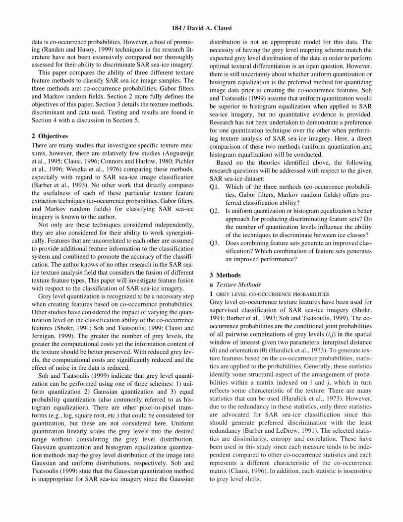
To study this question, each method was used to performtwo tests. First, the ground-validated data was used to trainthe system and the visually inspected data was classified.Then, the visually inspected data was used for training and thevalidated data was used for test classification. In addition torecording the kappa coefficients (κ) and confidence intervals(σ), the minimum and maximum Fisher criterion (fromexhaustive class-pairwise analysis) are recorded based on thetraining data. Three MRF orders (3, 4 and 5) are tested todetermine which order produces the most favourable results.Results are displayed in Table 1.

Co-occurrence results generated the best classificationaccuracies and the highest Fisher distances (see results in Q3for a discussion of the significance levels between the featuremethods). Gabor filters performed favourably but not to thesame extent as the co-occurrence method. MRF results werepoorer than Gabor and co-occurrence results. Based on usingindependent feature sets, co-occurrence was demonstrated tobe performing the best.

One may assume that 0.512 kappa value (the best co-occur-rence classification) is not a strong result. However, note thatother studies (Shokr, 1991; Barber et al., 1993) usually only


Z ~ .κ κ

σ σ1 2

12

22

−

+

TABLE 1. Classification results for each feature extraction method. κ – kappa coefficient, σ – standard deviation for κ, Min. and Max. J(ω) – minimum and maximumFisher criterion.

Validated Data Used for Training Inspected Data Used for Training

κ σ Min. J(ω) Max. J(ω) κ σ Min. J(ω) Max. J(ω)

Co-occurrence 0.475 0.0329 1.4 165.4 0.512 0.0324 0.9 204.1Gabor Filters 0.392 0.0325 1.0 113.4 0.448 0.0330 1.1 96.3MRF order 3 0.141 0.0270 0.2 6.5 0.192 0.0282 0.3 6.9MRF order 4 0.184 0.0280 0.4 9.5 0.173 0.0276 0.3 10.1MRF order 5 0.158 0.0262 0.4 10.7 0.158 0.0271 0.3 11.0

consider three classes (first-year rough, first-year smooth andmultiyear) while this study is considering a total of nine dif-ferent classes. For example, Barber and LeDrew (1991) hadtest kappas in the approximate range of 0.60 to 0.70, depend-ing on the experiment. Shokr (1991) performs a host of com-parative testing, but his results use classification accuraciesinstead of kappa coefficients, which does not allow for prop-er comparison. Tripling the number of classes dramaticallyincreases the difficulty of the problem. Here, a randomassignment of pixels would only generate about 11% classifi-cation accuracy, thus, a kappa value of 0.512 is quite strongconsidering this circumstance. The 4th order MRF kappavalue of 0.184 is above random assignment and thus, distin-guishing information is provided in this feature set. Note thateach feature set only captures textural information and not theaverage grey level i.e., the methods employed are insensitiveto grey level shifts.

The Fisher distances support the classification evidence.Co-occurrence and Gabor filtered features have high, similarFisher distances. The distances for the MRF methods areabout 10% of the values noted for co-occurrence and Gabormethods.

The statistical validity comparing the error matrix pro-duced by classifying the inspected data using a validated datadiscriminant versus the error matrix produced by classifyingthe trained data using an inspected data discriminant has beendetermined (Table 2). The null hypothesis states that, for eachfeature extraction method, the pair of error matrices are thesame. Table 2 reveals that there is no statistical significancebetween the error matrices created by classifying the test datausing either validation or inspected data for training (in thispaper, a 5% threshold is used i.e., 0.025 and 0.975 are theconfidence levels). Since the null hypothesis is not false, the

error matrices are not demonstrated to be statistically differ-ent. As a result, for the rest of this paper, the test error matri-ces produced by the validation and inspected data arecombined into a joint error matrix. The classification accura-cy provided by this joint error matrix is provided in Table 3.Results are in agreement with those found in Table 1.

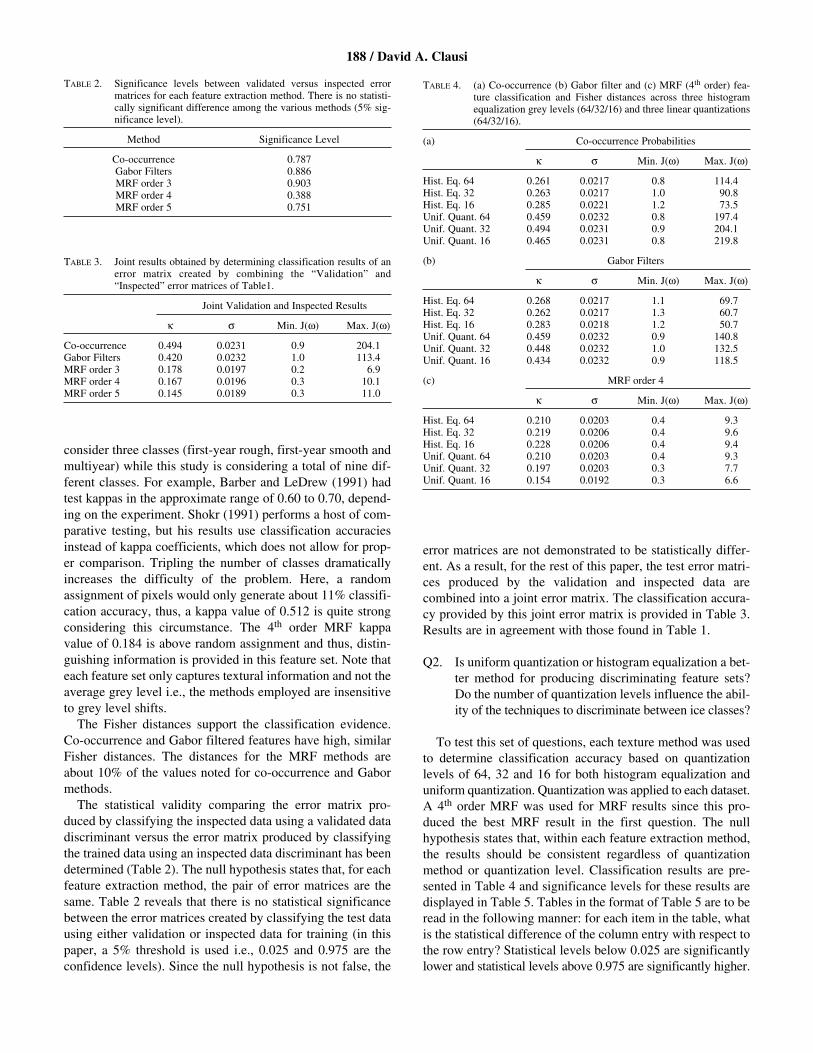
Q2. Is uniform quantization or histogram equalization a bet-ter method for producing discriminating feature sets?Do the number of quantization levels influence the abil-ity of the techniques to discriminate between ice classes?

To test this set of questions, each texture method was usedto determine classification accuracy based on quantizationlevels of 64, 32 and 16 for both histogram equalization anduniform quantization. Quantization was applied to each dataset.A 4th order MRF was used for MRF results since this pro-duced the best MRF result in the first question. The nullhypothesis states that, within each feature extraction method,the results should be consistent regardless of quantizationmethod or quantization level. Classification results are pre-sented in Table 4 and significance levels for these results aredisplayed in Table 5. Tables in the format of Table 5 are to beread in the following manner: for each item in the table, whatis the statistical difference of the column entry with respect tothe row entry? Statistical levels below 0.025 are significantlylower and statistical levels above 0.975 are significantly higher.


TABLE 2. Significance levels between validated versus inspected errormatrices for each feature extraction method. There is no statisti-cally significant difference among the various methods (5% sig-nificance level).

Method Significance Level

Co-occurrence 0.787Gabor Filters 0.886MRF order 3 0.903MRF order 4 0.388MRF order 5 0.751

TABLE 3. Joint results obtained by determining classification results of anerror matrix created by combining the “Validation” and“Inspected” error matrices of Table1.

Joint Validation and Inspected Results

κ σ Min. J(ω) Max. J(ω)

Co-occurrence 0.494 0.0231 0.9 204.1Gabor Filters 0.420 0.0232 1.0 113.4MRF order 3 0.178 0.0197 0.2 6.9MRF order 4 0.167 0.0196 0.3 10.1MRF order 5 0.145 0.0189 0.3 11.0

TABLE 4. (a) Co-occurrence (b) Gabor filter and (c) MRF (4th order) fea-ture classification and Fisher distances across three histogramequalization grey levels (64/32/16) and three linear quantizations(64/32/16).

(a) Co-occurrence Probabilities


Hist. Eq. 64 0.261 0.0217 0.8 114.4Hist. Eq. 32 0.263 0.0217 1.0 90.8Hist. Eq. 16 0.285 0.0221 1.2 73.5Unif. Quant. 64 0.459 0.0232 0.8 197.4Unif. Quant. 32 0.494 0.0231 0.9 204.1Unif. Quant. 16 0.465 0.0231 0.8 219.8

(b) Gabor Filters



(c) MRF order 4



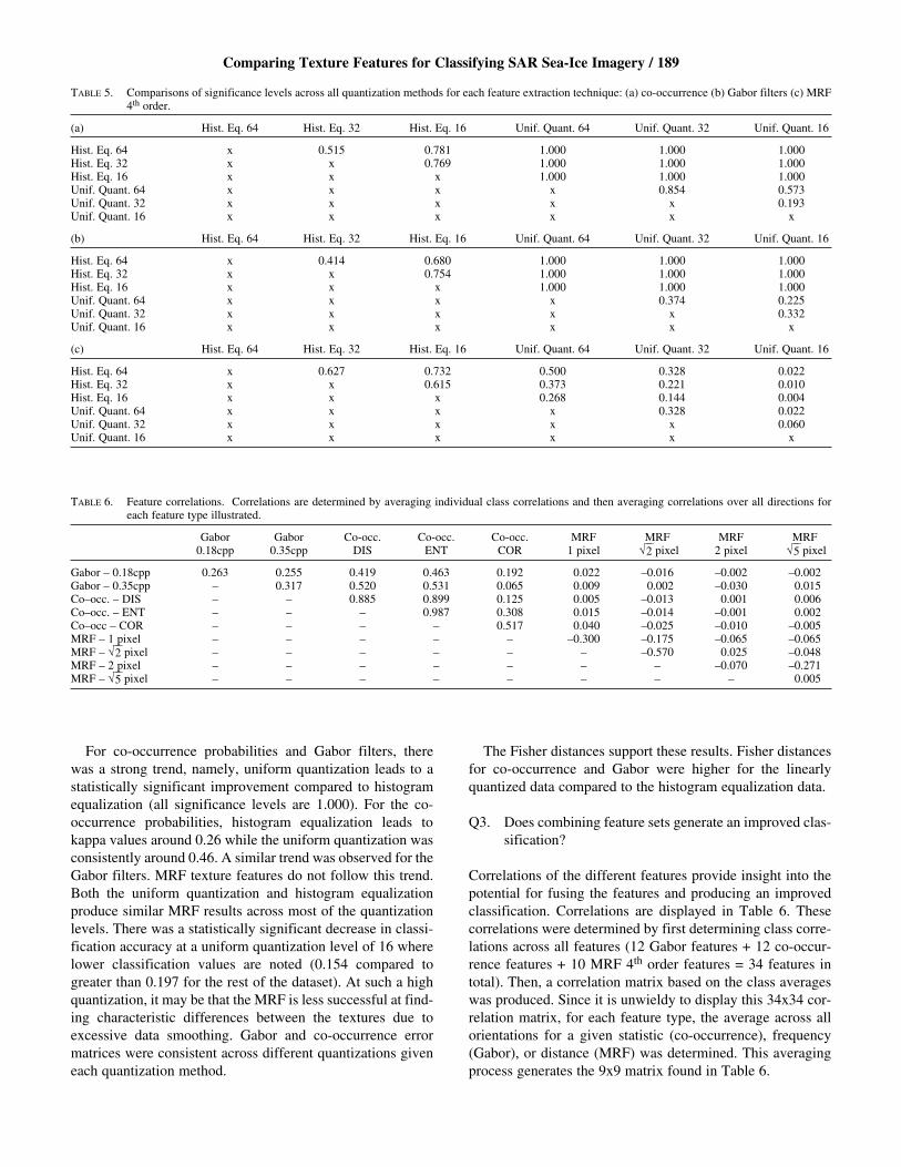
For co-occurrence probabilities and Gabor filters, therewas a strong trend, namely, uniform quantization leads to astatistically significant improvement compared to histogramequalization (all significance levels are 1.000). For the co-occurrence probabilities, histogram equalization leads tokappa values around 0.26 while the uniform quantization wasconsistently around 0.46. A similar trend was observed for theGabor filters. MRF texture features do not follow this trend.Both the uniform quantization and histogram equalizationproduce similar MRF results across most of the quantizationlevels. There was a statistically significant decrease in classi-fication accuracy at a uniform quantization level of 16 wherelower classification values are noted (0.154 compared togreater than 0.197 for the rest of the dataset). At such a highquantization, it may be that the MRF is less successful at find-ing characteristic differences between the textures due toexcessive data smoothing. Gabor and co-occurrence errormatrices were consistent across different quantizations giveneach quantization method.

The Fisher distances support these results. Fisher distancesfor co-occurrence and Gabor were higher for the linearlyquantized data compared to the histogram equalization data.

Q3. Does combining feature sets generate an improved clas-sification?

Correlations of the different features provide insight into thepotential for fusing the features and producing an improvedclassification. Correlations are displayed in Table 6. Thesecorrelations were determined by first determining class corre-lations across all features (12 Gabor features + 12 co-occur-rence features + 10 MRF 4th order features = 34 features intotal). Then, a correlation matrix based on the class averageswas produced. Since it is unwieldy to display this 34x34 cor-relation matrix, for each feature type, the average across allorientations for a given statistic (co-occurrence), frequency(Gabor), or distance (MRF) was determined. This averagingprocess generates the 9x9 matrix found in Table 6.


TABLE 5. Comparisons of significance levels across all quantization methods for each feature extraction technique: (a) co-occurrence (b) Gabor filters (c) MRF4th order.

(a) Hist. Eq. 64 Hist. Eq. 32 Hist. Eq. 16 Unif. Quant. 64 Unif. Quant. 32 Unif. Quant. 16

Hist. Eq. 64 x 0.515 0.781 1.000 1.000 1.000Hist. Eq. 32 x x 0.769 1.000 1.000 1.000Hist. Eq. 16 x x x 1.000 1.000 1.000Unif. Quant. 64 x x x x 0.854 0.573Unif. Quant. 32 x x x x x 0.193Unif. Quant. 16 x x x x x x

(b) Hist. Eq. 64 Hist. Eq. 32 Hist. Eq. 16 Unif. Quant. 64 Unif. Quant. 32 Unif. Quant. 16


(c) Hist. Eq. 64 Hist. Eq. 32 Hist. Eq. 16 Unif. Quant. 64 Unif. Quant. 32 Unif. Quant. 16


TABLE 6. Feature correlations. Correlations are determined by averaging individual class correlations and then averaging correlations over all directions foreach feature type illustrated.

Gabor Gabor Co-occ. Co-occ. Co-occ. MRF MRF MRF MRF0.18cpp 0.35cpp DIS ENT COR 1 pixel √2 pixel 2 pixel √5 pixel

Gabor – 0.18cpp 0.263 0.255 0.419 0.463 0.192 0.022 –0.016 –0.002 –0.002Gabor – 0.35cpp – 0.317 0.520 0.531 0.065 0.009 0.002 –0.030 0.015Co–occ. – DIS – – 0.885 0.899 0.125 0.005 –0.013 0.001 0.006Co–occ. – ENT – – – 0.987 0.308 0.015 –0.014 –0.001 0.002Co–occ – COR – – – – 0.517 0.040 –0.025 –0.010 –0.005MRF – 1 pixel – – – – – –0.300 –0.175 –0.065 –0.065MRF – √2 pixel – – – – – – –0.570 0.025 –0.048MRF – 2 pixel – – – – – – – –0.070 –0.271MRF – √5 pixel – – – – – – – – 0.005

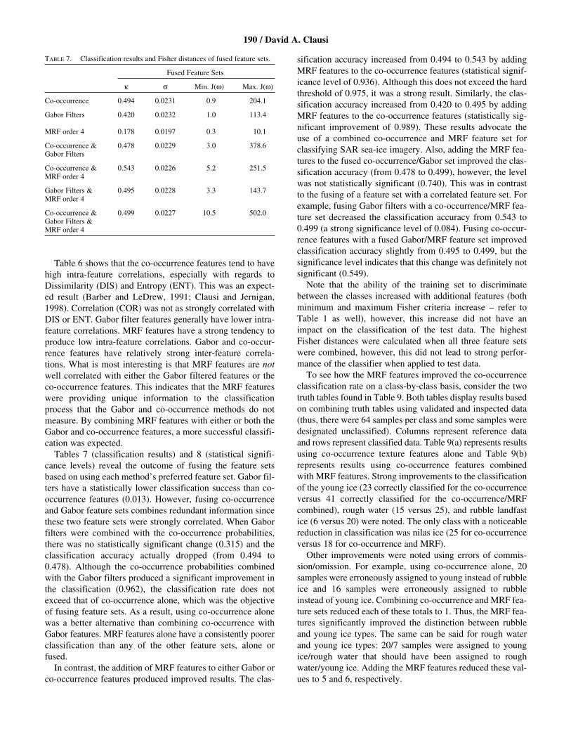
Table 6 shows that the co-occurrence features tend to havehigh intra-feature correlations, especially with regards toDissimilarity (DIS) and Entropy (ENT). This was an expect-ed result (Barber and LeDrew, 1991; Clausi and Jernigan,1998). Correlation (COR) was not as strongly correlated withDIS or ENT. Gabor filter features generally have lower intra-feature correlations. MRF features have a strong tendency toproduce low intra-feature correlations. Gabor and co-occur-rence features have relatively strong inter-feature correla-tions. What is most interesting is that MRF features are notwell correlated with either the Gabor filtered features or theco-occurrence features. This indicates that the MRF featureswere providing unique information to the classificationprocess that the Gabor and co-occurrence methods do notmeasure. By combining MRF features with either or both theGabor and co-occurrence features, a more successful classifi-cation was expected.

Tables 7 (classification results) and 8 (statistical signifi-cance levels) reveal the outcome of fusing the feature setsbased on using each method’s preferred feature set. Gabor fil-ters have a statistically lower classification success than co-occurrence features (0.013). However, fusing co-occurrenceand Gabor feature sets combines redundant information sincethese two feature sets were strongly correlated. When Gaborfilters were combined with the co-occurrence probabilities,there was no statistically significant change (0.315) and theclassification accuracy actually dropped (from 0.494 to0.478). Although the co-occurrence probabilities combinedwith the Gabor filters produced a significant improvement inthe classification (0.962), the classification rate does notexceed that of co-occurrence alone, which was the objectiveof fusing feature sets. As a result, using co-occurrence alonewas a better alternative than combining co-occurrence withGabor features. MRF features alone have a consistently poorerclassification than any of the other feature sets, alone orfused.

In contrast, the addition of MRF features to either Gabor orco-occurrence features produced improved results. The clas-

sification accuracy increased from 0.494 to 0.543 by addingMRF features to the co-occurrence features (statistical signif-icance level of 0.936). Although this does not exceed the hardthreshold of 0.975, it was a strong result. Similarly, the clas-sification accuracy increased from 0.420 to 0.495 by addingMRF features to the co-occurrence features (statistically sig-nificant improvement of 0.989). These results advocate theuse of a combined co-occurrence and MRF feature set forclassifying SAR sea-ice imagery. Also, adding the MRF fea-tures to the fused co-occurrence/Gabor set improved the clas-sification accuracy (from 0.478 to 0.499), however, the levelwas not statistically significant (0.740). This was in contrastto the fusing of a feature set with a correlated feature set. Forexample, fusing Gabor filters with a co-occurrence/MRF fea-ture set decreased the classification accuracy from 0.543 to0.499 (a strong significance level of 0.084). Fusing co-occur-rence features with a fused Gabor/MRF feature set improvedclassification accuracy slightly from 0.495 to 0.499, but thesignificance level indicates that this change was definitely notsignificant (0.549).

Note that the ability of the training set to discriminatebetween the classes increased with additional features (bothminimum and maximum Fisher criteria increase – refer toTable 1 as well), however, this increase did not have animpact on the classification of the test data. The highestFisher distances were calculated when all three feature setswere combined, however, this did not lead to strong perfor-mance of the classifier when applied to test data.

To see how the MRF features improved the co-occurrenceclassification rate on a class-by-class basis, consider the twotruth tables found in Table 9. Both tables display results basedon combining truth tables using validated and inspected data(thus, there were 64 samples per class and some samples weredesignated unclassified). Columns represent reference dataand rows represent classified data. Table 9(a) represents resultsusing co-occurrence texture features alone and Table 9(b)represents results using co-occurrence features combinedwith MRF features. Strong improvements to the classificationof the young ice (23 correctly classified for the co-occurrenceversus 41 correctly classified for the co-occurrence/MRFcombined), rough water (15 versus 25), and rubble landfastice (6 versus 20) were noted. The only class with a noticeablereduction in classification was nilas ice (25 for co-occurrenceversus 18 for co-occurrence and MRF).

Other improvements were noted using errors of commis-sion/omission. For example, using co-occurrence alone, 20samples were erroneously assigned to young instead of rubbleice and 16 samples were erroneously assigned to rubbleinstead of young ice. Combining co-occurrence and MRF fea-ture sets reduced each of these totals to 1. Thus, the MRF fea-tures significantly improved the distinction between rubbleand young ice types. The same can be said for rough waterand young ice types: 20/7 samples were assigned to youngice/rough water that should have been assigned to roughwater/young ice. Adding the MRF features reduced these val-ues to 5 and 6, respectively.


TABLE 7. Classification results and Fisher distances of fused feature sets.

Fused Feature Sets


Co-occurrence 0.494 0.0231 0.9 204.1

Gabor Filters 0.420 0.0232 1.0 113.4

MRF order 4 0.178 0.0197 0.3 10.1

Co-occurrence & 0.478 0.0229 3.0 378.6Gabor Filters

Co-occurrence & 0.543 0.0226 5.2 251.5MRF order 4

Gabor Filters & 0.495 0.0228 3.3 143.7MRF order 4

Co-occurrence & 0.499 0.0227 10.5 502.0Gabor Filters &MRF order 4

To simulate results based on fewer classes to verify that thetest results were consistent, classes were merged based ontheir relative Fisher distance. A preferred classification wasgenerated when the co-occurrence and 4th order MRF featuresets were combined. Consider the relative Fisher distancesbetween each pair of classes based on the training data usingMRF and co-occurrence features (Table 10). The objectivewas to merge classes that are closest together in the featurespace. The nearest classes were combined until an arbitrarynumber of four classes remained i.e., combine the closest twoclasses, namely, calm water and smooth ice at 5.2; then com-bine nilas/new ice and grey ice since they were the next clos-est at a distance of 8.4; etc. This merging process, as

expected, grouped classes that were visually similar in thefeature set. The four merged classes were as follows:

Class I – nilas/new ice, grey ice, medium first-year ice floesClass II – young ice floes, rough waterClass III – calm open water, smooth first-year iceClass IV – rubble landfast ice, multi-year ice

The classification results based on each of the three texturemethods individually, pairs of texture methods, and all threemethods together using the four class representation are dis-played in Table 11. Table 12 contains the parallel results forsignificance level testing. Results were consistent with previ-


TABLE 8. Statistical significance levels between combined validation/inspected error matrices for the identified feature sets.

Co-occurrence Gabor Filters MRF 4th Co-occurrence Co-occurrence Gabor Filters Co-occurrence& Gabor Filters & MRF 4th & MRF 4th & Gabor Filters

& MRF 4th

Co-occurrence x 0.013 0.000 0.315 0.936 0.514 0.563

Gabor Filters x x 0.000 0.962 1.000 0.989 0.992

MRF 4th x x x 1.000 1.000 1.000 1.000

Co-occurrence x x x x 0.978 0.698 0.740& Gabor Filters

Co-occurrence x x x x x 0.067 0.084& MRF 4th

Gabor Filters x x x x x x 0.549& MRF 4th

Co-occurrence x x x x x x x& Gabor Filters& MRF 4th

TABLE 9. Combined truth tables for validation and visually inspected classifications given (a) co-occurrence alone (b) co-occurrence with MRF features added.Classes: nilas/new ice, grey ice, young ice floes, medium first-year ice floes, rough open water, calm open water, smooth first-year ice, rubble land-fast ice, and multi-year (my) ice.

(a) nilas grey young medium rough calm smooth rubble my

nilas 41 11 0 2 0 0 4 0 0 58grey 5 25 2 4 0 1 1 11 0 49young 0 0 23 1 20 0 0 20 0 64medium 5 18 12 48 18 0 0 4 2 107rough 0 0 7 4 15 0 0 15 1 42calm 0 1 0 0 0 49 11 0 0 61smooth 7 4 0 0 0 12 47 0 0 70rubble 2 0 16 2 7 0 0 6 1 34my 0 0 2 0 0 0 0 3 60 65

60 59 62 61 60 62 63 59 64

(b) nilas grey young medium rough calm smooth rubble my

nilas 39 5 0 0 0 1 4 1 0 50grey 5 18 2 7 2 3 3 6 0 46young 0 0 41 1 5 0 0 1 1 49medium 4 16 9 44 13 0 0 5 2 93rough 0 0 6 7 25 0 0 15 1 54calm 0 2 0 0 0 46 8 0 0 56smooth 7 4 0 0 0 12 46 0 0 69rubble 0 0 1 2 10 0 0 20 2 35my 2 0 1 1 0 0 0 7 58 69

57 45 60 62 55 62 61 55 64

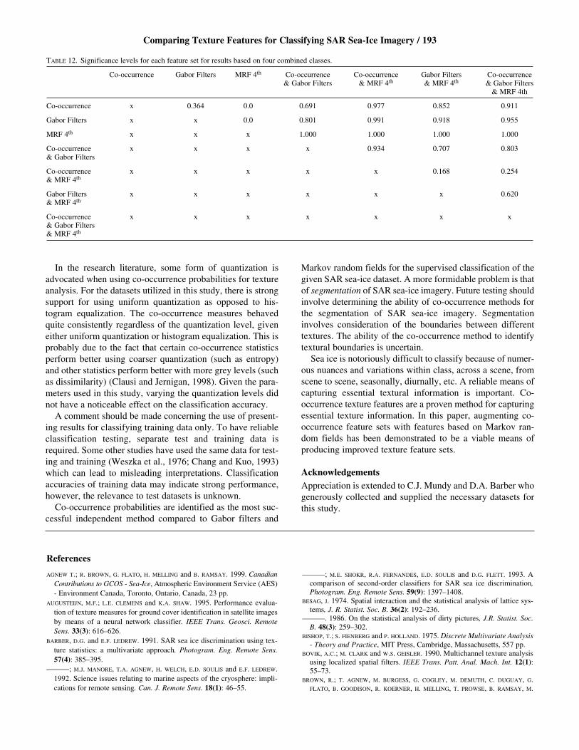
ous testing. As individual feature sets, co-occurrence and Gaborproduce strong results. Here, co-occurrence and Gabor do nothave a significant difference (0.364 significance level). As withnine classes, MRF results significantly lagged co-occurrenceand Gabor results. Fusing Gabor features with co-occurrencefeatures increased the success compared to using co-occur-rence features alone, and this increase was not statisticallysignificant (0.691). Fusing co-occurrence with Gabor filtersimproved the classification results compared to Gabor alone,however, this result was not statistically significant (0.801).

Combining MRF with Gabor and combining MRF with co-occurrence produced much improved results over eitherGabor or co-occurrence alone (significance levels of 0.977and 0.918, respectively). The best results were obtained byfusing MRF features with co-occurrence features (kappa of0.733). Merging all three feature sets dramatically increasedthe separability of the training data (maximum Fisher criterionof 107.4), but the results were not reflected in the test classi-fication. Fusing Gabor filter features to the co-occurrence/MRF feature set reduced the classification accuracy (from0.733 to 0.712).

5 DiscussionThe Gabor filter and co-occurrence probability methods mea-sure texture features in SAR sea-ice imagery basically bymeasuring local frequency. Gabor filters directly measure

local frequency components by acting as a bandpass filtercentred on the frequency of interest. The two co-occurrencemeasures that generally perform more strongly (dissimilarityand entropy) (Clausi and Jernigan, 1998) correlate well withlocal frequency measures. For example, smooth textures tendto have fewer entries in the co-occurrence matrix (low entropy)which are located close to the diagonal (low dissimilarity).MRF features measure something completely different aboutthe local texture compared to Gabor filters and co-occurrenceprobabilities. Here, model parameters are generated to best fita Gaussian distribution. However, there is no correlationbetween the MRF features and the co-occurrence or betweenthe MRF and Gabor features. Yet, the MRF classificationaccuracy indicates that they provide meaningful information.Fusing MRF features with Gabor filter features improves theclassification accuracy of using Gabor features alone. FusingMRF features with co-occurrence features produces the sameeffect. The combination of MRF and co-occurrence featuresis advocated for improved texture feature recognition of SARsea-ice imagery since it consistently generated preferred results.

The MRF features add to the classification accuracy byimproving the distinction of a number of class pairs confusedby using only the co-occurrence features. In this dataset, MRFfeatures improved the distinction between rough open water,rubble zones and young ice. Distinctions between these icetypes are recognized as being difficult, especially in the con-text of identifying the other six classes in this dataset. Thissupports the use of MRF features for assisting the discrimina-tion of SAR sea-ice imagery.

Gabor filters, implemented as wavelet operators, are notideal candidates for solving the texture classification prob-lem. Their inherent multiresolutional ability is not utilized forfixed-sized samples. The effective window size for the Gaborwavelet filters is gauged by the centre frequency of interest.Higher frequencies utilize smaller windows and lower fre-quencies utilize larger windows. This ability is more suited tothe segmentation problem where the window size is not pre-defined. A future recommendation for classification testing isto redesign the filter bank to set the effective spatial filterextent to match that of the window size, regardless of the fre-quency of interest. This moves away from the concept of awavelet filter bank, however, to ensure better coverage of theentire window sample by each filter, this approach for featureextraction should be attempted.


TABLE 10. Fisher distances between each class using combined cooccurrence and 4th order MRF features. Classes: nilas/new ice, grey ice, young ice floes, mediumfirst-year ice floes, rough open water, calm open water, smooth first-year ice, rubble landfast ice, and multi-year (my) ice.

nilas grey young medium rough calm smooth rubble my

nilas – 8.4 67.3 24.6 49.3 41.4 31.3 61.7 69.1grey – – 121.6 11.1 68.6 21.4 16.7 93.3 102.1young – – – 27.0 12.9 176.3 211.6 14.4 43.2medium – – – – 13.6 29.2 35.1 31.4 45.7rough – – – – – 133.4 148.5 6.4 30.9calm – – – – – – 5.2 136.4 155.9smooth – – – – – – – 160.4 178.3rubble – – – – – – – – 12.5my – – – – – – – – –

TABLE 11. Classification test results based on four combined classes.

Combined Classes


Co-occurrence 0.667 0.0243 2.1 81.4

Gabor Filters 0.655 0.0246 2.5 53.6

4th order MRF 0.251 0.0275 0.4 1.6

Co-occurrence & 0.684 0.0238 4.0 94.4Gabor Filters

Co-occurrence & 0.733 0.0224 5.1 89.54th order MRF

Gabor Filters & 0.702 0.0233 5.0 56.54th order MRF

Co-occurrence & 0.712 0.0229 6.1 107.4Gabor Filters &4th order MRF

In the research literature, some form of quantization isadvocated when using co-occurrence probabilities for textureanalysis. For the datasets utilized in this study, there is strongsupport for using uniform quantization as opposed to his-togram equalization. The co-occurrence measures behavedquite consistently regardless of the quantization level, giveneither uniform quantization or histogram equalization. This isprobably due to the fact that certain co-occurrence statisticsperform better using coarser quantization (such as entropy)and other statistics perform better with more grey levels (suchas dissimilarity) (Clausi and Jernigan, 1998). Given the para-meters used in this study, varying the quantization levels didnot have a noticeable effect on the classification accuracy.

A comment should be made concerning the use of present-ing results for classifying training data only. To have reliableclassification testing, separate test and training data isrequired. Some other studies have used the same data for test-ing and training (Weszka et al., 1976; Chang and Kuo, 1993)which can lead to misleading interpretations. Classificationaccuracies of training data may indicate strong performance,however, the relevance to test datasets is unknown.

Co-occurrence probabilities are identified as the most suc-cessful independent method compared to Gabor filters and

Markov random fields for the supervised classification of thegiven SAR sea-ice dataset. A more formidable problem is thatof segmentation of SAR sea-ice imagery. Future testing shouldinvolve determining the ability of co-occurrence methods forthe segmentation of SAR sea-ice imagery. Segmentationinvolves consideration of the boundaries between differenttextures. The ability of the co-occurrence method to identifytextural boundaries is uncertain.

Sea ice is notoriously difficult to classify because of numer-ous nuances and variations within class, across a scene, fromscene to scene, seasonally, diurnally, etc. A reliable means ofcapturing essential textural information is important. Co-occurrence texture features are a proven method for capturingessential texture information. In this paper, augmenting co-occurrence feature sets with features based on Markov ran-dom fields has been demonstrated to be a viable means ofproducing improved texture feature sets.

AcknowledgementsAppreciation is extended to C.J. Mundy and D.A. Barber whogenerously collected and supplied the necessary datasets forthis study.


TABLE 12. Significance levels for each feature set for results based on four combined classes.

Co-occurrence Gabor Filters MRF 4th Co-occurrence Co-occurrence Gabor Filters Co-occurrence& Gabor Filters & MRF 4th & MRF 4th & Gabor Filters

& MRF 4th

Co-occurrence x 0.364 0.0 0.691 0.977 0.852 0.911

Gabor Filters x x 0.0 0.801 0.991 0.918 0.955

MRF 4th x x x 1.000 1.000 1.000 1.000

Co-occurrence x x x x 0.934 0.707 0.803& Gabor Filters

Co-occurrence x x x x x 0.168 0.254& MRF 4th

Gabor Filters x x x x x x 0.620& MRF 4th

Co-occurrence x x x x x x x& Gabor Filters& MRF 4th

References

AGNEW T.; R. BROWN, G. FLATO, H. MELLING and B. RAMSAY. 1999. CanadianContributions to GCOS - Sea-Ice, Atmospheric Environment Service (AES)- Environment Canada, Toronto, Ontario, Canada, 23 pp.

AUGUSTEIJN, M.F.; L.E. CLEMENS and K.A. SHAW. 1995. Performance evalua-tion of texture measures for ground cover identification in satellite imagesby means of a neural network classifier. IEEE Trans. Geosci. RemoteSens. 33(3): 616–626.

BARBER, D.G. and E.F. LEDREW. 1991. SAR sea ice discrimination using tex-ture statistics: a multivariate approach. Photogram. Eng. Remote Sens.57(4): 385–395.

———; M.J. MANORE, T.A. AGNEW, H. WELCH, E.D. SOULIS and E.F. LEDREW.1992. Science issues relating to marine aspects of the cryosphere: impli-cations for remote sensing. Can. J. Remote Sens. 18(1): 46–55.

———; M.E. SHOKR, R.A. FERNANDES, E.D. SOULIS and D.G. FLETT. 1993. Acomparison of second-order classifiers for SAR sea ice discrimination,Photogram. Eng. Remote Sens. 59(9): 1397–1408.

BESAG, J. 1974. Spatial interaction and the statistical analysis of lattice sys-tems, J. R. Statist. Soc. B. 36(2): 192–236.

———. 1986. On the statistical analysis of dirty pictures, J.R. Statist. Soc.B. 48(3): 259–302.

BISHOP, T.; S. FIENBERG and P. HOLLAND. 1975. Discrete Multivariate Analysis- Theory and Practice, MIT Press, Cambridge, Massachusetts, 557 pp.

BOVIK, A.C.; M. CLARK and W.S. GEISLER. 1990. Multichannel texture analysisusing localized spatial filters. IEEE Trans. Patt. Anal. Mach. Int. 12(1):55–73.

BROWN, R.; T. AGNEW, M. BURGESS, G. COGLEY, M. DEMUTH, C. DUGUAY, G.FLATO, B. GOODISON, R. KOERNER, H. MELLING, T. PROWSE, B. RAMSAY, M.

SHARP, S. SMITH and A. WALKER. 1999. Development of a Canadian GCOSworkplan for the cryosphere, Atmospheric Environment Service (AES),Environment Canada, Toronto, Ontario, Canada.

CARSEY, F. 1989. Review and status of remote sensing of sea ice. IEEE J.Oceanic Eng. 14(2): 127–138.

CHANG, T. and C.C.J. KUO. 1993. Texture analysis and classification with tree-structured wavelet transform. IEEE Trans. Image Proc. 2(4): 429–441.

CHELLAPPA, R. 1985. Two-dimensional discrete Gaussian Markov randomfield models for image processing. In: Machine Intelligence and PatternRecognition: Progress in Pattern Recognition 2, G.T. Toussaint (Ed.),Elsevier Science Publishers, B.V. (North-Holland). pp. 79–112.

——— and S. CHATTERJEE. 1985. Classification of textures using GaussianMarkov random fields. IEEE Trans. Acous., Speech Signal Proc. 33(4):959–963.

CLAUSI, D.A. 1996. Texture Segmentation of SAR Sea Ice Imagery. Ph.D. thesis,University of Waterloo, Waterloo, Ontario, Canada N2L 3G1, 175 pp.

——— and M.E. JERNIGAN. 1998. A fast method to determine co-occurrencetexture features. IEEE Trans. Geosci. Remote Sens. 36(1): 298–300.

——— and ———. 1999. Designing Gabor filters for optimal texture sepa-rability. Pattern Recog. 33(11): 1835–1849.

COHEN, F.S.; Z. FAN and M.A. PATEL. 1991. Classification of rotated and scaledtexture images using Gaussian Markov random field models. IEEE Trans.Patt. Anal. Mach. Int. 13(2): 192–203.

CONGALTON, R.G.; R.G. ODERWALD and R.A. MEAD. 1983. Assessing Landsatclassification accuracy using discrete multivariate analysis statistical tech-niques. Photogram. Eng. Remote Sens. 49(12): 1671–1678.

CONNERS, R.W. and C.A. HARLOW. 1980. A theoretical comparison of texturealgorithms. IEEE Trans. Patt. Anal. Mach. Int. 2(3): 204–222.

CROSS, G.R. and A.K. JAIN. 1983. Markov random field texture models. IEEETrans. Patt. Anal. Mach. Int. PAMI-5(1): 25–39.

DAUGMAN, J.G. 1985. Uncertainty relation for resolution in space, spatial fre-quency, and orientation optimized by two-dimensional visual cortex fil-ters. J. Opt. Soc. Am. A A, 2(7): 1160–1169.

DUDA, R.O. and P.E. HART. 1973. Pattern Classification and Scene Analysis,John Wiley and Sons. Toronto, 482 pp.

HARALICK, R.M.; K. SHANMUGAN and I. DINSTEIN. 1973. Textural features forimage classification. IEEE Trans. Syst. Man. Cybern. SMC-3(6): 610–621.

HOLMES, Q.A.; D.R. NUESCH and R.A. SHUCHMAN. 1984. Textural analysis andreal-time classification of sea-ice types using digital SAR data. IEEETrans. Geosci. Remote Sens. GE-22(2): 113–120.

JAIN, A.K. and F. FARROKHNIA. 1991. Unsupervised texture segmentation usingGabor filters. Pattern Recog. 24(12): 1167–1186.

KURVONEN, L.; J. PULLIAINEN and M. HALLIKAINEN. 1999. Retrieval of biomassin boreal forests from multitemporal ERS-1 and JERS-1 SAR images.IEEE Trans. Geosci. Remote Sens. 37(1): 198–205.

MANJUNATH, B.S. and R. CHELLAPPA. 1991. Unsupervised texture segmentationusing Markov random field models. IEEE Trans. Patt. Anal. Mach. Int.13(5): 478–482.

MUNDY, C.J. and D.A. BARBER. 2001. On the Relationship between SpatialPatterns of Sea-Ice Type and the Mechanisms which Create and Maintainthe North Water (NOW) Polynya. ATMOSPHERE-OCEAN, 39: 327–341.

NYSTUEN, J.A. and F.W. GARCIA JR. 1992. Sea ice classifaication using SARbackscatter statistics. IEEE Trans. Geosci. Remote Sens. 30(3): 502–509.

PARTINGTON, K.C. and C. BERTOIA. 1997. Science Plan - Version 6.0, NationalIce Center, Washington, DC.

PICHLER, O.; A. TEUNER and B.J. HOSTICKA. 1996. A comparison of texture fea-ture extraction using adaptive Gabor filtering, pyramidal and tree struc-tured wavelet transforms. Pattern Recog. 29(5): 733–742.

RANDEN, T. and J.H. HUSOY. 1999. Filtering for texture classification: A com-parative study. IEEE Trans. Patt. Anal. Mach. Int. 21(4): 291–310.

SHANMUGAN, K.S.; V. NARAYANAN, V.S. FROST, J.A. STILES and J.C. HOLTZMAN.1981. Textural features for radar image analysis. IEEE Trans. Geosci.Remote Sens. GE-19(3): 153–156.

SHOKR, M.E. 1991. Evaluation of second-order texture parameters for sea iceclassification from radar images. J. Geophys. Res. 96(C6): 10625–10640.

SOH, L.K. and C. TSATSOULIS. 1999. Texture analysis of SAR Sea ice imageryusing gray level co-occurrence matrices. IEEE Trans. Geosci. RemoteSens. 37(2): 780–795.

TEUNER, A.; O. PICHLER and B.J. HOSTICKA. 1995. Unsupervised texture seg-mentation of images using tuned matched Gabor filters. IEEE Trans.Image Proc. 4(6): 863–869.

TOM, C.H. and L.D. MILLER. 1984. An automated land-use mapping compari-son of the Bayesian maximum likelihood and linear discriminant analysisalgorithms. Photogram. Eng. Remote Sens. 50(2): 193–207.

WESZKA, J.S.; C.R. DYER and A. ROSENFELD. 1976. A comparative study of tex-ture measures for terrain classification. IEEE Trans. Syst. Man. Cybern.SMC-6(4): 269–285.

WIEBE, J.A. 1998. Texture Estimates Of Operational Forestry Parameters.M.Sc. Thesis, University of Calgary, Calgary, Alberta. 99 pp.

WOODS, J.W. 1972. Two-dimensional discrete Markovian fields. IEEE Trans.Info. Theory. 18(2): 232–240.

YACKEL, J.J.; D.A. BARBER and T.N. PAPKYRIAKU. 2001. On the examination ofspring melt in the North Water (NOW) using RADARSAT-1. ATMOSPHERE-OCEAN, 39: 195–208.

YAMAZAKI, T. and D. GINGRAS. 1995. Image classification using spectral andspatial information based on MRF models. IEEE Trans. Image Proc. 4(9):1333–1339.


Documents

Comparison and Fusion of Co-occurrence, Gabor and …dclausi/Papers/Published 2001/Clausi...MRF Texture Features for Classification of SAR Sea-Ice Imagery David A. Clausi* ... privilégier