Comparison between Charges on Flow and Charges … · 62 Apuntes 78, First Semester 2016 / Chve-Bedoya and amíre ondn Acronyms AFP Pension fund management company (Administradora

61Comparison between Charges on Flow and Charges on Balance in Individual-Account Pension Systems

Vol. XLIII, N° 78, First Semester 2016: pages 61-88 / ISSN 0252-1865DOI: http://dx.doi.org/10.21678/apuntes.78.835

Copyright 2016: Centro de Investigación de la Universidad del Pacífico

Luis Chávez-Bedoya

ESAN, Lima

Nelson Ramírez Rondán*

Banco Central de Reserva del Perú, Lima

Abstract

In this present article, we develop a discrete-time methodology to compare front-end load and balance fees in the accumulation phase of a defined-contribution pension fund under a system of individual accounts. Using this methodology, we study the effect of risk aversion and other relevant variables in the performance and suitability of the aforementioned types of fees. Finally, we carry out a practical application and show the results for the Peruvian Private Pension System, including indifference values between fees and certainty equivalent ratios.

Key words: Pension funds; front-end load fee; balance fee; individual accounts.

Comparison between Charges on Flow and Charges on Balance in Individual-Account Pension Systems

* Article received on April 17, 2015; final version approved on March 11, 2016. The authors thank Guillermo Moloche and the Apuntes reviewer for their valuable comments, as well

as the participants of the Central Reserve Bank of Peru’s (Banco Central de Reserva del Perú, BCRP) research seminar, the 31st Meeting of BCRP Economists, and the 2014 Annual Congress of the Peruvian Association of Economics (Asociación Peruana de Economía, APE) for the comments and discussions that enriched this study. Any possible errors are the responsibility of the authors.

Luis Chávez-Bedoya holds a Ph.D. in Management Sciences from Northwestern University. He is currently professor of finances at the ESAN Graduate School of Business. His research has been published in Quantitative Finance, Journal of Pension Economics and Finance, CEPAL Review, Estudios de Economía de la Universidad de Chile and Journal of Asset Management, among other specialized journals.

Email: [email protected] Nelson Ramírez Rondán holds a Ph.D. in Economics from the University of Wisconsin-Madison. He is

currently a researcher at the BCRP Department of Economic Research. His areas of interest are theoretical econometrics and empirical macroeconomics.

Email: [email protected]

DOI: http://dx.doi.org/10.21678/apuntes.78.835

Apuntes 78, First Semester 2016 / Chávez-Bedoya and Ramírez Rondán 62

Acronyms

AFP Pension fund management company (Administradora de fondos de pensiones)

APE Peruvian Association of Economics (Asociación Peruana de Economía)

BCRP Central Reserve Bank of Peru (Banco Central de Reserva del Perú) CRRA Constant relative risk aversion GBM Geometric Brownian movement IA Individual account SDE Stochastic differential equation SBS Superintendence of Banking, Insurance, and AFPs (Superintendencia

de Banca, Seguros y AFP) SPP Private Pension Pystem (Sistema Privado de Pensiones)


1. INTRODUCTION

During the final quarter of the last century, many Latin American countries reformed their pension systems, switching from public pay-as-you-go (PAYG) systems to private systems based on individual accounts (IAs).1 According to Escrivá et al. (2010), these new systems constitute an attempt to adapt to the new risks and challenges faced by countries in the region, including factors such as: the vulnerability of public finances, changes in birth rates, greater life expectancy, problems of efficiency in public administration, and greater potential development of financial markets. However, a new series of reforms are now being proposed, whose fundamental objectives, discussed by Kritzer et al. (2011), are to increase coverage and competition in pension systems while reducing administrative costs.

Two important characteristics of IA pension systems are, on the one hand, the fact that affiliates assume the risk associated with fluctuation in the value of administrative assets; and on the other, the fact that the administrative fees (commissions) charged by pension fund management companies (administradoras de fondos de pensiones, AFPs) have a significant impact on the final balance of IAs.2 Furthermore, as stated in James et al. (2001), Whitehouse (2001), and Mitchell (1998), one of the main criticisms of IA systems is their high cost, since this does nothing to encourage participation, damages the image of the systems as a whole, reduces the value of future pensions, and increases the future costs to the government of a guaranteed minimum pension.

According to Kritzer et al. (2011), the most common type of administrative fees in IA pension systems are: proportional charges on flow (expressed as a percentage of income or contribution), fixed charges on flow, and charges on excess returns.3 This article analyzes

1. The most documented case is Chile. For the main aspects of this reform, see: Arrau et al. (1993); Diamond and Valdés-Prieto (1994); Edwards (1998); and Arenas de Mesa and Mesa-Lago (2006). In the case of Peru, a complete analysis of pension system reform and its current status is provided in Marthans and Stok (2013). Queisser (1998), Sinha (2000), Kay and Kritzer (2001), Mesa-Lago (2006), and Kritzer et al. (2011) are good references for the study of the reform, status, and perspective of Latin American pension systems.

2. Devesa-Carpio et al. (2003) argue that the levy scheme adopted in IA systems is very important because the accumulation process is exponential and directed toward long time horizons. For example, Murthi et al. (2001) estimate that in the United Kingdom, 40% of the value of IAs is dissipated by administrative fees, while Whitehouse (2001) finds that an annual levy of 1% of assets represents nearly 20% of the final pension value.

3. Analyses and comparison of administrative fees across different countries can be found in: James et al. (2001); Whitehouse (2001); Gómez-Hernández and Stewart (2008); Corvera et al. (2006); Tapia and Yermo (2008); Devesa-Carpio et al. (2003). Moreover, Sinha (2001), Masías and Sánchez (2007), and Martínez and Murcia (2008) perform a detailed analysis (notwithstanding the changes that have since been made) of administrative fees in Mexico, Peru, and Colombia, respectively.


4. A full analysis on the suitability of some of the commissions with respect to the economy could be performed as part of the general equilibrium model.

only proportional charges on flow and income, which are the most common and important types of levy in Latin America. For Queisser (1998), charges on flow are more advantageous to AFPs during the initial phase of the system, and despite the fact that income-based commission is aligned to AFPs’ objectives in terms of increasing fund profitability, they tend to be more expensive in the long run given that IAs increase in value. Meanwhile, Shah (1997) argues that charges on flow give rise to distortions and undesirable tendencies, such as engendering high AFP set-up costs, discouraging competition in the system, and generating losses for older affiliates. In Peru, the 1992 reform of the Private Pension System (Sistema Privado de Pensiones, SPP) sought to lend the system the financial sustainability that it had previously lacked. Recently, and in the framework of SPP reform, an important point of debate has been the commissions charged by AFPs. Thus, regulation should assure the type of commission that generates the greatest terminal wealth for affiliates, which is an important consideration in the SPP.

The traditional way of comparing commission on balance with commission on flow is through a commission on equivalent risk-neutral balance, which is equal to the expected value of the funds (under both levy schemes) at the end of the period of accumulation. This approach is employed by Shah (1997), Diamond (2000), Blake and Board (2000), Whitehouse (2001), Devesa-Carpio et al. (2003), and Gómez-Hernández and Stewart (2008). Moloche (2012), through a model (or benchmark) that maximizes the terminal utility of an affiliate in a context of dynamic optimization, compares certain scenarios of commissions on flow and on balance, and in the empirical case of the SPP concludes that such maximization would not be apt for less risk-adverse affiliates given current levels of commission on flow. It is in this context that this study employs two methods for comparing these commissions and, in turn, analyzes their sensitivity to changes of certain important parameters, especially affiliate risk aversion. The methods of comparison, which have been considered only from the point of view of affiliates,4 are the ratio of expected values of terminal wealth and the difference in expected utilities of terminal wealth. In the theoretical section, a series of assumptions are made from which closed expressions can be derived to explain the behavior of the commissions under the above-mentioned methods of comparison. The most important assumptions are: the use of a geometric Brownian movement (GBM) for the quota value of the fund, and the fact that the preferences of the affiliate can be


expressed in terms of the mean and the variance in terminal wealth. Subsequently, in the practical application to the SPP, a sensitivity analysis of the commissions is conducted in relation to certain fundamental variables, but by relaxing certain assumptions such as that corresponding to the function of affiliate utility. In general terms, it can be concluded that the performance of commission on balance improves as affiliate risk aversion increases, while higher growth rates on the quota value render commission on flow preferable to commission on balance in risk-neutral scenarios.

This study is structured as follows: Section 2 proposes a modeling and comparison methodology for commission on flow and commission on balance; Section 3 provides a practical application of the methodology to the SPP. Finally, Section 4 concludes, provides a number of recommendations, and proposes some extensions to the methodology.

2. METHODOLOGY

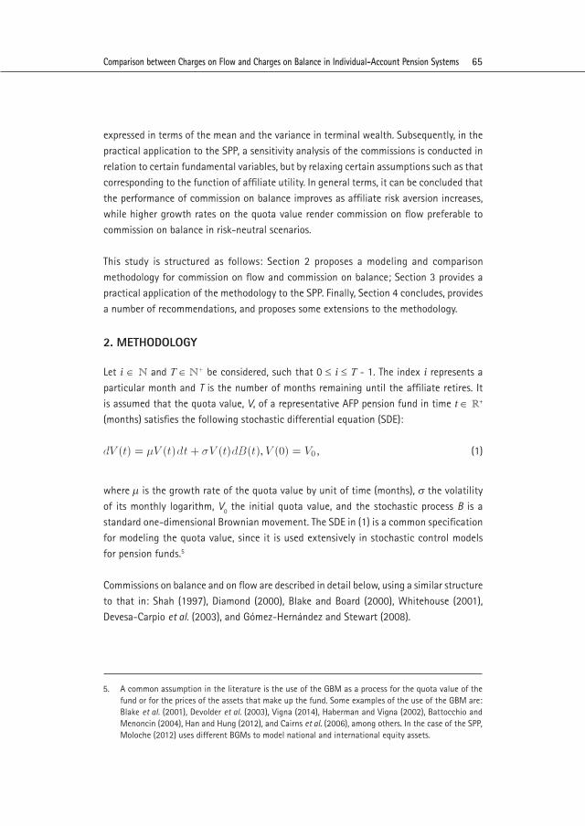
Let i ∈ N and T ∈ N+ be considered, such that 0 ≤ i ≤ T - 1. The index i represents a particular month and T is the number of months remaining until the affiliate retires. It is assumed that the quota value, V, of a representative AFP pension fund in time t ∈ R+

(months) satisfies the following stochastic differential equation (SDE):

(1)

where m is the growth rate of the quota value by unit of time (months), s the volatility of its monthly logarithm, V0 the initial quota value, and the stochastic process B is a standard one-dimensional Brownian movement. The SDE in (1) is a common specification for modeling the quota value, since it is used extensively in stochastic control models for pension funds.5

Commissions on balance and on flow are described in detail below, using a similar structure to that in: Shah (1997), Diamond (2000), Blake and Board (2000), Whitehouse (2001), Devesa-Carpio et al. (2003), and Gómez-Hernández and Stewart (2008).

5. A common assumption in the literature is the use of the GBM as a process for the quota value of the fund or for the prices of the assets that make up the fund. Some examples of the use of the GBM are: Blake et al. (2001), Devolder et al. (2003), Vigna (2014), Haberman and Vigna (2002), Battocchio and Menoncin (2004), Han and Hung (2012), and Cairns et al. (2006), among others. In the case of the SPP, Moloche (2012) uses different BGMs to model national and international equity assets.


i

6. A constant value of δ could imply that the system has reached maturity with respect to this type of levy.

7. Also known as commission on balance, it can be levied as a percentage of an affiliate’s income or contribution.

2.1. Commission on balanceLet δ > 0 be the monthly commission on balance expressed in continuous time.6 Moreover, in month i the affiliate contributes a sum Wi > 0 into their individual account. If the quota value, V, is normalized to the unit in the period i, then the contribution Wi is equivalent to the same number of quotas. That is, for t ≥ i, and based on the SDE (1), the contribution made in i would follow the GBM below:

(2)

The affiliate seeks to determine the final value of their fund, Ws ( T ), which is the sum of

the final values of all contributions made per the sequence WT = {Wi | Wi > 0,0 ≤ i ≤ T - 1}.Then,

(3)

where the processes Ws in (2) are subject to the same source of uncertainty B given by (1). Moreover, the expectation E [Ws (T )

], of the final value of the fund is:

(4)

The variance in the affiliate’s final fund under commission on balance is given by:

(5)

See the demonstration in Annex A.

2.2. Commission on flowLet α > 0 be the commission on flow.7 If the affiliate makes a contribution Wi in month i, the commission they would pay to the AFP (at the time of contributing) would be equal to Ci = Wi (1 - e- α). Considering that the commission Ci was invested in the fund, the affiliate’s contribution adjusted for the opportunity cost of Ci can be expressed as e- α Wi . Based on


i

8. It is well-documented that expected inflation, unexpected inflation shocks, and changes to expected inflation are negatively correlated with returns on shares. See: Fama and Schwert (1977), and Geske and Roll (1983). However, Boudoukh and Richardson (1993) find evidence which suggests that nominal long-term returns on shares are positively correlated with long-term ex ante and ex post inflation.

this assumption, the adjusted contribution of commission on flow in month i, Wf , would evolve according to the following GBM:

(6)

For the affiliate, it is important to calculate the value of the final fund adjusted for the opportunity cost of commission on flow per the sequence of contributions WT = {Wi | Wi

> 0,0 ≤ i ≤ T - 1}. If this final amount is denoted as Wf (T ), the following is obtained:

(7)

Using (4) and the variance of the final fund (5), it is shown that the expectation and the variance of Wf

(T ) can be calculated through the following expressions:

(8)

(9)

It is important to stress that Wf (T ) does not represent the true final value of the affiliate’s

fund, but one that is adjusted for the opportunity costs of the commission on flow. Moreover, the affiliate’s final fund would be equal to eαWf

(T ).

2.3. Risk factorsThus far, only one risk factor has been accounted for in the model: the returns of the fund’s quota value given by (1). Randomness in the sequence of contributions has not been accounted for, despite the fact that it is generally expressed as a percentage of income which in turn, is indexed to inflation. Furthermore, in a market with stochastic rates of return, a correlation is known to exist between inflation rates and the returns on assets.8 Thus, introducing randomness in the yields but not in the contributions could lead to false conclusions, since both processes depend on inflation. One option is to work in terms of nominal yields and by imposing a stochastic process upon contributions, but with some


9. For example, Moloche (2012) assumes that the savings made under commissions on flow compared with those under commissions on balance are deposited in a savings account with characteristics that are different and independent from the pension fund.

correlation with the quota value; however, we have opted to do so using a deterministic sequence of contributions and, to include inflation, we express and calibrate the quota value and the contributions in real terms.

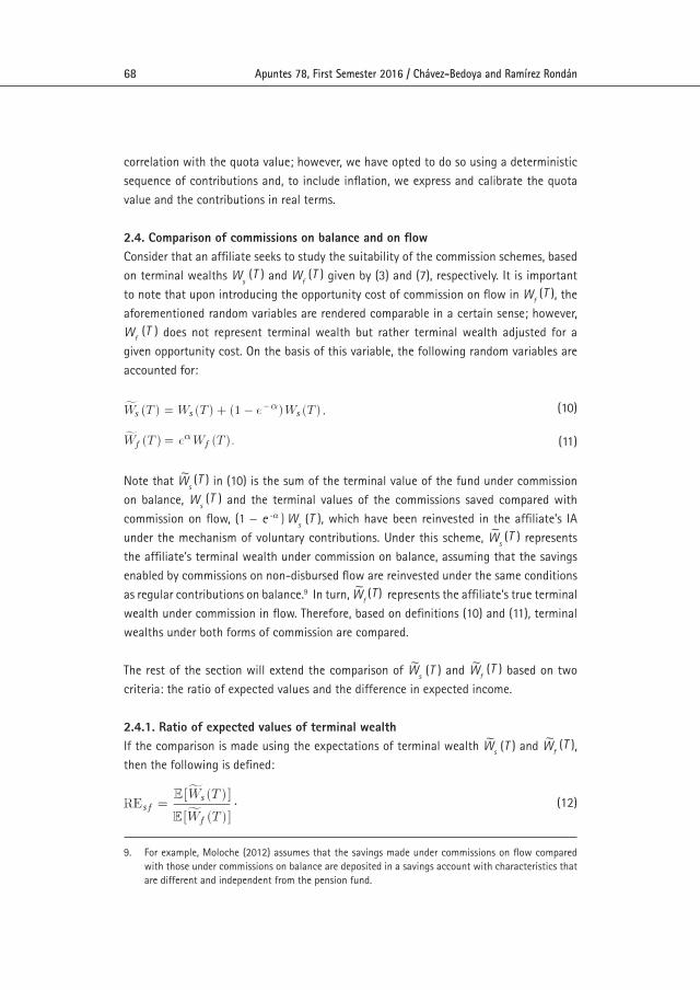
2.4. Comparison of commissions on balance and on flowConsider that an affiliate seeks to study the suitability of the commission schemes, based on terminal wealths Ws

(T ) and Wf (T ) given by (3) and (7), respectively. It is important

to note that upon introducing the opportunity cost of commission on flow in Wf (T ), the

aforementioned random variables are rendered comparable in a certain sense; however, Wf

(T ) does not represent terminal wealth but rather terminal wealth adjusted for a given opportunity cost. On the basis of this variable, the following random variables are accounted for:

(10)

(11)

Note that Ws (T ) in (10) is the sum of the terminal value of the fund under commission

on balance, Ws (T ) and the terminal values of the commissions saved compared with

commission on flow, (1 - e -α ) Ws (T ), which have been reinvested in the affiliate’s IA

under the mechanism of voluntary contributions. Under this scheme, Ws (T ) represents

the affiliate’s terminal wealth under commission on balance, assuming that the savings enabled by commissions on non-disbursed flow are reinvested under the same conditions as regular contributions on balance.9 In turn, Wf

(T ) represents the affiliate’s true terminal wealth under commission in flow. Therefore, based on definitions (10) and (11), terminal wealths under both forms of commission are compared.

The rest of the section will extend the comparison of Ws (T ) and Wf

(T ) based on two criteria: the ratio of expected values and the difference in expected income.

2.4.1. Ratio of expected values of terminal wealthIf the comparison is made using the expectations of terminal wealth Ws (T

) and Wf (T ),

then the following is defined:

(12)


10. Note that δ * (T = 1, α) = v and ∂αδ * (T, α) > 0) for any scenario N; and since the ratio of expected values of terminal wealth, REsf , is decreasing at higher rates of growth in the quota value, m , then ∂m δ * (T, m) < 0 is obtained for T > 1.

N

NN

*

*

** *

*

If REsf > 1, then commission on balance would be preferable; if REsf < 1, then commission on flow would be preferable. Therefore, when REsf = 1, the affiliate would be indifferent to both options. Note that these comparison criteria assume an affiliate who is indifferent to risk.

It is shown that the ratio of expected values of terminal wealth, REsf , is decreasing at higher rates of growth in the quota value (see Annex B). That is, REsf is a strictly decreasing function in µ and this relationship is independent of the contribution sequence WT . The above implies that commission on flow improves compared with commission on balance when the rate of growth in the quota value increases. Below we define the equivalent commission on balance for a risk-neutral affiliate.

For a given set of parameters N = {T, α, m, s2, WT} and REsf , the equivalent risk-neutral

commission on balance, δN (N), is defined as the value of the commission on balance, δ,

such that REsf = 1. Moreover, if the explicit dependence of δN (N) with respect to T, α, or

both is to be denoted, it is possible to use δN (T ), δN (α

) and δN (T, α), respectively. Moreover,

δN will be used when referring to equivalent commission in general.10

2.4.2. Expected utility of terminal wealthConsider a risk-adverse affiliate and let U (W ) be their earnings when a realization of terminal wealth is equal to W > 0. To determine the most appropriate type of commission, the affiliate needs to compare the expected utilities of terminal wealth E [U (Ws (T ) ) ] and E [U (Wf (T

) ) ]. However, explicit analytical expressions for these expected utilities are not generally available.

Because there are explicit formulas for the first and second moment of terminal wealths Ws (T ) and Wf (T ) and the objective is to find generalizable properties and/or closed formulas, then it is appropriate to consider a quadratic utility function given by:

UMV (W ) = αW - bW 2, (13)

where α > 0 and b > 0 is the coefficient of risk aversion. Note that when b = 0, the affiliate would be risk neutral. Moreover, α = 1 + 2b E [W ] is fixed in a similar manner to Zhou and Li (2000). If the utility of terminal wealth, U, is like in (13), the following is obtained:


T

A

(14)

(15)

and the expressions of E [Ws (T )2] and E [Wf (T

)2] can be explicitly obtained.

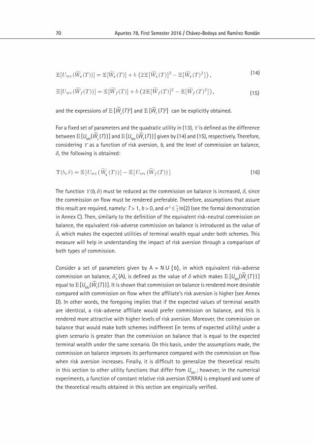
For a fixed set of parameters and the quadratic utility in (13), ϒ is defined as the difference between E [UMV(Ws (T

) ) ] and E [UMV (Wf (T ) ) ] given by (14) and (15), respectively. Therefore,

considering ϒ as a function of risk aversion, b, and the level of commission on balance, δ, the following is obtained:

(16)

The function ϒ (b, δ ) must be reduced as the commission on balance is increased, δ, since the commission on flow must be rendered preferable. Therefore, assumptions that assure this result are required, namely: T > 1, b > 0, and s 2 ≤ 1 ln(2) (see the formal demonstration in Annex C). Then, similarly to the definition of the equivalent risk-neutral commission on balance, the equivalent risk-adverse commission on balance is introduced as the value of δ, which makes the expected utilities of terminal wealth equal under both schemes. This measure will help in understanding the impact of risk aversion through a comparison of both types of commission.

Consider a set of parameters given by A = N U {b}, in which equivalent risk-adverse commission on balance, δ * (A), is defined as the value of δ which makes E [UMV(Ws (T

) ) ] equal to E [UMV(Wf (T

) ) ]. It is shown that commission on balance is rendered more desirable compared with commission on flow when the affiliate’s risk aversion is higher (see Annex D). In other words, the foregoing implies that if the expected values of terminal wealth are identical, a risk-adverse affiliate would prefer commission on balance, and this is rendered more attractive with higher levels of risk aversion. Moreover, the commission on balance that would make both schemes indifferent (in terms of expected utility) under a given scenario is greater than the commission on balance that is equal to the expected terminal wealth under the same scenario. On this basis, under the assumptions made, the commission on balance improves its performance compared with the commission on flow when risk aversion increases. Finally, it is difficult to generalize the theoretical results in this section to other utility functions that differ from UMV ; however, in the numerical experiments, a function of constant relative risk aversion (CRRA) is employed and some of the theoretical results obtained in this section are empirically verified.


3. APPLICATION OF THE METHODOLOGY TO PERU’S PRIVATE PENSION SYSTEM

This section applies the proposed methodology to the SPP. This application is relevant given that the SPP is undergoing an important reform process 20 years after its creation.11 Part of the reform entails replacing the commission on flow with commission on balance, as a result of which this study analyzes the effect of certain variables in the comparison of these commissions.

3.1. Parameters of the modelThe numerical applications take into account a retirement age of 65, the current structure of commissions on flow used by the SPP, the real growth rate of income, and a scenario for the quota value, V, of the fund, which corresponds to the medium-risk fund (Type 2) in the SPP.

3.1.1. Calibration of the quota value GBM To implement the methodology, it is necessary to calculate the growth parameters of the quota value, µ, and the volatility parameters of the quota value returns, s, of the stochastic process corresponding to the quota value of the fund described by the SDE (1). It is important to mention that an SPP affiliate can change fund provided that they remain in a low-risk SPP fund (Type 1) after reaching the age of 65. Moreover, it is possible to incorporate changes of fund by the affiliate into the methodology in a framework of dynamic optimization; but in this article it is assumed that the affiliate remains in a single type of fund throughout the entire accumulation phase.

Historic logarithmic yields corrected for inflation are employed to estimate the volatility of the respective GBM.12 For the scenario of moderate profitability (Type 2 fund), the monthly volatility of the quota value returns under a GBM is sM = 2.643%. Given the short history of SPP fund returns, it is to be expected that the calibrated growth rate (µ) will have a high estimation error. Therefore, and following the justifications of the “Anexo Técnico Nº 1” of the Superintendencia de Banca, Seguros y AFP (SBS 2013), a real annual return equal to 5.0% is assumed for the moderate scenario (the real historical return of the Type 2 fund has been

11. Law Nº 29903 provides for the primary aspects of the reform, one of which is that affiliates are to migrate to a mixed commission scheme, which includes a transitional front-loaded 10-year flow component, while from the eleventh year, the commission will be solely on balance. The reform also includes the tender mechanism for new IAs, and regulations for the incorporation of independent workers.

12. The series of historical quota value returns employed correspond to the AFP Integra, because it cons-titutes a suitable benchmark for the SPP; moreover, it is the only AFP that has been in existence (and which has not been merged) since the start of the available historical observations. In the case of the Type 2 fund, quota value observations from February 2, 2001 to April 30, 2014 are considered.


*

approximately 6.0% per annum). By way of GBM theory, it is verified that mM = rM + 0.5s 2, where rM is the expected monthly return in continuous time, and the subindex M refers to the Type 2 fund. After the appropriate transformations, mM = 0.004415 is obtained.

3.1.2. Commission on flowThree levels of commission on flow have been set (expressed as percentages of the affiliate’s income): fmin = 1.47%, fmax = 1.69% and fpro = 1.58%; which correspond to the minimum, maximum, and average charges on flow, respectively, under the SPP as at May 16, 2014. Because dependent workers in Peru are subject to an obligatory contribution of 10% of their income and f i is applied to this, α = - ln (1 - 10f ) is obtained, with which αmin = 0.1590, αmax = 0.185 y αpro = 0.172.

3.1.3. Real growth in incomeThe monthly succession of the affiliate’s real contributions (WT ) is assumed, such that Wi +1 = (1 + Ti )Wi for i ≥ 0 and arbitrary W0 > 0. The monthly factors T are calculated through the sum of the corresponding growth throughout the income curve plus an earnings component due to increased productivity. Moreover, T depends on different classifications of affiliates according to gender (F: female, M: male), education level (NU: non-university educated; U: university educated), and age. The details of the calibration of the factors are set out in SBS (2013), but it is important to mention that in the case of young affiliates, the average growth factors fluctuate between 2.5% and 3.5% per annum.

3.2. Numerical resultsThe parameters of the model employed in Section 3.1 are used first to determine the equivalent risk-neutral commission, δN . Then, a CRRA utility function of terminal wealth is used to evaluate the certainty equivalents generated by both types of commission and the effect that affiliate risk aversion has on them.

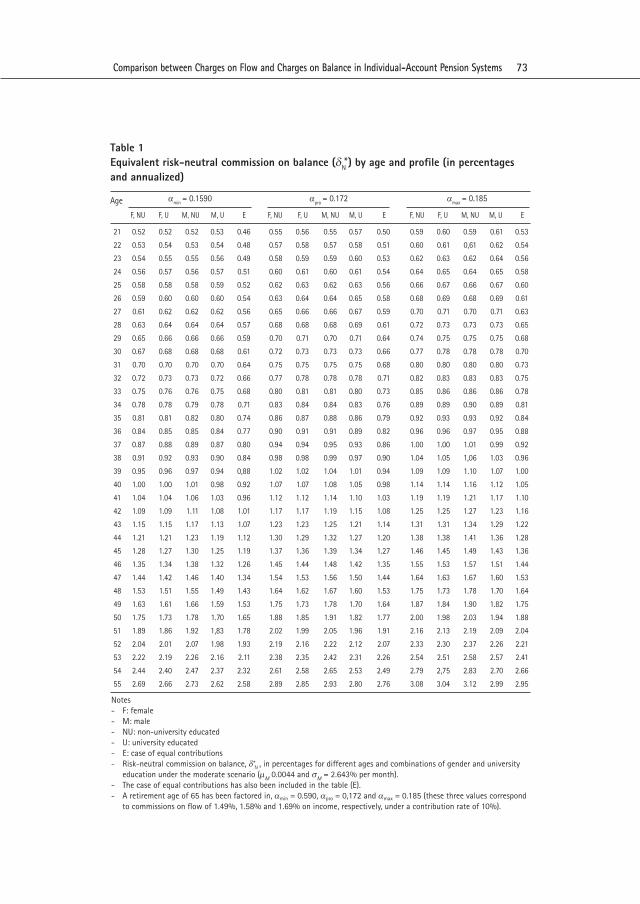
3.2.1. Equivalent risk-neutral commission on balance (δN )Table 1 shows the values of this commission, δN , annualized and expressed as percentages, for certain ages, five profiles,13 a moderate scenario (assuming a real fund return of 5.0%), and three different values of commission on flow (αmin = 0.1590, αpro = 0.172, and αmax = 0.185). It should be noted that δN is independent of the initial contribution W0 > 0. Table 1 shows that δN is strictly increasing with age (or strictly decreasing in T ) for a contribution profile and a fixed level of commission on flow - that is, the greater the age at the time of entry to the system, the more attractive the commission on flow will be.

M

*

*

*

*

13. The contribution profiles accounted for are: F, NU; F, U; M, NU; M, U; and E. The first four are described in Section 3.1.3, while E corresponds to a sequence of real contributions equal to W0 > 0 .


Table 1Equivalent risk-neutral commission on balance (δN

) by age and profile (in percentages and annualized)

*

21 0.52 0.52 0.52 0.53 0.46 0.55 0.56 0.55 0.57 0.50 0.59 0.60 0.59 0.61 0.53

22 0.53 0.54 0.53 0.54 0.48 0.57 0.58 0.57 0.58 0.51 0.60 0.61 0,61 0.62 0.54

23 0.54 0.55 0.55 0.56 0.49 0.58 0.59 0.59 0.60 0.53 0.62 0.63 0.62 0.64 0.56

24 0.56 0.57 0.56 0.57 0.51 0.60 0.61 0.60 0.61 0.54 0.64 0.65 0.64 0.65 0.58

25 0.58 0.58 0.58 0.59 0.52 0.62 0.63 0.62 0.63 0.56 0.66 0.67 0.66 0.67 0.60

26 0.59 0.60 0.60 0.60 0.54 0.63 0.64 0.64 0.65 0.58 0.68 0.69 0.68 0.69 0.61

27 0.61 0.62 0.62 0.62 0.56 0.65 0.66 0.66 0.67 0.59 0.70 0.71 0.70 0.71 0.63

28 0.63 0.64 0.64 0.64 0.57 0.68 0.68 0.68 0.69 0.61 0.72 0.73 0.73 0.73 0.65

29 0.65 0.66 0.66 0.66 0.59 0.70 0.71 0.70 0.71 0.64 0.74 0.75 0.75 0.75 0.68

30 0.67 0.68 0.68 0.68 0.61 0.72 0.73 0.73 0.73 0.66 0.77 0.78 0.78 0.78 0.70

31 0.70 0.70 0.70 0.70 0.64 0.75 0.75 0.75 0.75 0.68 0.80 0.80 0.80 0.80 0.73

32 0.72 0.73 0.73 0.72 0.66 0.77 0.78 0.78 0.78 0.71 0.82 0.83 0.83 0.83 0.75

33 0.75 0.76 0.76 0.75 0.68 0.80 0.81 0.81 0.80 0.73 0.85 0.86 0.86 0.86 0.78

34 0.78 0.78 0.79 0.78 0.71 0.83 0.84 0.84 0.83 0.76 0.89 0.89 0.90 0.89 0.81

35 0.81 0.81 0.82 0.80 0.74 0.86 0.87 0.88 0.86 0.79 0.92 0.93 0.93 0.92 0.84

36 0.84 0.85 0.85 0.84 0.77 0.90 0.91 0.91 0.89 0.82 0.96 0.96 0.97 0.95 0.88

37 0.87 0.88 0.89 0.87 0.80 0.94 0.94 0.95 0.93 0.86 1.00 1.00 1.01 0.99 0.92

38 0.91 0.92 0.93 0.90 0.84 0.98 0.98 0.99 0.97 0.90 1.04 1.05 1,06 1.03 0.96

39 0.95 0.96 0.97 0.94 0,88 1.02 1.02 1.04 1.01 0.94 1.09 1.09 1.10 1.07 1.00

40 1.00 1.00 1.01 0.98 0.92 1.07 1.07 1.08 1.05 0.98 1.14 1.14 1.16 1.12 1.05

41 1.04 1.04 1.06 1.03 0.96 1.12 1.12 1.14 1.10 1.03 1.19 1.19 1.21 1.17 1.10

42 1.09 1.09 1.11 1.08 1.01 1.17 1.17 1.19 1.15 1.08 1.25 1.25 1.27 1.23 1.16

43 1.15 1.15 1.17 1.13 1.07 1.23 1.23 1.25 1.21 1.14 1.31 1.31 1.34 1.29 1.22

44 1.21 1.21 1.23 1.19 1.12 1.30 1.29 1.32 1.27 1.20 1.38 1.38 1.41 1.36 1.28

45 1.28 1.27 1.30 1.25 1.19 1.37 1.36 1.39 1.34 1.27 1.46 1.45 1.49 1.43 1.36

46 1.35 1.34 1.38 1.32 1.26 1.45 1.44 1.48 1.42 1.35 1.55 1.53 1.57 1.51 1.44

47 1.44 1.42 1.46 1.40 1.34 1.54 1.53 1.56 1.50 1.44 1.64 1.63 1.67 1.60 1.53

48 1.53 1.51 1.55 1.49 1.43 1.64 1.62 1.67 1.60 1.53 1.75 1.73 1.78 1.70 1.64

49 1.63 1.61 1.66 1.59 1.53 1.75 1.73 1.78 1.70 1.64 1.87 1.84 1.90 1.82 1.75

50 1.75 1.73 1.78 1.70 1.65 1.88 1.85 1.91 1.82 1.77 2.00 1.98 2.03 1.94 1.88

51 1.89 1.86 1.92 1,83 1.78 2.02 1.99 2.05 1.96 1.91 2.16 2.13 2.19 2.09 2.04

52 2.04 2.01 2.07 1.98 1.93 2.19 2.16 2.22 2.12 2.07 2.33 2.30 2.37 2.26 2.21

53 2.22 2.19 2.26 2.16 2.11 2.38 2.35 2.42 2.31 2.26 2.54 2.51 2.58 2.57 2.41

54 2.44 2.40 2.47 2.37 2.32 2.61 2.58 2.65 2.53 2.49 2.79 2,75 2.83 2.70 2.66

55 2.69 2.66 2.73 2.62 2.58 2.89 2.85 2.93 2.80 2.76 3.08 3.04 3.12 2.99 2.95

F, NU F, U M, NU M, U E

Age αmin = 0.1590 αpro = 0.172 αmax = 0.185

F, NU F, U M, NU M, U E F, NU F, U M, NU M, U E

Notes- F: female- M: male- NU: non-university educated- U: university educated- E: case of equal contributions - Risk-neutral commission on balance, δ* , in percentages for different ages and combinations of gender and university

education under the moderate scenario (mM 0.0044 and sM = 2.643% per month). - The case of equal contributions has also been included in the table (E). - A retirement age of 65 has been factored in, αmin = 0.590, αpro = 0,172 and αmax = 0.185 (these three values correspond

to commissions on flow of 1.49%, 1.58% and 1.69% on income, respectively, under a contribution rate of 10%).

N


*

*Considering a 30-year-old affiliate pertaining to the M, NU profile, δN = 0.68% per annum is obtained for αmin = 0.1590, δN = 0.73% for αpro = 0.172 and δN = 0.78% for αmax = 0.185. For example, this implies that if a commission on flow equal to αmin is used, then a charge on flow of less than 0.68% would render commission on flow preferable for all affiliates over the age of 30 and pertaining to the M, NU profile who enter the system. Note that δN > 0.52% for all scenarios in Table 1 (without accounting for profile E). This value corresponds to a 21-year-old affiliate with a F, NU profile and a commission on flow equal to αmin. That is, a level of commission on flow of less than or equal to 0.52% would render this commission preferable (for a risk-neutral affiliate) under all contribution profiles (without E) and scenarios included in the study. The equal contributions profile (E) benefits the commission on flow, since the values of δN generated are lower than those corresponding to other profiles. This is based on the fact that the rise in income can be considered as an increase in the growth rate µ. Finally, and by way of example, Graph 1 shows equivalent risk-neutral commission on balance, δN, as a function of age and contribution profile, but only for average commission on flow, αprom.

Graph 1Risk-neutral commission on balance δN by age (in percentages)

* *

*

*

*

*

Notes - Risk-neutral commission on balance, δN, in percentages and annualized for different combinations of age and

gender/university education under the moderate scenario (mM 0.0044 and sM = 2.643% per month). - The case of equal contributions (E) has been included. - α = 0.172 has been assumed (corresponding to a charge on flow equal to 1.58% of income under a constant

contribution rate of 10% of income) and a retirement age of 65.


3.2.2. Comparison of certainty equivalents (DCEsf )This section will empirically study the following ratio:

(17)

where CE [Ws(T ) ] and CE [Wf (T

) ] are the certainty equivalents of Ws (T ) and Wf (T

), assuming an arbitrary utility function U of terminal wealth - that is, it satisfies both E [U (Ws (T

) ) ] = U (CE[Ws (T

) ] ) and E [U (Wf (T ) ) ] = U (CE[Wf (T

) ] ). The value of DCEsf under the quadratic utility function given by (13) has an explicit analytical expression because the expressions for the means and variances of Ws(T

) and Wf (T ) are available and can be used in (17). But,

in this case, DCEsf will depend on W0 even if it is assumed that WT , as in Section 3.1.3. In consequence, this fact complicates the study of the behavior of DCEsf because of changes in the coefficient of risk aversion, b, of the quadratic utility function given by (13).

An option for eliminating the dependence of W0 is to employ a utility function, such that DCEsf will be independent of W0 when WT is assumed, as in Section 3.1.3. If a CRRA utility function is considered such that:

(18)

where W > 0 is the terminal wealth and ϒ > 0 is the risk aversion coefficient, then DCEsf will not depend on W0 . This fact will be important in separating the effect of risk aversion on DCEsf from that caused by the initial contribution W0 . It is important to mention that closed expressions for CE [Ws (T

) ] and CE [Wf (T ) ] are not available for the utility (18), with

which simulation would have to be used to obtain an estimator of DCEsf in (17). Moreover, in the literature on pension fund management, the use of a CRRA utility is more common and appropriate, as in (18), than the quadratic given by (13).

Table 2 presents the estimated values of DCEsf for different ages, the F, NU contribution profile (since the results for other profiles in Section 3.1.3 are very similar, they are not reported), and under the moderate profitability scenario described in Section 3.1.1. Following Poterba et al. (2005), three different values of affiliate risk aversion are accounted for: ϒ = 1 for a low degree; and in this case U (W ) = ln(W ), ϒ = 4 for a moderate degree; and ϒ = 8 for a high degree. The level of commission on balance, δ, is set at three levels: 0,5%, 1,0% and 1,5% per annum, while the level of commission on flow is set at αpro = 0.172 (current average value of the SPP). The number of sample


20 1.38 2.40 3.63 - 10.89 - 9.07 - 6.82 - 21.32 - 18.94 - 16.01

21 1.71 2.70 3.92 - 10.31 - 8.56 - 6.47 - 20.59 - 18.30 - 15.40

22 2.04 2.99 4.15 - 9.74 - 8.06 - 6.05 - 19.85 - 17.61 - 14.80

23 2.38 3.29 4.39 - 9.16 - 7.53 - 5.59 - 19.08 - 16.92 - 14.31

24 2.71 3.59 4.63 - 8.56 - 7.00 - 5.14 - 18.31 - 16.24 - 13.61

25 3.05 3.90 4.89 - 7.98 - 6.47 - 4.64 - 17.54 - 15.54 - 13.11

26 3.39 4.20 5.14 - 7.38 - 5.94 - 4.21 - 16.76 - 14.83 - 12.58

27 3.74 4.50 5.41 - 6.78 - 5.41 - 3.75 - 15.97 - 14.13 - 11.92

28 4.08 4.80 5.68 - 6.17 - 4.87 - 3.24 - 15.16 - 13.41 - 11.25

29 4.42 5.11 5.97 - 5.56 - 4.32 - 2.86 - 14.36 - 12.67 - 10.63

30 4.76 5.42 6.23 - 4.96 - 3.78 - 2.32 - 13.55 - 11.94 - 9.99

31 5.11 5.73 6.47 - 4.35 - 3.22 - 1.85 - 12.73 - 11.19 - 9.34

32 5.45 6.04 6.74 - 3.74 - 2.67 - 1.38 - 11.92 - 10.45 - 8.69

33 5.79 6.34 7.03 - 3.14 - 2.12 - 0.87 - 11.09 - 9.71 - 8.00

34 6.13 6.65 7.28 - 2.53 - 1.56 - 0.40 - 10.27 - 8.97 - 7.33

35 6.46 6.96 7.56 - 1.92 - 1.01 0.10 - 9.45 - 8.20 - 6.70

36 6.80 7.26 7.82 - 1.31 - 0.46 0.57 - 8.62 - 7.45 - 6.01

37 7.13 7.57 8.09 - 0.70 0.10 1.08 - 7.79 - 6.69 - 5.33

38 7.47 7.87 8.37 - 0.09 0.66 1.57 - 6.96 - 5.92 - 4.63

39 7.80 8.18 8.64 0.51 1.21 2.09 - 6.13 - 5.16 - 3.94

40 8.13 8.48 8.92 1.12 1.77 2.56 - 5.29 - 4.39 - 3.25

41 8.46 8.78 9.17 1.72 2.32 3.08 - 4.47 - 3.62 - 2.57

42 8.78 9.08 9.45 2.32 2.88 3.58 - 3.63 - 2.85 - 1.88

43 9.10 9.38 9.72 2.92 3.44 4.07 - 2.80 - 2.07 - 1.16

44 9.42 9.68 9.99 3.52 3.99 4.59 - 1.97 - 1.30 - 0.46

45 9.74 9.97 10.26 4.11 4.54 5.09 - 1.14 - 0.52 0.25

46 10.06 10.27 10.53 4.70 5.09 5.58 - 0.31 0.25 0.95

47 10.37 10.56 10.79 5.29 5.65 6.09 0.52 1.03 1.66

48 10.69 10.85 11.06 5.88 6.20 6.60 1.36 1.81 2.38

49 11.00 11.15 11.34 6.47 6.75 7.11 2.20 2.60 3.11

50 11.31 11.44 11.60 7.06 7.31 7.63 3.03 3.39 3.84

Ageg = 1 g = 4 g = 8

δ = 0.50% δ = 1.00% δ = 1.50%

g = 1 g = 4 g = 8 g = 1 g = 4 g = 8

~ ~

paths of wealth used to estimate DCEsf is determined using the sequential procedure of Kelton and Law (2000) with a relative error of 0.0001 and a confidence level of 99%. Moreover, Graph 2 outlines all of the information contained in Table 2.

Table 2Estimated certainty equivalent values, DCEsf by age (in percentages)

Notes

- Estimated values of DCEsf = CE [Ws (T ) ] / CE [Wf (T ) ] - 1 in percentages for different ages, risk aversion coefficient values

(g = 1, 4, 8), F, SU contribution profile as per Section 3.1.3 and the moderate scenario (mM = 0.0044 and sM = 2.643%

per month).

- δ = 0.5%, 1.0%, 1.5% per annum α = 0,172 has been assumed (corresponding to a charge on flow equal to 1.58% of

income under a constant contribution rate of 10% of income) and a retirement age of 65.


Graph 2Percentage difference in CE (moderate scenario; in percentages)

Notes - Estimated values of DCEsf = CE [Ws

(T ) ] / CE [Wf (T ) ] - 1 in percentages, for different ages, risk aversion coeffi-cient values (g = 1, 4, 8), and under the moderate scenario (mM = 0.0044 and sM = 2.643% per month) with F, NU contribution profile as per Section 3.1.3.

- δ = 0,5%, 1,0%, 1,5% per annum α = 0.172 has been assumed (corresponding to a charge on flow equal to 1.58% of income under a constant contribution rate of 10% of income) and a retirement age of 65.

~ ~

From the information provided, it can be observed that DCEsf is an increasing function in the degree of risk aversion, ϒ, for a fixed age and level of commission, which empirically corroborates the fact that with greater risk aversion, commission on balance is improved compared with commission on flow. However, DCEsf > 0 is not obtained for all ages, since δ is fixed at certain fixed values instead of working with risk-neutral commission on balance, δN

, corresponding to each age. Moreover, when δ decreases, commission on balance is rendered more attractive, since the DCEsf curves for a fixed ϒ go up. It is also observed that the DCEsf slope tends to be positive, remaining constant with age and decreasing slightly as the affiliate’s degree of risk aversion increases. It is important to note that δ = 0.5% guarantees that DCEsf > 0 for all ages and levels of risk aversion accounted for. Moreover, when δ = 1%, the indifference age between commissions fluctuates between 35 (ϒ = 8) and 38 (ϒ = 1). When δ = 0.5%, the indifference age is around 45 (ϒ = 8) and 47 (ϒ = 1). It should be recalled that affiliates who are below the difference age will prefer commission on flow. If δ = 1% and the commission on flow is 1.58% of income (SPP average as at May 2014), a 20-year-old affiliate would experience a percentage loss in certainty equivalent

*


in the range of 7% (ϒ = 8) to 11% (ϒ = 1); while if the commission is δ = 1.5%, the loss would be in the range of 16% (ϒ = 8) to 21% (ϒ = 1).

4. CONCLUSIONS

This study develops a discrete-time method that enables comparison of commissions on flow with commissions on balance in IA pension systems. The comparison methods employed are the ratio of expected values of terminal wealth and the difference in expected utilities of terminal wealth. In many cases, very general results are obtained with respect to the relative performance of the commission schemes and these are achieved without the need to assume a particular pattern in the sequence of contributions. Moreover, formulas and/or expressions are provided in order to determine the most appropriate type of commission for each affiliate. A quadratic utility function is employed to demonstrate theoretically that, in general, increases in risk aversion improve the performance of the commission on balance compared with commission on flow, a result which is in keeping with the empirical conclusion of Moloche (2012).

On the basis of the theoretical analysis carried out and its practical application to the SPP, it can be stated that commission on balance equal to 0.5% per annum would render commission on balance preferable to commission on flow across almost all scenarios included in the study, based on commission on flow equal to 15.80% of contributions (SPP average as at May 2014). At this level of commission on flow and when commission on balance is equal to 1% per annum, affiliates below the age of 37 (approximately) will prefer the charge on flow; but when commission is 1.5% per annum, the indifference age increases to 45 (approximately). Moreover, an affiliate who enters the system at 20 years of age under a commission on balance scheme equal to 1% per annum could lose between 7% and 11% in terminal wealth certainty equivalent, in comparison with commission on flow. If the rate of commission were 1.5% per annum, the percentage loss would be between 16% and 21%. It is important to state that the lower and upper values in the ranges correspond to a high and low level of risk aversion, respectively.

It is possible to make many refinements to the methodology and the comparison methods. For example, variable commissions on balance according to the evolution of equivalent commissions from the perspective of the AFP, and commission on results that are strictly dependent on the stock exchange, more sophisticated stochastic processes for the quota value, and the relevant economic variables could be considered. Moreover, it would be interesting to contrast the schemes by using optimal policies that allow changes in the level of fund risk and returns according to the age of the affiliate and the size of the fund, in a context of discrete-time stochastic optimization. In these terms, the study by


Moloche (2012) could be built upon for different ages and reinvestment rates of saved commissions on flow. In addition, it is possible to work under the assumption of market completion and provide expressions to determine indifference values between fees by using valuation in the absence of arbitrage opportunities. But such extensions are beyond the scope of this study.


i

ANNEXES

Annex A

Demonstration of the terminal wealth variableFor the calculation of Var (Ws (T ) ), it is necessary to calculate the variance of Ws (T ) and the covariance between Ws (T ) and Ws (T ). Because Ws (T ) has a log-normal distribution, then:

(19)

Therefore, it is to be verified that for j > i and Wj > 0:

(20)

where the GBM Ws is defined in (2).

From the properties of Ws , the following is obtained:

(21)

(22)

(23)

(24)

(25)

(26)

i

i i j

i

To obtain (23), the fact that B (T ) - B ( j ) is independent of B ( j ) - B (i ) is utilized.

Formulas (19) and (20) generate the following expression for the covariance of the final values of the contributions i and j for all 0 ≤ i ≤ T - 1 and 0 ≤ j ≤ T - 1:

(27)


By using (27), the variance of Ws (T ) can be calculated through:

(28)

ANNEX B

Demonstration that the derivative of REsf (m) with respect to m is negative

Let v = ln(2 - e -α). For the case of contributions according to sequence WT and when

T > 1, it can be expressed that REsf in (12) as follows:

(29)

The following is obtained, based on the expression given in (29):

(30)

The partial derivative of REsf (µ) with respect to µ is:

(31)

(32)


Because δ > 0 and Wi for all i, it is clear that for T > 1.

On the basis of which, to demonstrate that < 0, it would only remain to be verified

that:

(33)

Proceeding by induction, for T = 2 in (33) the following is obtained:

(34)

Assuming that (33) is fulfilled, it must be demonstrated that:

(35)

The inequality (35) is equivalent to:

(36)

Because it is assumed that (33) and WT > 0, the inequality (36) implies:

(37)

which in turn is equivalent to:

(38)

To conclude, it is observed that the inequality (38) is fulfilled, since T - i ≥ 1, Wi > 0 and δ > 0.


Annex C

Monotonicity of ϒ (b, δ ) with respect to δ

From the definition of ϒ given by (16), the following is obtained:

(39)

Since ∂δ E [Ws (T ) ] < 0 for scenario A and it is assumed that b > 0 , only the conditions for ∂δ(2 E [Ws (T ) ]2 - E [Ws (T )2 ] ) ≤ 0 must be established. Using the expressions for E [Ws (T ) ]2 and E [Ws (T )2 ], it is verified that:

(40)

(41)

From the results before and after some simplifications, the following is obtained:

(42)

Finally, (42) will be less than or equal to zero if 2 - e s2 (T - i ) ≥ 0 for all i, which is fulfilled

when 2 - e s2T ≥ 0.


∞

1T

N ∞

*

Annex D

For the case of high risk aversion, commission on balance is preferable to commission on flow

First, the following ratios are defined:

If δ is fixed at the level given by δN and the fact that Hs > Hf is used (the demonstration is available upon request), then E [Wf (T ) ] = E [Ws (T ) ], E [Wf (T )2] > E [Ws(T )2], and:

(44)

are obtained.

Since the right side of (44) is positive and increasing in b, ϒ (b, δ * ) > 0 as well as ∂bϒ (b,

δ * ) > 0 are obtained. Then, for δ > 0, the function L (δ ) is defined as:N

N

(45)

From previous demonstrations it is known that if s 2 ≤ ln(2), then ∂δ L (δ ) < 0. Moreover,

δ * > δ N will exist, such that L(δ * ) = 0. For any b > 0, the following is obtained:

(46)

Note that K < 0 is independent of b. If two arbitrary values of the risk aversion coefficient, b1 > 0 and b2 > 0, are taken, such that b1 > b2 and δ ∈ (δ * , δ * ), then it can be affirmed that ϒ (b1, δ

) > ϒ (b2 , δ ) with δ inside the previously established interval, and also

that δ * (b1) y δ * (b2). Note that both, δ * (b1) and δ * (b2), exist because ϒ (b, δ * ) > 0, ϒ (b, δ * ) < 0, and ∂δ ϒ (b, δ ) < 0 for any b > 0.

* ∞

AA A A N

∞

(43)


REFERENCES

ARENAS DE MESA, Alberto and Carmelo MESA-LAGO2006 “The Structural Pension Reform in Chile: Effects, Comparisons with other Latin American

Reforms, and Lessons.” In: Oxford Review of Economic Policy, vol. 22, no. , pp. 149-167.

ARRAU, Patricio; Salvador VALDÉS-PRIETO and Klaus SCHMIDT-HEBBEL1993 “Privately Managed Pension Systems: Design Issues and the Chilean Experience” [mimeo.].

Technical report. Washington D.C.: World Bank.

BATTOCCHIO, Paolo and Francesco MENONCIN2004 “Optimal Pension Management in a Stochastic Framework.” In: Insurance: Mathematics and

Economics, vol. 34, no. 1, pp. 79-95.

BLAKE, David and John BOARD2000 “Measuring Value Added in the Pensions Industry.” In: Geneva Papers on Risk and Insurance-

Issues and Practice, vol. 25, no. 4, pp. 539-567.

BLAKE, David; Andrew J. G. CAIRNS and Kevin DOWD2001 “Pensionmetrics: Stochastic Pension Plan Design and Value-at-risk During the Accumulation

Phase.” In: Insurance: Mathematics and Economics, vol. 29, no. 2, pp. 187-215.

BOUDOUKH, Jacob and Matthew RICHARDSON1993 “Stock Returns and Inflation: A Long-horizon Perspective.” In: The American Economic Review,

vol. 83, no. 5, pp. 1346-1355.

CAIRNS, Andrew J. G.; David BLAKE and Kevin DOWD2006 “Stochastic Lifestyling: Optimal Dynamic Asset Allocation for Defined Contribution Pension

Plans.” In: Journal of Economic Dynamics and Control, vol. 30, no. 5, pp. 843-877.

CORVERA, F.; J. LARTIGUE and D. MADERO2006 “Análisis comparativo de las comisiones por administración de los fondos de pensiones en los

países de América Latina” [mimeo.] Mexico.

DEVESA-CARPIO, José Enrique; R. RODRÍGUEZ-BARRERA and Carlos VIDAL-MELIÁ2003 “Medición y comparación internacional de los costes de administración para el afiliado en las

cuentas individuales de capitalización.” In: Revista Española de Financiación y Contabilidad, vol. XXXII, no. 116, pp. 95-144.

DEVOLDER, Pierre; Manuela BOSCH PRINCEP and Inmaculada DOMÍNGUEZ FABIÁN2003 “Stochastic Optimal Control of Annuity Contracts.” In: Insurance: Mathematics and Economics,

vol. 33, no. 2, pp. 227-238.


DIAMOND, Peter2000 “Administrative Costs and Equilibrium Charges with Individual Accounts.” In: SHOVEN, J. (ed.).

Administrative Aspects of Investment-based Social Security Reform. Chicago: University of Chicago Press, pp. 137-172.

DIAMOND, Peter and Salvador VALDÉS-PRIETO1994 “Social Security Reforms.” In: BOSWORTH, B. P.; R. DORNBUSCH and R. LABÁN (eds.). The

Chilean Economy: Policy Lessons and Challenges. Washington D.C.: The Brookings Institution, pp. 257-328.

EDWARDS, Sebastian1998 “The Chilean Pension Reform: A Pioneering Program. In: FELDSTEIN, M. (ed.). Privatizing Social

Security. Chicago: University of Chicago Press, pp. 33-62.

ESCRIVÁ José Luis; Eduardo FUENTES and Alicia GARCÍA-HERRERO2010 “A. Balance de las reformas de pensiones en Latinoamérica.” In: BBVA (ed.). Las reformas de

los sistemas de pensiones en Latinoamérica: avances y temas pendientes. Madrid: BBVA, pp. 11-39.

FAMA, Eugene and G. William SCHWERT1977 “Asset Returns and Inflation.” In: Journal of Financial Economics, vol. 5, no. 2, pp. 115-146.

GESKE, Robert and Richard ROLL1983 “The Fiscal and Monetary Linkage Between Stock Returns and Inflation.” In: The Journal of

Finance, vol. 38, no. 1, pp. 1-33.

GÓMEZ-HERNÁNDEZ, Denise and Fiona STEWART2008 “Comparison of Costs and Fees in Countries with Private Defined Contribution Pension Systems.”

Working paper. Paris: International Organisation of Pension Supervisors.

HABERMAN, Steven and Elena VIGNA2002 “Optimal Investment Strategies and Risk Measures in Defined Contribution Pension Schemes.”

In: Insurance: Mathematics and Economics, vol. 31, no. 1, pp. 35-69.

HAN, Nan-wei. and Mao-wei HUNG2012 “Optimal Asset Allocation for DC Pension Plans Under Inflation. In: Insurance: Mathematics

and Economics, vol. 51, no. 1, pp. 172-181.

JAMES, Etelle; James SMALHOUT and Dimitri VITTAS2001 “Administrative Costs and the Organization of Individual Retirement Account Systems: A

Comparative Perspective.” Policy research working paper No. 2554. New York: World Bank.


KAY, Stephen and Barbara KRITZER2001 “Social Security in Latin America: Recent Reforms and Challenges. In: Federal Reserve Bank

of Atlanta Economic Review, vol. 86, no. 1, pp. 41-52.

KELTON, W. David and Averill M. LAW2000 Simulation Modeling and Analysis. Boston: McGraw Hill.

KRITZER, Barbara; Stephen KAY and Tapen SINHA2011 “Next Generation of Individual Account Pension Reforms in Latin America.” In: Social Security

Bulletin, vol. 71, no. 1, pp. 35-76.

MARTHANS, Juan and José STOK2013 “Una propuesta para reformar los sistemas privados de pensiones: el caso peruano.” Working

paper. Piura: Universidad de Piura.

MARTÍNEZ, Óscar and Andrés MURCIA2008 “Sistema de comisiones de las administradoras de fondos de pensiones en Colombia.” Reporte

de estabilidad financiera. Bogotá: Banco de la República de Colombia.

MASÍAS, Lorena and Elio SÁNCHEZ2007 “Competencia y reducción de comisiones en el sistema privado de pensiones: el caso peruano.”

Working paper No. DT/02/2006. Lima: SBS.

MESA-LAGO, Carmelo2006 “Private and Public Pension Systems Compared: An Evaluation of the Latin American

Experience.” In: Review of Political Economy, vol. 18, no. 3, pp. 317-334.

MITCHELL, Olivia1998 “Administrative Costs in Public and Private Retirement Systems.” In: FELDSTEIN, M. (ed.).

Privatizing Social Security. Chicago: University of Chicago Press, pp. 403-456.

MOLOCHE, Guillermo2012 Política óptima de inversiones de las AFPs: implicancias del marco regulatorio y los esquemas

de comisiones. Lima: CIES.

MURTHI, Mamta; J. Michael ORSZAG and Peter R. ORSZAG2001 “Administrative Costs Under a Decentralized Approach to Individual Accounts: Lessons from

the United Kingdom.” In: HOLZMANN, R. and J. STIGLITZ (eds.). New Ideas about Old Age Security. New York: World Bank, pp. 308-335.

POTERBA, James; Joshua RAUH; Steven VENTI and David WISE2005 “Utility Evaluation of Risk in Retirement Saving Accounts.” In: WISE, D. (ed.). Analyses in the

Economics of Aging. Chicago: University of Chicago Press, pp. 13-58.


QUEISSER, Monika1998 “Regulation and Supervision of Pension Funds: Principles and Practices.” In: International

Social Security Review, vol. 51, no. 2, pp. 39-55.

SBS2013 “Anexo técnico 1. Metodología aplicable a los cálculos del aplicativo de comparación de

comisiones.” Lima: SBS.

SHAH, Hemant 1997 “Towards Better Regulation of Private Pension Funds.” Policy research working paper. Nº 1791.

New York: World Bank.

SINHA, Tapen2001 “Analyzing Management Fees of Pension Funds: A Case Study of Mexico.” In: Journal of

Actuarial Practice, no. 9, pp. 5-43.2000 Pension Reform in Latin America and its Lessons for International Policymakers, vol. 23.

Dordrecht: Kluwer Academic Publishers.

TAPIA, Waldo and Juan YERMO2008 “Fees in Individual Account Pension Systems: A Cross-country Comparison.” Working Paper

on Insurance and Private Pensions No. 27. París: OECD Publishing.

VIGNA, Elena2014 “On Efficiency of Mean-variance Based Portfolio Selection in Defined Contribution Pension

Schemes.” In: Quantitative Finance, vol. 14, no. 2, pp. 237-258.

WHITEHOUSE, Edward2001 “Administrative Charges for Funded Pensions: Comparison and Assessment of 13 Countries.”

In: Private Pension Systems: Administrative Costs and Reforms, Private Pensions Series. OECD, no. 2, pp. 85-154.

ZHOU, X. Y. and D. LI2000 “Continuous-time Mean-variance Portfolio Selection: A Stochastic LQ Framework.” In: Applied

Mathematics and Optimization, vol. 42, no. 1, pp. 19-33.

Documents

Comparison between Charges on Flow and Charges … · 62 Apuntes 78, First Semester 2016 / Chve-Bedoya and amíre ondn Acronyms AFP Pension fund management company (Administradora