COMPARISON OF CAVITATION MODELS FOR THE PREDICTION …

JET 41

JET Volume 14 (2021) p.p. 41-55Issue 1, April 2021

Type of article 1.01www.fe.um.si/en/jet.html

COMPARISON OF CAVITATION MODELS FOR THE PREDICTION OF CAVITATION

AROUND A HYDROFOIL

PRIMERJAVA KAVITACIJSKIH MODELOV ZA NUMERIČNO NAPOVED KAVITACIJE

NA HIDRODINAMIČNEM PROFILU Marko PezdevšekR, Ignacijo Biluš, Gorazd Hren

Keywords: Hydrofoil, cavitation, Ansys CFX

Abstract

In this paper, four different cavitation models were compared for predicting cavitation around a hy-drofoil. A blocked structured mesh was created in ICEM CFD. Steady-state 2D simulations were per-formed in Ansys CFX. For all cases, the SST turbulence model with Reboud’s correction was used. For Zwart and Schnerr cavitation models, the recommended values were used for the empirical co-efficients. For the full cavitation model and Kunz cavitation model, values for the empirical coeffici-ents were determined as the recommended values did not provide satisfactory results. For the full cavitation model, the effect of non-condensable gases was neglected. For all the above-mentioned cavitation models, the pressure coefficient distribution was compared to experimental results from the literature.

PovzetekV prispevku je narejena primerjava med štirimi kavitacijskimi modeli pri numerični napovedi kavita-cije na hidrodinamičnem profilu. V ICEM CFD je bila izdelana blokovna strukturirana mreža. V Ansys CFX so se izvedle 2D stacionarne simulacije. Za vse simulacije je bil uporabljen SST turbulentni model s korekcijo, ki jo je uvedel Reboud. Za kavitacijska modela Zwart in Schnerr smo uporabili privzete vrednosti empirični koeficientov. Za full cavitation model in Kunzov kavitacijski model smo vrednosti

R Corresponding author: Marko Pezdevšek, University of Maribor, Faculty of Energy Technology, Hočevarjev trg 1, 8270 Krško, E-mail address: [email protected]

42 JET

JET Vol. 14 (2021)Issue 4

Marko Pezdevšek, Ignacijo Biluš, Gorazd Hren2 Marko Pezdevšek, Ignacijo Biluš, Gorazd Hren JET Vol. 14 (2021) Issue 1

‐‐‐‐‐‐‐‐‐‐

koeficientov določili sami, saj privzete vrednosti niso dale zadovoljivih rezultatov. Za vse štiri zgoraj omenjene kavitacijske modele smo primerjali porazdelitev tlačnega koeficienta z eksperimentalnimi rezultati iz literature.

1 INTRODUCTION

Cavitation is a phenomenon that occurs when a combination of low local static pressure and high velocities leads to pressures lower than the vapour pressure. Vapour structures occur in locations where the local pressure is below the vapour pressure.

In some areas, cavitation can be beneficial, for example, in the medical field to remove kidney stones, but in engineering applications such as turbines, pump, and rudders, it is an undesirable effect. Cavitation may cause deterioration in performance, vibrations, and noise. Cavitation erosion occurs when the cavities collapse near the surface of a blade. Cavitation erosion is usually combined with other before mentioned unwanted cavitation effects.

The development of cavitation in liquids can take different patterns. Typical types of cavitation have been classified based on their physical appearance. Some typical cavitation types are presented in Figure 1 and include bubble cavitation, sheet cavitation, vortex cavitation and cloud cavitation.

Figure 1: Typical cavitation types, upper left travelling bubble cavitation, upper right leading

edge sheet cavity, lower left vortex cavitation and lower right cloud cavitation, [1].

To reduce the cost of maintenance and improve the overall performance of a turbine, propellers, pumps or similar machinery, understanding and predicting cavitation and its effects is crucial.

JET 43

Comparison of cavitation models for the prediction of cavitation around a hydrofoil Comparison of cavitation models for the prediction of cavitation around a hydrofoil 3

‐‐‐‐‐‐‐‐‐‐

2 GEOMETRY AND MESH

The hydrofoil geometry was obtained from [2]. As seen in Figure 2, the chord length of the hydrofoil is 152.4 mm, and the angle of attack is 1 °. The size of the domain also shown in Figure 2 is four chord lengths before, six chord lengths after and 2.5 chord length below and above the hydrofoil.

Figure 2: Model dimensions.

For the hydrofoil domain, a blocked structured mesh was created in ICEM CFD. The final mesh consisted of approximately 76,500 elements. The maximum dimensionless value y+ is below 1, as shown in Figure 3.

Figure 3: Dimensionless y+ values on the hydrofoil surface.

44 JET



‐‐‐‐‐‐‐‐‐‐

The upper image in Figure 4 shows the surface mesh of the model. The middle image shows a magnified cut‐out section of the domain, which shows the mesh distribution around the hydrofoil. The bottom image in Figure 4 is a cut out magnified section of the middle image, where mesh distribution near the hydrofoil surface is visible.

Figure 4: Surface mesh of the hydrofoil domain (upper image), cut‐out magnified section of the upper image (middle section) and cut‐out magnified section of the middle image (lower image).

JET 45


‐‐‐‐‐‐‐‐‐‐

3 GOVERNING EQUATIONS, CAVITATION MODELS

In CFX, the homogenous mixture flow is governed by the following set of equations, phases are considered incompressible and share the same velocity field U:

Continuity equation:

∇ � 𝑼𝑼 � 𝑚𝑚� �1𝜌𝜌� �

1𝜌𝜌��

(3.1)

Where:

𝑼𝑼 – time‐averaged mixture velocity [m/s], 𝑚𝑚� – interphase mass transfer rate due to cavitation [kg/m³s], 𝜌𝜌� – vapour density [kg/m³], 𝜌𝜌� – liquid density [kg/m³].

Momentum equation for the liquid vapour mixture:

𝜕𝜕�𝜌𝜌𝑼𝑼�𝜕𝜕𝜕𝜕 � ∇ � �𝜌𝜌𝑼𝑼𝑼𝑼� � �∇𝑃𝑃 � ∇ � ��𝜇𝜇 � 𝜇𝜇��∇𝑼𝑼 � �∇𝑼𝑼�� (3.2)

Where:

𝜌𝜌 – density of the water‐vapour mixture [kg/m³], 𝑃𝑃 – time averaged pressure [Pa], 𝜇𝜇 – dynamic viscosity of the water‐vapour mixture [kg/m s], 𝜇𝜇� – turbulent viscosity [kg/m s].

Volume fraction equation for the liquid phase.

𝜕𝜕𝜕𝜕𝜕𝜕𝜕𝜕 � ∇ � �𝜕𝜕𝑼𝑼� � 𝑚𝑚�

𝜌𝜌� (3.3)

Where:

𝜕𝜕 – water volume fraction [/].

The water volume fraction and vapour volume fraction are defined as:

γ � liquid volumetotal volume ; � � vapour volume

total volume (3.4)

The relation between the water and vapour fraction can be expressed as:

γ � � � 1 (3.5)

The water‐vapour mixture density can be defined as:

𝜌𝜌 � 𝜕𝜕𝜌𝜌� � �1 � 𝜕𝜕�𝜌𝜌� (3.6)

The water‐vapour mixture dynamic viscosity is defined as:

𝜇𝜇 � 𝜕𝜕𝜇𝜇� � �1 � 𝜕𝜕�𝜇𝜇� (3.7)

46 JET


Marko Pezdevšek, Ignacijo Biluš, Gorazd Hren

6 Marko Pezdevšek, Ignacijo Biluš, Gorazd Hren JET Vol. 14 (2021) Issue 1

‐‐‐‐‐‐‐‐‐‐

3.1 Turbulence model

Two‐equation turbulence models are very widely used, as they offer good compromises between numerical effort and computational accuracy. In the models, the velocity and length scale are solved using separate transport equations. The k‐ε and k‐ω two‐equation models use the gradient diffusion hypothesis to relate the Reynolds stresses to the mean velocity gradients and the turbulent viscosity. The turbulent viscosity is modelled as the product of a turbulent velocity and turbulent length scale.

The turbulence velocity scale is computed from the turbulent kinetic energy, which is provided from the solution of its transport equation. The turbulent length scale is estimated from two properties of the turbulence field, usually the turbulent kinetic energy and its dissipation rate. The dissipation rate of the turbulent kinetic energy is provided from the solution of its transport equation.

3.1.1 The Shear Stress Transport (SST) Model The SST turbulence model was proposed by Menter, [3], and is a blend between the k‐ω model for the region near the surface and k‐ε model for the outer region. The model consists of a transformation of the k‐ε model to a k‐ω formulation. This is achieved by the use of a blending function F1. F1 is equal to one near the surface and decreases to a value of zero outside the boundary layer. [1]

The turbulent kinetic energy k is defined by:

𝜕𝜕�𝜌𝜌𝜌𝜌�𝜕𝜕𝜕𝜕 � 𝜕𝜕

𝜕𝜕𝜕𝜕� �𝜌𝜌��𝜌𝜌� �𝜕𝜕𝜕𝜕𝜕𝜕� ��𝜇𝜇 �

𝜇𝜇�𝜎𝜎��

𝜕𝜕𝜌𝜌𝜕𝜕𝜕𝜕�� 𝑃𝑃� � 𝛽𝛽�𝜌𝜌𝜌𝜌𝜌𝜌 � 𝑃𝑃�� (3.8)

Where:

𝑃𝑃� – production rate turbulence, 𝜌𝜌 – turbulent kinetic energy [m2/s2], 𝑃𝑃�� – buoyancy production term.

The specific dissipation rate ω is obtained:

𝜕𝜕�𝜌𝜌𝜌𝜌�𝜕𝜕𝜕𝜕 � 𝜕𝜕

𝜕𝜕𝜕𝜕� �𝜌𝜌��𝜌𝜌� �𝜕𝜕𝜕𝜕𝜕𝜕� ��𝜇𝜇 �

𝜇𝜇�𝜎𝜎��

𝜕𝜕𝜌𝜌𝜕𝜕𝜕𝜕�� 𝜌𝜌𝜌𝜌 𝑃𝑃� � 𝛽𝛽𝜌𝜌𝜌𝜌� � 𝑃𝑃�� (3.9)

Where:

𝜌𝜌 – specific dissipation rate [s‐1], 𝑃𝑃�� – buoyancy term.

The model constants are: 𝛽𝛽� � 0.09, � � 5/9, 𝛽𝛽 � 0.075, 𝜎𝜎� � 2, 𝜎𝜎� � 2.

JET 47


‐‐‐‐‐‐‐‐‐‐

If we use 𝛷𝛷�, 𝛷𝛷� and 𝛷𝛷� to represent the terms in the k‐ε, k‐ω and SST model then the coefficients of the SST model are a linear combination of the corresponding coefficients of the underlying models [1]:

𝛷𝛷� � 𝑆𝑆�𝛷𝛷� � �1� 𝑆𝑆��𝛷𝛷� (3.10)

The turbulent viscosity is modified to account for the transport of the turbulent shear stress. The turbulent viscosity is defined as:

𝜇𝜇� � 𝑎𝑎�𝑘𝑘𝜌𝜌max�𝑎𝑎�𝜔𝜔, 𝑆𝑆𝑆𝑆�� (3.11)

Where:

𝑆𝑆 – strain rate magnitude [s‐1], 𝑎𝑎� – constant (0.31), 𝑆𝑆� – second blending function.

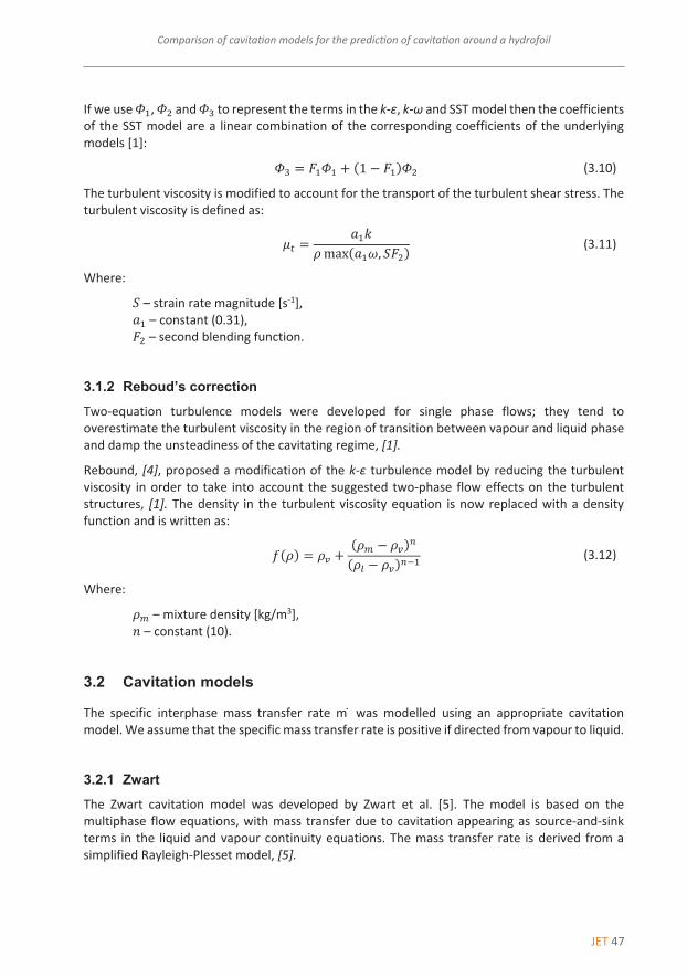
3.1.2 Reboud’s correction Two‐equation turbulence models were developed for single phase flows; they tend to overestimate the turbulent viscosity in the region of transition between vapour and liquid phase and damp the unsteadiness of the cavitating regime, [1].

Rebound, [4], proposed a modification of the k‐ε turbulence model by reducing the turbulent viscosity in order to take into account the suggested two‐phase flow effects on the turbulent structures, [1]. The density in the turbulent viscosity equation is now replaced with a density function and is written as:

𝑓𝑓�𝜌𝜌� � 𝜌𝜌� � �𝜌𝜌� � 𝜌𝜌��𝜌𝜌� � 𝜌𝜌�� (3.12)

Where:

𝜌𝜌� – mixture density [kg/m3], 𝑛𝑛 – constant (10).

3.2 Cavitation models

The specific interphase mass transfer rate m ̇ was modelled using an appropriate cavitation model. We assume that the specific mass transfer rate is positive if directed from vapour to liquid.

3.2.1 Zwart The Zwart cavitation model was developed by Zwart et al. [5]. The model is based on the multiphase flow equations, with mass transfer due to cavitation appearing as source‐and‐sink terms in the liquid and vapour continuity equations. The mass transfer rate is derived from a simplified Rayleigh‐Plesset model, [5].

48 JET



‐‐‐‐‐‐‐‐‐‐

𝑚𝑚� �

⎩⎪⎨⎪⎧𝐹𝐹�� 3𝑟𝑟��1 � 𝛼𝛼�𝜌𝜌�

𝑅𝑅� �23𝑃𝑃� � 𝑃𝑃𝜌𝜌� if 𝑃𝑃 � 𝑃𝑃�

𝐹𝐹�� 3𝛼𝛼𝜌𝜌�𝑅𝑅� �2

3𝑃𝑃 � 𝑃𝑃�𝜌𝜌� if 𝑃𝑃 � 𝑃𝑃�

(3.13)

Where:

𝑟𝑟�� – nucleation site volume fraction [m], 𝑅𝑅� – bubble radius [m], 𝑃𝑃� – vapour pressure [Pa], 𝐹𝐹�� – evaporation coefficient [/], 𝐹𝐹�� – condensation coefficient [/].

The recommended values for the two coefficients are 𝐹𝐹�� 50 and 𝐹𝐹�� 0.01. The recommended values for the nucleation site volume fraction and bubble radius are 𝑟𝑟�� 5 ∙10�� and 𝑅𝑅� � 10��.

3.2.2 Schnerr Schnerr and Sauer, [6], assumed that the vapour structure is filled with spherical bubbles, which are governed by the simplified Rayleigh Plesset equation. The mass transfer rate in the Schnerr and Sauer model is proportional to 𝛼𝛼�1 � 𝛼𝛼�. Moreover, the function �� 𝛼𝛼�1 � 𝛼𝛼� has the interesting property that it approaches zero when 𝛼𝛼 � 0 and 𝛼𝛼 � 1 and reaches the maximum in between, [1].

𝑚𝑚� �

⎩⎪⎨⎪⎧𝐹𝐹�� 𝜌𝜌�𝜌𝜌�𝜌𝜌 𝛼𝛼�1 � 𝛼𝛼� 3

𝑅𝑅� �23𝑃𝑃� � 𝑃𝑃𝜌𝜌� if 𝑃𝑃 � 𝑃𝑃�

𝐹𝐹�� 𝜌𝜌�𝜌𝜌�𝜌𝜌 𝛼𝛼�1 � 𝛼𝛼� 3𝑅𝑅� �

23𝑃𝑃 � 𝑃𝑃�𝜌𝜌� if 𝑃𝑃 � 𝑃𝑃�

(3.14)

Where:

𝑅𝑅� – bubble radius [m], 𝐹𝐹�� – evaporation coefficient [/], 𝐹𝐹�� – condensation coefficient [/].

𝑅𝑅� � � 𝛼𝛼

1 � 𝛼𝛼3

4𝜋𝜋𝜋𝜋�� (3.15)

Where:

𝜋𝜋 – bubble number density [/],

The recommended values for the two coefficients are 𝐹𝐹�� 1 and 𝐹𝐹�� 0.2. The recommended values for the bubble number density is 𝜋𝜋 � 10��.

JET 49


‐‐‐‐‐‐‐‐‐‐

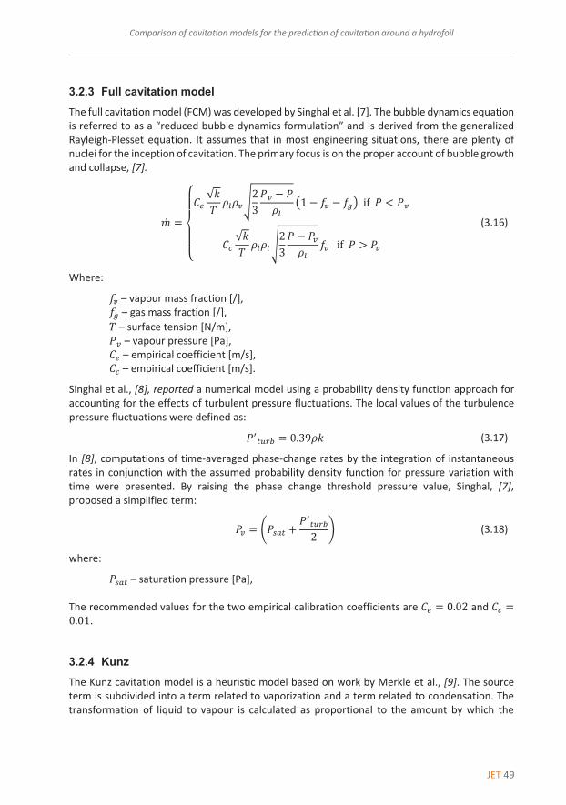
3.2.3 Full cavitation model The full cavitation model (FCM) was developed by Singhal et al. [7]. The bubble dynamics equation is referred to as a “reduced bubble dynamics formulation” and is derived from the generalized Rayleigh‐Plesset equation. It assumes that in most engineering situations, there are plenty of nuclei for the inception of cavitation. The primary focus is on the proper account of bubble growth and collapse, [7].

𝑚𝑚� �

⎩⎪⎨⎪⎧𝐶𝐶� √𝑘𝑘𝑇𝑇 𝜌𝜌�𝜌𝜌��2

3𝑃𝑃� � 𝑃𝑃𝜌𝜌� �1 � 𝑓𝑓� � 𝑓𝑓�� if 𝑃𝑃 � 𝑃𝑃�

𝐶𝐶� √𝑘𝑘𝑇𝑇 𝜌𝜌�𝜌𝜌��23𝑃𝑃 � 𝑃𝑃�𝜌𝜌� 𝑓𝑓� if 𝑃𝑃 � 𝑃𝑃�

(3.16)

Where:

𝑓𝑓� – vapour mass fraction [/], 𝑓𝑓� – gas mass fraction [/], 𝑇𝑇 – surface tension [N/m], 𝑃𝑃� – vapour pressure [Pa], 𝐶𝐶� – empirical coefficient [m/s], 𝐶𝐶� – empirical coefficient [m/s].

Singhal et al., [8], reported a numerical model using a probability density function approach for accounting for the effects of turbulent pressure fluctuations. The local values of the turbulence pressure fluctuations were defined as:

𝑃𝑃�� 0.39𝜌𝜌𝑘𝑘 (3.17)

In [8], computations of time‐averaged phase‐change rates by the integration of instantaneous rates in conjunction with the assumed probability density function for pressure variation with time were presented. By raising the phase change threshold pressure value, Singhal, [7], proposed a simplified term:

𝑃𝑃� � �𝑃𝑃�� 𝑃𝑃��2 � (3.18)

where:

𝑃𝑃�� – saturation pressure [Pa], The recommended values for the two empirical calibration coefficients are 𝐶𝐶� � 0.02 and 𝐶𝐶� �0.01.

3.2.4 Kunz The Kunz cavitation model is a heuristic model based on work by Merkle et al., [9]. The source term is subdivided into a term related to vaporization and a term related to condensation. The transformation of liquid to vapour is calculated as proportional to the amount by which the

50 JET



‐‐‐‐‐‐‐‐‐‐

pressure is below the vapour pressure. For the transformation of vapour to liquid, a simplified form of the Ginzburg‐Landau potential is employed, [10].

𝑚𝑚� �⎩⎪⎨⎪⎧

𝐶𝐶��𝜌𝜌��𝛾𝛾� � 𝛾𝛾��𝑡𝑡�

𝐶𝐶��𝜌𝜌�𝛾𝛾min�0,� � ��1

2𝜌𝜌�𝑈𝑈�� 𝑡𝑡� (3.19)

where:

𝐶𝐶�� – empirical coefficient [/], 𝐶𝐶�� – empirical coefficient [/], 𝑈𝑈� – free stream velocity [m/s], 𝑡𝑡� – mean flow time scale [s].

The mean flow time scale is defined as:

𝑡𝑡� � 𝐿𝐿/𝑈𝑈� (3.20)

where:

𝐿𝐿 – characteristic length scale [m].

The recommended values for the two empirical coefficients are 𝐶𝐶�� 100 and 𝐶𝐶�� 100.

4 BOUNDARY CONDITIONS AND SIMULATION SETTINGS

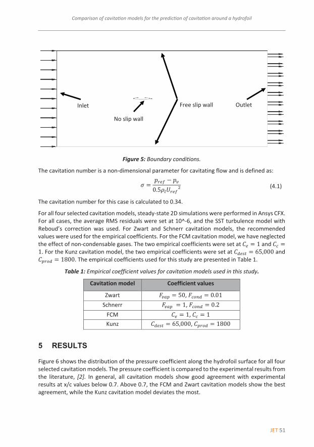
For this problem, the following boundary conditions were applied (shown in Figure 5):

‐ The left surface was specified as an inlet, where a normal velocity of 16.91 m/s was defined.

‐ The right surface was defined as an outlet, where a static pressure of 51,957 Pa was defined.

‐ The top and bottom surfaces were defined as a free‐slip wall.

‐ The symmetry boundary condition was applied for the side surfaces.

‐ The hydrofoil surface was defined as a no‐slip wall.

JET 51


‐‐‐‐‐‐‐‐‐‐

Figure 5: Boundary conditions.

The cavitation number is a non‐dimensional parameter for cavitating flow and is defined as:

� � 𝑝𝑝�� 𝑝𝑝�0.5𝜌𝜌�𝑈𝑈�� (4.1)

The cavitation number for this case is calculated to 0.34.

For all four selected cavitation models, steady‐state 2D simulations were performed in Ansys CFX. For all cases, the average RMS residuals were set at 10^‐6, and the SST turbulence model with Reboud’s correction was used. For Zwart and Schnerr cavitation models, the recommended values were used for the empirical coefficients. For the FCM cavitation model, we have neglected the effect of non‐condensable gases. The two empirical coefficients were set at 𝐶𝐶� � 1 and 𝐶𝐶� �1. For the Kunz cavitation model, the two empirical coefficients were set at 𝐶𝐶�� 65,000 and 𝐶𝐶�� 1800. The empirical coefficients used for this study are presented in Table 1.

Table 1: Empirical coefficient values for cavitation models used in this study.

Cavitation model Coefficient values

Zwart 𝐹𝐹�� 50, 𝐹𝐹�� 0.01 Schnerr 𝐹𝐹�� 1, 𝐹𝐹�� 0.2 FCM 𝐶𝐶� � 1, 𝐶𝐶� � 1 Kunz 𝐶𝐶�� 65,000, 𝐶𝐶�� 1800

5 RESULTS

Figure 6 shows the distribution of the pressure coefficient along the hydrofoil surface for all four selected cavitation models. The pressure coefficient is compared to the experimental results from the literature, [2]. In general, all cavitation models show good agreement with experimental results at x/c values below 0.7. Above 0.7, the FCM and Zwart cavitation models show the best agreement, while the Kunz cavitation model deviates the most.

Outlet Inlet

No slip wall

Free slip wall

52 JET



‐‐‐‐‐‐‐‐‐‐

Figure 6: Pressure coefficient distribution.

The cavitation for the Schnerr model starts at x/c=0.2; for the FCM and Kunz model, it starts at approximately x/c=0.3. For the Zwart model, the cavitation starts at x/c=0.4. Vapour volume fraction distribution for all cavitation models is seen in Figure 7.

Figure 7: Vapour volume fraction distribution.

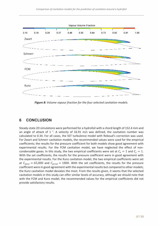
Figure 8 shows the vapour volume fraction for all cavitation models. The Zwart and FCM models predicted cavitation in a very similar manner, which is also evident from the pressure coefficient distribution. For the Schnerr cavitation model, the values for the vapour volume fraction are higher compared to the other three models.

‐0,4

‐0,3

‐0,2

‐0,1

0,0

0,1

0,2

0,3

0,0 0,1 0,2 0,3 0,4 0,5 0,6 0,7 0,8 0,9 1,0

Cp [/]

x/c [/]

Exp. Zwart Schnerr FCM Kunz

0,00,10,20,30,40,50,60,70,80,91,0

0,0 0,2 0,4 0,6 0,8 1,0

Volume vapo

ur fractio

n [/]

x/c [/]

ZwartSchnerrFCMKunz

JET 53


‐‐‐‐‐‐‐‐‐‐

Figure 8: Volume vapour fraction for the four selected cavitation models.

6 CONCLUSION

Steady‐state 2D simulations were performed for a hydrofoil with a chord length of 152.4 mm and an angle of attack of 1 °. A velocity of 16.91 m/s was defined, the cavitation number was calculated to 0.34. For all cases, the SST turbulence model with Reboud’s correction was used. For Zwart and Schnerr cavitation models, the recommended values were used for the empirical coefficients; the results for the pressure coefficient for both models show good agreement with experimental results. For the FCM cavitation model, we have neglected the effect of non‐condensable gases. In this study, the two empirical coefficients were set at 𝐶𝐶� � 1 and 𝐶𝐶� � 1. With the set coefficients, the results for the pressure coefficient were in good agreement with the experimental results. For the Kunz cavitation model, the two empirical coefficients were set at 𝐶𝐶�� 65,000 and 𝐶𝐶�� 1800. With the set coefficients, the results for the pressure coefficient were in good agreement with the experimental results but compared to other models; the Kunz cavitation model deviates the most. From the results given, it seems that the selected cavitation models in this study can offer similar levels of accuracy, although we should note that with the FCM and Kunz model, the recommended values for the empirical coefficients did not provide satisfactory results.

Zwart

FCM

Schnerr

Kunz

54 JET



‐‐‐‐‐‐‐‐‐‐

References

[1] D. Ziru LI: Assessment of Cavitation Erosion with a Multiphase Reynolds‐Averaged Navier‐Stokes Method, Wuhan University of Technology, Wuhan, P.R. China, 2012.

[2] ANSYS, Inc.: ANSYS CFX tutorials, 2016

[3] F. R. Menter: Two‐Equation Eddy‐Viscosity Turbulence Models for Engineering Applications, AIAA Journal, Volume 32, No. 8, August 1994.

[4] J. L. Reboud, B. Stutz, O. Coutier‐Delgosha: Two phase flow structure of cavitation: experiment and modeling of unsteady effects, Proceedings of the 3rd International Symposium on Cavitation, Grenoble, France, 1998.

[5] P. J. Zwart, A. G. Gerber, T. Belamri: A Two‐Phase Flow Model for Predicting Cavitation Dynamics, ICMF 2004 International Conference on Multiphase Flow, Yokohama, Japan, 2004

[6] G. H. Schnerr: Physical and Numerical Modeling of Unsteady Cavitation Dynamics, ICMF‐2001, 4th International Conference on Multiphase Flow, New Orleans, USA, 2001

[7] A. K. Singhal, H. Li, Y. Jiang: Mathematical Basis and Validation of the Full Cavitation Model, Journal of Fluids Engineering, 2002

[8] A. K. Singhal, N. Vaidya, A. D. Leonard: Multi‐Dimensional Simulation of Cavitating Flows Using a PDF Model for Phase Change, ASME FED Meeting, Vancouver, Canada, 1997.

[9] C. L. Merkle, J. Feng, P. Buelow: Computational modelling of the dynamics of sheet cavitation, Proceedings of 3rd International Symposium on Cavitation, Grenoble, France, 1998.

[10] R. F. Kunz, D. A. Boger, D. R. Stinebring, T. S. Chyczewski, J. W. Lindau, H. J. Gibeling, S. Venkateswaran, T. R. Govindan: Preconditioned Navier‐Stokes Method for Two‐Phase Flows with Application to Cavitation Prediction, Computers & Fluids 29, 2000.

Nomenclature (Symbols) (Symbol meaning)

𝑼𝑼 time‐averaged mixture velocity

𝒎𝒎� interphase mass transfer rate due to cavitation

𝝆𝝆𝐯𝐯 vapour density

𝝆𝝆𝐥𝐥 liquid density

𝝆𝝆 density of the water‐vapour mixture

𝑷𝑷 time‐averaged pressure

𝝁𝝁 dynamic viscosity of the water‐vapour mixture

𝝁𝝁𝒕𝒕 turbulent viscosity

𝜸𝜸 water volume fraction

14 Marko Pezdevšek, Ignacijo Biluš, Gorazd Hren JET Vol. 14 (2021) Issue 1

‐‐‐‐‐‐‐‐‐‐

References

[1] D. Ziru LI: Assessment of Cavitation Erosion with a Multiphase Reynolds‐Averaged Navier‐Stokes Method, Wuhan University of Technology, Wuhan, P.R. China, 2012.

[2] ANSYS, Inc.: ANSYS CFX tutorials, 2016

[3] F. R. Menter: Two‐Equation Eddy‐Viscosity Turbulence Models for Engineering Applications, AIAA Journal, Volume 32, No. 8, August 1994.

[4] J. L. Reboud, B. Stutz, O. Coutier‐Delgosha: Two phase flow structure of cavitation: experiment and modeling of unsteady effects, Proceedings of the 3rd International Symposium on Cavitation, Grenoble, France, 1998.

[5] P. J. Zwart, A. G. Gerber, T. Belamri: A Two‐Phase Flow Model for Predicting Cavitation Dynamics, ICMF 2004 International Conference on Multiphase Flow, Yokohama, Japan, 2004

[6] G. H. Schnerr: Physical and Numerical Modeling of Unsteady Cavitation Dynamics, ICMF‐2001, 4th International Conference on Multiphase Flow, New Orleans, USA, 2001

[7] A. K. Singhal, H. Li, Y. Jiang: Mathematical Basis and Validation of the Full Cavitation Model, Journal of Fluids Engineering, 2002

[8] A. K. Singhal, N. Vaidya, A. D. Leonard: Multi‐Dimensional Simulation of Cavitating Flows Using a PDF Model for Phase Change, ASME FED Meeting, Vancouver, Canada, 1997.

[9] C. L. Merkle, J. Feng, P. Buelow: Computational modelling of the dynamics of sheet cavitation, Proceedings of 3rd International Symposium on Cavitation, Grenoble, France, 1998.

[10] R. F. Kunz, D. A. Boger, D. R. Stinebring, T. S. Chyczewski, J. W. Lindau, H. J. Gibeling, S. Venkateswaran, T. R. Govindan: Preconditioned Navier‐Stokes Method for Two‐Phase Flows with Application to Cavitation Prediction, Computers & Fluids 29, 2000.

Nomenclature (Symbols) (Symbol meaning)

𝑼𝑼 time‐averaged mixture velocity

𝒎𝒎� interphase mass transfer rate due to cavitation

𝝆𝝆𝐯𝐯 vapour density

𝝆𝝆𝐥𝐥 liquid density

𝝆𝝆 density of the water‐vapour mixture

𝑷𝑷 time‐averaged pressure

𝝁𝝁 dynamic viscosity of the water‐vapour mixture

𝝁𝝁𝒕𝒕 turbulent viscosity

𝜸𝜸 water volume fraction

JET 55

Comparison of cavitation models for the prediction of cavitation around a hydrofoil Comparison of cavitation models for the prediction of cavitation around a

hydrofoil 15

‐‐‐‐‐‐‐‐‐‐

𝑷𝑷𝒌𝒌 production rate turbulence

𝒌𝒌 turbulent kinetic energy

𝑷𝑷𝒌𝒌𝒌𝒌 buoyancy production term

𝝎𝝎 specific dissipation rate

𝑷𝑷𝝎𝝎𝒌𝒌 buoyancy term

𝑺𝑺 strain rate magnitude

𝑭𝑭𝟐𝟐 second blending function

𝝆𝝆𝒎𝒎 mixture density

𝒓𝒓𝒏𝒏𝒏𝒏𝒏𝒏 nucleation site volume fraction

𝑹𝑹𝑩𝑩 bubble radius

𝑷𝑷𝒗𝒗 vapour pressure

𝑭𝑭𝒗𝒗𝒗𝒗𝒗𝒗 evaporation coefficient

𝑭𝑭𝒏𝒏𝒄𝒄𝒏𝒏𝒄𝒄 condensation coefficient

𝑹𝑹𝑩𝑩 bubble radius

𝒏𝒏 bubble number density

𝒇𝒇𝒗𝒗 vapour mass fraction

𝒇𝒇𝒈𝒈 gas mass fraction

𝑻𝑻 surface tension

𝑷𝑷𝒗𝒗 vapour pressure

𝑪𝑪𝒆𝒆 empirical coefficient

𝑪𝑪𝒏𝒏 empirical coefficient

𝑷𝑷′𝒕𝒕𝒏𝒏𝒓𝒓𝒌𝒌 local values of the turbulence pressure fluctuations

𝑷𝑷𝒔𝒔𝒗𝒗𝒕𝒕 saturation pressure

𝑪𝑪𝒗𝒗𝒓𝒓𝒄𝒄𝒄𝒄 empirical coefficient

𝑪𝑪𝒄𝒄𝒆𝒆𝒔𝒔𝒕𝒕 empirical coefficient

𝑼𝑼� free stream velocity

𝒕𝒕∞ mean flow time scale

𝑳𝑳 characteristic length scale

𝝈𝝈 cavitation number

Documents

COMPARISON OF CAVITATION MODELS FOR THE PREDICTION …