Embed Size (px)
Citation preview

COMPARISON OF GENETIC OPERATORS ON A
GENERAL GENETIC ALGORITHM
PACKAGE
By
HUAWEN XU
Master of Science
Shanghai Jiao Tong University
Shanghai, China
1999
Submitted to the Faculty of the Graduate College of the
Oklahoma State University in partial fulfillment of
the requirements for the Degree of
MASTER OF SCIENCE May, 2005

ii
COMPARISON OF GENETIC OPERATORS ON A
GENERAL GENETIC ALGORITHM
PACKAGE
Thesis Approved:
J.P. Chandler Thesis Adviser
B.E. Mayfield
D.R. Heisterkamp
A. Gordon Emslie Dean of the Graduate College

iii
ACKNOWLEDGEMENTS
I would like to express my sincere appreciation to my thesis committee for their guidance
and support. As the chairman of the committee, Professor J.P. Chandler offered his
academic expertise and insightful knowledge all the way through completion of this
thesis. His affable manner of communication made the tense research process much less
stressful. I also thank the other two committee members, Dr. Blayne E. Mayfield and Dr.
Douglas R. Heisterkamp, for their thoughtful comments and the time they spent on
reviewing this document.
As always, my wife Haowen Yu has provided the much needed understanding and
encouragement. Her love gives me the courage to face the difficulties in daily life. I also
thank all of my friends for the good memories and wish them all successful in their future
endeavor.

iv
TABLE OF CONTENTS
Chapter Page I. Introduction to Genetic Algorithms
1.1 General Introduction…………………………………………………... 1 1.2 Biological Terminology……………………………………………….. 2 1.3 How GAs Work……………………………………………………….. 3 1.4 An Example…………………………………………………………… 4
II. Literature Review 2.1 Brief Introduction to Optimization…………………………………….. 7
2.2 GA Packages Review…………………………………………………... 9 2.2.1 GAlib………………………………………………………… 9 2.2.2 Genesis……………………………………………………….. 10 2.2.3 Genetic Algorithm Driver……………………………………. 12
2.2.4 Other GA Packages…………………………………………... 13 III. Blueprint of a General GA Package
3.1 Encoding……………………………………………………………….. 14 3.1.1 Bit-string Encoding…………………………………………... 15 3.1.2 Integer Encoding……………………………………………... 15 3.1.3 Floating-point Encoding……………………………………... 17
3.2 Selection Methods……………………………………………………… 17 3.2.1 Improved Roulette Wheel Selection……………………......... 18 3.2.2 Stochastic Universal Sampling………………………………. 19 3.2.3 Rank Selection……………………………………………….. 20
3.2.3.1 Baker Linear Rank Method………………………… 21 3.2.3.2 Reeves Rank Method………………………………. 22
3.2.4 Tournament Selection………………………………………... 23 3.3 Generation Replacement Model……………………………………...... 24
3.3.1 Generational Replacement…………………………………… 24 3.3.2 Steady State Replacement……………………………………. 24 3.3.3 Evolution Strategy (N+m) Replacement……………………... 24 3.3.4 Elitism………………………………………………………... 25
3.4 Crossover………………………………………………………. ……... 25 3.4.1 Single Point Crossover………………………………….......... 26 3.4.2 Double Point Crossover……………………………………… 26 3.4.3 Uniform Crossover……………………………………………27 3.4.4 Arithmetical Crossover………………………………………. 27 3.4.5 Heuristic Crossover…………………………………………... 28
3.5 Mutation………………………………………………………………... 29

v
3.5.1 Uniform Mutation……………………………………………. 29 3.5.2 Non-uniform Mutation……………………………………….. 30 3.5.3 Boundary Mutation…………………………………………... 31 3.5.4 Creep Mutation………………………………………………. 31
3.6 Termination Condition…………………………………………………. 32 3.6.1 Maximum Number of Generations…………………………... 32 3.6.2 Convergence Termination……………………………………. 32 3.6.3 Progress in Fitness…………………………………………… 33
IV. Implementation of the GA Package 4.1 Introduction to Modules………………………………………………... 34
4.1.1 Initialization Module………………………………………… 34 4.1.2 Genetic Operation Module…………………………………… 35 4.1.3 Output Module……………………………………………….. 39 4.1.4 Utility Module………………………………………………... 39
4.2 Program Structure……………………………………………………… 40 4.3 Data Structures…………………………………………………………. 41 4.4 A Sample Run………………………………………………………….. 42
V. Tests and Results
5.1 General Testing………………………………………………………… 47 5.1.1 Mixed Mode Rosenbrock Functions……………………......... 47 5.1.2 0/1 Knapsack Problem……………………………………….. 49 5.1.3 Floating-point Functions……………………………………... 52
5.2 Comparison Experiments………………………………………………. 53 5.2.1 Comparison Experiments on Encodings……………………... 53 5.2.2 Comparison Experiments on Selection Methods…………….. 55 5.2.3 Comparison Experiments on Crossover Methods…………….60
VI. Conclusions and future Work
6.1 Conclusions…………………………………………………………….. 65 6.2 Future Work …………………………………………………………… 67
REFERENCES…………………………………………………………………….. 69 APPENDIX
Input Files of Tests and Experiments………………………………………. 71

vi
LIST OF TABLES Table Page 1.1 One Max individual values……………………………………………............. 4
1.2 Population after crossover……………………………………………………...5
1.3 Final population……………………………………………………………….. 6
3.1 Gray codes of first 6 integers………………………………………………….. 16
3.2 Single point crossover………………………………………………………..... 26
3.3 Double point crossover……………………………………………………....... 27
3.4 Uniform crossover…………………………………………………………….. 27
3.5 Arithmetical crossover…………………………………………………............ 28
5.1 Results of Flat-ground Rosenbrock function………………………………….. 48
5.2 Results of Hollow-ground Rosenbrock function……………………………… 49
5.3 Weights and Profits of Knapsack problem …………………………………… 50
5.4 Results of Knapsack problem with 10 items…………………………………...51
5.5 Results of Knapsack problem with 100 items………………………………….51
5.6 Results of Bohachevsky function………………………………………………52
5.7 Results of Schaffer function F7……………………………………………….. 53
5.8 Encoding comparison ………………………………………………….............54
5.9 Selection methods comparison I………………………………………………. 56
5.10 Time complexity of selection methods I…………………………………….. 57
5.11 Selection methods comparison II…………………………………………...... 58

vii
5.12 Time complexity of selection methods II……………………………………. 59
5.13 Crossover methods comparison I…………………………………………….. 60
5.14 Time complexity of crossover methods I…………………………………….. 62
5.15 Crossover methods comparison II……………………………………............ 62
5.16 Time complexity of crossover methods II…………………………………… 63

viii
LIST OF FIGURES Figure Page
1.1 Procedures of Simple GA ………………………..…………………………… 3
1.2 A descriptive version of GA…………………………………………………... 3
1.3 Single point crossover demonstration…………………………………............. 5
3.1 Binary and Gray code conversion functions…………………………………... 16
3.2 Roulette wheel selection procedures…………………………………………... 18
3.3 SUS procedures……………………………………………………………….. 20
4.1 Program flow chart……………………………………………………............. 41
4.2 Input file of the sample run…………………………………………………… 43
4.3 User function specification……………………………………………………. 45
4.4 Output file……………………………………………………………………... 46
5.1 Encoding comparison…………………………………………………..............55
5.2 Selection methods comparison I………………………………………............. 57
5.3 Selection methods comparison II……………………………………………… 59
5.4 Crossover methods comparison I……………………………………………… 61
5.5 Crossover methods comparison II…………………………………………….. 63

1
Chapter I. Introduction to Genetic Algorithms
1.1 General Introduction
Genetic algorithms are now widely applied in science and engineering as stochastic
algorithms for solving practical optimization problems. Genetic algorithms (GA)
were first introduced by John H. Holland in his fundamental book “Adaptation in
Natural and Artificial Systems” in 1975 [4]. Holland presented the algorithm as an
abstraction of biological evolution and his schema theory laid a theoretical foundation
for GA.
The idea behind GAs is to simulate what nature does. Simply speaking, GA is a
simulation of Darwin’s Theory of Evolution – the fittest survive. A simple GA works
as follows: First, a number of individuals (the population) are randomly initialized at
the beginning of the algorithm. Individuals are then selected according to their fitness.
Next, the genetic operators (crossover, mutation) are applied with certain probabilities
on these selected individuals, the parents, to produce offspring. The original
generation is then replaced by the new generation which consists in whole or in part
of the newly created offspring. The above process is repeated if the termination
criterion is not met; otherwise, the algorithm stops. [2]
Whereas in nature the "fitness" relates to the ability of the organism to survive and
reproduce, that is, organisms with a better "fitness" score are more likely to be
selected for reproduction, in genetic algorithms, the "fitness" is the evaluated result of
a user-defined objective function. [1]

2
1.2 Biological Terminology [1] [2]
Let us introduce some of the basic biological terminology that is useful for a better
understanding of GAs.
Each cell of a living creature consists of a certain set of chromosomes. Chromosomes
are made of genes, which are blocks of DNA. Each gene encodes one or more
characters (eye color, hair color, etc) that can be passed on to the next generation.
Each gene can be in different states, called alleles. Genes are located at certain
positions on the chromosome, which are called loci.
The cell of many creatures has more than one chromosome. The entire set of
chromosomes in the cell is called the genome. If the chromosomes in each cell of the
organism are unpaired, the organism is called haploid. If, on the other hand, the
chromosomes are paired, the organism is called diploid. In nature, many living
organisms are diploid, but almost all GAs employ haploid representations, since they
are simple to construct.
In the natural reproduction process, pieces of gene material are exchanged between
the two parents’ chromosomes to form new genes. This process is called
recombination or crossover. Genes in the offspring are subject to mutation, in which
a certain block of DNA in the gene undergoes a random change.
In genetic algorithms, a chromosome is used to represent a potential solution to a
problem. Since we use single-chromosome individuals to represent the problem
solution, the term individual and chromosome are often used interchangeably.

3
1.3 How GAs Work
Despite its amazing power, a genetic algorithm is actually quite elegant and so easy to
understand that it can be expressed in just a few lines of computer pseudo-codes.
Following is the C version of the GA structure originally presented in [1]:
Figure 1.1 Procedure of Simple GA
where, P(t) is the population of individuals for iteration t.
Here is a more descriptive version of GA, slightly modified from [1]:
Figure 1.2 A descriptive version of GA
Procedure Simple GA {
t=0; initialize P(t); evaluate P(t); while(! termination-condition) { select P(t+1) from P(t); genetic_operate P(t+1); evaluate P(t+1); t++; }
}
1. [Initialize] Generate a random population of n chromosomes (suitable solutions for the problem).
2. [Evaluate] Evaluate the fitness f(x) of each chromosome x in the population. 3. [Offspring] Create a new population by executing the following steps.
a. [Selection] Select n parent chromosomes from the population according to their fitness (the better the fitness, the better the chance to be selected).
b. [Crossover] Recombine the parents with a certain crossover probability to form new offspring.
c. [Mutation] Mutate the new offspring with certain mutation probability at each locus (position in chromosome).
4. [Replace] Replace the current population with the newly generated population.
5. [Test] If the termination condition is satisfied, stop, and return the best chromosome found; otherwise, go to step 2.

4
The convergence of a genetic algorithm is originally based on Holland’s schema
theory [4]. However, his theory has raised criticism and controversy over the years.
Since this thesis is focused on the real world application of GAs instead of theoretical
deduction, interested readers may refer to [5] for a precise mathematical description
of genetic algorithms.
1.4 An Example
A good example speaks better than thousands of words. Let’s work on a simple
example, One Max [6], to illustrate the basic steps of GA. As its name says, the goal
of One Max is to maximize the number of 1’s in 8-bit-strings such as 10010011.
First, we create an initial population of individuals. For simplicity, we assume a
population of size 4. The value of each individual is initially assigned randomly.
Then the population is evaluated based on a fitness function to determine how well
each individual does the required task. In our case, the fitness function is
straightforward:
f (v) = n, where n is the number of 1’s in individual v.
For example, the fitness value of an individual with chromosome 10011001 would be
4. After initialization, a random population of four individuals and their fitness values
are listed in Table 1.1.
Individual String Representation Fitness V1 01101001 4 V2 00100100 2 V3 11110001 5 V4 00001110 3
Table 1.1 One max individual values

5
Next, select two parents to generate two offspring. In this example, we use the plain
but widely adopted fitness-proportionate selection scheme, in which the probability of
an individual being chosen to reproduce is proportional to its fitness value. In our
case, let’s assume that the parents selected are [V3, V1] and [V3, V4], with V3 being
selected twice because of its higher fitness. Note that V2 may also be selected, with a
lower probability, in real world applications.
After the selection, we are ready to apply the crossover operator to the selected
individuals. Suppose the crossover probability is 0.5, which means 50% of the
population will undergo crossover (2 individuals in our case). Let’s say parent V3
and V1 undergo crossover after the fourth bit, the process is shown in the figure
below:
Figure 1.3 Single point crossover demonstration
The offspring generated are V1’ = 01100001 and V3’ = 11111001. On the other hand,
the offspring of V3 and V4, which do not go through crossover, are the exact copies
of themselves. Suppose we utilize generational replacement model, i.e., replace the
parents with the newly generated offspring, the new population now becomes:
Individual String Representation Fitness V1’ 01100001 3 V2’ (V3) 11110001 5 V3’ 11111001 6 V4 00001110 3
Table 1.2 Population after crossover
0110 1001
1111 0001
0110 0001
1111 1001
Parents Offspring
6
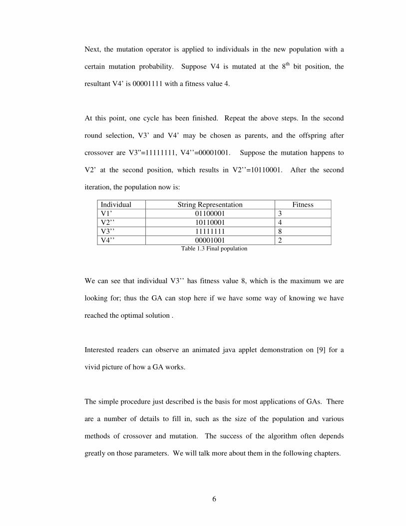
Next, the mutation operator is applied to individuals in the new population with a
certain mutation probability. Suppose V4 is mutated at the 8th bit position, the
resultant V4’ is 00001111 with a fitness value 4.
At this point, one cycle has been finished. Repeat the above steps. In the second
round selection, V3’ and V4’ may be chosen as parents, and the offspring after
crossover are V3”=11111111, V4’’=00001001. Suppose the mutation happens to
V2’ at the second position, which results in V2’’=10110001. After the second
iteration, the population now is:
Individual String Representation Fitness V1’ 01100001 3 V2’’ 10110001 4 V3’’ 11111111 8 V4’’ 00001001 2
Table 1.3 Final population
We can see that individual V3’’ has fitness value 8, which is the maximum we are
looking for; thus the GA can stop here if we have some way of knowing we have
reached the optimal solution .
Interested readers can observe an animated java applet demonstration on [9] for a
vivid picture of how a GA works.
The simple procedure just described is the basis for most applications of GAs. There
are a number of details to fill in, such as the size of the population and various
methods of crossover and mutation. The success of the algorithm often depends
greatly on those parameters. We will talk more about them in the following chapters.

7
Chapter II. Literature Review
2.1 Brief Introduction to Optimization
The purpose of optimization is to find the minimum or maximum result of a
mathematical function, called the objective function, by tuning the values of its
variables. During the past decades, the significance of optimization has grown
dramatically in engineering application, mathematical and computational models.
Consequently, dozens of optimization methods have been developed over the years.
The exhaustive search method searches a sufficiently large sampling space of the
objective function to find the global optimum. This brute force approach involves a
huge number of function evaluations, which makes it only practical for a small
number of parameters in a limited search space. [7]
Calculus optimization is a mathematical approach that can be applied if the objective
function is smooth (continuously differentiable). First, the objective function is
differentiated with respect to all the independent variables; next, the derivatives of
function are set to zero and the equations are then solved to find the parameter values.
This method is more computationally efficient than many of its peers. However, if
the problem has too many parameters, then it becomes quite difficult or even
impossible to solve the derivative equations, let alone that some practical problems
can’t be expressed as mathematical functions [7]. Also, the nonlinear equations may
have no solution, many solutions, or even infinity of solution points.

8
A hill-climbing method starts from a single point and selects a new point from the
vicinity of the current point in each iteration. If the new point has a better value, the
current point is replaced by the new point. Otherwise, the current point is kept and
the process continues with a smaller step size or in another direction until the
termination criterion is met. The drawback of this method is that it only guarantees a
local optimum, which is determined by the position of the start point. Also, the
objective function must be smooth (continuously differentiable) for most hill-
climbing methods to succeed.
Two relatively new natural optimization methods, Simulated Annealing (SA) and
Genetic Algorithm (GA) are successful in the area where the traditional methods fall
short. Whereas GA models the natural selection and evolution process, SA simulates
the annealing phenomenon. Compared with hill-climbing, SA introduces a
probability of accepting the new point and the probability is controlled by an
additional parameter T, the temperature. With a high temperature at the beginning,
the algorithm is more likely to accept new points, and thus explore more regions in
the solution space. As the temperature goes down, the probability of accepting new
points becomes smaller and smaller. Since T is lowered in small steps, the algorithm
has an opportunity to discover the global optimum instead of converging to a local
optimal point [8]. Some published SA algorithms fail on many practical problems [24].
Perhaps the best existing SA software package is the free c language program ASA,
which was developed by Lester Ingber and is downloadable at [25].
Compared with traditional optimization methods, GA has advantages in several
aspects [7]: it can optimize both continuous and discrete functions; it does not require

9
complicated differential equations or a smooth objective function; it can be highly
parallelized to improve computational performance; it searches more of the solution
space and thus increases the probability of finding the global optimum. The
disadvantage is that GA is often much slower than calculus methods, when the latter
can used.
2.2 GA Packages Review
Due to their inherent advantages, GAs have been widely applied in numerous
scientific and engineering problems. A number of GA packages have been developed
as implementations of genetic algorithms over the years. In this section, we will give
a short review of existing GA packages.
2.2.1 GAlib [10]
GAlib is a C++ genetic algorithm package developed at MIT (GAlib should not be
confused with GALib, developed at the University of Tulsa). This genetic algorithm
will create a population of solutions based on a sample data structure that you provide.
In GAlib, the sample data structure is called a GAGenome, which functions as a
chromosome. The library contains four types of genomes: GAListGenome,
GATreeGenome, GAArrayGenome, and GABinaryStringGenome.
Each genome type has three operators: initialization, mutation, and crossover.
• Initialization operator: Initializes a genome when the genetic algorithm starts.
• Mutation operator: Mutates each genome based on its data type. For example,
mutation on a binary string genome flips the bits in the string, but mutation on a
tree would swap subtrees.

10
• Crossover operator: Generates children from two parent genomes based on data
types. Users are allowed to develop new mating methods other than the default
ones.
GAlib comes with these operators pre-defined for each genome type, but you can
customize any of them so that it is specific not only to the data type, but also to the
problem type.
The library contains four basic types of genetic algorithms.
• Simple genetic algorithm: The classical replacement method in which the entire
generation is replaced by the newly produced individuals.
• Steady-state genetic algorithm: Only a fraction of the population is replaced by the
offspring. The user can specify how large the fraction is.
• Incremental genetic algorithm: Only one or two children are created in each
generation and the users have the choices to select the parents that are to be
replaced. For example, the child could replace an individual randomly, or replace
an individual that is most like it.
• Deme genetic algorithm: This algorithm “evolves multiple populations in parallel
using a steady-state algorithm”. In each generation, some of the individuals are
copied from one population to the other to maintain the population diversity.
2.2.2 Genesis [11]
Genesis, which stands for GENEtic Search Implementation System, is a popular
genetic algorithm package developed by John J. Grefenstette using C language.

11
Genesis has three levels of representation for its evolving structures. The lowest level
(Packed representation) is used to “maximize both space and time efficiency in
manipulating structures”. The middle level (String representation) represents
structures as arrays of characters. This level provides the users the freedom to create
their own genetic structures. The third level (Floating-point representation) represents
the genetic structures as vectors of real numbers. Numeric optimization problems are
solved by working on this level.
The user can specify the range, number of values, and output format of each
parameter. The system then automatically translates the structure among the three
representation levels.
Genesis consists of two main modules – initialization and generation. Initialization
module sets up the initial population using a file named "init.c". The generation
module (file "generate.c") comprises mainly the following procedures: selection,
mutation, crossover, and evaluation.
• Selection: The default selection procedure is Universal Sampling Selection
implemented in file "select.c". Genesis also provides users the linear ranking
selection method if the option ‘R’ is specified.
• Mutation: Genesis implements the classical mutation method – Uniform Mutation
in file “mutate.c”.
• Crossover: Genesis implements the traditional two-point crossover method in file
"cross.c".

12
Genesis requires the user to write an evaluation procedure to serve as the objective
function. The procedure must be declared in the user's input file in a certain format.
Genesis allows a number of options to employ different strategies during the search.
Each option is associated with a single character. For instance,
E - Use the "elitist" selection strategy. The elitist strategy stipulates that the
best performing structure always survives from one generation to the next.
G - Use Gray code to encode integers.
2.2.3 Genetic Algorithm Driver [15]
The FORTRAN Genetic Algorithm Driver is a GA package created by D.L. Carroll.
The latest version of this driver is dated 2001. The features of this package are listed
as follows:
• Encoding: Bits string, which is the only option provided by this package.
• Selection: Tournament selection with “a shuffling technique for choosing random
pairs for mating”.
• Mutation: The package implements jump mutation and creep mutation.
• Crossover: The package provides the option for single-point or uniform crossover.
In the latest version, the author added two features into the package. One is niching,
the process of dividing individuals that are in some sense similar into groups; the
other is micro-GA, the process of reinitializing a small subset of population.
For the use of his package, Carroll recommends the following settings:
• Binary coding (the only option of his GA)

13
• Tournament selection (the only option of his GA)
• Uniform crossover (iunifrm=1)
• Creep mutations (icreep=1)
• Niching or sharing (iniche=1)
• Elitism (ielite=1)
Carroll also suggests using the micro-GA technique (microga=1) with uniform
crossover (iunifrm=1). Besides that, he advises using certain formulas to calculate the
population size and creep mutation rate. Interested readers may refer to [15] for the
detailed formulas.
2.2.4 Other GA Packages
Besides the GA packages introduced above, there are quite a number of other good
ones such as GENETIC, GENOCOP, GAJIT, etc. GA-Archive [13] is an excellent
source to explore the existing GA packages. GA packages on that website are either
archived as compressed files or maintained as links to the package authors’ web pages.
There is an index of source code for implementations of genetic algorithms. The GA
packages listed on the site are categorized according to the implementation language
such as C/C++, Java, FORTRAN, Perl, Lisp, etc.

14
Chapter III. Blueprint of a General GA Package
In chapter 2, we reviewed several existing GA packages. Most packages use a single
representation: either binary string or floating point; some packages are specially
designed for certain types of problems. To handle the variety of optimization
problems in practical applications, I will design and implement a general GA package
that gives users much more options on the problem representation and genetic
operators. In other words, this package offers the choice of representing the
chromosome using bit-string, integer, or floating-point or a combination of the three.
A preliminary version of this package, which only implements the simplest methods
of crossover and mutation, was developed by Ting Zhu [26]. The package I propose
will significantly extend the original package by providing users the choice of
choosing from a rich set of selection, replacement, mutation, and crossover methods
based on the specific problem type.
How to encode the chromosomes is the problem to solve when starting to work on a
problem with GA. Encoding depends heavily on the problem. In this chapter, we
will start with the introduction to some encodings that will be implemented in this
package.
3.1 Encoding The way in which candidate solutions are encoded is “a central factor in the success
of a genetic algorithm” [1]. This package will employ three commonly used

15
encodings – bit-string, Gray-coded integer, and floating point, to represent candidate
solutions.
3.1.1 Bit-string Encoding
Bit-string encoding, introduced by Holland in his original GA book, is the most
widely used encoding method. Bit-string encoding has its own inherent advantages.
First, it is easy to understand and implement; second, researchers have accumulated
rather rich experiences on the parameter settings such as population size, crossover,
and mutation rate in its context.
3.1.2 Integer Encoding
When the parameters of the problem are integers, it is natural to use a binary string to
encode the variables. However, there is a problem with representing integers by
ordinary binary strings. Consider the following example. Two integers 15 (01111)
and 16 (10000) are selected as parents. Note that the integers are quite close to each
other and their fitness values are also likely to be close. But, their binary string
representations are quite different from each other. Moreover, let’s assume a single
point crossover is applied after bit position 1. The resultant offspring are 11111 and
00000, whose corresponding integer values are 31 and 0, respectively. We can see
that the offspring fall far away from their parents, which tends to interfere with the
expected convergence [7].
One way to overcome this problem is to encode the binary string using Gray code.
The procedures for converting a binary number b=b1b2…bm into a Gray code number
g=g1g2…gm and vice versa are given in the following figure [2].

16
Figure 3.1 Binary and Gray code conversion functions
According to these conversion procedures, the Gray codes of the first 6 integers are
listed in Table 3.1.
Decimal value Binary string Gray code 0 0000 0000 1 0001 0001 2 0010 0011 3 0011 0010 4 0100 0110 5 0101 0111 6 0110 0101
Table 3.1 Gray codes of first 6 integers
Note that the Gray coding representation has the property that any two consecutive
points in the problem space differ by only one bit in the representation space, which is
highly desired for GA convergence. Let’s reconsider the previous example using
Gray coding. The Gray codes of 15 and 16 are 01000 and 11000 respectively. After
applying the same crossover procedure, the offspring are 11000 and 01000, whose
integer values are 16 and 15 respectively. Thus we can observe that offspring are
function Binary-to-Gray { g1 =b 1; for ( k = 2; k <= m; k++) {
gk= bk-1 XOR bk ; } } function Gray-to-Binary { temp = g1; b1= temp; for ( k = 2; k <= m; k++) {
if (gk==1) temp = NOT temp; bk = temp ;
} }

17
much closer (actually identical in this extreme case) to their parents than in the
previous case, which helps preserve the desired characteristics of the parents.
3.1.3 Floating-point Encoding
Despite the advantages it has, binary encoding has some drawbacks when applied to
problems with continuous parameters. In such numerical problems that demand
parameters of high precision, each variable requires a rather long binary string to fully
represent it. This results in a huge search space which bogs down the GA
performance severely [2].
For applications with variables over continuous domains, it is more natural and
logical to encode them using floating-point numbers instead of binary strings. In
contrast to bit-string encodings, floating-point encoding represents the continuous
parameters more accurately, requires less storage space, and makes it more
straightforward to implement the genetic operators [7].
3.2 Selection Methods
The next decision to make after encoding is selection – the process of selecting the
individuals from the population as parents that will create offspring for the next
generation. The aim of selection is to assign higher probabilities to individuals with
greater fitness. There are two main issues associated with selection: population
diversity and selective pressure [16]. A high selective pressure will result in only good
individuals being selected, reducing the diversity needed for evolution toward the
global optimum, thus tending to lead the GA to a premature convergence. On the
other hand, a weak selective pressure will get too many not-so-good individuals
18
involved in the population and slow down the evolution process. Therefore, it is
critical to seek a balance between these two factors [16].
Numerous selection schemes have been developed over the years. Every method has
its own strength and weakness; it is still an open question which method is superior to
the others. In the following subsections, I will describe the selection methods that
will be implemented in this package.
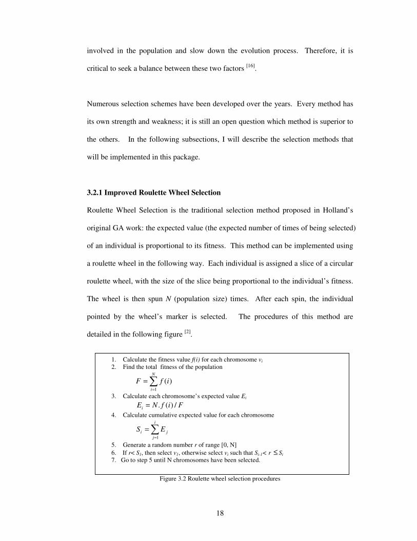
3.2.1 Improved Roulette Wheel Selection
Roulette Wheel Selection is the traditional selection method proposed in Holland’s
original GA work: the expected value (the expected number of times of being selected)
of an individual is proportional to its fitness. This method can be implemented using
a roulette wheel in the following way. Each individual is assigned a slice of a circular
roulette wheel, with the size of the slice being proportional to the individual’s fitness.
The wheel is then spun N (population size) times. After each spin, the individual
pointed by the wheel’s marker is selected. The procedures of this method are
detailed in the following figure [2].
Figure 3.2 Roulette wheel selection procedures
1. Calculate the fitness value f(i) for each chromosome vi 2. Find the total fitness of the population
�=
=N
i
ifF1
)(
3. Calculate each chromosome’s expected value Ei FifNEi /)(.= 4. Calculate cumulative expected value for each chromosome
�=
=i
jji ES
1
5. Generate a random number r of range [0, N] 6. If r< S1, then select v1, otherwise select vi such that Si-1< r ≤ Si
7. Go to step 5 until N chromosomes have been selected.

19
We can see that it takes O(N) time in step 6 to locate the individual with the
accumulative expected value that equals to r . If we notice that Si is a sorted array in
ascending order, it is natural to come up with some ideas about binary search.
Therefore, we replace step 6 with finding Si using binary search in the above
algorithm. Thus the performance of the algorithm can be improved from O(N) to
O(logN).
In the case of a theoretically infinite population, the roulette wheel method will
allocate the expected values of each chromosome in proportion to its fitness.
However, if the real GA application has a relatively small population size, the actual
number of an individual being chosen may be quite different from its expected value.
In the worst case scenario, an extreme series of spin of the wheel can “allocate all the
offspring to the worst individual in the population” [1]. Another restriction of roulette
wheel method is that all fitness values of the objective function must be positive. The
minimum value of the function is important: adding a constant to all the fitness values,
a scaling technique that should be harmless, will change the expected values of
individuals.
3.2.2 Stochastic Universal Sampling
To overcome the drawback of roulette wheel selection, James Baker proposed
Stochastic Universal Sampling (SUS) [17]. SUS rebuilds the roulette wheel with N
equally spaced pointers. Thus unlike roulette wheel selection, SUS spins the wheel
only once, and the individuals pointed by each of the N markers are selected as
parents. Below is an elegant C implementation of SUS [17].

20
Figure 3.3 SUS procedure
Where S[i] is the accumulative probability of chromosome i. Under this method,
each individual is guaranteed to be selected at least floor(Ei) times but no more than
ceiling(Ei) times, where floor and ceiling functions are the same as defined in C
language.
SUS does a better job in sampling than roulette wheel, but does not solve the major
problems with fitness proportionate selection. Under the fitness proportionate
selection, a small number of highly fit individuals are much more likely to be selected
and their descendants will quickly dominate the population. After a few generations,
the super individuals may eliminate the desirable diversity and lead the GA to a
premature convergence [1].
3.2.3 Rank Selection
One way to address the problems associated with fitness proportionate selection
methods is to introduce a mapping mechanism that maps the raw fitness values to
intermediate parameters. These parameters are then used to calculate the expected
values. Rank selection is a method in this category: the individuals are sorted
according to their fitness values, and then the selection probabilities of individuals are
calculated based on their ranks rather than on their actual fitness values. Doing so
avoids allocating too much quota of the offspring to individuals with high fitness
SUS Algorithm: ptr=rand(); //random pointer in range [0,1] for(i=1; i<=N; i++)
while( ptr<=S[i] ) //increases ptr to simulate equally spaced pointers. { select(i); ptr++; }

21
values. This also solves the problem associated with a scaling technique in roulette
wheel and SUS selection.
Like everything else in the universe, the rank method also has drawbacks. In some
cases, the GA takes a longer time to converge to an optimum point because of the
lower selection pressure. Rank also requires sorting the entire population for each
generation, which is a time consuming task in the case of a large population size [18].
There are many approaches to calculating the expected values based on ranking. Two
ranking methods are employed in this GA package.
3.2.3.1 Baker Linear Rank Method [12]
The linear ranking method proposed by Baker is quite straightforward. In his method,
each individual is ranked in ascendant order of fitness, from 1 to N. The expected
value of each individual is set by the following formula,
N-
Rank(j)-(Max-Min).MinjE
11
)( +=
where Min is the expected value of individual with rank 1, Max is the expected value
of the individual with rank N, and also is the upper bound of expected values defined
by the user. Given the condition that� =j
NjE )( , it is easy to show that Min= 2-
Max. Baker recommended the user to take Max=1.1. Once the expected values are
established, the SUS method is used to sample the population.

22
3.2.3.2 Reeves Rank Method [18]
Colin R. Reeves proposed another method of linear ranking, in which the probability
of selecting the individual ranked k in the population is denoted by
Pr[k] = a + bk
where a and b are positive scalars. The fact that Pr[k] must be a probability
distribution gives us the following deduction:
1)2
1(1)(
1
=++�=+�=
NbaNbka
N
k
In his work, Reeves gives a formal definition of the selection pressure:
]Pr[]Pr[
individualaverageselectingindividualfittestselecting=φ , which is a parameter specified by the user.
If we interpret the average as the median individual, it is easy to get
2/)1( +++=Nba
bNaφ .
In terms ofφ and N, we are able to get
)1()1(2
)1()1(2
−+−=
−−=
NNNN
aandNN
bφφ
,
which implies 21 ≤≤ φ . It is easy to see that the cumulative probability of each
individual can be expressed in terms of the sum of an arithmetic progression, so that
finding the k for a given random number r is simply to solve the quadratic equation
rkk
bak =++2
)1( for k . Note that k is an integer, thus
��
�
�
��
�
� ++++−=
bbrbaba
ceilingk2
8)2()2( 2
.
Note that the individual can be directly found by the above formula, which takes only
O(1) time, whereas the traditional roulette wheel method takes O(N) time to find the

23
corresponding individual with a cumulative probability equal to r. For a large size of
population, this will considerably improve the computational efficiency.
3.2.4 Tournament Selection
The tournament selection method is akin to the rank method, but is more time-
efficient than rank selection because it works on a smaller set of individuals instead of
working on the whole population. This method randomly picks a set of m individuals
from the population and then chooses the best one of them to be the parent. This
process is repeated N times to get the N parents needed [2]. Obviously, selection
pressure rises as m increases. The commonly used value of m is 2.
Michalewicz proposed a tournament selection method which is blended with some
simulated annealing flavor [2]. Two individuals are randomly chosen, and then a
random number r in [0, 1] is generated. The winner is determined in the following
way: If e T
jfif |)()(|
1
1−
+< r, then the fitter individual is chosen; otherwise, the less fit
individual is chosen. In the formula, T is the temperature and f(i) and f(j) are the
fitness values.
As in simulated annealing, the temperature starts at a high value, which indicates a
low selection pressure. The temperature is gradually lowered according to a
predefined scheme. The lower the temperature goes, the higher the selection pressure
becomes, therefore allowing the GA to narrow down the search space on highly fit
individuals.

24
3.3 Generation Replacement Model
The generation replacement model determines how the population proceeds from one
generation to the next generation. In this package, several choices are provided as
described in the following subsections.
3.3.1 Generational Replacement
This is the classical replacement method presented in Holland’s original GA work – at
each generation, N offspring are generated to make up the new generation. In other
words, the entire generation is replaced; no individual from the last generation is kept.
3.3.2 Steady State Replacement
The potential problem of the generational replacement is that we are running the risk
of discarding some good individuals in the old generation. To address this problem,
De Jong introduced the idea of a ‘generation gap’ in his Ph.D. thesis [19]. At each
generation, only a fraction of the population is replaced by the offspring. This
fraction is called the generation gap. Therefore overlap is allowed between
successive generations.
There are a number of mechanisms to select the parents that are to be replaced. In this
package, I use the classical method: the least fit individuals in the old generation are
chosen to be replaced by the newly generated offspring.
3.3.3 Evolution Strategy (N+m) Replacement [2]
Unlike the previous two replacement schemes, in which the children replace their
parents, in this evolution scheme, the children compete with their parents for survival.

25
In a single generation, m offspring are generated and then are combined with the N
parent to constitute an intermediate population of size N+m, from which the best N
individuals are chosen to form the next generation.
3.3.4 Elitism [2]
It is possible that some individuals in the earlier generation are fitter than the best
individual found in the last generation. Such individuals may be lost if they are not
selected or are ruined by crossover or mutation. Thus it is intuitive to keep track of
the best individuals in the entire evolution process and this is called elitism. Elitism
ensures that the best nElite individuals of the population are passed on to the next
generation without being altered by genetic operators. Elitism is essentially a special
case of (N+m) replacement.
3.4 Crossover
After parents have been selected through one of the methods introduced above, they
are randomly paired. The genetic operators are then applied on these paired parents to
produce offspring. There are two main categories of operators: crossover and
mutation. Let us have a look at crossover in this section and move on to mutation in
the next section.
The purpose of crossover is to vary the individual quality by combining the desired
characteristics from two parents. Over the years, numerous variants of crossover have
been developed in the GA literature, and comparisons also have been made among
these methods [20]. However, most of these studies rely on a small set of test problems,
and thus it is hard to draw a general conclusion on which method is better than others.

26
In this GA package, a number of commonly used crossover techniques are
implemented. Some of them apply only to bit-string or Gray-coded integer genes on
the chromosome.
3.4.1 Single Point Crossover
This is the traditional and the simplest way of crossover: a position is randomly
chosen as the crossover point and the segment of the parents after the point are
exchanged to form two offspring. The position can be anywhere between the first and
the last allele. For example, let us suppose position 2 is the crossover point, the
process is shown in the following table. Please note that xi or yi stands for a bit for
bit-string chromosomes; whereas for floating point chromosome, it stands for a
floating point variable.
Parent Offspring [x1,x2, x3, x4, x5, x6] [x1,x2, y3, y4, y5, y6] [y1,y2, y3, y4, y5, y6] [y1,y2, x3, x4, x5, x6]
Table 3.2 Single point crossover
Single point crossover has several drawbacks. One of them is the so-called positional
bias: the single point combination of this method can’t create certain schemas [20].
The other is the endpoint effect – the end point of the two parents is always
exchanged, which is unfair to other points [1].
3.4.2 Double Point Crossover
In this crossover method, two positions are randomly chosen and the segments
between them are exchanged. For instance, assuming position 2 and 5 are chosen as
crossover points, the process is shown in the following table.

27
Parent Offspring [x1,x2, x3, x4, x5, x6] [x1,x2, y3, y4, x5, x6] [y1,y2, y3, y4, y5, y6] [y1,y2, x3, x4, y5, y6]
Table 3.3 Double point crossover
Compared with single point crossover, double point crossover is able to combine
more schemas and eliminate the ending point effect. But similar to single point
crossover, there are some schemas that it can’t create.
3.4.3 Uniform Crossover
As a natural extension to single and double point crossover, uniform crossover allows
each allele in the parents to be exchanged with a certain probability p. For example,
given p=0.6, and the series of random numbers drawn for alleles 1 to 6 are: 0.4, 0.7,
0.3, 0.8, 0.9, 0.5, the results will be:
Parent Offspring [x1,x2, x3, x4, x5, x6] [x1,y2, x3, y4, y5, x6] [y1,y2, y3, y4, y5, y6] [y1,x2, y3, x4, x5, y6]
Table 3.4 Uniform crossover
Since any point in the parent can be exchanged, uniform crossover can recombine any
schemas. However, this advantage comes at cost. The random bit exchange may
prevent the forming of valuable building blocks (short and highly fit segments that are
able to form strings of potentially higher fitness through recombination) [3], because
the random exchange of uniform crossover can be highly disruptive to any evolution
schemas [21].
3.4.4 Arithmetic Crossover (floating point only)
The above crossover methods work fine for the bit-string representation. However,
there is a problem when applying them to floating-point encoding: the crossed

28
parameter values in the parents are propagated to their offspring unchanged, only in
different combinations [7]. In other words, no new parameter values are introduced.
To address this problem, GA researchers introduced arithmetical crossover [7]: the ith
parameter in offspring, Zi, is a linear combination of the ith parameters of two parents,
Xi and Yi, i.e.,
iii YaaXZ )1( −+=
where a is a random value in the interval [0,1].
This linear formula guarantees that the value of the newly created offspring is always
within the domain of the problem. For example, suppose the crossover happens at
position 2 and 5, the resultant offspring are given in the table below:
Parent Offspring [x1,x2, x3, x4, x5, x6] [x1, ax2+(1-a)y2, x3, x4, ax5+(1-a)y5, x6] [y1,y2, y3, y4, y5, y6] [y1, ay2+(1-a)x2, y3, y4, ay5+(1-a)x5, y6]
Table 3.5 Arithmetical crossover
3.4.5 Heuristic Crossover (floating point only)
Heuristic crossover [22] uses the values of the fitness function to determine the
direction of search according to the following formula:
�
+−≤+−
=otherwiseXYXa
XfYfifYXYaZ
)()()()(
where a is also a random value in the interval [0,1]; X and Y are the parental
parameter vectors; f(X) and f(Y) are the fitness function values.
Contrary to arithmetic crossover which always creates offspring within the range of
their parents, heuristic crossover always generates offspring outside of the range of

29
the parents. Sometimes the offspring values are so far away from their parents that
they get beyond the allowed range of that variable. In such a case, the offspring is
discarded, and a new a is tried and a new offspring created. If after a specified
number times no feasible offspring is generated, the operator quits with no offspring
produced.
In this package, instead of being discarded, the infeasible offspring is assigned the
maximum or minimum permissible value as follows:
�
+−≤+−
=otherwiseiMaxxyxaiMin
XfYfifiMaxyxyaiMinz
iii
iiii )),)(min(,max(
)()()),)(min(,max(
where iMin and iMax are the minimum and maximum allowable values for the ith
parameter.
3.5 Mutation
Mutation is another essential operator of genetic algorithm. The idea behind mutation
is to introduce diversity into the population and thus prevent the premature
convergence. Like crossover, GA researchers have developed numerous variants of
mutation method over the GA history. Since every method has its strength and
weakness, it is still an open question as to claim which method is the best. This
general GA package employs a number of widely used mutation procedures.
3.5.1 Uniform Mutation
This is the conventional method of mutation, in which each allele has an equal
opportunity to be mutated. For each allele, a random number r is generated and then

30
compared with the mutation rate pm (a user specified parameter), if r > pm, then this
allele is mutated; otherwise, stays unchanged.
For the binary encoding, either bit-string or Gray-coded integer, the mutation simply
flips the bit from 0 to 1 or vice versa. For floating-point encoding, the allele is
replaced with a random value within the domain of that variable. For example, if x2 is
selected for mutation in the chromosome X= [3.221, 4.556, 2.341, 5.897], and the
domain of x2 is [3.000, 5.500], then the chromosome after mutation may be X= [3.221,
3.938, 2.341, 5.897].
3.5.2 Non-uniform Mutation (floating point only)
To increase the fine tuning of the chromosome and reduce the randomness of uniform
mutation, Michalewicz presented a dynamic mutation operator called non-uniform
mutation [2]. The mechanism works as follows: if element ix was selected for
mutation, the resultant offspring is determined by the following formula,
�
≤−∆−>−∆+
=5.0),(
5.0),(
aifLBxtx
aifxUBtxz
iii
iiii
where a is a random number between 0 and 1, LBi and UBi represent lower and upper
bounds of variable ix . The function ),( xt∆ is defined by
)1(),( )/1( bTtrxxt −−=∆
where r is also a random number between 0 and 1, T is the maximal generation
number, and b is a user-defined system parameter that determines the degree of
dependency on iteration number t. This simulated annealing flavored formula returns
a value in the range [0, x] such that the probability of ),( xt∆ being close to 0
increases as t increases. This property guarantees the newly created offspring is in the
31
feasible range. Moreover, it enables the operator to explore the space broadly with an
initially large mutation step, but very locally at later stages; thus make the newly
generated offspring closer to its predecessor than a randomly generated one [2].
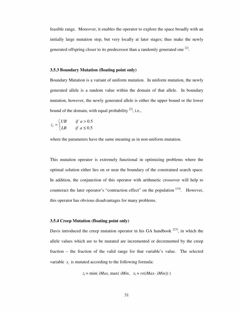
3.5.3 Boundary Mutation (floating point only)
Boundary Mutation is a variant of uniform mutation. In uniform mutation, the newly
generated allele is a random value within the domain of that allele. In boundary
mutation, however, the newly generated allele is either the upper bound or the lower
bound of the domain, with equal probability [2], i.e.,
�
≤>
=5.05.0
aifLB
aifUBzi
where the parameters have the same meaning as in non-uniform mutation.
This mutation operator is extremely functional in optimizing problems where the
optimal solution either lies on or near the boundary of the constrained search space.
In addition, the conjunction of this operator with arithmetic crossover will help to
counteract the later operator’s “contraction effect” on the population [14]. However,
this operator has obvious disadvantages for many problems.
3.5.4 Creep Mutation (floating point only)
Davis introduced the creep mutation operator in his GA handbook [23], in which the
allele values which are to be mutated are incremented or decremented by the creep
fraction – the fraction of the valid range for that variable’s value. The selected
variable ix is mutated according to the following formula:
zi = min( iMax, max( iMin, xi + rs(iMax- iMin)) )

32
where iMax and iMin are the upper bound and lower bound of the variable’s domain
respectively; r is a random number in the range [-1, 1]; s is the creep factor, a user-
defined number between 0 and 1.
It is equally likely that the allele value will be incremented or decremented, and the
value is adjusted to the boundary value if the newly generated allele falls out of the
valid range of the allele.
3.6 Termination Condition
Unlike the traditional search methods that terminates when a local optimum is reached,
GAs are stochastic methods that could run forever. The termination criterion plays an
important role in the solution quality. Three commonly used approaches are adopted
in this package.
3.6.1 Maximum Number of Generations
The simplest and most common method is to check the current generation number;
the genetic process will end when the specified number of generations has been
reached. This method has several variants such as using a maximum number of
fitness function evaluations, or using a maximum elapsed time, as the termination
criterion [1].
3.6.2 Convergence Termination
The drawback of the above termination criterion and its variants is that they assume
the user’s knowledge of the characteristics of the problems to be solved. In many
occasions, however, it is quite difficult to specify the number of generations (or

33
evaluation or elapse time) without prior experience on the problem. Thus it is much
better if the evolution process stalls when the chance for a significant improvement is
fairly slim [18].
There are mainly two categories of termination criteria to tell the chances of
improvement of the algorithm: chromosome structure diversity, and fitness
improvement [18]. Convergence termination belongs to the first category. It makes
the termination decision by checking the number of converged alleles. If a predefined
percentage of the chromosomes of the whole population have the same or similar
values for this allele, the algorithm stops.
3.6.3 Progress in Fitness
As an instance of the second category mentioned above, this approach measures the
progress made by the algorithm in a predefined number of generations. If there is no
change, or if the improvement on the best chromosome is smaller than a user
specified factor, the genetic process ends.

34
Chapter IV. Implementation of the GA Package
In this chapter, we’ll implement the GA package based on the population model and
operators described in the previous chapter. The package is written in Fortran 77, a
simple but powerful and highly efficient programming language. The program can
mainly be divided into four function modules: Initialization, Genetic Operations,
Output, and Utility. We begin with the introduction to the main modules.
4.1 Introduction to Modules
The package is designed with modular programming principles in mind. By
partitioning associated functionalities into relatively independent modules, the
package is made easier to understand, maintain and upgrade.
4.1.1 Initialization Module
This module reads from the input file the GA parameters such as population size,
mutation rate, crossover rate, etc; and randomly populates the initial generation. The
functionality of this module is implemented through two Fortran files: Inputf.for and
Init.for.
Inputf.for contains the following subroutines:
• InputF: The main subroutine of the unit, which reads the GA configuration
information from the input file by calling other auxiliary subroutines or functions.

35
• rdLine: This subroutine reads one line from the input file and extract a real number
or a string from the line.
• rdInt: Reads an integer from the input file.
• rdRgeF: Reads the ranges of floating point variables.
• rdRgeI: Reads the ranges of integer variables.
Init.for is made up of the following subroutines:
• Init: The main subroutine of the unit, which calls subsidiary subroutines based on
the type of encoding and the types of variables.
• InitB: This subroutine randomly initializes population in the form of bit strings.
• InitI: This subroutine randomly initializes the integer variables of the
chromosomes.
• InitF: This subroutine randomly initializes the floating point variables of the
chromosomes.
4.1.2 Genetic Operation Module
This module is the core algorithm of the package, which implements the key GA
operations including selection, crossover, mutation, replacement, etc. This module
comprises five Fortran source files, which are listed below.
Eval.for includes two subroutines:
• Eval: The main subroutine of the unit, which evaluates the fitness of each
chromosome by calling user-defined function and records the best chromosome in
the current generation.
36
• usrFun: The user-defined function, which is used to calculate the fitness value
each chromosome. Users may modify this function to optimize different problems.
Select.for comprises the following subroutines:
• Select: The main subroutine of the unit, which selects parents for the next
generation based on various selection methods.
• Roulet: This subroutine performs the roulette wheel selection.
• SUS: This subroutine performs the stochastic uniform sampling selection.
• Baker: This subroutine calculates the expected value based on Baker linear method.
• Reeves: This subroutine performs the Reeves Rank linear selection.
• Tourna: This subroutine performs the tournament selection.
• ToNewB: This subroutine copies the selected chromosomes (bit-string encoding)
into the new population.
• ToNewD: This subroutine copies the selected chromosomes (integer/floating-point
variables) into the new population.
Cross.for contains the following subroutines:
• Cross: The main subroutine of the unit, which recombines the selected parent
chromosomes to generate offspring based on different crossover methods.
• ScrosB: This subroutine performs single-point crossover on a pair of selected
parent chromosomes (bit-string encoding).
• ScrosD: This subroutine performs single-point crossover on a pair of selected
parent chromosomes (integer/floating-point encoding).
• DcrosB: This subroutine performs double-point crossover on a pair of selected
parent chromosomes (bit-string encoding).

37
• DcrosD: This subroutine performs double-point crossover on a pair of selected
parent chromosomes (integer/floating-point encoding).
• UcrosB: This subroutine performs uniform crossover on a pair of selected parent
chromosomes (bit-string encoding).
• UcrosD: This subroutine performs uniform crossover on a pair of selected parent
chromosomes (integer/floating-point encoding).
• Across: This subroutine performs arithmetic crossover on a pair of selected parent
chromosomes (integer/floating-point encoding).
• Hcross: This subroutine performs heuristic crossover on a pair of selected parent
chromosomes (integer/floating-point encoding).
Mutate.for contains the following subroutines:
• Mutate: The main subroutine of the unit, which mutates the offspring according to
various mutation methods.
• MuteB: This subroutine performs uniform mutation on the selected chromosome
(bit-string encoding).
• UmuteI: This subroutine performs uniform mutation on the integer variables of the
selected chromosome.
• UmuteF: This subroutine performs uniform mutation on the floating point
variables of the selected chromosome.
• DmuteI: This subroutine performs dynamic (non-uniform) mutation on the integer
variables of the selected chromosome.
• DmuteF: This subroutine performs dynamic (non-uniform) mutation on the
floating point variables of the selected chromosome.

38
• CmuteI: This subroutine performs creep mutation on the integer variables of the
selected chromosome.
• CmuteF: This subroutine performs creep mutation on the floating point variables
of the selected chromosome.
• BmuteI: This subroutine performs boundary mutation on the integer variables of
the selected chromosome.
• BmuteF: This subroutine performs the boundary mutation on the floating point
variables of the selected chromosome.
Replace.for includes the following subroutines:
• Replac: The main subroutine of the unit, which replaces parents with the newly
generated offspring based on various replacement methods.
• GReplB: This subroutine replaces the whole generation with the newly
generated offspring (bit-string encoding).
• GReplD: This subroutine replaces the whole generation with the newly
generated offspring (integer/floating-point encoding).
• SReplB: This subroutine performs the steady state replacement on the generation
(bit-string encoding).
• SReplD: This subroutine performs the steady state replacement on the generation
(integer/floating-point encoding).
• EReplB: This subroutine performs the evolutionary strategy replacement on the
generation (bit-string encoding).
• EReplD: This subroutine performs the evolutionary strategy replacement on the
generation (integer/floating-point encoding).

39
Terminate.for comprises the following subroutines:
• Termin: The main subroutine of the unit, which stops the GA by different
termination criteria.
• tNGen: This function terminates the GA by the number of generations the GA is
supposed to run.
• tAlleB: This function terminates the GA by the percentage of converged alleles in
the current generation (bit-string encoding).
• tAlleD: This function terminates the GA by the percentage of converged alleles in
the current generation (integer/floating-point encoding).
• tFitP: This function terminates the GA by fitness progress made in a certain
number of generations.
4.1.3 Output Module
The output module writes the results of the GA package, such as the optimal
chromosome, the optimal fitness, the corresponding generation number, to the output
file. The functionality of this module is implemented through a single Fortran file–
Output.for, which is composed of one subroutine. The user may modify this
subroutine to customize the output information.
4.1.4 Utility Module
This module groups the utility functions such as search, random, Gray/DeGray, bit-
string operation, sort, etc. Doing so prevents the main GA program unit from being
filled up with utility codes, and thus makes the main program clean and easy to follow.
40
The functionality of utility module is implemented in a single Fortran file—Util.for.
This file contains quite a number of subroutines and functions. Some of the key units
are listed below:
• binSch: This function does a binary search on a sorted array and returns the index
of the element found.
• linSch: This function does a linear search on a regular array and returns the index
of element found.
• sort: This subroutine sorts an array into descending order.
• schRnk: This function returns the rank of a chromosome for use in some rank
selection methods.
• random: This function returns a randomly generated number between 0.0 and 1.0.
• delta: A simulated annealing flavored function used in dynamic mutation.
• bitLen: This function returns the length of the binary string required to represent
an integer/floating-point variable.
• binToD: This subroutine converts the bit strings representation of the current
generation into the integer/floating-point representation.
• btsToI: This function converts a single bit-string to an integer.
• Gray: This subroutine converts binary integers into the Gray-coded integers.
• deGray: This subroutine reverses the Gray-coded integers into binary integers.
• doXOR: This function does an exclusive OR on two bits.
4.2 Program Structure
The modules described in the above sections are linked together by the main
program—GA, which performs the genetic operations by calling the subroutines
implemented in separate files.

41
The flow char below outlines how the program runs:
Figure 4.1 Program flow chart
4.3 Data Structures
The major population data are stored in the following data structures:
• bitStr(i, j, k): This three-dimensional array stores the bit-string representation of
the population, where i stands for the chromosome index, j stands for the string
index, and j stands for the bit index.
• ints(i, j): This two-dimensional array stores the integer variables in the
chromosome, where i stands for the chromosome index, j stands for the index of an
integer variable.
program GA
1. InputF - Reads the GA configuration information from the input file.
2. Init - Randomly initialize the population within domains of the problem.
3. Eval - Evaluate the fitness of each chromosome in the 1st generation.
4. while (termination condition not met)
Select - Select parents based on various selection methods.
Cross - Recombine the parents based on various crossover methods.
Mutate - Mutate the offspring based on various mutation methods.
Replac - Replace the generation based on various selection methods.
Eval - Evaluate the fitness of each chromosome of the current generation.
5. Output - Write the result to output file.
End

42
• floats(i, j): This two-dimensional array stores the floating point variables in the
chromosome, where i stands for the chromosome index, j stands for the index of an
floating point variable.
• iRange(i, j): This two-dimensional array stores the domain of integer variables,
where i stands for variable index; j=1 represents lower bound, j=2 represents upper
bound.
• fRange(i, j): This two-dimensional array stores the domain of floating point
variables, where i stands for variable index; j=1 represents lower bound, j=2
represents upper bound.
• GrayBs(i, j): This two-dimensional array stores the Gray-coded integer
representation of the population.
• fits(i): This one-dimensional array stores the fitness values of all the chromosomes
in the population, where i stands for the chromosome index.
• strLen(i): This one-dimensional array stores the bit-string length of each variable,
where i stands for the variable index.
• fBest(i): This one-dimensional array stores the floating point variables of the
optimal chromosome, where i stands for the variable index.
• iBest(i): This one-dimensional array stores the integer variables of the optimal
chromosome, where i stands for the variable index.
4.4 A Sample Run
In this section, we will go through an example to show how the package works. The
function to be optimized is one of the Rosenbrock functions:
f(x1,x2)=100(x12-x2)2 + (1-x1)2 , -3� x1�3 , -2.0� x2�2.0,
where x1 is an integer and x2 is a floating point variable.

43
Step 1: Input file
First, we must set up the GA configuration parameters in an input file; the name of the
file could be arbitrary, let’s name it ‘ga.inp’ in our case. Below is the format and
content of this input file:
Figure 4.2 Input file of the sample run
We can see that most of the settings in the input file are self-explanatory. Please note
that lines starting with '#' are comments. The user may add his or her own comments
to make the input file even more readable.
We used ‘Mix’ in the encoding type, which means the problem has both integers and
floating point variables and they are encoded in integer/floating-point format. On the
###################Start of input file########################### Population Size: 100 Crossover Rate: 0.4 Mutation Rate: 0.3 ### Seed for Random Function: 10000 ### Encoding: Mix ### Selection Method: SUS Crossover Method: Crossover Method(Non-FP): Double Point Crossover Method(FP): Double Point Mutation Method(Non-FP): Uniform Mutation Method(FP): Uniform Replacement Method: Generational ### Termination Criterion: Number of Generations Number of Generations: 200 Percentage of Converged Alleles: 0.9 Factor of Fitness Progress: 0.01 ### ###Variables setting Number of Bit-string Variables: 0 #String Var1 length: 12 Number of Floating-point Variables: 1 FP Var1 Range: -2.0, 2.0 Number of Integer Variables: 1 Int Var1 Range: -3, 3 ### ####################End of input file###########################

44
other hand, if the encoding type is set to ‘Bit String’, then all the variables will be
encoded in the form of bit strings.
The package provides plenty of options the user can choose. They are listed as
follows:
• Selection methods include: Roulette Wheel, SUS, Baker Rank, Reeves Rank, and
Tournament.
• Crossover methods include: Single-point, Double-point, Uniform, Arithmetic, and
Heuristic.
• Mutation methods include: Uniform, Dynamic (Non-uniform), Boundary, and
Creep.
• Replacement method include: Generational, Steady State, and Evolution Strategy.
• Termination criteria include: Number of Generations, Percentage of Converged
Alleles, Fitness Progress, and Hybrid. Hybrid uses all the three termination criteria,
and the GA stops if any of them is satisfied.
The function setting section specifies the number of integer and floating point
variables and their ranges. If the problem has only one type of variables, then the
number of variables of the unenclosed type should be set to zero.
Step 2: User function
After the setup of the input file, the next step is to specify the function to be optimized.
To do this, we need to customize the ‘usrFun’ function in file ‘Eval.for’.

45
Figure 4.3 User function specification
Step 3: Compile and run
After the specification of the user function, compile the package by issuing the
following command on UNIX platform:
g77 GA.for –o GA.out
To run the program, type in
g77 GA.out
The system will prompt you for names of the input file and the output file. Enter
them, and the program will then start running and the result will be written into the
output file you specified.
Step 4: Output
The output file records the result of the program, which includes the optimal
chromosome, its fitness value, and its generation number. The user may modify the
double precision function usrFun(ix, fx) c------------------------------------------------------------------ c This function calculates the fitness value for each chromosome. c User may modify this function to define his own function. c Called by: Eval c------------------------------------------------------------------ integer ix(*) double precision fx(*) c c Integer variables integer x1 c Floating point variables double precision x2 c x1=ix(1) x2=fx(1) c Rosenbrock function usrFun=100*(x1**2-x2)**2 + (1-x1)**2 c return end

46
subroutine ‘Output’ to write other information into the output file. The output file for
our sample run is shown below:
Figure 4.4 Output file
Our sample Rosenbrock function has the minimum value 0.0 at (1, 1.0). Obviously,
the package found a solution that is very close to the theoretical optimum. While
working with other problems, if the user is not satisfied with the results, he/she can
always adjust the GA parameters such as population size, number of generations,
another crossover method, etc, to get a better result.
Optimal fitness: 0.00000590 Optimal chromosome: 1, 0.99975700 Generation number: 197

47
Chapter V. Tests and Results
In this chapter, we will test the GA package using various testing functions. The tests
will be performed in two parts. In the first part, a variety of optimization problems
will be input to the package and the output from the package will be compared with
the theoretical optimal solution. In the second part, we will test certain problems by
varying the selection, crossover, or mutation methods in order to compare the
performances of different genetic operation methods. To save space and highlight the
test results, the input files of all the test cases are not included here but are placed in
the appendices of the thesis.
5.1 General Testing
In this section, experiments will be conducted to test the robustness of this GA
package on a wide range of optimization problems. Let’s start with some classical
testing problems – Rosenbrock functions.
5.1.1 Mixed Mode Rosenbrock Functions
Rosenbrock functions have several variants, one of which, the Standard Rosenbrock
function, has been used as a sample in the previous chapter. In this subsection, we
will test the other two forms: Flat-ground and Hollow-ground Rosenbrock functions.
Test 1. Flat-ground Rosenbrock Function
f(x1,x2)=100|x12 - x2| + (x1 -1)2, -3� x1�3 , -2.5� x2�2.5,

48
where x1 is an integer and x2 is a floating point number. This function has a minimum
value 0 at (1, 1.0). It is called flat-ground because a cross-section parallel to the x2
axis shows a V shape, like a flat-ground knife blade.
The results of a single run are shown in the following table:
Number of Generations Best Fitness Best Chromosome 100 0.07821111 1, 0.97203375 200 0.07821111 1, 0.97203375 400 0.00384010 1, 1.00619685 600 0.00384010 1, 1.00619685 800 0.00007044 1, 1.00083928 1000 0.00000016 1, 1.00003996
Table 5.1 Results of Flat-ground Rosenbrock function
It is easy to observe from the result table that, as the number generations grows, the
GA converges to a point near the optimal point of the flat-ground Rosenbrock
function. At generation 1000, the output result is already quite close to the theoretical
optimal value.
However, it is worth mentioning that since the results come from a single run of the
GA, there are some flat points existing between generations. For example, generation
100 and 200 have the same best fitness, so do generation 400 and 600. We will see in
the next experiment that this phenomenon can be eliminated by using the average
results of a number of runs.
Test 2. Hollow-ground Rosenbrock function
f(x1, x2)=100 21
212 )1(|| −+− xxx , -3� x1�3 , -2.5� x2�2.5,

49
where x1 is an integer and x2 is a floating point number. This function also has a
minimum value 0 at (1, 1.0). It is called hollow-ground because a cross-section
parallel to the x2 axis shows a square root cusp, like a hollow-ground knife blade.
The following table shows the average results of 20 runs:
Number of Generations Average Best Fitness 100 1.35859689 200 1.06156089 400 0.74671261 600 0.64429165 800 0.45186317 1000 0.39576666
Table 5.2 Results of Hollow-ground Rosenbrock function
Mathematically speaking, the hollow-ground function is more difficult to optimize
than flat-ground, because its partial derivatives have infinite discontinuities rather
than finite discontinuities as in the flat-ground function. However, the GA package
works remarkably well on this function. The GA converges as the number of
generations grows; and at generation 1000, it presents us a solution close to the
theoretical optimal value.
Moreover, we can see that the flat point phenomenon has been eliminated by using
the average results of a number of runs instead of a single run. That is, the average
fitness value decreases steadily as the number of generations increases.
5.1.2 0/1 Knapsack Problem
An important combinatorial optimization problem is the 0/1 knapsack problem, the
task of this problem is to find a binary vector v=b1b2….bn such that

50
][1
iPbPn
ii�
=
= is maximized while the constraint CiWbn
ii ≤�
=1
][ is satisfied,
where W[i], P[i] are the given sets of item weights and profits respectively; C is the
capacity of the sack, and is defined as half of the sum of the item weights; n is the
total number of items.
Various heuristic and exact methods have been devised to solve this problem. Among
these, genetic algorithms have emerged as a powerful new search paradigms. The
solution of this problem can be represented using bit string encoding: 1 indicates the
corresponding item is selected, 0 not selected. For instance, the bit string 100101
means that item 1, 4, and 6 are selected into the sack.
Experiment 1. Knapsack Problem with 10 Items
In this experiment, we test the problem with 10 items. The item weights and profits
are shown in the table below:
Item Weight Profit 1 100 40 2 50 35 3 45 18 4 20 4 5 10 10 6 5 2 7 1 50 8 5 20 9 10 49
10 8 19 Table 5.3 Weights and Profits of Knapsack problem
The results of this experiment are shown in the following table in next page:

51
Number of Generations Best Fitness Best Chromosome 50 191 0 1 1 0 0 0 1 1 1 1 100 191 0 1 1 0 0 0 1 1 1 1 150 193 0 1 1 0 0 1 1 1 1 1 200 193 0 1 1 0 0 1 1 1 1 1 300 193 0 1 1 0 0 1 1 1 1 1 500 193 0 1 1 0 0 1 1 1 1 1
Table 5.4 Results of Knapsack problem with 10 items
It took the GA only 150 generations to catch the maximum profit value, 193, for this
knapsack. In the next experiment, we are going to test a much harder knapsack
problem with 100 items.
Experiment 2. Knapsack Problem with 100 Items
In this experiment, we test the problem with 100 items. We intentionally built the
item weights and profits such that the first 50 items ought to be put into the sack. By
this way, we are able to know what the correct solution is. GA reads the item weights
and profits from an input file named knapsack.txt, which is too lengthy to be listed
here and thus is attached in the appendices of this thesis.
The results of this experiment are shown in the following table:
Number of Generations Best Fitness 500 3325 1000 3556 1500 3608 2000 3701 2500 3701 3000 3701 3500 3759
Table 5.5 Results of Knapsack problem with 100 items
Even though the large number of items makes this problem much more difficult to
optimize, the GA still successfully discovers the maximum profit value, 3759, which
is the exact solution for this knapsack.

52
5.1.3 Floating-point Functions
In general, floating point problems are harder to optimize than integer problems.
Thus, in this subsection we are going to test the more challenging problems with pure
floating-point variables. It is not a surprise to observe that these problems usually
require many more generations to obtain satisfactory results.
Test1. Bohachevsky Function
The Bohachevsky function [2] is defined as follows:
7.0)4cos(4.0)3cos(3.02),( 212
22
121 +−−+= xxxxxxf ππ
where -5.0� x1�5.0 , -5.0� x2�5.0, and x1 and x2 are both floating-point numbers.
This function has a minimum value of 0 at (0.0, 0.0).
The average results of 20 runs are shown in the following table:
Number of Generations Average Best Fitness 500 0.10841466 1000 0.01410626 1500 0.00421070 2000 0.00072386 2500 0.00014686 3000 0.00006754
Table 5.6 Results of Bohachevsky function
The GA package performs well on this tough problem. After 3000 iterations, it found
the solution value 0.00006754, which is very close to the optimal value 0.
Test2. Schaffer Function F7
The Schaffer function F7 [2] is defined as follows:
]0.1))(50([sin)(),( 1.022
21
225.022
2121 +++= xxxxxxf ,
where -5.0� x1�5.0 , -4.0� x2�4.0, and x1 and x2 are both floating-point numbers.
This function also has a minimum value of 0 at (0.0, 0.0).

53
The average results of 20 runs of this experiment are shown in the following table:
Number of Generations Average Best Fitness 500 0.13019798 1000 0.10833847 1500 0.10169734 2000 0.09560061 2500 0.09227524 3000 0.07749864 3500 0.07537527
Table 5.7 Results of Schaffer function F7
Clearly, this problem is tougher than Bohachevsky function, because after 3500
iterations, the package has not yet found a solution that is as good as the one found in
the Bohachevsky function test. Nonetheless, the solution found is still rather
satisfactory. Moreover, it is easy to see the trend from the table that the fitness value
keeps getting better as the generation number increases.
5.2 Comparison Experiments
In the section, we will test certain problems by varying the encodings or genetic
operators to compare their performances. We start with the comparison test on bit
string encoding (Gray-coded integer stored as bit string) and floating-point encoding.
5.2.1 Comparison Experiments on Encodings
The function used to test the encodings is defined as follows:
||||||10),,,( 4322
14321 xxxxxxxxf ++−= ,
where -5.0� x1�5.0 , -8.0� x2�8.0, -10.0� x3, x4�10.0. All are floating-point numbers.
This function has a minimum value of -8.0 at (0.0, -8.0, 0.0, 0.0). The reason we

54
choose such a relatively simple function is that both encodings will make observable
progresses within a reasonable amount of generations.
The two tests differ only by representation and applicable crossover methods, and
equivalent in all other aspects. Such an approach gives us a better basis for a
relatively fair comparison.
Following is the average results of 20 runs given by both of the encodings:
Number of Generations Average Best Fitness (Bit string)
Average Best Fitness (Floating-point)
100 -6.90264789 -7.85441872 200 -7.12828289 -7.91631431 300 -7.22735720 -7.95372628 400 -7.33161072 -7.97331920 500 -7.40571019 -7.98351918 600 -7.41846586 -7.98543751 700 -7.44085430 -7.98692431 800 -7.47598949 -7.98820886 900 -7.49707214 -7.99019063 1000 -7.49821985 -7.99132945
Table 5.8 Encoding comparison
To make it easier to compare the progress of the encodings, the following chart in the
next page is drawn based on the results table.

55
Comparison of Encodings
-8.00-7.95-7.90-7.85-7.80-7.75-7.70-7.65-7.60-7.55-7.50-7.45-7.40-7.35-7.30-7.25-7.20-7.15-7.10
200 300 400 500 600 700 800 900 1000
Number of Generations
Fitn
ess
Val
ue
Bit string Floating-point
Figure 5.1 Encoding comparison
It is easy to conclude from the results table and the comparison chart that floating-
point encoding outperforms bit string encoding on all the 10 runs and converges much
faster. The same conclusion was also reached in [22]. Another important standard
not shown in the above figure but worth mentioning is the time performance. It took
bit string encoding 60 seconds to finish a single run whereas floating-point only 7
seconds. That is, floating-point encoding is approximately 10 times faster than its
contender. Needless to say, for optimization problems with pure floating-point
variables, floating-point encoding is a better choice than bit string encoding.
5.2.2 Comparison Experiments on Selection Methods
In this subsection, we compare the performances of the different selection methods
implemented in this package.

56
Experiment 1. Six-hump Camel-back Function
The first function used to test the encodings is defined as follows [2]:
22
2221
21
41
2121 )44()
31
1.24(),( xxxxxxxxxf +−+++−= ,
where -3.0� x1�3.0 , -2.0� x2�2.0, and they are both floating-point numbers. This
function has a minimum value of -1.0316 at (-0.0898, 0.7126).
In this experiment, only the selection methods change from run to run, while all the
other parameters remain the same. The average experiment results of 20 runs are
given by all the selection methods are displayed in the table below:
Average Best Fitness from Selection Methods Number of Generation Roulette Wheel SUS Baker Rank Reeves Rank Tournament 100 -1.03114500 -1.03100989 -1.03105640 -1.03125479 -1.03106746 200 -1.03140260 -1.03140046 -1.03141977 -1.03134332 -1.03143091 300 -1.03148664 -1.03141983 -1.03149341 -1.03144544 -1.03149980 400 -1.03151137 -1.03147497 -1.03151160 -1.03150060 -1.03152329 500 -1.03153135 -1.03148977 -1.03153912 -1.03152207 -1.03153050 600 -1.03154257 -1.03153066 -1.03155011 -1.03156348 -1.03156149 700 -1.03155473 -1.03154150 -1.03155882 -1.03157261 -1.03156222 800 -1.03157913 -1.03155637 -1.03157120 -1.03157741 -1.03156657 900 -1.03157961 -1.03156444 -1.03157651 -1.03157851 -1.03156785 1000 -1.03158692 -1.03157732 -1.03157993 -1.03158432 -1.03157703
Table 5.9 Selection methods comparison I
The following figure gives us a more direct portrait of the performance comparison:

57
Comparison of Selection Methods
-1.03159-1.03158-1.03157-1.03156-1.03155-1.03154-1.03153-1.03152-1.03151-1.03150-1.03149-1.03148-1.03147-1.03146-1.03145-1.03144-1.03143-1.03142-1.03141-1.03140
200 300 400 500 600 700 800 900 1000
Number of Generations
Fitn
ess
Val
ue
Roulette SUS Baker Reeves Tournament
Figure 5.2 Selection methods comparison I
The results indicate that all the selection methods converge to the optimal value with
Roulette wheel the closest and SUS the furthest. Generally speaking, SUS has better
performance than Roulette wheel [1], but this is not observed in our case. This may be
attributed to the relatively large population size used in our experiment, which helps
Roulette wheel reduce the statistical error in the sampling process.
In the real world, we need a GA that not only converges to the global optimum, but
also accomplishes the searching within a reasonable period of time. The following
table presents the average time of the 20 runs of the selection methods.
Roulette Wheel SUS Baker Rank Reeves Rank Tournament Time (sec) 39 41 76 79 43
Table 5.10 Time complexity of selection methods I

58
Even though time performance depends on the machine on which the program is
running, and thus may vary from machine to machine, the table still offers us a
general view about the time performances of the experimented selection methods. We
can see that the rank methods are slower than the non-rank methods. That is because
the rank methods require the extra workload of sorting the entire population for each
generation.
Experiment 2. A Variant of Rosenbrock Function
We do the experiment with a smaller population size using the following function:
||||510),,,( 432
24
14321 xxxxxxxxf +++= ,
where -3.0� x1�3.0 , -2.0� x2�2.0, -10.0� x3 , x4�10.0, and they are all floating-point
numbers. This function has a minimum value of 0.0 at (0.0, 0.0, 0.0, 0.0).
The average experiment results of 20 runs given by all the selection methods are
demonstrated in the table below:
Average Best Fitness from Selection Methods Number of Generation Roulette Wheel SUS Baker Rank Reeves Rank Tournament 200 0.62074692 1.17537384 1.01028536 0.91488335 0.99969623 400 0.24587467 0.49969066 0.36765408 0.36795605 0.45573758 600 0.12767855 0.22791289 0.17581551 0.18460126 0.18285148 800 0.06404160 0.10356454 0.09113826 0.10086967 0.09976915 1000 0.03956093 0.06685801 0.04961130 0.05218824 0.06214369 1200 0.02484145 0.04334301 0.02697711 0.04040424 0.03401128 1400 0.01926923 0.02958915 0.01850648 0.03021167 0.02649636 1600 0.01613904 0.02274243 0.01202055 0.02358456 0.01735248 1800 0.01147213 0.01620587 0.00933664 0.01928891 0.01478172 2000 0.01048350 0.01448187 0.00702963 0.01782664 0.01256342
Table 5.11 Selection methods comparison II
The average results are drawn in the following chart. Please note that the fitness
value axis used a logarithmic scale (“semi-log”) to make the small differences among
selection methods more observable.

59
Comparison of Selection Methods
0.00
0.01
0.10
1.00400 600 800 1000 1200 1400 1600 1800 2000
Number of Generations
Fitn
ess
Val
ue
Roulette SUS Baker Reeves Tournament
Figure 5.3 Selection methods comparison II
Similar to the previous experiment, the results indicate that all the selection methods
are converging toward the optimal value. However, unlike experiment 1, Baker rank
outperforms all the other competitors. Roulette wheel not winning the game may be
attributed to the smaller population size employed in this experiment.
The average time performances are compared in the following table.
Roulette Wheel SUS Baker Rank Reeves Rank Tournament Time (sec) 52 58 101 99 60
Table 5.12 Time complexity of selection methods II
The same pattern is observed as in the previous experiment. That is, the non-rank
methods are much faster than the rank methods.

60
There are other interesting phenomena worth mentioning. For example, SUS
selection methods did not perform well in either experiment (second worst in test 2
and worst in the test 1). As for the two rank methods, Baker performs slightly better
than Reeves in both the experiments.
5.2.3 Comparison Experiments on Crossover Methods
In this subsection, we conduct experiments to compare the performance of crossover
methods implemented in this package.
Experiment 1. A Variant of Easom Function
The function selected for this experiment is defined as follows [2]:
||21050)cos()cos(1),,,,( 52
44
3)()(
2154321
22
21 xxxexxxxxxxf xx +++−= −−−− ππ ,
where -3.0� x1 , x2�5.0 , -10.0� x3 , x4 , x5�10.0, and they are all floating-point
numbers. This function has a minimum value of 0.0 at (�, �, 0.0, 0.0, 0.0).
The average experiment results of 20 runs given by all the crossover methods are
demonstrated in the table below:
Average Best Fitness from Crossover Methods Number of Generation Single Point Double Point Uniform Arithmetic Heuristic 300 6.53963748 5.90342281 7.22753797 3.52300873 7.04832794 600 3.84814084 3.76738204 3.09755289 1.69161245 3.83451180 900 2.48216041 2.86849293 2.16271252 1.05478382 2.26491010 1200 1.91600364 1.82472980 1.77030236 0.76704362 1.93611046 1500 1.49884491 1.65801896 1.50038787 0.49035510 1.41774216 1800 1.18686305 1.48398141 1.19765466 0.33054074 1.23351500 2100 1.00443808 1.20197642 1.00505996 0.19386521 1.04875887 2400 0.83122766 1.00045785 0.85575393 0.09411635 0.90943283 2700 0.68335077 0.78665758 0.71635394 0.06433915 0.81680672 3000 0.50794689 0.65037215 0.54692489 0.04681860 0.69502116 3300 0.41780563 0.53414647 0.41821502 0.03354762 0.57154467
Table 5.13 Crossover methods comparison I

61
The results are drawn using logarithmic scale in the following chart:
Comparison of Crossover Methods
0.01
0.1
1
10
300 600 900 1200 1500 1800 2100 2400 2700 3000 3300Number of Generations
Fitn
ess
Val
ue
Single Point Double Point Uniform Arithmetic Heuristic
Figure 5.4 Crossover methods comparison I
Similar to the selection methods experiment, the results obtained from this experiment
also indicate that all the crossover methods lead the GA to the convergence with
Arithmetic the closest and Heuristic the furthest.
If we take a closer look, the performance of the contenders can roughly be divided
into three groups: Arithmetic in the superior group, Uniform and Single point in the
intermediate group, Heuristic and Double point in the inferior group. Arithmetic
outperforming other competitors may be attributed to its unique capability of
generating new offspring within the range of the parents and its ability of creating
more genetic schemas than the single point and double point crossovers.

62
The time performances of the crossover methods are compared in the following table.
Single Point Double Point Uniform Arithmetic Heuristic Time (sec) 220 226 231 221 219
Table 5.14 Time complexity of crossover methods I
Unlike the time complexity variation observed in the selection methods test, the time
performances of all the crossover methods are pretty close to each other.
Experiment 2. A Variant of Squared Radius Function
The experimented is repeated using the following function:
2n
n
xny �= ,
where -10.0� xn �10.0 , for n =1 to 5, and are all floating-point numbers. This
function has a minimum value of 0.0 at (0.0, 0.0, 0.0, 0.0, 0.0).
The average experiment results of 20 runs given by all the crossover methods are
demonstrated in the table below:
Average Best Fitness from Crossover Methods Number of Generation Single Point Double Point Uniform Arithmetic Heuristic 300 23.59322033 20.19726184 21.23134067 7.82278207 34.01789885 600 11.84879552 13.07524367 11.31882723 2.78603796 20.25611526 900 6.27316003 7.24433722 6.44028531 1.03588042 13.80272412 1200 4.17823117 4.32724269 3.24527675 0.53103251 10.13046719 1500 2.48152476 3.01946040 1.98943355 0.19708694 9.41284500 1800 1.88963018 2.34222704 1.40765973 0.08382558 7.07262043 2100 1.27979614 1.36751549 0.99008349 0.04833465 4.94206167 2400 1.03410710 0.96161507 0.80888099 0.02563513 4.05980383 2700 0.81998893 0.71481592 0.52794773 0.01396669 2.77400604 3000 0.56398378 0.54536879 0.38935216 0.00887969 2.28372226 3300 0.46887681 0.45644971 0.30927899 0.00636384 2.17092762
Table 5.15 Crossover methods comparison II
The results are drawn using logarithmic scale in the following chart:

63
Comparison of Crossover Methods
0.0
0.0
0.1
1.0
10.0
100.0
300 600 900 1200 1500 1800 2100 2400 2700 3000 3300
Number of Generations
Fitn
ess
Val
ue
Single Point Double Point Uniform Arithmetic Heuristic
Figure 5.5 Crossover methods comparison II
The same convergence pattern is observed in this experiment. Moreover, the
performance hierarchy is nearly preserved: Arithmetic, Uniform, Double Point, Single
Point, and Heuristic. In both the competitions, Arithmetic is the leading performer
whereas Heuristic is the worst player.
The time performances of the crossover methods are compared in the following table.
Single Point Double Point Uniform Arithmetic Heuristic Time (sec) 218 222 227 230 226
Table 5.16 Time complexity of crossover methods II
Like the time complexity observed in the experiment 1, the time performances of all
the crossover methods are at the same level.

64
As we have mentioned in Chapter 3, the performance of crossover methods have
complicated relationships with the fitness function, encoding, and other parameters of
the GA. There is no crossover method that guarantees to work best in all the cases.
With that said, however, the experiments of this section still offer us some guidance
on the usage of crossover methods. In general, Arithmetic or Uniform crossover
should be the first choice. Only when you are not satisfied with the results obtained,
then consider trying other candidates.

65
Chapter VI. Conclusions and Future Work
6.1 Conclusions
Genetic Algorithm models the natural selection and evolution process and has been
successful in areas where the traditional methods fall short. GA has quite a number
of advantages over traditional optimization methods: it can optimize both continuous
and discrete functions; it does not require complicated differential equations or a
smooth objective function; it can be highly parallelized to improve computation
performance; it searches more of the solution space and thus increases the probability
of finding the global optimum.
Most of the existing GA packages either use single representation or offer limited
choices of genetic operator. To handle the variety of optimization problems in
practical applications, a more comprehensive and powerful general GA package is
designed and implemented in this thesis. This package gives users a rich set of
options on the problem representation and genetic operators based on the specific
problem type. The following list outlines the feature methods that are implemented in
the package:
• Encodings: Bit strings, Floating point, Integer (Gray code)
• Selection Methods: Improved Roulette Wheel, Stochastic Universal Sampling,
Baker Linear Rank, Reeves Rank, Tournament

66
• Generation Replacement Models: Generational, Steady State, Evolution Strategy
(N+m) Replacement, Elitism
• Crossover Methods: Single Point, Double Point, Uniform, Arithmetic, Heuristic
• Mutation Methods: Uniform, Dynamic(Non-uniform), Boundary, Creep
• Termination Criteria: Hybrid, Number of Generations, Convergence, Progress in
Fitness
The package has been tested through two groups of experiments. The first group tests
the general robustness by inputting a variety of optimization problems to the package.
The second group compares the performances of different genetic operators by
varying the encoding, selection, or crossover methods on a certain input function.
The experiments results indicate that the GA package achieved convergence and
found satisfactory solution.
Some other experiments are made but are not listed in Chapter 5. Based on all the
experiments conducted, I summarized the following tips regarding the usage of this
package:
• To optimize problems with pure floating-point variables, floating-point encoding
outperforms bit string encoding in both the solution quality and time required.
• Baker rank SUS are both recommended for selection methods. If time is also
considered, then SUS has the upper hand.
• Arithmetic and Uniform are recommended for crossover methods.
• Uniform and Dynamic are recommended for mutation methods.

67
• Generational replacement converges faster than Steady state, but has more risk of
leading the GA to a local optimum point. In contrast, Steady state converges
relatively slow, but usually leads the GA to the global optimum point.
• For termination criteria, Number of generations is recommended. The other two
criteria have small probabilities to lead the GA into infinite loop in case the
expected progress is not made. In this package, this case is handled by specifying
an upper bound of loops.
Once again, these tips just serve as general suggestions. Please keep in mind that the
performances of genetic operators are intricately related to the problem context and
other GA parameters. No operator is guaranteed to work best in all the cases. When
the results obtained are inferior to the expectation, the best way is to adjust the GA
parameters and give it another try.
6.2 Future Work
More experiments can be done in effort to resolve the influence of various factors on
the performance of genetic algorithms. In particular, the answer to question like how
to select the best representation and operators for a specific problem will save the time
people spend on trying different sets of GA configurations.
There is still room for improvement to make this package more powerful. The
following features may be considered to be added into this package in the future:

68
• The combination with other optimization methods: Needless to say, GA is a
powerful optimization technique. On the other hand, there exists a rich set of
optimization methods and each of them has its unique strength. The combination
of GA with these methods will help yield better solution on some problems. For
example, after a certain number of generations, GA is probably in the valley where
the global optimum resides, and a hill-climbing method might be used to take over
the task hereafter to locate the optimum point more rapidly and accurately,
providing the function is smooth (continuously differentiable).
• Parallelism: Genetic algorithms are very suitable for parallel implementation. The
inclusion of parallelism will enable this GA package to search a wide range of
sampling space simultaneously, and thus greatly reduce the time complexity.

69
REFERENCES [1] Melanie Mitchell, An Introduction to Genetic Algorithms, The MIT Press, 1996. [2] Zbigniew Michalewicz, Genetic Algorithms+Data Structure=Evolution Programs, Springer, 1996. [3] D.E. Goldberg, Genetic Algorithms in Search, Optimization, and Machine Learning, Addison-Wesley, 1989. [4] John H. Holland, Adaptation in Natural and Artificial Systems, The University of Michigan Press, 1975. [5] Michael D. Vose, The Simple Genetic Algorithm, The MIT Press, 1999. [6] Thomas H. Cormen, Charles E. Leiserson, Ronald L. Rivest� Introduction to Algorithms, The MIT Press, 2001. [7] Randy L. Haupt, Sue E. Haupt, Practical Genetic Algorithms, John Wiley & Sons, 1998. [8] E.H.L. Aarts, J. Korst, Simulated Annealing and Boltzman Machines, John Wiley, UK, 1989. [9] GA Animation, http://homepage.sunrise.ch/homepage/pglaus/gentore.htm [10] GAlib, http://lancet.mit.edu/galib-2.4/ [11] GENESIS, http://www-2.cs.cmu.edu/afs/cs/project/ai- repository/ai/areas/genetic/ga/systems/genesis/0.html [12] James E. Baker, Adaptive Selection Methods for Genetic Algorithms, Proceedings of 1st International Conference on Genetic Algorithms and Their Applications, pp. 101-111, LEA, Hillsdale, NJ, 1985. [13] GA Archive, http://www.aic.nrl.navy.mil/galist/src/ [14] GENIAL Package, http://hjem.get2net.dk/widell/genial.htm [15] Fortran GA Driver, http://cuaerospace.com/carroll/ga.html [16] D. Whitley, The Genitor Algorithm and Selection Pressure: Why Rank-Based Allocation of Reproductive Trials is Best, Proceedings of 3rd International

70
Conference on Genetic Algorithms, pp. 116-121, Morgan Kaufmann Publishers, San Mateo, CA, 1989. [17] James E. Baker, Reducing Bias and Inefficiency in the Selection Algorithm, Proceedings of 2nd International Conference on Genetic Algorithms and Their Applications, pp. 14-21, LEA, Mahwah, NJ, 1987. [18] Colin R. Reeves, Jonathan E. Rowe, Genetic Algorithms - Principles and Perspectives: A Guide to GA Theory, Kluwer Academic Publishers, 2003.
[19] Kenneth A. De Jong, An Analysis of the Behavior of a Class of Genetic Adaptive Systems, Doctoral Dissertation, University of Michigan, Ann Arbor, 1975.
[20] L.J. Eshelman, R.A. Caruana, J.D. Schaller, Biases in the Crossover Landscape, Proceedings of 3rd International Conference on Genetic Algorithms, pp. 10-19, Morgan Kaufmann Publishers, San Mateo, CA, 1989. [21] W.M. Spears, K.A. De Jong, On the Virtues of Parameterized uniform Crossover, Proceedings of 4th International Conference on Genetic Algorithms, pp. 230-236, Morgan Kaufmann Publishers, San Mateo, CA, 1991. [22] A.H. Wright, Genetic Algorithms for Real Parameter Optimization, Foundations of Genetic Algorithms, First Workshop on the Foundations of Genetic Algorithms and Classifier Systems, pp. 205-218, Morgan Kaufmann Publishers, San Mateo, CA, 1991. [23] Lawrence Davis, The Handbook of Genetic Algorithms, Van Nostrand Reinhold, New York, 1991. [24] Dong-Yeol Ohm, Generalized Simulated Annealing for Function Optimization Over Continuous Variables, Master Degree Thesis, Oklahoma State University, Stillwater, 1994. [25] Lester Ingber's Archive, http://www.ingber.com [26] Ting Zhu, A General Genetic Algorithm Package, Master Degree Thesis, Oklahoma State University, Stillwater, 2003.

71
APPENDIX
INPUT FILES OF TESTS AND EXPERIMENTS
Input file for Flat-round Rosenbrock function
Population Size: 500 Crossover Rate: 0.4 Mutation Rate: 0.1 ### Seed for Random Function: 100589 ### Encoding: Mix ### ###Selection methods include: Roulette Wheel, SUS,Baker Rank,Reeves Rank,Tournament ###Crossover methods include: Single Point, Double Point,Uniform, Arithmetic, Heuristic ###Mutation methods include: Boundary, Creep ###Replacement Method include: Generational,Steady State,Evolution Strategy ### Selection Method: SUS Crossover Method(Non-FP): Uniform Crossover Method(FP): Arithmetic Mutation Method(Non-FP): Uniform Mutation Method(FP): Uniform Replacement Method: Steady State ### Termination Criterion: Number of Generations Number of Generations: 1000 Percentage of Converged Alleles: 0.9 Factor of Fitness Progress: 0.01 ### ###Variables setting Number of Bit-string Variables: 0 Number of Floating-point Variables: 1 FP Var1 Range: -2.5,2.5 ### Number of Integer Variables: 1 Int Var1 Range: -3, 3 ###
Input file for Hollow-round Rosenbrock function
Population Size: 500 Crossover Rate: 0.4 Mutation Rate: 0.1 ### Seed for Random Function: 100589 ### Encoding: Mix ###

72
###Selection methods include: Roulette Wheel, SUS,Baker Rank,Reeves Rank,Tournament ###Crossover methods include: Single Point, Double Point,Uniform, Arithmetic, Heuristic ###Mutation methods include: Boundary, Creep ###Replacement Method include: Generational,Steady State,Evolution Strategy ### Selection Method: SUS Crossover Method(Non-FP): Uniform Crossover Method(FP): Arithmetic Mutation Method(Non-FP): Uniform Mutation Method(FP): Dynamic Replacement Method: Generational ### Termination Criterion: Number of Generations Number of Generations: 1000 #Percentage of Converged Alleles: 0.9 #Factor of Fitness Progress: 0.01 ### ###Variables setting Number of Bit-string Variables: 0 Number of Floating-point Variables: 1 FP Var1 Range: -2.5,2.5 ### Number of Integer Variables: 1 Int Var1 Range: -3, 3 ###
Weights and profits of Knapsack problem with 100 items Item 1: 6, 98 Item 2: 3, 67 Item 3: 8, 86 Item 4: 2, 75 Item 5: 8, 71 Item 6: 3, 76 Item 7: 3, 60 Item 8: 10, 83 Item 9: 2, 63 Item 10: 5, 58 Item 11: 2, 58 Item 12: 7, 81 Item 13: 5, 52 Item 14: 1, 91 Item 15: 1, 83 Item 16: 4, 98 Item 17: 8, 93 Item 18: 9, 99 Item 19: 9, 51 Item 20: 8, 82 Item 21: 4, 89 Item 22: 5, 53 Item 23: 4, 76 Item 24: 2, 62 Item 25: 5, 71
Item 26: 8, 90 Item 27: 4, 95 Item 28: 5, 67 Item 29: 9, 59 Item 30: 3, 63 Item 31: 7, 84 Item 32: 7, 92 Item 33: 2, 68 Item 34: 2, 92 Item 35: 5, 71 Item 36: 6, 96 Item 37: 2, 82 Item 38: 5, 51 Item 39: 2, 73 Item 40: 5, 92 Item 41: 4, 53 Item 42: 1, 67 Item 43: 10, 79 Item 44: 3, 58 Item 45: 7, 76 Item 46: 10, 92 Item 47: 1, 97 Item 48: 9, 81 Item 49: 4, 59 Item 50: 9, 46
Item 51: 51, 27 Item 52: 71, 41 Item 53: 82, 34 Item 54: 109, 2 Item 55: 70, 31 Item 56: 28, 40 Item 57: 22, 18 Item 58: 15, 8 Item 59: 76, 39 Item 60: 83, 32 Item 61: 97, 16 Item 62: 26, 29 Item 63: 102, 31 Item 64: 77, 10 Item 65: 91, 29 Item 66: 68, 31 Item 67: 61, 7 Item 68: 30, 30 Item 69: 77, 17 Item 70: 76, 50 Item 71: 86, 18 Item 72: 47, 15 Item 73: 91, 4 Item 74: 32, 42 Item 75: 94, 20
Item 76: 106, 17 Item 77: 22, 23 Item 78: 108, 40 Item 79: 66, 36 Item 80: 32, 10 Item 81: 92, 27 Item 82: 108, 22 Item 83: 84, 2 Item 84: 75, 39 Item 85: 12, 32 Item 86: 72, 40 Item 87: 87, 1 Item 88: 88, 38 Item 89: 65, 24 Item 90: 41, 1 Item 91: 44, 28 Item 92: 29, 35 Item 93: 47, 24 Item 94: 83, 39 Item 95: 78, 16 Item 96: 11, 49 Item 97: 27, 13 Item 98: 98, 21 Item 99: 30, 1 Item 100: 36, 38

73
Input file for Knapsack problem with 100 items
Population Size: 100 Crossover Rate: 0.4 Mutation Rate: 0.1 ### Seed for Random Function: 100589 ### Encoding: Bit String ### Selection Method: SUS Crossover Method(Non-FP): Uniform Crossover Method(FP): Uniform Mutation Method(Non-FP): Uniform Mutation Method(FP): Uniform Replacement Method: Steady State ### Termination Criterion: Number of Generations Number of Generations: 2000 Percentage of Converged Alleles: 0.9 Factor of Fitness Progress: 0.01 ### ###Variables setting Number of Bit-string Variables: 1 String Var1 length: 100 Number of Floating-point Variables: 0 ### Number of Integer Variables: 0 ###
Input file for Bohachevsky function
Population Size: 600 Crossover Rate: 0.4 Mutation Rate: 0.1 ### Seed for Random Function: 10058 ### Encoding: Mix ### Selection Method: SUS Crossover Method(Non-FP): Uniform Crossover Method(FP): Arithmetic Mutation Method(Non-FP): Uniform Mutation Method(FP): Dynamic Replacement Method: Steady State ### Termination Criterion: Number of Generations Number of Generations: 3000 Percentage of Converged Alleles: 0.9 Factor of Fitness Progress: 0.01 ### ###Variables setting Number of Bit-string Variables: 0 Number of Floating-point Variables: 2 FP Var1 Range: -5, 5 FP Var2 Range: -5, 5 ###
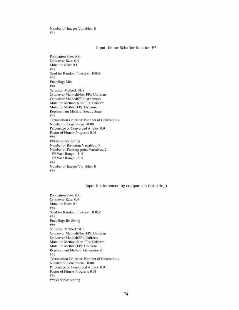
74
Number of Integer Variables: 0 ###
Input file for Schaffer function F7
Population Size: 600 Crossover Rate: 0.4 Mutation Rate: 0.1 ### Seed for Random Function: 10058 ### Encoding: Mix ### Selection Method: SUS Crossover Method(Non-FP): Uniform Crossover Method(FP): Arithmetic Mutation Method(Non-FP): Uniform Mutation Method(FP): Dynamic Replacement Method: Steady State ### Termination Criterion: Number of Generations Number of Generations: 4000 Percentage of Converged Alleles: 0.9 Factor of Fitness Progress: 0.01 ### ###Variables setting Number of Bit-string Variables: 0 Number of Floating-point Variables: 2 FP Var1 Range: -5, 5 FP Var2 Range: -5, 5 ### Number of Integer Variables: 0 ###
Input file for encoding comparison (bit-string) Population Size: 800 Crossover Rate: 0.4 Mutation Rate: 0.4 ### Seed for Random Function: 10059 ### Encoding: Bit String ### Selection Method: SUS Crossover Method(Non-FP): Uniform Crossover Method(FP): Uniform Mutation Method(Non-FP): Uniform Mutation Method(FP): Uniform Replacement Method: Generational ### Termination Criterion: Number of Generations Number of Generations: 1000 Percentage of Converged Alleles: 0.9 Factor of Fitness Progress: 0.01 ### ###Variables setting

75
Number of Bit-string Variables: 0 Number of Floating-point Variables: 4 FP Var1 Range: -5, 5 FP Var2 Range: -8, 8 FP Var3 Range: -10,10 FP Var4 Range: -10,10 ### Number of Integer Variables: 0 ###
Input file for encoding comparison (floating point)
Population Size: 800 Crossover Rate: 0.4 Mutation Rate: 0.4 ### Seed for Random Function: 10059 ### Encoding: Bit String ### Selection Method: SUS Crossover Method(Non-FP): Uniform Crossover Method(FP): Heuristic Mutation Method(Non-FP): Uniform Mutation Method(FP): Uniform Replacement Method: Generational ### Termination Criterion: Number of Generations Number of Generations: 1000 Percentage of Converged Alleles: 0.9 Factor of Fitness Progress: 0.01 ### ###Variables setting Number of Bit-string Variables: 0 Number of Floating-point Variables: 4 FP Var1 Range: -5, 5 FP Var2 Range: -8, 8 FP Var3 Range: -10,10 FP Var4 Range: -10,10 ### Number of Integer Variables: 0 ###
Input file for selection methods comparison I
#Change the selection method(FP) for each run. Population Size: 300 Crossover Rate: 0.4 Mutation Rate: 0.1 ### Seed for Random Function: 10058 ### Encoding: Mix ### Selection Method: Roulette Wheel Crossover Method(Non-FP): Uniform Crossover Method(FP): Arithmetic

76
Mutation Method(Non-FP): Uniform Mutation Method(FP): Dynamic Replacement Method: Steady State ### Termination Criterion: Number of Generations Number of Generations: 1000 Percentage of Converged Alleles: 0.9 Factor of Fitness Progress: 0.01 ### ###Variables setting Number of Bit-string Variables: 0 Number of Floating-point Variables: 2 FP Var1 Range: -3, 3 FP Var2 Range: -2, 2 ### Number of Integer Variables: 0 ###
Input file for selection methods comparison II
#Change the selection method(FP) for each run. Population Size: 200 Crossover Rate: 0.4 Mutation Rate: 0.1 ### Seed for Random Function: 10058 ### Encoding: Mix ### Selection Method: Roulette Wheel Crossover Method(Non-FP): Uniform Crossover Method(FP): Arithmetic Mutation Method(Non-FP): Uniform Mutation Method(FP): Dynamic Replacement Method: Steady State ### Termination Criterion: Number of Generations Number of Generations: 1000 Percentage of Converged Alleles: 0.9 Factor of Fitness Progress: 0.01 ### ###Variables setting Number of Bit-string Variables: 0 Number of Floating-point Variables: 4 FP Var1 Range: -3, 3 FP Var2 Range: -2, 2 FP Var3 Range: -10,10 FP Var4 Range: -10,10 ### Number of Integer Variables: 0 ###
Input file for crossover methods comparison I #Change the crossover method (FP) for each run. Population Size: 500 Crossover Rate: 0.4

77
Mutation Rate: 0.1 ### Seed for Random Function: 100589 ### Encoding: Mix ### Selection Method: SUS Crossover Method(Non-FP): Uniform Crossover Method(FP): Single Point Mutation Method(Non-FP): Uniform Mutation Method(FP): Dynamic Replacement Method: Steady State ### Termination Criterion: Number of Generations Number of Generations: 3300 Percentage of Converged Alleles: 0.9 Factor of Fitness Progress: 0.01 ### ###Variables setting Number of Bit-string Variables: 0 Number of Floating-point Variables: 5 FP Var1 Range: -3, 5 FP Var2 Range: -3, 5 FP Var3 Range: -10,10 FP Var4 Range: -10,10 FP Var5 Range: -10,10 ### Number of Integer Variables: 0 ###
Input file for crossover methods comparison II
#Change the crossover method(FP) for each run. Population Size: 500 Crossover Rate: 0.4 Mutation Rate: 0.1 ### Seed for Random Function: 1005896 ### Encoding: Mix ### Selection Method: SUS Crossover Method(Non-FP): Uniform Crossover Method(FP): Single Point Mutation Method(Non-FP): Uniform Mutation Method(FP): Dynamic Replacement Method: Steady State ### Termination Criterion: Number of Generations Number of Generations: 3300 Percentage of Converged Alleles: 0.9 Factor of Fitness Progress: 0.01 ### ###Variables setting Number of Bit-string Variables: 0 Number of Floating-point Variables: 5 FP Var1 Range: -10,10 FP Var2 Range: -10,10

78
FP Var3 Range: -10,10 FP Var4 Range: -10,10 FP Var5 Range: -10,10 ### Number of Integer Variables: 0 ###

VITA
Huawen Xu
Candidate for the Degree of
Master of Science Thesis: COMPARISON OF GENETIC OPERATORS ON A GENERAL GENETIC ALGORITHM PACKAGE Major Field: Computer Science Education: Graduated from Shanghai Jiao Tong University, Shanghai, China in July
1996; received Bachelor of Science degree in Naval and Ocean Engineering. Then graduated from the same university in April 1999; received Master of Science degree in Structural Mechanics. Completed the requirements for the Master of Science degree with a major in Computer Science at Oklahoma State University in May, 2005.
Experience: Worked as a software engineer in Marine Research and Design Institute
of China from 1999 to 2000.