Comparison of Low-Frequency Internal Climate Variability in CMIP5Models and Observations

ANSON H. CHEUNG

Department of Geosciences, The University of Arizona, Tucson, Arizona

MICHAEL E. MANN

Department of Meteorology and Atmospheric Science, and Earth and Environmental Systems Institute,

The Pennsylvania State University, University Park, Pennsylvania

BYRON A. STEINMAN

Department of Earth and Environmental Sciences, and Large Lakes Observatory, University of Minnesota

Duluth, Duluth, Minnesota

LEELA M. FRANKCOMBE AND MATTHEW H. ENGLAND

ARC Centre of Excellence for Climate System Science, and Climate Change Research Centre, University of

New South Wales, Sydney, New South Wales, Australia

SONYA K. MILLER

Department of Meteorology and Atmospheric Science, and Earth and Environmental Systems Institute,

The Pennsylvania State University, University Park, Pennsylvania

(Manuscript received 4 October 2016, in final form 28 February 2017)

ABSTRACT

Low-frequency internal climate variability (ICV) plays an important role in modulating global surface tempera-

ture, regional climate, and climate extremes. However, it has not been completely characterized in the instrumental

record and in the Coupled Model Intercomparison Project phase 5 (CMIP5) model ensemble. In this study, the

surface temperature ICV of the North Pacific (NP), North Atlantic (NA), and Northern Hemisphere (NH) in the

instrumental record and historical CMIP5 all-forcing simulations is isolated using a semiempirical method wherein

the CMIP5 ensemble mean is applied as the external forcing signal and removed from each time series. Comparison

of ICV signals derived from this semiempirical method as well as from analysis of ICV in CMIP5 preindustrial

control runs reveals disagreement in the spatial pattern and amplitude between models and instrumental data on

multidecadal time scales (.20 yr). Analysis of the amplitude of total variability and the ICV in the models and

instrumental data indicates that the models underestimate ICV amplitude on low-frequency time scales (.20 yr in

the NA; .40 yr in the NP), while agreement is found in the NH variability. A multiple linear regression analysis of

ICV in the instrumental record shows that variability in the NP drives decadal-to-interdecadal variability in the NH,

whereas the NA drives multidecadal variability in the NH. Analysis of the CMIP5 historical simulations does not

reveal such a relationship, indicating model limitations in simulating ICV. These findings demonstrate the need to

better characterize low-frequency ICV, which may help improve attribution and decadal prediction.

1. Introduction

Characterization of low-frequency (decadal to multi-

decadal) internal climate variability is crucial for un-

derstanding the timing and magnitude of changes in

global mean surface temperature (Kosaka and Xie 2013;

Trenberth and Fasullo 2013; England et al. 2014; Dai

et al. 2015), regional climate (e.g., Knight et al. 2006;

Folland et al. 1986; Power et al. 1999), and climate ex-

tremes (e.g., Seager et al. 2015; McCabe et al. 2004).

Internal climate variability is, however, very difficult to

precisely quantify because of the short length of the

instrumental record. Additionally, there are challengesCorresponding author: Anson H. Cheung, ansoncheung@email.

arizona.edu

15 JUNE 2017 CHEUNG ET AL . 4763

DOI: 10.1175/JCLI-D-16-0712.1

� 2017 American Meteorological Society. For information regarding reuse of this content and general copyright information, consult the AMS CopyrightPolicy (www.ametsoc.org/PUBSReuseLicenses).

in attempting to isolate internal climate variability from

external forcing (Steinman et al. 2015; Frankcombe et al.

2015). Nevertheless, past studies have identified internal

variability in Pacific, Atlantic, and Northern Hemi-

sphere (NH) surface temperatures (Mann and Park

1999) and have investigated the implications of these

intrinsic oscillations on Northern Hemisphere temper-

atures (Steinman et al. 2015), hurricane frequency and

intensity (Mann and Emanuel 2006), and drought pat-

terns (Seager et al. 2015), as well as their potential re-

sponses to changes in external forcing.

Low-frequency oscillatory signals in the Pacific basin

have been identified using several methods. Studies

based on empirical orthogonal function (EOF) analysis

indicate a decadal to interdecadal (;15–30-yr period)

variability in the Pacific (Zhang et al. 1997; Power et al.

1999) referred to as the Pacific decadal oscillation

(PDO), and a basinwide counterpart of the PDO known

as the interdecadal Pacific oscillation. During a warm

phase of the PDO, the sea surface temperature (SST)

in the Kuroshio–Oyashio Extension and western Pacific

exhibits a cool anomaly, while a warm anomaly occurs in

the central and eastern equatorial Pacific extending

northwestward along the North American coast (Mantua

et al. 1997; Mantua and Hare 2002). During a negative

phase, the SST pattern is similar but with the opposite sign

in those regions. Additional studies focused on the fre-

quency domain suggest a 15–18-yr (Mann and Park 1999)

and a 50–70-yr periodicity (Minobe 1997) in Pacific SSTs.

Proxy records (Mann et al. 1995; MacDonald and Case

2005) and model simulations (Latif and Barnett 1996;

Meehl et al. 2011) confirm the existence of these signals but

provide disparate perspectives on the exact time scales and

spatial patterns of variability. Newman et al. (2016) suggest

that multiple processes, including atmospheric stochastic

forcing, ocean memory, and Rossby wave propagation,

have to be consideredwhen studying thePDO.All of these

processes together contribute to the spatial and temporal

PDO characteristics identified by other studies (e.g.,

Mantua et al. 1997; Zhang et al. 1997).

In the Atlantic basin, the most prominent low-

frequency signal is the Atlantic multidecadal oscilla-

tion (AMO; Kerr 2000), which operates on a 50–70-yr

period (Delworth and Mann 2000). The AMO spatial

pattern is characterized by a meridional SST dipole

pattern, with a positive SST anomaly in the North At-

lantic (NA) and a negative SST anomaly in the South

Atlantic during the positive phase and vice versa during

the negative phase. This mode of variability was first

identified in instrumental records (Folland et al. 1986;

Schlesinger and Ramankutty 1994) and was later vali-

dated by analysis of proxy records (Delworth and Mann

2000) and model simulations (Delworth et al. 1997;

Knight et al. 2005). Further investigation byKnight et al.

(2005) indicates that the AMO is related to the Atlantic

meridional overturning circulation (AMOC), which

implies possible predictability of the AMO.

The NH mean temperature has also been shown to

vary over decadal and multidecadal time scales. Mann

and Park (1996) suggest that the NH mean surface

temperature is characterized by a 50–70-yr periodicity,

with the Atlantic acting as the ‘‘pacemaker’’ of this

variability, along with a secondary 16–20-yr oscillatory

signal. More recent studies related to the global warm-

ing hiatus/slowdown suggest that global surface tem-

peratures exhibit decadal variability (15–25 yr; e.g., Dai

et al. 2015; Trenberth and Fasullo 2013) and that the

Pacific plays a more prominent role than previously

thought in modulating global mean surface temperature

changes. These studies further suggest that the AMO,

which is currently in a neutral phase, has played only a

minor role in modulating global temperatures in recent

decades.

Climate model simulations, in particular the Coupled

Model Intercomparison Project phase 5 (CMIP5) sim-

ulation ensemble (Taylor et al. 2012), provide a useful

test bed for assessing the nature of forced versus in-

ternal variability in surface temperatures. Despite con-

tinuous improvement in climatemodels, there are notable

biases that lead to the likely underestimation of low-

frequency climate variability (Ault et al. 2012; Laepple

andHuybers 2014; Frankcombe et al. 2015). Additionally,

disagreements on the definition, properties, and mech-

anisms of different modes of climate variability (e.g., Liu

2012) have undermined efforts to characterize internal

oscillations in climate models. Several techniques that

have since been shown to be inadequate, including EOF

analysis (e.g., Zhang et al. 1997; Power et al. 1999) and

simple linear detrending of SST time series (e.g., Enfield

et al. 2001; Goldenberg et al. 2001; Zhang and Delworth

2007; Wyatt et al. 2012), have been applied to identify

and characterize climate modes, attribute climate ex-

tremes, and understand teleconnection patterns. These

methods suffer from biases that potentially contaminate

the putative signals they are designed to identify and

thus have limited utility in investigations of internal

climate variability (Mann and Park 1999; Knight 2009;

Trenberth and Shea 2006; Mann et al. 2014; Steinman

et al. 2015; Frankcombe et al. 2015).

In this study, we analyze preindustrial control and

historical simulations from the CMIP5 ensemble and

apply a semiempirical method (Steinman et al. 2015)

that combines analysis of instrumental records and his-

torical model simulations to investigate the amplitude

and spatial pattern of the intrinsic multidecadal (.40 yr)

component of North Pacific (NP), NA, and NH surface

4764 JOURNAL OF CL IMATE VOLUME 30

temperatures. We define these indices of internal vari-

ability as the Pacific multidecadal oscillation (PMO),

the AMO, and the northern multidecadal oscillation

(NMO). While these indices might not represent true

physical modes that involve ocean–atmosphere feed-

backs and coupling, we call them ‘‘oscillations’’ for

simplicity, and to be consistent with past literature (e.g.,

Steinman et al. 2015). Moreover, our objective is to

extend Steinman et al. (2015) and Frankcombe et al.

(2015) by 1) assessing whether the spatial patterns and

amplitude of internal variability in the NP, NA, and NH

simulated bymodels are consistent with semiempirically

derived patterns from observations; 2) analyzing the

impacts of time scales on the agreement betweenmodels

and observations; and 3) identifying the extent to which

each ocean basin impacts NH internal variability on

different time scales.

2. Data and methods

a. Data

We used the Goddard Institute of Space Studies (GISS)

surface temperature (GISTEMP) product (Hansen et al.

2010) to define the observational NHmean (land1 ocean)

temperature series. For SST, we employed themean of the

Hadley Center Global Sea Ice and Sea Surface Tempera-

ture (HadISST; Cowtan andWay 2014), National Oceanic

andAtmosphericAdministrationExtendedReconstructed

Sea Surface Temperature (ERSST; Rayner et al. 2003;

Smith et al. 2008), and Kaplan extended SST products

(Kaplan et al. 1998).

Themodel data consists of the CMIP5 historical (herein

HIST) and preindustrial (herein PIcontrol; Table 1) simu-

lation ensembles. To allowmore accurate comparisonwith

observations, we analyzed observations and HIST simu-

lations spanning 1880–2005 CE, the time period of com-

mon overlap between all model realizations and the

instrumental data. For the PIcontrol analyses, we obtained

the high-pass filtered data (f5 1/120 cycles per year) by

applying an adaptive filter (Mann 2008) to minimize the

effects of model drift due to incomplete spinup. To avoid

introducing spurious filtering artifacts, only PIcontrol simu-

lations longer than 250 years were considered. All ob-

served, CMIP5 HIST, and CMIP5 PIcontrol simulations

were regridded to a 58 3 58 grid prior to analysis.

b. Methods

We defined the NA and NP as the areal, latitude-

weighted mean over all SST grid boxes in the region

spanning from 08 to 608N over the Atlantic (2808–3608E)and Pacific (1208–2608E) basins, respectively. For the

CMIP5 NH analyses, we determined the mean (latitude

weighted) surface air temperature (SAT) over land by

masking ocean grid cells and themean (latitudeweighted)

SST over the ocean. We then combined the two series

using a weighted average based on a land coverage value

TABLE 1. List of CMIP5 climate model simulations used in the

present study. Shown are the length of the PIcontrol simulations in

years, and the number of HIST simulations available. For GISS

E2-R and GISS E2-H, the single PIcontrol run was separated into two

because of a data gap. A single asterisk (*) indicates that one re-

alization from this model is not included in the SAT/SST model

means. Two asterisks (**) indicate that thismodel is not included in

the SAT/SST model means. ND means data not available or not

used. (Expansions of acronyms are available online at http://www.

ametsoc.org/PubsAcronymList.)

Model

Length of

control runs (yr)

Number of

HIST realizations

GISS-E2-R 200 1 650 24

GISS-E2-H 240 1 540 17

CNRM-CM5 850 10

CSIRO-Mk3.6.0 500 10

GFDL-CM2.1 ND 10

HadCM3 ND 10

CCSM4 1051 6

IPSL-CM5A-LR 1000 6

CanESM2 996 5

GFDL-CM3* 500 5

HadGEM2-ES 575 5

MIROC5 ND 5

MRI-CGCM3 500 4

ACCESS1.3 500 3

BCC-CSM1.1 500 3

BCC-CSM1.1m 400 3

CESM1-CAM5 319 3

CESM1-FASTCHEM 222 3

FIO-ESM 800 3

IPSL-CM5A-MR 300 3

MPI-ESM-MR** 650 3

MIROC-ESM 630 3

MPI-ESM-LR* 1000 3

NorESM1-M 501 3

MPI-ESM-P** 1156 2

CESM1-WACCM 200 1

HadGEM2-CC 240 1

HadGEM2-AO** ND 1

ACCESS1.0 300 1

BNU-ESM 559 1

CESM1-BGC 123 1

CMCC-CESM 277 1

CMCC-CM 330 1

CMCC-CMS 500 1

CNRM-CM5.2 359 1

GFDL-ESM2G 500 1

GFDL-ESM2M 500 1

GISS-E2-H-CC 251 1

GISS-E2-R-CC 251 1

INM-CM4 500 1

IPSL-CM5B-LR 300 1

MRI-ESM1 ND 1

FGOALS-g2** ND 1

NorESM1-ME 252 1

15 JUNE 2017 CHEUNG ET AL . 4765

of 39%and an ocean coverage value of 61%. This allowed

direct comparison of themodel data with the instrumental

NH mean series, which are based on SAT over land and

SST over ocean (Cowtan et al. 2015).

We estimated the observed PMO, AMO, and NMO

signals by employing the semiempirical target region

regression method introduced by Steinman et al. (2015)

(henceforth known as ‘‘observation’’). This method is

based on the use of CMIP5 multimodel historical en-

semble mean as an estimate of the forced signal for each

target region, and assumes that internal variability in the

individual model realizations cancels when averaged

over a large ensemble. To account for the bias in-

troduced bymodels with a larger number of realizations,

we averaged the realizations from the same model prior

to calculating the multimodel mean results. The in-

strumental temperature series was then regressed onto

the forced component to account for the potential dif-

ference in amplitude between the true forced response

and the multimodel mean response. The internal vari-

ability signal is defined as the difference between the

observations and the rescaled forced component. We

smoothed the data at different frequencies ( f5 0.1, 0.05,

and 0.025 cycles per year) with a low-pass filter (Mann

2008) to compare the observational results with model

simulation results on various time scales.

To assess the internal variability signals in the HIST

model simulations, we again employed the target region

regression method, except that we replaced the obser-

vational temperature series with individual HIST re-

alizations. To account for the bias introduced by models

with a larger number of realizations, we averaged the

results from the same model in all analyses prior to

calculating the multimodel mean. For the PIcontrol ana-

lyses, we calculated the mean annual average of the NP,

NA, and NH regional surface temperature to estimate

internal variability. Similar to Frankcombe et al. (2015),

we then divided each PIcontrol series into 126-yr segments

in order to make more accurate comparisons with the

HIST and observational results. We then averaged the

results from each model to reduce biasing the analysis

toward models with more and/or longer runs. We

smoothed the data at different frequencies ( f5 0.1, 0.05,

and 0.025 cycles per year) with a low-pass filter (Mann

2008) to compare the model results with observational

estimates on various time scales.

To test the significance of the difference between

observation and HIST amplitudes, we used a Monte

Carlo approach wherein we first produced 1000 white

noise time series with the amplitude of the unfiltered

target region time series, added each series to the ob-

served smoothed time series to obtain 1000 individual

surrogates, and then smoothed the resulting surrogates

with a 40-yr low-pass filter (Mann 2008). We then cal-

culated the amplitude (i.e., standard deviation) and used

the distribution to compare with the HIST data.

When estimating the significance of the correlation,

we accounted for the reduced degrees of freedom due to

serial correlation and low-pass smoothing.We estimated

the effective sample size using Eq. (1) for unfiltered time

series, and Eq. (2) for filtered time series (Trenberth

1984):

N0 5N(12 r

1,xr1,y)

(11 r1,xr1,y), (1)

N0 5NDT

T0

, (2)

where N0 is the effective sample size, N is the nominal

sample size, r1,x and r1,y are the lag-1 autocorrelation

coefficients of each series, DT is the sampling interval,

and T0 is the effectively independent temporal spacing

(which is equal to 1/2f, where f is the filtering frequency).

To analyze the relative roles of NA andNP on the NH

in the observations and the HIST ensemble, we carried

out a linear regression analysis whereby we regressed

the observed PMO and AMO onto the NMO with dif-

ferent smoothing time scales and compared the results

with those from the HIST ensemble. We employed a

two-sided Student’s t test to determine the significance

of the PMO and AMO projection onto the NMO. We

also applied a two-sided paired Student’s t test to de-

termine whether the regression coefficients are signifi-

cantly different from each other. We accounted for

reduced degrees of freedomdue to serial correlation and

low-pass smoothing and estimated the effective sample

size by using Eq. (3):

N0 5N(12 r

1)

(11 r1), (3)

where N0 is the effective sample size, N is the nominal

sample size, and r1 is the lag-1 autocorrelation co-

efficient of the time series on the time scales we are

interested in.

3. Spatial pattern and amplitude of PMO, AMO,and NMO

Comparison of observations with HIST and PIcontrolresults reveals a disagreement on the spatial patterns of

the PMO,AMO, and NMO (Figs. 1a–c), with the largest

spatial disparity occurring in the PMO (Table 2). Regions

that display major differences include the Kuroshio–

Oyashio Extension region for the PMO and the Gulf

4766 JOURNAL OF CL IMATE VOLUME 30

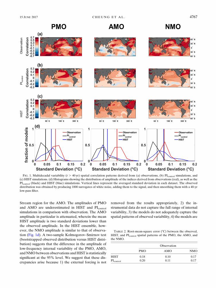
Stream region for the AMO. The amplitudes of PMO

and AMO are underestimated in HIST and PIcontrolsimulations in comparison with observation. The AMO

amplitude in particular is attenuated, wherein the mean

HIST amplitude is two standard deviations lower than

the observed amplitude. In the HIST ensemble, how-

ever, the NMO amplitude is similar to that of observa-

tion (Fig. 1d). A two-sample Kolmogorov–Smirnov test

(bootstrapped observed distribution versus HIST distri-

bution) suggests that the difference in the amplitude of

low-frequency internal variability of the PMO, AMO,

andNMObetween observations andHIST is statistically

significant at the 95% level. We suggest that these dis-

crepancies arise because 1) the external forcing is not

removed from the results appropriately, 2) the in-

strumental data do not capture the full range of internal

variability, 3) the models do not adequately capture the

spatial patterns of observed variability, 4) themodels are

FIG. 1. Multidecadal variability (t . 40 yr) spatial correlation patterns derived from (a) observations, (b) PIcontrol simulations, and

(c) HIST simulations. (d) Histograms showing the distribution of amplitude of the indices derived from observations (red), as well as the

PIcontrol (black) and HIST (blue) simulations. Vertical lines represent the averaged standard deviation in each dataset. The observed

distribution was obtained by producing 1000 surrogates of white noise, adding them to the signal, and then smoothing them with a 40-yr

low-pass filter.

TABLE 2. Root-mean-square error (8C) between the observed,

HIST, and PIcontrol spatial patterns of the PMO, the AMO, and

the NMO.

Observation

PMO AMO NMO

HIST 0.18 0.10 0.17

PIcontrol 0.20 0.11 0.17

15 JUNE 2017 CHEUNG ET AL . 4767

underestimating the amplitude of variability, or 5) some

combination of the above factors. These potential ex-

planations are further evaluated below.

We first consider whether external forcing is fully and

appropriately removed from the observational record as

well as from HIST. Using the target region regression

approach (Steinman et al. 2015), the external forcing is

estimated using the scaled CMIP5 ensemble mean (see

methods above). Steinman et al. (2015) showed that

internal variability can be cancelled when averaging

over a large model ensemble and thus can be used to

estimate the forced component. This method, however,

does not account for the different relative climate sen-

sitivity to certain forcings (e.g., volcanic, aerosols,

greenhouse gases) in each model. Hence, simply using

one factor to scale the external forcing could lead to

erroneous results, and in particular a significant differ-

ence between the HIST and PIcontrol amplitude. To as-

sess the facility of the target region approach method in

fully removing the external forcing, Frankcombe et al.

(2015) applied multifactor scaling methods that make

use of two or three factors (anthropogenic and natural;

anthropogenic, natural, and residual) to scale the ex-

ternal forcing signal. Their results, which focus on the

AMO, show that although the amplitude of the internal

variability signal is affected by the choice of scaling

factors, the external forcing signal is better removed (in

comparison to the linear detrending method) when ei-

ther the multifactor scaling or the single factor scaling

method of Steinman et al. (2015) are applied.We extend

the Frankcombe et al. (2015) analysis by also in-

vestigating the PMO and NMO time series. Our results

suggest that the difference between the PIcontrol and

HIST standard deviation distributions (for both PMO

and NMO) is statistically significant, as shown in two-

sample Kolmogorov–Smirnov tests (p , 0.01; Fig. 1d).

Meanwhile, the AMO results are in agreement with

Frankcombe et al. (2015) where the PIcontrol and HIST

standard deviation distributions are not significantly

different. The different results obtained for the PMO,

AMO, and NMO (significant for PMO and NMO; not

significant for AMO) indicate that our method might

inadequately remove external forcing in NP and NH,

which may cause a discrepancy between PMO and

NMO variability in the observations and HIST.

The uncertainty in external forcings employed in

CMIP5 experiments, for instance related to aerosol and

volcanic forcing, might also cause disagreement be-

tween the variability in models and observations. In the

target region regression method, we assume that the

scaled CMIP5 full-forcing ensemble mean can accu-

rately reflect forced changes in the temperature record.

However, several studies indicate that large uncertainty

exists in aerosol forcing (Otto et al. 2013; Schmidt et al.

2014), and this forcing might cause inaccurate model

simulations of the externally forced component. Con-

sequently, this might mask part of the low-frequency

internal variability in CMIP5 models (DelSole et al.

2011; Frankcombe et al. 2015). As a result, the target

region regression method might wrongly attribute in-

ternal forcing to forced changes or vice versa. This un-

certainty might not affect the amplitude significantly

(Frankcombe et al. 2015; Brown et al. 2015); however,

Brown et al. (2015) showed that applying two different

methods to isolate internal variability can yield two

different spatial patterns. Hence, the spatial pattern

discrepancy between models and observations might be

caused by uncertainties in external forcing.

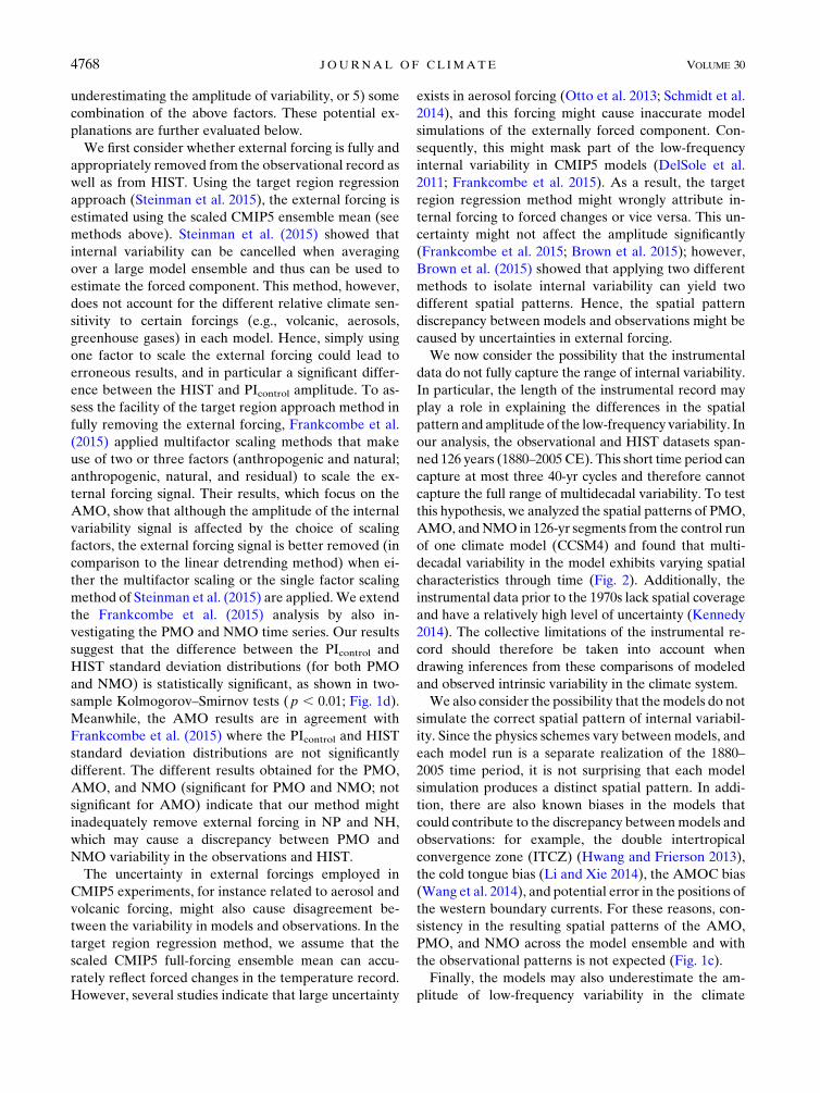
We now consider the possibility that the instrumental

data do not fully capture the range of internal variability.

In particular, the length of the instrumental record may

play a role in explaining the differences in the spatial

pattern and amplitude of the low-frequency variability. In

our analysis, the observational and HIST datasets span-

ned 126 years (1880–2005 CE). This short time period can

capture at most three 40-yr cycles and therefore cannot

capture the full range of multidecadal variability. To test

this hypothesis, we analyzed the spatial patterns of PMO,

AMO, andNMO in 126-yr segments from the control run

of one climate model (CCSM4) and found that multi-

decadal variability in the model exhibits varying spatial

characteristics through time (Fig. 2). Additionally, the

instrumental data prior to the 1970s lack spatial coverage

and have a relatively high level of uncertainty (Kennedy

2014). The collective limitations of the instrumental re-

cord should therefore be taken into account when

drawing inferences from these comparisons of modeled

and observed intrinsic variability in the climate system.

We also consider the possibility that themodels do not

simulate the correct spatial pattern of internal variabil-

ity. Since the physics schemes vary between models, and

each model run is a separate realization of the 1880–

2005 time period, it is not surprising that each model

simulation produces a distinct spatial pattern. In addi-

tion, there are also known biases in the models that

could contribute to the discrepancy betweenmodels and

observations: for example, the double intertropical

convergence zone (ITCZ) (Hwang and Frierson 2013),

the cold tongue bias (Li and Xie 2014), the AMOC bias

(Wang et al. 2014), and potential error in the positions of

the western boundary currents. For these reasons, con-

sistency in the resulting spatial patterns of the AMO,

PMO, and NMO across the model ensemble and with

the observational patterns is not expected (Fig. 1c).

Finally, the models may also underestimate the am-

plitude of low-frequency variability in the climate

4768 JOURNAL OF CL IMATE VOLUME 30

system (see, e.g., Ault et al. 2012; England et al. 2014;

Laepple and Huybers 2014; Frankcombe et al. 2015;

Kociuba and Power 2015; Power et al. 2017).

Frankcombe et al. (2015) applied single scaling and

multiple scaling methods to analyze Atlantic multi-

decadal variability. They show a significant difference

between the magnitude of observed and modeled mul-

tidecadal variability (both in HIST and PIcontrol) and

therefore suggest that models might be underestimating

the amplitude of the multidecadal climate signal. Here

we have extended the work of Frankcombe et al. (2015)

by also comparing the NMO and PMO amplitudes de-

rived from the observational, HIST, and PIcontrol ana-

lyses. We find that the AMO, PMO, and NMO

amplitudes derived from HIST and PIcontrol are signifi-

cantly lower than the observational values, as suggested

by two Kolmogorov–Smirnov tests (Fig. 1d), indicating

an underestimation of low-frequency climate variability

in the target regions. Although we cannot determine the

exact reason for the discrepancy between the observa-

tional and model results, we suggest that it is due to four

main factors: 1) forcing uncertainties represented in

climate models, 2) the relatively short length of the in-

strumental data, 3) the inconsistency between modeled

and real-world spatial expressions of internal variability,

and 4) the underestimation of low-frequency internal

variability by the models.

4. ICV characteristics on different time scales

In section 3, we showed that the spatial pattern and

amplitude derived from theHIST andPIcontrol analyses are

FIG. 2. Spatial pattern of the (a) PMO, (b) AMO, and (c) NMO from the CCSM4 PIcontrol simulations. Each subplot represents the spatial

pattern derived from one 126-yr segment.

15 JUNE 2017 CHEUNG ET AL . 4769

inconsistent with the observational results over multi-

decadal time scales. Recent studies suggest that models

tend to underestimate the low-frequency component of

internal climate variability (ICV; e.g., Frankcombe et al.

2015), whereas the higher-frequency components are

better simulated (Laepple and Huybers 2014). To assess

whether the external or internal component is incorrectly

estimated, and whether there is a threshold frequency at

which models begin to underestimate the variability, we

analyzed the characteristics of the total and internal vari-

ability by low-pass filtering the time series on four different

time scales: 0, 10, 20, and 40 years.

We find that the total variability in all target regions is

reasonably well simulated (Fig. 3). The HIST internal

variability also agrees with observed internal variability

for higher-frequency (0–10yr) amplitudes, with the ob-

served amplitude lying within 1 standard deviation of the

modeled amplitudes (Fig. 3). The difference between

HIST and observed amplitude, however, increases for

longer time scales. Substantial disagreement can be found,

for example, for the AMO over 20-yr and longer time

scales (Fig. 3b). Discrepancies exist, but are less obvious

for the PMO, over 40-yr time scales (Fig. 3a). We do not

find any substantial disagreement between HIST and the

observational NMOamplitude (Fig. 3c). Spectral analyses

show consistent results regarding the discrepancy between

observed and HIST time series (Fig. 4).

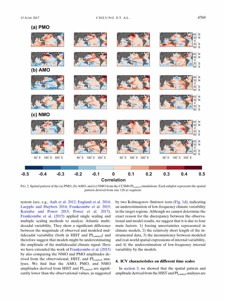
We further investigate the HIST and observed ICV

amplitudes by calculating their relative amplitudes

(modeled/observed). We show that uncertainty in-

creases with the length of the time scale and is largest for

the low-frequency component (Fig. 5). This suggests

that the magnitude of model–observed disagreement

varies between time scales and depends on the region of

FIG. 3. Amplitude of total and internal components of surface temperature variability (mean for model values) in the (a) PMO,

(b) AMO, and (c) NMO. Error bars indicate 1 standard deviation of the amplitude. Internal amplitude can account for a large fraction of

the total amplitude in surface temperature variability.

FIG. 4. Power spectra of observed (red line), meanHIST (black), and individual HISTmodel simulations (gray lines): (a) PMO, (b) AMO,

and (c) NMO.

4770 JOURNAL OF CL IMATE VOLUME 30

focus, with a general increasing disagreement with in-

creasing time scale (except the NMO).

Kociuba and Power (2015) suggest that the tropical

Pacific decadal variability modeled in CMIP5 is too

weak because models tend to be too oscillatory, or bi-

modal, with regard to ENSO. Since the tropical Pacific

can influence the NP via the atmospheric bridge

(Newman et al. 2016), the hypothesis posed by Kociuba

and Power (2015) might be applicable to explain the

weak low-frequency internal variability in the NP.

However, spectral analyses (Fig. 4a) show that this is not

fully reflected in our results. While ;75% of the HIST

simulations exhibit a spectral density that is lower

than observations over multidecadal time scales, the

spectral density for most HIST simulations is compara-

ble to observations on interannual time scales. Other

possible mechanisms might be invoked to explain the

observed–model differences; for example, too large ef-

fective horizontal diffusivity (Laepple and Huybers

2014) or teleconnections from the North Atlantic

(Knight et al. 2005; Zhang and Zhao 2015; Chafik et al.

2016). However, this topic goes beyond the scope of the

present paper.

The NA, on the other hand, exhibits a substantial

underestimation in variability and magnitude on time

scales with a .40-yr period, whereas higher-frequency

variability is reasonably well modeled (see Figs. 3b and

4b). This result aligns with previous studies (e.g., Zhang

and Wang 2013; Frankcombe et al. 2015) finding an

underestimation of magnitude and variability on multi-

decadal time scales. Such underestimation might be

caused by the systematic underestimation of AMOC

strength by CMIP5 models (see, e.g., Wang et al. 2014).

It is interesting to note that the HIST mean NMO and

median of relative NMO amplitude do not indicate a

significant disagreement between models and observa-

tions (Figs. 3c and 5c). This is a bit surprising because

two major components of the NMO, the PMO and

AMO (Steinman et al. 2015), are shown to be in-

consistent with observations. Consequently, it is ex-

pected that the NMO should also be inconsistent

between the models and observations, which in this case

it is not. We suggest that the NMO agreement arises by

coincidence, perhaps because the errors in PMO and

AMO cancel out. This argument can be further sup-

ported by analyzing spatial patterns derived from HIST

and the observations (Figs. 6 and 7). The disagreement

betweenHIST and observedNMO is substantial over all

time scales and is comparable to the disagreements in

the NP (Table 3). Moreover, the uncertainties also in-

crease for the NMO as we focus longer time scales

(Fig. 5). Therefore, we conclude that the agreement of

the NMO amplitude arises purely from coincidence.

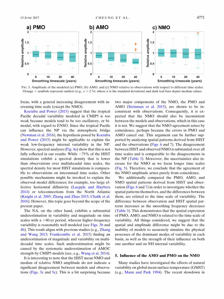
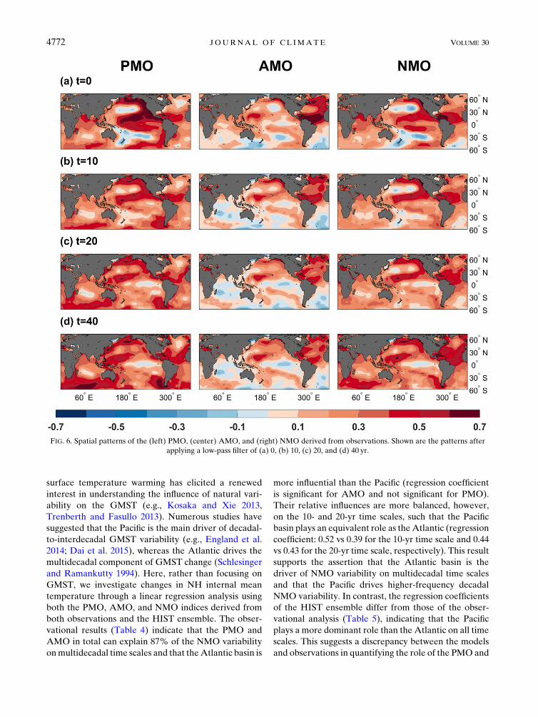
We additionally compared the PMO, AMO, and

NMO spatial patterns derived from HIST and obser-

vation (Figs. 6 and 7) in order to investigate whether the

spatial patterns themselves, and the differences between

them, are related to the time scale of variability. The

difference between observation and HIST spatial pat-

terns increases as the smoothing frequency decreases

(Table 3). This demonstrates that the spatial expression

of PMO, AMO, and NMO is related to the time scale of

variability. All things considered, we suggest that the

spatial and amplitude difference might be due to the

inability of models to accurately simulate the physical

processes of the dominant modes of variability in each

basin, as well as the strength of their influence on both

one another and on NH internal variability.

5. Influence of the AMO and PMO on the NMO

Many studies have investigated the effects of natural

variability on global mean surface temperature (GMST)

(e.g., Mann and Park 1994). The recent slowdown in

FIG. 5. Amplitude of the modeled (a) PMO, (b) AMO, and (c) NMO relative to observations with respect to different time scales.

Orange 1 symbols represent outliers (e.g., x . 2.7s; where s is the standard deviation) and dark teal bars depict median values.

15 JUNE 2017 CHEUNG ET AL . 4771

surface temperature warming has elicited a renewed

interest in understanding the influence of natural vari-

ability on the GMST (e.g., Kosaka and Xie 2013,

Trenberth and Fasullo 2013). Numerous studies have

suggested that the Pacific is the main driver of decadal-

to-interdecadal GMST variability (e.g., England et al.

2014; Dai et al. 2015), whereas the Atlantic drives the

multidecadal component of GMST change (Schlesinger

and Ramankutty 1994). Here, rather than focusing on

GMST, we investigate changes in NH internal mean

temperature through a linear regression analysis using

both the PMO, AMO, and NMO indices derived from

both observations and the HIST ensemble. The obser-

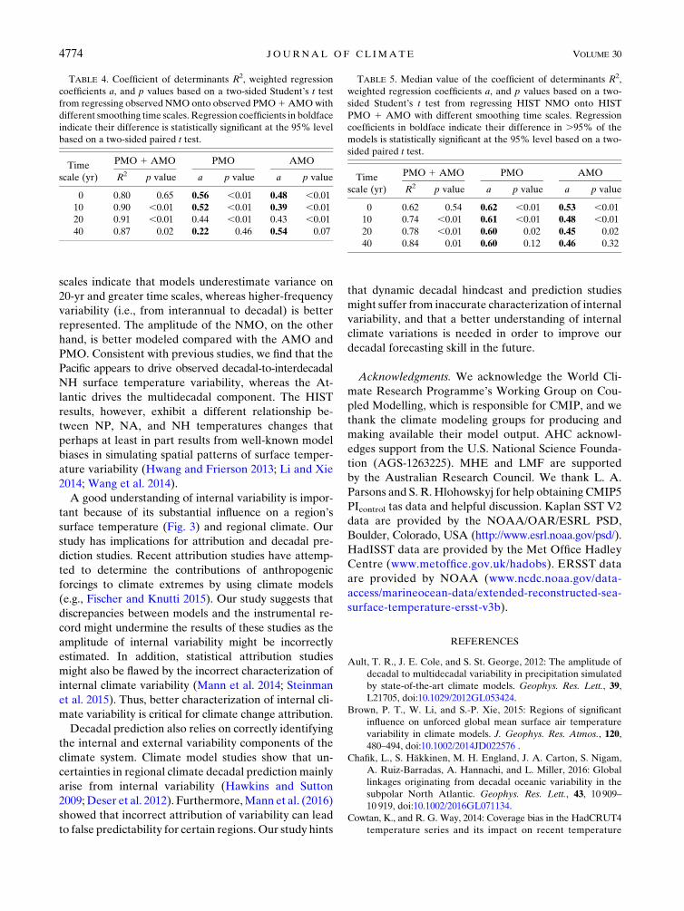
vational results (Table 4) indicate that the PMO and

AMO in total can explain 87% of the NMO variability

onmultidecadal time scales and that theAtlantic basin is

more influential than the Pacific (regression coefficient

is significant for AMO and not significant for PMO).

Their relative influences are more balanced, however,

on the 10- and 20-yr time scales, such that the Pacific

basin plays an equivalent role as theAtlantic (regression

coefficient: 0.52 vs 0.39 for the 10-yr time scale and 0.44

vs 0.43 for the 20-yr time scale, respectively). This result

supports the assertion that the Atlantic basin is the

driver of NMO variability on multidecadal time scales

and that the Pacific drives higher-frequency decadal

NMO variability. In contrast, the regression coefficients

of the HIST ensemble differ from those of the obser-

vational analysis (Table 5), indicating that the Pacific

plays a more dominant role than the Atlantic on all time

scales. This suggests a discrepancy between the models

and observations in quantifying the role of the PMO and

FIG. 6. Spatial patterns of the (left) PMO, (center) AMO, and (right) NMO derived from observations. Shown are the patterns after

applying a low-pass filter of (a) 0, (b) 10, (c) 20, and (d) 40 yr.

4772 JOURNAL OF CL IMATE VOLUME 30

AMOonNH temperature variability, which agrees with

results from a previous study (Douville et al. 2015). Such

discrepancies could be caused by 1) the relatively short

length of the observational record and the associated

limitation in capturing the full expression of multi-

decadal variability or 2) well-known model biases

(Hwang and Frierson 2013; Li and Xie 2014; Wang et al.

2014; Power et al. 2017).

6. Conclusions

Our results suggest that the CMIP5 simulated spatial

pattern and amplitude of the PMO,AMO, and NMOon

long time scales are inconsistent with observations. We

suggest that the discrepancy could be due to several

factors including 1) forcing uncertainties represented in

climate models, 2) the relatively short length of the in-

strumental data, 3) the inconsistency between modeled

and real-world spatial expressions of internal variability,

and 4) the underestimation of low-frequency internal

variability by the models. Our analyses of these internal

oscillations (i.e., the PMO and AMO) on different time

FIG. 7. As in Fig. 6, but for theHIST simulations. Note that the correlation color bar scale is different than in Fig. 6. Stippling indicates that

at least 50% of the models exhibit a statistically significant correlation (p , 0.05).

TABLE 3. Root-mean-square error (8C) between the observed

andHIST spatial patterns of the PMO, theAMO, and the NMOon

different time scales.

Time scale (yr) PMO AMO NMO

0 0.13 0.09 0.12

10 0.13 0.09 0.12

20 0.15 0.09 0.13

40 0.18 0.10 0.17

15 JUNE 2017 CHEUNG ET AL . 4773

scales indicate that models underestimate variance on

20-yr and greater time scales, whereas higher-frequency

variability (i.e., from interannual to decadal) is better

represented. The amplitude of the NMO, on the other

hand, is better modeled compared with the AMO and

PMO. Consistent with previous studies, we find that the

Pacific appears to drive observed decadal-to-interdecadal

NH surface temperature variability, whereas the At-

lantic drives the multidecadal component. The HIST

results, however, exhibit a different relationship be-

tween NP, NA, and NH temperatures changes that

perhaps at least in part results from well-known model

biases in simulating spatial patterns of surface temper-

ature variability (Hwang and Frierson 2013; Li and Xie

2014; Wang et al. 2014).

A good understanding of internal variability is impor-

tant because of its substantial influence on a region’s

surface temperature (Fig. 3) and regional climate. Our

study has implications for attribution and decadal pre-

diction studies. Recent attribution studies have attemp-

ted to determine the contributions of anthropogenic

forcings to climate extremes by using climate models

(e.g., Fischer and Knutti 2015). Our study suggests that

discrepancies between models and the instrumental re-

cord might undermine the results of these studies as the

amplitude of internal variability might be incorrectly

estimated. In addition, statistical attribution studies

might also be flawed by the incorrect characterization of

internal climate variability (Mann et al. 2014; Steinman

et al. 2015). Thus, better characterization of internal cli-

mate variability is critical for climate change attribution.

Decadal prediction also relies on correctly identifying

the internal and external variability components of the

climate system. Climate model studies show that un-

certainties in regional climate decadal prediction mainly

arise from internal variability (Hawkins and Sutton

2009; Deser et al. 2012). Furthermore,Mann et al. (2016)

showed that incorrect attribution of variability can lead

to false predictability for certain regions. Our study hints

that dynamic decadal hindcast and prediction studies

might suffer from inaccurate characterization of internal

variability, and that a better understanding of internal

climate variations is needed in order to improve our

decadal forecasting skill in the future.

Acknowledgments. We acknowledge the World Cli-

mate Research Programme’s Working Group on Cou-

pled Modelling, which is responsible for CMIP, and we

thank the climate modeling groups for producing and

making available their model output. AHC acknowl-

edges support from the U.S. National Science Founda-

tion (AGS-1263225). MHE and LMF are supported

by the Australian Research Council. We thank L. A.

Parsons and S. R. Hlohowskyj for help obtaining CMIP5

PIcontrol tas data and helpful discussion. Kaplan SST V2

data are provided by the NOAA/OAR/ESRL PSD,

Boulder, Colorado, USA (http://www.esrl.noaa.gov/psd/).

HadISST data are provided by the Met Office Hadley

Centre (www.metoffice.gov.uk/hadobs). ERSST data

are provided by NOAA (www.ncdc.noaa.gov/data-

access/marineocean-data/extended-reconstructed-sea-

surface-temperature-ersst-v3b).

REFERENCES

Ault, T. R., J. E. Cole, and S. St. George, 2012: The amplitude of

decadal to multidecadal variability in precipitation simulated

by state-of-the-art climate models. Geophys. Res. Lett., 39,

L21705, doi:10.1029/2012GL053424.

Brown, P. T., W. Li, and S.-P. Xie, 2015: Regions of significant

influence on unforced global mean surface air temperature

variability in climate models. J. Geophys. Res. Atmos., 120,

480–494, doi:10.1002/2014JD022576 .

Chafik, L., S. Häkkinen, M. H. England, J. A. Carton, S. Nigam,

A. Ruiz-Barradas, A. Hannachi, and L. Miller, 2016: Global

linkages originating from decadal oceanic variability in the

subpolar North Atlantic. Geophys. Res. Lett., 43, 10 909–

10 919, doi:10.1002/2016GL071134.

Cowtan, K., and R. G. Way, 2014: Coverage bias in the HadCRUT4

temperature series and its impact on recent temperature

TABLE 4. Coefficient of determinants R2, weighted regression

coefficients a, and p values based on a two-sided Student’s t test

from regressing observed NMO onto observed PMO1AMOwith

different smoothing time scales. Regression coefficients in boldface

indicate their difference is statistically significant at the 95% level

based on a two-sided paired t test.

Time

scale (yr)

PMO 1 AMO PMO AMO

R2 p value a p value a p value

0 0.80 0.65 0.56 ,0.01 0.48 ,0.01

10 0.90 ,0.01 0.52 ,0.01 0.39 ,0.01

20 0.91 ,0.01 0.44 ,0.01 0.43 ,0.01

40 0.87 0.02 0.22 0.46 0.54 0.07

TABLE 5. Median value of the coefficient of determinants R2,

weighted regression coefficients a, and p values based on a two-

sided Student’s t test from regressing HIST NMO onto HIST

PMO 1 AMO with different smoothing time scales. Regression

coefficients in boldface indicate their difference in .95% of the

models is statistically significant at the 95% level based on a two-

sided paired t test.

Time

scale (yr)

PMO 1 AMO PMO AMO

R2 p value a p value a p value

0 0.62 0.54 0.62 ,0.01 0.53 ,0.01

10 0.74 ,0.01 0.61 ,0.01 0.48 ,0.01

20 0.78 ,0.01 0.60 0.02 0.45 0.02

40 0.84 0.01 0.60 0.12 0.46 0.32

4774 JOURNAL OF CL IMATE VOLUME 30

trends. Quart. J. Roy. Meteor. Soc., 140, 1935–1944,

doi:10.1002/qj.2297.

——, and Coauthors, 2015: Robust comparison of climate models

with observations using blended land air and ocean sea surface

temperatures.Geophys. Res. Lett., 42, 6526–6534, doi:10.1002/

2015GL064888.

Dai, A., J. C. Fyfe, S.-P. Xie, andX.Dai, 2015: Decadal modulation

of global surface temperature by internal climate variability.

Nat. Climate Change, 5, 555–559, doi:10.1038/nclimate2605.

DelSole, T., M. Tippett, and J. Shukla, 2011: A significant com-

ponent of unforced multidecadal variability in the recent ac-

celeration of global warming. J. Climate, 24, 909–926,

doi:10.1175/2010JCLI3659.1.

Delworth, T. L., and M. E. Mann, 2000: Observed and simulated

multidecadal variability in the NH.Climate Dyn., 16, 661–676,

doi:10.1007/s003820000075.

——, S. Manabe, and R. J. Stouffer, 1997: Multidecadal climate

variability in the Greenland Sea and surrounding regions: A

coupled model simulation. Geophys. Res. Lett., 24, 257–260,

doi:10.1029/96GL03927.

Deser, C., A. Phillips, V. Bourdette, and H. Teng, 2012: Uncertainty

in climate change projections: The role of internal variability.

Climate Dyn., 38, 527–546, doi:10.1007/s00382-010-0977-x.

Douville, H., A. Voldoire, and O. Geoffroy, 2015: The recent

global warming hiatus: What is the role of Pacific variability?

Geophys. Res. Lett., 42, 880–888, doi:10.1002/2014GL062775.

Enfield, D. B., A. M. Mestas-Nunez, and P. J. Trimble, 2001: The

Atlantic multidecadal oscillation and its relation to rainfall

and river flows in the continental U.S.Geophys. Res. Lett., 28,

2077–2080, doi:10.1029/2000GL012745.

England, M. H., and Coauthors, 2014: Recent intensification of

wind-driven circulation in the Pacific and the ongoing warm-

ing hiatus. Nat. Climate Change, 4, 222–227, doi:10.1038/

nclimate2106.

Fischer, E. M., and R. Knutti, 2015: Anthropogenic contribution to

global occurrence of heavy-precipitation and high-temperature

extremes. Nat. Climate Change, 5, 560–564, doi:10.1038/

nclimate2617.

Folland, C. K., D. E. Parker, and T. N. Palmer, 1986: Sahel rainfall

and worldwide sea temperatures 1901–85. Nature, 320, 602–

607, doi:10.1038/320602a0.

Frankcombe, L. M., M. H. England, M. E. Mann, and B. A.

Steinman, 2015: Separating internal variability from the ex-

ternally forced climate response. J. Climate, 28, 8184–8202,

doi:10.1175/JCLI-D-15-0069.1.

Goldenberg, S. B., C.W. Landsea, A.M.Mestas-Nuñez, andW.M.

Gray, 2001: The recent increase in Atlantic hurricane activity:

Causes and implications. Science, 293, 474–479, doi:10.1126/

science.1060040.

Hansen, J., R. Ruedy, M. Sato, and K. Lo, 2010: Global surface

temperature change. Rev. Geophys., 48, RG4004, doi:10.1029/

2010RG000345.

Hawkins, E., and R. Sutton, 2009: The potential to narrow un-

certainty in regional climate predictions. Bull. Amer. Meteor.

Soc., 90, 1095–1107, doi:10.1175/2009BAMS2607.1.

Hwang, Y.-T., and D. M. W. Frierson, 2013: Link between the

double-Intertropical Convergence Zone problem and cloud

biases over the Southern Ocean. Proc. Natl. Acad. Sci. USA,

110, 4935–4940, doi:10.1073/pnas.1213302110.

Kaplan, A., M. A. Cane, Y. Kushnir, A. C. Clement, M. B.

Blumenthal, and B. Rajagopalan, 1998: Analyses of global sea

surface temperature 1856–1991. J. Geophys. Res., 103, 18 567–

18 589, doi:10.1029/97JC01736.

Kennedy, J. J., 2014: A review of uncertainty in in situ measure-

ments and data sets of sea surface temperature.Rev.Geophys.,

52, 1–32, doi:10.1002/2013RG000434.

Kerr, R. A., 2000: A North Atlantic climate pacemaker for the cen-

turies.Science, 288, 1984–1985, doi:10.1126/science.288.5473.1984.Knight, J. R., 2009: The Atlantic multidecadal oscillation inferred

from the forced climate response in coupled general circula-

tion models. J. Climate, 22, 1610–1625, doi:10.1175/

2008JCLI2628.1.

——,R. J. Allan, C. K. Folland,M.Vellinga, andM. E.Mann, 2005:

A signature of persistent natural thermohaline circulation

cycles in observed climate. Geophys. Res. Lett., 32, L20708,

doi:10.1029/2005GL024233.

——, C. K. Folland, and A. A. Scaife, 2006: Climate impacts of the

Atlantic multidecadal oscillation. Geophys. Res. Lett., 33,

L17706, doi:10.1029/2006GL026242.

Kociuba, G., and S. B. Power, 2015: Inability of CMIP5 models to

simulate recent strengthening of the Walker circulation: Im-

plications for projection. J. Climate, 28, 20–35, doi:10.1175/

JCLI-D-13-00752.1.

Kosaka, Y., and S.-P. Xie, 2013: Recent global-warming hiatus tied

to equatorial Pacific surface cooling. Nature, 501, 403–407,

doi:10.1038/nature12534.

Laepple, T., and P. Huybers, 2014: Global and regional variability

in marine surface temperatures.Geophys. Res. Lett., 41, 2528–

2534, doi:10.1002/2014GL059345.

Latif, M., and T. P. Barnett, 1996: Decadal climate variability

over the North Pacific and North America: Dynamics and

predictability. J. Climate, 9, 2407–2423, doi:10.1175/

1520-0442(1996)009,2407:DCVOTN.2.0.CO;2.

Li, G., and S.-P. Xie, 2014: Tropical biases in CMIP5 multimodel

ensemble: The excessive equatorial Pacific cold tongue and

double ITCZ problems. J. Climate, 27, 1765–1780, doi:10.1175/

JCLI-D-13-00337.1.

Liu, Z., 2012: Dynamics of interdecadal climate variability: A his-

torical perspective. J. Climate, 25, 1963–1995, doi:10.1175/

2011JCLI3980.1.

MacDonald, G. M., and R. A. Case, 2005: Variations in the Pacific

decadal oscillation over the past millennium. Geophys. Res.

Lett., 32, L08703, doi:10.1029/2005GL022478.

Mann, M. E., 2008: Smoothing of climate time series revisited.

Geophys. Res. Lett., 35, L16708, doi:10.1029/2008GL034716.

——, and J. Park, 1994: Global-scale modes of surface temperature

variability on interannual to century timescales. J. Geophys.

Res., 99, 25 819–25 833, doi:10.1029/94JD02396.

——, and ——, 1996: Joint spatio-temporal modes of surface

temperature and sea level pressure variability in the NH

during the last century. J. Climate, 9, 2137–2162, doi:10.1175/

1520-0442(1996)009,2137:JSMOST.2.0.CO;2.

——, and——, 1999: Oscillatory spatiotemporal signal detection in

climate studies: A multiple-taper spectral domain approach.

Adv.Geophys., 41, 1–131, doi:10.1016/S0065-2687(08)60026-6.——, and K. A. Emanuel, 2006: Atlantic hurricane trends linked to

climate change. Eos, Trans. Amer. Geophys. Union, 87, 233–

241, doi:10.1029/2006EO240001.

——, J. Park, and R. S. Bradley, 1995: Global interdecadal and

century-scale climate oscillations during the past 5 centuries.

Nature, 378, 266–270, doi:10.1038/378266a0.

——, B. A. Steinman, and S. K. Miller, 2014: On forced tempera-

ture changes, internal variability, and the AMO. Geophys.

Res. Lett., 41, 3211–3219, doi:10.1002/2014GL059233.

——, ——, ——, L. M. Frankcombe, M. H. England, and A. H.

Cheung, 2016: Predictability of the recent slowdown and

15 JUNE 2017 CHEUNG ET AL . 4775

subsequent recovery of large-scale surface warming using

statistical methods. Geophys. Res. Lett., 43, 3459–3467,

doi:10.1002/2016GL068159.

Mantua, N. J., and S. R. Hare, 2002: The Pacific decadal oscillation.

J. Oceanography, 58, 35–44.

——,——,Y.Zhang, J.M.Wallace, andR.C. Francis, 1997:APacific

interdecadal climate oscillation with impacts on salmon pro-

duction. Bull. Amer. Meteor. Soc., 78, 1069–1079, doi:10.1175/1520-0477(1997)078,1069:APICOW.2.0.CO;2.

McCabe, G. J., M. A. Palecki, and J. L. Betancourt, 2004: Pacific

and Atlantic Ocean influences on multidecadal drought fre-

quency in the United States. Proc. Natl. Acad. Sci. USA, 101,4136–4141, doi:10.1073/pnas.0306738101.

Meehl, G. A., J. M. Arblaster, J. T. Fasullo, A. Hu, and K. E.

Trenberth, 2011: Model-based evidence of deep-ocean heat

uptake during surface-temperature hiatus periods. Nat. Cli-

mate Change, 1, 360–364, doi:10.1038/nclimate1229.

Minobe, S., 1997: A 50–70 year climatic oscillation over the North

Pacific and North America. Geophys. Res. Lett., 24, 683–686,doi:10.1029/97GL00504.

Newman, M., and Coauthors, 2016: The Pacific decadal oscillation,

revisited. J.Climate, 29, 4399–4427, doi:10.1175/JCLI-D-15-0508.1.

Otto, A., and Coauthors, 2013: Energy budget constraints on climate

response. Nat. Geosci., 6, 415–416, doi:10.1038/ngeo1836.

Power, S., T. Casey, C. Folland, A. Colman, and V. Mehta, 1999:

Inter-decadal modulation of the impact of ENSO on Aus-

tralia. Climate Dyn., 15, 319–324, doi:10.1007/s003820050284.

——, F. Delage, G. Wang, I. Smith, and G. Kociuba, 2017: Ap-

parent limitations in the ability of CMIP5 climate models to

simulate recent multi-decadal change in surface temperature:

Implications for global temperature projections. Climate

Dyn., doi:10.1007/s00382-016-3326-x, in press.

Rayner, N. A., D. E. Parker, E. B. Horton, C. K. Folland, L. V.

Alexander, D. P. Rowell, E. C. Kent, and A. Kaplan, 2003:

Global analyses of sea surface temperature, sea ice, and night

marine air temperature since the late nineteenth century.

J. Geophys. Res., 108, 4407, doi:10.1029/2002JD002670.

Schlesinger, M. E., and N. Ramankutty, 1994: An oscillation in the

global climate system of period 65–70 years.Nature, 367, 723–

726, doi:10.1038/367723a0.

Schmidt, G. A., D. T. Shindell, and K. Tsigaridis, 2014: Reconciling

warming trends. Nat. Geosci., 7, 158–160, doi:10.1038/ngeo2105.

Seager, R.,M.Hoerling, S. Schubert, H.Wang, B. Lyon,A. Kumar,

J. Nakamura, and N. Henderson, 2015: Causes of the 2011–14

California drought. J. Climate, 28, 6997–7024, doi:10.1175/

JCLI-D-14-00860.1.

Smith, T. M., R. W. Reynolds, T. C. Peterson, and J. Lawrimore,

2008: Improvements to NOAA’s historical merged land–

ocean surface temperature analysis (1880–2006). J. Climate,

21, 2283–2296, doi:10.1175/2007JCLI2100.1.

Steinman, B. A., M. E. Mann, and S. K. Miller, 2015: Atlantic

and Pacific multidecadal oscillations and Northern Hemi-

sphere temperatures. Science, 347, 988–991, doi:10.1126/

science.1257856.

Taylor, K. E., R. J. Stouffer, andG.A.Meehl, 2012:An overview of

CMIP5 and the experiment design. Bull. Amer. Meteor. Soc.,

93, 485–498, doi:10.1175/BAMS-D-11-00094.1.

Trenberth, K. E., 1984: Some effects of finite sample size and

persistence on meteorological statistics. Part I: Autocorre-

lations. Mon. Wea. Rev., 112, 2359–2368, doi:10.1175/

1520-0493(1984)112,2359:SEOFSS.2.0.CO;2.

——, and D. J. Shea, 2006: Atlantic hurricanes and natural vari-

ability in 2005. Geophys. Res. Lett., 33, L12704, doi:10.1029/2006GL026894.

——, and J. T. Fasullo, 2013: An apparent hiatus in global warm-

ing? Earth’s Future, 1, 19–32, doi:10.1002/2013EF000165.

Wang, C., L. Zhang, S.-K. Lee, L. Wu, and C. R. Mechoso, 2014: A

global perspective on CMIP5 climate model biases. Nat. Cli-

mate Change, 4, 201–205, doi:10.1038/nclimate2118.

Wyatt, M. G., S. Kravtsov, and A. A. Tsonis, 2012: Atlantic

multidecadal oscillation and Northern Hemisphere’s cli-

mate variability. Climate Dyn., 38, 929–949, doi:10.1007/

s00382-011-1071-8.

Zhang, L., and C. Wang, 2013: Multidecadal North Atlantic sea

surface temperature and Atlantic meridional overturning cir-

culation variability in CMIP5 historical simulations. J. Geophys.

Res. Oceans, 118, 5772–5791, doi:10.1002/jgrc.20390.

——, and C. Zhao, 2015: Processes and mechanisms for the

model SST biases in the North Atlantic and North Pacific: A

link with the Atlantic meridional overturning circulation.

J. Adv. Model. Earth Syst., 7, 739–758, doi:10.1002/

2014MS000415.

Zhang, R., and T. L. Delworth, 2007: Impact of Atlantic multi-

decadal oscillation on North Pacific climate variability. Geo-

phys. Res. Lett., 34, L23708, doi:10.1029/2007GL031601.

Zhang, Y., J. M. Wallace, and D. S. Battisti, 1997: ENSO-like in-

terdecadal variability: 1900–93. J. Climate, 10, 1004–1020,

doi:10.1175/1520-0442(1997)010,1004:ELIV.2.0.CO;2.

4776 JOURNAL OF CL IMATE VOLUME 30