Embed Size (px)
Citation preview
COMPARISON OF METHODS OF ANALYSIS FOR PRETEST AND POSTTEST DATA
by
EMILY LAUREN FANCHER
(Under the Direction of Jaxk Reeves)
ABSTRACT
In this thesis I compare methods of statistical analyses for Pretest and Posttest Control
Group Designs and Non-equivalent Group Designs. I compare the strengths and weaknesses of
different methods of analyses, including ANOVA for the difference, ANCOVA, and Repeated
Measures ANOVA. Four different data sets are analyzed and compared based on fit statistics
and LS mean estimates.
INDEX WORDS: Pretest Posttest Control Group Design, Non-equivalent Group Design,
Experimental Validity, ANOVA, ANCOVA, Repeated Measures ANOVA, Longitudinal Study, Mixed Model, Quasi-Experiment
COMPARISON OF METHODS OF ANALYSIS FOR PRETEST AND POSTTEST DATA
by
EMILY LAUREN FANCHER
B.B.A., University of Georgia, 2010
A Thesis Submitted to the Graduate Faculty of the University of Georgia in Partial Fulfillment of
the Requirements for the Degree
MASTER OF SCIENCE
ATHENS, GEORGIA
2013

© 2013
Emily Lauren Fancher
All Rights Reserved
COMPARISON OF METHODS OF ANALYSIS FOR PRETEST AND POSTTEST DATA
by
EMILY LAUREN FANCHER
Major Professor: Jaxk Reeves
Committee: Kimberly Love-Myers Jennifer Kaplan Electronic Version Approved: Maureen Grasso Dean of the Graduate School The University of Georgia August 2013

iv
TABLE OF CONTENTS
Page
LIST OF TABLES ...........................................................................................................................v
LIST OF FIGURES ...................................................................................................................... vii
CHAPTER
1 INTRODUCTION .........................................................................................................1
2 LITERATURE REVIEW ..............................................................................................4
2.1 VALIDITY ........................................................................................................4
2.2 METHODS OF DATA ANALYSIS ...............................................................11
3 THE DATA SETS .......................................................................................................21
4 METHODS ..................................................................................................................25
5 THE ANALYSES ........................................................................................................31
5.1 THE NURSING DATA SET ...........................................................................31
5.2 THE ICA DATA SET ......................................................................................41
5.3 THE ECON DATA SET ..................................................................................51
5.4 THE SHI DATA SET ......................................................................................62
6 CONCLUSIONS..........................................................................................................72
REFERENCES ..............................................................................................................................77

v
LIST OF TABLES
Page
Table 2.1: Transformation Equations for Posttest-Pretest Differences .........................................14
Table 2.2: Repeated Measures ANOVA Table ..............................................................................18
Table 3.1: Summary of Characteristics of Four Data Sets .............................................................25
Table 4.1: The General Linear Model for Predicting Posttest Scores ...........................................27
Table 5.1: Summary Statistics for Nursing Data Set .....................................................................33
Table 5.2: Table of Model Results: Nursing Data Set ...................................................................36
Table 5.3: Type 3 Tests of Fixed Effects for Nursing Data Set .....................................................39
Table 5.4: Differences for Least Square Means for Nursing Data Set ..........................................40
Table 5.5: Comparison of Best GLM with Mixed Model for Nursing Data Set ...........................40
Table 5.6: Frequency Table for Year by Group for ICA Data Set ................................................41
Table 5.7: Summary Statistics for ICA Data Set ...........................................................................43
Table 5.8: Table of Model Results: ICA Data Set .........................................................................47
Table 5.9: Type 3 Tests of Fixed Effects for ICA Data Set ...........................................................49
Table 5.10: Differences for Least Squares Means for ICA Data Set .............................................50
Table 5.11: Comparison of Best GLM with Mixed Model for ICA Data Set ...............................50
Table 5.12: LS Means from Best GLM at Common Pretest Mean for ICA Data Set ...................51
Table 5.13: Summary Statistics for Econ Data Set ........................................................................52
Table 5.14: Table of Model Results: Econ Data Set ......................................................................56
Table 5.15: Type 3 Tests of Fixed Effects for Econ Data Set .......................................................59
vi
Table 5.16: Differences for Least Square Means for Econ Data Set .............................................60
Table 5.17: Comparison of Best GLM with Mixed Model for Econ Data Set ..............................61
Table 5.18: LS Means from Best GLM at Common Pretest Mean for Econ Data Set ..................61
Table 5.19: Summary Statistics for Original SHI Data Set ...........................................................62
Table 5.20: Summary Statistics for Condensed SHI Data Set .......................................................63
Table 5.21: Table of Model Results: SHI Data Set .......................................................................67
Table 5.22: Type 3 Tests of Fixed Effects for SHI Data Set .........................................................70
Table 5.23: Differences for Least Squares Means for SHI Data Set .............................................70
Table 5.24: Comparison of Best GLM with Mixed Model for SHI Data Set ................................70
Table 5.25: LS Means from Best GLM at Common Pretest Mean for SHI Data Set ....................71

vii
LIST OF FIGURES
Page
Figure 2.1: Illustration of Intrasession and History Effects .............................................................7
Figure 5.1: Histogram of Nursing Pretest Scores ..........................................................................33
Figure 5.2: Histogram of Nursing Posttest Scores .........................................................................33
Figure 5.3: Histogram of Nursing Difference Scores ....................................................................34
Figure 5.4 Trend Plot for Nursing Scores ......................................................................................34
Figure 5.5 ANCOVA with Interaction Plot for Nursing Data Set .................................................37
Figure 5.6: Histogram of ICA Pretest Scores ................................................................................43
Figure 5.7: Histogram of ICA Posttest Scores ...............................................................................44
Figure 5.8: Histogram of ICA Difference Scores ..........................................................................44
Figure 5.9 Trend Plot for ICA Scores ............................................................................................45
Figure 5.10 ANCOVA with Interaction Plot for ICA Data Set .....................................................48
Figure 5.11: Histogram of Econ Pretest Scores .............................................................................53
Figure 5.12: Histogram of Econ Posttest Scores ...........................................................................53
Figure 5.13 Histogram of Econ Difference Scores ........................................................................54
Figure 5.14 Trend Plot for Econ Scores .........................................................................................55
Figure 5.15 ANCOVA with Interaction Plot for Econ Data Set....................................................58
Figure 5.16 Histogram of SHI Pretest Scores ................................................................................64
Figure 5.17 Histogram of SHI Posttest Scores ..............................................................................64
Figure 5.18 Histogram of SHI Difference Scores ..........................................................................65

viii
Figure 5.19 Trend Plot for SHI Scores .........................................................................................66
Figure 5.20 ANCOVA with Interaction Plot for SHI Data Set .....................................................68

1
CHAPTER 1
INTRODUCTION
Pretest-Posttest designs are very common in scientific study. A characteristic common to
true Pretest-Posttest designs is that two or more measurements are taken on each experimental
unit. Subjects within each group receive a treatment of interest, no treatment, or a neutral
treatment. Ideally, these experiments have a completely randomized design, whereby subjects
are randomly assigned to the different levels of treatment. Through randomization, the effects of
extraneous variables should be removed. Once the subjects are assigned to the groups, but before
the actual treatment (if any) begins, each subject is measured on some characteristic to obtain his
or her “Pretest” score. After the experiment has commenced, each subject is measured again one
or more times to obtain his or her “Posttest” score or scores. When there are a number of such
measurements taken at set periods of times for each subject, this is called a longitudinal or
repeated measures study. In this thesis, we are primarily interested in the special case where
there is only one final Posttest score. For a Pretest-Posttest Group Design (PPGD), the effect of
the treatment is assessed by comparing the results for the treatment group to that of the control.
When random assignment is used, differences should be primarily attributable to the treatment.
In many settings, however, the ability to randomize may be limited, or the groups may
not have been identical at the start of the experiment. This is referred to as Non-equivalent Group
Design (NEGD), as the experiment lacks randomization, which is a necessary requirement for
the PPGD. NEGDs are a subset of quasi-experimental designs, which are quite common in social
science research. For instance, educational studies are often limited due to restrictions on human

2
subjects, and randomization is nearly impossible. Additionally, even if random assignment is
possible, groups can potentially become non-equivalent if records for subjects cannot be
obtained throughout the study. This can occur if there is a loss of subjects between Pretest and
Posttest sessions.
In addition to a lack of randomization, other common issues can arise with this type of
design. These issues may include intervention between tests—an event can occur after the
Pretest, creating a difference in scores between groups, though the event is not directly related to
the treatment itself. Testing effects may occur from prior exposure to the test; subjects tend to
score higher simply from receiving an identical test. Maturation is possible, where the two
groups change naturally between the tests, unrelated to treatment. Regression toward the mean
can also occur between Pretest and Posttest scores. That is, for more extreme Pretest scores, a
subject’s corresponding Posttest score may appear to have a larger relative gain/loss simply
because the original (Pretest) score differed significantly from the average.
There are multiple methods that can be used to analyze PPGDs. If the two groups were
truly equivalent at Pretest, one-way analysis of variance (ANOVA) on Posttest scores should be
a sufficient method to evaluate differences between the control and treatment groups.
Alternatively, an ANOVA on the difference in scores (Posttest – Pretest) could be used to
analyze whether the changes in scores from pretest to posttest were different for the groups.
Thirdly, analysis of covariance (ANCOVA), using Pretest scores as a covariate, can be used to
remove the effect of Pretest scores and fairly compare Posttest scores between groups. Finally,
Mixed Modeling can also be used to analyze differences between groups, where treatment type
and time are fixed effects and each subject has a random effect. These methods may give

3
similar results, but depending on what a researcher is hoping to infer or how the data fit, some
methods may be more appropriate than others.
4
CHAPTER 2
LITERATURE REVIEW
The purpose of many group design experiments is to allow conclusions to be drawn about
cause and effect. This cause and effect relationship is subject to alternative explanations; before a
researcher can infer a causal relationship exists between variables, he or she must rule out rival
hypotheses. If alternative explanations are ruled out, an experiment is said to possess validity.
Experimental validity is an important consideration in both educational and psychological
testing, as the interpretations of analyses are dependent on the validity of tests. For a valid PPGD
experiment, the results of analyses can be used to determine if there is a difference between
groups after a treatment has been imposed. A review of the literature confirms that this design is
widely used in scientific investigation, and that a variety of statistical tests exist to analyze this
particular design. There is not, however, any consensus on what statistical methods are most
appropriate for these analyses. These sources illustrate that more than one statistical method may
be used for analyses, but the results of such methods are valid only when the assumptions are
met. Additionally, much debate exists about how to treat the baseline (Pretest) information,
when it is included. This lack of consensus in the literature stems largely from violations of
model assumptions, threats to experimental validity, and lack of guidance on how to best present
the analyses.

5
2.1 EXPERIMENTAL VALIDITY
Experimental validity is a common topic discussed within PPGD research, and this
section will discuss two of the main components of experimental validity: internal and external
validity. It should be mentioned here that the field of Psychometrics is also concerned with an
entirely different concept of validity, known as test validity (including construct, criterion, and
content validity). Test validity tends to be more emphasized in social sciences than natural
sciences, as variables used in social sciences are typically less subjective or more difficult to
quantify. This is often the case with survey data and educational testing. Such validity is not the
focus of this research, but more about test validity can be found in references such as Construct
Validity in Psychological Tests (Cronbach and Meehl, 1955).
A seminal piece of literature on experimental validity for both true and quasi-experiments
is Experimental and Quasi-Experimental Designs for Research, by Campbell, Stanley, and Gage
(1963). In this text, the PPGD and NEGD are both noted for their strong control over most
threats to experimental validity—one of the causes of its popular usage in research. The text also
notes the many factors that jeopardize the experimental validity of an experimental design and
the design weakness of the PPGD and NEGD. If not corrected, these factors could lead to
erroneous conclusions about the treatment effect. Experimental validity can be decomposed
into two main categories: internal and external. Internal validity is the property of a scientific
study necessary to infer a causal relationship between two variables; external validity is the
property such that causal inference from a study may be extended to the population. Many of
these threats to validity are often overlooked or are unavoidable. If the experimental design is not
valid, scientific conclusions or relational causation cannot necessarily be inferred.
6
2.1.1 Internal Validity
When a relationship can be established between two variables, it is necessary to account
for potential third variable alternative explanations; this is the essence of internal validity (Cook,
1979). An experiment with high internal validity has control over potential threats, which may
become confounded with the treatment, if they are present. Threats to an experiment’s internal
validity may involve history, maturation, testing, selection bias, experimental mortality, and the
interaction of these effects with selection (Campbell, 1963). Because the PPGD requires
randomization, these experiments should have high internal validity and guard against the
majority of these threats. The NEGD, more commonly used in Education, is susceptible to
internal validity threats. History and selection-maturation interactions are the primary factors
affecting internal validity (Cook, 1979).
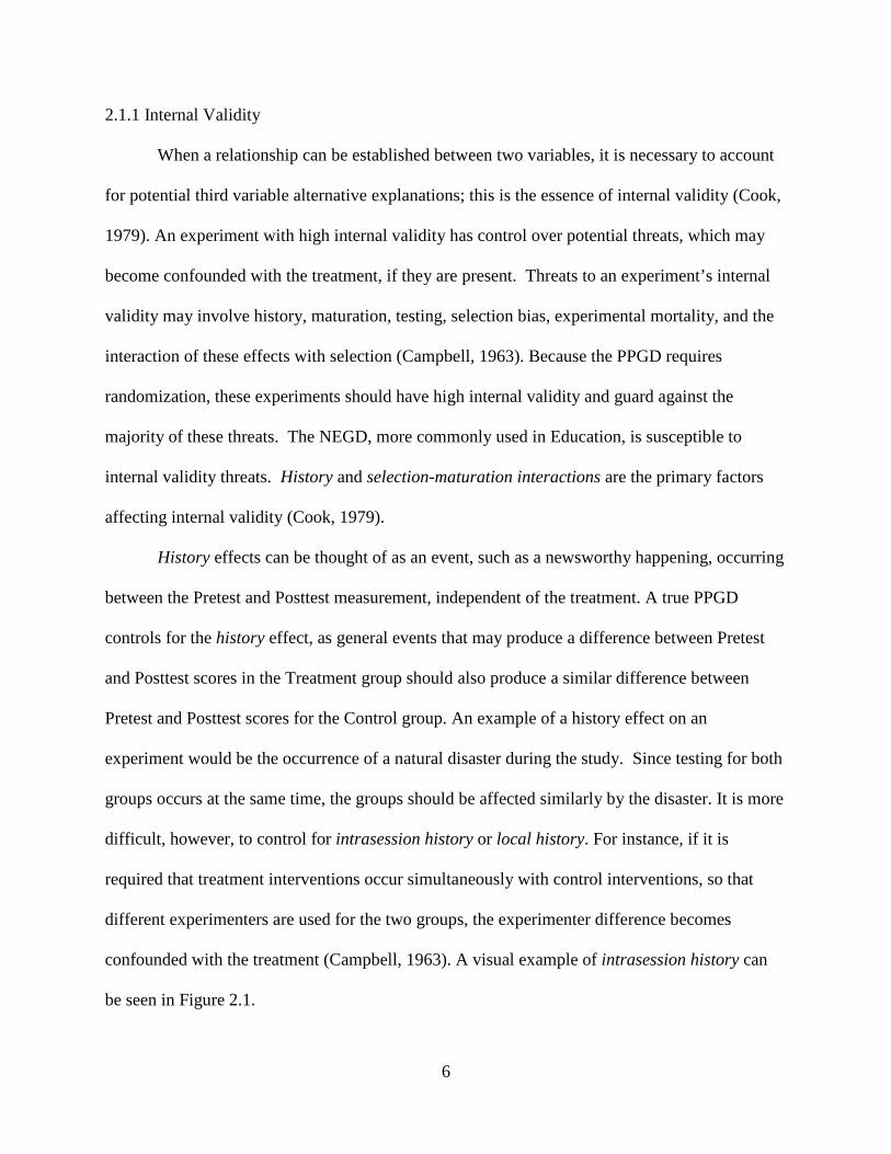
History effects can be thought of as an event, such as a newsworthy happening, occurring
between the Pretest and Posttest measurement, independent of the treatment. A true PPGD
controls for the history effect, as general events that may produce a difference between Pretest
and Posttest scores in the Treatment group should also produce a similar difference between
Pretest and Posttest scores for the Control group. An example of a history effect on an
experiment would be the occurrence of a natural disaster during the study. Since testing for both
groups occurs at the same time, the groups should be affected similarly by the disaster. It is more
difficult, however, to control for intrasession history or local history. For instance, if it is
required that treatment interventions occur simultaneously with control interventions, so that
different experimenters are used for the two groups, the experimenter difference becomes
confounded with the treatment (Campbell, 1963). A visual example of intrasession history can
be seen in Figure 2.1.
7
Maturation can be thought of as biological and psychological characteristics of subjects
that change during the experiment, thus affecting the Posttest scores (Dimitrov, 2003). While
maturation is generally accounted for in a PPGD, selection-maturation interaction may arise in
the NEGD case. For instance, in Education, where classes are a natural way to group, students
may mature at different rates during the experiment, resulting from the way that students were
assigned to classes, and not necessarily from the treatment. It is particularly common to see
differences in growth rates between treatment groups when subjects self-select themselves into
receiving a treatment (Cook, 1979). Changes in within-group variances between tests for both
Treatment and Control groups may indicate that maturation has occurred (an example of this can
be seen in Table 5.1). Additionally, if the change in score variances from Pretest to Posttest is

8
significantly different between the Control and Treatment groups, this may indicate that there is
a selection-maturation interaction.
When subjects are randomly assigned to treatment groups, each group experiences the
same testing conditions and the same patterns of global history, so that many of the threats to
internal validity may be ruled out. In NEGD studies, however, it is imperative that a researcher
examine the data and investigate how these threats may have possibly influenced the study.
Further, though randomization should makes causal inference easier, inequities may still exist
between groups. For the purpose of this thesis, it was assumed that administering a Pretest is a
reasonable way to measure prior differences between groups. This is a major assumption about
the validity of the Pretest; while the inclusion of a Pretest is one potential way to measure
differences between groups, it is not the only way. One may not conclude a causal relationship
exists until all threats to internal validity have been eliminated.
2.1.2 External Validity
The central idea behind sampling for research is to obtain a representative subset of the
population of interest, from which to estimate characteristics about the population. If the
sampling frame is not representative of its intended population, then an experiment’s external
validity is compromised. Often in experimentation, aspects of the environment may make the
exact experiment unreplicable. An experiment with high internal validity and high control over
experimental factors may actually reduce external validity; control factors may not be
reproducible in a natural setting. Sources of external invalidity stem from uncertainty as to
which factors truly interact with the treatment and which factors can be disregarded (Campbell,
1963). Factors that Campbell references as threats to external validity include interactions of the

9
treatment with: testing, selection bias, and reactive effects of experimental arrangements. If
these factors are confounded with the treatment, results of analysis will not be generalizable to
the population.
For the PPGD, the most likely threat to external validity is treatment and testing
interaction. An example of interaction of testing and treatment may be seen in attitude-change
studies. The introduction of a Pretest may redirect a subject’s focus or create changes in
behavior, influencing a subject’s response at Posttest. If the Pretest sensitizes the subjects to a
problem addressed within the Pretest, it may actually increase or decrease the effect of the
treatment (Campbell, 1963). If the effect of testing and treatment interaction occurs in the study,
the results may not necessarily be extended to the population as a whole, as the introduction of
Pretest itself changed behavior.
While the randomization of the PPGD controls for selection within a study, it does not
necessarily control for the interaction of the treatment and selection within a population. This
becomes more likely as it becomes increasingly difficult to recruit subjects for an experiment.
Say, for instance, there is resistance from particular groups or entities, such as schools in high
socio-economic neighborhoods, to being included in an experiment. If only schools in lower
socio-economic neighborhoods are willing to participate in the experiment, the results of that
experiment cannot necessarily be extended to the population of all schools, even if the
experiment is internally valid (Campbell, 1963).
A common source of non-representativeness in experimentation comes from reactive
arrangements. This is somewhat unavoidable for well-designed experiments. The threat of this
effect can come from artificial experimental settings (such as a laboratory), a subject’s awareness
that he or she is participating in an experiment, or any aspect of the experimental procedure. In

10
research on teaching methods, it may be easier to disguise aspects of experimentation, such as
including a Pretest or Posttest as part of the typical academic curriculum (Campbell, 1963). The
NEGD, though said to have generally weaker internal validity, may in some cases have greater
external validity, since it allows the assignment to treatment groups to occur naturally. This
reduces the reactive effects of experimental procedure and improves the overall external validity
of the design, relative to the randomized design (Dimitrov, 2003).

11
2.2 METHODS OF DATA ANALYSIS
The most appropriate method to analyze Pretest-Posttest data is highly debated.
According to Bonate (2000), a method sensitive to the validity of its assumptions may result in
inaccurate P-values and false conclusions, while a test with low power is likely to result in a
Type II error, with the researcher coming to no conclusions about a study. The ideal method for
analysis should maximize power, while minimizing the probability of a making a Type I error.
2.2.1 ANOVA Method
Ambiguity concerning how to analyze or interpret PPGD experiments is prevalent in the
literature. In general analyses for the difference between groups (where there isn’t necessarily a
Pretest score), analysis of variance (ANOVA, which is equivalent to the two-sample t-test if
there are only two groups) on Posttest scores is the most commonly used method. For NEGD,
this method may not be appropriate, due to possible violations of the assumptions needed for the
ANOVA approach to be correct. Bonate (2000) emphasizes the importance of utilizing the
Pretest data, although he notes the lack of consensus concerning the precise way in which such
Pretest information should be incorporated.
For both the t-test and ANOVA, a primary assumption is that the groups are statistically
equivalent at the baseline (i.e. the time at which the Pretest is conducted). Analyzing only the
Posttest data does not take into account within-subject variation. Analyses using only Posttest
data may provide insufficient power for detecting differences between groups; ignoring the
baseline information can potentially lead either to no conclusion or to an incorrect conclusion.
Further, even if the Pretest results are statistically equivalent (as they should be under PPGD),
applying the t-test or ANOVA to Posttest scores alone may not be the most powerful test for

12
detecting differences between treatment effects. Using Pretest information in the statistical
analysis of the Posttest measurements should account for differences between subjects, and
allows each subject to act as its own control. By including the Pretest data in the analysis, a
researcher can increase the probability of detecting a significant difference between groups,
thereby increasing the power of the statistical test.
2.2.2 Difference Method
One of the most commonly used methods in analyzing Pretest-Posttest data is the
difference method, or gain in scores. In this analysis, the data are simplified by transforming the
bivariate (Pretest, Posttest) into univariate via the relationship, Difference=Posttest–Pretest
(Equation 1, Table 2.1). The response variable is calculated as either Posttest minus Pretest, or
vice-versa, and ANOVA is performed on the differences. A major advantage of this method is
ease of interpretation of the transformed variable, either a net gain or loss in score (Bonate,
2000). This method also assumes that each subject’s score is independent of the other subjects’
scores.
Other methods involving transformations similar to the difference method have also been
used in analysis of Pretest-Posttest data. Normalized learning gains (Equation 2, Table 2.1) were
developed in Education to offset the effect of large learning gains; they attempt to compare
learning or gains fairly. For example, subjects who scored extremely low on the Pretest may
appear to gain more between testing sessions (Weber, 2005). For Pretest scorers near 100% of
the maximum possible score, these normalized learning gains may be exaggerated. Another
transformation is the relative change. Relative change transforms Pretest and Posttest scores into
a proportional change of the scores (Equation 3, Table 2.1). Relative change and normalized

13
learning gains may be analyzed in the same manner as the difference in score, but encounter
similar problems in analysis. A particular drawback of relative change scores is that they are
often not normally distributed (Bonate, 2000). The difference between scores is generally
preferred to these methods for its ease in interpretation. A fourth method, overcoming some of
the difficulties of both normalized learning gain and relative change, is the logit transform
(Equation 4, Table 2.1).
All four of these transformations assume that Pretest and Posttest scores are in the same
scale. Equations 2 and 4 further assume that Pretest and Posttest scores are expressed as %
correct on a 0 to 100 scale. Note that Equation 2's transform (nlg) becomes undefined if Pretest is
100%, while Equation 3's transform (relative change) becomes undefined if pretest is zero (or
0%). Equation 4's transform (logit) is undefined if either Pretest or Posttest is exactly 0% or
100%. In practice, one adjusts equations 2, 3, or 4, if necessary, so that undefined values don't
occur, typically by replacing zero scores by a value that is half-way between zero and the lowest
observed non-zero score, and similarly on the high end. Of course, if one finds that such
definability adjustments need to be made for more than a few subjects, this might be an
indication that the transform being contemplated is not appropriate for the data set under
consideration. In that sense, Equation 1's difference transform (which is always defined and is
easy to understand), might be preferable to others, but one shouldn't necessarily conclude that it
is always the best transformation to use.

14
Table 2.1 Transformation Equations for Posttest-Pretest Differences
Equation 1. Difference in Scores ���������� � �� �� � �� �� �
Equation 2. Normalized Learning Gains ��� � �� �� � �� �� �100% � �� �� �
Equation 3. Relative Change ���� ��� ������ � �� �� � �� �� ��� ��
Equation 4. Logit Transformation ���� � �� ��� �� �� �� � 100% � �� �� �
100% � �� �� ��
2.2.3 ANCOVA Method
The method that has received the most positive remarks in PPGD literature is the analysis
of covariance (ANCOVA), using Pretest as a covariate and Posttest as the response. In using the
Pretest scores as a covariate, ANCOVA treats the Pretest score as a source of variation
uncontrolled for in the experiment. ANCOVA is shown to be more powerful and more versatile
in situations where basic ANOVA assumptions, particularly randomization, are violated.
ANCOVA has all of the same functions as the Difference method; in fact, the Difference method
is actually a specific case of ANCOVA where the regression coefficient for Posttest scores onto
Pretest scores is set equal to one (Brogan, 1980). The general ANCOVA model, for the PPGD or
NEGD is:
�� �� � �� � �� � !��� "�� � � �# � �� �� � ����� For this model, I(Treatment) is an indicator variable. The indicator takes on values of
either ‘0’ or ‘1’ for Pretest-Posttest data with only one treatment. For this model, a value of ‘1’
15
indicates that a subject belongs to the Treatment group and ‘0’ that the subject belongs to the
Control group. In non-randomized designs, ANCOVA may be used to adjust for differences that
exist between groups at the Pretest, which is likely to occur with intact groups [if treatment
groups are formed naturally, for example, through self-selection or assignment of treatment to
existing groups (such as a classroom), prior differences unrelated to the treatment are more likely
to exist, than if subjects were randomized].The basic questions answered by ANCOVA and
ANOVA are similar. While ANOVA tests the overall effect of the treatment at Posttest,
ANCOVA tests the effect of the treatment for a specified score at Pretest. If the regression
coefficient for Posttest scores onto Pretest scores is close to 1.0, ANOVA for the difference in
scores will tend to produce similar results to ANCOVA. Since the ANCOVA requires loss of an
additional degree of freedom compared to ANOVA on the differences, ANOVA on the
differences will tend to be the more powerful test when the slope for Pretest is near one
(Dimitrov, 2003). If the slope is near zero, then simple ANOVA on the Posttest scores will be
more efficient than ANCOVA. If this slope is not near either zero or one, then ANCOVA is a
more powerful method for analysis than either ANOVA on Posttest scores (β2=0) or ANOVA on
differences (β2=1). Additionally, unlike the Difference method, which requires that Pretest and
Posttest scores be in the same units, the ANCOVA method does not require that covariates (in
this case, Pretest) be in the same units as the response (Posttest) (Bonate, 2000).
Though ANCOVA has received much positive acknowledgment from researchers for
analysis of Pretest-Posttest data, it has a few shortcomings. ANCOVA assumes that the slopes
are equal for the Treatment and the Control group (i.e. that the linear relationship between
Pretest and Posttest scores is the same for both groups). This assumption is often violated in
practice. For self-selecting treatment groups, ANCOVA may result in biased treatment effects.

16
When groups are self-selected, estimation of the true treatment effect cannot necessarily be
separated from an individuals’ preference for that particular method. An example of this occurs
when groups have similar Pretest scores, but the two groups mature at different rates over time.
Say, for instance, eighth grade students had the option of taking college preparatory (Control) or
honors (Treatment) courses in high school, and also take a middle school exit exam (Pretest).
Say, then, that the mean Pretest scores are the same for students who took college prep and
honors courses. Assume further that the students take a high school exit exam (Posttest), and the
mean score for the honors students is higher. Here, the treatment cannot necessarily be separated
from the fact that the honors students (or their parents) desired more challenges, and thus may
have responded differently to their high school education, compared to their college prep
classmates.

17
2.2.4 Repeated Measures Method (Mixed Model)
Repeated Measures ANOVA has become very popular in research for PPGD. This design
is also referred to as a Split-Plot analysis (Agricultural origin), within-subjects ANOVA, or
treatment-by-subjects ANOVA (Vogt, 1999). For this design, an experimental unit is one
subject, where each subject is treated as a block, and measurements are taken repeatedly (in
Pretest-Posttest Design, only twice). For a Repeated Measures design with ‘I’ between-subjects
effects (treatment types), the linear model is:
$����%&' � (� � )% � !&%� � �' � )�%' � �%&' The variable, Score represents the score for the i th treatment, the j th subject and the kth trial
for:
i=1,2,..., I (Treatment Groups)
j=1,2,..., ni (Subjects in Group i)
k=1,2. ..., K (Trials, or Time-points at which each subject is measured)
where
µ0 is the baseline score
αi is the treatment or main effect, a fixed effect,
Tj(i) is the subject effect nested within treatment, a random effect,
βk is the time effect, a fixed effect,
αβik is the treatment x time interaction
and eijk is the error corresponding to the score for the kth test taken by subject j in group i ,
which remains unexplained by the other terms within the model.

18
For the PPGD, the within-subjects effect can have only two levels (K = 2), either Pretest
or Posttest. The number of groups, I, is usually small; I=2 in the most common case where there
is one Control and one Treatment group. The number of subjects within a group, ni, depends on
the experiment; more power accrues as ni becomes large. Although it is not necessary for n1 = n2
= ... = nI =J, most researchers attempt to keep the ni relatively balanced in order to maximize
power. The summary table for Repeated Measures Analysis provides three F-tests: a main effect
for the Groups, a main effect for Time or Trial, and an effect for the Groups-by-Time interaction.
See Table 2.2 below for the general format in the case of complete balance, where N=I*J*K
represents the total number of scores observed in the data set. This last test (Groups-by-Time
interaction) is the one of primary interest when using Repeated Measures Analysis on PPGD.
Table 2.2 Repeated Measures ANOVA Table
Effect Numerator DF Denom. DF F Value
Group � 1 * + � 1� ,$-/,$/0
Time 1 � 1 * + � 1� * 1 � 1� ,$!/,$/2
Group*Time � 1�1 � 1� * + � 1� * 1 � 1� ,$!-/,$/0*2
If applied naively, Repeated Measures ANOVA is misleading because the between-
subjects main effect (Group effect) F is too small (Huck, 1975). While Huck makes valid points
about potential misinterpretations of the fixed effects, the F value being too small may be a
specific case where it is assumed there is little difference between groups at the Pretest, and a
significant difference at Posttest. Repeated Measures ANOVA has also been criticized, as its
linear model assumes that randomization and treatment intervention occurs prior to the Pretest;
19
in reality the treatment affects only the Posttest. Repeated Measures Analysis may therefore
result in biased estimation of the treatment effect. Because the model assumes that treatment
occurs at the Pretest, the actual treatment effect is “spread across” the Pretest and the Posttest in
computation for the main effect (Huck, 1975). Similarly, the Time effect is the average of
Posttest-Pretest improvement over the two groups, and may not be easily interpretable when
these two improvements are dissimilar. Dimitrov (2003) also notes that using the F value from
the between subjects factor (Treatment) would be a common mistake. Using the F-test for the
main effect of Treatment can be too conservative and increase the probability of making a Type
II error, though this too may be a special case. The F-test for the Group-by-Time interaction,
however, is an unbiased estimate of the treatment effect (Brogan, 1980).
For Repeated Measures ANOVA, the assumptions are similar to typical ANOVA, but it
requires more assumptions than other suggested methods. One additional assumption concerns
the structure of the Variance-Covariance matrix for observations on the same individual. The
classical assumption is that the error terms are assumed to be independently and identically
distributed (iid), and have the same variance for both the Pretest and Posttest scores (Kutner,
2005). Furthermore, it is assumed that the Pretest and Posttest Variance-Covariance matrix is the
same for both (or all) treatment groups. While sphericity (which assumes the correlations across
repeated measures are the same) is an assumption necessary for Repeated Measures ANOVA, it
is not relevant to the PPGD since there is only one pair of measurements (i.e. the Variance-
Covariance matrix is 2*2).
Additional criticisms have arisen from the use of Repeated Measures ANOVA for the
Pretest-Posttest design. Other methods of analysis provide the same results, but are less
complicated. The F-statistic for single-factor repeated measures with only two treatments is

20
equivalent to a two-sided t-test for paired observations (Kutner, 2005). The F-statistic for the
Time (trials) does not necessarily reveal anything about the treatments; since the scores are
averaged across groups, it indicates only that scores, on average, changed from Pretest to
Posttest.
Repeated Measures ANOVA, as it has been referenced in PPGD literature, is a special
form of the Mixed Model which assumes the Variance-Covariance matrix has compound
symmetry, or that the variance for the Pretest is equal to that of the Posttest. The F-test for the
Group-by-Time interaction of Repeated Measures ANOVA and the F-test of an analysis of
difference scores will always be the same, as a result of this assumption (Brogan, 1980).
Deviations from the compound symmetry assumption are less examined in PPGD
literature. Mixed Models may, however, prove to be useful for analysis in situations where the
variances differ between Pretest and Posttest. A benefit of the Mixed Model is that the variance
structure of this method can be altered. Of course, for a 2*2 Variance-Covariance matrix, there
are only three possible parameters [VAR(Pre), Var(Post), and COV(Pre,Post) =
ρ*SD(Pre)*SD(Post)], and the compound symmetry assumption reduces this to two by requiring
that the Pretest and Posttest variances be equal. If the additional parameters do not dramatically
improve the model’s estimate of the treatment effect, it may be better to make the simpler
compound-symmetry assumption of the classical repeated measures design. On the other hand, it
may be the case that an even more complex structure, such as separate variance-covariance
matrices for each group (requiring up to I*K*(K+1)/2 Variance-Covariance parameters in the
most general case) may be needed. This goes beyond the level of complexity desired for this
thesis, but such complex structure might be needed for proper analysis of some Pretest-Posttest
designs.

21
CHAPTER 3
THE DATA SETS
Four different data sets were analyzed for the purpose of comparing the methods of
analysis. Each set involves one Pretest score and one Posttest score (only two within-subject
measurements; K=2). Each set also has one Control group and one Treatment group (I=2), used
in its final analysis. The sampling frame, for each data set, was taken from an academic setting;
all subjects were enrolled in a graduate or undergraduate program at a university at the time of
study. Two data sets are NEGDs, lacking randomization in one form or another; two are
completely randomized, or PPGDs.
The Nursing (PPGD) data are from an assessment of junior-year undergraduate Nursing
students of the Medical College of Georgia. There were 33 total students, combined from two
separate campuses. The 33 students took an assessment, called the Self-Directed Learning
Readiness Scale (SDLRS or Learning Preference Assessment, LPA), which is intended to
measure an individual’s readiness to manage his or her own learning. The assessment was given
to all 33 students in order to obtain Pretest scores, and then 16 students were randomly selected
to receive an “intervention”, which consisted of watching an online self-directed learning
module. These 16 individuals became the Treatment group; the remaining 17 students who
received no intervention were considered the Control group. The 33 students were given the
same assessment (the Posttest) again after the “intervention”.

22
The ICA data set is an NEGD that involves an assessment called Intercultural
Communication Apprehension (ICA). The ICA was intended to measure, over time, students’
fears and attitudes of other cultures. All students who participated in the study were enrolled in a
Global Design course at UGA. The students self-selected themselves into treatment groups (the
non-equivalent component), students who studied abroad (Treatment) and those who did not
(Control). There were three levels of treatment for this study, as study abroad was segmented
into two groups based on the duration of travel (Short or Long). For purposes of comparability,
and after preliminary analyses indicated no differences between them, the 'Short' and 'Long'
groups were combined into one 'Treatment' group, so that the analysis of the ICA data set in
Chapter 5 uses I=2 groups. The Control group consisted of students that did not choose to travel.
The Pretests were given to all students at the beginning of the Global Design course. The
Posttests were given after students had completed the course (for those in the Control group) and
studied abroad (if they belonged to the Short or Long Treatment groups). The data originally
consisted of 145 records [111 students who did not study abroad, 15 students who studied abroad
for an extended period (Long), and 29 students who studied abroad for a shorter period (Short)].
Seventeen of these students had incomplete records for either the Pretest or the Posttest. These
seventeen students’ records were removed from the data set, so that final data for ICA
assessment contains 128 records (87 students for Control, 15 students for Long, and 26 students
for Short).
The Econ (NEGD) data set contains records for 200 students (subjects) enrolled in an
Introductory Economics course at a large state university. The 200 students took a lecture-style
class together, with a co-requisite lab. Two different teaching methods were used for the lab
classes: a new more statistical teaching method (Treatment), and the traditional teaching method

23
(Control). The 200 students were divided into eight different lab classes (25 in each), which were
taught by four Teaching Assistants (TAs). Each TA was assigned one Treatment lab and one
Control lab to prevent the confounding of method with lab instructor, so the final Econ data set
consists of records for 100 students each in Control and Treatment groups. Students chose the
lab section to which lab section they were assigned (the non-equivalent component), although
they did not know at the time of selection which type of lab they had chosen. All students took a
Pretest at the beginning of the semester, and prior to any lab instruction. The Pretest was
actually a copy of the previous year’s final exam, so the scores on this Pretest tended to be rather
low (mean score = 30% correct). The Posttest exam was the course's actual final exam, different
from the Pretest. The data set for the study contains, for each student, the teaching method
received, the Pretest score, and the Posttest score. Additional demographic information about the
students or which of the four TAs instructed them is not available in the data set. The primary
objective of this study is to determine if the newer, more statistical method (Treatment) is more
effective than the traditional (Control) method, for helping students to learn Introductory
Economics.
The final data set examined in this thesis is an example from Bonate (2000) and is
referred to as the Sexual Harassment Inventory (SHI) data set (PPGD). The study was intended
to measure male college students’ attitudes toward sexual harassment. The researchers tested 96
college freshmen at a Midwestern university. After the Pretest, students were randomized into
one of three treatment groups: Educational Literature, Video, or Control. For each group,
students reviewed literature on sexual harassment, watched a video on sexual harassment, or
were given a “neutral control task involving attitudes toward male and female names” (Bonate,
2000, p. 64), respectively. Students’ attitudes toward sexual harassment were tested again (using
24
the same SHI instrument), one week after intervention (Posttest). Higher scores on the
assessments indicate higher sensitivity toward sexual harassment. As with the ICA study, the
SHI study originally contained I=3 treatment groups (30 subjects in Control, 33 in the
Educational Literature Group, and 33 in the Video group), but the latter two groups are
combined to form the Treatment group used in the analysis performed in Chapter 5. The goal of
this study is to determine if the students in the Treatment group improved their SHI scores
significantly more than the students in the Control group did.
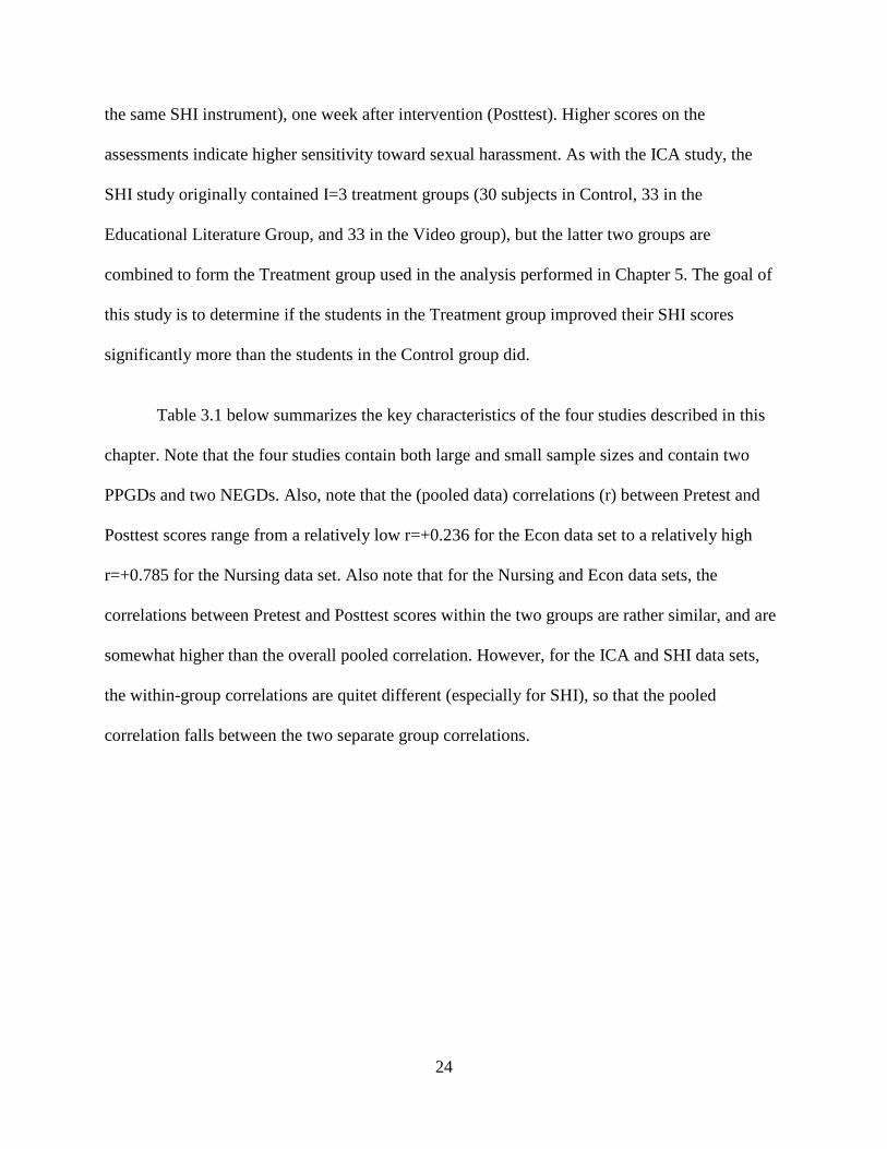
Table 3.1 below summarizes the key characteristics of the four studies described in this
chapter. Note that the four studies contain both large and small sample sizes and contain two
PPGDs and two NEGDs. Also, note that the (pooled data) correlations (r) between Pretest and
Posttest scores range from a relatively low r=+0.236 for the Econ data set to a relatively high
r=+0.785 for the Nursing data set. Also note that for the Nursing and Econ data sets, the
correlations between Pretest and Posttest scores within the two groups are rather similar, and are
somewhat higher than the overall pooled correlation. However, for the ICA and SHI data sets,
the within-group correlations are quitet different (especially for SHI), so that the pooled
correlation falls between the two separate group correlations.
25
Table 3.1 Summary of Characteristics of Four Data Sets Study Name N ncontrol ntreatment Design r
(pre/post) rC
(pre/post) rT
(pre/post)
1 Nursing 33 17 16 PPGD 0.785 0.816 0.825
2 ICA 128 87 41 NEGD 0.531 0.497 0.703
3 Econ 200 100 100 NEGD 0.236 0.389 0.397
4 SHI 96 30 66 PPGD 0.430 0.908 0.216

26
CHAPTER 4
METHODS
A goal of this thesis is to determine which methods of analyses are optimal for PPGDs
and NEGDs under different scenarios.hoped The two fundamental models used for analysis are
the General Linear Model (GLM) and the Mixed Model. Note that all analyses were performed
using SAS 9.2 and 9.3.
The GLM may be written in matrix notation as:
3 � 4� � �
Where Y and e are (n*1) vectors, β is an ((k+1)*1) vector, X is a (n * (k+1)) matrix. Here, ‘k’ is
the number of predictor variables and ‘n’ is the number of observations. For the PPGD, Y
represents a vector of Posttest scores, X is the design matrix, β is a vector containing the
parameter estimates for the linear model, and e is the random error that remains unexplained by
the model.
The data sets were modeled using six different parameterizations or combinations of
explanatory variables. The general linear models used for analyses (in terms of the i th individual)
are displayed in Table 4.1 below.

27
Table 4.1
The General Linear Model for Predicting Posttest scores
MODEL EQUATION
Null 3% � �� � �%
Regression 3% � �� � �#4#% � �%
ANOVA * 3% � �� � ��4�% � �#4#% � �%
DIFF* 3% � �� � ��4�% � �#4#% � �%
ANCOVA* 3% � �� � ��4�% � �#4#% � �%
Full (Interaction) 3% � �� � ��4�% � �#4#% � �54�%4#% � �%
*Note. For the ANOVA Model, B2=0 by definition; For the DIFFERENCE Model, B2=1 by definition.
Where Yi is the Posttest score for the i th individual,
β0 is the intercept or baseline,
β1 is the estimate for the treatment effect,
β2 is the slope estimate for Pretest scores,
β3 is the estimate for the interaction of Pretest score with the treatment,
X1i is an indicator for group (1 if subject ‘i’ belongs to Treatment, 0 if Control).
X2i is the Pretest score for the i th individual,
and e is the random error (assumed i.i.d., with mean 0 and unknown but constant variance
σ2).
For the Null model, the mean Posttest score, for all subjects, is used to predict all Posttest
scores, without using any other information (β70 is the mean Posttest score). The Regression
model utilizes Pretest as an explanatory variable for predicting Posttest scores. The ANOVA
model is equivalent to a 2-sample t-test, and attempts to predict Posttest scores from group

28
membership. The DIFF model uses treatment type to explain changes in score from Pretest to
Posttest, and is equivalent to the model where the response variable is the change in score
(Difference=Posttest – Pretest).
The ANCOVA model utilizes both treatment type and Pretest scores as explanatory
variables for predicting Posttest scores. The ANOVA model and DIFF model are actually special
cases of the ANCOVA model. For the ANOVA model, the value for the Pretest coefficient (β2)
is ‘0’; for the DIFF model, the value for β2 is ‘1’. The Full(Interaction) model is a further
extension of the ANCOVA model, where there is an additional term for the interaction of Pretest
score and Treatment, if such an interaction exists. If the interaction effect for Pretest and
Treatment is significant, the predictor variables are dependent upon one another. In other words,
an interaction would indicate for the PPGD that the effect of the treatment is dependent upon
how a subject scored on the Pretest. Unlike the ANCOVA model, the treatment effect is not
constant across groups; an estimate for the treatment effect cannot be isolated without
considering Pretest.
To construct these models, each was run individually using SAS’s PROC REG with
requests for ‘Solutions’, ‘AIC’, and ‘BIC’ (called 'SBC' within SAS's PROC REG). Since
Treatment is a dichotomous variable for each data set, an indicator variable (IT) was created for
each (‘1’ for a subject belonging to the Treatment group, ‘0’ for a subject in the Control group).
To compare the results of these linear models, Posttest scores were regressed onto the selected
explanatory variables (if any). Although the response variable for the DIFF model is (Difference
= Posttest – Pretest), the DIFF model was regressed using Posttest as the response variable, with
a restriction placed on the parameter estimate for Pretest such that the β2 parameter was set equal
to one. This ensured that the fit statistics and parameter estimates for the six General Linear

29
Models, shown in Table 4.1, were directly comparable. The best model was selected using AIC
or BIC. While R-square and RMSE are important considerations, one must remember that when
comparing two hierarchical models with different numbers of parameters, R-square will always
be larger for the more complex model (and RMSE will typically be smaller), so neither of these
two are useful model selection criteria. It should also be noted that these tests are being
performed at a nominal 0.05 level, as if the test/model under examination were the only one
which the researcher were considering. If, in fact, a researcher were considering many possible
models before selecting one under which to conduct the analyses of interest, then, of course, the
researcher would need to make some sort of suitable adjustment for multiple tests being
conducted.
A Mixed Model was analyzed separately for each data set, as well. In the PPGD
literature, the particular Mixed Model used is more commonly referred to as Repeated Measures
ANOVA. A benefit of analyzing the data sets using the Mixed Model is that this formulation
allows the repeated measures on the same individual to exhibit correlation, rather than assuming
that they are independent of one another. Also, the Variance-Covariance structure can be
changed, so that the Pretest and Posttest variances need not be assumed to be constant. Parameter
estimates for the covariance are what distinguish the Mixed Model from the GLM. When
analyzing each data set, each subject was treated as one cluster, with two observations per cluster
(Pretest and Posttest).
The general notation for the mixed model in matrix form is:
3 � 4� � 89 � � ,
where Y is a vector of observed scores,
� is a vector of fixed-effects parameters,

30
X is the design matrix of fixed factors,
9 is a vector of random-effects parameters,
Z is the design matrix of random factors,
and e is a vector of residual errors (whose elements need not necessarily be homogenous
nor independent).
The Mixed Model analysis for each data set was run using SAS’s PROC MIXED. For
each analysis, the response variable was ‘Score’, and the fixed effects tested for were Group
(Control or Treatment), Time (Pretest or Posttest), and Group*Time. The PROC MIXED
RANDOM statement (with intercept) was used to determine estimates for the γ vector. The
estimates for the Variance-Covariance parameters were computed via Restricted Maximum
Likelihood (REML), the denominator degrees freedom specified were estimated via the
Kenward-Roger procedure, and the subject effect specified was subject, within group. SAS’s
default Variance-Covariance structure was used, which assumes the Pretest and Posttest variance
are equal. The same procedures and same specifications were used for each data set.
SAS’s LS means, for all Group-by-Time effects, were requested for each analysis, with
P-values for all pairs of differences specified as an option [(PDIFF = “pairs of differences”). For
an example, see Table 5.4 of the Nursing Data Set]. This provided estimates for the difference in
scores at all possible levels of Group and Time, along with the corresponding P-values. The
‘Estimate’ coefficient shown in these tables is such that Group=’C’ and/or Time=’Pretest’ is
used as the baseline, so that the estimates are for the expected change in score from Pretest to
Posttest or from Control to Treatment (or both, if applicable). For an example, see Table Table
5.16 of the Econ data set.

31
Since the Mixed Model and the GLM have different parameterizations, SAS’s LS Means
option was used to compare the results of the two analyses directly. Joint tables were created to
show the relationship between the SAS LS Mean estimates (actually a Maximum Likelihood
estimate) for the Mixed Model, and LS mean estimates from the GLM. Only the LS means for
the best fit GLM were computed (where 'best' was determined by finding the GLM with the
lowest AIC or BIC). The LS means estimates for the GLM were computed using two different
specifications. The first estimate was found specifying BY LEVEL, which uses the conditional
mean for each group, at Pretest, in the linear model, for the Posttest estimates (for an example,
see Table 5.17). The second estimate used SAS’s default mean, which is the overall Pretest mean
(for an example, see Table 5.18). Standard errors and P-values were requested for both of these
methods.
32
CHAPTER 5
THE ANALYSES
5.1 THE NURSING DATA SET
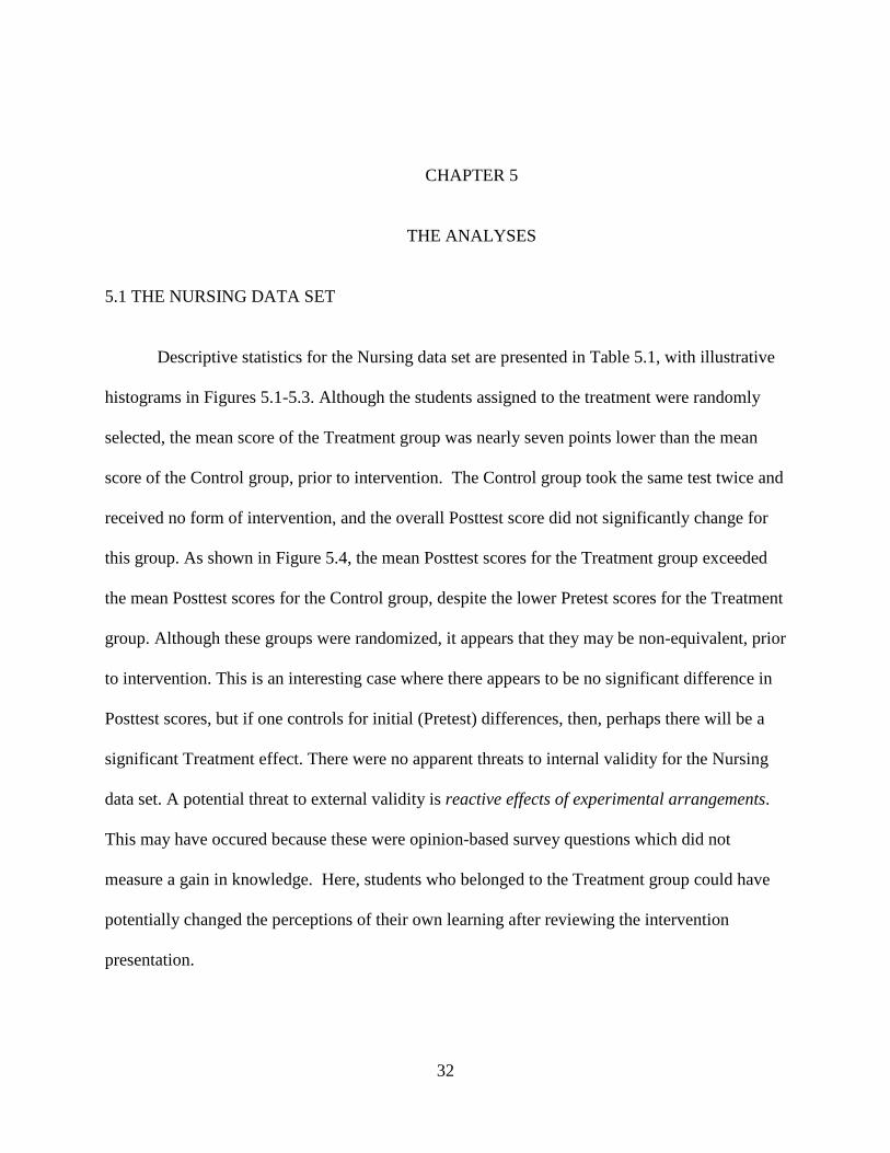
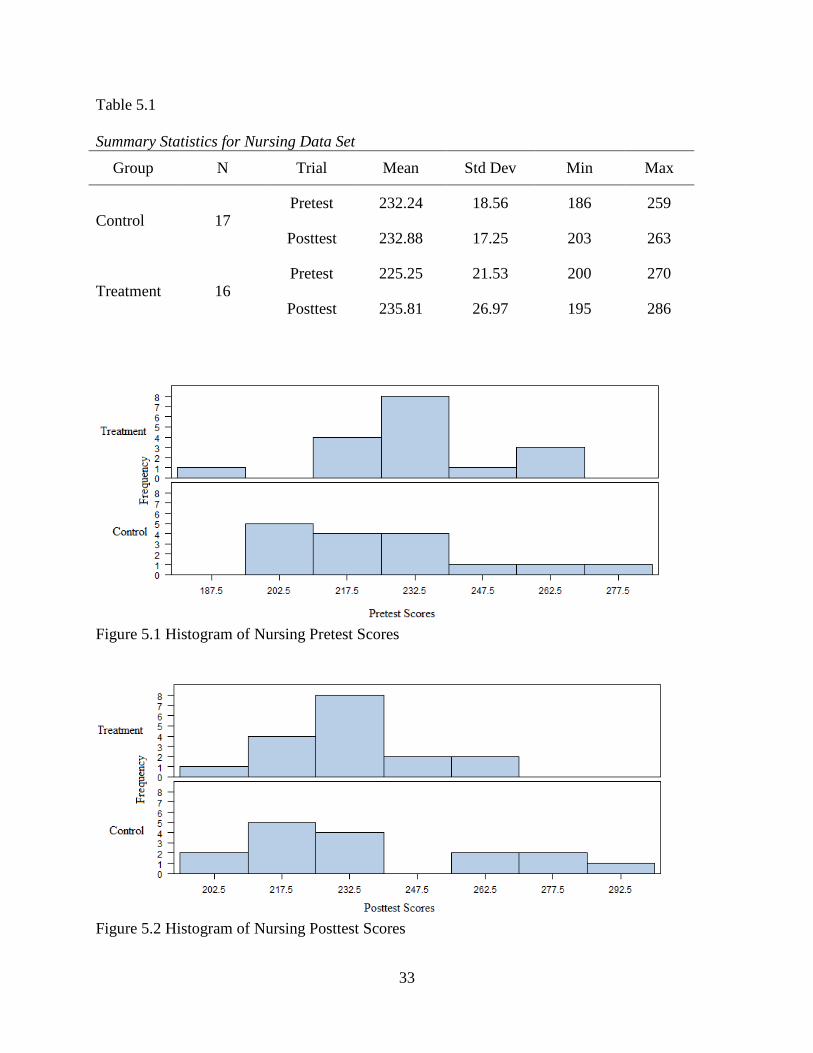
Descriptive statistics for the Nursing data set are presented in Table 5.1, with illustrative
histograms in Figures 5.1-5.3. Although the students assigned to the treatment were randomly
selected, the mean score of the Treatment group was nearly seven points lower than the mean
score of the Control group, prior to intervention. The Control group took the same test twice and
received no form of intervention, and the overall Posttest score did not significantly change for
this group. As shown in Figure 5.4, the mean Posttest scores for the Treatment group exceeded
the mean Posttest scores for the Control group, despite the lower Pretest scores for the Treatment
group. Although these groups were randomized, it appears that they may be non-equivalent, prior
to intervention. This is an interesting case where there appears to be no significant difference in
Posttest scores, but if one controls for initial (Pretest) differences, then, perhaps there will be a
significant Treatment effect. There were no apparent threats to internal validity for the Nursing
data set. A potential threat to external validity is reactive effects of experimental arrangements.
This may have occured because these were opinion-based survey questions which did not
measure a gain in knowledge. Here, students who belonged to the Treatment group could have
potentially changed the perceptions of their own learning after reviewing the intervention
presentation.
33
Table 5.1 Summary Statistics for Nursing Data Set
Group N Trial Mean Std Dev Min Max
Control 17 Pretest 232.24 18.56 186 259
Posttest 232.88 17.25 203 263
Treatment 16 Pretest 225.25 21.53 200 270
Posttest 235.81 26.97 195 286
Figure 5.1 Histogram of Nursing Pretest Scores
Figure 5.2 Histogram of Nursing Posttest Scores
34
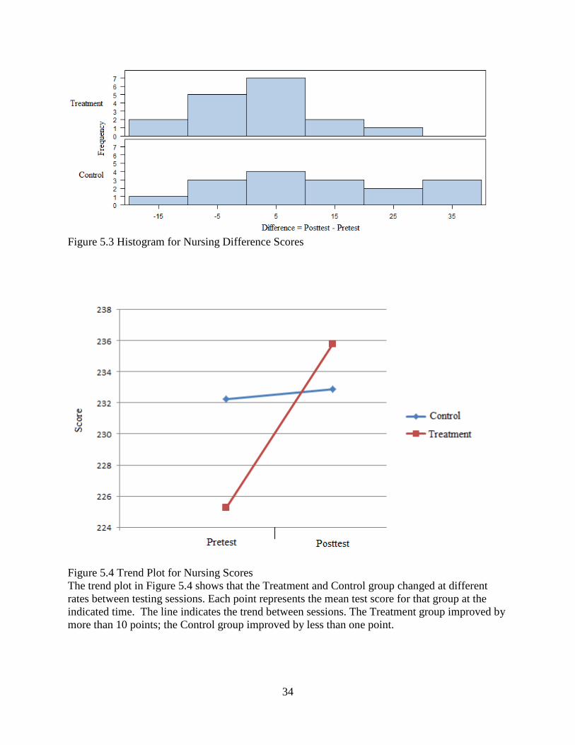
Figure 5.3 Histogram for Nursing Difference Scores
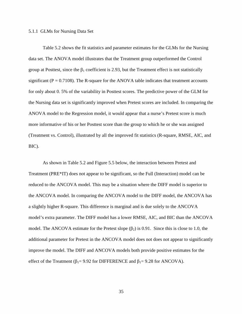
Figure 5.4 Trend Plot for Nursing Scores The trend plot in Figure 5.4 shows that the Treatment and Control group changed at different rates between testing sessions. Each point represents the mean test score for that group at the indicated time. The line indicates the trend between sessions. The Treatment group improved by more than 10 points; the Control group improved by less than one point.
35
5.1.1 GLMs for Nursing Data Set
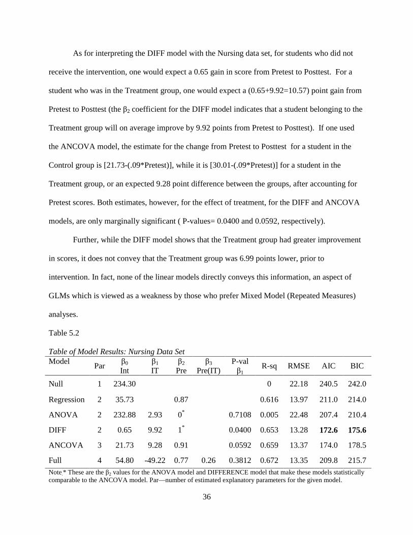
Table 5.2 shows the fit statistics and parameter estimates for the GLMs for the Nursing
data set. The ANOVA model illustrates that the Treatment group outperformed the Control
group at Posttest, since the β1 coefficient is 2.93, but the Treatment effect is not statistically
significant (P = 0.7108). The R-square for the ANOVA table indicates that treatment accounts
for only about 0. 5% of the variability in Posttest scores. The predictive power of the GLM for
the Nursing data set is significantly improved when Pretest scores are included. In comparing the
ANOVA model to the Regression model, it would appear that a nurse’s Pretest score is much
more informative of his or her Posttest score than the group to which he or she was assigned
(Treatment vs. Control), illustrated by all the improved fit statistics (R-square, RMSE, AIC, and
BIC).
As shown in Table 5.2 and Figure 5.5 below, the interaction between Pretest and
Treatment (PRE*IT) does not appear to be significant, so the Full (Interaction) model can be
reduced to the ANCOVA model. This may be a situation where the DIFF model is superior to
the ANCOVA model. In comparing the ANCOVA model to the DIFF model, the ANCOVA has
a slightly higher R-square. This difference is marginal and is due solely to the ANCOVA
model’s extra parameter. The DIFF model has a lower RMSE, AIC, and BIC than the ANCOVA
model. The ANCOVA estimate for the Pretest slope (β2) is 0.91. Since this is close to 1.0, the
additional parameter for Pretest in the ANCOVA model does not does not appear to significantly
improve the model. The DIFF and ANCOVA models both provide positive estimates for the
effect of the Treatment (β1= 9.92 for DIFFERENCE and β1= 9.28 for ANCOVA).
36
As for interpreting the DIFF model with the Nursing data set, for students who did not
receive the intervention, one would expect a 0.65 gain in score from Pretest to Posttest. For a
student who was in the Treatment group, one would expect a (0.65+9.92=10.57) point gain from
Pretest to Posttest (the β2 coefficient for the DIFF model indicates that a student belonging to the
Treatment group will on average improve by 9.92 points from Pretest to Posttest). If one used
the ANCOVA model, the estimate for the change from Pretest to Posttest for a student in the
Control group is [21.73-(.09*Pretest)], while it is [30.01-(.09*Pretest)] for a student in the
Treatment group, or an expected 9.28 point difference between the groups, after accounting for
Pretest scores. Both estimates, however, for the effect of treatment, for the DIFF and ANCOVA
models, are only marginally significant ( P-values= 0.0400 and 0.0592, respectively).
Further, while the DIFF model shows that the Treatment group had greater improvement
in scores, it does not convey that the Treatment group was 6.99 points lower, prior to
intervention. In fact, none of the linear models directly conveys this information, an aspect of
GLMs which is viewed as a weakness by those who prefer Mixed Model (Repeated Measures)
analyses.
Table 5.2 Table of Model Results: Nursing Data Set Model
Par β0 Int
β1
IT β2
Pre β3
Pre(IT) P-val β1
R-sq RMSE AIC BIC
Null 1 234.30 0 22.18 240.5 242.0
Regression 2 35.73 0.87 0.616 13.97 211.0 214.0
ANOVA 2 232.88 2.93 0* 0.7108 0.005 22.48 207.4 210.4
DIFF 2 0.65 9.92 1* 0.0400 0.653 13.28 172.6 175.6
ANCOVA 3 21.73 9.28 0.91 0.0592 0.659 13.37 174.0 178.5
Full 4 54.80 -49.22 0.77 0.26 0.3812 0.672 13.35 209.8 215.7
Note.* These are the β2 values for the ANOVA model and DIFFERENCE model that make these models statistically comparable to the ANCOVA model. Par—number of estimated explanatory parameters for the given model.
37
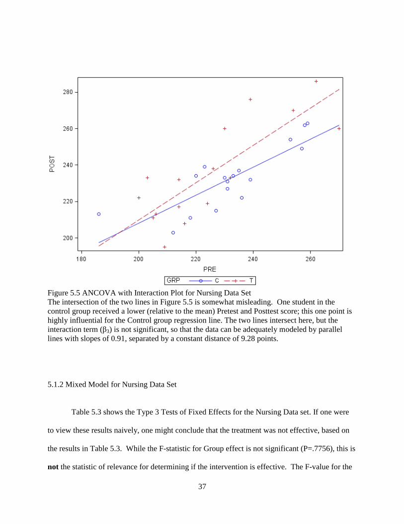
Figure 5.5 ANCOVA with Interaction Plot for Nursing Data Set The intersection of the two lines in Figure 5.5 is somewhat misleading. One student in the control group received a lower (relative to the mean) Pretest and Posttest score; this one point is highly influential for the Control group regression line. The two lines intersect here, but the interaction term (β3) is not significant, so that the data can be adequately modeled by parallel lines with slopes of 0.91, separated by a constant distance of 9.28 points.
5.1.2 Mixed Model for Nursing Data Set
Table 5.3 shows the Type 3 Tests of Fixed Effects for the Nursing Data set. If one were
to view these results naively, one might conclude that the treatment was not effective, based on
the results in Table 5.3. While the F-statistic for Group effect is not significant (P=.7756), this is
not the statistic of relevance for determining if the intervention is effective. The F-value for the

38
interaction of Group-by-Time indicates that the change in score from Pretest to Posttest is
marginally significantly different (P=0.0400) between the Treatment group and the Control
group. As is always the case with P-values based on an F-statistic, the F-statistic alone does not
indicate the direction of the difference, although the afore-mentioned equivalence between the
test of the Group-by-Time effect under the Mixed Model (see Table 5.3) and the test for
Treatment effect in the DIFF model (see Table 5.2) does show that it is the Treatment group
which improves significantly more than the Control group The F-value for Time is also
significant (P=.0214), which indicates that the overall change in scores (when averaged over
Group) is significantly different from 0 over the time period from Pretest to Posttest.
This data set is somewhat unusual in that the groups were randomized (PPGD), and the
Pretest scores are not significantly different from one another (P=.3528 from row 3 of Table 5.4),
but if the Pretest scores are ignored (as the ANOVA model assumes), no significant effect due to
Treatment is found (P=.7108). On the other hand, if Posttest-Pretest differences are used (either
directly or through the Mixed Model), a marginally significant Treatment effect is found. The
ANCOVA model shows that the DIFF model perhaps slightly overstates the effect of Pretest
score (β2=0.91 vs. β2=1.00), but it (ANCOVA) still estimates a Treatment effect of +9.28 points,
which is not quite significant at the 5% level (P=.0592). Overall, it appears that this is a case
where, even though PPGD was used, examination via ANCOVA, ANOVA on differences (i.e.
DIFF model), or Mixed Models all find borderline significant results which would not have been
apparent in the absence of Pretest information.
39
Table 5.3 Type 3 Tests of Fixed Effects for Nursing Data Set
Effect Numerator DF Denom. DF F Value Pr > F
Group 1 31 0.08 0.7756
Time 1 31 5.87 0.0214
Group*Time 1 31 4.59 0.0400
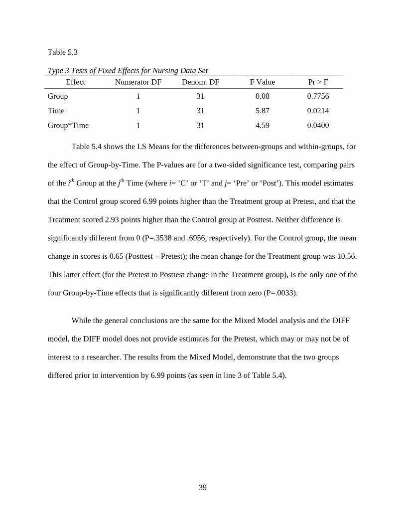
Table 5.4 shows the LS Means for the differences between-groups and within-groups, for
the effect of Group-by-Time. The P-values are for a two-sided significance test, comparing pairs
of the i th Group at the j th Time (where i= ‘C’ or ‘T’ and j= ‘Pre’ or ‘Post’). This model estimates
that the Control group scored 6.99 points higher than the Treatment group at Pretest, and that the
Treatment scored 2.93 points higher than the Control group at Posttest. Neither difference is
significantly different from 0 (P=.3538 and .6956, respectively). For the Control group, the mean
change in scores is 0.65 (Posttest – Pretest); the mean change for the Treatment group was 10.56.
This latter effect (for the Pretest to Posttest change in the Treatment group), is the only one of the
four Group-by-Time effects that is significantly different from zero (P=.0033).
While the general conclusions are the same for the Mixed Model analysis and the DIFF
model, the DIFF model does not provide estimates for the Pretest, which may or may not be of
interest to a researcher. The results from the Mixed Model, demonstrate that the two groups
differed prior to intervention by 6.99 points (as seen in line 3 of Table 5.4).
40
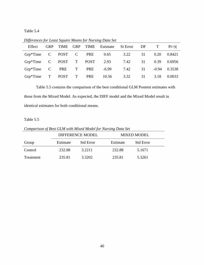
Table 5.4 Differences for Least Square Means for Nursing Data Set
Effect GRP TIME GRP TIME Estimate St Error DF T Pr>|t|
Grp*Time C POST C PRE 0.65 3.22 31 0.20 0.8421
Grp*Time C POST T POST 2.93 7.42 31 0.39 0.6956
Grp*Time C PRE T PRE -6.99 7.42 31 -0.94 0.3538
Grp*Time T POST T PRE 10.56 3.32 31 3.18 0.0033
Table 5.5 contains the comparison of the best conditional GLM Postetst estimates with
those from the Mixed Model. As expected, the DIFF model and the Mixed Model result in
identical estimates for both conditional means.
Table 5.5 Comparison of Best GLM with Mixed Model for Nursing Data Set
DIFFERENCE MODEL MIXED MODEL
Group Estimate Std Error Estimate Std Error
Control 232.88 3.2211 232.88 5.1671
Treatment 235.81 3.3202 235.81 5.3261

41
5.2 THE ICA DATA SET
Table 5.6 shows the academic year in which students traveled abroad and took the ICA
assessment. This table illustrates there is a potential threat to internal validity for this experiment:
the history effect. Since data were collected over seven years, the thoughts and experiences
between subjects could be different. For example, a student’s decision to travel abroad in a
given year could be impacted by global events during that time period, or the availability of
funding for a given year. Further, the overall increase in technology would increase the
availability of global information. Students who took the Global Design course in 2009 (as
compared to 2003) could potentially have more intercultural awareness simply because of the
increase in available information, created by technological advances (example—smart phones
and hand-held internet usage became more readily available).
Table 5.6 Frequency Table for Year by Group for ICA Data Set
Frequency Long N/A Short
2003 0 2 3
2004 0 4 3
2005 0 17 4
2006 6 25 6
2007 6 24 4
2008 0 1 3
2009 3 14 3
Total 15 87 26
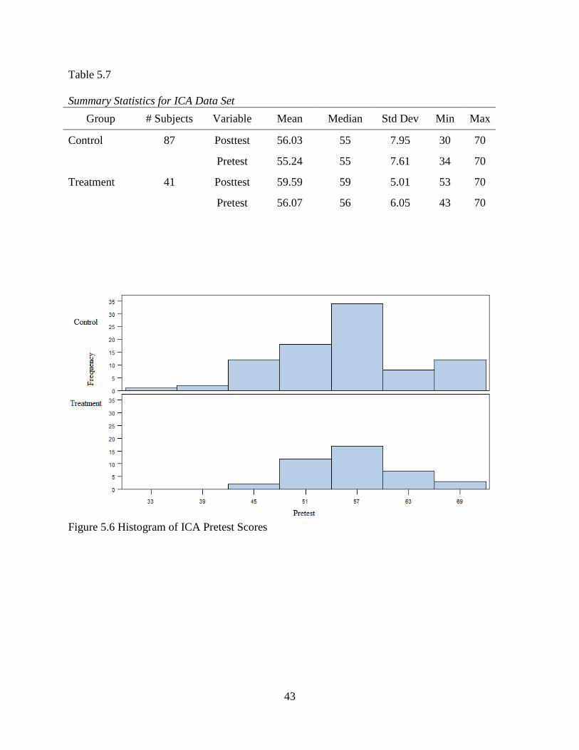
Table 5.7 shows the summary statistics for the ICA Data Set, with illustrative histograms
in Figures 5.6-5.8. The mean Pretest scores for the Control and Treatment group differ by 0.83,

42
where the Treatment group received a slightly higher score. This indicates that, at the time of the
Pretest, those who eventually chose to study abroad reported feeling only slightly less
apprehensive about other cultures, on average, than did their classmates, who ultimately did not
choose to travel. At Posttest, students who traveled abroad scored 3.56 points higher on the ICA
than their peers who did not choose to travel. The ICA scores were slightly more variable for the
Control group variable than for the Treatment group at both time-points; the Posttest variance
declined for the Treatment group, but increased for the Control group.
43
Table 5.7 Summary Statistics for ICA Data Set
Group # Subjects Variable Mean Median Std Dev Min Max
Control 87 Posttest 56.03 55 7.95 30 70
Pretest 55.24 55 7.61 34 70
Treatment 41 Posttest 59.59 59 5.01 53 70
Pretest 56.07 56 6.05 43 70
Figure 5.6 Histogram of ICA Pretest Scores
44
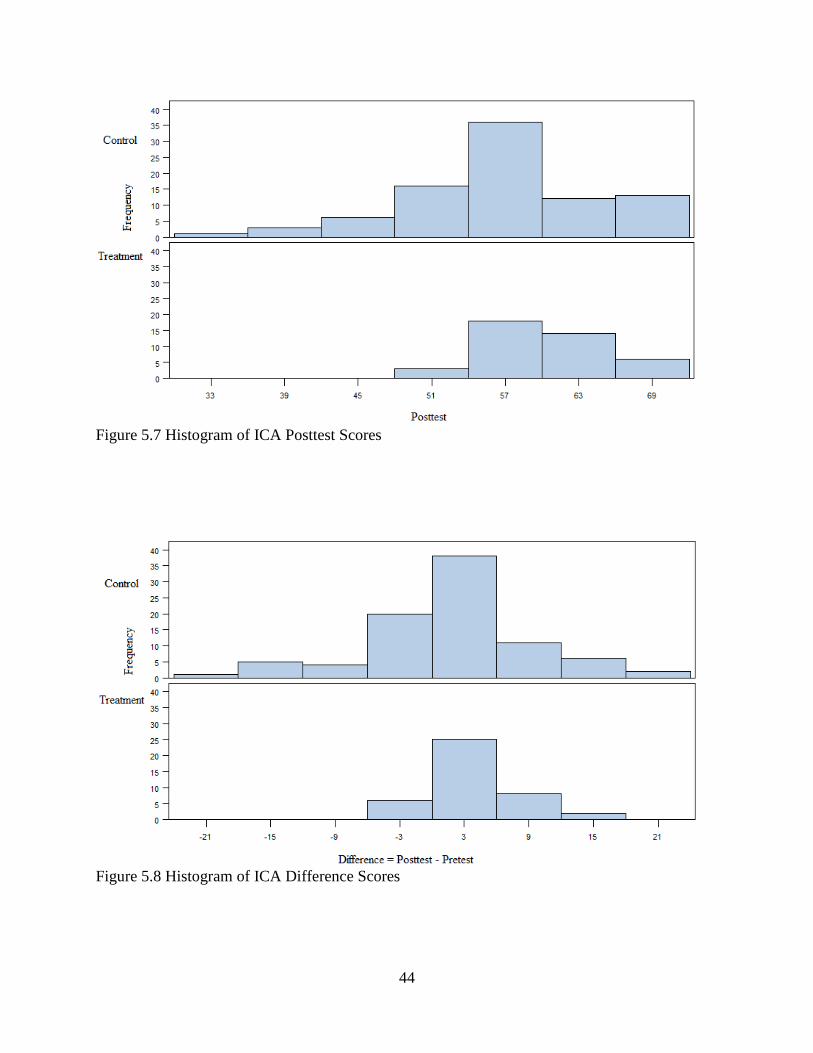
Figure 5.7 Histogram of ICA Posttest Scores
Figure 5.8 Histogram of ICA Difference Scores
45
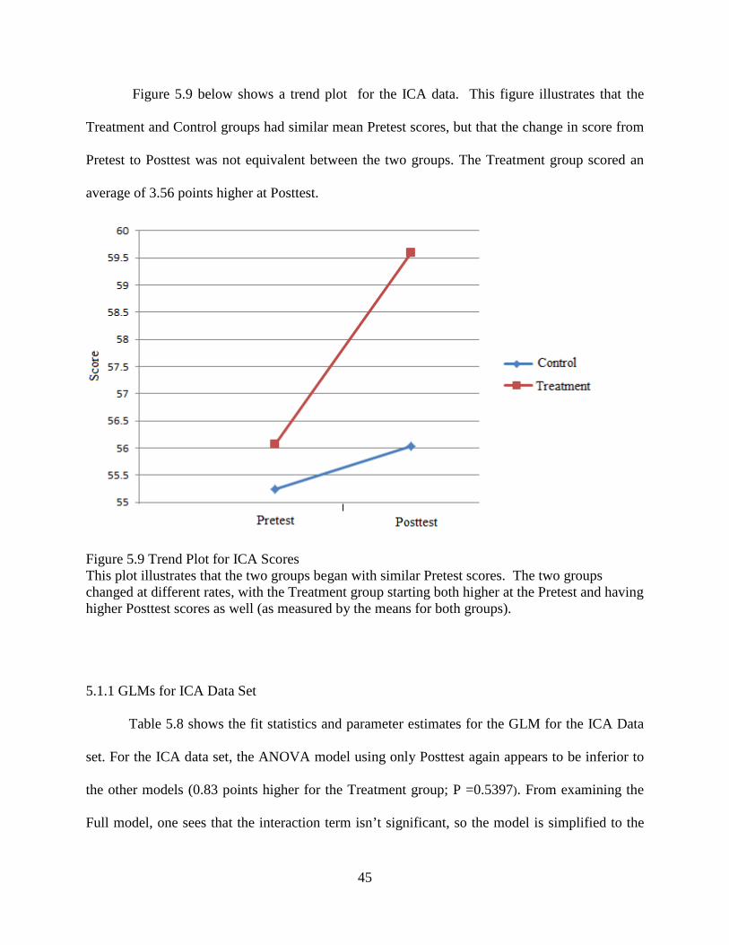
Figure 5.9 below shows a trend plot for the ICA data. This figure illustrates that the
Treatment and Control groups had similar mean Pretest scores, but that the change in score from
Pretest to Posttest was not equivalent between the two groups. The Treatment group scored an
average of 3.56 points higher at Posttest.
Figure 5.9 Trend Plot for ICA Scores This plot illustrates that the two groups began with similar Pretest scores. The two groups changed at different rates, with the Treatment group starting both higher at the Pretest and having higher Posttest scores as well (as measured by the means for both groups).
5.1.1 GLMs for ICA Data Set
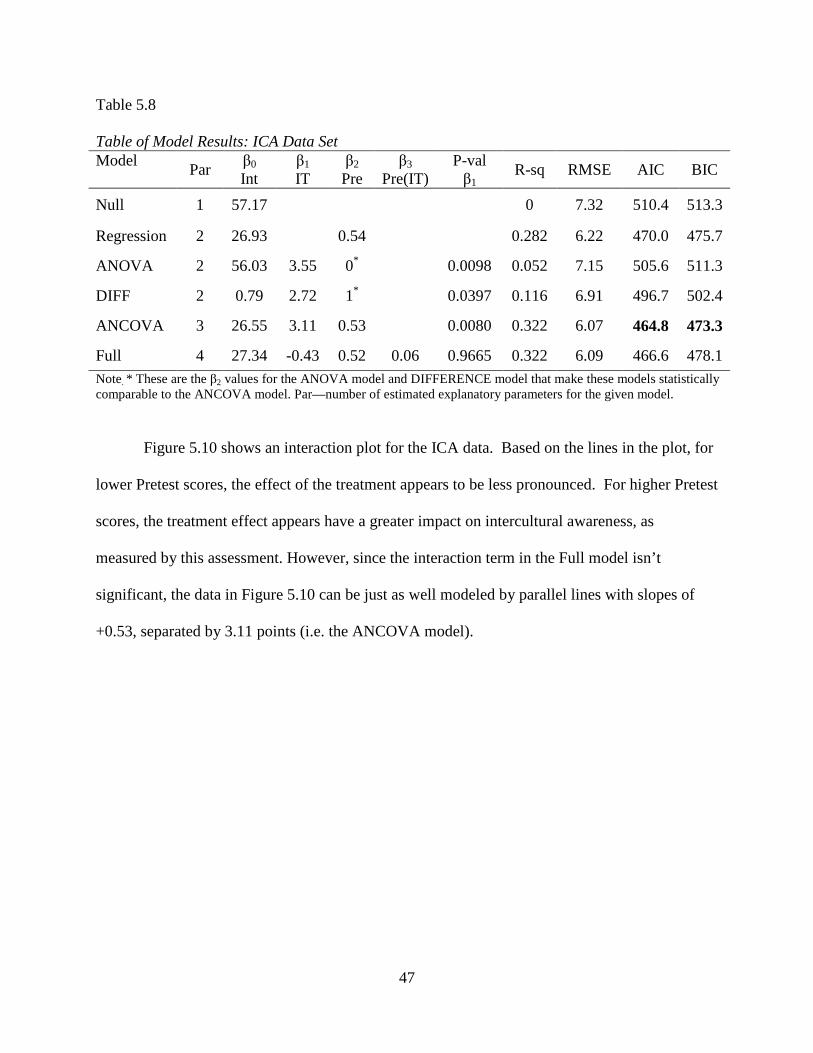
Table 5.8 shows the fit statistics and parameter estimates for the GLM for the ICA Data
set. For the ICA data set, the ANOVA model using only Posttest again appears to be inferior to
the other models (0.83 points higher for the Treatment group; P =0.5397). From examining the
Full model, one sees that the interaction term isn’t significant, so the model is simplified to the

46
ANCOVA model. Since the slope estimate for the Pretest is very different from either 0 or 1 (β2
= 0.53 for the ANCOVA model), neither the DIFF model nor the ANOVA model yield as good
fits for this data set as the ANCOVA model does.
Upon considering AIC and BIC, one observes that the ANCOVA model best predicts
Posttest scores for the ICA data. Although the R-square is lower for the ANCOVA model than
for the Full model, the difference is primarily due to the extra parameter for the interaction
(Pretest*IT) term. The ANCOVA model for the ICA data set predicts that for students with the
same Pretest score, on average, a student who studied abroad would score 3.11 points higher on
the Posttest than a student who did not travel. For example, a student who scored a 55 on the
ICA at Pretest but did not study abroad would be predicted to score 55.7 at Posttest; a similar
scoring student who did travel abroad would be predicted to score 58.81 at Posttest.
There is, of course, selection bias for this study. The treatment criteria, which was
whether a student participated in study abroad, was self-selected. Since students self-selected
themselves to be part of the treatment, their true apprehensions about intercultural
communication could potentially be confounded with the treatment. Did students who traveled
abroad really feel less apprehensive after international travel? Or, are students who want to
pursue international travel less apprehensive about other cultures in the first place? If the latter
were the only reason, one would have expected a larger difference in Pretest scores between
groups.
47
Table 5.8 Table of Model Results: ICA Data Set Model
Par β0 Int
β1
IT β2
Pre β3
Pre(IT) P-val β1
R-sq RMSE AIC BIC
Null 1 57.17 0 7.32 510.4 513.3
Regression 2 26.93 0.54 0.282 6.22 470.0 475.7
ANOVA 2 56.03 3.55 0* 0.0098 0.052 7.15 505.6 511.3
DIFF 2 0.79 2.72 1* 0.0397 0.116 6.91 496.7 502.4
ANCOVA 3 26.55 3.11 0.53 0.0080 0.322 6.07 464.8 473.3
Full 4 27.34 -0.43 0.52 0.06 0.9665 0.322 6.09 466.6 478.1
Note. * These are the β2 values for the ANOVA model and DIFFERENCE model that make these models statistically comparable to the ANCOVA model. Par—number of estimated explanatory parameters for the given model.
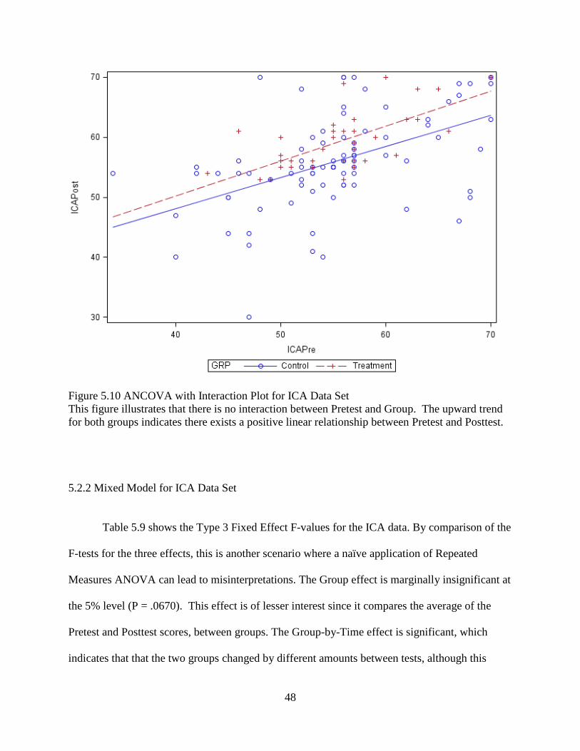
Figure 5.10 shows an interaction plot for the ICA data. Based on the lines in the plot, for
lower Pretest scores, the effect of the treatment appears to be less pronounced. For higher Pretest
scores, the treatment effect appears have a greater impact on intercultural awareness, as
measured by this assessment. However, since the interaction term in the Full model isn’t
significant, the data in Figure 5.10 can be just as well modeled by parallel lines with slopes of
+0.53, separated by 3.11 points (i.e. the ANCOVA model).
48
Figure 5.10 ANCOVA with Interaction Plot for ICA Data Set This figure illustrates that there is no interaction between Pretest and Group. The upward trend for both groups indicates there exists a positive linear relationship between Pretest and Posttest.
5.2.2 Mixed Model for ICA Data Set
Table 5.9 shows the Type 3 Fixed Effect F-values for the ICA data. By comparison of the
F-tests for the three effects, this is another scenario where a naïve application of Repeated
Measures ANOVA can lead to misinterpretations. The Group effect is marginally insignificant at
the 5% level (P = .0670). This effect is of lesser interest since it compares the average of the
Pretest and Posttest scores, between groups. The Group-by-Time effect is significant, which
indicates that that the two groups changed by different amounts between tests, although this
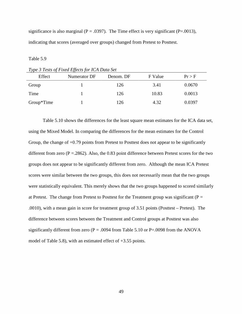
49
significance is also marginal (P = .0397). The Time effect is very significant (P=.0013),
indicating that scores (averaged over groups) changed from Pretest to Posttest.
Table 5.9 Type 3 Tests of Fixed Effects for ICA Data Set
Effect Numerator DF Denom. DF F Value Pr > F
Group 1 126 3.41 0.0670
Time 1 126 10.83 0.0013
Group*Time 1 126 4.32 0.0397
Table 5.10 shows the differences for the least square mean estimates for the ICA data set,
using the Mixed Model. In comparing the differences for the mean estimates for the Control
Group, the change of +0.79 points from Pretest to Posttest does not appear to be significantly
different from zero (P =.2862). Also, the 0.83 point difference between Pretest scores for the two
groups does not appear to be significantly different from zero. Although the mean ICA Pretest
scores were similar between the two groups, this does not necessarily mean that the two groups
were statistically equivalent. This merely shows that the two groups happened to scored similarly
at Pretest. The change from Pretest to Posttest for the Treatment group was significant (P =
.0010), with a mean gain in score for treatment group of 3.51 points (Posttest – Pretest). The
difference between scores between the Treatment and Control groups at Posttest was also
significantly different from zero (P = .0094 from Table 5.10 or P=.0098 from the ANOVA
model of Table 5.8), with an estimated effect of +3.55 points.
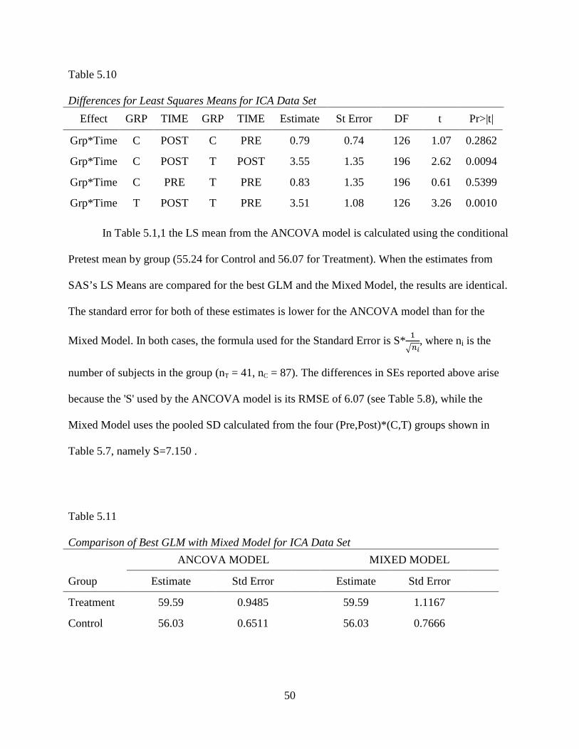
50
Table 5.10 Differences for Least Squares Means for ICA Data Set
Effect GRP TIME GRP TIME Estimate St Error DF t Pr>|t|
Grp*Time C POST C PRE 0.79 0.74 126 1.07 0.2862
Grp*Time C POST T POST 3.55 1.35 196 2.62 0.0094
Grp*Time C PRE T PRE 0.83 1.35 196 0.61 0.5399
Grp*Time T POST T PRE 3.51 1.08 126 3.26 0.0010
In Table 5.1,1 the LS mean from the ANCOVA model is calculated using the conditional
Pretest mean by group (55.24 for Control and 56.07 for Treatment). When the estimates from
SAS’s LS Means are compared for the best GLM and the Mixed Model, the results are identical.
The standard error for both of these estimates is lower for the ANCOVA model than for the
Mixed Model. In both cases, the formula used for the Standard Error is S*�
:;<, where ni is the
number of subjects in the group (nT = 41, nC = 87). The differences in SEs reported above arise
because the 'S' used by the ANCOVA model is its RMSE of 6.07 (see Table 5.8), while the
Mixed Model uses the pooled SD calculated from the four (Pre,Post)*(C,T) groups shown in
Table 5.7, namely S=7.150 .
Table 5.11 Comparison of Best GLM with Mixed Model for ICA Data Set
ANCOVA MODEL MIXED MODEL
Group Estimate Std Error Estimate Std Error
Treatment 59.59 0.9485 59.59 1.1167
Control 56.03 0.6511 56.03 0.7666
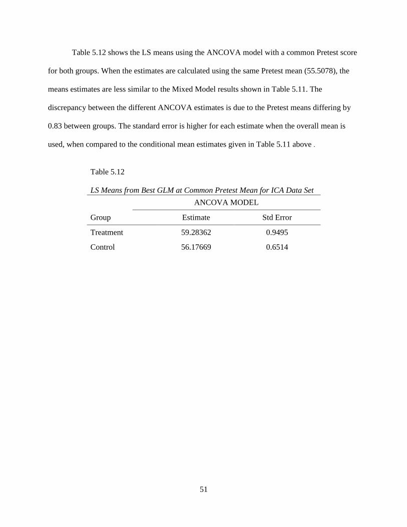
51
Table 5.12 shows the LS means using the ANCOVA model with a common Pretest score
for both groups. When the estimates are calculated using the same Pretest mean (55.5078), the
means estimates are less similar to the Mixed Model results shown in Table 5.11. The
discrepancy between the different ANCOVA estimates is due to the Pretest means differing by
0.83 between groups. The standard error is higher for each estimate when the overall mean is
used, when compared to the conditional mean estimates given in Table 5.11 above .
Table 5.12 LS Means from Best GLM at Common Pretest Mean for ICA Data Set
ANCOVA MODEL
Group Estimate Std Error
Treatment 59.28362 0.9495
Control 56.17669 0.6514

52
5.3 THE ECON DATA SET
This is another example of possible non-equivalent groups prior to intervention. Although
the groups selected to receive the treatment were randomized, the groups themselves were self-
selected. Thus, it is possible that some sections simply had better or worse students due to factors
unrelated to the study. Table 5.13 shows the summary statistics for the Econ data set, with
illustrative histograms shown in Figures 5.11-5.13. For this data set, the Treatment group
average score was 8.05 points lower than the average score for the Control group, at Pretest. The
Treatment Group scored 5.27 points higher than the Control group at Posttest. The standard
deviations of scores for the two groups are similar at Pretest and Posttest. Although the SD of
scores between testing sessions increases (from Pretest to Posttest) for both groups, the
distribution of both Pretest and Posttest scores are somewhat skewed. For this data set, the logit
transformation (Equation 4 of Table 2.1) yields slightly better results than untransformed scores,
but for ease of comparability with analyses from the other three data sets, we will not examine
that transformation here. Trend plots for these data are shown in Figure 5.14.
Table 5.13 Summary Statistics for Econ Data Set
Group # Subjects Variable Mean Median Std Dev Min Max
Control 100 Posttest 73.87 75 12.64 30 95
Pretest 34.44 34.5 8.43 14 54
Treatment 100 Posttest 79.14 81 10.21 44 98
Pretest 26.39 26 7.12 10 48
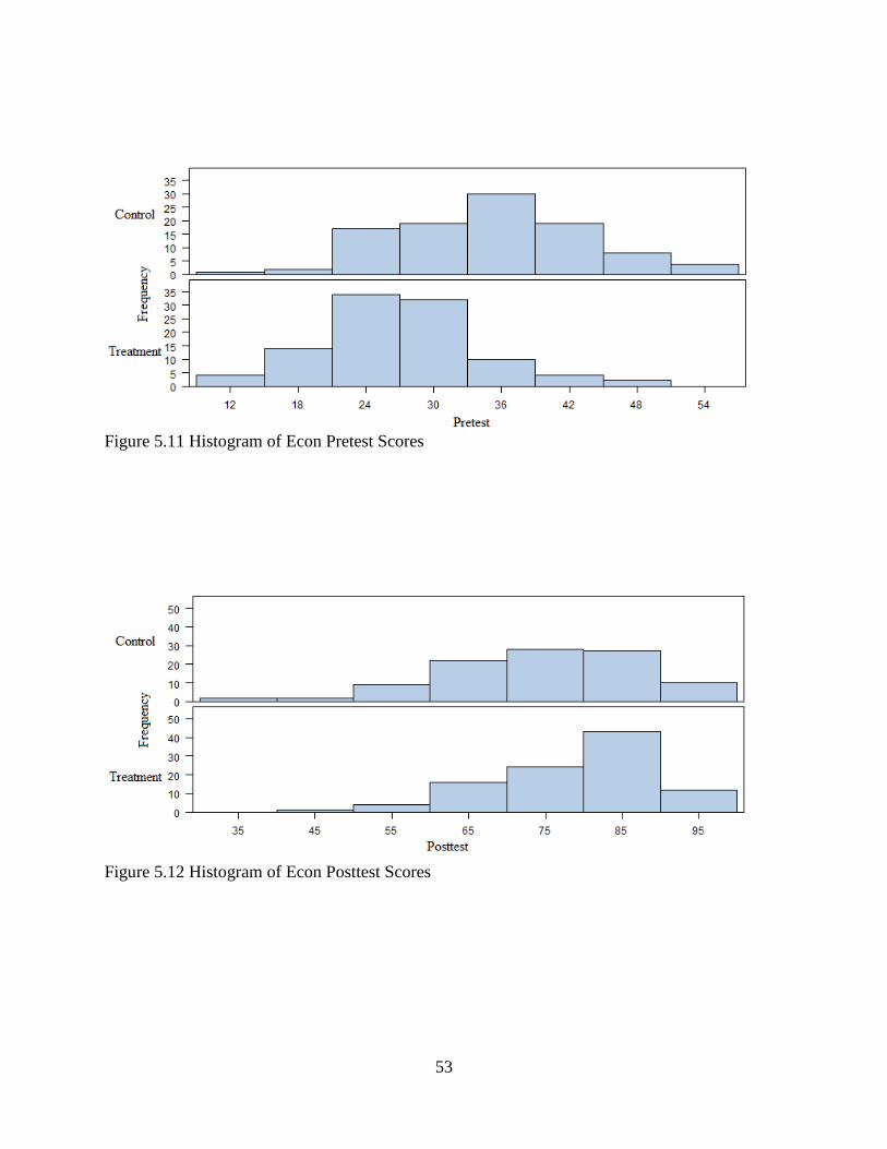
53
Figure 5.11 Histogram of Econ Pretest Scores
Figure 5.12 Histogram of Econ Posttest Scores
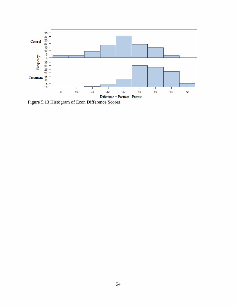
54
Figure 5.13 Histogram of Econ Difference Scores
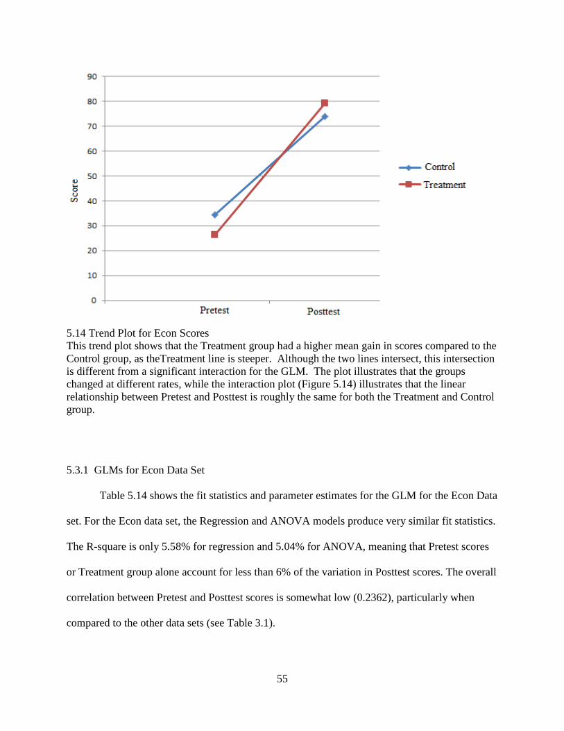
55
5.14 Trend Plot for Econ Scores This trend plot shows that the Treatment group had a higher mean gain in scores compared to the Control group, as theTreatment line is steeper. Although the two lines intersect, this intersection is different from a significant interaction for the GLM. The plot illustrates that the groups changed at different rates, while the interaction plot (Figure 5.14) illustrates that the linear relationship between Pretest and Posttest is roughly the same for both the Treatment and Control group.
5.3.1 GLMs for Econ Data Set Table 5.14 shows the fit statistics and parameter estimates for the GLM for the Econ Data
set. For the Econ data set, the Regression and ANOVA models produce very similar fit statistics.
The R-square is only 5.58% for regression and 5.04% for ANOVA, meaning that Pretest scores
or Treatment group alone account for less than 6% of the variation in Posttest scores. The overall
correlation between Pretest and Posttest scores is somewhat low (0.2362), particularly when
compared to the other data sets (see Table 3.1).
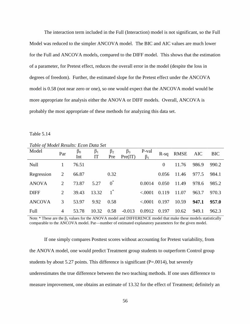
56
The interaction term included in the Full (Interaction) model is not significant, so the Full
Model was reduced to the simpler ANCOVA model. The BIC and AIC values are much lower
for the Full and ANCOVA models, compared to the DIFF model. This shows that the estimation
of a parameter, for Pretest effect, reduces the overall error in the model (despite the loss in
degrees of freedom). Further, the estimated slope for the Pretest effect under the ANCOVA
model is 0.58 (not near zero or one), so one would expect that the ANCOVA model would be
more appropriate for analysis either the ANOVA or DIFF models. Overall, ANCOVA is
probably the most appropriate of these methods for analyzing this data set.
Table 5.14 Table of Model Results: Econ Data Set Model
Par β0 Int
β1
IT β2
Pre β3
Pre(IT) P-val β1
R-sq RMSE AIC BIC
Null 1 76.51 0 11.76 986.9 990.2
Regression 2 66.87 0.32 0.056 11.46 977.5 984.1
ANOVA 2 73.87 5.27 0* 0.0014 0.050 11.49 978.6 985.2
DIFF 2 39.43 13.32 1* <.0001 0.119 11.07 963.7 970.3
ANCOVA 3 53.97 9.92 0.58 <.0001 0.197 10.59 947.1 957.0
Full 4 53.78 10.32 0.58 -0.013 0.0912 0.197 10.62 949.1 962.3
Note. * These are the β2 values for the ANOVA model and DIFFERENCE model that make these models statistically comparable to the ANCOVA model. Par—number of estimated explanatory parameters for the given model.
If one simply compares Posttest scores without accounting for Pretest variability, from
the ANOVA model, one would predict Treatment group students to outperform Control group
students by about 5.27 points. This difference is significant (P=.0014), but severely
underestimates the true difference between the two teaching methods. If one uses difference to
measure improvement, one obtains an estimate of 13.32 for the effect of Treatment; definitely an
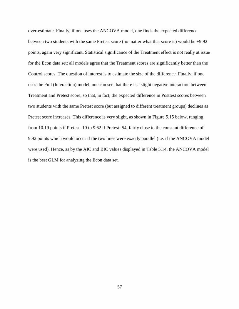
57
over-estimate. Finally, if one uses the ANCOVA model, one finds the expected difference
between two students with the same Pretest score (no matter what that score is) would be +9.92
points, again very significant. Statistical significance of the Treatment effect is not really at issue
for the Econ data set: all models agree that the Treatment scores are significantly better than the
Control scores. The question of interest is to estimate the size of the difference. Finally, if one
uses the Full (Interaction) model, one can see that there is a slight negative interaction between
Treatment and Pretest score, so that, in fact, the expected difference in Posttest scores between
two students with the same Pretest score (but assigned to different treatment groups) declines as
Pretest score increases. This difference is very slight, as shown in Figure 5.15 below, ranging
from 10.19 points if Pretest=10 to 9.62 if Pretest=54, fairly close to the constant difference of
9.92 points which would occur if the two lines were exactly parallel (i.e. if the ANCOVA model
were used). Hence, as by the AIC and BIC values displayed in Table 5.14, the ANCOVA model
is the best GLM for analyzing the Econ data set.
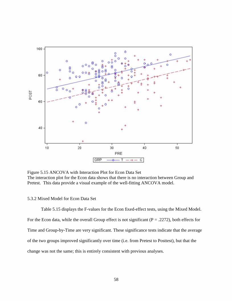
58
Figure 5.15 ANCOVA with Interaction Plot for Econ Data Set The interaction plot for the Econ data shows that there is no interaction between Group and Pretest. This data provide a visual example of the well-fitting ANCOVA model. 5.3.2 Mixed Model for Econ Data Set
Table 5.15 displays the F-values for the Econ fixed-effect tests, using the Mixed Model.
For the Econ data, while the overall Group effect is not significant (P = .2272), both effects for
Time and Group-by-Time are very significant. These significance tests indicate that the average
of the two groups improved significantly over time (i.e. from Pretest to Posttest), but that the
change was not the same; this is entirely consistent with previous analyses.
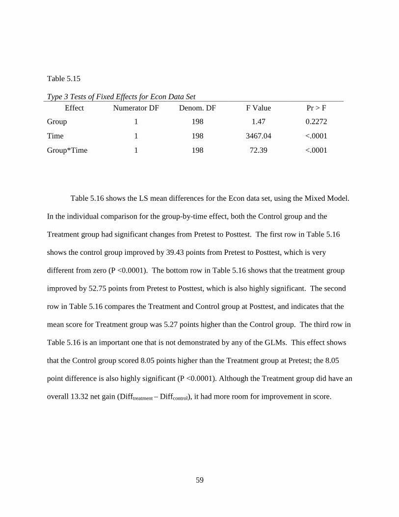
59
Table 5.15 Type 3 Tests of Fixed Effects for Econ Data Set
Effect Numerator DF Denom. DF F Value Pr > F
Group 1 198 1.47 0.2272
Time 1 198 3467.04 <.0001
Group*Time 1 198 72.39 <.0001
Table 5.16 shows the LS mean differences for the Econ data set, using the Mixed Model.
In the individual comparison for the group-by-time effect, both the Control group and the
Treatment group had significant changes from Pretest to Posttest. The first row in Table 5.16
shows the control group improved by 39.43 points from Pretest to Posttest, which is very
different from zero (P <0.0001). The bottom row in Table 5.16 shows that the treatment group
improved by 52.75 points from Pretest to Posttest, which is also highly significant. The second
row in Table 5.16 compares the Treatment and Control group at Posttest, and indicates that the
mean score for Treatment group was 5.27 points higher than the Control group. The third row in
Table 5.16 is an important one that is not demonstrated by any of the GLMs. This effect shows
that the Control group scored 8.05 points higher than the Treatment group at Pretest; the 8.05
point difference is also highly significant (P <0.0001). Although the Treatment group did have an
overall 13.32 net gain (Difftreatment – Diffcontrol), it had more room for improvement in score.

60
Table 5.16 Differences for Least Square Means for Econ Data Set
Effect GRP TIME GRP TIME Estimate St Error DF t Pr>|t|
Grp*Time C POST C PRE 39.43 1.11 198 35.62 <.0001
Grp*Time C POST T POST 5.27 1.39 349 3.79 0.0002
Grp*Time C PRE T PRE -8.05 1.39 349 -5.80 <.0001
Grp*Time T POST T PRE 52.75 1.11 198 47.65 <.0001
Table 5.17 shows the comparison of LS mean estimates for ANCOVA and the Mixed
Model. The ANCOVA mean estimates, computed with the conditional Pretest scores, are
identical to the estimates from the Mixed Model. When comparing the ANCOVA results to that
of the Mixed Model, both show that the difference in scores at Posttest was approximately 5.27
points. For the Econ data set, unlike the case with the ICA data set, however, the standard error is
less for the Mixed Model estimates than the ANCOVA estimates. In this case, the ANCOVA
standard errors are more accurate as they are S*�
:;<= 10.595/10 = 1.0595, where the 'S' is the
RMSE estimated from the 200 residual used in fitting the ANCOVA models. The formula for the
standard error for the Mixed Model is also S*�
:;< but the 'S' used is the pooled SD obtained from
combining the four SD estimates shown in Table 5.13 (S=9.821). However, that pooling assumes
all four SD's are estimating the same thing, whereas it is fairly clear that the two Pretest SDs are
much smaller than two Posttest SDs, so this method of pooling used in the Mixed Model
artificially deflates the standard error for predicting Posttest scores. This drawback could be
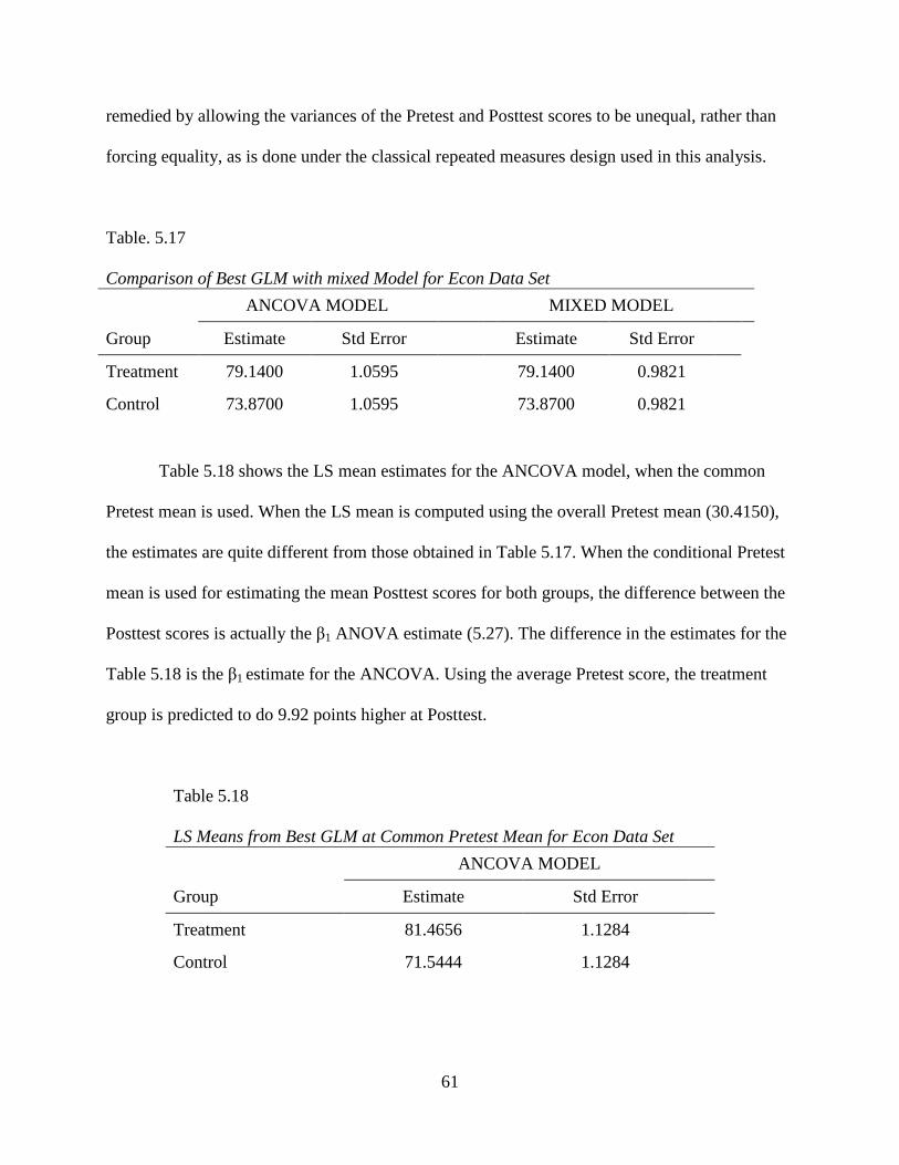
61
remedied by allowing the variances of the Pretest and Posttest scores to be unequal, rather than
forcing equality, as is done under the classical repeated measures design used in this analysis.
Table. 5.17 Comparison of Best GLM with mixed Model for Econ Data Set
ANCOVA MODEL MIXED MODEL
Group Estimate Std Error Estimate Std Error
Treatment 79.1400 1.0595 79.1400 0.9821
Control 73.8700 1.0595 73.8700 0.9821
Table 5.18 shows the LS mean estimates for the ANCOVA model, when the common
Pretest mean is used. When the LS mean is computed using the overall Pretest mean (30.4150),
the estimates are quite different from those obtained in Table 5.17. When the conditional Pretest
mean is used for estimating the mean Posttest scores for both groups, the difference between the
Posttest scores is actually the β1 ANOVA estimate (5.27). The difference in the estimates for the
Table 5.18 is the β1 estimate for the ANCOVA. Using the average Pretest score, the treatment
group is predicted to do 9.92 points higher at Posttest.
Table 5.18 LS Means from Best GLM at Common Pretest Mean for Econ Data Set
ANCOVA MODEL
Group Estimate Std Error
Treatment 81.4656 1.1284
Control 71.5444 1.1284

62
5.4 THE SHI DATA SET
Table 5.19 shows the summary statistics for the SHI data set. The mean Pretest score for
the Educational Literature group was around 9 or 10 points lower than that of the Video or
Control groups, respectively. For the Control group, there was a 0.83 decline in mean SHI scores
from Pretest to Posttest. The Educational Literature and the Video groups had mean gains of
20.34 points and 9.52 points, respectively. Although the Educational Literature group had a
mean gain more than double the gain of the Video group, the difference in gains between the
Educational Literature group and the Video group was not significant. When these groups were
compared, pairwise, with the Control group, however, the difference in scores for the
Educational Literature and Video groups were both significantly different from the Control
group (alpha = 0.05). However, since the Educational Literature group and Video group did not
differ significantly from one another, for purposes of analysis, they were combined into one
group called “Treatment”.
Table 5.19 Summary Statistics for Original SHI Data Set
Group # Subjects Variable Mean Median Std Dev Min Max
Control 30 Posttest 164.70 167.5 30.21 75 216
Pretest 165.53 164 22.92 105 211
Educational Literature
33 Posttest 177.64 183 24.99 125 210
Pretest 157.30 156 24.15 116 200
Video 33 Posttest 176.70 182 24.13 106 207
Pretest 167.18 170 21.85 116 203
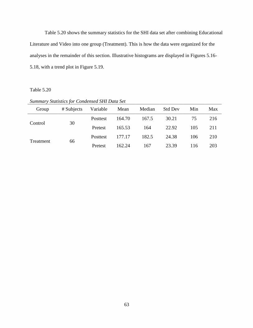
63
Table 5.20 shows the summary statistics for the SHI data set after combining Educational
Literature and Video into one group (Treatment). This is how the data were organized for the
analyses in the remainder of this section. Illustrative histograms are displayed in Figures 5.16-
5.18, with a trend plot in Figure 5.19.
Table 5.20 Summary Statistics for Condensed SHI Data Set
Group # Subjects Variable Mean Median Std Dev Min Max
Control 30 Posttest 164.70 167.5 30.21 75 216
Pretest 165.53 164 22.92 105 211
Treatment 66 Posttest 177.17 182.5 24.38 106 210
Pretest 162.24 167 23.39 116 203
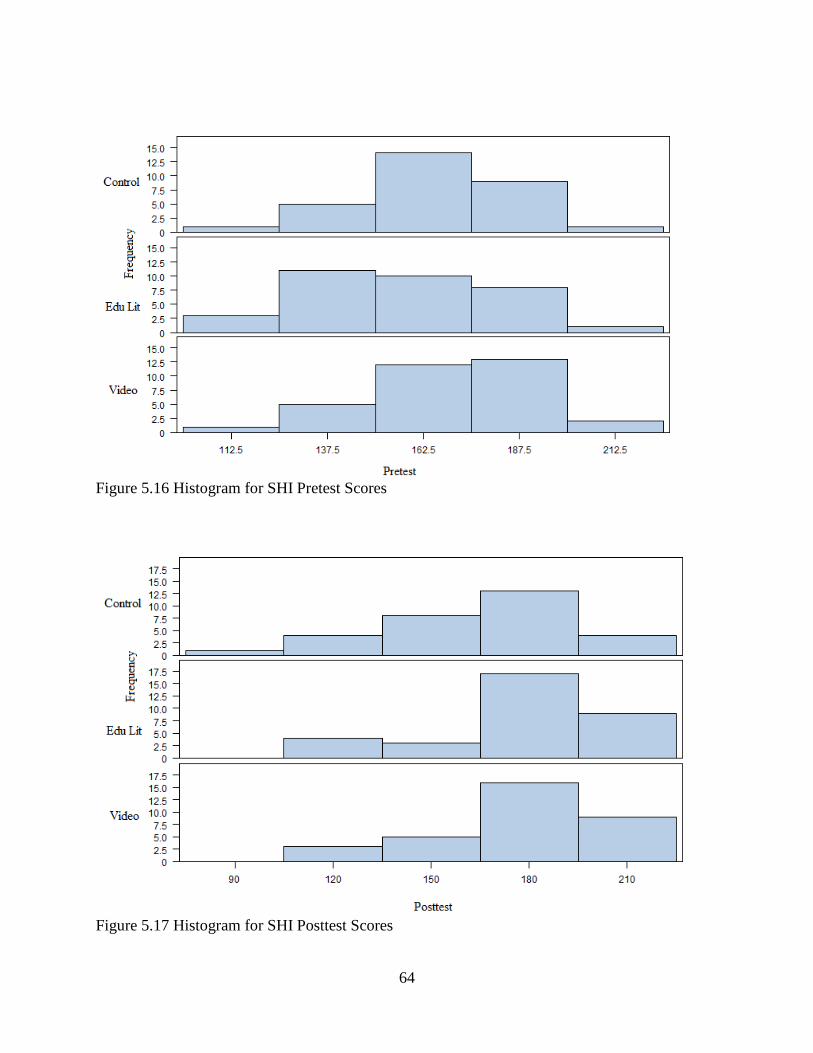
64
Figure 5.16 Histogram for SHI Pretest Scores
Figure 5.17 Histogram for SHI Posttest Scores
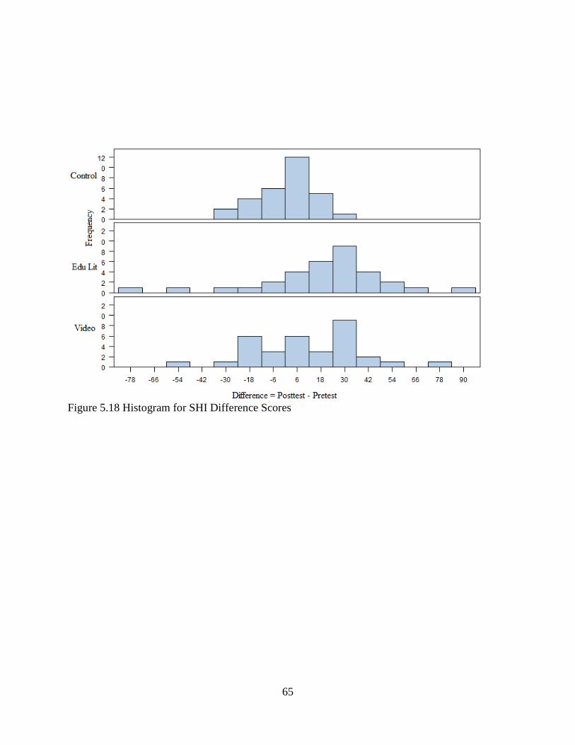
65
Figure 5.18 Histogram for SHI Difference Scores
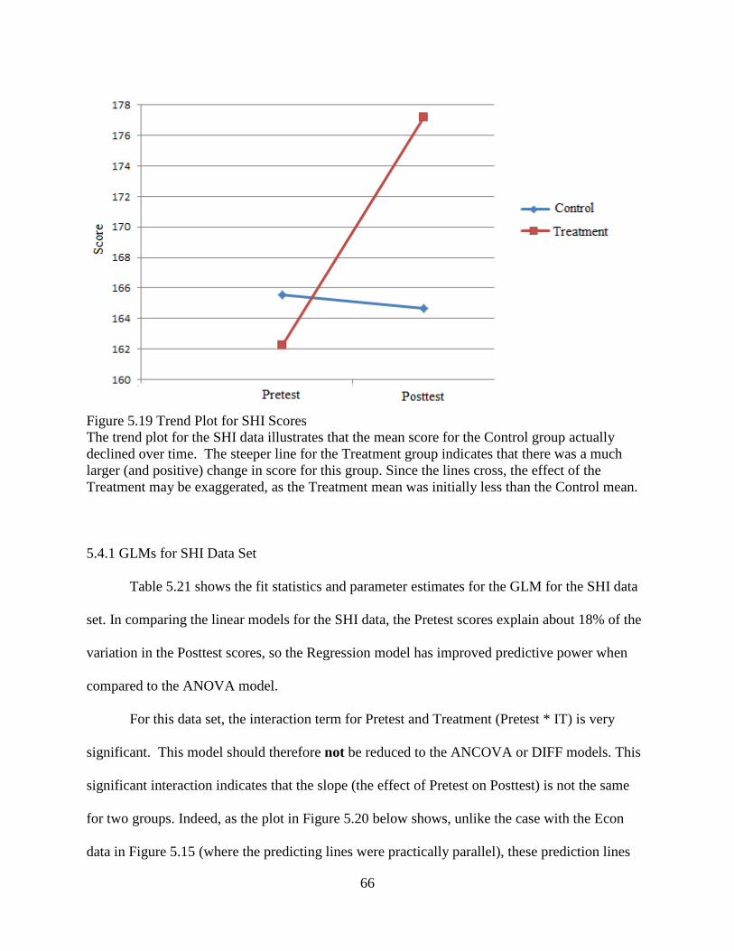
66
Figure 5.19 Trend Plot for SHI Scores The trend plot for the SHI data illustrates that the mean score for the Control group actually declined over time. The steeper line for the Treatment group indicates that there was a much larger (and positive) change in score for this group. Since the lines cross, the effect of the Treatment may be exaggerated, as the Treatment mean was initially less than the Control mean. 5.4.1 GLMs for SHI Data Set
Table 5.21 shows the fit statistics and parameter estimates for the GLM for the SHI data
set. In comparing the linear models for the SHI data, the Pretest scores explain about 18% of the
variation in the Posttest scores, so the Regression model has improved predictive power when
compared to the ANOVA model.
For this data set, the interaction term for Pretest and Treatment (Pretest * IT) is very
significant. This model should therefore not be reduced to the ANCOVA or DIFF models. This
significant interaction indicates that the slope (the effect of Pretest on Posttest) is not the same
for two groups. Indeed, as the plot in Figure 5.20 below shows, unlike the case with the Econ
data in Figure 5.15 (where the predicting lines were practically parallel), these prediction lines
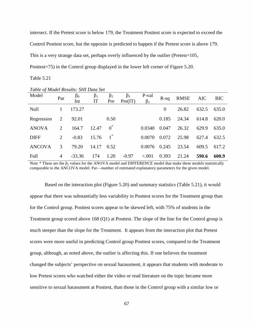
67
intersect. If the Pretest score is below 179, the Treatment Posttest score is expected to exceed the
Control Posttest score, but the opposite is predicted to happen if the Pretest score is above 179.
This is a very strange data set, perhaps overly influenced by the outlier (Pretest=105,
Posttest=75) in the Control group displayed in the lower left corner of Figure 5.20.
Table 5.21 Table of Model Results: SHI Data Set Model
Par β0 Int
β1
IT β2
Pre β3
Pre(IT) P-val β1
R-sq RMSE AIC BIC
Null 1 173.27 0 26.82 632.5 635.0
Regression 2 92.01 0.50 0.185 24.34 614.8 620.0
ANOVA 2 164.7 12.47 0* 0.0340 0.047 26.32 629.9 635.0
DIFF 2 -0.83 15.76 1* 0.0070 0.072 25.98 627.4 632.5
ANCOVA 3 79.20 14.17 0.52 0.0076 0.245 23.54 609.5 617.2
Full 4 -33.36 174 1.20 -0.97 <.001 0.393 21.24 590.6 600.9 Note. * These are the β2 values for the ANOVA model and DIFFERENCE model that make these models statistically comparable to the ANCOVA model. Par—number of estimated explanatory parameters for the given model.
Based on the interaction plot (Figure 5.20) and summary statistics (Table 5.21), it would
appear that there was substantially less variability in Posttest scores for the Treatment group than
for the Control group. Posttest scores appear to be skewed left, with 75% of students in the
Treatment group scored above 168 (Q1) at Posttest. The slope of the line for the Control group is
much steeper than the slope for the Treatment. It appears from the interaction plot that Pretest
scores were more useful in predicting Control group Posttest scores, compared to the Treatment
group, although, as noted above, the outlier is affecting this. If one believes the treatment
changed the subjects’ perspective on sexual harassment, it appears that students with moderate to
low Pretest scores who watched either the video or read literature on the topic became more
sensitive to sexual harassment at Posttest, than those in the Control group with a similar low or
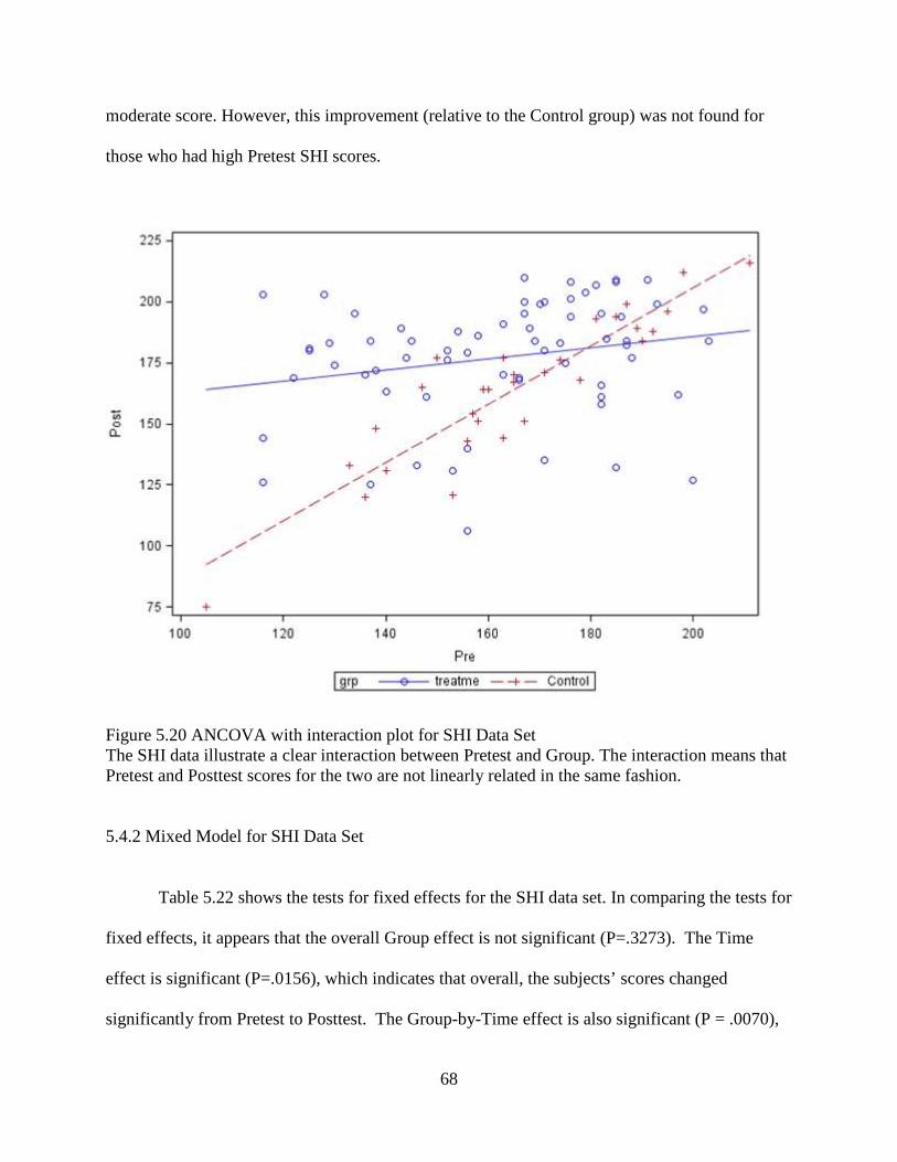
68
moderate score. However, this improvement (relative to the Control group) was not found for
those who had high Pretest SHI scores.
Figure 5.20 ANCOVA with interaction plot for SHI Data Set The SHI data illustrate a clear interaction between Pretest and Group. The interaction means that Pretest and Posttest scores for the two are not linearly related in the same fashion. 5.4.2 Mixed Model for SHI Data Set
Table 5.22 shows the tests for fixed effects for the SHI data set. In comparing the tests for
fixed effects, it appears that the overall Group effect is not significant (P=.3273). The Time
effect is significant (P=.0156), which indicates that overall, the subjects’ scores changed
significantly from Pretest to Posttest. The Group-by-Time effect is also significant (P = .0070),

69
which indicates that the change in score, from Pretest to Posttest, was not the same for both
groups (i.e. one group had a greater change in score). This F-test statistic does not illustrate
which group had a higher gain, although as noted for the previous data sets, this Group*Time test
is equivalent to the test of the IT effect in the DIFF model, which from Table 5.21, shows that
the Treatment score is expected to be 15.76 higher than the Control score.
Table 5.22 Type 3 Tests of Fixed Effects for the SHI Data Set
Effect Numerator DF Denom. DF F Value Pr > F
Group 1 94 0.97 0.3273
Time 1 94 6.07 0.0156
Group*Time 1 94 7.59 0.0070
Table 5.23 shows the differences for the LS means for the SHI data. In comparing the
difference estimates, the change in score from Pretest to Posttest for the Control group does not
appear to be significantly different from 0. Similarly, in the comparison of Pretest scores
between the Treatment group and the Control group, the two groups are not significantly
different. This indicates that the two groups, prior to intervention, did not respond significantly
differently to the sexual harassment assessment. The estimate for the difference between Pretest
and Posttest scores for the Treatment group is highly significant (P = <.0001). The associated
coefficient estimate indicates that the mean change from Pretest to Posttest (or Posttest – Pretest)
was 14.92 points, and that the Treatment group had a significant positive change in score over
time. Also significant was the LS mean difference for the comparison of the Control and the
Treatment group, at Posttest. The estimate for the mean difference was 12.47 points, or the
Treatment group scored an average of 12.47 points higher on the SHI assessment at Posttest than

70
the Control group. This is exactly the same estimate as obtained by the ANOVA model of Table
5.21; the minor discrepancies in P-values (.0430 vs. .0239) are due to the slightly different
procedures for estimating residual variances under the two procedures.
For this data set, the Mixed Model illustrates that the two groups did not significantly
differ at Pretest, but did differ significantly at Posttest. Also, it shows that the Control group did
not significantly change from Pretest to Posttest, but the Treatment group did.
Table 5.23 Differences for Least Squares Means for SHI Data Set
Effect GRP TIME GRP TIME Estimate St Error DF t Pr>|t|
Grp*Time C POST C PRE -0.83 4.74 94 -0.18 0.8609
Grp*Time C POST T POST 12.47 5.47 156 2.28 0.0239
Grp*Time C PRE T PRE -3.29 5.47 156 -0.60 0.5481
Grp*Time T POST T PRE 14.92 3.20 94 4.67 <.0001
Table 5.24 shows the LS mean estimates for the best GLM (Full model) with conditional
means and the Mixed Model. As seen in the other data sets, the SHI data also provides identical
LS mean estimates for the best GLM (the Full(INTERACTION) model), using the conditional
mean, and the Mixed Model. The standard error for the SHI data is lower for the Full model.
Table. 5.24 Comparison of Best GLM with Mixed Model for SHI Data Set
INTERACTION MODEL MIXED MODEL
Group Estimate Std Error Estimate Std Error
Treatment 177.1667 2.6141 177.1700 3.0561
Control 164.7000 3.8774 164.7000 4.5329
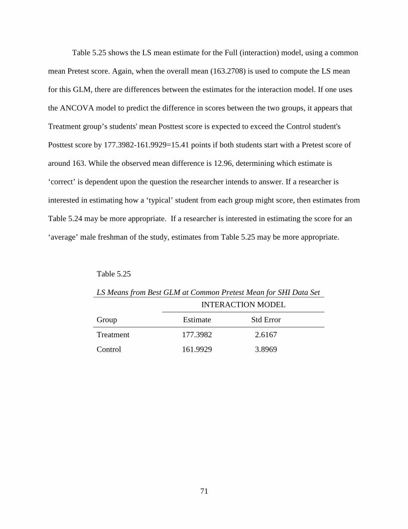
71
Table 5.25 shows the LS mean estimate for the Full (interaction) model, using a common
mean Pretest score. Again, when the overall mean (163.2708) is used to compute the LS mean
for this GLM, there are differences between the estimates for the interaction model. If one uses
the ANCOVA model to predict the difference in scores between the two groups, it appears that
Treatment group’s students' mean Posttest score is expected to exceed the Control student's
Posttest score by 177.3982-161.9929=15.41 points if both students start with a Pretest score of
around 163. While the observed mean difference is 12.96, determining which estimate is
‘correct’ is dependent upon the question the researcher intends to answer. If a researcher is
interested in estimating how a ‘typical’ student from each group might score, then estimates from
Table 5.24 may be more appropriate. If a researcher is interested in estimating the score for an
‘average’ male freshman of the study, estimates from Table 5.25 may be more appropriate.
Table 5.25 LS Means from Best GLM at Common Pretest Mean for SHI Data Set
INTERACTION MODEL
Group Estimate Std Error
Treatment 177.3982 2.6167
Control 161.9929 3.8969
72
CHAPTER 6
CONCLUSIONS
A purpose of this thesis is to find optimal ways to analyze Pretest-Posttest designed
studies. Whether it is a true experiment (PPGD) or quasi-experiment (NEGD), a researcher
should attempt, prior to experimentation and analysis, to rule out all rival hypotheses to those
being tested. Causation between two variables cannot be accurately inferred if the experimental
design is not valid. Despite the lack of randomization, the NEGD can still be a beneficial design,
as samples are generally easier to form than in true randomized experiments, and there is relative
ease in creating a single-blind study (thus minimizing reactive arrangements).
There are numerous methods, beyond those presented in this thesis, that exist for
analyzing PPGD and NEGD. The best GLM for data analysis is dependent upon the data. For
each data set, utilizing the Pretest data in the analyses improved the fit statistics and reduced the
proportion of unexplained variance compared to using the ANOVA model, which completely
ignores Pretest information. From these examples, neither the Pretest nor the Group alone is most
powerful in predicting Posttest scores; a form of the ANCOVA model usually provides the best
analysis for the GLM. In building a GLM for these studies, one should probably start with the
Full Model (including an interaction term) and reduce to the ANCOVA if the interaction is not
significant. When the slope estimate for the Pretest is near ‘1’ or ‘0’, the ANCOVA model may
be further reduced to the DIFF model or the ANOVA model, respectively. In these two
scenarios, the DIFF model and ANOVA model will generally provide better fit statistics than the

73
ANCOVA, as the additional parameter estimate for Pretest slope does not significantly reduce
the SSE. In cases where groups are non-equivalent prior to treatment intervention, LS means
predictions using the overall Pretest mean may distort the true gains or losses between groups at
Posttest. On the other hand, this method may give a truer estimate of the difference between
groups at Posttest if they had been equivalent at Pretest. This is a philosophical battle that can’t
really be answered with certainty if the design is NEGD.
While the Mixed Model may be more difficult to understand, it is more flexible in
scenarios where the assumption of constant variability may be violated (though these examples
are not shown for simplicity of comparison). Further, the Mixed Model provides estimates for
both the Posttest and Pretest scores. Estimation of the Pretest may or may not be of interest to the
researcher. If LS means are computed using the conditional group means for the best GLM, the
GLM and Mixed Model will yield identical estimates for the Posttest means.
If a researcher prefers the analysis of the GLM and chooses to apply the same mean for
both groups, discrepancies between Pretest scores should be taken into account, if they exist. If a
researcher prefers the Mixed Model or Repeated Measures ANOVA, it is important to utilize
‘Group-by-Time’ effect rather than the ‘Group’ effect. A significant ‘Group’ effect will tend to
show if the groups were different at Pretest and Posttest, which may be due to a lack of
equivalence, rather than a treatment intervention. A significant ‘Group-by-Time’ effect will tend
to show if the groups experienced significantly different gains or losses from Pretest to Posttest,
which should be the case if the treatment method caused the change in scores. If a researcher is
interested in analysis of the difference where the ANCOVA slope is near one and is interested in
interested in modeling Pretest scores, the Mixed Model is an ideal fit.

74
An original goal of this thesis was to provide statistical consultants with some advice
concerning how to best explain analyses of Pretest-Posttest designs to clients. Although the
preceding discussion has demonstrated that there is generally not one method of analysis which
is always best, this investigation has provided data summaries which would be useful no matter
what form of analysis is later pursued. These will be illustrated below by referring to the
appropriate tables and figures from the Econ data set analysis, although what is said is applicable
to all four data sets. First, almost obviously, a consultant should display the summary statistics
for the Group*Time samples, as shown in a table such as Table 5.13. One can then
simultaneously examine the distribution of Pretest and Posttest scores by Group, as shown in
Figures such as 5.12 and 5.13. One could also take the four Group*Time means reported in the
original data summary (Table 5.13) and plot them graphically as shown in Figure 5.14 (ignoring,
for now, the connecting lines). Alternatively, one could plot (Pretest,Posttest) scores for all
subjects in the population, using color coding to represent group membership, as done in Figure
5.15 (again ignoring the plotted lines).
All of the above-mentioned tables and plots are not really analyses at all – they simply
display the data in various formats that may be useful. It is recommended that statistical
consultants show clients all of these representations of the data before performing any analyses.
Many of the ‘mistakes’ made in performing analyses of Pretest-Posttest designs occur because
clients and/or consultants rush into analyses without carefully understanding their data. Once all
of the has been done, one can begin performing various analyses. One could perform statistical
tests to compare any of the pairs of means shown in the original data summary. These are the
four tests shown in tables such as Table 5.16 (between Posttest and Pretest scores for Control
group, between Treatment and Control groups for Posttest scores, between Treatment and

75
Control groups for Pretest scores, and between Posttest and Pretest scores for the Treatment
group, respectively). The first and fourth of these tests are equivalent to testing that the slopes of
the two lines given in the trend plot (Figure 5.14) are zero. The second of these tests is roughly
equivalent to the ANOVA model performed on the Posttest scores. The third of these is the test
for equality of Treatment and Control means at Pretest, an often ignored, but rather useful, test.
Finally, after examining all of the above, one might conduct what many consider to be
the ‘real’ test of interest. If one believes that Posttest-Pretest difference (i.e. ‘gain’) is the
relevant measure of success, then one is interested in testing whether the means of difference
histograms (such as those plotted in Figure 5.13) are significantly different from one another.
This is exactly equivalent to testing that the slopes of the two trend lines plotted in Figure 5.14
are equal to one another. The test statistic for performing this test is given by the Group*Time
interaction test shown as the last line of Table 5.15.
Alternatively, if one isn’t certain that ‘gain’ is the appropriate measure, one can consider
various linear models that incorporate Pretest score into the analysis. In such cases, one would
want to consider plots like those shown in Figure 5.15. The data are the points displayed in the
figure, and the only question is which pair of lines should be superimposed as lines of best fit.
The pair which are actually drawn in Figure 5.15 (and in analogous figures for other data sets in
this thesis) are the Full model lines, which allow the lines to have separate slopes and intercepts.
If one constrains oneself to the two parallel lines which best fit the data, this would correspond to
the ANCOVA model. If one constrained the best-fitting lines to not only be parallel but also to
be flat (zero slope), this would correspond to the ANOVA model. If one searched for the best-
fitting pair of lines such that both had slope=1.0, this would correspond to the DIFF model.

76
While all of the above may seem obvious, it appears that even experienced statisticians
can become confused (or confuse clients!) when explaining such results. Presenting graphical
displays of the type mentioned above would definitely help consultants to clarify many of the
analyses explored in this thesis.
One final caution must be delivered. An underlying assumption within this thesis is that
the Pretest score is a valid measurement for determining whether two groups are equivalent.
While the Pretest addresses some aspects of validity, the two groups can potentially differ (and
likely do differ, particularly for cases of self-selection) in many aspects that the Pretest cannot
measure or detect. Additionally, the mere idea of prior exposure to a test may affect how
subjects respond at Posttest (test effects). If a Pretest is administered for a study, and the mean
scores across groups are similar, it does not necessarily indicate that two groups are equivalent.
While the ANCOVA adjusts for Pretest scores, it can potentially be a false sense of adjustment
in the case where the testing cannot capture the existing differences between groups (likely to
occur in the non-randomized case).
77
REFERENCES
Bonate, P. L. (2000). Analysis of pretest-posttest designs. Boca Raton, FL: CRC Press.
Brogan, D. R., & Kutner, M. H. (1980). Comparative analyses of pretest-posttest research
designs. The American Statistician, 34(4), 229-232.
Campbell, D. T., Stanley, J. C., & Gage, N. L. (1963). Experimental and quasi-experimental
designs for research. Boston: Houghton Mifflin.
Cook, T. D., Campbell, D. T., & Day, A. (1979). Quasi-experimentation: Design & analysis
issues for field settings. Boston, MA: Houghton Mifflin.
Cronbach, L. J., & Meehl, P. E. (1955). Construct validity in psychological tests. Psychological
bulletin, 52(4), 281.
Dimitrov, D. M., & Rumrill, Jr, P. D. (2003). Pretest-posttest designs and measurement of
change. Work: A Journal of Prevention, Assessment and Rehabilitation, 20(2), 159-165.
Huck, S. W., & McLean, R. A. (1975). Using a repeated measures ANOVA to analyze the data
from a pretest-posttest design: A potentially confusing task. Psychological
Bulletin, 82(4), 511-518.
Kutner, M. H., Nachtsheim, C. J., Neter, J., & Li, W. (2005). Applied linear statistical
models (Vol. 6, No. 8). New York, NY: McGraw-Hill.
Vogt, W. P., & Johnson, R. B. (1999). Dictionary of statistics & methodology: A nontechnical
guide for the social sciences. Thousand Oaks, CA: SAGE Publications, Incorporated.

78
Weber, E. (2005). Quantifying student learning: how to analyze assessment data. Bulletin of the
Ecological Society of America, 90(4), 501-511.