Comparison of Random Vibration Theory and Time Series

Seismic Site Response Analyses

Albert R. Kottke and Ellen M. Rathje

May 12, 2010

Contents

Contents 1

List of Figures 3

List of Tables 9

1 Introduction 10

2 Site Response Methods 122.1 Introduction . . . . . . . . . . . . . . . . . . . . . . . . . . . . . . . . . . 122.2 Equivalent-Linear Method . . . . . . . . . . . . . . . . . . . . . . . . . . 132.3 Nonlinear Method . . . . . . . . . . . . . . . . . . . . . . . . . . . . . . 152.4 Input Motion Specification . . . . . . . . . . . . . . . . . . . . . . . . . . 182.5 Linear Elastic Simplification . . . . . . . . . . . . . . . . . . . . . . . . . 22

3 Site Profiles Analyzed 233.1 Introduction . . . . . . . . . . . . . . . . . . . . . . . . . . . . . . . . . . 233.2 Turkey Flat Site . . . . . . . . . . . . . . . . . . . . . . . . . . . . . . . 233.3 Sylmar County Hospital Site . . . . . . . . . . . . . . . . . . . . . . . . 253.4 Calvert Cliffs Site . . . . . . . . . . . . . . . . . . . . . . . . . . . . . . . 30

4 Input Ground Motion Characterization 374.1 Introduction . . . . . . . . . . . . . . . . . . . . . . . . . . . . . . . . . . 374.2 Stochastically Simulated Ground Motions . . . . . . . . . . . . . . . . . 384.3 Recorded Ground Motions . . . . . . . . . . . . . . . . . . . . . . . . . . 41

4.3.1 Ground Motion Selection . . . . . . . . . . . . . . . . . . . . . . 414.3.2 Maximum Usable Frequency . . . . . . . . . . . . . . . . . . . . 47

4.4 Spectrally Matched Ground Motions . . . . . . . . . . . . . . . . . . . . 524.5 Response Spectrum Compatible Motion for RVT . . . . . . . . . . . . . 57

5 Comparison of Equivalent-Linear Methods 625.1 Introduction . . . . . . . . . . . . . . . . . . . . . . . . . . . . . . . . . . 625.2 Comparison Using Stochastic Input Motions . . . . . . . . . . . . . . . . 635.3 Comparisons Using Scaled Time Series . . . . . . . . . . . . . . . . . . . 85

1

5.4 Comparisons Using Spectrally Matched Time Series . . . . . . . . . . . 965.5 Summary . . . . . . . . . . . . . . . . . . . . . . . . . . . . . . . . . . . 108

6 Comparison of Equivalent-Linear and Nonlinear Methods 1116.1 Introduction . . . . . . . . . . . . . . . . . . . . . . . . . . . . . . . . . . 1116.2 Linear Elastic Analysis . . . . . . . . . . . . . . . . . . . . . . . . . . . . 1126.3 Analyses for Low-Intensity Input Motions . . . . . . . . . . . . . . . . . 1186.4 Analyses for Moderate- to High-Intensity Input

Motions . . . . . . . . . . . . . . . . . . . . . . . . . . . . . . . . . . . . 1256.5 Summary . . . . . . . . . . . . . . . . . . . . . . . . . . . . . . . . . . . 134

7 Conclusion 1367.1 Summary . . . . . . . . . . . . . . . . . . . . . . . . . . . . . . . . . . . 1367.2 Recommendations for Future Work . . . . . . . . . . . . . . . . . . . . . 138

Bibliography 139

A Input Files 144A.1 SMSIM Parameter File . . . . . . . . . . . . . . . . . . . . . . . . . . . . 144

B Scaled Time Series 147

C Spectrally-Matched Time Series 163

2

List of Figures

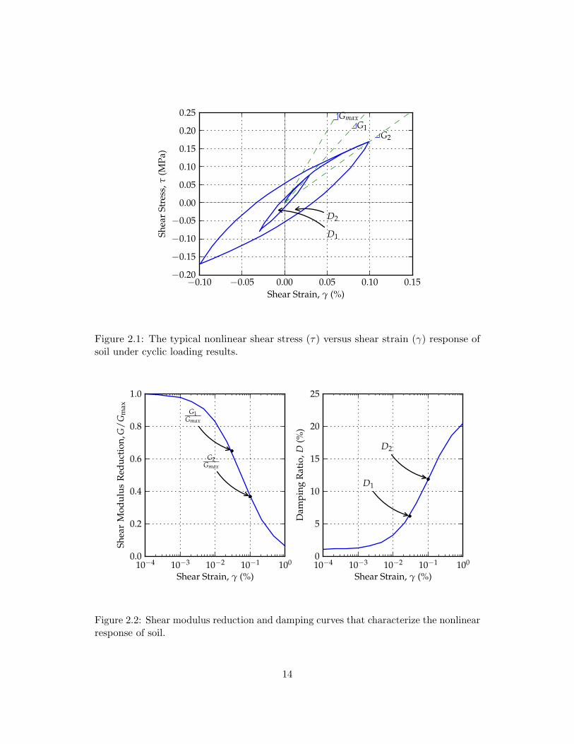
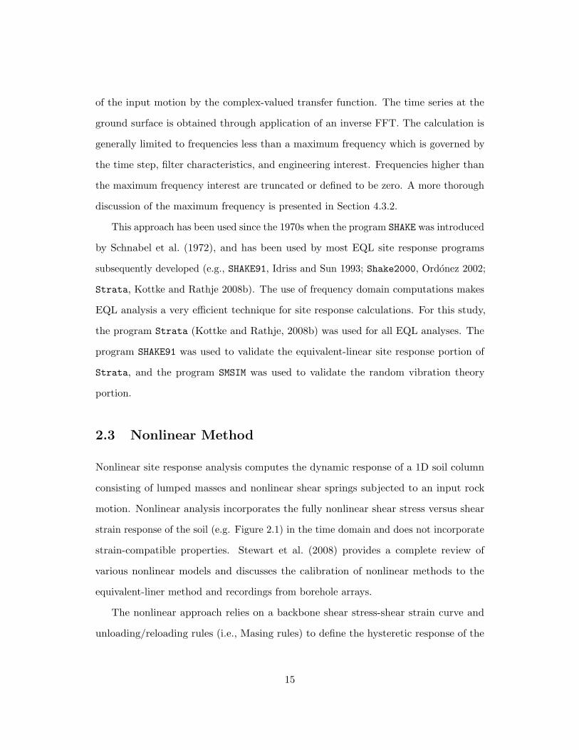
2.1 The typical nonlinear shear stress (τ) versus shear strain (γ) response ofsoil under cyclic loading results. . . . . . . . . . . . . . . . . . . . . . . . 14

2.2 Shear modulus reduction and damping curves that characterize thenonlinear response of soil. . . . . . . . . . . . . . . . . . . . . . . . . . . 14

2.3 The fit of an MKZ nonlinear curve to nonlinear curves computed withthe Darendeli (2001) model. . . . . . . . . . . . . . . . . . . . . . . . . . 17

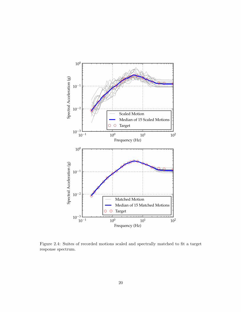
2.4 Suites of recorded motions scaled and spectrally matched to fit a targetresponse spectrum. . . . . . . . . . . . . . . . . . . . . . . . . . . . . . . 20

3.1 The shear-wave velocity profile of the Turkey Flat site (Real, 1988). . . 253.2 The shear-wave velocity profile of the SCH site (Chang, 1996). . . . . . 273.3 The Darendeli (2001) and MKZ curves for the SCH site. . . . . . . . . . 293.4 The shear-wave velocity profile of the CC site (UniStar Nuclear Services,

2007). . . . . . . . . . . . . . . . . . . . . . . . . . . . . . . . . . . . . . 323.5 The Darendeli (2001) and MKZ curves for the CC site (soil types 1 to 3). 343.6 The Darendeli (2001) and MKZ curves for the CC site (soil types 4 to 6). 353.7 The Darendeli (2001) and MKZ curves for the CC site (soil types 7 to 9). 36

4.1 The stochastic FAS computed with seismological theory using the pa-rameters listed in Table 4.1. . . . . . . . . . . . . . . . . . . . . . . . . . 39

4.2 A FAS of a single simulated ground motion, along with the average of100 stochastic simulations and the target FAS . . . . . . . . . . . . . . . 40

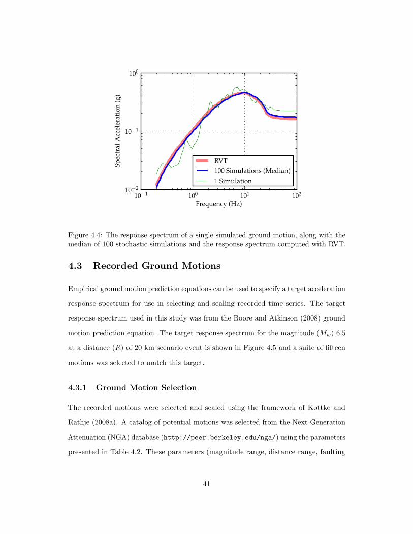
4.3 The acceleration-time series of a single simulated ground motion. . . . . 404.4 The response spectrum of a single simulated ground motion, along with

the median of 100 stochastic simulations and the response spectrumcomputed with RVT. . . . . . . . . . . . . . . . . . . . . . . . . . . . . . 41

4.5 The target acceleration response spectrum computed using the Booreand Atkinson (2008) ground motion prediction equation. . . . . . . . . . 42

4.6 The response spectra of the fifteen ground motions scaled to the targetresponse spectrum. . . . . . . . . . . . . . . . . . . . . . . . . . . . . . . 44

4.7 The FAS of the fifteen ground motions scaled to the target responsespectrum. . . . . . . . . . . . . . . . . . . . . . . . . . . . . . . . . . . . 46

3

4.8 The median response spectrum of the fifteen scaled motions and an RVTmotion defined by the root-mean-square FAS of the scaled motions anda duration of 4.83 seconds. . . . . . . . . . . . . . . . . . . . . . . . . . . 46

4.9 Distribution of the low-pass frequency used in the processing of motionsin the NGA database. . . . . . . . . . . . . . . . . . . . . . . . . . . . . 48

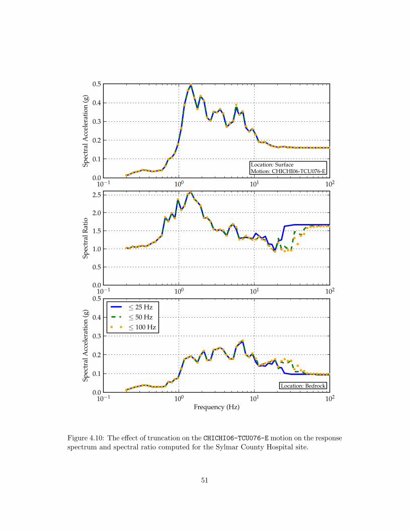
4.10 The effect of truncation on the CHICHI06-TCU076-E motion on the re-sponse spectrum and spectral ratio computed for the Sylmar CountyHospital site. . . . . . . . . . . . . . . . . . . . . . . . . . . . . . . . . . 51

4.11 The effect of truncation on the suite of input ground motions used inthis study. . . . . . . . . . . . . . . . . . . . . . . . . . . . . . . . . . . . 52

4.12 The response spectrum for the scaled, scaled prior to spectral matching,and spectrally matched versions of the NORTHR-WON185 ground motion,along with the target response spectrum. . . . . . . . . . . . . . . . . . . 54

4.13 The acceleration-, velocity-, and displacement-time series for the scaledand spectrally matched versions of the NORTHR-WON185 ground motion. . 55

4.14 The fifteen ground motions spectrally matched and truncated at 25 Hz. 564.15 The standard deviation of the stochastically simulated, scaled, and spec-

trally matched ground motion suites. . . . . . . . . . . . . . . . . . . . . 564.16 A response spectrum compatible RVT motion computed for a seismologi-

cal theory derived target response spectrum, along with the comparisonof the associated FAS . . . . . . . . . . . . . . . . . . . . . . . . . . . . 61

4.17 A response spectrum compatible RVT motion computed from a GMPEderived target response spectrum. . . . . . . . . . . . . . . . . . . . . . . 61

5.1 The input Fourier amplitude and response spectra for the stochasticinput motions. . . . . . . . . . . . . . . . . . . . . . . . . . . . . . . . . 64

5.2 The relative difference of the input response spectrum for the stochasticinput motions. . . . . . . . . . . . . . . . . . . . . . . . . . . . . . . . . 65

5.3 The response spectrum, spectral ratio, and relative difference for theTurkey Flat site computed with LE site response using simulated timeseries and an RVT motion defined by seismological theory. . . . . . . . . 66

5.4 The response spectrum, spectral ratio, and relative difference for theSCH site computed with LE site response using simulated time seriesand an RVT motion defined by seismological theory. . . . . . . . . . . . 67

5.5 The response spectrum, spectral ratio, and relative difference for the CCsite computed with LE site response using simulated time series and anRVT motion defined by seismological theory. . . . . . . . . . . . . . . . 68

5.6 The linear-elastic transfer functions for the three sites used in this study. 705.7 The input FAS for the time series with the largest and smallest spectral

ratios for the SCH site, along with the input FAS of the RVT analysisand the LE transfer function. . . . . . . . . . . . . . . . . . . . . . . . . 71

5.8 The input FAS for the time series with the largest and smallest spectralratios for the CC site, along with the input FAS of the RVT analysis andthe LE transfer function. . . . . . . . . . . . . . . . . . . . . . . . . . . . 72

4

5.9 Sensitivity of the relative difference of the spectral ratio at the sitefrequency and at a frequency of 0.01 seconds to various site characteristics. 74

5.10 The response spectrum, spectral ratio, and relative difference for theSCH computed with EQL site response using simulated time series andan RVT motion defined by seismological theory (input PGA of 0.17 g). . 76

5.11 The response spectrum, spectral ratio, and relative difference for theSCH computed with EQL site response using simulated time series andan RVT motion defined by seismological theory (input PGA of 0.40 g). . 77

5.12 The relative difference of the spectral ratio of the SCH site computedusing simulated time series and an RVT motion defined by seismologicaltheory. . . . . . . . . . . . . . . . . . . . . . . . . . . . . . . . . . . . . . 78

5.13 The maximum strain profiles for the SCH site computed using simulatedtime series and an RVT motion defined by seismological theory. . . . . . 80

5.14 The spectral ratio and maximum strain profiles for selected motionspropagated through the SCH site with an input PGA of 0.40 g. . . . . . 81

5.15 Histograms of the spectral ratio at the site frequency of the RVT analysisfor the SCH site. . . . . . . . . . . . . . . . . . . . . . . . . . . . . . . . 82

5.16 The relative difference of the spectral ratio of the CC site computed usingsimulated time series and an RVT motion defined by seismological theory. 83

5.17 The maximum strain profiles for the CC site computed using simulatedtime series and an RVT motion defined by seismological theory. . . . . . 84

5.18 The input Fourier amplitude and response spectra for the scaled inputmotions, as well as FAS and response spectrum compatible RVT motions. 87

5.19 The relative difference of the input response spectra for the FAS andresponse spectrum compatible RVT motions. . . . . . . . . . . . . . . . 88

5.20 The response spectrum, spectral ratio, and relative difference for theSCH site computed with LE site response using scaled time series, aswell as FAS and response spectrum compatible RVT motions. . . . . . . 89

5.21 The spectral ratios for the SCH site computed with EQL site responseusing scaled time series, as well as FAS and response spectrum compatibleRVT motions. . . . . . . . . . . . . . . . . . . . . . . . . . . . . . . . . . 91

5.22 The maximum strain profiles for the SCH site computed using scaledtime series and a response spectrum compatible RVT motion. . . . . . . 92

5.23 The relative difference of the spectral ratio of the SCH and CC sitescomputed using scaled time series and a response spectrum compatibleRVT motion. . . . . . . . . . . . . . . . . . . . . . . . . . . . . . . . . . 94

5.24 The maximum strain profiles for the CC site computed using scaled timeseries and a response spectrum compatible RVT motion. . . . . . . . . . 95

5.25 The input Fourier amplitude and response spectra for the spectrally-matched time series and a response spectrum compatible RVT motion. . 97

5.26 The relative difference of the input response spectra computed using aresponse spectrum compatible RVT motion. . . . . . . . . . . . . . . . . 98

5

5.27 The response spectrum, spectral ratio, and relative difference for theSCH site computed with LE site response using spectrally-matched timeseries and a response spectrum compatible RVT motion. . . . . . . . . . 99

5.28 The response spectrum, spectral ratio, and relative difference for theSCH site computed with EQL site response using spectrally-matchedtime series and a response spectrum compatible RVT motion (input PGAof 0.13 g). . . . . . . . . . . . . . . . . . . . . . . . . . . . . . . . . . . . 100

5.29 The response spectrum, spectral ratio, and relative difference for theSCH site computed with EQL site response using spectrally-matchedtime series and a response spectrum compatible RVT motion (input PGAof 0.40 g). . . . . . . . . . . . . . . . . . . . . . . . . . . . . . . . . . . . 101

5.30 The maximum strain profiles for the SCH site computed using spectrally-matched time series and a response spectrum compatible RVT motion. . 102

5.31 The relative difference of the spectral ratio of the SCH site computedusing spectrally-matched time series and a response spectrum compatibleRVT motion. . . . . . . . . . . . . . . . . . . . . . . . . . . . . . . . . . 103

5.32 The response spectrum, spectral ratio, and relative difference for the CCsite computed with EQL site response using spectrally-matched timeseries and a response spectrum compatible RVT motion (input PGA of0.13 g). . . . . . . . . . . . . . . . . . . . . . . . . . . . . . . . . . . . . 105

5.33 The maximum strain profiles for the CC site computed using spectrally-matched time series and a response spectrum compatible RVT motion. . 106

5.34 The relative difference of the spectral ratio of the CC site computed usingspectrally-matched time series and a response spectrum compatible RVTmotion. . . . . . . . . . . . . . . . . . . . . . . . . . . . . . . . . . . . . 107

5.35 The computed spectral ratios for the SCH and CC sites at an inputintensity of 0.40 g. . . . . . . . . . . . . . . . . . . . . . . . . . . . . . . 110

6.1 Variation of damping ratio with frequency for the full Rayleigh dampingformulation. . . . . . . . . . . . . . . . . . . . . . . . . . . . . . . . . . . 114

6.2 Spectral ratio of the SCH and CC sites using linear-elastic time domainand frequency domain methods. . . . . . . . . . . . . . . . . . . . . . . . 115

6.3 Amplitude of the transfer function computed for the SCH and CC sitesusing LE time-domain (TD) and frequency-domain (FD) methods. . . . 117

6.4 The spectral ratio and relative difference for the SCH site computed withtime domain and frequency domain methods using the spectrally-matchedground motions. . . . . . . . . . . . . . . . . . . . . . . . . . . . . . . . 120

6.5 The spectral ratio and relative difference for the CC site computed withtime domain and frequency domain methods using the spectrally-matchedground motions. . . . . . . . . . . . . . . . . . . . . . . . . . . . . . . . 121

6.6 Amplitude and phase of the transfer functions computed by the EQLand nonlinear methods for the SCH site (input PGA of 0.01 g). . . . . . 123

6.7 Amplitude and phase of the transfer functions computed by the EQLand nonlinear methods for the CC site (input PGA of 0.01 g). . . . . . . 124

6

6.8 The spectral ratio and relative difference for the SCH site computedwith nonlinear and EQL methods using the spectrally-matched groundmotions (input PGA of 0.13 g). . . . . . . . . . . . . . . . . . . . . . . . 126

6.9 Amplitude and phase of the transfer functions computed by the EQLand nonlinear methods for SCH (input PGA of 0.13 g). . . . . . . . . . 127

6.10 The effect of smooth phase on the surface response spectrum for the SCHsite. . . . . . . . . . . . . . . . . . . . . . . . . . . . . . . . . . . . . . . 129

6.11 The spectral ratio and relative difference for the SCH site computedwith nonlinear and EQL methods using the spectrally-matched groundmotions (input PGA of 0.40 g). . . . . . . . . . . . . . . . . . . . . . . . 130

6.12 The maximum strain profile for the SCH site computed with the nonlinearand EQL methods. . . . . . . . . . . . . . . . . . . . . . . . . . . . . . . 131

6.13 The spectral ratio and relative difference for the CC site computed withnonlinear and EQL methods using the spectrally-matched ground motions.133

6.14 The relative difference of the spectral ratio of the SCH and CC sitescomputed with nonlinear and EQL methods using the spectrally-matchedground motions. . . . . . . . . . . . . . . . . . . . . . . . . . . . . . . . 135

B.1 The CHICHI06-TCU076-E time series scaled by 0.79. . . . . . . . . . . . 148B.2 The ITALY-A-AUL270 time series scaled by 1.55. . . . . . . . . . . . . . 149B.3 The ITALY-A-BAG00 time series scaled by 0.62. . . . . . . . . . . . . . . 150B.4 The ITALY-A-STU270 time series scaled by 0.25. . . . . . . . . . . . . . 151B.5 The ITALY-B-AUL270 time series scaled by 4.19. . . . . . . . . . . . . . 152B.6 The KOZANI-KOZ--L time series scaled by 0.73. . . . . . . . . . . . . . . 153B.7 The LOMAP-G01000 time series scaled by 0.33. . . . . . . . . . . . . . . . 154B.8 The LOMAP-GIL067 time series scaled by 0.32. . . . . . . . . . . . . . . . 155B.9 The MORGAN-GIL337 time series scaled by 2.01. . . . . . . . . . . . . . . 156B.10 The NORTHR-H12180 time series scaled by 0.66. . . . . . . . . . . . . . . 157B.11 The NORTHR-HOW330 time series scaled by 0.83. . . . . . . . . . . . . . . 158B.12 The NORTHR-LV1000 time series scaled by 1.30. . . . . . . . . . . . . . . 159B.13 The NORTHR-LV3090 time series scaled by 1.24. . . . . . . . . . . . . . . 160B.14 The NORTHR-WON185 time series scaled by 0.76. . . . . . . . . . . . . . . 161B.15 The VICT-CPE045 time series scaled by 0.21. . . . . . . . . . . . . . . . . 162

C.1 The spectrally-matched CHICHI06-TCU076-E time series. . . . . . . . . . 164C.2 The spectrally-matched ITALY-A-AUL270 time series. . . . . . . . . . . . 165C.3 The spectrally-matched ITALY-A-BAG000 time series. . . . . . . . . . . . 166C.4 The spectrally-matched ITALY-A-STU270 time series. . . . . . . . . . . . 167C.5 The spectrally-matched ITALY-B-AUL270 time series. . . . . . . . . . . . 168C.6 The spectrally-matched KOZANI-KOZ--L time series. . . . . . . . . . . . 169C.7 The spectrally-matched LOMAP-G01000 time series. . . . . . . . . . . . . 170C.8 The spectrally-matched LOMAP-GIL067 time series. . . . . . . . . . . . . 171C.9 The spectrally-matched MORGAN-GIL337 time series. . . . . . . . . . . . 172C.10 The spectrally-matched NORTHR-H12180 time series. . . . . . . . . . . . 173

7

C.11 The spectrally-matched NORTHR-HOW330 time series. . . . . . . . . . . . 174C.12 The spectrally-matched NORTHR-LV1000 time series. . . . . . . . . . . . 175C.13 The spectrally-matched NORTHR-LV3090 time series. . . . . . . . . . . . 176C.14 The spectrally-matched NORTHR-WON185 time series. . . . . . . . . . . . 177C.15 The spectrally-matched VICT-CPE045 time series. . . . . . . . . . . . . . 178

8

List of Tables

3.1 The shear-wave velocity profile for the Turkey Flat site (Real, 1988). . . 243.2 The shear-wave velocity profile for the SCH site (Chang, 1996). . . . . . 263.3 The soil types and model parameters of the SCH site profile. . . . . . . 283.4 The shear-wave velocity profile for the CC site (UniStar Nuclear Services,

2007). . . . . . . . . . . . . . . . . . . . . . . . . . . . . . . . . . . . . . 313.5 The soil types and model parameters of the CC site profile. . . . . . . . 33

4.1 The selected input parameters used by SMSIM for the calculation of theFourier amplitude spectrum shown in Figure 4.1. . . . . . . . . . . . . . 38

4.2 The parameters used to define the ground motion library for considerationby the selection algorithm. . . . . . . . . . . . . . . . . . . . . . . . . . . 42

4.3 The earthquake events and number of records used in the library ofground motions. . . . . . . . . . . . . . . . . . . . . . . . . . . . . . . . 44

4.4 The ground motions and their properties for the suite shown in Figure 4.6. 454.5 The high-pass and low-pass frequencies of the suite of motions, as well

as the recorded time step. . . . . . . . . . . . . . . . . . . . . . . . . . . 494.6 Parameters for the Abrahamson and Silva (1996) empirical duration model. 59

5.1 Site properties used in the sensitivity analysis. . . . . . . . . . . . . . . 73

9

Chapter 1

Introduction

Local soil conditions influence the characteristics of earthquake ground shaking and

these effects must be taken into account when specifying ground shaking levels for

seismic design. These effects are quantified via site response analysis, which involves

the propagation of earthquake motions from the base rock through the overlying soil

layers to the ground surface. Site response analysis provides surface acceleration-time

series, surface acceleration response spectra, and/or spectral amplification factors based

on the dynamic response of the local soil conditions.

Site response analyses are used to specify the site-specific ground motion response

spectrum (GMRS) used in the seismic design and evaluation of nuclear power plants,

as outlined in NUREG/CR-6728 (McGuire et al., 2001), NUREG/CR-6769 (McGuire

et al., 2002), and Regulatory Guide 1.208 (NRC, 2007). In most cases, one-dimensional

(1D) site response analysis is performed to assess the effect of soil conditions on ground

shaking because vertically-propagating, horizontally-polarized shear waves dominate

the earthquake ground motion wave field. The input motion specification, the 1D wave

propagation, and the model for soil response may vary between different site response

techniques. The most common techniques for site response analysis are equivalent-linear

(EQL) analysis using the time series approach, EQL analysis using the random vibration

10

theory (RVT) approach, or fully nonlinear analysis using the time series approach. These

three techniques are explicitly cited in NUREG/CR-6728 and Regulatory Guide 1.208

as appropriate techniques for site response analysis. However, the dynamic responses

computed via these techniques can vary considerably due to inherent differences in

the numerical approaches (time series vs. RVT), differences in how the nonlinear soil

response is modeled (EQL vs. nonlinear), and differences in the specification of the

input rock motion (time series vs. Fourier amplitude spectrum). This report presents a

comprehensive comparison of these different site response techniques over a range of

site conditions (i.e., shallow soil to very deep soil) and over a range of input intensities

that induce different levels of nonlinearity.

The following report consists of seven chapters. Chapter 2 introduces the equivalent-

linear and nonlinear site response methods, as well as the random vibration theory

approach to site response. Chapter 3 then presents the characteristics and nonlinear

properties of the three sites used in this study. In Chapter 4, the input motions

used in the analyses found in this report are presented. This discussion includes

the characterization of the stochastically-simulated time series, scaled time series and

spectrally-matched time series, as well as response spectrum compatible motion for

random vibration theory. Chapter 5 presents a comparison of the equivalent-linear

method using time series and random vibration theory approaches. Chapter 6 compares

the equivalent-linear and nonlinear methods using a suite of spectrally-match time

series. Chapter 7 presents a summary of the findings of this report and provides

recommendations for future studies.

11

Chapter 2

Site Response Methods

2.1 Introduction

Site response analysis numerically propagates shear waves from the base rock through

the overlying layers of soil to the ground surface. One-dimensional site response analysis

is commonly performed and requires the following information: (1) the shear-wave

velocity profile of the site, (2) the nonlinear stress-strain response of the soil, and

(3) an input rock motion. The shear-wave velocity profile represents the small-strain

stiffness of the soil and is required for all types of site response analysis. The nonlinear

response of the soil can be characterized either through the EQL approach or through

the fully nonlinear approach. Traditionally, all site response methods have required

the specification of an acceleration-time series as the input rock motion, and a suite of

motions is commonly used to develop a statistically stable estimate of the response due

to motion-to-motion variability. Alternatively, RVT can be applied to EQL analysis,

such that only an Fourier amplitude spectrum (FAS) is required as input and the

selection of input motions is avoided. The details regarding the different approaches to

site response analysis (EQL vs. nonlinear) and the different methods of input motion

specification (time series vs. RVT) are discussed in the following chapter.

12

2.2 Equivalent-Linear Method

Equivalent-linear (EQL) site response analysis uses one-dimensional, linear-elastic wave

propagation through layered media to model the dynamic response of the soil deposit.

The method incorporates soil nonlinearity through the use of strain-compatible soil

properties for each soil layer. The typical nonlinear shear stress (τ) versus shear strain

(γ) response of soil under cyclic loading results in a hysteresis loop (Figure 2.1). The

hysteresis loop for a given level of shear strain can be characterized by a secant shear

modulus (G) and a damping ratio (D) that is related to the size of the loop. Generally,

as the shear strain increases, G decreases and D increases. The variations of shear

modulus and damping ratio with shear strain are prescribed through modulus reduction

(G/Gmax) and damping (D) curves (Figure 2.2), in which Gmax is the shear modulus

at small strains. Gmax can be related to shear-wave velocity (Vs) through the mass

density (ρ) of the soil (Gmax = ρV 2s ).

The key to the EQL approach is the selection of soil properties (G and D) for each

soil layer that are consistent with the level of shear strain induced by the input rock

motion. Development of strain-compatible properties requires an iterative approach

in which the strains are computed, the properties are revised based on the strains,

and revised strains are computed based on the updated properties. These iterations

continue until the properties assigned to each layer in the wave-propagation analysis

are consistent with the strains generated in each layer. The strain level used to select

the strain-compatible properties is not the peak time domain shear strain, but rather

an effective shear strain (γeff) that typically is about 65% of the peak value.

Another important aspect of EQL site response analysis is that it is performed in the

frequency domain using transfer functions. The input time series is first converted to the

frequency domain using the Fast Fourier Transform (FFT), and the wave propagation

calculations are simply performed by multiplying the complex-valued Fourier amplitudes

13

−0.10 −0.05 0.00 0.05 0.10 0.15Shear Strain, γ (%)

−0.20

−0.15

−0.10

−0.05

0.00

0.05

0.10

0.15

0.20

0.25

Shea

rSt

ress

,τ(M

Pa)

GmaxG1

G2

D1

D2

Figure 2.1: The typical nonlinear shear stress (τ) versus shear strain (γ) response ofsoil under cyclic loading results.

10−4 10−3 10−2 10−1 100

Shear Strain, γ (%)

0.0

0.2

0.4

0.6

0.8

1.0

Shea

rM

odul

usR

educ

tion

,G/

Gm

ax

G1Gmax

G2Gmax

10−4 10−3 10−2 10−1 100

Shear Strain, γ (%)

0

5

10

15

20

25

Dam

ping

Rat

io,D

(%)

D1

D2

Figure 2.2: Shear modulus reduction and damping curves that characterize the nonlinearresponse of soil.

14

of the input motion by the complex-valued transfer function. The time series at the

ground surface is obtained through application of an inverse FFT. The calculation is

generally limited to frequencies less than a maximum frequency which is governed by

the time step, filter characteristics, and engineering interest. Frequencies higher than

the maximum frequency interest are truncated or defined to be zero. A more thorough

discussion of the maximum frequency is presented in Section 4.3.2.

This approach has been used since the 1970s when the program SHAKE was introduced

by Schnabel et al. (1972), and has been used by most EQL site response programs

subsequently developed (e.g., SHAKE91, Idriss and Sun 1993; Shake2000, Ordonez 2002;

Strata, Kottke and Rathje 2008b). The use of frequency domain computations makes

EQL analysis a very efficient technique for site response calculations. For this study,

the program Strata (Kottke and Rathje, 2008b) was used for all EQL analyses. The

program SHAKE91 was used to validate the equivalent-linear site response portion of

Strata, and the program SMSIM was used to validate the random vibration theory

portion.

2.3 Nonlinear Method

Nonlinear site response analysis computes the dynamic response of a 1D soil column

consisting of lumped masses and nonlinear shear springs subjected to an input rock

motion. Nonlinear analysis incorporates the fully nonlinear shear stress versus shear

strain response of the soil (e.g. Figure 2.1) in the time domain and does not incorporate

strain-compatible properties. Stewart et al. (2008) provides a complete review of

various nonlinear models and discusses the calibration of nonlinear methods to the

equivalent-liner method and recordings from borehole arrays.

The nonlinear approach relies on a backbone shear stress-shear strain curve and

unloading/reloading rules (i.e., Masing rules) to define the hysteretic response of the

15

soil under cyclic loading. A common backbone curve is the MKZ model (Matasovic and

Vucetic, 1993), which is a modified hyperbola defined as:

τ =Gmax · γ

1 + α(γγr

)s (2.1)

This curve requires three fitting parameters: α, γr, and s, in addition to Gmax (which

is defined for each layer based on the shear-wave velocity profile). The Masing rules

use the backbone curve to generate the unload/reload response under cyclic loading,

and these hysteresis loops represent the modeled levels of damping. Additional viscous

damping (Dmin) is required to model energy dissipation at very small strains where

hysteretic damping is essentially zero and not representative of soil.

Most laboratory tests provide information regarding the nonlinear properties of

soil in the form of modulus reduction and damping curves (Figure 2.2) rather than

shear-stress shear-strain curves. To relate a nonlinear stress-strain model to measured

modulus reduction and damping curves, a nonlinear backbone curve and its associated

hysteresis loops at different strain levels are converted into equivalent G/Gmax and D

curves. The nonlinear fitting parameters are selected such that the equivalent modulus

reduction and damping curves from the nonlinear model match those specified for the

soil. Figure 2.3 shows a comparison of modulus reduction and damping curves from

the empirical model of Darendeli (2001) with those from the MKZ model. The MKZ

parameters were selected based on a least-sum-square-of-error fit to the Darendeli (2001)

curves over the entire strain range. While the MKZ curves show favorable agreement at

smaller strains, they deviate from the empirical curves at larger strains. In particular,

the MKZ damping curve produces much larger damping at larger strains. This issue is

common with nonlinear models and is caused by the shape of the modified hyperbolic

stress-strain curve at large strains and the use of the Masing rules to generate the

hysteresis loops.

16

10−4 10−3 10−2 10−1 1000.0

0.2

0.4

0.6

0.8

1.0Sh

ear

Mod

ulus

Red

ucti

on,G

/G

max

10−4 10−3 10−2 10−1 100

Shear Strain, γ (%)

0

5

10

15

20

25

30

35

Dam

ping

Rat

io,D

(%)

Darendeli (σ′m=1 atm, PI=20, OCR=1)

MKZ (α=0.60, γr=0.036, s=0.79, Dmin= 0.69%)

Figure 2.3: The fit of an MKZ nonlinear curve to nonlinear curves computed with theDarendeli (2001) model.

17

For this study, the nonlinear site response program DeepSoil (Hashash, 2002;

Hashash and Park, 2001) was used. DeepSoil incorporates the MKZ backbone model,

and viscous damping is incorporated via the Rayleigh damping formulation. Rayleigh

damping is frequency dependent, and thus the target viscous damping is achieved

only at specified target frequencies. The target frequencies were generally specified as

the first mode natural frequency (fs) and five times the first mode natural frequency

(5 · fs), as recommended by Stewart et al. (2008). Additionally, frequency-independent

Rayleigh damping (Phillips and Hashash, 2009) was also investigated. The MKZ model

parameters were selected to best fit both the specified modulus reduction and damping

curves for each layer.

2.4 Input Motion Specification

Equivalent-linear and nonlinear wave propagation analysis requires specification of an

input rock motion. For EQL analysis, this input acceleration-time series is converted to

the frequency domain using the FFT, the resulting FAS is multiplied by the transfer

function that represents wave propagation to the ground surface, and the FAS at the

surface is converted to an acceleration-time series using the inverse FFT. Nonlinear

analysis solves the differential equations of motion in the time domain using numerical

time stepping methods, and the properties of the system vary with each time step to

incorporate the nonlinear response of the soil. Here, the input time series is used as the

forcing function for the time stepping method.

Commonly, a suite of input motions is used to capture the motion-to-motion

variability present in earthquake ground motions for similar events. A suite is required

because the detailed characteristics of each input motion influence the induced dynamic

response. A suite of recorded motions can be linearly scaled to match, on average, a

target acceleration response spectrum (Figure 2.4). In this case, the median response

18

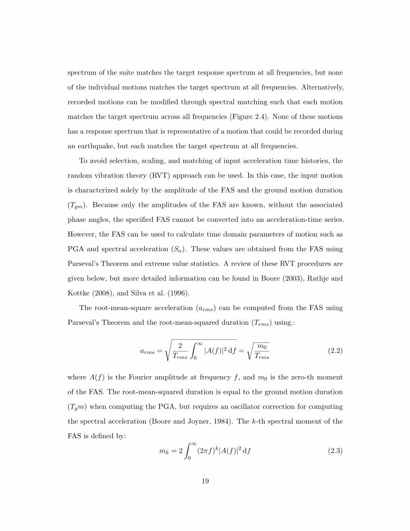
spectrum of the suite matches the target response spectrum at all frequencies, but none

of the individual motions matches the target spectrum at all frequencies. Alternatively,

recorded motions can be modified through spectral matching such that each motion

matches the target spectrum across all frequencies (Figure 2.4). None of these motions

has a response spectrum that is representative of a motion that could be recorded during

an earthquake, but each matches the target spectrum at all frequencies.

To avoid selection, scaling, and matching of input acceleration time histories, the

random vibration theory (RVT) approach can be used. In this case, the input motion

is characterized solely by the amplitude of the FAS and the ground motion duration

(Tgm). Because only the amplitudes of the FAS are known, without the associated

phase angles, the specified FAS cannot be converted into an acceleration-time series.

However, the FAS can be used to calculate time domain parameters of motion such as

PGA and spectral acceleration (Sa). These values are obtained from the FAS using

Parseval’s Theorem and extreme value statistics. A review of these RVT procedures are

given below, but more detailed information can be found in Boore (2003), Rathje and

Kottke (2008), and Silva et al. (1996).

The root-mean-square acceleration (arms) can be computed from the FAS using

Parseval’s Theorem and the root-mean-squared duration (Trms) using.:

arms =

√2

Trms

∫ ∞0|A(f)|2 df =

√m0

Trms(2.2)

where A(f) is the Fourier amplitude at frequency f , and m0 is the zero-th moment

of the FAS. The root-mean-squared duration is equal to the ground motion duration

(Tgm) when computing the PGA, but requires an oscillator correction for computing

the spectral acceleration (Boore and Joyner, 1984). The k-th spectral moment of the

FAS is defined by:

mk = 2∫ ∞

0(2πf)k|A(f)|2 df (2.3)

19

10−1 100 101 102

Frequency (Hz)

10−3

10−2

10−1

100

Spec

tral

Acc

eler

atio

n(g

)

Scaled MotionMedian of 15 Scaled MotionsTarget

10−1 100 101 102

Frequency (Hz)

10−3

10−2

10−1

100

Spec

tral

Acc

eler

atio

n(g

)

Matched MotionMedian of 15 Matched MotionsTarget

Figure 2.4: Suites of recorded motions scaled and spectrally matched to fit a targetresponse spectrum.

20

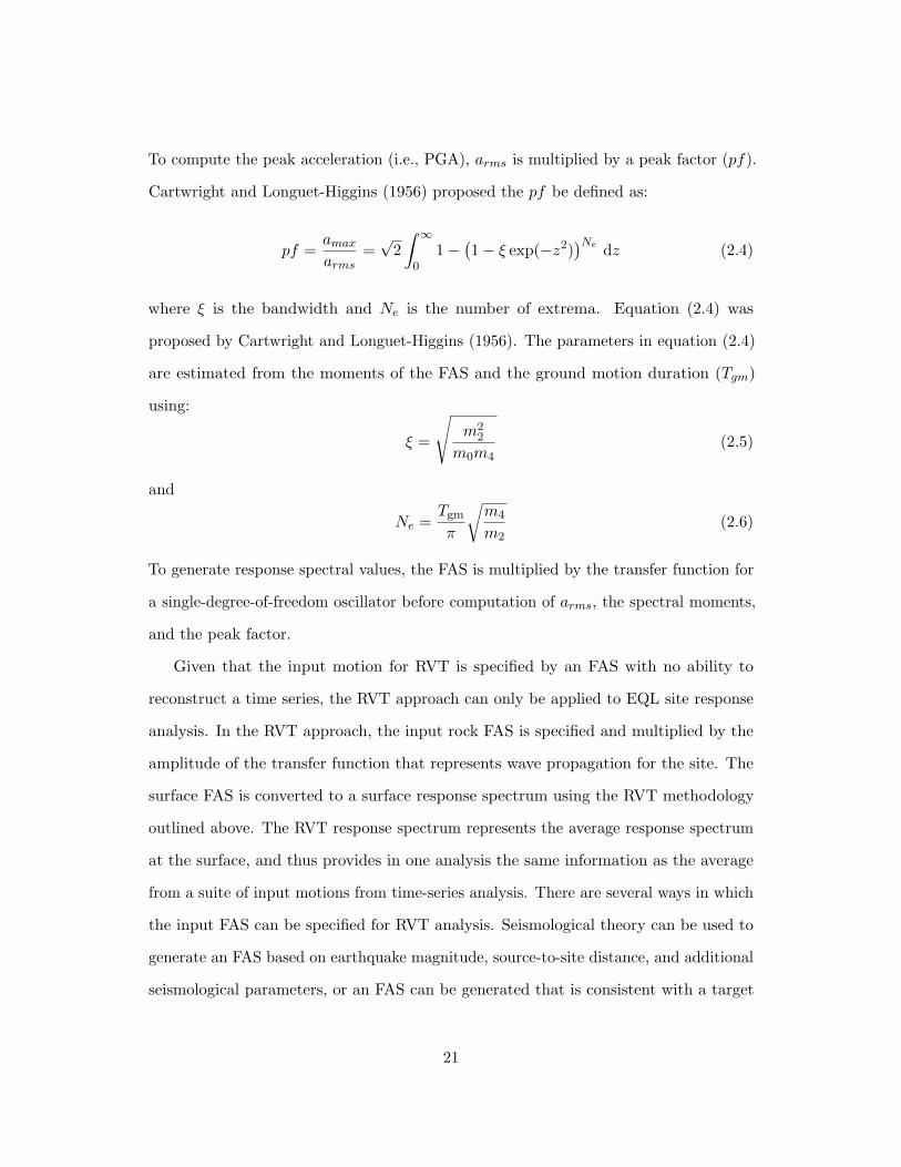
To compute the peak acceleration (i.e., PGA), arms is multiplied by a peak factor (pf).

Cartwright and Longuet-Higgins (1956) proposed the pf be defined as:

pf =amaxarms

=√

2∫ ∞

01− (1− ξ exp(−z2)

)Ne dz (2.4)

where ξ is the bandwidth and Ne is the number of extrema. Equation (2.4) was

proposed by Cartwright and Longuet-Higgins (1956). The parameters in equation (2.4)

are estimated from the moments of the FAS and the ground motion duration (Tgm)

using:

ξ =

√m2

2

m0m4(2.5)

and

Ne =Tgm

π

√m4

m2(2.6)

To generate response spectral values, the FAS is multiplied by the transfer function for

a single-degree-of-freedom oscillator before computation of arms, the spectral moments,

and the peak factor.

Given that the input motion for RVT is specified by an FAS with no ability to

reconstruct a time series, the RVT approach can only be applied to EQL site response

analysis. In the RVT approach, the input rock FAS is specified and multiplied by the

amplitude of the transfer function that represents wave propagation for the site. The

surface FAS is converted to a surface response spectrum using the RVT methodology

outlined above. The RVT response spectrum represents the average response spectrum

at the surface, and thus provides in one analysis the same information as the average

from a suite of input motions from time-series analysis. There are several ways in which

the input FAS can be specified for RVT analysis. Seismological theory can be used to

generate an FAS based on earthquake magnitude, source-to-site distance, and additional

seismological parameters, or an FAS can be generated that is consistent with a target

21

input rock acceleration response spectrum or an FAS from a suite of time series. These

different methods are discussed and compared in Chapter 4.

2.5 Linear Elastic Simplification

In both equivalent-linear and nonlinear methods, the strain dependence of the properties

can obscure the differences of various approaches and methods. In this report, strain-

independent linear-elastic (LE) analyses are used as an initial point of comparison. In

the equivalent-linear method, the linear-elastic simplification is achieved by using the

maximum shear-modulus value and a fixed value for the damping ratio. Whereas in the

nonlinear method, the linear elastic simplification is made by defining the exponent term

(s) in equation (2.1) to be zero and damping ratio is defined solely by the viscous damping

(Dmin) value. The linear-elastic simplification is made to facilitate the identification

and explanation of differences not associated with discrepancies strain level. However,

in comparing the actual differences it is important that the differences in computed

strain level are considered.

22

Chapter 3

Site Profiles Analyzed

3.1 Introduction

Three sites were analyzed as part of this study to compare the different site response

methods. The sites range from shallow to deep, and were selected to investigate a range

of fundamental site frequencies and regional characteristics. The characteristics of these

sites as well as their characterization for site response analysis are discussed in this

chapter.

3.2 Turkey Flat Site

The Turkey Flat site is located in the central California Coast Range near the town

of Parkfield, California. The site consists generally of 20 meters of coarse-grained

alluvium over bedrock. The site characteristics presented in Table 3.1 were proposed

by Real et al. (2006) and are plotted in Figure 3.1. No nonlinear curves for the soil

are presented because the site will only be used in LE analyses that require only a

prescribed damping. The natural frequency of a site (fs) can be estimated as the

23

quarter-wavelength frequency, using:

fs =Vs4H

(3.1)

where H is the depth to bedrock and Vs is the time-averaged shear-wave velocity defined

by:

Vs =∑

i hi∑i hi/Vs,i

(3.2)

where hi and Vs,i are the thickness and shear-wave velocity, respectively, of layer i.

Using equation (3.1) the site frequency for Turkey Flat is estimated to be 4.76 Hz.

Depth Thickness Soil Type Vs γt Damping(m) (m) (m/s) (kN/m3) (%)0 2.4 Alluvium 135 18 5

2.4 5.2 Alluvium 460 18 57.6 13.7 Alluvium 610 18 521.3 ∞ Bedrock 1340 22 1

Table 3.1: The shear-wave velocity profile for the Turkey Flat site (Real, 1988).

24

0 200 400 600 800 1000 1200 1400Shear-wave Velocity (m/s)

0

5

10

15

20

25

Dep

th(m

)

Figure 3.1: The shear-wave velocity profile of the Turkey Flat site (Real, 1988).

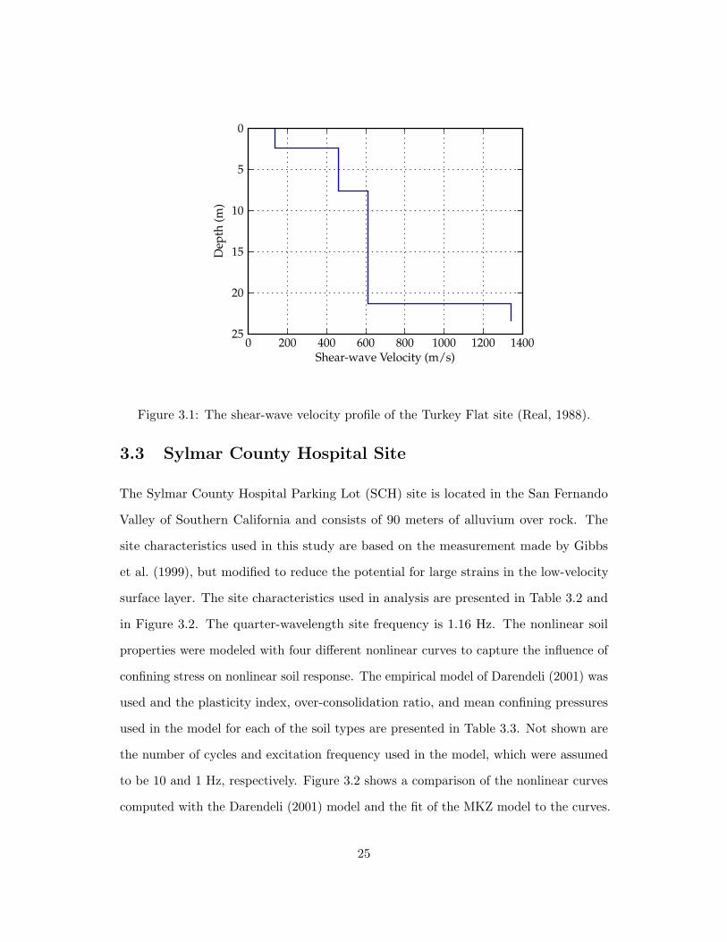
3.3 Sylmar County Hospital Site

The Sylmar County Hospital Parking Lot (SCH) site is located in the San Fernando

Valley of Southern California and consists of 90 meters of alluvium over rock. The

site characteristics used in this study are based on the measurement made by Gibbs

et al. (1999), but modified to reduce the potential for large strains in the low-velocity

surface layer. The site characteristics used in analysis are presented in Table 3.2 and

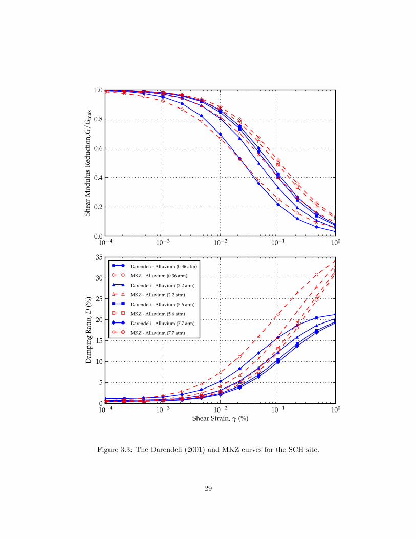
in Figure 3.2. The quarter-wavelength site frequency is 1.16 Hz. The nonlinear soil

properties were modeled with four different nonlinear curves to capture the influence of

confining stress on nonlinear soil response. The empirical model of Darendeli (2001) was

used and the plasticity index, over-consolidation ratio, and mean confining pressures

used in the model for each of the soil types are presented in Table 3.3. Not shown are

the number of cycles and excitation frequency used in the model, which were assumed

to be 10 and 1 Hz, respectively. Figure 3.2 shows a comparison of the nonlinear curves

computed with the Darendeli (2001) model and the fit of the MKZ model to the curves.

25

There is generally good agreement between the curves, except that the MKZ damping

curves are higher at strains greater than about 0.1%. The resulting MKZ parameters

are listed in Table 3.3. The bedrock layer was assumed to have a damping ratio of 1%.

Depth Thickness Soil Type Vs

(m) (m) (m/s)0 6 Alluvium (0.36 atm) 2506 25 Alluvium (2.2 atm) 30031 30 Alluvium (5.6 atm) 46061 30 Alluvium (7.7 atm) 70091 ∞ Bedrock 760

Table 3.2: The shear-wave velocity profile for the SCH site (Chang, 1996).

26

200 300 400 500 600 700 800Shear-wave Velocity (m/s)

0

20

40

60

80

100

120

Dep

th(m

)

Figure 3.2: The shear-wave velocity profile of the SCH site (Chang, 1996).

27

Dar

end

eli

Par

amet

ers

MK

ZP

aram

eter

sS

oil

Typ

eU

nit

Wt.

σ′ m

PI

OC

Rα

γr

sD

min

(kN

/m3)

(atm

)(%

)(%

)A

lluvi

um(0

.36

atm

)18

0.36

01.

01.

237

3.25

E-0

20.

772

0.43

8A

lluvi

um(2

.2at

m)

182.

20

1.0

0.85

65.

10E

-02

0.81

60.

388

Allu

vium

(5.6

atm

)19

5.6

01.

00.

605

5.18

E-0

20.

837

0.33

6A

lluvi

um(7

.7at

m)

227.

70

1.0

0.51

54.

97E

-02

0.84

40.

317

Bed

rock

22–

––

––

––

Tab

le3.

3:T

heso

ilty

pes

and

mod

elpa

ram

eter

sof

the

SCH

site

profi

le.

28

10−4 10−3 10−2 10−1 1000.0

0.2

0.4

0.6

0.8

1.0Sh

ear

Mod

ulus

Red

ucti

on,G

/G

max

10−4 10−3 10−2 10−1 100

Shear Strain, γ (%)

0

5

10

15

20

25

30

35

Dam

ping

Rat

io,D

(%)

Darendeli - Alluvium (0.36 atm)

MKZ - Alluvium (0.36 atm)

Darendeli - Alluvium (2.2 atm)

MKZ - Alluvium (2.2 atm)

Darendeli - Alluvium (5.6 atm)

MKZ - Alluvium (5.6 atm)

Darendeli - Alluvium (7.7 atm)

MKZ - Alluvium (7.7 atm)

Figure 3.3: The Darendeli (2001) and MKZ curves for the SCH site.

29

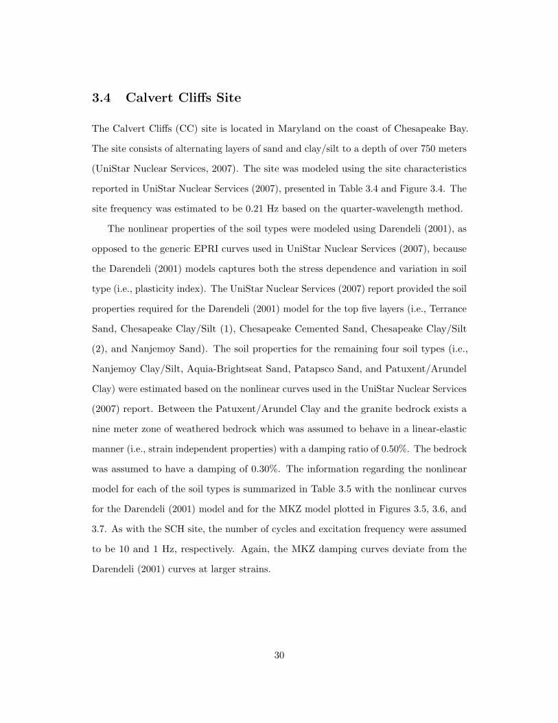
3.4 Calvert Cliffs Site

The Calvert Cliffs (CC) site is located in Maryland on the coast of Chesapeake Bay.

The site consists of alternating layers of sand and clay/silt to a depth of over 750 meters

(UniStar Nuclear Services, 2007). The site was modeled using the site characteristics

reported in UniStar Nuclear Services (2007), presented in Table 3.4 and Figure 3.4. The

site frequency was estimated to be 0.21 Hz based on the quarter-wavelength method.

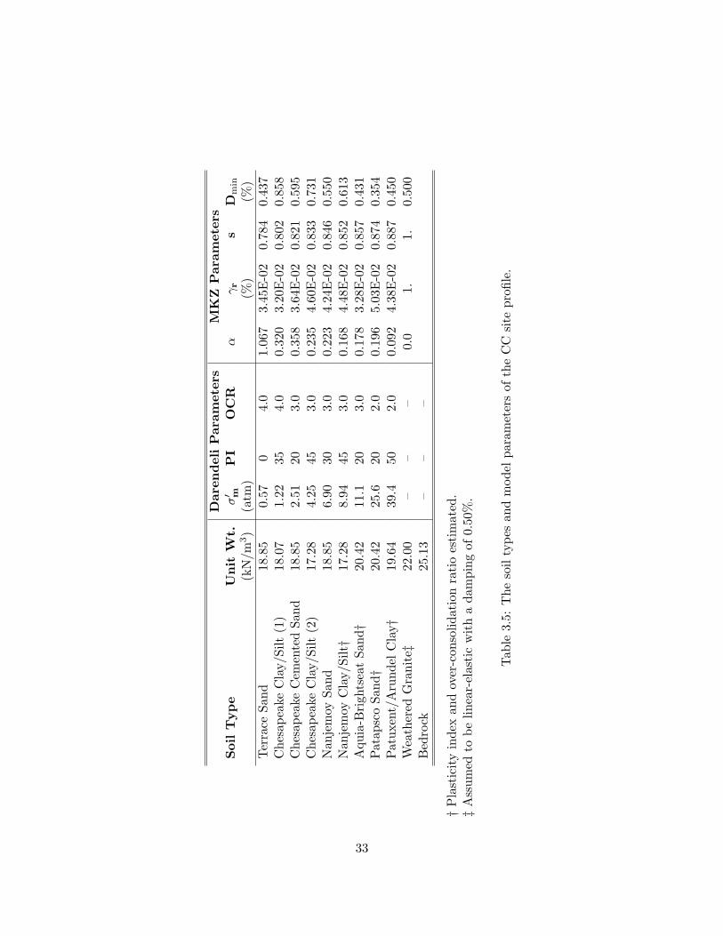
The nonlinear properties of the soil types were modeled using Darendeli (2001), as

opposed to the generic EPRI curves used in UniStar Nuclear Services (2007), because

the Darendeli (2001) models captures both the stress dependence and variation in soil

type (i.e., plasticity index). The UniStar Nuclear Services (2007) report provided the soil

properties required for the Darendeli (2001) model for the top five layers (i.e., Terrance

Sand, Chesapeake Clay/Silt (1), Chesapeake Cemented Sand, Chesapeake Clay/Silt

(2), and Nanjemoy Sand). The soil properties for the remaining four soil types (i.e.,

Nanjemoy Clay/Silt, Aquia-Brightseat Sand, Patapsco Sand, and Patuxent/Arundel

Clay) were estimated based on the nonlinear curves used in the UniStar Nuclear Services

(2007) report. Between the Patuxent/Arundel Clay and the granite bedrock exists a

nine meter zone of weathered bedrock which was assumed to behave in a linear-elastic

manner (i.e., strain independent properties) with a damping ratio of 0.50%. The bedrock

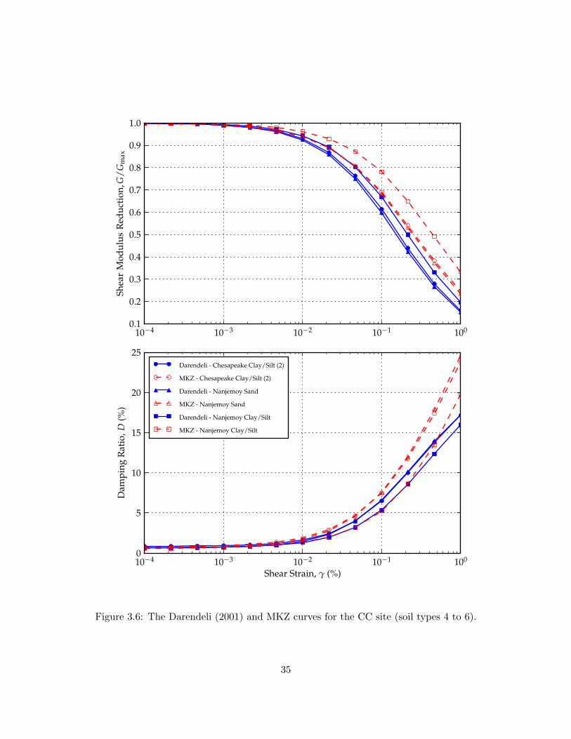
was assumed to have a damping of 0.30%. The information regarding the nonlinear

model for each of the soil types is summarized in Table 3.5 with the nonlinear curves

for the Darendeli (2001) model and for the MKZ model plotted in Figures 3.5, 3.6, and

3.7. As with the SCH site, the number of cycles and excitation frequency were assumed

to be 10 and 1 Hz, respectively. Again, the MKZ damping curves deviate from the

Darendeli (2001) curves at larger strains.

30

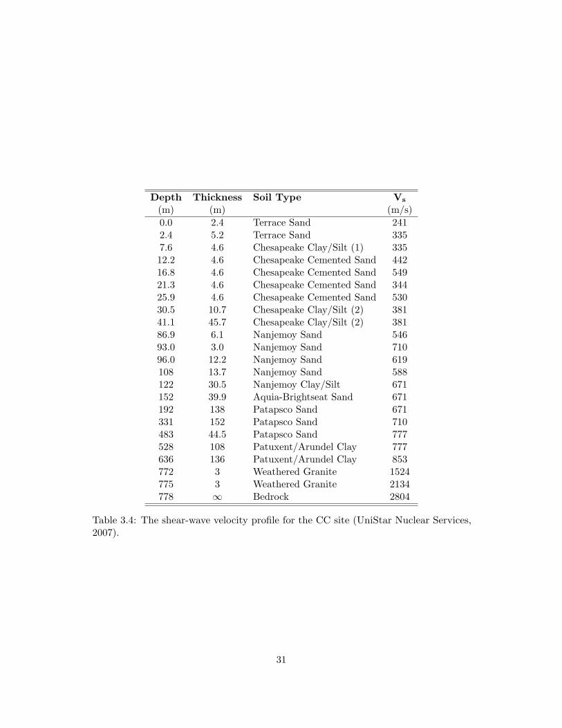
Depth Thickness Soil Type Vs

(m) (m) (m/s)0.0 2.4 Terrace Sand 2412.4 5.2 Terrace Sand 3357.6 4.6 Chesapeake Clay/Silt (1) 33512.2 4.6 Chesapeake Cemented Sand 44216.8 4.6 Chesapeake Cemented Sand 54921.3 4.6 Chesapeake Cemented Sand 34425.9 4.6 Chesapeake Cemented Sand 53030.5 10.7 Chesapeake Clay/Silt (2) 38141.1 45.7 Chesapeake Clay/Silt (2) 38186.9 6.1 Nanjemoy Sand 54693.0 3.0 Nanjemoy Sand 71096.0 12.2 Nanjemoy Sand 619108 13.7 Nanjemoy Sand 588122 30.5 Nanjemoy Clay/Silt 671152 39.9 Aquia-Brightseat Sand 671192 138 Patapsco Sand 671331 152 Patapsco Sand 710483 44.5 Patapsco Sand 777528 108 Patuxent/Arundel Clay 777636 136 Patuxent/Arundel Clay 853772 3 Weathered Granite 1524775 3 Weathered Granite 2134778 ∞ Bedrock 2804

Table 3.4: The shear-wave velocity profile for the CC site (UniStar Nuclear Services,2007).

31

0 500 1000 1500 2000 2500 3000Shear-wave Velocity (m/s)

0

100

200

300

400

500

600

700

800

900

Dep

th(m

)

Figure 3.4: The shear-wave velocity profile of the CC site (UniStar Nuclear Services,2007).

32

Dar

end

eli

Par

amet

ers

MK

ZP

aram

eter

sS

oil

Typ

eU

nit

Wt.

σ′ m

PI

OC

Rα

γr

sD

min

(kN

/m3)

(atm

)(%

)(%

)T

erra

ceSa

nd18

.85

0.57

04.

01.

067

3.45

E-0

20.

784

0.43

7C

hesa

peak

eC

lay/

Silt

(1)

18.0

71.

2235

4.0

0.32

03.

20E

-02

0.80

20.

858

Che

sape

ake

Cem

ente

dSa

nd18

.85

2.51

203.

00.

358

3.64

E-0

20.

821

0.59

5C

hesa

peak

eC

lay/

Silt

(2)

17.2

84.

2545

3.0

0.23

54.

60E

-02

0.83

30.

731

Nan

jem

oySa

nd18

.85

6.90

303.

00.

223

4.24

E-0

20.

846

0.55

0N

anje

moy

Cla

y/Si

lt†

17.2

88.

9445

3.0

0.16

84.

48E

-02

0.85

20.

613

Aqu

ia-B

righ

tsea

tSa

nd†

20.4

211

.120

3.0

0.17

83.

28E

-02

0.85

70.

431

Pat

apsc

oSa

nd†

20.4

225

.620

2.0

0.19

65.

03E

-02

0.87

40.

354

Pat

uxen

t/A

rund

elC

lay†

19.6

439

.450

2.0

0.09

24.

38E

-02

0.88

70.

450

Wea

ther

edG

rani

te‡

22.0

0–

––

0.0

1.1.

0.50

0B

edro

ck25

.13

––

–

†Pla

stic

ity

inde

xan

dov

er-c

onso

lidat

ion

rati

oes

tim

ated

.‡A

ssum

edto

belin

ear-

elas

tic

wit

ha

dam

ping

of0.

50%

.

Tab

le3.

5:T

heso

ilty

pes

and

mod

elpa

ram

eter

sof

the

CC

site

profi

le.

33

10−4 10−3 10−2 10−1 1000.0

0.2

0.4

0.6

0.8

1.0Sh

ear

Mod

ulus

Red

ucti

on,G

/G

max

10−4 10−3 10−2 10−1 100

Shear Strain, γ (%)

0

5

10

15

20

25

30

35

Dam

ping

Rat

io,D

(%)

Darendeli - Terrace Sand

MKZ - Terrace Sand

Darendeli - Chesapeake Clay/Silt (1)

MKZ - Chesapeake Clay/Silt (1)

Darendeli - Chesapeake Cemented Sand

MKZ - Chesapeake Cemented Sand

Figure 3.5: The Darendeli (2001) and MKZ curves for the CC site (soil types 1 to 3).

34

10−4 10−3 10−2 10−1 1000.1

0.2

0.3

0.4

0.5

0.6

0.7

0.8

0.9

1.0Sh

ear

Mod

ulus

Red

ucti

on,G

/G

max

10−4 10−3 10−2 10−1 100

Shear Strain, γ (%)

0

5

10

15

20

25

Dam

ping

Rat

io,D

(%)

Darendeli - Chesapeake Clay/Silt (2)

MKZ - Chesapeake Clay/Silt (2)

Darendeli - Nanjemoy Sand

MKZ - Nanjemoy Sand

Darendeli - Nanjemoy Clay/Silt

MKZ - Nanjemoy Clay/Silt

Figure 3.6: The Darendeli (2001) and MKZ curves for the CC site (soil types 4 to 6).

35

10−4 10−3 10−2 10−1 1000.1

0.2

0.3

0.4

0.5

0.6

0.7

0.8

0.9

1.0Sh

ear

Mod

ulus

Red

ucti

on,G

/G

max

10−4 10−3 10−2 10−1 100

Shear Strain, γ (%)

0

5

10

15

20

25

30

Dam

ping

Rat

io,D

(%)

Darendeli - Aquia-Brightseat Sand

MKZ - Aquia-Brightseat Sand

Darendeli - Patapsco Sand

MKZ - Patapsco Sand

Darendeli - Patuxent/Arundel Clay

MKZ - Patuxent/Arundel Clay

Figure 3.7: The Darendeli (2001) and MKZ curves for the CC site (soil types 7 to 9).

36

Chapter 4

Input Ground Motion

Characterization

4.1 Introduction

Three separate suites of input ground motions were generated for the site response

analyses for a hypothetical magnitude 6.5 earthquake at a distance of 20 km. The

first suite consisted of numerically simulated time series generated via seismological

simulations using a theoretical FAS and stochastic simulation methods using SMSIM

(Boore, 2003). The second suite consisted of recorded motions selected and scaled to fit

a response spectrum from a ground motion prediction equation. The third suite was

generated by spectral matching the selected motions to fit the response spectrum from

the ground motion prediction equation. The consistency of each of the suites of time

series with the input required for RVT analysis (i.e., the Fourier amplitude spectra and

response spectra) is also considered.

37

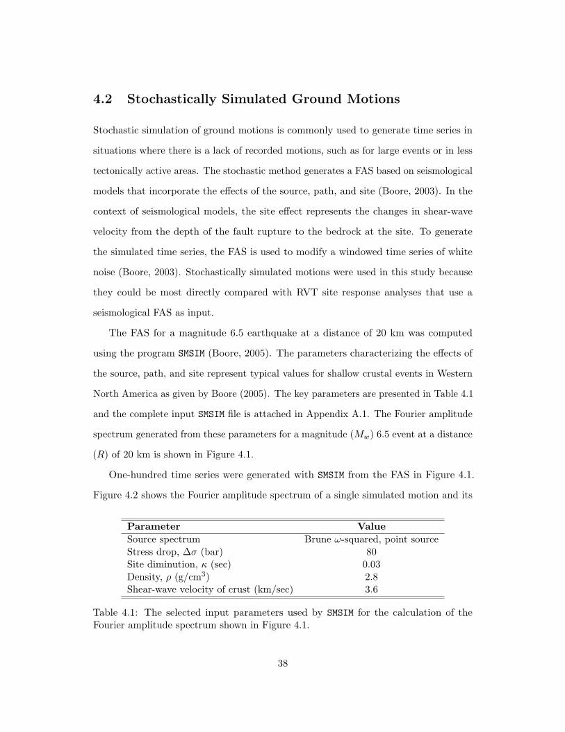
4.2 Stochastically Simulated Ground Motions

Stochastic simulation of ground motions is commonly used to generate time series in

situations where there is a lack of recorded motions, such as for large events or in less

tectonically active areas. The stochastic method generates a FAS based on seismological

models that incorporate the effects of the source, path, and site (Boore, 2003). In the

context of seismological models, the site effect represents the changes in shear-wave

velocity from the depth of the fault rupture to the bedrock at the site. To generate

the simulated time series, the FAS is used to modify a windowed time series of white

noise (Boore, 2003). Stochastically simulated motions were used in this study because

they could be most directly compared with RVT site response analyses that use a

seismological FAS as input.

The FAS for a magnitude 6.5 earthquake at a distance of 20 km was computed

using the program SMSIM (Boore, 2005). The parameters characterizing the effects of

the source, path, and site represent typical values for shallow crustal events in Western

North America as given by Boore (2005). The key parameters are presented in Table 4.1

and the complete input SMSIM file is attached in Appendix A.1. The Fourier amplitude

spectrum generated from these parameters for a magnitude (Mw) 6.5 event at a distance

(R) of 20 km is shown in Figure 4.1.

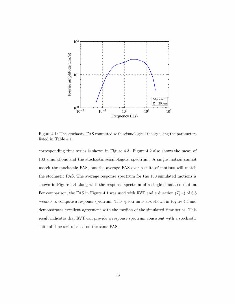
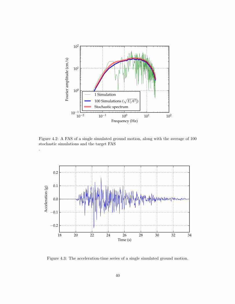
One-hundred time series were generated with SMSIM from the FAS in Figure 4.1.

Figure 4.2 shows the Fourier amplitude spectrum of a single simulated motion and its

Parameter ValueSource spectrum Brune ω-squared, point sourceStress drop, ∆σ (bar) 80Site diminution, κ (sec) 0.03Density, ρ (g/cm3) 2.8Shear-wave velocity of crust (km/sec) 3.6

Table 4.1: The selected input parameters used by SMSIM for the calculation of theFourier amplitude spectrum shown in Figure 4.1.

38

10−2 10−1 100 101 102

Frequency (Hz)

100

101

102

Four

ier

ampl

itud

e(c

m/s

)

Mw = 6.5R = 20 km

Figure 4.1: The stochastic FAS computed with seismological theory using the parameterslisted in Table 4.1.

corresponding time series is shown in Figure 4.3. Figure 4.2 also shows the mean of

100 simulations and the stochastic seismological spectrum. A single motion cannot

match the stochastic FAS, but the average FAS over a suite of motions will match

the stochastic FAS. The average response spectrum for the 100 simulated motions is

shown in Figure 4.4 along with the response spectrum of a single simulated motion.

For comparison, the FAS in Figure 4.1 was used with RVT and a duration (Tgm) of 6.8

seconds to compute a response spectrum. This spectrum is also shown in Figure 4.4 and

demonstrates excellent agreement with the median of the simulated time series. This

result indicates that RVT can provide a response spectrum consistent with a stochastic

suite of time series based on the same FAS.

39

10−2 10−1 100 101 102

Frequency (Hz)

10−1

100

101

102

Four

ier

ampl

itud

e(c

m/s

)

1 Simulation

100 Simulations (√

E[A2])Stochastic spectrum

Figure 4.2: A FAS of a single simulated ground motion, along with the average of 100stochastic simulations and the target FAS.

18 20 22 24 26 28 30 32 34Time (s)

−0.2

−0.1

0.0

0.1

0.2

Acc

eler

atio

n(g

)

Figure 4.3: The acceleration-time series of a single simulated ground motion.

40

10−1 100 101 102

Frequency (Hz)

10−2

10−1

100

Spec

tral

Acc

eler

atio

n(g

)

RVT100 Simulations (Median)1 Simulation

Figure 4.4: The response spectrum of a single simulated ground motion, along with themedian of 100 stochastic simulations and the response spectrum computed with RVT.

4.3 Recorded Ground Motions

Empirical ground motion prediction equations can be used to specify a target acceleration

response spectrum for use in selecting and scaling recorded time series. The target

response spectrum used in this study was from the Boore and Atkinson (2008) ground

motion prediction equation. The target response spectrum for the magnitude (Mw) 6.5

at a distance (R) of 20 km scenario event is shown in Figure 4.5 and a suite of fifteen

motions was selected to match this target.

4.3.1 Ground Motion Selection

The recorded motions were selected and scaled using the framework of Kottke and

Rathje (2008a). A catalog of potential motions was selected from the Next Generation

Attenuation (NGA) database (http://peer.berkeley.edu/nga/) using the parameters

presented in Table 4.2. These parameters (magnitude range, distance range, faulting

41

10−1 100 101 102

Frequency (Hz)

10−3

10−2

10−1

100

Spec

tral

Acc

eler

atio

n(g

)

Mw = 6.5R = 20 km

Figure 4.5: The target acceleration response spectrum computed using the Boore andAtkinson (2008) ground motion prediction equation.

mechanism, and rock site conditions) are specified to represent the scenario event but

are expanded such that a variety of motions are present in the catalog. The search

resulted in a total of 105 ground motions from 14 events, as summarized in Table 4.3.

The Kottke and Rathje (2008a) procedure generates a number of potential suites

through a combination of trial and error, and iteration. The top suites that best

matched the target response spectrum were saved and from these suites one suite was

selected. The suite of motions was scaled to match the target response spectrum and

Parameter ValuesMagnitude (Mw) 6.1 to 6.94Distance 5 to 40 kmFault Type Strike-Slip, Reverse, and NormalVs,30 600 to 2500 m/sGeoMatrix 1 Class A, B, and I

Table 4.2: The parameters used to define the ground motion library for considerationby the selection algorithm.

42

minimize the variation within the suite. The scaled response spectra for the final suite

of fifteen ground motions selected to fit the scenario event are shown in Figure 4.6 and

the motions are listed in Table 4.4. The acceleration-, velocity-, and displacement-time

series, as well as the acceleration response spectra, for all selected ground motions are

included in Appendix B. The median of the suite shows excellent agreement with the

target response spectrum (Figure 4.6) with a root-mean-square error of 0.031 and a

maximum error of 7.4%. Nonetheless, within the suite each motion varies significantly

from the median.

The FAS of the scaled ground motions are shown in Figure 4.7 and an FAS for

use with RVT was developed by calculating the average squared Fourier amplitudes

(Boore, 2003). The average of the squared Fourier amplitudes are used because RVT

uses squared Fourier amplitudes in the calculations (see equation (2.3)). The median

duration between the 5% and 75% of the maximum Arias intensity was calculated to

be 4.83 seconds for the suite of ground motions. Using this duration as Tgm with the

average FAS, the expected response spectrum was computed using RVT is shown in

Figure 4.8. The response spectrum computed with RVT fits well at frequencies above

about 10 Hz, but slightly over predicts spectral accelerations at lower frequencies.

43

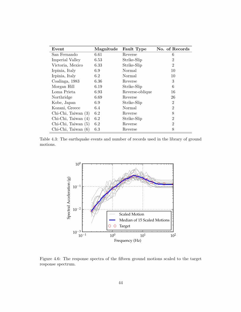
Event Magnitude Fault Type No. of RecordsSan Fernando 6.61 Reverse 6Imperial Valley 6.53 Strike-Slip 2Victoria, Mexico 6.33 Strike-Slip 2Irpinia, Italy 6.9 Normal 10Irpinia, Italy 6.2 Normal 10Coalinga, 1983 6.36 Reverse 3Morgan Hill 6.19 Strike-Slip 6Loma Prieta 6.93 Reverse-oblique 16Northridge 6.69 Reverse 26Kobe, Japan 6.9 Strike-Slip 2Kozani, Greece 6.4 Normal 2Chi-Chi, Taiwan (3) 6.2 Reverse 8Chi-Chi, Taiwan (4) 6.2 Strike-Slip 2Chi-Chi, Taiwan (5) 6.2 Reverse 2Chi-Chi, Taiwan (6) 6.3 Reverse 8

Table 4.3: The earthquake events and number of records used in the library of groundmotions.

10−1 100 101 102

Frequency (Hz)

10−3

10−2

10−1

100

Spec

tral

Acc

eler

atio

n(g

)

Scaled MotionMedian of 15 Scaled MotionsTarget

Figure 4.6: The response spectra of the fifteen ground motions scaled to the targetresponse spectrum.

44

Fil

enam

eS

cale

PG

A†

PG

V†

PG

D†

D5−

75

D5−

95

Det

ails

(g)

(cm

/sec

)(c

m)

(sec

)(s

ec)

CH

ICH

I06-

TC

U07

6-E

0.79

0.10

8.99

3.91

7.60

12.4

8C

hi-C

hiA

fter

shoc

k09

/25/

99,

23:5

2,T

CU

076,

EIT

ALY

-A-A

UL

270

1.55

0.10

9.46

5.71

13.1

119

.21

Irpi

nia,

11/2

3/80

,19

:34:

54,

Aul

etta

,27

0IT

ALY

-A-B

AG

000

0.62

0.09

13.7

45.

775.

2619

.51

Irpi

nia,

11/2

3/80

,19

:34,

Bag

noli

Irpi

no,

000

ITA

LY-A

-ST

U27

00.

250.

0912

.73

7.87

6.23

15.2

2Ir

pini

a,11

/23/

80,

19:3

4:54

,St

urno

,27

0IT

ALY

-B-A

UL

270

4.19

0.10

9.70

3.52

7.89

17.8

0Ir

pini

a,11

/23/

80,

19:3

5:04

,A

ulet

ta,

270

KO

ZA

NI-

KO

Z–L

0.73

0.16

6.83

1.21

2.49

6.44

Koz

ani,

05/1

3/95

,08

:47,

Koz

ani,

LL

OM

AP

-G01

000

0.33

0.14

10.4

12.

092.

006.

53L

oma

Pri

eta,

10/1

8/89

,00

:05,

Gilr

oyA

rray

#1,

000

LO

MA

P-G

IL06

70.

320.

119.

182.

041.

575.

00L

oma

Pri

eta,

10/1

8/89

,00

:05,

Gilr

oyG

avila

nC

oll,

067

MO

RG

AN

-GIL

337

2.01

0.19

5.77

1.90

4.70

8.18

Mor

gan

Hill

,04

/24/

84,

04:2

4,G

ilroy

Gav

ilan

Col

l,33

7N

OR

TH

R-H

1218

00.

660.

175.

882.

735.

409.

81N

orth

ridg

e,1/

17/9

4,12

:31,

Lak

eH

ughe

s#

12A

,18

0N

OR

TH

R-H

OW

330

0.83

0.14

7.01

1.50

5.06

7.99

Nor

thri

dge,

1/17

/94,

12:3

1,B

urba

nk-

How

ard,

330

NO

RT

HR

-LV

1000

1.30

0.12

10.1

02.

115.

4212

.42

Nor

thri

dge,

1/17

/94,

12:3

1,L

eona

Val

ley

#1,

000

NO

RT

HR

-LV

3090

1.24

0.13

10.0

22.

155.

8013

.60

Nor

thri

dge,

1/17

/94,

12:3

1,L

eona

Val

ley

#3,

090

NO

RT

HR

-WO

N18

50.

760.

138.

972.

115.

126.

67N

orth

ridg

e,1/

17/9

4,12

:31,

LA

-W

onde

rlan

d,18

5V

ICT

-CP

E04

50.

210.

136.

752.

804.

418.

57V

icto

ria,

Mex

ico,

06/0

9/80

,03

:28,

Cer

roP

riet

o,04

5

†Sca

led

valu

es

Tab

le4.

4:T

hegr

ound

mot

ions

and

thei

rpr

oper

ties

for

the

suit

esh

own

inF

igur

e4.

6.

45

10−1 100 101 102

Frequency (Hz)

10−3

10−2

10−1

100

101

102

Four

ier

ampl

itud

e(c

m/s

)

Scaled Motion

15 Scaled Motions (√

E[A2])

Figure 4.7: The FAS of the fifteen ground motions scaled to the target responsespectrum.

10−1 100 101 102

Frequency (Hz)

10−3

10−2

10−1

100

Spec

tral

Acc

eler

atio

n(g

)

Median of 15 Scaled MotionsExpected Median (RVT)

Figure 4.8: The median response spectrum of the fifteen scaled motions and an RVTmotion defined by the root-mean-square FAS of the scaled motions and a duration of4.83 seconds.

46

4.3.2 Maximum Usable Frequency

In defining the maximum frequency used in site response analysis, it is necessary to

consider the frequency content of the input time series, the numerical model used for the

site response analysis, and the frequencies of engineering interest in the design/evaluation

process.

The maximum frequency captured by a time series is known as the Nyquist frequency

(fNyq) and is related to the time step (∆t) by:

fNyq =1

2 ·∆t (4.1)

However, the Nyquist frequency does not typically represent the maximum usable

frequency in a time series because ground motion processing involves removing the

high-frequency noise using a low-pass filter. A low-pass filter is described by a low-pass

filter frequency (fLP ) which is defined as the frequency at which the filter response is 1√2

(≈ 0.707) of the maximum response. The NGA time series database contains motions

with fLP ranging from 4 to 90 Hz, but fLP for the majority of records ranges between

20 and 40 Hz, as shown in Figure 4.9. While an fLP of 30 Hz may be appropriate for

time series recorded in the Western US, a higher fLP would be required for a time

series recorded in the Central or Eastern US where the properties of the bedrock result

in significant earthquake motion at higher frequencies. Abrahamson and Silva (1997)

defined the maximum usable frequency as 0.80 · fLP. For example, a motion processed

using an fLP of 30 Hz would have a maximum usable frequency of 24 Hz. Frequencies

above the maximum usable frequency are significantly affected by the filter response, and

therefore do not represent earthquake motions and are inappropriate for consideration

in an engineering analysis.

The time step and filter characteristics of the suite of selected input motions used in

this study are presented in Table 4.5. The fLP of the selected motions ranges between 23

47

0 10 20 30 40 50 60 70 80 90Low-Pass Frequency (Hz)

0

500

1000

1500

2000

2500

Cou

nt

Figure 4.9: Distribution of the low-pass frequency used in the processing of motions inthe NGA database.

to 62.5 Hz. Of the fifteen records, nine of the records have maximum usable frequencies

less than 24 Hz (fLP < 30 Hz). For these nine motions, it would be inappropriate

to consider frequencies higher than 24 Hz in the site response analysis because these

high frequencies have already been modified through the processing of the time series.

Furthermore, it is important that the maximum frequency be consistent between analyses

performed with different motions. For this reason, it was decided to universally truncate

all motions at used in this study 25 Hz. Again, it is important to acknowledge that

this maximum frequency would not be appropriate for: (1) seismological conditions

in the Central and Eastern US with more high frequency motion, and (2) structures

(buildings and/or sites) where the dynamic response above 25 Hz is important in the

design process.

The truncation of the motions was achieved by defining the Fourier amplitudes

above 25 Hz to be zero. The abrupt truncation of the motion is only appropriate when

the amplitude of the motion above the truncation frequency is relatively insignificant.

48

Filename Time Step High Pass† Low Pass†(sec) (Hz) (Hz)

CHICHI06-TCU076-E 0.005 0.12 50.0ITALY-A-AUL270 0.0029 0.10 30.0ITALY-A-BAG000 0.0029 0.10 35.0ITALY-A-STU270 0.0024 0.08 30.0ITALY-B-AUL270 0.0029 0.30 23.0KOZANI-KOZ–L 0.005 0.20 25.0LOMAP-G01000 0.005 0.20 50.0LOMAP-GIL067 0.005 0.20 45.0MORGAN-GIL337 0.005 0.10 30.0NORTHR-H12180 0.01 0.12 46.0NORTHR-HOW330 0.01 0.10 30.0NORTHR-LV1000 0.02 0.20 23.0NORTHR-LV3090 0.02 0.20 23.0NORTHR-WON185 0.01 0.10 30.0VICT-CPE045 0.01 0.20 62.5

† Defined by the frequency at which the filter response is 1√2

(or ≈ 0.707) of themaximum response.

Table 4.5: The high-pass and low-pass frequencies of the suite of motions, as well as therecorded time step.

49

Thus, the effect of this truncation is most influential to records with fLP greater than

25 Hz. To demonstrate the impact of the truncation on the input motion and the site

response results, the CHICHI06-TCU076-E motion (fNyq = 100 Hz and fLP = 50 Hz) is

truncated at 25 and 50 Hz and then propagated through the Sylmar County Hospital

site (see Section 3.3). Figure 4.10 shows the surface response spectra, spectral ratios,

and bedrock response spectra for the motion truncated at 25 and 50 Hz, as well as the

original recording with a maximum frequency of 100 Hz. The truncation at 50 Hz only

slightly influences the bedrock response spectrum because of the minimal energy in

the time series at frequencies above 50 Hz. However, when the motion is truncated

at 25 Hz the effect on the bedrock motion is more pronounced with reduced spectral

accelerations at frequencies above 20 Hz. At the surface of the site, all three motions

produce nearly identical response spectra (Figure 4.10). Truncation does not affect

the computed surface response because the site does not amplify the high frequencies,

instead the site acts as a low-pass filter and attenuates the high-frequency content of

the time series. However, the computed spectral ratio between 25 and 50 Hz is affected

by truncation due to the high frequency content in the input motion. These results

indicate that truncating records below fLP affects the bedrock response spectrum, but

does not affect the response spectrum computed at the surface for this site.

Considering the fifteen scaled motions selected for this study, only two motions

(CHICHI06-TCU076-E and VICT-CPE045) have considerable earthquake motion at fre-

quencies greater than 25 Hz (Figure 4.11). As shown in Figure 4.10, the removal of this

high-frequency motion does not affect the computed surface response, although it does

affect the high-frequency spectral ratios. Nonetheless, only two motions out of fifteen

show this effect and therefore the median response from this suite should be minimally

affected by truncation.

50

10−1 100 101 1020.0

0.1

0.2

0.3

0.4

0.5Sp

ectr

alA

ccel

erat

ion

(g)

Location: SurfaceMotion: CHICHI06-TCU076-E

10−1 100 101 1020.0

0.5

1.0

1.5

2.0

2.5

Spec

tral

Rat

io

10−1 100 101 102

Frequency (Hz)

0.0

0.1

0.2

0.3

0.4

0.5

Spec

tral

Acc

eler

atio

n(g

)

Location: Bedrock

≤ 25 Hz≤ 50 Hz≤ 100 Hz

Figure 4.10: The effect of truncation on the CHICHI06-TCU076-E motion on the responsespectrum and spectral ratio computed for the Sylmar County Hospital site.

51

10−1 100 101 102

Frequency (Hz)

10−3

10−2

10−1

100

Spec

tral

Acc

eler

atio

n(g

)Original

10−1 100 101 102

Frequency (Hz)

10−3

10−2

10−1

100

Truncated

Scaled MotionMedianTarget

Figure 4.11: The effect of truncation on the suite of input ground motions used in thisstudy.

4.4 Spectrally Matched Ground Motions

Spectral matching modifies the frequency content of a time series to improve the fit

of the time series to a target response spectrum. Using the suite of fifteen motions

selected in the previous section, the program RSPMatch (Abrahamson, 1992; Hancock,

2006) was used to spectrally match each record to the target response spectrum.

The spectral matching procedure is illustrated by matching the NORTHR-WON185

motion to the target response spectrum from Figure 4.5. The frequency spacing in the

target response spectrum was increased to 60 points equally spaced in log space from

0.2 to 25 Hz. Prior to modifying the time series, it was scaled to best fit (defined by the

least sum of squared errors) the target response spectrum at frequencies between 0.2

and 1 Hz to reduce the required modifications to the record at low frequencies (Hancock,

2006). Figure 4.12 shows the original scaled response spectrum and the spectrally

matched response spectrum along with the target response spectrum. As expected,

52

the spectrally matched time series shows excellent agreement with the target response

spectrum over the range in matched frequencies (0.2 to 25 Hz) while maintaining some

of the time domain characteristics of the original recording as shown in Figure 4.13.

RSPMatch superimposes wavelets on the time series that adjust the amplitudes of

the oscillator responses to fit the target response spectrum at each frequency. The

procedure requires that the time step of the motion be reduced to allow for the creation

of the wavelets at the highest target frequencies. The time step of the time series is

adjusted such that the number of samples per second is ten times greater than the

maximum frequency (e.g., to spectrally match to 25 Hz requires 250 samples per second,

or a time step of 0.004 seconds). The increased time step is required to create the

zero-displacement wavelets used in adjusting the time series. These higher frequencies

are then removed by the truncation at a maximum frequency 25 Hz prior to being used

in the site response analyses.

The suite of fifteen spectrally matched motions was developed by applying a similar

technique to each of the remaining motions. The individual response spectra for the

spectrally matched time series matched and then truncated to 25 Hz, along with the

median and target response spectra, are shown in Figure 4.14. The acceleration-,

velocity-, and displacement-time series, as well as the acceleration response spectra, for

all spectrally-matched ground motions are included in Appendix C. These spectrally-

matched motions demonstrate excellent agreement with the target response spectrum

over frequencies from 0.2 to 25 Hz. By adjusting each motion in the suite to fit the

target response spectrum, the standard deviation of the suite of spectrally matched

motions is greatly reduced compared to the suite of stochastically simulated or scaled

ground motions, shown in Figure 4.15.

53

10−1 100 101 102

Frequency (Hz)

10−3

10−2

10−1

100

Spec

tral

Acc

eler

atio

n(g

)

ScaledPrior to MatchingSpectrally MatchedTarget

Figure 4.12: The response spectrum for the scaled, scaled prior to spectral matching,and spectrally matched versions of the NORTHR-WON185 ground motion, along with thetarget response spectrum.

54

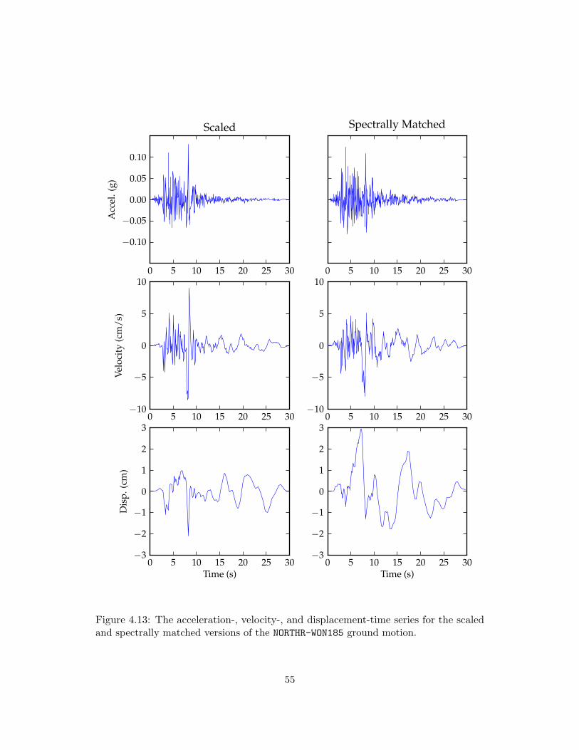
0 5 10 15 20 25 30

−0.10

−0.05

0.00

0.05

0.10

Acc

el.(

g)

Scaled

0 5 10 15 20 25 30

Spectrally Matched

0 5 10 15 20 25 30−10

−5

0

5

10

Velo

city

(cm

/s)

0 5 10 15 20 25 30−10

−5

0

5

10

0 5 10 15 20 25 30Time (s)

−3

−2

−1

0

1

2

3

Dis

p.(c

m)

0 5 10 15 20 25 30Time (s)

−3

−2

−1

0

1

2

3

Figure 4.13: The acceleration-, velocity-, and displacement-time series for the scaledand spectrally matched versions of the NORTHR-WON185 ground motion.

55

10−1 100 101 102

Frequency (Hz)

10−3

10−2

10−1

100

Spec

tral

Acc

eler

atio

n(g

)

Matched MotionMedian of 15 Matched MotionsTarget

Figure 4.14: The fifteen ground motions spectrally matched and truncated at 25 Hz.

10−1 100 101 102

Frequency (Hz)

0.0

0.1

0.2

0.3

0.4

0.5

0.6

0.7

Stan

dard

Dev

iati

on,σ

ln

StochasticScaledMatched

Figure 4.15: The standard deviation of the stochastically simulated, scaled, and spec-trally matched ground motion suites.

56

4.5 Response Spectrum Compatible Motion for RVT

An acceleration response spectrum computed with a ground motion prediction equation

provides the frequency content information required for an RVT analysis. However,

as the response spectrum retains no information regarding the duration of the ground

motion, RVT analyses require an independent estimate of the duration. With the

response spectrum and duration, an FAS can be derived for input into an RVT site

response analysis. However, it must be noted that this relationship between the response

spectrum and FAS is not unique because the phase information is not available and the

RVT calculation invokes an independent assessment of duration.

In the procedure proposed by Gasparini and Vanmarcke (1976) and described in

Rathje and Kottke (2008), the initial estimate of the Fourier amplitude (A) is computed

from the spectral acceleration at f = fn using:

|A(fn)|2 ≈ 1fn(π

4D − 1) (Trms

2· Sa,target(fn)2

pf2−∫ fn

0|A(f)|2 df

)(4.2)

where fn and D are the natural frequency and damping ratio, respectively, of the

oscillator at the frequency of interest; Sa(fn) is the spectral acceleration at the oscillator

frequency fn; Trms is the root-mean-square duration (see Section 2.4); pf is the peak

factor; and A(f) represents the Fourier amplitudes as a function of f . The peak factor is

initially assumed to be 2.5 for all frequencies which is within the typical range of 2 to 3.5.

Equation (4.2) is applied starting at low frequencies of the target response spectrum,

where the influence of higher frequencies in the integral in (4.2) can be ignored, and it

is then incrementally applied to higher frequencies. The resulting FAS generally shows

good agreement with the target response spectrum, but the fit can be further improved

by correcting the FAS based on the misfit between the target response spectral values

(Sa,target) and the values calculated from the FAS with RVT (Sa,calc).

The correction between the target and calculated response spectra relies on the

57

properties of the single-degree-of-freedom acceleration transfer function. For an oscillator

with light damping, the peak is narrow and tall which strongly connects the amplitude

of |A(f)| to Sa at the same frequency. Using this connection, an iterative correction is

defined as:

|A(f)|i+1 =Sa,target(f)Sa,calc(f)

|A(f)|i (4.3)

The frequency-dependent correction is applied to the FAS at each frequency, and then a

new response spectrum is calculated. After less than ten iterations, the misfit between

the target and calculated response spectra typically reaches a minimum.

A response spectrum provides no information regarding the duration of the event,

therefore an independent of estimate of the duration is required. Abrahamson and Silva

(1996) proposed an empirical duration model that is presented here for completeness.

The model defines the duration based on normalized Arias intensity. First, relating

source and site characteristics to the duration between a normalized Arias intensity of

0.05 and 0.75 (D0.05−0.75). Then, D0.05−0.75 is generalized for any duration defined by a

final normalized Arias intensity (D0.05−I). The empirical model is defined as:

lnD0.05−I = ln

(

∆σ(M)101.5M+16.05

)−1/3

4.9 · 106β+ Sc1 + c2 max(r − rc, 0)

+ ln

(D0.05−ID0.05−0.75

)(4.4)

where ∆σ(M) is the stress drop as a function of magnitude (M), β is the shear-wave

velocity at the source, S is a dummy variable for soil conditions (1 for soil or 0 for rock),

and , and r is the distance. In equation (4.4), ∆σ(M) is defined as:

∆σ(M) = exp (b1 + b2 (M − 6)) (4.5)

58

and D0.05−I

D0.05−0.75is defined as:

ln(

D0.05−ID0.05−0.75

)= a1 + a2 ln

(I − 0.05

1− I)

+ a3

(ln(I − 0.05

1− I))2

(4.6)

The coefficients for use in equations (4.4), (4.5), and (4.6) are presented in Table 4.6.

In a random vibration theory analysis, D0.05−0.75 is used as the duration, as previous

studies have shown that this value is similar to the source duration from seismological

models.

To evaluate this procedure, a target response spectrum was generated from an FAS

specified from seismological theory (Figure 4.16). Using this target response spectrum

and the procedure described above, an FAS was calculated that is compatible with the

target response spectrum (Figure 4.16). The FAS was then used to generate a response

spectrum. The results show very good agreement between the target and calculated

response spectra over the range in frequencies of shown (0.2 to 100 Hz). Agreement

between the seismological FAS and the FAS derived from the response spectrum is good

over the frequency range defined by the response spectrum (greater than 0.2 Hz). At

frequencies less than 0.2 Hz, discrepancies between the seismological FAS and the FAS

derived from the response spectrum are present due to a lack of information regarding

low frequency energy in the target response spectrum.

Coefficient Horizontal Verticala1 -0.532 -0.466a2 0.552 0.540a3 -0.0262 -0.0537b1 5.204 4.61b2 0.851 1.536c1 0.805 1.076c2 0.063 0.107rc (km) 10 10β (km/s) 3.2 3.2

Table 4.6: Parameters for the Abrahamson and Silva (1996) empirical duration model.

59

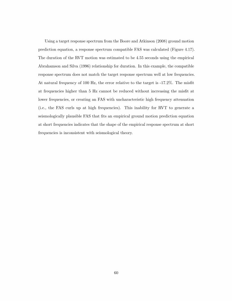
Using a target response spectrum from the Boore and Atkinson (2008) ground motion

prediction equation, a response spectrum compatible FAS was calculated (Figure 4.17).

The duration of the RVT motion was estimated to be 4.55 seconds using the empirical

Abrahamson and Silva (1996) relationship for duration. In this example, the compatible

response spectrum does not match the target response spectrum well at low frequencies.

At natural frequency of 100 Hz, the error relative to the target is -17.2%. The misfit

at frequencies higher than 5 Hz cannot be reduced without increasing the misfit at

lower frequencies, or creating an FAS with uncharacteristic high frequency attenuation

(i.e., the FAS curls up at high frequencies). This inability for RVT to generate a

seismologically plausible FAS that fits an empirical ground motion prediction equation

at short frequencies indicates that the shape of the empirical response spectrum at short

frequencies is inconsistent with seismological theory.

60

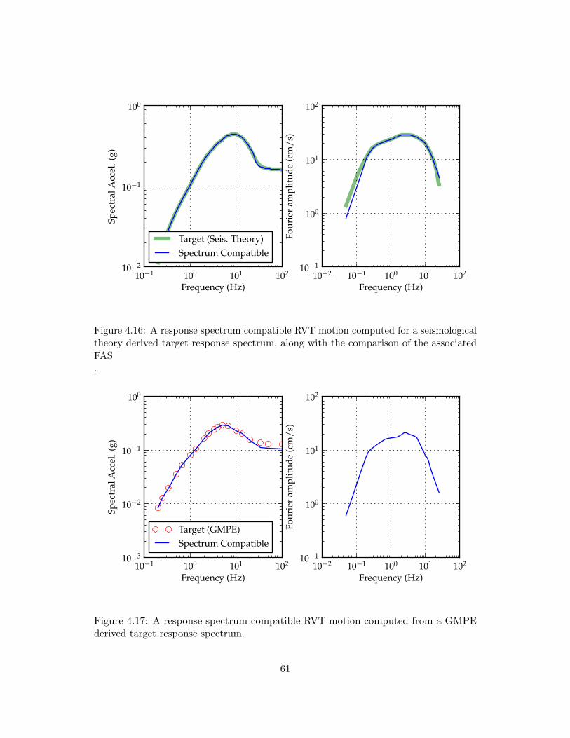
10−1 100 101 102

Frequency (Hz)

10−2

10−1

100Sp

ectr

alA

ccel

.(g)

Target (Seis. Theory)Spectrum Compatible

10−2 10−1 100 101 102

Frequency (Hz)

10−1

100

101

102

Four

ier

ampl

itud

e(c

m/s

)

Figure 4.16: A response spectrum compatible RVT motion computed for a seismologicaltheory derived target response spectrum, along with the comparison of the associatedFAS.

10−1 100 101 102

Frequency (Hz)

10−3

10−2

10−1

100

Spec

tral

Acc

el.(

g)

Target (GMPE)Spectrum Compatible

10−2 10−1 100 101 102

Frequency (Hz)

10−1

100

101

102

Four

ier

ampl

itud

e(c

m/s

)

Figure 4.17: A response spectrum compatible RVT motion computed from a GMPEderived target response spectrum.

61

Chapter 5

Comparison of Equivalent-Linear

Methods

5.1 Introduction

The different approaches of equivalent-linear (EQL) analysis (time series and RVT) are

compared in this chapter using the different input motion characterizations discussed

in Chapter 4. Comparisons will focus on the median spectral accelerations (Sa) and

the median spectral ratios (SR = Sa,soil/Sa,rock) predicted from a suite of time series

and the values predicted by RVT. Comparisons will be made through calculation of the

difference of RVT relative to time-series analysis. The relative difference of the spectral

acceleration (δSa) is defined as:

δSa =Sa,RV T − Sa,TS

Sa,TS(5.1)

where Sa,TS is the median spectral acceleration of the time series simulations and Sa,RV T

is the spectral acceleration computed with RVT. Similarly, the relative difference of the

62

spectral ratio for RVT (δSR) is defined as:

δSR =SRRV T − SRTS

SRTS(5.2)

where SRTS is the median spectral ratio of the time series simulations, and SRRV T is

the spectral ratio computed with RVT.

5.2 Comparison Using Stochastic Input Motions

The consistency between an FAS derived from seismological theory and stochastically

generated time series (Section 4.2) makes for an ideal situation in comparing RVT

and time series based site response analysis. The input motions for the time series

and RVT analyses are in general agreement when visualized as an FAS and as an

acceleration response spectrum (Figure 5.1). Figure 5.2 shows the relative difference of

the RVT input motion relative to the median of the time series simulations. In general,

the RVT motion is within 10% of the median of the time series with a tendency for

over prediction of the spectral accelerations at low frequencies and under prediction of

spectral accelerations at high frequencies.

The stochastically simulated motions are propagated through the Turkey Flat,

Sylmar County Hospital, and Calvert Cliffs sites; first assuming the response of the soil

is linear-elastic (LE) with 5% damping. The results of the Turkey Flat site for the time

series and RVT analyses are shown in Figure 5.3. The results show good agreement

between the surface response spectrum computed with RVT and the median from time

series analyses. Nonetheless, the relative difference in the surface response spectrum is

as large as 10% and it tends to be dominated by the relative differences of the input

motions (Figure 5.2). By examining the relative difference of the spectral ratio, the

differences caused by the site response calculation can be separated from differences in

the input motions.

63

10−1 100 101 10210−3

10−2

10−1

100

Spec

tral

Acc

eler

atio

n(g

)

Simulated Time SeriesRVT (Seismo. Theory)

10−1 100 101 102

Frequency (Hz)

10−1

100

101

102

Four

ier

ampl

itud

e(c

m/s

)

Figure 5.1: The input Fourier amplitude and response spectra for the stochastic inputmotions.

64

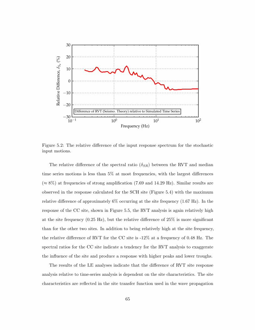
10−1 100 101 102

Frequency (Hz)

−30

−20

−10

0

10

20

30

Rel

ativ

eD

iffer

ence

,δS a

(%)

Difference of RVT (Seismo. Theory) relative to Simulated Time Series

Figure 5.2: The relative difference of the input response spectrum for the stochasticinput motions.

The relative difference of the spectral ratio (δSR) between the RVT and median

time series motions is less than 5% at most frequencies, with the largest differences

(≈ 8%) at frequencies of strong amplification (7.69 and 14.29 Hz). Similar results are

observed in the response calculated for the SCH site (Figure 5.4) with the maximum

relative difference of approximately 6% occurring at the site frequency (1.67 Hz). In the

response of the CC site, shown in Figure 5.5, the RVT analysis is again relatively high

at the site frequency (0.25 Hz), but the relative difference of 25% is more significant

than for the other two sites. In addition to being relatively high at the site frequency,

the relative difference of RVT for the CC site is -12% at a frequency of 0.48 Hz. The

spectral ratios for the CC site indicate a tendency for the RVT analysis to exaggerate

the influence of the site and produce a response with higher peaks and lower troughs.

The results of the LE analyses indicate that the difference of RVT site response

analysis relative to time-series analysis is dependent on the site characteristics. The site

characteristics are reflected in the site transfer function used in the wave propagation

65

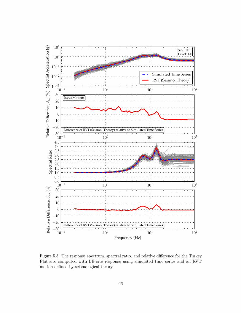
10−1 100 101 10210−3

10−2

10−1

100

101Sp

ectr

alA

ccel

erat

ion

(g)

Site: TFLevel: LE

Simulated Time SeriesRVT (Seismo. Theory)

10−1 100 101 102−30

−20

−10

0

10

20

30

Rel

ativ

eD

iffer

ence

,δS a

(%)

Input Motions

Difference of RVT (Seismo. Theory) relative to Simulated Time Series

10−1 100 101 1020.00.51.01.52.02.53.03.54.04.5

Spec

tral

Rat

io

10−1 100 101 102

Frequency (Hz)

−30

−20

−10

0

10

20

30

Rel

ativ

eD

iffer

ence

,δSR

(%)

Difference of RVT (Seismo. Theory) relative to Simulated Time Series

Figure 5.3: The response spectrum, spectral ratio, and relative difference for the TurkeyFlat site computed with LE site response using simulated time series and an RVTmotion defined by seismological theory.

66

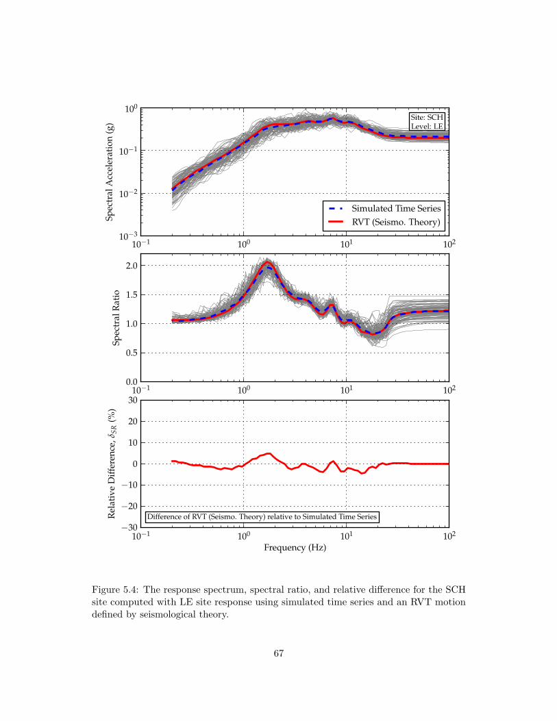
10−1 100 101 10210−3

10−2

10−1

100Sp

ectr

alA

ccel

erat

ion

(g)

Site: SCHLevel: LE

Simulated Time SeriesRVT (Seismo. Theory)

10−1 100 101 1020.0

0.5

1.0

1.5

2.0

Spec

tral

Rat

io

10−1 100 101 102

Frequency (Hz)

−30

−20

−10

0

10

20

30

Rel

ativ

eD

iffer

ence

,δSR

(%)

Difference of RVT (Seismo. Theory) relative to Simulated Time Series

Figure 5.4: The response spectrum, spectral ratio, and relative difference for the SCHsite computed with LE site response using simulated time series and an RVT motiondefined by seismological theory.

67

10−1 100 101 10210−3

10−2

10−1

100Sp

ectr

alA

ccel

erat

ion

(g)

Site: CCLevel: LE

Simulated Time SeriesRVT (Seismo. Theory)

10−1 100 101 1020.0

0.5

1.0

1.5

2.0

2.5

3.0

3.5

4.0

Spec

tral

Rat

io

10−1 100 101 102

Frequency (Hz)

−30

−20

−10

0

10

20

30

Rel

ativ

eD

iffer

ence

,δSR

(%)

Difference of RVT (Seismo. Theory) relative to Simulated Time Series

Figure 5.5: The response spectrum, spectral ratio, and relative difference for the CCsite computed with LE site response using simulated time series and an RVT motiondefined by seismological theory.

68

analysis. The LE transfer functions for the three sites are shown in Figure 5.6 and

these transfer functions represent what was used for both the time series and the RVT

analyses. Figure 5.6 shows that the transfer function of the Turkey Flat site has a

strong narrow peak at 14 Hz; the SCH site has a less strong, but wide, peak at 1.7 Hz;

and the CC site has several strong, narrow peaks at frequencies below 1 Hz and its

largest peak is at 0.23 Hz. Differences in the spectral ratios computed by RVT and

time-series analysis are a result of differences in the shape of the FAS of the simulated

time series and of the RVT input motion relative to these transfer functions.

Figure 5.7 shows the input FAS for the time series with the largest and smallest

spectral ratios at a frequency of 1.7 Hz (the approximate site frequency) for the SCH

site. Also shown is the input FAS for the RVT analysis. The time series with the

smallest spectral ratio (SR(1.67Hz) = 1.72) shows a deficiency in motion at or near

the frequency of the peak in the transfer function, while the time series with the largest

spectral ratio (SR(1.67Hz) = 2.13) contains enhanced amplitudes around the same

frequency. Additionally, the time series FAS display peaks and valleys within the

frequency range of the peak of the transfer function. On the other hand, the RVT input

motion contains no peaks and valleys in its FAS and varies smoothly. Because RVT

varies smoothly and does not have any valleys or peaks within the width of the peak

of the transfer function, it propagates the full strength of the transfer function to the

surface and predicts a larger spectral ratio. As all time series motions will have some

irregularities in the FAS across the peak in the transfer function, the median spectral

ratio from a suite of time-series analyses will never be as large as calculated by RVT.

The effect of the smooth RVT input motion is magnified when the peak in the

transfer function is multiplied by only a small number of frequencies of the input time

series. The frequency increment at which the FAS is defined is constant for a given

time series, and therefore the effect is magnified when the natural frequency of the site

is low. Additionally, the effect will be magnified when the width of the transfer function

69

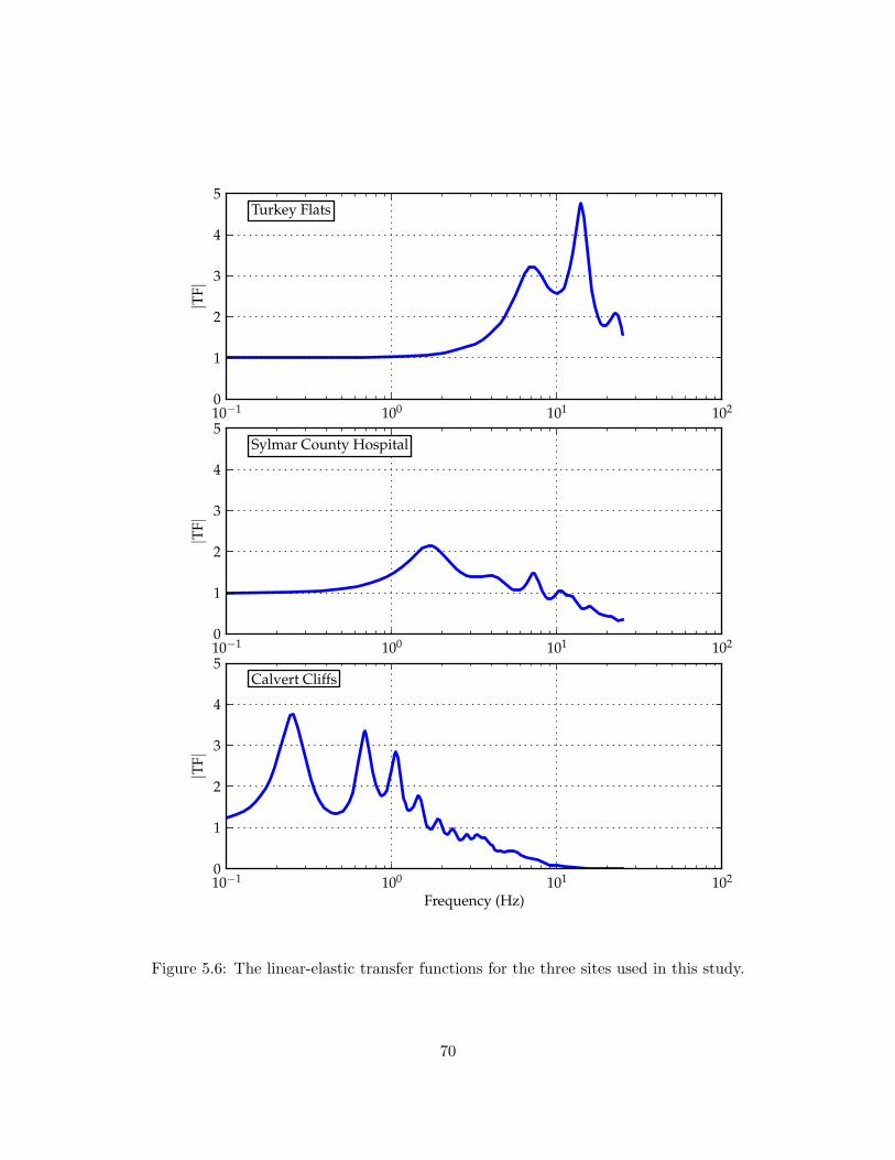
10−1 100 101 1020

1

2

3

4

5|T

F|Turkey Flats

10−1 100 101 1020

1

2

3

4

5

|TF|

Sylmar County Hospital

10−1 100 101 102

Frequency (Hz)

0

1

2

3

4

5

|TF|

Calvert Cliffs

Figure 5.6: The linear-elastic transfer functions for the three sites used in this study.

70

0.8 1.0 1.2 1.4 1.6 1.8 2.0 2.2 2.4 2.6Frequency (Hz)

0

10

20

30

40

50

60

70Fo

urie

ram

plit

ude

(cm

/s)

SCHRVT (SR(0.60 s)= 2.06)Time Series (SR(0.60 s)= 1.72)Time Series (SR(0.60 s)= 2.13)Transfer Function

0.8 1.0 1.2 1.4 1.6 1.8 2.0 2.2 2.4 2.60

1

2

3

4

5

6

|TF|

Figure 5.7: The input FAS for the time series with the largest and smallest spectralratios for the SCH site, along with the input FAS of the RVT analysis and the LEtransfer function.

is very narrow, or there is significant amplification by the site.

For the CC site, the input FAS for the time series with the largest and smallest

spectral ratios at a frequency of 0.25 Hz (the approximate site frequency) are shown in

Figure 5.8 along with the LE transfer function and the input FAS for RVT. The first

mode amplification for the CC site, shown in Figure 5.8, occurs at a lower frequency

and over a narrower frequency range than the first mode amplification for the SCH

site, thus there is more difference between the spectral ratios from the time series

analysis and RVT for the CC site (approximately 25% relative difference, see Figure 5.5).

Additionally, there is more variability in the spectral ratios at the site frequency within

the time series analysis for CC site, with the maximum spectral ratio being 81% larger

than the minimum spectral ratio. For SCH site, the maximum spectral ratio is only

23% larger than the minimum spectral ratio.

Understanding the disparity in the relative difference computed for the SCH and

71

0.05 0.10 0.15 0.20 0.25 0.30 0.35 0.40Frequency (Hz)

0

5

10

15

20

25

30

35Fo

urie

ram

plit

ude

(cm

/s)

CCRVT (SR(3.95 s)= 3.39)Time Series (SR(3.95 s)= 1.84)Time Series (SR(3.95 s)= 3.33)Transfer Function

0.05 0.10 0.15 0.20 0.25 0.30 0.35 0.400

1

2

3

4

5

6

|TF|

Figure 5.8: The input FAS for the time series with the largest and smallest spectralratios for the CC site, along with the input FAS of the RVT analysis and the LE transferfunction.

CC sites is complicated by the significant differences in site characteristics. A sensitivity

analysis was performed on a fictitious sites to identity which site characteristics (i.e.,

site frequency, soil damping, bedrock Vs) most influence the differences in time series

and RVT analyses. The site characteristics used in the sensitivity analysis are presented

in Table 5.1. A constant shear-wave velocity of 400 m/s was used but the thickness was

varied such that the site frequency ranged from 0.31 to 10 Hz. Soil damping ratios of 1

and 5% were considered, as well as bedrock shear-wave velocities of 1000 and 3000 m/s.

Using linear-elastic analysis, the median spectral ratio was computed from the stochastic

input motions using the time series and RVT approaches. The relative difference of

the RVT spectral ratio at the site frequency for each site is shown in Figure 5.9, as

well as the relative difference at 100 Hz. As the site frequency increases, the relative

difference at the site frequency increases because the peak in the transfer function is

affecting fewer points in the time series. More important than the natural frequency of

72

the site is the shear-wave velocity of the bedrock (Vs,rock), with the relative difference

increasing by a factor of two when using very hard rock (Vs,rock = 3000 m/s) versus soft

rock (Vs,rock = 1000 m/s). The increase in the bedrock shear-wave velocity increases

the impedance contrast at the site, which increases the height in the transfer function.

This increase in the peak height magnifies the differences caused by the different FAS

shapes for the time series and RVT motions. The damping of the soil, which influences

somewhat the width and height of the transfer functions, seems to have little influence

over the relative difference. The relative difference of the spectral ratio at 0.01 seconds

is generally less influenced by changes in properties (Figure 5.9), but the trend of

increasing relative difference with increasing site frequency can still be observed.

Equivalent-linear analyses were performed to investigate how the relative differ-

ence changes with input intensity and induced strain level. The input motions were

propagated through the Sylmar County Hospital site at two different intensity levels.

The lower intensity level is the expected PGA predicted for the scenario event from

seismological theory (PGA of 0.17 g, Figure 5.1). For the higher intensity level, all of

the input motions were increased by a factor 2.35, increasing the median input PGA to

0.40 g. Figure 5.10 shows the site response results for both the RVT and time-series

analysis for a median input PGA of 0.17 g. In general, the results show good agreement

between the time series and RVT analyses. However, the relative difference in the RVT

Layer Property Value(s)Soil Thickness (m) 10, 32, 100, 316

Shear-wave Velocity (m/s) 400Unit Weight (kN/m3) 18Damping (%) 1, 5

Bedrock Shear-wave Velocity (m/s) 1000, 3000Unit Weight (kN/m3) 22Damping (%) 1

Table 5.1: Site properties used in the sensitivity analysis.

73

10−1 100 101 102−5

0

5

10

15

20

25

30

35

40R

elat

ive

Bias

ofSR

atf s

(%)

10−1 100 101 102

Site Frequency (Hz)

−5

0

5

10

15

20

25

30

35

40

Rel

ativ

eBi

asof

PGA

(%)

Vs,rock=1000 m/s, Dsoil= 1%

Vs,rock=1000 m/s, Dsoil= 5%

Vs,rock=3000 m/s, Dsoil= 5%

Figure 5.9: Sensitivity of the relative difference of the spectral ratio at the site frequencyand at a frequency of 0.01 seconds to various site characteristics.

74

analysis has increased compared to the LE analysis (Figure 5.4), with the maximum

relative difference at the site frequency now approaching 10%. At frequencies with no

site amplification (i.e., troughs in the transfer function, such as at 0.11, 0.21, and 0.40

seconds), there is a consistent under prediction of the spectral ratio. These trends are

even stronger when the intensity of the input motions increase to 0.40 g (Figure 5.11),

where the relative difference at the site frequency exceeds 10%. Figure 5.12 summarizes

the relative difference in the spectral ratios computed at the SCH site for the three

sets of analyses performed. These data show that as the intensity of the input motion

increases, the relative difference at the site frequency increases and it shifts to lower

frequencies due to the increase in the site frequency associated with softening of the

site.

To explain the increase in the relative difference with increase in intensity level,

it is important to understand how the median response from the time series analyses

are influenced by the different strain levels induced by each individual motion. The

maximum strain profiles for the input intensities of 0.17 g and 0.40 g intensity level

events are shown in Figure 5.13. These profiles indicate that the strain computed by the

RVT analysis is very similar to the median strain in the time series analysis. However,

the maximum strain profiles fail to capture the connection between the maximum strain

and the computed spectral ratios for individual motions. Consider the two stochastic

motions shown in Figure 5.14. Motion #68 tends to strain the site less than the median,

which makes the peak in the spectral ratio occur at a higher frequency (i.e., stiffer site).

Motion #7 induces strains in the site larger than the median, causing the peak in the

spectral ratio to be shifted towards lower frequencies. At the frequency of approximately

1.11 Hz (approximately the average degraded site frequency), these two motions both

have spectral ratios less than the median of all of the motions, and thus motions that

strain a site more than or less than the median produce smaller spectral ratios at the

average site frequency. Motions that induce strains similar to the median response

75

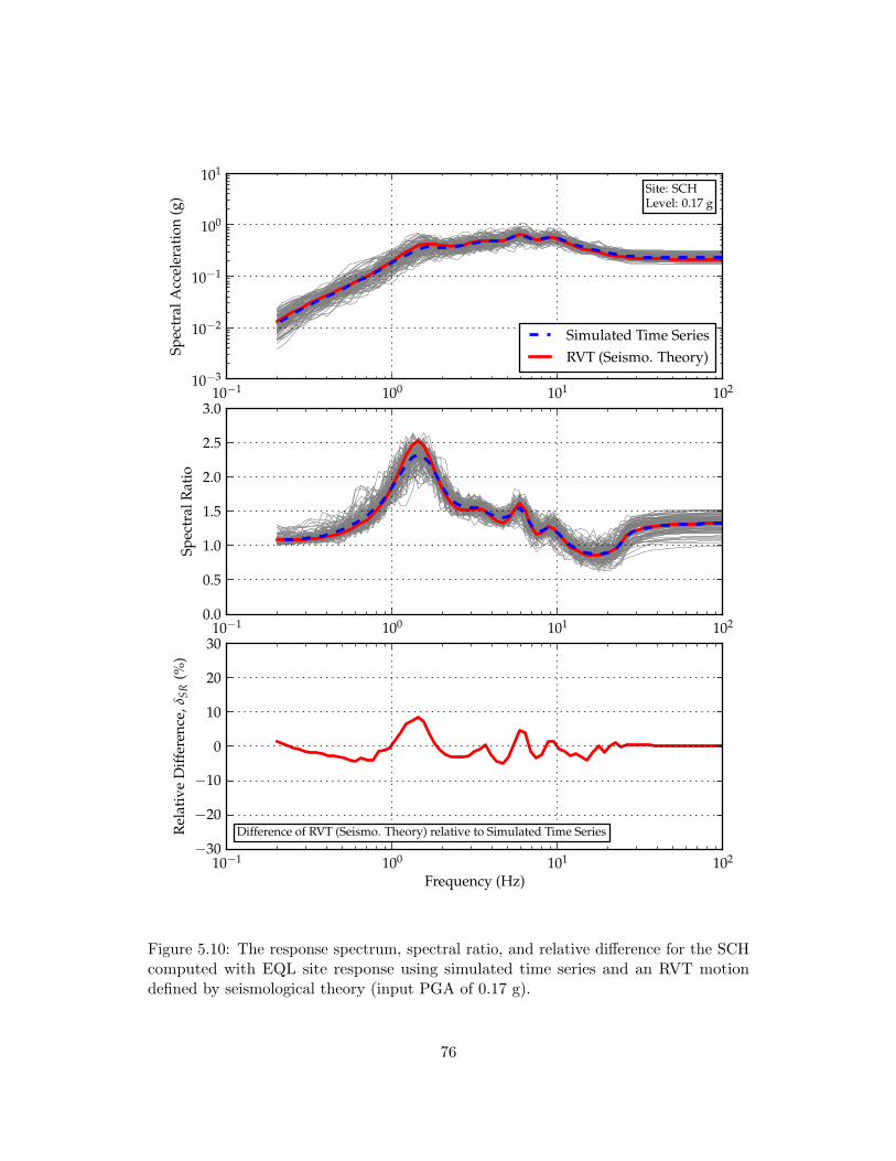
10−1 100 101 10210−3

10−2

10−1

100

101Sp

ectr

alA

ccel

erat

ion

(g)

Site: SCHLevel: 0.17 g

Simulated Time SeriesRVT (Seismo. Theory)

10−1 100 101 1020.0

0.5

1.0

1.5

2.0

2.5

3.0

Spec

tral

Rat

io

10−1 100 101 102

Frequency (Hz)

−30

−20

−10

0

10

20

30

Rel

ativ

eD

iffer

ence

,δSR

(%)

Difference of RVT (Seismo. Theory) relative to Simulated Time Series

Figure 5.10: The response spectrum, spectral ratio, and relative difference for the SCHcomputed with EQL site response using simulated time series and an RVT motiondefined by seismological theory (input PGA of 0.17 g).

76

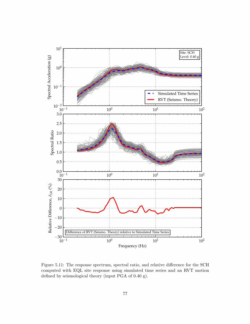
10−1 100 101 10210−2

10−1

100

101Sp

ectr

alA

ccel

erat

ion

(g)

Site: SCHLevel: 0.40 g

Simulated Time SeriesRVT (Seismo. Theory)

10−1 100 101 1020.0

0.5

1.0

1.5

2.0

2.5

3.0

Spec

tral

Rat

io

10−1 100 101 102

Frequency (Hz)

−30

−20

−10

0

10

20

30

Rel

ativ

eD

iffer

ence

,δSR

(%)

Difference of RVT (Seismo. Theory) relative to Simulated Time Series

Figure 5.11: The response spectrum, spectral ratio, and relative difference for the SCHcomputed with EQL site response using simulated time series and an RVT motiondefined by seismological theory (input PGA of 0.40 g).

77

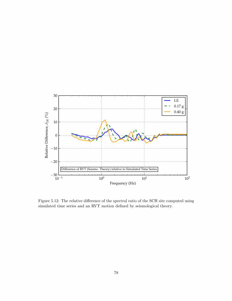
10−1 100 101 102

Frequency (Hz)

−30

−20

−10

0

10

20

30

Rel

ativ

eD

iffer

ence

,δSR

(%)

Difference of RVT (Seismo. Theory) relative to Simulated Time Series

LE0.17 g0.40 g

Figure 5.12: The relative difference of the spectral ratio of the SCH site computed usingsimulated time series and an RVT motion defined by seismological theory.

78

have the largest spectral ratio at the average site frequency. When all of the motions

within the suite are averaged together, the effect of these differences is to pull down

the average spectral response at the site frequency. At frequencies away from the peak

spectral ratio, the motions #68 and #7 balance each other out (i.e., one is larger than

the median and the other is smaller) such that the median of the time-series analyses is

similar to RVT.

The strain effect is further illustrated by comparing histograms of the spectral ratios

at the site frequency for each set of analyses (Figure 5.15). For the LE analysis, the

histogram is quite narrow with a small skew to smaller values and the median from the

suite of time-series analysis is larger than the value from RVT analysis. This difference is

caused predominantly by the spectral shape effects discussed. For the EQL analyses, the

median spectral ratios from the time series analysis increase relative to the linear-elastic

analyses, but the histograms widen and become more skewed to smaller spectral ratios

due to the fact that motions with relatively larger and relatively smaller shear strains

both result in smaller spectral ratios at the site frequency. The skewness reduces the

median from the time-series analysis, causing enhanced differences between time-series

and RVT analyses.

The relative difference of the EQL RVT analysis and the EQL time-series analysis

for the CC site (Figure 5.16) shows slightly different trends than were observed for the

SCH site. The low site frequency of approximately 0.25 Hz along with high bedrock

shear-wave velocity of this Eastern US site (Figure 3.4) accentuates the positive bias of

the RVT spectral ratio at frequencies associated with peaks in the transfer function.

This positive bias is as large as 25%. Additionally, the relative difference becomes

increasingly negative at high frequencies and becomes increasingly negative as the input

intensity increases. Unlike SCH, for CC the strains induced by the RVT analysis are

larger than for the time-series analysis (Figure 5.17). The larger strains lead to more

damping and reduced spectral ratios at higher frequencies for the RVT analysis.

79

10−3

10−2

10−1

100

Max

imum

Shea

rSt

rain

(%)

0 20 40 60 80 100

Depth(m)

Site

:SC

HLe

vel:

0.17

g

10−3

10−2

10−1

100

Max

imum

Shea

rSt

rain

(%)

0 20 40 60 80 100

Site

:SC

HLe

vel:

0.40

g

Sim

ulat

edTi

me

Seri

esRV

T(S

eism

o.Th

eory

)

Fig

ure

5.13

:T

hem

axim

umst

rain

profi

les

for

the

SCH

site

com

pute

dus

ing

sim

ulat

edti

me

seri

esan

dan

RV

Tm

otio

nde

fined

byse

ism

olog

ical

theo

ry.

80

10−1 100 101

Frequency (Hz)

0.0

0.5

1.0

1.5

2.0

2.5Sp

ectr

alR

atio

RVTTime Series (Median)Time Series (#68)Time Series (#7)

10−2 10−1 100

Max Strain (%)

0

20

40

60

80

100D

epth

(m)

10−1 100 101 102

Frequency (Hz)

10−2

10−1

100

Spec

tral

Acc

eler

atio

n(g

)

Figure 5.14: The spectral ratio and maximum strain profiles for selected motionspropagated through the SCH site with an input PGA of 0.40 g.

81

1.6 1.8 2.0 2.2 2.4 2.60

5

10

15

20C

ount

Level: LEfs: 1.67 Hz

Time Series (Median)RVT

1.6 1.8 2.0 2.2 2.4 2.60

5

10

15

20

Cou

nt

Level: 0.17 gfs: 1.43 Hz

1.6 1.8 2.0 2.2 2.4 2.6Spectral Ratio at RVT Site Frequency ( fs)

0

5

10

15

20

Cou

nt

Level: 0.40 gfs: 1.13 Hz

Figure 5.15: Histograms of the spectral ratio at the site frequency of the RVT analysisfor the SCH site.

82

10−1 100 101 102

Frequency (Hz)

−30

−20

−10

0

10

20

30

Rel

ativ

eD

iffer

ence

,δSR

(%)

Difference of RVT (Seismo. Theory) relative to Simulated Time Series

LE0.17 g0.40 g

Figure 5.16: The relative difference of the spectral ratio of the CC site computed usingsimulated time series and an RVT motion defined by seismological theory.

83

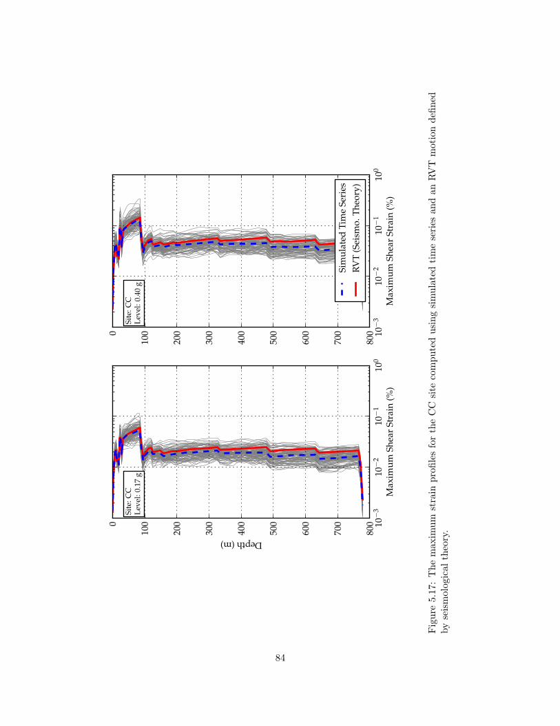
10−3

10−2

10−1

100

Max

imum

Shea

rSt

rain

(%)

0

100

200

300

400

500

600

700

800

Depth(m)

Site

:CC

Leve

l:0.

17g

10−3

10−2

10−1

100

Max

imum

Shea

rSt

rain

(%)

0

100

200

300

400

500

600

700

800

Site

:CC

Leve

l:0.

40g

Sim

ulat

edTi

me

Seri

esRV

T(S

eism

o.Th

eory

)

Fig

ure

5.17

:T

hem

axim

umst

rain

profi

les

for

the

CC

site

com

pute

dus

ing

sim

ulat

edti

me

seri

esan

dan

RV

Tm

otio

nde

fined

byse

ism

olog

ical

theo

ry.

84

To summarize, the difference in the site response computed using RVT analysis is

affected by the characteristics of both the site and the input motions. The smooth shape

of the RVT input FAS is more sensitive to the site transfer function than the irregular

FAS of a time series, which results in larger amplification at the frequencies associated

with peaks in the transfer function and less amplification at frequencies associated with

troughs in the transfer function for RVT analyses. These differences are more significant

for sites with low natural frequencies because the site amplification transfer function

tends to be narrower and the number of points in the FAS affected by the amplification

is smaller. Also important is the amplitude of the transfer function which increases for

sites with large bedrock shear-wave velocity velocities or other strong velocity contrasts.

The relative difference of RVT at the site frequency increases with increasing intensity

because the RVT analysis does not take into account how individual motions strain a

site differently (e.g. Figure 5.14). Finally, sites that have a large, positive bias at the

site frequency for RVT analysis may induce larger strains that lead to negative bias for

RVT at high frequencies.

5.3 Comparisons Using Scaled Time Series

The previous section focused on comparing RVT and time-series analyses using stochas-

tically simulated input motions. However, most engineering practice uses recorded

motions as input into site response analysis. Therefore, the suite of fifteen recorded

ground motions discussed in Section 4.3 was used in a set of analyses to compare

time-series and RVT methods and confirm the differences observed for simulated input

motions. The scaled input motions have a median PGA of 0.13 g and are shown in

Figure 5.18. These motions were also scaled to a median of 0.40 g and used as input.

To develop the input RVT motion for comparison to a scaled suite of time series, one

may derive a FAS compatible with the median response spectrum of the input time

85

series (called a response spectrum compatible input motion) or one may directly use

the average FAS of the input time series (called an FAS compatible input motion).

The response spectrum computed for the response spectrum compatible RVT input

motion is within 5 to 10% of the median response spectrum of the scaled time series

for frequencies less than 25 Hz (Figure 5.19) but under predicts the PGA (Sa at 100

Hz) by more than 10%. The response spectrum computed by the FAS compatible RVT

input motion matches the target PGA but it is 10 to 60% larger than the median of

the time series at frequencies lower than 10 Hz. The observed difference is frequency

dependent and increases with increasing frequency. This observed trend is similar to

what was observed for the stochastically simulated time series (Figure 5.2) although

here the difference is much larger.

The observed differences between the response spectrum and FAS compatible RVT

input motions is significant as it indicates a disconnect between the response spectra and

FAS of recorded motions and RVT. As was previously shown, the stochastically simulated

motions agreed with the RVT input motion in terms of both the FAS and the response

spectrum (Figure 5.1) with a relative difference in the response spectrum ranging from

-10 to 10%. However, when recorded motions are used it is nearly impossible to fit both

the input response spectrum and the input FAS simultaneously. Even when using the

average FAS of the input motions, the input response spectrum computed by RVT is 10

to 60% larger than the median response spectrum of the suite of scaled time series. As

random phase angle is assumed in both the generation of stochastically simulated time

series and RVT, it may play a role in the observed differences. However, characterization

of the differences in the phase angle between stochastically simulated time series and

recorded time series is beyond the scope of this report. The shape of the FAS derived

from the response spectrum is different from the FAS of the input time series in terms

of the relative amplitudes at high and low frequencies. These differences in the FAS

shape are important because the differences in shape affect the response of the site.

86

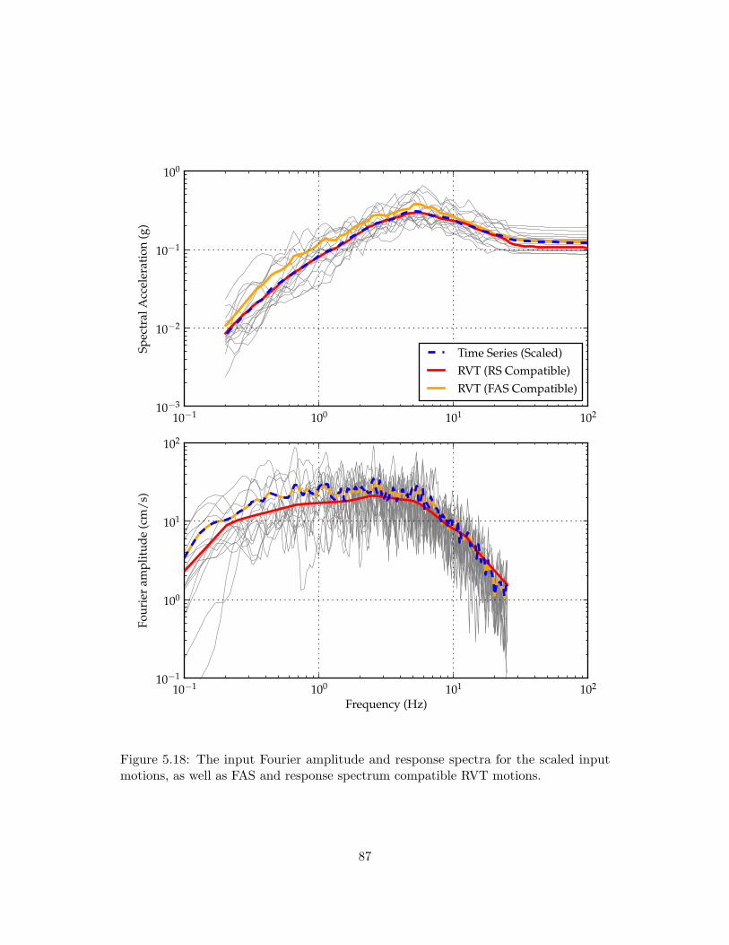
10−1 100 101 10210−3

10−2

10−1

100

Spec

tral

Acc

eler

atio

n(g

)

Time Series (Scaled)RVT (RS Compatible)RVT (FAS Compatible)

10−1 100 101 102

Frequency (Hz)

10−1

100

101

102

Four

ier

ampl

itud

e(c

m/s

)

Figure 5.18: The input Fourier amplitude and response spectra for the scaled inputmotions, as well as FAS and response spectrum compatible RVT motions.

87

10−1 100 101 102

Frequency (Hz)

−30

−20

−10

0

10

20

30

40

50

60

Rel

ativ

eD

iffer

ence

,δS a

(%)

Difference of RVT relative to Time Series (Scaled)

RVT (RS Compatible)RVT (FAS Compatible)

Figure 5.19: The relative difference of the input response spectra for the FAS andresponse spectrum compatible RVT motions.

The linear-elastic response of the SCH site for these three different input motions

is shown in Figure 5.20 and these results are similar to those shown previously for

the stochastically simulated input motions (Figure 5.4). A large positive bias in the

RVT spectral ratio occurs at the site frequency, although the relative difference is

slightly larger than the relative difference observed for the stochastically simulated input

motions (8% versus 5%). There is a difference in the spectral ratios computed by the

two different RVT methods at low frequencies as a result of differences in the shapes of

the input FAS, as discussed previously (Figure 5.18).

The EQL spectral ratios computed for the SCH site for 0.13 and 0.40 g are shown

in Figure 5.21. The RVT analysis with a response spectrum compatible input motion

generally maintains a difference less than 10 to 15%, whereas the RVT analysis with the

FAS compatible input motion produces large, negative bias (-20 to -30%) at frequencies

between 1.43 and 14.3 Hz. The significant difference between responses computed by

the two RVT motions is a result of differences in strains generated by the different

88

10−1 100 101 10210−3

10−2

10−1

100Sp

ectr

alA

ccel

erat

ion

(g)

Site: SCHLevel: LE

Time Series (Scaled)RVT (RS Compatible)RVT (FAS Compatible)

10−1 100 101 1020.0

0.5

1.0

1.5

2.0

Spec

tral

Rat

io

10−1 100 101 102

Frequency (Hz)

−30

−20

−10

0

10

20

30

Rel

ativ

eD

iffer

ence

,δSR

(%) Difference of RVT relative to Time Series (Scaled)

Figure 5.20: The response spectrum, spectral ratio, and relative difference for theSCH site computed with LE site response using scaled time series, as well as FAS andresponse spectrum compatible RVT motions.

89

input motions (Figure 5.22). The maximum strain predicted by the response spectrum

compatible RVT motion agrees better with the time-series analysis than the FAS

compatible RVT input motion at both intensities, and thus the response spectrum

compatible motion yields more comparable results with time-series analysis. The

improved performance of the response spectrum compatible motion is due to the fact

that the FAS was developed to match the target input response spectrum for the

specified duration. The FAS compatible RVT input motion is developed from the

average FAS alone without ensuring that the FAS and the specified duration generate a

response spectrum similar to the target response spectrum.

Using the response spectrum compatible RVT motion, the relative difference of the

median spectral ratio was computed for the SCH and CC sites for input intensities

of 0.13 and 0.40 g (Figure 5.23). For the SCH site, as the input intensity increases

there is an increase in relative difference at the site frequency, as was observed with

the stochastically simulated motions. However, the peak RVT difference of 15% in

Figure 5.23 is larger than the peak RVT difference of about 10% observed for the

stochastically simulated motions (Figure 5.12). This increase in RVT relative difference

for the scaled motions is caused by a reduction in the median spectral ratio predicted

by time-series analysis due to differences in the strains induced by individual time series.

The data in Figure 5.23 also show increasingly negative relative difference for RVT at

frequencies less than 0.1 seconds due to differences in FAS shape. The characteristics of

the CC site result in greater amplification by the RVT analysis and a large positive bias

at the site frequency at all intensity levels (≈ 25% at 0.40 g, Figure 5.23). Additionally,

there is a negative relative bias at frequencies higher than about 1.67 Hz, and this

difference is also significant for linear-elastic analysis. This increasingly negative bias

for RVT is due to the RVT analysis predicting larger strains (Figure 5.24).

90

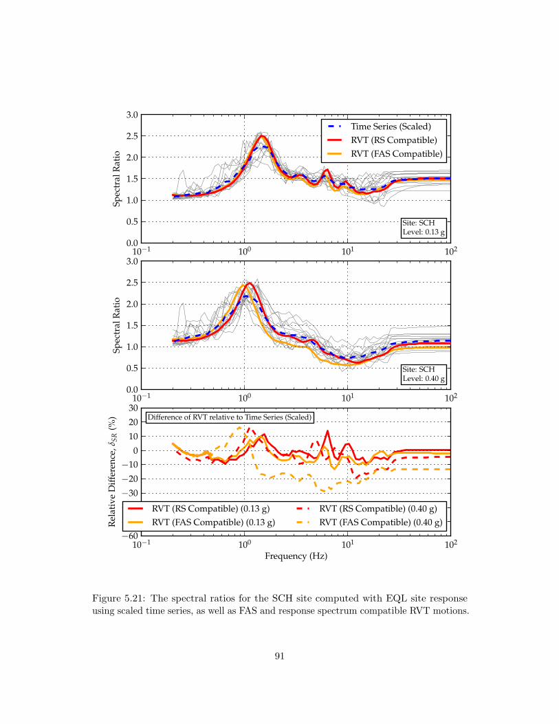
10−1 100 101 1020.0

0.5

1.0

1.5

2.0

2.5

3.0Sp

ectr

alR

atio

Site: SCHLevel: 0.13 g

Time Series (Scaled)RVT (RS Compatible)RVT (FAS Compatible)

10−1 100 101 102

Frequency (Hz)

−60

−50

−40

−30

−20

−100

10

20

30

Rel

ativ

eD

iffer

ence

,δSR

(%) Difference of RVT relative to Time Series (Scaled)

RVT (RS Compatible) (0.13 g)RVT (FAS Compatible) (0.13 g)

RVT (RS Compatible) (0.40 g)RVT (FAS Compatible) (0.40 g)

10−1 100 101 1020.0

0.5

1.0

1.5

2.0

2.5

3.0

Spec

tral

Rat

io

Site: SCHLevel: 0.40 g

Figure 5.21: The spectral ratios for the SCH site computed with EQL site responseusing scaled time series, as well as FAS and response spectrum compatible RVT motions.

91

10−3

10−2

10−1

100

Max

imum

Shea

rSt

rain

(%)

0 20 40 60 80 100

Depth(m)

Site

:SC

HLe

vel:

0.13

g

10−3

10−2

10−1

100

Max

imum

Shea

rSt

rain

(%)

0 20 40 60 80 100

Site

:SC

HLe

vel:

0.40

g

Tim

eSe

ries

(Sca

led)

RVT

(RS

Com

pati

ble)

RVT

(FA

SC

ompa

tibl

e)

Fig

ure

5.22

:T

hem

axim

umst

rain

profi

les

for

the

SCH

site

com

pute

dus

ing

scal

edti

me

seri

esan

da

resp

onse

spec

trum

com

pati

ble

RV

Tm

otio

n.

92

To summarize, the difference of RVT analysis assessed using scaled motions was

similar to that assessment using stochastically simulated motions. It is recommended

that a response spectrum compatible RVT input motion be developed for use in RVT

analysis.

93

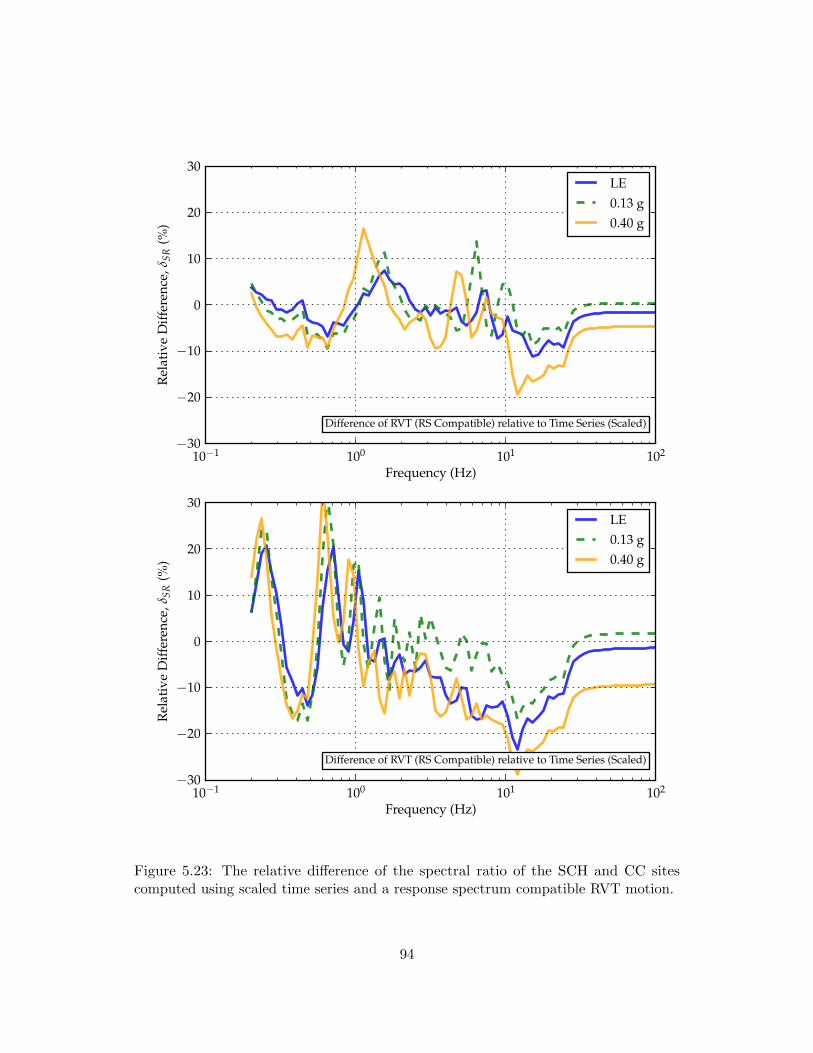
10−1 100 101 102

Frequency (Hz)

−30

−20

−10

0

10

20

30R

elat

ive

Diff

eren

ce,δ

SR(%

)

Difference of RVT (RS Compatible) relative to Time Series (Scaled)

LE0.13 g0.40 g

10−1 100 101 102

Frequency (Hz)

−30

−20

−10

0

10

20

30

Rel

ativ

eD

iffer

ence

,δSR

(%)

Difference of RVT (RS Compatible) relative to Time Series (Scaled)

LE0.13 g0.40 g

Figure 5.23: The relative difference of the spectral ratio of the SCH and CC sitescomputed using scaled time series and a response spectrum compatible RVT motion.

94

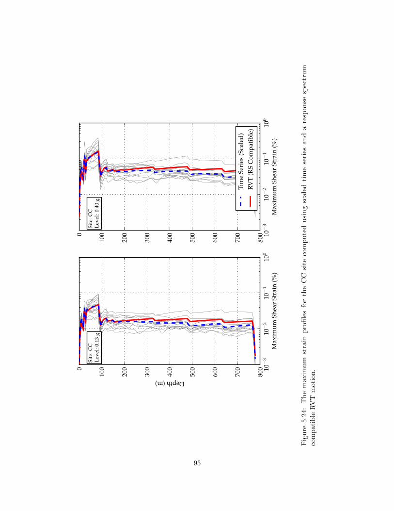
10−3

10−2

10−1

100

Max

imum

Shea

rSt

rain

(%)

0

100

200

300

400

500

600

700

800

Depth(m)

Site

:CC

Leve

l:0.

13g

10−3

10−2

10−1

100

Max

imum

Shea

rSt

rain

(%)

0

100

200

300

400

500

600

700

800

Site

:CC

Leve

l:0.

40g

Tim

eSe

ries

(Sca

led)

RVT

(RS

Com

pati

ble)

Fig

ure

5.24

:T

hem

axim

umst

rain

profi

les

for

the

CC

site

com

pute

dus

ing

scal

edti

me

seri

esan

da

resp

onse

spec

trum

com

pati

ble

RV

Tm

otio

n.

95

5.4 Comparisons Using Spectrally Matched Time Series

The time-series analysis from the previous section involved a suite of input motions with

significant motion-to-motion variability. For the time series analyses, this variability

causes the site to strain and respond differently to each motion and results in a reduced

median amplification at the site frequency, as previously shown in Figure 5.14. Spectrally

matched motions display excellent agreement with the target response spectrum with

very little variability, thus should provide results more similar to RVT analysis. The

fifteen spectrally-matched input time series along with the response spectrum compatible

input motion for RVT are shown in Figure 5.25. Generally, both the RVT response

spectrum and FAS match the time series values, unlike the recorded time series which

fit to either the FAS or the response spectrum. The variability in the time series at

frequencies greater than 25 Hz is a result of the spectral matching only being performed

up to 25 Hz. The difference of the RVT input response spectrum relative to the median

of the time series is shown in Figure 5.26 and is less than 10% over the entire frequency

range. The maximum relative difference of approximately 10% occurs at a frequency of

25 Hz and corresponds to the cutoff frequency used in the site response analysis (see

Section 4.5).

The LE response of the SCH site for RVT and time-series analyses is shown in

Figure 5.27. The results show excellent agreement between the response computed

with the spectrally-matched time series and the RVT input motion, with the maximum

difference of approximately 5% occurring at the site frequency (1.67 Hz). The EQL

response of the site at 0.13 g is shown in Figure 5.28. There is generally less than

5% difference between the time series and RVT analysis, except at the site frequency

frequency (1.49 Hz) and at a higher mode of vibration (7.69 Hz) where the relative

difference is about 10%. Figure 5.29 shows the EQL response for an input motion inten-

sity of 0.40 g. At this input intensity, differences between the spectrally-matched time

96

10−1 100 101 10210−3

10−2

10−1

100

Spec

tral

Acc

eler

atio

n(g

)

Time Series (Matched)RVT (RS Compatible)

10−1 100 101 102

Frequency (Hz)

10−1

100

101

102

Four

ier

ampl

itud

e(c

m/s

)

Figure 5.25: The input Fourier amplitude and response spectra for the spectrally-matched time series and a response spectrum compatible RVT motion.

97

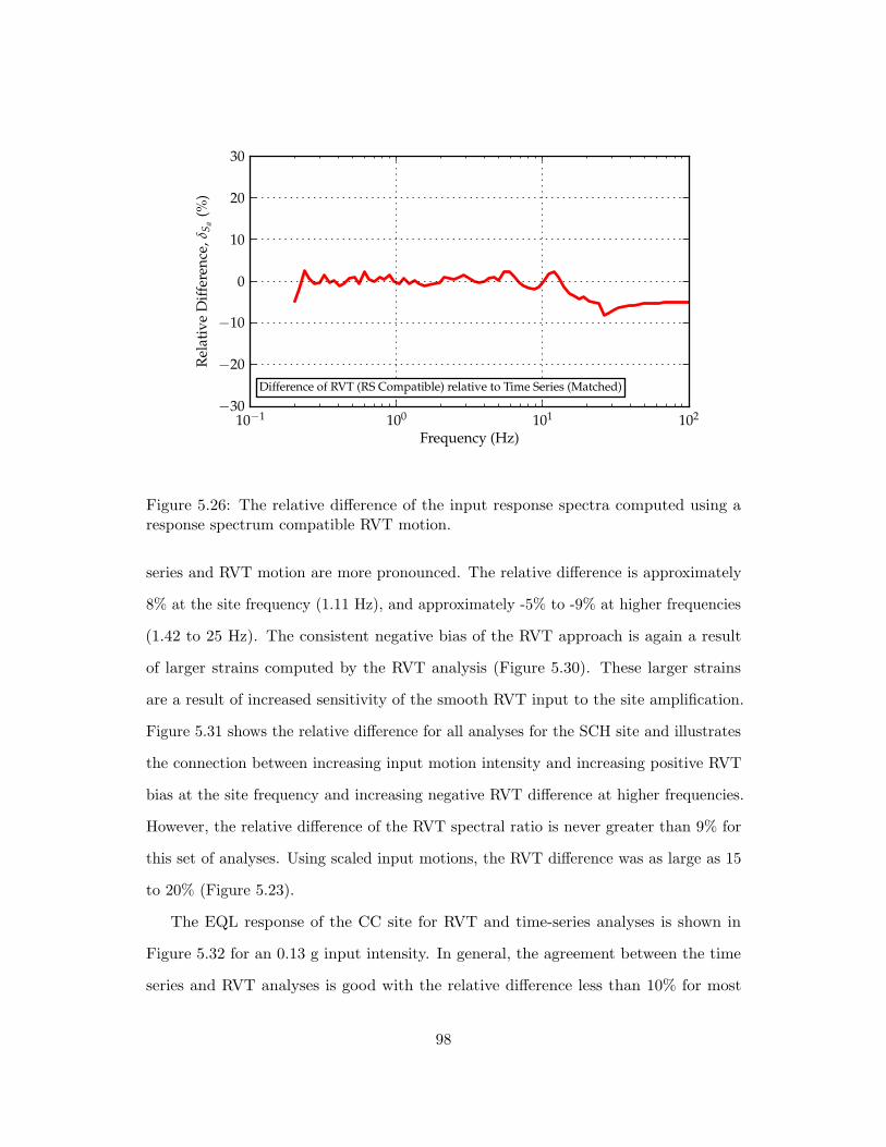
10−1 100 101 102

Frequency (Hz)

−30

−20

−10

0

10

20

30

Rel

ativ

eD

iffer

ence

,δS a

(%)

Difference of RVT (RS Compatible) relative to Time Series (Matched)

Figure 5.26: The relative difference of the input response spectra computed using aresponse spectrum compatible RVT motion.

series and RVT motion are more pronounced. The relative difference is approximately

8% at the site frequency (1.11 Hz), and approximately -5% to -9% at higher frequencies

(1.42 to 25 Hz). The consistent negative bias of the RVT approach is again a result

of larger strains computed by the RVT analysis (Figure 5.30). These larger strains

are a result of increased sensitivity of the smooth RVT input to the site amplification.

Figure 5.31 shows the relative difference for all analyses for the SCH site and illustrates

the connection between increasing input motion intensity and increasing positive RVT

bias at the site frequency and increasing negative RVT difference at higher frequencies.

However, the relative difference of the RVT spectral ratio is never greater than 9% for

this set of analyses. Using scaled input motions, the RVT difference was as large as 15

to 20% (Figure 5.23).

The EQL response of the CC site for RVT and time-series analyses is shown in

Figure 5.32 for an 0.13 g input intensity. In general, the agreement between the time

series and RVT analyses is good with the relative difference less than 10% for most

98

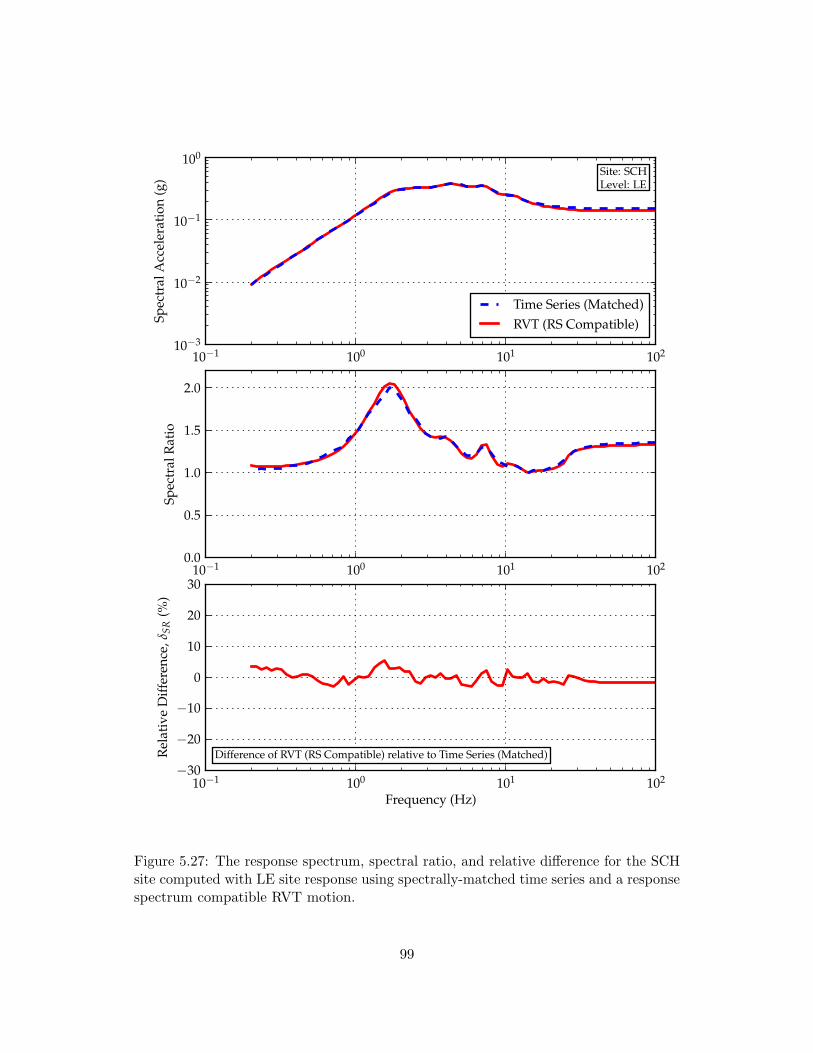
10−1 100 101 10210−3

10−2

10−1

100Sp

ectr

alA

ccel

erat

ion

(g)

Site: SCHLevel: LE

Time Series (Matched)RVT (RS Compatible)

10−1 100 101 1020.0

0.5

1.0

1.5

2.0

Spec

tral

Rat

io

10−1 100 101 102

Frequency (Hz)

−30

−20

−10

0

10

20

30

Rel

ativ

eD

iffer

ence

,δSR

(%)

Difference of RVT (RS Compatible) relative to Time Series (Matched)

Figure 5.27: The response spectrum, spectral ratio, and relative difference for the SCHsite computed with LE site response using spectrally-matched time series and a responsespectrum compatible RVT motion.

99

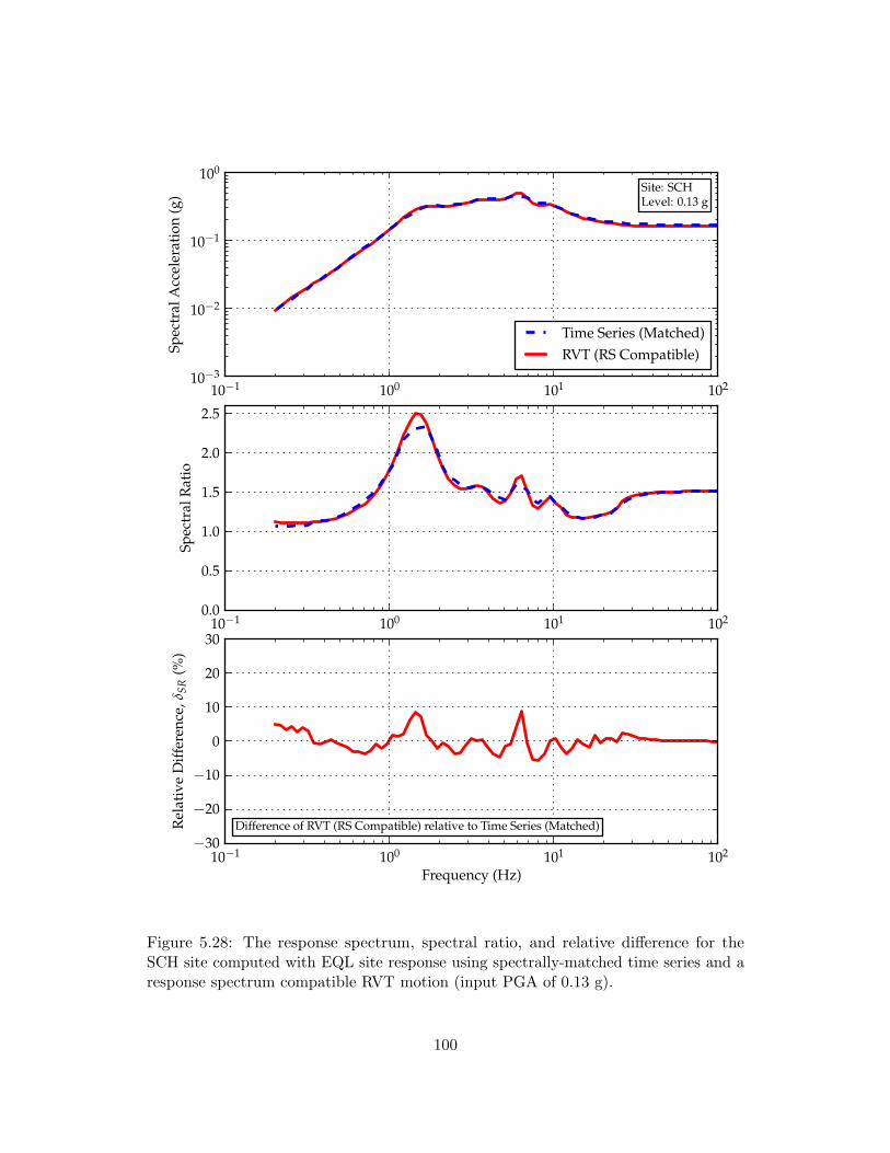
10−1 100 101 10210−3

10−2

10−1

100Sp

ectr

alA

ccel

erat

ion

(g)

Site: SCHLevel: 0.13 g

Time Series (Matched)RVT (RS Compatible)

10−1 100 101 1020.0

0.5

1.0

1.5

2.0

2.5

Spec

tral

Rat

io

10−1 100 101 102

Frequency (Hz)

−30

−20

−10

0

10

20

30

Rel

ativ

eD

iffer

ence

,δSR

(%)

Difference of RVT (RS Compatible) relative to Time Series (Matched)

Figure 5.28: The response spectrum, spectral ratio, and relative difference for theSCH site computed with EQL site response using spectrally-matched time series and aresponse spectrum compatible RVT motion (input PGA of 0.13 g).

100

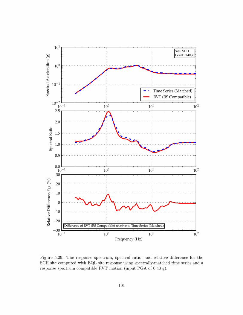
10−1 100 101 10210−2

10−1

100

101Sp

ectr

alA

ccel

erat

ion

(g)

Site: SCHLevel: 0.40 g

Time Series (Matched)RVT (RS Compatible)

10−1 100 101 1020.0

0.5

1.0

1.5

2.0

2.5

Spec

tral

Rat

io

10−1 100 101 102

Frequency (Hz)

−30

−20

−10

0

10

20

30

Rel

ativ

eD

iffer

ence

,δSR

(%)

Difference of RVT (RS Compatible) relative to Time Series (Matched)

Figure 5.29: The response spectrum, spectral ratio, and relative difference for theSCH site computed with EQL site response using spectrally-matched time series and aresponse spectrum compatible RVT motion (input PGA of 0.40 g).

101

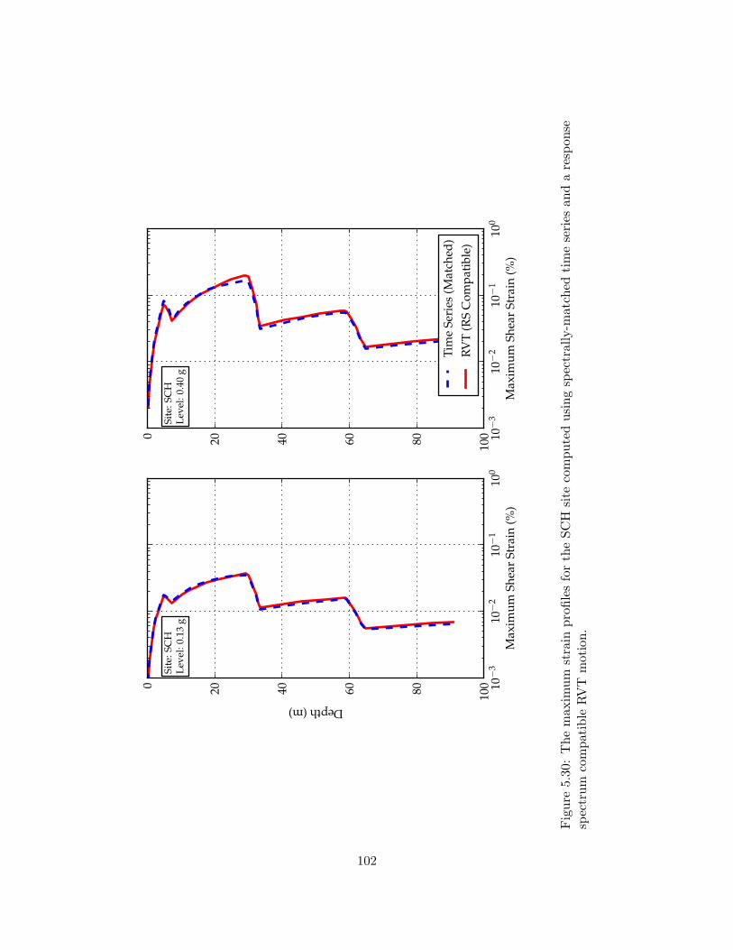
10−3

10−2

10−1

100

Max

imum

Shea

rSt

rain

(%)

0 20 40 60 80 100

Depth(m)

Site

:SC

HLe

vel:

0.13

g

10−3

10−2

10−1

100

Max

imum

Shea

rSt

rain

(%)

0 20 40 60 80 100

Site

:SC

HLe

vel:

0.40

g

Tim

eSe

ries

(Mat

ched

)RV

T(R

SC

ompa

tibl

e)

Fig

ure

5.30

:T

hem

axim

umst

rain

profi

les

for

the

SCH

site

com

pute

dus

ing

spec

tral

ly-m

atch

edti

me

seri

esan

da

resp

onse

spec

trum

com

pati

ble

RV

Tm

otio

n.

102

10−1 100 101 102

Frequency (Hz)

−30

−20

−10

0

10

20

30

Rel

ativ

eD

iffer

ence

,δSR

(%)

Difference of RVT (RS Compatible) relative to Time Series (Matched)

LE0.13 g0.40 g

Figure 5.31: The relative difference of the spectral ratio of the SCH site computed usingspectrally-matched time series and a response spectrum compatible RVT motion.

103

frequencies, except in two key regions. The first region is at low frequencies where

the smooth input FAS used in RVT produces more amplification than the time-series

analysis, and thus the RVT results are positively biased. The second region is around 0.1

Hz where there is a relative difference of -10%, which is associated with over-damping

caused by the larger strains predicted by the RVT analysis (Figure 5.33). The RVT

difference for CC and the 0.40 g input intensity is shown in Figure 5.34 along with the

RVT difference for the other analyses already discussed. As with the previous results

from SCH, as the intensity of the input motion increases the positive bias at the site

frequency increases and the negative bias at high frequencies increases. Additionally,

the RVT difference for the spectrally matched input motions (Figure 5.34) is somewhat

smaller than for scaled input motions (Figure 5.23)

104

10−1 100 101 10210−2

10−1

100Sp

ectr

alA

ccel

erat

ion

(g)

Site: CCLevel: 0.13 g

Time Series (Matched)RVT (RS Compatible)

10−1 100 101 1020.0

0.5

1.0

1.5

2.0

2.5

3.0

3.5

4.0

4.5

Spec

tral

Rat

io

10−1 100 101 102

Frequency (Hz)

−30

−20

−10

0

10

20

30

Rel

ativ

eD

iffer

ence

,δSR

(%)

Difference of RVT (RS Compatible) relative to Time Series (Matched)

Figure 5.32: The response spectrum, spectral ratio, and relative difference for theCC site computed with EQL site response using spectrally-matched time series and aresponse spectrum compatible RVT motion (input PGA of 0.13 g).

105

10−3

10−2

10−1

100

Max

imum

Shea

rSt

rain

(%)

0

100

200

300

400

500

600

700

800

Depth(m)

Site

:CC

Leve

l:0.

13g

10−3

10−2

10−1

100

Max

imum

Shea

rSt

rain

(%)

0

100

200

300

400

500

600

700

800

Site

:CC

Leve

l:0.

40g

Tim

eSe

ries

(Mat

ched

)RV

T(R

SC

ompa

tibl

e)

Fig

ure

5.33

:T

hem

axim

umst

rain

profi

les

for

the

CC

site

com

pute

dus

ing

spec

tral

ly-m

atch

edti

me

seri

esan

da

resp

onse

spec

trum

com

pati

ble

RV

Tm

otio

n.

106

10−1 100 101 102

Frequency (Hz)

−30

−20

−10

0

10

20

30

Rel

ativ

eD

iffer

ence

,δSR

(%)

Difference of RVT (RS Compatible) relative to Time Series (Matched)

LE0.13 g0.40 g

Figure 5.34: The relative difference of the spectral ratio of the CC site computed usingspectrally-matched time series and a response spectrum compatible RVT motion.

107

5.5 Summary

This section has shown that the surface response spectrum and associated spectral ratios

computed using the RVT approach may be noticeably different than the median response

computed from a suite of input motions. Figure 5.35 summarizes these differences

for the different input motion characterizations used and the two site analyzed. The

smooth shape of the input FAS used in RVT analyses produces higher peaks and lower

troughs in the spectral ratio and results in a consistent positive difference at the site

frequency and first few modes, as shown in Figure 5.35. The positive bias of RVT is

influenced most by site frequency and the shear-wave velocity of the bedrock. Lower

site frequencies and larger bedrock velocities result in larger relative differences for RVT

analysis, with relative differences as large as 30%. As the input intensity increases, the

positive bias at the site frequency for RVT analysis generally increases, but the difference

becomes negative at high frequencies. The negative bias (i.e., under prediction) at high

frequencies is caused by RVT predicting larger strains and associated damping than the

time-series analysis.

The time-series analyses performed using different suites of input motions demon-

strated the influence of ground motion selection on the results from site response

analysis. While each of the suites of input motions predicted responses that peaked

at the same frequency, the median spectral ratio at the site frequency was largest for

the spectrally matched motions and smallest for the scaled motions (Figure 5.35). The

differences in the median spectral ratio are due to differences in the motion-to-motion

variability within each suite of input motions. The suite of scaled ground motions

had the greatest variability and produced the smallest median spectral ratio at the

site frequency. Additionally, the results in Figure 5.35 show that the stochastically

simulated input motions produced the smallest spectral ratios at high frequencies (i.e.,

above 10 Hz). This result is due to the FAS shape for the stochastically simulated input

108

motions, which has relatively greater high-frequency content. This effect also influenced

the high-frequency spectral ratios for the response spectrum compatible RVT analysis

and for the spectrally matched TS analysis.

109

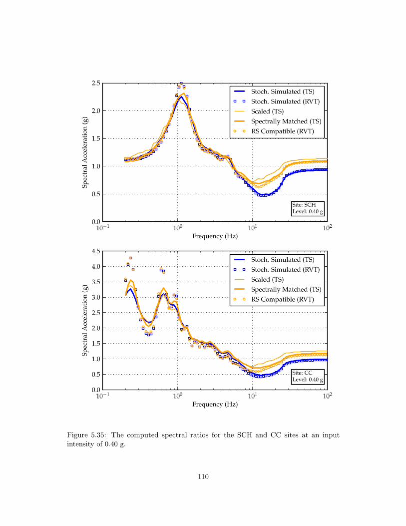
10−1 100 101 102

Frequency (Hz)

0.0

0.5

1.0

1.5

2.0

2.5Sp

ectr

alA

ccel

erat

ion

(g)

Site: SCHLevel: 0.40 g

Stoch. Simulated (TS)Stoch. Simulated (RVT)Scaled (TS)Spectrally Matched (TS)RS Compatible (RVT)

10−1 100 101 102

Frequency (Hz)

0.0

0.5

1.0

1.5

2.0

2.5

3.0

3.5

4.0

4.5

Spec

tral

Acc

eler

atio

n(g

)

Site: CCLevel: 0.40 g

Stoch. Simulated (TS)Stoch. Simulated (RVT)Scaled (TS)Spectrally Matched (TS)RS Compatible (RVT)

Figure 5.35: The computed spectral ratios for the SCH and CC sites at an inputintensity of 0.40 g.

110

Chapter 6

Comparison of Equivalent-Linear

and Nonlinear Methods

6.1 Introduction

Nonlinear site response analysis propagates the input ground motion through the soil

deposit in the time domain and varies the soil properties with time. This approach allows

for more realistic modeling of the nonlinear response of the soil. The nonlinear method

is believed to provide more realistic site response results especially for high-intensity

input motions. In this section, the equivalent-linear (EQL) method is compared to the

nonlinear method using the suite of spectrally matched motions described in Section 4.4.

Analyses are performed for linear-elastic conditions, as well as for nonlinear conditions

with low-, moderate-, and high-intensity input motions. To maintain similarity between

the nonlinear and equivalent-linear analyses, each time series used as input in the

nonlinear analysis is truncated at 25 Hz. This filtering mimics the truncation performed

in the equivalent-linear analysis.

111

6.2 Linear Elastic Analysis

A suite of linear-elastic analyses was performed to evaluate the influence of performing

site response analysis in the time domain, which is used in nonlinear analysis, and

performing site response analysis in the frequency domain, which is used in EQL analysis.

The key differences in these two approaches are the treatment of damping and the

numerical methods used to solve the equations of motion.

The nonlinear method incorporates damping in two ways: through a small-strain

viscous damping matrix and through the nonlinear, cyclic stress-strain response. The

viscous damping represents the damping at small strains (Dmin), while the nonlinear,

stress-strain response represents the hysteretic damping at larger strains. The majority

of the damping for moderate to high levels of ground shaking comes from the nonlinear

stress-strain response, while the viscous damping is more critical at lower intensities.

The viscous damping has been traditionally modeled using the full Rayleigh damping

formulation (Rayleigh and Lindsay, 1945), which generates the damping matrix (C) as

a linear combination of the initial stiffness (K) and mass (M) matrices:

C = a0K + a1M (6.1)

This formulation results in frequency-dependent viscous damping (e.g., Chopra (2007)).

The coefficients a0 and a1 are selected to tune the viscous damping ratio to a target

damping ratio at two frequencies. Stewart et al. (2008) recommends that Rayleigh

damping be fit to the target damping at the natural frequency of the site (fs) and

five times the natural frequency of the site (5fs). Using this guideline, the frequency-

dependent viscous damping is computed for both the SCH and CC sites (Figure 6.1).

For the SCH site, the Rayleigh damping ratio is within a factor of 2.0 of the target value

between about 0.40 and 15 Hz. Considering that the target Dmin value is typically

around 1% and that the equivalent viscous damping due to the nonlinear soil response

112

may be well above 10%, this error should no not significantly impact site response

results for the damping levels induced by moderate to high intensity levels of shaking.

For the CC site, the Rayleigh damping ratio may be as much as 5 to 20 times larger

than the target value at frequencies above 6.5 Hz. These large levels of damping at

high frequencies are caused by fitting the Rayleigh damping to the very small natural

frequency (fs = 0.21 Hz) of the CC site. This level of excessive damping will lead to

under prediction of high-frequency response from nonlinear analysis for sites with low

natural frequencies like CC. Phillips and Hashash (2009) offer a potential solution to

the problem of frequency-dependent damping by proposing a method that allows for

frequency-independent Rayleigh damping.

To illustrate the influence of the Rayleigh damping model on site response results,

linear-elastic (LE) site response analyses are conducted for both the SCH and CC sites.

Results from time-domain analyses are compared with results from frequency-domain

wave propagation, which rigorously solves the one-dimensional wave equation with

frequency-independent damping. Figure 6.2 shows the computed median spectral ratio

for the suite of spectrally-matched input motions using: (1) the frequency domain (FD)

method, (2) the time domain (TD) method using Rayleigh damping tuned at fs and

5fs, and (3) the TD method using the frequency-independent damping formulation.

Compared to the frequency-domain results, the time-domain results with Rayleigh

damping underestimate the spectral ratio at frequencies greater than 10 Hz for SCH.

The underestimation is on the order of 10 to 25%. The frequency-independent damping

improves the agreement, but only slightly (5 to 15% under prediction). For CC, the

time-domain results start to deviate from the FD results at about 1.67 Hz when the

viscous damping is tuned to fs and 5fs and the underestimation is as large as 50 to

75%. This reduction is caused by the large levels of Rayleigh damping at moderate to

high frequencies (Figure 6.1). The results in Figure 6.2 for the CC site also include

the response when tuning the Rayleigh damping to 3.3fs (0.7 Hz) and 16.5fs (3.5 Hz).

113

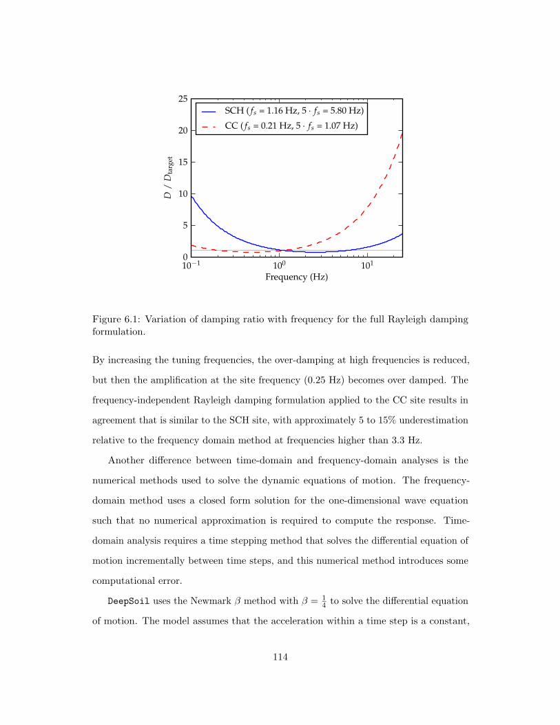
10−1 100 101

Frequency (Hz)

0

5

10

15

20

25

D/

Dta

rget

SCH ( fs = 1.16 Hz, 5 · fs = 5.80 Hz)

CC ( fs = 0.21 Hz, 5 · fs = 1.07 Hz)

Figure 6.1: Variation of damping ratio with frequency for the full Rayleigh dampingformulation.

By increasing the tuning frequencies, the over-damping at high frequencies is reduced,

but then the amplification at the site frequency (0.25 Hz) becomes over damped. The

frequency-independent Rayleigh damping formulation applied to the CC site results in

agreement that is similar to the SCH site, with approximately 5 to 15% underestimation

relative to the frequency domain method at frequencies higher than 3.3 Hz.

Another difference between time-domain and frequency-domain analyses is the

numerical methods used to solve the dynamic equations of motion. The frequency-

domain method uses a closed form solution for the one-dimensional wave equation

such that no numerical approximation is required to compute the response. Time-

domain analysis requires a time stepping method that solves the differential equation of

motion incrementally between time steps, and this numerical method introduces some

computational error.

DeepSoil uses the Newmark β method with β = 14 to solve the differential equation

of motion. The model assumes that the acceleration within a time step is a constant,

114

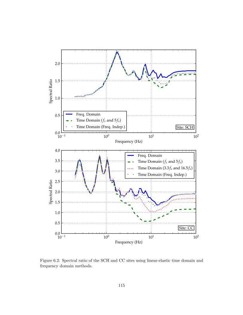
10−1 100 101 102

Frequency (Hz)

0.0

0.5

1.0

1.5

2.0

Spec

tral

Rat

io

Site: SCH

Freq. DomainTime Domain ( fs and 5 fs)

Time Domain (Freq. Indep.)

10−1 100 101 102

Frequency (Hz)

0.0

0.5

1.0

1.5

2.0

2.5

3.0

3.5

4.0

Spec

tral

Rat

io

Site: CC

Freq. DomainTime Domain ( fs and 5 fs)

Time Domain (3.3 fs and 16.5 fs)

Time Domain (Freq. Indep.)

Figure 6.2: Spectral ratio of the SCH and CC sites using linear-elastic time domain andfrequency domain methods.

115

average value. This time stepping method is unconditionally stable (Chopra, 2007),

which is advantageous for multi-degree-of-freedom systems. However, numerical errors

are also introduced that cause frequency elongation and amplitude decay (Chopra,

2007).

To illustrate these errors, the linear-elastic results (with frequency-independent

damping) are considered. The site response results are presented as the ratio of the FAS

of the surface motion to the FAS of the input motion, which represents the equivalent

transfer function for the site. Figure 6.3 shows the amplitude of the SCH and CC

transfer functions for the closed form solution in the frequency domain and for three

different motions used in the linear-elastic, time-domain analysis. The time step (∆t) for

the three input motions vary from 0.005 to 0.02 seconds. For the time-domain analyses,

the peaks at high frequencies shift towards lower frequencies, which represents frequency

shortening, and the amplitudes of the peaks decrease, which represents amplitude decay.

The frequency shortening and amplitude decay for SCH becomes noticeable at about

10 Hz and significant at about 15 Hz. The frequency shortening and amplitude decay

are more significant for motions with larger ∆t. Because of the depth of the CC site,

the character of the transfer function is different than SCH, with are many modes (i.e.,

peaks) at low frequencies (Figure 6.3). Nonetheless, frequency shortening and amplitude

decay are again noticeable at frequencies greater than about 10 to 15 Hz, and they are

more significant for motions with larger ∆t.

The frequency elongation and amplitude decay observed in Figure 6.3 directly

influence the spectral ratios at high frequencies. For both the SCH and CC sites, the

spectral ratios from the time domain analysis with frequency-independent damping

are 5 to 15% smaller than the frequency domain results at frequencies above 10 Hz,

and this result is caused by the frequency shortening and amplitude decay observed at

frequencies above 10 Hz in Figure 6.3.

The results from linear-elastic analysis illustrate two important effects that cause an

116

0 5 10 15 20 25Frequency, f (Hz)

0.0

0.5

1.0

1.5

2.0

2.5

3.0

3.5A

mpl

itud

e,A

FDTD ∆t= 0.020 secTD ∆t= 0.010 secTD ∆t= 0.005 sec

0 5 10 15 20 25Frequency, f (Hz)

0

1

2

3

4

5

6

7

Am

plit

ude,

A

FDTD ∆t= 0.020 secTD ∆t= 0.010 secTD ∆t= 0.005 sec

Figure 6.3: Amplitude of the transfer function computed for the SCH and CC sitesusing LE time-domain (TD) and frequency-domain (FD) methods.

117

underestimation of the site response at high frequencies for time domain methods. First,

frequency-dependent viscous damping tuned to fs and 5fs in time domain analysis can

significantly underestimate the site response at frequencies greater than 5 · fs. The issue

is most critical for low frequency sites, because the over-damped frequencies are in the

range of engineering interest. The frequency-independent Rayleigh damping formulation

of Phillips and Hashash (2009) can reduce this underestimation, but at the expense of

computational effort. Additionally, numerical errors introduced by the time-stepping

integration used in time-domain analysis influence the site response at frequencies

greater than about 10 Hz. For linear-elastic analysis, the errors associated with the

time-stepping integration are pronounced because the modes above 10 Hz contribute

significantly to the response. For fully nonlinear analysis, these errors should not be

significant because the modes at frequencies greater than 10 Hz no longer contribute

significantly to the response.

6.3 Analyses for Low-Intensity Input Motions

It is generally believed that nonlinear and EQL analysis provide similar estimates

of site response at low-intensity levels because the induced strains are small and the

equivalent-linear assumption is valid at these strain levels. However, the previous

section showed that even under linear-elastic conditions the frequency-domain approach

(used in the EQL analysis) and the time-domain approach (used in the nonlinear

analysis) do not provide similar results. To investigate the differences between nonlinear

and EQL analysis at low-intensity levels, analyses were performed using the suite of

spectrally-matched input motions scaled to a median PGA of 0.01 g.

The spectral ratio and relative difference between nonlinear and EQL analysis

are shown in Figure 6.4 for the SCH site. The linear-elastic results with frequency-

independent damping are shown for comparison. In general, these low-intensity motions

118

show a result similar to the linear-elastic results (i.e., nonlinear analysis under predicts

the response at high frequencies relative to EQL analyses). However, the nonlinear

results at low-intensity show more under prediction than the linear-elastic analysis

at frequencies higher than 20 Hz. Between 7 and 20 Hz, the nonlinear results at

low-intensity and the LE results are similar. The results for CC are shown in Figure 6.5

and the trends are similar. At frequencies above about 17 Hz, the nonlinear results

at low-intensity show more under prediction than the LE results. Interestingly, at

frequencies between 3 and 17 Hz the nonlinear results at low-intensity show less under

prediction than the LE results.

To investigate these results, let us consider the equivalent transfer functions for

the sites. The transfer function is complex valued, and computed from the Fourier

Amplitudes of the surface and input motions using:

TF (f) =asurf(f) + ıbsurf(f)ain(f) + ıbin(f)

= a(f) + ıb(f) (6.2)

The previous section only considered the amplitude of the transfer function (A(f) =√a(f)2 + b(f)2); this section will also consider the phase of the transfer function

(φ(f) = arctan[b(f)/a(f)]). The amplitude and phase of the equivalent transfer functions

derived from nonlinear and EQL analysis for the KOZANI-KOZ--L motion and the SCH

site are shown in Figure 6.6. The results from linear elastic TD analysis are also shown

for comparison. At low frequencies (less than 10 Hz), the amplitude and phase of the

transfer functions are similar for the nonlinear, EQL, and linear-elastic analyses. The

saw-tooth pattern for the phase represents the variation in phase as one moves from

one mode to another. At higher frequencies (greater than 15 to 20 Hz), the nonlinear

method predicts larger amplitudes and the phase becomes more irregular or incoherent.

The phase remains smooth at all frequencies for the EQL analysis, and is also smooth

for the linear-elastic analysis in the time domain (Figure 6.6).

119

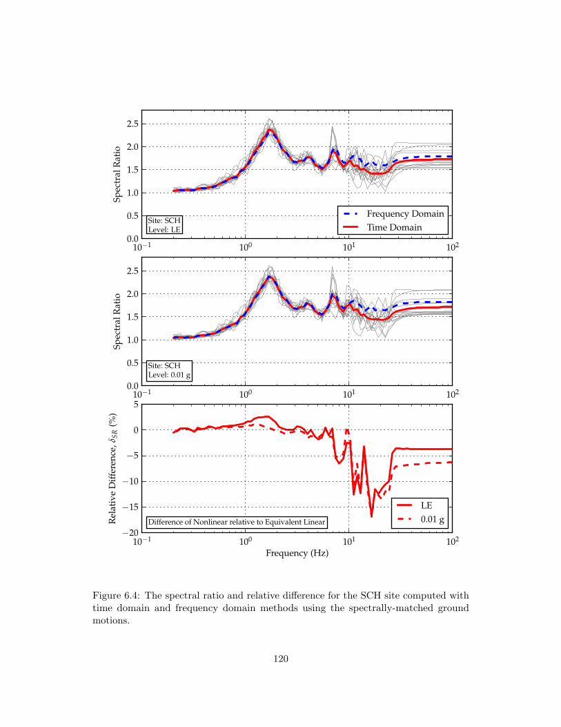
10−1 100 101 1020.0

0.5

1.0

1.5

2.0

2.5Sp

ectr

alR

atio

Site: SCHLevel: LE

Frequency DomainTime Domain

10−1 100 101 102

Frequency (Hz)

−20

−15

−10

−5

0

5

Rel

ativ

eD

iffer

ence

,δSR

(%)

Difference of Nonlinear relative to Equivalent Linear

LE0.01 g

10−1 100 101 1020.0

0.5

1.0

1.5

2.0

2.5

Spec

tral

Rat

io

Site: SCHLevel: 0.01 g

Figure 6.4: The spectral ratio and relative difference for the SCH site computed withtime domain and frequency domain methods using the spectrally-matched groundmotions.

120

10−1 100 101 1020

1

2

3

4

5

6Sp

ectr

alR

atio

Site: CCLevel: LE

Frequency DomainTime Domain

10−1 100 101 102

Frequency (Hz)

−15

−10

−5

0

5

Rel

ativ

eD

iffer

ence

,δSR

(%)

Difference of Nonlinear relative to Equivalent Linear

LE0.01 g

10−1 100 101 1020

1

2

3

4

5

6

Spec

tral

Rat

io

Site: CCLevel: 0.01 g

Figure 6.5: The spectral ratio and relative difference for the CC site computed with timedomain and frequency domain methods using the spectrally-matched ground motions.

121

The phase incoherence at high frequencies, as well as the large peaks in the amplitude

of the transfer function at high frequencies, is the result of the soil properties changing

with time in nonlinear analysis, in particular the instantaneous change in stiffness

that occurs upon load reversal. These effects are present in addition to the effects

of frequency elongation and amplitude decay discussed previously, and all of these

effects are concentrated at frequencies greater than about 10 Hz. Generally, an increase

in transfer function amplitude should generate larger spectral accelerations at these

frequencies. However, the phasing of these frequencies is incoherent such that they

destructively interfere with one another. Considering the relative differences for SCH

shown in Figure 6.4, it is the phase incoherence effect that further reduces the nonlinear

response compared with the LE response at frequencies above 20 Hz. At frequencies 10

and 20 Hz, the linear-elastic and nonlinear results are similar indicating that neither the

increase in high frequency amplitudes nor the incoherence in high-frequency phasing

significantly influences the spectral ratios in this frequency range. The amplitude and

phase of the equivalent transfer functions for the CC site are shown in Figure 6.7.

Large amplitudes and incoherent phases at high frequencies are clearly observed, and it

is the phase incoherence effect further reduces the nonlinear response relative to the

EQL response at high frequencies. However, in this case the increase in high frequency

amplitudes results in less under prediction for the spectral accelerations between 3 and

17 Hz.

122

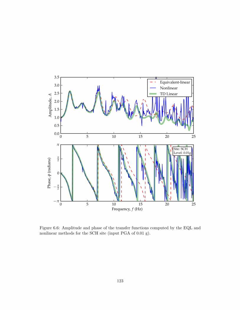
0 5 10 15 20 250.0

0.5

1.0

1.5

2.0

2.5

3.0

3.5

Am

plit

ude,

A

Equivalent-linearNonlinearTD Linear

0 5 10 15 20 25Frequency, f (Hz)

−π

−π2

0

π2

π

Phas

e,φ

(rad

ians

)

Site: SCHLevel: 0.01g

Figure 6.6: Amplitude and phase of the transfer functions computed by the EQL andnonlinear methods for the SCH site (input PGA of 0.01 g).

123

0 5 10 15 20 250

1

2

3

4

5

6

7

Am

plit

ude,

A

Equivalent-linearNonlinear

0 5 10 15 20 25Frequency, f (Hz)

−π

−π2

0

π2

π

Phas

e,φ

(rad

ians

)

Site: CCLevel: 0.01g

Figure 6.7: Amplitude and phase of the transfer functions computed by the EQL andnonlinear methods for the CC site (input PGA of 0.01 g).

124

6.4 Analyses for Moderate- to High-Intensity Input

Motions

The previous section showed that the time variation of soil properties in nonlinear

analysis causes an increase in the high-frequency amplitudes of motion, but at the same

time causes these high-frequency motions to be incoherent in phase. This section further

investigates the results from nonlinear analysis, and its comparison with EQL analysis,

at higher input intensities of 0.13 g and 0.40 g.

Figure 6.8 shows the spectral ratios and relative differences between nonlinear and

EQL analysis for the SCH site and the 0.13 g input intensity. The nonlinear and EQL

analyses provide similar results at frequencies below 10 Hz, with the spectral ratios

within 6% of one another. However, the nonlinear analysis now predicts larger spectral

ratios than EQL analysis at frequencies between 10 and 25 Hz. This result can be

explained by the equivalent transfer functions shown in Figure 6.9, which shows that

the nonlinear analysis amplifies significantly the motions at frequencies greater than 10

Hz. Despite these large amplitudes at high frequencies, the spectral ratios at frequencies

above 25 Hz from nonlinear analysis are still more than 10% smaller than those from

EQL analysis (Figure 6.8). This reduction is caused by the phase incoherence that

is introduced by the time varying properties, which in this case now extends down

to about 10 Hz (Figure 6.9). Finally, the spectral ratios from nonlinear analysis are

about 5% smaller than those from EQL analysis for frequencies from about 1 to 5

Hz (Figure 6.8). This difference most likely results from EQL analysis using constant

strain-compatible softened properties throughout the time series, while the softened

properties in nonlinear analysis vary within the time series based on the induced strains

at any one time.

To further illustrate the influence of phase incoherence on the computed site response,

a hybrid transfer function is created by combining the transfer function amplitude

125

10−1 100 101 1020.0

0.5

1.0

1.5

2.0

2.5

3.0

Spec

tral

Rat

io

Site: SCHLevel: 0.13 g

Equivalent LinearNonlinear

10−1 100 101 102

Frequency (Hz)

−15

−10

−5

0

5

10

15

20

25

Rel

ativ

eD

iffer

ence

,δSR

(%) Difference of Nonlinear relative to Equivalent Linear

Figure 6.8: The spectral ratio and relative difference for the SCH site computed withnonlinear and EQL methods using the spectrally-matched ground motions (input PGAof 0.13 g).

126

0 5 10 15 20 250.0

0.5

1.0

1.5

2.0

2.5

3.0

3.5

Am

plit

ude,

A

Equivalent-linearNonlinear

0 5 10 15 20 25Frequency, f (Hz)

−π

−π2

0

π2

π

Phas

e,φ

(rad

ians

)

Site: SCHLevel: 0.13g

Figure 6.9: Amplitude and phase of the transfer functions computed by the EQL andnonlinear methods for SCH (input PGA of 0.13 g).

127

inferred from the nonlinear analysis with a smooth phase relationship derived from the

EQL analysis. A new surface motion and associated response spectrum is computed by

applying this hybrid transfer function to the original input motion. Figure 6.10 shows

the surface response spectra predicted for the SCH site and the KOZANI-KOZ-L input

motion using nonlinear analysis and using the hybrid transfer function. Smoothing the

phase incoherence via the hybrid transfer function increases the spectral acceleration at

frequencies below 25 Hz by more than 10%, but it does not affect the lower frequencies.

Thus, it is the phase incoherence that causes the nonlinear analysis to predict smaller

spectral accelerations at very high frequencies.

The site response predictions for the SCH site and an input motion intensity of

0.40 g are shown in Figure 6.11. The trends previously observed at high frequencies

are magnified. The nonlinear analysis predicts spectral ratios almost 20% smaller than

EQL analyses at frequencies above 25 Hz, and predicts spectral ratios 30 to 60% larger

than EQL analysis at frequencies between 5 and 25 Hz. Close to the site frequency

(1.1 Hz), the nonlinear analysis predicts a spectral ratio about 15% smaller than EQL

analysis. This difference is again caused by the continuously varying softened properties

in nonlinear analysis, but may also be influenced by the divergence in the MKZ damping

curves and the damping curves used in the EQL analysis at large strains (Figure 3.3).

This difference could be reduced by fitting the MKZ model parameters over the strain

level experienced by the site for this input intensity. Interestingly, the maximum shear

strains induced by nonlinear and EQL analyses are similar for all the input intensities

investigated (Figure 6.12).

The nonlinear and EQL site response predictions for the CC site for input intensities

of 0.13 g and 0.40 g are shown in Figure 6.13. At an input intensity of 0.13 g, the

nonlinear analysis predicts spectral ratios about 5 to 10% smaller than EQL analysis at

frequencies above 20 Hz. At frequencies between 5 and 20 Hz, the nonlinear analysis

predicts spectral ratios between 10 and 20% larger than the EQL analysis. Outside

128

10−1 100 101 102

Frequency (Hz)

0.00

0.05

0.10

0.15

0.20

0.25

0.30

0.35

0.40

0.45

Spec

tral

Acc

el.(

g)

Site: SCHLevel: 0.13g

NonlinearHybrid

Figure 6.10: The effect of smooth phase on the surface response spectrum for the SCHsite.

129

10−1 100 101 1020.0

0.5

1.0

1.5

2.0

2.5

3.0

Spec

tral

Rat

io

Site: SCHLevel: 0.40 g

Equivalent LinearNonlinear

10−1 100 101 102

Frequency (Hz)

−20

−10

0

10

20

30

40

50

60

Rel

ativ

eD

iffer

ence

,δSR

(%) Difference of Nonlinear relative to Equivalent Linear

Figure 6.11: The spectral ratio and relative difference for the SCH site computed withnonlinear and EQL methods using the spectrally-matched ground motions (input PGAof 0.40 g).

130

10−4

10−3

10−2

10−1

100

Max

imum

Shea

rSt

rain

(%)

0 20 40 60 80 100

Depth(m)

Site

:SC

HLe

vel:

0.01

g

10−4

10−3

10−2

10−1

100

Max

imum

Shea

rSt

rain

(%)

0 20 40 60 80 100

Site

:SC

HLe

vel:

0.13

g

10−4

10−3

10−2

10−1

100

Max

imum

Shea

rSt

rain

(%)

0 20 40 60 80 100

Site

:SC

HLe

vel:

0.40

g

Equi

vale

ntLi

near

Non

linea

r

Fig

ure

6.12

:T

hem

axim

umst

rain

profi

lefo

rth

eSC

Hsi

teco

mpu

ted

wit

hth

eno

nlin

ear

and

EQ

Lm

etho

ds.

131

of this frequency range, the nonlinear analysis predicts spectral ratios within 10% of

the EQL analysis. As the intensity level increases, the nonlinear analysis predicts even

larger spectral ratios between 5 and 20 Hz with relative differences exceeding 60%. The

difference in this frequency range is influenced also by over-damping in the EQL at large

strain levels. The relative difference for the spectral ratios outside of this frequency

range are similar to those for an input intensity of 0.13 g.

132

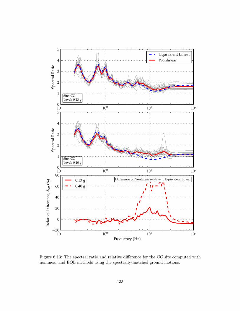
10−1 100 101 1020

1

2

3

4

5Sp

ectr

alR

atio

Site: CCLevel: 0.13 g

Equivalent LinearNonlinear

10−1 100 101 102

Frequency (Hz)

−20

0

20

40

60

80

Rel

ativ

eD

iffer

ence

,δSR

(%) Difference of Nonlinear relative to Equivalent Linear0.13 g

0.40 g

10−1 100 101 1020

1

2

3

4

5

Spec

tral

Rat

io

Site: CCLevel: 0.40 g

Figure 6.13: The spectral ratio and relative difference for the CC site computed withnonlinear and EQL methods using the spectrally-matched ground motions.

133

6.5 Summary

The comparisons between nonlinear and EQL analysis for different input intensities and

the two site considered are summarized in Figure 6.14. At frequencies above 25 Hz, the

nonlinear method consistently predicts smaller spectral ratios and spectral acceleration

than EQL analysis due to the phase incoherence introduced at high frequencies. This

effect generally increases with input intensity, and may be as larger as 15 to 20%. At

frequencies between about 5 and 20 Hz, the nonlinear method predicts smaller spectral

ratios than EQL analyses at very low-input intensities due to numerical errors associated

with the time stepping method used to solve the dynamic equations of motions. At

larger input intensities (greater than about 0.1 g), the nonlinear method predicts larger

spectral ratios than EQL analysis in this frequency range (5 and 25 Hz). This difference

is caused by two things: high-frequency amplification in nonlinear analysis caused

by instantaneous changes in stiffness upon load reversal, and over-damping of high

frequencies in EQL analysis at larger strains. At frequencies above 5 Hz, nonlinear

analysis generally predicts smaller spectral ratios than EQL analysis and this difference

may be as large as 10 to 15% at the site frequency at larger intensities. This difference

is caused by the continuously-varying softened properties used in nonlinear analysis.

134

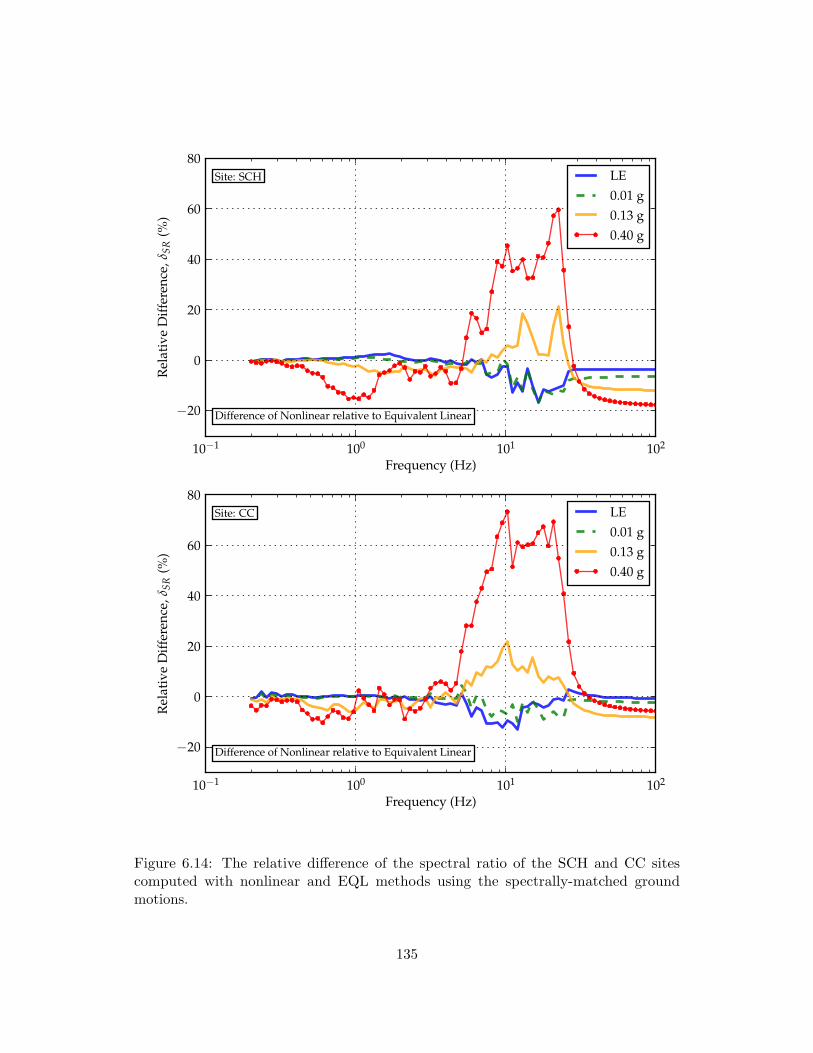
10−1 100 101 102

Frequency (Hz)

−20

0

20

40

60

80R

elat

ive

Diff

eren

ce,δ

SR(%

)Site: SCH

Difference of Nonlinear relative to Equivalent Linear

LE0.01 g0.13 g0.40 g

10−1 100 101 102

Frequency (Hz)

−20

0

20

40

60

80

Rel

ativ

eD

iffer

ence

,δSR

(%)

Site: CC

Difference of Nonlinear relative to Equivalent Linear

LE0.01 g0.13 g0.40 g

Figure 6.14: The relative difference of the spectral ratio of the SCH and CC sitescomputed with nonlinear and EQL methods using the spectrally-matched groundmotions.

135

Chapter 7

Conclusion

7.1 Summary

In this report, suites of input ground motions were used to compare relative differences

between various site response techniques. Specifically, results from equivalent-linear

(EQL) site response analysis using time-series and random-vibration-theory (RVT)

approaches were compared, as well as results from equivalent-linear and nonlinear site

response approaches.

When compared to the time series approach, the RVT approach may over-predict

the spectral ratio at the site frequency by as much as 30%, as well as over predict the

maximum strains. The over amplification computed by the RVT approach is a result of

the smooth shape of the input Fourier amplitude spectrum used in the RVT analysis.

This smooth shape has a greater sensitivity to the site transfer function. The level of

over-amplification and associated RVT difference is dependent on the site characteristics,

with the difference of the RVT approach increasing with increasing bedrock impedance

contrast, and increasing site frequency. The over-prediction of strains is also caused

by the smooth input FAS used in the RVT approach, and these larger strains lead to

over-damping of high frequencies for larger input intensities.

136

This study also provided some interesting insights regarding the influence of input

motion specification on the results from site response analysis. Three different suites of

time series were used in the EQL analysis: stochastically-simulated motions, linearly-

scaled motions, and spectrally-matched motions. While each of the suites of input

motions predicted responses that peaked at the same frequency, the median spectral

ratio at the site frequency was largest for the spectrally-matched motions and smallest

for the scaled motions. The differences in the median spectral ratio was due to differences

in the motion-to-motion variability within each suite of input motions. The suite of

scaled ground motions had the greatest variability and produced the smallest median

spectral ratio at the site frequency. The spectral ratio at the site frequency is sensitive

to the variability in the suite of input motions because each input motion induces a

different level of strain and a different site frequency. The averaging of the individual

input motions pulls down the median spectral ratio. The reduced variability in the

suite of spectrally matched ground motions produced the most similar results to the

RVT approach.

The comparisons between the EQL and nonlinear methods yielded several important

findings. For deep sites, it is recommended that the frequency-independent Rayleigh

damping formulation proposed by Phillips and Hashash (2009) be used. However,

even with this frequency-independent damping, the nonlinear method predicts smaller

spectral ratios at high frequencies (above 5 Hz) under small intensities (less than about

0.1 g) due to numerical errors associated with the time stepping algorithm. At larger

input intensities, the nonlinear method predicts less amplification than the EQL method

at very high frequencies (above 25 Hz), more amplification than the EQL method at

high frequencies (5 to 25 Hz for the SCH site), and less amplification than the EQL

method at the site frequency. The nonlinear method predicts less amplification at very

short frequencies due to the incoherence in the phase introduced by the nonlinear stress-

strain response. The greater amplification predicted by the nonlinear method at high

137

frequencies is a result of high-frequency amplification generated by the instantaneous

change in stiffness upon stress reversal in the nonlinear analysis, as well as over-damping

of high frequencies in the EQL analysis. The smaller amplification predicted by the

nonlinear method close to the site frequency is caused by the continuously changing

stiffness modeled in nonlinear analysis.

7.2 Recommendations for Future Work

The comparisons performed in this study were limited to hypothetical events, which

only allow for relative comparisons to be made between the different methods of analysis.

Future research work should employ data from borehole arrays that provide both

the recorded input and surface ground motions. This information would allow for

an assessment of the true performance of the site response methods, instead of only

providing relative comparisons.

The results of this study indicate that there is a significant difference in the site

response predicted RVT approach due to the smooth FAS used as the input motion in

RVT analysis. Further work needs to be done to establish a method to correct for this

difference in a manner that could be implemented into future site response analyses.

138

Bibliography

N. Abrahamson and W. Silva. Empirical response spectral attenuation relations for

shallow crustal earthquakes. Seismological Research Letters, 68:94–127, 1997.

N. A. Abrahamson. Non-stationary spectral matching. Seismological Review Letters, 63

(1):30, 1992.

N. A. Abrahamson and W. J. Silva. Empirical ground motion models. Technical report,

Brookhaven National Laboratory, Lipton, New York, 1996.

D. M. Boore. Simulation of ground motion using the stochastic method. Pure and

Applied Geophysics, 160(3-4):635–676, March 2003.

D. M. Boore. SMSIM – fortran programs for simulating ground motions from earthquakes:

version 2.3. Open-File Report OFR 96-80-A, U.S. Geological Survey, Menlo Park,

California, 2005.

D. M. Boore and G. M. Atkinson. Ground-motion prediction equations for the average

horizontal component of PGA, PGV, and 50.01 s and 10.0 s. Earthquake Spectra, 24

(1):99–138, Feburary 2008.

D. M. Boore and W. B. Joyner. A note on the use of random vibration theory to predict

peak amplitudes of transient signals. Bulletin of the Seismological Society of America,

74(5):2035–2039, October 1984.

139

D. Cartwright and M. Longuet-Higgins. The statistical distribution of the maxima of a

random function. Proceedings of the Royal Society of London. Series A, Mathematical

and Physical Sciences, 237(1209):212–232, 1956.

S. W.-Y. Chang. Seismic response of deep stiff soil deposits. PhD thesis, University of

California, Berkeley, December 1996.

A. K. Chopra. Dynamics of Structures: Theory and Applications to Earthquake En-

gineering. Prentice Hall, Upper Saddle River, New Jersey, third edition edition,

2007.

M. B. Darendeli. Development of a new family of normalized modulus reduction and

material damping curves. PhD thesis, The University of Texas, Austin, 2001.

D. A. Gasparini and E. H. Vanmarcke. Simulated earthquake motions compatible with

prescribed response spectra. Technical Report R76-4, Massachusetts Institute of

Technology, Department of Civil Engineering, Cambridge, Massachusetts, 1976.

J. Gibbs, J. Tinsley, D. Boore, and W. Joyner. Seismic velocities and geological

conditions at twelve sites subjected to strong ground motion in the 1994 Northridge,

California, earthquake: a revision of OFR 96-740. U.S. Geological Survey Open-File

Report 99-446, U.S. Department of the Interior, U.S. Geological Survey, 1999.

J. Hancock. An improved method of matching response spectra of recorded earthquake

ground motion using wavelets. Journal of Earthquake Engineering, 10(1):67–89, 2006.

Y. M. Hashash. Viscous damping formulation and high frequency motion propagation

in nonlinear site response analysis. Soil Dynamics and Earthquake Engineering, 22

(7):611–624, September 2002.

Y. M. A. Hashash and D. Park. Nonlinear one-dimensional seismic ground motion

140

propagation in the mississippi embayment. Engineering Geology, 62(1-3):185 – 206,

2001.

I. M. Idriss and J. I. Sun. User’s manual for shake91: a computer program for

conducting equivalent linear seismic response analyses of horizontally layered soil

deposits. Technical report, Center for Geotechnical Modeling, University of California,

Davis, 1993.

A. R. Kottke and E. M. Rathje. A semi-automated procedure for selection and scaling

of recorded earthquake motions for dynamic analysis. Earthquake Spectra, 24(4):

911–932, November 2008a.

A. R. Kottke and E. M. Rathje. Technical manual for Strata. Report 2008/10, Pacific

Earthquake Engineering Research (PEER) Center, Berkeley, California, 2008b.

N. Matasovic and M. Vucetic. Cyclic characterization of liquefiable sands. Journal of

Geotechnical Engineering, 119(11):1805–1822, November 1993.

R. K. McGuire, W. J. Silva, and C. J. Costantino. Technical basis for revision of regula-

tory guidance on design ground motions: Hazard- and risk-consistent ground motion

spectra guidelines. Technical Report NUREG/CR-6728, U.S. Nuclear Regulatory

Commission, Washington, DC, 2001.

R. K. McGuire, W. J. Silva, and C. J. Costantino. Technical basis for revision of

regulatory guidance on design ground motions: Development of hazard- and risk-

consistent seismic spectra for two site. Technical Report NUREG/CR-6769, U.S.

Nuclear Regulatory Commission, Washington, DC, 2002.

G. Ordonez. User’s manual for shake91: a computer program for conducting equivalent

linear seismic response analyses of horizontally layered soil deposits. Technical report,

GeoMotions, 2002.

141

C. Phillips and Y. M. Hashash. Damping formulation for nonlinear 1d site response

analysis. Soil Dynamics and Earthquake Engineering, 29(7):1143–1158, July 2009.

E. M. Rathje and A. R. Kottke. Procedure for random vibration theory based seismic

site response analyses. Geotechnical Engineering Report GR08-09, The University of

Texas at Austin, Austin, TX, 2008.

J. Rayleigh and R. Lindsay. The theory of sound. Dover Publications, New York, 1st

american edition, 1945.

C. Real, A. Shakal, and B. Tucker. Overview of the Turkey Flat ground motion

prediction experiment. In Proc. SMIP06 Seminar on Utilization of Strong-Motion

Data, pages 117–136, 2006.

C. R. Real. Turkey flat, USA site effects test area – report 2: Site characterization. TR

88-2, California Division of Mines and Geology, 1988.

P. B. Schnabel, J. Lysmer, and H. B. Seed. SHAKE: A computer program for earthquake

response analysis of horizontally layered site. Report UCB/EERC-72/12, Earthquake

Engineering Research Center, University of California, Berkeley, California, 1972.

W. Silva, N. Abrahamson, G. Toro, and C. Costantino. Description and validation of the

stochastic ground motion model. Report 770573, Brookhaven National Laboratory,

Upton, New York, 1996.

J. P. Stewart, A. O.-L. Kwok, Y. M. Hashash, N. Matasovic, R. Pyke, Z. Wang, and

Z. Yang. Benchmarking of nonlinear geotechnical ground response analysis procedures.

Report 2008/04, Pacific Earthquake Engineering Research (PEER) Center, Berkeley,

California, 2008.

UniStar Nuclear Services. Calvert Cliffs nuclear power plant unit 3, combined license

application, part 2: Final safety analysis report, rev. 6, 2007.

142

Regulatory Guide 1.208: A performance-based approach to define the site-specific earth-

quake ground motion. U.S. Nuclear Regulatory Commission, Washington, DC, 2007.

143

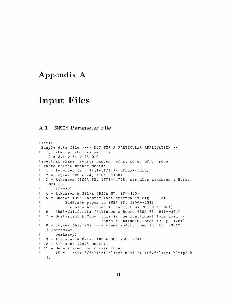
Appendix A

Input Files

A.1 SMSIM Parameter File

!TitleSample data file **** NOT FOR A PARTICULAR APPLICATION **

!rho , beta , prtitn , radpat , fs:2.8 3.6 0.71 0.55 2.0

!spectral shape: source number , pf_a , pd_a , pf_b , pd_a! where source number means:! 1 = 1-corner (S = 1/(1+(f/fc)**pf_a)**pd_a)! 2 = Joyner (BSSA 74, 1167 - -1188)! 3 = Atkinson (BSSA 83, 1778 - -1798; see also Atkinson & Boore ,

BSSA 85,! 17--30)! 4 = Atkinson & Silva (BSSA 87, 97--113)! 5 = Haddon 1996 (approximate spectra in Fig. 10 of! Haddon ’s paper in BSSA 86, 1300 - -1313;! see also Atkinson & Boore , BSSA 78, 917- -934)! 6 = AB98 -California (Atkinson & Boore BSSA 78, 917- -934)! 7 = Boatwright & Choy (this is the functional form used by! Boore & Atkinson , BSSA 79, p. 1761)! 8 = Joyner (his ENA two -corner model , done for the SSHAC

elicitation! workshop)! 9 = Atkinson & Silva (BSSA 90, 255- -274)! 10 = Atkinson (2005 model),! 11 = Generalized two corner model! (S = [1/(1+(f/fa)**pf_a)**pd_a ]*[1/(1+(f/fb)**pf_b)**pd_b

])

144

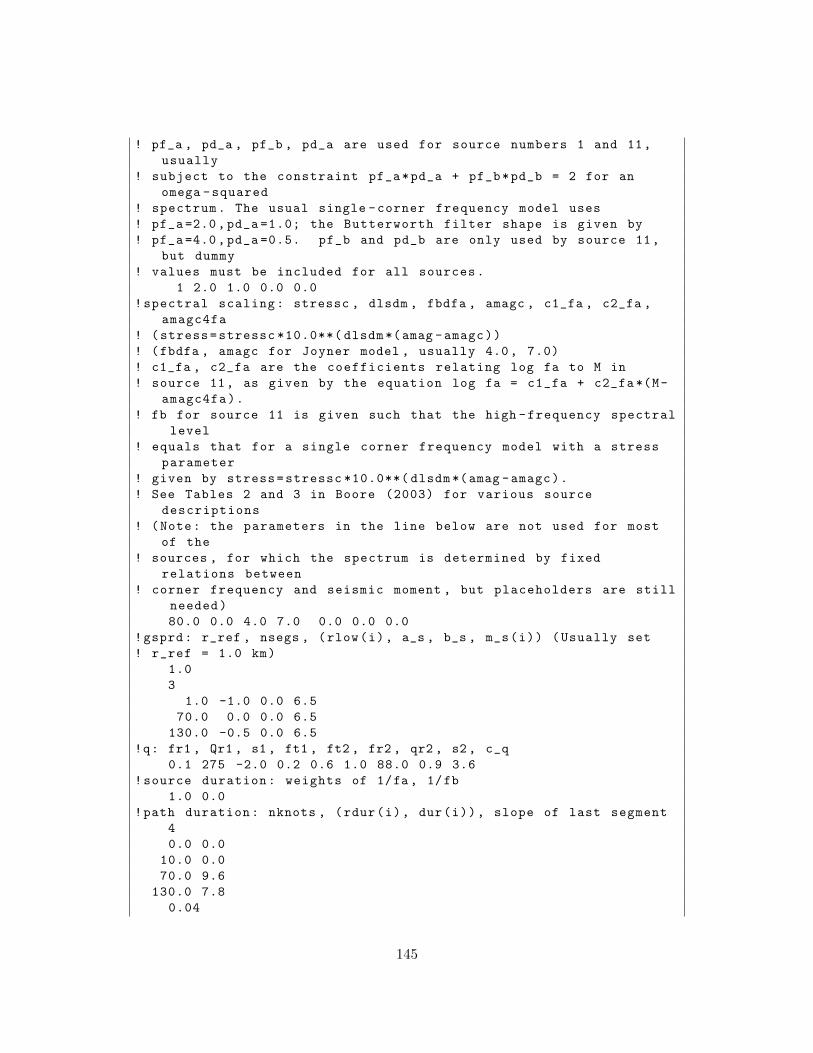
! pf_a , pd_a , pf_b , pd_a are used for source numbers 1 and 11,usually

! subject to the constraint pf_a*pd_a + pf_b*pd_b = 2 for anomega -squared

! spectrum. The usual single -corner frequency model uses! pf_a =2.0, pd_a =1.0; the Butterworth filter shape is given by! pf_a =4.0, pd_a =0.5. pf_b and pd_b are only used by source 11,

but dummy! values must be included for all sources.

1 2.0 1.0 0.0 0.0!spectral scaling: stressc , dlsdm , fbdfa , amagc , c1_fa , c2_fa ,

amagc4fa! (stress=stressc *10.0**( dlsdm *(amag -amagc))! (fbdfa , amagc for Joyner model , usually 4.0, 7.0)! c1_fa , c2_fa are the coefficients relating log fa to M in! source 11, as given by the equation log fa = c1_fa + c2_fa *(M-

amagc4fa).! fb for source 11 is given such that the high -frequency spectral

level! equals that for a single corner frequency model with a stress

parameter! given by stress=stressc *10.0**( dlsdm *(amag -amagc).! See Tables 2 and 3 in Boore (2003) for various source

descriptions! (Note: the parameters in the line below are not used for most

of the! sources , for which the spectrum is determined by fixed

relations between! corner frequency and seismic moment , but placeholders are still

needed)80.0 0.0 4.0 7.0 0.0 0.0 0.0

!gsprd: r_ref , nsegs , (rlow(i), a_s , b_s , m_s(i)) (Usually set! r_ref = 1.0 km)

1.03

1.0 -1.0 0.0 6.570.0 0.0 0.0 6.5

130.0 -0.5 0.0 6.5!q: fr1 , Qr1 , s1 , ft1 , ft2 , fr2 , qr2 , s2, c_q

0.1 275 -2.0 0.2 0.6 1.0 88.0 0.9 3.6!source duration: weights of 1/fa, 1/fb

1.0 0.0!path duration: nknots , (rdur(i), dur(i)), slope of last segment

40.0 0.0

10.0 0.070.0 9.6

130.0 7.80.04

145

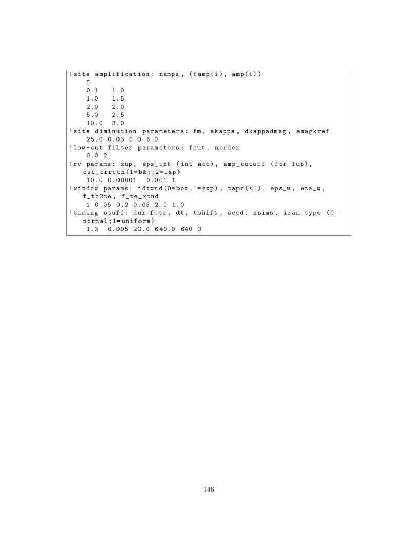
!site amplification: namps , (famp(i), amp(i))50.1 1.01.0 1.52.0 2.05.0 2.510.0 3.0

!site diminution parameters: fm, akappa , dkappadmag , amagkref25.0 0.03 0.0 6.0

!low -cut filter parameters: fcut , norder0.0 2

!rv params: zup , eps_int (int acc), amp_cutoff (for fup),osc_crrctn (1=b&j;2=l&p)10.0 0.00001 0.001 1

!window params: idxwnd (0=box ,1=exp), tapr(<1), eps_w , eta_w ,f_tb2te , f_te_xtnd1 0.05 0.2 0.05 2.0 1.0

!timing stuff: dur_fctr , dt , tshift , seed , nsims , iran_type (0=normal ;1= uniform)1.3 0.005 20.0 640.0 640 0

146

Appendix B

Scaled Time Series

147

0 10 20 30 40 50 60−0.10

−0.05

0.00

0.05

0.10A

ccel

erat

ion

(g)

0 10 20 30 40 50 60−10

−5

0

5

10

Velo

city

(cm

/s)

0 10 20 30 40 50 60Time (s)

−4−3−2−1

01234

Dis

plac

emen

t(cm

)

10−1 100 101 102

Frequency (Hz)

10−2

10−1

100

Spec

tral

Acc

eler

atio

n(g

)

Figure B.1: The CHICHI06-TCU076-E time series scaled by 0.79.

148

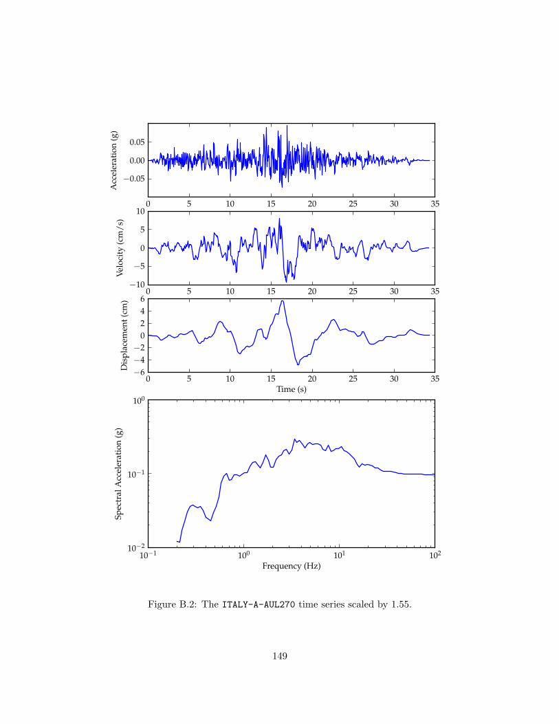
0 5 10 15 20 25 30 35

−0.05

0.00

0.05

Acc

eler

atio

n(g

)

0 5 10 15 20 25 30 35−10

−5

0

5

10

Velo

city

(cm

/s)

0 5 10 15 20 25 30 35Time (s)

−6−4−2

0246

Dis

plac

emen

t(cm

)

10−1 100 101 102

Frequency (Hz)

10−2

10−1

100

Spec

tral

Acc

eler

atio

n(g

)

Figure B.2: The ITALY-A-AUL270 time series scaled by 1.55.

149

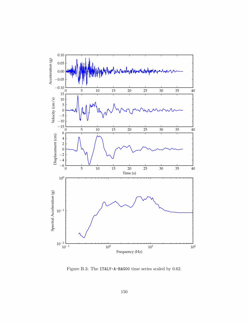
0 5 10 15 20 25 30 35 40−0.10

−0.05

0.00

0.05

0.10A

ccel

erat

ion

(g)

0 5 10 15 20 25 30 35 40−15−10−5

05

1015

Velo

city

(cm

/s)

0 5 10 15 20 25 30 35 40Time (s)

−6−4−2

0246

Dis

plac

emen

t(cm

)

10−1 100 101 102

Frequency (Hz)

10−2

10−1

100

Spec

tral

Acc

eler

atio

n(g

)

Figure B.3: The ITALY-A-BAG00 time series scaled by 0.62.

150

0 5 10 15 20 25 30 35 40−0.10

−0.05

0.00

0.05

0.10A

ccel

erat

ion

(g)

0 5 10 15 20 25 30 35 40−15−10−5

05

1015

Velo

city

(cm

/s)

0 5 10 15 20 25 30 35 40Time (s)

−8−6−4−2

02468

Dis

plac

emen

t(cm

)

10−1 100 101 102

Frequency (Hz)

10−2

10−1

100

Spec

tral

Acc

eler

atio

n(g

)

Figure B.4: The ITALY-A-STU270 time series scaled by 0.25.

151

0 5 10 15 20 25 30 35−0.10

−0.05

0.00

0.05

0.10A

ccel

erat

ion

(g)

0 5 10 15 20 25 30 35−10

−5

0

5

10

Velo

city

(cm

/s)

0 5 10 15 20 25 30 35Time (s)

−4−3−2−1

01234

Dis

plac

emen

t(cm

)

10−1 100 101 102

Frequency (Hz)

10−3

10−2

10−1

100

Spec

tral

Acc

eler

atio

n(g

)

Figure B.5: The ITALY-B-AUL270 time series scaled by 4.19.

152

0 5 10 15 20 25 30−0.20−0.15−0.10−0.05

0.000.050.100.150.20

Acc

eler

atio

n(g

)

0 5 10 15 20 25 30−8−6−4−2

02468

Velo

city

(cm

/s)

0 5 10 15 20 25 30Time (s)

−1.5−1.0−0.5

0.00.51.01.5

Dis

plac

emen

t(cm

)

10−1 100 101 102

Frequency (Hz)

10−3

10−2

10−1

100

Spec

tral

Acc

eler

atio

n(g

)

Figure B.6: The KOZANI-KOZ--L time series scaled by 0.73.

153

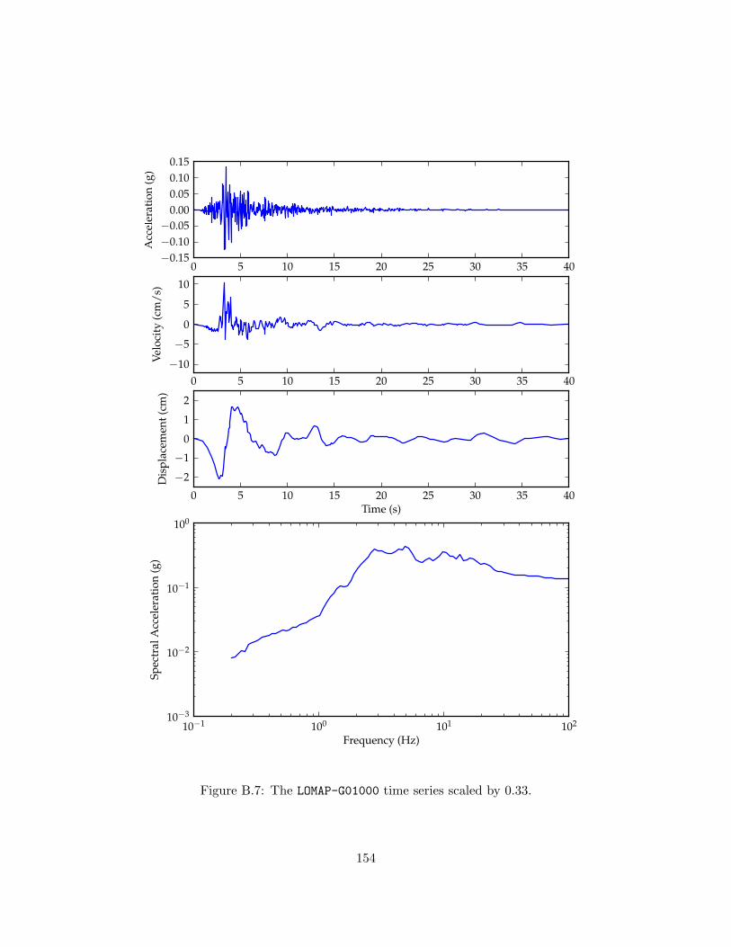
0 5 10 15 20 25 30 35 40−0.15−0.10−0.05

0.000.050.100.15

Acc

eler

atio

n(g

)

0 5 10 15 20 25 30 35 40−10

−5

0

5

10

Velo

city

(cm

/s)

0 5 10 15 20 25 30 35 40Time (s)

−2

−1

0

1

2

Dis

plac

emen

t(cm

)

10−1 100 101 102

Frequency (Hz)

10−3

10−2

10−1

100

Spec

tral

Acc

eler

atio

n(g

)

Figure B.7: The LOMAP-G01000 time series scaled by 0.33.

154

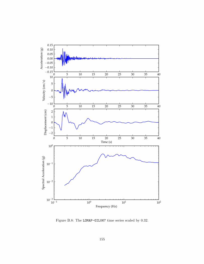
0 5 10 15 20 25 30 35 40−0.15−0.10−0.05

0.000.050.100.15

Acc

eler

atio

n(g

)

0 5 10 15 20 25 30 35 40−10

−5

0

5

10

Velo

city

(cm

/s)

0 5 10 15 20 25 30 35 40Time (s)

−2

−1

0

1

2

Dis

plac

emen

t(cm

)

10−1 100 101 102

Frequency (Hz)

10−3

10−2

10−1

100

Spec

tral

Acc

eler

atio

n(g

)

Figure B.8: The LOMAP-GIL067 time series scaled by 0.32.

155

0 5 10 15 20 25 30−0.20−0.15−0.10−0.05

0.000.050.100.150.20

Acc

eler

atio

n(g

)

0 5 10 15 20 25 30−6−4−2

0246

Velo

city

(cm

/s)

0 5 10 15 20 25 30Time (s)

−2.0−1.5−1.0−0.5

0.00.51.01.52.0

Dis

plac

emen

t(cm

)

10−1 100 101 102

Frequency (Hz)

10−3

10−2

10−1

100

Spec

tral

Acc

eler

atio

n(g

)

Figure B.9: The MORGAN-GIL337 time series scaled by 2.01.

156

0 5 10 15 20 25 30 35 40−0.20−0.15−0.10−0.05

0.000.050.100.150.20

Acc

eler

atio

n(g

)

0 5 10 15 20 25 30 35 40−6−4−2

0246

Velo

city

(cm

/s)

0 5 10 15 20 25 30 35 40Time (s)

−3−2−1

0123

Dis

plac

emen

t(cm

)

10−1 100 101 102

Frequency (Hz)

10−3

10−2

10−1

100

Spec

tral

Acc

eler

atio

n(g

)

Figure B.10: The NORTHR-H12180 time series scaled by 0.66.

157

0 5 10 15 20 25 30−0.15−0.10−0.05

0.000.050.100.15

Acc

eler

atio

n(g

)

0 5 10 15 20 25 30−8−6−4−2

02468

Velo

city

(cm

/s)

0 5 10 15 20 25 30Time (s)

−1.5−1.0−0.5

0.00.51.01.5

Dis

plac

emen

t(cm

)

10−1 100 101 102

Frequency (Hz)

10−3

10−2

10−1

100

Spec

tral

Acc

eler

atio

n(g

)

Figure B.11: The NORTHR-HOW330 time series scaled by 0.83.

158

0 5 10 15 20 25 30 35−0.15−0.10−0.05

0.000.050.100.15

Acc

eler

atio

n(g

)

0 5 10 15 20 25 30 35−15−10−5

05

1015

Velo

city

(cm

/s)

0 5 10 15 20 25 30 35Time (s)

−2

−1

0

1

2

Dis

plac

emen

t(cm

)

10−1 100 101 102

Frequency (Hz)

10−3

10−2

10−1

100

Spec

tral

Acc

eler

atio

n(g

)

Figure B.12: The NORTHR-LV1000 time series scaled by 1.30.

159

0 5 10 15 20 25 30 35−0.15−0.10−0.05

0.000.050.100.15

Acc

eler

atio

n(g

)

0 5 10 15 20 25 30 35−15−10−5

05

1015

Velo

city

(cm

/s)

0 5 10 15 20 25 30 35Time (s)

−2

−1

0

1

2

Dis

plac

emen

t(cm

)

10−1 100 101 102

Frequency (Hz)

10−3

10−2

10−1

100

Spec

tral

Acc

eler

atio

n(g

)

Figure B.13: The NORTHR-LV3090 time series scaled by 1.24.

160

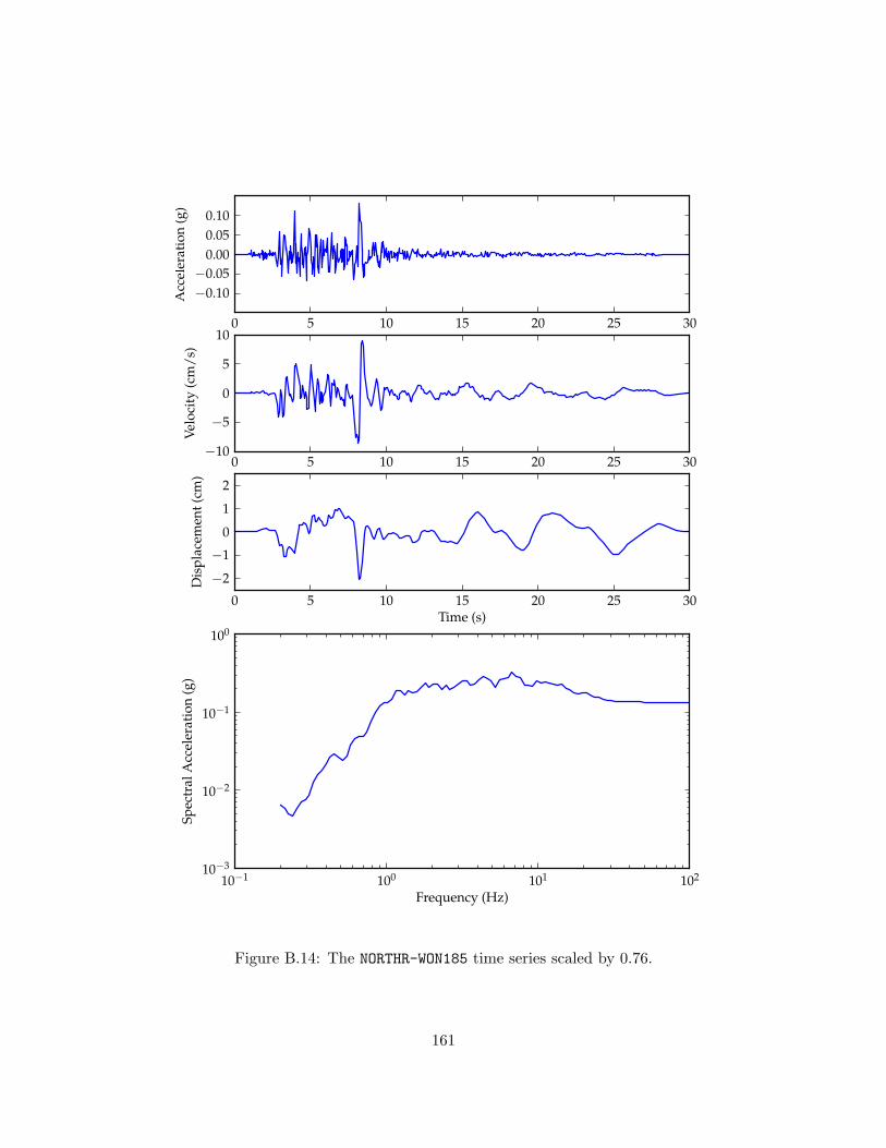
0 5 10 15 20 25 30

−0.10−0.05

0.000.050.10

Acc

eler

atio

n(g

)

0 5 10 15 20 25 30−10

−5

0

5

10

Velo

city

(cm

/s)

0 5 10 15 20 25 30Time (s)

−2

−1

0

1

2

Dis

plac

emen

t(cm

)

10−1 100 101 102

Frequency (Hz)

10−3

10−2

10−1

100

Spec

tral

Acc

eler

atio

n(g

)

Figure B.14: The NORTHR-WON185 time series scaled by 0.76.

161

0 5 10 15 20 25−0.15−0.10−0.05

0.000.050.100.15

Acc

eler

atio

n(g

)

0 5 10 15 20 25−8−6−4−2

02468

Velo

city

(cm

/s)

0 5 10 15 20 25Time (s)

−3−2−1

0123

Dis

plac

emen

t(cm

)

10−1 100 101 102

Frequency (Hz)

10−3

10−2

10−1

100

Spec

tral

Acc

eler

atio

n(g

)

Figure B.15: The VICT-CPE045 time series scaled by 0.21.

162

Appendix C

Spectrally-Matched Time Series

163

0 10 20 30 40 50 60−0.15−0.10−0.05

0.000.050.100.15

Acc

eler

atio

n(g

)

0 10 20 30 40 50 60−8−6−4−2

02468

Velo

city

(cm

/s)

0 10 20 30 40 50 60Time (s)

−3−2−1

0123

Dis

plac

emen

t(cm

)

10−1 100 101 102

Frequency (Hz)

10−3

10−2

10−1

100

Spec

tral

Acc

eler

atio

n(g

)

Figure C.1: The spectrally-matched CHICHI06-TCU076-E time series.

164

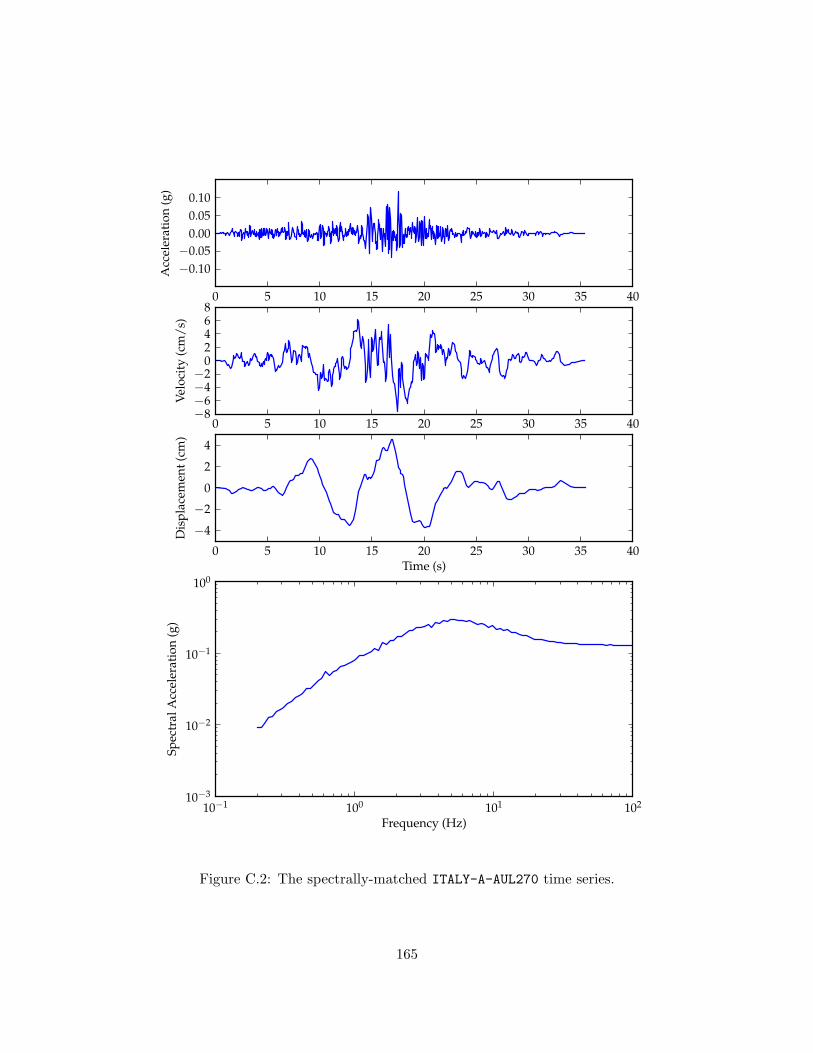
0 5 10 15 20 25 30 35 40

−0.10−0.05

0.000.050.10

Acc

eler

atio

n(g

)

0 5 10 15 20 25 30 35 40−8−6−4−2

02468

Velo

city

(cm

/s)

0 5 10 15 20 25 30 35 40Time (s)

−4

−2

0

2

4

Dis

plac

emen

t(cm

)

10−1 100 101 102

Frequency (Hz)

10−3

10−2

10−1

100

Spec

tral

Acc

eler

atio

n(g

)

Figure C.2: The spectrally-matched ITALY-A-AUL270 time series.

165

0 5 10 15 20 25 30 35 40−0.10

−0.05

0.00

0.05

0.10A

ccel

erat

ion

(g)

0 5 10 15 20 25 30 35 40−8−6−4−2

02468

Velo

city

(cm

/s)

0 5 10 15 20 25 30 35 40Time (s)

−4−3−2−1

01234

Dis

plac

emen

t(cm

)

10−1 100 101 102

Frequency (Hz)

10−3

10−2

10−1

100

Spec

tral

Acc

eler

atio

n(g

)

Figure C.3: The spectrally-matched ITALY-A-BAG000 time series.

166

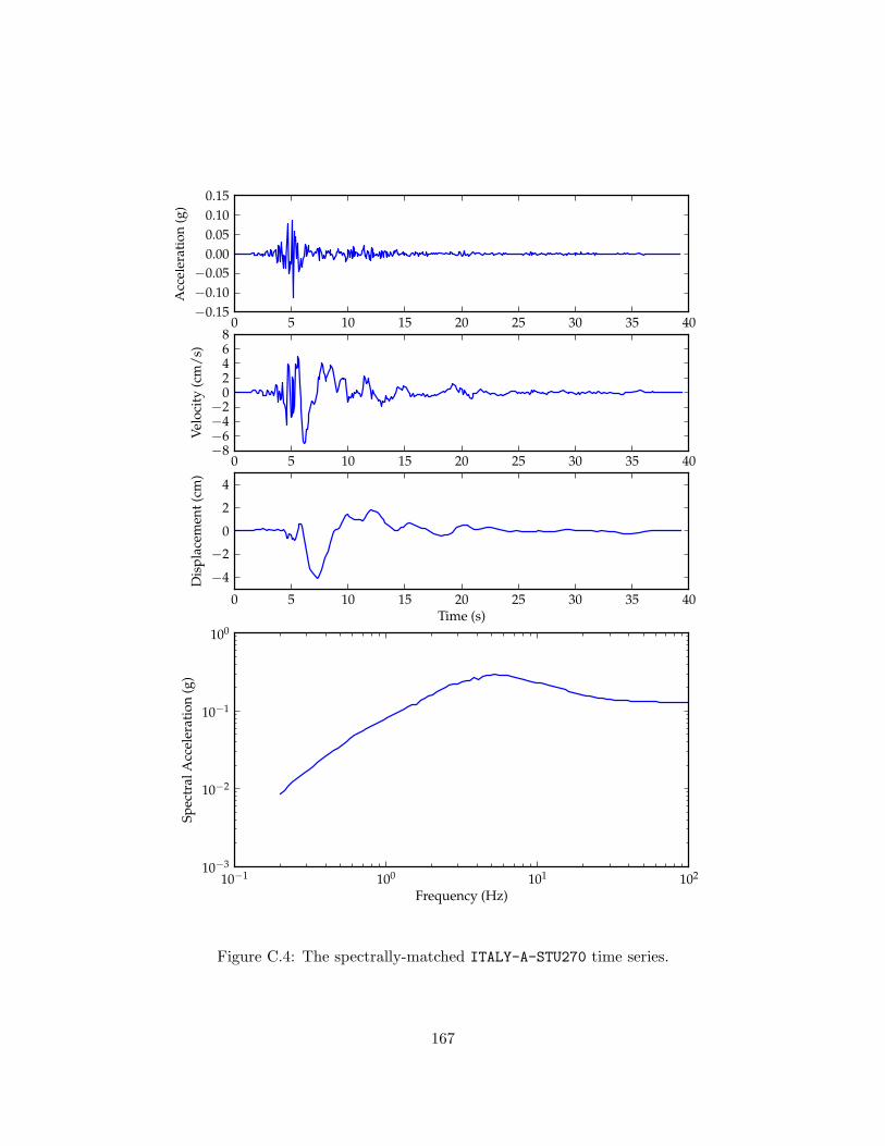
0 5 10 15 20 25 30 35 40−0.15−0.10−0.05

0.000.050.100.15

Acc

eler

atio

n(g

)

0 5 10 15 20 25 30 35 40−8−6−4−2

02468

Velo

city

(cm

/s)

0 5 10 15 20 25 30 35 40Time (s)

−4

−2

0

2

4

Dis

plac

emen

t(cm

)

10−1 100 101 102

Frequency (Hz)

10−3

10−2

10−1

100

Spec

tral

Acc

eler

atio

n(g

)

Figure C.4: The spectrally-matched ITALY-A-STU270 time series.

167

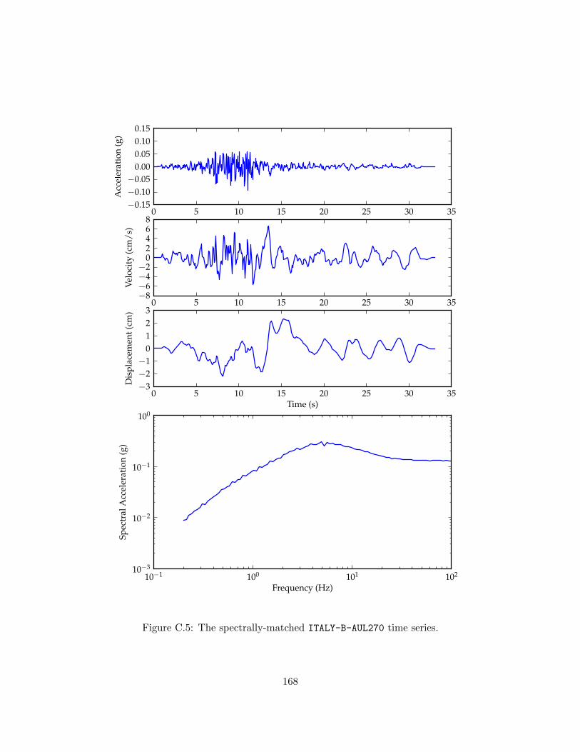
0 5 10 15 20 25 30 35−0.15−0.10−0.05

0.000.050.100.15

Acc

eler

atio

n(g

)

0 5 10 15 20 25 30 35−8−6−4−2

02468

Velo

city

(cm

/s)

0 5 10 15 20 25 30 35Time (s)

−3−2−1

0123

Dis

plac

emen

t(cm

)

10−1 100 101 102

Frequency (Hz)

10−3

10−2

10−1

100

Spec

tral

Acc

eler

atio

n(g

)

Figure C.5: The spectrally-matched ITALY-B-AUL270 time series.

168

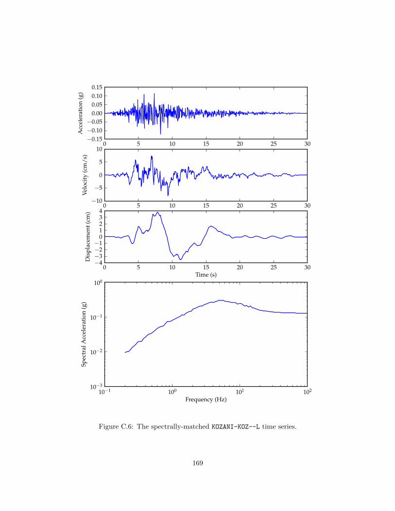
0 5 10 15 20 25 30−0.15−0.10−0.05

0.000.050.100.15

Acc

eler

atio

n(g

)

0 5 10 15 20 25 30−10

−5

0

5

10

Velo

city

(cm

/s)

0 5 10 15 20 25 30Time (s)

−4−3−2−1

01234

Dis

plac

emen

t(cm

)

10−1 100 101 102

Frequency (Hz)

10−3

10−2

10−1

100

Spec

tral

Acc

eler

atio

n(g

)

Figure C.6: The spectrally-matched KOZANI-KOZ--L time series.

169

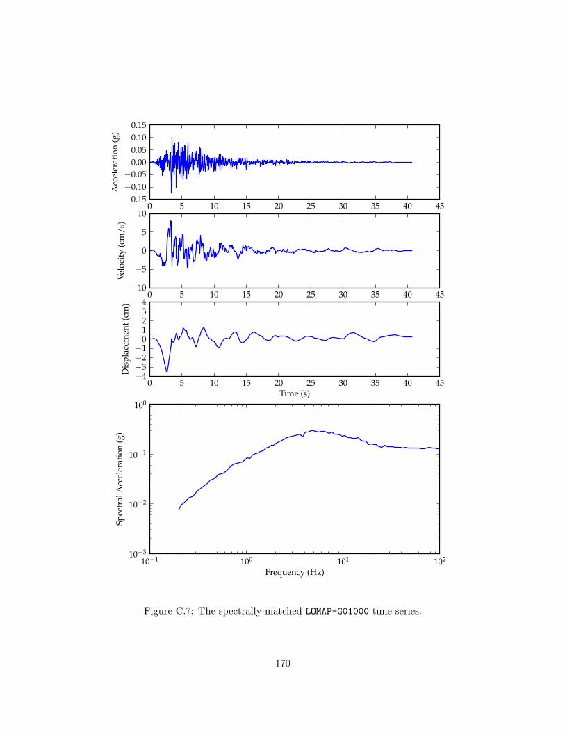
0 5 10 15 20 25 30 35 40 45−0.15−0.10−0.05

0.000.050.100.15

Acc

eler

atio

n(g

)

0 5 10 15 20 25 30 35 40 45−10

−5

0

5

10

Velo

city

(cm

/s)

0 5 10 15 20 25 30 35 40 45Time (s)

−4−3−2−1

01234

Dis

plac

emen

t(cm

)

10−1 100 101 102

Frequency (Hz)

10−3

10−2

10−1

100

Spec

tral

Acc

eler

atio

n(g

)

Figure C.7: The spectrally-matched LOMAP-G01000 time series.

170

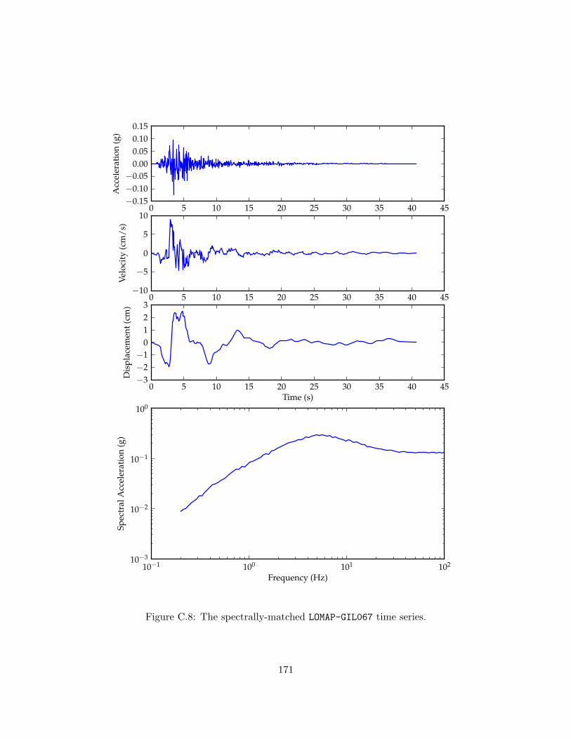
0 5 10 15 20 25 30 35 40 45−0.15−0.10−0.05

0.000.050.100.15

Acc

eler

atio

n(g

)

0 5 10 15 20 25 30 35 40 45−10

−5

0

5

10

Velo

city

(cm

/s)

0 5 10 15 20 25 30 35 40 45Time (s)

−3−2−1

0123

Dis

plac

emen

t(cm

)

10−1 100 101 102

Frequency (Hz)

10−3

10−2

10−1

100

Spec

tral

Acc

eler

atio

n(g

)

Figure C.8: The spectrally-matched LOMAP-GIL067 time series.

171

0 5 10 15 20 25 30 35

−0.10−0.05

0.000.050.10

Acc

eler

atio

n(g

)

0 5 10 15 20 25 30 35−8−6−4−2

02468

Velo

city

(cm

/s)

0 5 10 15 20 25 30 35Time (s)

−4

−2

0

2

4

Dis

plac

emen

t(cm

)

10−1 100 101 102

Frequency (Hz)

10−3

10−2

10−1

100

Spec

tral

Acc

eler

atio

n(g

)

Figure C.9: The spectrally-matched MORGAN-GIL337 time series.

172

0 5 10 15 20 25 30 35 40 45−0.15−0.10−0.05

0.000.050.100.15

Acc

eler

atio

n(g

)

0 5 10 15 20 25 30 35 40 45−10

−5

0

5

10

Velo

city

(cm

/s)

0 5 10 15 20 25 30 35 40 45Time (s)

−4

−2

0

2

4

Dis

plac

emen

t(cm

)

10−1 100 101 102

Frequency (Hz)

10−3

10−2

10−1

100

Spec

tral

Acc

eler

atio

n(g

)

Figure C.10: The spectrally-matched NORTHR-H12180 time series.

173

0 5 10 15 20 25 30 35−0.15−0.10−0.05

0.000.050.100.15

Acc

eler

atio

n(g

)

0 5 10 15 20 25 30 35−8−6−4−2

02468

Velo

city

(cm

/s)

0 5 10 15 20 25 30 35Time (s)

−3−2−1

0123

Dis

plac

emen

t(cm

)

10−1 100 101 102

Frequency (Hz)

10−3

10−2

10−1

100

Spec

tral

Acc

eler

atio

n(g

)

Figure C.11: The spectrally-matched NORTHR-HOW330 time series.

174

0 5 10 15 20 25 30 35−0.15−0.10−0.05

0.000.050.100.15

Acc

eler

atio

n(g

)

0 5 10 15 20 25 30 35−8−6−4−2

02468

Velo

city

(cm

/s)

0 5 10 15 20 25 30 35Time (s)

−6−4−2

0246

Dis

plac

emen

t(cm

)

10−1 100 101 102

Frequency (Hz)

10−3

10−2

10−1

100

Spec

tral

Acc

eler

atio

n(g

)

Figure C.12: The spectrally-matched NORTHR-LV1000 time series.

175

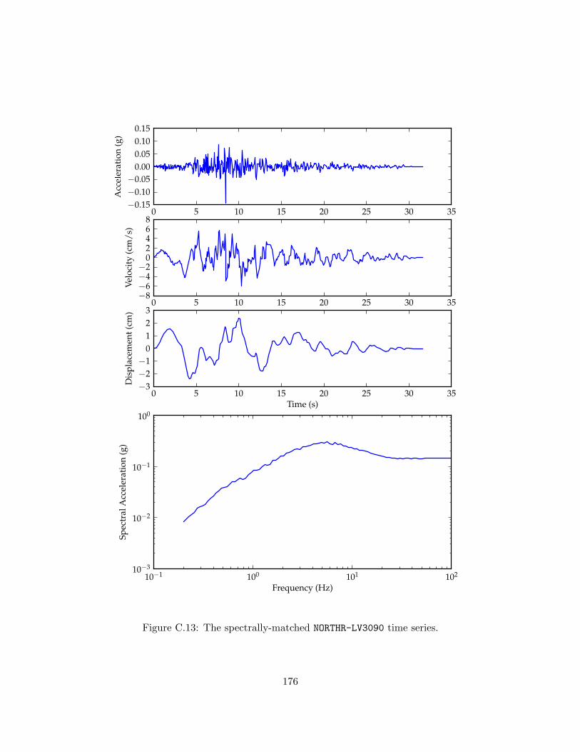
0 5 10 15 20 25 30 35−0.15−0.10−0.05

0.000.050.100.15

Acc

eler

atio

n(g

)

0 5 10 15 20 25 30 35−8−6−4−2

02468

Velo

city

(cm

/s)

0 5 10 15 20 25 30 35Time (s)

−3−2−1

0123

Dis

plac

emen

t(cm

)

10−1 100 101 102

Frequency (Hz)

10−3

10−2

10−1

100

Spec

tral

Acc

eler

atio

n(g

)

Figure C.13: The spectrally-matched NORTHR-LV3090 time series.

176

0 5 10 15 20 25 30 35

−0.10−0.05

0.000.050.10

Acc

eler

atio

n(g

)

0 5 10 15 20 25 30 35−10

−5

0

5

10

Velo

city

(cm

/s)

0 5 10 15 20 25 30 35Time (s)

−3−2−1

0123

Dis

plac

emen

t(cm

)

10−1 100 101 102

Frequency (Hz)

10−3

10−2

10−1

100

Spec

tral

Acc

eler

atio

n(g

)

Figure C.14: The spectrally-matched NORTHR-WON185 time series.

177

0 5 10 15 20 25−0.15−0.10−0.05

0.000.050.100.15

Acc

eler

atio

n(g

)

0 5 10 15 20 25−8−6−4−2

02468

Velo

city

(cm

/s)

0 5 10 15 20 25Time (s)

−3−2−1

0123

Dis

plac

emen

t(cm

)

10−1 100 101 102

Frequency (Hz)

10−3

10−2

10−1

100

Spec

tral

Acc

eler

atio

n(g

)

Figure C.15: The spectrally-matched VICT-CPE045 time series.

178