HAL Id: hal-02059287https://hal.univ-lorraine.fr/hal-02059287

Submitted on 6 Mar 2019

HAL is a multi-disciplinary open accessarchive for the deposit and dissemination of sci-entific research documents, whether they are pub-lished or not. The documents may come fromteaching and research institutions in France orabroad, or from public or private research centers.

L’archive ouverte pluridisciplinaire HAL, estdestinée au dépôt et à la diffusion de documentsscientifiques de niveau recherche, publiés ou non,émanant des établissements d’enseignement et derecherche français ou étrangers, des laboratoirespublics ou privés.

Comparison of theory and experiment for NAPLdissolution in porous media

T. Bahar, Fabrice Golfier, C. Oltean, E. Lefevre, C. Lorgeoux

To cite this version:T. Bahar, Fabrice Golfier, C. Oltean, E. Lefevre, C. Lorgeoux. Comparison of theory and experimentfor NAPL dissolution in porous media. Journal of Contaminant Hydrology, Elsevier, 2018, 211, pp.49-64. �10.1016/j.jconhyd.2018.03.004�. �hal-02059287�

Comparison of theory and experiment for NAPL dissolution in

porous media

T. Bahara,∗, F. Golfiera, C. Olteana, E. Lefevrea, C. Lorgeouxa

aUniversite de Lorraine, CNRS, CREGU, GeoRessources lab., Vandœuvre-les-Nancy Cedex, F-54518,France

Abstract

Contamination of groundwater resources by an immiscible organic phase commonly calledNAPL (Non Aqueous Phase Liquid) represents a major scientific challenge considering theresidence time of such a pollutant. This contamination leads to the formation of NAPLblobs trapped in the soil and impact of this residual saturation cannot be ignored for correctpredictions of the contaminant fate. In this paper, we present results of micromodel experi-ments on the dissolution of pure hydrocarbon phase (toluene). They were conducted for twovalues of the Peclet number. These experiments provide data for comparison and validationof a two-phase non-equilibrium theoretical model developped by Quintard and Whitaker(1994) using the volume averaging method. The model was directly upscaled from the aver-aged pore-scale mass balance equations. The effective properties of the macroscopic modelwere calculated over periodic unit cells designed from images of the experimental flow cell.Comparison of experimental and numerical results shows that the transport model predictscorrectly - with no fitting parameters - the main mechanisms of NAPL mass transfer. Thestudy highlights the crucial need of having a fair recovery of pore-scale characteristic lengthsto predict the mass transfer coefficient with accuracy.

Keywords:Porous media, NAPL dissolution, Upscaling, Volume averaging method

List of symbols

Aij Interface between the i- phase and j- phase (i,j : ω, β, γ, k)b′

β Dimensionless form of the closure variable bβ, (−)

Ca =‖vβ‖µβσβγ

, Capillary number, (−)

cAβ Pore scale concentration of species A in the β phase, (kg m−3)〈cAβ〉 Averaged concentration of species A in the β- phase, (kg m−3)ceqAβ Concentration of species A in the β- phase in equilibrium with ργ, (kg m−3)

cf Circularity, (-)c0 Injected concentration in the complex 2D geometry , (kg m−3)

∗Corresponding authorEmail address: tidjani.bahar@univ-lorraine.fr (T. Bahar)

Preprint submitted to Journal of Contaminant Hydrology February 7, 2018

DAβ Diffusion coefficient of species A in the β- phase, (m2 s−1)D∗βω Darcy scale effective dispersion tensor for the species A , (m2 s−1)Df Feret diameter, (cm)d∗βω A velocity-like effective transport coefficient, (m s−1)I Unit tensorKij Equilibrium partitioning coefficient between the i-phase and j-phase for the species A, (−)L Characteristic length associated with the averaging volume,(m)Lc Characteristic length defining the macroscale,(m)li Lattice vector for the ith direction (i=1,2,3), (m)lβ Characteristic length associated to the β-phase,(m)nij Normal vector pointing outward from the i- phase toward the j-phasepβ Fluid pressure in the β-phase, (Pa)

Pe =‖vβ‖lβDAβ

, Pore Peclet number, (−)

Re =ρβ‖vβ‖lβ

µβ, Pore Reynolds number, (−)

Sc =µβ

ρβDAβ, Schmidt number, (−)

Swi Initial saturation, (−)

Sh′

=α∗Al

2β

DAβ, Modified Sherwood number, (−)

s′

β Dimensionless form of the closure variable sβ, (−)t Time, (s)t′

Dimensionless time, (-)Uβω A velocity-like effective transport coefficient, (m s−1)V Averaging volume, (m3)Vi Volume of the i-phase, (m3)vi Velocity of the i-phase, (m s−1)vi Spatial deviation of vi, (m s−1)

Greek Symbols

α∗A Mass-transfer coefficient for the species A, (m s−1)β Fluid phaseγ NAPL phaseε Total porosityεi Volume fraction of the i-phaseµβ Fluid dynamic viscosity, (Pa.s)λf Lacunarity, (-)ργ NAPL phase density, (kg m−3)ρβ Water phase density, (kg m−3)σ Solid phaseσβγ water/toluene interfacial tension, (N m−1)〈.〉i Intrinsic average for the i-phase

2

〈.〉 Superficial average

1. Introduction

The problem of non-aqueous phase liquids (NAPLs) dissolution in porous media is oftenviewed in the context of groundwater pollution by hydrocarbon compounds (e.g., toluene,benzene, trichloroethylene). Among the sources of groundwater pollution, we can cite Abri-ola (1989): the drilling practices (i.e., drill-rig operations, transportation, illegal oil trap-ping) or hydrocarbon storage tanks (i.e., leaking underground storage tanks). Because oftheir high toxicity and low solubility in water and the associated risks to human healthand environment, NAPLs represent a highly dangerous and durable contamination sourceof groundwater (Quintard and Whitaker, 1994; Schubert et al., 2007). Firstly, the pollu-tant migrates through the porous formation in the unsatured zone and then reaches theaquifer. Under the action of capillary forces, this contamination leads to the formation ofNAPL blobs or ganglia trapped in the soil (Hunt et al., 1988). The assessment, design andimplementation of efficient cleanup and remediation strategies for systems containing resid-ual NAPL are of great importance for environmental and earth sciences research (NationalResearch Council (NRC), 2005; Mainhagu and Brusseau, 2016; Atteia et al., 2017).

In the past years, various investigations were conducted to characterize the transportmechanisms of NAPLs in fluid saturated-porous media (i.e., morphology of NAPLs in porousmedia systems, dissolution processes, fingering phenomena). Historically, NAPL dissolutionwas first observed in laboratory column experiments (Miller and Poirier-Mcnell, 1990; Powerset al., 1992; Conrad et al., 1992; Powers et al., 1994; Yra et al., 2006; Javanbakht and Goual,2016; Padgett et al., 2017). These works helped to give an insight on driving mechanismsbut the obtained informations are averaged over the entire system since the breakthroughcurves are measured at the column outlet. Considering the heterogeneous distribution ofNAPL blobs in porous media, the effective properties calculated at the column-scale suchas mass transfer coefficient or longitudinal dispersion cannot predict the impact of localheterogeneities neither describe the behavior of NAPL ganglia at the pore-scale. In addi-tion, the phase distribution is not known. The measurement of microscale quantities suchas interfacial areas are of critical importance to characterize the NAPL dissolution. Var-ious three-dimensional imaging techniques (Culligan et al., 2006; Al-Raoush, 2009; Ghoshand Tick, 2013; Kashuk et al., 2014; Al-Raoush, 2014; Javanbakht et al., 2017) have beendeveloped in the last decades to address this lack of data and characterize the microscalestructure of NAPL ganglia. Recent improvements in the X-ray microtomography (Arm-strong et al., 2016; Garing et al., 2017) led to capture pore-scale interfacial processes andthe NAPL dynamics but experimental constraints remain on the size of the sample domain,usually far from the size of the REV (Representative Elementary Volume). In parallel, ex-perimental studies (Jia et al., 1999; Jeong et al., 2000; Corapcioglu et al., 2009a; Sahloulet al., 2002; Chomsurin and Werth, 2003; Armstrong and Berg, 2013; Kashuk et al., 2014)using transparent flow cells or micromodels have shown their ability to visualize the changesin NAPL saturation in porous media. Micromodels are 2D networks of transparent channelsmanufactured artificially and used to mimic natural porous media. Due to their design and

3

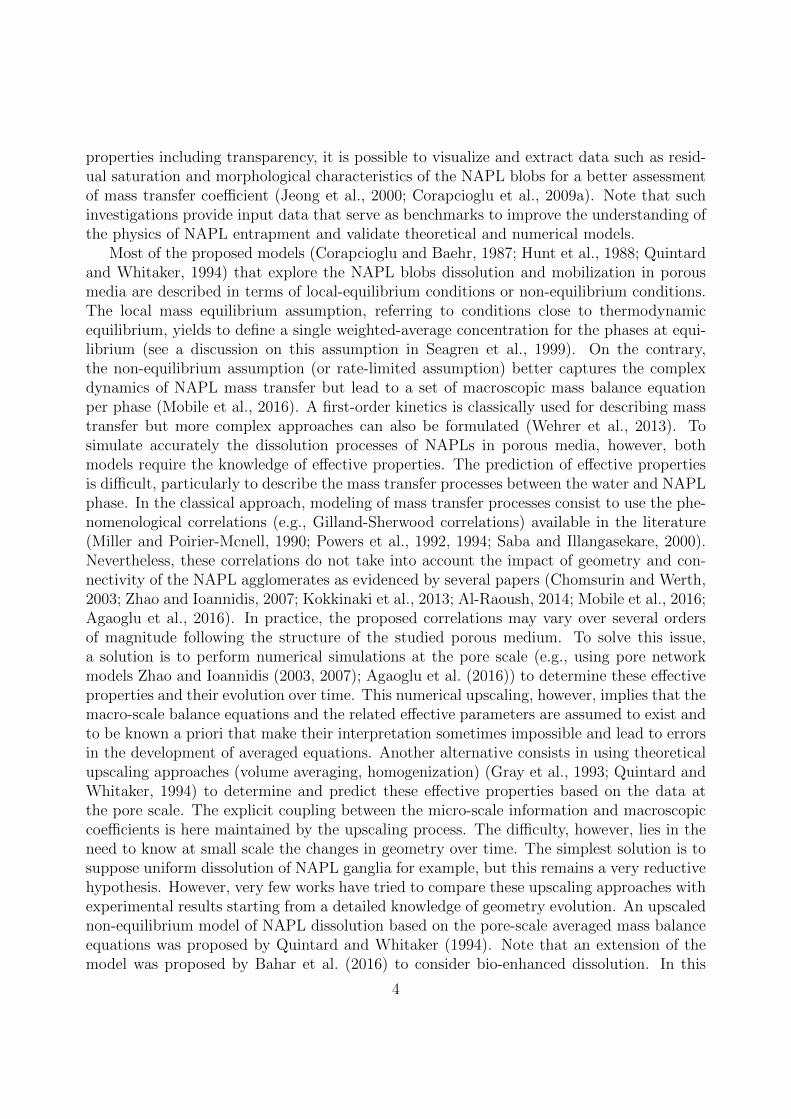
properties including transparency, it is possible to visualize and extract data such as resid-ual saturation and morphological characteristics of the NAPL blobs for a better assessmentof mass transfer coefficient (Jeong et al., 2000; Corapcioglu et al., 2009a). Note that suchinvestigations provide input data that serve as benchmarks to improve the understanding ofthe physics of NAPL entrapment and validate theoretical and numerical models.

Most of the proposed models (Corapcioglu and Baehr, 1987; Hunt et al., 1988; Quintardand Whitaker, 1994) that explore the NAPL blobs dissolution and mobilization in porousmedia are described in terms of local-equilibrium conditions or non-equilibrium conditions.The local mass equilibrium assumption, referring to conditions close to thermodynamicequilibrium, yields to define a single weighted-average concentration for the phases at equi-librium (see a discussion on this assumption in Seagren et al., 1999). On the contrary,the non-equilibrium assumption (or rate-limited assumption) better captures the complexdynamics of NAPL mass transfer but lead to a set of macroscopic mass balance equationper phase (Mobile et al., 2016). A first-order kinetics is classically used for describing masstransfer but more complex approaches can also be formulated (Wehrer et al., 2013). Tosimulate accurately the dissolution processes of NAPLs in porous media, however, bothmodels require the knowledge of effective properties. The prediction of effective propertiesis difficult, particularly to describe the mass transfer processes between the water and NAPLphase. In the classical approach, modeling of mass transfer processes consist to use the phe-nomenological correlations (e.g., Gilland-Sherwood correlations) available in the literature(Miller and Poirier-Mcnell, 1990; Powers et al., 1992, 1994; Saba and Illangasekare, 2000).Nevertheless, these correlations do not take into account the impact of geometry and con-nectivity of the NAPL agglomerates as evidenced by several papers (Chomsurin and Werth,2003; Zhao and Ioannidis, 2007; Kokkinaki et al., 2013; Al-Raoush, 2014; Mobile et al., 2016;Agaoglu et al., 2016). In practice, the proposed correlations may vary over several ordersof magnitude following the structure of the studied porous medium. To solve this issue,a solution is to perform numerical simulations at the pore scale (e.g., using pore networkmodels Zhao and Ioannidis (2003, 2007); Agaoglu et al. (2016)) to determine these effectiveproperties and their evolution over time. This numerical upscaling, however, implies that themacro-scale balance equations and the related effective parameters are assumed to exist andto be known a priori that make their interpretation sometimes impossible and lead to errorsin the development of averaged equations. Another alternative consists in using theoreticalupscaling approaches (volume averaging, homogenization) (Gray et al., 1993; Quintard andWhitaker, 1994) to determine and predict these effective properties based on the data atthe pore scale. The explicit coupling between the micro-scale information and macroscopiccoefficients is here maintained by the upscaling process. The difficulty, however, lies in theneed to know at small scale the changes in geometry over time. The simplest solution is tosuppose uniform dissolution of NAPL ganglia for example, but this remains a very reductivehypothesis. However, very few works have tried to compare these upscaling approaches withexperimental results starting from a detailed knowledge of geometry evolution. An upscalednon-equilibrium model of NAPL dissolution based on the pore-scale averaged mass balanceequations was proposed by Quintard and Whitaker (1994). Note that an extension of themodel was proposed by Bahar et al. (2016) to consider bio-enhanced dissolution. In this

4

model, the effective parameters (mass transfer coefficient and the effective dispersion) are de-termined by solving two closure problems on representative unit cells of the porous medium.Calculations of these properties on very simple unit cells were conducted by Ahmadi et al.(2001). Radilla et al. (1997, 1998) made an attempt to compare their column experimentswith the predictions of the macroscopic model by considering simple geometry to calculatethe effective coefficients but the lack of data on pore-scale structure made impossible a faircomparison.

In the present paper, we study both theoretically and experimentally residual NAPLaqueous dissolution and transport of dissolved species in a saturated 2D porous medium.The ultimate goal of this work is to provide a fair comparison between experimental resultsof dissolution and predictions of the upscaled model based on realistic unit cells designedfrom images of the experimental flow cell. The transport of dissolved species is modelledusing a macroscopic model of multiphase transport at the Darcy-scale obtained from thevolume averaging method (Quintard and Whitaker, 1994). The experimental set-up is madeof a micromodel (i.e., a 2D transparent flow cell) used to study dissolution of toluene andprovide data for comparison with the results of the theoretical model. In order to make thiscomparison, knowledge of the effective properties of the theoretical model is paramount.We assess the mass transfer coefficient and the effective dispersion by referring to the realarchitecture of the porous medium inferred from experimental data.

2. Experimental study

In this section, we will present the methodology that enabled the establishment of theexperimental set-up. Then, we will focus on the presentation of results concerning thedissolution of NAPL blobs initially trapped at residual saturation.

2.1. Experimental set-up and procedure

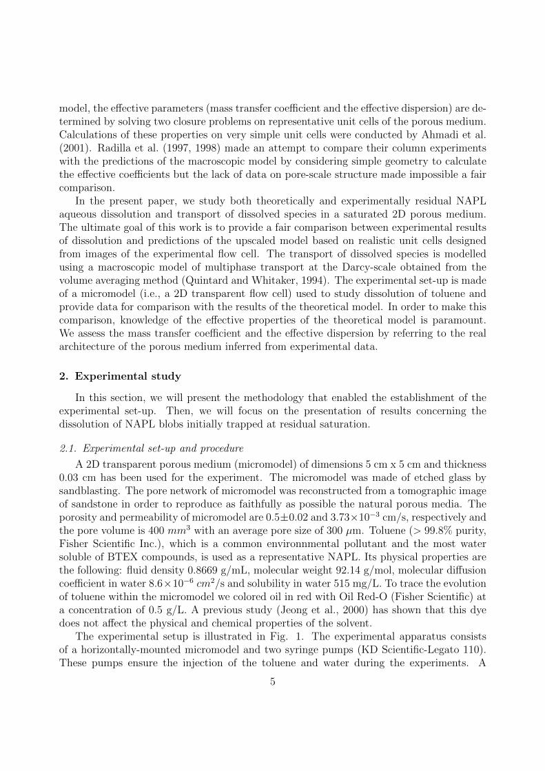
A 2D transparent porous medium (micromodel) of dimensions 5 cm x 5 cm and thickness0.03 cm has been used for the experiment. The micromodel was made of etched glass bysandblasting. The pore network of micromodel was reconstructed from a tomographic imageof sandstone in order to reproduce as faithfully as possible the natural porous media. Theporosity and permeability of micromodel are 0.5±0.02 and 3.73×10−3 cm/s, respectively andthe pore volume is 400 mm3 with an average pore size of 300 µm. Toluene (> 99.8% purity,Fisher Scientific Inc.), which is a common environnmental pollutant and the most watersoluble of BTEX compounds, is used as a representative NAPL. Its physical properties arethe following: fluid density 0.8669 g/mL, molecular weight 92.14 g/mol, molecular diffusioncoefficient in water 8.6×10−6 cm2/s and solubility in water 515 mg/L. To trace the evolutionof toluene within the micromodel we colored oil in red with Oil Red-O (Fisher Scientific) ata concentration of 0.5 g/L. A previous study (Jeong et al., 2000) has shown that this dyedoes not affect the physical and chemical properties of the solvent.

The experimental setup is illustrated in Fig. 1. The experimental apparatus consistsof a horizontally-mounted micromodel and two syringe pumps (KD Scientific-Legato 110).These pumps ensure the injection of the toluene and water during the experiments. A

5

camera (Canon EOS 400D) and the AZ100 Multizoom Microscope (Nikon Instruments Inc.)mounted directly on a system Charlyrobot Isel Automation controlled by the computer, wereemployed to follow spatial and temporal changes of NAPL blob within the porous medium.The experimental set-up is completed by gas chromatograph (Varian GC-450) to measurethe concentration of toluene. First, the micromodel is saturated with deionized deaired waterand then flooded with toluene until the irreducible water saturation is obtained. After thisstep, the micromodel is flushed with deionized deaired water at a flow rate of 5 ml/h untilthe residual oil saturation is reached. Then, the system is left at rest during twenty-fourhours to get complete concentration equilibrium and a satisfactory initial residual saturation.At this point, NAPL is trapped in the form of isolated ganglia mainly driven by capillaryforces, as suggested by the low value of the capillary number (cf. Table 1). This step isfollowed by the injection of demineralized water at a constant flow rate corresponding to theflow rate or Peclet number used for the dissolution experiments. Monitoring of dissolutionis performed through two methods (Figure 1). First, we observe the changes in toluenesaturation within the porous medium using CCD camera. The images of residual NAPLsaturation are analyzed with ImageJ software. The area and perimeter of toluene blobsare directly measured with ImageJ from recorded two-dimensional images. In parallel, thedissolution of residual toluene is measured by gas chromatograph (GC) coupled with a flameiomization detector (FID). Due to the high volatility of toluene, headspace (HS) injectiontechnique is used and peculiar precautions are taken for collecting samples and obtainingoptimum reproducible results. The oven heat ramp was 10 °C/min to 140 °C and the carriergas was hydrogen at 1.8 mL/min constant flow. At the flow cell outlet, a gas-tight syringe isused to extract 5 mL of solution into 10mL sealed vials before HS-GC analysis. The tolueneconcentrations of samples are obtained by means of the calibration curve established usinga standard protocol.

6

Figure 1: Experimental set-up

2.2. Experimental results

2.2.1. NAPL dissolution monitoring

We investigate dissolution of trapped toluene at two different flow rates, respectively at9.20×10−3 mL/min (Pe = 7) and 2.81×10−2 mL/min (Pe = 22). Note the above-mentionedPeclet number (Pe) is a pore Peclet number defined as follows:

Pe =vβ lβDAβ

(1)

where vβ is the average pore velocity, lβ represents the pore characteristic length (300 µm)and DAβ is the molecular diffusion coefficient of toluene in water. The two-step experimentalprocedure of flow cell saturation and the injection protocol as described in the previousparagraph are the same for both experiments. The experimental data and the relevantdimensionless numbers are summarized in Table 1.

In both cases, we start with NAPL mainly trapped as large disconnected clusters. Dueto the medium heterogeneity and the large aspect ratio of pores, NAPL trapping is prefer-entially found within the largest pores. This is consistent with by-passing mechanism wherethe wetting fluid (water) circumvents the largest pores through the smallest ones. However,isolated small ganglia due to snap-off can also be found, especially at high flow rates.

7

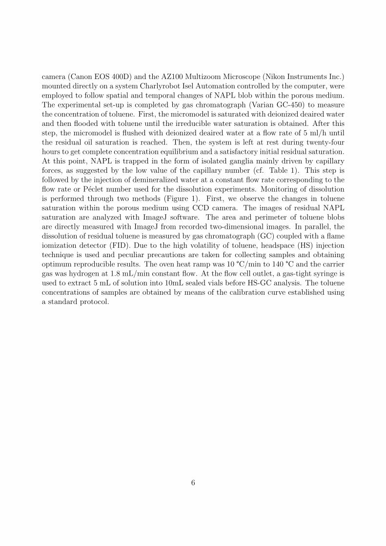
Table 1: Experimental data

Properties Experiment I Experiment II

Flow rate q (ml/min) 9.20× 10−3 2.81× 10−2

Pore-scale velocity vβ (cm/min) 0.12 0.37

Initial saturation Swi 0.32 0.25

Pore Peclet number (Pe) 7 22

Pore Reynolds number (Re) 6.13× 10−3 1.87× 10−2

Schmidt number (Sc) 1.16× 103 1.16× 103

Capillary number (Ca) 4.14× 10−7 1.28× 10−6

Typical patterns observed during dissolution experiments are illustrated in Fig. 2. Assoon as the co-current imbibition begins, we identify two mechanisms that contribute toNAPL recovery. First, NAPL remobilisation prevails. This phenomenon mainly occursclose to the inlet or near the highly polluted regions (areas marked in red on the images inFig. 2) where high velocities - due to preferential flows - may be sufficient to overcome theforces of trapping, i.e. capillary forces). Anyway, this mechanism is present only at shorttimes and never after t = 50 h. Then, a progressive dissolution of toluene blobs over timeis observed. Due to reduced water permeability in highly contaminated zones, preferentialdissolution pathways occur (Fig. 2 - see the changes in regions marked in yellow). Similarresults were obtained by Corapcioglu et al. (2009a).

8

Figure 2: Progressive dissolution of toluene blobs in the micromodel for two experiments (images (a) and(a’) corresponding to zero pore volumes injected, image (b) to 69 pore volumes injected, image (b’) to 210pore volumes injected, image (c) to 138 pore volumes injected and image (c’) to 420 pore volumes injected).Direction of water flow was found from right to left

2.2.2. Experimental uncertainty assessment

First, experiments have been repeated twice to assess measurement uncertainty. Com-parison of the resulting breakthrough curves are shown in Figs. 3 and 4. We observe arelatively good repeatability of the experiments for the two values of Peclet. Discrepancy

9

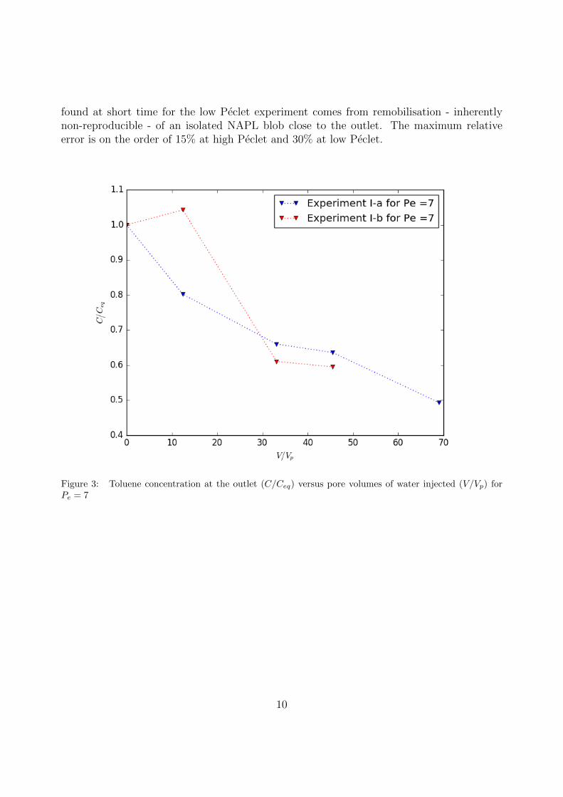
found at short time for the low Peclet experiment comes from remobilisation - inherentlynon-reproducible - of an isolated NAPL blob close to the outlet. The maximum relativeerror is on the order of 15% at high Peclet and 30% at low Peclet.

Figure 3: Toluene concentration at the outlet (C/Ceq) versus pore volumes of water injected (V/Vp) forPe = 7

10

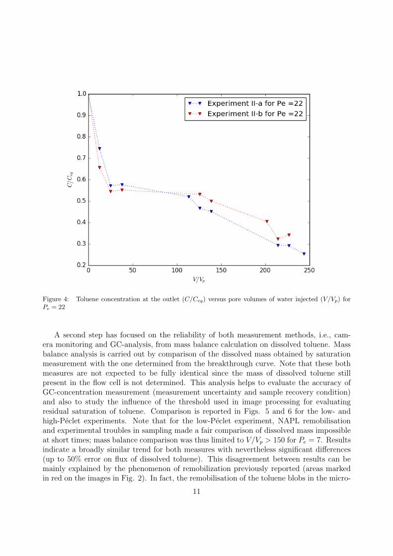
Figure 4: Toluene concentration at the outlet (C/Ceq) versus pore volumes of water injected (V/Vp) forPe = 22

A second step has focused on the reliability of both measurement methods, i.e., cam-era monitoring and GC-analysis, from mass balance calculation on dissolved toluene. Massbalance analysis is carried out by comparison of the dissolved mass obtained by saturationmeasurement with the one determined from the breakthrough curve. Note that these bothmeasures are not expected to be fully identical since the mass of dissolved toluene stillpresent in the flow cell is not determined. This analysis helps to evaluate the accuracy ofGC-concentration measurement (measurement uncertainty and sample recovery condition)and also to study the influence of the threshold used in image processing for evaluatingresidual saturation of toluene. Comparison is reported in Figs. 5 and 6 for the low- andhigh-Peclet experiments. Note that for the low-Peclet experiment, NAPL remobilisationand experimental troubles in sampling made a fair comparison of dissolved mass impossibleat short times; mass balance comparison was thus limited to V/Vp > 150 for Pe = 7. Resultsindicate a broadly similar trend for both measures with nevertheless significant differences(up to 50% error on flux of dissolved toluene). This disagreement between results can bemainly explained by the phenomenon of remobilization previously reported (areas markedin red on the images in Fig. 2). In fact, the remobilisation of the toluene blobs in the micro-

11

model shown in Fig. 2 can lead to an overestimation of the residual saturation and hence ofthe solubilized mass. The experimental observations (Fig. 2) have identified this remobilisa-tion of toluene blobs at short times and this occurence coincides strongly with the changesin the mass balance. The remobilized toluene blobs may subsequently become entrappedwithin the outlet tank of micromodel where they will continue to dissolve slowly, whichjustifies identical long-term concentrations for both methods. In addition, non-negligiblemeasurement uncertainties remain in the oil saturation-estimation method by imaging anal-ysis. Results at low Peclet indicate a low sensitivity of saturation measures to the valueof thresholding but geometrical simplifications are made. Indeed, this calculation is basedon the assumption that the micromodel is perfectly two-dimensional, which is not the case.The thickness of the micromodel may vary locally, thus modifying the measured volume.Moreover, the toluene droplets have a curvature according to the vertical. These variouscumulative errors may lead to a significant uncertainty on the solubilized mass of toluenederived from imaging analysis because it depends directly on the geometric parameters ofthe pore network. As a conclusion, the measurement of output concentration seems the mostreliable and this is the one we will use later for quantitative comparison with the numericalmodel. The monitoring of the saturation will be mainly used in a more qualitative manner,for the purpose of understanding the dissolution mechanisms involved and of identifying themost important geometrical features (e.g., pore size distribution, pore connectivity, NAPLsurface area) required for the upscaling procedure as discussed in Section 4 .

12

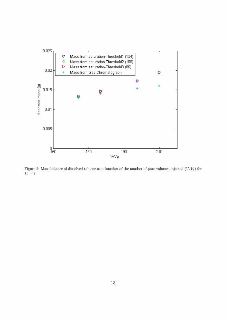
Figure 5: Mass balance of dissolved toluene as a function of the number of pore volumes injected (V/Vp) forPe = 7

13

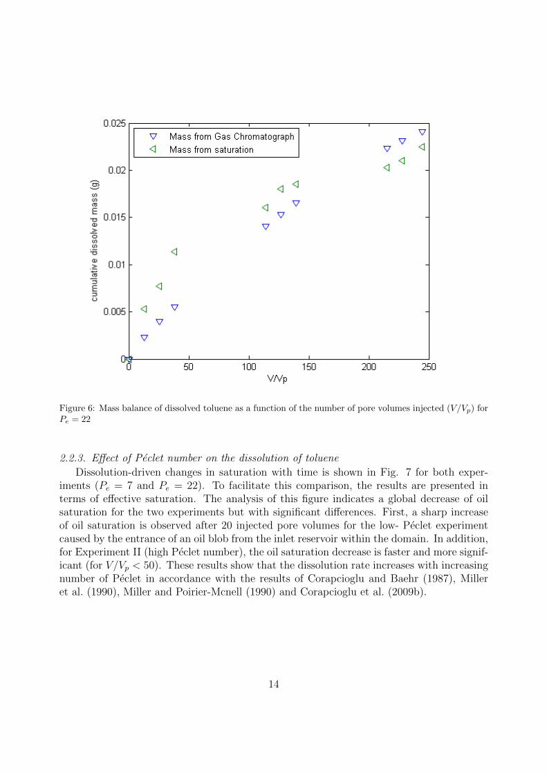
Figure 6: Mass balance of dissolved toluene as a function of the number of pore volumes injected (V/Vp) forPe = 22

2.2.3. Effect of Peclet number on the dissolution of toluene

Dissolution-driven changes in saturation with time is shown in Fig. 7 for both exper-iments (Pe = 7 and Pe = 22). To facilitate this comparison, the results are presented interms of effective saturation. The analysis of this figure indicates a global decrease of oilsaturation for the two experiments but with significant differences. First, a sharp increaseof oil saturation is observed after 20 injected pore volumes for the low- Peclet experimentcaused by the entrance of an oil blob from the inlet reservoir within the domain. In addition,for Experiment II (high Peclet number), the oil saturation decrease is faster and more signif-icant (for V/Vp < 50). These results show that the dissolution rate increases with increasingnumber of Peclet in accordance with the results of Corapcioglu and Baehr (1987), Milleret al. (1990), Miller and Poirier-Mcnell (1990) and Corapcioglu et al. (2009b).

14

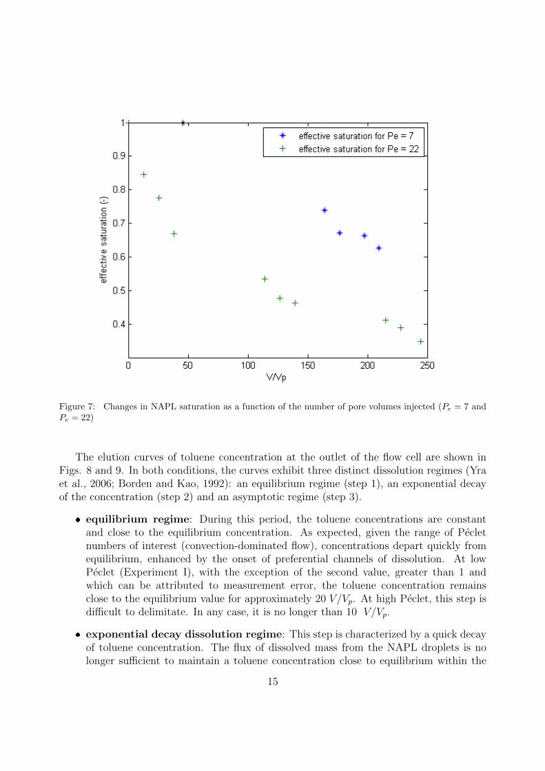
Figure 7: Changes in NAPL saturation as a function of the number of pore volumes injected (Pe = 7 andPe = 22)

The elution curves of toluene concentration at the outlet of the flow cell are shown inFigs. 8 and 9. In both conditions, the curves exhibit three distinct dissolution regimes (Yraet al., 2006; Borden and Kao, 1992): an equilibrium regime (step 1), an exponential decayof the concentration (step 2) and an asymptotic regime (step 3).

� equilibrium regime: During this period, the toluene concentrations are constantand close to the equilibrium concentration. As expected, given the range of Pecletnumbers of interest (convection-dominated flow), concentrations depart quickly fromequilibrium, enhanced by the onset of preferential channels of dissolution. At lowPeclet (Experiment I), with the exception of the second value, greater than 1 andwhich can be attributed to measurement error, the toluene concentration remainsclose to the equilibrium value for approximately 20 V/Vp. At high Peclet, this step isdifficult to delimitate. In any case, it is no longer than 10 V/Vp.

� exponential decay dissolution regime: This step is characterized by a quick decayof toluene concentration. The flux of dissolved mass from the NAPL droplets is nolonger sufficient to maintain a toluene concentration close to equilibrium within the

15

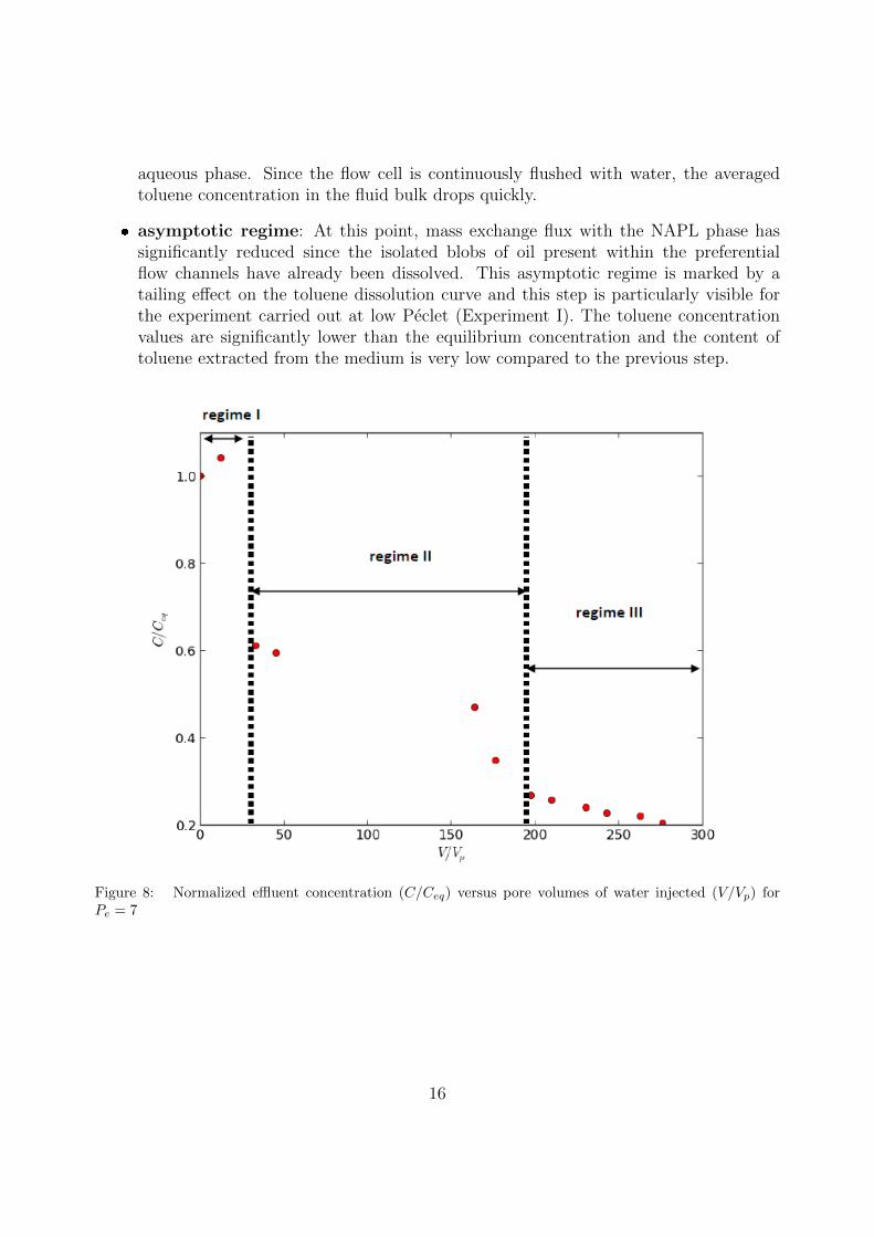
aqueous phase. Since the flow cell is continuously flushed with water, the averagedtoluene concentration in the fluid bulk drops quickly.

� asymptotic regime: At this point, mass exchange flux with the NAPL phase hassignificantly reduced since the isolated blobs of oil present within the preferentialflow channels have already been dissolved. This asymptotic regime is marked by atailing effect on the toluene dissolution curve and this step is particularly visible forthe experiment carried out at low Peclet (Experiment I). The toluene concentrationvalues are significantly lower than the equilibrium concentration and the content oftoluene extracted from the medium is very low compared to the previous step.

Figure 8: Normalized effluent concentration (C/Ceq) versus pore volumes of water injected (V/Vp) forPe = 7

16

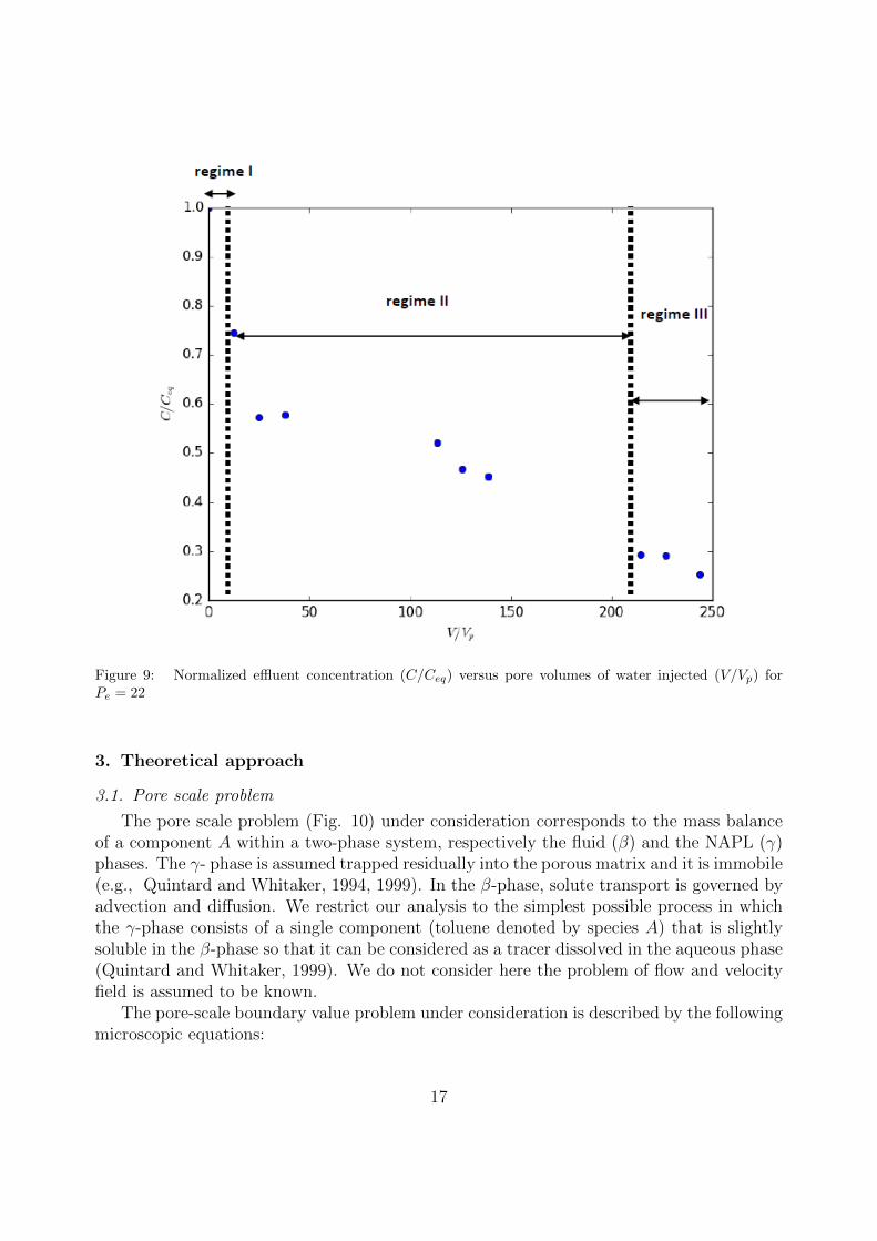
Figure 9: Normalized effluent concentration (C/Ceq) versus pore volumes of water injected (V/Vp) forPe = 22

3. Theoretical approach

3.1. Pore scale problem

The pore scale problem (Fig. 10) under consideration corresponds to the mass balanceof a component A within a two-phase system, respectively the fluid (β) and the NAPL (γ)phases. The γ- phase is assumed trapped residually into the porous matrix and it is immobile(e.g., Quintard and Whitaker, 1994, 1999). In the β-phase, solute transport is governed byadvection and diffusion. We restrict our analysis to the simplest possible process in whichthe γ-phase consists of a single component (toluene denoted by species A) that is slightlysoluble in the β-phase so that it can be considered as a tracer dissolved in the aqueous phase(Quintard and Whitaker, 1999). We do not consider here the problem of flow and velocityfield is assumed to be known.

The pore-scale boundary value problem under consideration is described by the followingmicroscopic equations:

17

Figure 10: Representative elementary volume and associated phases

Momentum equation

∇pβ = µβ∇2vβ in the β-phase (2)

Mass balance equations

∂(cAβ)

∂t+∇ · (vAβcAβ) = 0 in the β-phase (3)

∂ργ∂t

= 0 in the γ-phase (4)

B.C.1 cAβ(vAβ −wβσ) · nβσ = 0 at Aβσ (5)

B.C.2 cAβ = Kβγργ = ceqAβ at Aβγ (6)

B.C.3 cAβ(vAβ −wβγ) · nβγ = −ργwβγ · nβγ at Aβγ (7)

B.C.4 vβ = 0 at Aβσ (8)

B.C.5 vβ = 0 at Aβγ (9)

Here, cAβ represent the mass concentration of component A in the fluid phase; ργ is the massconcentration of pure species A in the γ phase; vAβ represent the velocity of component A

18

in the β phase and vβ the mass average fluid velocity; ceqAβ is the concentration of species Ain the β- phase in equilibrium with γ;

In addition, we determine the volumetric rate of dissolution of the NAPL phase byarranging the form of Eq.(7) as:

wβγ · nβγ = − 1

ργcAβ(vAβ −wβγ) · nβγ at Aβγ (10)

where wβγ is the velocity of the fluid-NAPL interface Aβγ. Under these assumptions, thepore-scale problem is similar to the one treated by Quintard and Whitaker (1994).

3.2. Volume averaging

As mentioned in the introduction, our upscaling approach is based on the volume averag-ing method. The goal of this multiscale analysis is to compare these results with laboratoryexperiments; upscaling is necessary here to connect the micro-scale information with thebehavior at the macroscale. In this present study, we recall the main definitions that haveallowed the development of the macro-scale model. Referring to the method of volume av-eraging Whitaker (1999), we define the superficial average concentration of species A in theβ-phase as:

〈cAβ〉 =1

V

∫ϑβ(x,t)

cAβdV (11)

with V , describing the averaging volume (the averaging domain is a geometric entity ofmacroscopic field VM) and ϑβ(x, t) is the Euclidean space representing the β-phase containedin the volume V . The intrinsic average concentration for the β-phase is given by:

〈cAβ〉β =1

Vβ(x, t)

∫ϑβ(x,t)

cAβdV (12)

with Vβ(x, t) is the Lebesgue measure of ϑβ(x, t), that is, the volume of the β phase. Super-ficial and intrinsic averages given by Eqs.(11) and (12) are related by:

〈cAβ〉 = εβ(x, t)〈cAβ〉β (13)

where εβ(x, t) represents the volume fraction of the β-phase defined as:

εβ(x, t) =Vβ(x, t)

V(14)

In the development of the model, the pore-scale concentration cAβ can be expressed followingGray’s decomposition (Gray et al., 1993):

cAβ = 〈cAβ〉β + cAβ (15)

with cAβ the spatial deviation concentration in β phase.

19

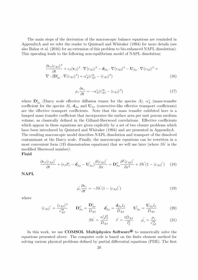
The main steps of the derivation of the macroscopic balance equations are reminded inAppendixA and we refer the reader to Quintard and Whitaker (1994) for more details (seealso Bahar et al. (2016) for an extension of this problem to bio-enhanced NAPL dissolution).This upscaling leads to the following non-equilibrium model of NAPL dissolution:

∂εβ〈cAβ〉β

∂t+ εβ〈vβ〉β · ∇〈cAβ〉β − dβω · ∇〈cAβ〉β −Uβω · ∇〈cAβ〉β =

∇ · (D∗βω · ∇〈cAβ〉β) + α∗A(ceqAβ − 〈cAβ〉β) (16)

ργ∂εγ∂t

= −α∗A(ceqAβ − 〈cAβ〉β) (17)

where D∗βω (Darcy scale effective diffusion tensor for the species A), α∗A (mass-transfercoefficient for the species A), dβω and Uβω (convective-like effective transport coefficients)are the effective transport coefficients. Note that the mass transfer exhibited here is alumped mass transfer coefficient that incorporates the surface area per unit porous mediumvolume, as classically defined in the Gilland-Sherwood correlations. Effective coefficientswhich appear in these equations are given explicitly by a set of two closure problems whichhave been introduced by Quintard and Whitaker (1994) and are presented in AppendixA.The resulting macroscopic model describes NAPL dissolution and transport of the dissolvedcontaminant at the Darcy scale. Finally, the macroscopic equations can be rewritten in amost convenient form (1D dimensionless equations) that we will use later (where Sh

′is the

modified Sherwood number):Fluid

∂εβ〈cAβ〉′

∂t+ (εβPe − d

′

βω −U′

βω)∂〈cAβ〉

′

∂x= D∗

′

βω

∂2〈cAβ〉′

∂x2+ Sh

′(1− 〈cAβ〉

′) (18)

NAPL

ρ′

γ

∂εγ∂t′

= −Sh′(1− 〈cAβ〉′) (19)

where

〈cAβ〉′=〈cAβ〉β

ceqAβD∗′

βω =D∗βωDAβ

d′

βω =dβωlβDAβ

U′

βω =UβωlβDAβ

(20)

Sh′=α∗Al

2β

DAβ

t′=tDAβ

l2βρ′

γ =ργceqAβ

(21)

In this work, we use COMSOL Multiphysics Software® to numerically solve theequations presented above. The computer code is based on the finite element method forsolving various physical problems defined by partial differential equations (PDE). The first

20

step is to calculate the effective parameters from solving two closure problems associated withthe macroscopic model on the representative unit cell of the porous medium. The resolutionmethod of these closure problems is the same as detailed by Bahar et al. (2016). The secondstep is solving the macroscopic equation on the entire domain. The macroscopic problem isone-dimensional and transient. Ultimately, we obtain the changes in concentration versustime (breakthrough curve) that we compare to the experimental curve of residual toluenedissolution.

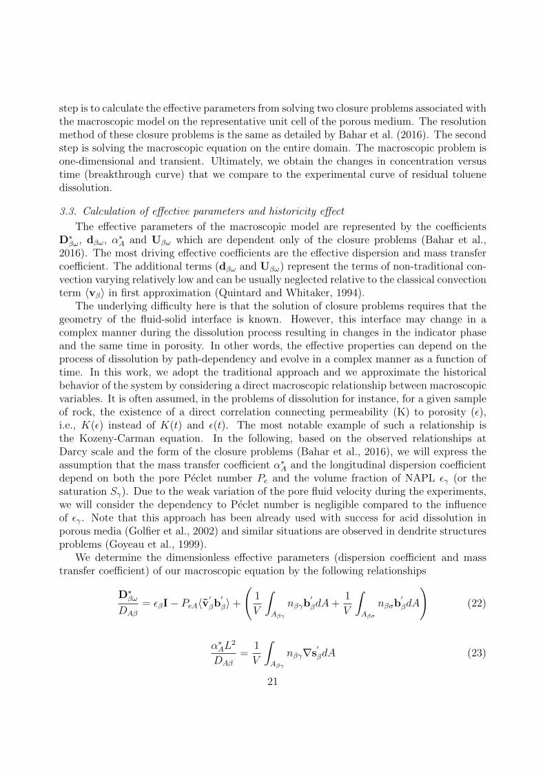
3.3. Calculation of effective parameters and historicity effect

The effective parameters of the macroscopic model are represented by the coefficientsD∗βω, dβω, α∗A and Uβω which are dependent only of the closure problems (Bahar et al.,2016). The most driving effective coefficients are the effective dispersion and mass transfercoefficient. The additional terms (dβω and Uβω) represent the terms of non-traditional con-vection varying relatively low and can be usually neglected relative to the classical convectionterm 〈vβ〉 in first approximation (Quintard and Whitaker, 1994).

The underlying difficulty here is that the solution of closure problems requires that thegeometry of the fluid-solid interface is known. However, this interface may change in acomplex manner during the dissolution process resulting in changes in the indicator phaseand the same time in porosity. In other words, the effective properties can depend on theprocess of dissolution by path-dependency and evolve in a complex manner as a function oftime. In this work, we adopt the traditional approach and we approximate the historicalbehavior of the system by considering a direct macroscopic relationship between macroscopicvariables. It is often assumed, in the problems of dissolution for instance, for a given sampleof rock, the existence of a direct correlation connecting permeability (K) to porosity (ε),i.e., K(ε) instead of K(t) and ε(t). The most notable example of such a relationship isthe Kozeny-Carman equation. In the following, based on the observed relationships atDarcy scale and the form of the closure problems (Bahar et al., 2016), we will express theassumption that the mass transfer coefficient α∗A and the longitudinal dispersion coefficientdepend on both the pore Peclet number Pe and the volume fraction of NAPL εγ (or thesaturation Sγ). Due to the weak variation of the pore fluid velocity during the experiments,we will consider the dependency to Peclet number is negligible compared to the influenceof εγ. Note that this approach has been already used with success for acid dissolution inporous media (Golfier et al., 2002) and similar situations are observed in dendrite structuresproblems (Goyeau et al., 1999).

We determine the dimensionless effective parameters (dispersion coefficient and masstransfer coefficient) of our macroscopic equation by the following relationships

D∗βωDAβ

= εβI− PeA〈v′

βb′

β〉+

(1

V

∫Aβγ

nβγb′

βdA+1

V

∫Aβσ

nβσb′

βdA

)(22)

α∗AL2

DAβ

=1

V

∫Aβγ

nβγ∇s′

βdA (23)

21

where b′

β and s′

β are the closure variables, solutions of the closure problems I and II (Eqs.A.18-A.23 and Eqs. A.24-A.29 in AppendixA).

4. Comparisons and discussions

Firstly, we present the results of calculation of effective parameters based on the unit cellsreconstructed from the images of the experimental flow cell (micromodel). These realisticgeometries are expected to capture most of the microscopic geometrical features of theporous medium. The dissolution of toluene with time induced spatio-temporal changesof these properties (e.g., toluene saturation, volume fractions of the phases) and a correctprediction requires considering the experiments and all of their variability. Our experimentalset-up offers us the benefit of having images of the process of dissolution versus time whichsubsequently will be processed for obtaining realistic configurations. In a second step, themacroscopic equations will be solved on the entire domain (1D domain).

4.1. Selection and construction of unit cells

The unit cells constructed from the images of the experimental micromodel are shownin Fig. 11. The unit cell (A) shows the initial state of micromodel (image of the residualsaturation in toluene at t = 0 hour), the unit cell (B) was imaged after two hundred hours ofdissolution (residual saturation at t = 200 hours) and finally the unit cell (C) illustrates thefinal state of the experiment after three hundred sixty-seven hours of dissolution (residualsaturation at t = 367 hours). These three representative images are chosen to approximatethe historical behaviour of the dissolution process due to the variation over time of the geom-etry and by the same of the effective parameters. The main physical parameters associatedwith the different unit cells are summarized in Table 2. Morphological analysis conducted onthese geometries (see Table 2) give interesting insights on the changes in pore-scale featurescaptured by these unit cells. Feret diameter (also known as maximum caliper) measuresthe longest distance between any two pixels along the NAPL boundary and circularity is acompactness measure of the shape of NAPL phase (a value of 1.0 indicates a perfect circle).Lacunarity is measured from digital images using the box counting method and indicatesthe coefficient of variation (CV) for the number of NAPL pixels per box. Wwe refer thereader to the ImageJ documentation (Rasband, 1997-2016) for more details about their cal-culation. The decrease of maximal Feret diameter for the non-wetting phase is consistentwith the progressive dissolution of NAPL ganglia with time. The similar trend for lacunaritythat indicates a decrease of heterogeneity support this finding and emphasizes a preferentialdissolution of the smallest isolated NAPL blobs. This preferential dissolution mechanismis consistent with the increase of compacity of the oil phase as indicated by the circularityvalue for unit cell (B). Note that these unit cells are extracted from experiments at lowPeclet number. For the calculation at high Peclet, we keep the same unit cells, consideringthat the dissolution patterns observed have a similar behavior.

The construction of these unit cells is based on a procedure combining several imageprocessing and analysis tools. The first step consists in extracting the active part of the

22

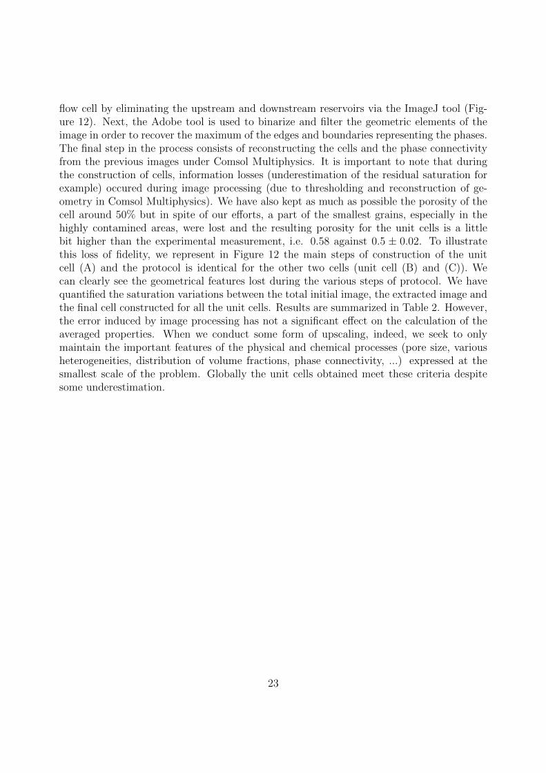
flow cell by eliminating the upstream and downstream reservoirs via the ImageJ tool (Fig-ure 12). Next, the Adobe tool is used to binarize and filter the geometric elements of theimage in order to recover the maximum of the edges and boundaries representing the phases.The final step in the process consists of reconstructing the cells and the phase connectivityfrom the previous images under Comsol Multiphysics. It is important to note that duringthe construction of cells, information losses (underestimation of the residual saturation forexample) occured during image processing (due to thresholding and reconstruction of ge-ometry in Comsol Multiphysics). We have also kept as much as possible the porosity of thecell around 50% but in spite of our efforts, a part of the smallest grains, especially in thehighly contamined areas, were lost and the resulting porosity for the unit cells is a littlebit higher than the experimental measurement, i.e. 0.58 against 0.5 ± 0.02. To illustratethis loss of fidelity, we represent in Figure 12 the main steps of construction of the unitcell (A) and the protocol is identical for the other two cells (unit cell (B) and (C)). Wecan clearly see the geometrical features lost during the various steps of protocol. We havequantified the saturation variations between the total initial image, the extracted image andthe final cell constructed for all the unit cells. Results are summarized in Table 2. However,the error induced by image processing has not a significant effect on the calculation of theaveraged properties. When we conduct some form of upscaling, indeed, we seek to onlymaintain the important features of the physical and chemical processes (pore size, variousheterogeneities, distribution of volume fractions, phase connectivity, ...) expressed at thesmallest scale of the problem. Globally the unit cells obtained meet these criteria despitesome underestimation.

23

Figure 11: Unit cells constructed from the images of the experimental cell

24

Figure 12: Representation side by side of the initial image used (image of residual saturation at t = 0), theimage extracted and the unit cell built from this image.

4.2. Calculation of the effective properties

The calculation of effective properties is based on unit cells shown in Figure 11. Closureproblems 1 and 2 are solved for each unit cell at high and low Peclet number and resultsfor the two effective coefficients are reported as a function of the NAPL volume fraction. Itshould be emphasized that the values of effective coefficients obtained can be significantlydifferent from those that could be measured experimentally (e.g., back-calculated valuesusing image analysis). The solution given by the closure problem corresponds indeed tothe asymptotic conditions. The choice of the unit cell is for this reason quite significant:if the choice of periodic conditions is perfectly appropriate far from boundary conditions,it becomes debatable when getting close macroscopic limits of the domain (cf. the paperof Cushman and Moroni (2001) in particular on the influence of non-local effects on thedispersion tensor). On the other hand, the dispersion tensor and the mass transfer coefficientare parameters inherently dependent of the scale of observation and their experimental

25

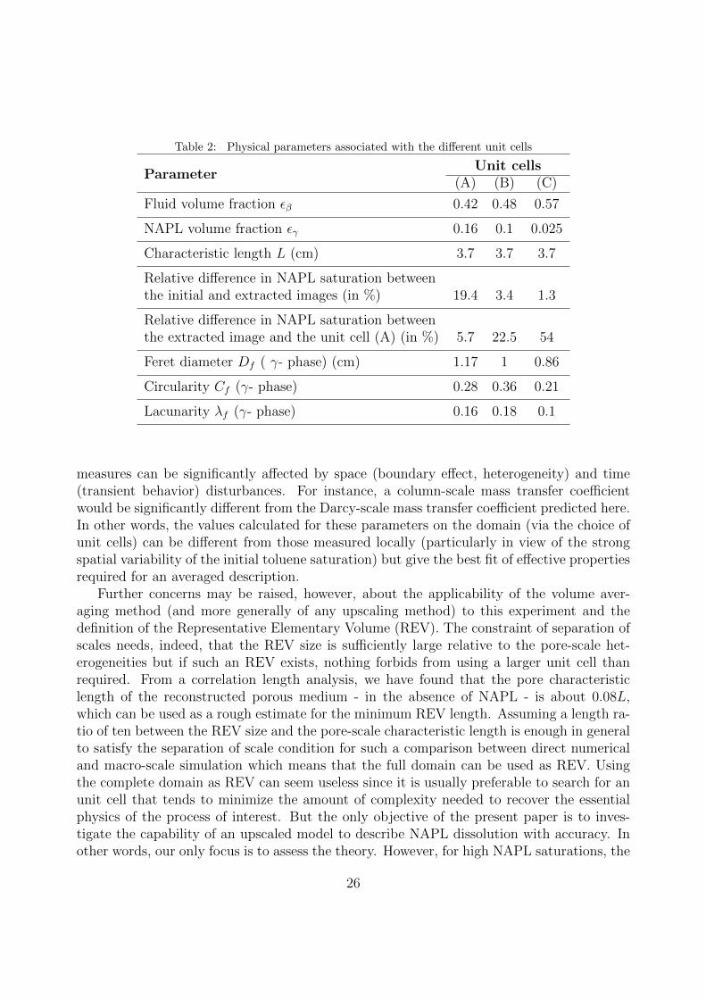
Table 2: Physical parameters associated with the different unit cells

ParameterUnit cells

(A) (B) (C)

Fluid volume fraction εβ 0.42 0.48 0.57

NAPL volume fraction εγ 0.16 0.1 0.025

Characteristic length L (cm) 3.7 3.7 3.7

Relative difference in NAPL saturation betweenthe initial and extracted images (in %) 19.4 3.4 1.3

Relative difference in NAPL saturation betweenthe extracted image and the unit cell (A) (in %) 5.7 22.5 54

Feret diameter Df ( γ- phase) (cm) 1.17 1 0.86

Circularity Cf (γ- phase) 0.28 0.36 0.21

Lacunarity λf (γ- phase) 0.16 0.18 0.1

measures can be significantly affected by space (boundary effect, heterogeneity) and time(transient behavior) disturbances. For instance, a column-scale mass transfer coefficientwould be significantly different from the Darcy-scale mass transfer coefficient predicted here.In other words, the values calculated for these parameters on the domain (via the choice ofunit cells) can be different from those measured locally (particularly in view of the strongspatial variability of the initial toluene saturation) but give the best fit of effective propertiesrequired for an averaged description.

Further concerns may be raised, however, about the applicability of the volume aver-aging method (and more generally of any upscaling method) to this experiment and thedefinition of the Representative Elementary Volume (REV). The constraint of separation ofscales needs, indeed, that the REV size is sufficiently large relative to the pore-scale het-erogeneities but if such an REV exists, nothing forbids from using a larger unit cell thanrequired. From a correlation length analysis, we have found that the pore characteristiclength of the reconstructed porous medium - in the absence of NAPL - is about 0.08L,which can be used as a rough estimate for the minimum REV length. Assuming a length ra-tio of ten between the REV size and the pore-scale characteristic length is enough in generalto satisfy the separation of scale condition for such a comparison between direct numericaland macro-scale simulation which means that the full domain can be used as REV. Usingthe complete domain as REV can seem useless since it is usually preferable to search for anunit cell that tends to minimize the amount of complexity needed to recover the essentialphysics of the process of interest. But the only objective of the present paper is to inves-tigate the capability of an upscaled model to describe NAPL dissolution with accuracy. Inother words, our only focus is to assess the theory. However, for high NAPL saturations, the

26

pore-scale characteristic length can be larger than 0.08L and the size of the domain mightbe not sufficient to ensure the separation of scales. It means that the asymptotic values ofthe effective coefficients (longitudinal dispersion, mass transfer coefficient) as predicted bythe closure problem could underestimate the averaged behavior of the experimental domainat very short times. Upscaling theories requires also that spatial localization constraints areimposed upon averaged fields. Roughly speaking, it means in our case that the averagedspatial concentration gradients are small enough at the REV scale. Occurence of a verysharp macroscopic reaction front that could break down the validity of our upscaled the-ory is driven by conditions at both local and global scales but it usually requires that themacroscopic Damkohler number (calculated from the mass transfer coefficient value) is verylarge compared to the macroscopic Peclet number and it does not correspond to the currentexperimental conditions. In any case, no assumption is needed on the microscale concen-tration gradients. We do not use in the present study, indeed, an local mass equilibriumassumption that implies that microscale gradients are relatively small, so that both phasescan be treated in exactly the same way. On the contrary, a local non-equilibrium model isconsidered so that strong concentration gradients may exist at the NAPL/fluid interface

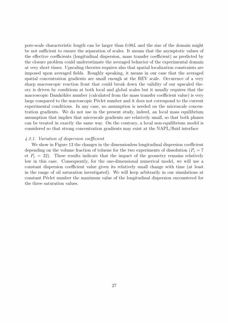
4.2.1. Variation of dispersion coefficient

We show in Figure 13 the changes in the dimensionless longitudinal dispersion coefficientdepending on the volume fraction of toluene for the two experiments of dissolution (Pe = 7et Pe = 22). These results indicate that the impact of the geometry remains relativelylow in this case. Consequently, for the one-dimensional numerical model, we will use aconstant dispersion coefficient value given its relatively small change with time (at leastin the range of oil saturation investigated). We will keep arbitrarily in our simulations atconstant Peclet number the maximum value of the longitudinal dispersion encountered forthe three saturation values.

27

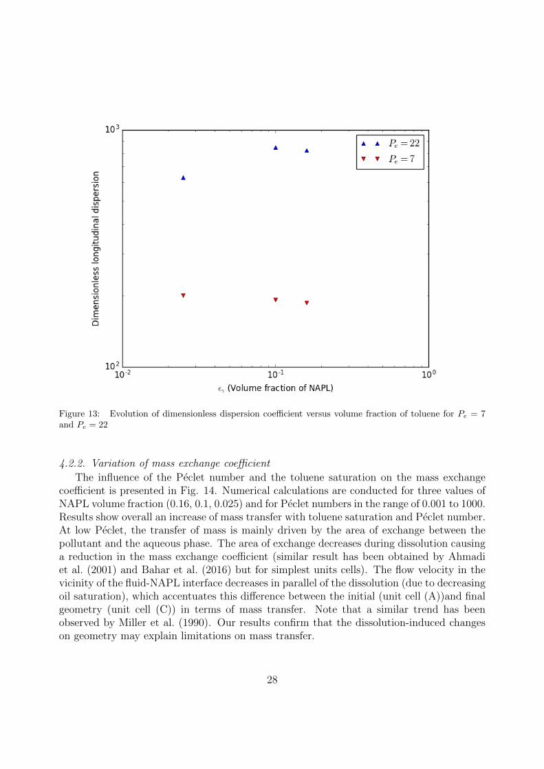
Figure 13: Evolution of dimensionless dispersion coefficient versus volume fraction of toluene for Pe = 7and Pe = 22

4.2.2. Variation of mass exchange coefficient

The influence of the Peclet number and the toluene saturation on the mass exchangecoefficient is presented in Fig. 14. Numerical calculations are conducted for three values ofNAPL volume fraction (0.16, 0.1, 0.025) and for Peclet numbers in the range of 0.001 to 1000.Results show overall an increase of mass transfer with toluene saturation and Peclet number.At low Peclet, the transfer of mass is mainly driven by the area of exchange between thepollutant and the aqueous phase. The area of exchange decreases during dissolution causinga reduction in the mass exchange coefficient (similar result has been obtained by Ahmadiet al. (2001) and Bahar et al. (2016) but for simplest units cells). The flow velocity in thevicinity of the fluid-NAPL interface decreases in parallel of the dissolution (due to decreasingoil saturation), which accentuates this difference between the initial (unit cell (A))and finalgeometry (unit cell (C)) in terms of mass transfer. Note that a similar trend has beenobserved by Miller et al. (1990). Our results confirm that the dissolution-induced changeson geometry may explain limitations on mass transfer.

28

Figure 14: Dimensionless mass exchange coefficient: influence of Peclet number and toluene saturation

In a second step, we extract from these calculations the mass transfer coefficients valuesat different NAPL saturations for low- and high-Peclet experiments. For prediction of theexperimental breakthrough curve, indeed, the numerical model requires knowledge of masstransfer coefficient. By keeping a constant value in the calculations, it is highly probablethat the dissolution curve will not be correctly predicted. For that reason, we opted fora dependency of mass transfer coefficient (or modified Sherwood number) on the NAPLcontent, based on the numerical results obtained Fig. 14. The main advantage of thisapproach resides in the fact that the mass exchange coefficient is now correlated with thedynamics of the physical problem. Contrary to the empirical correlations valid for a specificrange of hydrodynamic conditions, our upscaled mass transfer is expected to follow a physicalbehavior, i.e., the molecular diffusion prevails for low values of Pe (Pe < 1) and maintainsa non-zero mass flux between the NAPL phase and the bulk fluid. As mentioned in theintroduction, indeed, a large number of relationships expressing the modified Sherwoodnumber in terms of Reynolds number, Schmidt number, Peclet number and the oil volumefraction are available in the literature. We list in Table 3 some of the most significantcorrelations (Miller et al., 1990; Nambi and Powers, 2003; Saba and Illangasekare, 2000)used for predicting the lumped mass transfer coefficient and their range of validity.

29

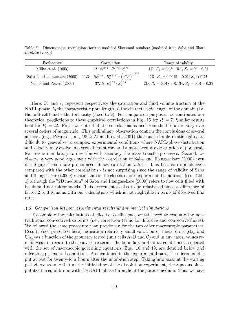
Table 3: Dimensionless correlations for the modified Sherwood numbers (modified from Saba and Illan-gasekare (2000))

Reference Correlation Range of validity

Miller et al. (1990) 12 · Sc0.5 ·R0.75e · ε0.6γ 1D, Re = 0.05− 0.1, Sγ = 0.− 0.21

Saba and Illangasekare (2000) 11.34 · Sc0.33 ·R0.2767e ·

(lβεγτL

)1.0372D, Re = 0.0015− 0.01, Sγ ≈ 0.22

Nambi and Powers (2003) 37.15 ·R0.75e · S0.24

γ 2D, Re = 0.018− 0.134, Sγ = 0.01− 0.35

Here, Sγ and εγ represent respectively the saturation and fluid volume fraction of theNAPL-phase, lβ the characteristic pore length, L the characteristic length of the domain (i.e,the unit cell) and τ the tortuosity (fixed to 2). For comparison purposes, we confronted ourtheoretical predictions to these empirical correlations in Fig. 15 for Pe = 7. Similar resultshold for Pe = 22. First, we note that the correlations issued from the literature vary overseveral orders of magnitude. This preliminary observation confirm the conclusions of severalauthors (e.g., Powers et al., 1992; Ahmadi et al., 2001) that such simple relationships aredifficult to generalise to complex experimental conditions where NAPL-phase distributionand velocity may evolve in a very different way and a more accurate description of pore-scalefeatures is mandatory to describe with accuracy the mass transfer processes. Second, weobserve a very good agreement with the correlation of Saba and Illangasekare (2000) evenif the gap seems more pronounced at low saturation values. This best correspondence -compared with the other correlations - is not surprising since the range of validity of Sabaand Illangasekare (2000) relationship is the closest of our experimental conditions (see Table1) although the ”2D medium” of Saba and Illangasekare (2000) refers to flow cells filled withbeads and not micromodels. This agreement is also to be relativised since a difference offactor 2 to 3 remains with our calculations which is not negligible in terms of dissolved fluxrates.

4.3. Comparison between experimental results and numerical simulations

To complete the calculations of effective coefficients, we still need to evaluate the non-traditional convective-like terms (i.e., correction terms for diffusive and convective fluxes).We followed the same procedure than previously for the two other macroscopic parameters.Results (not presented here) indicate a relatively small variation of these terms (dβω andUβω) as a function of the geometry tested (unit cells A, B and C) and in any cases, values re-main weak in regard to the convective term. The boundary and initial conditions associatedwith the set of macroscopic governing equations, Eqs. 18 and 19, are detailed below andrefer to experimental conditions. As mentioned in the experimental part, the micromodel isput at rest for twenty-four hours after the imbibition step. Taking into account the waitingperiod, we assume that at the initial time of the dissolution experiment, the aqueous phaseput itself in equilibrium with the NAPL phase throughout the porous medium. Thus we have

30

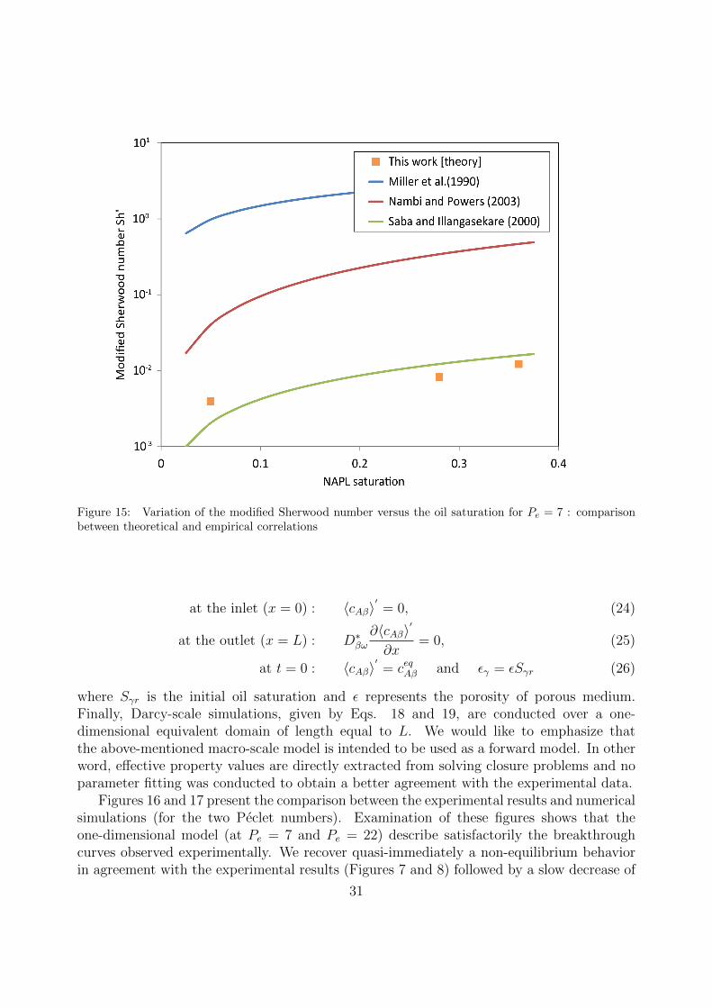
Figure 15: Variation of the modified Sherwood number versus the oil saturation for Pe = 7 : comparisonbetween theoretical and empirical correlations

at the inlet (x = 0) : 〈cAβ〉′= 0, (24)

at the outlet (x = L) : D∗βω∂〈cAβ〉

′

∂x= 0, (25)

at t = 0 : 〈cAβ〉′= ceqAβ and εγ = εSγr (26)

where Sγr is the initial oil saturation and ε represents the porosity of porous medium.Finally, Darcy-scale simulations, given by Eqs. 18 and 19, are conducted over a one-dimensional equivalent domain of length equal to L. We would like to emphasize thatthe above-mentioned macro-scale model is intended to be used as a forward model. In otherword, effective property values are directly extracted from solving closure problems and noparameter fitting was conducted to obtain a better agreement with the experimental data.

Figures 16 and 17 present the comparison between the experimental results and numericalsimulations (for the two Peclet numbers). Examination of these figures shows that theone-dimensional model (at Pe = 7 and Pe = 22) describe satisfactorily the breakthroughcurves observed experimentally. We recover quasi-immediately a non-equilibrium behaviorin agreement with the experimental results (Figures 7 and 8) followed by a slow decrease of

31

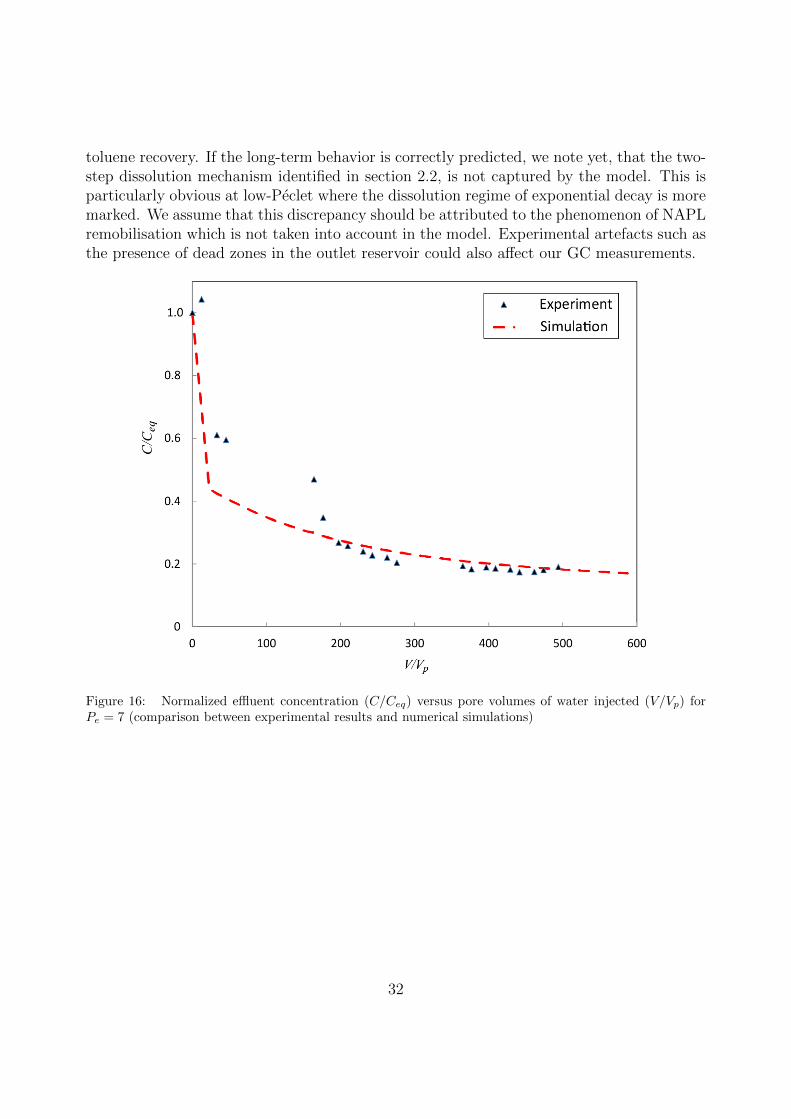
toluene recovery. If the long-term behavior is correctly predicted, we note yet, that the two-step dissolution mechanism identified in section 2.2, is not captured by the model. This isparticularly obvious at low-Peclet where the dissolution regime of exponential decay is moremarked. We assume that this discrepancy should be attributed to the phenomenon of NAPLremobilisation which is not taken into account in the model. Experimental artefacts such asthe presence of dead zones in the outlet reservoir could also affect our GC measurements.

Figure 16: Normalized effluent concentration (C/Ceq) versus pore volumes of water injected (V/Vp) forPe = 7 (comparison between experimental results and numerical simulations)

32

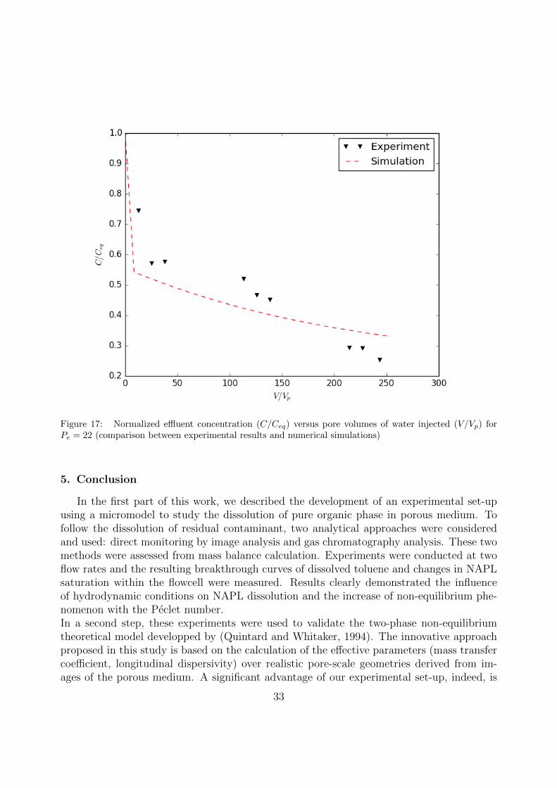
Figure 17: Normalized effluent concentration (C/Ceq) versus pore volumes of water injected (V/Vp) forPe = 22 (comparison between experimental results and numerical simulations)

5. Conclusion

In the first part of this work, we described the development of an experimental set-upusing a micromodel to study the dissolution of pure organic phase in porous medium. Tofollow the dissolution of residual contaminant, two analytical approaches were consideredand used: direct monitoring by image analysis and gas chromatography analysis. These twomethods were assessed from mass balance calculation. Experiments were conducted at twoflow rates and the resulting breakthrough curves of dissolved toluene and changes in NAPLsaturation within the flowcell were measured. Results clearly demonstrated the influenceof hydrodynamic conditions on NAPL dissolution and the increase of non-equilibrium phe-nomenon with the Peclet number.In a second step, these experiments were used to validate the two-phase non-equilibriumtheoretical model developped by (Quintard and Whitaker, 1994). The innovative approachproposed in this study is based on the calculation of the effective parameters (mass transfercoefficient, longitudinal dispersivity) over realistic pore-scale geometries derived from im-ages of the porous medium. A significant advantage of our experimental set-up, indeed, is

33

to provide a direct monitoring of NAPL dissolution with time that can be processed forobtaining 2D realistic configurations. Comparison of 1D macroscopic simulations with theexperimental breakthrough curves indicates that the proposed model is able to describe withsatisfactory accuracy the dissolution of NAPL in porous media and support a posteriori thecalculation of effective coefficients. The differences between curves could be assigned toNAPL remobilization during the experiments and problems associated with the design ofthe micromodel, in particular with the reservoirs (presence of dead zones) that may inducea more or less significant error on the chromatographic measurements. As a conclusion,this study highlights the crucial need of having a fair recovery of pore-scale characteristiclengths to properly determine the changes with time in mass transfer mechanisms whenusing upscaling methods.

Acknowledgements

This work was partially supported by the French National Research Agency (ANR)through the MOBIOPOR project, with the reference ANR-10-BLAN-0908 and was per-formed as part of the French Scientific Interest Group-Industrial Wasteland (GISFI) pro-gram. This project has also received partial funding from the European Union’s Horizon2020 research and innovation program through the PROTINUS project under Grant Agree-ment No. 645717.

6. References

Abriola, L., 1989. Modeling multiphase migration of organic chemicals in groundwater systems- a reviewand assessment. Environmental Health Perspectives 83, 143–148.

Agaoglu, B., Scheytt, T., Copty, N., 2016. Impact of napl architecture on interphase mass transfer: A porenetwork study. Advances in Water Resources 95, 138–151.

Ahmadi, A., Aigueperse, A., Quintard, M., 2001. Calculation of the effective properties describing activedispersion in porous media: from simple to complex unit cells. Advances in Water Ressources 24, 423–431.

Al-Raoush, R., 2009. Impact of wettability on pore-scale characteristics of residual nonaqueous phase liquids.Environmental Science and Technology 43, 4796–4801.

Al-Raoush, R., 2014. Experimental investigation of the influence of grain geometry on residual napl usingsynchrotron microtomography. Journal of Contaminant Hydrology 159, 1–10.

Armstrong, R., Berg, S., 2013. Interfacial velocities and capillary pressure gradients during haines jumps.Physical Review E 88, 1–9.

Armstrong, R., McClure, J., Berrill, M., Rcker, M., Schlter, S., Berg, S., 2016. Beyond darcy’s law: Therole of phase topology and ganglion dynamics for two-fluid flow. Physical Review E 94, 043113.

Atteia, O., Jousse, F., Cohen, G., Hohener, P., 2017. Comparison of residual napl source removal techniquesin 3d metric scale experiments. Journal of Contaminant Hydrology 202, 23–32.

Bahar, T., Golfier, F., Oltean, C., Benioug, M., 2016. An upscaled model for bio-enhanced napl dissolutionin porous media. Transport in Porous Media 113, 653–693.

Borden, R., Kao, C.-M., 1992. Evaluation of groundwater extraction for remediation of petroleum-contaminated aquifers. Water Environment Research 64, 28–36.

Chomsurin, C., Werth, C., 2003. Analysis of pore-scale nonaqueous phase liquid dissolution in etched siliconpore networks. Water Resources Research 39, 1265.

Conrad, S., Wilson, J., Mason, W., Peplinski, W., 1992. Visualisation of residual organic liquid trapped inaquifers. Water Resources research 28, 467–478.

34

Corapcioglu, M., Baehr, A., 1987. A compositional multiphase model for groundwater contamination bypetroleum 1: Theroretical considerations. Water Resources Research 23, 191–200.

Corapcioglu, M., Yoon, S., Chowdhury, S., 2009a. Pore-Scale Analysis of NAPL Blob Dissolution andMobilization in Porous Media. Transport in Porous Media 79, 419–442.

Corapcioglu, M., Yoon, S., Chowdhury, S., 2009b. Pore-scale analysis of napl blob dissolution and mobiliza-tion in porous media. Transport in Porous Media 79, 419–442.

Culligan, K., Wildenschild, D., Christensen, B., Gray, W., Rivers, M., 2006. Pore-scale characteristics ofmultiphase flow in porous media: A comparison of air-water and oil-water experiments. Advances inWater Resources 29, 227–238.

Cushman, H., Moroni, M., 2001. Statistical mechanics with three-dimensional particle tracking velocimetryexperiments in the study of anomalous dispersion. i. theory. Phys. Fluids 13, 75–80.

Garing, C., de Chalendar, J., Voltolini, M., Ajo-Franklin, J., Benson, S., 2017. Pore-scale capillary pressureanalysis using multi-scale x-ray micromotography. Advances in Water Resources 104, 223–241.

Ghosh, J., Tick, G., 2013. A pore scale investigation of crude oil distribution and removal from homogeneousporous media during surfactant-induced remediation. Journal of Contaminant Hydrology 155, 20?30.

Golfier, F., Quintard, M., Whitaker, S., 2002. Heat and mass transfer in tubes: An analysis using the methodof volume averaging. Journal of Porous Media 5, 169–185.

Goyeau, B., Benihaddadene, T., Gobin, D., Quintard, M., 1999. Numerical calculation of the permeabilityin a dendritic mushy zone. Metall.and Mater.Trans 30B, 613–622.

Gray, W., Leijnse, A., Kolar, R., Blain, C., 1993. Mathematical tools for changing spatial scales in theanalysis of physical systems. CRC Press: Boca Raton.

Hunt, J., Sitar, N., Udell, K., 1988. Nonaqueous phase liquid transport and cleanup: 1. analysis of mecha-nisms. Water Resources Research 24, 1247–1258.

Javanbakht, G., Arshadi, M., Qin, T., Goual, L., 2017. Micro-scale displacement of napl by surfactant andmicroemulsion in heterogeneous porous media. Advances in Water Resources 105, 173–187.

Javanbakht, G., Goual, L., 2016. Mobilization and micellar solubilization of napl contaminants in aquiferrocks. Journal of Contaminant Hydrology 185-186, 61–73.

Jeong, S.-W., Corapcioglu, M., Roosevelt, S., 2000. Micromodel study of surfactant foam remediation ofresidual trichloroethylene. Environ. Sci. Technol 34, 3456–3461.

Jia, C., Shing, K., Yortsos, Y., 1999. Visualization and simulation of non-aqueous phase liquids solubilizationin pore networks. Journal of Contaminant Hydrology 25, 363–387.

Kashuk, S., Mercurio, S., Iskander, M., 2014. Visualization of dyed napl concentration in transparent porousmedia using color space components. Journal of Contaminant Hydrology 162-163, 1–16.

Kokkinaki, A., O’Carroll, D., Werth, C., Sleep, B., 2013. An evaluation of sherwoodgilland models for napldissolution and their relationship to soil properties. Journal of Contaminant Hydrology 155, 87–98.

Mainhagu, J., Brusseau, M., 2016. Estimating initial contaminant mass based on fitting mass-depletionfunctions to contaminant mass discharge data: Testing method efficacy with sve operations data. Journalof Contaminant Hydrology 192, 152–157.

Miller, C., Poirier-McNeill, M., Mayer, A., 1990. Dissolution of trapped nonaqueous phase liquids : Masstransfer characteristics. Water Resources Research 26, 2783–2796.

Miller, C., Poirier-Mcnell, M., 1990. Dissolution of trapperd nonaqueous phase liquids : Mass transfercharacteristics. Water Resources Research 26, 2783–2796.

Mobile, M., Widdowson, M., Stewart, L., Nyman, J., Deeb, R., Kavanaugh, M., Mercer, J., Gallagher, D.,2016. In-situ determination of field-scale napl mass transfer coefficients: Performance, simulation andanalysis. Journal of Contaminant Hydrology 187, 31–46.

Nambi, I., Powers, S., 2003. Mass transfer correlations for nonaqueous phase liquid dissolution from regionswith high initial saturations. Water Resources Research 39, 10–30.

National Research Council (NRC), 2005. Contaminants in the Subsurface: Source Zone Assessment andRemediation. National Academies Press.

Padgett, M., Tick, G., Carroll, K., Burke, W., 2017. Chemical structure influence on napl mixture nonidealityevolution, rate-limited dissolution, and contaminant mass flux. Journal of Contaminant Hydrology 198,

35

11–23.Powers, S., Abriola, L., Weber, W., 1992. An experimental investigation of nonaqueous phase liquid disso-

lution in saturated subsurface systems : Steady state mass transfer rates. Water Resources Research 28,2691–2705.

Powers, S., Abriola, L., Weber, W., 1994. An experimental investigation of nonaqueous phase liquid dis-solution in saturated subsurface systems: Transient mass transfer rates. Water Ressources Research 30,321–332.

Quintard, M., Whitaker, S., 1994. Convection, dispersion, and interfacial transport of contaminants: Ho-mogenous porous media. Advances in Water Ressources 17, 221–239.

Quintard, M., Whitaker, S., 1999. Dissolution of an immobile phase during flow in porous media. Ind. Eng.Chem. Res 38, 833–844.

Radilla, G., Quintard, M., Bertin, H., 1997. NAPL dissolution in saturated porous media: model experimentsand pore scale interpretation. In: Sixth Symposium on multiphase transport in porous media. Vol. FED244. pp. 423–429.

Radilla, G., Quintard, M., Bertin, H., 1998. Theoretical study and experimental validation of transport co-efficients for hydrocarbon pollutants in aquifers. In: Recent Advances in Problems of Flow and Transportin Porous Media, ? Edition. Lewis publishers, pp. 143–152.

Rasband, W., 1997-2016. Image J. U.S. National Institutes of Health, Bethesda, Maryland, USA,https://imagej.nih.gov/ij/.

Saba, T., Illangasekare, T., 2000. Effect of groundwater flow dimensionality on mass transfer from entrappednonaqueous phase liquid contaminants. Water Resources Research 36, 971–979.

Sahloul, N., Ioannidis, M., Chatzis, I., 2002. Dissolution of residual non-aqueous phase liquids in porousmedia: pore-scale mechanisms and mass transfer rates. Advances in Water Resources 25, 33–49.

Schubert, M., Paschke, A., Lau, S., Geyer, W., Knoller, K., 2007. Radon as a naturally occurring tracer forthe assessment of residual napl contamination of aquifers. Environmental Pollution 145, 920–927.URL https://doi.org/10.1016/j.envpol.2006.04.029

Seagren, E., Rittmann, B., Valocchi, A., 1999. A critical evaluation of the local-equilibrium assumption inmodeling napl-pool dissolution. Journal of Contaminant Hydrology 39, 109–135.

Wehrer, M., Mai, J., Attinger, S., Totsche, K., 2013. Kinetic control of contaminant release from napls -information potential of concentration time profiles. Environmental Pollution 179, 301–314.

Whitaker, S., 1999. The method of volume averaging. Dordrecht: Kluwer Academic Publishers.Yra, A., Bertin, H., Ahmadi, A., 2006. etude experimentale de la dispersion active d’un polluant hydrocar-

bone en milieu poreux heterogene. C. R. Mecanique 334, 58–67.Zhao, W., Ioannidis, M., 2003. Pore network simulation of the dissolution of a single component wetting

nonaqueous phase liquid. Water Resources Research 39, 1291.Zhao, W., Ioannidis, M., 2007. Effect of napl film stability on the dissolution of residual wetting napl in

porous media: A pore-scale modeling study. Advances in Water Resources 30, 171–181.

AppendixA. Upscaling of the mass transport equations

We begin our analysis by applying the spatial and temporal averaging theorems, thatcan be expressed as (Whitaker, 1999):

〈∇cAβ〉 = ∇〈cAβ〉+1

V

∫Aβγ

nβγcAβdA+1

V

∫Aβσ

nβσcAβdA (A.1)

〈∇ · (vAβcAβ)〉 = ∇ · 〈vAβcAβ〉+1

V

∫Aβγ

nβγ · (vAβcAβ)dA

+1

V

∫Aβσ

nβσ · (vAβcAβ)dA (A.2)

36

〈∂cAβ∂t〉 =

∂〈cAβ〉∂t

− 1

V

∫Aβγ

nβγ · cAβwβγdA−1

V

∫Aβσ

nβσ · cAβwβσdA (A.3)

The volume averaging theorems have been used for obtaining the averaged transport equa-tion in each phase:β-phase

∂(εβ〈cAβ〉β)

∂t︸ ︷︷ ︸Accumulation

+∇ · 〈vAβcAβ〉︸ ︷︷ ︸Advection

+1

V

∫Aβγ

nβγ · cAβ(vAβ −wβγ)dA︸ ︷︷ ︸Interfacial flux

+1

V

∫Aβσ

nβσ · cAβ(vAβ −wβσ)dA︸ ︷︷ ︸Interfacial flux

= 0 (A.4)

γ-phase

∂〈ργ〉∂t︸ ︷︷ ︸

Accumulation

+1

V

∫Aβγ

ργnβγ.wβγdA︸ ︷︷ ︸Interfacial flux

= 0 (A.5)

Taking into account the relationships expressing the condition of a dilute solution of speciesA (additional details are available in Quintard and Whitaker (1999)),

cAβvAβ = cAβvβ −DAβ∇cAβ (A.6)

the superficial average equation, Eq.(A.4), in the β-phase becomes:β-phase

∂(εβ〈cAβ〉β)

∂t︸ ︷︷ ︸Accumulation

+∇ · 〈vβcAβ〉︸ ︷︷ ︸Advection

= − 1

V

∫Aβγ

nβγ · (cAβ(vβ −wβγ)−DAβ∇cAβ)dA︸ ︷︷ ︸Interfacial flux

+∇ · 〈DAβ∇cAβ〉︸ ︷︷ ︸Dispersion

− 1

V

∫Aβσ

nβσ · (cAβ(vβ −wβσ)−DAβ∇cAβ)dA︸ ︷︷ ︸Interfacial flux

(A.7)

Finally the unclosed form of the averaged equation in the β-phase can be expressed as (thecomplete development for averaged equations is available in Quintard and Whitaker (1994)):

37

β-phase

∂〈cAβ〉β

∂t︸ ︷︷ ︸Accumulation

+ 〈vβ〉β · ∇〈cAβ〉β︸ ︷︷ ︸Advection

+ ε−1β ∇ · 〈vβ cAβ〉︸ ︷︷ ︸Dispersive transport

= ∇ · (DAβ∇〈cAβ〉β)︸ ︷︷ ︸Dispersion

+ ε−1β ∇ · [DAβ(1

V

∫Aβγ

nβγ cAβdA+1

V

∫Aβσ

nβσ cAβdA)]︸ ︷︷ ︸Dispersion

−ε−1βV

∫Aβγ

nβγ · cAβ(vβ −wβγ)dA︸ ︷︷ ︸Interfacial flux

−ε−1βV

∫Aβσ

nβσ · cAβ(vβ −wβσ)dA+ε−1βV

∫Aβγ

nβγ ·DAβ∇cAβdA︸ ︷︷ ︸Interfacial flux

+ε−1βV

∫Aβσ

nβσ ·DAβ∇cAβdA︸ ︷︷ ︸Interfacial flux

(A.8)

For a binary system and under the dilute solution approximation (Quintard and Whitaker,1999), the velocity of interface Aβγ can be expressed as,

wβγ · nβγ =1

ργnβγ ·DAβ∇cAβ at Aβγ (A.9)

Finally, substituting the last equation, Eq.(A.9), into the averaged equation, Eq.A.5, wederived the unclosed form of macroscopic equation in the γ-phase:

ργ∂εγ∂t︸ ︷︷ ︸

Accumulation

+1

V

∫Aβγ

nβγ ·DAβ∇〈cAβ〉βdA+1

V

∫Aβγ

nβγ ·DAβ∇cAβdA︸ ︷︷ ︸Interfacial flux

= 0 (A.10)

AppendixA.1. Closure

Firstly, we recall our original differential equation defined in the β- phase at the porescale,

∂(cAβ)

∂t+∇ · (vβcAβ) = ∇ · (DAβ∇cAβ) (A.11)

By subtracting Eq.(A.8) from Eq.(A.11), we obtain the set of equations governing the con-

38

centration deviations:

vβ · ∇cAβ + vβ · ∇〈cAβ〉β = ∇ · (DAβ∇cAβ) +ε−1βV

∫Aβγ

nβγ · cAβ(vβ −wβγ)dA

+ε−1βV

∫Aβσ

nβσ · cAβ(vβ −wβσ)dA−ε−1βV

∫Aβγ

nβγ ·DAβ∇cAβdA

−ε−1βV

∫Aβσ

nβσ ·DAβ∇cAβdA (A.12)

B.C.1 − nβσ ·DAβ∇〈cAβ〉β︸ ︷︷ ︸Source

= nβσ ·DAβ∇cAβ at Aβσ (A.13)

B.C.2 cAβ = ceqAβ − 〈cAβ〉β︸ ︷︷ ︸

Source

at Aβγ (A.14)

B.C.3 (Periodicity) cAβ(r + li) = cAβ(r), i = 1, 2, 3 (A.15)

B.C.4 〈cAβ〉β = 0 (A.16)

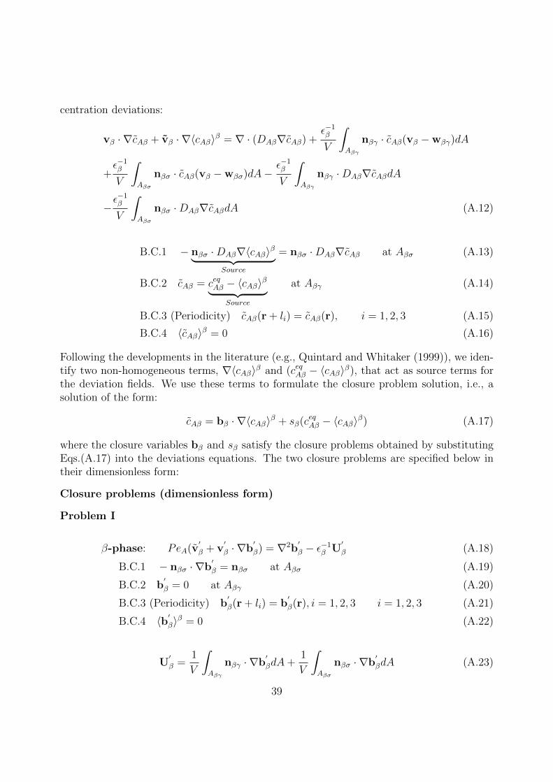
Following the developments in the literature (e.g., Quintard and Whitaker (1999)), we iden-tify two non-homogeneous terms, ∇〈cAβ〉β and (ceqAβ − 〈cAβ〉β), that act as source terms forthe deviation fields. We use these terms to formulate the closure problem solution, i.e., asolution of the form:

cAβ = bβ · ∇〈cAβ〉β + sβ(ceqAβ − 〈cAβ〉β) (A.17)

where the closure variables bβ and sβ satisfy the closure problems obtained by substitutingEqs.(A.17) into the deviations equations. The two closure problems are specified below intheir dimensionless form:

Closure problems (dimensionless form)

Problem I

β-phase: PeA(v′

β + v′

β · ∇b′

β) = ∇2b′

β − ε−1β U′

β (A.18)

B.C.1 − nβσ · ∇b′

β = nβσ at Aβσ (A.19)

B.C.2 b′

β = 0 at Aβγ (A.20)

B.C.3 (Periodicity) b′

β(r + li) = b′

β(r), i = 1, 2, 3 i = 1, 2, 3 (A.21)

B.C.4 〈b′β〉β = 0 (A.22)

U′

β =1

V

∫Aβγ

nβγ · ∇b′

βdA+1

V

∫Aβσ

nβσ · ∇b′

βdA (A.23)

39

Problem II

β-phase: PeAv′

β · ∇s′

β = ∇2s′

β − ε−1β S′

β (A.24)

B.C.1 − nβσ · ∇s′

β = 0 at Aβσ (A.25)

B.C.2 s′

β = 1 at Aβγ (A.26)

B.C.3 (Periodicity) s′

β(r + li) = s′

β(r), i = 1, 2, 3 i = 1, 2, 3 (A.27)

B.C.4 〈s′β〉β = 0 (A.28)

S′

β =1

V

∫Aβγ

nβγ · ∇s′

βdA+1

V

∫Aβσ

nβσ · ∇s′

βdA (A.29)

where the dimensionless variables and the parameters have been defined by

v′

β =vβ‖ vβ ‖

v′

β =vβ‖ vβ ‖

PeA =‖ vβ ‖ lβDAβ

(A.30)

AppendixA.2. Closed Form of the Macroscopic Equations

Now we introduce the closure solution, Eq. (A.17), into the unclosed averaged equation.The following closed form of the mass transport equations is obtained:

∂εβ〈cAβ〉β

∂t+ εβ〈vβ〉β · ∇〈cAβ〉β − dβω · ∇〈cAβ〉β −Uβω · ∇〈cAβ〉β =

∇ · (D∗βω · ∇〈cAβ〉β) + α∗A(ceqAβ − 〈cAβ〉β) (A.31)

ργ∂εγ∂t

= −α∗A(ceqAβ − 〈cAβ〉β) (A.32)

40