Comparison of Three Perturbation Molecular Dynamics Methods for Modeling Conformational Transitions

Comparison of Three Perturbation Molecular DynamicsMethods for Modeling Conformational Transitions

He Huang,† Elif Ozkirimli,†,‡ and Carol Beth Post*,†

Department of Medicinal Chemistry and Molecular Pharmacology, Markey Center forStructural Biology and Purdue Cancer Center, Purdue UniVersity,

West Lafayette, Indiana 47907, and Department of Chemical Engineering,Bogazici UniVersity, Bebek, 34342, Turkey

Received January 9, 2009

Abstract: Targeted, steered, and biased molecular dynamics (MD) are widely used methodsfor studying transition processes of biomolecules. They share the common feature of addingexternal perturbations along a conformational progress variable to guide the transition in apredefined direction in conformational space, yet differ in how these perturbations are applied.In the present paper, we report a comparison of these three methods on generating transitionpaths for two different processes: the unfolding of the B domain of protein A and a conformationaltransition of the catalytic domain of a Src kinase Lyn. Transition pathways were calculated withdifferent simulation parameters including the choice of progress variable and the simulationlength or biasing force constant. A comparison of the generated paths based on structuralsimilarity finds that the three perturbation MD methods generate similar transition paths for agiven progress variable in most cases. On the other hand, the path depends more strongly onthe choice of progress variable used to move the system between the initial and final states.Potentials of mean force (PMF) were calculated starting from unfolding trajectories to estimatethe relative probabilities of the paths. A lower PMF was found for the lowest biasing force constantwith BMD.

1. Introduction

Functionally important dynamic processes of proteins, suchas folding/unfolding and allosteric conformational transitions,occur on the microsecond to millisecond time scale. Mo-lecular dynamics simulation is a useful tool to elucidate theatomistic detail of protein dynamics; however, simulationsof all-atom models are limited to the submicrosecond timerange. To overcome this time scale problem, methods thatutilize the principles of molecular dynamics, with someexternal perturbations to accelerate the reaction and guidethe system toward a target state, have been developed.1-6

Here, such methods are collected under the title of “perturba-tion molecular dynamics”. They aim to identify possibletransition pathways as well as energy barriers and metastable

intermediates. Such pathways can then be further examinedby thermodynamic simulation methods.

The most commonly used perturbation molecular dynamicsmethods are targeted molecular dynamics (TMD), steeredmolecular dynamics (SMD), and biased molecular dynamics(BMD). These methods share the common feature of guidingthe transition between two end states through some progressvariable (reaction coordinate), though they differ in the waythat the progress variable is controlled. As originallyintroduced by Schlitter,1,2 the TMD methodology imposesa time-dependent holonomic constraint on the rmsd to a targetstructure. SMD simulations were first used by Grubmueller3

and Leech,4 and were widely applied shortly after bySchulten et al.7-10 SMD is akin to atomic force microscopy(AFM) in that a harmonic restraint based on a reference pointmoves the system toward the target when the reference pointis updated. We note that in some later publications11-16 theterm TMD was associated with the rmsd progress variable

* Corresponding author e-mail: [email protected].† Purdue University.‡ Bogazici University.

J. Chem. Theory Comput. 2009, 5, 1304–13141304

10.1021/ct9000153 CCC: $40.75 2009 American Chemical SocietyPublished on Web 04/09/2009

with harmonic restraint rather than holonomic constraint. Inthe present paper, we denote the holonomic constraint asTMD and the harmonic restraint as SMD to distinguish theperturbation form regardless of the progress variable. BMD,also known as the adiabatic bias molecular dynamics, wasoriginally proposed independently by Marchi and Ballone5

and Paci and Karplus.6 It provides the least perturbationamong the three in that the system feels no force if it movestoward the target and the biasing potential is nonzero onlyif the system moves away from the target.

These three methods are commonly used to study transitionprocesses of biomolecules11-30 They are also used to comple-ment AFM experiments that examine the mechanical propertiesof macromolecules.10,31 Given the interest in these perturbationMD methods, an assessment of the effect of the choice ofperturbation method, progress variable, and other simulationparameters on the resulting transition paths is of value.

In the present paper, we report a systematic comparisonof the conformations and energetics of trajectories generatedby the three perturbation molecular dynamics methods fortwo transition processes. The first example system is theunfolding of the B domain of staphylococcal protein A(BdpA). BdpA is a three-helix-bundle protein for whichfolding/unfolding has been studied extensively by experi-ments32-34 and computer simulations.35-38 Its unfolding isan example where the progress variable does not define asingle target configuration. The second process is theconformational change between active and inactive structuresof the kinase catalytic domain (CD) of Lyn, a member ofthe Src family of protein tyrosine kinases. This transition isan example that has defined target configurations at both endstates. For TMD, SMD, and BMD paths generated for bothsystems, we examined the effect of different simulationconditions, including the choice of progress variable andperturbation strength. Our results suggest that, for the mostpart, the three perturbation MD methods generate similartransition paths for a given progress variable even thoughthe time dependence of the progress variables differssubstantially. On the other hand, the path depends stronglyon the choice of the progress variable.

2. Methods

2.1. Three Perturbation MD Methods. Targeted mo-lecular dynamics (TMD) introduces the most constrainedperturbation among the three methods. While the other twomethods add restraining potentials to guide the system, TMDimposes a holonomic constraint onto the dynamics of thesystem:2

φ(F(x(t)), F0(t))) 0 (1)

where F(x) is the progress variable defined as a function ofthe coordinate, x, F0(t) is the reference value of F at time t,and φ is a function of F and F0 which equals zero when F )F0; for example

φ(x))F-F0 (2)

The constraint adds onto the system a constraining force

FC ) λ∇xφ (3)

which keeps the progress variable F following the referencevalue F0(t) exactly. Here λ is a Lagrange parameter deter-mined according to eq 1, and the reference value F0(t) movesat a constant rate V toward the target value:

F0(t))F0(t0)+V(t- t0) (4)

Steered molecular dynamics (SMD) corresponds closelyto micromanipulation by AFM39 when it uses a singleinteratomic distance as the progress variable. Computation-ally, it adds a full harmonic potential to restrain the progressvariable around a reference value, which is moved to thetarget value at a constant rate V:

H(F)) R2

(F- F0)2 (5)

F0(t))F0(t0)+V(t- t0) (6)

where H is the biasing potential, R is the force constant, Fis the progress variable, and F0 is the reference point.

Biased molecular dynamics (BMD) guides the change ofthe progress variable by penalizing a move in the undesireddirection through a one-sided harmonic potential. At eachtime step, the reference point is updated to the previouslysampled value that is closest to the target. The method isdefined by the following equations assuming the system ismoved in the direction in which the progress variable Fincreases:

H(F)) {R2 (F- F0)2 (F < F0)

0 (Fg F0)(7)

F0(t)) {F0(t-∆t) (F < F0)F(t) (Fg F0)

(8)

where ∆t is the simulation time step. Among the threemethods, BMD provides the least restrained perturbation tothe molecular system in that progress in the direction towardthe target occurs without external perturbation.

2.2. Molecular Systems. The molecular system of BdpAwas derived from the NMR structure (PDB ID: 1BDD).40

The C- and N-terminal loops were removed, and residues10-55 were kept. A 2-ns equilibrium MD simulation wascalculated with the CHARMM22 force field and the GBSWimplicit solvent model41 in CHARMM.42 Four configurationsfrom the equilibrium run separated by 500 ps were savedand used as initial structures of the perturbation MD runs.The CHARMM22 force field and GBSW solvation modelwere used in all perturbation MD runs for BdpA unfolding.

For the Lyn CD, the active and inactive coordinates wereobtained by homology modeling based on crystallographicstructures of the Lck kinase (PDB ID: 3LCK)43 and Hckkinase (PDB ID: 1QCF),44 respectively. Both structures wereequilibrated with the CHARMM22 force field with ap-proximately 9400 TIP3P waters in a periodic rhombicdodecahedral box at 298 K for 300-400 ps, as previouslyreported.23 The CHARMM22 force field with explicit TIP3Pwater was also used in all perturbation MD runs for the LynCD conformational transition.

2.3. Progress Variables. For BdpA unfolding, the threeperturbation MD methods were examined with two progressvariables, either the end-to-end distance between the two

MD Methods for Modeling Conformational Transitions J. Chem. Theory Comput., Vol. 5, No. 5, 2009 1305

terminal CR atoms (F ) h) or the radius of gyration basedon all heavy atoms (F ) Rg), which is defined as

Rg )� 1N∑

i

N |ri -1N∑

j

N

rj|2 (9)

where ri is the Cartesian coordinate of the ith heavy atomand N equals the total number of heavy atoms. Eachcombination of method and progress variable was used withthree different perturbation strengths as reflected by thesimulation lengths: 0.5, 2, and 10 ns. With TMD or SMD,the simulation length was controlled directly by the rate forupdating the reference point, while in BMD, in which nosuch parameter is available, it was controlled by tuning theforce constant so that the unfolding process happens inroughly the specified time. For each set of simulationconditions (perturbation method, progress variable, andsimulation length), two to four (see Table 1 for details)trajectories were calculated with different initial coordinatesand velocities.

The Lyn CD conformational transition for both activation(inactive to active CD) and deactivation (active to inactive)was simulated by all three perturbation MD methods withthe progress variable mean square internal deviation (F )MSID) defined in terms of internal distances:

MSID) 2N(N- 1)∑i)1

N

∑j>i

N

(dij - dij0)2 (10)

where dij and dij0 are distances between heavy atoms i and j

in the current and target structures, respectively, and N isthe number of atoms. This progress variable was originallyused to investigate partially unfolded protein in combinationwith BMD by Paci et al.,45 and later applied to Src kinaseactivation.23 A similar progress variable defined upon internaldistances was used by Markwick et al. together with a massweighting.46

A second progress variable, root-mean-square deviation(F ) rmsd), was examined with only the TMD method, andis defined as

RMSD)� 1N∑

i)1

N

|ri - ri0|2 (11)

where ri and ri0 are Cartesian coordinates of the ith heavy

atom in the superimposed current and target structures,respectively, and N is the total number of heavy atoms. Thecombination of rmsd as the progress variable and theholonomic constraint as the perturbation method coincideswith the original TMD method used by Schlitter et al.1,2 Foreach combination of method, progress variable, and direction,two to four (see Table 2 for details) trajectories werecalculated with different updating rates, V, of the progressvariable (TMD, SMD) or force constants, R (BMD).

2.4. Trajectory Averaged rmsd. The structural similarityof the BdpA unfolding trajectories was evaluated from atrajectory averaged rmsd calculated to measure the pairwisesimilarity between different trajectories. For each unfoldingtrajectory with either h or Rg as the progress variable,snapshots were binned according to Rg into 0.5-Å-wide bins.An average configuration Xjk was calculated for each bin kto represent the snapshots within that bin. Snapshots withineach bin have similar structures, as indicated by the averagerms fluctuation of 2.0, 2.0, and 1.6 Å for TMD, SMD, andBMD 10 ns trajectories, respectively. The within-bin vari-ances for shorter trajectories are expected to be even lower.Between trajectories i and j, the trajectory averaged rmsd isdefined as

rmsdij )1M∑

k)1

M

rmsd(Xki, Xk

j) (12)

where M is the number of bins and rmsd is calculated aftersuperimposing all heavy atoms. This single value providesa metric for the overall similarity between two trajectories.Because the rmsd between two extended structures is alwayssmall, we ignored snapshots with Rg greater than 17 Å inthis calculation.

Table 1. Summary of BdpA Unfolding Trajectories

progressvariable method

length(ns)

force constant(kcal/(mol ·Å2))

rate(Å/ps) no.a code

hTMD

0.5 - 0.1 2 hT12 - 0.025 2 hT2

10 - 0.005 2 hT3

SMD0.5 50 0.1 2 hS12 50 0.025 2 hS2

10 50 0.005 2 hS3

BMD0.5 50 - 2 hB12 20 - 2 hB2

10 8 - 2 hB3Rg

TMD0.5 - 0.05 2 RT12 - 0.0125 2 RT2

10 - 0.0025 4 RT3

SMD0.5 5000 0.05 2 RS12 5000 0.0125 2 RS2

10 5000 0.0025 4 RS3

BMD0.5 5000 - 2 RB12 400 - 2 RB2

10 110 - 4 RB3

a Number of independent trajectories that were calculated.

Table 2. Summary of Lyn CD Activation/DeactivationTrajectories

progressvariable method directiona

length(ns)

force constant(kcal/(mol ·Å4))

rate(Å/ps) colorb

MSID

TMDA f I

0.16 - 0.1 black1.0 - 0.016 red

I f A0.16 - 0.1 green1.0 - 0.016 blue

SMDA f I

0.16 1000 0.1 black1.0 1000 0.016 red

I f A0.16 1000 0.1 green1.0 1000 0.016 blue

BMD

A f I

1.9 1000 - black1.5 2000 - red1.5 3000 - yellow1.3 5000 - brown

I f A

1.9 1000 - green1.9 2000 - blue1.7 3000 - gray1.0 5000 - purple

rmsd

TMDA f I

0.2 - 0.03 black1.0 - 0.006 red

I f A0.2 - 0.03 green1.0 - 0.006 blue

a A, active state; I, inactive state. b Coloring for Figure 8a.

1306 J. Chem. Theory Comput., Vol. 5, No. 5, 2009 Huang et al.

2.5. Potential of Mean Force Calculation. The potentialof mean force (PMF) was calculated with an initial pathdefined by a Rg-perturbed BdpA unfolding trajectory by usingumbrella sampling47 and the weighted histogram analysismethod (WHAM).48 For each trajectory, 41 snapshots weretaken as the initial coordinates for umbrella sampling bychoosing coordinates with Rg values closest to an equallyspaced Rg series ranging from 9.75 to 15.75 Å in incrementsof 0.15 Å. Each of the 41 umbrella windows was simulatedfor 400 ps using a harmonic umbrella potential with forceconstant 10 kcal/(mol ·Å2) to restrain Rg around the initialvalue. The last 200 ps of the sampling was analyzed byWHAM to reconstruct the PMF profile with respect to Rg.The effect of initial-coordinate bias for a given trajectorywas examined by choosing a different set of initial coordi-nates with a shifted Rg series ranging from 9.83 to 15.83 Åwith 0.15 Å increments for the PMF calculations. Resultsfor two trajectories showed that very similar PMF curvesare obtained for each trajectory, indicating that the calculatedPMF curve characterizes a trajectory rather than the specificselection of snapshots (data not shown).

3. Results

Tables 1 and 2 summarize the perturbation MD simulationscarried out for the two transition systems. All simulationsand analyses were carried out with the molecular dynamicsprogram CHARMM.42

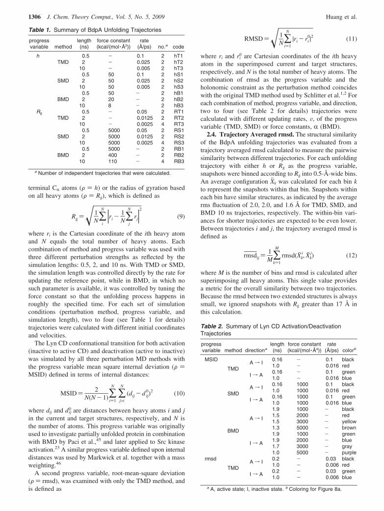
3.1. BdpA Unfolding. BdpA is a three-helix-bundleprotein with a highly symmetrical topology. The three helices(H1, H2, and H3) of comparable length are joined by twoturns (T1 and T2) in an antiparallel alignment to form twohelix-turn-helix motifs (see Figure 1).

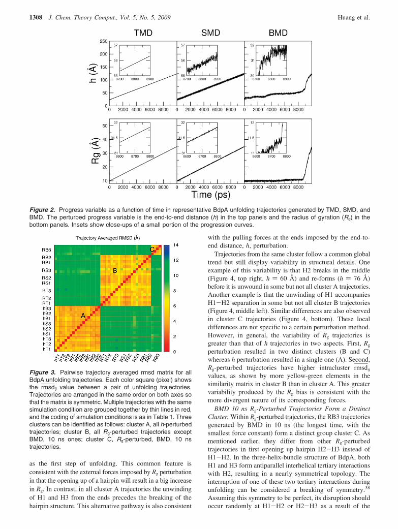
As listed in Table 1, a total of 42 unfolding trajectories ofBdpA were generated with three perturbation MD methods(BMD/SMD/TMD), two progress variables (end-to-enddistance h/radius of gyration Rg), and three different simula-tion lengths (0.5 ns/2 ns/10 ns). Figure 2 shows the timeprofiles of the progress variables for representative trajec-tories generated by the three methods. With TMD, theprogress variables scale linearly with time as expected fromthe holonomic constraint. SMD also generated nearly linearprogression curves due to the linear updating of the referencepoint, but the actual progress variables fluctuate about thelinear line. With BMD, the dynamics of the progressvariables appear more similar to natural fluctuation in thesense that their values change nonlinearly over time. Forexample, in the Rg-perturbed BMD simulation (Figure 2, right

bottom panel), the progress variable Rg increases slowly forthe first 8 ns until it reaches ∼11.5 Å, after which it riseswith a much steeper slope. This nonlinear progression canbe utilized to identify possible free energy barriers, becausea barrier impedes spontaneous fluctuations along the progressvariable and thus longer sampling time is needed to crossit.20,21

Effect of Perturbation Methods and Progress Variableon Determining Path. Rg and h were used to guide theunfolding transition of BdpA. Unfolding trajectories, fromTMD, SMD and BMD, were compared by the trajectoryaveraged rmsd values (rmsdij), for which the snapshots fromeach trajectory were binned according to their Rg values. Thecalculated unfolding trajectories were thus examined as pathsconnecting conformations in space rather than time evolutionof the system. To compare two trajectories, the rmsd wascalculated between average structures from each Rg bin, andthe rmsd values were averaged over all bins (see Methodsfor details). The resulting rmsdij value measures the overallspatial similarity between two trajectories, and the all-against-all evaluation is plotted in the matrix in Figure 3 accordingto the code shown in Table 1. This pairwise similarity matrixshows that the 42 trajectories naturally fall into three clusters.Interestingly, all h-perturbed trajectories fall into cluster A,all Rg-perturbed trajectories except RB3 fall into cluster B,and all Rg-perturbed, RB3 trajectories fall into cluster C. Thegroups of trajectories are clearly distinct from each other:The rmsdij value within any cluster is around 4 Å while thatbetween two different clusters averages near 11 Å.

It is apparent from the distinct clustering in Figure 3 that,for the case of BdpA unfolding, the global geometry of thetransition path is largely determined by the progress variablebeing h or Rg, and not by the perturbation method. Com-parison of trajectories within a cluster provides no evidencethat trajectories generated by either TMD, SMD, or BMDdiffer. The rmsdij values calculated between unfoldingtrajectories generated with different perturbation methods areequivalent to values obtained by comparing multiple runsby the same method and simulation length.

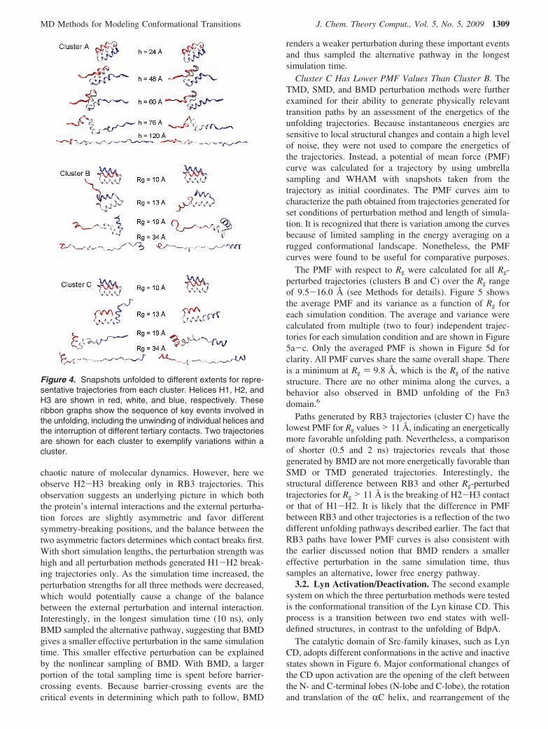
Inspecting all trajectories with the visualization programVMD49 identified the global features shared by all membersfrom the same cluster. These common features are shownin Figure 4 by two representative trajectories for unfoldingfrom each cluster. In cluster A trajectories, the protein unfoldsby first extending and unwinding H1 and H3 from the ends.Breaking of the H1-H2 and H2-H3 interhelical contactsfollows as a result of the stretching at the ends by perturbingh. The protein then extends into a linear chain. In cluster Btrajectories, the H1-H2 hairpin always opens up with aflipping of H1 at an early stage of unfolding. The openingup of the H2-H3 hairpin occurs later. In contrast, these twoevents happen in the opposite order in cluster C, where H3flips to lose contact with H2 earlier than the separation ofH1 and H2.

The stronger dependence of the transition path on theprogress variable than the method is evident from a similarityshared by cluster B and C paths regardless of the big rmsdbetween them. In these two clusters, the opening up of oneof the two hairpins (H1-H2 in B and H2-H3 in C) happens

Figure 1. The native structure of BdpA40 shown in cartoonrepresentation. Helices H1, H2, and H3 are colored in red,white, and blue, respectively. This figure was generated withVisual Molecular Dynamics (VMD).49


as the first step of unfolding. This common feature isconsistent with the external forces imposed by Rg perturbationin that the opening up of a hairpin will result in a big increasein Rg. In contrast, in all cluster A trajectories the unwindingof H1 and H3 from the ends precedes the breaking of thehairpin structure. This alternative pathway is also consistent

with the pulling forces at the ends imposed by the end-to-end distance, h, perturbation.

Trajectories from the same cluster follow a common globaltrend but still display variability in structural details. Oneexample of this variability is that H2 breaks in the middle(Figure 4, top right, h ) 60 Å) and re-forms (h ) 76 Å)before it is unwound in some but not all cluster A trajectories.Another example is that the unwinding of H1 accompaniesH1-H2 separation in some but not all cluster B trajectories(Figure 4, middle left). Similar differences are also observedin cluster C trajectories (Figure 4, bottom). These localdifferences are not specific to a certain perturbation method.However, in general, the variability of Rg trajectories isgreater than that of h trajectories in two aspects. First, Rg

perturbation resulted in two distinct clusters (B and C)whereas h perturbation resulted in a single one (A). Second,Rg-perturbed trajectories have higher intracluster rmsdij

values, as shown by more yellow-green elements in thesimilarity matrix in cluster B than in cluster A. This greatervariability produced by the Rg bias is consistent with themore divergent nature of its corresponding forces.

BMD 10 ns Rg-Perturbed Trajectories Form a DistinctCluster. Within Rg-perturbed trajectories, the RB3 trajectoriesgenerated by BMD in 10 ns (the longest time, with thesmallest force constant) form a distinct group cluster C. Asmentioned earlier, they differ from other Rg-perturbedtrajectories in first opening up hairpin H2-H3 instead ofH1-H2. In the three-helix-bundle structure of BdpA, bothH1 and H3 form antiparallel interhelical tertiary interactionswith H2, resulting in a nearly symmetrical topology. Theinterruption of one of these two tertiary interactions duringunfolding can be considered a breaking of symmetry.38

Assuming this symmetry to be perfect, its disruption shouldoccur randomly at H1-H2 or H2-H3 as a result of the

Figure 2. Progress variable as a function of time in representative BdpA unfolding trajectories generated by TMD, SMD, andBMD. The perturbed progress variable is the end-to-end distance (h) in the top panels and the radius of gyration (Rg) in thebottom panels. Insets show close-ups of a small portion of the progression curves.

Figure 3. Pairwise trajectory averaged rmsd matrix for allBdpA unfolding trajectories. Each color square (pixel) showsthe rmsdij value between a pair of unfolding trajectories.Trajectories are arranged in the same order on both axes sothat the matrix is symmetric. Multiple trajectories with the samesimulation condition are grouped together by thin lines in red,and the coding of simulation conditions is as in Table 1. Threeclusters can be identified as follows: cluster A, all h-perturbedtrajectories; cluster B, all Rg-perturbed trajectories exceptBMD, 10 ns ones; cluster C, Rg-perturbed, BMD, 10 nstrajectories.


chaotic nature of molecular dynamics. However, here weobserve H2-H3 breaking only in RB3 trajectories. Thisobservation suggests an underlying picture in which boththe protein’s internal interactions and the external perturba-tion forces are slightly asymmetric and favor differentsymmetry-breaking positions, and the balance between thetwo asymmetric factors determines which contact breaks first.With short simulation lengths, the perturbation strength washigh and all perturbation methods generated H1-H2 break-ing trajectories only. As the simulation time increased, theperturbation strengths for all three methods were decreased,which would potentially cause a change of the balancebetween the external perturbation and internal interaction.Interestingly, in the longest simulation time (10 ns), onlyBMD sampled the alternative pathway, suggesting that BMDgives a smaller effective perturbation in the same simulationtime. This smaller effective perturbation can be explainedby the nonlinear sampling of BMD. With BMD, a largerportion of the total sampling time is spent before barrier-crossing events. Because barrier-crossing events are thecritical events in determining which path to follow, BMD

renders a weaker perturbation during these important eventsand thus sampled the alternative pathway in the longestsimulation time.

Cluster C Has Lower PMF Values Than Cluster B. TheTMD, SMD, and BMD perturbation methods were furtherexamined for their ability to generate physically relevanttransition paths by an assessment of the energetics of theunfolding trajectories. Because instantaneous energies aresensitive to local structural changes and contain a high levelof noise, they were not used to compare the energetics ofthe trajectories. Instead, a potential of mean force (PMF)curve was calculated for a trajectory by using umbrellasampling and WHAM with snapshots taken from thetrajectory as initial coordinates. The PMF curves aim tocharacterize the path obtained from trajectories generated forset conditions of perturbation method and length of simula-tion. It is recognized that there is variation among the curvesbecause of limited sampling in the energy averaging on arugged conformational landscape. Nonetheless, the PMFcurves were found to be useful for comparative purposes.

The PMF with respect to Rg were calculated for all Rg-perturbed trajectories (clusters B and C) over the Rg rangeof 9.5-16.0 Å (see Methods for details). Figure 5 showsthe average PMF and its variance as a function of Rg foreach simulation condition. The average and variance werecalculated from multiple (two to four) independent trajec-tories for each simulation condition and are shown in Figure5a-c. Only the averaged PMF is shown in Figure 5d forclarity. All PMF curves share the same overall shape. Thereis a minimum at Rg ) 9.8 Å, which is the Rg of the nativestructure. There are no other minima along the curves, abehavior also observed in BMD unfolding of the Fn3domain.6

Paths generated by RB3 trajectories (cluster C) have thelowest PMF for Rg values > 11 Å, indicating an energeticallymore favorable unfolding path. Nevertheless, a comparisonof shorter (0.5 and 2 ns) trajectories reveals that thosegenerated by BMD are not more energetically favorable thanSMD or TMD generated trajectories. Interestingly, thestructural difference between RB3 and other Rg-perturbedtrajectories for Rg > 11 Å is the breaking of H2-H3 contactor that of H1-H2. It is likely that the difference in PMFbetween RB3 and other trajectories is a reflection of the twodifferent unfolding pathways described earlier. The fact thatRB3 paths have lower PMF curves is also consistent withthe earlier discussed notion that BMD renders a smallereffective perturbation in the same simulation time, thussamples an alternative, lower free energy pathway.

3.2. Lyn Activation/Deactivation. The second examplesystem on which the three perturbation methods were testedis the conformational transition of the Lyn kinase CD. Thisprocess is a transition between two end states with well-defined structures, in contrast to the unfolding of BdpA.

The catalytic domain of Src-family kinases, such as LynCD, adopts different conformations in the active and inactivestates shown in Figure 6. Major conformational changes ofthe CD upon activation are the opening of the cleft betweenthe N- and C-terminal lobes (N-lobe and C-lobe), the rotationand translation of the RC helix, and rearrangement of the

Figure 4. Snapshots unfolded to different extents for repre-sentative trajectories from each cluster. Helices H1, H2, andH3 are shown in red, white, and blue, respectively. Theseribbon graphs show the sequence of key events involved inthe unfolding, including the unwinding of individual helices andthe interruption of different tertiary contacts. Two trajectoriesare shown for each cluster to exemplify variations within acluster.


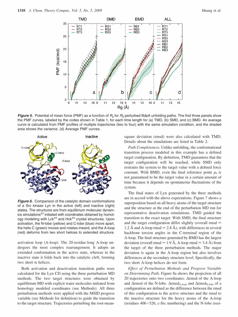
activation loop (A-loop). The 20-residue-long A-loop un-dergoes the most complex rearrangement. It adopts anextended conformation in the active state, whereas in theinactive state it folds back into the catalytic cleft, formingtwo short R helices.

Both activation and deactivation transition paths werecalculated for the Lyn CD using the three perturbation MDmethods. The two target structures were obtained byequilibrium MD with explicit water molecules initiated fromhomology modeled coordinates (see Methods). All threeperturbation methods were applied with the MSID progressvariable (see Methods for definition) to guide the transitionto the target structure. Trajectories perturbing the root-mean-

square deviation (rmsd) were also calculated with TMD.Details about the simulations are listed in Table 2.

Path Completeness. Unlike unfolding, the conformationaltransition process modeled in this example has a definedtarget configuration. By definition, TMD guarantees that thetarget configuration will be reached, while SMD onlyrestrains the system to the target value with a defined forceconstant. With BMD, even the final reference point F0 isnot guaranteed to be the target value in a certain amount oftime because it depends on spontaneous fluctuations of thesystem.

The final states of Lyn generated by the three methodsare in accord with the above expectations. Figure 7 shows asuperposition based on all heavy atoms of the target structureand the structure at the end of the perturbation MD run forrepresentative deactivation simulations. TMD guided thetransition to the exact target. With SMD, the final structureand the target configuration differ slightly (overall rmsd )1.2 Å and A-loop rmsd ) 2.8 Å), with differences in severalbackbone torsion angles in the C-terminal region of theA-loop. The final structure generated by BMD has the largestdeviation (overall rmsd ) 1.9 Å, A-loop rmsd ) 3.4 Å) fromthe target of the three perturbation methods. The majordeviation is again in the A-loop region but also involvesdifferences at the secondary structure level. Specifically, thetwo short A-loop helices do not form.

Effect of Perturbation Methods and Progress Variableon Determining Path. Figure 8a shows the projection of all20 trajectories onto two coordinates: ∆rmsd of the A-loopand ∆rmsd of the N-lobe. ∆rmsdA-loop and ∆rmsdN-lobe of aconfiguration are defined as the difference between the rmsdof this configuration to the active structure and the rmsd tothe inactive structure for the heavy atoms of the A-loop(residues 406-526, c-Src numbering) and the N-lobe (resi-

Figure 5. Potential of mean force (PMF) as a function of Rg for Rg-perturbed BdpA unfolding paths. The first three panels showthe PMF curves, labeled by the codes shown in Table 1, for each time length for (a) TMD, (b) SMD, and (c) BMD. An averagecurve is calculated from PMF profiles of multiple trajectories (two to four) with the same simulation condition, and the shadedarea shows the variance. (d) Average PMF curves.

Figure 6. Comparison of the catalytic domain conformationsof a Src kinase Lyn in the active (left) and inactive (right)states. The structures are from equilibrium molecular dynam-ics simulations23 initiated with coordinates obtained by homol-ogy modeling with Lck43 and Hck44 crystal structures. Uponactivation, the N-lobe (yellow) and C-lobe (blue) move apart,the helix C (green) moves and rotates inward, and the A-loop(red) deforms from two short helices to extended structure.


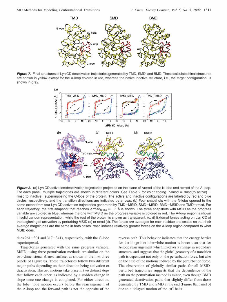
dues 261-301 and 317-341), respectively, with the C-lobesuperimposed.

Trajectories generated with the same progress variable,MSID, using three perturbation methods are similar on thetwo-dimensional ∆rmsd surface, as shown in the first threepanels of Figure 8a. These trajectories follow two differentmajor paths depending on their direction being activation ordeactivation. The two motions take place in two distinct stepsthat follow each other, as indicated by a sudden change inslope once one change is completed. For either direction,the lobe-lobe motion occurs before the rearrangement ofthe A-loop and the forward path is not the opposite of the

reverse path. This behavior indicates that the energy barrierfor the hinge-like lobe-lobe motion is lower than that forA-loop rearrangement which involves a change in secondarystructure, and suggests that the global geometry of a transitionpath is dependent not only on the perturbation force, but alsoon the ease of the motions induced by the perturbation force.The observation of globally similar paths for all MSID-perturbed trajectories suggests that the dependence of thepath on the perturbation method is minor, even though BMDgenerated deactivation paths that slightly differ from thosegenerated by TMD and SMD at the end (Figure 8a, panel 3)due to a delayed motion of the RC helix.

Figure 7. Final structures of Lyn CD deactivation trajectories generated by TMD, SMD, and BMD. These calculated final structuresare shown in yellow except for the A-loop colored in red, whereas the native inactive structure, i.e., the target configuration, isshown in gray.

Figure 8. (a) Lyn CD activation/deactivation trajectories projected on the plane of ∆rmsd of the N-lobe and ∆rmsd of the A-loop.For each panel, multiple trajectories are shown in different colors. See Table 2 for color coding. ∆rmsd ) rmsd(to active) -rmsd(to inactive), superimposing the C-lobe of the protein. The active and inactive configurations are labeled by red and bluecircles, respectively, and the transition directions are indicated by arrows. (b) Four snapshots with the N-lobe opened to thesame extent from four Lyn CD activation trajectories generated by TMD-MSID, SMD-MSID, BMD-MSID and TMD-rmsd. Foreach trajectory, the first snapshot that reaches ∆rmsdN-lobe ) -5 Å is shown. The three snapshots with MSID as the progressvariable are colored in blue, whereas the one with MSID as the progress variable is colored in red. The A-loop region is shownin solid cartoon representation, while the rest of the protein is shown as transparent. (c, d) External forces acting on Lyn CD atthe beginning of activation by perturbing MSID (c) or rmsd (d). The forces are averaged for each residue and scaled so that theiraverage magnitudes are the same in both cases. rmsd induces relatively greater forces on the A-loop region compared to whatMSID does.


The fourth combination of perturbation method andprogress variable, TMD with the rmsd progress variable,generated paths globally different from all MSID paths. Onthe two-dimensional surface, these paths progress morelinearly rather than stepwise, which suggests that the N-lobeand the A-loop move toward the target structure with a higherdegree of cooperativity. This result is again in accord withthe notion that the global path is largely determined by thechoice of the progress variable.

The difference in the linearity between paths generatedwith MSID and rmsd as the progress variable can be seenstructurally in snapshots from representative activationtrajectories. Figure 8b shows an overlay of four snapshotsfrom activation trajectories generated by the four combina-tions of perturbation method and progress variable. Uponactivation, both the N-lobe and the A-loop open up from aclosed conformation, and the four snapshots were chosenso that their N-lobes are opened to the same extent:∆rmsdN-lobe ) -5 Å. Figure 8b shows that, in the snapshotgenerated by perturbing rmsd (red), the A-loop motion hasprogressed further toward the active conformation whileA-loops of the other snapshots generated by perturbing MSID(blue) remain close to the inactive state. It is worth notingthat both MSID and rmsd are global measurements of thedistance between two structures, and therefore as progressvariables they are less distinct than h and Rg. Nonetheless,the subtle distinction does result in visible differencesbetween generated paths, again showing the sensitivity ofthe perturbation MD methods to the choice of progressvariable.

To examine the reason for the generation of different pathswith the two progress variables, the forces imposed byperturbation on MSID or rmsd on each residue at thebeginning of the activation are shown in Figure 8c,d. Themagnitudes of the forces are scaled so that their averagemagnitude for the molecule is the same. It can be seen inthe visualization that rmsd induces relatively greater initialforces on the A-loop region compared to the forces imposedby MSID. The variation and difference in direction in theforce vectors explains the observed differences between thepaths. Simulations perturbing the rmsd progress variable werenot carried out with BMD and SMD, but results similar tothat observed by TMD are expected.

4. Conclusions and Discussion

In the present study, we compared TMD, SMD, and BMDmethods for guiding conformational transitions with externalperturbation. Two distinct transition systems were explored:the unfolding of BdpA with implicit solvation and aheterogeneous end state, and the activation of Lyn CD inexplicit water with two well-defined end states. Results fromthe three perturbation methods with two choices of progressvariable and varying simulation length or biasing forceconstant showed that the perturbation methods generatesimilar transition paths for a given progress variable, asdefined by global structural features. On the other hand, thepath was strongly dependent on the choice of progressvariable. Specifically, choosing to perturb Rg or h forunfolding BdpA determines whether the protein unfolds by

stretching from the ends or by opening up one of the twointerhelical contacts. Also, choosing to perturb MSID or rmsdto guide the conformational change of Lyn CD affects thecooperativity of the movements of its N-lobe and A-loop.

The path dependence on the progress variable wasobserved to be related to the direction and relative magnitudeof the perturbation force, and these were the dominantinfluence regardless of the perturbation method. The alterna-tive forces induce different motions of the molecule in certaindirections and, together with the intrinsic ease of thesemotions, determine the transition path. In most cases, it isnot clear that a priori knowledge can be used to decide whichprogress variable is a good reaction coordinate.

Although the three methods generated similar paths interms of the global structural features for a given progressvariable in most cases, the RB3 BdpA unfolding simulationsgenerated by BMD with the lowest force constant identifiedan alternative class of paths, whereas longer SMD and TMDsimulations generated similar paths to those generated byshorter simulations. The fact that this alternative class ofpaths is more energetically favorable is likely due to thesofter and nonlinear perturbation rendered by BMD. BMDrealizes a nonlinear updating scheme for moving along theprogress variable, and thus the perturbation strength variesalong a trajectory. In simulations of the same total length,BMD spends a greater amount of time going up a barrierthan going down a slope. Thus the perturbation strength iscomparatively low with BMD when the system searches foran easy route to overcome a free energy barrier. It shouldbe noted that this nonlinear updating scheme of BMD wouldnot guarantee the sampling of globally lower free energypaths, because an effectively lower perturbation strength onlyhelps find an easy route to cross a local free energy barrier,which may or may not be a part of the global optimal path.In fact, the blindness to global features of the free energysurface is a common problem shared by all three perturbationmethods.

In the conformational transition of Lyn CD, the backwardpaths are not the reverse copies of the forward paths withall three perturbation methods. This apparent violation ofthe microscopic reversibility suggests that the nonequilibriumresults obtained with the perturbation MD methods do notapproach the equilibrium results at the time lengths examinedin our simulations. With the perturbation methods in thenonequilibrium scenario, the sequence of events along a pathis determined by a combined effect of the perturbation andthe internal ease of certain motions. Under the perturbation,the parts that feel the strongest perturbation and the weakesthindrance move toward the target first. Due to this lack ofreversibility, caution should be taken when interpretingperturbation MD results to infer features such as sequenceof events. Nevertheless, some insight into the ease of a certainmotion can be obtained with these perturbation methods.

Global and/or local structural properties of the proteinsshould be considered when choosing a perturbation MDmethod. As our simulations on the conformational transitionof Lyn CD show, BMD trajectories can be trapped in localminima in the presence of significant energy barriers (suchas the A-loop rearrangement), preventing the system from


arriving at the target conformation. TMD and, for the mostpart, SMD ensure the completeness of the transition, althoughthe likelihood of the path followed by TMD has not beenassessed here. SMD closely resembles the AFM experiment,and it is preferred when direct analogy is desired. Furtheruse of SMD allows the application of the Jarzynski equalityto calculate equilibrium free energy differences.50 Jarzynski’sequality requires the external perturbation to be a componentof the Hamiltonian as an explicit function of time, a conditionsatisfied by the perturbation form of SMD but by neitherTMD nor BMD.51

Abbreviations and Symbols. BMD, biased moleculardynamics; TMD, targeted molecular dynamics; SMD, steeredmolecular dynamics; F, progress variable; h, end-to-enddistance; Rg, radius of gyration; rmsd, root-mean-squaredeviation; MSID, mean square internal deviation.

Acknowledgment. This work was supported by Na-tional Institutes of Health (NIH) Grants GM039478 andGM083605 (C.B.P.), and a Purdue University reinvestmentgrant. E.O. and H.H. were supported by Purdue ResearchFoundation Fellowships. The authors acknowledge contribu-tions from Bonnie Co in the initial stages of this work.

References

(1) Schlitter, J.; Engels, M.; Kruger, P.; Jacoby, E.; Wollmer, A.Mol. Simul. 1993, 10, 291–308.

(2) Schlitter, J.; Engels, M.; Kruger, P. J. Mol. Graphics 1994,12, 84–89.

(3) Grubmueller, H.; Heymann, B.; Tavan, P. Science 1996, 271,997–999.

(4) Leech, J.; Prins, J.; Hermans, J. IEEE Comput. Sci. Eng.1996, 3, 38–45.

(5) Marchi, M.; Ballone, P. J. Chem. Phys. 1999, 110, 3697–3702.

(6) Paci, E.; Karplus, M. J. Mol. Biol. 1999, 288, 441–459.

(7) Izrailev, S.; Stepaniants, S.; Balsera, M.; Oono, Y.; Schulten,K. Biophys. J. 1997, 72, 1568–1581.

(8) Lu, H.; Isralewitz, B.; Krammer, A.; Vogel, V.; Schulten, K.Biophys. J. 1998, 75, 662–671.

(9) Krammer, A.; Lu, H.; Isralewitz, B.; Schulten, K.; Vogel, V.Proc. Natl. Acad. Sci. U.S.A. 1999, 96, 1351–1356.

(10) Marszalek, P. E.; Lu, H.; Li, H. B.; Carrion-Vazquez, M.;Oberhauser, A. F.; Schulten, K.; Fernandez, J. M. Nature(London) 1999, 402, 100–103.

(11) Law, R. J.; Munson, K.; Sachs, G.; Lightstone, F. C. Biophys.J. 2008, 95, 2739–2749.

(12) Swift, R. V.; McCammon, J. A. Biochemistry 2008, 47, 4102–4111.

(13) Zou, J.; Wang, Y.-D.; Ma, F.-X.; Xiang, M.-L.; Shi, B.; Wei,Y.-Q.; Yang, S.-Y. Proteins: Struct., Funct., Bioinf. 2008,72, 323–332.

(14) Apostolakis, J.; Ferrara, P.; Caflisch, A. J. Chem. Phys. 1999,110, 2099–2108.

(15) Bui, J. M.; McCammon, J. A. Proc. Natl. Acad. Sci. U.S.A.2006, 103, 15451–15456.

(16) Ferrara, P.; Apostolakis, J.; Caflisch, A. J. Phys. Chem. B2000, 104, 4511–4518.

(17) Ma, J.; Karplus, M. Proc. Natl. Acad. Sci. U.S.A. 1997, 94,11905–11910.

(18) Ferrara, P.; Apostolakis, J.; Caflisch, A. Proteins: Struct.,Funct., Genet. 2000, 39, 252–260.

(19) Paci, E.; Caflisch, A.; Pluckthun, A.; Karplus, M. J. Mol. Biol.2001, 314, 589–605.

(20) Morra, G.; Hodoscek, M.; Knapp, E. W. Proteins: Struct.,Funct., Genet. 2003, 53, 597–606.

(21) Li, Y.; Zhou, Z.; Post, C. B. Proc. Natl. Acad. Sci. U.S.A.2005, 102, 7529–7534.

(22) Stultz, C. M. Protein Sci. 2006, 15, 2166–2177.

(23) Ozkirimli, E.; Post, C. B. Protein Sci. 2006, 15, 1051–1062.

(24) Levinson, N. M.; Kuchment, O.; Shen, K.; Young, M. A.;Koldobskiy, M.; Karplus, M.; Cole, P. A.; Kuriyan, J. PLoSBiol. 2006, 4, e144.

(25) Kastenholz, M. A.; Schwartz, T. U.; Hunenberger, P. H.Biophys. J. 2006, 91, 2976–2990.

(26) Perdih, A.; Kotnik, M.; Hodoscek, M.; Solmajer, T. Proteins:Struct., Funct., Bioinf. 2007, 68, 243–254.

(27) Ozkirimli, E.; Yadav, S. S.; Miller, W. T.; Post, C. B. ProteinSci. 2008, 17, 1871–1880.

(28) Tikhonova, I. G.; Best, R. B.; Engel, S.; Gershengorn, M. C.;Hummer, G.; Costanzi, S. J. Am. Chem. Soc. 2008, 130,10141–10149.

(29) Zhong, W.; Guo, W.; Ma, S. FEBS Lett. 2008, 582, 3320–3324.

(30) Matrai, J.; Jonckheer, A.; Joris, E.; Kruger, P.; Carpenter, E.;Tuszynski, J.; Maeyer, M. D.; Engelborghs, Y. Eur. Biophys.J. 2008, 38, 13–23.

(31) Carrion-Vazquez, M.; Li, H.; Lu, H.; Marszalek, P. E.;Oberhauser, A. F.; Fernandez, J. M. Nat. Struct. Biol. 2003,10, 738–743.

(32) Sato, S.; Religa, T. L.; Fersht, A. R. J. Mol. Biol. 2006, 360,850–864.

(33) Vu, D. M.; Myers, J. K.; Oas, T. G.; Dyer, R. B. Biochemistry2004, 43, 3582–3589.

(34) Myers, J. K.; Oas, T. G. Nat. Struct. Biol. 2001, 8, 552–558.

(35) Guo, Z.; Brooks, C. L.; Boczko, E. M. Proc. Natl. Acad.Sci. U.S.A. 1997, 94, 10161–10166.

(36) Garcia, A. E.; Onuchic, J. N. Proc. Natl. Acad. Sci. U.S.A.2003, 100, 13898–13903.

(37) Cheng, S.; Yang, Y.; Wang, W.; Liu, H. J. Phys. Chem. B2005, 109, 23645–23654.

(38) Itoh, K.; Sasai, M. Proc. Natl. Acad. Sci. U.S.A. 2006, 103,7298–7303.

(39) Binnig, G.; Quate, C. F.; Gerber, C. Phys. ReV. Lett. 1986,56, 930–933.

(40) Gouda, H.; Torigoe, H.; Saito, A.; Sato, M.; Arata, Y.;Shimada, I. Biochemistry 1992, 31, 9665–9672.

(41) Im, W.; Lee, M. S.; Brooks, C. L. J. Comput. Chem. 2003,24, 1691–1702.

(42) Brooks, B. R.; Bruccoleri, R. E.; Olafson, B. D.; States, D. J.;Swaminathan, S.; Karplus, M. J. Comput. Chem. 1983, 4,187–217.

(43) Yamaguchi, H.; Hendrickson, W. A. Nature (London) 1996,384, 484–489.


(44) Schindler, T.; Sicheri, F.; Pico, A.; Gazit, A.; Levitzki, A.;Kuriyan, J. Mol. Cell 1999, 3, 639–648.

(45) Paci, E.; Smith, L. J.; Dobson, C. M.; Karplus, M. J. Mol.Biol. 2001, 306, 329–347.

(46) Markwick, P. R. L.; Doltsinis, N. L.; Schlitter, J. J. Chem.Phys. 2007, 126, 045104.

(47) Torrie, G. M.; Valleau, J. P. J. Comput. Phys. 1977, 23, 187–199.

(48) Ferrenberg, A. M.; Swendsen, R. H. Phys. ReV. Lett. 1989,63, 1195–1198.

(49) Humphrey, W.; Dalke, A.; Schulten, K. J. Mol. Graphics1996, 14 (33-8), 27-8.

(50) West, D. K.; Olmsted, P. D.; Paci, E. J. Chem. Phys. 2006,125, 204909.

(51) Jarzynski, C. Phys. ReV. Lett. 1997, 78, 2690.

CT9000153


Documents

Comparison of Three Perturbation Molecular Dynamics Methods for Modeling Conformational Transitions