Competition and Car Longevity - rff.org · Competition and Car Longevity Bruce W. Hamilton Molly K. Macauley ... environment in the auto industry is likely to be an important cause

Competition and Car Longevity

Bruce W. HamiltonMolly K. Macauley

Discussion Paper 98-20

March 1998

1616 P Street, NWWashington, DC 20036Telephone 202-328-5000Fax 202-939-3460

© 1998 Resources for the Future. All rights reserved.No portion of this paper may be reproduced without permission ofthe authors.

Discussion papers are research materials circulated by their authorsfor purposes of information and discussion. They have notundergone formal peer review or the editorial treatment accordedRFF books and other publications.

ii

COMPETITION AND CAR LONGEVITY

Bruce W. Hamilton and Molly K. Macauley

Abstract

We examine determinants of the nearly 30 percent increase in the average age ofdomestically produced, registered automobiles since the mid-1960s. We find that very littleof the increase in car longevity is attributable to improvements in the inherent durability ofcars. Rather, we find that the temporal pattern of longevity improvement is highly correlatedwith the level of market concentration in the auto industry. In particular, we argue that thearrival of competition in the industry led to an increase in longevity largely by forcing areduction in the price of auto maintenance and repair, which in turn induced consumers tomaintain their cars into older age.

Key Words: market concentration, automobile industry, scrappage models

JEL Classification Nos.: L1, L9

iii

Table of Contents

I. Introduction ........................................................................................................................... 1

II. Monopoly and Longevity ...................................................................................................... 4

III. Prior Research on Automobile Longevity .............................................................................. 6

IV. Patterns in Auto Death Rates ................................................................................................. 7

V. The Scrappage Decision ........................................................................................................ 9

The Scrappage Model ............................................................................................................ 9

Transition Effects ................................................................................................................ 11

VI. Direct Evidence on Maintenance Cost ................................................................................. 13

VII. Estimation ........................................................................................................................... 16

Transition Effects ................................................................................................................ 19

Vintage Vintages ................................................................................................................. 21

Specific Models ................................................................................................................... 22

VIII. Japanese Cars ...................................................................................................................... 24

IX. Conclusion .......................................................................................................................... 26

References ..................................................................................................................................... 27

List of Figures and Tables

Figure 1. Mean age, domestic fleet ............................................................................................... 2

Figure 2. Auto life expectancy ...................................................................................................... 2

Figure 3. Average new car prices .................................................................................................. 3

Figure 4. The HHI for the auto industry ........................................................................................ 5

Figure 5. Fraction of domestic fleet surviving to age 15 ................................................................ 8

Figure 6. Death rates, 10-year-old cars ......................................................................................... 8

Figure 7. The CPI for auto maintenance and parts, deflated ......................................................... 14

Figure 8. Auto maintenance per mile from PCE and Runzheimer ................................................ 14

Figure 9. Unexplained longevity ................................................................................................. 22

Figure 10. Life expectancy by year ............................................................................................... 24

Figure 11. Japanese share of the U.S. auto market ........................................................................ 25

Figure 12. Japanese and domestic auto death rates, by vintage ...................................................... 26

Table 1. Effect of P/m0 on Lifetimes ......................................................................................... 10

Table 2. Regression Results ...................................................................................................... 17

Table 3. Effect of Regressors on Steady-State Life Expectancy ................................................. 18

Table 4. Coefficients of Specific Disembodied Year Effects ...................................................... 19

Table 5. Disembodied Year Effects ........................................................................................... 20

Table 6. Contribution of Regressors to Life Expectancy ............................................................ 20

Table 7. Characteristics of 1962 Models .................................................................................... 23

1

COMPETITION AND CAR LONGEVITY

Bruce W. Hamilton and Molly K. Macauley1

I. INTRODUCTION

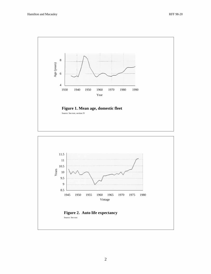
The average age of domestically produced automobiles has increased by nearly30 percent since the mid 1960s--from 5.6 years in 1969 to 7.2 years in 1991 (see Figure 1).Over the same time period, life expectancy has increased by approximately the same relativeamount (see Figure 2). Using automobile registration data from R. L. Polk and Co., weconstruct standard life tables for domestic autos, for imports, and for various individual makesof cars. We then examine the patterns of age-specific auto mortality rates to determine some ofthe causes of the dramatic increase in longevity. We report two significant empirical findings.

Our first finding is that regime shifts from high to low mortality occurred approximatelysimultaneously across auto vintages; in those calendar years in which mortality declined, itdeclined for both new and old vintages. No mortality improvement appears to be statisticallyattributable to specific vintages. In other words, some vintages of cars began life during ahigh-mortality regime, and accordingly "died off" quickly. But when the shift to lowmortality occurred, these erstwhile fast-dying cars saw an improvement in their mortality. Orto put it yet another way, declines in the age-specific death rates of 5-year-old cars occurred inthe same calendar year as declines for 10-year-olds and 15-year-olds. Regardless of anyeconomic explanation for this finding, it is sufficient to lead to the following conclusion:Essentially none of the improvement in car longevity is attributable to improvements in theinherent durability of cars, for such an improvement would not reduce death rates on older,pre-improvement cars.2 The improvement in longevity must be due to some force external tothe cars themselves.

Our second finding is that the temporal pattern of mortality improvement is highlycorrelated with the level of market concentration in the automobile industry (even aftercorrecting for other regressors). This leads us to believe that the changing competitiveenvironment in the auto industry is likely to be an important cause of the change in themortality pattern. We argue below that the arrival of competition in the industry led to an

1 Hamilton is Professor of Economics, Johns Hopkins University, and Macauley is Senior Fellow, Resources forthe Future. Correspondence: [email protected]. We thank Bob Crandall, George Eads, and participants insessions at the American Economic Association meetings, the Southern Economic Association meetings, and inworkshops at Resources for the Future and Johns Hopkins University for helpful comments. Responsibility forerrors or opinions rests with the authors.2 Indeed, as we will see, an improvement in the longevity of new cars should lead to a "premature" die-off ofolder, pre-regime-shift cars.

Hamilton and Macauley RFF 98-20

2

Figure 1. Mean age, domestic fleetSource: See text, section IV

1930 1940 1950 1960 1970 1980 1990

4

6

8

Age

(ye

ars)

Year

1945 1950 1955 1960 1965 1970 1975 1980

11.5

11

10.5

10

9.5

9

8.5

Yea

rs

Vintage

Figure 2. Auto life expectancySource: See text


3

increase in longevity largely by forcing a reduction in the price of auto maintenance andrepair, which in turn induced consumers to maintain their cars into older age.

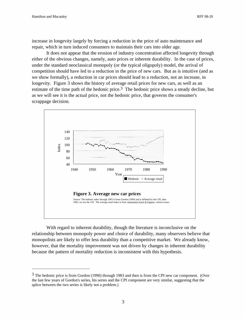
It does not appear that the erosion of industry concentration affected longevity througheither of the obvious changes, namely, auto prices or inherent durability. In the case of prices,under the standard neoclassical monopoly (or the typical oligopoly) model, the arrival ofcompetition should have led to a reduction in the price of new cars. But as is intuitive (and aswe show formally), a reduction in car prices should lead to a reduction, not an increase, inlongevity. Figure 3 shows the history of average retail prices for new cars, as well as anestimate of the time path of the hedonic price.3 The hedonic price shows a steady decline, butas we will see it is the actual price, not the hedonic price, that governs the consumer'sscrappage decision.

1940 1950 1960 1970 1980 1990

140

120

100

80

60

40

Year

Figure 3. Average new car pricesSource: The hedonic index through 1983 is from Gordon (1990) and is deflated by the CPI; after1983, we use the CPI. The average retail index is from Automotive Facts & Figures, various issues.

Hedonic + Average retail

Inde

x

With regard to inherent durability, though the literature is inconclusive on therelationship between monopoly power and choice of durability, many observers believe thatmonopolists are likely to offer less durability than a competitive market. We already know,however, that the mortality improvement was not driven by changes in inherent durabilitybecause the pattern of mortality reduction is inconsistent with this hypothesis.

3 The hedonic price is from Gordon (1990) through 1983 and then is from the CPI new car component. (Overthe last few years of Gordon's series, his series and the CPI component are very similar, suggesting that thesplice between the two series is likely not a problem.)


4

We believe that the observed pattern of mortality decline is most consistent with thefollowing hypothesis. When the industry was more concentrated it succumbed to the "Coasetemptation" to price cars near cost, placing much of its monopoly markup not on cars but onrepair and replacement parts. The arrival of competition in the mid-1970s reduced this profitmargin and induced consumers to maintain their cars longer. Thus we find that the industry inits high concentration was able to defy Coase and charge a supercompetitive price, but themarkup was predominantly on parts rather than cars. To our knowledge, this represents thefirst empirical test of any version of the Coase conjecture.

In sections II and III we discuss literature that bears on our research, the relationshipbetween longevity and industry concentration, and models of auto longevity. In section IVwe describe our data and trends in auto lifetimes. Section V is a model of the scrappagedecision and the effects on this decision of inherent durability and the prices of cars, parts,and gasoline. In section VI we discuss direct evidence on maintenance cost, new car prices,and fuel efficiency. In sections VII and VIII we estimate the empirical relationship betweenconcentration and longevity and discuss other evidence regarding longevity, including theeffects of imports of Japanese cars. Section IX is a summary.

II. MONOPOLY AND LONGEVITY

One of the major new forces in the automobile industry is competition. In the late1950s and early 1960s, automobile manufacturing was the most highly concentrated majorindustry in the United States. As Figure 4 shows, the Hirschman-Herfindahl index ofconcentration stood at about 3500 to 3700.4 By 1990, the index stood at approximately 2000.This decline in concentration could affect automobile longevity through several channels:(1) the price of new cars; (2) the inherent durability of cars; and (3) the price of auto repairand maintenance parts.

Two strands of literature address the link between monopoly power and the longevityof durable goods. In one strand, Swan (1972) argues that market structure has no effect onproduct durability; the demand for a durable good is derived from the demand for its services,and a monopolist maximizes profit by producing these services as cheaply as possible (i.e.,using socially optimal durability) and charging the monopoly price. This independence (-of-market-structure) result rests on the assumption that longevity is a feature of the product itselfand does not depend upon consumers' maintenance decisions.

4 The Hirschman-Herfindahl index (HHI) is the sum of squares of market shares. We calculate this index basedon sales of new automobiles in the United States (data from Automotive News, various issues). For purposes ofcalculating the index, a manufacturer's market share is its share of total sales of new cars in the United States inthat year. Our calculations are based on the shares of both domestic and foreign manufacturers in domesticautomobile sales.


5

1940 1950 1960 1970 1980 1990 2000

4000

3500

3000

2500

2000

1500

Inde

x

Year

Figure 4. The HHI for the auto industrySource: See text

As Schmalensee (1974) and Rust (1986) note, consumers who can purchasecompetitively priced maintenance will be induced by the monopoly price of the originalequipment to maintain the good "too long." The monopolist can respond by setting a non-optimal inherent durability.5 The likely net effect is that durable goods survive longer undermonopoly than competition; the effect of the monopoly price upon consumers' maintenancedecisions unambiguously raises longevity, and the effect of the monopolist's countermove isambiguous.

The second strand of literature follows the Coase (1972) conjecture whereby aperfectly-durable-good monopolist has no monopoly power at all and is forced "in thetwinkling of an eye" to price at marginal cost. In the Coase model, the good is perfectlydurable; there is neither limited durability nor replacement demand. In subsequent research,Bond and Samuelson (1984) find that time-consistent monopoly power increases as thedurability of the good declines exogenously. Bulow (1986) shows that a monopolist who hascontrol over durability can partially escape the Coase problem by reducing durability (andthus reducing the Coase temptation).

Hamilton and Burke (1996) argue that a durable-goods monopolist which also hasmarket power over some maintenance and repair parts is likely to take a much larger markupon repair parts than on original equipment. They consider a good whose longevity isdetermined jointly by inherent durability and the amount of maintenance provided by the

5 The monopolist may either raise or reduce durability from its optimum, depending upon the parameter valuesof the model.


6

consumer/owner of the good. A monopolist selling such a good faces both the Coase time-consistency and the Schmalensee excess-maintenance problems. In this case, a durable-goodsmonopolist with some monopoly control over repair/replacement parts can charge a relativelylow markup on original equipment and a higher markup on parts.6 In the case of automobiles,the parts-pricing monopolist sells cars relatively close to cost and in the process creates amonopoly market for consumables, for which there is no Coase temptation. By charging ahigh markup on maintenance parts, the original equipment manufacturer (OEM) curbsconsumers' temptation to over-maintain their cars. Under reasonable parameter values, themonopoly markup on parts is several times higher than on original equipment. In this case, adecline in market power leads to substantial erosion in the parts' markup, which in turn leadsto an increase in automobile lifetimes.

III. PRIOR RESEARCH ON AUTOMOBILE LONGEVITY

In two respects the empirical research we present follows several prior empiricalstudies of auto lifetimes. All use either the same U.S. automobile registration data or similardata from other countries, and all model auto lifetimes based on survival models using eitherlogistic transformation of the age-specific auto death rate or simply the log of the death rate.7

Our approach is similar to Parks (1977). He begins with an intertemporal optimizationmodel in which survival is driven by the ratio of the initial purchase price to maintenance cost.Instead of incorporating a logistic functional form, however, he uses a set of dummy variablesto capture the effects of age. He also includes dummy variables for vintages; these coefficientsare generally insignificant and show no obvious relationship to any economic variables.

Greene and Chen (1981) estimate a logistic equation separately for domestic andimported cars, and for light trucks. They find that the shapes of the domestic and importlogistics are somewhat different, but life expectancies are very similar. Light trucks, on theother hand, survive much longer than cars.8

Several other studies include auto mortality. Berkovec (1985) estimates a scrappagemodel in which he regresses the log of the death rate on auto prices, price squared, and dummyvariables for vintage and class (e.g., subcompact). Berkovec does not consider the economiccauses of the movements in mortality. Greenspan and Cohen and (1996) estimate automortality as an input to the study of the demand for new cars. Another strand of researchexamines the effect of the aging of the auto fleet on air pollution and policy options associatedwith this relationship. For example, Gruenspecht (1982) estimates the effect of federal 6 Of course, this requires the monopolist to have power over at least some repair/maintenance parts. In the caseof automobiles, there is strong reason to believe that OEM's have substantial power in this aftermarket. Perhapsthe strongest evidence is that an automobile purchased one piece at a time from a dealership's parts departmentwould be substantially more costly than a fully assembled car.7 In addition to the research noted above, econometric models of the auto market include Bresnahan (1981);Berry, Levinsohn, and Pakes (1995); and Goldberg (1995). These models focus on new car demand and supply;they do not explicitly address longevity and scrappage decisions, and Bresnahan examines only 1977-78 vintages.8 See also discussion of the logistic scrappage function in Fenney and Cardebring (1988).


7

emissions standards set in 1981 on the composition of the fleet (extrapolated forward to 1990)and consequently upon auto emissions. He finds that the effect of the new standards onscrappage is "not large;" nevertheless, in his simulations the imposition of the 1981 standardsdoes increase emissions of hydrocarbons and carbon monoxide up until 1985. The increasesare small (on the range of 1-2 percent), and by 1990 the standards lead to a substantial decreasein emissions (16.19 percent for hydrocarbons and 5.31 percent for carbon monoxide).

Alberini et al. (1995) and Hahn (1995) analyze cash-for-clunkers programs (governmentoffers to purchase and retire older polluting cars to reduce aggregate emissions). Whereas thesestudies tend to confirm that retirement of older cars would improve air quality, they are notinconsistent with the basic conclusion of our study--that the aging of the automobile fleet overthe past 25 years was brought about almost entirely by forces unrelated to the tightening ofemissions standards.

Thus there is extensive research which models or incorporates auto longevity, but none ofthis research considers the causes of the substantial improvement in auto longevity since 1960.

IV. PATTERNS IN AUTO DEATH RATES

The patterns we observe in auto death rates are based on the automobile registrationdata base provided to us by R. L. Polk & Co. For each year since 1946, Polk reports the totalnumber of cars registered in the United States by make and vintage (beginning in 1975, eachmake is disaggregated into specific models). We calculate age-specific death ratesrespectively for the domestically produced fleet and for six specific makes for each year since1947, and for the import fleet, and for Japanese cars, since 1958.9

Polk's coverage varies somewhat from year to year. Subsequent to 1975 they reportthe number of registered vehicles in each vintage up to age 15, plus an open-ended "older"category. For some prior years, registration data up to age 18 plus an "older" category areincluded. In calculating the average age of cars reported in the Introduction, we haveaggregated all cars over age 15 into a single category, and allocated this group to agesaccording to the following weights: {age 16; 0.3}, {age 17; 0.25}, {age 18; 0.2}, {age 19;0.15}, {age 20; 0.1}. The time series of average age (Figure 1) is not very sensitive to theweights chosen for these vintages. We do not use this arbitrary assignment of cars to oldercohorts in any other part of our analysis.

The aging of the fleet is quite dramatic. Just under 7 percent of 1957-vintage carslived to age 15. Figure 5 shows that this fraction rose steadily to over 40 percent of 1976-vintage domestic cars in 1991. Figure 2, referenced in the Introduction, plots the ex post lifeexpectancy for each vintage from 1946 through 1976.10 Figure 2 (misleadingly) implies very

9 The Polk data for imports are not as complete as for domestics prior to 1975. There are no data at all prior to(calendar year) 1957, and for most years from 1957-1974 data were recorded only for age 6 and younger. Sincealmost all of the mortality "action" occurs at older ages, we are unable to estimate life tables for imports prior to 1975.10 Life expectancies are calculated ex post from each vintage's actual survival rates up to age 15. As noted inthe text, for all vintages life expectancy is understated for failure to include older ages. This bias is clearly muchmore significant for more recent vintages, as a much larger fraction of recent vintages survives beyond age 15.Rough eyeball extrapolation suggests that life expectancy of 1960 vintage cars would rise by about 0.1 year if weincluded data from ages 16-20, and by about .75 years for 1977 cars.


8

1945 1955 1965 1975

Vintage

0.5

0.4

0.3

0.2

0.1

0

Frac

tion

of f

leet

Figure 5. Fraction of domestic fleet surviving to age 15Source: See text

1930 1940 1950 1960 1970 1980 1990

0.3

0.25

0.2

0.15

0.1

0.05

0

Vintage

Frac

tion

Ret

ired

Figure 6. Death rates, 10-year old carsSource: See text


9

modest improvement for vintages earlier than the mid-1970s. From Figure 6, which showsthe death rates of age-10 cars, by vintage, it appears that the improvement in mortality beganwith the mid-60s vintages.

V. THE SCRAPPAGE DECISION

The Scrappage Model

In this section we illustrate the nature and size of possible sources of improvements inlongevity, including improvements in inherent durability and other economic forces whichinduce consumers to maintain cars into older age. We begin with a simple nonstochasticmodel of scrappage in which all autos are scrapped at the same age. In this model, all cars areretired at the same age, d. Our purpose in this model is to develop a feel for the plausiblequantitative importance of the various forces which influence the longevity of a durable. Thiswill help us to interpret the coefficients of our empirical model.

Suppose that the price of a new car is P0 and that the car requires maintenanceaccording to

m m eaga= 0 (1)

where

ma a= ⋅π µ

and π is the price of maintenance, µa is the quantity of maintenance required at age a, and g isthe growth rate of maintenance cost. µ0 is the (inverse) index of inherent durability (it is the"quantity" of maintenance required for an age-0 car). The stream of costs of owning andmaintaining a car until it is retired at age d, then replacing it with another that lasts d yearsand so on, is V:

V Pm

ge

e

mg dd= +

−−

⋅

−

+−

−00 11

1

1ρ ρρ

ρ( ) or

(2)

$ ( )V Pm

ge

eg d

d= +−

−

⋅

−

−−0

0 11

1ρρ

ρ

where m1 is age-independent maintenance such as fuel and insurance, d is the retirement age,and ρ is the discount rate. $V is the perpetual cost of operating a car exclusive of these age-independent terms. In the steady state the optimal time to scrap a car is found by differentiating(2) with respect to d and setting the result equal to zero. The solution, obviously independent ofm1, is the following (implicit) function of d:


10

1 1 0

0

0

0ρ ρ ρ ρ π µρ⋅ −

−⋅ +

−= =

⋅→−e

gg

eg

P

m

Pgd g d

( )( )

ρ ⋅ =$ ,V m e gd0 or (3)

d dP

g=

0

0πµρ; ,

By (3) retirement age, d, rises as P0 rises and as either π or µ0 declines. Any factor whichinfluences longevity must operate through µ0 (inherent durability) or through one of the pricesP0 or π. The second line of (3) gives rise to a natural interpretation: the car is maintaineduntil the rate of maintenance, m e gd

0 , is equal to the rental rate, ρ $V .

Table 1. Effect of P/m0 on Lifetimes (ρρ = .03)

P/mo d d d D(g = .05) (g = .1) (g = .15) (g = .2)

5 12.25 7.9 6.15 5.1

7 14.15 9.1 6.95 5.8

10 16.4 10.4 7.95 6.55

15 19.4 12.1 9.2 7.5

20 21.7 13.4 10.1 8.25

30 25.35 15.45 11.55 9.35

40 28.21 16.97 12.60 10.19

50 30.55 18.25 13.51 10.86

60 32.6 19.3 14.2 11.4

70 34.35 20.23 14.85 11.92

Table 1 suggests the quantitative importance of P0/m0 in determining automobilelifetimes. For four different growth rates of maintenance cost, the table shows the optimumlifetime as P0/m0 varies from 5 to 70.11 The double-lined boxes indicate approximately thepostwar variation in actual life expectancy, suggesting that the recent rise in car longevity mustbe due to an approximate doubling of P0/m0 , regardless of the value of g. Below we reportempirical results indicating that new emissions controls had no discernible effect on auto

11 The average retail price of new cars was approximately $15,000 in the mid-1990s. There are three sources onauto maintenance expenditure per car: the National Income Accounts, the Survey of Consumer Expenditures,and an independent survey run by Runzheimer International. We discuss these later in the text. All of thesources suggest that maintenance expenditure is in the range of $325-$400 per car, implying that P0/m0 ≈ 40. Incombination with table 1, this implies that g must be at least 0.15.


11

mortality. The very small elasticity of life expectancy with respect to P0/m0 implied byTable 1 may explain this effect. We would expect a 10 percent rise in the price of new cars toincrease life expectancies by about 6 weeks (for both new and grandfather cars; as we discussbelow). This simple model of scrappage, in other words, is enough to tell us that any historicalchanges in emissions or safety standards are much too small to have had any appreciable effecton survival rates.12

Transition Effects

Equation (3) describes the forces which govern longevity in the steady state. Here weexplore the behavior of the longevity of grandfather cars during the transition from one steadystate to another. What happens to the longevity of cars which were born under one regime

},,,{ 10 mP oµπ but then live part of their lives in a changed regime? The answer varies

according to which parameter changes.

i. π/0P : if there is a regime change in either P0 or π (the price of new cars or the

price of maintenance services), then grandfather cars behave as if they were born into the newregime. If P0 rises, used cars will realize a capital gain, and their owners will not retire them

until the flow of maintenance costs equals V̂ρ for the new-regime car which must be bought

as a replacement. Similarly, a change in π alters the flow of maintenance cost equally fornew-regime and grandfather cars, and grandfathers will be retired as if they had been borninto the new regime. If the regime shift is a price change (either P0 or π), then there is notransition; the mortality pattern of all cars jumps instantly to the new steady-state pattern.

ii. µ0: if at some point in time there is a decline in µ0 (the "amount" of requiredmaintenance), then a technical improvement of this sort is embodied only in new cars. Anygrandfather cars built with the old technology must behave as old-regime cars but competewith new-regime cars until they die. During the transition in which there are still grandfathercars, these cars will not behave like new-regime cars, nor will they even behave like old-regime cars would have behaved but for the regime shift. The grandfather car will be retiredwhen its stream of maintenance costs obeys equation (4):

1

ˆ

0,0 V̂em dg ρ= (4)

where µ0,0 is µ0 for the regime-0 (old regime), d̂ is retirement age for the grandfather car, and

1̂V is V̂ for new regime cars. The left hand side of (4) gives the cost of maintenance of the

12 According to Crandall and co-authors (1982), emissions, safety, and fuel efficiency standards may haveraised the price of a new 1984 car by as much as $2000 (relative to the no-standards baseline), though Bresnahan(1986) argues that this is a substantial over-estimate. Even the estimates in Crandall represent about a 10-15percent increase in new car prices, enough to increase lifetimes by about 6 weeks.

},,,{ mP µπ


12

old-regime car as a function of age; when this expression reaches the rental rate under thenew-car regime,13 it is time to scrap the old car. A fall in µ reduces the right-hand side of (4)but not the left-hand side (since the left-hand side pertains to old-µ cars). Thus (4) dictatesthat the old-regime car will be retired earlier than it would have had there been no regime-

change (i.e., had 0̂V prevailed). A reduction in µ increases the lifetimes of new cars relative

to the old steady state and causes transition cars to die younger than in the old steady state.The quantitative importance of this transitional effect is suggested by the following

exercise: Suppose that in some year µ0 falls by 10 percent and that g = .15. The steady state

lifetimes of cars increases by about 0.2 years (see Table 1). Suppose further than half of 1̂V is

maintenance; thus 1̂V falls by 5 percent.14 By (4), grandfather cars are retired about 0.3 years

prematurely because they are forced to compete with more maintenance-free new cars.

iii. m1: age-independent cost, m1 (e.g., gas mileage) does not appear in equation (3)and has no effect on steady state longevity. But as in the case of a change in µ0, old-regimecars must compete with new-regime cars even though they cannot behave like new-regimecars. A decline in m1 causes old-regime cars to die prematurely, for much the same reason asdoes a decline in µ0. Again we use the structure of the middle line of equation (3), whichcompares the instantaneous cost of keeping the old car with the instantaneous cost ofswitching to a new car. In the case of a change in m1, this cost comparison is as follows:

1,10,1

ˆ

0ˆ mVmem dg +⋅=+ ρ ⇒

)(ˆ0,11,1

ˆ

0 mmVem dg −+⋅= ρ (5)

where m1,0 and m1,1, are, respectively, age-independent maintenance for grandfather and new-regime cars. The left-hand side of (5) is the instantaneous cost of keeping the old-regime car;the right-hand side is again the cost of buying a new one (recognizing the futureconsequences). When m1 does not change, it drops out of this expression and, as we haveseen, has no effect on longevity. If m1 is lower for new than grandfather cars, (5) tells us thatgrandfather retirement is hastened to enable the owner to escape the high m1.

To illustrate the quantitative importance of this transition effect, suppose that ρ $V =$1000. In the steady state the car is maintained until the rate of maintenance cost, m e gd

0 =

$1000. But if enhanced fuel efficiency reduces the annual fuel cost for new cars by $300then the old car should be scrapped when m e gd

0 = $700.15 It would be retired about 2 years

13 Exclusive of age-independent costs such as gasoline, represented by m1.14 If g = .15 and P/mo = 40, the share of maintenance in V = .52.15 A consumer would save $300/year in fuel by replacing a 12-mpg car with a 20-mpg car, assuming 10,000miles per year (approximately the national average) at $1/gal.


13

prematurely if g = .15. Any improvement in the operating efficiency of new cars, of the typeembodied in m1, depresses the lifetimes of grandfathers (substantially) but leaves the steadystate unchanged. In fact, average fuel efficiency for new cars more than doubled (from 12 to25 miles per gallon) between 1973 and 1983. This should have led to a large retirement of1970s-vintages cars in the 1980s, but our data show that the opposite happened.

To summarize this discussion,

• A rise in P0/π increases longevity of both new and grandfather cars; a doubling ofthis ratio adds about 2 years to car lifetimes, for most parameter values.

• A reduction in µ0 raises the lifetimes of new-regime cars and reduces the lifetimes ofgrandfathers. Reducing µ0 by 50 percent adds approximately 2 years to the lifetimes ofnew cars and causes grandfathers to be retired about 1.5 years prematurely.

• A reduction in m1 has no effect on the lifetimes of new cars (relative to the steadystate in which the grandfathers formerly lived) but depresses the lifetimes oftransition grandfathers. A 30 percent fall in m1 causes grandfathers to die about 2years prematurely.

VI. DIRECT EVIDENCE ON MAINTENANCE COST

In principle, the most straightforward way to separate the effects of prices and innate carcharacteristics on auto mortality would be to regress a transformation of scrappage rates on theprice of cars, the price of maintenance, and measures of inherent durability and fuel economy.Data on maintenance prices and expenditures are highly problematic, however, and there are nodata on inherent durability. We have located two price and two expenditure time series on automaintenance. The two price series are the Consumer Price Index (CPI) for auto maintenanceand for auto parts. The maintenance series includes body work, the drive train, maintenanceand service, power plant, and an "other" maintenance category. The Bureau of Labor Statisticsnotes that pricing these activities in a consistent manner is quite difficult. The auto parts seriesincludes batteries, tires, floor mats, tune-up parts, and audio equipment. Figure 7 plots bothprice series. Since its introduction, the parts price series has fallen approximately 40 percentand clearly behaves in a strikingly different way from the maintenance price series.

There are also two series on maintenance expenditure. One of these series is our ownestimate of auto maintenance per mile based on the auto maintenance component of PersonalConsumption Expenditure (deflated by the CPI) from the National Income and ProductAccounts (NIPA). We estimate auto maintenance expenditure per vehicle by dividing totalauto maintenance expenditure by the stock of privately owned automobiles and trucks foreach year, as reported by the Federal Highway Administration.16 Next, we deflate by the 16 We would like to deflate by the number of cars and trucks in the personal fleet, but such data do not exist. Wedeflated by cars plus trucks rather than just cars for two related reasons. First, in at least some years minivans arecounted as trucks. Second, and related to the first, the data for cars and trucks individually show wide fluctuations, butthe data for the sum are quite smooth (strongly suggesting that some vehicles are counted as cars some years andtrucks in other years.) Though heavy trucks are improperly included in the series, they represent only about 3 percentof the fleet, and their inclusion will not bias the pattern of maintenance per vehicle unless the share of heavy trucks inthe fleet has changed significantly. Limited data suggest that this share has been stable.


14

1950 1960 1970 1980 1990 2000

1.2

1.1

1

0.9

0.8

0.7

0.6

1.05

1

0.95

0.9

0.85

Part

s

Year

Mai

nten

ance

Maintenance Parts

Figure 7. The CPI for auto maintenance andparts, deflatedSource: U.S. Bureau of Labor Statistics

Figure 8. Auto maintenance per mile from PCE and RunzheimerSource: See text

1940 1950 1960 1970 1980 1990 2000Year

Rel

ativ

e to

yea

r 1

1.110.90.80.70.60.50.40.3

PCE Runzheimer


15

average number of miles per vehicle (which has risen about 30 percent, from 9000 to 12000miles per year, between 1970 and 1995).

Our other series on maintenance expenditure is direct estimates reported in surveys ofautomobile dealers by Runzheimer International.17 Runzheimer surveys dealers (but notindependent mechanics) annually to estimate the cost of "normal" maintenance for a 2-yearold, mid-size car. Crash repair is excluded.18 Thus the Runzheimer series is close to a directestimate of our m0.19 Figure 8 shows both of these expenditure series. They indicate thesame broad pattern, though the Runzheimer data show a much more precipitous and earlierdecline in expenditure per mile than does the series constructed from the NIPA. Thisdifference is not surprising; the NIPA-constructed series covers the entire population of cars(and, unfortunately, trucks). The aging of the fleet from 1970 onward should have caused thisseries to decline less quickly than the Runzheimer series.

Because the Runzheimer data are gathered directly from auto dealers, these data seemto be the most reliable of the four series (though unfortunately the data are expenditure, and notdecomposed into price and quantity).20 All four series are problematic in that they includeboth m0 (age-related maintenance) and m1 (age-independent maintenance), whereas only theformer influences steady-state longevity.21 Nonetheless, if the Runzheimer data are at leastapproximately correct, the series suggests a fall of about 60 percent in m0 from 1960 to 1985.

From Table 1, this decline is the right order of magnitude to be a strong candidate forexplaining the secular rise in longevity. The empirical question is then whether the pattern ofdecline in expenditure is embodied in specific vintages (due to improvements in durability ofnewer cars) or disembodied (due to a decline in the price of maintenance). Given theambiguity of the series on maintenance prices and expenditure, we address this question bytrying to determine directly whether the decline in auto scrappage over the past 25 yearsappears to be vintage-specific (embodied) or year-specific (disembodied).22

17 Runzheimer's data are published both by the American Automobile Association and the American AutomobileManufacturers' Association. Their operating-cost data provide the basis for Internal Revenue Service mileage allowances.18 Runzheimer also reports average insurance premiums. Between 1975 and 1985 the average property andliability premium fell by 54 percent, and the collision premium fell by 38 percent (in real dollars).19 Details of the Runzheimer series were kindly provided in a telephone interview with Carl Hart of RunzheimerInternational, Inc.20 Of course, it is possible to reconcile the Runzheimer and NIPA maintenance series by postulating that theprice of auto maintenance has indeed risen about 20 percent as indicated by the CPI, and that expenditure hasfallen about 50 percent because, with improvements in built-in durability, the quantity of required maintenancehas declined (by about 60 percent).21 For example, since batteries can easily be removed from scrapped cars, it is implausible that the price ofbatteries influences the scrappage decision.22 Parks (1977) and Greenspan and Cohen (1996) use the ratio of the new-car CPI to the auto maintenance CPIin auto scrappage regressions. In both studies the coefficient has the right sign and is significant. Parks' sampleperiod is from 1947 through 1969 (almost entirely before the substantial rise in the maintenance CPI from thelate 1960s through the mid-1970s), and the sample used by Cohen and Greenspan is from 1973 to 1991 (entirelyafter the maintenance CPI spurt). Virtually all of the postwar variation in maintenance CPI is missing from bothstudies. When we estimate the same regression over the entire postwar period, the sign of this coefficientbecomes perverse (a rise in the relative price of maintenance leads to reduced mortality).


16

VII. ESTIMATION

In the model of auto mortality developed above, we assumed that the arrival ofmaintenance needs was continuous and deterministic. As a result, the model predicted thatthe age at death of a car was also deterministic, determined only by prices and the parametersof the exponential maintenance-cost function. Clearly, the actual arrival of maintenanceneeds is both episodic and stochastic, and as a result, the optimal time to scrap a car isstochastic. The deterministic model gives a feel (a good feel, we believe) for the magnitudesof the forces governing car longevity. But like most deterministic models it must be modifiedbefore applying it to the data.

We do not model the stochastic process that generates maintenance requirements orthe formal decision calculus of a consumer faced with such a process. Rather, we followvirtually all of the automobile-mortality literature in assuming that the pattern of automortality can be characterized by the logistic function below. In discussing the empiricalresults, we assume that the life expectancy implied by our logistic coefficients is generated bythe deterministic model presented above.

Accordingly, consistent with the extant literature in modeling auto scrappage, weassume that the age-specific death rates of automobiles tend to follow a logistic

ageva

es

⋅++=−

γβα1

1 (6)

where vas is the survival rate for age-a cars of vintage v. We assume that the parameters α and β

are constant across all vintages and years and that any variation in the shape of the logistic manifestsitself in γ. We rearrange (6) to form (7) and then estimate (7) using nonlinear least squares:

ln ln ( ( ))s

sEXP agea

v

av1

1−

= − + + ⋅α β γ (7)

where

( )γ γ δ= +0 1 1Σ X (8)

and the X's are the other regressors.23 We estimate (7) for all cars manufactured in the UnitedStates after World War II and for all ages greater than 4 years.24

23 Obviously it is possible to model the X's as modifiers of α or β rather than γ. We choose γ because we aremore able to approximate the actual patterns of mortality by varying γ. For example, for most reasonable valuesof β and γ, it is impossible to generate actual changes in life expectancy through "permissible" changes in α.When we estimate the model in a form in which the X's modify α, the estimated coefficients generate "logistic"curves with negative death rates beginning at about age 14.24 Actual death rates of cars below the age of 4 are very low. However, the data for these younger cars aresomewhat noisy. Death rates are calculated comparing the ratio of a given vintage car registered in one year tothe number registered in the subsequent year. Early in a car's life, these numbers are heavily influenced by salesof new cars a year or two after their introduction.


17

In column (a) of Table 2 we estimate the logistic, equation (7). In column (b) weinclude the Hirschman-Herfindahl index of industry concentration in the current year (asopposed to the year in which the automobile was manufactured). This index (HHIy) allowsthe current-year industry concentration to affect current-year death rates on all living vintagesof grandfather cars. The coefficient is of the predicted sign and is highly significant.25 As wediscuss below, the point estimate is quite "large."

Table 2. Regression Results

Dependent variable: ))/(ln( va

va sls −

A b c d e f g h i

α 4.00 3.62 3.70 3.75 3.71 3.65 3.71 3.65 3.53(.080) (.066) (.066) (.064) (.065) (.063) (.064) (.065) (.064)

β 6.97 6.68 6.62 6.65 6.58 6.58 6.51 6.58 6.49

(.012) (.066) (.066) (.065) (.065) (.062) (.066) (.064) (.061)

γ0 -.609 -.295 -.234 -.125 -.096 -.135 -3.80 -4.49 -5.28

(.070) (.000) (.018) (.022) (.022) (.021) (.709) (.081) (.668)HHIy* -.959 -.902 -.836 -.935 -.500 -.435 -.425

(.012) (.047) (.044) (.044) (.081) (.081) (.078)HHIv* -.247

(.060)HHIv* -.647 -.543 -.530 -.659 -.643 -.4925 yr avg (.076) (.077) (.073) (.078) (.074) (.070)HHIy* -1.055 yr avg (.054)U .013 .014

(.001) (.001)year .002

(.000)vin .002 .003

(.000) (.001)R2 .788 .821 .826 .831 .830 .837 .833 .832 .841* x10-4

(standard errors in parentheses)Sample: domestic automobile fleet: vin > 1945 & age > 4 Definitions are as follows:α0: The constant term in the logistic, independent of other regressorsβ: The constant term in the exponential portion of the logisticγ : The age coefficient in the logistic

25 For all of the X's, a positive coefficient means that a rise in X reduces mortality and increases life expectancy.In this case, the negative coefficient suggests that a rise in HHI reduces life expectancy.


18

In column (c) we add HHIv, the index from the year in which the car was built, to testfor an embodied change in inherent durability associated with competition. If competitionforced manufacturers to build more durable cars, then this effect reduces death rates only forpost-competition cars, not simultaneously for all vintages as with HHIy. The coefficient issignificant, of the predicted sign, and about 30 percent as large as the disembodied effect.Inclusion of HHIv has virtually no effect on the coefficient of HHIy.

In columns (d) and (e) we replace HHIv and HHIy with their 5-year moving averages.In the case of HHIv, it seems implausible that durability responds instantly to changes inindustry concentration. Indeed, the magnitude and significance of HHIv rise when we use themoving average, as does the overall fit of the equation. HHHy, on the other hand, performs(very slightly) better than its moving average. In the remaining regressions we use HHIv(5-yr.

avg) and HHIy.In column (f) we include the deviation of unemployment (U) from its linear trend. If

consumers postpone new-car purchases during recessions, they are likely also to postponescrapping old cars. The coefficient is significant and of the predicted sign, and the fitimproves slightly. In columns (g) and (h) we include (separately) linear vintage (vin) andtime trends, testing for embodied (vin) and disembodied (year) trends in mortality. Each issignificant when entered separately, though the equation does not converge when both areincluded. In subsequent regressions we include vin but not year.

Column (i) includes the variables which were significant in the prior regressions. In thisregression the embodied and disembodied effects of HHI are of approximately equal magnitude.

Table 3 summarizes the quantitative importance of each regressor by its contributionto variation in life expectancy. Entries in the table all report the variation in life expectancygiven average values of the other variables as the indicated variable ranges from its sampleminimum to its maximum. For example, in column (b) life expectancy falls by 2.14 years asHHIy varies from 2000 to 3700.

Table 3. Effect of Regressors on Steady-State Life Expectancy

b c d e f g h i

HHIy -2.14 -1.74 -1.72 -1.37 -0.91 -1.00 -0.87HHIv -0.48HHIv(avg) -1.34 -0.80 -0.78 -1.22 -1.55 -0.89HHIy(avg) -1.54

U 0.40 0.45year 0.82vin 0.75 0.32

(all coefficients significant at 5 percent level)


19

Transition Effects

To this point, we have not identified any transitional effects of changes in technology.If there has been an improvement in either µo or m1 in year i, then all cars built before year ishould be retired younger than in the steady state. In principle we can search for transitionaleffects by incorporating a series of dummies into the regression as follows:

ln ln ( )s

sEXP X Da

v

av j

j ji

D ii1 0−

= + + ⋅ + + ⋅ ⋅

α β γ γ γage age ageΣ Σ (9)

where Di = 1 if year > i and vin < I; = 0 otherwise.γDi represents the change in the shape of the logistic survival function, after year i, for

cars that were built prior to year i. Because the equation does not converge with more thanthree specific-year dummies, we estimate it separately for i = 1950 through i = 1989. Table 4lists dummy coefficients and their standard errors.

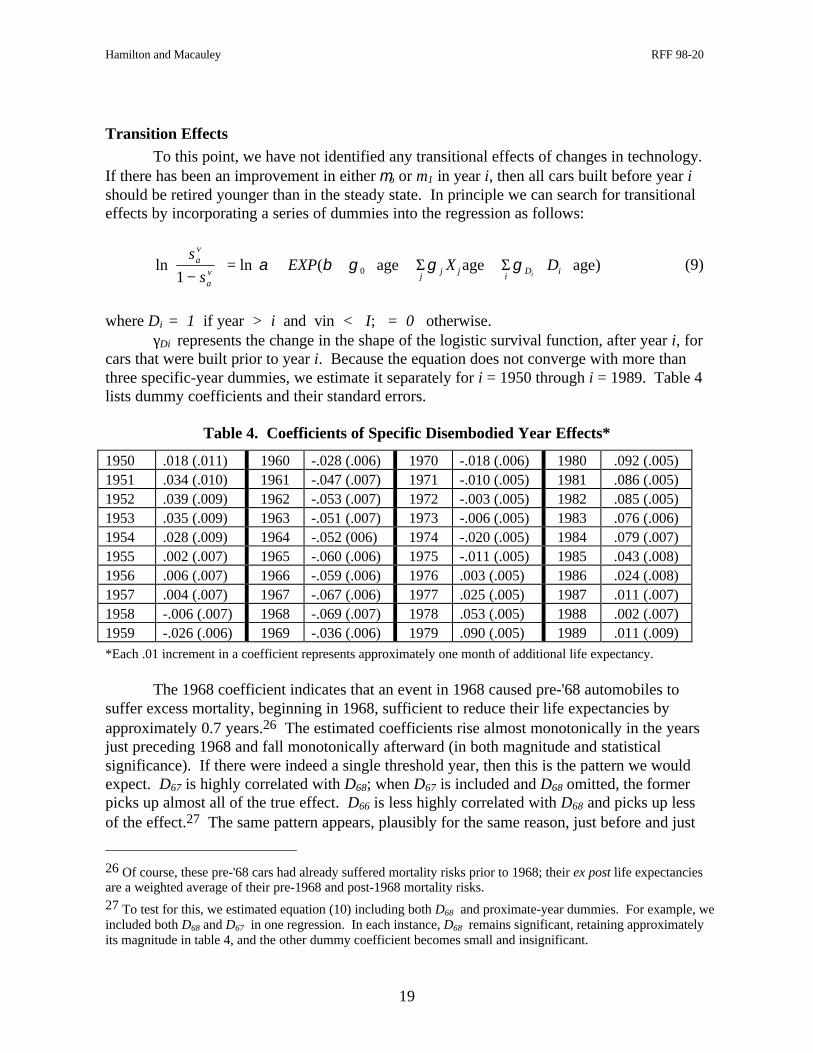
Table 4. Coefficients of Specific Disembodied Year Effects*

1950 .018 (.011) 1960 -.028 (.006) 1970 -.018 (.006) 1980 .092 (.005)1951 .034 (.010) 1961 -.047 (.007) 1971 -.010 (.005) 1981 .086 (.005)1952 .039 (.009) 1962 -.053 (.007) 1972 -.003 (.005) 1982 .085 (.005)1953 .035 (.009) 1963 -.051 (.007) 1973 -.006 (.005) 1983 .076 (.006)1954 .028 (.009) 1964 -.052 (006) 1974 -.020 (.005) 1984 .079 (.007)1955 .002 (.007) 1965 -.060 (.006) 1975 -.011 (.005) 1985 .043 (.008)1956 .006 (.007) 1966 -.059 (.006) 1976 .003 (.005) 1986 .024 (.008)1957 .004 (.007) 1967 -.067 (.006) 1977 .025 (.005) 1987 .011 (.007)1958 -.006 (.007) 1968 -.069 (.007) 1978 .053 (.005) 1988 .002 (.007)1959 -.026 (.006) 1969 -.036 (.006) 1979 .090 (.005) 1989 .011 (.009)*Each .01 increment in a coefficient represents approximately one month of additional life expectancy.

The 1968 coefficient indicates that an event in 1968 caused pre-'68 automobiles tosuffer excess mortality, beginning in 1968, sufficient to reduce their life expectancies byapproximately 0.7 years.26 The estimated coefficients rise almost monotonically in the yearsjust preceding 1968 and fall monotonically afterward (in both magnitude and statisticalsignificance). If there were indeed a single threshold year, then this is the pattern we wouldexpect. D67 is highly correlated with D68; when D67 is included and D68 omitted, the formerpicks up almost all of the true effect. D66 is less highly correlated with D68 and picks up lessof the effect.27 The same pattern appears, plausibly for the same reason, just before and just

26 Of course, these pre-'68 cars had already suffered mortality risks prior to 1968; their ex post life expectanciesare a weighted average of their pre-1968 and post-1968 mortality risks.27 To test for this, we estimated equation (10) including both D68 and proximate-year dummies. For example, weincluded both D68 and D67 in one regression. In each instance, D68 remains significant, retaining approximatelyits magnitude in table 4, and the other dummy coefficient becomes small and insignificant.


20

after the peak year 1980. Thus there seems to be one event which caused pre-'68 cars to dobadly after 1968 and one which caused pre-'80 cars to do well after 1980.28

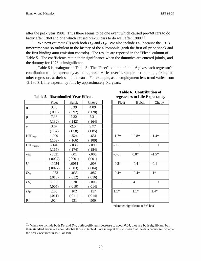
We next estimate (9) with both D68 and D80. We also include D73 because the 1973timeframe was so turbulent in the history of the automobile (with the first oil price shock andthe first binding auto emission controls). The results are reported in the "Fleet" column ofTable 5. The coefficients retain their significance when the dummies are entered jointly, andthe dummy for 1973 is insignificant.

Table 6 is analogous to Table 3. The "Fleet" column of table 6 gives each regressor'scontribution to life expectancy as the regressor varies over its sample-period range, fixing theother regressors at their sample means. For example, as unemployment less trend varies from-2.1 to 3.1, life expectancy falls by approximately 0.2 years.

Table 5. Disembodied Year EffectsTable 6. Contribution of

regressors to Life Expectancy

Fleet Buick Chevy Fleet Buick Chevy

α 3.76 3.39 4.09(.095) (.092) (.128)

β 7.18 7.32 7.31(.132) (.142) (.164)

γ 3.67 -2.54 9.77(1.37) (1.58) (1.85)

HHIyear -.909 -.524 -.651 -1.7* -0.8* -1.4*(.152) (.166) (.189)

HHIvin(avg) -.146 -.036 -.090 -0.2 0 0(.165) (.174) (.184)

vin -.0021 .001 -.005 -0.6 0.8* -1.5*(.0027) (.0001) (.001)

U -.0054 -.0061 -.003 -0.2* -0.4* -0.1(.0027) (.003) (.004)

D68 -.053 -.035 -.087 -0.4* -0.4* -1*(.013) (.012) (.016)

D73 -.001 .030 -.006 0 .4 0(.005) (.010) (.014)

D80 .103 .102 .117 1.1* 1.1* 1.4*(.011) (.011) (.014)

R2 .924 .931 .900

*denotes significant at 5% level

28 When we include both D79 and D80, both coefficients decrease to about 0.04; they are both significant, buttheir standard errors are about double those in table 4. We interpret this to mean that the data cannot tell whetherthe break occurred in 1979 or 1980.


21

In this regression, we find a disembodied effect similar to what we started with(equation (b) in Table 2); the erosion of industry concentration has led to approximately a 1.7year disembodied increase in life expectancy. On the other hand, the embodied effect (built-in durability) is statistically insignificant and very small. In addition, the linear vin effect issmall and of perverse sign. The dummy coefficients show that pre-68 cars did poorly after1968 and pre-1980 cars did well after 1980. The dummy for 1973 is insignificant, and thebusiness cycle effect is small and of perverse sign.

Why might the years 1968 and 1980 stand out? Although the first significant safetystandards became effective on January 1, 1968, Crandall and co-authors estimate the full costof these standards at only $138 per car. The more important information from this portion ofthe time series is that there is no significant change in mortality during the early 1970s (exceptthat which is explained by the other regressors). Increasingly stringent emissions and otherstandards do not appear to have reduced mortality for grandfather cars in the aftermath of the1973 energy crisis.

It seems likely that the D68 coefficient reflects a spurious movement in HHI immediatelyafter 1968. HHI fell from just over 3000 in 1968 to approximately 2500 in 1969 and 1970, andthen recovered to about 2800 in the mid-1970s. This drop is due almost entirely to a decline insales by General Motors from 4.2 million autos (54.7 percent of the market) in 1967 to 3.3million autos (46.3 percent) in 1970. Sales partially recovered to 4.7 million (53.6 percent) in1971. In other words, the HHI-measured concentration declined (temporarily) in 1969 and1970 because GM, the industry leader, had a couple of bad years. Given the estimated HHIy

coefficient, mortality of pre-'68 cars "should" have fallen just after 1968 but did not.Reduced grandfather mortality after 1980 may be due to the Voluntary Export

Restraints (VER) entered into with Japan. With this agreement, the "effective" HHI waslikely considerably higher than the calculated HHI, since Japan and Detroit were effectivelyprecluded from competing for market share.29 As many observers have noted, Detroitevidently took advantage of the VER to raise the price of its new cars.30

Aside from 1968 and 1980, there is no evidence of embodied effects which lefttransitional legacies with older vintages. Most significantly, the dramatic fuel-economyimprovements of the late 1970s did not result in the large predicted die-off of old gasguzzlers. One possibility, of course, is that these fuel-efficiency improvements just offsetsome negative embodied changes.

Vintage Vintages

Next we look for the effect of embodied changes not in the grandfathers but in the newcars themselves. We estimate the fleet regression of Table 5 separately with a vintage dummy

29 Of course, the VER, as price effect, should have reduced scrappage of new cars as well. We do not have thedata to study this, as the sample period ends in 1991 when these cars are still quite young and not likely to die.30 Winston and Associates (1987) estimate that VER raised the prices of 1984 domestic cars by 8.0 percent.According to table 1, this price increase is too small to have generated an almost-one-year increase in lifetimes.


22

for each vintage from 1950 through 1985 (we omit D73, which was small and insignificant).Inclusion of the vintage dummy has virtually no effect on the remaining coefficients. Figure 9illustrates the vintage dummy coefficients which are statistically significant, converted intotheir contribution to life expectancy and correcting for the other regressors. For example, thecoefficient for vintage 1950 implies that 1950-cars had a life expectancy 0.44 years greaterthan other vintages.

50 52 54 56 58 60 62 64 66 68 70 72 74 76

1

0.5

0

-0.5

-1

-1.5

Vintage

Dif

fere

nce

Figure 9. Unexplained longevitySource: See text

Cars of vintage 1958 survived almost 1.5 years less than otherwise similar cars. Carsbuilt in the early 1970s also do poorly, likely due to the rapid onset of regulations whichforced Detroit to build less well-engineered cars in the early '70s (as argued by Crandall andco-authors).31

Specific Models

Particularly in the case of these specific-year embodied effects, it seems prudent toexamine separate automobile models. For example, energy-price shocks may havedifferentially affected large and small cars. Because we do not have pre-1976 data on specificmodels, we work with automobile makes. We report results for 1962 Buicks and Chevrolets,

31 We are unable to estimate precise coefficients for vintages later than the late '70s as we increasingly lose dataon the older cars (the part of the age distribution in which high or low mortality most starkly reveals itself).Thus the lack of significant coefficients from the 1980s conveys little information about the inherent durabilityof these vintages.


23

chosen because they are near opposite ends of the price distribution and because Buicks priorto the energy crises tended to be larger and less fuel efficient than Chevrolets (see Table 7).32

Table 7. Characteristics of 1962 Models

Horsepower Wheelbase Price Weight

Chevy* 80-170 110-119 1800-2450 2250-3500

Buick 155-325 112-126 2475-3450 2700-4319

Data for 1962 models from Kelley Blue BookPrice is 1962 (November-December) used-car price for 1962 model.*Excludes Corvette

We proceed in the same manner as with the fleet. We first estimate (9) separately foreach year from 1951-1989; the pattern (not reproduced here) is virtually identical to that forthe fleet. Next we estimate (9) separately for Chevys and Buicks, including D68, D73, and D80.The results appear in the "Buick" and "Chevy" columns of tables 5 and 6. For both makes,the disembodied HHI effect is large and significant; the embodied effect is small andinsignificant. For Buicks, life expectancy grows linearly with vintage (by .8 years),suggesting a steady improvement in inherent durability. But for Chevys, life expectancydeclines by .75 years as vintage goes from 1948 to 1990. For both makes, unemployment hasa perverse sign, pre-'67 cars did badly after 1967, and pre-'80 cars did well after 1980.Interestingly, we find that pre-'73 Buicks did well after 1973; whatever happened in 1973added about .35 years to the life expectancy of old Buicks. It certainly does not appear thatthe energy crisis caused consumers to retire their old Buicks after 1973.

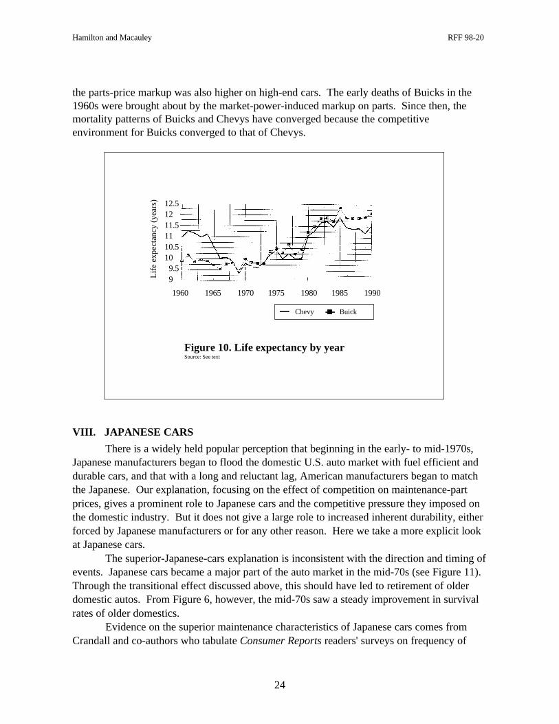
Figure 10 shows the cross-section life expectancies of both Chevys and Buicks from196033 through 1990. From 1960 through 1967, Chevys lived approximately a year longerthan Buicks. Over the next 15 years Buick generally outlived Chevys, though in most yearsthe difference was less than ¼ year. Beginning in the mid-1980s, Buicks began to outliveChevys by as much as half a year.

This pattern, on its face, is odd. As we have seen, Buicks in 1962 were about 50percent more expensive than Chevys; this should have caused Buicks to outlive Chevys byabout 2 years.34 We believe that the market-power/parts-pricing model discussed earlieroffers the explanation for the mortality pattern displayed in Figure 10. During the 1960s themarket for high-end cars was less competitive than that for low-end cars, with the result that

32 We estimated similar regressions for Fords, Mercurys, Chryslers, and Oldsmobiles, with very similar results(not reported). We also attempted to estimate the regression for imports, but the poor quality of the data prior to1975 made this impossible.33 1960 is the first year for which life expectancies can be constructed solely from post-war vintage cars.34 When we examine other makes, the pattern is quite similar. Until the late 1960s, more expensive makes diedsubstantially younger than cheaper makes; in more recent years there has been little mortality difference betweencheap and expensive makes.


24

the parts-price markup was also higher on high-end cars. The early deaths of Buicks in the1960s were brought about by the market-power-induced markup on parts. Since then, themortality patterns of Buicks and Chevys have converged because the competitiveenvironment for Buicks converged to that of Chevys.

1960 1965 1970 1975 1980 1985 1990

12.51211.51110.510 9.5 9

Chevy Buick

Figure 10. Life expectancy by yearSource: See text

Lif

e ex

pect

ancy

(ye

ars)

VIII. JAPANESE CARS

There is a widely held popular perception that beginning in the early- to mid-1970s,Japanese manufacturers began to flood the domestic U.S. auto market with fuel efficient anddurable cars, and that with a long and reluctant lag, American manufacturers began to matchthe Japanese. Our explanation, focusing on the effect of competition on maintenance-partprices, gives a prominent role to Japanese cars and the competitive pressure they imposed onthe domestic industry. But it does not give a large role to increased inherent durability, eitherforced by Japanese manufacturers or for any other reason. Here we take a more explicit lookat Japanese cars.

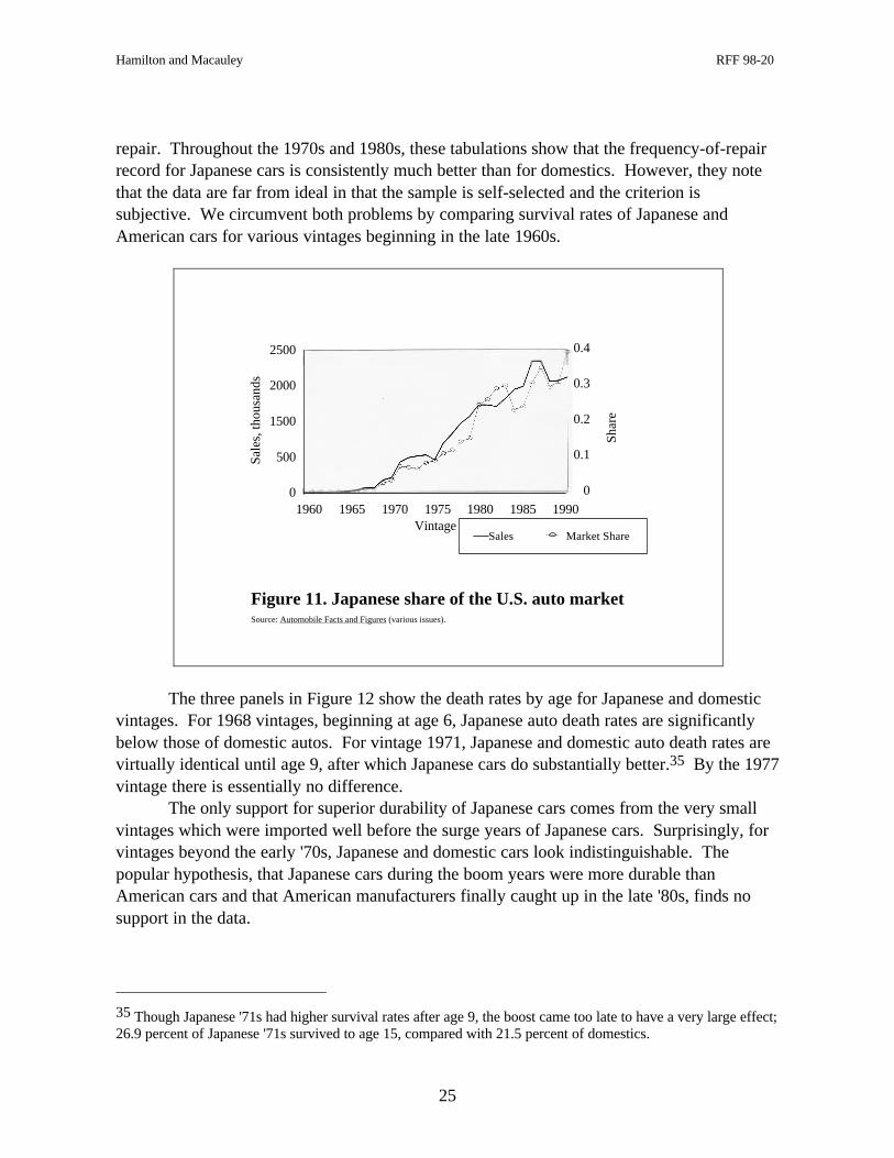
The superior-Japanese-cars explanation is inconsistent with the direction and timing ofevents. Japanese cars became a major part of the auto market in the mid-70s (see Figure 11).Through the transitional effect discussed above, this should have led to retirement of olderdomestic autos. From Figure 6, however, the mid-70s saw a steady improvement in survivalrates of older domestics.

Evidence on the superior maintenance characteristics of Japanese cars comes fromCrandall and co-authors who tabulate Consumer Reports readers' surveys on frequency of


25

repair. Throughout the 1970s and 1980s, these tabulations show that the frequency-of-repairrecord for Japanese cars is consistently much better than for domestics. However, they notethat the data are far from ideal in that the sample is self-selected and the criterion issubjective. We circumvent both problems by comparing survival rates of Japanese andAmerican cars for various vintages beginning in the late 1960s.

1960 1965 1970 1975 1980 1985 1990

2500

2000

1500

500

0

0.4

0.3

0.2

0.1

0

Sale

s, th

ousa

nds

Vintage

Shar

e

Sales Market Share

Figure 11. Japanese share of the U.S. auto marketSource: Automobile Facts and Figures (various issues).

The three panels in Figure 12 show the death rates by age for Japanese and domesticvintages. For 1968 vintages, beginning at age 6, Japanese auto death rates are significantlybelow those of domestic autos. For vintage 1971, Japanese and domestic auto death rates arevirtually identical until age 9, after which Japanese cars do substantially better.35 By the 1977vintage there is essentially no difference.

The only support for superior durability of Japanese cars comes from the very smallvintages which were imported well before the surge years of Japanese cars. Surprisingly, forvintages beyond the early '70s, Japanese and domestic cars look indistinguishable. Thepopular hypothesis, that Japanese cars during the boom years were more durable thanAmerican cars and that American manufacturers finally caught up in the late '80s, finds nosupport in the data.

35 Though Japanese '71s had higher survival rates after age 9, the boost came too late to have a very large effect;26.9 percent of Japanese '71s survived to age 15, compared with 21.5 percent of domestics.


26

2 4 6 8 10 12 14 16Age

Rat

e

0.25 0.20.15 0.10.05 0

J68 D68

Figure 12. Japanese and domestic auto deathrates, by vintageSource: See text

2 4 6 8 10 12 14 16Age

Rat

e

0.2

0.15

0.1

0.05

0J71 D71

2 4 6 8 10 12 14 16Age

Rat

e

0.2

0.15

0.1

0.05

0J77 D77

IX. CONCLUSION

Given the timing of changes in auto death rates, we conclude that essentially none ofthe massive increase in automobile longevity over the past 25 years can be attributed toimprovements in the inherent durability of cars. The rise in lifetimes was driven by someforce external to the new cars themselves.

The strong correlation of mortality rates with the Hirschman-Herfindahl index ofindustry concentration leads us to believe that much of the longevity increase was induced bycompetition, and we find that the most plausible mechanism through which competition wouldraise lifetimes is through an erosion of repair-and-replacement parts prices. A simple model ofauto scrappage enables us to determine that roughly a 50 percent decline in parts prices wouldbe sufficient to explain the recent decline in auto mortality. This magnitude coincides closelywith the roughly 60 percent decline in the cost of maintenance per mile for 2-year-old cars, asestimated by Runzheimer International. Finally, there is some evidence that the VoluntaryExport Restrictions with Japan increased car longevity in the early 1980s. But there is noevidence of a retirement of fuel-inefficient cars in the aftermath of either oil shock.


27

REFERENCES

Alberini, Anna, Winston Harrington, and Virginia McConnell. 1995. "Determinants ofParticipation in Accelerated Vehicle-Retirement Programs," RAND Journal of Economicsvol. 26, pp. 93-112.

American Automobile Association. Various issues. Your Driving Costs.

Automobile Manufacturers' Association. Various issues. Motor Vehicle Facts and Figures.

Berkovec, James. 1985. "New Car Sales and Used Car Stocks: A Model of the AutomobileMarket," RAND Journal of Economics vol. 16, pp. 195-214.

Berry, Steven, James Levinsohn, and Ariel Pakes. 1995. "Automobile Prices in MarketEquilibrium," Econometrica vol. 63, no. 4 (July), pp. 841-890.

Bond, Eric, and Larry Samuelson. 1984. "Durable Goods Monopolies with RationalExpectations and Replacement Sales," RAND Journal of Economics vol. 15, pp. 336-345.

Bresnahan, Timothy F. 1981. "Departures from Marginal-Cost Pricing in the AmericanAutomobile Industry: Estimates for 1977-1978," Journal of Econometrics vol. 17, no. 2(November), pp. 201-227.

Bresnahan, Timothy. 1986. "Crandall, Gruenspecht, Keeler, and Lave's Regulating theAutomobile," RAND Journal of Economics vol. 17, pp. 641-645.

Bulow, Jeremy. 1986. "The Economic Theory of Planned Obsolescence," Quarterly Journalof Economics vol. 101, pp. 729-750.

Coase, Ronald. 1972. "Durability and Monopoly," Journal of Law and Economics vol. 15,pp. 143-149.

Crandall, Robert, Howard Gruenspecht, and Lester Lave. 1982. Regulating the Automobile(Washington, D.C.: Brookings Institution).

Fenney, Bernard P., and Peter Cardebring. 1988. "Car Longevity in Sweden: A RevisedEstimate," Transportation Research vol. 22A, pp. 455-464.

Goldberg, Pinelopi Koujianou. 1995. "Product Differentiation and Oligopoly in InternationalMarkets: The Case of the U.S. Automobile Industry," Econometrica vol. 63, no. 4 (July),pp. 891-951.

Gordon, Robert J. 1990. The Measurement of Durable Goods Prices (Chicago: University ofChicago Press.

Greene, David, and C. K. Eric Chen. 1981. "Scrappage and Survival Rates of Passenger Carsand Light Trucks in the U.S. 1966-77," Transport Research vol. 15A, pp. 383-389.

Greenspan, Alan, and Darrel Cohen. 1996. "Motor Vehicle Stocks, Scrappage, and Sales,"Finance and Economics Discussion Series #1996-40 (Washington, D.C.: Federal ReserveBoard).


28

Gruenspecht, Howard. 1982. "Differentiated Regulation: The Case of Auto EmissionsStandards," American Economic Review vol. 72, pp. 328-331.

Hahn, Robert W. 1995. "An Economic Analysis of Scrappage," RAND Journal ofEconomics vol. 26, pp. 222-242.

Hamilton, Bruce, and Mary A. Burke. 1996. "The Coase Conjecture in Continuous Time:Imperfect Durability, Endogenous Durability, and Aftermarkets," Johns HopkinsWorking Paper #362 (Baltimore, MD: Johns Hopkins University).

Kelley Blue Book Co. Various issues. Kelley Blue Book.

Parks, Richard W. 1977. "Determinants of Scrappage Rates for Postwar Vintage Automobiles,"Econometrica vol. 45, pp. 1099-1116.

R. L. Polk & Co. Vehicles in Operation (unpublished database).

Rust, John. 1986. "When Is It Optimal to Kill Off the Market for Used Durable Goods?'Econometrica vol. 54, pp. 65-68.

Schmalensee, Richard. 1974. "Market Structure, Durability, and Maintenance Effort,"Review of Economic Studies vol. 41, pp. 277-287.

Schmalensee, Richard. 1979. "Market Structure, Durability, and Quality: A SelectiveSurvey," Economic Inquiry vol. 27, pp. 177-195.

Swan, Peter. 1972. "Optimum Durability, Second Hand Markets, and PlannedObsolescence," Journal of Political Economy vol. 80, pp. 575-585.

Winston, Clifford, and Associates. 1987. Blind Intersection? Policy and the AutomobileIndustry (Washington, D.C.: Brookings Institution).

Documents

Competition and Car Longevity - rff.org · Competition and Car Longevity Bruce W. Hamilton Molly K. Macauley ... environment in the auto industry is likely to be an important cause