COMPETITIVE BIDDING STRATEGY IN BUYER-DETERMINED

ONLINE REVERSE AUCTIONS

Ernan Haruvy School of Management

University of Texas at Dallas

Sandy Jap Goizueta Business School

Emory University

June 2008

Abstract Many industries utilize competitive, online reverse auctions for industrial procurement. In many of these auctions, the lowest price bidder is not guaranteed to be the winner and the buyer has full latitude to select the winner from any of the qualified bidders. What are the competitive bidding strategies of bidders in these online auctions? Using an adaptive hierarchical bounded rationality mixture model framework and point-by-point bid data from ten lots of industrial reverse auctions, we find that some bidders incorporate quality information from competitive bids over the course of the auction; that is, suppliers not only adjust their bids for their own quality-advantage or disadvantage – they also account for opponents’ perceived quality differences (on the basis of anonymous price bids). This behavior has implications for the optimal choice of auction format. We estimate bidder rationality from the data and use the estimated parameters to then examine predictions for artificial adaptive agents under different assumptions. We find that the choice of a full price visibility auction design versus a partial price visibility format critically depends on the relationship between cost and quality as well the number of competing sellers.

Keywords: Auctions, Procurement, Learning

JEL Classification: D44; D83

Acknowledgements This research was funded by the Center for E-Business (now called the MIT Center for Digital Business) at the Massachusetts Institute of Technology. Special thanks to Elena Katok, Ram Chellapa, and Jinhong Xie for helpful comments on early drafts of the paper.

1

1. Introduction As interorganizational processes at the boundaries of the firm become increasingly

digitized, new forums for competitive dynamics in the sourcing process have emerged.

Specifically, online reverse auctions, in which sellers bid prices down, is a widely used practice

(Fuller 2004) across a wide range of industries ranging from manufacturing, agricultural, and

government and defense sectors to consumer products, services, pharmaceutical, and high-tech

industries. The main impetus for the use of these online auctions is price savings (Tully 2000;

Cohn 2000) and the use of these auctions is growing (Beall et al 2003). Academic interest in

online reverse auctions is also on the rise, with growing streams of research on their benefits and

risks (Mabert and Skeels 2002; Smeltzer and Carr 2003; Bandyopadhyay, Barron, and

Chaturvedi, 2005) as well as the performance implications of auction design choices (Che, 1993;

Branco, 1997; Chen-Ritzo at al., 2006).

IT-enabled procurement auctions gives rise to novel forms of bidding competition and

strategies. For example, in many procurement settings, buyers must consider important non-

price factors such as product quality supplier responsiveness and capabilities, etc.. Hence, many

industrial buyers rely on “buyer-determined” full-price visibility auctions in which suppliers own

qualities are known, but competitor qualities and identities are unknown. Only price bids, which

are a non-guarantor of winning, is visible to all bidders and this information is constantly

changing over the course of the auction. In addition, the buyer has full latitude to select the

winner on any basis (Jap 2002; Engelbrecht-Wiggans et al., 2006). While this format enables

buyers to consider an array of non-price attributes in its selection decision, it also opens the door

for new bidding strategies on the part of suppliers. If the lowest price bidder is not guaranteed

the win, suppliers lose the incentive to bid down to their costs, which is the dominant bidding

2

strategy in English auctions (McAfee and McMillan, 1987). What bidding strategies might

suppliers use in these auctions? How does this context impact the nature of competitive bidding

that arises? And how do variations in this digitized context (e.g., differences in the amount of

information regarding the nature of the price bids) alter the nature of competition? The answers

to these questions speak to the goal of the Special Issue and hold important implications for the

buyer’s design of procurement auctions. Effective auction design can constitute a key strategic

choice of the firm, as noted by economist Hal Varian:

Designing the right kind of auction will have as big an impact on the brand, customer loyalty, and profit margins of the undertaking as will the designing of the right kind of products. (Schrage 2000).

In this research, we take an initial step toward illuminating our understanding of

competitive bidding strategies in this online reverse auction format. Specifically we propose that

the goal of the bidder is to remain in the buyer’s consideration set in accordance with their non-

price attributes (i.e., quality) as opposed to their costs. Thus, each bid depends on the bidder’s

privately known quality and inferences of the competition’s quality from the bids observed over

the course of the auction, creating a dynamic adjustment process that requires continuous

updating of beliefs regarding other bidders’ qualities. To this end, we develop an analytical

model of how bidders use information from observed bids by others and then estimate the degree

of information use by bidders via the use of point-by-point bid data from ten online reverse

auction lots for metal parts and plastics. Specifically, we first assess the extent to which bidders

adjust their bids for known and perceived quality differences and find that bids are adjusted

according to what bidders believe the quality level of their competition might be. That is, a high

quality supplier will not bid aggressively against what are likely to be low quality suppliers, but

will remain competitive with the bids of those it perceives to be similar high quality suppliers.

3

In order to study the implications of this finding for auction design, we then use a

simulation analysis with artificial adaptive agents (e.g., Andreoni and Miller 1995) to make

forecasts about buyer surplus and price in these online auctions. The adaptive agents are either

sophisticated or naïve bidders, referring to the extent to which they utilize price data. Buyers can

vary the auction format by truncating the price information revealed to the bidders. Since a

bidder might partially deduce the quality of its competition in a full price visibility format, a

buyer could limit that ability by truncating bids that are above the minimum and showing the

minimum price at any given point without attributing the lowest price to any one seller. This is a

common format, which we refer to as “partial visibility” (Jap, 2007).

Hence, we consider the buyer’s preference for auction format as a function of the

relationship between cost and quality and the number of bidders, two common pillars of auction

design research (see McAfee and McMillan 1987 for a review and Bapna, Jank and Shmueli,

2008). We find that when the relationship between product cost and quality is positive

(negative), the partial price visibility format is better (worse) for the buyer; with “better”

referring to the buyer surplus, or value minus price paid. However, when there are few bidders

in the event, the buyer is better off utilizing a full price visibility format and when there are many

bidders, a partial price visibility format is better for the buyer.

Together, we are able to make several contributions to our understanding of bidding

behavior in dynamic procurement auctions: (1) We propose a theoretical framework to

characterize dynamic bidding behavior with hierarchical boundedly rational agents. (2) We

propose an econometric framework that follows our theoretical framework and applies a mixture

model approach to account for different hierarchies of rationality. (3) We estimate our

econometric model on real procurement data and find support for the theory. We are able to

4

show that suppliers are sensitive to competitors’ qualities implied by their bids. This is a useful

step in moving from previously investigated dynamic settings in which qualities are observed

(Asker and Cantillon, 2008; Chen-Ritzo at al., 2005) to more realistic settings in which qualities

are only inferred. (4) We use our estimated parameters and qualities to make recommendations

regarding optimal auction formats. Since the data come from one auction format, we study

artificial adaptive agents to gain insights about alternative formats, an approach which has been

previously used in the literature (e.g., Herbert 1999; Consiglio and Russino 2007; Duffy and

Unver 2007).

In the sections that follow, we describe the auction setting (section 2) and develop a

model of how bidders use information from observed bids by others (section 3). We derive

hypotheses based on the model (section 4). We then describe the empirical investigation (section

5). We conclude with a discussion of key insights, limitations, managerial implications and

directions for future research.

2. The Online Reverse Auction Process

There are numerous papers that describe the online reverse auction process in great detail

from preliminary steps to contract awards (e.g., Emiliani 2000, Mabert and Skeels 2002, Stein

Hawking and Wyld 2003). In general, the buyer will issue a request for purchase to a set of

suppliers that details the nature of the purchase contract as well as product, delivery, and

handling specifications and expectations. Then, the buyer will invite a set of prequalified1

suppliers to bid in an online auction for the opportunity to win the contract. The auction may be

designed and executed by the buyer or in many cases, as in the present data, the auction process

1 Prequalification procedures might include site visits, research, extensive surveys on capabilities and manufacturing processes, or other buyer designed, quality inspection processes.

5

is conducted by a third party auctioneer who informs the suppliers of the event rules such as: (i)

the buyer can select a winner on any basis; the lowest bid is not guaranteed to win the contract2,

(ii) the sourcing manager is prohibited from bidding against suppliers in the auction (a practice

known as “shilling”), (iii) all competitors are viable pre-qualified sourcing options for the buyer,

and (iv) supplier bids are legally binding. The suppliers are not told who their competitors are or

how many suppliers would bid against them.

The most common industrial reverse auction format is the full price visibility format

(Rangan 1998) in which bidders observe anonymous price bids and can respond in real time.

Many industrial buyers tend to favor moving end-times (a “soft close”), meaning that any bid

within the last minute of the designated closing time would automatically extend the close time

by a few minutes to allow other bidders to respond.

Following the auction, the buyer may take 4-6 weeks to evaluate the individual bids and

select a winner. During this time the buyer considers non-price attributes of interest and may

review the bids with other functional units in its organization. Then all suppliers are notified as

to whether they had won or lost the auction.

Given this approach to winner selection, it would seem that typical bidding strategies

identified in the literature on forward auctions (such as outbidding the opponent as long as one’s

reservation price has not been reached (McAfee & McMillan 1987)) may not be appropriate in

this context. Being the lowest or second lowest bidder does not guarantee success and in fact,

may cause the supplier to unnecessarily lose profit margin. Since suppliers do not know the

identities of their competitors, they can only infer quality based on the bids that they observe

2 As an example, out of 13 lots for which we know the outcome, 4 winners had the lowest bid, and 6 winners had the second lowest bid; 3 winners were not the first or second lowest.

6

over the course of the auction. Our goal in the next section is to model how suppliers infer

others’ qualities from their bids.

3. Model: A Model of Price Information Use

How do bidders respond to information from observed bids by others? Ariely &

Simonson (1993) suggest that consumers’ general difficulty of assessing the value of goods and

services in combination with the dynamic nature of decision-making in an auction can lead to an

escalation of commitment to winning and consequent overpayment. This is because the

subjective value of winning the auction increases when a consumer perceives others to be

competitive for the same item (Heyman, Orhun & Ariely 2004). Ku, Malhotra & Munighan

(2005) find that bidders get caught up in the “competitive arousal” of an auction, which leads to

overbidding. While behavioral explanations are increasingly accepted in consumer auctions, the

literature on business-to-business auctions has for the most part neglected individual level

measures of bidding behavior. However, with the plethora of point-by-point bid data from

online reverse auctions, the opportunity to better understand individual behavior is created.

In English auction settings, there is generally a weakly dominant strategy of outbidding

competitors at each point in time by the minimum increment, as long as the net value of winning

is positive to the bidder3. For example, if the bidding increment is $1000, a bidder should counter

an opponent’s bid by bidding $1000 lower than the opponent. Regardless of one’s bidding

strategy, a bidder should never let the auction expire at a winning price below his valuation and

3 The dominant strategy described here is the same for forward or reverse, private, affiliated and common value auctions, but not for situations where sniping is possible. Since the present data has a soft ending time, sniping is not an issue.

7

should never enter a bid that is more than the minimum increment above the present highest bid4

(McAfee & McMillan 1987). Even though this prediction is not always observed, it can serve as

a useful benchmark model.

Not so in buyer-determined auctions, where the buyer chooses the winner based on

quality as well as price. Since bidders know their own quality and will not overly discount their

bid (i.e., high quality bidders will not bid as low as low quality bidders), each bidder’s bids may

reveal something about his quality—i.e., higher bids may be indicative of higher costs and might

signal that the bid comes from a high quality bidder -- and therefore affect each bidder’s

assessment of his own ranking on quality. Hence, the bidding behavior should depend on an

inference about one’s chances of winning based on others’ bids. Though bidders do not know the

other bidders’ attributes, they can nevertheless adjust their beliefs about others in response to

past bidding behavior. This adjustment and response to competitive bidding represents a

significant departure from the extant literature, which uses simplifying assumptions about perfect

observability of quality attributes; i.e., new bids reveal no new information about bidders (Asker

and Cantillon, 2008; Chen-Ritzo at al., 2005). In a online auction context, quality of others is not

directly observed, nor can we assume it to be observed. Hence, we propose a model that would

allow bidders to infer others’ qualities based on their bids.

In behavioral economics, a dominant theory is the theory of hierarchical thinking (Stahl

and Wilson, 1994; Camerer, Ho and Chong 2004), which posits that human decision makers use

iterative self-referential models of others. As a simple example (Bosch- Domènech et al., 2002),

consider the following task. You must choose a number between 0-100. You will win a prize if

your number is closest to 2/3 of the average choice by others like you faced with the same task.

4 Note that this definition of the set of weakly dominant strategies does not change in response to observed bids. That is, if the winning bid was 30 instead of 21, the set of dominant strategies would still be defined this way.

8

What will you choose? A naïve player might guess that since the possible range of numbers is

from 0 to 100, the average will be in the middle of this range, at 50. In that case, the best choice

is 33.3, which is 2/3 of the middle. One iteration on this idea-- thinking that others are naïvely

choosing 33.3-- will result in a choice of 22.2. It turns out that empirically (in classroom,

laboratory and newspaper experiments) the largest modes are indeed at 33 and 22 and that these

modes are robust (in location though not in magnitude) (Bosch-Domènech et al., 2002).

In our setting, this suggests that bidders consider past bids and respond in one of two

ways: (1) Naïve bidders try to outbid the minimum bid after adjusting for own quality. (2)

Sophisticated bidders update their assessments of others according to how far others’ bids are

from the minimum observed bid; they then try to outbid the minimum of quality-adjusted bids.

The classification of behavior into hierarchies of bounded rationality has been shown

useful in different economic settings (Stahl and Wilson, 1994, 1995; Haruvy, Stahl and Wilson,

2001). Gneezy (2006), using the framework of Camerer, Ho and Chong (2004), applied a

hierarchical classification to bidding in auctions. Whereas Gneezy restricted his attention to

sealed bid forward auctions (in which bidders submit a single bid), in this work we apply a

hierarchical theory to dynamic reverse auctions (in which bids are updated over time).

In an online reverse auction context, we can likewise model the two largest types of

hierarchical thinking, which we call naïve and sophisticated. The naïve belief reflects an

“insufficient prior,” and is defined as the belief that others possess identical qualities. We let that

belief be an unbiased estimate of the true mean quality, meaning that the belief is correct on

average. We define a “sophisticated belief” as the belief that all bidders other than oneself hold

the beliefs that others hold insufficient priors. Then, we can state the following:

9

Proposition. A bidder with an insufficient prior will bid incrementally below the last

observed minimum bid, adjusted for own quality. A bidder with a sophisticated belief

will bid incrementally below the last observed quality-adjusted bid by others, adjusted for

own quality.

All proofs are in the appendix.

4. Hypotheses

Our first hypothesis tests the basic premise of the model that the population consists of

naïve bidders and boundedly rational sophisticated bidders. This hypothesis is consistent with the

large stream of literature on hierarchical thinking reviewed earlier (see overview in Camerer, Ho,

and Chong 2004) and with the finding that hierarchical rationality is consistent with auction data

(Gneezy 2006).

Hypothesis 1. The population of bidders is a mixture of naïve and sophisticated bidders.

The buyer’s goal is to generate a surplus and competitive bidding. The next two

hypotheses relate these outcomes to the correlation of bidder costs and qualities. Consider the

case of positive and negative cost-quality relationships. A positive cost-quality relationship is

likely when higher quality involves costly materials or operations (Asker and Cantillon, 2008).

For example, more quality control generally increases both the cost and quality of a product.

Negative cost-quality relationships occur when specialization is important in production (Smith,

1776). To this end,, a number of large diversified firms such as IBM, Hewlett Packard, General

10

Motors and Motorola have sold off non-core operations in an effort to simultaneously improve

quality and reduce costs (Burrow, 2005; Musgrove, 2004; Reardon, 2008; Welch et al., 2005).

We propose that competitive bid prices for a naive population will be lower than prices

for a sophisticated population when quality is highly positively correlated with costs and vice

versa when quality is highly negatively correlated with costs. The rationale is that with sufficient

positive correlation, the high quality bidders are also the high cost bidders and will be priced out

of the auction before the lower quality bidders. Hence, the competition late in the auction will be

between low-quality low-cost bidders. If the low quality bidders are sophisticated, they are

aware that they are competing against other low-quality bidders, and they will therefore realize

that they do not need to provide deep price discounts to remain competitive. However, if the low

quality bidders are naïve, they will continue to provide deep discounts, to the great benefit of the

buyer. In contrast, if there is a highly negative relationship between quality and cost, low quality

sellers will be priced out first, leaving the high quality low cost sellers to compete later in the

auction. In that case, the naive high quality low cost sellers will over-estimate their quality

advantage vis-à-vis their surviving opponents, so bids will be higher than optimal in a naive

population, to the buyer’s detriment.

Hypothesis 2. The lowest bid in a naïve bidder population is lower than the lowest bid in

a sophisticated bidder population when quality and costs are sufficiently positively

correlated. The highest bid in a naïve bidder population is higher than the highest bid in a

sophisticated bidder population when quality and costs are sufficiently negatively

correlated..

11

The next hypothesis is the natural extension of the price comparison in the last hypothesis to

buyer surplus. As long as the winner is the same winner in both populations, lower prices will

translate into higher surplus for the buyer, where buyer surplus is defined as the highest score in

the auction. Of course, this is not a direct mapping in the buyer-determined case, since it is often

the case that the winners are not the same for both populations. However, if the relationship is

sufficiently strong so that the set of bidders that are priced out is close in both populations, the

savings on price will be the key difference. That is, when the cost-quality relationship is positive,

buyer surplus will be higher for a population of naive types than for a population of sophisticated

types and vice versa when the relationship is negative. Formally:

Hypothesis 3. The buyer surplus in a naïve bidder population is greater than the buyer

surplus in a sophisticated bidder population when quality and costs are positively

correlated and vice versa when they are negatively correlated.

This hypothesis need not imply a symmetric direction. Naive sellers, by virtue of behaving sub-

optimally will typically yield additional surplus to the buyer over rational maximizing bidders.

The buyer under most circumstances would prefer sellers to optimize poorly. The relationship

between cost and quality should be quite negative before the buyer realizes significant benefit to

rational bidders, and even then the benefit is expected to be quite limited. Also note that this

hypothesis directly extends to the comparison of partial and full price information formats, as

discussed in the previous section.

Note that the arguments with regard to positive cost-quality correlation apply only to

populations with sufficiently large number of bidders. This is because the arguments rely on

high-cost-high-quality bidders dropping out before the completion of the auction due to a

12

competitive process that eliminates them on cost-competitiveness. However, when there are few

bidders and costs and qualities are drawn randomly, this argument may not hold. That is, when

there are few bidders then with a high likelihood there will be cases where all bidders are high-

cost-high-quality bidders. In these cases, naive bidders will bid too high relative to sophisticated,

so sophisticated bidders would be strongly preferred in such cases. This leads us to hypotheses

4 and 5.

Hypothesis 4. The lowest bid in a naïve bidder population is greater than the lowest bid

in a sophisticated bidder population when the number of bidders is sufficiently low

regardless of correlation.

Hypothesis 5. The buyer surplus in a naïve bidder population is lower than the buyer

surplus in a sophisticated bidder population when the number of bidders is sufficiently

low regardless of correlation.

5. Empirical Investigation

In this section, we examine the hypotheses via proprietary data from two auction events

and a simulation. The event data is used to test H1 (5.1-5.3) and simulations provide insights on

H2 through H5 (5.4).

It is important to stress that the data does not include costs or qualities for each supplier,

nor surplus for the buyer. Therefore, hypotheses 2 and 3 regarding cost-quality relationships

cannot be reliably tested with the data, although the data is useful in calibrating the model for

13

subsequent simulation studies which we describe shortly.5 Likewise, due to the absence of buyer

surplus information we cannot make conclusive statements about hypothesis 5 without a

simulation approach. Hypothesis 4 includes variables for which we do have reliable measures

(price, number of bidders, and bidder sophistication) but we simply do not have a sufficient

number of independent auctions with different number of suppliers to be able to have reliable

estimates. The simulation is helpful in that it can take parameters estimated from bid data, for

which we have numerous observations, and use them to calibrate a simulation model which can

then provide as many observations as we would like about hypothetical scenarios.

5.1. The Data

An industrial buyer in the automotive industry provided point-by-point bid data of ten

online reverse auction lots held for two events-- metal parts and plastics. The combined contract

value of these auctions was approximately $19.2 million. None of these products were pure

commodities, such as MRO supplies or highly customized strategic parts. All the products were

used in production or directly for parts in production. The product categories thus differed in

non-price characteristics, and supplier relationships and quality could play a role in the

procurement decision. The auction for metal parts consisted of 6 product lots and 20 bidders,

while the plastics auction was comprised of 9 lots and involved 12 bidders. The lots are bid on

simultaneously with bidders that overlap within each lot, but not across the two auction events.

Since some of the lots have few or no multiple bids by the same firms, we cannot use these lots

for estimation of dynamic updating. Deleting these lots, we are left with five lots in plastics and

5 Incumbency is one potential measure of quality. We find that incumbency is negatively correlated with both the number of bids made in an auction and the concession made between the starting price and the ending price by the bidder. These could be indications that the incumbent faces a higher cost, or alternatively that the incumbent is sufficiently confident about its quality that it does not need to respond to others’ bids.

14

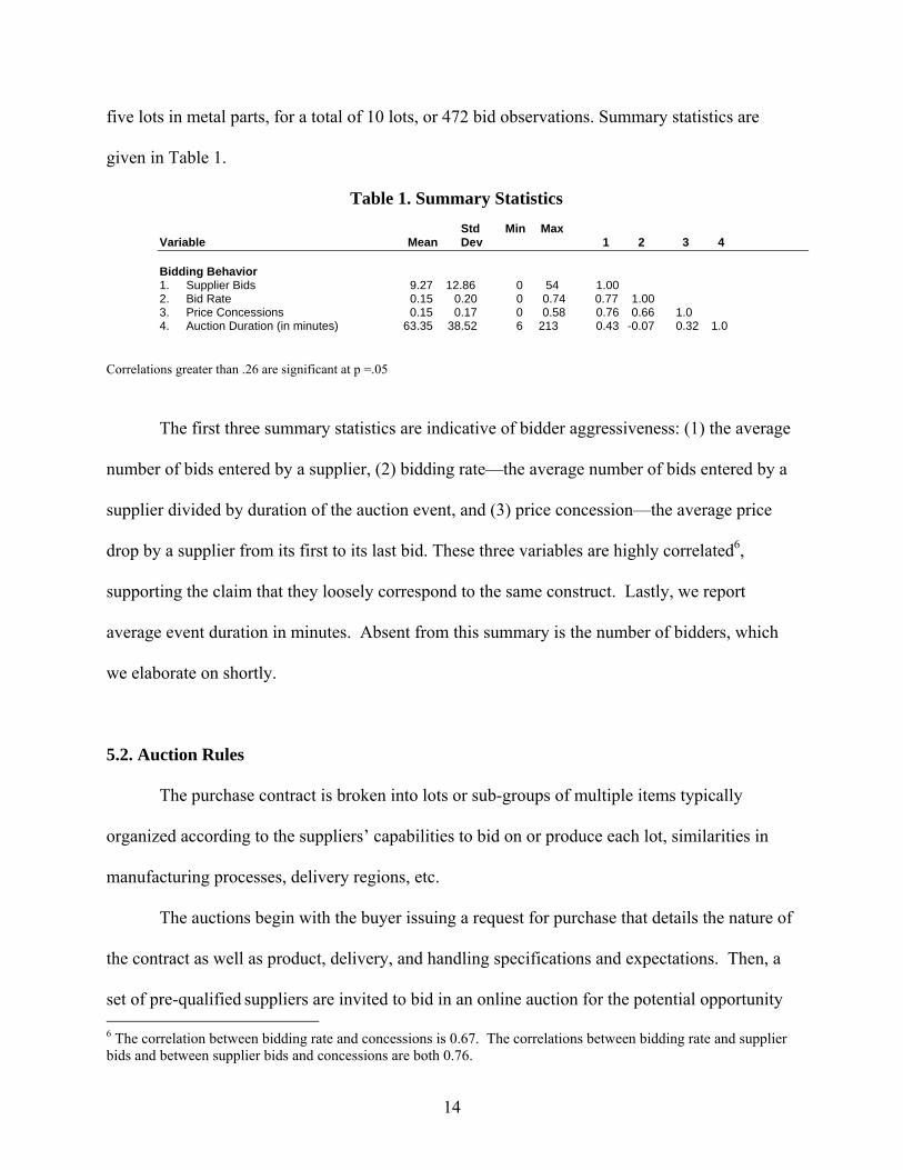
five lots in metal parts, for a total of 10 lots, or 472 bid observations. Summary statistics are

given in Table 1.

Table 1. Summary Statistics

Std Min Max Variable Mean Dev 1 2 3 4 Bidding Behavior 1. Supplier Bids 9.27 12.86 0 54 1.00 2. Bid Rate 0.15 0.20 0 0.74 0.77 1.00 3. Price Concessions 0.15 0.17 0 0.58 0.76 0.66 1.0 4. Auction Duration (in minutes) 63.35 38.52 6 213 0.43 -0.07 0.32 1.0

Correlations greater than .26 are significant at p =.05

The first three summary statistics are indicative of bidder aggressiveness: (1) the average

number of bids entered by a supplier, (2) bidding rate—the average number of bids entered by a

supplier divided by duration of the auction event, and (3) price concession—the average price

drop by a supplier from its first to its last bid. These three variables are highly correlated6,

supporting the claim that they loosely correspond to the same construct. Lastly, we report

average event duration in minutes. Absent from this summary is the number of bidders, which

we elaborate on shortly.

5.2. Auction Rules

The purchase contract is broken into lots or sub-groups of multiple items typically

organized according to the suppliers’ capabilities to bid on or produce each lot, similarities in

manufacturing processes, delivery regions, etc.

The auctions begin with the buyer issuing a request for purchase that details the nature of

the contract as well as product, delivery, and handling specifications and expectations. Then, a

set of pre-qualified suppliers are invited to bid in an online auction for the potential opportunity 6 The correlation between bidding rate and concessions is 0.67. The correlations between bidding rate and supplier bids and between supplier bids and concessions are both 0.76.

15

to win the purchase contract. The auctions are “buyer-determined” score auctions, allowing

buyers to integrate non-price considerations (e.g., quality and reliability) into their selection

decision.7 The score is defined as

Score(bidder j) = Monetary Quality measure for bidder j – bid by bidder j (1)

The bidder with the highest score wins, rather than the bidder with the lowest price. In contrast to

score auctions with endogenously determined qualities, however, in the present auctions, the

bidders bid on price only. Their qualities, as far as the auction goes, are exogenous.

Quality determination occurs both before the start of the auction and after the conclusion

of the bidding. Prior to the auction, bidders are pre-qualified to ensure that they meet the

minimum quality standards. In addition, the minimum measurable product quality and technical

specifications are provided to the bidders in detail and it is made clear that the products must

meet these specifications. Following the conclusion of the bidding, the buyer takes several weeks

to evaluate the bids based on any number of criteria, including past relationships with the

supplier, reputation for service, etc. Visits to the bidding firm to inspect the manufacturing

process and quality control are common.

All the auctions were conducted by a third party auctioneer who informed the suppliers of

the event rules. The suppliers were not told who their competitors were or how many suppliers

would bid against them and featured a soft close.

7 It is important to note that though the auction itself may not determine the winner, a buyer-determined auction nevertheless plays a critical role in the buyer’s price discovery efforts and supplier choice. Instead of thinking of each bidder as submitting a price, one could think of each bidder as submitting a score involving a price + non-price attributes. The winner is not the lowest bidder, but the one that presumably scores the highest on both price and non-price characteristics. To this end, the theoretical treatment of this price discovery mechanism is equivalent in all respects to that of auctions in which the lowest bidder wins.

16

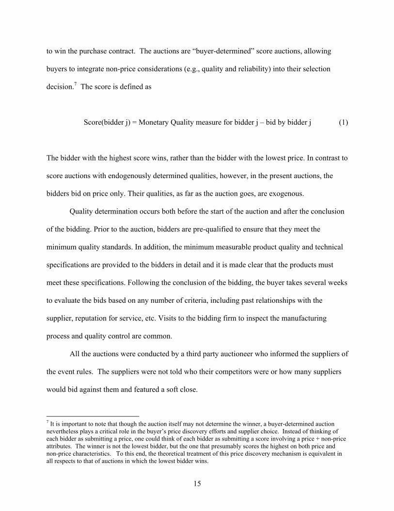
The average number of active bidders was 7.1. The distribution of the number of bidders

in our auctions is given below.

Figure 1. The distribution of the number of bidders over lots.

0

0.5

1

1.5

2

2.5

3

3.5

5 6 7 8 9 10

Number of bidders

Freq

uenc

y (n

umbe

r of l

ots)

5.3. Estimation Methodology

As mentioned earlier, heterogeneity in bidder sophistication is a critical aspect of the

current estimation methodology and the normative predictions of the model. Heterogeneity

considerations have been shown to be critical in the design of auctions (Bapna, Goes, Gupta and

Jin, 2004). We utilize a mixture model to assess the degree of hierarchical thinking among the

bidders. The mixture model contains two types of bidders: naïve and sophisticated. The

proportion of each segment in the population is denoted by αj, where j is the corresponding

segment.

Denote by itbid the last observed bid by firm i at or before time t and let the variable

0itdiff denotes the bidder’s demanded premium over the unadjusted last minimum observed bid

by others. The variable 1itdiff denotes the bidder’s demanded premium over the last minimum

17

observed bid by others, adjusted for others’ quality advantages or disadvantages inferred from

their bids.

The adjustment rate is denoted by parameter β , which represents the degree of

adjustment of firms’ beliefs about the qualities of other firms. If β =1, firms fully adjust their

belief regarding others’ qualities in response to the last observed bid. That is, each sophisticated

firm believes that firm k’s quality advantage is fully reflected by its last observed bid. If β =0,

firms never update their initial belief (which would mean that sophisticated firms are essentially

naive). For any intermediate β , the new belief is equal to a convex combination of the previous

belief and the last observation, with a weight of (1- β ) on the previous belief and a weight of β

on the last observed bid. Note that the belief regarding firm k is only updated when a new bid is

observed by firm k.

Since 0itdiff and 1

itdiff need to be initialized, we initialize them at the first observed

difference and drop the first observation from estimation.

01 1, 1 , 1min min( ,..., )t t n tbid bid− − −= (2)

0 0 01 1(1 ) ( min )it it it tdiff diff bidβ β− −= − + − (3)

),...,min(min 011

01111

11 −−−−− −−= ntntttt diffbiddiffbid (4)

1 1 11 1(1 ) ( min )it it it tdiff diff bidβ β− −= − + − (5)

Since some buyers bid on several lots within an event, we need to account for potential

correlation. To do that we use the random effects model to allow for a common error term, iε ,

to enter for bids by the same firm across lots. The error term iε is assumed to come from a

18

normal distribution with mean zero and standard deviation indσ . The likelihood over firm i’s bids

conditional on firm i being naïve (Type 0 in equations 6 and 7) or sophisticated (Type 1 in

equations 6 and 7) is:

1

1

min1( )j jT

it t it ii

t lot lot

bid diffL Type j εφσ σ

−

=

⎛ ⎞− − += ⎜ ⎟

⎝ ⎠∏ (6)

The unconditional likelihood of firm i’s bids is:

{0,1}( )i j i

jL L Type jα

∈

= ∑ (7)

The parameter α1 denotes the proportion of sophisticated firms.

This gives us a model with two main parameters α1 and β. We also need a parameter for

the standard deviation of error for each lot and one parameter for the standard deviation of

individual random effects. Though we assume the same α1 and β over lots, the scale is different

between lots, requiring a separate sigma (variance parameter) for each lot. Model estimation is

detailed in the next section (§5.3).

5.3. Estimation Results

The estimation was run in Gauss, and an optimization procedure (OPTMUM) was used

for maximization. We estimated three models—the homogeneous naive model, the homogenous

sophisticated model, and a mixture model that allows for both types of bidders as subpopulations

in the bidder population. Table 2 shows the parameter estimates and their significance for the

mixture model only; we use the likelihoods from the homogenous models for hypothesis testing.

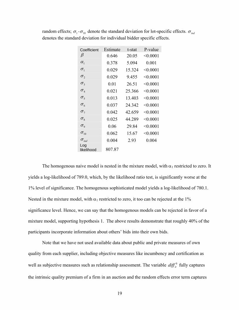
Table 2 Results for all events pooled

Coefficient α1 denotes the proportion of sophisticated bidders; β is the degree of adjustment of firms’ beliefs about the qualities of other firms. 1σ - 10σ and indσ are

19

random effects; 1σ - 10σ denote the standard deviation for lot-specific effects. indσ

denotes the standard deviation for individual bidder specific effects.

Coefficient Estimate t-stat P-value β 0.646 20.05 <0.0001

1α 0.378 5.094 0.001 1σ 0.029 15.324 <0.00012σ 0.029 9.455 <0.00013σ 0.01 26.51 <0.00014σ 0.021 25.366 <0.00015σ 0.013 13.403 <0.00016σ 0.037 24.342 <0.00017σ 0.042 42.659 <0.00018σ 0.025 44.289 <0.00019σ 0.06 29.84 <0.000110σ 0.062 15.67 <0.0001indσ 0.004 2.93 0.004

Log likelihood 807.87

The homogenous naive model is nested in the mixture model, with α1 restricted to zero. It

yields a log-likelihood of 789.0, which, by the likelihood ratio test, is significantly worse at the

1% level of significance. The homogenous sophisticated model yields a log-likelihood of 780.1.

Nested in the mixture model, with α1 restricted to zero, it too can be rejected at the 1%

significance level. Hence, we can say that the homogenous models can be rejected in favor of a

mixture model, supporting hypothesis 1. The above results demonstrate that roughly 40% of the

participants incorporate information about others’ bids into their own bids.

Note that we have not used available data about public and private measures of own

quality from each supplier, including objective measures like incumbency and certification as

well as subjective measures such as relationship assessment. The variable 0itdiff fully captures

the intrinsic quality premium of a firm in an auction and the random effects error term captures

20

remaining firm-specific effects, leaving no room for additional firm level regressors to improve

the fit.8 Hence, we will have to conduct a separate analysis for these individual firm variables

using a somewhat different framework.

5.4. Simulation Results

The current data does not allow for good estimates of bidder costs or consideration of the

implications for auction format selection. First, these estimates would be inseparable from any

error in the estimate of the quality for each bidder. Second, since bidders enter at random times,

we do not have perfect observability of when the bidder exits, which would be necessary to

pinpoint its cost. We could make various assumptions and get some numbers, but these numbers

would not be very meaningful. Moreover, we would like to ask “what if” questions about the

relationship between cost and quality and the impact of the number of bidders.

To understand how the relationship between cost and quality affects buyer surplus and

the choice of optimal auction format, we simulate bidders with different costs and qualities. The

bidders come from one of two bidder populations (i.e., naïve and sophisticated) that together

make up the mixture observed in the data. Instead of looking only at the mixed population, we

examine each population type separately. This is because each population type represents a mode

of behavior we expect to see prevalent in one either the full or partial price visibility formats.

Under the partial price visibility format, the only bidding strategy possible is one corresponding

to the behavior of a naive population, whereas under the full-visibility format, more sophisticated

strategies are possible, as demonstrated by a sophisticated population. It is therefore of interest to

separately compare these two extreme cases of pure populations.

8 With individual effects terms, additional demographic variables, unless they vary over time, cannot add to fit or be identified since all the heterogeneity in the intercept is already captured.

21

The parameters of the simulation are as follows. We simulate 2 to 20 bidders for each of

the 10 auction lots with cost-quality covariance parameter of -30 to 30 (correlation is covariance

divided by the product of the standard deviations). For each lot, we begin with an average initial

bid that is the initial bid we observed in the actual data. The quality differential of each bidder is

randomly determined and uniformly distributed between 00.4*b− and 00.4*b . The cost is

related to the quality differential through ci idiffγ= where γ determines the sign and strength of

the relationship between cost and quality differential and is the parameter we vary to study the

effect of this relationship on buyer surplus. Another stochastic element of the simulation is in

the incidence and timing of each bidder’s bid (which of course, affects the bid amount). Each

bidder bids probabilistically at each point in time, with a probability of 1/10.

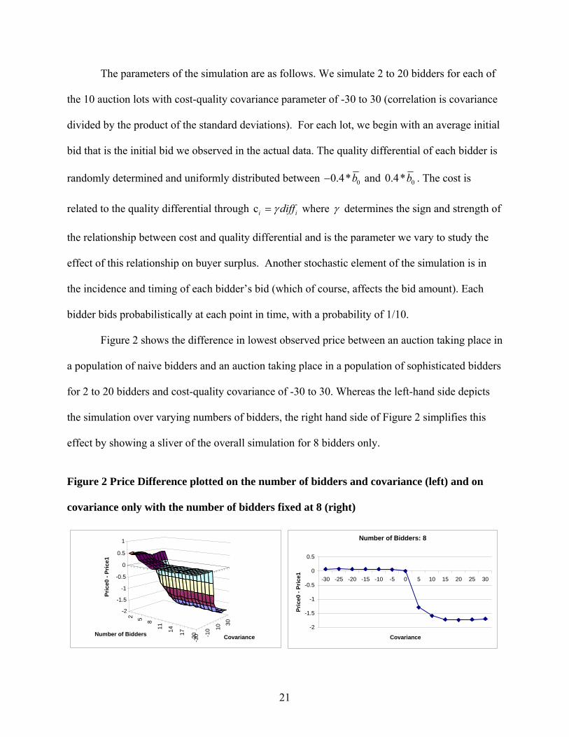
Figure 2 shows the difference in lowest observed price between an auction taking place in

a population of naive bidders and an auction taking place in a population of sophisticated bidders

for 2 to 20 bidders and cost-quality covariance of -30 to 30. Whereas the left-hand side depicts

the simulation over varying numbers of bidders, the right hand side of Figure 2 simplifies this

effect by showing a sliver of the overall simulation for 8 bidders only.

Figure 2 Price Difference plotted on the number of bidders and covariance (left) and on

covariance only with the number of bidders fixed at 8 (right)

Number of Bidders: 8

-2

-1.5

-1

-0.5

0

0.5

-30 -25 -20 -15 -10 -5 0 5 10 15 20 25 30

Covariance

Pric

e0 -

Pric

e1

2 5 8

11 14 17 20 -30 -1

0 10

30

-2

-1.5

-1

-0.5

0

0.5

1

Pric

e0 -

Pric

e1

Number of Bidders Covariance

22

We see from Figure 2 that for any given number of bidders, there is a cutoff covariance for

which the naive population’s price drops below the sophisticated population’s price. We see on

the right hand side that for 8 bidders that cutoff is at a covariance of 0. That is, for 8 bidders, a

positive correlation between cost and quality implies that the price would be higher with a

sophisticated population.

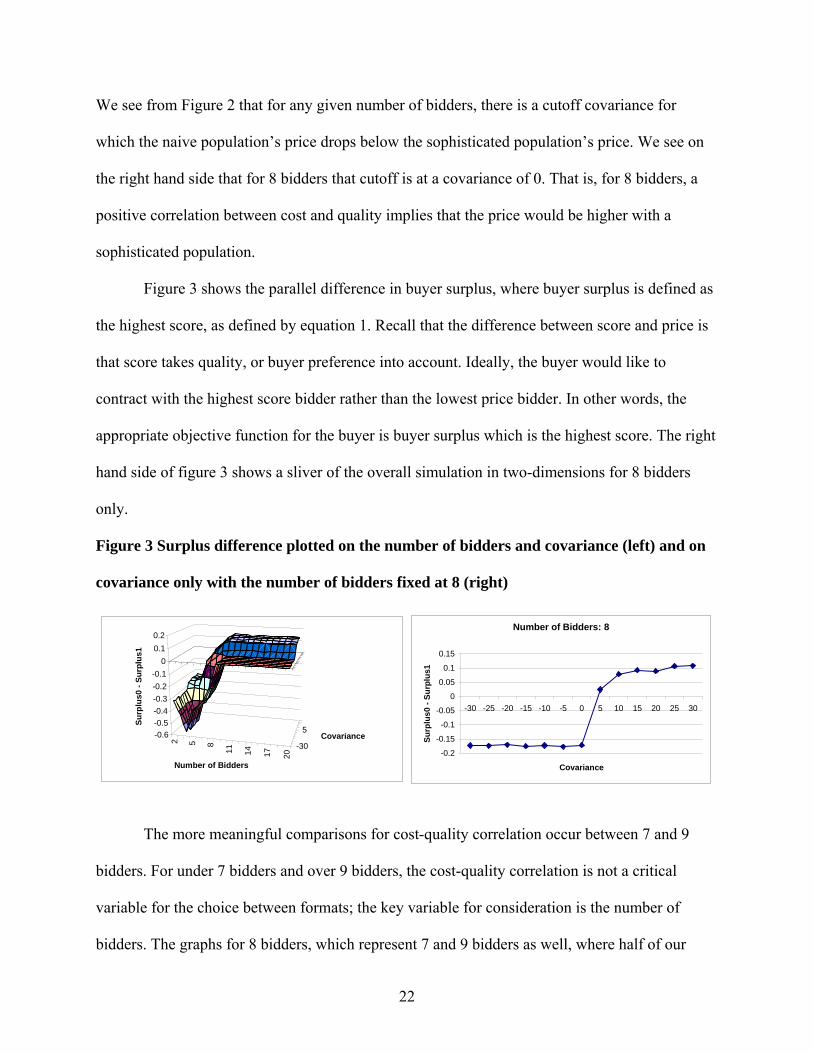
Figure 3 shows the parallel difference in buyer surplus, where buyer surplus is defined as

the highest score, as defined by equation 1. Recall that the difference between score and price is

that score takes quality, or buyer preference into account. Ideally, the buyer would like to

contract with the highest score bidder rather than the lowest price bidder. In other words, the

appropriate objective function for the buyer is buyer surplus which is the highest score. The right

hand side of figure 3 shows a sliver of the overall simulation in two-dimensions for 8 bidders

only.

Figure 3 Surplus difference plotted on the number of bidders and covariance (left) and on

covariance only with the number of bidders fixed at 8 (right)

2 5 8

11 14 17 20

-30

5-0.6-0.5-0.4-0.3-0.2-0.1

00.10.2

Surp

lus0

- Su

rplu

s1

Number of Bidders

Covariance

Number of Bidders: 8

-0.2

-0.15

-0.1

-0.05

0

0.05

0.1

0.15

-30 -25 -20 -15 -10 -5 0 5 10 15 20 25 30

Covariance

Surp

lus0

- Su

rplu

s1

The more meaningful comparisons for cost-quality correlation occur between 7 and 9

bidders. For under 7 bidders and over 9 bidders, the cost-quality correlation is not a critical

variable for the choice between formats; the key variable for consideration is the number of

bidders. The graphs for 8 bidders, which represent 7 and 9 bidders as well, where half of our

23

observations fall, clearly show that when the cost-quality relationship is strongly positive, lower

price would be observed in a naive population of bidders than in a sophisticated bidder

population. This provides insight into hypothesis 2 in the positive relationship case. The opposite

holds for the negative cost-quality relationship scenario. In terms of surplus, when the cost-

quality relationship is positive, the buyer would obtain greater surplus with a naive population

than a sophisticated population, or alternatively pursue a partial price information auction format

rather than a full price information format. When the relationship is strongly negative, the buyer

would slightly prefer a sophisticated population or a full price information format. This speaks to

hypothesis 3.

Note that when the cost-quality relationship is negative, the price and score differences

between the populations/formats are largely negligible for 9 or more bidders, though they are

substantial for 8 bidders or less. In other words, the optimal choice of populations/formats does

not yield symmetric benefits. Choosing the partial price information auction format when it is the

optimal format could yield tremendous benefits over a full-price-information format. But

choosing it when it is not optimal will not cause great, if any, losses to the buyer provided the

number of bidders is sufficiently large. This is not an artifact of the parameters chosen for the

simulation. Rather, it is a robust characteristic of this setting. To understand this, note that the

critical statistic in a naive population is the minimum price bid. In the positive relationship

scenario, the buyer surplus advantage of a naive population over a sophisticated population stems

from low quality bidders over-discounting their own qualities relative to their opponents, which

results in jump bidding or bidding down in increments greater than the minimum increment. In

contrast, in the negative cost-quality relationship scenario, the naive bidders are expected to bid

higher than optimal because high quality naive bidders (the bidders whose low cost allows them

24

to continue bidding late into the game) will overestimate their quality advantage relative to their

opponents. However, any bidding up will not affect the minimum price bid statistic which is the

only information the naive evaluate. Hence, the effect is minimal. Mostly, what is happening is

that prices decline by the minimum increment instead of by jump bids. But this is exactly the

pattern in the sophisticated population. While the impact is therefore negligible on the prices, it

is somewhat more significant for buyer surplus. In the calculation of buyer surplus, bids higher

than the minimum matter and this is why surplus appears to be more affected than prices by the

population makeup in the negative relationship scenario.

As predicted by hypotheses 4 and 5, when the number of bidders is small, the covariance,

and therefore correlation, will not be a key determinant in population or format choice. Price will

always be higher and buyer surplus will always be smaller for the naive population regardless of

the correlation. This is because high-cost bidders are less likely to drop out of the auction. We

find strong support for this notion, related to hypotheses 4 and 5.

In summary, when the buyer knows the cost-quality relationship and the number of

bidders is sufficiently large, a positive cost-quality relationship implies an advantage for a partial

price format or naive population and vice versa. When the number of bidders is sufficiently large

and the buyer is uncertain about the cost-quality relationship, the buyer’s format choice is not

difficult—the partial price information dominates easily. However, when the number of bidders

is small this preference reverses and the optimal format choice becomes full price visibility.

6. Conclusions

We proposed that in procurement auction settings sellers’ bids should increase in their

qualities. Accordingly, bidders should be able to infer others’ perceived quality advantage or

25

disadvantage and to re-assess their own relative standing. Since the equilibrium is intractable in

such settings, we proposed a framework of hierarchical bounded rationality with two levels of

sophistication.

We examined the assertion that sellers infer others’ qualities from their bids using data

from ten auction lots. We found that a little over 60% of suppliers were naïve bidders in that they

did not appear to derive information from others’ bids. Almost 40% of participants could be said

to have sophistication in that they attempted to infer others’ qualities from their bids. While

others (Gneezy, 2006) have suggested a hierarchical mixture approach to bidding, this is the first

demonstration that the hierarchical mixture approach can be successfully applied to dynamic

reverse auctions.

From the buyer’s perspective, we showed that when the number of bidders is sufficiently

large, a buyer would prefer to be facing a naïve population of bidders when the relationship

between cost and quality is positive, but would prefer to face a more sophisticated bidder

population when the cost-quality relationship is negative. When the number of bidders is small,

however, the buyer would prefer to face a sophisticated population. While a buyer may not

always have a choice of which bidder population to face, the buyer typically has a choice of

which auction format to use. In partial price visibility formats, sellers are essentially reduced to

naive behavior as they have no ability to assess other bidders’ qualities. Hence, the comparison

between naive and sophisticated populations directly pertains to the comparisons between partial

and full price visibility formats. We can conclude that when the expected number of bidders is

sufficiently large, a buyer would prefer a full price visibility format to the partial price visibility

format when the cost-quality relationship is negative and vice versa. When the expected number

of bidders is small, the full visibility is preferred regardless of the cost-quality relationship. This

26

is an important characterization to sellers facing this critical format choice. This result appears to

be in contrast to findings elsewhere (e.g., Goeree and Offerman, 2003) that more information

provided by the auctioneer reduces uncertainty and thereby promotes more aggressive bidding.

The difference is that the bidders in our model are boundedly rational and map information in

ways that are not in accordance with full rationality.

Limitations

Since the findings of the paper are simulation-based, the data simply served as a

benchmark calibration of the model and presented some limited evidence for the model’s

predictive power. Nevertheless, while this data set is novel and informative, it is not necessarily

ideal. The main limitation of the present study is that the data did not contain the actual qualities

and costs of the bidders. Instead, they had to be estimated under the assumptions of the model,

which could lead to misspecification-related biases.

Another approach for examining alternative levels of bidder sophistication would be to

use experimental data in which the qualities and costs are known. However, this approach is not

without tradeoffs. Even under such conditions, it can still be quite difficult to decipher and

isolate alternative levels of sophistication. This is the what Gneezy (2005) finds. In addition,

external validity might also be sacrificed.

Managerial Implications

With the popularity of procurement auctions fast rising, numerous new formats have been

proposed. Most of these formats have been devised to satisfy buyer and seller needs and requests

27

with little regard for the theoretical tractability of such formats for economists, leaving a large

vacuum in the academic auction literature.

In this work we examined the surplus implications for the buyer of truncating price

information. We noted that price truncation would lead to less aggressive responses to high

quality bidders’ bids and to more aggressive responses to low quality bidders’ bids. Hence, the

surplus difference of truncating prices could go either way.

With few bidders, the surplus loss from less aggressive competition in a group of high

quality bidders far outweighs the surplus gain in a group of low quality or mixed quality bidders

since the high quality bidders have a greater surplus potential. Hence, with small groups, the

buyer should opt for full price visibility. Larger groups of bidders are likely to consist of the full

quality spectrum and in these auctions the low quality bidders drive the price down for the high

quality bidders. Hence, for larger numbers of bidders the buyer should opt for a partial price

visibility format.

The cost-quality relationship is equally important for the price visibility decision. With

partial price visibility , low quality bidders are the ones that drive prices down relative to full

price bidding, whereas high quality bidders drive prices up. With a positive cost-quality

relationship, low quality bidders are also low-cost and therefore can drive prices down more.

With negative cost-quality relationship, low quality bidders are high-cost and are priced out of

the market early in the bidding. Hence, in the positive cost-quality relationship, the buyer would

opt for price truncation where with a negative cost-quality relationship, full price visibility would

be preferred.

While our framework is useful for the buyer’s decision on price visibility in online

reverse auctions, it is also useful for the seller’s bid decision. From a seller’s perspective,

28

knowing where your company stands relative to others is invaluable information to managers.

Any statistical method which can help infer others’ qualities would be tremendously helpful to

formulate a bidding strategy. No less important is knowing how the competition might use one’s

bids to infer information about one’s competitive position and bidding strategy. Both of these

issues were addressed by our empirical model and we believe they will prove important to

managers.

Future Research

Future research should sort out various dynamic bidding strategies. With more and

cleaner data, one might be able to identify higher levels in the sophistication hierarchy as well as

dynamic strategies such as signaling and collusion.

In the limitations section, we mentioned the potential ability of experimental research to

cleanly estimate and test the explanatory power of the present model and alternative models.

However, the most promising experimental route for this line of research, in our opinion, would

be to examine the implications of the price truncation policy offered here, rather than to try to

confirm one model or another.

In this work we examined partial versus full price visibility. Another increasingly popular

format is the rank-based format which can be studied in the present framework. The rank-based

format, where bidders are informed of their rank relative to others but not of any competing price

offers, can be thought of as a hybrid between full and partial price visibility and we expect

results in-between the two formats we already studied.

The attributes we focused on were the degree of correlation between cost and quality and

the number of bidders. Another related attribute which could be studied in the present format is

29

the variance in bidder quality. Together, these possibilities present exciting avenues for future

research.

30

REFERENCES

Andreoni, J. and J. H. Miller (1995), “Auctions with Artificial Adaptive Agents,” Games and Economic Behavior 10, 38-64.

Asker, John and Estelle Cantillon (2008), Properties of Scoring Auctions RAND Journal of Economics, v39(1), pp 69-85

Bandyopadhyay, Subhajyoti, John M. Barron, and Alok R. Chaturvedi (2005), Competition Among Sellers in Online Exchanges, Information Systems Research, 16, 47 - 60.

Bapna, Ravi, Paulo Goes, Alok Gupta, and Yiwei Jin (2004). "User Heterogeneity and its Impact on Electronic Auction Market Design: An Empirical Exploration," MIS Quarterly, 28(1) 21-43.

Bapna, Ravi, Wolfgang Jank, Galit Shmueli (2008), Consumer Surplus in Online Auctions, forthcoming in Information Systems Research

Beall, Stewart, Craig Carter, Phillip L. Carter, Thomas Germer, Thomas Hendrick, Sandy D. Jap, Lutz Kaufmann, Debbie Maciejewski, Robert Monczka, Ken Petersen (2003), “The Role of Reverse Auctions in Strategic Sourcing,” Center for Advanced Purchasing Studies (CAPS), research paper.

Bosch-Domènech, Antoni, José G. Montalvo, Rosemarie Nagel, Albert Satorra (2002), One, Two, (Three), Infinity, ... Newspaper and Lab Beauty-Contest Experiments, The American Economic Review, Vol. 92 (5), 1687-1701.

Branco, Fernando (1997), “The Design of Multi– Dimensional Auctions,” RAND Journal of Economics 28(1) 63– 81.

Burrows, Peter (2005), Can This Really Be Hewlett-Packard? Business Week, December 19. Camerer, C.F., Ho, T-H, Chong, J-K. (2004), "A Cognitive Hierarchy Model of One-Shot

Games," Quarterly Journal of Economics, 119(3), 861-898. Che, Yeon-Koo (1993) “Design Competition through Multi– Dimensional Auctions,” RAND

Journal of Economics 24 (4) 668– 680. Chen-Ritzo, Ching-Hua, Terry P Harrison, Anthony M Kwasnica, Douglas J Thomas (2005),

“Better, Faster, Cheaper: An Experimental Analysis of a Multiattribute Reverse Auction Mechanism with Restricted Information Feedback,” Management Science, 51(12), pp. 1753-1762.

Cohn, L. (2000), “B2B: the Hottest Net Bet Yet?” Business Week, January 17, pp. 36-7. Consiglio, Andrea and Annalisa Russino (2007), How does learning affect market liquidity? A

simulation analysis of a double-auction financial market with portfolio traders, Journal of Economic Dynamics and Control, In Press.

Duffy, J. and U. Unver (2007), Internet Auctions with Artificial Adaptive Agents: A Study on Market Design, working paper.

Emiliani, Mario L. (2000), “Business-to-Business Online Auctions: Key Issues for Purchasing Process Improvement,” Supply Chain Management, 5(4), 176-86.

Engelbrecht-Wiggans, Richard, Ernan Haruvy and Elena Katok (2006), “A Comparison of Buyer-determined and Price-Based Multi-Attribute Mechanisms,” working paper.

Fuller, Neil (2004), “Low Points,” Supply Management, 9(19), 37. Gneezy, Uri (2005), “Step-Level Reasoning and Bidding in Auctions,” Management Science,

51(11), 1633-43. Goeree, J. K. and T. Offerman, 2003 J. Goeree and T. Offerman, Competitive bidding in

auctions with private and common values, The Economic Journal 113 (2003), pp. 598–613.

31

Haruvy, E., D. Stahl and P. Wilson, (1999), "Evidence for Optimistic and Pessimistic Behavior in Normal-Form Games," Economics Letters, 63, 1999, 255-260.

Herbert Dawid (1999), On the convergence of genetic learning in a double auction market, Journal of Economic Dynamics and Control, 23, 1545-1567

Jap, Sandy D. (2002), “Online, Reverse Auctions: Issues, Themes, and Prospects for the Future,” The Marketing Science Institute-Journal of the Academy of Marketing Science Special Issue on Marketing to and Serving Customers Through the Internet: Conceptual Frameworks, Practical Insights and Research Directions, Parsu Parasuraman and George Zinkhan, eds., 30(4), 506-25.

------------ (2007), “The Impact of Online Auction Design on Buyer-Supplier Relationships,” Journal of Marketing, 71(1), 146-59.

Kagel, John H. (1995), "Auctions: A Survey of Experimental Research," in The Handbook of Experimental Economics, J. H. Kagel and A. E. Roth, Eds., Princeton, NJ, Princeton University Press

Mabert, Vincent A. and Jack A. Skeels (2002), “Internet Reverse Auctions: Valuable Tools in Experienced Hands,” Business Horizons, July-August, 70-76.

McAfee, R. Preston and John McMillan (1987), “Auctions and Bidding,” Journal of Economic Literature, 25(2), 699-738.

Musgrove, Mike (2004), IBM Sells PC Business to Chinese Firm in $1.75 Billion Deal, Washington Post, Wednesday, December 8, 2004; Page A01

Pavlou, Paul A. and David Gefen (2004), Building Effective Online Marketplaces with Institution-Based Trust, Information Systems Research, 15, 37 - 59.

Rangan, V. Kasturi (1998), “Freemarkets Online,” Boston, MA: Harvard Business School Publishing, Case #598109, 1-20.

Reardon, Marguerite (2008), Motorola hits redial on handset biz, CNET News, March 26. Rothkopf, M.H., Pekec, A, and Harstad, R.M. (1998), "Computationally manageable

combinational auctions,” Management Science, 44, 1131-1147. Smeltzer, Larry R. and Amelia S. Carr (2003), "Electronic Reverse Auctions: Promises, Risks

and Conditions for Success," Industrial Marketing Management, 32, 481-88. Smith, Adam (1976). An Inquiry into the Nature and Causes of the Wealth of Nations, Clarendon

Press, Oxford. Stahl, D. and P. Wilson (1994), "Experimental Evidence of Players' Models of Other Players,"

J. of Econ. Behavior and Org., 25, 309-327. Stahl, D. and P. Wilson (1995), "On Players Models of Other Players: Theory and Experimental

Evidence," Games and Economic Behavior, 10, 218-254. Stein, Andrew, Paul Hawking and David C. Wyld (2003), "The 20% Solution?: A Case Study on

the Efficacy of Reverse Auctions," Management Research News, 26(5): 1-20. Tully, S. (2000), “The B2B Tool That Really is Changing the World,” Fortune, March 20,

141(6), p. 132-45. Welch, David, Ronald Grover, and Ira Sager (2005), Kerkorian's Axman Cometh, Business

Week, May 30.

32

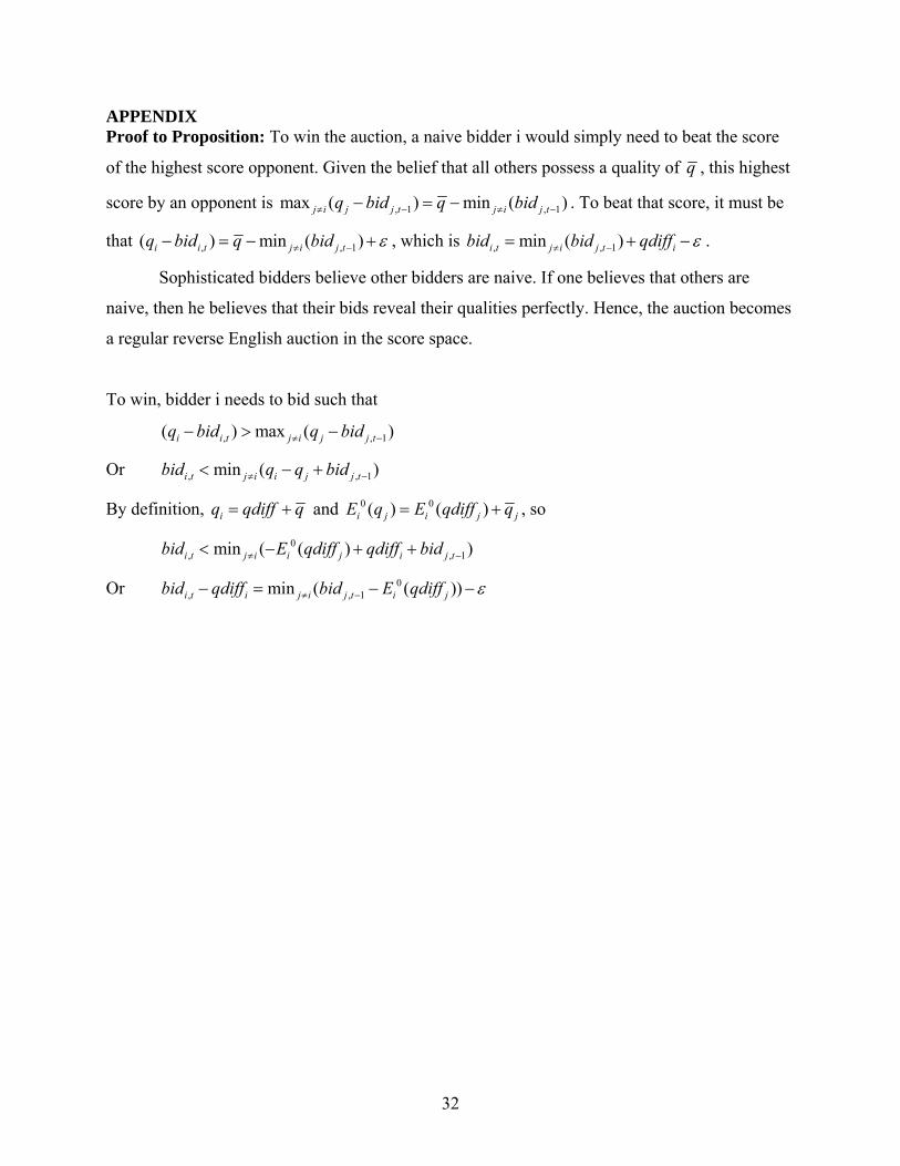
APPENDIX Proof to Proposition: To win the auction, a naive bidder i would simply need to beat the score

of the highest score opponent. Given the belief that all others possess a quality of q , this highest

score by an opponent is , 1 , 1max ( ) min ( )j i j j t j i j tq bid q bid≠ − ≠ −− = − . To beat that score, it must be

that , , 1( ) min ( )i i t j i j tq bid q bid ε≠ −− = − + , which is , , 1min ( )i t j i j t ibid bid qdiff ε≠ −= + − .

Sophisticated bidders believe other bidders are naive. If one believes that others are

naive, then he believes that their bids reveal their qualities perfectly. Hence, the auction becomes

a regular reverse English auction in the score space.

To win, bidder i needs to bid such that

, , 1( ) max ( )i i t j i j j tq bid q bid≠ −− > −

Or , , 1min ( )i t j i i j j tbid q q bid≠ −< − +

By definition, iq qdiff q= + and 0 0( ) ( )i j i j jE q E qdiff q= + , so

0, , 1min ( ( ) )i t j i i j i j tbid E qdiff qdiff bid≠ −< − + +

Or 0, , 1min ( ( ))i t i j i j t i jbid qdiff bid E qdiff ε≠ −− = − −