Competitive Threats and the Cost of Debt∗

Katarzyna Platt†

Job Market Paper

January 8, 2015

Abstract

This study demonstrates that competition plays an important role in determin-

ing a firm’s cost of debt. Specifically, I analyze how competitive threats affect the

yield spread of corporate bonds. I find that firms that face high levels of competition

also face higher costs of debt. After controlling for common bond-level, firm-level and

macroeconomic variables, I find that bondholders of firms that are subject to increased

competition demand significantly higher credit spreads than holders of otherwise simi-

lar bonds. My analysis also reveals that information about competition is incorporated

in corporate bond credit ratings. Combined, these findings provide strong evidence that

competitive threats are being reflected in corporate debt prices and that competitive

dynamics influence firms’ access to capital.

∗I would like to thank Armen Hovakimian, Lin Peng and Ted Joyce for their invaluable comments andadvice.†Department of Economics and Finance, Zicklin School of Business, Baruch College / CUNY, 55 Lex-

ington Avenue, Box B10-225, New York, NY 10010. Phone: 646-312-3457. Fax: 646-312-3451. Email:katarzyna.platt@baruch.cuny.edu

1 Introduction

Competitive threats in the product market in which firms operate influence their financial

policies. Recent empirical work shows that higher levels of competition lead to higher level

of cash holdings, lower dividend payments, and greater hedging (e.g., Haushalter, Klasa,

and Maxwell (2007); Hoberg, Phillips, and Prabhala (2014) Chi and Su (2013)). Further-

more, firms facing more competition face increased cost of bank loan financing (Valta, 2012).

However, the question of how product market threats affect the cost of public debt remains

unexplored. Corporate bondholders focus on future cash flows to ensure a firm’s ability to

pay periodic interest and bond principal. Because higher levels of product market threats

may have negative impact on future cash flows, bondholders are likely to be concerned about

the firm’s competitive position. Therefore, the goal of this paper is to identify whether prod-

uct market competition is an important determinant of bond market prices.

Traditional competitive economic theory predicts that the level of product market com-

petition increases with the number of competitors. For this reason, market concentration,

proxied by either the Herfindahl-Hirschman Index (henceforth HHI) or the four-firm con-

centration ratio, is frequently used to measure competition. Both measures focus on the

distribution of production across firms within an industry. However, market concentration

may not accurately reflect the changes in the competitive dynamics of product markets that

occur within industries that do not experience the addition or loss of a competitor. For

example, competition becomes more intense if one firm’s products are more ready substi-

tutes for another firm’s product. An additional problem with the traditional measures of

competition is that they do not capture potential competition and they require a definition

of the relevant product market. However, this could be difficult for some industries, such as

business services, which are not well defined (Phillips, 2013). What is more, using HHI as a

proxy for market competition inevitably leads to an endogeneity problem if financial policy

and product market strategy are jointly determined. Therefore, it may be problematic to

1

draw clear inferences from empirical research based on HHI. The level of HHI in a specific

industry could very likely represent an equilibrium outcome of competition for that industry.

Because of this, it may be unclear whether higher levels of industry HHI measures represent

higher or lower levels of competition. Valta and Fresard (2013), using reductions in import

tariff rates as a source of variation in competitive pressure, find that firms’ reaction to in-

creased competition is indeed heterogeneous and depends on competitive position as well as

on the structure of the product markets. Also, Kjenstad and Su (2013) show that under cer-

tain market structures a larger number of competitors may reduce the chances of predation,

if the predator has to share the profit from predation with more competitors or free-riders.

Hence, increasing the number of competitors may decrease the intensity of competition.

Therefore, HHI may not accurately capture all different dimensions of competition, and HHI

as an industry-level measure may not reflect some of the dynamic interactions between firms

within the industry.

In this study, I am using a novel measure of competition, fluidity, developed by Hoberg,

Phillips, and Prabhala (2014). There are two important reasons for this measure choice.

Firstly, fluidity captures the similarity between a firm’s products and the product evolution

of its rivals. It allows for the separation of the effect of competitive threats from the effect of

market concentration. Secondly, because it measures moves made by rival firms competing

in a product space, the potential endogeneity problem is mitigated.

Although fluidity is a novel measure, it has been used in several recent studies as a proxy

for product market competition. Hoberg, Phillips, and Prabhala (2014) show that product

market fluidity decreases firm propensity to make payouts via dividends or repurchases. It

also increases cash held by firms, especially for firms with less access to financial markets.

When product markets are changing rapidly, the future is less certain and this, in turn,

has an effect on firm’s payout policy, which is based on the expectations about the future

market for the firms’ products. Kjenstad and Su (2012) find that for small firms, fluidity

is significantly related to the use of performance sensitive debt. Specifically, they find that

2

product market threats are negatively related to the probability of bank loan contracts having

the performance-sensitive feature. Morellec, Valta, and Zhdanov (2014) look at the firm’s

decision to issue bank debt versus public debt. In their study, they find that firms operating

in more competitive product market and facing lower credit supply are more likely to issue

public debt.

Another strand of literature investigates the relationship between product market com-

petition and debt financing costs. Valta (2012) links product market competition to spreads

on bank loans. Using several market concentration-based proxies for product market compe-

tition, the author empirically shows that firms operating in competitive environments have

significantly higher costs of debt financing. Moreover, his paper shows that the effect of

competition on debt pricing depends also on rival financial strength, meaning that the firms

who are in industry leading positions not only benefit from cheaper financing but could also

increase the cost of financing for their rivals. Paligorova and Yang (2014) examine the im-

pact of product market competition and corporate governance on the cost of debt financing

and the use of bond covenants. The article uses market concentration as a proxy for prod-

uct market competition and concludes that firms with higher anti-takeover provisions pay a

lower cost of debt only in competitive industries, as product market competition increases

the probability of takeovers.

In this paper, using the universe of bond transactions, I find that higher product fluidity is

associated with higher costs of debt financing. After controlling for industry and firm specific

attributes, my analysis indicates that debt costs are significantly higher for firms with high

product similarity to their competitors. I also find a negative relationship between product

fluidity and bond credit rating. Specifically, I find that one standard deviation increase in

fluidity decreases firm’s bond credit rating by one half of a credit rating notch. The results

are robust to various specifications and control variables and are both economically and

statistically significant. Overall, my results suggest that bondholders take product markets

into consideration in the pricing of the firm’s debt.

3

This paper is closest to that of Valta (2012) who also studies the effect of product market

competition on the cost of debt. However, this paper uses product fluidity rather than market

concentration measures to proxy for product market threats. Also, this paper analyzes public

bond markets, whereas Valta (2012) concentrates on the market for bank loans.

This paper contributes to the literature by identifying that changes in product market

dynamics affect corporate bond valuation. First, I add to to the literature that studies

the interactions between product markets and financial markets. By providing compelling

evidence that bond yields incorporate a substantial product market dimension, this analysis

broadens the understanding of the implications of the industry structure for the cost of

debt financing. Also, my study complements recent papers that document how corporate

behavior is influenced by the decisions of firms’ peers (MacKay and Phillips, 2005; Leary and

Roberts, 2014). By establishing a link between product market threats and corporate bond

pricing, the findings of this paper suggest that there are spillover effects between product

market rivals. Those effects have implications for the firm’s financial decisions. Studies by

Fresard (2010) and Chi and Su (2013) also show that firms do not operate in isolation, but

incorporate rivals’ financial status and competitive position in their decision process. Their

research sheds light on the role of cash holdings and product market threats. Firms that hold

large cash reserves enjoy future market share gains at the expense of their rivals. Last, but

not least, I also extend the recent research in corporate bond pricing explaining what factors

affect bond credit spreads (Collin-Dufresne, Goldstein, and Martin, 2001; Elton, Gruber,

Agrawal, and Mann, 2001; Campbell and Taksler, 2003; Chen, Lesmond, and Wei, 2007;

Dick-Nielsen, Feldhtter, and Lando, 2012).

The remainder of the paper is organized as follows. Section 2 develops the hypotheses.

Section 3 introduces the data, presents the summary statistics, and describes the empirical

strategy. Section 4 presents the main results and sensitivity tests. Section 5 presents the

paper’s conclusions.

4

2 Hypothesis Development

Credit spread has two main determinants: the risk of default itself; and the recovery rate,

where, in the event of default, the bondholder receives only a portion of the promised pay-

ments (Collin-Dufresne, Goldstein, and Martin, 2001). Product market competition levels

influence both of these determinants. The higher the competitive threats from rival firms,

the less certain are the future cash flows of the firm. This, in turn, increases firm’s default

risk. Hou and Robinson (2006) argue that the structure of product markets helps to deter-

mine a firms risk by affecting the equilibrium operating decisions it makes. They find that

stocks of companies operating in more competitive industries earn higher average returns

and attribute this premium to higher default risk of these firms. When competition is more

intense, firms that fail to quickly adapt to changes in the environment are drawn out of

business. Therefore it is likely that creditors require higher rates of return on their capital

from firms that face more product market competition.

Furthermore, the asset liquidation value may also be affected by competition. Whenever

firms assets are liquidated, the highest value potential buyers are likely to be other firms in

the industry, provided that they have financial slack. Otherwise the assets may be sold to

industry outsiders for a lower price (Shleifer and Vishny, 1992). Since competitive product

market may influence both the financial strength and number of firms in the industry, higher

levels of product market competition may also affect the cost of debt by reducing the firm’s

liquidation value (Ortiz-Molina and Phillips, 2014).

In his article, Valta (2012) finds that competition is an important determinant of banks’

willingness to provide financing and the price of the offer. He examines how competition

relates to the cost of bank debt and finds that the bank loans of firms that operate in

competitive product markets exhibit higher spreads. This result should also hold true for

bondholders. Consequently, I expect the bond market participants to take product market

threats into consideration when pricing the firm’s debt. Accordingly, my first hypothesis is:

5

Hypothesis 1: Competitive threats measured by product market fluidity are positively related

to bond yield spreads.

Also, higher cost of debt will lead rating agencies to assign lower bond ratings to firms

where product market threats are more substantial. In conducting its surveillance, a rating

agency will consider many factors, including, but not limited to: changes in the business cli-

mate, credit markets, new technology or competition that may hurt an issuer’s earnings or

projected revenues; issuer performance; and regulatory changes (Standard & Poor’s, 2011).

Credit agencies pay close attention to product differentiation, competitive advantage and its

sustainability. Thus, to examine whether product market threats have an impact on bond

ratings I formulate the next hypothesis as follows:

Hypothesis 2: The level of competitive threats measured by product market fluidity is nega-

tively related to bond ratings.

3 Methodology and Descriptive Statistics

3.1 Sample

The data for this study come from several sources. The main sample of firms is obtained

from Annual Compustat files. Following the standard approach, I exclude firms in the finan-

cial sector (SIC codes 6000-6999) and utilities (4900-4999). I also exclude firms with values

of total assets or sales are less than one million dollars and replace extreme observations of

all ratio variables with missing values (those in one percent in both tails of the distribution).

Leverage ratios are trimmed at the value one.

There is no readily available dataset of bond pricing. In order to construct bond prices, I

use bond transaction data from the Transaction Reporting and Compliance Engine (TRACE)

database which reports individual bond transactions at a daily (or finer) frequency. This

6

database, operated by FINRA,1 is a result of a recent regulatory initiative to increase the

price transparency in secondary corporate bond markets. The TRACE database initiated in

2002, became fully operational in 20052 and now covers essentially all publicly traded bonds

(Bessembinder, Maxwell, and Venkataraman, 2006; Edwards, Harris, and Piwowar, 2007).

Since the TRACE database provides me with a short time series of data, I extend the

sample with data from the National Association of Insurance Commissioners’s (NAIC) bond

transaction file, which cover all insurance companies’ trading records of publicly traded

bonds in the post-1994 period. NAIC data is obtained from Mergent Fixed Income Secu-

rities Database (FISD) and contains prices for all trades in public corporate bonds made

by insurance companies since 1994. I follow the cleaning procedure of bond data outlined

in Dick-Nielsen (2009) and (Bessembinder, Kahle, Maxwell, and Xu, 2009) and eliminate

canceled, corrected, and commission trades. I also eliminate observations that are obvious

data entry errors, e.g. with negative prices, with maturity dates prior to issuance or trade

dates, etc.

Mergent’s FISD portion of the database contains a comprehensive set of bond character-

istics. I use FISD to obtain bond-level information such as issue date, issuance size, coupon

rate, and credit rating, as well as to identify the special features of bonds. I exclude all con-

vertible bonds, pay-in-kind bonds, asset-backed securities, Yankee bonds, Canadian bonds,

bonds denominated in non-U.S. currencies, floating-rate bonds, unit deals, puttable bonds,

exchangeable bonds, perpetual bonds and agency bonds from my sample.

In order to calculate bond prices using the combined TRACE and NAIC dataset, I follow

the methodology proposed by (Bessembinder, Kahle, Maxwell, and Xu, 2009) and eliminate

all trades that are below $ 100,000 and construct a daily price by weighing each trade by its

size. I calculate bond returns using formula (1) where AI is accrued interest, C is coupon

1The Financial Industry Regulatory Authority, Inc. (FINRA), formerly National Association of SecuritiesDealers, Inc. (NASD), is a private corporation that acts as a non-governmental, self-regulatory organizationthat regulates member brokerage firms and exchange markets. http://www.finra.org/AboutFINRA/

2See FINRA news release http://www.finra.org/Newsroom/NewsReleases/2005/P013274.

7

rate and P reflects the price of the bond.

Bond Return =Pt + AIt + Ct − (Pt−1 + AIt−1)

Pt−1 + AIt−1

(1)

For my sample, I retain the last daily price available for a given bond that is closest to

the end of the fiscal year, provided that the difference between the last trade date and the

end of the fiscal year is less than 90 days. In tests of new bond issues, I employ the promised

yield to maturity at issue reported by Mergent FISD.

Information on stock prices, trading volume, and market capitalizations are obtained

from the Center for Research in Security Prices (CRSP). S&P and Moody’s credit ratings

are obtained from Mergent FISD database.

I obtain data related to firms product market environment, including data on HHI, in-

dustry classification and product market fluidity, from the Hoberg- Phillips data library3.

Data on foreign trade are acquired from Peter Schott’s Web site. Macroeconomic data

are retrieved from U.S. Bureau of Economic Analysis and the Treasury bond data from

Federal Reserve Bank in St. Louis. Data on firm level default probability is obtained from

Kamakura’s Risk Manager.

3.2 Variables

3.2.1 Measuring bond yield spreads and bond credit ratings

The dependent variables in my analysis are bond yield spreads and bond ratings. My

first dependent variable, natural logarithm of bond yield spread, measures the cost of debt

(Elton, Gruber, Agrawal, and Mann, 2001; Klock, Mansi, and Maxwell, 2005). The yield

spread is defined as the difference between the yield-to-maturity on a corporate bond and

3The data is available at http://www.rhsmith.umd.edu/industrydata/.

8

the yield-to-maturity on its maturity-equivalent risk-free bond. To calculate yield spreads

for individual corporate bonds, I use the constant maturity Benchmark Treasury rates as

risk-free rates. Since the rates are available for maturities of 1, 3, 5, 7, 10, and 30 years,

I perform a linear interpolation between the two closest maturity matches to estimate the

entire yield curve.

My second dependent variable is bond credit rating, which measures the perceived risk

of the bond. I measure the bonds’ credit rating by the S&P credit ratings that assess the

creditworthiness of the obligor with respect to its debt obligations. There are 21 ratings

ranging from highest (AAA) to lowest (C) in the S&P rating sample. I convert the letter

ratings into numerical equivalents using an ordinal scale ranging from 1 for the lowest rated

firms to 17 for the highest rated firms (AAA). Because I have very few observations with a C

rating, I follow Alp (2013) and I pool C, CC, CCC+ and CCC- together to form the lowest

ordinal category. I also exclude observations with credit ratings D that indicate default from

the analysis.

3.2.2 Measuring product market threats

My main variable of interest, fluidity, is a proxy for rival threats. It captures how com-

pany’s i ’s rivals are changing the product words that overlap with company i ’s vocabulary.

Technically, fluidity is the dot product between the words used in a firms business descrip-

tion and the change in the words used by its rivals. The variable is constructed by Hoberg

et al. (2014) using text-based analysis of 10K product descriptions. Fluidity reflects product

market threats and instabilities arising from actions of firm i ’s competitors. Because fluidity

is calculated each year and captures the change in rivals word usage relative to the firms

word usage, it is a dynamic measure of product similarity.

In order to distinguish the effect of rival threats from that of market concentration, I con-

trol for market concentration in some of my regression tests. Herfindhal-Hirschman Index

9

(HHI ) is widely used in the literature as a proxy for the intensity of product market com-

petition. A higher HHI implies weaker competition. I use the fitted Herfindhal-Hirschman

industry concentration ratio at the three digit SIC code industry level suggested by Hoberg

and Phillips (2010). This ratio combines Herfindhal data from U.S. Commerce department,

employee data from Bureau of Labor Statistics and Compustat data and covers public and

private firms (see Hoberg and Phillips (2010)). An advantage of the fitted HHI measure is

that it captures the influence of both public and private firms.

3.2.3 Control variables

I selected a number of explanatory variables based on prior research on the determinants

of corporate bond spreads and credit ratings. The studies typically explain bond spreads in

terms of issue characteristics, issuer characteristics and macroeconomic variables. Therefore,

in my study, I control for several macroeconomic, bond-specific, and firm-specific proxies for

common default and recovery risk factors. This is to verify that known determinants of

credit spreads do not drive my results. Table A1 in the Appendix provides the list of all

variables with brief descriptions.

All of my regressions control for the characteristics of the bond issued. Since the increase

in leverage makes the bond riskier, then the issue size relative to firm’s assets should be

related to higher yield spread (Datta, Iskandar-Datta, and Patel, 1999). Longer maturity

debt is subject to greater interest rate risk exposure and can have a higher default risk. What

is more, longer maturities may make it easier for shareholders to gain at the expense of the

bondholders by means of selecting riskier projects. Therefore, the relationship between a

bond’s maturity and yield spreads is expected to be negative (Ortiz-Molina, 2006).

Following Elton, Gruber, Agrawal, and Mann (2004) and Campbell and Taksler (2003) I

include coupon rate in my analysis. Throughout most of the period used in our study the

tax rates on capital gains and interest income were the same, but since capital gains are

10

paid at the time of sale, bonds with lower coupons may be more valuable due to the fact

that some taxes are postponed until the time of sale and because the holder of the bond has

control over when these taxes are paid.

In certain specifications, I also include a dummy variable controlling for the callable

feature of the bond. From the bondholder’s perspective, callable bonds bear prepayment

risk. Therefore I expect callable bonds to have higher yield spreads.

Several recent studies such as Bao, Pan, and Wang (2011), Longstaff, Mithal, and Neis

(2005) and Chen, Lesmond, and Wei (2007) posit that liquidity is priced in the yield spread.

For the same promised cash flows, less liquid bonds trade less frequently, realize lower prices

and exhibit higher spreads. Therefore, I control for bond liquidity by including a trading

activity measure. Turnover is the natural logarithm of yearly turnover in percent of the total

amount outstanding.

To control for firm-specific variation, I use accounting variables similar to measures used

in Campbell and Taksler (2003); Klock et al. (2005), and Dick-Nielsen, Feldhtter, and Lando

(2012). High levels of profitability, measured as operating income to sales indicate that the

firm is financially healthy and are expected to be associated with a low yield spread. On

the other hand, high levels of leverage are expected to to be associated with a higher yield

spread, as higher debt usage is associated with an increase on the probability of default and

therefore a higher cost of debt financing. Firm size is measured as the natural log of total

assets and is expected to be negatively related to yield spreads, as larger firms are generally

considered safer investments because of larger asset bases, higher likelihood of diversified

assets, greater proportion of tangible assets and overall better chances of survival in the long

run (Ortiz-Molina, 2006).

Because investment in fixed capital is easily observable and can provide for good collateral,

firms with high levels of tangible assets are generally considered less risky, Therefore, I expect

asset tangibility to be negatively correlated with yield spreads.

11

I also include firm-level default probability obtained from Kamakura’s Risk Manager.

It is based on Merton Structural Model that uses option pricing methods to relate the

probability of firm default to its financial structure and information about the firms market

price of equity. The variables used in the model include a measure of the firms outstanding

debt, its market valuation, and information about firm and market equity price behavior.4

Since yield spreads vary through time, I include a set of year dummy variables to capture

the potential effects of changes in the term structure and the economic environment that

may affect the bond yield spreads in a given year. Also, I include 49 industry dummies

based on Fama and French (1997) to ensure that it is the variation in product fluidity within

industries that identifies the coefficients I estimate in my regressions.

3.3 Specifications

To test the relation between product market competition and bond yields and ratings, I

use the following two general specifications. First, to test whether product market fluidity

predicts bond spreads, I estimate the following fixed effects model:

yj,i,n,t = δ(Fluidityi,t−1) + β′Xi,t−1 + γ′Yj,t−1 + αt + λn + εj,i,n,t (2)

Subscripts j, i, n, and t, represent the bond, firm, industry and year, respectively. The

dependent variable yj,i,n,t is the logarithm of the bond yield spread. My primary interest

is in the marginal effect of product market fluidity on bond credit spreads δ. The vector

Xi,t−1 includes control variables at firm level and the vector Yj,t−1 includes control variables

at the bond level. I also include year dummies αt and industry fixed effects λn in some

specifications. I cluster all standard errors at the firm level.

Next, to test whether product market competition predicts bond ratings I estimate the

4http://www.kamakuraco.com

12

ordered probit model, given that the dependent variable is ordinal (Ederington, 1985).

Ri,t =

17 if Zi,t ∈ [µ16,∞)

16 if Zi,t ∈ [µ15, µ16)

...

2 if Zi,t ∈ [µ1, µ2)

1 if Zi,t ∈ [−∞), µ1)

(3)

Zi,t = αt + β′Xi,t (4)

E[ε|Xi,t] = 0 (5)

In the model, Ri,t denotes the long-tem issuer rating of bond i in the year t, αt is the

intercept for the year t, β is the vector of slope coefficients and Zi,t is the latent variable

linking bond and firm characteristics to the rating categories Ri,t according to partition

points µi. The matrix Xi,t contains explanatory variables.

3.4 Descriptive Statistics

Table 1 presents bond, firm and product market competition characteristics. There are

6118 bonds in my full sample, although the total number of bonds varies from year to year.

The total number of firms issuing the bonds in my sample is 1231 firms, which amounts to

around 5 bonds per firm.

Panel A of Table 1 reports bond characteristics. In the sample, the average bond credit

spread is 307 basis points over a corresponding maturity Treasury instrument, whereas a

median bond credit spread is 206 basis points. The average bond maturity is about 10 years

13

and the bonds mean offering size is $390 million. Over 70 percent of the bond sample is

callable bonds. Around 33% of the bonds in my sample are non-investment grade.

Panel B presents firm level statistics. The average bond issuer in my study is the firm

with approximately $11 billion in total assets. The average firm exhibits high leverage, with

the mean leverage ratio of 35.5%. The mean profitability level of my sample firms is 15%.

The average market-to-book is 1.5 and tangibility ratio is almost 36%.

Finally, Panel C shows the pairwise correlation coefficients between the competition prox-

ies and measures of cost of debt. In general, fluidity is positively related to bond yield spread

and negatively related to concentration ratio (Fitted HHI ) and S&P Rating. This suggests

that firms that exhibit higher levels of fluidity, lower concentration ratios have higher cost

of debt capital and lower ratings. However, the multivariate framework is necessary since

other factors such as firm size are known to have an effect on debt yields.

In order to obtain further insight on the relation between competition and bond credit

spreads, I analyze the distribution of bond credit spreads across groups based on the fluidity

level and concentration ratio. First, Panel A of Table 2 reports the average and median bond

credit spreads for quartile portfolios of bonds formed using the Fluidity measure. In each

year, I group observations into four groups based on Fluidity. Observations with low levels

of Fluidity are assigned into quartile 1 (Q1) and observations with high levels of Fluidity are

assigned into quartile 4 (Q4). The last row reports the differences between the means and

the medians of the first and fourth quartile along with their level of significance.

Panel A of Table Table 2 shows that there are significant differences between bond credit

spreads of firms that exhibit high levels of product market fluidity versus the firms that

exhibit low levels of product market fluidity. The average bond credit spread for firms that

exhibit high levels of fluidity is 363 basis points. The spread decreases monotonically from

higher to lower levels of fluidity. For firms with low level of fluidity the average spread is 260

basis points. The difference of 102 basis points is economically and statistically significant.

14

Also, firms with low fluidity have a median spread lower by almost 81 basis points and

that difference is also statistically significant. This suggests that bondholders of firms that

operate in more dynamic, competitive environment demand higher yields than bondholders

of firms operating in less competitive markets.

Next, I conduct a quartile analysis based on product market concentration measure, HHI.

Panel B presents average and median corporate bond spreads for quartile portfolios formed

using the Herfindhal-Hirschman Index (HHI ) at the three-digit industry level from Hoberg

and Phillips (2010). Higher values of HHI are associated with lower level of competition.

In order to form quartile portfolios, I sort bonds each year based on HHI and assign bonds

into quartiles. Next, I compute average and median loan spreads for each quartile. I report

the difference in means and medians between competitive (Q4) and concentrated (Q1) in-

dustries. The spread decreases monotonically from more to less concentrated industries with

a significant difference of 43 basis points. Also, firms with low concentration have a median

spread higher by almost 46 basis points and that difference is also statistically significant.

4 Empirical Results

In this section, I empirically test the hypotheses formed earlier. In my tests, all t-values

are based on standard errors adjusted for heteroskedasticity and firm-level clustering.

4.1 Regression Analysis

4.1.1 OLS

Using the yield spread to the Treasury benchmark for every bond at the end of each year

as a dependent variable, I first consider how product fluidity affects the cost of public debt.

Table 3 presents the coefficient estimates for my primary specification. In column 1, the

15

coefficient of Fluidity is 0.0295 and it is statistically significant at the 1% confidence level.

This implies that firms that exhibit higher fluidity of their products have higher spreads on

their corporate bonds as their counterparts with less fluid products. The coefficients on the

control variables have the expected signs. Negative coefficient on size suggests that larger

firms have easier access to financing. The coefficient on proxy for growth opportunities,

market-to-book, is also negative. Other control variables such as interest coverage, tangibil-

ity, profitability, bond size and bond maturity are consistent with previous literature (Valta,

2012). In column 2 I include year fixed effects to control for unobserved time effects that

could influence bond credit spreads while in column 3 I include and industry fixed effects to

control for differences between industries that are unrelated to product market competition.

The coefficient on Fluidity remains statistically and economically significant. In column 3

I include both time and industry fixed effects to demonstrate the robustness of the main

result.

In column 4 I estimate the equation using Fama and MacBeth (1973) approach. Still,

the coefficient on Fluidity is positive and significant. In column 5 I control for default risk

using the default probability from the Merton model. The effect of fluidity on bond yield

spread remains positive after these controls are added, which suggests that these proxies of

firm’s default risk do not fully capture the bond market’s assessment of competitive threats.

In column 6 I include S&P bond credit rating dummy as a control variable. I also follow

Klock, Mansi, and Maxwell (2005) and include a control variable High Yield, which is a

dummy variable indicating a below investment-grade credit rating. This is to control for a

fact that yield spread exhibits a distinct jump when going from investment to non-investment

rating. The coefficient of Fluidity remains highly significant. In column 7, I include other

control variables that capture other unobservable effects, such as Credit spread (a difference

between BAA and AAA corporate bonds), Term spread (difference between yields on 10-year

Treasury bonds and 2-year Treasury bonds) and the Z-score as additional measure of default

probability. The inclusion of these additional variables does not change the significance or

16

economic magniture of the coefficient of Fluidity.

From my analysis so far, I clearly observe that product market fluidity is significantly

positively related to the cost of public debt. In column 6 I add the market concentration

measure, Fitted HHI, to the regression specification. The coefficient is positive and insignif-

icant, suggesting that concentration measure does not capture any information about bond

credit spreads that are distinct from the effects already accounted for by the control vari-

ables and Fluidity. Finally, in column 8 I include the concentration measure Fitted HHI and

exclude Fluidity. The coefficient on the Fitted HHI remains insignificant.

Next, I examine new issues of corporate bonds. My dependent variable is bond credit

spreads at issue. The new issues data provides direct transaction prices and does not rely

on potentially less accurate matrix prices taken from secondary data. Table 4 presents the

results. The coefficient on Fluidity is positive and significant for all specifications. The

analysis confirms my initial result that product similarity proxied by Fluidity is significantly

related to the cost of debt.

4.1.2 Ordered Probit

One of the most important factors influencing bond yield spread is the credit rating. I

examine whether credit rating agencies incorporate product market threats in bond ratings.

In this section, I estimate the ordered probit model to relate bond ratings to my measure of

product market threats and bond and firm characteristics. The model is given in equations

(3) to (5). The dependent variable is the S&P Credit Rating for a given corporate bond

converted into numerical identifiers 1 through 17 (AAA receives a score of 17). I also estimate

the same model using Moody’s Credit Rating as my dependent variable and obtain similar

results (not reported for brevity).

Control variables include firm level controls such as leverage, size, profitability, tangibil-

ity, market-to-book ratio, total assets and default probability, as well as bond level controls

17

such as bond size, coupon and maturity. Table 5 presents the maximum likelihood estimates

of the credit rating using an ordered probit specification. Except for tangibility in certain

specifications, most of firm characteristics are significant and consistent with prior literature

and expectations. Larger, more profitable and less levered firms obtain better credit ratings.

The coefficient estimate on market-to-book ratio is positive, which indicates that firms which

exhibit higher growth opportunities are less risky. As expected, default probability is nega-

tively related to credit ratings. Bond characteristics are significant for some specifications.

My explanatory variable of interest, Fluidity is negative and significant for all specifications.

This result implies that greater product market fluidity decreases credit ratings. However,

in an ordered probit model, the coefficients are in units of the latent variable and hence it

is difficult to interpret its economic significance. To address this problem, I calculate the

product of the estimated coefficient and the standard deviation of the relevant independent

variable. Next, I divide the product by the average distance between the rating categories.

Average notch length is calculated as (µ16 − µ1)/15). This gives a number of rating notches

that the firm would improve its rating if there was a one standard deviation increase in the

explanatory variable. Therefore, one standard deviation increase in Fluidity decreases the

credit rating by 0.52 notches. This analysis reveals that information about product markets

incorporated in my variable of interest, Fluidity is valuable for determining ratings on corpo-

rate bonds. This indicates that product market fluidity captures certain aspects of product

market risk that are not reflected in other variables.

4.1.3 Tangibility

Valta (2012) posits that competitive threats may impact dimensions that may be distinct

from default risk, such as firm’s collateral value. Ortiz-Molina and Phillips (2014), show that

firms with more illiquid real assets have a higher cost of capital. In adverse economic circum-

stances, firms may be under pressure to restructure their operations in order to avoid default,

especially if they own unproductive assets which generate large fixed costs. Therefore, firms

18

that own more illiquid assets will be subject to increased cost of debt financing. Firms that

operate in markets that exhibit more fluidity, may be especially susceptible to such effect,

because in those markets firms that fail to quickly adapt to changes in the environment will

be drawn out of business quicker.

Generally firms that exhibit high tangibility are believed to be less risky as a result of

high collateral value; however, it is possible that firms that face high fluidity of their product

market and have lower profit margins than firms from less competitive industries have liq-

uidation values of their tangible assets lower than firms from less dynamic markets. This is

because there may be fewer potential buyers that would have enough financial slack to pur-

chase the bankrupt or restructuring firm’s assets. Therefore, it is possible that competition

affects bond credit spreads through an impact on firm’s collateral value.

In Table 6 I analyze the effect of fluidity on cost of public debt conditional on tangibility

of the assets. Although there is no direct effect of tangibility on bond credit spread, its

interaction with fluidity is positive and significant for all specifications, which implies that

tangibility indeed increases the cost of debt of highly competitive firms. This is consistent

with Ortiz-Molina and Phillips (2014) findings that asset illiquidity increases the cost of

capital more for firms that face more competition.

4.2 Sensitivity Analysis

4.2.1 Reductions of import tariff rates

In order to further confirm the results of my analysis, I examine the response of the

corporate bond spreads to unexpected variations of industry import tariff rates. I follow

Valta (2012) and Fresard (2010) and use large reductions of tariff import rates as events

that can trigger a sudden increase in competitive pressure from foreign rivals. In order to

conduct this analysis, I use U.S. import data compiled by Schott (2010). For each industry-

19

year I calculate the ad-valorem tariff rate as the duties collected by U.S. custom divided by

the Free-on-Board value of imports. Next, I compare the tariff reduction in a given industry

to the same industry’s average change over the whole sample period. I first compute the

average and median tariff rate changes and the largest tariff rate change for each industry

(the averages and medians are negative). Next, I identify all industries in which the largest

tariff rate reduction is larger than three times the average (median) tariff rate reduction

for that industry. I also exclude tariff rate reductions that are preceded or followed by

equivalently large increases in tariff rates.

In order to test for the effect of large changes in import tariff rates on corporate bond

yield spreads, I follow Valta (2012) and estimate the model:

yi,j,t = δ(Post-Reductionj,t) + β′Xi,t−1 + αt + εi,j,t (6)

In the model, the subscripts i, j and t represent the borrower, industry and the year,

respectively. The dependent variable yi,j,t is the natural logarithm of the loan spread. The

vector Xi,t−1 includes the control variables. The variable Post-Reductionj,t is a dummy

variable that equals one if industry j has experienced a tariff rate reduction by year t that is

larger than three times the median tariff rate reduction in industry j and zero otherwise. I

also include year fixed effects αt in the estimations. The coefficient δ on the Post-Reductionj,t

variable is the estimate of the competitive shock’s effect on bond credit spreads.

Table 7 presents the univariate tests that explore whether bond credit spreads are affected

by tariff rate reductions. Specifically, the table presents average bond credit spreads before

and after a competitive shock for all firms as well as for the subsamples of large and small

firms. Large firms are defined as having their total asset size above the sample median and

small firms are defined as having their total asset size below the sample median. Panel A

shows that loan spreads increase by 44 basis points after tariff rate reduction for the full

sample of firms. This increase is statistically and economically significant. Further analysis

20

of panels B and C reveals that the effect is more prominent for large firms: almost 56 basis

points increase in bond credit spreads, whereas only 13 basis points increase for small firms.

Table 8 presents the estimation results from equation 6. I define the variable of interest,

Post-Reductionj,t three different ways: In column 1 Post-Reductionj,t is equal to one if tariff

rate reduction is at least three times larger than the median tariff rate reduction in that

industry. In column 2, Post-Reductionj,t equals one if the tariff rate reduction is two times

larger than the median tariff rate reduction in that industry. In column 1 Post-Reductionj,t

is equal to one if tariff rate reduction is at least three times larger than the mean tariff

rate reduction in that industry. Post-Reductionj,t is positive and significant in all three

specifications. The results suggest that the bondholders require higher bond spreads in the

aftermath of a competitive shock. To sum up, the results in Table 8 further confirm the

main findings of this paper that a higher intensity of competition significantly increases

bond credit spreads.

4.2.2 Multiple Issues and Other Controls

Given that there is variation in the number of bonds issued by each firm during the sample

period, one could argue that firms with many issues in a year tend to receive too much weight

while firms with only a few issues per year receive too little weight in the estimation. To

address this concern, I follow Klock, Mansi, and Maxwell (2005) and Ortiz-Molina (2006)

and I restrict the sample to allow only one issue per firm-year. For firms with multiple issues

in a given year, I select the bond with the largest amount issued. Although not reported,

the results persist.

In order to control for industry-specific changes in the economic environment from one

year to another, which could affect industry risk I also interact industry and year dummies.

This procedure also does not change my results.

21

5 Conclusion

This paper provides evidence that connects product market competition to bond credit

spreads. The main finding is that firms operating in more dynamic environments have signif-

icantly higher cost of debt financing. Also, the results suggest that product market fluidity

is an important dimension of market structure that is distinct from market concentration.

Overall, the results confirm that there product markets and financial markets are linked to-

gether. Also, the analysis suggests that there might be potential spill-over effects on industry

rivals that need to be taken into account when evaluating firm’s cost of debt.

My analysis also shows that information about product markets is incorporated in the

bond credit ratings. Together, these findings suggest that product market threats are being

reflected in corporate debt prices and that product market dynamics influence firms’ access

to capital. Overall, this study adds to previous work by showing that lenders rationally price

bond issues using the information about the firm’s product market dynamics.

22

References

Alp, A. (2013). Structural shifts in credit rating standards. The Journal of Finance 68 (6),2435–2470.

Bao, J., J. Pan, and J. Wang (2011). The illiquidity of corporate bonds. The Journal ofFinance 66 (3), 911–946.

Bessembinder, H., K. M. Kahle, W. F. Maxwell, and D. Xu (2009). Measuring abnormalbond performance. Review of Financial Studies 22 (10), 4219–4258.

Bessembinder, H., W. Maxwell, and K. Venkataraman (2006). Market transparency, liquidityexternalities, and institutional trading costs in corporate bonds. Journal of FinancialEconomics 82 (2), 251–288.

Campbell, J. Y. and G. B. Taksler (2003). Equity volatility and corporate bond yields. TheJournal of Finance 58 (6), 2321–2350.

Chen, L., D. A. Lesmond, and J. Wei (2007). Corporate yield spreads and bond liquidity.The Journal of Finance 62 (1), 119–149.

Chi, J. and X. Su (2013). Product market predation risk and the value of cash holdings.Working paper .

Collin-Dufresne, P., R. S. Goldstein, and J. S. Martin (2001). The determinants of creditspread changes. The Journal of Finance 56 (6), 2177–2207.

Datta, S., M. Iskandar-Datta, and A. Patel (1999). Bank monitoring and the pricing ofcorporate public debt. Journal of Financial Economics 51 (3), 435 – 449.

Dick-Nielsen, J. (2009). Liquidity biases in trace. Journal of Fixed Income 19 (2), 43–55.

Dick-Nielsen, J., P. Feldhtter, and D. Lando (2012). Corporate bond liquidity before andafter the onset of the subprime crisis. Journal of Financial Economics 103 (3), 471 – 492.

Ederington, L. H. (1985). Classification models and bond ratings. Financial Review 20 (4),237–262.

Edwards, A. K., L. E. Harris, and M. S. Piwowar (2007). Corporate bond market transactioncosts and transparency. The Journal of Finance 62 (3), 1421–1451.

Elton, E. J., M. J. Gruber, D. Agrawal, and C. Mann (2001). Explaining the rate spread oncorporate bonds. The Journal of Finance 56 (1), 247–277.

Elton, E. J., M. J. Gruber, D. Agrawal, and C. Mann (2004). Factors affecting the valuationof corporate bonds. Journal of Banking & Finance 28 (11), 2747 – 2767.

Fama, E. F. and K. R. French (1997). Industry costs of equity. Journal of FinancialEconomics 43 (2), 153 – 193.

23

Fama, E. F. and J. D. MacBeth (1973). Risk, return, and equilibrium: Empirical tests.Journal of Political Economy 81 (3), 607–636.

Fresard, L. (2010). Financial strength and product market behavior: The real effects ofcorporate cash holdings. The Journal of Finance 65 (3), 1097–1122.

Haushalter, D., S. Klasa, and W. F. Maxwell (2007). The influence of product market dynam-ics on a firm’s cash holdings and hedging behavior. Journal of Financial Economics 84 (3),797–825.

Hoberg, G. and G. Phillips (2010). Real and financial industry booms and busts. TheJournal of Finance 65 (1), 45–86.

Hoberg, G., G. Phillips, and N. Prabhala (2014). Product market threats, payouts, andfinancial flexibility. The Journal of Finance 69 (1), 293–324.

Hou, K. and D. T. Robinson (2006). Industry concentration and average stock returns. TheJournal of Finance 61 (4), 1927–1956.

Kjenstad, E. and X. Su (2012). Product market predatory threats and the use of performance-sensitive debt. Working paper .

Kjenstad, E. C. and X. Su (2013). Predatory threats and contractual constraints of debt.Western Finance Association Conference Paper 2013 .

Klock, M. S., S. A. Mansi, and W. F. Maxwell (2005). Does corporate governance matter tobondholders? The Journal of Financial and Quantitative Analysis 40 (4), 693–719.

Leary, M. T. and M. R. Roberts (2014). Do peer firms affect corporate financial policy? TheJournal of Finance 69 (1), 139–178.

Longstaff, F. A., S. Mithal, and E. Neis (2005). Corporate yield spreads: Default risk or liq-uidity? new evidence from the credit default swap market. The Journal of Finance 60 (5),2213–2253.

MacKay, P. and G. M. Phillips (2005). How does industry affect firm financial structure?Review of Financial Studies 18 (4), 1433–1466.

Morellec, E., P. Valta, and A. Zhdanov (2014). Financing investment: The choice betweenbonds and bank loans. HEC Paris Research Paper No. FIN-2013-1010 .

Ortiz-Molina, H. (2006). Top management incentives and the pricing of corporate publicdebt. The Journal of Financial and Quantitative Analysis 41 (2), pp. 317–340.

Ortiz-Molina, H. and G. M. Phillips (2014). Real asset illiquidity and the cost of capital.Journal of Financial and Quantitative Analysis Forthcoming.

Paligorova, T. and J. Yang (2014). Corporate governance, product market competition anddebt financing. Bank of Canada Working Paper, No. 2014-5 .

24

Phillips, G. M. (2013). Discussion of a measure of competition based on 10-k filings. Journalof Accounting Research 51 (2), 437–447.

Schott, P. K. (2010). U.s. manufacturing exports and imports by sic and naics category andpartner country, 1972-2005. Working paper. Yale School of Management .

Shleifer, A. and R. W. Vishny (1992). Liquidation values and debt capacity: A marketequilibrium approach. The Journal of Finance 47 (4), 1343–1366.

Standard & Poor’s (2011). Guide to credit rating essentials: What are credit ratings andhow do they work?

Valta, P. (2012). Competition and the cost of debt. Journal of Financial Economics 105 (3),661–682.

Valta, P. and L. Fresard (2013). Competitive pressure and corporate investment: Evidencefrom trade liberalization. Working paper .

25

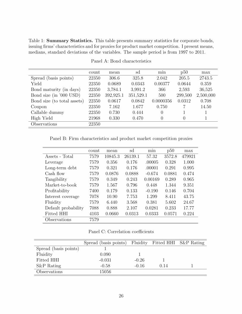
Table 1: Summary Statistics. This table presents summary statistics for corporate bonds,issuing firms’ characteristics and for proxies for product market competition. I present means,medians, standard deviations of the variables. The sample period is from 1997 to 2011.

Panel A: Bond characteristics

count mean sd min p50 maxSpread (basis points) 22350 306.6 325.8 2.042 205.5 2743.5Yield 22350 0.0689 0.0343 0.00377 0.0644 0.359Bond maturity (in days) 22350 3,784.1 3,991.2 366 2,593 36,525Bond size (in ’000 USD) 22350 392,925.1 351,529.1 500 299,500 2,500,000Bond size (to total assets) 22350 0.0617 0.0842 0.0000356 0.0312 0.708Coupon 22350 7.162 1.677 0.750 7 14.50Callable dummy 22350 0.730 0.444 0 1 1High Yield 21968 0.330 0.470 0 0 1Observations 22350

Panel B: Firm characteristics and product market competition proxies

count mean sd min p50 maxAssets - Total 7579 10845.3 26139.1 57.32 3572.8 479921Leverage 7579 0.356 0.176 .00005 0.328 1.000Long-term debt 7579 0.321 0.176 .00001 0.291 0.995Cash flow 7579 0.0876 0.0888 -0.674 0.0881 0.474Tangibility 7579 0.349 0.243 0.00169 0.289 0.965Market-to-book 7579 1.567 0.796 0.448 1.344 9.351Profitability 7400 0.179 0.133 -0.190 0.146 0.704Interest coverage 7078 10.90 7.753 1.299 8.411 43.75Fluidity 7579 6.440 3.568 0.381 5.602 24.67Default probability 7088 0.888 2.107 0.0281 0.233 17.77Fitted HHI 4103 0.0660 0.0313 0.0333 0.0571 0.224Observations 7579

Panel C: Correlation coefficients

Spread (basis points) Fluidity Fitted HHI S&P RatingSpread (basis points) 1Fluidity 0.090 1Fitted HHI -0.031 -0.26 1S&P Rating -0.58 -0.16 0.14 1Observations 15056

26

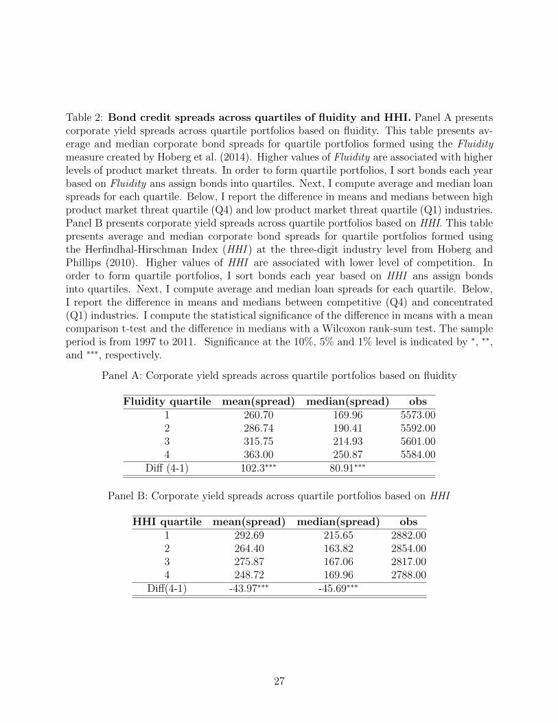
Table 2: Bond credit spreads across quartiles of fluidity and HHI. Panel A presentscorporate yield spreads across quartile portfolios based on fluidity. This table presents av-erage and median corporate bond spreads for quartile portfolios formed using the Fluiditymeasure created by Hoberg et al. (2014). Higher values of Fluidity are associated with higherlevels of product market threats. In order to form quartile portfolios, I sort bonds each yearbased on Fluidity ans assign bonds into quartiles. Next, I compute average and median loanspreads for each quartile. Below, I report the difference in means and medians between highproduct market threat quartile (Q4) and low product market threat quartile (Q1) industries.Panel B presents corporate yield spreads across quartile portfolios based on HHI. This tablepresents average and median corporate bond spreads for quartile portfolios formed usingthe Herfindhal-Hirschman Index (HHI ) at the three-digit industry level from Hoberg andPhillips (2010). Higher values of HHI are associated with lower level of competition. Inorder to form quartile portfolios, I sort bonds each year based on HHI ans assign bondsinto quartiles. Next, I compute average and median loan spreads for each quartile. Below,I report the difference in means and medians between competitive (Q4) and concentrated(Q1) industries. I compute the statistical significance of the difference in means with a meancomparison t-test and the difference in medians with a Wilcoxon rank-sum test. The sampleperiod is from 1997 to 2011. Significance at the 10%, 5% and 1% level is indicated by ∗, ∗∗,and ∗∗∗, respectively.

Panel A: Corporate yield spreads across quartile portfolios based on fluidity

Fluidity quartile mean(spread) median(spread) obs1 260.70 169.96 5573.002 286.74 190.41 5592.003 315.75 214.93 5601.004 363.00 250.87 5584.00

Diff (4-1) 102.3∗∗∗ 80.91∗∗∗

Panel B: Corporate yield spreads across quartile portfolios based on HHI

HHI quartile mean(spread) median(spread) obs1 292.69 215.65 2882.002 264.40 163.82 2854.003 275.87 167.06 2817.004 248.72 169.96 2788.00

Diff(4-1) -43.97∗∗∗ -45.69∗∗∗

27

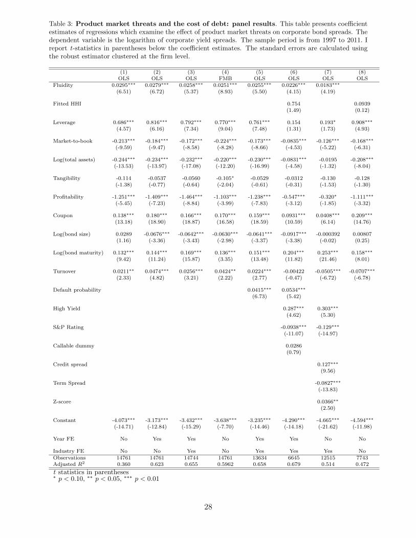
Table 3: Product market threats and the cost of debt: panel results. This table presents coefficientestimates of regressions which examine the effect of product market threats on corporate bond spreads. Thedependent variable is the logarithm of corporate yield spreads. The sample period is from 1997 to 2011. Ireport t-statistics in parentheses below the coefficient estimates. The standard errors are calculated usingthe robust estimator clustered at the firm level.

(1) (2) (3) (4) (5) (6) (7) (8)OLS OLS OLS FMB OLS OLS OLS OLS

Fluidity 0.0295∗∗∗ 0.0279∗∗∗ 0.0258∗∗∗ 0.0251∗∗∗ 0.0255∗∗∗ 0.0226∗∗∗ 0.0183∗∗∗

(6.51) (6.72) (5.37) (8.93) (5.50) (4.15) (4.19)

Fitted HHI 0.754 0.0939(1.49) (0.12)

Leverage 0.686∗∗∗ 0.816∗∗∗ 0.792∗∗∗ 0.770∗∗∗ 0.761∗∗∗ 0.154 0.193∗ 0.908∗∗∗

(4.57) (6.16) (7.34) (9.04) (7.48) (1.31) (1.73) (4.93)

Market-to-book -0.213∗∗∗ -0.184∗∗∗ -0.172∗∗∗ -0.224∗∗∗ -0.173∗∗∗ -0.0835∗∗∗ -0.126∗∗∗ -0.168∗∗∗

(-9.59) (-9.47) (-8.58) (-8.28) (-8.66) (-4.53) (-5.22) (-6.31)

Log(total assets) -0.244∗∗∗ -0.234∗∗∗ -0.232∗∗∗ -0.220∗∗∗ -0.230∗∗∗ -0.0831∗∗∗ -0.0195 -0.208∗∗∗

(-13.53) (-13.97) (-17.08) (-12.20) (-16.99) (-4.58) (-1.32) (-8.04)

Tangibility -0.114 -0.0537 -0.0560 -0.105∗ -0.0529 -0.0312 -0.130 -0.128(-1.38) (-0.77) (-0.64) (-2.04) (-0.61) (-0.31) (-1.53) (-1.30)

Profitability -1.251∗∗∗ -1.409∗∗∗ -1.464∗∗∗ -1.103∗∗∗ -1.238∗∗∗ -0.547∗∗∗ -0.320∗ -1.111∗∗∗

(-5.45) (-7.23) (-8.84) (-3.99) (-7.83) (-3.12) (-1.85) (-3.32)

Coupon 0.138∗∗∗ 0.180∗∗∗ 0.166∗∗∗ 0.170∗∗∗ 0.159∗∗∗ 0.0931∗∗∗ 0.0408∗∗∗ 0.209∗∗∗

(13.18) (18.90) (18.87) (16.58) (18.59) (10.59) (6.14) (14.76)

Log(bond size) 0.0289 -0.0676∗∗∗ -0.0642∗∗∗ -0.0630∗∗∗ -0.0641∗∗∗ -0.0917∗∗∗ -0.000392 0.00807(1.16) (-3.36) (-3.43) (-2.98) (-3.37) (-3.38) (-0.02) (0.25)

Log(bond maturity) 0.132∗∗∗ 0.144∗∗∗ 0.169∗∗∗ 0.136∗∗∗ 0.151∗∗∗ 0.204∗∗∗ 0.253∗∗∗ 0.158∗∗∗

(9.42) (11.24) (15.87) (3.35) (13.48) (11.82) (21.46) (8.01)

Turnover 0.0211∗∗ 0.0474∗∗∗ 0.0256∗∗∗ 0.0424∗∗ 0.0224∗∗∗ -0.00422 -0.0505∗∗∗ -0.0707∗∗∗

(2.33) (4.82) (3.21) (2.22) (2.77) (-0.47) (-6.72) (-6.78)

Default probability 0.0415∗∗∗ 0.0534∗∗∗

(6.73) (5.42)

High Yield 0.287∗∗∗ 0.303∗∗∗

(4.62) (5.30)

S&P Rating -0.0938∗∗∗ -0.129∗∗∗

(-11.07) (-14.97)

Callable dummy 0.0286(0.79)

Credit spread 0.127∗∗∗

(9.56)

Term Spread -0.0827∗∗∗

(-13.83)

Z-score 0.0366∗∗

(2.50)

Constant -4.073∗∗∗ -3.173∗∗∗ -3.432∗∗∗ -3.638∗∗∗ -3.235∗∗∗ -4.290∗∗∗ -4.665∗∗∗ -4.594∗∗∗

(-14.71) (-12.84) (-15.29) (-7.70) (-14.46) (-14.18) (-21.62) (-11.98)

Year FE No Yes Yes No Yes Yes No No

Industry FE No No Yes No Yes Yes Yes NoObservations 14761 14761 14744 14761 13634 6645 12515 7743Adjusted R2 0.360 0.623 0.655 0.5962 0.658 0.679 0.514 0.472

t statistics in parentheses∗ p < 0.10, ∗∗ p < 0.05, ∗∗∗ p < 0.01

28

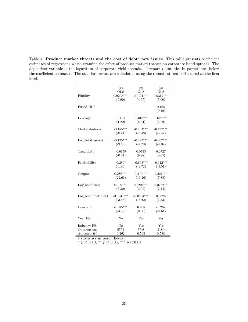
Table 4: Product market threats and the cost of debt: new issues. This table presents coefficientestimates of regressions which examine the effect of product market threats on corporate bond spreads. Thedependent variable is the logarithm of corporate yield spreads. I report t-statistics in parentheses belowthe coefficient estimates. The standard errors are calculated using the robust estimator clustered at the firmlevel.

(1) (2) (3)OLS OLS OLS

Fluidity 0.0208∗∗∗ 0.0171∗∗∗ 0.0312∗∗∗

(5.90) (4.57) (5.00)

Fitted HHI 0.165(0.19)

Leverage 0.110 0.402∗∗∗ 0.625∗∗∗

(1.22) (5.34) (5.29)

Market-to-book -0.155∗∗∗ -0.103∗∗∗ -0.127∗∗∗

(-8.24) (-5.48) (-5.47)

Log(total assets) -0.125∗∗∗ -0.127∗∗∗ -0.207∗∗∗

(-9.58) (-7.79) (-8.04)

Tangibility -0.0159 0.0733 0.0727(-0.31) (0.98) (0.65)

Profitability -0.286∗ -0.608∗∗∗ -0.642∗∗∗

(-1.90) (-3.72) (-3.51)

Coupon 0.286∗∗∗ 0.319∗∗∗ 0.207∗∗∗

(22.61) (16.26) (7.85)

Log(bond size) 0.109∗∗∗ 0.0294∗∗∗ 0.0752∗∗

(6.30) (3.01) (2.44)

Log(bond maturity) -0.0631∗∗∗ -0.0604∗∗∗ 0.0326(-3.56) (-3.22) (1.33)

Constant -1.085∗∗∗ 0.205 -0.262(-4.39) (0.96) (-0.61)

Year FE No Yes Yes

Industry FE No Yes YesObservations 5754 5748 2180Adjusted R2 0.462 0.595 0.588

t statistics in parentheses∗ p < 0.10, ∗∗ p < 0.05, ∗∗∗ p < 0.01

29

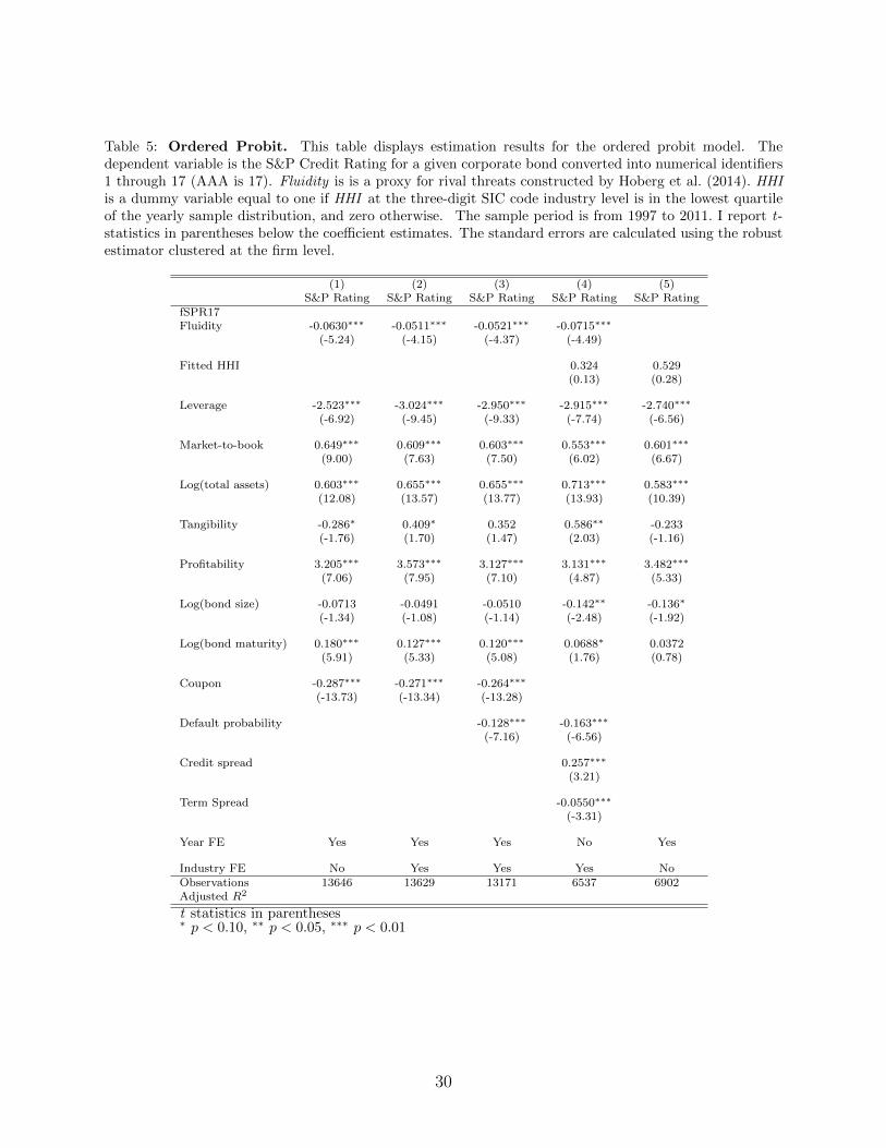
Table 5: Ordered Probit. This table displays estimation results for the ordered probit model. Thedependent variable is the S&P Credit Rating for a given corporate bond converted into numerical identifiers1 through 17 (AAA is 17). Fluidity is is a proxy for rival threats constructed by Hoberg et al. (2014). HHIis a dummy variable equal to one if HHI at the three-digit SIC code industry level is in the lowest quartileof the yearly sample distribution, and zero otherwise. The sample period is from 1997 to 2011. I report t-statistics in parentheses below the coefficient estimates. The standard errors are calculated using the robustestimator clustered at the firm level.

(1) (2) (3) (4) (5)S&P Rating S&P Rating S&P Rating S&P Rating S&P Rating

fSPR17Fluidity -0.0630∗∗∗ -0.0511∗∗∗ -0.0521∗∗∗ -0.0715∗∗∗

(-5.24) (-4.15) (-4.37) (-4.49)

Fitted HHI 0.324 0.529(0.13) (0.28)

Leverage -2.523∗∗∗ -3.024∗∗∗ -2.950∗∗∗ -2.915∗∗∗ -2.740∗∗∗

(-6.92) (-9.45) (-9.33) (-7.74) (-6.56)

Market-to-book 0.649∗∗∗ 0.609∗∗∗ 0.603∗∗∗ 0.553∗∗∗ 0.601∗∗∗

(9.00) (7.63) (7.50) (6.02) (6.67)

Log(total assets) 0.603∗∗∗ 0.655∗∗∗ 0.655∗∗∗ 0.713∗∗∗ 0.583∗∗∗

(12.08) (13.57) (13.77) (13.93) (10.39)

Tangibility -0.286∗ 0.409∗ 0.352 0.586∗∗ -0.233(-1.76) (1.70) (1.47) (2.03) (-1.16)

Profitability 3.205∗∗∗ 3.573∗∗∗ 3.127∗∗∗ 3.131∗∗∗ 3.482∗∗∗

(7.06) (7.95) (7.10) (4.87) (5.33)

Log(bond size) -0.0713 -0.0491 -0.0510 -0.142∗∗ -0.136∗

(-1.34) (-1.08) (-1.14) (-2.48) (-1.92)

Log(bond maturity) 0.180∗∗∗ 0.127∗∗∗ 0.120∗∗∗ 0.0688∗ 0.0372(5.91) (5.33) (5.08) (1.76) (0.78)

Coupon -0.287∗∗∗ -0.271∗∗∗ -0.264∗∗∗

(-13.73) (-13.34) (-13.28)

Default probability -0.128∗∗∗ -0.163∗∗∗

(-7.16) (-6.56)

Credit spread 0.257∗∗∗

(3.21)

Term Spread -0.0550∗∗∗

(-3.31)

Year FE Yes Yes Yes No Yes

Industry FE No Yes Yes Yes NoObservations 13646 13629 13171 6537 6902Adjusted R2

t statistics in parentheses∗ p < 0.10, ∗∗ p < 0.05, ∗∗∗ p < 0.01

30

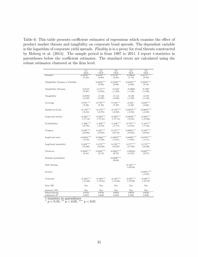
Table 6: This table presents coefficient estimates of regressions which examine the effect ofproduct market threats and tangibility on corporate bond spreads. The dependent variableis the logarithm of corporate yield spreads. Fluidity is is a proxy for rival threats constructedby Hoberg et al. (2014). The sample period is from 1997 to 2011. I report t-statistics inparentheses below the coefficient estimates. The standard errors are calculated using therobust estimator clustered at the firm level.

(1) (2) (3) (4) (5)OLS OLS OLS OLS OLS

Fluidity 0.0259∗∗∗ 0.0162∗∗∗ 0.0170∗∗∗ 0.00654 0.0171∗∗∗

(5.33) (2.90) (3.05) (1.19) (3.02)

Tangibility Dummy x Fluidity 0.0225∗∗∗ 0.0199∗∗∗ 0.0196∗∗∗ 0.0229∗∗∗

(3.05) (2.69) (3.02) (3.10)

Tangibility Dummy 0.0115 -0.117∗∗ -0.104∗ -0.0666 -0.109∗

(0.25) (-2.03) (-1.84) (-1.36) (-1.88)

Tangibility -0.0764 -0.126 -0.114 -0.108 -0.191(-0.58) (-0.95) (-0.89) (-1.02) (-1.44)

Leverage 0.791∗∗∗ 0.778∗∗∗ 0.748∗∗∗ 0.161∗ 0.645∗∗∗

(7.38) (7.34) (7.49) (1.92) (4.66)

Market-to-book -0.172∗∗∗ -0.173∗∗∗ -0.174∗∗∗ -0.0816∗∗∗ -0.0939∗∗∗

(-8.54) (-8.70) (-8.80) (-5.63) (-3.49)

Log(total assets) -0.232∗∗∗ -0.229∗∗∗ -0.228∗∗∗ -0.0928∗∗∗ -0.230∗∗∗

(-17.14) (-17.21) (-17.13) (-6.45) (-15.96)

Profitability -1.466∗∗∗ -1.463∗∗∗ -1.238∗∗∗ -0.775∗∗∗ -1.413∗∗∗

(-8.76) (-8.78) (-7.77) (-6.33) (-7.43)

Coupon 0.166∗∗∗ 0.165∗∗∗ 0.157∗∗∗ 0.0894∗∗∗ 0.162∗∗∗

(19.08) (19.05) (18.76) (13.83) (18.65)

Log(bond size) -0.0642∗∗∗ -0.0660∗∗∗ -0.0659∗∗∗ -0.0690∗∗∗ -0.0783∗∗∗

(-3.44) (-3.59) (-3.51) (-4.65) (-4.11)

Log(bond maturity) 0.169∗∗∗ 0.170∗∗∗ 0.152∗∗∗ 0.177∗∗∗ 0.172∗∗∗

(15.88) (16.08) (13.67) (17.59) (16.28)

Turnover 0.0256∗∗∗ 0.0256∗∗∗ 0.0223∗∗∗ -0.00541 0.0227∗∗∗

(3.21) (3.17) (2.73) (-0.79) (2.77)

Default probability 0.0408∗∗∗

(6.68)

S&P Rating -0.122∗∗∗

(-22.94)

Z-score -0.0591∗∗∗

(-3.35)

Constant -3.432∗∗∗ -3.340∗∗∗ -3.152∗∗∗ -2.872∗∗∗ -3.045∗∗∗

(-15.29) (-14.81) (-14.02) (-15.82) (-12.79)

Year FE Yes Yes Yes Yes Yes

Industry FE Yes Yes Yes Yes YesObservations 14744 14744 13634 13679 13632

Adjusted R2 0.655 0.656 0.659 0.706 0.656

t statistics in parentheses∗ p < 0.10, ∗∗ p < 0.05, ∗∗∗ p < 0.01

31

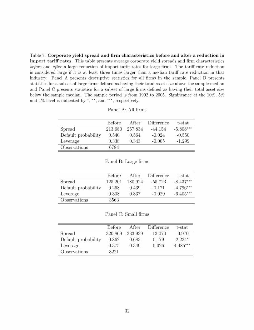
Table 7: Corporate yield spread and firm characteristics before and after a reduction inimport tariff rates. This table presents average corporate yield spreads and firm characteristicsbefore and after a large reduction of import tariff rates for large firms. The tariff rate reductionis considered large if it is at least three times larger than a median tariff rate reduction in thatindustry. Panel A presents descriptive statistics for all firms in the sample, Panel B presentsstatistics for a subset of large firms defined as having their total asset size above the sample medianand Panel C presents statistics for a subset of large firms defined as having their total asset sizebelow the sample median. The sample period is from 1992 to 2005. Significance at the 10%, 5%and 1% level is indicated by ∗, ∗∗, and ∗∗∗, respectively.

Panel A: All firms

Before After Difference t-statSpread 213.680 257.834 -44.154 -5.808∗∗∗

Default probability 0.540 0.564 -0.024 -0.550Leverage 0.338 0.343 -0.005 -1.299Observations 6784

Panel B: Large firms

Before After Difference t-statSpread 125.201 180.924 -55.723 -8.437∗∗∗

Default probability 0.268 0.439 -0.171 -4.796∗∗∗

Leverage 0.308 0.337 -0.029 -6.405∗∗∗

Observations 3563

Panel C: Small firms

Before After Difference t-statSpread 320.869 333.939 -13.070 -0.970Default probability 0.862 0.683 0.179 2.234∗

Leverage 0.375 0.349 0.026 4.485∗∗∗

Observations 3221

32

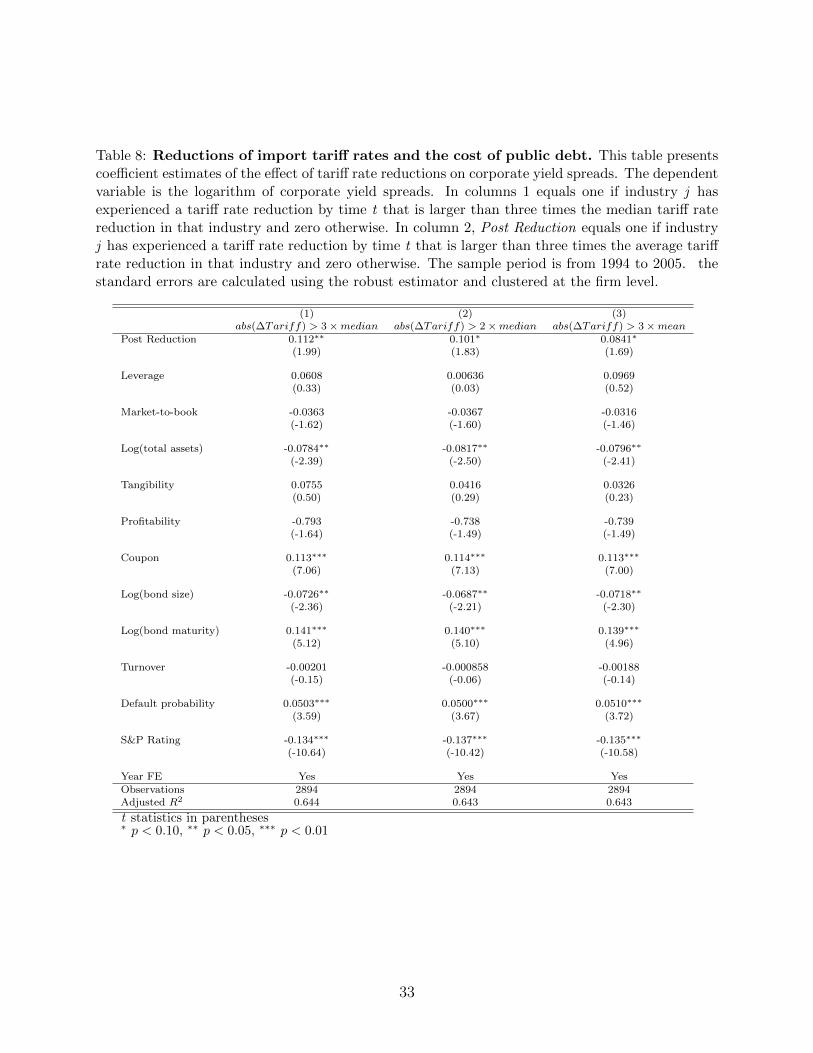
Table 8: Reductions of import tariff rates and the cost of public debt. This table presentscoefficient estimates of the effect of tariff rate reductions on corporate yield spreads. The dependentvariable is the logarithm of corporate yield spreads. In columns 1 equals one if industry j hasexperienced a tariff rate reduction by time t that is larger than three times the median tariff ratereduction in that industry and zero otherwise. In column 2, Post Reduction equals one if industryj has experienced a tariff rate reduction by time t that is larger than three times the average tariffrate reduction in that industry and zero otherwise. The sample period is from 1994 to 2005. thestandard errors are calculated using the robust estimator and clustered at the firm level.

(1) (2) (3)abs(∆Tariff) > 3×median abs(∆Tariff) > 2×median abs(∆Tariff) > 3×mean

Post Reduction 0.112∗∗ 0.101∗ 0.0841∗

(1.99) (1.83) (1.69)

Leverage 0.0608 0.00636 0.0969(0.33) (0.03) (0.52)

Market-to-book -0.0363 -0.0367 -0.0316(-1.62) (-1.60) (-1.46)

Log(total assets) -0.0784∗∗ -0.0817∗∗ -0.0796∗∗

(-2.39) (-2.50) (-2.41)

Tangibility 0.0755 0.0416 0.0326(0.50) (0.29) (0.23)

Profitability -0.793 -0.738 -0.739(-1.64) (-1.49) (-1.49)

Coupon 0.113∗∗∗ 0.114∗∗∗ 0.113∗∗∗

(7.06) (7.13) (7.00)

Log(bond size) -0.0726∗∗ -0.0687∗∗ -0.0718∗∗

(-2.36) (-2.21) (-2.30)

Log(bond maturity) 0.141∗∗∗ 0.140∗∗∗ 0.139∗∗∗

(5.12) (5.10) (4.96)

Turnover -0.00201 -0.000858 -0.00188(-0.15) (-0.06) (-0.14)

Default probability 0.0503∗∗∗ 0.0500∗∗∗ 0.0510∗∗∗

(3.59) (3.67) (3.72)

S&P Rating -0.134∗∗∗ -0.137∗∗∗ -0.135∗∗∗

(-10.64) (-10.42) (-10.58)

Year FE Yes Yes YesObservations 2894 2894 2894Adjusted R2 0.644 0.643 0.643

t statistics in parentheses∗ p < 0.10, ∗∗ p < 0.05, ∗∗∗ p < 0.01

33

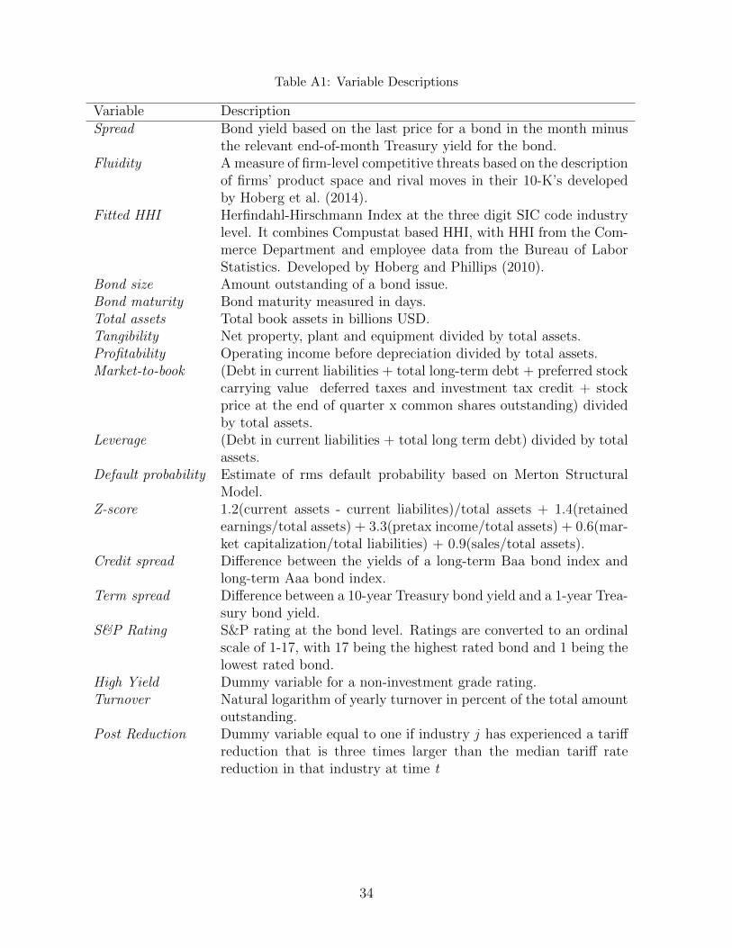
Table A1: Variable Descriptions

Variable DescriptionSpread Bond yield based on the last price for a bond in the month minus

the relevant end-of-month Treasury yield for the bond.Fluidity A measure of firm-level competitive threats based on the description

of firms’ product space and rival moves in their 10-K’s developedby Hoberg et al. (2014).

Fitted HHI Herfindahl-Hirschmann Index at the three digit SIC code industrylevel. It combines Compustat based HHI, with HHI from the Com-merce Department and employee data from the Bureau of LaborStatistics. Developed by Hoberg and Phillips (2010).

Bond size Amount outstanding of a bond issue.Bond maturity Bond maturity measured in days.Total assets Total book assets in billions USD.Tangibility Net property, plant and equipment divided by total assets.Profitability Operating income before depreciation divided by total assets.Market-to-book (Debt in current liabilities + total long-term debt + preferred stock

carrying value deferred taxes and investment tax credit + stockprice at the end of quarter x common shares outstanding) dividedby total assets.

Leverage (Debt in current liabilities + total long term debt) divided by totalassets.

Default probability Estimate of rms default probability based on Merton StructuralModel.

Z-score 1.2(current assets - current liabilites)/total assets + 1.4(retainedearnings/total assets) + 3.3(pretax income/total assets) + 0.6(mar-ket capitalization/total liabilities) + 0.9(sales/total assets).

Credit spread Difference between the yields of a long-term Baa bond index andlong-term Aaa bond index.

Term spread Difference between a 10-year Treasury bond yield and a 1-year Trea-sury bond yield.

S&P Rating S&P rating at the bond level. Ratings are converted to an ordinalscale of 1-17, with 17 being the highest rated bond and 1 being thelowest rated bond.

High Yield Dummy variable for a non-investment grade rating.Turnover Natural logarithm of yearly turnover in percent of the total amount

outstanding.Post Reduction Dummy variable equal to one if industry j has experienced a tariff

reduction that is three times larger than the median tariff ratereduction in that industry at time t

34