Competitive Viral Marketing Based on:

S. Bharathi et al. Competitive Influence Maximization in Social Networks, WINE 2007. C. Budak et al. Limiting the spread of misinformation in social networks. In WWW'11. A. Borodin et al. Threshold models for competitive influence in social networks. In Proc. 6th Workshop on Internet and Network Economic, 2010. X. He et al. Influence Blocking Maximization in Social Networks under the Competitive Linear Threshold Model. In Proc. 2012 SIAM Conf. on Data Mining, pages 463–474, 2012. W. Chen et al. Influence Maximization in Social Networks When Negative Opinions May Emerge and Propagate. In SDM, pages 379–390, 2011.

Why Competition?

• To be blunt, non-competitive is not super realistic.

• Marketing of products, spread of ideas, innovations, political campaigns – all involve competition.

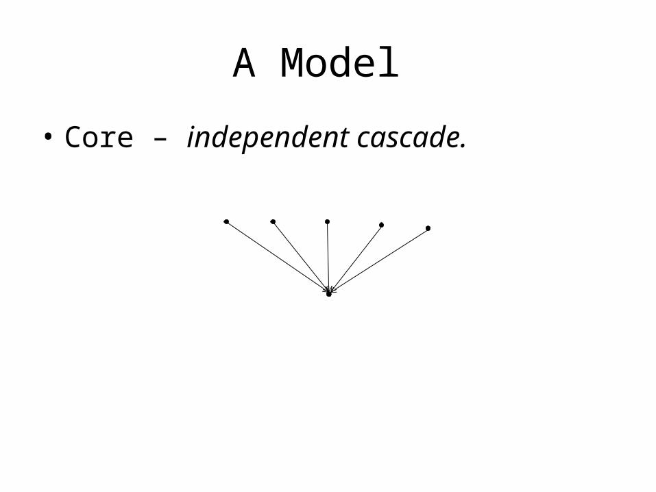
A Model

• Core – independent cascade.

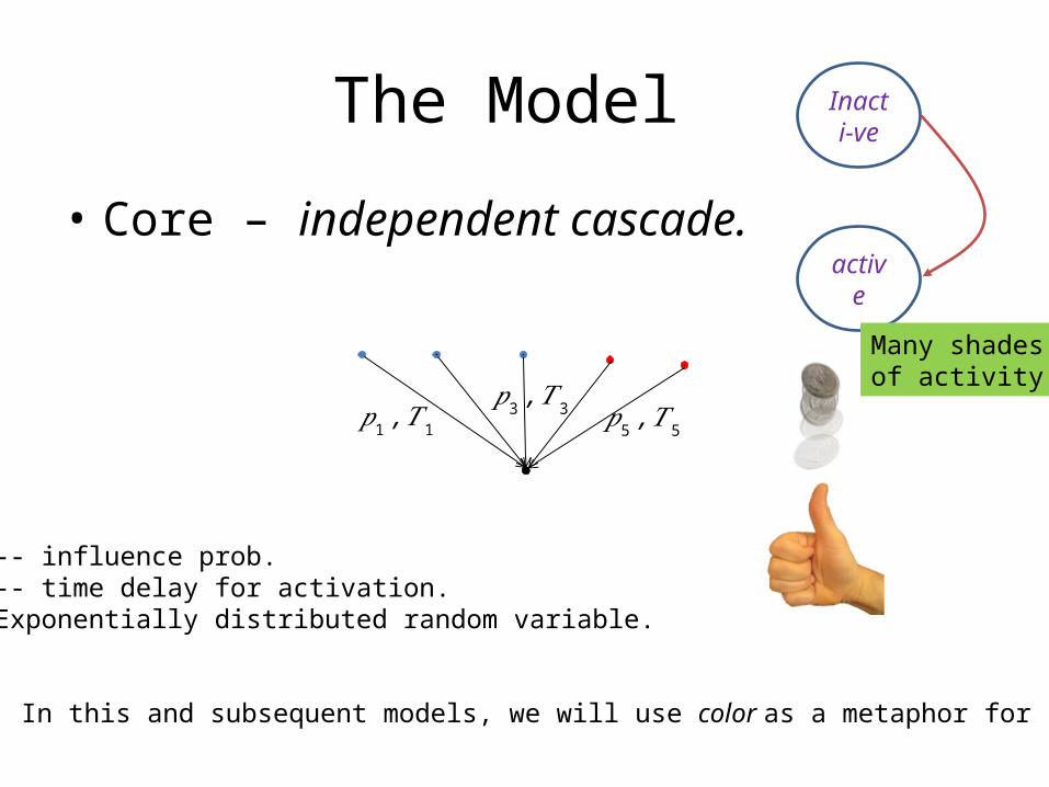
The Model

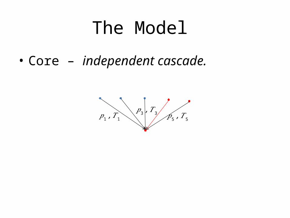
• Core – independent cascade.

𝑝1 ,𝑇 1 𝑝5 ,𝑇5

𝑝3 ,𝑇3

-- influence prob. -- time delay for activation. Exponentially distributed random variable.

Inacti-ve

active

Note: In this and subsequent models, we will use color as a metaphor for state.

Many shades of activity

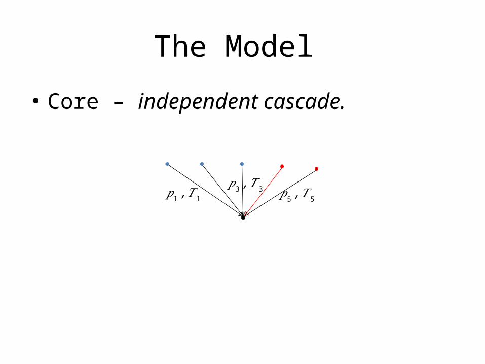
The Model

• Core – independent cascade.

𝑝1 ,𝑇 1 𝑝5 ,𝑇5

𝑝3 ,𝑇3

The Model

• Core – independent cascade.

𝑝1 ,𝑇 1 𝑝5 ,𝑇5

𝑝3 ,𝑇3

The Model

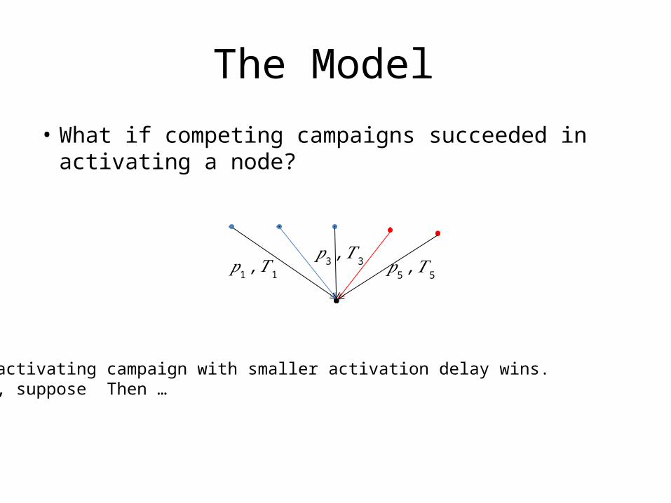
• What if competing campaigns succeeded in activating a node?

𝑝1 ,𝑇 1 𝑝5 ,𝑇5

𝑝3 ,𝑇3

The activating campaign with smaller activation delay wins.E.g., suppose Then …

The Model

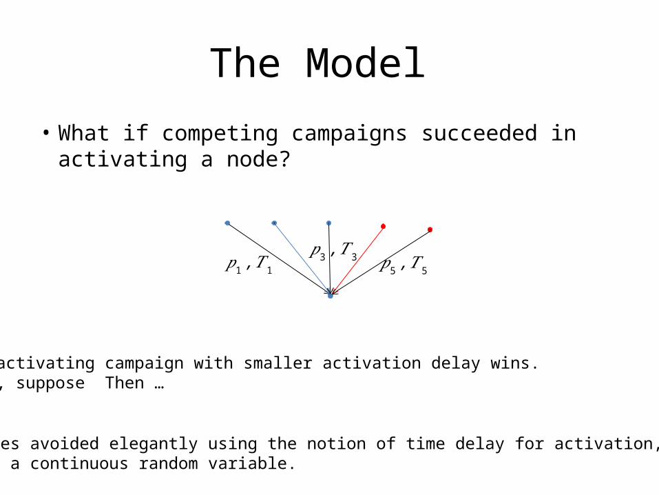
• What if competing campaigns succeeded in activating a node?

𝑝1 ,𝑇 1 𝑝5 ,𝑇5

𝑝3 ,𝑇3

The activating campaign with smaller activation delay wins.E.g., suppose Then …

Note: Ties avoided elegantly using the notion of time delay for activation, which is a continuous random variable.

Properties of the Model

• Let denote the expected #nodes activated with color given the seed sets

• Can show is monotone and submodular in given fixed seed sets for other colors.

• Proof of monotonicity is trivial. • For submodularity, it is analogous to that for the IC

model. • The last player can adopt a greedy strategy to

achieve a -approximation to the optimal spread for its color.

• Can we guarantee this for other players?

Discrete Time Models

• Recall, classical IC/LT models are discrete time. • Use of continuous time in Bharathi et al.’s

competitive IC model is mainly to avoid ties in activation by rival campaigns.

• Discrete time will bring us back to ties and we need tie-breaking rules.

• E.g., competitive IC model: what if two different companies succeed in activating a node?

• Several options exist.

(Discrete Time) CIC Model

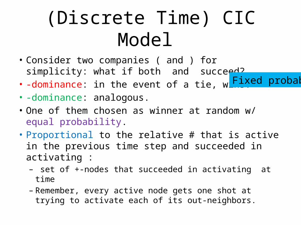
• Consider two companies ( and ) for simplicity: what if both and succeed?

• -dominance: in the event of a tie, wins. • -dominance: analogous. • One of them chosen as winner at random w/ equal

probability. • Proportional to the relative # that is active in the

previous time step and succeeded in activating : – set of +-nodes that succeeded in activating at time – Remember, every active node gets one shot at trying to

activate each of its out-neighbors.

Fixe

d pr

obab

ility

.

CIC Model (contd.)

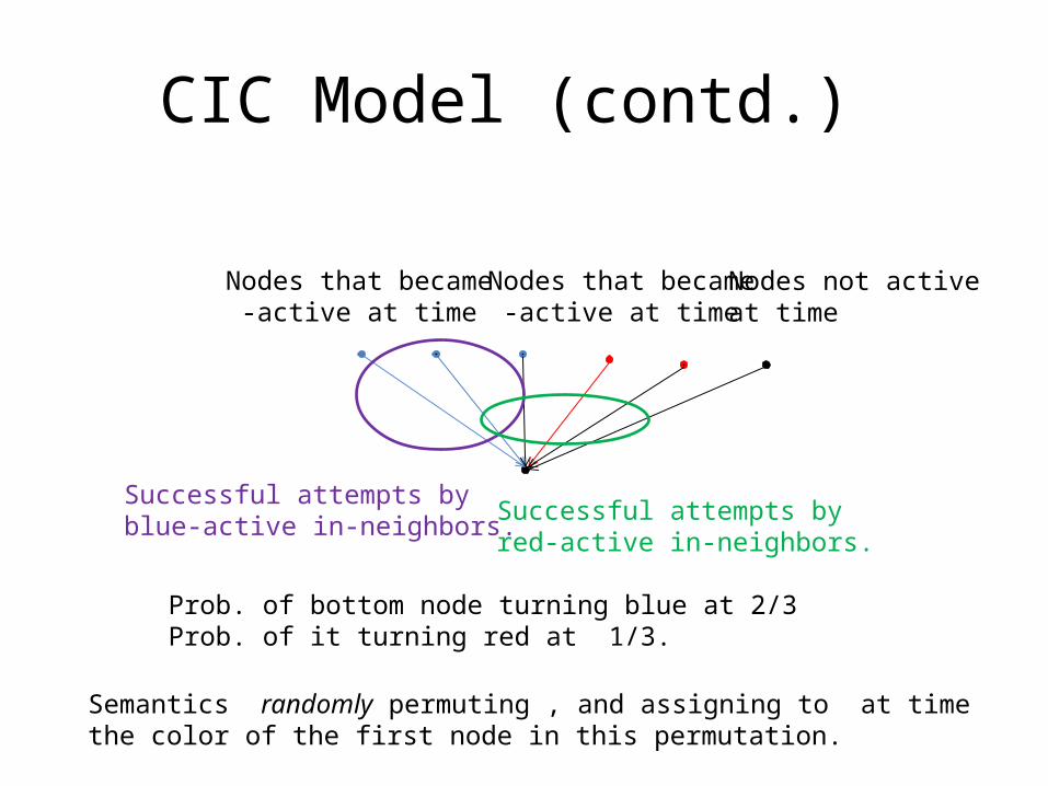
Nodes that became -active at time

Nodes that became -active at time

Nodes not activeat time

Successful attempts by blue-active in-neighbors.

Successful attempts by red-active in-neighbors.

Prob. of bottom node turning blue at 2/3 Prob. of it turning red at 1/3.

Semantics randomly permuting , and assigning to at time the color of the first node in this permutation.

CIC Model (contd.)

• Some generalizations/observations: – Positive and negative influence probs could be

different: e.g., say your neighbors are more easily convinced by any negative opinion from you, but are more cautious in reacting to positive opinion from you:

– Model semantics is still well-defined. – Natural assumption: seed sets for diff. campaigns

are disjoint: technically don’t need this!

CIC Model (concluded)

• How do the propagations happen? • seeds for color • ; • Add a node iff – or – There was a tie and won the tie.

• Continue until is inactive, being the current time.

Competitive LT (CLT) Model

• General case: weights and , for each link • Each node picks activation thresholds and

independently and uniformly at random from • turns if and

CLT Model (contd.)

• turns if and • When both thresholds are exceeded, apply a

tie-breaker rule. • dominance, fixed probability rules –

analogous to CIC. • Proportionate prob. case not fully explored in

the literature, but has potential.

CIC – Equiv. Live-Edge Model

• Let be given prob. graph. • Toss coins associated with all arcs w.p. to generate one

possible world a deterministic graph. • Generate similarly; note, the generations are

independent. • Predetermine random choices for tie-breaking in

advance (just in case!): – If fixed prob., toss a coin for each node with that prob.: let

remember that outcome. – For proportionate, its in-neighbors in and remembers this

permutation

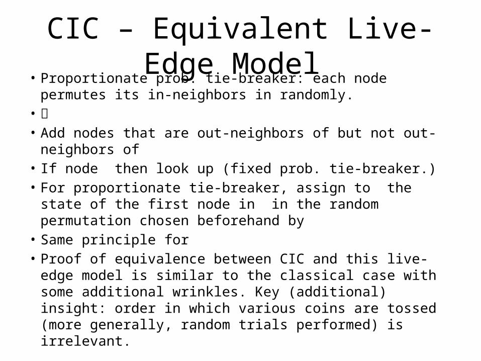
CIC – Equivalent Live-Edge Model • Proportionate prob. tie-breaker: each node permutes its in-

neighbors in randomly. • • Add nodes that are out-neighbors of but not out-neighbors of • If node then look up (fixed prob. tie-breaker.)• For proportionate tie-breaker, assign to the state of the first

node in in the random permutation chosen beforehand by • Same principle for • Proof of equivalence between CIC and this live-edge model is

similar to the classical case with some additional wrinkles. Key (additional) insight: order in which various coins are tossed (more generally, random trials performed) is irrelevant.

CLT – Equivalent Live-Edge Model

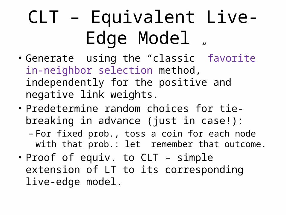
• Generate using the “classic” favorite in-neighbor selection method, independently for the positive and negative link weights.

• Predetermine random choices for tie-breaking in advance (just in case!): – For fixed prob., toss a coin for each node with

that prob.: let remember that outcome. • Proof of equiv. to CLT – simple extension of LT

to its corresponding live-edge model.

What do we want to optimize?

• expected #nodes that are positively activated at end of campaign, given seeds .

• expected #nodes that are negatively activated at end of campaign, given seeds .

• Some interesting questions: Given graph, seed budget , and negative seed set , find the positive seed set of size that maximizes – Symmetry between and – Influence maximization under competition. – How hard is IM under competition?

What else do we want to optimize?

• Given negative seeds, positive seeds tend to counteract their influence (and vice versa), i.e., We can thus ask, given the graph, negative seeds and budget , find the positive seed set that maximizes the reduction: . influence blocking maximization. (“damage control” maximization!)

Influence Maximization under Competition

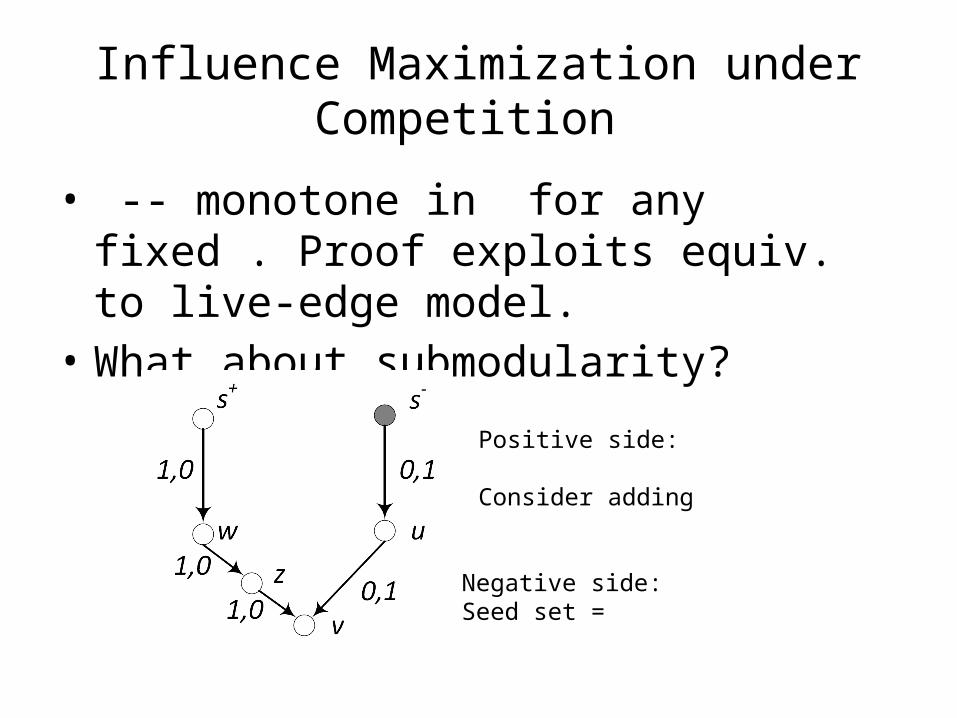
• -- monotone in for any fixed . Proof exploits equiv. to live-edge model.

• What about submodularity?

Positive side:

Consider adding

Negative side: Seed set =