Embed Size (px)
Citation preview
1
COMPETITIVENESS AND EFFICIENCY OF RICE
PRODUCTION IN MALAYSIA
Dissertation
to obtain the Ph. D. degree
in the International Ph. D. Program for Agricultural Sciences in Goettingen (IPAG)
at the Faculty of Agricultural Sciences,
Georg-August-University Göttingen, Germany
presented by
FAZLEEN ABDUL FATAH
born in Kelantan, Malaysia
Göttingen, February 2017
2
D7
1. Name of supervisor : Professor Dr. Stephan von Cramon-Taubadel
2. Name of co-supervisor: Professor Dr. Bernhard Brümmer
Date of dissertation: 3rd
February 2017
i
Acknowledgement
I knew from the beginning that pursuing my doctoral degree would be both a painful and
rewarding experience. This poignant journey has taught me the importance of persevering
despite hardship. However, despite having endured challenging times, I am grateful for all of
the support and contributions I received during this journey. As I reflect upon this
mesmerizing adventure, I realize that I owe my success to the camaraderie and assistance of
numerous people who I am indebted to. Words cannot express my gratitude to all of the
people who have helped me in many ways.
First and foremost, I would like to give my sincere thanks to my honorific advisor, Professor
Dr. Stephan von Cramon-Taubadel, who accepted me as his PhD student without hesitation
when I presented him with my first proposal nearly three years ago. Ever since, he has
supported me not only by consistently providing excellent resources and scholarly inputs, but
also by delivering academic and emotional support along the difficult road to finishing this
dissertation. He gave me countless advice, patiently offered his supervision and always
guided me in the right direction. I am especially grateful for his ability to understand my
needs while writing this dissertation. During the most difficult times, he gave me the
permission I needed to move on. I cannot imagine having a better advisor and mentor for my
PhD study.
I am also very grateful to my second advisor, Professor Dr. Bernhard Brümmer for his
scientific advice, knowledge and suggestions, which led to numerous insightful discussions.
He is my primary resource for answering technical questions and was instrumental in helping
me crank out the decomposition section of my dissertation; thanks to him I was able to
accomplish this in one month! In addition to my advisors, I would like to thank another
essential member of my dissertation committee, Professor Dr. Reimund P. Rötter for his
perceptive comments and encouragement, but also for posing the tough questions, which
encouraged me to widen my research from various perspectives.
My sincere thanks additionally go to the local people and stakeholders in Muda Agricultural
Development Authority (MADA), Kedah; the experts working with BERNAS, the Ministry
of Agriculture Malaysia (MOA); and the Kemubu Agricultural Development Authority
(KADA), Kelantan. Each of these individuals generously gave their time and ideas during the
research assessment. I wish to deliver a special thanks to En. Kamaruddin Dahuli and En.
Rumzi bin Ahmad from Muda Agricultural Development Authority (MADA). These
individuals allowed me to conduct my study in the local area and provided me with access to
the necessary data and research facilities. Without their precious support and invaluable
inputs, it would not have been possible to conduct this research. I am especially grateful to
En. Sufri, Cik Anis Azura Abd. Rahman and En. Yusoff who offered me their time and
cooperation when I collected important data for my dissertation.
I would like also to convey my heartfelt thanks to the Ministry of Higher Education (MOHE)
Malaysia and the Universiti Teknologi MARA, Malaysia (UiTM) for awarding me the
Academic Training Scheme for Lecturers (SLAI) Scholarship for my postgraduate study.
Without their support and financial assistance, I would not have been able to successfully
complete this dissertation.
A lot of people say that the pursuit of your PhD can be quite a lonely process. I was fortunate
enough to have the opposite experience as I was surrounded by a brilliant and supportive

ii
community. For that, I thank my dearest Kamlisa Uni Kamlun who has been a very critical
and passionate friend- someone whom I could trust and soundboard with, and even voice my
frustrations to. She inspired strength when I was feeling lost. Thanks for the stimulating
discussions, for the sleepless nights we spent together before deadlines and, of course, during
the difficult, early stages of my pregnancy, and for all the fun we had in the last two and half
years in Göttingen. You have always been a great friend and words cannot express how truly
grateful I am to you and your wonderful family. Special thanks also to my friends in
Göttingen for their support from the beginning of my arrival in Göttingen until the end: Alisa
Ali, Shahril Anuar Bahari, Suhaidah Mohd Jofrry and Wan Ilma Dewiputri.
In addition, I would like to extend a thank you to all the colleagues at the Chair of
Agricultural Policy for the lively discussions and support during these years: Antje Wagener,
Dr. Said Tifaoui, Dr. Ganzorig Gonchigsumlaa, Dr. Nelissa Jamora, Dr. Sebastian Lakner, Dr.
Carsten Holst, Evgeniya Pavlova, Luis De los Santos, Qu Yi and Jorge Carcamo. Particularly,
I am utmost grateful to Dr. Jonathan Holtkamp for providing me with ample guidance and
support with solving a lot of research and technical problems.
Thank you to the friends I have made along the way in Göttingen for your unconditional love
and support: Dr. Nadzifah Yaakob, Syahidah Mohd Nor and Wan Elhami Wan Omar. Special
thanks to the top management of the Faculty of Plantation and Agrotechnology, UiTM:
Assoc. Professor. Dr. Fauziah Ismail and Assoc. Professor Dr. Asmah Awal who helped me
secure scholarships when I expressed my desire to pursue my PhD degree at the University of
Göttingen in Germany. Their encouragement and assistance enabled me to confidently fulfill
my desire and to overcome the challenges I encountered.
I especially thank my dad, Abdul Fatah Haron, my mom, Rahimah Hussein and my family.
My hardworking parents dedicated their lives to ensuring the well-being of my siblings and
myself and they have provided us with unconditional love and care. I love them so much and I
would not have made it this far without them. My sisters and brothers have been my best
friends all my life. I love them dearly and I thank them for all their advice and support. I know
that I can always count on my family when times are tough.
Special thanks to my devoted husband, Ahmad Zulhilmi Mokhtar, as well as my father-in-
law, Dr. Mokhtar Nor and my mother-in-law, Kamariah Ismail, and the rest of Zulhilmi’s
wonderful family who have been supportive and caring during this process. My husband has
been a true and great supporter and has loved me unconditionally during my good and bad
times. He has reserved judgment and was instrumental in instilling confidence in me. These
past several years have not been an easy ride, both academically and personally. I truly thank
him for sticking by my side, even when I was irritable and depressed. Playing the role of both
father and mother while I was studying was not an easy task for him. He assumed every
responsibility and graciously cared for my son and my family. Finally, thank you to our
children: our darling Fudhail Zahran who was such a good boy, and to the newest addition to
our family, baby ‘F’, who was such a sweet little angel in my tummy for the past seven
months, because of that it was possible for me to complete what I started. I owe my every
achievement to them.
Above all, I owe it all to ALLAH, the Almighty God, for granting me the wisdom, health and
strength to undertake this research task and enabling me to ensure its completion.
iii
Abstract
Rice is one of the most essential staple foods for a large part of the world’s human population and
has a large influence on human nutrition, the livelihood and food security of several billion people
living across the globe. Similar to other Asian countries, the rice crop plays an important role in
Malaysian society as it fosters agricultural activity and is a major source of employment for many
Malaysian farmers. However, the advent of free trade agreements, including the Asean Free Trade
Agreement (AFTA) and the WTO accession, pose challenges for the Malaysian rice production as
the sector must compete with low-cost exporting countries. This outcome implies the need for not
only structural changes in trade, but also adjustments at the farm level to improve efficiency and
competitiveness. Further developments in the rice sector will therefore depend on the availability
of sufficient, relatively low-cost and high-quality rice, or in other words, on the competitiveness
of rice production.
In line with that, the primary objective of this dissertation is to look into a competitiveness
assessment of rice production in Malaysia. Furthermore, the work aims to analyze the changes in
farm level efficiency over time for rice farms in Malaysia and to gain insight into the factors that
determine the distribution of efficiency and competitiveness. Finally, by establishing the linkage
between both comparative advantage/competitiveness and technical efficiency, the results of this
research would then provide us with a foundation for understanding the information, the
measurements and the characteristics associated with each method and how this link may
contribute to explaining competitiveness. Overall, this newly accumulated knowledge has the
potential to guide the direction of the policy’s effects.
In order to achieve the established goals, the dissertation adopts a new extension to the Policy
Analysis Matrix approach proposed by Monke and Pearson (1989) using farm level survey data.
The measurement of competitiveness in agriculture is often based on the average farms or
aggregate data. If the farms that are summarized in this manner are heterogeneous, inferences
based on aggregated measure can be misleading. As means of addressing misrepresentative
information and the pitfalls of using aggregated data, this extension will allow us to take farm
level heterogeneity into account and study the distributions of the competitiveness scores for each
rice farm. Subsequently, we conduct an empirical technical efficiency analysis with unobserved
heterogeneity and employ a recent fixed effect model. The static decomposition of
competitiveness, which is presented by linking comparative advantage/competitiveness and
technical efficiency, concludes this PhD dissertation.
The main findings of this dissertation can be summarized in the following points: three out of four
granary areas have comparative advantages in rice production using the average data; however,
regional averages can hide considerable variation among farms. Between 2011 and 2014, the
average SCB ratios were greater than 1, which indicates that rice production was not competitive
in MADA granary areas. Despite this observation, many farmers appear to be competitive; more
than 60% of farms produce rice competitively and these competitive farms account for a
disproportionately large share of rice production when using disaggregate data. Additionally, in
the period from 2010 to 2014, many farms showed improvements in the technical efficiency with
more efficient farms produced disproportionately more rice outputs. Specifically, the mean values
were around 50-60%, implying many farms were far from the frontier. However, the rice output
per farm can be increased through the efficient use of the resources. Finally, the results presented
in this dissertation demonstrate that competitiveness has a positive relationship with the level of
technical efficiency, thus confirming our perception of the static decomposition.
iv
Table of Content
Acknowledgement ....................................................................................................................... i
Abstract ..................................................................................................................................... iii
Table of Content ........................................................................................................................ iv
List of Figures ........................................................................................................................... vi
List of Tables ............................................................................................................................ vii
List of Appendices .................................................................................................................. viii
List of Abbreviations ................................................................................................................. ix
Chapter 1 ............................................................................................................................... 1
1.1 Background and objectives ......................................................................................... 1
1.2 Agriculture overview in Malaysia ............................................................................... 3
1.2.1 Significant roles of rice in Malaysian economy ................................................... 5
1.2.2 Rice policy in Malaysia ......................................................................................... 7
1.2.3 Case study site: MADA granary area .................................................................. 12
1.3 Objectives and research questions ............................................................................. 15
1.4 Overview and outline of the chapters ........................................................................ 16
Chapter 2 ............................................................................................................................. 27
2.1 Introduction ............................................................................................................... 28
2.2 Policy measures in the rice industry .......................................................................... 31
2.3 Material and Method ................................................................................................. 34
2.3.1 Policy Analysis Matrix ........................................................................................ 34
2.3.2 Data collection ..................................................................................................... 38
2.4 Result and Discussion ............................................................................................... 40
2.4.1 Policy analysis matrix in the context of import parity price of rice .................... 40
2.4.2 Sensitivity analysis .............................................................................................. 44
2.5 Conclusion ................................................................................................................. 46
Chapter 3 ............................................................................................................................. 54
3.1 Introduction ............................................................................................................... 55
3.2 Rice production and policies in Malaysia ................................................................. 56
v
3.3 Measuring .................................................................................................................. 58
3.4 Data and ..................................................................................................................... 59
3.5 Results and discussion ............................................................................................... 61
3.5.1 The profile of rice farming .................................................................................. 61
3.5.2 The competitiveness of rice production .............................................................. 63
3.5.3 The determinants of rice competitiveness ........................................................... 65
3.6 Results and Discussion .............................................................................................. 67
3.7 Conclusion and recommendations ............................................................................ 70
Chapter 4 ............................................................................................................................. 84
4.1 Introduction ............................................................................................................... 85
4.2 Methods to measure efficiency using panel data ...................................................... 87
4.3 Data and empirical definitions of the variables ......................................................... 90
4.4 Results and discussions ............................................................................................. 96
4.5 Conclusions ............................................................................................................. 103
Chapter 5 ........................................................................................................................... 113
5.1 Introduction ............................................................................................................. 113
5.2 Strength and weaknesses of the PAM and SFA approaches ................................... 116
5.3 Policy Analysis Matrix (PAM) ............................................................................... 119
5.4 Stochastic Frontier Analysis (SFA) approach ......................................................... 122
5.4.1 Fixed effect panel model using CFE estimation ............................................... 122
5.4.2 A primal system of Profit Maximization ........................................................... 124
5.5 Static decomposition of competitiveness ................................................................ 128
5.5.1 Decomposition of PCB ...................................................................................... 128
5.5.2 Decomposition of SCB ...................................................................................... 130
5.6 Empirical Illustration ............................................................................................... 133
5.7 Conclusion ............................................................................................................... 138
Chapter 6 ........................................................................................................................... 146
6.1 Key contributions and summary ............................................................................. 146
6.2 Policy implications and options .............................................................................. 150
6.3 Data limitations and methodological issues ............................................................ 153
6.4 Directions for future research .................................................................................. 154
vi
List of Figures
Figure 2.1: Rice Production, Consumption, Yield and Harvested Area in Malaysia (1980-
2013) ........................................................................................................................................ 29
Figure 2.2: Change of Domestic resource cost (DRC) in the import rice prices in Malaysia .. 44
Figure 3.1: Average rice yields, ASEAN countries for 2010-2013.. ....................................... 57
Figure 3.2: Distribution of competitiveness scores (SCB) for the rice farms, 2010-2014 ....... 64
Figure 4.1: Distribution of the TE of rice farms, 2010-2014 ................................................... 99
Figure 5.1: Distribution of rice farms’ competitiveness scores (PCB and SCB) ................... 133
Figure 5.2: Distribution rice farms’ technical efficiency, 2010-2014 .................................... 134
Figure 5.3: Demonstration of decomposition of competitiveness level (logPCB versus TE) 135
Figure 5.4: Distributions of Technical Inefficiency (TI) and Allocative Inefficiency (AI) ... 136
vii
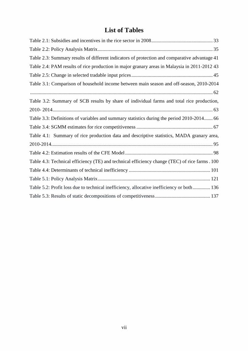
List of Tables
Table 2.1: Subsidies and incentives in the rice sector in 2008 ................................................. 33
Table 2.2: Policy Analysis Matrix ............................................................................................ 35
Table 2.3: Summary results of different indicators of protection and comparative advantage 41
Table 2.4: PAM results of rice production in major granary areas in Malaysia in 2011-2012 43
Table 2.5: Change in selected tradable input prices ................................................................. 45
Table 3.1: Comparison of household income between main season and off-season, 2010-2014
.................................................................................................................................................. 62
Table 3.2: Summary of SCB results by share of individual farms and total rice production,
2010- 2014 ................................................................................................................................ 63
Table 3.3: Definitions of variables and summary statistics during the period 2010-2014 ....... 66
Table 3.4: SGMM estimates for rice competitiveness ............................................................. 67
Table 4.1: Summary of rice production data and descriptive statistics, MADA granary area,
2010-2014. ................................................................................................................................ 95
Table 4.2: Estimation results of the CFE Model ...................................................................... 98
Table 4.3: Technical efficiency (TE) and technical efficiency change (TEC) of rice farms . 100
Table 4.4: Determinants of technical inefficiency ................................................................. 101
Table 5.1: Policy Analysis Matrix .......................................................................................... 121
Table 5.2: Profit loss due to technical inefficiency, allocative inefficiency or both .............. 136
Table 5.3: Results of static decompositions of competitiveness ............................................ 137
viii
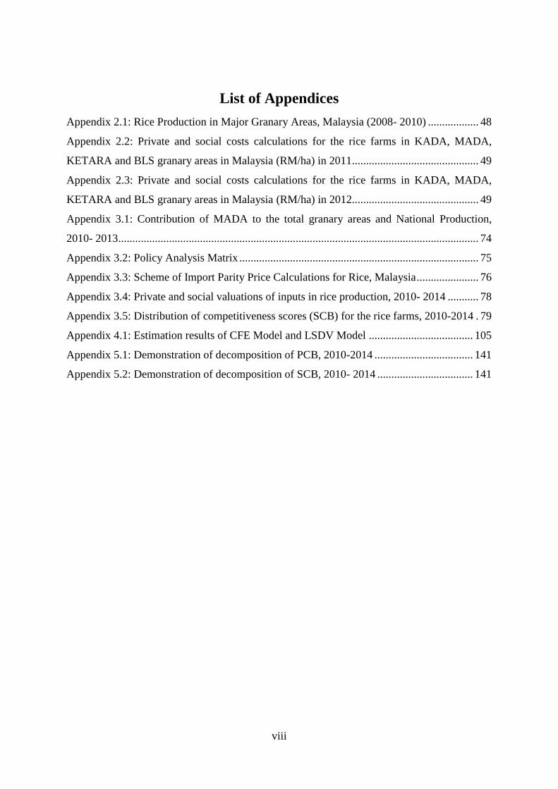
List of Appendices
Appendix 2.1: Rice Production in Major Granary Areas, Malaysia (2008- 2010) .................. 48
Appendix 2.2: Private and social costs calculations for the rice farms in KADA, MADA,
KETARA and BLS granary areas in Malaysia (RM/ha) in 2011............................................. 49
Appendix 2.3: Private and social costs calculations for the rice farms in KADA, MADA,
KETARA and BLS granary areas in Malaysia (RM/ha) in 2012............................................. 49
Appendix 3.1: Contribution of MADA to the total granary areas and National Production,
2010- 2013 ................................................................................................................................ 74
Appendix 3.2: Policy Analysis Matrix ..................................................................................... 75
Appendix 3.3: Scheme of Import Parity Price Calculations for Rice, Malaysia ...................... 76
Appendix 3.4: Private and social valuations of inputs in rice production, 2010- 2014 ........... 78
Appendix 3.5: Distribution of competitiveness scores (SCB) for the rice farms, 2010-2014 . 79
Appendix 4.1: Estimation results of CFE Model and LSDV Model ..................................... 105
Appendix 5.1: Demonstration of decomposition of PCB, 2010-2014 ................................... 141
Appendix 5.2: Demonstration of decomposition of SCB, 2010- 2014 .................................. 141
ix
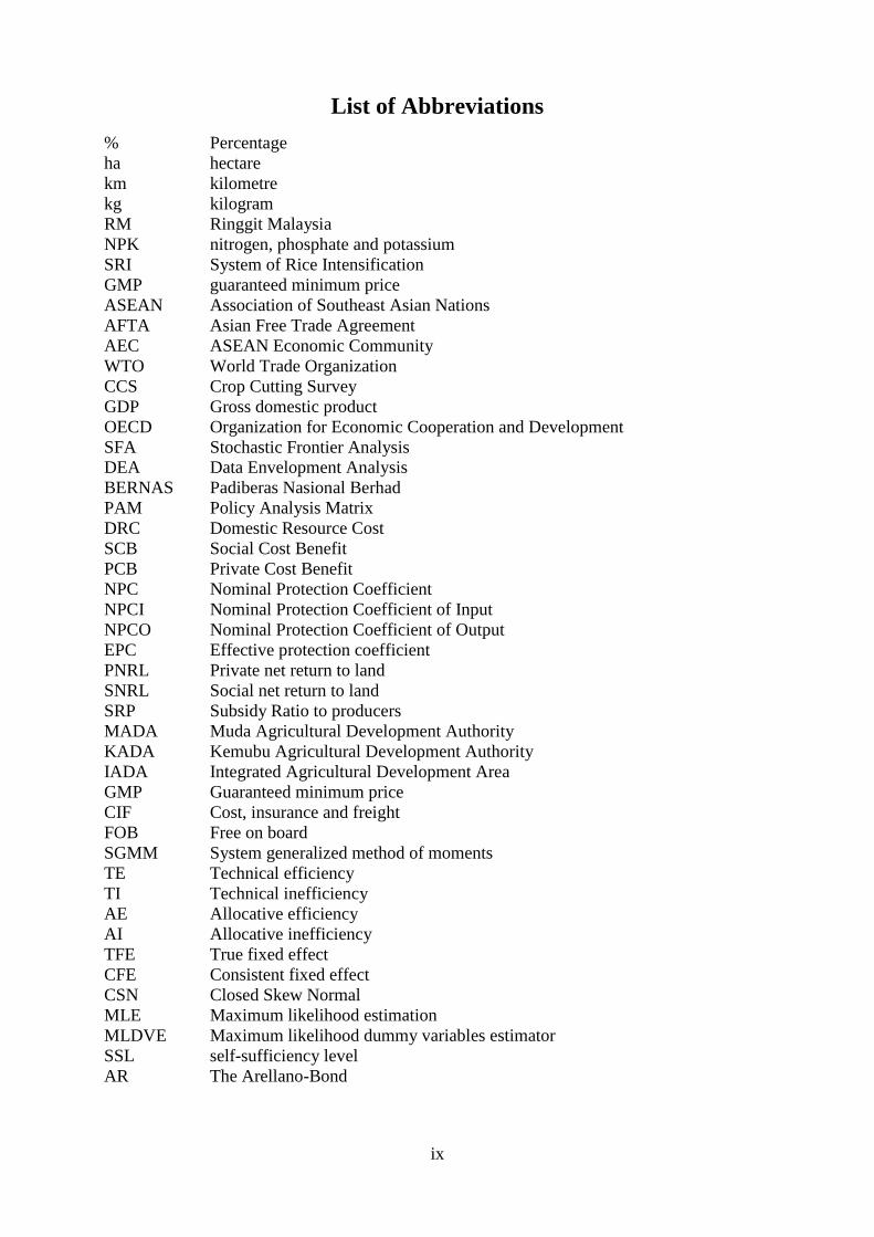
List of Abbreviations
% Percentage
ha hectare
km kilometre
kg kilogram
RM Ringgit Malaysia
NPK nitrogen, phosphate and potassium
SRI System of Rice Intensification
GMP guaranteed minimum price
ASEAN Association of Southeast Asian Nations
AFTA Asian Free Trade Agreement
AEC ASEAN Economic Community
WTO World Trade Organization
CCS Crop Cutting Survey
GDP Gross domestic product
OECD Organization for Economic Cooperation and Development
SFA Stochastic Frontier Analysis
DEA Data Envelopment Analysis
BERNAS Padiberas Nasional Berhad
PAM Policy Analysis Matrix
DRC Domestic Resource Cost
SCB Social Cost Benefit
PCB Private Cost Benefit
NPC Nominal Protection Coefficient
NPCI Nominal Protection Coefficient of Input
NPCO Nominal Protection Coefficient of Output
EPC Effective protection coefficient
PNRL Private net return to land
SNRL Social net return to land
SRP Subsidy Ratio to producers
MADA Muda Agricultural Development Authority
KADA Kemubu Agricultural Development Authority
IADA Integrated Agricultural Development Area
GMP Guaranteed minimum price
CIF Cost, insurance and freight
FOB Free on board
SGMM System generalized method of moments
TE Technical efficiency
TI Technical inefficiency
AE Allocative efficiency
AI Allocative inefficiency
TFE True fixed effect
CFE Consistent fixed effect
CSN Closed Skew Normal
MLE Maximum likelihood estimation
MLDVE Maximum likelihood dummy variables estimator
SSL self-sufficiency level
AR The Arellano-Bond
Background of study
1
Chapter 1
Background of study
1.1 Background and objectives
Rice is the most economically important staple food crop for a large part of the human
population, providing more than 3 billion people in Asia with two thirds of their caloric
intake, and supplying nearly 1.5 billion people in Africa and Latin America with one third of
their caloric needs (FAO, 1995a). The total rice harvested globally in 2010 equated to
approximately 154 million hectare (ha). The majority of this amount was harvested in Asia
(137 million ha or 88% of the rice harvested globally), 31% of which, or about 48 million ha,
was harvested in Southeast Asia alone (Redfern et al, 2012).
Given the economic predominance of rice and its direct link to global food security, the state
of the economy in the region in which rice is produced plays a significant role. The World
Food Summit (1996) succinctly describes food security as “when all people, at all times, have
physical and economic access to sufficient, safe and nutritious food to meet their dietary
needs and food preferences for an active and healthy life”. In Asia, food security has been
defined as maintaining stable prices for rice in the major urban markets of each country (The
Asia Foundation, 2010) in which rice is a major staple food for more than half of the
population. In South Asia, rice makes up a dominant portion of approximately 70% of the
population’s diet. This degree of rice consumption is the highest in the world; hence food
security is essentially a reflection of rice security in this region. Therefore, an effective way to
promote national level food security is by achieving self-sufficiency in rice production
(Bishwajit et al, 2013).
When food security is equated with food self-sufficiency, this strategy makes sense since it is
easier to stabilize domestic food prices using domestic production by stimulating high prices
than to depend on the world rice market, which has great price volatility. However, this
approach may significantly increase the spread of poverty as it forces poor consumers to pay
high prices for rice. As Timmer (2010) argued, if the countries were more open to the rice
trade, they would be richer not poorer.
Background of study
2
At the same time, most governments in Southeast Asia have pursued price stabilization
mechanisms or provided supports to protect their domestic producers. These mechanisms
incorporate a vast array of instruments from storage, input subsidies, income supports, floor
prices and rice distribution programs to trade policies, such as tariffs and quantitative
restrictions. However, these mechanisms and supports have been subject to intense debate in
the policy analysis arena since five decades ago (Timmer, 1989). On the one hand, rice prices
need to be affordable so that poor consumers benefit most from the stable rice prices. In
contrast, farm prices need to be high enough for the farmers, who often lead precarious lives
and are net rice sellers, to sustain their incomes. Additionally, rice prices must be high enough
to provide farmers with adequate incentives to continue investing in rice production.
However, simultaneously protecting both producers and consumers is very costly (Warr and
Yusuf, 2014) and has become a politically contentious issue.
Recently, the implementation of the Asian Free Trade Agreement (AFTA) and the
Association of Southeast Asian Nations (ASEAN) Economic Community (AEC) has signified
a major milestone in the region’s economic integration and free trade status. The region has
remained ambitious with aims of becoming integrated, competitive, innovative and dynamic
enough to integrate domestic markets fully into the global economy. In the context of the
products and crops sectors of Malaysia’s farms particularly rice, this objective leads to
increased competition with other countries exporting rice at a low-cost. Furthermore, the
introduction of domestic markets into the global economy creates opportunities for trade
between ASEAN countries and imposes new conditions on local farms that include
opportunities to enhance profits, while potentially enhances competitiveness of each farm’s
production. This implies that not only structural changes to trading practices, but also
adjustments at the farm level are required to improve each farm’s efficiency and profitability.
Further developments in the rice sector will, therefore, depend on the availability of sufficient,
relatively low-cost and high-quality rice, or in other words, on the competitiveness of rice
production. Consequently, understanding the key factors, the driving forces and the
limitations of rice production under the dynamics of the global rice market is crucial to
improving the overall competitiveness and efficiency of Malaysia’s rice production.
Background of study
3
1.2 Agriculture overview in Malaysia
Malaysia is located in Southeast Asia and has a total area of 329,758 square kilometers
(127,320 square miles). It is divided into two similarly sized regions, Peninsular Malaysia and
East Malaysia (Malaysian Borneo). Peninsular Malaysia is bordered by Thailand in the north,
Indonesia and Singapore in the south, and the Philippines in the east, while East Malaysia
borders with Brunei and Indonesia (Kalimantan). The country consists of 13 states, and is
divided into 2 parts: 11 states are located in Peninsular Malaysia and 2 states are situated on
the island of Borneo (see map). The Malaysian population is nearly 28 million, while the
population density was 86 people per square kilometer in 2010 (Department of Statistics
Malaysia, 2011)
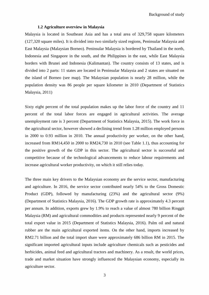
Sixty eight percent of the total population makes up the labor force of the country and 11
percent of the total labor forces are engaged in agricultural activities. The average
unemployment rate is 3 percent (Department of Statistics Malaysia, 2015). The work force in
the agricultural sector, however showed a declining trend from 1.28 million employed persons
in 2000 to 0.93 million in 2010. The annual productivity per worker, on the other hand,
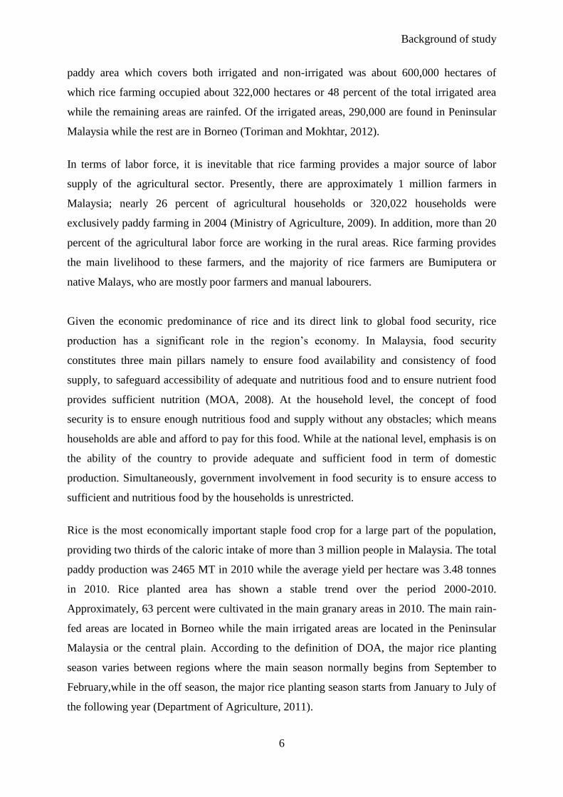
increased from RM14,450 in 2000 to RM24,730 in 2010 (see Table 1.1), thus accounting for
the positive growth of the GDP in this sector. The agricultural sector is successful and
competitive because of the technological advancements to reduce labour requirements and
increase agricultural worker productivity, on which it still relies today.
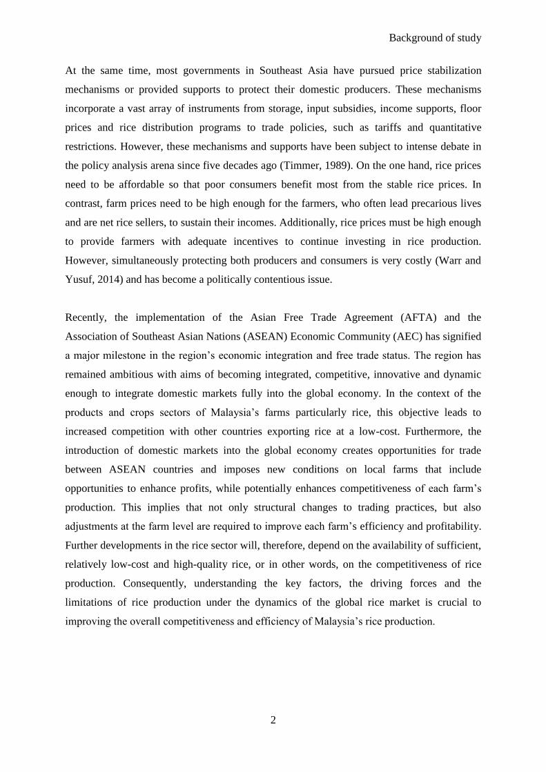
The three main key drivers to the Malaysian economy are the service sector, manufacturing
and agriculture. In 2016, the service sector contributed nearly 54% to the Gross Domestic
Product (GDP), followed by manufacturing (23%) and the agricultural sector (9%)
(Department of Statistics Malaysia, 2016). The GDP growth rate is approximately 4.3 percent
per annum. In addition, exports grew by 1.9% to reach a value of almost 780 billion Ringgit
Malaysia (RM) and agricultural commodities and products represented nearly 9 percent of the
total export value in 2015 (Department of Statistics Malaysia, 2016). Palm oil and natural
rubber are the main agricultural exported items. On the other hand, imports increased by
RM2.71 billion and the total import share were approximately 686 billion RM in 2015. The
significant imported agricultural inputs include agriculture chemicals such as pesticides and
herbicides, animal feed and agricultural tractors and machinery. As a result, the world prices,
trade and market situation have strongly influenced the Malaysian economy, especially its
agriculture sector.
Background of study
4
Figure 1.1 Percentage share to GDP at Constant 2010 Price
Note: Exclude import duties. Source: Department of Statistics Malaysia, 2016
Table 1.1: Employment and Agricultural Productivity, 1985- 2010
Source: Economic Planning Unit, Department of Statistics, Malaysia
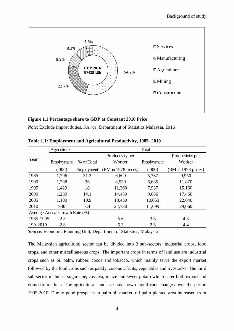
The Malaysian agricultural sector can be divided into 3 sub-sectors: industrial crops, food
crops, and other miscelllaneous crops. The important crops in terms of land use are industrial
crops such as oil palm, rubber, cocoa and tobacco, which mainly serve the export market
followed by the food crops such as paddy, coconut, fruits, vegetables and livestocks. The third
sub-sector includes, sugarcane, cassava, maize and sweet potato which cater both export and
domestic markets. The agricultural land use has shown significant changes over the period
1995-2010. Due to good prospects in palm oil market, oil palm planted area increased from
54.2%
22.7%
8.9%
8.2%
4.6%
GDP 2016
RM281.8b
Services
Manufacturing
Agriculture
Mining
Construction
Agriculture Total
Employment % of Total
Productivity per
Worker Employment
Productivity per
Worker
('000) Employment (RM in 1978 prices) ('000) (RM in 1978 prices)
1985 1,796 31.3 6,600 5,737 9,950
1990 1,738 26 8,530 6,685 11,870
1995 1,429 18 11,360 7,937 15,160
2000 1,280 14.1 14,450 9,066 17,460
2005 1,100 10.9 18,450 10,053 22,640
2010 930 8.4 24,730 11,099 29,060
Average Annual Growth Rate (%)
1985-1995 -2.3 5.6 3.3 4.3
199-2010 -2.8 5.3 2.3 4.4
Year
Background of study
5
2540 thousand hectares in 1995 to 3637 thousand hectares in 2010. Conversely, the planted
area for paddy continued to decline to 450 thousand hectares in 2010 compared to 673
thousand hectares in 1995 as a result of conversion of paddy land for other land uses,
including urbanisation (Table 1.2).
Interestingly, agricultural value-added grew at 3.0 per cent per annum over 2001-2005 and 5
per cent per annum over the period 2006-2010. In 2005, agricultural value added was RM21.6
billion (in 1987 constant prices) or 8.2 % of the GDP and it increased to RM49.7 billion or
14.2% of the GDP in 2010 (Olaniyi et al. 2013).
Table 1.2: Agricultural land use in Malaysia and average annual growth rate, 1995-
2010 (in 1000 ha)
Crops Year Average Annual Growth Rate (%)
1995 2000 2005 2010 1995 2000 2005 2010
Industrial crops
Rubber 1679 1560 1395 1185 -1.5 -2.2 -3.2 -2.3
Oil palm 2540 3131 3461 3637 4.3 2 1 2.4
Cocoa 191 164 160 160 -3 -0.5 0 -1.2
Tobacco 11 9 8 6 -2.4 -3.5 -4.5 -3.5
Food crops
Paddy 673 521 475 450 -5 -1.8 -1.1 -2.6
Coconut 249 214 193 176 -3 -2 -1.9 -2.3
Pepper 10 9 9 8 -2 -1.6 -1 -1.5
Vegetables 42 48 64 86 2.7 5.7 6.2 4.9
Fruits 258 292 330 373 2.5 2.5 2.5 2.5
Others 99 106 111 130 1.4 0.9 3.1 1.8
Total 5,751 6,055 6,205 6,211 1 0.5 0 0.5
Source: Economic Planning Unit, Ministry of Agriculture, Malaysia
1.2.1 Significant roles of rice in Malaysian economy
The agricultural sector has played a significant role in the Malaysian economy and has been
considered as the third engine of growth, after services and manufacturing. In fact, the rice
sector employs many Malaysians as well as creates food supply, food-sufficiency and income
for the farmers.
Rice is grown in all states of Malaysia. In terms of land use, rice farming occupies 8 percent
(465 thousand hectares) of the agricultural land of the country, while other food crops, such as
coconut, fruits and vegetables share about 10 percent of agricultural land. In 1993, the total
Background of study
6
paddy area which covers both irrigated and non-irrigated was about 600,000 hectares of
which rice farming occupied about 322,000 hectares or 48 percent of the total irrigated area
while the remaining areas are rainfed. Of the irrigated areas, 290,000 are found in Peninsular
Malaysia while the rest are in Borneo (Toriman and Mokhtar, 2012).
In terms of labor force, it is inevitable that rice farming provides a major source of labor
supply of the agricultural sector. Presently, there are approximately 1 million farmers in
Malaysia; nearly 26 percent of agricultural households or 320,022 households were
exclusively paddy farming in 2004 (Ministry of Agriculture, 2009). In addition, more than 20
percent of the agricultural labor force are working in the rural areas. Rice farming provides
the main livelihood to these farmers, and the majority of rice farmers are Bumiputera or
native Malays, who are mostly poor farmers and manual labourers.
Given the economic predominance of rice and its direct link to global food security, rice
production has a significant role in the region’s economy. In Malaysia, food security
constitutes three main pillars namely to ensure food availability and consistency of food
supply, to safeguard accessibility of adequate and nutritious food and to ensure nutrient food
provides sufficient nutrition (MOA, 2008). At the household level, the concept of food
security is to ensure enough nutritious food and supply without any obstacles; which means
households are able and afford to pay for this food. While at the national level, emphasis is on
the ability of the country to provide adequate and sufficient food in term of domestic
production. Simultaneously, government involvement in food security is to ensure access to
sufficient and nutritious food by the households is unrestricted.
Rice is the most economically important staple food crop for a large part of the population,
providing two thirds of the caloric intake of more than 3 million people in Malaysia. The total
paddy production was 2465 MT in 2010 while the average yield per hectare was 3.48 tonnes
in 2010. Rice planted area has shown a stable trend over the period 2000-2010.
Approximately, 63 percent were cultivated in the main granary areas in 2010. The main rain-
fed areas are located in Borneo while the main irrigated areas are located in the Peninsular
Malaysia or the central plain. According to the definition of DOA, the major rice planting
season varies between regions where the main season normally begins from September to
February,while in the off season, the major rice planting season starts from January to July of
the following year (Department of Agriculture, 2011).
Background of study
7
Like Japan, Thailand and many other Asian countries, rice farmers and rural communities are
perceived as preservers of Malaysian cultural values. Instead of commercial reasons like food
exports and tourism, the cultural values associates with the rice farming help to create strong
communal bonds, which have been involved in the local beliefs, traditions, ceremonies and
religious activities. In Japan, agriculture is commonly considered as a way of life and the
autumn festivals as thanksgiving of good harvest and reunion time where family members
return to their hometowns to worship their ancestors are still being practiced. Whereas in
Thailand, an annual important occasion of the Royal Ploughing Ceremony is held in May at
the Royal Field in front of the Grand Palace in Bangkok (TRFRP, 2006). This ceremony gives
people, especially rice farmers, the opportunity to collect the rice seeds sowed by ‘Phaya
Raek Na’ which is believed to bring good luck. In Malaysia, The Gawai Day is celebrated
every June by the Dayaks (natives of Sarawak state). It is a celebration for giving thanks to
God for a good harvest. This is a celebration for tourists as well, where they can partake in
the unique agricultural atmosphere. (Chuen-Khee, 2009).
1.2.2 Rice policy in Malaysia
Rice is a major staple food and it is one of the major calorie providers for many Malaysians.
Given its economic importance in the society and the country, the government has been
intervening more in the rice sector than in most others. There are three main obejctives of the
different rice policies adopted by the government through the decades; i) to ensure food
security; ii) to raise productivity and income of the farmers and iii) to ensure adequate food
supply at reasonable costs. The intervention levels through direct or indirect support are
mandated under various National Agricultural Plan (NAP).
Background of study
8
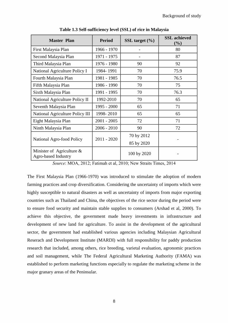
Table 1.3 Self-sufficiency level (SSL) of rice in Malaysia
Master Plan Period SSL target (%) SSL achieved
(%)
First Malaysia Plan 1966 - 1970 - 80
Second Malaysia Plan 1971 - 1975 - 87
Third Malaysia Plan 1976 - 1980 90 92
National Agriculture Policy I 1984- 1991 70 75.9
Fourth Malaysia Plan 1981 - 1985 70 76.5
Fifth Malaysia Plan 1986 - 1990 70 75
Sixth Malaysia Plan 1991 - 1995 70 76.3
National Agriculture Policy II 1992-2010 70 65
Seventh Malaysia Plan 1995 - 2000 65 71
National Agriculture Policy III 1998- 2010 65 65
Eight Malaysia Plan 2001 - 2005 72 71
Ninth Malaysia Plan 2006 - 2010 90 72
National Agro-food Policy 2011 - 2020 70 by 2012
- 85 by 2020
Minister of Agriculture &
Agro-based Industry
100 by 2020 -
Source: MOA, 2012; Fatimah et al, 2010; New Straits Times, 2014
The First Malaysia Plan (1966-1970) was introduced to stimulate the adoption of modern
farming practices and crop diversification. Considering the uncertainty of imports which were
highly susceptible to natural disasters as well as uncertainty of imports from major exporting
countries such as Thailand and China, the objectives of the rice sector during the period were
to ensure food security and maintain stable supplies to consumers (Arshad et al, 2000). To
achieve this objective, the government made heavy investments in infrastructure and
development of new land for agriculture. To assist in the development of the agricultural
sector, the government had established various agencies including Malaysian Agricultural
Reserach and Development Institute (MARDI) with full responsibility for paddy production
research that included, among others, rice breeding, varietal evaluation, agronomic practices
and soil management, while The Federal Agricultural Marketing Authority (FAMA) was
established to perform marketing functions especially to regulate the marketing scheme in the
major granary areas of the Peninsular.
Background of study
9
However, in the early 70s, rice policy in Malaysia had shifted from focusing exclusively on
food security, as in the 1960s, to the objectives of self-sufficiency and income distribution
between producers and consumers. In the Third Malaysia Plan (1976-1980), the goverment
aimed to achieve the self-sufficiency level of 90 percent. These goals were pursued through
double cropping on increasing acreage, drainage and irrigation infrastructure expansion, price
support, and extension services.
Through the years, the self-sufficiency targets were deliberately lowered because of the
government's decision to diversify and intensify agriculture, particularly the production of
industrial crops which provide higher earnings than rice. However, in the Third National
Agriculture Policy (1998-2010), eight granary areas were designated as permanent rice
growing areas responsible for achieving at least 65 percent self-sufficiency. The Eight
Malaysia Plan (2001-2005) increased this target to 72 percent, and the Ninth Malaysia Plan
(2006-2010) increased it further to 90 percent. However, these targets were not met. In 2014,
the Minister of Agriculture and Agro-based Industry announced that Malaysia is determined
to achieve its target to end rice imports and be fully self-sufficient by 2020.
In order to ensure that rice supply is sufficient for the nation various measures have been
taken: subsidies, ranging from a fertilizer subsidy and cash assistance to rice farmers; direct
intervention of the government in price stabilization; development of irrigation and
infrastructure; as well as mechanization projects have been introduced. In terms of production
incentives, the government has implemented a Guaranteed Minimum Price (GMP), paddy
price subsidy and an input subsidy. This price guarantee is to ensure that the paddy price
remains above GMP or at least at GMP level. GMP was first introduced in 1949 at the rate of
248 RM per ton to ensure paddy farmers receive a reasonable minimum farm income. The
rate was later revised in 2014 to increase to 1,200 RM per ton, partly due to the increase in
input prices and labor costs.
Another form of production incentive is the price subsidy. This scheme was introduced in
1980 at the rate of 165 RM per ton and was then revised and increased to 248.10 RM per ton
in 1990. The high poverty prevalance among the rural farmers has directed the intervention by
the government to address the situation and raise farmers’ income to at least above the
poverty line of 300 RM per month.
Background of study
10
Considering the increasing cost of paddy production in the granary areas, the government
provided input subsidies to the farmers in the form of fertilizer, and chemical inputs. Since
1974, farmers who owned less than 10 hectares of lands received free fertilizers (240 kg per
hectare of mixed fertilizer, 80 kg per hectare of organic fertilizer and 150 kg (3 bags) of
NPK;nitrogen, phosphate and potassium). Along with trying to shield farmers’ income from
high input costs, the objective of input subsidy is to encourage farmers to use fertilizers
efficiently according to the recommendation rate proposed by Department of Agriculture or
Malaysian Agriculture Research and Development Institute (MARDI). In addition, farmers
also receive a coupon of chemical inputs for purchasing weed and pest controls worth of 200
RM/ha.
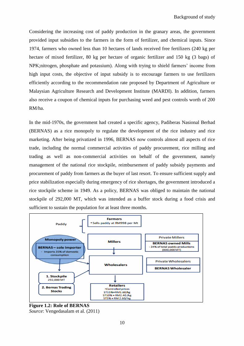
In the mid-1970s, the government had created a specific agency, Padiberas Nasional Berhad
(BERNAS) as a rice monopoly to regulate the development of the rice industry and rice
marketing. After being privatized in 1996, BERNAS now controls almost all aspects of rice
trade, including the normal commercial activities of paddy procurement, rice milling and
trading as well as non-commercial activities on behalf of the government, namely
management of the national rice stockpile, reimbursement of paddy subsidy payments and
procurement of paddy from farmers as the buyer of last resort. To ensure sufficient supply and
price stabilization especially during emergency of rice shortages, the government introduced a
rice stockpile scheme in 1949. As a policy, BERNAS was obliged to maintain the national
stockpile of 292,000 MT, which was intended as a buffer stock during a food crisis and
sufficient to sustain the population for at least three months.
Figure 1.2: Role of BERNAS
Source: Vengedasalam et al. (2011)
Background of study
11
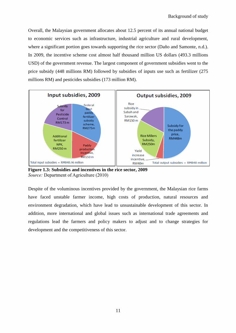
Overall, the Malaysian government allocates about 12.5 percent of its annual national budget
to economic services such as infrastructure, industrial agriculture and rural development,
where a significant portion goes towards supporting the rice sector (Daño and Samonte, n.d.).
In 2009, the incentive scheme cost almost half thousand million US dollars (493.3 millions
USD) of the government revenue. The largest component of government subsidies went to the
price subsidy (448 millions RM) followed by subsidies of inputs use such as fertilizer (275
millions RM) and pesticides subsidies (173 million RM).
Figure 1.3: Subsidies and incentives in the rice sector, 2009
Source: Department of Agriculture (2010)
Despite of the voluminous incentives provided by the government, the Malaysian rice farms
have faced unstable farmer income, high costs of production, natural resources and
environment degradation, which have lead to unsustainable development of this sector. In
addition, more international and global issues such as international trade agreements and
regulations lead the farmers and policy makers to adjust and to change strategies for
development and the competitiveness of this sector.
Background of study
12
1.2.3 Case study site: MADA granary area
After Independence in 1957, the government made massive public investments, including
irrigation infrastructure to supplement rainfall of a single crop. By early 1970, the first phase
of rice double cropping was successfully launched through the implementation of a
development project for both water resources and irrigation as well as drainage infrastructures
(which received irrigation water from the dam for the first time). This project which is known
as Muda Irrigation Project has allowed irrigating the rice fields during the dry season and
supplementing the supply of water for crop requirements during the end of the wet season
(less rainfall). The project has resulted in a massive increase in the cropping intensity of
approximately 190% (Chan and Cho, 2012). Increased investment in irrigation and drainage
facilities, together with improved farm road networks and other infrastructures had been
instrumental in changing the scenario of rice production in Malaysia.
The success of rice double cropping has been furthered through the development of irrigation
infrastructures to eight permanent designated granary areas. Granary Areas are the irrigated
areas that refer to major irrigation schemes (areas greater than 4,000 hectares) and recognized
by the Government in the National Agricultural Policy as the main paddy producing areas
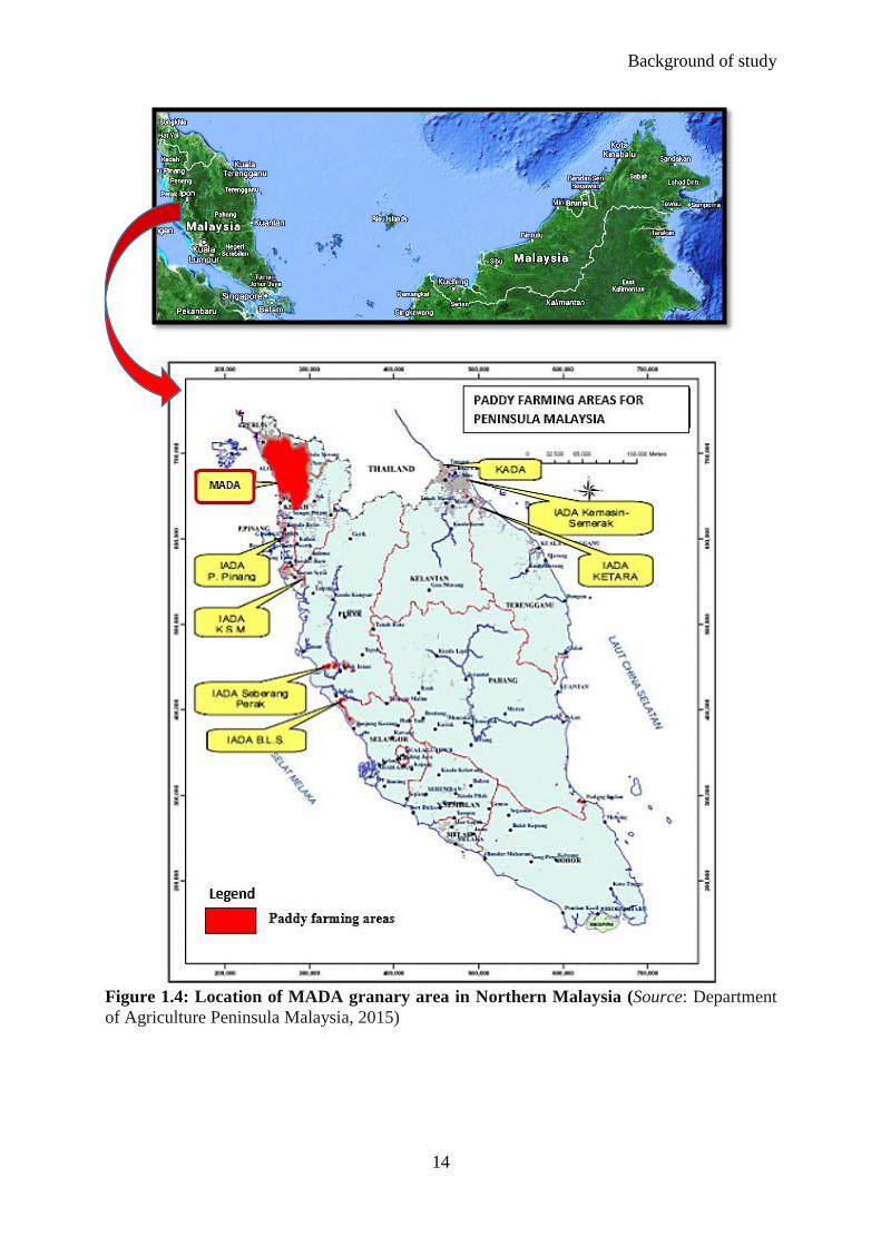
(Department of Agriculture, 2014). There are eight granary areas in Malaysia, namely Muda
Agricultural Development Authority (MADA), Kemubu Agricultural Development Authority
(KADA), Kemasin Semerak Integrated Agricultural Development Area (IADA Kemasin-
Semerak), Kerian-Sg. Manik Integrated Agricultural Development Area (IADA KSM), Barat
Laut Selangor Integrated Agricultural Development Area (IADA BLS), Pulau Pinang
Integrated Agricultural Development Area (IADA P. Pinang), Seberang Perak Integrated
Agricultural Development Area (IADA Seberang Perak), and Northern Terengganu
Integrated Agricultural Development Area (IADA KETARA) (refer to Figure 1.4). These
eight granaries have been responsible for scaling up and increasing productivity in the rice
farming as well as contributing to at least 65% of total rice production in the country.
This study was performed in the MADA granary area in Kedah, located in northern Malaysia
(Figure 2). MADA is located in the Muda Irrigation Scheme that covers about 130,282 ha of
which about 108,581 ha or 84% of the total irrigated areas are in the north-west of Kedah
state and 21,701 ha (19%) are located in the southern part of Perlis State. MADA is the
largest granary area in Malaysia and contributed 51% of total granary production in 2013. It
Background of study
13
consistently generates 37% of Malaysia’s total annual rice production on 33% of the
country’s rice area.
The average temperature in MADA was 27.4°C in 2008 with an average maximum
temperature of 33°C, and average minimum of 22° (Afroz and Ba, n.d.). The optimum
temperature of 34°C allows for the high-yielding rice cultivars of MR219, MR220 and
MR232 to be grown in this granary area. Annual rainfall averages over 2,500mm; this far
exceeds the global annual average of 1,050mm (Chan and Cho 2012). Rainfall is inextricably
linked to the seasonal monsoons; the southwest monsoon and the northeast monsoon
seasons.The northeast monsoons,which are usually established in early May and end in
September, provide a wet season in Kedah, particularly for the MADA granary area in which
rice grows. The northeast monsoon of early November until late March provides a dry season
that allows the rice fields to dry out and rice to ripen and be harvested. During this dry season,
the Muda Irrigation Scheme allows rice fields to be flooded so as to enable double cropping
of rice in a more intensive fashion.
Since its establishment in 1970, MADA has been given the responsibility to undertake any
agricultural development in the Muda area in Kedah and Perlis. The main function of MADA
is to improve the social economics and well-being of the farmers, especially the rural
population, and to implement efficient and effective use of irrigation and water resources for
irrigated paddy cultivation as well as provide credit and agricultural services to farmers under
MADA.
Background of study
14
Figure 1.4: Location of MADA granary area in Northern Malaysia (Source: Department
of Agriculture Peninsula Malaysia, 2015)
Background of study
15
1.3 Objectives and research questions
In correspondence to the previously mentioned problems, the overall objective of this study is
to empirically analyze the current effects of policies, and to investigate the level and
composition of policy supports and the actual market structure inherent to economic
incentives in Malaysia’s rice sector. In particular, this study will serve four main purposes:
First, it will present an analysis of the comparative advantages or competitiveness of rice
production under different scenarios of existing policies and economic reforms.
Second, it will contribute to the understanding of the forces that drive the competitiveness of
rice production in Malaysia.
Third, it will investigate the technical efficiency among the rice farms in Malaysia and
determine the factors that influence it.
Fourth, by establishing the linkage between both competitiveness and efficiency, the results
of this research will enable the comprehension of this information, the measurements and the
characteristics associated with each method and how these details may contribute to
explaining competitiveness.
The central research questions addressed in this dissertation are as follows:
i) Is rice sufficiently profitable privately to provide farmers with the incentive to
maintain or expand output?
ii) Is rice production in Malaysia socially profitable, and hence, should Malaysia
endeavor for self-sufficiency?
iii) Is rice production in Malaysia competitive?
iv) What are the factors that influence competitiveness at the individual farm level?
v) Will a farm that becomes more efficient become competitive as a result?
vi) Are rice farms in Malaysia technically efficient?
vii) Does efficiency enhance competitiveness?
viii) Is there a positive correlation between a farm’s comparative/competitive advantage
and efficiency?
ix) How are these two types of analysis (competitiveness and efficiency) related?
Background of study
16
1.4 Overview and outline of the chapters
To comprehend the remainder of this work, it is essential to have a clear understanding of
‘competitiveness’. This section aims to introduce further insights on the term’s conceptual
foundation as means of achieving clarity for the following chapters.
Most of the questions posed by the relevant economic literature revolve around how to
allocate resources in order to ensure social welfare, including the establishment of high living
standards and high employment rates. Researchers often rely on the concept of
competitiveness as the basis of analysis when they are interested in determining which sector
contributes the most to the nation’s economic growth. ‘Competitiveness’ has a broad meaning
that has yet to gain universal definition acceptance in economics (Sharples, 1990). The
Organization for Economic Cooperation and Development (OECD) succinctly describes
competitiveness as “the ability of companies, industries, regions, nations and supranational
regions to generate, while being and remaining exposed to international competition, a
relatively high factor of income and factor employment levels on a sustainable basis”
(Hatzichronologou, 1996). The European Commission (2001) defines competitiveness as "the
ability of an economy to provide its population with high and rising standards of living and
high rates of employment on a sustainable basis”. Others relate this meaning to profitability.
Agriculture Canada (1991) defines competitiveness as “the ability to gain profits and
maintain market share”.
Given the broad concept and ambiguity present in the literature, competitiveness is a relative
measure. Thus, depending on the purpose of the study, the level of analysis, and the
commodity in question, several methodologies for estimating competitiveness have been
developed (see more in Hatzichronoglou, 1996; Latruffe, 2010; von Cramon-Taubadel and
Nivyevskyi, 2008 etc.). Latruffe (2010) classifies measurement into two disciplines: 1) the
neoclassical economies that place emphasis on trade and measure competitiveness with
comparative advantages, exchange rates and export or import indices and; 2) the strategic
management that focuses on the firm’s structure and strategy, as well as measures the firm’s
competitiveness based on various cost indicators, including productivity and efficiency. These
two measurements of competitiveness are presented in the remaining chapters, which can be
categorized into the first stream of the literature on the comparative advantage/
competitiveness described by Monke and Pearson (1989), while the second stream of
literature mainly focuses on efficiency.
Background of study
17
Within the context of this work, ‘comparative/competitive advantage’ is defined as a
country’s ability to produce a good or service at a lower cost than other countries can.
Specifically, this dissertation, whether qualitative or quantitative in nature, serves two
fundamental tasks: First, it explores the ability of Malaysian rice farms to gain private and
social profits under the current policy scenario and takes into consideration potential external
factors that contribute to or hinder this competitiveness; Second, it measures the consequences
of public intervention, as well as assesses the consequences of these interventions with respect
to the national policy objectives or development of rice production. This information on
competitiveness and the factors that influence it is crucial for local policymakers to be
conscious of in order to design targeted and efficient policies for agricultural practices.
Among the measures surveyed, the Domestic Resource Cost or DRC is regarded as the true
measure of comparative advantage (Singgel, 2006). The DRC compares the domestic
resources cost at social prices to the value added measured at social prices1. The use of the
social price ensures that the DRC measures the true comparative advantage that can be
derived from the Ricardian framework.
However, Masters and Winter-Nelson (1995) and Singgel (2006) have demonstrated that the
DRC understates the competitiveness of activities relying on a high level of non-tradable
inputs. The bias is more pronounced if the activities include very divergent combinations of
traded and non-traded inputs. Consequently, Masters and Winter-Nelson (1995) proposed the
Social Cost Benefit (SCB), which is analogous to the unit cost ration (UCs) proposed by
Singgel (2006). SCB compares total domestic costs at social prices to the total outputs
measured at social prices. This concept is regularly cited in economic literature and is also an
indicator of comparative advantage, which can be calculated using the Policy Analysis Matrix
(PAM) framework (Monke and Pearson, 1989). Since SCB does not include the calculation of
the value added in the critical dimension, it is not affected by the classifications of tradable or
non-tradable costs.
The second stream of literature is related to efficiency, which is often cited as an indicator of
competitiveness. Efficiency can be defined as a farm’s ability to use existing technology in
1 The development of the DRC ratio draws back to Bruno (1965) as a project appraisal indicator to evaluate the
benefits of new activities.
Background of study
18
the best way (Latruffe, 2010). The concept consists of three components: scale efficiency
(whether the firm operates at an optimal or sub-optimal rate), technical efficiency (relative to
the best possible output in the industry) and allocative efficiency (a farm’s ability to use
inputs in optimal proportions given their respective prices). Further information on this can be
found in Farrell (1957).
Technical efficiency offers the opportunity to measure the degree to which a farmer produces
maximum potential output, information that is obtainable from a given set of inputs and a
specific technology (Kumbhakar and Lovell, 2000). More importantly, it allows for
measuring the shortfall of the observed output to the maximum feasible output, as well as the
possible causes of this shortfall. This shortfall is known as technical inefficiency and is
attributed to a farm’s managerial inefficiency, which refers to aspects that are not under the
control of the producers, such as the farmer’s age or managerial experience.
Technical efficiency can be estimated using either a parametric approach, such as the
Stochastic Frontier Analysis (SFA), or a non-parametric approach, for example, the Data
Envelopment Analysis (DEA). Through linear programming, DEA provides a simple way to
estimate technical efficiency by conducting a benchmarking assessment of the most efficient
farms in the frontier. However, the major drawback of DEA is that all deviations from the
production frontier are attributed to technical inefficiencies, and any consideration of random
events is ignored (Coelli et al., 2005). On the other hand, SFA distinguishes statistical noise
from inefficiency, which is a pragmatic assumption for a real world application.
This dissertation presents four papers on the topic of the competitiveness and efficiency of the
rice farms in Malaysia. A brief description of the four core papers is detailed as below:
Paper 1 (Chapter 2): 'Assessing Competitiveness of Rice Production in Malaysia using the
Policy Analysis Matrix'. In this paper, we perform an analysis of comparative advantage, or
an aggregate competitiveness of the rice production, using the Policy Analysis Matrix (PAM)
as the core analytical approach. PAM, as developed by Monke and Pearson (1989), is a
straight-forward policy induced transfer analysis that allows policymakers to analyze the
impact of current policies and market structures on commodities in question by comparing the
private and social structures of incentives to producers. The first perspectives on private
incentives are the incentives that motivate the behavior of the individuals actively involved in
Background of study
19
the rice chain business, including the farmers, the processors, the millers and the wholesalers
whose questions or aims are primarily profit and income oriented. The second perspectives on
the social incentives refer to the nation as a whole and thus the questions focus on economic
growth, social wellbeing, or the international comparative advantage of the commodity. In the
context of rice production in Malaysia, these incentives aim to enhance rice production levels,
secure self-sufficiency by 2020 and maintain food security. Utilizing a PAM model, this study
investigated whether the government’s interventions make economic sense to be fully self-
efficient. In order to arrive at this conclusion, the competitiveness of Malaysia’s rice
production, particularly in the four granary areas, was analyzed.
In the PAM framework, there are several indicators that can be calculated to measure the
protection rate, including the Nominal Protection Coefficient (NPC), the Effective Protection
Coefficient (EPC), the Domestic Resources Cost (DRC), and the Social Cost Benefit (SCB).
These protection rates were used throughout this study to measure comparative advantages.
Among these indicators, the DRC indicator is widely employed as a measure of
competitiveness. The DRC compares the cost of domestic resources measured at social prices
to value added measured in social prices. 0 < DRC < 1 indicates comparative advantage (the
social opportunity cost of domestic resources used is smaller than the corresponding social
value added). The opposite is true for the DRC > 1.
The empirical results show that three out of four granary areas have comparative advantages
in the production of rice with Domestic Resource Cost values or DRCs of less than 1. The
farms located in these areas produce a net surplus for the country. In the other region, rice
farming appears to be marginally competitive and imparts relatively low social profits. As one
might expect, such average or representative data might suffer from several significant
problems. As described by von Cramon Taubadel and Nivyevskyi (2008; 2009), the results
based on aggregated data most certainly conceal relevant variations and the underlying
distribution of competitiveness across a set of heterogeneous producers. In other words, the
results presented in this paper aggregate very efficient farms that are more competitive than
average with less efficient farms that are less competitive than average. This can have great,
far-reaching implications for policy conclusions based on the PAM results. Therefore, only
cautious conclusions based on average DRCs have been made in this paper and further
Background of study
20
analyses of DRC distributions are required to determine which factors influence a farm’s
competitiveness.
Paper 2 (Chapter 3): ‘Determinants of Rice Farming Competitiveness in Malaysia: An
Extension of the Policy Analysis Matrix’. In consideration of the disadvantage of using
aggregated data, as outlined in the first paper, and in light of the aforementioned aspects of
measuring a farm’s competitiveness, this paper provides a disaggregated analysis that allowed
us to construct the distributions of SCB scores for rice production and individual rice farms.
By considering the distribution of competitiveness, we therefore avoid the shortcomings of
working with average or aggregated data. These shortcomings arise since results based on
average data ignore the facts that farms are heterogeneous with very few farms might actually
resemble the average.
Since DRC understates the competitiveness of activities relying on a high level of non-
tradable inputs, therefore the Social Cost Benefit Ratio (SCB) indicator is employed in this
paper as a measure of competitiveness. SCB compares total costs at social prices to the social
value of producing that unit of output in question. The SCB ratio is always greater than 0, and
a SCB greater than 1 indicates that production is uncompetitive, while a SCB ratio of less
than 1 indicates that total input costs are less than revenue and that production is competitive.
SCB distributions are generated using farm-level data provided by the Muda Agricultural
Development Authority (MADA). This dataset is a balanced panel of 6750 rice farms over the
period 2010- 2014. For each rice farm, it was possible to generate information on
disaggregated input use and output of the rice production. The conversion from private to
social prices and costs was based on the available sources of data, as well as interviews with
the traders and government-related agencies.
The results demonstrate that many Malaysian rice farms were able to produce rice
competitively from 2010 until 2013, but not in 2014. For example, in 2010, 70% of all farms
that produced rice did so competitively. Corresponding shares for rice in 2011 until 2014
were 73%, 61%, 62% and 48% respectively, which point to a sizeable competitive core.
These competitive farms account for a disproportionately large share of total rice output; the
73% of the rice producing farms that were competitive in 2011, for example, accounted for
almost 90% of total rice production in that year. This suggests that competitive rice
production takes place mainly on a large scale in Malaysia.
Background of study
21
However, as one might expect, several issues impede the aggregated data on representative
farms; the consideration of average SCBs alone conceal important variations among the
farms. For example, in 2013, the average ton of paddy was produced at a SCB of 1.02, i.e. not
competitive. This result obscures the fact that more than half of the farms (62%) in this region
were competitive, and that these competitive farms together accounted for about 83% of the
total rice production. Therefore, the analysis conveys there is substantial variation in the
competitiveness of farms producing rice in the MADA granary area. This highlights the major
pitfall of grounding policy based on the average data and the main advantage of using the
distribution analysis as presented in this paper.
In the second stage of analysis, we identified factors that explain this variation and that could
be used to improve the competitiveness of individual farms by essentially focusing on the
determinants of rice competitiveness in Malaysia. In particular we looked at the impact of the
farm’s size, its distance from the milling factories, the farmer’s access to credit, off-farm
income, landownership, cost of hired labor, farmers’ organization and subsidies on
competitiveness. The analysis draws specific attention to the impact of input and output
subsidies on farm-level performance. Subsidies are of considerable interest to policy makers
in Malaysia considering the WTO commitments to the reduction of domestic support.
The empirical analysis in the paper employs farm-level survey data on input use, output, farm
characteristics and subsidies from 2010 to 2014. We used the System Generalized Methods of
Moments (SGMM) estimator. The SGMM includes dynamics in the estimation of farm
competitiveness. That is, we could use previous farm competitiveness or the SCB ratio as a
regressor and control for potential endogeneity, unobserved heterogeneity and persistency of
the series. In this case, the SCB was advantageous because it allowed us to calculate the social
profits without government intervention or subsidies.
Our results indicate that participation in the farmers’ organization, the farmer’s gender and the
total farm size are the major determinants of rice competitiveness, while the farm’s distance
from the rice mills, off-farm income and the cost of hired labor are the main constraints that
reduce competitiveness. Finally, our estimates revealed that there are no significant
differences between types of policies (input subsidies and bonuses) and competitiveness.
Background of study
22
Paper 3 (Chapter 4): ‘Estimating Technical Efficiency and Unobserved Heterogeneity on
Rice Farms in Malaysia’. In this paper, we performed an analysis of the farm’s performance
and its determinants in Malaysian rice farming. In contrast to the second paper introduced
above, here we measured performance using efficiency analysis methods. Increasing resource
use efficiency has become a critical issue on the policy agenda for enhancing food
productivity and food security in Malaysia. Heterogeneous environmental and biophysical
characteristics, such as soil condition, rainfall or droughts, as well as managerial
characteristics, may influence the input and output of production processes. When such
differences are observed and captured by proxies, they can be incorporated into the model so
that measured technical efficiency can be determined by these factors. However, when such
heterogeneity is neglected or omitted, it leads to biased estimations of the parameters
concerning the production frontier and it could induce overstatement of the farm’s technical
inefficiency. The framework provided in this paper will, therefore, focus on the cases in
which managerial characteristics and environmental conditions are not observed, but are
assumed to be constant or different for each rice farm. This is crucial considering the panel
data collections provided by developing countries are significantly costlier, and,
consequently, a long tradition of statistical collection may not exist. This issue is particularly
relevant when the data exhibits a missing variable problem where firm heterogeneity is not
accounted for in the model due to aggregation or a lack of information.
In view of this lack of information, we applied a Stochastic Frontier model of Chen et al.
(2014) that allowed us to distinguish technical inefficiency from individual fixed effects. The
advantage of this model specification is that it allows for unmeasured characteristics and the
estimation is free of incidental parameters.
The results imply that roughly 60% of the rice farms experienced improvements in technical
efficiency with more efficient farms produce disproportionately more outputs over the period
2010-2014. However, the efficiency fluctuated over this period; mean efficiency was 61% in
2010, decreased in 2011, and increased steadily for the next two years before it declined again
in 2014. A high standard deviation throughout the years is indicative of the large degree of
heterogeneity within the rice production system, which means that some farms improved,
while some farms did not. The low mean values of TEC further revealing that the frontier is
shifting inward and some farms are essentially moving farther from the frontier. However, the
potential for increasing individual farm output varies considerably since many farms became
Background of study
23
much better while others became much worse. Government support, such as input and output
subsidies, availability of credit facilities and off-farm activities, are identified as important
factors causing variations in the level of technical efficiency among rice farmers. This
suggests that a serious policy recommendation that facilitates farmers’ accessibility to credit,
capital, land and other inputs, and improved access to and distribution of input subsidies
especially for small farms, must be carefully designed and well-targeted.
Paper 4 (Chapter 5): ‘A Note on Farm Competitiveness and Efficiency'. This paper
concludes this PhD dissertation by linking the two strands of analysis on competitiveness
measurements. The first strand focuses on the analysis of comparative advantages or
competitiveness while the second strand of literature focuses on efficiency where technical
efficiency analysis is the main interest. For the purpose of this paper, we developed a simple
model that relates competitiveness and technical efficiency and proposed a PCB criterion
decomposition that formally relates improvements in efficiency to improvements in PCB
ratio.
In particular, we demonstrated that efficiency enhances a farm’s competitiveness, thus
supporting the common perception of a connection between efficiency and competitiveness.
While comparative advantage and efficiency have been long-standing measurements of
competitiveness, both analyses used for this research required different data, expertise,
computation, framework and calculation. Therefore, to help us clearly define competitiveness
and guide the direction of the policy’s effects, we briefly contrast these two largely
independent methods. Establishing the linkage will help policy makers and others make better
use of one or the other measure if they knew how it relates to the other.
PAM has many disadvantages including the common perception on the static nature due to its
limitation of the Leontief fixed input-output coefficients which do not take into account the
farmer’s behavior or reaction to the changes in domestic prices as well as the difficulty in
estimating social prices. However, the advantages of PAM go beyond its pure analytic nature
in terms of policy analysis. Due to its intuitively comprehensive concept, communicability
and easiness, PAM results can serve as an appropriate tool for delivering the information
needs of politicians and officials interested in evaluating the impact of policies. It is very
intuitive and non-technical; even anybody who can do as simple gross margin calculation can
understand the PAM. In contrast, a competent empirical application of efficiency approach
Background of study
24
(i.e SFA) requires a clear understanding of both the production economics and the
econometric theory behind the specified model along with adequate programming skills,
which can often prove to be a difficult task and challenging. Furthermore, the results of
efficiency analysis is quite complex and hardly being applied especially a more sophisticated
analysis such as profit function or distance function approach, which makes it relatively
difficult to explain particularly for the policy-makers dialog or ministry discussions. In some
cases, there might be almost better to use PAM rather than a more sophisticated SFA model
as it is easier to communicate, carry out and more intuitive. However, if both methods
produce a fairly similar result, it is therefore easier to use PAM method. If so, then it leads to
the question; what additional information that we get in return for complexity of SFA
estimation? To this end, by linking these two methods, the results will provide us with
additional information on understanding competitiveness and how these two approaches are
related and applied in a more comprehensive manner.
References
Afroz, R., and A.B. Ba. “Environmental Efficiency of Rice Production : a Case Study in
Kedah Malaysia.” Management (1976):1–11.
Bishwajit, G., S. Sarker, M.A. Kpoghomou, H. Gao, L. Jun, D. Yin, and S. Ghosh. 2013.
“Self-sufficiency in rice and food security: a South Asian perspective.” Agriculture &
Food Security 2(1):10. Available at:
http://www.agricultureandfoodsecurity.com/content/2/1/10.
Bruno, M. 1965. The Optimal Selection of Export-promoting and Import-substituting
Projects. Project for Quantitative Research in Economic Development, Center for
International Affairs, Harvard University. Available at:
https://books.google.de/books/about/The_Optimal_Selection_of_Export_promotin.html?
id=ZBzbHgAACAAJ&pgis=1 [Accessed December 15, 2015].
Chan, C.W., and M.C. Cho. 2012. “Country Report: Malaysia, Asia Pacific Economic
Cooperation (APEC), Workshop on Food Security.” Available at: http://www.apip-
apec.com/my/good-practices/1_1/1_1_1/country_report_malaysia.html.
Chen, Y.Y., P. Schmidt, and H.J. Wang. 2014. “Consistent estimation of the fixed effects
stochastic frontier model.” Journal of Econometrics 181(2):65–76. Available at:
http://dx.doi.org/10.1016/j.jeconom.2013.05.009.
Chuen-Khee, P. 2009. “Malaysian Agricultural: Conventional and Extended Thoughts.”
Journal of Sustainable Development 2(1):80–86.
Background of study
25
Coelli, T.J., D.S.P. Rao, C.J. O’Donnell, and G.E. Battes. 2005. An introduction to efficiency
and productivity analysis.
Daño, E.C., and E.D. Samonte. “Public Sector Intervention in the Rice Industry in Malaysia
Southeast Asia Regional Initiatives for Community Empowerment (SEARICE).”
Department of Agriculture Peninsular Malaysia. 2011. “Perangkaan Padi Malaysia (Paddy
Statistics of Malaysia).” :1–106. Available at: http://nkea.mardi.gov.my/index.php/epp-
pertanian/epp/30-epp9-pengeluaran-beras-wangi-di-kawasan-luar-jelapang-padi.
Department of Agriculture, M. 2014. “Perangkaian Padi Malaysia (Paddy Statistics of
Malaysia) 2013.”
Department of Statistics Malaysia, (DOS). 2015. “Labour Force Survey Report, Malaysia,
2014.” Available at:
https://www.statistics.gov.my/index.php?r=column/ctheme&menu_id=U3VPMldoYUxz
VzFaYmNkWXZteGduZz09&bul_id=NHUxTlk1czVzMGYwS29mOEc5NUtOQT09.
Department of Statistics Malaysia, (DOS). 2016. “Gross Domestic Product Third Quarter
2016.” Available at:
https://www.statistics.gov.my/index.php?r=column/cthemeByCat&cat=100&bul_id=ellh
Q3N0dURzVThUQmtFSkxHRUphQT09&menu_id=TE5CRUZCblh4ZTZMODZIbmk2
aWRRQT09.
Farrell, M.J. 1957. “The Measurement of Productive Efficiency.” Journal of the Royal
Statistical Society. Series A (General) 120(3):pp. 253–290. Available at:
http://www.jstor.org/stable/2343100.
Kumbhakar, S.C., and C. a. K. Lovell. 2000. “Stochastic frontier analysis.” Stochastic frontier
analysis 69:680. Available at:
http://books.google.com/books?hl=en&lr=&id=wrKDztxLWZ8C&oi=fnd&pg=PR9&dq
=Stochastic+frontier+analysis&ots=L1Ptx0MJ21&sig=k1yR968QVtd1YCORupspxcLgt
Ds.
Latruffe, L. 2010. “Competitiveness, Productivity and Efficiency in the Agricultural and
Agri-Food Sectors.” OECD Food, Agriculture and Fisheries Papers 30(30):1–63.
Masters, W.A., and A. Winter-Nelson. 1995. “Measuring the Comparative Advantage of
Agricultural Activities: Domestic Resource Costs and the Social Cost-Benefit Ratio.”
American Journal of Agricultural Economics 77(2):243–250.
Ministry of Agriculture. 2009. Overview of Agriculture Sector in Malaysia. Available at:
http://www.slideshare.net/ranzcdadavao/overview-of-agriculture-sector-in-malaysia
presentation
Monke, E.A., and S.R. Pearson. 1989. The Policy Analysis Matrix For Agricultural
Development. Ithaca, NY: Cornell University Press. Available at:
http://web.stanford.edu/group/FRI/indonesia/documents/pambook/pambook.pdf
[Accessed December 14, 2015].
Background of study
26
Nivievskyi, O., S. von Cramon-Taubadel and B. Brummer. 2010. “A Note on Technical
Efficiency, Productivity Growth and Competitiveness.” Annual Meeting, July. Available
at: http://ageconsearch.umn.edu/bitstream/61759/2/11234 AAEA 2010.pdf.
Olaniyi, A.O., A.M. Abdullah, M.F. Ramli, and A.M. Sood. 2013. “Agricultural Land Use in
Malaysia: An Historical Overview and Implications for Food Security.” Bulgarian
Journal of Agricultural Science 19(1):60–69.
Redfern, S.K., N. Azzu, and J.S. Binamira. 2012. “Rice in Southeast Asia: facing risks and
vulnerabilities to respond to climate change.” Building resilience for adaptation to
climate change in the Agriculture sector (2002):295–314. Available at:
http://www.fao.org/fileadmin/templates/agphome/documents/faooecd/oecd_proceedings.
pdf#page=302.
Singgel, E. 2006. “International Competitiveness and Comparative Advantage: A Survey and
a Proposal for Measurement.” Journal of Industry Competition and Trade 6(2):137–159.
Available at: https://www.cesifo-
group.de/portal/pls/portal/!PORTAL.wwpob_page.show?_docname=956160.PDF
[Accessed December 15, 2015].
The Asia Foundation. 2010. “Food Security in Asia and the Changing Role of Rice.” No.
Occational Paper No. 4, Available at: http://asiafoundation.org/publication/food-
security-in-asia-and-the-changing-role-of-rice/.
Toriman, M.E., and M. Mokhtar. 2012. Irrigation: Types, Sources and Problems in Malaysia,
Irrigation Systems and Practices in Challenging Environment in Dr. Teang Shui Lee, ed.
InTech.
Vengedasalam, D., M. Harris, and G. MacAulay. 2011. “Malaysian Rice Trade and
Government Interventions.” In 55th Annual Conference of the Australian Agricultural
and Resource Economics Society. Available at:
http://ageconsearch.umn.edu/bitstream/100726/2/Vengedasalam.pdf [Accessed March
21, 2016].
von Cramon Taubadel, S., & Nivyevskyi, O. (2009). Belarus agricultural productivity and
competitiveness: impact of state support and market intervention. Retrieved from
https://openknowledge.worldbank.org/bitstream/handle/10986/18897/483350ESW0REVI
110FINAL0for0printing.pdf?sequence=1&isAllowed=y
von Cramon-Taubadel, S., & Nivyevskyi, O. (2008). Ukraine-ag-competitiveness-policy note
– final
Warr, P., and A.A. Yusuf. 2014. “Fertilizer subsidies and food self-sufficiency in Indonesia.”
Agricultural Economics 45(5):571–588. Available at:
http://doi.wiley.com/10.1111/agec.12107 [Accessed December 10, 2015].
Assessing Competitiveness of Malaysian Rice Production
27
Chapter 2
Assessing Competitiveness of Malaysian Rice Production
Using the Policy Analysis Matrix
In recent years, the Malaysian rice sector has experienced structural changes to increase its
competitiveness within a dynamic environment that is influenced by political, technical,
economic and international trade challenges. Malaysia’s high dependency on food imports
makes the country vulnerable to international market shocks as well as policy disruptions in
major rice exporting countries. Using a Policy Analysis Matrix, this paper examines whether
Malaysia would have a comparative advantage in rice production under different scenarios of
existing policies and economic reforms. The empirical results show that three out of four
granary areas have comparative advantages in the production of rice with Domestic Resource
Cost values or DRCs of less than one. The farms located in these areas produce a net surplus
for the country. In the other region, rice farming appears to be marginally competitive and
imparts relatively low social profits. To fully understand the impact of these farms, they must
be identified and studied by further research using disaggregated data. This finding suggests
that policy should focus on encouraging structural changes capable of enabling the local
farms to grow enough to generate a sufficient income from social profits and thus improving
overall competitiveness of rice production in the country.
Keywords: policy analysis matrix, self-sufficiency, comparative advantage, rice production,
Malaysia
Assessing Competitiveness of Malaysian Rice Production
28
2.1 Introduction
Rice is one of the most important staple foods for a large part of the world’s human
population and has a large influence on human nutrition, the livelihood and food security of
several billion people across the globe. In Asia alone, rice provides about 60 to 70% of the
average inhabitant’s daily calorie intake and contributes to 50 to 55% of the average protein
consumption (Bishwajit et al. 2013). The total rice harvested globally in 2010 equated to
approximately 154 million hectare. The majority of this amount was harvested in Asia (137
million ha or 88% of the rice harvested global) of which about 48 million ha or 31% of the
global rice total was harvested in Southeast Asia (Redfern et al, 2012). Given the economic
predominance of rice and its direct link to global food security, rice production places a
significant role on the region’s economy.
Similar to other Asian countries, the rice crop plays an important role in Malaysian society as
it fosters agricultural activity and contributes to the nourishment of a rising population. This
sector is an important source of employment and constitutes as a significant pillar of the
Malaysian agricultural production. However, its contribution to the agricultural economy is
relatively small compared to industrial export crops, such as palm oil and rubber. The rice
sector’s contribution to the agricultural GDP was only 4 percent of the sector’s total value in
2010. In 1995, rice farms occupied a mere 6.9 percent of the total agricultural land. In 2005
this share increased slightly to an estimated 9.7 percent. This outcome was partly due to the
expansion of rice production in new regions. Industrial export crops, such as rubber and palm
oil, dominated the agricultural sector and combined accounted for 77% of the country’s total
agricultural land use in 2010 (Perangkaan, Perancangan and Pertanian, 2013).
Malaysia’s rice production has fluctuated over the last two decades. However, production has
exceeded the long-term trend in recent years (2006- 2013, see Figure 2.1). High yielding
varieties and generally favorable growing conditions (Rittgers and Wahab, 2014) have
resulted; production area and yields have additionally increased above previous trends. The
harvested area increased from 660,000 ha in 2005 to 690,000 ha in 2013. With higher
productivity levels leading to an increase in yields, an increasing trend in rice production has
been recorded during this period.
However, the country’s rice yield is still below the world average and the levels of
productivity vary in the country’s major producing states. In 2011, the government launched
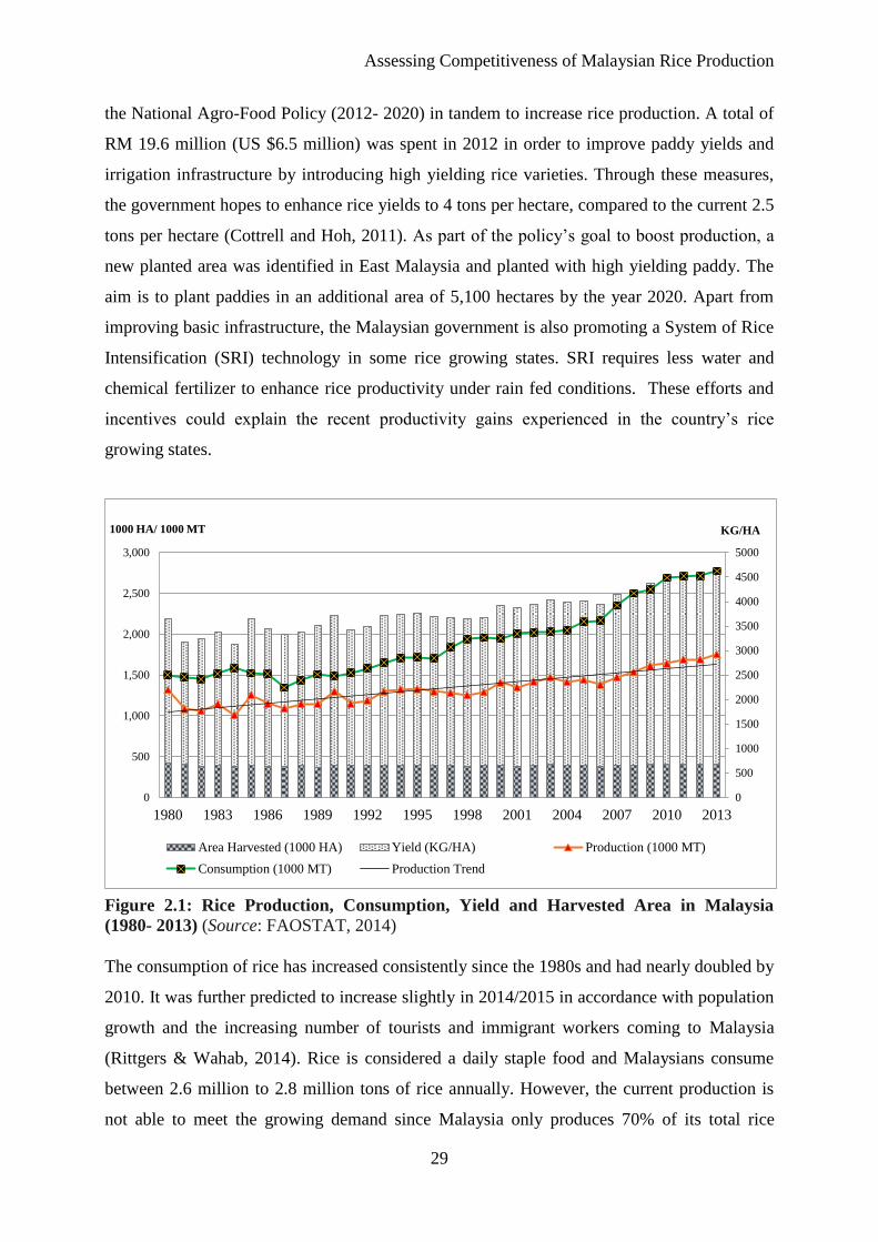
Assessing Competitiveness of Malaysian Rice Production
29
0
500
1000
1500
2000
2500
3000
3500
4000
4500
5000
0
500
1,000
1,500
2,000
2,500
3,000
1980 1983 1986 1989 1992 1995 1998 2001 2004 2007 2010 2013
KG/HA 1000 HA/ 1000 MT
Area Harvested (1000 HA) Yield (KG/HA) Production (1000 MT)
Consumption (1000 MT) Production Trend
the National Agro-Food Policy (2012- 2020) in tandem to increase rice production. A total of
RM 19.6 million (US $6.5 million) was spent in 2012 in order to improve paddy yields and
irrigation infrastructure by introducing high yielding rice varieties. Through these measures,
the government hopes to enhance rice yields to 4 tons per hectare, compared to the current 2.5
tons per hectare (Cottrell and Hoh, 2011). As part of the policy’s goal to boost production, a
new planted area was identified in East Malaysia and planted with high yielding paddy. The
aim is to plant paddies in an additional area of 5,100 hectares by the year 2020. Apart from
improving basic infrastructure, the Malaysian government is also promoting a System of Rice
Intensification (SRI) technology in some rice growing states. SRI requires less water and
chemical fertilizer to enhance rice productivity under rain fed conditions. These efforts and
incentives could explain the recent productivity gains experienced in the country’s rice
growing states.
Figure 2.1: Rice Production, Consumption, Yield and Harvested Area in Malaysia
(1980- 2013) (Source: FAOSTAT, 2014)
The consumption of rice has increased consistently since the 1980s and had nearly doubled by
2010. It was further predicted to increase slightly in 2014/2015 in accordance with population
growth and the increasing number of tourists and immigrant workers coming to Malaysia
(Rittgers & Wahab, 2014). Rice is considered a daily staple food and Malaysians consume
between 2.6 million to 2.8 million tons of rice annually. However, the current production is
not able to meet the growing demand since Malaysia only produces 70% of its total rice
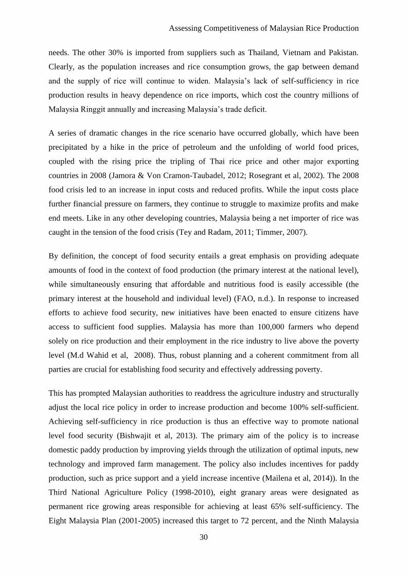
Assessing Competitiveness of Malaysian Rice Production
30
needs. The other 30% is imported from suppliers such as Thailand, Vietnam and Pakistan.
Clearly, as the population increases and rice consumption grows, the gap between demand
and the supply of rice will continue to widen. Malaysia’s lack of self-sufficiency in rice
production results in heavy dependence on rice imports, which cost the country millions of
Malaysia Ringgit annually and increasing Malaysia’s trade deficit.
A series of dramatic changes in the rice scenario have occurred globally, which have been
precipitated by a hike in the price of petroleum and the unfolding of world food prices,
coupled with the rising price the tripling of Thai rice price and other major exporting
countries in 2008 (Jamora & Von Cramon-Taubadel, 2012; Rosegrant et al, 2002). The 2008
food crisis led to an increase in input costs and reduced profits. While the input costs place
further financial pressure on farmers, they continue to struggle to maximize profits and make
end meets. Like in any other developing countries, Malaysia being a net importer of rice was
caught in the tension of the food crisis (Tey and Radam, 2011; Timmer, 2007).
By definition, the concept of food security entails a great emphasis on providing adequate
amounts of food in the context of food production (the primary interest at the national level),
while simultaneously ensuring that affordable and nutritious food is easily accessible (the
primary interest at the household and individual level) (FAO, n.d.). In response to increased
efforts to achieve food security, new initiatives have been enacted to ensure citizens have
access to sufficient food supplies. Malaysia has more than 100,000 farmers who depend
solely on rice production and their employment in the rice industry to live above the poverty
level (M.d Wahid et al, 2008). Thus, robust planning and a coherent commitment from all
parties are crucial for establishing food security and effectively addressing poverty.
This has prompted Malaysian authorities to readdress the agriculture industry and structurally
adjust the local rice policy in order to increase production and become 100% self-sufficient.
Achieving self-sufficiency in rice production is thus an effective way to promote national
level food security (Bishwajit et al, 2013). The primary aim of the policy is to increase
domestic paddy production by improving yields through the utilization of optimal inputs, new
technology and improved farm management. The policy also includes incentives for paddy
production, such as price support and a yield increase incentive (Mailena et al, 2014)). In the
Third National Agriculture Policy (1998-2010), eight granary areas were designated as
permanent rice growing areas responsible for achieving at least 65% self-sufficiency. The
Eight Malaysia Plan (2001-2005) increased this target to 72 percent, and the Ninth Malaysia
Assessing Competitiveness of Malaysian Rice Production
31
Plan (2006-2010) increased it further to a 90%. Unfortunately, these targets were not met.
Correspondingly, the Minister of Agriculture and the Agro-based Industry announced that
Malaysia is determined to achieve its target to end rice imports and become entirely self-
sufficient by 2020 (New Straits Times, 2014).
Against this background, several pertinent questions can be raised: Is rice sufficiently
profitable privately to provide farmers with the incentive to maintain or expand output? Is rice
production in Malaysia socially profitable, and hence should Malaysia endeavor for self-
sufficiency? Answers to these questions are essential in order to evaluate the current policy
environment. If Malaysia is not adequately competitive in rice production, then the
government’s plan to become self-sufficient by 2020 will impose costs on the rest of the
economy. This might be politically desirable, but if rice is not competitive, then Malaysia
would be better off putting its agricultural resources to other uses where they generate higher
returns, and using these proceeds to import rice instead. Therefore, a comparative advantage
assessment of rice production is required to address the issue of rice’s self-sufficiency in the
country and to shed light on these questions.
2.2 Policy measures in the rice industry
Malaysia is one of the most liberalized trading nations with low tariffs on the majority of
commodities and products (Tengku Mohd Ariff and Ariffin, 1999). The concept of low tariffs
as an agricultural protection and as a national security measure is intended to: maintain food
security and to make it the food available to all consumers at low prices, improve terms of
trade, provide a source of government revenue, protect domestic programs, balance trade
deficit, enhance national health standards, improve national safety and protect the local
environment.
Since rice is considered a strategically important commodity, however, the Malaysian
government intervenes more on the rice market than in most others. Policy measures for rice
include: a monopoly on imports, controlled prices for milling, wholesale and retail rice, a
fertilizer subsidy, price support, provision of drainage and irrigation facilities, spurring
innovation, and public investments in research and development (R&D) support.
Assessing Competitiveness of Malaysian Rice Production
32
The Malaysian government has been intervening in the rice industry since the country’s
independence in 1957. Since then, three main goals of rice policy have changed in relative
importance over time. The transition from colonial to post independence government resulted
in a shift of rice policy towards achieving self-sufficiency, as a strategy to save on the rapidly
rising food imports and reduce the country’s dependency on essential food supplies coming
from overseas. Hence, the goal of achieving independence from food imports by 1963 was
adopted by the government (Rudner, 1975). For rice specifically, 65 percent self-sufficiency
was targeted in order to ensure rice’s availability, especially during a food crisis. Beyond
these 65%, the government argued that it is cheaper to import rice from the world market so
as to release arable land to more lucrative and profitable industrial crops that yield high-value
products and provide more export earnings.
In the 1960s, the government initiated several land development programs, notably related to
irrigation and drainage works necessary for double cropping. The Muda Irrigation Scheme in
Kedah, the country’s largest rice growing state is an example of these programs (Rudner,
1975). Another prominent intervention was the provision of a fertilizer subsidy scheme,
which began in the late 1950s. This scheme has remained active over the decades and the
continuous increase in global fertilizer prices prompted a more comprehensive fertilizer
subsidy program in 2008, which aimed to expand support to paddy producers. The 2008
scheme included the implementation of additional fertilizer, pesticides, lime and yield
increase incentives, and cost $493.3 million US dollars (Department of Agriculture, 2010). Of
the total costs, more than 525 million RM ($154.4) were allocated to the fertilizer subsidy
scheme to benefit the farmers who owned less than 10 hectares of land. As a result of the
scheme, farmers received free fertilizers: 240 kg per hectare of mixed fertilizer, 80 kg per
hectare of organic fertilizer and 150 kg (3 bags) of NPK (nitrogen, phosphate and potassium).
Middlemen have always played a dominant role in the marketing, milling and purchasing
activities of Malaysia’s rice market. Consequently, in the mid-1970s, the government created
a specific agency called Padiberas Nasional Berhad (BERNAS) to serve as a rice monopoly.
The agency’s purpose was to regulate the development of the rice industry and rice
marketing. After being privatized in 1996, BERNAS controlled nearly every aspect of the rice
trade, including the normal commercial activities of paddy procurement, rice milling and
trading, as well as non-commercial activities on behalf of the government. Such activities
conducted for the government’s sake involved namely the management of the national rice
Assessing Competitiveness of Malaysian Rice Production
33
stockpile, reimbursement of paddy subsidy payments and the procurement of paddy from
farmers as the buyer of last resort (Tengku Mohd Ariff and Ariffin, 1999). As a consequence
of rice being used as a buffer stock to ensure sufficient supply and price stabilization,
BERNAS was obliged to maintain the national stockpile of 92,000 metric tons of rice in 1994.
A summary of subsidies and major incentives with the respective allocations in the rice sector
is presented in Table 2.1.
Table 2.1: Subsidies and incentives in the rice sector in 2008 Types of subsidies Descriptions Allocations (RM mil.)
Federal Government paddy
fertilizer subsidy scheme
-RM240 kg/ hectare mixed fertilizer (12 bags @
20kg/bag)
-80kg/ hectare for organic fertilizer (4bags @
20kg/bag)
275
Price Subsidy Scheme RM248.10/MT 448
Paddy production incentive RM140/ha/season
Ploughing expenses at a maximum of RM100
95
Additional fertilizer NPK 3 bag @ 50kg each bag/hectare
250
Pesticide Control Subsidy RM200/ha/season
173
Lime Application RM850/ha 46
Rice Millers Subsidy Peninsular Malaysia; RM750/Mt
Sabah & Sarawak: RM600/Mt
(to encourage domestic millers to produce ST15
(Peninsular) and SS15 (Sabah & Sarawak)
250
Rice Subsidy in Sabah and
Sarawak
Difference between wholesaler price and
purchasing cost of rice import
150
Source: Department of Agriculture (last updated 29 December, 2010).
One of the primary problems regarding sectoral constraints is that rice production has
developed in an instable market environment, which has been characterized by price
variability and strong fluctuations in product supply and demand (Amaya Montoya, 2011).
Therefore, rice farmers are exposed to variable levels of profitability. Furthermore, the
Malaysian rice sector consistently encountered difficulties in increasing its competitiveness
within a dynamic environment influenced by political, technical, economic and trade
challenges. Globalization and international trade have additionally played defining roles in the
country’s national development, however these factors have equally important implications
for Malaysia’s rice sector, which must compete with other international producers.

Assessing Competitiveness of Malaysian Rice Production
34
As a member of the World Trade Organization (WTO), Malaysia is bound by the stipulations
of the Uruguay Round Agreement on Agriculture. These include rules and regulations
regarding domestic support, export subsidies and market access in agriculture. Regardless of
whether or not Malaysian rice production is profitable from a comprehensive economic
perspective depends on its comparative advantage, under the conditions of no subsidies or
with limited subsidies that have been permitted by the rules for all trading partners. Therefore,
an assessment of comparative advantage can be helpful in this respect.
2.3 Material and Method
2.3.1 Policy Analysis Matrix
The policy analysis matrix (PAM), as developed by Monke and Pearson, (1989) is a double
entry bookkeeping analytical framework that helps policymakers to address central issues
regarding agricultural policy developments. PAM is widely used for measuring the impact of
policies on farm competitiveness and farm level profits. The framework additionally measures
the influence public investments have on the agricultural system’s efficiency, and the effect
agricultural research and development have on economic efficiency and comparative
advantages (Masters and Winter-Nelson 1995; Siggel 2006).
PAM takes the influence policies have on the costs and returns of agricultural production and
investment projects into account. The principal strength of PAM is that it provides a
straightforward policy-induced transfer analysis and allows for varying levels of
disaggregation. In addition, PAM results show the net effects under the complex and
contradictory policies as well as the individual effects of these policies. However, PAM also
has its shortcomings, one of which is the assumption of fixed input-output coefficients, or
static nature. Production is described by a string of techniques in which each has a fixed
input-output coefficient representing some share of total production, whereas others do not
consider the results to be realistic in a dynamic setting (Monke and Pearson 1989; Nelson and
Panggabean 2011).
PAM is composed of two cost columns (shown in Table 2.2); one representing tradable inputs
and the other domestic factors. Intermediate inputs, which consist of fertilizers, pesticides,
compound feed, transportation, electricity, fuel and purchased seeds, are divided into tradable
inputs and domestic factor components. This disaggregation process allows for intermediate
goods to be separated into four categories: tradable inputs, domestic factors, transfers (taxes
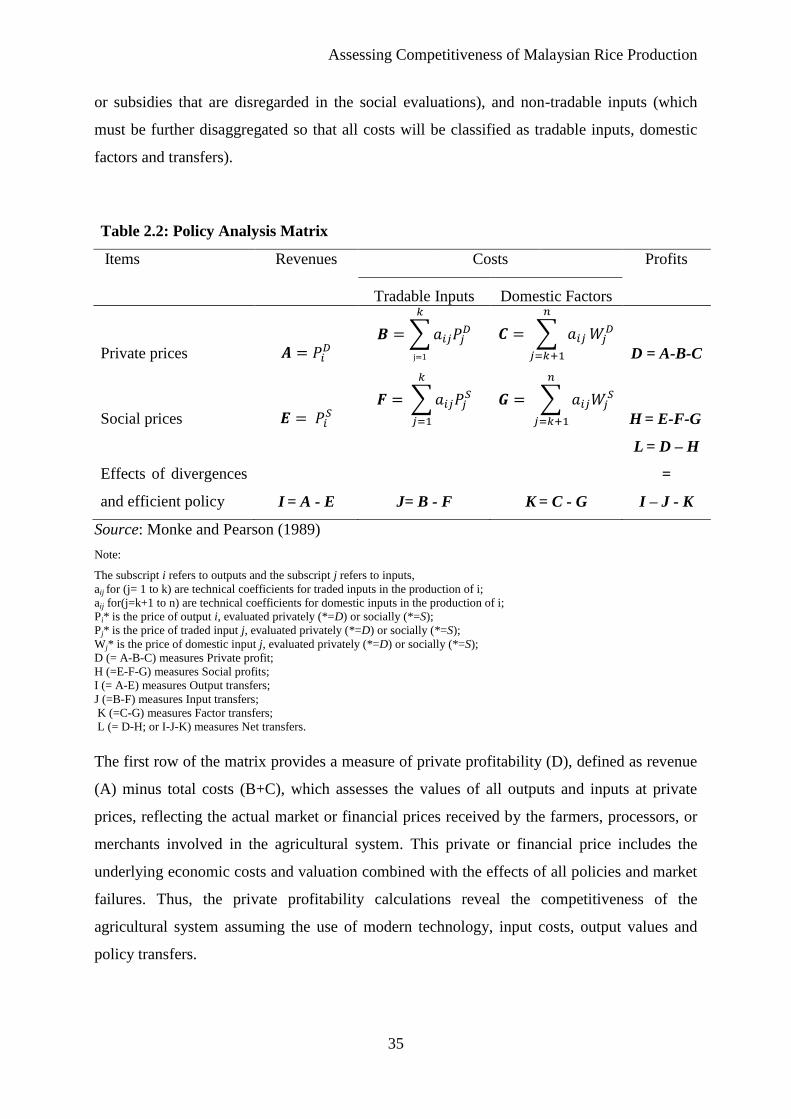
Assessing Competitiveness of Malaysian Rice Production
35
or subsidies that are disregarded in the social evaluations), and non-tradable inputs (which
must be further disaggregated so that all costs will be classified as tradable inputs, domestic
factors and transfers).
Table 2.2: Policy Analysis Matrix
Items Revenues Costs Profits
Tradable Inputs Domestic Factors
Private prices 𝑨 = 𝑃𝑖𝐷
𝑩 = ∑ 𝑎𝑖𝑗𝑃𝑗𝐷
𝑘
j=1
𝑪 = ∑ 𝑎𝑖𝑗
𝑛
𝑗=𝑘+1
𝑊𝑗𝐷
D = A-B-C
Social prices 𝑬 = 𝑃𝑖𝑆
𝑭 = ∑ 𝑎𝑖𝑗𝑃𝑗𝑆
𝑘
𝑗=1
𝑮 = ∑ 𝑎𝑖𝑗𝑊𝑗𝑆
𝑛
𝑗=𝑘+1
H = E-F-G
Effects of divergences
and efficient policy I = A - E J= B - F K = C - G
L = D – H
=
I – J - K
Source: Monke and Pearson (1989)
Note:
The subscript i refers to outputs and the subscript j refers to inputs,
aij for (j= 1 to k) are technical coefficients for traded inputs in the production of i;
aij for(j=k+1 to n) are technical coefficients for domestic inputs in the production of i;
Pi* is the price of output i, evaluated privately (*=D) or socially (*=S);
Pj* is the price of traded input j, evaluated privately (*=D) or socially (*=S);
Wj* is the price of domestic input j, evaluated privately (*=D) or socially (*=S);
D (= A-B-C) measures Private profit;
H (=E-F-G) measures Social profits;
I (= A-E) measures Output transfers;
J (=B-F) measures Input transfers;
K (=C-G) measures Factor transfers;
L (= D-H; or I-J-K) measures Net transfers.
The first row of the matrix provides a measure of private profitability (D), defined as revenue
(A) minus total costs (B+C), which assesses the values of all outputs and inputs at private
prices, reflecting the actual market or financial prices received by the farmers, processors, or
merchants involved in the agricultural system. This private or financial price includes the
underlying economic costs and valuation combined with the effects of all policies and market
failures. Thus, the private profitability calculations reveal the competitiveness of the
agricultural system assuming the use of modern technology, input costs, output values and
policy transfers.
Assessing Competitiveness of Malaysian Rice Production
36
The table’s second row measures the social profits (H), which reflect the agricultural system’s
efficient use of resources and overall comparative advantage. Efficient outcomes are
attainable when economy´s resources are used to create the highest income and output levels.
To determine social profits, social prices are used for the valuation of inputs and outputs.
Social values, or prices, demonstrate a policy benchmark for comparisons because they are
considered the prevailing prices in a free market in the absence of policy interventions,
distortions or market failures (Kanaka and Chinnadurai, 2013; Monke and Pearson, 1989).
Social prices reflect the opportunity cost or the value of using a good or service produced by a
particular activity in order to achieve the objective of optimizing income and social welfare.
Thus, considering that output (E) and input (F+G) are valued at social prices that reflect the
scarcity values or opportunity costs, social profits are an efficiency measure. For output (E)
and input (F) traded internationally, world export prices (free on board) are used. The cost of
insurance freight prices (CIF) is used to deduce domestic factors, which are not traded in the
international market. Social profits indicate that the foreign exchange either cut costs by
reducing imports or earned by expanding exports of each unit of production. A positive value
indicates that production contributes to national income, while a negative value suggests that
the country’s national growth would be improved by not producing the commodity. Thus, it is
a signal of measuring international comparative advantage (Kanaka and Chinnadurai, 2013).
The second identity located in the third row of the accounting matrix measures divergences,
which are defined as the differences between private and social valuations of revenues, costs
and profits. Any divergence between private and social prices, which is measured vertically,
must be explained by the effects of the policies. The effects of divergences are disaggregated
into three categories: distorting policies, market failure and efficient policies. When
government enforced market failure correction policies are not in place, distorting policies are
the cause of divergences between the private and social prices of tradable outputs and inputs.
However, if efficient policies enacted by the government are able to correct or offset market
failures and create a greater income, the differences between private and social valuations will
be reduced, since efficient policies correct divergences (Masters and Winter-Nelson 1995;
Monke and Pearson 1989). The PAM framework also calculates the protection rate generated
by different ratios such as the NPC, EPC, DRC, and SCB. These protection rates were used
throughout this study to measure comparative advantages.
Assessing Competitiveness of Malaysian Rice Production
37
The Nominal Protection Coefficient (NPC) is one of the most widely used methods of
measuring price distortions (Fang and Beghin 2000; S. Mohanty, Fang, and Chaudhary 2003;
Sadoulet and Janvry 1995; S. J. Yao 1997). The NPC is defined as:
NPCi = 𝑃𝑖𝐷/ 𝑃𝑖
𝑆 (1)
NPC ratio compares the private and social prices of a commodity. This ratio demonstrates the
impact a policy has on the two prices; domestic price compared to the world price that causes
a divergence. NPC can be calculated for both inputs (NPCI) and outputs (NPCO). Subsidies
on outputs are indicated by NPCO (which is A/E) if its value is larger than one, while input
subsidies are represented by NPCI (which is B/F) if its value is smaller than one (Fang and
Beghin, 2000). From a strictly theoretical point of view in the context of trade, if NPC>1,
producers are protected and consumers taxed; this scenario suggests that the production is
inefficient and the price is heavily affected by government policies or by other factors of that
commodity.
The effective protection coefficient (EPC) is defined as the ratio of distorted tradable value,
which has been added at market price to its undistorted value at the border price level. EPC
captures the effect of government policies on input as well as on output markets (Hayat and
Islam 2005; Javed et al. 2006). EPC is defined as:
EPC= (𝑃𝑖𝐷 – ∑ 𝑎𝑖𝑗𝑃𝑗
𝐷𝑘j=1 / (𝑃𝑖
𝑆-∑ 𝑎𝑖𝑗𝑃𝑗𝑆𝑘
𝑗=1 ) (2)
Based on the PAM table, EPC is the ratio of the value of added private prices (A-B) to the
value of added social prices (E-F). This coefficient indicates the degree of policy transfer
from output and tradable input distortions. A value greater (or less) than one indicates a net
subsidy (or net tax) to value added (Beghin and Fang, 2002; Monke and Pearson, 1989).
Additionally, if EPC>1, it suggests that government policies impart positive incentives to
producers while EPC<1 indicates that producers are not protected through policy
interventions (Mohanty et. al, 2003).
The Domestic Resources Cost (DRC) is widely used to measure comparative advantages or
relative efficiency between agricultural commodities (e.g.von Cramon Taubadel and
Nivyevskyi, 2008; 2009). DRC was developed simultaneously in the 1960s by Bruno (1965)
in Israel and by Krueger (1966) in United States. The DRC is defined as the shadow value of
Assessing Competitiveness of Malaysian Rice Production
38
non-tradable inputs used in an activity per unit of tradable value added (G/ (E-F)). The
formula for DRC is written as;
DRC= ∑ 𝑎𝑖𝑗𝑊𝑗𝑆𝑛
𝑗=𝑘+1 / (𝑃𝑖𝑆 -∑ 𝑎𝑖𝑗𝑃𝑗
𝑆𝑘𝑗=1 ) (3)
DRC indicates whether or not the use of domestic factors is socially profitable (DRC<1)
(DRC>1). We calculate the DRCs to enable cross-commodity comparisons in each Malaysian
state. The commodities can be ranked according to the DRC values and thus can provide
indications of comparative advantage or disadvantage within that state. A state is said to have
a comparative advantage due to a given crop if the value of the DRC for that crop is lower
than the DRC for other crops grown in that state.
The Social Cost Benefit (SCB) is defined as (F+G)/E, and provides information similar to the
DRC. Finally, the indicators private net return to land (PNRL) and social net return to land
(SNRL) were used to measure the return to the fixed factor for this study. Hayat and Islam,
(2005) state that the net economic benefit per unit of land is likely to be more relevant when
ranking crops, as opposed to calculating domestic resources per unit (or ringgit/domestic
currency). The PAM table provides the PNRL, which is defined as A-B-C without the cost of
land use and SNRL as E-F-G without the cost of land use. Greater values of PNRL indicate
that the crop in question is more desirable for the producer, but not necessarily for society. A
higher value of SNRL suggests both a product’s stronger competitiveness as well as its
desirability for the society (Fang and Beghin, 2000; Yao, 1997).
2.3.2 Data collection
In the 1980s, the government enhanced further irrigation developments in order to enable rice
double cropping in eight designated granary areas. Of these, four were chosen as the study
areas: Muda Agricultural Development Authority (MADA); Kemubu Agricultural
Development Authority (KADA); Barat Laut Selangor Integrated Agricultural Development
(BLS); and North Terengganu Integrated Agricultural Development (KETARA). The
contributions of the four granary areas are presented in Appendix 2.1.
The data employed in this study are collected from various national and international
published and unpublished resources. In order to estimate the PAM, a comprehensive set of
data including yields, input requirements of the markets, and social prices of inputs and
Assessing Competitiveness of Malaysian Rice Production
39
outputs were required. The aggregate output and input coefficients for the four granary areas
were taken from Terano and Mohamed, (2011), Mohd Rashid and Mohd Dainuri, (2013) and
KADA (2014). These authors used a fairly large-scale survey that encompassed different agro
ecological zones. The survey focused on generating information related to the production
costs of rice for the provinces over the period 2011-2012. These output and input coefficients
were then complied according to the land’s hectare count.
The output (rice) and input farm gate prices (urea, compound or TSP, NPK and organic
fertilizers, pesticides and lime) were taken from nationally and internationally published and
unpublished sources. Social prices of tradable commodities are based on import parity prices
or export parity prices, depending on the trade status of the commodity in question. Since
Malaysia frequently imports rice, an import parity price is used to measure the social price of
rice. The CIF price of 25 percent broken rice and the official exchange rate were collected
from FAO and the Central Bank Malaysia. CIF prices for fertilizers, including urea (Europe),
TSP (US Gulf ports), organic and NPK, were collected from the World Bank, IRRI, and the
FAO food outlook. The fuel price was obtained from Domestic Trade and Consumer Affairs
Ministry in Malaysia, whereas the data pertaining to lime, pesticides and wages were
collected from the Ministry of International Trade and Industry, the Department of Statistics
Malaysia and FAOSTAT.
The social price of land is one of the more important and complicated components of
domestic factors. With regard to land valuation, Gittinger, (1984) describe the social cost of
land, which is considered when determining border prices, as the net value of production
forgone when the status of the land changed from ‘without land use’ to ‘with land use’. In a
free market, the market price of a piece of land will reflect its economic value. However, Van
Schalkwyk and Van Zyl (1994) argue that non-farm related factors, such as policy distortions
may get capitalized as market values and thus, land values tend to not reflect its true
economic value. In this respect, Monke and Pearson (1989) propose using the rental value
instead of market value, because the rental value reflects the relationship between opportunity
cost and land use. They further argue that in the absence of both financial cost and rental
value that reflect the opportunity cost of a land, its ‘potential productive capacity’ can be used
to access its value in the best alternative use. For example, if oil palm production represents
the best alternative to rice production in granary areas, the social costs of land for rice
production equals the social profits (excluding land) from the oil palm production.

Assessing Competitiveness of Malaysian Rice Production
40
In the studied areas, many farmers preferred sharecropping or producing oil palm as a
substitute commodity for rice (Terano and Mohamed 2011). Hence, in estimating social prices
for land, we used the average net income of palm oil in each granary area. Due to the
challenges inherent to estimating the social profits of oil palm production, these figures are
based on primary data provided by an agricultural officer and a land value officer in Selangor,
Malaysia. Other data pertaining to the conversion of private to social prices are presented in
Appendix 2.2 and 2.3.
2.4 Result and Discussion
2.4.1 Policy analysis matrix in the context of import parity price of rice
In this section, the results of the policy analysis matrix and sensitivity analysis are discussed
sequentially and with necessary interpretations. The main results of the protection and
comparative advantage coefficients for the four observed granary areas are shown in Table
2.3. Domestic Resource Cost (DRC) and Social Cost Benefit (SCB) were estimated in order
to measure the competitiveness of Malaysia’s rice sector. DRC compares the domestic costs
of resources measured at the corresponding social price with the value added measured in the
social prices. The use of the social prices in DRC measure allows us to test whether the
employment of scarce domestic inputs in the production of rice generates positive returns for
Malaysia.
The empirical analysis presented in this paper demonstrates that three of four study areas
(BLS, MADA and KADA) had comparative advantages in the production of rice (DRC<1)
between 2011 and 2012. However, the results indicate no comparative advantage for rice
production in the KETARA area because the DRC was greater than one. It is more
advantageous for the nation to produce rice in the three granary areas and to expand its
production considering the added social value is greater than the cost of importing rice.
However, the estimated DRCs are closer to unity, indicating that there may be some
competing demand on resources for production of other crops. Moreover, the closer the DRC
value is to one, the more impact a small change in prices can have. With the estimated DRC
of rice grown in KETARA observed to be greater than one under the circumstances of import
parity prices, no comparative advantage is detected. As a result, the emphasis on the
attainment of self-sufficiency in rice production appears to be uneconomically justified and
remains debatable.
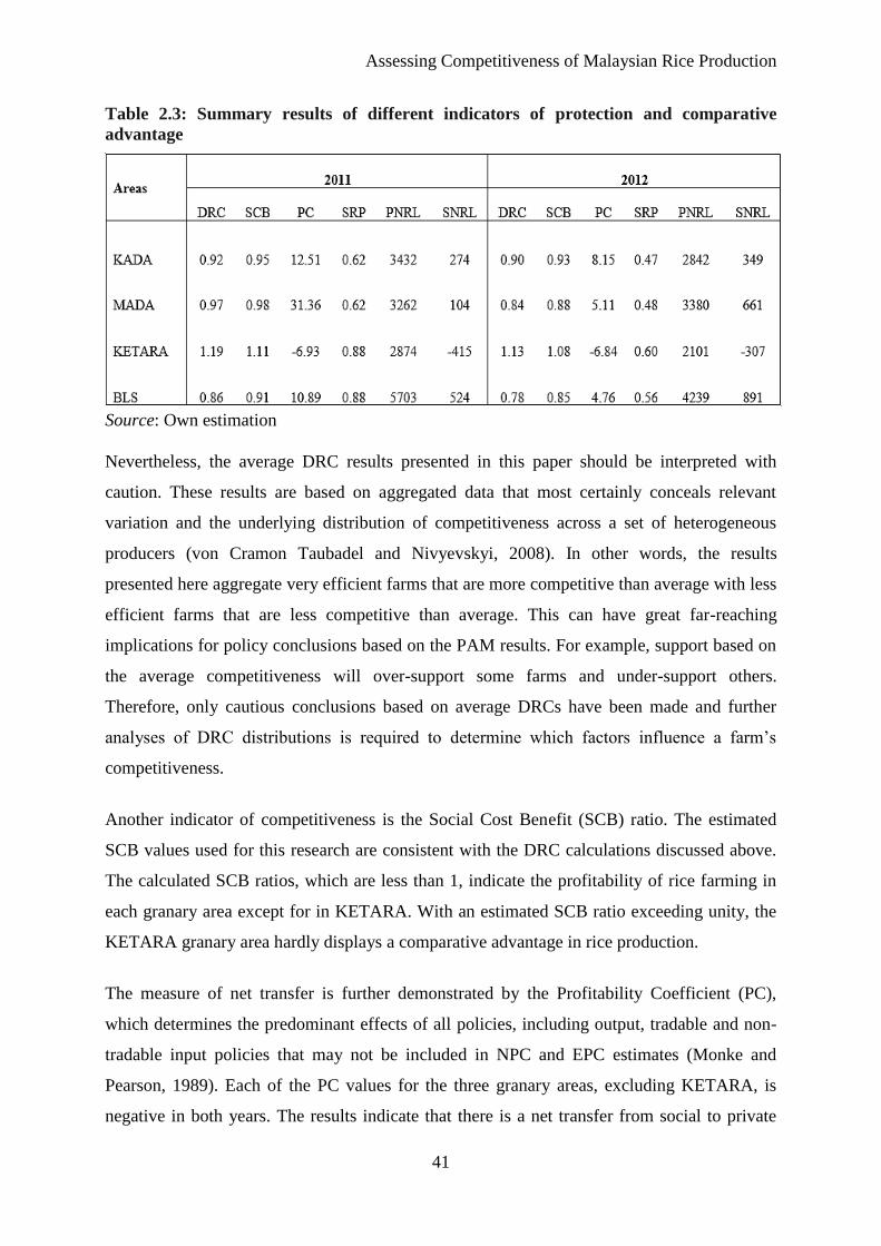
Assessing Competitiveness of Malaysian Rice Production
41
Table 2.3: Summary results of different indicators of protection and comparative
advantage
Source: Own estimation
Nevertheless, the average DRC results presented in this paper should be interpreted with
caution. These results are based on aggregated data that most certainly conceals relevant
variation and the underlying distribution of competitiveness across a set of heterogeneous
producers (von Cramon Taubadel and Nivyevskyi, 2008). In other words, the results
presented here aggregate very efficient farms that are more competitive than average with less
efficient farms that are less competitive than average. This can have great far-reaching
implications for policy conclusions based on the PAM results. For example, support based on
the average competitiveness will over-support some farms and under-support others.
Therefore, only cautious conclusions based on average DRCs have been made and further
analyses of DRC distributions is required to determine which factors influence a farm’s
competitiveness.
Another indicator of competitiveness is the Social Cost Benefit (SCB) ratio. The estimated
SCB values used for this research are consistent with the DRC calculations discussed above.
The calculated SCB ratios, which are less than 1, indicate the profitability of rice farming in
each granary area except for in KETARA. With an estimated SCB ratio exceeding unity, the
KETARA granary area hardly displays a comparative advantage in rice production.
The measure of net transfer is further demonstrated by the Profitability Coefficient (PC),
which determines the predominant effects of all policies, including output, tradable and non-
tradable input policies that may not be included in NPC and EPC estimates (Monke and
Pearson, 1989). Each of the PC values for the three granary areas, excluding KETARA, is
negative in both years. The results indicate that there is a net transfer from social to private
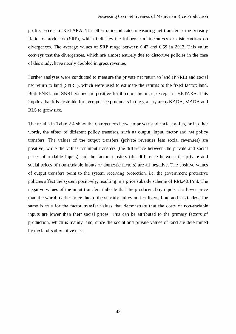
Assessing Competitiveness of Malaysian Rice Production
42
profits, except in KETARA. The other ratio indicator measuring net transfer is the Subsidy
Ratio to producers (SRP), which indicates the influence of incentives or disincentives on
divergences. The average values of SRP range between 0.47 and 0.59 in 2012. This value
conveys that the divergences, which are almost entirely due to distortive policies in the case
of this study, have nearly doubled in gross revenue.
Further analyses were conducted to measure the private net return to land (PNRL) and social
net return to land (SNRL), which were used to estimate the returns to the fixed factor: land.
Both PNRL and SNRL values are positive for three of the areas, except for KETARA. This
implies that it is desirable for average rice producers in the granary areas KADA, MADA and
BLS to grow rice.
The results in Table 2.4 show the divergences between private and social profits, or in other
words, the effect of different policy transfers, such as output, input, factor and net policy
transfers. The values of the output transfers (private revenues less social revenues) are
positive, while the values for input transfers (the difference between the private and social
prices of tradable inputs) and the factor transfers (the difference between the private and
social prices of non-tradable inputs or domestic factors) are all negative. The positive values
of output transfers point to the system receiving protection, i.e. the government protective
policies affect the system positively, resulting in a price subsidy scheme of RM240.1/mt. The
negative values of the input transfers indicate that the producers buy inputs at a lower price
than the world market price due to the subsidy policy on fertilizers, lime and pesticides. The
same is true for the factor transfer values that demonstrate that the costs of non-tradable
inputs are lower than their social prices. This can be attributed to the primary factors of
production, which is mainly land, since the social and private values of land are determined
by the land’s alternative uses.
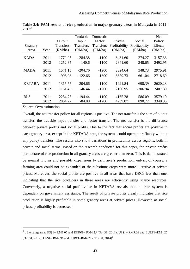
Assessing Competitiveness of Malaysian Rice Production
43
Table 2.4: PAM results of rice production in major granary areas in Malaysia in 2011-
20122
Granary
Area Year
Output
Transfers
(RM/ha)
Tradable
Input
Transfers
(RM/ha)
Domestic
Factor
Transfers
(RM/ha)
Private
Profitability
(RM/ha)
Social
Profitability
(RM/ha)
Net
Policy
Effects
(RM/ha)
KADA 2011 1772.95 -284.38 -1100 3431.60 274.27 3157.33
2012 1252.35 -140.6 -1100 2841.60 348.65 2492.95
MADA 2011 1571.15 -204.76 -1200 3324.64 348.73 2975.91
2012 996.03 -122.66 -1600 3379.73 661.04 2718.69
KETARA 2011 1315.57 -204.66 -1100 1921.84 -698.39 2620.23
2012 1161.45 -46.44 -1200 2100.95 -306.94 2407.89
BLS 2011 2284.75 -194.44 -1100 4165.28 586.09 3579.19
2012 2064.27 -84.08 -1200 4239.07 890.72 3348.35
Source: Own estimation
Overall, the net transfer policy for all regions is positive. The net transfer is the sum of output
transfer, the tradable input transfer and factor transfer. The net transfer is the difference
between private profits and social profits. Due to the fact that social profits are positive in
each granary area, except in the KETARA area, the systems could operate profitably without
any policy transfers. The results also show variations in profitability across regions, both in
private and social terms. Based on the research conducted for this paper, the private profits
per hectare of rice production in all granary areas are greater than zero. This is demonstrated
by normal returns and possible expansions to each area’s production, unless, of course, a
farming area could not be expanded or the substitute crops were more lucrative at private
prices. Moreover, the social profits are positive in all areas that have DRCs less than one,
indicating that the rice producers in these areas are efficiently using scarce resources.
Conversely, a negative social profit value in KETARA reveals that the rice system is
dependent on government assistance. The result of private profits clearly indicates that rice
production is highly profitable in some granary areas at private prices. However, at social
prices, profitability is decreased.
2 . Exchange rate: US$1= RM3.05 and EUR€1= RM4.25 (Oct 31, 2011); US$1= RM3.06 and EUR€1=RM4.27
(Oct 31, 2012); US$1= RM2.96 and EUR€1=RM4.21 (Nov 30, 2014)2
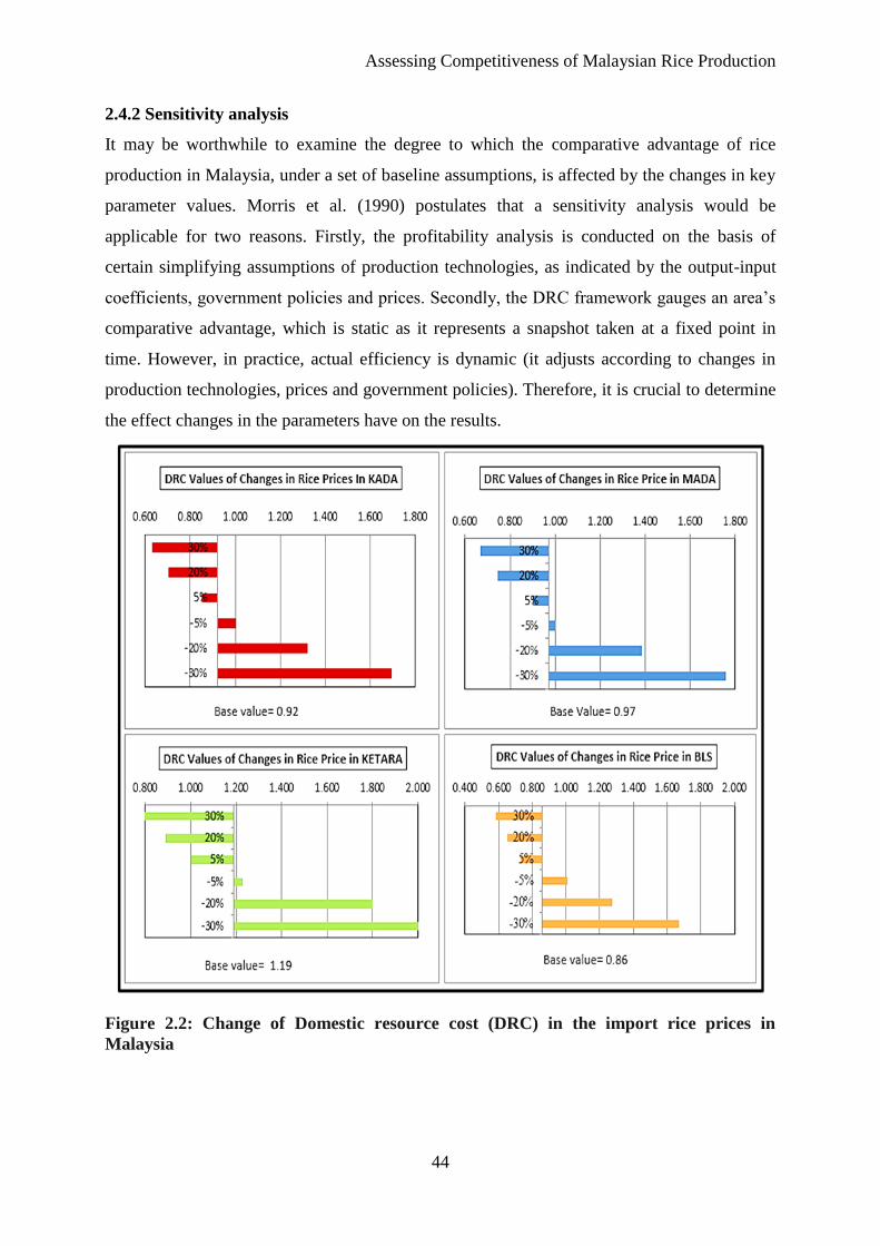
Assessing Competitiveness of Malaysian Rice Production
44
2.4.2 Sensitivity analysis
It may be worthwhile to examine the degree to which the comparative advantage of rice
production in Malaysia, under a set of baseline assumptions, is affected by the changes in key
parameter values. Morris et al. (1990) postulates that a sensitivity analysis would be
applicable for two reasons. Firstly, the profitability analysis is conducted on the basis of
certain simplifying assumptions of production technologies, as indicated by the output-input
coefficients, government policies and prices. Secondly, the DRC framework gauges an area’s
comparative advantage, which is static as it represents a snapshot taken at a fixed point in
time. However, in practice, actual efficiency is dynamic (it adjusts according to changes in
production technologies, prices and government policies). Therefore, it is crucial to determine
the effect changes in the parameters have on the results.
Figure 2.2: Change of Domestic resource cost (DRC) in the import rice prices in
Malaysia
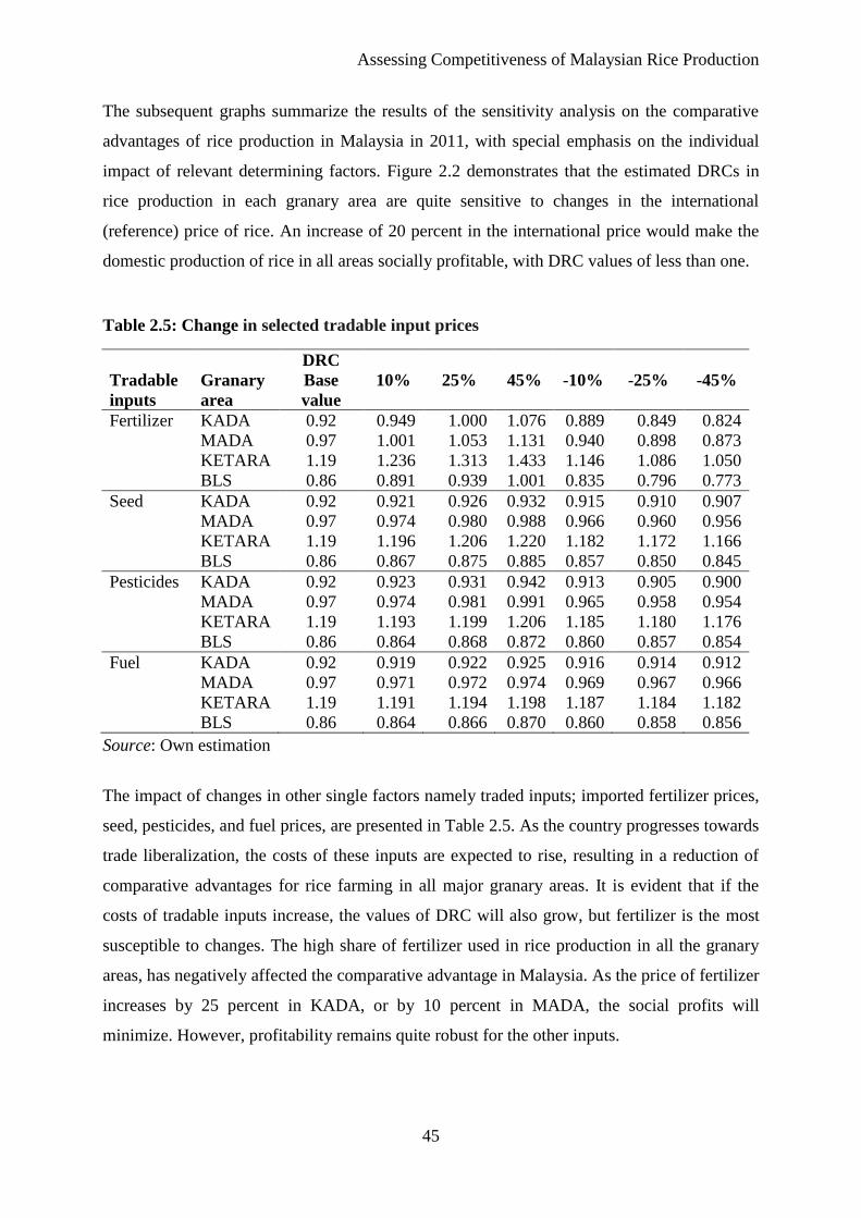
Assessing Competitiveness of Malaysian Rice Production
45
The subsequent graphs summarize the results of the sensitivity analysis on the comparative
advantages of rice production in Malaysia in 2011, with special emphasis on the individual
impact of relevant determining factors. Figure 2.2 demonstrates that the estimated DRCs in
rice production in each granary area are quite sensitive to changes in the international
(reference) price of rice. An increase of 20 percent in the international price would make the
domestic production of rice in all areas socially profitable, with DRC values of less than one.
Table 2.5: Change in selected tradable input prices
Tradable
inputs
Granary
area
DRC
Base
value
10%
25%
45%
-10%
-25%
-45%
Fertilizer KADA 0.92 0.949 1.000 1.076 0.889 0.849 0.824
MADA 0.97 1.001 1.053 1.131 0.940 0.898 0.873
KETARA 1.19 1.236 1.313 1.433 1.146 1.086 1.050
BLS 0.86 0.891 0.939 1.001 0.835 0.796 0.773
Seed KADA 0.92 0.921 0.926 0.932 0.915 0.910 0.907
MADA 0.97 0.974 0.980 0.988 0.966 0.960 0.956
KETARA 1.19 1.196 1.206 1.220 1.182 1.172 1.166
BLS 0.86 0.867 0.875 0.885 0.857 0.850 0.845
Pesticides KADA 0.92 0.923 0.931 0.942 0.913 0.905 0.900
MADA 0.97 0.974 0.981 0.991 0.965 0.958 0.954
KETARA 1.19 1.193 1.199 1.206 1.185 1.180 1.176
BLS 0.86 0.864 0.868 0.872 0.860 0.857 0.854
Fuel KADA 0.92 0.919 0.922 0.925 0.916 0.914 0.912
MADA 0.97 0.971 0.972 0.974 0.969 0.967 0.966
KETARA 1.19 1.191 1.194 1.198 1.187 1.184 1.182
BLS 0.86 0.864 0.866 0.870 0.860 0.858 0.856
Source: Own estimation
The impact of changes in other single factors namely traded inputs; imported fertilizer prices,
seed, pesticides, and fuel prices, are presented in Table 2.5. As the country progresses towards
trade liberalization, the costs of these inputs are expected to rise, resulting in a reduction of
comparative advantages for rice farming in all major granary areas. It is evident that if the
costs of tradable inputs increase, the values of DRC will also grow, but fertilizer is the most
susceptible to changes. The high share of fertilizer used in rice production in all the granary
areas, has negatively affected the comparative advantage in Malaysia. As the price of fertilizer
increases by 25 percent in KADA, or by 10 percent in MADA, the social profits will
minimize. However, profitability remains quite robust for the other inputs.
Assessing Competitiveness of Malaysian Rice Production
46
The sensitivity analysis of increasing or decreasing the costs of imported rice, fertilizer, seed,
pesticides and fuel shows that the coefficients have similar patterns of competitiveness. Under
certain unfavorable economic conditions, average Malaysian rice producers could lose their
comparative advantages. For example, in the event of higher input costs, with particular
emphasis on fertilizer costs or the deterioration of the international market’s price of rice, a
rice producer’s comparative advantage could diminish.
2.5 Conclusion
The challenges presented by trade liberalization have created tougher competition and
unfavorable conditions for Malaysia to strengthen its economic growth. The country’s rice
sector, which is an important part of the economy because of its production value and the
source of employment it provides, also faces these challenges. More than 100,000 farmers are
involved in rice farming. In an effort to increase paddy production, the government has
provided a great degree of support to paddy producers, most of whom live in poverty. These
incentives aim to enhance rice production levels, secure self-sufficiency by 2020 and maintain
food security. Utilizing a PAM model, this study investigated whether the government’s
interventions make economic sense to be fully self-efficient. In order to arrive at this
conclusion, the competitiveness of Malaysia’s rice production, particularly in the KADA,
MADA, KETARA and BLS granary areas, was analyzed.
The results indicate that three out of four granary areas have comparative advantages in rice
production with Domestic Resource Cost values, or DRCs, of less than one. Conversely, the
results indicated no comparative advantage for rice production in the KETARA area, as the
DRC is greater than one. Similarly, Social Cost Benefit or SCB values in these areas are less
than one indicating that the comparative advantages in rice production are noteworthy.
Therefore, social profitability appears in three of the four areas, although there are farms that
generate a net surplus for the country. To fully understand the impact of these farms, they
must be identified and studied by further research using disaggregated data. These farms may
generate social profits, but they might depend on financial government support to provide for
their families. In this case, policies should focus on encouraging structural changes, which
enable these farms to grow enough to generate a sufficient income from social profits alone,
i.e. without (or with much less) subsidy. This way the government could encourage self-
sufficiency and spend less money. In the other region, the average farm does not yield a social
Assessing Competitiveness of Malaysian Rice Production
47
profit. However, it is likely that this area also has farms that are socially profitable. In all four
regions (and especially in the KETARA region there must be many farms that are not
producing a social profit. Thus, further research with disaggregated data is required to
determine why this is the case, and how the situation can be improved.
Additional Notes:
The empirical analysis presented in Appendix 2.2 and 2.3 is based on secondary data provided
by R.Terano et al (2013), Rabu and Mohd Shah (2013) and KADA (2014). The data were
then crosschecked with a local expert from BERNAS to ensure reliability and validity. Each
calculation was conducted on a hectare basis and in Malaysia currency, the Malaysian Ringgit
(RM). As means of determining the PAM, the authors of this text classified input items into
tradable and non-tradable inputs categories. In the context of rice farms, tradable inputs
include fertilizers, chemicals, seeds and fuel, while the other inputs, such as labor, capital and
land rent were categorized as non-tradable inputs. The social price (shadow price) of all the
inputs and the output (rice) was subsequently estimated, and finally, the commodity and
system budget tables were configured to the PAM table and relevant policy parameters were
derived.
The conversion of private to social prices is based on several data and assumptions:
i. Rice is an imported good; therefore, the social price for rice is the import parity price
of rice equivalents at the farm gate.
ii. As for the tradable inputs, the social prices of fertilizers, pesticides, seeds, fuel and
lime are the respective import parity prices at the farm gate.
iii. Social costs of transplanting packages are also assumed to equal the private costs
considering that the owners determine the value of these packages and services.
iv. Domestic inputs, such as land, for which no international prices exist is valued at local
opportunity costs. Hence, the rental values of land per hectare for different granary
areas were obtained from an agricultural officer and a land value officer in Selangor.
Based on the information provided, it is clear that all approaches used to determine the
value of agricultural land are subject to criticism. In this regard, one can argue that this
is due to the extreme difficulty of assigning a price to land.
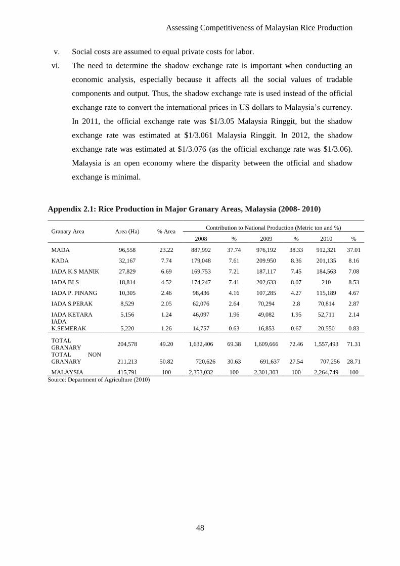
Assessing Competitiveness of Malaysian Rice Production
48
v. Social costs are assumed to equal private costs for labor.
vi. The need to determine the shadow exchange rate is important when conducting an
economic analysis, especially because it affects all the social values of tradable
components and output. Thus, the shadow exchange rate is used instead of the official
exchange rate to convert the international prices in US dollars to Malaysia’s currency.
In 2011, the official exchange rate was $1/3.05 Malaysia Ringgit, but the shadow
exchange rate was estimated at $1/3.061 Malaysia Ringgit. In 2012, the shadow
exchange rate was estimated at $1/3.076 (as the official exchange rate was $1/3.06).
Malaysia is an open economy where the disparity between the official and shadow
exchange is minimal.
Appendix 2.1: Rice Production in Major Granary Areas, Malaysia (2008- 2010)
Granary Area Area (Ha) % Area Contribution to National Production (Metric ton and %)
2008 % 2009 % 2010 %
MADA 96,558 23.22 887,992 37.74 976,192 38.33 912,321 37.01
KADA 32,167 7.74 179,048 7.61 209.950 8.36 201,135 8.16
IADA K.S MANIK 27,829 6.69 169,753 7.21 187,117 7.45 184,563 7.08
IADA BLS 18,814 4.52 174,247 7.41 202,633 8.07 210 8.53
IADA P. PINANG 10,305 2.46 98,436 4.16 107,285 4.27 115,189 4.67
IADA S.PERAK 8,529 2.05 62,076 2.64 70,294 2.8 70,814 2.87
IADA KETARA 5,156 1.24 46,097 1.96 49,082 1.95 52,711 2.14
IADA
K.SEMERAK 5,220 1.26 14,757 0.63 16,853 0.67 20,550 0.83
TOTAL
GRANARY 204,578 49.20 1,632,406 69.38 1,609,666 72.46 1,557,493 71.31
TOTAL NON
GRANARY 211,213 50.82 720,626 30.63 691,637 27.54 707,256 28.71
MALAYSIA 415,791 100 2,353,032 100 2,301,303 100 2,264,749 100
Source: Department of Agriculture (2010)
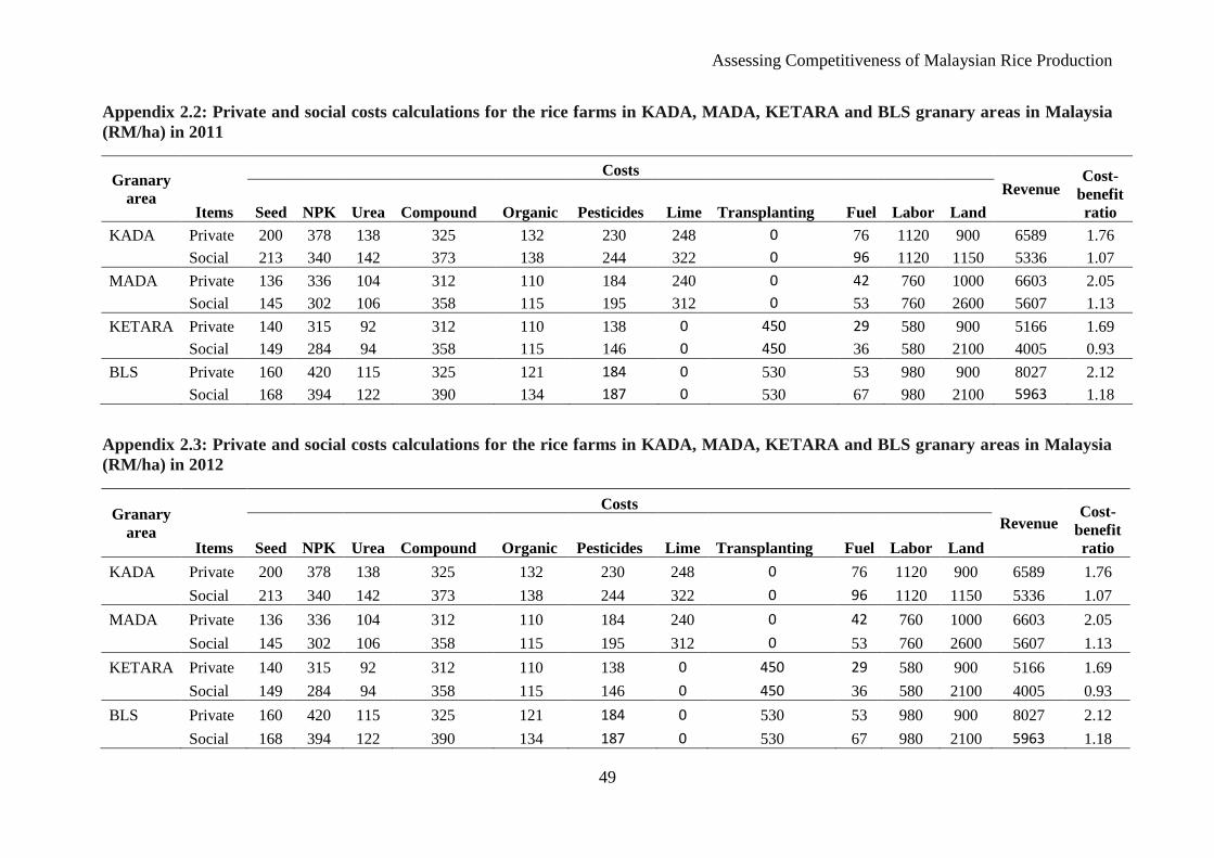
Assessing Competitiveness of Malaysian Rice Production
49
Appendix 2.2: Private and social costs calculations for the rice farms in KADA, MADA, KETARA and BLS granary areas in Malaysia
(RM/ha) in 2011
Granary
area Items
Costs
Revenue Cost-
benefit
ratio Seed NPK Urea Compound Organic Pesticides Lime Transplanting Fuel Labor Land
KADA Private 200 378 138 325 132 230 248 0 76 1120 900 6589 1.76
Social 213 340 142 373 138 244 322 0 96 1120 1150 5336 1.07
MADA Private 136 336 104 312 110 184 240 0 42 760 1000 6603 2.05
Social 145 302 106 358 115 195 312 0 53 760 2600 5607 1.13
KETARA Private 140 315 92 312 110 138 0 450 29 580 900 5166 1.69
Social 149 284 94 358 115 146 0 450 36 580 2100 4005 0.93
BLS Private 160 420 115 325 121 184 0 530 53 980 900 8027 2.12
Social 168 394 122 390 134 187 0 530 67 980 2100 5963 1.18
Appendix 2.3: Private and social costs calculations for the rice farms in KADA, MADA, KETARA and BLS granary areas in Malaysia
(RM/ha) in 2012
Granary
area Items
Costs
Revenue Cost-
benefit
ratio Seed NPK Urea Compound Organic Pesticides Lime Transplanting Fuel Labor Land
KADA Private 200 378 138 325 132 230 248 0 76 1120 900 6589 1.76
Social 213 340 142 373 138 244 322 0 96 1120 1150 5336 1.07
MADA Private 136 336 104 312 110 184 240 0 42 760 1000 6603 2.05
Social 145 302 106 358 115 195 312 0 53 760 2600 5607 1.13
KETARA Private 140 315 92 312 110 138 0 450 29 580 900 5166 1.69
Social 149 284 94 358 115 146 0 450 36 580 2100 4005 0.93
BLS Private 160 420 115 325 121 184 0 530 53 980 900 8027 2.12
Social 168 394 122 390 134 187 0 530 67 980 2100 5963 1.18
Assessing Competitiveness of Malaysian Rice Production
50
References
Amaya Montoya, J.D. (2011). The Colombian rice sector scenarios and strategic options for
increasing the competitiveness considering international free trade agreements: Master
Thesis. Wageningen University, Management Studies.
Bishwajit, G., Sarker, S., Kpoghomou, M.-A., Gao, H., Jun, L., Yin, D., & Ghosh, S. (2013).
Self-sufficiency in rice and food security: a South Asian perspective. Agriculture &
Food Security, 2(1), 10. http://doi.org/10.1186/2048-7010-2-10
Department of Agriculture. (2010). Subsidi, Bantuan dan Insebtif Pertanian.
http://pmr.penerangan.gov.my/index.php/penstrukturan-subsidi/9893-subsidi-bantuan-
dan-insentif-pertanian.html
Fang, C., & Beghin, J. C. (2000). Self-sufficiency, Comparative Advantages, and Agricultural
Trade: A Policy Analysis Matrix for Chinese Agriculture. Retrieved from
http://down.cenet.org.cn/upfile/52/20062232278169.pdf
FAO. Food and Agriculture Organization of the United Nations, (n.d.). The State of Food
Insecurity in the World. Retrieved December 6, 2015, from
http://www.fao.org/docrep/014/i2330e/i2330e.pdf
Gittinger, J.P. (1982). Economic Analysis of Agricultural Projects, 2nd ed. Baltimore MD:
The Johns Hopkins University Press, London
Hayat, A., & Islam, S. (2005). Protection and comparative advantage of rice production in
Bangladesh : A policy analysis matrix.
https://ejournals.unm.edu/index.php/nsc/article/view/626
Jamora, N., & von Cramon-Taubadel, S. (2012). RTG 1666 GlobalFood Discussion Papers.
RTG 1666 GlobalFood.Transformation of Global Agri-Food Systems: Trends, Driving
Forces, and Implications for Developing Countries.
Javed, S., Hassan, S., Adil, S. A., Ghafoor, A., Bakhsh, K., & Siddique, A. (2006).
Comparative Advantage of Cotton Production and Its Policy, 43, 193–196.
Kanaka, D. S., & Chinnadurai, M. (2013). The Policy Analysis of Rice Cultivation in India.
European Journal of Physical and Agricultural Sciences, 1(1). Retrieved from
http://www.idpublications.org/wp-content/uploads/2013/11/the-policy-analysis-matrix-
of-rice-cultivation-in-india.pdf
Krueger, A.O. (1966). Some economic costs of exchange control: the Turkish case. Journal of
Political Economy. 74, 466-480.
Assessing Competitiveness of Malaysian Rice Production
51
M.d Wahid, M., Nik Hashim, N. M., & Chamhuri, S. (2008). Review of Malaysian
Agricultural Policies with Regards to Sustainability. American Journal of
Environmental Sciences, 4(6), 608–614. Retrieved from
http://thescipub.com/PDF/ajessp.2008.608.614.pdf
Mailena, L., Shamsudin, M. N., Radam, A., & Latief, I. (2014). Rice farms efficiency and
factors affecting the efficiency in MADA Malaysia. Journal of Applied Sciences.
http://doi.org/10.3923/jas.2014.2177.2182
Masters, W. A., & Winter-Nelson, A. (1995). Measuring the Comparative Advantage of
Agricultural Activities: Domestic Resource Costs and the Social Cost-Benefit Ratio.
American Journal of Agricultural Economics, 77(2), 243–250.
http://doi.org/10.2307/1243534
Mohanty, S., Fang, C., & Chaudhary, J. (2003). Assessing the Competitiveness of Indian
Cotton Production: A Policy Analysis Matrix Approach. Journal of Cotton Science,
7(3). Retrieved from
http://www.support.aaec.ttu.edu/CERI/NewPolicy/Publications/WorkingPapers/Assessi
ng the Competitiveness of Indian Cotton Production.pdf
Mohd Rashid, R., & Mohd Dainuri, M. S. (2013). Food and livelihood security of the
Malaysian paddy farmers. Economic and Technology Management Review, 8, 59–69.
Monke, E. A., & Pearson, S. R. (1989). The Policy Analysis Matrix for Agricultural
Development. Ithaca, NY: Cornell University Press. Retrieved from
http://web.stanford.edu/group/FRI/indonesia/documents/pambook/pambook.pdf
Morris, M.L. (1990). Determining Comparative Advantage Through DRC Analysis:
Guidelines Emerging from CIMMYT's Experience. CIMMYT Economics Paper NO.1.
Mexico, D.F.: CIMMYT.
Nelson, G. C., & Panggabean, M. (2011). Matrix Policy : Approach Analysis, 73(3), 703–712.
Perangkaan, Perancangan, & Pertanian, (2013). Sub Sektor Tanaman Makanan. Booklet
Statistik Tanaman, 1–114.
Redfern, S. K., Azzu, N., & Binamira, J. S. (2012). Rice in Southeast Asia: facing risks and
vulnerabilities to respond to climate change. Building Resilience for Adaptation to
Climate Change in the Agriculture Sector, (2002), 295–314. Retrieved from
http://www.fao.org/fileadmin/templates/agphome/documents/faooecd/oecd_proceedings
.pdf#page=302
Rittgers, C., & Wahab, A. G. (2014). Malaysia Grain and Feed Annual. GAIN Report, 1–5.
Assessing Competitiveness of Malaysian Rice Production
52
Rosegrant, M. W., & Sulser, T. (2002). Rice Price Crisis : Causes , Impacts , and Solutions.
Asian Journal of Agriculture and Development, Vol. 7, No. 2, 7(2), 1–15.
Rudner, M. (1975). The State and Peasant Innovation in Rural Development: The Case of
Malaysian Rubber in D.Lim (ed), Readings on Malaysian Economic Development.
Oxford University Press, Kuala Lumpur.
Sadoulet, E., & Janvry, A. de. (1995). Quantitative Development Policy Analysis. The Johns
Hopkins University Press, Baltimore and London. Retrieved from
http://caoye.lzu.edu.cn/upload/news/N20141106111536.pdf
Siggel, E. (2006). International competitiveness and comparative advantage: A survey and a
proposal for measurement. Journal of Industry, Competition and Trade, 6(2), 137–159.
http://doi.org/10.1007/s10842-006-8430-x
Tengku Mohd Ariff, T. A., & Ariffin, T. (1999). Effect of Trade Liberalization on Agriculture
in Malaysia: Commodity Aspects (The CGPRT Center Working Paper Series no. 46.).
Retrieved from http://ageconsearch.umn.edu/bitstream/32694/1/wp990046.pdf
Terano, R., & Mohamed, Z. (2011). Household Income Structure Among Paddy Farmers in
the Granary Areas of Malaysia. International Conference on Innovation, Management
and Service, IPEDR, 14, 160–165.
Tey, (John) Yeong-Sheng, & Radam, A. (2011). Demand patterns of rice imports in Malaysia:
Implications for food security. Food Security, 3(2), 253–261.
http://doi.org/10.1007/s12571-011-0128-1
Timmer, C. P. (2007). Structural Transformation , the Changing Role of Rice , and Food
Security in Asia : Small Farmers and Modern Supply Chains. Asian Journal of
Agriculture and Development, 9(1), 21–35. Retrieved from
http://ageconsearch.umn.edu/bitstream/204258/2/AJAD_2011_9_1_2Timmer.pdf
von Cramon Taubadel, S., & Nivyevskyi, O. (2009). Belarus Agricultural Productivity and
Competitiveness: Impact of State Support and Market Intervention. Retrieved from
https://openknowledge.worldbank.org/bitstream/handle/10986/18897/483350ESW0RE
VI110FINAL0for0printing.pdf?sequence=1&isAllowed=y
von Cramon-Taubadel, S., & Nivyevskyi, O. (2008). Ukraine-Ag-Competitiveness-Policy
Note - Final.
Yao, S. (1997). Comparative Advantages and Crop Diversification: A Policy Analysis Matrix
for Thai Agriculture. Journal of Agricultural Economics, 48(1-3), 211–222.
http://doi.org/10.1111/j.1477-9552.1997.tb01146.x
Assessing Competitiveness of Malaysian Rice Production
53
Yao, S. J. (1997). Rice production in Thailand seen through a policy analysis matrix. Food
Policy, 22(6), 547–560. http://doi.org/10.1016/S0306-9192(98)00007-4
Determinants of Rice Farming Competitiveness in Malaysia
54
Chapter 3
Determinants of Rice Farming Competitiveness in Malaysia
: An Extension of the Policy Analysis Matrix
The advent of free trade agreements, including the Asean Free Trade agreement (AFTA) and
WTO accession, hampers the Malaysian rice sector as the sector must compete with low-cost
exporting countries. This implies that structural changes in trade and adjustments at the farm
level are needed to improve competitiveness. In this paper we aim to understand the driving
forces behind competitive rice production in Malaysia; to do so, an extension of the Policy
Analysis Matrix proposed by Monke and Pearson (1989) is applied. This extension allows us
to take farm-level heterogeneity into account and derive competitiveness score distributions
for each rice farm. In a second step of analysis, we use dynamic panel regression methods to
examine factors influencing rice competitiveness. Our results demonstrate that considering
the aggregate data or average Social Cost Benefit alone may conceal important variations
across the farms. Many farmers are shown to be competitive; however these competitive
farms account for a disproportionately large share of rice production when using disaggregate
data. We concluded participation in the farmers’ organization, gender and farm size are the
major determinants of rice competitiveness, while the increasing distance to rice mills, off-
farm income and the use of hired labor may reduce competitiveness.
Keywords: policy analysis matrix, competitiveness, self-sufficiency, comparative advantage,
rice production, Malaysia
Determinants of Rice Farming Competitiveness in Malaysia
55
3.1 Introduction
Agriculture is an important sector of Malaysia’s economy as it provides employment and is
the main source of income for the population, as well as it alleviates poverty in rural areas.
Rice is a major staple food in Malaysia and the industry provides employment for 11.6
million Malaysian rice farmers (12% of the national workforce), and contributes about 7.7%
to the national GDP (Chan and Cho, 2012).
Since rice is a strategically important staple commodity, the government intervenes more in
this sector than in others. Rice is highly protected due to food security concerns and the
critical role it plays in supporting farmers’ incomes. However, the liberalization of rice trade
fostered by the World Trade Organization (WTO), the Uruguay Round Agreement on
Agriculture, and regional trade agreements such as the ASEAN Free Trade Area (AFTA), has
bound Malaysia to commitments in the areas of domestic support, export subsidies and
market access to agriculture. The key factors that affect the global rice trade are import tariffs,
tariff rate quotas in major importing countries and price supports in major exporting countries
(Wailes, 2005).
The recent dramatic changes on the international rice scenario precipitated by the price
increase in petroleum, high prices of agricultural inputs and the spike in world food prices,
have had considerable effects on rice farmers and rice production (Timmer and Dawe, 2007;
Jamora and von Cramon-Taubadel, 2012). The world food price crisis of 2008 placed a
particularly heavy burden on the balance of trade in many developing countries, especially
Malaysia, which has been a large net importer of rice for centuries. Rice imports account for a
larger share of GDP in Malaysia than in other countries. Malaysia’s high dependency on rice
imports makes the country vulnerable to international market shocks and disruptions in major
rice exporting countries.
For these reasons rice production will continue to receive significant attention from
policymakers. The Malaysian government has provided considerable support to rice
producers, and some economic analysts argue that without this support rice production could
not compete internationally (Arshad et al. 2011; Umar et al. 2014; Tengku Mohd Ariff and
Ariffin 1999). Some of these analysts find that the price support scheme has increased rice
outputs and the income generated from them by more than 50%, and that repealing this policy
would render the rice sector uncompetitive. However, other analyses indicate that rice
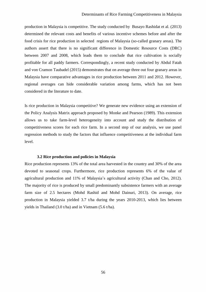
Determinants of Rice Farming Competitiveness in Malaysia
56
production in Malaysia is competitive. The study conducted by Busayo Rashidat et al. (2013)
determined the relevant costs and benefits of various incentive schemes before and after the
food crisis for rice production in selected regions of Malaysia (so-called granary areas). The
authors assert that there is no significant difference in Domestic Resource Costs (DRC)
between 2007 and 2008, which leads them to conclude that rice cultivation is socially
profitable for all paddy farmers. Correspondingly, a recent study conducted by Abdul Fatah
and von Cramon Taubadel (2015) demonstrates that on average three out four granary areas in
Malaysia have comparative advantages in rice production between 2011 and 2012. However,
regional averages can hide considerable variation among farms, which has not been
considered in the literature to date.
Is rice production in Malaysia competitive? We generate new evidence using an extension of
the Policy Analysis Matrix approach proposed by Monke and Pearson (1989). This extension
allows us to take farm-level heterogeneity into account and study the distribution of
competitiveness scores for each rice farm. In a second step of our analysis, we use panel
regression methods to study the factors that influence competitiveness at the individual farm
level.
3.2 Rice production and policies in Malaysia
Rice production represents 13% of the total area harvested in the country and 30% of the area
devoted to seasonal crops. Furthermore, rice production represents 6% of the value of
agricultural production and 11% of Malaysia’s agricultural activity (Chan and Cho, 2012).
The majority of rice is produced by small predominantly subsistence farmers with an average
farm size of 2.5 hectares (Mohd Rashid and Mohd Dainuri, 2013). On average, rice
production in Malaysia yielded 3.7 t/ha during the years 2010-2013, which lies between
yields in Thailand (3.0 t/ha) and in Vietnam (5.6 t/ha).
Determinants of Rice Farming Competitiveness in Malaysia
57
Figure 3.1: Average rice yields, ASEAN countries for 2010-2013. (Source: FAOSTAT,
2016).
Rice is a staple food, and Malaysians consume nearly 2.2 million tons of rice annually, 70%
of which is produced domestically and the rest of which is imported from major rice
exporting countries such as Vietnam and Thailand. During the period 2000-2005, the country
imported 515 thousand metric tons of rice, making Malaysia the third largest Asian rice
importer after the Philippines and Indonesia (FAOSTAT, 2016). During this time, the
government argued that it was cheaper to import rice from other countries so as to release
arable lands for other cash crops that have the potential to produce higher earnings and yield
more profits. However, the world food crisis in 2008 led to an increased emphasis on self-
sufficiency, and in 2012 the Malaysian government increased price support measures in the
form of a guaranteed minimum price (GMP), and paddy bonus payments to stimulate supply.
This output support was supplemented by input subsidies, particularly through the provision
of fertilizer, low cost credit and irrigation facilities. In addition, to stabilize consumer prices,
the government allowed the national rice company Padiberas Nasional Berhad (BERNAS) to
import rice at low or zero tariffs.
These types of programs are common in most developing countries. In Asia, countries such as
India, Bangladesh, Indonesia and Pakistan implement food price stabilization programs and
input subsidies (Dorosh, 2009; Timmer and Dawe, 2007; Warr and Yusuf, 2014). However,
simultaneously protecting both producers and consumers is very costly (Warr and Yusuf,
2014) and has become one of Malaysia’s most politically contentious issues.
0.0
1.0
2.0
3.0
4.0
5.0
6.0
Vietnam Indonesia Philippines Malaysia Laos Myanmar Cambodia Thailand
Av
era
ge
Yie
ld t
/ha
Determinants of Rice Farming Competitiveness in Malaysia
58
According to Malaysia’s WTO trade report review (2014), the total support given to
agriculture consisted of reduction commitments amounting to 1 billion RM. Of this,
approximately 74% was related to Green Box assistance, mainly in the form of income
support for farmers while others involved the fertilizer subsidy scheme. In 2013, price support
(incentives or bonus payments for paddy rice production) remained the largest part of
expenditures (480 million RM) followed by the fertilizer subsidy (465 million RM).
In addition, the Malaysian government has announced the goal of becoming 100% self-
sufficient in rice by the year 2020. Since preliminary evidence (Abdul Fatah and von Cramon,
2015) indicates that much of Malaysia’s rice production is competitive at both private and
social prices, producer support measures might be unnecessary. The goal of this paper is to
generate more detailed evidence on the competitiveness of rice production in Malaysia.
3.3 Measuring the competitiveness of rice production
The Social Cost Benefit (SCB) ratio is one of the indicators that can be calculated to measure
competitiveness using the Policy Analysis Matrix (PAM) framework developed by Monke
and Pearson (1989). The PAM is described in Appendix 3.2.
It is defined as:
SCB = [ ∑ 𝑎𝑖𝑗𝑃𝑗𝑆𝑘
𝑗=1 + ∑ 𝑎𝑖𝑗𝑊𝑗𝑆𝑛
𝑗=𝑘+1 ] / 𝑃𝑖𝑆 (1)
where Pi is the price of the output i, the Pj are the prices of the k tradeable inputs, the Wj are
the prices of the n-k non-tradeable inputs, and the ij are technical coefficients which measure
the amount of input j that is required to produce one unit of output i. Throughout, the
superscript S indicates that social rather than private prices are employed. Hence, the SCB is
simply the ratio of the social cost of producing one unit of an output, such as rice, to the social
value of that unit of output. An SCB value between zero and one indicates that the activity in
question is competitive, while a value greater than one indicates that social cost exceeds
social value and the activity is not competitive.3
3 Another PAM-based indicator that is commonly used is the Domestic Resource Cost (DRC) ratio.
However, as Frohberg and Hartmann (1997), Masters and Winter-Nelson (1995) and von Cramon-
Taubadel and Nivyevskyi (2008) discuss, the DRC suffers from several weaknesses. In particular, it is
sensitive to the classification of inputs into tradable and non-tradable, which can be difficult in applied
work (Monke and Pearson, 1989), and it has a discontinuity at zero, which makes the interpretation of
DRC distributions difficult. We therefore consider only the SCB ratio.
Determinants of Rice Farming Competitiveness in Malaysia
59
The PAM approach and associated indicators, such as the SCB, have been used by analysts
working in many developing countries where price distortions are often substantial (Yao
1997; Reig-Martínez et al. 2008; Erenstein 2010; Zheng et al. 2015). However, one major
drawback of almost all applied PAM analysis to date is that it is carried out with aggregate
data, for example for average or representative farms. This will provide an incomplete picture
of sectoral competitiveness since results based on average data may conceal important
variations in competitiveness among heterogeneous producers (Nivievskyi et al 2010; von
Cramon-Taubadel and Nivyevskyi 2008). To improve the usefulness of indicators based on
the PAM, Morrison and Balcombe (2002) suggest resampling data using the bootstrapping
method. This method can generate distributional properties of the indicators and thus allow
the calculation of standard deviations and confidence intervals for PAM indicators. von
Cramon Taubadel and Nivyevskyi (2009) propose the calculation of the distributions of PAM
indicators using farm-level survey data. Using kernel methods, they estimate SCB
distributions for different agricultural products (e.g. wheat) over a large sample of farms in
Ukraine. Using these distributions they estimate the proportion of farms that produces
competitively for each product and the proportion of the total production of that product that
is produced competitively.
We adapt the methods proposed by von Cramon-Taubadel and Nivyevskyi (2008, 2009) to
calculate SCB distributions for rice production in Malaysia using panel data during 2010-
2014 period. The calculation of SCB distributions is purely a descriptive technique; however
its use here is motivated by the hypothesis that Malaysia has the potential to grow more rice if
analysis can identify those farms that are currently competitive and the reasons for their
superior performance, thus providing benchmarks for other, currently less competitive farms.
3.4 Data and assumptions
In Malaysia, the rice-cropping season is categorized into main and off-seasons. The main
season usually begins in September and runs through December, while the off-season runs
from February to May. During the off-season the amount and frequency of precipitation is
lower than it is during the main season. Therefore, the off-season crop relies heavily on the
irrigation system.
Determinants of Rice Farming Competitiveness in Malaysia
60
In the Third National Agriculture Policy (1998-2010), eight granary areas4 were designated as
permanent rice granary areas responsible for scaling up and increasing productivity in the rice
farming industry. The eight granaries contribute about 75% of the national rice production.
The data used in this analysis are from the Muda Agricultural Development Authority
(MADA), which is the largest granary area and contributed 51% of total granary production
in 2013 and consistently generates 37% of Malaysia’s total annual rice production on 33% of
the country’s rice area (Appendix 3.1). The farm level data is collected twice a year and each
survey period includes a balanced sample of 675 farming households. The panel is composed
of ten cross-sections, covering main and off- seasons over the five-year period from 2010 to
2014. This data set provides comprehensive information, including input use, output and
corresponding prices.
The farm-level panel data described above allows us to estimate the financial costs (profits)
and social costs (profits) of rice production for each farm in each of the ten seasons. The
result is a panel of 6750 PAMs one for each farm and season. To complete these PAMs
(Appendix table 3.2), we first need to classify and decompose input items into tradable and
non-tradable input categories. In Malaysian rice farming, the tradable inputs are fertilizers,
seeds and agro-chemicals including pesticides, herbicides, rat and golden snail control, while
other inputs such as labor, capital and land rent are categorized as non-tradable. Using the
available data we complete the row of each PAM that describes costs and revenues at private
prices. Second, we estimate the social prices (shadow price) of all the inputs and of the output
(rice) and complete the row of the PAM that describes costs and revenues at social prices.
Finally, we calculate the SCB ratio for each farm and season and derive the distribution of the
SCB across farms for each season.
Social prices of output and tradable inputs are based on import or export parity prices,
depending on the trade status of the commodity in question. Since Malaysia is a net importer
of rice, an import parity is used to measure the social price of rice. The major rice imports are
25 percent broken rice mainly from Vietnam, followed by milled rice and glutinous rice
(Department of Agriculture, 2014). We use the CIF price of 25% broken rice as the reference
price (social price), obtained from the International Rice Reserch Institute (IRRI). To
4 Granary Areas refer to major irrigation schemes (areas greater than 4,000 hectares) and recognized
by the Government in the National Agricultural Policy as the main paddy producing areas. There are
eight granary areas in Malaysia, namely MADA, KADA, IADA KERIAN, IADA BLS, IADA P.
Pinang, IADA Seberang Perak, IADA KETARA and IADA Kemasin Semerak (Appendix 2).
Determinants of Rice Farming Competitiveness in Malaysia
61
calculate the farm gate equivalent of this CIF price5, we use information regarding costs of
handling, transportation, freight and insurance based on an interview with an officer from
BERNAS. For the tradable inputs, the social prices are also import parity prices converted to
the farm gate price. CIF prices for fertilizers, including urea (Europe), TSP (US Gulf ports),
organic and NPK are provided by the World Bank, IRRI, and various issues of the FAO food
outlook. The costs of moving these inputs from the port of entrance to the farm gate are based
on information provided by traders.
For the non-tradeable input of land we assume a social price of zero. This is because of the
impossibility of growing alternative crops on the land presently devoted to harvesting rice,
both for legal reasons derived from land regulations and for physical reasons connected to the
condition of the soil and the risk of seasonal flooding of the cultivation plots.
In some countries where the labor market is imperfect or there are macroeconomic
imbalances, current wages may be a distorted indicator of the social cost of labor. In such
cases, the current wages are corrected by using conversion factors to compute social wages
(European Commission, 2014). However, in the case of a small country, such as Malaysia,
where the unemployment rate is low, the social wage for labor can be assumed to be equal to
the market wage. Therefore, we set conversion factor used to convert private into social
wages equal to one.
The costs of machinery services hired for harvesting, transplanting and threshing were
included in the capital account. However, payment for these services includes tradable
components such as machine depreciation, fuel and oil, and non-tradable components such as
labor for maintenance and the administration of rental operations. Therefore, we decompose
machinery services into tradable and non-tradable components.
3.5 Results and discussion
3.5.1 The profile of rice farming
Rice farming in the MADA region is dominated by a small landholding size ranging between
1.70 to 2.17 hectares (Table 3.1). Investments in tertiary irrigation development have
5 The conversion factors of paddy to rice are based on percentages of paddy recovery rates at 0.65.
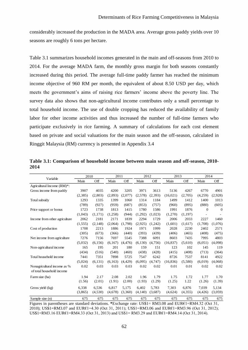
Determinants of Rice Farming Competitiveness in Malaysia
62
considerably increased the production in the MADA area. Average gross paddy yields over 10
seasons are roughly 6 tons per hectare.
Table 3.1 summarizes household incomes generated in the main and off-seasons from 2010 to
2014. For the average MADA farm, the monthly gross margin for both seasons constantly
increased during this period. The average full-time paddy farmer has reached the minimum
income objective of 960 RM per month, the equivalent of about 8.50 USD per day, which
meets the government’s aims of raising rice farmers’ income above the poverty line. The
survey data also shows that non-agricultural income contributes only a small percentage to
total household income. The use of double cropping has reduced the availability of family
labor for other income activities and thus increased the number of full-time farmers who
participate exclusively in rice farming. A summary of calculations for each cost element
based on private and social valuations for the main season and the off-season, calculated in
Ringgit Malaysia (RM) currency is presented in Appendix 3.4
Table 3.1: Comparison of household income between main season and off-season, 2010-
2014
Figures in parentheses are standard deviations. *Exchange rate: US$1= RM3.08 and EUR€1=RM4.32 (Oct 31,
2010); US$1=RM3.07 and EUR€1=4.30 (Oct 31, 2011); US$1=RM3.06 and EUR€1=RM3.96 (Oct 31, 2012);
US$1=RM3.16 EUR€1=RM4.33 (Oct 31, 2013) and US$1= RM3.29 and EUR€1=RM4.14 (Oct 31, 2014).
Main Off Main Off Main Off Main Off Main Off
Agricultural Income (RM)*:
Gross income from paddy 3907 4035 4200 3205 3971 3613 5136 4267 6770 4901
(2,385) (2,803) (2,893) (2,077) (2,578) (2,393) (16,021) (2,705) (4,259) (2,928)
Total subsidy 1293 1335 1399 1060 1314 1184 1499 1412 1400 1013
(789) (927) (959) (687) (853) (757) (960) (895) (880) (605)
Price support or bonus 1723 1738 1813 1415 1780 1586 1991 1876 0 0
(1,043) (1,171) (1,258) (944) (1,292) (1,023) (1,270) (1,197) - -
Income from other agriculture 2062 2181 2171 1839 2294 1729 2006 2033 2227 1460
(1,555) (2,148) (2,064) (1,798) (2,925) (1,242) (1,601) (1,617) (1,708) (1,076)
Cost of production 1708 2213 1886 1924 1971 1999 2028 2230 2402 2571
(305) (673) (366) (440) (393) (439) (406) (465) (408) (475)
Net income from agriculture 7276 7156 7697 5545 7388 6091 8603 7435 7995 4803
(5,032) (6,156) (6,167) (4,476) (6,130) (4,756) (16,837) (5,610) (6,051) (4,098)
Non-agricultural income 165 195 201 180 159 151 123 102 145 119
(434) (516) (540) (460) (438) (428) (415) (408) (713) (364)
Total household income 7441 7351 7898 5725 7547 6242 8726 7537 8141 4922
(5,024) (6,131) (6,163) (4,429) (6,095) (4,747) (16,836) (5,580) (6,019) (4,068)
Nonagricultural income as % 0.02 0.03 0.03 0.03 0.02 0.02 0.01 0.01 0.02 0.02
of total household income
Farm size (ha) 1.94 2.17 2.08 2.02 1.96 1.79 1.75 1.72 1.77 1.70
(1.56) (2.01) (1.91) (2.00) (1.93) (1.29) (1.25) 1.22 (1.26) (1.39)
Gross yield (kg) 6,338 6,536 6,817 5,175 6,402 5,783 7,303 6,876 7,039 5,134
(3,865) (4,530) (4,678) (3,360) (4,140) (3,687) (4,624) (4,355) (4,426) (3,059)
Sample size (n) 675 675 675 675 675 675 675 675 675 675
2014Variable
2010 2011 2012 2013
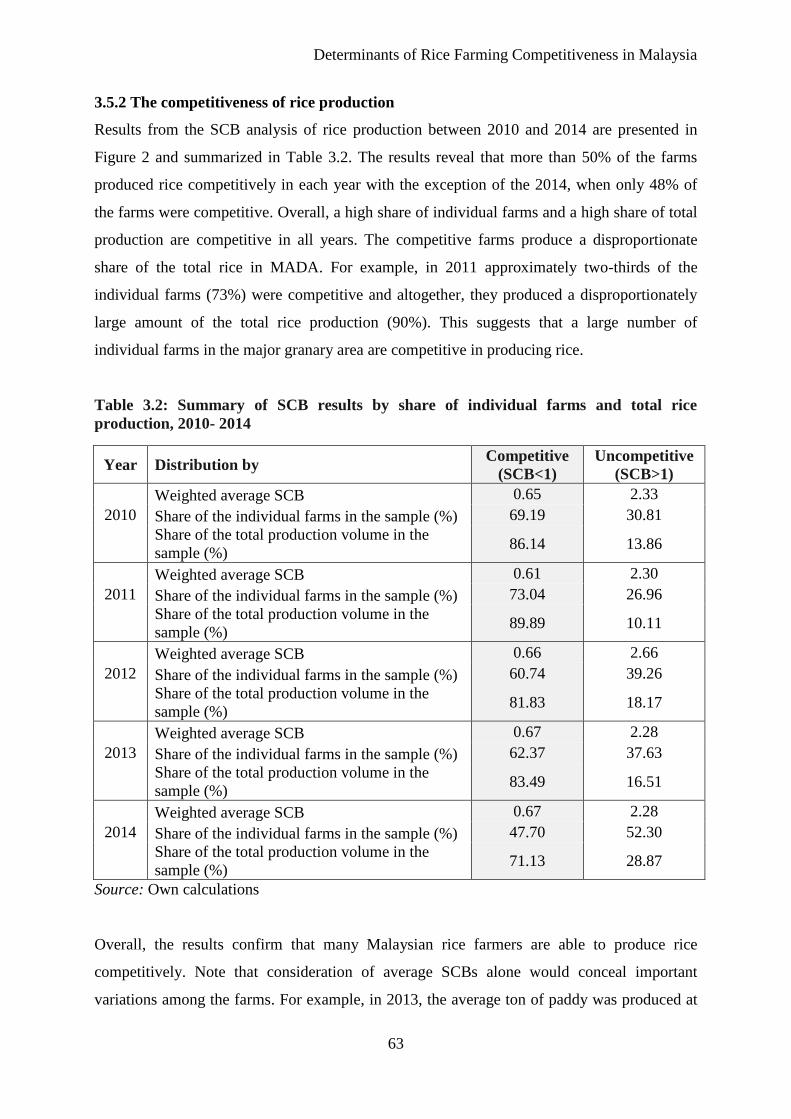
Determinants of Rice Farming Competitiveness in Malaysia
63
3.5.2 The competitiveness of rice production
Results from the SCB analysis of rice production between 2010 and 2014 are presented in
Figure 2 and summarized in Table 3.2. The results reveal that more than 50% of the farms
produced rice competitively in each year with the exception of the 2014, when only 48% of
the farms were competitive. Overall, a high share of individual farms and a high share of total
production are competitive in all years. The competitive farms produce a disproportionate
share of the total rice in MADA. For example, in 2011 approximately two-thirds of the
individual farms (73%) were competitive and altogether, they produced a disproportionately
large amount of the total rice production (90%). This suggests that a large number of
individual farms in the major granary area are competitive in producing rice.
Table 3.2: Summary of SCB results by share of individual farms and total rice
production, 2010- 2014
Year Distribution by Competitive
(SCB<1)
Uncompetitive
(SCB>1)
Weighted average SCB 0.65 2.33
2010 Share of the individual farms in the sample (%) 69.19 30.81
Share of the total production volume in the
sample (%) 86.14 13.86
Weighted average SCB 0.61 2.30
2011 Share of the individual farms in the sample (%) 73.04 26.96
Share of the total production volume in the
sample (%) 89.89 10.11
Weighted average SCB 0.66 2.66
2012 Share of the individual farms in the sample (%) 60.74 39.26
Share of the total production volume in the
sample (%) 81.83 18.17
Weighted average SCB 0.67 2.28
2013 Share of the individual farms in the sample (%) 62.37 37.63
Share of the total production volume in the
sample (%) 83.49 16.51
Weighted average SCB 0.67 2.28
2014 Share of the individual farms in the sample (%) 47.70 52.30
Share of the total production volume in the
sample (%) 71.13 28.87
Source: Own calculations
Overall, the results confirm that many Malaysian rice farmers are able to produce rice
competitively. Note that consideration of average SCBs alone would conceal important
variations among the farms. For example, in 2013, the average ton of paddy was produced at
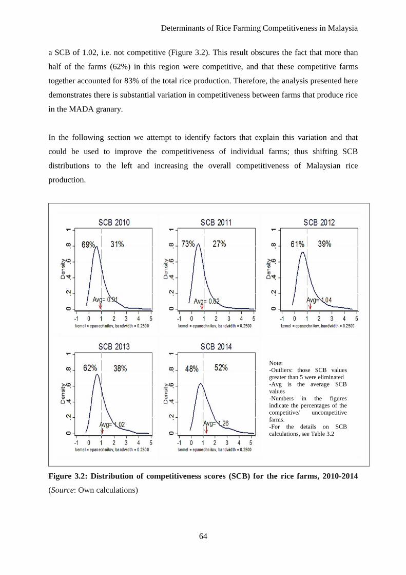
Determinants of Rice Farming Competitiveness in Malaysia
64
a SCB of 1.02, i.e. not competitive (Figure 3.2). This result obscures the fact that more than
half of the farms (62%) in this region were competitive, and that these competitive farms
together accounted for 83% of the total rice production. Therefore, the analysis presented here
demonstrates there is substantial variation in competitiveness between farms that produce rice
in the MADA granary.
In the following section we attempt to identify factors that explain this variation and that
could be used to improve the competitiveness of individual farms; thus shifting SCB
distributions to the left and increasing the overall competitiveness of Malaysian rice
production.
Figure 3.2: Distribution of competitiveness scores (SCB) for the rice farms, 2010-2014
(Source: Own calculations)
Note:
-Outliers: those SCB values
greater than 5 were eliminated
-Avg is the average SCB
values
-Numbers in the figures
indicate the percentages of the
competitive/ uncompetitive
farms.
-For the details on SCB
calculations, see Table 3.2
Determinants of Rice Farming Competitiveness in Malaysia
65
3.5.3 The determinants of rice competitiveness
To explain differences in competitiveness among farms we use the following dynamic panel
data model:
Yit = β1Yit-1 + β2Xit-1 + αi + εit (2)
where Yit is farm i’s SCB score in period t, Xit-1 is a vector of exogenous explanatory variables
(farm size, distance to milling factories, access to credit, off-farm income, landownership,
hired cost labor, farmers’ organization, land ownership and a time trend), and αi and εit are
error terms (αi captures unobserved and time constant farm specific effects and εit is an
idiosyncratic error term).
Since the lagged dependent variable in equation (2) can be correlated with the error term (),
it violates the assumption of exogeneity. Furthermore, the unobserved farm specific effects
() can be correlated with explanatory variables in X. To account for these problems,
Anderson & Hsiao (1981) propose a difference generalized method of moments (DGMM)
estimator to obtain unbiased estimates. The model is specified using a system of equations,
one per period, and uses all available lags of the dependent variable as instruments for each
first-difference equation (Bond et al, 2001). However, if the parameter β1 is close to a random
walk, then the lagged levels are weak instruments for differences, because, in this case, past
levels of SCB scores do not convey much information about present changes. A more suitable
alternative is to use the system generalized method of moments (SGMM) proposed by
Arellano and Bover (1995) and Blundell and Bond (1998) that estimates the model in levels,
as well as in differences, by using the lagged instruments for the level equations.
We employ the SGMM and perform several tests to determine the most appropriate model
specification. The Arellano-Bond test is executed to determine serial correlation on the
residuals, under the hypothesis of no first (AR1) or second (AR2) order serial correlation of
the residuals (Roodman, 2009a). In order to check for endogeneity bias and potential
problems of specification in the model estimation we use the Hansen test of over-identifying
restrictions (Bond, Hoeffler, and Temple 2001). In addition, we use the difference-in-Hansen
test statistic to test the validity of specific subsets of instruments.
Where valid instruments are usually scant, the Arellano Bond estimation procedure is useful
since any lagged level is a valid instrument. To avoid the proliferation of instruments,
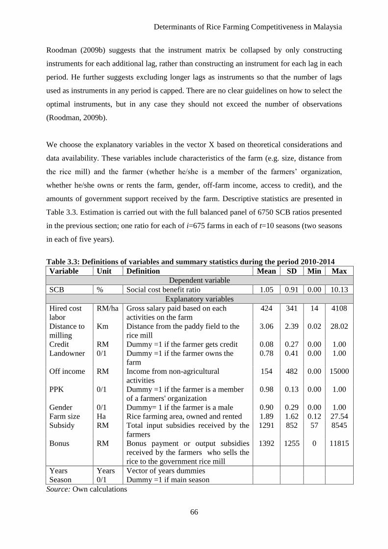
Determinants of Rice Farming Competitiveness in Malaysia
66
Roodman (2009b) suggests that the instrument matrix be collapsed by only constructing
instruments for each additional lag, rather than constructing an instrument for each lag in each
period. He further suggests excluding longer lags as instruments so that the number of lags
used as instruments in any period is capped. There are no clear guidelines on how to select the
optimal instruments, but in any case they should not exceed the number of observations
(Roodman, 2009b).
We choose the explanatory variables in the vector X based on theoretical considerations and
data availability. These variables include characteristics of the farm (e.g. size, distance from
the rice mill) and the farmer (whether he/she is a member of the farmers’ organization,
whether he/she owns or rents the farm, gender, off-farm income, access to credit), and the
amounts of government support received by the farm. Descriptive statistics are presented in
Table 3.3. Estimation is carried out with the full balanced panel of 6750 SCB ratios presented
in the previous section; one ratio for each of i=675 farms in each of t=10 seasons (two seasons
in each of five years).
Table 3.3: Definitions of variables and summary statistics during the period 2010-2014
Variable Unit Definition Mean SD Min Max
Dependent variable
SCB % Social cost benefit ratio 1.05 0.91 0.00 10.13
Explanatory variables
Hired cost
labor
RM/ha
Gross salary paid based on each
activities on the farm
424
341
14
4108
Distance to
milling
Km
Distance from the paddy field to the
rice mill
3.06
2.39
0.02
28.02
Credit RM Dummy =1 if the farmer gets credit 0.08 0.27 0.00 1.00
Landowner
0/1
Dummy =1 if the farmer owns the
farm
0.78
0.41
0.00
1.00
Off income
RM
Income from non-agricultural
activities
154
482
0.00
15000
PPK
0/1
Dummy =1 if the farmer is a member
of a farmers' organization
0.98
0.13
0.00
1.00
Gender 0/1 Dummy= 1 if the farmer is a male 0.90 0.29 0.00 1.00
Farm size Ha Rice farming area, owned and rented 1.89 1.62 0.12 27.54
Subsidy
RM
Total input subsidies received by the
farmers
1291
852
57
8545
Bonus
RM
Bonus payment or output subsidies
received by the farmers who sells the
rice to the government rice mill
1392
1255
0
11815
Years Years Vector of years dummies
Season 0/1 Dummy =1 if main season
Source: Own calculations
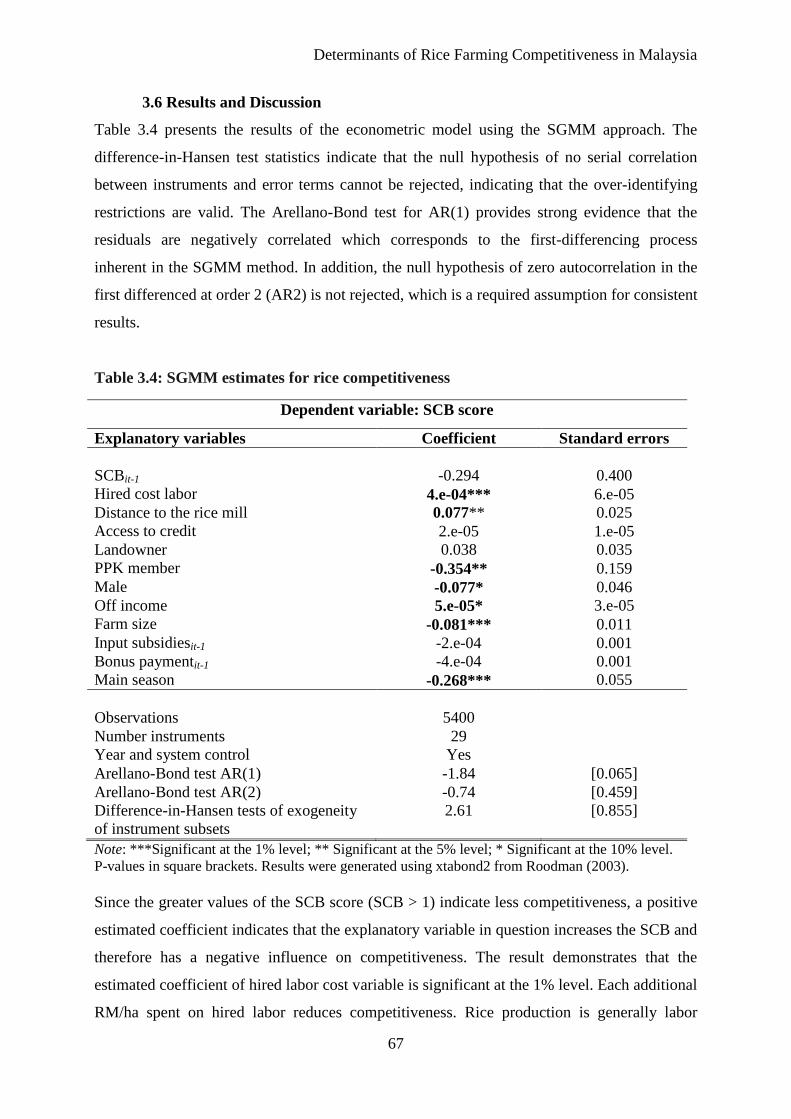
Determinants of Rice Farming Competitiveness in Malaysia
67
3.6 Results and Discussion
Table 3.4 presents the results of the econometric model using the SGMM approach. The
difference-in-Hansen test statistics indicate that the null hypothesis of no serial correlation
between instruments and error terms cannot be rejected, indicating that the over-identifying
restrictions are valid. The Arellano-Bond test for AR(1) provides strong evidence that the
residuals are negatively correlated which corresponds to the first-differencing process
inherent in the SGMM method. In addition, the null hypothesis of zero autocorrelation in the
first differenced at order 2 (AR2) is not rejected, which is a required assumption for consistent
results.
Table 3.4: SGMM estimates for rice competitiveness
Dependent variable: SCB score
Explanatory variables Coefficient Standard errors
SCBit-1 -0.294 0.400
Hired cost labor 4.e-04*** 6.e-05
Distance to the rice mill 0.077** 0.025
Access to credit 2.e-05 1.e-05
Landowner 0.038 0.035
PPK member -0.354** 0.159
Male -0.077* 0.046
Off income 5.e-05* 3.e-05
Farm size -0.081*** 0.011
Input subsidiesit-1 -2.e-04 0.001
Bonus paymentit-1 -4.e-04 0.001
Main season -0.268*** 0.055
Observations 5400
Number instruments 29
Year and system control Yes
Arellano-Bond test AR(1) -1.84 [0.065]
Arellano-Bond test AR(2) -0.74 [0.459]
Difference-in-Hansen tests of exogeneity
of instrument subsets
2.61 [0.855]
Note: ***Significant at the 1% level; ** Significant at the 5% level; * Significant at the 10% level.
P-values in square brackets. Results were generated using xtabond2 from Roodman (2003).
Since the greater values of the SCB score (SCB > 1) indicate less competitiveness, a positive
estimated coefficient indicates that the explanatory variable in question increases the SCB and
therefore has a negative influence on competitiveness. The result demonstrates that the
estimated coefficient of hired labor cost variable is significant at the 1% level. Each additional
RM/ha spent on hired labor reduces competitiveness. Rice production is generally labor
Determinants of Rice Farming Competitiveness in Malaysia
68
intensive. Much of the labor requirements for the nursery, land preparation, fertilizer
application, pest control, as well as postharvest activities are mainly completed by farmers
with the help of hired labors, for whom wages are high, particularly during weeding and
harvesting periods. For example, for 2013, the average daily wage rate is 38 RM (equivalent
to 8.5 EUR) (Department of Agriculture, 2014). If a 3 ha farm hires a half-time labor, then the
SCB scores will fall by 0.04.
The variable “distance to milling” has a statistically strong effect on competitiveness at the
5% level. The farther a farm is located from the closest milling factory, the lower its
competitiveness. The delayed drying of a paddy can cause severe losses of moisture due to
high transpiration rates and microorganisms, especially during the dry season (off-season). To
avoid high post-harvest losses, farmers have to sell paddy immediately after harvest. To
proceed with this, farmers have the option of selling a paddy directly to a local miller or
allowing the paddy to be collected by local traders. Most farmers prefer to wait for collection
because they do not own trucks to load their harvest. Thus, farmers must bear the transaction
costs, which increase as the distance to the rice mills increases.
It appears that growers who engage collectively in a farmer’s organization (PPK) are
accessing social and economic benefits greater than non-collective action participants. The
results are consistent with the predicted function of agricultural cooperatives in improving the
performance of their members in the market by providing easy access to productive inputs
and technical and management services, such as training, information and extension on input
application (Addai et al, 2014). Many governments establish farmer-based cooperation groups
to improve rural service delivery and access to the market, as well as reduce transaction costs
and achieve competitiveness.
Male farmers are observed to be operating at a higher level of profitability than their female
counterparts. It implies that male farmers earned more social profits from rice production and
are more competitive than the female farmers. This could be due to the limited access the
female farmers usually have to resources of production in comparison with the male farmers.
This corroborates the results of many previous studies on the role of gender in agricultural
production. The study by Siriwardana and Jayawardena (2014) in Sri Lanka found male
household heads to be more productive than female household heads in mechanized farms.
Koirala et al. (2015) found female heads of households to be less productive than men in rice

Determinants of Rice Farming Competitiveness in Malaysia
69
production in a study in the Philippines, a fact that the authors attributed to culture, access to
land and economic factors.
Another important finding is that involvement in off-farm activities appears to reduce
competitiveness. The increasing importance of off-farm work implies less labor effort and
time spent on the farm. The coefficient suggests that off-farm income tends to increase the
SCB ratio by 5x10⁻⁴
. Such an effect, though small, is statistically significant at the 10% level.
Our result confirms the finding made by Goodwin and Ashok (2004) who noted that increased
reliance on off-farm work may have implied less attention paid to the on-farm productivity
issues such as adoption of best management practices and technologies, and in turn decreases
competitiveness.
We used the farm size variable to test whether competitiveness increases with the scale of
operation. Our result indicates that increasing the farm size per hectare reduces the SCB of
rice production by 0.081. This finding suggests that the consolidation of small farms in the
MADA granary area will lead to the realization of economies of scale in rice production.
Other variables such as access to credit and landownership have no significant effect on
competitiveness.
We turned our attention to the rice policies and different mechanisms affecting
competitiveness. To avoid the effects of heterogeneity on total subsidies, we disaggregated
subsidies into input subsidies and bonus payments. The whole idea of the SCB is that we
calculated the social profits without government intervention or subsidies. To determine
whether these subsidies would improve SCBs, we tested the hypothesis in a dynamic setting;
do past subsidies affect current competitiveness or are the farms that previously received
more subsidies more competitive today? We hypothesize that input subsidies, by encouraging
input use, might lead farms to produce in more efficient, more beneficial ways when
evaluated at social prices. Additionally, if the bonus payments are more coupled from
intensity and production decisions, they might not have a negative effect on competitiveness.
In fact, they may lead to a wealth effect which can reduce farmers’ aversion to risks and
facilitate investment and thus increase outputs. The various mechanism through which
decoupled payment and inputs subsidies may affect production are well discussed in the
literature (see Goodwin and Ashok 2005; Femenia et al. 2010; Sunding and Zilberman 2000).
Determinants of Rice Farming Competitiveness in Malaysia
70
Our SGMM results, however, indicate no significant difference between these types of
policies and competitiveness scores. The general evidence seems to be that input subsidies
and bonuses are, if anything, increasing competitiveness. Subsidies, by encouraging input use,
may indeed be increasing production and making it more competitive. Since the evidence
shows no strong effects of subsidies and bonus payments, then the policy implications are that
the policies are not having a strong effect on competitiveness, and the money in question
could perhaps be better spent in other ways. At best, the subsidies are a form of social policy
that simply increases farm incomes, but then the question arises as to why larger farms, that
are presumably not poor, should also receive these payments. So current spending is poorly
targeted as social policy, and ineffective as an economic policy to boost competitiveness.
3.7 Conclusion and recommendations
The Malaysian rice market has been characterized in the past decade by pervasive government
interventions for various purposes, such as to alleviate poverty and increase self-sufficiency
levels. Since rice is a staple food, the government intervenes more in the rice market than in
most others. These interventions include support for producers through subsidies on
fertilizers, lime and pesticides on the input side and a subsidized guaranteed minimum price
coupled with price bonuses on the output side. However, the successful completion of WTO
negotiations together with Asean Free Trade Agreement (AFTA) negotiations would imply
that significant structural changes must be made not only to the trade regime, but also to the
rice sector and adjustments at the farm level are needed in order for greater efficiency and
competitiveness to be achieved.
Previous literature had discussed the impact of policies on agricultural competitiveness using
the Policy Analysis Matrix (PAM) in many developing countries. However, one major
drawback of almost all applied PAM analysis to date is that it is carried out with aggregate
data, for example for average or representative farms. This will provide an incomplete picture
of sectoral competitiveness since results based on average data may conceal important
variations in competitiveness among heterogeneous producers. We have addressed this
shortcoming, using a unique, farm level survey data from rice farmers in the major granary
area in Malaysia over the period 2010 to 2014. Our contribution to the existing literature is
twofold. First, we provide new evidence on rice competitveness using an extension to the
Policy Analysis Matrix approach proposed by (Monke and Pearson (1989). This extension
allows us to take farm-level heterogeneity into account and derive competitiveness score
Determinants of Rice Farming Competitiveness in Malaysia
71
distributions for each rice farm. To improve the usefulness of SCB indicator, we use a kernel-
based estimate to demonstrate the distribution of competitiveness scores and determine the
proportion of farms that are producing competitively and the proportion of total
production/output value of the product that is produced competitively. Second, we develop a
panel regression model to examine the factors that influence rice competitiveness at the
individual farm level. This approach may also be useful for other evaluation in other contexts,
thus contributing to the broader research direction on agricultural competitiveness.
The empirical results reveal that more than 50% of farmers produce rice competitively from
2010 until 2013 and altogether, they produce a disproportionately large number of the total
rice production (80%). This suggests that a large number of individual farms in the granary
area are competitive in producing rice. Additionally, we briefly note the contrast between the
distributions of using disaggregate SCB and average SCB that would result from the use of
aggregated data.
Our dynamic SGMM estimates revealed that participation in a farmer’s organization, gender
and total farm size are the major determinants of rice competitiveness, while the distance to
the rice mills, off-farm income and the use of hired labor are the main constraints that reduce
competitiveness. Additionally, there are no signicant differences between the types of policies
employed (input subsidies and bonuses) and competitiveness. The estimates produced for this
paper have the potential to influence on-going debates on federal budget reduction, as well as
add to the discussion on the agricultural subsidy reform policy.
Policies for rice farmers need to vary depending on the context. This statement is bolstered by
our empirical analysis, which reveals that the types of supports do not have significant effects
on competitiveness and the money in question could be spent in other ways. Bonus payments
and input subsidies in their current form are not as efficient as they seem to be considering
that essentially only large farms and high-income groups benefit from them. The existing set
of programs was designed to address situations that are now out-of-date and, as a
consequence, may no longer be relevant.
If the government decides to preserve small and marginal farms, assistance measures should
be directed towards these specific groups to prevent such problematic outcomes. For instance,
improving infrastructure that links farmers to millers would help improve competitiveness. In
Determinants of Rice Farming Competitiveness in Malaysia
72
addition, offering support in the form of providing technical assistance through farmers’
organization so that farmers can receive a better share of market prices could improve
competitiveness. If this were the case for the policy agenda, such support could become a
social safety net for the poor and could facilitate a comfortable exit from farming for small
farmers through job provision or income support programs. The replacement of the fertilizer
subsidy by direct income support programs would be tantamount to income support without
any waste and lack of efficient distribution associated with the fertilizer and input subsidy
scheme.
In other cases, policy-makers must consider whether there are social reasons to support large
farms. The empirical evidence reveals that farmers are fully aware of the utility of subsidies;
considering the fact that the previous provision of input subsidies does not improve current
competitiveness. If profits generated by farming activities were to be ensured by the
government, the incentive to adopt innovate practices and technology would diminish.
Similarly, the incorporation of the paddy bonus into the guaranteed minimum price is justified
on the grounds of increasing rice prices and cost control. Efforts to direct paddy bonus
payments to poor and small farms by incorporating the access to farm size and production
deliveries seem achievable. However, regardless of whether the farms are small or large,
paddy bonuses are given to all farmers. It is important to note that not all paddy growers are
poor; some support goes to larger farms where profits are already substantial. The drawback
implies that the support may be biased towards larger farms and is not well-targeted.
Therefore, a combination of both subsidy schemes is not completely necessary and
improvement would result in a more efficient use of public money.
Given the fact that the sample in this study constitutes only a dataset of individual rice farms
selected from one granary area of the country, our findings and policy recommendations
cannot be generalized to the national level. These results are situation specific and thus cannot
be extrapolated to other granary areas with different conditions. The SGMM provides an
appropriate framework to analyse the determinants of rice competitiveness, however data
limitation prevents the consideration of all aspects in the analysis. We suggest for future
research to determine the characteristics of farms (bio-physical conditions such as soil types
and climate variability) and different agro-ecological regions, as well as other farmer’s
characteristics such as age, education and human capital. Extending this research topic would

Determinants of Rice Farming Competitiveness in Malaysia
73
not only supplement the contribution of this study but also can shed light on the variations and
differences in competitiveness level among rice farms and region specific priorities.
Additionally, further research will lead to the policies that would enhance farmers income,
shifting from less efficient to more efficient farms and allowing them to better contribute to
the national goal of food self-sufficiency.
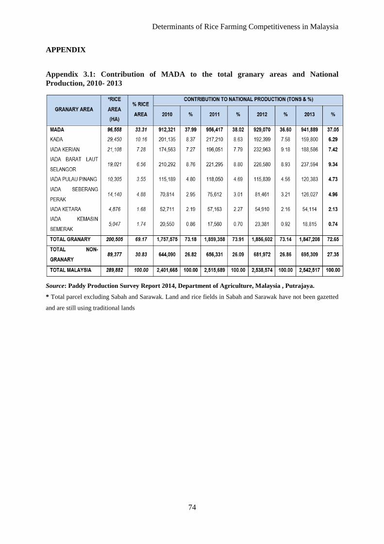
Determinants of Rice Farming Competitiveness in Malaysia
74
APPENDIX
Appendix 3.1: Contribution of MADA to the total granary areas and National
Production, 2010- 2013
Source: Paddy Production Survey Report 2014, Department of Agriculture, Malaysia , Putrajaya.
* Total parcel excluding Sabah and Sarawak. Land and rice fields in Sabah and Sarawak have not been gazetted
and are still using traditional lands
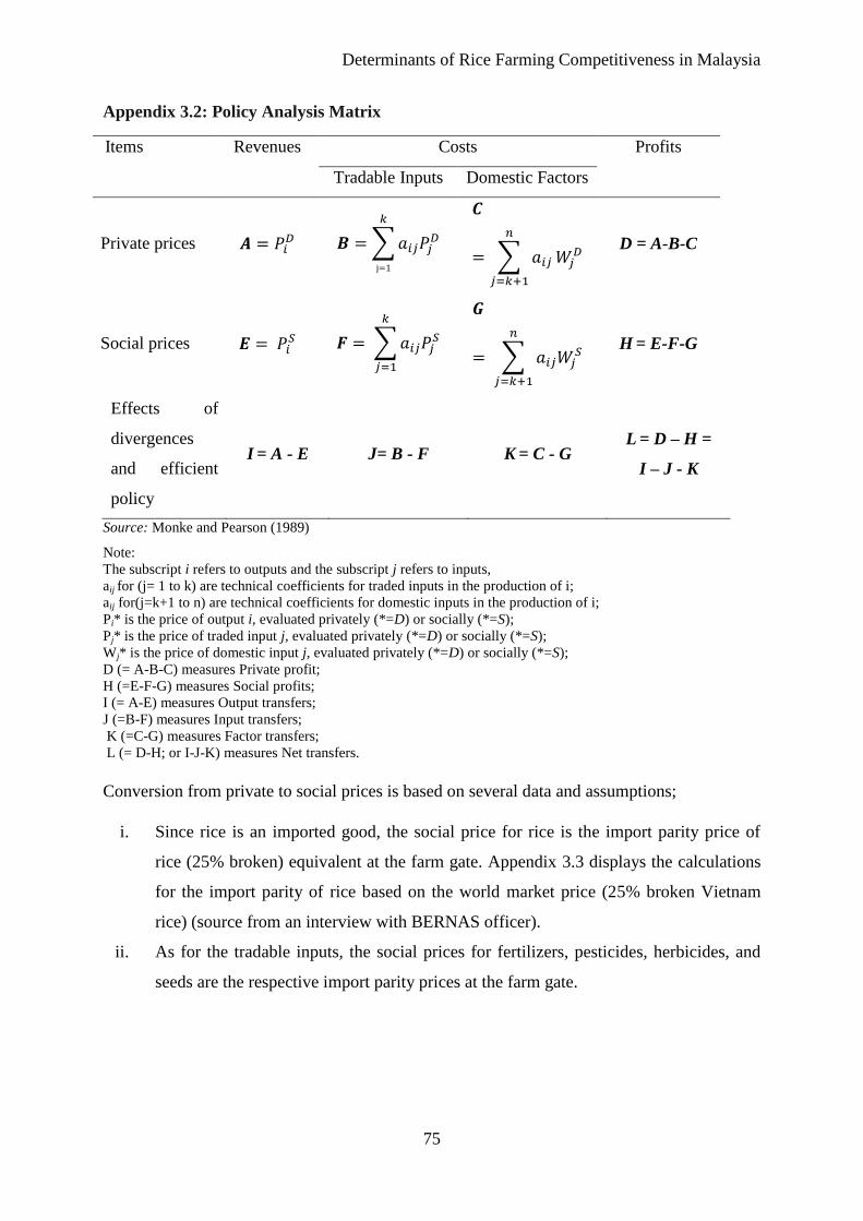
Determinants of Rice Farming Competitiveness in Malaysia
75
Appendix 3.2: Policy Analysis Matrix
Items Revenues Costs Profits
Tradable Inputs Domestic Factors
Private prices 𝑨 = 𝑃𝑖𝐷 𝑩 = ∑ 𝑎𝑖𝑗𝑃𝑗
𝐷
𝑘
j=1
𝑪
= ∑ 𝑎𝑖𝑗
𝑛
𝑗=𝑘+1
𝑊𝑗𝐷
D = A-B-C
Social prices 𝑬 = 𝑃𝑖𝑆 𝑭 = ∑ 𝑎𝑖𝑗𝑃𝑗
𝑆
𝑘
𝑗=1
𝑮
= ∑ 𝑎𝑖𝑗𝑊𝑗𝑆
𝑛
𝑗=𝑘+1
H = E-F-G
Effects of
divergences
and efficient
policy
I = A - E J= B - F K = C - G L = D – H =
I – J - K
Source: Monke and Pearson (1989)
Note:
The subscript i refers to outputs and the subscript j refers to inputs,
aij for (j= 1 to k) are technical coefficients for traded inputs in the production of i;
aij for(j=k+1 to n) are technical coefficients for domestic inputs in the production of i;
Pi* is the price of output i, evaluated privately (*=D) or socially (*=S);
Pj* is the price of traded input j, evaluated privately (*=D) or socially (*=S);
Wj* is the price of domestic input j, evaluated privately (*=D) or socially (*=S);
D (= A-B-C) measures Private profit;
H (=E-F-G) measures Social profits;
I (= A-E) measures Output transfers;
J (=B-F) measures Input transfers;
K (=C-G) measures Factor transfers;
L (= D-H; or I-J-K) measures Net transfers.
Conversion from private to social prices is based on several data and assumptions;
i. Since rice is an imported good, the social price for rice is the import parity price of
rice (25% broken) equivalent at the farm gate. Appendix 3.3 displays the calculations
for the import parity of rice based on the world market price (25% broken Vietnam
rice) (source from an interview with BERNAS officer).
ii. As for the tradable inputs, the social prices for fertilizers, pesticides, herbicides, and
seeds are the respective import parity prices at the farm gate.
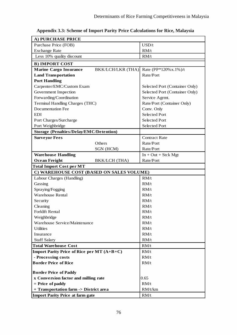
Determinants of Rice Farming Competitiveness in Malaysia
76
Appendix 3.3: Scheme of Import Parity Price Calculations for Rice, Malaysia
A) PURCHASE PRICE
Purchase Price (FOB) USD/t
Exchange Rate RM/t
Less 10% quality discount RM/t
Marine Cargo Insurance BKK/LCH/LKR (THA) Rate (PP*120%x.1%)/t
Land Transportation Rate/Port
Port Handling
Carpenter/EMC/Custom Exam Selected Port (Container Only)
Government Inspection Selected Port (Container Only)
Forwarding/Coordination Service Agrmt.
Terminal Handling Charges (THC) Rate/Port (Container Only)
Documentation Fee Conv. Only
EDI Selected Port
Port Charges/Surcharge Selected Port
Port Weighbridge Selected Port
Storage (Penalties/Delay/EMC/Detention)
Surveyor Fees Contract Rate
Others Rate/Port
SGN (HCM) Rate/Port
Warehouse Handling In + Out + Stck Mgt
Ocean Freight BKK/LCH (THA) Rate/Port
C) WAREHOUSE COST (BASED ON SALES VOLUME)
Labour Charges (Handling) RM/t
Gassing RM/t
Spraying/Fogging RM/t
Warehouse Rental RM/t
Security RM/t
Cleaning RM/t
Forklift Rental RM/t
Weighbridge RM/t
Warehouse Service/Maintenance RM/t
Utilities RM/t
Insurance RM/t
Staff Salary RM/t
Total Warehouse Cost RM/t
Import Parity Price of Rice per MT (A+B+C) RM/t
- Processing costs RM/t
Border Price of Rice RM/t
Border Price of Paddy
x Conversion factor and milling rate 0.65
= Price of paddy RM/t
+ Transportation farm -> District area RM/t/km
Import Parity Price at farm gate RM/t
Total Import Cost per MT
B) IMPORT COST
Determinants of Rice Farming Competitiveness in Malaysia
77
iii. The need to determine the shadow exchange rate is important for an economic
analysis. The shadow exchange rate affects all the social values of tradable inputs and
output. This is the point when various opportunities for alternative investment present
themselves to a nation and they must be properly evaluated and then the same foreign
exchange premium must be used in the economic analysis for each alternative. Thus,
instead of the official exchange rate, the shadow exchange rate is used to convert
international prices from US dollars to Malaysia’s currency. Malaysia is a small open
trading nation where such discrepancy between official exchange rate and shadow
exchange rate is quite small.
iv. Domestic inputs such as land for which no international prices exist is valued at local
opportunity costs. However, in this view the rental values of land per hectare for
granary area at social prices are assumed to be zero since the conversion of paddy
fields to other crops is unfeasible due to its soil condition and flooding area suitable
for only rice cropping. In addition Malaysian government has already officially
recognized the field as the permanent rice growing areas responsible for achieving the
minimum level of self-sufficiency under the National Agriculture Policy (1984).
v. Social costs are assumed to equal private costs for labor. Distortions in the labor
market are minimal since minimum wage is not enforced in agriculture and has
limited impact on the Malaysian economy. Therefore, the private wage rate for rural
labor is a good approximation of the social wage and thus, the conversion factor for
the labor is assumed to be equal to 1.
vi. Some of the taxes, including land tax and water tax, are viewed as pure transfers from
one agent to another within the society, which does not create economic value or
induce an economic impact (European Commission, 2008). In this case, all prices of
input and output should be a net of VAT or other indirect taxes and should be omitted
from revenues under economic analysis. Therefore, the conversion factor for the taxes
is assumed to be 0.
vii. The following table provides a summary of calculations for each cost element based
on private and social valuations for the main season and the off-season, calculated in
Ringgit Malaysia (RM) currency.
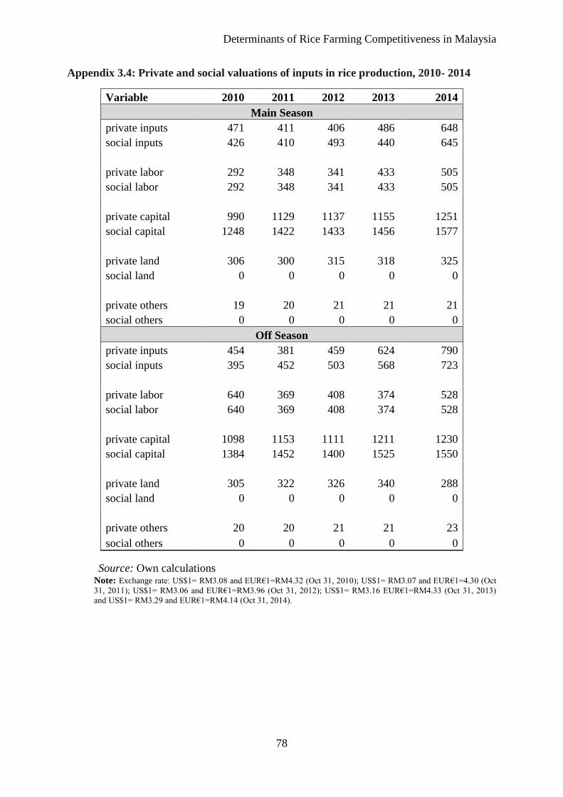
Determinants of Rice Farming Competitiveness in Malaysia
78
Appendix 3.4: Private and social valuations of inputs in rice production, 2010- 2014
Variable 2010 2011 2012 2013 2014
Main Season
private inputs 471 411 406 486 648
social inputs 426 410 493 440 645
private labor 292 348 341 433 505
social labor 292 348 341 433 505
private capital 990 1129 1137 1155 1251
social capital 1248 1422 1433 1456 1577
private land 306 300 315 318 325
social land 0 0 0 0 0
private others 19 20 21 21 21
social others 0 0 0 0 0
Off Season
private inputs 454 381 459 624 790
social inputs 395 452 503 568 723
private labor 640 369 408 374 528
social labor 640 369 408 374 528
private capital 1098 1153 1111 1211 1230
social capital 1384 1452 1400 1525 1550
private land 305 322 326 340 288
social land 0 0 0 0 0
private others 20 20 21 21 23
social others 0 0 0 0 0
Source: Own calculations Note: Exchange rate: US$1= RM3.08 and EUR€1=RM4.32 (Oct 31, 2010); US$1= RM3.07 and EUR€1=4.30 (Oct
31, 2011); US$1= RM3.06 and EUR€1=RM3.96 (Oct 31, 2012); US$1= RM3.16 EUR€1=RM4.33 (Oct 31, 2013)
and US$1= RM3.29 and EUR€1=RM4.14 (Oct 31, 2014).
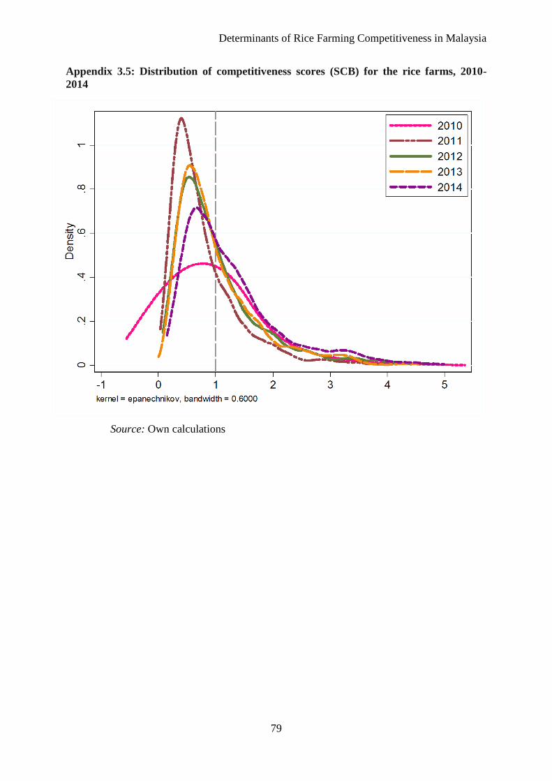
Determinants of Rice Farming Competitiveness in Malaysia
79
Appendix 3.5: Distribution of competitiveness scores (SCB) for the rice farms, 2010-
2014
Source: Own calculations
Determinants of Rice Farming Competitiveness in Malaysia
80
References
Abdul Fatah, F., & von Cramon Taubadel, S. (2015). The policy analysis matrix of
profitability and competitiveness of rice farming in Malaysia. In 29th International
Conference of Agricultural Economists, Milan, Italy. Retrieved from
http://ageconsearch.umn.edu/bitstream/210872/2/Abdul Fatah-The Policy Analysis
Matrix of Profitability and Competitiveness of Rice Farming-896.pdf
Addai, K. N., Owusu, V., & Danso-Abbeam, G. (2014). Effects of farmer – based-
organization on the technical efficiency of maize farmers across various agro - ecological
zones of Ghana. Journal of Economics and Development Studies, 2(1), 141–161.
Retrieved from http://jedsnet.com/journals/jeds/Vol_2_No_1_March_2014/7.pdf
Anderson, T. W., & Hsiao, C. (1981). Estimation of dynamic models with error components.
Journal of the American Statistical Association, 76(375), 598.
Arellano, M., & Bover, O. (1995). Another look at the instrumental variable estimation of
error-components models. Journal of Econometrics, 68, 29–51. Retrieved from
http://www.cemfi.es/~arellano/arellano-bover-1995.pdf
Arshad, F. M., Alias, E. F., Noh, K. M., & Muhammad, T. (2011). Food security: self-
sufficiency of rice in Malaysia. International Journal of Management Studies, 18(2), 83–
100. Retrieved from http://www.ijms.uum.edu.my/images/pdf/18no2ijms/ijms1825.pdf
Blundell, R., & Bond, S. (1998). Initial conditions and moment restrictions in dynamic panel
data models. Journal of Econometrics, 87, 115–143. Retrieved from
http://www.ucl.ac.uk/~uctp39a/Blundell-Bond-1998.pdf
Bond, S. R., Hoeffler, A., & Temple, J. (2001). GMM estimation of empirical growth models.
Discussion Paper No. 3048. Retrieved from
https://www.nuffield.ox.ac.uk/users/bond/CEPR-DP3048.PDF
Busayo Rashidat, Y., Mohd Mansor, I., & Nolila Mohd, N. (2013). Comparative study of two
incentive schemes in Malaysian paddy production. Institute of Agricultural and Food
Policy Studies, Putra Infoport, 23, 27–31.
http://doi.org/10.5829/idosi.wasj.2013.23.eemcge.2206
Chan, C.-W., & Cho, M.-C. (2012). Country report: Malaysia, Asia Pacific Economic
Cooperation (APEC). Workshop on Food Security. Retrieved from http://www.apip-
apec.com/my/good-practices/1_1/1_1_1/country_report_malaysia.html
Department of Agriculture, M. (2014). Perangkaaan padi Malaysia (paddy statistics of
Malaysia 2013). Putrajaya, Malaysia.
Determinants of Rice Farming Competitiveness in Malaysia
81
Dorosh, P. A. (2009). Price stabilization, international trade and national cereal stocks: world
price shocks and policy response in South Asia. Food Security, 1(2), 137–149.
http://doi.org/10.1007/s12571-009-0013-3
Erenstein, O. (2010). A comparative analysis of rice-wheat systems in Indian Haryana and
Pakistan Punjab. Land Use Policy, 27(3), 869–879.
http://doi.org/10.1016/j.landusepol.2009.12.001
European Commission. (2014). Guide to Cost-benefit Analysis of Investment Projects
Economic appraisal tool for Cohesion Policy 2014-2020. Retrieved from
http://ec.europa.eu/regional_policy/sources/docgener/studies/pdf/cba_guide.pdf
FAOSTAT. (2016). Food and Agriculture Organization of the United Nations statistics
division. Retrieved January 4, 2016, from http://faostat3.fao.org/download/Q/QC/E
Femenia, F., Gohin, A., & Carpentier, A. (2010). The decoupling of farm programs:
Revisiting the wealth effect. American Journal of Agricultural Economics, 92(3), 836–
848. http://doi.org/10.1093/ajae/aap029
Frohberg, K., & Hartmann, M. (1997). Comparing measures of competitiveness. Discussion
paper No. 2. Institute of Agricultural Development in Central and Eastern Europe.
Retrieved from http://www.econstor.eu/bitstream/10419/28566/1/241163463.pdf
Goodwin, B. K., & Ashok, K. M. (2004). Farming efficiency and the determinants of multiple
job handling by farm operators. American Journal of Agricultural Economics, 86(3),
722–729. Retrieved from
http://pubag.nal.usda.gov/pubag/downloadPDF.xhtml?id=38670&content=PDF
Goodwin, B. K., & Ashok, K. M. (2005). Another look at decoupling: additional evidence on
the production effects of direct payments. American Journal of Agricultural Economics,
87(5), 1200–1210. Retrieved from
http://pubag.nal.usda.gov/pubag/downloadPDF.xhtml?id=6842&content=PDF
Jamora, N., & Von Cramon-Taubadel, S. (2012). What world price? GlobalFood Discussion
Paper. Georg-August-Universitaet Goettingen. ISSN 2192-3248. Retrieved from
file:///C:/Users/userdell/Downloads/GlobalFood_DP17%20(2).pdf
Kanaka, D. S., & Chinnadurai, M. (2013). The policy analysis of rice cultivation in India.
European Journal of Physical and Agricultural Sciences, 1(1). Retrieved from
http://www.idpublications.org/wp-content/uploads/2013/11/the-policy-analysis-matrix-
of-rice-cultivation-in-india.pdf
Determinants of Rice Farming Competitiveness in Malaysia
82
Koirala, K. H., Ashok, K. M., & Mohanty, S. (2015). The role of gender in agricultural
productivity in the Philippines: the average treatment effect. In Southern Agricultural
Economics Association’s 2015 Annual Meeting, Atlanta, Georgia. Retrieved from
http://ageconsearch.umn.edu/bitstream/195705/2/ATT_SAEA_2015 (1).pdf
Masters, W. A., & Winter-Nelson, A. (1995). Measuring the comparative advantage of
agricultural activities: domestic resource costs and the social cost-benefit ratio. American
Journal of Agricultural Economics, 77(2), 243–250. http://doi.org/10.2307/1243534
Mohd Rashid, R., & Mohd Dainuri, M. S. (2013). Food and livelihood security of the
Malaysian paddy farmers. Economic and Technology Management Review, 8, 59–69.
Monke, E. A., & Pearson, S. R. (1989). The policy analysis matrix for agricultural
development. Ithaca, NY: Cornell University Press. Retrieved from
http://web.stanford.edu/group/FRI/indonesia/documents/pambook/pambook.pdf
Morrison, J., & Balcombe, K. (2002). Policy analysis matrices: beyond simple sensitivity
analysis. Journal of International Development, 14(4), 459–471.
http://doi.org/10.1002/jid.887
Nivievskyi, O., von Cramon-Taubadel, S., & Brummer, B. (2010). A note on technical
efficiency, productivity growth and competitiveness. Annual Meeting, July. Retrieved
from http://ageconsearch.umn.edu/bitstream/61759/2/11234 AAEA 2010.pdf
Reig-Martínez, E., Picazo-Tadeo, A. J., & Estruch, V. (2008). The policy analysis matrix with
profit-efficient data: evaluating profitability in rice cultivation. Spanish Journal of
Agricultural Research, 6(3), 309–319. Retrieved from
file:///C:/Users/userdell/Downloads/324-324-1-PB.pdf
Roodman, D. (2009a). A note on the theme of too many instruments. Oxford Bulletin of
Economics and Statistics, 71(1), 135–158. Retrieved from
http://www.cgdev.org/files/14256_file_Instruments.pdf
Roodman, D. (2009b). How to do xtabond2: An introduction to difference and system GMM
in Stata. Stata Journal, 9(1), 86–136. http://doi.org/The Stata Journal
Siriwardana, A. N., & Jayawardena, L. N. A. C. (2014). Socio-demographic factors
contributing to the productivity in paddy farming: a case study. Tropical Agricultural
Research, 25(3), 437–444. Retrieved from
http://www.pgia.ac.lk/files/Annual_congress/journel/v25/Journal-No 3/Poster/14.
siriwardana 20 ok final - OK.pdf
Determinants of Rice Farming Competitiveness in Malaysia
83
Sunding, D., & Zilberman, D. (2000). The agricultural innovation process : research and
technology adoption in a changing agricultural sector. Handbook of Agricultural
Economics, 1–105. http://doi.org/10.1016/S1574-0072(01)10007-1
Tengku Mohd Ariff, T. A., & Ariffin, T. (1999). Effect of trade liberalization on agriculture in
Malaysia: commodity aspects. The CGPRT Center Working Paper Series no. 46.
Retrieved from http://ageconsearch.umn.edu/bitstream/32694/1/wp990046.pdf
Timmer, C. P. (2005). Food security and economic growth: an Asian perspective. Working
Paper No. 50, December 2004 (Revised December 2005).
Timmer, C. P., & Dawe, D. (2007). Managing food price instability in Asia: A macro food
security perspective. Asian Economic Journal, 21(1), 1–18. http://doi.org/10.1111/j.1467-
8381.2007.00244.x
Umar, S. H., Abdullah, A. M., Shamsudin, M. N., & Mohamed, Z. A. (2014). Effects of
paddy price support withdrawal on Malaysian rice sector: time series econometric
approach. Asian Journal of Agriculture and Rural Development, 4(7), 401–413. Retrieved
from http://www.aessweb.com/pdf-files/3-484-AJARD-4(7)2014-401-413.pdf
von Cramon Taubadel, S., & Nivyevskyi, O. (2009). Belarus agricultural productivity and
competitiveness: impact of state support and market intervention. Retrieved from
https://openknowledge.worldbank.org/bitstream/handle/10986/18897/483350ESW0REVI
110FINAL0for0printing.pdf?sequence=1&isAllowed=y
von Cramon-Taubadel, S., & Nivyevskyi, O. (2008). Ukraine-ag-competitiveness-policy note
- final.
Wailes, E. J. (2005). Rice: Global trade, protectionist policies, and the impact of trade
liberalization. M. Ataman Aksoy and John C. Beghin, 2(576), 177.
Warr, P., & Yusuf, A. A. (2014). Fertilizer subsidies and food self-sufficiency in Indonesia.
Agricultural Economics, 45(5), 571–588. http://doi.org/10.1111/agec.12107
World Trade Organization. (2014). Trade Policy Review Malaysia: World Trade Organization
(Vol. WT/TPR/S/2). Retrieved from
https://www.wto.org/english/tratop_e/tpr_e/tp392_e.htm
Yao, S. (1997). Rice production in Thailand seen through a policy analysis matrix. Food
Policy, 22(6), 547–560. http://doi.org/10.1016/S0306-9192(98)00007-4
Zheng, S., Lambert, D., Wang, S., & Wang, Z. (2015). Effects of agricultural subsidy policies
on comparative advantage and production protection in China: An Application with a
Policy Analysis Matrix Model. The Chinese Economy, 46(1), 20–37. Retrieved from
Estimating Technical Efficiency and Unobserved Heterogeneity
84
http://web.a.ebscohost.com.ezaccess.library.uitm.edu.my/ehost/pdfviewer/pdfviewer?sid
=355ac440-f279-4b04-b575-17b9212254a2%40sessionmgr4005&vid=2&hid=4101
Chapter 4
Estimating Technical Efficiency and Unobserved Heterogeneity
On Rice Farms in Malaysia
Changes and trends in farm efficiency have been of considerable interest to many Asian
governments due to a strong link between food security and rice production. We use farm
level data to gain insights on the technical efficiency of the Malaysia’s rice farming. Although
panel data are available, some important descriptive attributes are scarce. As a result, we take
unobserved heterogeneity into account and use the recent fixed effect model implemented by
Chen et al (2014). During the period of 2010-2014, technical efficiency was found to be
fluctuating, with an average mean value of 60 percent. The low mean values of technical
efficiency change further revealing that the frontier is shifting inward and some farms are
essentially moving farther from the frontier. In a second stage of analysis, we examine the
factors that account for the variations in inefficiencies across the farms as well as their
potential to improve efficiency and resource use using a fixed effect model regression. Our
empirical results indicate that access to credit, non-farm income, distance to the rice mill,
farm size and hired labor are the major determinants of technical efficiency. Additionally,
government input subsidies are found to have a positive impact on farm technical efficiency
and thus support the argument that agricultural subsidies may create incentives for farmers to
improve their efficiency. Overall, the results indicate that rice production can be improved by
continuously increasing a farm’s resources and technical efficiency. This suggests that a
serious policy recommendation that facilitates farmers’ accessibility to credit, capital, land
and other inputs, especially for small farms, must be carefully designed and well-targeted.
Improved access to and distribution of input subsidies must also occur.
Keywords: rice, technical efficiency, fixed effect, panel data, unobserved heterogeneity
Estimating Technical Efficiency and Unobserved Heterogeneity
85
4.1 Introduction
The efficiency of the rice production sector has been the subject of considerable interest and
policy focus for many Asian governments due to the strong relationship between food
security and rice production (Timmer and Dawe 2007). The global rice market crisis of 2007-
2008 led to sudden spikes in rice prices, which further marginalized poor populations in many
developing countries and hindered their access to sufficient basic food supplies (Dawe, 2010).
Rice is a primary food staple for a large part of the world’s human population and has a large
influence on the livelihood of farmers. For this reason, policymakers have become
particularly concerned with the efficiency of rice production. Reliable research results on the
efficiency of rice production can contribute to policies that increase agricultural production,
promote adequate food supplies, and boost incomes and food security for low income
farmers.
Research on production efficiency can also contribute to the debate on whether it is necessary
to support rice production, for example with price support or input subsidies. Many countries
in Southeast Asia, including Malaysia, protect and support domestic rice producers. Since the
inception of the ASEAN free trade agreement (AFTA), rice tariffs have been reduced to 0-5%
for all trading partners in the region. However, in the major rice importing countries, such as
Malaysia, rice is considered a key to food security and, therefore, is subject to tariffs up to
20%. Both the volumes of the input subsidies and price support have increased remarkably
over the years. This support, however, has been the subject of a long-standing debate (Hoang
and Meyers, 2015). Some argue that deviations from production and international trade based
on comparative advantage will result in allocative inefficiencies and rent-seeking behavior.
Policy makers counter that support is required to boost domestic self-sufficiency and to
protect farmers from the effects of what is perceived to be unfair competition. Research can
inform this debate by providing facts on whether and which rice producers are efficient, and
the factors that contribute to differences in productivity and efficiency among producers.
Malaysia has the potential to grow more rice if analysis can identify efficient farms and the
causes of their superior performance, thus, providing benchmarks for less efficient farms. The
study of the rice markets in Malaysia is somehow unique in the region as it exhibits some
exceptional features and is worth investigating for several reasons. First, Malaysia lies
entirely in the equatorial zone with uniform temperature, high humidity and rainfall that are
Estimating Technical Efficiency and Unobserved Heterogeneity
86
favorable for the development and growth of the tropical rice crop. The copious rainfall
provides important water sources for successful cultivation of rice. However, despite of its
natural endowments, the country’s topography leaves limited arable land to expand rice
production (Arshad et al. 2011). Second, the average yield in Malaysia from 2010- 2013 was
4.60 tons paddy per hectare, compared to just 3.44 tons paddy per hectare in the major rice
exporters in Southeast Asia (Mutert and Fairhurst, 2002). Yet, the evidence indicates that the
average potential rice yield in the country is 10 tons per hectare (Siwar et al. 2014). The yield
gap between potential and actual yield levels in Malaysia is nearly twice that of the current
yield which requires further improvement in efficiency in order to close the gap. Third, the
2% national population growth rate is resulting in a demand that outpaces the production
growth. At the same time, there is little scope to extend the crop land frontier: rice land
availability in Malaysia has declined by 10,600 ha (0.30%) from 1990-1995 (Daño and
Samonte, n.d.). Consequently, Malaysia needs to produce more rice, while at the same time
increase the efficiency of the scarce resource, which is largely possible by increasing the
adoption rate of high-yielding rice varieties in all seasons to up to 90 per cent of total rice area
(Abiola et al. 2016). This implies that Malaysian farmers need to increase their efficiency by
utilising the scarce resources efficiently. Therefore, studying the potential of inefficiencies in
farm performance is important not only from the policy standpoint but also from a global
context.
However, literature on the efficiency of Malaysian rice production has typically used cross-
sectional data (Thiam et al. 2001). To the best of our knowledge, the technical efficiency of
Malaysian rice farms, and its evolution over time, have not been studied using representative
farm panel data. This study is an attempt to narrow this gap. For this purpose, we conduct an
empirical technical efficiency analysis with unobserved heterogeneity and employ an
implementation by Chen et al (2014) of a fixed effect model. We study data from a panel of
6,570 rice farms covering the years 2010-2014. These data provide a unique opportunity to
analyze the changes in farm level efficiency over time for rice farms in Malaysia and to gain
insights into the factors that determine differences in efficiency between farms.
The rest of this paper is structured as follows. In section 4.2 we present the panel data model
of technical efficiency that we employ. Section 4.3 describes the data that we use. In section
4.4 we present and discuss results, and Section 4.5 concludes.
Estimating Technical Efficiency and Unobserved Heterogeneity
87
4.2 Methods to measure efficiency using panel data
Since the seminal work conducted by Aigner et al. (1977), the Stochastic Frontier (SF) model
has been widely use to estimate the technical efficiency in applied economic research.
Extensive research in this field has resulted in a growing arsenal of methods and econometrics
techniques pertaining to specifications, estimation and testing issue. Despite that, when
productivity or efficiency is analyzed at the farm level, the problem arises that not all relevant
factor can be observed or measured adequately. Therefore, some environmental, such as soil
condition, weather, rainfall or droughts, and managerial characteristics are often omitted from
the model specifications because of unavailable or missing information. This information is
referred to as unobserved heterogeneity (Álvarez et al, 2009). As a result, inference based on
the output comparison could be biased and is often criticized because farms are heterogeneous
and operate under different production and environmental conditions (Abdulai and Tietje,
2007).
To overcome the challenge of unobserved heterogeneity, the standard stochastic frontier
models, such as the fixed-effects or random-effects model, can be employed (Pitt and Lee
1981; Schmidt and Sickles 1984). A frequent case in most classical stochastic frontier occurs
when the information that accounts for unobserved heterogeneity not included in the model is
considered time-invariant and these specifications interpret time-invariant unobserved
heterogeneity as inefficiency, thus do not provide any mechanism to disentangle the former
from the latter. The consideration on how heterogeneity is treated has induced several
extensions of the standard stochastic frontier model (see Greene (2008) for a recent survey).
These extensions distinguish between the aforementioned latent components by separating the
inefficiency from the time invariant unobserved heterogeneity that are unrelated with the
production process but affect the output (Kumbhakar and Hjalmarsson, 1995; Greene,
2005a,b; Wang and Ho, 2010; Chen et al. 2014).
In the dataset that we employ, managerial characteristics and environmental conditions are not
directly observed and can be interpreted as unobserved farm heterogeneity. Consider the
following specification of the fixed-effect stochastic production frontier model for panel
data6:
𝑦𝑖𝑡 = 𝛼𝑖 + 𝛽′𝑥𝑖𝑡 + 𝑣𝑖𝑡 − 𝑢𝑖𝑡 (1)
𝜀𝑖𝑡 = 𝑣𝑖𝑡 − 𝑢𝑖𝑡 (2)
6 In the following method, i draw heavily on the following sources; Belotti and Giuseppe (2012) and
Holtkamp (2015).
Estimating Technical Efficiency and Unobserved Heterogeneity
88
where 𝑦𝑖𝑡 is the vector of the output of firm i (i=1,...,N) in period t (t=1,...,T); xit is a set of
inputs that produce output 𝑦𝑖𝑡; 𝛼𝑖 is the unit fixed-effect; β is the associated vector that
describes technology parameters to be estimated. The composite error term 𝜀𝑖𝑡 is the
difference between the idiosyncratic error that captures noise 𝑣𝑖𝑡, and the one-sided
disturbance 𝑢𝑖𝑡 which represents inefficiency. Under the frequently used normal-half normal
model, the distributional assumptions are 𝑣𝑖𝑡 ~ 𝑁(0, 𝜎𝑣2) and 𝑢𝑖𝑡 ~ 𝑁+(0, 𝜎𝑢
2). However, as
mentioned previously whether or not to separate 𝛼𝑖 from 𝑢𝑖𝑡 has been the subject of much
debate in the stochastic frontier literature. A major limitation of the model in equation (1) is
related to an identification problem which arises when the inefficiency term is time-variant. It
is not likely that a constant level of inefficiency would extend over long periods of time; i.e.
process of learning or managerial ability. In this case, it is difficult to disentangle the
unobserved farm-specific heterogeneity from inefficiency (Greene, 2005).
Greene (2005) proposed a “true fixed effects” or TFE model that includes a maximum
likelihood dummy variables estimator (MLDVE), in which the unit-specific intercepts are
estimated with structural parameters. The TFE model places unobserved heterogeneity as
fixed effects in the stochastic frontier model (equation 1) and generates a neutral shift of the
function specific to each farm (Porcelli, 2009) while allowing for time-varying inefficiency
(Belotti and Giuseppe, 2012). This approach is frequently applied, however it leads to
inconsistent variance parameter estimates due to the incidental parameters problem especially
in the short panel because the number of parameters depends on the sample size (there are
firm effects 𝛼𝑖; and the number of parameters, N which increases with the sample size).
Hence, the estimated error variance, and the parameter 𝜎𝑢2 is inconsistent.
To account for this limitation, Chen et al. (2014) propose a consistent estimator for the TFE
normal-half normal model based on the within transformed model where the fixed effects
have been removed. This procedure is commonly used in the panel data:
𝑧�̅�𝑡 = 𝑧𝑖𝑡 − 𝑧�̅� (3)
For any corresponding variable (𝑧) in each panel i, the individual mean (𝑧�̅�) is subtracted from
the observed value in period t (𝑧𝑖𝑡). Correspondingly, the model can be represented by using
Estimating Technical Efficiency and Unobserved Heterogeneity
89
the deviations from means (𝑧�̅�) so that the transformed model is free from incidental
parameters problem (αi):
�̅�𝑖𝑡 = 𝛽′�̅�𝑖𝑡 + �̅�𝑖𝑡 − �̅�𝑖𝑡 (4)
As outlined by (Holtkamp, 2015) the model in equation (4) has the following features: first,
the incidental parameters problem is removed by a within-transformation; second, it produces
a consistent estimator of the error variance since the relevant likelihood function is derived
from T-1 deviations; and third, this approach, which is based on a more general distributional
theory, allows for the maintenance of the firm-specific and time varying inefficiency 𝑢𝑖𝑡.
The distribution of the composed error, 𝜖𝑖𝑡 is defined by the Closed Skew Normal (CSN)
distribution in the stochastic frontier context (Chen et al. 2014). The CSN is a generalization
of the skew normal distribution (González-Farías et al. 2004), which is itself a generalization
of the normal distribution. Therefore, the CSN family preserves some properties of the normal
distribution (Chen et al. 2014). With panel data, the distribution of the composed error can be
written as:
𝜖𝑖 ~ 𝐶𝑆𝑁1,1(0, 𝜎2, − 𝜆
𝜎, 0, 𝐼) (5)
where the density of a CSN distribution includes a p-dimensional pdf and a q-dimensional cdf
of a normal distribution; parameters in the bracket describe location (0), scale (𝜎2), skewness
(𝜆
𝜎), as well as the mean vector (0) and covariance matrix in the cdf (𝐼) . In the panel data, the
vector (𝜀𝑖 = 𝜀𝑖1, 𝜀𝑖2 … … 𝜖𝑖𝑇)′ is distributed as:
𝜖𝑖𝑡 ~ 𝐶𝑆𝑁𝑇,𝑇(0𝑇 , 𝜎2𝐼𝑇 , − 𝜆
𝜎𝐼𝑇 , 0𝑇 , 𝐼𝑇) (6)
where I is the identity matrix and the vector is divided into a linear combination; its mean is
represented by 𝜀�̅� and its first T-1 deviations as 𝜀̅∗𝑖
= (𝜀�̅�1, 𝜀�̅�2 … . . , 𝜀�̅�,𝑇−1)′; and within MLE,
which is defined by the maximization of the within likelihood with respect to β, λ and 𝜎2,
which is not subject to the incidental parameters problem, (where β = within estimator,
𝜆 = 𝜎𝑢
𝜎𝑣 and 𝜎2 = 𝜎𝑢
2 + 𝜎𝑣2).
Estimating Technical Efficiency and Unobserved Heterogeneity
90
The point estimator of Battese and Coelli (1988) can be used to assess technical effciency.
Therefore, the composed error has to be recovered:
𝜀𝑖𝑡 = 𝑦𝑖𝑡 − �̂�𝑖𝑡 = 𝑦𝑖𝑡 − 𝛽′𝑥𝑖𝑡 − �̂�𝑖 (7)
The estimate �̂�𝑖, can be obtained by mean-adjusting the usual estimator for the fixed effects
linear model. In this model if �̂� is the within estimator, then the fixed effects estimates of
individual effects are; �̂�𝑖 = �̅�𝑖 − �̅�𝐼�̂�. However, in the stochastic frontier model, since the 𝜀�̅�
is not zero because −𝐸(𝑢𝑖𝑡) = √2
𝜋𝜎𝑢, the estimator needs to be modified and �̂�𝑖 can be
calculated as the mean-adjusted estimate by (Chen et al. 2014):
�̂�𝐼𝑀 = �̅�𝑖 − �̂�′�̅�𝑖 + √
2
𝜋�̂�𝑢 (8)
where �̂� and �̂�𝑢 are the within MLE estimates.
4.3 Data and empirical definitions of the variables
We estimate the stochastic frontier model outlined above using farm-level survey data over
the period 2010-2014. These farms are located in Muda Agricultural Kemubu Authority
(MADA), Kedah, which is the largest granary area in Malaysia and located in north Malaysia.
Granary Areas7 are acknowledged by the Government in the National Agricultural Policy as
the main paddy producing areas. These eight areas are irrigated according to large irrigation
schemes (areas greater than 4,000 hectares) (Department of Agriculture, 2014).
The output variable is defined as the total output of rice production in kilograms (kg). The
consideration of the gross output of rice in kg has the advantage of taking quality differences
into account. The actual purchasing price that farmers normally receive from the processors or
the rice millers depends on the grain’s purity, quality and moisture content. Corresponding to
the standards enforced by the local and government millers, the acceptable moisture content
of paddies in Malaysia is 14%. If the moisture in a sample of paddy surpasses this limit, the
per kg price of this rice is adjusted accordingly. The vector X includes five inputs: land (in
7 There are eight granary areas in Malaysia, namely MADA, KADA, IADA KERIAN, IADA BLS,
IADA P. Pinang, IADA Seberang Perak, IADA KETARA and IADA Kemasin Semerak.
Estimating Technical Efficiency and Unobserved Heterogeneity
91
ha), labor, is approximated by the wage expenditure per day in Ringgit Malaysia (RM),
capital costs, also in RM (which include the costs of machinery services hired for harvesting,
transplanting, seedling and threshing), quantity of seeds used (in kg), and the value of
agricultural chemicals in RM.
These variables are transformed and scaled to their respective means before taking logarithms.
With this transformation, the elasticities of the output regarding the inputs are the first-order
coefficients of the inputs in a translog function (evaluated at the means of the variables).
Prior to further analysis, we remove outliers from the balanced panel data of 6,750 rice farms
for the period 2010-2014. Here, all observations were detected as outliers if 99% of the
variable of interest (output, capital, labor and seed) lied outside ± 3 standard deviations from
the mean. To account for zero usage of agricultural chemicals, the values of this variable are
added to the amount of pesticides subsidies of 200 RM per hectare. Additionally, many data
sets are incomplete or indicate obvious errors. As a consequence, the remaining panel is
unbalanced with 6,570 and we continued working with the unbalanced panel data for the rice
farms in Malaysia.
We use a translog functional form which includes a time trend, 𝑡 as an additional input in
order to allow for non-neutral technical change. The model specification is therefore:
𝑙𝑛𝑦𝑖𝑡 = 𝛼𝑖 + ∑ 𝛽𝑗𝑙𝑛𝑥𝑗𝑖𝑡
5
𝑗=1
+1
2∑ ∑ 𝛽𝑗𝑙𝑙𝑛𝑥𝑗𝑖𝑡𝑙𝑛𝑥𝑙𝑖𝑡
5
𝑙=1
5
𝑗=1
+ 𝛽𝑡𝑡 +1
2𝛽𝑡𝑡𝑡2 + ∑ 𝛽𝑡𝑗
5𝑗=1 𝑙𝑛𝑥𝑗𝑖𝑡𝑡 + 𝑣𝑖𝑡 − 𝑢𝑖𝑡 (9)
In this equation, αi is the unobserved heterogeneity which is treated as fixed; xit is a set of
inputs that produce output 𝑦𝑖𝑡; 𝑣𝑖𝑡 is the statistical error; and the non-negative random
variable 𝑢𝑖𝑡 is the technical inefficiency.
Both output and input exhibit substantial variation over time. For example, the average output
increased from 5,359 kg in 2010 to 6,316 kg in 2013, but then decreased strongly to 4947 kg
in 2014. Individual inputs such as seed, agricultural chemicals and capital costs also vary
considerably over time. The standard deviations indicate a higher degree of heterogeneity
among the rice producers in the dataset, even though they are all located in the same granary
Estimating Technical Efficiency and Unobserved Heterogeneity
92
area. This heterogeneity is presumably due to farm-level variation in factors which are not
captured in the dataset, including biophysical conditions (e.g. climate, irrigation, soil
condition), farmer characteristics (e.g. age, education, experience, household size), and
managerial skills. The CFE model described above allows us to account for this farm-level
heterogeneity when estimating efficiency.
In a second step, we use a fixed effect panel regression to analyze the determinants of
technical efficiency. Exogenous variables that we hypothesize will affect technical efficiency
include farm characteristics (e.g. size, distance from the rice mill), farmer characteristics
(whether he/she is a member of the farmers’ organization, whether he/she owns or rents the
farm, gender, off-farm income, access to credit), and the amount of government support
received by the farm. This support includes subsidies on input use such as fertlizer, lime and
chemical inputs. Since 1974, farmers who owned less than 10 hectares of lands received free
fertilizers of 240 kg per hectare of mixed fertilizer, 80 kg per hectare of organic fertilizer and
150 kg (3 bags) of NPK (nitrogen, phosphate and potassium). In addition, all farmers receive
a coupon of agricultural chemical inputs for purchasing weeds and pest controls worth of 200
RM/ha. Another form of support is the price subsidy. This scheme was introduced in 1980 at
the rate of 165 RM per ton and was then revised and increased to 248.10 RM per ton in
1990.A list of these variables and descriptive statistics are provided in Table 4.1.
The relationship between off-farm income and technical efficiency is complex and
ambiguous. Kumbhakar and Lien, (2010) and Abdulai and Eberlin (2001) postulated higher
production inefficiency is associated with the involvement of households in off-farm
activities. Farmers who have various sources of income may devote more time to off-farm
activities and, hence, pay less attention and effort to farm activities, such as agronomical
practices. However, off-farm income might also have a beneficial effect on technical
efficiency. Fernandez-Cornejo et al. (2007) argue that off farm income increases the adoption
of agricultural innovations through managerial time. Additionally, an increase in nonfarm
employment reduces financial constraints, especially for resource constrained farmers who
may require the additional income to purchase productivity enhancing inputs (Huffman,
1980).
Access to formal credit may relieve financial constraints otherwise hindering farmers from
investing in efficiency enhancing inputs (Abdulai and Eberlin, 2001; Brummer and Loy,
Estimating Technical Efficiency and Unobserved Heterogeneity
93
2000; von Cramon-Taubadel and Saldias, 2014). In this case, credit could therefore increase
the net revenue obtained from fixed inputs, market conditions and individual characteristics.
On the other hand, a credit constrained farmer will be less efficient if credit shortage
adversely affects access to input and limits the adoption of high yielding varieties and the
acquisition of information relevant for increasing productivity (Wozniak, 1993). Credit
can also be worrisome if default costs are seen to be minor and a credit is therefore used as a
welfare support measure by the household (Binswanger and Deininger, 1997).
Other variables representing characteristics of the farmers include gender, participation in a
farmer’s organization and land ownership. The household head, whether male or female, is
assumed to be the primary decision maker for that household and therefore contributes to
efficiency. Farmers who participate in a farmers’ organization might be more efficient due to
easier access to productive inputs and technical and management services, such as training,
information and extension on input application (Addai et al, 2014). Economic theory suggests
that lack land ownership negatively affects a farmer’s access to credit designated to improve
land-based practices. Therefore, land ownership reduces uncertainty which helps farmers to
make investment decisions on land, adopt the best cropping system, use the land as collateral
for credit and thus improves efficiency (Koirala et al, 2016).
Two variables that represent farm characteristics employed in the analysis of the determinants
of technical inefficiency include land and distance to the rice mill. The relationship between
farm size and efficiency has gain much attention in the literature. In most developed
countries, farm size is found to increase consistently in the last decades. Some authors
hypothesize that larger farms benefited from higher efficiency than smaller farms (Olson and
Vu 2009; Masterson, 2007). However, other authors, particularly in the developing countries
studies argue that smaller farms are more productive because they make use of the land more
intensively (Johnson and Ruttan,1994; Binswanger and Elgin, 1998; Bhatt and Bhat, 2014).
We hypothesize that smaller farms are more technically efficient than the larger farm,
considering a relatively small farm with limited access to resources may use the combined
resources (use labor more intensively, use more of available land for land improvement) in a
diligent manner in order to survive. Additionally, our hypothesis is that distance to the rice
mills reduces technical inefficiency. With greater access to the market and better roads and
transport infrastructure, farmers are able to reduce the risk and uncertainty of postharvest
losses as well as achieve greater information on market prices.

Estimating Technical Efficiency and Unobserved Heterogeneity
94
The effect of subsidies is ambiguous and remains a controversial issue. The arguments for a
negative impact of subsidies on technical efficiency point to the weakening of the managerial
efforts and unfairly undermining poor farmers, reducing incentives for producers to boost
efficiency and shifting their focus from crops to farming subsidies (Martin and Page 1983;
Serra et al, 2008). On the other hand, explanations for a positive relationship between
subsidies and efficiency include the incentives to adopt technologies or practices that are not
common for the farmers and subsidization may help them to overcome financial constraints
(Kumbhakar and Lien 2010; Zhu and Lansink 2010).
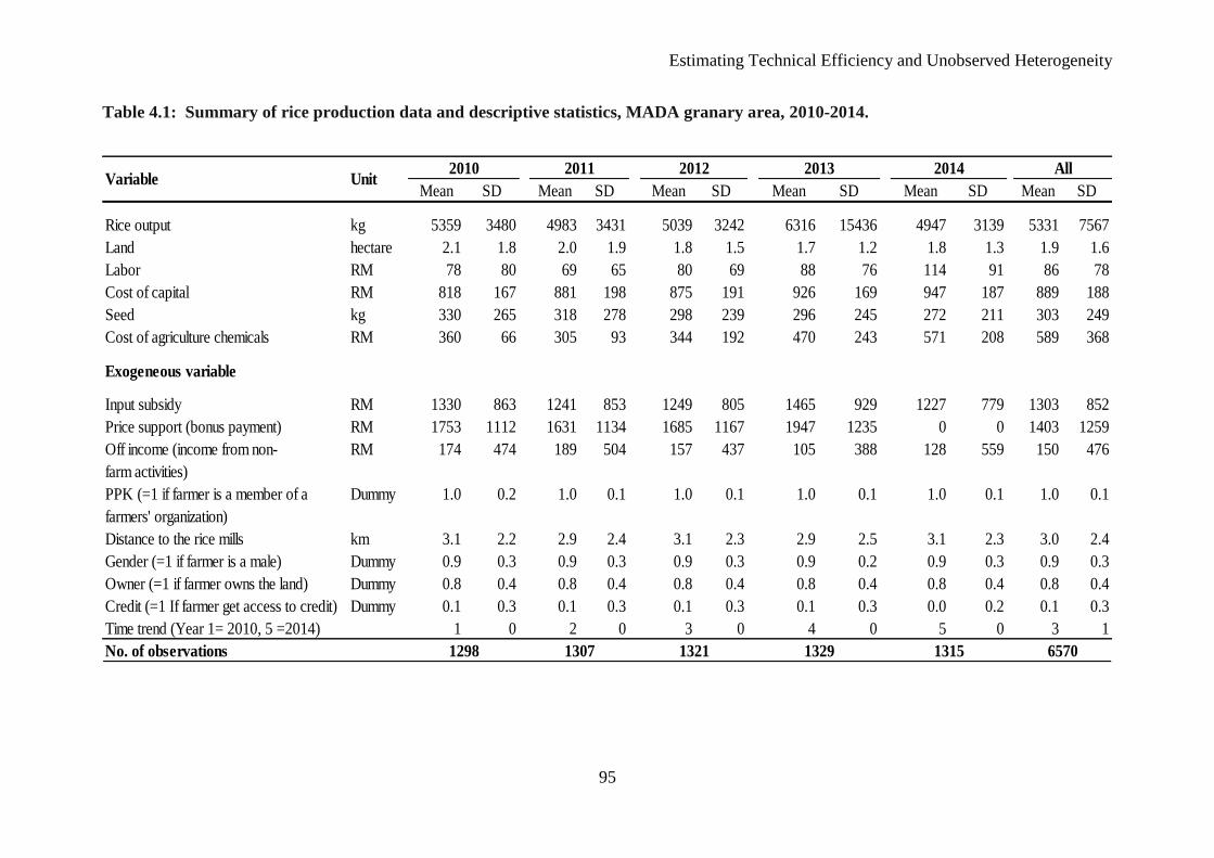
Estimating Technical Efficiency and Unobserved Heterogeneity
95
Table 4.1: Summary of rice production data and descriptive statistics, MADA granary area, 2010-2014.
Mean SD Mean SD Mean SD Mean SD Mean SD Mean SD
Rice output kg 5359 3480 4983 3431 5039 3242 6316 15436 4947 3139 5331 7567
Land hectare 2.1 1.8 2.0 1.9 1.8 1.5 1.7 1.2 1.8 1.3 1.9 1.6
Labor RM 78 80 69 65 80 69 88 76 114 91 86 78
Cost of capital RM 818 167 881 198 875 191 926 169 947 187 889 188
Seed kg 330 265 318 278 298 239 296 245 272 211 303 249
Cost of agriculture chemicals RM 360 66 305 93 344 192 470 243 571 208 589 368
Exogeneous variable
Input subsidy RM 1330 863 1241 853 1249 805 1465 929 1227 779 1303 852
Price support (bonus payment) RM 1753 1112 1631 1134 1685 1167 1947 1235 0 0 1403 1259
Off income (income from non- RM 174 474 189 504 157 437 105 388 128 559 150 476
farm activities)
PPK (=1 if farmer is a member of a Dummy 1.0 0.2 1.0 0.1 1.0 0.1 1.0 0.1 1.0 0.1 1.0 0.1
farmers' organization)
Distance to the rice mills km 3.1 2.2 2.9 2.4 3.1 2.3 2.9 2.5 3.1 2.3 3.0 2.4
Gender (=1 if farmer is a male) Dummy 0.9 0.3 0.9 0.3 0.9 0.3 0.9 0.2 0.9 0.3 0.9 0.3
Owner (=1 if farmer owns the land) Dummy 0.8 0.4 0.8 0.4 0.8 0.4 0.8 0.4 0.8 0.4 0.8 0.4
Credit (=1 If farmer get access to credit) Dummy 0.1 0.3 0.1 0.3 0.1 0.3 0.1 0.3 0.0 0.2 0.1 0.3
Time trend (Year 1= 2010, 5 =2014) 1 0 2 0 3 0 4 0 5 0 3 1
No. of observations
2014 All
1298 1307 1321 1329 1315 6570
Variable Unit2010 2011 2012 2013
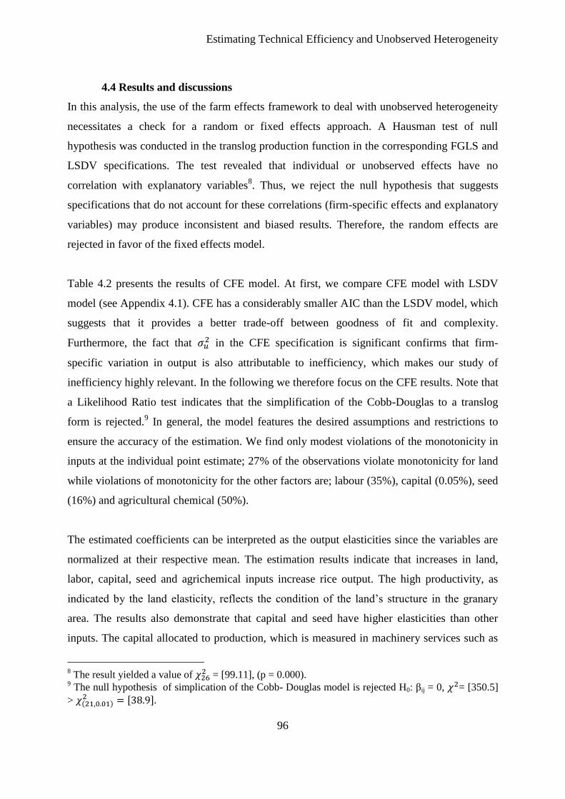
Estimating Technical Efficiency and Unobserved Heterogeneity
96
4.4 Results and discussions
In this analysis, the use of the farm effects framework to deal with unobserved heterogeneity
necessitates a check for a random or fixed effects approach. A Hausman test of null
hypothesis was conducted in the translog production function in the corresponding FGLS and
LSDV specifications. The test revealed that individual or unobserved effects have no
correlation with explanatory variables8. Thus, we reject the null hypothesis that suggests
specifications that do not account for these correlations (firm-specific effects and explanatory
variables) may produce inconsistent and biased results. Therefore, the random effects are
rejected in favor of the fixed effects model.
Table 4.2 presents the results of CFE model. At first, we compare CFE model with LSDV
model (see Appendix 4.1). CFE has a considerably smaller AIC than the LSDV model, which
suggests that it provides a better trade-off between goodness of fit and complexity.
Furthermore, the fact that 𝜎𝑢2 in the CFE specification is significant confirms that firm-
specific variation in output is also attributable to inefficiency, which makes our study of
inefficiency highly relevant. In the following we therefore focus on the CFE results. Note that
a Likelihood Ratio test indicates that the simplification of the Cobb-Douglas to a translog
form is rejected.9 In general, the model features the desired assumptions and restrictions to
ensure the accuracy of the estimation. We find only modest violations of the monotonicity in
inputs at the individual point estimate; 27% of the observations violate monotonicity for land
while violations of monotonicity for the other factors are; labour (35%), capital (0.05%), seed
(16%) and agricultural chemical (50%).
The estimated coefficients can be interpreted as the output elasticities since the variables are
normalized at their respective mean. The estimation results indicate that increases in land,
labor, capital, seed and agrichemical inputs increase rice output. The high productivity, as
indicated by the land elasticity, reflects the condition of the land’s structure in the granary
area. The results also demonstrate that capital and seed have higher elasticities than other
inputs. The capital allocated to production, which is measured in machinery services such as
8 The result yielded a value of 𝜒26
2 = [99.11], (p = 0.000). 9 The null hypothesis of simplication of the Cobb- Douglas model is rejected H0: βij = 0, 𝜒2= [350.5]
> 𝜒(21,0.01)2 = [38.9].
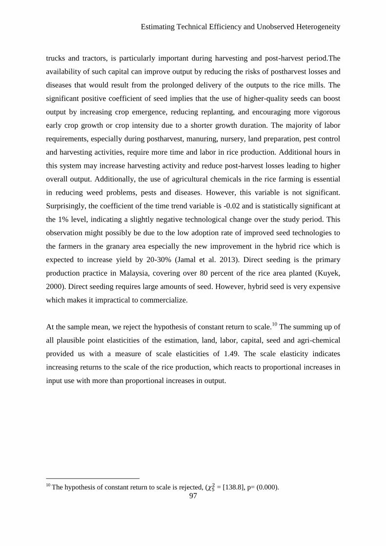
Estimating Technical Efficiency and Unobserved Heterogeneity
97
trucks and tractors, is particularly important during harvesting and post-harvest period.The
availability of such capital can improve output by reducing the risks of postharvest losses and
diseases that would result from the prolonged delivery of the outputs to the rice mills. The
significant positive coefficient of seed implies that the use of higher-quality seeds can boost
output by increasing crop emergence, reducing replanting, and encouraging more vigorous
early crop growth or crop intensity due to a shorter growth duration. The majority of labor
requirements, especially during postharvest, manuring, nursery, land preparation, pest control
and harvesting activities, require more time and labor in rice production. Additional hours in
this system may increase harvesting activity and reduce post-harvest losses leading to higher
overall output. Additionally, the use of agricultural chemicals in the rice farming is essential
in reducing weed problems, pests and diseases. However, this variable is not significant.
Surprisingly, the coefficient of the time trend variable is -0.02 and is statistically significant at
the 1% level, indicating a slightly negative technological change over the study period. This
observation might possibly be due to the low adoption rate of improved seed technologies to
the farmers in the granary area especially the new improvement in the hybrid rice which is
expected to increase yield by 20-30% (Jamal et al. 2013). Direct seeding is the primary
production practice in Malaysia, covering over 80 percent of the rice area planted (Kuyek,
2000). Direct seeding requires large amounts of seed. However, hybrid seed is very expensive
which makes it impractical to commercialize.
At the sample mean, we reject the hypothesis of constant return to scale.10
The summing up of
all plausible point elasticities of the estimation, land, labor, capital, seed and agri-chemical
provided us with a measure of scale elasticities of 1.49. The scale elasticity indicates
increasing returns to the scale of the rice production, which reacts to proportional increases in
input use with more than proportional increases in output.
10
The hypothesis of constant return to scale is rejected, (𝜒52 = [138.8], p= (0.000).
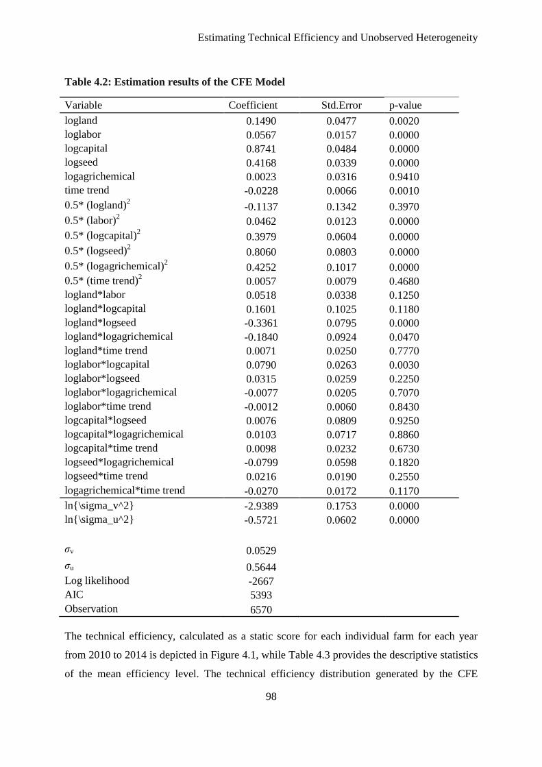
Estimating Technical Efficiency and Unobserved Heterogeneity
98
Table 4.2: Estimation results of the CFE Model
Variable Coefficient Std.Error p-value
logland 0.1490 0.0477 0.0020
loglabor 0.0567 0.0157 0.0000
logcapital 0.8741 0.0484 0.0000
logseed 0.4168 0.0339 0.0000
logagrichemical 0.0023 0.0316 0.9410
time trend -0.0228 0.0066 0.0010
0.5* (logland)2 -0.1137 0.1342 0.3970
0.5* (labor)2 0.0462 0.0123 0.0000
0.5* (logcapital)2 0.3979 0.0604 0.0000
0.5* (logseed)2 0.8060 0.0803 0.0000
0.5* (logagrichemical)2 0.4252 0.1017 0.0000
0.5* (time trend)2 0.0057 0.0079 0.4680
logland*labor 0.0518 0.0338 0.1250
logland*logcapital 0.1601 0.1025 0.1180
logland*logseed -0.3361 0.0795 0.0000
logland*logagrichemical -0.1840 0.0924 0.0470
logland*time trend 0.0071 0.0250 0.7770
loglabor*logcapital 0.0790 0.0263 0.0030
loglabor*logseed 0.0315 0.0259 0.2250
loglabor*logagrichemical -0.0077 0.0205 0.7070
loglabor*time trend -0.0012 0.0060 0.8430
logcapital*logseed 0.0076 0.0809 0.9250
logcapital*logagrichemical 0.0103 0.0717 0.8860
logcapital*time trend 0.0098 0.0232 0.6730
logseed*logagrichemical -0.0799 0.0598 0.1820
logseed*time trend 0.0216 0.0190 0.2550
logagrichemical*time trend -0.0270 0.0172 0.1170
ln{\sigma_v^2} -2.9389 0.1753 0.0000
ln{\sigma_u^2} -0.5721 0.0602 0.0000
σv 0.0529
σu 0.5644
Log likelihood -2667
AIC 5393
Observation 6570
The technical efficiency, calculated as a static score for each individual farm for each year
from 2010 to 2014 is depicted in Figure 4.1, while Table 4.3 provides the descriptive statistics
of the mean efficiency level. The technical efficiency distribution generated by the CFE
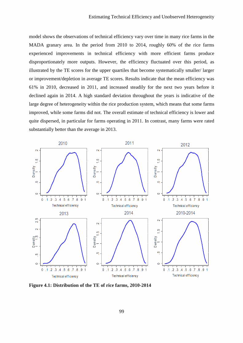
Estimating Technical Efficiency and Unobserved Heterogeneity
99
model shows the observations of technical efficiency vary over time in many rice farms in the
MADA granary area. In the period from 2010 to 2014, roughly 60% of the rice farms
experienced improvements in technical efficiency with more efficient farms produce
disproportionately more outputs. However, the efficiency fluctuated over this period, as
illustrated by the TE scores for the upper quartiles that become systematically smaller/ larger
or improvement/depletion in average TE scores. Results indicate that the mean efficiency was
61% in 2010, decreased in 2011, and increased steadily for the next two years before it
declined again in 2014. A high standard deviation throughout the years is indicative of the
large degree of heterogeneity within the rice production system, which means that some farms
improved, while some farms did not. The overall estimate of technical efficiency is lower and
quite dispersed, in particular for farms operating in 2011. In contrast, many farms were rated
substantially better than the average in 2013.
Figure 4.1: Distribution of the TE of rice farms, 2010-2014
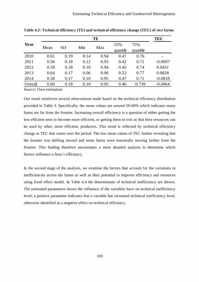
Estimating Technical Efficiency and Unobserved Heterogeneity
100
Table 4.3: Technical efficiency (TE) and technical efficiency change (TEC) of rice farms
Source: Own estimation
Our result reinforces several observations made based on the technical efficiency distribution
provided in Table 3. Specifically, the mean values are around 50-60% which indicates many
farms are far from the frontier. Increasing overall efficiency is a question of either getting the
less efficient ones to become more efficient, or getting them to exit so that their resources can
be used by other, more efficient, producers. This trend is reflected by technical efficiency
change or TEC that varies over the period. The low mean values of TEC further revealing that
the frontier was shifting inward and some farms were essentially moving farther from the
frontier. This finding therefore necessitates a more detailed analysis to determine which
factors influence a farm’s efficiency.
In the second stage of the analysis, we examine the factors that account for the variations in
inefficiencies across the farms as well as their potential to improve efficiency and resources
using fixed effect model. In Table 4.4 the determinants of technical inefficiency are shown.
The estimated parameters shows the influence of the variables have on technical inefficiency
level; a positive parameter indicates that a variable has increased technical inefficiency level,
otherwise identified as a negative effect on technical efficiency.
TEC
Mean SD Min Max25%
quantile
75%
quantile
2010 0.61 0.19 0.14 0.94 0.47 0.76 -
2011 0.56 0.18 0.12 0.93 0.42 0.71 -0.0697
2012 0.59 0.18 0.10 0.94 0.45 0.74 0.0431
2013 0.64 0.17 0.06 0.96 0.52 0.77 0.0828
2014 0.58 0.17 0.10 0.95 0.47 0.71 -0.0818
Overall 0.60 0.18 0.10 0.95 0.46 0.739 -0.0064
Year
TE
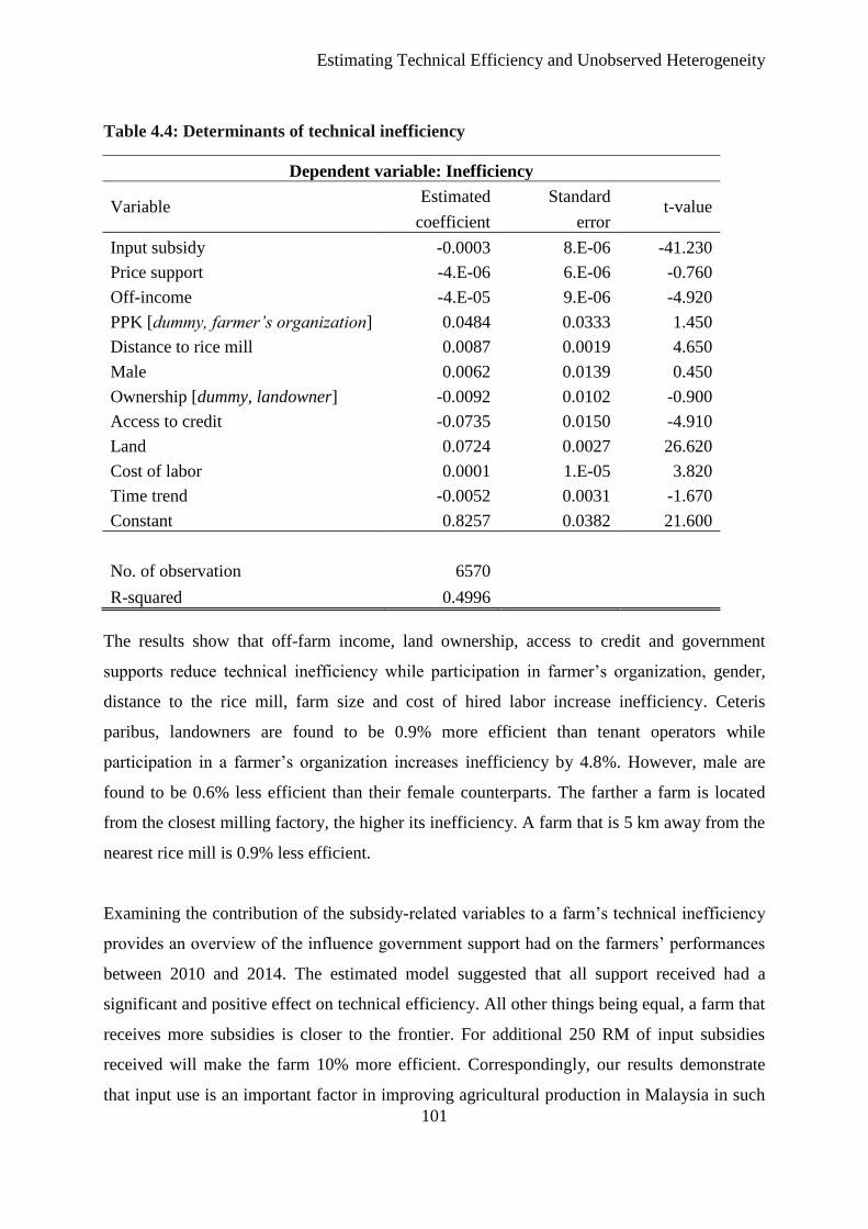
Estimating Technical Efficiency and Unobserved Heterogeneity
101
Table 4.4: Determinants of technical inefficiency
Dependent variable: Inefficiency
Variable Estimated Standard
t-value coefficient error
Input subsidy -0.0003 8.E-06 -41.230
Price support -4.E-06 6.E-06 -0.760
Off-income -4.E-05 9.E-06 -4.920
PPK [dummy, farmer’s organization] 0.0484 0.0333 1.450
Distance to rice mill 0.0087 0.0019 4.650
Male 0.0062 0.0139 0.450
Ownership [dummy, landowner] -0.0092 0.0102 -0.900
Access to credit -0.0735 0.0150 -4.910
Land 0.0724 0.0027 26.620
Cost of labor 0.0001 1.E-05 3.820
Time trend -0.0052 0.0031 -1.670
Constant 0.8257 0.0382 21.600
No. of observation 6570
R-squared 0.4996
The results show that off-farm income, land ownership, access to credit and government
supports reduce technical inefficiency while participation in farmer’s organization, gender,
distance to the rice mill, farm size and cost of hired labor increase inefficiency. Ceteris
paribus, landowners are found to be 0.9% more efficient than tenant operators while
participation in a farmer’s organization increases inefficiency by 4.8%. However, male are
found to be 0.6% less efficient than their female counterparts. The farther a farm is located
from the closest milling factory, the higher its inefficiency. A farm that is 5 km away from the
nearest rice mill is 0.9% less efficient.
Examining the contribution of the subsidy-related variables to a farm’s technical inefficiency
provides an overview of the influence government support had on the farmers’ performances
between 2010 and 2014. The estimated model suggested that all support received had a
significant and positive effect on technical efficiency. All other things being equal, a farm that
receives more subsidies is closer to the frontier. For additional 250 RM of input subsidies
received will make the farm 10% more efficient. Correspondingly, our results demonstrate
that input use is an important factor in improving agricultural production in Malaysia in such
Estimating Technical Efficiency and Unobserved Heterogeneity
102
a way that an increase in input subsidy reduces technical inefficiency. Our results corroborate
the findings made by Tian (2000) on Chinese rice farms and Zhu et al, (2012).
The coefficient of the price support indicates that the provision of price support would have a
negative impact on technical inefficiency. The result indicates that 1000 RM of subsidies will
make farm 10% more efficient. A possible explanation could be that when these supports are
available, they help less efficient farms make investments required to make them more
competitive.
Farmers who were engaged in off-farm activities, depicted by a negative and significant
coefficient for off-farm income, tend to exhibit lower inefficiency. Ceteris paribus, a farm
with 4,000 RM more off-farm income will be 10% more efficient. This positive relationship is
expected because as the households move towards spending more time off of the farm, they
will require time and management saving technologies (like herbicide-tolerant crops) to
maintain production. In addition, they are less likely to adopt management-intensive
technologies, such as integrated pest manage and agricultural machinery, which corroborates
the finding made by Ji et al. (2012). Additionally, Takahashi and Otsuka (2009) propose that
increased nonfarm income may assist in accessing credit; therefore adding to the long-term
financial investment among rice farmers in the Central Luzon, Philippines.
Similarly, our results show that access to credit has a negative and statistically significant
relationship with technical inefficiency. All other things being equal, a farm with 200 RM
more credit volume is 10% more efficient. These results confirm the previously stated
assumption that by overcoming financial constraint, credit availability helps farmers attain
higher levels of efficiency through the purchase of higher quality farm inputs, such as
fertilizers, new technologies and high-yielding varieties of rice seeds.
As expected, technical efficiency decreases with the increasing use of land and it is significant
at the 1% level. Results imply that large farms are 7.2% more technically inefficient, which
confirms our expectations. It is often recognized that in the land market especially in
Malaysia where labor use intensities on small farms are high, smaller farms face higher
effective purchase prices for land. More land alone does not make a farm more efficient, but
more land coupled with equivalent increases in other inputs will lead to increased productivity
Estimating Technical Efficiency and Unobserved Heterogeneity
103
(higher frontier). Therefore, small farms engage in more intensive use of resources; they use
labor more intensively and use more of available land for land improvement in a diligent
manner and thereby are more technically efficient.
Additionally, we find that the use of hired labor has a positive effect on technical inefficiency,
implying family labor is more crucial than hired labor for higher efficiency. Small farmers,
predominantly are taking advantage of the fact that household labor has very low opportunity
costs which make their production is more efficient.
4.5 Conclusions
The rice sector is one of the major sectors of Malaysian agriculture. However, there are few
studies of the efficiency of rice production in Malaysia. We used farm level data to gain
insights on the technical efficiency of the country’s rice farming. Although panel data were
available, some important descriptive attributes were scarce. As a result we took unobserved
heterogeneity into account. In this framework, we applied the recent fixed effect Stochastic
Frontier model of Chen et al. (2014), which allows for unmeasured characteristics while
simultaneously the model estimation is free of incidental parameters.
In the observation period from 2010 to 2014, technical efficiency appeared to be fluctuate in
rice production. Our results indicate that the mean efficiency was 61% in 2010; it decreased in
2011 and increased steadily for the next two years, before it declined again in 2014. However,
technical efficiency change has been quite low during the period.
The potential for increasing individual farm output varies considerably since many farms
became much better while others became much worse. Government support such as input
subsidies, credit facilities and off-farm activities are identified as important factors
contributing to the improvement in the level of technical efficiency among rice farmers. Our
empirical result points to a significant relationship between efficiency and access to credit.
Overcoming financial constraints with better credit availability helps farmers attain higher
levels of efficiency through the purchase of higher quality farm inputs such as fertilizers, new
technologies and high-yielding varieties of rice seeds. The positive impact of nonfarm income
on technical efficiency is another reason for the continued and sizeable contribution of
Estimating Technical Efficiency and Unobserved Heterogeneity
104
nonfarm sources of farm household income. Subsidies seem to be an important component of
increasing rice production. Our main result indicates that input subsidies have a positive,
significant influence on the technical efficiency of the Malaysian rice farms. Subsidies can
improve the technical efficiency if they encourage them to be innovative, to improve the
implementation of the existing technologies, to increase ability of the farms to adjust their
behavior and thereby operate more efficiently. Therefore, the direction of subsidies and
supports affecting farm performance is crucial and the results of this study will help
policymakers to identify the positive and negative effects and better target public intervention
to improve farm efficiency.
However, public support provided to the small farmers mainly for political reasons will most
likely not be enough for these farmers to become efficient. This effort must come to be
realized through a combination of access to land and capital since poor farmers with small
landholdings usually need capital in almost all economies (Abdulai and Eberlin 2001). Our
result supports this notion since the technical efficiency increases with the decreasing use of
land. A redistribution of land to small farmers with an adequate provision of finance could
increase technical efficiency.
Overall, the results indicate that rice production can be improved by continuously increasing a
farm’s resources and technical efficiency. This can only be achieved if agricultural
development and the policies facilitating farmers’ accessibility to credit, capital, land and off-
farm activities, especially for small farms, are carefully designed and well-targeted. Improved
access to and distribution of input subsidies must also occur.
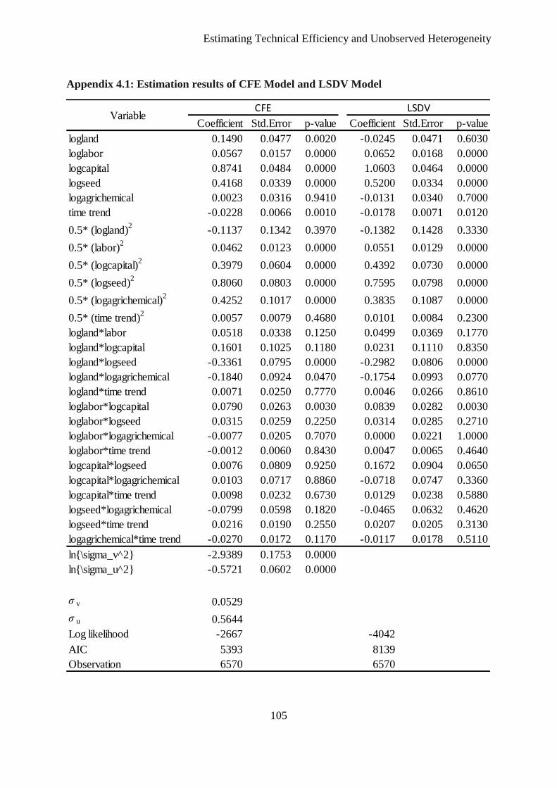
Estimating Technical Efficiency and Unobserved Heterogeneity
105
Appendix 4.1: Estimation results of CFE Model and LSDV Model
Coefficient Std.Error p-value Coefficient Std.Error p-value
logland 0.1490 0.0477 0.0020 -0.0245 0.0471 0.6030
loglabor 0.0567 0.0157 0.0000 0.0652 0.0168 0.0000
logcapital 0.8741 0.0484 0.0000 1.0603 0.0464 0.0000
logseed 0.4168 0.0339 0.0000 0.5200 0.0334 0.0000
logagrichemical 0.0023 0.0316 0.9410 -0.0131 0.0340 0.7000
time trend -0.0228 0.0066 0.0010 -0.0178 0.0071 0.0120
0.5* (logland)2
-0.1137 0.1342 0.3970 -0.1382 0.1428 0.3330
0.5* (labor)2
0.0462 0.0123 0.0000 0.0551 0.0129 0.0000
0.5* (logcapital)2
0.3979 0.0604 0.0000 0.4392 0.0730 0.0000
0.5* (logseed)2
0.8060 0.0803 0.0000 0.7595 0.0798 0.0000
0.5* (logagrichemical)2
0.4252 0.1017 0.0000 0.3835 0.1087 0.0000
0.5* (time trend)2
0.0057 0.0079 0.4680 0.0101 0.0084 0.2300
logland*labor 0.0518 0.0338 0.1250 0.0499 0.0369 0.1770
logland*logcapital 0.1601 0.1025 0.1180 0.0231 0.1110 0.8350
logland*logseed -0.3361 0.0795 0.0000 -0.2982 0.0806 0.0000
logland*logagrichemical -0.1840 0.0924 0.0470 -0.1754 0.0993 0.0770
logland*time trend 0.0071 0.0250 0.7770 0.0046 0.0266 0.8610
loglabor*logcapital 0.0790 0.0263 0.0030 0.0839 0.0282 0.0030
loglabor*logseed 0.0315 0.0259 0.2250 0.0314 0.0285 0.2710
loglabor*logagrichemical -0.0077 0.0205 0.7070 0.0000 0.0221 1.0000
loglabor*time trend -0.0012 0.0060 0.8430 0.0047 0.0065 0.4640
logcapital*logseed 0.0076 0.0809 0.9250 0.1672 0.0904 0.0650
logcapital*logagrichemical 0.0103 0.0717 0.8860 -0.0718 0.0747 0.3360
logcapital*time trend 0.0098 0.0232 0.6730 0.0129 0.0238 0.5880
logseed*logagrichemical -0.0799 0.0598 0.1820 -0.0465 0.0632 0.4620
logseed*time trend 0.0216 0.0190 0.2550 0.0207 0.0205 0.3130
logagrichemical*time trend -0.0270 0.0172 0.1170 -0.0117 0.0178 0.5110
ln{\sigma_v^2} -2.9389 0.1753 0.0000
ln{\sigma_u^2} -0.5721 0.0602 0.0000
σ v 0.0529
σ u 0.5644
Log likelihood -2667 -4042
AIC 5393 8139
Observation 6570 6570
CFE LSDVVariable
Estimating Technical Efficiency and Unobserved Heterogeneity
106
Additional notes:
The data employed in this study are based on the panel of 6750 rice farms in MADA granary
area. The farm level data is collected twice a year and each survey period includes a balanced
sample of 675 farming households. The panel is composed of ten cross-sections, covering
main and off- seasons over the five-year period from 2010 to 2014. This data set provides
comprehensive information, including input use, output and corresponding prices.
However, despite of the rich dataset provided, the data suffers from ambiguous values and
substantial zero users of variable inputs, particularly agricultural chemicals. For example, the
standard deviation for the output is 7486, while for the input variables such as agricultural
chemical and seed, the standard deviations are approximately 217 and 241 respectively, which
indicate large variations in output and inputs. Additionally, many data sets are not complete
or show noticeable errors. We found 1,208 zero values in agrichemicals, 45 in seed, 21 in
cost capital, 113 in labor and 1 in output. To account for these extreme values, we use a rule
of thumb of 3 standard deviations from the mean to detect outliers or if 99% of the variable of
interest lied outside ± 3 standard deviations from the mean. Since all farmers received
pesticides subsidies in a form of coupon worth 200 RM, we therefore use this value to
account for zero usage of agricultural chemicals, by adding this amount to the agricultural
chemical values. Other implausible values were also detected in capital, seed as well as
agricultural chemicals. These values were then properly adjusted according to the normal
standard rate proposed by MADA. As a consequence, the remaining panel is unbalanced with
6,570 out of 6,750 observations were used for the estimation. All the monetary values have
been deflated by the 2010 consumer price index. Finally, to avoid data inaccuracy or bias, the
dataset were then crosschecked by MADA officers.
Details on the data treatment are summarized in the following Appendix 4.2;
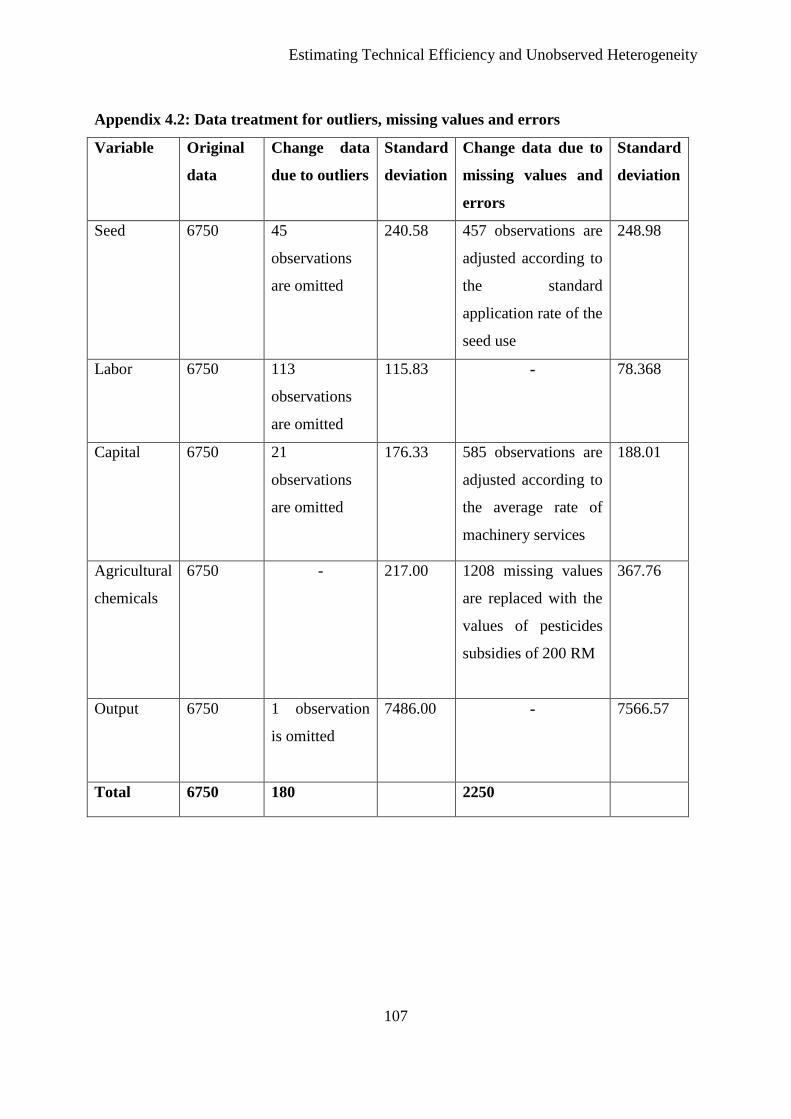
Estimating Technical Efficiency and Unobserved Heterogeneity
107
Appendix 4.2: Data treatment for outliers, missing values and errors
Variable Original
data
Change data
due to outliers
Standard
deviation
Change data due to
missing values and
errors
Standard
deviation
Seed 6750 45
observations
are omitted
240.58
457 observations are
adjusted according to
the standard
application rate of the
seed use
248.98
Labor 6750 113
observations
are omitted
115.83
- 78.368
Capital 6750 21
observations
are omitted
176.33
585 observations are
adjusted according to
the average rate of
machinery services
188.01
Agricultural
chemicals
6750 - 217.00
1208 missing values
are replaced with the
values of pesticides
subsidies of 200 RM
367.76
Output 6750 1 observation
is omitted
7486.00
- 7566.57
Total 6750 180 2250
Estimating Technical Efficiency and Unobserved Heterogeneity
108
References
Abdulai, A., and H. Tietje. 2007. “Estimating technical efficiency under unobserved
heterogeneity with stochastic frontier models: Application to northern German dairy
farms.” European Review of Agricultural Economics 34(3):393–416.
Abdulai, A., and R. Eberlin. 2001. “Technical efficiency during economic reform in
Nicaragua: Evidence from farm household survey data.” Economic Systems 25(2):113–
125.
Abiola, O.A., S. Mad Nasir, R. Alias, and A. Ismail. 2016. “Effect of Improved High Yielding
Rice Variety on Farmers Productivity in Mada, Malaysia.” International Journal of
Agricultural Sciences and Veterinary Medicine 4(1):38–52.
Addai, K.N., V. Owusu, and G. Danso-Abbeam. 2014. “Effects of Farmer – Based-
Organization on the Technical efficiency of Maize Farmers across Various Agro -
Ecological Zones of Ghana.” Journal of Economics and Development Studies 2(1):141–
161. Available at: http://jedsnet.com/journals/jeds/Vol_2_No_1_March_2014/7.pdf
[Accessed April 14, 2016].
Aigner DJ, Lovell CAK, Schmidt P. 1977. “Formulation and estimation of stochastic frontier
production function models”. J Econ 6:21–37.
Álvarez, A., J. Del Corral, And A. Fernández. 2009. “Modeling Regional Heterogeneity With
Panel Data: With Application To Spanish Provinces.” Uclm.Es (May). Available at:
http://www3.uclm.es/profesorado/jcorral/Trabajando/6f10da_Efi_Regions_12.pdf.
Arshad, F.M., E.F. Alias, K.M. Noh, and T. Muhammad. 2011. “Food Security: Self-
Sufficiency of Rice in Malaysia.” International Journal of Management Studies
18(2):83–100. Available at:
http://www.ijms.uum.edu.my/images/pdf/18no2ijms/ijms1825.pdf [Accessed March 21,
2016].
Assunção, J.J., and M. Ghatak. 2003. “Can unobserved heterogeneity in farmer ability explain
the inverse relationship between farm size and productivity?” Economics Letters
80(2):189–194.
Belotti, F., and I. Giuseppe. 2012. “Consistent estimation of the ‘true’ fixed-effects stochastic
frontier model.” 5 No. 231,
Bhatt, M.S., and S.A. Bhat. 2014. “Technical Efficiency and Farm Size Productivity ― Micro
Level Evidence From Jammu & Kashmir.” International Journal of Food and
Agricultural Economics 2(4):27–49. Available at:
http://www.foodandagriculturejournal.com/vol2.no4.pp27.pdf.
Binswanger, H. and Elgin M. 1998. “Reflections on land reform and farm size.” In: Eicher,
C.,Staatz, J. (Eds.), International Agricultural Development, third ed. Johns Hopkin,
Baltimore, pp. 316-328.
Binswanger, H.P. and K. Deininger. 2005. “Explaining Agricultural and Agrarian Policies
in Developing Countries.” Journal of Economic Literature. XXXV(Dec. 1997):1958-
2005.
Estimating Technical Efficiency and Unobserved Heterogeneity
109
Brummer, B., and J. Loy. 2000. “The Technical Efficiency Impact of Farm Credit
Programmes: A Case Study of Northern Germany.” Journal of Agricultural Economics
51(3):405–418.
Chakrabarty, T., S. Akter, a S.M. Saifullah, S. Sheikh, and A.C. Bhowmick. 2014. “Use of
Fertilizer and Pesticide for Crop Production in Agrarian Area of Tangail District,
Bangladesh.” Environment and Ecology Research 2(6):253–260.
Chen, Y.Y., P. Schmidt, and H.J. Wang. 2014. “Consistent estimation of the fixed effects
stochastic frontier model.” Journal of Econometrics 181(2):65–76. Available at:
http://dx.doi.org/10.1016/j.jeconom.2013.05.009.
Daño, E.C., and E.D. Samonte. “Public Sector Intervention in the Rice Industry in Malaysia.
Southeast Asia Regional Initiatives for Community Empowerment (SEARICE).”
Dawe, D. 2010. The Rice Crisis: Markets, Policies and Food Security. The Food and
Agriculture Organization of the United Nations and Earthscan. Available at:
http://www.fao.org/3/a-an794e.pdf [Accessed December 6, 2015].
Department of Agriculture, M. 2014. “Perangkaian Padi Malaysia (Paddy Statistics of
Malaysia) 2013.”
Diaz, C., M. Hossain, S. Merca, and T. Mew. 1998. “Seed Quality and Effect on Rice Yields:
Findings from Farmer Participatory Experiments in Central Luzon, Philippines.”
Philippines Journal Crop Science 23(2):111–119.
Elbehri, A., and A. Sarris. 2009. “Farm Support Policies That Minimize Global Distortionary
Effects.” In FAO Expert Meeting on “How to Feed the World in 2050.” Available at:
http://www.fao.org/wsfs/forum2050/wsfs-forum/en/.
Fernandez-Cornejo, J., M. Ashok, R. Nehring, C. Hendricks, M. Southern, and a Gregory.
2007. “Off-farm income, technology adoption, and farm economic performance.”
Economic Research Report - Economic Research Service, USDA (36):53 pp. Available
at: <Go to ISI>://CABI:20073230903.
Gianessi, L.P. 2014. “Importance of Pesticides for Growing Rice in South and South East
Asia.” CropLife Foundation (International Pesticide Benefit Case Study 108):30–33.
González-Farías, G., A. Domínguez-Molina, and A.K. Gupta. 2004. “Additive properties of
skew normal random vectors.” Journal of Statistical Planning and Inference 126(2):521–
534.
Greene, W. 2005. “Reconsidering heterogeneity in panel data estimators of the stochastic
frontier model.” Journal of Econometrics 126(2):269–303.
Greene, W. 2008. “The econometric approach to efficiency analysis”. In H. O. Fried, C. A. K.
Lovell, & S. S. Schmidt (Eds.), The Measurement of Productive Efficiency and
Productivity Change chapter 2. (pp. 92–250). Oxford University Press. New York.
Heshmati, A., S.C. Kumbhakar, and L. Hjalmarsson. 1995. “Efficiency of the Swedish pork
industry: A farm level study using rotating panel data 1976-1988.” European Journal of
Operational Research 80(3):519–533.
Estimating Technical Efficiency and Unobserved Heterogeneity
110
Hoang, H.K., and W.H. Meyers. 2015. “Price stabilization and impacts of trade liberalization
in the Southeast Asian rice market.” Food Policy 57:26–39. Available at:
http://dx.doi.org/10.1016/j.foodpol.2015.07.009.
Holtkamp, J. 2015. “Unobserved heterogeneity in productivity analysis of panel data:
Applications to meat chain firms and global growth in agriculture.” Available at:
http://hdl.handle.net/11858/00-1735-0000-0022-5DE0-E.
Hsiao, C. 2007. “Panel data analysis - Advantages and Challenges.” Sociedad de Estadística e
Investigación Operativa 00(0):1–63. Available at:
http://www.springerlink.com/index/10.1007/s11749-007-0046-
x\nhttp://www.springerlink.com/index/9870132756017386.pdf.
Huffman, W.E. “Farm and Off-Farm Work Decisions: the Role of Human Capital,” Review
of Economics and Statistics 62(1)(1980): 14-23.
International Rice Research Institute (IRRI). 2002. Available at: http://www.irri.org.
Jamal, K., N.H. Kamarulzaman, A.M. Abdullah, M.M. Ismail, and M. Hashim. 2013.
“Farmer’s acceptance towards fragrant rice farming: The case of non-granary areas in the
East Coast, Malaysia.” International Food Research Journal 20(5):2895–2899.
Ji, Y., X. Yu, and F. Zhong. 2012. “Machinery investment decision and off-farm employment
in rural China.” China Economic Review 23(1):71–80. Available at:
http://dx.doi.org/10.1016/j.chieco.2011.08.001.
Johnson, N., Ruttan, V. 1994. Why are farms so small? World Development 5, 691-706.
Koirala, K.H., A. Mishra, and S. Mohanty. 2016. “Impact of land ownership on productivity
and efficiency of rice farmers: The case of the Philippines.” Land Use Policy 50:371–
378. Available at: http://ac.els-cdn.com/S0264837715002987/1-s2.0-
S0264837715002987-main.pdf?_tid=232317b2-98f2-11e5-b3d1-
00000aacb361&acdnat=1449060324_bb4fbf2206458aa6ee59de4d75848197.
Kumbhakar, S.C., and G. Lien. 2010. “Impact of Subsidies on Farm Productivity and
Efficiency.” In The Economic Impact of Public Support to Agriculture. New York, NY:
Springer New York, pp. 109–124. Available at: http://link.springer.com/10.1007/978-1-
4419-6385-7_6 [Accessed November 13, 2016].
Kuyek, D. 2000. “Hybrid Rice in Asia: An Unfolding Threat.” March, 2000. Available at
file:///C:/Users/userdell/Downloads/grain-34-hybrid-rice-in-asia-an-unfolding-
threat%20(2).pdf
Martin, J.P., and J.M. Page. 1983. “The Impact of Subsidies on X-Efficiency in LDC
Industry: Theory and an Empirical Test.” The Review of Economics and Statistics
65(4):608. Available at: http://www.jstor.org/stable/1935929?origin=crossref [Accessed
November 13, 2016].
Masterson, T. 2007. “Productivity, Technical Efficiency, and Farm Size in Paraguayan
Agriculture by Keywords : Farm Size, Productivity, Technical Efficiency, Paraguay.”
Working Paper (490):37. Available at: http://ssrn.com/abstract=964722.
Estimating Technical Efficiency and Unobserved Heterogeneity
111
Mundlak, Y. 1978. “On the Pooling of Time Series and Cross Section Data.” Econometrica
46(1):69–85.
Mutert, E., and T.H. Fairhurst. 2002. “Southeast Asia Developments in Rice Production in
Southeast Asia.” Better Crops International, 15.
Olson, K., and L. Vu. 2009. “Productivity growth, Technical Efficiency and Technical
Change on Minnesota farms Productivity growth, Technical Efficiency and Technical
Change on Minnesota farms.” In Agricultural & Applied Economics Association’s 2009
AAEA & ACCI Joint Annual Meeting, Milwaukee, WI, July 26-28.
Pitt, M.M., and L. Lee. 1981. “The Measurement and Sources of Technical Inefficiency In
The Indonesian Weaving Industry.” Journal of Development Economics 9:43–64.
Porcelli, F. 2009. “Measurement of Technical Efficiency. A brief survey on parametric and
non-parametric techniques.” Retrieved February (January):1–27. Available at:
http://citeseerx.ist.psu.edu/viewdoc/download?doi=10.1.1.232.4843&rep=rep1&type=pd
f.
Schmidt, P., and R.C. Sickles. 1984. “Production frontiers and panel data.” Journal of
Business and Economic Statistics 2(4):367–374.
Serra, T., D. Zilberman, and J.M. Gil. 2008. “Farms’ technical inefficiencies in the presence
of government programs.” The Australian Journal of Agricultural and Resource
Economics 52(1):57–76. Available at: http://doi.wiley.com/10.1111/j.1467-
8489.2008.00412.x [Accessed November 13, 2016].
Siwar, C., D.M. Idris, M. Yasar, and G. Morshed. 2014. “Issues and Challenges Facing Rice
Production and Food Security in the Granary Areas in the East Coast Economic Region
(ECER), Malaysia.” Research Journal of Applied Sciences, Engineering and Technology
7(4):711–722.
Takahashi, K., and K. Otsuka. 2009. “The increasing importance of nonfarm income and the
changing use of labor and capital in rice farming: the case of Central Luzon, 1979-2003.”
Agricultural Economics 40(2):231–242. Available at:
http://doi.wiley.com/10.1111/j.1574-0862.2009.00372.x [Accessed November 3, 2016].
Tetteh Anang, B., and J. Amikuzuno. 2015. “Factors Influencing Pesticide Use in Smallholder
Rice Production in Northern Ghana.” Agriculture, Forestry and Fisheries 4(2):77.
Available at:
http://www.sciencepublishinggroup.com/journal/paperinfo.aspx?journalid=119&doi=10.
11648/j.aff.20150402.19.
Thiam, A., B.E. Bravo-Ureta, and T.E. Rivas. 2001. “Technical efficiency in developing
country agriculture: a meta-analysis.” Agricultural Economics 25:235–243. Available at:
http://citeseerx.ist.psu.edu/viewdoc/download?doi=10.1.1.336.2197&rep=rep1&type=pd
f [Accessed December 14, 2015].
Tian, W. 2000. “Technical Efficiency and Its Determinants in China’s Grain Production.”
Journal of Productivity Analysis 13:159–174.
Estimating Technical Efficiency and Unobserved Heterogeneity
112
Timmer, C.P., and D. Dawe. 2007. “Managing food price instability in Asia: A macro food
security perspective.” Asian Economic Journal 21(1):1–18.
von Cramon-Taubadel, S., and R. Saldias. 2014. “Access to credit and determinants of
technical inefficiency of specialized smallholder farmers in Chile.” Chilean journal of
agricultural research 74(4):413–420. Available at:
http://www.scielo.cl/scielo.php?script=sci_arttext&pid=S0718-
58392014000400006&lng=en&nrm=iso&tlng=en.
Wozniack, G.D. “Joint Information Acquisition and New Technology Adoption: Late Versus
Early Adoption,” The Review of Economics and Statistics 75(1993): 438-445.
Zhu, X., and A.O. Lansink. 2010. “Impact of CAP Subsidies on Technical Efficiency of Crop
Farms in Germany, the Netherlands and Sweden.” Journal of Agricultural Economics
61(3):545–564. Available at: http://doi.wiley.com/10.1111/j.1477-9552.2010.00254.x
[Accessed November 13, 2016].
Zhu, X., R.M. Demeter, and A.O. Lansink. 2012. “Technical efficiency and productivity
differentials of dairy farms in three EU countries: the role of CAP subsidies.”
Agricultural Economics Review 13(1):66–92.
A Note on Farm Competitiveness and Efficiency
113
Chapter 5
A Note on Farm Competitiveness and Efficiency
5.1 Introduction
The concept of competitiveness permeates the economic literature in several areas, including:
the microeconomic level, where competitiveness is measured at a single firm/farm level; the
meso-economic level, where it is measured at commodity or sector level; and finally at the
macroeconomic level, where competitiveness is measured at an aggregate or country level
(Latruffe, 2010). ‘Competitiveness’ has a broad meaning, which has yet to gain universal
definition acceptance in economics (Ahearn et al 1990; Sharples 1990). The ambiguity
associated with the term allows researchers to apply their own definition based on different
ways and perspectives they put forward in the literature. The Organisation for Economic
Cooperation and Development (OECD) succinctly describes competitiveness as “the ability of
companies, industries, regions, nations and supranational regions to generate, while being
and remaining exposed to international competition, a relatively high factor of income and
factor employment levels on a sustainable basis” (Hatzichronologou, 1996). The European
Commission (2001) defines competitiveness as: "the ability of an economy to provide its
population with high and rising standards of living and high rates of employment on a
sustainable basis”. However, given the evolution of the concept over time, this term was
redefined by the Aiginger et al, (2013) as "the ability of a country (region, location) to deliver
the beyond-GDP goals for its citizens". Others relate this meaning with profitability.
Agriculture Canada (1991) defines “competitiveness as the ability to gain profits and
maintain market share”. Latruffe (2010) clarifies competitiveness as “the ability to
successfully face and engage with the competition, either domestically or internationally”.
Subsequently, competitiveness equates to the ability to sell the products that satisfy the
demand while simultaneously securing profits over time.
Despite the vast research efforts dedicated to this subject during the last two decades,
considerable misunderstandings exist and interminable debates over the precise meaning of
‘competitiveness’ and its scope have occurred (Sarker and Ratnasena, 2014). Thus, depending
A Note on Farm Competitiveness and Efficiency
114
on the purpose of the study, the level of analysis, and the commodity in question, a large
number of measures of competitiveness have been developed. Latruffe (2010) classifies
measurement into two disciplines; 1) the neoclassical economies which places emphasis on
trade and measure competitiveness with comparative advantages, exchange rate and export or
import indices and; 2) the strategic management which focuses on the firm’s structure and
strategy, as well as measures the firm’s competitiveness based on various cost indicators,
including productivity and efficiency.
The first strand of literature suggests that a nation’s competitiveness is based on comparative
advantage. Comparative advantage, as conceptualised by the Ricardian and Hecksher-Ohlin
models for two inputs in a two country case11, postulates that differences in production costs
among countries have resulted in trade flows and that the country with a cost advantage will
specialize in the production of that good. Such a concept is widely used when comparing the
international competitiveness between countries. However, a large number of measures for
determining comparative advantage have been developed due to uncertainty on the precise
meaning of the comparative/competitive advantage. Singgel (2006) and Latruffe (2010)
provide a comprehensive survey and discussion on these measures and concepts. Among the
measures surveyed, the Domestic Resource Cost or DRC is regarded as the true measure of
comparative advantage (Singgel, 2006). The DRC compares the domestic resources cost at
social prices to the value added measured at social prices12. The use of the social price ensures
that the DRC measures the true comparative advantage that can be derived from the Ricardian
framework. The DRC is a widely applied concept used in economic literature that is also an
indicator of comparative advantage which can be calculated from the Policy Analysis Matrix
(PAM) framework (Monke and Pearson, 1989).
Despite the wide use and acceptance of the DRC as an indicator of comparative advantage in
PAM, it is criticized for yielding potential inaccuracies in the ranking of activities. Masters
and Winter-Nelson (1995) and Singgel (2006) have demonstrated that the DRC understates
the competitiveness of activities relying on a high level of non-tradable inputs. The bias is
11
Findlay and Grubert (1959) who were among the first to use a two country, two good, two factor model to
consider the effects of Ricardian productivity and factor abundance in jointly determining factor prices and
production patterns. 12
The development of the DRC ratio draws back to Bruno (1965) as a project appraisal indicator to evaluate the
benefits of new activities.
A Note on Farm Competitiveness and Efficiency
115
more pronounced if the activities include very divergent combinations of traded and non-
traded inputs. Consequently, Masters and Winter-Nelson (1995) proposed the Social Cost
Benefit (SCB), which is analogous to the unit cost ratio (UCs) proposed by Singgel (2006).
SCB compares total domestic costs at social prices to the total outputs measured at social
prices. Since SCB does not include the calculation of the value added in the critical
dimension, it is not affected by the classifications of tradable or non-tradable costs.
The second strand of literature focuses on the efficiency and productivity analysis as the
measurement of competitiveness where technical efficiency and Total Factor Productivity
(TFP) have been the main long-term interest. Productivity analysis has been heavily applied
on the micro level. Furthermore, a profusion of studies have been conducted to investigate
technical efficiency and to a lesser extent, the allocative efficiency of farms in various
countries (Bhatt and Bhat 2014; Brummer and Loy 2000; Kumbhakar 1987; Masterson 2007;
Yao and Gerald 2007; Abdulai and Huffman 1998). The theoretical elements of these
concepts are empirically constructed and the practical applications of modeling these
functions, as well as the measurements using parametric and non-parametric methods, are
extensive. The competitiveness or the comparative advantage is determined by the Decision
Making Unit (DMU) and its distance to the best-practice frontier, which is based on relative
rates of TFP change (Nishimizu and Page, 1986).
Although authors have been prolific in exploring the connection between
competitiveness/comparative advantage and efficiency, the theoretical treatment does not
offer any ready conclusions. The SCB approach works with social prices in measuring
international competitiveness. Efficiency measurement simply compares DMUs with one
another – the frontier is defined by the best. But whether the best are good enough (whether
they are actually competitive) is never answered directly by efficiency analysis. It could be
that even the best are not competitive, but they are surviving due to subsidies or protection.
There should nevertheless be a relationship – the DMUs that are closest to the frontier should
have better SCBs, but they might still have ‘bad’ SCBs overall: in other words they might be
relatively efficient but nonetheless not competitive. Recently, researchers have started to
produce PAM results with disaggregated data and others use the same types to efficiency
analysis, this leads to the natural question, how are these two types of analysis related?
A Note on Farm Competitiveness and Efficiency
116
Establishing the linkage will help policy makers and others make better use of one or the
other measure if they knew how it relates to the other.
To motivate our empirical analysis, we develop a simple model that relates competitiveness
and technical efficiency, and propose a PCB criterion decomposition that formally relates
improvements in efficiency to improvements in PCB ratio. To date, no empirical work on this
link has been published, therefore we aim to fill that gap. Our paper makes several
contributions to the literature. Firstly, our research offers a novel approach for determining
the relationship between competitiveness and efficiency. Secondly, in addition to introducing
a theoretical link between the two strands, our analysis provides a foundation for
understanding the information, the measurements, and the characteristics associated with each
method and how these links may contribute to explaining competitiveness.
The rest of the paper proceeds as follows: Section 5.2 provides an overview of the strengths
and weakness of each approach to measuring competitiveness. Section 5.3 outlines the SCB
and PCB calculations using the Policy Analysis Matrix framework; Section 5.4 provides the
model estimations using both CFE and primal system of profit maximization; Section 5.5
provides a decomposition of static competitiveness, distinguished into technical efficiency
and allocative efficiency; Section 6 describes the empirical illustration we used to test the
relationship; and the final section concludes the paper.
5.2 Strength and weaknesses of the PAM and SFA approaches
In this paper, we showed two alternative tools or methods that can be used to explain
competitiveness and efficiency. In doing so, we proposed a simple decomposition of
competitiveness into technical efficiency. The proposed technique provides a clear analytical
link between two largely separate methodologies for assessing economic performance, cost-
benefit indicators based on the international price rule and efficiency analysis, and thus,
facilitates a more detailed understanding of the definition of competitiveness.
Despite the acknowledged methodological reservations, SCB or Private Cost Benefit (PCB)
measurements as described by the PAM framework have proved to be highly useful policy
tools when market and shadow prices diverge. Activities with the lowest SCB ratios are
normally assumed to exhibit the greatest potential for expansion as exports or efficient
substitutes for imports and, defined in this way, the greatest comparative advantage.
A Note on Farm Competitiveness and Efficiency
117
Additionally, PAM is a straightforward policy analysis that provides a quantitative estimate of
the impact of policies and market structure of the commodity by comparing the private and
social structure of incentives on the microeconomic level (i.e. incentives to producers,
processors, and marketing agents). Moreover, it potentially serves as an information baseline
used for evaluating agricultural and trade policy analysis, as well as to support policy
planning or project appraisal needs. PAM is a purely descriptive analysis and its results are
relatively easy to estimate, however, the advantages of PAM go beyond its pure analytic
nature in terms of policy analysis. Due to its intuitively comprehensive concept, PAM results
can serve as an appropriate tool for delivering the information needs of politicians and
officials interested in evaluating the impact of policies. PAM’s ability to inform provides
critical information to the best-positioned individuals who are then able to effectively allocate
funds or budgets for investment and research pathways. It can also inform policy makers
about the weaknesses and strengths of environments specific to the country. Furthermore,
PAM’s analysis and results are more relaxed and easy to present; the main users of
competitiveness indicators are the ministry or government departments designing policies,
consulting and negotiating trade agreements or writing development plans, as well as private
sector agents, like banks and industrial corporations.
A major drawback of PAM, however, is that it does not provide an understanding of the
historical forces of the current pattern of measured comparative advantage, nor does it expand
much on the notion of dynamic. Since PAM’s assessment of differences between private and
social incentives is carried out based on a static approach, or in other words, it is based on
Leontief fixed-input-output coefficients. This is important, because when we use the observed
coefficients, that are observed under conditions of private prices, and then assume that these
coefficients would be the same under social prices, we could be making a mistake. If social
input price ratios differ from private input price ratios, for example, then farmers would use a
different input mix under social prices than they do under private prices – they would
reallocate (also on the output side). Therefore in the longer run, and if there are large gaps
between private and social prices, SCB measures are likely to be inaccurate. Efficiency
analysis that is based on flexible functional forms does not suffer from this limitation. It does
not take the reactions of the producers’ change in domestic prices into account. Additionally,
PAM’s assessment of differences delivers less insight into the direction of future changes to
A Note on Farm Competitiveness and Efficiency
118
SCB. Therefore, its applicability to long-term projections is limited and inferences of SCB
must be interpreted as short-term or as a current incentive structure.
Historical analyses of economic performance have also tended to focus on the measurement
of efficiency. Efficiency improvement has been regarded as one of the most important goals
or analyses for many social and economic policies and reforms. Efficiency measurement
compares the actual performance with the optimal performance located on the relevant
frontier. However, an empirical approximation is needed since the true frontier is unobserved.
This approximation is frequently referred as a “best-practice frontier”. The economic theory
of production is based on the production (cost or profit) frontiers and efficiency relative to
those frontiers; where emphasis is often placed on optimizing behavior subject to constraint.
However, estimation of efficiency relative to the constructed frontiers using econometric
approach or mathematical programming are both analytically rigorous benchmarking
assessment to measure efficiency (profit) relative to a frontier. A competent empirical
application of parametric approach (i.e Stochastic Frontier Analysis) requires a clear
understanding of both the production economics and the econometric theory behind the
specified model along with adequate programming skills. Where econometric approach is
parametric and efficiency analysis is to be taken seriously, producer performance evaluation
must be robust to both statistical noise and specification error. Obtaining efficient and
unbiased estimates of production structures can often prove to be a difficult task and
challenging.
Despite of its prominence measurement of competitiveness, efficiency studies or analyses are
costly, due to their complexity. The literature relevant to this wider purpose is not surveyed
here, but Latruffe (2010) provide such a survey, as far as trade policy analysis is concerned.
Efficiency models are sufficiently detailed, given their comprehensive nature, and they are
fully reliable, due to the simplifying assumptions on which they rely. Additionally, efficiency
studies, whether of using parametric or non-parametric methods, are normally based on the
domestic prices. Inferences drawn on the comparative advantage are normally grounded in
terms of technical efficiency change between countries or competing industries or sectors. In
highly distorted economies, efficiency studies however do not provide information regarding
the domestic costs relative to international competitors. On the other hand, competitive and
comparative advantage indicators as described by PAM framework are more manageable and
A Note on Farm Competitiveness and Efficiency
119
less costly, while permitting the analyst to monitor the impact of policy changes on the
competitive environment, the cost structure of industries and the resulting market structure.
5.3 Policy Analysis Matrix (PAM)
The policy analysis matrix (PAM), as developed by Monke & Pearson, (1989) is a double
entry bookkeeping analytical framework that helps policymakers to address central issues
regarding agricultural policy developments. PAM is widely used for measuring the impact of
policies on farm competitiveness and farm level profits. The framework additionally measures
the influence public investments have on the agricultural system’s efficiency, and the effect
agricultural research and development have on economic efficiency and comparative
advantages (Masters and Winter-Nelson 1995; Siggel 2006).
PAM is composed of two cost columns (shown in Table 5.1); one representing tradable inputs
and the other domestic factors. Intermediate inputs, which consist of fertilizers, pesticides,
compound feed, transportation, electricity, fuel and purchased seeds, are divided into tradable
inputs and domestic factor components. This disaggregation process allows for intermediate
goods to be separated into four categories: tradable inputs, domestic factors, transfers (taxes
or subsidies that are disregarded in the social evaluations), and non-tradable inputs (which
must be further disaggregated so that all costs will be classified as tradable inputs, domestic
factors and transfers).
The first row of the matrix provides a measure of private profitability (D), defined as revenue
(A) minus total costs (B+C), which assesses the values of all outputs and inputs at private
prices, reflecting the actual market or financial prices received by the farmers, processors, or
merchants involved in the agricultural system. This private or financial price includes the
underlying economic costs and valuation combined with the effects of all policies and market
failures. Thus, the private profitability calculations reveal the competitiveness of the
agricultural system assuming the use of modern technology, input costs, output values and
policy transfers.
The second row of PAM table measures the social profits (H), which reflect the agricultural
system’s efficient use of resources and overall comparative advantage. Efficient outcomes are
attainable when economy´s resources are used to create the highest income and output levels.
A Note on Farm Competitiveness and Efficiency
120
To determine social profits, social prices are used for the valuation of inputs and outputs.
Social values, or prices, demonstrate a policy benchmark for comparisons because they are
considered the prevailing prices in a free market in the absence of policy interventions,
distortions or market failures (Kanaka and Chinnadurai, 2013; Monke and Pearson, 1989).
The second identity located in the third row of the accounting matrix measures divergences,
which are defined as the differences between private and social valuations of revenues, costs
and profits. Any divergence between private and social prices, which is measured vertically,
must be explained by the effects of the policies which are disaggregated into three categories:
distorting policies, market failure and efficient policies. When government enforced market
failure correction policies are not in place, distorting policies are the cause of divergences
between the private and social prices of tradable outputs and inputs. However, if efficient
policies enacted by the government are able to correct or offset market failures and create a
greater income, the differences between private and social valuations will be reduced, since
efficient policies correct divergences (Monke and Pearson 1989; Masters and Winter-Nelson
1995).
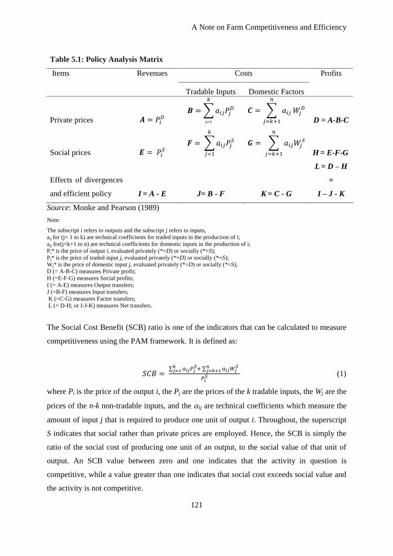
A Note on Farm Competitiveness and Efficiency
121
Table 5.1: Policy Analysis Matrix
Items Revenues Costs Profits
Tradable Inputs Domestic Factors
Private prices 𝑨 = 𝑃𝑖𝐷
𝑩 = ∑ 𝑎𝑖𝑗𝑃𝑗𝐷
𝑘
j=1
𝑪 = ∑ 𝑎𝑖𝑗
𝑛
𝑗=𝑘+1
𝑊𝑗𝐷
D = A-B-C
Social prices 𝑬 = 𝑃𝑖𝑆
𝑭 = ∑ 𝑎𝑖𝑗𝑃𝑗𝑆
𝑘
𝑗=1
𝑮 = ∑ 𝑎𝑖𝑗𝑊𝑗𝑆
𝑛
𝑗=𝑘+1
H = E-F-G
Effects of divergences
and efficient policy I = A - E J= B - F K = C - G
L = D – H
=
I – J - K
Source: Monke and Pearson (1989)
Note:
The subscript i refers to outputs and the subscript j refers to inputs,
aij for (j= 1 to k) are technical coefficients for traded inputs in the production of i;
aij for(j=k+1 to n) are technical coefficients for domestic inputs in the production of i;
Pi* is the price of output i, evaluated privately (*=D) or socially (*=S);
Pj* is the price of traded input j, evaluated privately (*=D) or socially (*=S);
Wj* is the price of domestic input j, evaluated privately (*=D) or socially (*=S);
D (= A-B-C) measures Private profit;
H (=E-F-G) measures Social profits;
I (= A-E) measures Output transfers;
J (=B-F) measures Input transfers;
K (=C-G) measures Factor transfers;
L (= D-H; or I-J-K) measures Net transfers.
The Social Cost Benefit (SCB) ratio is one of the indicators that can be calculated to measure
competitiveness using the PAM framework. It is defined as:
𝑆𝐶𝐵 = ∑ 𝑎𝑖𝑗𝑃𝑗
𝑆+ ∑ 𝑎𝑖𝑗𝑊𝑗𝑆𝑛
𝑗=𝑘+1 𝑘𝑗=1
𝑃𝑖𝑆 (1)
where Pi is the price of the output i, the Pj are the prices of the k tradable inputs, the Wj are the
prices of the n-k non-tradable inputs, and the ij are technical coefficients which measure the
amount of input j that is required to produce one unit of output i. Throughout, the superscript
S indicates that social rather than private prices are employed. Hence, the SCB is simply the
ratio of the social cost of producing one unit of an output, to the social value of that unit of
output. An SCB value between zero and one indicates that the activity in question is
competitive, while a value greater than one indicates that social cost exceeds social value and
the activity is not competitive.
A Note on Farm Competitiveness and Efficiency
122
Another indicator which is closely related to SCB is the private cost benefit (PCB). It is
defined as:
𝑃𝐶𝐵 =∑ 𝑎𝑖𝑗
𝑛𝑗=𝑘+1 𝑊𝑗
𝐷
𝑃𝑖𝐷−∑ 𝑎𝑖𝑗𝑃𝑗
𝐷𝑘j=1
(2)
where Pi is the price of the output i, the Pj are the prices of the k tradable inputs, the Wj are the
prices of the n-k non-tradable inputs, and the ij are technical coefficients which measure the
amount of input j that is required to produce one unit of output i. Here, the superscript D
indicates private prices are employed throughout the system, reflecting the actual market or
financial prices. Hence, PCB is the ratio of private costs of domestic factor use to the private
value added. Similar to SCB, PCB is an indicator of comparative competitiveness. It shows
how much the production system affords to pay for the domestic factors and still remain
competitive (break even after earning normal profits which is defined as (A-B-C) = D = 0. In
this case, excess profits are attainable if the private costs are less than their value added in
private prices. This can be achieved by holding down factor and tradable inputs costs so that it
can minimize the private cost and hence maximize excess profit. Therefore, a PCB value
between zero and one indicates that the commodity is competitive while a value greater than
one indicates that the commodity in question is uncompetitive.
5.4 Stochastic Frontier Analysis (SFA) approach
5.4.1 Fixed effect panel model using CFE estimation
Since the seminal work conducted by Aigner et al. (1977), the Stochastic Frontier (SF) model
has been widely use to estimate the technical efficiency in applied economic research.
Extensive research in this field has resulted in a growing arsenal of methods and econometrics
techniques pertaining to specifications, estimation and testing issue. Despite that, when
productivity and efficiency are analyzed at the farm level, the problem arises that not all
relevant factor can be observed or measured adequately. Heterogeneous environmental and
biophysical characteristics, such as soil condition, rainfall or droughts, as well as managerial
characteristics, are often omitted from the model specifications due to a lack of information
available for many of these variables. This information is referred to as unobserved
heterogeneity (Álvarez et al, 2009). As a result, inference based on the output comparison
could be biased and is often criticized because farms are heterogeneous and operate under
different production and environmental conditions (Abdulai and Tietje, 2007). To overcome
A Note on Farm Competitiveness and Efficiency
123
the challenge of unobserved heterogeneity, we apply the recent fixed effect model
implemented by Chen et al. (2014). Consider the following specification of the stochastic
production frontier model for panel data:
𝑦𝑖𝑡 = 𝛼𝑖 + 𝛽′𝑥𝑖𝑡 + 𝑣𝑖𝑡 − 𝑢𝑖𝑡 (3)
𝜀𝑖𝑡 = 𝑣𝑖𝑡 − 𝑢𝑖𝑡 (4)
where 𝑦𝑖𝑡 is the vector of the output of firm i (i=1,...,N) in period t (t=1,...,T); xit is a set of
inputs that produce output 𝑦𝑖𝑡; β is the associated vector that describes technology parameters
to be estimated. The composite error term 𝜀𝑖𝑡 is the difference between the idiosyncratic error
that captures noise 𝑣𝑖𝑡, and the one-sided disturbance 𝑢𝑖𝑡 which represents inefficiency. Under
the frequently used normal-half normal model, the distributional assumptions are
𝑣𝑖𝑡 ~ 𝑁(0, 𝜎𝑣2) and 𝑢𝑖𝑡 ~ 𝑁+(0, 𝜎𝑢
2). Time-invariant unobserved heterogeneity is captured by
the vector of incidental parameter, 𝛼𝑖 which is the number of individual intercepts that equal
to the number of farms. However, whether or not to separate 𝛼𝑖 from 𝑢𝑖𝑡 has been the subject
of much debate in the stochastic frontier literature. A major limitation of the model in
equation (4) is related to an identification problem which arises when the inefficiency term is
time-variant. In many situations, a constant level of inefficiency does not likely to prevail
over longer period due to several reasons (i.e. process of learning). In this case, it is difficult
to disentangle the unobserved farm-specific heterogeneity from inefficiency (Greene 2005).
Greene (2005) proposed a “true fixed effects” or TFE model that includes a maximum
likelihood dummy variables estimator (MLDVE), in which the unit-specific intercepts are
estimated with structural parameters. The TFE model places unobserved heterogeneity as
fixed effects in the stochastic frontier model (equation 3) and generates a neutral shift of the
function specific to each farm (Porcelli 2009) while allowing for time-varying inefficiency
(Belotti and Giuseppe 2012). This approach is frequently applied, however it leads to
inconsistent variance parameter estimates due to the incidental parameters problem especially
in the short panel because the number of parameters depends on the sample size (there are
firm effects 𝛼𝑖; and the number of parameters, N which increases with the sample size).
Hence, the estimated error variance, and the parameter 𝜎𝑢2 is inconsistent.
A Note on Farm Competitiveness and Efficiency
124
To account for this limitation, Chen et al. (2014) propose a consistent estimator for the TFE
normal-half normal model based on the within transformed model where the fixed effects
have been removed. This procedure is commonly used in the panel data:
𝑧�̅�𝑡 = 𝑧𝑖𝑡 − 𝑧�̅� (5)
For any corresponding variable (𝑧) in each panel i, the individual mean (𝑧�̅�) is subtracted from
the observed value in period t (𝑧𝑖𝑡). Correspondingly, the model can be represented by using
the deviations from means (𝑧�̅�) so that the transformed model is free from incidental
parameters problem (αi):
�̅�𝑖𝑡 = 𝛽′�̅�𝑖𝑡 + �̅�𝑖𝑡 − �̅�𝑖𝑡 (6)
As outlined by (Holtkamp, 2015) the model in equation (6) has the following features: first,
the incidental parameters problem is removed by a within-transformation; second, it produces
a consistent estimator of the error variance since the relevant likelihood function is derived
from T-1 deviations; and third, this approach, which is based on a more general distributional
theory, allows for the maintenance of the firm-specific and time varying inefficiency 𝑢𝑖𝑡.
5.4.2 A primal system of Profit Maximization
The standard microeconomic theory of producer behavior is almost entirely based on the
neoclassical approach which assumes that firms are efficient both technically and allocatively.
There is, however, an extensive literature on the measurement of productive efficiency which
extended the basic neoclassical approach by allowing firms to make mistakes in the
production of outputs and use of inputs (Kumbhakar, 1987).
Allocative inefficiency as defined by Schmidt and Lovell (1979) is a failure to allocate right
proportions of inputs given the input prices. Under the production process that has allocative
inefficiency, the marginal revenue product is not equal to the marginal resource cost.
Technical inefficiency occurs when producers fail to maximize the output for a given set of
inputs. Under the behavioral assumption of profit maximization, we assume that farms
maximize their profits in making their decision on inputs use and production of outputs. That
A Note on Farm Competitiveness and Efficiency
125
is, we can consider non-optimal allocation of inputs and output where farms can be both
allocatively inefficient and technically inefficient.
However, estimation that accounts both technical and allocative inefficiency with the profit
function approach is not straightforward and complex. In most of the cases, the estimation
requires large variations in the price variables in order to get precise parameter estimates,
which may not usually occur in practice especially when we work with a cross-section in
which most farms have probably faced quite similar prices. Details on the model and
estimation issues are discussed comprehensively in Kumbhakar (2001) and Kumbhakar and
Wang (2006). Alternatively, Kumbhakar et.al, (2015) proposed other modeling strategy which
is the primal system approach by using transcendental logarithmic functional form of the
stochastic frontier. The authors argue that if the input endogeneity is considered during the
implementation of the econometric problem, then the output-oriented or input-oriented
technical inefficiencies are the same. The primal system technique is algebraically equivalent
to the profit system for self-dual production function. The advantage of the primal system is
that it solves the problem of insufficient price variability. Furthermore, the model is based on
the production function, therefore there is no need to take log of profit, which could be an
issue when profit is negative for some observations.
The production function (Aigner et.al, 1977) for a typical producer (i) can be written as;
yi = f(xi) exp(v - u), i= 1,2,....n (7)
where f(.) is the production frontier; x is the vector of inputs, v is production uncertainty or
noise and u is technical inefficiency. The profit maximization problem for a producer
(omitting the subscript i) can be represented as:
max𝑦,𝑥 𝛱 = py – wx s.t y = f(x) exp(v - u), u ≥ 0 (8)
⇒ max 𝑥
𝛱 = 𝑝𝑓(𝑥) exp(𝑣 − 𝑢) − 𝑤𝑥 (9)
⇒ max𝑥 𝛱 = 𝑝𝑓 ∗ (𝑥) − 𝑤𝑥 (10)
where p is a vector of output prices; y is the level of production; w is the vector of input
prices; x is the vector of inputs; v is the random error and u is the output-oriented technical
A Note on Farm Competitiveness and Efficiency
126
inefficiency. Note that we substitute y.exp(v-u) by f* to follow the standard neoclassical
maximization problem analytics.
The first-order conditions of a profit-maximization problem can be implicitly formulated as:
𝑝𝑓𝑗∗ = 𝑤𝑗
exp (𝜂1), 𝜂𝑗 ⋛ 0 , 𝑗 = 1, … . . 𝐽 (11)
The first-order condition indicates that the value of the marginal product of input i can be
expanded until it equals price of the input or marginal cost. It can therefore be expressed as:
𝑓𝑗
∗
𝑓1∗ =
𝑤𝑗
𝑤1exp(𝜉𝑗) , 𝑗 = 2, 3, … . . 𝐽, (12)
𝑝𝑓𝑗∗ = 𝑤1 exp(𝜂1), (13)
𝑤ℎ𝑒𝑟𝑒, 𝜉 = 𝜂𝑗 − 𝜂1 (14)
where fj and f1 are the marginal products of input j and input 1, respectively; wj and w1 are
prices of input j and input 1, respectively; and 𝜉 is allocative inefficiency for the input pair (j,
1). The use of allocative inefficiency in equation 12 which is defined by Schmidt and Lovell,
(1979) is appropriate, because a producer is said to be allocatively inefficient if he fails to
allocate input in a way that the ratio of input prices equates the marginal rate of substitution
(MRTS).
Using the result 𝑠𝑗 ≡ 𝜕 𝑙𝑛𝑓∗
𝜕 ln 𝑥𝑗= (
𝜕𝑓∗
𝜕𝑥𝑗)(
𝑥𝑗
𝑓∗), where 𝑠𝑗 are cost shares of the input 𝑥𝑗 given the
input price 𝑤𝑗, we obtain the following equations:
𝑠𝑗
𝑠1=
𝑤𝑗
𝑤1
𝑥𝑗
𝑥1exp( 𝜉𝑗), 𝑗 = 2,3, … … . . 𝐽, (15)
𝑝𝑠1𝑦
𝑥1= 𝑤1exp (𝜂1) (16)
Finally the primal system to be estimated can be obtained by taking logarithms of equations
(15) and (16):
𝑙𝑛 𝑠𝑗 − 𝑙𝑛𝑠1 = ln (𝑤𝑗
𝑤1) + ln (
𝑥𝑗
𝑥1) + 𝜉𝑗, 𝑗 = 2, … … … 𝐽 (17)
ln 𝑝 + 𝑙𝑛𝑠1 + ln 𝑦 − 𝑙𝑛𝑥1 − ln 𝑤1 = 𝜂1 (18)
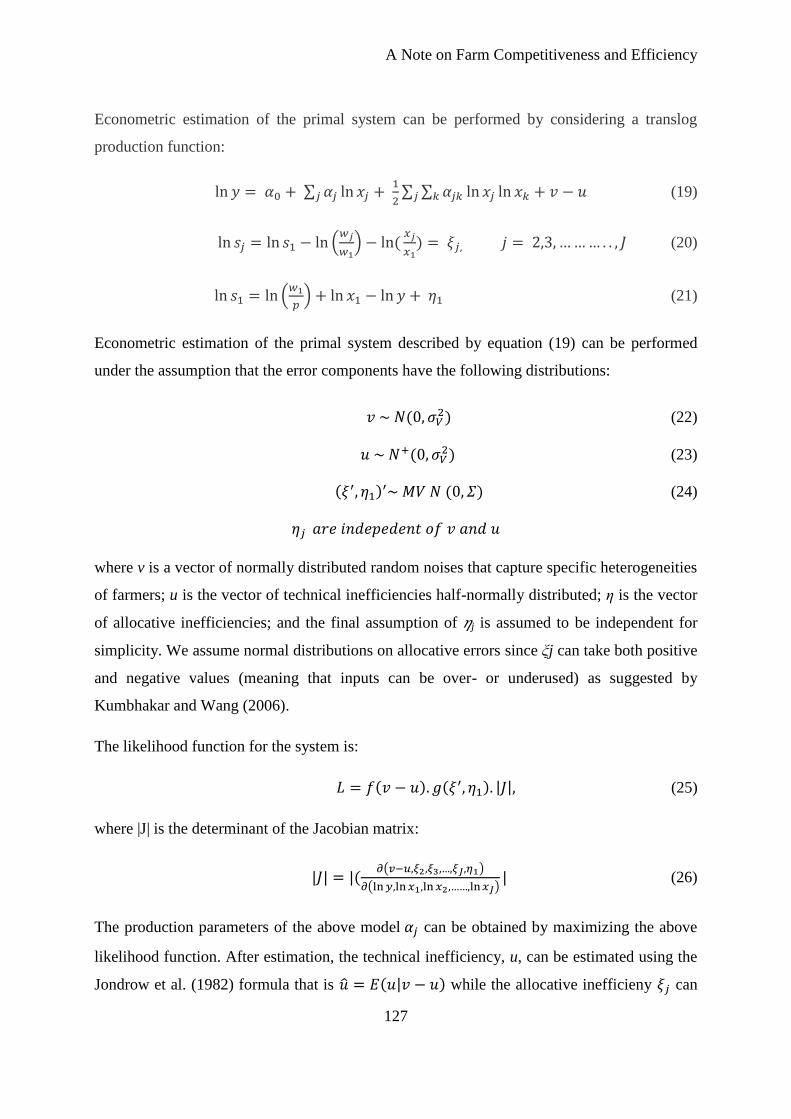
A Note on Farm Competitiveness and Efficiency
127
Econometric estimation of the primal system can be performed by considering a translog
production function:
ln 𝑦 = 𝛼0 + ∑ 𝛼𝑗 ln 𝑥𝑗𝑗 + 1
2∑ ∑ 𝛼𝑗𝑘 ln 𝑥𝑗𝑘𝑗 ln 𝑥𝑘 + 𝑣 − 𝑢 (19)
ln 𝑠𝑗 = ln 𝑠1 − ln (𝑤𝑗
𝑤1) − ln (
𝑥𝑗
𝑥1) = 𝜉𝑗, 𝑗 = 2,3, … … … . . , 𝐽 (20)
ln 𝑠1 = ln (𝑤1
𝑝) + ln 𝑥1 − ln 𝑦 + 𝜂1 (21)
Econometric estimation of the primal system described by equation (19) can be performed
under the assumption that the error components have the following distributions:
𝑣 ~ 𝑁(0, 𝜎𝑉2) (22)
𝑢 ~ 𝑁+(0, 𝜎𝑉2) (23)
(𝜉′, 𝜂1)′~ 𝑀𝑉 𝑁 (0, 𝛴) (24)
𝜂𝑗 𝑎𝑟𝑒 𝑖𝑛𝑑𝑒𝑝𝑒𝑑𝑒𝑛𝑡 𝑜𝑓 𝑣 𝑎𝑛𝑑 𝑢
where v is a vector of normally distributed random noises that capture specific heterogeneities
of farmers; u is the vector of technical inefficiencies half-normally distributed; η is the vector
of allocative inefficiencies; and the final assumption of 𝜂j is assumed to be independent for
simplicity. We assume normal distributions on allocative errors since ξj can take both positive
and negative values (meaning that inputs can be over- or underused) as suggested by
Kumbhakar and Wang (2006).
The likelihood function for the system is:
𝐿 = 𝑓(𝑣 − 𝑢). 𝑔(𝜉′, 𝜂1). |𝐽|, (25)
where |J| is the determinant of the Jacobian matrix:
|𝐽| = |(𝜕(𝑣−𝑢,𝜉2,𝜉3,…,𝜉𝐽,𝜂1)
𝜕(ln 𝑦,ln 𝑥1,ln 𝑥2,……,ln 𝑥𝐽)| (26)
The production parameters of the above model 𝛼𝑗 can be obtained by maximizing the above
likelihood function. After estimation, the technical inefficiency, u, can be estimated using the
Jondrow et al. (1982) formula that is �̂� = 𝐸(𝑢|𝑣 − 𝑢) while the allocative inefficieny 𝜉𝑗 can
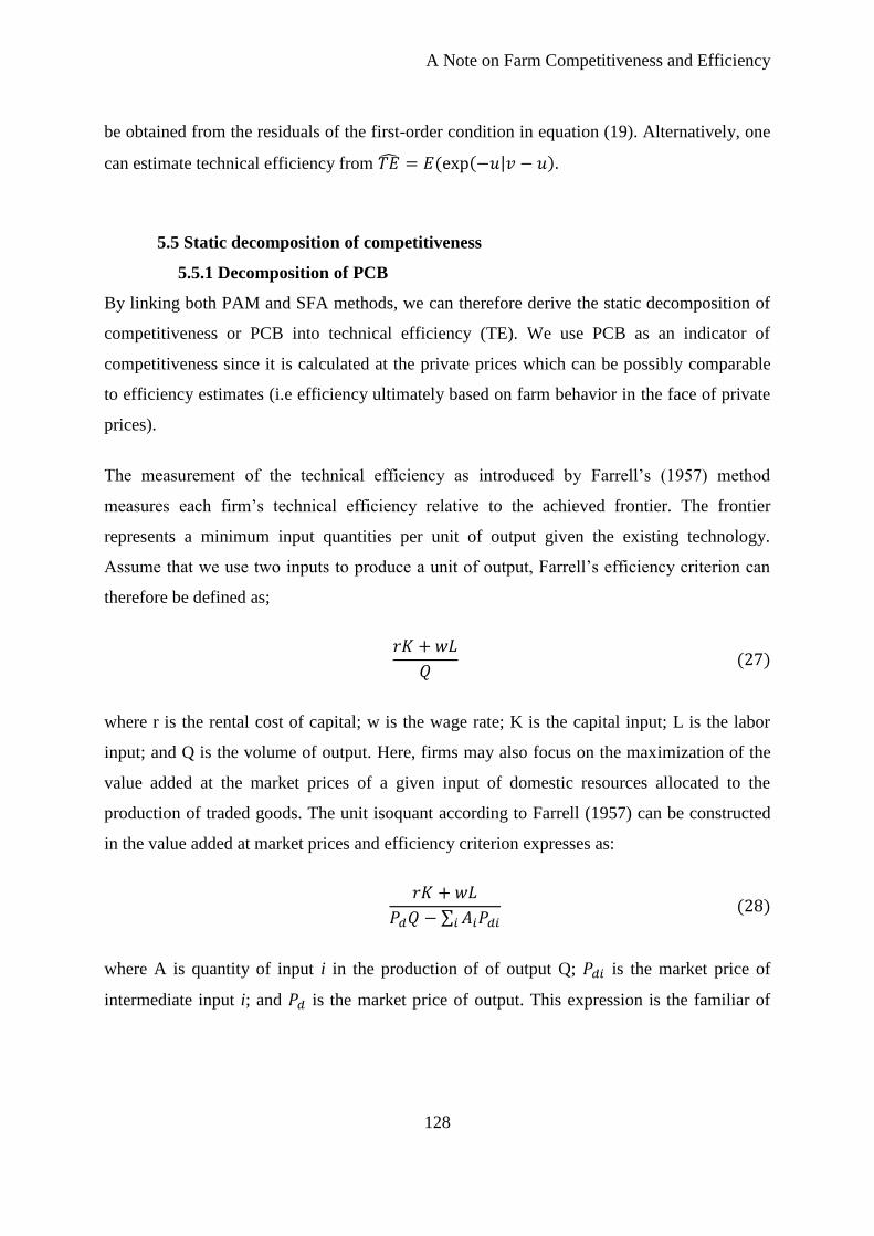
A Note on Farm Competitiveness and Efficiency
128
be obtained from the residuals of the first-order condition in equation (19). Alternatively, one
can estimate technical efficiency from 𝑇�̂� = 𝐸(exp(−𝑢|𝑣 − 𝑢).
5.5 Static decomposition of competitiveness
5.5.1 Decomposition of PCB
By linking both PAM and SFA methods, we can therefore derive the static decomposition of
competitiveness or PCB into technical efficiency (TE). We use PCB as an indicator of
competitiveness since it is calculated at the private prices which can be possibly comparable
to efficiency estimates (i.e efficiency ultimately based on farm behavior in the face of private
prices).
The measurement of the technical efficiency as introduced by Farrell’s (1957) method
measures each firm’s technical efficiency relative to the achieved frontier. The frontier
represents a minimum input quantities per unit of output given the existing technology.
Assume that we use two inputs to produce a unit of output, Farrell’s efficiency criterion can
therefore be defined as;
𝑟𝐾 + 𝑤𝐿
𝑄 (27)
where r is the rental cost of capital; w is the wage rate; K is the capital input; L is the labor
input; and Q is the volume of output. Here, firms may also focus on the maximization of the
value added at the market prices of a given input of domestic resources allocated to the
production of traded goods. The unit isoquant according to Farrell (1957) can be constructed
in the value added at market prices and efficiency criterion expresses as:
𝑟𝐾 + 𝑤𝐿
𝑃𝑑𝑄 − ∑ 𝐴𝑖𝑃𝑑𝑖𝑖 (28)
where A is quantity of input i in the production of of output Q; 𝑃𝑑𝑖 is the market price of
intermediate input i; and 𝑃𝑑 is the market price of output. This expression is the familiar of
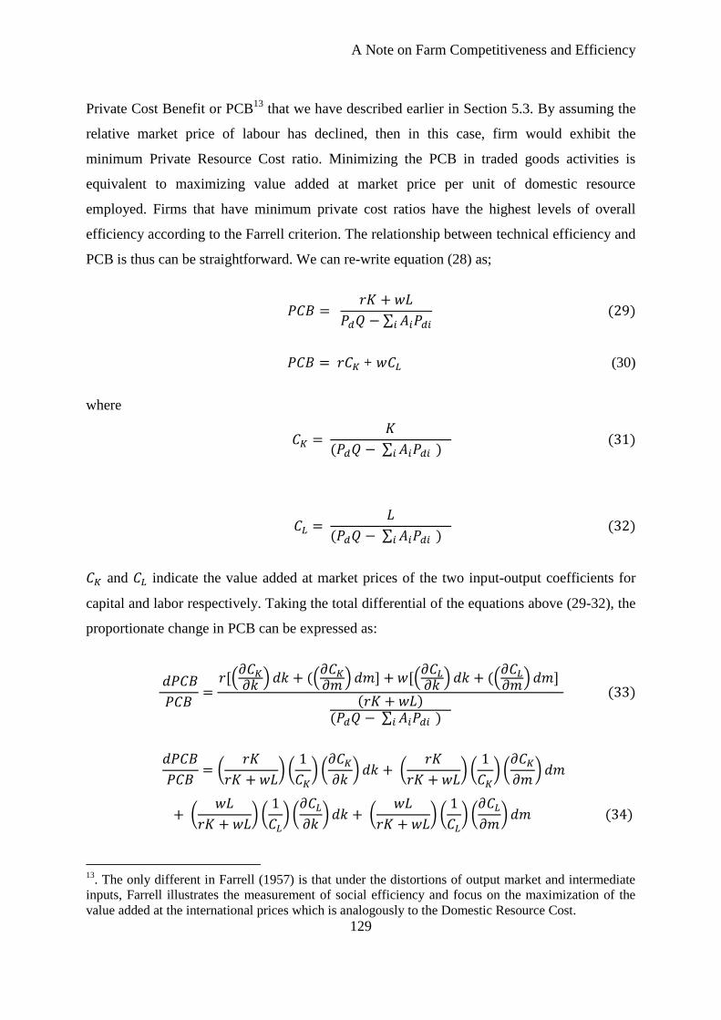
A Note on Farm Competitiveness and Efficiency
129
Private Cost Benefit or PCB13
that we have described earlier in Section 5.3. By assuming the
relative market price of labour has declined, then in this case, firm would exhibit the
minimum Private Resource Cost ratio. Minimizing the PCB in traded goods activities is
equivalent to maximizing value added at market price per unit of domestic resource
employed. Firms that have minimum private cost ratios have the highest levels of overall
efficiency according to the Farrell criterion. The relationship between technical efficiency and
PCB is thus can be straightforward. We can re-write equation (28) as;
𝑃𝐶𝐵 = 𝑟𝐾 + 𝑤𝐿
𝑃𝑑𝑄 − ∑ 𝐴𝑖𝑃𝑑𝑖𝑖 (29)
𝑃𝐶𝐵 = 𝑟𝐶𝐾 + 𝑤𝐶𝐿 (30)
where
𝐶𝐾 = 𝐾
(𝑃𝑑𝑄 − ∑ 𝐴𝑖𝑃𝑑𝑖 ) 𝑖 (31)
𝐶𝐿 = 𝐿
(𝑃𝑑𝑄 − ∑ 𝐴𝑖𝑃𝑑𝑖 ) 𝑖 (32)
𝐶𝐾 and 𝐶𝐿 indicate the value added at market prices of the two input-output coefficients for
capital and labor respectively. Taking the total differential of the equations above (29-32), the
proportionate change in PCB can be expressed as:
𝑑𝑃𝐶𝐵
𝑃𝐶𝐵=
𝑟[(𝜕𝐶𝐾
𝜕𝑘) 𝑑𝑘 + ((
𝜕𝐶𝐾
𝜕𝑚) 𝑑𝑚] + 𝑤[(
𝜕𝐶𝐿
𝜕𝑘) 𝑑𝑘 + ((
𝜕𝐶𝐿
𝜕𝑚) 𝑑𝑚]
(𝑟𝐾 + 𝑤𝐿)(𝑃𝑑𝑄 − ∑ 𝐴𝑖𝑃𝑑𝑖 ) 𝑖
(33)
𝑑𝑃𝐶𝐵
𝑃𝐶𝐵= (
𝑟𝐾
𝑟𝐾 + 𝑤𝐿) (
1
𝐶𝐾) (
𝜕𝐶𝐾
𝜕𝑘) 𝑑𝑘 + (
𝑟𝐾
𝑟𝐾 + 𝑤𝐿) (
1
𝐶𝐾) (
𝜕𝐶𝐾
𝜕𝑚) 𝑑𝑚
+ (𝑤𝐿
𝑟𝐾 + 𝑤𝐿) (
1
𝐶𝐿) (
𝜕𝐶𝐿
𝜕𝑘) 𝑑𝑘 + (
𝑤𝐿
𝑟𝐾 + 𝑤𝐿) (
1
𝐶𝐿) (
𝜕𝐶𝐿
𝜕𝑚) 𝑑𝑚 (34)
13
. The only different in Farrell (1957) is that under the distortions of output market and intermediate
inputs, Farrell illustrates the measurement of social efficiency and focus on the maximization of the
value added at the international prices which is analogously to the Domestic Resource Cost.
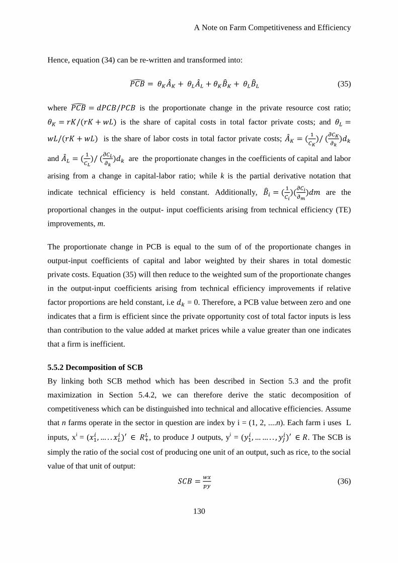
A Note on Farm Competitiveness and Efficiency
130
Hence, equation (34) can be re-written and transformed into:
𝑃𝐶�̂� = 𝜃𝐾�̂�𝐾 + 𝜃𝐿�̂�𝐿 + 𝜃𝐾�̂�𝐾 + 𝜃𝐿�̂�𝐿 (35)
where 𝑃𝐶�̂� = 𝑑𝑃𝐶𝐵/𝑃𝐶𝐵 is the proportionate change in the private resource cost ratio;
𝜃𝐾 = 𝑟𝐾/(𝑟𝐾 + 𝑤𝐿) is the share of capital costs in total factor private costs; and 𝜃𝐿 =
𝑤𝐿/(𝑟𝐾 + 𝑤𝐿) is the share of labor costs in total factor private costs; �̂�𝐾 = (1
𝐶𝐾)/ (
𝜕𝐶𝐾
𝜕𝑘)𝑑𝑘
and �̂�𝐿 = (1
𝐶𝐿)/ (
𝜕𝐶𝐿
𝜕𝑘)𝑑𝑘 are the proportionate changes in the coefficients of capital and labor
arising from a change in capital-labor ratio; while k is the partial derivative notation that
indicate technical efficiency is held constant. Additionally, �̂�𝑖 = (1
𝐶𝑖)(
𝜕𝐶𝑖
𝜕𝑚)𝑑𝑚 are the
proportional changes in the output- input coefficients arising from technical efficiency (TE)
improvements, m.
The proportionate change in PCB is equal to the sum of of the proportionate changes in
output-input coefficients of capital and labor weighted by their shares in total domestic
private costs. Equation (35) will then reduce to the weighted sum of the proportionate changes
in the output-input coefficients arising from technical efficiency improvements if relative
factor proportions are held constant, i.e 𝑑𝑘 = 0. Therefore, a PCB value between zero and one
indicates that a firm is efficient since the private opportunity cost of total factor inputs is less
than contribution to the value added at market prices while a value greater than one indicates
that a firm is inefficient.
5.5.2 Decomposition of SCB
By linking both SCB method which has been described in Section 5.3 and the profit
maximization in Section 5.4.2, we can therefore derive the static decomposition of
competitiveness which can be distinguished into technical and allocative efficiencies. Assume
that n farms operate in the sector in question are index by i = (1, 2, ....n). Each farm i uses L
inputs, xi = (𝑥1
𝑖 , … . . 𝑥𝐿𝑖 )′ ∈ 𝑅+
𝐿 , to produce J outputs, yi = (𝑦1
𝑖 , … … . . , 𝑦𝐽𝑖)′ ∈ 𝑅. The SCB is
simply the ratio of the social cost of producing one unit of an output, such as rice, to the social
value of that unit of output:
𝑆𝐶𝐵 =𝑤𝑥
𝑝𝑦 (36)
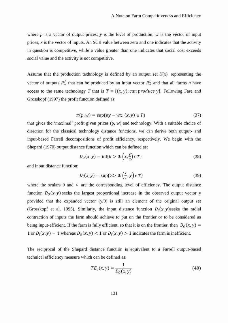
A Note on Farm Competitiveness and Efficiency
131
where p is a vector of output prices; y is the level of production; w is the vector of input
prices; x is the vector of inputs. An SCB value between zero and one indicates that the activity
in question is competitive, while a value greater than one indicates that social cost exceeds
social value and the activity is not competitive.
Assume that the production technology is defined by an output set Y(x), representing the
vector of outputs 𝑅+𝐽 that can be produced by an input vector 𝑅+
𝐿 and that all farms n have
access to the same technology T that is 𝑇 ≡ {(𝑥, 𝑦): 𝑐𝑎𝑛 𝑝𝑟𝑜𝑑𝑢𝑐𝑒 𝑦}. Following Fare and
Grosskopf (1997) the profit function defined as:
𝜋(𝑝, 𝑤) = sup {𝑝𝑦 − 𝑤𝑥: (𝑥, 𝑦) ∈ 𝑇} (37)
that gives the ‘maximal’ profit given prices (p, w) and technology. With a suitable choice of
direction for the classical technology distance functions, we can derive both output- and
input-based Farrell decompositions of profit efficiency, respectively. We begin with the
Shepard (1970) output distance function which can be defined as:
𝐷𝑂(𝑥, 𝑦) = inf {𝜃 > 0: (𝑥,𝑦
𝜃) 𝜖 𝑇} (38)
and input distance function:
𝐷𝑖(𝑥, 𝑦) = sup {⋋> 0: (𝑥
⋋, 𝑦) 𝜖 𝑇} (39)
where the scalars θ and ⋋ are the corresponding level of efficiency. The output distance
function 𝐷𝑂(𝑥, 𝑦) seeks the largest proportional increase in the observed output vector y
provided that the expanded vector (y/θ) is still an element of the original output set
(Grosskopf et al. 1995). Similarly, the input distance function 𝐷𝑖(𝑥, 𝑦)seeks the radial
contraction of inputs the farm should achieve to put on the frontier or to be considered as
being input-efficient. If the farm is fully efficient, so that it is on the frontier, then 𝐷𝑂(𝑥, 𝑦) =
1 or 𝐷𝑖(𝑥, 𝑦) = 1 whereas 𝐷𝑂(𝑥, 𝑦) < 1 or 𝐷𝑖(𝑥, 𝑦) > 1 indicates the farm is inefficient.
The reciprocal of the Shepard distance function is equivalent to a Farrell output-based
technical efficiency measure which can be defined as:
𝑇𝐸𝑜(𝑥, 𝑦) =1
𝐷𝑂(𝑥, 𝑦) (40)
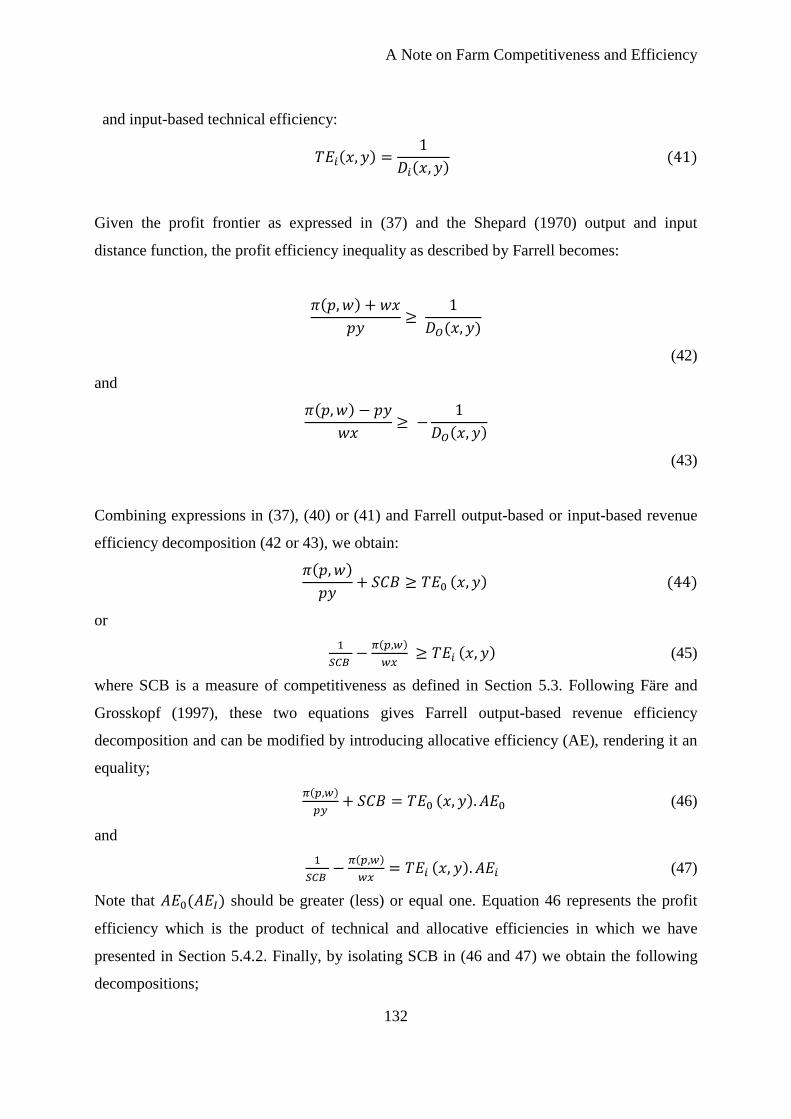
A Note on Farm Competitiveness and Efficiency
132
and input-based technical efficiency:
𝑇𝐸𝑖(𝑥, 𝑦) =1
𝐷𝑖(𝑥, 𝑦) (41)
Given the profit frontier as expressed in (37) and the Shepard (1970) output and input
distance function, the profit efficiency inequality as described by Farrell becomes:
𝜋(𝑝, 𝑤) + 𝑤𝑥
𝑝𝑦≥
1
𝐷𝑂(𝑥, 𝑦)
(42)
and
𝜋(𝑝, 𝑤) − 𝑝𝑦
𝑤𝑥≥ −
1
𝐷𝑂(𝑥, 𝑦)
(43)
Combining expressions in (37), (40) or (41) and Farrell output-based or input-based revenue
efficiency decomposition (42 or 43), we obtain:
𝜋(𝑝, 𝑤)
𝑝𝑦+ 𝑆𝐶𝐵 ≥ 𝑇𝐸0 (𝑥, 𝑦) (44)
or
1
𝑆𝐶𝐵 −
𝜋(𝑝,𝑤)
𝑤𝑥 ≥ 𝑇𝐸𝑖 (𝑥, 𝑦) (45)
where SCB is a measure of competitiveness as defined in Section 5.3. Following Färe and
Grosskopf (1997), these two equations gives Farrell output-based revenue efficiency
decomposition and can be modified by introducing allocative efficiency (AE), rendering it an
equality;
𝜋(𝑝,𝑤)
𝑝𝑦+ 𝑆𝐶𝐵 = 𝑇𝐸0 (𝑥, 𝑦). 𝐴𝐸0 (46)
and
1
𝑆𝐶𝐵 −
𝜋(𝑝,𝑤)
𝑤𝑥= 𝑇𝐸𝑖 (𝑥, 𝑦). 𝐴𝐸𝑖 (47)
Note that 𝐴𝐸0(𝐴𝐸𝐼) should be greater (less) or equal one. Equation 46 represents the profit
efficiency which is the product of technical and allocative efficiencies in which we have
presented in Section 5.4.2. Finally, by isolating SCB in (46 and 47) we obtain the following
decompositions;
A Note on Farm Competitiveness and Efficiency
133
𝑆𝐶𝐵 = 𝑇𝐸0 (𝑥, 𝑦). 𝐴𝐸0 −𝜋(𝑝,𝑤)
𝑝𝑦 (48)
and
1
𝑆𝐶𝐵= 𝑇𝐸𝑖 (𝑥, 𝑦). 𝐴𝐸𝑖 +
𝜋(𝑝,𝑤)
𝑤𝑥 (49)
5.6 Empirical Illustration
This section applies our competitive analysis-based methodology and technical efficiency
with both CFE and primal profit maximization estimates. The data was collected between
2010 and 2014 from Malaysian rice farms, which consist of a representative farm panel of
6570 rice farms in Malaysia’s largest granary area14
.
Our decomposition provides some insights into the origins of the Malaysian rice industry’s
comparative advantage and efficiency. Figure 5.1 shows the average mean values of the PCB
and SCB distributions that were collected during the given period.
Figure 5.1: Distribution of rice farms’ competitiveness scores (PCB and SCB)
14
Granary areas are the irrigated areas which refer to major irrigation schemes (areas greater than
4,000 hectares) and recognized by the Government in the National Agricultural Policy as the main
paddy producing areas (Department of Agriculture, 2014).
A Note on Farm Competitiveness and Efficiency
134
During the expressed time period, the average PCB value was 0.94, indicating that rice
production was competitive during the period. This implies that, on average, many more
competitive farms disproportionately produced more rice outputs at private prices. However,
at social prices, the average SCB value was 1.05, implying that rice production was slightly
uncompetitive during the studied period.
Additionally, the technical efficiency distribution generated by the CFE model shows that
roughly 53% of the rice farms made improvements to their technical efficiency while more
efficient farms disproportionately produced more outputs.
Figure 5.2: Distribution rice farms’ technical efficiency, 2010-2014
By linking the PCB method, as demonstrated in Section 5.3, and technical efficiency using
the SFA method, shown in Section 5.4, and by interpreting the information derived from this
decomposition, it is possible to comprehend both relationships to explore the extent to which
variation in the level of technical efficiency affects the performance of a farm’s
competitiveness, i.e. PCB.
We used Spearman’s correlation to assess the relationship between PCB and TE. There is a
negative correlation between these two variables, which is statistically significant, [rs = -
0.5969], (p = 0.000).
The decomposition subplot portrayed in Figure 5.3 displays a scatter plot of PCB versus
technical efficiency (TE). It demonstrates that competitive/comparative advantage (PCB<1)
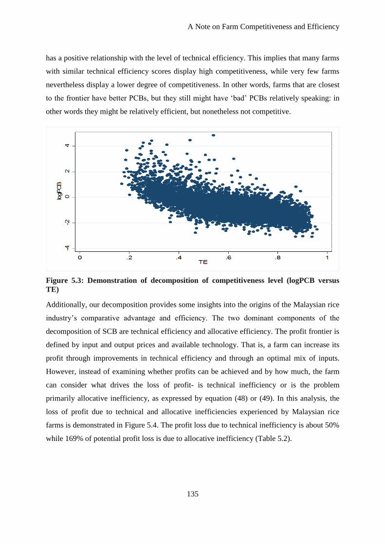
A Note on Farm Competitiveness and Efficiency
135
has a positive relationship with the level of technical efficiency. This implies that many farms
with similar technical efficiency scores display high competitiveness, while very few farms
nevertheless display a lower degree of competitiveness. In other words, farms that are closest
to the frontier have better PCBs, but they still might have ‘bad’ PCBs relatively speaking: in
other words they might be relatively efficient, but nonetheless not competitive.
Figure 5.3: Demonstration of decomposition of competitiveness level (logPCB versus
TE)
Additionally, our decomposition provides some insights into the origins of the Malaysian rice
industry’s comparative advantage and efficiency. The two dominant components of the
decomposition of SCB are technical efficiency and allocative efficiency. The profit frontier is
defined by input and output prices and available technology. That is, a farm can increase its
profit through improvements in technical efficiency and through an optimal mix of inputs.
However, instead of examining whether profits can be achieved and by how much, the farm
can consider what drives the loss of profit- is technical inefficiency or is the problem
primarily allocative inefficiency, as expressed by equation (48) or (49). In this analysis, the
loss of profit due to technical and allocative inefficiencies experienced by Malaysian rice
farms is demonstrated in Figure 5.4. The profit loss due to technical inefficiency is about 50%
while 169% of potential profit loss is due to allocative inefficiency (Table 5.2).
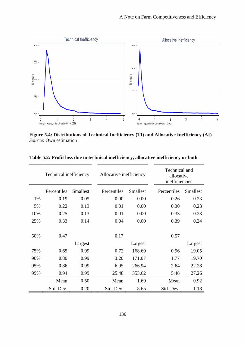
A Note on Farm Competitiveness and Efficiency
136
Figure 5.4: Distributions of Technical Inefficiency (TI) and Allocative Inefficiency (AI)
Source: Own estimation
Table 5.2: Profit loss due to technical inefficiency, allocative inefficiency or both
Technical inefficiency Allocative inefficiency
Technical and
allocative
inefficiencies
Percentiles Smallest Percentiles Smallest Percentiles Smallest
1% 0.19 0.05 0.00 0.00 0.26 0.23
5% 0.22 0.13 0.01 0.00 0.30 0.23
10% 0.25 0.13 0.01 0.00 0.33 0.23
25% 0.33 0.14 0.04 0.00 0.39 0.24
50% 0.47 0.17 0.57
Largest Largest Largest
75% 0.65 0.99 0.72 168.69 0.96 19.05
90% 0.80 0.99 3.20 171.07 1.77 19.70
95% 0.86 0.99 6.95 266.94 2.64 22.28
99% 0.94 0.99 25.48 353.62 5.48 27.26
Mean 0.50 Mean 1.69 Mean 0.92
Std. Dev. 0.20 Std. Dev. 8.65 Std. Dev. 1.18
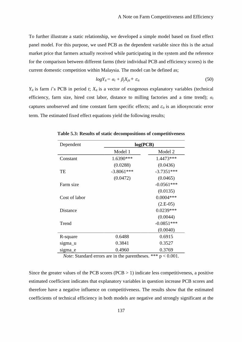
A Note on Farm Competitiveness and Efficiency
137
To further illustrate a static relationship, we developed a simple model based on fixed effect
panel model. For this purpose, we used PCB as the dependent variable since this is the actual
market price that farmers actually received while participating in the system and the reference
for the comparison between different farms (their individual PCB and efficiency scores) is the
current domestic competition within Malaysia. The model can be defined as;
logYit = αi + βjXjit+ εit (50)
Yit is farm i’s PCB in period t; Xit is a vector of exogenous explanatory variables (technical
efficiency, farm size, hired cost labor, distance to milling factories and a time trend); αi
captures unobserved and time constant farm specific effects; and εit is an idiosyncratic error
term. The estimated fixed effect equations yield the following results;
Table 5.3: Results of static decompositions of competitiveness
Dependent log(PCB)
Model 1
Model 2
Constant 1.6390***
1.4473***
(0.0288)
(0.0436)
TE -3.8061***
-3.7351***
(0.0472)
(0.0465)
Farm size
-0.0561***
(0.0135)
Cost of labor
0.0004***
(2.E-05)
Distance
0.0239***
(0.0044)
Trend
-0.0851***
(0.0040)
R-square 0.6488
0.6915
sigma_u 0.3841
0.3527
sigma_e 0.4960
0.3769
Note: Standard errors are in the parentheses. *** p < 0.001.
Since the greater values of the PCB scores (PCB > 1) indicate less competitiveness, a positive
estimated coefficient indicates that explanatory variables in question increase PCB scores and
therefore have a negative influence on competitiveness. The results show that the estimated
coefficients of technical efficiency in both models are negative and strongly significant at the
A Note on Farm Competitiveness and Efficiency
138
1% level. The TE coefficient indicates that a 1% increase in technical efficiency will lead to a
38% decrease in the PCB unit, assuming that all other variables remain constant. This
outcome implies a relationship between high levels of efficiency and lower scores of PCB and
indicates a higher competitiveness, thus confirming our prior hypothesis on static
decomposition. We anticipated this relationship and it goes in the predicted direction,
however, other factors also influence the PCB.
Although, beyond the application of simple regression, if we are interested in identifying
competitive farms we can do PAM analysis that gives the ranking and by simply performing
the rank correlation of technical efficiency, we can identify the farms that are in the top 10%
tier of competitiveness are also generally in the top 10% of technical efficiency. However,
what other factors beyond a farm’s technical efficiency can explain its competitiveness?
Technical efficiency should be able to explain this relationship; if farms are not technically
efficient, then they are not receiving the most possible output for a given number of inputs,
therefore not receiving the most possible revenue for the given cost, and thus such farms
cannot be profitable if they are not technically efficient. Nevertheless, if the regression shows
that profitability is 70% accounted for by technical efficiency, the question is, where is the
remaining 30%? This could be due to some other variations or factors that influence
competitiveness. Farms that are technically inefficient could still be profitable by
compensating and excelling in other areas. This possibility is something that we cannot
directly measure; it could also be the outcome of unexplained variations or the result of the
measured factors, such as scale efficiency or allocative efficiency. This can be achieved with
the use of the Stochastic Frontier Analysis, which allows for the more efficient use of inputs
and identifies additional information on the factors that cause variation.
5.7 Conclusion
In this paper we have demonstrated how one can use two alternative methods or tools to
explain comeptitiveness, i.e PAM analysis as well as a more sophisticated SFA method. By
linking both approaches, we have proposed a method for a static decomposition of
competitiveness measured by the Private Cost Benefit (PCB) into technical efficiency (TE).
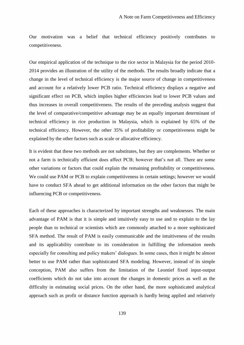
A Note on Farm Competitiveness and Efficiency
139
Our motivation was a belief that technical efficiency positively contributes to
competitiveness.
Our empirical application of the technique to the rice sector in Malaysia for the period 2010-
2014 provides an illustration of the utility of the methods. The results broadly indicate that a
change in the level of technical efficiency is the major source of change in competitiveness
and account for a relatively lower PCB ratio. Technical efficiency displays a negative and
significant effect on PCB, which implies higher efficiencies lead to lower PCB values and
thus increases in overall competitiveness. The results of the preceding analysis suggest that
the level of comparative/competitive advantage may be an equally important determinant of
technical efficiency in rice production in Malaysia, which is explained by 65% of the
technical efficiency. However, the other 35% of profitability or competitiveness might be
explained by the other factors such as scale or allocative efficiency.
It is evident that these two methods are not substitutes, but they are complements. Whether or
not a farm is technically efficient does affect PCB; however that’s not all. There are some
other variations or factors that could explain the remaining profitability or competitiveness.
We could use PAM or PCB to explain competitiveness in certain settings; however we would
have to conduct SFA ahead to get additional information on the other factors that might be
influencing PCB or competitiveness.
Each of these approaches is characterized by important strengths and weaknesses. The main
advantage of PAM is that it is simple and intuitively easy to use and to explain to the lay
people than to technical or scientists which are commonly attached to a more sophisticated
SFA method. The result of PAM is easily communicable and the intuitiveness of the results
and its applicability contribute to its consideration in fulfilling the information needs
especially for consulting and policy makers’ dialogues. In some cases, then it might be almost
better to use PAM rather than sophisticated SFA modeling. However, instead of its simple
conception, PAM also suffers from the limitation of the Leontief fixed input-output
coefficients which do not take into account the changes in domestic prices as well as the
difficulty in estimating social prices. On the other hand, the more sophisticated analytical
approach such as profit or distance function approach is hardly being applied and relatively
A Note on Farm Competitiveness and Efficiency
140
difficult to understand and explain due to its complexity and rigorously mathematical
programming or calculations.
Our discussions on these two approaches and how they are linked may help policy makers
and others make better use of one or the other measure. Although they reveal important
differences between the two sets of estimates, both approaches point to a fairly similar result
or conclusion on the competitiveness. Therefore, it is suggested that further efforts should be
made to combine the advantages of existing methodologies and to improve the collection,
precision and consistency of data.
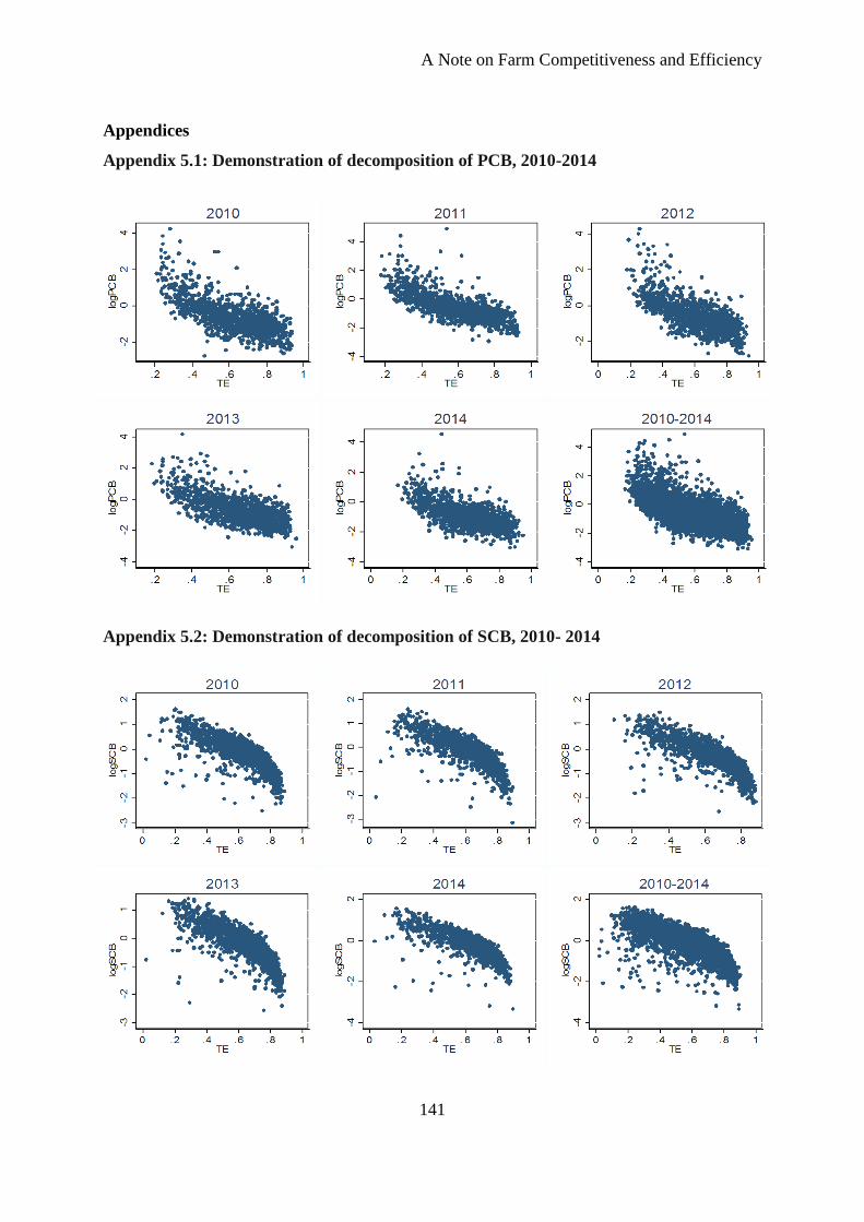
A Note on Farm Competitiveness and Efficiency
141
Appendices
Appendix 5.1: Demonstration of decomposition of PCB, 2010-2014
Appendix 5.2: Demonstration of decomposition of SCB, 2010- 2014
A Note on Farm Competitiveness and Efficiency
142
References
Abdulai, A., and H. Tietje. 2007. “Estimating technical efficiency under unobserved
heterogeneity with stochastic frontier models: Application to northern German dairy
farms.” European Review of Agricultural Economics 34(3):393–416.
Abdulai, A., and W.E. Huffman. 1998. “An Examination of Profit Inefficiency of Rice
Farmers in Northern Ghana An Examination of Profit Inefficiency of Rice farmers in
Northern Ghana.” Staff Paper No. 296. (January):1–27.
Agriculture Canada. 1990. “Report to the Minister of Agriculture of the Task Force on
Competitiveness in the Agri-Food Industry.” Ottawa, Ontario, June.
Aiginger, K., S. Bärenthaler-sieber, and J. Vogel. 2013. “Competitiveness under New
Perspectives.” Working Paper No. 44. October 2013. Available at:
http://www.foreurope.eu/.
Aigner, D.J., Lovell, C.A.K., and Schmidt, P., 1977. “Formulation and estimation of
stochastic frontier production function models.” J. Econometrics 6, 21–37.
Álvarez, A., J. Del Corral, and A. Fernández. 2009. “Modeling Regional Heterogeneity with
Panel Data: With Application to Spanish Provinces.” Uclm.Es (May). Available at:
http://www3.uclm.es/profesorado/jcorral/Trabajando/6f10da_Efi_Regions_12.pdf.
Belotti, F., and I. Giuseppe. 2012. “Consistent estimation of the ‘true’ fixed-effects stochastic
frontier model.” 5 No. 231, American Journal of Agricultural Economics 83(1):1-19
Bhatt, M.S., and S.A. Bhat. 2014. “Technical Efficiency and Farm Size Productivity ― Micro
Level Evidence from Jammu & Kashmir.” International Journal of Food and Agricultural
Economics 2(4):27–49. Available at:
http://www.foodandagriculturejournal.com/vol2.no4.pp27.pdf.
Brummer, B., and J. Loy. 2000. “The Technical Efficiency Impact of Farm Credit
Programmes: A Case Study of Northern Germany.” Journal of Agricultural Economics
51(3):405–418.
Bruno, M. 1965. “The Optimal Selection of Export-promoting and Import-substituting
Projects.” Project for Quantitative Research in Economic Development, Center for
International Affairs, Harvard University. Available at:
https://books.google.de/books/about/The_Optimal_Selection_of_Export_promotin.html?
id=ZBzbHgAACAAJ&pgis=1 [Accessed December 15, 2015].
Department of Agriculture, Malaysia. 2014. Perangkaian Padi Malaysia (Paddy Statistics of
Malaysia) 2013.
A Note on Farm Competitiveness and Efficiency
143
European Commission. 2009. “European Competitiveness Report 2008.” European
Commission, Brussels.
Färe, R., and S. Grosskopf.(1997). “Profit Efficiency, Farrell Decompositions and the
Mahler Inequality.” Economics Letters, 283-287. Available at:
http://www.sciencedirect.com/science/article/pii/S0165176597002346.
Findlay, Ronald, and Harry Grubert. 1959. “Factor intensities, technological progress, and the
terms of trade.” Oxford Economic Papers 11, no. 1: 111–21.
Frohberg, Klaus, and Hartmann, Monika. 1997. “Comparing measures of competitiveness.”
Discussion Paper, Institute of Agricultural Development in Central and Eastern Europe,
No. 2, http://nbn-resolving.de/urn:nbn:de:gbv:3:2-22616
Greene, W. 2005. “Reconsidering heterogeneity in panel data estimators of the stochastic
frontier model.” Journal of Econometrics 126(2):269–303.
Hatzichronoglou, T. 1996. “Globalisation and Competitiveness: Relevant Indicators.” OECD
Science, Technology and Industry Working Papers, 1996/5, OECD Publishing,
Organisation for Economic Co-operation and Development, Paris, France.
Holtkamp, J. 2015. “Unobserved heterogeneity in productivity analysis of panel data:
Applications to meat chain firms and global growth in agriculture.” :90. Available at:
http://hdl.handle.net/11858/00-1735-0000-0022-5DE0-E.
Jondrow, J., C. A. K. Lovell, I. S. Materov and P. Schmidt, On the estimation of technical
inefficiency in the stochastic frontier production functions model, Journal of
Econometrics, 1982, 19, pp.233-238.
Kanaka, D.S., and M. Chinnadurai. 2013. “The Policy Analysis of Rice Cultivation in India.”
European Journal of Physical and Agricultural Sciences 1(1). Available at:
http://www.idpublications.org/wp-content/uploads/2013/11/The-Policy-Analysis-Matrix-
of-Rice-Cultivation-In-India.pdf [Accessed March 21, 2016].
Kumbhakar, S.C. 1987. “The specification of technical and allocative inefficiency in
stochastic production and profit frontiers.” Journal of Econometrics 34(3):335–348.
Kumbhakar, S. 2001. “Estimation of Profit Functions When Profit Is Not
Maximum”. American Journal of Agricultural Economics, 83(1), 1-19. Retrieved from
http://www.jstor.org/stable/1244296
Kumbhakar, S.C., H.J. Wang and A. P. Horncastle. 2015. A Practitioner’s Guide to Stochastic
Frontier Analysis. 1st edition. Cambridge University Press.
Kumbhakar, S.C., and H.J. Wang. 2006. “Estimation of technical and allocative inefficiency-
a primal system approach”. Journal of Econometrics, 134(2), 419–440.
A Note on Farm Competitiveness and Efficiency
144
Latruffe, L. 2010. “Competitiveness, Productivity and Efficiency in the Agricultural and
Agri-Food Sectors.” OECD Food, Agriculture and Fisheries Papers 30(30):1–63.
Masters, W.A., and A. Winter-Nelson. 1995. “Measuring the Comparative Advantage of
Agricultural Activities: Domestic Resource Costs and the Social Cost-Benefit Ratio.”
American Journal of Agricultural Economics 77(2):243–250.
Masterson, T. 2007. “Productivity, Technical Efficiency, and Farm Size in Paraguayan
Agriculture.” Working Paper (490):37. Available at: http://ssrn.com/abstract=964722.
Monke, E.A., and S.R. Pearson. 1989. “The Policy Analysis Matrix for Agricultural
Development.” Ithaca, NY: Cornell University Press. Available at:
http://web.stanford.edu/group/FRI/indonesia/documents/pambook/pambook.pdf
[Accessed December 14, 2015].
Nishimizu, M., and J.M. Page. 1986. “Productivity Change and Dynamic Comparative.” The
Review of Economics and Statistics 68(2) (May ,1986), pp . 241-247 Published by: The
MIT Press Stable URL: http://www.jstor.org/stable/1925503 com.” The Review of
Economics and Statistics 68(2):241–247.
Nivievskyi, O., B. Brummer, and S. von Cramon-Taubadel. 2010. “A Note on Technical
Efficiency, Productivity Growth and Competitiveness.” Annual Meeting, July. Available
at: http://ageconsearch.umn.edu/bitstream/61759/2/11234 AAEA 2010.pdf.
Porcelli, F. 2009. “Measurement of Technical Efficiency. A brief survey on parametric and
non-parametric techniques.” Retrieved February (January):1–27. Available at:
http://citeseerx.ist.psu.edu/viewdoc/download?doi=10.1.1.232.4843&rep=rep1&type=pdf
Sarker, R., and S. Ratnasena. 2014. “Revealed Comparative Advantage and Half-a-Century
Competitiveness of Canadian Agriculture: A Case Study of Wheat, Beef, and Pork
Sectors.” Canadian Journal of Agricultural Economics/Revue canadienne
d’agroeconomie 62(4):519–544. Available at: http://doi.wiley.com/10.1111/cjag.12057.
Schmidt, P. and Lovell, C.A.K. (1979). Estimating Technical and Allocative Inefficiency
Relative to Stochastic Production and Cost Frontiers. Journal of Econometrics, 9: 343–
366.
Shephard, R. W. (1970), Theory of Cost and Production Functions. Princeton: Princeton
University Press.
Singgel, E. 2006. “International Competitiveness and Comparative Advantage: A Survey and
a Proposal for Measurement.” Journal of Industry Competition and Trade 6(2):137–159.
Available at: https://www.cesifo-
group.de/portal/pls/portal/!PORTAL.wwpob_page.show?_docname=956160.PDF
[Accessed December 15, 2015].
A Note on Farm Competitiveness and Efficiency
145
von Cramon-Taubadel, S., and O. Nivyevskyi. 2008. “Ukraine-Ag-Competitiveness-Policy
Note - Final.”
von Cramon-Taubadel, S., and O. Nivyevskyi. 2009. “Belarus Agricultural Productivity and
Competitiveness: Impact of State Support and Market Intervention.” Available at:
https://openknowledge.worldbank.org/bitstream/handle/10986/18897/483350ESW0REV
I110FINAL0for0printing.pdf?sequence=1&isAllowed=y [Accessed April 18, 2016].
Yao, R.T., and E.S. Gerald. 2007. “Technical Change and Productive Efficiency: Irrigated
Rice in the Philippines.” Asian Economic Journal 21(2):155–168. Available at:
http://web.a.ebscohost.com/ehost/pdfviewer/pdfviewer?sid=146d041d-9cfe-4315-95df-
2c88f34b2f56%40sessionmgr4005&vid=1&hid=4114 [Accessed January 23, 2016].

Concluding Remarks
146
Chapter 6
Concluding Remarks
This dissertation presents four selected studies on the topic of the “competitiveness and
efficiency of rice production in Malaysia”. Chapter 2 analyses the profitability and
competitiveness of the rice sector using the Policy Analysis Matrix (PAM) developed by
Monke and Pearson (1989) and aggregated data. Chapter 3 extends the PAM method by
performing a disaggregated competitiveness analysis and analysing the determinants of
competitiveness. Chapter 4 examines the performance of a rice farm using an efficiency
analysis. Finally, Chapter 5 concludes the dissertation by linking both competitiveness and
efficiency analyses using a static decomposition of competitiveness. In this section, we
present a summary of the main results and their implications, discuss the limitations and
challenges of the estimations, and present recommendations for future work.
6.1 Key contributions and summary
Rice is the most important source of livelihood and is a major source of employment for more
than 100,000 farmers and agricultural workers in Malaysia. It accounts for about 9% of the
country’s gross value added in agriculture and is grown on approximately 1.8 million hectares
of arable land (FAO, 2001). Rice is also the main source of caloric intake for many
Malaysians, contributing to nearly half of the average Malaysian’s total caloric intake per day.
Malaysia’s agro-climatic and geographical location provides the basis for the country’s
potential in agricultural production. The tropical climate and suitable soil conditions are
favorable for the development and growth of the tropical rice crop. The country lies entirely
in the equatorial zone with uniform temperatures, high humidity and a long wet season. The
copious rainfall is an important water source necessary for the successful cultivation of rice.
Hence, the rice sector plays a notable role in the society and government’s agricultural
policies and interventions aim to achieve “several, often conflicting, objectives”, including the
augmentation of farmers’ incomes, delivering quality products at low prices to consumers,
maintaining price stabilization, and an attainment of self-sufficiency.
Concluding Remarks
147
However, despite its high dependency on the importation of rice, the country continues its
aggresive pursuit of rice self-sufficiency, which involves the commitment to end rice imports
and become 100% self-sufficient in terms of rice production by the year 2020. The most
impeding constraint to Malaysia’s competitiveness is that the country’s endowment of natural
advantage and agro-climatic conditions do not automatically yield sufficient qualities of
complementary efforts, including a coherent policy framework, facilities and transport
infrastructures, as well information and marketing systems, all of which are essential to the
establishment of a competitive rice sector.
The recent free trade agreements, including the ASEAN Free Trade Agreement (AFTA) and
the World Trade Organization (WTO) accession, offer attractive opportunities, but also pose
challenges for the Malaysian rice sector as it must compete with other low-cost exporting
countries. This implies that not only structural changes in trade, but also adjustments at the
farm-level are needed to improve the sector’s efficiency and competitiveness. Further
developments in the rice sector will, therefore, depend on the availability of adequate supplies
of relatively low-cost and high-quality rice, or in other words, on the competitiveness of rice
production. This dissertation offers an analytical work to provide new insights into this issue
and the opportunities for improvement as well as the determinants of Malaysia’s rice
competitiveness.
In the first paper, the Domestic Resource Cost (DRC) indicator using aggregate data is
employed to shed light on the competitiveness of Malaysia’s rice sector. The main conclusion
is that rice production demonstrates modest international competitiveness. The empirical
results show that three out of four granary areas have comparative advantages in the
production of rice with Domestic Resource Cost values, or DRCs, of less than one. The farms
located in these areas produce a net surplus for the entire country. In the remaining region,
rice farming appears to be marginally competitive and imparts relatively low social profits.
For the second paper, we essentially continued the analysis performed in the first paper and
focused on a disaggregated competitiveness analysis and the determinants of rice
competitiveness in Malaysia. The weakness of the DRC method is that it is based on average,
or representative, farms. The conclusions that can be drawn from the average indicator might
Concluding Remarks
148
be misleading as the variations across heterogeneous producers grow. For this reason, we
employed the Social Benefit Cost (SCB) indicator using farm-level survey data to generate
SCB distributions that demonstrate the competitiveness of rice production in Malaysia. The
results of the SCB analysis reveal that a large proportion of farms are able to produce rice
competitively; more than 60% of rice farmers produced rice competitively over the period
from 2010 to 2013 and these competitive farms produced a disproportionately large number
of the total rice production (80%) each year. The only exception was in 2014, where 48% of
the farms that were identified as competitive accounted for 71% of the total rice production.
From 2012 to 2014, the SCB scores based on average revenue and cost data were greater than
1. This indicates that social revenue was not enough to cover the social value added,
suggesting these farms are losing their international competitiveness, in other words they are
uncompetitive. However, the SCB distributions based on disaggregated data revealed that
many farms were competitive and these competitive farms accounted for a disproportionately
large share of rice production during that period. Hence, the competitive farms, on average,
tend to produce more rice than non-competitive farms. This information highlights the
primary advantage of using disaggregated SCB distributions and avoids the pitfalls working
with the average data. In the second stage of the analysis, we further analysed the factors that
might influence a farm’s degree of competitiveness. The available evidence suggests that
participation in the farmers’ organization, gender and farm size are the major determinants of
rice competitiveness, while the increasing travel distance to rice mills, off-farm income and
the use of hired labour may reduce competitiveness.
For the third paper, we performed an efficiency analysis method to measure the technical
efficiency of the performance of Malaysia’s rice farms. The framework provided in the paper
took unobserved heterogeneity into account using the recent fixed effect model (Chen et al,
2014); the cases in which managerial characteristics and environmental conditions are not
observed are assumed to be constant or different for each rice farm. This is crucial
considering the panel data collections provided by developing countries are significantly
costlier and some important attributes may not exist. Therefore, the model allows for
unobserved heterogeneity and the estimation is free of incidental parameters. In the
observation period from 2010 to 2014, technical efficiency appearead to be fluctuate in rice
production. Our results indicate that the mean efficiency was 61% in 2010, it decreased in
Concluding Remarks
149
2011 and increased steadily for the next two years, before it declined again in 2014. However,
the low mean values of technical efficiency change (TEC) further revealing that the frontier is
shifting inward and some farms are essentially moving farther from the frontier.
In the second stage of the analysis, we examine the factors that account for the variations in
inefficiencies across the farms as well as their potential to improve efficiency and resources
using an a fixed effect panel regression. Our empirical results indicate that access to credit,
non-farm income, farm size and hired labor are the major determinants of technical efficiency.
The potential for increasing individual farm output varies considerably since many farms
became much better while others became much worse. Government support such as input
subsidies, credit facilities, distance to the rice mills and off-farm activities are identified as
important factors causing variations in the level of technical efficiency among rice farmers.
Furthermore, the scale elasticity of 1.49 indicates a strong economy of scale; in which outputs
can be increased with more than proportionate increases in inputs. This is imperative
considering that rice production in Malaysia is small and most of the farmers might depend on
capital and other inputs which necessitates a serious policy recommendation. It is possible to
achieve more if the provisions of inputs particularly mechanization and transport facilities as
well as improvement in high-yielding rice variety are further well distributed and reinforced
in the future so that it will help to increase the overall efficiency of rice production in
Malaysia.
Finally, the fourth paper links the two strands of analysis on competitiveness. The first strand
of the literature focuses on the analysis of comparative advantages/competitiveness, while the
second strand emphasizes the efficiency analysis where the concept of technical efficiency is
of prime interest. To demonstrate this relationship, we proposed a static decomposition of the
PCB into technical efficiency. Our result demonstrates that technical efficiency positively
contributes to competitiveness, thus confirming the common perception of the static
decomposition. By comparing PCB and TE, our result reveals a clear relationship between
competitiveness and efficiency, however higher technical efficiency alone does not translated
into higher competitiveness. The low R-square indicates that other unexplained variations
may exist or perhaps other factors may affect this relationship such as scale efficiency,
allocative efficiency and other few relations; an evidence in which is demonstrated by the
Concluding Remarks
150
fixed effect panel regression. This leads us to conclude that both approaches (PAM analysis
and SFA method) are not substituted but they are rather complementing. We use PCB to
explain competitiveness in certain settings; however we would have to conduct SFA ahead to
get additional information on the other factors that might be influencing PCB or
competitiveness.
6.2 Policy implications and options
Factors like a lack of coherent policy action, poor transportation and infrastructure, low
availability of credit and marketing, and information asymmetries exacerbate the underlying
barriers to achieving rice competitiveness that are listed in Section 6.1. These barriers can be
diminished or even eliminated with better political leadership capable of setting a new frontier
and priorities with the past misallocation as well as working hand-in-hand with partners (i.e.,
international institutions) and various stakeholders to balance their priorities and provide
insightful information and funding, while simultaneously minimizing the repercussions of the
development of agricultural competitiveness in Malaysia.
Since the inception of the AFTA, in compilation with the trade liberalization fostered by the
WTO, rice tariffs have been reduced to 0-5% for all trading partners in the region. Regardless,
in the major rice importing countries, such as Malaysia, rice is considered highly vulnerable
to food security and, therefore, is subject to up to 20% tariffs. Both the WTO accession and
on-going negotiations on a free trade agreement with ASEAN countries will require further
improvements in productivity and competitiveness at the farm-level. In particular, the
conditions of Malaysia’s accession to the WTO include the commitment to reducing trade
distortions and interventions on agricultural markets, a strategy which policymakers have
employed in the rice sector in recent years. Consequently, import barriers such as seeds, agri-
chemicals and agricultural machineries which make imports are expensive and lessens
competitiveness should be reduced.
According to Malaysia’s WTO Trade Report Review (2014), the total support given to
agriculture consisted of reduction commitments amounting to 1 billion Ringgit Malaysia
(RM). Of this, approximately 74% was related to Green Box assistance, mainly in the form of
income support for farmers while others involved the fertilizer subsidy scheme. In 2013, price
Concluding Remarks
151
support (incentives or bonus payments for paddy rice production) remained the largest part of
expenditures (480 million RM) followed by the fertilizer subsidy (465 million RM). This
form of agricultural support has cost Malaysian agriculture billions of RM in revenue. Since
our preliminary evidence indicates that many rice farmers are socially competitive, the
subsidization and price support of rice production, which are poorly targeted and distort
incentives, should be phased out. This could be replaced with targeted, direct income support
and income stabilisation measures.
Further efforts are required to reduce marketing margins and farm gate prices that may reduce
competitiveness; this could be accomplished by upgrading local storage facilities,
transportation infrastructure and the logistics associated with the rice delivery system and
marketing chain. Postharvest and value addition are integral components of strategies to
improve agricultural productivity and linkages between farmers and the markets. The causes
of storage losses and waste are principally connected to the managerial and technical
limitations of harvesting techniques, storage and cooling facilities in difficult climatic
conditions, infrastructure, packaging and marketing systems (Kiaya, 2014). Proper drying and
transport facilities are therefore important to minimize storage/postharvest losses. In addition,
a well-developed system of transport and infrastructure, including quality roads, ports, or air
transport, reduces the distance between regions and integrates national markets as well as
facilitates the movement of rice outputs to the market in a secure and timely manner.
Financial support and agricultural credit for rice farmers needs to be emphasized further. The
current policy of subsidization on credit is given at interest rates of 4.5% per season.
However, for many small farmers who harvest less than 3t/ha per season, a lack of finance
and collateral has forced them to borrow money from relatives or family members instead of
from agricultural credit institutions. Therefore, a strategy for coping with this problem would
be for the government to offer loans with lower or zero interest rates, which should be granted
regardless of a farmer’s capital (this is especially relevant for small farmers). Similarly, the
acquisition of flexible agricultural credit schemes will allow farmers to better access and
incorporate modern technologies into their rice production.
Concluding Remarks
152
Additionally, more investments in research and development (R&D) are required to enhance
competitiveness. It is important that public and private sectors play important roles in
supporting and nurturing an environment that is conducive to innovative activity. This
progression requires access to complementary inputs and sufficient investments, especially by
the private sectors. This includes high-quality research institutions and universities to inject
local communities with knowledge, and an expansion of human capital used to build new
technologies. Extensive collaborative actions between universities and industries in research
and technological developments are additionally necessitated. A review of the analysis on the
disaggregated competitiveness reveals that there is some variability in the average SCB ratios
from year to year that could be explained by other factors such as weather conditions
(monsoons during the main season and drought during the off-season) and pest attacks.
Therefore, further research and experimentation that are applicable to specific local conditions
are required to ensure that their durability in a variety of local conditions as well as for the
adaptation to general agriculture environments such as temperature, soil, water conditions and
local pests.
Between 2010 and 2014, the mean values of technical efficiency in the rice production were
50 to 60 percent. This average masks important differences among rice farms and points to
substantial scope for further efficiency improvement. This has certainly implications for the
efficiency-enhancing policies in the country. Furthermore, the findings on the estimates scale
elasticities deserve further attention in policy-decision making. Apparently, there is a strong
trend towards increasing returns to scale. The outputs elasticities of the inputs are higher
especially for capital and seed. Correspondingly, the positive elasticity of land indicates that
land is an important input which represents a high cost share (particularly for the rice farming
with low land endowment) such that it is farmed intensively. This suggests the role of
policies in fostering efficiency of the inputs and creating an enabling environments in terms of
infrastructure and capital as well as access to the input resources that provide adequate
incentives for the farmers particularly small farmers to invest in productive inputs.
Accordingly, this should be a strong signal for the government to change priorities in budget
allocations by providing more funds in investment that could enhance the technical efficiency
of rice production.
Concluding Remarks
153
6.3 Data limitations and methodological issues
Due to the fact that the production of rice provides the majority of agricultural and economic
opportunities in the case study region, this dissertation focuses on the competitiveness and
efficiency of rice production. Using the extension of the Policy Analysis Matrix approach,
which is based on the disaggregate competitiveness analysis, we demonstrate a simple and
effective way to estimate competitiveness. Additionally, our research allowed us to determine
how to take unobserved heterogeneity in the recent fixed model to analyse technical
efficiency into account. Although our analysis sheds some insight into the constraints of
competitiveness and efficiency in the context of the rice sector, and provide policy
recommendations for future intervention programs, we acknowledge several limitations of
this study.
First, the study only focuses on one granary area although there are eight granary areas in
Malaysia that are projected to be completely self-sufficient in rice production by the year
2020. Therefore, the dataset is not representative of Malaysia as a whole. The results
presented in this study are situation specific and cannot be extrapolated to other states or
granaries with different settings and conditions. The results of a similar study conducted in
other regions of Malaysia might differ to those presented in Chapter 3 depending on the
context and situation of the study. Of course, different granaries may vary with respect to
farm structure, management, soil condition, climate or temperature, and on-farm practices.
The study should be repeated at different ecological zones and areas in order to generate more
information on overall competitiveness of rice production in Malaysia.
Second, the SGMM estimation provides an appropriate framework to analyse the
determinants of change in competitiveness, but certainly it does not capture all aspects of this
process. While this study identifies and analyses the factors that could explain the variation in
competitiveness among rice farms, it omitted many factors associated with a lack of data
regarding biophysical conditions such as soil, climate, pests, diseases, and other
characteristics of the farmers including age, experience and education level. These factors are
important in explaining potential determinants of competitiveness.
Concluding Remarks
154
Additionally, the average mean value of efficiency found in rice farming was much lower
during 2010 to 2014, while the variations in technical efficiency scores were much higher.
These divergences are likely to be associated with the effect of unobserved heterogeneity that
are not accounted in this model i.e, although the analyses account for the individual effect, the
performance among the farms may differ a lot. For the rice production in Malaysia, natural
conditions such as weather, pest attacks, the spread of disease and managerial skills are likely
to account for this inefficiency performance. The full potential of production is not utilized in
the analysis presumably due to either the omission or the lack of data available on these
natural conditions and the management that is not completely captured by the noise
component. This is reflected by the MADA dataset analyzed in Chapter 4. Many data sets are
incomplete or indicate obvious errors that might also affect our estimation on technical
efficiency.
Finally, as shown in Chapter 5, we attempted to relate technical efficiency and
competitiveness in the static case. To do this, we decomposed the PCB measure into technical
efficiency. In other words, this distinction demonstrates how efficiently farms utilize the
inputs they possess to produce the maximum of possible outputs. While the results confirm
the perception of the static competitiveness that exists in the relevant literature, they do not
demonstrate the dynamic pattern of the competitiveness growth. The theoretical background
of efficiency and the Total Factor Productivity (TFP) is well-established (Fare and Primont,
1995: Kumbhakar et al, 2007). The extension of the dynamic or productivity decomposition
can address the mixtures of output and input as well as the potential determinants of
competitiveness (Nishimizu and Page, 1986: Bruemmer et al, 2002). Nevertheless, the
ignorance of such effects and concepts is predominantly due to the limitations of the data and
insufficient technical knowledge on the correct measurement of outputs and inputs as well as
dynamic decomposition that is ultimately dependent on data sources.
6.4 Directions for future research
Since we performed a disaggregated competitiveness analysis, the impacts of policies and
other determinants on farm competitiveness can be monitored by extending the SCB
distributions introduced in this study as new years of detailed farm-level data become
available in the future. The SCB analysis could also be applied to data from earlier years to
Concluding Remarks
155
generate long-term panel data and information on year-to-year fluctuations such as the years
leading up to the 2008 food crisis, during the food crisis, and the period after the food crisis.
To provide a sounder basis for the interpretation of the data as it pertains to future rice
developments, a more detailed analysis could further disaggregate SCB distributions by
region, farm size, and each individual product. An interesting follow-up work could also be
conducted on overall farm competitiveness. Some of the farms may produce multiple outputs
and hence, the incentives might vary depending on, for example, the degree of specialization
and technological requirements. Therefore, one might compare the distributions of
competitiveness scores for each individual product and for the whole farm.
In this study, we performed an analysis using a large dataset exclusively covering a five-year
period. The implications of the policy are informative; however, they must be interpreted with
caution especially if one wants to relate to the determinants of technological improvements.
The process of technology adoption usually takes longer and requires longer panel data to
generate more information and implications at the farm-level. Given the availability of
sufficiently long panels, a potential work could investigate the dynamic decomposition of
productivity growth and the performance patterns of rice production in Malaysia. This way,
we could obtain a detailed analysis of the sources of productivity growth, including technical
change, technical efficiency change and returns to scale, which can shed light on the sources
of differences in technological gaps or improvements.
Moreover, further research could be done with respect to explaining the potential
determinants of the rice sector’s competitiveness in Malaysia as a whole. This study can be
replicated and extended to the different granary areas or different systems of rice production
(irrigated or rain-fed). Nonetheless, the level of competitiveness might differ across regions,
and may depend on natural conditions, management practices and postharvest losses that
occur over time. Improvements to such estimation will provide a more practical interpretation
and comparison of the competitiveness of rice production, which in turn will confirm the
results of this study.
The framework that we used in Chapter 4 regarding the recent fixed effect model (Chen et al,
2014) assumes that inefficiency varies over time and this assumption is theoretically required
Concluding Remarks
156
in the panel data. Assuming that unobserved heterogeneity is time-invariant is more of a
philosophical issue (Chen et al, 2014). For the farm-level data, this assumption is acceptable
since many unobserved characteristics are fixed for either a certain period or only in the short-
run. In the context of the long series of agricultural data, the acceptance of persistent technical
inefficiency within this problem seems more problematic (Colombi et al, 2014). Farms that
exhibit a constant level of inefficiency are likely to drop out of the competition and exit the
markets, which subsequently leads to the farm’s restricted access to technology and market
failure. Accordingly, future research should address these consequences in productivity
analysis and the necessity of improving farm or sectoral data quality and comparability should
also be fortified further.
Finally, we demonstrate the link between competitiveness and technical efficiency and how
these two approaches (PAM analysis and SFA method) are related. We use PCB and SCB as
indicators to explain competitiveness while SFA approach to estimate technical efficiency.
Nevertheless, the decomposition of SCB is quite complex and proved to be challenging. The
use of primal profit maximization is intuitive since it avoids the problem of large variations in
prices, which is commonly occurring in practice. However, beyond its implementation, it
requires rigorous mathematical programming and strong economic foundation. Alternatively,
one could possibly decompose SCB using the cost function or cost-share equation or
production frontier which requires less severe exercise when estimating both technical
efficiency and allocative efficiency.
Concluding Remarks
157
References
Brummer, B., T. Glauben, and G. Thijssen. 2002. “Decomposition of Productivity Growth
Using Distance Functions: The Case of Dairy Farms in Three European Countries.”
American Journal of Agricultural Economics 84(August):628–644.
Chee.,W.C., and Peng, C.C. “Country Pasture/Forage Resource Profiles. Malaysia”. Country
Report. Available at: http://www.fao.org/ag/agp/agpc/doc/Counprof/Malaysia.htm.
Chen, Y.Y., P. Schmidt, and H.J. Wang. 2014. “Consistent estimation of the fixed effects
stochastic frontier model.” Journal of Econometrics 181(2):65–76. Available at:
http://dx.doi.org/10.1016/j.jeconom.2013.05.009.
Colombi, R., Kumbhakar, S. C., Martini, G. and Vittadini, G. (2014). Closed-Skew Normality
in Stochastic Frontiers with Individual E_ects and Long/Short-Run Efficiency. Journal
of Productivity Analysis.
Kiaya, V. 2014. “Post-Harvest Losses and Strategies to Reduce Them.” Technical paper on
Post-Harvest Losses. Action Contre la Faim (ACF). January 2014.
Nishimizu, M., and J.M. Page. 1986. “Productivity Change and Dynamic Comparative
Advantage The Review of Economics and Statistics, 68 (2): 241-247 (May, 1986).
Published by: The MIT Press Stable URL: http://www.jstor.org/stable/1925503
COM.” The Review of Economics and Statistics 68(2):241–247.
Subal Kumbhakar and Dan Wang, 2007. "Economic reforms, efficiency and productivity in
Chinese banking," Journal of Regulatory Economics, Springer, vol. 32(2):105-129,
October.
World Trade Organization. 2014. “Trade Policy Review. Malaysia: World Trade
Organization.”