Embed Size (px)
Citation preview
Compilation and Application of Asset-Liability Matrices:
A Flow-of-Funds Analysis of the Japanese Economy 1954-1999
Kazusuke Tsujimura Masako Mizoshita
November 3, 2004 ver.1.1 October 15, 2004 ver.1.0
K.E.O. DISCUSSION PAPER No. 93
1
Abstract In this paper, we will discuss the details of the compilation process of asset-liability matrix from flow-of-funds account (financial balance sheets) taking the example of Japan 1954-1999. Asset-liability matrix is a sector-by-sector square matrix, so the advantage is that we can apply the tremendous asset that the input-output analysis has accumulated since the early days of its development. However, input-output and asset-liability matrices are not necessarily identical twins. One of the leading peculiarities of the asset-liability matrix is that two distinct sector-by-sector matrices are derived from a set of balance sheets. The first one describes the propagation process of fund-raising while the other one depicts that of fund-employment. When there are discrepancies in the valuation of assets and liabilities, the magnitude of the dispersion could be different in one system from another. This will give us a clue to the generation mechanism of financial bubbles.
Key Words Asset-liability matrix, Flow-of-funds analysis, Dispersion index, Financial bubbles,
Japanese economy
JEL Classification Numbers E50; C67; O11
2
1. Introduction Since the early days of its development, the flow-of-funds accounts were in the form of a display rack of the balance sheets of various institutional sectors1. A merit of this type of tabulation is that we can use all the basic principles of modern accounting system. The quadruple entry system proposed by Copeland (1952) is a logical evolution of the double entry system commonly practiced in business accounting. Another merit is that it is not too difficult to collect the balance sheets because most of the institutional sectors have some sort of balance sheets whatsoever. Especially in case of financial institutions, they are obliged to make detailed balance sheets. So the coverage is quite high, if not one hundred per cent. In addition to that, detailed statements attached to them often disclose the particulars of the counter parties of the transactions. That is why we can reconstruct the balance sheet of the household sector, for example, even though it does not make one by itself. Some other merits include the fact that the advances in the information technology allow the financial institutions to collect the data real-time. These merits are rarely found in other fields of economic statistics.
Although Stone (1966), Brainard and Tobin (1968) and Klein (1983, 2003) among others proposed alternative flow-of-funds accounts in the form of asset-liability matrices (i.e. sector-by-sector square matrix), this kind of tabulation practice was never realized except in few experimental project like that of the Economic Planning Agency of Japan in the 1950s. The advantage of asset-liability matrix is that you can make good use of the wealth the input-output analysis has accumulated for more than half century. Between 1950 and 1980, the input-output analysis was one of the most frequently employed techniques in economic forecasting. Even today, it is often used in China and other rapidly developing countries. Actually, it is demonstrated in Tsujimura and Mizoshita (2003) that the combination of asset-liability matrix and the Leontief inverse could be a powerful weapon to analyse the effect of money-market operations of the central banks in details. The only problem is that it is an enormous work to compile an asset-liability matrix from scratch.
At Keio Economic Observatory, we have compiled asset-liabilities matrices of Japan for 1954-1999. The fundamental technique we have employed is the supply-and-use method originally proposed by Stone and Klein cited above. However, supply-and-use method is too mechanical to include all the detailed information available in this country, so that we have explored dummy-instrument method in addition to that. Although the asset-liability matrix is based on the 1968 SNA flow-of-funds accounts originally prepared by the Bank of Japan, the number of the institutional sectors is almost doubled to 35. (An aggregated 11-sector matrix is also
3
available.) The list of the institutional sectors is given in Table 1. The financial institutions, especially the banking sector is divided into as many sub-groups as possible to examine their role in the development of the Japanese economy. The non-financial private corporations have been divided into four sub-groups while the non-corporate enterprises have been separated from the households. The asset-liability matrix is based on the 1968 SNA, unless otherwise stated.
In the latter half of this treatise, the results of the overall analysis of the Japanese economy in transition from poverty to prosperity will be discussed. For reasons of space, only the indices obtainable directly from the Leontief inverse will be examined in this tract. One of the leading peculiarities of the asset-liability matrix is that two distinct sector-by-sector matrices are derived from a set of balance sheets. That means there are two Leontief inverses as well. The first one describes the propagation process of fund-raising while the other one depicts that of fund-employment. We call them liability-oriented system and asset-oriented system respectively. In this regard, the valuation of the assets and liabilities plays important role. When there are discrepancies in the valuation of assets and liabilities, the magnitude of the dispersion could be different in one system from another. This will give us a clue to the generation mechanism of financial bubbles. 2. Compilation of Asset-Liability Matrix The first step to create an asset-liability-matrix is to collect balance sheets of the institutional sectors and put them side-by-side into a display case called flow-of-funds accounts. In this section, we will discuss the details of the compilation process of asset-liability matrix, a sector-by-sector square matrix, from flow-of-funds accounts. The fundamental approach employed here is the supply-and-use method widely used in the compilation of input-output tables. Supply-and-use method is a tool to tabulate the transactions of each financial instrument by particular institutional sector in asset-liability matrix under an assumption that every supplier of funds put them into one reservoir representing the market of the instrument and every user of funds draw them from that reservoir. Although supply-and-use method portrays the transactions of negotiable instruments like stocks and bonds on organized markets (stock exchange etc.) very well, it is a poor tool to depict the direct transactions of non-negotiable instruments including deposits and loans. In this regard, we have introduced dummy-instrument method as a remedy.
4
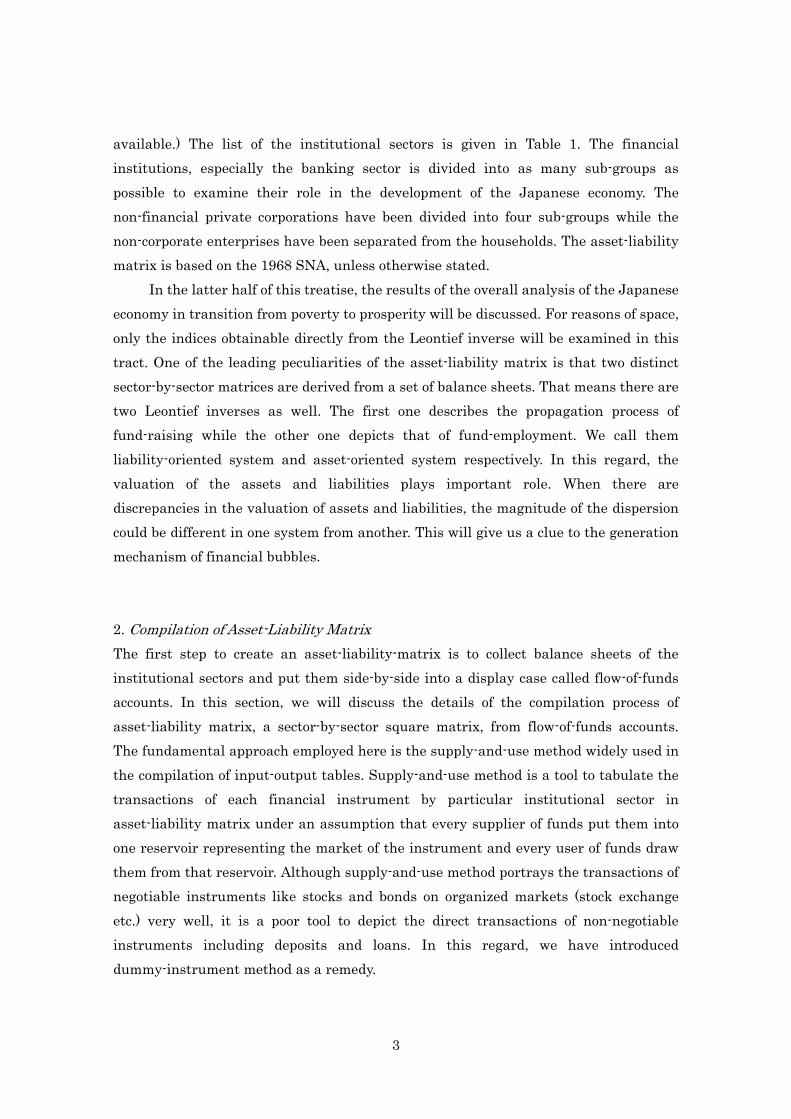
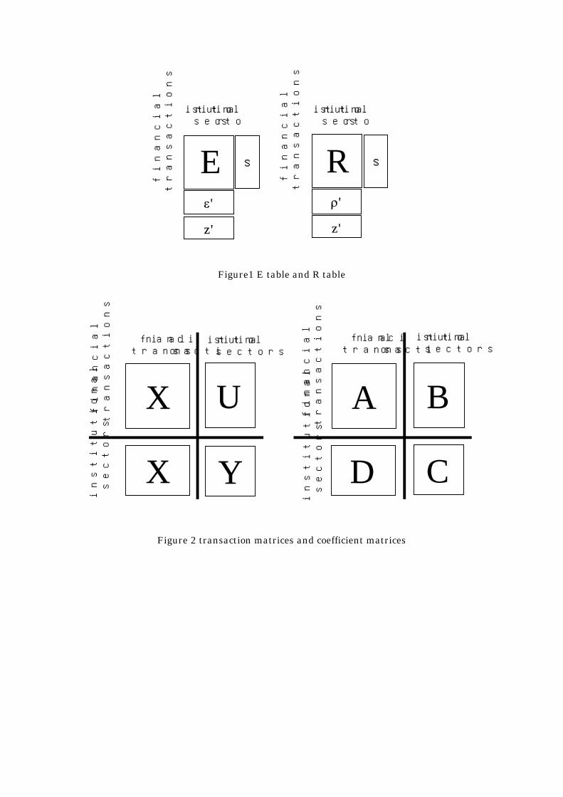
2.1. Supply-and-Use Method 2.1.1. Asset and Liability Matrices As mentioned above, flow-of-funds accounts are in form of a display rack of balance sheets of various institutional sectors. By picking out each row of assets and liabilities of the balance sheet of a sector separately, we can form two matrices E (Asset Matrix) and R (Liability Matrix). As depicted in Figure 1, E table consists of a matrix E and
vectors ε , Es , z . Each element ( ije ) of matrix E represents the amount of funds
allocated to the i’th financial instrument by the j’th institutional sector. Vectors ε is
the excess liabilities, Es is the total amount of the financial instrument in terms of assets, z is either the sum of assets or liabilities of particular sector whichever is greater; where, n is the number of financial instruments while m is the number of the institutional sectors.
⎥⎥⎥⎥
⎦
⎤
⎢⎢⎢⎢
⎣
⎡
=
nmnn
m
m
eee
eeeeee
L
MOMM
L
L
21
22221
11211
E
⎥⎥⎥⎥⎥
⎦
⎤
⎢⎢⎢⎢⎢
⎣
⎡
=
mε
εε
M2
1
ε
⎥⎥⎥⎥⎥
⎦
⎤
⎢⎢⎢⎢⎢
⎣
⎡
=
En
E2
E1
s
ss
M
Es
⎥⎥⎥⎥
⎦
⎤
⎢⎢⎢⎢
⎣
⎡
=
m
2
1
z
zz
Mz
Likewise, R table consists of a matrix R and vectors ρ , Rs , z . Each element ( ijr ) of
matrix R represents the amount of funds raised in the form of i’th financial instrument by the j’th institutional sector. Vectors ρ is the excess financial assets, Rs is the total amount of the financial instruments in terms of liabilities.
⎥⎥⎥⎥
⎦
⎤
⎢⎢⎢⎢
⎣
⎡
=
nmnn
m
m
rrr
rrrrrr
L
MOMM
L
L
21
22221
11211
R
⎥⎥⎥⎥⎥
⎦
⎤
⎢⎢⎢⎢⎢
⎣
⎡
=
mρ
ρρ
M2
1
ρ
⎥⎥⎥⎥⎥
⎦
⎤
⎢⎢⎢⎢⎢
⎣
⎡
=
Rn
R2
R1
s
ss
M
Rs ⎥⎥⎥⎥
⎦
⎤
⎢⎢⎢⎢
⎣
⎡
=
m
2
1
z
zz
Mz
In this expression, the column sum jz is either the sum of assets or liabilities of the
j’th institutional sector whichever is larger.
(1) ⎟⎟⎠
⎞⎜⎜⎝
⎛= ∑ ∑
= =
n
i
n
iijijj r,emaxz
1 1
In case
(2) ∑∑==
>n
iij
n
iij re
11,
5
the excess financial assets jρ and the excess liabilities jε are defined as follows.
(3) ∑=
−=n
iijjj rz
1
ρ
(4) 0=jε .
In contrast to this, when
(5) ∑∑==
<n
iij
n
iij re
11
is the case, jε and jρ are expressed in the following manner.
(6) ∑=
−=n
iijjj ez
1
ε
(7) 0=jρ
In case
(8) ∑∑==
=n
iij
n
iij re
11,
then
(9) 0== jj ρε .
2.1.2. Asset-Oriented System vs. Liability Oriented System
In the field of input-output analysis, certain mathematical method has been used to convert the supply-and-use matrices into one square matrix. In Fig.2, V is the supply matrix while U is the use matrix. Firstly, let us pay our attention to the flow of funds itself. From this point of view, each column of R is the vector that represents the fund raising portfolio of the institutional sector. Since the fund raising portfolio of an institutional sector in the flow-of-funds analysis corresponds to the input structure of an industry in the input-output analysis, we can put R into the place of U in Fig.2. From the same viewpoint, each row of the transposition matrix of E is the vector that represents the allocation of the funds of the institutional sector. Since the allocation of funds of an institutional sector in the flow-of-funds analysis corresponds to the supply structure of an industry in the input-output analysis, we can put E′ into the place of V in Fig.2.
Alternatively, let us pay our attention to the flow of financial instruments rather than the flow of funds itself. From this viewpoint, everything looks the other way round.
6
Now, each column of E is the vector that represents the demand for various financial instruments while each row of the transposition matrix of R is the vector that represents the supply of each financial instrument. In that sense, we can put E into the place of U and R′ into the place of V in Fig.2. This two-sided nature of the flow-of-funds analysis generates two sector-by-sector matrices rather than one. We will call the former liability-oriented system and the latter asset-oriented system. That is
(10) RU ≡
(11) EV ′≡
in the liability-oriented system, and
(12) EU ≡*
(13) R'V ≡*
in the asset-oriented system (denoted by superscript *). Following the footsteps of the input-output analysis, the sector-by-sector
flow-of-funds matrix or asset-liability matrix of the liability-oriented system could be derived in the succeeding formulae. Firstly, the input coefficients are defined for matrix U .
(14) j
ij
j
ijij z
rzu
b ==
Secondly, the allocation coefficients are defined for matrix V .
(15) Ej
ji
j
ijij
s
e
s
vd ==
E
So that,
⎥⎥⎥⎥
⎦
⎤
⎢⎢⎢⎢
⎣
⎡
=
nmnn
m
m
bbb
bbbbbb
L
MOMM
L
L
21
22221
11211
B ,
and
⎥⎥⎥⎥
⎦
⎤
⎢⎢⎢⎢
⎣
⎡
=
mnmm
n
n
ddd
dddddd
L
MOMM
L
L
21
22221
11211
D .
Next, we will define the sector-by-sector flow-of-funds matrix Y and its input coefficient matrix as follows.
7
⎥⎥⎥⎥
⎦
⎤
⎢⎢⎢⎢
⎣
⎡
=
mmmm
m
m
yyy
yyyyyy
L
MOMM
L
L
21
22221
11211
Y ,
⎥⎥⎥⎥
⎦
⎤
⎢⎢⎢⎢
⎣
⎡
=
mmmm
m
m
ccc
cccccc
L
MOMM
L
L
21
22221
11211
C ,
where
(16) j
ijij z
yc = .
In the field of input-output analysis, several methods have been proposed to convert the supply-and-use matrices into one square matrix. The mathematical methods used when transferring outputs and associated inputs hinge on two types of technology assumptions as stated in paragraph 15.144 of the 1993 SNA; (a) industry technology assumption and (b) product technology assumption. The former assumes that all products produced by an industry are produced with the same input structure while the latter assumes that a product has the same input structure in whichever industry it is produced. In flow-of-funds analysis, these two assumptions could be translated into (a’) institutional sector portfolio assumption (corresponding to industry technology assumption) and (b’) financial instrument portfolio assumption (corresponding to product technology assumption). The former assumes that institutional sectors allocate (raise) funds according to their own portfolio regardless of the means of raising (employing) funds while the latter assumes that they allocate (raise) the funds according to the portfolio peculiar to the financial instrument through which the funds have been raised (will be employed).
In case of input-output analysis, the input structure is considered to be commodity specific rather than industry specific. So, the industry technology assumption is considered to perform rather poorly as stated in paragraph 15.146 of the 1993 SNA. On the contrary, in case of flow-of-funds analysis, the portfolio should be institutional sector specific rather than financial instrument specific because it is common to categorize the institutional sectors by their means of fund raising. According to this assumption, we can obtain the following formula based on the institutional sector portfolio assumption. (17) DBC =
In this formula, each element of matrix C could be expressed as follows.
8
(18) kj
n
kikij bdc ∑
=
=1
Since ikd is the i’th institutional sector’s asset-market share of financial instrument k, and kjb is the k’th financial instrument’s share in the j’th institutional sector’s fund-raising portfolio, ijc means how much funds j’th institutional sector raise from
i’th sector. Therefore, each element of matrix Y could be obtained by the following relation. (19) jijij zcy =
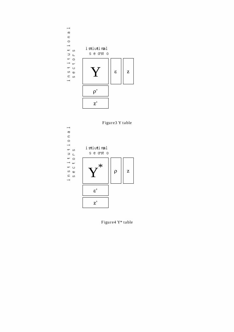
The composition of Y table is depicted in Fig.3. Likewise, the sector-by-sector flow-of-funds matrix or asset-liability matrix of the
asset-oriented system could be derived in the succeeding formulae. Firstly, the input
coefficients are defined for matrix *U .
(20) j
*ij
j
*ij*
ij ze
zu
b ==
Secondly, the allocation coefficients are defined for matrix *V .
(21) Rj
jiRj
ijij s
r
s
vd
*** ==
So that,
⎥⎥⎥⎥⎥
⎦
⎤
⎢⎢⎢⎢⎢
⎣
⎡
=
**2
*1
*2
*22
*21
*1
*12
*11
nmnn
m
m
bbb
bbbbbb
L
MOMM
L
L
B*
and
⎥⎥⎥⎥⎥
⎦
⎤
⎢⎢⎢⎢⎢
⎣
⎡
=
**2
*1
*2
*22
*21
*1
*12
*11
*
mnmm
n
n
ddd
dddddd
L
MOMM
L
L
D .
Next, we will define the sector-by-sector flow-of-funds matrix *Y and its input coefficient matrix *C as follows.
⎥⎥⎥⎥⎥
⎦
⎤
⎢⎢⎢⎢⎢
⎣
⎡
=
**2
*1
*2
*22
*21
*1
*12
*11
*
mmmm
m
m
yyy
yyyyyy
L
MOMM
L
L
Y ,
9
⎥⎥⎥⎥⎥
⎦
⎤
⎢⎢⎢⎢⎢
⎣
⎡
=
**2
*1
*2
*22
*21
*1
*12
*11
*
mmmm
m
m
ccc
cccccc
L
MOMM
L
L
C ,
where
(22) j
ijij z
yc
** = .
According to this assumption, we obtain the following formula.
(23) *** BDC =
In this formula, each element of matrix *C could be expressed as follows.
(24) *
1
**kj
n
kikij bdc ∑
=
=
Since *ikd is the i’th institutional sector’s liability market share of financial instrument
k, and *kjb is the k’th financial instrument’s share in the j’th institutional sector’s
fund-employment portfolio, *ijc means how much funds j’th institutional sector employ
to i’th sector. Therefore, each element of matrix Y* could be obtained by the following relation.
(25) jijij zcy ** =
The composition of Y* table is depicted in Fig.4. 2.1.3. Issue Value vs. Current Market Value Only when the following relation is maintained, the succeeding relations are proved. If both sides of the balance sheets in the original flow-of-funds accounts are measured in common value (either issue value or current market value), that is (26) RE ss = then
(27) j
m
iijj
Yj ρyzρ =−= ∑
=1
,
(28) i
m
jiji
Yi εyzε =−= ∑
=1
,
(29) *' YY = . In this special case, the liability-oriented system and the asset-oriented system produce
10
a unique matrix; i.e. the transposition matrix of Y is *Y and vice versa (see Appendix 1 at the end of this tract in addition to the appendix to Tsujimura and Mizoshita (2003)).
Paragraph 2.87 of the 1968 SNA as well as paragraph 10.14 of the 1993 SNA clearly states that both assets and liabilities should be expressed in current market value. The principle of SNA is that a financial claim should be measured by the amount that a debtor must pay to the creditor to extinguish the claim. In this case, there is no discrepancy in the measurement of assets and liabilities. However, when we simply sum up the existing balance sheets of the institutions, some sort of discordance is inevitable. Indeed, paragraph 101 of the IASB2 Framework, recognizes historical cost (the amount of cash or cash equivalent paid) as the basis for the financial statements. Although paragraphs 69 and 93 of IAS 39 stipulate that the financial assets as well as financial liabilities held for trading should be measured at fair value (i.e. current market value), equity instruments of their own issuance are exempted. The principle of IAS is that equity instruments must be recorded at the amount of proceeds received in exchange at the time of issuance.
It is no wonder that the issuer of the corporate stocks enters it on their own book in issue value while the holder of the stocks enters it on their book in the current market value. If we simply sum up those figures, we will have flow-of-funds accounts that have discrepancy in the total value of assets and liabilities. It is rather awkward to have discordance in book keeping values, but this is the reality we face everyday. It is proved if, (30) RE ss ≠ then, equations (27), (28) and (29) are no longer maintained. (See Appendix 1.) The liability-oriented system and the asset-oriented system produce two different matrices. Isn’t it awful? But, let us face the reality. As we discuss later in this treatise, there will
be a rewards if we could overcome this problem. In case of discrepancy, Y and *Y tables are presented in manners depicted in Fig.A1-2 and Fig.A1-3 of Appendix 1. It should be noted that the columns containing the differences between the issue and current market values are accommodated in these tables. 2.2. Dummy Instrument Method Supply-and-use method is a convenient way to transform the balance sheets of flow-of-funds accounts into sector-by-sector asset-liability matrix. As far as those openly traded securitized financial instruments (e.g. bonds, stocks etc.) are concerned, there is no alternative but allocate them according to the market share. However, as for those
11
financial instruments directly traded between the parties concerned (e.g. deposits, loans etc.), it is not uncommon that some additional information is available. In case of Japan, all deposit and loan transactions are earmarked by creditors and debtors. Whenever such additional information is attainable, dummy instrument method should be used together with supply-and-use method.
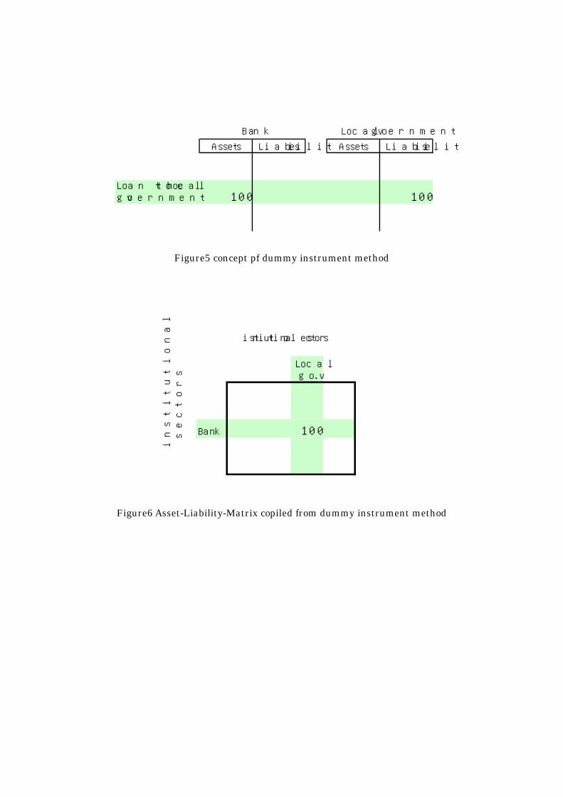
The idea is quite simple. If we know that the bank made a loan (say amounting to 100) to the local government, we add a dummy financial instrument just to record this single transaction. As depicted in Fig.5, we enter 100 on the asset side of the balance sheet of the bank while registering the same amount to the liability side of the local government. Since these transactions are entered in the dummy instrument row, no other transactions will be made entry in this particular row. When we apply supply-and-use method to these balance sheets, we will have an asset-liability-matrix depicted in Fig.6. The result of the trick is that the transaction is entered in the row of the bank and in the column of the local government on the sector-by-sector matrix in the liability-oriented system. (Of course, this transaction will be registered in the row of the local government and in the column of the bank in the asset-oriented system.) 3. Two Alternative Matrices and their Leontief Inverse 3.1. Power-of-Dispersion and Sensitivity-of-Dispersion Indices 3.1.1. Four Indices Defined In the previous section, we have derived two distinct sector-by-sector square matrices from a set of balance sheets. However we did not elaborate in details. Why that is necessary is the question to be answered in this section. The fundamental equations of both liability-oriented system and asset-oriented system are written as follows. (See
Appendix 1 for the case RE ss ≠ .)
(31) ii
m
jij zy =+∑
=
ε1
(32) ii
m
jij zy =+∑
=
ρ1
*
These equations could be expressed in the matrix formula. (33) zεzC =+
(34) zρzC* =+
Solving each equations for z yields (35) εCIz 1)( −−= ,
(36) ρCIz 1* )( −−= .
12
We will denote 1)( −− CI and 1* )( −− CI as Γ and *Γ respectively.
⎥⎥⎥⎥
⎦
⎤
⎢⎢⎢⎢
⎣
⎡
=−= −
mmmm
m
m
γγγ
γγγγγγ
L
MOMM
L
L
21
22221
11211
1)( CIΓ
⎥⎥⎥⎥⎥
⎦
⎤
⎢⎢⎢⎢⎢
⎣
⎡
=−= −
mmmm
m
m
*2
*1
*
2*
22*
21*
1*
12*
11*
1)(
γγγ
γγγγγγ
L
MOMM
L
L
** CIΓ
The elements ijγ indicate direct as well as indirect demand for funds in i’th
institutional sector induced by the increment in demand for funds jε
(excess-investments in terms of objective economy) by j’th sector. On the other hand, *ijγ
indicate the supply of funds in i’th sector induced by the increment in supply of funds jρ (excess-savings in terms of object economy) by j’th sector. Since demand and supply
of funds are propagated through different systems, there is an asymmetry in induced demand and supply of funds. This is one of the most prominent properties of flow-of-funds analysis.
On the analogy to input-output analysis, the indices of the power-of-dispersion and the indices of the sensitivity-of-dispersion could be calculated in the following manner. As for the liability-oriented system, the two indices are defined as follow.
(37)
∑∑
∑
= =
== m
j
m
iij
m
iij
Yj
m
wp
1 1
1
1 γ
γ
(38)
∑∑
∑
= =
==m
i
m
jij
m
jij
Yi
m
ws
1 1
1
1 γ
γ
In this system, the power-of-dispersion index indicate the direct as well as indirect demand for funds in total induced by the increment in demand for funds (excess-investments in terms of objective economy) by j’th institutional sector. The sensitivity-of-dispersion index in the liability-oriented system indicate the direct as well
13
as indirect demand for funds in i’th institutional sector induced by the increment in demand for funds by each institutional sector.
The two indices are defined for the asset-oriented system as well.
(39)
∑∑
∑
= =
==m
j
m
iij
m
iij
Yj
m
wp
1 1
*
1
*
*
1 γ
γ
(40)
∑∑
∑
= =
== m
i
m
jij
m
jij
Yi
m
ws
1 1
*
1
*
*
1 γ
γ
In this system, the power-of-dispersion index indicate direct as well as indirect supply of funds in total induced by the increment in supply of funds (excess-savings in terms of objective economy) by j’th institutional sector. The sensitivity-of-dispersion index in the asset-oriented system indicate the direct as well as indirect supply of funds in i’th institutional sector induced by the increment in supply of funds by each institutional sector. While the indices represent the chain reaction originated in the demand for funds (excess-investments in terms of objective economy) in the liability-oriented system, the indices represent that originated in the supply of funds (excess-savings in terms of objective economy) in the asset-oriented system. 3.1.2. The Principal Institutional Sectors Figure 7 displays the power-of-dispersion indices for households, non-financial corporations and banks picked out of the 11-sector aggregated asset-liability matrix. Each plot indicate the combination of the year referring to asset (vertical axis) and liability (horizontal axis) oriented system. Both indices are normalized so that the diagram is divided into quadrants by vertical and horizontal lines indicating unity. The households, with primary savings, are located in the midst of the second quadrant while the non-financial private corporations, with primary investments, are situated in the fourth quadrant. The government, not plotted in the figure though, stays in the fourth quadrant as well, probing that the role of government in the financial market is not much different from the non-financial private corporations. The banks, intermediaries by their nature, are placed in the middle of the chart neighbouring to the intersecting point. The most prominent thing is that, the location of the plots on the diagram show minimal change despite the laps of time.
The power-of-dispersion index in the liability-oriented system and the
14
sensitivity-of-dispersion index in the asset-oriented system is something like the two side of the same coin. The former is an index that exhibits how far the influence spreads when the institutional sector raises new money from the market. The latter is an indicator to demonstrate how much effect the institutional sector gains when the fund-raising is activated in general. The relations between the two indices are depicted in Figure 8. In this diagram, the households are located in the third quadrant while the non-financial corporations are situated in the first quadrant. The government stays mainly in the first quadrant though some scatters are belonging to the fourth quadrant suggesting that the government does not immediately react to an increment in the savings as the non-financial corporations do. However, the plots of the non-financial corporations are wide spreading. Especially in the latter half of the observation period, the sensitivity-of-dispersion index is getting smaller with the years. When Japan was growing fast to get rid of the poverty brought by the defeat in the World WarⅡ, the corporate sector absorbed whatever funds made available for them. But, after reaching maturity, the Japanese corporations have some difficulty to find investment opportunity just as their counterparts in other so-called advanced countries. In 1999, the position of the corporate sector is much more like that of the government. Rather, the government is taking over the role of excess-funds absorber in the aftermath of the financial bubble of 1980s.
Figure 9 displays the relations between the power-of-dispersion index of the asset-oriented system and the sensitivity-of-dispersion index of the liability-oriented system. In this diagram, the households are located in the middle of the first quadrant while the non-financial private corporations are situated in the lower part of the second quadrant. Most probably this is because they are acting as financial intermediaries for their affiliated companies. Unlike the corporate sector, the government is situated in the third quadrant suggesting that it plays no role as financial mediator what so ever. 3.1.3. The Financial Mediators Talking about financial mediator, the dispersion indices are rigorous device to identify the role of each category of financial institutions. The power-of-dispersion index of the asset-oriented system and the sensitivity-of-dispersion index of the liability-oriented system are depicted in Figure 10. In this diagram, banks are scattered around the vertical axis between 1.5 and 2.5 on its scale that is upper left of the figure extending over the first and second quadrant. The public financial corporations are situated about middle of the figure in the first quadrant while non-bank financial companies are placed in the fourth quadrant. This means that banks supply funds to only limited number of
15
customers who spend them directly on capital investments. On the other hand, the non-bank financial companies make loans to wide-ranging customers who spend them as working-funds. The other implication is that people tend to tap banks for money first, then public financial corporation, then non-bank financial companies in that order (in the order of the sensitivity-of-dispersion index). 3.1.4 The Column Sums It is well known that the dispersion indices are obtained by normalizing either the column sum (in case of power-of-dispersion index) or the row sum (sensitivity-of-dispersion index) of the Leontief inverse matrix. Then what about those sums themselves? Figures 11 and 12 display the fluctuations in the column sum of the liability-oriented system and the asset-oriented system respectively. In Figure 11, all the lines but that of the households moves as if they are interlocked. The only exception is that the line of the government between 1962 and 1967. In Figure 12, all the lines but that of the government are synchronized. This fact suggest that we may be able to throw light upon the mechanism of the business cycle from the view point of the financial market structure.
3.2. The Sum Total of the Leontief Inverse 3.2.1 Asset and Liability Dispersion Indices Defined If there is synchronization among the column sums of each institutional sector, the total sum of them must be a useful indicator. In this sub-section, we are to examine the asset-liability matrix in terms of the sum total of the elements of its Leontief-Inverse.
Let us denote the sum of elements of Γ as Yw and the sum of elements of *Γ as *Yw .
(41) ∑∑= =
=m
i
m
jij
Yw1 1
γ
(42) ∑∑= =
=m
i
m
jij
Yw1 1
** γ
We will call them liability dispersion index ( Yw ) and asset dispersion index ( *Yw ) respectively. The fluctuations in the two indices are depicted in Figure 13. These indices are obtained from the asset-liability matrix (with 35 institutional sectors) based on the balance sheets, in which the corporate stocks are registered in issue value on both asset and liability sides. In this case, the two indices move hand in hand. The two lines cut each other around 1984.
Figure 14 displays the fluctuations in the same two indices. The only difference is
16
that both indices are obtained from the asset-liability matrix based on the balance sheets, in which the corporate stocks are expressed in current market value on the asset side and in issue value on the liability side. The dissimilarity between the two figures is plain for everyone to see. In the latter case, the asset dispersion index and the liability dispersion index go apart from one another. The subtraction of the liability dispersion index from the asset dispersion index gives the dispersion discrepancy index. (43) Y*YY*Y www −=− In Figure 15 that corresponds to Figure 14, the dispersion discrepancy index, the difference between the two indices, shows sudden increase between 1973 and 1975, then between 1987 and 1992. Is it just a casual coincidence that Japan was experiencing the first oil crisis and the financial bubble during these periods? These two periods are distinguished for asset inflation in land, corporate stocks and so on. The dispersion indices are derived solely from the portfolio apportionment of the institutional sectors and free from the value of assets and liabilities itself. Yet there seems a close relationship between the dispersion indices and the asset prices. (See Appendix 2 for further details.) This observation suggests that the structure of the financial market represented in the asset-liability matrix could be the clue to the origin of the financial bubbles. 3.2.2. The Method of Decomposition As we have mentioned before, the asset and liability dispersion indices are the total sum of each element of the respective asset-liability matrices. Although there are no systematic relations (see Appendix 3), it is obvious that there is a one-to-one relation between the coefficient matrix and its Leontief inverse. We can decompose the causes for the alteration in the Leontief inverse into two categories3. One is the total sum of each element of the coefficient matrix, and the other is the apportionment of coefficients among them. While the latter is a purely monetary phenomenon, the former is considered to be the reflection of the object economy because the excess assets and liabilities are corresponding to excess savings and investments respectively. This kind of decomposition is useful to determine either the cause of financial bubbles lies in the structure of the financial market itself or it is merely a mirror image of the object economy i.e. lack of investments in plants and equipments and so on.
Let us take the example of the liability-oriented system first, followed by the asset-oriented system later. In Section 2, we defined the coefficients ijc after the
manner of input-output analysis.
17
(16)’ j
ijij z
yc =
You might recall that jz could be written as follows (even if the asset-liability matrix is
based on the balance sheets, in which the corporate stocks are expressed in current
value on the asset side and in issue value on the liability side, i.e. RE ss ≠ ).
(44) j
m
iijj ρyz +=∑
=1
If we omit jρ , we can redefine coefficient matrix C as #C , in which each element
could be defined in the following manner.
(45)
∑=
= m
iij
ijij
y
yc
1
#
Now, let us define the ratio of jρ to jz as follows.
(46) ∑=
−==m
iij
j
jjρ c
zρ
c1
1
Then the relations between ijc and #ijc are explicit.
(47) )c(cc jρ#ijij −×= 1
By introducing subscript of time t , the differences in ijc could be decomposed in
the following manner. When there are two such subscripts, the former one refers to the
time concerning to #ijc while the latter one refers to the time concerning to jcρ .
(48)
{ } { }
{ } { }2
)1()1()1()1(
2)1()1()1()1(
2)1()1(
2)1()1(
2)1(2)1(2
)1()1(
)(
1,#
1,1,#
,
)(
,#
1,,#
,
)(
1,#
1,,#
1,
)(
1,#
,,#
,
,#
1,,#
1,1,#
,1,#
,
1,#
1,,#
,
1,#
1,,#
,
1,1,,,,,
4444444 84444444 76444444 8444444 76
4444444 84444444 76444444 8444444 76
iv
tjtijtjtij
iii
tjtijtjtij
ii
tjtijtjtij
i
tjtijtjtij
tjtijtjtijtjtijtjtij
tjtijtjtij
tjtijtjtij
ttijttijttij
cccccccc
cccccccc
cccccccc
cccc
cccc
ccc
−−−−
−−−−
−−−−
−−
−−
−−
−×−−×+−×−−×+
−×−−×+−×−−×=
−×−−×+
−×−−×+
−××−−××=
−×−−×=
−=Δ
ρρρρ
ρρρρ
ρρρρ
ρρ
ρρ
18
(i) The differences in ijc caused by the transition of jρc from t-1 to t while #ijc is kept
at t.
(ii) The differences in ijc caused by the transition of jρc from t-1 to t while #ijc is kept
at t-1.
(iii) The differences in ijc caused by the transition of #ijc from t-1 to t while jρc is kept
at t.
(iv) The differences in ijc caused by the transition of #ijc from t-1 to t while jρc is kept
at t-1. Therefore, the first term of (48) represents the differences in ijc caused by the
transition of jρc from t-1 to t, equally arithmetically weighted by #ijc at t-1 and t.
Likewise, the second term of the equation indicates the differences in ijc caused by the
transition of #ijc from t-1 to t, equally arithmetically weighted by jρc at t-1 and t. In
matrix notation, we could rewrite (48) as follows.
(49) ( ) ( ){ } ( ) ( ){ }22
1,11,,1,1,1,11,,
1,1,,
−−−−−−−−
−−
−+−+
−+−=
−=Δ
tttttttttttttttt
tttttt
CCCCCCCCCCC
When the equation above is retained, the following relation is also proved. (See Appendix4.)
(50) 22
)}Γ(Γ)Γ{(Γ)}Γ(Γ)Γ{(ΓΓΓΔΓ
1t1,t1tt,t1,ttt,1t1,tt1,t1tt,tt,
1t1,ttt,tt,
−−−−−−−−
−−
−+−+
−+−=
−=
Then the differences in liability dispersion index could be decomposed as follows. (See Appendix4 also.)
19
(51)
2)}(){(
2)}(){( 1,11,,1,1,1,11,,
1,1,,
Ytt
Ytt
Ytt
Ytt
Ytt
Ytt
Ytt
Ytt
Ytt
Ytt
Ytt
wwwwwwww
www
−−−−−−−−
−−
−+−+
−+−=
−=Δ
Therefore, the first term of the expanded right side of the above equation represents the
differences in Yw caused by the transition of jρc from t-1 to t, equally arithmetically
weighted by #ijc at t-1 and t. Likewise, the second term of the equation indicates the
differences in Yw caused by the transition of #ijc from t-1 to t, equally arithmetically
weighted by jρc at t-1 and t. In other words, the first term is the portion attributed to
the changes in the objective economy (decline or increment in savings) while the second term is the segment referring to the changes in the structure of the financial market (alterations in liability portfolio allocation etc.).
There must be no use to repeat all the process for the asset-oriented system. Exactly following the above procedure, we will obtain the following relation for the asset dispersion index.
(52)
2)}(){(
2)}(){( *
1,1*
1,*
,1*
,*
1,1*
,1*
1,*
,
*1,1
*,
*,
Ytt
Ytt
Ytt
Ytt
Ytt
Ytt
Ytt
Ytt
Ytt
Ytt
Ytt
wwwwwwww
www
−−−−−−−−
−−
−+−+
−+−=
−=Δ
If we recall (43), the differences in the dispersion discrepancy index could be written as follows.
(53) )()(
)()(
1,1,*
1,1*
,
1,1*
1,1,*
,*
,
Ytt
Ytt
Ytt
Ytt
Ytt
Ytt
Ytt
Ytt
YYtt
wwww
wwwww
−−−−
−−−−−
−−−=
−−−=Δ
Then, we can make decomposition of the differences in the index as well by subtracting (51) from (52).
20
(54)
2)}(){()}(){(
2)}(){()}(){(
1,11,,1,*
1,1*
1,*
,1*
,
1,1,11,,*
1,1*
,1*
1,*
,*,
Ytt
Ytt
Ytt
Ytt
Ytt
Ytt
Ytt
Ytt
Ytt
Ytt
Ytt
Ytt
Ytt
Ytt
Ytt
YttYY
tt
wwwwwwww
wwwwwwwww
−−−−−−−−
−−−−−−−−−
−+−−−+−+
−+−−−+−=Δ
On the right side of the equation, the first term is the portion attributed to the changes in the objective economy (i.e. excess savings or excess investments) while the second term is the segment referring to the changes in the structure of the financial market (i.e. asset or liability portfolio selection of the institutional sectors). 3.2.3. The Results of the Decomposition The decomposition of the differences in the dispersion discrepancy index is depicted in Figure 16. The pillars are divided into two parts; the dotted portion indicates the alteration attributable to the mutation of the financial structure, and the segment with oblique lines attributable to the changes in the object economy. All the pillars exhibit that the effects of the mutation of the financial structure are not significant as those of the object economy reflected in the excess assets and liabilities, that should be a mirror image of excess savings and investments. The conclusion is that the financial bubble or asset inflation is not merely a financial phenomenon, but deeply rooted into the object economy.
To examine the problem in details let us see Figure 17 and 18 that display the fluctuations in excess asset or liability of the households and the non-financial private corporations. Taking the example of the bubble era (late 1980s through early 1990s), the excess asset is shooting up between 1987 and 1989. On the other hand, excess liability of the large manufacturing corporations turned into excess asset in 1988 and reached more than 50 trillion yen in 1990. Although the large non-manufacturing corporations remain in excess liability during this period, the shape of the line is synchronizing to that of large manufacturing corporations as if a curious coincidence. By summing up these casual observations, we may tentatively conclude that misalignment of the household savings and the corporate investments led us to the financial bubbles of this period. 4. Concluding Remarks In this tract, we have demonstrated the detailed process of compiling asset-liability matrix from flow-of-funds accounts (financial balance sheets) readily available in most
21
of the OECD countries. Asset-liability matrix is a sector-by-sector square matrix, so the advantage is that we can apply the tremendous asset that the input-output analysis has accumulated since the early days of its development. However, input-output and asset-liability matrices are not necessarily identical twins. One of the leading peculiarities of the asset-liability matrix is that two distinct sector-by-sector matrices are derived from a set of balance sheets. That means there are two Leontief inverses as well. The first one describes the propagation process of fund-raising while the other one depicts that of fund-employment. We called them liability-oriented system and asset-oriented system respectively. In this regard, the valuation of the assets and liabilities plays important role. When there are discrepancies in the valuation of assets and liabilities, the magnitude of the dispersion could be different in one system from another.
In the latter half of the paper, we have examined the nature of the asset-liability matrices of Japan between 1954 and 1999. The most distinctive observation is that, the role of the principal institutional sectors of Japan exhibited minimum change in terms of dispersion indices in the transition process from the poverty in 1950s to the prosperity in the recent years. Only the sensitivity-of-dispersion index of the non-financial private corporations in the asset-oriented system has decreased significantly in the latter half of the twentieth century. In the past, the corporate sector was willing to absorb all the funds that the households would supply. But, after reaching maturity, the Japanese corporations no longer have inexhaustible opportunity to invest in plants and equipments they used to have. This widened the gap between the asset dispersion index and the liability dispersion index causing the financial bubbles in late 1980s. The result of the decomposition analysis exhibit that the effects of the mutation of the financial structure are not significant as those of the object economy reflected in the excess assets and liabilities, that should be a mirror image of excess savings and investments. The conclusion is that the financial bubble or asset inflation is not merely a financial phenomenon, but deeply rooted into the object economy.
The flow-of-funds analysis based on the asset-liability matrix is still in the cradle when we take the quantity and the quality of the input-output analysis of the past half-century into consideration. But we have no reason to be pessimistic. The Samaritans are there willing to give us helping hands. One of the most prominent observations in this treatise is that the coefficients of the asset-liability matrix are not so changeable as many people have suspected. If it is the case, asset-liability matrix should be a powerful weapon to make economic projections at least in the short run. The application to the money-market operation of the central bank is clearly demonstrated
22
in Tsujimura and Mizoshita (2003) cited before. We sincerely hope to see remarkable developments in this field of study in the very near future. References
Alford, Roger F. G., Flow of Funds, Gower Publishing, Aldershot, 1986. Alho, Kari, Financial Markets and Macroeconomic policy in the Flow-of-Funds
Framework, Aldershot, Brookfield, 1991. Andreosso-O’Callaghan, Bernadette and Guoqiang Yue, “Sources of Output Change in
China: 1987-1997: Application of a Structural Decomposition Analysis,” Applied Economics, vol. 34, 2227-2237, 2002.
Bank of Japan, Guide to Japan’s Flow of Funds Accounts, Tokyo, 1999. ---------- Compilation Method of Japan’s Flow of Funds Accounts, Tokyo, 2000. Betts, Julian R., “Two Exact, Non-arbitrary and General Methods of Decomposing
Temporal Change,” Economics Letters, vol. 30, 151-156, 1989. Brainard, William C. and James Tobin, “Pitfalls in Financial Model Building,” American
Economic Review, vol.58, 99-122, 1968. Carter, Anne P., Structural Change in the American Economy, Harvard University
Press, Cambridge, U.S.A., 1970. Chenery, Hollis B., “Patterns of Industrial Growth,” American Economic Review, vol. 60,
624-53, 1960. Chenery, Hollis B., Shuntaro Shishido, and Tsunehiko Watanabe, “The pattern of
Japanese Growth,” Econometrica, vol. 30, 1914-1954, 1962. Cohen, Jacob, “Circular Flow Models in the Flow of Funds,” International Economic
Review, vol. 4, 153-170, 1963. ---------- Money and Finance; A Flow-of-Funds Approach, The Iowa State University
Press, Iowa, 1986. Commission of the European Communities, International Monetary Fund,
Organisation for Economic Co-operation and Development, United Nations, World Bank, System of National Accounts 1993, Brussels/Luxembourg, New York, Paris, Washington D.C., 1993.
Copeland, Morris A. “Social Accounting for Moneyflows,” The Accounting Review, vol. 24, 254-64, 1949.
---------- A study of Moneyflows in the United States, National Bureau of Economic
23
Research, New York, 1952. Cronin, Francis J. and Mark Gold, “Analytical Problems in Decomposing the
System-wide effects of Sectoral Technical Change,” Economic Systems Research, vol. 10, 325-36, 1998.
Davidson, Russell and James G. MacKinnon, Estimation and Inference in Econometrics, Oxford University Press, New York, 1993.
Dawson, John C. “A Cyclical Model for Postwar U.S. Financial Markets,” American Economic Review, vol. 48, 145-57, 1958.
---------- “The Asian Crisis and Flow-of-Funds Analysis,” The Review of Income and Wealth, Series 50, 243-260, June 2004.
Dawson, John C. ed., Flow of Funds Analysis: A Handbook for Practitioners, M.E. Sharpe, New York, 1996.
Dietzenbacher, Erik and Bart Los, “Structural Decomposition Techniques: Sense and Sensitivity,” Economic Systems Research, vol. 10, 307-24, 1998.
Engle, Robert F., and Clive W. J. Granger, “Cointegration and Error Correction: Representation, Estimation and Testing,” Econometrica, vol. 55, 251-276, 1987.
Feldman, S. J., McClain, D. and Palmer, K., “Sources of Structural Change in the United States, 1963-1978: an Input-Output Perspective,” Review of Economics and Statistics, vol. 69, 461-514, 1987.
Fisher, Irving, The Making of Index Numbers, 3rd edn., Houghton Mifflin, Boston, 1927.
International Accounting Standards Board, International Financial Reporting Standards 2004, IASCF Publications Department, London, 2004.
International Monetary Fund, Monetary and Financial Statistics Manual, Washington D.C., 2000.
Keynes, John M., The General Theory of Employment, Interest and Money, Macmillan, London, 1936.
Klein, Lawrence R., Lectures in Econometrics, North-Holland, Amsterdam, 1983. ---------- “Some Potential Linkages for Input-Output Analysis with Flow-of-Funds,”
Economic Systems Research, vol. 15, 269-277, 2003. Korres, George M., “Sources of Structural Change: an Input-Output Decomposition
Analysis for Greece,” Applied Economic Letters, vol. 3, 707-710, 1996. Leontief, Wassily W., The Structure of American Economy, 1919-1939, Oxford
University Press, New York, 1941. Liu, Aying and David S. Saal, “Structural Change in Apartheid-era South Africa:
1975-93,” Economic Systems Research, vol. 13, 235-257, 2001.
24
Powelson, John P., National Income and Flow-of-Funds Analysis, McGraw-Hill, New York, 1960.
Rasmussen, Poul N., Studies in Inter-Sectoral Relations, North-Holland, Amsterdam, 1957.
Roe, Alan R., “The Case for Flow of Funds and National Balance Sheet Accounts,” The Economic Journal, vol.83, 399-420, 1973.
Ruggles, Nancy D., ”Financial Accounts and Balance Sheets: Issues for the Revision of SNA,” The Review of Income and Wealth, Series 33, 39-62, 1987.
Ruggles, Nancy D. and Richard Ruggles, “Household and Enterprise Saving and Capital Formation in the United States: A Market Transactions View,” The Review of Income and Wealth, Series 38, 119-127, 1992.
Stone, Richard, “The Social Accounts from a Consumer’s Point of View,” The Review of Income and Wealth, Series 12, 1-33, 1966.
Tobin, James, “A General Equilibrium Approach to Monetary Theory,” Journal of Money, Credit and Banking, vol. 1, 15-29, 1969.
Tsujimura, Kazusuke and Masako Mizoshita, “Asset-Liability-Matrix Analysis Derived from Flow-of-Funds Accounts: the Bank of Japan’s Quantitative Monetary Policy Examined,” Economic Systems Research, vol. 15, 51-67, 2003.
United Nations, A System of National Accounts, Studies in Methods, Series F, No. 2, Rev.3, New York, 1968.
---------- Handbook of Input-Output Table Compilation and Analysis, New York, 1999. Wolff, Edward N., “Industrial Composition, Interindustry Effect, and the US
Productivity Slowdown,” Review of Economics and Statistics, vol. 57, 268-277, 1985. Notes
1. Paragraph 11.103 of the 1993 SNA states that the flow-of-funds accounts record the ‘net acquisition’ of financial assets and ‘net incurrence’ of liabilities for all institutional sectors by type of financial assets. This terminology is in contradiction to the U.S. Flow of Funds Accounts that include both ‘flow’ and ‘levels’ since its inauguration back in 1955. U.S. Guide to Flow of Funds Accounts (p.31 of the 2000 edition) state that “in many cases, data collected from reports or other sources for use in the accounts are in levels form; staff members of the Flow of Funds Section calculate the flows from these series”. 1993 SNA does not elaborate in this respect.
25
2. International Accounting Standards Board. 3. Input-output structural decomposition analysis was originally proposed by Chenery (1960), Chenery, Shishido & Watanabe (1962) and Carter (1970). The method has been developed by Wolff (1985), Feldman, McClain & Palmer (1987), Korres (1996), Cronin & Gold (1998), Liu & Saal (2001) and Andresso-O’Callaghan & Yue (2002) among others. The detailed comparison of the methods is found in Betts (1989) and Dietzenbacher & Los (1998).
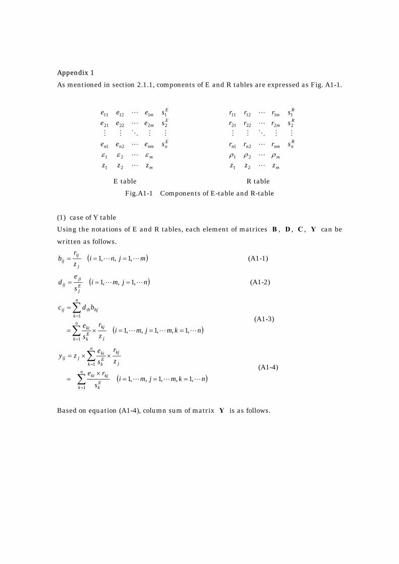
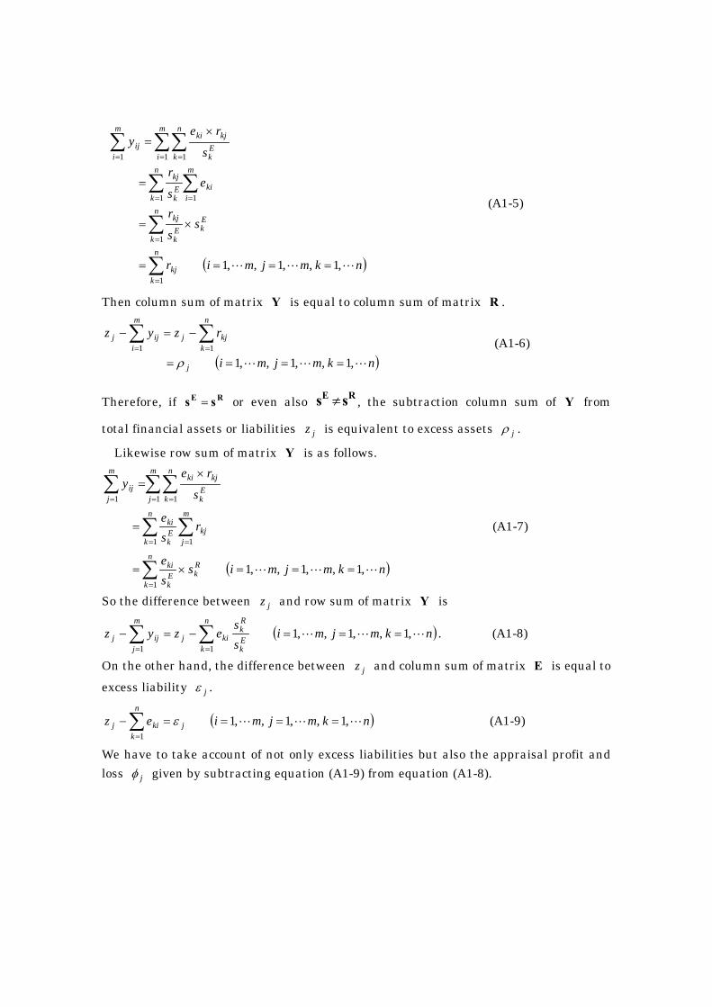
Appendix 1 As mentioned in section 2.1.1, components of E and R tables are expressed as Fig. A1-1.
m
m
Ennmnn
Em
Em
zzz
seee
seeeseee
L
L
L
MMOMM
L
L
21
21
21
222221
111211
εεε
m
m
Rnnmnn
Rm
Rm
zzz
srrr
srrrsrrr
L
L
L
MMOMM
L
L
21
21
21
222221
111211
ρρρ
E table R table Fig.A1-1 Components of E-table and R-table
(1) case of Y table Using the notations of E and R tables, each element of matrices , , , can be written as follows.
B D C Y
( mjnizr
bj
ijij LL ,1,,1 === ) (A1-1)
( njmis
ed E
j
jiij LL ,1,,1 === ) (A1-2)
( )nkmjmizr
se
bdc
n
k j
kjEk
ki
n
khjihij
LLL ,1,,1,,11
1
===×=
=
∑
∑
=
= (A1-3)
( )nkmjmis
re
zr
se
zy
n
kEk
kjki
n
k j
kjEk
kijij
LLL ,1,,1,,11
1
===×
=
××=
∑
∑
=
= (A1-4)
Based on equation (A1-4), column sum of matrix is as follows. Y
( )nkmjmir
ss
r
es
rs
rey
n
kkj
Ek
n
kEk
kj
m
iki
n
kEk
kj
m
i
n
kEk
kjkim
iij
LLL ,1,,1,,11
1
11
1 11
====
×=
=
×=
∑
∑
∑∑
∑∑∑
=
=
==
= ==
(A1-5)
Then column sum of matrix is equal to column sum of matrix Y R .
( )nkmjmi
rzyz
j
n
kkjj
m
iijj
LLL ,1,,1,,111
====
−=− ∑∑==
ρ (A1-6)
Therefore, if or even also , the subtraction column sum of Y from
total financial assets or liabilities is equivalent to excess assets .
RE ss = RE ss ≠
jz jρ
Likewise row sum of matrix is as follows. Y
( )nkmjmisse
rse
s
rey
n
k
RkE
k
ki
n
k
m
jkjE
k
ki
m
j
n
kEk
kjkim
jij
LLL ,1,,1,,11
1 1
1 11
===×=
=
×=
∑
∑ ∑
∑∑∑
=
= =
= ==
(A1-7)
So the difference between and row sum of matrix is jz Y
( )nkmjmiss
ezyzn
kEk
Rk
kij
m
jijj LLL ,1,,1,,1
11
===−=− ∑∑==
. (A1-8)
On the other hand, the difference between and column sum of matrix is equal to excess liability .
jz E
jε
( nkmjmiez j
n
kkij LLL ,1,,1,,1
1
====−∑=
ε ) (A1-9)
We have to take account of not only excess liabilities but also the appraisal profit and loss given by subtracting equation (A1-9) from equation (A1-8). jφ
( )nkmjmiss
e
ss
ee
ezss
ez
n
kEk
Rk
ki
n
kEk
Rk
ki
n
kki
n
kkij
n
kEk
Rk
kijj
LLL ,1,,1,,1)1(
)()(
1
11
11
===−=
−=
−−−=
∑
∑∑
∑∑
=
==
==
φ
(A1-10)
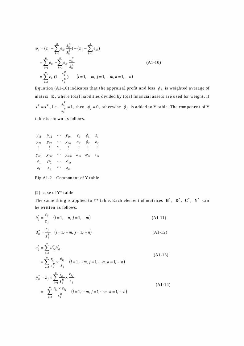
Equation (A1-10) indicates that the appraisal profit and loss is weighted average of
matrix , where total liabilities divided by total financial assets are used for weight. If
, i.e.
jφ
E
RE ss = 1=Ek
Rk
ss , then , otherwise is added to Y table. The component of Y
table is shown as follows.
0=jφ jφ
m
m
mmmmmmm
m
m
zzz
zyyy
zyyyzyyy
L
L
L
MMMMOMM
L
L
21
21
21
22222221
11111211
ρρρφε
φεφε
Fig.A1-2 Component of Y table (2) case of Y* table
The same thing is applied to Y* table. Each element of matrices , , , can be written as follows.
*B *D *C *Y
( mjnize
bj
ijij LL ,1,,1* === ) (A1-11)
( njmis
rd R
j
jiij LL ,1,,1* === ) (A1-12)
( )nkmjmize
sr
bdc
n
k j
kjRk
ki
n
kkjikij
LLL ,1,,1,,11
1
***
===×=
=
∑
∑
=
= (A1-13)
( )nkmjmis
er
ze
sr
zy
n
kRk
kjki
n
k j
kjRk
kijij
LLL ,1,,1,,11
1
*
===×
=
××=
∑
∑
=
= (A1-14)
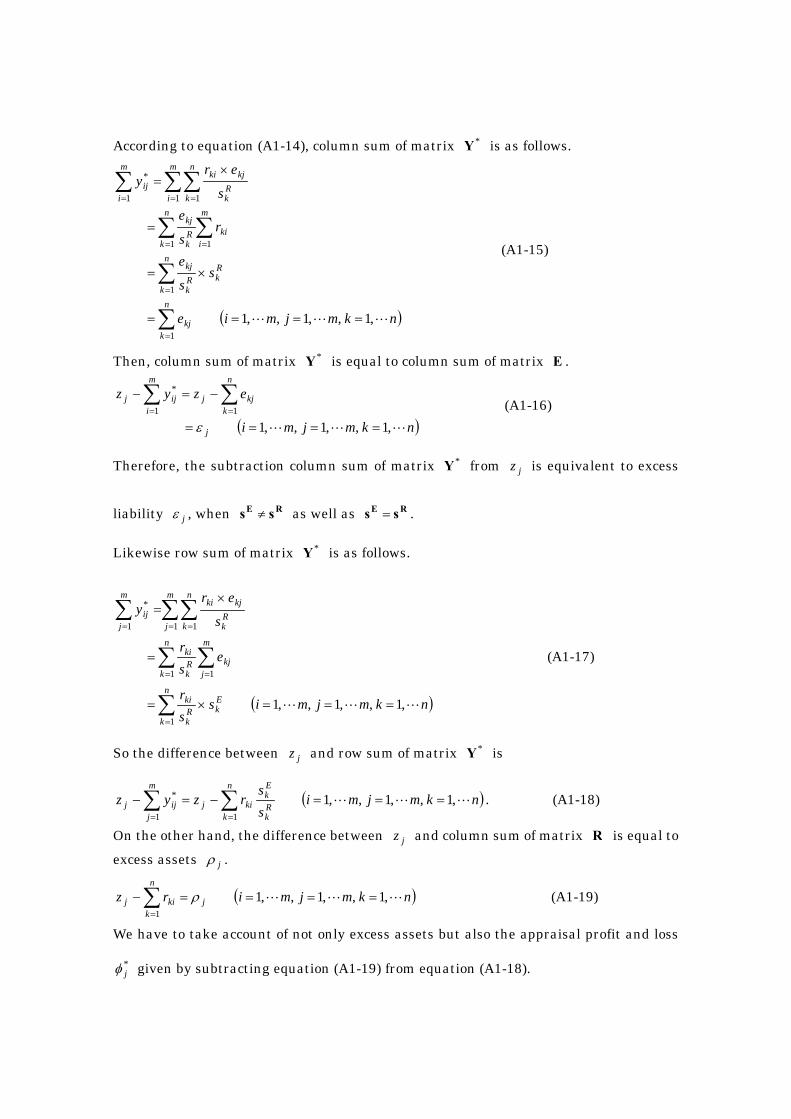
According to equation (A1-14), column sum of matrix is as follows. *Y
( )nkmjmie
ss
e
rs
es
ery
n
kkj
Rk
n
kRk
kj
m
iki
n
kRk
kj
m
i
n
kRk
kjkim
iij
LLL ,1,,1,,11
1
11
1 11
*
====
×=
=
×=
∑
∑
∑∑
∑∑∑
=
=
==
= ==
(A1-15)
Then, column sum of matrix is equal to column sum of matrix . *Y E
( )nkmjmi
ezyz
j
n
kkjj
m
iijj
LLL ,1,,1,,111
*
====
−=− ∑∑==
ε (A1-16)
Therefore, the subtraction column sum of matrix from is equivalent to excess
liability , when as well as .
*Y jz
jεRE ss ≠ RE ss =
Likewise row sum of matrix is as follows. *Y
( )nkmjmissr
esr
s
ery
n
k
EkR
k
ki
n
k
m
jkjR
k
ki
m
j
n
kRk
kjkim
jij
LLL ,1,,1,,11
1 1
1 11
*
===×=
=
×=
∑
∑ ∑
∑∑∑
=
= =
= ==
(A1-17)
So the difference between and row sum of matrix is jz *Y
( )nkmjmiss
rzyzn
kRk
Ek
kij
m
jijj LLL ,1,,1,,1
11
* ===−=− ∑∑==
. (A1-18)
On the other hand, the difference between and column sum of matrix jz R is equal to excess assets . jρ
( nkmjmirz j
n
kkij LLL ,1,,1,,1
1
====−∑=
ρ ) (A1-19)
We have to take account of not only excess assets but also the appraisal profit and loss
given by subtracting equation (A1-19) from equation (A1-18). *jφ
( )nkmjmiss
r
ss
rr
rzss
rz
n
kRk
Ek
ki
n
kRk
Ek
ki
n
kki
n
kkij
n
kRk
Ek
kijj
LLL ,1,,1,,1)1(
)()(
1
11
11
*
===−=
−=
−−−=
∑
∑∑
∑∑
=
==
==
φ
(A1-20)
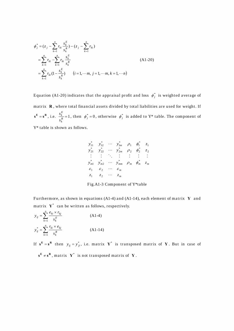
Equation (A1-20) indicates that the appraisal profit and loss is weighted average of
matrix
*jφ
R , where total financial assets divided by total liabilities are used for weight. If
, i.e. RE ss = 1=Rk
Ek
ss , then , otherwise is added to Y* table. The component of
Y* table is shown as follows.
0* =jφ*jφ
m
m
mmmmmmm
m
m
zzz
zyyy
zyyyzyyy
L
L
L
MMMMOMM
L
L
21
21
***2
*1
2*22
*2
*22
*21
1*11
*1
*12
*11
εεεφρ
φρφρ
Fig.A1-3 Component of Y*table Furthermore, as shown in equations (A1-4) and (A1-14), each element of matrix and
matrix can be written as follows, respectively.
Y*Y
∑=
×=
n
kEk
kjkiij s
rey
1
(A1-4)
∑=
×=
n
kRk
kjkiij s
ery
1
* (A1-14)
If then , i.e. matrix is transposed matrix of . But in case of
, matrix is not transposed matrix of .
RE ss =
RE ss ≠
*jiij yy =
*Y
*Y Y
Y
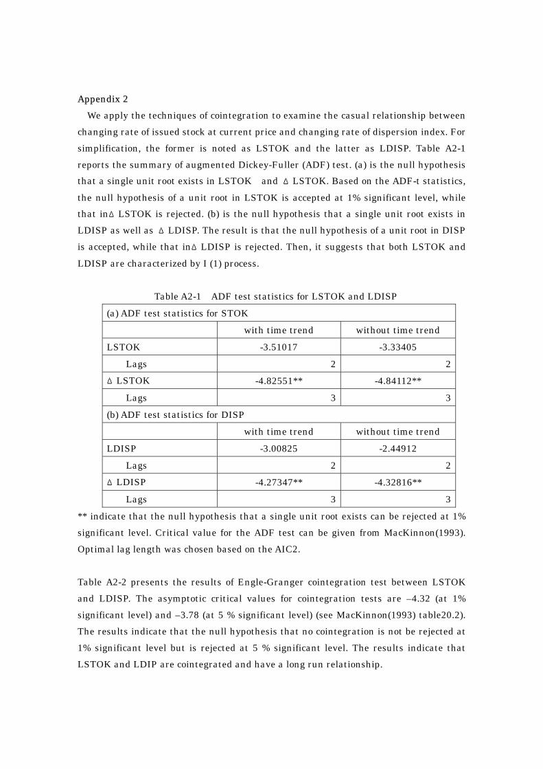
Appendix 2 We apply the techniques of cointegration to examine the casual relationship between
changing rate of issued stock at current price and changing rate of dispersion index. For simplification, the former is noted as LSTOK and the latter as LDISP. Table A2-1 reports the summary of augmented Dickey-Fuller (ADF) test. (a) is the null hypothesis that a single unit root exists in LSTOK and ΔLSTOK. Based on the ADF-t statistics, the null hypothesis of a unit root in LSTOK is accepted at 1% significant level, while that inΔLSTOK is rejected. (b) is the null hypothesis that a single unit root exists in LDISP as well as ΔLDISP. The result is that the null hypothesis of a unit root in DISP is accepted, while that inΔLDISP is rejected. Then, it suggests that both LSTOK and LDISP are characterized by I (1) process.
Table A2-1 ADF test statistics for LSTOK and LDISP (a) ADF test statistics for STOK with time trend without time trend LSTOK -3.51017 -3.33405
Lags 2 2 ΔLSTOK -4.82551** -4.84112**
Lags 3 3 (b) ADF test statistics for DISP with time trend without time trend LDISP -3.00825 -2.44912
Lags 2 2 ΔLDISP -4.27347** -4.32816**
Lags 3 3 ** indicate that the null hypothesis that a single unit root exists can be rejected at 1% significant level. Critical value for the ADF test can be given from MacKinnon(1993). Optimal lag length was chosen based on the AIC2. Table A2-2 presents the results of Engle-Granger cointegration test between LSTOK and LDISP. The asymptotic critical values for cointegration tests are –4.32 (at 1% significant level) and –3.78 (at 5 % significant level) (see MacKinnon(1993) table20.2). The results indicate that the null hypothesis that no cointegration is not be rejected at 1% significant level but is rejected at 5 % significant level. The results indicate that LSTOK and LDIP are cointegrated and have a long run relationship.
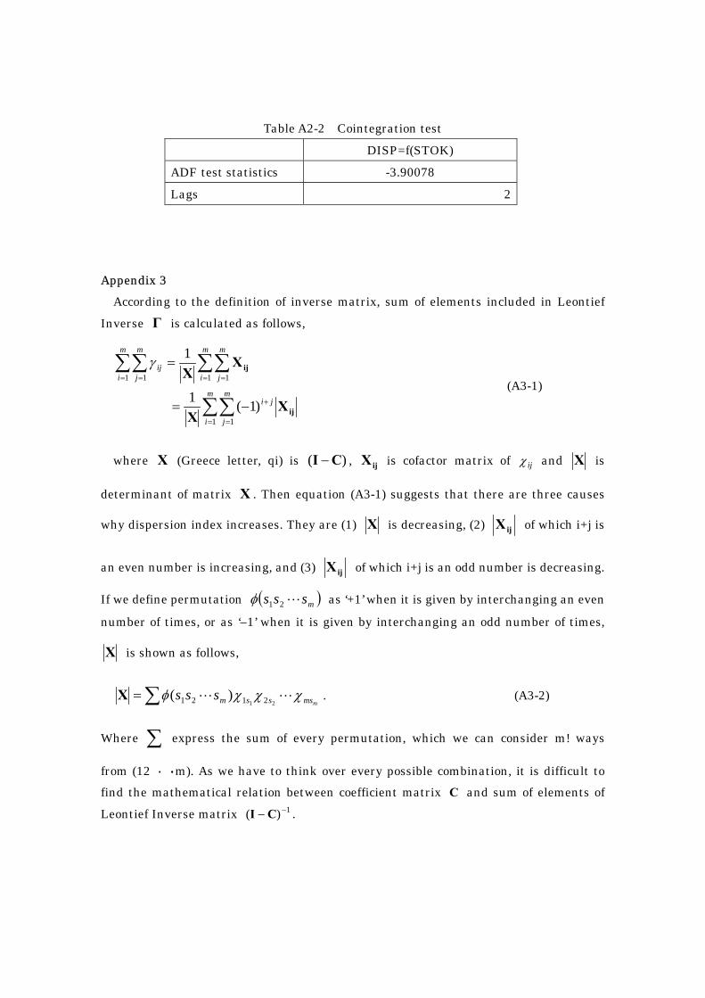
Table A2-2 Cointegration test DISP=f(STOK) ADF test statistics -3.90078 Lags 2
Appendix 3
According to the definition of inverse matrix, sum of elements included in Leontief Inverse is calculated as follows, Γ
∑∑
∑∑∑∑
= =
+
= == =
−=
=
m
i
m
j
ji
m
i
m
j
m
i
m
jij
1 1
1 11 1
)1(1
1
ij
ij
ΧΧ
ΧΧ
γ
(A3-1)
where (Greece letter, qi) is (Χ )CI − , is cofactor matrix of and ijΧ ijχ Χ is
determinant of matrix . Then equation (A3-1) suggests that there are three causes
why dispersion index increases. They are (1)
Χ
Χ is decreasing, (2) ijΧ of which i+j is
an even number is increasing, and (3) ijΧ
)ms
of which i+j is an odd number is decreasing.
If we define permutation ( ss L21φ as ‘+1’ when it is given by interchanging an even
number of times, or as ‘–1’ when it is given by interchanging an odd number of times,
Χ is shown as follows,
∑= mmsssmsss χχχφ LL21 2121 )(Χ . (A3-2)
Where express the sum of every permutation, which we can consider m! ways
from (12 ・・・m). As we have to think over every possible combination, it is difficult to find the mathematical relation between coefficient matrix and sum of elements of Leontief Inverse matrix .
∑
C1)( −−CI
Appendix 4
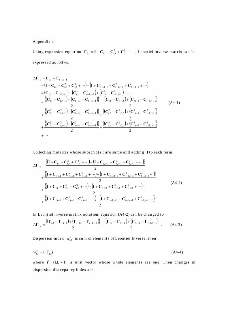
Using expansion equation , Leontief inverse matrix can be
expressed as follws.
L++++= 3,
2,,, tttttttt CCCIΓ
( ) (( ) ( ) ( )( ) ( ){ }
)
( ) ({ })
( ) ( ){ } ( ) ({ })
( ) ( ){ } ( ) ({ })
L
L
LL
+
−+−+
−+−+
−+−+
−+−+
−+−+
−+−=
+−+−+−=
++++−++++=
−=∆
−−−−−−−−
−−−−−−−−
−−−−−−−−
−−−−−−
−−−−−−
−−
22
22
22
31,1
31,
2,1
3,
31,1
3,1
31,
3,
21,1
21,
2,1
2,
21,1
2,1
21,
2,
1,11,11,111,
31,1
321,1
21,1
31,1
21,11,1
32
1,1,,
tttttttttttttttt
tttttttttttttttt
ttt,tttt,ttt,ttttt,t
ttt,tttt,tttt,t
ttttttt,tt,tt,t
tttttt
CCCCCCCC
CCCCCCCC
CCCCCCCCCCCCCC
CCCICCCI
ΓΓΓ
(A4-1)
Collecting matrices whose subscripts t are same and adding to each term. I
( ) ( ){ }
( ) ({ })
( ) ({ })
( ) ({ })2
2
2
2
31,1
21,11,1
31,
21,1
2,1
2,1,1
3,
2,
31,1
21,11,1
3,1
2,11
31,
21,1,
3,
2,
,
LL
LL
LL
LL
−−−−−−−−−
−−−
−−−−−−−−−
−−−
+++−+++++
++++−+++++
+++−+++++
++++−++++=∆
ttttttttttt,t
ttttttttttt,t
tttttttttt,tt
ttttttttttt,ttt
CCCICCCI
CCCICCCI
CCCICCCI
CCCICCCIΓ
(A4-2)
In Leontief inverse matrix notation, equation (A4-2) can be changed to ( ) ( ){ } ( ) ( ){ }
221,11,,1,1,1,11,,
,−−−−−−−− −+−
+−+−
=∆ tttttttttttttttttt
ΓΓΓΓΓΓΓΓΓ . (A4-3)
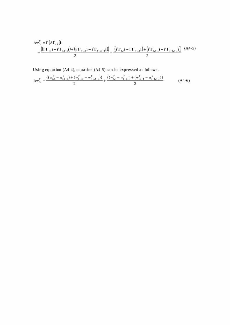
Dispersion index is sum of elements of Leontief Inverse, then Yttw ,
iΓi ttY
ttw ,, ′= (A4-4)
where is unit vector whose whole elements are one. Then changes in
dispersion discrepancy index are
)1,1,1( L=′i
( )( ) ( ){ } ( ) ({ })
221,11,,1,1,1,11,,
,,
iΓiiΓiiΓiiΓiiΓiiΓiiΓiiΓiiΓi
−−−−−−−− ′−′+′−′+
′−′+′−′=
∆′=∆
tttttttttttttttt
ttY
ttw (A4-5)
Using equation (A4-4), equation (A4-5) can be expressed as follows.
2)}(){(
2)}(){( 1,11,,1,1,1,11,,
,
Ytt
Ytt
Ytt
Ytt
Ytt
Ytt
Ytt
YttY
ttwwwwwwww
w −−−−−−−− −+−+
−+−=∆ (A4-6)
Eε'
s
z'
Rρ'
s
z'
institutionalsectors
finan
cia
ltr
ansa
ctions
institutionalsectors
finan
cia
ltr
ansa
ctions
Figure1 E table and R table
Xfinan
cia
ltr
ansa
ctions
financialtransactions
institutionalsectors
inst
itutional
secto
rs Y
U
X
A
finan
cia
ltr
ansa
ctions
financialtransactions
institutionalsectors
inst
itutional
secto
rs C
B
D
Figure 2 transaction matrices and coefficient matrices
Y ε
z'
institutionalsectors
inst
itutional
secto
rs
ρ'
z
Figure3 Y table
Y* ρ
z'
institutionalsectors
inst
itutional
secto
rs
ε'
z
Figure4 Y* table
Assets Liabilities Assets Liabilities
Loan to the localgovernment 100 100
Bank Local government
Figure5 concept pf dummy instrument method
Localgov.
Bank 100
institutional sectors
inst
itutional
secto
rs
Figure6 Asset-Liability-Matrix copiled from dummy instrument method
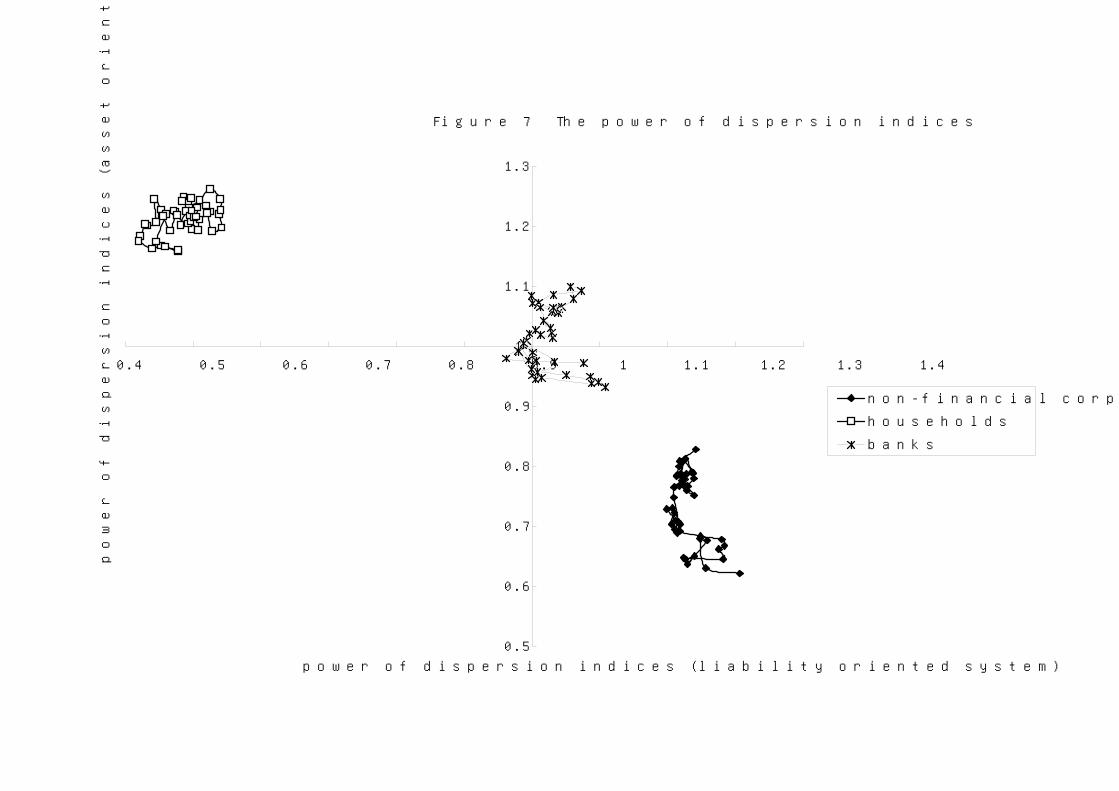
Figure 7 The power of dispersion indices
0.5
0.6
0.7
0.8
0.9
1
1.1
1.2
1.3
0.4 0.5 0.6 0.7 0.8 0.9 1 1.1 1.2 1.3 1.4
power of dispersion indices (liability oriented system)
pow
er
of
disp
ers
ion indi
ces
(ass
et
oriente
d sy
stem
)
non-financial corporations
households
banks
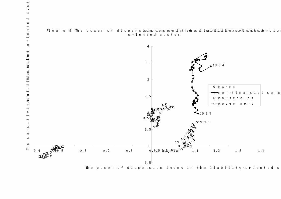
Figure 8 The power of dispersion index in the liability-oriented system and the sensitivity of dispersion index in the asset-oriented system
0.5
1
1.5
2
2.5
3
3.5
4
0.4 0.5 0.6 0.7 0.8 0.9 1 1.1 1.2 1.3 1.4
The power of dispersion index in the liability-oriented system
The s
ensi
tivi
ty o
f di
spers
ion inde
x in
the a
sset-
oriente
d sy
stem
banks
non-financial corporations
households
government
1954
1999
1999
1954
1962
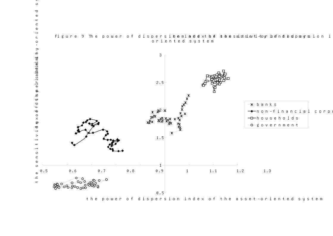
Figure 9 The power of dispersion index of the asset-oriented system and the sensitivity of dispersion index of the liability-oriented system
0.5
1
1.5
2
2.5
3
0.5 0.6 0.7 0.8 0.9 1 1.1 1.2 1.3
the power of dispersion index of the asset-oriented system
the s
ensi
tivi
ty o
f di
spers
ion inde
x of
the lia
bilit
y-oriente
d sy
stem
banks
non-financial corporations
households
government
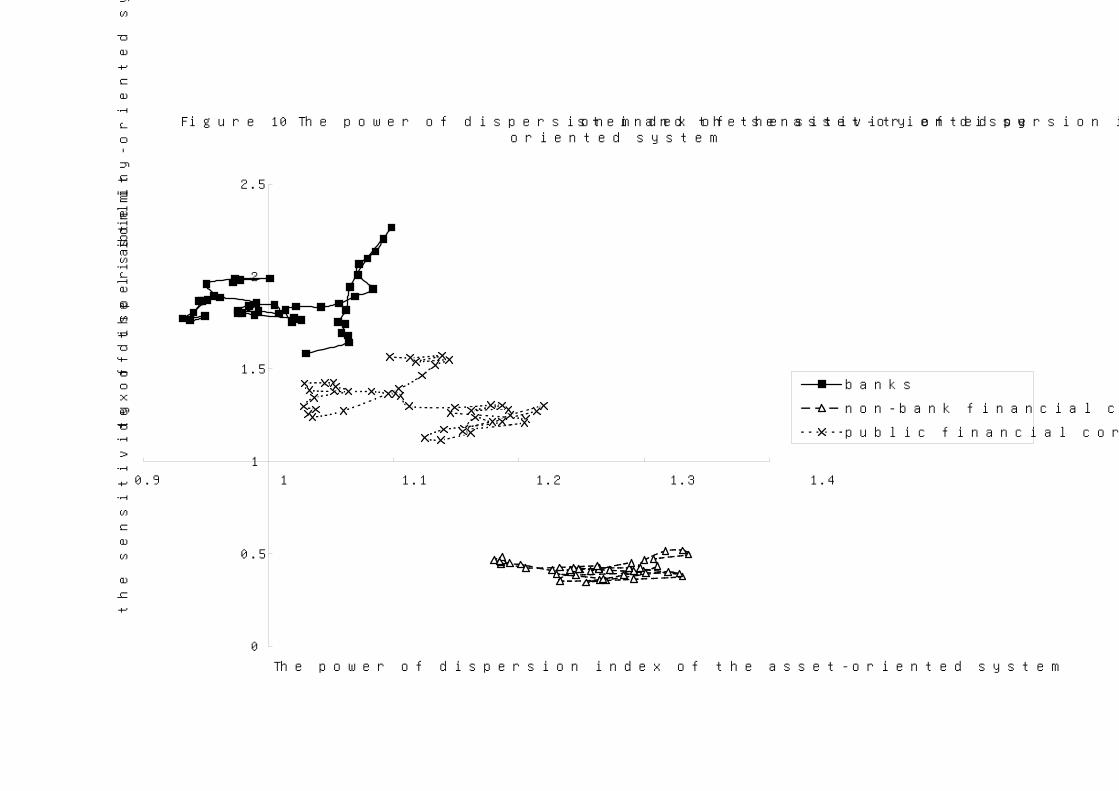
Figure 10 The power of dispersion index of the asset-oriented system and the sensitivity of dispersion index of the liability-oriented system
0
0.5
1
1.5
2
2.5
0.9 1 1.1 1.2 1.3 1.4
The power of dispersion index of the asset-oriented system
the s
ensi
tivi
ty o
f di
spers
ion inde
x of
the lia
bilit
y-oriente
d sy
stem
banks
non-bank financial companies
public financial corporations
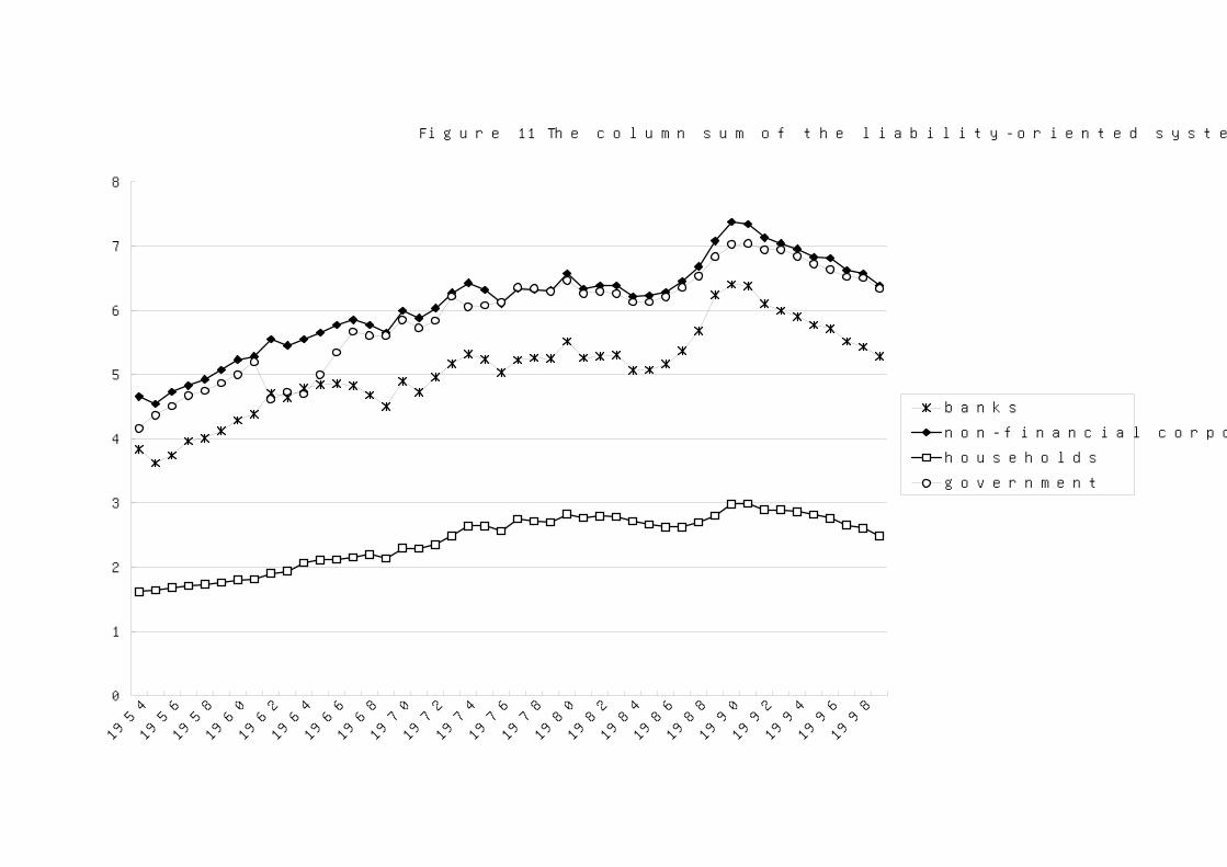
Figure 11 The column sum of the liability-oriented system
0
1
2
3
4
5
6
7
8
1954
1956
1958
1960
1962
1964
1966
1968
1970
1972
1974
1976
1978
1980
1982
1984
1986
1988
1990
1992
1994
1996
1998
banks
non-financial corporations
households
government
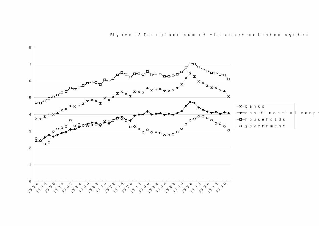
Figure 12 The column sum of the asset-oriented system
0
1
2
3
4
5
6
7
8
1954
1956
1958
1960
1962
1964
1966
1968
1970
1972
1974
1976
1978
1980
1982
1984
1986
1988
1990
1992
1994
1996
1998
banks
non-financial corporations
households
government
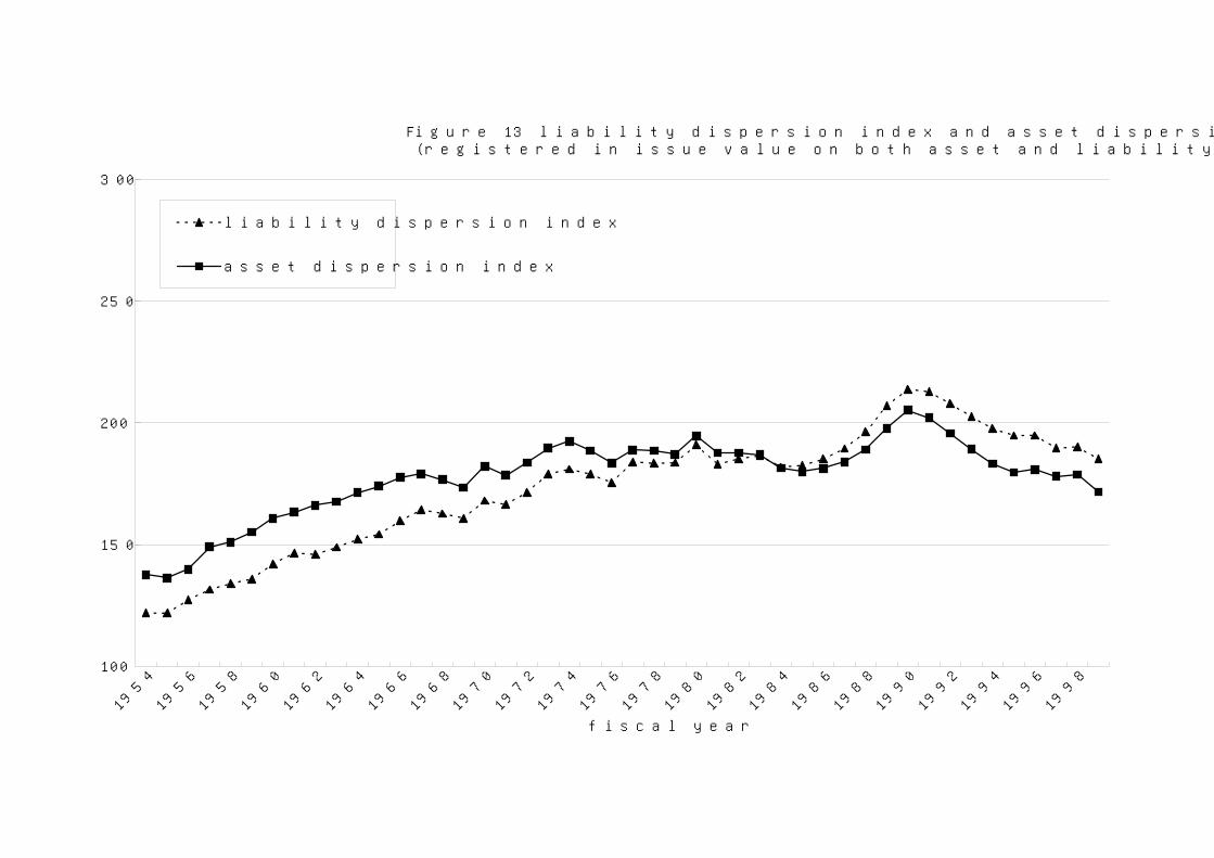
Figure 13 liability dispersion index and asset dispersion index(registered in issue value on both asset and liability sides)
100
150
200
250
300
1954
1956
1958
1960
1962
1964
1966
1968
1970
1972
1974
1976
1978
1980
1982
1984
1986
1988
1990
1992
1994
1996
1998
fiscal year
liability dispersion index
asset dispersion index
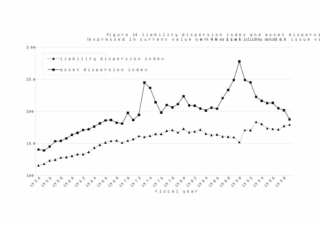
Figure 14 liability dispersion index and asset dispersion index(expressed in current value on the asset side and in issue value on the liability side)
100
150
200
250
300
1954
1956
1958
1960
1962
1964
1966
1968
1970
1972
1974
1976
1978
1980
1982
1984
1986
1988
1990
1992
1994
1996
1998
fiscal year
liability dispersion index
asset dispersion index
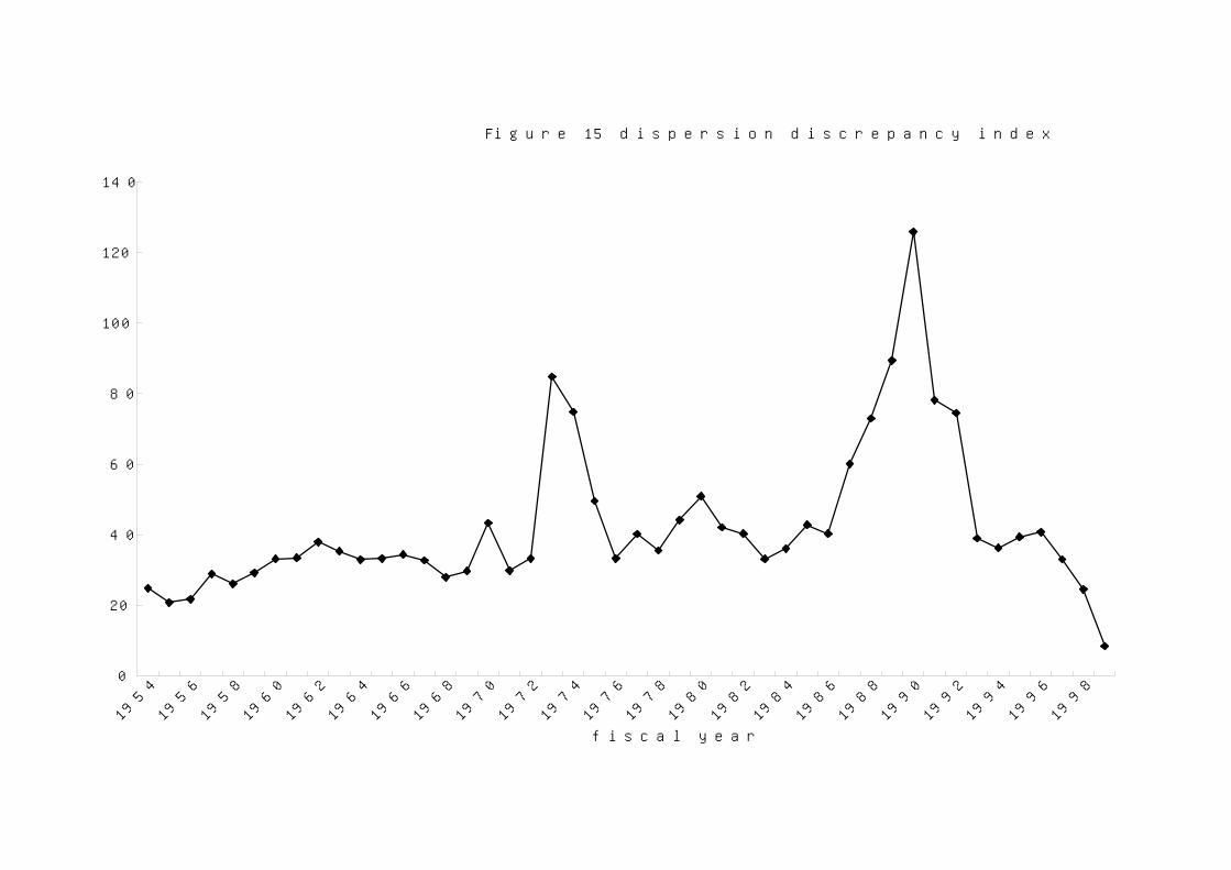
Figure 15 dispersion discrepancy index
0
20
40
60
80
100
120
140
1954
1956
1958
1960
1962
1964
1966
1968
1970
1972
1974
1976
1978
1980
1982
1984
1986
1988
1990
1992
1994
1996
1998
fiscal year
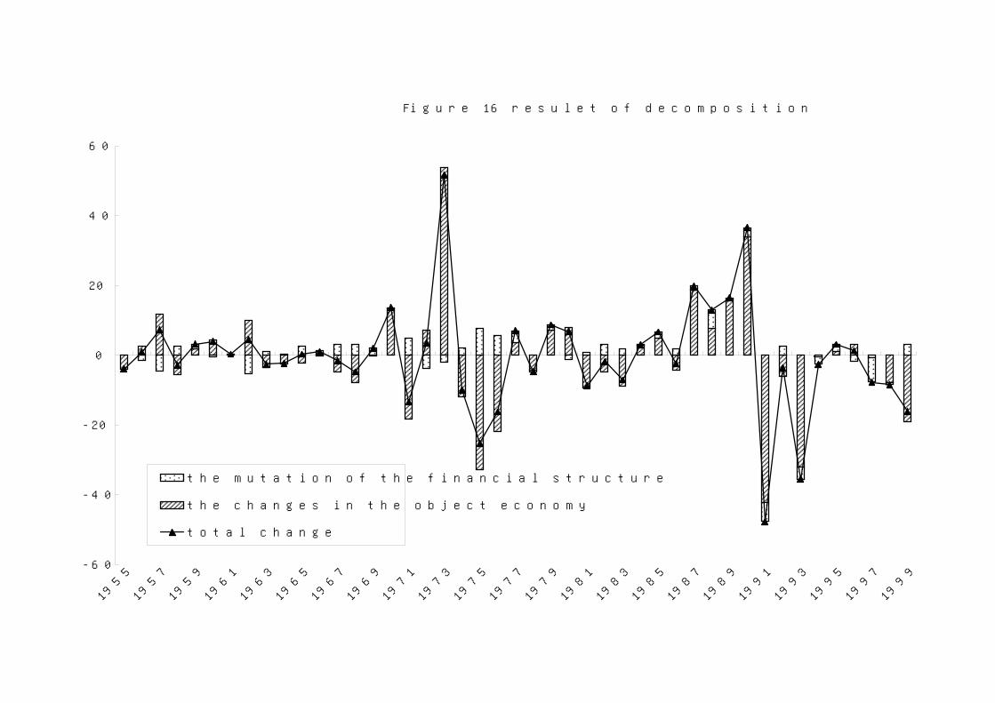
Figure 16 resulet of decomposition
-60
-40
-20
0
20
40
60
1955
1957
1959
1961
1963
1965
1967
1969
1971
1973
1975
1977
1979
1981
1983
1985
1987
1989
1991
1993
1995
1997
1999
the mutation of the financial structure
the changes in the object economy
total change
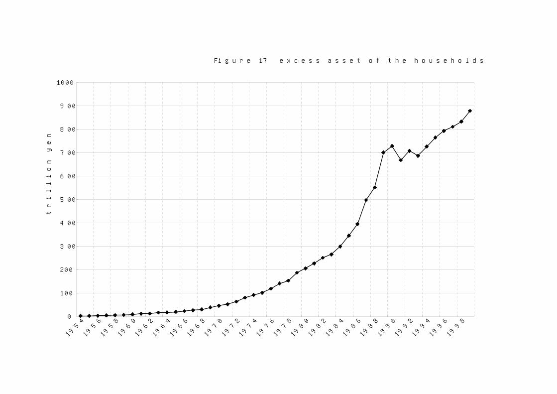
Figure 17 excess asset of the households
0
100
200
300
400
500
600
700
800
900
1000
1954
1956
1958
1960
1962
1964
1966
1968
1970
1972
1974
1976
1978
1980
1982
1984
1986
1988
1990
1992
1994
1996
1998
trill
ion y
en
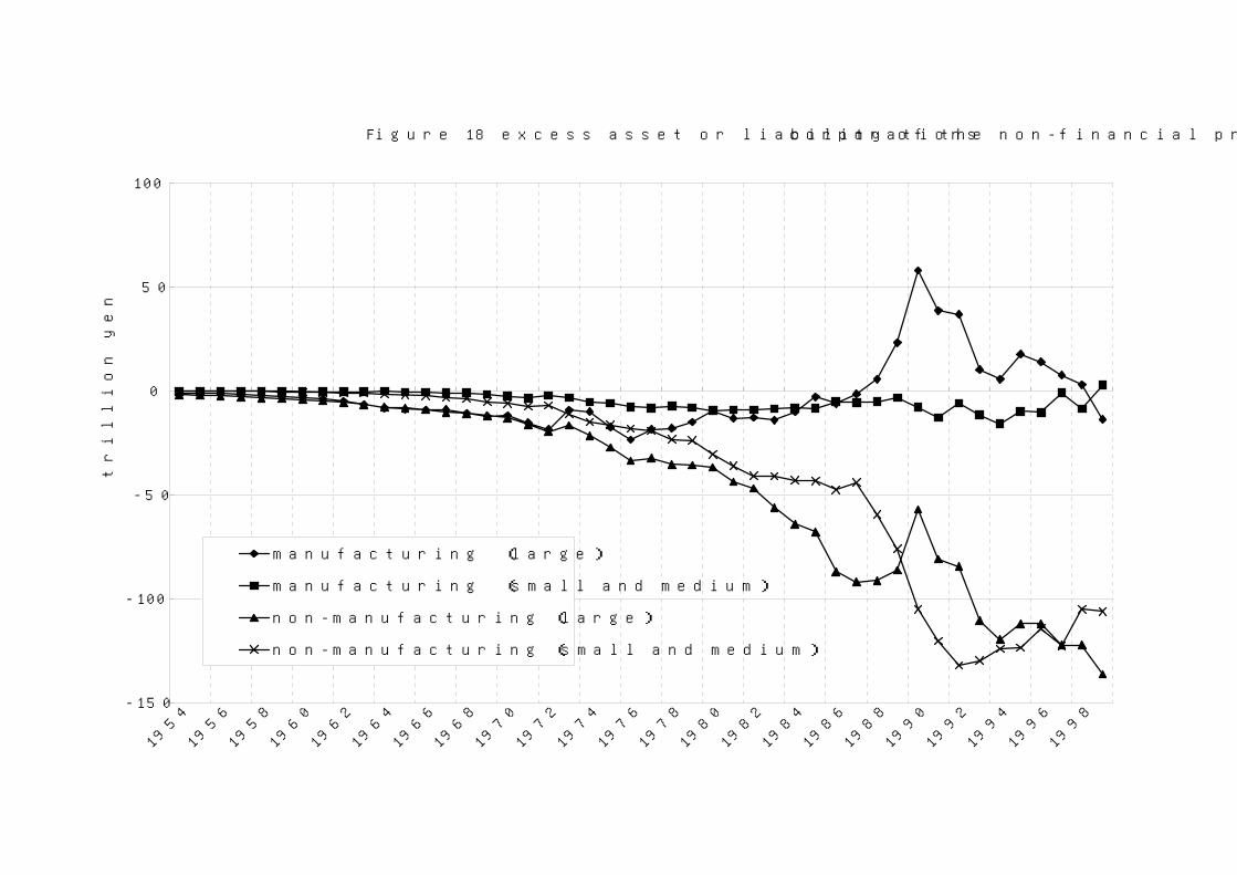
Figure 18 excess asset or liability of the non-financial private corporations
-150
-100
-50
0
50
100
1954
1956
1958
1960
1962
1964
1966
1968
1970
1972
1974
1976
1978
1980
1982
1984
1986
1988
1990
1992
1994
1996
1998
trill
ion y
en
manufacturing (large)
manufacturing (small and medium)
non-manufacturing (large)
non-manufacturing (small and medium)
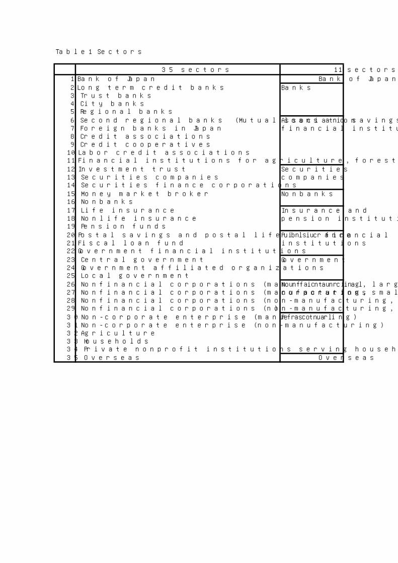
Table1 Sectors
35 sectors 11 sectors
1 Bank of Japan Bank of Japan2 Long term credit banks3 Trust banks4 City banks5 Regional banks6 Second regional banks (Mutual loans and savings banks)7 Foreign banks in Japan8 Credit associations9 Credit cooperatives
10 Labor credit associations11 Financial institutions for agriculture, forestry and fisheries12 Investment trust13 Securities companies14 Securities finance corporations15 Money market broker16 Nonbanks17 Life insurance18 Nonlife insurance19 Pension funds20 Postal savings and postal life insurance21 Fiscal loan fund22 Government financial institutions23 Central government24 Government affiliated organizations25 Local government26 Nonfinancial corporations (manufacturing, large)27 Nonfinancial corporations (manufacturing, small and medium)28 Nonfinancial corporations (non-manufacturing, large)29 Nonfinancial corporations (non-manufacturing, small and medium)30 Non-corporate enterprise (manufacturing)31 Non-corporate enterprise (non-manufacturing)32 Agriculture33 Households34 Private nonprofit institutions serving households35 Overseas Overseas
Personal
Insurance andpension institutions
Public financialinstitutions
Government
Nonfinancialcorporations
Banks
Associationfinancial institutions
Securitiescompanies
Nonbanks
Table2 Financial transactions
Financial transactions1 Deposits with the Bank of Japan2 Government deposits3 Currency4 Transferable deposits5 Time and savings deposits6 Certificates of deposit7 Foreign currency deposits8 Postal saving9 Trust beneficiary rights
10 Life insurance reserves11 Nonlife insurance reserves12 Mutual aid insurance 13 Deposit insurance14 Pension reserves15 Financing bills16 Central government securities17 Local government securities18 Public corporation securities19 Bank debentures20 Industrial securities21 Corporate stocks22 Investment trust beneficiary certificates23 External securities issued by residents24 Bank of Japan loans25 Call loan and money26 Bills purchased and sold27 Commercial paper28 Loan of trust accounts29 Loans by private financial institutions, (to corporations)30 Loans by private financial institutions, (to small enterprises)31 Loans by private financial institutions, (to public organizations)32 Loans by private financial institutions, (to non-corporate enterprises)33 Loans by private financial institutions, (housing loans)34 Loans by private financial institutions, (consumer credit)35 Loans by private financial institutions, (to overseas)36 Loans by public financial institutions, (to corporations)37 Loans by public financial institutions, (to small enterprises)38 Loans by public financial institutions, (to public organizations)39 Loans by public financial institutions, (to non-corporate enterprises)40 Loans by public financial institutions, (housing loans)41 Loans by public financial institutions, (consumer credit)42 Loans by public financial institutions, (to overseas)43 Trade credits and foreign trade credits44 Deposits with the Fiscal Loan Fund45 Foreign exchange reserves46 External claims and debts47 Others48 Difference between financial assets and liabilities49 Total