COMPLEMENTARY INFORMATION FOR REDUCING PARAMETER UNCERTAINTY IN DISTRIBUTED RAINFALL-RUNOFF MODELING

Giha LEE1, Yasuto Tachikawa2, Takahiro Sayama3 and Kaoru Takara4

1Doctoral Student, Department of Urban and Environmental Engineering, Kyoto University Nishikyo-ku, Kyoto, 615-8540, Japan, leegiha@flood.dpri.kyoto-u.ac.jp

2Associate Professor, Department of Urban and Environmental Engineering, Kyoto University Nishikyo-ku, Kyoto, 615-8540, Japan, tachikawa@mbox.kudpc.kyoto-u.ac.jp 3Assistant Professor, Disaster Prevention Research Institute, Kyoto University

Gokasho, Uji, Kyoto, 611-0011, Japan, sayama@flood.dpri.kyoto-u.ac.jp 4 Professor, Disaster Prevention Research Institute, Kyoto University

Gokasho, Uji, Kyoto, 611-0011, Japan, takara@flood.dpri.kyoto-u.ac.jp

ABSTRACT

A natural rainfall-runoff process is conceptualized (or modeled) by hydrologist’s perception or experience in mathematical form. These rainfall-runoff models are usually calibrated and verified based on streamflow data at the outlet of interest. The streamflow data, aggregated response over a catchment is obviously required but is not sufficient information to identify conceptual parameters of such models since numerous parameter combinations can often result in either identical model performance measures or indistinguishable hydrographs. One of the efficient techniques to enhance the parameter identification is to use additional constraints (or complementary information) in model calibration. This study aims to exemplify the equifinality problem due to insufficiency of model identification based only on streamflow data in distributed rainfall-runoff modeling. Moreover, a potential use of additional constraints provided by a computational tracer method is presented in order to reject non-physical parameter set(s) among numerous plausible ones.

Keywords: parameter identification, complementary information, computational tracer

method 1. INTRODUCTION

One of fundamental steps in rainfall-runoff modeling is parameter identification, which is typically referred to as calibration. However, despite many advanced automatic optimization algorithms, uncertainty in the calibrated parameter estimates still remains very large. For example, a large number of different parameter sets can lead to equivalent model performance measures and even indistinguishable streamflow sequences. Beven and Binley (1992) used the special term ‘equifinality’ to explain the possibility of plausible parameter sets and it has been an interesting issue in hydrological modeling (Savenije, 2001).

A rainfall-runoff model is usually identified based on streamflow. Kuczera and Franks (2002) argued that it is required, but is not sufficient information to identify the conceptual model parameter(s) accurately. They pointed out that one of the effective techniques to resolve this insufficiency is to increase the contents of information using complementary output variables such as runoff, soil moisture, piezometric levels measured at different locations within a catchment, environmental isotopes, etc. Then, the model parameters are constrained by the additional information augmented by these newly adopted hydrological variables.

Experimental methods such as isotopic hydrograph separations by isotope tracers and

Advances in Hydro-Science and Engineering, vol. VIII Proc. of the 8th International Conference on Hydro-Science and Engineering, Nagoya, Japan, Sept. 9-12, 2008

stream water residence time have been useful to provide additional evaluative criteria for water quantity or quality modeling. However, these approaches require the revision of models for producing multiple output variables so that it may worsen parameter identifiability. Moreover, these approaches to reduce parameter uncertainty involved in modeling processes are limited to small scale well-measured experimental sites. Therefore, it is essential to develop the method capable of providing complementary constraints for further parameter identification in large scale basins.

Sayama et al. (2007) proposed a computational tracer method to track the spatiotemporal origin of simulated hydrograph using a new concept, named spatiotemporal record matrix of streamflow. Then, they combined this scheme with the nonlinear distributed model, KWMSS2 that takes into account unsaturated and saturated subsurface flows. This method can temporally split the hydrograph into the same number of components corresponding to the selected number of rainfall segments without any hydrochemical measure. Moreover, it can trace the spatial origin of streamflow at the time step of interest and also visualize the spatially-distributed runoff sources within a catchment. Consequently, this new technique enables modelers to assess the effects of plausible parameter combinations on internal responses of a catchment as well as global responses such as hydrographs. Then, these internal behaviours can be used as posterior evaluative criteria to either reject erroneous parameter set(s) or confirm reliable one(s) among numerous plausible sets.

This paper aims to exemplify the equifinality problem due to insufficiency of model identification based only on streamflow data in distributed rainfall-runoff modeling. A potential use of additional constraints provided by the computational tracer method is presented in order to reduce parameter uncertainty. 2. DISTRIBUTED RAINFALL-RUNOFF MODEL & STUDY CATCHMENT

Kinematic Wave Method for Surface and Subsurface runoff (KWMSS) assumes that a permeable soil layer covers the hillslope as illustrated in Figure 1. The soil layer consists of a capillary layer in which unsaturated flow occurs and a non-capillary layer where saturated flow occurs. According to this runoff mechanism, if the water depth, h is higher than the soil depth, D then overland flow occurs. The stage-discharge relationship (Tachikawa et al., 2004) is defined as:

⎪⎩

⎪⎨

⎧

≤−+−+≤≤−+≤≤

=hddhdhvdv

dhddhvdvdhdhdv

q

sm

scacc

sccacc

cccc

,)()(),(

0,)/(

α

β

(1)

Figure 1 Schematic model structure and extended stage- discharge relationship of KWMSS.

)(trxq

th

=∂∂

+∂∂

(2)

Flow rate, q of each slope segment is calculated by above governing equations

combined with the continuity equation (2), where =c cv k i ; =a av k i ; / β=c ak k ; /α = i n ; i is slope gradient, ck is hydraulic conductivity of the capillary soil layer, ak is

hydraulic conductivity of the non-capillary soil layer, n is roughness coefficient, the water depth corresponding to the water content is sd and the water depth corresponding to maximum water content in the capillary pore is cd . There are five parameters (n, ak , sd , cd and β ), which are assumed to be spatially uniform over the catchment, to be optimized in KWMSS.

This model is applied to model a mesoscale mountainous catchment (211km2). The study site is the Kamishiiba catchment which lies within Kyushu region in Japan. The topography of this area is hilly with the elevation varying from 400m to 1700m and land-use type is mostly forest. 3. SELECTION OF PLAUSIBLE PARAMETER SETS

In this study, seven different parameter sets are prepared to investigate their influences

on global and internal catchment responses. Table 1 summarizes all parameter values used here. The first three parameter sets are estimated by Shuffled Complex Evolution (SCE) method (Duan et al., 1992) with three different Objective Functions (OFs): Simple Least Squares (SLS), Heteroscedastic Maximum Likelihood Estimator (HMLE), and Relative Modified Index of Agreement (RMIA) (Lee et al., 2007). The next is the optimal value (i.e. OPT, the highest densities in each posterior parameter distribution) tuned by Shuffled Complex Evolution Metropolis (SCEM) method (Vrugt et al., 2003). Finally, the other three remainders are sampled from the estimated posterior parameter distribution based on different events (i.e. Sample (1), (2) and (3)). Figure 2 presents the examples of both the marginal posterior probability distributions and the optimal values of chosen parameter values for three parameters, ak , sd and cd of KWMSS. Note that the posterior distributions are estimated by behavioral 6000 parameter sets after convergence of SCEM trials.

Table 1 Selected plausible parameter sets of KWMSS2.

Parameter

ID n [m-1/3 s] ka [m/s] ds [m] dc [m] β [-]

SLS 0.5 0.013 0.893 0.496 19.8

HMLE 0.5 0.011 0.485 0.085 2.95

RMIA 0.5 0.010 0.468 0.068 2.59

OPT 0.5 0.013 0.865 0.472 18.6

Sample(1) 0.49 0.049 0.510 0.480 2.95

Sample(2) 0.5 0.050 0.610 0.430 4.47

Sample(3) 0.5 0.019 0.619 0.468 6.20

Figure 2 Selected plausible parameter sets and marginal posterior probability distributions of three parameters: ak , sd and cd . 4. GLOBAL RESPONSES OF CATCHMENT TO PLAUSIBLE PARAMETER SETS

Probabilistic results of the hydrograph are obtained from the ensemble simulation of

KWMSS associated with 6000 parameter sets sampled from the posterior parameter distribution. Figure 3 shows how the parameter uncertainty propagates into estimates of hydrograph simulation uncertainty. Moreover, hydrographs reproduced by the plausible parameter sets are also included in this Figure. The black dotted line indicates the observed streamflow data and the grey shaded region is 90% simulation uncertainty with respect to the posterior distribution of the parameter estimates.

Figure 3 Simulation uncertainty associated with the behavioral parameter sets, having 90% confidence interval (i.e. 5400 (6000×90%) hydrographs are plotted), derived by SCEM-UA and simulated hydrographs associated with plausible parameter sets.

In spite of considerable parameter uncertainty, the ensemble simulation results match

well to the observed runoff and the simulation uncertainty boundary is very narrow. Therefore, it can be said that the distributed rainfall-runoff model, KWMSS is likely to be exposed to equifinality problem that makes it difficult to discriminate between reliable and unreliable parameter sets. Moreover, this figure supports that only streamflow data is not enough to identify the model parameters accurately.

Hence, the complementary constraint is necessary to augment the power to select the erroneous parameter combination(s) out from a large number of plausible ones. The subsequent sections demonstrate the internal dynamic responses of the catchment to these plausible parameter sets.

ka ds dc

5. COMPLEMENTARY INFORMATION FOR FURTHER PARAMETER IDENTIFICATION

In this study, the spatiotemporal variation of streamflow origin due to different

parameter values is applied as complementary information for further parameter identification. For this objective, two experiments are implemented by the computational tracer method with a newly developed concept, spatiotemporal matrix. First, the spatial origin of streamflow observations within the catchment is traced by this tracer method with respect to specific four time steps: 1, 48, 134 and 182hours in order to examine the effect of model parameters on the internal catchment responses. Second, the simulated hydrographs generated by these mimic parameter combinations are temporally separated into six runoff components corresponding to pre-decided rainfall components by using temporal record of the spatiotemporal matrix. 5.1 Brief Introduction of Computational Tracer Method based on Spatiotemporal

Matrix of Streamflow

The spatiotemporal record matrix as illustrated in Figure 4 is used in order to trace where streamflow comes from when it rains. The dimensions of matrix ( )Ri t are given with S rows, number of sub-units within catchment and T columns, number of temporal classes where i is specific slope element; t is time. Figure 4(c) shows the spatiotemporal matrix at time t at the catchment outlet. For example, the value belonging to spatial zone C and temporal class 2 implies that the proportion of runoff in (C,2) entry to the streamflow observation at time t is 6%. When summarizing the whole values vertically along the columns, the temporal contribution of rainfall to streamflow can be obtained. Likewise, the spatial contribution of sub-catchments on streamflow is calculated by horizontal summation along the rows. As a result, modelers can distinguish the difference between old water (i.e. pre-event water at time class 0 possesses 15%) and new water (i.e. new water components are 30% at time class 1 and 55% at time class 2, respectively) at the specific time t. Moreover, it is possible to track the spatially-distributed origin for runoff generation using this matrix with information stored in each slope element, for instance, downstream spatial zones (e.g. D, E and F) contribute more than 60% of streamflow whereas upstream classes (e.g. A, B and C) affect runoff generation less at time t. More details about this conceptual matrix are presented in Sayama et al., (2007).

Figure 4 Schematic diagram of hydrograph separation based on (a) temporal record of streamflow, (b) spatial record of streamflow and (c) spatiotemporal record matrix of streamflow (Sayama et al., 2007); S=6, T=5.

5.2 Variation of Spatial Origin of Streamflow due to Plausible Parameter Sets

Figure 5 shows the drainage network based on 250m DEM, separated sub-catchments and the divided rainfall components for application of the computational tracer method. Here, the Kamishiiba catchment is represented by 3190 slope elements (i.e. S=3190, see Figure 5(a)).

Figure 5 Drainage network of the Kamishiiba catchment based on 250m DEM, (b) eight divided sub-catchment and (c) divided rainfall components of historical flood event.

The contributions of each slope element to streamflow observations at particular time steps, 1, 48, 134 and 182 hours are illustrated in Figure 6. At the beginning of rainfall-runoff process, the adjacent slope elements to river channel, which is referred to as riparian zone constitute primarily of the streamflow while the water stored in upstream slope elements do not reach the river channel yet. As time goes on, contributive areas spread gradually over the catchment and eventually, all slope elements contribute for the streamflow generation.

The contribution of each slope element to streamflow at the specific time step is represented by Relative Ratio of Total Discharge (RRTD), defined as:

=1

( )RRTD ( ) 100 (%)( )

RRTD ( ) 100 (%)S

= ×

=∑

ii outlet

ii

D ttD t

t (3)

where i is slope element number; ( )iD t is discharge at the outlet from slope element i within catchment at time t; ( )outletD t is total discharge of the outlet at time t. The RRTD is categorized into eight classes. In addition, to quantify the variation of spatial distribution of streamflow origin at sub-catchment scale, a simple index, Contributing Percentage of the sub-catchment (CP) is proposed as follows:

8

1

CP ( ) RRTD ( )

CP ( ) 100 (%)∈

=

=

=

∑

∑

j ji j

jj

t t

t (4)

where j is the sub-catchment number; the study catchment is divided into eight sub-catchments to investigate the variations of contributing area due to plausible parameter

combinations (see Figure 5(b)).

Figure 6 Spatially-distributed origin of streamflow for each parameter set. Colorful snapshots for the spatially-distributed origin of streamflow apparently present

that even though global responses of catchment with respect to the plausible parameter sets are nearly identical, the internal responses are completely different. For example, the predominant class of the RRTDs for Sample (1) and Sample (2) is class 3 at 1hour while major classes are 5 and 7 in the applications of other parameter sets. Moreover, the slope elements near the river channel have remarkable influence on the peak discharge in SLS, HMLE and RMIA cases at the peak time, 134hours. On the other hand, contributing slope elements of Sample (1) are not limited to river channel in particular but much broader than other applications. Figure 6 obviously supports the fact that the spatial distribution of streamflow origin is quite sensitive to the parameter values.

However, interesting finding is that the difference of spatial distribution of streamflow origin due to the distinct parameter values is attenuated (or dampened) as the water stored in grid cells go into the outlet through the catchment. As a result of this kind of spatial deterioration phenomenon, equifinality could arise in distributed rainfall-runoff modeling. This attenuation effect is also captured by the CP index as shown in Figure 7. The contribution of sub-catchment 1 of Sample (1) to the runoff at the 1hour time step is 4% larger than other results based on the different parameter sets. However, all CPs for each sub-

SLS HMLE RMIA Sample(1) Sample(2) Sample(3) OPT

1hr

48hrs

134hrs

182hrs

1 2 3 4 5 6 7 8

1 2 3 4 5 6 7 8

1 2 3 4 5 6 7 8

1 2 3 4 5 6 7 8

catchment do not show significant difference with other time steps despite the considerable difference in terms of plots for spatially-distributed origin of streamflow.

Figure 7 Calculated CPs for specific time steps; 1, 48, 134 and 182hours.

5.3 Variation of Temporal Origin of Streamflow due to Plausible Parameter Sets

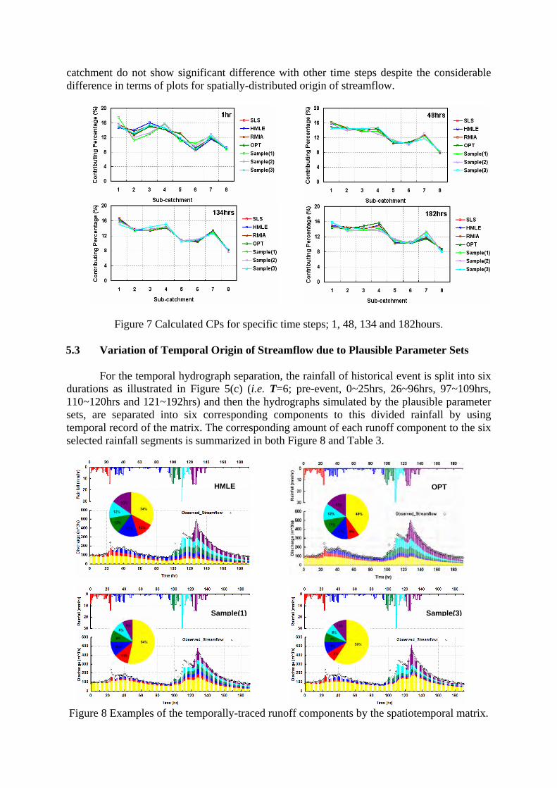
For the temporal hydrograph separation, the rainfall of historical event is split into six durations as illustrated in Figure 5(c) (i.e. T=6; pre-event, 0~25hrs, 26~96hrs, 97~109hrs, 110~120hrs and 121~192hrs) and then the hydrographs simulated by the plausible parameter sets, are separated into six corresponding components to this divided rainfall by using temporal record of the matrix. The corresponding amount of each runoff component to the six selected rainfall segments is summarized in both Figure 8 and Table 3.

Figure 8 Examples of the temporally-traced runoff components by the spatiotemporal matrix.

HMLE OPT

Sample(1) Sample(3)

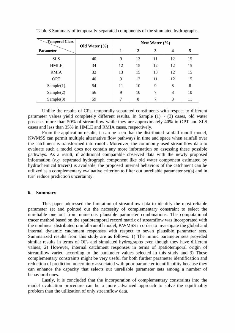
Table 3 Summary of temporally-separated components of the simulated hydrographs.

New Water (%) Temporal Class

Parameter Old Water (%)

1 2 3 4 5

SLS 40 9 13 11 12 15 HMLE 34 12 15 12 12 15 RMIA 32 13 15 13 12 15 OPT 40 9 13 11 12 15

Sample(1) 54 11 10 9 8 8 Sample(2) 56 9 10 7 8 10 Sample(3) 59 7 8 7 8 11

Unlike the results of CPs, temporally separated constituents with respect to different

parameter values yield completely different results. In Sample (1) ~ (3) cases, old water posseses more than 50% of streamflow while they are approximately 40% in OPT and SLS cases and less than 35% in HMLE and RMIA cases, respectively.

From the application results, it can be seen that the distributed rainfall-runoff model, KWMSS can permit multiple alternative flow pathways in time and space when rainfall over the catchment is transformed into runoff. Moreover, the commonly used streamflow data to evaluate such a model does not contain any more information on assessing these possible pathways. As a result, if additional comparable observed data with the newly proposed information (e.g. separated hydrograph component like old water component estimated by hydrochemical tracers) is available, the proposed internal behaviors of the catchment can be utilized as a complementary evaluative criterion to filter out unreliable parameter set(s) and in turn reduce prediction uncertainty.

6. Summary This paper addressed the limitation of streamflow data to identify the most reliable

parameter set and pointed out the necessity of complementary constraint to select the unreliable one out from numerous plausible parameter combinations. The computational tracer method based on the spatiotemporal record matrix of streamflow was incorporated with the nonlinear distributed rainfall-runoff model, KWMSS in order to investigate the global and internal dynamic catchment responses with respect to seven plausible parameter sets. Summarized results from this study are as follows: 1) The mimic parameter sets provided similar results in terms of OFs and simulated hydrographs even though they have different values; 2) However, internal catchment responses in terms of spatiotemporal origin of streamflow varied according to the parameter values selected in this study and 3) These complementary constraints might be very useful for both further parameter identification and reduction of prediction uncertainty associated with poor parameter identifiability because they can enhance the capacity that selects out unreliable parameter sets among a number of behavioral ones.

Lastly, it is concluded that the incorporation of complementary constraints into the model evaluation procedure can be a more advanced approach to solve the equifinality problem than the utilization of only streamflow data.

REFERENCES Beven, K. and Binley, A.M. (1992), The future of distributed models: model calibration and

uncertainty prediction, Hydrol. Processes, 6(3), pp.279-298. Duan, Q., Sorooshian, S. and Gupta, V.K.(1992), Effective and efficient global optimization

for conceptual rainfall-runoff models, Water Resour. Res., 28(4), pp.1015-1031. Kuczera, G. and Franks, S.W. (2002), Testing hydrologic models: Fortification or

Falsification?, in Mathematical Models of Large Watershed Hydrology, edited by V.P. Singh, and D. Frevert, pp.141-185, Water Resources Publishers, Highland Ranch, Colorado.

Lee, G., Tachikawa, Y. and Takara, K. (2007), Identification of model structural stability through comparison of hydrologic models, Annual J. Hydraul. Eng., JSCE, 51, pp.49-54.

Savenije H.H.G. (2001), Equifinality, a blessing in disguise?, Hydrological Processes, 15, pp. 2835-2838.

Sayama, T., Tatsumi, K., Tachikawa, Y. and Takara, K. (2007), Hydrograph separation based on spatiotemporal record of streamflow in a distributed rainfall-runoff model, J. Japan Society of Hydrol. & Water Resours., JSCE, 20(3), pp.214-225 (in Japanese).

Tachikawa, Y., Nagatani, G. and Takara, K. (2004), Development of stage-discharge relationship equation incorporating saturated–unsaturated flow mechanism, Annual J. Hydraul. Eng., JSCE, 48, pp.7-12 (in Japanese).

Vrugt, J.A., Gupta, H.V., Bouten, W. and Sorooshian, S. (2003), A shuffled complex evolution metropolis algorithm for optimization and uncertainty assessment of hydrologic model parameters, Water Resour. Res., 39(8), 1201, doi:10.1029/2002WR001642.