Embed Size (px)
Citation preview
Nonlinear Analysis, Theory. Merhods & Applicarions, Vol. 5, No 8, pp. 821-833, 1981. 0362-546X/81 080821-13 $02.00/O
Printed in Great Britain. 0 1981 Pergamon Press Ltd
COMPLETE COMPARATIVE STATIC DIFFERENTIAL EQUATIONS*
ROBERT KALABA and LEIGH TESFATSION
Department of Economics, University of Southern California, Los Angeles, California 90007, U.S.A
(Received 24 June 1980)
Key words and phrases: Parameterized system of equations, complete variational equations, qualitative analysis, numerical implementation, economic applications.
1. INTRODUCTION
COMPARATIVE static problems in economics typically reduce to determining the response of a
vector x = (x,, . . . , xn) to changes in a scalar parameter ~1, where x and t( satisfy a system of one- dimensional equations
Y”(X, a)
0 = Y(x, a) =
i:r
. . (1)
Equations having form (1) arise as first-order conditions in microeconomic constrained optimiza- tion models, as defining characterizations for general equilibrium and macroeconomic models, and as steady-state solution characterizations for descriptive and optimal growth models. (See Silberberg [12], Hansen [7], Cass and Shell [3], and Brock [l].)
If Y :R"' ' -+ R" is continuously differentiable over a neighborhood of a point (x0, a”) in R n+l for which Y(xO, LX’) = 0 and IY,( x0, or’)] # 0, then the implicit function theorem guarantees the existence of a continuously differentiable function x: N(cr’) + R" over some open neighbor-
hood N(crO) of CX’ in R such that dx z (ix) = - YX(X(X), a)-lYJx(a), X), G! E N(cP). (2)
Equation (2) is the fundamental relation underlying almost all comparative static studies in economics.t The basic objective of these studies is to obtain determinate signs for the components of dx(cl)/da, so that in principle the economic theory underlying the system of equations (1) can be empirically tested. Unfortunately, optimality and stability postulates, which place
* This work was partially supported by the National Science Foundation under Grant ENG 77-28432 and the National Institutes of Health under Grant GM 23732-03.
7 Silberberg [ 1 l] has recently shown that the usual comparative statics relations in maximization models which are obtainable by use of (2) are special cases of the positive semi-definiteness of a matrix of cross partials of the Lagrangean function for a certain primal-dual problem introduced by Samuelson [lo].
821
822 R. KALABA and L. TESFATSION
restrictions on the Jacobian matrix
J(z) = ‘y&(X), X(x (3)
often allow at best a partial signing of the components of dx(a)/da. (See Silberberg [ 121.) A third type of postulate, specific functional forms for Y( .), leads in principle to a complete signing of dx(x)/dx, but such postulates are rarely used in theoretical economic studies.
One basic reason for the relatively limited local nature of the comparative static results obtain- able by use of equation (2) is that (2) is typically an analytically incomplete differential system, even for known functions ‘Y( .). Specifically, closed form representations for the Jacobian inverse J(a)-’ as a function of u are often not feasible when n 3 3. Thus initial conditions requires the supplementary
process. This was Davidenko’s original proposal in [6], and it has since become a standard
explicit representation dictates that qualitative obtained by use of (2) must be strictly nature.
In 2, below, we a complete differential system for x(a) and J(I)- ‘. More precisely, adjoint matrix A(a) and determinant validate a differential
z (a) = Trace(44Ha)),
(44
(4b)
(4c)
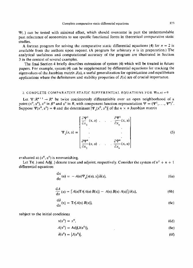
where B(a) E dJ(a)/dcc is expressible as a known function of x(a), A(a), 6(a), and CC Initial conditions for system (4) must be provided at a parameter point a” by specifying values for ~(a’), A(@‘), and 6(r0) satisfying Y(x(u’), r”) = 0, ,4(x0) = Adj(J(aO)), and &a’) = IJ(a’)l # 0, where J(cr’) is defined as in (3). In general there may be more than one vector X(X’) satisfying Y(x(a’), x”) = 0 for any given CC’. System (4) tracks the solution branch corresponding to the selected X(X”). (See the illustrative examples in Section 3, below.)
The basic system of comparative static differential equations (4) can be used in a qualitative manner to investigate sign retention over parameter intervals of interest. The sign of 6(a) is obviously of critical importance.
Alternatively, system (4) can be numerically integrated on a computer. The ability to obtain explicit solution trajectories for x(a), Adj(J(z)), and IJ(n)] over parameter intervals of interest would seem to provide a useful additional tool for examining and suggesting theoretical con- jectures about system (1). It is important to stress that initial value problems such as (4), com- prising n2 + n + 1 ordinary differential equations, can be solved with great speed and accuracy by present-day computers even if n is of the order 102, and this computer capability is steadily being improved. (See [2, 4, 51.) Thus, using (4) a wide variety of specific functional forms for
Complete comparative static differential equations R23
Y( .) can be tested with minimal effort, which should overcome in part the understandable past reluctance of economists to use specific functional forms in theoretical comparative static studies.
A fortran program for solving the comparative static differential equations (4) for n = 2 is available from the authors upon request. (A program for arbitrary II is in preparation.) The analytical usefulness and computational accuracy of the program are illustrated in Section 3 in the context of several examples.
The final Section 4 briefly describes extensions of system (4) which will be treated in future papers. For example, system (4) can be supplemented by differential equations for tracking the eigenvalues of the Jacobian matrix J(U), a useful generalization for optimization and equilibrium applications where the definiteness and stability properties of J(X) are of crucial importance.
2. COMPLETE COMPARATIVE STATIC DIFFERENTIAL EQUATIONS FOR yl(x,a) = 0
Let Y :R”+ ’ + R” be twice continuously differentiable over an open neighborhood of a point (x0, a’), x0 in R” and CL’ in R, with component function representation Y = (Y’, . . , Yn)7. Suppose Y(x”, c(O) = 0 and the determinant IYX(xo, x0)1 of the n x n Jacobian matrix
Y,(x, x) =
$,,a) . . . 1
g (x, 4 II
E(x,a) . . g&.) 1 ”
(5)
evaluated at (x0, a’) is nonvanishing. Let Tr( .) and Adj( .) denote trace and adjoint, respectively. Consider the system of n2 + n + 1
differential equations
g (4 = - Awgx(r), +%a),
dA -s (a) = [A(4Tr(A(4 B(4) - A(4 W4 A(41/&4,
$ (tl) = Tr(A(cc) B(a)),
(64
W
(6~)
subject to the initial conditions
X(P) = x0,
A(a’) = Adj(.I(crO)),
@O) = IJ(@.O)l,
(6d)
(he)
(0

X24 R. KALABA and L. TESFATSION
where J(a) = YX( x a a , ( ), ) given by
and the 0th component b,,(u) of the IZ x n matrix B(a) = dJ(a)jda is
h,,(U) E i iJ2yi ~ (x(4, X0 2 (2) + g (x(N), X0. (6g) m = 1 ax,ax m J
Note, using (6a). that B(H) is expressible as a known function of x(a), A(H), and CI. It ~111 now be estabhshed that system (6) has a unique solution over some open interval iV(z’)
containing a”. Moreover, this solution satisfies Y(x(cl), E) = 0, A(E) = Adj(J(E)), and 6(a) = 15(x)1 for z E N(aO). It should be remarked that existence and uniqueness theorems for solutions of initial value problems such as (6) have to be local in nature in view of the nonlinearity of the differential equations. In practice, however, the length of AJ(aO) may actually be infinite. If one or both of the largest possible values 2 and s2 satisfying (a0 - .si, z” + 2) c N(a’) are finite. numerical integration of the initial value problem (6) can be used to locate the critical endpoints.
(See the examples in Section 3, below).
LEMMA 1. Let M(U) be an n x n matrix function of cx over an open neighborhood of a point U’ in R such that M,(U) E dM(a)jda exists and is continuous over this neighborhood and IA4(a”)l # 0. Then, for some open neighborhood N(n”) of z”, there exists a unique continuously differentiable II x n matrix function A( .) and a unique continuously differentiable scalar function 6( .) over
N(xO) satisfying
2 (a) = [A(a)Tr(A(a)Ma(a)) - ~(a)~,(+l(~)ll~(~), (74
g (a) = Tr(44Ml(4), x E N(xO),
subject to the initial conditions
A(crO) = Adj(M(z’)),
&X0) = IM(aO)l.
Moreover, A(. ) and 6(. ) satisfy
A(z) = Adj(M(z)), x E iV(a’),
(7b)
(7c)
(7d)
(8a)
6(a) = (M(x)l, x E LwO). (8b)
Proqf: The existence of a unique continuously differentiable solution to system (7) over some open neighborhood of x0 follows directly from Theorem 9.1 in Hartman [8, p. 1371. TO establish Lemma 1, it thus suffices to show that one solution to system (7) in an open neighborhood of x0 is given by A*(a) E Adj(M(a)) and S*(z) = [Mu.
By definition of M(U), the adjoint A*(x) and determinant 6*(a) of M(U) are continuously differentiable functions of ‘X over some open neighborhood N’(a’) of a’, and
A”(u) M(a) = d*(a)z, a E N’(crO). (9)
By assumption, S*(zO) # 0. Without loss of generality, suppose 6*(z) # 0 for a~ IVYa’).

Complete comparative static differential equations X25
Differentiating (9) with respect to ct, multiplying through by A*(a), and rearranging terms, one obtains
z (CY) = [A*(U) dd*(cc)/dcr - A*(a)M,(a)A*(a)]/s*(a), tl E N’(aO). (10)
It remains to determine dd*(a)/dcr. Letting mij(a) denote the ijth element of M(a), and letting Cij(oz) denote the cofactor of mij(a), the determinant 6*(a) of M(a) may be expressed as
6*(a) = igl m&l C&J (11)
foranyjE{l,..., rz}. Thus, using the chain rule together with (1 l), one obtains
= i f: Cij(cx)~(2) is1 j=l
= Tr(CT(z) M,(g))
= Tr(A*(cr) MS(a)), a E N’(cr’), (12)
where the ijth element of the n x n matrix C(a) is C&a), and superscript T denotes transpose. Combining (10) and (12), A*( _) and 6*( .) are solutions to system (7) over some open neighborhood
of UO. Q.E.D.
THEOREM 1. For some open neighborhood N(clO) of R’, there exist unique continuously differenti- able solution functions 6( .), x( .), and A( .) for the initial value problem (6) over N(u’). Moreover, these solution functions satisfy
Y(x(a), a) = 0, t( E N(cP), (13a)
A(U) = Adj(J(cc)), a E N(aO), (13b)
and 6(a) = (J(cr)(, c1 E N(P). (13c)
Proof The regularity conditions imposed on Y( .) guarantee, by the implicit function theorem, the existence of a unique continuously differentiable function x( .) over some open neighborhood N’(cr’) of x0 satisfying ~(a’) = x0, Y(x(cc), N) = 0, cx E N’(aO), and
g (4 = -J(a) - l Y,(x(a), a), a E N’(aO), (14)
where J(U) E Y,(x(u), x). In particular, J(a) is a continuously differentiable n x n matrix function of c1 over N’(cr’) with (J(u’)) # 0. The remainder of Theorem 1 follows immediately from Lemma 1.
Q.E.D.
For some comparative static studies it may be useful to have a differential system directly in terms of x(a) and the Jacobian inverse matrix J(E)-‘. This approach was first suggested in [9]. The next theorem provides such a system.
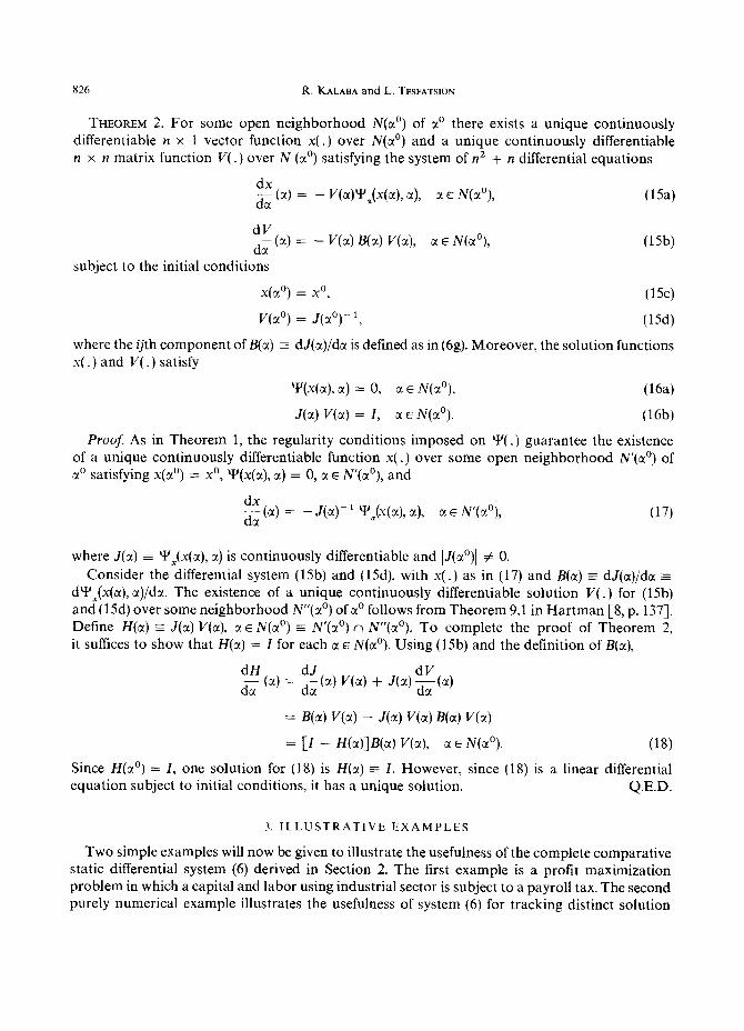
826 R. KALABA and L. TESFATSION
THEOREM 2. For some open neighborhood N(a”) of x0 there exists a unique continuously differentiable n x 1 vector function x( .) over N(a’) and a unique continuously differentiable n x n matrix function V( .) over N (a’) satisfying the system of n2 + n differential equations
dx G(Z) = - WX)Y~(X(X), z), tl E N(cr’), (154
E(a) = - V(cx) B(E) V(a), ct E N(a'), (1%)
subject to the initial conditions
x(aO) = x0, (15c)
V(crO) = J(XO)_ l, (15d)
where the ijth component of B(z) = dJ(a)/da is defined as in (6g). Moreover, the solution functions x( .) and V( .) satisfy
Y(x(cc), u) = 0, a E N(x’), (16a)
J(a) V(a) = I, z E N(a’). (16b)
Proqf: As in Theorem 1, the regularity conditions imposed on Y( .) guarantee the existence of a unique continuously differentiable function x( .) over some open neighborhood N’(cr’) of x0 satisfying X(CL’) = x0, Y(x(~), a) = 0, a E N’(u’), and
dx z (~1) = -J(a)- ’ Y,(x(ct), z), a E N’(ccO), (17)
where J(X) = YX(x(x), u) is continuously differentiable and (J(n’)l # 0.
Consider the differential system (15b) and (15d), with x( .) as in (17) and &cc) 3 dJ(cl)jdcc E dYX(x(u), a)/dcc. The existence of a unique continuously differentiable solution V( .) for (15b) and (15d) over some neighborhood N”(Lx’) of a0 follows from Theorem 9.1 in Hartman [S, p. 1373. Define H(a) E J(a) V(a), TV E N(a’) = N’(a’) n N”(x’). To complete the proof of Theorem 2, it suffices to show that H(m) = I for each a E N(cY’). Using (15b) and the definition of B(z),
g! (a) = E(a) V(a) + J(a) $4 = B(a) V(cc) - J(a) V(a) B(x) V(a)
= [Z - H(a)]B(c() V(a), x E N(a'). (18)
Since ~(a~) = I, one solution for (18) is H(a) = I. However, since (18) is a linear differential equation subject to initial conditions, it has a unique solution. Q.E.D.
3. ILLUSTRATIVE EXAMPLES
Two simple examples will now be given to illustrate the usefulness of the complete comparative static differential system (6) derived in Section 2. The first example is a profit maximization problem in which a capital and labor using industrial sector is subject to a payroll tax. The second purely numerical example illustrates the usefulness of system (6) for tracking distinct solution

Complete comparative static differential equations 827
branches, and for locating critical parameter values a where the Jacobian matrix J(U) becomes singular.
Let F:R:+ -+ R be a production function defined by
F(K, L) = KYE, 0 < y, 0 < /3, y + p < 1, (19)
where K and L denote capital and labor services, and let P, R, and W denote output price, nominal capital rental rate, and nominal wage rate, respectively. Consider the problem of maxi- mizing profits
PF(K, L) - RK - [l + M”] WL (20)
with respect to K > 0 and L > 0 for given P > 0, R > 0, W > 0, and t1’ > 0, where t1’ denotes a payroll tax rate.
Since F( .) is strictly concave over R: +, necessary and sufficient conditions for positive K” and L? to maximize profits (20) are given by
0 = FJK’, L?) - (R/P) = FJK’, 12’) - r, (214
0 = F,(K’, I!?) - [l + ~“1 (W/P) = F,(K’, I!?) - [l + CL’]W. (2lb)
It is easily checked that the Jacobian matrix associated with system (21) is nonsingular. Thus, using standard implicit function arguments, the existence of positive K” and L!? satisfying (21) guarantees the existence of unique continuously differentiable functions K( .) and L( .) in a neighborhood iV(crO) of ct” satisfying
K(aO) = K”, L(a”) = Lo, (224
0 = FJK(a), L(a)) - r, a E N(a’), (22’9
0 = F,(K(a), L(a)) - w, a E N(a’), (224
dL z(to =
UK@4 44)w < 0
(WI ’
c( E N(ao)
’
(224
(224
where the determinant IJ(cr)l of the Jacobian matrix J(cr) associated with system (22b) and (22~) is given by
IQ)1 = &,(K(cO, L(4) F&K@), L(4) - P,,(K(4, .&))I2
= y#lK(a)2’- 2 L(ay2 [l - y - p] > 0, ccEN(tlO). (220
It will now be shown how Theorem 1 can be applied to this profit maximization problem to obtain explicit solution trajectories for K(a), L(a), IJ(a)l, and other relevant terms over arbitrary tax rate intervals of the form [a’, a’], 0 < a0 < a’, given arbitrary admissible numerical values for r, w, y, and fl. Define a function Y = (Y’, Y2)’ taking R3 into R2 by
Y”(K, L, a) = FJK, L) - r, (234
Y’(K, L, a) = F,(K, L) - [I + a]w. (23b)
Assume (21) holds for some K” > 0, Lo > 0, and a0 3 0, hence Y(K”, L!‘, a’) = 0. Clearly Y( .)

818 R. KALABA and L. TESFATSION
is twice continuously differentiable in a neighborhood of the point (K’, Lo, @), and, by (22f), the determinant \J(aO)l of the Jacobian matrix.
(24)
evaluated at a0 is nonvanishing. Thus, by Theorem 1, over some open neighborhood N(a’) of CI’ there exist unique con-
tinuously differentiable scalar functions K( .), L(.), and 6( .), and a unique continuously differenti- able 2 x 2 matrix function A(.) satisfying the system of 22 + 2 + 1 differential equations
= - A(a) ‘I’&W, L(a), cr)/@), (25a)
$ (4 = C&4 Tr(64 H4) - 44 B(x) &)]/G(x),
d6 z(z) = Tr(&x) B(x)),
Subject to the initial conditions
K(x") = K", L(a") = L?,
II(MO) = Adj(J(uO)),
GO) = JJ(aO)l,
where B(a) = dJ(cl)/da. Moreover, K( .), L( . ), A( .), and 6(.) satisfy
Y(K(a), Lb),a) = 0, z EN,
A(a) = Adj(J(cr)), tl E AJ(a’),
6(a) = /J(n)), n E AJ(aO).
(254
(25e)
(2%)
(264
(26b)
(2k)
The comparative static differential equations (25) were integrated on an IBM 370/Model 158 for various admissible parameter specifications (r, tv, 6, 8) and initial values (K', Lo, a") using a single precision Fortran program designed for arbitrary functions Y: R3 + R'. Table 1 describes
one such experiment. Note that the monotonic behavior of K( .), L( .), and 6( ,) is as expected, using the analytically derivable results (22) for this simple 2 x 2 example. The last two columns indicate the high numerical accuracy of the computer program. The actual step size in a was 0.01, with fifty steps taken in all. The CPU execution time was 1.08 seconds. The program of course evaluates many additional interesting and useful expressions not appearing in Table 1, e.g. A(u), dK(cc)/dcc, dL(cc)/dcr, d&cc)/da, and dA(cc)/dcc. A fourth order Adams-Moulton integration method with a Runge-Kutta start was employed.

Complete comparative static differential equations 829
Table 1. Trajectories for capital K(a), labor L(a), and the Jacobian determinant 6(a) as the payroll tax a increases from 0 to 0.5, and a check of the first order conditions (26a)
a a) L(a) YWa), L(a), a)
000 1.0 1.0 0.034 72 0.0 0.05 0.971 15 0.92490 0.040 59 -3.95 x lo-’ 0.10 0.944 42 0,858 56 0.047 11 -6.05 x lo-’ 0.15 0.91956 0.199 62 0.054 3 1 6.63 x lo-’ 0.20 0.89638 0.74698 0.062 23 -6.61 x lo-’ 0.25 0.87469 0.699 75 0.07091 -2.92 x lo-’ 0.30 0.854 35 0.657 19 0.080 39 -8.80 x lo-’ 0.35 0.83522 0.61868 0.090 7 1 -5.66 x lo-’ 0.40 0.817 19 0,583 71 0.10191 4.51 x lo-’ 0.45 0.800 16 0.55184 0.11402 1.59 x 10⁻⁶ 0.50 0.78405 0.522 70 0.12709 4.75 x lo-’
0.0 1.04 x 10-G 6.66 x lo-’ 3.66 x lo-’ 7.43 x 10⁻⁷ 6.19 x lo-’ 2.84 x lo-’ 2.35 x lo-’
-1.24 x 10m6 -1.90 x 10-h
5.35 x 10⁻¹
Parameter values: y = r = $, /I = w = *. Initial values: K” = Lo = 1. E0 = 0.
The comparative static differential equations (25) also facilitate multiparameter sensitivity studies. For example, as indicated in Fig. 1, a simultaneous increase in the Table I parameters p and w from $ to 5 uniformly lowers capital usage from K(M) to K*(cr) and uniformly increases the value of the Jacobian determinant from I to 6*(a). Similarly, labor usage L(E) uniformly decreases. Such monotonic shifts in K(a), L(a), and 6(cr) in response to multiple changes in r, w, y, and p do not appear to be easily detectable from the usual comparative static relations (22).
06 t
Fig. 1. Response of K(a) and Z(a) to a simultaneous increase in the production function coefficient #l and the real wage rate w.

830 R. KALABA andL. TESFATSION
Now consider the following simple system of equations
0 = xy - X = Y”(X, y, a),
0 = x + 3y - 1 EE Y2(x, y, CX).
(27a)
(27b)
Given any real CX, system (27) has the two solutions
x = 1 - 3g, y = [1 + 41 - 12a]/6,
x = 1 - 3y, I‘ = [l - 4’ - 12~]/6.
(28a)
(2gb)
The Jacobian matrix associated with system (27) is singular if and only if 3y = x, i.e. using (28)
if and only if cI = 75. Note that the solutions x and y in (28) are real if and only if tl lies in the interval
t--a, A). Given any x0. y”, and a0 E (- cc, &) satisfying (27), implicit function arguments guarantee the existence of unique real-valued continuously differential functions x( .) and y( .) over an open neighborhood N(x”) of x0 satisfying
X(X0) = x0, y(aO) = yo, (29a)
X(U) y(a) - X = 0, L? E N(aO), (29b)
x(a) + 34’(U) - 1 = 0, z E A&P), (29~)
where [J(a)1 denotes the determinant of the Jacobian matrix
(29f.l
It is immediate that Theorem 1 is applicable to system (27), given any initial solution values x0, yO, and U” E (- ca, &). Specifically, over some open neighborhood IV(#) of E” there exist unique continuously differentiable scalar functions x( . ), y( .), and 6( .) and a unique continuously differentiable 2 x 2 matrix function A( .) satisfying
dA da (x) = [Afa)Tr(A(a) B(a)) - A(4 Ha) A(41/@cO,
(30a)
WV
(3Oc) z (a) = Tr(&) B(a)),

Complete comparative static differential equations 831
subject to the initial conditions
x(aO) = x0, yhO) = YO,
II = Adj(J(cr’)),
S(aO) = IJ(aO)(,
(304
(30e)
(3Of)
where B(cr) E dJ(a)/da. Moreover, x( .), y( .), A( .), and 6( .) satisfy
x(a) y(a) - a = 0, il E iv(uO),
x(a) + 3y(cr) - 1 = 0, CI E iv@,
A(a) = Adj(J(a)), tl E N(a’),
&Lxx) = (@)I, crEN(RO).
(314
(31b)
(31c)
(314
The comparative differential equations (30) were integrated over the CI interval [0,&l for each of the two distinct initial solution values x0 and y” corresponding to a0 = 0, namely,
and
x0 = 1 and y” = 0
x0 = 0 and y” = $.
(32)
(33)
The step size in CL was $ 2 0.00833, and the CPU execution time was on the order of 0.36
seconds. As expected, in each case the singularity of J(a) at a = A was strongly indicated by a blow-up of the determinant derivative db(a)/dcc as CI neared the critical point & z 0.08333. Table 2 describes the trajectories for xl@), y’(cr), #(cr), and d#(cr)/da corresponding to the first root (32). The final two columns of Table 2 indicate the high numerical accuracy of the computer program, even near the critical point c1 = &.
Similar results were obtained for the trajectories x’(a), y2(a), S2(cr), and da2(cr)/dcr corresponding to the second root (33). Figure 2 compares the x(a) and y(a) trajectories corresponding to the two roots (32) and (33).
Table 2. Trajectories for x’(u). y’(a), a’(u), and dJl(or)/dcc as the parameter a varies from 0 to &, and a check of the lirst- order conditions (31a) and (31 b).
a 4.w S’(z) dP(a)/da x’(a) $(a) - r x’(z) + 31”(E) - 1
0 1.0 0.0 - 1.0 oGX3 33 0.974 34 0.008 55 -0.94869 0.01667 0.947 21 0.01760 -0.89443 0.025 00 0.91833 0,027 22 -0.83666 0.033 33 0,887 30 0037 57 -0.77459 0.04167 0.853 55 ow3 82 -0.707 10 0.050 00 0.81622 0.06 126 -0.63244 0.058 33 0.773 84 0.075 39 -0.54767 0.066 67 0.723 53 0.092 16 - 044707 0.075 00 0.657 82 0.11406 -0.31563 0,083 33 0.52435 015855 -0.04870 0.09 167 0.72655
Initial values: x0 = 1. Jo = 0, u” = 0.
6.3246 6.7082 7.1714 7.7460 8.4854 9.4871 1.10 X 10’ 1.34 X 10’ 1.90 X 10’ 1.23 x lo*
0.0 6.07 x lo-’ 8.96 x lo-’
-3.06 x 10mh 1.00 X 10-S 3.11 X lo-’ 1.64 x 1O-6 1.00 X 10-S 1.00 x 10-S 3-00 X 10-S 1.94 X 10-b
0.0 _ 1.00 X 10⁻⁵
I.00 X to-5 -1GO x 10-S
1.00 X 10-S lG0 x 10-5 0.0 1.00 X 10-S 1.00 x 10⁻⁵ 0.0 0.0

832 R. KALABA and L. TESFATSION
04
03
02
0,
dl 0 0025 0 050 0 075
Fig. 2. Solution trajectories for x(a) and ~(2) corresponding to the initial solution values (321 and (33)
4. DISCUSSION
Given an economic model characterized by a parameterized system of equations Y(x, a) = 0, the usual comparative static differential equations dx/dcc = -J(a)- lYE are often analytically incomplete in the sense that their integration requires the algebraic determination of the Jacobian inverse J(a)- ’ at each step in the integration process. The present paper supplements these equations by differential equations for the adjoint A(a) and determinant &CC) of J(a). The resulting initial value problem can be solved with great speed and accuracy on present-day computers to provide explicit trajectories for x(a), A(M), and d(a) over parameter intervals of interest. Alter- natively, the complete differential system can be used in a qualitative manner to investigate sign retention over parameter intervals.
In optimization and equilibrium investigations the definiteness and stability properties of J(a) are of major concern. In future papers it will be shown how the differential equations for x(a), A(a), and 6(a) can be supplemented by differential equations for the eigenvalues and right and left eigenvectors of J(a). It may also be possible to bypass the eigenvectors and directly treat the coefficients of the characteristic polynomial and the number of eigenvalues in any given region of the complex plane. (See [13,14,15].)
1.
2. 3 4. 5. 6.
BROCK W., Some results on the uniqueness of steady states in multisector models of optimum growth when future utilities are discounted, In?. econ. Ret>. 14, 535-559, (1973). CARNAHAN B., LUTHHER H. & WILKES J., Applied Numerical Methods, John Wiley, New York (1969). CAss D. & SHELL K.. The Hamiltonian Approach to Dynamic Economics. Academic Press. New York (1976). CASTI J. Sr KALABA R., Imbeddiny Methods in Applied Mathematics, Addison-Wesley, Reading, MA (1973). COLLAI'Z L., The Numerrcul Treatment of DijJerentiul L@utwns, Sprmger-Verlag, Berlm (1960). DAVIIXNKO D.. Oh odnom novom methode chislennovo resheniya sistem nelineinykh uravnenii. Dokl. Akad. Nauk SSR, 87,601-602, (1953).
I. HANSON B., A Surcey oJ Gerwul Equilibrium Systems. McGraw-HIII. New York (1970). 8. HARTMAN P., Ordinary Differential Equations, John Wiley, New York (1964).
REFERENCES

Complete comparative static differential equations 833
9. KALABA R., ZACIJSTIN E., HOLBROW W. & Huss R., A modification of Davidenko’s method for nonlinear systems, Comput. Math. Applic. 3, 315-319 (1977).
10. SAMUELSON P., Using full duality to show that simultaneously additive direct and indirect utilities implies unitary price elasticity of demand, Econometrica 33, 781-796 (1965).
11. SILBERBERG E., A revision of comparative statics methodology in economics, or, how to do comparative statics on the back of an envelope, J. Econ. Theory 7,159-172 (1974).
12. SILBERBERG E., The Structure of’.&onomirs, McGraw -Hill, New York (1978). 13. KALABA, R., SPINGARN, K. & T~FATSION, L., Variational equations for the eigenvalues and eigenvectors of non-
symmetric matrices, J. optimization Theory Appl. 33, 1-8 (1981). 14. KALABA, R., SPINGARN, K. & TESFATSION, L., Individual tracking of an eigenvalue and eigenvector of a parametrized
matrix, Nonlinear Analysis TMA, to appear. 15. KALABA, R., SPINGARN, K. & TESFATSION, L., A new differential equations method for finding the Perron root of
a positive matrix, Appl. Math. Computation 7, 187-193 (1980).