Embed Size (px)
Citation preview

Completely Completely Randomized DesignRandomized Design
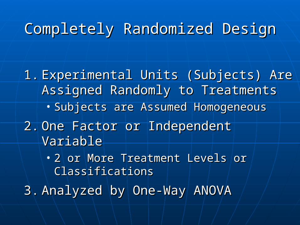
Completely Randomized DesignCompletely Randomized Design
1.1. Experimental Units (Subjects) Are Experimental Units (Subjects) Are Assigned Randomly to TreatmentsAssigned Randomly to Treatments• Subjects are Assumed HomogeneousSubjects are Assumed Homogeneous
2.2. One Factor or Independent VariableOne Factor or Independent Variable• 2 or More Treatment Levels or 2 or More Treatment Levels or
ClassificationsClassifications
3.3. Analyzed by One-Way ANOVAAnalyzed by One-Way ANOVA
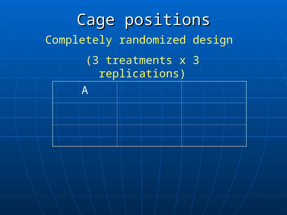
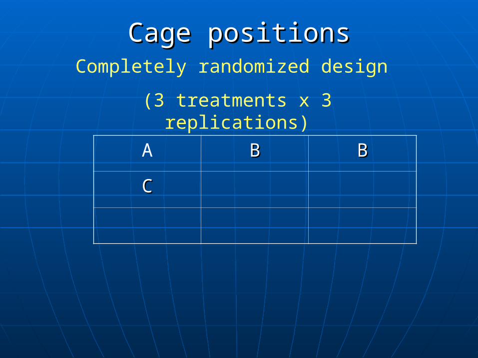
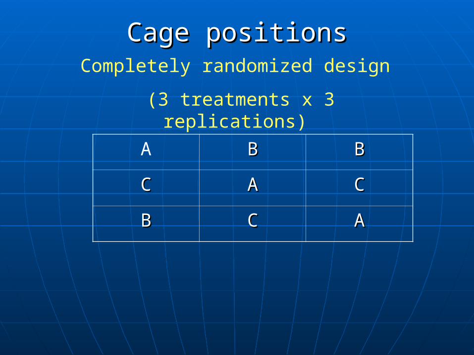
Cage positionsCage positionsCompletely randomized design
(3 treatments x 3 replications)
A
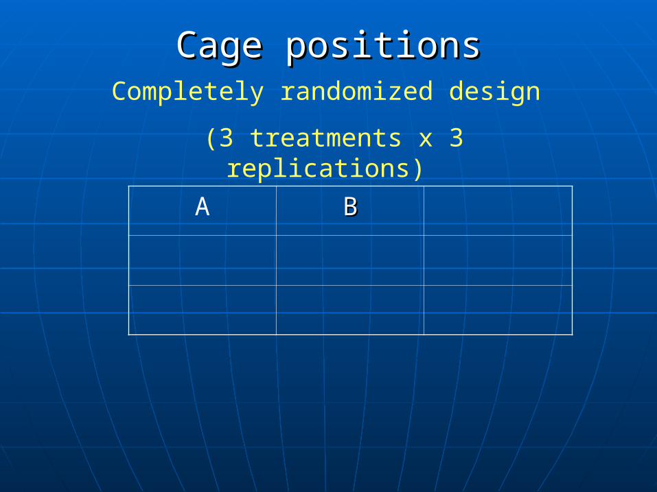
Cage positionsCage positionsCompletely randomized design
(3 treatments x 3 replications)
A BB
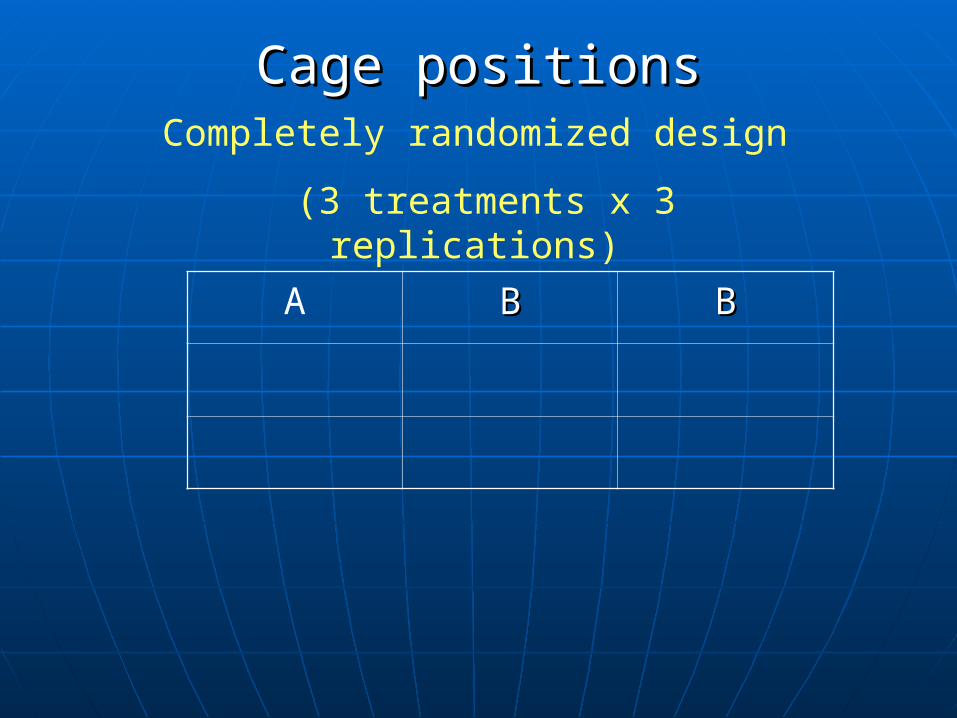
Cage positionsCage positionsCompletely randomized design
(3 treatments x 3 replications)
A BB BB
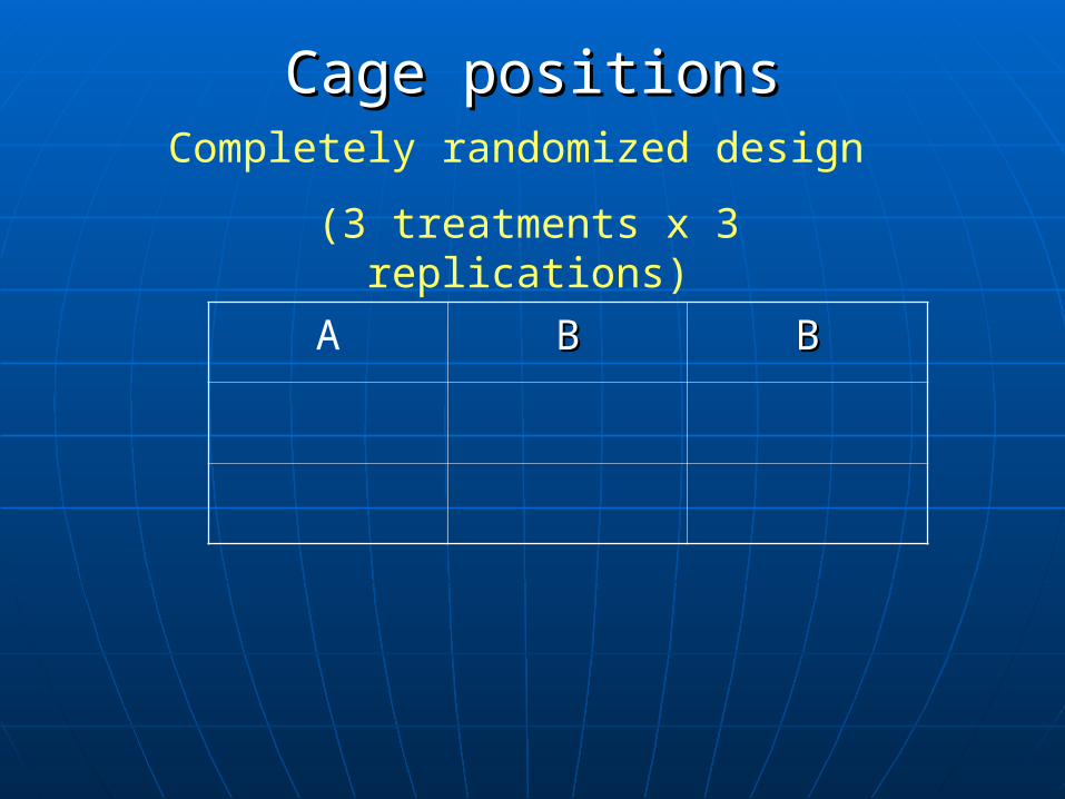
Cage positionsCage positionsCompletely randomized design
(3 treatments x 3 replications)
A BB BB
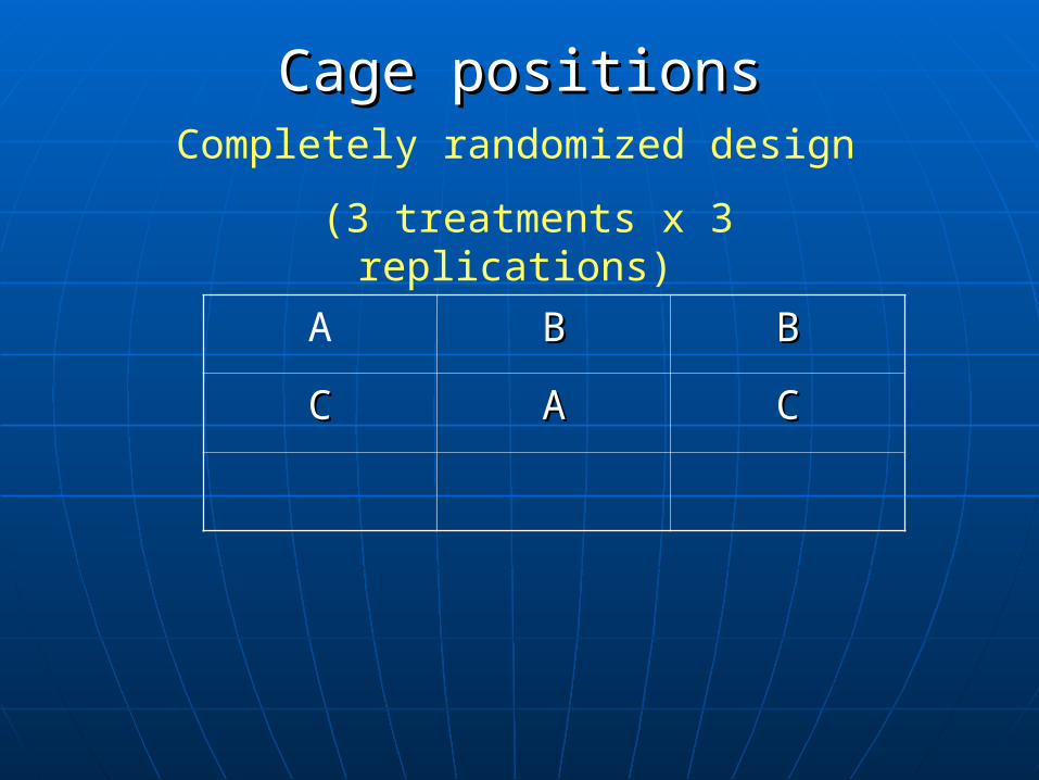
Cage positionsCage positionsCompletely randomized design
(3 treatments x 3 replications)
A BB BB
CC

Cage positionsCage positionsCompletely randomized design
(3 treatments x 3 replications)
A BB BB
CC AA
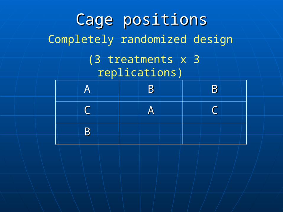
Cage positionsCage positionsCompletely randomized design
(3 treatments x 3 replications)
A BB BB
CC AA CC
Cage positionsCage positionsCompletely randomized design
(3 treatments x 3 replications)
A BB BB
CC AA CC
BB
Cage positionsCage positionsCompletely randomized design
(3 treatments x 3 replications)
A BB BB
CC AA CC
BB CC
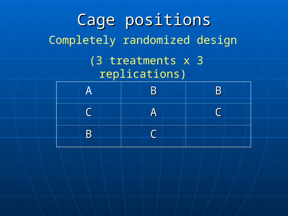
Cage positionsCage positionsCompletely randomized design
(3 treatments x 3 replications)
A BB BB
CC AA CC
BB CC AA
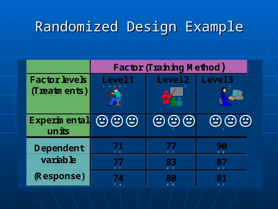
Factor (Training Method) Factor levels (Treatments)
Level 1
Level 2
Level 3
Experimental units
Dependent 71 77 90
variable 77 83 87
(Response) 74 80 81
Factor (Training Method) Factor levels (Treatments)
Level 1
Level 2
Level 3
Experimental units
Dependent 71 77 90
variable 77 83 87
(Response) 74 80 81
Randomized Design ExampleRandomized Design Example
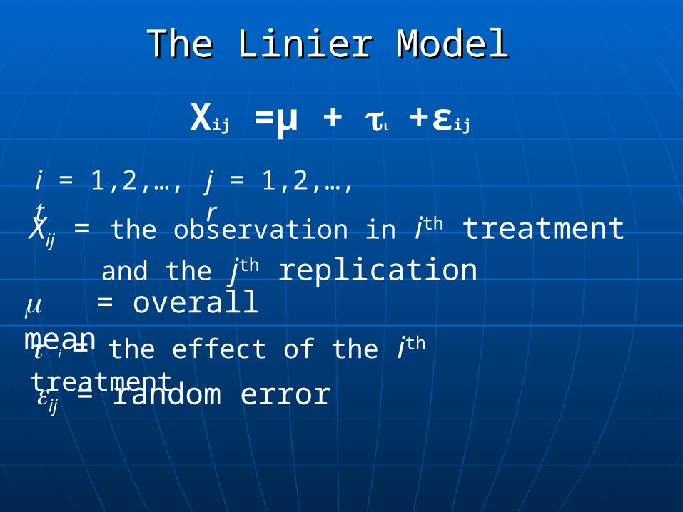
The Linier Model The Linier Model
i = 1,2,…, t
j = 1,2,…, r
Xij = the observation in ith treatment and
the jth replication = overall meani = the effect of the ith treatmentij = random error
Xij =μ + +εij
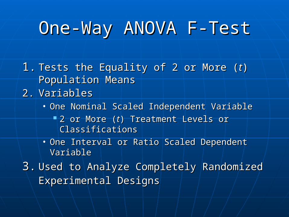
One-Way ANOVA F-TestOne-Way ANOVA F-Test
1.1. Tests the Equality of 2 or More (Tests the Equality of 2 or More (tt) ) Population MeansPopulation Means
2.2. VariablesVariables• One Nominal Scaled Independent VariableOne Nominal Scaled Independent Variable
2 or More (2 or More (tt) Treatment Levels or ) Treatment Levels or ClassificationsClassifications
• One Interval or Ratio Scaled Dependent VariableOne Interval or Ratio Scaled Dependent Variable
3.3. Used to Analyze Completely Randomized Used to Analyze Completely Randomized Experimental DesignsExperimental Designs
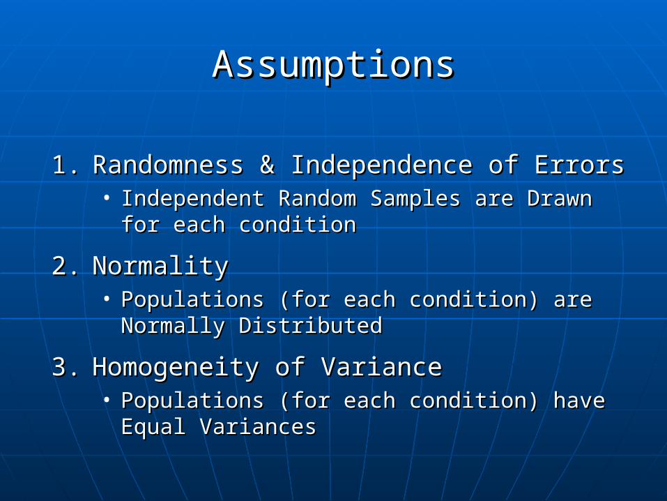
AssumptionsAssumptions
1.1. Randomness & Independence of ErrorsRandomness & Independence of Errors• Independent Random Samples are Drawn Independent Random Samples are Drawn
for each conditionfor each condition
2.2. NormalityNormality• Populations (for each condition) are Populations (for each condition) are
Normally DistributedNormally Distributed
3.3. Homogeneity of VarianceHomogeneity of Variance• Populations (for each condition) have Equal Populations (for each condition) have Equal
VariancesVariances
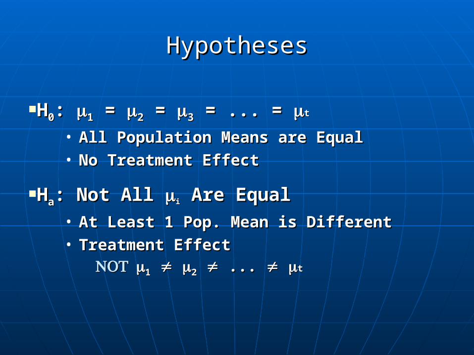
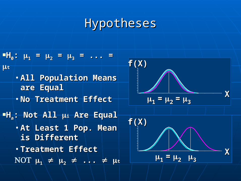
HypothesesHypotheses
HH00: : 11 = = 22 = = 33 = ... = = ... = tt
• All Population Means are EqualAll Population Means are Equal• No Treatment EffectNo Treatment Effect
HHaa: Not All : Not All ii Are Equal Are Equal• At Least 1 Pop. Mean is DifferentAt Least 1 Pop. Mean is Different• Treatment EffectTreatment Effect11 22 ... ... tt
HypothesesHypotheses
HH00: : 11 = = 22 = = 33 = ... = = ... = tt
• All Population Means All Population Means are Equalare Equal
• No Treatment EffectNo Treatment Effect
HHaa: Not All : Not All ii Are Equal Are Equal
• At Least 1 Pop. Mean At Least 1 Pop. Mean is Differentis Different
• Treatment EffectTreatment Effect11 22 ... ... tt
XX
f(X)f(X)
11 = = 22 = = 33
XX
f(X)f(X)
11 = = 22 33
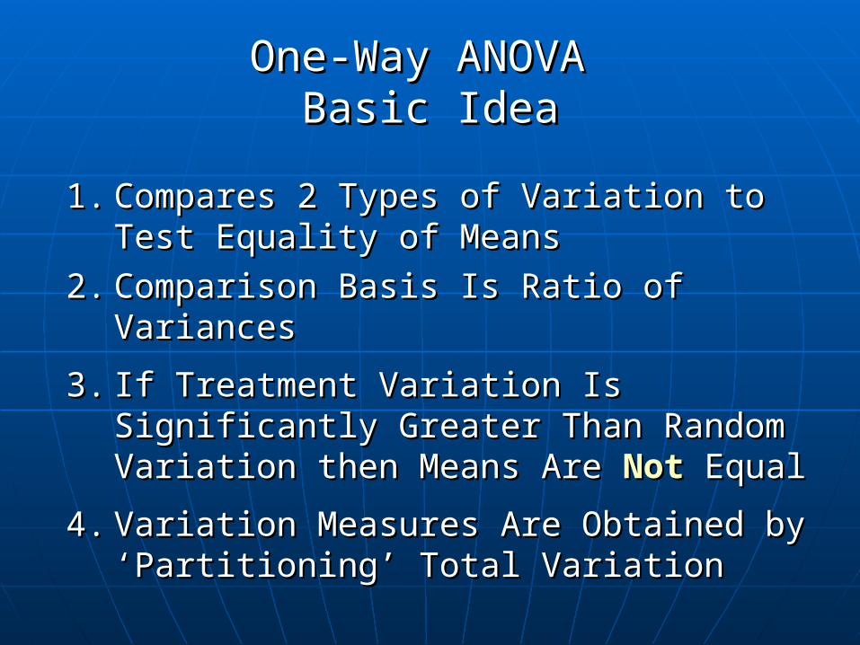
1.1. Compares 2 Types of Variation to Compares 2 Types of Variation to Test Equality of MeansTest Equality of Means
2.2. Comparison Basis Is Ratio of Comparison Basis Is Ratio of Variances Variances
3.3. If Treatment Variation Is If Treatment Variation Is Significantly Greater Than Random Significantly Greater Than Random Variation then Means Are Variation then Means Are NotNot Equal Equal
4.4. Variation Measures Are Obtained by Variation Measures Are Obtained by ‘Partitioning’ Total Variation‘Partitioning’ Total Variation
One-Way ANOVA One-Way ANOVA Basic IdeaBasic Idea
One-Way ANOVA One-Way ANOVA Partitions Total VariationPartitions Total Variation
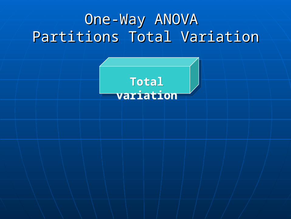
One-Way ANOVA One-Way ANOVA Partitions Total VariationPartitions Total Variation
Total variationTotal variation
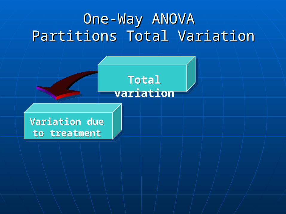
One-Way ANOVA One-Way ANOVA Partitions Total VariationPartitions Total Variation
Variation due to treatment
Variation due to treatment
Total variationTotal variation
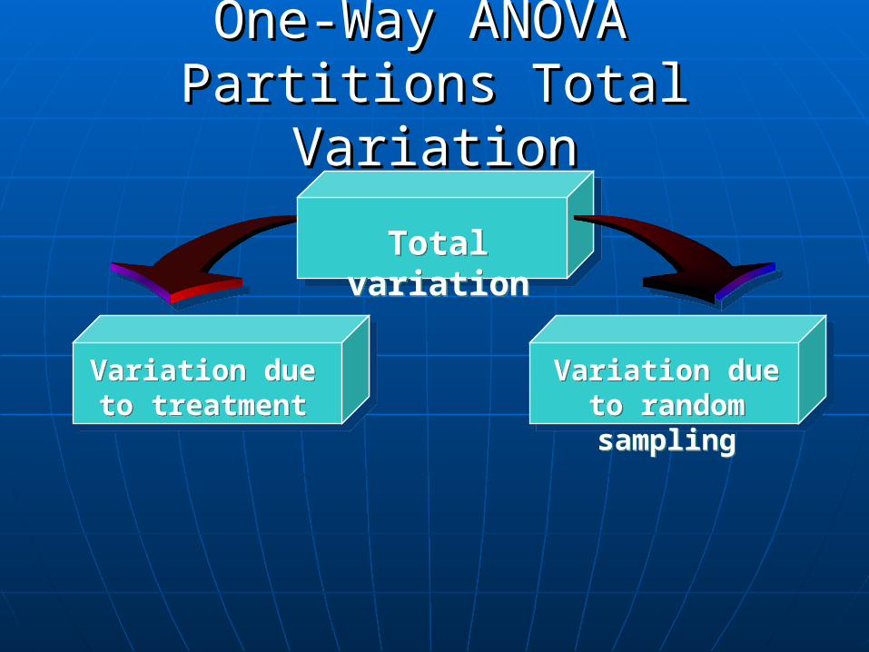
One-Way ANOVAOne-Way ANOVA Partitions Total VariationPartitions Total Variation
Variation due to treatment
Variation due to treatment
Variation due to random samplingVariation due to
random sampling
Total variationTotal variation
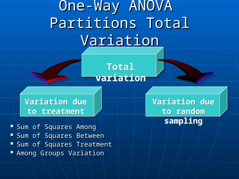
One-Way ANOVAOne-Way ANOVA Partitions Total VariationPartitions Total Variation
Variation due to treatment
Variation due to treatment
Variation due to random samplingVariation due to
random sampling
Total variationTotal variation
Sum of Squares AmongSum of Squares Among Sum of Squares BetweenSum of Squares Between Sum of Squares TreatmentSum of Squares Treatment Among Groups VariationAmong Groups Variation
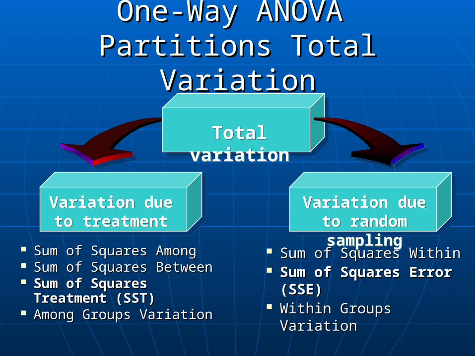
One-Way ANOVAOne-Way ANOVA Partitions Total VariationPartitions Total Variation
Variation due to treatment
Variation due to treatment
Variation due to random samplingVariation due to
random sampling
Total variationTotal variation
Sum of Squares WithinSum of Squares Within Sum of Squares Sum of Squares
Error (SSE)Error (SSE) Within Groups Within Groups
VariationVariation
Sum of Squares AmongSum of Squares Among Sum of Squares BetweenSum of Squares Between Sum of Squares Sum of Squares
Treatment (SST)Treatment (SST) Among Groups VariationAmong Groups Variation
Total VariationTotal Variation
XX
Group 1Group 1 Group 2Group 2 Group 3Group 3
Response, XResponse, X
22
21
2
11 XXXXXXTotalSS ij 22
21
2
11 XXXXXXTotalSS ij
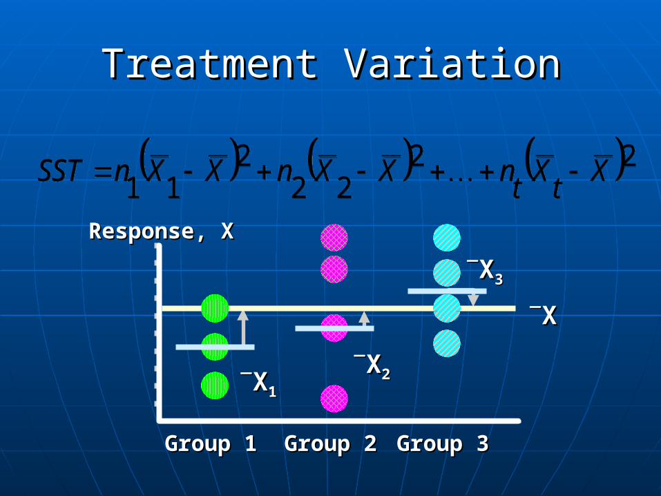
Treatment VariationTreatment Variation
XX
XX33
XX22XX11
Group 1Group 1 Group 2Group 2 Group 3Group 3
Response, XResponse, X
2222
211
XtXtnXXnXXnSST 22
222
11X
tXtnXXnXXnSST
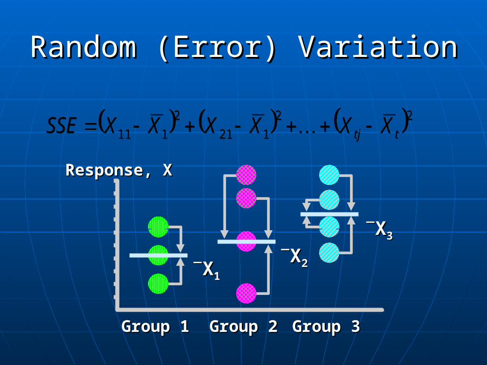
Random (Error) VariationRandom (Error) Variation
XX22XX11
XX33
Group 1Group 1 Group 2Group 2 Group 3Group 3
Response, XResponse, X
22
121
2
111 ttj XXXXXXSSE 22
121
2
111 ttj XXXXXXSSE
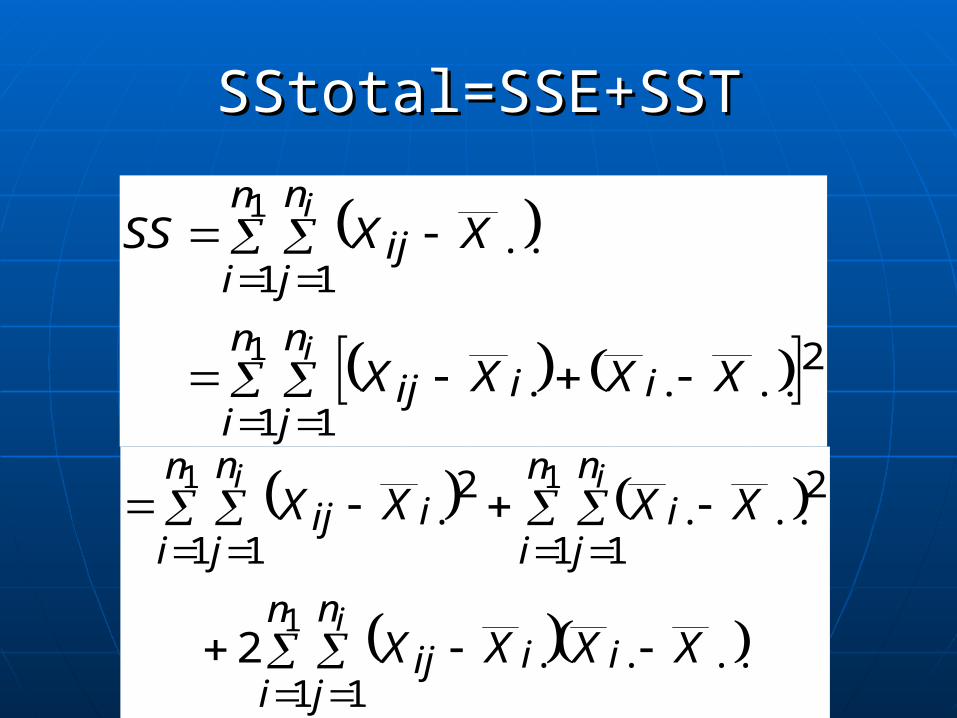
SStotal=SSE+SSTSStotal=SSE+SST
1
1
1 1
2....
1 1..
n
i
n
jiiij
n
i
n
jij
i
i
XXXX
XXSS
...1 1
.
1 1
2...
1 1
2.
1
11
2 XXXX
XXXX
in
i
n
jiij
n
i
n
ji
n
i
n
jiij
i
ii
ButBut
0
1
1
1
1.....
1 1....
...1 1
.
n
iiii
n
i
n
jiiji
in
i
n
jiij
XnXnXX
XXXX
XXXX
i
i
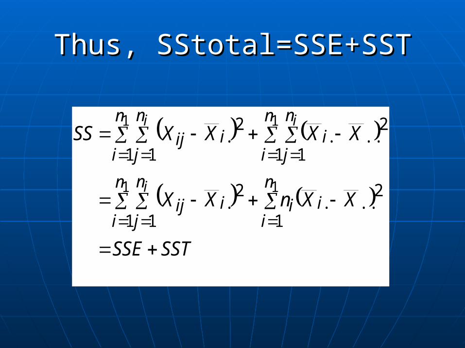
Thus, SStotal=SSE+SSTThus, SStotal=SSE+SST
11
11
1
2...
1 1
2.
1 1
2...
1 1
2.
SSTSSE
XXnXX
XXXXSS
n
iii
n
i
n
jiij
n
i
n
ji
n
i
n
jiij
i
ii
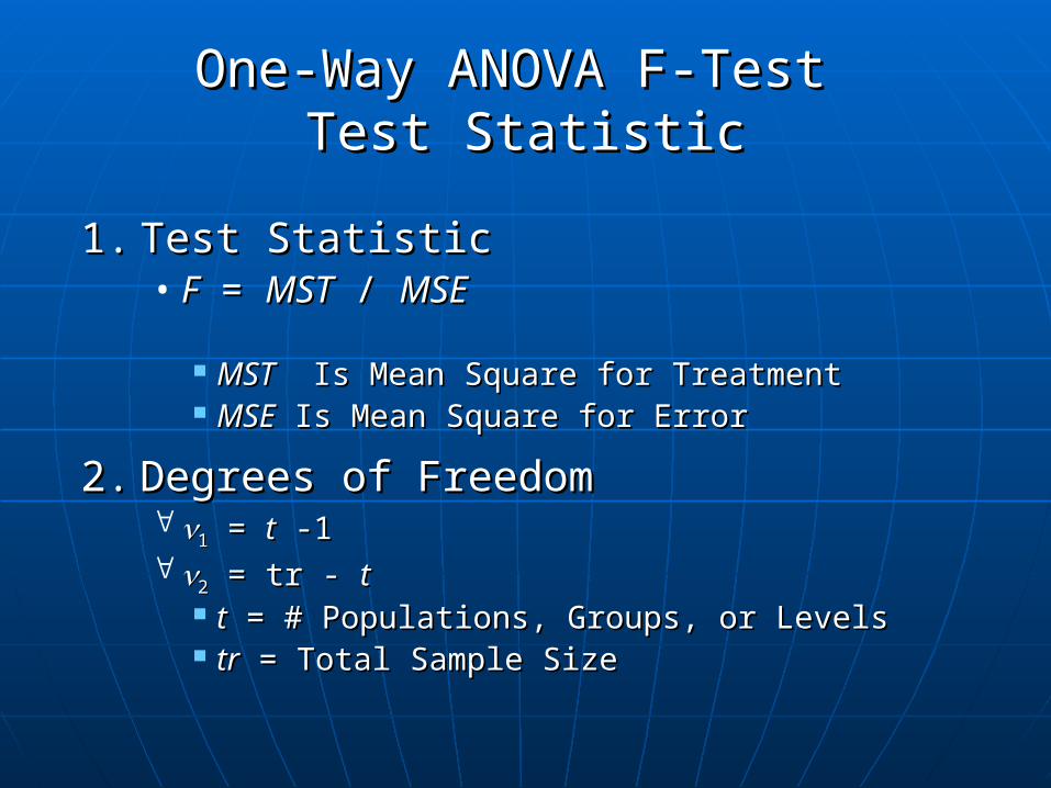
One-Way ANOVA F-Test One-Way ANOVA F-Test Test StatisticTest Statistic
1.1. Test StatisticTest Statistic• FF = = MSTMST / / MSEMSE
MSTMST Is Mean Square for Treatment Is Mean Square for Treatment MSEMSE Is Mean Square for Error Is Mean Square for Error
2.2. Degrees of FreedomDegrees of Freedom 11 = = tt -1 -1 22 = tr - = tr - tt
tt = # Populations, Groups, or Levels = # Populations, Groups, or Levels trtr = Total Sample Size = Total Sample Size
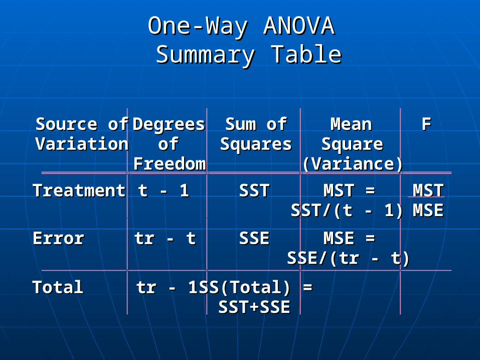
One-Way ANOVA One-Way ANOVA Summary TableSummary Table
Source ofSource ofVariationVariation
DegreesDegreesofof
FreedomFreedom
Sum ofSum ofSquaresSquares
MeanMeanSquareSquare
(Variance)(Variance)
FF
TreatmentTreatment t - 1t - 1 SSTSST MST =MST =SST/(t - 1)SST/(t - 1)
MSTMSTMSEMSE
ErrorError tr - ttr - t SSESSE MSE =MSE =SSE/(tr - t)SSE/(tr - t)
TotalTotal tr - 1tr - 1 SS(Total) =SS(Total) =SST+SSESST+SSE
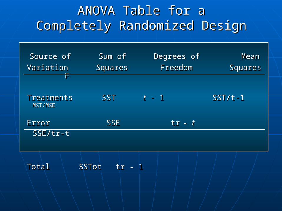
ANOVA Table for aANOVA Table for aCompletely Randomized DesignCompletely Randomized Design
Source of Sum of Degrees of MeanSource of Sum of Degrees of Mean
Variation Squares Freedom Squares FVariation Squares Freedom Squares F
TreatmentsTreatments SSTSST tt - 1 - 1 SST/t-1 SST/t-1 MST/MSE MST/MSE
ErrorError SSE trSSE tr - - tt SSE/tr-t SSE/tr-t
TotalTotal SSTotSSTot tr - 1tr - 1
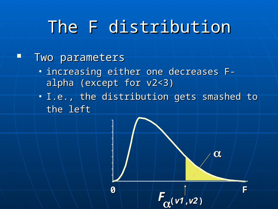
The F distributionThe F distribution
Two parametersTwo parameters• increasing either one decreases F-alpha increasing either one decreases F-alpha
(except for(except for v2<3) v2<3)
• I.e., the distribution gets smashed to the leftI.e., the distribution gets smashed to the left
FF v1v1 v2v2(( ,, ))00 FF
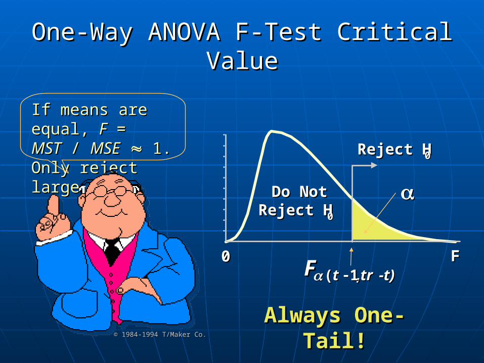
One-Way ANOVA F-Test Critical One-Way ANOVA F-Test Critical ValueValue
If means are If means are equal, equal, FF = = MSTMST / / MSEMSE 1. Only 1. Only reject large reject large FF!!
Always One-Always One-Tail!Tail!
FF tt trtr -t)-t)(( ,, 1100
Reject HReject H00
Do NotDo NotReject HReject H00
FF
© 1984-1994 T/Maker Co.© 1984-1994 T/Maker Co.
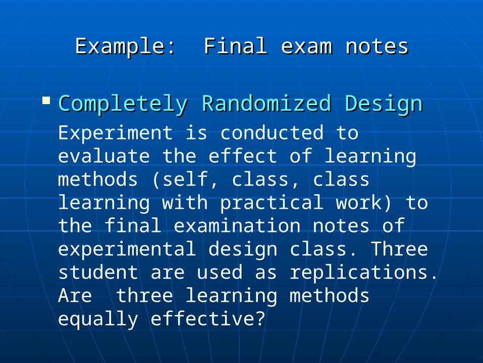
Example: Final exam notesExample: Final exam notes
Completely Randomized DesignCompletely Randomized DesignExperiment is conducted to evaluate the effect of learning methods (self, class, class learning with practical work) to the final examination notes of experimental design class. Three student are used as replications. Are three learning methods equally effective?
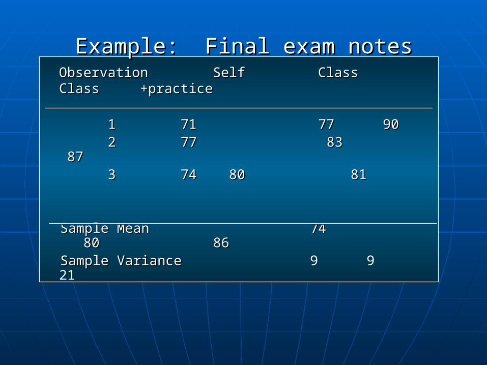
Example: Final exam notesExample: Final exam notesObservationObservation Self Self Class Class Class Class +practice+practice
11 71 71 77 77 90 90 22 77 83 87 77 83 87 33 74 74 80 81 80 81
Sample MeanSample Mean 74 80 74 80 86 86
Sample VarianceSample Variance 9 9 21
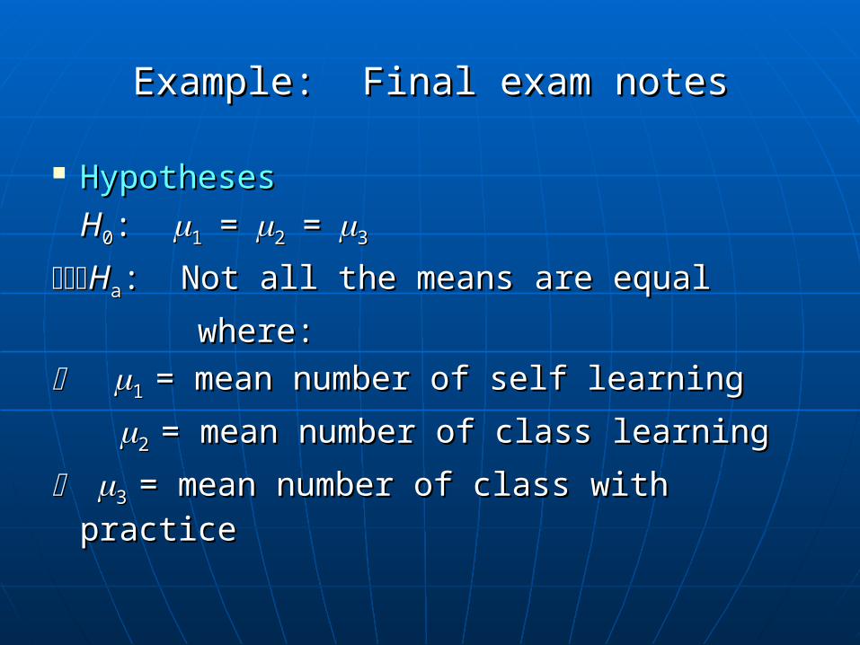
HypothesesHypotheses
HH00: : 11==22==33
HHaa: : Not all the means are equalNot all the means are equal
where:where:
1 1 = = mean number of self learningmean number of self learning
2 2 = = mean number of class learningmean number of class learning
3 3 = = mean number of class with practicemean number of class with practice
Example: Final exam notesExample: Final exam notes
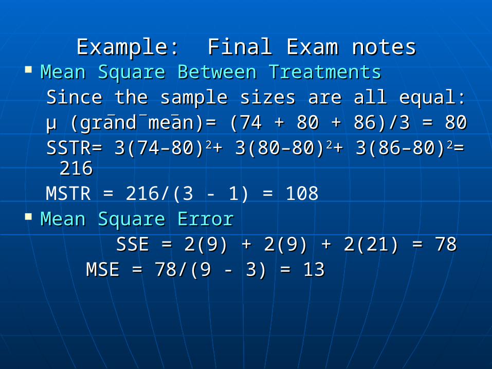
Mean Square Between TreatmentsMean Square Between TreatmentsSince the sample sizes are all equal:Since the sample sizes are all equal:μμ (grand mean)= (74 + 80 + 86)/3 = 80 (grand mean)= (74 + 80 + 86)/3 = 80SSTR= 3(74–80)SSTR= 3(74–80)22+ 3(80–80)+ 3(80–80)22+ 3(86–+ 3(86–
80)80)22= 216= 216MSTR = 216/(3 - 1) = 108
Mean Square ErrorMean Square Error SSE = 2(9) + 2(9) + 2(21) = 78SSE = 2(9) + 2(9) + 2(21) = 78
MSE = 78/(9 - 3) = 13MSE = 78/(9 - 3) = 13
______
Example: Final Exam notesExample: Final Exam notes
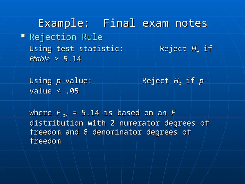
Rejection RuleRejection RuleUsing test statistic:Using test statistic: Reject Reject HH00 if if FtableFtable > > 5.145.14
Using Using pp-value:-value: Reject Reject HH00 if if pp-value < .05-value < .05
where where FF.05.05 = 5.14 is based on an = 5.14 is based on an FF distribution distribution with 2 numerator degrees of freedom and 6 with 2 numerator degrees of freedom and 6 denominator degrees of freedomdenominator degrees of freedom
Example: Final exam notesExample: Final exam notes
Example: Final exam notesExample: Final exam notes
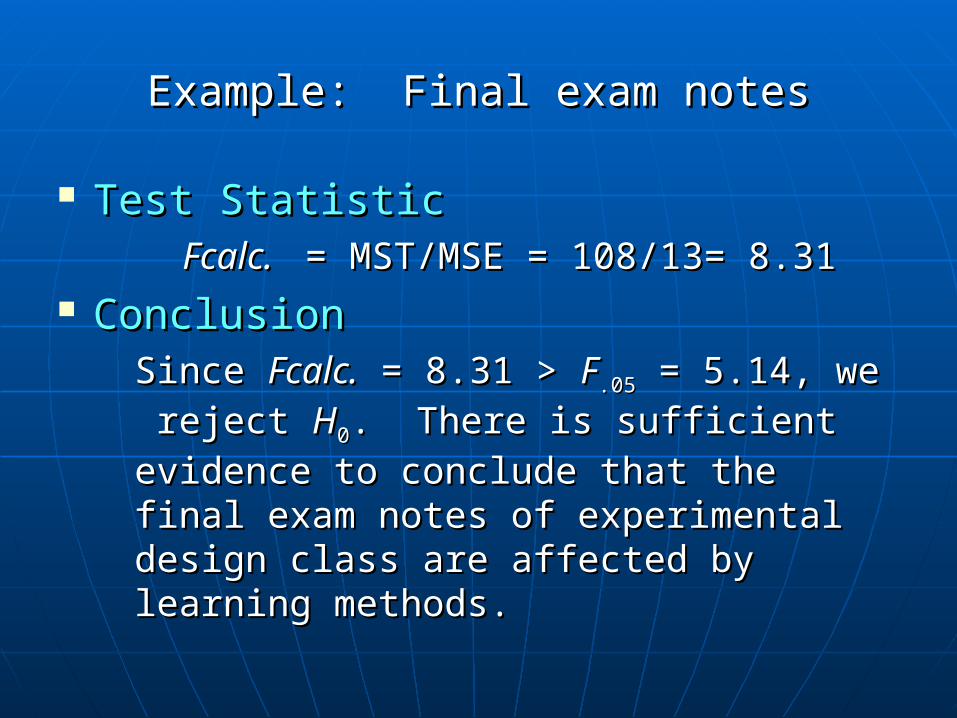
Test StatisticTest Statistic Fcalc. Fcalc. = MST/MSE = 108/13= = MST/MSE = 108/13=
8.318.31 ConclusionConclusion
Since Since Fcalc.Fcalc. = 8.31 > = 8.31 > FF.05.05 = 5.14, we = 5.14, we reject reject HH00. There is sufficient evidence . There is sufficient evidence to conclude that the final exam notes of to conclude that the final exam notes of experimental design class are affected experimental design class are affected by learning methods.by learning methods.
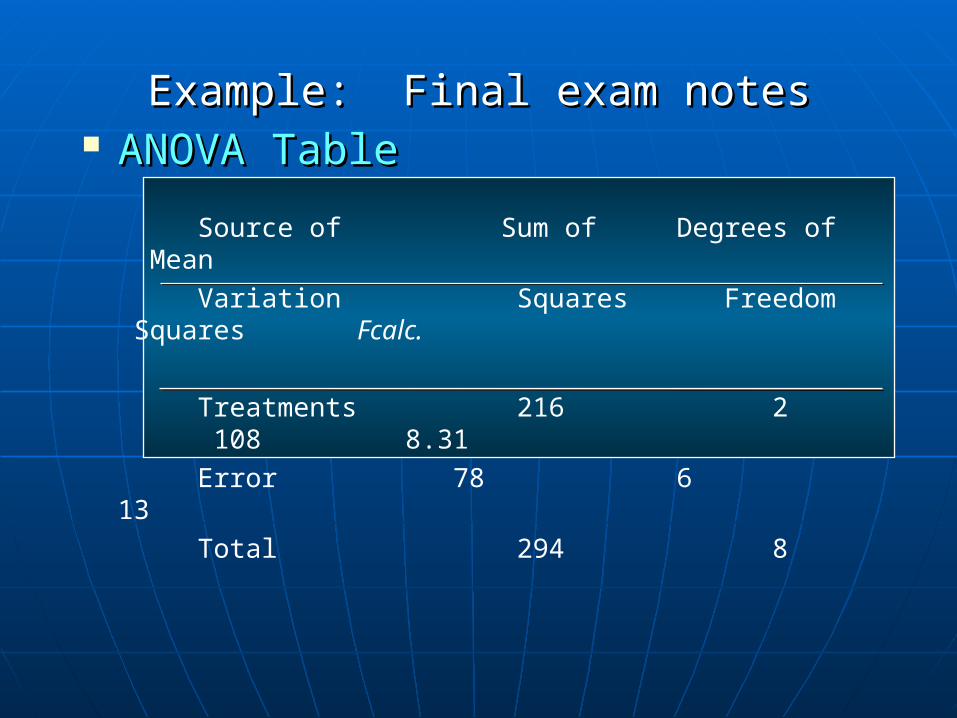
ANOVA TableANOVA Table
Source of Sum of Degrees of Mean Variation Squares Freedom Squares Fcalc.
Treatments 216 2 108 8.31 Error 78 6 13 Total 294 8
Example: Final exam notesExample: Final exam notes
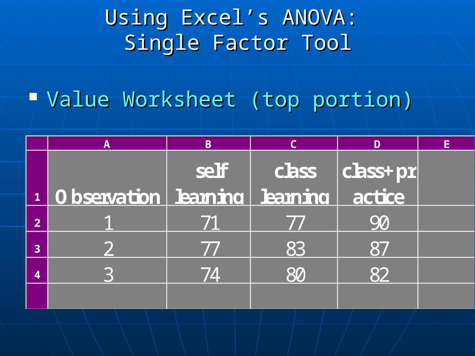
Value Worksheet (top portion)Value Worksheet (top portion)
Using Excel’s ANOVA: Using Excel’s ANOVA: Single Factor ToolSingle Factor Tool
A B C D E
1 Observationself
learningclass
learningclass+practice
2 1 71 77 90 3 2 77 83 874 3 74 80 82
Value Worksheet (bottom portion)
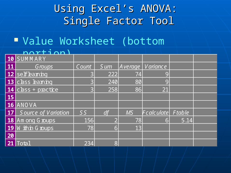
Using Excel’s ANOVA:Using Excel’s ANOVA: Single Factor Tool Single Factor Tool
10 SUMMARY11 Groups Count Sum Average Variance12 self learning 3 222 74 913 class learning 3 240 80 914 class + practice 3 258 86 211516 ANOVA17 Source of Variation SS df MS Fcalculate Ftable18 Among Groups 156 2 78 6 5.1419 Within Groups 78 6 132021 Total 234 8
RCBDRCBD((Randomized Complete Block DesignRandomized Complete Block Design))
Randomized Complete Block Randomized Complete Block DesignDesign
An experimental design in which there is one An experimental design in which there is one independent variable, and a second variable known independent variable, and a second variable known as a blocking variable, that is used to control for as a blocking variable, that is used to control for confounding or concomitant variables.confounding or concomitant variables.
It is used when the experimental unit or material are It is used when the experimental unit or material are heterogeneousheterogeneous
There is a way to block the experimental units or There is a way to block the experimental units or materials to keep the variability among within a materials to keep the variability among within a block as small as possible and to maximize block as small as possible and to maximize differences among blockdifferences among block
The block (group) should consists units or materials The block (group) should consists units or materials which are as uniform as possiblewhich are as uniform as possible
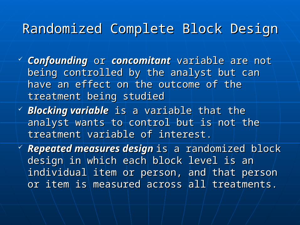
ConfoundingConfounding or or concomitantconcomitant variable are variable are not being controlled by the analyst but can not being controlled by the analyst but can have an effect on the outcome of the have an effect on the outcome of the treatment being studiedtreatment being studied
Blocking variableBlocking variable is a variable that the is a variable that the analyst wants to control but is not the analyst wants to control but is not the treatment variable of interest.treatment variable of interest.
Repeated measures designRepeated measures design is a randomized is a randomized block design in which each block level is an block design in which each block level is an individual item or person, and that person or individual item or person, and that person or item is measured across all treatments.item is measured across all treatments.
Randomized Complete Block DesignRandomized Complete Block Design
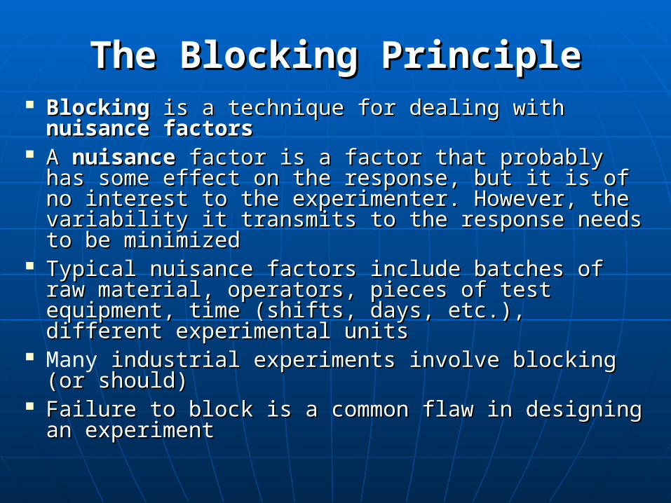
The Blocking PrincipleThe Blocking Principle BlockingBlocking is a technique for dealing with is a technique for dealing with nuisancenuisance
factorsfactors A A nuisance nuisance factor is a factor that probably has factor is a factor that probably has
some effect on the response, but it is of no interest some effect on the response, but it is of no interest to the experimenter. However, the variability it to the experimenter. However, the variability it transmits to the response needs to be minimizedtransmits to the response needs to be minimized
Typical nuisance factors include batches of raw Typical nuisance factors include batches of raw material, operators, pieces of test equipment, time material, operators, pieces of test equipment, time (shifts, days, etc.), different experimental units(shifts, days, etc.), different experimental units
Many industrial experiments involve blocking (or industrial experiments involve blocking (or should)should)
Failure to block is a common flaw in designing an Failure to block is a common flaw in designing an experimentexperiment
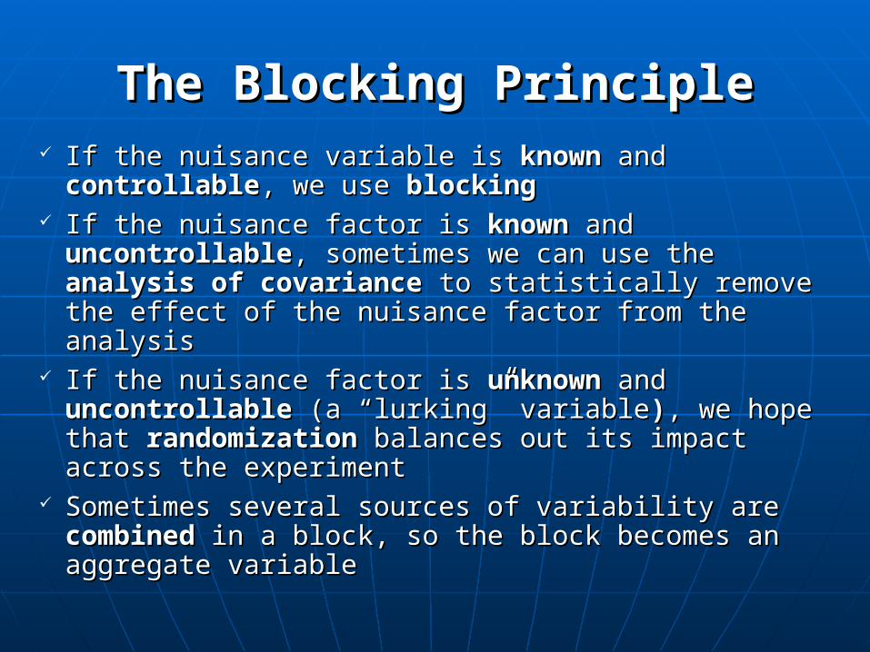
The Blocking PrincipleThe Blocking Principle If the nuisance variable is If the nuisance variable is knownknown and and
controllablecontrollable, we use , we use blockingblocking If the nuisance factor is If the nuisance factor is knownknown and and
uncontrollableuncontrollable, sometimes we can use the , sometimes we can use the analysis of covarianceanalysis of covariance to statistically remove the to statistically remove the effect of the nuisance factor from the analysiseffect of the nuisance factor from the analysis
If the nuisance factor is If the nuisance factor is unknownunknown and and uncontrollableuncontrollable (a “lurking” variable (a “lurking” variable)), we hope , we hope that that randomizationrandomization balances out its impact balances out its impact across the experimentacross the experiment
Sometimes several sources of variability are Sometimes several sources of variability are combinedcombined in a block, so the block becomes an in a block, so the block becomes an aggregate variableaggregate variable

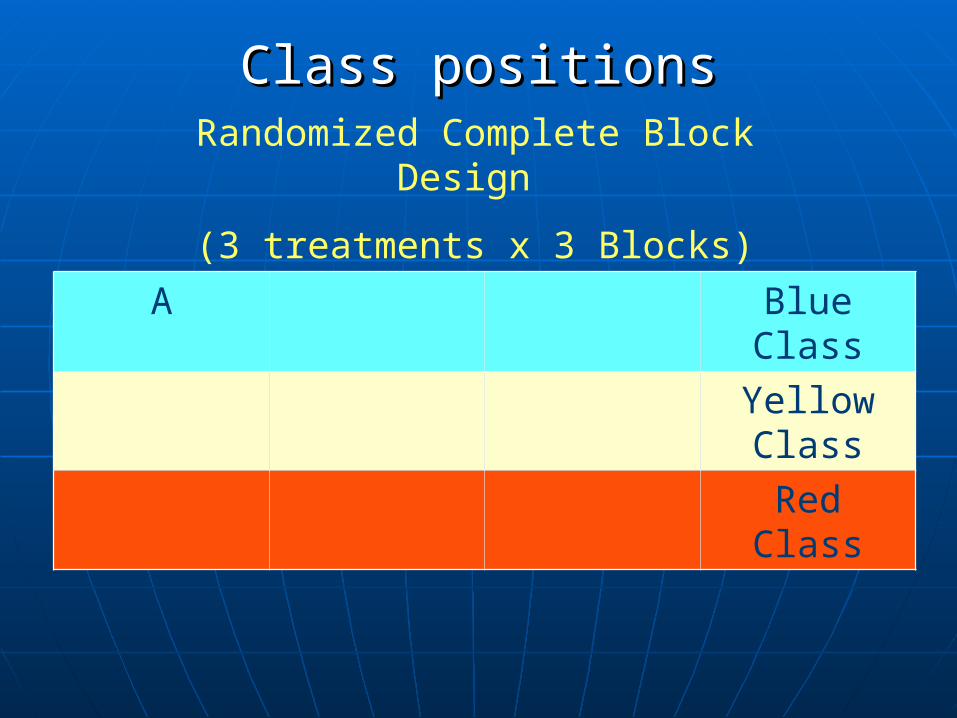
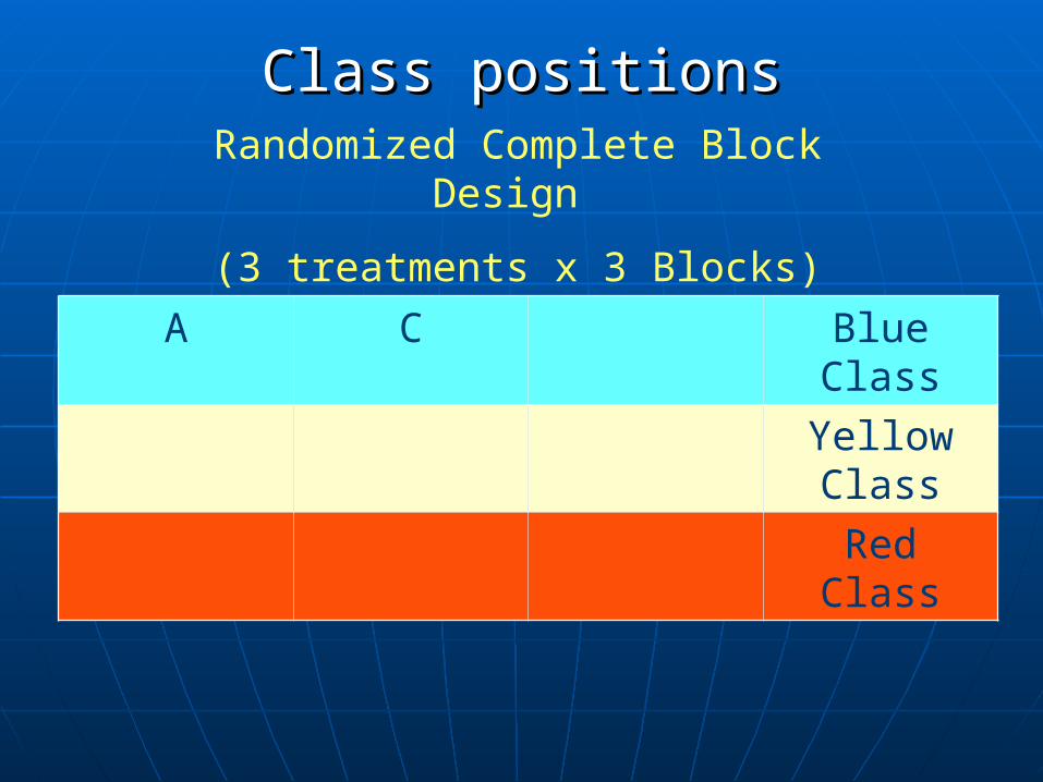
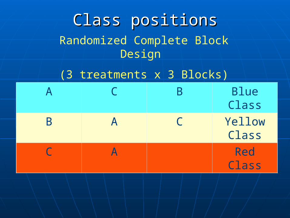
Class positionsClass positionsRandomized Complete Block Design
(3 treatments x 3 Blocks)
Blue Class
Yellow Class
Red Class
Class positionsClass positionsRandomized Complete Block Design
(3 treatments x 3 Blocks)
A Blue Class
Yellow Class
Red Class
Class positionsClass positionsRandomized Complete Block Design
(3 treatments x 3 Blocks)
A C Blue Class
Yellow Class
Red Class
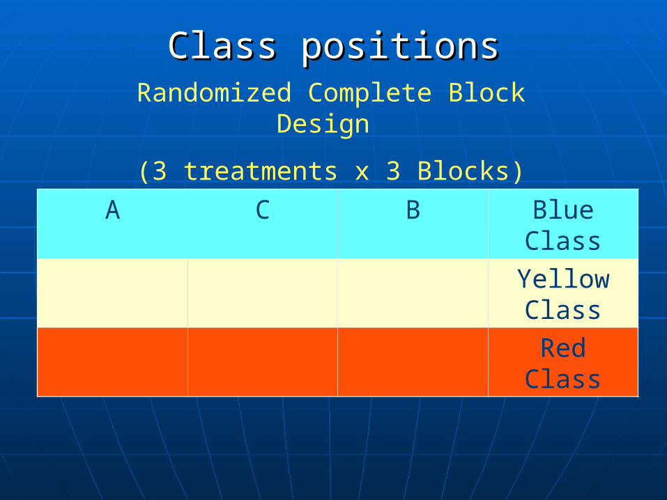
Class positionsClass positionsRandomized Complete Block Design
(3 treatments x 3 Blocks)
A C B Blue Class
Yellow Class
Red Class
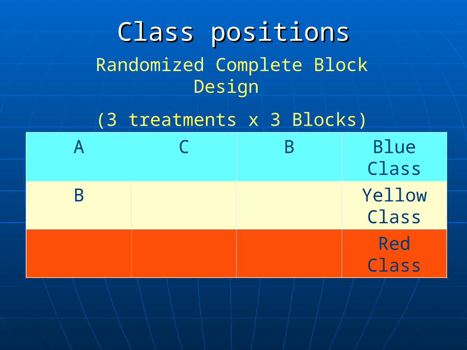
Class positionsClass positionsRandomized Complete Block Design
(3 treatments x 3 Blocks)
A C B Blue Class
B Yellow Class
Red Class
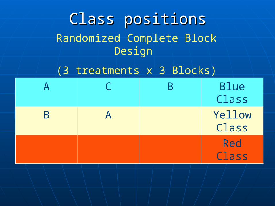
Class positionsClass positionsRandomized Complete Block Design
(3 treatments x 3 Blocks)
A C B Blue Class
B A Yellow Class
Red Class

Class positionsClass positionsRandomized Complete Block Design
(3 treatments x 3 Blocks)
A C B Blue Class
B A C Yellow Class
Red Class

Class positionsClass positionsRandomized Complete Block Design
(3 treatments x 3 Blocks)
A C B Blue Class
B A C Yellow Class
C Red Class
Class positionsClass positionsRandomized Complete Block Design
(3 treatments x 3 Blocks)
A C B Blue Class
B A C Yellow Class
C A Red Class
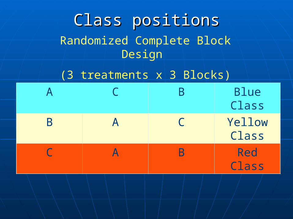
Class positionsClass positionsRandomized Complete Block Design
(3 treatments x 3 Blocks)
A C B Blue Class
B A C Yellow Class
C A B Red Class
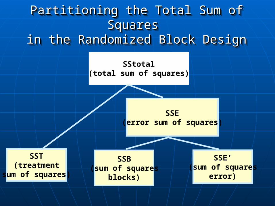
Partitioning the Total Sum of Squares Partitioning the Total Sum of Squares in the Randomized Block Designin the Randomized Block Design
Partitioning the Total Sum of Squares Partitioning the Total Sum of Squares in the Randomized Block Designin the Randomized Block Design
SStotal(total sum of squares)
SST(treatment
sum of squares)
SSE(error sum of squares)
SSB(sum of squares
blocks)
SSE’(sum of squares
error)
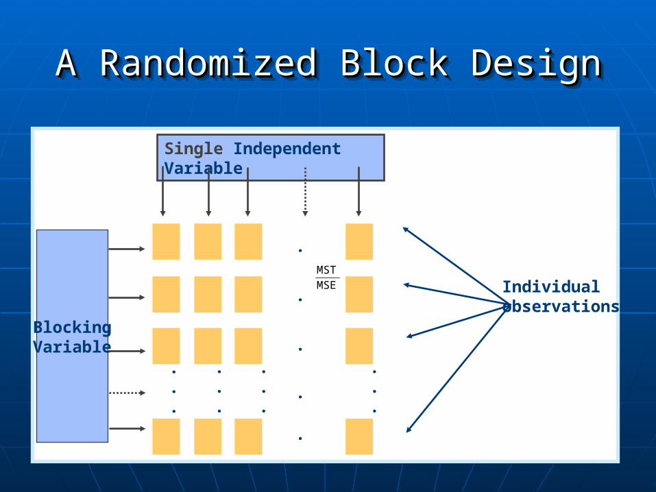
A Randomized Block DesignA Randomized Block DesignA Randomized Block DesignA Randomized Block Design
Individualobservations
.
.
.
.
.
.
.
.
.
.
.
.
Single Independent Variable
BlockingVariable
.
.
.
.
.
MSE
MST
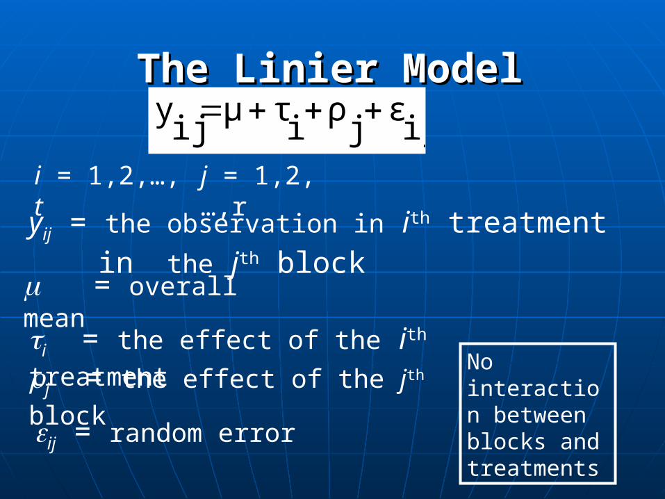
The Linier ModelThe Linier Modelij
εj
ρi
τμij
y
i = 1,2,…, t
j = 1,2,…,r
yij = the observation in ith treatment in the jth block
= overall mean
i = the effect of the ith treatmentj = the effect of the jth block
ij = random error
No interaction between blocks and treatments
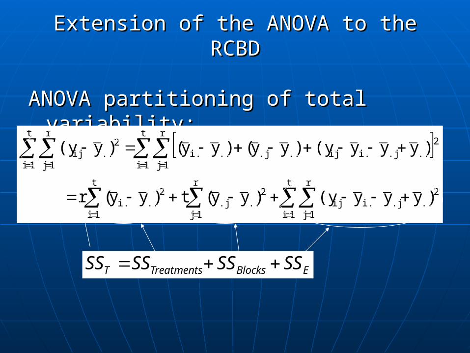
Extension of the ANOVA to the RCBDExtension of the ANOVA to the RCBD
ANOVA partitioning of total ANOVA partitioning of total variability:variability:
t
1i
r
1j
2...ji.ij
r
1j
2...j
t
1i
2..i.
t
1i
r
1j
2...ji.ij...j..i.
t
1i
r
1j
2..ij
)yyy(y)yy(t)yy(r
)yyy(y)yy()yy()y(y
EBlocksTreatmentsT SSSSSSSS
Extension of the ANOVA to the Extension of the ANOVA to the RCBDRCBD
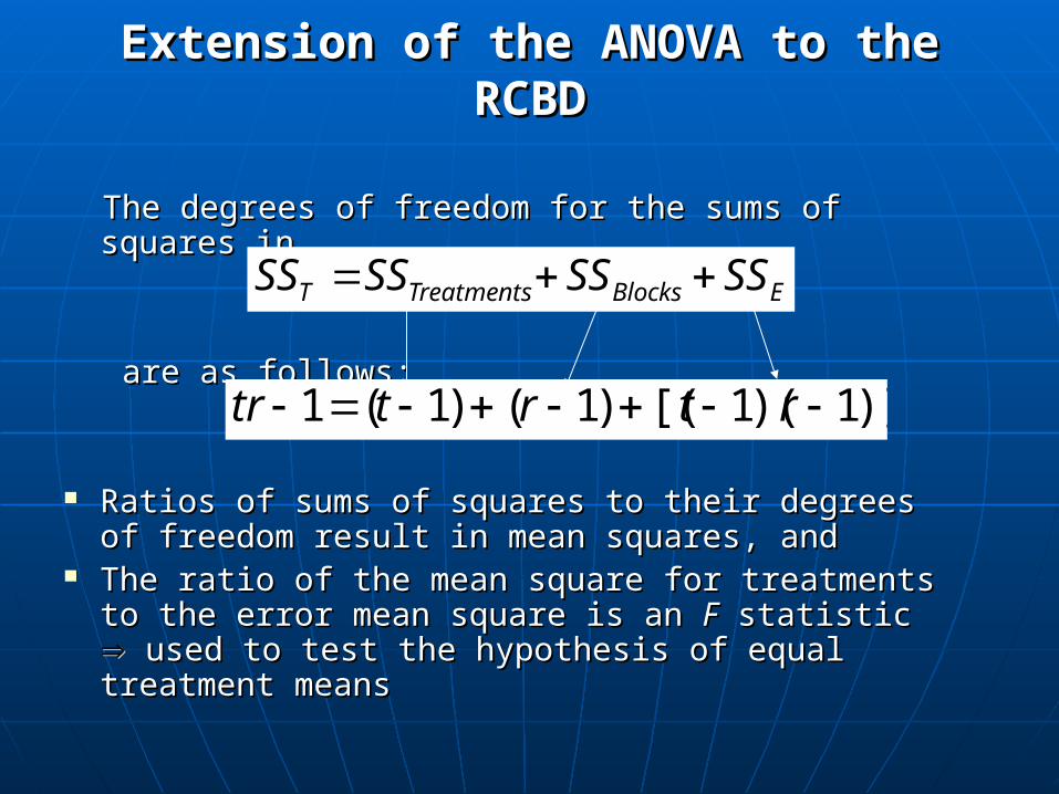
The degrees of freedom for the sums of squares The degrees of freedom for the sums of squares in in
are as follows:are as follows:
Ratios of sums of squares to their degrees of Ratios of sums of squares to their degrees of freedom result in mean squares, and freedom result in mean squares, and
The ratio of the mean square for treatments to The ratio of the mean square for treatments to the error mean square is an the error mean square is an FF statistic statistic used used to test the hypothesis of equal treatment meansto test the hypothesis of equal treatment means
EBlocksTreatmentsT SSSSSSSS
)]1)(1[( )1( )1( 1 rtrttr
ANOVA ProcedureANOVA Procedure
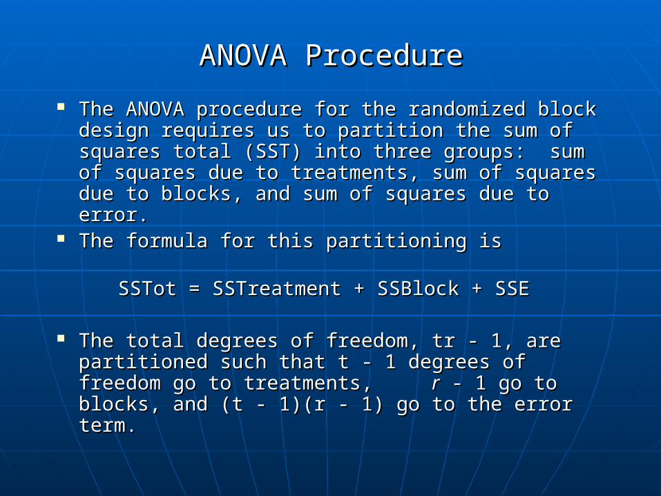
The ANOVA procedure for the randomized block The ANOVA procedure for the randomized block design requires us to partition the sum of design requires us to partition the sum of squares total (SST) into three groups: sum of squares total (SST) into three groups: sum of squares due to treatments, sum of squares due squares due to treatments, sum of squares due to blocks, and sum of squares due to error.to blocks, and sum of squares due to error.
The formula for this partitioning isThe formula for this partitioning is
SSTot = SSTreatment + SSBlock SSTot = SSTreatment + SSBlock + SSE+ SSE
The total degrees of freedom, tr - 1, are The total degrees of freedom, tr - 1, are partitioned such that t - 1 degrees of freedom go partitioned such that t - 1 degrees of freedom go to treatments, to treatments, rr - 1 go to blocks, and (t - 1)(r - - 1 go to blocks, and (t - 1)(r - 1) go to the error term. 1) go to the error term.
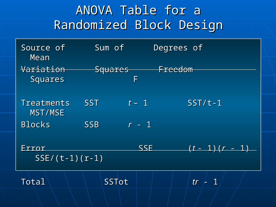
ANOVA Table for aANOVA Table for aRandomized Block DesignRandomized Block Design
Source of Sum of Degrees of MeanSource of Sum of Degrees of Mean
Variation Squares Freedom Squares Variation Squares Freedom Squares F F
TreatmentsTreatments SSTSST t t – 1– 1 SST/t-1 SST/t-1 MST/MSEMST/MSE
BlocksBlocks SSBSSB rr - 1 - 1
ErrorError SSE (SSE (t t - 1)(- 1)(rr - 1) SSE/(t-1)(r-1) - 1) SSE/(t-1)(r-1)
TotalTotal SSTotSSTot trtr - 1 - 1
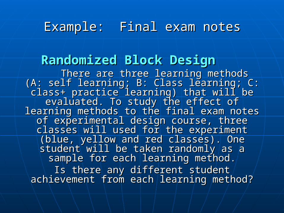
Example: Final exam notesExample: Final exam notes
Randomized Block DesignRandomized Block Design There are three learning methods (A: There are three learning methods (A:
self learning; B: Class learning; C: class+ self learning; B: Class learning; C: class+ practice learning) that will be evaluated. To practice learning) that will be evaluated. To study the effect of learning methods to the study the effect of learning methods to the
final exam notes of experimental design final exam notes of experimental design course, three classes will used for the course, three classes will used for the
experiment (blue, yellow and red classes). experiment (blue, yellow and red classes). One student will be taken randomly as a One student will be taken randomly as a
sample for each learning method.sample for each learning method.Is there any different student achievement Is there any different student achievement
from each learning method?from each learning method?
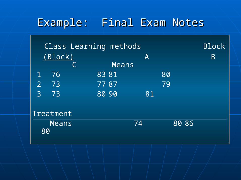
Example: Final Exam NotesExample: Final Exam Notes
Class Learning methods Block (Block) A B C
Means 1 76 83 81 80 2 73 77 87 79 3 73 80 90 81
Treatment Means 74 80 86 80
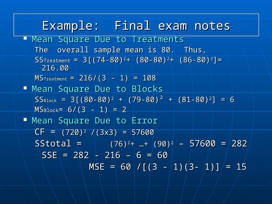
Example: Final exam notesExample: Final exam notes Mean Square Due to TreatmentsMean Square Due to Treatments
The overall sample mean is 80. Thus,The overall sample mean is 80. Thus,SSSSTreatment Treatment = 3[(74-80)= 3[(74-80)22+ (80-80)+ (80-80)22+ (86-80)+ (86-80)22]= ]=
216.00216.00MSMSTreatment Treatment = 216/(3 - 1) = 108= 216/(3 - 1) = 108
Mean Square Due to BlocksMean Square Due to BlocksSSSSBlockBlock = 3[(80-80) = 3[(80-80)22 + (79-80)² + (81-80) + (79-80)² + (81-80)22] = 6] = 6MSMSBlockBlock= 6/(3 - 1) = 2 = 6/(3 - 1) = 2
Mean Square Due to ErrorMean Square Due to ErrorCF = CF = (720)(720)22 /(3x3) = 57600 /(3x3) = 57600
SStotal = SStotal = (76)(76)22+ …+ (90)+ …+ (90)22 – 57600 = 282 – 57600 = 282SSE = 282 - 216 – 6 = 60SSE = 282 - 216 – 6 = 60 MSE = 60 /[(3 - 1)(3- 1)] = 15MSE = 60 /[(3 - 1)(3- 1)] = 15
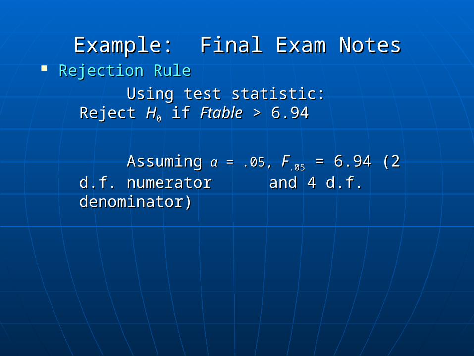
Rejection RuleRejection Rule
Using test statistic:Using test statistic: Reject Reject HH00 if if FtableFtable > 6.94 > 6.94
AssumingAssuming αα = .05, = .05, FF.05.05 = 6.94 (2 d.f. = 6.94 (2 d.f. numerator numerator and 4 d.f. denominator)and 4 d.f. denominator)
Example: Final Exam NotesExample: Final Exam Notes
Example: Final Exam NotesExample: Final Exam Notes
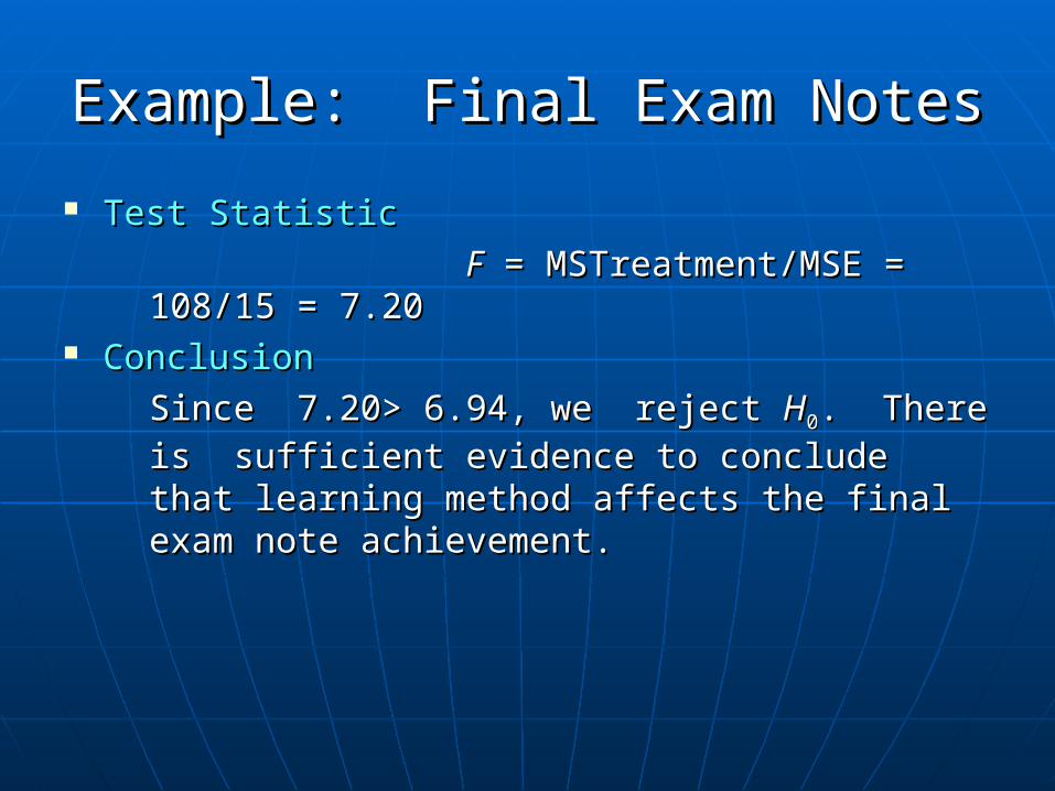
Test StatisticTest Statistic
FF = MSTreatment/MSE = 108/15 = MSTreatment/MSE = 108/15 = 7.20= 7.20
ConclusionConclusion
Since 7.20> 6.94, we reject Since 7.20> 6.94, we reject HH00. There is . There is sufficient evidence to conclude that learning sufficient evidence to conclude that learning method affects the final exam note method affects the final exam note achievement.achievement.

Using Excel’s AnovaUsing Excel’s Anova
Step 1Step 1 Select the Select the ToolsTools pull-down menu pull-down menu Step 2Step 2 Choose the Choose the Data AnalysisData Analysis option option Step 3Step 3 Choose Choose Anova: Two Factor Without Anova: Two Factor Without
Replication Replication from the list of Analysis Toolsfrom the list of Analysis Tools
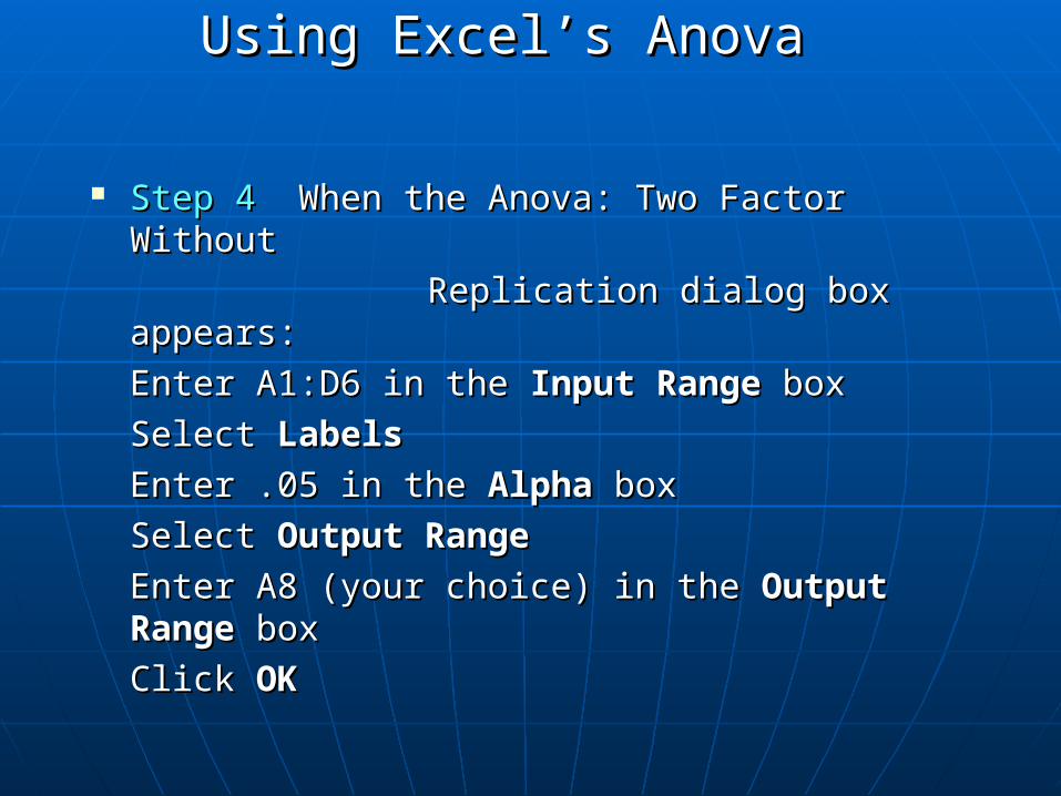
Step 4Step 4 When the Anova: Two Factor Without When the Anova: Two Factor Without
Replication dialog box appears:Replication dialog box appears:
Enter A1:D6 in the Enter A1:D6 in the Input RangeInput Range box box
Select Select LabelsLabels
Enter .05 in the Enter .05 in the AlphaAlpha box box
Select Select Output RangeOutput Range
Enter A8 (your choice) in the Enter A8 (your choice) in the Output RangeOutput Range boxbox
Click Click OKOK
Using Excel’s AnovaUsing Excel’s Anova
Value Worksheet (top portion)Value Worksheet (top portion)
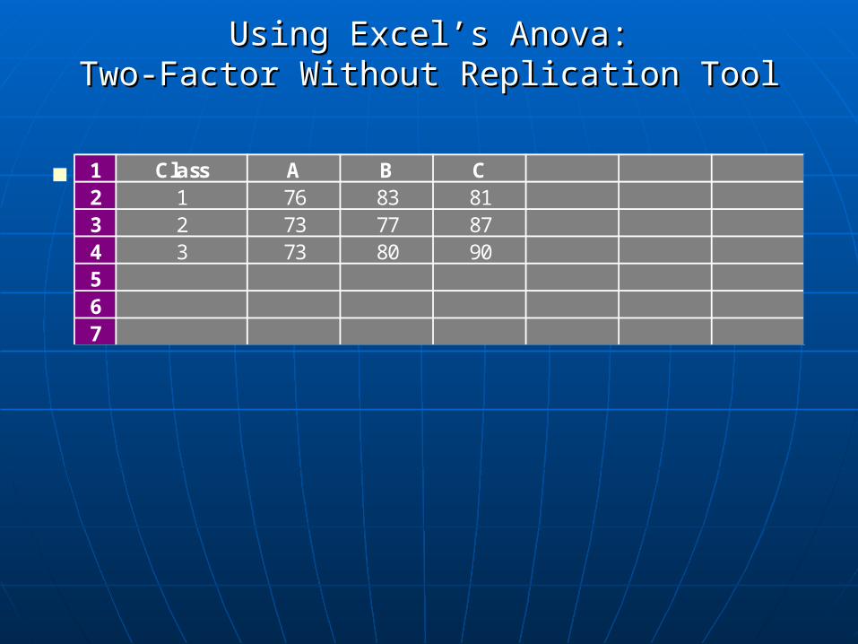
Using Excel’s Anova:Using Excel’s Anova:Two-Factor Without Replication ToolTwo-Factor Without Replication Tool
1 Class A B C2 1 76 83 81 3 2 73 77 874 3 73 80 90 5 6 7
Value Worksheet (middle portion)Value Worksheet (middle portion)
Using Excel’s Anova:Using Excel’s Anova:Two-Factor Without Replication ToolTwo-Factor Without Replication Tool
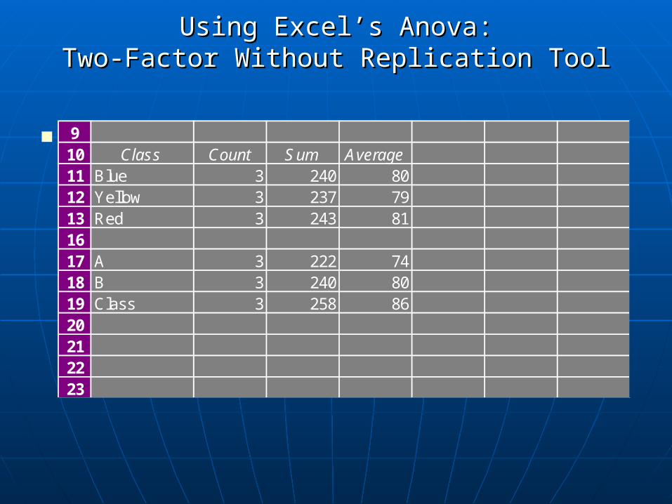
910 Class Count Sum Average11 Blue 3 240 8012 Yellow 3 237 7913 Red 3 243 811617 A 3 222 7418 B 3 240 8019 Class 3 258 8620212223
Using Excel’s AnovaUsing Excel’s Anova
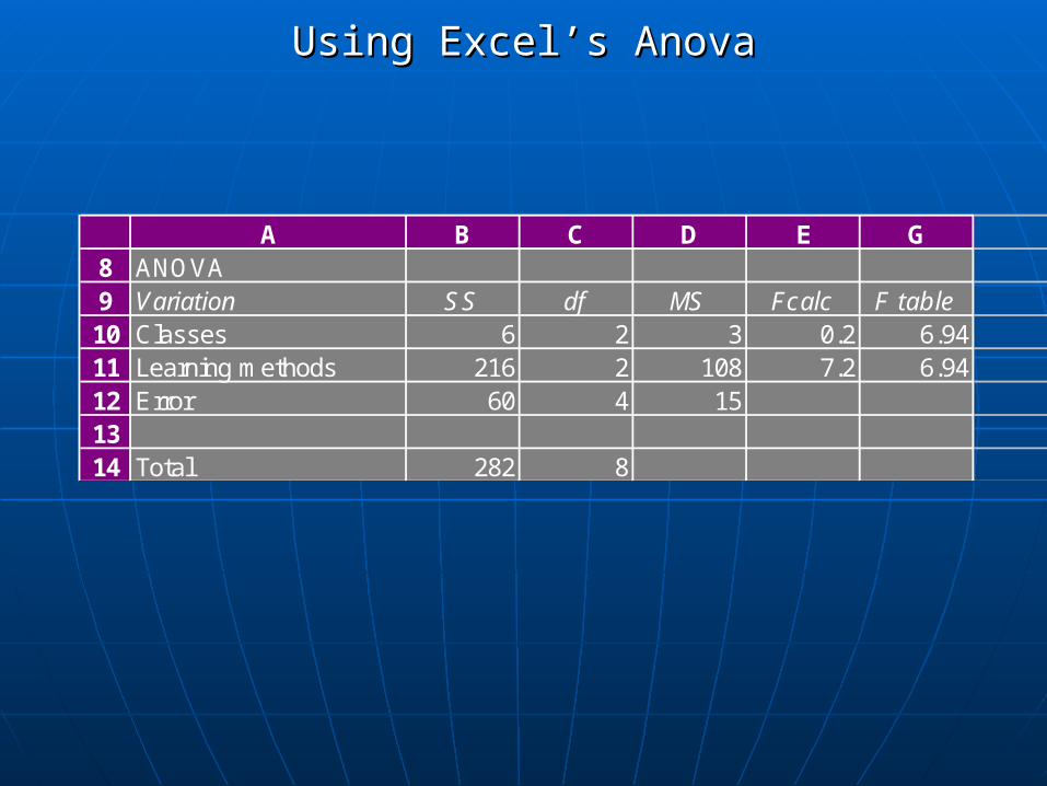
A B C D E G8 ANOVA9 Variation SS df MS Fcalc F table10 Classes 6 2 3 0.2 6.9411 Learning methods 216 2 108 7.2 6.9412 Error 60 4 151314 Total 282 8
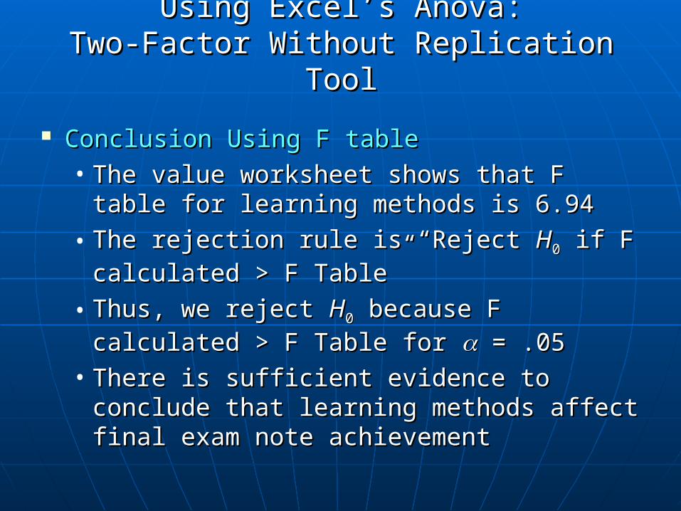
Conclusion Using F tableConclusion Using F table• The value worksheet shows that F table The value worksheet shows that F table
for learning methods is 6.94for learning methods is 6.94
• The rejection rule is “The rejection rule is “Reject Reject HH00 if F if F calculated > F Table”calculated > F Table”
• Thus, we reject Thus, we reject HH00 because F calculated because F calculated > F Table for > F Table for = .05 = .05
• There is sufficient evidence to conclude There is sufficient evidence to conclude that learning methods affect final exam that learning methods affect final exam note achievementnote achievement
Using Excel’s Anova:Using Excel’s Anova:Two-Factor Without Replication ToolTwo-Factor Without Replication Tool
Similarities and differences Similarities and differences between CRD and RCBD: between CRD and RCBD:
ProceduresProcedures RCBD: Every level of “treatment” encountered RCBD: Every level of “treatment” encountered
by each experimental unit; CRD: Just one level by each experimental unit; CRD: Just one level eacheach
Descriptive statistics and graphical display: the Descriptive statistics and graphical display: the same as CRDsame as CRD
Model adequacy checking procedure: the same Model adequacy checking procedure: the same except: specifically, except: specifically, NO Block x Treatment NO Block x Treatment InteractionInteraction
ANOVA: Inclusion of the Block effect; ANOVA: Inclusion of the Block effect; dfdferrorerror change from change from tt((rr – 1) to ( – 1) to (tt – 1)( – 1)(rr – 1) – 1)

Latin Square DesignLatin Square Design
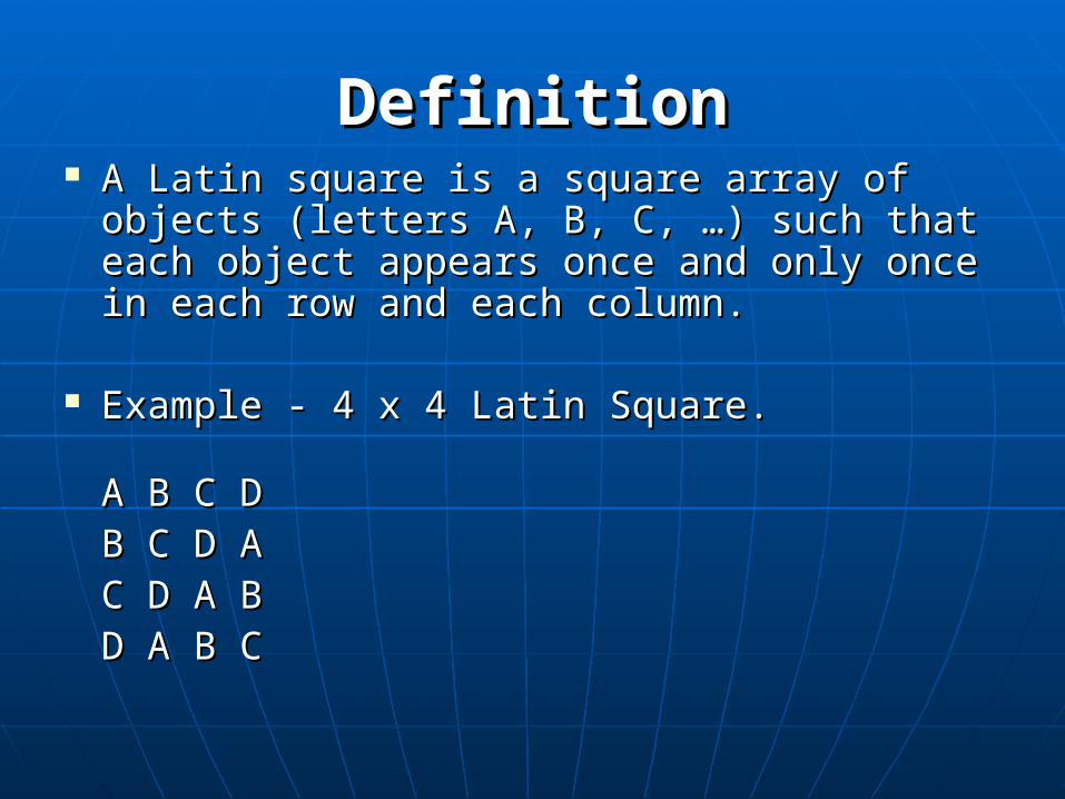
DefinitionDefinition A Latin square is a square array of objects A Latin square is a square array of objects
(letters A, B, C, …) such that each object (letters A, B, C, …) such that each object appears once and only once in each row appears once and only once in each row and each column. and each column.
Example - 4 x 4 Latin Square.Example - 4 x 4 Latin Square.
A B C DA B C DB C D AB C D AC D A BC D A BD A B CD A B C
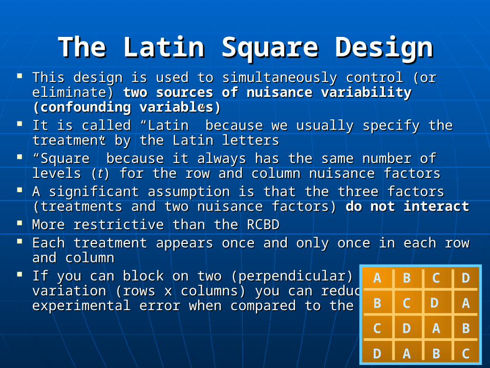
The Latin Square DesignThe Latin Square Design This design is used to simultaneously control (or This design is used to simultaneously control (or
eliminate) eliminate) two sources of nuisance variability two sources of nuisance variability (confounding variables)(confounding variables)
It is called “Latin” because we usually specify the It is called “Latin” because we usually specify the treatment by the Latin letterstreatment by the Latin letters
““Square” because it always has the same number of Square” because it always has the same number of levels (levels (tt) for the row and column nuisance factors) for the row and column nuisance factors
A significant assumption is that the three factors A significant assumption is that the three factors (treatments and two nuisance factors) (treatments and two nuisance factors) do not interactdo not interact
More restrictive than the RCBDMore restrictive than the RCBD Each treatment appears once and only once in each row Each treatment appears once and only once in each row
and columnand column If you can block on two (perpendicular) sources of If you can block on two (perpendicular) sources of
variation (rows x columns) you can reduce experimental variation (rows x columns) you can reduce experimental error when compared to the RCBDerror when compared to the RCBD
A
B C D
A
B C D A
BC D
A
B CD

Useful in Animal Nutrition Useful in Animal Nutrition StudiesStudies
Suppose you had four feeds you wanted to test Suppose you had four feeds you wanted to test on dairy cows. The feeds would be tested over on dairy cows. The feeds would be tested over time during the lactation periodtime during the lactation period
This experiment would require 4 animals (think This experiment would require 4 animals (think of these as the rows)of these as the rows)
There would be 4 feeding periods at even There would be 4 feeding periods at even intervals during the lactation period beginning intervals during the lactation period beginning early in lactation (these would be the columns)early in lactation (these would be the columns)
The treatments would be the four feeds. Each The treatments would be the four feeds. Each animal receives each treatment one time only.animal receives each treatment one time only.
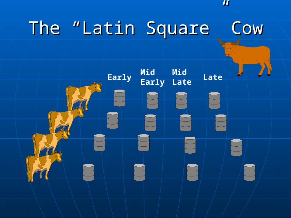
The “Latin Square” CowThe “Latin Square” Cow
EarlyMidEarly
MidLate Late
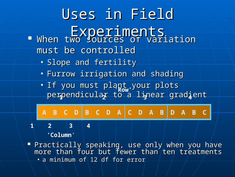
When two sources of variation must be When two sources of variation must be controlledcontrolled• Slope and fertilitySlope and fertility• Furrow irrigation and shadingFurrow irrigation and shading• If you must plant your plots perpendicular If you must plant your plots perpendicular
to a linear gradientto a linear gradient
Uses in Field ExperimentsUses in Field Experiments
B C DA B C D A A BC D A B CD
‘Row’1 2 3 4
1 2 3 4
‘Column’
Practically speaking, use only when you have Practically speaking, use only when you have more than four but fewer than ten treatmentsmore than four but fewer than ten treatments• a minimum of 12 df for errora minimum of 12 df for error
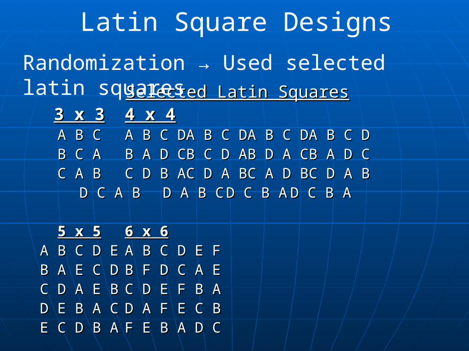
Selected Latin SquaresSelected Latin Squares3 x 33 x 3 4 x 44 x 4A B CA B C A B C DA B C D A B C DA B C D A B C DA B C D A B C DA B C DB C AB C A B A D CB A D C B C D AB C D A B D A CB D A C B A D CB A D CC A BC A B C D B AC D B A C D A BC D A B C A D BC A D B C D A BC D A B
D C A BD C A B D A B CD A B C D C B AD C B A D C B AD C B A
5 x 55 x 5 6 x 66 x 6A B C D EA B C D E A B C D E FA B C D E FB A E C DB A E C D B F D C A EB F D C A EC D A E BC D A E B C D E F B AC D E F B AD E B A CD E B A C D A F E C BD A F E C BE C D B AE C D B A F E B A D CF E B A D C
Latin Square Designs
Randomization → Used selected latin squares
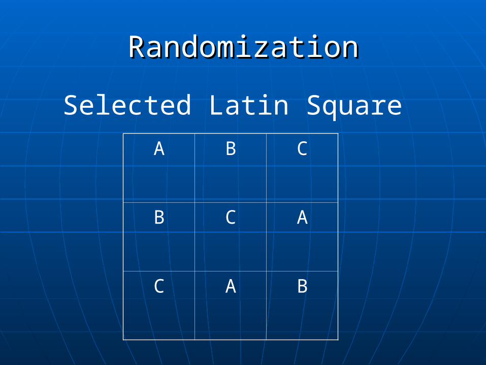
RandomizationRandomization
Selected Latin Square
A B C
B C A
C A B
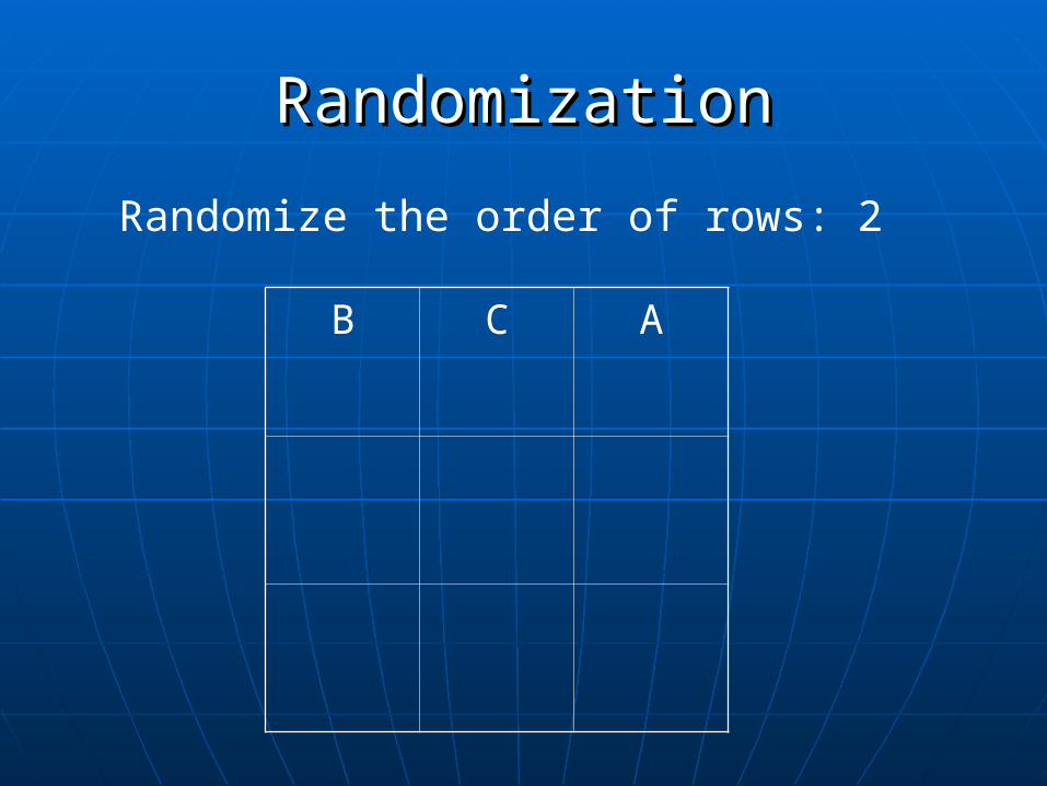
RandomizationRandomization
Randomize the order of rows: 2
B C A
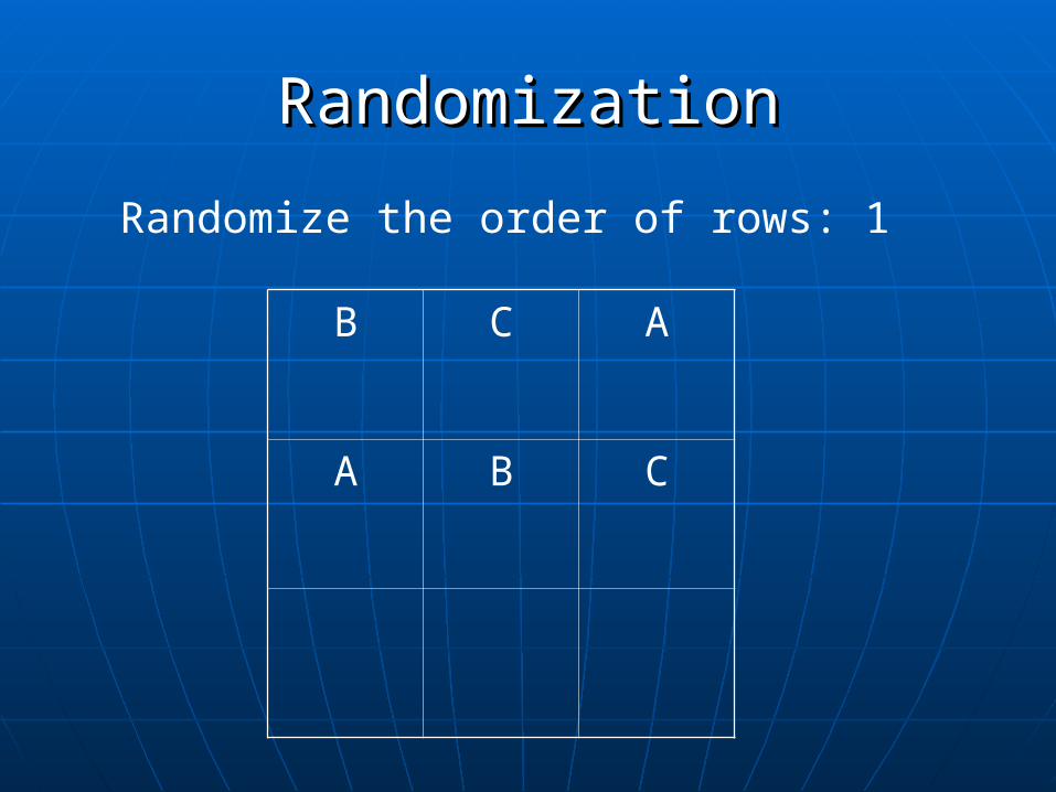
RandomizationRandomization
Randomize the order of rows: 1
B C A
A B C
RandomizationRandomization
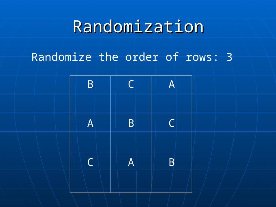
Randomize the order of rows: 3
B C A
A B C
C A B
RandomizationRandomization
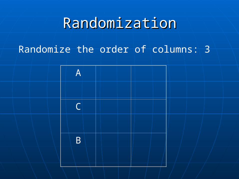
Randomize the order of columns: 3
A
C
B
RandomizationRandomization
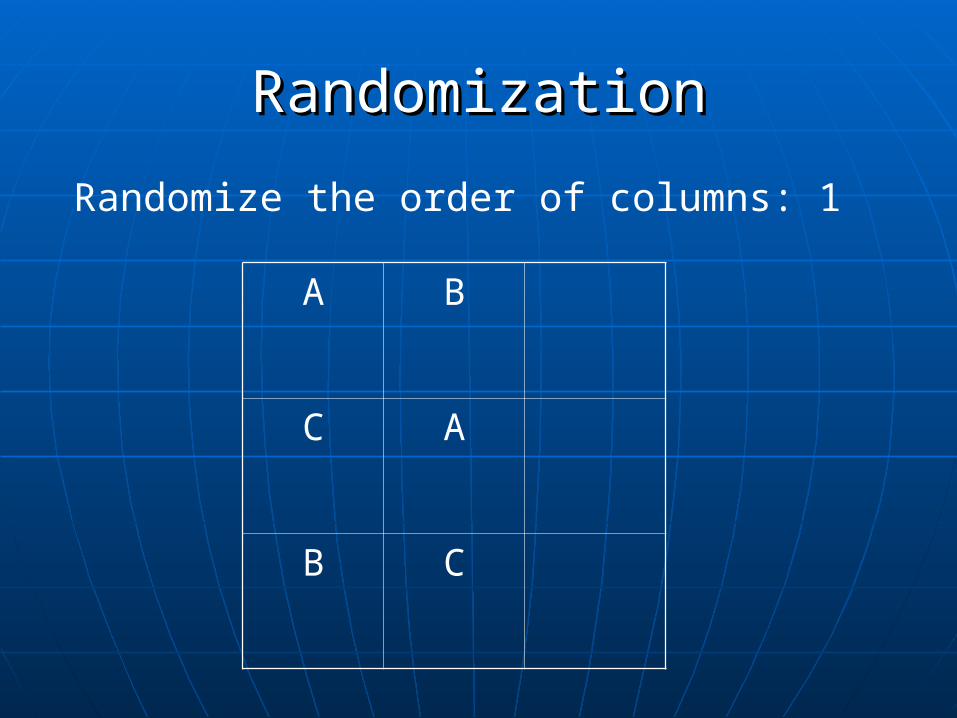
Randomize the order of columns: 1
A B
C A
B C
RandomizationRandomization
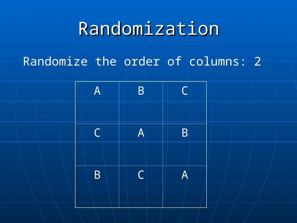
Randomize the order of columns: 2
A B C
C A B
B C A
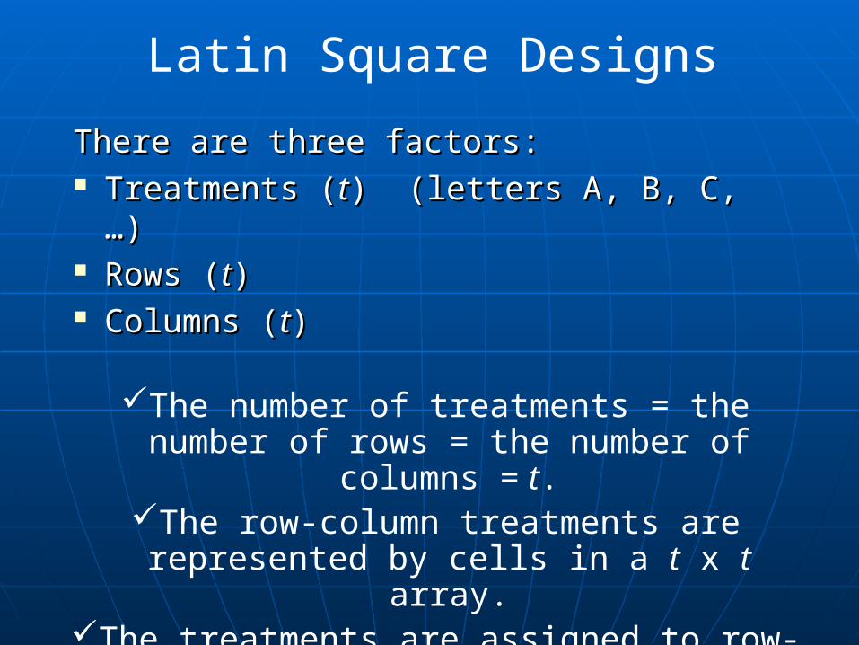
There are three factors:There are three factors: Treatments (Treatments (tt) (letters A, B, C, …)) (letters A, B, C, …) Rows (Rows (tt) ) Columns (Columns (tt) )
The number of treatments = the number of rows = the number of columns = t.The row-column treatments are represented by cells in a t x t array.
The treatments are assigned to row-column combinations using a Latin-
square arrangement
Latin Square Designs
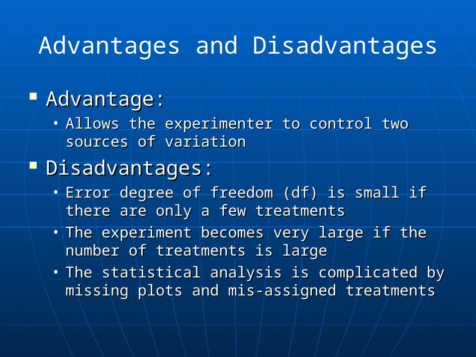
Advantages and Disadvantages
Advantage:Advantage:• Allows the experimenter to control two Allows the experimenter to control two
sources of variationsources of variation
Disadvantages:Disadvantages:• Error degree of freedom (df) is small if there Error degree of freedom (df) is small if there
are only a few treatmentsare only a few treatments• The experiment becomes very large if the The experiment becomes very large if the
number of treatments is largenumber of treatments is large• The statistical analysis is complicated by The statistical analysis is complicated by
missing plots and mis-assigned treatmentsmissing plots and mis-assigned treatments
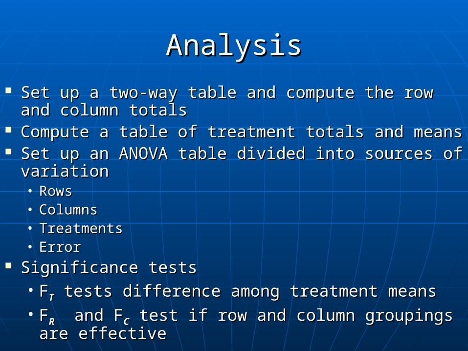
AnalysisAnalysis Set up a two-way table and compute the row and Set up a two-way table and compute the row and
column totalscolumn totals Compute a table of treatment totals and meansCompute a table of treatment totals and means Set up an ANOVA table divided into sources of Set up an ANOVA table divided into sources of
variationvariation• RowsRows• ColumnsColumns• TreatmentsTreatments• ErrorError
Significance testsSignificance tests• FFTT tests difference among treatment means tests difference among treatment means• FFRR and F and FCC test if row and column groupings are test if row and column groupings are
effectiveeffective
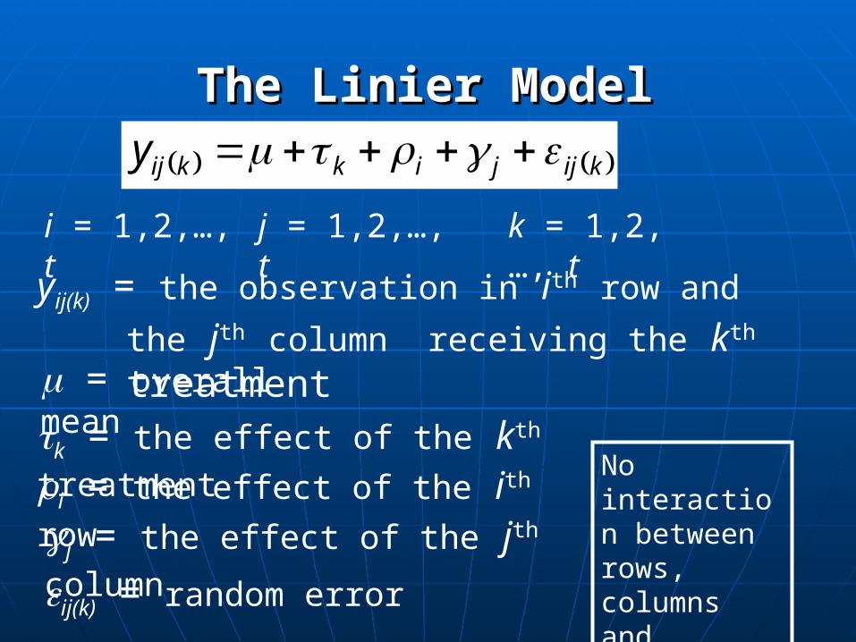
The Linier ModelThe Linier Model
kijjikkijy
i = 1,2,…, t
j = 1,2,…, t
yij(k) = the observation in ith row and the jth column receiving the kth treatment
= overall mean
k = the effect of the kth treatmenti = the effect of the ith row
ij(k) = random error
k = 1,2,…, t
j = the effect of the jth column
No interaction between rows, columns and treatments
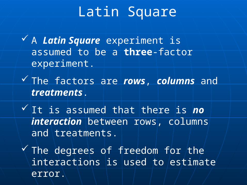
A Latin Square experiment is assumed to be a three-factor experiment.
The factors are rows, columns and treatments.
It is assumed that there is no interaction between rows, columns and treatments.
The degrees of freedom for the interactions is used to estimate error.
Latin Square
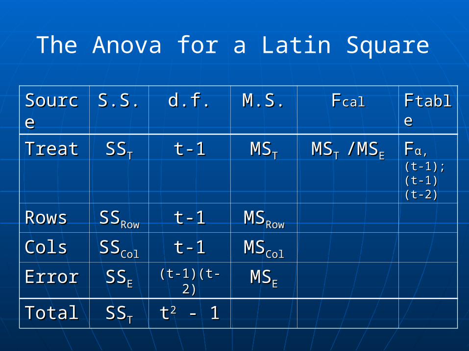
The Anova for a Latin Square
SourcSourcee
S.S.S.S. d.f.d.f. M.S.M.S. FFcalcal FFtabltablee
TreatTreat SSSSTT t-1t-1 MSMSTT MSMST T /MS/MSEE FFαα, (t-, (t-1); (t-1)1); (t-1)(t-2)(t-2)
RowsRows SSSSRowRow t-1t-1 MSMSRowRow
ColsCols SSSSColCol t-1t-1 MSMSColCol
ErrorError SSSSEE(t-1)(t-2)(t-1)(t-2) MSMSEE
TotalTotal SSSSTT tt22 - 1 - 1

ExampleExampleThe effect of learning methods on the final The effect of learning methods on the final exam note of experimental design course.exam note of experimental design course.
Student as an experimental unit can be grouped Student as an experimental unit can be grouped based on academic year and high school origin based on academic year and high school origin
Treatment: A: self learning B: Class learning C: Class and Practice learning
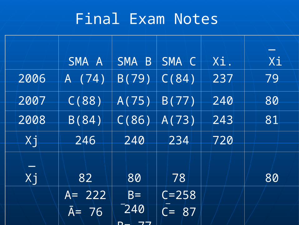
SMA A SMA B
SMA C
Xi._
Xi
2006 A (74) B(79) C(84) 237 79
2007 C(88) A(75) B(77) 240 80
2008 B(84) C(86) A(73) 243 81
Xj 246 240 234 720
_Xj 82 80 78 80
A= 222Ā= 76
B= 240
B= 77
C=258
C= 87
_ _
Final Exam Notes
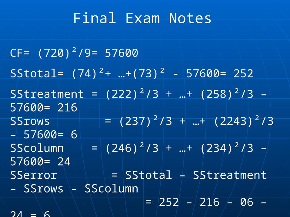
Final Exam Notes
CF= (720)²/9= 57600
SStotal= (74)²+ …+(73)² - 57600= 252
SStreatment = (222)²/3 + …+ (258)²/3 – 57600= 216SSrows = (237)²/3 + …+ (2243)²/3 – 57600= 6SScolumn = (246)²/3 + …+ (234)²/3 – 57600= 24SSerror = SStotal – SStreatment – SSrows – SScolumn = 252 – 216 – 06 – 24 = 6
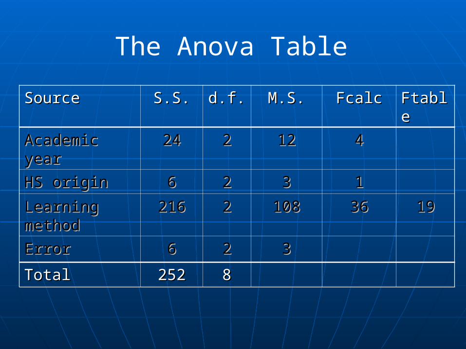
The Anova Table
SourceSource S.S.S.S. d.f.d.f. M.S.M.S. FcalcFcalc FtablFtablee
Academic Academic yearyear
2424 22 1212 44
HS originHS origin 66 22 33 11
Learning Learning methodmethod
216216 22 108108 3636 1919
ErrorError 66 22 33
TotalTotal 252252 88

Graeco-Latin Square Graeco-Latin Square DesignsDesigns
Mutually orthogonal Squares
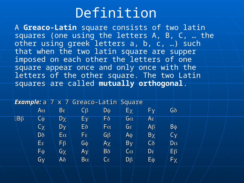
DefinitionA Greaco-Latin square consists of two latin squares (one using the letters A, B, C, … the other using greek letters a, b, c, …) such that when the two latin square are supper imposed on each other the letters of one square appear once and only once with the letters of the other square. The two Latin squares are called mutually orthogonal.
Example: Example: a 7 x 7 Greaco-Latin Squarea 7 x 7 Greaco-Latin SquareAA BB CC DD EE FF GG
BB CC DD EE FF GG AACC DD EE FF GG AA BBDD EE FF GG AA BB CCEE FF GG AA BB CC DDFF GG AA BB CC DD EEGG AA BB CC DD EE FF
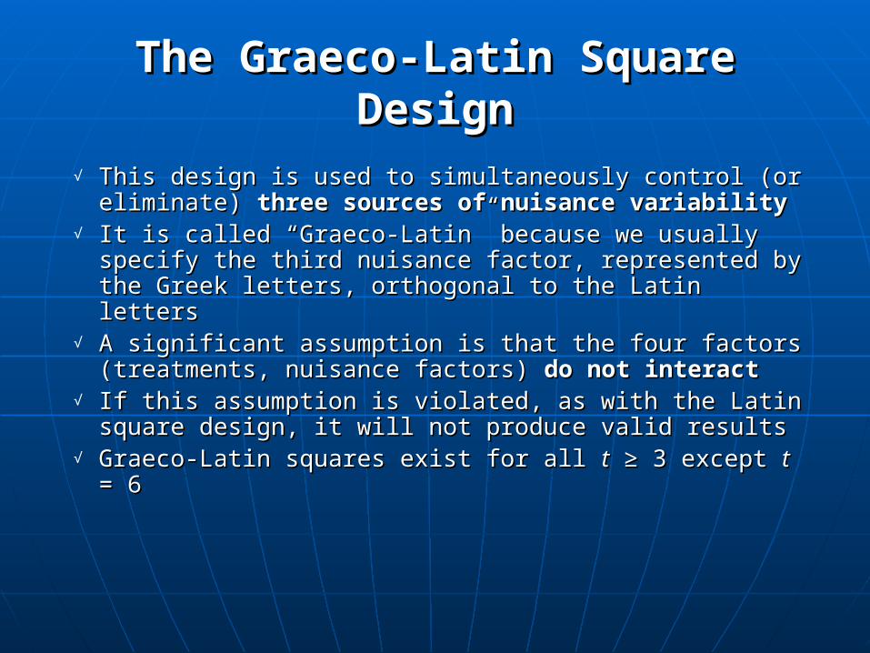
The Graeco-Latin Square The Graeco-Latin Square DesignDesign
√ This design is used to simultaneously control (or This design is used to simultaneously control (or eliminate) eliminate) three sources of nuisance three sources of nuisance variabilityvariability
√ It is called “Graeco-Latin” because we usually It is called “Graeco-Latin” because we usually specify the third nuisance factor, represented by specify the third nuisance factor, represented by the Greek letters, orthogonal to the Latin lettersthe Greek letters, orthogonal to the Latin letters
√ A significant assumption is that the four factors A significant assumption is that the four factors (treatments, nuisance factors) (treatments, nuisance factors) do not interactdo not interact
√ If this assumption is violated, as with the Latin If this assumption is violated, as with the Latin square design, it will not produce valid resultssquare design, it will not produce valid results
√ Graeco-Latin squares exist for all Graeco-Latin squares exist for all tt ≥ 3 except ≥ 3 except tt = 6= 6
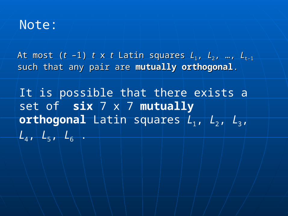
Note:
At most (At most (tt –1) –1) tt x x tt Latin squares Latin squares LL11, , LL22, …, , …, LLt-1t-1 such that any pair are such that any pair are mutually orthogonalmutually orthogonal..
It is possible that there exists a set of six 7 x 7 mutually orthogonal Latin squares L1, L2, L3, L4, L5, L6 .
The Greaco-Latin Square DesignThe Greaco-Latin Square Design - An Example - An Example
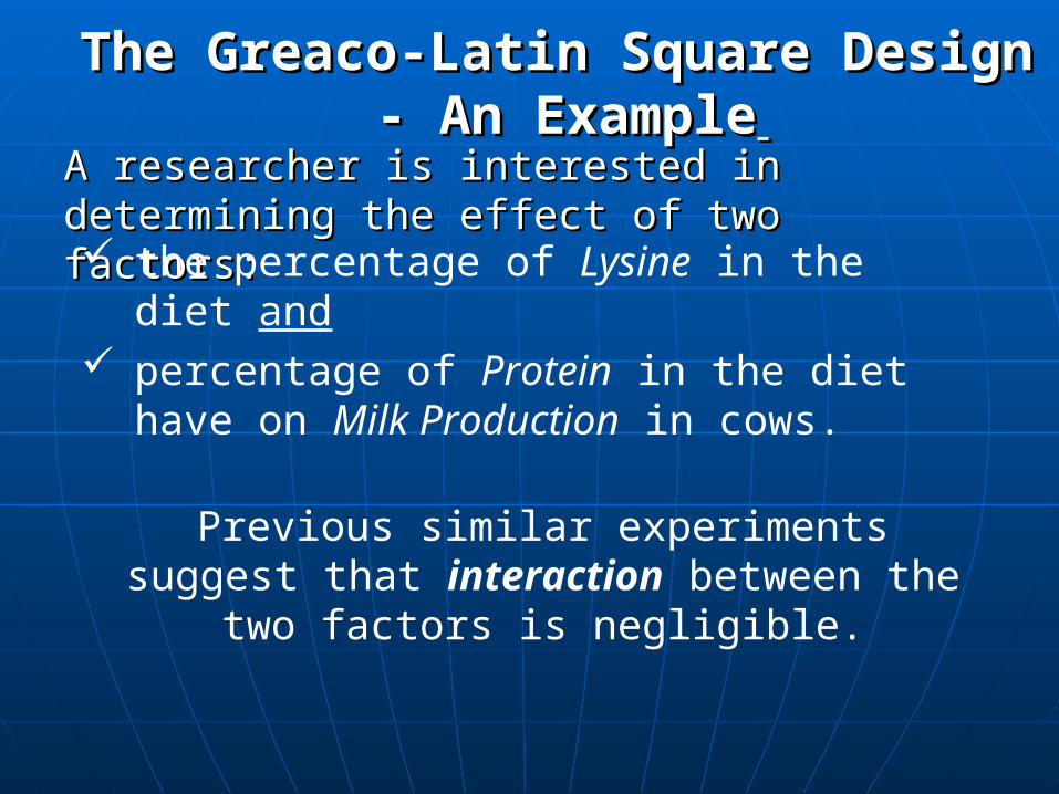
A researcher is interested in determining A researcher is interested in determining the effect of two factors:the effect of two factors: the percentage of Lysine in the diet
and percentage of Protein in the diet have
on Milk Production in cows.
Previous similar experiments suggest that interaction between the two factors is
negligible.
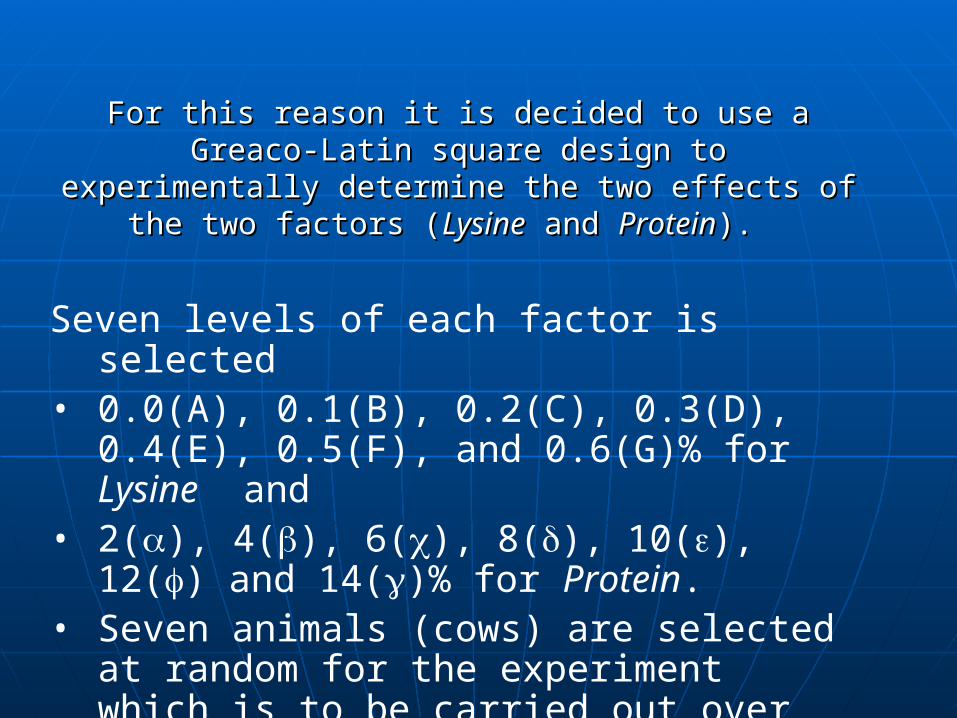
For this reason it is decided to use a Greaco-For this reason it is decided to use a Greaco-Latin square design to experimentally determine Latin square design to experimentally determine
the two effects of the two factors (the two effects of the two factors (LysineLysine and and ProteinProtein). ).
Seven levels of each factor is selected• 0.0(A), 0.1(B), 0.2(C), 0.3(D), 0.4(E),
0.5(F), and 0.6(G)% for Lysine and • 2(), 4(), 6(), 8(), 10(), 12() and
14()% for Protein. • Seven animals (cows) are selected at
random for the experiment which is to be carried out over seven three-month periods.
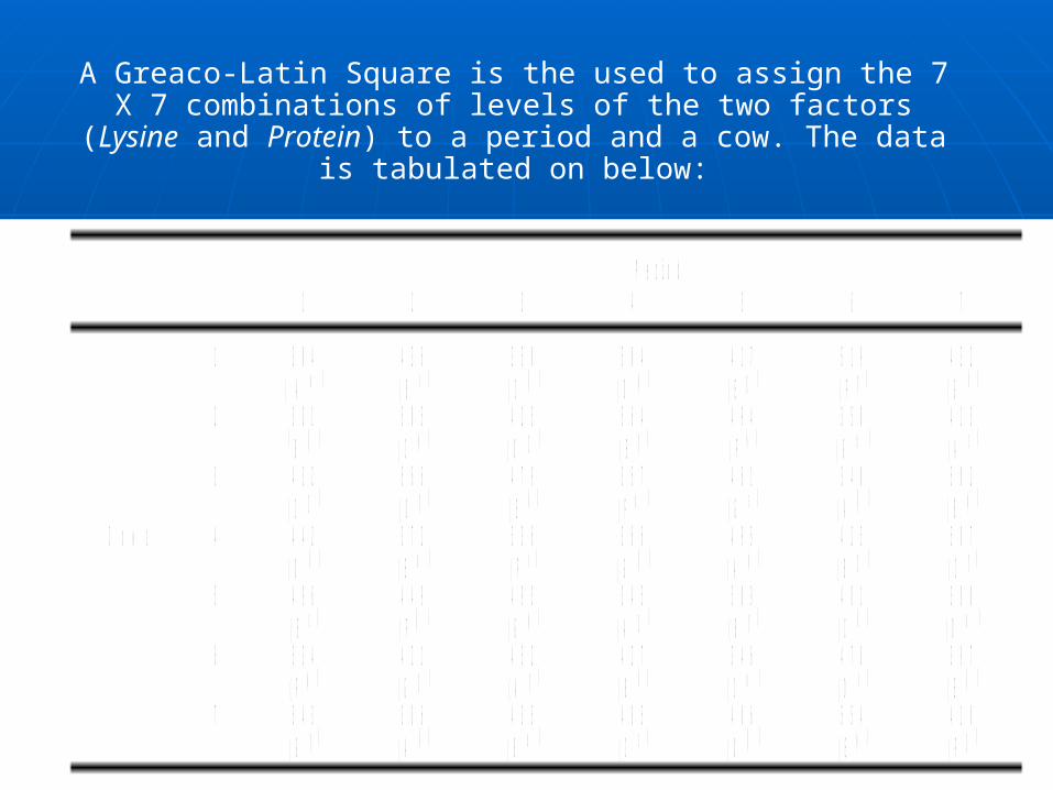
A Greaco-Latin Square is the used to assign the 7 X 7 combinations of levels of the two factors (Lysine and
Protein) to a period and a cow. The data is tabulated on below:
P e r i o d
1 2 3 4 5 6 7
1 3 0 4 4 3 6 3 5 0 5 0 4 4 1 7 5 1 9 4 3 2
( A ( B ( C ( D ( E ( F ( G 2 3 8 1 5 0 5 4 2 5 5 6 4 4 9 4 3 5 0 4 1 3 B ( C ( D ( E ( F ( G ( A 3 4 3 2 5 6 6 4 7 9 3 5 7 4 6 1 3 4 0 5 0 2 ( C ( D ( E ( F ( G ( A ( B C o w s 4 4 4 2 3 7 2 5 3 6 3 6 6 4 9 5 4 2 5 5 0 7 ( D ( E ( F ( G ( A ( B ( C 5 4 9 6 4 4 9 4 9 3 3 4 5 5 0 9 4 8 1 3 8 0 ( E ( F ( G ( A ( B ( C ( D 6 5 3 4 4 2 1 4 5 2 4 2 7 3 4 6 4 7 8 3 9 7 ( F ( G ( A ( B ( C ( D ( E 7 5 4 3 3 8 6 4 3 5 4 8 5 4 0 6 5 5 4 4 1 0 ( G ( A ( B ( C ( D ( E ( F
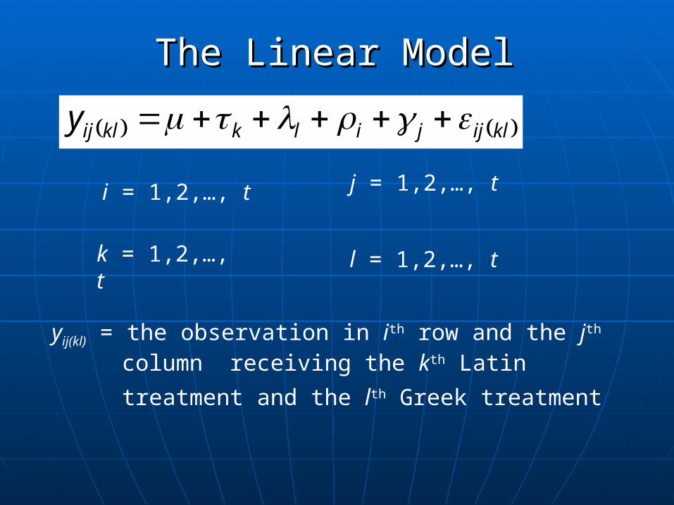
The Linear ModelThe Linear Model
klijjilkklijy
i = 1,2,…, t j = 1,2,…, t
yij(kl) = the observation in ith row and the jth column receiving the kth Latin treatment and the lth
Greek treatment
k = 1,2,…, t l = 1,2,…, t
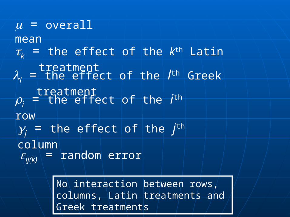
= overall mean
k = the effect of the kth Latin treatment
i = the effect of the ith row
ij(k) = random error
j = the effect of the jth column
No interaction between rows, columns, Latin treatments and Greek treatments
l = the effect of the lth Greek treatment
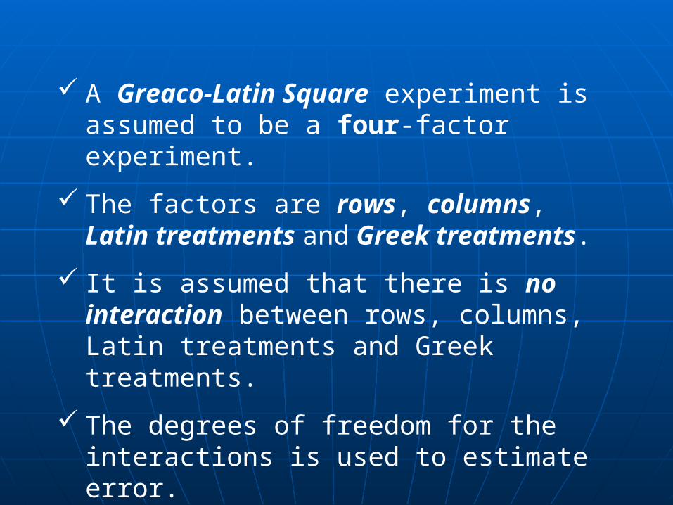
A Greaco-Latin Square experiment is assumed to be a four-factor experiment.
The factors are rows, columns, Latin treatments and Greek treatments.
It is assumed that there is no interaction between rows, columns, Latin treatments and Greek treatments.
The degrees of freedom for the interactions is used to estimate error.