Embed Size (px)
Citation preview

Complex Analysis and Riemann Surfaces
Professor Duong Hong PhongDept. of Mathematics
Columbia University
Notes by Yiqiao Yin in LATEX
May 5, 2017
Abstract
This is the notes for Complex Analysis and Riemann Surfaces, a gradlevel course offered in 2016 ∼ 2017 school year by Professor Duong HongPhong1. Topics include holomorphic functions, analytic continuation, Rie-mann surfaces, theta functions, and modular forms.
Professor Phong’s lectures are not just delivering inspiring elements ofmathematical world; they are also expressions of human minds reflectingactive will and the desire of aesthetic perfection. I also want to expressspecial thanks to Qi You 2.
1Duong H. Phong is Professor of Mathematics at Columbia University. His website ishttp://www.math.columbia.edu/~phong/.
2Qi You is Gibbs Assistant Professor at Yale. He is a previous grad student at ColumbiaUniversity. His website is http://users.math.yale.edu/~yq64/.
1
This note is dedicated to Duong H. Phong and Mihai Bailesteanu, sinequibus non discere geometriam.
2
PrefaceWhen I wrote this, I was a graduate visiting student ap-plying for PhD in math. I did my undergrad at Universityof Rochester in mathematics. Inspired by Professor Mi-hai Bailesteanu, I fell in love with upper level geometry.I want to move forward and beyond so I traveled to NewYork to pursue more advanced thinking in my field of in-terest, Riemann Surfaces, following Professor Duong HongPhong at Columbia University.
I found Phong’s work very unique and different than mostof the texts out there. It was definitely difficult to fullyunderstand his lecture at first, but after spending somequality time I realized that the knowledge Phong deliv-ered is not just elegant theorems and advanced proofs butalso inspirational elements reflecting the aesthetic perfec-tion of the geometry world. This beautiful extension ofart is something I have never encountered before. Suchknowledge is too perfect to be forgotten and should beappreciated by us. Therefore, I have decided to put ev-erything down and document Phong’s work for the futuregenerations.
Yiqiao Yin
2016 ∼ 2017 at Columbia University
3
Contents
1 Local Theory of Holomorphic Functions 51.1 Holomorphic Functions . . . . . . . . . . . . . . . . . . . . . 51.2 Consequences of Holomorphicity . . . . . . . . . . . . . . . 51.3 Examples of Holomorphic Functions . . . . . . . . . . . . . 101.4 Open Mapping and Maximal Modulars Theorems . . . . . . 101.5 Applications: Method of Residues . . . . . . . . . . . . . . . 131.6 Analytic Continuation . . . . . . . . . . . . . . . . . . . . . 14
2 Riemann Surfaces 182.1 Simple Model . . . . . . . . . . . . . . . . . . . . . . . . . . 182.2 Another Basic Example . . . . . . . . . . . . . . . . . . . . 212.3 Key Strategy . . . . . . . . . . . . . . . . . . . . . . . . . . 24
2.3.1 Construction of Holomorphic Differentials . . . . . . 242.4 Method of Abelian Integral (Riemann) . . . . . . . . . . . . 30
3 Function Theory on Tori 333.1 Function Theory According to Weierstrass . . . . . . . . . . 343.2 Function Theory According to Jacobi . . . . . . . . . . . . . 383.3 Meromorphic Forms . . . . . . . . . . . . . . . . . . . . . . 403.4 Special Properties of θ-Functions . . . . . . . . . . . . . . . 413.5 Function Theory Using PDE . . . . . . . . . . . . . . . . . 44
4 General Theory 484.1 Riemann Surface . . . . . . . . . . . . . . . . . . . . . . . . 484.2 Chern Connection . . . . . . . . . . . . . . . . . . . . . . . 504.3 Commutation Rules . . . . . . . . . . . . . . . . . . . . . . 514.4 Basic Residue Formula for Holomorphic Line Bundles . . . 514.5 Spectral Decomposition of Laplacian 4− . . . . . . . . . . 554.6 Serre Duality . . . . . . . . . . . . . . . . . . . . . . . . . . 57
5 Curvatures on Vector Bundles 66
6 Kodaira Vanishing Theorem 78
7 Kahler Manifolds 817.1 Kahler Condition . . . . . . . . . . . . . . . . . . . . . . . . 81
8 The Calabi Conjecture 848.1 Reduction to a Monge-Ampere equation . . . . . . . . . . . 858.2 Method of Continuity . . . . . . . . . . . . . . . . . . . . . 868.3 Verifying the Hypotheses of IFT . . . . . . . . . . . . . . . 888.4 Basic Fact From Linear Analysis . . . . . . . . . . . . . . . 89
4
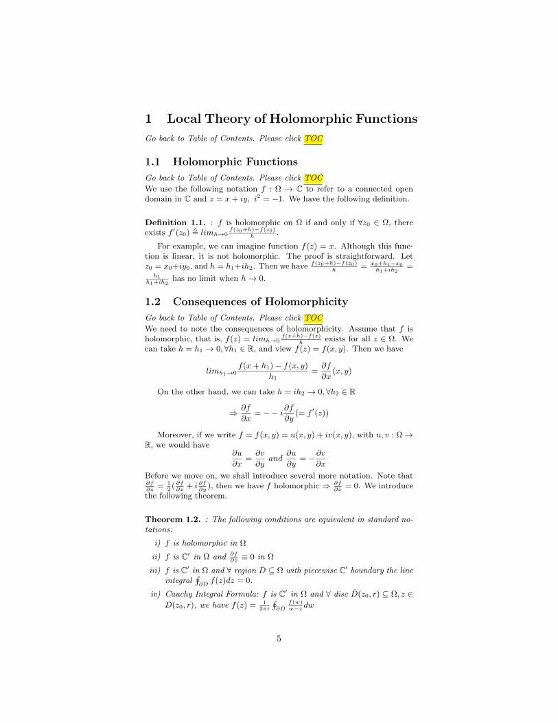
1 Local Theory of Holomorphic Functions
Go back to Table of Contents. Please click TOC
1.1 Holomorphic Functions
Go back to Table of Contents. Please click TOC
We use the following notation f : Ω → C to refer to a connected opendomain in C and z = x+ iy, i2 = −1. We have the following definition.
Definition 1.1. : f is holomorphic on Ω if and only if ∀z0 ∈ Ω, thereexists f ′(z0) , limh→0
f(z0+h)−f(z0)h
.
For example, we can imagine function f(z) = x. Although this func-tion is linear, it is not holomorphic. The proof is straightforward. Letz0 = x0+iy0, and h = h1+ih2. Then we have f(z0+h)−f(z0)
h= x0+h1−x0
h1+ih2=
h1h1+ih2
has no limit when h→ 0.
1.2 Consequences of Holomorphicity
Go back to Table of Contents. Please click TOC
We need to note the consequences of holomorphicity. Assume that f isholomorphic, that is, f(z) = limh→0
f(z+h)−f(z)h
exists for all z ∈ Ω. Wecan take h = h1 → 0,∀h1 ∈ R, and view f(z) = f(x, y). Then we have
limh1→0f(x+ h1)− f(x, y)
h1=∂f
∂x(x, y)
On the other hand, we can take h = ih2 → 0, ∀h2 ∈ R
⇒ ∂f
∂x= −− i∂f
∂y(= f ′(z))
Moreover, if we write f = f(x, y) = u(x, y) + iv(x, y), with u, v : Ω→R, we would have
∂u
∂x=∂v
∂yand
∂u
∂y= −∂v
∂x
Before we move on, we shall introduce several more notation. Note that∂f∂z
= 12( ∂f∂x
+ i ∂f∂y
), then we have f holomorphic ⇒ ∂f∂z
= 0. We introducethe following theorem.
Theorem 1.2. : The following conditions are equivalent in standard no-tations:
i) f is holomorphic in Ω
ii) f is C′ in Ω and ∂f∂z≡ 0 in Ω
iii) f is C′ in Ω and ∀ region D ⊆ Ω with piecewise C′ boundary the lineintegral
∮∂D
f(z)dz = 0.
iv) Cauchy Integral Formula: f is C′ in Ω and ∀ disc D(z0, r) ⊆ Ω, z ∈D(z0, r), we have f(z) = 1
2πi
∮∂D
f(w)w−z dw
5

v) ∀z0 ∈ Ω, ∃ disc D(z0, r) ⊆ Ω, s.t. f(z) =∑∞n=0 cn(z − z0)n, ∀z ∈
D(z0, r). In particular, we have f ∈ Cω(Ω) ⊆ C∞(Ω).
With the idea above, we can observe the following (which is alsoGreen’s Theorem):
Theorem 1.3. : Green’s Theorem (in the plane): Let D be the regionin R2 with piecewise C′ boundary ∂D, then we have
∮∂D
D(x, y)dx +
Q(x, y)dy =∫∫D
( ∂Q∂x− ∂P
∂y)dxdy.
We can apply this theorem to the case of functions of a complex vari-able z, f(z) = u+ iv and we have
∮∂D
f(z)dz =∮∂D
(u+ iv)(dx+ idy) =∮udx − vdy + i
∮∂D
udy + vdx, by Green’s Theorem, we would have∮∂D
f(z)dz=∮∂D
(u+ iv)(dx+ idy) =∮udx− vdy + i
∮∂D
udy + vdx
=∫∫D
(− ∂u∂y− ∂v
∂x)dxdy + i
∫∫D
( ∂u∂x− ∂v
∂y)dxdy
=∫∫D
[(− ∂u∂y− ∂v
∂x) + i( ∂u
∂x− ∂v
∂y)]dxdy
= 2i∫∫D∂f∂zdxdy Hence, we say that
∮∂D
f(z)dz = 0 if f is holomorphic,
then ∂f∂z≡ 0.
Proof:In this proof we need to proof that (ii)⇔ (iii), (iii)⇔ (iv), (iv)⇔ (v),
(v)⇔ (i), and (i)⇔ (ii). We prove them accordingly.(ii)⇔ (iii)“⇒” Notice that f ∈ C′(Ω), we apply Green’s formula to complete the
proof.“⇐” We show this part by contradiction. Assume ∂f
∂z6= 0 for some
z0 ∈ Ω. Take an arbitrary disc D around z0. By (iii), we have
0 = |∮∂D
f(z)dz| = |2i∫∫∂D
∂zdxdy|= |2i
∫∫D
( ∂f∂z
(z)− ∂f∂z
(z0))dxdy + 2i ∂f∂z
(z0)∫∫Ddxdy|
≥ 2| ∂f∂z
(z0)∫∫Ddxdy| − 2|
∫∫D
( ∂f∂z
(z)− ∂f∂z
(z0))dxdy|≥ 2| ∂f
∂z(z0)|Area(D)− 2
∫∫D| ∂f∂z
(z)− ∂f∂z
(z0)|dxdy
Since f is C′, ∃δ > 0, s.t. |z − z0| < δ ⇒ | ∂f∂z
(z) − ∂f∂z
(z0)| < 12| ∂f∂z
(z0)|,which imples that 0 ≥ | ∂f
∂z(z0)|πδ2 > 0. This is a contradiction.
Q.E.D.
(iii)⇔ (iv)
We fix z ∈ Ω, and set g(ω) = f(ω)−f(z)ω−z , ω ∈ Ω|z. We then claim that
∂∂ω≡ 0 on Ω z, because ∂
∂ωg(ω) =
∂∂ω
(f(ω)−f(z))(ω−z)−(f(ω)−f(z)) ∂∂ω
(ω−z)(ω−z)2 −
0 since f(ω)− f(z), ω − z are holomorphic.Moreover, g is C on Ω|z since f(ω)− f(z) and ω− z are ⇒ satisfies
(ii) on Ω|z⇒ satisfies (iii) on Ω|zThen we apply (iii) to ε < |ω − z| < δ:
6

Figure 1: Graphic illustration of a disk such that ε < |ω − z| < δ
Then we have ⇒ 0 =∮∂Dg(ω)dω =
∮|ω−z|=δ g(ω)dω −
∮|ω−z|=ε =
g(ω)dω (*)We claim that
∮ω−z|=z g(ω)dω → 0 as ε → 0. This is because Taylor
Formula: (for C′)f(ω) = f(z) + ∂f
∂ω(ω − z)− ∂f
∂ω(ω − z) + 0(|ω − z|)
⇒ g(ω) = ∂f∂ω
(ω − z) + 0(|ω − z|)g can be extended as a continuous function on Ω, thus bounded on|ω − z| ≤ ε⇒ |
∮|ω−z|=ε g(ω)dω| ≤
∮|ω−z|=ε sup|ω−z|≤ε|g(ω)| = 2πε, then sup|ω−z|≤ε|g(ω)| →
0 as ε→ 0. Further, we know that it’s independent of ε by (*).Thus, we have
0 =∮|ω−z|=ε
f(ω)−f(z)ω−z dω =
∮|ω−z|=ε
f(ω)ω−z dω − f(z)
∮|ω−z|=ε
1ω−zdω
=∮|ω−z|=ε
f(ω)ω−z dω − f(z)
∫|ξ|=ε
dξξ
, while ξ = δeiθ
=∮|ω−z|=ε
f(ω)ω−z dω − f(z)
∫ 2x
0iδeiθ
δeiθdθ
=∮|ω−z|=ε
f(ω)ω−z dω − 2πif(z)
⇒ f(z) = 12πi
∮|ω−z|=ε
f(ω)ω−z dω
This is the case that z = z0 in (iv). More generally, for any point z
in |z − z0| < δ, consider the integral of f(ω)ω−z on the boundary of the
region bounded by |ω − z| < δ and |ω − z| < ε, ε small enough so
that it is contained in |ω − z0| < δ, then we have 12πi
∮|ω−z|=ε
f(ω)ω−z dω −
12πi
∮|ω−z|=ε
f(ω)ω−z dω = 0⇒ f(z) = 1
2πi
∮|ω−z|=ε
f(ω)ω−z dω = 1
2πi
Figure 2: Graphic illustration of a region bounded by |ω−z| < δ and |ω−z| < εwith ε small enough so that it is contained in |ω − z0| < δ
(iv)⇒ (v)Now we have f(z) = 1
2πi
∮|ω−z|=ε f(ω) 1
(ω−z0)−(z−z0)dω
= 12πi
∮|ω−z|=ε
f(ω)ω−z0
1
1− z−z0ω−ω0
dω
= 12πi
∮|ω−z|=ε
f(ω)ω−z0
∑∞n=0( z−z0
ω−ω0)ndω
7
= 12πi
∑∞n=0(
∮|ω−z|=ε
f(ω)
(ω−z0)n+1 dω)(z − z0)n
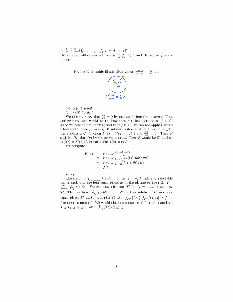
Here the equalities are valid since | z−z0ω−z0
| < 1 and the convergence isuniform.
Figure 3: Graphic illustration when | z−z0ω−z0 | =rδ < 1
(v)⇒ (i) trivial!(i)⇒ (ii) harder!We already know that ∂f
∂z= 0 by analysis before the theorem. Thus
our primary step would be to show that f is holomorphic ⇒ f ∈ C′since we now do not know apriori that f is C′, we can not apply Green’sTheorem to prove (i)→ (iii). It suffices to show that for any disc D ⊆ Ω,there exists a C′ function F s.t. F ′(z) = f(z) and ∂F
∂z= 0. Then F
satisfies (ii) thus (v) by the previous proof. Then F would be Cω and sois f(z) = F ′(z)C′, in particular f(z) is in C′.
We compute
F ′(z) = limh→0F (z+h)−F (z)
h
= limh→01h
(∫Lz+hz
(•)), (aclaim)
= limh→01h
(∫ 1
0f(z + th)hdt)
= f(z)
Proof:The claim ⇔
∮Triangle
f(z)dz = 0. Let I =∮Tf(z)dz and subdivide
the triangle into the four equal pieces as in the picture on the right I =∑4i=1
∮T i1f(z)dz. We can now pick one T i1 for (i = 1, ..., 4) s.t. say
T i1 . Then we have |∮T iif(z)dz| ≥ I
4. We further subdivide T 1
1 into four
equal pieces T 12 , ..., T
42 , and pick T i2 s.t. |
∮T2i| ≥ 1
4|∮T1
1f(z)dz| ≥ I
42 ...
(iterate this process). We would obtain a sequence of “nested triangles”:T ⊇ T i1 ⊇ T i2 ⊇ ... with |
∮T ikf(z)dz| ≥ i
4k.
8

Figure 4: Graphic illustration when triangles are subdivided.
Moreover ∩∞k=1Tik = z0. Since f is holomorphic at z0, f(z) = f(z0)+
f(z0)(z−z0)+0(|z−z0|) in a sufficiently small neighborhood of z0. When
9
k is large enough, T ik will be contained in this neighborhood. Thus
|∮∂T ikf(z)dz| = |
∮∂T ik(f(z0) + f ′(z))(z − z0) + 0(|z − z0|))dz|
≤ |∮∂T ik(f(z0) + f ′(z0)(z − z0))dz|+ |
∮∂T ik
0(|z − z0|)dz|≤
∮∂T ik|0(|z − z0|)||dz|
≤ 3 diam T ik ε diam T ik= 3ε diam T
2kdiam T
2k
= 3 (diam T )2
4nε where ε is arbitrarily small,
since limz→z00(|z−z0|)|z−z0|
→ 0
⇒ I4k≤ 3ε (diam T )2
4k
⇒ I ≤ 3(diam T )2ε
Thus I = 0 since ε is arbitrarily small.
Q.E.D.
1.3 Examples of Holomorphic Functions
Go back to Table of Contents. Please click TOC
We have the following examples.Consider the following equation, ez ,
∑∞n=1
zn
n!converges for all z ⇒
ez is holomorphic on C and ddzez = ez and ez+ω = ezeω.
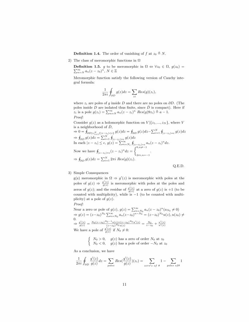
Moreover, we can define log z as the inverse of ez, i.e. elog z = z. Setlog z = u + iv, z = elog z = eueiv ⇒ u = |z|, v = Arg z, but until weintroduce a cut on C, Arg z can’t be a well-defined function on C.
Figure 5: Graphic illustration when triangles are subdivided.
1.4 Open Mapping and Maximal Modulars The-orems
Go back to Table of Contents. Please click TOC
Let us take f to be holomorphic in Ω, we have the following
1) f 6≡ 0 ⇒ the zero’s of f are isolated, i.e. f(z0) = 0 ⇒ ∃V , neigh-borhood of z0 s.t. ∀z ∈ V |z0, f(z) 6= 0. This is because we canexpand f as a power series near z0, then f(z) =
∑∞n=0 an(z − z0)n
in nhd of z0. f 6≡ 0 ⇒ ∃n : an 6= 0. Take the smallest such n, say,an 6= 0,⇒ f(z) = (z−z0)n(aN +AN+1(z−z0)+ ...) = (z−z0)Ng(z),where g(z0) = aN 6= 0. Thus in a small enough neighborhood wehave g(z) 6= 0.
We have the following definition.
10
Definition 1.4. The order of vanishing of f at z0 , N .
2) The class of meromorphic functions in Ω
Definition 1.5. g to be meromorphic in Ω ⇔ ∀z0 ∈ Ω, g(z0) =∑∞n=N an(z − z0)n, N ∈ Z
Meromorphic function satisfy the following version of Cauchy inte-gral formula:
1
2πi
∮∂D
g(z)dz =∑zi
Res(g)(zi),
where zi are poles of g inside D and there are no poles on ∂D. (Thepoles inside D are isolated thus finite, since D is compact). Here ifzi is a pole g(zi) =
∑∞n=N an(z − zi)n Res(g)9zi) , a− 1.
Proof:
Consider g(z) as a holomorphic function on V |z1, ..., zN, where Vis a neighborhood of D,⇒ 0 =
∮∂D|∪Ni=1|z−zi|<ε
g(z)dz =∮∂D
g(z)dz−∑Ni=1
∮|z−zi|=ε
g(z)dz
⇒∮∂D
g(z)dz =∑Ni=1
∮|z−zi|=ε
g(z)dz
In each |z − zi| ≤ ε, g(z) =∑∞n=Ni
∮|z−zi|=ε
an(z − zi)ndz.
Now we have∮|z−zi|=ε
(z − zi)ndz =
0,n6=−1
2πi,n=−1
.
⇒∮∂D
g(z)dz =∑Ni=1 2πi Res(g)(zi).
Q.E.D.
3) Simple Consequences
g(z) meromorphic in Ω ⇒ g′(z) is meromorphic with poles at the
poles of g(z) ⇒ g′(z)g(z)
is meromorphic with poles at the poles and
zeros of g(z); and the residue of g′(z)g(z)
at a zero of g(z) is +1 (to be
counted with multiplicity), while is −1 (to be counted with multi-plicity) at a pole of g(z).
Proof:
Near a zero or pole of g(z), g(z) =∑∞n=N0
an(z − z0)n(aN0 6= 0)
⇒ g(z) = (z−z0)N0∑∞n=N0
an(z−z0)n−N0 = (z−z0)N0u(z), u(z0) 6=0.⇒ g′(z)
g(z)= N0(z−z0)N0−1u(z)+(z−z0)N0u′(z)
(z−z0)N0u(z)= N0
z−z0+ u′(z)
u′(z)
We have a pole of g′(z)g(z)
if N0 6= 0:N0 > 0, g(z) has a zero of order N0 at z0
N0 < 0, g(z) has a pole of order −N0 at z0
As a conclusion, we have
1
2πi
∮∂D
g′(z)
g(z)dz =
∑poles
Res(g′(z)
g(z))(zi) =
∑zero′s of θ
1−∑
poles ofθ
1
11
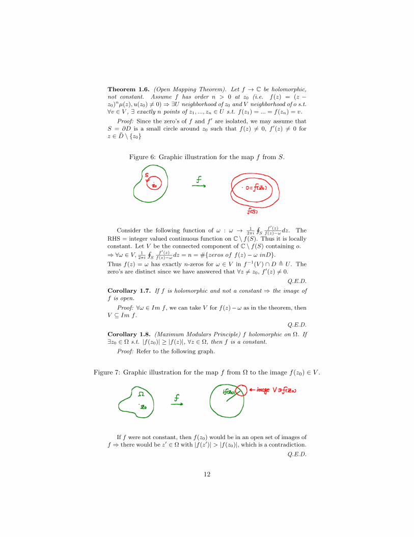
Theorem 1.6. (Open Mapping Theorem). Let f → C be holomorphic,not constant. Assume f has order n > 0 at z0 (i.e. f(z) = (z −z0)nµ(z), u(z0) 6= 0)⇒ ∃U neighborhood of z0 and V neighborhood of o s.t.∀v ∈ V , ∃ exactly n points of z1, ..., zn ∈ U s.t. f(z1) = ... = f(zn) = v.
Proof: Since the zero’s of f and f ′ are isolated, we may assume thatS = ∂D is a small circle around z0 such that f(z) 6= 0, f ′(z) 6= 0 forz ∈ D \ z0
Figure 6: Graphic illustration for the map f from S.
Consider the following function of ω : ω → 12πi
∮S
f ′(z)f(z)−ωdz. The
RHS = integer valued continuous function on C \ f(S). Thus it is locallyconstant. Let V be the connected component of C \ f(S) containing o.
⇒ ∀ω ∈ V, 12πi
∮S
f ′(z)f(z)−ωdz = n = #zeros of f(z)− ω inD.
Thus f(z) = ω has exactly n-zeros for ω ∈ V in f−1(V ) ∩ D , U . Thezero’s are distinct since we have answered that ∀z 6= z0, f ′(z) 6= 0.
Q.E.D.
Corollary 1.7. If f is holomorphic and not a constant ⇒ the image off is open.
Proof: ∀ω ∈ Im f , we can take V for f(z)−ω as in the theorem, thenV ⊆ Im f .
Q.E.D.
Corollary 1.8. (Maximum Modulars Principle) f holomorphic on Ω. If∃z0 ∈ Ω s.t. |f(z0)| ≥ |f(z)|, ∀z ∈ Ω, then f is a constant.
Proof: Refer to the following graph.
Figure 7: Graphic illustration for the map f from Ω to the image f(z0) ∈ V .
If f were not constant, then f(z0) would be in an open set of images off ⇒ there would be z′ ∈ Ω with |f(z′)| > |f(z0)|, which is a contradiction.
Q.E.D.
12

1.5 Applications: Method of Residues
Go back to Table of Contents. Please click TOC
1) Calculate∫ +∞
01
1+x2 dx using residue formula
I = 12
∫∞−∞
11+x2 dx = 1
2limR→∞
∫ R−R
11+z2 dz, and we can construct
an integral contour as follows:
I = 12limR→∞(
∫∩
dz1+z2 −
∫∩
dz1+z2 ).
Figure 8: Graphic illustration for the integral contour.
By the residue theorem∫∩
dz1+z2 = 2πiRes( 1
1+z2 )(i), and 11+z2 =
1z+i
1z−i ⇒ Res( 1
1+z2 )(i) = 12i
.
⇒∫∩
dz1+z2 = π
Moreover, |∫∩
dz1+z2 | ≤
∫ π0
|dz||z2|−1
=∫ pi
0RdθR2−1
= πRR2−1
→ 0 as R→ 0.
⇒ I = π2
.
2) Calculate∫∞
0
sin(x)x
dx
First of all, the integral converges: x→ 0, sin(x)x→ 1, and the func-
tion is smooth (analytic), thus integrable near 0; |∫∞
1
sin(x)x
dx| =
|−cos(x)x|∞1 = |−cos(x)
x|∞1 −
∫∞1
cos(x)
x2 dx| ≤ 1 +∫∞
01x2 dx, thus is in-
tegrable near ∞.
We want to apply the method of residue. Consider eiz = cos(z) +
isin(z), and∫∞∞
sin(x)x
dx = Im(∫−∞
∞ eiz
zdz).
To calculate∫∞−∞
eiz
zdz, we take the following contour
∮eiz
zdz =
Res( eiz
z)(0) = 2πi.
Figure 9: Graphic illustration calculating the integral following the contour.
13
On I : we have eiz
z= 1
z+ u(z) where u(z) is holomophic, then∫
Ieiz
zdz =
∫ 2π
π1z
+∫ 2π
πu(r, θ)ireiθdθ = πi+ o(r)→ πi(r → 0).
On II and IV : |∫II
eiz
zdz| = |
∫ R0
ei(R+iy)
R+iydy| = |
∫ R0
eiRe−y
R+iydy| ≤∫ R
0| eiRe−y
R+iy|dy ≤
∫ R0
e−y
Rdy ≤ 1
R
∫∞0e−ydy → 0, as R→∞.
On III : we have |∫III
eiz
zdz| = |
∫ −RR
eix−R
x+iRdx| ≤
∫ −RR| eix−R
x+iR|dx ≤
e−R∫ −RR
1Rdx = 2e−R → 0 as (R → ∞). Thus, it follows that
2πi =∫∞−∞
eiz
zdz + πi+ 0 + 0
⇒∫∞
0
sin(x)x
dx = 12
∫∞−∞
sin(x)x
dx = π2
.
3) Evaluate∫∞
0vz−1
1+vdv (0 < z < 1, which ensures the convergence).
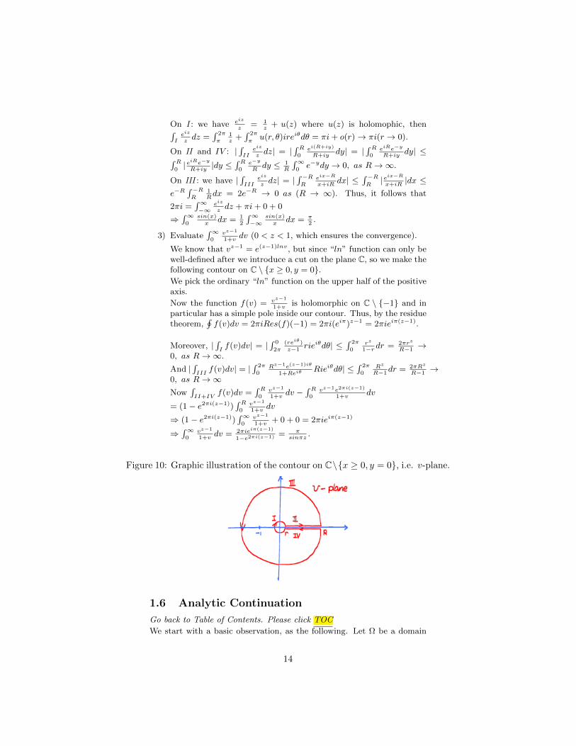
We know that vz−1 = e(z−1)lnv, but since “ln” function can only bewell-defined after we introduce a cut on the plane C, so we make thefollowing contour on C \ x ≥ 0, y = 0.We pick the ordinary “ln” function on the upper half of the positiveaxis.
Now the function f(v) = vz−1
1+vis holomorphic on C \ −1 and in
particular has a simple pole inside our contour. Thus, by the residuetheorem,
∮f(v)dv = 2πiRes(f)(−1) = 2πi(eiπ)z−1 = 2πieiπ(z−1).
Moreover, |∫If(v)dv| = |
∫ 0
2π
(reiθ)z−1
rieiθdθ| ≤∫ 2π
0rz
1−rdr = 2πrz
R−1→
0, as R→∞.
And |∫III
f(v)dv| = |∫ 2π
0Rz−1e(z−1)iθ
1+ReiθRieiθdθ| ≤
∫ 2π
0Rz
R−1dr = 2πRz
R−1→
0, as R→∞Now
∫II+IV
f(v)dv =∫ R
0vz−1
1+vdv −
∫ R0
vz−1e2πi(z−1)
1+vdv
= (1− e2πi(z−1))∫ R
0vz−1
1+vdv
⇒ (1− e2πi(z−1))∫∞
0vz−1
1+v+ 0 + 0 = 2πieiπ(z−1)
⇒∫∞
0vz−1
1+vdv = 2πieiπ(z−1)
1−e2πi(z−1) = πsinπz
.
Figure 10: Graphic illustration of the contour on C\x ≥ 0, y = 0, i.e. v-plane.
1.6 Analytic Continuation
Go back to Table of Contents. Please click TOC
We start with a basic observation, as the following. Let Ω be a domain
14
(connected), f a holomorphic function. If f = 0 on a non-empty open setΩ′ ⊆ Ω, then f ≡ 0 on Ω.
Proof: Let Ω = z0 ∈ Ω : f = 0 in a neighborhood ofz0. Then wehave
(i) Ω ⊇ Ω′ thus 6= ∅
(ii) Ω is open from definition
(iii) Ω is closed
Then we can say that Ω = Ω since Ω is connected. For (iii), we argue
the following. For all z1 ∈ Ωc, i.e. f is not identically 0 around z1. We canwrite f(z) =
∑∞n=0 Cn(z − z1)n, then some CN must be non-zero. Take
minimal such number would imply f(z) = (z − z1)N f(z) with f(z) 6= 0.
Thus f(z) 6≡ 0 on an open neighborhood where f(z) 6= 0.Here is a basic question: given Ω ⊆ C and f holomorphic on Ω. What
is the largest Ω′ s.t. ∃g(z) holomorphic on Ω′ s.t. g|Ωf . (Note that forsmooth functions smooth extensions need not be unique.
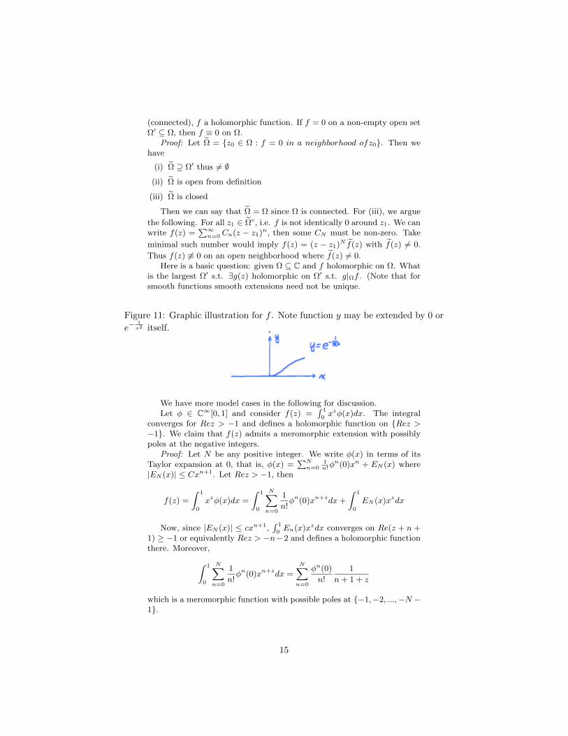
Figure 11: Graphic illustration for f . Note function y may be extended by 0 or
e−1x2 itself.
We have more model cases in the following for discussion.Let φ ∈ C∞[0, 1] and consider f(z) =
∫ 1
0xzφ(x)dx. The integral
converges for Rez > −1 and defines a holomorphic function on Rez >−1. We claim that f(z) admits a meromorphic extension with possiblypoles at the negative integers.
Proof: Let N be any positive integer. We write φ(x) in terms of itsTaylor expansion at 0, that is, φ(x) =
∑Nn=0
1n!φn(0)xn + EN (x) where
|EN (x)| ≤ Cxn+1. Let Rez > −1, then
f(z) =
∫ 1
0
xzφ(x)dx =
∫ 1
0
N∑n=0
1
n!φn(0)xn+zdx+
∫ 1
0
EN (x)xzdx
Now, since |EN (x)| ≤ cxn+1,∫ 1
0En(x)xzdx converges on Re(z + n +
1) ≥ −1 or equivalently Rez > −n−2 and defines a holomorphic functionthere. Moreover,∫ 1
0
N∑n=0
1
n!φn(0)xn+zdx =
N∑n=0
φn(0)
n!
1
n+ 1 + z
which is a meromorphic function with possible poles at −1,−2, ...,−N −1.
15
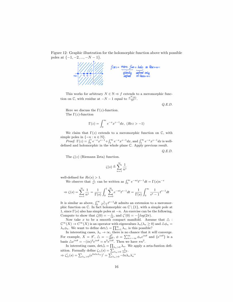
Figure 12: Graphic illustration for the holomorphic function above with possiblepoles at −1,−2, ...,−N − 1.
This works for arbitrary N ∈ N ⇒ f extends to a meromorphic func-
tion on C, with residue at −N − 1 equal to φN (0)N !
.
Q.E.D.
Here we discuss the Γ(z)-function.The Γ(z)-function
Γ(z) =
∫ ∞0
e−xxz−1dx, (Rez > −1)
We claim that Γ(z) extends to a meromorphic function on C, withsimple poles in −n : n ∈ N.
Proof: Γ(z) =∫ 1
0e−xxz−1+
∫∞1e−xxz−1dx, and
∫∞1e−xxz−1dx is well-
defined and holomorphic in the whole plane C. Apply previous result.
Q.E.D.
The ζ(z) (Riemann Zeta) function.
ζ(s) ,∞∑n=1
1
ns
well-defined for Re(s) > 1.We observe that 1
nscan be written as
∫∞0e−ntts−1dt = Γ(s)n−s
⇒ ζ(s) =
∞∑n=1
1
ns=
1
Γ(s)
∫ 1
0
∞∑n=0
e−ntts−1dt =1
Γ(s)
∫ ∞0
1
et − 1ts−1dt
It is similar as above,∫∞
01
et−1ts−1dt admits an extension to a meromor-
phic function on C. In fact holomorphic on C \ 1, with a simple pole at1, since Γ(s) also has simple poles at −n. An exercise can be the following.Compute to show that ζ(0) = − 1
12, and ζ′(0) = − 1
2log(2π).
Now take x to be a smooth compact manifold. Assume that 4 :C∞(X)→ C∞(X) is an operator with eigenvalues λn(λn ≥ 0) and4φn =λnφn. We want to define det4 =
∏∞n=1 λn, is this possible?
In interesting cases, λn →∞, there is no chance that it will converge.
For example, X = S′, 4 = − d2
dθ2, φ =
∑∞n=−∞ φne
inθ and einθ is a
basis 4einθ = −(in)2einθ = n2einθ. Then we have πn2.In interesting cases, det4 =
∏λn>0 λn. We apply a zeta-funtion defi-
nition. Formally define ζ4(s) =∑λn>0
1λn3 .
⇒ ζ′4(s) =∑λn>0(e0slnλn)′ =
∑λn>0−lnλnλ
−sn
16

⇒ ζ′4(0) =∑λn>0−lnλn = −ln
∏λn>0 λn
⇒∏n>0 λn = e−ζ
′4(0)
For another example, X = S′, ζ4(s) = 2∑∞n=1
1n2s = 2ζ(2s).
Note that λ−sn = 1Γ(s)
∫∞0e−λntts−1dt
⇒∑λn>0 λ
−sn = 1
Γ(s)
∫∞0
∑λn>0 e
−λntts−1dt. DefineK(t) =∑λn>0 e
−λnt
Using the same analysis as we did for ζ(s), we obtain a sufficientcondition for ζ4(s) to extend holomorphically for s near s = 0.
Proposition 1.9. Assume λn grows polynomially in n and K(t) is asmooth function for t > 0, furthermore:
(a) K(t) ≤ Ce−µt for t >> 0
(b) K(t) ∼∑nl=1 Clt
−l for t ∈ [0, 1).
Then ζ4(s) admits a meromorphic extension for s ∈ C, which is holo-morphic at 0.
Proof: Since |∫∞
0K(t)ts−1dt| ≤
∫∞0|K(t)|ts−1dt <
∫∞0Ce−µtts−1dt
converges for Res > −1, thus defines a holomorphic function there.Now
∫∞0K(t)ts−1dt =
∫ 1
0K(t)ts−1 +
∫∞1K(t)ts−1dt
Since∫∞
1K(t)ts−1 id well-defined and holomorphic for all s ∈ C, it
suffices to show that∫ 1
0K(t)ts−1dt can be so extended.
Indeed,∫ 1
0K(t)ts−1 =
∑Nm=0 Cm
∫ 1
0t−m−1+sds+
∫ 1
0En(t)ts−1dt
=∑Nm=1
CmS−m +
∫ 1
0EN (t)ts−1dt, for Re(s) > N + 1
Since∑Nm=1
Cms−m is already meromorphic on C, it suffices to show that∫ 1
0EN (t)ts−1dt extends to be a meromorphic function on C.
Take the Taylor expansion of EN (t) =∑Mm=0 amt
m+FM (t), am =EmNm!
.
Then |FM (t)| ≤ DtM+1 for t ∈ (0, 1), and we have∫ 1
0(∑Mm=0 amt
m +
FM (t))ts−1dt =∑Mm=0 am
1m+s
+∫ 1
0FM (t)ts−1dt
But |∫ 1
0FM (t)ts−1dt| <
∫ 1
0|FM (t)ts−1|dt <
∫ 1
0DtM+Sdt converges
for Res > −M − 1 and define sa meromorphic function there. The resutlfollows.
Finally ζK(t) has at msot simple poles at N,N − 1, ..., 1, 0,−1, ...and Γ(s)−1 vanishes at s = 0, the last statement follows.
Q.E.D.
We have the following observations: We shall later prove that if 4 isan elliptic PDF of positive order, then λn →∞ polynomially and Tre−t4
admits an expansion as in (b), where Tre−t4 = dim ker4+∑λn>0 e
−λnt.
We will show that Tre−t4 satisfies (b) by solving ( ∂∂t
+ 4)H(t) = 0
H(t)|t=0 = I and set H(t) = e−t4.A basic example is the following. Consider X = C\Z⊗Zr, r = r1+r2i,
with r2 > 0. Then 4 = −4 ∂2
∂z∂zacting on periodic functions
φ(z + 1) = φ(z)φ(z + r) = φ(z)
17
Exercise can be (1) show that the eigenvalues of 4 are given by λmn =4π2
r22|m + nr|2, m, n ∈ Z, (2) (det4)′ = 1
(2π)4r22|η(q)|4 where η(q) =
q112∏∞n=1(1− qn) and q = e2πr.
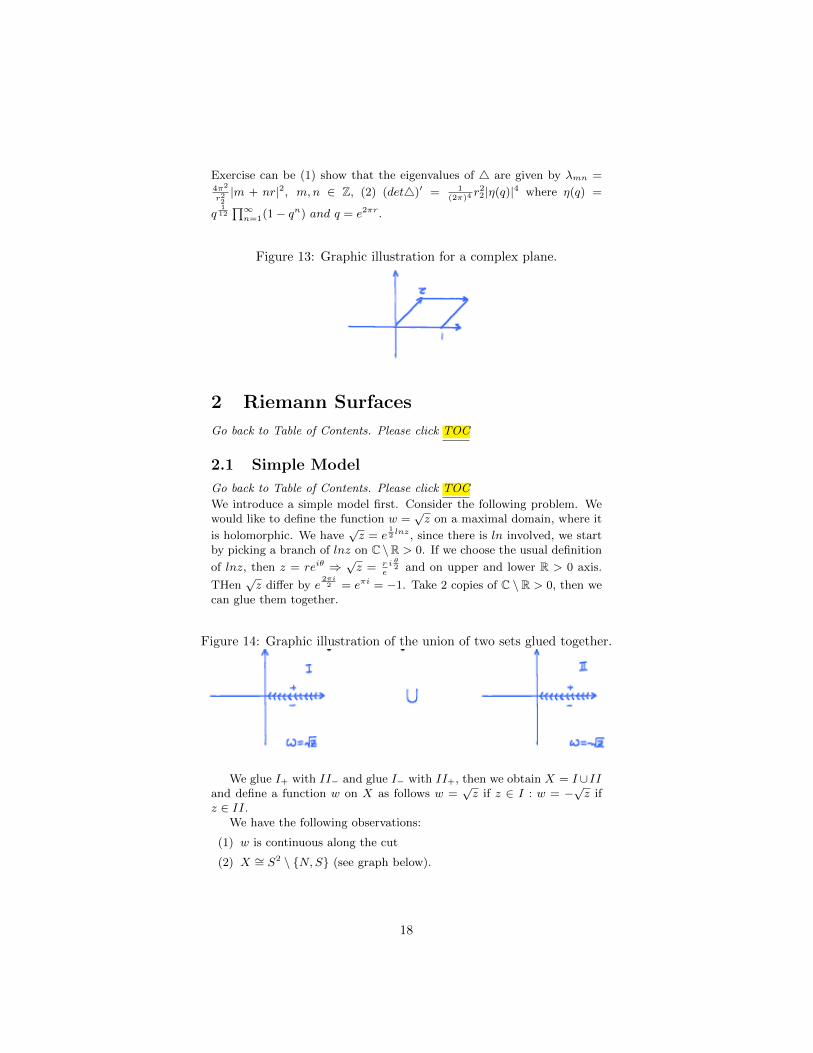
Figure 13: Graphic illustration for a complex plane.
2 Riemann Surfaces
Go back to Table of Contents. Please click TOC
2.1 Simple Model
Go back to Table of Contents. Please click TOC
We introduce a simple model first. Consider the following problem. Wewould like to define the function w =
√z on a maximal domain, where it
is holomorphic. We have√z = e
12lnz, since there is ln involved, we start
by picking a branch of lnz on C \R > 0. If we choose the usual definition
of lnz, then z = reiθ ⇒√z = r
ei θ2 and on upper and lower R > 0 axis.
THen√z differ by e
2πi2 = eπi = −1. Take 2 copies of C \ R > 0, then we
can glue them together.
Figure 14: Graphic illustration of the union of two sets glued together.
We glue I+ with II− and glue I− with II+, then we obtain X = I∪IIand define a function w on X as follows w =
√z if z ∈ I : w = −
√z if
z ∈ II.We have the following observations:
(1) w is continuous along the cut
(2) X ∼= S2 \ N,S (see graph below).
18

Figure 15: Graphic illustration gluing I+ with II− and gluing I− with II+.
We make the following clam. Each point z0 of X admits a neighbor-hood Wz0 which is in one-one correspondence with a disc D in C. This isobvious for z0 /∈ R>0 (the cut) Wz0 = z|z − z0 < δ.
If z0 is on the cut, we can just take 2 half discs in I and II to gluetogether, as shown in the following graph.
Figure 16: Graphic illustration taking 2 half discs in I and II to glue together.
Thus we can give X = S2 \ N,S coordinate charts by these Wz0’s,Wz0 → D and z → t = z − z0.
Definition 2.1. Let f be a function on S. We say f is holomorphic if∀z0 ∈ S, f |Wz0 (z(t)) is holomorphic as a function of t.
In this sense, we have
w(z) =
√z, z∈I−√z, z∈II
is holomorphic on X.
19
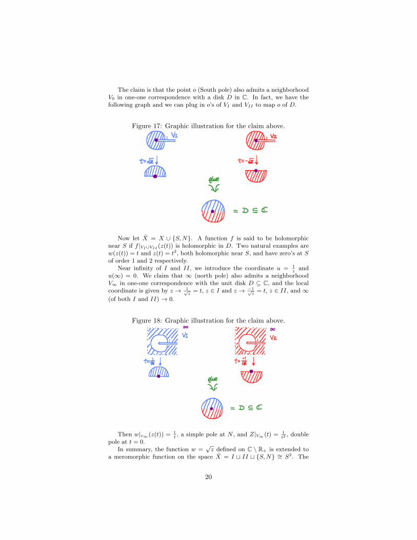
The claim is that the point o (South pole) also admits a neighborhoodV0 in one-one correspondence with a disk D in C. In fact, we have thefollowing graph and we can plug in o’s of VI and VII to map o of D.
Figure 17: Graphic illustration for the claim above.
Now let X = X ∪ S,N. A function f is said to be holomorphicnear S if f |VI∪VII (z(t)) is holomorphic in D. Two natural examples arew(z(t)) = t and z(t) = t2, both holomorphic near S, and have zero’s at Sof order 1 and 2 respectively.
Near infinity of I and II, we introduce the coordinate u = 1z
andu(∞) = 0. We claim that ∞ (north pole) also admits a neighborhoodV∞ in one-one correspondence with the unit disk D ⊆ C, and the localcoordinate is given by z → 1√
z= t, z ∈ I and z → −1√
z= t, z ∈ II, and ∞
(of both I and II) → 0.
Figure 18: Graphic illustration for the claim above.
Then w|v∞(z(t)) = 1t, a simple pole at N , and Z|V∞(t) = 1
t2, double
pole at t = 0.In summary, the function w =
√z defined on C \ R+ is extended to
a meromorphic function on the space X = I t II t S,N ∼= S2. The
20

function w has a simple o at 0, and a simple pole at ∞. The function zhas a double o at 0, and a double pole at∞. Under the natural involution(switching) I ← II, the function z is even and the function w is odd.
2.2 Another Basic Example
Go back to Table of Contents. Please click TOC
The following basic example helps illustrate the idea. Consider w2 =z(z − 1)(z − λ), (λ 6= 0, 1).
Problem: analytically continue w =√z(z − 1)(z − λ) defined on some
domain of C. For w to be defined, it suffices√z,√z − 1,
√z − λ be well-
defined. Thus take the domain C \ L, where L passes through 0, 1, λ.Clearly,
√z,√z − 1, and
√z − λ are all well defined and holomorphic on
C \ L.Consider a point z ∈ [0, 1] : z → e2πiz on the circle C, but
√z − 1
and√z − λ are both well-defined, while
√z
c→ −√z ⇒ w → −w =
−√z(z − 1)(z − λ) under C.
Figure 19: Graphic illustration forthe path L.
Next, consider z ∈ L1,λ. Similarly, we have√z
D→ −√z,√z − 1
D→−√z − 1,
√z − λ D→
√z − λ ⇒ w
D→ w is invariant nad continuous (holo-morphic).
Figure 20: Graphic illustration for the map on the circle C.
Finally, consider z ∈ Lλ∞, and a similar loop⇒√z → −
√z,√z − 1→
−√z − 1,
√z − λ→ −
√z − λ and w → −w under the loop.
21

Figure 21: Graphic illustration for map on λ.
In summary, singularities occur only on [0, 1] t Lλ∞. Thus w =±√z(z − 1)(z − λ) are holomophic on C \ ([0, 1]tLλ∞). Take two copies
and glue similarly as in the previous case.
Figure 22: Graphic illustration for taking two copies and glue similarly as inthe previous case.
22
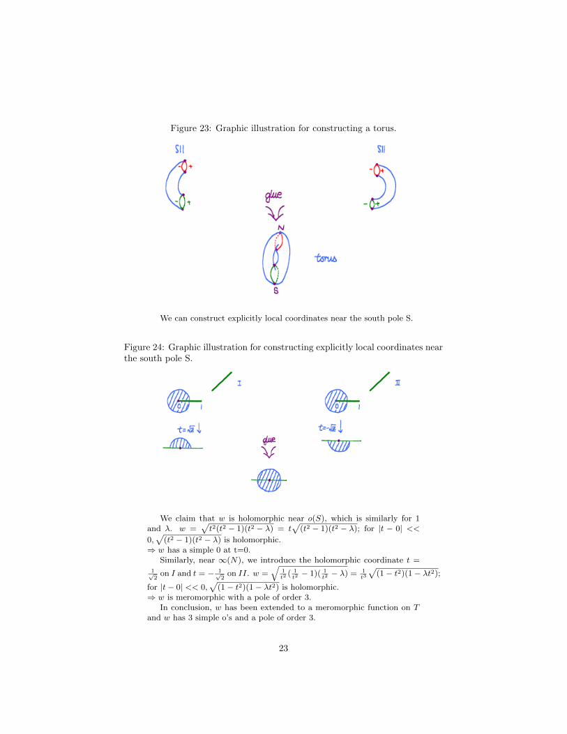
Figure 23: Graphic illustration for constructing a torus.
We can construct explicitly local coordinates near the south pole S.
Figure 24: Graphic illustration for constructing explicitly local coordinates nearthe south pole S.
We claim that w is holomorphic near o(S), which is similarly for 1and λ. w =
√t2(t2 − 1)(t2 − λ) = t
√(t2 − 1)(t2 − λ); for |t − 0| <<
0,√
(t2 − 1)(t2 − λ) is holomorphic.⇒ w has a simple 0 at t=0.
Similarly, near ∞(N), we introduce the holomorphic coordinate t =1√2
on I and t = − 1√2
on II. w =√
1t2
( 1t2− 1)( 1
t2− λ) = 1
t3
√(1− t2)(1− λt2);
for |t− 0| << 0,√
(1− t2)(1− λt2) is holomorphic.⇒ w is meromorphic with a pole of order 3.
In conclusion, w has been extended to a meromorphic function on Tand w has 3 simple o’s and a pole of order 3.
23
The function z is also extended meromorphically, with an order 2, 0at S and an order 2 pole at N .
2.3 Key Strategy
Go back to Table of Contents. Please click TOC
There are many tori with a complex structure (i.e. a notion of holomorphicor meromorphic function applies). For instance, Tz , C \ Z ⊕ Zr, r ∈C, Imr > 0. A function φ on Tz can be identified with a function onC satisfying φ(z + m + nz) = φ(z), ∀m,nZ, and φ on Tz is holomorphic(meromorphic) if the corresponding φ on C is holomorphic (meromorphic).Thus we need to see if X can be identified with Tz for some r, and if yeshow do we determine such a r?
2.3.1 Construction of Holomorphic Differentials
Go back to Table of Contents. Please click TOC
There are very few (in fact, only constants, by maximal modulus theorem)holomorphic functions on x. Rather we work instead with (1) holomorphicforms and/or (2) meromorphic functions. Then proceed in the following3 steps:
1) Construct these objects (← explicit forms)
2) Develop techniques for manipulating them (← Riemann bilinear re-lations and abelian integrals)
3) Use them to construct a holomorphic map x→ C\Z+Z+r (← TheAbel map: Jacobi inversion theorem, based on Abel’s theorem).
The Construction of holomorphic differentials is as follows. Recall thatx has two meromorphic functions on x, namely z : x→ Ct∞, p→ z(p)and w(p) =
√z(z − 1)(z − λ) on I and w(p) = −
√z(z − 1)(z − λ) on II.
We have a key observation. Consider the differential “ dzw
” is actually aholomorphic differential form on all of x. To see this, we express dz
win a
local coordinate system. dzw
= dz√z(z−1)(z−λ)
. Near z = 0, recall that the
holomorphic coordinate is given by t =√z ⇒ z = t2, thus dz = 2tdt ⇒
2tdt√t2(t−1)(t−λ
= 2dt√(t−1)(t−λ
, which is holomorphic for |t| << 1. The same
reason applies to z0 = 1, and λ. Near z0 =∞, the holomorphic coordinate
is given by t = 1√z⇒ z = 1
t2, dz = −2 dt
t3. Thus dz
w= −2dt/t2
1t2
( 1t2−1)( 1
t2−λ)
=
−2dt/t2
1t2
√(1−t2)(1−λt2)
= −2dt√(1−t2)(1−λt2)
, which is again holomorphic for |t| <<
1.Using this form w = dz
w, we can construct a map from x to C\ lattice
in the following way: the Abel map.Abel’s Map. Fix p0 ∈ x, ∀P ∈ x. Consider
∫ pp0w, integration along γ.
If γ can be continuously deformed to γ′, then∫γw =
∫γ′ w. Pick A, B
two cycles on x.We have a topological fact. Any two γ, γ′ connecting p0 and p have
γ−γ′ ' nA+mB, n,m ∈ Z⇒∫γw =
∫γ′ w+n
∮Aw+m
∮Bw, n,m ∈ Z.
24
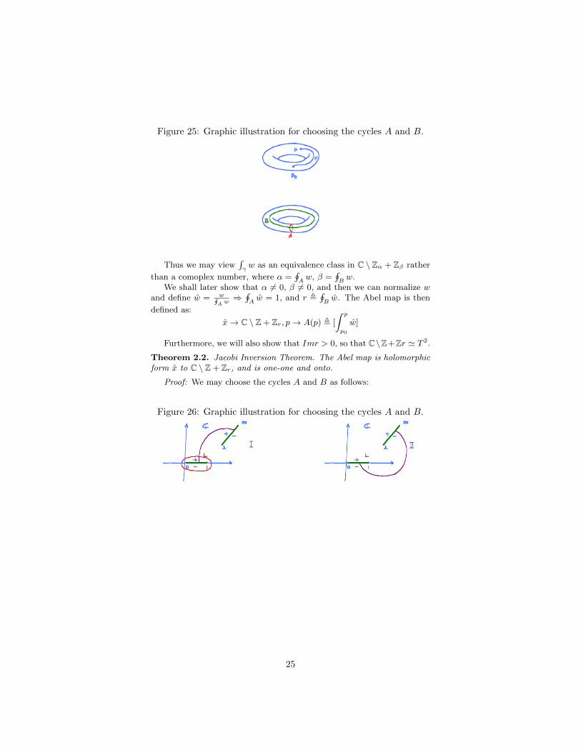
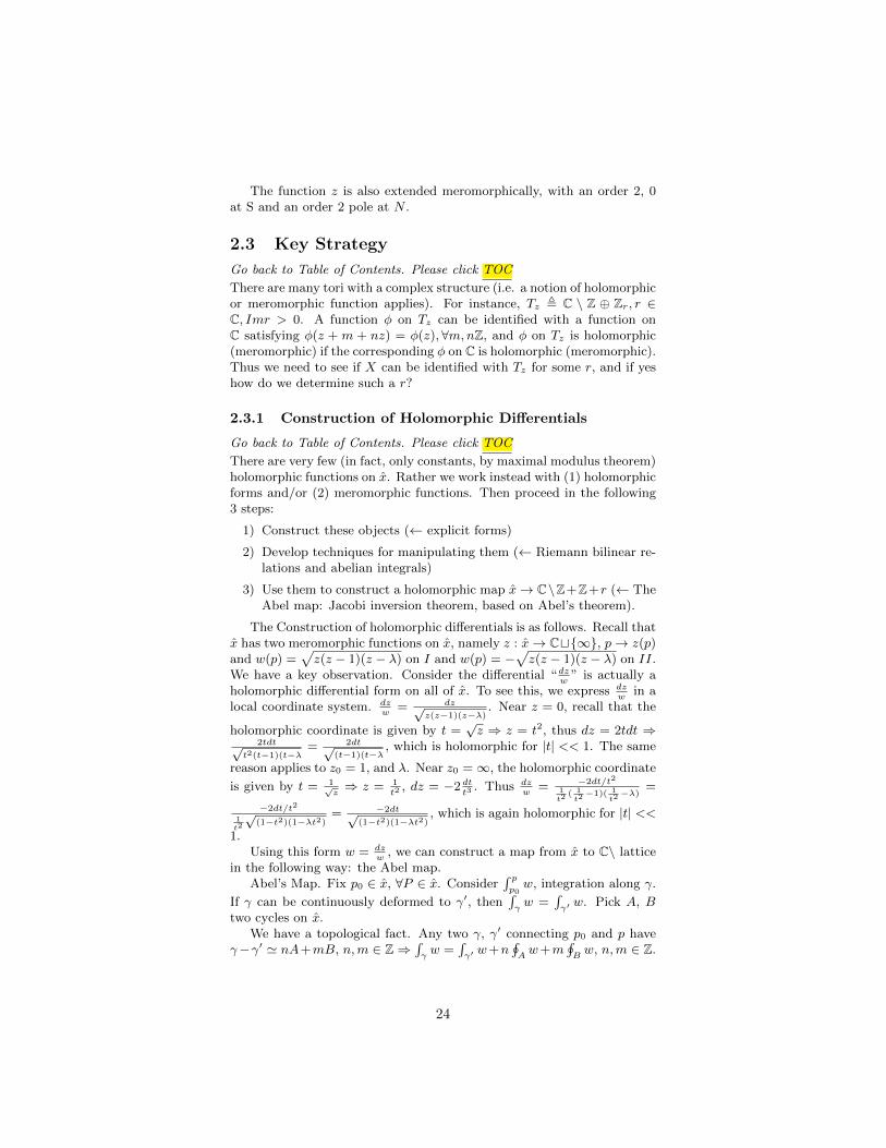
Figure 25: Graphic illustration for choosing the cycles A and B.
Thus we may view∫γw as an equivalence class in C \ Zα + Zβ rather
than a comoplex number, where α =∮Aw, β =
∮Bw.
We shall later show that α 6= 0, β 6= 0, and then we can normalize wand define w = w∮
A w⇒∮Aw = 1, and r ,
∮Bw. The Abel map is then
defined as:
x→ C \ Z + Zr, p→ A(p) , [
∫ p
p0
w]
Furthermore, we will also show that Imr > 0, so that C\Z+Zr ' T 2.
Theorem 2.2. Jacobi Inversion Theorem. The Abel map is holomorphicform x to C \ Z + Zr, and is one-one and onto.
Proof: We may choose the cycles A and B as follows:
Figure 26: Graphic illustration for choosing the cycles A and B.
25
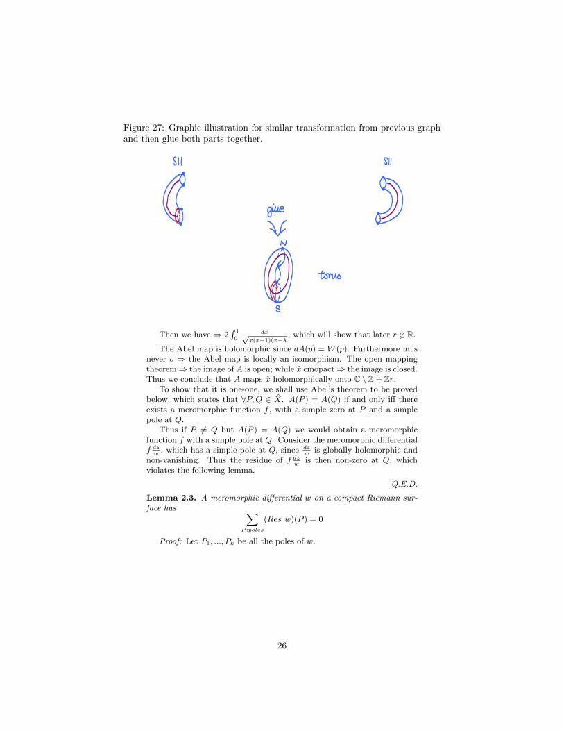
Figure 27: Graphic illustration for similar transformation from previous graphand then glue both parts together.
Then we have ⇒ 2∫ 1
0dx√
x(x−1)(x−λ, which will show that later r 6∈ R.
The Abel map is holomorphic since dA(p) = W (p). Furthermore w isnever o ⇒ the Abel map is locally an isomorphism. The open mappingtheorem⇒ the image of A is open; while x cmopact⇒ the image is closed.Thus we conclude that A maps x holomorphically onto C \ Z + Zr.
To show that it is one-one, we shall use Abel’s theorem to be provedbelow, which states that ∀P,Q ∈ X. A(P ) = A(Q) if and only iff thereexists a meromorphic function f , with a simple zero at P and a simplepole at Q.
Thus if P 6= Q but A(P ) = A(Q) we would obtain a meromorphicfunction f with a simple pole at Q. Consider the meromorphic differentialf dzw
, which has a simple pole at Q, since dzw
is globally holomorphic andnon-vanishing. Thus the residue of f dz
wis then non-zero at Q, which
violates the following lemma.
Q.E.D.
Lemma 2.3. A meromorphic differential w on a compact Riemann sur-face has ∑
P :poles
(Res w)(P ) = 0
Proof: Let P1, ..., Pk be all the poles of w.
26
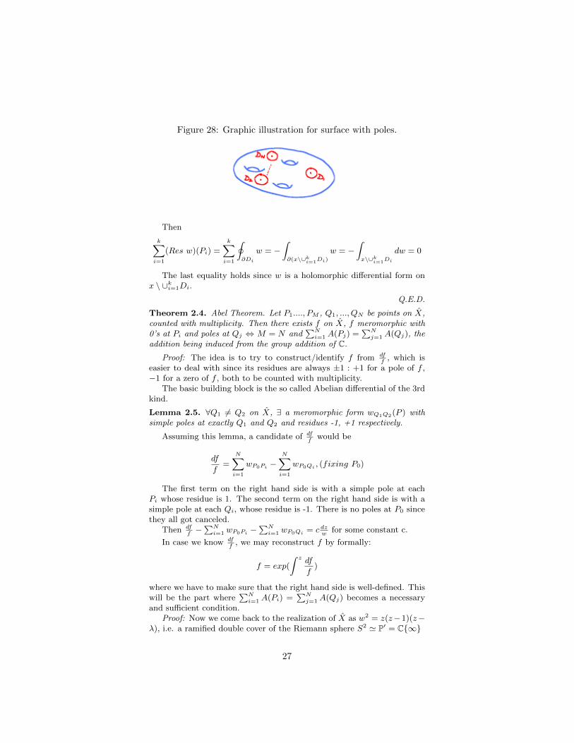
Figure 28: Graphic illustration for surface with poles.
Then
k∑i=1
(Res w)(Pi) =
k∑i=1
∮∂Di
w = −∫∂(x\∪ki=1Di)
w = −∫x\∪ki=1Di
dw = 0
The last equality holds since w is a holomorphic differential form onx \ ∪ki=1Di.
Q.E.D.
Theorem 2.4. Abel Theorem. Let P1...., PM , Q1, ..., QN be points on X,counted with multiplicity. Then there exists f on X, f meromorphic with0’s at Pi and poles at Qj ⇔ M = N and
∑Ni=1 A(Pj) =
∑Nj=1 A(Qj), the
addition being induced from the group addition of C.
Proof: The idea is to try to construct/identify f from dff
, which iseasier to deal with since its residues are always ±1 : +1 for a pole of f ,−1 for a zero of f , both to be counted with multiplicity.
The basic building block is the so called Abelian differential of the 3rdkind.
Lemma 2.5. ∀Q1 6= Q2 on X, ∃ a meromorphic form wQ1Q2(P ) withsimple poles at exactly Q1 and Q2 and residues -1, +1 respectively.
Assuming this lemma, a candidate of dff
would be
df
f=
N∑i=1
wP0Pi −N∑i=1
wP0Qi , (fixing P0)
The first term on the right hand side is with a simple pole at eachPi whose residue is 1. The second term on the right hand side is with asimple pole at each Qi, whose residue is -1. There is no poles at P0 sincethey all got canceled.
Then dff−∑Ni=1 wP0Pi −
∑Ni=1 wP0Qi = c dz
wfor some constant c.
In case we know dff
, we may reconstruct f by formally:
f = exp(
∫ z df
f)
where we have to make sure that the right hand side is well-defined. Thiswill be the part where
∑Ni=1 A(Pi) =
∑Nj=1 A(Qj) becomes a necessary
and sufficient condition.Proof: Now we come back to the realization of X as w2 = z(z−1)(z−
λ), i.e. a ramified double cover of the Riemann sphere S2 ' P′ = C∞
27
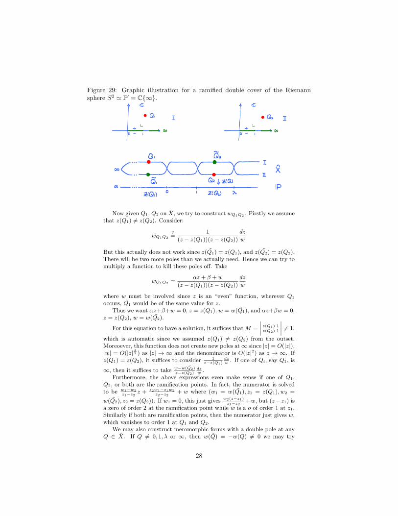
Figure 29: Graphic illustration for a ramified double cover of the Riemannsphere S2 ' P′ = C∞.
Now given Q1, Q2 on X, we try to construct wQ1Q2 . Firstly we assumethat z(Q1) 6= z(Q2). Consider:
wQ1Q2
?=
1
(z − z(Q1))(z − z(Q2))
dz
w
But this actually does not work since z(Q1) = z(Q1), and z(Q2) = z(Q2).There will be two more poles than we actually need. Hence we can try tomultiply a function to kill these poles off. Take
wQ1Q2 =αz + β + w
(z − z(Q1))(z − z(Q2))
dz
w
where w must be involved since z is an “even” function, wherever Q1
occurs, Q1 would be of the same value for z.Thus we want αz+β+w = 0, z = z(Q1), w = w(Q1), and αz+βw = 0,
z = z(Q2), w = w(Q2).
For this equation to have a solution, it suffices that M =
∣∣∣∣ z(Q1) 1z(Q2) 1
∣∣∣∣ 6= 1,
which is automatic since we assumed z(Q1) 6= z(Q2) from the outset.Moreoever, this function does not create new poles at∞ since |z| = O(|z|),|w| = O(|z|
z2 ) as |z| → ∞ and the denominator is O(|z|2) as z → ∞. If
z(Q1) = z(Q2), it suffices to consider 1z−z(Q1)
dzw
. If one of Qi, say Q1, is
∞, then it suffices to take w−w(Q2)z−z(Q2)
dzw
.Furthermore, the above expressions even make sense if one of Q1,
Q2, or both are the ramification points. In fact, the numerator is solvedto be w1−w2
z1−z2z + z2w1−z1w2
z2−z2+ w where (w1 = w(Q1), z1 = z(Q1), w2 =
w(Q2), z2 = z(Q2)). If w1 = 0, this just gives w2(z−z1)z1−z2
+w, but (z−z1) isa zero of order 2 at the ramification point while w is a o of order 1 at z1.Similarly if both are ramification points, then the numerator just gives w,which vanishes to order 1 at Q1 and Q2.
We may also construct meromorphic forms with a double pole at anyQ ∈ X. If Q 6= 0, 1, λ or ∞, then w(Q) = −w(Q) 6= 0 we may try
28
αz+βw+γ2
(z−z(Q))2dzw
such that αz + βw + γ vanishes to order 2 at Q, where
Q, Q are the two distinct points on X lying over z(Q). Then considerαz + βw + γ = ((z(Q) − 1)(z(Q) − λ) + z(Q)(z(Q) − 1) + z(Q)(z(Q) −λ)(z − z(Q))− 2w(Q)(w − (wQ)).
Indeed (w−w(Q) +w(Q))2 = z(z− 1)(z−λ) = (z− z(Q) + z(Q))(z−z(Q) + z(Q)− 1)(z − z(Q) + z(Q)− λ), then we have
(w − w(Q))2
+2w(Q)(w − w(Q))
+w(Q)2 = z(Q)(z(Q)− 1)(z(Q)− λ)+((z(Q)− 1)(z(Q)− λ)+z(Q)(z(Q)− 1)+z(Q)(z(Q)− λ))(z − z(Q))+(z(Q) + z(Q)− 1 + z(Q)− λ)(z − z(Q))2
+(z − z(Q))3
(note z(Q) = z(Q), and w(Q)2 = z(Q)(z(Q)− 1)(z(Q)− λ))⇒ ((z(Q)− 1)(z(Q)− λ)
+z(Q)(z(Q)− 1) + z(Q)(z(Q)− λ))(z − z(Q))
−2w(Q)w
= (w − w(Q))2 − (z(Q) + z(Q)− 1 + z(Q)−λ)(z − z(Q))2 − (z − z(Q))3
= o(|z − z(Q)|2)
since w − w(Q) is locally a holomorphic function in z − z(Q), i.e. w −w(Q) = (z − z(Q))h(z − z(Q)). Moreover, since in our case w(Q) =−w(Q) 6= 0, αz+βw+γ|(z(Q),w(Q)) = −4w(Q)2 6= 0, and o(|αz+βw+γ|) =
O(|z|32 )(|z| → ∞), while o(|z− z(Q)|2) = o(|z|2) as |z| → ∞. If z(Q) = 0,
1, or λ, it suffices to take 1z−z(Q)
dzw
, since (z − z(Q)) vanishes to order 2
at these ramification points. If z(Q) =∞, it suffices to take z dzw
, since zhas an order 2 pole at ∞.
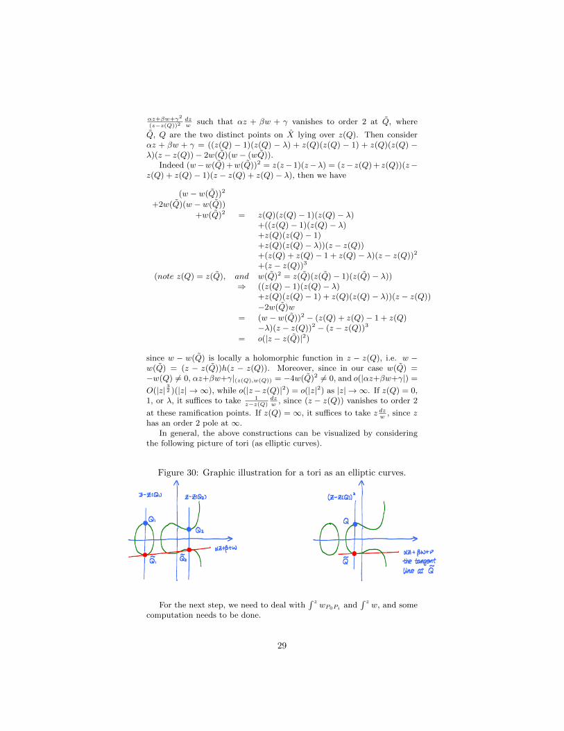
In general, the above constructions can be visualized by consideringthe following picture of tori (as elliptic curves).
Figure 30: Graphic illustration for a tori as an elliptic curves.
For the next step, we need to deal with∫ zwP0Pi and
∫ zw, and some
computation needs to be done.
29
2.4 Method of Abelian Integral (Riemann)
Go back to Table of Contents. Please click TOC
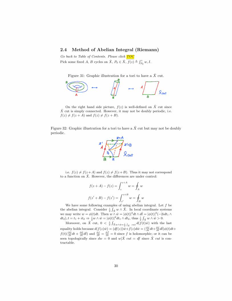
Pick some fixed A, B cycles on X, P0 ∈ X, f(z) ,∫ zP0w, I.
Figure 31: Graphic illustration for a tori to have a X cut.
On the right hand side picture, f(z) is well-defined on X cut sinceX cut is simply connected. However, it may not be doubly periodic, i.e.f(z) 6= f(z +A) and f(z) 6= f(z +B).
Figure 32: Graphic illustration for a tori to have a X cut but may not be doublyperiodic.
i.e. f(z) 6= f(z+A) and f(z) 6= f(z+B). Thus it may not correspondto a function on X. However, the differences are under control:
f(z +A)− f(z) =
∫ z+A
z
w =
∮A
w
f(z′ +B)− f(z′) =
∫ z+B
z′w =
∮B
w
We have some following examples of using abelian integral. Let f bethe abelian integral. Consider i
2
∫Xw ∧ X. In local coordinate systems
we may write w = φ(t)dt. Then w ∧ w = |φ(t)|2dt∧ dt = |φ(t)|2(−2idt1 ∧dt2), t = t1 + it2 ⇒ i
2w ∧ w = |φ(t)|2dt1 ∧ dt2, thus i
2
∫Xw ∧ w > 0.
Moreover, on X cut, 0 < i2
∫Xw∧w= i
2
∫X
cutd(f(t)w) with the last
equality holds because d(f(z)w) = (df(z))w+f(z)dw = ( ∂f∂tdt+ ∂f
∂tdt)φ(t)dt+
f(t)( ∂φ∂tdt + ∂φ
∂tdt) and ∂f
∂t= ∂f
∂t= 0 since f is holomorphic; or it can be
seen topologically since dw = 0 and w|X cut = df since X cut is con-tractable.
30
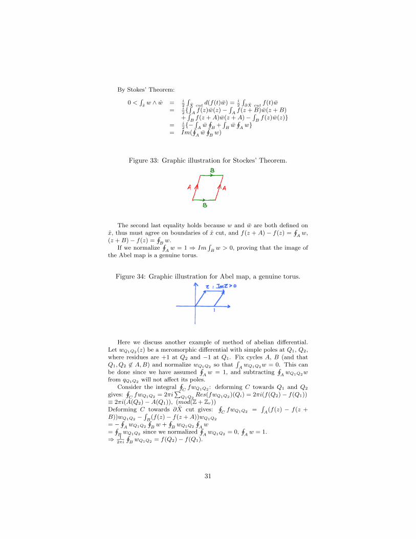
By Stokes’ Theorem:
0 <∫xw ∧ w = i
2
∫X cut
d(f(t)w) = i2
∫∂X cut
f(t)w= i
2∫Af(z)w(z)−
∫Af(z +B)w(z +B)
+∫Bf(z +A)w(z +A)−
∫Bf(z)w(z)
= i2−∫Aw∮B
+∫Bw∮Aw
= Im(∮Aw∮Bw)
Figure 33: Graphic illustration for Stockes’ Theorem.
The second last equality holds because w and w are both defined onx, thus must agree on boundaries of x cut, and f(z + A) − f(z) =
∮Aw,
(z +B)− f(z) =∮Bw.
If we normalize∮Aw = 1 ⇒ Im
∫Bw > 0, proving that the image of
the Abel map is a genuine torus.
Figure 34: Graphic illustration for Abel map, a genuine torus.
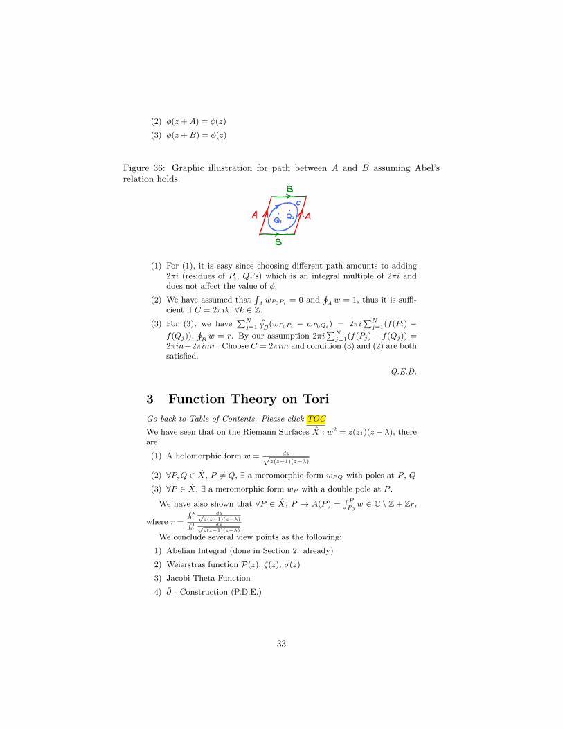
Here we discuss another example of method of abelian differential.Let wQ1Q2(z) be a meromorphic differential with simple poles at Q1, Q2,where residues are +1 at Q2 and −1 at Q1. Fix cycles A, B (and thatQ1, Q2 6∈ A,B) and normalize wQ1Q2 so that
∫AwQ1Q2w = 0. This can
be done since we have assumed∮Aw = 1, and subtracting
∮AwQ1Q2w
from qQ1Q2 will not affect its poles.Consider the integral
∮CfwQ1Q2 : deforming C towards Q1 and Q2
gives:∮CfwQ1Q2 = 2πi
∑Q1Q2
Res(fwQ1Q2)(Qi) = 2πi(f(Q2)− f(Q1))≡ 2πi(A(Q2)−A(Q1)), (mod(Z + Zr))Deforming C towards ∂X cut gives:
∮CfwQ1Q2 =
∫A
(f(z) − f(z +B))wQ1Q2 −
∫B
(f(z)− f(z +A))wQ1Q2
= −∮AwQ1Q2
∮Bw +
∮BwQ1Q2
∮Aw
=∮BwQ1Q2 since we normalized
∮AwQ1Q2 = 0,
∮Aw = 1.
⇒ 12πi
∮BwQ1Q2 = f(Q2)− f(Q1).
31
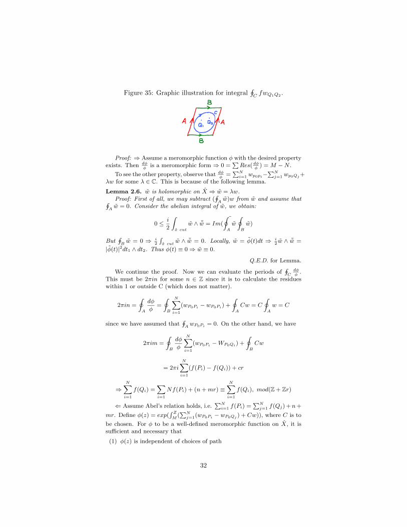
Figure 35: Graphic illustration for integral∮CfwQ1Q2
.
Proof: ⇒ Assume a meromorphic function φ with the desired propertyexists. Then dφ
φis a meromorphic form ⇒ 0 =
∑Res( dφ
φ) = M −N .
To see the other property, observe that dφφ
=∑Ni=1 wp0pi−
∑Nj=1 wp0Qj+
λw for some λ ∈ C. This is because of the following lemma.
Lemma 2.6. w is holomorphic on X ⇒ w = λw.Proof: First of all, we may subtract (
∮Aw)w from w and assume that∮
Aw = 0. Consider the abelian integral of w, we obtain:
0 ≤ i
2
∫x cut
w ∧ ¯w = Im(¯∮A
w
∮B
w)
But∮Bw = 0 ⇒ i
2
∫x cut
w ∧ ¯w = 0. Locally, w = φ(t)dt ⇒ i2w ∧ ¯w =
|φ(t)|2dt1 ∧ dt2. Thus φ(t) ≡ 0⇒ w ≡ 0.
Q.E.D. for Lemma.
We continue the proof. Now we can evaluate the periods of∮Cdφφ
.This must be 2πin for some n ∈ Z since it is to calculate the residueswithin 1 or outside C (which does not matter).
2πin =
∮A
dφ
φ=
∮B
N∑i=1
(wP0Pi − wP0Pi) +
∮A
Cw = C
∮A
w = C
since we have assumed that∮AwP0Pi = 0. On the other hand, we have
2πim =
∮B
dφ
φ
N∑i=1
(wP0Pi −WP0Qi) +
∮B
Cw
= 2πi
N∑i=1
(f(Pi)− f(Qi)) + cr
⇒N∑i=1
f(Qi) =∑i=1
Nf(Pi) + (n+mr) ≡N∑i=1
f(Qi), mod(Z + Zr)
⇐ Assume Abel’s relation holds, i.e.∑Ni=1 f(Pi) =
∑Nj=1 f(Qj) +n+
mr. Define φ(z) = exp(∫ ZM
(∑Nj=1(wP0Pi − wP0Qj ) + Cw)), where C is to
be chosen. For φ to be a well-defined meromorphic function on X, it issufficient and necessary that
(1) φ(z) is independent of choices of path
32
(2) φ(z +A) = φ(z)
(3) φ(z +B) = φ(z)
Figure 36: Graphic illustration for path between A and B assuming Abel’srelation holds.
(1) For (1), it is easy since choosing different path amounts to adding2πi (residues of Pi, Qj ’s) which is an integral multiple of 2πi anddoes not affect the value of φ.
(2) We have assumed that∫AwP0Pi = 0 and
∮Aw = 1, thus it is suffi-
cient if C = 2πik, ∀k ∈ Z.
(3) For (3), we have∑Nj=1
∮B
(wP0Pi − wP0Qi) = 2πi∑Nj=1(f(Pi) −
f(Qj)),∮Bw = r. By our assumption 2πi
∑Nj=1(f(Pj) − f(Qj)) =
2πin+2πimr. Choose C = 2πim and condition (3) and (2) are bothsatisfied.
Q.E.D.
3 Function Theory on Tori
Go back to Table of Contents. Please click TOC
We have seen that on the Riemann Surfaces X : w2 = z(z1)(z − λ), thereare
(1) A holomorphic form w = dz√z(z−1)(z−λ)
(2) ∀P,Q ∈ X, P 6= Q, ∃ a meromorphic form wPQ with poles at P , Q
(3) ∀P ∈ X, ∃ a meromorphic form wP with a double pole at P .
We have also shown that ∀P ∈ X, P → A(P ) =∫ PP0w ∈ C \ Z + Zr,
where r =
∫ λ0
dz√z(z−1)(z−λ)∫ 1
0dz√
z(z−1)(z−λ)
We conclude several view points as the following:
1) Abelian Integral (done in Section 2. already)
2) Weierstras function P(z), ζ(z), σ(z)
3) Jacobi Theta Function
4) ∂ - Construction (P.D.E.)
33

3.1 Function Theory According to Weierstrass
Go back to Table of Contents. Please click TOC
Let C \ Z + Zr be a given complex torus, im r > 0. A function φ onCZ+Zr is simply a function on C satisfying a doubly periodic condition:φ(z+1)=φ(z)
φ(z+r)=φ(z)
A holomorphic one-form: z → z +m+ nr by C⊕ Z action. But dz isinvariant under this action ⇒ dz is a holomorphic one-form on X.
Suppose P = 0, we want to construct a meromorphic form with adouble pole at P . In view of the form dz, we can identify forms andfunctions, which is possible because dz has neither 0’s nor poles, f(z) ↔f(z)dz. Thus we need to construct a function with exactly a double poleat 0 and which is doubly periodic:
The first attempt would be to average at 1z2 over the lattice L , Z +
Zr∑w∈L
1(z+w)2
, but unfortunately it does not converge. (∫∫
...∫Rm
dz|1+|x||P <
∞ if P > n.)Define P(z) , 1
z2 +∑w∈L∗
1
(z+w)2− 1w2 and L∗ = L\ 0. Note that
when |w| → ∞, 1(z+w)2
− 1w2 = 1
w2 ( 1(1+ z
w)2− 1) = 0( 1
|w| ), ∀z fixed. Thus
the sum converges.From the discussion above, the series converges for any z and defines
a meromorphic function with poles on L.Claim: P(z) is doubly periodic. In deed we can compute that
P ′(z) = − 2
z3−∑w∈L∗
2
(z + w)3= −2
∑w∈L
1
(z + w)3
⇒ P ′ is doubly periodic: P ′(z + 1) = P ′(z), P ′(z + r) = P ′(z). Butthis implies that d
dz(P(z + 1)− P(z)) = 0, and d
dz(P(z + r)− P(z)) = 0.
⇒ P(z + 1) = P(z) + C1, and P(z + r) = P(z) + C2.Moreover, since P(z) is even (the lattice is symmetric with respect
to 0), taking z to be − 12, − r
2respectively gives P( 1
2) = P(− 1
2) + C1,
P( r2) = P(− r
2) + C2 ⇒ C1 = C2 = 0.
Observe that on C we have the function z which is holomorphic with asimple zero. Thus functions with given zero’s and poles can immediatelybe written as f(z) = Π(z−Pi)
Π(z−Qj).
Is there an analogue for such a function on the torus? i.e. a functionwith a single 0? Not true by maximal modulus principle. But there is anadequate replacement.
The idea is the following: (1) Integrate P(z) twice to get a log(z) andtake exponential, (2) Integrals give rise to Abelian integrals, so we needto keep track of the periods: (φ(z + 1)− φ(z), φ(z + r)− φ(z)).
Integral of P is discussed here. Consider 1z
+∑w∈P∗
1z+w
+ zw2 ,
which is the formal integration of −P(z). But again this has convergenceproblems. How to correct this?
1
z + w=
1
w
1
(1 + zw
)=
1
w(1− z
w+z2
w2+ ...)⇒ 1
z + w+
z
w2=
1
w+o(
1
|w|3 )
34
We define ζ(z) = 1z
+∑w∈L∗
1z+w− 1
w+ z
w2 , which is meromorphicon the whole plane and with simple poles at L.
Clearly, ζ′(z) = −P(z) and we are just subtracting constants fromthe formal anti-derivative of P. We need to determine ζ(z + 1) − ζ(z).ζ(z + r) − ζ(z). But d
dz(ζ(z + 1) − ζ(z)) = −P(z + 1) + P(z) = 0 ⇒
ζ(z + 1) = ζ(z) + η1. Similarly, we have ζ(z + r) = ζ(z) + η2.
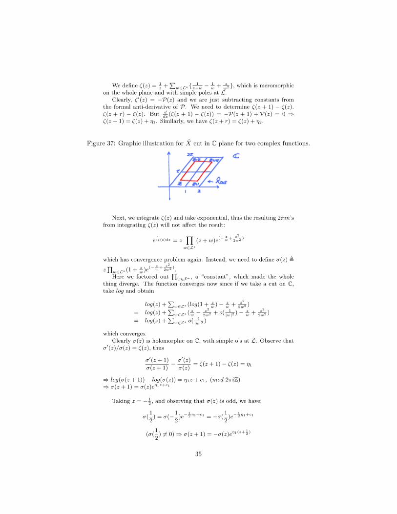
Figure 37: Graphic illustration for X cut in C plane for two complex functions.
Next, we integrate ζ(z) and take exponential, thus the resulting 2πin’sfrom integrating ζ(z) will not affect the result:
e∫ζ(z)dz = z
∏w∈L∗
(z + w)e(− z
w+ z2
2w2 )
which has convergence problem again. Instead, we need to define σ(z) ,
z∏w∈L∗(1 + z
w)e
(− zw
+ z2
2w2 ).
Here we factored out∏w∈P∗ , a “constant”, which made the whole
thing diverge. The function converges now since if we take a cut on C,take log and obtain
log(z) +∑w∈L∗(log(1 + z
w)− z
w+ z2
2w2 )
= log(z) +∑w∈L∗(
zw− z2
2w2 + o( 1|w|2 )− z
w+ z2
2w2 )
= log(z) +∑w∈L∗ o(
1|w|3 )
which converges.Clearly σ(z) is holomorphic on C, with simple o’s at L. Observe that
σ′(z)/σ(z) = ζ(z), thus
σ′(z + 1)
σ(z + 1)− σ′(z)
σ(z)= ζ(z + 1)− ζ(z) = η1
⇒ log(σ(z + 1))− log(σ(z)) = η1z + c1, (mod 2πiZ)⇒ σ(z + 1) = σ(z)eη1z+c1
Taking z = − 12, and observing that σ(z) is odd, we have:
σ(1
2) = σ(−1
2)e−
12η1+c1 = −σ(
1
2)e−
12η1+c1
(σ(1
2) 6= 0)⇒ σ(z + 1) = −σ(z)eη1(z+ 1
2)
35
Similarly, we have σ(z+r) = −σ(z)eη2(z+ r2
). Here we introduce Abel’sSecond Theorem, which states the following.
Theorem 3.1. Given∑Ni=1 A(Pi) =
∑Nj=1 A(Qj) ⇔ ∃f meromorphic
with zero’s at Pi and poles at Qj.
Proof: With the σ(z) function, we may try f(z) =ΠNi=1(σ(z−Pi))ΠNi=1(σ(z−Qj))
and
see if they descend to a function on X, i.e. if it is doubly periodic on C:f(z + 1) = f(z)f(z + r) = f(z)
But f(z + 1) =ΠNi=1(σ(z+1−Pi))ΠNi=1(σ(z+1−Qj))
=[(−1)NΠN
i=1σ(z − Pi)eη1(z−Pi+ 12
)]
[(−1)NΠNi=1σ(z −Qj)eη1(z−Qj+ 1
2)]
=
(ΠNi=1σ(z − Pi)
ΠNi=1σ(z −Qj)
)eη1(
∑Qj−
∑Qi)
The Abel map in this case is A(P ) =∫ P
0dz = P , thus
∑Ni=1 A(Pi) =∑N
j=1 A(Qj)⇒∑Nj=1 Qj−
∑Ni=1 Pi = n+mr. IT is not a priori true that
η1(n+mr) = 0.The correct solution is thus to change different Pi, Qj ’s, for instance
we may take Q′1 = Q1 − n−mr, Q′i = Qi, i = 2, ...N and take
f(z) ,ΠNi=1σ(z − Pi)
ΠNj=1σ(z −Qj)
which would then descend to X.Similar as in the previous section, we may produce the following. A
form with a double pole at P such that wp(z) , L(z − p)dz, since P(z)is already a meromorphic function on C with a double pole at o whichdescends to X. Moreover, a form with 2 simple poles at P , and Q: thedifference is that, since ζ(z + 1)− ζ(z) = ηi : ζ(z + r)− ζ(z) = η2.
Recall that the Riemann Surface was originally defined by w2 = z(z−1)(z − λ)
Figure 38: Graphic illustration for an Abel map that is one-to-one and onto.
36
First, the lattice L is given, we may express ‡ as a Laurent series:
P(z) = 1z2 +
∑w∈L∗(
1(w+z)2
− 1w2 )
= 1z2 +
∑w∈L∗(
1w2 ( 1
1+ zw
)2 − 1w2 )
= 1z2 +
∑w∈L∗(
1w2
∑∞k=0(−1)k(k + 1)( z
w)k − 1
w2 )
= 1z2 +
∑w∈L∗(
∑∞l=1(2l + 1) z2l
w2l+2 )
= 1z2 +
∑∞w∈L∗(2k + 1)z2k∑
w∈L∗1
w2k+2
We are able to do the second to last step because the odd order termsget canceled since L∗ is symmetric: w ∈ L∗ ⇒ −w ∈ L∗.
Define GR(L) ,∑w∈L∗
1w2k
, the Einsenstein series, then
P(z) =1
z2+
∞∑k=1
(2k + 1)Gk+1z2k
After we differentiate it, we obtain:
P ′(z) = − 2z3 +
∑∞k=1(2k + 1)2kGk+1z
2k−1
= − 2z3 + 6G2z + 20G3z
3 +O(z5)
⇒ (P ′(z))4 = 4z6 − 24G2
z2 − 80G3 +O(z2)
And we have
P(z)3 = ( 1z2 + 3G2z
2 + 5G3z4 +O(z6))3
= ( 1z4 + 6G2 + 10G3z
2 +O(z4))( 1z2 + 3G2z
2 + 5G3z4 +O(z6))
= 1z6 + 9G2
1z2 + 15G3 +O(z2)
⇒ (P(z))2 − 4(P(z))3 = −60G21z2 − 140G3 +O(z2)
⇒ (P(z))2 − 4(P(z))3 + 60G2P(z) + 140G3 = O(z2) = 0
which is Liouville’s Theorem.We can define g260G2, g3 = 140G3, then we conclude that
(P(z))2 = 4P(z)3 − g2P(z)− g3
Compared with w2 = z(z−1)(z−λ), which may be changed into the formw2 = 4z3 − g2z− g3 by a linear transformation. Hence the inverse map isgiven by z = P(s) while w = P ′(s).Remark 3.2. The Weierstrass P function answers an old question fromcalculus: what is an elliptic integral?
z =
∫ z P ′√4P3 − g2P − g3
dz =
∫ P(z) du√4u3 − g2u− g3
= E(P(z))
That is, E (elliptic integral) is the inverse of Weierstranss function. Wesee this by comparing with the more familiar:∫ u du√
1− u2= arcsin u and arcsin(sinz) = z
37
3.2 Function Theory According to Jacobi
Go back to Table of Contents. Please click TOC
From Weierstranss, we know that it is easy to follow but not easy togeneralize to other Riemann Surface. From Jacobi, we know we can gen-eralize well to the other Riemann Surfaces. The key notion is the thetafunction. Similar as above, we need to construct: (1) a holomorphic formw = dz, (2) Meromorphic forms with simple poles at P 6= Q : wPQ, and(3) meromorphic forms with a double pole at P : WP .
Let us fix C\Z+Zr : (imr > 0). Define θ(z|r) =∑∞n=−∞ e
πin2r+2πinz,z ∈ C.
The Key Transformations are
(I) θ(z + 1|r) = θ(z|r)(II) θ(z + r|r) = e−2πiz−πirθ(z|r). Note in particular that −2πiz − iπr
is linear in z.
Proof:
θ(z + r) =∑∞n=−∞ e
iπn2r+2πin(z+r) =∑∞n=−∞ e
iπr(n2+2n+1−1)+2πinz
=∑∞n=−∞ e
iπr(n+1)2−iπr−2πiz+2πi(n+1)z
= e−2πiz−πir∑∞n=−∞ e
iπr(n+1)2+2πi(n+1)z
= e−2πiz−πirθ(z)
Q.E.D.
Theorem 3.3. θ(z|r) = 0⇔ z = 1+r2
(mod L), where L = Z + ZrProof: We count the number of zero’s inside a fundamental parallel-
ogram, i.e. we compute the integral 12πi
∫∂X cut
θ′(z)θ(z)
dz = #, which arezero’s inside a fundamental parallelogram.
12πi
∮∂X cut
θ′(z)θ(z)
dz = 12πi
∫ 1
0θ′
θdz +
∫ 1+r
1θ′
θdz −
∫ 1+r
rθ′
θdz −
∫ r0θ′
θdr
= 1
2πi
∫ 1
0( θ′
θ(z)− θ′
θ(z + r))dz−∫ r
0( θ′
θ(z)− θ
θ(z + 1))dz
Now by (I) and (II), we have
= θ′
θ(z)− θ
θ(z + r) = (lnθ(z))′ − (lnθ(z + r))′ = 2πi
⇒ θ′
θ(z)− θ′
θ(z + 1) = (lnθ(z))′ − (lnθ(z + 1))′ = 0
⇒ 12πi
∮∂X cut
θ′
θdz = 1
To find where the zero is, consider θ(z|r) , θ(z + 1+r2|r)
θ(z|r) =∑∞n=−∞ e
iπn2r+2πin(z+ 1+r2
) =∑∞n=−∞ e
iπn2r+iπnr+πin+2πinz
=∑∞n=−∞ e
iπr(n2+n+ 14
)− 14iπr+2πi(n+ 1
2z)−πiz+πin
= e−14iπr−πiz∑∞
n=−∞ eiπr(n+ 1
2)2+2πi(n+ 1
2)z(−1)n
Evaluated at 0, then we have: θ(0|r) = e−14iπr∑∞
n=−∞ eiπr4
(2n+1)2(−1)n
But (2n + 1)2 = (2k + 1)2 (k ≥ 0) ⇒ 2n + 1 = ±(2k + 1) ⇒ n = k or−k − 1, which are of different parity ⇒ θ(0|r) = 0. The result follows.
38
Q.E.D.
Figure 39: Graphic illustration for integral inside a fundamental parallelogram.
Remark 3.4. The factor of θ(z+r|r) = e−2πiz−πirθ(z|r) shows that θ(z|r)is a section of a line bundle L on X, and the above computation showsthat C1(L) = 1.
Remark 3.5. Define θ1(z|r) , eπir4
+πi(z+ 12
)θ(z+ 1+r2|r), then θ1 is an odd
function. This again explains that θ(z+ 1+22|r) has a zero at 0. Moreover
θ1 satisfies the following transformation relations:(III ) θ1(z + 1|r) = −θ1(z|r)(IV ) θ1(z + r|r) = e−iπr−2πizθ1(z|r)
Proof By definition,
θ1(z) = eπi2 eiπr(n+ 1
2)2+2πi(n+ 1
2)z+nπi
=∑∞n=−∞ e
iπr(n+ 12
)2+2πi(n+ 12
)z+πi(n+ 12
)
Thus
θ1(−z) =∑∞n=−∞ e
iπr(−(n+ 12
))2+2πi(−(n+ 12
))z+πi(−(n+ 12
))+(2n+1)πi
= (−1)∑∞k=−∞ e
iπr(k+ 12
)2+2πi(k+ 12
)z+πi(k+ 12
)
= −θ1(z)
For the transformation relations, we note that
θ1(z) = e14πr+πi(z+ 1
2)θ(z|r) = eiπr(n+ 1
2)2+2πi(n+ 1
2)z(−1)n
Hence:
θ1(z + 1) = eπ2i∑∞
n=−∞ eiπr(n+ 1
2)2+2πi(n+ 1
2)z+2πi(n+ 1
2)(−1)n
= −eπ2i∑∞
n=−∞ eiπr(n+ 1
2)2+2πi(n+ 1
2)z(−1)n = −θ1(z)
θ1(z + r) = eπ2i∑∞−∞ e
iπr(n+ 12
)2+2πi(n+ 12
(z+r)(−1)n
= eπ2i∑∞
n=−∞
eiπr(n+ 12
)2+2πir(n+ 12
)+πir−πir+2πi(n+ 12
+1)z−2πz
(−1)(−1)n+1
= −eπ2i(∑∞n=−∞ e
iπr(n+1+ 12
)2+2πi(n+ 12
+1)z(−1)n+1)
e−πir−2πiz
= −e−πir−2πizθ1(z)
39

Q.E.D.
Proof: Now we prove Abel’s Theorem (third proof)“Given
∑Ni=1 A(Pi) =
∑Nj=1(Qj) ⇔ ∃ f meromorphic with zero’s at Pi
and poles at Qj”.Now given
∑Pi =
∑Qj + n + mr, and to construct f , we now use θ-
function:For a first attempt, try f =
∏Ni=1 θ1(z−Pi)∏Nj=1(z−Qj)
f(z+1) =
∏Ni=1 θ1(z + 1 + 1+r
r−Qj)∏N
i=1 θ1(z + 1 + 1+r2−Qi)
=(−1)N
∏Ni=1 θ1(z + 1+r
2− Pi)
(−1)N∏Nj=1 θ1(z + 1+r
2−Qj)
= f(z)
f(z + r) =∏Ni=1 θ1(z+r+ 1+r
2−Pi)∏N
j=1 θ1(z+r+ 1+r2−Qj)
=(−1)N
∏Ni=1 θ1(z+ 1+r
2−Pi)e−2πi(z−Pi)−πir
(−1)N∏Nj=1(z+ 1+r
2−Qj)e
−2πi(z−Qj)−πir
= e2πi(∑Qj−
∑Pif(z)
That is, we may replace one of the points, say, Q1 by Q1 + n + mr, sothat
∑Pi =
∑Qj , and the result follows.
Q.E.D.
3.3 Meromorphic Forms
Go back to Table of Contents. Please click TOC
We can also construct WPQ(z), a meromorphic form with simple poles atP 6= Q as follows: since θ1 satisfies the transformation rules III and IV,
(lnθ1)′ =θ′1θ1
will be a meromorphic function with a simple pole at theorigin, and furthermore it satisfies:
θ′1(z + 1)
θ1(z + 1)=θ′1(z)
θ1(z)
θ′1(z + r)
θ1(z + r)= −2πi+
θ′1(z)
θ1(z)
⇒ θ′1(z−P )
θ1(z−P )− θ′1(z−Q)
θ1(z−Q)is doubly periodic with simple poles at P and Q,
and thus defines the required function on X.To construct WP with a double pole at P , note that: (lnθ1)′′(z) =
(θ′1θ1
)′(z) has a double pole at P and is doubly periodic on C, thus it suffices
to consider −( d2
dz2 lnθ1)(z−P ). We can also connect Jacobi’s theory withWeierstrass’s theory, and we have the following identities.
P(z) = − d2
dz2logθ1(z) + c(r)
Indeed, P(z)− (− d2
dz2 logθ1(z)) is holomorphic on C and doubly periodic.
σ(z) =e
12η1z
2θ1(z|r)
θ′1(o|r)
40

Proof: We first show that : σ′(z)σ(z)
= η1z +θ′1(z)
θ1(z). Indeed, we have
σ′(z)σ(z)
= ζ(z) and ζ(z + 1) = ζ(z) + η1 while ζ(z + r) = ζ(z) + η2, andrη1 − η2 = 2πi as proved before, similarly we have: θ′1
θ1(z + 1) + η1(z + 1)− θ′1
θ1(z)− η1z = η1
θ′1θ1
(z + r) + η1(z + r)− θ′1θ1
(z)− η1z = −2πi+ η1r = η2
⇒ (η1z − θ′
θ(z)) − ζ(z) is doubly periodic and holomorphic, thus it is
constant. But we also know that ζ(z) → 1z
and η1z − θ′1θ
(z) → 1z
wherez → 0 and both have no constant terms.⇒ η1z− θ′1
θ(z) = ζ(z). It follows that cσ(z) = e
12η1z
2
θ1(z|r). To specify c,
we note that σ′(o) = 1 and θ1(z|r)(0) = 0 ⇒ c = limz→0e12η1z
2 θ1(z|r)σ(z)
=
θ′1(0|r). The formula follows.
Q.E.D.
From this proof, we can introduce some special properties of θ-Functions,which are two important formulas.
3.4 Special Properties of θ-Functions
Go back to Table of Contents. Please click TOC
We start by introducing the product representation. With that in mind,we observe the modular transformation law. This leads us to PoissonSummation Formula and we can further discuss Hodge Decomposition.
The product representation: let us set q = eπir, then
θ(z|r) =
∞∏n=1
(1− q2n)(1 + q2m+1e2πiz)(1 + q2m+1e−2πiz), (1)
From the equation, we observe that since r and − 1r
are parametersfor the same lattice (differ an SL(z| − 1
r). Indeed, there is the modular
transformation law :
θ(z| − 1
r) =
√r
ieiπrz
2
θ(rz|r), (2)
where√t is the main branch which is positive for t > 0. In particular, we
have
θ(0| − 1
r=
√r
iθ(0|r), duclity
Proof of the product presentation:Step 1: Denote the R.H.S. of (1) by T (z|r). We will first show that
θ(z|r) = c(q)T (z|r) for some constant c(q) (let this be (1)’).First of all, T vanishes when 1 + qe−2πiz = 0, or erπi−2πiz = eπi. In
particular it vanishes when z = 1+rr
.Secondly, T transforms similarly as θ does under translations by by L,
i.e. T (z + 1|r) = T (z + r), (3)T (z + r|r) = e−2πiz−πirT (z|r), (4)
41
Then it follows that T vanishes at every 1+rr
+L and Tθ
is a holomor-phic, doubly periodic function on C, thus must be constant.
Now let us check (3) and (4). We know (3) follows since it is invarianttermwise. Let us discuss (4).
T (z + r|r) =∏∞n=1(1− q2n)(1 + q2n−1e2πi(z+r))(1 + q2n−1e−2πi(z+r))
=∏∞n=1(1− q2n)(1 + q2n+1e2πiz)(1 + q2n−3e−2πiz)
= (∏∞n=1(1− q2n)(1 + q2n−1e2πiz)(1 + q2n−1e−2πiz))
×(
(1+q−1e−2πiz)
(1+qe2πiz)
)= T (z|r)(qe2πiz)−1
(1+q−1e−2πiz
1+q−1e−2πiz
)= e−2πiz−πirT (z|r)
Step 2: First we shall show that c(g) = 1. We claim that c(q) =c(q4), (5). Then it follows that c(q) = c(q)4 = c(q16) = ... = c(qn)2 = ....
Since Im(r) > 0, then |qn2
| = e−n2πIm(r) < 1.
⇒ c(q) = limq→0c(q), but in both cases θ(0|r) → 1, T (0|r) → 1, whenn2Im(r)→∞.⇒ c(q) = limp→0c(q) = 1.
Now we prove (5). Apply (1)’ at z = 12, we obtain that :
θ(1
2|r) =
∑n∈Z
qn2
(−1)n
and T ( 12|r) =
∏n≥1(1− q2n)(1− q2n−1)2 =
∏n≥1(1− qn)(1− q2n−1)
⇒ c(q) =
∑n∈Zqn2
(−1)n∏n≥1(1− qn)(1− q2n−1)
, (6)
Again apply (1)’ at z = 14
we obtain that :
θ(1
4|r) =
∑n∈Z
qn2
in
However, we also observe that n = ±(2k + 1), k ∈ N ⇒ q(2k+1)2 i2k+1 +
q−(2k+1)2 i−(2k+1) = q2k+1(−1)k(i+ i−1) = 0.
⇒ θ( 14|r) =
∑n even q
n2
in =∑n≥1 q
4n2
(−1)n
T ( 14|r) =
∏n≥1(1− q2n)(1 + q2n−1i)(1− q2n−1i)
=∏n≥1(1− q2n)(1 + q4n−2)
=∏n≥1(1− q4n)(1− q4n−2)(1 + q4n−2)
=∏n≥1(1− q4n)(1− q8n−4)
=∏n≥1(1− (q4)n)(1− (q4)2n−1)
⇒ c(q) =(∑n≥1(q4)n(−1)n)∏
n≥1(1−(q4)n)(1−(q4)2n−1), (7)
Compare (6) and (7), we obtain that c(q) = c(q4) as asserted, and finishesthe proof of the product presentation.
42

Q.E.D.
Proof of the modular transformation: Note that θ(z|r) is holomorphicin both z and r, it suffices to prove for z ∈ R and r = ir2 while r2 > 0.Now the R.H.S. of (2) reads
√re−πr2z
2
θ(izr2|ir2) =√r2e−πr2z2 ∑
n∈Z
e−πr2n2+2πi(izr2)n
=√r2e−πr2z2 ∑
n∈Z
e−πr2n2−2πzr2n
=√r2
∑n∈Z
eeπr2(z+n)2
Thus (2) ⇔∑n∈Z e
− πr2n2+2πinz
=√r2
∑n∈Z e
−πr2(z+n)2 , which is actu-ally a special case of the Poisson summation formula, which leads to thefollowing theorem.
Theorem 3.6. Poisson Summation Formula. Let f be a smooth, rapidlydecaying function. Define the Fourier transformation f(ζ) =
∑n∈Z e
2πinθ f(n)∀θ ∈R. In particular, let θ = 0, then we have∑
n∈Z
f(n) =∑n∈Z
f(n)
“Rapidly decaying” guarantees that∑n∈Z f(n) converges for all θ ∈ R.
For example, we can take the Gaussian: f = e−π2x2
, f(ζ) =√
2e−2πζ2
.
Thus apply this formula to our problem: f = e−πr2z2
, z ∈ R ⇒ f(ζ) =
1√r2e−πn
2
r2 .
⇒∑n∈Z e
−πr2(z+n)2 =∑n∈Z e
2πinz 1√r2e−πn
2
r2
⇒ √r2
∑n ∈ Ze−πr2(z+n)2 =
∑n∈Z e
−πn2
r2+2πinz
which completes the proof.Proof of Poisson Summation formula: Now we can go ahead to prove
this theorem. For a rapidly decaying function f , we may define ψ(θ) =∑n∈Z f(n+ θ). Moreover ψ(θ + 1) = ψ(θ). Thus ψ is a smooth periodic
function, which can be expanded into Fourier series: ψ(θ) =∑n cne
2πinθ,
where cn =∫ 1
0ψ(θ)e−2πinθdθ. However, we have
cn =∫ 1
0e−2πinθ(
∑k∈Z f(k + θ))dθ =
∑k∈Z
∫ 1
0e−2πinθf(k + θ)dθ
=∑k∈Z
∫ k+1
ke−2πinθf(θ)dθ =
∫R e−2πinθf(θ) = f(n)
It follows that ψ(θ) =∑n∈Z f(n)e2πinθ. Hence by definition of ψ we have∑
n∈Z
f(n+ θ) =∑n∈Z
f(n)e2πinθ.
Q.E.D.
43

3.5 Function Theory Using PDE
Go back to Table of Contents. Please click TOC
The goal is to construct holomorphic and meromorphic forms on a surfaceX, on which every point has locally holomorphic coordinates.
Figure 40: Graphic illustration for construction of holomorphic and meromor-phic forms on a surface X.
The idea is simple. Suppose we want to construct a form wp mero-morphic on X with a double pole at p. Using local coordinate charts, wehave
Figure 41: Graphic illustration for using coordinate charts.
(1) Take dtt2
to obtain a form w on V .
(2) Extend w to X by considering χw, where χ ∈ c0(v).
Then χ ≡ 1 in a smaller neighborhood of p in V , but χw is no longermeromorphic on X. We shall correct χw by subtracting a form ψ, so that∂(χw), where ∂ = ∂
∂z. More precisely, we proceed as follows:
Theorem 3.7. (Hodge Decomposition.) Let Φ be any smooth (0, 1) -form on X, locally Φ = Φ(z)dz. Then these exists a smooth functionf ∈ C∞(X) and a (0, 1) - form Φ0 s.t.
Φ =∂f
∂zdz + Φ0 and
∂Φ0
∂z= 0
An observation is the following Φ0 is a holomorphic (1,0) - form and weshall show that the space holomorphic (1,0) - forms is finite dimensional.
Assuming the Hodge decomposition theorem, we consider the followingform
Φ ,∂
∂z(χ(z)
1
z)dz ∈ C∞(X \ p)
on X. Since ∂∂z
( 1z) = 0 for z 6= p, we may just extend it by 0 at p, and 0
outside V , then it’s a smooth (0,1)-form on X.By Hodge decomposition, we may write it as Φ = ∂zfdz+Φ0, with Φ0
an anti-holomorphic (0,1)-form. Now we try the form w , ∂z(χ 1z−f(z))dz
We claim that w is holomorphic. This is because ∂∂zw = ∂z(∂z(χ 1
z−
f(z)))dz = ∂z(Φ− ∂zf(dz))dz = ∂zΦ0dz = 0.
44

Moreover we may construct a form with simple poles at P 6= Q. Theobservation is that how can one construct a form with a single pole?Naively, one may try ∂z(χln z), but ln z has singularities along a “long”cut, which is not compact, and the above “cut off” trick does not apply(since suppχ is compact!)
Figure 42: Graphic illustration for attempting “cut off’ trick.
However, if P 6= Q are inside a same coordinate chart, we may intro-duce a cut by connecting P and Q, which is compact and the “cut off”technique applies:
ΦPQ , ∂z(χ(z)ln(z − pz −Q ))
If P 6= Q are not in the same chart, we may just take a sequencePini=0, P0 = P , Pn = Q, and each neighboring ones are in a same chart.Then apply the above construction to get ΦPiPi+1 and define ΦPQ =∑n−1i=0 ΦPiPi+1.
Figure 43: Graphic illustration for applying construction to get ΦPiPi+1 .
Proof: More general statements will be proven latter, which holds forany dimension. At the present time, we give an explicit proof for C\Z+Zr,using explicit formula.
The observation is straightforward. On C \ Z + Zr, forms can beidentified with doubly periodic functions on C via the correspondence:Φ(z)dz ⇔ Φ(z). Thus the problem becomes the following. Given a func-tion Φ, is it possible to argue the following “∃f,Φ = ∂
∂zf”.
(1) Solving ∂-equation in C.
Let Φ be a smooth function with compact support. Define f(z) ,1
2πi
∫∫C
Φ(ζ)ζ−z dζ ∧ dζ.
Then ∂f∂z
= Φ,∂f∂z
= 12πi
∫∫C
Φ(ζ)ζ−z dζ ∧ dw
= 12πi
∂∂z
∫∫C
Φ(z+z)w
dw ∧ dw while (w = ζ − z)= 1
2πi
∫∫C
1w
∂∂w
(Φ(w + z))dw ∧ dw= 1
2πi
∫∫C
1w
∂∂w
(Φ(w + z))dw ∧ dw while ( ∂∂w
= ∂∂( ¯z+w)
Φ(z + w) =∂∂w
Φ(z + w))
45

= 12πi
limε→0
∫∫|w|≥ε
1w∂Φ∂w
(w + z)dw ∧ dw= 1
2πilimε→0
∫∫|w|≥ε−d( 1
wΦ(w + z)dw)
= 12πi
limε→0
∮|w|≥ε
1w
Φ(w + z)dw
= 12πi
2πiΦ(z)
= Φ(z)
Using this result, we may also solve the equation4g = Φ,4 = ∂z∂z,where Φ is a smooth function with compact support. Indeed, justtake
g(z) =1
2πi
∫∫Clog |z − w|2Φ(w)dw ∧ dw
which is becuase
∂zg =1
2πi
∫∫C
1
z − wΦ(w)dw ∧ dw
and∂z∂zg = Φ(z).
(2) The torus case: C \ Z + Zr. The question is the following. Givena C∞-function φ on C \ Z + Zr, when can we solve: ∂f
∂z= φ for (f
doubly periodic with respect to Z+Zr), 4g = φ (4 = ∂z∂z, again g
doubly periodic), f(z) = 12πi
∫∫Cφ(w)z−w dw∧dw, g(z) = 1
2πi
∫∫C(log|z−
w|2)φ(w)dw ∧ w.
Returning to the torus case C \ Z + Zr, we try a formula of similarkind:
g(z) =1
2πi
∫∫C\Z+Zr
G(z − w)φ(w)dw ∧ dw
A key observation is the following:
By∫∫
C\Z+Zr, we mean an integral over a fundamental domain D.
Furthermore, since∫∫D+m+nr
G(z − w)φ(w)dw ∧ dw=
∫∫DG(z −m− nz − w′)φ(w′ +m+ nr)dw′ ∧ dw′
=∫∫DG(z −m− nr − w′)φ(w′)dw′ ∧ dw′
when G(z − w) is doubly periodic, the integral is doubly periodicand g(z) is well-defined. Thus we look for G(z) doubly periodic andG(z) ∼ log|z|2 for z ∼ 0.
Try log|θ(z|r)|2. Note that θ1(z|r) = θ1(0|r) + zθ′1(0|r) + z2E(z),E(z) is holomorphic or θ1 = z(θ′1(0|r) + zE(z)) as θ1(0|r) = 0. Thus
we try log| θ(z|r)θ′1(0|r) |
2.
Recall that: θ1(z + 1|r)− θ1(z|r)
θ(z + r|r) = −e−πir−2πizθ1(z|r)
Clearly:|θ1(z+1|r)|2|θ′1(0|r)|2 = |θ1(z|r)|2
|θ′1(0|r)|2|θ1(z+r|r)|2|θ′1(0|r)|2 = |e−πir−2πiz|2 |θ1(z|r)|2
|θ′1(0|r)|2 = |eπr2+2πy|2 |θ1(z|r)|2|θ′1(0|r)|2
46
while r = r + ir2 and z = x+ iy
⇒
log |θ1(z+r|r)|2|θ′1(0|r)|2 = log |θ1(z|r)|2
|θ′1(0|r)|2
log |θ1(z+r|r)|2θ′1(0|r) = 2πr2 + 4πy + log |θ1(z|r)|2
|θ′1(0|r)|2
Thus we may try instead log |θ1(z|r)|2|θ′1(0|r)|2 −
2πr2y2. under the transforma-
tion z → z + r (or x+ yi→ x+ r1 + (y + r22)i, y → y + r2):
2π
r2y2 → 2π
r2(y2 + 2yr2 + r2
2) =2πr2
y
2
+ 4πy + 2πr2
which cancels the extra factor.
Definition 3.8. (Green’s Function on Torus). G(z) = log |θ1(z|r)|2|θ(0|r)|2 −
2πr2
(Im z)2
Set g(z) = 12πi
∫∫C\Z+Zr G(z − w)φ(w)dw ∧ dw (*). We compute
4(g(z)) = ∂z∂zg(z). We shall bring ourselves back to the complex, whichis the following case:
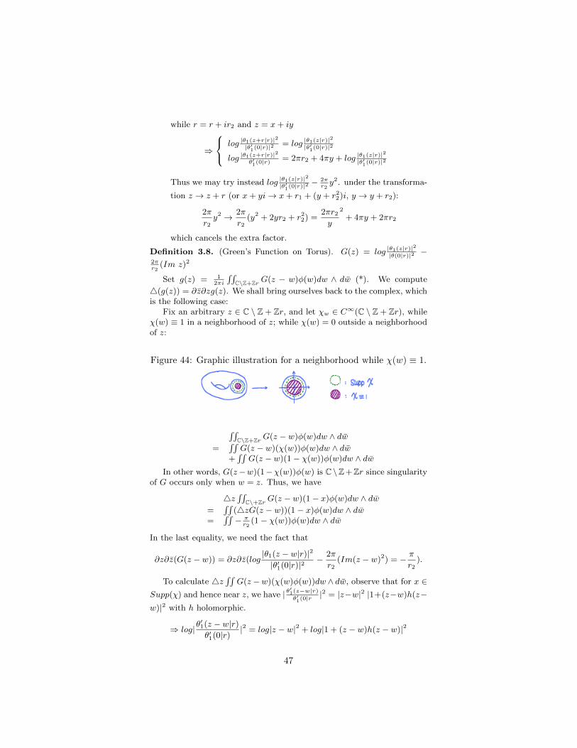
Fix an arbitrary z ∈ C \ Z + Zr, and let χw ∈ C∞(C \ Z + Zr), whileχ(w) ≡ 1 in a neighborhood of z; while χ(w) = 0 outside a neighborhoodof z:
Figure 44: Graphic illustration for a neighborhood while χ(w) ≡ 1.
∫∫C\Z+Zr G(z − w)φ(w)dw ∧ dw
=∫∫
G(z − w)(χ(w))φ(w)dw ∧ dw+∫∫
G(z − w)(1− χ(w))φ(w)dw ∧ dwIn other words, G(z−w)(1−χ(w))φ(w) is C \Z+Zr since singularity
of G occurs only when w = z. Thus, we have
4z∫∫
C\+Zr G(z − w)(1− x)φ(w)dw ∧ dw=
∫∫(4zG(z − w))(1− x)φ(w)dw ∧ dw
=∫∫− πr2
(1− χ(w))φ(w)dw ∧ dw
In the last equality, we need the fact that
∂z∂z(G(z − w)) = ∂z∂z(log|θ1(z − w|r)|2
|θ′1(0|r)|2 − 2π
r2(Im(z − w)2) = − π
r2).
To calculate 4z∫∫
G(z−w)(χ(w)φ(w))dw ∧ dw, observe that for x ∈Supp(χ) and hence near z, we have | θ
′1(z−w|r)θ′1(0|r |
2 = |z−w|2 |1+(z−w)h(z−w)|2 with h holomorphic.
⇒ log|θ′1(z − w|r)θ′1(0|r) |2 = log|z − w|2 + log|1 + (z − w)h(z − w)|2
47
⇒ G(z − w) = log|z − w|2 + log|1 + (z − w)h(z − w)|2 − 2π
r0Im(z − w)2
⇒4z∫∫
G(z−w)(χ(w)φ(w))dw∧dw = 4z∫∫
log|z−w|2χφ(w)dw∧dw+0
+
∫∫4z(−2π
r2Im(z − w)2χφ(w))dw ∧ dw
and by the C-case we have 4z∫∫
log|z − w|2χφ(w)dw ∧ dw = φ(z).Altogether we have the following
4g = φ(z)− 1
2r2i
∫∫C\Z+Zr
φ(w)dw ∧ dw (∗∗)
and we make the following observations.
(1) If∫∫
C\Z+Zr φ(w)dw ∧ dw = 0, then 4 = φ admits a solution and is
given explicitly by the formula (*).
(2) If the equation 4g = φ admits a solution,∫∫
C\Z+Zr φdw ∧ dw = 0.
Indeed∫∫
φdz ∧ dz =∫∫
∂z∂zg(z)dz ∧ dz =∫∫
d(∂zg(z)dz) = 0 byStokes’ Theorem.
(3) The space φ|4g = φ is solvable and has codimension 1 in C∞(Z \z + Zr).
(4) The equation (**) ⇒ φ(z) = ∂z∂zg + φ0 = ∂zf + φ0, f = ∂zg andφ0 a constant. This is exactly the Hodge Decomposition Theoremon C \ Z + Zr.
4 General Theory
Go back to Table of Contents. Please click TOC
4.1 Riemann Surface
Go back to Table of Contents. Please click TOC
We start discussing this section by defining Riemann Surface (notated tobe R.S. in this note).
Definition 4.1. X is called a Riemann Surface (R.S.) if X = ∪αXα withproperty
Φα : Xα → D ⊆ C (D : unit disk)
and∀α, β, Φβ Φ−1
α : Φα(Xα ∩Xβ)→ Φβ(Xα ∩Xβ)
is holomorphic, one-one, (Φβ Φ−1α )′(z) 6= 0 and with holomorphic inverse.
48

Figure 45: Graphic illustration for a Riemann Surface with Φα and Φβ .
For notational sanity, we will use z ∈ Xα such that zΦα→ zα ∈ D.
Definition 4.2. Definition of Line Bundles (Generalization of DifferentialForms). A line bundle L is an assignment: L ↔ tαβ , where tαβ arefunctions on Xα ∩Xβ , satisfying the following cocycle conditions.
tαβtβγ , Xα ∩Xβ ∩Xγtαα = 1
We have the following properties:
(1) L is said to be C∞ if each tαβ is smooth.
(2) L is said to be holomorphic if each tαβ is holomorphic.
(3) L is said to be antiholomorphic if each tαβ is antiholomorphic.
To a line bundle corresponds its space of smooth sections. L ↔Γ(X,L). Γ(X,L) = (ϕα)|ϕα : Xα → C, C∞−function on Xα and ϕα =tαβϕβ on Xα∩Xβ. To a holomorphic line bundle there is also the space ofholomorphic sections: H0(X,L) = (ϕα)|ϕα holomorphic on Xα and ϕα =tαβϕβ on Xα ∪Xβ.
To a line bundle corresponds its space of smooth sections, L↔ Γ(X,L).Γ(X,L) = (ϕα)|ϕα : Xα → C, C∞ − function on Xα and ϕα =tαβϕβ on Xα ∩Xβ.
For example, we can refer to the fololwing list of cases.
(1) L = the trivial bundle ↔ tαβ ≡ 1, ∀α, βThen
Γ(X,L) = (ϕα) = ϕα functions on Xα;ϕα = ϕβ on Xα ∩Xβ= all functions on X
(2) The canonical bundle Λ1,0(x) (or Kx)
Λ1,0(X) = tαβ =∂zβ∂zα
onXα ∩Xβ, chain rule⇒ tαβ satisfy the cocycle condition
Γ(X,L) = (ϕα) : ϕα defined on Xα and ϕα =∂zβ∂zα
ϕβ= (ϕαdzα), ϕαdzα = ϕβ
∂zβ∂zα
dzα = ϕβdzβ on Xα ∩Xβ= smooth (1, 0)− forms on X.
49
In general, for arbitrary complex manifold of dim n, we have X =∪αXα and Φα : Xα → D ⊆ Cn. Then z → zα = (zjα) ∈ Cn, andwe may similarly define a rank n vector bundle Λ1,0(X) : Λ1,0(X) =
tαβ = (∂zjβ
∂zkα)n×n, holomorphic functions taking value in GLn(C).
In dimCX = 1, we will use the notation Kx synoymously.
(3) The holomorphic tangent bundle L↔ tαβ = (∂zβ∂zβ
−1) = ∂zα
∂zβon Xα∩
Xβ. Then that implies
Γ(X,L) = ϕα : ϕα = ∂zα∂zβ
ϕβ on Xα ∩Xβ= (ϕα ∂
∂zα), ϕα
∂∂zα
= ϕβ∂zα∂zβ
∂∂zα
= ϕβ∂∂zβ
More generally, given a bundle L on X, L ↔ tαβ, we can defineanother bundle Lk ↔ tkαβ, k ∈ Z. For example, consider L = KX ,
L3 ↔ ( ∂zβ∂zα
)3 and Γ(X,L) = (ϕα) : ϕα defined on Xα with ϕα(dzα)3 =
ϕβ(dzβ)3.Covariant derivatives, metrics, and curvature on line bundles. The
question is: can we differentiate sections of L?
ϕ∈Γ(X,L)↔ (ϕα(z)) : ϕα : Xα → C, ϕα = tαβϕβ
A naive attempt is to take ∂φα∂zα, can this be glued back to a section of
some line bundle? Consider
∂ϕα∂zα
=∂(tαβϕβ)
∂zα=∂tαβ∂zα
ϕβ +∂ϕβ∂zα
tαβ =∂ϕβ∂zα
ϕβ +∂ϕβ∂zβ
∂zβ∂zα
tαβ
Observe that if L is holomorphic, then∂tαβ∂zα
= 0, thus
∂ϕα∂zα
= tαβ∂zβ∂zα
∂ϕβ∂zβ
.
i.e. ( ∂ϕα∂zα
) is a section of L⊗ Λ1,0(X) = L⊗Λ0,1(X). This is the so calledChern Connection.
4.2 Chern Connection
Go back to Table of Contents. Please click TOC
Definition 4.3. The Chern Connection is defined by
∂ :→ Γ(X,L⊗ Γ0,1), ϕ = ϕα → ∂ϕ=∂ϕα∂zα
Definition 4.4. A metric on L = tαβ is an assignment h: h = (hα) :hα : Xα → R>0, smooth, strictly positive onXα satisfying hα = |tαβ |−2hβ on Xα∩Xβ. Equivalently, h is a strictly positive section in L−1 ⊗ L−1. Thereare plenty of such sections by glueing local sections.
Definition 4.5. Given ϕ∈Γ(X,L), ϕ=ϕα, we can define its norm by
||ϕ|| 4= ϕαϕαhα
well-defined since onXα∩Xβ , ϕαϕαhα = tαβϕβ tαβϕβ |tαβ |−2hβ = ϕβϕβhβ .
50

Given a metric h on L, we can define the covariant derivative 5 asfollows:
5z : Γ(X,L)→ Γ(X,L⊗ Λ1,0),
φ = ϕα → h−1α
∂
∂zα(hαϕα)
Indeed hαϕα ∈ Γ(X,L−1 ⊗ L−1 ⊗L) ' Γ(X, L−1) is a section of anantiholomorphic bundle and ∂
∂zα(hαϕα) is thus a well-defined section of
Γ(X, L−1 ⊗ Λ1,0).Another way writing Oz would be useful: Ozϕ = ∂zαϕα+h−1
α (∂zαhα)ϕα =∂zαϕα + ∂zα(log hα)ϕα.
4.3 Commutation Rules
Go back to Table of Contents. Please click TOC
For this rule, we wnat fix L → X a holomorphic line bundle L = tαβ,metric h = hα, ψ = ψα ∈ Γ(X,L). Then we have
OzOzϕ− OzOzϕ = 4z(∂zϕ)−4z(h−1∂z(hϕ))= h−1∂z(h(∂zϕ))− ∂z(h−1∂z(hϕ))= ∂z∂zϕ+ Γ∂zϕ− ∂z(Γϕ+ ∂zϕ)= −(∂zΓ)ϕ
Note that Ozϕ ∈ Γ(X,L ⊗ Λ1,0), a section of a holomorphic line bundleto which ∂z applies; ∂zϕ ∈ Γ(X,L⊗Λ1,0), h∂zϕ ∈ Γ(X, :−1 ⊗L−1 ⊗ L⊗Λ0,1) ' Γ(X, L−1⊗Λ0,1), i.e. a section of an anti-holomorphic bundle, towhich ∂z applies.
Here we obtain:[Oz,Oz]ϕ = F zzψ
where F zz = −∂zΓ = −∂z∂zlog h, which is called the curvature of theline bundle L w.r.t. h
An observation F zz = F zαzα is a section of Λ1,1 ' λ1,1 ' Λ1,0 ⊗λ0,1. Explicitly,
∂zα∂zαlog hα =∂zβ∂zα
∂zβ∂zα
∂zβ∂zβ(log hβ − log tαβ − log tαβ)
=∂zβ∂zα
∂zβ∂zα
∂zβ∂zβlog hβ
It is not cohomologically trivial since in general (∂zαlog hα)dzα is nota global form on X.
4.4 Basic Residue Formula for Holomorphic LineBundles
Go back to Table of Contents. Please click TOC
For any L → X, holomorphic line bundle, any metric h and any mero-morphic section ψ = ψα, i.e. ψα is a meromorphic function on Xα:
#zeros of ψ −#poles of ψ =i
2π
∫X
F zzdz ∧ dz
We have the following observations.
51

(1) L.H.S. does not depend on the metric chosen.
(2) R.H.S. does not depend on the meromorphic section chosen.
(3) Meromorphic sections always exist (to be proven). We want to knowif holomorphic sections exist. If i
2π
∫XF zzdz ∧ dz < 0, then for any
ψ, #poles of ψ > 0⇒6 ∃ holomorphic sections. Thus the sign ofcurvature is of great importance.
Definition 4.6. The 1st Chern Class. C1(L)4= i
2π
∫XF zzdz ∧ dz.
Proof: We shall compute the R.H.S., and locally, we have
F zzdz ∧ dz = −∂z∂zlog hdz ∧ dz = −d((∂zlog h)dz)
Notice that ∂zlog hdz is not a section of ∧1,0. Note that
F zzdz ∧ z = −∂z∂z(log||ϕ||2)dz ∧ dz,
away from the zeros and poles of ϕ, which are denoted as P1, ..., PN.Take ε small enough, so that each disk D(Pi, ε)(
4= Di) contains only one
Pi. Thus∫xF zzdz ∧ dz = limε→0
∫X\∪Ni=1Di
−∂z∂z(log||ϕ||2)dz ∧ z
= limε→0
N∑i=1
∮∂Di
∂z(log||ϕ||2)dz
On each Di (contained in a coordinate chart), we have ϕ = zMΦ(z) withΦ : holomorphic and Φ(0) 6= 0.
Figure 46: Graphic illustration for Di.
Then we have∮∂Di
∂z(log||ϕ||2)dz =∮∂Di
∂z(log|z|2M + log(h|Φ(z)|2))dz
=∮∂Di
(Mz
+ ∂zlogh|Φ(z)|2)dz
= −2πiM +O(ε)→ −2πiM(ε→ 0)⇒
i2π
∫XF zzdz ∧ dz =
∑Ni=1 Mi = #zeros of ϕ −#poles of ϕ
Q.E.D.
Now we introduce the Riemann-Roch Theorem
Theorem 4.7. Notation: H0(X,L)4= holomorphic sections of L =
ϕ = (ϕα)|∂zαϕα = 0For any line bundle: L→ X, we have the following formula (Riemann-
Roch):
dim H0(X,L)− dim H0(X,L−1 ⊗Kx) = c1(L) +1
2χ(x)
52
where Kx = ∧1,0(x), and χ(x)4= c1(K−1
x ) = the Euler characteristic ofX.
Furthermore, we shall prove the following (Gauss-Bonnet), if X is asurface with g holes, then χ(x) = 2− 2g.
Corollary 4.8. This corollary states the following:(1) Let X be a Riemann surface with g holes. Take L = Kx, then we
have K−1x ⊗Kx is trivial, thus by Riemann-Roch Theorem
dim H0(X,L)− 1 = −χ(x) +1
2(x) = g − 1
⇒ dim H0(X,L) = g
For example, on the torus, we exhibited w = dz√z(z−1)(z−λ)
, which is a
basis of H0(X,Kx).(2) Use of point bundles. Fix a Riemann Surface X and p ∈ X.
We construct a line bundle in the following way. Pick a coordinate sys-tem in a neighborhood XD of P , and set X∞ = X \ p. Let L bet0,∞(z) = z on XD ∩ X∞. This defines a holomorphic line bundlewhich admits a holomorphic section 1p = 1 on X∞; z on X0, and 1p|X0 =
z = z1 = t0,∞1p|x∞. Thus 1p is a section of L4= [P ], which is holomor-
phic, and has exactly 1 zero at p. In particular c1(L) = #(zeros of 1p)−#(poles of 1p) = 1.
Similarly, given any integer n ∈ Z, we may define [nP ] by the transitionfunction zn, and a holomorphic / meromorphic section 1nP dependingon n ≥ 0/n < 0. It follows that c1([nP ]) = n.
More generally, given P1, ..., PM on X and integers n1, ..., nM , we mayconstruct [n1P1 + · · ·+nmPM ] = L ' [n1P1]⊗· · ·⊗ [nMPM ], and c1(L) =∑Mi=1 ni. Proof that any holomorphic line bundle admits a non-trivial
meromorphic section. Pick a point P , consider L ⊗ [nP ], then c1(L ⊗[nP ]) = c1(L) + n. By Riemann-Roch Theorem,
dim H0(X,L⊗ [nP ])− dim H0(X,L−1 ⊗ [−nP ]⊗K)= c1(L) + n− 1
2χ(x) > 0(n >> 0)
⇒ dim H0(X,L⊗ [nP ]) > 0(n >> 0)⇒ dim H0(X,L⊗ [nP ]) > 0(n >> 0)⇒ ∃ϕ 6= 0, ϕ a section of L⊗ [nP ], ϕ holomorphic⇒ ψ = ϕ1nP is a non− zero meromorphic section of L
(3) Given any two points P1 6= P2, we show that Riemann−Roch ⇒∃ meromorphic form ϕ with simple poles P1 and P2.
Consider the bundle L = [−P1 − P2] ⇒ c1(L) = −2 and L cannotadmit any holomorphic section.
Rieman−Roch ⇒ 0− dim H0([P1 + P2]⊗Kx) = −2 + 1− g⇒ dim H0([P1 + P2]⊗Kx) = g + 1
Let ψ1, ..., ψg be a basis of H0(X,Kx), then 1[P1 + P2]ψ1, ..., 1[P1 +P2]ψg are linearly indepenent sections of [P1 + P2] ⊗ Kx. Let Φ be aholomorphic section of the bundle which is linearly independent of 1[P1 +
53

P2]ψ1, ..., 1[P1 + P2]ψg, and set ϕ = 1[−P1 − P2]Φ is a section we need.(Potentially ϕ may not have 2 poles, then it would have no pole at allsince
∑P=Pi
Res(ϕ)(p) = 0. In that case ϕ is a holomorphic section and1[P1 + P2]ϕ = Φ would be holomorphic, thus a linear combination ofψ1, ..., ψg, which contradicts the fact that Φ being linearly independentfrom 1[P1 + P2]ψ, ..., 1[P1 + P2]ψg.)
Proof: (Proof of Riemann-Roch Theorem)The basic idea behind the index theorems, i.e., heuristic point of view.Assume D is a linear operator between two vector spaces: D : H1 →
H2 where H and H1 are Hilbert spaces (in general, H1 6= H2, for instance,∂ : Γ(X,L) → Γ(X,L ⊗ ∧0,1), ϕ → ∂ϕ). Since the spectrum of D is notavailable. Consider 4− = D†D, where D† is the adjoint of D (which isdefined by < Du, v >=< u,D†v >, ∀u ∈ H1, v ∈ H2), 4− : H1 → H1,self-adjoint. Hence we can talk about the spectrum of 4−. Spectrum4− = λn : ∃0 6= ϕn ∈ H1,4−ϕn = λnϕn. Furthermore, ker4− = ϕ :D†Dϕ = 0 = ϕ :< ϕ,D†Dϕ >= 0 = ϕ : ||Dϕ|| = 0 = ϕ : Dϕ =0 = KerD.
Another natural operator: 4+ = DD† : H2 → H2 and again, wedefine the spectrum 4+ = λ†n|∃ψ ∈ H2,4+ψ = λ†nψ, and similarlyker4+ = kerD†.
A simple observation is the following. The spectra of 4− and 4+ arethe same (counted with multiplicity) are the same except for the kernels.Indeed, D†Dψ = λ−nϕ ⇒ 4†(Dϕ) = DD†Dϕ = λ−nDϕ, that is, ∀λn anon-zero eigen-value of 4−, λn is also an eigen value of 4†.
Consider ∀t > 0, Tr(et4−)−Tr(et4+). Here we assume that 4−, 4+
can be diagonalized, i.e. ∃ and o.n.b. ϕ−n of H1 with 4−ϕ−n = λnϕ−n ,
an o.n.b. ϕ†n of H2 with 4†ϕ†n = λ†nϕ†n. We may define f(4−)ϕ−n =
f(λn)ϕn, that is, we would have
e−t4− =∑ (−t)n
n!(4−)n ⇒ e−t4−ϕn = e−tλnϕ−n
Q.E.D.
In general, ϕ =∑cnϕ
−n , f(4−)ϕ =
∑cnf(4−)ϕ−n =
∑cnf(λn)ϕn.
Notice that ϕ ∈ H ⇒∑|cn|2 <∞, for f(4−)ϕ ∈ H, we need
∑|cn|2|f(λn)|2 <
∞. In our case it is good since λn > 0, e−tλn < 1. That is, we would
have Tr(f(4−))4=∑n f(λn) if it converges. Then
Tr(e−t4−)−Tr(e−t4+) =∑
e−tλn−∑
e−tλ†n = dimKerD−dimKerD†.
Our next observation is that the LHS can be computed using pertur-bation theory. More precisely, set p = e−t4, then we have
( ∂∂t
+4)P = 0P |t=0 = Id
which is the famous Heat Equation, and solutions of the heat equationcan be computed asymptotically for small t.
Here is the detail. Let L→ X be a holomorphic line bundle. We wantto set up
∂ : Γ(X,L)→ Γ(X,L⊗ Λ0,1)
54
We want the inner products on Γ(X,L) and Γ(X,L⊗Λ0,1). Pick a metrich on L, and a metric g on (Λ0,1)−1 = fα ∂
∂zα the holomorphic tangent
bundle. Recall that for a holo line bundle L, a metric is a positive sectionof L−1⊗ L−1. Thus g is a positive section of Λ1,0⊗ Λ1,0 ' Λ1,1, a positiveone-one form; we shall write gzz to stress it is a one-one form.
Definition 4.9. ∀ϕ,ψ ∈ Γ(X,L),Φ,Ψ ∈ Γ(X,L⊗ Λ0,1), we define innerproducts
< ϕ,ψ >4=
∫x
hϕϕgzz
< Φ,Ψ >4=
∫x
hΦΨ
Here we notice that hϕψgzz ∈ Γ(X,L−1 ⊗ L−1 ⊗ L ⊗ L ⊗ Λ1,1) =Γ(X,Λ1,1) and hΦΨ ∈ Γ(X,L−1⊗L−1⊗L⊗Λ0,1⊗L⊗Λ1,0) = Γ(X,Λ1,1).Hence both are one-one forms, and thus
∫X
makes sense.
Now we can discuss formal adjoint ∂† of ∂. That is, we have ∂† :Γ(X,L ⊗ Λ0,1) → Γ(X,L) with respect to the inner products above isdefined by
< ∂ϕ,Φ >=< ϕ, ∂†Φ >
More explicitly, we have∫Xh∂zϕΦ =
∫xhϕ∂Φgzz. The LHS would be
LHS =∫X∂zϕhΦ
= −∫x∂z(hΦ), (I.B.P.)
= −∫xhϕgzzh−1h−1∂z(hΦ)gzz, (gzzgzz = 1)
⇒ ∂+Φ = −gzzOzΦ
Indeed, gzz4zΦ ∈ Γ(X, (Λ1,1)−1 ⊗ L ⊗ Λ0,1 ⊗ Λ1,0) = Γ(X,L) so this isa valid definition. Then we define 4− = ∂†∂ : Γ(X,L) → Γ(X,L) and4+ = ∂∂† : Γ(X,L⊗ Λ0,1)→ Γ(X,L⊗ Λ0,1)
4.5 Spectral Decomposition of Laplacian 4−
Go back to Table of Contents. Please click TOC
Theorem 4.10. (Spectral Decomposition of Laplacian 4−). This theo-rem has four parts:
(1) ∃ϕn ∈ Γ(X,L), n ∈ Z+ an o.n.b. of H1 = Γ(X,L) which consistsonly of eigenfunctions for 4−, i.e. 4−ϕn = λnϕn.
(2) λn ≥ 0 and λn → ∞ at least at polynomial growth rate as n → ∞,i.e. cnγ ≥ λn ≥ Dnδ for some C,D, γ, δ > 0.
(3) For any k ∈ Z+, ∃δk such that ||ϕn||ck ≤ Ak|λn|δk for some constant
Ak. Here ||ϕ||c0 4= supx|ϕn|2h; ||ϕ||c1 4= ||ϕ||c0 + sup
x|Ozϕ|2hgzz +
supx|Ozϕ|2hgzz, etc.
(4) Each eigenvalue λn occurs with finite multiplicity, which implies thatker4− is finite dimensional.
Assume this theorem, we can now define e−t4− and its trace as thefollowing.
55
Definition 4.11. For u ∈ Γ(X,L), we wrtie u =∞∑n=0
unϕn, un =<
u,ϕn >, with the series converging in the L2-sense with respect to <,>on H1. Define
e−t4−u4=
∞∑n=0
e−tλnunϕn, (?)
The RHS is a well-define element of H1 and then we can discuss Riesz-Fischer Theorem.
Theorem 4.12. (Riesz-Fischer Theorem).∞∑n=0
unϕn converges in H1 if
and only if∞∑n=0
|un|2 <∞.
Proof: We have N∑n=0
unϕn ⇔ Cauchy ⇔ ||M∑n=N
un||2 < ε, ∀M,N >>
0⇔∞∑n=0
|un|2 < +∞.
Q.E.D.
Observe that ϕn is also an o.n.b. of eigen-functions for e−t4− .
Indeed e−4−ϕn = (e−tλ−n )ϕn with eigenvalues e−tλ
−n . It follows from
out theorem that Tr(e−t4−) =∑n
e−tλ−n < ∞, ∀t > 0. Since λ−n ≥ cnδ
for n >> 0. It follows that dim ker∂ − dim ker∂† = dim ker4− −dim ker4+ = Tr(e−t4
−)− Tr(e−t4
+
).We want to evaluate Tr(e−t4−) There are two steps:
(1) We can express it as a kernel. That is, ∀u ∈ Γ(X,L), we have
(e−t4−u)(z) =∑n
e−tλ−n unϕn(z)
=∑n
e−tλ−n (∫xhuϕngωω
i2dω ∧ dω)ϕN (z)
=∫x(∑n
e−tλ−n ϕn(z)ϕn(ω)hgωωu(ω) i
2dω ∧ dω)
Note that we may interchange sum and integral since ||ϕn||ck ≤Ak|λδkn and thus the sum converges, which implies (e−t4
−u)(z) =∫
xKt(z, ω)u(ω) i
2dω∧dω whereKt(z, ω) =
∑n
e−tλ−n ϕn(z)ϕn(ω)h(ω)gωω,
which is the heat kernel. This leads to Kt(z, z) ∈ Γ(X,Λ1,1). Thenwe have∫
xKt(z, z)
i2dz ∧ dz =
∫x
∑n
e−tλ−n |ϕn(z)|2h(z)gzz
i2dz ∧ dz
=∑n
e−tλ−n∫x|ϕn(z)|2h(z)gzz
i2dz ∧ dz
=∑n
e−tλ−n ||ϕn||
=∑n
e−tλ−n
= Tr e−t4−
56
(2) Then we need to determine Kt(z, z) for small g. There are twoclaims:
The first claim is that there exists an asymptotic expansion ofKt(z, z),in the sense that Kt(z, z) = uzz
t+ Vzz +O(t) and ||Kt(z, z)− uzz
t−
Vzz||cm ≤ Amt, while t << 1. Clearly uzz ∈ Γ(X,Λ1,1) and so isVzz.
The second claim is that uzz and vzz depend on h of L and g ofΛ−1,0. Key observation is the following: uzz does not depend on thederivatives of h and g, while uzz depends on derivatives of h, g upto order 2. This will follow from heat kernel equation theory to beexplained below:
uzz = agzzvzz = bFhzz + cF gzz
This can be guessed from power counting. We write specifically for4− and4+. The kernel of4− is K−t (z, z) = a− gzz
t+b−Fhzz+c−F gzz.
The kernel of4+ is K+y (z, z) = a+ gzz
t+b+Fhzz+c+F gzz. This implies
that Tr(e−t4−
)−Tr(e−t4†) = (a−a+)V ol(X)
t+(b−−b+)c1(L)+(c−−
c+)c1(K−1x ). Clearly a− = a+ otherwise the L.H.S. would blow-up.
This implies that Tr(e−t4−
)−Tr(e−t4†) = βc1(L)+γc1(K−1
x ). Wecan even determine the coefficients β and γ.
4.6 Serre Duality
Go back to Table of Contents. Please click TOC
This subsection we discuss Serre Duality. We know that Tr(e−t4−
) −Tr(e−t4
†) = dim ker∂−dim ker∂† but how does ker∂† ∼ H0(L−1⊗Kx)?
The claim is that Φ → hΦ gives an isomorphism: Γ(X,L ⊗ Λ0,1) →Γ(X,L−1 ⊗ Kx). Indeed Φ ∈ Γ(X,L ⊗ Λ0,1) → hΦ ∈ Γ(X, L ⊗ Λ1,0 ⊗L−1 ⊗ L−1) = Γ(X,L−1 ⊗ Λ1,0). Moreover, we have
Φ ∈ ker∂† ⇔ ∂†Φ = 0⇔ gzzh−1(∂zhΦ) = 0⇔ ∂zhΦ = 0⇔ ∂zhΦ = 0, h > 0, h ∈ R⇔ hΦ ∈ H0(X,L−1 ⊗Kx)
Thus dim ker∂† = dimH0(X,L−1⊗Kx). Now dim ker∂−dim ker ¯partial†
=dim H0(X,L)− dim H0(X,L−1 ⊗Kx) = βC − 1(L) + γC1(K−1
x ). Laterwe will see that β and γ are universal constants.
For special cases, we can discuss the following.
(1) L = trivial ⇒ 1− dim H0(X,Kx) = 0 + γC1(K−1x ).
(2) L = Kx ⇒ dim H0(X,Kx)− 1 = βC1(Kx) + γC1(K−1x ).
Combination of (1) and (2) will give us γ = β2
. To determine the overallvalue (assuming Gauss-Bonnet Theroem), consider X = S2, c1(K−1
x ) =2 − 2g = 2 ⇒ c1(Kx) = −2 and H0(X,Kx) = 0. This implies that1 − 0 = γc1(K−1
x ) = 2γ ⇒ γ = 12. Hence, it gives us Riemann-Roch
Theorem.Let us present the road map and summary for three main ingredients.
57
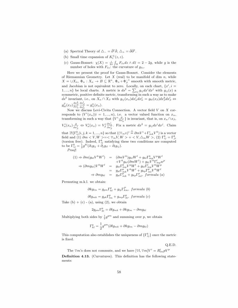
(a) Spectral Theory of 4− = ∂†∂, 4+ = ∂∂†.
(b) Small time expansion of K±t (z, z).
(c) Gauss-Bonnet: χ(X) = i2π
∫XFzzdz ∧ dz = 2 − 2g, while g is the
number of holes with Fzz: the curvature of gzz.
Here we present the proof for Gauss-Bonnet. Consider the elementsof Riemannian Geometry. Let X (real) to be manifold of dim n, whileX = ∪Xα, Φα : Xα → B ⊆ Rn, Φα Φ−1
β smooth with smooth metric,
and Jacobian is not equivalent to zero. Locally, on each chart, xi, i =1, ..., n be local charts. A metric is ds2 =
∑ij gijdx
idxj with gij(x) asymmetric, positive definite metric, transforming in such a way as to makeds2 invariant, i.e., on Xα ∩Xβ with gij(xα)dxiαdx
jα = gkl(xβ)dxkβdx
lβ ⇔
gβkl(xβ)∂xkβ∂xiα
∂xlβ
∂xjα
= gαij(xα).
Now we discuss Levi-Civita Connection. A vector field V on X cor-responds to (V i(xα)|i = 1, ..., n), i.e. a vector valued function on xα,transforming in such a way that V i ∂
∂xiα is invariant, that is, on xα∩xβ ,
V iα(xα) ∂
∂xjβ
⇔ V iα(xα) = V jβ∂xiα
∂xjβ
. Fix a metric dx2 = gijdxidxj . Claim
that ∃!Γkij |i, j, k = 1, ..., n so that ((Omv)i4= ∂mV i+ΓimkV
k) is a vectorfield and (1) ∂m < V,W >=< OmV,W > + < V,4mW >, (2) Γkij = Γkji(torsion free). Indeed, Γkij satisfying these two conditions are computedto be Γkij = 1
2gkl(∂iglj + ∂jgil − ∂lgij).
Proof:
(1)⇒ ∂m(gklVkW l) = (∂mV k)gklW
l + gklΓkmpV
pW l
+V kgkl(∂mWl) + gklV
kΓlmpwp
⇒ (∂mgkl)VkW l = gklΓ
kmpV
pW l + gklΓlmpV
kW p
= gplΓpmkV
kW l + gkpΓpmlV
kW l
⇒ ∂mgkl = gplΓpmk + gkpΓ
pml, formula (a)
Permuting m.k.l. we obtain:
∂kglm = gpmΓpkl + glpΓPkm, formula (b)
∂lgmk = gpkΓplm + gmpΓplk, formula (c)
Take (b) + (c) - (a), using (2), we obtain
2gpmΓpkl = ∂lgmk + ∂kglm − ∂mgkl
Multiplying both sides by 12gqm and summing over p, we obtain
Γqkl =1
2gqm(∂lgmk + ∂kglm − ∂mgkl)
This computation also establishes the uniqueness of Γkij once the metricis fixed.
Q.E.D.
The Om’s does not commute, and we have [Ol,Om]V i = RilmpVp
Definition 4.13. (Curvatures). This definition has the following state-ments:
58

(1) Rilmp = ∂lΓimp−∂mΓilp+Γqlq−ΓimqΓqlp is the Riemannian curvature.
(2) Rmp = Rllmp is the Ricci curvature.
(3) R = gpmRmp is the scalar curvature.
Note that our convention for raising and lowering indices: V i → Vj4=
V igij . For example, R = Rpp = gpmRmp = Rmm.For example, X be a Riemann Surface with a metric gzz on Λ−1,0 gives
rise to a Riemannian metric on X. We set up a dictionary. That is, ona holomorphic chart we have z = x1 + ix2 ↔ (x1, x2) and we have thefollowing.
(1) V ∈ Γ(X,Λ−1,0), V = V ∂z ↔ V : vector field V + V . Explicitly,we have V ∂z = (V 1 + iV 2) 1
2(∂x1 − i∂x2) = 1
2(V 1∂x1 + V 2∂x2) +
i2(V 2∂x1 − V 1∂x2) ⇒ v = V 1∂x1 + V 2∂x2. Conversely, define
J : V 1∂x1 + V 2∂x2 → V 2∂x1 − V 1∂x2, then V = 12(v + iJv).
(2) A metric gzz on Λ−1,0 : ||V || = V V gzz. Define ||v||2 4= ||v||2 =((V 1)2 + (V 2)2)gzz. Compared with ||v||2 =
∑gijv
ivj ⇒ ds2 =gijdx
idxj = gzz((dx1)2 + (dx2)2). Thus, we have (gzz ↔ ds2 =
gzz((dx1)2 + (dx2)2).
(3) Connection, that is,
OzV ↔ O1v = (Oz +4z)(V + V )(Chern connection) levi− Civita connection
defined by gzz w.r.t. ds2 = gzz((dx1)2 + (dx2)2)
The dependence of Γkij and Rilmp on the metric gij . We determine thevariations of Γkij and Rilmp under variations of g. The derivative linearapproximation is simpler than the function itself. Since gij → Γkij , andδgij → δΓkij .
The key variation formulae (which we will prove later) is the following:
(1) δΓlijk = 12gkl(Ojδgil + Oiδglj − Olδgij).
(2) δRljmk = Oj(δΓlmk)− Om(δΓljk).
(3) δRml = Oj(δΓjml)−
12Om4l(gjpδgpj).
(4) δR = −δglmRml + Oj4lδglj −4(gmlδglm).
where δgij4= (δgkl)g
kiglj .Using these formula, we claim the following.
Theorem 4.14. Define the functional on the space of all Riemannianmetrics on X, say,
gij → I(g) =1
2π
∫X
(R√g)dx,
then δI(g) = 0 for any δgij.
Proof: Claim that
δI(g) =1
2π
∫X
δ(R√g)dx =
1
2π
∫X
(δR√g +
1
2δg/√gR)dx
59
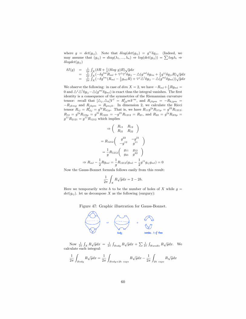
where g = det(gij). Note that δlog(det(gij) = gijδgji. (Indeed, wemay assume that (gij) = diag(λ1, ..., λn) ⇒ log(det(gij)) =
∑logλi ⇒
δlogdet(gij)
δI(g) = 12π
∫X
(δR+ 12(δlog g)R)
√gdx
= 12π
∫X
(−δglmRml + OjOlδglj −4(gmlδglm + 12gijδgjiR)
√gdx
= 12π
∫X
(−δglm(Rml − 12gmlR) + Oj4lδglj −4(gmlδgml))
√gdx
We observe the following: in case of dim X = 2, we have −Rml+ 12Rgml =
0 and4j4lδglj−4(gmlδgml) is exact thus the integral vanishes. The firstidentity is a consequence of the symmetries of the Riemannian curvaturetensor: recall that [4j ,4k]V l = RljkmV
m, and Rjkpm = −Rkjpm =−Rjkmp and Rjkpm = Rpmjk. In dimension 2, we calculate the Riccitensor Rij = Rlilj = glpRiljp. That is, we have R11g
lpR1l1p = g22R1212;
R12 = glpR1l2p = g21R1221 = −g21R1212 = R21, and R22 = glpR2l2p =g11R2121 = g11R1212 which implies
⇒(
R11 R12
R21 R22
)
= R1212
(g22 −g21
−g12 g11
)=
1
gR1212
(g11 g12
g21 g22
)⇒ Rml −
1
2Rgml =
1
gR1212(gml −
1
2gijgijgml) = 0
Now the Gauss-Bonnet formula follows easily from this result:
1
2π
∫X
R√gdx = 2− 2h.
Here we temporarily write h to be the number of holes of X while g =det(gij). let us decompose X as the following (surgury):
Figure 47: Graphic illustration for Gauss-Bonnet.
Now 12π
∫XR√gdx = 1
2π
∫Body
R√gdx +
∑1
2π
∫Handle
R√gdx. We
calculate each integral:
1
2π
∫Body
R√gdx =
1
2π
∫Body+2h caps
R√gdx− 1
2π
∫2h caps
R√gdx
60

Figure 48: Graphic illustration for Gauss-Bonnet.
By the previous claim, 12π
∫Body+2h caps
R√gdx = 1
2π
∫S2 R
′√g′dx,
where (g′ij), g′, R′ are derived from the standard metric on S2 as the unit
sphere, and a direct calculation shows that R′ = 1, thus 12π
∫S2 R
′√g′dx =4π/2π = 2.
Moreover, for each cap 12π
∫cap
R√gdx = 1
2( 1
2π
∫sphere
R√g) = 1
2×2 =
1.
Figure 49: Graphic illustration for Gauss-Bonnet.
Lastly, for each handle, we have
12π
∫handle
R√gdx = 1
2π
∫handle+2 caps
R√gdx− 1
2π
∫2 caps
R√gdx
= 2− 2× 1 = 0
Altogether:
12π
∫XR√gdx = 1
2π
∫Body
R√gdx+
∑1
2π
∫Handle
R√g
= 2− 2h
Figure 50: Graphic illustration for Gauss-Bonnet.
Main valuation formulaeNow let us derive our key variational formulae. First of all, asusming
(1) and (2):
61

(1) δΓkij = 12gkl(Ojδgil + Oiδglj − Olδgij)
(2) δRljmk = Oj(δΓlmk)− Om(δΓljk)
We shall evaluate δRmk and δR:
δRmk = δ(Rjjmk) = δ(OjδΓjmk − OmδΓ
ijk)
However, note that
δΓjjk = 12gjp(Okδgjp + Ojδgpk − Opδgjk)
= 12gjpOkδgjp
= 12Ok(gjpδgjp)
The second equality holds because Ojδgpk −Opδgjk is antisymmetric in pand j while gjp is symmetric. The last equality holds since Ojδgpk = 0,which follows from
∂jgpk = gplΓljk + glkΓljp
(known as Ricci’s lemma, see the general remark on covariant differentia-tion of tensors.) Thus, δRmk = Oj(δΓ
jmk) − 1
2OmOk(gjpOgjp, as claimed
in 3).Next,
δR = δ(gmkRmk)
= (δgmk)Rmk + gkmδRmk= −gkp(δgpq)gqmRmk + gkm(Oj(δΓ
jmk)− 1
2OmOk(gjpδgjp)).
(Here we used that G ·G−1 = Id⇒ (δG)G−1 +Gδ(G−1) = 0⇒ δG−1 =−G−1(δG)G−1).
δR = −δgkmRmk + Oj(gkmδΓjmk)− 1
24(gjpδgjp)
(where by definition, 4f 4= gkmOmOkf = gkmOm(∂kf), for any smoothf).
We compute gkmδΓjmk:
gkmδΓjmk = gkm 12gjp(Okδgmp + Omδgpk − Opδgmk)
= gkmgjpOkδgmp − 12gjpOp(gkmδgmk)
(since Okδgmp +Omδgpk is symmetric in k, p and so is gkm; Opgkm = 0.)
gkmδΓjmk = Ok(δgkj)− 12gjpOp(gkmδgmk)
Plugging in, we obtain:
δR = −δgkmRmk + OjOk(δgkj)−4(gjpδgpj)
which is the key variational formula, 4), with the term OjOk(δgkj) −4(gjpδgpj) being an exact term.
Thirdly, we calculate δRljmk. One way of doing this is via the formula
Rljmk = ∂jΓlmk − ∂mΓljk + ΓljpΓ
pmk − ΓlmpΓ
pjk
62
Instead, we shall use the defining equation below to simplify computations:
[Oj ,Om]V l = RljmkVk
⇒ δ([Oj ,Om]V l) = δ(RljmkVk) = (δRljmk)V k
, since V k is a fixed vector field thus independent of variations. On theother hand:
δ([Oj ,Om]V l) = δ(OjOmV l − OmOjV l)= (δOj)OmV l + Oj(δOm)V l − (δOm)OjV l − Om(δOj)V l
= ((δOj)OmV l − Om(δOj)V l) + (Oj(δOm)V l − (δOm)OjV l)= [δOj ,Om]V l + [Oj , δOm]V l
Observation: (to be shown in the remark after the verification of theseformulae). If wlm is a (1,1)-tensor, then Oj(wlm = ∂jw
lm+Γljkw
km−Γkjmw
lk.
Hence, viewing δOj as an (infinitesimal) difference of two connections,which is a tensor, we have :
(δOj)OmVl = (δΓljk)OmV
k − δΓkjmOkV l
while Om(δOj)V l = Om(δΓljkVk) = (OmδΓljk)V k + δΓljkOmV
k. Note theunderlined terms cancel when substracting. Furthermore, the expression
[δOj ,Om]V l + [Oj , δOm]V l = [δOj ,Om]V l − [δOm,Oj ]Vl
is anti-symmetic in j, m. It follows that −δΓkjmOkV l, which is symmetricin j, m, will eventually get cancelled in the final expression. Hence
δRljmkVk = (−(OmδΓ
ljk) + OjδΓ
lmk)V k
Since this is true for arbitrary vector fields, we obtain 2)
∂Rljmk = −(OmδΓljk) + OjδΓmk
Finally, it remains to show 1) the variation of Γkij . Recall that Γkij =12gkl(∂iglj + ∂jgil − ∂lgij), consequently:
δΓkij =1
2gkl(∂iδglj + ∂jδgil − ∂lδgij)−
1
2gksδgsrg
rl(∂iglj + ∂jgil − ∂lgij)
Since we know that δΓkij should be an (infinitesimal) tensor, the termsas ∂kδglj will have to be replace by tensors like Ojδglj and formula 1)follows. More explicitly
1
2gksδgsrg
rl(∂iglj + ∂jgil − ∂lgij) = gksδgsrΓrij
and form taking covariant derivative of (2,0) - tensor δgij , we have:
∂i(δglj) = Oi(δglj + Γsilδgsj + Γsijδgls∂j(δgil) = Oj(δgil) + Γsijδgsl + Γsjlδgis−∂l(δgij) = −Ol(δgij)− Γsliδgsj − Γsljδgis
Summing up, it gives us
δΓkij = 12gkl(Oiδglj + Ojδgil − Olδgij) + gklδglsΓ
sij − gksδgsrΓrij
= 12gkl(Oiδglj + Ojδgil − Olδgij)
63

Remark 4.15. Throughout, we used the covariant derivative of tensorfields, which is uniquely extended from covariant derivative of vector fieldsby the rule:
(a) OiTj1...jni1...is
is a tensor of type (r, s+ 1)
(b) Oif = ∂if , OiV j = ∂iVj + ΓjikV
k
(c) Oi(Tj1...jri1...is
·Rk1...kul1...lv
) = (OiTj1...jri1...is
)Rj1...jni1...is+ T j1...jri1...is
· OiRk1...kul1...lv
(d) Oi cmmutes with contraction of indices
Example 4.16. For example:
(∂iVj)Wj + V j(∂iWj) = ∂i(V
jWj), by b)= Oi(V jWj), by c) and d)= (OiV j)Wj + V j(OiWj)
= (∂iVj)Wj + ΓjikV
kWj + V j(OiWj)
⇒ V j(OiWj) = V j∂iWj − V jΓkijWk
⇒ OiWj = ∂iWj − ΓkijWk
Sketch of spectral decomposition of Laplacian.Recall our setting: L → X, holomorphic line bundle with a metric h,
gzz is a metric on Λ−1,0, we have ∂ and its formal adjoint:
Γ(X,L)∂⇔∂+1
Γ(X,L⊗ Λ0,1)
adjoint in the sense that < ∂ϕ, ψ >=< ϕ, ∂†ψ >.A key fact is: A Priori Estimate: ∀ϕ ∈ Γ(X,L) a smooth section is
||ϕ||(2) ≤ C · (||4ϕ||(0) + ||ϕ||(1))
where ||ϕ||(s) denotes the Sobolev norm defined below:
Definition 4.17. (Sobolev norm ||ϕ||(s)).
||ϕ||2(0)4= ||ϕ||2 the L2 − norm ofϕ
||ϕ||2(1)4= ||ϕ||2(0) + || 5z ϕ||2 + || 5z ϕ||2
||ϕ||2(2)4= ||ϕ||2(1) + || 5z 5zϕ||2 + || 5z 5zϕ||2 + || 5z 5zϕ||2
Here || · || are various L2-norms in different line bundles. For instance
5zϕ ∈ Γ(X,L⊗ Λ1,0), || 5z ϕ||24=
∫x
5zϕ5zϕh
5z 5z ϕ ∈ Γ(X,L⊗ ΛP 0, 1⊗ Λ1,0), || 5z 5zϕ5z 5z ϕhgzzdzdz
In geenral, in n-dimensional case ||ϕ||(s)4=
∑0≤p∈S
∫xgi1i1 . . . gipip 5i1
· · · 5ip ϕ5i1 · · · 5ip ϕhdv where dv is the volume element, i1, . . . , ip ∈1, . . . , n, 1, . . . n.
64

With respect to || · ||(s), we define H(s)4= Γ(X,L), the completion, the
Sobolev space (This is a stronger sense of convergence by giving restric-tions on all less or equal to sth derivatives).
A trivial observation: ||4ϕ||(0) ≤ C||ϕ||(2)
Indeed, recall that ∂†ϕ = −gzz 5z ϕ, 4ϕ = −gzz 5z 5zϕ, which isjust a rescaling of 5z 5z ϕ.
General a priori estimate: ∀s ∈ N ∪ 0, ∃Cs > 0 such that ∀ϕ ∈Γ(X,L),
||ϕ||2(s+2) ≤ Cs(||4ϕ||2(s) + ||ϕ||2(s+1))
Two basic lemmas about Sobolev spacesSobolev lemma: X: a mnifold of real dimiension n. Then ∀ϕ ∈
Γ(X,L).
(a) ||ϕ||ck ≤ C · ||ϕ||(k+s), ∀s > n2
(b) H(k+s) ⊆ Ck(X,L)
(c) As a consequence of (b), ∩s≥0H(s) = Γ(X,L)
Lemma 4.18. Rellich’s lemma: X: compact manifold. Let t > s. Thena sequence ϕj in H(t) with ||ϕj || ≤ C (bounded) has a subsequenceconverging in H(s). (aka: H(s) ← H(t) being compact).
Using a Priori Estimate:Basic observations:
(a) We can extend 4 : Γ(X,L) → Γ(X,L) to 4 : H(2) → H(0), acontinuous map. Namely, ∀ϕ ∈ H(2), ϕ = limϕn w.r.t. || · ||(2), thenby the trivial observation made aobve:
||4ϕi − Oϕj ||(0) ≤ C · ||ϕi − ϕj ||(2) → 0 as (i, j →∞).
(b) Define the range of 4: Range4 = 4ϕ|ϕ ∈ H(2). Then a prioriestimate implies that Range4 is closed.
Claim: A priori estimate ⇒ ∃C > 0 such that ∀ϕ ∈ Γ(X,L), ϕ ⊥Ker4, we have
||ϕ||(2) ≤ C · ||4ϕ||(0), (∗)
Then ∀Φ ∈ Range4, Φn = 4ϕn, ϕn ⊥ Ker4, and Φn → Φ in H(2). Nowby (∗) ||ϕn−ϕm||(2) ≤ C·||4ϕn−4ϕm||(0) = C||Φn−Φm||(0) → 0⇒ ϕnconverges in H2, say ϕn → ϕ. Then 4ϕ = lim4ϕn = Φ.
Proof:Otherwise, ∀n ∈ N, ∃ϕn ∈ Γ(X,L), ϕn ⊥ Ker4 with ||ϕn||(2) ≥
n||4ϕn||(0). Define ψn4= ϕn/||ϕn||(2). Then ||4ψn||(0) ≤ 1
bn, ||ψn||(2) =
1.By a priori estimate, ||ψn − ψm||(2) ≤ D · (||4ψn −4ψm||(0) + ||ψn −
ψm||(1)) for some D > 0, Rellich’s lemma ⇒ ∃ subsequence, which wemay assume to be ψn to start with such that ||ψn − ψm||(1) → 0 asn,m → ∞ ⇒ ψn → ψ in H(2), with ||ψ||(2) = lim ||ψn||(2) = 1 and4ψ = limn4ψn = 0 ⇒ ψ ∈ Ker4 ⊆ H(2). On the other hand, ψn ∈(Ker4)⊥ ⇒ ψ ∈ (Ker4)⊥ ⊆ H(2). It follows that ψ = 0, contradictionto ||ψ||(2) = 1.
Now Range 4 being closed allows us to construct an “inverse” of 4 asfollows. By basic Hilbert space theorey, H(0) = Range4⊕ (Range4)⊥.
65
(In general, if we don’t know that Range4 is closed, we can only say thatH(0) = Range4⊕ (Range4)⊥.)
Given ψ ∈ H(0)(X,L), ψ = 4ϕ + ψ⊥, and ϕ is unique by requiringthat ϕ ⊥ Ker4 (this will be explained in more detail in the next chapter).
Then define Gψ4=, i.e., 4G = I − Pr(Range4)⊥ .
Finally, G : H(0) → H(2) → H(0) is a self-adjoint operator on a Hilbertspace and we may talk about eigenvalues of G. Riesz-Schauder theoremimplies that there exists orthonomral basis of eigen-functions ϕn.
In general, we can construct extensions of 4 to H(S+2) → H(S) andG : H(s) → H(s+2), then the general a priori estimate shows that Range4is closed and G is similarly constructed. Now:
Gϕn = λnϕn ∈ H(0) ⊇ H(2)
⇒ ϕn ∈ H(2) ⇒ ϕn ∈ H(4) ⇒ · · · ⇒ ϕn ∈ ∩nH(n) = Γ(X,L), bySobolev’s lemma.
A sketch of A Priori Estimate on Riemann surfaces .
∀ϕ ∈ Γ(X,L), ||4ϕ||(0) =∫xgzz 5z 5zϕ5z 5z ϕhgzzgzzdzdz
=∫x5z 5z ϕ · 5z 5z ϕhgzzdzdz
= || 5z 5zϕ||2
The remaining terms || 5z 5zϕ||2 can also be bounded by ||4ϕ||(0). Forexample:
|| 5z 5zϕ||2 =∫x5z 5z ϕ5z 5z ϕ(gzz)2gzzdzdz
= −∫x5zϕ
5z5z5zϕg
zz
hdzdz, by integration by parts
= −∫x5z 5z ϕ5z 5z ϕgzzhdzdz + terms in || 5z ϕ||2
≤ ||4ϕ||(0) + C||ϕ||(1)
⇒ ||ϕ||(2) ≤ C(||4ϕ||(0) + ||ϕ||(1), as asserted.
5 Curvatures on Vector Bundles
Go back to Table of Contents. Please click TOC
Definition 5.1. (Complex Manifolds) X = UµXµ, φµ : Xµ → Cn: localcoordinate charts, with φµ φ−1
ν |φν(Xµ ∩Xν) holomorphic, and 1-1 andhas invertible Jacobian.
The observation is the following: let f : Ω→ C(z1, ..., zn)→ f(z1, .., zn),Ω ⊆ En. We say that f is holomorphic if f is holomorphic in each variablez1, ..., zn. Such f is characterized by:
Theorem 5.2. (Hartog) f is holomorphic (in the above sense) if and onlyif f can be expanded as a power series near any point ξ ∈ Ω:
f(z) =
∞∑|α|=0
cα(z − ξ)α
for |z − ξ| < ε, some ε > 0.
66
Notation: α is the multi-index: α = (α1, ..., αn) ∈ Nn, ξα4= ξα1
1 . . . ξαnn ,
|α| 4= α1 + . . . αn.There is no such characterization in the smooth category. Notation:
F : Ω→ Cn, F : (z1, ..., zn)→ (f1(z), ..., fn(z)), F is said to be holomor-phic if each of tis copmonent f9 is holomoprhic. The Jacobian of F isdefined as:
Jac(F ) = (∂fi∂zj
)n×n
Definition 5.3. (Holomorphic Vector Bundle). Eπ→ X is a holomorphic
vector bundle of rank r ⇔ X + UµXµ, with (tαµνβ)(z) on Xµ ∩Xν , 1 ≤α, β ≤ r with
• (tαµνβ)r×r holomorphic and invertible
• tαµνβtβνpν = tαµpγ on Xα ∩Xβ ∩Xγ(Recall that for holomorphic line bundles over a Riemann surface: L →X ⇔ tµν(z) : Xµ∩Xν → C∗, holomorphic; tµν(z)tνp(z) = tµp(z) on Xµ ∩Xν ∩Xρ.)Definition 5.4. (Smooth) Sections of E → X. ϕ ∈ Γ(X,E) ⇔ ϕαµ(z):smooth functions defined on Xµ, 1 ≤ α ≤ r, with (ϕ1
µ, ..., ϕrµ)t the Cr-
valued function satisfying ϕαµ(z) = tαµνβϕβν (z) on Xµ ∩Xν.
Definition 5.5. (Covariant Derivatives of Sections of Holomorphic Vec-tor Bundles). E → X: holomorphic vector bundle ϕ ∈ Γ(X,E) = ϕµ.
∂ϕ4= ∂
∂zjϕdzj = ∂
∂zjµϕαµdz
jµ on Xµ
How do they glue together?Recall
ϕαµ = tαµνβϕβν on Xµ ∩Xν
⇒ ∂
∂zjµϕαµ = ∂
∂zjµ
(tαµνβϕβν ) = tαµνβ
∂
∂zjµϕβν = tαµνβ
∂zkν
∂zjµ
∂∂zkν
ϕβν
⇒ ∂
∂zjµϕαµ = tβµνβ( ∂
∂zkνϕβν )
∂zkν
∂zjµ
i.e. it is a section of E ⊗ Λ0,1, where Λ0,1 is the vector bundle on X
with transition functions tkµνj =∂zkν
∂zjµ
(transforms as row vectors, so that
∂
∂zjµϕαµdz
jµ is invariant).
To differentiate in the zj direction, we need a connection. An impor-tant connection is a unitary connection:
Let Hβα be a metric on E → X, i.e. given ϕinΓ(X,E), we associate its length
||ϕ||2 = ||ϕµ4= (Hν)βα(z)ϕαµ
¯ϕβν s.t.||ϕ||2µ = ||ϕ||2ν on Xµ ∩Xν
⇒ (Hµ)βαϕαµ¯ϕβµ = (Hν)γδϕδν ϕ
γν on Xµ ∩Xν
⇒ (Hµ)βαtαµνδϕδν
¯tβµνγϕ
γν = (Hν)γδϕδν ϕ
γν on Xµ ∩Xν
Hence, (Hµ)βαtαµνδ¯
tβµνγ = (Hν)γδ(∗).
67
Definition 5.6. A metric on E → X is an assignment of (Hµ)βα on Xµsuch that (*) holds and ||ϕ||2 ≥ 0, “ =′′ if and only if ϕ = 0.
The observation is the following. A short hand for a metric is that:
||ϕ||2µ = (. . . ϕαµ . . . )((Hµ)αβ
)...
ϕβµ...
so that if
...
ϕβµ...
= (tβµνγ)
...ϕαν...
, then
(Hν)γδ =¯
tβµνγ(Hµ)βαtαµνδ
i.e. if we define (t†µν)γ β =¯
(tµν)βγ , then Hν = t†µνHµtµν .Now given a metric Hαβ on E, we can define the corresponding co-
variant derivative on Γ(X,E).
Definition 5.7. (Connection unitary). ϕ ∈ Γ(X,E), 5ϕ 4= 5jϕdzj,where 5jϕ = Hαβ ∂
∂zj(Hβγϕ
γ). Here HαβHβγ = δαγ. 5 : Γ(X,E) →Γ(X,E ⊗ Λ1,0) is the unitary connection on E.
This definition makes sense since Hβγϕγ is a section of the bundle
E†, which is anti-holomorphic and thus ∂jHβγϕγ ∈ Γ(X,E† ⊗ Λ1,0),
tensoring with Hαβ gives us a section of E ⊗ Λ1,0.Now,
5jϕα = HαβHβγ∂jϕγ + (∂jHβγ)ϕγ= δαγ∂jϕ
γ + (Hαβ∂jHβγ)ϕγ
= ∂jϕα + (Hαβ∂jHβγ)ϕγ (∗)
Denote Aαjγ = Hαβ∂jHβγ , 1 ≤ α, β ≤ r, 1 ≤ j ≤ n.
Definition 5.8. (Connection general form). A connection on E is anassignment Aαjγ satisfying the requirement that (∗) defines a section inΓ(X,E,⊗Λ1,0).
Thus, a unitary connection is a connection with Aαjγ = Hαβ∂jHβγ .View Aαjγ as entries of the matrix Aj = H−1∂jH.
It is also convenient to introduce the connection form A4= Ajdz
j .However, A is notglobally defined, i.e. Aj does not transform as a global(1,0)-form under change of coordinates. This is readily seen since by (*),5jϕα transforms like a tensor while ∂jϕ
α does not.In the spectial case of line bundles, rank(E) = 1, H = h is a complex
scalar function, thus we have our former Aj = h−1∂jh = ∂j(log h).Commutation Rules for Covariant derivative.We compute
5k 5j ϕα −5j 5k ϕα = 5k(∂jϕα +Aαjγϕ
γ)−5j(∂kϕα)= ∂k∂jϕ
α + ∂k(Aαjγϕγ)− ∂j∂kϕα −Aαjγ∂k
= (∂kAαjγ)ϕγ
68
Definition 5.9. (Curvature of E w.r.t. Hαβ). Fαkjγ4= −∂kAαjγ =
−∂k(Hαβ∂jHβγ) = [−∂k(H−1∂jH)]αγ is the curvature associated withmetric Hαβ . Thus in summary, we have the key formula:
[5k,5j ]ϕα = −Fαkjγϕ
γ
Invariant Point of View:Given a bundle E → X, we can construct the bundle End(E) → X
as follows: T ∈ Γ(X,End(E))⇔ Tαµβ(z), smooth matrix-valued function
defined on Xµ, satisfying the condition that Tαµβϕβµ is a globally definedsection of Γ(X,E) whenever ϕ = ϕαµ ∈ Γ(X,E).
More explicitly, Tαµβϕβµ = tαµνγT
γνδϕ
δν on Xµ ∩ Xν . But since ϕβµ =
tβµνδϕδν , we have
Tαµβϕβµ = Tαµβt
αµνδϕ
δν = tαµνγT
γνδϕ
δν
Tαµβtβµνδ = tαµνγT
γνδ
Hence: Tαµβtβµνδ = tαµνγT
γνδ. Or more compactly, in matrix form: Tµ =
tµνTνt−1µν .
Observation: Fkj is a section of Γ(X,End(E)). This follows by defi-nition of End(E) and the key formula above.
We may also introduce the curvature form F = Fkjdzj ∧ dzk, which is
a section of Γ(X,End(E)⊗ Λ1,1). First let us review:Formalism of Differential Forms:Diggression: deRham complex.Recall that if X is a smooth manifold, then we have the notions:
• Γ(X,Λp) = 1P !ϕi1...ipdx
i1 ∧ · · · ∧ dxip• The exterior derivative: d : Γ(X,Λp)→ Γ(X,Λp+1).
Also recall that d is defined by
(1) On functions, df4=∑i
∂f∂xi
dxi in a local coordinate chart.
(2) On higher forms, it is extended by: d( 1p!
∑I
ϕIdxI) = 1
P !
∑i,I
∂ϕI∂xi
dxi ∧
dxI . This local definition is well-defined globally. For instance, ondifferent coordinate neighborhoods,
∑ϕidx
i =∑ϕjdy
j ⇒ ϕi =
ϕj∂yj
∂xi. Thus, by definition,
d(∑ϕidx
i) =∑i,j
∂ϕi∂xj
dxj ∧ dxi
= 12
∑i,j
( ∂ϕi∂xj− ∂ϕj
∂xi)dxj ∧ dxi
= 12
∑i,j,k
( ∂ϕk∂xj
∂yk
∂xi+ ϕk
∂2yk
∂xi∂xj− ∂ϕk
∂xi∂yk
∂xj− ϕk ∂2yk
∂xj∂xi)dxj ∧ dxi
= 12
∑i,j,k,l
( ∂ϕk∂yl
∂yl
∂xj∂yk
∂xi− ∂ϕk
∂yl∂yl
∂xi∂yk
∂xj)dxj ∧ dxi
= 12
∑k,l
( ∂ϕk∂yl− ∂ϕl
∂yk)dyl ∧ dyk
= d(∑k
ϕkdyk)
69

Now in our case, E → X is a vector bundle, we can similarly define,with a fixed connection A (associated with a Hermitian metric)
• ϕ ∈ Γ(X,E)dA→ dAϕ
4= 5jϕdzj +5jϕdzϕdzj ∈ Γ(X,E ⊗ Λ1).
• dA( 1p!q!
∑ϕJIdz
IdzJ)4= 1
p!q!(dAϕJIdz
IdzJ , I = (i1, ..., ip), J =
(j1, ..., jq).
Now, in this formalism, we have the following basic identities
• d2Aϕ = F ∧ ϕ
• F = dA+A ∧A• dAF = 0 (the 2nd - Bianchi’s identity)
Proof of Identities.Take ϕ ∈ Γ(X,E), we compute:
dAϕ = 5kϕdzk +5kϕdzkd2Aϕ = (DA 5k ϕ)dzk + (dA 5k ϕ)dzk
= (5j 5k ϕdzj +5j 5 ϕdzj)dzk + (5j 5k ϕdzj +5j 5k ϕdzj)dzk= 5j 5k ϕdzjdzk +5j 5k ϕdzjdzk +5j 5k ϕdzjdzk +5j 5k ϕdzjdzk
Note that
5j 5k ϕdzjdzk = 12(5j 5k ϕdzjdzk −5k 5j ϕdzjdzk)
= 12(∂j∂kdz
jdzk − ∂k∂jϕdzjdzk)= 0
and
5j 5k ϕdzjdzk +5j 5k ϕdzjdzk= 5j 5k ϕ−5k 5j ϕ)dzj ∧ dzk= 1
2(∂j(∂kϕ+Akϕ) +Aj(∂kϕ+Akϕ)− terms(j ↔ k))dzj ∧ dzk
= 12(∂j∂kϕ+ (∂jAk)ϕ+Ak∂jϕ+Aj∂kϕ+AjAkϕ− terms(j ↔ k))dzj ∧ dzk
= 12[(∂jAk − ∂kAj) + (AjAk −AkAj)]ϕdzjdzk
claim= 0 since Aj is induced from a Hermitian metric
Proof of claim:
∂jAk = ∂j(H−1∂kH) = −H−1(∂jH)H−1∂kH
(Recall that H−1H = I ⇒ (∂jH−1)H+H−1∂jH = 0⇒ −H−1∂jHH
−1).Hence,
(∂jAk − ∂kAj) + (AjAk −AkAj)= −H−1(∂jH)H−1(∂kH) +H−1(∂ − kH)H−1(∂jH)
+(H−1∂jH)(H−1∂kH)− (H−1∂kH)(H−1∂jH)= 0
and5j 5k ϕdzjdzk
= 5j 5k ϕdzjdzk +5jϕdzjdzk= [5j5k]ϕdzjdzk
= Fkjϕdzjdzk
70

Summarizing, we have
d2A = Fkjϕdz
jdzk = F ∧ ϕ
Next, we observe that
dA = d(∑Ajdz
j)=
∑dAjdz
j
=∑∂kAjdz
kdzj + ∂kAjdzkdzj
= 12
∑(∂kAj − ∂jAk)dzkdzj +
∑∂kAjdz
kdzj
= 12(AjAk −AkAj)dzkdzj + Fkjdz
kdzj (by the claim above)
= AjAkdzkdzj + Fkjdz
kdzj
= −AjAzjAkdzk + Fkjdzkdzj
= −A ∧A+ F
⇒ F = dA+A ∧A, as asserted.Thirdly,
dF = d(dA+A ∧A)= dA ∧A−A ∧ dA= (F −A ∧A) ∧A−A ∧ (F −A ∧A)= F ∧A−A ∧ F
Or equivalently, dF + A ∧ F − F ∧ A = 0. Observation: dAF = dF +A ∧ F − F ∧ A. Recall that F ∈ Γ(X,End(E) ⊗ Λ1,1), F = Fkjdz
jdzk,
then dAF = (dAFkj)dzjdzk. The observation comes from the simple
fact a connection on E determines a connection on End(E) ' E ⊗ E∗(In fact, over the tensor algebra of E and E∗). Let T ∈ Γ(X,End(E)),ϕ ∈ Gamma(X,E), then Tϕ ∈ Γ(X,E), and:
5j(Tϕ) = (5jT )ϕ+ T 5j ϕ
⇒ (5jT )ϕ = 5j(Tϕ)− T 5j ϕExplicitly,
(5jT )ϕ = ∂j(Tϕ) +AjTϕ− T∂jϕ− TAjϕ= (∂jT )ϕ+ T∂jϕ+AjTϕ− T∂jϕ− TAjϕ= (∂jT +AjT − TAj)ϕ
⇒5jT = ∂jT +AjT − TAj⇒ dAT = dT +A ∧ T − T ∧A
Componentwise: 5jTαβ = ∂jTαβ + AαjγT
γβ − T
αγ A
γjβ . Notice that −Aγjβ
comes from the connection of E∗. This finishes the proof of the basicequalities.
Special case of E = T 1,0X, Γ(X,T 1,0X) = V j∂j |holomorphic vector fields.V ∈ Γ(X,T 1,0X)↔ V jµ (z) on Xµ s.t. V
jµ (z) =
∂zjµ∂zkν
V kν (z), i.e., tjµνk =∂zjµ∂zkν
.
In this case, the connection takes the form Aαjβ = Aljk(j, k, l ∈ 1, ..., n),and the curvature takes the form Fαkjβ = F lkjm(j, k, l,m ∈ 1, ..., n).
Definition 5.10. A metric gkj on T 1,0 is said to be Kahler if ∂lgkj =∂jgkl. This condition is invariant under change of coordinates because it’sequivalent to the global condition 0 = dw = d(
∑gkjdz
jdzk).
71
For a Kahler metric gkj (we denote the curvature for tangent bundlesby R instead of K), we have
Rkjpm = Rpmkj = Rkmpj (the 1st Bianchi identify)
where Rkjpm = gplRlkjm.
Proof:
Rkjpm = gplRlkjm
= gpl(−∂k(glq∂jgqm))
= gpl(− (∂kg
lq)∂jgqm − glq∂k∂j∂qm)
= gpl(gls(∂kgsr)g
rq · ∂jgqm − glq∂k∂jgqm= ∂kgprg
rq∂jgqm − ∂k∂jgpm
By definition of Kahler metrics, (j ↔ m) (k ↔ p) does not change Rkjpm.All of the above formalism extends trivially to the case of smooth
bundles. Consider E → X a smooth complex vector bundle over a smoothmanifold. By definition, a smooth vector bundle is defined by smoothtransition functions tµν : smooth invertible matrix valued functions onXµ ∩Xν.Definition 5.11. A connection on E → X = ∪µXµ is given by Aµ =Aαjβdx
j 1 ≤ α, β ≤ r on Xµ satisfying: ϕ = ϕα ∈ Γ(X,E) such that
ϕ→5jϕ = ∂jϕα +Aαjβϕ
β ∈ Γ(X,E ⊗ Λ1).
Definition 5.12. The curvature tensor is defined by
[5i,5j ]ϕα = −Fαijβϕβ
It follows from a simple computation that
Fαijβ = −(∂iAαjβ − ∂jAαiβ +AαiγA
γjβ −A
αjγA
γiβ)
If X has more structure, say, X is a complex manifold, x → (z, z), weare interested in a more special class of connections, which respect thecomplex structure of X as much as possible.
Definition 5.13. A = Aαjβdxj is called a Chern conenction if Aαjβdz
j = 0,i.e. 5jϕα = ∂jϕ
α.
Assume that A is a Chern connection, i.e. Aj is 0, we have
Fkj = −(∂kAj − ∂jAk +AkAj −AjAk)= −∂kAj
However, Fij may not be 0. However, we have the following characteriza-tion:
Theorem 5.14. (Newlander & Nirenberg). If A is a Chern connectionwith Fij = 0 (Fij=0 by definition of Chern connection), then E → Xadmits a holomorphic structure.
For a proof, c.f. Donaldson-Kronheimer, The Geometry of Four Man-ifolds).
72
Definition 5.15. (Characteristic Classes). E → X: smooth complexvector bundle over compact X. Let A be any connection on E.
Cm(A) = tr(ΛmF ) = tr(F ∧ F ∧ · · · ∧ F ) ∈ Γ(X,Λ2m)
where F = Fαijβdxjdxi ∈ Γ(X,End(E)⊗ Λ2).
Basic observation: dcm(A) = 0, indeed, dCm(A) = Tr(d(F ∧ · · · ∧F ))and thus
dCm(A) = Tr(d(F ∧ · · · ∧ F ))= Tr(dF ∧ F ∧ · · · ∧ F + F ∧ dF ∧ · · · ∧ F + · · ·+ F ∧ F ∧ · · · ∧ dF )= Tr(mdF ∧ F ∧ · · · ∧ F ) (since Tr(AB) = Tr(BA))= Tr(m(F ∧A−A ∧ F ) ∧ F ∧ · · · ∧ F ) (2nd Bianchi′sidentity)= Tr(m(A ∧ F ∧ · · · ∧ F −A ∧ F ∧ · · · ∧ F )= 0
Definition 5.16. We define the Chern classes of E as [Cm(A)].
The claim is the following: [Cm(A)] is independent of choices of A.More precisely, if A′ is any other connection, we can write:
Cm(A′)− Cm(A) = d(m
∫ 1
0
Tr(B ∧ Ftm−1)dt)
where B = A′−A, At+A+tB and Ft is the curvature of the connection At.Note that B is an End(E)-valued 1-form. (since ∀ϕ ∈ Γ(X,E), ∂jϕ+Ajϕand ∂jϕ + A′jϕ are both global ⇒ Ajϕ − A′jϕ is global ⇒ Aj − A′j ∈Γ(X,End(E)). )
Proof:
Cm(A′)− Cm(A) =∫ 1
0
dCm(At)dt
dt
=∫ 1
0ddt
(Tr(Ft ∧ · · · ∧ Ft))dt=
∫ 1
0Tr(Ft ∧ Ft ∧ · · · ∧ Ft + Ft ∧ Ft ∧ · · · ∧ Ft + · · ·+ Ft ∧ Ft ∧ · · · ∧ Ft)dt
73
Since
Ft = dAt +At ∧At ⇒ Ft = dAt + At ∧At +At ∧ At⇒ Ft = dB +B ∧At +At ∧B⇒ Tr(Ft ∧ Ft ∧ · · · ∧ Ft + Ft ∧ Ft ∧ · · · ∧ Ft + · · ·+ Ft ∧ Ft ∧ · · · ∧ Ft)= Tr(mFt ∧ Ft ∧ · · · ∧ Ft)= Tr(m(dB +B ∧At +At ∧B) ∧ Ft ∧ · · · ∧ Ft)
= mTr(d(B ∧ Ft ∧ · · · ∧ Ft) +B ∧ (m−1∑i=1
Λi−1Ft ∧ dFt ∧ Λm−i−1Ft)
+B ∧At ∧ Λm−1Ft +At ∧B ∧ Λm−1Ft)
= mTR(d(B ∧ Λm−1Ft) +B ∧ (m−1∑i=1
Λi−1Ft ∧At −At ∧ Ft) ∧ Λm−i−1Ft)
+B ∧At ∧ Λm−1Ft −B ∧ Λm−1Ft ∧At)
= mTr(d(B ∧ Λm−1Ft) +B ∧ (m−1∑i=1
ΛiFt ∧At ∧ Λm−i−1Ft
−m−2∑i=0
ΛiFt ∧At ∧ λm−i−1Ft
+At ∧ Λm−1Ft − Λm−1Ft ∧At))= mTr(d(B ∧ Λm−1Ft) +B ∧ (Λm−1Ft ∧At −At ∧ Λm−1Ft
+At ∧ Λm−1Ft − Λm−1Ft ∧At))= mTr(d(B ∧ Λm−1Ft))= d(mTr(B ∧ Λm−1)Ft))
Note that in the computation we used the fact that T (ABC) = Tr(BCA)and differential forms form a Z/2-graded ring.
Q.E.D.
Definition 5.17. The ordinary Chern classes Cm(E) are obtained fromCm(E) as follows: The two basis of symmetric functions are related bypolynomial relations: i.e. if
σ1 = x1 + · · ·+ xrσ2 =
∑i6=jxixj
. . .σr = x1 . . . xr
and S1 = x1 + · · ·+ xrS2 = x2
1 + · · ·+ x22
. . .Sr = xn1 + · · ·+ xnr
then Si = Pi(σ1, ..., σr), i = 1, ..., n. For instance: S1 = σ1, S2σ21 −σ2, . . .
Then:Ci(E)
4= Pi(C1(E), . . . , Cr(E))
Note that Ci(E) is well-defined by the ring structure of deRham co-homology.
Interclude: Maxwell equations, geometric interpretation. X = R1,3,ds2 = −(dt)2 + dx2 + dy2 + dz2, L = R1,3 × C. Let the connection be
74
given by A = Ajdxj = −ϕdx0 +Axdx+Aydy +Azdz.
F = dA+A ∧A= dA (since A is just a 1− form (U(1)− connection).)=
∑µAµdx
µ
= 12
∑(∂Aµ∂xν− ∂Aν
∂xµ)dxν ∧ dxµ
= 12Fµνdx
ν ∧ dxµ
where we define the curvature Fµν = 12(∂Aµ∂xν− ∂Aν∂xµ
), which is also referrredto as the field strength in physics literature.
Definition 5.18. The electric field→E = (E1, E2, E3) is defined by Ej =
Ej0. The magnetic field→B = (B1, B2, B3) is defined by Bx = Fyz. By =
Fzx, Bz = Fxy. We also write Fµν in a matirx form:
Fµν =
0 −Ex −Ey −EzEx 0 −Fyx −FzxEy Fyx 0 −FzyEz Ezx Fzy 0
Recall that F satisfies Bianchi’s identify: dAF = 0:
⇒ 0 = dAF = dF +A ∧ F − F ∧A = dF
⇒ 0 = 12
∑dFµνdx
νdxµ = 12
∂Fµν∂xp
dxp ∧ dxν ∧ dxµ⇒ ∂pFµν + ∂µFνp + ∂νFρµ = 0, ∀p, µ, ν
In terms of the electric and magnetic fields:
(1) All p, µν are space indices: (p = x, µ = y, ν = z)
⇒ ∂xFyz + ∂yFzx + ∂zFxy = 0∂xBx + ∂yBy + ∂zBz = 0
5 ·→B = 0
(2) One index is the time index∂tFxy + ∂xFyo + ∂yFox = 0, i.e. ∂tBz + ∂xEy − ∂yEx = 0∂tFyz + ∂yFzo + ∂zFoy = 0, i.e. ∂tBx + ∂yEz − ∂zEy = 0∂tFzx + ∂zFxo + ∂xFoz = 0, i.e. ∂tBy + ∂zEx − ∂xEz = 0
or ∂r→B +
→5+
→5x→E = 0.
Thus the Bianchi’s identity accounts for two of Maxwell’s equations.The other two equations arise from a variational principle, i.e. givena connection A, we can associate with it its action I(A) =
∫R3,1 |F |2.
The electric magnetic fields are the ones that minimize this action,namely,
δI(A) =δI
δA· δA
and the critical points are the ones satifying δI/δA = 0.
In the case of connections, the critical point equation is
5µFµν = 0 (Y ang −Mills Equation)
75
This will be shown later. Explicitly in the present case, 5µFµν =∂ρ(g
ρµFµν), where gµν = diag(−1, 1, 1, 1), and thus
gρµFµν
−Foν ρ = 0Fρν ρ = x, y, z
(3) Take ν = 0, then
0 = ∂ρ(gρµFµo) = ∂o(−Foo) + ∂xFxo + ∂yFyo + ∂zFzo
i.e. ∂xEx + ∂yEy + ∂zEz = 0or 5 · E
→= 0
(4) Take ν = x(or y, z), then0 = ∂ρ(g
ρµFµx) = ∂o(−Fox) + ∂xFxx + ∂yFyx + ∂zFzx0 = ∂ρ(g
ρµFµy) = ∂o(−Foy) + ∂xFxy + ∂yFyy + ∂zFzy0 = ∂ρ(g
ρµFµz) = ∂o(−Foz) + ∂xFxz + ∂yFyz + ∂zFzz
i.e. ∂tEx − (∂yBz − ∂zBy) = 0∂tEy − (∂zBx − ∂xBz) = 0∂tEz − (∂xBy − ∂yBx) = 0
or ∂t→E −5×
→B = 0.
Theorem 5.19. (Variational Formula). Given a variation A ∼ A + δA(note that δA is a 1-form). Recall that
Fjk = −(∂jAk − ∂kAj +AjAk −AkAj)
⇒ δFjk = −(∂jδA− k − ∂kδAj + δAjAk +AjδAk − δAkAj −AkδAj)= −(∂jδAk +AjδAk − δAkAj − (∂kδAj +AkδAj − δAjAk)= −(5jδAk −5kδAj)
Thus,
δI = δ∫x< F,F >
= 2∫x< δF, F >
= 2∫x(5jδAk −5kδAj)gjlgkmFml
= 2∫x−δAkgkm 5l Fml + δAjg
jl 5jl 5mFml (Integration by parts)
= 4∫xδAkg
km 5 lFlm
The right hand side is linear in δAk now, thus
δI/δA = 0⇔5lFlm = 0
A basic example of complex manifolds: C|Pn
Definition 5.20. C|Pn = Cn+1\0/ ∼, where (ξ0, . . . , ξn) ∼ λ(ξ0, . . . , ξn),∀λ ∈ C∗. we use the following coordinate system, ∀j = 0, ..., n,
Xj4= [ξ0, . . . ξn]|ξj 6= 0
and we identify Xj with Cn via:
(ξ0, . . . , ξn) ∈ Xj → (ξ0
ξj, . . . ,
ξj
ξj, . . . ,
ξn
ξj)4= Z ∈ Cn
76

The transition functions, for instance, on X0 ∩Xn, is given by:
[ξ0, . . . , ξn]
while
ξ0 → Z4= (
xi1
ξ0, . . . ,
ξn
ξ0)
and
ξn →W4= (
xi1
ξn, . . . ,
ξn−1
ξn)
then x0 = 1zn
, w1 = z1
zn, w2 = z2
zn, ....
Definition 5.21. The The universal line bundle L−1 assigns each pointof C|Pn the line it represents. Note that the total space of L−1 \ 0 −section ' Cn+1
∗ . We trivialize L−1 in the following way:On X0, (ξ0, . . . , ξn)→ ([ξ0, . . . , ξn], ξ0) ∈ CPn × COn Xn, (ξ0, . . . , ξn)→ ([ξ0, . . . , ξn], ξn) ∈ C|Pn × CSince ξ0 = (ξ0/ξn) · ξn, we define L−1 as the holomorphic line bundle
with transition functions tjk = ξj/ξk on Xj ∩Xk, i.e.
ϕ ∈ Γ(X,L−1)⇔ ϕj = ξj/ξkϕk on Xj ∩Xk
An example of a meromorphic section is given as follows:
On X0, set ϕ0 = 1. This determines ϕj = ξj
ξ)· 1 = ξj
ξ)on Xj ∩ X0.
This is meromorphic section of L−1 with poles along the codimension 1subvariety ξ0 = 0.
The universal bundle L−1 admits a natural metric: The invariant wayof defining it is if ϕ = (ξ0, . . . , ξn), set
||ϕ||2 =
n∑i=0
|ξi|2
Locally, say, on X0:
||ϕ||2 = |ξ0|2(1 +∣∣ ξ1ξ0
∣∣2 + · · ·+ | ξn
ξ0|2)
= |ξ0|2h(z)
Thus h(z) = (1+||z||2), where ||z||2 = |Z1|2+· · ·+|Zn|2 on each coordinatechart.
Curvature of L−1. By our previous formula:
Fkj = −∂k∂j log h= −∂k∂j(log(1 + ||z||2))= −∂k∂j(log(1 + ||z||2))
= −∂k(
zj
1+||z||2)
= − δkj1+||z||2 −
zjzk
(1+||z||2)2
Observe that if v = (v1, ..., vn) is a vector
Fkjvj vk = − ||v||
2
1+||z||2 −<v,z><z,v>(1+||z||2)2
= − ||v||
2+||v||2||z||2−|<v,z>|2(1+||z||2)2
< − ||v||2
(1+||z||2)2
Thus, the curvature is a negative definite (1,1) form.
77

Definition 5.22. Let the hyperplane bundle L be the inverse of L−1, i.e.,
L is defined by the transition functions ξk
ξjon Xj ∩Xk, i.e.
ϕ ∈ Γ(X,L)↔ ϕj = ξk/ξjϕk on Xj ∩Xk
Similarly, Lm = (ξk/ξj)m on Xj ∩ Xk. L admits a natural metric
hL(z)4= 1
1+||z||2 , the Fubini-Study metric. The curvature of this metric is
(Fl)kj = δjk
1 + ||z||2 −zkzj
(1 + ||z||2)2
which is strictly positive:
(Fl)kjvj vk = ||v||
2
1+||z||2 −<v,z><z,v>(1+||z||2)2
= ||v||
2+||v||2||z||2−|<v,z>|2(1+||z||2)2
> |v||2
(1+||z||2)2
The holomorphic sections of Lm can be identified with homogeneouspolynomials P (ξ0, ξ1, . . . , ξn) of orderm. (Homogeneous means P (λξ0, λξ1, . . . λξn) =λmP (ξ0, ξ1, . . . , ξn).) Given P (ξ), we may define, for instance on X0,P0(z) = P (1, Z1, . . . , Zn). Then, on X0 ∩Xn:
P0(1, Z1, ..., Zn) = P (1, ξ1
ξ0, . . . , ξ
n
ξ0)
=(
1ξ0
)mP (ξ0, ξ1, . . . , ξn)
=(ξn
ξ0
)mP ( ξ
0
ξn, ξ
1
ξn, . . . , 1)
=(ξn
ξ0
)mPn(w0, w1, . . . , 1)
In summary, we have the following set-up: L→ C|Pn admits a metrichL with strictly positive curvature FL. Then we may pick FL to be ametric for C|Pn since after all it is just a (1,1)-form. Thus in the future,the Fubini-Study metric will mean two things:
(1) The metric hL on L
(2) Curvature FL of (L, hL), regarded as a metric gkj = (FL)kj on C|Pn.
6 Kodaira Vanishing Theorem
Go back to Table of Contents. Please click TOC For this section, we
have the following road map. Our first goal is the Kodaira EmbeddingTheorem.
Theorem 6.1. (Kodaira Embedding Theorem). Let L→ X be a positiveline bundle over a compact complex manifold. Then for m large enough,the map
X → C|PNm
z → [S0(z), . . . , SNm(z)]
is an embedding. here Sα(z), α = 0, . . . , Nm is a basis of the spaceH0(X,Lm) and dimH0(X,Lm) = Nm + 1.
The main ingredients of the proof is the following. We need manyholmorphic sections of Lm.
78
• Vanishing theorems: If E is a holomorphic bundle, when is KerE⊗Λp,q =? . . .
∂⇔∂†E ⊗ Λp,q−1 ∂⇔
∂†E ⊗ Λp,q
∂⇔∂†E ⊗ Λp,q+1 ∂⇔
∂†. . . while
= ∂∂† + ∂†∂
Observation is the following. Naively, ker|E⊗Λp,q depends on met-rics because ∂† does. It is however only dependent on the complexstructure.
• Hodge decomposition theorem
Ker|E ⊗ Λp,q ≡ Hp,q
∂(X,E) : Dolbeaultcohomology.
• Sheaf cohomology: Hp,q
∂(X,E) = Hq(X,Ωp(E)), where ΩP (E) is
the sheaf of E-valued (p, o) forms.
Advantage of sheaf cohomology:
0→ F → G → H → 0
⇒ 0→ H0(X,F)→ H0(X,G)→ H0(X,H)→ H1(X,F)→ . . .
Then once we know H1(X,F) vanishes and H0(X,H) is big enough,it would imply H0(X,G) is big enough.
Theorem 6.2. (Bochner-Kodaira Formulas). Characteristic feature: ingeometry, there are many “Laplacians”. A Bocher-Kodaira formula is aformula of the type:
4 = 4+ Curvature terms
where 4, 4 are different Laplacians.
The base case is: for E → X: a holomorphic line bundle. Hαβ : metricon E. gkj : metric on X. (Hermitian metric ⇒ ¯H ¯ βα = Hβα). We have
· · · ∂→ E ⊗ Λp,q−1 ∂→ E ⊗ Λp,q∂→ E ⊗ Λp,q+1 p,q+1→ . . .
In presence of metrics Hαβ , gkj , there is a norm on Γ(X,E ⊗Λp,q), given
by: ∀ϕ ∈ Γ(X,E ⊗ Λp,q), ϕ = 1p!q!
∑ϕαJIdz
IdzJ , wheredzI = dzi1 ∧ · · · ∧ dzipdzJ = dzj1 ∧ · · · ∧ dzjqϕαJI = ϕαjq...j1ip...i1
||ϕ||2 4= 1
p!q!
∫XϕαJI ϕ
β
KLHβαg
kJgIL wn
n!
= 1p!q!
∫Xϕαj1...j1ip...i1
¯ϕ¯kq . . . k1lp . . . l1Hβαgk1 j1 . . . gkq j1 . . . gkq jqgip lp . . . gi1 l1 w
n
n!
Here ω denotes the symplectic form ω = i2gkjdz
j ∧ dzk and ωn
n!is the
volume form on X: ωn
n!= det(gkj)
n∏j=1
(dzj ∧ dzj). Note that we can also
define the inner product similarly. Now we define the formal adjoint ∂†
by:< ∂, ψ >=< ϕ, ∂†ψ >
79
for any ϕ ∈ Γ(X,E⊗Λp,q), ψ ∈ Γ(X,E⊗Λp,q+1), with compact support.Then, there is a natural Laplacian = ∂∂† + ∂†∂ on Γ(X,E ⊗ Λp,q).However, there is another natural Laplacian (metric):
ϕ ∈ Γ(X,E ⊗ Λp,q)→ −gjk 5j 5kϕαJK ∈ Γ(X,E ⊗ Λp,q)
Question: Compare “” and “−gjk 5j 5k”.A simple example is the following: on Γ(Cn,Λ0,1), with flat metric
gkj = δkj (E trivial). We compute ∂ on Λ0,0 and Λ0,1. Take f ∈ Λ0,0,ϕ ∈ Λ0,1.
∂f = ∂j
∫dzj
∂ϕ = ∂(ϕjdzj) = ∂ϕjdz
j = ∂kϕjdzk ∧ dzj =
1
2(∂kϕj − ∂jϕk)dzk ∧ dzj
i.e. (∂ϕ)jk = ∂kϕj − ∂jϕk in components.Next we compute ∂† on Λ0,2 and Λ0,1, by the defining equation:
< ∂, ψ >=< ϕ, ∂†ψ >, ∀ϕ ∈ Γc(Cn,Λ0,1), ψ ∈ Γ(Cn,Λ0,2)
l.h.s. = 12
∫x(∂ϕ)jkψlm gmk · vol
=∫x(∂kϕj)ψlmg
ljgmk · vol= −
∫xϕj5kψlmgkm · vol
The last step using integration by parts and reason we use 5k will beclarified in detail later.
Thus, on Λ0,2, (∂†ψ)l = −5k ψlmgkm = −5k ψlk (flat metric). OnΛ0,1, take ϕ ∈ Γc(Cn,Λ0,0), ψ ∈ Γ(Cn,Λ0,1):
l.h.s. =∫x(∂jϕ)ψlg
lj · vol=
∫xϕ(−5j ψl · gjl) · vol
Thus on Λ0,1, the Laplacian is given by (ϕ = ϕjdzj
(ϕ)j = ∂∂†ϕj + ∂†∂j= ∂j(−∂lϕl + (−∂k(∂ϕ)jk)= −∂j∂lϕl − (∂k(∂kϕj − ∂jϕk)= −∂j∂lϕl + ∂k∂kϕk − ∂k∂kϕj= −∂k∂kϕj
Note that in the last step, we used the fact that on flat spaces, ∂j∂k = ∂k∂j(or more precisely, 5j 5k − 5k 5j = 0). In general, this results incurvature terms. In this case, two Laplacians agree.
General case: = ∂∂† + ∂†∂ on E ⊗ Λp,q.
(1) Computation of ∂ on E ⊗ Λp,q
∂(1
p!q!
∑ϕαJIdz
I ∧ dzJ) =1
p!q!
∑∂kϕ
αJIdz
k ∧ dzI ∧ dzJ
Here we need some explanation: this means without anti-symmetrization,
(∂ϕ)αJIK = (q + 1)∂kϕαJI
However, with antisymmetrization, we can also write
(∂ϕ)αJIk = (∂ϕ)jq...j1Ik= ∂kϕjq...j1I − ∂J1
ϕjq...j−2kI − ∂j2ϕjq...kj1I − · · · − ∂jqϕkjq−1...j1I
80
7 Kahler Manifolds
Go back to Table of Contents. Please click TOC
Recall that for a complex manifold X and E → X holomorphic vectorbundle we have
∂ : Γ(X,E ⊗ ∧p,q)⇒ Γ(X,E ⊗ ∧p,q+1)
while φ→ ∂φ. We have
∀ϕ,ψ ∈ ΓC(X,E ⊗ ∧p,q),
we have
< ϕ,ψ >=1
p!q!
∫X
ϕαJIΨ¯lkβgkjgILHβαvol
is an L2-inner product. To define this we only needed
(1) A hermitian metric on E and on TX
(2) A volume element
Recall that if (x, t) is Kahler, then
(∂†ψ)βKL
= −gkl 5k Ψβ
kLl
Remark 7.1. Kahler condition enters as we used integration by parts.Furthermore, 5 is the connection on E ⊗ ∧p,q, which is the Levi-ouitaand Chern connection.
7.1 Kahler Condition
Go back to Table of Contents. Please click TOC
Let (X, J) complex manifold. J : almost complex structure, g: Rieman-nian metric, compatible with J :
g(Ju, Jv) = g(u, v)
i.e. it’s a Hermitian metric. Let w(u, v) = g(Ju, v), w is alternating. Notethat g induces the following structure:
(1) 5LC : Levi-Civita connection on TCX = TX ⊗R C = T 1,0X ⊕T 0,1X.
(2) A hermitian metric on T 1,0 and thus the Chern connection 5CH .
Theorem 7.2. The following are equivalent:(1) (X, J, g) is Kahler.(2) 5LCJ = 0(3) 5LCw = 0(4) 5LC = 5Ch(5) ∀p ∈ X, ∃p ∈ U , such that z(p) = 0 and gkj = δkj +O(|z|2)
Theorem 7.3. Generalized Jacobi’s identity. Let A ∈ Γ(X,∧a⊗End(E)),B ∈ Γ(X,∧b ⊗ End(E)), we may define their generalized Lie bracket[A,B] ∈ Γ(X,∧a+b ⊗ End(E)): and that
4= AB − (−1)abBA
81
We have Jacobi’s identify: ad[A,B] = [adA, adB ], i.e. ∀C ∈ Γ(X,∧c ⊗End(E)):
[[A,B], C] = [A[B,C]]− (−1)ab[B, [A,C]]
Recall that we defined
L : Γ(X,E ⊗ ∧p,q)→ Γ(X,E ⊗ ∧p+1,q+1), ψ → w ∧ ψ
and its adjoint:
∧ : Γ(X,E ⊗ ∧p,q)→ (X,E ⊗ ∧p−1,q−1)
Theorem 7.4. (Hodge identities) (X, J, g) Kahler and (E,H)/X a her-mitian holomorphic vector bundle. Then:
(1). [∂†, L] =√−1∂
(2). [∂†, L] = −√−1∂
(3). [∧, ∂] = −√−1∂†
(4). [∧, ∂] =√−1∂†
where ∂ = 51,0CH on E.
Proof: We have shown this in local coordinates before. HEre is theproof in the notation introduced above.
Note that (1)† ⇒ (3) and (2)† ⇒ (4), and ¯(1) ⇒ (2). Thus it sufficesto show (1). Since ∂ψ = dzβ ∧5βψ, we have ∂†ψ = −((dzα)5α ψ, where((dzα) acts on forms by:
(i) On one-form, l(dzα)(θ) =< θ, dzα >g, the Euclidean inner product.
Thus l(dzα)(dzβ) = 0, (dzα)(dzβ) = gαβ .(ii) l(dzα) acta as a derivation: for ϕ ∧ ψ, we have
l(dzα)(ϕ ∧ ψ) = l(dzα)(ϕ) ∧ ψ + (−1)|ϕ|ϕ ∧ (dzα)ψ
Then
∂†Lψ = ∂†(w ∧ ψ)= −l(dzα)5α (w ∧ ψ)= −l(dzα)w ∧5αψ= −(l(dzα)w) ∧5αψ − w ∧ (l(dzα)5α ψ)
= −(l(dzα)w) ∧5αψ + L∂†ψ
But w =√−1gβγdz
γ ∧ dzβ
⇒ l(dzα)(w)) =√−1gβγ l(dz
α)(dzα) ∧ dzβ −√−1gβγdz
γ ∧ l(dzα)(dzβ)⇒ −l(dzα)(w) ∧5αψ =
√−1gβγdz
γ
=√−1dzα ∧5αψ
=√−1∂ψ
Let us see some applications.(1) (KAN identity) ∂ − ∂ = [
√−1F,∧]. This is proven before. In
particular, if E = Ox is trivial, F = 0, and ∂ = ∂.
Theorem 7.5. For Kahler manifolds, 4d = 2∂ = 2∂.
82
Proof: Recall that
4d = dd† + d†d
= [d, d†]
= [∂ + ∂, ∂† + ∂†]
= [∂, ∂†] + [∂, ∂†] + [∂, ∂†] + [∂, ∂†]
= ∂ +∂ + [∂, ∂†] + [∂, ∂†]
Thus it suffices to show that [∂, ∂†] = [∂, ∂†] = 0. Thus,
[∂, ∂†] = [−1√−1[∂†, L], ∂†]
= −√−1([[L, ∂†]− [L, 2∂†∂†])
=√−1([[∂†, L], ∂†])
= −[∂, ∂†]
and this gives us [∂, ∂†] = 0, and similarly for [∂, ∂†].
Q.E.D.
Corollary 7.6. 4d preserves p, q-types, i.e. ψ ∈ Γ(X,∧p,q) ⇒ 4dψ ∈Γ(X,∧p,q).
Theorem 7.7. (Hodge decomposition) Consider X: a compact Kahlermanifold, then
Hr(X) = ⊗p+q=rHp,q(X)
Proof: Take a Kahler metric on X. By Hodge’s theorem Hr(X) 'Hr(X). The space of harmonic d-forms, ∀ψ ∈ Hr(X). We may decomposeit into its (p, q)-type:
ψ =∑p+q=r
ψp,q
and0 = 4dψ =
∑p+q=r(4dψ)p,q
=∑p+q=r4dψ
p,q
⇒4dψp,q = 2∂ψp,q = 0 = ψp,q ∈ Hp,q(X)
Corollary 7.8. If X is a compact Kahler manifold, then hr(X) is evenfor r odd.
Proof: Indeed by the theorem. Hr(X) ' Hr,0(X) ⊗ Hr−1,1(X) ⊗· · · ⊗ H1,r−1(X) ⊗ H0,r(X). Note that (·) : Hp,q(X)
'→ Hq,p(X) is acomplex conjugate linear isomorphism of vector spaces and this gives ushr(X) = 2hr,0 + 2hr−1,1 + . . . is even.
Hopf Surface: Non-Kahler Complex Manifold:S3 × R ' R4 \ 0 'C2 \ 0 is a complex manifold. Define ZS3 × R by (
→v , λ) = (
→v , λ + n),
(or on C2 \ 0, n acts by multiplication by en). Z preserves the complexstructure on C2 \ 0. Thus S3 ×R \ Z ' S3 × S1 is a complex manifold.But it’s not Kahler since h′(x) = 1 is odd.
(ii) (∂∂ - lemma) If ϕ ∈ Ωp,q is d-exact, i.e. ϕ = dψ for some ψ, then∃η ∈ Ωp−1,q−1 such that ϕ = ∂∂η.
Remark 7.9. The converse is easy: ϕ = ∂∂η = (∂ + ∂η)∂η = d∂η.
83

Proof: ϕ is d-exact and this gives us [ϕ] = 0 in Hr(X), while r = p+q.Let Γ(X,∧p,q) = Hp,q(X)⊗ Im∂⊗ Im∂†, which generates ϕ = ∂G∂ϕ =(∂∂† + ∂††)G∂ϕ.
Since [∂, G∂ = 0, then we have ϕ = ∂∂†G∂ϕ+ ∂†G∂ ∂ϕ and this endsup with ϕ = ∂∂†G∂ϕ.
Let η = ∂†G∂ϕ ∈ Γ(X,∧p,q−1), then
∂η = ∂∂G∂ϕ
= ∂†∂G∂ ([∂, ∂†] = 0)
= ∂†∂G∂ϕ (G∂ = G∂)
= ∂†G∂∂ϕ= 0
and this gives us η is ∂-closed form, which implies that η = π∂η+∂G∂ηwhile π∂η ∈ Hp,q∂ = Hp,q∂ and moreover ϕ = ∂(π∂η + (∂∂† + ∂†∂)G∂η) =∂∂∂†G∂η.
Q.E.D.
8 The Calabi Conjecture
Go back to Table of Contents. Please click TOC
Let us start with a few definitions.
Definition 8.1. Given a deRhan holomogy class, [Ψ]dR we say that thisclass is positive if there exists ∃Ψ ∈ [Ψ]dR which is positive definite (1,1)form. There is
Ψ′ = iΨ′kjdzj ∧ dzk (Ψkj > 0
as a matrix
(Yao 1978). Let X be a compact Kalabi manifold and assume thatc1(X) = 0 (c1(X) ≡ c1(kX). Then for any [w0] Kahler htere exists w ∈[wo] with Ricci(w) = 0.
Consider X a complex manifold of dimension n, we have
ds2 = gkjdzjdzk, v = vj
∂
∂zj|v|2 = gkjv
jvk
and thus5kvg = ∂zkv
j
5vj = gjm∂(gvp) = ∂lvj + (gjm∂lgmp)v
p = ∂lvj + ∧jlpv
p
which ∧jlp = gjm∂lgmp. Consider X a compact complex manifold. The
question raised here is the following. Let w0 = i2gokjdz
j ∧ dzk be a Kahler
form w′ in the same class as w0 satisfying Rkj(w) = Tkj?
Here we have c1(X)4= c1(T 1,0X). Calabi conjectured that the answer
is yes, and such an w is unique within the class of w0.
Definition 8.2. gkl is Kahler if Tmkl = 0⇒ Amkl = Amlk ⇔ ∂lgmp = ∂pgml⇔ d(wmpdz
p ∧ dzm) = 0.
84
We assume that gkl is Kahler. This gives us Rklqp = Rqlkp = Rkpqj .Then the Ricci Curvature is Rkl = Rp
klp= gpqRkqp. The scalar Curvature
is R = glkRkl(= Rlk = Rkk).The key observation is the following. Set Ricci(w) ≡ i
2πRkjdz
j ∧dzk. Then Ricci(w) ∈ c1(X). Indeed, then we have Rkl = −∂k∧
plp =
−∂k(gpm∂lgmp = −∂k log(det gpq).Note the following
∂l(log det∧) = Tv(∧−1∂l∧)∂l log(Πλj) =
∑j ∂l log λi
= ∂l log(Πλj)=
∑∂l log λk
=∑ ∂lλj
λj= k(∧−1∂∧)
while we define ∧ =
λ1 . . . . . ....
. . ....
. . . λj
and indeed we also have
Rkl = −∂kAplp = −∂k(gpm∂lgmp)
Rkl = −∂k∂l log(det gpp)
Recall that if L→ X holomorphic line bundle, and if h is a metric on L,then we have −∂l∂k log h to be a Chern curvature. However, det gqp canbe viewed as a metric on K−1
x . and that is, Kx = ϕdz∧· · ·∧dzn which ispointwise section if Kx ⊗ Kx. This gives us −∂j∂k log(dvgqp) ∈ C1(K−1
x )by definition is equivalent as c1(X).
Theorem 8.3. (Yau) The Calabi conjecture is true.
Corollary 8.4. Let X be a compact complex manifold with c1(X) = 0.Then if w0 is any Kahler class, there is a unique w ∈ [w0] with Rkj(w) =0.
8.1 Reduction to a Monge-Ampere equation
Go back to Table of Contents. Please click TOC
Consider w ∈ [w0] means that w − w0 = dΦ is exact. By the ∂∂-lemma,we have w − w0 = i
2∂∂ϕ where ϕ ∈ C∞(X,R). Thus we are looking for
with
w4= w0 +
i
2∂∂ϕ > 0 (w0 − pluri− subharmonic condition)
andRkj(w) = Tkj(?)
The equation (?) may be written as
−∂j∂k logwn = Tkj (?)′
Observe that wn is not a scalar function on X, but if we change variables,we get wn(z) = wn(w)| ∂w
∂z|2, and logwn = log wn + log( ∂w
∂z) + log ∂w
∂z.
Thus we have
−∂∂ logwn = −∂∂ log wn − ∂∂ log( ∂w∂z
)− ∂∂(log( ∂w∂z
))= −∂∂ log wn
85
is a well-defined (1,1)-form.To write the left-hand side of (?)′ in terms of scalars, note that
−∂j∂k logwn = −∂j∂k logwn0 − ∂j∂k log wn
wn0
= Rkj(w0)− ∂j∂k log wn
wn0
where wn
wn0is now a ascalar function. Then (?)′ is equivalent to
−∂j∂k log(wn
wn0) = Tkj −Rkj(w0)
= ∂j∂kF
In other words, −∂j∂k(log wn
wn0−F ) = 0, where F is a given smooth function
on X (by ∂∂-lemma again).The claim is the following log wn
wn0− F ≡ C
Proof:
∂j∂kh = 0 ⇒∫X∂j∂kh · hgjk w
n
n!= 0
⇒ 0 =∫X∂kh ¯∂jhg
jk wn
n!
−||∂h||2L2
Thus h is globally holomorphic and thus a constant.
Q.E.D.
Changing F into F + C, we are reduced to solve
wn = eFwn0
More explicitly:det(g0
kj + ∂j∂kϕ) = eF det(g0kj)
where F is a global smooth function determined up to a constant. Thisis the Monge-Ampere equation. Note that the constant can be fixed asfollows: ∫
xwn =
∫X
(w0 + i2∂∂ϕ)n
=∫Xwn0 + nwn−1
0 ∧ ( i2∂∂ϕ) + · · ·+ ( i
2∂∂ϕ)n
=∫xwn0
since ∂∂ϕ = d(∂ϕ) is exact and w0 is closed. Thus wn = eFwn0 gives∫x
eFwn0 =
∫x
wn =
∫x
wn0
and this condition uniquely determines F in the Monge-Ampere equation.
8.2 Method of Continuity
Go back to Table of Contents. Please click TOC
Introduce the following family of equations, for the unknown ϕt(0 ≤ t ≤1):
det(g0kj + ∂j∂kϕt) = etF−Ct det(g0
kj) (?)t
where Ct is so chosen that∫X
etF−Ctwn0 =
∫X
wn0
i.e. as Ct = log∫X etFwn0∫X wn0
.
86
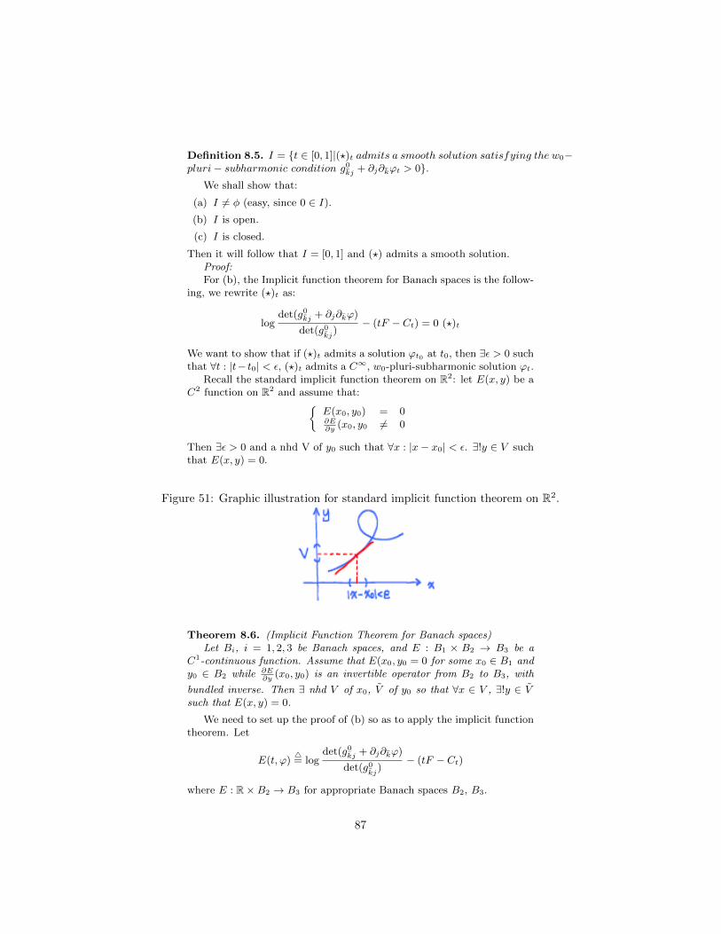
Definition 8.5. I = t ∈ [0, 1]|(?)t admits a smooth solution satisfying the w0−pluri− subharmonic condition g0
kj + ∂j∂kϕt > 0.We shall show that:
(a) I 6= φ (easy, since 0 ∈ I).
(b) I is open.
(c) I is closed.
Then it will follow that I = [0, 1] and (?) admits a smooth solution.Proof:For (b), the Implicit function theorem for Banach spaces is the follow-
ing, we rewrite (?)t as:
logdet(g0
kj + ∂j∂kϕ)
det(g0kj
)− (tF − Ct) = 0 (?)t
We want to show that if (?)t admits a solution ϕt0 at t0, then ∃ε > 0 suchthat ∀t : |t− t0| < ε, (?)t admits a C∞, w0-pluri-subharmonic solution ϕt.
Recall the standard implicit function theorem on R2: let E(x, y) be aC2 function on R2 and assume that:
E(x0, y0) = 0∂E∂y
(x0, y0 6= 0
Then ∃ε > 0 and a nhd V of y0 such that ∀x : |x− x0| < ε. ∃!y ∈ V suchthat E(x, y) = 0.
Figure 51: Graphic illustration for standard implicit function theorem on R2.
Theorem 8.6. (Implicit Function Theorem for Banach spaces)Let Bi, i = 1, 2, 3 be Banach spaces, and E : B1 × B2 → B3 be a
C1-continuous function. Assume that E(x0, y0 = 0 for some x0 ∈ B1 andy0 ∈ B2 while ∂E
∂y(x0, y0) is an invertible operator from B2 to B3, with
bundled inverse. Then ∃ nhd V of x0, V of y0 so that ∀x ∈ V , ∃!y ∈ Vsuch that E(x, y) = 0.
We need to set up the proof of (b) so as to apply the implicit functiontheorem. Let
E(t, ϕ)4= log
det(g0kj + ∂j∂kϕ)
det(g0kj
)− (tF − Ct)
where E : R×B2 → B3 for appropriate Banach spaces B2, B3.
87

Definition 8.7. (Schauder spaces) On Rn, fix 0 < α, 1.
||ϕ||C0,α4= sup |ϕ|+ ϕx 6=y
|ϕ(x)− ϕ(y)||x− y|α
while C0,α(Rn)4= ϕ|||ϕ||C0,α(Rn), ∀|γ| ≤ k.
More generally, we have Ck,α4= ϕ|∂γϕ ∈ C0,α(Rn), ∀|γ| ≤ k. On
a compact manifold, similar spaces Ck,α(X) can be defined via taking apartition of unity.
Next, observe that the solution to (?)t is not unique: ϕt satisfies (?)tand thus ∂t+ is constant. We introduce:
Ck,α0 (X)4= ϕ ∈ Ck,α(X)|
∫x
ϕwn0 = 0
Then we claim that E(t, ϕ) : R× C2,α0 → C0,α
0 . Indeed:∫X
(wn
wn0− etF−Ct)wn0 =
∫X
wn −∫X
etF−Ctwn0 = 0
since Ct is so chosen.
8.3 Verifying the Hypotheses of IFT
Go back to Table of Contents. Please click TOC
Given f : B2 → B3, we say that f is differentiable at y0 ∈ B2 if thereexists a bounded linear map L : B2 → B3 (bounded: ∃C > 0 such that∀y ∈ B2, ||Ly||B3 ≤ C||y||B2) such that
limy→y0
||f(y)− f(y0)− Ly0(y − y0)||B3
||y − y0||B2
= 0
Thus Hom(B2, B3) = bounded linear operations sending B2 into B3is a Banach space, with norm defined by
||T || 4= supy∈B2,y 6=0
||Ty||B3
||y||B2
E ∈ C1(Ω) if y → Ly is defined for all y ∈ Ω and is continuous as amapping Ω→ Hom(B2, B3). Thus now in our case, we want to
(1) E ∈ C1
(2) Compute “ ∂E∂ϕ∈ Hom(C2,α
0 , C0,α0 ) (boundedness)
(3) “ ∂E∂ϕ
” has a bounded inverse.
Computation of “ ∂E∂ϕ
”: by variation: imaging that ϕ→ ϕ+ δϕ.
δ(E) = (det(g0
kj+∂j∂kϕ)
det g0kk
− etF−Ct)= 1
det g0kj
δ(det(g0kj + ∂j∂kϕ))
88

Observe that if G is an invertible matrix:
δ(detG) = ((detG)−1δ(detG)) · detG= δ(ln detG) ·G= Tr(G−1δG) detG
Hence,
δE = 1det(g0
kj)
det(gkjgjkδgkj
= 1det(g0
kj)
det(gkjgjk∂j∂kδϕ
= 1det(g0
kj)
det(gkj4gδϕ
and
L : δϕ→det gkjdet g0
kj
4gδϕ
We have the following claim: Lϕ admits a bounded inverse, i.e. ∀µ ∈C0,α
0 , ∃!v ∈ C2,α0 such that
Lν = µ
Furthermore,||v||C2,α ≤ C||µ||C0,α
for some constant C > 0. This follows from the following.
8.4 Basic Fact From Linear Analysis
Go back to Table of Contents. Please click TOC
Let (X, gij) be any compoact Riemannian manifold, then the equation
4gν = µ
admist a solution if and only if∫X
µ√g = 0
The solution ν is unique if require the normalization condition:∫X
ν√g = 0
Now in our case, Lϕν = µ ⇔ 4gν =wn0wnµ. This is solvable since
µ ∈ C0,α0 , and the solution is unique if we specify∫
X
νwn0 = 0
The similar a priori estimates hold for Schauder spaces, which impliesthe boundedness of the inverse of L (the Green’s operator).
Proof:For (c), I is closed. We want to show that tj ∈ I, tj → T ⇒ T ∈ I,
i.e. ϕtj admits a solution of (?)tj , and tj → T , then ∃ϕ a solution of(?)T satisfying tyhe Monge-Ampere equation and the pluri-subharmonicconditon.
89

To start, we would wish to show that a subsequence, renamed stillby ϕj converges in C3,α (or all Cm,α). If so, and the limit ϕ satisfiesthe M − A equation, we see that the determinant of g0
kj + ∂j∂kϕ fixed
pointwise. If we can further show that the eigenvalues of g0kj + ∂j∂kϕ
is bounded from above, they will also be bounded from below, whenceg0kj + ∂j∂kϕ > 0.
To achieve this, it suffices to show that, ∀m,
||ϕtj ||cm ≤ Am, (AP )m
since ||ϕtj ||C1 + ||ϕtj ||C0 ⇒ ϕtj is equicontinuous. (The standard trickas used in Hodge theory: |ϕti(x)− ϕti(y) ≤ sup || 5 || · |x− y|.) Then byArezela-Ascoli theorem, there would be a convergent subsequence.
References
[1] Ahlfors, Lars, Complex Analysis.
[2] Farkas, Hershel M., and Kra, Iwrin, Riemann Surfaces.
[3] Forster, Otto, Lectures on Riemann Surfaces.
[4] Huybrechts, Daniel, Complex Geometry: An Introduction.
[5] McDonald, John N., and Weiss, Neil A., A Course in Real Analysis.
[6] Miranda, Rick, Algebraic Curves and Riemann Surfaces.
[7] Krantz, Steven G., A Guide to Complex Variables, 2007.
[8] Tsimerman, Jacob, Analytic Theory of Modular Forms, 2012.
[9] V. Villani , Complex Geometry and Analysis.
90