Embed Size (px)
Citation preview
Complex Analysis Oral Exam study notes
Notes transcribed by Mihai Nica
Abstract. These are some study notes that I made while studying for myoral exams on the topic of Complex Analysis. I took these notes from partsof the textbook by Joseph Bak and Donald J. Newman [1] and also a real lifecourse taught by Fengbo Hang in Fall 2012 at Courant. Please be extremelycaution with these notes: they are rough notes and were originally only for meto help me study. They are not complete and likely have errors. I have madethem available to help other students on their oral exams.
Contents
Introductory Stu 61.1. Fundamental Theorem of Algebra 61.2. Power Series 71.3. Fractional Linear Transformations 91.4. Rational Functions 101.5. The Cauchy-Riemann Equations 11
The Complex Numbers 13
Functions of the Complex Variable z 143.6. Analytic Polynomials 143.7. Power Series 143.8. Dierentiability and Uniqueness of Power Series 15
Analytic Functions 164.9. Analyticity and the Cauchy-Riemann Equations 164.10. The functions ez, sin z and cos z 16
Line Integrals and Entire Functions 185.11. Properties of the Line Integral 185.12. The Closed Curve Theorem for Entire Functions 19
Properties of Entire Functions 216.13. The Cauchy Integral Formula and Taylor Expansion for Entire
Functions 216.14. Liouville Theorems and the Fundemental Theorem of Algebra 23
Properties of Analytic Functions 257.15. The Power Series Representation for Functions Analytic in a Disc 257.16. Analytic in an Arbitarty Open Set 267.17. The Uniqueness, Mean-Value and Maximum-Modulus Theorems 26
Further Properties 298.18. The Open Mapping Theorem; Schwarz' Lemma 298.19. The Converse of Cauchy's Theorem: Morera's Theorem; The Schwarz
Reection Principle 30
Simply Connected Domains 329.20. The General Cauchy Closed Curve Theorem 329.21. The Analytic Function log z 32
Isolated Singularities of an Analytic Function 34
3
CONTENTS 4
10.22. Classication of Isolated Singularties; Riemann's Principle and theCasorati-Weirestrass Theorem 34
10.23. Laurent Expansions 35
Introduction to Conformal Mapping 3811.24. Conformal Equivalence 3811.25. Special Mappings 40
The Riemann Mapping Theorem 4112.26. Conformal Mapping and Hydrodynamics 4112.27. The Riemann Mapping Theorem 4112.28. Connection to the Dirichlet problem for the Laplace Eqn 4412.29. Complex Theorems to Memorize 45
Bibliography 46
CONTENTS 5
Bas
ics
of P
ower
Ser
ies
-Rad
ius
of C
onve
rgen
ce-D
iffer
entia
bilit
y-U
niqu
enes
s
Bas
ics
of L
ine
Inte
gral
s-M
-L fo
rmul
a-U
nifo
rm C
onve
rgen
ce-A
nti-d
eriv
ativ
e B
ehav
iour
Rec
tang
le T
hmIn
tegr
al a
roun
d a
rect
angl
e of
a e
ntire
func
tion
vani
shes
Inte
gral
Thm
Eve
ry a
naly
tic fu
nctio
n ha
s an
ant
i-der
ivat
ive
Clo
sed
Cur
ve T
hmIn
tegr
al a
roun
d cl
osed
cu
rve
vani
shes
Rec
tang
le T
hm II
Inte
gral
aro
und
a re
ctan
gle
for t
he "s
ecan
t" fu
nctio
n va
nish
es
Clo
sed
Cur
ve T
hm II
Inte
gral
Thm
II
Cau
chy
Inte
gral
For
mul
aIn
tegr
al a
roun
d a
rect
angl
e of
a
entir
e fu
nctio
n va
nish
es
Inte
gral
of (
z-a)
^-1
= 2
\pi i
Tayl
or S
erie
sE
ntire
func
tions
hav
e co
nver
gent
Tay
lor s
erie
s
Mor
era'
s Th
mIf
inte
gral
van
ishe
s al
ong
rect
angl
es, t
hen
f is
anal
ytic
Mea
n Va
lue
Theo
rem
f is
equa
l to
the
aver
age
of f
in a
circ
le
Max
imum
Mod
ulou
s Th
mf h
as n
o in
terio
r max
ima
Min
imum
Mod
ulou
s Th
mA
ny in
terio
r min
imum
has
|f|
=0
Ope
n M
appi
ng T
heor
emf(O
pen)
is O
pen
Schw
arz
Lem
ma
f <<
1 in
uni
t dis
k m
eans
f<
<z a
nd f'
(0) <
< 1
in d
isc
FLTs
are
Uni
que
D->
D m
ap
Uni
f on
Cpc
t Lim
s ar
e D
ifff n a
naly
tic a
nd f n -
> f
unifo
rmly
on
com
pact
set
s,
then
f an
alyt
ic
Ana
lytic
eve
ryw
here
exc
ept
a lin
e +
Con
tinuo
us =
> A
naly
tic E
very
whe
re
Schw
arz
Ref
lect
ion
Prin
cip
f rea
l on
real
axi
s ca
n be
ex
tend
ed b
y \b
ar f
\ba
r z
Introductory Stu
From real life course by Fengbo Hang.
1.1. Fundamental Theorem of Algebra
We can motivate the study of complex analysis by the fundamental theorem ofalgebra. This theorem says that, unlike real numbers, every n−th degree complexvalued polynomial has n roots. Already this shows us that some things are muchnicer in complex numbers than real numbers. Let us begin by dening the complexnumbers as a 2-d vector space over R:
Definition. Let i so that i2 = −1 and dene C = a+ ib : a, b ∈ C. This isa vector space over R with basis 1, i. We also equip ourselves with the natural
norm, |a+ ib| =√a2 + b2.
Remark. To really be precise, one can check that the set of matrices
[a −bb a
]is a commutative 2-dimensional eld and make the identication 1 ↔ Id and
i ↔[
0 −11 0
]to precisely dene the complex numbers. Notice that this ma-
trix arises as the matrix for the operator φz : C → C by φz(w) = zw. When
z = a+ ib, the matrix for φz in the basis 1, i is precisely[a −bb a
].
Lemma. Let p(z) =∑nk=0 akz
k be any polynomial of degree n ≥ 1. Then p(z)has at least one root in C.
Proof. Suppose by contradiction p has no zeros. Let z0 ∈ C be such that|p(z0)| > 0 is minimal. By translating, we may suppose without loss of generalitythat z0 = 0. We have then the expression for p:
p(z) = a0 + amzm +O(zm+1)
= a0
(1 +
ama0zm +O(zm+1)
)Write am
a0= Reiφ in polar notation, and then for a parameter t > 0, plugin z? =
teiπ−φm to get:
|p(z?)| =
∣∣∣∣a0
(1 +
ama0zm +O(zm+1)
)∣∣∣∣= |a0|
(∣∣1 +Reφtmeπ−φ∣∣+O(tm+1)
)= |a0|
(1−Rtm +O(tm+1)
)But if we take t suciently small, we will get |p(z?)| < |a0| = |p(0)| which
contradicts the fact that z = 0 has minimal modulus.
6
1.2. POWER SERIES 7
Lemma. Let p(z) =∑nk=0 akz
k be any polynomial. Then p has n complexroots.
Proof. (By induction on n) The base case n = 1 is clear. The above lemma,along with the factoring algorithm to factor out roots reduces the degree by one.
1.2. Power Series
Definition. A power series is a function f : Ω→ C where Ω ⊂ C is a functiondened as an innite sum:
f(z) =
∞∑n=0
an(z − z0)n
Remark. The disadvantage of power series is that, because of the way they aredened, there can be problems with convergence of the innite sum. For examplethe function 1
1−z is dened when z 6= 1 but it happens that 11−z =
∑zn for |z| < 1.
Definition. We say that a function f : Ω→ C is C−dierentiable at a pointz if the following limit exists:
f ′ (z) = limh→0
f(z + h)− f(z)
h
Here h is a complex number, and the limit is to be interpreted with the topologyon C induced by the norm |·|. (This is the same topology as on R2)
Remark. It turns out that C−dierentiable functions and power series areactually the same! We will see what this is later.
Example. The usual tricks for dierentiation in R will work for C too. Forexample, all polynomials are dierentiable, and one can prove the quotient ruleworks too, so that rational functions are dierentiable too. The following specialclass of rational functions will be of interest to us, so we dene it below:
Definition. A fractional linear transformation is a rational function of theform:
f(z) =az + b
cz + d
Where
∣∣∣∣ a bc d
∣∣∣∣ 6= 0.
We will now prove some results about power series.
Lemma. Let f(z) =∑cnz
n be a power series and suppose that z1 ∈ C is sothat the power series converges at z1 (i.e. f(z1) ∈ C makes sense). Then f(z) isabsolutely convergent for all z with |z| < |z1|.
Proof. The proof is a simple comparison to a geometric series. Since f(z1) isconvergent, we know that |cnzn1 | → 0 as n→∞. In particular, this sequence mustbe bounded then, i.e. we have a constant C so that |cnzn1 | < C. But then |cnzn| <C∣∣∣ zz1 ∣∣∣n and the convergence follows by comparison to a geometric series.
Corollary. For f(z) =∑cnz
n, there exists an R ∈ R so that f(z) is abso-lutely convergent for all z with |z| < R and divergent for all z with |z| > R.
1.2. POWER SERIES 8
Proof. Just let R = sup |z| : f(z) is convergentand the result follows fromthe above lemma.
Definition. The R above is often called the radius of convergence.
Corollary. Power series are continuous inside their radius of convergence.
Proof. Recall the Weirstrass M-Test says if |fn(x)| < Mn and if∑Mn <∞,
then∑fn(x) is converging uniformly. Using this convergence test, along with the
fact that a uniform limit of continuous functions is continuous we get the result.
Theorem. [Power series are dierentiable] For a power series f(z) =∑cnz
n,we have that f is dierentiable with:
f ′(z) =∑
ncnzn−1
Proof. We introduce the notation: fn(z) =∑nk=1 ckz
k, gn(z) =∑nk=1 kckz
k,and g(z) =
∑∞k=1 kckz
k−1. The problem becomes showing that f is dierentiableand f ′ = g. We rst remark that g has the same (or larger) radius of convergenceas f , indeed following the idea of the lemma 1.2.7 above, let f(z1) be convergent
we get the comparison that |kckzk−1| ≤ Ck∣∣∣ zz1 ∣∣∣k−1
, so the series for g(z) converges
by comparison to an arithmetico-geometric sequence whenever |z| < |z1|. Next,using the Weirestrass M-Test in a similar fashion to Corollary 1.2.10, we knowthat fn converges uniformly to f and gn converges uniformly to g inside the radiusof convergence. Now, using the Fundemental Theorem of Calculus applied to thePolynomials fnand gnwe have for any h that:
fn(z + h)− fn(z) =
ˆ 1
0
gn(z + th)dt
Now, by our uniform convergence, we can take the limit n → ∞ to establishthat:
f(z + h)− f(z) =
ˆ 1
0
g(z + th)dt
Since this holds for any h, we can now divide by h and take the limit h → 0.
Noticing that limh→0 h−1´ 1
0g(z + th)dt = g(z) by the mean value theorem gives
the result.
Definition. A Laurent series is a two-sided power series of the form f(z) =∑n cnz
n +∑n c−nz
−n.
Remark. One can see that Laurent series convergence inside an annulus (i.e.a donut) because the rst sum convergences inside a circle of radius R1 while thesecond will converge outside a circle of radius R2 (since
∣∣z−1∣∣ < R ⇐⇒ |z| > R−1).
Example. A branch of the logarithm is another example of a dierentiablefunction. This can be dened by removing a ray from Cso that we can have inpolar coordinates that −π < θ < π and then dene log
(reiθ
)= log r + iθ.One can
verify (using a change of variables to polar coordinates) that ddz log z = 1
z .
1.3. FRACTIONAL LINEAR TRANSFORMATIONS 9
1.3. Fractional Linear Transformations
Recall that a fractional linear transformation is one of the form φ(z) = az+bcz+d
where
∣∣∣∣ a bc d
∣∣∣∣ 6= 0. The relationship between fractional linear transformations
and matrices is made by viewing C in so called homogenous coordinates.
Definition. Consider C×C with the equivalence relationship z1× z2 ∼ w1×w2 ⇐⇒ ∃λ ∈ C : w1 = λz1, w2 = λz2 . It is an easy exercise to verify thatthe extended complex plane C = C ∪ ∞ can be written in these coordinates,
namely:C ∼= C×C/∼ with the identiction
[z1
z2
]:= z1
z2. These coordinates are
called homogenous coordinates
Remark. These coordinates show exactly how fractional linear transforma-
tions behaive like matrices, for if w =
[z1
z2
], then:
aw + b
cw + d=
[a bc d
] [z1
z2
]From this, we can easily see the rules for how fractional linear transformations
compose/invert etc. i.e. if A =
[a bc d
]and φA(z) = az+b
cz+d then φA φB = φAB
etc. We can also see, since we are only looking at invertible matrices, that thesemaps are bijections from C to itself.
Proposition. Let φA be a fractional linear transformtion. Then φA(z) = zhas at most two solutions, unless A = Id.
Proof. Write out φA(z) = az+bcz+d , so that φA(z) = z gives (cz + d)z = az + b.
This is a quadratic equation! If c 6= 0 then it is non-degenerate and the quadraticformula gives exactly two solutions. If c = 0 then it is really a linear transformation,and there are NO solutions unless.
Proposition. Fractional linear transformations are uniquely specied by theaction on 3 points.
Proof. Suppose M,N are two fractional linear transformations that haveM(zi) = wi for i = 1, 2, 3. Then M N−1 is a fractional linear transformationwith 3 xed points. By the above proposition, M N−1 must be the identity!Hence M = N . This shows uniqueness. The existence of such a map is easy-ily veried by expicitly writing down the map that sends z1 → 0, z1 → 1, andz3 →∞:
φ(z) =z−z2z−z3/
z1−z2z1−z3
Proposition. The image of any circle or line in the complex plane through afractional linear transformations is again a circle or line.
Proof. It suces to verify that inversion z → 1z has this property, as every
FLT can be written as a composition of dilation z → az, translation z → z+ b andinversion, and the rst two clearly preserve circles and lines. This can be verieddirectly with a not-so-dicult analytic computation, or can be seen by looking at
1.4. RATIONAL FUNCTIONS 10
the stereographic projection. z → 1z is circle inversion, which is a reection of the
sphere through the plane, while z → z is a reection of the sphere through thevericle plane passing through the real axis. Hence z → 1
z is the composition ofthese two operations, and can be done in one shot as a rotation of the sphere!
Remark. Fractional linear transformations also preserve symmetric points.This can be veried analytically.
Example. Find the fractional linear transformation that takes the point z0 inthe unit disk D to the origin, and also takes the unit disk to the unit disk.
Proof. Firstly, we see why such an FLT must exist. One way is to map theunit disk to the upper half plane (take any three points on the boundary to 0,1,∞to do this). Then z0 will be some point in the upper half plane. From here we cantake z0to i with a dilation and a translation, this will also ensure that the points ofthe upper half plane don't change. Finally, we map back to the unit disk in such away so that i goes to the origin.
To nd the solution, we want φ with z0 → 0 . Since FLTs preserve symetricpoints we must have 1
z0→∞ too. This suggests a FLT of the form:
φ(z) = Cz − z0
z − 1z0
To ensure this keeps the unit disk in place, we impost that |φ(1)| = 1 and get
the condition |C| =∣∣∣∣ 1− 1
z0
1−z0
∣∣∣∣ so the most general solution is:
φ(z) = eiθ
∣∣∣∣∣1−1z0
1− z0
∣∣∣∣∣ z − z0
z − 1z0
Notice there is one parameter of freedom here! We have specied the image oftwo points (z0,
1z0) and we know there is a one parameter family for the image of
the point 1 (has to be on the unit circle). Hence, since 3 points uniquely determinea FLT, there is a one parameter family of FLTs here.
Definition. The cross-ratio of four points (z1, z2, z3, z4) is dened by:
(z1, z2, z3, z4) =z1−z3z1−z4/
z2−z3z2−z4
Alternatively, it is the image of z1 in the unique FLT that takes z2 → 1, z3 → 0and z4 →∞.
Proposition. For an FLT φwe have that (z1, z2, z3, z4) = (φz1, φz2, φz3, φz4).
Proof. Can be checked directly. Alternatively, let ψz2,z3,z4 be the unique FLTthat takes z2 → 1, z3 → 0, z4 →∞. Then check that ψz2,z3,z4(z) = ψφz2,φz3,φz4(φz)since both have the property that z2 → 1, z3 → 0, z4 →∞. Now the result followsby the alternative denition of the cross-ratio: the cross ration is the image of z1
through this map.
1.4. Rational Functions
A rational function is a function of the form R(z) = P (z)Q(z) with P,Q polynomials.
For convenience, we will label the roots of Q by β1 . . . βn. By the quotient rule, onecan see that R is holomorphic on C\β1, . . . , βn. Notice that limz→βj R(z) = ∞
1.5. THE CAUCHY-RIEMANN EQUATIONS 11
. We call such points poles of the function. The following theorem is a usefuldecompostion for rational functions:
Theorem. Suppose that R(z) = P (z)Q(z) is a rational function with poles β1 . . . βn.
By using the division algorithm, we can write R(z) = G(z) +H(z) where G(z) is apolynomial without a constant term, and H(z) is a rational function with the degreeof the numerator not more than the degree of the denominator. In the same vein, wecan consider the rational function R(βj + 1
ζ ) and write R(βj + 1ζ ) = Gj(ζ) +Hj(ζ),
where Gj and Hj are akin to G,H respectively. Then we have:
R(z) = G(z) +
n∑j=1
Gj
(1
z − βj
)Proof. Doing a change of variable z = βj + 1
ζ on R(βj + 1ζ ) = Gj(ζ) +Hj(ζ),
we have R(z) = Gj
(1
z−βj
)+Hj
(1
z−βj
). Since Gj is a polynomial, Gj
(1
z−βj
)is a
rational function and it can only have a pole at z = βj . Notice also that Hj
(1
z−βj
)is nite at z = βj , because z = βj corresponds to ζ = ∞, and since Hj (ζ) is arational function with the degree of the denominator ≥degree of numerator, thelimit ζ →∞ is nite.
Now consider the expression:
R(z)−
G(z) +
n∑j=1
Gj
(1
z − βj
)This is a sum of rational functions, and it can only possibly have poles at
z = β1, . . . , βn. For a xed j, the only terms with poles at z = βj are R(z)
and Gj
(1
z−βj
). However, since R(z) − Gj
(1
z−βj
)= Hj
(1
z−βj
), and since
limz→βj Hj
(1
z−βj
)is nite, there is in fact NO pole at z = βj . That is to
say limz→βj R(z) −(G(z) +
∑nj=1Gj
(1
z−βj
))= G(βj) +
∑k 6=j Gk
(1
βj−βk
)+
limz→βj Hj
(1
z−βj
)is nite. Since this works for every choice of j, we see that
this expression is a rational function with no poles at all. But the only such ratio-nal function is a constant. Absorbing the constant into G(z) gives the result.
1.5. The Cauchy-Riemann Equations
Suppose that f : Ω → Ω is holomorphic. We can think of f as a functionf : R2 → C by the identication f(x, y) = f(x+ iy). Notice that:
∂f
∂x= limδ→0
f((x+ δ) + iy)− f(x+ iy)
δ= f ′(z)
The x−derivative is the directional derivative in the complex plane in the real-axis-direction! Similarly:
∂f
∂y= lim
δ→0
f(x+ i(y + δ))− f(x+ iy)
δ
= limδ→0
if(x+ iy + iδ)− f(x+ iy)
iδ= if ′(z)
1.5. THE CAUCHY-RIEMANN EQUATIONS 12
Hence it must be the case that fy = ifx! This is known as the Cauchy-Riemannequation. If we write the real and imaginary part of f separately, say f(z) =u(z)+iv(z) so that in our identication z = x+iy we have f(x, y) = u(x, y)+iv(x, y)then by matching the real and imaginary parts the C-R equation is saying that:
ux = vy
uy = −vxConversely, if we have a function f : R2 → R2 which is R2−dierentiable, and
f satises the Cauchy Riemmann equations above, then one can show that f isindeed a holomorphic function. To see this, we suppose without loss of generalityby translations that f(0) = 0 and that we have only to prove dierentialbilityat 0. By Taylors theorem, we know that in a n'h'd of 0 we can write f(x, y) =u(x, y) + iv(x, y) = ax + by + η(z)z with η(z) → 0 as z → 0 and a = fx, b = fy.Rewriting, this is:
f(z) = ax+ by + η(z)z
=a+ ib
2z +
a− ib2
z + η(z)z
But, the C-R equations are exactly saying that a − ib = 0, so the z termvanishes, and we get:
f(z)
z=a+ ib
2+ η(z)
Since the limit exists as z → 0, we see that f is indeed dierentiable here.Notice that if f = u + iv satises the C-R equations, then ∆u = uxx + uyy = 0and ∆v = 0 (this is immediate by equality of mixed partials when the functionis twice dierentiable; we will see later that all holomorphic functions are twicedierentiable!) The converse is also true, given u with ∆u = 0, there exists aholomorphic function f so that f = u+iv. This boils down to an existence theoremfor PDE;s in practice.
The Complex Numbers
These are notes from Chapter 1 of [1]. Basic properties of complex numbersand so on go here.
Definition. An open connected set is called a region. All regions are polygonallyconnected, which means that there is a path from one point to any other pointwhich consists of a nite number of lines. Every region is polygonally connected;let U = points reachable by a polygonal line and since the unit ball is polygonallyconnected, U is open. Similarly, the set S\U is open. By connectedness, U = S.
Theorem. (1.9) (M-test) Suppose fk is continuous in D, if |fk(z)| ≤ Mk
throughout D and if∑∞k=1Mk < ∞ then
∑∞k=1 fk(z) converges (uniformly) to a
function f which is continuous in D.
Proof. It is clear that at each point, |∑∞k=1 fk(z)| ≤
∑∞k=1Mk <∞ so we can
dene its pointwise limit f . Moreover, the convergence is uniform, because for any
ε > 0 choose N so large so that∑∞k=N Mk < ε and we will have
∣∣∣f −∑k≥N fk
∣∣∣ < ε.
A uniform limit of continuous functions is continuous by a classic ε/3 argument:
Given ε > 0 choose N so large so that∣∣∣f −∑k≥N fk
∣∣∣ < ε/3 and then choose δ for
ε/3-continuity of fN and have |f(x)− f(y)| ≤ |f(x)− fN (x)|+ |fN (x)− fN (y)|+|fN (y)− f(y)| < ε/3 + ε/3 + ε/3.
Theorem. (1.10) Suppose u(x, y) has partial derivatives uxand uy that vanishat every point in a region D. Then u is constant on D.
Proof. Let (x1, y1) and (x2, y2) be any two points in D. They are connectedby a polygonal path. On each segment of the polygonal path, we have u(y)−u(x) =´v · u(z)dz = 0 for some direction v. Hence u is constant on each segment.
(Section on stereographic projection here)
Definition. (1.11) We say zk →∞ if |zk| → ∞.
Proposition. Stereographic projection takes circles/lines to circles/lines
13
Functions of the Complex Variable z
These are notes from Chapter 2 of [1].
3.6. Analytic Polynomials
Definition. A polynomial P (x, y) is called analytic polynomial if thereexists complex constants αk such that:
P (x, y) =∑
αk (x+ iy)k
Notice that most polynomials of two variables are NOT analytic, only veryspecial ones are.
Proposition. A polynomial is analytic if and only if Py = iPx
Proof. (⇒) is clear, since it holds for each term (x+ iy)k individually.(⇐) We will show this folds for any polynomial where the degree of any term
is n (i.e. the degree of the x power plus the degree of the y power) by linearitythis it will then hold for all polynomials. Suppose Qy = iQx. then write outQ =
∑Ckx
n−kyk. Qy = iQx gives us a linear system of equations, which can besolved one at a time inorder and leads to Ck = ik
(nk
)C0. But then Q = C0(x+ iy)n
by the binomial theorem.
Remark. fy = ifx as complex variables is the same as :
ux = vy
uy = −vxWhere u = Ref and v = Imf . These are called the Cauchy Riemann
Equations
Definition. A complex valued fuction is called dierentiable at z if:
limh→0
f(z + h)− f(z)
h
exist. Here we mean h→ 0 w.r.t. the topology on R2. The sum rule, productrule, and quotient rule all work for dierentiable functions.
3.7. Power Series
Definition. A power series in z is an innite series of the form∑∞k=0 Ckz
k
Theorem. (2.8.) Suppose that lim sup |Ck|1/k = L then:i) If L = 0 then
∑Ckz
k converges for all zii) If L =∞ then
∑Ckz
k converges for z = 0 onlyiii) If 0 < L <∞ then let R = 1
L and we will have that∑Ckz
k converges for|z| < R and diverges for |z| > R.
14
3.8. DIFFERENTIABILITY AND UNIQUENESS OF POWER SERIES 15
R here is called the radius of convergence of the power series.
Proof. All the proofs go by comparison to the geometric power series and thedenition of limsup.
3.8. Dierentiability and Uniqueness of Power Series
Theorem. (2.9.) If f(z) =∑Cnz
n converges for |z| < R then f ′(z) existsand equals
∑nCnz
n−1 throughout |z| < R
Proof. (Can do this by hand by looking at (z+h)n−znh , here is a slicker way)
First see that the sequence g(z) =∑nCnz
n−1 has the same radius of convergence.Then let fn =
∑nk=1 Ckz
k and gn =∑nk=1 kCkz
k−1 Now fn → f and gn → guniformly on compact subsets inside the radius of convergence. Notice that for
every gn = f ′n and so we have for any h that fn(z+h)−fn(z)h =
´ 1
0gn(z+ht)dt (think
of this as a real integral by looking at the imaginary and real parts seperatly) Sincefn → f uniformly and gn → g uniformly, have the same holding for f and g. Butthen taking h→ 0 (use LDCT) we get that f ′ = g as desired.
Corollary. Power series are innetly dierentiable within their domain ofconvergence
Corollary. If f(z) =∑∞n=0 Cnz
n has a non-zero radius of convergence then:
Cn =f (n)(0)
n!for all n
Theorem. (Uniqueness Theorem for Power Series)Suppose
∑Cnz
n vanishes for all points of a non-zero sequence zk and zk → 0as k →∞. Then
∑Cnz
n ≡ 0
Proof. Have C0 = limk→∞ f(zk) = 0. Now let f1(z) = f(z)/z, since C0 = 0f1 =
∑k≥1 Ckz
k. Since zk 6= 0 for all k and f(zk) = 0 we have that f1(zk) = 0
for every k too, now C1 = limk→∞ f1(zk) = 0 too! Repeating this argument showsthat every coecient is zero.
Corollary. If a power series equals zero at all the points of a set with anaccumulation point at the origin, the power series is identically zero.
Analytic Functions
These are notes from Chapter 3 of [1].
4.9. Analyticity and the Cauchy-Riemann Equations
Proposition. (3.1) If f is dierentiable then fy = ifx.
Proof. fx = limh→0∆fh for h real while
fyi = limh→0
∆fh for h imaginary.
Since the limit exists, these are equal.
Proposition. (3.2.) If fx and fy eixsts in a n'h'd and if fx and fy are con-tinuous at z and fy = ifx there, then f is dierentiable at z.
Proof. Can show that limh→0∆fh = fx by using the mean value theorem to
nd, for any h, a real number 0 < a < Re(h) and 0 < b < Im(h) so that
f(x+ h)− f(x) = f(x+ h)− f(x+ Re(h)) + f(x+ Re(h))− f(x)
= fy(x+ Re(h) + ib)Im(h) + fx(x+ a)Re(h)
Now we are almost done, since we see that by continuiy of fx and fy the RHS,loosely speaking, looks like fy(x)Im(h) + fx(x)Re(h) = fx(x) (iIm(h) + Re(h)) =hfx(x) and this will prove the result. This can be made more precise, but I'll stophere.
Definition. We say f is analytic at z if it is dierntiable in a n'h'd of z andanalytic in a set if it is dierntiable in that set.
Proposition. (3.6) If f = u+ iv and u is constant in some region, then f isconstant in that region too.
Proof. Since u is constant, ux = uy = 0 so by the C-R equations, vx = vy ≡ 0in the region too. Now by the mean value theorem, both u and v are constant.
Proposition. (3.7) If |f | is constant in a region then f is constant in theregion
Proof. Write out u2 + v2 = |f |2 = cons; t so taking partials and mixing themup a bit using the C.R. equations leads us to the result.
4.10. The functions ez, sin z and cos z
We wish to nd an analytic function f(z) so that:
f(z1 + z2) = f(z1)f(z2)
f(x) = ex for all real x
16
4.10. THE FUNCTIONS ez , sin z AND cos z 17
By putting in z1 = x and z2 = iy we arrive at:
f(x+ iy) = exA(y) + iexB(y)
where A,B are real valued. By the Cauchy Riemann equations, it must be thatA(y) = B′(y) and A
′(y) = −B(y) from these dierential equations, we nd that A
and B have to linear combinations of sin and cos. But since f(x) = ex is enforced,we get A = cos and B = sin so nally we have:
f(z) = ex cos(y) + iex sin(y)
Then dene:
sin(z) =1
2i
(eiz − e−iz
)cos(z) =
1
2
(eiz + e−iz
)
Line Integrals and Entire Functions
These are notes from Chapter 4 of [1].
5.11. Properties of the Line Integral
Definition. (4.1.) For any curve C parametrized by z(t) we dene:ˆC
f(z)dz =
ˆ b
a
f(z(t))z(t)dt
By the change of variable rule (i.e. in R2) this is invarient under the parametriza-tion of C (expcept for chaning direction)
.... I skip some stu about this here....
Lemma. (4.9.) ∣∣∣∣∣ˆ b
a
G(t)dt
∣∣∣∣∣ ≤ˆ b
a
|G(t)| dt
Proof. Write´G(t)dt = Reiθ for some R and θ, then multiply out by e−iθ ,
take Re part, and use the inequality Re(z) ≤ |z|.
Proposition. (4.10) (The M-L formula)Suppose that C is a smooth curve of length L and f is continuous on C and
that |f | ≤M trhoughout C then:∣∣∣∣ˆC
f(z)dz
∣∣∣∣ ≤ML
Proof. By the previous lemma,∣∣´Cf(z)dz
∣∣ ≤ ´ ba|f(z(t))| |z(t)| dt If you as-
sume a unit speed parametrization here you can nish the result, otherwise you can
use the mean value theorem for integrals to get that this = |f(z(t0))|´ ba|z(t)| dt for
some t0 and then get the result from´|z(t)| dt = L.
Proposition. (4.11) If fn are continuous and fn → f uniformly on C then:ˆC
f(z)dz = limn→∞
ˆC
fn(z)dz
Proof. Take n so large so that |f − fn| < ε everyewher on C and then applythe ML theorem to get that the integrals are no more than ε·length of C appart.
Proposition. (4.12) If f(z) = F ′(z) then:ˆC
f(z)dz = F (z(b))− F (z(a))
18
5.12. THE CLOSED CURVE THEOREM FOR ENTIRE FUNCTIONS 19
Proof. Take any parametrization z for the curve C and let γ(t) = F (z(t))with a bit of work, we can show that γ(t) = f(z(t))z(t) then will have:ˆ
C
f(z)dz =
ˆf(z(t))z(t)
=
ˆγ(t)dt
= γ(b)− γ(a)
= F (z(b))− F (z(a))
5.12. The Closed Curve Theorem for Entire Functions
5.12.1. Important!
Definition. (4.13) A curve C is closed if its intial and terminal poitns coin-cide.
Theorem. (4.14) (The Rectangle Thereom)Suppose f is entire and Γ is the boundary of a rectangle R. Then:ˆ
Γ
f(z)dz = 0
Proof. Suppose´
Γf(z)dz = I. The proof goes by subdividing into smaller
and smaller rectangles so that´Rkf(z)dz I
4k. These rectangles converge to a
point z0 around which we have the estimate f(z) = f(z0)+(z−z0)f ′(z0)+εz(z−z0)with εz → 0 as z → z0. The linear term f(z0) + (z − z0)f ′(z0) integrates tozero around a rectangle. For any ε > 0, choose a rectangle Rk small enough sothat εz ε for all z on the rectangles, then use the M-L to control the size of´R(k)
f(z) ε c4k
. Combining the upper and lower bound on Rk gives that I cε
and since this works for every ε > 0 we conclude that I = 0.
Theorem. (4.15) (Integral Theorem)If f is entire, then f is everywhere the derivative of an analytic function. That
is there exists an entrie function F so that F ′(z) = f(z)
Proof. Dene F (z) as´
[0,Rez]+[Rez,z]f(ζ)dζ. Since the integral around a rec-
tangle is zero, we get that F (z + h) − F (z) =´
[z,z+Reh]+[z+Reh,z+h]f(ζ)dζ and
hence F (z+h)−F (z)h − f(z) =
´ z+hz
(f(ζ)− f(z)) dζ → 0 as h → 0 by the M − Ltheorem since f is continuous here.
Theorem. (4.16.) (Closed Curve Theorem)If f is entire and if C is a closed curve then:ˆ
C
f(z)dz = 0
Proof. Write f(z) = F ′(z) for some analytic F . Then´Cf(z)dz = F (z(b))−
F (z(a)) = 0 since C is a closed curve.
5.12. THE CLOSED CURVE THEOREM FOR ENTIRE FUNCTIONS 20
Remark. The closed curve theorem works as long as f = F ′ for some anayticF . The integral theorem tells us that every analytic function is of this form, butthere are additionally some other non-analytic functions that are of this form. For
example z−2 is not anayltic at 0, but it has z−2 =(−z−1
)′on the curve C so the
integral would still be zero.
Theorem. (Morera's Theorem)(This comes later in the book and uses the fact that analytic functions are
innetly dierentiable...but I will put it here too)If f is continuous on an open set D and if
´Γf(z)dz = 0 for every rectangle Γ,
then f is analytic on D
Proof. Write F (z) =´
[0,Rez]+[Rez,z]f(ζ)dζ. As in the proof of the Integral
theorem, (using the hypotheiss that´
Γf(z)dz = 0 for rectangles) we have that
F ′(z) = f(z). Now, since F is analytic it is twice dierentiable (this fact will beproven later...can be thought of as a consequence of Cauchy integral formula), sof ′(z) = F ′′(z) is once dierentiable.
Properties of Entire Functions
These are notes from Chapter 5 of [1].
6.13. The Cauchy Integral Formula and Taylor Expansion for EntireFunctions
6.13.1. Important! A common technique/tool in complex analysis is to startwith a function f and dene a function g by:
g(z) =
f(z)−f(a)
z−a z 6= a
f ′(a) z = a
We will show that the rectangle theorem still applies to g.
Theorem. (5.1.) (Rectangle Theorem II)g dened as above has
´Γg(ζ)dζ = 0 for all rectangle Γ.
Proof. We consider three cases:i) If a ∈ ext R. In this case, by the quotient rule, g is analytic trhoughout the
rectangle so the proof is exactly the same as in the proof of the rectangle theorem.ii) If a ∈ Γ or ∈ int R. Divide up the rectangle into smaller rectangles so that
the point a is isolated to a very small rectangle. On the rectangles that don't toucha, we are reduced to case i. For the rectangle that touches a, use the ML theorem(g is continuous and hence bounded by some M on the rectangle) to see that theintegral → 0 as the size of the rectangle shrinks.
Corollary. The integral theorem and the closed curve theorem both apply tog.
Proof. g is continuous and has the rectangle theorem, so the proofs go as theydid before.
Theorem. (5.3.) (Cauchy Integral Formula)If f is entire and a is a xed complex number and C is a circle centered at the
origin a (i.e. R > |a|) then:
f(a) =1
2πi
ˆC
f(z)
z − adz
Proof. By the closed curve theorem for g we have that:ˆC
f(z)− f(a)
z − adz = 0
Rearranging and using that´
dzz−a = 2πi gives the result (pf of this is in the
next lemma).
21
6.13. THE CAUCHY INTEGRAL FORMULA AND TAYLOR EXPANSION FOR ENTIRE FUNCTIONS22
Lemma. (5.4.) If a circle Cρof radius ρ centered at α contains the point athen: ˆ
Cρ
dz
z − a= 2πi
Proof. Check by bare hands denition using the parametrization ρeiθ + αthat: ˆ
Cρ
dz
z − α= 2πi
Now for any k we see that:ˆCρ
dz
(z − α)k+1= 0
This can be seen in two dierent ways:i) bare hands again (works out to the same calculation as before)ii) by the remark to the integral formula, its ok because (z − α)−(k+1) is an
antiderivative on C.Now with these two facts in hand, we do an expansion:
1
z − a=
1
(z − α) + (α− a)
=1
z − α1
1− a−αz−α
=1
z − α
(1 +
a− αz − α
+
(a− αz − α
)2
+ . . .
)
The sum converges uniformly inside the circle because |a− α| < |z − α| = Ron the conotur in question. Have then:
ˆCρ
1
z − adz =
ˆ1
z − αdz + (a− α)
ˆCρ
1
(z − α)2dz + . . .
= 2πi+ 0 + 0 + . . .
The interchange of integral with the innite sum is ok because the sum convergesuniformly.
Theorem. (5.5.) (Taylor Expansion of an Entire Function)If f is entire, it has a power series representation. In fact f (k)(0) exists for all
k and:
f(z) =
∞∑k=0
f (k)(0)
k!zk
Proof. By the Cauchy integral formula, we can choose a circle C containingthe point z and then have:
f(z) =1
2πi
ˆC
f(w)
w − zdw
6.14. LIOUVILLE THEOREMS AND THE FUNDEMENTAL THEOREM OF ALGEBRA 23
Now we can do the following expansion for 1w−z :
1
w − z=
1
w
1
1− zw
=1
w
(1 +
z
w+( zw
)2
+ . . .
)We know that this converges uniformly inside the circle since |z| < |w| = R on
the contour in question. Have then:
f(z) =
(1
2πi
ˆC
f(w)
wdw
)+
(1
2πi
ˆC
f(w)
w2dw
)z +
(1
2πi
ˆC
f(w)
w3dw
)z2 + . . .
The switch of the integral and the innte sum is ok becasue the sum convergesuniformly here.
This shows that f(z) is equal to (in the circle we chose at least) an innte power
series. By our study of power series, we know then that(
12πi
´Cf(w)w2 dw
)= f(k)(0)
k!
and this completes the proof.
Corollary. (5.6.) An entire function is innitely dierentiable.
Proof. We saw that power series are intetly dierentiable, the above showsthat every entire function is a power series.
Proposition. (5.8) If f is entire and we dene g(z) = f(z)−f(z)z−a for z 6= a
and f ′(a) for z = a then g is entire.
Proof. Let h(z) = f′(a) + f ′′(a)
2! (z − a) + . . .. By the Taylor series expansionfor f when z 6= a we see that g = h. We also notice that h(a) = g(a) = f ′(a).Hence g ≡ h. Since g is a power series, it is entire.
Corollary. (5.9.) If f is entire with zeros at a1, a2, . . . then we may dene:
g(z) =f(z)
(z − a1) . . . (z − an)for z 6= aj
and dened by g(ak) = limz→ak g(z) when these limits exists. Then g is entire.
Proof. Induction using the last proposition.
6.14. Liouville Theorems and the Fundemental Theorem of Algebra
Theorem. (5.10) (Liouville's Theorem)A bounded entire function is constant
Proof. (The idea is to get the value of the function from the Cauchy integralformula. If the function is bounded we have a bound on the integral from the MLtheorem)
6.14. LIOUVILLE THEOREMS AND THE FUNDEMENTAL THEOREM OF ALGEBRA 24
Take any two points a and b and then take a circle of radius R centerd at theorigin and large enough to contain both points. Then have the by the CIF that:
f(b)− f(a) =1
2πi
ˆC
f(z)
z − bdz − 1
2πi
ˆf(z)
z − adz
=1
2πi
ˆC
f(z)(b− a)
(z − a)(z − b)dz
M |b− a|R(R− |a|) (R− |b|)
→ 0
as R→∞. Hence f(b) = f(a)
Theorem. (5.11) (Extended Liouville Theorem)
If f is entire and |f(z)| ≤ A+B |z|k then f is a polynomial of degree at mostk.
Proof. There are two proofs(1) By induction using g(z) = (f(z)− f(0)) /z which eectivly reduces the
value of k by one.(2) Use the extended Cauchy Integral formula that we found earlier that:
f (k)(z) =k!
2πi
ˆC
f(w)
wkdw
and then do the same type of argument as from the ordinarty Louiville theorem.
Theorem. (5.12) (Fundemental Theorem of Algebra)Every non-constant (with complex valued coecients) polynomial has a zero in
C
Proof. Otherwise 1/P (z) is an entire function, and it is bounded since |P (z)| →∞ as |z| → ∞ (highest order term dominates eventaully). By Louivlle's thm,1/P (z) must be constant, a contradiciton.
Properties of Analytic Functions
These are notes from Chapter 6 of [1].We will now look at functions which are not entire, but instead are only analytic
in some region.
7.15. The Power Series Representation for Functions Analytic in a Disc
Theorem. (6.1.) Supposef is analytic in D = D(α; r). If the closed rectanlgeR and the point a are both contined in D and Γ is the boundary of R then:ˆ
Γ
f(z)dz =
ˆΓ
f(z)− f(a)
z − adz = 0
Proof. Same idea as for entire functions.
Definition. From now on we write g(z) = f(z)−f(a)z−a to mean this when z 6= a
and its limit limz→a when z = a.
Theorem. (6.2.) If f is analytic in D(α; r) and a ∈ D(α; r) then there existfunctions F and G anayltic in D such that:
F ′(z) = f(z), G′(z) =f(z)− f(a)
z − aProof. Same idea as for entire functions.
Theorem. (6.3.) If f and a are as above, and C is any smooth closed curvecontained in D(α; r) then:ˆ
C
f(z)dz =
ˆC
f(z)− f(a)
z − adz = 0
Proof. Same idea as for entire functions.
Theorem. (6.4.) (Cauchy Integral Formula) If f is analytic in D(α; r) and0 < ρ < r and |a− α| < ρ then:
f(a) =1
2πi
ˆCρ
f(z)
z − adz
Proof. Same idea as for entire functions.
Theorem. (6.5.) Power Series Representation for Functions Analytic in aDisc
If f is analytic in D(α; r) there exist constants Ck such that:
f(z) =
∞∑k=0
Ck(z − α)k
for all z ∈ D(α; r)
25
7.17. THE UNIQUENESS, MEAN-VALUE AND MAXIMUM-MODULUS THEOREMS 26
Proof. Same idea as for entire functions.
7.16. Analytic in an Arbitarty Open Set
The above methods cannot work in an arbitary open set because we really on
the fact that∣∣∣ a−αw−α
∣∣∣ < 1 to hold in our open set. The best we can do is:
Theorem. (6.6.) If f is analytic in an arbitary open domain D, then for eachα ∈ D there exist constants Cksuch that:
f(z) =
∞∑k=0
Ck(z − α)k
for all points z inside the largest disc centered at α and contained in D.
7.17. The Uniqueness, Mean-Value and Maximum-Modulus Theorems
We now explore consequences of the power series representation.Here is a local version of Prop 5.8.
Proposition. (6.7.) If f is analytic at α, so is:
g(z) =
f(z)−f(α)
z−α z 6= α
f ′(α) z = α
Proof. By Thm 6.6., in some n'h'd of α we have a power series rep for f .Thus we have a power series rep for g in the same n'h'd, so g is analytic.
Theorem. (6.8.) If f is analytic at z, then f is inntely di at z
Proof. If its analytic, then it has a power series rep, so its intenly di.
Theorem. (6.9.) Uniqueness ThmSuppose that f is analytic in a region D and that f(zn) = 0 where zn is a
sequence of distinct points zn → z0 ∈ D. Then f ≡ 0 in D.
Proof. By the power series rep for f in some disk centered at z0, and theuniqueness theorem for power series, we know that f ≡ 0 in some disk containingz0. To see that f is identically 0 now, do a connectedness argument with the setA = z ∈ D : z is a limit of zeros of f and Ac.
Remark. The point z0 ∈ D is required. For example sin( 1z ) has zeros with a
limit point at 0, but it is not identlically zero as 0 /∈ D
Theorem. (6.11.) If f is entire and f(z) → ∞ as z → ∞, then f is apolynomial.
Proof. f is 1 outside some disk R, so it can have no zeros outside R. Itcan have only netly many zeros inside R or else it would be identically zero byBolzanno Weirestrass+Uniqueness thm. Divide out those zeros to get a function
with no zeros. Then look at 1/g = (zero monomials)/f ≤ A+ |z|N shows that 1/gis a polynomial by extended Louiville thm.
Remark. The uniqueness thm can be used to show that things like ez1+z2 =ez1ez2 which are true on the real line, are true everywhere.
We now examine the local behaviour of analytic functions
7.17. THE UNIQUENESS, MEAN-VALUE AND MAXIMUM-MODULUS THEOREMS 27
Theorem. (6.12.) Mean Value TheoremIf f is analytic in D then f(α) is equal to the mean value of f taken around
the boundary of any disc centered at α and contained in D that is:
f(α) =1
2π
ˆ 2π
0
f(α+ reiθ)dθ
Proof. This is just the Cauchy Integral Formula with the paramaterizationz = α+ reiθ
Definition. We call a point z a relative maximum for a function f if|f(z)| ≥ |f(w)| for all w in a n'h'd of z. A relative maximum is dened similarly,
Theorem. (6.13) Maximum-Modulus TheoremA non-constant analytic function in a region D does not have any interior
maximum points.
Proof. If z was an interior maximum, then it would violate the mean valuetheorem unless it is constant on a disk.
Definition. We say that f is C−analytic in a region D to mean that fis analytic in D and is continous on D.
Theorem. Maximum-Modulus Theorem 2If f is C−analytic in a compact domain D, then f achieves its maximum on
∂D.
Theorem. (6.14) Minimum Modulous PrincipleIf f is a non-constant analytic fucntion in a region D, then no point z ∈ D can
be a relative minimum of f unless f(z) ≡ 0
Proof. Assume by contradiction that f(z) 6= 0. Restrict attention to a diskaround z where f 6= 0 by continuity, then apply the maximum modulous thm tog = 1/f in this n'h'd.
Remark. The Maximum-Modulous Principle can also be seen by examing localpower series. Around any point α we have a power series:
f(z) = C0 + Ck(z − α)k + higher order terms . . .
where k is the rst non-zero term. Choose θ so that C0 and Ckeiθ have the
same direction, and we will have:
f(α+ δeiθ/k) = C0 + Ckδkeiθ + higher order terms
But then:∣∣∣f(α+ δeiθ/k)∣∣∣ ≥ ∣∣C0 + Ckδ
keiθ∣∣− |higher order terms|
= |C0|+ |Ck| δk −O(δk+1)
Where we have used the face that Ckeiθ is the same direction as C0. Then
taking δ → 0 the δk term will dominate the higher order terms and we will have apoint which has higher modulus than |f(α)| = C0.
Theorem. (6.15) Anti-Calculus PropositionSuppose f is analytic throughout a closed disc and assumes its maximumum
modulus at the boundary point α. Then f′(α) 6= 0 unless f is constant.
7.17. THE UNIQUENESS, MEAN-VALUE AND MAXIMUM-MODULUS THEOREMS 28
Proof. Goes by examinging the power series, as we did above: if C1 = 0 thenthere are at leat two directions which we can nd a maximum in (Arg= θ/k+2πn/kwill work for any 0 ≤ n < k) and one of those directions must be on the interior ofthe disc.
Further Properties
These are notes from Chapter 7 of [1].
8.18. The Open Mapping Theorem; Schwarz' Lemma
The uniqueness theorem states that a non-constant function in aregion cannotbe constant on any open-set. Similarly, |f | cannot be constant on an open set.
Geometrically, this is saying that a non-constant analytic function cannot mapan open set to a point or to a circular arc. By applyting the maximum modulousprinciple, we can derive the following sharper result.
Theorem. (7.1.) Open Mapping TheoremThe image of an open set under an analytic function f is open.
Proof. We will show that the image under f of some small disc centered atα will contain a disc about f(α). WOLOG center the picture so that f(α) = 0
By the uniqueness theorem, nd a circle C centered at α so that f(z) 6= 0for z ∈ C (if every circle had a zero, αwould be a limit points of zeros and theuniqueness theorem would tell us f is always zero). Let 2ε = minz∈C |f(z)|, we willshows that the image of the disk bounded by C contains the disk D(0; ε).
Suppose w ∈ D(0; ε). We wish to show that w = f(z) for some z in the diskbounded by C. Notice that for all z ∈ C we have that |f(z)− w| ≥ |f(z)| − |w| ≥2ε − ε = ε. Also notice that |f(α)− w| = |0− w| < ε. Since the disc bounded byC is a compact set, we know that f(disk) − w must have a minimum somewhere.It cannot be on the boundary, (since we just showed that|f(z)− w| ≥ ε while|f(α)− w| < ε). Hence it is an interior maximum! By the minimum modulousprinciple, the value there must be 0. But that is exactly saying that there exists apoint with f(z) = w in this region.
Theorem. (7.2.) Schwarz' LemmaSuppose that f is analytic in the unit disk, that f 1 on the unit disk and that
f(0) = 0. Then:i) |f(z)| ≤ |z|ii) |f ′(0)| ≤ 1with equality in either of the above if and only if f(z) = eiθz
Proof. The idea is to apply the maximum modulous to the analytic secant
function g(z) = f(z)z in a smart way. (One hiccup is that you can only apply max
mod for open sets) Take the open disc or radius r and notice that since f 1we know that g 1/r on the circle of radius r. Taking r → 1 gives that g 1thoughout the unit disk, and this proves i) and ii). If we have equality, then themaximum mod principle says that g must be constant, so therefore f = eiθz
29
8.19. THE CONVERSE OF CAUCHY'S THEOREM: MORERA'S THEOREM; THE SCHWARZ REFLECTION PRINCIPLE30
Remark. The class of conformal maps that map the unit disk to the unitdisk are (recall there are 3 real paramters...(since if a mobius tranformation xes 3points it is the identity...boils down to quadratic))
eiθBα(z) = eiθz − α1− αz
These functions can be composed/dividided in order to force the condition thatf(0) = 0 needed for the Schwarz lemma.
Example. (1)Suppose that f is analytic and bounded by 1 in the unit disk and that f( 1
2 ) = 0
we wish to estimate∣∣f( 3
4 )∣∣. Since f( 1
2 ) = 0 let h = f B−112
. Notice that h( 12 ) =
f( 12 ) = 0 and h 1 since f 1 and B1/2 preserves the unit disc. By Schwarz
lemma, |h(z)| ≤ |z|, hence |f(3/4)| =∣∣h(B1/2(3/4))
∣∣ ≤ ∣∣B1/2(3/4)∣∣ = 2/5 and
there is equaltiy only when f = B1/2 so that h ≡id.(In the book example he unpacked this and used the max-modulous principle
instead of Schwarz lemma)
Example. (2)Claim: among all functions f which are analytic and bounded by 1 in the unit
disc, max |f ′(1/3)| is maximized by the function f which has f(1/3) = 0Pf: Suppose f(1/3) 6= 0. Then let:
g(z) =f(z)− f(1/3)
1− f(1/3)f(z)= Bf(1/3) f
(Notice that g(1/3) = 0)g 1 in the unit disc since f 1 in the unit disc andBf(1/3) preserves the unit disc. A direct calculation shows that:
g′(1/3) = B′f(1/3)(f(1/3))f ′(1/3)
And B′α(α) = 11−|α|2 > 1 when α 6= 0.
A similar phenonmenon will come into play for the Riemann mapping theorem.
Proposition. (7.3.)If f is entire and satises |f(z)| ≤ 1/ |Imz| then f ≡ 0
Proof. f is bounded outside of −1 ≤ Imz ≤ 1 , so we just have to check itsbounded there too. To do this we will use the maximum modulus principle in aclever way. I'm going to skip the details for now.
8.19. The Converse of Cauchy's Theorem: Morera's Theorem; TheSchwarz Reection Principle
Theorem. (7.4.) Morera's TheoremLet f be continuous on an open set D. If:ˆ
Γ
f(z)dz = 0
whenever Γ is the boundary of a closed rectangle in D, then f is analytic on D.
Proof. Since we have essentially a rectangle theorem for f , we get an integraltheorem, so that there is an F ′ = f . But then since F is intenly dierentiable, wehave f ′ = F ′′ and so f is analytic.
8.19. THE CONVERSE OF CAUCHY'S THEOREM: MORERA'S THEOREM; THE SCHWARZ REFLECTION PRINCIPLE31
Remark. Morera's theorem is often used to establish the analyticicy of func-tions given in integral form. For example in the left half plane (where Rez < 0)conisder:
f(z) =
ˆ ∞0
ezt
t+ 1dt
For any rectangle Γ examing´
Γf(z)dz =
´Γ
´∞0
ezt
t+1dtdz which we can inter-
change by Fubini/Tonelli (check its absolutly convergegent!) , and when we do this´Γezt
t+1dz vanishes for each t by the closed curve theorem.
Definition. (7.5.) Suppose fn and f are dened in D. We will say that fnconverges to f uniformly on comapcta if fn → f uniformly on every compactsubset K ⊂ D.
Theorem. (7.6.) If fn converges to f uniformly on compacta in a domain Dand the fn are analytic in D, then f is analytic in D.
Proof. Every rectangle is contained in a comapct set and so´
Γf =´
Γlim fn =
limn
´Γfn = 0 (interchange ok because fn → f uniformly here), so by Morera f is
analytic.
Theorem. (7.7.) If f is contious in a set D and analytic there except possiblya line L, then f is analytic there.
Proof. Any rectangle can be approximated by rectanlges not touching L (viacontinuity of f) all of these vanish, so by Morera f is analytic.
Theorem. (7.8.) Schwarz Reection PrincipleYou can extend a function which is analytic in the upper half plane and real on
the real axis, to the whole complex plane by:
g(z) =
f(z) z ∈ H+
f(z) z ∈ H−
Proof. Clearly analytic everywhere except possibly on the real line. It iscontinous on the real line, so by the last theorem it is actually analytic everywhre.
Simply Connected Domains
These are notes from Chapter 8 of [1].
9.20. The General Cauchy Closed Curve Theorem
The begining of this chapter deals with generalizing the results above fromentire functions on the whole complex plane to functions on a simply connecteddomain. This book denes simply connected as:
Definition. (8.1) A region is simply connected if its complement is con-nected with ε to ∞.
He then does some stu using polygonal paths and things.....which I am not ahuge fan of. Instead I like doing it the way that I learned in Prof Hang's class oncomplex variables:
Definition. A region is simply connected if every point is homotopic to apoint.
And then everything we will want will follow from the theorem that:
Theorem. If γ1 is homotopic to γ2 in Ω and f is analytic in Ω then´γ1f(z)dz =´
γ2f(z)dz
The proof of this relies on a few lemmas, which use the method of slicing anddicing to prove things:
Lemma. If Ω is ANY open set, f ∈ H(Ω) then if A ⊂ Ω is a compact set witha curve ∂A as its boundary, then
´∂Af(z)dz = 0
Proof. Chop up A so that each piece is a convex region, and the integral iszero on each piece.
Lemma. If φ : A → Ω is piecewise smooth, A is compact set with a curve ∂Aas its boundary, f is analytic in φ(A) then
´φ(∂A)
f(z)dz = 0
Proof. Same idea as the rst lemma, just chop things up.
Finally then then homopy theorem is proven by using A = [0, 1]× [0, 1] and themap φ is the homotopy.
This gives us a general Cauchy closed curve theorem on simply connected do-mains, and thus antiderivatives, a Cuachy integral formula etc.
9.21. The Analytic Function log z
Definition. (8.7) We will say f is an analytic branch of log z in a domainD if:
i) f is analytic in Dii) exp (f(z)) = z for all z ∈ D
32
9.21. THE ANALYTIC FUNCTION log z 33
Remark. Notice that it must be the case if f(z) = u(z)+iv(z) then exp (f(z)) =exp (u(z)) exp (iv(z)) so we must have that u(z) = log |z| and exp (iv(z)) = exp (i arg(z)).In other words, it must be that f(z) = log |z|+ i arg(z) where arg is some argumentfunction.
Theorem. (8.8) If D is simply connected and 0 /∈ D then for any choice ofz0 ∈ D, the following function is always an analytic branch of log z :
f(z) =
zˆ
z0
dw
w+ log (z0)
=
zˆ
z0
dw
w+ log |z0|+ i arg(z0)
Proof. This is well dened since 1/z is analytic in the simply connected regionD. To see that its a branch of log, dene g(z) = ze−f(z) and check that g′(z) = 0and g(z0) = 1.
Theorem. If f 6= 0 in a region D then we can dene an analytic branch oflog f(z) by:
log f(z) =
zˆ
z0
f ′(w)
f(w)dw + log(f(z0))
Proof. Same as above.Note that we can dene things like
√z anywhere we can dene log.
Proposition. If f, g are branches of log is some set D, then f − g = 2πik forsome k
Proof. Have ef(z) = z = eg(z) so ef(z)−g(z) = 1 =⇒ f(z) − g(z) = 2πik(z)but k(z) must be continuous, so it is constant on connected components.
Isolated Singularities of an Analytic Function
These are notes from Chapter 9 of [1].
10.22. Classication of Isolated Singularties; Riemann's Principle andthe Casorati-Weirestrass Theorem
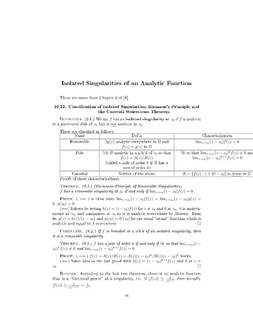
Definition. (9.1.) We say f has an isolated singularity at z0 if f is analyticin a punctured disk of z0 but is not analytic at z0.
These are classied as follows:Name Def'n Characterization
Removable ∃g(z) analytic everywhere in Ω andf(z) = g(z) in Ω
limz→z0(z − z0)f(z) = 0
Pole ∃A,B analytic in a n'h'd of z0 so thatf(z) = A(z)/B(z)
(called a pole of order k if B has azero of order k)
∃k so that limz→z0(z − z0)kf(z) 6= 0 andlimz→z0(z − z0)k+1f(z) = 0
Essential Neither of the above R = f(z) : z ∈ D − z0 is dense in C.Proofs of these characterizations:
Theorem. (9.3.) (Riemanns Principle of Removable Singularities)f has a removable singularity at z0 if and only if limz→z0(z − z0)f(z) = 0
Proof. ( =⇒ ) is clear since limz→z0(z − z0)f(z) = limz→z0(z − z0)g(z) =0 · g(z0) = 0
(⇐=) follows by letting h(z) = (z−z0)f(z) for z 6= z0 and 0 at z0. h is analyticexcept at z0, and continuous at z0 so it is analytic everywhere by Morera. Thenlet g(z) = h(z)/(z − z0) and g(z0) = h′(z0) be the usual secant function which isanalytic and equal to f everywhere.
Corollary. (9.4.) If f is bounded in a n'h'd of an isolated singularity, thenit is a removable singularity.
Theorem. (9.5.) f has a pole of order k if and only if ∃k so that limz→z0(z−z0)kf(z) 6= 0 and limz→z0(z − z0)k+1f(z) = 0
Proof. ( =⇒ ) f(z) = A(z)/B(z) = A(z)(z − z0)k/B(z)(z − z0)k works.(⇐=) Same idea as the last proof with h(z) = (z − z0)k+1f(z) and 0 at z =
z0
Remark. According to the last two theorems, there is no analytic functionthat is a fractional power at a singularity, i.e. if |f(z)| ≤ 1
|z|5/2 then actually
|f(z)| ≤ 1|z|d5/2e = 1
z3 .
34
10.23. LAURENT EXPANSIONS 35
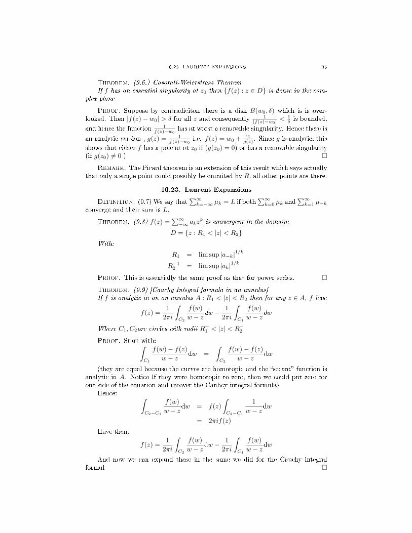
Theorem. (9.6.) Casorati-Weierstrass TheoremIf f has an essential singularity at z0 then f(z) : z ∈ D is dense in the com-
plex plane
Proof. Suppose by contradiciton there is a disk B(w0, δ) which is is over-looked. Then |f(z)− w0| > δ for all z and consequently 1
|f(z)−w0| <1δ is bounded,
and hence the function 1f(z)−w0
has at worst a removable singularity. Hence there is
an analytic version , g(z) = 1f(z)−w0
i.e. f(z) = w0 + ‘1g(z) . Since g is analytic, this
shows that either f has a pole at at z0 if (g(z0) = 0) or has a removable singularity(if g(z0) 6= 0 )
Remark. The Picard theorem is an extension of this result which says actuallythat only a single point could possibly be ommited by R, all other points are there.
10.23. Laurent Expansions
Definition. (9.7) We say that∑∞k=−∞ µk = L if both
∑∞k=0 µk and
∑∞k=1 µ−k
converge and their sum is L.
Theorem. (9.8) f(z) =∑∞−∞ akz
k is convergent in the domain:
D = z : R1 < |z| < R2With:
R1 = lim sup |a−k|1/k
R−12 = lim sup |ak|1/k
Proof. This is essentially the same proof as that for power series.
Theorem. (9.9) [Cauchy Integral formula in an annulus]If f is analytic in an an annulus A : R1 < |z| < R2 then for any z ∈ A, f has:
f(z) =1
2πi
ˆC2
f(w)
w − zdw − 1
2πi
ˆC1
f(w)
w − zdw
Where C1, C2are circles with radii R+1 < |z| < R−2
Proof. Start with:ˆC1
f(w)− f(z)
w − zdw =
ˆC2
f(w)− f(z)
w − zdw
(they are equal because the curves are homotopic and the secant function isanalytic in A. Notice If they were homotopic to zero, then we could put zero forone side of the equation and recover the Cauhcy integral formula)
Hence: ˆC2−C1
f(w)
w − zdw = f(z)
ˆC2−C1
1
w − zdw
= 2πif(z)
Have then:
f(z) =1
2πi
ˆC2
f(w)
w − zdw − 1
2πi
ˆC1
f(w)
w − zdw
And now we can expand these in the same we did for the Cauchy integralformul
10.23. LAURENT EXPANSIONS 36
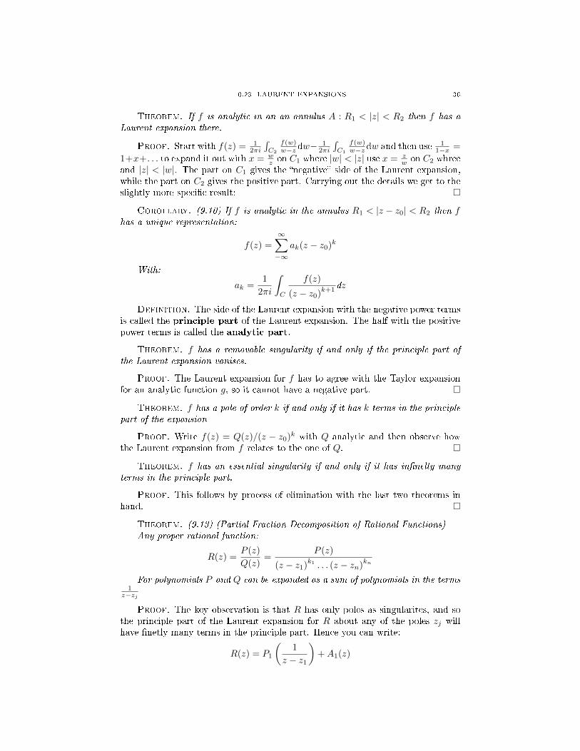
Theorem. If f is analytic in an an annulus A : R1 < |z| < R2 then f has aLaurent expansion there.
Proof. Start with f(z) = 12πi
´C2
f(w)w−z dw−
12πi
´C1
f(w)w−z dw and then use 1
1−x =
1+x+. . . to expand it out with x = wz on C1 where |w| < |z| use x = z
w on C2 whreeand |z| < |w|. The part on C1 gives the negative side of the Laurent expansion,while the part on C2 gives the positive part. Carrying out the details we get to theslightly more specic result:
Corollary. (9.10) If f is analytic in the annulus R1 < |z − z0| < R2 then fhas a unique representation:
f(z) =
∞∑−∞
ak(z − z0)k
With:
ak =1
2πi
ˆC
f(z)
(z − z0)k+1
dz
Definition. The side of the Laurent expansion with the negative power termsis called the principle part of the Laurent expansion. The half with the positivepower terms is called the analytic part.
Theorem. f has a removable singularity if and only if the principle part ofthe Laurent expansion vanises.
Proof. The Laurent expansion for f has to agree with the Taylor expansionfor an analytic function g, so it cannot have a negative part.
Theorem. f has a pole of order k if and only if it has k terms in the principlepart of the expansion
Proof. Write f(z) = Q(z)/(z − z0)k with Q analytic and then observe howthe Laurent expansion from f relates to the one of Q.
Theorem. f has an essential singularity if and only if it has innelty manyterms in the principle part,
Proof. This follows by process of elimination with the last two theorems inhand.
Theorem. (9.13) (Partial Fraction Decomposition of Rational Functions)Any proper rational function:
R(z) =P (z)
Q(z)=
P (z)
(z − z1)k1 . . . (z − zn)
kn
For polynomials P and Q can be expanded as a sum of polynomials in the terms1
z−zj
Proof. The key observation is that R has only poles as singularites, and sothe principle part of the Laurent expansion for R about any of the poles zj willhave netly many terms in the principle part. Hence you can write:
R(z) = P1
(1
z − z1
)+A1(z)
10.23. LAURENT EXPANSIONS 37
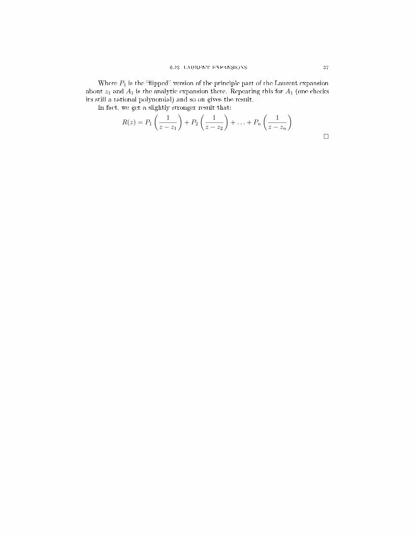
Where P1 is the ipped version of the principle part of the Laurent expansionabout z1 and A1 is the analytic expansion there. Repeating this for A1 (one checksits still a rational polynomial) and so on gives the result.
In fact, we get a slightly stronger result that:
R(z) = P1
(1
z − z1
)+ P2
(1
z − z2
)+ . . .+ Pn
(1
z − zn
)
Introduction to Conformal Mapping
These are notes from Chapter 13 of [1].
11.24. Conformal Equivalence
Definition. (13.1.) Suppsoe two smooth curves C1 and C2 intersect at z0.The angle from C1 to C2 at z0 is measured as the angle counterclockwise from thetangent of C1 at z0 to the tangent of C2 at z0. We write this as ∠C1, C2.
Definition. (13.2) Suppose f is dened in a neigbouthood of z0. f is saidto be conformal at z0 if f preserves angles there. That is to say, for every pairof smooth curves C1, C2 intersecting at z0, we have ∠C1, C2 = ∠f(C1), f(C2). Wesay f is conformal in a region D if it is conformal at every point z ∈ D.
Remark. We will see that holomorphic functions are conformal except atpoints where f ′(z) = 0. For example, f(z) = z2 is not conformal at z = 0.One way to see this for example is to notice that the angle between the positivereal and positive imaginary axis goes from π/2 to π under the map z → z2.
Definition. (13.3.)a) f is locally 1-1 at z0 if for some δ > 0 and any distinct z1, z2 ∈ D(z0; δ)
we have f(z1) 6= f(z2)b) f is locally 1-1 throughout a region D if f is locally 1-1 at every point
z ∈ D.c) f is (globally) 1-1 function in a region D if for every distinct z1, z2 ∈ D
f(z1) 6= f(z2)
Theorem. (13.4) Suppose f is analytic at z0 and f ′(z0) 6= 0. Then f isconformal and locally 1− 1 at z0.
Proof. (Conformal) Take any curve z(t) = x(t) + iy(t), then the tangent tothe curve at a point z0 = z(t0) is given by the derivative z(t0) = x′(t0) + iy′(t0).Examine now Γ = f(C). This is parametrized by w(t) = f(z(t)) and consequentlywe calculate the tangent by the chain rule w(t0) = f ′(z0)z(t0). Hence:
arg(w(t0)) = arg (f ′(z0)z(t0)) = arg(f ′(z0)) + arg(z(t0))
This shows that the dierence arg(w(t0)) − arg(z(t0)) = arg(f ′(z0)) does notdepend on the curves at all...only on the function f and the point z0. Since everycurve has its tangent line rotated by the same amount, the map is conformal.
(Notice that the argument breaks down if f ′(z0) = 0 since arg(f ′(z0)) isnot dened. (No matter how one denes it: the equality arg (f ′(z0)z(t0)) =arg(f ′(z0)) + arg(z(t0)) cannot possibly hold if f ′(z0) = 0))
38
11.24. CONFORMAL EQUIVALENCE 39
(Locally 1-1 at z0) This essentially uses the argument principle applied aroundthe two contours Take f(z0) = α and take δ0 > 0 small enough so that f(z)−α hasno zeros in D(z0; δ0). Let C be the curve that goes over the boundary of D(z0; δ0)and let Γ = f(C). By the argument principle we have that:
#zeros = 1 =1
2πi
ˆ
C
f ′(z)
f(z)− αdz =
1
2πi
ˆ
Γ
dω
ω − α=
1
2πi
ˆdω
ω − β
Where β is any number so that |α− β| ≤ maxω∈D(z0,δ0) |ω|. This shows theeach value β in this disk is achieved exactly once by the function f . Hence f islocally 1-1. (If it was not 1− 1 it would take some value twice!)
Example. (1) f(z) = ez has a nonzero derivative at all points, and hence iseverywhere conformal and locally 1− 1. We see that this function does a transfor-mation from polar to rectangular coordinates in a way: f(x+ iy) = exeiy so the xcoordinate gets mapped to the radius r = ex and the y coordinate gets mapped tothe argument of the polar coordinate θ = y mod 2π. Notice that the map is NOTglobally 1-1...it maps each vertical strip of with 2π conformally to the whole plane.
Example. (2) f(z) = z2 has f ′(z) = 2z which is non-zero everywhere exceptat z = 0. Hence f is a conformal map except at z = 0. Notice that Ref(x+ iy) =x2 − y2 while Im(f(x+ iy)) = 2xy. Fro this we can see that the x-axis and y-axisare mapped through f into hyperbolas that intesect at right angles. Notice thateach hyperbola has two branches...this reects the fact that f is globally 2-1 insome sense....
Definition. (13.5.) Let k be a positive integer. We say f is a k-to-1 mappingof D1 onto D2 if for every α ∈ D2 the equation f(z) = α has k roots (countingmultiplicity) in D2.
Lemma. (13.6) Let f(z) = zk for k a positive integer. Then f magnies anglesat 0 by a factor of k and maps the disk D(0; δ) to the disc D(0, δk) in a k − to− 1manner.
Proof. The rotation bit is clear since f(reiθ) = rkeikθso arg(f(z)) = k arg(z)here. The k roots of unity scaled up by size δ and rotated show the k-to-1 mappingcriteria.
Theorem. (13.7.) Suppose f is analytic with f ′(z0) = 0. Assume that f isnot constant. Let k be the smallest positive integer for which f (k)(z0) 6= 0. Then insome suciently small open set containing z0 we have that f is a k-to-1 mappingand f magnies angles at z0 by a factor of k. (i.e. f locally looks like z → zk.)
Proof. Assume WOLOG that f(z0) = 0. We have from the power seriesexpansion that f(z) = (z− z0)kg(z) where g(z) is given by a power series about z0
and g(z0) 6= 0. Since g 6= 0 in a n'h'd of z0, we can dene a k-th root of g in thisn'h'd. (We can dene a k-th root/a branch of log in any simply connected region
not containing 0) Let h(z) = (z − z0)g1/k(z) then so that f(z) = [h(z)]k. notice
that at h is an analytic function with h(z0) = and h′(z0) = g1/k(z0) 6= 0. Thismeans that h is locally 1-1. Since f is a composition of a locally 1− 1 map h andthe k-to-1 map zk we see that f must be k-to-1 too.
11.25. SPECIAL MAPPINGS 40
Remark. An alternative proof is to go though the same kind of argumentprinciple we did for the 1-1 proof. In this case you'll have there are exactly k rootsin the n'h'd in question. One advantage of going through the function h is that younow view f as the composition of z → zk and the map z → h(z) both of which areeasier to understand than f .
Theorem. (13.8) Suppose f is a 1-1 analytic function in a region D. Then:a) f−1 exists and is analytic in f(D)b) f and f−1 are conformal in D and f(D) respectivly.
Proof. Since f is 1 − 1, f ′ 6= 0. Hence f−1 is also analytic and (f−1)′
=1/f ′ shows that f−1 also has non-zero derivatives in f(D) and so they are bothconformal.
Definition. (13.9) In the setting of the above theorem we call f a conformalmap and we say that D and f(D) are conformally equivalent. More generally:
i) a 1-1 analytic mapping is called a conformal mappingii) Two regions D1 and D2 are said to be conformally equaivalent if there
exists a conformal mapping of D1 onto D2.
11.25. Special Mappings
This section goes through power laws, and fractional linear transformations.The Fractional Linear Transformations are proved to be the unique mappings fromthe unit disk to the unit disc by the Schwarz lemma. For two conformal regionsD1 and D2, there will be a 3 parameter family of conformal mapping theorems bycomposing with the right things to bring it to the form of mappings from the unitdisk to itself (this requires the Riemann mapping theorem).
The Riemann Mapping Theorem
These are notes from Chapter 14 of [1].
12.26. Conformal Mapping and Hydrodynamics
Irrotational, source free ows correspond to holomorphic functions. (We have´Cg(z)dz = σ + iτ where σ is the circulation and τ is the ux. If this is always 0,
then the fucntion f(z) = g(z) is analytic by Morera's theorem.)
12.27. The Riemann Mapping Theorem
The Riemann Mapping Theorem, in its most common form asserts that anytwo simply connected proper subdomains of the complex plane are conformallyequivalent. Note that neither region can be all of C or we would get a violation ofLoiuville's theorem. To prove the theorem it suces to show that there is a mappingfrom any region R to the open disc U . By composing mappings of this sort we willget mappings between any two regions. By composing with the conformal mapsU → U (the FLT's) we can get a map with the property that ϕ(z0) = 0 andϕ′(z0) > 0 (by imposing this it makes the map uniquely determined!).
Theorem. (The Riemann Mapping Theorem)For any simply connected domain R (6= C) and z0 ∈ R, there exists a unique
conformal mapping ϕ of R onto U such that ϕ(z0) = 0 and ϕ′(z0) > 0.
Proof. (Uniqueness) By composing two such maps we would get a mappingfrom the unit disc to the unit disc. But this map would have to be the identitybecause of the proeperites specied ϕ(z0) = 0 and ϕ′(z0) > 0 and because we knowexactly the 3 parameter family of maps from the unit disc to itself.
(Existence) We will phrase the problem as a extreme problem of nding thefunction ϕ from a certain family of functions that is the most extreme in some way.
Recall that the 1-1 mappings from the unit disk to itself that maximize |ϕ′(α)|are precisly those of the form:
ϕ(z) = eiθz − α1− αz
These also happen to be the ones that map α → 0 and map U to U . Thissuggests that we should look for the map that maximizes |ϕ′(z0)|. We divide thedetails of the proof into three steps:
Step 0: Dene F = f : R→ U : f ′(z0) > 0 f is 1-1 here (Notice f(z0) = 0 isnot imposed)
Step 1: Show that F is non-emptyStep 2: Show that supf∈F f
′(z0) = M < ∞ and that there exists a functionϕ ∈ F such that ϕ′(z0) = M
41
12.27. THE RIEMANN MAPPING THEOREM 42
Step 3: Show that ϕ is the function we are looking for! i.e. ϕ is a conformalmap from R onto U such that ϕ(z0) and ϕ′(z0) > 0.
Proof of Step 1:The idea is to start with a point ρ0 outside of R. Such a point exists since
R 6= C.If we could nd a disk around ρ0 say of radius δ then the map f(z) = δ
z−ρ0
would have |f(z)| < 1 for z ∈ R and we would be done!If we cannot nd such a disk, we must be more clever. Since the map z → z−ρ0
is never 0 on R, we can dene a square root/branch of log for this function. Dene:
g(z) =√
z−ρ0
z0−ρ0with the branches chosen so that g(z0) = 1. We claim now that g
stays bounded away from the value −1. Otherwise, if g(ξn) =√
ξn−ρ0
z0−ρ0→ −1 we
will have ξn → z0 but then g(ξn) → 1 6= −1. Now f(z) = δg(z)−(−1) does the trick
for us. By multiplying by a constant eiθ we can suppose WOLOG that f ′(z0) > 0 .Proof of Step 2:First we notice that f ′(z0) is bounded by using a Cauchy-integral-formula es-
timate since |f | ≤ 1 is known. Take a disk D(z0; 2δ) ⊂ R and have:
|f ′(z0)| =
∣∣∣∣∣∣∣1
2πi
ˆ
C(z0;δ)
f(z)
(z − z0)2 dz
∣∣∣∣∣∣∣ ≤1
2π
1
δ2|2πiδ| = 1
δ<∞
Hence supf∈F f′(z0) = M <∞ exists.
Idea of the rest of the proof: The family of functions f ∈ F is uniformly bounded(|f | < 1 again) and it is roughly an equicontinuous family since we have control onthe derivatives in terms of Cauchy-integral-formula estimates. This will allow us touse an Arzel-Ascoli type argument to get us a limit function ϕ that we want.
First take a sequence fn ⊂ F so that f ′n(z0)→M as n→∞. Take ξ1, . . . acountable dense collection of points of R. For each k, the sequence fn(ξk) is bounded(since |f | ≤ 1) and so has a convergence subsequence. Taking subsequences ofsubsequences in this way, we get a diagonal sequence call it ϕn ⊂ fn so thatϕn(ξk) converges for all k ∈ N. Dene ϕ by ϕ(ξk) = limk→∞ ϕn(ξk) and extend itby continiuty to all of R.
We will now show that ϕn converges everywhere in R (not just on the denseset) and that the convergence is uniform on compact subsets K ⊂ R. Since everycompact subset is contained in a nite union of closed discs, it suces to check thatϕn converges uniformly on closed discs in R. Let 2d = d(K, Rc) be the distance fromthe closed disc K to the outside of the region R. Now we have a uniform estimateon the magnitude of the derivative |ϕ′n(z)| from the Cauchy integral formula (againsince |ϕ| ≤ 1:
|ϕ′n(z)| =
∣∣∣∣∣∣∣1
2πi
ˆ
C(z,d)
ϕn(ξ)
(ξ − z)2
∣∣∣∣∣∣∣ ≤1
2π
2πd
d2=
1
d
and hence we have:
|ϕn(z1)− ϕn(z2)| ≤
∣∣∣∣∣∣z2ˆ
z1
ϕ′n(z)dz
∣∣∣∣∣∣ ≤ |z1 − z2|d
12.27. THE RIEMANN MAPPING THEOREM 43
This shows the family ϕn is equicontinuous (in fact they are uniformly Lipshitzon K with Lipshitz constant 1
d )! This shows that ϕn is convergent not just at theξk's but for any z since:
|ϕn(z)− ϕm(z)| ≤ |ϕn(z)− ϕn(ξ)|+ |ϕn(ξ)− ϕm(ξ)|+ |ϕm(ξ)− ϕm(z)|
≤ |z − ξ| 1d
+ |ϕn(ξ)− ϕm(ξ)|+ |z − ξ| 1d
And the three terms on the RHS can be made arbitarily small by choosing ξvery close to z and using the fact that ϕn(ξ) converges so its a Cauchy sequence.Moreover, the limit function ϕ will also be Liphitz on K with Lipshitz constant 1
d(just write it out to see this)
Finally, to see that ϕn → ϕ uniformly on K, we apply the follow standardargument. (We are using the fact that an equicontinuous family that convergespointwise on a compact set actually converges uniformly) Fix ε > 0 and let Sj =z ∈ K : |ϕn(z)− ϕ(z)| < ε for all n > j. Since the family ϕn is equicontinuous,each set Sj is open. Since ϕn → ϕ pointwise, we know that Sj covers all of K. Nowsince K is compact, we can nd a nite subcover and thus get an integer N so largeso that K ⊂ ∪Nj=1Sj . But then |ϕn(z)− ϕ(z)| < ε for all z ∈ K whenever n > Nand the convergence is uniform.
Since ϕn → ϕ uniformly on compacta, ϕ is analytic (by e.g. Morera's theroem).Moreover, ϕ′n(z0) → ϕ′(z0) (e.g. by Cauchy integral formula), and hence ϕ′(z0) =limn→∞ ϕ′n(z0) = M . ϕ is also 1-1 since it is the unifrom limit of 1-1 function (e.g.by the Argument principle)
Proof of Step 3:Recall the maps:
eiθBα(z) = eiθz − α1− αz
These are the maps that map α → 0 and the unit disc U → U . To see thatϕ(z0) = 0 notice that if ϕ(z0) = α 6= 0 then composing Bα ϕ gives a map whose
derivative at 0 is ϕ′(z0)
1−|α|2 , contradiciting the maximality of ϕ.
To see that the image of ϕ is exactly the unit disc, suppose by contradictionthat some point −t2eiθ is missed. By rotating the whole disk by θ we may assumeWOLOG that the point −t2 that is missed is on the negative real axis. If ϕ 6=−t2 ever then the map B−t2 ϕ is never 0. Hence we can dene its square root:√B−t2 ϕ. Now compose this to get a new map from R → D namely: Bt √B−t2 ϕ. One can check that this still maps into U and that its derivative at z0
is ϕ′(z0)(1+t2)2t ϕ′(z0) which is a contradiction of the choice of ϕ!
Remark. Step 2 is a bit quicker if you just say By Arzela-Ascoli....we repro-duced the proof of that theorem in our proof of step 2. (Recall Arzela Ascoli saysthat if you have a family of function f that are bounded and are equicontinuous,the there is a uniformly convergent subsequence) The two steps in the proof ofArzela-Ascoli are:
1. Choose a coutnable dense set of points. By the Bolzanno-Weirestrass the-orem, there is a convergent subsequence at each point. Take sub-sub-sequences toget a diagonal sequence that covnerges at every point of the dense set.
2. By equicontinuity, we actually have convergence everywhere. (ε/3 argument|ϕn(z)− ϕm(z)| ≤ |ϕn(z)− ϕn(ξ)|+ |ϕn(ξ)− ϕm(ξ)|+ |ϕm(ξ)− ϕm(z)|)
12.28. CONNECTION TO THE DIRICHLET PROBLEM FOR THE LAPLACE EQN 44
2. Let Sj = z ∈ K : |ϕn(z)− ϕ(z)| < ε for all n > j and then thse are openby equicontinuity. They form an open cover for the compact set in question and sothey have a nite subcover. The nite subcover shows that the converge is uniform.
12.28. Connection to the Dirichlet problem for the Laplace Eqn
Proposition. The real part of any holomorphic function is harmonic ∆u = 0
Proof. This is just from the Cauchy Riemann equations ux = −vy and uy =
vx because then we can rewrite: uxx + uyy = ∂2
∂x∂yv −∂2
∂x∂yv = 0
Proposition. Conversely, given any harmonic function ∆u = 0, we can nda conjugate function v so that u+ iv is a holomorphic function
Proof. The trick is to go through the derivative rst, and then integrate atthe end. If we dene ∂z := ∂x − i∂y and ∂z := ∂x + i∂y then one can check that∆ = 4∂z∂z. Moreover, the Cauchy Riemann equations tell us that a function isholomorphic if and only if ∂zf = 0. Now if ∆u = 0 then we have ∂z (∂zu) =0. Hence ∂zu is a holomorphic function! Since holomorphic function have anti-derivatives, there is a holomoprhic function F so that F ′ = ∂zu. We claim nowthat u = 2Re(F ) + const. Indeed if we write F = a + ib then ∂zu = F ′ =⇒∂xu − i∂yu = 2∂xa − 2i∂ya (Use Cauchy Riemann equations to manipulate whatcomplex dierentiation means in terms of real and imaginary parts). Equatingthese we get ∂xu = 2∂xa and ∂ya = 2∂ya from which we conclud that it must bethe case that u = a+ const = Re(F ) + const
Proposition. Let R be a simply connected domain with a smooth boundaryand suppose 0 ∈ R. Then the Diriclet problem:
∆u = 0 inR
u |∂R = − log |z| on ∂R
Then the analytic function corresponding to the harmonic function u that hasf(z) = u+ iv. Dene ϕ by
ϕ(z) = zef(z)
Then ϕ is the map R→ U
Proof. Check that on ∂R we have |ϕ(z)| = |z|∣∣ef(z)
∣∣ = |z| eu(z) = |z| e− log|z| =1 so indeed the boundary of R is mapped to the unit disc. Moreover, we check thatϕ is 1-1 as follows. For any point ξ ∈ U in the unit disk, since |ϕ(z)| = 1 for z ∈ ∂R,we can nd an region (∂R)ε close to the boundary ∂R so that |ϕ(z)| > 1− |ξ| /2 inthis region. But then, taking a closed curve γε that stays in this region we have bythe argument prinicple (/Rouche's theorem) that:
1
2πi
ˆ
γε
ϕ′(z)
ϕ(z)− ξ=
1
2πi
ˆ
γε
ϕ′(z)
ϕ(z)= 1
This is 1 since it counts the number of times ϕ is equal to zero in R (Argumentprinciple) and since ϕ(z) = zef(z) is only zero at z = 0.
12.29. COMPLEX THEOREMS TO MEMORIZE 45
12.29. Complex Theorems to Memorize
Theorem. (Riemann Mapping Theorem)Any simply connected domain that is not all of C is conformally equivalent to
the unit disc.
Theorem. (Little Picard Theorem)If f : C → C is entire and non-constant, then w : ∃f(x) = w is the whole
complex plane or the whole complex plane minus a point.(ez hits every value except 0)
Theorem. (Big Picard)If an analytic function has an essential singularity at a point w, then on a
punctured n'h'd of w, f(z) takes on all possible complex values with at most asingle exception.
(e1/z has an essential singularity at 0 but still never attains 0 as a value)
Theorem. (Product Representation for sin):sin(πz) = (πz)
∏∞k=1
(1− z
k
)ez/k
∏(1 + z
k )e−z/k
Bibliography
[1] J. Bak and D.J. Newman. Complex Analysis. Encyclopaedia of Mathematical Sciences.Springer, 1997.
46