Embed Size (px)
Citation preview
Complex Analysis Summer 2001
Kenneth Kuttler
July 17, 2003

2
Contents
1 General topology 51.1 Compactness in metric space . . . . . . . . . . . . . . . . . . . . . . . . . . . . . . . . . . . . 111.2 Connected sets . . . . . . . . . . . . . . . . . . . . . . . . . . . . . . . . . . . . . . . . . . . . 141.3 Exercises . . . . . . . . . . . . . . . . . . . . . . . . . . . . . . . . . . . . . . . . . . . . . . . 17
2 Spaces of Continuous Functions 212.1 Compactness in spaces of continuous functions . . . . . . . . . . . . . . . . . . . . . . . . . . 212.2 Stone Weierstrass theorem . . . . . . . . . . . . . . . . . . . . . . . . . . . . . . . . . . . . . . 232.3 Exercises . . . . . . . . . . . . . . . . . . . . . . . . . . . . . . . . . . . . . . . . . . . . . . . 27
3 The complex numbers 313.1 Exercises . . . . . . . . . . . . . . . . . . . . . . . . . . . . . . . . . . . . . . . . . . . . . . . 343.2 The extended complex plane . . . . . . . . . . . . . . . . . . . . . . . . . . . . . . . . . . . . 353.3 Exercises . . . . . . . . . . . . . . . . . . . . . . . . . . . . . . . . . . . . . . . . . . . . . . . 36
4 Riemann Stieltjes integrals 374.1 Exercises . . . . . . . . . . . . . . . . . . . . . . . . . . . . . . . . . . . . . . . . . . . . . . . 46
5 Analytic functions 475.1 Exercises . . . . . . . . . . . . . . . . . . . . . . . . . . . . . . . . . . . . . . . . . . . . . . . 495.2 Examples of analytic functions . . . . . . . . . . . . . . . . . . . . . . . . . . . . . . . . . . . 505.3 Exercises . . . . . . . . . . . . . . . . . . . . . . . . . . . . . . . . . . . . . . . . . . . . . . . 51
6 Cauchy’s formula for a disk 536.1 Exercises . . . . . . . . . . . . . . . . . . . . . . . . . . . . . . . . . . . . . . . . . . . . . . . 58
7 The general Cauchy integral formula 637.1 The Cauchy Goursat theorem . . . . . . . . . . . . . . . . . . . . . . . . . . . . . . . . . . . . 637.2 The Cauchy integral formula . . . . . . . . . . . . . . . . . . . . . . . . . . . . . . . . . . . . 667.3 Exercises . . . . . . . . . . . . . . . . . . . . . . . . . . . . . . . . . . . . . . . . . . . . . . . 72
8 The open mapping theorem 758.1 Zeros of an analytic function . . . . . . . . . . . . . . . . . . . . . . . . . . . . . . . . . . . . 758.2 The open mapping theorem . . . . . . . . . . . . . . . . . . . . . . . . . . . . . . . . . . . . . 768.3 Applications of the open mapping theorem . . . . . . . . . . . . . . . . . . . . . . . . . . . . 788.4 Counting zeros . . . . . . . . . . . . . . . . . . . . . . . . . . . . . . . . . . . . . . . . . . . . 798.5 The estimation of eigenvalues . . . . . . . . . . . . . . . . . . . . . . . . . . . . . . . . . . . . 828.6 Exercises . . . . . . . . . . . . . . . . . . . . . . . . . . . . . . . . . . . . . . . . . . . . . . . 85
3
4 CONTENTS
9 Singularities 879.1 The Concept Of An Annulus . . . . . . . . . . . . . . . . . . . . . . . . . . . . . . . . . . . . 879.2 The Laurent Series . . . . . . . . . . . . . . . . . . . . . . . . . . . . . . . . . . . . . . . . . . 889.3 Isolated Singularities . . . . . . . . . . . . . . . . . . . . . . . . . . . . . . . . . . . . . . . . . 919.4 Partial Fraction Expansions . . . . . . . . . . . . . . . . . . . . . . . . . . . . . . . . . . . . . 939.5 Exercises . . . . . . . . . . . . . . . . . . . . . . . . . . . . . . . . . . . . . . . . . . . . . . . 95
10 Residues and evaluation of integrals 9710.1 The argument principle and Rouche’s theorem . . . . . . . . . . . . . . . . . . . . . . . . . . 10710.2 Exercises . . . . . . . . . . . . . . . . . . . . . . . . . . . . . . . . . . . . . . . . . . . . . . . 10810.3 The Poisson formulas and the Hilbert transform . . . . . . . . . . . . . . . . . . . . . . . . . 11010.4 Exercises . . . . . . . . . . . . . . . . . . . . . . . . . . . . . . . . . . . . . . . . . . . . . . . 11310.5 Infinite products . . . . . . . . . . . . . . . . . . . . . . . . . . . . . . . . . . . . . . . . . . . 11410.6 Exercises . . . . . . . . . . . . . . . . . . . . . . . . . . . . . . . . . . . . . . . . . . . . . . . 120
11 Harmonic functions 12311.1 The Dirichlet problem for a disk . . . . . . . . . . . . . . . . . . . . . . . . . . . . . . . . . . 12311.2 Exercises . . . . . . . . . . . . . . . . . . . . . . . . . . . . . . . . . . . . . . . . . . . . . . . 128
12 Complex mappings 13112.1 Fractional linear transformations . . . . . . . . . . . . . . . . . . . . . . . . . . . . . . . . . . 13112.2 Some other mappings . . . . . . . . . . . . . . . . . . . . . . . . . . . . . . . . . . . . . . . . 13312.3 The Dirichlet problem for a half plane . . . . . . . . . . . . . . . . . . . . . . . . . . . . . . . 13412.4 Other problems involving Laplace’s equation . . . . . . . . . . . . . . . . . . . . . . . . . . . 13612.5 Exercises . . . . . . . . . . . . . . . . . . . . . . . . . . . . . . . . . . . . . . . . . . . . . . . 13712.6 Schwarz Christoffel transformation . . . . . . . . . . . . . . . . . . . . . . . . . . . . . . . . . 13812.7 Exercises . . . . . . . . . . . . . . . . . . . . . . . . . . . . . . . . . . . . . . . . . . . . . . . 14112.8 Riemann Mapping theorem . . . . . . . . . . . . . . . . . . . . . . . . . . . . . . . . . . . . . 14112.9 Exercises . . . . . . . . . . . . . . . . . . . . . . . . . . . . . . . . . . . . . . . . . . . . . . . 147
13 Approximation of analytic functions 14913.1 Runge’s theorem . . . . . . . . . . . . . . . . . . . . . . . . . . . . . . . . . . . . . . . . . . . 15213.2 Exercises . . . . . . . . . . . . . . . . . . . . . . . . . . . . . . . . . . . . . . . . . . . . . . . 154
General topology
This chapter is a brief introduction to general topology. Topological spaces consist of a set and a subset ofthe set of all subsets of this set called the open sets or topology which satisfy certain axioms. Like otherareas in mathematics the abstraction inherent in this approach is an attempt to unify many different usefulexamples into one general theory.
For example, consider Rn with the usual norm given by
|x| ≡
(n∑i=1
|xi|2)1/2
.
We say a set U in Rn is an open set if every point of U is an “interior” point which means that if x ∈U ,there exists δ > 0 such that if |y − x| < δ, then y ∈U . It is easy to see that with this definition of open sets,the axioms (1.1) - (1.2) given below are satisfied if τ is the collection of open sets as just described. Thereare many other sets of interest besides Rn however, and the appropriate definition of “open set” may bevery different and yet the collection of open sets may still satisfy these axioms. By abstracting the conceptof open sets, we can unify many different examples. Here is the definition of a general topological space.
Let X be a set and let τ be a collection of subsets of X satisfying
∅ ∈ τ, X ∈ τ, (1.1)
If C ⊆ τ, then ∪ C ∈ τ
If A,B ∈ τ, then A ∩B ∈ τ. (1.2)
Definition 1.1 A set X together with such a collection of its subsets satisfying (1.1)-(1.2) is called a topo-logical space. τ is called the topology or set of open sets of X. Note τ ⊆ P(X), the set of all subsets of X,also called the power set.
Definition 1.2 A subset B of τ is called a basis for τ if whenever p ∈ U ∈ τ , there exists a set B ∈ B suchthat p ∈ B ⊆ U . The elements of B are called basic open sets.
The preceding definition implies that every open set (element of τ) may be written as a union of basicopen sets (elements of B). This brings up an interesting and important question. If a collection of subsets Bof a set X is specified, does there exist a topology τ for X satisfying (1.1)-(1.2) such that B is a basis for τ?
Theorem 1.3 Let X be a set and let B be a set of subsets of X. Then B is a basis for a topology τ if andonly if whenever p ∈ B ∩C for B,C ∈ B, there exists D ∈ B such that p ∈ D ⊆ C ∩B and ∪B = X. In thiscase τ consists of all unions of subsets of B.
5
6 GENERAL TOPOLOGY
Proof: The only if part is left to the reader. Let τ consist of all unions of sets of B and suppose B satisfiesthe conditions of the proposition. Then ∅ ∈ τ because ∅ ⊆ B. X ∈ τ because ∪B = X by assumption. IfC ⊆ τ then clearly ∪C ∈ τ . Now suppose A,B ∈ τ, A = ∪S, B = ∪R, S,R ⊆ B. We need to showA ∩ B ∈ τ . If A ∩ B = ∅, we are done. Suppose p ∈ A ∩ B. Then p ∈ S ∩ R where S ∈ S, R ∈ R. Hencethere exists U ∈ B such that p ∈ U ⊆ S ∩R. It follows, since p ∈ A ∩B was arbitrary, that A ∩B = unionof sets of B. Thus A ∩B ∈ τ . Hence τ satisfies (1.1)-(1.2).
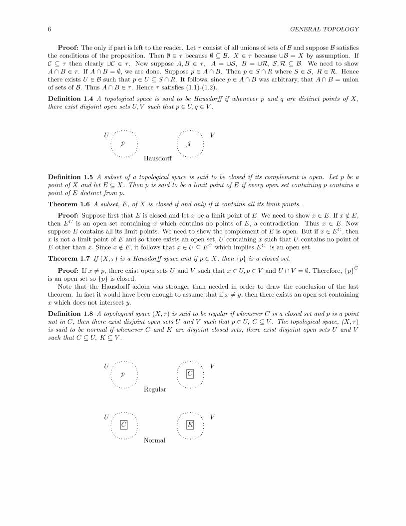
Definition 1.4 A topological space is said to be Hausdorff if whenever p and q are distinct points of X,there exist disjoint open sets U, V such that p ∈ U, q ∈ V .
Hausdorff
·pU
·qV
Definition 1.5 A subset of a topological space is said to be closed if its complement is open. Let p be apoint of X and let E ⊆ X. Then p is said to be a limit point of E if every open set containing p contains apoint of E distinct from p.
Theorem 1.6 A subset, E, of X is closed if and only if it contains all its limit points.
Proof: Suppose first that E is closed and let x be a limit point of E. We need to show x ∈ E. If x /∈ E,then EC is an open set containing x which contains no points of E, a contradiction. Thus x ∈ E. Nowsuppose E contains all its limit points. We need to show the complement of E is open. But if x ∈ EC , thenx is not a limit point of E and so there exists an open set, U containing x such that U contains no point ofE other than x. Since x /∈ E, it follows that x ∈ U ⊆ EC which implies EC is an open set.
Theorem 1.7 If (X, τ) is a Hausdorff space and if p ∈ X, then {p} is a closed set.
Proof: If x 6= p, there exist open sets U and V such that x ∈ U, p ∈ V and U ∩ V = ∅. Therefore, {p}Cis an open set so {p} is closed.
Note that the Hausdorff axiom was stronger than needed in order to draw the conclusion of the lasttheorem. In fact it would have been enough to assume that if x 6= y, then there exists an open set containingx which does not intersect y.
Definition 1.8 A topological space (X, τ) is said to be regular if whenever C is a closed set and p is a pointnot in C, then there exist disjoint open sets U and V such that p ∈ U, C ⊆ V . The topological space, (X, τ)is said to be normal if whenever C and K are disjoint closed sets, there exist disjoint open sets U and Vsuch that C ⊆ U, K ⊆ V .
Regular
·pU
CV
Normal
CU
KV
7
Definition 1.9 Let E be a subset of X. E is defined to be the smallest closed set containing E. Note thatthis is well defined since X is closed and the intersection of any collection of closed sets is closed.
Theorem 1.10 E = E ∪ {limit points of E}.
Proof: Let x ∈ E and suppose that x /∈ E. If x is not a limit point either, then there exists an openset, U,containing x which does not intersect E. But then UC is a closed set which contains E which doesnot contain x, contrary to the definition that E is the intersection of all closed sets containing E. Therefore,x must be a limit point of E after all.
Now E ⊆ E so suppose x is a limit point of E. We need to show x ∈ E. If H is a closed set containingE, which does not contain x, then HC is an open set containing x which contains no points of E other thanx negating the assumption that x is a limit point of E.
Definition 1.11 Let X be a set and let d : X ×X → [0,∞) satisfy
d(x, y) = d(y, x), (1.3)
d(x, y) + d(y, z) ≥ d(x, z), (triangle inequality)
d(x, y) = 0 if and only if x = y. (1.4)
Such a function is called a metric. For r ∈ [0,∞) and x ∈ X, define
B(x, r) = {y ∈ X : d(x, y) < r}
This may also be denoted by N(x, r).
Definition 1.12 A topological space (X, τ) is called a metric space if there exists a metric, d, such that thesets {B(x, r), x ∈ X, r > 0} form a basis for τ . We write (X, d) for the metric space.
Theorem 1.13 Suppose X is a set and d satisfies (1.3)-(1.4). Then the sets {B(x, r) : r > 0, x ∈ X} forma basis for a topology on X.
Proof: We observe that the union of these balls includes the whole space, X. We need to verify thecondition concerning the intersection of two basic sets. Let p ∈ B (x, r1) ∩B (z, r2) . Consider
r ≡ min (r1 − d (x, p) , r2 − d (z, p))
and suppose y ∈ B (p, r) . Then
d (y, x) ≤ d (y, p) + d (p, x) < r1 − d (x, p) + d (x, p) = r1
and so B (p, r) ⊆ B (x, r1) . By similar reasoning, B (p, r) ⊆ B (z, r2) . This verifies the conditions for this setof balls to be the basis for some topology.
Theorem 1.14 If (X, τ) is a metric space, then (X, τ) is Hausdorff, regular, and normal.
Proof: It is obvious that any metric space is Hausdorff. Since each point is a closed set, it suffices toverify any metric space is normal. Let H and K be two disjoint closed nonempty sets. For each h ∈ H, thereexists rh > 0 such that B (h, rh) ∩K = ∅ because K is closed. Similarly, for each k ∈ K there exists rk > 0such that B (k, rk) ∩H = ∅. Now let
U ≡ ∪{B (h, rh/2) : h ∈ H} , V ≡ ∪{B (k, rk/2) : k ∈ K} .
then these open sets contain H and K respectively and have empty intersection for if x ∈ U ∩ V, thenx ∈ B (h, rh/2) ∩B (k, rk/2) for some h ∈ H and k ∈ K. Suppose rh ≥ rk. Then
d (h, k) ≤ d (h, x) + d (x, k) < rh,
a contradiction to B (h, rh) ∩K = ∅. If rk ≥ rh, the argument is similar. This proves the theorem.
8 GENERAL TOPOLOGY
Definition 1.15 A metric space is said to be separable if there is a countable dense subset of the space.This means there exists D = {pi}∞i=1 such that for all x and r > 0, B(x, r) ∩D 6= ∅.
Definition 1.16 A topological space is said to be completely separable if it has a countable basis for thetopology.
Theorem 1.17 A metric space is separable if and only if it is completely separable.
Proof: If the metric space has a countable basis for the topology, pick a point from each of the basicopen sets to get a countable dense subset of the metric space.
Now suppose the metric space, (X, d) , has a countable dense subset, D. Let B denote all balls havingcenters in D which have positive rational radii. We will show this is a basis for the topology. It is clear itis a countable set. Let U be any open set and let z ∈ U. Then there exists r > 0 such that B (z, r) ⊆ U. InB (z, r/3) pick a point from D, x. Now let r1 be a positive rational number in the interval (r/3, 2r/3) andconsider the set from B, B (x, r1) . If y ∈ B (x, r1) then
d (y, z) ≤ d (y, x) + d (x, z) < r1 + r/3 < 2r/3 + r/3 = r.
Thus B (x, r1) contains z and is contained in U. This shows, since z is an arbitrary point of U that U is theunion of a subset of B.
We already discussed Cauchy sequences in the context of Rp but the concept makes perfectly good sensein any metric space.
Definition 1.18 A sequence {pn}∞n=1 in a metric space is called a Cauchy sequence if for every ε > 0 thereexists N such that d(pn, pm) < ε whenever n,m > N . A metric space is called complete if every Cauchysequence converges to some element of the metric space.
Example 1.19 Rn and Cn are complete metric spaces for the metric defined by d(x,y) ≡ |x− y| ≡ (
∑ni=1 |xi−
yi|2)1/2.
Not all topological spaces are metric spaces and so the traditional ε− δ definition of continuity must bemodified for more general settings. The following definition does this for general topological spaces.
Definition 1.20 Let (X, τ) and (Y, η) be two topological spaces and let f : X → Y . We say f is continuousat x ∈ X if whenever V is an open set of Y containing f(x), there exists an open set U ∈ τ such that x ∈ Uand f(U) ⊆ V . We say that f is continuous if f−1(V ) ∈ τ whenever V ∈ η.
Definition 1.21 Let (X, τ) and (Y, η) be two topological spaces. X×Y is the Cartesian product. (X×Y ={(x, y) : x ∈ X, y ∈ Y }). We can define a product topology as follows. Let B = {(A × B) : A ∈ τ, B ∈ η}.B is a basis for the product topology.
Theorem 1.22 B defined above is a basis satisfying the conditions of Theorem 1.3.
More generally we have the following definition which considers any finite Cartesian product of topologicalspaces.
Definition 1.23 If (Xi, τi) is a topological space, we make∏ni=1Xi into a topological space by letting a basis
be∏ni=1Ai where Ai ∈ τi.
Theorem 1.24 Definition 1.23 yields a basis for a topology.
The proof of this theorem is almost immediate from the definition and is left for the reader.The definition of compactness is also considered for a general topological space. This is given next.
9
Definition 1.25 A subset, E, of a topological space (X, τ) is said to be compact if whenever C ⊆ τ andE ⊆ ∪C, there exists a finite subset of C, {U1 · · · Un}, such that E ⊆ ∪ni=1Ui. (Every open covering admitsa finite subcovering.) We say E is precompact if E is compact. A topological space is called locally compactif it has a basis B, with the property that B is compact for each B ∈ B. Thus the topological space is locallycompact if it has a basis of precompact open sets.
In general topological spaces there may be no concept of “bounded”. Even if there is, closed and boundedis not necessarily the same as compactness. However, we can say that in any Hausdorff space every compactset must be a closed set.
Theorem 1.26 If (X, τ) is a Hausdorff space, then every compact subset must also be a closed set.
Proof: Suppose p /∈ K. For each x ∈ X, there exist open sets, Ux and Vx such that
x ∈ Ux, p ∈ Vx,
and
Ux ∩ Vx = ∅.
Since K is assumed to be compact, there are finitely many of these sets, Ux1 , · · ·, Uxm which cover K. Thenlet V ≡ ∩mi=1Vxi . It follows that V is an open set containing p which has empty intersection with each of theUxi . Consequently, V contains no points of K and is therefore not a limit point. This proves the theorem.
Lemma 1.27 Let (X, τ) be a topological space and let B be a basis for τ . Then K is compact if and only ifevery open cover of basic open sets admits a finite subcover.
The proof follows directly from the definition and is left to the reader. A very important property enjoyedby a collection of compact sets is the property that if it can be shown that any finite intersection of thiscollection has non empty intersection, then it can be concluded that the intersection of the whole collectionhas non empty intersection.
Definition 1.28 If every finite subset of a collection of sets has nonempty intersection, we say the collectionhas the finite intersection property.
Theorem 1.29 Let K be a set whose elements are compact subsets of a Hausdorff topological space, (X, τ) .Suppose K has the finite intersection property. Then ∅ 6= ∩K.
Proof: Suppose to the contrary that ∅ = ∩K. Then consider
C ≡{KC : K ∈ K
}.
It follows C is an open cover of K0 where K0 is any particular element of K. But then there are finitely manyK ∈ K, K1, · · ·,Kr such that K0 ⊆ ∪ri=1K
Ci implying that ∩ri=0Ki = ∅, contradicting the finite intersection
property.It is sometimes important to consider the Cartesian product of compact sets. The following is a simple
example of the sort of theorem which holds when this is done.
Theorem 1.30 Let X and Y be topological spaces, and K1, K2 be compact sets in X and Y respectively.Then K1 ×K2 is compact in the topological space X × Y .
Proof: Let C be an open cover of K1×K2 of sets A×B where A and B are open sets. Thus C is a opencover of basic open sets. For y ∈ Y , define
Cy = {A×B ∈ C : y ∈ B}, Dy = {A : A×B ∈ Cy}

10 GENERAL TOPOLOGY
Claim: Dy covers K1.Proof: Let x ∈ K1. Then (x, y) ∈ K1 × K2 so (x, y) ∈ A × B ∈ C. Therefore A × B ∈ Cy and so
x ∈ A ∈ Dy.Since K1 is compact,
{A1, · · ·, An(y)} ⊆ Dy
covers K1. Let
By = ∩n(y)i=1 Bi
Thus {A1, · · ·, An(y)} covers K1 and Ai ×By ⊆ Ai ×Bi ∈ Cy.Since K2 is compact, there is a finite list of elements of K2, y1, · · ·, yr such that
{By1 , · · ·, Byr}
covers K2. Consider
{Ai ×Byl}n(yl) ri=1 l=1.
If (x, y) ∈ K1 ×K2, then y ∈ Byj for some j ∈ {1, · · ·, r}. Then x ∈ Ai for some i ∈ {1, · · ·, n(yj)}. Hence(x, y) ∈ Ai ×Byj . Each of the sets Ai ×Byj is contained in some set of C and so this proves the theorem.
Another topic which is of considerable interest in general topology and turns out to be a very usefulconcept in analysis as well is the concept of a subbasis.
Definition 1.31 S ⊆ τ is called a subbasis for the topology τ if the set B of finite intersections of sets of Sis a basis for the topology, τ .
Recall that the compact sets in Rn with the usual topology are exactly those that are closed and bounded.We will have use of the following simple result in the following chapters.
Theorem 1.32 Let U be an open set in Rn. Then there exists a sequence of open sets, {Ui} satisfying
· · ·Ui ⊆ Ui ⊆ Ui+1 · · ·
and
U = ∪∞i=1Ui.
Proof: The following lemma will be interesting for its own sake and in addition to this, is exactly whatis needed for the proof of this theorem.
Lemma 1.33 Let S be any nonempty subset of a metric space, (X, d) and define
dist (x,S) ≡ inf {d (x, s) : s ∈ S} .
Then the mapping, x→ dist (x, S) satisfies
|dist (y, S)− dist (x, S)| ≤ d (x, y) .
Proof of the lemma: One of dist (y, S) ,dist (x, S) is larger than or equal to the other. Assume withoutloss of generality that it is dist (y, S). Choose s1 ∈ S such that
dist (x, S) + ε > d (x, s1)
1.1. COMPACTNESS IN METRIC SPACE 11
Then
|dist (y, S)− dist (x, S)| = dist (y, S)− dist (x, S) ≤
d (y, s1)− d (x, s1) + ε ≤ d (x, y) + d (x, s1)− d (x, s1) + ε
= d (x, y) + ε.
Since ε is arbitrary, this proves the lemma.If U = R
n it is clear that U = ∪∞i=1B (0, i) and so, letting Ui = B (0, i),
B (0, i) = {x ∈Rn : dist (x, {0}) < i}
and by continuity of dist (·, {0}) ,
B (0, i) = {x ∈Rn : dist (x, {0}) ≤ i} .
Therefore, the Heine Borel theorem applies and we see the theorem is true in this case.Now we use this lemma to finish the proof in the case where U is not all of Rn. Since x→dist
(x,UC
)is
continuous, the set,
Ui ≡{
x ∈U : dist(x,UC
)>
1i
and |x| < i
},
is an open set. Also U = ∪∞i=1Ui and these sets are increasing. By the lemma,
Ui ={
x ∈U : dist(x,UC
)≥ 1i
and |x| ≤ i},
a compact set by the Heine Borel theorem and also, · · ·Ui ⊆ Ui ⊆ Ui+1 · · · .
1.1 Compactness in metric space
Many existence theorems in analysis depend on some set being compact. Therefore, it is important to beable to identify compact sets. The purpose of this section is to describe compact sets in a metric space.
Definition 1.34 In any metric space, we say a set E is totally bounded if for every ε > 0 there exists afinite set of points {x1, · · ·, xn} such that
E ⊆ ∪ni=1B (xi, ε).
This finite set of points is called an ε net.
The following proposition tells which sets in a metric space are compact.
Proposition 1.35 Let (X, d) be a metric space. Then the following are equivalent.
(X, d) is compact, (1.5)
(X, d) is sequentially compact, (1.6)
(X, d) is complete and totally bounded. (1.7)
12 GENERAL TOPOLOGY
Recall that X is “sequentially compact” means every sequence has a convergent subsequence convergingso an element of X.
Proof: Suppose (1.5) and let {xk} be a sequence. Suppose {xk} has no convergent subsequence. If thisis so, then {xk} has no limit point and no value of the sequence is repeated more than finitely many times.Thus the set
Cn = ∪{xk : k ≥ n}
is a closed set and if
Un = CCn ,
then
X = ∪∞n=1Un
but there is no finite subcovering, contradicting compactness of (X, d).Now suppose (1.6) and let {xn} be a Cauchy sequence. Then xnk → x for some subsequence. Let ε > 0
be given. Let n0 be such that if m,n ≥ n0, then d (xn, xm) < ε2 and let l be such that if k ≥ l then
d (xnk , x) < ε2 . Let n1 > max (nl, n0). If n > n1, let k > l and nk > n0.
d (xn, x) ≤ d(xn, xnk) + d (xnk , x)
<ε
2+ε
2= ε.
Thus {xn} converges to x and this shows (X, d) is complete. If (X, d) is not totally bounded, then thereexists ε > 0 for which there is no ε net. Hence there exists a sequence {xk} with d (xk, xl) ≥ ε for all l 6= k.This contradicts (1.6) because this is a sequence having no convergent subsequence. This shows (1.6) implies(1.7).
Now suppose (1.7). We show this implies (1.6). Let {pn} be a sequence and let {xni }mni=1 be a 2−n net for
n = 1, 2, · · ·. Let
Bn ≡ B(xnin , 2
−n)be such that Bn contains pk for infinitely many values of k and Bn ∩ Bn+1 6= ∅. Let pnk be a subsequencehaving
pnk ∈ Bk.
Then if k ≥ l,
d (pnk , pnl) ≤k−1∑i=l
d(pni+1 , pni
)<
k−1∑i=l
2−(i−1) < 2−(l−2).
Consequently {pnk} is a Cauchy sequence. Hence it converges. This proves (1.6).Now suppose (1.6) and (1.7). Let Dn be a n−1 net for n = 1, 2, · · · and let
D = ∪∞n=1Dn.
Thus D is a countable dense subset of (X, d). The set of balls
B = {B (q, r) : q ∈ D, r ∈ Q ∩ (0,∞)}
1.1. COMPACTNESS IN METRIC SPACE 13
is a countable basis for (X, d). To see this, let p ∈ B (x, ε) and choose r ∈ Q ∩ (0,∞) such that
ε− d (p, x) > 2r.
Let q ∈ B (p, r) ∩D. If y ∈ B (q, r), then
d (y, x) ≤ d (y, q) + d (q, p) + d (p, x)< r + r + ε− 2r = ε.
Hence p ∈ B (q, r) ⊆ B (x, ε) and this shows each ball is the union of balls of B. Now suppose C is any opencover of X. Let B denote the balls of B which are contained in some set of C. Thus
∪B = X.
For each B ∈ B, pick U ∈ C such that U ⊇ B. Let C be the resulting countable collection of sets. Then C isa countable open cover of X. Say C = {Un}∞n=1. If C admits no finite subcover, then neither does C and wecan pick pn ∈ X \ ∪nk=1Uk. Then since X is sequentially compact, there is a subsequence {pnk} such that{pnk} converges. Say
p = limk→∞
pnk .
All but finitely many points of {pnk} are in X \ ∪nk=1Uk. Therefore p ∈ X \ ∪nk=1Uk for each n. Hence
p /∈ ∪∞k=1Uk
contradicting the construction of {Un}∞n=1. Hence X is compact. This proves the proposition.Next we apply this very general result to a familiar example, Rn. In this setting totally bounded and
bounded are the same. This will yield another proof of the Heine Borel theorem.
Lemma 1.36 A subset of Rn is totally bounded if and only if it is bounded.
Proof: Let A be totally bounded. We need to show it is bounded. Let x1, · · ·,xp be a 1 net for A. Nowconsider the ball B (0, r + 1) where r > max (||xi|| : i = 1, · · ·, p) . If z ∈A, then z ∈B (xj , 1) for some j andso by the triangle inequality,
||z− 0|| ≤ ||z− xj ||+ ||xj || < 1 + r.
Thus A ⊆ B (0,r + 1) and so A is bounded.Now suppose A is bounded and suppose A is not totally bounded. Then there exists ε > 0 such that
there is no ε net for A. Therefore, there exists a sequence of points {ai} with ||ai − aj || ≥ ε if i 6= j. SinceA is bounded, there exists r > 0 such that
A ⊆ [−r, r)n.
(x ∈[−r, r)n means xi ∈ [−r, r) for each i.) Now define S to be all cubes of the formn∏k=1
[ak, bk)
where
ak = −r + i2−pr, bk = −r + (i+ 1) 2−pr,
for i ∈ {0, 1, · · ·, 2p+1 − 1}. Thus S is a collection of(2p+1
)n nonoverlapping cubes whose union equals[−r, r)n and whose diameters are all equal to 2−pr
√n. Now choose p large enough that the diameter of
these cubes is less than ε. This yields a contradiction because one of the cubes must contain infinitely manypoints of {ai}. This proves the lemma.
The next theorem is called the Heine Borel theorem and it characterizes the compact sets in Rn.

14 GENERAL TOPOLOGY
Theorem 1.37 A subset of Rn is compact if and only if it is closed and bounded.
Proof: Since a set in Rn is totally bounded if and only if it is bounded, this theorem follows fromProposition 1.35 and the observation that a subset of Rn is closed if and only if it is complete. This provesthe theorem.
The following corollary is an important existence theorem which depends on compactness.
Corollary 1.38 Let (X, τ) be a compact topological space and let f : X → R be continuous. Thenmax {f (x) : x ∈ X} and min {f (x) : x ∈ X} both exist.
Proof: Since f is continuous, it follows that f (X) is compact. From Theorem 1.37 f (X) is closed andbounded. This implies it has a largest and a smallest value. This proves the corollary.
1.2 Connected sets
Stated informally, connected sets are those which are in one piece. More precisely, we give the followingdefinition.
Definition 1.39 We say a set, S in a general topological space is separated if there exist sets, A,B suchthat
S = A ∪B, A,B 6= ∅, and A ∩B = B ∩A = ∅.
In this case, the sets A and B are said to separate S. We say a set is connected if it is not separated.
One of the most important theorems about connected sets is the following.
Theorem 1.40 Suppose U and V are connected sets having nonempty intersection. Then U ∪ V is alsoconnected.
Proof: Suppose U ∪ V = A ∪B where A ∩B = B ∩A = ∅. Consider the sets, A ∩ U and B ∪ U. Since
(A ∩ U) ∩ (B ∩ U) = (A ∩ U) ∩(B ∩ U
)= ∅,
It follows one of these sets must be empty since otherwise, U would be separated. It follows that U iscontained in either A or B. Similarly, V must be contained in either A or B. Since U and V have nonemptyintersection, it follows that both V and U are contained in one of the sets, A,B. Therefore, the other mustbe empty and this shows U ∪ V cannot be separated and is therefore, connected.
The intersection of connected sets is not necessarily connected as is shown by the following picture.
U
V
Theorem 1.41 Let f : X → Y be continuous where X and Y are topological spaces and X is connected.Then f (X) is also connected.

1.2. CONNECTED SETS 15
Proof: We show f (X) is not separated. Suppose to the contrary that f (X) = A ∪ B where A and Bseparate f (X) . Then consider the sets, f−1 (A) and f−1 (B) . If z ∈ f−1 (B) , then f (z) ∈ B and so f (z)is not a limit point of A. Therefore, there exists an open set, U containing f (z) such that U ∩ A = ∅. Butthen, the continuity of f implies that f−1 (U) is an open set containing z such that f−1 (U) ∩ f−1 (A) = ∅.Therefore, f−1 (B) contains no limit points of f−1 (A) . Similar reasoning implies f−1 (A) contains no limitpoints of f−1 (B). It follows that X is separated by f−1 (A) and f−1 (B) , contradicting the assumption thatX was connected.
An arbitrary set can be written as a union of maximal connected sets called connected components. Thisis the concept of the next definition.
Definition 1.42 Let S be a set and let p ∈ S. Denote by Cp the union of all connected subsets of S whichcontain p. This is called the connected component determined by p.
Theorem 1.43 Let Cp be a connected component of a set S in a general topological space. Then Cp is aconnected set and if Cp ∩ Cq 6= ∅, then Cp = Cq.
Proof: Let C denote the connected subsets of S which contain p. If Cp = A ∪B where
A ∩B = B ∩A = ∅,
then p is in one of A or B. Suppose without loss of generality p ∈ A. Then every set of C must also becontained in A also since otherwise, as in Theorem 1.40, the set would be separated. But this implies B isempty. Therefore, Cp is connected. From this, and Theorem 1.40, the second assertion of the theorem isproved.
This shows the connected components of a set are equivalence classes and partition the set.A set, I is an interval in R if and only if whenever x, y ∈ I then (x, y) ⊆ I. The following theorem is
about the connected sets in R.
Theorem 1.44 A set, C in R is connected if and only if C is an interval.
Proof: Let C be connected. If C consists of a single point, p, there is nothing to prove. The interval isjust [p, p] . Suppose p < q and p, q ∈ C. We need to show (p, q) ⊆ C. If
x ∈ (p, q) \ C
let C ∩ (−∞, x) ≡ A, and C ∩ (x,∞) ≡ B. Then C = A ∪B and the sets, A and B separate C contrary tothe assumption that C is connected.
Conversely, let I be an interval. Suppose I is separated by A and B. Pick x ∈ A and y ∈ B. Supposewithout loss of generality that x < y. Now define the set,
S ≡ {t ∈ [x, y] : [x, t] ⊆ A}
and let l be the least upper bound of S. Then l ∈ A so l /∈ B which implies l ∈ A. But if l /∈ B, then forsome δ > 0,
(l, l + δ) ∩B = ∅
contradicting the definition of l as an upper bound for S. Therefore, l ∈ B which implies l /∈ A after all, acontradiction. It follows I must be connected.
The following theorem is a very useful description of the open sets in R.
Theorem 1.45 Let U be an open set in R. Then there exist countably many disjoint open sets, {(ai, bi)}∞i=1
such that U = ∪∞i=1 (ai, bi) .
16 GENERAL TOPOLOGY
Proof: Let p ∈ U and let z ∈ Cp, the connected component determined by p. Since U is open, thereexists, δ > 0 such that (z − δ, z + δ) ⊆ U. It follows from Theorem 1.40 that
(z − δ, z + δ) ⊆ Cp.
This shows Cp is open. By Theorem 1.44, this shows Cp is an open interval, (a, b) where a, b ∈ [−∞,∞] .There are therefore at most countably many of these connected components because each must contain arational number and the rational numbers are countable. Denote by {(ai, bi)}∞i=1 the set of these connectedcomponents. This proves the theorem.
Definition 1.46 We say a topological space, E is arcwise connected if for any two points, p, q ∈ E, thereexists a closed interval, [a, b] and a continuous function, γ : [a, b]→ E such that γ (a) = p and γ (b) = q. Wesay E is locally connected if it has a basis of connected open sets. We say E is locally arcwise connected ifit has a basis of arcwise connected open sets.
An example of an arcwise connected topological space would be the any subset of Rn which is thecontinuous image of an interval. Locally connected is not the same as connected. A well known example isthe following. {(
x, sin1x
): x ∈ (0, 1]
}∪ {(0, y) : y ∈ [−1, 1]} (1.8)
We leave it as an exercise to verify that this set of points considered as a metric space with the metric fromR
2 is not locally connected or arcwise connected but is connected.
Proposition 1.47 If a topological space is arcwise connected, then it is connected.
Proof: Let X be an arcwise connected space and suppose it is separated. Then X = A ∪ B whereA,B are two separated sets. Pick p ∈ A and q ∈ B. Since X is given to be arcwise connected, theremust exist a continuous function γ : [a, b] → X such that γ (a) = p and γ (b) = q. But then we would haveγ ([a, b]) = (γ ([a, b]) ∩A)∪ (γ ([a, b]) ∩B) and the two sets, γ ([a, b])∩A and γ ([a, b])∩B are separated thusshowing that γ ([a, b]) is separated and contradicting Theorem 1.44 and Theorem 1.41. It follows that Xmust be connected as claimed.
Theorem 1.48 Let U be an open subset of a locally arcwise connected topological space, X. Then U isarcwise connected if and only if U if connected. Also the connected components of an open set in such aspace are open sets, hence arcwise connected.
Proof: By Proposition 1.47 we only need to verify that if U is connected and open in the context of thistheorem, then U is arcwise connected. Pick p ∈ U . We will say x ∈ U satisfies P if there exists a continuousfunction, γ : [a, b]→ U such that γ (a) = p and γ (b) = x.
A ≡ {x ∈ U such that x satisfies P.}
If x ∈ A, there exists, according to the assumption that X is locally arcwise connected, an open set, V,containing x and contained in U which is arcwise connected. Thus letting y ∈ V, there exist intervals, [a, b]and [c, d] and continuous functions having values in U , γ, η such that γ (a) = p, γ (b) = x, η (c) = x, andη (d) = y. Then let γ1 : [a, b+ d− c]→ U be defined as
γ1 (t) ≡{γ (t) if t ∈ [a, b]η (t) if t ∈ [b, b+ d− c]
Then it is clear that γ1 is a continuous function mapping p to y and showing that V ⊆ A. Therefore, A isopen. We also know that A 6= ∅ because there is an open set, V containing p which is contained in U and isarcwise connected.

1.3. EXERCISES 17
Now consider B ≡ U \ A. We will verify that this is also open. If B is not open, there exists a pointz ∈ B such that every open set conaining z is not contained in B. Therefore, letting V be one of the basicopen sets chosen such that z ∈ V ⊆ U, we must have points of A contained in V. But then, a repeat of theabove argument shows z ∈ A also. Hence B is open and so if B 6= ∅, then U = B ∪A and so U is separatedby the two sets, B and A contradicting the assumption that U is connected.
We need to verify the connected components are open. Let z ∈ Cp where Cp is the connected componentdetermined by p. Then picking V an arcwise connected open set which contains z and is contained in U,Cp ∪ V is connected and contained in U and so it must also be contained in Cp. This proves the theorem.
1.3 Exercises
1. Prove the definition of distance in Rn or Cn satisfies (1.3)-(1.4). In addition to this, prove that ||·||given by ||x|| = (
∑ni=1 |xi|2)1/2 is a norm. This means it satisfies the following.
||x|| ≥0, ||x|| = 0 if and only if x = 0.
||αx|| = |α|||x|| for α a number.
||x + y|| ≤||x||+ ||y||.
2. Completeness of R is an axiom. Using this, show Rn and Cn are complete metric spaces with respect
to the distance given by the usual norm.
3. Prove Urysohn’s lemma. A Hausdorff space, X, is normal if and only if whenever K and H are disjointnonempty closed sets, there exists a continuous function f : X → [0, 1] such that f(k) = 0 for all k ∈ Kand f(h) = 1 for all h ∈ H.
4. Prove that f : X → Y is continuous if and only if f is continuous at every point of X.
5. Suppose (X, d), and (Y, ρ) are metric spaces and let f : X → Y . Show f is continuous at x ∈ X if andonly if whenever xn → x, f (xn)→ f (x). (Recall that xn → x means that for all ε > 0, there exists nεsuch that d (xn, x) < ε whenever n > nε.)
6. If (X, d) is a metric space, give an easy proof independent of Problem 3 that whenever K,H aredisjoint non empty closed sets, there exists f : X → [0, 1] such that f is continuous, f(K) = {0}, andf(H) = {1}.
7. Let (X, τ) (Y, η)be topological spaces with (X, τ) compact and let f : X → Y be continuous. Showf (X) is compact.
8. (An example ) Let X = [−∞,∞] and consider B defined by sets of the form (a, b), [−∞, b), and (a,∞].Show B is the basis for a topology on X.
9. ↑ Show (X, τ) defined in Problem 8 is a compact Hausdorff space.
10. ↑ Show (X, τ) defined in Problem 8 is completely separable.
11. ↑ In Problem 8, show sets of the form [−∞, b) and (a,∞] form a subbasis for the topology describedin Problem 8.
12. Let (X, τ) and (Y, η) be topological spaces and let f : X → Y . Also let S be a subbasis for η. Showf is continuous if and only if f−1(V ) ∈ τ for all V ∈ S. Thus, it suffices to check inverse images ofsubbasic sets in checking for continuity.
18 GENERAL TOPOLOGY
13. Show the usual topology of Rn is the same as the product topology of
n∏i=1
R ≡ R× R× · · · × R.
Do the same for Cn.
14. If M is a separable metric space and T ⊆M , then T is separable also.
15. Prove the Heine Borel theorem as follows. First show [a, b] is compact in R. Next use Theorem 1.30to show that
∏ni=1 [ai, bi] is compact. Use this to verify that compact sets are exactly those which are
closed and bounded.
16. Show the rational numbers, Q, are countable.
17. Verify that the set of (1.8) is connected but not locally connected or arcwise connected.
18. Let α be an n dimensional multi-index. This means
α = (α1, · · ·, αn)
where each αi is a natural number or zero. Also, we let
|α| ≡n∑i=1
|αi|
When we write xα, we mean
xα ≡ xα11 xα2
2 · · · xαn3 .
An n dimensional polynomial of degree m is a function of the form∑|α|≤m
dαxα.
Let R be all n dimensional polynomials whose coefficients dα come from the rational numbers, Q.Show R is countable.
19. Let (X, d) be a metric space where d is a bounded metric. Let C denote the collection of closed subsetsof X. For A,B ∈ C, define
ρ (A,B) ≡ inf {δ > 0 : Aδ ⊇ B and Bδ ⊇ A}
where for a set S,
Sδ ≡ {x : dist (x, S) ≡ inf {d (x, s) : s ∈ S} ≤ δ} .
Show Sδ is a closed set containing S. Also show that ρ is a metric on C. This is called the Hausdorffmetric.
20. Using 19, suppose (X, d) is a compact metric space. Show (C, ρ) is a complete metric space. Hint:Show first that if Wn ↓ W where Wn is closed, then ρ (Wn,W ) → 0. Now let {An} be a Cauchysequence in C. Then if ε > 0 there exists N such that when m,n ≥ N, then ρ (An, Am) < ε. Therefore,for each n ≥ N,
(An)ε⊇∪∞k=nAk.

1.3. EXERCISES 19
Let A ≡ ∩∞n=1∪∞k=nAk. By the first part, there exists N1 > N such that for n ≥ N1,
ρ(∪∞k=nAk, A
)< ε, and (An)ε ⊇ ∪∞k=nAk.
Therefore, for such n, Aε ⊇Wn ⊇ An and (Wn)ε ⊇ (An)ε ⊇ A because
(An)ε ⊇ ∪∞k=nAk ⊇ A.
21. In the situation of the last two problems, let X be a compact metric space. Show (C, ρ) is compact.Hint: Let Dn be a 2−n net for X. Let Kn denote finite unions of sets of the form B (p, 2−n) wherep ∈ Dn. Show Kn is a 2−(n−1) net for (C, ρ) .

20 GENERAL TOPOLOGY
Spaces of Continuous Functions
This chapter deals with vector spaces whose vectors are continuous functions.
2.1 Compactness in spaces of continuous functions
Let (X, τ) be a compact space and let C (X;Rn) denote the space of continuous Rn valued functions. Forf ∈ C (X;Rn) let
||f ||∞ ≡ sup{|f (x) | : x ∈ X}
where the norm in the parenthesis refers to the usual norm in Rn.The following proposition shows that C (X;Rn) is an example of a Banach space.
Proposition 2.1 (C (X;Rn) , || ||∞) is a Banach space.
Proof: It is obvious || ||∞ is a norm because (X, τ) is compact. Also it is clear that C (X;Rn) is a linearspace. Suppose {fr} is a Cauchy sequence in C (X;Rn). Then for each x ∈ X, {fr (x)} is a Cauchy sequencein Rn. Let
f (x) ≡ limk→∞
fk (x).
Therefore,
supx∈X|f (x)− fk (x) | = sup
x∈Xlimm→∞
|fm (x)− fk (x) |
≤ lim supm→∞
||fm − fk||∞ < ε
for all k large enough. Thus,
limk→∞
supx∈X|f (x)− fk (x) | = 0.
It only remains to show that f is continuous. Let
supx∈X|f (x)− fk (x) | < ε/3
whenever k ≥ k0 and pick k ≥ k0.
|f (x)− f (y) | ≤ |f (x)− fk (x) |+ |fk (x)− fk (y) |+ |fk (y)− f (y) |< 2ε/3 + |fk (x)− fk (y) |
21
22 SPACES OF CONTINUOUS FUNCTIONS
Now fk is continuous and so there exists U an open set containing x such that if y ∈ U , then
|fk (x)− fk (y) | < ε/3.
Thus, for all y ∈ U , |f (x)− f (y) | < ε and this shows that f is continuous and proves the proposition.This space is a normed linear space and so it is a metric space with the distance given by d (f, g) ≡
||f − g||∞ . The next task is to find the compact subsets of this metric space. We know these are the subsetswhich are complete and totally bounded by Proposition 1.35, but which sets are those? We need another wayto identify them which is more convenient. This is the extremely important Ascoli Arzela theorem which isthe next big theorem.
Definition 2.2 We say F ⊆ C (X;Rn) is equicontinuous at x0 if for all ε > 0 there exists U ∈ τ, x0 ∈ U ,such that if x ∈ U , then for all f ∈ F ,
|f (x)− f (x0) | < ε.
If F is equicontinuous at every point of X, we say F is equicontinuous. We say F is bounded if there existsa constant, M , such that ||f ||∞ < M for all f ∈ F .
Lemma 2.3 Let F ⊆ C (X;Rn) be equicontinuous and bounded and let ε > 0 be given. Then if {fr} ⊆ F ,there exists a subsequence {gk}, depending on ε, such that
||gk − gm||∞ < ε
whenever k,m are large enough.
Proof: If x ∈ X there exists an open set Ux containing x such that for all f ∈ F and y ∈ Ux,
|f (x)− f (y) | < ε/4. (2.1)
Since X is compact, finitely many of these sets, Ux1 , · · ·, Uxp , cover X. Let {f1k} be a subsequence of{fk} such that {f1k (x1)} converges. Such a subsequence exists because F is bounded. Let {f2k} be asubsequence of {f1k} such that {f2k (xi)} converges for i = 1, 2. Continue in this way and let {gk} = {fpk}.Thus {gk (xi)} converges for each xi. Therefore, if ε > 0 is given, there exists mε such that for k,m > mε,
max {|gk (xi)− gm (xi)| : i = 1, · · ·, p} < ε
2.
Now if y ∈ X, then y ∈ Uxi for some xi. Denote this xi by xy. Now let y ∈ X and k,m > mε. Then by(2.1),
|gk (y)− gm (y)| ≤ |gk (y)− gk (xy)|+ |gk (xy)− gm (xy)|+ |gm (xy)− gm (y)|
<ε
4+ max {|gk (xi)− gm (xi)| : i = 1, · · ·, p}+
ε
4< ε.
It follows that for such k,m,
||gk − gm||∞ < ε
and this proves the lemma.
Theorem 2.4 (Ascoli Arzela) Let F ⊆C (X;Rn). Then F is compact if and only if F is closed, bounded,and equicontinuous.
2.2. STONE WEIERSTRASS THEOREM 23
Proof: Suppose F is closed, bounded, and equicontinuous. We will show this implies F is totallybounded. Then since F is closed, it follows that F is complete and will therefore be compact by Proposition1.35. Suppose F is not totally bounded. Then there exists ε > 0 such that there is no ε net. Hence thereexists a sequence {fk} ⊆ F such that
||fk − fl|| ≥ ε
for all k 6= l. This contradicts Lemma 2.3. Thus F must be totally bounded and this proves half of thetheorem.
Now suppose F is compact. Then it must be closed and totally bounded. This implies F is bounded.It remains to show F is equicontinuous. Suppose not. Then there exists x ∈ X such that F is notequicontinuous at x. Thus there exists ε > 0 such that for every open U containing x, there exists f ∈ Fsuch that |f (x)− f (y)| ≥ ε for some y ∈ U .
Let {h1, · · ·, hp} be an ε/4 net for F . For each z, let Uz be an open set containing z such that for ally ∈ Uz,
|hi (z)− hi (y)| < ε/8
for all i = 1, · · ·, p. Let Ux1 , · · ·, Uxm cover X. Then x ∈ Uxi for some xi and so, for some y ∈ Uxi ,there existsf ∈ F such that |f (x)− f (y)| ≥ ε. Since {h1, · · ·, hp} is an ε/4 net, it follows that for some j, ||f − hj ||∞ < ε
4and so
ε ≤ |f (x)− f (y)| ≤ |f (x)− hj (x)|+ |hj (x)− hj (y)|+
|hi (y)− f (y)| ≤ ε/2 + |hj (x)− hj (y)| ≤ ε/2 +
|hj (x)− hj (xi)|+ |hj (xi)− hj (y)| ≤ 3ε/4,
a contradiction. This proves the theorem.
2.2 Stone Weierstrass theorem
In this section we give a proof of the important approximation theorem of Weierstrass and its generalizationby Stone. This theorem is about approximating an arbitrary continuous function uniformly by a polynomialor some other such function.
Definition 2.5 We say A is an algebra of functions if A is a vector space and if whenever f, g ∈ A thenfg ∈ A.
We will assume that the field of scalars is R in this section unless otherwise indicated. The approachto the Stone Weierstrass depends on the following estimate which may look familiar to someone who hastaken a probability class. The left side of the following estimate is the variance of a binomial distribution.However, it is not necessary to know anything about probability to follow the proof below although what isbeing done is an application of the moment generating function technique to find the variance.
Lemma 2.6 The following estimate holds for x ∈ [0, 1].
n∑k=0
(n
k
)(k − nx)2
xk (1− x)n−k ≤ 2n
24 SPACES OF CONTINUOUS FUNCTIONS
Proof: By the Binomial theorem,
n∑k=0
(n
k
)(etx)k (1− x)n−k =
(1− x+ etx
)n.
Differentiating both sides with respect to t and then evaluating at t = 0 yields
n∑k=0
(n
k
)kxk (1− x)n−k = nx.
Now doing two derivatives with respect to t yields
n∑k=0
(n
k
)k2(etx)k (1− x)n−k = n (n− 1)
(1− x+ etx
)n−2e2tx2
+n(1− x+ etx
)n−1xet.
Evaluating this at t = 0,
n∑k=0
(n
k
)k2 (x)k (1− x)n−k = n (n− 1)x2 + nx.
Therefore,
n∑k=0
(n
k
)(k − nx)2
xk (1− x)n−k = n (n− 1)x2 + nx− 2n2x2 + n2x2
= n(x− x2
)≤ 2n.
This proves the lemma.
Definition 2.7 Let f ∈ C ([0, 1]). Then the following polynomials are known as the Bernstein polynomials.
pn (x) ≡n∑k=0
(n
k
)f
(k
n
)xk (1− x)n−k.
Theorem 2.8 Let f ∈ C ([0, 1]) and let pn be given in Definition 2.7. Then
limn→∞
||f − pn||∞ = 0.
Proof: Since f is continuous on the compact [0, 1], it follows f is uniformly continuous there and so ifε > 0 is given, there exists δ > 0 such that if
|y − x| ≤ δ,
then
|f (x)− f (y)| < ε/2.
By the Binomial theorem,
f (x) =n∑k=0
(n
k
)f (x)xk (1− x)n−k

2.2. STONE WEIERSTRASS THEOREM 25
and so
|pn (x)− f (x)| ≤n∑k=0
(n
k
) ∣∣∣∣f (kn)− f (x)
∣∣∣∣xk (1− x)n−k
≤∑
|k/n−x|>δ
(n
k
) ∣∣∣∣f (kn)− f (x)
∣∣∣∣xk (1− x)n−k +
∑|k/n−x|≤δ
(n
k
) ∣∣∣∣f (kn)− f (x)
∣∣∣∣xk (1− x)n−k
< ε/2 + 2 ||f ||∞∑
(k−nx)2>n2δ2
(n
k
)xk (1− x)n−k
≤2 ||f ||∞n2δ2
n∑k=0
(n
k
)(k − nx)2
xk (1− x)n−k + ε/2.
By the lemma,
≤4 ||f ||∞δ2n
+ ε/2 < ε
whenever n is large enough. This proves the theorem.The next corollary is called the Weierstrass approximation theorem.
Corollary 2.9 The polynomials are dense in C ([a, b]).
Proof: Let f ∈ C ([a, b]) and let h : [0, 1]→ [a, b] be linear and onto. Then f ◦h is a continuous functiondefined on [0, 1] and so there exists a polynomial, pn such that
|f (h (t))− pn (t)| < ε
for all t ∈ [0, 1]. Therefore for all x ∈ [a, b],∣∣f (x)− pn(h−1 (x)
)∣∣ < ε.
Since h is linear pn ◦ h−1 is a polynomial. This proves the theorem.The next result is the key to the profound generalization of the Weierstrass theorem due to Stone in
which an interval will be replaced by a compact or locally compact set and polynomials will be replaced withelements of an algebra satisfying certain axioms.
Corollary 2.10 On the interval [−M,M ], there exist polynomials pn such that
pn (0) = 0
and
limn→∞
||pn − |·|||∞ = 0.

26 SPACES OF CONTINUOUS FUNCTIONS
Proof: Let pn → |·| uniformly and let
pn ≡ pn − pn (0).
This proves the corollary.The following generalization is known as the Stone Weierstrass approximation theorem. First, we say
an algebra of functions, A defined on A, annihilates no point of A if for all x ∈ A, there exists g ∈ A suchthat g (x) 6= 0. We say the algebra separates points if whenever x1 6= x2, then there exists g ∈ A such thatg (x1) 6= g (x2).
Theorem 2.11 Let A be a compact topological space and let A ⊆ C (A;R) be an algebra of functions whichseparates points and annihilates no point. Then A is dense in C (A;R).
Proof: We begin by proving a simple lemma.
Lemma 2.12 Let c1 and c2 be two real numbers and let x1 6= x2 be two points of A. Then there exists afunction fx1x2 such that
fx1x2 (x1) = c1, fx1x2 (x2) = c2.
Proof of the lemma: Let g ∈ A satisfy
g (x1) 6= g (x2).
Such a g exists because the algebra separates points. Since the algebra annihilates no point, there existfunctions h and k such that
h (x1) 6= 0, k (x2) 6= 0.
Then let
u ≡ gh− g (x2)h, v ≡ gk − g (x1) k.
It follows that u (x1) 6= 0 and u (x2) = 0 while v (x2) 6= 0 and v (x1) = 0. Let
fx1x2 ≡c1u
u (x1)+
c2v
v (x2).
This proves the lemma. Now we continue with the proof of the theorem.First note that A satisfies the same axioms as A but in addition to these axioms, A is closed. Suppose
f ∈ A and suppose M is large enough that
||f ||∞ < M.
Using Corollary 2.10, let pn be a sequence of polynomials such that
||pn − |·|||∞ → 0, pn (0) = 0.
It follows that pn ◦ f ∈ A and so |f | ∈ A whenever f ∈ A. Also note that
max (f, g) =|f − g|+ (f + g)
2
min (f, g) =(f + g)− |f − g|
2.
2.3. EXERCISES 27
Therefore, this shows that if f, g ∈ A then
max (f, g) , min (f, g) ∈ A.
By induction, if fi, i = 1, 2, · · ·,m are in A then
max (fi, i = 1, 2, · · ·,m) , min (fi, i = 1, 2, · · ·,m) ∈ A.
Now let h ∈ C (A;R) and use Lemma 2.12 to obtain fxy, a function of A which agrees with h at x andy. Let ε > 0 and let x ∈ A. Then there exists an open set U (y) containing y such that
fxy (z) > h (z)− ε if z ∈ U(y).
Since A is compact, let U (y1) , · · ·, U (yl) cover A. Let
fx ≡ max (fxy1 , fxy2 , · · ·, fxyl).
Then fx ∈ A and
fx (z) > h (z)− ε
for all z ∈ A and fx (x) = h (x). Then for each x ∈ A there exists an open set V (x) containing x such thatfor z ∈ V (x),
fx (z) < h (z) + ε.
Let V (x1) , · · ·, V (xm) cover A and let
f ≡ min (fx1 , · · ·, fxm).
Therefore,
f (z) < h (z) + ε
for all z ∈ A and since each
fx (z) > h (z)− ε,
it follows
f (z) > h (z)− ε
also and so
|f (z)− h (z)| < ε
for all z. Since ε is arbitrary, this shows h ∈ A and proves A = C (A;R). This proves the theorem.
2.3 Exercises
1. Let (X, τ) , (Y, η) be topological spaces and let A ⊆ X be compact. Then if f : X → Y is continuous,show that f (A) is also compact.
2. ↑ In the context of Problem 1, suppose R = Y where the usual topology is placed on R. Show fachieves its maximum and minimum on A.

28 SPACES OF CONTINUOUS FUNCTIONS
3. Let V be an open set in Rn. Show there is an increasing sequence of compact sets, Km, such thatV = ∪∞m=1Km. Hint: Let
Cm ≡{
x ∈ Rn : dist(x,V C
)≥ 1m
}where
dist (x,S) ≡ inf {|y − x| such that y ∈ S}.
Consider Km ≡ Cm ∩B (0,m).
4. Let B (X;Rn) be the space of functions f , mapping X to Rn such that
sup{|f (x)| : x ∈ X} <∞.
Show B (X;Rn) is a complete normed linear space if
||f || ≡ sup{|f (x)| : x ∈ X}.
5. Let α ∈ [0, 1]. We define, for X a compact subset of Rp,
Cα (X;Rn) ≡ {f ∈ C (X;Rn) : ρα (f) + ||f || ≡ ||f ||α <∞}
where
||f || ≡ sup{|f (x)| : x ∈ X}
and
ρα (f) ≡ sup{ |f (x)− f (y)||x− y|α
: x,y ∈ X, x 6= y}.
Show that (Cα (X;Rn) , ||·||α) is a complete normed linear space.
6. Let {fn}∞n=1 ⊆ Cα (X;Rn) where X is a compact subset of Rp and suppose
||fn||α ≤M
for all n. Show there exists a subsequence, nk, such that fnk converges in C (X;Rn). We say thegiven sequence is precompact when this happens. (This also shows the embedding of Cα (X;Rn) intoC (X;Rn) is a compact embedding.)
7. Let f :R× Rn → Rn be continuous and bounded and let x0 ∈ Rn. If
x : [0, T ]→ Rn
and h > 0, let
τhx (s) ≡{
x0 if s ≤ h,x (s− h) , if s > h.
For t ∈ [0, T ], let
xh (t) = x0 +∫ t
0
f (s, τhxh (s)) ds.
2.3. EXERCISES 29
Show using the Ascoli Arzela theorem that there exists a sequence h→ 0 such that
xh → x
in C ([0, T ] ;Rn). Next argue
x (t) = x0 +∫ t
0
f (s,x (s)) ds
and conclude the following theorem. If f :R× Rn → Rn is continuous and bounded, and if x0 ∈ Rn is
given, there exists a solution to the following initial value problem.
x′ = f (t,x) , t ∈ [0, T ]x (0) = x0.
This is the Peano existence theorem for ordinary differential equations.
8. Show the set of polynomials R described in Problem 18 of Chapter 1 is dense in the space C (A;R)when A is a compact subset of Rn. Conclude from this other problem that C (A;R) is separable.
9. Let H and K be disjoint closed sets in a metric space, (X, d), and let
g (x) ≡ 23h (x)− 1
3where
h (x) ≡ dist (x,H)dist (x,H) + dist (x,K)
.
Show g (x) ∈[− 1
3 ,13
]for all x ∈ X, g is continuous, and g equals −1
3 on H while g equals 13 on K. Is
it necessary to be in a metric space to do this?
10. ↑ Suppose M is a closed set in X where X is the metric space of problem 9 and suppose f : M → [−1, 1]is continuous. Show there exists g : X → [−1, 1] such that g is continuous and g = f on M . Hint:Show there exists
g1 ∈ C (X) , g1 (x) ∈[−13,
13
],
and |f (x)− g1 (x)| ≤ 23 for all x ∈ H. To do this, consider the disjoint closed sets
H ≡ f−1
([−1,−13
]), K ≡ f−1
([13, 1])
and use Problem 9 if the two sets are nonempty. When this has been done, let
32
(f (x)− g1 (x))
play the role of f and let g2 be like g1. Obtain∣∣∣∣∣f (x)−n∑i=1
(23
)i−1
gi (x)
∣∣∣∣∣ ≤(
23
)nand consider
g (x) ≡∞∑i=1
(23
)i−1
gi (x).
Is it necessary to be in a metric space to do this?

30 SPACES OF CONTINUOUS FUNCTIONS
11. ↑ Let M be a closed set in a metric space (X, d) and suppose f ∈ C (M). Show there exists g ∈ C (X)such that g (x) = f (x) for all x ∈M and if f (M) ⊆ [a, b], then g (X) ⊆ [a, b]. This is a version of theTietze extension theorem. Is it necessary to be in a metric space for this to work?
12. Let X be a compact topological space and suppose {fn} is a sequence of functions continuous on Xhaving values in Rn. Show there exists a countable dense subset of X, {xi} and a subsequence of {fn},{fnk}, such that {fnk (xi)} converges for each xi. Hint: First get a subsequence which converges atx1, then a subsequence of this subsequence which converges at x2 and a subsequence of this one whichconverges at x3 and so forth. Thus the second of these subsequences converges at both x1 and x2
while the third converges at these two points and also at x3 and so forth. List them so the secondis under the first and the third is under the second and so forth thus obtaining an infinite matrix ofentries. Now consider the diagonal sequence and argue it is ultimately a subsequence of every one ofthese subsequences described earlier and so it must converge at each xi. This procedure is called theCantor diagonal process.
13. ↑ Use the Cantor diagonal process to give a different proof of the Ascoli Arzela theorem than thatpresented in this chapter. Hint: Start with a sequence of functions in C (X;Rn) and use the Cantordiagonal process to produce a subsequence which converges at each point of a countable dense subsetof X. Then show this sequence is a Cauchy sequence in C (X;Rn).
14. What about the case where C0 (X) consists of complex valued functions and the field of scalars is Crather than R? In this case, suppose A is an algebra of functions in C0 (X) which separates the points,annihilates no point, and has the property that if f ∈ A, then f ∈ A. Show that A is dense in C0 (X).Hint: Let ReA ≡ {Ref : f ∈ A}, ImA ≡{Imf : f ∈ A}. Show A =ReA+ iImA =ImA+ iReA. Thenargue that both ReA and ImA are real algebras which annihilate no point of X and separate the pointsof X. Apply the Stone Weierstrass theorem to approximate Ref and Imf with functions from thesereal algebras.
15. Let (X, d) be a metric space where d is a bounded metric. Let C denote the collection of closed subsetsof X. For A,B ∈ C, define
ρ (A,B) ≡ inf {δ > 0 : Aδ ⊇ B and Bδ ⊇ A}
where for a set S,
Sδ ≡ {x : dist (x, S) ≡ inf {d (x, s) : s ∈ S} ≤ δ} .
Show x→ dist (x, S) is continuous and that therefore, Sδ is a closed set containing S. Also show thatρ is a metric on C. This is called the Hausdorff metric.
16. ↑Suppose (X, d) is a compact metric space. Show (C, ρ) is a complete metric space. Hint: Show firstthat if Wn ↓ W where Wn is closed, then ρ (Wn,W ) → 0. Now let {An} be a Cauchy sequence inC. Then if ε > 0 there exists N such that when m,n ≥ N, then ρ (An, Am) < ε. Therefore, for eachn ≥ N,
(An)ε⊇∪∞k=nAk.
Let A ≡ ∩∞n=1∪∞k=nAk. By the first part, there exists N1 > N such that for n ≥ N1,
ρ(∪∞k=nAk, A
)< ε, and (An)ε ⊇ ∪∞k=nAk.
Therefore, for such n, Aε ⊇Wn ⊇ An and (Wn)ε ⊇ (An)ε ⊇ A because
(An)ε ⊇ ∪∞k=nAk ⊇ A.
17. ↑ Let X be a compact metric space. Show (C, ρ) is compact. Hint: Let Dn be a 2−n net for X. Let Kndenote finite unions of sets of the form B (p, 2−n) where p ∈ Dn. Show Kn is a 2−(n−1) net for (C, ρ) .
The complex numbers
In this chapter we consider the complex numbers, C and a few basic topics such as the roots of a complexnumber. Just as a real number should be considered as a point on the line, a complex number is considereda point in the plane. We can identify a point in the plane in the usual way using the Cartesian coordinatesof the point. Thus (a, b) identifies a point whose x coordinate is a and whose y coordinate is b. In dealingwith complex numbers, we write such a point as a + ib and multiplication and addition are defined in themost obvious way subject to the convention that i2 = −1. Thus,
(a+ ib) + (c+ id) = (a+ c) + i (b+ d)
and
(a+ ib) (c+ id) = (ac− bd) + i (bc+ ad) .
We can also verify that every non zero complex number, a+ ib, with a2 + b2 6= 0, has a unique multiplicativeinverse.
1a+ ib
=a− iba2 + b2
=a
a2 + b2− i b
a2 + b2.
Theorem 3.1 The complex numbers with multiplication and addition defined as above form a field.
The field of complex numbers is denoted as C. An important construction regarding complex numbersis the complex conjugate denoted by a horizontal line above the number. It is defined as follows.
a+ ib = a− ib.
What it does is reflect a given complex number across the x axis. Algebraically, the following formula iseasy to obtain. (
a+ ib)
(a+ ib) = a2 + b2.
The length of a complex number, refered to as the modulus of z and denoted by |z| is given by
|z| ≡(x2 + y2
)1/2= (zz)1/2
,
and we make C into a metric space by defining the distance between two complex numbers, z and w as
d (z, w) ≡ |z − w| .
We see therefore, that this metric on C is the same as the usual metric of R2. A sequence, zn → z if andonly if xn → x in R and yn → y in R where z = x + iy and zn = xn + iyn. For example if zn = n
n+1 + i 1n ,
then zn → 1 + 0i = 1.
31
32 THE COMPLEX NUMBERS
Definition 3.2 A sequence of complex numbers, {zn} is a Cauchy sequence if for every ε > 0 there existsN such that n,m > N implies |zn − zm| < ε.
This is the usual definition of Cauchy sequence. There are no new ideas here.
Proposition 3.3 The complex numbers with the norm just mentioned forms a complete normed linear space.
Proof: Let {zn} be a Cauchy sequence of complex numbers with zn = xn + iyn. Then {xn} and {yn}are Cauchy sequences of real numbers and so they converge to real numbers, x and y respectively. Thuszn = xn + iyn → x + iy. By Theorem 3.1 C is a linear space with the field of scalars equal to C. It onlyremains to verify that | | satisfies the axioms of a norm which are:
|z + w| ≤ |z|+ |w|
|z| ≥ 0 for all z
|z| = 0 if and only if z = 0
|αz| = |α| |z| .
We leave this as an exercise.
Definition 3.4 An infinite sum of complex numbers is defined as the limit of the sequence of partial sums.Thus,
∞∑k=1
ak ≡ limn→∞
n∑k=1
ak.
Just as in the case of sums of real numbers, we see that an infinite sum converges if and only if thesequence of partial sums is a Cauchy sequence.
Definition 3.5 We say a sequence of functions of a complex variable, {fn} converges uniformly to a func-tion, g for z ∈ S if for every ε > 0 there exists Nε such that if n > Nε, then
|fn (z)− g (z)| < ε
for all z ∈ S. The infinite sum∑∞k=1 fn converges uniformly on S if the partial sums converge uniformly on
S.
Proposition 3.6 A sequence of functions, {fn} defined on a set S, converges uniformly to some function,g if and only if for all ε > 0 there exists Nε such that whenever m,n > Nε,
||fn − fm||∞ < ε.
Here ||f ||∞ ≡ sup {|f (z)| : z ∈ S} .
Just as in the case of functions of a real variable, we have the Weierstrass M test.
Proposition 3.7 Let {fn} be a sequence of complex valued functions defined on S ⊆ C. Suppose there existsMn such that ||fn||∞ < Mn and
∑Mn converges. Then
∑fn converges uniformly on S.

33
Since every complex number can be considered a point in R2, we define the polar form of a complexnumber as follows. If z = x+ iy then
(x|z| ,
y|z|
)is a point on the unit circle because(
x
|z|
)2
+(y
|z|
)2
= 1.
Therefore, there is an angle θ such that (x
|z|,y
|z|
)= (cos θ, sin θ) .
It follows that
z = x+ iy = |z| (cos θ + i sin θ) .
This is the polar form of the complex number, z = x+ iy.One of the most important features of the complex numbers is that you can always obtain n nth roots
of any complex number. To begin with we need a fundamental result known as De Moivre’s theorem.
Theorem 3.8 Let r > 0 be given. Then if n is a positive integer,
[r (cos t+ i sin t)]n = rn (cosnt+ i sinnt) .
Proof: It is clear the formula holds if n = 1. Suppose it is true for n.
[r (cos t+ i sin t)]n+1 = [r (cos t+ i sin t)]n [r (cos t+ i sin t)]
which by induction equals
= rn+1 (cosnt+ i sinnt) (cos t+ i sin t)
= rn+1 ((cosnt cos t− sinnt sin t) + i (sinnt cos t+ cosnt sin t))
= rn+1 (cos (n+ 1) t+ i sin (n+ 1) t)
by standard trig. identities.
Corollary 3.9 Let z be a non zero complex number. Then there are always exactly k kth roots of z in C.
Proof: Let z = x+ iy. Then
z = |z|(x
|z|+ i
y
|z|
)and from the definition of |z| , (
x
|z|
)2
+(y
|z|
)2
= 1.
Thus(x|z| ,
y|z|
)is a point on the unit circle and so
y
|z|= sin t,
x
|z|= cos t
for a unique t ∈ [0, 2π). By De Moivre’s theorem, a number is a kth root of z if and only if it is of the form
|z|1/k(
cos(t+ 2lπk
)+ i sin
(t+ 2lπk
))for l an integer. By the fact that the cos and sin are 2π periodic, if l = k in the above formula the samecomplex number is obtained as if l = 0. Thus there are exactly k of these numbers.
If S ⊆ C and f : S → C, we say f is continuous if whenever zn → z ∈ S, it follows that f (zn)→ f (z) .Thus f is continuous if it takes converging sequences to converging sequences.
34 THE COMPLEX NUMBERS
3.1 Exercises
1. Let z = 3 + 4i. Find the polar form of z and obtain all cube roots of z.
2. Prove Propositions 3.6 and 3.7.
3. Verify the complex numbers form a field.
4. Prove that∏nk=1 zk =
∏nk=1 zk. In words, show the conjugate of a product is equal to the product of
the conjugates.
5. Prove that∑nk=1 zk =
∑nk=1 zk. In words, show the conjugate of a sum equals the sum of the conjugates.
6. Let P (z) be a polynomial having real coefficients. Show the zeros of P (z) occur in conjugate pairs.
7. If A is a real n× n matrix and Ax = λx, show that Ax = λx.
8. Tell what is wrong with the following proof that −1 = 1.
−1 = i2 =√−1√−1 =
√(−1)2 =
√1 = 1.
9. If z = |z| (cos θ + i sin θ) and w = |w| (cosα+ i sinα) , show
zw = |z| |w| (cos (θ + α) + i sin (θ + α)) .
10. Since each complex number, z = x + iy can be considered a vector in R2, we can also consider it avector in R3 and consider the cross product of two complex numbers. Recall from calculus that forx ≡ (a, b, c) and y ≡ (d, e, f) , two vectors in R3,
x× y ≡ det
i j ka b cd e f
and that geometrically |x× y| = |x| |y| sin θ, the area of the parallelogram spanned by the two vectors,x,y and the triple, x,y,x× y forms a right handed system. Show
z1 × z2 = Im (z1z2) k.
Thus the area of the parallelogram spanned by z1 and z2 equals |Im (z1z2)| .
11. Prove that f : S ⊆ C→ C is continuous at z ∈ S if and only if for all ε > 0 there exists a δ > 0 suchthat whenever w ∈ S and |w − z| < δ, it follows that |f (w)− f (z)| < ε.
12. Verify that every polynomial p (z) is continuous on C.
13. Show that if {fn} is a sequence of functions converging uniformly to a function, f on S ⊆ C and if fnis continuous on S, then so is f.
14. Show that if |z| < 1, then∑∞k=0 z
k = 11−z .
15. Show that whenever∑an converges it follows that limn→∞ an = 0. Give an example in which
limn→∞ an = 0, an ≥ an+1 and yet∑an fails to converge to a number.
16. Prove the root test for series of complex numbers. If ak ∈ C and r ≡ lim supn→∞ |an|1/n then
∞∑k=0
ak
converges absolutely if r < 1diverges if r > 1test fails if r = 1.
3.2. THE EXTENDED COMPLEX PLANE 35
17. Does limn→∞ n(
2+i3
)nexist? Tell why and find the limit if it does exist.
18. Let A0 = 0 and let An ≡∑nk=1 ak if n > 0. Prove the partial summation formula,
q∑k=p
akbk = Aqbq −Ap−1bp +q−1∑k=p
Ak (bk − bk+1) .
Now using this formula, suppose {bn} is a sequence of real numbers which converges to 0 and isdecreasing. Determine those values of ω such that |ω| = 1 and
∑∞k=1 bkω
k converges. Hint: FromProblem 15 you have an example of a sequence {bn} which shows that ω = 1 is not one of those valuesof ω.
19. Let f : U ⊆ C→ C be given by f (x+ iy) = u (x, y) + iv (x, y) . Show f is continuous on U if and onlyif u : U → R and v : U → R are both continuous.
3.2 The extended complex plane
The set of complex numbers has already been considered along with the topology of C which is nothing butthe topology of R2. Thus, for zn = xn + iyn we say zn → z ≡ x+ iy if and only if xn → x and yn → y. Thenorm in C is given by
|x+ iy| ≡ ((x+ iy) (x− iy))1/2 =(x2 + y2
)1/2which is just the usual norm in R2 identifying (x, y) with x + iy. Therefore, C is a complete metric spaceand we have the Heine Borel theorem that compact sets are those which are closed and bounded. Thus, asfar as topology is concerned, there is nothing new about C.
We need to consider another general topological space which is related to C. It is called the extendedcomplex plane, denoted by C and consisting of the complex plane, C along with another point not in C knownas ∞. For example, ∞ could be any point in R3. We say a sequence of complex numbers, zn, converges to∞ if, whenever K is a compact set in C, there exists a number, N such that for all n > N, zn /∈ K. Sincecompact sets in C are closed and bounded, this is equivalent to saying that for all R > 0, there exists Nsuch that if n > N, then zn /∈ B (0, R) which is the same as saying limn→∞ |zn| =∞ where this last symbolhas the same meaning as it does in calculus.
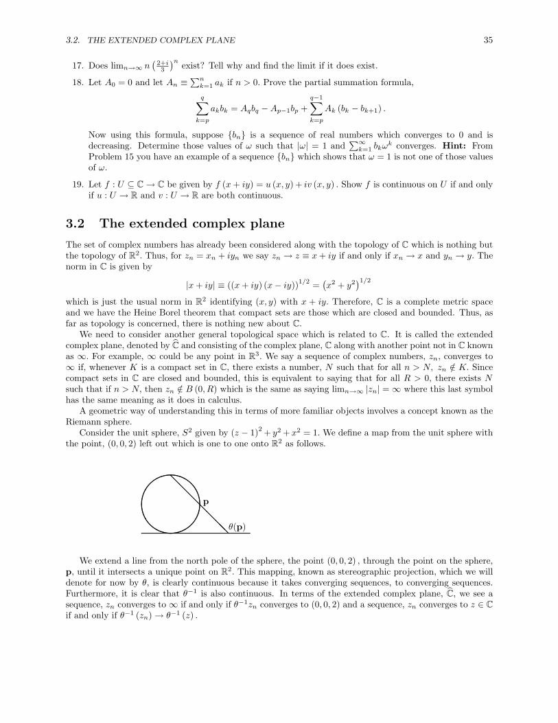
A geometric way of understanding this in terms of more familiar objects involves a concept known as theRiemann sphere.
Consider the unit sphere, S2 given by (z − 1)2 + y2 +x2 = 1. We define a map from the unit sphere withthe point, (0, 0, 2) left out which is one to one onto R2 as follows.
@@@@@@@θ(p)
p
We extend a line from the north pole of the sphere, the point (0, 0, 2) , through the point on the sphere,p, until it intersects a unique point on R2. This mapping, known as stereographic projection, which we willdenote for now by θ, is clearly continuous because it takes converging sequences, to converging sequences.Furthermore, it is clear that θ−1 is also continuous. In terms of the extended complex plane, C, we see asequence, zn converges to ∞ if and only if θ−1zn converges to (0, 0, 2) and a sequence, zn converges to z ∈ Cif and only if θ−1 (zn)→ θ−1 (z) .

36 THE COMPLEX NUMBERS
3.3 Exercises
1. Try to find an explicit formula for θ and θ−1.
2. What does the mapping θ−1 do to lines and circles?
3. Show that S2 is compact but C is not. Thus C 6= S2. Show that a set, K is compact (connected) in Cif and only if θ−1 (K) is compact (connected) in S2 \ {(0, 0, 2)} .
4. Let K be a compact set in C. Show that C \K has exactly one unbounded component and that thiscomponent is the one which is a subset of the component of S2 \K which contains ∞. If you need torewrite using the mapping, θ to make sense of this, it is fine to do so.
5. Make C into a topological space as follows. We define a basis for a topology on C to be all open setsand all complements of compact sets, the latter type being those which are said to contain the point∞. Show this is a basis for a topology which makes C into a compact Hausdorff space. Also verify thatC with this topology is homeomorphic to the sphere, S2.
Riemann Stieltjes integrals
In the theory of functions of a complex variable, the most important results are those involving contourintegration. Before we define what we mean by contour integration, it is necessary to define the notion ofa Riemann Steiltjes integral, a generalization of the usual Riemann integral and the notion of a function ofbounded variation.
Definition 4.1 Let γ : [a, b]→ C be a function. We say γ is of bounded variation if
sup
{n∑i=1
|γ (ti)− γ (ti−1)| : a = t0 < · · · < tn = b
}≡ V (γ, [a, b]) <∞
where the sums are taken over all possible lists, {a = t0 < · · · < tn = b} .
The idea is that it makes sense to talk of the length of the curve γ ([a, b]) , defined as V (γ, [a, b]) . For thisreason, in the case that γ is continuous, such an image of a bounded variation function is called a rectifiablecurve.
Definition 4.2 Let γ : [a, b] → C be of bounded variation and let f : [a, b] → C. Letting P ≡ {t0, · · ·, tn}where a = t0 < t1 < · · · < tn = b, we define
||P|| ≡ max {|tj − tj−1| : j = 1, · · ·, n}
and the Riemann Steiltjes sum by
S (P) ≡n∑j=1
f (τj) (γ (tj)− γ (tj−1))
where τj ∈ [tj−1, tj ] . (Note this notation is a little sloppy because it does not identify the specific point, τjused. It is understood that this point is arbitrary.) We define
∫γf (t) dγ (t) as the unique number which
satisfies the following condition. For all ε > 0 there exists a δ > 0 such that if ||P|| ≤ δ, then∣∣∣∣∫γ
f (t) dγ (t)− S (P)∣∣∣∣ < ε.
Sometimes this is written as ∫γ
f (t) dγ (t) ≡ lim||P||→0
S (P) .
The function, γ ([a, b]) is a set of points in C and as t moves from a to b, γ (t) moves from γ (a) to γ (b) .Thus γ ([a, b]) has a first point and a last point. If φ : [c, d]→ [a, b] is a continuous nondecreasing function,then γ ◦ φ : [c, d]→ C is also of bounded variation and yields the same set of points in C with the same firstand last points. In the case where the values of the function, f, which are of interest are those on γ ([a, b]) ,we have the following important theorem on change of parameters.
37
38 RIEMANN STIELTJES INTEGRALS
Theorem 4.3 Let φ and γ be as just described. Then assuming that∫γ
f (γ (t)) dγ (t)
exists, so does ∫γ◦φ
f (γ (φ (s))) d (γ ◦ φ) (s)
and ∫γ
f (γ (t)) dγ (t) =∫γ◦φ
f (γ (φ (s))) d (γ ◦ φ) (s) . (4.1)
Proof: There exists δ > 0 such that if P is a partition of [a, b] such that ||P|| < δ, then∣∣∣∣∫γ
f (γ (t)) dγ (t)− S (P)∣∣∣∣ < ε.
By continuity of φ, there exists σ > 0 such that if Q is a partition of [c, d] with ||Q|| < σ,Q = {s0, · · ·, sn} ,then |φ (sj)− φ (sj−1)| < δ. Thus letting P denote the points in [a, b] given by φ (sj) for sj ∈ Q, it followsthat ||P|| < δ and so∣∣∣∣∣∣
∫γ
f (γ (t)) dγ (t)−n∑j=1
f (γ (φ (τj))) (γ (φ (sj))− γ (φ (sj−1)))
∣∣∣∣∣∣ < ε
where τj ∈ [sj−1, sj ] . Therefore, from the definition we see that (4.1) holds and that∫γ◦φ
f (γ (φ (s))) d (γ ◦ φ) (s)
exists.This theorem shows that
∫γf (γ (t)) dγ (t) is independent of the particular γ used in its computation to
the extent that if φ is any nondecreasing function from another interval, [c, d] , mapping to [a, b] , then thesame value is obtained by replacing γ with γ ◦ φ.
The fundamental result in this subject is the following theorem.
Theorem 4.4 Let f : [a, b] → C be continuous and let γ : [a, b] → C be of bounded variation. Then∫γf (t) dγ (t) exists. Also if δm > 0 is such that |t− s| < δm implies |f (t)− f (s)| < 1
m , then∣∣∣∣∫γ
f (t) dγ (t)− S (P)∣∣∣∣ ≤ 2V (γ, [a, b])
m
whenever ||P|| < δm.
Proof: The function, f , is uniformly continuous because it is defined on a compact set. Therefore, thereexists a decreasing sequence of positive numbers, {δm} such that if |s− t| < δm, then
|f (t)− f (s)| < 1m.
Let
Fm ≡ {S (P) : ||P|| < δm}.
39
Thus Fm is a closed set. (When we write S (P) in the above definition, we mean to include all sumscorresponding to P for any choice of τj .) We wish to show that
diam (Fm) ≤ 2V (γ, [a, b])m
(4.2)
because then there will exist a unique point, I ∈ ∩∞m=1Fm. It will then follow that I =∫γf (t) dγ (t) . To
verify (4.2), it suffices to verify that whenever P and Q are partitions satisfying ||P|| < δm and ||Q|| < δm,
|S (P)− S (Q)| ≤ 2mV (γ, [a, b]) . (4.3)
Suppose ||P|| < δm andQ ⊇ P. Then also ||Q|| < δm. To begin with, suppose that P ≡ {t0, · · ·, tp, · · ·, tn}and Q ≡ {t0, · · ·, tp−1, t
∗, tp, · · ·, tn} . Thus Q contains only one more point than P. Letting S (Q) and S (P)be Riemann Steiltjes sums,
S (Q) ≡p−1∑j=1
f (σj) (γ (tj)− γ (tj−1)) + f (σ∗) (γ (t∗)− γ (tp−1))
+f (σ∗) (γ (tp)− γ (t∗)) +n∑
j=p+1
f (σj) (γ (tj)− γ (tj−1)) ,
S (P) ≡p−1∑j=1
f (τj) (γ (tj)− γ (tj−1)) +
=f(τp)(γ(tp)−γ(tp−1))︷ ︸︸ ︷f (τp) (γ (t∗)− γ (tp−1)) + f (τp) (γ (tp)− γ (t∗))
+n∑
j=p+1
f (τj) (γ (tj)− γ (tj−1)) .
Therefore,
|S (P)− S (Q)| ≤p−1∑j=1
1m|γ (tj)− γ (tj−1)|+ 1
m|γ (t∗)− γ (tp−1)|+
1m|γ (tp)− γ (t∗)|+
n∑j=p+1
1m|γ (tj)− γ (tj−1)| ≤ 1
mV (γ, [a, b]) . (4.4)
Clearly the extreme inequalities would be valid in (4.4) if Q had more than one extra point. We wouldsimply do the above trick more than one time. Let S (P) and S (Q) be Riemann Steiltjes sums for which||P|| and ||Q|| are less than δm and let R ≡ P ∪Q. Then from what was just observed,
|S (P)− S (Q)| ≤ |S (P)− S (R)|+ |S (R)− S (Q)| ≤ 2mV (γ, [a, b]) .
and this shows (4.3) which proves (4.2). Therefore, there exists a unique complex number, I ∈ ∩∞m=1Fmwhich satisfies the definition of
∫γf (t) dγ (t) . This proves the theorem.
The following theorem follows easily from the above definitions and theorem.
40 RIEMANN STIELTJES INTEGRALS
Theorem 4.5 Let f ∈ C ([a, b]) and let γ : [a, b]→ C be of bounded variation. Let
M ≥ max {|f (t)| : t ∈ [a, b]} . (4.5)
Then ∣∣∣∣∫γ
f (t) dγ (t)∣∣∣∣ ≤MV (γ, [a, b]) . (4.6)
Also if {fn} is a sequence of functions of C ([a, b]) which is converging uniformly to the function, f, then
limn→∞
∫γ
fn (t) dγ (t) =∫γ
f (t) dγ (t) . (4.7)
Proof: Let (4.5) hold. From the proof of the above theorem we know that when ||P|| < δm,∣∣∣∣∫γ
f (t) dγ (t)− S (P)∣∣∣∣ ≤ 2
mV (γ, [a, b])
and so ∣∣∣∣∫γ
f (t) dγ (t)∣∣∣∣ ≤ |S (P)|+ 2
mV (γ, [a, b])
≤n∑j=1
M |γ (tj)− γ (tj−1)|+ 2mV (γ, [a, b])
≤ MV (γ, [a, b]) +2mV (γ, [a, b]) .
This proves (4.6) since m is arbitrary. To verify (4.7) we use the above inequality to write∣∣∣∣∫γ
f (t) dγ (t)−∫γ
fn (t) dγ (t)∣∣∣∣ =
∣∣∣∣∫γ
(f (t)− fn (t)) dγ (t)∣∣∣∣
≤ max {|f (t)− fn (t)| : t ∈ [a, b]}V (γ, [a, b]) .
Since the convergence is assumed to be uniform, this proves (4.7).It turns out that we will be mainly interested in the case where γ is also continuous in addition to being
of bounded variation. Also, it turns out to be much easier to evaluate such integrals in the case where γis also C1 ([a, b]) . The following theorem about approximation will be very useful but first we give an easylemma.
Lemma 4.6 Let γ : [a, b]→ C be in C1 ([a, b]) . Then V (γ, [a, b]) <∞ so γ is of bounded variation.
Proof: This follows from the followingn∑j=1
|γ (tj)− γ (tj−1)| =n∑j=1
∣∣∣∣∣∫ tj
tj−1
γ′ (s) ds
∣∣∣∣∣≤
n∑j=1
∫ tj
tj−1
|γ′ (s)| ds
≤n∑j=1
∫ tj
tj−1
||γ′||∞ ds
= ||γ′||∞ (b− a) .
Therefore it follows V (γ, [a, b]) ≤ ||γ′||∞ (b− a) .
41
Theorem 4.7 Let γ : [a, b]→ C be continuous and of bounded variation, let f : [a, b]×K → C be continuousfor K a compact set in C, and let ε > 0 be given. Then there exists η : [a, b] → C such that η (a) =γ (a) , γ (b) = η (b) , η ∈ C1 ([a, b]) , and
||γ − η|| < ε, (4.8)
∣∣∣∣∫γ
f (t, z) dγ (t)−∫η
f (t, z) dη (t)∣∣∣∣ < ε, (4.9)
V (η, [a, b]) ≤ V (γ, [a, b]) , (4.10)
where ||γ − η|| ≡ max {|γ (t)− η (t)| : t ∈ [a, b]} .
Proof: We extend γ to be defined on all R according to γ (t) = γ (a) if t < a and γ (t) = γ (b) if t > b.Now we define
γh (t) ≡ 12h
∫ t+ 2h(b−a) (t−a)
−2h+t+ 2h(b−a) (t−a)
γ (s) ds.
where the integral is defined in the obvious way. That is,∫ b
a
α (t) + iβ (t) dt ≡∫ b
a
α (t) dt+ i
∫ b
a
β (t) dt.
Therefore,
γh (b) =1
2h
∫ b+2h
b
γ (s) ds = γ (b) ,
γh (a) =1
2h
∫ a
a−2h
γ (s) ds = γ (a) .
Also, because of continuity of γ and the fundamental theorem of calculus,
γ′h (t) =1
2h
{γ
(t+
2hb− a
(t− a))(
1 +2hb− a
)−
γ
(−2h+ t+
2hb− a
(t− a))(
1 +2hb− a
)}and so γh ∈ C1 ([a, b]) . The following lemma is significant.
Lemma 4.8 V (γh, [a, b]) ≤ V (γ, [a, b]) .
Proof: Let a = t0 < t1 < · · · < tn = b. Then using the definition of γh and changing the variables tomake all integrals over [0, 2h] ,
n∑j=1
|γh (tj)− γh (tj−1)| =
42 RIEMANN STIELTJES INTEGRALS
n∑j=1
∣∣∣∣∣ 12h
∫ 2h
0
[γ
(s− 2h+ tj +
2hb− a
(tj − a))−
γ
(s− 2h+ tj−1 +
2hb− a
(tj−1 − a))]∣∣∣∣
≤ 12h
∫ 2h
0
n∑j=1
∣∣∣∣γ (s− 2h+ tj +2hb− a
(tj − a))−
γ
(s− 2h+ tj−1 +
2hb− a
(tj−1 − a))∣∣∣∣ ds.
For a given s ∈ [0, 2h] , the points, s−2h+tj+ 2hb−a (tj − a) for j = 1, · · ·, n form an increasing list of points in
the interval [a− 2h, b+ 2h] and so the integrand is bounded above by V (γ, [a− 2h, b+ 2h]) = V (γ, [a, b]) .It follows
n∑j=1
|γh (tj)− γh (tj−1)| ≤ V (γ, [a, b])
which proves the lemma.With this lemma the proof of the theorem can be completed without too much trouble. First of all, if
ε > 0 is given, there exists δ1 such that if h < δ1, then for all t,
|γ (t)− γh (t)| ≤ 12h
∫ t+ 2h(b−a) (t−a)
−2h+t+ 2h(b−a) (t−a)
|γ (s)− γ (t)| ds
<1
2h
∫ t+ 2h(b−a) (t−a)
−2h+t+ 2h(b−a) (t−a)
εds = ε (4.11)
due to the uniform continuity of γ. This proves (4.8). From (4.2) there exists δ2 such that if ||P|| < δ2, thenfor all z ∈ K, ∣∣∣∣∫
γ
f (t, z) dγ (t)− S (P)∣∣∣∣ < ε
3,
∣∣∣∣∫γh
f (t, z) dγh (t)− Sh (P)∣∣∣∣ < ε
3
for all h. Here S (P) is a Riemann Steiltjes sum of the form
n∑i=1
f (τi, z) (γ (ti)− γ (ti−1))
and Sh (P) is a similar Riemann Steiltjes sum taken with respect to γh instead of γ. Therefore, fix thepartition, P, and choose h small enough that in addition to this, we have the following inequality valid forall z ∈ K.
|S (P)− Sh (P)| < ε
3
We can do this thanks to (4.11) and the uniform continuity of f on [a, b]×K. It follows∣∣∣∣∫γ
f (t, z) dγ (t)−∫γh
f (t, z) dγh (t)∣∣∣∣ ≤

43∣∣∣∣∫γ
f (t, z) dγ (t)− S (P)∣∣∣∣+ |S (P)− Sh (P)|
+∣∣∣∣Sh (P)−
∫γh
f (t, z) dγh (t)∣∣∣∣ < ε.
Formula (4.10) follows from the lemma. This proves the theorem.Of course the same result is obtained without the explicit dependence of f on z.This is a very useful theorem because if γ is C1 ([a, b]) , it is easy to calculate
∫γf (t) dγ (t) . We will
typically reduce to the case where γ is C1 by using the above theorem. The next theorem shows how easy itis to compute these integrals in the case where γ is C1. First note that if f is continuous and γ ∈ C1 ([a, b]) ,then by Lemma 4.6 and the fundamental existence theorem, Theorem 4.4, that
∫γf (t) dγ (t) exists. We only
need to see how to find it.
Theorem 4.9 If f : [a, b]→ C be continuous and γ : [a, b]→ C is in C1 ([a, b]) , then∫γ
f (t) dγ (t) =∫ b
a
f (t) γ′ (t) dt. (4.12)
Proof: Let P be a partition of [a, b], P = {t0, · · ·, tn} and ||P|| is small enough that whenever |t− s| <||P|| ,
|f (t)− f (s)| < ε (4.13)
and ∣∣∣∣∣∣∫γ
f (t) dγ (t)−n∑j=1
f (τj) (γ (tj)− γ (tj−1))
∣∣∣∣∣∣ < ε.
Nown∑j=1
f (τj) (γ (tj)− γ (tj−1)) =∫ b
a
n∑j=1
f (τj)X[tj−1,tj ] (s) γ′ (s) ds
where here
X[a,b] (s) ≡{
1 if s ∈ [a, b]0 if s /∈ [a, b] .
Also, ∫ b
a
f (s) γ′ (s) ds =∫ b
a
n∑j=1
f (s)X[tj−1,tj ] (s) γ′ (s) ds
and thanks to (4.13),∣∣∣∣∣∣∣∣∣∣∣
=∑nj=1 f(τj)(γ(tj)−γ(tj−1))︷ ︸︸ ︷∫ b
a
n∑j=1
f (τj)X[tj−1,tj ] (s) γ′ (s) ds−
=∫ baf(s)γ′(s)ds︷ ︸︸ ︷∫ b
a
n∑j=1
f (s)X[tj−1,tj ] (s) γ′ (s) ds
∣∣∣∣∣∣∣∣∣∣∣
44 RIEMANN STIELTJES INTEGRALS
≤n∑j=1
∫ tj
tj−1
|f (τj)− f (s)| |γ′ (s)| ds ≤ ||γ′||∞∑j
ε (tj − tj−1)
= ε ||γ′||∞ (b− a) .
It follows that∣∣∣∣∣∫γ
f (t) dγ (t)−∫ b
a
f (s) γ′ (s) ds
∣∣∣∣∣ <∣∣∣∣∣∣∫γ
f (t) dγ (t)−n∑j=1
f (τj) (γ (tj)− γ (tj−1))
∣∣∣∣∣∣+
∣∣∣∣∣∣n∑j=1
f (τj) (γ (tj)− γ (tj−1))−∫ b
a
f (s) γ′ (s) ds
∣∣∣∣∣∣ ≤ ε ||γ′||∞ (b− a) + ε.
Since ε is arbitrary, this verifies (4.12).
Definition 4.10 Let γ : [a, b]→ U be a continuous function with bounded variation and let f : U → C be acontinuous function. Then we define, ∫
γ
f (z) dz ≡∫γ
f (γ (t)) dγ (t) .
The expression,∫γf (z) dz, is called a contour integral and γ is referred to as the contour. We also say that
a function f : U → C for U an open set in C has a primitive if there exists a function, F, the primitive, suchthat F ′ (z) = f (z) . Thus F is just an antiderivative. Also if γk : [ak, bk]→ C is continuous and of boundedvariation, for k = 1, · · ·,m and γk (bk) = γk+1 (ak) , we define∫
∑mk=1 γk
f (z) dz ≡m∑k=1
∫γk
f (z) dz. (4.14)
In addition to this, for γ : [a, b] → C, we define −γ : [a, b] → C by −γ (t) ≡ γ (b+ a− t) . Thus γ simplytraces out the points of γ ([a, b]) in the opposite order.
The following lemma is useful and follows quickly from Theorem 4.3.
Lemma 4.11 In the above definition, there exists a continuous bounded variation function, γ defined onsome closed interval, [c, d] , such that γ ([c, d]) = ∪mk=1γk ([ak, bk]) and γ (c) = γ1 (a1) while γ (d) = γm (bm) .Furthermore, ∫
γ
f (z) dz =m∑k=1
∫γk
f (z) dz.
If γ : [a, b]→ C is of bounded variation and continuous, then∫γ
f (z) dz = −∫−γ
f (z) dz.
Theorem 4.12 Let K be a compact set in C and let f : U ×K → C be continuous for U an open set in C.Also let γ : [a, b]→ U be continuous with bounded variation. Then if r > 0 is given, there exists η : [a, b]→ Usuch that η (a) = γ (a) , η (b) = γ (b) , η is C1 ([a, b]) , and∣∣∣∣∫
γ
f (z, w) dz −∫η
f (z, w) dz∣∣∣∣ < r, ||η − γ|| < r.
45
Proof: Let ε > 0 be given and let H be an open set containing γ ([a, b]) such that H is compact. Thenf is uniformly continuous on H ×K and so there exists a δ > 0 such that if zj ∈ H, j = 1, 2 and wj ∈ K forj = 1, 2 such that if
|z1 − z2|+ |w1 − w2| < δ,
then
|f (z1, w1)− f (z2, w2)| < ε.
By Theorem 4.7, let η : [a, b] → C be such that η ([a, b]) ⊆ H, η (x) = γ (x) for x = a, b, η ∈ C1 ([a, b]) ,||η − γ|| < min (δ, r) , V (η, [a, b]) < V (γ, [a, b]) , and∣∣∣∣∫
η
f (γ (t) , w) dη (t)−∫γ
f (γ (t) , w) dγ (t)∣∣∣∣ < ε
for all w ∈ K. Then, since |f (γ (t) , w)− f (η (t) , w)| < ε for all t ∈ [a, b] ,∣∣∣∣∫η
f (γ (t) , w) dη (t)−∫η
f (η (t) , w) dη (t)∣∣∣∣ < εV (η, [a, b]) ≤ εV (γ, [a, b]) .
Therefore, ∣∣∣∣∫η
f (z, w) dz −∫γ
f (z, w) dz∣∣∣∣ =
∣∣∣∣∫η
f (η (t) , w) dη (t)−∫γ
f (γ (t) , w) dγ (t)∣∣∣∣ < ε+ εV (γ, [a, b]) .
Since ε > 0 is arbitrary, this proves the theorem.We will be very interested in the functions which have primitives. It turns out, it is not enough for f to
be continuous in order to possess a primitive. This is in stark contrast to the situation for functions of a realvariable in which the fundamental theorem of calculus will deliver a primitive for any continuous function.The reason for our interest in such functions is the following theorem and its corollary.
Theorem 4.13 Let γ : [a, b] → C be continuous and of bounded variation. Also suppose F ′ (z) = f (z) forall z ∈ U, an open set containing γ ([a, b]) and f is continuous on U. Then∫
γ
f (z) dz = F (γ (b))− F (γ (a)) .
Proof: By Theorem 4.12 there exists η ∈ C1 ([a, b]) such that γ (a) = η (a) , and γ (b) = η (b) such that∣∣∣∣∫γ
f (z) dz −∫η
f (z) dz∣∣∣∣ < ε.
Then since η is in C1 ([a, b]) , we may write∫η
f (z) dz =∫ b
a
f (η (t)) η′ (t) dt =∫ b
a
dF (η (t))dt
dt
= F (η (b))− F (η (a)) = F (γ (b))− F (γ (a)) .
Therefore, ∣∣∣∣(F (γ (b))− F (γ (a)))−∫γ
f (z) dz∣∣∣∣ < ε
and since ε > 0 is arbitrary, this proves the theorem.
46 RIEMANN STIELTJES INTEGRALS
Corollary 4.14 If γ : [a, b]→ C is continuous, has bounded variation, is a closed curve, γ (a) = γ (b) , andγ ([a, b]) ⊆ U where U is an open set on which F ′ (z) = f (z) , then∫
γ
f (z) dz = 0.
4.1 Exercises
1. Let γ : [a, b]→ R be increasing. Show V (γ, [a, b]) = γ (b)− γ (a) .
2. Suppose γ : [a, b]→ C satisfies a Lipschitz condition, |γ (t)− γ (s)| ≤ K |s− t| . Show γ is of boundedvariation and that V (γ, [a, b]) ≤ K |b− a| .
3. We say γ : [c0, cm] → C is piecewise smooth if there exist numbers, ck, k = 1, · · ·,m such thatc0 < c1 < · · · < cm−1 < cm such that γ is continuous and γ : [ck, ck+1] → C is C1. Show that suchpiecewise smooth functions are of bounded variation and give an estimate for V (γ, [c0, cm]) .
4. Let γ : [0, 2π]→ C be given by γ (t) = r (cosmt+ i sinmt) for m an integer. Find∫γdzz .
5. Show that if γ : [a, b] → C then there exists an increasing function h : [0, 1] → [a, b] such thatγ ◦ h ([0, 1]) = γ ([a, b]) .
6. Let γ : [a, b]→ C be an arbitrary continuous curve having bounded variation and let f, g have contin-uous derivatives on some open set containing γ ([a, b]) . Prove the usual integration by parts formula.∫
γ
fg′dz = f (γ (b)) g (γ (b))− f (γ (a)) g (γ (a))−∫γ
f ′gdz.
7. Let f (z) ≡ |z|−(1/2)e−i
θ2 where z = |z| eiθ. This function is called the principle branch of z−(1/2). Find∫
γf (z) dz where γ is the semicircle in the upper half plane which goes from (1, 0) to (−1, 0) in the
counter clockwise direction. Next do the integral in which γ goes in the clockwise direction along thesemicircle in the lower half plane.
8. Prove an open set, U is connected if and only if for every two points in U, there exists a C1 curvehaving values in U which joins them.
9. Let P,Q be two partitions of [a, b] with P ⊆ Q. Each of these partitions can be used to form anapproximation to V (γ, [a, b]) as described above. Recall the total variation was the supremum of sumsof a certain form determined by a partition. How is the sum associated with P related to the sumassociated with Q? Explain.
10. Consider the curve,
γ (t) ={t+ it2 sin
(1t
)if t ∈ (0, 1]
0 if t = 0 .
Is γ a continuous curve having bounded variation? What if the t2 is replaced with t? Is the resultingcurve continuous? Is it a bounded variation curve?
11. Suppose γ : [a, b]→ R is given by γ (t) = t. What is∫γf (t) dγ? Explain.

Analytic functions
In this chapter we define what we mean by an analytic function and give a few important examples offunctions which are analytic.
Definition 5.1 Let U be an open set in C and let f : U → C. We say f is analytic on U if for every z ∈ U,
limh→0
f (z + h)− f (z)h
≡ f ′ (z)
exists and is a continuous function of z ∈ U. Here h ∈ C.
Note that if f is analytic, it must be the case that f is continuous. It is more common to not include therequirement that f ′ is continuous but we will show later that the continuity of f ′ follows.
What are some examples of analytic functions? The simplest example is any polynomial. Thus
p (z) ≡n∑k=0
akzk
is an analytic function and
p′ (z) =n∑k=1
akkzk−1.
We leave the verification of this as an exercise. More generally, power series are analytic. We will showthis later. For now, we consider the very important Cauchy Riemann equations which give conditions underwhich complex valued functions of a complex variable are analytic.
Theorem 5.2 Let U be an open subset of C and let f : U → C be a function, such that for z = x+ iy ∈ U,
f (z) = u (x, y) + iv (x, y) .
Then f is analytic if and only if u, v are C1 (U) and
∂u
∂x=∂v
∂y,∂u
∂y= −∂v
∂x.
Furthermore, we have the formula,
f ′ (z) =∂u
∂x(x, y) + i
∂v
∂x(x, y) .
47

48 ANALYTIC FUNCTIONS
Proof: Suppose f is analytic first. Then letting t ∈ R,
f ′ (z) = limt→0
f (z + t)− f (z)t
=
limt→0
(u (x+ t, y) + iv (x+ t, y)
t− u (x, y) + iv (x, y)
t
)
=∂u (x, y)∂x
+ i∂v (x, y)∂x
.
But also
f ′ (z) = limt→0
f (z + it)− f (z)it
=
limt→0
(u (x, y + t) + iv (x, y + t)
it− u (x, y) + iv (x, y)
it
)
1i
(∂u (x, y)∂y
+ i∂v (x, y)∂y
)
=∂v (x, y)∂y
− i∂u (x, y)∂y
.
This verifies the Cauchy Riemann equations. We are assuming that z → f ′ (z) is continuous. Therefore, thepartial derivatives of u and v are also continuous. To see this, note that from the formulas for f ′ (z) givenabove, and letting z1 = x1 + iy1∣∣∣∣∂v (x, y)
∂y− ∂v (x1, y1)
∂y
∣∣∣∣ ≤ |f ′ (z)− f ′ (z1)| ,
showing that (x, y)→ ∂v(x,y)∂y is continuous since (x1, y1)→ (x, y) if and only if z1 → z. The other cases are
similar.Now suppose the Cauchy Riemann equations hold and the functions, u and v are C1 (U) . Then letting
h = h1 + ih2,
f (z + h)− f (z) = u (x+ h1, y + h2)
+iv (x+ h1, y + h2)− (u (x, y) + iv (x, y))
We know u and v are both differentiable and so
f (z + h)− f (z) =∂u
∂x(x, y)h1 +
∂u
∂y(x, y)h2 +
i
(∂v
∂x(x, y)h1 +
∂v
∂y(x, y)h2
)+ o (h) .

5.1. EXERCISES 49
Dividing by h and using the Cauchy Riemann equations,
f (z + h)− f (z)h
=∂u∂x (x, y)h1 + i∂v∂y (x, y)h2
h+
i ∂v∂x (x, y)h1 + ∂u∂y (x, y)h2
h+o (h)h
=∂u
∂x(x, y)
h1 + ih2
h+ i
∂v
∂x(x, y)
h1 + ih2
h+o (h)h
Taking the limit as h→ 0, we obtain
f ′ (z) =∂u
∂x(x, y) + i
∂v
∂x(x, y) .
It follows from this formula and the assumption that u, v are C1 (U) that f ′ is continuous.It is routine to verify that all the usual rules of derivatives hold for analytic functions. In particular, we
have the product rule, the chain rule, and quotient rule.
5.1 Exercises
1. Verify all the usual rules of differentiation including the product and chain rules.
2. Suppose f and f ′ : U → C are analytic and f (z) = u (x, y) + iv (x, y) . Verify uxx + uyy = 0and vxx + vyy = 0. This partial differential equation satisfied by the real and imaginary parts ofan analytic function is called Laplace’s equation. We say these functions satisfying Laplace’s equa-tion are harmonic functions. If u is a harmonic function defined on B (0, r) show that v (x, y) ≡∫ y
0ux (x, t) dt−
∫ x0uy (t, 0) dt is such that u+ iv is analytic.
3. Define a function f (z) ≡ z ≡ x− iy where z = x+ iy. Is f analytic?
4. If f (z) = u (x, y) + iv (x, y) and f is analytic, verify that
det(ux uyvx vy
)= |f ′ (z)|2 .
5. Show that if u (x, y) + iv (x, y) = f (z) is analytic, then ∇u · ∇v = 0. Recall
∇u (x, y) = 〈ux (x, y) , uy (x, y)〉.
6. Show that every polynomial is analytic.
7. If γ (t) = x (t) + iy (t) is a C1 curve having values in U, an open set of C, and if f : U → C is analytic,we can consider f ◦ γ, another C1 curve having values in C. Also, γ′ (t) and (f ◦ γ)′ (t) are complexnumbers so these can be considered as vectors in R2 as follows. The complex number, x+iy correspondsto the vector, 〈x, y〉. Suppose that γ and η are two such C1 curves having values in U and thatγ (t0) = η (s0) = z and suppose that f : U → C is analytic. Show that the angle between (f ◦ γ)′ (t0)and (f ◦ η)′ (s0) is the same as the angle between γ′ (t0) and η′ (s0) assuming that f ′ (z) 6= 0. Thusanalytic mappings preserve angles at points where the derivative is nonzero. Such mappings are calledisogonal. . Hint: To make this easy to show, first observe that 〈x, y〉 · 〈a, b〉 = 1
2 (zw + zw) wherez = x+ iy and w = a+ ib.
50 ANALYTIC FUNCTIONS
8. Analytic functions are even better than what is described in Problem 7. In addition to preservingangles, they also preserve orientation. To verify this show that if z = x + iy and w = a + ib aretwo complex numbers, then 〈x, y, 0〉 and 〈a, b, 0〉 are two vectors in R3. Recall that the cross product,〈x, y, 0〉×〈a, b, 0〉, yields a vector normal to the two given vectors such that the triple, 〈x, y, 0〉, 〈a, b, 0〉,and 〈x, y, 0〉 × 〈a, b, 0〉 satisfies the right hand rule and has magnitude equal to the product of the sineof the included angle times the product of the two norms of the vectors. In this case, the cross producteither points in the direction of the positive z axis or in the direction of the negative z axis. Thus, eitherthe vectors 〈x, y, 0〉, 〈a, b, 0〉,k form a right handed system or the vectors 〈a, b, 0〉, 〈x, y, 0〉,k form a righthanded system. These are the two possible orientations. Show that in the situation of Problem 7 theorientation of γ′ (t0) , η′ (s0) ,k is the same as the orientation of the vectors (f ◦ γ)′ (t0) , (f ◦ η)′ (s0) ,k.Such mappings are called conformal. If f is analytic and f ′ (z) 6= 0, then we know from this problemand the above that f is a conformal map. Hint: You can do this by verifying that (f ◦ γ)′ (t0) ×(f ◦ η)′ (s0) = |f ′ (γ (t0))|2 γ′ (t0) × η′ (s0). To make the verification easier, you might first establishthe following simple formula for the cross product where here x+ iy = z and a+ ib = w.
〈x, y, 0〉 × 〈a, b, 0〉 = Re (ziw) k.
9. Write the Cauchy Riemann equations in terms of polar coordinates. Recall the polar coordinates aregiven by
x = r cos θ, y = r sin θ.
This means, letting u (x, y) = u (r, θ) , v (x, y) = v (r, θ) , write the Cauchy Riemann equations in termsof r and θ. You should eventually show the Cauchy Riemann equations are equivalent to
∂u
∂r=
1r
∂v
∂θ,∂v
∂r= −1
r
∂u
∂θ
5.2 Examples of analytic functions
A very important example of an analytic function is ez ≡ ex (cos y + i sin y) ≡ exp (z) . We can verifythis is an analytic function by considering the Cauchy Riemann equations. Here u (x, y) = ex cos y andv (x, y) = ex sin y. The Cauchy Riemann equations hold and the two functions u and v are C1 (C) . Therefore,z → ez is an analytic function on all of C. Also from the formula for f ′ (z) given above for an analytic function,
d
dzez = ex (cos y + i sin y) = ez.
We also see that ez = 1 if and only if z = 2πk for k an integer. Other properties of ez follow from theformula for it. For example, let zj = xj + iyj where j = 1, 2.
ez1ez2 ≡ ex1 (cos y1 + i sin y1) ex2 (cos y2 + i sin y2)= ex1+x2 (cos y1 cos y2 − sin y1 sin y2) +
iex1+x2 (sin y1 cos y2 + sin y2 cos y1)
= ex1+x2 (cos (y1 + y2) + i sin (y1 + y2)) = ez1+z2 .
Another example of an analytic function is any polynomial. We can also define the functions cos z andsin z by the usual formulas.
sin z ≡ eiz − e−iz
2i, cos z ≡ eiz + e−iz
2.
5.3. EXERCISES 51
By the rules of differentiation, it is clear these are analytic functions which agree with the usual functionsin the case where z is real. Also the usual differentiation formulas hold. However,
cos ix =e−x + ex
2= coshx
and so cos z is not bounded. Similarly sin z is not bounded.A more interesting example is the log function. We cannot define the log for all values of z but if we
leave out the ray, (−∞, 0], then it turns out we can do so. On R + i (−π, π) it is easy to see that ez is oneto one, mapping onto C \ (−∞, 0]. Therefore, we can define the log on C \ (−∞, 0] in the usual way,
elog z ≡ z = eln|z|ei arg(z),
where arg (z) is the unique angle in (−π, π) for which the equal sign in the above holds. Thus we need
log z = ln |z|+ i arg (z) . (5.1)
There are many other ways to define a logarithm. In fact, we could take any ray from 0 and define alogarithm on what is left. It turns out that all these logarithm functions are analytic. This will be clearfrom the open mapping theorem presented later but for now you may verify by brute force that the usualdefinition of the logarithm, given in (5.1) and referred to as the principle branch of the logarithm is analytic.This can be done by verifying the Cauchy Riemann equations in the following.
log z = ln(x2 + y2
)1/2+ i
(− arccos
(x√
x2 + y2
))if y < 0,
log z = ln(x2 + y2
)1/2+ i
(arccos
(x√
x2 + y2
))if y > 0,
log z = ln(x2 + y2
)1/2+ i(
arctan(yx
))if x > 0.
With the principle branch of the logarithm defined, we may define the principle branch of zα for any α ∈ C.We define
zα ≡ eα log(z).
5.3 Exercises
1. Verify the principle branch of the logarithm is an analytic function.
2. Find ii corresponding to the principle branch of the logarithm.
3. Show that sin (z + w) = sin z cosw + cos z sinw.
4. If f is analytic on U, an open set in C, when can it be concluded that |f | is analytic? When can it beconcluded that |f | is continuous? Prove your assertions.
5. Let f (z) = z where z ≡ x− iy for z = x+ iy. Describe geometrically what f does and discuss whetherf is analytic.

52 ANALYTIC FUNCTIONS
6. A fractional linear transformation is a function of the form
f (z) =az + b
cz + d
where ad− bc 6= 0. Note that if c = 0, this reduces to a linear transformation (a/d) z + (b/d) . Specialcases of these are given defined as follows.
dilations: z → δz, δ 6= 0, inversions: z → 1z,
translations: z → z + ρ.
In the case where c 6= 0, let S1 (z) = z + dc , S2 (z) = 1
z , S3 (z) = (bc−ad)c2 z and S4 (z) = z + a
c . Verifythat f (z) = S4 ◦ S3 ◦ S2 ◦ S1. Now show that in the case where c = 0, f is still a finite composition ofdilations, inversions, and translations.
7. Show that for a fractional linear transformation described in Problem 6 circles and lines are mappedto circles or lines. Hint: This is obvious for dilations, and translations. It only remains to verify thisfor inversions. Note that all circles and lines may be put in the form
α(x2 + y2
)− 2ax− 2by = r2 −
(a2 + b2
)where α = 1 gives a circle centered at (a, b) with radius r and α = 0 gives a line. In terms of complexvariables we may consider all possible circles and lines in the form
αzz + βz + βz + γ = 0,
Verify every circle or line is of this form and that conversely, every expression of this form yields eithera circle or a line. Then verify that inversions do what is claimed.
8. It is desired to find an analytic function, L (z) defined for all z ∈ C \ {0} such that eL(z) = z. Is thispossible? Explain why or why not.
9. If f is analytic, show that z → f (z) is also analytic.
10. Find the real and imaginary parts of the principle branch of z1/2.
Cauchy’s formula for a disk
In this chapter we prove the Cauchy formula for a disk. Later we will generalize this formula to much moregeneral situations but the version given here will suffice to prove many interesting theorems needed in thelater development of the theory. First we give a few preliminary results from advanced calculus.
Lemma 6.1 Let f : [a, b]→ C. Then f ′ (t) exists if and only if Ref ′ (t) and Imf ′ (t) exist. Furthermore,
f ′ (t) = Ref ′ (t) + iImf ′ (t) .
Proof: The if part of the equivalence is obvious.Now suppose f ′ (t) exists. Let both t and t+ h be contained in [a, b]∣∣∣∣Ref (t+ h)− Ref (t)
h− Re (f ′ (t))
∣∣∣∣ ≤ ∣∣∣∣f (t+ h)− f (t)h
− f ′ (t)∣∣∣∣
and this converges to zero as h→ 0. Therefore, Ref ′ (t) = Re (f ′ (t)) . Similarly, Imf ′ (t) = Im (f ′ (t)) .
Lemma 6.2 If g : [a, b] → C and g is continuous on [a, b] and differentiable on (a, b) with g′ (t) = 0, theng (t) is a constant.
Proof: From the above lemma, we can apply the mean value theorem to the real and imaginary partsof g.
Lemma 6.3 Let φ : [a, b]× [c, d]→ R be continuous and let
g (t) ≡∫ b
a
φ (s, t) ds. (6.1)
Then g is continuous. If ∂φ∂t exists and is continuous on [a, b]× [c, d] , then
g′ (t) =∫ b
a
∂φ (s, t)∂t
ds. (6.2)
Proof: The first claim follows from the uniform continuity of φ on [a, b]× [c, d] , which uniform continuityresults from the set being compact. To establish (6.2), let t and t+ h be contained in [c, d] and form, usingthe mean value theorem,
g (t+ h)− g (t)h
=1h
∫ b
a
[φ (s, t+ h)− φ (s, t)] ds
=1h
∫ b
a
∂φ (s, t+ θh)∂t
hds
=∫ b
a
∂φ (s, t+ θh)∂t
ds,
53
54 CAUCHY’S FORMULA FOR A DISK
where θ may depend on s but is some number between 0 and 1. Then by the uniform continuity of ∂φ∂t , it
follows that (6.2) holds.
Corollary 6.4 Let φ : [a, b]× [c, d]→ C be continuous and let
g (t) ≡∫ b
a
φ (s, t) ds. (6.3)
Then g is continuous. If ∂φ∂t exists and is continuous on [a, b]× [c, d] , then
g′ (t) =∫ b
a
∂φ (s, t)∂t
ds. (6.4)
Proof: Apply Lemma 6.3 to the real and imaginary parts of φ.With this preparation we are ready to prove Cauchy’s formula for a disk.
Theorem 6.5 Let f : U → C be analytic on the open set, U and let
B (z0, r) ⊆ U.
Let γ (t) ≡ z0 + reit for t ∈ [0, 2π] . Then if z ∈ B (z0, r) ,
f (z) =1
2πi
∫γ
f (w)w − z
dw. (6.5)
Proof: Consider for α ∈ [0, 1] ,
g (α) ≡∫ 2π
0
f(z + α
(z0 + reit − z
))reit + z0 − z
rieitdt.
If α equals one, this reduces to the integral in (6.5). We will show g is a constant and that g (0) = f (z) 2πi.First we consider the claim about g (0) .
g (0) =(∫ 2π
0
reit
reit + z0 − zdt
)if (z)
= if (z)(∫ 2π
0
11− z−z0
reit
dt
)= if (z)
∫ 2π
0
∞∑n=0
r−ne−int (z − z0)n dt
because∣∣ z−z0reit
∣∣ < 1. Since this sum converges uniformly we may interchange the sum and the integral toobtain
g (0) = if (z)∞∑n=0
r−n (z − z0)n∫ 2π
0
e−intdt
= 2πif (z)
because∫ 2π
0e−intdt = 0 if n > 0.
55
Next we show that g is constant. By Corollary 6.4, for α ∈ (0, 1) ,
g′ (α) =∫ 2π
0
f ′(z + α
(z0 + reit − z
)) (reit + z0 − z
)reit + z0 − z
rieitdt
=∫ 2π
0
f ′(z + α
(z0 + reit − z
))rieitdt
=∫ 2π
0
d
dt
(f(z + α
(z0 + reit − z
)) 1α
)dt
= f(z + α
(z0 + rei2π − z
)) 1α− f
(z + α
(z0 + re0 − z
)) 1α
= 0.
Now g is continuous on [0, 1] and g′ (t) = 0 on (0, 1) so by Lemma 6.2, g equals a constant. This constantcan only be g (0) = 2πif (z) . Thus,
g (1) =∫γ
f (w)w − z
dw = g (0) = 2πif (z) .
This proves the theorem.This is a very significant theorem. We give a few applications next.
Theorem 6.6 Let f : U → C be analytic where U is an open set in C. Then f has infinitely many derivativeson U . Furthermore, for all z ∈ B (z0, r) ,
f (n) (z) =n!
2πi
∫γ
f (w)(w − z)n+1 dw (6.6)
where γ (t) ≡ z0 + reit, t ∈ [0, 2π] for r small enough that B (z0, r) ⊆ U.
Proof: Let z ∈ B (z0, r) ⊆ U and let B (z0, r) ⊆ U. Then, letting γ (t) ≡ z0 + reit, t ∈ [0, 2π] , and hsmall enough,
f (z) =1
2πi
∫γ
f (w)w − z
dw, f (z + h) =1
2πi
∫γ
f (w)w − z − h
dw
Now
1w − z − h
− 1w − z
=h
(−w + z + h) (−w + z)
and so
f (z + h)− f (z)h
=1
2πhi
∫γ
hf (w)(−w + z + h) (−w + z)
dw
=1
2πi
∫γ
f (w)(−w + z + h) (−w + z)
dw.
Now for all h sufficiently small, there exists a constant C independent of such h such that∣∣∣∣ 1(−w + z + h) (−w + z)
− 1(−w + z) (−w + z)
∣∣∣∣=
∣∣∣∣∣ h
(w − z − h) (w − z)2
∣∣∣∣∣ ≤ C |h|

56 CAUCHY’S FORMULA FOR A DISK
and so, the integrand converges uniformly as h→ 0 to
=f (w)
(w − z)2
Therefore, we may take the limit as h→ 0 inside the integral to obtain
f ′ (z) =1
2πi
∫γ
f (w)(w − z)2 dw.
Continuing in this way, we obtain (6.6).This is a very remarkable result. We just showed that the existence of one continuous derivative implies
the existence of all derivatives, in contrast to the theory of functions of a real variable. Actually, we justshowed a little more than what the theorem states. The above proof establishes the following corollary.
Corollary 6.7 Suppose f is continuous on ∂B (z0, r) and suppose that for all z ∈ B (z0, r) ,
f (z) =1
2πi
∫γ
f (w)w − z
dw,
where γ (t) ≡ z0 + reit, t ∈ [0, 2π] . Then f is analytic on B (z0, r) and in fact has infinitely many derivativeson B (z0, r) .
We also have the following simple lemma as an application of the above.
Lemma 6.8 Let γ (t) = z0 + reit, for t ∈ [0, 2π], suppose fn → f uniformly on B (z0, r), and suppose
fn (z) =1
2πi
∫γ
fn (w)w − z
dw (6.7)
for z ∈ B (z0, r) . Then
f (z) =1
2πi
∫γ
f (w)w − z
dw, (6.8)
implying that f is analytic on B (z0, r) .
Proof: From (6.7) and the uniform convergence of fn to f on γ ([0, 2π]) , we have that the integrals in(6.7) converge to
12πi
∫γ
f (w)w − z
dw.
Therefore, the formula (6.8) follows.
Proposition 6.9 Let {an} denote a sequence of complex numbers. Then there exists R ∈ [0,∞] such that
∞∑k=0
ak (z − z0)k
converges absolutely if |z − z0| < R, diverges if |z − z0| > R and converges uniformly on B (z0, r) for allr < R. Furthermore, if R > 0, the function,
f (z) ≡∞∑k=0
ak (z − z0)k
is analytic on B (z0, R) .

57
Proof: The assertions about absolute convergence are routine from the root test if we define
R ≡(
lim supn→∞
|an|1/n)−1
with R = ∞ if the quantity in parenthesis equals zero. The assertion about uniform convergence followsfrom the Weierstrass M test if we use Mn ≡ |an| rn. (
∑∞n=0 |an| rn < ∞ by the root test). It only remains
to verify the assertion about f (z) being analytic in the case where R > 0. Let 0 < r < R and definefn (z) ≡
∑nk=0 ak (z − z0)k . Then fn is a polynomial and so it is analytic. Thus, by the Cauchy integral
formula above,
fn (z) =1
2πi
∫γ
fn (w)w − z
dw
where γ (t) = z0 + reit, for t ∈ [0, 2π] . By Lemma 6.8 and the first part of this proposition involving uniformconvergence, we obtain
f (z) =1
2πi
∫γ
f (w)w − z
dw.
Therefore, f is analytic on B (z0, r) by Corollary 6.7. Since r < R is arbitrary, this shows f is analytic onB (z0, R) .
This proposition shows that all functions which are given as power series are analytic on their circleof convergence, the set of complex numbers, z, such that |z − z0| < R. Next we show that every analyticfunction can be realized as a power series.
Theorem 6.10 If f : U → C is analytic and if B (z0, r) ⊆ U, then
f (z) =∞∑n=0
an (z − z0)n (6.9)
for all |z − z0| < r. Furthermore,
an =f (n) (z0)
n!. (6.10)
Proof: Consider |z − z0| < r and let γ (t) = z0 + reit, t ∈ [0, 2π] . Then for w ∈ γ ([0, 2π]) ,∣∣∣∣ z − z0
w − z0
∣∣∣∣ < 1
and so, by the Cauchy integral formula, we may write
f (z) =1
2πi
∫γ
f (w)w − z
dw
=1
2πi
∫γ
f (w)
(w − z0)(
1− z−z0w−z0
)dw=
12πi
∫γ
f (w)(w − z0)
∞∑n=0
(z − z0
w − z0
)ndw.
Since the series converges uniformly, we may interchange the integral and the sum to obtain
f (z) =∞∑n=0
(1
2πi
∫γ
f (w)(w − z0)n+1
)(z − z0)n
≡∞∑n=0
an (z − z0)n

58 CAUCHY’S FORMULA FOR A DISK
By Theorem 6.6 we see that (6.10) holds.The following theorem pertains to functions which are analytic on all of C, “entire” functions.
Theorem 6.11 (Liouville’s theorem) If f is a bounded entire function then f is a constant.
Proof: Since f is entire, we can pick any z ∈ C and write
f ′ (z) =1
2πi
∫γR
f (w)(w − z)2 dw
where γR (t) = z +Reit for t ∈ [0, 2π] . Therefore,
|f ′ (z)| ≤ C 1R
where C is some constant depending on the assumed bound on f. Since R is arbitrary, we can take R→∞ toobtain f ′ (z) = 0 for any z ∈ C. It follows from this that f is constant for if zj j = 1, 2 are two complex num-bers, we can consider h (t) = f (z1 + t (z2 − z1)) for t ∈ [0, 1] . Then h′ (t) = f ′ (z1 + t (z2 − z1)) (z2 − z1) = 0.By Lemma 6.2 h is a constant on [0, 1] which implies f (z1) = f (z2) .
With Liouville’s theorem it becomes possible to give an easy proof of the fundamental theorem of algebra.It is ironic that all the best proofs of this theorem in algebra come from the subjects of analysis or topology.Out of all the proofs that have been given of this very important theorem, the following one based onLiouville’s theorem is the easiest.
Theorem 6.12 (Fundamental theorem of Algebra) Let
p (z) = zn + an−1zn−1 + · · ·+ a1z + a0
be a polynomial where n ≥ 1 and each coefficient is a complex number. Then there exists z0 ∈ C such thatp (z0) = 0.
Proof: Suppose not. Then p (z)−1 is an entire function. Also
|p (z)| ≥ |z|n −(|an−1| |z|n−1 + · · ·+ |a1| |z|+ |a0|
)and so lim|z|→∞ |p (z)| = ∞ which implies lim|z|→∞
∣∣∣p (z)−1∣∣∣ = 0. It follows that, since p (z)−1 is bounded
for z in any bounded set, we must have that p (z)−1 is a bounded entire function. But then it must beconstant. However since p (z)−1 → 0 as |z| → ∞, this constant can only be 0. However, 1
p(z) is never equalto zero. This proves the theorem.
6.1 Exercises
1. Show that if |ek| ≤ ε, then∣∣∑∞
k=m ek(rk − rk+1
)∣∣ < ε if 0 ≤ r < 1. Hint: Let |θ| = 1 and verify that
θ∞∑k=m
ek(rk − rk+1
)=
∣∣∣∣∣∞∑k=m
ek(rk − rk+1
)∣∣∣∣∣ =∞∑k=m
Re (θek)(rk − rk+1
)where −ε < Re (θek) < ε.
6.1. EXERCISES 59
2. Abel’s theorem says that if∑∞n=0 an (z − a)n has radius of convergence equal to 1 and if A =
∑∞n=0 an,
then limr→1−∑∞n=0 anr
n = A. Hint: Show∑∞k=0 akr
k =∑∞k=0Ak
(rk − rk+1
)where Ak denotes the
kth partial sum of∑aj . Thus
∞∑k=0
akrk =
∞∑k=m+1
Ak(rk − rk+1
)+
m∑k=0
Ak(rk − rk+1
),
where |Ak −A| < ε for all k ≥ m. In the first sum, write Ak = A + ek and use Problem 1. Use thistheorem to verify that arctan (1) =
∑∞k=0 (−1)k 1
2k+1 .
3. Find the integrals using the Cauchy integral formula.
(a)∫γ
sin zz−i dz where γ (t) = 2eit : t ∈ [0, 2π] .
(b)∫γ
1z−adz where γ (t) = a+ reit : t ∈ [0, 2π]
(c)∫γ
cos zz2 dz where γ (t) = eit : t ∈ [0, 2π]
(d)∫γ
log(z)zn dz where γ (t) = 1 + 1
2eit : t ∈ [0, 2π] and n = 0, 1, 2.
4. Let γ (t) = 4eit : t ∈ [0, 2π] and find∫γ
z2+4z(z2+1)dz.
5. Suppose f (z) =∑∞n=0 anz
n for all |z| < R. Show that then
12π
∫ 2π
0
∣∣f (reiθ)∣∣2 dθ =∞∑n=0
|an|2 r2n
for all r ∈ [0, R). Hint: Let
fn (z) ≡n∑k=0
akzk,
show
12π
∫ 2π
0
∣∣fn (reiθ)∣∣2 dθ =n∑k=0
|ak|2 r2k
and then take limits as n→∞ using uniform convergence.
6. The Cauchy integral formula, marvelous as it is, can actually be improved upon. The Cauchy integralformula involves representing f by the values of f on the boundary of the disk, B (a, r) . It is possibleto represent f by using only the values of Ref on the boundary. This leads to the Schwarz formula .Supply the details in the following outline.
Suppose f is analytic on |z| < R and
f (z) =∞∑n=0
anzn (6.11)
with the series converging uniformly on |z| = R. Then letting |w| = R,
2u (w) = f (w) + f (w)

60 CAUCHY’S FORMULA FOR A DISK
and so
2u (w) =∞∑k=0
akwk +
∞∑k=0
ak (w)k . (6.12)
Now letting γ (t) = Reit, t ∈ [0, 2π]∫γ
2u (w)w
dw = (a0 + a0)∫γ
1wdw
= 2πi (a0 + a0) .
Thus, multiplying (6.12) by w−1,
1πi
∫γ
u (w)w
dw = a0 + a0.
Now multiply (6.12) by w−(n+1) and integrate again to obtain
an =1πi
∫γ
u (w)wn+1
dw.
Using these formulas for an in (6.11), we can interchange the sum and the integral (Why can we dothis?) to write the following for |z| < R.
f (z) =1πi
∫γ
1z
∞∑k=0
( zw
)k+1
u (w) dw − a0
=1πi
∫γ
u (w)w − z
dw − a0,
which is the Schwarz formula. Now Rea0 = 12πi
∫γu(w)w dw and a0 = Rea0 − iIma0. Therefore, we can
also write the Schwarz formula as
f (z) =1
2πi
∫γ
u (w) (w + z)(w − z)w
dw + iIma0. (6.13)
7. Take the real parts of the second form of the Schwarz formula to derive the Poisson formula for a disk,
u(reiα
)=
12π
∫ 2π
0
u(Reiθ
) (R2 − r2
)R2 + r2 − 2Rr cos (θ − α)
dθ. (6.14)
8. Suppose that u (w) is a given real continuous function defined on ∂B (0, R) and define f (z) for |z| < Rby (6.13). Show that f, so defined is analytic. Explain why u given in (6.14) is harmonic. Show that
limr→R−
u(reiα
)= u
(Reiα
).
Thus u is a harmonic function which approaches a given function on the boundary and is therefore, asolution to the Dirichlet problem.
9. Suppose f (z) =∑∞k=0 ak (z − z0)k for all |z − z0| < R. Show that f ′ (z) =
∑∞k=0 akk (z − z0)k−1 for
all |z − z0| < R. Hint: Let fn (z) be a partial sum of f. Show that f ′n converges uniformly to somefunction, g on |z − z0| ≤ r for any r < R. Now use the Cauchy integral formula for a function and itsderivative to identify g with f ′.
6.1. EXERCISES 61
10. Use Problem 9 to find the exact value of∑∞k=0 k
2(
13
)k.
11. Prove the binomial formula,
(1 + z)α =∞∑n=0
(α
n
)zn
where (α
n
)≡ α · · · (α− n+ 1)
n!.
Can this be used to give a proof of the binomial formula, (a+ b)n =∑nk=0
(nk
)an−kbk? Explain.

62 CAUCHY’S FORMULA FOR A DISK
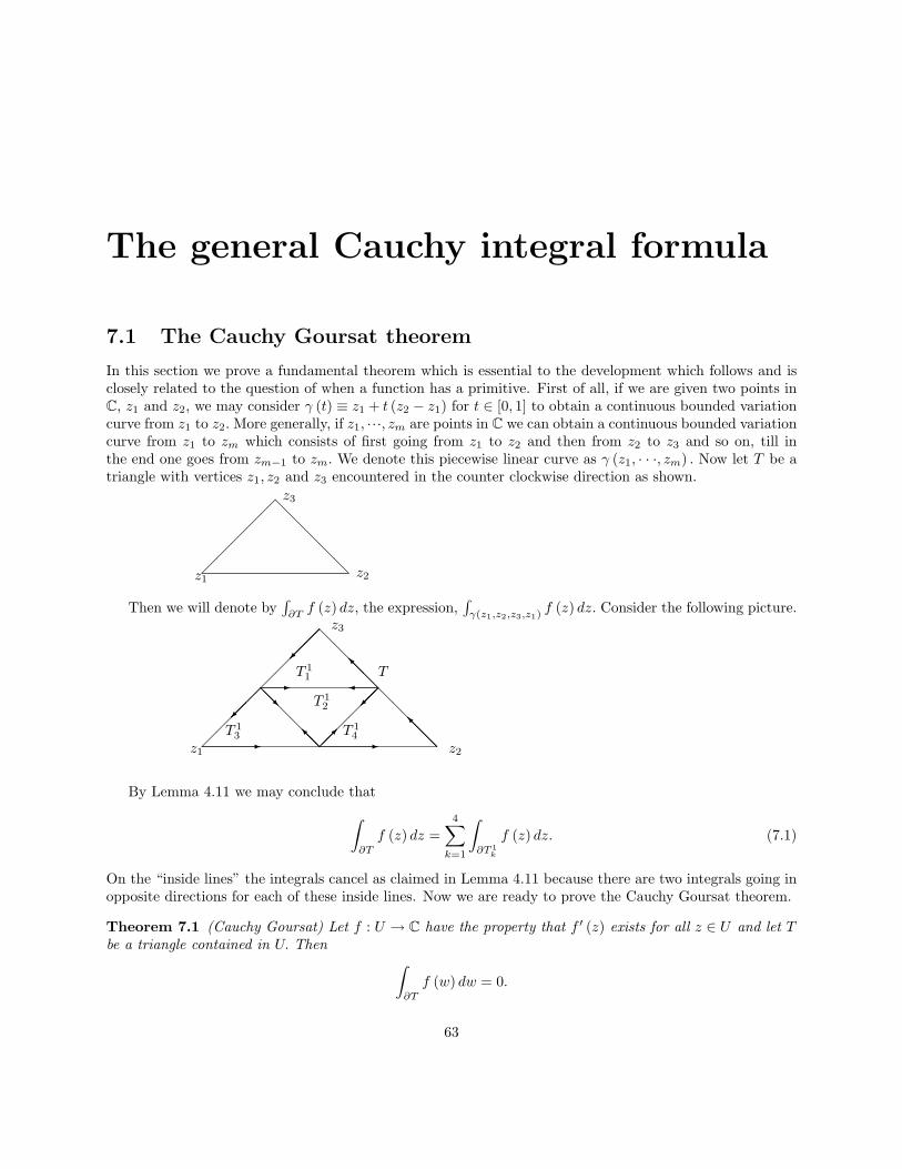
The general Cauchy integral formula
7.1 The Cauchy Goursat theorem
In this section we prove a fundamental theorem which is essential to the development which follows and isclosely related to the question of when a function has a primitive. First of all, if we are given two points inC, z1 and z2, we may consider γ (t) ≡ z1 + t (z2 − z1) for t ∈ [0, 1] to obtain a continuous bounded variationcurve from z1 to z2. More generally, if z1, ···, zm are points in C we can obtain a continuous bounded variationcurve from z1 to zm which consists of first going from z1 to z2 and then from z2 to z3 and so on, till inthe end one goes from zm−1 to zm. We denote this piecewise linear curve as γ (z1, · · ·, zm) . Now let T be atriangle with vertices z1, z2 and z3 encountered in the counter clockwise direction as shown.
�����@@@@@z1 z2
z3
Then we will denote by∫∂Tf (z) dz, the expression,
∫γ(z1,z2,z3,z1)
f (z) dz. Consider the following picture.
���������
-
@@@@@@@@@
���
���
-
TT 11
T 12
T 13 T 1
4@@@I
@@@I
���-
@@R
���@@I
@@@@@�����
z1 z2
z3
By Lemma 4.11 we may conclude that∫∂T
f (z) dz =4∑k=1
∫∂T 1
k
f (z) dz. (7.1)
On the “inside lines” the integrals cancel as claimed in Lemma 4.11 because there are two integrals going inopposite directions for each of these inside lines. Now we are ready to prove the Cauchy Goursat theorem.
Theorem 7.1 (Cauchy Goursat) Let f : U → C have the property that f ′ (z) exists for all z ∈ U and let Tbe a triangle contained in U. Then ∫
∂T
f (w) dw = 0.
63
64 THE GENERAL CAUCHY INTEGRAL FORMULA
Proof: Suppose not. Then ∣∣∣∣∫∂T
f (w) dw∣∣∣∣ = α 6= 0.
From (7.1) it follows
α ≤4∑k=1
∣∣∣∣∣∫∂T 1
k
f (w) dw
∣∣∣∣∣and so for at least one of these T 1
k , denoted from now on as T1, we must have∣∣∣∣∫∂T1
f (w) dw∣∣∣∣ ≥ α
4.
Now let T1 play the same role as T , subdivide as in the above picture, and obtain T2 such that∣∣∣∣∫∂T2
f (w) dw∣∣∣∣ ≥ α
42.
Continue in this way, obtaining a sequence of triangles,
Tk ⊇ Tk+1,diam (Tk) ≤ diam (T ) 2−k,
and ∣∣∣∣∫∂Tk
f (w) dw∣∣∣∣ ≥ α
4k.
Then let z ∈ ∩∞k=1Tk and note that by assumption, f ′ (z) exists. Therefore, for all k large enough,∫∂Tk
f (w) dw =∫∂Tk
f (z) + f ′ (z) (w − z) + g (w) dw
where |g (w)| < ε |w − z| . Now observe that w → f (z) + f ′ (z) (w − z) has a primitive, namely,
F (w) = f (z)w + f ′ (z) (w − z)2/2.
Therefore, by Corollary 4.14. ∫∂Tk
f (w) dw =∫∂Tk
g (w) dw.
From the definition, of the integral, we see
α
4k≤
∣∣∣∣∫∂Tk
g (w) dw∣∣∣∣ ≤ εdiam (Tk) (length of ∂Tk)
≤ ε2−k (length of T ) diam (T ) 2−k,
and so
α ≤ ε (length of T ) diam (T ) .
Since ε is arbitrary, this shows α = 0, a contradiction. Thus∫∂Tf (w) dw = 0 as claimed.
This fundamental result yields the following important theorem.
7.1. THE CAUCHY GOURSAT THEOREM 65
Theorem 7.2 (Morera) Let U be an open set and let f ′ (z) exist for all z ∈ U . Let D ≡ B (z0, r) ⊆ U.Then there exists ε > 0 such that f has a primitive on B (z0, r + ε).
Proof: Choose ε > 0 small enough that B (z0, r + ε) ⊆ U. Then for w ∈ B (z0, r + ε) , define
F (w) ≡∫γ(z0,w)
f (u) du.
Then by the Cauchy Goursat theorem, and w ∈ B (z0, r + ε) , it follows that for |h| small enough,
F (w + h)− F (w)h
=1h
∫γ(w,w+h)
f (u) du
=1h
∫ 1
0
f (w + th)hdt =∫ 1
0
f (w + th) dt
which converges to f (w) due to the continuity of f at w. This proves the theorem.We can also give the following corollary whose proof is similar to the proof of the above theorem.
Corollary 7.3 Let U be an open set and suppose that whenever
γ (z1, z2, z3, z1)
is a closed curve bounding a triangle T, which is contained in U, and f is a continuous function defined onU, it follows that ∫
γ(z1,z2,z3,z1)
f (z) dz = 0,
then f is analytic on U.
Proof: As in the proof of Morera’s theorem, let B (z0, r) ⊆ U and use the given condition to constructa primitive, F for f on B (z0, r) . Then F is analytic and so by Theorem 6.6, it follows that F and hence fhave infinitely many derivatives, implying that f is analytic on B (z0, r) . Since z0 is arbitrary, this shows fis analytic on U.
Theorem 7.4 Let U be an open set in C and suppose f : U → C has the property that f ′ (z) exists for eachz ∈ U. Then f is analytic on U.
Proof: Let z0 ∈ U and let B (z0, r) ⊆ U. By Morera’s theorem f has a primitive, F on B (z0, r) . It followsthat F is analytic because it has a derivative, f, and this derivative is continuous. Therefore, by Theorem6.6 F has infinitely many derivatives on B (z0, r) implying that f also has infinitely many derivatives onB (z0, r) . Thus f is analytic as claimed.
It follows that we can say a function is analytic on an open set, U if and only if f ′ (z) exists for z ∈ U.We just proved the derivative, if it exists, is automatically continuous.
The same proof used to prove Theorem 7.2 implies the following corollary.
Corollary 7.5 Let U be a convex open set and suppose that f ′ (z) exists for all z ∈ U. Then f has a primitiveon U.
Note that this implies that if U is a convex open set on which f ′ (z) exists and if γ : [a, b]→ U is a closed,continuous curve having bounded variation, then letting F be a primitive of f Theorem 4.13 implies∫
γ
f (z) dz = F (γ (b))− F (γ (a)) = 0.
66 THE GENERAL CAUCHY INTEGRAL FORMULA
Notice how different this is from the situation of a function of a real variable. It is possible for a functionof a real variable to have a derivative everywhere and yet the derivative can be discontinuous. A simpleexample is the following.
f (x) ≡{x2 sin
(1x
)if x 6= 0
0 if x = 0 .
Then f ′ (x) exists for all x ∈ R. Indeed, if x 6= 0, the derivative equals 2x sin 1x − cos 1
x which has no limitas x → 0. However, from the definition of the derivative of a function of one variable, we see easily thatf ′ (0) = 0.
7.2 The Cauchy integral formula
Here we develop the general version of the Cauchy integral formula valid for arbitrary closed rectifiablecurves. The key idea in this development is the notion of the winding number. This is the number definedin the following theorem, also called the index. We make use of this winding number along with the earlierresults, especially Liouville’s theorem, to give an extremely general Cauchy integral formula.
Theorem 7.6 Let γ : [a, b]→ C be continuous and have bounded variation with γ (a) = γ (b) . Also supposethat z /∈ γ ([a, b]) . We define
n (γ, z) ≡ 12πi
∫γ
dw
w − z. (7.2)
Then n (γ, ·) is continuous and integer valued. Furthermore, there exists a sequence, ηk : [a, b] → C suchthat ηk is C1 ([a, b]) ,
||ηk − γ|| <1k, ηk (a) = ηk (b) = γ (a) = γ (b) ,
and n (ηk, z) = n (γ, z) for all k large enough. Also n (γ, ·) is constant on every component of C \ γ ([a, b])and equals zero on the unbounded component of C \ γ ([a, b]) .
Proof: First we verify the assertion about continuity.
|n (γ, z)− n (γ, z1)| ≤ C
∣∣∣∣∫γ
(1
w − z− 1w − z1
)dw
∣∣∣∣≤ C (Length of γ) |z1 − z|
whenever z1 is close enough to z. This proves the continuity assertion.Next we need to show the winding number equals an integer. To do so, use Theorem 4.12 to obtain ηk,
a function in C1 ([a, b]) such that z /∈ ηk ([a, b]) for all k large enough, ηk (x) = γ (x) for x = a, b, and∣∣∣∣ 12πi
∫γ
dw
w − z− 1
2πi
∫ηk
dw
w − z
∣∣∣∣ < 1k, ||ηk − γ|| <
1k.
We will show each of 12πi
∫ηk
dww−z is an integer. To simplify the notation, we write η instead of ηk.∫
η
dw
w − z=∫ b
a
η′ (s) dsη (s)− z
.
We define
g (t) ≡∫ t
a
η′ (s) dsη (s)− z
. (7.3)
7.2. THE CAUCHY INTEGRAL FORMULA 67
Then (e−g(t) (η (t)− z)
)′= e−g(t)η′ (t)− e−g(t)g′ (t) (η (t)− z)
= e−g(t)η′ (t)− e−g(t)η′ (t) = 0.
It follows that e−g(t) (η (t)− z) equals a constant. In particular, using the fact that η (a) = η (b) ,
e−g(b) (η (b)− z) = e−g(a) (η (a)− z) = (η (a)− z) = (η (b)− z)
and so e−g(b) = 1. This happens if and only if −g (b) = 2mπi for some integer m. Therefore, (7.3) implies
2mπi =∫ b
a
η′ (s) dsη (s)− z
=∫η
dw
w − z.
Therefore, 12πi
∫ηk
dww−z is a sequence of integers converging to 1
2πi
∫γ
dww−z ≡ n (γ, z) and so n (γ, z) must also
be an integer and n (ηk, z) = n (γ, z) for all k large enough.Since n (γ, ·) is continuous and integer valued, it follows that it must be constant on every connected
component of C \ γ ([a, b]) . It is clear that n (γ, z) equals zero on the unbounded component because fromthe formula,
limz→∞
|n (γ, z)| ≤ limz→∞
V (γ, [a, b])(
1|z| − c
)where c ≥ max {|w| : w ∈ γ ([a, b])} .This proves the theorem.
It is a good idea to consider a simple case to get an idea of what the winding number is measuring. Todo so, consider γ : [a, b]→ C such that γ is continuous, closed and bounded variation. Suppose also that γ isone to one on (a, b) . Such a curve is called a simple closed curve. It can be shown that such a simple closedcurve divides the plane into exactly two components, an “inside” bounded component and an “outside”unbounded component. This is called the Jordan Curve theorem or the Jordan separation theorem. For aproof of this difficult result, see the chapter on degree theory. For now, it suffices to simply assume that γis such that this result holds. This will usually be obvious anyway. We also suppose that it is possible tochange the parameter to be in [0, 2π] , in such a way that γ (t) +λ
(z + reit − γ (t)
)− z 6= 0 for all t ∈ [0, 2π]
and λ ∈ [0, 1] . (As t goes from 0 to 2π the point γ (t) traces the curve γ ([0, 2π]) in the counter clockwisedirection.) Suppose z ∈ D, the inside of the simple closed curve and consider the curve δ (t) = z + reit fort ∈ [0, 2π] where r is chosen small enough that B (z, r) ⊆ D. Then we claim that n (δ, z) = n (γ, z) .
Proposition 7.7 Under the above conditions,
n (δ, z) = n (γ, z)
and n (δ, z) = 1.
Proof: By changing the parameter, we may assume that [a, b] = [0, 2π] . From Theorem 7.6 it suffices toassume also that γ is C1. Define hλ (t) ≡ γ (t) + λ
(z + reit − γ (t)
)for λ ∈ [0, 1] . (This function is called a
homotopy of the curves γ and δ.) Note that for each λ ∈ [0, 1] , t→ hλ (t) is a closed C1 curve. Also,
12πi
∫hλ
1w − z
dw =1
2πi
∫ 2π
0
γ′ (t) + λ(rieit − γ′ (t)
)γ (t) + λ (z + reit − γ (t))− z
dt.
We know this number is an integer and it is routine to verify that it is a continuous function of λ. Whenλ = 0 it equals n (γ, z) and when λ = 1 it equals n (δ, z). Therefore, n (δ, z) = n (γ, z) . It only remains tocompute n (δ, z) .
n (δ, z) =1
2πi
∫ 2π
0
rieit
reitdt = 1.
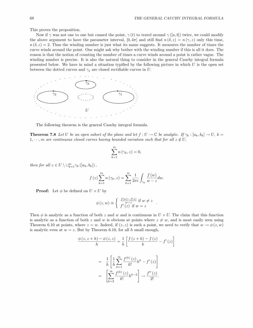
68 THE GENERAL CAUCHY INTEGRAL FORMULA
This proves the proposition.Now if γ was not one to one but caused the point, γ (t) to travel around γ ([a, b]) twice, we could modify
the above argument to have the parameter interval, [0, 4π] and still find n (δ, z) = n (γ, z) only this time,n (δ, z) = 2. Thus the winding number is just what its name suggests. It measures the number of times thecurve winds around the point. One might ask why bother with the winding number if this is all it does. Thereason is that the notion of counting the number of times a curve winds around a point is rather vague. Thewinding number is precise. It is also the natural thing to consider in the general Cauchy integral formulapresented below. We have in mind a situation typified by the following picture in which U is the open setbetween the dotted curves and γj are closed rectifiable curves in U.
-γ1γ2
�
γ3
�
U
The following theorem is the general Cauchy integral formula.
Theorem 7.8 Let U be an open subset of the plane and let f : U → C be analytic. If γk : [ak, bk]→ U, k =1, · · ·,m are continuous closed curves having bounded variation such that for all z /∈ U,
m∑k=1
n (γk, z) = 0,
then for all z ∈ U \ ∪mk=1γk ([ak, bk]) ,
f (z)m∑k=1
n (γk, z) =m∑k=1
12πi
∫γk
f (w)w − z
dw.
Proof: Let φ be defined on U × U by
φ (z, w) ≡{
f(w)−f(z)w−z if w 6= z
f ′ (z) if w = z.
Then φ is analytic as a function of both z and w and is continuous in U × U. The claim that this functionis analytic as a function of both z and w is obvious at points where z 6= w, and is most easily seen usingTheorem 6.10 at points, where z = w. Indeed, if (z, z) is such a point, we need to verify that w → φ (z, w)is analytic even at w = z. But by Theorem 6.10, for all h small enough,
φ (z, z + h)− φ (z, z)h
=1h
[f (z + h)− f (z)
h− f ′ (z)
]
=1h
[1h
∞∑k=1
f (k) (z)k!
hk − f ′ (z)
]
=
[ ∞∑k=2
f (k) (z)k!
hk−2
]→ f ′′ (z)
2!.
7.2. THE CAUCHY INTEGRAL FORMULA 69
Similarly, z → φ (z, w) is analytic even if z = w.We define
h (z) ≡ 12πi
m∑k=1
∫γk
φ (z, w) dw.
We wish to show that h is analytic on U. To do so, we verify∫∂T
h (z) dz = 0
for every triangle, T, contained in U and apply Corollary 7.3. To do this we use Theorem 4.12 to obtain foreach k, a sequence of functions, ηkn ∈ C1 ([ak, bk]) such that
ηkn (x) = γk (x) for x ∈ [ak, bk]
and
ηkn ([ak, bk]) ⊆ U, ||ηkn − γk|| <1n,
∣∣∣∣∫ηkn
φ (z, w) dw −∫γk
φ (z, w) dw∣∣∣∣ < 1
n, (7.4)
for all z ∈ T. Then applying Fubini’s theorem, we can write∫∂T
∫ηkn
φ (z, w) dwdz =∫ηkn
∫∂T
φ (z, w) dzdw = 0
because φ is given to be analytic. By (7.4),∫∂T
∫γk
φ (z, w) dwdz = limn→∞
∫∂T
∫ηkn
φ (z, w) dwdz = 0
and so h is analytic on U as claimed.Now let H denote the set,
H ≡
{z ∈ C\ ∪mk=1 γk ([ak, bk]) :
m∑k=1
n (γk, z) = 0
}.
We know that H is an open set because z →∑mk=1 n (γk, z) is integer valued and continuous. Define
g (z) ≡
{h (z) if z ∈ U
12πi
∑mk=1
∫γk
f(w)w−z dw if z ∈ H . (7.5)
We need to verify that g (z) is well defined. For z ∈ U ∩H, we know z /∈ ∪mk=1γk ([ak, bk]) and so
g (z) =1
2πi
m∑k=1
∫γk
f (w)− f (z)w − z
dw
=1
2πi
m∑k=1
∫γk
f (w)w − z
dw − 12πi
m∑k=1
∫γk
f (z)w − z
dw
=1
2πi
m∑k=1
∫γk
f (w)w − z
dw
70 THE GENERAL CAUCHY INTEGRAL FORMULA
because z ∈ H. This shows g (z) is well defined. Also, g is analytic on U because it equals h there. It isroutine to verify that g is analytic on H also. By assumption, UC ⊆ H and so U ∪H = C showing that g isan entire function.
Now note that∑mk=1 n (γk, z) = 0 for all z contained in the unbounded component of C\∪mk=1 γk ([ak, bk])
which component contains B (0, r)C for r large enough. It follows that for |z| > r, it must be the case thatz ∈ H and so for such z, the bottom description of g (z) found in (7.5) is valid. Therefore, it follows
lim|z|→∞
|g (z)| = 0
and so g is bounded and entire. By Liouville’s theorem, g is a constant. Hence, from the above equation,the constant can only equal zero.
For z ∈ U \ ∪mk=1γk ([ak, bk]) ,
0 =1
2πi
m∑k=1
∫γk
f (w)− f (z)w − z
dw =
12πi
m∑k=1
∫γk
f (w)w − z
dw − f (z)m∑k=1
n (γk, z) .
This proves the theorem.
Corollary 7.9 Let U be an open set and let γk : [ak, bk] → U , k = 1, · · ·,m, be closed, continuous and ofbounded variation. Suppose also that
m∑k=1
n (γk, z) = 0
for all z /∈ U. Then if f : U → C is analytic, we have
m∑k=1
∫γk
f (w) dw = 0.
Proof: This follows from Theorem 7.8 as follows. Let
g (w) = f (w) (w − z)
where z ∈ U \ ∪mk=1γk ([ak, bk]) . Then by this theorem,
0 = 0m∑k=1
n (γk, z) = g (z)m∑k=1
n (γk, z) =
m∑k=1
12πi
∫γk
g (w)w − z
dw =1
2πi
m∑k=1
∫γk
f (w) dw.
Another simple corollary to the above theorem is Cauchy’s theorem for a simply connected region.
Definition 7.10 We say an open set, U ⊆ C is a region if it is open and connected. We say U is simplyconnected if C \U is connected.
7.2. THE CAUCHY INTEGRAL FORMULA 71
Corollary 7.11 Let γ : [a, b] → U be a continuous closed curve of bounded variation where U is a simplyconnected region in C and let f : U → C be analytic. Then∫
γ
f (w) dw = 0.
Proof: Let D denote the unbounded component of C\γ ([a, b]). Thus ∞ ∈ C\γ ([a, b]) .Then theconnected set, C \U is contained in D since every point of C \U must be in some component of C\γ ([a, b])and ∞ is contained in both C\U and D. Thus D must be the component that contains C \U. It follows thatn (γ, ·) must be constant on C \ U, its value being its value on D. However, for z ∈ D,
n (γ, z) =1
2πi
∫γ
1w − z
dw
and so lim|z|→∞ n (γ, z) = 0 showing n (γ, z) = 0 on D. Therefore we have verified the hypothesis of Theorem7.8. Let z ∈ U ∩D and define
g (w) ≡ f (w) (w − z) .
Thus g is analytic on U and by Theorem 7.8,
0 = n (z, γ) g (z) =1
2πi
∫γ
g (w)w − z
dw =1
2πi
∫γ
f (w) dw.
This proves the corollary.The following is a very significant result which will be used later.
Corollary 7.12 Suppose U is a simply connected open set and f : U → C is analytic. Then f has aprimitive, F, on U. Recall this means there exists F such that F ′ (z) = f (z) for all z ∈ U.
Proof: Pick a point, z0 ∈ U and let V denote those points, z of U for which there exists a curve,γ : [a, b] → U such that γ is continuous, of bounded variation, γ (a) = z0, and γ (b) = z. Then it is easy toverify that V is both open and closed in U and therefore, V = U because U is connected. Denote by γz0,zsuch a curve from z0 to z and define
F (z) ≡∫γz0,z
f (w) dw.
Then F is well defined because if γj , j = 1, 2 are two such curves, it follows from Corollary 7.11 that∫γ1
f (w) dw +∫−γ2
f (w) dw = 0,
implying that ∫γ1
f (w) dw =∫γ2
f (w) dw.
Now this function, F is a primitive because, thanks to Corollary 7.11
(F (z + h)− F (z))h−1 =1h
∫γz,z+h
f (w) dw
=1h
∫ 1
0
f (z + th)hdt
and so, taking the limit as h→ 0, we see F ′ (z) = f (z) .

72 THE GENERAL CAUCHY INTEGRAL FORMULA
7.3 Exercises
1. If U is simply connected, f is analytic on U and f has no zeros in U, show there exists an analyticfunction, F, defined on U such that eF = f.
2. Let f be defined and analytic near the point a ∈ C. Show that then f (z) =∑∞k=0 bk (z − a)k whenever
|z − a| < R where R is the distance between a and the nearest point where f fails to have a derivative.The number R, is called the radius of convergence and the power series is said to be expanded abouta.
3. Find the radius of convergence of the function 11+z2 expanded about a = 2. Note there is nothing wrong
with the function, 11+x2 when considered as a function of a real variable, x for any value of x. However,
if we insist on using power series, we find that there is a limitation on the values of x for which thepower series converges due to the presence in the complex plane of a point, i, where the function failsto have a derivative.
4. What if we defined an open set, U to be simply connected if C \ U is connected. Would it amount tothe same thing? Hint: Consider the outside of B (0, 1) .
5. Let γ (t) = eit : t ∈ [0, 2π] . Find∫γ
1zn dz for n = 1, 2, · · ·.
6. Show i∫ 2π
0(2 cos θ)2n
dθ =∫γ
(z + 1
z
)2n ( 1z
)dz where γ (t) = eit : t ∈ [0, 2π] . Then evaluate this
integral using the binomial theorem and the previous problem.
7. Let f : U → C be analytic and f (z) = u (x, y) + iv (x, y) . Show u, v and uv are all harmonic althoughit can happen that u2 is not. Recall that a function, w is harmonic if wxx + wyy = 0.
8. Suppose that for some constants a, b 6= 0, a, b ∈ R, f (z + ib) = f (z) for all z ∈ C and f (z + a) = f (z)for all z ∈ C. If f is analytic, show that f must be constant. Can you generalize this? Hint: Thisuses Liouville’s theorem.
9. Suppose f (z) = u (x, y) + iv (x, y) is analytic for z ∈ U, an open set. Let g (z) = u∗ (x, y) + iv∗ (x, y)where (
u∗
v∗
)= Q
(uv
)where Q is a unitary matrix. That is QQ∗ = Q∗Q = I. When will g be analytic?
10. Suppose f is analytic on an open set, U, except for γ ([a, b]) ⊂ U where γ is a continuous functionhaving bounded variation, but it is known that f is continuous on γ ([a, b]) . Show that in fact fis analytic on γ ([a, b]) also. Hint: Pick a point on γ ([a, b]) , say γ (t0) and suppose for now thatt0 ∈ (a, b) . Pick r > 0 such that B = B (γ (t0) , r) ⊆ U. Then show there exists t1 < t0 and t2 > t0such that γ ([t1, t2]) ⊆ B and γ (ti) /∈ B. Thus γ ([t1, t2]) is a path across B going through the centerof B which divides B into two open sets, B1, and B2 along with γ ([a, b]) . Let the boundary of Bkconsist of γ ([t1, t2]) and a circular arc, Ck. Now letting z ∈ Bk, the line integral of f(w)
w−z over γ ([a, b])
in two different directions cancels. Therefore, if z ∈ Bk, you can argue that f (z) = 12πi
∫Cf(w)w−z dw.
By continuity, this continues to hold for z ∈ γ ((t1, t2)) . Therefore, f must be analytic on γ ((t1, t1))also. This shows that f must be analytic on γ ((a, b)) . To get the endpoints, simply extend γ to havethe same properties but defined on [a− ε, b+ ε] and repeat the above argument or else do this at thebeginning and note that you get [a, b] ⊆ (a− ε, b+ ε) .
11. Let U be an open set contained in the upper half plane and suppose that there are finitely many linesegments on the x axis which are contained in the boundary of U. Now suppose that f is defined and
7.3. EXERCISES 73
real on these line segments and is defined and analytic on U. Now let U denote the reflection of Uacross the x axis. Show that it is possible to extend f to a function, g defined on all of
W ≡ U ∪ U ∪ {the line segments mentioned earlier}
such that g is analytic in W . Hint: For z ∈ U , the reflection of U across the x axis, let g (z) ≡ f (z).Show that g is analytic on U ∪U and continuous on the line segments. Then use Problem 10 to arguethat g is analytic on the line segments also. The result of this problem is know as the Schwarz reflectionprinciple.
12. Show that rotations and translations of analytic functions yield analytic functions and use this obser-vation to generalize the Schwarz reflection principle to situations in which the line segments are partof a line which is not the x axis. Thus, give a version which involves reflection about an arbitrary line.

74 THE GENERAL CAUCHY INTEGRAL FORMULA
The open mapping theorem
In this chapter we present the open mapping theorem for analytic functions. This important result statesthat analytic functions map connected open sets to connected open sets or else to single points. It is verydifferent than the situation for a function of a real variable.
8.1 Zeros of an analytic function
In this section we give a very surprising property of analytic functions which is in stark contrast to whattakes place for functions of a real variable. It turns out the zeros of an analytic function which is not constanton some region cannot have a limit point.
Theorem 8.1 Let U be a connected open set (region) and let f : U → C be analytic. Then the followingare equivalent.
1. f (z) = 0 for all z ∈ U
2. There exists z0 ∈ U such that f (n) (z0) = 0 for all n.
3. There exists z0 ∈ U which is a limit point of the set,
Z ≡ {z ∈ U : f (z) = 0} .
Proof: It is clear the first condition implies the second two. Suppose the third holds. Then for z nearz0 we have
f (z) =∞∑n=k
f (n) (z0)n!
(z − z0)n
where k ≥ 1 since z0 is a zero of f. Suppose k <∞. Then,
f (z) = (z − z0)k g (z)
where g (z0) 6= 0. Letting zn → z0 where zn ∈ Z, zn 6= z0, it follows
0 = (zn − z0)k g (zn)
which implies g (zn) = 0. Then by continuity of g, we see that g (z0) = 0 also, contrary to the choice of k.Therefore, k cannot be less than ∞ and so z0 is a point satisfying the second condition.
Now suppose the second condition and let
S ≡{z ∈ U : f (n) (z) = 0 for all n
}.
75
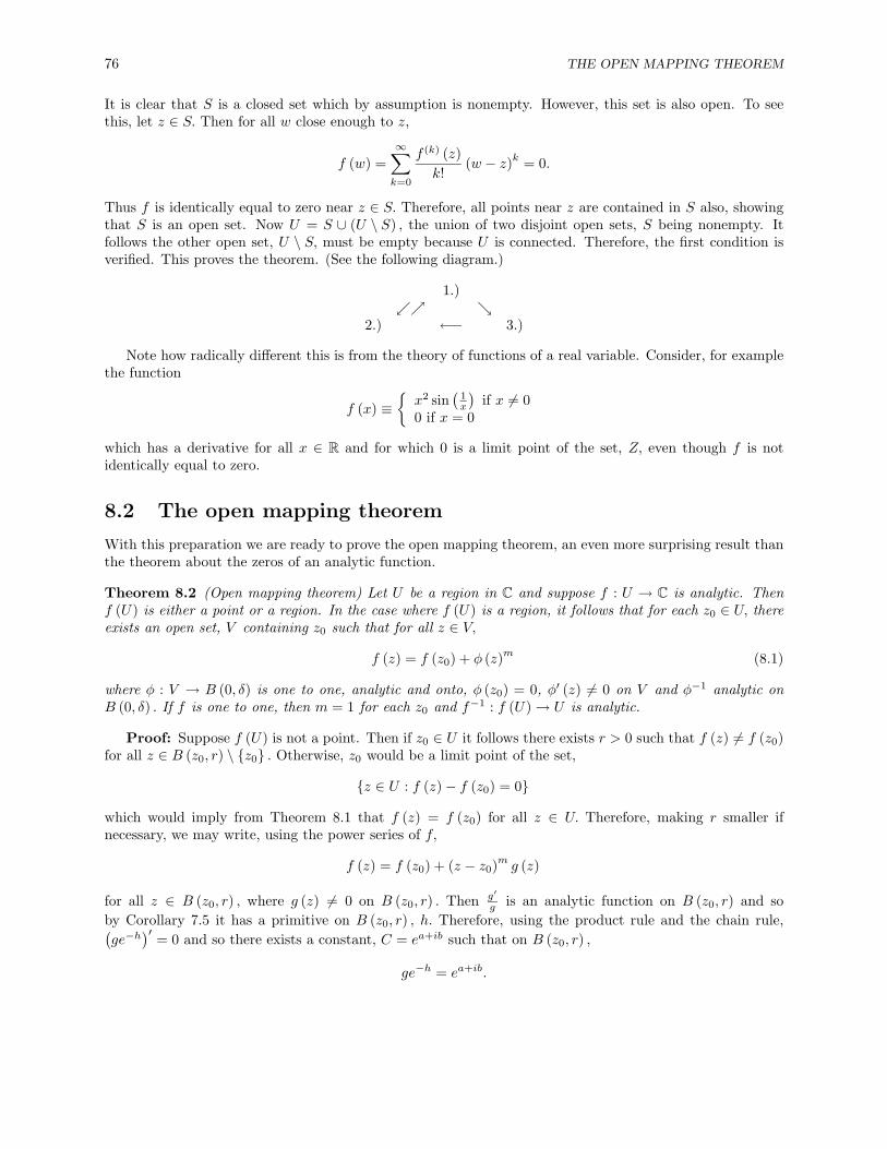
76 THE OPEN MAPPING THEOREM
It is clear that S is a closed set which by assumption is nonempty. However, this set is also open. To seethis, let z ∈ S. Then for all w close enough to z,
f (w) =∞∑k=0
f (k) (z)k!
(w − z)k = 0.
Thus f is identically equal to zero near z ∈ S. Therefore, all points near z are contained in S also, showingthat S is an open set. Now U = S ∪ (U \ S) , the union of two disjoint open sets, S being nonempty. Itfollows the other open set, U \ S, must be empty because U is connected. Therefore, the first condition isverified. This proves the theorem. (See the following diagram.)
1.)↙↗ ↘
2.) ←− 3.)
Note how radically different this is from the theory of functions of a real variable. Consider, for examplethe function
f (x) ≡{x2 sin
(1x
)if x 6= 0
0 if x = 0
which has a derivative for all x ∈ R and for which 0 is a limit point of the set, Z, even though f is notidentically equal to zero.
8.2 The open mapping theorem
With this preparation we are ready to prove the open mapping theorem, an even more surprising result thanthe theorem about the zeros of an analytic function.
Theorem 8.2 (Open mapping theorem) Let U be a region in C and suppose f : U → C is analytic. Thenf (U) is either a point or a region. In the case where f (U) is a region, it follows that for each z0 ∈ U, thereexists an open set, V containing z0 such that for all z ∈ V,
f (z) = f (z0) + φ (z)m (8.1)
where φ : V → B (0, δ) is one to one, analytic and onto, φ (z0) = 0, φ′ (z) 6= 0 on V and φ−1 analytic onB (0, δ) . If f is one to one, then m = 1 for each z0 and f−1 : f (U)→ U is analytic.
Proof: Suppose f (U) is not a point. Then if z0 ∈ U it follows there exists r > 0 such that f (z) 6= f (z0)for all z ∈ B (z0, r) \ {z0} . Otherwise, z0 would be a limit point of the set,
{z ∈ U : f (z)− f (z0) = 0}
which would imply from Theorem 8.1 that f (z) = f (z0) for all z ∈ U. Therefore, making r smaller ifnecessary, we may write, using the power series of f,
f (z) = f (z0) + (z − z0)m g (z)
for all z ∈ B (z0, r) , where g (z) 6= 0 on B (z0, r) . Then g′
g is an analytic function on B (z0, r) and soby Corollary 7.5 it has a primitive on B (z0, r) , h. Therefore, using the product rule and the chain rule,(ge−h
)′ = 0 and so there exists a constant, C = ea+ib such that on B (z0, r) ,
ge−h = ea+ib.

8.2. THE OPEN MAPPING THEOREM 77
Therefore,
g (z) = eh(z)+a+ib
and so, modifying h by adding in the constant, a+ ib, we see g (z) = eh(z) where h′ (z) = g′(z)g(z) on B (z0, r) .
Letting
φ (z) = (z − z0) eh(z)m
we obtain the formula (8.1) valid on B (z0, r) . Now
φ′ (z0) = eh(z0)m 6= 0
and so, restricting r we may assume that φ′ (z) 6= 0 for all z ∈ B (z0, r). We need to verify that there is anopen set, V contained in B (z0, r) such that φ maps V onto B (0, δ) for some δ > 0.
Let φ (z) = u (x, y) + iv (x, y) where z = x+ iy. Then(u (x0, y0)v (x0, y0)
)=(
00
)because for z0 = x0 + iy0, φ (z0) = 0. In addition to this, the functions u and v are in C1 (B (0, r)) becauseφ is analytic. By the Cauchy Riemann equations,∣∣∣∣ ux (x0, y0) uy (x0, y0)
vx (x0, y0) vy (x0, y0)
∣∣∣∣ =∣∣∣∣ ux (x0, y0) −vx (x0, y0)vx (x0, y0) ux (x0, y0)
∣∣∣∣= u2
x (x0, y0) + v2x (x0, y0) = |φ′ (z0)|2 6= 0.
Therefore, by the inverse function theorem there exists an open set, V, containing z0 and δ > 0 such that(u, v)T maps V one to one onto B (0, δ) . Thus φ is one to one onto B (0, δ) as claimed. It follows that φm
maps V onto B (0, δm) . Therefore, the formula (8.1) implies that f maps the open set, V, containing z0 toan open set. This shows f (U) is an open set. It is connected because f is continuous and U is connected.Thus f (U) is a region. It only remains to verify that φ−1 is analytic on B (0, δ) . We show this by verifyingthe Cauchy Riemann equations.
Let (u (x, y)v (x, y)
)=(uv
)(8.2)
for (u, v)T ∈ B (0, δ) . Then, letting w = u + iv, it follows that φ−1 (w) = x (u, v) + iy (u, v) . We need toverify that
xu = yv, xv = −yu. (8.3)
The inverse function theorem has already given us the continuity of these partial derivatives. From theequations (8.2), we have the following systems of equations.
uxxu + uyyu = 1vxxu + vyyu = 0 ,
uxxv + uyyv = 0vxxv + vyyv = 1 .
Solving these for xu, yv, xv, and yu, and using the Cauchy Riemann equations for u and v, yields (8.3).It only remains to verify the assertion about the case where f is one to one. If m > 1, then e
2πim 6= 1 and
so for z1 ∈ V,
e2πim φ (z1) 6= φ (z1) .
78 THE OPEN MAPPING THEOREM
But e2πim φ (z1) ∈ B (0, δ) and so there exists z2 6= z1(since φ is one to one) such that φ (z2) = e
2πim φ (z1) . But
then
φ (z2)m =(e
2πim φ (z1)
)m= φ (z1)m
implying f (z2) = f (z1) contradicting the assumption that f is one to one. Thus m = 1 and f ′ (z) = φ′ (z) 6=0 on V. Since f maps open sets to open sets, it follows that f−1 is continuous and so we may write(
f−1)′
(f (z)) = limf(z1)→f(z)
f−1 (f (z1))− f−1 (f (z))f (z1)− f (z)
= limz1→z
z1 − zf (z1)− f (z)
=1
f ′ (z).
This proves the theorem.One does not have to look very far to find that this sort of thing does not hold for functions mapping R
to R. Take for example, the function f (x) = x2. Then f (R) is neither a point nor a region. In fact f (R)fails to be open.
8.3 Applications of the open mapping theorem
Definition 8.3 We will denote by ρ a ray starting at 0. Thus ρ is a straight line of infinite length extendingin one direction with its initial point at 0.
As a simple application of the open mapping theorem, we give the following theorem about branches ofthe logarithm.
Theorem 8.4 Let ρ be a ray starting at 0. Then there exists an analytic function, L (z) defined on C \ ρsuch that
eL(z) = z.
We call L a branch of the logarithm.
Proof: Let θ be an angle of the ray, ρ. The function, ez is a one to one and onto mapping fromR + i (θ, θ + 2π) to C \ ρ and so we may define L (z) for z ∈ C \ ρ such that eL(z) = z and we see that Ldefined in this way is analytic on C \ ρ because of the open mapping theorem. Note we could just as wellhave considered R + i (θ − 2π, θ) . This would have given another branch of the logarithm valid on C \ ρ.Also, there are infinitely many choices for θ, each of which leads to a branch of the logarithm by the processjust described.
Here is another very significant theorem known as the maximum modulus theorem which follows imme-diately from the open mapping theorem.
Theorem 8.5 (maximum modulus theorem) Let U be a bounded region and let f : U → C be analytic andf : U → C continuous. Then if z ∈ U,
|f (z)| ≤ max {|f (w)| : w ∈ ∂U} . (8.4)
If equality is achieved for any z ∈ U, then f is a constant.
Proof: Suppose f is not a constant. Then f (U) is a region and so if z ∈ U, there exists r > 0 such thatB (f (z) , r) ⊆ f (U) . It follows there exists z1 ∈ U with |f (z1)| > |f (z)| . Hence max
{|f (w)| : w ∈ U
}is
not achieved at any interior point of U. Therefore, the point at which the maximum is achieved must lie onthe boundary of U and so
max {|f (w)| : w ∈ ∂U} = max{|f (w)| : w ∈ U
}> |f (z)|
for all z ∈ U or else f is a constant. This proves the theorem.

8.4. COUNTING ZEROS 79
8.4 Counting zeros
The above proof of the open mapping theorem relies on the very important inverse function theorem fromreal analysis. The proof features this and the Cauchy Riemann equations to indicate how the assumptionf is analytic is used. There are other approaches to this important theorem which do not rely on thebig theorems from real analysis and are more oriented toward the use of the Cauchy integral formula andspecialized techniques from complex analysis. We give one of these approaches next which involves the notionof “counting zeros”. The next theorem is the one about counting zeros. We will use the theorem later in theproof of the Riemann mapping theorem.
Theorem 8.6 Let U be a region and let γ : [a, b] → U be closed, continuous, bounded variation, andn (γ, z) = 0 for all z /∈ U. Suppose also that f is analytic on U having zeros a1, · · ·, am where the zeros arerepeated according to multiplicity, and suppose that none of these zeros are on γ ([a, b]) . Then
12πi
∫γ
f ′ (z)f (z)
dz =m∑k=1
n (γ, ak) .
Proof: We are given f (z) =∏mj=1 (z − aj) g (z) where g (z) 6= 0 on U. Hence
f ′ (z)f (z)
=m∑j=1
1z − aj
+g′ (z)g (z)
and so
12πi
∫γ
f ′ (z)f (z)
dz =m∑j=1
n (γ, aj) +1
2πi
∫γ
g′ (z)g (z)
dz.
But the function, z → g′(z)g(z) is analytic and so by Corollary 7.9, the last integral in the above expression
equals 0. Therefore, this proves the theorem.
Theorem 8.7 Let U be a region, let γ : [a, b] → U be closed continuous, and bounded variation such thatn (γ, z) = 0 for all z /∈ U. Also suppose f : U → C is analytic and that α /∈ f (γ ([a, b])) . Then f◦γ : [a, b]→ C
is continuous, closed, and bounded variation. Also suppose {a1, · · ·, am} = f−1 (α) where these points arecounted according to their multiplicities as zeros of the function f − α Then
n (f ◦ γ, α) =m∑k=1
n (γ, ak) .
Proof: It is clear that f ◦ γ is continuous. It only remains to verify that it is of bounded variation.Suppose first that γ ([a, b]) ⊆ B ⊆ B ⊆ U where B is a ball. Then
|f (γ (t))− f (γ (s))| =
∣∣∣∣∫ 1
0
f ′ (γ (s) + λ (γ (t)− γ (s))) (γ (t)− γ (s)) dλ∣∣∣∣
≤ C |γ (t)− γ (s)|
where C ≥ max{|f ′ (z)| : z ∈ B
}. Hence, in this case,
V (f ◦ γ, [a, b]) ≤ CV (γ, [a, b]) .
80 THE OPEN MAPPING THEOREM
Now let ε denote the distance between γ ([a, b]) and C \ U. Since γ ([a, b]) is compact, ε > 0. By uniformcontinuity there exists δ = b−a
p for p a positive integer such that if |s− t| < δ, then |γ (s)− γ (t)| < ε2 . Then
γ ([t, t+ δ]) ⊆ B(γ (t) ,
ε
2
)⊆ U.
Let C ≥ max{|f ′ (z)| : z ∈ ∪pj=1B
(γ (tj) , ε2
)}where tj ≡ j
p (b− a) + a. Then from what was just shown,
V (f ◦ γ, [a, b]) ≤p−1∑j=0
V (f ◦ γ, [tj , tj+1])
≤ C
p−1∑j=0
V (γ, [tj , tj+1]) <∞
showing that f ◦ γ is bounded variation as claimed. Now from Theorem 7.6 there exists η ∈ C1 ([a, b]) suchthat
η (a) = γ (a) = γ (b) = η (b) , η ([a, b]) ⊆ U,
and
n (η, ak) = n (γ, ak) , n (f ◦ γ, α) = n (f ◦ η, α) (8.5)
for k = 1, · · ·,m. Then
n (f ◦ γ, α) = n (f ◦ η, α)
=1
2πi
∫f◦η
dw
w − α
=1
2πi
∫ b
a
f ′ (η (t))f (η (t))− α
η′ (t) dt
=1
2πi
∫η
f ′ (z)f (z)− α
dz
=m∑k=1
n (η, ak)
By Theorem 8.6. By (8.5), this equals∑mk=1 n (γ, ak) which proves the theorem.
The next theorem is very interesting for its own sake.
Theorem 8.8 Let f : B (a,R)→ C be analytic and let
f (z)− α = (z − a)m g (z) , ∞ > m ≥ 1
where g (z) 6= 0 in B (a,R) . (f (z) − α has a zero of order m at z = a.) Then there exist ε, δ > 0 with theproperty that for each z satisfying 0 < |z − α| < δ, there exist points,
{a1, · · ·, am} ⊆ B (a, ε) ,
such that
f−1 (z) ∩B (a, ε) = {a1, · · ·, am}
and each ak is a zero of order 1 for the function f (·)− z.
8.4. COUNTING ZEROS 81
Proof: By Theorem 8.1 f is not constant on B (a,R) because it has a zero of order m. Therefore, usingthis theorem again, there exists ε > 0 such that B (a, 2ε) ⊆ B (a,R) and there are no solutions to the equationf (z) − α = 0 for z ∈ B (a, 2ε) except a. Also we may assume ε is small enough that for 0 < |z − a| ≤ 2ε,f ′ (z) 6= 0. Otherwise, a would be a limit point of a sequence of points, zn, having f ′ (zn) = 0 which wouldimply, by Theorem 8.1 that f ′ = 0 on B (0, R) , contradicting the assumption that f has a zero of order mand is therefore not constant.
Now pick γ (t) = a+ εeit, t ∈ [0, 2π] . Then α /∈ f (γ ([0, 2π])) so there exists δ > 0 with
B (α, δ) ∩ f (γ ([0, 2π])) = ∅. (8.6)
Therefore, B (α, δ) is contained on one component of C \ f (γ ([0, 2π])) . Therefore, n (f ◦ γ, α) = n (f ◦ γ, z)for all z ∈ B (α, δ) . Now consider f restricted to B (a, 2ε) . For z ∈ B (α, δ) , f−1 (z) must consist of a finiteset of points because f ′ (w) 6= 0 for all w in B (a, 2ε) \ {a} implying that the zeros of f (·) − z in B (a, 2ε)have no limit point. Since B (a, 2ε) is compact, this means there are only finitely many. By Theorem 8.7,
n (f ◦ γ, z) =p∑k=1
n (γ, ak) (8.7)
where {a1, · · ·, ap} = f−1 (z) . Each point, ak of f−1 (z) is either inside the circle traced out by γ, yieldingn (γ, ak) = 1, or it is outside this circle yielding n (γ, ak) = 0 because of (8.6). It follows the sum in (8.7)reduces to the number of points of f−1 (z) which are contained in B (a, ε) . Thus, letting those points inf−1 (z) which are contained in B (a, ε) be denoted by {a1, · · ·, ar}
n (f ◦ γ, α) = n (f ◦ γ, z) = r.
We need to verify that r = m. We do this by computing n (f ◦ γ, α) . However, this is easy to compute byTheorem 8.6 which states
n (f ◦ γ, α) =m∑k=1
n (γ, a) = m.
Therefore, r = m. Each of these ak is a zero of order 1 of the function f (·) − z because f ′ (ak) 6= 0. Thisproves the theorem.
This is a very fascinating result partly because it implies that for values of f near a value, α, at whichf (·) − α has a root of order m for m > 1, the inverse image of these values includes at least m points, notjust one. Thus the topological properties of the inverse image changes radically. This theorem also showsthat f (B (a, ε)) ⊇ B (α, δ) .
Theorem 8.9 (open mapping theorem) Let U be a region and f : U → C be analytic. Then f (U) is eithera point or a region. If f is one to one, then f−1 : f (U)→ U is analytic.
Proof: If f is not constant, then for every α ∈ f (U) , it follows from Theorem 8.1 that f (·)−α has a zeroof order m <∞ and so from Theorem 8.8 for each a ∈ U there exist ε, δ > 0 such that f (B (a, ε)) ⊇ B (α, δ)which clearly implies that f maps open sets to open sets. Therefore, f (U) is open, connected because f iscontinuous. If f is one to one, Theorem 8.8 implies that for every α ∈ f (U) the zero of f (·)− α is of order1. Otherwise, that theorem implies that for z near α, there are m points which f maps to z contradictingthe assumption that f is one to one. Therefore, f ′ (z) 6= 0 and since f−1 is continuous, due to f being anopen map, it follows we may write(
f−1)′
(f (z)) = limf(z1)→f(z)
f−1 (f (z1))− f−1 (f (z))f (z1)− f (z)
= limz1→z
z1 − zf (z1)− f (z)
=1
f ′ (z).
This proves the theorem.
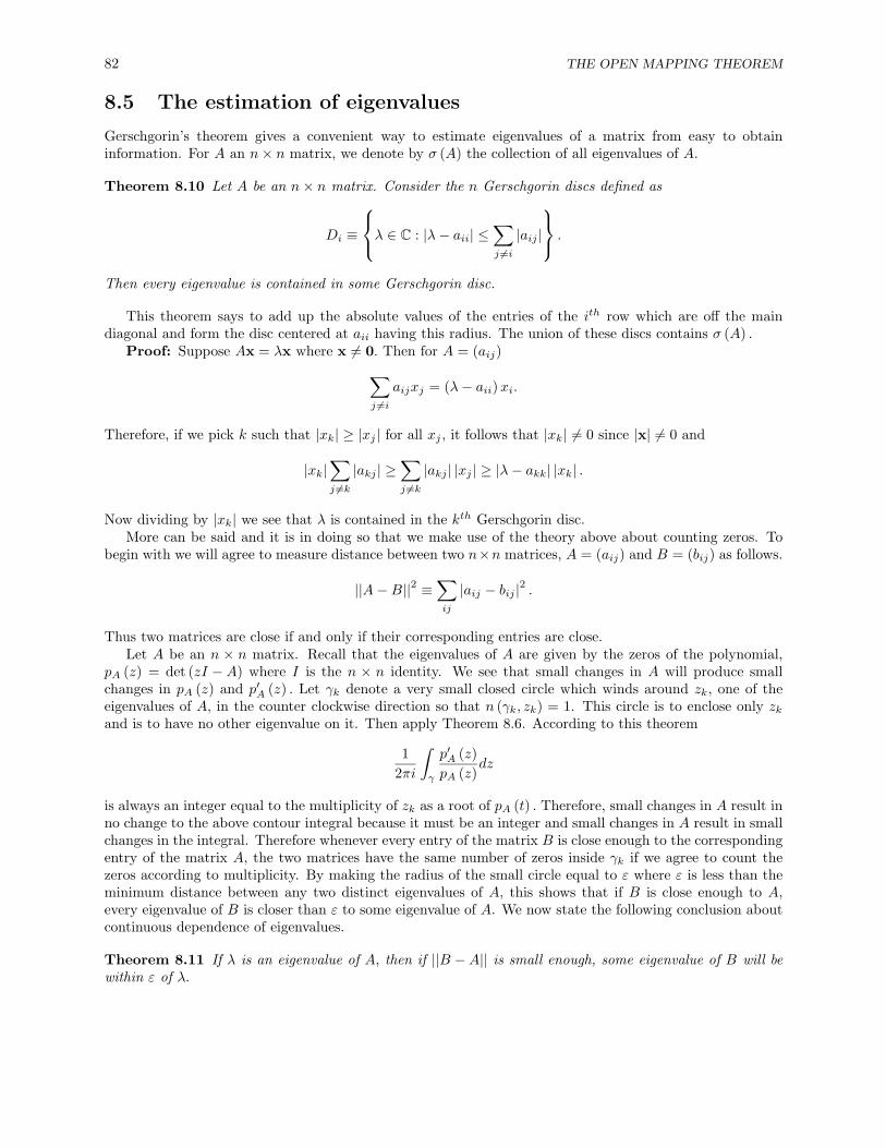
82 THE OPEN MAPPING THEOREM
8.5 The estimation of eigenvalues
Gerschgorin’s theorem gives a convenient way to estimate eigenvalues of a matrix from easy to obtaininformation. For A an n× n matrix, we denote by σ (A) the collection of all eigenvalues of A.
Theorem 8.10 Let A be an n× n matrix. Consider the n Gerschgorin discs defined as
Di ≡
λ ∈ C : |λ− aii| ≤∑j 6=i
|aij |
.
Then every eigenvalue is contained in some Gerschgorin disc.
This theorem says to add up the absolute values of the entries of the ith row which are off the maindiagonal and form the disc centered at aii having this radius. The union of these discs contains σ (A) .
Proof: Suppose Ax = λx where x 6= 0. Then for A = (aij)∑j 6=i
aijxj = (λ− aii)xi.
Therefore, if we pick k such that |xk| ≥ |xj | for all xj , it follows that |xk| 6= 0 since |x| 6= 0 and
|xk|∑j 6=k
|akj | ≥∑j 6=k
|akj | |xj | ≥ |λ− akk| |xk| .
Now dividing by |xk| we see that λ is contained in the kth Gerschgorin disc.More can be said and it is in doing so that we make use of the theory above about counting zeros. To
begin with we will agree to measure distance between two n×n matrices, A = (aij) and B = (bij) as follows.
||A−B||2 ≡∑ij
|aij − bij |2 .
Thus two matrices are close if and only if their corresponding entries are close.Let A be an n × n matrix. Recall that the eigenvalues of A are given by the zeros of the polynomial,
pA (z) = det (zI −A) where I is the n × n identity. We see that small changes in A will produce smallchanges in pA (z) and p′A (z) . Let γk denote a very small closed circle which winds around zk, one of theeigenvalues of A, in the counter clockwise direction so that n (γk, zk) = 1. This circle is to enclose only zkand is to have no other eigenvalue on it. Then apply Theorem 8.6. According to this theorem
12πi
∫γ
p′A (z)pA (z)
dz
is always an integer equal to the multiplicity of zk as a root of pA (t) . Therefore, small changes in A result inno change to the above contour integral because it must be an integer and small changes in A result in smallchanges in the integral. Therefore whenever every entry of the matrix B is close enough to the correspondingentry of the matrix A, the two matrices have the same number of zeros inside γk if we agree to count thezeros according to multiplicity. By making the radius of the small circle equal to ε where ε is less than theminimum distance between any two distinct eigenvalues of A, this shows that if B is close enough to A,every eigenvalue of B is closer than ε to some eigenvalue of A. We now state the following conclusion aboutcontinuous dependence of eigenvalues.
Theorem 8.11 If λ is an eigenvalue of A, then if ||B −A|| is small enough, some eigenvalue of B will bewithin ε of λ.

8.5. THE ESTIMATION OF EIGENVALUES 83
We now consider the situation that A (t) is an n×n matrix and that t→ A (t) is continuous for t ∈ [0, 1] .
Lemma 8.12 Let λ (t) ∈ σ (A (t)) for t < 1 and let Σt = ∪s≥tσ (A (s)) . Also let Kt be the connectedcomponent of λ (t) in Σt. Then there exists η > 0 such that Kt ∩ σ (A (s)) 6= ∅ for all s ∈ [t, t+ η] .
Proof: Denote by D (λ (t) , δ) the disc centered at λ (t) having radius δ > 0, with other occurrences ofthis notation being defined similarly. Thus
D (λ (t) , δ) ≡ {z ∈ C : |λ (t)− z| ≤ δ} .
Suppose δ > 0 is small enough that λ (t) is the only element of σ (A (t)) contained in D (λ (t) , δ) and thatpA(t) has no zeroes on the boundary of this disc. Then by continuity, and the above discussion and theoremwe can say there exists η > 0, t+ η < 1, such that for s ∈ [t, t+ η] , pA(s) also has no zeroes on the boundaryof this disc and that A (s) has the same number of eigenvalues, counted according to multiplicity, in the discas A (t) . Thus σ (A (s)) ∩D (λ (t) , δ) 6= ∅ for all s ∈ [t, t+ η] . Now let
H =⋃
s∈[t,t+η]
σ (A (s)) ∩D (λ (t) , δ) .
We will show H is connected. Suppose not. Then H = P ∪Q where P,Q are separated and λ (t) ∈ P. Let
s0 ≡ inf {s : λ (s) ∈ Q for some λ (s) ∈ σ (A (s))} .
We know there exists λ (s0) ∈ σ (A (s0)) ∩D (λ (t) , δ) . If λ (s0) /∈ Q, then from the above discussion thereare
λ (s) ∈ σ (A (s)) ∩Q
for s > s0 arbitrarily close to λ (s0) . Therefore, λ (s0) ∈ Q which shows that s0 > t because λ (t) is the onlyelement of σ (A (t)) in D (λ (t) , δ) and λ (t) ∈ P. Now let sn ↑ s0. We know λ (sn) ∈ P for any
λ (sn) ∈ σ (A (sn)) ∩D (λ (t) , δ)
and we also know from the above discussion that for some choice of sn → s0, we have λ (sn)→ λ (s0) whichcontradicts P and Q separated and nonempty. Since P is nonempty, this shows Q = ∅. Therefore, H isconnected as claimed. But Kt ⊇ H and so Kt ∩ σ (A (s)) 6= ∅ for all s ∈ [t, t+ η] . This proves the lemma.
Now we are ready to prove the theorem we need.
Theorem 8.13 Suppose A (t) is an n × n matrix and that t → A (t) is continuous for t ∈ [0, 1] . Letλ (0) ∈ σ (A (0)) and define Σ ≡ ∪t∈[0,1]σ (A (t)) . Let Kλ(0) = K0 denote the connected component of λ (0)in Σ. Then K0 ∩ σ (A (t)) 6= ∅ for all t ∈ [0, 1] .
Proof: Let S ≡ {t ∈ [0, 1] : K0 ∩ σ (A (s)) 6= ∅ for all s ∈ [0, t]} . Then 0 ∈ S. Let t0 = sup (S) . Sayσ (A (t0)) = λ1 (t0) , · · ·, λr (t0) . We claim at least one of these is a limit point of K0 and consequentlymust be in K0 which will show that S has a last point. Why is this claim true? Let sn ↑ t0 so sn ∈ S.Now let the discs, D (λi (t0) , δ) , i = 1, · · ·, r be disjoint with pA(t0) having no zeroes on γi the boundaryof D (λi (t0) , δ) . Then for n large enough we know from Theorem 8.6 and the discussion following it thatσ (A (sn)) is contained in ∪ri=1D (λi (t0) , δ). It follows that K0 ∩ (σ (A (t0)) +D (0, δ)) 6= ∅ for all δ smallenough. This requires at least one of the λi (t0) to be in K0. Therefore, t0 ∈ S and S has a last point.
Now by Lemma 8.12, if t0 < 1, then K0∪Kt would be a strictly larger connected set containing λ (0) . (Thereason this would be strictly larger is that K0 ∩ σ (A (s)) = ∅ for some s ∈ (t, t+ η) while Kt ∩ σ (A (s)) 6= ∅for all s ∈ [t, t+ η].) Therefore, t0 = 1 and this proves the theorem.
Now we can prove the following interesting corollary of the Gerschgorin theorem.

84 THE OPEN MAPPING THEOREM
Corollary 8.14 Suppose one of the Gerschgorin discs, Di is disjoint from the union of the others. ThenDi contains an eigenvalue of A. Also, if there are n disjoint Gerschgorin discs, then each one contains aneigenvalue of A.
Proof: Denote by A (t) the matrix(atij)
where if i 6= j, atij = taij and atii = aii. Thus to get A (t) wemultiply all non diagonal terms by t. We let t ∈ [0, 1] . Then A (0) = diag (a11, · · ·, ann) and A (1) = A.Furthermore, the map, t → A (t) is continuous. Denote by Dt
j the Gerschgorin disc obtained from the jth
row for the matrix, A (t). Then it is clear that Dtj ⊆ Dj the jth Gerschgorin disc for A. We see that aii is
the eigenvalue for A (0) which is contained in the disc, consisting of the single point aii which is contained inDi. Letting K be the connected component in Σ for Σ defined in Theorem 8.13 which is determined by aii,we know by Gerschgorin’s theorem that K ∩ σ (A (t)) ⊆ ∪nj=1D
tj ⊆ ∪nj=1Dj = Di ∪ (∪j 6=iDj) and also, since
K is connected, we cannot have points of K in both Di and (∪j 6=iDj) . Since we know at least one point ofK which is in Di,(aii) it follows all of K must be contained in Di. Now by Theorem 8.13 this shows thereare points of K ∩ σ (A) in Di. The last assertion follows immediately.
Actually, we can improve the conclusion in this corollary slightly. It involves the following lemma.
Lemma 8.15 In the situation of Theorem 8.13 suppose λ (0) = K0 ∩ σ (A (0)) and that λ (0) is a simpleroot of the characteristic equation of A (0). Then for all t ∈ [0, 1] ,
σ (A (t)) ∩K0 = λ (t)
where λ (t) is a simple root of the characteristic equation of A (t) .
Proof: Let S ≡
{t ∈ [0, 1] : K0 ∩ σ (A (s)) = λ (s) , a simple eigenvalue for all s ∈ [0, t]} .
Then 0 ∈ S so it is nonempty. Let t0 = sup (S) and suppose λ1 6= λ2 are two elements of σ (A (t0)) ∩K0.Then choosing η > 0 small enough, and letting Di be disjoint discs containing λi respectively, we can usesimilar arguments to those of Lemma 8.12 to conclude that
Hi ≡ ∪s∈[t0−η,t0]σ (A (s)) ∩Di
is a connected and nonempty set for i = 1, 2 which would require that Hi ⊆ K0. But then there would betwo different eigenvalues of A (s) contained in K0, contrary to the definition of t0. Therefore, there is at mostone eigenvalue, λ (t0) ∈ K0 ∩ σ (A (t0)) . We now need to rule out the possibility that it could be a repeatedroot of the characteristic equation. Suppose then that λ (t0) is a repeated root of the characteristic equation.As before, we can choose a small disc, D centered at λ (t0) and η small enough that
H ≡ ∪s∈[t0−η,t0]σ (A (s)) ∩D
is a nonempty connected set containing either multiple eigenvalues of A (s) or else a single repeated root tothe characteristic equation of A (s) . But since H is connected and contains λ (t0) it must be contained inK0 which contradicts the condition for s ∈ S for all these s ∈ [t0 − η, t0] . Therefore, t0 ∈ S as we hoped.If t0 < 1, there exists a small disc centered at λ (t0) and η > 0 such that for all s ∈ [t0, t0 + η] , A (s) hasonly simple eigenvalues in D and the only eigenvalues of A (s) which could be in K0 are in D. (This lastassertion follows from noting that λ (t0) is the only eigenvalue of A (t0) in K0 and so the others are at apositive distance from K0. For s close enough to t0, we know the eigenvalues of A (s) are either close to theseeigenvalues of A (t0) at a positive distance from K0 or they are close to the eigenvalue, λ (t0) in which casewe can assume they are in D.) But this shows that t0 is not really an upper bound to S. Therefore, t0 = 1and the lemma is proved.
With this lemma, we can now sharpen the conclusion of the above corollary.
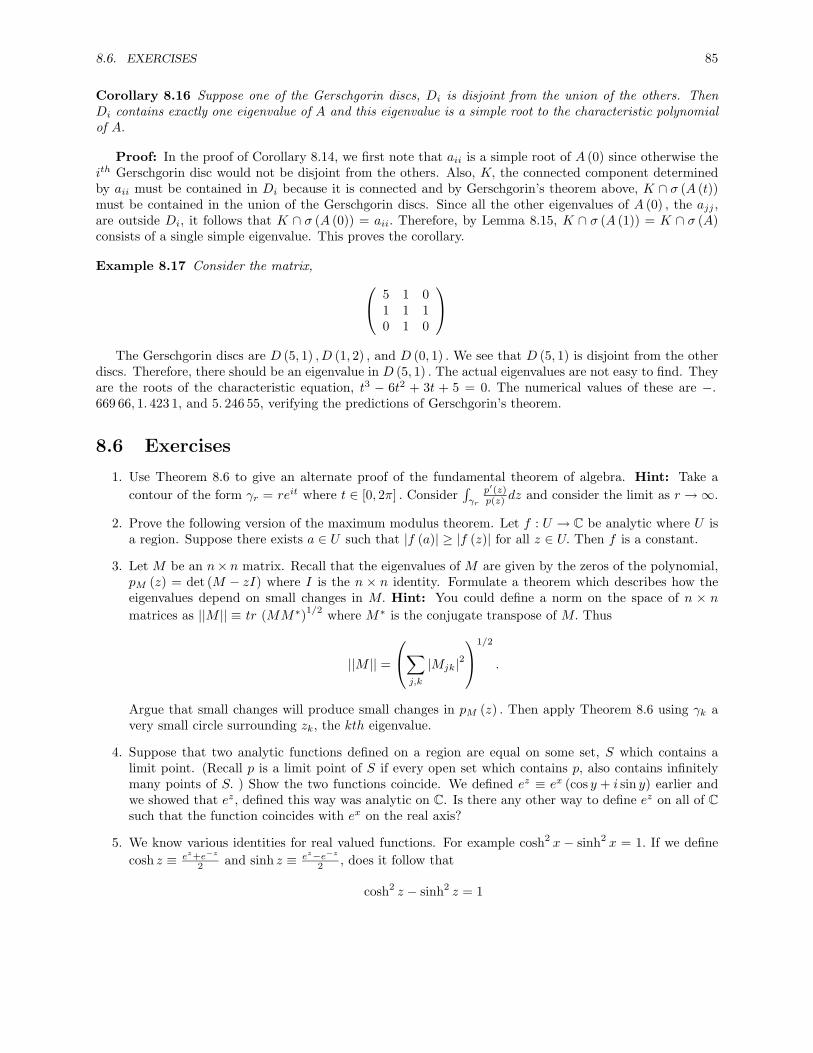
8.6. EXERCISES 85
Corollary 8.16 Suppose one of the Gerschgorin discs, Di is disjoint from the union of the others. ThenDi contains exactly one eigenvalue of A and this eigenvalue is a simple root to the characteristic polynomialof A.
Proof: In the proof of Corollary 8.14, we first note that aii is a simple root of A (0) since otherwise theith Gerschgorin disc would not be disjoint from the others. Also, K, the connected component determinedby aii must be contained in Di because it is connected and by Gerschgorin’s theorem above, K ∩ σ (A (t))must be contained in the union of the Gerschgorin discs. Since all the other eigenvalues of A (0) , the ajj ,are outside Di, it follows that K ∩ σ (A (0)) = aii. Therefore, by Lemma 8.15, K ∩ σ (A (1)) = K ∩ σ (A)consists of a single simple eigenvalue. This proves the corollary.
Example 8.17 Consider the matrix, 5 1 01 1 10 1 0
The Gerschgorin discs are D (5, 1) , D (1, 2) , and D (0, 1) . We see that D (5, 1) is disjoint from the other
discs. Therefore, there should be an eigenvalue in D (5, 1) . The actual eigenvalues are not easy to find. Theyare the roots of the characteristic equation, t3 − 6t2 + 3t + 5 = 0. The numerical values of these are −.669 66, 1. 423 1, and 5. 246 55, verifying the predictions of Gerschgorin’s theorem.
8.6 Exercises
1. Use Theorem 8.6 to give an alternate proof of the fundamental theorem of algebra. Hint: Take acontour of the form γr = reit where t ∈ [0, 2π] . Consider
∫γr
p′(z)p(z) dz and consider the limit as r →∞.
2. Prove the following version of the maximum modulus theorem. Let f : U → C be analytic where U isa region. Suppose there exists a ∈ U such that |f (a)| ≥ |f (z)| for all z ∈ U. Then f is a constant.
3. Let M be an n× n matrix. Recall that the eigenvalues of M are given by the zeros of the polynomial,pM (z) = det (M − zI) where I is the n × n identity. Formulate a theorem which describes how theeigenvalues depend on small changes in M. Hint: You could define a norm on the space of n × nmatrices as ||M || ≡ tr (MM∗)1/2 where M∗ is the conjugate transpose of M. Thus
||M || =
∑j,k
|Mjk|21/2
.
Argue that small changes will produce small changes in pM (z) . Then apply Theorem 8.6 using γk avery small circle surrounding zk, the kth eigenvalue.
4. Suppose that two analytic functions defined on a region are equal on some set, S which contains alimit point. (Recall p is a limit point of S if every open set which contains p, also contains infinitelymany points of S. ) Show the two functions coincide. We defined ez ≡ ex (cos y + i sin y) earlier andwe showed that ez, defined this way was analytic on C. Is there any other way to define ez on all of Csuch that the function coincides with ex on the real axis?
5. We know various identities for real valued functions. For example cosh2 x − sinh2 x = 1. If we definecosh z ≡ ez+e−z
2 and sinh z ≡ ez−e−z2 , does it follow that
cosh2 z − sinh2 z = 1
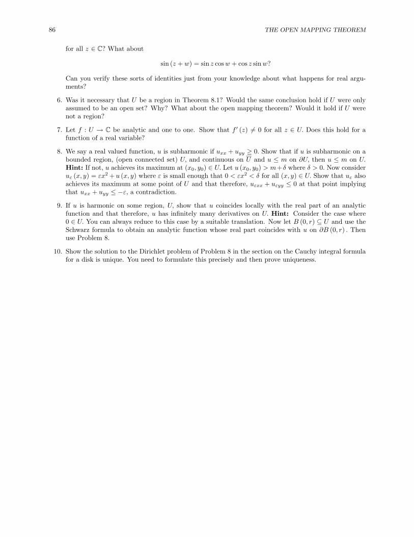
86 THE OPEN MAPPING THEOREM
for all z ∈ C? What about
sin (z + w) = sin z cosw + cos z sinw?
Can you verify these sorts of identities just from your knowledge about what happens for real argu-ments?
6. Was it necessary that U be a region in Theorem 8.1? Would the same conclusion hold if U were onlyassumed to be an open set? Why? What about the open mapping theorem? Would it hold if U werenot a region?
7. Let f : U → C be analytic and one to one. Show that f ′ (z) 6= 0 for all z ∈ U. Does this hold for afunction of a real variable?
8. We say a real valued function, u is subharmonic if uxx + uyy ≥ 0. Show that if u is subharmonic on abounded region, (open connected set) U, and continuous on U and u ≤ m on ∂U, then u ≤ m on U.Hint: If not, u achieves its maximum at (x0, y0) ∈ U. Let u (x0, y0) > m+δ where δ > 0. Now consideruε (x, y) = εx2 + u (x, y) where ε is small enough that 0 < εx2 < δ for all (x, y) ∈ U. Show that uε alsoachieves its maximum at some point of U and that therefore, uεxx + uεyy ≤ 0 at that point implyingthat uxx + uyy ≤ −ε, a contradiction.
9. If u is harmonic on some region, U, show that u coincides locally with the real part of an analyticfunction and that therefore, u has infinitely many derivatives on U. Hint: Consider the case where0 ∈ U. You can always reduce to this case by a suitable translation. Now let B (0, r) ⊆ U and use theSchwarz formula to obtain an analytic function whose real part coincides with u on ∂B (0, r) . Thenuse Problem 8.
10. Show the solution to the Dirichlet problem of Problem 8 in the section on the Cauchy integral formulafor a disk is unique. You need to formulate this precisely and then prove uniqueness.

Singularities
9.1 The Concept Of An Annulus
In this chapter we consider the functions which are analytic in some open set except at isolated points. Thefundamental formula in this subject which is used to classify isolated singularities is the Laurent series.
Definition 9.1 Define ann (a,R1, R2) ≡ {z : R1 < |z − a| < R2} .
Thus ann (a, 0, R) would denote the punctured ball, B (a,R) \ {0} . Here is an important lemma.
Lemma 9.2 Let γr (t) ≡ a + reit for t ∈ [0, 2π] and let |z − a| < r. Then n (γr, z) = 1. If |z − a| > r, thenn (γr, z) = 0.
Proof: For the first claim, consider for t ∈ [0, 1] ,
f (t) ≡ n (γr, a+ t (z − a)) .
Then from properties of the winding number derived earlier, f (t) ∈ Z, f is continuous, and f (0) = 1.Therefore, f (t) = 1 for all t ∈ [0, 1] . This proves the first claim because f (1) = n (γr, z) .
For the second claim,
n (γr, z) =1
2πi
∫γr
1w − z
dw =1
2πi
∫γr
1w − a− (z − a)
dw
=1
2πi−1z − a
∫γr
1
1−(w−az−a
)dw=
−12πi (z − a)
∫γr
∞∑k=0
(w − az − a
)kdw.
The series converges uniformly for w ∈ γr because∣∣∣∣w − az − a
∣∣∣∣ =r
r + c
for some c > 0 due to the assumption that |z − a| > r. Therefore, the sum and the integral can be interchangedto give
n (γr, z) =−1
2πi (z − a)
∞∑k=0
∫γr
(w − az − a
)kdw = 0
because w →(w−az−a
)khas an antiderivative. This proves the lemma.
87
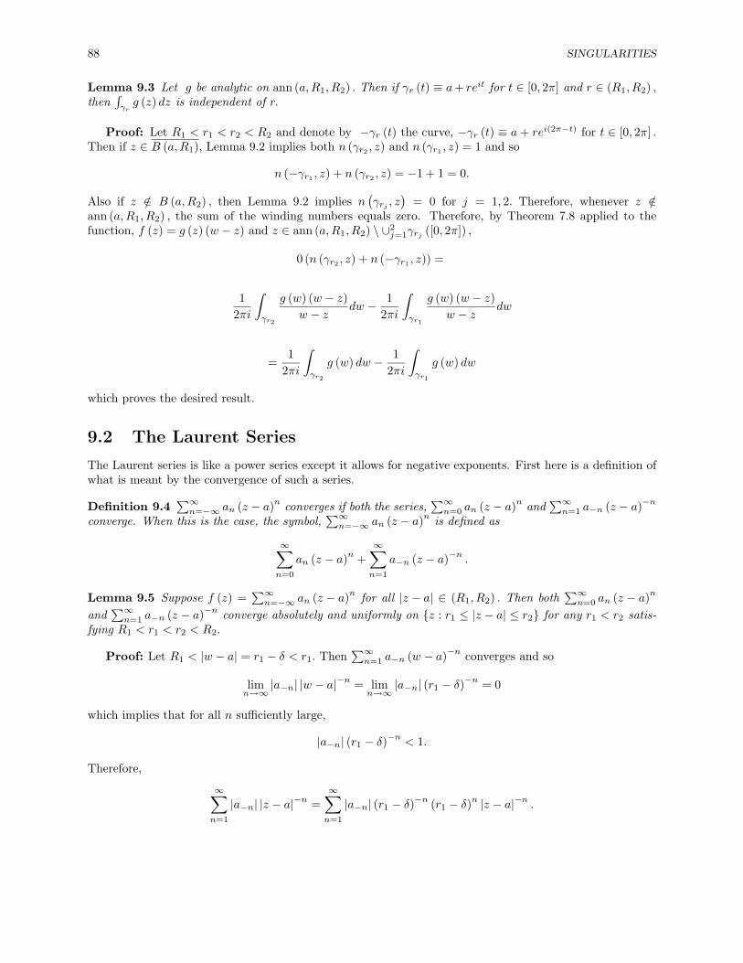
88 SINGULARITIES
Lemma 9.3 Let g be analytic on ann (a,R1, R2) . Then if γr (t) ≡ a+ reit for t ∈ [0, 2π] and r ∈ (R1, R2) ,then
∫γrg (z) dz is independent of r.
Proof: Let R1 < r1 < r2 < R2 and denote by −γr (t) the curve, −γr (t) ≡ a+ rei(2π−t) for t ∈ [0, 2π] .Then if z ∈ B (a,R1), Lemma 9.2 implies both n (γr2 , z) and n (γr1 , z) = 1 and so
n (−γr1 , z) + n (γr2 , z) = −1 + 1 = 0.
Also if z /∈ B (a,R2) , then Lemma 9.2 implies n(γrj , z
)= 0 for j = 1, 2. Therefore, whenever z /∈
ann (a,R1, R2) , the sum of the winding numbers equals zero. Therefore, by Theorem 7.8 applied to thefunction, f (z) = g (z) (w − z) and z ∈ ann (a,R1, R2) \ ∪2
j=1γrj ([0, 2π]) ,
0 (n (γr2 , z) + n (−γr1 , z)) =
12πi
∫γr2
g (w) (w − z)w − z
dw − 12πi
∫γr1
g (w) (w − z)w − z
dw
=1
2πi
∫γr2
g (w) dw − 12πi
∫γr1
g (w) dw
which proves the desired result.
9.2 The Laurent Series
The Laurent series is like a power series except it allows for negative exponents. First here is a definition ofwhat is meant by the convergence of such a series.
Definition 9.4∑∞n=−∞ an (z − a)n converges if both the series,
∑∞n=0 an (z − a)n and
∑∞n=1 a−n (z − a)−n
converge. When this is the case, the symbol,∑∞n=−∞ an (z − a)n is defined as
∞∑n=0
an (z − a)n +∞∑n=1
a−n (z − a)−n .
Lemma 9.5 Suppose f (z) =∑∞n=−∞ an (z − a)n for all |z − a| ∈ (R1, R2) . Then both
∑∞n=0 an (z − a)n
and∑∞n=1 a−n (z − a)−n converge absolutely and uniformly on {z : r1 ≤ |z − a| ≤ r2} for any r1 < r2 satis-
fying R1 < r1 < r2 < R2.
Proof: Let R1 < |w − a| = r1 − δ < r1. Then∑∞n=1 a−n (w − a)−n converges and so
limn→∞
|a−n| |w − a|−n = limn→∞
|a−n| (r1 − δ)−n = 0
which implies that for all n sufficiently large,
|a−n| (r1 − δ)−n < 1.
Therefore,
∞∑n=1
|a−n| |z − a|−n =∞∑n=1
|a−n| (r1 − δ)−n (r1 − δ)n |z − a|−n .
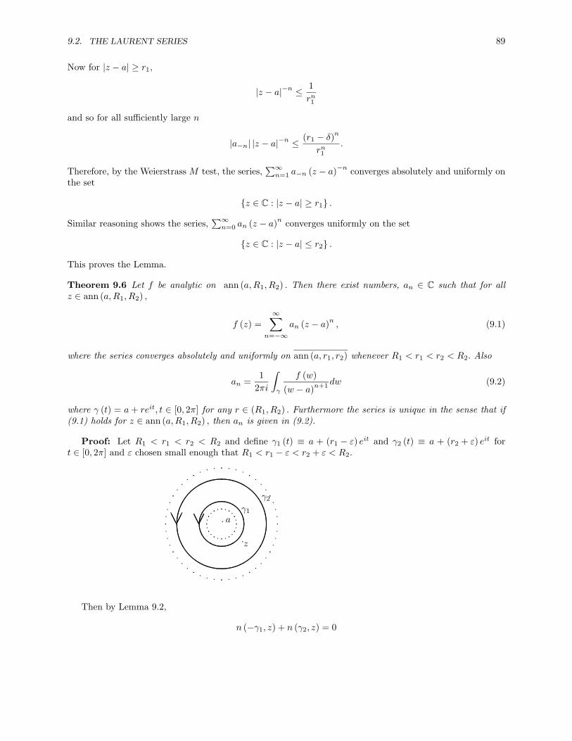
9.2. THE LAURENT SERIES 89
Now for |z − a| ≥ r1,
|z − a|−n ≤ 1rn1
and so for all sufficiently large n
|a−n| |z − a|−n ≤(r1 − δ)n
rn1.
Therefore, by the Weierstrass M test, the series,∑∞n=1 a−n (z − a)−n converges absolutely and uniformly on
the set
{z ∈ C : |z − a| ≥ r1} .
Similar reasoning shows the series,∑∞n=0 an (z − a)n converges uniformly on the set
{z ∈ C : |z − a| ≤ r2} .
This proves the Lemma.
Theorem 9.6 Let f be analytic on ann (a,R1, R2) . Then there exist numbers, an ∈ C such that for allz ∈ ann (a,R1, R2) ,
f (z) =∞∑
n=−∞an (z − a)n , (9.1)
where the series converges absolutely and uniformly on ann (a, r1, r2) whenever R1 < r1 < r2 < R2. Also
an =1
2πi
∫γ
f (w)(w − a)n+1 dw (9.2)
where γ (t) = a+ reit, t ∈ [0, 2π] for any r ∈ (R1, R2) . Furthermore the series is unique in the sense that if(9.1) holds for z ∈ ann (a,R1, R2) , then an is given in (9.2).
Proof: Let R1 < r1 < r2 < R2 and define γ1 (t) ≡ a + (r1 − ε) eit and γ2 (t) ≡ a + (r2 + ε) eit fort ∈ [0, 2π] and ε chosen small enough that R1 < r1 − ε < r2 + ε < R2.
��AA · a
z·
γ1
γ2
��AA
Then by Lemma 9.2,
n (−γ1, z) + n (γ2, z) = 0
90 SINGULARITIES
off ann (a,R1, R2) and that on ann (a, r1, r2) ,
n (−γ1, z) + n (γ2, z) = 1.
Therefore, by Theorem 7.8, for z ∈ ann (a, r1, r2)
f (z) =1
2πi
[∫−γ1
f (w)w − z
dw +∫γ2
f (w)w − z
dw
]
=1
2πi
∫γ1
f (w)
(z − a)[1− w−a
z−a
]dw +∫γ2
f (w)
(w − a)[1− z−a
w−a
]dw
=1
2πi
∫γ2
f (w)w − a
∞∑n=0
(z − aw − a
)ndw +
12πi
∫γ1
f (w)(z − a)
∞∑n=0
(w − az − a
)ndw. (9.3)
From the formula (9.3), it follows that for z ∈ ann (a, r1, r2), the terms in the first sum are bounded by an
expression of the form C(
r2r2+ε
)nwhile those in the second are bounded by one of the form C
(r1−εr1
)nand
so by the Weierstrass M test, the convergence is uniform and so the integrals and the sums in the aboveformula may be interchanged and after renaming the variable of summation, this yields
f (z) =∞∑n=0
(1
2πi
∫γ2
f (w)(w − a)n+1 dw
)(z − a)n +
−1∑n=−∞
(1
2πi
∫γ1
f (w)(w − a)n+1
)(z − a)n . (9.4)
Therefore, by Lemma 9.3, for any r ∈ (R1, R2) ,
f (z) =∞∑n=0
(1
2πi
∫γr
f (w)(w − a)n+1 dw
)(z − a)n +
−1∑n=−∞
(1
2πi
∫γr
f (w)(w − a)n+1
)(z − a)n . (9.5)
and so
f (z) =∞∑
n=−∞
(1
2πi
∫γr
f (w)(w − a)n+1 dw
)(z − a)n .
where r ∈ (R1, R2) is arbitrary.If f (z) =
∑∞n=−∞ an (z − a)n on ann (a,R1, R2) let
fn (z) ≡n∑
k=−n
ak (z − a)k . (9.6)

9.3. ISOLATED SINGULARITIES 91
This function is analytic in ann (a,R1, R2) and so from the above argument,
fn (z) =∞∑
k=−∞
(1
2πi
∫γr
fn (w)
(w − a)k+1dw
)(z − a)k . (9.7)
Also if k > n or if k < −n, (1
2πi
∫γr
fn (w)
(w − a)k+1dw
)= 0.
and so
fn (z) =n∑
k=−n
(1
2πi
∫γr
fn (w)
(w − a)k+1dw
)(z − a)k
which implies from (9.6) that for each k ∈ [−n, n] ,
12πi
∫γr
fn (w)
(w − a)k+1dw = ak
However, from the uniform convergence of the series,∑∞n=0 an (w − a)n and
∑∞n=1 a−n (w − a)−n ensured
by Lemma 9.5 which allows the interchange of sums and integrals, if k ∈ [−n, n] ,
12πi
∫γr
f (w)
(w − a)k+1dw =
12πi
∫γr
∑∞m=0 am (w − a)m +
∑∞m=1 a−m (w − a)−m
(w − a)k+1dw
=∞∑m=0
am1
2πi
∫γr
(w − a)m−(k+1)dw +
∞∑m=1
a−m
∫γr
(w − a)−m−(k+1)dw
=n∑
m=0
am1
2πi
∫γr
(w − a)m−(k+1)dw +
n∑m=1
a−m
∫γr
(w − a)−m−(k+1)dw
=1
2πi
∫γr
fn (w)
(w − a)k+1dw
because if l > n or l < −n, ∫γr
al (w − a)l
(w − a)k+1dw = 0
for all k ∈ [−n, n] . Therefore,
ak =1
2πi
∫γr
f (w)
(w − a)k+1dw
and so this establishes uniqueness. This proves the theorem.
9.3 Isolated Singularities
Definition 9.7 We say f has an isolated singularity at a ∈ C if there exists R > 0 such that f is analyticon ann (a, 0, R) . Such an isolated singularity is said to be a pole of order m if a−m 6= 0 but ak = 0 for allk < −m. The singularity is said to be removable if an = 0 for all n < 0, and it is said to be essential ifam 6= 0 for infinitely many m < 0.
92 SINGULARITIES
Note that thanks to the Laurent series, the possibilities enumerated in the above definition are the onlyones possible. Also observe that a is removable if and only if f (z) = g (z) for some g analytic near a. Howcan we recognize a removable singularity or a pole without computing the Laurent series? This is the contentof the next theorem.
Theorem 9.8 Let a be an isolated singularity of f . Then a is removable if and only if
limz→a
(z − a) f (z) = 0 (9.8)
and a is a pole if and only if
limz→a|f (z)| =∞. (9.9)
The pole is of order m if
limz→a
(z − a)m+1f (z) = 0
but
limz→a
(z − a)m f (z) 6= 0.
Proof: First suppose a is a removable singularity. Then it is clear that (9.8) holds since am = 0 for allm < 0. Now suppose that (9.8) holds and f is analytic on ann (a, 0, R). Then define
h (z) ≡{
(z − a) f (z) if z 6= a0 if z = a
We verify that h is analytic near a by using Morera’s theorem. Let T be a triangle in B (a,R) . If T doesnot contain the point, a, then Corollary 7.11 implies
∫∂Th (z) dz = 0. Therefore, we may assume a ∈ T. If a
is a vertex, then, denoting by b and c the other two vertices, we pick p and q, points on the sides, ab and acrespectively which are close to a. Then by Corollary 7.11,∫
γ(q,c,b,p,q)
h (z) dz = 0.
But by continuity of h, it follows that as p and q are moved closer to a the above integral converges to∫∂Th (z) dz, showing that in this case,
∫∂Th (z) dz = 0 also. It only remains to consider the case where a
is not a vertex but is in T. In this case we subdivide the triangle T into either 3 or 2 subtriangles having aas one vertex, depending on whether a is in the interior or on an edge. Then, applying the above result tothese triangles and noting that the integrals over the interior edges cancel out due to the integration beingtaken in opposite directions, we see that
∫∂Th (z) dz = 0 in this case also.
Now we know h is analytic. Since h equals zero at a, we can conclude that
h (z) = (z − a) g (z)
where g (z) is analytic in B (a,R) . Therefore, for all z 6= a,
(z − a) g (z) = (z − a) f (z)
showing that f (z) = g (z) for all z 6= a and g is analytic on B (0, R) . This proves the converse.It is clear that if f has a pole at a, then (9.9) holds. Suppose conversely that (9.9) holds. Then we know
from the first part of this theorem that 1/f (z) has a removable singularity at a. Also, if g (z) = 1/f (z) forz near a, then g (a) = 0. Therefore, for z 6= a,
1/f (z) = (z − a)m h (z)

9.4. PARTIAL FRACTION EXPANSIONS 93
for some analytic function, h (z) for which h (a) 6= 0. It follows that 1/h ≡ r is analytic near a with r (a) 6= 0.Therefore, for z near a,
f (z) = (z − a)−m∞∑k=0
ak (z − a)k , a0 6= 0,
showing that f has a pole of order m. This proves the theorem.Note that this is very different than what occurs for functions of a real variable. Consider for example,
the function, f (x) = x−1/2. We see x(|x|−1/2
)→ 0 but clearly |x|−1/2 cannot equal a differentiable function
near 0.We have considered the case of a removable singularity or a pole and proved theorems about this case.
What about the case where the singularity is essential? We give an interesting theorem about this case next.
Theorem 9.9 (Casorati Weierstrass) If f has an essential singularity at a then for all r > 0,
f (ann (a, 0, r)) = C
Proof: If not there exists c ∈ C and r > 0 such that c /∈ f (ann (a, 0, r)). Therefore,there exists ε > 0such that B (c, ε) ∩ f (ann (a, 0, r)) = ∅. It follows that
limz→a|z − a|−1 |f (z)− c| =∞
and so by Theorem 9.8 z → (z − a)−1 (f (z)− c) has a pole at a. It follows that for m the order of the pole,
(z − a)−1 (f (z)− c) =m∑k=1
ak
(z − a)k+ g (z)
where g is analytic near a. Therefore,
f (z)− c =m∑k=1
ak
(z − a)k−1+ g (z) (z − a) ,
showing that f has a pole at a rather than an essential singularity. This proves the theorem.This theorem is much weaker than the best result known, the Picard theorem which is stated without
proof next. A proof of this famous theorem may be found in Conway [1].
Theorem 9.10 If f is an analytic function having an essential singularity at z, then in every open setcontaining z the function f, assumes each complex number, with one possible exception, an infinite numberof times.
9.4 Partial Fraction Expansions
What about rational functions, those which are a quotient of two polynomials? It seems reasonable tosuppose, since every finite partial sum of the Laurent series is a rational function just as every finite sum ofa power series is a polynomial, it might be the case that something interesting can be said about rationalfunctions in the context of Laurent series. In fact we will show the existence of the partial fraction expansionfor rational functions. First we need the following simple lemma.
Lemma 9.11 If f is a rational function which has no poles in C then f is a polynomial.

94 SINGULARITIES
Proof: We can write
f (z) =p0 (z − b1)l1 · · · (z − bn)ln
(z − a1)r1 · · · (z − am)rm,
where we can assume the fraction has been reduced to lowest terms. Thus none of the bj equal any of theak. But then, by Theorem 9.8 we would have poles at each ak. Therefore, the denominator must reduce to1 and so f is a polynomial.
Theorem 9.12 Let f (z) be a rational function,
f (z) =p0 (z − b1)l1 · · · (z − bn)ln
(z − a1)r1 · · · (z − am)rm, (9.10)
where the expression is in lowest terms. Then there exist numbers, bkj and a polynomial, p (z) , such that
f (z) =m∑l=1
rl∑j=1
blj
(z − al)j+ p (z) . (9.11)
Proof: We see that f has a pole at a1 and it is clear this pole must be of order r1 since otherwisewe could not achieve equality between (9.10) and the Laurent series for f near a1 due to different rates ofgrowth. Therefore, for z ∈ ann (a1, 0, R1)
f (z) =r1∑j=1
b1j
(z − a1)j+ p1 (z)
where p1 is analytic in B (a1, R1) . Then define
f1 (z) ≡ f (z)−r1∑j=1
b1j
(z − a1)j
so that f1 is a rational function coinciding with p1 near a1 which has no pole at a1. We see that f1 has a poleat a2 or order r2 by the same reasoning. Therefore, we may subtract off the principle part of the Laurentseries for f1 near a2 like we just did for f. This yields
f (z) =r1∑j=1
b1j
(z − a1)j+
r2∑j=1
b2j
(z − a2)j+ p2 (z) .
Letting
f (z)−
r1∑j=1
b1j
(z − a1)j+
r2∑j=1
b2j
(z − a2)j
= f2 (z) ,
and continuing in this way we finally obtain
f (z)−m∑l=1
rl∑j=1
blj
(z − al)j= fm (z)
where fm is a rational function which has no poles. Therefore, it must be a polynomial. This proves thetheorem.
9.5. EXERCISES 95
How does this relate to the usual partial fractions routine of calculus? Recall in that case we had toconsider irreducible quadratics and all the constants were real. In the case from calculus, since the coefficientsof the polynomials were real, the roots of the denominator occurred in conjugate pairs. Thus we would havepaired terms like
b
(z − a)j+
c
(z − a)j
occurring in the sum. We leave it to the reader to verify this version of partial fractions does reduce to theversion from calculus.
9.5 Exercises
1. Classify the singular points of the following functions according to whether they are poles or essentialsingularities. If poles, determine the order of the pole.
(a) cos zz2
(b) z3+1z(z−1)
(c) cos(
1z
)2. Suppose f is defined on an open set, U, and it is known that f is analytic on U \ {z0} but continuous
at z0. Show that f is actually analytic on U.
3. A function defined on C has finitely many poles and lim|z|→∞ f (z) exists. Show f is a rational function.Hint: First show that if h has only one pole at 0 and if lim|z|→∞ h (z) exists, then h is a rationalfunction. Now consider
h (z) ≡∏mk=1 (z − zk)rk∏m
k=1 zrk
f (z)
where zk is a pole of order rk.

96 SINGULARITIES

Residues and evaluation of integrals
It turns out that the theory presented above about singularities and the Laurent series is very useful incomputing the exact value of many hard integrals. First we define what we mean by a residue.
Definition 10.1 Let a be an isolated singularity of f. Thus
f (z) =∞∑
n=−∞an (z − a)n
for all z near a. Then we define the residue of f at a by
Res (f, a) = a−1.
Now suppose that U is an open set and f : U \ {a1, · · ·, am} → C is analytic where the ak are isolatedsingularities of f.
·
'
&
$
%
��HH
γ
a1
−γ1
��
· a2
−γ2
��
Let γ be a simple closed continuous, and bounded variation curve enclosing these isolated singulari-ties such that γ ([a, b]) ⊆ U and {a1, · · ·, am} ⊆ D ⊆ U, where D is the bounded component (inside) ofC \ γ ([a, b]) . Also assume n (γ, z) = 1 for all z ∈ D. As explained earlier, this would occur if γ (t) traces outthe curve in the counter clockwise direction. Choose r small enough that B (aj , r) ∩B (ak, r) = ∅ wheneverj 6= k, B (ak, r) ⊆ U for all k, and define
−γk (t) ≡ ak + re(2π−t)i, t ∈ [0, 2π] .
Thus n (−γk, ai) = −1 and if z is in the unbounded component of C\γ ([a, b]) , n (γ, z) = 0 and n (−γk, z) = 0.If z /∈ U \ {a1, · · ·, am} , then z either equals one of the ak or else z is in the unbounded component just
97

98 RESIDUES AND EVALUATION OF INTEGRALS
described. Either way,∑mk=1 n (γk, z) + n (γ, z) = 0. Therefore, by Theorem 7.8, if z /∈ D,
m∑j=1
12πi
∫−γj
f (w)(w − z)(w − z)
dw +1
2πi
∫γ
f (w)(w − z)(w − z)
dw =
m∑j=1
12πi
∫−γj
f (w) dw +1
2πi
∫γ
f (w) dw =(m∑k=1
n (−γk, z) + n (γ, z)
)f (z) (z − z) = 0.
and so, taking r small enough,
12πi
∫γ
f (w) dw =m∑j=1
12πi
∫γj
f (w) dw
=1
2πi
m∑k=1
∞∑l=−∞
akl
∫γk
(w − ak)l dw
=1
2πi
m∑k=1
ak−1
∫γk
(w − ak)−1dw
=m∑k=1
ak−1 =m∑k=1
Res (f, ak) .
Now we give some examples of hard integrals which can be evaluated by using this idea. This will bedone by integrating over various closed curves having bounded variation.
Example 10.2 The first example we consider is the following integral.∫ ∞−∞
11 + x4
dx
One could imagine evaluating this integral by the method of partial fractions and it should work out bythat method. However, we will consider the evaluation of this integral by the method of residues instead.To do so, consider the following picture.
x
y
Let γr (t) = reit, t ∈ [0, π] and let σr (t) = t : t ∈ [−r, r] . Thus γr parameterizes the top curve and σrparameterizes the straight line from −r to r along the x axis. Denoting by Γr the closed curve traced out
99
by these two, we see from simple estimates that
limr→∞
∫γr
11 + z4
dz = 0.
This follows from the following estimate.∣∣∣∣∫γr
11 + z4
dz
∣∣∣∣ ≤ 1r4 − 1
πr.
Therefore, ∫ ∞−∞
11 + x4
dx = limr→∞
∫Γr
11 + z4
dz.
We compute∫
Γr1
1+z4 dz using the method of residues. The only residues of the integrand are located atpoints, z where 1 + z4 = 0. These points are
z = −12
√2− 1
2i√
2, z =12
√2− 1
2i√
2,
z =12
√2 +
12i√
2, z = −12
√2 +
12i√
2
and it is only the last two which are found in the inside of Γr. Therefore, we need to calculate the residuesat these points. Clearly this function has a pole of order one at each of these points and so we may calculatethe residue at α in this list by evaluating
limz→α
(z − α)1
1 + z4
Thus
Res(f,
12
√2 +
12i√
2)
=
limz→ 1
2
√2+ 1
2 i√
2
(z −
(12
√2 +
12i√
2))
11 + z4
= −18
√2− 1
8i√
2
Similarly we may find the other residue in the same way
Res(f,−1
2
√2 +
12i√
2)
=
limz→− 1
2
√2+ 1
2 i√
2
(z −
(−1
2
√2 +
12i√
2))
11 + z4
= −18i√
2 +18
√2.
Therefore, ∫Γr
11 + z4
dz = 2πi(−1
8i√
2 +18
√2 +
(−1
8
√2− 1
8i√
2))
=12π√
2.
Thus, taking the limit we obtain 12π√
2 =∫∞−∞
11+x4 dx.
Obviously many different variations of this are possible. The main idea being that the integral over thesemicircle converges to zero as r →∞. Sometimes one must be fairly creative to determine the sort of curveto integrate over as well as the sort of function in the integrand and even the interpretation of the integralwhich results.
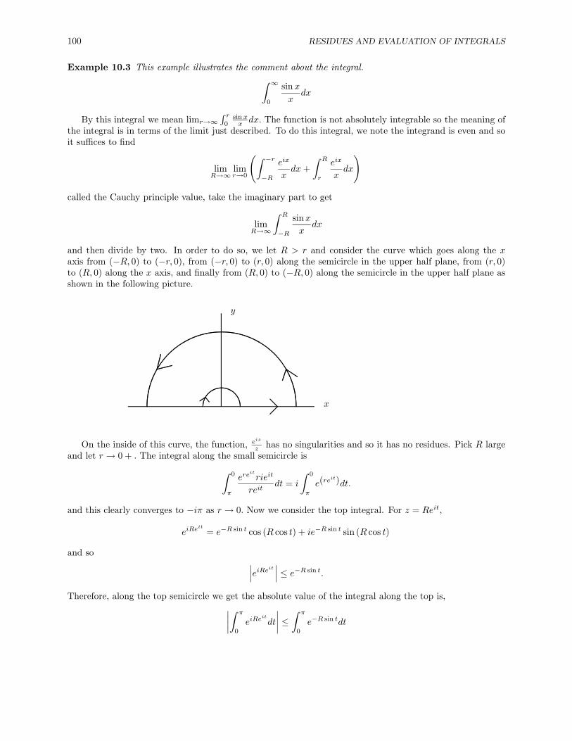
100 RESIDUES AND EVALUATION OF INTEGRALS
Example 10.3 This example illustrates the comment about the integral.∫ ∞0
sinxx
dx
By this integral we mean limr→∞∫ r
0sin xx dx. The function is not absolutely integrable so the meaning of
the integral is in terms of the limit just described. To do this integral, we note the integrand is even and soit suffices to find
limR→∞
limr→0
(∫ −r−R
eix
xdx+
∫ R
r
eix
xdx
)
called the Cauchy principle value, take the imaginary part to get
limR→∞
∫ R
−R
sinxx
dx
and then divide by two. In order to do so, we let R > r and consider the curve which goes along the xaxis from (−R, 0) to (−r, 0), from (−r, 0) to (r, 0) along the semicircle in the upper half plane, from (r, 0)to (R, 0) along the x axis, and finally from (R, 0) to (−R, 0) along the semicircle in the upper half plane asshown in the following picture.
x
y
On the inside of this curve, the function, eiz
z has no singularities and so it has no residues. Pick R largeand let r → 0 + . The integral along the small semicircle is∫ 0
π
ereit
rieit
reitdt = i
∫ 0
π
e(reit)dt.
and this clearly converges to −iπ as r → 0. Now we consider the top integral. For z = Reit,
eiReit
= e−R sin t cos (R cos t) + ie−R sin t sin (R cos t)
and so ∣∣∣eiReit∣∣∣ ≤ e−R sin t.
Therefore, along the top semicircle we get the absolute value of the integral along the top is,∣∣∣∣∫ π
0
eiReit
dt
∣∣∣∣ ≤ ∫ π
0
e−R sin tdt
101
≤∫ π−δ
δ
e−R sin δdt+∫ π
π−δe−R sin tdt+
∫ δ
0
e−R sin tdt
≤ e−R sin δπ + ε
whenever δ is small enough. Letting δ be this small, it follows that
limR→∞
∣∣∣∣∫ π
0
eiReit
dt
∣∣∣∣ ≤ εand since ε is arbitrary, this shows the integral over the top semicircle converges to 0. Therefore, for somefunction e (r) which converges to zero as r → 0,
e (r) =∫
top semicircle
eiz
zdz − iπ +
∫ R
r
eix
xdx+
∫ −r−R
eix
xdx
=∫
top semicircle
eiz
zdz − iπ + i
[∫ R
r
sinxx
dx+∫ −r−R
sinxx
dx
]
Letting r → 0, we see
iπ =∫
top semicircle
eiz
zdz + i
∫ R
−R
sinxx
dx
and so, taking R→∞,
iπ = 2 limR→∞
i
∫ R
0
sinxx
,
showing that π2 =
∫∞0
sin xx dx with the above interpretation of the integral.
Sometimes we don’t blow up the curves and take limits. Sometimes the problem of interest reducesdirectly to a complex integral over a closed curve. Here is an example of this.
Example 10.4 The integral is ∫ π
0
cos θ2 + cos θ
dθ
This integrand is even and so we may write it as
12
∫ π
−π
cos θ2 + cos θ
dθ.
For z on the unit circle, z = eiθ, z = 1z and therefore, cos θ = 1
2
(z + 1
z
). Thus dz = ieiθdθ and so dθ = dz
iz .Note that we are proceeding formally in order to get a complex integral which reduces to the one of interest.It follows that a complex integral which reduces to the one we want is
12i
∫γ
12
(z + 1
z
)2 + 1
2
(z + 1
z
) dzz
=12i
∫γ
z2 + 1z (4z + z2 + 1)
dz
where γ is the unit circle. Now the integrand has poles of order 1 at those points where z(4z + z2 + 1
)= 0.
These points are
0,−2 +√
3,−2−√
3.

102 RESIDUES AND EVALUATION OF INTEGRALS
Only the first two are inside the unit circle. It is also clear the function has simple poles at these points.Therefore,
Res (f, 0) = limz→0
z
(z2 + 1
z (4z + z2 + 1)
)= 1.
Res(f,−2 +
√3)
=
limz→−2+
√3
(z −
(−2 +
√3)) z2 + 1
z (4z + z2 + 1)= −2
3
√3.
It follows ∫ π
0
cos θ2 + cos θ
dθ =12i
∫γ
z2 + 1z (4z + z2 + 1)
dz
=12i
2πi(
1− 23
√3)
= π
(1− 2
3
√3).
Other rational functions of the trig functions will work out by this method also.Sometimes we have to be clever about which version of an analytic function that reduces to a real function
we should use. The following is such an example.
Example 10.5 The integral here is ∫ ∞0
lnx1 + x4
dx.
We would like to use the same curve we used in the integral involving sin xx but this will create problems
with the log since the usual version of the log is not defined on the negative real axis. This does not needto concern us however. We simply use another branch of the logarithm. We leave out the ray from 0 alongthe negative y axis and use Theorem 8.4 to define L (z) on this set. Thus L (z) = ln |z| + i arg1 (z) wherearg1 (z) will be the angle, θ, between −π2 and 3π
2 such that z = |z| eiθ. Now the only singularities containedin this curve are
12
√2 +
12i√
2,−12
√2 +
12i√
2
and the integrand, f has simple poles at these points. Thus using the same procedure as in the otherexamples,
Res(f,
12
√2 +
12i√
2)
=
132
√2π − 1
32i√
2π
and
Res(f,−12
√2 +
12i√
2)
=

103
332
√2π +
332i√
2π.
We need to consider the integral along the small semicircle of radius r. This reduces to∫ 0
π
ln |r|+ it
1 + (reit)4
(rieit
)dt
which clearly converges to zero as r → 0 because r ln r → 0. Therefore, taking the limit as r → 0,∫large semicircle
L (z)1 + z4
dz + limr→0+
∫ −r−R
ln (−t) + iπ
1 + t4dt+
limr→0+
∫ R
r
ln t1 + t4
dt = 2πi(
332
√2π +
332i√
2π +132
√2π − 1
32i√
2π).
Observing that∫
large semicircleL(z)1+z4 dz → 0 as R→∞, we may write
e (R) + 2 limr→0+
∫ R
r
ln t1 + t4
dt+ iπ
∫ 0
−∞
11 + t4
dt =(−1
8+
14i
)π2√
2
where e (R)→ 0 as R→∞. From an earlier example this becomes
e (R) + 2 limr→0+
∫ R
r
ln t1 + t4
dt+ iπ
(√2
4π
)=(−1
8+
14i
)π2√
2.
Now letting r → 0+ and R→∞, we see
2∫ ∞
0
ln t1 + t4
dt =(−1
8+
14i
)π2√
2− iπ
(√2
4π
)
= −18
√2π2,
and so ∫ ∞0
ln t1 + t4
dt = − 116
√2π2,
which is probably not the first thing you would thing of. You might try to imagine how this could be obtainedusing elementary techniques.
The next example illustrates the use of what is refered to as a branch cut. It includes many examples.
Example 10.6 Mellin transformations are of the form∫ ∞0
f (x)xadx
x.
Sometimes it is possible to evaluate such a transform in terms of the constant, a.
We assume f is an analytic function except at isolated singularities, none of which are on (0,∞) . Wealso assume that f has the growth conditions,
|f (z)| ≤ C
|z|b, b > a

104 RESIDUES AND EVALUATION OF INTEGRALS
for all large |z| and we assume that
|f (z)| ≤ C ′
|z|b1, b1 < a
for all |z| sufficiently small. It turns out we can give an explicit formula for this Mellin transformation underthese conditions. We use the following contour.
�
−R
-
�
In this contour the small semicircle in the center has radius ε and we will be letting ε→ 0. Denote by γRthe large circular path which starts at the upper edge of the slot and continues to the lower edge. Denoteby γε the small semicircular contour and denote by γεR+ the straight part of the contour from 0 to R whichprovides the top edge of the slot. Finally denote by γεR− the straight part of the contour from R to 0 whichprovides the bottom edge of the slot. The interesting aspect of this problem is the way we define f (z) zα−1.We let
zα−1 ≡ e(ln|z|+i arg(z))(α−1) = e(α−1) log(z)
where arg (z) is the angle of z in (0, 2π) . Thus we use a branch of the logarithm which is defined on C\(0,∞) .Then it is routine to verify from the assumed estimates that
limR→∞
∫γR
f (z) zα−1dz = 0
and
limε→0+
∫γε
f (z) zα−1dz = 0.
Also, it is routine to verify
limε→0+
∫γεR+
f (z) zα−1dz =∫ R
0
f (x)xα−1dx
and
limε→0+
∫γεR−
f (z) zα−1dz = −ei2π(α−1)
∫ R
0
f (x)xα−1dx.
105
Therefore, letting ΣR denote the sum of the residues of f (z) zα−1 which are contained in the disk of radiusR except for the possible residue at 0, we have
e (R) +(
1− ei2π(α−1))∫ R
0
f (x)xα−1dx = 2πiΣR
where e (R)→ 0 as R→∞. Now letting R→∞, we obtain
limR→∞
∫ R
0
f (x)xα−1dx =2πi
1− ei2π(α−1)Σ =
πe−πia
sin (πa)Σ
where Σ denotes the sum of all the residues of f (z) zα−1 except for the residue at 0.The next example is similar to the one on the Mellin transform. In fact it is a Mellin transform but
we work it out independently of the above to emphasize a slightly more informal technique related to thecontour.
Example 10.7∫∞
0xp−1
1+x dx, p ∈ (0, 1) .
Since the exponent of x in the numerator is larger than −1. The integral does converge. However, thetechniques of real analysis don’t tell us what it converges to. The contour we will use is as follows: From(ε, 0) to (r, 0) along the x axis and then from (r, 0) to (r, 0) counter clockwise along the circle of radius r,then from (r, 0) to (ε, 0) along the x axis and from (ε, 0) to (ε, 0) , clockwise along the circle of radius ε. Youshould draw a picture of this contour. The interesting thing about this is that we cannot define zp−1 all theway around 0. Therefore, we use a branch of zp−1 corresponding to the branch of the logarithm obtained bydeleting the positive x axis. Thus
zp−1 = e(ln|z|+iA(z))(p−1)
where z = |z| eiA(z) and A (z) ∈ (0, 2π) . Along the integral which goes in the positive direction on the xaxis, we will let A (z) = 0 while on the one which goes in the negative direction, we take A (z) = 2π. Thisis the appropriate choice obtained by replacing the line from (ε, 0) to (r, 0) with two lines having a smallgap joinded by a circle of radius ε and then taking a limit as the gap closes. We leave it as an exercise toverify that the two integrals taken along the circles of radius ε and r converge to 0 as ε→ 0 and as r →∞.Therefore, taking the limit,∫ ∞
0
xp−1
1 + xdx+
∫ 0
∞
xp−1
1 + x
(e2πi(p−1)
)dx = 2πiRes (f,−1) .
Calculating the residue of the integrand at −1, and simplifying the above expression, we obtain(1− e2πi(p−1)
)∫ ∞0
xp−1
1 + xdx = 2πie(p−1)iπ.
Upon simplification we see that ∫ ∞0
xp−1
1 + xdx =
π
sin pπ.
Example 10.8 The Fresnel integrals are∫ ∞0
cos(x2)dx,
∫ ∞0
sin(x2)dx.
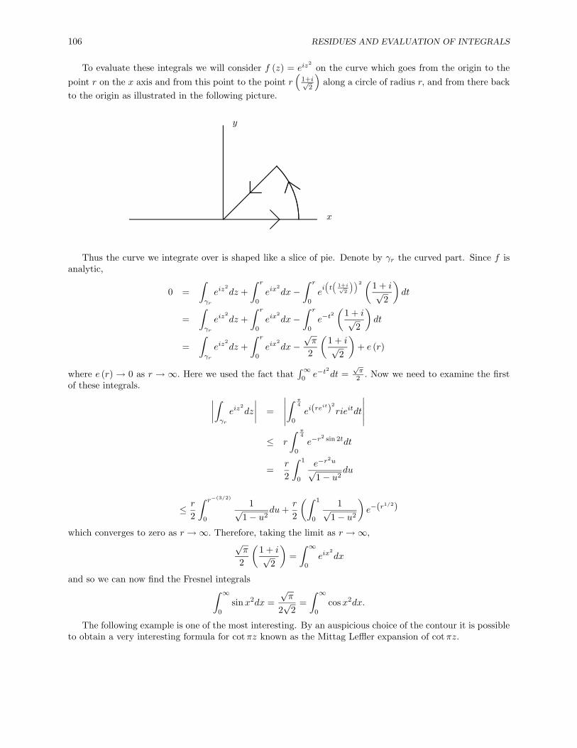
106 RESIDUES AND EVALUATION OF INTEGRALS
To evaluate these integrals we will consider f (z) = eiz2
on the curve which goes from the origin to thepoint r on the x axis and from this point to the point r
(1+i√
2
)along a circle of radius r, and from there back
to the origin as illustrated in the following picture.
x
y
@�
Thus the curve we integrate over is shaped like a slice of pie. Denote by γr the curved part. Since f isanalytic,
0 =∫γr
eiz2dz +
∫ r
0
eix2dx−
∫ r
0
ei(t(
1+i√2
))2 (1 + i√2
)dt
=∫γr
eiz2dz +
∫ r
0
eix2dx−
∫ r
0
e−t2(
1 + i√2
)dt
=∫γr
eiz2dz +
∫ r
0
eix2dx−
√π
2
(1 + i√
2
)+ e (r)
where e (r) → 0 as r → ∞. Here we used the fact that∫∞
0e−t
2dt =
√π
2 . Now we need to examine the firstof these integrals. ∣∣∣∣∫
γr
eiz2dz
∣∣∣∣ =
∣∣∣∣∣∫ π
4
0
ei(reit)2
rieitdt
∣∣∣∣∣≤ r
∫ π4
0
e−r2 sin 2tdt
=r
2
∫ 1
0
e−r2u
√1− u2
du
≤ r
2
∫ r−(3/2)
0
1√1− u2
du+r
2
(∫ 1
0
1√1− u2
)e−(r1/2)
which converges to zero as r →∞. Therefore, taking the limit as r →∞,√π
2
(1 + i√
2
)=∫ ∞
0
eix2dx
and so we can now find the Fresnel integrals∫ ∞0
sinx2dx =√π
2√
2=∫ ∞
0
cosx2dx.
The following example is one of the most interesting. By an auspicious choice of the contour it is possibleto obtain a very interesting formula for cotπz known as the Mittag Leffler expansion of cotπz.
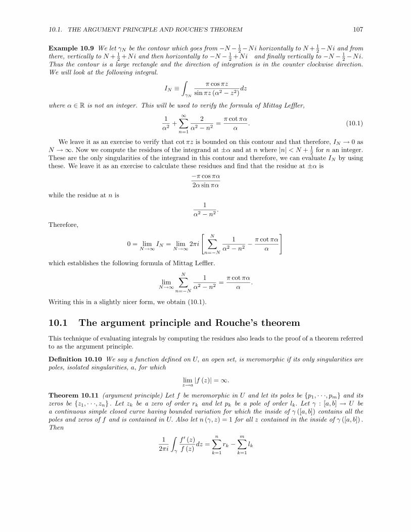
10.1. THE ARGUMENT PRINCIPLE AND ROUCHE’S THEOREM 107
Example 10.9 We let γN be the contour which goes from −N− 12−Ni horizontally to N+ 1
2−Ni and fromthere, vertically to N + 1
2 +Ni and then horizontally to −N − 12 +Ni and finally vertically to −N − 1
2 −Ni.Thus the contour is a large rectangle and the direction of integration is in the counter clockwise direction.We will look at the following integral.
IN ≡∫γN
π cosπzsinπz (α2 − z2)
dz
where α ∈ R is not an integer. This will be used to verify the formula of Mittag Leffler,
1α2
+∞∑n=1
2α2 − n2
=π cotπα
α. (10.1)
We leave it as an exercise to verify that cotπz is bounded on this contour and that therefore, IN → 0 asN →∞. Now we compute the residues of the integrand at ±α and at n where |n| < N + 1
2 for n an integer.These are the only singularities of the integrand in this contour and therefore, we can evaluate IN by usingthese. We leave it as an exercise to calculate these residues and find that the residue at ±α is
−π cosπα2α sinπα
while the residue at n is1
α2 − n2.
Therefore,
0 = limN→∞
IN = limN→∞
2πi
[N∑
n=−N
1α2 − n2
− π cotπαα
]which establishes the following formula of Mittag Leffler.
limN→∞
N∑n=−N
1α2 − n2
=π cotπα
α.
Writing this in a slightly nicer form, we obtain (10.1).
10.1 The argument principle and Rouche’s theorem
This technique of evaluating integrals by computing the residues also leads to the proof of a theorem referredto as the argument principle.
Definition 10.10 We say a function defined on U, an open set, is meromorphic if its only singularities arepoles, isolated singularities, a, for which
limz→a|f (z)| =∞.
Theorem 10.11 (argument principle) Let f be meromorphic in U and let its poles be {p1, · · ·, pm} and itszeros be {z1, · · ·, zn} . Let zk be a zero of order rk and let pk be a pole of order lk. Let γ : [a, b] → U bea continuous simple closed curve having bounded variation for which the inside of γ ([a, b]) contains all thepoles and zeros of f and is contained in U. Also let n (γ, z) = 1 for all z contained in the inside of γ ([a, b]) .Then
12πi
∫γ
f ′ (z)f (z)
dz =n∑k=1
rk −m∑k=1
lk
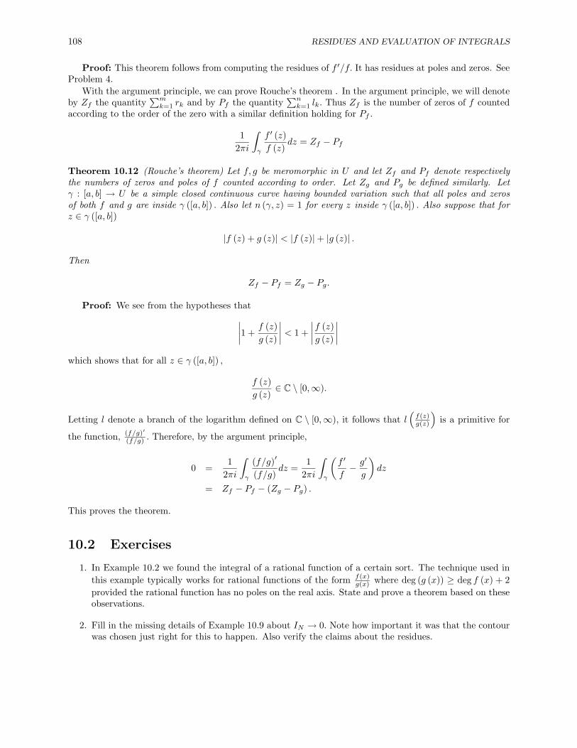
108 RESIDUES AND EVALUATION OF INTEGRALS
Proof: This theorem follows from computing the residues of f ′/f. It has residues at poles and zeros. SeeProblem 4.
With the argument principle, we can prove Rouche’s theorem . In the argument principle, we will denoteby Zf the quantity
∑mk=1 rk and by Pf the quantity
∑nk=1 lk. Thus Zf is the number of zeros of f counted
according to the order of the zero with a similar definition holding for Pf .
12πi
∫γ
f ′ (z)f (z)
dz = Zf − Pf
Theorem 10.12 (Rouche’s theorem) Let f, g be meromorphic in U and let Zf and Pf denote respectivelythe numbers of zeros and poles of f counted according to order. Let Zg and Pg be defined similarly. Letγ : [a, b] → U be a simple closed continuous curve having bounded variation such that all poles and zerosof both f and g are inside γ ([a, b]) . Also let n (γ, z) = 1 for every z inside γ ([a, b]) . Also suppose that forz ∈ γ ([a, b])
|f (z) + g (z)| < |f (z)|+ |g (z)| .
Then
Zf − Pf = Zg − Pg.
Proof: We see from the hypotheses that∣∣∣∣1 +f (z)g (z)
∣∣∣∣ < 1 +∣∣∣∣f (z)g (z)
∣∣∣∣which shows that for all z ∈ γ ([a, b]) ,
f (z)g (z)
∈ C \ [0,∞).
Letting l denote a branch of the logarithm defined on C \ [0,∞), it follows that l(f(z)g(z)
)is a primitive for
the function, (f/g)′
(f/g) . Therefore, by the argument principle,
0 =1
2πi
∫γ
(f/g)′
(f/g)dz =
12πi
∫γ
(f ′
f− g′
g
)dz
= Zf − Pf − (Zg − Pg) .
This proves the theorem.
10.2 Exercises
1. In Example 10.2 we found the integral of a rational function of a certain sort. The technique used inthis example typically works for rational functions of the form f(x)
g(x) where deg (g (x)) ≥ deg f (x) + 2provided the rational function has no poles on the real axis. State and prove a theorem based on theseobservations.
2. Fill in the missing details of Example 10.9 about IN → 0. Note how important it was that the contourwas chosen just right for this to happen. Also verify the claims about the residues.
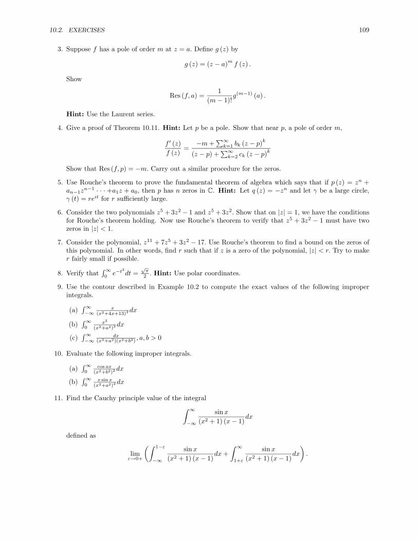
10.2. EXERCISES 109
3. Suppose f has a pole of order m at z = a. Define g (z) by
g (z) = (z − a)m f (z) .
Show
Res (f, a) =1
(m− 1)!g(m−1) (a) .
Hint: Use the Laurent series.
4. Give a proof of Theorem 10.11. Hint: Let p be a pole. Show that near p, a pole of order m,
f ′ (z)f (z)
=−m+
∑∞k=1 bk (z − p)k
(z − p) +∑∞k=2 ck (z − p)k
Show that Res (f, p) = −m. Carry out a similar procedure for the zeros.
5. Use Rouche’s theorem to prove the fundamental theorem of algebra which says that if p (z) = zn +an−1z
n−1 · · · +a1z + a0, then p has n zeros in C. Hint: Let q (z) = −zn and let γ be a large circle,γ (t) = reit for r sufficiently large.
6. Consider the two polynomials z5 + 3z2 − 1 and z5 + 3z2. Show that on |z| = 1, we have the conditionsfor Rouche’s theorem holding. Now use Rouche’s theorem to verify that z5 + 3z2 − 1 must have twozeros in |z| < 1.
7. Consider the polynomial, z11 + 7z5 + 3z2 − 17. Use Rouche’s theorem to find a bound on the zeros ofthis polynomial. In other words, find r such that if z is a zero of the polynomial, |z| < r. Try to maker fairly small if possible.
8. Verify that∫∞
0e−t
2dt =
√π
2 . Hint: Use polar coordinates.
9. Use the contour described in Example 10.2 to compute the exact values of the following improperintegrals.
(a)∫∞−∞
x(x2+4x+13)2 dx
(b)∫∞
0x2
(x2+a2)2 dx
(c)∫∞−∞
dx(x2+a2)(x2+b2) , a, b > 0
10. Evaluate the following improper integrals.
(a)∫∞
0cos ax
(x2+b2)2 dx
(b)∫∞
0x sin x
(x2+a2)2 dx
11. Find the Cauchy principle value of the integral∫ ∞−∞
sinx(x2 + 1) (x− 1)
dx
defined as
limε→0+
(∫ 1−ε
−∞
sinx(x2 + 1) (x− 1)
dx+∫ ∞
1+ε
sinx(x2 + 1) (x− 1)
dx
).
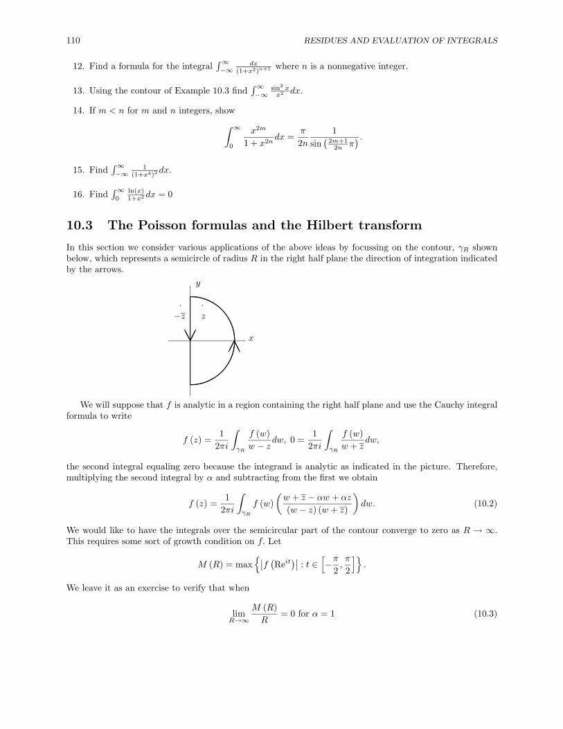
110 RESIDUES AND EVALUATION OF INTEGRALS
12. Find a formula for the integral∫∞−∞
dx(1+x2)n+1 where n is a nonnegative integer.
13. Using the contour of Example 10.3 find∫∞−∞
sin2 xx2 dx.
14. If m < n for m and n integers, show∫ ∞0
x2m
1 + x2ndx =
π
2n1
sin(
2m+12n π
) .15. Find
∫∞−∞
1(1+x4)2 dx.
16. Find∫∞
0ln(x)1+x2 dx = 0
10.3 The Poisson formulas and the Hilbert transform
In this section we consider various applications of the above ideas by focussing on the contour, γR shownbelow, which represents a semicircle of radius R in the right half plane the direction of integration indicatedby the arrows.
AA����AA
x
y
z··
−z
We will suppose that f is analytic in a region containing the right half plane and use the Cauchy integralformula to write
f (z) =1
2πi
∫γR
f (w)w − z
dw, 0 =1
2πi
∫γR
f (w)w + z
dw,
the second integral equaling zero because the integrand is analytic as indicated in the picture. Therefore,multiplying the second integral by α and subtracting from the first we obtain
f (z) =1
2πi
∫γR
f (w)(w + z − αw + αz
(w − z) (w + z)
)dw. (10.2)
We would like to have the integrals over the semicircular part of the contour converge to zero as R → ∞.This requires some sort of growth condition on f. Let
M (R) = max{∣∣f (Reit
)∣∣ : t ∈[−π
2,π
2
]}.
We leave it as an exercise to verify that when
limR→∞
M (R)R
= 0 for α = 1 (10.3)
10.3. THE POISSON FORMULAS AND THE HILBERT TRANSFORM 111
and
limR→∞
M (R) = 0 for α 6= 1, (10.4)
then this condition that the integrals over the curved part of γR converge to zero is satisfied. We assumethis takes place in what follows. Taking the limit as R→∞
f (z) =−12π
∫ ∞−∞
f (iξ)(iξ + z − αiξ + αz
(iξ − z) (iξ + z)
)dξ (10.5)
the negative sign occurring because the direction of integration along the y axis is negative. If α = 1 andz = x+ iy, this reduces to
f (z) =1π
∫ ∞−∞
f (iξ)
(x
|z − iξ|2
)dξ, (10.6)
which is called the Poisson formula for a half plane.. If we assume M (R) → 0, and take α = −1, (10.5)reduces to
i
π
∫ ∞−∞
f (iξ)
(ξ − y|z − iξ|2
)dξ. (10.7)
Of course we can consider real and imaginary parts of f in these formulas. Let
f (iξ) = u (ξ) + iv (ξ) .
From (10.6) we obtain upon taking the real part,
u (x, y) =1π
∫ ∞−∞
u (ξ)
(x
|z − iξ|2
)dξ. (10.8)
Taking real and imaginary parts in (10.7) gives the following.
u (x, y) =1π
∫ ∞−∞
v (ξ)
(y − ξ|z − iξ|2
)dξ, (10.9)
v (x, y) =1π
∫ ∞−∞
u (ξ)
(ξ − y|z − iξ|2
)dξ. (10.10)
These are called the conjugate Poisson formulas because knowledge of the imaginary part on the y axis leadsto knowledge of the real part for Rez > 0 while knowledge of the real part on the imaginary axis leads toknowledge of the real part on Rez > 0.
We obtain the Hilbert transform by formally letting z = iy in the conjugate Poisson formulas and pickingx = 0. Letting u (0, y) = u (y) and v (0, y) = v (y) , we obtain, at least formally
u (y) =1π
∫ ∞−∞
v (ξ)(
1y − ξ
)dξ,
v (y) = − 1π
∫ ∞−∞
u (ξ)(
1y − ξ
)dξ.
Of course there are major problems in writing these integrals due to the integrand possessing a nonintegrablesingularity at y. There is a large theory connected with the meaning of such integrals as these known as the

112 RESIDUES AND EVALUATION OF INTEGRALS
theory of singular integrals. Here we evaluate these integrals by taking a contour which goes around thesingularity and then taking a limit to obtain a principle value integral.
The case when α = 0 in (10.5) yields
f (z) =1
2π
∫ ∞−∞
f (iξ)(z − iξ)
dξ. (10.11)
We will use this formula in considering the problem of finding the inverse Laplace transform.We say a function, f, defined on (0,∞) is of exponential type if
|f (t)| < Aeat (10.12)
for some constants A and a. For such a function we can define the Laplace transform as follows.
F (s) ≡∫ ∞
0
f (t) e−stdt ≡ Lf. (10.13)
We leave it as an exercise to show that this integral makes sense for all Res > a and that the function sodefined is analytic on Rez > a. Using the estimate, (10.12), we obtain that for Res > a,
|F (s)| ≤∣∣∣∣ A
s− a
∣∣∣∣ . (10.14)
We will show that if f (t) is given by the formula,
e−(a+ε)tf (t) ≡ 12π
∫ ∞−∞
eiξtF (iξ + a+ ε) dξ,
then Lf = F for all s large enough.
L(e−(a+ε)tf (t)
)=
12π
∫ ∞0
e−st∫ ∞−∞
eiξtF (iξ + a+ ε) dξdt
Now if ∫ ∞−∞|F (iξ + a+ ε)| dξ <∞, (10.15)
we can use Fubini’s theorem to interchange the order of integration. Unfortunately, we do not know this.The best we have is the estimate (10.14). However, this is a very crude estimate and often (10.15) will hold.Therefore, we shall assume whatever we need in order to continue with the symbol pushing and interchangethe order of integration to obtain with the aid of (10.11) the following:
L(e−(a+ε)tf (t)
)=
12π
∫ ∞−∞
(∫ ∞0
e−(s−iξ)tdt
)F (iξ + a+ ε) d
=1
2π
∫ ∞−∞
F (iξ + a+ ε)s− iξ
dξ
= F (s+ a+ ε)
for all s > 0. (The reason for fussing with ξ + a+ ε rather than just ξ is so the function, ξ → F (ξ + a+ ε)will be analytic on Reξ > −ε, a region containing the right half plane allowing us to use (10.11).) Now withthis information, we may verify that L (f) (s) = F (s) for all s > a. We just showed∫ ∞
0
e−wte−(a+ε)tf (t) dt = F (w + a+ ε)
10.4. EXERCISES 113
whenever Rew > 0. Let s = w + a + ε. Then L (f) (s) = F (s) whenever Res > a + ε. Since ε is arbitrary,this verifies L (f) (s) = F (s) for all s > a. It follows that if we are given F (s) which is analytic for Res > aand we want to find f such that L (f) = F, we should pick c > a and define
e−ctf (t) ≡ 12π
∫ ∞−∞
eiξtF (iξ + c) dξ.
Changing the variable, to let s = iξ + c, we may write this as
f (t) =1
2πi
∫ c+i∞
c−i∞estF (s) ds, (10.16)
and we know from the above argument that we can expect this procedure to work if things are not toopathological. This integral is called the Bromwich integral for the inversion of the Laplace transform. Thefunction f (t) is the inverse Laplace transform.
We illustrate this procedure with a simple example. Suppose F (s) = s(s2+1)2 . In this case, F is analytic
for Res > 0. Let c = 1 and integrate over a contour which goes from c − iR vertically to c + iR and thenfollows a semicircle in the counter clockwise direction back to c − iR. Clearly the integrals over the curvedportion of the contour converge to 0 as R→∞. There are two residues of this function, one at i and one at−i. At both of these points the poles are of order two and so we find the residue at i by
Res (f, i) = lims→i
d
ds
(etss (s− i)2
(s2 + 1)2
)
=−iteit
4
and the residue at −i is
Res (f,−i) = lims→−i
d
ds
(etss (s+ i)2
(s2 + 1)2
)
=ite−it
4
Now evaluating the contour integral and taking R→∞, we find that the integral in (10.16) equals
2πi(ite−it
4+−iteit
4
)= iπt sin t
and therefore,
f (t) =12t sin t.
You should verify that this actually works giving L (f) = s(s2+1)2 .
10.4 Exercises
1. Verify that the integrals over the curved part of γR in (10.2) converge to zero when (10.3) and (10.4)are satisfied.
2. Obtain similar formulas to (10.8) for the imaginary part in the case where α = 1 and formulas (10.9)- (10.10) in the case where α = −1. Observe that these formulas give an explicit formula for f (z) ifeither the real or the imaginary parts of f are known along the line x = 0.
114 RESIDUES AND EVALUATION OF INTEGRALS
3. Verify that the formula for the Laplace transform, (10.13) makes sense for all s > a and that F isanalytic for Rez > a.
4. Find inverse Laplace transforms for the functions,a
s2+a2 ,a
s2(s2+a2) ,1s7 ,
s(s2+a2)2 .
5. Consider the analytic function e−z. Show it satisfies the necessary conditions in order to apply formula(10.6). Use this to verify the formulas,
e−x cos y =1π
∫ ∞−∞
x cos ξx2 + (y − ξ)2 dξ,
e−x sin y =1π
∫ ∞−∞
x sin ξx2 + (y − ξ)2 dξ.
6. The Poisson formula gives
u (x, y) =1π
∫ ∞−∞
u (0, ξ)
(x
x2 + (y − ξ)2
)dξ
whenever u is the real part of a function analytic in the right half plane which has a suitable growthcondition. Show that this implies
1 =1π
∫ ∞−∞
(x
x2 + (y − ξ)2
)dξ.
7. Now consider an arbitrary continuous function, u (ξ) and define
u (x, y) ≡ 1π
∫ ∞−∞
u (ξ)
(x
x2 + (y − ξ)2
)dξ.
Verify that for u (x, y) given by this formula,
limx→0+
|u (x, y)− u (y)| = 0,
and that u is a harmonic function, uxx + uyy = 0, on x > 0. Therefore, this integral yields a solutionto the Dirichlet problem on the half plane which is to find a harmonic function which assumes givenboundary values.
8. To what extent can we relax the assumption that ξ → u (ξ) is continuous?
10.5 Infinite products
In this section we give an introduction to the topic of infinite products and apply the theory to the Gammafunction. To begin with we give a definition of what is meant by an infinite product.
Definition 10.13∏∞n=1 (1 + un) ≡ limn→∞
∏nk=1 (1 + uk) whenever this limit exists. If un = un (z) for
z ∈ H, we say the infinite product converges uniformly on H if the partial products,∏nk=1 (1 + uk (z))
converge uniformly on H.
10.5. INFINITE PRODUCTS 115
Lemma 10.14 Let PN ≡∏Nk=1 (1 + uk) and let QN ≡
∏Nk=1 (1 + |uk|) . Then
QN ≤ exp
(N∑k=1
|uk|
), |PN − 1| ≤ QN − 1
Proof: To verify the first inequality,
QN =N∏k=1
(1 + |uk|) ≤N∏k=1
e|uk| = exp
(N∑k=1
|uk|
).
The second claim is obvious if N = 1. Consider N = 2.
|(1 + u1) (1 + u2)− 1| = |u2 + u1 + u1u2|≤ 1 + |u1|+ |u2|+ |u1| |u2| − 1= (1 + |u1|) (1 + |u2|)− 1
Continuing this way the desired inequality follows.The main theorem is the following.
Theorem 10.15 Let H ⊆ C and suppose that∑∞n=1 |un (z)| converges uniformly on H. Then
P (z) ≡∞∏n=1
(1 + un (z))
converges uniformly on H. If (n1, n2, · · ·) is any permutation of (1, 2, · · ·) , then for all z ∈ H,
P (z) =∞∏k=1
(1 + unk (z))
and P has a zero at z0 if and only if un (z0) = −1 for some n.
Proof: We use Lemma 10.14 to write for m < n, and all z ∈ H,∣∣∣∣∣n∏k=1
(1 + uk (z))−m∏k=1
(1 + uk (z))
∣∣∣∣∣≤
∣∣∣∣∣m∏k=1
(1 + |uk (z)|)
∣∣∣∣∣∣∣∣∣∣
n∏k=m+1
(1 + uk (z))− 1
∣∣∣∣∣≤ exp
( ∞∑k=1
|uk (z)|
)∣∣∣∣∣n∏
k=m+1
(1 + |uk (z)|)− 1
∣∣∣∣∣≤ C
(exp
( ∞∑k=m+1
|uk (z)|
)− 1
)≤ C (eε − 1)
whenever m is large enough. This shows the partial products form a uniformly Cauchy sequence and henceconverge uniformly on H. This verifies the first part of the theorem.
116 RESIDUES AND EVALUATION OF INTEGRALS
Next we need to verify the part about taking the product in different orders. Suppose then that(n1, n2, · · ·) is a permutation of the list, (1, 2, · · ·) and choose M large enough that for all z ∈ H,∣∣∣∣∣
∞∏k=1
(1 + uk (z))−M∏k=1
(1 + uk (z))
∣∣∣∣∣ < ε.
Then for all N sufficiently large, {n1, n2, · · ·, nN} ⊇ {1, 2, · · ·,M} . Then for N this large, we use Lemma10.14 to obtain ∣∣∣∣∣
M∏k=1
(1 + uk (z))−N∏k=1
(1 + unk (z))
∣∣∣∣∣ ≤∣∣∣∣∣M∏k=1
(1 + uk (z))
∣∣∣∣∣∣∣∣∣∣∣1−
∏k≤N,nk>M
(1 + unk (z))
∣∣∣∣∣∣≤
∣∣∣∣∣M∏k=1
(1 + uk (z))
∣∣∣∣∣∣∣∣∣∣∣
∏k≤N,nk>M
(1 + |unk (z)|)− 1
∣∣∣∣∣∣≤
∣∣∣∣∣M∏k=1
(1 + uk (z))
∣∣∣∣∣∣∣∣∣∣∞∏l=M
(1 + |ul (z)|)− 1
∣∣∣∣∣≤
∣∣∣∣∣M∏k=1
(1 + uk (z))
∣∣∣∣∣(
exp
( ∞∑l=M
|ul (z)|
)− 1
)
≤
∣∣∣∣∣M∏k=1
(1 + uk (z))
∣∣∣∣∣ (exp ε− 1) (10.17)
≤
∣∣∣∣∣∞∏k=1
(1 + |uk (z)|)
∣∣∣∣∣ (exp ε− 1) (10.18)
whenever M is large enough. Therefore, this shows, using (10.18) that∣∣∣∣∣N∏k=1
(1 + unk (z))−∞∏k=1
(1 + uk (z))
∣∣∣∣∣ ≤∣∣∣∣∣N∏k=1
(1 + unk (z))−M∏k=1
(1 + uk (z))
∣∣∣∣∣+
∣∣∣∣∣M∏k=1
(1 + uk (z))−∞∏k=1
(1 + uk (z))
∣∣∣∣∣≤ ε+
(∣∣∣∣∣∞∏k=1
(1 + |uk (z)|)
∣∣∣∣∣+ ε
)(exp ε− 1)
which verifies the claim about convergence of the permuted products.

10.5. INFINITE PRODUCTS 117
It remains to verify the assertion about the points, z0, where P (z0) = 0. Obviously, if un (z0) = −1,then P (z0) = 0. Suppose then that P (z0) = 0. Letting nk = k and using (10.17), we may take the limit asN →∞ to obtain ∣∣∣∣∣
M∏k=1
(1 + uk (z0))
∣∣∣∣∣ =
∣∣∣∣∣M∏k=1
(1 + uk (z0))−∞∏k=1
(1 + uk (z0))
∣∣∣∣∣≤
∣∣∣∣∣M∏k=1
(1 + uk (z0))
∣∣∣∣∣ (exp ε− 1) .
If ε is chosen small enough in this inequality, we see this implies
M∏k=1
(1 + uk (z)) = 0
and therefore, uk (z0) = −1 for some k ≤M. This proves the theorem.Now we present the Weierstrass product formula. This formula tells how to factor analytic functions into
an infinite product. It is a very interesting and useful theorem. First we need to give a definition of theelementary factors.
Definition 10.16 Let E0 (z) ≡ 1− z and for p ≥ 1,
Ep (z) ≡ (1− z) exp(z +
z2
2+ · · ·+ zp
p
)The fundamental factors satisfy an important estimate which is stated next.
Lemma 10.17 For all |z| ≤ 1 and p = 0, 1, 2, · · ·,
|1− Ep (z)| ≤ |z|p+1.
Proof: If p = 0 this is obvious. Suppose therefore, that p ≥ 1.
E′p (z) = − exp(z +
z2
2+ · · ·+ zp
p
)+
(1− z) exp(z +
z2
2+ · · ·+ zp
p
)(1 + z + · · ·+ zp−1
)and so, since (1− z)
(1 + z + · · ·+ zp−1
)= 1− zp,
E′p (z) = −zp exp(z +
z2
2+ · · ·+ zp
p
)which shows that E′p has a zero of order p at 0. Thus, from the equation just derived,
E′p (z) = −zp∞∑k=0
akzk
118 RESIDUES AND EVALUATION OF INTEGRALS
where each ak ≥ 0 and a0 = 1. This last assertion about the sign of the ak follows easily from differentiatingthe function f (z) = exp
(z + z2
2 + · · ·+ zp
p
)and evaluating the derivatives at z = 0. A primitive for E′p (z)
is of the form −∑∞k=0 ak
zk+1+p
k+p+1 and so integrating from 0 to z along γ (0, z) we see that
Ep (z)− Ep (0) =
Ep (z)− 1 = −∞∑k=0
akzk+p+1
k + p+ 1
= −zp+1∞∑k=0
akzk
k + p+ 1
which shows that (Ep (z)− 1) /zp+1 has a removable singularity at z = 0.Now from the formula for Ep (z) ,
Ep (z)− 1 = (1− z) exp(z +
z2
2+ · · ·+ zp
p
)− 1
and so
Ep (1)− 1 = −1 = −∞∑k=0
ak1
k + p+ 1
Since each ak ≥ 0, we see that for |z| = 1,
|1− Ep (z)||zp+1|
≤∞∑k=1
ak1
k + p+ 1= 1.
Now by the maximum modulus theorem,
|1− Ep (z)| ≤ |z|p+1
for all |z| ≤ 1. This proves the lemma.
Theorem 10.18 Let zn be a sequence of nonzero complex numbers which have no limit point in C andsuppose there exist, pn, nonnegative integers such that
∞∑n=1
(r
|zn|
)1+pn
<∞ (10.19)
for all r ∈ R. Then
P (z) ≡∞∏n=1
Epn
(z
zn
)is analytic on C and has a zero at each point, zn and at no others. If w occurs m times in {zn} , then P hasa zero of order m at w.
Proof: The series∞∑n=1
∣∣∣∣ zzn∣∣∣∣1+pn
10.5. INFINITE PRODUCTS 119
converges uniformly on any compact set because if |z| ≤ r, then∣∣∣∣∣(z
zn
)1+pn∣∣∣∣∣ ≤
(r
|zn|
)1+pn
and so we may apply the Weierstrass M test to obtain the uniform convergence of∑∞n=1
(zzn
)1+pnon |z| < r.
Also, ∣∣∣∣Epn ( z
zn
)− 1∣∣∣∣ ≤ ( |z||zn|
)pn+1
by Lemma 10.17 whenever n is large enough because the hypothesis that {zn} has no limit point requiresthat limn→∞ |zn| =∞. Therefore, by Theorem 10.15,
P (z) ≡∞∏n=1
Epn
(z
zn
)converges uniformly on compact subsets of C. Letting Pn (z) denote the nth partial product for P (z) , wehave for |z| < r
Pn (z) =1
2πi
∫γr
Pn (w)w − z
dw
where γr (t) ≡ reit, t ∈ [0, 2π] . By the uniform convergence of Pn to P on compact sets, it follows the sameformula holds for P in place of Pn showing that P is analytic in B (0, r) . Since r is arbitrary, we see that Pis analytic on all of C.
Now we ask where the zeros of P are. By Theorem 10.15, the zeros occur at exactly those points, z,where
Epn
(z
zn
)− 1 = −1.
In that theorem Epn
(zzn
)− 1 plays the role of un (z) . Thus we need Epn
(zzn
)= 0 for some n. However,
this occurs exactly when zzn
= 1 so the zeros of P are the points {zn} .If w occurs m times in the sequence, {zn} , we let n1, · · ·, nm be those indices at which w occurs. Then
we choose a permutation of (1, 2, · · ·) which starts with the list (n1, · · ·, nm) . By Theorem 10.15,
P (z) =∞∏k=1
Epnk
(z
znk
)=(
1− z
w
)mg (z)
where g is an analytic function which is not equal to zero at w. It follows from this that P has a zero oforder m at w. This proves the theorem.
The next theorem is the Weierstrass factorization theorem which can be used to factor a given function,f, rather than only deciding convergence questions.
Theorem 10.19 Let f be analytic on C, f (0) 6= 0, and let the zeros of f be {zk} , listed according to order.(Thus if z is a zero of order m, it will be listed m times in the list, {zk} .) Then there exists an entirefunction, g and a sequence of nonnegative integers, pn such that
f (z) = eg(z)∞∏n=1
Epn
(z
zn
). (10.20)
120 RESIDUES AND EVALUATION OF INTEGRALS
Note that eg(z) 6= 0 for any z and this is the interesting thing about this function.Proof: We know {zn} cannot have a limit point because if there were a limit point of this sequence, it
would follow from Theorem 8.1 that f (z) = 0 for all z, contradicting the hypothesis that f (0) 6= 0. Hencelimn→∞ |zn| =∞ and so
∞∑n=1
(r
|zn|
)1+n−1
=∞∑n=1
(r
|zn|
)n<∞
by the root test. Therefore, by Theorem 10.18 we may write
P (z) =∞∏n=1
Epn
(z
zn
)a function analytic on C by picking pn = n− 1 or perhaps some other choice. (We know pn = n− 1 worksbut we do not know this is the only choice that might work.) Then f/P has only removable singularities inC and no zeros thanks to Theorem 10.18. Thus, letting h (z) = f (z) /P (z) , we know from Corollary 7.12that h′/h has a primitive, g. Then (
he−g)′
= 0
and so
h (z) = ea+ibeg(z)
for some constants, a, b. Therefore, letting g (z) = g (z) + a + ib, we see that h (z) = eg(z) and thus (10.20)holds. This proves the theorem.
Corollary 10.20 Let f be analytic on C, f has a zero of order m at 0, and let the other zeros of f be {zk} ,listed according to order. (Thus if z is a zero of order l, it will be listed l times in the list, {zk} .) Then thereexists an entire function, g and a sequence of nonnegative integers, pn such that
f (z) = zmeg(z)∞∏n=1
Epn
(z
zn
).
Proof: Since f has a zero of order m at 0, it follows from Theorem 8.1 that {zk} cannot have a limitpoint in C and so we may apply Theorem 10.19 to the function, f (z) /zm which has a removable singularityat 0. This proves the corollary.
10.6 Exercises
1. Show∏∞n=2
(1− 1
n2
)= 1
2 . Hint: Take the ln of the partial product and then exploit the telescopingseries.
2. Suppose P (z) =∏∞k=1 fk (z) 6= 0 for all z ∈ U, an open set, that convergence is uniform on compact
subsets of U, and fk is analytic on U. Show
P ′ (z) =∞∑k=1
f ′k (z)∏n 6=k
fn (z) .
Hint: Use a branch of the logarithm, defined near P (z) and logarithmic differentiation.
10.6. EXERCISES 121
3. Show that sinπzπz has a removable singularity at z = 0 and so there exists an analytic function, q, defined
on C such that sinπzπz = q (z) and q (0) = 1. Using the Weierstrass product formula, show that
q (z) = eg(z)∏
k∈Z,k 6=0
(1− z
k
)ezk
= eg(z)∞∏k=1
(1− z2
k2
)for some analytic function, g (z) and that we may take g (0) = 0.
4. ↑ Use Problem 2 along with Problem 3 to show that
cosπzz− sinπz
πz2= eg(z)g′ (z)
∞∏k=1
(1− z2
k2
)−
2zeg(z)∞∑n=1
1n2
∏k 6=n
(1− z2
k2
).
Now divide this by q (z) on both sides to show
π cotπz − 1z
= g′ (z) + 2z∞∑n=1
1z2 − n2
.
Use the Mittag Leffler expansion for the cotπz to conclude from this that g′ (z) = 0 and hence, g (z) = 0so that
sinπzπz
=∞∏k=1
(1− z2
k2
).
5. ↑ In the formula for the product expansion of sinπzπz , let z = 1
2 to obtain a formula for π2 called Wallis’s
formula. Is this formula you have come up with a good way to calculate π?
6. This and the next collection of problems are dealing with the gamma function. Show that∣∣∣(1 +z
n
)e−zn − 1
∣∣∣ ≤ C (z)n2
and therefore,
∞∑n=1
∣∣∣(1 +z
n
)e−zn − 1
∣∣∣ <∞with the convergence uniform on compact sets.
7. ↑ Show∏∞n=1
(1 + z
n
)e−zn converges to an analytic function on C which has zeros only at the negative
integers and that therefore,
∞∏n=1
(1 +
z
n
)−1
ezn
is a meromorphic function (Analytic except for poles) having simple poles at the negative integers.
122 RESIDUES AND EVALUATION OF INTEGRALS
8. ↑Show there exists γ such that if
Γ (z) ≡ e−γz
z
∞∏n=1
(1 +
z
n
)−1
ezn ,
then Γ (1) = 1. Hint:∏∞n=1 (1 + n) e−1/n = c = eγ .
9. ↑Now show that
γ = limn→∞
[n∑k=1
1k− lnn
]Hint: Show
γ =∞∑n=1
[ln(
1 +1n
)− 1n
]=∞∑n=1
[ln (1 + n)− lnn− 1
n
].
10. ↑Justify the following argument leading to Gauss’s formula
Γ (z) = limn→∞
(n∏k=1
(k
k + z
)ezk
)e−γz
z
= limn→∞
(n!
(1 + z) (2 + z) · · · (n+ z)ez(∑nk=1
1k ))e−γz
z
= limn→∞
n!(1 + z) (2 + z) · · · (n+ z)
ez(∑nk=1
1k )e−z[
∑nk=1
1k−lnn]
= limn→∞
n!nz
(1 + z) (2 + z) · · · (n+ z).
11. ↑ Verify from the Gauss formula above that Γ (z + 1) = Γ (z) z and that for n a nonnegative integer,Γ (n+ 1) = n!.
12. ↑ The usual definition of the gamma function for positive x is
Γ1 (x) ≡∫ ∞
0
e−ttx−1dt.
Show(1− t
n
)n ≤ e−t for t ∈ [0, n] . Then show∫ n
0
(1− t
n
)ntx−1dt =
n!nx
x (x+ 1) · · · (x+ n).
Use the first part and the dominated convergence theorem or heuristics if you have not studied thistheorem to conclude that
Γ1 (x) = limn→∞
n!nx
x (x+ 1) · · · (x+ n)= Γ (x) .
Hint: To show(1− t
n
)n ≤ e−t for t ∈ [0, n] , verify this is equivalent to showing (1− u)n ≤ e−nu foru ∈ [0, 1].
13. ↑Show Γ (z) =∫∞
0e−ttz−1dt. whenever Rez > 0. Hint: You have already shown that this is true for
positive real numbers. Verify this formula for Rez yields an analytic function.
14. ↑Show Γ(
12
)=√π. Then find Γ
(52
).
Harmonic functions
11.1 The Dirichlet problem for a disk
Definition 11.1 Let U be an open set in Rn and suppose u : U → R satisfies ∆u ≡∑nj=1 uxjxj = 0 for
x ∈ U. Then we say u is harmonic.
One of the most important theorems related to harmonic functions is the maximum principle.
Theorem 11.2 Let U be a bounded open set in Rn and suppose u ∈ C2 (U) ∩ C(U)
such that ∆u ≥ 0 inU. Then letting ∂U = U \ U, it follows that max
{u (x) : x ∈ U
}= max {u (x) : x ∈ ∂U} .
Proof: If this is not so, there exists x0 ∈ U such that u (x0) > max {u (x) : x ∈ ∂U} . Since U is boundedthere exists ε > 0 such that u+ε |x|2 also has its maximum in U. If this is not so, there exists a sequence, {εn}of positive numbers converging to zero and a point xεn ∈ ∂U such that u (xεn) + εn |xεn |
2 ≥ u (x) + εn |x|2for all x ∈ U. Then using compactness of ∂U, there exists a subsequence, still denoted by εn such thatxεn → x1 ∈ ∂U and so, taking the limit, we obtain
u (x1) ≥ u (x) for all x ∈ U,
contrary to what was assumed about x0.Now let x1 be the point in U at which u (x) + ε |x|2 achieves its maximum. Therefore, we must have
0 ≥ ∆u (x1) + 2nε ≥ 2nε,
a contradiction. This proves the theorem.
Corollary 11.3 Let f ∈ C (∂U) where U is a bounded open set as above. Then there exists at most onesolution, u ∈ C2 (U) ∩ C
(U)
and ∆u = 0 in U.
Proof: Suppose both u1 and u2 work. Then we let w = u1 − u2. It follows w ∈ C2 (U) ∩ C(U)
and∆w = 0 with w = 0 on ∂U. Therefore, w = u1 − u2 ≤ 0. Similarly, u2 − u1 ≤ 0 and so u1 = u2. This provesthe corollary.
The following theorem is interesting because it relates harmonic functions on a disk to analytic functions.
Theorem 11.4 Let B = B ((a, b) , r) be a disk in R2. Let u be a real valued C1 function defined on B whichhas uxx and uyy continuous and for which ∆u = 0. Then u is infinitely differentiable in B and there existsv such that u+ iv is analytic on B.
Proof: Define
v (x, y) ≡∫ x
a
−∂u∂y
(t, b) dt+∫ y
b
∂u
∂x(x, t) dt.
123

124 HARMONIC FUNCTIONS
Then by continuity of the partial derivatives of u we may use the fundamental theorem of calculus to write
∂v
∂y(x, y) =
∂u
∂x(x, y) . (11.1)
Next we can write, using the fundamental theorem of calculus and the mean value theorem
1h
∫ y
b
(∂u
∂x(x+ h, t)− ∂u
∂x(x, t)
)dt =
1h
∫ y
b
∫ x+h
x
∂2u
∂x2(s, t) dsdt =
∫ y
b
∂2u
∂x2(x+ θh, t) dt
where θ ∈ (0, 1) . Using the uniform continuity of uxx on B (x, δ) × [b, y] we can argue this last integralconverges to ∫ y
b
∂2u
∂x2(x, t) dt
as h→ 0. (This can be done much easier if you know the dominated convergence theorem.) Therefore,
∂v
∂x= −∂u
∂y(x, b) +
∫ y
b
uxx (x, t) dt
= −∂u∂y
(x, b)−∫ y
b
uyy (x, t) dt
= −∂u∂y
(x, b)−[∂u
∂y(x, y)− ∂u
∂y(x, b)
]= −∂u
∂y(x, y) .
Since the partial derivatives of u and v are continuous and the Cauchy Riemann equations hold, it followsthat u+ iv is analytic as we had hoped. It follows that both u and v are infinitely differentiable on B.
Corollary 11.5 Suppose ∆u = 0 on an open set, U ⊆ R2 and u is C1 and uxx is continuous. Then u isinfinitely differentiable on U.
Proof: Simply let B ((a, b) , r) ⊆ U and apply the above result on the disk, B ((a, b) , r) .One of the important problems which comes up from physics and engineering applications is to find
various solutions to ∆u = 0 where u is an unknown function defined on some open set, U. It turns out thatin the case of two dimensions, one of the very best ways to attack this problem is through the use of complexvariable techniques. First we consider the problem of representing the solution of ∆u = 0 in B (0, R) andu = h on ∂B (0, R) . In discussing this we let u (x, y) = u (r, θ) . Thus we use the polar coordinates to specifya point in two dimensional space. Now from Theorem 11.4 we have that there exists an analytic function, fand another harmonic function, v (harmonic because it is the complex part of an analytic function and theCauchy Riemann equations imply both the real and complex parts are harmonic) such that
f (z) = u (r, θ) + iv (r, θ) .
Therefore,
f (z) =∞∑k=0
(ak + ibk) zk
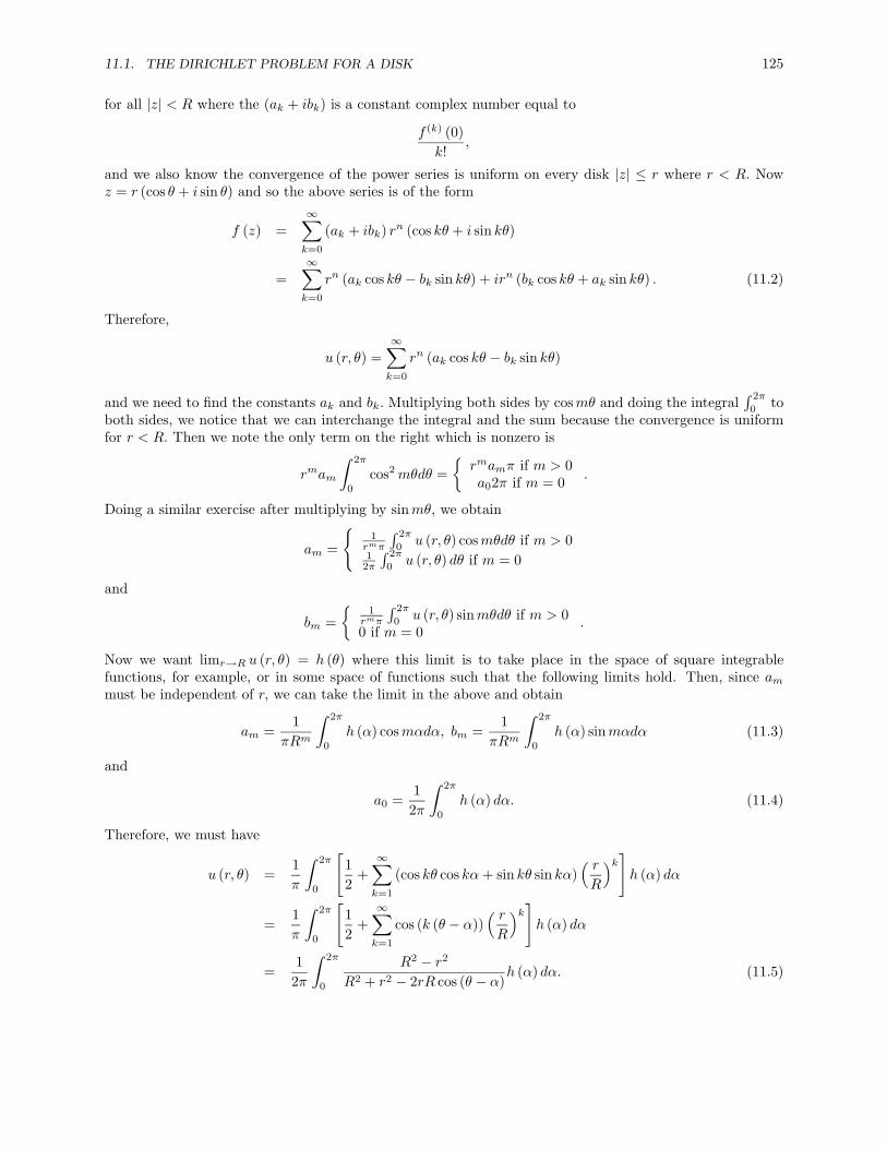
11.1. THE DIRICHLET PROBLEM FOR A DISK 125
for all |z| < R where the (ak + ibk) is a constant complex number equal to
f (k) (0)k!
,
and we also know the convergence of the power series is uniform on every disk |z| ≤ r where r < R. Nowz = r (cos θ + i sin θ) and so the above series is of the form
f (z) =∞∑k=0
(ak + ibk) rn (cos kθ + i sin kθ)
=∞∑k=0
rn (ak cos kθ − bk sin kθ) + irn (bk cos kθ + ak sin kθ) . (11.2)
Therefore,
u (r, θ) =∞∑k=0
rn (ak cos kθ − bk sin kθ)
and we need to find the constants ak and bk. Multiplying both sides by cosmθ and doing the integral∫ 2π
0to
both sides, we notice that we can interchange the integral and the sum because the convergence is uniformfor r < R. Then we note the only term on the right which is nonzero is
rmam
∫ 2π
0
cos2mθdθ ={rmamπ if m > 0a02π if m = 0 .
Doing a similar exercise after multiplying by sinmθ, we obtain
am =
{1
rmπ
∫ 2π
0u (r, θ) cosmθdθ if m > 0
12π
∫ 2π
0u (r, θ) dθ if m = 0
and
bm ={
1rmπ
∫ 2π
0u (r, θ) sinmθdθ if m > 0
0 if m = 0.
Now we want limr→R u (r, θ) = h (θ) where this limit is to take place in the space of square integrablefunctions, for example, or in some space of functions such that the following limits hold. Then, since ammust be independent of r, we can take the limit in the above and obtain
am =1
πRm
∫ 2π
0
h (α) cosmαdα, bm =1
πRm
∫ 2π
0
h (α) sinmαdα (11.3)
and
a0 =1
2π
∫ 2π
0
h (α) dα. (11.4)
Therefore, we must have
u (r, θ) =1π
∫ 2π
0
[12
+∞∑k=1
(cos kθ cos kα+ sin kθ sin kα)( rR
)k]h (α) dα
=1π
∫ 2π
0
[12
+∞∑k=1
cos (k (θ − α))( rR
)k]h (α) dα
=1
2π
∫ 2π
0
R2 − r2
R2 + r2 − 2rR cos (θ − α)h (α) dα. (11.5)

126 HARMONIC FUNCTIONS
This comes by computing the above sum using that it is the real part of the geometric sum,
12
+∞∑k=1
eik(θ−α)( rR
)k.
The details are completely routine and are left for the reader. The formula (11.5) is called the Poissonintegral formula for a disk. There are versions of this which are valid in any dimension but we emphasizetwo dimensional problems because this is a compex variable course. With (11.5) we can prove the followinguseful lemma called the mean value property.
Lemma 11.6 Suppose u is harmonic on U, an open subset of R2. Then if z ∈ B (z, r) ⊆ U,
u (z) =1
2π
∫ 2π
0
u(z + reiθ
)dθ.
In other words, u (z) equals the average of the values of u on any disk centered at z.
Proof: Let z = x0 + iy0 and define v (x, y) ≡ u (x0 + x, y0 + y) . Then (x, y) → v (x, y) is harmonic onB (0, r) and so from (11.5) we have
v (0, θ) = u (x0, y0) =1
2π
∫ 2π
0
R2
R2u(z + reiθ
)dθ.
Lemma 11.7 The following formula is obtained.
1 =1
2π
∫ 2π
0
R2 − r2
R2 + r2 − 2rR cos (θ − α)dα
and for all r < R,
R2 − r2
R2 + r2 − 2rR cos (θ − α)≥ 0
Proof: This follows immediately from (11.5) by letting u (z) ≡ 1. By the uniqueness theorem we obtainthe desired equation.
Definition 11.8 We define h (x+) and h (x−) as follows.
h (x+) ≡ limx→x+
h (x)
h (x−) ≡ limx→x−
h (x)
Theorem 11.9 Let h be 2π periodic and piecewise continuous. Also suppose that h (θ+) and h (θ−) bothexist. Then if u is given by (11.5), it follows that
limr→R−
u (r, θ) =h (θ+) + h (θ−)
2
and that ∆u = 0 in B (0, R) .
Proof: Using Lemma 11.7 and the peiodicity of h and u
u (r, θ) =1
2π
∫ 2π
0
R2 − r2
R2 + r2 − 2rR cos (θ − α)h (α) dα
=1
2π
∫ θ+π
θ−π
R2 − r2
R2 + r2 − 2rR cos (θ − α)h (α) dα
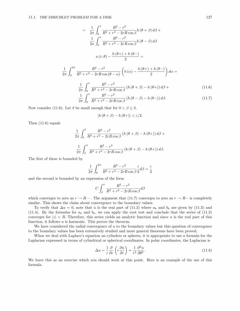
11.1. THE DIRICHLET PROBLEM FOR A DISK 127
=1
2π
∫ π
0
R2 − r2
R2 + r2 − 2rR cosβh (θ + β) dβ +
12π
∫ π
0
R2 − r2
R2 + r2 − 2rR cosβh (θ − β) dβ
u (r, θ)− h (θ+) + h (θ−)2
=
12π
∫ 2π
0
R2 − r2
R2 + r2 − 2rR cos (θ − α)
(h (α)− h (θ+) + h (θ−)
2
)dα =
12π
∫ π
0
R2 − r2
R2 + r2 − 2rR cosβ(h (θ + β)− h (θ+)) dβ + (11.6)
12π
∫ π
0
R2 − r2
R2 + r2 − 2rR cosβ(h (θ − β)− h (θ−)) dβ. (11.7)
Now consider (11.6). Let δ be small enough that for 0 < β ≤ δ,
|h (θ + β)− h (θ+)| < ε/2.
Then (11.6) equals
12π
∫ δ
0
R2 − r2
R2 + r2 − 2rR cosβ(h (θ + β)− h (θ+)) dβ +
12π
∫ π
δ
R2 − r2
R2 + r2 − 2rR cosβ(h (θ + β)− h (θ+)) dβ.
The first of these is bounded by
12π
∫ 2π
0
R2 − r2
R2 + r2 − 2rR cosβε
2dβ =
ε
2
and the second is bounded by an expression of the form
C
∫ π
δ
R2 − r2
R2 + r2 − 2rR cosβdβ
which converges to zero as r → R − . The argument that (11.7) converges to zero as r → R− is completelysimilar. This shows the claim about convergence to the boundary values.
To verify that ∆u = 0, note that u is the real part of (11.2) where ak and bk are given by (11.3) and(11.4). By the formulas for ak and bk, we can apply the root test and conclude that the series of (11.2)converges for |z| < R. Therefore, this series yields an analytic function and since u is the real part of thisfunction, it follows u is harmonic. This proves the theorem.
We have considered the radial convergence of u to the boundary values but this question of convergenceto the boundary values has been extensively studied and more general theorems have been proved.
When we deal with Laplace’s equation on cylinders or spheres, it is appropriate to use a formula for theLaplacian expressed in terms of cylindrical or spherical coordinates. In polar coordinates, the Laplacian is
∆u =1r
∂
∂r
(r∂u
∂r
)+
1r2
∂2u
∂θ2. (11.8)
We leave this as an exercise which you should work at this point. Here is an example of the use of thisformula.

128 HARMONIC FUNCTIONS
Example 11.10 Let U be the anulus between the disks, B (0, 2) and B (0, 5) . Find u such that ∆u = 0 inthe anulus and u = 0 on the inside boundary, ∂B (0, 2) and u = 8 on the outside boundary, ∂B (0, 5) .
We look for a solution, u which does not depend on θ. Thus we need to solve for u = u (r) and
ru′′ + u′ = 0, u (2) = 0, u (5) = 8.
It is routine to verify the solution is:
u (r) = 8ln 2
ln 2− ln 5− 8
ln 2− ln 5ln r
If you wanted to put this in terms of x and y, it would be unnatural, but you could do it of course. Simplyreplace r with
√x2 + y2.
11.2 Exercises
1. Suppose ∆u = 0 in U a bounded region of R2(connected open set) with u continuous on U and supposealso that
u (z) = max {u (w) : w ∈ ∂U} ≡M
for some z ∈ U. Show that then u (z) = M for all z ∈ U. Hint: Use the mean value property toverify that {z ∈ U : u (z) = M} is an open set. By continuity of u it is a closed set also. Now use theassumption that U is connected. Sometimes this result is called the strong mean value property.
2. Show that
uxx + uyy =1r
(rur)r +1r2uθθ
where here x = r cos θ and y = r sin θ. Hint: This is actually a very easy problem if the right materialon vector analysis has been learned earlier. Since this is not assumed, you will be well advised to startwith the right and show that you obtain the left by using the chain rule.
3. Using this result, show directly that the solution given by the Poisson integral formula is harmonic.
4. Let U be the anulus between the disks, B (0, 1) and B (0, 5) . Find u such that ∆u = 0 in the anulusand u = 1 on the inside boundary, ∂B (0, 1) and u = 8 on the outside boundary, ∂B (0, 5) .
5. Show that ln r is harmonic in R2 and that 1/rn−2 is harmonic in Rn.
6. If u ≥ 0 and satisfies ∆u = 0 in a disk, B (0, R) , then letting R1 < R, use the Poisson integral formulato verify that for r < R1,
u (0)R1 − rR1 + r
≤ u (r, θ) ≤ u (0)R1 + r
R1 − r.
This remarkable inequality is known as Harnack’s inequality. As with everything done in this chapterit has a generalization to n dimensions.
7. Show that if {un} is an increasing sequence of functions harmonic on B (0, R) , then if {un (0)} con-verges, it follows that {un} converges uniformly on every compact subset of B (0, R) . Furthermore, if{un (0)} converges to ∞, then for every r < R, we have limn→∞ un (r, θ) = ∞. Hint: Use Harnack’sinequality on un (r, θ)− um (r, θ) where n > m to verify that if un (0) converges to a finite value, thenwe have uniform convergence on any closed ball of the form B (0, R1) where R1 < R. Then argue thisrequires uniform convergence on every compact subset of B (0, R) . To establish the last claim, use thebottom half of Harnack’s inequality.
11.2. EXERCISES 129
8. Show that if {un} is a sequence of harmonic functions defined on B (0, R) which converge uniformlyto u on every compact set, then it follows that u is also harmonic. Hint: Use the Poisson integralformula and argue that if u is given by this formula, it follows u is harmonic.
9. To see all of this chapter done in more generality see a good book on partial differential equations.One of the best is the one by Evans, [3] or the book version of the same set of notes. You will beamazed how the big theorems of real analysis such as the divergence theorem can be used to give anelegant treatment of much more general results than those presented here. Look it up and write inyour own words a presentation of the Poisson integral formula in n dimensions as well as the materialon Harnack’s inequality and the other notions presented above.

130 HARMONIC FUNCTIONS
Complex mappings
Recall from the problem on page 50, if f is an analytic function defined on an open set with f ′ (z) 6= 0, thenf is a conformal map. This means it preserves angles between curves as well as orientations. In this chapter,we will refer to analytic functions whose derivatives do not vanish as conformal maps. There are two maintypes of conformal maps which occur often in applications. The first sort is discussed in the next sectionand the second kind come from the Schwarz Christoffel transformations.
12.1 Fractional linear transformations
In this section we consider an important class of mappings which are defined in the following definition. Theprinciple result pertaining to these mappings is that they map lines and circles to either lines or circles.
Definition 12.1 A fractional linear transformation is a function of the form
f (z) =az + b
cz + d(12.1)
where ad− bc 6= 0.
Note that if c = 0, this reduces to a linear transformation (a/d) z+(b/d) . Special cases of these are givendefined as follows.
dilations: z → δz, δ 6= 0, inversions: z → 1z,
translations: z → z + ρ.
Lemma 12.2 The fractional linear transformation, (12.1) can be written as a finite composition of diations,inversions, and translations.
Proof: Let S1 (z) = z + dc , S2 (z) = 1
z , S3 (z) = (bc−ad)c2 z and S4 (z) = z + a
c in the case where c 6= 0.Then
f (z) = S4 ◦ S3 ◦ S2 ◦ S1.
Here is why. S2 (S1 (z)) = S2
(z + d
c
)≡ 1
z+ dc
= czc+d . Now we consider S3
(c
zc+d
)≡ (bc−ad)
c2
(c
zc+d
)=
bc−adc(zc+d) . Finally, we consider S4
(bc−adc(zc+d)
)≡ bc−ad
c(zc+d) + ac = b+az
zc+d . In case that c = 0, we simply have
f (z) = adz+ b
d which is a translation composed with a dilation. Because of the assumption that ad− bc 6= 0,we know that since c = 0 we must have both a and d 6= 0. This proves the lemma.
With this lemma we can show the following interesting corollary.
131
132 COMPLEX MAPPINGS
Corollary 12.3 Fractional linear transformations map circles and lines to circles or lines.
Proof: It is obvious that dilations and translations map circles to circles and lines to lines. We need toconsider inversions. Then when this is done, the above lemma implies a general fractional linear transfor-mation has this property as well.
Note that all circles and lines may be put in the form
α(x2 + y2
)− 2ax− 2by = r2 −
(a2 + b2
)where α = 1 gives a circle centered at (a, b) with radius r and α = 0 gives a line. In terms of complexvariables we may therefore consider all possible circles and lines in the form
αzz + βz + βz + γ = 0, (12.2)
To see this let β = β1 + iβ2 where β1 ≡ −a and β2 ≡ b. Note that even if α is not 0 or 1 the expression stillcorresponds to either a circle or a line because we can divide by α if α 6= 0. Now we verify that replacing zwith 1
z we still end up with an expression of the form in (12.2). Thus, let w = 1z where z satisfies (12.2).
Then (α+ βw + βw + γww
)=
1zz
(αzz + βz + βz + γ
)= 0
and so w also satisfies a relation like (12.2). One simply switches α with γ and β with β. Note the situationis slightly different than with dilations and translations. In the case of an inversion, a circle becomes eithera line or a circle and similarly, a line becomes either a circle or a line. This proves the corollary.
Example 12.4 Consider the fractional linear transformation, w = z−iz+i .
First we see what this mapping does to the points of the form z = x+ i0. Substituting into the expressionfor w, we obtain
w =x− ix+ i
=x2 − 1− 2xi
x2 + 1,
a point on the unit circle. Thus this transformation maps the real axis to the unit circle.The upper half plane is composed of points of the form x + iy where y > 0. Substituting in to the
transformation, we obtain
w =x+ i (y − 1)x+ i (y + 1)
=x2 + y2 − 1− 2ixx2 + (y + 1)2 ,
which is seen to be a point on the interior of the unit disk whose distance from 0 is x2+y2−2y+1x2+y2+2y+1 . Therefore,
this transformation maps the upper half plane to the interior of the unit disk.We might wonder whether the mapping is one to one and onto. The mapping is clearly one to one
because we can exhibit an inverse, z = −iw+1w−1 for all w in the interior of the unit disk. Also, a short
computation verifies that z so defined is in the upper half plane. Therefore, this transformation maps{z ∈ C such that Imz > 0} one to one and onto the unit disk {z ∈ C such that |z| < 1} .
There is a simple procedure for determining fractional linear transformations which map a given set ofthree points to another set of three points. The problem is as follows: There are three distinct points in theextended complex plane, z1, z2, and z3 and it is desired to find a fractional linear transformation such thatzi → wi for i = 1, 2, 3 where here w1, w2, and w3 are three distinct points in the extended complex plane.Then the proceedure says that to find the desired fractional linear transformation we solve the followingequation for w.
w − w1
w − w3· w2 − w3
w2 − w1=z − z1
z − z3· z2 − z3
z2 − z1
12.2. SOME OTHER MAPPINGS 133
The result will be a fractional linear transformation with the desired properties. If any of the points equals∞, then the quotient containing this point must be replaced with 1.
Why should this proceedure work? We give a heuristic argument to indicate why we should expect this tohappen rather than a rigorous proof. The reader may want to tighten the argument to give a proof. We notethat the equation is of the form F (w) = G (z) where F andG are fractional linear transformations. Therefore,w = F−1 (G (z)) also a fractional linear transformation because inverses of fractional linear transformationsare fractional linear transformations and the composition of two fractional linear transformations is alsoa fractional linear transformation. Now F (w1) = 0, F (w2) = 1, and F (w3) = ∞ because it involvesdivision by 0. Also, G (z1) = 0, G (z2) = 1, and G (z3) = ∞. Therefore, F−1 (G (z1)) = F−1 (0) = w1. Also,F−1 (G (z2)) = F−1 (1) = w2, and F−1 (G (z3)) = F−1 (∞) = w3.
Example 12.5 Let Imξ > 0 and consider the fractional linear transformation which takes ξ to 0, ξ to ∞and 0 to ξ/ξ, .
The equation we need to solve for w is
w − 0w −
(ξ/ξ) =
z − ξz − 0
· ξ − 0ξ − ξ
After some computations, we see that
w =z − ξz − ξ
.
Note that this has the property that x−ξx−ξ is always a point on the unit circle because it is a complex number
divided by its conjugate. Therefore, this fractional linear transformation maps the real line to the unit circle.It also takes the point, ξ to 0 and so it must map the upper half plane to the unit disk. You can verify themapping is onto as well. We use this example in Section 12.3.
Example 12.6 Let z1 = 0, z2 = 1, and z3 = 2 and let w1 = 0, w2 = i, and w3 = 2i.
Then the equation we must solve is
w
w − 2i· −ii
=z
z − 2· −1
1
Solving this yields w = iz which clearly works.
12.2 Some other mappings
There are many useful mappings which are known and there is a convenient list in [10] which can be consulted.We consider a few of these here.
Example 12.7 The infinite sector between the two rays determined by the positive x axis and the linewhose angle with the positive x axis is π/m where m is a positive integer is mapped onto the half planeH = {w : Imw > 0} by the mapping w = zm.
The claim in this example is obvious because for z in this sector, z = reiθ where θ ∈ (0, π/m) and sozm = rmeimθ, an element of H. Furthermore, it is clear every element of H if obtained in this way becausethe argument of these elements are between 0 and π.
Example 12.8 An infinite strip of width a determined by the x axis and the line y = a can be mapped tothe upper half plane, H by the transformation, w = eπz/a.
134 COMPLEX MAPPINGS
This is easily seen by noting that eπ(x+iy)
a = eπxa
(cos(πya
)+ i sin
(πya
))∈ H and that if α+ iβ ∈ H, then
we can determine x such that eπxa =
(α2 + β2
)1/2. Also, arg (α+ iβ) ∈ (0, π) and so we can find y ∈ (0, a)such that πy
a = arg (α+ iβ) .
Example 12.9 The upper half of the unit circle can be mapped to H also. This can be done by the trans-
formation, w =(
1+z1−z
)2
.
To see this is the case, first note that the unit disk maps to the upper half plane, H by i(
1+z1−z
)and so
w =(
1+z1−z
)maps the unit disk to the right half plane. Now note that if this transformation takes the upper
half of the unit disk to the first quadrant because if the imaginary part is nonnegative, the transformed pointalso has imaginary part nonnegative. Now w = z2 we have already seen mapps the first quadrant to theupper half plane, H.
Example 12.10 The circular sector {z ∈ unit disk such that arg z ∈ (0, π/m)} where m is a positive inte-
ger can be mapped to H by using w =(
1+zm
1−zm
)2
.
This is obvious from observing that zm maps the given sector to the upper half disk and then using theabove example.
Example 12.11 The annulus between the disks B (0, b) and B (0, a) minus the negative real axis can bemapped to a rectangle by using w = ln z.
Recall ln z = ln |z| + i arg (z) where arg (z) is the angle between −π and π. Consider r ∈ (a, b) and letz = reiθ where θ ∈ (−π, π) . Then ln z = ln r+ iθ. In other words the real part is constant and the imaginarypart goes from −π to π. Since we can do this for each such r ∈ (a, b) , it follows the image of this anulus is(ln a, ln b)× (−π, π) , a rectangle.
12.3 The Dirichlet problem for a half plane
To begin with we consider a general theorem.
Theorem 12.12 Let U and V be two regions in R2 and suppose h : U → V is analytic. Then if ∆v = 0on V, it follows that ∆h∗v = 0 on U. Here h∗v (z) ≡ v (h (z)) .
Proof: Let z = x+ iy. Then (h∗v)x = v,1 (h (z)) Rehx + v,2 (h (z)) Imhx. Also,
(h∗v)xx = v,11 (Rehx)2 + v,12ImhxRehx +
v,21ImhxRehx + v,22 (Imhx)2
+v,1Rehxx + v,2Imhxx
Similarly,
(h∗v)yy = v,11 (Rehy)2 + v,12ImhyRehy +
v,21ImhyRehy + v,22 (Imhy)2
+v,1Rehyy + v,2Imhyy
Now we apply the Cauchy Riemann equations to say that Rehx = Imhy, Rehy = −Imhx and we get fromthe above
(h∗v)xx = v,11 (Rehx)2 + v,12ImhxRehx +
v,21ImhxRehx + v,22 (Rehy)2
+v,1Rehxx + v,2Imhxx
12.3. THE DIRICHLET PROBLEM FOR A HALF PLANE 135
(h∗v)yy = v,11 (Rehy)2 − v,12RehxImhx +
−v,21RehxImhx + v,22 (Rehx)2
+v,1Rehyy + v,2Imhyy
∆ (h∗v) =
=0︷ ︸︸ ︷(v,11 + v,22)
((Rehx)2 + (Rehy)2
)+v,1
=0︷ ︸︸ ︷(Rehyy + Rehxx) + v,1
=0︷ ︸︸ ︷(Rehyy + Rehxx) .
This proves the theorem. (Rehyy+Rehxx = 0 because of the Cauchy Riemann equations and the assumptionthat h is analytic.)
Corollary 12.13 Let U and V be two regions in R2 and suppose h : U → V is analytic, one to one andonto. Then ∆v = 0 on V, if and only if ∆h∗v = 0 on U. Here h∗v (z) ≡ v (h (z)) .
Proof: This follows from the open mapping theorem and the above theorem applied to(h−1
)∗.
With this preparation, we can give a formula for the solution to the Dirichlet problem on the half plane,the Poisson integral formula for a half plane.
Theorem 12.14 Let g (x) be a bounded continuous function defined on R. Let H ≡ {(x, y) : y > 0} . Thenthe solution to
∆v = 0 on H,
v = g on ∂H
is given by
v (a, b) =b
π
∫ ∞−∞
g (x)(x− a)2 + b2
dx.
Proof: Let ξ ∈ H. Then the fractional linear transformation,
hξ (z) ≡ z − ξz − ξ
maps H one to one and onto B, the unit disk and let φξ = h−1ξ . From Theorem 12.12, ∆φ∗ξv = 0 in B and
φ∗ξv = φ∗ξg on ∂B. Therefore, from the formula for a disk,
v (φξ (w)) =1
2π
∫ 2π
0
(1− r2
1 + r2 − 2r cos (θ − α)
)g(φξ(eiα))dα. (12.3)
Now we let w = hξ (z) so z ∈ H. For w ∈ ∂B, we have z = x ∈ R and w = eiα so hξ (x) = eiα. Therefore,taking derivatives,
dw = ieiαdα = h′ξ (x) dx
=2iImξ(x− ξ
)2 dx.Therefore, letting ξ = (a, b) ,
dα =2Imξ
hξ (x)(x− ξ
)2 dx=
2Imξ(x− ξ)
(x− ξ
)dx=
2Imξ(x− a)2 + b2
dx
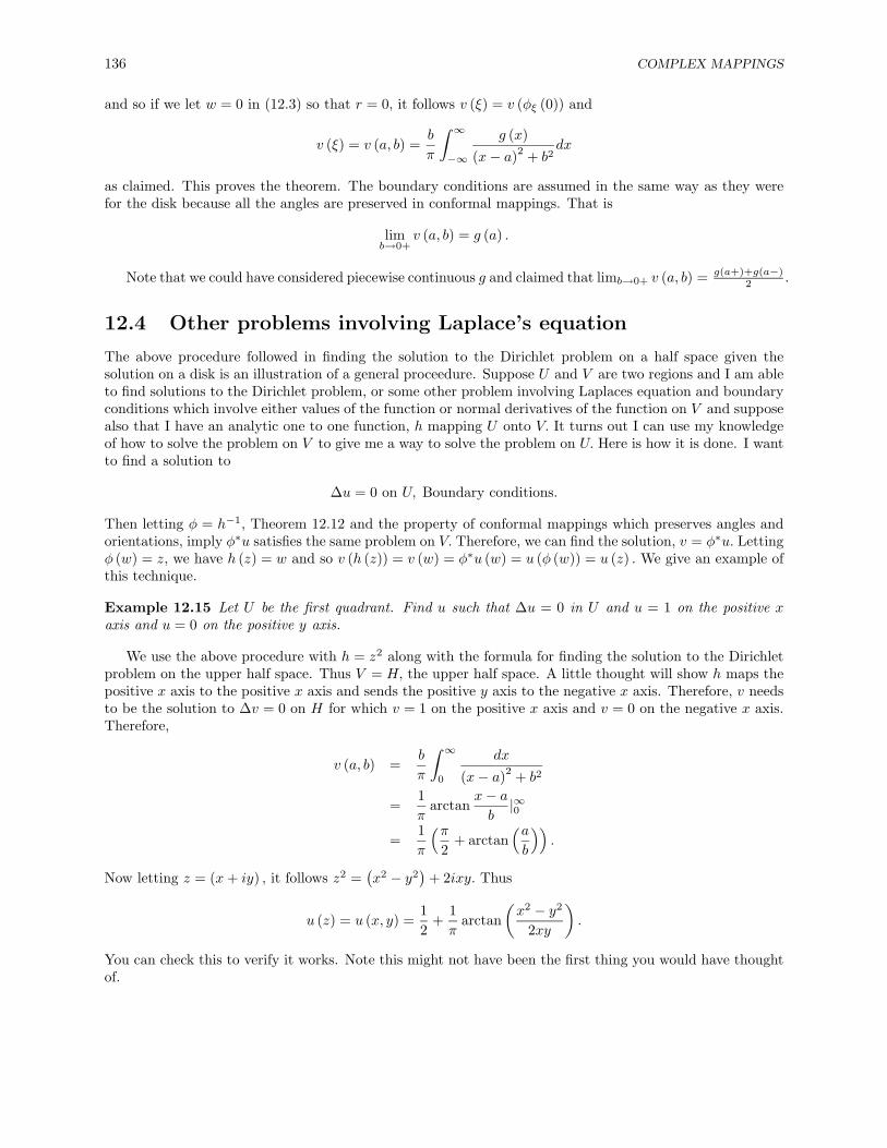
136 COMPLEX MAPPINGS
and so if we let w = 0 in (12.3) so that r = 0, it follows v (ξ) = v (φξ (0)) and
v (ξ) = v (a, b) =b
π
∫ ∞−∞
g (x)(x− a)2 + b2
dx
as claimed. This proves the theorem. The boundary conditions are assumed in the same way as they werefor the disk because all the angles are preserved in conformal mappings. That is
limb→0+
v (a, b) = g (a) .
Note that we could have considered piecewise continuous g and claimed that limb→0+ v (a, b) = g(a+)+g(a−)2 .
12.4 Other problems involving Laplace’s equation
The above procedure followed in finding the solution to the Dirichlet problem on a half space given thesolution on a disk is an illustration of a general proceedure. Suppose U and V are two regions and I am ableto find solutions to the Dirichlet problem, or some other problem involving Laplaces equation and boundaryconditions which involve either values of the function or normal derivatives of the function on V and supposealso that I have an analytic one to one function, h mapping U onto V. It turns out I can use my knowledgeof how to solve the problem on V to give me a way to solve the problem on U. Here is how it is done. I wantto find a solution to
∆u = 0 on U, Boundary conditions.
Then letting φ = h−1, Theorem 12.12 and the property of conformal mappings which preserves angles andorientations, imply φ∗u satisfies the same problem on V. Therefore, we can find the solution, v = φ∗u. Lettingφ (w) = z, we have h (z) = w and so v (h (z)) = v (w) = φ∗u (w) = u (φ (w)) = u (z) . We give an example ofthis technique.
Example 12.15 Let U be the first quadrant. Find u such that ∆u = 0 in U and u = 1 on the positive xaxis and u = 0 on the positive y axis.
We use the above procedure with h = z2 along with the formula for finding the solution to the Dirichletproblem on the upper half space. Thus V = H, the upper half space. A little thought will show h maps thepositive x axis to the positive x axis and sends the positive y axis to the negative x axis. Therefore, v needsto be the solution to ∆v = 0 on H for which v = 1 on the positive x axis and v = 0 on the negative x axis.Therefore,
v (a, b) =b
π
∫ ∞0
dx
(x− a)2 + b2
=1π
arctanx− ab|∞0
=1π
(π2
+ arctan(ab
)).
Now letting z = (x+ iy) , it follows z2 =(x2 − y2
)+ 2ixy. Thus
u (z) = u (x, y) =12
+1π
arctan(x2 − y2
2xy
).
You can check this to verify it works. Note this might not have been the first thing you would have thoughtof.
12.5. EXERCISES 137
Example 12.16 Consider the upper half of the unit disk and find the solution, u, to Laplace’s equationwhich equals 0 on the top curved boundary and 1 on the the flat part of the boundary on the x axis.
Tracing through the reasoning that w =(
1+z1−z
)2
maps this upper half of the unit disk to the upper halfplane, you can see that the negative x axis corresponds to the curved part of the half disk and the positive xaxis corresponds to the flat part of the boundary of the half disk. Therefore, as in the preceeding example,
v (a, b) =b
π
∫ ∞0
dx
(x− a)2 + b2
=1π
(π2
+ arctan(ab
)),
but here we have an entirely different h. Letting z = x+ iy, we have
h (z) =(
1 + x+ iy
1− x− iy
)2
=1− 2x2 − 6y2 + x4 + 2x2y2 + y4 − 4iyx2 + 4iy − 4iy3
1− 4x+ 6x2 + 2y2 − 4x3 − 4xy2 + x4 + 2x2y2 + y4
and so
u (x, y) =12
+1π
arctan(
1− 2x2 − 6y2 + x4 + 2x2y2 + y4
−4yx2 + 4y − 4y3
).
If the preceeding example was obvious, perhaps this one isn’t.
12.5 Exercises
1. For v given in Theorem 12.14 and g bounded and piecewise continuous, verify directly that
limb→0+
v (a, b) =g (a+) + g (a−)
2.
Also verify directly that for v given this way, it satisfies ∆v = 0 in H.
2. In Theorem 11.9 show using Formula (11.8) that the solution given in that theorem does satisfyLaplace’s equation.
3. Let U denote the infinite sector determined by the positive x axis and the ray having an angle of π/6with the positive x axis. Let u = 0 on this ray and let u = 1 on the positive x axis. Find u satisfyingthese boundary conditions and ∆u = 0 in U.
4. Let U denote the circular sector determined by the positive x axis and the ray having an angle of π/6with the positive x axis and the unit circle. Let u = 1 on this ray, let u = 1 on the positive x axis, andlet u = 0 on the curved part of the circular sector. Find u satisfying these boundary conditions and∆u = 0 in U.
5. In [10] on page 206 we see that w = sin(πza
)maps the semi infinite strip of width a of the form x+ iy
where x ∈(−a2 ,
a2
)to the upper half plane in such a way that −a/2 goes to −1 and a/2 goes to 1.
Using this, solve the Dirichlet problem where ∆u = 0 in the semi infinite strip and on the left andright edge, u = 0 while on the bottom, the part between −a/2 and a/2 on the x axis, u = 1.
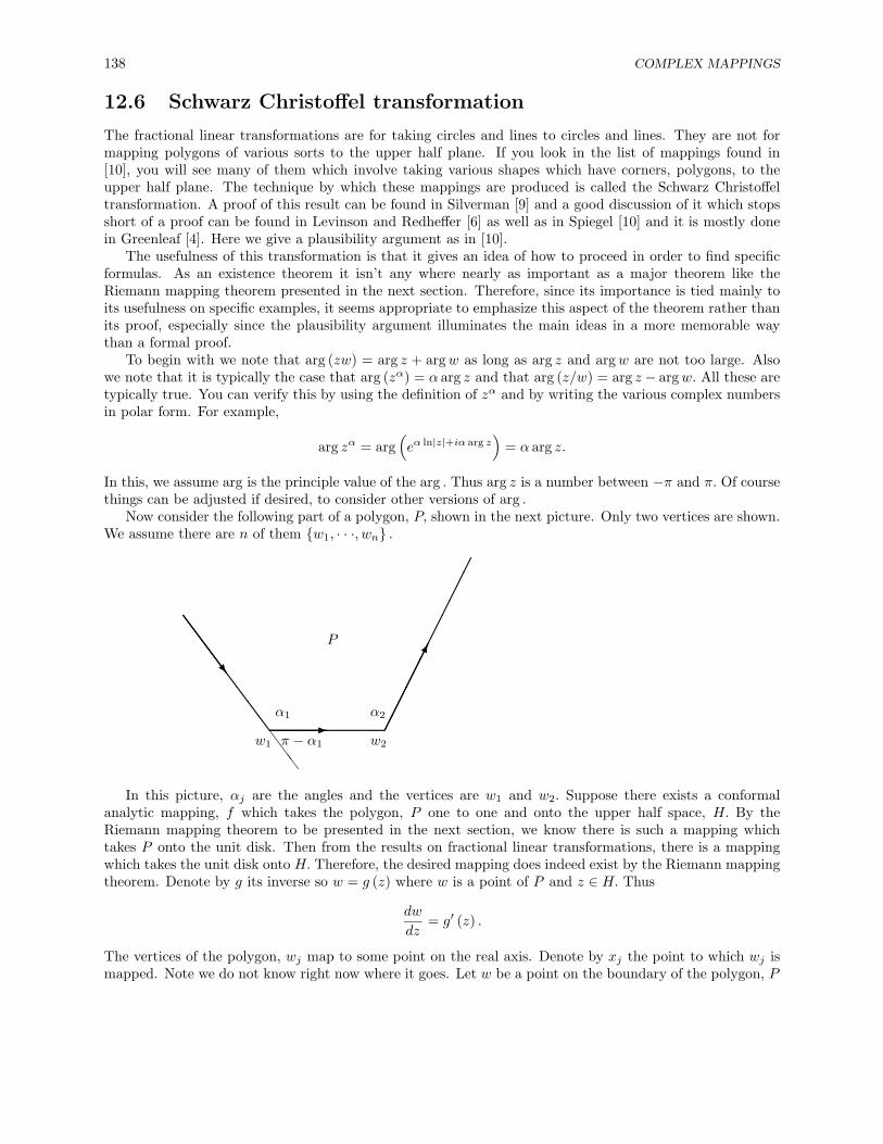
138 COMPLEX MAPPINGS
12.6 Schwarz Christoffel transformation
The fractional linear transformations are for taking circles and lines to circles and lines. They are not formapping polygons of various sorts to the upper half plane. If you look in the list of mappings found in[10], you will see many of them which involve taking various shapes which have corners, polygons, to theupper half plane. The technique by which these mappings are produced is called the Schwarz Christoffeltransformation. A proof of this result can be found in Silverman [9] and a good discussion of it which stopsshort of a proof can be found in Levinson and Redheffer [6] as well as in Spiegel [10] and it is mostly donein Greenleaf [4]. Here we give a plausibility argument as in [10].
The usefulness of this transformation is that it gives an idea of how to proceed in order to find specificformulas. As an existence theorem it isn’t any where nearly as important as a major theorem like theRiemann mapping theorem presented in the next section. Therefore, since its importance is tied mainly toits usefulness on specific examples, it seems appropriate to emphasize this aspect of the theorem rather thanits proof, especially since the plausibility argument illuminates the main ideas in a more memorable waythan a formal proof.
To begin with we note that arg (zw) = arg z + argw as long as arg z and argw are not too large. Alsowe note that it is typically the case that arg (zα) = α arg z and that arg (z/w) = arg z − argw. All these aretypically true. You can verify this by using the definition of zα and by writing the various complex numbersin polar form. For example,
arg zα = arg(eα ln|z|+iα arg z
)= α arg z.
In this, we assume arg is the principle value of the arg . Thus arg z is a number between −π and π. Of coursethings can be adjusted if desired, to consider other versions of arg .
Now consider the following part of a polygon, P, shown in the next picture. Only two vertices are shown.We assume there are n of them {w1, · · ·, wn} .
SSSSw
SSSSSSSS - �
�����������
�������
α1 α2
w1 w2
P
SSS
π − α1
In this picture, αj are the angles and the vertices are w1 and w2. Suppose there exists a conformalanalytic mapping, f which takes the polygon, P one to one and onto the upper half space, H. By theRiemann mapping theorem to be presented in the next section, we know there is such a mapping whichtakes P onto the unit disk. Then from the results on fractional linear transformations, there is a mappingwhich takes the unit disk onto H. Therefore, the desired mapping does indeed exist by the Riemann mappingtheorem. Denote by g its inverse so w = g (z) where w is a point of P and z ∈ H. Thus
dw
dz= g′ (z) .
The vertices of the polygon, wj map to some point on the real axis. Denote by xj the point to which wj ismapped. Note we do not know right now where it goes. Let w be a point on the boundary of the polygon, P
12.6. SCHWARZ CHRISTOFFEL TRANSFORMATION 139
moving over the boundary of P such that the area of P is on the left, and let z be the point correspondingto w which is on the real axis which we assume is moving from left to right. Then because conformal mapspreserve orientations, it follows that g (P ) will be on the left of the point, z which is moving from left to right.Thus g (P ) is contained in the upper half plane. When we encounter a vertex, wk on P this corresponds tothe point, xk to which wk was mapped. We consider the following:
A = arg dw
and
B =(α1
π− 1)
arg (z − x1) + · · ·+(αnπ− 1)
arg (z − xn) .
Never mind that we have never given any sort of precise meaning to dw and so the above is pseudo math-ematical garbage. Think of dw as an infinitesimal complex number and as such it has an argument. If youlike, think of it as an infinitesimal vector whatever that would mean. The idea is that dw points in thedirection of travel as we move along the sides of P. Therefore, as shown in the above picture, as we passthrough the vertex, w1, arg dw increases by π − α1. As we do this, z passes through x1 on the boundaryof H and arg (z − x1) goes from π to 0. The other terms in B are unchanged. Therefore, B changes by(α1π − 1
)(−π) = (π − α1) also. When w encounters w2, a similar situation occurs, resulting in the same
change to A and B. Therefore, we see that as we move over the boundary of P with P on the left and overH with H on the left, A−B is a constant. Therefore, it seems we should be able to find a constant K suchthat
A︷ ︸︸ ︷arg dw =
=0︷ ︸︸ ︷arg dz +
argK +
B︷ ︸︸ ︷(α1
π− 1)
arg (z − x1) + · · ·+(αnπ− 1)
arg (z − xn).
By adjusting the size of K if necessary, this shows we should expect to have
dw
dz= K (z − x1)(
α1π −1) + · · ·+ (z − xn)(
αnπ −1)
which is the Schwarz Christoffel transformation. Notice we do not know what K is or what any of the xjare. However, it turns out that we can pick two of the finite xk and find K such that things work out. Thisis not surprising because you would expect to have two constants to choose when you solve the differentialequation, K and a constant of integration. Also, we pick xn to equal ∞ and then leave out the factor whichwould have appeared. This is because you never get to ∞ so there is never a change occuring in B whichresults from passing through ∞.
This completes our plausibility argument. Nothing has been proved but hopefully, the formula is at leastplausible. Now we give some examples of the use of this formula. Think of this formula as a hint on whatto look for in producing a conformal map of a polygonal region onto the upper half plane.
Example 12.17 Let P be the infinite strip defined as w = x+ iy such that x ∈(−a
2 ,a2
)and y ≥ 0. We wish
to map this to H such that −a2 goes to −1 and a2 goes to 1.
In this example the two angles both equal π/2 and we can take w3 = x3 =∞ and so the formula for thetransformation desired should be of the form
dw
dz= A (z + 1)−1/2 (z − 1)−1/2
.
140 COMPLEX MAPPINGS
We need to consider what A should be so that motion from left to right on the segment(−a
2 ,a2
)of P
corresponds to positive motion on the segment (−1, 1). This is appropriate since this is what was assumedin the above derivation and plausibility argument. Thus we modify A to write
dw
dz= K (1 + z)−1/2 (1− z)−1/2 =
K√1− z2
.
Therefore, we need
w = K arcsin (z) + L
and so
z = sin(w − LK
)Now we want
−1 = sin(− (a/2)− L
K
)and also
1 = sin(
(a/2)− LK
).
This is satisfies when L = 0 and (a/2)K = π
2 so K = aπ . The transformation is then
z = sin(πwa
).
You can check that this does what is is supposed to do at this point. Note that the formula gave us an ideaof what to look for which is a very useful thing.
Example 12.18 Consider the infinite sector having angle α which is formed by the ray y = (tanα)x andthe positive x axis. Here we assume α ∈ (0, π) .
We have already examined a case of this but now we consider it in the context of the Schwarz Christoffeltransformation. Thus we assume 0 corresponds to 0 and we get
dw
dz= K (z − 0)(
απ−1) .
Therefore, we need w = K(πα
)zα/π and it doesn’t seem to matter how we choose K as long as it is positive.
Thus we let w = zα/π. Therefore, solving for z we should have z = wπ/α.
Example 12.19 Let P be the infinite strip of the form w = x+ iy where x > 0 and y ∈ (0, a) .
We will map ai to −1 and 0 to 1. As in an earlier example, we let w3 = ∞ and x3 = ∞. The SchwarzChristoffel transformation is then
dw
dz= A (z + 1)−1/2 (z − 1)−1/2
.
It looks like we want A > 0 so that dw/dz > 0 for x > 1. Therefore, we have
dw
dz= A
(z2 − 1
)−1/2
12.7. EXERCISES 141
and so we would get w = A cosh−1 (z) +B. Now using the conditions that ai goes to −1 and 0 goes to 1, wemust have
0 = A cosh−1 (1) +B
= A · 0 +B
so B = 0. Then also we need z = cosh(wA
)and letting w = ai, we must have −1 = cosh
(aiA
)and so
−1 = cos(aA
). Therefore, we need a
A = π and so A = aπ . Therefore the desired transformation is z = cosh πw
a .You may want to check to see that this works.
12.7 Exercises
1. Solve ∆u = 0 on the infinite strip z = x + iy such that y ∈ (0, 2) and x > 0 if we want u = 1 on thetop edge, and u = 0 on the bottom edge, and left side.
2. Solve ∆u = 0 on the infinite strip z = x+ iy such that x ∈ (−1, 1) and y > 0 if we want u = 1 on thebottom edge, and u = 0 on the other edges.
3. Solve ∆u = 0 on the infinite sector infinite sector having angle α which is formed by the ray y =(tanα)x and the positive x axis if we have u = 0 on the top ray and u = 1 on the bottom. Here weassume α ∈ (0, π) .
4. Consider the rectangle determined by the points (0, 0) , (0, 1) , (2, 0) , and (2, 1) . Describe a conformalmap which takes this rectangle to the upper half plane. Hint: You may need to write your answer interms of something of the form ∫
γ(0,z)
f (t) dt = w
where γ (0, z) denotes a contour between 0 and z. This is because you are likely to encounter a problemin finding the antiderivative of an integral in closed form. This illustrates the above procedure is notable to solve everything in terms of known functions. You might try to write your answer in terms ofreal integrals. Do you think it would be easy to invert the transformation and solve for z in terms ofw?
12.8 Riemann Mapping theorem
We have given many examples of analytic mappings between various regions of C and we have observedthat we can solve problems involving Laplace’s equation on regions which can be mapped into a region forwhich we know how to solve the problem. How general is this procedure? We know from the open mappingtheorem that analytic functions map regions to other regions or else to single points. In this chapter weprove the remarkable Riemann mapping theorem which states that for every simply connected region, Uthere exists an analytic function, f such that f (U) = B (0, 1) and in addition to this, f is one to one. Theproof involves several ideas which have been developed up to now. We also need the following importanttheorem, a case of Montel’s theorem. Before, beginning we note that the Riemann mapping theorem is aclassic example of a major existence theorem. In mathematics there are two sorts of questions, those relatedto whether something exists and those involving methods for finding it. In the above material, on complexmappings, we have emphasized the second of the two questions. However, it is often the case that questionsrelated to the existence of something are more profound. This is the case here. Both questions are veryimportant and this is why we give a proof of this major theorem below.
142 COMPLEX MAPPINGS
Theorem 12.20 Let U be an open set in C and let F denote a set of analytic functions mapping U toB (0,M) . Then there exists a sequence of functions from F , {fn}∞n=1 and an analytic function, f such thatf
(k)n converges uniformly to f (k) on every compact subset of U.
Proof: First we note there exists a sequence of compact sets, Kn such that Kn ⊆ intKn+1 ⊆ U forall n where here intK denotes the interior of the set K, the union of all open sets contained in K and∪∞n=1Kn = U. We leave it as an exercise to verify that B (0, n) ∩
{z ∈ U : dist
(z, UC
)≤ 1
n
}works for Kn.
Then there exist positive numbers, δn such that if z ∈ Kn, then B (z, δn) ⊆ intKn+1. Now denote by Fn theset of restrictions of functions of F to Kn. Then let z ∈ Kn and let γ (t) ≡ z + δne
it, t ∈ [0, 2π] . It followsthat for z1 ∈ B (z, δn) , and f ∈ F ,
|f (z)− f (z1)| =∣∣∣∣ 12πi
∫γ
f (w)(
1w − z
− 1w − z1
)dw
∣∣∣∣≤ 1
2π
∣∣∣∣∫γ
f (w)z − z1
(w − z) (w − z1)dw
∣∣∣∣Letting |z1 − z| < δn
2 , we can estimate this and write
|f (z)− f (z1)| ≤ M
2π2πδn
|z − z1|δ2n/2
≤ 2M|z − z1|δn
.
It follows that Fn is equicontinuous and uniformly bounded so by the Arzela Ascoli theorem there exists asequence, {fnk}∞k=1 ⊆ F which converges uniformly on Kn. Let {f1k}∞k=1 converge uniformly on K1. Thenuse the Arzela Ascoli theorem applied to this sequence to get a subsequence, denoted by {f2k}∞k=1 whichalso converges uniformly on K2. Continue in this way to obtain {fnk}∞k=1 which converges uniformly onK1, · · ·,Kn. Now the sequence {fnn}∞n=m is a subsequence of {fmk} ∞k=1 and so it converges uniformly onKm for all m. Denoting fnn by fn for short, this is the sequence of functions promised by the theorem. It isclear {fn}∞n=1 converges uniformly on every compact subset of U because every such set is contained in Km
for all m large enough. Let f (z) be the point to which fn (z) converges. Then f is a continuous functiondefined on U. We need to verify f is analytic. But, letting T ⊆ U,∫
∂T
f (z) dz = limn→∞
∫∂T
fn (z) dz = 0.
Therefore, by Morera’s theorem we see that f is analytic. As for the uniform convergence of the derivativesof f, this follows from the Cauchy integral formula. For z ∈ Kn, and γ (t) ≡ z + δne
it, t ∈ [0, 2π] ,
|f ′ (z)− f ′k (z)| ≤ 12π
∣∣∣∣∣∫γ
fk (w)− f (w)(w − z)2 dw
∣∣∣∣∣≤ ||fk − f ||
12π
2πδn1δ2n
= ||fk − f ||1δn,
where here ||fk − f || ≡ sup {|fk (z)− f (z)| : z ∈ Kn} . Thus we get uniform convergence of the derivatives.The consideration of the other derivatives is similar.
Since the family, F satisfies the conclusion of Theorem 12.20 it is known as a normal family of functions.The following result is about a certain class of fractional linear transformations,
12.8. RIEMANN MAPPING THEOREM 143
Lemma 12.21 For α ∈ B (0, 1) , let
φα (z) ≡ z − α1− αz
.
Then φα maps B (0, 1) one to one and onto B (0, 1), φ−1α = φ−α, and
φ′α (α) =1
1− |α|2.
Proof: First we show φα (z) ∈ B (0, 1) whenever z ∈ B (0, 1) . If this is not so, there exists z ∈ B (0, 1)such that
|z − α|2 ≥ |1− αz|2 .
However, this requires
|z|2 + |α|2 > 1 + |α|2 |z|2
and so
|z|2(
1− |α|2)> 1− |α|2
contradicting |z| < 1.It remains to verify φα is one to one and onto with the given formula for φ−1
α . But it is easy to verifyφα (φ−α (w)) = w. Therefore, φα is onto and one to one. To verify the formula for φ′α, just differentiate thefunction. Thus,
φ′α (z) = (z − α) (−1) (1− αz)−2 (−α) + (1− αz)−1
and the formula for the derivative follows.The next lemma, known as Schwarz’s lemma is interesting for its own sake but will also be an important
part of the proof of the Riemann mapping theorem.
Lemma 12.22 Suppose F : B (0, 1)→ B (0, 1) , F is analytic, and F (0) = 0. Then for all z ∈ B (0, 1) ,
|F (z)| ≤ |z| , (12.4)
and
|F ′ (0)| ≤ 1. (12.5)
If equality holds in (12.5) then there exists λ ∈ C with |λ| = 1 and
F (z) = λz. (12.6)
Proof: We know F (z) = zG (z) where G is analytic. Then letting |z| < r < 1, the maximum modulustheorem implies
|G (z)| ≤ sup
∣∣F (reit)∣∣r
≤ 1r.
Therefore, letting r → 1 we get
|G (z)| ≤ 1 (12.7)
It follows that (12.4) holds. Since F ′ (0) = G (0) , (12.7) implies (12.5). If equality holds in (12.5), then fromthe maximum modulus theorem, we see that G achieves its maximum at an interior point and is consequentlyequal to a constant, λ, |λ| = 1. Thus F (z) = zλ which shows (12.6). This proves the lemma.

144 COMPLEX MAPPINGS
Definition 12.23 We say a region, U has the square root property if whenever f, 1f : U → C are both
analytic, it follows there exists φ : U → C such that φ is analytic and f (z) = φ2 (z) .
The next theorem will turn out to be equivalent to the Riemann mapping theorem.
Theorem 12.24 Let U 6= C for U a region and suppose U has the square root property. Then for z0 ∈ Uthere exists h : U → B (0, 1) such that h is one to one, onto, analytic, and h (z0) = 0.
Proof: We define F to be the set of functions, f such that f : U → B (0, 1) is one to one and analytic.We will show F is nonempty. Then we will show using Montel’s theorem there is a function in F , h, suchthat for some fixed z0 ∈ U, |h′ (z0)| ≥ |ψ′ (z0)| for all ψ ∈ F . When we have done this, we show h is actuallyonto. This will prove the theorem.
Claim 1: F is nonempty.Proof of Claim 1: Since U 6= C it follows there exists ξ /∈ U. Then letting f (z) ≡ z − ξ, it follows
f and 1f are both analytic on U . Since U has the square root property, there exists an analytic function,
φ : U → C such that φ2 (z) = f (z) for all z ∈ U. Since f is not constant, we know from the open mappingtheorem that φ (U) is a region. Note also that φ is one to one because if φ (z1) = φ (z2) , then we can squareboth sides and conclude z1 − ξ = z2 − ξ implying z1 = z2. Also 0 /∈ φ (U) because if φ (z) = 0 then we couldsquare both sides and get z − ξ = 0 contrary to the assumption that ξ /∈ U . In addition to this, if a ∈ φ (U)so B (a, r) ⊆ φ (U) for some r > 0, then we claim that B (−a, r) ∩ φ (U) = ∅ as in the following picture.
·aB(a, r)
φ(U)·0
B(−a, r)
·−a
To show this, let
B (a, r) ⊆ φ (U) .
Then since 0 /∈ φ (U), it follows r < |a|. If for some z1 ∈ U, we have φ (z1) ∈ B (−a, r) , then −φ (z1) ∈ B (a, r)and so there exists z2 ∈ φ (U) such that
−φ (z1) = φ (z2) .
Squaring both sides, it follows that z1 − ξ = z2 − ξ and so z1 = z2. Therefore, φ (z1) = φ (z2) and the aboveequation implies −φ (z2) = φ (z2) and so φ (z2) = 0 contrary to the above observation that 0 /∈ φ (U). Nowthis shows that for all z ∈ U, |φ (z) + a| > r. Therefore, we can define an analytic function, ψ on U accordingto the formula,
ψ (z) ≡ r
φ (z) + a(12.8)
and conclude |ψ (z)| < 1. Therefore, we have shown that F 6= ∅. In particular, ψ ∈ F .Claim 2: Let z0 ∈ U . There exists a finite positive real number, η, defined by
η ≡ sup {|ψ′ (z0)| : ψ ∈ F} (12.9)
and an analytic function, h ∈ F such that |h′ (z0)| = η. Furthermore, h (z0) = 0.Proof of Claim 2: We first argue η <∞. Let γ (t) = z0 + reit for t ∈ [0, 2π] and r is small enough that
B (z0, r) ⊆ U . Then for ψ ∈ F , the Cauchy integral formula for the derivative implies
ψ′ (z0) =1
2πi
∫γ
ψ (w)(w − z0)2 dw
12.8. RIEMANN MAPPING THEOREM 145
and so |ψ′ (z0)| ≤ (1/2π) 2πr(1/r2
)= 1/r. Therefore, η < ∞ as we had hoped. For ψ defined above in
(12.8) we have
ψ′ (z0) =−rφ′ (z0)
(φ (z0) + a)2
and by the open mapping theorem, we know φ′ (z0) 6= 0 because φ is one to one. Therefore, η > 0. Itremains to verify the existence of the function, h.
By Theorem 12.20, there exists a sequence, {ψn}, of functions in F and an analytic function, h, suchthat
|ψ′n (z0)| → η (12.10)
and
ψn → h, ψ′n → h′, (12.11)
uniformly on all compact sets of U. It follows
|h′ (z0)| = limn→∞
|ψ′n (z0)| = η
and for all z ∈ U,
|h (z)| = limn→∞
|ψn (z)| ≤ 1.
We need to verify that h is one to one. Suppose h (z1) = α and z2 ∈ U with z2 6= z1. We must verify thath (z2) 6= α. We choose r > 0 such that h− α has no zeros on ∂B (z2, r), B (z2, r) ⊆ U, and
B (z2, r) ∩B (z1, r) = ∅.
We can do this because, the zeros of h−α are isolated since h is not constant due to the fact that |h′ (z0)| =η 6= 0. Let ψn (z1) ≡ αn. Thus ψn − αn has a zero at z1 and since ψn is one to one, ψn − αn has no zeros inB (z2, r). Thus by Theorem 8.6, the theorem on counting zeros, for γ (t) ≡ z2 + reit, t ∈ [0, 2π] ,
0 = limn→∞
12πi
∫γ
ψ′n (w)ψn (w)− αn
dw
=1
2πi
∫γ
h′ (w)h (w)− α
dw,
which shows that h−α has no zeros in B (z2, r) . This shows that h is one to one since z2 6= z1 was arbitrary.Therefore, h ∈ F . It only remains to verify that h (z0) = 0.
Suppose h (z0) 6= 0. Then we could consider φh(z0) ◦ h where φα is the fractional linear transformationdefined in Lemma 12.21. By this lemma it follows that φh(z0) ◦ h ∈ F . Now using the chain rule,∣∣∣(φh(z0) ◦ h
)′ (z0)∣∣∣ =
∣∣∣φ′h(z0) (h (z0))∣∣∣ |h′ (z0)|
=
∣∣∣∣∣ 11− |h (z0)|2
∣∣∣∣∣ |h′ (z0)|
> |h′ (z0)| = η
which contradicts the definition of η. This proves Claim 2.Claim 3: The function, h just obtained maps U onto B (0, 1).
146 COMPLEX MAPPINGS
Proof of Claim 3: To show h is onto, we use the fractional linear transformation of Lemma 12.21.Suppose h is not onto. Then there exists α ∈ B (0, 1) \ h (U) . Then 0 6= φα ◦ h (z) for all z ∈ U because
φα ◦ h (z) =h (z)− α1− αh (z)
and we are assuming α /∈ h (U) . Therefore, since U has the square root property, there exists g, an analyticfunction defined on U which is never equal to zero such that
g2 = φα ◦ h. (12.12)
The function g is one to one because if g (z1) = g (z2) , then we could square both sides and conclude that
φα ◦ h (z1) = φα ◦ h (z2)
and since φα and h are one to one, this shows z1 = z2. The function g, also maps into B (0, 1) by Lemma12.21. It follows that g ∈ F . Now let
ψ ≡ φg(z0) ◦ g. (12.13)
Thus
ψ (z0) = 0 (12.14)
and ψ is a one to one mapping of U into B (0, 1) so ψ is also in F . Therefore, we must have
|ψ′ (z0)| ≤ η, |g′ (z0)| ≤ η. (12.15)
If we define s (w) ≡ w2, then using Lemma 12.21, in particular, the description of φ−1α = φ−α, we obtain the
following from (12.13).
g = φ−g(z0) ◦ ψ
Therefore, from (12.12)
h (z) = φ−α(g2 (z)
)=
≡F︷ ︸︸ ︷φ−α ◦ s ◦ φ−g(z0) ◦ ψ
(z)
= (F ◦ ψ) (z) (12.16)
Now
F (0) = φ−1α
(φ−2g(z0) (0)
)= φ−1
α
(g2 (z0)
)= h (z0) = 0
and F maps B (0, 1) into B (0, 1). Also, we can see that F is not one to one because of the function, s in thedefinition of F . In fact, since φ−g(z0) maps B (0, 1) one to one onto B (0, 1) , there exist two different pointsin B (0, 1) , z1 and z2 such that φ−g(z0) (z1) = −1/2 and φ−g(z0) (z2) = 1/2. Therefore, from the formula forF we have F (z1) = F (z2) and so F is not one to one.
Since F (0) = h (z0) = 0, we can apply the Schwarz lemma to F . Since F is not one to one, we can’thave F (z) = λz for |λ| = 1 and so by the Schwarz lemma we must have |F ′ (0)| < 1. But this implies from(12.16) and (12.15) that
η = |h′ (z0)| = |F ′ (ψ (z0))| |ψ′ (z0)|= |F ′ (0)| |ψ′ (z0)| < |ψ′ (z0)| ≤ η,
a contradiction. This proves the theorem.We now give a simple lemma which will yield the usual form of the Riemann mapping theorem.
12.9. EXERCISES 147
Lemma 12.25 Let U be a simply connected region with U 6= C. Then U has the square root property.
Proof: Let f and 1f both be analytic on U. Then f ′
f is analytic on U so by Corollary 7.12, there exists
F , analytic on U such that F ′ = f ′
f on U. Then(fe−F
)′= 0 and so f (z) = CeF = ea+ibeF . Now let
F = F + a+ ib. Then F is still a primitive of f ′/f and we have f (z) = eF (z). Now let φ (z) ≡ e 12F (z). Then
φ is the desired square root and so U has the square root property.
Corollary 12.26 (Riemann mapping theorem) Let U be a simply connected region with U 6= C and letz0 ∈ U . Then there exists a function, f : U → B (0, 1) such that f is one to one, analytic, and onto withf (z0) = 0. Furthermore, f−1 is also analytic.
Proof: From Theorem 12.24 and Lemma 12.25 there exists a function, f : U → B (0, 1) which is oneto one, onto, and analytic such that f (z0) = 0. The assertion that f−1 is analytic follows from the openmapping theorem.
12.9 Exercises
1. Prove that in Theorem 12.20 it suffices to assume F is uniformly bounded on each compact subset ofU.
2. Verify the conclusion of Theorem 12.20 involving the higher order derivatives.
3. What if U = C? Does there exist an analytic function, f mapping U one to one and onto B (0, 1)?Explain why or why not. Was U 6= C used in the proof of the Riemann mapping theorem?
4. Verify that |φα (z)| = 1 if |z| = 1. Apply the maximum modulus theorem to conclude that |φα (z)| ≤ 1for all |z| < 1.
5. Suppose that |f (z)| ≤ 1 for |z| = 1 and f (α) = 0 for |α| < 1. Show that |f (z)| ≤ |φα (z)| for allz ∈ B (0, 1) . Hint: Consider f(z)(1−αz)
z−α which has a removable singularity at α. Show the modulus ofthis function is bounded by 1 on |z| = 1. Then apply the maximum modulus theorem.
6. Show that w = 1+z1−z maps {z ∈ C : Imz > 0 and |z| < 1} to the first quadrant, {z = x+ iy : x, y > 0} .

148 COMPLEX MAPPINGS
Approximation of analytic functions
Consider the function, 1z = f (z) for z defined on U ≡ B (0, 1) \ {0} . Clearly f is analytic on U. Suppose we
could approximate f uniformly by polynomials on ann(0, 1
2 ,34
), a compact subset of U. Then, there would
exist a suitable polynomial p (z) , such that∣∣∣ 1
2πi
∫γf (z)− p (z) dz
∣∣∣ < 110 where here γ is a circle of radius
23 . However, this is impossible because 1
2πi
∫γf (z) dz = 1 while 1
2πi
∫γp (z) dz = 0. This shows we cannot
expect to be able to uniformly approximate analytic functions on compact sets using polynomials. It turnsout we will be able to approximate by rational functions. The following lemma is the one of the key resultswhich will allow us to verify a theorem on approximation. We will use the notation
||f − g||K,∞ ≡ sup {|f (z)− g (z)| : z ∈ K}
which describes the manner in which the approximation is measured.
Lemma 13.1 Let R be a rational function which has a pole only at a ∈ V, a component of C \K where Kis a compact set. Suppose b ∈ V . Then for ε > 0 given, there exists a rational function, Q, having a poleonly at b such that
||R−Q||K,∞ < ε. (13.1)
If it happens that V is unbounded, then there exists a polynomial, P such that
||R− P ||K,∞ < ε. (13.2)
Proof: We say b ∈ V satisfies P if for all ε > 0 there exists a rational function, Qb, having a pole onlyat b such that
||R−Qb||K,∞ .
Now we define a set,
S ≡ {b ∈ V : b satisfies P } .
We observe that S 6= ∅ because a ∈ S.We now show that S is open. Suppose b1 ∈ S. Then there exists a δ > 0 such that∣∣∣∣b1 − bz − b
∣∣∣∣ < 12
(13.3)
for all z ∈ K whenever b ∈ B (b1, δ) . If not, there would exist a sequence bn → b for which∣∣∣ b1−bn
dist(bn,K)
∣∣∣ ≥ 12 .
Then taking the limit and using the fact that dist (bn,K)→ dist (b,K) > 0, (why?) we obtain a contradiction.
149

150 APPROXIMATION OF ANALYTIC FUNCTIONS
Since b1 satisfies P, there exists a rational function Qb1 with the desired properties. We will show we canapproximate Qb1 with Qb thus yielding an approximation to R by the use of the triangle inequality,
||R−Qb1 ||K,∞ + ||Qb1 −Qb||K,∞ ≥ ||R−Qb||K,∞ .
Since Qb1 has poles only at b1, it follows it is a sum of functions of the form αn(z−b1)n . Therefore, it suffices to
assume Qb1 is of the special form
Qb1 (z) =1
(z − b1)n.
However,
1(z − b1)n
=1
(z − b)n(
1− b1−bz−b
)n=
1(z − b)n
∞∑k=0
Ak
(b1 − bz − b
)k. (13.4)
We leave it as an exercise to find Ak and to verify using the Weierstrass M test that this series convergesabsolutely and uniformly on K because of the estimate (13.3) which holds for all z ∈ K. Therefore, asuitable partial sum can be made as close as desired to 1
(z−b1)n . This shows that b satisfies P whenever b isclose enough to b1 verifying that S is open.
Next we show that S is closed in V. Let bn ∈ S and suppose bn → b ∈ V. Then for all n large enough,
12
dist (b,K) ≥ |bn − b|
and so we obtain the following for all n large enough.∣∣∣∣ b− bnz − bn
∣∣∣∣ < 12,
for all z ∈ K. Now a repeat of the above argument in (13.4) with bn playing the role of b1 shows that b ∈ S.Since S is both open and closed in V it follows that, since S 6= ∅, we must have S = V . Otherwise V wouldfail to be connected.
Now let b ∈ ∂V. Then a repeat of the argument that was just given to verify that S is closed shows thatb satisfies P and proves (13.1).
It remains to consider the case where V is unbounded. Since S = V, pick b ∈ V = S large enough that∣∣∣zb
∣∣∣ < 12
(13.5)
for all z ∈ K. As before, it suffices to assume that Qb is of the form
Qb (z) =1
(z − b)n
Then we leave it as an exercise to verify that, thanks to (13.5),
1(z − b)n
=(−1)n
bn
∞∑k=0
Ak
(zb
)k(13.6)
with the convergence uniform on K. Therefore, we may approximate R uniformly by a polynomial consistingof a partial sum of the above infinite sum.
The next theorem is interesting for its own sake. It gives the existence, under certain conditions, of acontour for which the Cauchy integral formula holds.
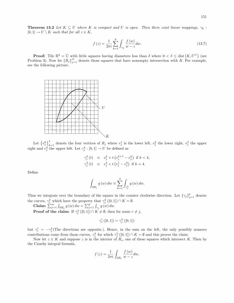
151
Theorem 13.2 Let K ⊆ U where K is compact and U is open. Then there exist linear mappings, γk :[0, 1]→ U \K such that for all z ∈ K,
f (z) =1
2πi
p∑k=1
∫γk
f (w)w − z
dw. (13.7)
Proof: Tile R2 = C with little squares having diameters less than δ where 0 < δ ≤ dist(K,UC
)(see
Problem 3). Now let {Rj}mj=1 denote those squares that have nonempty intersection with K. For example,see the following picture.
@@@@@@@@@K
U@@@@
Let{vkj}4
k=1denote the four vertices of Rj where v1
j is the lower left, v2j the lower right, v3
j the upperright and v4
j the upper left. Let γkj : [0, 1]→ U be defined as
γkj (t) ≡ vkj + t(vk+1j − vkj
)if k < 4,
γ4j (t) ≡ v4
j + t(v1j − v4
j
)if k = 4.
Define ∫∂Rj
g (w) dw ≡4∑k=1
∫γkj
g (w) dw.
Thus we integrate over the boundary of the square in the counter clockwise direction. Let {γj}pj=1 denotethe curves, γkj which have the property that γkj ([0, 1]) ∩K = ∅.
Claim:∑mj=1
∫∂Rj
g (w) dw =∑pj=1
∫γjg (w) dw.
Proof of the claim: If γkj ([0, 1]) ∩K 6= ∅, then for some r 6= j,
γlr ([0, 1]) = γkj ([0, 1])
but γlr = −γkj (The directions are opposite.). Hence, in the sum on the left, the only possibly nonzerocontributions come from those curves, γkj for which γkj ([0, 1]) ∩K = ∅ and this proves the claim.
Now let z ∈ K and suppose z is in the interior of Rs, one of these squares which intersect K. Then bythe Cauchy integral formula,
f (z) =1
2πi
∫∂Rs
f (w)w − z
dw,
152 APPROXIMATION OF ANALYTIC FUNCTIONS
and if j 6= s,
0 =1
2πi
∫∂Rj
f (w)w − z
dw.
Therefore,
f (z) =1
2πi
m∑j=1
∫∂Rj
f (w)w − z
dw
=1
2πi
p∑j=1
∫γj
f (w)w − z
dw.
This proves (13.7) in the case where z is in the interior of some Rs. The general case follows from using thecontinuity of the functions, f (z) and
z → 12πi
p∑j=1
∫γj
f (w)w − z
dw.
This proves the theorem.
13.1 Runge’s theorem
With the above preparation we are ready to prove the very remarkable Runge theorem which says that wecan approximate analytic functions on arbitrary compact sets with rational functions which have a certainnice form. Actually, the theorem we will present first is a variant of Runge’s theorem because it focuses ona single compact set.
Theorem 13.3 Let K be a compact subset of an open set, U and let {bj} be a set which consists of onepoint from the closure of each bounded component of C \K. Let f be analytic on U. Then for each ε > 0,there exists a rational function, Q whose poles are all contained in the set, {bj} such that
||Q− f ||K,∞ < ε. (13.8)
Proof: By Theorem 13.2 there are curves, γk described there such that for all z ∈ K,
f (z) =1
2πi
p∑k=1
∫γk
f (w)w − z
dw. (13.9)
Defining g (w, z) ≡ f(w)w−z for (w, z) ∈ ∪pk=1γk ([0, 1])×K, we see that g is uniformly continuous and so there
exists a δ > 0 such that if ||P|| < δ, then for all z ∈ K,∣∣∣∣∣∣f (z)− 12πi
p∑k=1
n∑j=1
f (γk (τj)) (γk (ti)− γk (ti−1))γk (τj)− z
∣∣∣∣∣∣ < ε
2.
The complicated expression is obtained by replacing each integral in (13.9) with a Riemann sum. Simplifyingthe appearance of this, it follows there exists a rational function of the form
R (z) =M∑k=1
Akwk − z
13.1. RUNGE’S THEOREM 153
where the wk are elements of components of C \K and Ak are complex numbers such that
||R− f ||K,∞ <ε
2.
Consider the rational function, Rk (z) ≡ Akwk−z where wk ∈ Vj , one of the components of C \K, the given
point of Vj being bj or else Vj is unbounded. By Lemma 13.1, there exists a function, Qk which is either arational function having its only pole at bj or a polynomial, depending on whether Vj is bounded, such that
||Rk −Qk||K,∞ <ε
2M.
Letting Q (z) ≡∑Mk=1Qk (z) ,
||R−Q||K,∞ <ε
2.
It follows
||f −Q||K,∞ ≤ ||f −R||K,∞ + ||R−Q||K,∞ < ε.
This proves the theorem.Runge’s theorem concerns the case where the given points are contained in C \ U for U an open set
rather than a compact set. Note that here there could be uncountably many components of C \ U becausethe components are no longer open sets. An easy example of this phenomenon in one dimension is whereU = [0, 1] \ P for P the Cantor set. Then you can show that R \ U has uncountably many components.Nevertheless, Runge’s theorem will follow from Theorem 13.3 with the aid of the following interesting lemma.
Lemma 13.4 Let U be an open set in C. Then there exists a sequence of compact sets, {Kn} such that
U = ∪∞k=1Kn, · · ·,Kn ⊆ intKn+1 · ··, (13.10)
and for any K ⊆ U,
K ⊆ Kn, (13.11)
for all n sufficiently large, and every component of C \Kn contains a component of C \ U.
Proof: Let
Vn ≡ {z : |z| > n} ∪⋃z/∈U
B
(z,
1n
).
Thus {z : |z| > n} contains the point, ∞. Now let
Kn ≡ C \ Vn = C \ Vn ⊆ U.
We leave it as an exercise to verify that (13.10) and (13.11) hold. It remains to show that every componentof C \Kn contains a component of C \ U. Let D be a component of C \Kn ≡ Vn.
If ∞ /∈ D, then D contains no point of {z : |z| > n} because this set is connected and D is a component.(If it did contain a point of this set, it would have to contain the whole set..) Therefore, D ⊆
⋃z/∈U
B(z, 1
n
)and so D contains some point of B
(z, 1
n
)for some z /∈ U. Therefore, since this ball is connected, it follows
D must contain the whole ball and consequently D contains some point of UC . (The point z at the center
154 APPROXIMATION OF ANALYTIC FUNCTIONS
of the ball will do.) Since D contains z /∈ U, it must contain the component, Hz, determined by this point.The reason for this is that
Hz ⊆ C \ U ⊆ C \Kn
and Hz is connected. Therefore, Hz can only have points in one component of C\Kn. Since it has a point inD, it must therefore, be totally contained in D. This verifies the desired condition in the case where ∞ /∈ D.
Now suppose that∞ ∈ D. We know that ∞ /∈ U because U is given to be a set in C. Letting H∞ denotethe component of C \ U determined by ∞, it follows from similar reasoning to the above that H∞ ⊆ D andthis proves the lemma.
Theorem 13.5 (Runge) Let U be an open set, and let A be a set which has one point in each boundedcomponent of C \ U and let f be analytic on U. Then there exists a sequence of rational functions, {Rn}having poles only in A such that Rn converges uniformly to f on compact subsets of U.
Proof: Let Kn be the compact sets of Lemma 13.4 where each component of C\Kn contains a componentof C \ U. It follows each bounded component of C \Kn contains a point of A. Therefore, by Theorem 13.3there exists Rn a rational function with poles only in A such that
||Rn − f ||Kn,∞ <1n.
It follows, since a given compact set, K is a subset of Kn for all n large enough, that Rn → f uniformly onK. This proves the theorem.
Corollary 13.6 Let U be simply connected and f is analytic on U. Then there exists a sequence of polyno-mials, {pn} such that pn → f uniformly on compact sets of U.
Proof: By definition of what is meant by simply connected, C \ U is connected and so there are nobounded components of C \ U. Therefore, A = ∅ and it follows that Rn in the above theorem must be apolynomial since it is rational and has no poles.
13.2 Exercises
1. Let K be any nonempty set in C and define
dist (z,K) ≡ inf {|z − w| : w ∈ K} .
Show that z → dist (z,K) is a continuous function.
2. Verify the series in (13.4) converges absolutely on K and find Ak. Also do the same for (13.6). Hint:You know that for |z| < 1, 1
1−z =∑∞k=0 z
k. Differentiate both sides as many times as needed to obtaina formula for Ak. Then apply the Weierstrass M test and the ratio test.
3. In Theorem 13.2 we had a compact set, K contained in an open set U and we used the fact that
dist(K,UC
)≡ inf
{|z − w| : w ∈ UC , z ∈ K
}> 0.
Prove this.
4. For U = [0, 1] \ P for P the Cantor set, show that R \ U has uncountably many components. Hint:Show that the component of R \U determined by p ∈ P, is just the single point, p and then show P isuncountable.
5. In the proof of Lemma 13.4, verify that (13.10) and (13.11) are satisfied for the given choice of Kn.
Bibliography
[1] Conway J. B. Functions of one Complex variable Second edition, Springer Verlag 1978.
[2] Dunford N. and Schwartz J.T. Linear Operators, Interscience Publishers, a division of John Wileyand Sons, New York, part 1 1958, part 2 1963, part 3 1971.
[3] Evans L.C. Partial Differential Equations, Berkeley Mathematics Lecture Notes. 1993.
[4] Greenleaf F.P. Introduction to Complex Variables, Saunders 1972
[5] Hardy G. A Course Of Pure Mathematics, Tenth edition Cambridge University Press 1992.
[6] Levinson, N. and Redheffer, R. Complex Variables, Holden Day, Inc. 1970
[7] Rudin W. Principles of Mathematical Analysis, McGraw Hill, 1976.
[8] Rudin W. Real and Complex Analysis, third edition, McGraw-Hill, 1987.
[9] Silverman R. Complex Analysis with Applications, Dover, 1974.
[10] Spiegel, M.R. Complex Variables Schaum’s outline series, McGraw Hill, 1998.
155
Index
Abel’s theorem, 59Analytic functions, 47argument principle, 107Ascoli Arzela theorem, 22
basic open set, 5basis, 5Bernstein polynomials, 24bounded variation, 37branches of the logarithm, 78Bromwich, 113
Cantor diagonal process, 30Casorati Weierstrass theorem, 93Cauchy
general Cauchy integral formula, 68integral formula for disk, 54
Cauchy Riemann equations, 47Cauchy sequence, 8closed set, 6closure of a set, 7compact set, 9complete metric space, 8completely separable, 8complex numbers, 31conformal maps, 50, 131conjugate Poisson formulas, 111connected, 14connected components, 15continuous function, 8counting zeros, 79
De Moivre’s theorem, 33differential equations
Peano existence theorem, 29dilations, 131
eigenvalues, 82, 85entire, 58epsilon net, 11equicontinuous, 22extended complex plane, 35
finite intersection property, 9fractional linear transformations, 131, 142
mapping three points, 132Fresnel integrals, 105fundamental theorem of algebra, 58
Gauss’s formula, 122Gerschgorin’s theorem, 82
harmonic, 123harmonic functions, 49
mean value property, 126Harnack’s inequality, 128Hausdorff metric, 18, 30Hausdorff space, 6Heine Borel theorem, 13, 18Hilbert transform, 111
infinite products, 114inversions, 131isogonal, 49
Laplace transform, 112Laurent series, 88limit point, 6Liouville theorem, 58locally compact , 9
maximum modulus theorem, 78Mellin transformations, 103metric space, 7Mittag Leffler, 106Montel’s theorem, 141
normal family of functions, 142normal topological space, 6
open cover, 9open mapping theorem, 76open sets, 5
partial fractions, 94Picard theorem, 93Poisson formula, 111
156

INDEX 157
Poisson integral formuladisk, 126half plane, 135
power seriesanalytic functions, 57
power set, 5precompact, 9, 28principle branch, 51product topology, 8
regular topological space, 6Riemann sphere, 35Rouche’s theorem, 108Runge’s theorem, 152
Schwarz Christoffel transformation, 138Schwarz formula, 59Schwarz reflection principle, 73Schwarz’s lemma, 143separable space, 8separated, 14singularities, 92stereographic projection, 35Stone Weierstrass, 26strong mean value property, 128subbasis, 10
Tietze extention theorem, 30topological space, 5totally bounded set, 11translations, 131
Wallis’s formula, 121Weierstrass, 25Weierstrass M test, 32winding number, 66