Complex Dynamics of V1 Population Responses Explained by …nn.cs.utexas.edu/downloads/papers/sit.neuron09.pdf · Complex Dynamics of V1 Population Responses Explained by a Simple

Neuron

Article

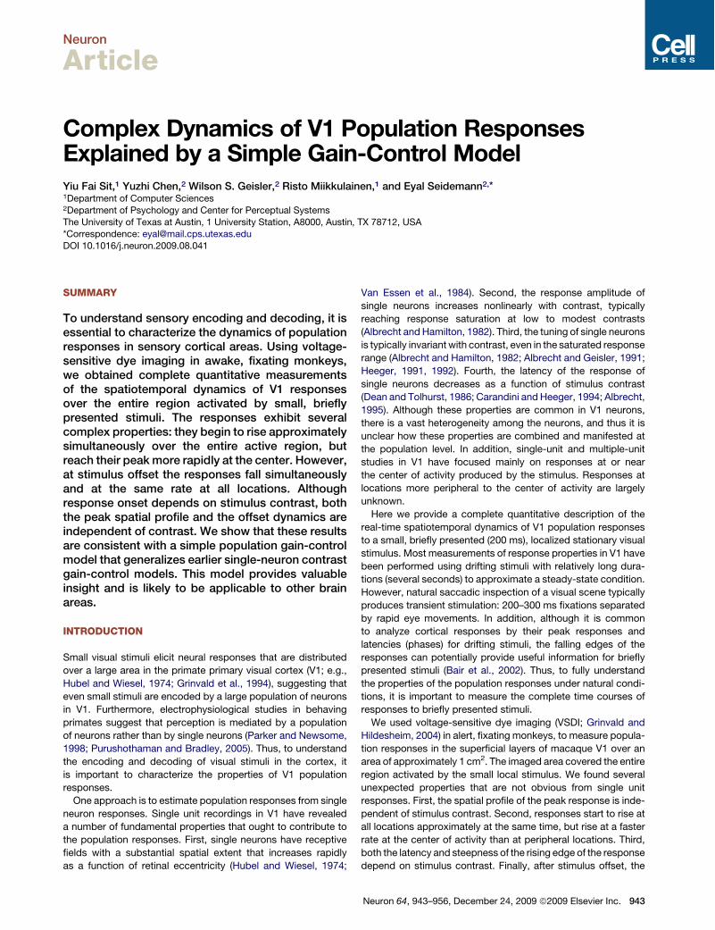
Complex Dynamics of V1 Population ResponsesExplained by a Simple Gain-Control ModelYiu Fai Sit,1 Yuzhi Chen,2 Wilson S. Geisler,2 Risto Miikkulainen,1 and Eyal Seidemann2,*1Department of Computer Sciences2Department of Psychology and Center for Perceptual SystemsThe University of Texas at Austin, 1 University Station, A8000, Austin, TX 78712, USA*Correspondence: [email protected] 10.1016/j.neuron.2009.08.041

SUMMARY

To understand sensory encoding and decoding, it isessential to characterize the dynamics of populationresponses in sensory cortical areas. Using voltage-sensitive dye imaging in awake, fixating monkeys,we obtained complete quantitative measurementsof the spatiotemporal dynamics of V1 responsesover the entire region activated by small, brieflypresented stimuli. The responses exhibit severalcomplex properties: they begin to rise approximatelysimultaneously over the entire active region, butreach their peakmore rapidly at the center. However,at stimulus offset the responses fall simultaneouslyand at the same rate at all locations. Althoughresponse onset depends on stimulus contrast, boththe peak spatial profile and the offset dynamics areindependent of contrast. We show that these resultsare consistent with a simple population gain-controlmodel that generalizes earlier single-neuron contrastgain-control models. This model provides valuableinsight and is likely to be applicable to other brainareas.

INTRODUCTION

Small visual stimuli elicit neural responses that are distributedover a large area in the primate primary visual cortex (V1; e.g.,Hubel and Wiesel, 1974; Grinvald et al., 1994), suggesting thateven small stimuli are encoded by a large population of neuronsin V1. Furthermore, electrophysiological studies in behavingprimates suggest that perception is mediated by a populationof neurons rather than by single neurons (Parker and Newsome,1998; Purushothaman and Bradley, 2005). Thus, to understandthe encoding and decoding of visual stimuli in the cortex, itis important to characterize the properties of V1 populationresponses.One approach is to estimate population responses from single

neuron responses. Single unit recordings in V1 have revealeda number of fundamental properties that ought to contribute tothe population responses. First, single neurons have receptivefields with a substantial spatial extent that increases rapidlyas a function of retinal eccentricity (Hubel and Wiesel, 1974;

Van Essen et al., 1984). Second, the response amplitude ofsingle neurons increases nonlinearly with contrast, typicallyreaching response saturation at low to modest contrasts(Albrecht and Hamilton, 1982). Third, the tuning of single neuronsis typically invariant with contrast, even in the saturated responserange (Albrecht and Hamilton, 1982; Albrecht and Geisler, 1991;Heeger, 1991, 1992). Fourth, the latency of the response ofsingle neurons decreases as a function of stimulus contrast(Dean and Tolhurst, 1986; Carandini and Heeger, 1994; Albrecht,1995). Although these properties are common in V1 neurons,there is a vast heterogeneity among the neurons, and thus it isunclear how these properties are combined and manifested atthe population level. In addition, single-unit and multiple-unitstudies in V1 have focused mainly on responses at or nearthe center of activity produced by the stimulus. Responses atlocations more peripheral to the center of activity are largelyunknown.Here we provide a complete quantitative description of the

real-time spatiotemporal dynamics of V1 population responsesto a small, briefly presented (200 ms), localized stationary visualstimulus. Most measurements of response properties in V1 havebeen performed using drifting stimuli with relatively long dura-tions (several seconds) to approximate a steady-state condition.However, natural saccadic inspection of a visual scene typicallyproduces transient stimulation: 200–300 ms fixations separatedby rapid eye movements. In addition, although it is commonto analyze cortical responses by their peak responses andlatencies (phases) for drifting stimuli, the falling edges of theresponses can potentially provide useful information for brieflypresented stimuli (Bair et al., 2002). Thus, to fully understandthe properties of the population responses under natural condi-tions, it is important to measure the complete time courses ofresponses to briefly presented stimuli.We used voltage-sensitive dye imaging (VSDI; Grinvald and

Hildesheim, 2004) in alert, fixating monkeys, to measure popula-tion responses in the superficial layers of macaque V1 over anarea of approximately 1 cm2. The imaged area covered the entireregion activated by the small local stimulus. We found severalunexpected properties that are not obvious from single unitresponses. First, the spatial profile of the peak response is inde-pendent of stimulus contrast. Second, responses start to rise atall locations approximately at the same time, but rise at a fasterrate at the center of activity than at peripheral locations. Third,both the latency and steepness of the rising edge of the responsedepend on stimulus contrast. Finally, after stimulus offset, the

Neuron 64, 943–956, December 24, 2009 ª2009 Elsevier Inc. 943

mailto:[email protected]

responses at all locations fall simultaneously and at the samerate, regardless of stimulus contrast. These complex propertiesillustrate the importance of quantitative characterization of pop-ulation responses in both space and time.

Next, we considered whether there is a general mechanismthat can account for these rich dynamics. To do this, we exploredseveral well-known families of computational models. We findthat the observed response properties are inconsistent withsimple models having a fixed linear operation followed bya nonlinearity that operates within the individual neuron (e.g.,a spike threshold or a refractory effect), and with models thatuse slow lateral connections to explain the difference in theresponse dynamics at different cortical locations. To accountfor the observed properties in both time and space, we proposea simple feedforward population gain-control (PGC) model thatgeneralizes earlier normalization models for single V1 neurons(Albrecht and Geisler, 1991; Heeger, 1991, 1992; Carandiniand Heeger, 1994; Carandini et al., 1997). In this model, thetemporal dynamics and the gain of the local responses arecontrolled by population activity in the network rather than bythe nonlinear properties of individual neurons or synapses. Wesimulated the early visual pathway from the retina to V1 by atwo-stage PGC model. The model’s dynamics closely resemblethose in the data.

Responses in the retina and LGN also show evidence ofnonlinear contrast gain-control (Shapley and Victor, 1978; Sclaret al., 1990; Kaplan and Benardete, 2001), and thus it is an openquestion whether a significant part of the nonlinearity in V1responses is inherited from its input. To address this importantquestion, we used the PGC model to predict how the relativecontributions of nonlinearities within layers 2-3 in V1 versus itsinputs affect the relationship between stimulus size and V1response amplitude. The results from a VSDI experiment varyingstimulus size were consistent with a PGCmodel in whichmost ofthe nonlinear processing occurs in the first stage, suggestingthat the nonlinearities observed in the VSDI responses may bemostly implemented prior to the superficial layers in V1.

In summary, our results illustrate the value of quantitativeanalysis and computational modeling in testing hypothesesregarding the biophysical and anatomical factors underlyingneural population activity. We characterized the spatiotemporalproperties of the V1 population responses to small, briefly pre-sented, stimuli that are relevant in natural vision, and foundthat the response dynamics are complex and unexpected fromthe results in single unit recordings. Importantly, we show thata simple PGC model can qualitatively account for the complexdynamics, suggesting that gain-control is likely to be a generalmechanism contributing to neural dynamics in the brain.

RESULTS

Population Responses to a Gabor Stimulus in V1We used VSDI to measure V1 population responses to a brieflypresented stationary Gabor stimulus while a monkey was per-forming a fixation task. The goal was to characterize the spatio-temporal dynamics of the population responses over the entirearea activated by a small Gabor stimulus. The spatiotemporaldynamics of the fine-scale columnar signals, which are modu-

lated by the orientation of the stimulus, were not measured inthe current study and will be addressed in future studies.

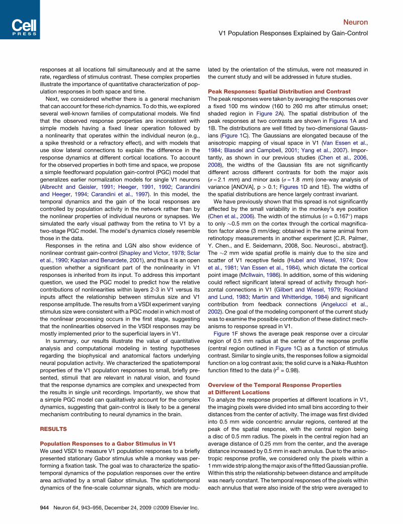
Peak Responses: Spatial Distribution and ContrastThe peak responseswere taken by averaging the responses overa fixed 100 ms window (160 to 260 ms after stimulus onset;shaded region in Figure 2A). The spatial distribution of thepeak responses at two contrasts are shown in Figures 1A and1B. The distributions are well fitted by two-dimensional Gauss-ians (Figure 1C). The Gaussians are elongated because of theanisotropic mapping of visual space in V1 (Van Essen et al.,1984; Blasdel and Campbell, 2001; Yang et al., 2007). Impor-tantly, as shown in our previous studies (Chen et al., 2006,2008), the widths of the Gaussian fits are not significantlydifferent across different contrasts for both the major axis(s= 2:1 mm) and minor axis (s= 1:8 mm) (one-way analysis ofvariance [ANOVA], p > 0.1; Figures 1D and 1E). The widths ofthe spatial distributions are hence largely contrast invariant.We have previously shown that this spread is not significantly

affected by the small variability in the monkey’s eye position(Chen et al., 2006). The width of the stimulus (s = 0.167!) mapsto only "0.5 mm on the cortex through the cortical magnifica-tion factor alone (3 mm/deg; obtained in the same animal fromretinotopy measurements in another experiment [C.R. Palmer,Y. Chen., and E. Seidemann, 2008, Soc. Neurosci., abstract]).The "2 mm wide spatial profile is mainly due to the size andscatter of V1 receptive fields (Hubel and Wiesel, 1974; Dowet al., 1981; Van Essen et al., 1984), which dictate the corticalpoint image (McIlwain, 1986). In addition, some of this wideningcould reflect significant lateral spread of activity through hori-zontal connections in V1 (Gilbert and Wiesel, 1979; Rocklandand Lund, 1983; Martin and Whitteridge, 1984) and significantcontribution from feedback connections (Angelucci et al.,2002). One goal of the modeling component of the current studywas to examine the possible contribution of these distinct mech-anisms to response spread in V1.Figure 1F shows the average peak response over a circular

region of 0.5 mm radius at the center of the response profile(central region outlined in Figure 1C) as a function of stimuluscontrast. Similar to single units, the responses follow a sigmoidalfunction on a log contrast axis; the solid curve is a Naka-Rushtonfunction fitted to the data (r2 = 0.98).

Overview of the Temporal Response Propertiesat Different LocationsTo analyze the response properties at different locations in V1,the imaging pixels were divided into small bins according to theirdistances from the center of activity. The image was first dividedinto 0.5 mm wide concentric annular regions, centered at thepeak of the spatial response, with the central region beinga disc of 0.5 mm radius. The pixels in the central region had anaverage distance of 0.25 mm from the center, and the averagedistance increased by 0.5 mm in each annulus. Due to the aniso-tropic response profile, we considered only the pixels within a1mmwide strip along themajor axis of the fittedGaussian profile.Within this strip the relationship between distance and amplitudewas nearly constant. The temporal responses of the pixels withineach annulus that were also inside of the strip were averaged to

Neuron

V1 Population Responses Explained by Gain-Control

944 Neuron 64, 943–956, December 24, 2009 ª2009 Elsevier Inc.

produce a single time course for the corresponding distance.Figure 1C shows the bins up to an average distance of2.75 mm; responses at greater distances were not analyzedbecause theywereweak andnoisy, especially at lower contrasts.Figure 2A shows the average time courses of the responses at

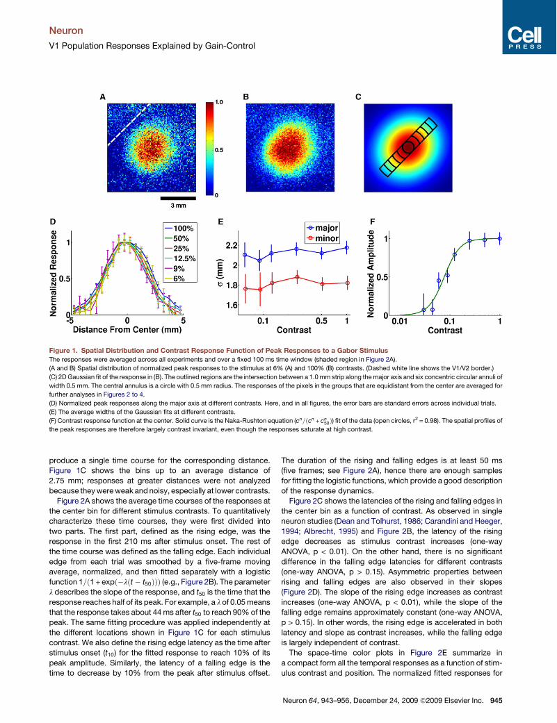
the center bin for different stimulus contrasts. To quantitativelycharacterize these time courses, they were first divided intotwo parts. The first part, defined as the rising edge, was theresponse in the first 210 ms after stimulus onset. The rest ofthe time course was defined as the falling edge. Each individualedge from each trial was smoothed by a five-frame movingaverage, normalized, and then fitted separately with a logisticfunction 1=#1+ exp#$l#t $ t50%%% (e.g., Figure 2B). The parameterl describes the slope of the response, and t50 is the time that theresponse reaches half of its peak. For example, a l of 0.05meansthat the response takes about 44ms after t50 to reach 90%of thepeak. The same fitting procedure was applied independently atthe different locations shown in Figure 1C for each stimuluscontrast. We also define the rising edge latency as the time afterstimulus onset (t10) for the fitted response to reach 10% of itspeak amplitude. Similarly, the latency of a falling edge is thetime to decrease by 10% from the peak after stimulus offset.

The duration of the rising and falling edges is at least 50 ms(five frames; see Figure 2A), hence there are enough samplesfor fitting the logistic functions, which provide a good descriptionof the response dynamics.Figure 2C shows the latencies of the rising and falling edges in

the center bin as a function of contrast. As observed in singleneuron studies (Dean and Tolhurst, 1986; Carandini and Heeger,1994; Albrecht, 1995) and Figure 2B, the latency of the risingedge decreases as stimulus contrast increases (one-wayANOVA, p < 0.01). On the other hand, there is no significantdifference in the falling edge latencies for different contrasts(one-way ANOVA, p > 0.15). Asymmetric properties betweenrising and falling edges are also observed in their slopes(Figure 2D). The slope of the rising edge increases as contrastincreases (one-way ANOVA, p < 0.01), while the slope of thefalling edge remains approximately constant (one-way ANOVA,p > 0.15). In other words, the rising edge is accelerated in bothlatency and slope as contrast increases, while the falling edgeis largely independent of contrast.The space-time color plots in Figure 2E summarize in

a compact form all the temporal responses as a function of stim-ulus contrast and position. The normalized fitted responses for

Figure 1. Spatial Distribution and Contrast Response Function of Peak Responses to a Gabor StimulusThe responses were averaged across all experiments and over a fixed 100 ms time window (shaded region in Figure 2A).

(A and B) Spatial distribution of normalized peak responses to the stimulus at 6% (A) and 100% (B) contrasts. (Dashed white line shows the V1/V2 border.)

(C) 2DGaussian fit of the response in (B). The outlined regions are the intersection between a 1.0mm strip along themajor axis and six concentric circular annuli of

width 0.5 mm. The central annulus is a circle with 0.5 mm radius. The responses of the pixels in the groups that are equidistant from the center are averaged for

further analyses in Figures 2 to 4.

(D) Normalized peak responses along the major axis at different contrasts. Here, and in all figures, the error bars are standard errors across individual trials.

(E) The average widths of the Gaussian fits at different contrasts.

(F) Contrast response function at the center. Solid curve is the Naka-Rushton equation (cn=#cn + cn50%) fit of the data (open circles, r2 = 0.98). The spatial profiles of

the peak responses are therefore largely contrast invariant, even though the responses saturate at high contrast.

Neuron



each contrast are shown as separate subplots; within eachsubplot the time course of the response at each of the sixlocation bins from Figure 1C is indicated by a horizontal row, pro-gressing from the center location at the top to the most periph-eral location at the bottom. For example, the upper horizontalrow in the plot for 100% contrast corresponds to the dark bluecurve in Figure 2B. Several qualitative observations can bemade from these maps (they will be quantified later). For eachcontrast, (1) the response latencies at different locations areapproximately equal, as can be seen by the vertically alignedtransitions from blue to cyan in each map, and (2) the responserises at a slower rate as distance from the center increases, ascan be seen by the increase in the tilt of the transition betweenthe colors as the normalized amplitude increases. In addition,for each location, as contrast increases (3) response latencydecreases, and (4) the response rises at a faster rate. Finally,(5) after stimulus offset, the falling edges are similar for all loca-

Figure 2. Spatiotemporal Responses to Dif-ferent Stimulus Contrasts(A) Time courses of the normalized responses to

different contrasts in the center region of

Figure 1C. Stimulus was presented at time 0 and

disappeared after 200 ms (dotted line). Average

responses in the shaded area were used to

compute the spatial profiles and contrast

response function in Figure 1.

(B) Logistic fits of the time courses in (A). The time

courses were divided into two parts by the dashed

line. Each part was fitted separately by a logistic

function. Diamond and square symbols on each

part indicate the latencies (t10) and times to half

peak (t50), respectively.

(C and D) Latencies (C) and slopes (D) of the rising

and falling edges of the fitted responses as a func-

tion of contrast.

(E) Logistic fits of the normalized time courses at

different locations for each stimulus contrast.

Each horizontal row within the space-time plot

for a given contrast shows the fitted time course

at one location, from the center (top row) to the

outmost region (bottom row). There is a systematic

change in slope and latency of the rising edges,

whereas the falling edges are similar for different

contrasts and locations.

tions and contrasts. All these key prop-erties were also observed in additionalexperiments in a second animal. Wenext examine these properties quantita-tively.

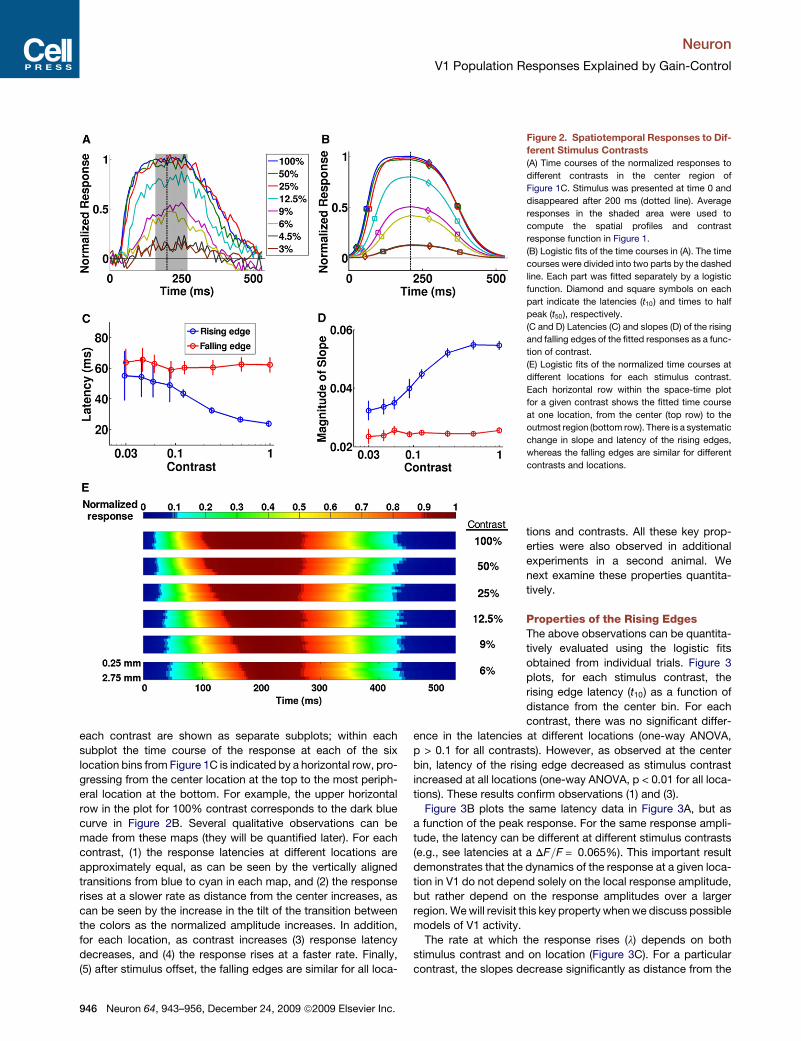
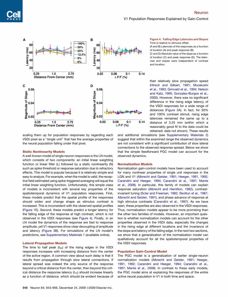
Properties of the Rising EdgesThe above observations can be quantita-tively evaluated using the logistic fitsobtained from individual trials. Figure 3plots, for each stimulus contrast, therising edge latency (t10) as a function ofdistance from the center bin. For eachcontrast, there was no significant differ-

ence in the latencies at different locations (one-way ANOVA,p > 0.1 for all contrasts). However, as observed at the centerbin, latency of the rising edge decreased as stimulus contrastincreased at all locations (one-way ANOVA, p < 0.01 for all loca-tions). These results confirm observations (1) and (3).Figure 3B plots the same latency data in Figure 3A, but as

a function of the peak response. For the same response ampli-tude, the latency can be different at different stimulus contrasts(e.g., see latencies at a DF=F = 0.065%). This important resultdemonstrates that the dynamics of the response at a given loca-tion in V1 do not depend solely on the local response amplitude,but rather depend on the response amplitudes over a largerregion.Wewill revisit this key property whenwe discuss possiblemodels of V1 activity.The rate at which the response rises (l) depends on both

stimulus contrast and on location (Figure 3C). For a particularcontrast, the slopes decrease significantly as distance from the

Neuron



center increases (one-way ANOVA, p < 0.01 for all contrasts),confirming observation (2). In addition, at a fixed location, theslope of the rising edge increases with contrast (one-wayANOVA, p < 0.01 for all locations), supporting observation (4).Furthermore, the slope also increases with peak response witha correlation coefficient of 0.94 (Figure 3D).Due to the decreasing slope as a function of distance from the

center, the time to half of the peak response (t50) increased atlocations peripheral to the center of activity. If t50 was employedas a measure of latency, a traveling wave of activity wouldappear to be originating from the center (Figures 3E and 3F),as observed previously in anesthetized animals (Grinvald et al.,1994; Jancke et al., 2004; Benucci et al., 2007). The averagedifference of the time to half peak between the locations0.25 mm and 2.75 mm away from the center was 6.2 ms. Thisdifference corresponds to a propagation speed of 0.4 mm/ms(for t50), which is at the higher end of the speed of propagationthrough lateral connections (0.1–0.4 mm/ms; Hirsch and Gilbert,1991; Murakoshi et al., 1993; Grinvald et al., 1994; Nelson andKatz, 1995; Gonzalez-Burgos et al., 2000). As we shall see later,such differences in time to half of the peak can be explained bya feedforward PGC model.

Figure 3. Temporal Properties of the RisingEdgesTime is relative to stimulus onset.

(A) Latencies of the responses at different cortical

distances from the center.

(B) Same data as (A), plotted as a function of peak

response.

(C and D) Slopes of the responses at different

locations (C) and peak responses (D).

(E and F) Time to half of the peak response as

a function of location (E) and peak response (F).

For a particular contrast, the responses at different

locations started to rise at about the same time,

but the slopes were shallower at locations that

were further away from the center, increasing the

times to half peak at these locations.

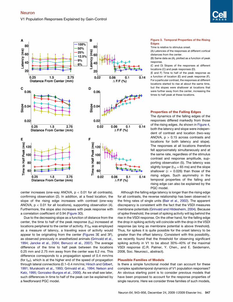
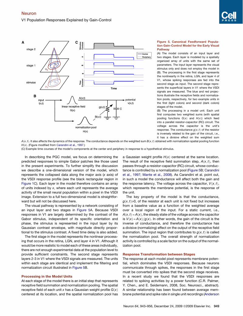
Properties of the Falling EdgesThe dynamics of the falling edges of theresponses differed markedly from thoseof the rising edges. As shown in Figure 4,both the latency and slope were indepen-dent of contrast and location (two-wayANOVA, p > 0.15 across contrasts andlocations for both latency and slope).The responses at all locations thereforefell approximately simultaneously and atthe same rate, regardless of the stimuluscontrast and response amplitude, sup-porting observation (5). The latency wasslightly longer (t10 = 65 ms) and the slopeshallower (l = 0.026) than those of therising edges. Such asymmetry in thetemporal properties of the falling andrising edge can also be explained by thePGC model.

Although the falling edge latency is longer than the rising edgefor all contrasts, the reverse relationship has been observed inthe firing rates of single units (Bair et al., 2002). The apparentdiscrepancy is consistent with the fact that the VSDI measuresmembrane potentials (Grinvald and Hildesheim, 2004). Becauseof spike threshold, the onset of spiking activity will lag behind therise in the VSDI response. On the other hand, for the falling edgethe drop in spiking activity will coincide with the drop in the VSDIresponse (as long as membrane potential is above threshold).Thus, for spikes it is quite possible for the onset latency to begreater than the offset latency. Consistent with this possibility,we recently found that the threshold for observing significantspiking activity in V1 to be about 30%–40% of the maximalVSDI response (C.R. Palmer, Y. Chen., and E. Seidemann,2008, Soc. Neurosci., abstract).

Plausible Families of ModelsIs there a simple functional model that can account for thesecomplex spatiotemporal dynamics of V1 population responses?An obvious starting point is to consider previous models thathave been proposed to account for the response properties ofsingle neurons. Here we consider three families of such models,

Neuron



scaling them up for population responses by regarding eachVSDI pixel as a ‘‘single unit’’ that has the average properties ofthe neural population falling under that pixel.

Static Nonlinearity ModelsA well-knownmodel of single neuron responses is the LNmodel,which consists of two components: an initial linear weightingfunction or linear filter (L) followed by a static nonlinearity (N)such as spike threshold or response saturation due to refractoryeffects. This model is popular because it is relatively simple andeasy to analyze. For example, when themodel is valid, the recep-tive field estimated using spike-triggered averaging will equal theinitial linear weighting function. Unfortunately, this simple classof models is inconsistent with several key properties of thespatiotemporal dynamics of V1 population responses. First,these models predict that the spatial profile of the responsesshould widen and change shape as stimulus contrast isincreased. This is inconsistent with the observed spatial profiles(Figure 1E). Second, these models predict a longer latency forthe falling edge of the response at high contrast, which is notobserved in the VSDI responses (see Figure 4). Finally, in anLN model the dynamics of the response are tied to responseamplitude, yet V1 responses show clear decoupling of amplitudeand latency (Figure 3B). For simulations of the LN model’spredictions, see Supplementary Materials 1 (available online).

Lateral Propagation ModelsThe time to half peak (t50) of the rising edges in the VSDIresponses increases with increasing distance from the centerof the active region. A common view about such delay is that itresults from propagation through slow lateral connections. Iflateral spread was indeed the only source of the responsebeyond a critical distance from the center, then beyond this crit-ical distance the response latency (t10) should increase linearlyas a function of distance, which should be evident because of

Figure 4. Falling Edge Latencies and SlopesTime is relative to stimulus offset.

(A and B) Latencies of the responses as a function

of location (A) and peak response (B).

(C and D) Absolute value of the slope as a function

of location (C) and peak response (D). The laten-

cies and slopes were independent of contrast

and location.

their relatively slow propagation speed(Hirsch and Gilbert, 1991; Murakoshiet al., 1993; Grinvald et al., 1994; Nelsonand Katz, 1995; Gonzalez-Burgos et al.,2000). However, there was no significantdifference in the rising edge latency ofthe VSDI responses for a wide range ofdistances (Figure 3A). In fact, for 50%and 100% contrast stimuli, rising edgelatencies remained the same up to adistance of 3.25 mm (within which areasonably good fit to the data could beobtained; data not shown). These results

and additional simulations (see Supplementary Materials 2)suggest that within the examined range the observed dynamicsare not consistent with a significant contribution of slow lateralconnections to the observed response spread. Below we showthat the simple feedforward PGC model can account for theobserved dynamics.

Normalization ModelsNormalization gain-control models have been used to accountfor many nonlinear properties of single unit responses in theLGN and V1 (Albrecht and Geisler, 1991; Heeger, 1991, 1992;Carandini and Heeger, 1994; Carandini et al., 1997; Manteet al., 2008). In particular, this family of models can explainresponse saturation (Albrecht and Hamilton, 1982), contrast-invariant tuning (Sclar and Freeman, 1982; Skottun et al., 1987;Albrecht and Geisler, 1991), and phase advance of response athigh stimulus contrasts (Carandini et al., 1997). As we haveseen, these properties are also observed in the VSDI responses.Thus, normalization models appear to be more promising thanthe other two families of models. However, an important ques-tion is whether normalization models can account for the otherproperties observed in the VSDI data, especially the changesin the rising edge at different locations and the invariance ofthe slope and latency of the falling edge. In the next two sections,we show that a generalization of the normalization model canqualitatively account for all the spatiotemporal properties ofthe VSDI responses.

Population Gain-Control ModelThe PGC model is a generalization of earlier single-neuronnormalization models (Albrecht and Geisler, 1991; Heeger,1991, 1992; Carandini and Heeger, 1994; Carandini et al.,1997; Mante et al., 2008). In contrast to these early models,the PGC model aims at explaining the responses of the entireactive neural population in V1 in both time and space.

Neuron



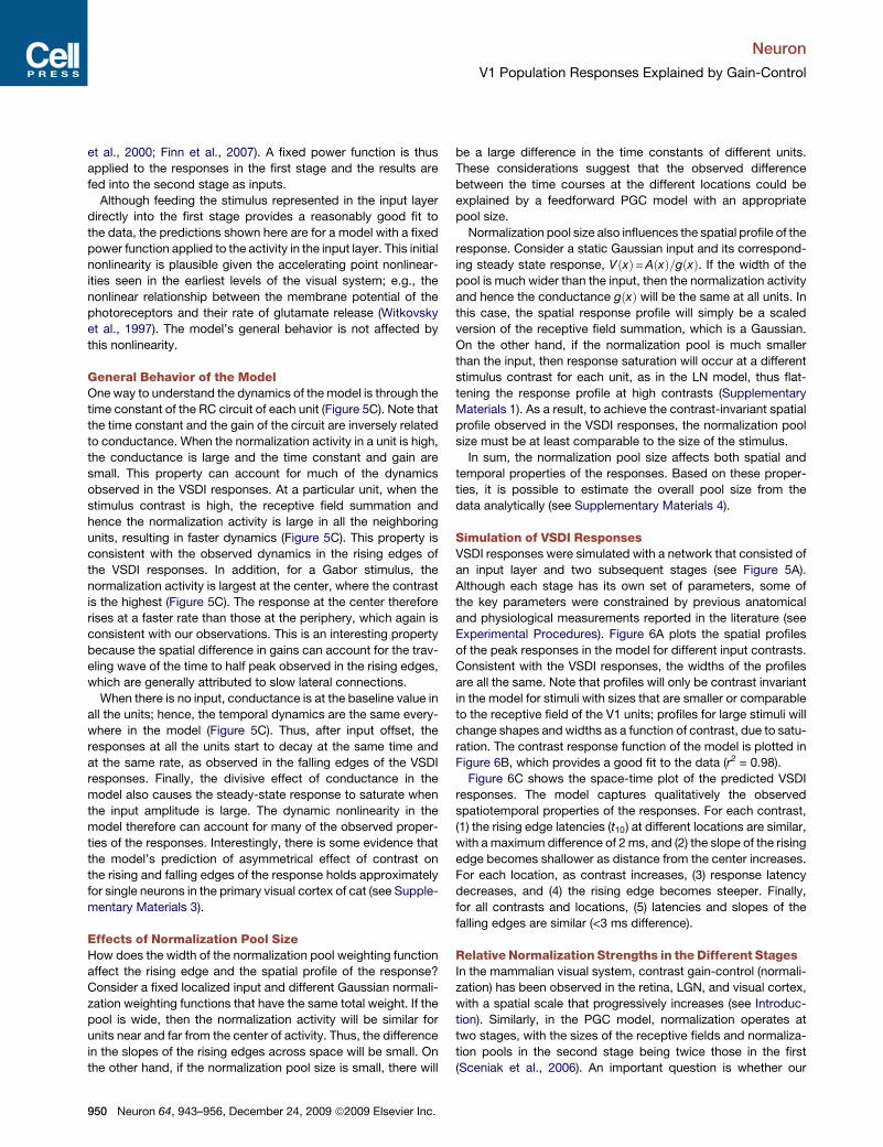
In describing the PGC model, we focus on determining thepredicted responses to simple Gabor patches like those usedin the present experiments. To further simplify the discussionwe describe a one-dimensional version of the model, whichrepresents the collapsed data along the major axis (x axis) ofthe VSDI response profile (see the black rectangular region inFigure 1C). Each layer in the model therefore contains an arrayof units indexed by x, where each unit represents the averageactivity of the small neural population within a pixel in the VSDIimage. Extension to a full two-dimensional model is straightfor-ward but will not be discussed here.The visual pathway is represented by a network consisting of

an input layer and two stages in Figure 5A. Because VSDIresponses in V1 are largely determined by the contrast of theGabor stimulus, independent of its specific orientation andphase, the stimulus is represented in the input layer by itsGaussian contrast envelope, with magnitude directly propor-tional to the stimulus contrast. A fixed time delay is also added.The first stage in the model represents the nonlinear process-

ing that occurs in the retina, LGN, and layer 4 in V1. Although itwould bemore realistic tomodel each of these areas individually,there are not enough experimental data at the population level toprovide sufficient constraints. The second stage representslayers 2-3 in V1 where the VSDI signals are measured. The unitswithin each stage are identical and implement the filtering andnormalization circuit illustrated in Figure 5B.

Processing in the Model UnitsAt each stage of the model there is an initial step that representsreceptive field summation and normalization pooling. The spatialreceptive field of each unit x has a Gaussian weight profile G#x%centered at its location, and the spatial normalization pool has

a Gaussian weight profile H#x% centered at the same location.The result of the receptive field summation step, A#x; t%, thenpasses through a resistor-capacitor (RC) circuit, whose conduc-tance is controlled by a normalization pool (Figure 5B; Carandiniet al., 1997; Mante et al., 2008). As Carandini et al. point out,in such a model the conductance will affect both the gain andthe response latency. The voltage across the capacitor, V#x; t%,which represents the membrane potential, is the response ofthe unit.The key property of the model is that the conductance,

g#x; t%>0, of the resistor at each unit is not fixed but increasesfrom a baseline value as a function of the weighted averageover a local region of the input. For a static current, i.e.,A#x; t%=A#x%, the steady state of the voltage across the capacitoris V#x%=A#x%=g#x%. In other words, the gain of the circuit is theinverse of conductance, and therefore the conductance hasa divisive (normalizing) effect on the output of the receptive fieldsummation. The input region that contributes to g#x; t% is calledthe normalization pool. The overall strength of normalizationactivity is controlled by a scale factor on the output of the normal-ization pool.

Response Transformation between StagesThe response at each model pixel represents membrane poten-tial, which dominates the VSDI responses. Because neuronscommunicate through spikes, the responses in the first stagemust be converted into spikes that the second stage receives.In a recent study we found that the VSDI responses arerelated to spiking activities by a power function (C.R. Palmer,Y. Chen., and E. Seidemann, 2008, Soc. Neurosci., abstract).A similar relationship has been found between average mem-brane potential and spike rate in single unit recordings (Anderson

Figure 5. Canonical Feedforward Popula-tion Gain-Control Model for the Early VisualPathway(A) The model consists of an input layer and

two stages. Each layer is modeled by a spatially

organized array of units with the same set of

parameters. The input layer represents the visual

stimulus only and does not employ the model in

(B). The processing in the first stage represents

the nonlinearity in the retina, LGN, and layer 4 of

V1, whose spiking responses are fed into the

second stage as input. The second stage repre-

sents the superficial layers in V1 where the VSDI

signals are measured. The blue and red projec-

tions illustrate the receptive fields and normaliza-

tion pools, respectively, for two example units in

the first (light colors) and second (dark colors)

stages of the model.

(B) The processing in a model unit. Each unit

first computes two weighted sums (with spatial

pooling functions G#x% and H#x%) which feed

into a parallel resistor-capacitor (RC) circuit. The

voltage across the capacitor is the unit’s

response. The conductance g#x; t% of the resistor

is inversely related to the gain of the circuit, i.e.,

it has a divisive effect on the weighted sum

A#x; t%. It also affects the dynamics of the response. The conductance depends on the weighted sum B#x; t% obtained with normalization spatial pooling function

H#x%. (Figure modified from Carandini et al., 1997.)

(C) Example time courses of the model’s components at the center and periphery in response to a hypothetical stimulus.

Neuron



et al., 2000; Finn et al., 2007). A fixed power function is thusapplied to the responses in the first stage and the results arefed into the second stage as inputs.

Although feeding the stimulus represented in the input layerdirectly into the first stage provides a reasonably good fit tothe data, the predictions shown here are for a model with a fixedpower function applied to the activity in the input layer. This initialnonlinearity is plausible given the accelerating point nonlinear-ities seen in the earliest levels of the visual system; e.g., thenonlinear relationship between the membrane potential of thephotoreceptors and their rate of glutamate release (Witkovskyet al., 1997). The model’s general behavior is not affected bythis nonlinearity.

General Behavior of the ModelOne way to understand the dynamics of the model is through thetime constant of the RC circuit of each unit (Figure 5C). Note thatthe time constant and the gain of the circuit are inversely relatedto conductance. When the normalization activity in a unit is high,the conductance is large and the time constant and gain aresmall. This property can account for much of the dynamicsobserved in the VSDI responses. At a particular unit, when thestimulus contrast is high, the receptive field summation andhence the normalization activity is large in all the neighboringunits, resulting in faster dynamics (Figure 5C). This property isconsistent with the observed dynamics in the rising edges ofthe VSDI responses. In addition, for a Gabor stimulus, thenormalization activity is largest at the center, where the contrastis the highest (Figure 5C). The response at the center thereforerises at a faster rate than those at the periphery, which again isconsistent with our observations. This is an interesting propertybecause the spatial difference in gains can account for the trav-eling wave of the time to half peak observed in the rising edges,which are generally attributed to slow lateral connections.

When there is no input, conductance is at the baseline value inall the units; hence, the temporal dynamics are the same every-where in the model (Figure 5C). Thus, after input offset, theresponses at all the units start to decay at the same time andat the same rate, as observed in the falling edges of the VSDIresponses. Finally, the divisive effect of conductance in themodel also causes the steady-state response to saturate whenthe input amplitude is large. The dynamic nonlinearity in themodel therefore can account for many of the observed proper-ties of the responses. Interestingly, there is some evidence thatthe model’s prediction of asymmetrical effect of contrast onthe rising and falling edges of the response holds approximatelyfor single neurons in the primary visual cortex of cat (see Supple-mentary Materials 3).

Effects of Normalization Pool SizeHow does the width of the normalization pool weighting functionaffect the rising edge and the spatial profile of the response?Consider a fixed localized input and different Gaussian normali-zation weighting functions that have the same total weight. If thepool is wide, then the normalization activity will be similar forunits near and far from the center of activity. Thus, the differencein the slopes of the rising edges across space will be small. Onthe other hand, if the normalization pool size is small, there will

be a large difference in the time constants of different units.These considerations suggest that the observed differencebetween the time courses at the different locations could beexplained by a feedforward PGC model with an appropriatepool size.Normalization pool size also influences the spatial profile of the

response. Consider a static Gaussian input and its correspond-ing steady state response, V#x%=A#x%=g#x%. If the width of thepool is much wider than the input, then the normalization activityand hence the conductance g#x% will be the same at all units. Inthis case, the spatial response profile will simply be a scaledversion of the receptive field summation, which is a Gaussian.On the other hand, if the normalization pool is much smallerthan the input, then response saturation will occur at a differentstimulus contrast for each unit, as in the LN model, thus flat-tening the response profile at high contrasts (SupplementaryMaterials 1). As a result, to achieve the contrast-invariant spatialprofile observed in the VSDI responses, the normalization poolsize must be at least comparable to the size of the stimulus.In sum, the normalization pool size affects both spatial and

temporal properties of the responses. Based on these proper-ties, it is possible to estimate the overall pool size from thedata analytically (see Supplementary Materials 4).

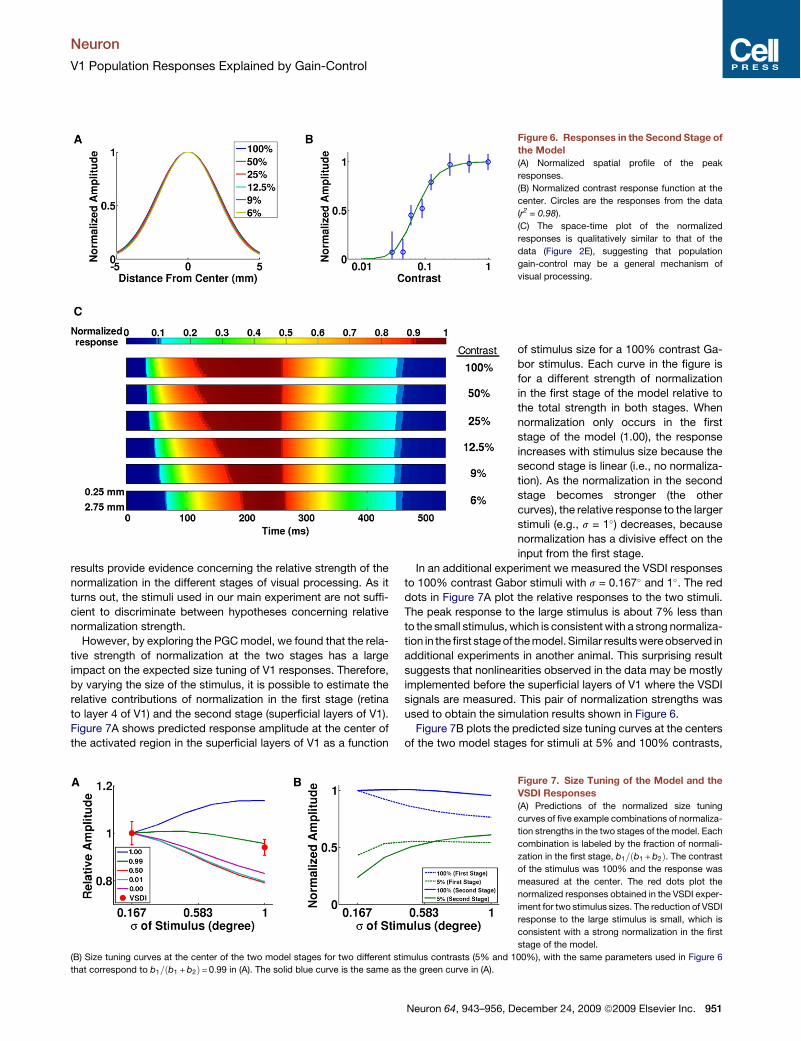
Simulation of VSDI ResponsesVSDI responses were simulated with a network that consisted ofan input layer and two subsequent stages (see Figure 5A).Although each stage has its own set of parameters, some ofthe key parameters were constrained by previous anatomicaland physiological measurements reported in the literature (seeExperimental Procedures). Figure 6A plots the spatial profilesof the peak responses in the model for different input contrasts.Consistent with the VSDI responses, the widths of the profilesare all the same. Note that profiles will only be contrast invariantin the model for stimuli with sizes that are smaller or comparableto the receptive field of the V1 units; profiles for large stimuli willchange shapes and widths as a function of contrast, due to satu-ration. The contrast response function of the model is plotted inFigure 6B, which provides a good fit to the data (r2 = 0.98).Figure 6C shows the space-time plot of the predicted VSDI

responses. The model captures qualitatively the observedspatiotemporal properties of the responses. For each contrast,(1) the rising edge latencies (t10) at different locations are similar,with a maximum difference of 2 ms, and (2) the slope of the risingedge becomes shallower as distance from the center increases.For each location, as contrast increases, (3) response latencydecreases, and (4) the rising edge becomes steeper. Finally,for all contrasts and locations, (5) latencies and slopes of thefalling edges are similar (<3 ms difference).

Relative Normalization Strengths in theDifferent StagesIn the mammalian visual system, contrast gain-control (normali-zation) has been observed in the retina, LGN, and visual cortex,with a spatial scale that progressively increases (see Introduc-tion). Similarly, in the PGC model, normalization operates attwo stages, with the sizes of the receptive fields and normaliza-tion pools in the second stage being twice those in the first(Sceniak et al., 2006). An important question is whether our

Neuron



results provide evidence concerning the relative strength of thenormalization in the different stages of visual processing. As itturns out, the stimuli used in our main experiment are not suffi-cient to discriminate between hypotheses concerning relativenormalization strength.However, by exploring the PGCmodel, we found that the rela-

tive strength of normalization at the two stages has a largeimpact on the expected size tuning of V1 responses. Therefore,by varying the size of the stimulus, it is possible to estimate therelative contributions of normalization in the first stage (retinato layer 4 of V1) and the second stage (superficial layers of V1).Figure 7A shows predicted response amplitude at the center ofthe activated region in the superficial layers of V1 as a function

Figure 6. Responses in the Second Stage ofthe Model(A) Normalized spatial profile of the peak

responses.

(B) Normalized contrast response function at the

center. Circles are the responses from the data

(r2 = 0.98).

(C) The space-time plot of the normalized

responses is qualitatively similar to that of the

data (Figure 2E), suggesting that population

gain-control may be a general mechanism of

visual processing.

Figure 7. Size Tuning of the Model and theVSDI Responses(A) Predictions of the normalized size tuning

curves of five example combinations of normaliza-

tion strengths in the two stages of the model. Each

combination is labeled by the fraction of normali-

zation in the first stage, b1=#b1 +b2%. The contrast

of the stimulus was 100% and the response was

measured at the center. The red dots plot the

normalized responses obtained in the VSDI exper-

iment for two stimulus sizes. The reduction of VSDI

response to the large stimulus is small, which is

consistent with a strong normalization in the first

stage of the model.

(B) Size tuning curves at the center of the two model stages for two different stimulus contrasts (5% and 100%), with the same parameters used in Figure 6

that correspond to b1=#b1 +b2%= 0:99 in (A). The solid blue curve is the same as the green curve in (A).

of stimulus size for a 100% contrast Ga-bor stimulus. Each curve in the figure isfor a different strength of normalizationin the first stage of the model relative tothe total strength in both stages. Whennormalization only occurs in the firststage of the model (1.00), the responseincreases with stimulus size because thesecond stage is linear (i.e., no normaliza-tion). As the normalization in the secondstage becomes stronger (the othercurves), the relative response to the largerstimuli (e.g., s = 1!) decreases, becausenormalization has a divisive effect on theinput from the first stage.

In an additional experiment we measured the VSDI responsesto 100% contrast Gabor stimuli with s = 0.167! and 1!. The reddots in Figure 7A plot the relative responses to the two stimuli.The peak response to the large stimulus is about 7% less thanto the small stimulus, which is consistentwith a strong normaliza-tion in thefirst stageof themodel. Similar resultswereobserved inadditional experiments in another animal. This surprising resultsuggests that nonlinearities observed in the data may be mostlyimplemented before the superficial layers of V1 where the VSDIsignals are measured. This pair of normalization strengths wasused to obtain the simulation results shown in Figure 6.Figure 7B plots the predicted size tuning curves at the centers

of the two model stages for stimuli at 5% and 100% contrasts,

Neuron



using the same parameters for Figure 6. Because normalizationin the second stage is relatively weak and because the receptivefields in the second stage are larger, the tuning curves for bothcontrasts peak at larger sizes than those in the first stage. Ineach stage, the peak of the tuning curve for low contrast occursat a larger size than that for high contrast, consistent with theobservations in single units in the LGN (Bonin et al., 2005) andV1 (Sceniak et al., 1999) and with previous models of nor-malization at the level of single neurons (Sceniak et al., 2001;Cavanaugh et al., 2002; Bonin et al., 2005).

DISCUSSION

VSDI in fixating monkeys was used to characterize the spatio-temporal dynamics of V1 population responses evoked bya small, briefly presented, visual stimulus. The VSDI signals areparticularly informative because they capture responses overthe entire active region in V1. The population responsesexhibited systematic and unexpected nonlinear properties. Atdifferent locations, they started to rise approximately all atonce, with the response at the center of the active region risingat a faster rate than those that were further away. Stimuluscontrast also affected the response latencies and slopes. Incontrast to the relatively complex dynamics at stimulus onset,the responses following stimulus offset fell together at approxi-mately the same time and rate, regardless of stimulus contrastand spatial location. We also found that the spatial profile ofthe peak response was constant and independent of contrast.

The rich spatiotemporal dynamics observed in the responsesplace strong constraints on models of V1. Models that rely solelyon a single-unit nonlinearity or slow lateral propagation in V1 areinconsistent with the observed properties of the VSDI responses.Instead, we find that a simple canonical normalization-basedPGC model can qualitatively account for such dynamics.

We also used the PGC model to examine the degree to whichnonlinearities in V1 responses are inherited from its inputs.Contrast gain-control has been used to explain many nonlinearproperties of single unit responses in the retina and LGN thatare also observed in V1, such as phase advance of responseat high contrast (Shapley and Victor, 1978; Victor, 1987),contrast saturation (Bonin et al., 2005), and size tuning (Boninet al., 2005). It is therefore possible that gain-control before V1contributes significantly to the response nonlinearities in V1.On the other hand, there is some evidence that the P-cells, whichprovide about 80% of the input to V1, are fairly linear (Derringtonand Lennie, 1984; but see Levitt et al., 2001). The PGC modelpredicts how the responses to a large stimulus depend onthe nonlinearity in V1 and its input. Results from an additionalVSDI experiment that varied stimulus size suggest that mostof the gain-control for localized stimuli is implemented beforethe superficial layers of V1 (i.e., in the retina, LGN, and/or layer 4in V1).

It is perhaps not surprising that contrast gain-control is imple-mented at various stages along the visual pathway, given itscrucial role in preserving tuning characteristics of V1 neurons(except contrast tuning), while allowing high sensitivity tocontrast. Potential advantages of implementing a large compo-nent of the contrast gain-control before V1 is that it could then

help preserve tuning in the retina and LGN (as well as in cortex),and it could be implemented with a spatial pooling that mightinvolve relatively fewer connections than required in V1.Population gain-control is a simple and effective mechanism

that can maintain the sensitivity and tuning of neurons; hence itis quite possible that it operates in most, if not all, sensorycortical areas. If so, then the population dynamics reportedhere in V1 may be observed in many other cortical areas, andthe corresponding pathways might be simulated by a cascadeof PGC stages.

Relationship between the Responses of a Single Neuronand a Neural PopulationWhen the responses of a large population of neurons are pooled,the result can behave quite differently from the individualneurons that contribute to it. This idea is illustrated nicely in thesize tuning behavior in our model. When all of the normalizationoccurs in the first stage of the model, then the units in this stagehave strong size tuning. However, when these units are pooledlinearly to produce the response of a unit in the second stage,this unit has much weaker size tuning (Figure 7A). The reasonis that as the size of the stimulus increases, some of the unitsin the first stage that provide input to this unit decrease theirresponses due to surround suppression, while others increasetheir responses, because the stimulus now enters the center oftheir receptive field. The net effect of increasing the stimulussize is therefore much weaker in the second-stage unit than inthe individual units in the first stage that provide input to it(Figure 7B). This is one factor that may explain why the VSDIresponses (which measure the summed activity of a large popu-lation of V1 neurons) are only slightly lower for a large stimulusthan for a small stimulus, even though strong size tuning hasbeen observed for single neurons in V1 (Sceniak et al., 1999,2001; Cavanaugh et al., 2002; Levitt and Lund, 2002).A second factor is the heterogeneity in the tuning properties of

the neurons within the population. For example, the size tuningfor different neurons varies greatly. There is also a large rangeof suppression: some neurons are suppressed to spontaneousfiring rate as stimulus size increased, while some neurons arenot suppressed at all. Overall, more than half of the neuronsare suppressed by less than 40% of their peak responses (Cav-anaugh et al., 2002). When the responses from these units arepooled together, the combined tuning curve will in general beshallower than the individual curves in the population.The above discussion illustrates how unexpected properties

can emerge at the level of neural population responses (for amore general discussion see Seidemann et al., 2009). In general,in many cases it will be difficult or even impossible to predict thepopulation responses based on a small sample of single-unitmeasurements. Our results on size tuning demonstrate this diffi-culty and emphasize the importance of direct measurements ofpopulation responses.

Possible Implementation of Divisive PopulationGain-ControlA central idea of our model is that the gain is controlled throughdivision. A key question is therefore: How is the division achievedin a neuron? It is possible that division is implemented by

Neuron



a combination of different biophysical mechanisms (Kayseret al., 2001; Carandini, 2004) at different scales. At the level ofindividual neurons, local nonlinearities such as synaptic depres-sion (Abbott et al., 1997; Tsodyks and Markram, 1997) havea divisive effect on the presynaptic activity, but these mecha-nisms are unlikely to account for the long-range effects that weobserve. Connections with inhibitory interneurons could deliverthe normalization signals at the population level.Noise reduction in the membrane potential could also

contribute to gain-control by reducing the likelihood of crossingspike threshold (Finn et al., 2007); however, noise reduction mayitself be the result of some form of gain-control (inmany systems,lowering gain lowers noise). Further investigations will berequired to understand the relationship between contrast gain-control and membrane-potential noise.Another key question is: Where do the signals that control the

gain come from? In the feedforward implementation, which isillustrated in Figure 5A, the gain of the individual neuron iscomputed at the same level as its input, and is provided to theneuron at the same time as (or before) the excitation. Alterna-tively, in a feedback implementation that has been previouslyproposed (Heeger, 1992; Carandini et al., 1997), the gain iscomputed from the output of the neuron and its neighbors. Inthis case the gain computation can occur either at the samelevel, or potentially even in a subsequent stage that then sendsfast feedback. Although a feedforward circuit appears to bethe simplest and most parsimonious implementation of thegain-control, a mechanism that involves very rapid feedback,potentially through a specialized subset of the neurons withfast dynamics, cannot be ruled out. Additional experiments areneeded to address this important question.The PGCmodel assumes that conductance changes instanta-

neously with the input. Although this is not plausible, there isevidence suggesting such a change occurs within milliseconds(Albrecht et al., 2002). In addition, simulations of a modifiedmodel where the conductance changed with a time constantof 10 ms showed that there was no qualitative difference in theresponses. The basic instantaneous model thus providesa reasonable approximation to a more realistic model.

Traveling Wave of Neural ResponsesConsistent with previous VSDI studies (Grinvald et al., 1994;Jancke et al., 2004; Benucci et al., 2007), our results show thatif the latency of the response is estimated from the time to halfpeak (t50) or from the response phase (using spectral analysis),then a traveling wave would appear to originate from the centerand propagate toward the periphery at a moderate speed of"0.4 mm/ms (see Figures 2E and 3E). Although the acceptedhypothesis for such spatiotemporal dynamics is that they reflectpropagation of responses through slow lateral connections inV1, our results suggest that lateral connections are not neces-sarily the major cause for such dynamics. In fact, the lateralconnections hypothesis predicts a spatial increase of responseonset latency (t10) that is not observed in our data. Our resultsare therefore inconsistent with a major contribution of slowlateral propagation to the observed dynamics in V1 in responsesto small stimuli (see Supplementary Materials 2 for a quantitativeanalysis of lateral spread). Instead, our measurements suggest

that these dynamics are the result of changes in the slope ofthe rising response, which could be explained as a gain-controleffect.Importantly, we show that a feedforward PGCmodel, in which

the responses reach all locations in V1 at the same time, canaccount for the spatial changes in t50 or phase of VSDI responsesshown here. In Supplementary Materials 5 we also show that themodel can account for the previously reported results of Benucciet al. (2007). Note that although the PGC model can explainthese results, it is currently specific to the stimuli used in ourexperiments; altering the stimulus properties can potentiallychange the dynamics of the responses. Thus, it remains to beseen if our simple feedforward model can predict the responsedynamics for a wider range of stimulus conditions.

CONCLUSION

To understand the processing of arbitrary visual stimuli in thecortex, it is important to characterize the properties of V1 popu-lation responses and evaluatemodels that can account for them.As an initial step, we used VSDI in fixating monkeys to fullycharacterize the spatiotemporal dynamics of the populationresponses in the superficial layers of V1 evoked by a small,briefly presented, visual stimulus. The population responsesexhibited several systematic and unexpected nonlinear proper-ties that are not obvious from single unit results. We also showedthat models with static nonlinearities and models with slowlateral propagation of responses in V1 are inconsistent with theobserved properties of the VSDI responses. Instead, a simplecanonical population gain-control model was found to qualita-tively account for such dynamics. The consistency of our datawith population gain-control and the advantages of such amech-anism for simultaneously providing tuning invariance and highsensitivity to weak signals suggests that population gain-controlis likely to operate in most, if not all, sensory cortical areas.

EXPERIMENTAL PROCEDURES

The results reported here are based on methods that have been described in

detail previously (Seidemann et al., 2002; Chen et al., 2006, 2008). Here we

focus on details that are of specific relevance to the current study. All proce-

dures have been approved by the University of Texas Institutional Animal

Care and Use Committee and conform to NIH standards.

Behavioral Task and Visual StimulusA monkey was trained to maintain fixation while a small oriented stationary

Gabor stimulus was presented on a uniform gray background. Each trial began

when the monkey fixated on a small spot of light (0.1! 3 0.1!) on a video

display. Following an initial fixation, the Gabor stimulus was presented for

200ms at 2.2! eccentricity, with s of 0.167! and spatial frequency of 2.5 cycles

per degree. Throughout the trial, the monkey was required to maintain gaze

within a small window (<2! full width) around the fixation point in order to obtain

a reward. Early fixation breaks invalidated the trials, which were not included in

the analysis. Each block of trials contained 8 to 12 different contrasts from 0%

(blank) to 100% presented pseudorandomly, and ten valid trials were run for

each condition.

In a separate set of experiments, the s of the Gabor stimulus was either

0.167! or 1! in each trial. The contrast of the stimulus was always 100%,

and it was presented for 100 ms. The other parameters of the stimulus were

the same as the experiment described above.

Neuron



Analysis of Imaging DataImaging data were collected at 100 Hz at a resolution of 5123 512 pixels. The

size of each pixel was 37 3 37 mm2. Our basic analysis is divided into four

steps: (i) normalize the responses at each pixel by the average fluorescence

at that pixel across all trials and frames, (ii) remove from each pixel a linear

trend estimated on the basis of the response in the 100 ms interval before

stimulus onset for each trial, (iii) remove trials with aberrant VSDI responses

(generally less than 1% of the trials) (see Chen et al., 2008), and (iv) subtract

the response to the blank condition from the stimulus-present conditions.

After the basic analysis described above, the spatial properties of the

responses in individual trials were determined. First, the center of the spatial

response of each experiment was estimated by fitting a 2D Gaussian to the

average response taken over a time window of 160–260 ms after stimulus

onset (shaded region in Figure 2A), for all stimulus contrasts (25% to 100%).

This center was then held fixed while the average response over the same

time window was fitted with a 2D Gaussian to determine the lengths of the

major and minor axes and the orientation of the major axis for each trial of

the experiment.

To include more trials at each contrast level in the analysis, we combined

responses of five experiments from one monkey. Due to the slight difference

in the setup of each experiment, the spatial responses could be translated

and rotated with respect to each other. The center and average orientation

of the 2D Gaussian fit of each experiment were used to transform the data

so that the spatial responses aligned and overlapped in all the experiments.

Data from individual experiments are similar to the combined data but noisier.

Model DefinitionProcessing in Each Model Unit

In the linear step of themodel, each unit in a stage computes theweighted sum

of the input I#x; t% by cross-correlation with a Gaussian spatial receptive field:

A#x; t%= I#x; t%5G#x%;

where G#x%= #1=sG!!!!!!2p

p%exp#$0:5#x=sG%2%, and 5 denotes cross-correlation

evaluated at x. Note that if the input is a Gaussian in space, then the weighted

sum across the population will also be a Gaussian. The summation then

passes through an RC circuit to produce the response. The response of the

unit at x can be described by the following RC circuit equation (see Figure 5B):

CdV#x; t%

dt=A#x; t% $ g#x; t%V#x; t%;

where C is the fixed capacitance, A#x; t% is the receptive field summation

activity, and g#x; t% is the conductance of the resistor for the stage. The

conductance at each unit increases with the normalization pool activityB#x; t%and is defined as

g#x; t%=g0#1+B#x; t%%;

where g0 is the fixed baseline conductance. For each unit the normalization

activity is given by: B#x; t%=b$I#x; t%5H#x%, where b is a scaling factor that

represents the strength of normalization and H#x% is the Gaussian weighting

function defining the normalization pool (see Figure 5B). All the parameters

are the same for the units in the same stage, but they can differ between

stages.

The detailed dynamics of the model are analyzed in Supplementary Mate-

rials 6.

Response TransformationBecause the response in each model stage represents average membrane

potential, responses in the first stage are converted into spikes by a power

function before being sent to the second stage. In other words, the input

I2#x; t% that the second stage receives from the first stage is:

I2#x; t%=V1#x; t%n;

where V1#x; t% is the response in the first stage. The same function is also

applied to the activity in the input layer before feeding into the first stage.

(Note that applying a power exponent to a Gaussian profile changes the width,

but leaves the shape Gaussian.)

Simulation of the ModelThe values of the parameters for the two stages in the model were estimated

by fitting the responses in the model V1 to the VSDI responses. To reduce the

number of free parameters, we assumed g0 =1 for both stages because it is

effectively a scaling factor of the response and the capacitance. The constant

delay in the input layer was chosen to be 20 ms, which was a few milliseconds

shorter than the shortest latency seen in the data. The exponent n of the power

function that converts membrane potential into spikes was chosen to be 2,

which is similar to what we found experimentally (C.R. Palmer, Y. Chen., and

E. Seidemann, 2008, Soc. Neurosci., abstract) and provides a good fit to the

data. The same exponent is used in the power function in the input layer.

Based on the literature suggesting that the widths of the center and surround

in the afferents of V1 are about half of those in V1 (Sceniak et al., 2006), we also

assumed sG;2 = 2sG;1 and sH;2 = 2sH;1. By assuming the width of the VSDI

spatial profile to be the result of cascaded receptive field summations and

the power functions, we estimated the value of sG;1. Using the difference in

the rising edge slopes at different locations, we estimated the normalization

pool size in the second stage, sH;2, by the procedure discussed in Supplemen-

tary Materials 4.

The remaining free parameters that needed to be estimated wereC1,C2, b1,

and b2. We first fitted the center’s normalized contrast response function to

the data by minimizing the sum of the squared error. This step enabled b1

and b2 to be determined separately fromC1 andC2, because the capacitances

do not affect the steady-state response in the model. After that, the normaliza-

tion strengths, b1 and b2, were held fixed, while the capacitances were

estimated by fitting the slopes of the rising and falling edges at different loca-

tions and stimulus contrasts simultaneously. The obtained parameters were

sG;1 = 0:983 mm, sH;1 = 1:386 mm, C1 = 3:19, C2 = 2:30, b1 = 1521, and b2 = 2.

The model was simulated for a 20 mm long strip (extending the black rectan-

gular region in Figure 1C) using the Matlab function ode45().

SUPPLEMENTAL DATA

Supplemental Data includemodeling details, 5 figures, and references and can

be found with this article online at http://www.cell.com/neuron/supplemental/

S0896-6273(09)00848-4.

ACKNOWLEDGMENTS

We thank W. Bosking, C. Michelson, C. Palmer, and Z. Yang for assistance

with experiments and for discussions, and T. Cakic for technical support.

This work was supported by National Eye Institute Grants EY-016454 and

EY-016752 (to E.S.) and EY-02688 (to W.S.G.) and by a Sloan Foundation

Fellowship (to E.S.).

Accepted: August 10, 2009

Published: December 23, 2009

REFERENCES

Abbott, L.F., Varela, J.A., Sen, K., and Nelson, S.B. (1997). Synaptic depres-

sion and cortical gain control. Science 275, 221–224.

Albrecht, D.G. (1995). Visual cortex neurons in monkey and cat: effect of

contrast on the spatial and temporal phase transfer functions. Vis. Neurosci.

12, 1191–1210.

Albrecht, D.G., and Geisler, W.S. (1991). Motion selectivity and the contrast-

response function of simple cells in the visual cortex. Vis. Neurosci. 7,

531–546.

Albrecht, D.G., Geisler, W.S., Frazor, R.A., and Crane, A.M. (2002). Visual

cortex neurons of monkeys and cats: temporal dynamics of the contrast

response function. J. Neurophysiol. 88, 888–913.

Albrecht, D.G., and Hamilton, D.B. (1982). Striate cortex of monkey and cat:

contrast response function. J. Neurophysiol. 48, 217–237.

Neuron



http://www.cell.com/neuron/supplemental/S0896-6273(09)00848-4

http://www.cell.com/neuron/supplemental/S0896-6273(09)00848-4

Anderson, J.S., Lampl, I., Gillespie, D., and Ferster, D. (2000). The contribution

of noise to contrast invariance of orientation tuning in cat visual cortex.

Science 290, 1968–1971.

Angelucci, A., Levitt, J.B., Walton, E.J., Hupe, J.M., Bullier, J., and Lund, J.S.

(2002). Circuits for local and global signal integration in primary visual cortex.

J. Neurosci. 22, 8633–8646.

Bair, W., Cavanaugh, J.R., Smith, M.A., and Movshon, J.A. (2002). The timing

of response onset and offset in macaque visual neurons. J. Neurosci. 22,

3189–3205.

Benucci, A., Frazor, R.A., and Carandini, M. (2007). Standing waves and trav-

eling waves distinguish two circuits in visual cortex. Neuron 55, 103–117.

Blasdel, G., and Campbell, D. (2001). Functional retinotopy of monkey visual

cortex. J. Neurosci. 21, 8286–8301.

Bonin, V., Mante, V., and Carandini, M. (2005). The suppressive field of

neurons in lateral geniculate nucleus. J. Neurosci. 25, 10844–10856.

Carandini, M. (2004). Receptive fields and suppressive fields in the early visual

system. In The Cognitive Neurosciences III, M.S. Gazzaniga, ed. (Cambridge,

MA: MIT Press), pp. 313–326.

Carandini, M., and Heeger, D.J. (1994). Summation and division by neurons

in primate visual cortex. Science 264, 1333–1336.

Carandini, M., Heeger, D.J., and Movshon, J.A. (1997). Linearity and normali-

zation in simple cells of the macaque primary visual cortex. J. Neurosci. 17,

8621–8644.

Cavanaugh, J.R., Bair, W., andMovshon, J.A. (2002). Nature and interaction of

signals from the receptive field center and surround in macaque V1 neurons.

J. Neurophysiol. 88, 2530–2546.

Chen, Y., Geisler, W.S., and Seidemann, E. (2006). Optimal decoding of corre-

lated neural population responses in the primate visual cortex. Nat. Neurosci.

9, 1412–1420.

Chen, Y., Geisler, W.S., and Seidemann, E. (2008). Optimal temporal decoding

of neural population responses in a reaction-time visual detection task.

J. Neurophysiol. 99, 1366–1379.

Dean, A.F., and Tolhurst, D.J. (1986). Factors influencing the temporal phase of

response to bar and grating stimuli for simple cells in the cat striate cortex.

Exp. Brain Res. 62, 143–151.

Derrington, A.M., and Lennie, P. (1984). Spatial and temporal contrast

sensitivities of neurones in lateral geniculate nucleus of macaque. J. Physiol.

357, 219–240.

Dow, B.M., Snyder, A.Z., Vautin, R.G., and Bauer, R. (1981). Magnification

factor and receptive field size in foveal striate cortex of the monkey. Exp. Brain

Res. 44, 213–228.

Finn, I.M., Priebe, N.J., and Ferster, D. (2007). The emergence of contrast-

invariant orientation tuning in simple cells of cat visual cortex. Neuron 54,

137–152.

Gilbert, C.D., andWiesel, T.N. (1979). Morphology and intracortical projections

of functionally characterised neurones in the cat visual cortex. Nature 280,

120–125.

Gonzalez-Burgos, G., Barrionuevo, G., and Lewis, D.A. (2000). Horizontal

synaptic connections in monkey prefrontal cortex: an in vitro electrophysiolog-

ical study. Cereb. Cortex 10, 82–92.

Grinvald, A., Lieke, E.E., Frostig, R.D., and Hildesheim, R. (1994). Cortical

point-spread function and long-range lateral interactions revealed by real-

time optical imaging of macaque monkey primary visual cortex. J. Neurosci.

14, 2545–2568.

Grinvald, A., and Hildesheim, R. (2004). VSDI: a new era in functional imaging

of cortical dynamics. Nat. Rev. Neurosci. 5, 874–885.

Heeger, D.J. (1991). Nonlinear model of neural responses in cat visual cortex.

In Computational Models of Visual Processing, M.S. Landy and J.A. Movshon,

eds. (Cambridge, MA: MIT Press), pp. 119–133.

Heeger, D.J. (1992). Normalization of cell responses in cat striate cortex. Vis.

Neurosci. 9, 181–197.

Hirsch, J.A., and Gilbert, C.D. (1991). Synaptic physiology of horizontal

connections in the cat’s visual cortex. J. Neurosci. 11, 1800–1809.

Hubel, D.H., and Wiesel, T.N. (1974). Uniformity of monkey striate cortex:

a parallel relationship between field size, scatter, and magnification factor.

J. Comp. Neurol. 158, 295–305.

Jancke, D., Chavane, F., Naaman, S., and Grinvald, A. (2004). Imaging cortical

correlates of illusion in early visual cortex. Nature 428, 423–426.

Kaplan, E., and Benardete, E. (2001). The dynamics of primate retinal ganglion

cells. Prog. Brain Res. 134, 17–34.

Kayser, A., Priebe, N.J., and Miller, K.D. (2001). Contrast-dependent nonline-

arities arise locally in amodel of contrast-invariant orientation tuning. J. Neuro-

physiol. 85, 2130–2149.

Levitt, J.B., and Lund, J.S. (2002). The spatial extent over which neurons in

macaque striate cortex pool visual signals. Vis. Neurosci. 19, 439–452.

Levitt, J.B., Schumer, R.A., Sherman, S.M., Spear, P.D., and Movshon, J.A.

(2001). Visual response properties of neurons in the LGN of normally

reared and visually deprived macaque monkeys. J. Neurophysiol. 85,

2111–2129.

Mante, V., Bonin, V., and Carandini, M. (2008). Functional mechanisms

shaping lateral geniculate responses to artificial and natural stimuli. Neuron

58, 625–638.

Martin, K.A., and Whitteridge, D. (1984). Form, function and intracortical

projections of spiny neurones in the striate visual cortex of the cat. J. Physiol.

353, 463–504.

McIlwain, J.T. (1986). Point images in the visual system: new interest in an old

idea. Trends Neurosci. 9, 354–358.

Murakoshi, T., Guo, J.Z., and Ichinose, T. (1993). Electrophysiological identifi-

cation of horizontal synaptic connections in rat visual cortex in vitro. Neurosci.

Lett. 163, 211–214.

Nelson, D.A., and Katz, L.C. (1995). Emergence of functional circuits in ferret

visual cortex visualized by optical imaging. Neuron 15, 23–34.

Parker, A.J., and Newsome,W.T. (1998). Sense and the single neuron: probing

the physiology of perception. Annu. Rev. Neurosci. 21, 227–277.

Purushothaman, G., and Bradley, D.C. (2005). Neural population code for fine

perceptual decisions in area MT. Nat. Neurosci. 8, 99–106.

Rockland, K.S., and Lund, J.S. (1983). Intrinsic laminar lattice connections in

primate visual cortex. J. Comp. Neurol. 216, 303–318.

Sceniak, M.P., Chatterjee, S., and Callaway, E.M. (2006). Visual spatial

summation in macaque geniculocortical afferents. J. Neurophysiol. 96,

3474–3484.

Sceniak, M.P., Hawken, M.J., and Shapley, R. (2001). Visual spatial character-

ization of macaque V1 neurons. J. Neurophysiol. 85, 1873–1887.

Sceniak, M.P., Ringach, D.L., Hawken, M.J., and Shapley, R. (1999).

Contrast’s effect on spatial summation by macaque V1 neurons. Nat. Neuro-

sci. 2, 733–739.

Sclar, G., and Freeman, R.D. (1982). Orientation selectivity in the cat’s striate

cortex is invariant with stimulus contrast. Exp. Brain Res. 46, 457–461.

Sclar, G., Maunsell, J.H., and Lennie, P. (1990). Coding of image contrast in

central visual pathways of the macaque monkey. Vision Res. 30, 1–10.

Seidemann, E., Arieli, A., Grinvald, A., and Slovin, H. (2002). Dynamics of depo-

larization and hyperpolarization in the frontal cortex and saccade goal.

Science 295, 862–865.

Seidemann, E., Chen, Y., and Geisler, W.S. (2009). Encoding and decoding

with neural populations in the primate cortex. In The Cognitive Neurosciences

IV, M.S. Gazzaniga, ed. (Cambridge, MA: MIT Press).

Shapley, R.M., and Victor, J.D. (1978). The effect of contrast on the transfer

properties of cat retinal ganglion cells. J. Physiol. 285, 275–298.

Skottun, B.C., Bradley, A., Sclar, G., Ohzawa, I., and Freeman, R.D. (1987).

The effects of contrast on visual orientation and spatial frequency discrimi-

nation: a comparison of single cells and behavior. J. Neurophysiol. 57,

773–786.

Neuron



Tsodyks, M.V., and Markram, H. (1997). The neural code between neocortical

pyramidal neurons depends on neurotransmitter release probability. Proc.

Natl. Acad. Sci. USA 94, 719–723.

Van Essen, D.C., Newsome, W.T., and Maunsell, J.H. (1984). The visual field

representation in striate cortex of the macaque monkey: asymmetries, anisot-

ropies, and individual variability. Vision Res. 24, 429–448.

Victor, J.D. (1987). The dynamics of the cat retinal X cell centre. J. Physiol. 386,

219–246.

Witkovsky, P., Schmitz, Y., Akopian, A., Krizaj, D., and Tranchina, D. (1997).

Gain of rod to horizontal cell synaptic transfer: relation to glutamate

release and a dihydropyridine-sensitive calcium current. J. Neurosci. 17,

7297–7306.

Yang, Z., Heeger, D.J., and Seidemann, E. (2007). Rapid and precise retino-

topic mapping of the visual cortex obtained by voltage-sensitive dye imaging

in the behaving monkey. J. Neurophysiol. 98, 1002–1014.

Neuron



Sit et al.

1

Neuron, volume 64 Supplemental Data Complex Dynamics of V1 Population Responses Explained by a Simple Gain-Control Model Yiu Fai Sit, Yuzhi Chen, Wilson S. Geisler, Risto Miikkulainen, and Eyal Seidemann

1 Static Nonlinearity Models

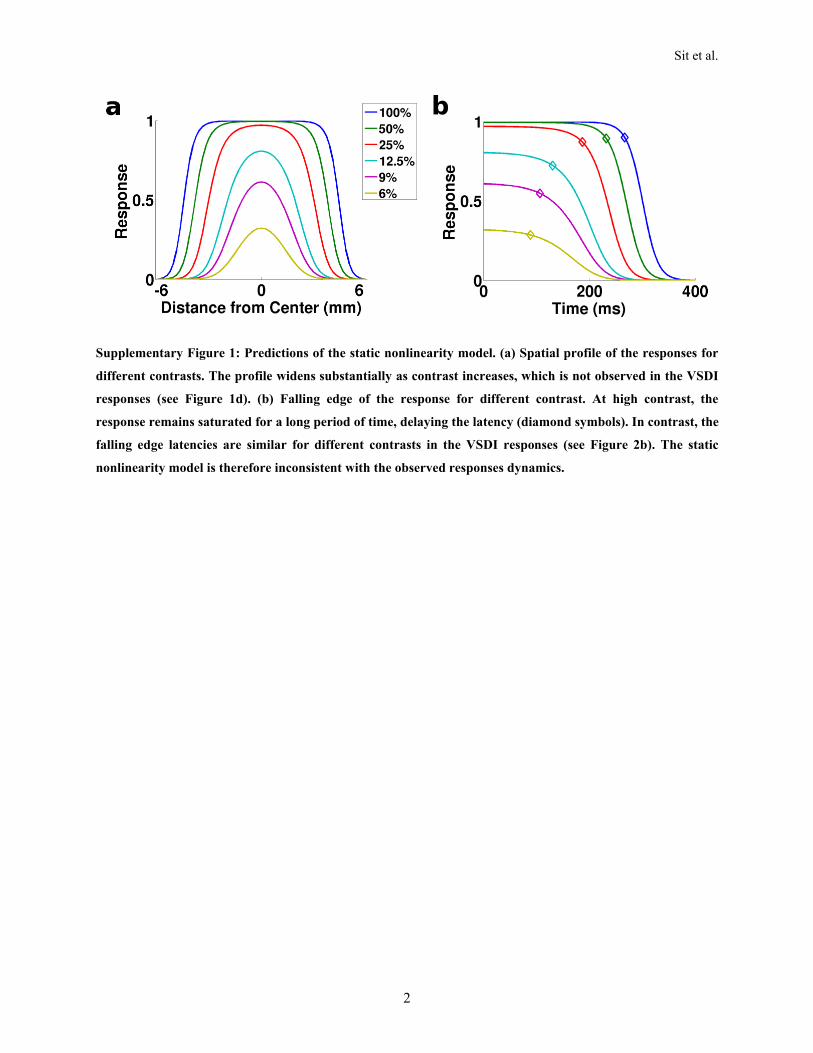
This section shows the predictions of a static nonlinearity model regarding the spatial profile and falling

edge latency of the responses as a function of contrast. The nonlinearity was a Naka-Rushton equation,

with parameters determined from the VSDI responses (Figure 1f). To obtain the spatial profile at a

particular contrast, a fixed Gaussian input with ! = 2.1 mm was first scaled linearly with contrast and

then passed through the Naka-Rushton equation. Supplementary Figure 1a plots the spatial profiles for the

contrasts used in the VSDI experiments. As contrast increased, the region with saturated responses

became larger, resulting in a wider spatial profile. To see this, note that at low contrast a model unit with

its receptive field centered on the stimulus would produce a much bigger response than a peripheral unit

with a receptive that only slightly overlaps the stimulus. But, at high contrasts the responses would

become much closer to equal, because the response to the central unit would have already saturated at a

low contrast, allowing the response of the peripheral unit to “catch up”. This property is inconsistent with

the VSDI responses, because the spatial profile does not depend on stimulus contrast (Figure 1e).

The simulation of the falling edges in the model was similar. A fixed sigmoidal time course using

parameters obtained from the VSDI responses (Figure 4) was first scaled with contrast and then the Naka-

Rushton equation was applied at each time point. Supplementary Figure 1b plots the falling edges for

different contrasts. The responses at higher contrast remained saturated for a longer time, thus increasing

the latency. To see this, consider the predicted response when the stimulus contrast is sufficiently high to

push the output of the initial linear filter above the level that produces response saturation. In this case the

response will remain saturated until the output of the linear filter drops below the point where saturation

is produced. Thus, the higher the contrast the longer the time after stimulus offset until the response

begins to fall below the saturated level. Such contrast dependence for the latency of falling edge of the

response is not observed in the VSDI responses (see Figure 4), suggesting that the nonlinearity models

cannot account for the VSDI responses.

Sit et al.

2

Supplementary Figure 1: Predictions of the static nonlinearity model. (a) Spatial profile of the responses for

different contrasts. The profile widens substantially as contrast increases, which is not observed in the VSDI

responses (see Figure 1d). (b) Falling edge of the response for different contrast. At high contrast, the

response remains saturated for a long period of time, delaying the latency (diamond symbols). In contrast, the

falling edge latencies are similar for different contrasts in the VSDI responses (see Figure 2b). The static

nonlinearity model is therefore inconsistent with the observed responses dynamics.

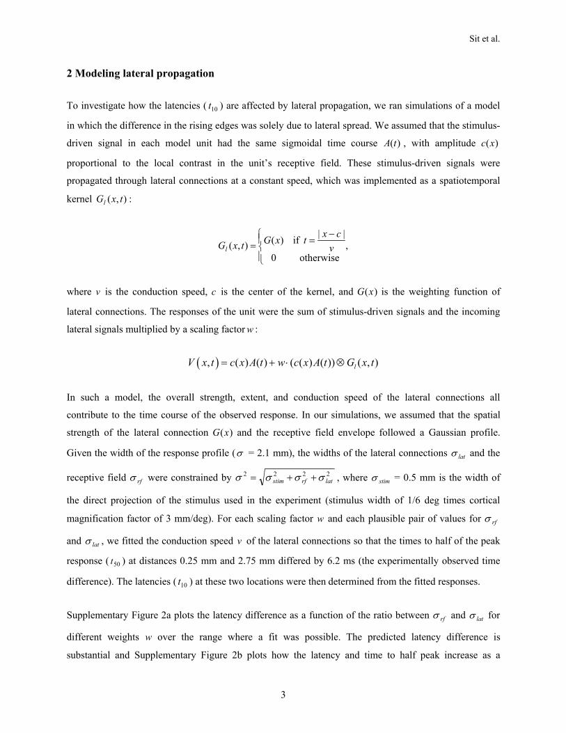
Sit et al.

3

2 Modeling lateral propagation

To investigate how the latencies ( 10t ) are affected by lateral propagation, we ran simulations of a model

in which the difference in the rising edges was solely due to lateral spread. We assumed that the stimulus-

driven signal in each model unit had the same sigmoidal time course )(tA , with amplitude )(xc

proportional to the local contrast in the unit’s receptive field. These stimulus-driven signals were

propagated through lateral connections at a constant speed, which was implemented as a spatiotemporal

kernel ),( txGl :

,otherwise0

||if)(),("#

"$% &

'' vcxtxGtxGl

where v is the conduction speed, c is the center of the kernel, and )(xG is the weighting function of

lateral connections. The responses of the unit were the sum of stimulus-driven signals and the incoming

lateral signals multiplied by a scaling factor w :

( ), ( ) ( ) ( ( ) ( )) ( , )lV x t c x A t w c x A t G x t' * + ,

In such a model, the overall strength, extent, and conduction speed of the lateral connections all

contribute to the time course of the observed response. In our simulations, we assumed that the spatial

strength of the lateral connection )(xG and the receptive field envelope followed a Gaussian profile.

Given the width of the response profile (! = 2.1 mm), the widths of the lateral connections lat! and the

receptive field rf! were constrained by 2222latrfstim !!!! **' , where stim! = 0.5 mm is the width of

the direct projection of the stimulus used in the experiment (stimulus width of 1/6 deg times cortical

magnification factor of 3 mm/deg). For each scaling factor w and each plausible pair of values for rf!

and lat! , we fitted the conduction speed v of the lateral connections so that the times to half of the peak

response ( 50t ) at distances 0.25 mm and 2.75 mm differed by 6.2 ms (the experimentally observed time

difference). The latencies ( 10t ) at these two locations were then determined from the fitted responses.

Supplementary Figure 2a plots the latency difference as a function of the ratio between rf! and lat! for

different weights w over the range where a fit was possible. The predicted latency difference is

substantial and Supplementary Figure 2b plots how the latency and time to half peak increase as a

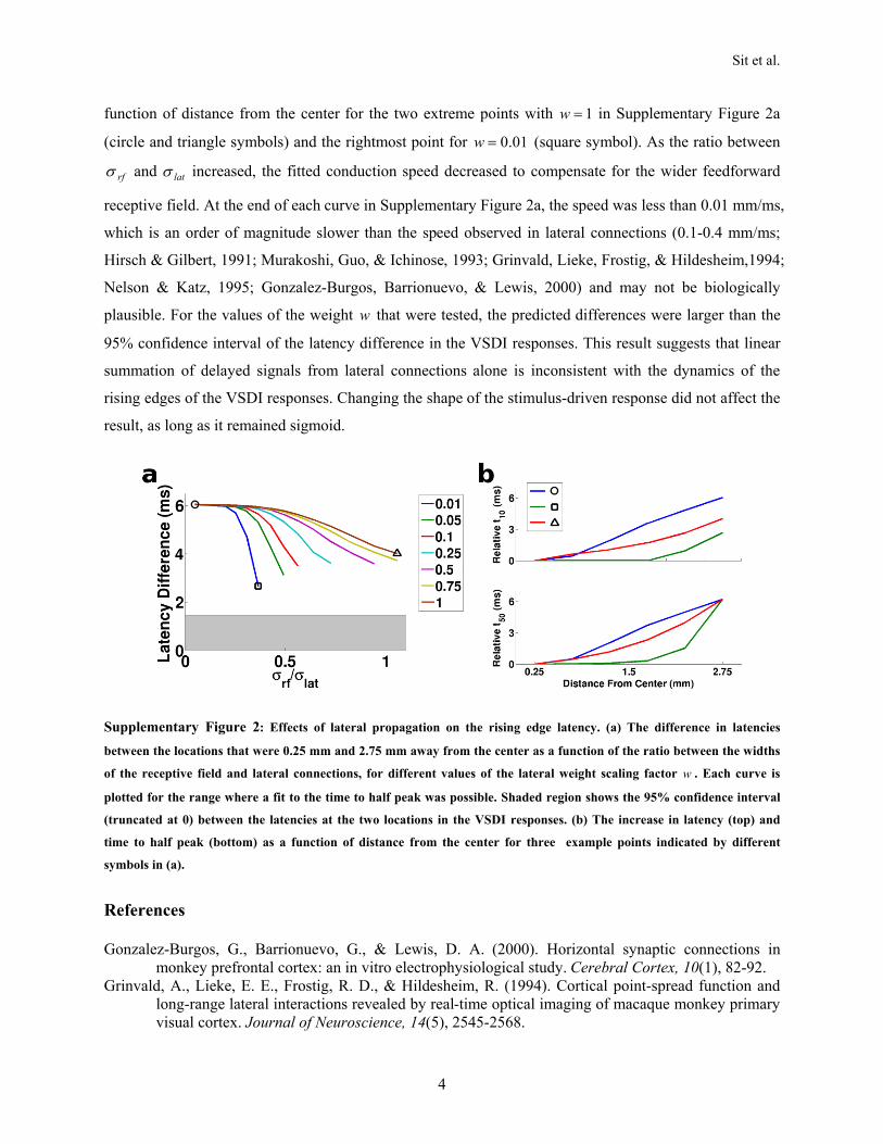
Sit et al.

4

function of distance from the center for the two extreme points with 1'w in Supplementary Figure 2a

(circle and triangle symbols) and the rightmost point for 01.0'w (square symbol). As the ratio between

rf! and lat! increased, the fitted conduction speed decreased to compensate for the wider feedforward

receptive field. At the end of each curve in Supplementary Figure 2a, the speed was less than 0.01 mm/ms,

which is an order of magnitude slower than the speed observed in lateral connections (0.1-0.4 mm/ms;

Hirsch & Gilbert, 1991; Murakoshi, Guo, & Ichinose, 1993; Grinvald, Lieke, Frostig, & Hildesheim,1994;

Nelson & Katz, 1995; Gonzalez-Burgos, Barrionuevo, & Lewis, 2000) and may not be biologically

plausible. For the values of the weight w that were tested, the predicted differences were larger than the

95% confidence interval of the latency difference in the VSDI responses. This result suggests that linear

summation of delayed signals from lateral connections alone is inconsistent with the dynamics of the

rising edges of the VSDI responses. Changing the shape of the stimulus-driven response did not affect the

result, as long as it remained sigmoid.

!

Supplementary Figure 2: Effects of lateral propagation on the rising edge latency. (a) The difference in latencies

between the locations that were 0.25 mm and 2.75 mm away from the center as a function of the ratio between the widths

of the receptive field and lateral connections, for different values of the lateral weight scaling factor w . Each curve is

plotted for the range where a fit to the time to half peak was possible. Shaded region shows the 95% confidence interval

(truncated at 0) between the latencies at the two locations in the VSDI responses. (b) The increase in latency (top) and

time to half peak (bottom) as a function of distance from the center for three example points indicated by different

symbols in (a).

References

Gonzalez-Burgos, G., Barrionuevo, G., & Lewis, D. A. (2000). Horizontal synaptic connections in monkey prefrontal cortex: an in vitro electrophysiological study. Cerebral Cortex, 10(1), 82-92.

Grinvald, A., Lieke, E. E., Frostig, R. D., & Hildesheim, R. (1994). Cortical point-spread function and long-range lateral interactions revealed by real-time optical imaging of macaque monkey primary visual cortex. Journal of Neuroscience, 14(5), 2545-2568.

Sit et al.

5

Hirsch, J. A., & Gilbert, C. D. (1991). Synaptic physiology of horizontal connections in the cat's visual cortex. Journal of Neuroscience, 11(6), 1800-1809.

Murakoshi, T., Guo, J. Z., & Ichinose, T. (1993). Electrophysiological identification of horizontal synaptic connections in rat visual cortex in vitro. Neuroscience Letters, 163(2), 211-214.

Nelson, D. A., & Katz, L. C. (1995). Emergence of functional circuits in ferret visual cortex visualized by optical imaging. Neuron, 15(1), 23-34.

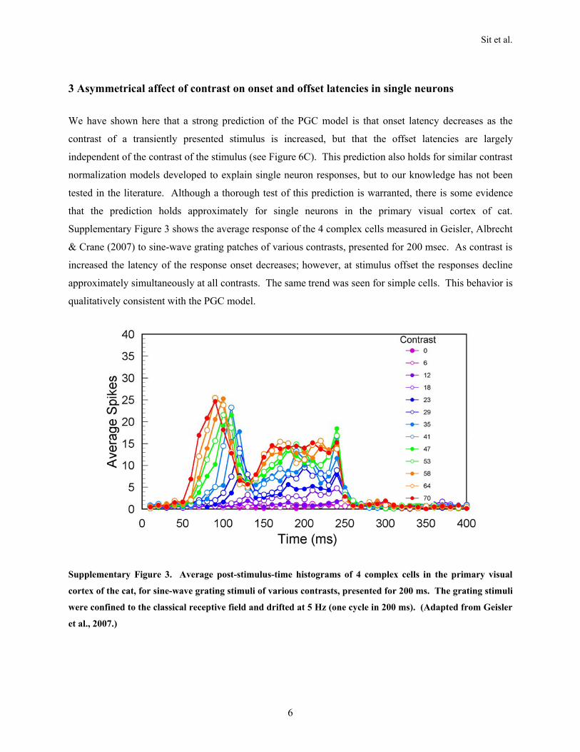
Sit et al.

6

3 Asymmetrical affect of contrast on onset and offset latencies in single neurons

We have shown here that a strong prediction of the PGC model is that onset latency decreases as the

contrast of a transiently presented stimulus is increased, but that the offset latencies are largely

independent of the contrast of the stimulus (see Figure 6C). This prediction also holds for similar contrast

normalization models developed to explain single neuron responses, but to our knowledge has not been

tested in the literature. Although a thorough test of this prediction is warranted, there is some evidence

that the prediction holds approximately for single neurons in the primary visual cortex of cat.

Supplementary Figure 3 shows the average response of the 4 complex cells measured in Geisler, Albrecht

& Crane (2007) to sine-wave grating patches of various contrasts, presented for 200 msec. As contrast is

increased the latency of the response onset decreases; however, at stimulus offset the responses decline

approximately simultaneously at all contrasts. The same trend was seen for simple cells. This behavior is

qualitatively consistent with the PGC model.

Supplementary Figure 3. Average post-stimulus-time histograms of 4 complex cells in the primary visual

cortex of the cat, for sine-wave grating stimuli of various contrasts, presented for 200 ms. The grating stimuli

were confined to the classical receptive field and drifted at 5 Hz (one cycle in 200 ms). (Adapted from Geisler

et al., 2007.)

Sit et al.

7

Reference

W.S., Albrecht D.G. & Crane A.M. (2007) Responses of cortical neurons to transient changes in local contrast and luminance. Journal of Neuroscience, 27, 5063-5067.

Sit et al.

8

4 Estimating normalization pool size

The width of the normalization pool affects how the time constant of the rising edge changes across space.

Given the measured rising edge time constants c- at the center c and p- at the periphery that is p mm

from the center, we can estimate the size of the pool in the second stage ( 2,H! ). This procedure gives the

lower bound for 2,H! , because it does not take the difference in the slopes of the input to the second

stage into account; if there is already some difference in the input, 2,H! would need to be larger to offset

the difference.

First, the time constant at center is given by

,1)(

))(1(0

&'

*'

c

c

cB

cBgC

--

-

where 0/ gC'- , which is the time constant of the falling edge. Since both - and c- are known, the

above equation can be evaluated to give a numerical value. Similarly, 1)( &'c

pB-- and can be

computed.

Note that B is a Gaussian with width 22,

21 H!! * , where 1! is the width of the spiking activity in the

first stage, which is related to the width of the input, x! , and the width of the receptive field in the first

stage, 1,G! , by 2/)2/( 21,

221 Gx !!! *' . )(cB and )( pB are the values at their corresponding points.

Dividing )(cB by )( pB , the width of the normalization pool in the second stage can be estimated:

Sit et al.

9

.

)()(ln2

)()(ln2

)(2exp

1)()(

21

2

2,

22

2,21

22,

21

2

!!

!!

!!

&

../

0112

3'

../

0112

3'*

.

./

0112

3

*&

'

pBcB

p

pBcB

p

ppBcB

H

H

H

Note that the above computation is independent of the normalization strength b .

Sit et al.

10

5 Simulation results for the experiments reported in Benucci, Frazor, & Carandini (2007) We have used the PGC model to simulate the experiments described in Benucci, Frazor, & Carandini

(2007), which reports traveling waves of neural responses (as measured by their phases) in the V1 of

anesthetized cats.

The stimuli used in theses experiments were square gratings that reversed contrast sinusoidally. In the

simulation, theses gratings were represented as rectangular envelopes with appropriate widths on the input

layer of the model so that the widths of the Gaussian point spread function (1.1 mm) and spatial response

(2.2 mm) match those reported in that paper. To represent the contrast reversing of the visual stimulus the

amplitude of the rectangular envelope modulated sinusoidally at 5 Hz and was full-wave rectified. The

model parameters used were 5.01, 'G! mm (resulting in a point spread of 1.1)25.0(5.0 22 '4* mm in

the second stage of the model), 9.01, 'H! mm, 46.21 'C , 53.12 'C , 1211 'b , and 202 'b . Note that

these values are specific for this simulation to provide a good fit to the data; they are different from those

used in the main text of the paper.

!

Supplementary Figure 4: Simulation results of the model. (A) Spatial profile of the 10 Hz component of the

responses. (B) The delay of the responses (computed from their phases) at different distances from the center.

The delay at a distance of 5 mm is about 15 ms. (C) Spatiotemporal response of the model, band-pass filtered

at 7-13 Hz as in Benucci et al., (2007).

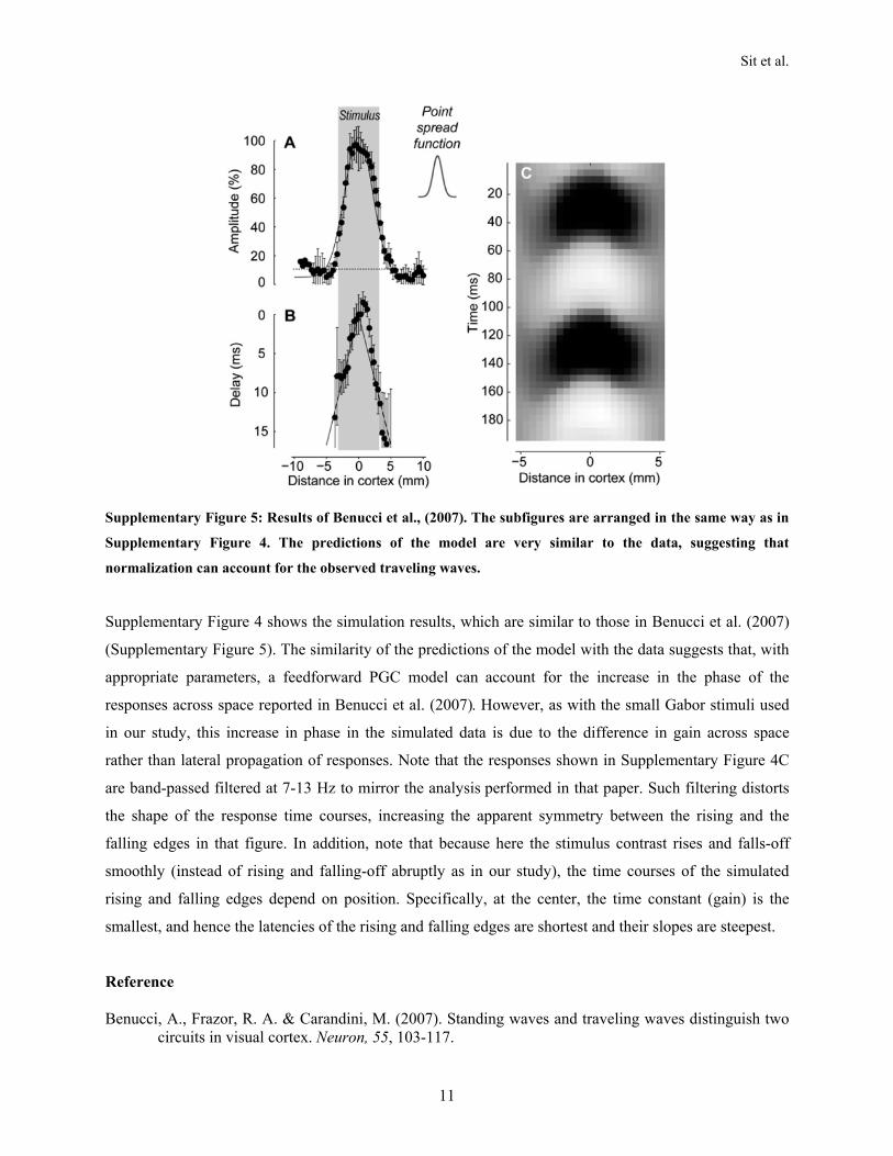
Sit et al.

11

!

Supplementary Figure 5: Results of Benucci et al., (2007). The subfigures are arranged in the same way as in

Supplementary Figure 4. The predictions of the model are very similar to the data, suggesting that

normalization can account for the observed traveling waves.

Supplementary Figure 4 shows the simulation results, which are similar to those in Benucci et al. (2007)

(Supplementary Figure 5). The similarity of the predictions of the model with the data suggests that, with

appropriate parameters, a feedforward PGC model can account for the increase in the phase of the

responses across space reported in Benucci et al. (2007). However, as with the small Gabor stimuli used

in our study, this increase in phase in the simulated data is due to the difference in gain across space

rather than lateral propagation of responses. Note that the responses shown in Supplementary Figure 4C

are band-passed filtered at 7-13 Hz to mirror the analysis performed in that paper. Such filtering distorts

the shape of the response time courses, increasing the apparent symmetry between the rising and the

falling edges in that figure. In addition, note that because here the stimulus contrast rises and falls-off

smoothly (instead of rising and falling-off abruptly as in our study), the time courses of the simulated

rising and falling edges depend on position. Specifically, at the center, the time constant (gain) is the

smallest, and hence the latencies of the rising and falling edges are shortest and their slopes are steepest.

Reference Benucci, A., Frazor, R. A. & Carandini, M. (2007). Standing waves and traveling waves distinguish two

circuits in visual cortex. Neuron, 55, 103-117.

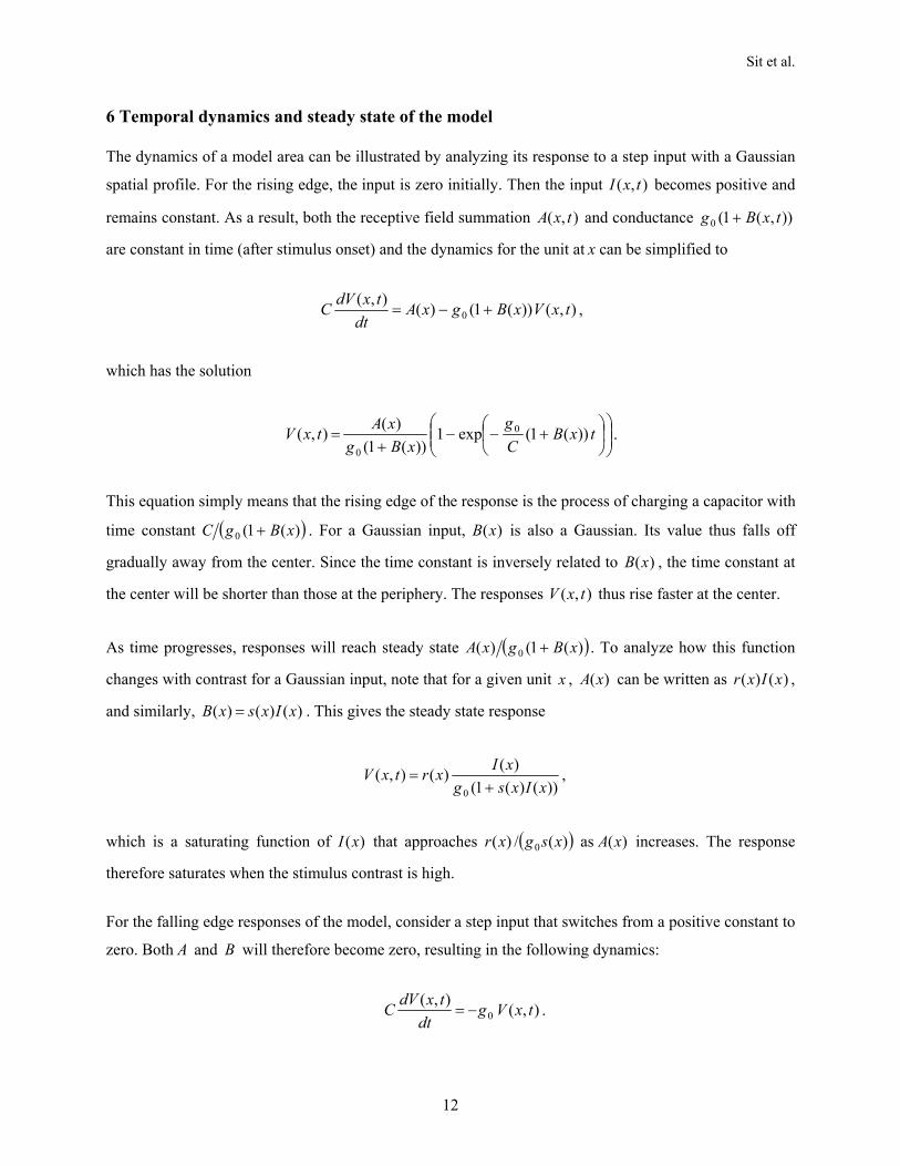
Sit et al.

12

6 Temporal dynamics and steady state of the model

The dynamics of a model area can be illustrated by analyzing its response to a step input with a Gaussian

spatial profile. For the rising edge, the input is zero initially. Then the input ),( txI becomes positive and

remains constant. As a result, both the receptive field summation ),( txA and conductance )),(1(0 txBg *

are constant in time (after stimulus onset) and the dynamics for the unit at x can be simplified to

),())(1()(),(0 txVxBgxA

dttxdVC *&' ,

which has the solution

../

0112

3./

012

3*&&

*' txB

Cg

xBgxAtxV ))(1(exp1

))(1()(),( 0

0.

This equation simply means that the rising edge of the response is the process of charging a capacitor with

time constant ( ))(1(0 xBgC * . For a Gaussian input, )(xB is also a Gaussian. Its value thus falls off

gradually away from the center. Since the time constant is inversely related to )(xB , the time constant at

the center will be shorter than those at the periphery. The responses ),( txV thus rise faster at the center.

As time progresses, responses will reach steady state ( ))(1()( 0 xBgxA * . To analyze how this function

changes with contrast for a Gaussian input, note that for a given unit x , )(xA can be written as )()( xIxr ,

and similarly, )()()( xIxsxB ' . This gives the steady state response

))()(1()()(),(

0 xIxsgxIxrtxV

*' ,

which is a saturating function of )(xI that approaches ( ))(/)( 0 xsgxr as )(xA increases. The response

therefore saturates when the stimulus contrast is high.

For the falling edge responses of the model, consider a step input that switches from a positive constant to

zero. Both A and B will therefore become zero, resulting in the following dynamics:

),(),(0 txVg

dttxdVC &' .

Sit et al.

13

The equation has a simple solution

)()(),(

oo tt

Cg

o exVtxV&&

' ,

where )(xVo and ot are the responses and the time at the offset of input, respectively. This solution has

two important implications. First, the responses at all locations will start to decay all at once after the

stimulus disappears, regardless of stimulus contrast and 0V . Second, the responses will decay with the

same time constant 0/ gC . In addition, note that the time constant of the rising edge ( )))(1(0 xBgC * is

smaller than 0/ gC . This result explains why the slopes of the falling edges were predicted to be smaller

than those in the rising edges, as observed in the data.

The V1 Population Gains Normalization

Elad Ganmor,1 Michael Okun,1 and Ilan Lampl1,*1Department of Neurobiology, Weizmann Institute of Science, Rehovot 76100, Israel*Correspondence: [email protected] 10.1016/j.neuron.2009.12.015

In this issue of Neuron, Busse et al. describe the population response to superimposed visual stimuli whileSit et al. examine the spatiotemporal evolution of cortical activation in response to small visual stimuli.Surprisingly, these two studies of V1 report that a single gain control model accounts for their results.

Orientation selectivity is the hallmarkof the primary visual cortex (V1). Whenthis property was discovered more than40 years ago by Hubel and Wiesel, itwas thought that the selectivity of corticalcells results only from the organization offeedforward inputs from the visual thal-amus. Today we know that the responseof cortical cells might be strongly affectedby inputs from the entire visual field.

Hubel and Wiesel showed that in V1cells, the response evoked by lines orbars at specific angles (orientation) ismuch greater than the response to cir-cular spots of light (Hubel and Wiesel,1962). However, the first-order corticalneurons that display this property (sim-ple cells) receive their afferent inputsfrom neurons of the lateral geniculatenucleus (LGN) of the thalamus, whichare not orientation selective. How thencan this behavior be explained? Hubeland Wiesel suggested a simple model inwhich simple cells receive feedforwardinputs from several LGN neurons withaligned receptive fields. When stimulatedby an elongated stimulus, aligned with thecollective receptive field structure ofthese thalamic cells, they are activatedsimultaneously, causing a large responsein simple cells.

Although many predictions of this feed-forward model were confirmed experi-mentally, other predictions failed. Onemajor discrepancy is the observation thatthe width of orientation tuning curves inV1 is independent of the stimulus contrast(Sclar andFreeman,1982), aphenomenoncalled contrast invariance. Since the firingof geniculate cells increases monotoni-cally with contrast, the feedforwardmodelpredicts that as contrast is increased,stimuli further away from the preferredorientation will evoke sufficient depolar-ization to cause firing. Thus, the tuning

curve of V1 neurons is expected to widenwhen contrast increases (Ferster andMiller, 2000).Another experimental observation not

explained by the simple feedforwardmodel is the strong suppression ofresponses to a stimulus at the preferredorientation by an orthogonal stimulus,even if the orthogonal stimulus by itselfevokes no response (Priebe and Ferster,2006). The feedforward model predictsthat the response to a combination ofstimuli is merely the sum of the responsesto each individual stimulus.Subsequently, new models were pro-

posed to account for the experimentalfindings described above. Roughly, theycan be described as belonging to twocategories: feedforward models extend-ing the original model of Hubel and Wie-sel, and models incorporating feedbackinputs. Normalization models, also knownas contrast gain control models (Albrechtand Geisler, 1991; Heeger, 1992), belongto the first category. In these models,two pathways determine the response ofa cortical neuron. One is a specific filterdefined by the neuron’s selectivity to thestimulus, as in the feedforward model ofHubel and Wiesel. The second pathwayintegrates less selective inputs from awider visual field, and serves as a normal-ization background. That is, the responseof the cell is a result of dividing theinput from the first pathway by the inputvia the second (gain control) pathway(Figure 1). At the level of single cells,contrast gain control models were foundto be successful in explaining severalkey features of visual processing, inparticular contrast invariance and cross-orientation suppression.Visual information, however, is repre-

sented by the joint activity of many neu-rons. Population models of V1 have relied

mostly on data gathered from singleneurons, yet neural populations may dis-play qualitatively different behaviors thanthe units that comprise them. For exam-ple, a population of contrast invariantneurons may not be contrast invariant initself (see below). Therefore, it is not clearwhether the aforementioned models,developed to describe the responsesof single neurons, can be successfullyapplied to neuronal populations.A study by Busse et al. (2009) in this

issue of Neuron efficiently addresses thisquestion, using multielectrode arrays torecord from many neurons in cat V1.Busse and colleagues characterized thetuning curves of multiple simultaneouslyrecorded neurons, and examined howtheir responses to a superposition oftwo oriented stimuli sum together. Thepopulation response was defined as theaverage firing rate of neurons grouped ac-cording to their preferred orientation.Interestingly, the authors found that asimple normalization model can accountfor their results.Initially Busse and her colleagues

verified that the population response iscontrast invariant and therefore a simplenormalization model, composed of aproduct of a tuning curve and a contrastgain function, may be applied to the pop-ulation response. How can a populationresponse not exhibit contrast invariancewhen single neurons are known to becontrast invariant? Consider, for example,a population in which sharply tunedneurons have high contrast thresholdswhereas widely tuned cells have lowthresholds. In such a population, ascontrast is increased, more sharply tunedneurons are recruited, resulting in asharpening of the population tuningcurve. However, the authors find thatcontrast sensitivity and tuning width are

778 Neuron 64, December 24, 2009 ª2009 Elsevier Inc.

Neuron

Previews


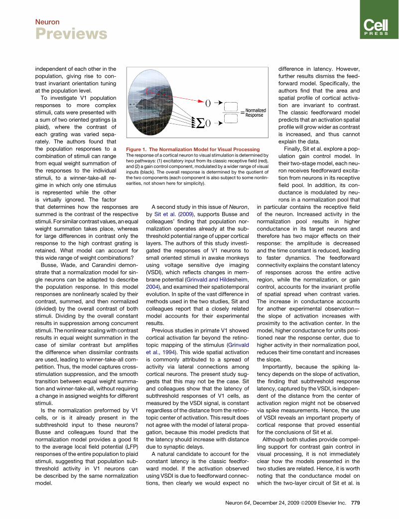
independent of each other in thepopulation, giving rise to con-trast invariant orientation tuningat the population level.To investigate V1 population

responses to more complexstimuli, cats were presented witha sum of two oriented gratings (aplaid), where the contrast ofeach grating was varied sepa-rately. The authors found thatthe population responses to acombination of stimuli can rangefrom equal weight summation ofthe responses to the individualstimuli, to a winner-take-all re-gime in which only one stimulusis represented while the otheris virtually ignored. The factorthat determines how the responses aresummed is the contrast of the respectivestimuli. For similar contrastvalues, anequalweight summation takes place, whereasfor large differences in contrast only theresponse to the high contrast grating isretained. What model can account forthis wide range of weight combinations?Busse, Wade, and Carandini demon-

strate that a normalization model for sin-gle neurons can be adapted to describethe population response. In this modelresponses are nonlinearly scaled by theircontrast, summed, and then normalized(divided) by the overall contrast of bothstimuli. Dividing by the overall constantresults in suppression among concurrentstimuli. Thenonlinear scalingwith contrastresults in equal weight summation in thecase of similar contrast but amplifiesthe difference when dissimilar contrastsare used, leading to winner-take-all com-petition. Thus, the model captures cross-stimulation suppression, and the smoothtransition between equal weight summa-tion and winner-take-all, without requiringa change in assigned weights for differentstimuli.Is the normalization preformed by V1

cells, or is it already present in thesubthreshold input to these neurons?Busse and colleagues found that thenormalization model provides a good fitto the average local field potential (LFP)responses of the entire population to plaidstimuli, suggesting that population sub-threshold activity in V1 neurons canbe described by the same normalizationmodel.

A second study in this issue of Neuron,by Sit et al. (2009), supports Busse andcolleagues’ finding that population nor-malization operates already at the sub-threshold potential range of upper corticallayers. The authors of this study investi-gated the responses of V1 neurons tosmall oriented stimuli in awake monkeysusing voltage sensitive dye imaging(VSDI), which reflects changes in mem-brane potential (Grinvald and Hildesheim,2004), and examined their spatiotemporalevolution. In spite of the vast difference inmethods used in the two studies, Sit andcolleagues report that a closely relatedmodel accounts for their experimentalresults.Previous studies in primate V1 showed

cortical activation far beyond the retino-topic mapping of the stimulus (Grinvaldet al., 1994). This wide spatial activationis commonly attributed to a spread ofactivity via lateral connections amongcortical neurons. The present study sug-gests that this may not be the case. Sitand colleagues show that the latency ofsubthreshold responses of V1 cells, asmeasured by the VSDI signal, is constantregardless of the distance from the retino-topic center of activation. This result doesnot agree with the model of lateral propa-gation, because this model predicts thatthe latency should increase with distancedue to synaptic delays.A natural candidate to account for the

constant latency is the classic feedfor-ward model. If the activation observedusing VSDI is due to feedforward connec-tions, then clearly we would expect no

difference in latency. However,further results dismiss the feed-forward model. Specifically, theauthors find that the area andspatial profile of cortical activa-tion are invariant to contrast.The classic feedforward modelpredicts that an activation spatialprofile will growwider as contrastis increased, and thus cannotexplain the data.Finally, Sit et al. explore a pop-

ulation gain control model. Intheir two-stagemodel, each neu-ron receives feedforward excita-tion from neurons in its receptivefield pool. In addition, its con-ductance is modulated by neu-rons in a normalization pool that

in particular contains the receptive fieldof the neuron. Increased activity in thenormalization pool results in higherconductance in its target neurons andtherefore has two major effects on theirresponse: the amplitude is decreasedand the time constant is reduced, leadingto faster dynamics. The feedforwardconnectivity explains the constant latencyof responses across the entire activeregion, while the normalization, or gaincontrol, accounts for the invariant profileof spatial spread when contrast varies.The increase in conductance accountsfor another experimental observation—the slope of activation increases withproximity to the activation center. In themodel, higher conductance for units posi-tioned near the response center, due tohigher activity in their normalization pool,reduces their time constant and increasesthe slope.

Importantly, because the spiking la-tency depends on the slope of activation,the finding that subthreshold responselatency, captured by the VSDI, is indepen-dent of the distance from the center ofactivation region might not be observedvia spike measurements. Hence, the useof VSDI reveals an important property ofcortical response that proved essentialfor the conclusions of Sit et al.

Although both studies provide compel-ling support for contrast gain control invisual processing, it is not immediatelyclear how the models presented in thetwo studies are related. Hence, it is worthnoting that the conductance model onwhich the two-layer circuit of Sit et al. is

Figure 1. The Normalization Model for Visual ProcessingThe response of a cortical neuron to visual stimulation is determined bytwo pathways: (1) excitatory input from its classic receptive field (red),and (2) a gain control component, modulated by awider range of visualinputs (black). The overall response is determined by the quotient ofthe two components (each component is also subject to some nonlin-earities, not shown here for simplicity).

Neuron 64, December 24, 2009 ª2009 Elsevier Inc. 779

Neuron

Previews

based was proposed as a possible bio-physically plausible implementation of anormalization operation (Carandini andHeeger, 1994), such as the one in Busseet al.

What biophysical mechanisms maybe responsible for divisive gain control?Different studies have addressed thisquestion. One candidate mechanism isshort-term synaptic depression (Freemanet al., 2002). Widely tuned, visuallyevoked cortical shunting inhibition mayalso contribute to contrast normalization.However, intracellular recording studiesin vivo of inhibitory tuning curve profilesand changes in evoked conductance inresponse to plaid stimuli (Priebe and Fer-ster, 2008) found no support for this view.

Divisive gain control might supporthigher-level aspects of visual processingbeyond the responses of V1 neurons torelatively simple stimuli. Some studiesdebate the role of normalization in redun-dancy reduction and efficient coding(Schwartz and Simoncelli, 2001; Shiet al., 2006), while others suggest that

changes in visual processing (sensitivity,gain, etc.) induced by shifts in attentionmay be explained by a modulation of theinput signal by an attentional filter fol-lowed by normalization (Reynolds andHeeger, 2009).Clearly, the functional implications of

contrast gain control for downstreamvisual areas and the contribution of dif-ferent biophysical mechanisms to itsimplementation are still open questions.Hopefully, further research and analysisof how large populations process com-plex stimuli may shed light on theseissues.

REFERENCES

Albrecht, D.G., and Geisler, W.S. (1991). Vis.Neurosci. 7, 531–546.

Busse, L., Wade, A.R., and Carandini, M. (2009).Neuron 64, this issue, 931–942.

Carandini, M., and Heeger, D.J. (1994). Science264, 1333–1336.

Ferster, D., and Miller, K.D. (2000). Annu. Rev.Neurosci. 23, 441–471.

Freeman, T.C.B., Durand, S., Kiper, D.C., andCarandini, M. (2002). Neuron 35, 759–771.

Grinvald, A., and Hildesheim, R. (2004). Nat. Rev.Neurosci. 5, 874–885.

Grinvald, A., Lieke, E.E., Frostig, R.D., and Hilde-sheim, R. (1994). J. Neurosci. 14, 2545–2568.

Heeger, D.J. (1992). Vis. Neurosci. 9, 181–197.

Hubel, D.H., and Wiesel, T.N. (1962). J. Physiol.160, 106–154.

Priebe, N.J., and Ferster, D. (2006). Nat. Neurosci.9, 552–561.

Priebe, N.J., and Ferster, D. (2008). Neuron 57,482–497.

Reynolds, J.H., and Heeger, D.J. (2009). Neuron61, 168–185.

Schwartz, O., and Simoncelli, E.P. (2001). Nat.Neurosci. 4, 819–825.

Sclar, G., and Freeman, R.D. (1982). Exp. BrainRes. 46, 457–461.

Shi, J., Wielaard, J., and Sajda, P. (2006). Conf.Proc. IEEE Eng. Med. Biol. Soc. 1, 4991–4994.

Sit, Y.F., Chen, Y., Geisler, W.S., Miikkulainen, R.,and Seidmann, E. (2009). Neuron 64, this issue,943–956.

Discreet Charm of the GABAergic Bourgeoisie:Superconnected Cells ConductDevelopmental Symphonies

Marianne Case1,* and Ivan Soltesz1,*1Department of Anatomy and Neurobiology, University of California, Irvine, Irvine, CA 92697, USA*Correspondence: [email protected] (M.C.), [email protected] (I.S.)DOI 10.1016/j.neuron.2009.12.013

In an exciting study in the December 4th issue of Science, Bonifazi and colleagues demonstrated the exis-tence and importance of exceedingly rare but unusually richly connected cells in the developing hippo-campus. Manipulating the activity of single GABAergic hub cells modulated network activity patterns,demonstrating their importance for coordinating synchronous activity.

Much to the chagrin of our latte-drinking,sushi-eating, Volvo-driving liberal friendsall over, networks in the real world aredecidedly not egalitarian but rather aristo-cratic in nature. Indeed, the dispropor-tionate influence of rare superconnectedhubs is well-known in technological, bio-logical, and social networks, including

aviation grids (such as LAX and JFK),biochemical reaction pathways (such aspyruvate and ATP), and the proverbialold boys’ networks. For neurosciencein particular, hub-like connectors areconsidered to be of great potential signif-icance because networks with sucharistocratic flavor have been predicted

by theoretical studies to represent aclever compromise between fast com-putation, economy of wiring, and robust-ness against random deletions (Buzsakiet al., 2004; Bullmore and Sporns, 2009).However, while we have thoroughlydefined neuronal networks lacking super-connected neurons (such as that of

780 Neuron 64, December 24, 2009 ª2009 Elsevier Inc.

Neuron

Previews



Documents

Complex Dynamics of V1 Population Responses Explained by …nn.cs.utexas.edu/downloads/papers/sit.neuron09.pdf · Complex Dynamics of V1 Population Responses Explained by a Simple