Complex Polynomial Mandalas and their Symmetries

Konstantin Poelke, Zoi Tokoutsi, Konrad PolthierFreie Universitat Berlin

{konstantin.poelke, zoi.tokoutsi, konrad.polthier}@fu-berlin.de

AbstractWe present an application of the classical Schwarz reflection principle to create complex mandalas—symmetricshapes resulting from the transformation of simple curves by complex polynomials—and give various illustrationsof how their symmetry relates to the polynomials’ set of zeros. Finally we use the winding numbers inside thesegments enclosed by the transformed curves to obtain fully coloured patterns in the spirit of many mandalas foundin real-life.

Introduction

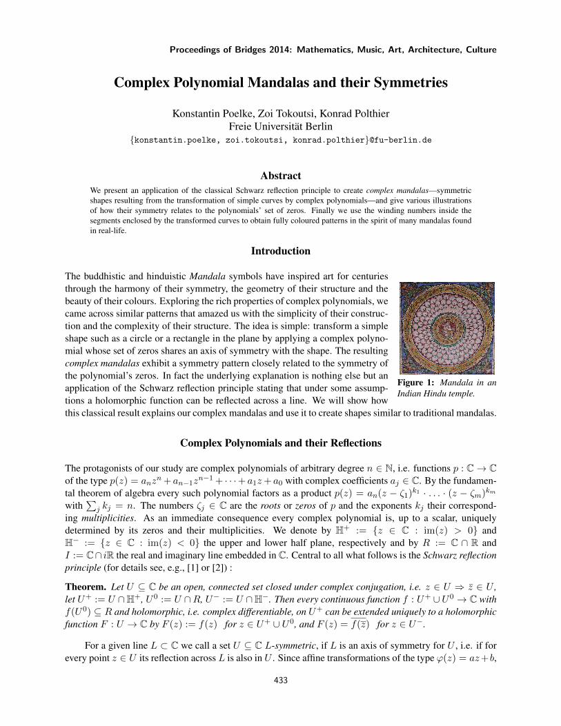
Figure 1: Mandala in anIndian Hindu temple.

The buddhistic and hinduistic Mandala symbols have inspired art for centuriesthrough the harmony of their symmetry, the geometry of their structure and thebeauty of their colours. Exploring the rich properties of complex polynomials, wecame across similar patterns that amazed us with the simplicity of their construc-tion and the complexity of their structure. The idea is simple: transform a simpleshape such as a circle or a rectangle in the plane by applying a complex polyno-mial whose set of zeros shares an axis of symmetry with the shape. The resultingcomplex mandalas exhibit a symmetry pattern closely related to the symmetry ofthe polynomial’s zeros. In fact the underlying explanation is nothing else but anapplication of the Schwarz reflection principle stating that under some assump-tions a holomorphic function can be reflected across a line. We will show howthis classical result explains our complex mandalas and use it to create shapes similar to traditional mandalas.

Complex Polynomials and their Reflections

The protagonists of our study are complex polynomials of arbitrary degree n ∈ N, i.e. functions p : C→ Cof the type p(z) = anz

n + an−1zn−1 + · · ·+ a1z+ a0 with complex coefficients aj ∈ C. By the fundamen-

tal theorem of algebra every such polynomial factors as a product p(z) = an(z − ζ1)k1 · . . . · (z − ζm)km

with∑

j kj = n. The numbers ζj ∈ C are the roots or zeros of p and the exponents kj their correspond-ing multiplicities. As an immediate consequence every complex polynomial is, up to a scalar, uniquelydetermined by its zeros and their multiplicities. We denote by H+ := {z ∈ C : im(z) > 0} andH− := {z ∈ C : im(z) < 0} the upper and lower half plane, respectively and by R := C ∩ R andI := C∩ iR the real and imaginary line embedded in C. Central to all what follows is the Schwarz reflectionprinciple (for details see, e.g., [1] or [2]) :

Theorem. Let U ⊆ C be an open, connected set closed under complex conjugation, i.e. z ∈ U ⇒ z ∈ U ,let U+ := U ∩H+, U0 := U ∩R, U− := U ∩H−. Then every continuous function f : U+ ∪U0 → C withf(U0) ⊆ R and holomorphic, i.e. complex differentiable, on U+ can be extended uniquely to a holomorphicfunction F : U → C by F (z) := f(z) for z ∈ U+ ∪ U0, and F (z) = f(z) for z ∈ U−.

For a given line L ⊂ C we call a set U ⊆ C L-symmetric, if L is an axis of symmetry for U , i.e. if forevery point z ∈ U its reflection across L is also in U . Since affine transformations of the type ϕ(z) = az+b,

Proceedings of Bridges 2014: Mathematics, Music, Art, Architecture, Culture

433

a, b ∈ C, a 6= 0, map L-symmetric sets to ϕ(L)-symmetric sets the reflection principle can be stated slightlymore general as

Corollary. Let L ⊂ C be a line, U ⊆ C be an open, connected L-symmetric set, U0 := U ∩ L, and letU+ and U− denote the subsets of U to the left and right hand side of L, respectively (pick an arbitraryorientation of L). If f : U+ ∪ U0 → C is a continuous function with f(U0) contained in a line L andholomorphic on U+, then f has a unique holomorphic extension F : U → C, and F (U) is L-symmetric.

If p is a complex polynomial let Z(p) denote the (finite) set of its zeros. Assume there is a line L ⊂ Csuch thatZ(p) is L-symmetric. Then every L-symmetric set U is mapped to an L-symmetric set U := p(U),where L is a line through p(L). Indeed there is an affine biholomorphic transformation ψ that maps R toL and R-symmetric sets to L-symmetric sets. Therefore p := p ◦ ψ is a polynomial whose set of zerosZ(p) = ψ−1(Z(p)) is R-symmetric. Then p is of the type p(z) = c

∏j(z − tj)

∏k(z − bk)(z − bk) =

c∏

j(z − tj)∏

k(z2 − 2re(bk)z + ‖bk‖2), where tj ∈ Z(p) ∩ R, bk, bk ∈ Z(p) \ R and c ∈ C. If c ∈ Rthen p(R) ⊂ R, otherwise p(R) is contained in the line L passing through the origin and forming an anglearg c to R, so p(L) = p ◦ ψ−1(L) ⊆ L and we can apply the corollary.

Symmetries, Construction and Colouring of Complex Mandalas

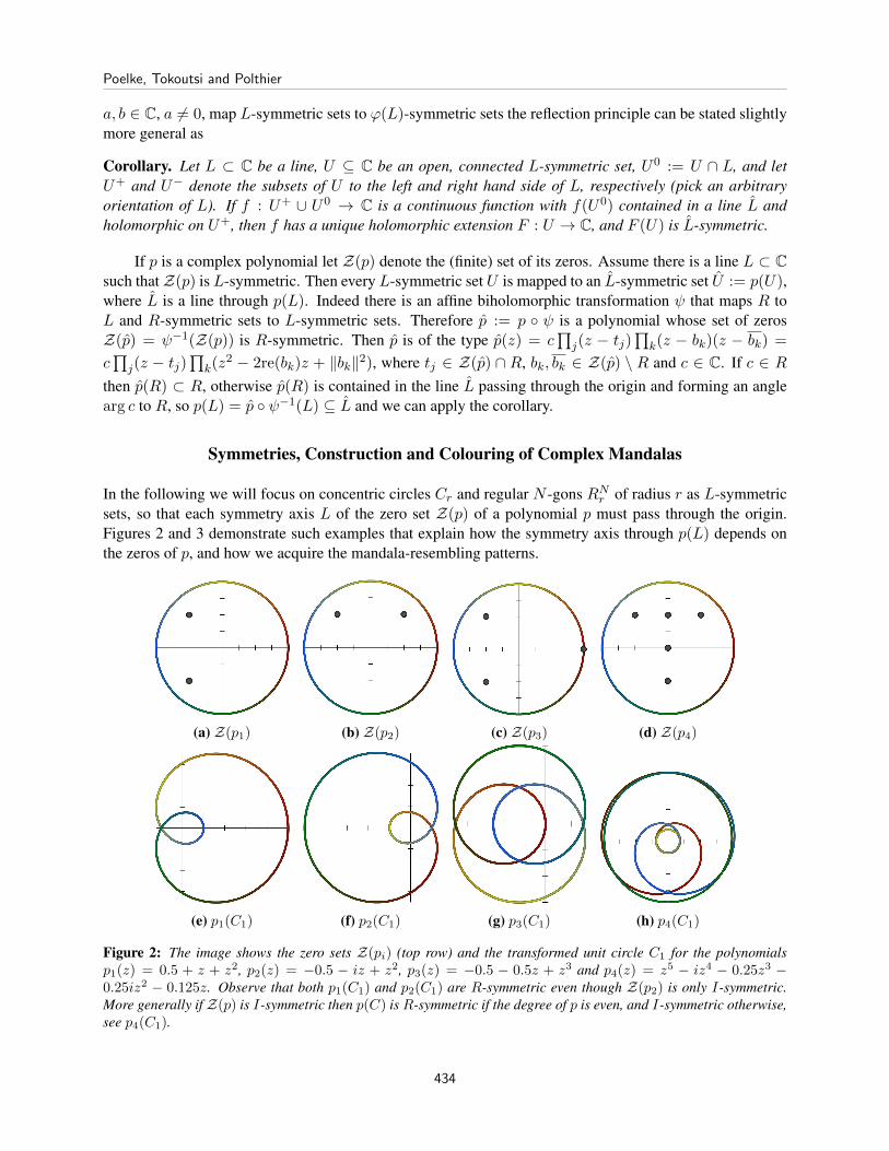
In the following we will focus on concentric circles Cr and regular N -gons RNr of radius r as L-symmetric

sets, so that each symmetry axis L of the zero set Z(p) of a polynomial p must pass through the origin.Figures 2 and 3 demonstrate such examples that explain how the symmetry axis through p(L) depends onthe zeros of p, and how we acquire the mandala-resembling patterns.

(a) Z(p1) (b) Z(p2) (c) Z(p3) (d) Z(p4)

(e) p1(C1) (f) p2(C1) (g) p3(C1) (h) p4(C1)

Figure 2: The image shows the zero sets Z(pi) (top row) and the transformed unit circle C1 for the polynomialsp1(z) = 0.5 + z + z2, p2(z) = −0.5 − iz + z2, p3(z) = −0.5 − 0.5z + z3 and p4(z) = z5 − iz4 − 0.25z3 −0.25iz2 − 0.125z. Observe that both p1(C1) and p2(C1) are R-symmetric even though Z(p2) is only I-symmetric.More generally if Z(p) is I-symmetric then p(C) is R-symmetric if the degree of p is even, and I-symmetric otherwise,see p4(C1).

Poelke, Tokoutsi and Polthier

434

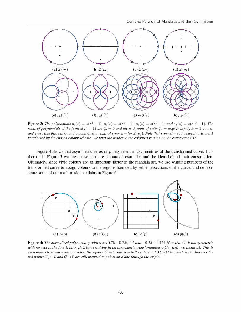
(a) Z(p5) (b) Z(p6) (c) Z(p7) (d) Z(p8)

(e) p5(C1) (f) p6(C1) (g) p7(C1) (h) p8(C1)

Figure 3: The polynomials p5(z) = z(z3 − 1), p6(z) = z(z4 − 1), p7(z) = z(z9 − 1) and p8(z) = z(z10 − 1). Theroots of polynomials of the form z(zn − 1) are ζ0 = 0 and the n-th roots of unity ζk = exp(2πik/n), k = 1, . . . , n,and every line through ζ0 and a point ζk is an axis of symmetry for Z(pj). Note that symmetry with respect to R and Iis reflected by the chosen colour scheme. We refer the reader to the coloured version on the conference CD.

Figure 4 shows that asymmetric zeros of p may result in asymmetries of the transformed curve. Fur-ther on in Figure 5 we present some more elaborated examples and the ideas behind their construction.Ultimately, since vivid colours are an important factor in the mandala art, we use winding numbers of thetransformed curve to assign colours to the regions bounded by self-intersections of the curve, and demon-strate some of our math-made mandalas in Figure 6.

(a) Z(p) (b) p(C1) (c) Z(p) (d) p(Q)

Figure 4: The normalized polynomial p with zeros 0.75− 0.25i, 0.5 and−0.25 + 0.75i. Note that C1 is not symmetricwith respect to the line L through Z(p), resulting in an asymmetric transformation p(C1) (left two pictures). This iseven more clear when one considers the square Q with side length 2 centered at 0 (right two pictures). However thered points C1 ∩ L and Q ∩ L are still mapped to points on a line through the origin.

Complex Polynomial Mandalas and their Symmetries

435

(a) Z(p9) (b) Z(p10) (c) Z(p11) (d) Z(p12)

(e) p9(R31.2) (f) p10(R6

1.1) (g) p11(C1) (h) p12(R41.5)

Figure 5: The four pictures on the left show the polynomials p9(z) = z(z3−1), p10(z) = z(z3−1)(z3 +1) = z7−z,that have prescribed zeros at the 3rd and 6th roots of unity and the origin, and how they transform the correspondingpolygonsR3

1.2 andR61.1. The remaining four pictures on the right show the polynomials p11(z) =

∫(z4− 1

16 )(z8−1) =113z

13− 1144z

9− 15z

5+ 116z and p12(z) =

∫(z4−1)(z4+ 1

4 ) = 19z

9− 320z

5− 14z. Note that this time these polynomials

are given as anti-derivatives (with vanishing constant term) of polynomials p′11, p′12 with prescribed zeros. It is thesezeros that cause p11(C1) to form spikes in the blue and orange region, related to so-called ramification that occurs atthese points. p12 transforms the regular 4-gon R4

1.5.

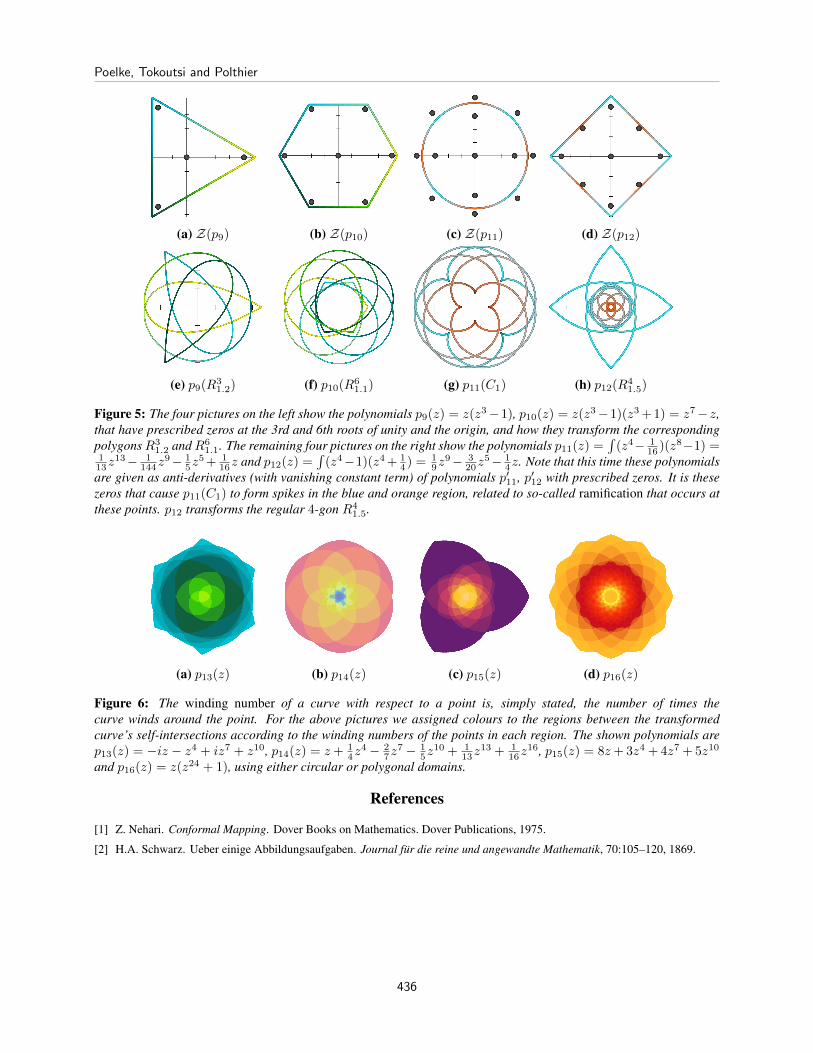
(a) p13(z) (b) p14(z) (c) p15(z) (d) p16(z)

Figure 6: The winding number of a curve with respect to a point is, simply stated, the number of times thecurve winds around the point. For the above pictures we assigned colours to the regions between the transformedcurve’s self-intersections according to the winding numbers of the points in each region. The shown polynomials arep13(z) = −iz − z4 + iz7 + z10, p14(z) = z+ 1

4z4− 2

7z7− 1

5z10 + 1

13z13 + 1

16z16, p15(z) = 8z+ 3z4 + 4z7 + 5z10

and p16(z) = z(z24 + 1), using either circular or polygonal domains.

References

[1] Z. Nehari. Conformal Mapping. Dover Books on Mathematics. Dover Publications, 1975.

[2] H.A. Schwarz. Ueber einige Abbildungsaufgaben. Journal fur die reine und angewandte Mathematik, 70:105–120, 1869.

Poelke, Tokoutsi and Polthier

436