Embed Size (px)
Citation preview
Complex Systems Architecture Framework. Extension to Multi-
Objective Optimization
Abdelkrim Doufene1, Hugo G. Chalé2 and Daniel Krob3
Abstract. This paper shows the utility to follow an architecture framework in order to design complex systems with a holistic approach. Multi-objective Optimization techniques extend and complete the architecture framework to support trade-off analysis and decision making in the Systems Engineering design process. The merging and combination of these two approaches, decision making and systems engineering, contribute to the efficient design of systems by helping to meet needs and constraints stemming mainly from the system analysis.
To support this assertion, we present a case study for an Electric Vehicle Powertrain. The decision problem is modeled as a Pareto model, in order to find a solution for the Electric Vehicle Powertrain that maximizes its autonomy and minimizes its total cost of ownership.
Keywords: complex systems, architecture framework, trade-off analysis, multi-
objective optimization, electric vehicle.
1 RENAULT & École polytechnique Laboratoire d'informa tique (LIX). [email protected], [email protected].
2 RENAULT, 1 avenue du Golf, 78288 Guyancourt, France. [email protected].
3 École polytechnique Laboratoire d'informatique (LIX) 91128 Palaiseau Cedex, France. [email protected].
1. Introduction
Trade-off analyses during complex systems design are inevitable. They are useful and necessary to make almost all the decisions during system design. Different kinds of decisions are involved: the choice of a safe and not too expensive architecture, the balance between the most reliable but still available architecture and so on. We can imagine a lot of possible tradeoffs taking into consideration the stakeholders’ needs, the total cost of ownership of the system we want to design, its lifecycle properties such as quality, reliability, safety, flexibility, robustness, durability, scalability, sustainability… In addition, economical, technological, societal and regulatory feasibility studies are indispensable in order to satisfy all the stakeholders’ needs around the system of interest.
Indeed, in industrial practice, in order to design a complex system, there are several multidisciplinary objectives and constraints. Making analyses, defining the right criteria and evaluating the possible alternatives are hard tasks. This difficulty is due in particular to the fact that the separation between the problem definition and the solution design is often blurry.
Using an architecture framework could considerably contribute to bridge this gap, and to clarify the link between design constraints and design variables, often mixed in practice. An architecture framework provides guidance and rules for structuring and organizing system architectures. The several viewpoints that allow covering all the scope of the system architecture and the different abstraction levels add clarity to the problem definition and solution design processes.
To explain this assertion, we present in this paper the architecture framework explained in (Krob, 2009 and 2010), and we show the contribution of multi-objective optimization models in the decision-making process. We illustrate these contributions on a simplified case study. Our system of interest is the Electric Vehicle Powertrain (EVP) whose mission is to propel an Electric Vehicle (EV). The two global measures of effectiveness related to EVs are the protection of the environment by the reduction of carbon dioxide emissions4 and a TCO (total cost of ownership), with a reasonable driving autonomy, that must at least be equivalent to internal combustion engine vehicles.
This paper is organized as follows. We begin with an overview of the background of our study, the architecture framework we use and the multi-objective optimization problem formulation. We then explain the context of the optimization problem studied in this paper. We present the requirements analysis and the objectives to reach, we define the parameters and variables to be used, we
4 The same way for other pollutants as : Nitrogen oxide (NOx), Hydrocarbon (HC) and
Carbon monoxide (CO). Source: Presentation of Rémi Bastien, Director of the Department of Research, Advanced Engineering, and Materials at Renault: The Electric Vehicle Program of the Renault-Nissan Alliance, in Automotive Electronics and Systems Congress CESA, Electric and Hybrid Vehicles, Paris, November 2010.
represent the optimization problem as a multi-objective optimization mathematical formulation. Finally, before concluding, we discuss some tests and results.
Note that this work is a part of current initiatives at Renault aiming at improving the efficiency of product development and mastering the complexity of automotive systems as reported in (Chalé Góngora et al. 2012).
2. Background
The decision problem model presented in this article is based on a systems architecture model. In this section, we briefly present the systems architecture framework we use, explained in (Krob 2009 and 2010). Then we present some related works on multi-objective optimization in the context of complex systems engineering.
2.1. Systems architecture framework In order to design our System of Interest (SOI), we follow a framework that
provides guidance and rules for structuring and organizing system architectures. The framework provides several viewpoints that allow covering the whole scope of the system architecture. It is inspired from the SAGACE method originally proposed in (Penalva 1997), which revolves around three main principles: a modeling approach, a representation of views (a matrix of nine points of view) and a graphical modeling language. In this method, the SOI is defined in an iterative manner. First, elements like issues and system environment, project purpose and missions, stakeholders are identified. Then, we can design the system and describe it with a matrix of nine points of view: Operational, Functional and Structural views, refined by three temporal perspectives (Benkhannouchel 1993; Chatel 2004; Meinadier 1998 and 2002).
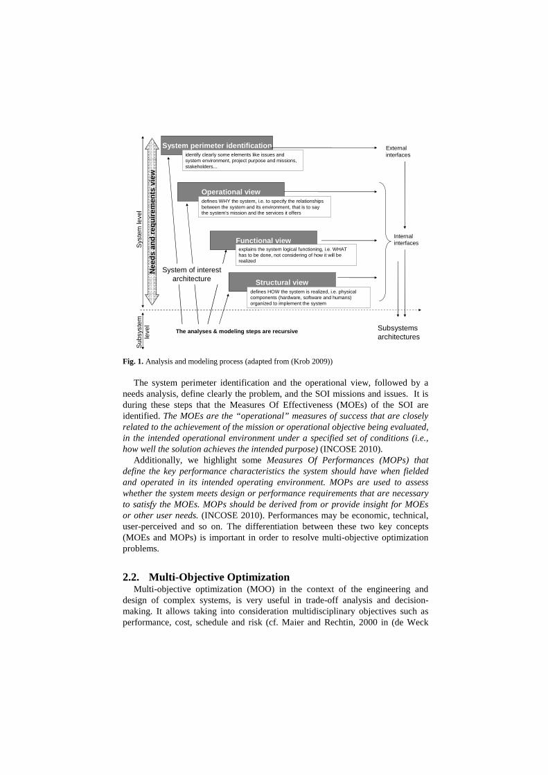
In our study, we also use these three main views but we refine them by behavioral - and not temporal, as in SAGACE - perspectives in order to be able to use the SysML modeling language, as explained in (Krob 2009 and 2010). This Framework was adapted for the automotive context as explained in (Chalé Góngora et al. 2012). Figure 1 gives an overview of the analysis and modeling steps used in our study.
System perimeter identification
Operational view
Functional view
Structural view
External interfaces
Internal interfaces
Subsystems architectures
Sys
tem
leve
lS
ubsy
stem
le
vel
System of interest architecture
The analyses & modeling steps are recursive
defines HOW the system is realized, i.e. physical components (hardware, software and humans) organized to implement the system
explains the system logical functioning, i.e. WHAT has to be done, not considering of how it will be realized
defines WHY the system, i.e. to specify the relationships between the system and its environment, that is to say the system's mission and the services it offers
identify clearly some elements like issues and system environment, project purpose and missions, stakeholders...
Nee
ds
and
req
uir
emen
ts v
iew
Fig. 1. Analysis and modeling process (adapted from (Krob 2009))
The system perimeter identification and the operational view, followed by a needs analysis, define clearly the problem, and the SOI missions and issues. It is during these steps that the Measures Of Effectiveness (MOEs) of the SOI are identified. The MOEs are the “operational” measures of success that are closely related to the achievement of the mission or operational objective being evaluated, in the intended operational environment under a specified set of conditions (i.e., how well the solution achieves the intended purpose) (INCOSE 2010).
Additionally, we highlight some Measures Of Performances (MOPs) that define the key performance characteristics the system should have when fielded and operated in its intended operating environment. MOPs are used to assess whether the system meets design or performance requirements that are necessary to satisfy the MOEs. MOPs should be derived from or provide insight for MOEs or other user needs. (INCOSE 2010). Performances may be economic, technical, user-perceived and so on. The differentiation between these two key concepts (MOEs and MOPs) is important in order to resolve multi-objective optimization problems.
2.2. Multi-Objective Optimization Multi-objective optimization (MOO) in the context of the engineering and
design of complex systems, is very useful in trade-off analysis and decision-making. It allows taking into consideration multidisciplinary objectives such as performance, cost, schedule and risk (cf. Maier and Rechtin, 2000 in (de Weck
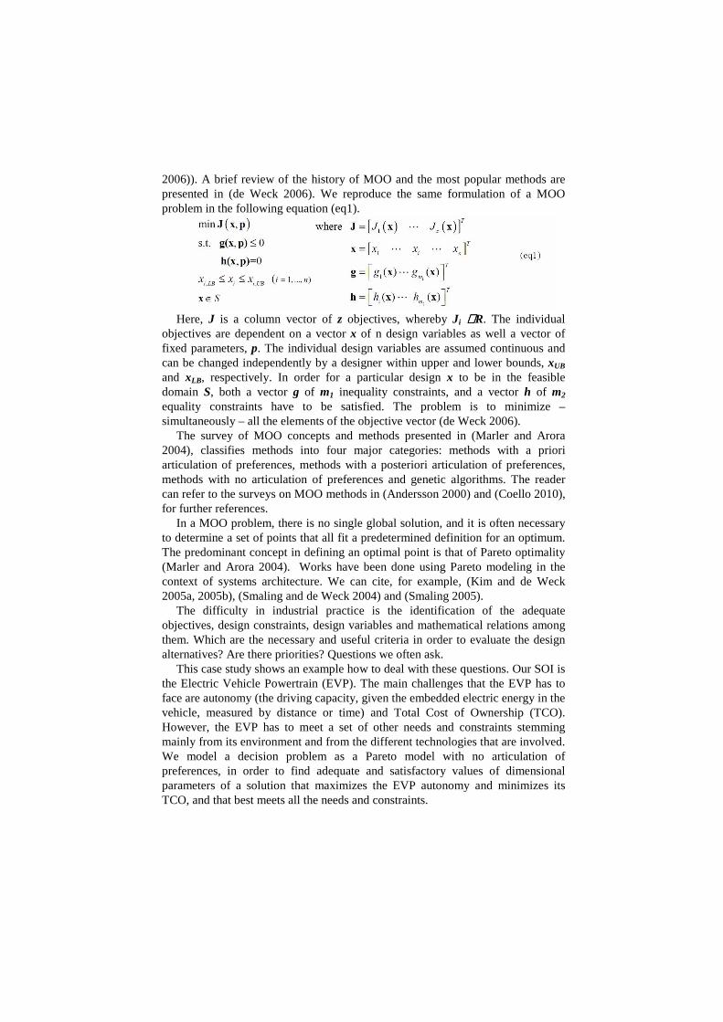
2006)). A brief review of the history of MOO and the most popular methods are presented in (de Weck 2006). We reproduce the same formulation of a MOO problem in the following equation (eq1).
Here, J is a column vector of z objectives, whereby Ji ∈∈∈∈R. The individual
objectives are dependent on a vector x of n design variables as well a vector of fixed parameters, p. The individual design variables are assumed continuous and can be changed independently by a designer within upper and lower bounds, xUB and xLB, respectively. In order for a particular design x to be in the feasible domain S, both a vector g of m1 inequality constraints, and a vector h of m2 equality constraints have to be satisfied. The problem is to minimize – simultaneously – all the elements of the objective vector (de Weck 2006).
The survey of MOO concepts and methods presented in (Marler and Arora 2004), classifies methods into four major categories: methods with a priori articulation of preferences, methods with a posteriori articulation of preferences, methods with no articulation of preferences and genetic algorithms. The reader can refer to the surveys on MOO methods in (Andersson 2000) and (Coello 2010), for further references.
In a MOO problem, there is no single global solution, and it is often necessary to determine a set of points that all fit a predetermined definition for an optimum. The predominant concept in defining an optimal point is that of Pareto optimality (Marler and Arora 2004). Works have been done using Pareto modeling in the context of systems architecture. We can cite, for example, (Kim and de Weck 2005a, 2005b), (Smaling and de Weck 2004) and (Smaling 2005).
The difficulty in industrial practice is the identification of the adequate objectives, design constraints, design variables and mathematical relations among them. Which are the necessary and useful criteria in order to evaluate the design alternatives? Are there priorities? Questions we often ask.
This case study shows an example how to deal with these questions. Our SOI is the Electric Vehicle Powertrain (EVP). The main challenges that the EVP has to face are autonomy (the driving capacity, given the embedded electric energy in the vehicle, measured by distance or time) and Total Cost of Ownership (TCO). However, the EVP has to meet a set of other needs and constraints stemming mainly from its environment and from the different technologies that are involved. We model a decision problem as a Pareto model with no articulation of preferences, in order to find adequate and satisfactory values of dimensional parameters of a solution that maximizes the EVP autonomy and minimizes its TCO, and that best meets all the needs and constraints.
3. Context of Our Optimization Problem
As explained previously, our study is based on the utilization of an architecture framework in order to design the SOI. In one word, all the information useful for the optimization problem stems from this architecture framework. The first steps highlight the SOI missions and its environment.
Our SOI is the EVP whose mission is to propel an EV. The EVP MOEs are: reasonable autonomy (the driving capacity, given the embedded electric energy in the vehicle, measured by distance or time) and total cost of ownership.
The EVP must be well integrated in its environment in order to achieve its mission. The environment modeling identifies the external systems that interact with the EVP. In this study, we consider the following significant external systems: the users, standards and regulations, roads, environmental conditions (weather), charging stations, and other subsystems of the vehicle (e.g. the charge management system).
The operational analysis of the EVP, following the architecture framework, highlights its lifecycle phases (Design, Production, Vehicle integration, Distribution/ Commercialization, Use/ Exploitation, Maintenance / Reparation and Recycling). In the present study, we will focus on the Use / Exploitation phase, for which Use Cases and Scenarios analyses help to discover the SOI functions.
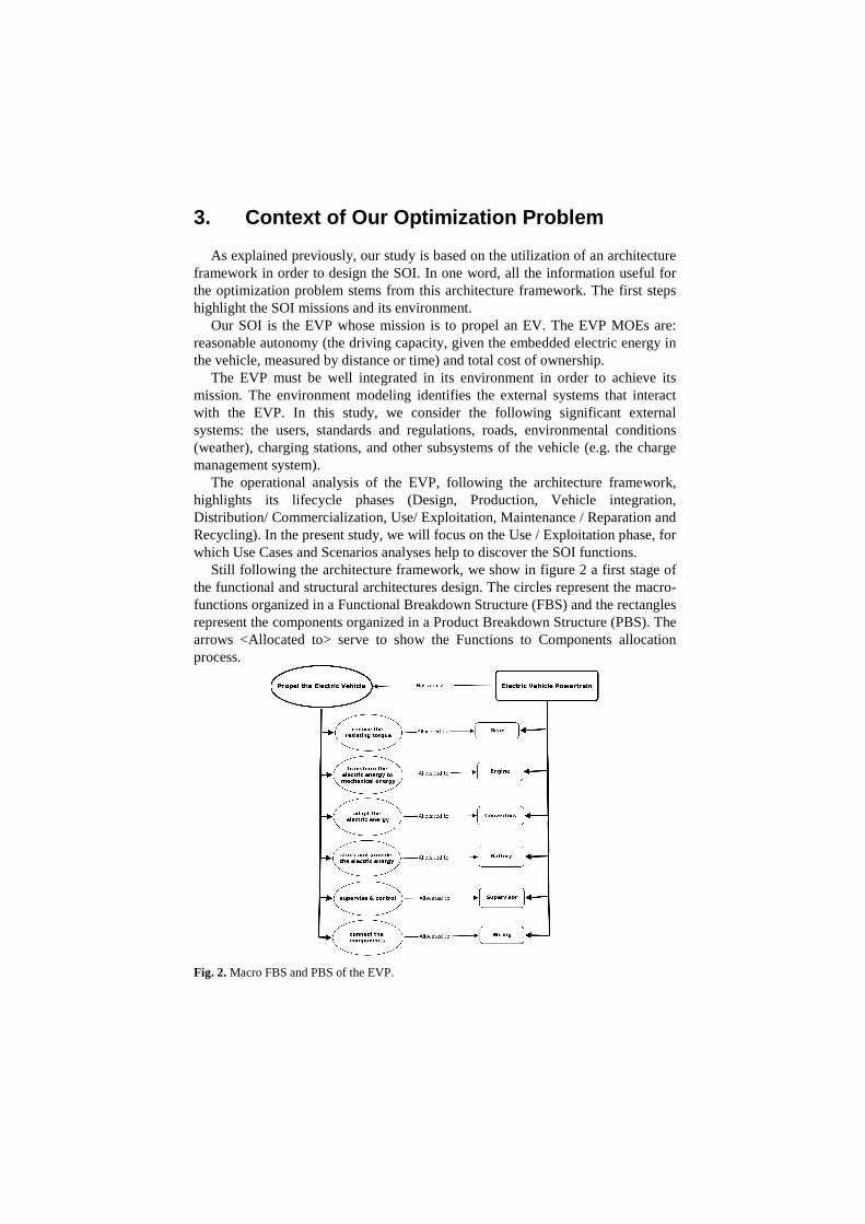
Still following the architecture framework, we show in figure 2 a first stage of the functional and structural architectures design. The circles represent the macro-functions organized in a Functional Breakdown Structure (FBS) and the rectangles represent the components organized in a Product Breakdown Structure (PBS). The arrows <Allocated to> serve to show the Functions to Components allocation process.
Fig. 2. Macro FBS and PBS of the EVP.
Globally, in order to provide the sufficient torque, the EVP transforms an electric energy into mechanical energy. A battery serves to stock and provide the electric energy. An engine transforms the electric energy to a mechanical energy. Converters are used in order to adapt the electric energy from the battery to the engine. A gear serves to reduce the resisting torque. A supervisor (actually a set of electronic control units) supervises and manages the EVP. Electric wiring connects all these components.
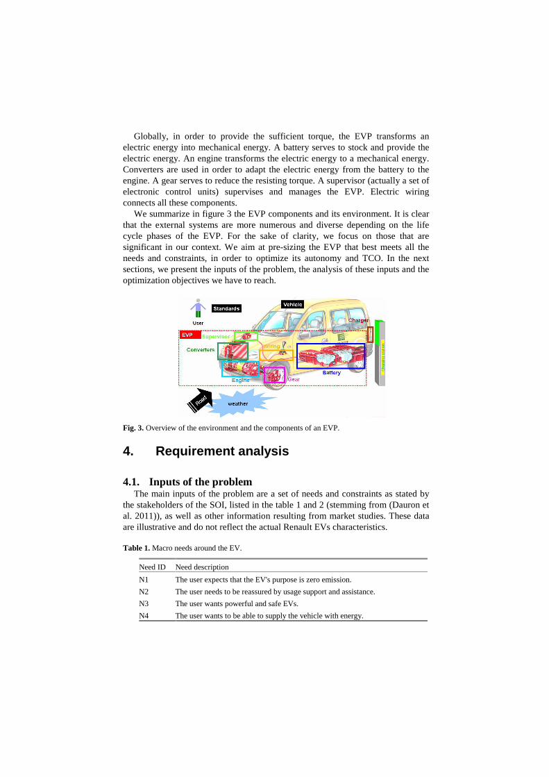
We summarize in figure 3 the EVP components and its environment. It is clear that the external systems are more numerous and diverse depending on the life cycle phases of the EVP. For the sake of clarity, we focus on those that are significant in our context. We aim at pre-sizing the EVP that best meets all the needs and constraints, in order to optimize its autonomy and TCO. In the next sections, we present the inputs of the problem, the analysis of these inputs and the optimization objectives we have to reach.
Fig. 3. Overview of the environment and the components of an EVP.
4. Requirement analysis
4.1. Inputs of the problem The main inputs of the problem are a set of needs and constraints as stated by
the stakeholders of the SOI, listed in the table 1 and 2 (stemming from (Dauron et al. 2011)), as well as other information resulting from market studies. These data are illustrative and do not reflect the actual Renault EVs characteristics.
Table 1. Macro needs around the EV.
Need ID Need description
N1 The user expects that the EV's purpose is zero emission.
N2 The user needs to be reassured by usage support and assistance.
N3 The user wants powerful and safe EVs.
N4 The user wants to be able to supply the vehicle with energy.
N5 The automotive manufacturer wants the EV to be an innovation for a large number of customers.
N6 The automotive manufacturer wants to offer an environment-friendly performance to the customers, combined with economic attractiveness and unique services.
N7 Green norms and automotive standards impose their constraints.
Table 2. Refinement of the macro need (N3).
Need ID Need description
N1-3 The user wants good acceleration level when fully pressing the accelerator pedal.
N3-2 The user does not want to feel the physical limitations of the EV autonomy.
N3-3 The user wants the maximum speed not to exceed a defined safety threshold.
N3-4 The user wants a completely safe behavior in respect to electric risk
There are other inputs to be taken into consideration resulting from market
studies. Indeed, the target market for our example is the European market. The business model takes into account the TCO that we define as sum of the acquisition cost, the costs of use (focusing only on the energy consumption by the vehicle) and maintenance costs. The battery, converters, wiring and supervisor technologies are imposed.
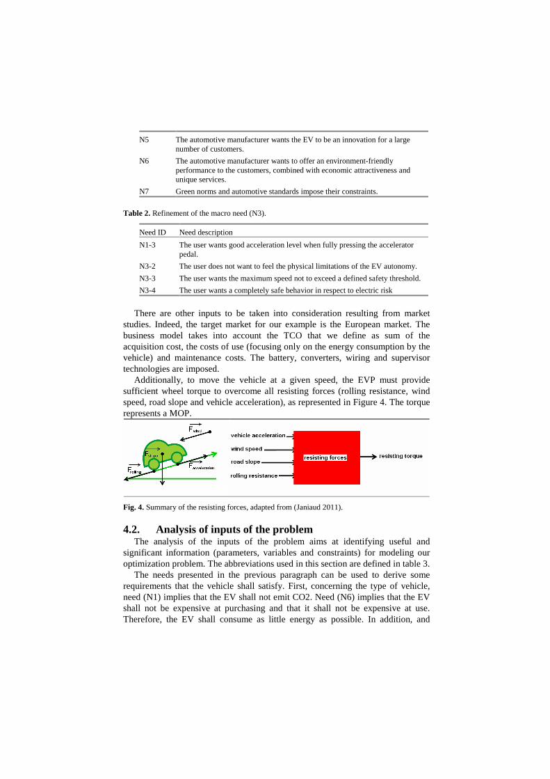
Additionally, to move the vehicle at a given speed, the EVP must provide sufficient wheel torque to overcome all resisting forces (rolling resistance, wind speed, road slope and vehicle acceleration), as represented in Figure 4. The torque represents a MOP.
Fig. 4. Summary of the resisting forces, adapted from (Janiaud 2011).
4.2. Analysis of inputs of the problem The analysis of the inputs of the problem aims at identifying useful and
significant information (parameters, variables and constraints) for modeling our optimization problem. The abbreviations used in this section are defined in table 3.
The needs presented in the previous paragraph can be used to derive some requirements that the vehicle shall satisfy. First, concerning the type of vehicle, need (N1) implies that the EV shall not emit CO2. Need (N6) implies that the EV shall not be expensive at purchasing and that it shall not be expensive at use. Therefore, the EV shall consume as little energy as possible. In addition, and
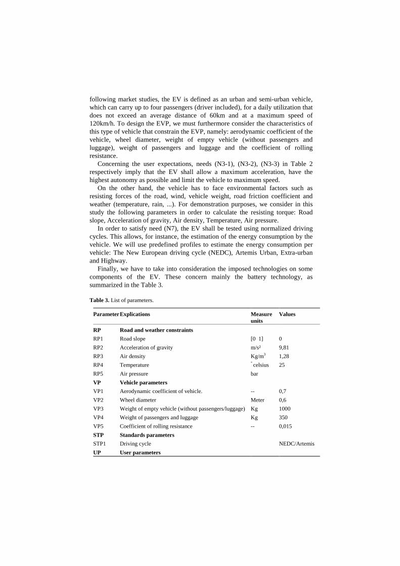
following market studies, the EV is defined as an urban and semi-urban vehicle, which can carry up to four passengers (driver included), for a daily utilization that does not exceed an average distance of 60km and at a maximum speed of 120km/h. To design the EVP, we must furthermore consider the characteristics of this type of vehicle that constrain the EVP, namely: aerodynamic coefficient of the vehicle, wheel diameter, weight of empty vehicle (without passengers and luggage), weight of passengers and luggage and the coefficient of rolling resistance.
Concerning the user expectations, needs (N3-1), (N3-2), (N3-3) in Table 2 respectively imply that the EV shall allow a maximum acceleration, have the highest autonomy as possible and limit the vehicle to maximum speed.
On the other hand, the vehicle has to face environmental factors such as resisting forces of the road, wind, vehicle weight, road friction coefficient and weather (temperature, rain, ...). For demonstration purposes, we consider in this study the following parameters in order to calculate the resisting torque: Road slope, Acceleration of gravity, Air density, Temperature, Air pressure.
In order to satisfy need (N7), the EV shall be tested using normalized driving cycles. This allows, for instance, the estimation of the energy consumption by the vehicle. We will use predefined profiles to estimate the energy consumption per vehicle: The New European driving cycle (NEDC), Artemis Urban, Extra-urban and Highway.
Finally, we have to take into consideration the imposed technologies on some components of the EV. These concern mainly the battery technology, as summarized in the Table 3.
Table 3. List of parameters.
Parameter Explications Measure units
Values
RP Road and weather constraints
RP1
RP2
RP3
RP4
RP5
Road slope
Acceleration of gravity
Air density
Temperature
Air pressure
[0 1]
m/s²
Kg/m3
° celsius
bar
0
9,81
1,28
25
VP Vehicle parameters
VP1
VP2
VP3
VP4
VP5
Aerodynamic coefficient of vehicle.
Wheel diameter
Weight of empty vehicle (without passengers/luggage)
Weight of passengers and luggage
Coefficient of rolling resistance
--
Meter
Kg
Kg
--
0,7
0,6
1000
350
0,015
STP Standards parameters
STP1 Driving cycle NEDC/Artemis
UP User parameters
UP1
UP2
Maximum acceleration
Maximum speed
m/s²
km/h
0-100km/h(20s)
120
CHP Electric charger parameters
CHP1
CHP2
CHP3
Charger performance
Weight of the Charger
Charger load power
--
Kg
kw
~1
10
BP Battery parameters
BP1
BP2
BP3
BP4
BP5
Weight of the battery
Energy of the battery
Battery voltage
Battery storage Performance
Battery cost
Kg
Kwh
Volt
--
Euros
250
24
400
~1
COP Converters parameters
COP1
COP2
COP3
Weight of the Converters
Converters cost
Performance of the Converters
Kg
euros
--
25
~1
WP Wiring parameters
WP1
WP2
WP3
Weight of the wiring
Wiring cost
Electric resistance
Kg
euros
ohm
3
~0
SP Supervisor parameters
SP1
SP2
Weight of the Supervisor
Supervisor cost
Kg
euros
2
4.3. Optimization Objectives On a first approach, some of the system requirements become optimization
objectives. In our context, for instance, the requirement « The EV shall not be expensive» yields an objective that is Minimize (the vehicle TCO). Another requirement « The EV shall not be expensive at use » yields another objective: Minimize (Energy consumption cost). Finally, the requirement « The EV shall have as long autonomy as possible» yields the objective Maximize (Vehicle autonomy). Note that in order to minimize the total cost of ownership of the EV, it is clear that we can study other factors such as maintenance costs, the battery rental costs, insurance costs,... In the present case, we focus only on the energy consumption cost for demonstration purposes. We explain in the following paragraphs how we simplify these objectives on the EVP. We summarize objectives simplification process in figure 5.
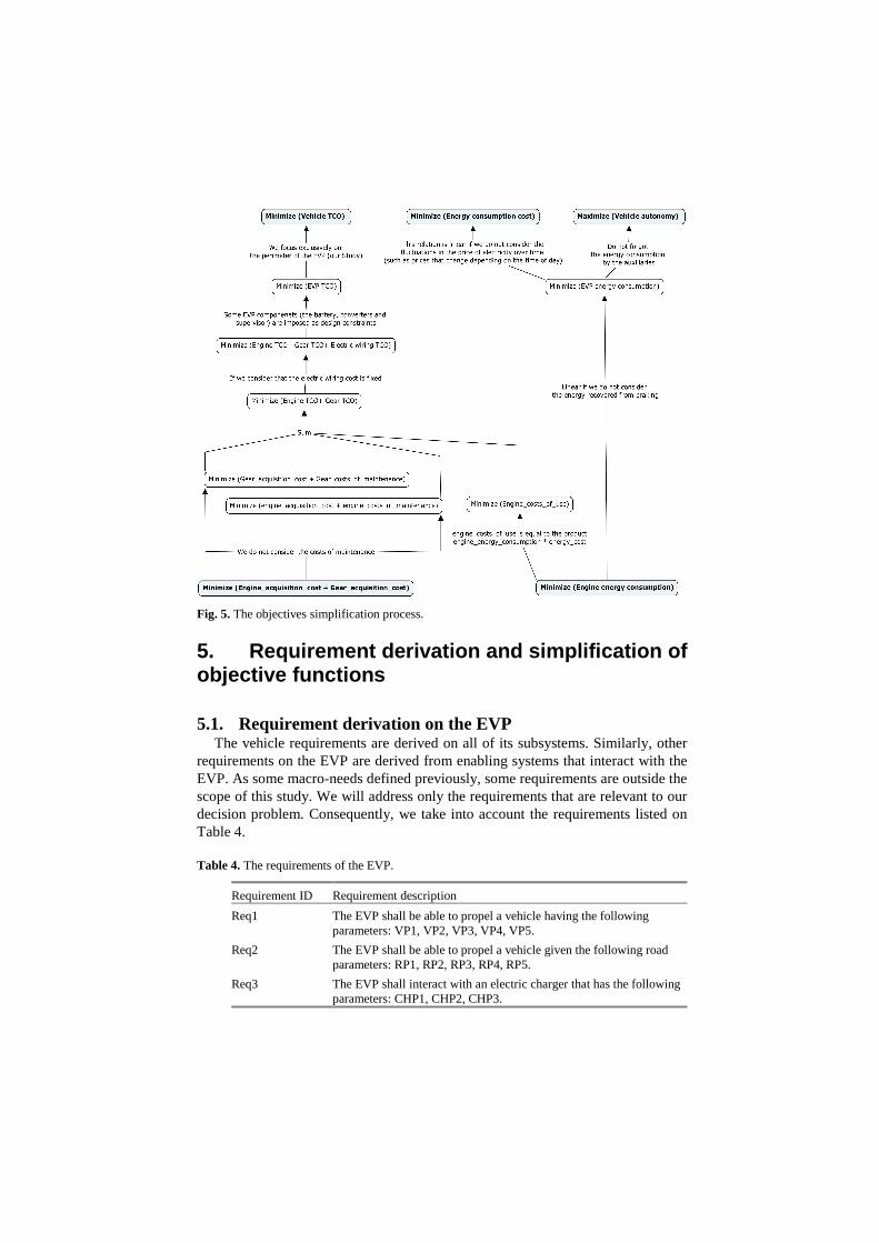
Fig. 5. The objectives simplification process.
5. Requirement derivation and simplification of objective functions
5.1. Requirement derivation on the EVP The vehicle requirements are derived on all of its subsystems. Similarly, other
requirements on the EVP are derived from enabling systems that interact with the EVP. As some macro-needs defined previously, some requirements are outside the scope of this study. We will address only the requirements that are relevant to our decision problem. Consequently, we take into account the requirements listed on Table 4.
Table 4. The requirements of the EVP.
Requirement ID Requirement description
Req1 The EVP shall be able to propel a vehicle having the following parameters: VP1, VP2, VP3, VP4, VP5.
Req2 The EVP shall be able to propel a vehicle given the following road parameters: RP1, RP2, RP3, RP4, RP5.
Req3 The EVP shall interact with an electric charger that has the following parameters: CHP1, CHP2, CHP3.
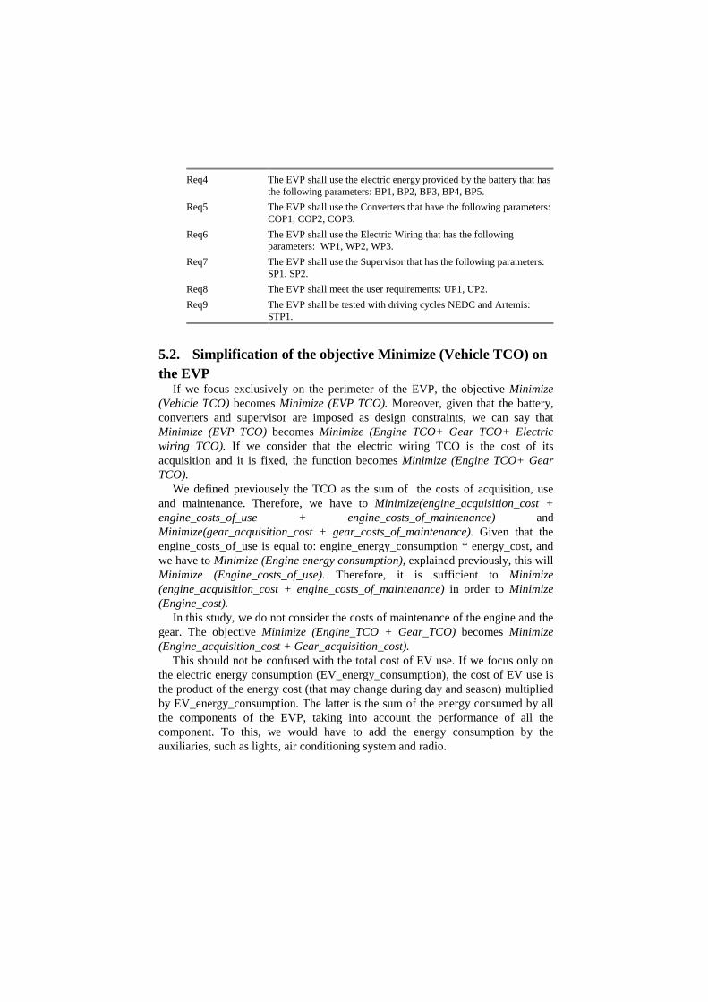
Req4 The EVP shall use the electric energy provided by the battery that has the following parameters: BP1, BP2, BP3, BP4, BP5.
Req5 The EVP shall use the Converters that have the following parameters: COP1, COP2, COP3.
Req6 The EVP shall use the Electric Wiring that has the following parameters: WP1, WP2, WP3.
Req7 The EVP shall use the Supervisor that has the following parameters: SP1, SP2.
Req8 The EVP shall meet the user requirements: UP1, UP2.
Req9 The EVP shall be tested with driving cycles NEDC and Artemis: STP1.
5.2. Simplification of the objective Minimize (Vehicle TCO) on the EVP
If we focus exclusively on the perimeter of the EVP, the objective Minimize (Vehicle TCO) becomes Minimize (EVP TCO). Moreover, given that the battery, converters and supervisor are imposed as design constraints, we can say that Minimize (EVP TCO) becomes Minimize (Engine TCO+ Gear TCO+ Electric wiring TCO). If we consider that the electric wiring TCO is the cost of its acquisition and it is fixed, the function becomes Minimize (Engine TCO+ Gear TCO).
We defined previousely the TCO as the sum of the costs of acquisition, use and maintenance. Therefore, we have to Minimize(engine_acquisition_cost + engine_costs_of_use + engine_costs_of_maintenance) and Minimize(gear_acquisition_cost + gear_costs_of_maintenance). Given that the engine_costs_of_use is equal to: engine_energy_consumption * energy_cost, and we have to Minimize (Engine energy consumption), explained previously, this will Minimize (Engine_costs_of_use). Therefore, it is sufficient to Minimize (engine_acquisition_cost + engine_costs_of_maintenance) in order to Minimize (Engine_cost).
In this study, we do not consider the costs of maintenance of the engine and the gear. The objective Minimize (Engine_TCO + Gear_TCO) becomes Minimize (Engine_acquisition_cost + Gear_acquisition_cost).
This should not be confused with the total cost of EV use. If we focus only on the electric energy consumption (EV_energy_consumption), the cost of EV use is the product of the energy cost (that may change during day and season) multiplied by EV_energy_consumption. The latter is the sum of the energy consumed by all the components of the EVP, taking into account the performance of all the component. To this, we would have to add the energy consumption by the auxiliaries, such as lights, air conditioning system and radio.

5.3. Simplification of the objective Maximize (Vehicle autonomy) on the EVP
There exists a dependency between the two functions: Minimize (Energy consumption cost) with Maximize (Vehicle autonomy). This relationship is linear if we do not take into account fluctuations in the price of electricity over time (such as prices that change depending on the time of day). Therefore, it is sufficient to Maximize (Vehicle autonomy) in order to Minimize (Energy consumption cost). Given that the battery technology is imposed, the function Maximize (Vehicle autonomy) becomes Minimize (EVP energy consumption).
The EVP energy consumption is the sum of the energy consumption by all its components. Since in our context the Converters are imposed and the consumption of the other components is negligible, then Minimize (EVP energy consumption) becomes Minimize (Engine energy consumption). This implication is completely true if we do not consider the energy that may be recovered during braking.
To calculate the electric energy consumption by the engine, we will adapt the
solution proposed in (Janiaud 2011), as follows: Given: t= time UP[t] is the vehicle speed at t on a given driving cycle.
741111243 VarVarSPWPCOPBPCHPVPVPM ++++++++= (eq2) Result, Gear_torque, Engine_torque, Engine_omega : intermediate variables. The estimation of the resisting forces is performed as follows.
• Force related to vehicle acceleration:
( ) ( ) ( )( )
×××= dt
tSTPdtMVPF 6.3
112
21 (eq3)
• Force related to wind speed: ( ) ( ) ( )( )( )²6.3
111321
222 ×××××= tSTPVPRPVPF (eq4)
• Force related to road slope: ( ) ( )122
23 RPRPMVPF ×××= (eq5)
• Force related to rolling resistance: ( ) ( )522
24 VPRPMVPF ×××= (eq6)
With 4321Re FFFFsult +++= (eq7)
( ) ( ) 1.0|3.61tSTP1| if Re {_ ≥×= sulttorqueGear (eq8)
( ) ( ) 1.0|3.61tSTP1| if {0_ <×=torqueGear (eq9)
Where Gear_torque represents the resisting torque which the EVP has to face in order to move the vehicle. It represents all the resistant forces, given the vehicle speed STP1 (t) with which it must advance (see Figure 2).
Then we reduce the resisting forces, as follows.
= 9
__ VartorqueGeartorqueEngine (eq10)
( ) ( )
××=
6.32
2191_ VPVartSTPomegaEngine (eq11)
Where • Engine_torque represents the torque against which the engine has to
face in order to move the vehicle. Engine_torque corresponds to Gear_torque divided by Gear_ratio.
• Engine_omega represents the rotational speed of the engine in order to move the vehicle with the speed required by the user.
The energy consumption by the engine « Engine_energy_consumption »
depends on the Engine_torque, Engine_omega, Engine_map and t. Indeed, we calculate the energy losses as a function of the engine torque and the engine speed:
( )tPelectE ×= and
= µPmecaPelect (eq12)
Where • E is Engine_energy_consumption • Pelect is the electric power • µ is the engine power according to a functioning point on the engine
map. • Pmeca is the mechanic power given by the relation:
( )gaEngine_omequeEngine_tor ×=Pmeca (eq13) The engine map gives the correspondence between Engine_omega and
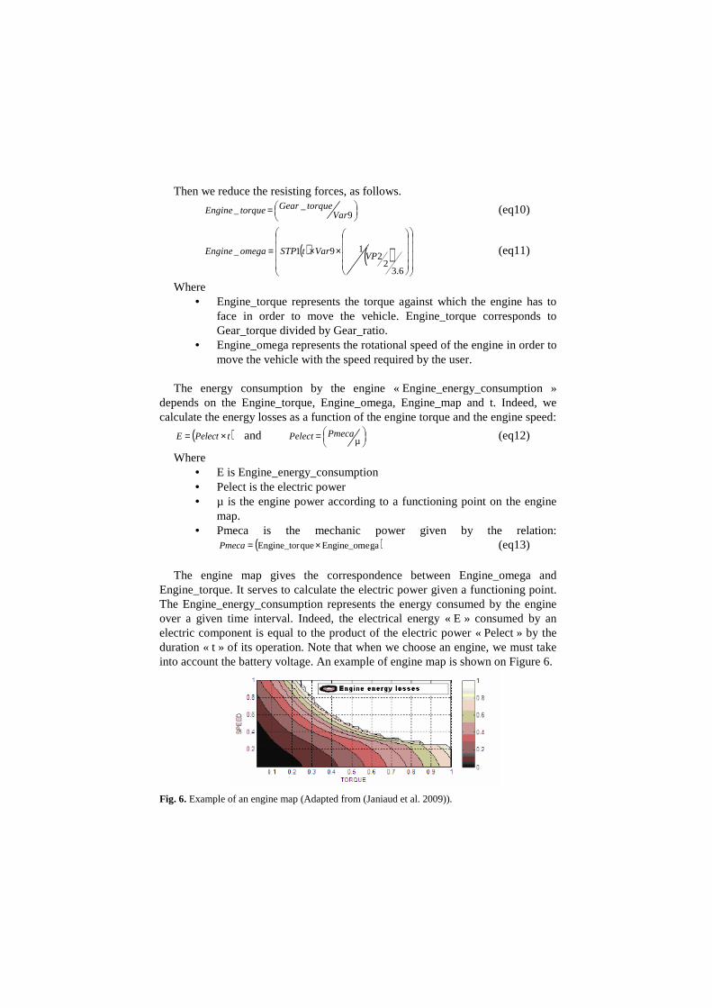
Engine_torque. It serves to calculate the electric power given a functioning point. The Engine_energy_consumption represents the energy consumed by the engine over a given time interval. Indeed, the electrical energy « E » consumed by an electric component is equal to the product of the electric power « Pelect » by the duration « t » of its operation. Note that when we choose an engine, we must take into account the battery voltage. An example of engine map is shown on Figure 6.
Fig. 6. Example of an engine map (Adapted from (Janiaud et al. 2009)).
NB. The maximum speed and acceleration (UP1, UP2) required by the user must be realizable by the engine. In order to verify this, we create a deriving cycle from these two data and make the same calculation as a driving cycle such as NEDC.
Finally, given a driving cycle, an estimation of the total EV autonomy is given by these equations:
cediscycle tan_||nconsumptioEV_energy_BP2|| ncey_by_distaEV_autonom ×
= (eq14)
durationcycle_||nconsumptioEV_energy_BP2||ion y_by_duratEV_autonom ×
= (eq15)
For example, in NEDC, Cycle_disance~11km and Cycle_duration~20minutes.
6. Synthesis of simplified functions to optimize
Coming back to our original problem, we have to choose an engine and a gear in order to reach two objectives:
• Minimize (Engine acquisition cost+ Gear acquisition cost). • Minimize (Engine energy consumption).
taking into consideration the parameters and the different variables related to the engine and to the gear summarized respectively in Table 3 and Table 5.
Table 5. List of the variables and their domain value constraints.
Variables Explications Measure units Upper bounds Lower bounds
Engine variables
• Engine map
• Var1
• Var2
• Var3
• Var0
• Var4
• Var5
that contains:
• Engine torque
• Engine rotation speed
• Engine power
• Engine cost
• Weight of the engine
• Engine voltage
N*m
Rad/s
Watt
Euros
Kg
volt
Gear variables
• Var6
• Var7
• Var8
• Var9
• Gear performance
• Weight of the gear
• Gear cost
• Gear ratio
--
Kg
Euros
--
7. Mathematical representation
In this section, we represent our optimization model following the equation (eq1) formulation:
Parameters “p”: P (VP, EP, CHP, RP, BP, COP, WP, SP, UP,STP) is a vector of parameters , where : • VP (VP1, VP2, VP3, VP4, VP5) is the vector of the vehicle parameters. • EP (EP1, EP2) is the vector of the charging station parameters. • RP (RP1, RP2, RP3, RP4, RP5) is the vector of the road/weather parameters. • CHP (CHP1, CHP2, CHP3) is the vector of the charger parameters. • UP (UP1, UP2) is the vector of the user parameters. • STP (STP1) is the vector of the user/standard parameters. • BP (BP1, BP2, BP3, BP4, BP5) is the vector of the battery parameters. • COP (COP1, COP2, COP3) is the vector of the converters’ parameters. • WP (WP1, WP2, WP3) is the vector of the wiring parameters. • SP (SP1, SP2) is the vector of the supervisor parameters. • t is the time.
Variables « x » : V (VE, VG) is the vector of the variables where: • VE (Var0, Var1, Var2, Var3, Var4, Var5) is the vector of the engine variables. • VG (Var6, Var7, Var8, Var9) is the vector of the gear variables.
Constraints « g » and « h »: (examples) g1(BP1,COP1,WP1,SP1,Var4,Var7)=(BP1+COP1+WP1+SP1+Var4+Var7)< 400
h1(BP3, Var5) =BP3 – Var5 = 0 Functions « J » to minimize :
J1: engine_energy_consumption = J1(VP1, VP2, VP3, VP4, VP5, BP1, RP2, RP3,
COP1, WP1, SP1, RP1,STP1,Var9,Var4,Var7, engine_map, t)
= equa(Engine_torque, Engine_omega , engine_map, t)5
Given the equations (eq2-eq3-eq4-eq5-eq6-eq7-eq8-eq9-eq10-eq11) J2: engine and gear acquisition costs = J2 (Var0, Var8) =Var0 + Var8
For the sake of clarity, we do not list all the constraints.
8. Tests, Results and Brief Discussion
In this section, we show simulation results of our example, simplified to compare two different engines and one same gear. The choice of the engine will be made according to the two criteria defined above (the acquisition cost of the engine and its energy consumption). The parameters values and measure units are shown in the Tables 3 and 5. The values of the variables of the gear we use are:
• Var9 = 10.4 • Var6 = ~1 • Var7 = 10 • Var8 =200
Figure 7 shows the simulation results: the acquisition cost of the two engines (in euros) and their energy consumptions (kWh) on the four driving cycles.
5 This equations system is resolved with a matlab-simulink model.
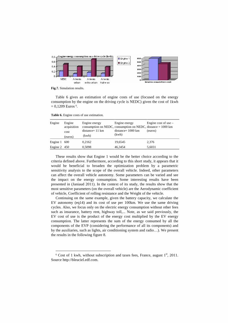
Fig.7. Simulation results.
Table 6 gives an estimation of engine costs of use (focused on the energy consumption by the engine on the driving cycle is NEDC) given the cost of 1kwh = 0,1209 Euros 6.
Table 6. Engine costs of use estimation.
Engine Engine acquisition
cost
(euros)
Engine energy consumption on NEDC, distance= 11 km
(kwh)
Engine energy consumption on NEDC, distance= 1000 km (kwh)
Engine cost of use – distance = 1000 km (euros)
Engine 1 600 0,2162 19,6545 2,376
Engine 2 450 0,5098 46,3454 5,6031
These results show that Engine 1 would be the better choice according to the
criteria defined above. Furthermore, according to this short study, it appears that it would be beneficial to broaden the optimization problem by a parametric sensitivity analysis to the scope of the overall vehicle. Indeed, other parameters can affect the overall vehicle autonomy. Some parameters can be varied and see the impact on the energy consumption. Some interesting results have been presented in (Janiaud 2011). In the context of its study, the results show that the most sensitive parameters (on the overall vehicle) are the Aerodynamic coefficient of vehicle, Coefficient of rolling resistance and the Weight of the vehicle.
Continuing on the same example, given the battery capacity, we calculate the EV autonomy (eq14) and its cost of use per 100km. We use the same driving cycles. Also, we focus only on the electric energy consumption without other fees such as insurance, battery rent, highway toll,... Note, as we said previously, the EV cost of use is the product of the energy cost multiplied by the EV energy consumption. The latter represents the sum of the energy consumed by all the components of the EVP (considering the performance of all its components) and by the auxiliaries, such as lights, air conditioning system and radio…). We present the results in the following figure 8.
6 Cost of 1 kwh, without subscription and taxes fees, France, august 1st, 2011.
Source http://bleuciel.edf.com.
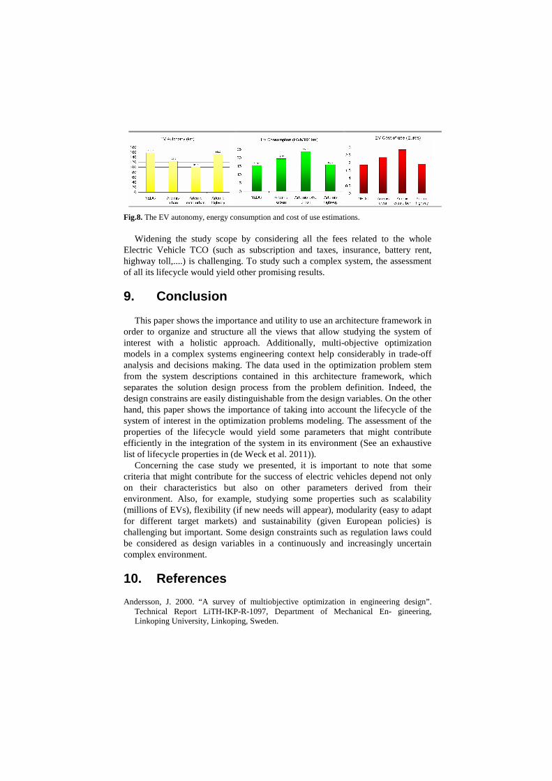
Fig.8. The EV autonomy, energy consumption and cost of use estimations.
Widening the study scope by considering all the fees related to the whole Electric Vehicle TCO (such as subscription and taxes, insurance, battery rent, highway toll,....) is challenging. To study such a complex system, the assessment of all its lifecycle would yield other promising results.
9. Conclusion
This paper shows the importance and utility to use an architecture framework in order to organize and structure all the views that allow studying the system of interest with a holistic approach. Additionally, multi-objective optimization models in a complex systems engineering context help considerably in trade-off analysis and decisions making. The data used in the optimization problem stem from the system descriptions contained in this architecture framework, which separates the solution design process from the problem definition. Indeed, the design constrains are easily distinguishable from the design variables. On the other hand, this paper shows the importance of taking into account the lifecycle of the system of interest in the optimization problems modeling. The assessment of the properties of the lifecycle would yield some parameters that might contribute efficiently in the integration of the system in its environment (See an exhaustive list of lifecycle properties in (de Weck et al. 2011)).
Concerning the case study we presented, it is important to note that some criteria that might contribute for the success of electric vehicles depend not only on their characteristics but also on other parameters derived from their environment. Also, for example, studying some properties such as scalability (millions of EVs), flexibility (if new needs will appear), modularity (easy to adapt for different target markets) and sustainability (given European policies) is challenging but important. Some design constraints such as regulation laws could be considered as design variables in a continuously and increasingly uncertain complex environment.
10. References
Andersson, J. 2000. “A survey of multiobjective optimization in engineering design”. Technical Report LiTH-IKP-R-1097, Department of Mechanical En- gineering, Linkoping University, Linkoping, Sweden.
Benkhannouchel S. and Penalva J.M. 1993. “Systemic Approach for Supervision Systems Design”. In Systems, Man and Cybernetics, International Conference on 'Systems Engineering in the Service of Humans', Conference Proceedings. 395 – 400, vol.1. Issue October 1993.
Chalé Góngora Hugo G., Alain Dauron, and Thierry Gaudré. 2012. “A Commonsense-Driven Architecture Framework. Part 1: A Car Manufacturer’s (naïve) Take on MBSE.” ”Accepted for publication in proceedings of the INCOSE International Symposium, Rome, INCOSE, 2012.
Chatel V. and Feliot C. 2004. “Functional analysis for safe and available system design”. IEEE International Conference Systems, Man and Cybernetics.
Coello Coello, C.A., Multiobjective Optimization Website and Archive: http://www.lania.mx/~ccoello/EMOO/ (last update February 23rd, 2010)
Dauron A., Doufene A. and Krob D., 2011. Complex systems operational analysis - A case study for electric vehicles. International Conference CSD&M, Poster session, Paris 2011.
De Weck, O.L. 2006. “Multiobjective optimization: History and promise”. in China-Japan-Korea Joint Symposium on Optimization of Structural and Mechanical Systems, s. d.
De Weck, O.L., Roos D. and Magee C.L.2011. Engineering Systems: Meeting Human Needs in a Complex Technological World. The MIT Press editions, October 2011.
INCOSE, 2010. Systems Engineering Handbook. A guide for system lifecycle processes and activities. International Council on Systems Engineering (INCOSE), San Diego, CA. January 2010.
Janiaud N., Vallet F.X., Petit M., Sandou G. 2009. “Electric Vehicle Powertrain Architecture and Control Global Optimization”, Electric Vehicle Symposium, Stavanger, Norway. Publication de l’article dans WEVA Journal (World Electric Vehicle Association), vol.3, 2009, ISSN 2032-6653.
Janiaud N. 2011. “Modélisation du système de puissance du véhicule électrique en régime transitoire en vue de l’optimisation de l’autonomie, des performances et des coûts associés”. PhD thesis, SUPELEC, France.
Kim, I. Y., and De Weck O. L. 2005. “Adaptive weighted sum method for multiobjective optimization: a new method for Pareto front generation”. Structural and Multidisciplinary Optimization 31 p. 105-116.
Kim, I.Y., et De Weck O.L. 2005. “Adaptive weighted-sum method for bi-objective optimization: Pareto front generation”. Structural and Multidisciplinary Optimization 29, no. 2 (2005): 149–158.
Krob D. 2009. “Eléments d’architecture des systèmes complexes, in "Gestion de la complexité et de l’information dans les grands systèmes critiques"”, A. Appriou, Ed., 179-207, CNRS Editions.
Krob D. 2009-2010. “Enterprise Architecture, Modules 1-10, Ecole Polytechnique”. Personal communication.
Meinadier J.P. 1998. “Ingénierie et intégration de systèmes”. Editions Hermès. Meinadier J.P. 2002. “Le métier d'intégration de systèmes”. Editions Hermès-Lavoisier. Marler, R.T., and Arora J.S. 2004. “Survey of multi-objective optimization methods for
engineering”. Structural and multidisciplinary optimization 26, no. 6 p. 369–395. Penalva J.M. 1997. “La modélisation par les systèmes en situations complexes”, PhD
Thesis, Université de Paris 11, Orsay, France. Smaling, R.M. 2005. “System architecture analysis and selection under uncertainty”. PhD
thesis, Massachusetts Institute of Technology. Smaling, R.M. and De Weck O.L. 2004: “Fuzzy pareto frontiers in multidisciplinary system
architecture analysis”. AIAA Paper 4553 1–18.