Complex trajectories of a simplependulum

Daniel W. Hook

Blackett Laboratory

Imperial College London

6th International Workshop on Pseudo-Hermitian Hamiltonians in Quantum Physics

City University London

16 July 2007

Complex trajectories of a simple pendulum – p. 1/22

Work based on:

Carl M. Bender, Darryl D. Holm, Daniel W. Hook (2007) “Complex Trajectories of aSimple Pendulum”, Journal of Physics A40, F81-F89, [math-ph/0609068]

Carl M. Bender, Darryl D. Holm, Daniel W. Hook (2007) “Complexified DynamicalSystems”, to appear: Journal of Physics A, [arXiv:0705.3893]

Carl M. Bender, Jun-Hua Chen, Daniel W. Darg, Kimball A. Milton “ClassicalTrajectories for Complex Hamiltonians” (2006) Journal of Physics A39, 4219-4238[math-ph/0602040]

Carl M. Bender, Daniel W. Darg (2007) “Spontaneous Breaking of Classical PTSymmetry”, [hep-th/0703072]

References – p. 2/22

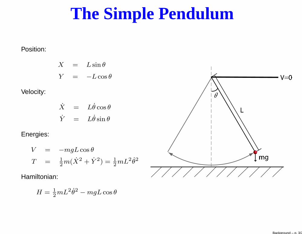
The Simple Pendulum

Position:

X = L sin θ

Y = −L cos θ

Velocity:

X = Lθ cos θ

Y = Lθ sin θ

Energies:

V = −mgL cos θ

T = 1

2m(X2 + Y 2) = 1

2mL2θ2

Hamiltonian:

H = 1

2mL2θ2

− mgL cos θ

Background – p. 3/22

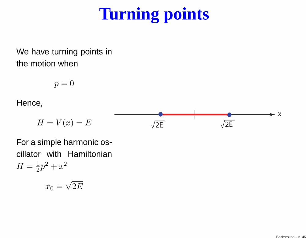
Turning points

We have turning points inthe motion when

p = 0

Hence,

H = V (x) = E

For a simple harmonic os-cillator with HamiltonianH = 1

2p2 + x2

x0 =√

2E

x

2E2E

Background – p. 4/22

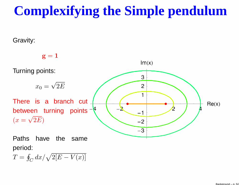
Complexifying the Simple pendulum

Gravity:

g = 1

Turning points:

x0 =√

2E

There is a branch cutbetween turning points(x =

√2E)

Paths have the sameperiod:T =

∮

Cdx/

√

2[E − V (x)]

Background – p. 5/22

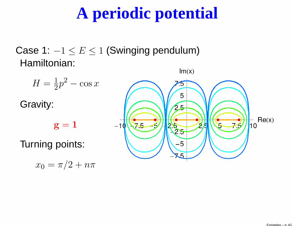
A periodic potential

Case 1: −1 ≤ E ≤ 1 (Swinging pendulum)Hamiltonian:

H = 1

2p2 − cos x

Gravity:

g = 1

Turning points:

x0 = π/2 + nπ

Exmaples – p. 6/22

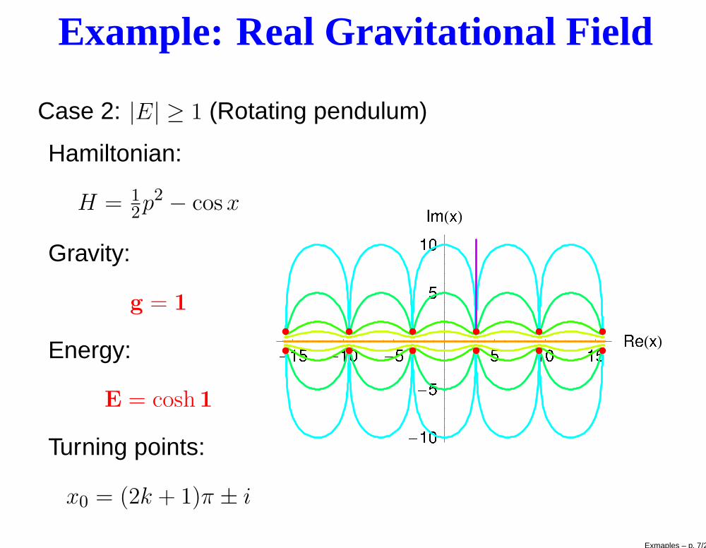
Example: Real Gravitational Field

Case 2: |E| ≥ 1 (Rotating pendulum)

Hamiltonian:

H = 1

2p2 − cos x

Gravity:

g = 1

Energy:

E = cosh1

Turning points:

x0 = (2k + 1)π ± i

Exmaples – p. 7/22

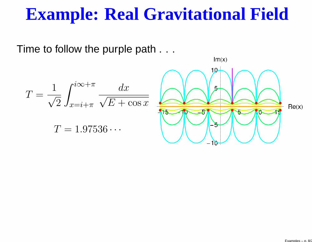
Example: Real Gravitational Field

Time to follow the purple path . . .

T =1√2

∫

i∞+π

x=i+π

dx√E + cos x

T = 1.97536 · · ·

Examples – p. 8/22

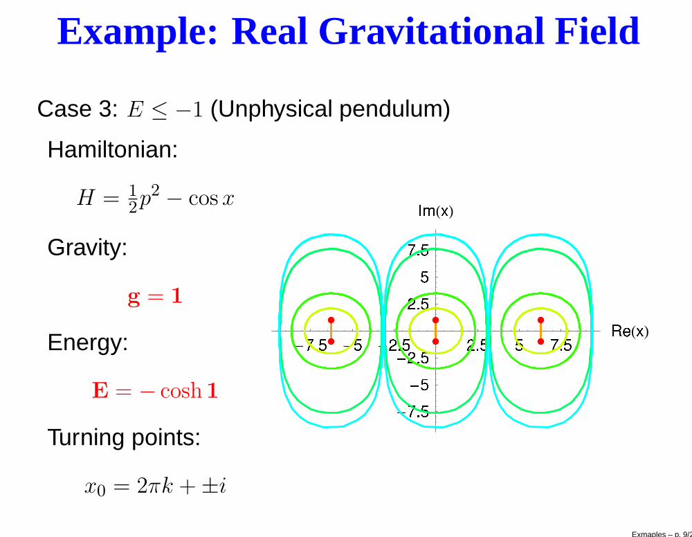
Example: Real Gravitational Field

Case 3: E ≤ −1 (Unphysical pendulum)

Hamiltonian:

H = 1

2p2 − cos x

Gravity:

g = 1

Energy:

E = − cosh1

Turning points:

x0 = 2πk + ±i

Exmaples – p. 9/22

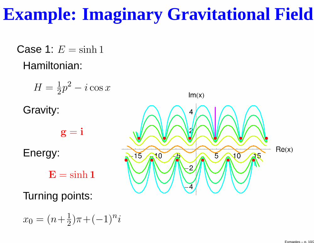
Example: Imaginary Gravitational Field

Case 1: E = sinh 1

Hamiltonian:

H = 1

2p2 − i cos x

Gravity:

g = i

Energy:

E = sinh1

Turning points:

x0 = (n+ 1

2)π+(−1)ni

Exmaples – p. 10/22

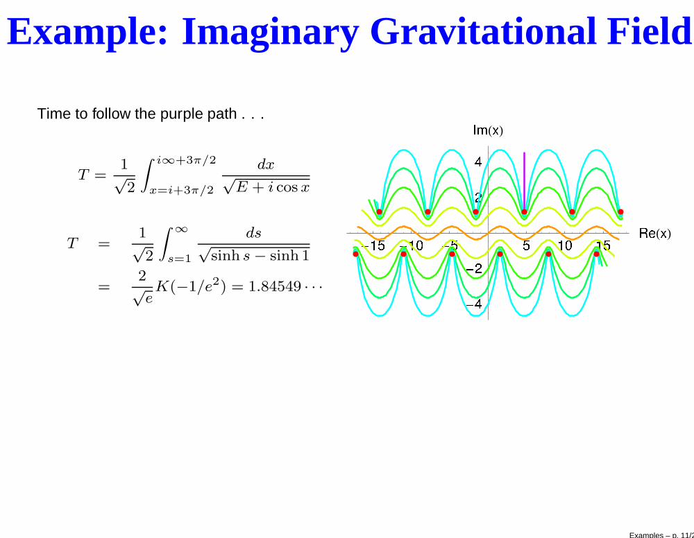
Example: Imaginary Gravitational Field

Time to follow the purple path . . .

T =1√

2

∫ i∞+3π/2

x=i+3π/2

dx√

E + i cos x

T =1√

2

∫

∞

s=1

ds√

sinh s − sinh 1

=2√

eK(−1/e2) = 1.84549 · · ·

Examples – p. 11/22

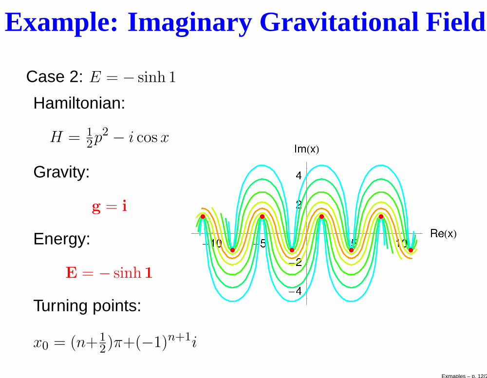
Example: Imaginary Gravitational Field

Case 2: E = − sinh 1

Hamiltonian:

H = 1

2p2 − i cos x

Gravity:

g = i

Energy:

E = − sinh1

Turning points:

x0 = (n+1

2)π+(−1)n+1i

Exmaples – p. 12/22

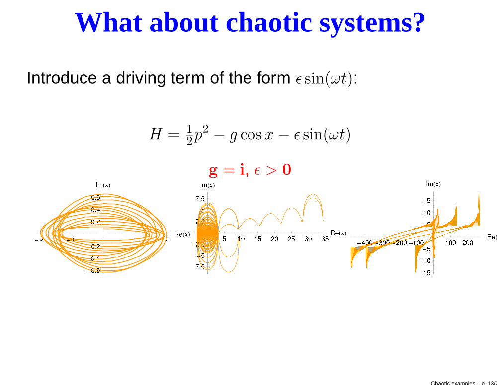
What about chaotic systems?

Introduce a driving term of the form ǫ sin(ωt):

H = 1

2p2 − g cos x − ǫ sin(ωt)

g = i, ǫ > 0

Chaotic examples – p. 13/22

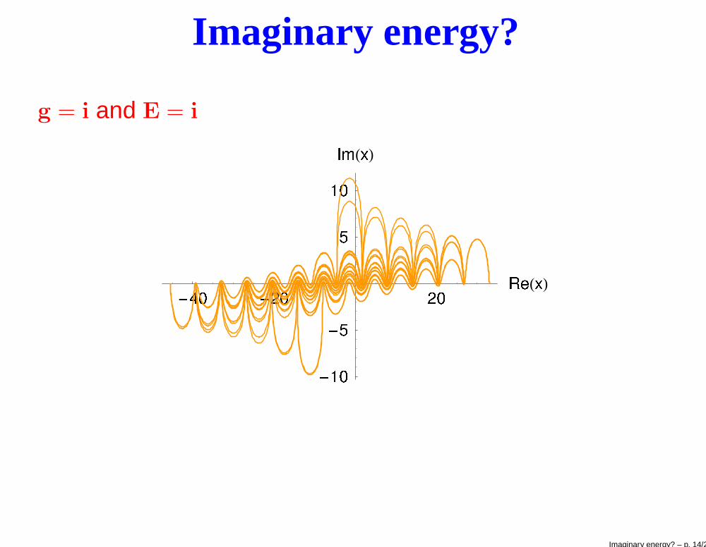
Imaginary energy?

g = i and E = i

Imaginary energy? – p. 14/22

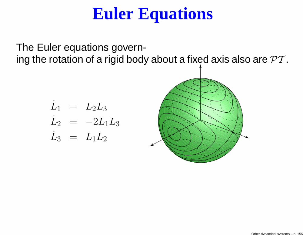
Euler Equations

The Euler equations govern-ing the rotation of a rigid body about a fixed axis also are PT .

L1 = L2L3

L2 = −2L1L3

L3 = L1L2

Other dynamical systems – p. 15/22

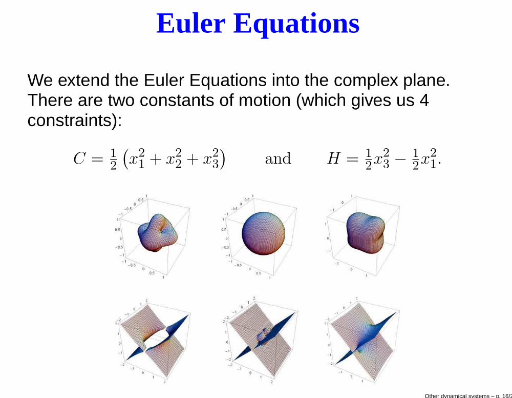
Euler Equations

We extend the Euler Equations into the complex plane.There are two constants of motion (which gives us 4constraints):

C = 1

2

(

x21 + x2

2 + x23

)

and H = 1

2x2

3 − 1

2x2

1.

Other dynamical systems – p. 16/22

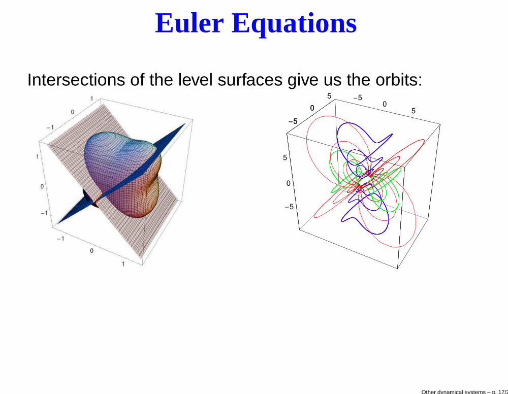
Euler Equations

Intersections of the level surfaces give us the orbits:-5

05

-5

0

5

-5

0

5

-5

0

5

Other dynamical systems – p. 17/22

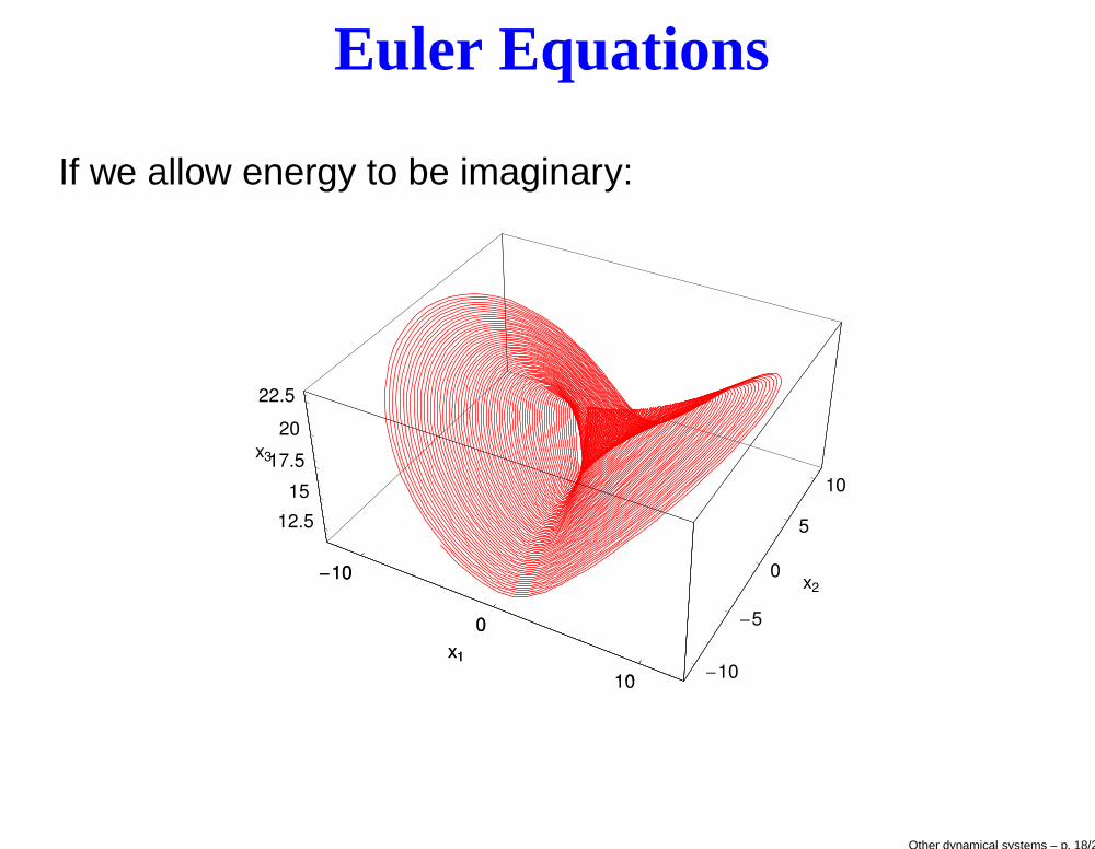
Euler Equations

If we allow energy to be imaginary:

-10

0

10

x1

-10

-5

0

5

10

x2

12.5

15

17.5

20

22.5

x3

-10

0

10

x1

Other dynamical systems – p. 18/22

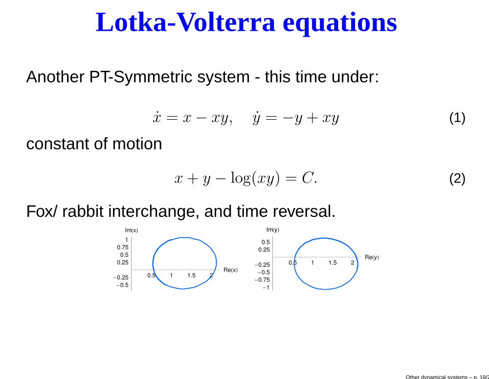
Lotka-Volterra equations

Another PT-Symmetric system - this time under:

x = x − xy, y = −y + xy (1)

constant of motion

x + y − log(xy) = C. (2)

Fox/ rabbit interchange, and time reversal.

0.5 1 1.5 2ReHxL

-0.5

-0.25

0.25

0.5

0.75

1

ImHxL

0.5 1 1.5 2ReHyL

-1

-0.75

-0.5

-0.25

0.25

0.5

ImHyL

Other dynamical systems – p. 19/22

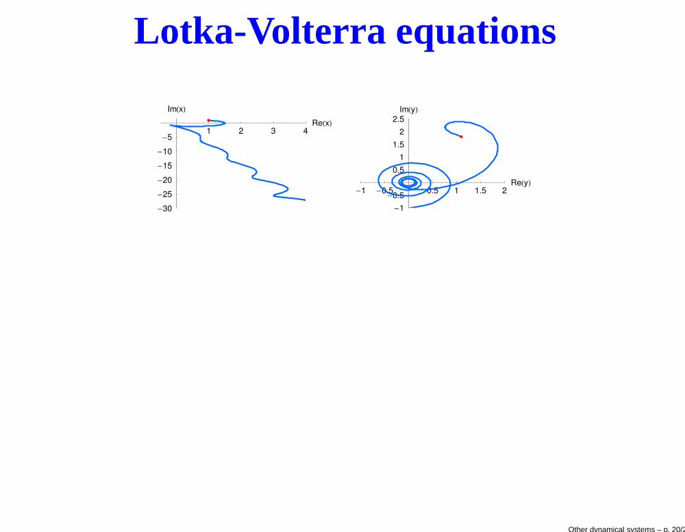
Lotka-Volterra equations

1 2 3 4ReHxL

-30

-25

-20

-15

-10

-5

ImHxL

-1 -0.5 0.5 1 1.5 2ReHyL

-1

-0.5

0.5

1

1.5

2

2.5ImHyL

Other dynamical systems – p. 20/22

Conclusions

Classical Mechanics seems to naturally extend into thecomplex plane to give some familiar and not so familiarresults

Complex extensions of classical mechanics help usunderstand well known systems

Conclusions – p. 21/22

Where next?

spherical pendulum, the spinning top

other discrete dynamical systems - SIR models etc.

classification of chaotic systems using PT Symmetry(see for example, the Kicked Rotor).

Where next? – p. 22/22