Embed Size (px)
DESCRIPTION
good book
Citation preview
COMPLEX VARIABLESand
APPLICATIONS
SEVENTH EDITION
JAMES WARD BROWN
RUEL V. CHURCHILL
COMPLEX VARIABLESAND APPLICATIONS
SEVENTH EDITION
James Ward BrownProfessor of Mathematics
The University of Michigan--Dearborn
Ruel V. ChurchillLate Professor of Mathematics
The University of Michigan
McGrawHill
Higher Education
Boston Burr Ridge, IL Dubuque, IA Madison, WI New YorkSan Francisco St. Louis Bangkok Bogota Caracas Kuala Lumpur
Lisbon London Madrid Mexico City Milan Montreal New DelhiSantiago Seoul Singapore Sydney Taipei Toronto
CONTENTS
Preface
Complex NumbersSums and Products 1
Basic Algebraic Properties 3
Further Properties 5
Moduli 8
Complex Conjugates 11
Exponential Form 15
Products and Quotients in Exponential Form 17
Roots of Complex Numbers 22Examples 25Regions in the Complex Plane 29
2 Analytic FunctionsFunctions of a Complex Variable 33Mappings 36Mappings by the Exponential Function 40Limits 43
Theorems on Limits 46Limits Involving the Point at Infinity 48Continuity 51
Derivatives 54Differentiation Formulas 57Cauchy-Riemann Equations 60
xv
Xi
Xll CONTENTS
Sufficient Conditions for Differentiability 63Polar Coordinates 65Analytic Functions 70Examples 72Harmonic Functions 75Uniquely Determined Analytic Functions 80Reflection Principle 82
3 Elementary FunctionsThe Exponential Function 87The Logarithmic Function 90Branches and Derivatives of Logarithms 92Some Identities Involving Logarithms 95Complex Exponents 97Trigonometric Functions 100Hyperbolic Functions 105
Inverse Trigonometric and Hyperbolic Functions 108
4 Integrals
Derivatives of Functions w(t) 111
Definite Integrals of Functions w(t) 113
Contours 116Contour Integrals 122
Examples 124Upper Bounds for Moduli of Contour Integrals 130
Antiderivatives 135
Examples 138Cauchy-Goursat Theorem 142Proof of the Theorem 144
Simply and Multiply Connected Domains 149
Cauchy Integral Formula 157Derivatives of Analytic Functions 158
Liouville's Theorem and the Fundamental Theorem of Algebra 165
Maximum Modulus Principle 167
87
5 Series 175
Convergence of Sequences 175
Convergence of Series 178Taylor Series 182Examples 185Laurent Series 190
Examples 195Absolute and Uniform Convergence of Power Series 200Continuity of Sums of Power Series 204Integration and Differentiation of Power Series 206Uniqueness of Series Representations 210Multiplication and Division of Power Series 215
CONTENTS Xiii
6 Residues and PolesResidues 221
Cauchy's Residue Theorem 225Using a Single Residue 227The Three Types of Isolated Singular Points 231Residues at Poles 234Examples 236Zeros of Analytic Functions 239Zeros and Poles 242Behavior off Near Isolated Singular Points 247
7 Applications of ResiduesEvaluation of Improper Integrals 251Example 254Improper Integrals from Fourier Analysis 259Jordan's Lemma 262Indented Paths 267An Indentation Around a Branch Point 270Integration Along a Branch Cut 273Definite integrals involving Sines and Cosines 278Argument Principle 281
Rouch6's Theorem 284Inverse Laplace Transforms 288Examples 291
8 Mapping by Elementary FunctionsLinear Transformations 299The Transformation w = liz 301Mappings by 1/z 303Linear Fractional Transformations 307An Implicit Form 310Mappings of the Upper Half Plane 313The Transformation w = sin z 318Mappings by z"' and Branches of z 1112 324Square Roots of Polynomials 329Riemann Surfaces 335Surfaces for Related Functions 338
9 Conformal MappingPreservation of Angles 343Scale Factors 346Local Inverses 348Harmonic Conjugates 351Transformations of Harmonic Functions 353Transformations of Boundary Conditions 355
221
251
299
343
XiV CONTENTS
10 Applications of Conformal MappingSteady Temperatures 361Steady Temperatures in a Half Plane 363A Related Problem 365Temperatures in a Quadrant 368Electrostatic Potential 373Potential in a Cylindrical Space 374Two-Dimensional Fluid Flow 379The Stream Function 381Flows Around a Corner and Around a Cylinder 383
11 The Schwarz-Christoffel TransformationMapping the Real Axis onto a Polygon 391Schwarz-Christoffel Transformation 393Triangles and Rectangles 397Degenerate Polygons 401Fluid Flow in a Channel Through a Slit 406Flow in a Channel with an Offset 408Electrostatic Potential about an Edge of a Conducting Plate 411
12 Integral Formulas of the Poisson TypePoisson Integral Formula 417Dirichlet Problem for a Disk 419Related Boundary Value Problems 423Schwarz Integral Formula 427Dirichiet Problem for a Half Plane 429Neumann Problems 433
AppendixesBibliography 437Table of Transformations of Regions 441
361
391
417
437
Index 451
PREFACE
This book is a revision of the sixth edition, published in 1996. That edition has served,just as the earlier ones did, as a textbook for a one-term introductory course in thetheory and application of functions of a complex variable. This edition preserves thebasic content and style of the earlier editions, the first two of which were written bythe late Ruel V. Churchill alone.
In this edition, the main changes appear in the first nine chapters, which make upthe core of a one-term course. The remaining three chapters are devoted to physicalapplications, from which a selection can be made, and are intended mainly for self-study or reference.
Among major improvements, there are thirty new figures; and many of the oldones have been redrawn. Certain sections have been divided up in order to emphasizespecific topics, and a number of new sections have been devoted exclusively to exam-ples. Sections that can be skipped or postponed without disruption are more clearlyidentified in order to make more time for material that is absolutely essential in a firstcourse, or for selected applications later on. Throughout the book, exercise sets occurmore often than in earlier editions. As a result, the number of exercises in any givenset is generally smaller, thus making it more convenient for an instructor in assigninghomework.
As for other improvements in this edition, we mention that the introductorymaterial on mappings in Chap. 2 has been simplified and now includes mappingproperties of the exponential function. There has been some rearrangement of materialin Chap. 3 on elementary functions, in order to make the flow of topics more natural.Specifically, the sections on logarithms now directly follow the one on the exponential
xv
XVi PREFACE
function; and the sections on trigonometric and hyberbolic functions are now closerto the ones on their inverses. Encouraged by comments from users of the book in thepast several years, we have brought some important material out of the exercises andinto the text. Examples of this are the treatment of isolated zeros of analytic functionsin Chap. 6 and the discussion of integration along indented paths in Chap. 7.
The first objective of the book is to develop those parts of the theory whichare prominent in applications of the subject. The second objective is to furnish anintroduction to applications of residues and conformal mapping. Special emphasisis given to the use of conformal mapping in solving boundary value problems thatarise in studies of heat conduction, electrostatic potential, and fluid flow. Hence thebook may be considered as a companion volume to the authors' "Fourier Series andBoundary Value Problems" and Rue! V, Churchill's "Operational Mathematics," whereother classical methods for solving boundary value problems in partial differentialequations are developed. The latter book also contains further applications of residuesin connection with Laplace transforms.
This book has been used for many years in a three-hour course given each term atThe University of Michigan. The classes have consisted mainly of seniors and graduatestudents majoring in mathematics, engineering, or one of the physical sciences. Beforetaking the course, the students have completed at least a three-term calculus sequence,a first course in ordinary differential equations, and sometimes a term of advancedcalculus. In order to accommodate as wide a range of readers as possible, there arefootnotes referring to texts that give proofs and discussions of the more delicate resultsfrom calculus that are occasionally needed. Some of the material in the book need notbe covered in lectures and can be left for students to read on their own. If mappingby elementary functions and applications of conformal mapping are desired earlierin the course, one can skip to Chapters 8, 9, and 10 immediately after Chapter 3 onelementary functions.
Most of the basic results are stated as theorems or corollaries, followed byexamples and exercises illustrating those results. A bibliography of other books,many of which are more advanced, is provided in Appendix 1. A table of conformaltransformations useful in applications appears in Appendix 2.
In the preparation of this edition, continual interest and support has been providedby a number of people, many of whom are family, colleagues, and students. Theyinclude Jacqueline R. Brown, Ronald P. Morash, Margret H. Hi ft, Sandra M. Weber,Joyce A. Moss, as well as Robert E. Ross and Michelle D. Munn of the editorial staffat McGraw-Hill Higher Education.
James Ward Brown
COMPLEX VARIABLES AND APPLICATIONS
CHAPTER
1
COMPLEX NUMBERS
In this chapter, we survey the algebraic and geometric structure of the complex numbersystem. We assume various corresponding properties of real numbers to be known.
1. SUMS AND PRODUCTS
Complex numbers can be defined as ordered pairs (x, y) of real numbers that are tobe interpreted as points in the complex plane, with rectangular coordinates x and y,just as real numbers x are thought of as points on the real line. When real numbersx are displayed as points (x, 0) on the real axis, it is clear that the set of complexnumbers includes the real numbers as a subset. Complex numbers of the form (0, y)correspond to points on the y axis and are called pure imaginary numbers. The y axisis, then, referred to as the imaginary axis.
It is customary to denote a complex number (x, y) by z, so that
(1) z = (x, y).
The real numbers x and y are, moreover, known as the real and imaginary parts of z,respectively; and we write
(2) Re z = x, Im z = Y.
Two complex numbers z1 = (x1, y1) and z2 = (x2, y2) are equal whenever they havethe same real parts and the same imaginary parts. Thus the statement "I = z2 meansthat z1 and z2 correspond to the same point in the complex, or z, plane.
2 CoMPLEx NUMBERS CHAP. I
The sum z1 + z2 and the product z1z2 of two complex numbers z1= (x1, y1) andz2 = (x2, Y2) are defined as follows:
(3) (XI, y1) + (x2, Y2) = (x1 + x2, y1 + Y2),
(4) (x1, y1)(x2, Y2) = (x1x2 -" YIY2, YlX2 + x1Y2).
Note that the operations defined by equations (3) and (4) become the usual operationsof addition and multiplication when restricted to the real numbers:
(x1, 0) + (x2, 0) = (xI + x2, 0),
(x1, 0)(x2, 0) = (x1x2, 0).
The complex number system is, therefore, a natural extension of the real numbersystem.
Any complex number z = (x, y) can be written z = (x, 0) + (0, y), and it is easyto see that (0, 1)(y, 0) = (0, y). Hence
z = (x, 0) + (0, 1)(Y, 0);
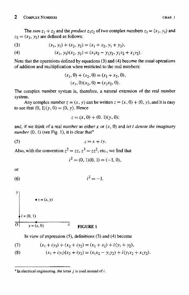
and, if we think of a real number as either x or (x, 0) and let i denote the imaginarynumber (0, 1) (see Fig. 1), it is clear that*
(5) z=x +iy.
Also, with the convention z2 = zz, z3 = zz2, etc., we find that
i2=(0, 1) (0, 1)=(-1,0),
or
Y
z=(x,Y)
0 X FIGURE 1
In view of expression (5), definitions (3) and (4) become
(7) (XI + iY1) + (x2 + iy2) = (x1 + x2) + i(y1 + Y2),
(8) (X1 + iY1)(x2 + iY2) = (x1x2 - y1y2) + i(y1x2 + x1y2)-
* In electrical engineering, the letter j is used instead of i.
SEC. 2 BASIC ALGEBRAIC PROPERTIES
Observe that the right-hand sides of these equations can be obtained by formallymanipulating the terms on the left as if they involved only real numbers and by
replacing i2 by -1 when it occurs.
2. BASIC ALGEBRAIC PROPERTIESVarious properties of addition and multiplication of complex numbers are the same asfor real numbers. We list here the more basic of these algebraic properties and verifysome of them. Most of the others are verified in the exercises.
The commutative laws
(1)
and the associative laws
Z1 + Z2 = Z2 + Z1, ZIZ2 = Z2ZI
(2) (ZI + Z2) + Z3 = z1 + (z2 + z3), (z1Z2)z3 = zi(z2z3)
follow easily from the definitions in Sec. 1 of addition and multiplication of complexnumbers and the fact that real numbers obey these laws. For example, if zt = (x1, y1)
and z2 = (x2, y2), then
z1 + Z2 = (x1 + X2, Y1 + Y2) = (x2 + xl, y2 yl) Z2+ZI.
Verification of the rest of the above laws, as well as the distributive law
(3) Z(ZI + Z2) = zz1 + zz2,
is similar.According to the commutative law for multiplication, iy = yi. Hence one can
write z = x + yi instead of z = x + iy. Also, because of the associative laws, a sum
z I + z2 + z3 or a product z 1z2z3 is well defined without parentheses, as is the case with
real numbers.The additive identity 0 = (0, 0) and the multiplicative identity 1= (1, 0) for real
numbers carry over to the entire complex number system. That is,
(4) z+0=z and z 1=
for every complex number z. Furthermore, 0 and 1 are the only complex numbers withsuch properties (see Exercise 9).
There is associated with each complex number z = (x, y) an additive inverse
(5) -z = (-x, -y),
satisfying the equation z + (-z) = 0. Moreover, there is only one additive inversefor any given z, since the equation (x, y) + (u, v) = (0, 0) implies that u = -x andv = -y. Expression (5) can also be written -z = -x - iy without ambiguity since
COMPLEX NUMBERS CHAP. I
(Exercise 8) -(iy) = (-i)y = i(-y). Additive inverses are used to define subtraction:
(6) z1-z2=Zi+(-z2).
So if z1 = (x1, Yi) and Z2 = (x2, Y2), then
(7) Z1 - Z2 = (XI - x2, Y1 - Y2) = (x1 - x2) + i(Yi - Y2).
For any nonzero complex number z = (x, y), there is a number z-I such thatzz-i = 1. This multiplicative inverse is less obvious than the additive one. To find it,we seek real numbers u and v, expressed in terms of x and y, such that
(x, y)(u, v) = (1, 0).
According to equation (4), Sec. 1, which defines the product of two complex numbers,u and v must satisfy the pair
xu-yv=1, yu+xv=0of linear simultaneous equations; and simple computation yields the unique solution
x -y_U - r
x2+y2, x2+YSo the multiplicative inverse of z = (x, y) is
X -V(z 0).(8)2'y xY+
The inverse z-1 is not defined when z = 0. In fact, z = 0 means that x2 + y2 = 0; andthis is not permitted in expression (8).
EXERCISES
1. Verify
(a) (/ - i) - i(1-i) _ -2i; (b) (2, -3)(-2, 1) = (-1, 8);
(c) (3, 1) (3, -1) (2, 1).
2. Show that(a) Re(iz) Im z; (b) Im(iz) = Re z.
3. Show that (l + z)2 = l + 2z + z2.
4. Verify that each of the two numbers z = 1 ± i satisfies the equation z2 - 2z + 2 = 0.
5. Prove that multiplication is commutative, as stated in the second of equations (1), Sec. 2.
6. Verify(a) the associative law for addition, stated in the first of equations (2), Sec. 2;
(b) the distributive law (3), Sec. 2.
SEC. 3 FURTHER PROPERTIES 5
7. Use the associative law for addition and the distributive law to show that
z(zi + Z2 + z3) = zzt + zz2 + zz3.
8. By writing i = (0, 1) and Y = (y, 0), show that -(iy) = (--i)y = i(-y).
9. (a) Write (x, y) + (u, v) = (x, y) and point out how it follows that the complex number0 = (0, 0) is unique as an additive identity.
(b) Likewise, write (x, y)(u, v) = (x, y) and show that the number 1= (1, 0) is a uniquemultiplicative identity.
10. Solve the equation z2 + z + I = 0 for z = (x, y) by writing
(x,Y)(x,y)+(x,y)+(1,0)=(0,0)
and then solving a pair of simultaneous equations in x and y.Suggestion: Use the fact that no real number x satisfies the given equation to show
that y 34 0.
Ans. z =
3. FURTHER PROPERTIES
In this section, we mention a number of other algebraic properties of addition andmultiplication of complex numbers that follow from the ones already described inSec. 2. Inasmuch as such properties continue to be anticipated because they also applyto real numbers, the reader can easily pass to Sec. 4 without serious disruption.
We begin with the observation that the existence of multiplicative inverses enablesus to show that if a product z 1z2 is zero, then so is at least one of the factors z I andz2. For suppose that ziz2 = 0 and zl 0. The inverse zl I exists; and, according to thedefinition of multiplication, any complex number times zero is zero. Hence
1 i
z2 = 1 z2 = (Z-
14. )z2 = `1 (zIZ2) = --I 0 = 0.
That is, if zlz2 = 0, either z1= 0 or z2 = 0; or possibly both zl and z2 equal zero.Another way to state this result is that if two complex numbers z I and z2 are nonzero,then so is their product z 1z2.
Division by a nonzero complex number is defined as follows:
(1) `1 = ztz; 1
Z2 -(z2 -A 0)
If z1= (x1, yl) and z2 = (x2, y2), equation (1) here and expression (8) in Sec. 2 tell usthat
z1 _ ) X2 -Y2 xlx2 + YiY2 YIx2 - x1Y2- (xl, y1 I, I ,
2z2 x2 + y2 x2 + y2 x2 + Y x2 + y2
6 COMPLEx NUMBERS CHAP. I
That is,
ZI = X1X2 + YIY2 Y1X2 -` X1Y2(2) - 1 2 -f i 2 2 (Z2 0 0)-X2 + Y2 x2 Y2
Although expression (2) is not easy to remember, it can be obtained by writing (seeExercise 7)
(3)ZI (x1 + iY1)(x2 - iY2)
Z2 (x2 + iY2)(x2 - iY2)
multiplying out the products in the numerator and denominator on the right, and thenusing the property
L1 rt 2 1 1 1 = L1 42(4) = (Z1 + z2)Z3 = Zlz3 + Z2Z3 + (Z3 36 0)-
Z3 Z3 Z3
The motivation for starting with equation (3) appears in Sec. 5.There are some expected identities, involving quotients, that follow from the
relation
(5) (z2 A O),1 --1-Z2
Z2
which is equation (1) when z1 = 1. Relation (5) enables us, for example, to writeequation (1) in the form
(6)Z1
=Zlt 1Z2 \ Z2
Also, by observing that (see Exercise 3)
(z2 A 0)
(z1z2) (Z1 1Z2 1) = (Zlz1 1)(Z2Z2 1) = 1 (z1 7- 0, z2 7- 0),
and hence that (z1z2)-1 = z,i-1z 1, one can use relation (5) to show that
(7) 1 = (z1z2Z 1Z2
(z1 36 0,z2 0 0)
Another useful identity, to be derived in the exercises, is
O, z4 36 O).(8)13Z4 Z3 ! ( 4
SEC. 3
EXAMPLE. Computations such as the following are now justified:
(23e)G+z)1
EXERCISES 7
(2 - 3i)(l + i) 5-i 5+i (5 - i)(5 + i)
_5+i5 i _5 I
26 26 + 26 26 + 26
Finally, we note that the binomial formula involving real numbers remains validwith complex numbers. That is, if z 1 and Z2 are any two complex numbers,
(9) (Zt + Z2)n
where
n
k.=0(:)
n-kzl
z2(n =
n _ n!(k = 0,
k k!(n - k)!
d where it is agreed that 0! = 1. The proof, by mathematical induction, is left as anexercise.
EXERCISES
1. Reduce each of these quantities to a real number:
1+2i 2-i 5i
(a) 3 - 4i + Si (b) (1 - i)(2 - i)(3 - i
Ans. (a) -2/5; (b) -1 /2; (c) -4.
2. Show that
(a) (-1)z - -z; (b) 1Iz = z (z A 0).
3. Use the associative and commutative laws for multiplication to show that
(zlz2)(z3z4) = (zlz3)(z2z4)
4. Prove that if z1z2z3 = 0, then at least one of the three factors is zero.Suggestion: Write (zlz2)z3 = 0 and use a similar result (Sec. 3) involving two
factors.
5. Derive expression (2), Sec. 3, for the quotient zt/Z2 by the method described just afterit.
6. With the aid of relations (6) and (7) in Sec. 3, derive identity (8) there.
7. Use identity (8) in Sec. 3 to derive the cancellation law:
i = zt (z2A0,zA0).z2z Z2
COMPLEX NUMBERS CHAP. I
8. Use mathematical induction to verify the binomial formula (9) in Sec. 3. More precisely,note first that the formula is true when n = 1. Then, assuming that it is valid when n = mwhere m denotes any positive integer, show that it must hold when n = m + 1.
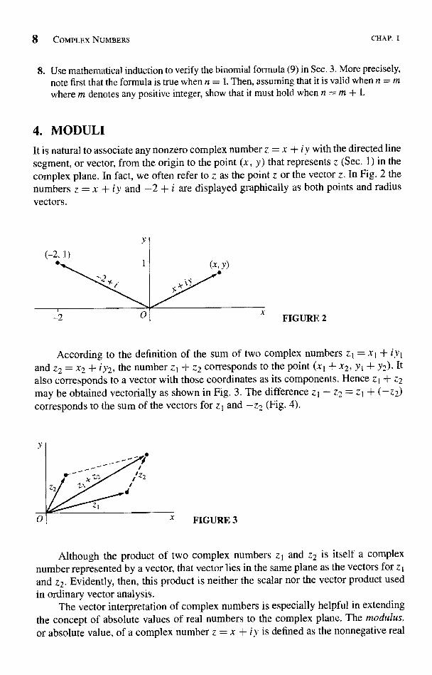
4. MODULIIt is natural to associate any nonzero complex number z = x + iy with the directed linesegment, or vector, from the origin to the point (x, y) that represents z (Sec. 1) in thecomplex plane. In fact, we often refer to z as the point z or the vector z. In Fig. 2 thenumbers z = x + iy and -2 + i are displayed graphically as both points and radiusvectors.
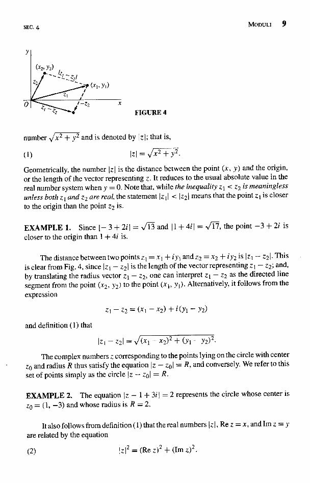
According to the definition of the sum of two complex numbers z1= xj + iy1and z2 = x2 + iY2, the number z1 + z2 corresponds to the point (x1 + x2, Yt + Y2). Italso corresponds to a vector with those coordinates as its components. Hence zl + z2may be obtained vectorially as shown in Fig. 3. The difference z1 - z2 = z1 + (-z2)corresponds to the sum of the vectors for z1 and -z2 (Fig. 4).
Although the product of two complex numbers z1 and z2 is itself a complexnumber represented by a vector, that vector lies in the same plane as the vectors for z 1and z2. Evidently, then, this product is neither the scalar nor the vector product usedin ordinary vector analysis.
The vector interpretation of complex numbers is especially helpful in extendingthe concept of absolute values of real numbers to the complex plane. The modulus,or absolute value, of a complex number z = x + iv is defined as the nonnegative real
SEC. 4 MODULI 9
FIGURE 4
number x2 + y2 and is denoted by Iz1; that is,
(1) IzI = x2 -+y 2.
Geometrically, the number Iz1 is the distance between the point (x, y) and the origin,
or the length of the vector representing z. It reduces to the usual absolute value in thereal number system when y = 0. Note that, while the inequality z1 < z2 is meaninglessunless both zI and z2 are real, the statement Izil < Iz21 means that thepoint z1 is closer
to the origin than the point z2 is.
EXAMPLE 1. Since 1- 3 + 2i I = 13 and 11 + 4i I = 17, the point -3 + 2i iscloser to the origin than I + 4i is.
The distance between two points z1= x1 + iy1 and z2 = x2 + iy2 is Izi - z21. Thisis clear from Fig. 4, since Izi - z21 is the length of the vector representing zi - z2; and,by translating the radius vector z I - z2, one can interpret z I - z2 as the directed linesegment from the point (x2, y2) to the point (x1, yi). Alternatively, it follows from the
expression
- Z2 = (XI - x2) + i(Y1 - Y2)
and definition (1) that
Izi-z21= (xi- (YI - Y2)2.
The complex numbers z corresponding to the points lying on thecircle with center
za and radius R thus satisfy the equation Iz - zal = R, and conversely. We refer to thisset of points simply as the circle Iz - zol = R.
EXAMPLE 2. The equation Iz - 1 + 3i j =2 represents the circle whose center iszo = (1, -3) and whose radius is R = 2.
It also follows from definition (1) that the real numbers I z 1, Re z = x, and Im z = y
are related by the equation
(2) Iz12 = (Re z)2 + (IM
10 COMPLEX NUMBERS CHAP. I
Thus
(3) Rez < Rez) < I and Im z< I lm z l< I z j.
We turn now to the triangle inequality, which provides an upper bound for themodulus of the sum of two complex numbers z 1 and z2:
<I + Iz21-
This important inequality is geometrically evident in Fig. 3, since it is merely astatement that the length of one side of a triangle is less than or equal to the sumof the lengths of the other two sides. We can also see from Fig. 3 that inequality (4)is actually an equality when 0, z1, and z2 are collinear. Another, strictly algebraic,derivation is given in Exercise 16, Sec. 5.
An immediate consequence of the triangle inequality is the fact that
(5) Iz1 + Z21 ? 11Z11 - Iz211-
To derive inequality (5), we write
Iz11 = I(zi + z2)
which means that
(6) (z1+Z21?Iz11-Iz21-
This is inequality (5) when jz11 > Iz21. Ifz2 in inequality (6) to get
2 , we need only interchange z1 and
Iz1 + z21 >- -(Iz11- Iz21),
which is the desired result. Inequality (5) tells us, of course, that the length of one sideof a triangle is greater than or equal to the difference of the lengths of the other twosides.
Because I- Z21 = Iz21, one can replace z2 by -z2 in inequalities (4) and (5) tosummarize these results in a particularly useful form:
(7) IzI Z21 < Iz11 + Iz21,
(8) Iz1 ± z21 ? 11z1I - Iz211.
EXAMPLE 3. If a point z lies on the unit circle IzI = 1 about the origin, then
-21<Iz1+2=3
and
-2I
2
SEC. 5 COMPLEX CONJUGATES
The triangle inequality (4) can be generalized by means of mathematical induc-tion to sums involving any finite number of terms:
(9) Iz11 (n=2,3,...).To give details of the induction proof here, we note that when n = 2, inequality (9) isjust inequality (4). Furthermore, if inequality (9) is assumed to be valid when n = m,it must also hold when n = in + 1 since, by inequality (4),
1(zl+z2+<(Iz11+Iz21+ +Izml)+Izm+ll
EXERCISES
1. Locate the numbers z1 + z2 and z1- Z2 vectorially when2
z1=2i, z2= -1; (b)z1=(-J , 1), z2=(-,/3-, 0);
(c)z1=(-3. 1), z2=(1,4); (d)z1=xi+iyl, z2=x2. Verify inequalities (3), Sec. 4, involving Re z, Im z, and IzI.
3. V e r i f y that / 2 - I z I ? IRe z1 + I lm z 1.Suggestion: Reduce this inequality to (lxI - Iyl)2 0.
4. In each case, sketch the set of points determined by the given condition:
(a)Iz-1+i1=1; (b)Iz+il<3; (c)Iz-4i1>4.5. Using the fact that 1z 1- z21 is the distance between two points z 1 and z2, give a geometric
argument that
(a) 1z - 4i l + Iz + 4i l = 10 represents an ellipse whose foci are (0, ±4);(b) Iz - 11 = Iz + i l represents the line through the origin whose slope is -1.
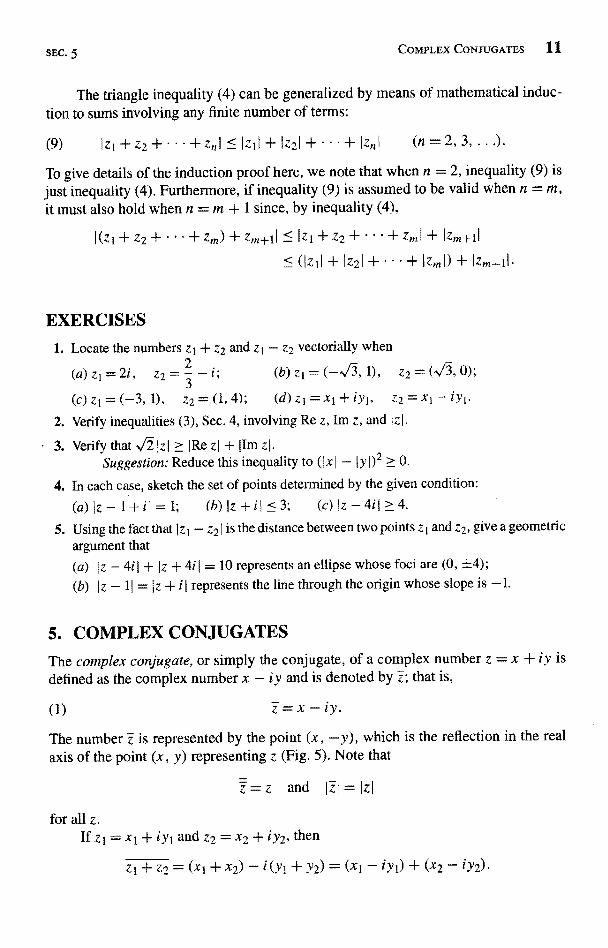
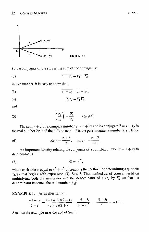
5. COMPLEX CONJUGATESThe complex conjugate, or simply the conjugate, of a complex number z = x + iy is
defined as the complex number x - iy and is denoted by z; that is,
(1) z=x-iy.The number i is represented by the point (x, -y), which is the reflection in the realaxis of the point (x, y) representing z (Fig. 5). Note that
z=
z and IzI
forallz.If z, =x1+iyl andZ2=x2+iY2,then
z
z1+z2=(x1+x2)-i(yl+y2)=(x1-iY1)+(x2-iy2)
2 COMPLEX NUMBERS
So the conjugate of the sum is the sum of the conjugates:
(2) ZI + z2 = z1 + z2.
In like manner, it is easy to show that
(3)
(4)
and
(5) (z2 0 0).
CHAP. I
The sum z + z of a complex number z = x + iy and its conjugate z = x - iy isthe real number 2x, and the difference z - z is the pure imaginary number 2iy. Hence
(6) Rez=z 2z, Imzz
=- 2iz.An important identity relating the conjugate of a complex number z = x + iy to
its modulus is
(7)
z1-Z2=ZI- Z2,
Z1Z2 = Z1 Z2,
zz =
where each side is equal to x2 + y2. It suggests the method for determining a quotientz1/z2 that begins with expression (3), Sec. 3. That method is, of course, based onmultiplying both the numerator and the denominator of zl/z2 by z2, so that thedenominator becomes the real number 1z212.
EXAMPLE 1. As an illustration,
-1+3i _ (-I+3i)(2+i) -5+5i -5+5i --12-i (2-i)(2+i)_ -
T2 -il2 5
See also the example near the end of Sec. 3.
SEC. 5 EXERCISES
Identity (7) is especially useful in obtaining properties of moduli from propertiesof conjugates noted above. We mention that
(8) IZIZ21= IZIIIZ2I
and
(9)zI
z2 Iz21
Property (8) can be established by writing
(z2 0 0)
1zIZ212 = (zlz2)(zjz2) = (ziz2)(ztz2) _ (zI (z2z2) = Izil21z212 = (IziIIz21)2
and recalling that a modulus is never negative. Property (9) can be verified in a similarway.
EXAMPLE 2. Property (8) tells us that 1z21 = Iz12 and Iz31 = Iz13. Hence if z is apoint inside the circle centered at the origin with radius 2, so that Izl < 2, it followsfrom the generalized form (9) of the triangle inequality in Sec. 4 that
Iz3+3z2-2z+ 11 < Iz13+3Iz12+2Iz) + 1 <25.
EXERCISES
1. Use properties of conjugates and moduli established in Sec. 5 to show that
(a).+3i=z-3i; (b)iz
(c) (2+i)2.=3-4i; (d) I(2z+5)(V-i)I ='I2z+51.2. Sketch the set of points determined by the condition
(a) Re(z - i) = 2; (b) 12z - iI = 4.
3. Verify properties (3) and (4) of conjugates in Sec. 5.
4. Use property (4) of conjugates in Sec. 5 to show that
(a) zlz2z3 = it z2 L3 ; (b) z4 = z 4.
5. Verify property (9) of moduli in Sec. 5.
6. Use results in Sec. 5 to show that when z2 and z3 are nonzero,
(a)zi .
Z2Z3 / Z2 Z3(b)
zi
Z2Z3
IziI
IZI-IIZ31
7. Use established properties of moduli to show that when Iz31 54 IZ41,
zi + z2 < IZII + Iz21Z3 + Z4 I IZ31 - IZ411
14 COMPLEx NUMBERS CHAP. I
8. Show that
IRe(2 + + z3)I < 4 when IzI < 1.
9. It is shown in Sec. 3 that if zlz, = 0, then at least one of the numbers z1 and z2 must bezero. Give an alternative proof based on the corresponding result for real numbers andusing identity (8), Sec. 5.
10. By factoring z4 - 4z2 + 3 into two quadratic factors and then using inequality (8), Sec. 4,show that if z lies on the circle IzI = 2, then
Iz4-4z2+3
11. Prove that
(a) z is real if and only if z = z;
(b) z is either real or pure imaginary if and only if `2 = z2.
12. Use mathematical induction to show that when n = 2, 3, ... ,(a)ZI+Z2+...+Zn=Z1+Z2+...+Zn;
13. Let ao, a1, a2, . . , a,, (n > 1) denote real numbers, and let z be any complex number.With the aid of the results in Exercise 12, show that
ao+alz+a2Z2+...+a,,zn=ao+aj +a2T2+...+anZn.
14. Show that the equation Iz - zol = R of a circle, centered at z0 with radius R, can bewritten
-2Re(zz0)+IZ01`=R2.
15. Using expressions (6), Sec. 5, for Re Z and Im z, show that the hyperbola x22 -can be written
z2+Z2=2.
16. Follow the steps below to give an algebraic derivation of the triangle inequality (Sec. 4)
Izi + z21 < Izll + Iz21
(a) Show
IZ1 + Z21` _ (z1 + z2) Zt + z2 = Z1zi + 2 Z1Z2) + Z2Z2-
(b) Point out why
z1Z2 + z1Z2 = 2 Re(z1Z2) < 21z111z21.
Use the results in parts (a) and (b) to obtain the inequality
Iz1 + z212 < (Iz11 + Iz21)2,
and note hQw the triangle inequality follows.
SEC. 6 EXPONENTIAL FORM 15
6. EXPONENTIAL FORMLet r and 9 be polar coordinates of the point (x, y) that corresponds to a nonzerocomplex number z = x + iy. Since x = r cos 0 and y = r sin 0, the number z can bewritten in polar form as
(1) z = r(cos 9 + i sin 9).
If z = 0, the coordinate 0 is undefined; and so it is always understood that z 34 0whenever arg z is discussed.
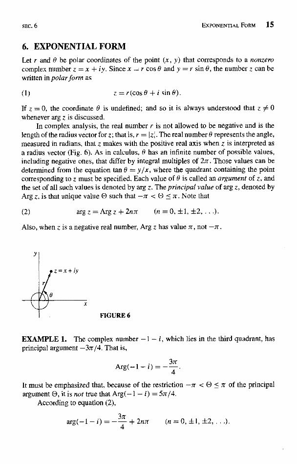
In complex analysis, the real number r is not allowed to be negative and is thelength of the radius vector for z; that is, r = (z j . The real number 0 represents the angle,measured in radians, that z makes with the positive real axis when z is interpreted asa radius vector (Fig. 6). As in calculus, 9 has an infinite number of possible values,including negative ones, that differ by integral multiples of 2nr. Those values can bedetermined from the equation tan 0 = y/x, where the quadrant containing the pointcorresponding to z must be specified. Each value of 9 is called an argument of z, andthe set of all such values is denoted by arg z. The principal value of arg z, denoted byArg z, is that unique value O such that -7r < O < Yr. Note that
(2) arg z = Arg z + 2njr (n = 0, ±1, ±2, ...).
Also, when z is a negative real number, Arg z has value 7r, not -sr.
FIGURE 6
EXAMPLE 1. The complex number -1 - i, which lies in the third quadrant, hasprincipal argument -3ir/4. That is,
Arg(-1 - i) it4
It must be emphasized that, because of the restriction -7r < Qargument O, it is not true that Arg(-1 - i) = 57r/4.
According to equation (2),
3
< of the principal
g(-1-i)=--+2nn (n=0,±1,±2,.
16 COMPLEX NUMBERS CHAP. I
Note that the term Arg z on the right-hand side of equation (2) can be replaced by anyparticular value of arg z and that one can write, for instance,
arg(-1-i)= 57r
4+2nn' (n=O,fl,f2,...).
The symbol ei0, or exp(iO), is defined by means of Euler's formula as
(3) eie = cos 6 + i sin 0,
where 0 is to be measured in radians. It enables us to write the polar form (1) morecompactly in exponential form as
(4) z = re`°.
The choice of the symbol eie will be fully motivated later on in Sec. 28. Its use in Sec.7 will, however, suggest that it is a natural choice.
EXAMPLE 2. The number -1 - i in Example 1 has exponential form
(5) -1-exp[i 34
) I
With the agreement that eJ`e = e'(-O), this can also be written -1 - i = e-i37r/4.
Expression (5) is, of course, only one of an infinite number of possibilities for theexponential form of -1 - i :
(6) -1- i = 4 exp C- 3 + 2nmr)] (n. = 0, ± 1, ±2, .
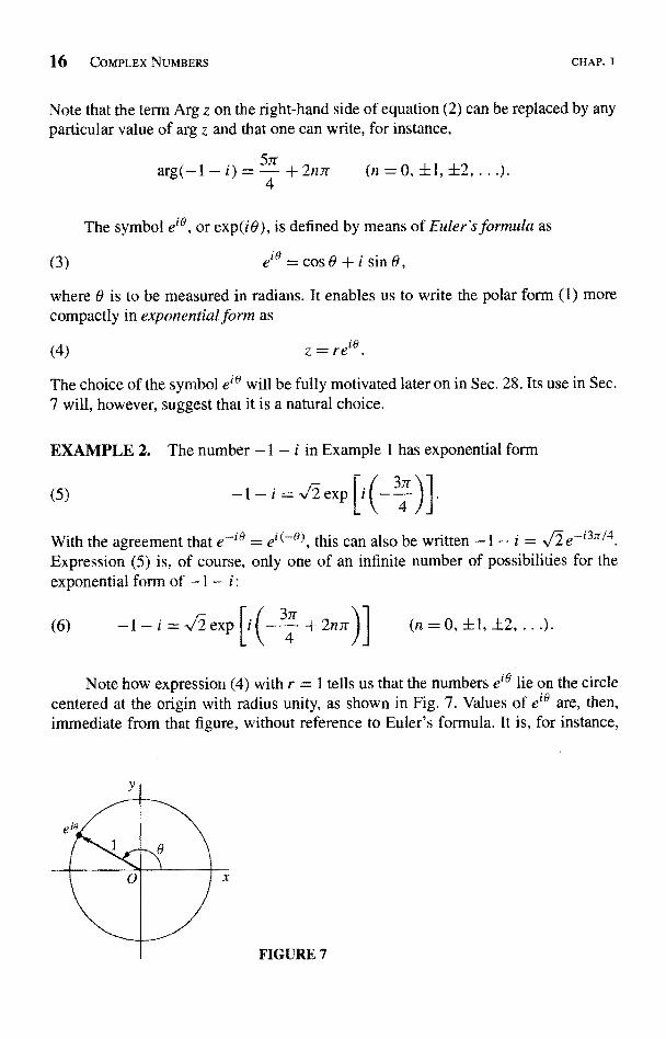
Note how expression (4) with r = 1 tells us that the numbers eie lie on the circlecentered at the origin with radius unity, as shown in Fig. 7. Values of ere are, then,immediate from that figure, without reference to Euler's formula. It is, for instance,
FIGURE 7
SEC. 7 PRODUCTS AND QUOTIENTS IN EXPONENTIAL FORM 17
geometrically obvious that
= -1, e-tn/2 = -i, and e-i4n _
Note, too, that the equation
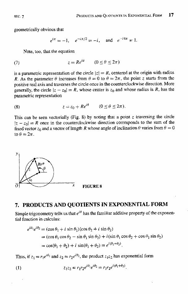
(7) z = Re'a (0 <
is a parametric representation of the circle I zI = R, centered at the origin with radiusR. As the parameter 0 increases from 0 = 0 to 0 = 27r, the point z starts from thepositive real axis and traverses the circle once in the counterclockwise direction. Moregenerally, the circle Iz - zp( = R, whose center is zo and whose radius is R, has theparametric representation
(8) z=z0+Reio (0<0<27r).
This can be seen vectorially (Fig. 8) by noting that a point z traversing the circleIz - zol = R once in the counterclockwise direction corresponds to the sum of thefixed vector zO and a vector of length R whose angle of inclination 0 varies from 0to 0 = 2,r.
FIGURE 8
7. PRODUCTS AND QUOTIENTS IN EXPONENTIAL FORM
Simple trigonometry tells us that ei0 has the familiar additive property of the exponen-tial function in calculus:
(cos 0, + i sin 01) (cos 02 + i sin 02)
= (cos 01 cos 0, - sin 01 sin 02) + i (sin 01 cos 02 + cos 01 sin 02)
= cos(01 + 02) + i sin(01 + 02) = ei(01+02).
Thus, if z1= r1e`Bt and z2 = r2e'°2, the product z1z2 has exponential fo
(1) ZIZ2 = rlr2eie,et82 = rir2ei(6I+e2)
8 COMPLEX NUMBERS CHAP. I
Moreover,
zl rl ei81e-i82 r, ei(81-82)(2)
_
Z2 r2 ei82e-i8, r2 eitl r2
Because 1 = lei0, it follows from expression (2) that the inverse of any nonzerocomplex number z = rei8 is
(3)
Expressions (1), (2), and (3) are, of course, easily remembered by applying the usualalgebraic rules for real numbers and ex.
Expression (1) yields an important identity involving arguments:
(4) arg(z1z2) = arg z1 + arg z2.
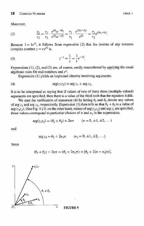
It is to be interpreted as saying that if values of two of these three (multiple-valued)arguments are specified, then there is a value of the third such that the equation holds.
We start the verification of statement (4) by letting 01 and 02 denote any valuesof arg zl and arg z2, respectively. Expression (1) then tells us that 01 + 02 is a value ofarg(z1z2 ). (See Fig. 9.) If, on the other hand, values of arg(z 1z2) and arg z1 are specified,those values correspond to particular choices of n and n 1 in the expressions
and
Since
arg(zIz2) = (01 + 02) + 2n.r (n = 0, +1, f2, ...)
argz1 =01+2n1?r (n1 =0, ±1, +2, .. .
(01 + 02) + 2n7r = (01 + 2n 17r) + [02 + 2(n - n
2142
SEC. 7 PRODUCTS AND QUOTIENTS IN EXPONENTIAL FORM 19
equation (4) is evidently satisfied when the value
arg z2=82+2(n-
is chosen. Verification when values of arg(z1z2) and arg z2 are specified follows bysymmetry.
Statement (4) is sometimes valid when arg is replaced everywhere by Arg (seeExercise 7). But, as the following example illustrates, that is not always the case.
EXAMPLE 1. When z 1= -1 and z2 = i ,
Arg(z1z2) = Arg(- but Argz1+Argz2=rr+ - = 3-.
it2
If, however, we take the values of arg z1 and arg z2 just used and select the value
Arg(ztz2) +
of arg(z1z2), we find that equation (4
Statement (4) tells us that
2.7r=-Z +2n'=32
is satisfied.
arg(zl = arg(zjz2 1) = arg z1 + arg(z2 1),2
and we can see from expression (3) that
(5)
Hence
(6) =argz1-argz2.
Statement (5) is, of course, to be interpreted as saying that the set of all values on theleft-hand side is the same as the set of all values on the right-hand side. Statement (6)is, then, to be interpreted in the same way that statement (4) is.
EXAMPLE 2. In order to find the principal argument Arg z when
-2Z-1+Ai
observe that
g(z21) _ -arg z2.
arg z = arg(-2) - arg(l
20 COMPLEx NUMBERS
Since
Arg(-2) = ir and Arg(1 + Vi) = 3
CHAP. I
one value of arg z is 27r/3; and, because 2ir/3 is between -7r and n, we find thatArgz=2nj3.
Another important result that can be obtained formally by applying rules for realnumbers to z = re`s is
(7)Zn = rnein8 (n = 0, ±l,±2,.
It is easily verified for positive values of n by mathematical induction. To be specific,we first note that it becomes z = re`s when n = 1. Next, we assume that it is validwhen n = in, where m is any positive integer. In view of expression (1) for the productof two nonzero complex numbers in exponential form, it is then valid for n = m + 1:
= ZZm = rei&rmeimo = rrn+lei(m-t-1)8
Expression (7) is thus verified when n is a positive integer. It also holds when nwith the convention that z0 = 1. If n = -1, -2, ... , on the other hand, we define znin terms of the multiplicative inverse of z by writing
zn=(z-l)m where m=-n=1,2,.
Then, since expression (7) is valid for positive integral powers, it follows from theexponential form (3) of
z-i that
elm(-8) _ ()-n ei(-n)(-8) _rnein8
r
Expression (7) is now established for all integral powers.Observe that if r = 1, expression (7) becomes
(8)(ei8)n = eine (n = 0, ±1, f2, ...).
When written in the form
(9) (cos 0 + i sin 9)n = cos nO + i sin nO (n = 0, ±1, ±2,
this is known as de Moivre's formula.Expression (7) can be useful in finding powers of complex numbers even when
they are given in rectangular form and the result is desired in that form.
SEC. 7 ExERCIsF.s 21
EXAMPLE 3. In order to put (f + i)7 in rectangular form, one need only write
+i)7=(2e
EXERCISES
1. Find the principal argument Arg z when
(a)z= -2 '2i
; (b)z=('-i)6.Ans. (a) -37r/4; (b) ir.
2. Show that (a) letei = 1; (b) eiO = e-'O
3. Use mathematical induction to show that
eroletO2 ... e'91 = ei(01+9Z+...+0n) (n = 2, 3, ...).
4. Using the fact that the modulus Ie`0 - 11 is the distance between the points e"9 and 1 (seeSec. 4), give a geometric argument to find a value of 8 in the interval 0 < 8 < 2ir thatsatisfies the equation Ie'e - 11 = 2.
Ans. ir.
5. Use de Moivre's formula (Sec. 7) to derive the following trigonometric identities:
(a) cos 30 = cos3 8 - 3 cos 8 sin 2 8; (b) sin 30 = 3 cost 8 sin 8 - sin3 8.
6. By writing the individual factors on the left in exponential form, performing the neededoperations, and finally changing back to rectangular coordinates, show that
(a)i(1- i)( +i)=2(1-I -i); (b)5i/(2+i)=1+2i;(c)(-1+i)7=-8(l+i); (d) (1+ i)-ZO=2-11(-l + 13i).
7. Show that if Re zt > 0 and Re z2 > 0, then
Arg(zlz2) = Arg zl + Arg z2,
where Arg(ztz2) denotes the principal value of arg(zlz2), etc.
8. Let z be a nonzero complex number and n a negative integer (n = -1, -2, ...). Also,write z = re`O and m = -n = 1, 2, .... Using the expressions
4m = rmeimO and z-1 = 1l et( a)
r
verify that (zm)_t = (z-')m and hence that the definition zn = (z-')m in Sec. 7 couldhave been written alternatively as z" = (zm)-t
9. Prove that two nonzero complex numbers zt and z2 have the same moduli if and only ifthere are complex numbers cl and c2 such that zt = clc2 and z2 = clc2.
Suggestion: Note that
22 COMPLEX NUMBERS
and [see Exercise 2(b)]
10. Establish the identity
expIi',
) exp( i V' I= exp(i82).2 2
1-zn+l+z+z`+ zn
1-z
and then use it to derive Lagrange's trigonometric identity:
1+cos8+cos20+ +cosn0=1`+ sin[(2n + 1)0/2]
2 sin(0/2)
CHAP. I
0 <2rr).
Suggestion: As for the first identity, write S = 1 + z + z2 + + zn and considerthe difference S - zS. To derive the second identity,, write z = e`9 in the first one.
) Use the binomial formula (Sec. 3) and de Moivre's formula (Sec. 7) to write
n
cos nO + i sin nO = { n cosh-k 0(i sin 0)k (n = 1, 2, . .
k=O
Then define the integer m by means of the equations
m= J n/2 if n is even,(n - 1)/2 if n is odd
and use the above sum to obtain the expression [compare Exercise 5(a)]
cos nd = E (2k I (-1)k cosn-2k 0 sink 0 (rt = 1, 2, ...11
0 lk=
(b) Write x = cos 0 and suppose that 0 -< 0 < it, in which case -1 <- x <- 1. Point outhow it follows from the final result in part (a) that each of the functions
T,(x) = cos(n cos`' x) (n = 0, 1, 2, ...}
is a polynomial of degree n in the variable x
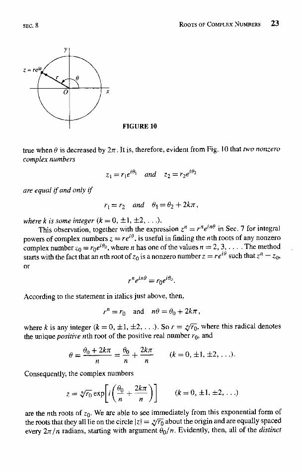
8. ROOTS OF COMPLEX NUMBERSConsider now a point z = re`n, lying on a circle centered at the origin with radius r (Fig.10). As 0 is increased, z moves around the circle in the counterclockwise direction. Inparticular, when 0 is increased by 2ir, we arrive at the original point; and the same is
* These polynomials are called Chebyshev polynomials and are prominent in approximation theory.
SEC. 8
FIGURE 10
ROOTS OF COMPLEX NUMBERS 23
true when 0 is decreased by 2,7. It is, therefore, evident from Fig. 10 that two nonzerocomplex numbers
z1 = rlei61 and z2 = r2eie2
are equal if and only if
r1= r2 and 01 = 02 + 2k7r,
where k is some integer (k = 0, +1, ±2, ...).This observation, together with the expression zn = rneine in Sec. 7 for integral
powers of complex numbers z = rei0, is useful in finding the nth roots of any nonzerocomplex number zo = rpei°0, where n has one of the values n = 2, 3, .... The methodstarts with the fact that an nth root of za is a nonzero number z = rei0 such that zn = z0,or
rneinO = rceie0.
According to the statement in italics just above, then,
and nO=00+2kir,
where k is any integer (k = 0, ±1, ±2, ...). So r = / rp, where this radical denotesthe unique positive nth root of the positive real number ra, and
0 0c + 2kir = 8a + 2k7r (k = 0, t1, t2, ...).n n n
Consequently, the complex numbers
V r-0 exp[,(10
+2 nr)
.1
(k = 0, +1, +2, .
are the nth roots of zo. We are able to see immediately from this exponential form ofthe roots that they all lie on the circle I z I = n rc about the origin and are equally spacedevery 2n/n radians, starting with argument 001n. Evidently, then, all of the distinct
24 COMPLEX NUMBERS CHAP. I
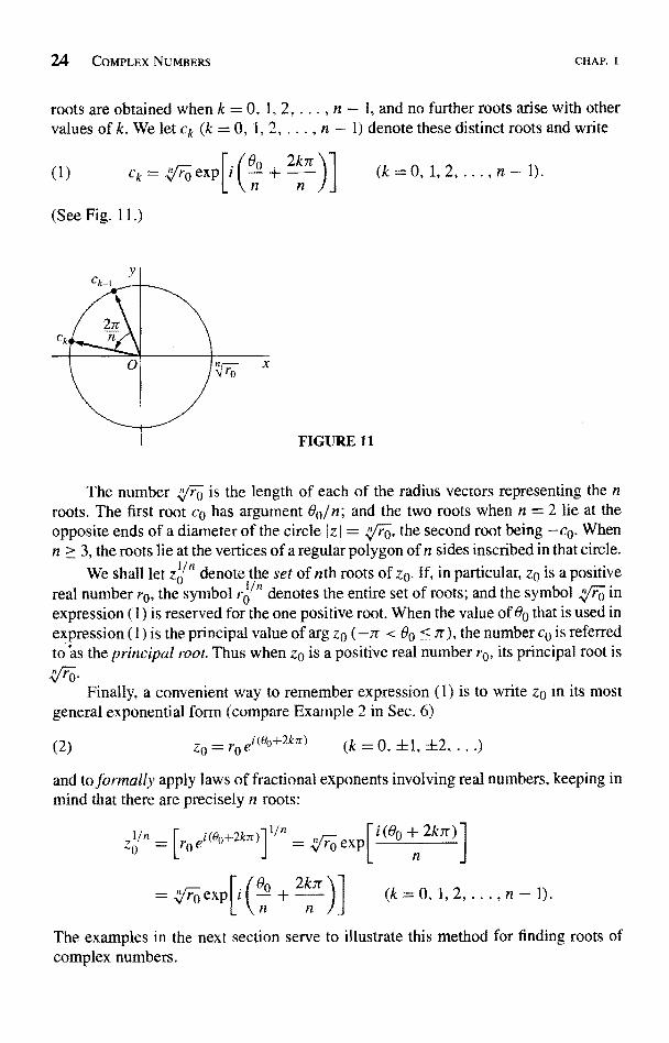
roots are obtained when k = 0, 1, 2, ... , n - 1, and no further roots arise with othervalues of k. We let ck (k = 0, 1, 2, ... , n - 1) denote these distinct roots and write
(1) ck = " ro exp
See Fig. 11
to + 2k7rn n
FIGURE 11
(k = 0, 1, 2, . . . , n - 1).
The number n ro is the length of each of the radius vectors representing the nroots. The first root co has argument 00/n; and the two roots when n = 2 lie at theopposite ends of a diameter of the circle Iz I = Mr--o, the second root being -co. Whenn > 3, the roots lie at the vertices of a regular polygon of n sides inscribed in that circle.
We shall let denote the set of nth roots of zo. If, in particular, zo is a positivereal number ro, the symbol rain denotes the entire set of roots; and the symbol rz re inexpression (1) is reserved for the one positive root. When the value of 8a that is used inexpression (1) is the principal value of arg zo (-:r < Oo < ;r), the number co is referredto as the principal root. Thus when zo is a positive real number ro, its principal root is
ro.Finally, a convenient way to remember expression (1) is to write zo in its most
general exponential form (compare Example 2 in Sec. 6)
(2)zo = ro e i(8 +2ksr) (k = 0, +1, +2, ...)
and to farmally apply laws of fractional exponents involving real numbers, keeping inmind that there are precisely n roots:
eX[(00 + 2kir)11n = [roe1(00+2k]1' = P n
_ F Fro2k7 ) ] (k = 0, 1, 2, ... , n - 1).
tI rz
The examples in the next section serve to illustrate this method for finding roots ofcomplex numbers.
SEC. 9 EXAMPLES 25
9. EXAMPLESIn each of the examples here, we start with expression (2), Sec. 8, and proceed in themanner described at the end of that section.
EXAMPLE 1. In order to determine the nth roots of unity, we write
1= 1 exp[i (0 + 2k7r)] (k = 0, f1, ±2 ...)
and find that
1/n = (0+
2kn-1 exp in n
2kn=exp i)
(k=0, 1,2,...,n-n
When n = 2, these roots are, of course, ± 1. When n > 3, the regular polygon at whosevertices the roots lie is inscribed in the unit circle I z I = 1, with one vertex correspondingto the principal root z = 1 (k = 0).
e write
(2) coil = exp
it follows from property (8), Sec. 7, of eie that
2k7r
n(k=0,1,2,...,n-1).
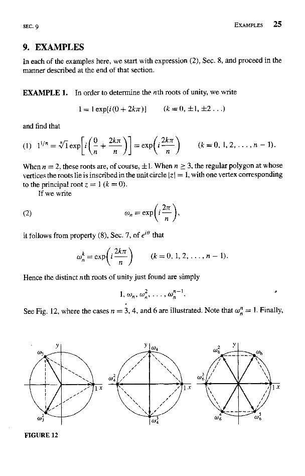
Hence the distinct nth roots of unity just found are simply
wn, wn, . . . ,Wn-1
See Fig. 12, where the cases n = 3, 4, and 6 are illustrated. Note that con= 1. Finally,
FIGURE 12
26 COMPLEX NUMBERS CHAP. I
it is worthwhile observing that if c is any particular nth root of a nonzero complexnumber zo, the set of nth roots can be put in the form
2C, cw, , Cw`t , .
nn
This is because multiplication of any nonzero complex number by wn increases theargument of that number by 2ir/n, while leaving its modulus unchanged.
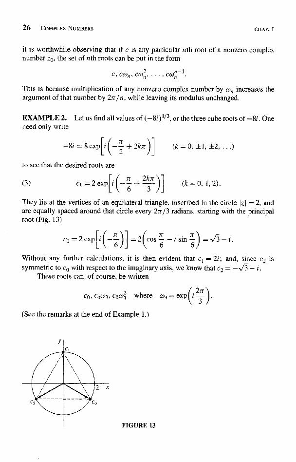
EXAMPLE 2. Let us find all values of (-8i)1/3, or the three cube roots of -8i. Oneneed only write
-8i = 8 exp i(- +2krc)] (k=O,+1,±2,.
to see that the desired roots are
(3) Ck=2exp(_,-r
23 (k = O, 1, 2
They lie at the vertices of an equilateral triangle, inscribed in the circle z j = 2, andare equally spaced around that circle every 2n/3 radians, starting with the principalroot (Fig. 13)
Co=2exp =2tcos6-1 sin6) =
Without any further calculations, it is then evident that cl = 2i; and, since c2 issymmetric to co with respect to the imaginary axis, we know that c, = -J - i.
These roots can, of course, be written
CO' COC031 COLtl3 where w3 = exp
(See the remarks at the end of Example 1.)
FIGURE 13
SEC. 9 EXAMPLES 27
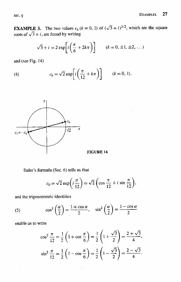
EXAMPLE 3. The two values ck (k = 0, 1) of (J + i)112, which are the squareroots of + i, are found by writing
/n+i =2exp[i(6 +2k7r
and (see Fig. 14)
(k=0,+1,±2,.
(4) C k k = exp[i ( 2 + kn (k = 0, 1).
2 x
FIGURE 14
Euler's formula (Sec. 6) tells us that
co = exp
and the trigonometric identities
(5)
ja l+cosacost I
2= 2
enable us to write
cos12+i sin12
s(a 1- cos a
2 2
28 COMPLEX NUMBERS
Consequently,
Since cl = -co, the two square roots of 113 + i are, then,
CHAP. I
EXERCISES1. Find the square roots of (a) 2i; (b)1 - 1-i and express them in rectangular coordinates.
Ans. (a) +(l + i); (b) +/3- i
.
2. In each case, find all of the roots in rectangular coordinates, exhibit them as vertices ofcertain squares, and point out which is the principal root:
( -16)114; (b) (-8 - 8-,/-3i) 1/4.
Ans. (a)+1/2-(1+i),±J (1-i); (b)+(13-i),+(I+13-i).3. In each case, find all of the roots in rectangular coordinates, exhibit them as vertices of
certain regular polygons, and identify the principal root:
(a) (-1)I/3; (b) 8116.
Ans. (b) +, + 1 + Vi
4. According to Example 1 in Sec. 9, the three cube roots of a nonzero complex number zocan be written co, coc3, cocoa, where co is the principal cube root of zo and
(a3 = exp-1+-03i
2
Show that if zo = -41T + 41/ i, then co = /(1 + i) and the other two cube roots are,in rectangular form, the numbers
-(11+1)+(V-1)i 2 ( -1)-(/+l)icow3 = , coww3 =-v/2-
5. (a) Let a denote any fixed real number and show that the two square roots of a + i are
+/A expi2 }
where A = of a2 + 1 and a = Arg(a + i ).
SEC. IO REGIONS IN THE COMPLEX PLANE 29
(b) With the aid of the trigonometric identities (5) in Example 3 of Sec. 9, show that thesquare roots obtained in part (a) can be written
1+( A+a+i A-a).
(Note that this becomes the final result in Example 3, Sec. 9, when a =.]
6. Find the four roots of the equation z4 + 4 = 0 and use them to factor z4 + 4 into quadraticfactors with real coefficients.
Ans. (z2 + 2z + 2)(z2 - 2z + 2).
7. Show that if c is any nth root of unity other than unity itself, then
1+c+c2+.. -+c"- t = 0.
Suggestion: Use the first identity in Exercise 10, Sec. 7.
8. (a) Prove that the usual formula solves the quadratic equation
az2+bz+c=0 (a 360)
when the coefficients a, b, and c are complex numbers. Specifically, by completingthe square on the left-hand side, derive the quadratic formula
-b + (b2 - 4ac) t,f2
2a
where both square roots are to be considered when b2 - 4ac A 0,
(b) Use the result in part (a) to find the roots of the equation z2 + 2z + (1 -
Ans. (b) (_i + +729. Let z = re`' be any nonzero complex number and n a negative integer (n = -1, -2, ...).
Then define zt/" by means of the equation zt/n = (z-t)1/m where m = -n. By showingthat the m values of (zi/m)-t and (z-1)t/m are the same, verify that zt/n = (zl/m)-t
(Compare Exercise 8, Sec. 7.)
10. REGIONS IN THE COMPLEX PLANEIn this section, we are concerned with sets of complex numbers, or points in the z plane,and their closeness to one another. Our basic tool is the concept of an E neighborhood
(1) 1z -zo1 «
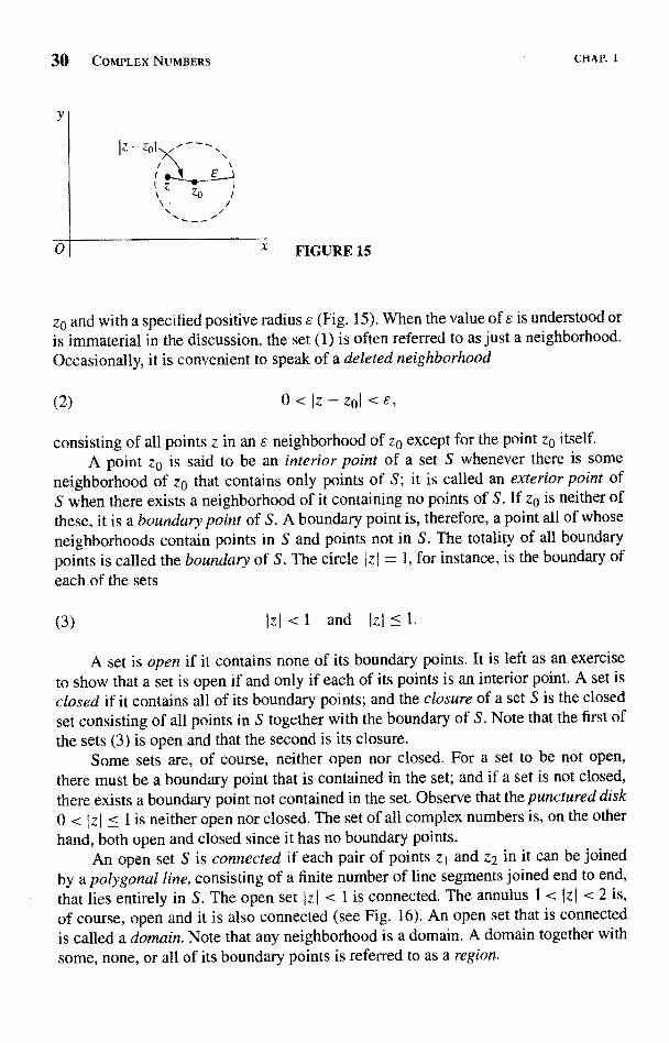
of a given point z0. It consists of all points z lying inside but not on a circle centered at
30 COMPLEX NUMBERS CHAP. 1
Y
z-zo
0 FIGURE 15
zo and with a specified positive radius E (Fig. 15). When the value of E is understood oris immaterial in the discussion, the set (1) is often referred to as just a neighborhood.Occasionally, it is convenient to speak of a deleted neighborhood
(2) Q<Iz - zol < £,
consisting of all points z in an e neighborhood of ze except for the point ze itself.
A point zo is said to be an interior point of a set S whenever there is someneighborhood of zo that contains only points of S; it is called an exterior point ofS when there exists a neighborhood of it containing no points of S. If zo is neither ofthese, it is a boundary point of S. A boundary point is, therefore, a point all of whoseneighborhoods contain points in S and points not in S. The totality of all boundarypoints is called the boundary of S. The circle Izl = 1, for instance, is the boundary ofeach of the sets
(3) IzI < 1 and lzl <
A set is open if it contains none of its boundary points. It is left as an exerciseto show that a set is open if and only if each of its points is an interior point. A set isclosed if it contains all of its boundary points; and the closure of a set S is the closed
set consisting of all points in S together with the boundary of S. Note that the first of
the sets (3) is open and that the second is its closure.Some sets are, of course, neither open nor closed. For a set to be not open,
there must be a boundary point that is contained in the set; and if a set is not closed,there exists a boundary point not contained in the set. Observe that the punctured disk
0 < I z I < 1 is neither open nor closed. The set of all complex numbers is, on the otherhand, both open and closed since it has no boundary points.
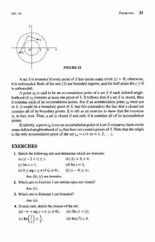
An open set S is connected if each pair of points z i and z2 in it can be joinedby a polygonal line, consisting of a finite number of line segments joined end to end,that lies entirely in S. The open set Izl < I is connected. The annulus 1 < IzI < 2 is,of course, open and it is also connected (see Fig. 16). An open set that is connectedis called a domain. Note that any neighborhood is a domain. A domain together withsome, none, or all of its boundary points is referred to as a region.
SEC. 10
FIGURE 16
EXERCISES 31
A set S is bounded if every point of S lies inside some circle lzj = R; otherwise,it is unbounded. Both of the sets (3) are bounded regions, and the half plane Re z > 0is unbounded.
A point z0 is said to be an accumulation point of a set S if each deleted neigh-borhood of z0 contains at least one point of S. It follows that if a set S is closed, thenit contains each of its accumulation points. For if an accumulation point z0 were notin S, it would be a boundary point of S; but this contradicts the fact that a closed setcontains all of its boundary points. It is left as an exercise to show that the converseis, in fact, true. Thus, a set is closed if and only if it contains all of its accumulationpoints.
Evidently, a point z0 is not an accumulation point of a set S whenever there existssome deleted neighborhood of z0 that does not contain points of S. Note that the originis the only accumulation point of the set z, = i/n (n = 1, 2, ...).
EXERCISES
1. Sketch the following sets and determine which are domains:
(a)Iz-2+iI<1; (b)E2z+31>4;(c) Im z > 1;
(e)O<argz<n/4(z34 O);
Ans. (b), (c) are domains.
(d) Im z = 1;
(f)Iz-4!>>lzl.
2. Which sets in Exercise I are neither open nor closed?
Ans. (e).
3. Which sets in Exercise 1 are bounded?
Ans. (a).
4. In each case, sketch the closure of the set:
(a) -rr < arg z < 7r (z 34 0); (b)JRezj<Izi;
(c) Re C L < 1; (d) Re(z2) > 0.z 2
32 COMPLEX NUMBERS CHAP. I
5. Let S be the open set consisting of all points z such that I z I < 1 or (z - 21 < 1. State whyS is not connected.
6. Show that a set S is open if and only if each point in S is an interior point.
7. Determine the accumulation points of each of the following sets:
(a) z = i" (n = 1, 2, ...); (b) z,, = i"/n (n = 1, 2, ...);
(c) 0 < arg z < n/2 (z 34 0); (d) zn = (-1)n(1+ i) n n
1 (n = 1, 2, ...).
Ans. (a) None; (b) 0; (d) ±(1 + i).
8. Prove that if a set contains each of its accumulation points, then it must be a closed set.
9. Show that any point zp of a domain is an accumulation point of that domain,
10. Prove that a finite set of points z1, z2, ... , z, cannot have any accumulation points.
CHAPTER
2ANALYTIC FUNCTIONS
We now consider functions of a complex variable and develop a theory of differenti-ation for them. The main goal of the chapter is to introduce analytic functions, whichplay a central role in complex analysis.
FUNCTIONS OF A COMPLEX VARIABLE
Let S be a set of complex numbers. A function f defined on S is a rule that assigns toeach z in S a complex number w. The number w is called the value of f at z and isdenoted by f (z), that is, w = f (z). The set S is called the domain of definition of f.*
It must be emphasized that both a domain of definition and a rule are needed inorder for a function to be well defined. When the domain of definition is not mentioned,we agree that the largest possible set is to be taken. Also, it is not always convenientto use notation that distinguishes between a given function and its values.
EXAMPLE 1. If f is defined on the set z 0 0 by means of the equation w = 1/z, itmay be referred to only as the function w = l/z, or simply the function 1/z.
Suppose that w = u + i v is the value of a function f at z = x + iy, so that
u -I- iv= f (x+iy).
* Although the domain of definition is often a domain as defined in Sec. 10, it need not be.
34 ANALYTIC FUNCTIONS CHAP. 2
Each of the real numbers u and v depends on the real variables x and y, and it followsthat f (z) can be expressed in terms of a pair of real-valued functions of the realvariables x and y:
(1) f(z) = u(x, y + i v (x, Y).
If the polar coordinates r and 8, instead of x and y, are used, then
u + i v = f (r
where w = u + iv and z = rein. In that case, we may write
(2) f (z) = u (r, 8
EXAMPLE 2. If f (z) = z2, then
f(x+iy)=(x+iy)2=x2-y2+i2xy.Hence
u(x, y) = x2 - y2 and v(x, y) = 2xy.
When polar coordinates are used,
2 = r2ei20 = r2 cos 28 + ir2 sin 28.
Consequently,
u(r, 8) = r2 cos 28 and v(r, 8) = r2 sin 28.
If, in either of equations (1) and (2), the function v always has value zero, thenthe value of f is always real. That is, f is a real-valued function of a complex variable.
EXAMPLE 3. A real-valued function that is used to illustrate some importanconcepts later in this chapter is
f(Z)=IZ12=x2+y2+ i0.
If n is zero or a positive integer and if a0, a1, a2, ... , an are complex constants,where an * 0, the function
P(z)=.a0+a1Z+a2Z2+...+a, Zn
is a polynomial of degree n. Note that the sum here has a finite number of terms and thatthe domain of definition is the entire z plane. Quotients P(z) /Q(z) of polynomials arecalled rational, functions and are defined at each point z where Q(z) * 0. Polynomialsand rational functions constitute elementary, but important, classes of functions of acomplex variable.
SEC. I I EXERCISES 35
A generalization of the concept of function is a rule that assigns more than onevalue to a point z in the domain of definition. These multiple-valued functions occurin the theory of functions of a complex variable, just as they do in the case of realvariables. When multiple-valued functions are studied, usually just one of the possiblevalues assigned to each point is taken, in a systematic manner, and a (single-valued)function is constructed from the multiple-valued function.
EXAMPLE 4. Let z denote any nonzero complex number. We know from Sec. 8that z 1/2 has the two values
z 1/2 = ± exp
where r = Ezl and (O(-7r < 0 < 7r) is the principal value of arg z. But, if we chooseonly the positive value of + and write
(3) f(z) = exp( i (r > 0, -1r < 0 < rr),
the (single-valued) function (3) is well defined on the set of nonzero numbers in the zplane. Since zero is the only square root of zero, we also write f (0) = 0. The functionf is then well defined on the entire plane.
EXERCISES
1. For each of the functions below, describe the domain of definition that is understood:
(a) f (z) =z21
1; (b) f (z) = Arg
Z(d) f (z) _
z+<,
1 -Izi2.
Ans. (a) z +i ; (c) Re z 0 0.
2. Write the function f (z) = z3 + z + 1 in the form f (z) = u(x, y) + iv(x, y).
Ans. (x3 - 3xy2 + x + 1) + i (3x2y - y3 + y).
3. Suppose that f (z) = x2 -sions (see Sec. 5)
- 2y + i (2x - 2xy), where z = x + iy. Use the expres-
x - z+zand
y
_z2 2i
to write f (z) in terms of z, and simplify the result.
Ans. z2 + 2i z.
4. Write the function
f(z)=z+- (z0O)
36 ANALYTIC FUNCTIONS CHAP. 2
in 6.
12. MAPPINGS
Properties of a real-valued function of a real variable are often exhibited by the graphof the function. But when w = f (z), where z and w are complex, no such convenientgraphical representation of the function f is available because each of the numbersz and w is located in a plane rather than on a line. One can, however, display someinformation about the function by indicating pairs of corresponding points z = (x, y)and w = (u, v). To do this, it is generally simpler to draw the z and w planes separately.
When a function f is thought of in this way, it is often referred to as a mapping,or transformation. The image of a point z in the domain of definition S is the pointw = f (z), and the set of images of all points in a set T that is contained in S is calledthe image of T. The image of the entire domain of definition S is called the range off. The inverse image of a point w is the set of all points z in the domain of definitionof f that have w as their image. The inverse image of a point may contain just onepoint, many points, or none at all. The last case occurs, of course, when w is not in therange of f.
Terms such as translation, rotation, and reflection are used to convey dominantgeometric characteristics of certain mappings. In such cases, it is sometimes convenientto consider the z and w planes to be the same. For example, the mapping
iy,
where z = x + iy, can be thought of as a translation of each point z one unit to theright. Since i = e`,'2, the mapping
r exp
where z = ret9, rotates the radius vector for each nonzero point z through a right angleabout the origin in the counterclockwise direction; and the mapping
transforms each point z = x + iy into its reflection in the real axis.More information is usually exhibited by sketching images of curves and regions
than by simply indicating images of individual points. In the following examples, weillustrate this with the transformation w = z2.
We begin by finding the images of some curves in the z plane.
SEC. 12 MAPPINGS 37
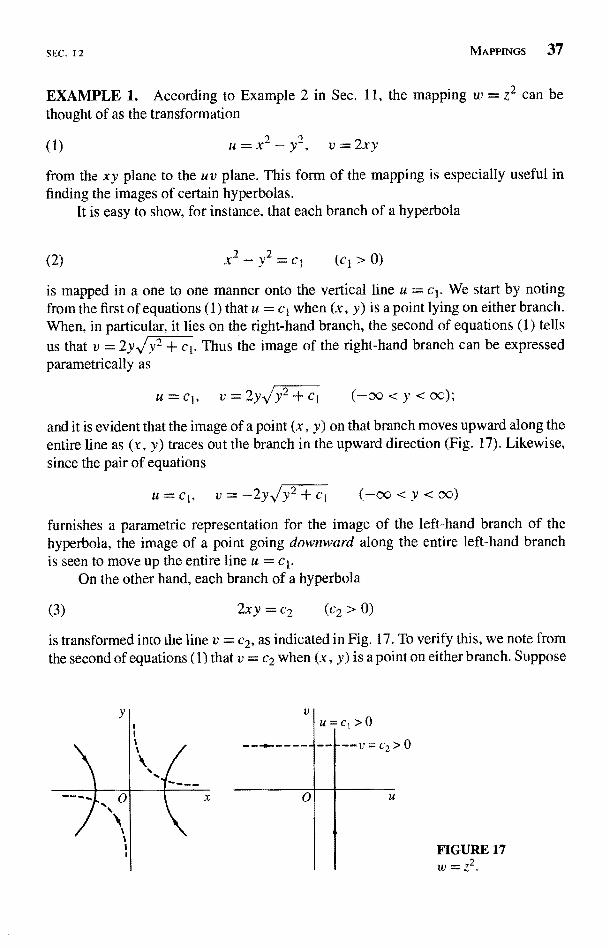
EXAMPLE 1. According to Example 2 in Sec. 11, the mapping w = 42 can bethought of as the transformation
(1)2u=x -y`, v=2xy
from the xy plane to the uv plane. This form of the mapping is especially useful infinding the images of certain hyperbolas.
It is easy to show, for instance, that each branch of a hyperbola
(2) x2-y2=c1 (ci>0)
is mapped in a one to one manner onto the vertical line u = c1. We start by notingfrom the first of equations (1) that u = c1 when (x, y) is a point lying on either branch.When, in particular, it lies on the right-hand branch, the second of equations (1) tellsus that v = 2y y2 + ci. Thus the image of the right-hand branch can be expressedparametrically as
v = 2y y2 + ci (-oo < y < 0c);
and it is evident that the image of a point (x, y) on that branch moves upward along theentire line as (x, y) traces out the branch in the upward direction (Fig. 17). Likewise,since the pair of equations
U = C v = -2y-2y/y2 +c1 (-oc<y<00)
furnishes a parametric representation for the image of the left-hand branch of thehyperbola, the image of a point going downward along the entire left-hand branchis seen to move up the entire line is = c1.
On the other hand, each branch of a hyperbola
(3) 2xy = c2 (c2 > 0)
is transformed into the line v = c2, as indicated in Fig. 17. To verify this, we note fromthe second of equations (1) that v = c2 when (x, y) is a point on either branch. Suppose
V
u=Cl >0
4--V = C2>0
U
FIGURE 17w =Z2.
38 ANALYTIC FUNCTIONS CHAP. 2
that it lies on the branch lying in the first quadrant. Then, since y = c21(2x), the firstof equations (1) reveals that the branch's image has parametric representation
cu=x2- 2, V4x2
Observe that
c2 (0<x<c ).
lim u = -oo and lim u = 00.x-#a x-+0ox>0
Since u depends continuously on x, then, it is clear that as (x, y) travels down the entireupper branch of hyperbola (3), its image moves to the right along the entire horizontalline v = c2. Inasmuch as the image of the lower branch has parametric representation
and since
lim u}'-+-00
and lim uy-#0y<0
it follows that the image of a point moving upward along the entire lower branch alsotravels to the right along the entire line v = c2 (see Fig. 17).
We shall now use Example i to find the image of a certain region.
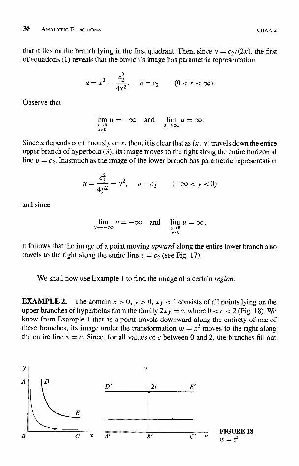
EXAMPLE 2. The domain x > 0, y > 0, xy < 1 consists of all points lying on theupper branches of hyperbolas from the family 2xy = c, where 0 < c < 2 (Fig. 18). Weknow from Example 1 that as a point travels downward along the entirety of one ofthese branches, its image under the transformation w = z2 moves to the right alongthe entire line v = c. Since, for all values of c between 0 and 2, the branches fill out
V
v=c2 (-oo <y
2i E`
C AB
CFIGURE 18
X, U w-z
SEC. 12 MAPPINGS 39
the domain x > 0, y > 0, xy < 1, that domain is mapped onto the horizontal strip0<v<2.
In view of equations (1), the image of a point (0, y) in the z plane is (-y2, 0).Hence as (0, y) travels downward to the origin along the y axis, its image moves to theright along the negative u axis and reaches the origin in the w plane. Then, since theimage of a point (x, 0) is (x2, 0), that image moves to the right from the origin alongthe u axis as (x, 0) moves to the right from the origin along the x axis. The imageof the upper branch of the hyperbola xy = 1 is, of course, the horizontal line v = 2.Evidently, then, the closed region x > 0, y ? 0, xy < 1 is mapped onto the closed strip0 < v < 2, as indicated in Fig. 18.
Our last example here illustrates how polar coordinates can be useful in analyzingcertain mappings.
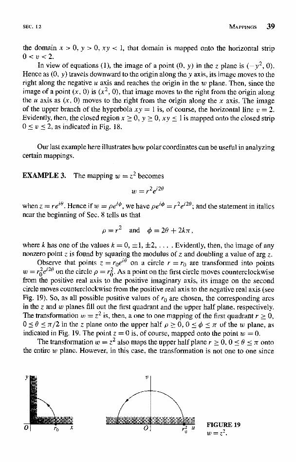
EXAMPLE 3. The mapping w = z2 becomes
w = r2e`20
when z = re`s. Hence if w = pe'O, we have pe`0 = r2ei20; and the statement in italicsnear the beginning of Sec. 8 tells us that
p=r2 and 0=20+2krr,where k has one of the values k = 0, ±1, ±2, .... Evidently, then, the image of anynonzero point z is found by squaring the modulus of z and doubling a value of arg z.
Observe that points z = roe'° on a circle r = re are transformed into pointsw = roei20 on the circle p = r0. As a point on the first circle moves counterclockwisefrom the positive real axis to the positive imaginary axis, its image on the secondcircle moves counterclockwise from the positive real axis to the negative real axis (seeFig. 19). So, as all possible positive values of r0 are chosen, the corresponding arcsin the z and w planes fill out the first quadrant and the upper half plane, respectively.The transformation w = z2 is, then, a one to one mapping of the first quadrant r > 0,0 < 0 < -r/2 in the z plane onto the upper half p > 0, 0 <,o < r of the w plane, asindicated in Fig. 19. The point z = 0 is, of course, mapped onto the point w = 0.
The transformation w = z2 also maps the upper half plane r > 0, 0 < 0 < -r ontothe entire w plane. However, in this case, the transformation is not one to one since
FIGURE 19w = z2.
40 ANALYTIC FUNCTIONS CHAP. 2
both the positive and negative real axes in the z plane are mapped onto the positivereal axis in the w plane.
When n is a positive integer greater than 2, various mapping properties of thetransformation w = zn, or pe`O = r"ein9, are similar to those of w = z2. Such atransformation maps the entire z plane onto the entire w plane, where each nonzeropoint in the w plane is the image of n distinct points in the z plane. The circle r = r0is mapped onto the circle p = ro; and the sector r < r0, 0 < 8 < 2n/n is mapped ontothe disk p < ro, but not in a one to one manner.
13. MAPPINGS BY THE EXPONENTIAL FUNCTION
In Chap. 3 we shall introduce and develop properties of a number of elementary func-tions which do not involve polynomials. That chapter will start with the exponentialfunction
z = x e
(1) e e e (z=x+iy),
the two factors ex and e`y being well defined at this time (see Sec. 6). Note thatdefinition (1), which can also be written
ex+iy =
is suggested by the familiar property
exl+x2 = exiex2
of the exponential function in calculus.The object of this section is to use the function ez to provide the reader with
additional examples of mappings that continue to be reasonably simple. We begin byexamining the images of vertical and horizontal lines.
EXAMPLE 1. The transformation
(2)
can be written pex ' = exe`y, where z = x + iy and w = pet '. Thus p = ex and(k = y + 2nn, where n is some integer (see Sec. 8); and transformation (2) can beexpressed in the form
(3) p= ex, (01=y.
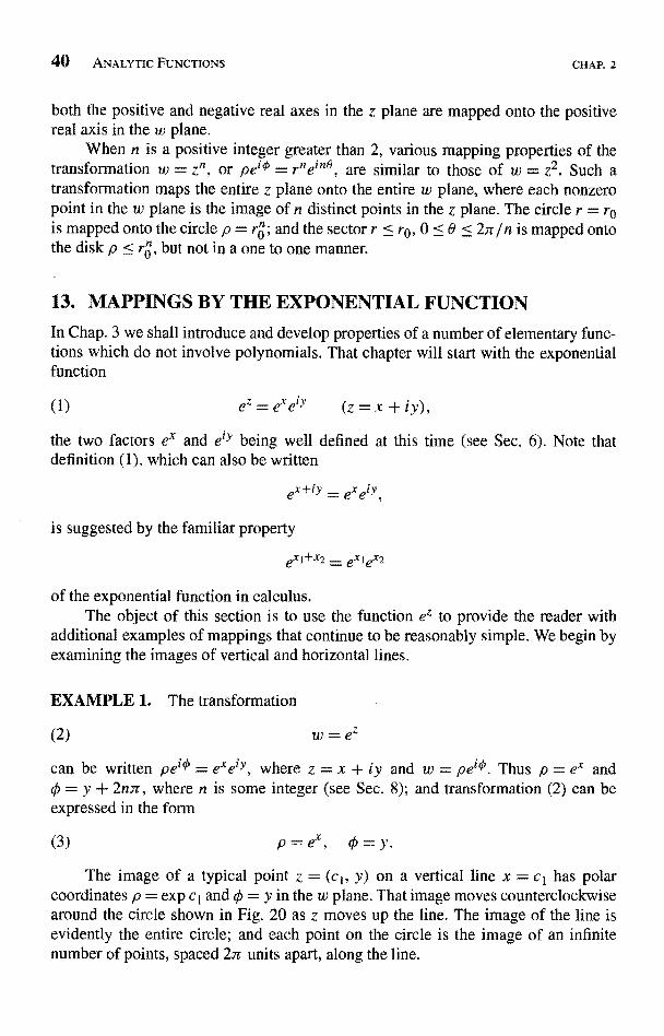
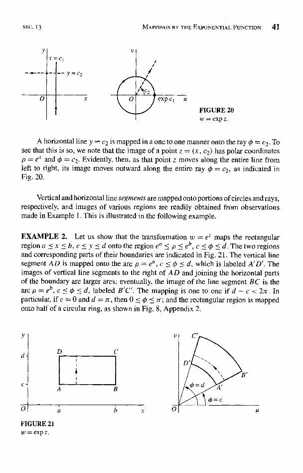
The image of a typical point z = (c1, y) on a vertical line x = Cr has polarcoordinates p = exp ct and 0 = y in the w plane. That image moves counterclockwisearound the circle shown in Fig. 20 as z moves up the line. The image of the line isevidently the entire circle; and each point on the circle is the image of an infinitenumber of points, spaced 2n units apart, along the line.
SEC. 13 MAPPINGS BY THE EXPONENTIAI. FUNCTION 41
V
.1=C
0FIGURE 20In = exp Z.
A horizontal line y = c2 is mapped in a one to one manner onto the ray 0 = c2. Tosee that this is so, we note that the image of a point z = (x, c2) has polar coordinatesp = ex and 0 = c2. Evidently, then, as that point z moves along the entire line fromleft to right, its image moves outward along the entire ray 0 = c2, as indicated inFig. 20.
Vertical and horizontal line segments are mapped onto portions of circles and rays,respectively, and images of various regions are readily obtained from observationsmade in Example 1. This is illustrated in the following example.
EXAMPLE 2. Let us show that the transformation w = ez maps the rectangularregion a < x < h, c < y < d onto the region e' < p < eb, c < 0 < d. The two regionsand corresponding parts of their boundaries are indicated in Fig. 21. The vertical linesegment AD is mapped onto the are p = e°, c < 0 < d, which is labeled A'D'. Theimages of vertical line segments to the right of AD and joining the horizontal partsof the boundary are larger arcs; eventually, the image of the line segment BC is theare p = eb, c < 0 < d, labeled B'C'. The mapping is one to one if d - c < 2n. Inparticular, if c = 0 and d = -r, then 0 < 0 < -r; and the rectangular region is mappedonto half of a circular ring, as shown in Fig. 8, Appendix 2.
y
C1
0
D C
B
FIGURE 21w = exp Z.
42 ANALYTIC FUNCTIONS CHAP. 2
Our final example here uses the images of horizontal lines to find the image of ahorizontal strip.
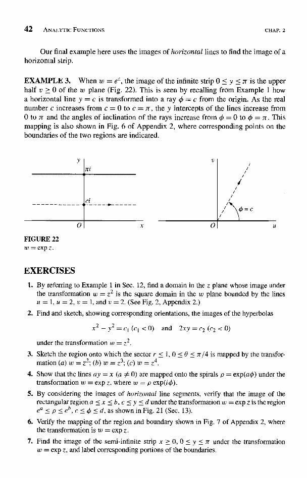
EXAMPLE 3. When w = eZ, the image of the infinite strip O < y ir is the upperhalf v > 0 of the w plane (Fig. 22). This is seen by recalling from Example 1 howa horizontal line y = c is transformed into a ray 0 = c from the origin. As the realnumber c increases from c = 0 to c = ar, the y intercepts of the lines increase from0 to -r and the angles of inclination of the rays increase from (k = 0 to (k = '-r. Thismapping is also shown in Fig. 6 of Appendix 2, where corresponding points on theboundaries of the two regions are indicated.
Y
0
FIGURE 22w=expz.
EXERCISES
x U
1. By referring to Example 1 in Sec. 12, find a domain in the z plane whose image underthe transformation w = z2 is the square domain in the w plane bounded by the linesu = 1, u = 2, v = 1, and v = 2. (See Fig. 2, Appendix 2.)
2. Find and sketch, showing corresponding orientations, the images of the hyperbolas
x2 - y2 = Cl (c1 < 0) and 2xy = c2 (c2 < 0)
under the transformation w = z2.
3. Sketch the region onto which the sector r < 1, 0 < 0 < it/4 is mapped by the transfor-mation (a) w = z2; (b) w = z3; (c) w = z4.
4. Show that the lines ay = x (a 0) are mapped onto the spirals p = exp(a i) under thetransformation w = exp z, where w = p exp(ir5).
5. By considering the images of horizontal line segments, verify that the image of therectangular region a < x < b, c < y < d under the transformation w = exp z is the regionea < p < e", c < 0 < d, as shown in Fig. 21 (Sec. 13).
6. Verify the mapping of the region and boundary shown in Fig. 7 of Appendix 2, wherethe transformation is w = exp z.
7. Find the image of the semi-infinite strip x > 0, 0 < y < 1r under the transformationw = exp z, and label corresponding portions of the boundaries.
ni
V
Cl
SEC. 14 LIMrrs 43
8. One interpretation of a function w = f (z) = u (x, y) + i v(x, y) is that of a vector field inthe domain of definition of f . The function assigns a vector w, with components u(x, y)and v(x, y), to each point z at which it is defined. Indicate graphically the vector fieldsrepresented by (a) w = iz; (b) w = z/Iz1.
14. LIMITSLet a function f be defined at all points z in some deleted neighborhood (Sec. 10) ofzo. The statement that the limit of f (z) as z approaches zo is a number wo, or that
{1) lim, f (z) = wo,--1zp
means that the point w = f (z) can be made arbitrarily close to wo if we choose thepoint z close enough to zo but distinct from it. We now express the definition of limitin a precise and usable form.
Statement (1) means that, for each positive number s, there is a positive numberS such that
(2) If (z) - wo whenever 0 < l.. - zol < S.
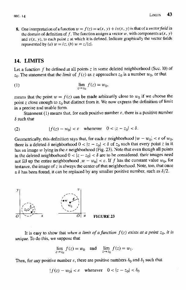
Geometrically, this definition says that, for each e neighborhood Iw - woI < s of wo,there is a deleted 8 neighborhood 0 < Iz - zol < S of zo such that every point z in ithas an image w lying in the e neighborhood (Fig. 23). Note that even though all pointsin the deleted neighborhood 0 < Iz - zoI < S are to be considered, their images neednot fill up the entire neighborhood Iw - woI < e. If f has the constant value wo, forinstance, the image of z is always the center of that neighborhood. Note, too, that oncea S has been found, it can be replaced by any smaller positive number, such as 3/2.
V
0
w
S Wp jlz0 )
x U FIGURE 23
It is easy to show that when a limit of a function f (z) exists at a point zo, it isunique. To do this, we suppose that
lim f (z) = wo and lim f (z) = w1.z-+zo Z- O
Then, for any positive number e, there are positive numbers So and S1 such that
if (z) - wol < 8 whenever 0 < Iz - zol < 30
44 ANALYTIC FUNCTIONS CHAP. 2
and
If (z) - wiI <e whenever 0 < Iz - zol < Si.
So if 0 < Iz - zol < 8, where 8 denotes the smaller of the two numbers 8o and 81, wefind that
Iwi-wol=I[.f(z)-wo]-[f(z)-wi]l: I.f(z)-wol+If(z)-wit<8+8=2e.But 1 w 1 - wo I is a nonnegative constant, and s can be chosen arbitrarily small. Hence
w1-wo=0, or w1=wo.
Definition (2) requires that f be defined at all points in some deleted neighbor-hood of zo. Such a deleted neighborhood, of course, always exists when zo is an interiorpoint of a region on which f is defined. We can extend the definition of limit to the casein which zo is a boundary point of the region by agreeing that the first of inequalities(2) need be satisfied by only those points z that lie in both the region and the deletedneighborhood.
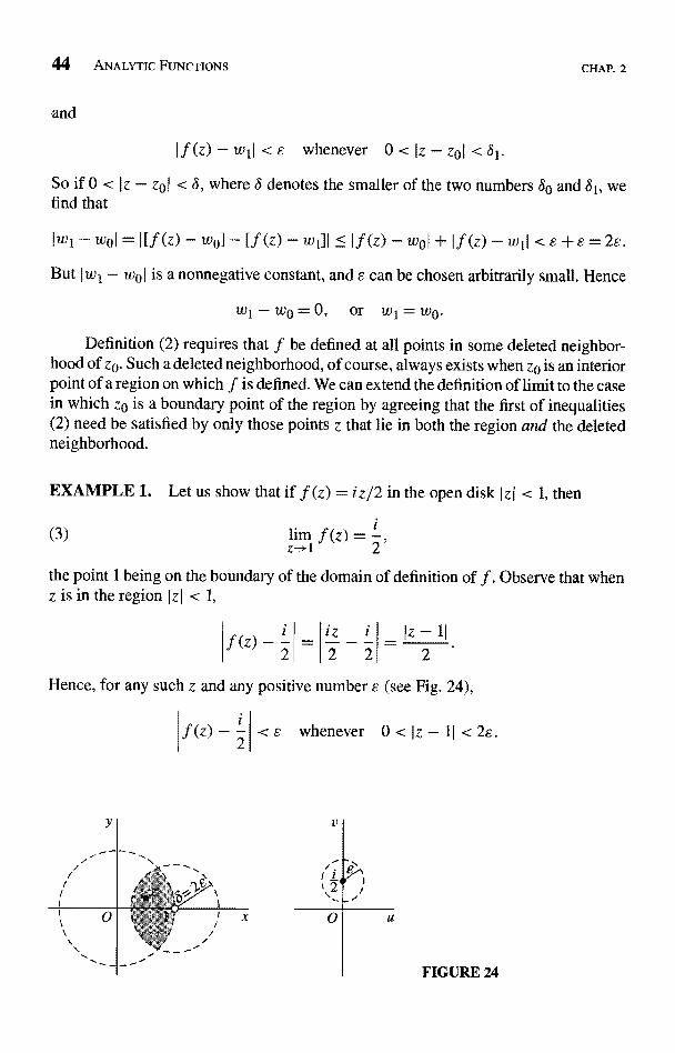
EXAMPLE 1. Let us show that if f (z) = iz/2 in the open disk Izj < 1, then
(3) lim f (z) = =,z->1 2
the point 1 being on the boundary of the domain of definition of f . Observe that whenz is in the region I z I < 1,
.f(z)-2iz i _Iz-112 2
_2
Hence, for any such z and any positive number £ (see Fig. 24),
f(z) -2
V I
/' 1
l 2
0
FIGURE 24
< e whenever 0 < Iz - 11 < 2e.
SEC. 14 LIMITS 45
Thus condition (2) is satisfied by points in the region IzJ < 1 when S is equal to 2e orany smaller positive number.
If z0 is an interior point of the domain of definition of f, and limit (1) is toexist, the first of inequalities (2) must hold for all points in the deleted neighborhood0 < Iz - zol < S. Thus the symbol z -3 z0 implies that z is allowed to approach z0in an arbitrary manner, not just from some particular direction. The next exampleemphasizes this.
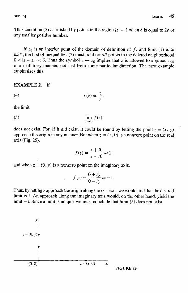
EXAMPLE 2. If
(4)
the limit
(5) lim f (z)z---> 0
does not exist. For, if it did exist, it could be found by letting the point z = (x, y)approach the origin in any manner. But when z = (x, 0) is a nonzero point on the realaxis (Fig. 25),
(z)x+i0f _ = 1;x-i0
and when z = (0, y) is a nonzero point on the imaginary axis,
0+iyf (Z) =0-ivThus, by letting z approach the origin along the real axis, we would find that the desiredlimit is 1. An approach along the imaginary axis would, on the other hand, yield thelimit -1. Since a limit is unique, we must conclude that limit (5) does not exist.
z=(0,y)
(0,0)1
z=(x,0) xFIGURE 25
46 ANALYTIC FUNCTIONS CHAP. 2
While definition (2) provides a means of testing whether a given point wo is alimit, it does not directly provide a method for determining that limit. Theorems onlimits, presented in the next section, will enable us to actually find many limits.
15. THEOREMS ON LIMITSWe can expedite our treatment of limits by establishing a connection between limitsof functions of a complex variable and limits of real-valued functions of two realvariables. Since limits of the latter type are studied in calculus, we use their definitionand properties freely.
Theorem 1. Suppose that
f(z)=u(x,y)+iv
Then
(1)
if and only if
y
z->z
iyo, and w0=uo+ivo.
(2) lim u(x, y) = uo and lim v(x, y) = vo.(x>Y)-(xo,Yo) (x,Y)->(xo,yo)
To prove the theorem, we first assume that limits (2) hold and obtain limitLimits (2) tell us that, for each positive number s, there exist positive numbers S1 andS2 such that
(3) lu - uol < - whenever 0 < x -x0)2 + (y - y0)2 < S
and
(4) Iv - vol < whenever 0 < (x - x0)2 + (y - yo)2 < b2.
Let b denote the smaller of the two numbers S1 and 82. Since
I(u+iv
and
(u0+iv0)I=1(u-u0
y-yo)2
u01+ V - vol
xo)+i(y-yo)I=1(x+iy)-(x0
it follows from statements (3) and (4) that
iv) - (u0+ivo)I < s 6
iyo)
SEC. 15 THEOREMS ON LIMITS 47
whenever
iy) - (x0 + iy0)I < S.
That is, limit (1) holds.Let us now start with the assumption that limit (1) holds. With that assumption,
we know that, for each positive number s, there is a positive number 6 such that
(u+iv)-(uo+ivo)I <s
But
and
0<I(x+iy)-(xo+iyo S.
lu - uol <l(u-uo)+i(v-vo)1 =I (u+iv) 0 ivo)I,
Iv - vol < I(u-uo)+i(v-vo)l=I(u+iv)-(uo+ivo)I,
I(x + iy) - (xo + iyo) =J(x---xo)+i(y-yo)I= (x-x0)2+(y-Yo)2
Hence it follows from inequalities (5) and (6) that
whenever
lu-uol <s and Iv-v0J <s
0 < (x - x0)2-+(y - yo)2 < S.
This establishes limits (2), and the proof of the theorem is complete.
Theorem 2. Suppose that
(7)
Then
z-+zo+ F(z)1 = wo
lim [f (z)F(z)] = w0 W0;z-+zo
lim f (z) = w0Z-+zo F(z) Wo
lim f (z) = w0 and lim F(z) = W0.Z-+ZO Z--- >Zo
48 ANALYTIC FUNCTIONS CHAP. 2
This important theorem can be proved directly by using the definition of the limitof a function of a complex variable. But, with the aid of Theorem 1, it follows almostimmediately from theorems on limits of real-valued functions of two real variables.
To verify property (9), for example, we write
f(z) = u(x, y) + i v(x, y), F(z) = U (x, y) + i V (x, y),
= xo o, W0=uo+iV0. W0=U0+iVO.
Then, according to hypotheses (7) and Theorem 1, the limits as (x, y) approaches(xo, yo) of the functions u, v, U, and V exist and have the values uo, vo, U0, and V0,
respectively. So the real and imaginary components of the product
f(z)F(z)=(uU-vV)+i(vU+uV)have the limits u0U0 - v0V0 and v0U0 + u0V0, respectively, as (x, y) approaches(xo, yo). Hence, by Theorem I again, f (z)F(z) has the limit
(uoUo - vo Vo) + i (v0U0 + uoVo)
as z approaches z0; and this is equal to w0W0. Property (9) is thus established.Corresponding verifications of properties (8) and (10) can be given.
It is easy to see from definition (2), Sec. 14, of limit that
lim c = c andz--'z0 4-y z0
= zo,
where zo and c are any complex numbers; and, by property (9) and mathematical
induction, it follows that
Jim z n = Z' (n = 1, 2, ...).Z--Z0
So, in view of properties (8) and (9), the limit of a polynomial
P(z) = ao + a]z + a2Z2 + ... + anZn
as z approaches a point zo is the value of the polynomial at that point:
(11} lim P(z) = P(zo).Z->ZO
16. LIMITS INVOLVING THE POINT AT INFINITY
It is sometimes convenient to include with the complex plane the point at infinity,denoted by oo, and to use limits involving it. The complex plane together with thispoint is called the extended complex plane. To visualize the point at infinity, one canthink of the complex plane as passing through the equator of a unit sphere centered atthe point z = 0 (Fig. 26). To each point z in the plane there corresponds exactly onepoint P on the surface of the sphere. The point P is determined by the intersection ofthe line through the point z and the north pole N of the sphere with that surface. In
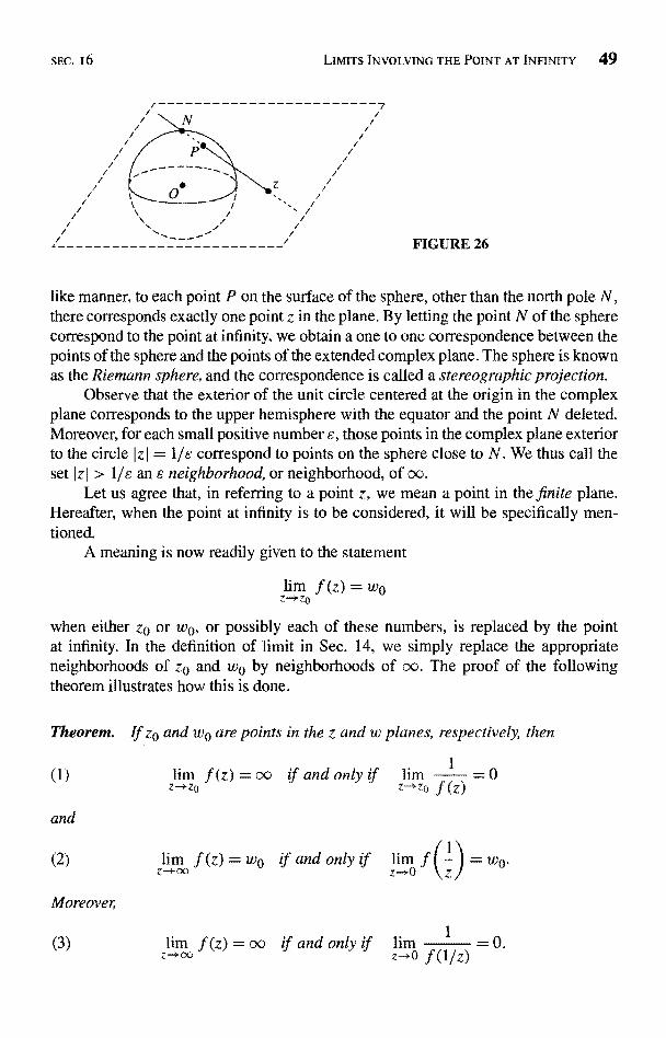
SEC. 16 LIMITS INVOLVING THE POINT AT INFINITY 49
r------------------------7
FIGURE 26
like manner, to each point P on the surface of the sphere, other than the north pole N,there corresponds exactly one point z in the plane. By letting the point N of the spherecorrespond to the point at infinity, we obtain a one to one correspondence between thepoints of the sphere and the points of the extended complex plane. The sphere is knownas the Riemann sphere, and the correspondence is called a stereographic projection.
Observe that the exterior of the unit circle centered at the origin in the complexplane corresponds to the upper hemisphere with the equator and the point N deleted.Moreover, for each small positive number s, those points in the complex plane exteriorto the circle I z I = 1/c correspond to points on the sphere close to N. We thus call theset J z J> 11c an s neighborhood, or neighborhood, o
Let us agree that, in referring to a point z, we mean a point in the finite plane.Hereafter, when the point at infinity is to be considered, it will be specifically men-tioned.
A meaning is now readily given to the statement
zo or w0, or possibly each of these numbers, is replaced by the pointat infinity. In the definition of limit in Sec. 14, we simply replace the appropriateneighborhoods of ze and we by neighborhoods of oc. The proof of the followingtheorem illustrates how this is done.
Theorem. If ze and we are points in the z and w planes, respectively, then
lim f (z) = oo if and only ifz->zo
limz->00
limZ-+00
z--+zo
if and only if liz 0
if and only if lim
1
(z)
1
z)
=0
0
50 ANALYTIC FUNCTIONS CHAP. 2
We start the proof by noting that the first of limits (1) means that, for each positivenumber s, there is a positive number S such that
(4) If (z) I > = whenever 0 <E
z - zol < S.
That is, the point w = f (z) lies in the s neighborhood Iw I > 1/s of oo whenever z lies
in the deleted neighborhood 0 < Iz - zol < S of zo. Since statement (4) can be written
I-0
f (z)<s whenever 0< Iz-zol <S,
the second of limits (1) follows.The first of limits (2) means that, for each positive number s, a positive number
S exists such that
(5) If (z) - woI < sl
whenever Iz I >
Replacing z by 1/z in statement (5) and then writing the result as
< s whenever 0 < Iz - OI < S,
we arrive at the second of limits (2).Finally, the first of limits (3) is to be interpreted as saying that, for each positive
number s, there is a positive number 8 such that
(6) If (z)I > s whenever IzI > 8
When z is replaced by l/z, this statement can be put in the form
I - 01 <s whenever 0 < Iz-01 <3;I f(1/z) I
and this gives us the second of limits (3).
EXAMPLES. Observe that
i z + 3 z -t- l= oo since limlim =z--1 z+1 Z-* liz+
and
hm2z + i = 2 since
1,m (2/z) + i = hm2+ i z
z- *o° z + 1 z-*o (I/z) + 1 z-*o I+ z
SEC. 17 CONTINUITY 51
Furthermore,
2z3 - 1 (1/z2) + 1 z + Z3urn = oo since lim = lim = (}.
Z2 + 1 z-*o (2/Z3) - 1 z-*o 2 - Z3
17. CONTINUITYA function f is continuous at a point zo if all three of the following conditions aresatisfied:
z-+zo(z) exists,
f (zo) exists,
z->zo (ZO)
Observe that statement (3) actually contains statements (1) and (2), since the existenceof the quantity on each side of the equation there is implicit. Statement (3) says that,for each positive number E, there is a positive number S such that
(4) If (Z) -- f(zo) < e whenever Iz - zol < S.
A function of a complex variable is said to be continuous in a region R if it iscontinuous at each point in R.
If two functions are continuous at a point, their sum and product are also continu-ous at that point; their quotient is continuous at any such point where the denominatoris not zero. These observations are direct consequences of Theorem 2, Sec. 15. Note,too, that a polynomial is continuous in the entire plane because of limit (11), Sec. 15.
We turn now to two expected properties of continuous functions whose verifica-tions are not so immediate. Our proofs depend on definition (4), and we present theresults as theorems.
Theorem 1. A composition of continuous functions is itself continuous.
A precise statement of this theorem is contained in the proof to follow. We letw = f (z) be a function that is defined for all z in a neighborhood Iz - zol < S of apoint zo, and we let W = g(w) be a function whose domain of definition contains theimage (Sec. 12) of that neighborhood under f . The composition W = g[ f (z) ] is, then,defined for all z in the neighborhood I z - zo I < S. Suppose now that f is continuous atzo and that g is continuous at the point f (zo) in the w plane. In view of the continuityof g at f (zo), there is, for each positive number s, a positive number y such that
Ig[f (z)] - g[f (zo)]I < e whenever If (z) - f (zo) I < y.
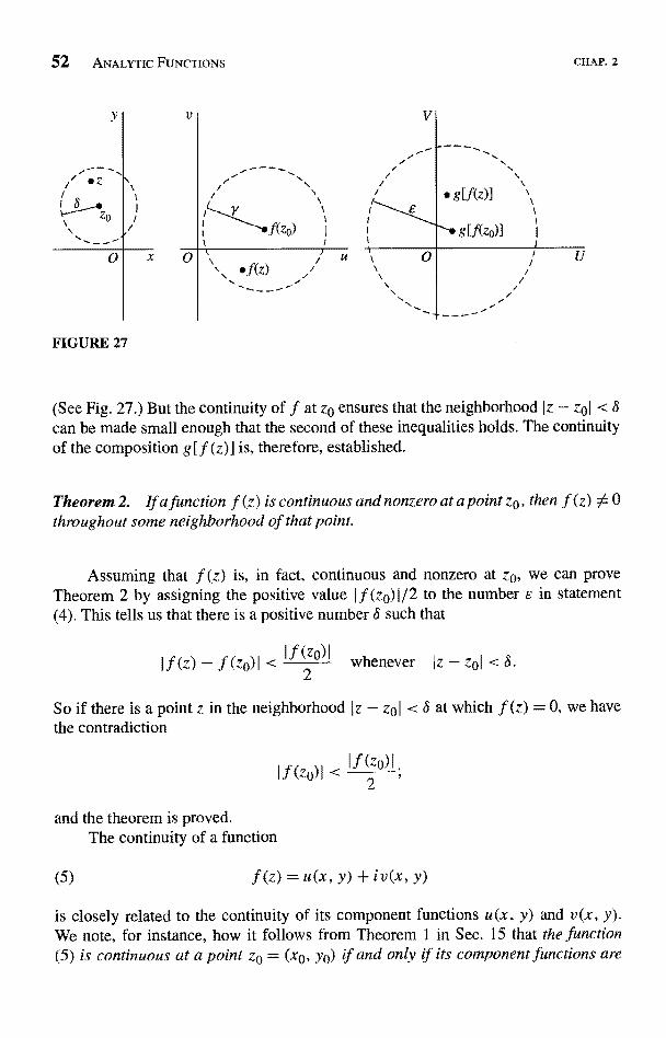
52 ANALYTIC FUNCTIONS
Zo
0
FIGURE 27
CHAP. 2
(See Fig. 27.) But the continuity off at z0 ensures that the neighborhood Iz - zol < Scan be made small enough that the second of these inequalities holds. The continuityof the composition g[f (z)] is, therefore, established.
Theorem 2. If a function f (z) is continuous and nonzero at a point z0, then f (z) 56throughout some neighborhood of that point.
Assuming that f (z) is, in fact, continuous and nonzero at zo, we can proveTheorem 2 by assigning the positive value If (zo) 1/2 to the number £ in statement(4). This tells us that there is a positive number 8 such that
If (z) - f (z0) I whenever Iz - zo1 < S.(zo) I
2
So if there is a point z in the neighborhood Iz - zol < S at which f (z) = 0, we havethe contradiction
I f (zo) I
and the theorem is proved.The continuity of a function
(5) f (z) = u(x, Y) + iv(x, Y)
is closely related to the continuity of its component functions u(x, y) and v(x, y).We note, for instance, how it follows from Theorem 1 in Sec. 15 that the function(5) is continuous at a point zo = (x0, yo) if and only if its component functions are
SEC. 1 7 EXERCISES 5
continuous there. To illustrate the use of this statement, suppose that the function (5) iscontinuous in a region R that is both closed and bounded (see Sec. 10). The function
y)]2 + [v(x, y)]2
is then continuous in R and thus reaches a maximum value somewhere in that region.*That is, f is bounded on R and If (z) I reaches a maximum value somewhere in R.More precisely, there exists a nonnegative real number M such that
(6) lf(z)I <M forallzinR,
where equality holds for at least one such z.
EXERCISES
1. Use definition (2), Sec. 14, of limit to prove that2z(a) lim Re z = Re z0; (b) lim z = Z0; (c) lim = 0.
z-'z0 z-'zo z-*0 z
2. Let a, b, and c denote complex constants. Then use definition (2), Sec. 14, of limit toshow that
(a) lim (az + b) = az0 + b; (b) lim (z2 + c)Z "."* Zo Z-* Zo
(c) lim [x + i(2x + y)] = 1+ i (z = x + iy).z-*3-i
3. Let n be a positive integer and let P (z) and Q(z) be polynomials, where Q(zo) } 0. UseTheorem 2 in Sec. 15 and limits appearing in that section to find-(a) lim n (z0 54 0); (b) Him
& z1; (c) lim P z)
Z oz Z-i z-+-i z-zoQ(z)Ans. (a) 1/za; (b) 0; (c) P(z0)l Q(z0).
4. Use mathematical induction and property (9), Sec. 15, of limits to show that
lim zn = zQz-> zo
when n is a positive integer (n = 1, 2, ...).
5. Show that the limit of the function
f(z)=
as z tends to 0 does not exist. Do this by letting nonzero points z = (x, 0) and z = (x, x)approach the origin. [Note that it is not sufficient to simply consider points z = (x, 0)and z = (0, y), as it was in Example 2, Sec. 14.]
* See, for instance, A. E. Taylor and W. R. Mann, "Advanced Calculus," 3d ed., pp. 125-126 and p. 529,1983.
54 ANALYTIC FUNCTIONS CHAP. 2
6. Prove statement (8) in Theorem 2 of Sec. 15 using
(a) Theorem 1 in Sec. 15 and properties of limits of real-valued functions of two realvariables;
(b) definition (2), Sec. 14, of limit.
7. Use definition (2), Sec. 14, of limit to prove that
if lim f (z) = wo, then urn If (z) I =z-> Zo Z-* Zo
Suggestion: Observe how inequality (8), Sec. 4, enables one to write
IIf(z)I - Iwo!I If(z) - WOI
8. Write Az = z - zo and show that
lim f (z) = wo if and only if lim f (zo + Az) = wo.Z *ZO dz->o
9. Show that
lim f(Z)g(z)=0 if lim f (z) = 0z->zo
and if there exists a positive number M such that Ig (z) I < M for all z in some neighbor-hood of zo.
10. Use the theorem in Sec. 16 to show that24z
= 4; (b) l =1)2 (z 1)sz
z2 +lim
z->oGZ-
With the aid of the theorem in Sec. 16, show that when
T (z) _az + b
(ad - be A 0),cz + d
(a)
(b)
12. State why limits involving the point at infinity are unique.
13. Show that a set S is unbounded (Sec. 10) if and only if every neighborhood of the pointat infinity contains at least one point in S.
lim T(z)=oo ifc=0;Z-/00
alim T(z) _ - and urn T(z) = oo if c t- 0.c z-,-d/c
z- Zc
18. DERIVATIVES
Let f be a function whose domain of definition contains a neighborhood of a point zo.The derivative of f at zo, written f'(zo), is defined by the equation
(1) ) = Jim f (z) - .f (zo)f'(zo,Z--*zo Z - Zo
provided this limit exists. The function f is said to be differentiable at zo when itsderivative at zo exists.
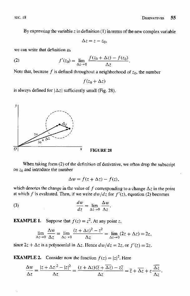
SEC. 18 DERIVATIVES 55
By expressing the variable z in definition (1) in terms of the new complex variable
Az = z - z0,
we can write that definition as
(2) f'(ze) = lim f (z0 + Az) - f (z0)Az--+o Az
Note that, because f is defined throughout a neighborhood of z0, the number
f(zo+Az)
is always defined for I Az I sufficiently small (Fig. 28).
FIGURE 28
When taking form (2) of the definition of derivative, we often drop the subscripton zo and introduce the number
Aw=f(z+Az)-f(z),which denotes the change in the value of f corresponding to a change Az in the pointat which f is evaluated. Then, if we write dw/dz for f`(z), equation (2) becomes
dw Aw(3)
_dZ 4zmO Az
EXAMPLE 1. Suppose that f (z) = z2. At any point z,
limdw = lim (z + Az)2 - z2
= lim (2z + Az) = 2z,dz-*O Az Az-*O Az nz->o
since 2z + Az is a polynomial in Az. Hence dw/dz = 2z, or f'(z) = 2z.
EXAMPLE 2, Consider now the function f (z) = Iz12. Here
Aw Iz+Azl2-1z12_(z+Az)(z+Oz)-zz Az+Az+zAz Az - Az Az
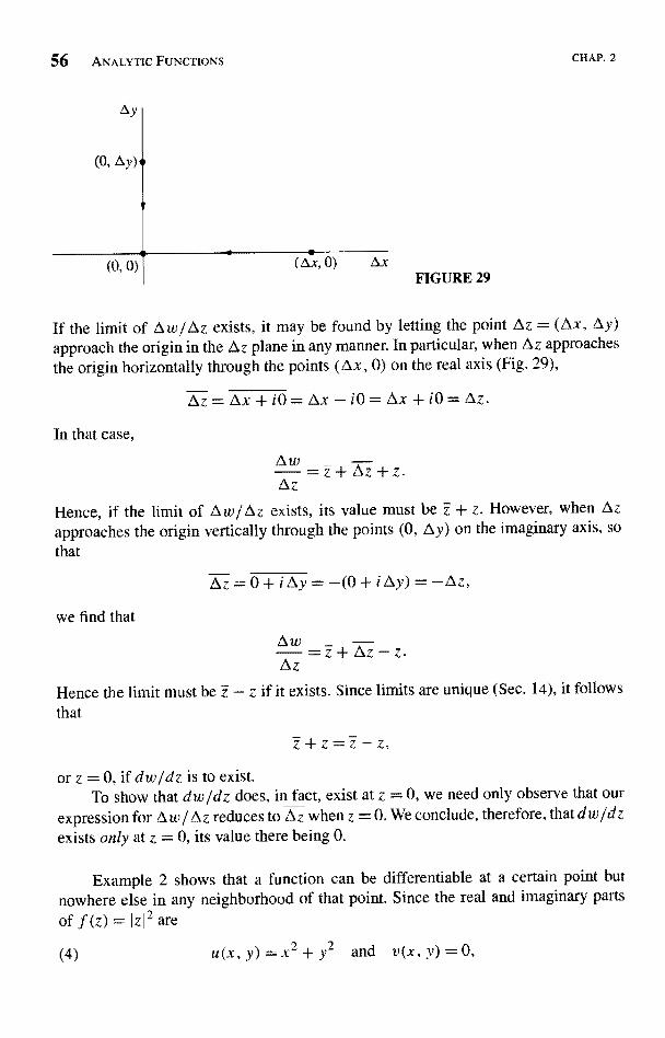
56 ANALYTIC FUNCTIONS
Ay
(0, Ay)
(0, 0) (Ax, 0) Ax
CHAP. 2
FIGURE 29
If the limit of L w/L z exists, it may be found by letting the point Az = (Ax, Ay)approach the origin in the Az plane in any manner. In particular, when dz approachesthe origin horizontally through the points (Ax, 0) on the real axis (Fig. 29),
+i0=Ax-i0=Ax +i0=Az.
In that case,
Aw =z+Az+z.
Hence, if the limit of taw/Az exists, its value must be z + z. However, when A zapproaches the origin vertically through the points (0, Ay) on the imaginary axis, so
that
=0+iAy=-(0+iLy)=-Az,we find that
- z.
Hence the limit must be i - z if it exists. Since limits are unique (Sec. 14), it follows
that
z+z=
or z = 0, if dw/dz is to exist.To show that dw/dz does, in fact, exist at z = 0, we need only observe that our
expression for A w / Az reduces to &z -when z = 0. We conclude, therefore, that d w /d z
exists only at z = 0, its value there being 0.
Example 2 shows that a function can be differentiable at a certain point butnowhere else in any neighborhood of that point. Since the real and imaginary parts
of f (z) = Iz12 are
(4) u(x, y) = x2 + y` and v(x, y) = 0,
SEC. 19 DIFFERENTIATION FORMULAS 57
respectively, it also shows that the real and imaginary components of a function of acomplex variable can have continuous partial derivatives of all orders at a point andyet the function may not be differentiable there.
The function f (Z) = Iz12 is continuous at each point in the plane since its com-ponents (4) are continuous at each point. So the continuity of a function at a pointdoes not imply the existence of a derivative there. It is, however, true that the existenceof the derivative of a junction at a point implies the continuity of the function at thatpoint. To see this, we assume that f'(zp) exists and write
lim If (z) - f (z0)] = lim f (z) - f (zo) lim (z - zc) = f'(zc) 0 = 0,Z--*Z0 z->zp Z - z0 Z--* z{}
from which it follows that
lim f (z) = .f (zo).z--+z0
This is the statement of continuity of f at zo (Sec. 17).Geometric interpretations of derivatives of functions of a complex variable are
not as immediate as they are for derivatives of functions of a real variable. We deferthe development of such interpretations until Chap. 9.
19. DIFFERENTIATION FORMULASThe definition of derivative in Sec. 18 is identical in form to that of the derivative of areal-valued function of a real variable. In fact, the basic differentiation formulas givenbelow can be derived from that definition by essentially the same steps as the ones usedin calculus. In these formulas, the derivative of a function f at a point z is denoted byeither
dzf (z) or ,f'(z),
depending on which notation is more convenient.Let c be a complex constant, and let f be a function whose derivative exists at a
point z. It is easy to show that
dzc
= 0. dzZ
1, d [cf (z)] = cf'(z).
Also, if n is a positive integer,
(2)d
n = nz'
This formula remains valid when n is a negative integer, provided that z 0 0.
58 ANALYTIC FUNCTIONS
If the derivatives of two functions f and F exist at a point z, then
[f (z) + F(z)] = .f '(z) + F'(z),d
dz
dz [f(z)F(z)] _ .f (z)F'(z) + f'(z)F(z);
0,
_ F(z)f'(z) - f (z) F'(z)dz [F(z)] [F(z)]2d ( .f (z)
CHAP. 2
Let us derive formula (4). To do this, we write the following expression for thechange in the product w = f (z)F(z):
Aw = f (z + Az)F(z + Az) - f (z)F(z)
Thus
[F(z + Az) - F(z)] + [f (z + Az) - f (z)]F
Aw = f(z) F(z + Az) - F(z) + f(z + AZ) -Az Az AZ
F(z + Az);
and, letting AZ tend to zero, we arrive at the desired formula for the derivative off (z) F(z). Here we have used the fact that F is continuous at the point z, since F'(z)exists; thus F(z + Az) tends to F(z) as Az tends to zero (see Exercise 8, Sec. 17).
There is also a chain rule for differentiating composite functions. Suppose that fhas a derivative at zo and that g has a derivative at the point f (z0). Then the functionF(z) = g[f(z)] has a derivative at zo, and
(6) F'(zo) = g'[.f (zo)]f'(zo).
If we write w = f (z) and W = g(w), so that W = F(z), the chain rule becomes
dW dWdwdz dw dl
EXAMPLE. To find the derivative of (2z2 + i)5, write w = 2z2 + i and W =Then
5w44z = 20z(2z` + 1)4.
To start the proof of formula (6), choose a specific point zo at which f'(zo)exists. Write wo = f (zo) and also assume that g'(wo) exists. There is, then, somee neighborhood I w - wo I < e of wo such that, for all points w in that neighborhood,
SEC. 19
we can define a function c which has the values (D (wo) = 0 and
(7) (D (w) = g(w) - S(wo) - g'(w0) when w 0 w0.w-w0
Note that, in view of the definition of derivative,
(8) lim (w) = 0.w->wp
EXERCISES 59
Hence <D is continuous at w0.Now expression (7) can be put in the form
(9) g(w) - g(wo) = [g'(w0) + 0(w)](w - 710) (Iw - wo1 < E),
which is valid even when w = w0; and, since f'(z0) exists and f is, therefore,continuous at zo, we can choose a positive number 8 such that the point f (z) lies inthe e neighborhood I w - w0I < e of w0 if z lies in the S neighborhood I z - zo I < 8 ofzo. Thus it is legitimate to replace the variable w in equation (9) by f (z) when z is anypoint in the neighborhood Iz - zoI < S. With that substitution, and with w0 = f (z0).equation (9) becomes
(10) g[f (z)] - g[f (z0)]= {g'[ f(zo)] + <D[f (z)]}
f (z) - f (z0)z - zo z -z0
(0 < Iz - z0I < S),
where we must stipulate that z z0 so that we are not dividing by zero. As alreadynoted, f is continuous at zo and 1 is continuous at the point w0 = f (zo). Thus thecomposition 4)[f (z)] is continuous at zo; and, since (D(w0) = 0,
lim <D[f(z)]=0.z-+zo
So equation (10) becomes equation (6) in the limit as z approaches zo.
EXERCISES
1. Use results in Sec. 19 to find f'(z) when
(a). (z) = 3z2 - 2z } 4; (b) f(z) _ (1 - 4z2)3;
(c)24
f(z)Z_
= 2z +ll (z 54 -1/2); (d) f(z) _ (1z) (z 54 0).
2. Using results in Sec. 19, show that
(a) a polynomial
P(z) = a0 + a1z + a2z2 + ... + anzn (an A 0)
of degree n (n > 1) is differentiable everywhere, with derivative
P'(z) = a1 + 2a2Z + ... + na,,zn-I
;
60 ANALYTIC FUNCTIONS
(b) the coefficients in the polynomial P(z) in part (a) can be written
"(0)
P(n)(Q)a0 = P(0), at =
P1! (0)
, a2 =P2f
'
a =ni
CHAP. 2
3. Apply definition (3), Sec. 18, of derivative to give a direct proof that
f'(z) = - 2 when f (z) = I (z * 0).Z z
4. Suppose that f (zo) = g(zo) = 0 and that f'(z0) and g'(zo) exist, where g'(zo) * 0. Usedefinition (1), Sec. 18, of derivative to show that
f (z) - f'(zo).
Z- ZQ g(z) g'(z0)
5. Derive formula (3), Sec. 19, for the derivative of the sum of two functions.
6. Derive expression (2), Sec. 19, for the derivative of z' when n is a positive integer byusing
(a) mathematical induction and formula (4), Sec. 19, for the derivative of the product oftwo functions;
(b) definition (3), Sec. 18, of derivative and the binomial formula (Sec .3).
7. Prove that expression (2), Sec. 19, for the derivative of zn remains valid when n is anegative integer (n = -1, -2, ...), provided that z 0.
Suggestion: Write m = -n and use the formula for the derivative of a quotient oftwo functions.
8. Use the method in Example 2, Sec. 18, to show that f(z) does not exist at any point zwhen
= z; (b) f (z) = Re z; (c) f (z) = Im z.
9. Let f denote the function whose values are
f(4)=when z A 0,
t 0 when z = 0.
Show that if z = 0, then Aw/Az = 1 at each nonzero point on the real and imaginaryaxes in the Az, or Ax Ay, plane. Then show that AW/Az = -I at each nonzero point(Ax, Ax) on the line Ay Ax in that plane. Conclude from these observations thatf'(0) does not exist. (Note that, to obtain this result, it is not sufficient to consider onlyhorizontal and vertical approaches to the origin in the Az plane.)
20. CAUCHY-RIEMANN EQUATIONSIn this section, we obtain a pair of equations that the first-order partial derivatives ofthe component functions u and v of a function
(1) f (z) = u(x, y) + iv(x, y)
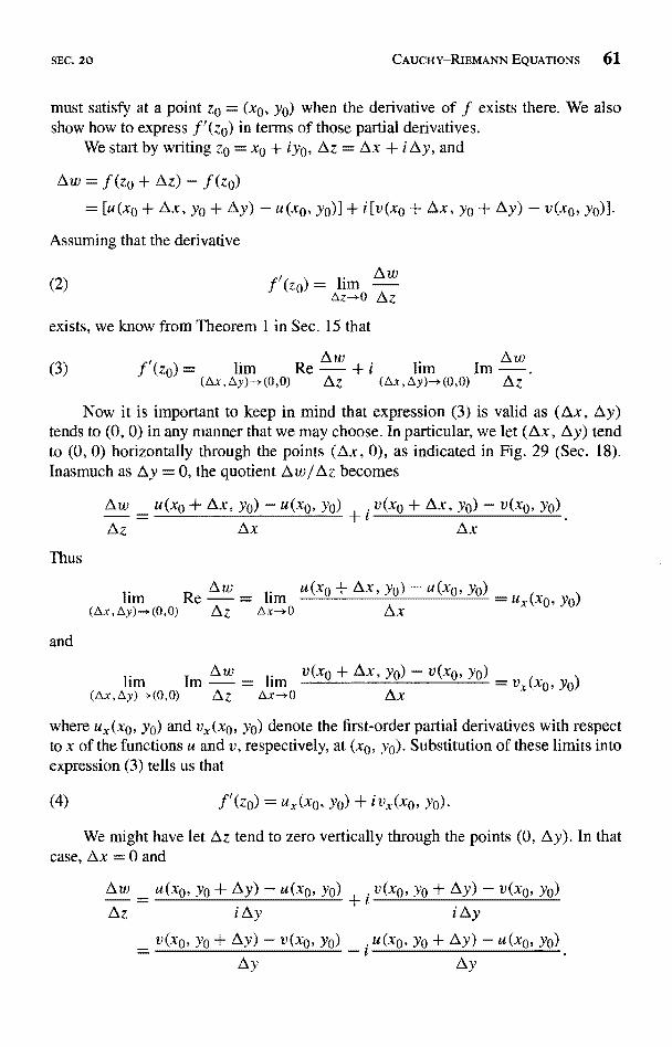
SEC. 20 CAUCHY-RIEMANN EQUATIONS 6
must satisfy at a point zo = (x0, yo) when the derivative of f exists there. We alsoshow how to express f'(zo) in terms of those partial derivatives.
We start by writing zo = x0 + iy0, Az = Ax + i Ay, and
Aw = f (zo + Az) - f (zo)
= [u(xo + Ax, yo + Ay) - u(xo, yo)] + i[v(xo + Ax, yo + Ay) -
Assuming that the derivative
(2)
f'(z0) = lim Rebww
+ i lim IM w(Ax,Ay)-- (O,O) AZ (Ax,Ay)-(O,O) AZ
exists, we know from Theorem 1 in Sec. 15 that
(
v(x0, y0))
Now it is important to keep in mind that expression (3) is valid as (Ax, Ay)tends to (0, 0) in any manner that we may choose. In particular, we let (Ax, Ay) tendto (0, 0) horizontally through the points (Ax, 0), as indicated in Fig. 29 (Sec. 18).Inasmuch as Ay = 0, the quotient Aw /Az becomes
z
Thus
and
(zo) = limAw
Az- O AZ
u(x0 + Ax, yo) - u(x0, Yo)
'Ay)-(O,O) AZ Ax-+O Ax
- u(x0 + Ax, y0) - u(xo, Yo) + i v(xo + Ax, Yo) - v(xo, Yo)Ax Ax
lim Re - = lim x (xo, yo)
where ux(xo, yo) and vx(xo, yo) denote the first-order partial derivatives with respectto x of the functions u and v, respectively, at (xo, yo). Substitution of these limits intoexpression (3) tells us that
(4) f'(Z0) = ux(xo, Yo) + ivx(xo, y0)
We might have let Az tend to zero vertically through the points (0, Ay). In thatcase, Ax = 0 and
Aw u(xo, yo + Ay) - u(xo, yo)+
v(x0, Yo + AY) - v(xo, yo)AZ i Ay i Ay
_ v(xo, Ye + Ay) - v(xo, yo) u(xo= yo + AY) - u(xo, yo)Ay Ay
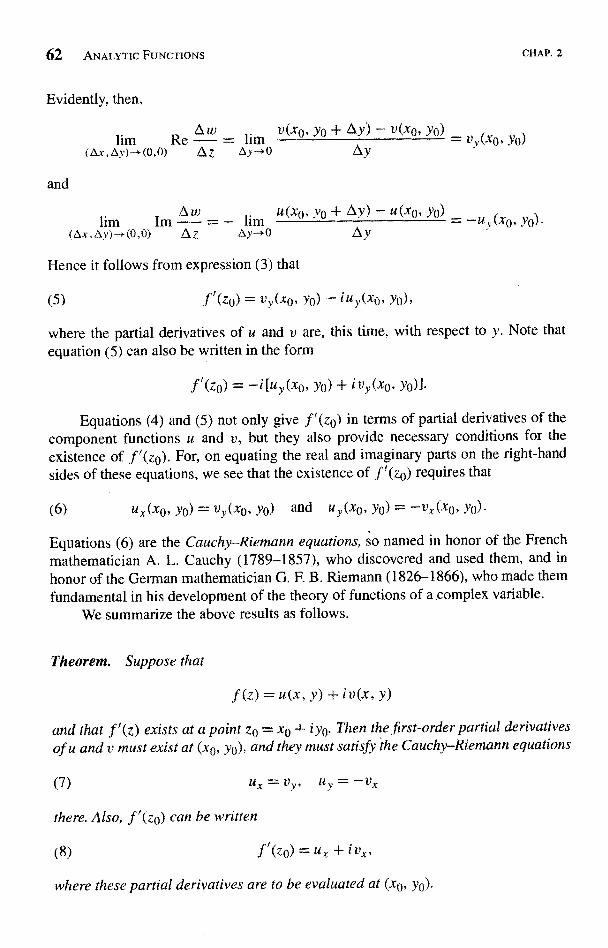
62 ANALYTIC FUNCTIONS
Evidently, then,
and
- li u (xo, Yo + Ay(ox,Ay)-+(o,o) AZ Ay--*o Ay
Hence it follows from expression (3) that
CHAP. 2
xo, yo)= vv(xo Yo)
X0, Yo) _ -u 0, yo)
(5) .f'(zo) = vy(x0, Yo) - iuy(xo, Yo),
where the partial derivatives of u and v are, this time, with respect to y. Note that
equation (5) can also be written in the form
f'(zp) = -i[uy(xo, Yo) + ivy(xo, Yo)J.
Equations (4) and (5) not only give f'(zo) in terms of partial derivatives of thecomponent functions u and v, but they also provide necessary conditions for theexistence of f'(zo). For, on equating the real and imaginary parts on the right-handsides of these equations, we see that the existence of f'(zo) requires that
(6) uX(xo, Yo) = vy(xo, yo) and o, yo) = -vX (xo, Yo)
Equations (6) are the Cauchy-Riemann equations, so named in honor of the Frenchmathematician A. L. Cauchy (1789-1857), who discovered and used them, and inhonor of the German mathematician G. F. B. Riemann (1826-1866), who made themfundamental in his development of the theory of functions of a complex variable.
We summarize the above results as follows.
Theorem. Suppose that
f(z)=u(x,y)+iv(x,Y)
and that f'(z) exists at a point zo = xa + iyo. Then the first-order partial derivativesof u and v must exist at (xo, yo), and they must satisfy the Cauchy-Riemann equations
(7)
there. Also, f'(zo) can be written
(8) .f'(zo) = ux + i vx,
where these partial derivatives are to be evaluated at (xo, yo).
AV)-+(0,O) AZ AV--+O trylim Re
taw = lim v(x0,Yo+AY)-v(-lim
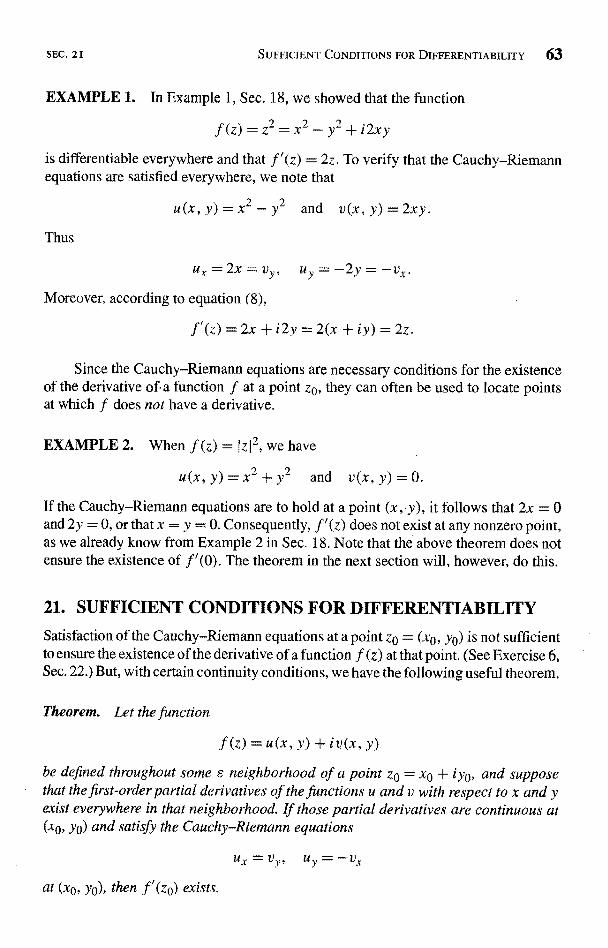
SEC. 21 SUFFICIENT CONDITIONS FOR DIFFERENTIABILITY 63
EXAMPLE 1. In Example 1, Sec. 18, we showed that the function
f(z) -y2+i2xy
is differentiable everywhere and that f(z) = 2z. To verify that the Cauchy-Riemannequations are satisfied everywhere, we note that
u(x, y) = x2 - y2 and v(x, y) = 2xy.
Thus
uz=2x=vy, uy=-2y=-vx.Moreover, according to equation (8),
f'(z) =2x + i2y = 2(x + iy) = 2z.
Since the Cauchy-Riemann equations are necessary conditions for the existenceof the derivative of, a function f at a point z0, they can often be used to locate pointsat which f does not have a derivative.
EXAMPLE 2. When f (z) = (z12, we have
y)=x2+y2 and v(x,y)=0.
If the Cauchy-Riemann equations are to hold at a point (x,-y), it follows that 2x = 0and 2y = 0, or that x = y = 0. Consequently, f'(z) does not exist at any nonzero point,as we already know from Example 2 in Sec. 18. Note that the above theorem does notensure the existence of f'(0). The theorem in the next section will, however, do this.
21. SUFFICIENT CONDITIONS FOR DIFFERENTIABILITY
Satisfaction of the Cauchy-Riemann equations at a point z0 = (x0, y0) is not sufficientto ensure the existence of the derivative of a function f (z) at that point. (See Exercise 6,Sec. 22.) But, with certain continuity conditions, we have the following useful theorem.
Theorem. Let the function
f(z)=u(x,y)+iv(x,.Y)be defined throughout some s neighborhood of a point z0 = x0 + iY0, and supposethat the first-order partial derivatives of the functions u and v with respect to x and yexist everywhere in that neighborhood. If those partial derivatives are continuous at(x0, yo) and satisfy the Cauchy-Riemann equations
uy=_Ux
at (x0, y0), then f(z0) exists.
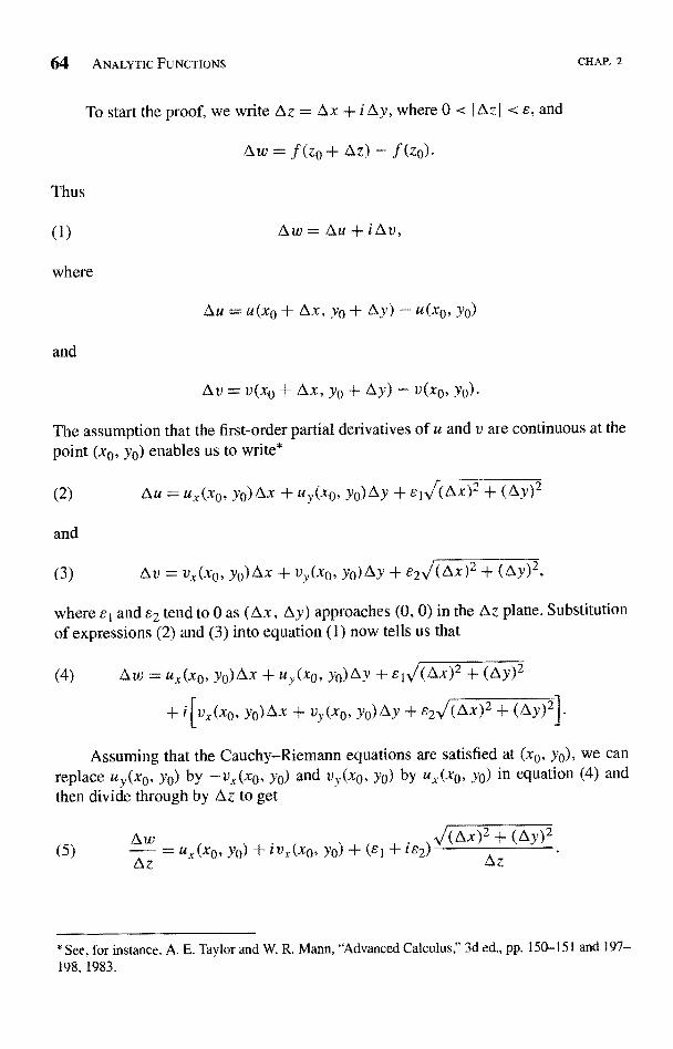
64 ANALYTIC FUNCTIONS
To start the proof, we write Az = Ax + i Ay, where 0 < I Az I < s, and
Aw=f(zo+Az)-f(zo)
Thus
(1)
where
and
iAv,
Au=u(xo+Ax,yo+Ay)-u(xo,yo)
Av = v(xe + Ax, yo + Ay) - v(xo, yo)
CHAP. 2
The assumption that the first-order partial derivatives of u and v are continuous at thepoint (xo, yo) enables us to write*
(2) Au = ux(xo,
and
uy(xo, yo)Ay +el (Ax)2 + (Ay)2
(3) Av = vx(xo, yo)Ax + vy(xo, Yo)AY + E2V (Ax)2 + (Ay)2,
where E1 and 82 tend to 0 as (Ax, Ay) approaches (0, 0) in the Az plane. Substitutionof expressions (2) and (3) into equation (1) now tells us that
(4) Aw = ux(xo, yo) Ax + uy(xo, yo) Ay + e1Vl-(AX)2 + (Ay)2
x(xo, yo)Ax + vy(xo, yo)Ay + s2I(Ax)2 + (Ay'
Assuming that the Cauchy-Riemann equations are satisfied at (xo, yo), we canreplace uy(xo, yo) by -vx(xo, yo) and v(xo, yo) by ux(xo, yo) in equation (4) andthen divide through by Az to get
(5)A z
= ux (xo, yo) + i vx (xo, yo) + (E 1 + i ${Llx)2 + (Ay
Az
2
* See, for instance, A. E. Taylor and W. R. Mann, "Advanced Calculus," 3d ed., pp. 150-151 and 197-198,1983.
SEC. 22 POLAR COORDINATES 65
But (11x)2 + (Ay)2 = lAzl, and so
bz
Ay=1.
Also, el + ie2 tends to 0 as (11x, 11y) approaches (0, 0). So the last term on the rightin equation (5) tends to 0 as the variable Az = Ax + i Ay tends to 0. This means thatthe limit of the left-hand side of equation (5) exists and that
(6) f'(zo) = Ux
where the right-hand side is to be evaluated at (xe, ye).
EXAMPLE 1. Consider the exponential function
f(z) =eZ=exe`y (Z=x+iy),some of whose mapping properties were discussed in Sec. 13. In view of Euler'sformula (Sec. 6), this function can, of course, be written
f (z) = ex cos y + i ex sin y,
where y is to be taken in radians when cos y and sin y are evaluated. Then
u(x, y) = ex cos y and v(x, y) = ex sin y.
Since ux = vY and uy = -vx everywhere and since these derivatives are everywherecontinuous, the conditions in the theorem are satisfied at all points in the complexplane. Thus f(z) exists everywhere, and
+ i vx = ex cos y + i ex sin y.
Note that f(z) =
EXAMPLE 2. It also follows from the theorem in this section that the functionf(z) = Iz12, whose components are
U (X' Y) =X2 + Y2 and v(x, y) = 0,
has a derivative at z = 0. In fact, f'(0) = 0 + i 0 = 0 (compare Example 2, Sec. 18). Wesaw in Example 2, Sec. 20, that this function cannot have a derivative at any nonzeropoint since the Cauchy-Riemann equations are not satisfied at such points.
22. POLAR COORDINATES
Assuming that zo 0, we shall in this section use the coordinate transformation
(1) x=rcos0, y=rsin0
66 ANALYTIC FUNCTIONS CHAP. 2
to restate the theorem in Sec. 21 in polar coordinates.Depending on whether we write
z=x+iy or z=refs 0
when w = f (z), the real and imaginary parts of w = u + i v are expressed in terms ofeither the variables x and y or r and 0. Suppose that the first-order partial derivativesof u and v with respect to x and y exist everywhere in some neighborhood of a givennonzero point zo and are continuous at that point. The first-order partial derivativeswith respect to r and 0 also have these properties, and the chain rule for differentiatingreal-valued functions of two real variables can be used to write them in terms of theones with respect to x and y. More precisely, since
au au 8x au 8y au au 8x au ayar ax car + ay car' a8 ax a8 + ay a O'
one can write
(2) ur = ux cos 0 + uy sin 0, us = -ux r sin 0 + uy r cos 0.
Likewise,
(3) vxcos0-I-vysin0, v9 = -vx r sin 0 + vy r cos 0.
If the partial derivatives with respect to x and y also satisfy the Cauchy-Riemannequations
(4)
at z0, equations (3) become
(5)
ux = vy, uy = -vx
Vr=-uycos0+uxsin0, vs=uyrsin0+uxrcos9
at that point. It is then clear from equations (2) and (5) that
(6) rur = v0, uo = -rvr
at the point z0.If, on the other hand, equations (6) are known to hold at zo, it is straightforward
to show (Exercise 7) that equations (4) must hold there. Equations (6) are, therefore,an alternative form of the Cauchy-Riemann equations (4).
We can now restate the theorem in Sec. 21 using polar coordinates.
Theorem. Let the function
f (z) = u(r, 0) + iv(r, 0)
be defined throughout some s neighborhood of a nonzero point zo = ro exp(i00), andsuppose that the first-order partial derivatives of the functions u and v with respect to r
SEC. 22 POLAR COORDINATES 67
and O exist everywhere in that neighborhood. If those partial derivatives are continuousat (r0, 00) and satisfy the polar form
rur = vg,
of the Cauchy-Riemann equations at (r0, 8Q), then f(z0) exists.
The derivative f'(z0) here can be written (see Exercise 8
(7) 01 =
COs"and v
r
where the right-hand side is to be evaluated at (re, 80).
EXAMPLE 1. Consider the function
(8) f (z) =1 = I
= le-`e = l (Cos 9 - i sin 6) (z A 0).z reie r r
Since
r+iVr},
the conditions in the above theorem are satisfied at every nonzero point z = re" in theplane. In particular, the Cauchy-Riemann equations
rur=- GOS S=v0 and u0=- sin g =-rvr
r
-e-i8e-YO
are satisfied. Hence the derivative of f exists when z 54 0; and, according to expres-sion (7),
z7=e
sin 9
r
r
I
r2 r2 ) r2 (ref8)2
EXAMPLE 2. The theorem can be used to show that, when a is a fixed real number,the function
0,a<9<a-4-2rr}
has a derivative everywhere in its domain of definition. Here
"rcos8
and v(r,6)- Yrsin 3
Inasmuch as
rur = -ftcos
8= vg and uo = --r sin
8 - -rvr3 3 3 3

68 ANALYTIC FUNCTIONS CHAP. 2
and since the other conditions in the theorem are satisfied, the derivative f'(z) existsat each point where f (z) is defined. Furthermore, expression (7) tells us that
or
3 [.f (z
Note that when a specific point z is taken in the domain of definition of f, thevalue f (z) is one value of z 113 (see Sec. 11). Hence this last expression for f'(z) canbe put in the form
when that value is taken. Derivatives of such power functions will be elaborated on inChap. 3 (Sec. 32).
EXERCISES
1. Use the theorem in Sec. 20 to show that f'(z) does not exist at any point if
z) = z; (b) f (z) = z - z; (c) f (z) = 2x + ixy2; (d) f(z) = eX
2. Use the theorem in Sec. 21 to show that f'(z) and its derivative f"(z) exist everywhere,and find f"(z) when
z) = i z + 2; (b) .f (z) = e-xe-`y;(z) = z3; (d) f (z) = cos x cosh y - i sin x sinh y.
Ans. (b) f"(z) = .f (z); (d
om results obtained in Sees. 20 and 21, determine where f'(z) exists and find its valuewhen
z; (b) .f (z) =
Ans.
iy2; z)=zImz.
1/z2 (z t 0); (b) f'(x + ix) = 2x; (c) .f'(0) = 0.
4. Use the theorem in Sec. 22 to show that each of these functions is differentiable in theindicated domain of definition, and then use expression (7) in that section to find f'(z):
(a) f (z) = 1/z4 (z t 0);(b) f(z)= trei912(r>0,a<0<a+27r);(c) f(z)
e-ecos(1n
r) + ie-osin(ln r) (r > 0, 0 < 0 < 2n).
Ans. (b) f'(z) = 2f (z) ;(c) f(z) = i f(z)
.
z
SEC. 2 2
5. Show that when f (z) = x3 + i (1 - y)3, it is legitimate to write
.f'(z) = ux + i vx = 3x2
EXERCISES 69
only when z = i.
6. Let u and v denote the real and imaginary components of the function f defined by theequations
.f (z) _z2- when z 0z
0 when z=0.Verify that the Cauchy-Riemann equations ux = vy and uy = -vx are satisfied at theorigin z = (0, 0). [Compare Exercise 9, Sec. 19, where it is shown that f'(0) neverthelessfails to exist.]
7. Solve equations (2), Sec. 22, for ux and uy to show that
sin 8 cosux = ur Cos UO , uy = ur sin 0 + uer .r
8
Then use these equations and similar ones for vx and vy to show that, in Sec. 22, equations(4) are satisfied at a point zo if equations (6) are satisfied there. Thus complete theverification that equations (6), Sec. 22, are the Cauchy-Riemann equations in polar form.
8. Let a function f (z) = a + iv be differentiable at a nonzero point zo = ro exp(i Bo). Usethe expressions for ux and vx found in Exercise 7, together with the polar form (6), Sec.22, of the Cauchy-Riemann equations, to rewrite the expression
in Sec. 21 as
f'(zo) = e-`o(ur + ivr),
where ur and yr are to be evaluated at (ro, 80).
9. (a) With the aid of the polar form (6), Sec. 22, of the Cauchy-Riemann equations, derivethe alternative form
f'(ZO) _ -(u0 +ivo)ZO
of the expression for f'(zo) found in Exercise 8.
(b) Use the expression for f'(zo) in part (a) to show that the derivative of the functionf (z) = 1/z (z 34 0) in Example 1, Sec. 22, is f'(z) _ -1/z2.
10. (a) Recall (Sec. 5) that if z = x + iy, then
x=z+zand
z -z2
y2i
70 ANALYTIC FUNCTIONS CHAP. 2
By formally applying the chain rule in calculus to a function F(x, y) of two realvariables, derive the expression
8F _ aF ax +aF ay = 1 (aF.L r
aF---- -az
_ax az ay az 2 ax
(b) Define the operator
a _l a a
+ ` ayaz 2 ax
suggested by part (a), to show that if the first-order partial derivatives of the realand imaginary parts of a function f (z) = a(x, y) + iv(x, y) satisfy the Cauchy-Riemann equations, then
- vY) + i (vx + ay)
Thus derive the complex form afjaz = 0 of the Cauchy-Riemann equations.
23. ANALYTIC FUNCTIONSWe are now ready to introduce the concept of an analytic function. A function f of thecomplex variable z is analytic in an open set if it has a derivative at each point in thatset.* If we should speak of a function f that is analytic in a set S which is not open,it is to be understood that f is analytic in an open set containing S. In particular, f isanalytic at a point zo if it is analytic throughout some neighborhood of z0.
We note, for instance, that the function f (z) = 1/z is analytic at each nonzeropoint in the finite plane. But the function f (z) = 1z12 is not analytic at any point sinceits derivative exists only at z = 0 and not throughout any neighborhood. (See Example2, Sec. 18.)
An entire function is a function that is analytic at each point in the entire finiteplane. Since the derivative of a polynomial exists everywhere, it follows that everypolynomial is an entire function.
If a function f fails to be analytic at a point ze but is analytic at some pointin every neighborhood of zo, then ze is called a singular point, or singularity, of f.The point z = 0 is evidently a singular point of the function f (z) = 1/z. The functionf (z) = I z 12, on the other hand, has no singular points since it is nowhere analytic.
A necessary, but by no means sufficient, condition for a function f to be analyticin a domain D is clearly the continuity of f throughout D. Satisfaction of the Cauchy-Riemann equations is also necessary, but not sufficient. Sufficient conditions foranalyticity in D are provided by the theorems in Sees. 21 and 22.
Other useful sufficient conditions are obtained from the differentiation formulasin Sec. 19. The derivatives of the sum and product of two functions exist wherever the
* The terms regular and holomorphic are also used in the literature to denote analyticity.
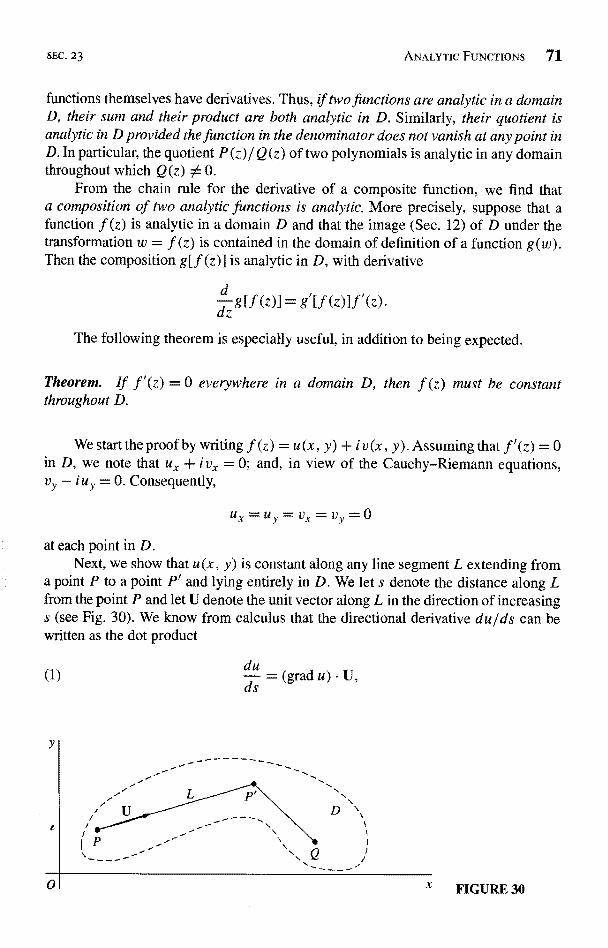
SEC. 23 ANALYTIC FUNCTIONS 7
functions themselves have derivatives. Thus, if two functions are analytic in a domainD, their sum and their product are both analytic in D. Similarly, their quotient isanalytic in D provided the function in the denominator does not vanish at any point inD. In particular, the quotient P (z)/ Q (z) of two polynomials is analytic in any domainthroughout which Q(z) 0.
From the chain rule for the derivative of a composite function, we find thata composition of two analytic functions is analytic. More precisely, suppose that afunction f (z) is analytic in a domain D and that the image (Sec. 12) of D under thetransformation w = f (z) is contained in the domain of definition of a function g(w).Then the composition g[f (z)] is analytic in D, with derivative
dzOf (z)] = Of (z)] f
The following theorem is especially useful, in addition to being expected.
Theorem. If f(z) = 0 everywhere in a domain D, then f (z) must be constantthroughout D.
We start the proof by writing f (z) = u (x, y) + i v (x, y). Assuming that f'(z) = 0in D, we note that ux + i vx = 0; and, in view of the Cauchy-Riemann equations,vy - i u y = 0. Consequently,
=vy=0
at each point in D.Next, we show that u (x, y) is constant along any line segment L extending from
a point P to a point P' and lying entirely in D. We let s denote the distance along Lfrom the point P and let U denote the unit vector along L in the direction of increasings (see Fig. 30). We know from calculus that the directional derivative duds can bewritten as the dot product
(1)du
= (grad u) . U,de
x FIGURE 30
72 ANALYTIC FUNCTIONS
where grad u is the gradient vector
(2) grad u =
CHAP. 2
Because ux and uy are zero everywhere in D, then, grad u is the zero vector at allpoints on L. Hence it follows from equation (1) that the derivative du Ids is zero alongL; and this means that u is constant on L.
Finally, since there is always a finite number of such line segments, joined endto end, connecting any two points P and Q in D (Sec. 10), the values of u at P andQ must be the same. We may conclude, then, that there is a real constant a such thatu(x, y) = a throughout D. Similarly, v(x, y) = b; and we find that f (z) = a + bi ateach point in D.
24. EXAMPLESAs pointed out in Sec. 23, it is often possible to determine where a given function isanalytic by simply recalling various differentiation formulas in Sec. 19.
EXAMPLE 1. The quotient
f(z)= z'+4(z2 - 3)(z2 + l)
is evidently analytic throughout the z plane except for the singular points z = fand z = ± i. The analyticity is due to the existence of familiar differentiation formulas,which need be applied only if the expression for f(z) is wanted.
When a function is given in terms of its component functions u (x, y) and v (x, y),its analyticity can be demonstrated by direct application of the Cauchy-Riemannequations.
EXAMPLE 2. When
f (z) = cosh x cos y + i sinh x sin y,
the component functions are
u(x, y) = cosh x cosy and v(x, y) = sinh x sin y.
Because
inh x cos y = v,, and uy = - cosh x sin y = -vx
everywhere, it is clear from the theorem in Sec. 21 that f is entire.
SEC. 24 EXERCISES 73
Finally, we illustrate how the theorems in the last four sections, in particular theone in Sec. 23, can be used to obtain some important properties of analytic functions.
EXAMPLE 3. Suppose that a function
f (z) = u(x, y) + iv(x, y)
and its conjugate
f (z) = u(x, y) - iv(x, y)
are both analytic in a given domain D. It is easy to show that f (z) must be constantthroughout D.
To do this, we write f (z) as
f (z) = U(x, Y) + i V (x, Y),
where
(1) U(x, Y) _ Y d V(x, y) = -v(x, y).
Because of the analyticity of f (z), the Cauchy-Riemann equations
(2) y, uy = -vX
hold in D, according to the theorem in Sec. 20. Also, the analyticity ous that
Ux=Vy, Uy=-Vx.
In view of relations (1), these last two equations can be written
z in D tells
uy=vx.
By adding corresponding sides of the first of equations (2) and (3), we find thatux = 0 in D. Similarly, subtraction involving corresponding sides of the second ofequations (2) and (3) reveals that vx = 0. According to expression (8) in Sec. 20, then,
f'(z)=ux+ivx=0+i0=0;and it follows from the theorem in Sec. 23 that f (z) is constant throughout D.
EXERCISES
1. Apply the theorem in Sec. 21 to verify that each of these functions is entire:
z) =3x+y+i(3y -x); (b) f(z) =sinx cosh y+i cosx sinh y;(c) f (z) = e-y sin x - i e_y cos x; (d) f (z) = (z2 - 2)e-xe-iY.
74 ANALYTIC FUNCTIONS CHAP. 2
2. With the aid of the theorem in Sec. 20, show that each of these functions is nowhereanalytic:
(a) f(z) = xy + iy; (b) .f (z) = 2xy + i (x2 - y2); (c) .f (z) = eyeix
3. State why a composition of two entire functions is entire. Also, state why any linearcombination cI f1(z) + c2f2(z) of two entire functions, where ct and c2 are complexconstants, is entire.
4. In each case, determine the singular points of the function and state why the function isanalytic everywhere except at those points:
2z + 1 z2 + 1z3 + tI ,) =) = (b) f (z ; z ii
z(z2 + 1) z2 - 3z+2I I'll
(z + 2)(z2 + 2z + 2) .Ans. (a) z = 0, t i ; (b)z=1,2; (c) z = -2, - i ± i .
5. According to Exercise 4(b), Sec. 22, the function
g(z) = -,,Ir-ei8/2 (r > 0, -,7 < 9 < r)
is analytic in its domain of definition, with derivative
g'(z) = 1
Show that the composite function G(z)
2g(z)
g(2z - 2 + i) is analytic in the half planex > 1. with derivative
G'(z)1
2z-2+i)g
Suggestion: Observe that Re(2z - 2 + i) > 0 when x > 1.
6. Use results in Sec. 22 to verify that the function
g(z) =lnr+i9 (r>0,0<9<2ir)is analytic in the indicated domain of definition, with derivative g'(z) = 1/z. Then showthat the composite function G(z) = g(z2 + 1) is analytic in the quadrant x > 0, y > 0,with derivative
2zG'(z) = z2 + 1
Suggestion: Observe that Im(z2 + 1) > 0 when x > 0, y > 0.
7. Let a function f (z) be analytic in a domain D. Prove that f (z) must be constantthroughout D if
(a) f (z) is real-valued for all z in D; (b) I f (z) I is constant throughout D.
Suggestion: Use the Cauchy-Riemann equations and the theorem in Sec. 23 toprove part (a). To prove part (b), observe that
c2if If(z)1 =c (c; 0);
z
then use the main result in Example 3, Sec. 24.
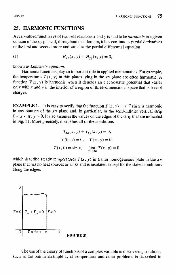
SEC. 25 HARMONIC FUNCTIONS 75
25. HARMONIC FUNCTIONS
A real-valued function H of two real variables x and y is said to be harmonic in a givendomain of the xy plane if, throughout that domain, it has continuous partial derivativesof the first and second order and satisfies the partial differential equation
(1) Hxx(x, y) + Hyy(x, y) = 0,
known as Laplace's equation.Harmonic functions play an important role in applied mathematics. For example,
the temperatures T (x, y) in thin plates lying in the xy plane are often harmonic. Afunction V(x, y) is harmonic when it denotes an electrostatic potential that variesonly with x and y in the interior of a region of three-dimensional space that is free ofcharges.
EXAMPLE 1. It is easy to verify that the function T (x, y) = e_y sin x is harmonicin any domain of the xy plane and, in particular, in the semi-infinite vertical strip0 <z x < ir, y > 0. It also assumes the values on the edges of the strip that are indicatedin Fig. 31. More precisely, it satisfies all of the conditions
Txx(x, Y) + Tyy(x, Y) = 0,
T(0, y) = 0, T (7r, y) = 0,
T (x, 0) = sin x, lim T (x, y) = 0,Y
which describe steady temperatures T(x, y) in a thin homogeneous plate in the xyplane that has no heat sources or sinks and is insulated except for the stated conditionsalong the edges.
FIGURE 31
The use of the theory of functions of a complex variable in discovering solutions,such as the one in Example 1, of temperature and other problems is described in
76 ANALYTIC FUNCTIONS CHAP. 2
considerable detail later on in Chap. 10 and in parts of chapters following it.* Thattheory is based on the theorem below, which provides a source of harmonic functions.
Theorem 1. If a function f (z) = u (x, y) + iv(x, y) is analytic in a domain D, thenits component functions u and v are harmonic in D.
To show this, we need a result that is to be proved in Chap. 4 (Sec. 48). Namely,if a function of a complex variable is analytic at a point, then its real and imaginarycomponents have continuous partial derivatives of all orders at that point.
Assuming that f is analytic in D, we start with the observation that the first-order partial derivatives of its component functions must satisfy the Cauchy-Riemannequations throughout D:
(2) ux=vy, uy,_ -vx..
Differentiating both sides of these equations with respect to x, we have
(3) = vyx, uyx = -vxx
Likewise, differentiation with respect to y yields
(4)
Now, by a theorem in advanced calculus,t the continuity of the partial derivatives ofu and v ensures that uyx = uxy and vyx = vxy. It then follows from equations (3) and(4) that
uxx + uyy = 0 and vxx + vy , = 0.
That is, u and v are harmonic in D.
uxv = vyy, uyy = --vxy.
EXAMPLE 2. The function f(z) = e-y sin x - i e-y cos x is entire, as is shownin Exercise 1(c), Sec. 24. Hence its real part, which is the temperature functionT (x, y) = e-y sin x in Example 1, must be harmonic in every domain of the xy plane.
EXAMPLE 3. Since the function f (z) i f z2 is analytic whenever z 0 and since
i2 2xy+i(x2IzI4
(x2 + y2
* Another important method is developed in the authors' "Fourier Series and Boundary Value Problems,"6th ed., 2001.
t See, for instance, A. E. Taylor and W. R. Mann, "Advanced Calculus," 3d ed., pp. 199-201, 1983.
SEC. 25 HARMONIC FUNCTIONS 77
the two functions
2xy x2 - y2u(x, y} - (x2 + y2)2 and v(x, y) _ (x2 + y2)2
are harmonic throughout any domain in the xy plane that does not contain the origin.
o given functions u and v are harmonic in a domain D and their first-orderpartial derivatives satisfy the Cauchy-Riemann equations (2) throughout D, v is saidto be a harmonic conjugate of u. The meaning of the word conjugate here is, of course,different from that in Sec. 5, where z is defined.
Theorem 2, A function f (z) = u (x, y) + i vonly if v is a harmonic conjugate of u,
is analytic in a domain D if andy
The proof is easy. If v is a harmonic conjugate of u in D, the theorem in Sec.21 tells us that f is analytic in D. Conversely, if f is analytic in D, we know fromTheorem 1 above that u and v are harmonic in D; and, in view of the theorem in Sec.20, the Cauchy-Riemann equations are satisfied.
The following example shows that if v is a harmonic conjugate of u in somedomain, it is not, in general, true that u is a harmonic conjugate of v there. (See alsoExercises 3 and 4.)
EXAMPLE 4. Suppose that
d v(x, y) = 2xy.
Since these are the real and imaginary components, respectively, of the entire functionf (z) = z2, we know that v is a harmonic conjugate of u throughout the plane. But ucannot be a harmonic conjugate of v since, as verified in Exercise 2(b), Sec. 24, thefunction 2xy + i (x2 - y2) is not analytic anywhere.
In Chap. 9 (Sec. 97) we shall show that a function u which is harmonic in adomain of a certain type always has a harmonic conjugate. Thus, in such domains,every harmonic function is the real part of an analytic function. It is also true that aharmonic conjugate, when it exists, is unique except for an additive constant.
EXAMPLE 5. We now illustrate one method of obtaining a harmonic conjugate ofa given harmonic function. The function
(5) u(x, y) = y3 - 3x2y
78 ANALYTIC FUNCTIONS CHAP. 2
is readily seen to be harmonic throughout the entire xy plane. Since a harmonicconjugate v(x, y) is related to u (x, y) by means of the Cauchy-Riemann equations
(6) ux = v,,
the first of these equations tells us that
vy(x, y) = -6xy.
Holding x fixed and integrating each side here with respect to y, we find that
(7) v(x, y) = -3xy2 +
where fi is, at present, an arbitrary function of x. Using the second of equations (6),we have
3y2 - 3x2 = 3y2 - 0'(x),
or i'(x) = 3x2. Thus fi (x) = x3 + C, where C is an arbitrary real number. Accordingto equation (7), then, the function
(8) v(x, y) = -3xy2 + x3 + C
is a harmonic conjugate of u(x, y).The corresponding analytic function is
(9) .f (z) = (y3 - 3x2y) + i (--3xy2 + x3 + C).
The form f (z) = i (z3 + C) of this function is easily verified and is suggested by notingthat when y = 0, expression (9) becomes f (x) = i (x3 + C).
EXERCISES
1. Show that u(x, y) is harmonic in some domain and find a harmonic conjugate v(x, y)when
a)u(x,y)=2x(1-y (b) u(x, y) = 2x -- x3 + 3xy2;
u(x, y) = sink x sin y; (d) u(x, y) = yl(x2 + y2).
Ans. (a) v(x, y) = x2 - y2 + 2y; (b) v(x, y) = 2y - 3x2y + y3;(c) v(x, y) = - cosh x cos y; (d) v(x, y) = x/(x2 + y2).
2. Show that if v and V are harmonic conjugates of u in a domain D, then v(x, y) andV (x, y) can differ at most by an additive constant.
3. Suppose that, in a domain D, a function v is a harmonic conjugate of u and also that uis a harmonic conjugate of v. Show how it follows that both u(x, y) and v(x, y) must beconstant throughout D.
4. Use Theorem 2 in Sec. 25 to show that, in a domain D, v is a harmonic conjugate ofuif and only if -u is a harmonic conjugate of v. (Compare the result obtained in Exer-cise 3.)
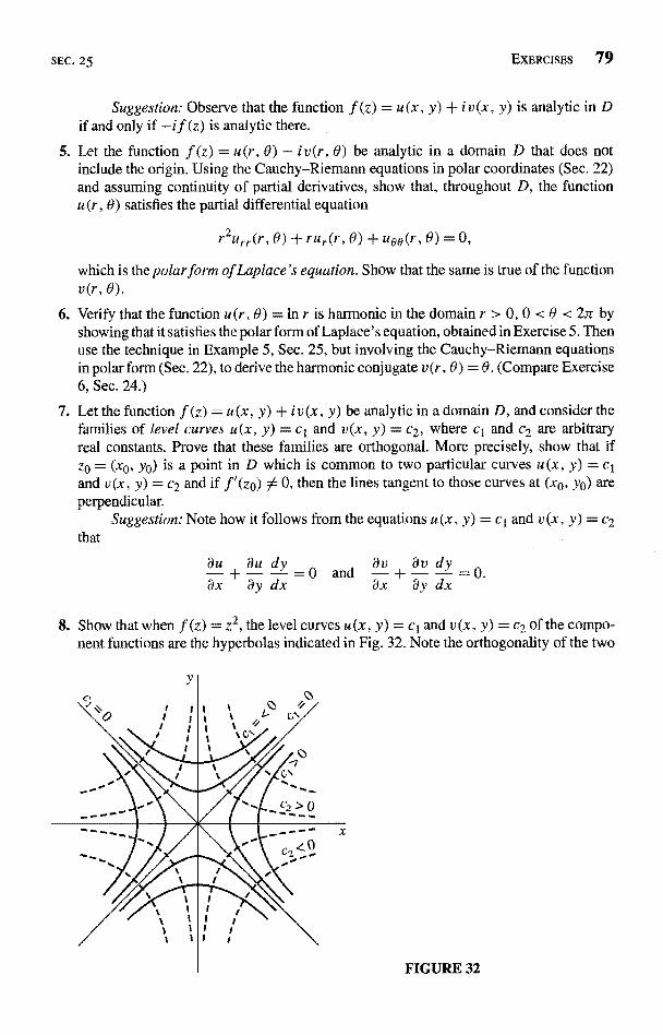
SEC. 25 EXERCISES 79
Suggestion: Observe that the function f (z) = u(x, y) + i v(x, y) is analytic in Dif and only if -if (z) is analytic there.
5. Let the function f (z) = u(r, 0) + iv(r, 6) be analytic in a domain D that does notinclude the origin. Using the Cauchy-Riemann equations in polar coordinates (Sec. 22)and assuming continuity of partial derivatives, show that, throughout D, the functionu(r, 0) satisfies the partial differential equation
rur(r, 0) + uee(r, 0) = 0,
which is the polar form of Laplace's equation. Show that the same is true of the functionv(r, 0).
6. Verify that the function u(r, 0) =1n r is harmonic in the domain r > 0, 0 < 6 < 27r byshowing that it satisfies the polar form of Laplace's equation, obtained in Exercise 5. Thenuse the technique in Example 5, Sec. 25, but involving the Cauchy-Riemann equationsin polar form (Sec. 22), to derive the harmonic conjugate v(r, 0) = 0. (Compare Exercise6, Sec. 24.)
7. Let the function f (z) = u(x, y) + i v (x, y) be analytic in a domain D, and consider thefamilies of level curves u(x, y) = ct and v(x, y) = c2, where cI and c2 are arbitraryreal constants. Prove that these families are orthogonal. More precisely, show that ifzo = (xo, yo) is a point in D which is common to two particular curves u(x, y) = cIand v(x, y) = c2 and if f'(zo) :0, then the lines tangent to those curves at (xo, yo) areperpendicular.
Suggestion: Note how it follows from the equations u(x, y) = cI and v(x, y) = c2that
au+au dy=0and
Jv+13v dyax ay dx ax ay dx
8. Show that when f (z) = z2, the level curves u(x, y) = cl and v(x, y) = c2 of the compo-nent functions are the hyperbolas indicated in Fig. 32. Note the orthogonality of the two
y
FIGURE 32
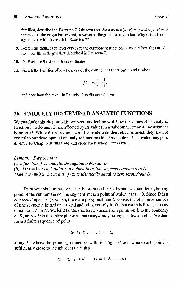
80 ANALYTIC FUNCTIONS CHAP. 2
families, described in Exercise 7. Observe that the curves u(x, y) = 0 and u(x, y) = 0intersect at the origin but are not, however, orthogonal to each other. Why is this fact inagreement with the result in Exercise 7?
9. Sketch the families of level curves of the component functions u and v when f (z) = 1/z,and note the orthogonality described in Exercise 7.
10. Do Exercise 9 using polar coordinates.
11. Sketch the families of level curves of the component functions u and v when
.f(z)=z+1
and note how the result in Exercise 7 is illustrated here.
26. UNIQUELY DETERMINED ANALYTIC FUNCTIONS
We conclude this chapter with two sections dealing with how the values of an analyticfunction in a domain D are affected by its values in a subdomain or on a line segmentlying in D. While these sections are of considerable theoretical interest, they are notcentral to our development of analytic functions in later chapters. The reader may passdirectly to Chap. 3 at this time and refer back when necessary.
Lemma. Suppose that(i) a function f is analytic throughout a domain D;(ii) f (z) = 0 at each point z of a domain or line segment contained in D.Then f (z) = 0 in D; that is, f (z) is identically equal to zero throughout D.
To prove this lemma, we let f be as stated in its hypothesis and let zo be anypoint of the subdomain or line segment at each point of which f (z) = 0. Since D is aconnected open set (Sec. 10), there is a polygonal line L, consisting of a finite numberof line segments joined end to end and lying entirely in D, that extends from zo to anyother point P in D. We let d be the shortest distance from points on L to the boundaryof D, unless D is the entire plane; in that case, d may be any positive number. We thenform a finite sequence of points
ZO, z1, Z2, ... , zn-1, zn
along L, where the point zn coincides with P (Fig. 33) and where each point issufficiently close to the adjacent ones that
`-'zk-1I <d (k=1,2,...,n).
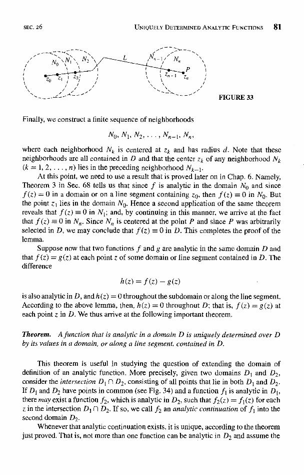
SEC. 26 UNIQUELY DETERMINED ANALYTIC FUNCTIONS 81
FIGURE 33
Finally, we construct a finite sequence of neighborhoods
No, N1, N2,...,N
where each neighborhood Nk is centered at Zk and has radius d. Note that theseneighborhoods are all contained in D and that the center zk of any neighborhood Nk(k = 1, 2, ... , n) lies in the preceding neighborhood Nk_1.
At this point, we need to use a result that is proved later on in Chap. 6. Namely,Theorem 3 in Sec. 68 tells us that since f is analytic in the domain No and sincef (z) = 0 in a domain or on a line segment containing zo, then f (z) = 0 in No. Butthe point z1 lies in the domain No. Hence a second application of the same theoremreveals that f (z) = 0 in N1; and, by continuing in this manner, we arrive at the factthat f (z) - 0 in N. Since Nn is centered at the point P and since P was arbitrarilyselected in D, we may conclude that f (z) - 0 in D. This completes the proof of thelemma.
Suppose now that two functions f and g are analytic in the same domain D andthat f (z) = g(z) at each point z of some domain or line segment contained in D. Thedifference
h (z) = f (z) - g (z)
is also analytic in D, and h (z) = 0 throughout the subdomain or along the line segment.According to the above lemma, then, h(z) = 0 throughout D; that is, f (z) = g(z) ateach point z in D. We thus arrive at the following important theorem.
Theorem. A function that is analytic in a domain D is uniquely determined over Dby its values in a domain, or along a line segment, contained in D.
This theorem is useful in studying the question of extending the domain ofdefinition of an analytic function. More precisely, given two domains DI and D2,consider the intersection D1 Cl D2, consisting of all points that lie in both D1 and D2.If D1 and D2 have points in common (see Fig. 34) and a function ft is analytic in D1,there may exist a function f2, which is analytic in D2, such that f2(z) = f1(z) for eachz in the intersection D1 (1 D2. If so, we call f2 an analytic continuation of f1 into thesecond domain D2.
Whenever that analytic continuation exists, it is unique, according to the theoremjust proved. That is, not more than one function can be analytic in D2 and assume the
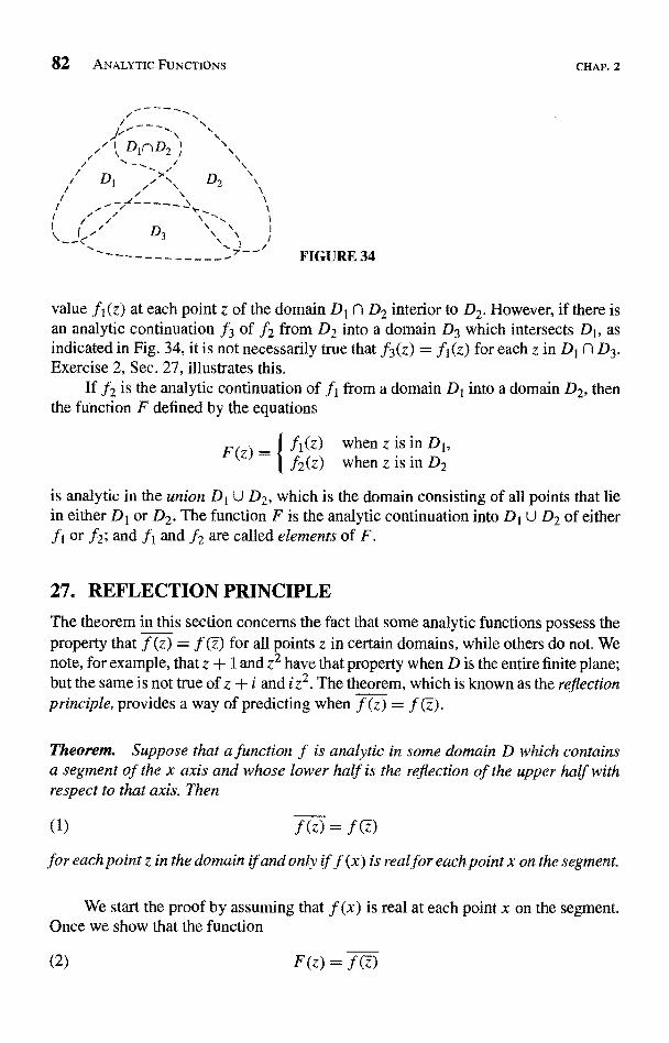
82 ANALYTIC FUNCTIONS
D1nD2f
't 1
`C ' D3 1 /ti IFIGURE 34
CHAP. 2
value fi(z) at each point z of the domain D1 f1 D2 interior to D2. However, if there isan analytic continuation f3 of f2 from D2 into a domain D3 which intersects D1, asindicated in Fig. 34, it is not necessarily true that f3(z) = fi(z) for each z in D1 fl D3.Exercise 2, Sec. 27, illustrates this.
If f2 is the analytic continuation of fi from a domain D1 into a domain D2, thenthe function F defined by the equations
F(z) fi(z) when z is in D1,f2(z) when z is in D2
is analytic in the union D1 U D2, which is the domain consisting of all points that liein either DI or D2. The function F is the analytic continuation into D1 U D2 of eitherfi or f2; and fi and f2 are called elements of F.
27. REFLECTION PRINCIPLE
The theorem in this section concerns the fact that some analytic functions possess theproperty that f (z) = f () for all points z in certain domains, while others do not. Wenote, for example, that z + 1 and z2 have that property when D is the entire finite plane;but the same is not true of z + i and iz2. The theorem, which is known as the reflectionprinciple, provides a way of predicting when f (z) = f ().
Theorem. Suppose that a function f is analytic in some domain D which containsa segment of the x axis and whose lower half is the reflection of the upper half withrespect to that axis. Then
(1) .f(z)=.f( )
or each point z in the domain if and only if f (x) is real for each point x on the segment.
We start the proof by assuming that f (x) is real at each point x on the segment.Once we show that the function
(2) F (z
SEC. 27 REFLECTION PRINCIPLE 83
is analytic in D, we shall use it to obtain equation (1). To establish the analyticity ofF(z), we write
f(z)=u(x,Y + iv(x, y), F(z) = U(x, y) + i V
and observe how it follows from equation (2) that, since
(3) f O = u(x, -y) - iv(x, -y),
the components of F(z) and f (z) are related by the equations
(4) U(x, y) = u(x, t) and V (x, y) -- -v(x, t),
,y
where t = -y. Now, because f (x + it) is an analytic function of x + it, the first-order partial derivatives of the functions a (x, t) and v (x, t) are continuous throughoutD and satisfy the Cauchy-Riemann equations*
(5) ux=vt, ut= -vx
Furthermore, in view of equations (4),
U Y
and it follows from these and the first of equations (5) that Ux = Vy. Similarly,
dx y I
U,U= u, V=
dt = -at, Vx = -vx;dy
and the second of equations (5) tells us that Uy = -Vx. Inasmuch as the first-orderpartial derivatives of U(x, y) and V(x, y) are now shown to satisfy the Cauchy-Riemann equations and since those derivatives are continuous, we find that the functionF (z) is analytic in D. Moreover, since f (x) is real on the segment of the real axis lyingin D, v(x, 0) = 0 on that segment; and, in view of equations (4), this means that
F(x) = U(x, 0) + iV(x, 0) = u(x, 0) - iv(x, 0) = u(x, 0
That is,
(6) F(z) = f (z)
at each point on the segment. We now refer to the theorem in Sec. 26, which tells usthat an analytic function defined on a domain D is uniquely determined by its valuesalong any line segment lying in D. Thus equation (6) actually holds throughout D.
* See the paragraph immediately following Theorem 1 in Sec. 25.
84 ANALYTIC FUNCTIONS
Because of definition (2) of the function F(z), then,
CHAP. 2
(7) .f O = f (z);
and this is the same as equation (1).To prove the converse of the theorem, we assume that equation (1) holds and note
that, in view of expression (3), the form (7) of equation (1) can be written
u(x, -y) - iv(x, --y) = u(x, y) + iv(x, y).
In particular, if (x, 0) is a point on the segment of the real axis that lies in D,
u(x,0) -iv(x,0)=u(x,0)+iv(x,0);
and, by equating imaginary parts here, we see that v(x, 0) = 0. Hence f (x) is real onthe segment of the real axis lying in D.
EXAMPLES. Just prior to the statement of the theorem, we noted that
z+l=z+1 and z2=Z2for all z in the finite plane. The theorem tells us, of course, that this is true, since x + 1and x2 are real when x is real. We also noted that z + i and i z2 do not have the reflectionproperty throughout the plane, and we now know that this is because x + i and ix2 arenot real when x is real.
EXERCISES
1. Use the theorem in Sec. 26 to show that if f (z) is analytic and not constant throughouta domain D, then it cannot be constant throughout any neighborhood lying in D.
Suggestion: Suppose that f (z) does have a constant value w0 throughout someneighborhood in D.
2. Starting with the function
fi(z)_mete/2 (r>0,0<0«)and referring to Exercise 4(b), Sec. 22, point out why
f2 (Z) = (r>0, <0<2z2
is an analytic continuation of fi across the negative real axis into the lower half plane.Then show that the function
f3(z) =1rei9/2
is an analytic continuation of f2 across the positive real axis into the first quadrant butthat f3(z) _ -fl(z) there.
SEC. 27 EXERCISES 85
3. State why the function
f4 (z) = ve(r > 0, -ar < 8 < 7r)
is the analytic continuation of the function fl(z) in Exercise 2 across the positive realaxis into the lower half plane.
4. We know from Example 1, Sec. 21, that the function
f(z)=ehas a derivative everywhere in the finite plane. Point out how it follows from the reflectionprinciple (Sec. 27) that
f (z) = f (z)
for each z. Then verify this directly.
5. Show that if the condition that f (x) is real in the reflection principle (Sec. 27) is replacedby the condition that f (x) is pure imaginary, then equation (1) in the statement of theprinciple is changed to
f(z)=-fO.
CHAPTER
ELEMENTARY FUNCTIONS
We consider here various elementary functions studied in calculus and define corre-sponding functions of a complex variable. To be specific, we define analytic functionsof a complex variable z that reduce to the elementary, functions in calculus whenz = x + i0. We start by defining the complex exponential function and then use itto develop the others.
28. THE EXPONENTIAL FUNCTIONAs anticipated earlier (Sec. 13), we define here the exponential function ez by
(1) ez=exe`y (z=x+iy),
where Euler's formula (see Sec. 6)
(2) ezy =cosy +i sin y
n
is used and y is to be taken in radians. We see from this definition that ez reduces tothe usual exponential function in calculus when y = 0; and, following the conventionused in calculus, we often write exp z for e`.
Note that since the positive nth root n e of e is assigned to ex when x = l/n(n = 2, 3, ...), expression (1) tells us that the complex exponential function ez is also
e when z = 1/n (n = 2, 3, ...). This is an exception to the convention (Sec. 8) thatwould ordinarily require us to interpret e1/n as the set of nth roots of e.
87
88 ELEMENTARY FUNCTIONS CHAP. 3
According to definition (1), exeiy = ex+lY; and, as already pointed out in Sec. 13,the definition is suggested by the additive property
exlex2 = exl+x2
of ex in calculus. That property's extension,
(3) eZ'eZ2 = eZl+Z2
to complex analysis is easy to prove. To do this, we write
Then
z1 = xl -f- iyl and z2 = x2 -- iy2.
e`Z1eZ2 = (ex1e"1)(ex2e'Y2) = (ex,ex2)(e'y1e1Y2
But xl and x2 are both real, and we know from Sec. 7 that
iY2 = ei(Y]+Y2)
eZ2 = e(xl+x2
and, since
)+i(yi+Y2)=(x1+iY (x2+iy2)=Z1+z2,
the right-hand side of this last equation becomes eZI+Z2. Property (3) is now established.Observe how property (3) enables us to write ezl-z2eZ2 = eZl, or
(4)eZl
eZ2
i (YI+Y2) .
-Z2
From this and the fact that e° = 1, it follows that 1/eZ = e-z.There are a number of other important properties of eZ that are expected. Accord-
ing to Example 1 in Sec. 21, for instance,
(5)d
eZ = eZ
everywhere in the z plane. Note that the differentiability of ez for all z tells us thatez is entire (Sec. 23). It is also true that
(6) ez 0 for any complex number z.
This is evident upon writing definition (1) in the form
eZ = pe"' where p = ex and = y,
SEC. 28 EXERCISES 89
which tells us that
(7) 1ezI = eX and arg(ez) = y + 2n7r (n = 0, ±1, +2, ...).
Statement (6) then follows from the observation that IezI is always positive.Some properties of ez are, however, not expected. For example, since
ez+2ni = eze27ri and e"` = 1,
we find that ez is periodic, with a pure imaginary period 27ri:
(8)
The following example illustrates another property of ez that ex does not have.Namely, while ex is never negative, there are values of e~ that are.
EXAMPLE. There are values of z, for instance, such that
(9) ez= -I.
To find them, we write equation (9) as e'e'Y = lei's. Then, in view of the statementin italics at the beginning of Sec. 8 regarding the equality of two nonzero complexnumbers in exponential form,
e' = l and v = 7r + 2n7r (n = 0, +l, +2, ..
Thus x = 0, and we find that
(10) z = (2n + 1)
EXERCISES
1. Show that
(a) exp(2 ± 3n i) = -e2; (b) exp
(c)exp(z+zi)=-expz.2. State why the function 2z2 - 3 - zez + e-z is entire.
3. Use the Cauchy-Riemann equations and the theorem in Sec. 20 to show that the functionf (z) = expz is not analytic anywhere.
4. Show in two ways that the function exp(z2) is entire. What is its derivative?
Ans. 2z exp(z2).
5. Write lexp(2z + i)I and lexp(iz2)1 in terms of x and y. Then show that
lexp(2z + i) + exp(iz2)I e2x + e-2Xy
6. Show that lexp(z2)1 < exp(Iz12).
90 ELEMENTARY FUNCTIONS
7. Prove that !exp(-2z) J < 1 if and only if Re z > 0.
8. Find all values of z such that
a) ez = -2; (b) ez = I + 'i; (c) exp(2z - 1) = 1.
An. (a)z=1n2+(2n+l)ir
(b)z=In2+1
(n = 0, ±1, ±2, ...);
(c)z=-+nni (n=0,±1,±2,..
CHAP. 3
9. Show that exp(iz) = exp(iz) if and only if z = nir (n = 0, t1, ±2, ...). (CompareExercise 4, Sec. 27.)
10. (a) Show that if ez is real, then Im z = njr (n = 0, ±1, +2, ...).(b) If ez is pure imaginary, what restriction is placed on z?
Describe the behavior of ez = eXe`Y' as (a) x tends to -oo; (b) y tends to oo.
12. Write Re(el/z) in terms of x and y. Why is this function harmonic in every domain thatdoes not contain the origin?
13. Let the function f (z) = u (x, y) + i v (x, y) be analytic in some domain D. State why thefunctions
U (x, y) = e"(x, y) cos u(x, y), V (x, y) = e"(x,Y) sin u(x, y)
are harmonic in D and why V (x, y) is, in fact, a harmonic conjugate of U (x, y).
14. Establish the identity
(ez)n = enz 0, ±1, ±2,
in the following way.
Use mathematical induction to show that it is valid when n = 0, 1, 2, . ,
(b) Verify it for negative integers n by first recalling from Sec. 7 that
Zn = (z-1)m (m = -n = 1, 2, ...)
when z 0 0 and writing (ez)n = (1/ez)m. Then use the result in part (a), togetherwith the property 1/ez = e-z (Sec. 28) of the exponential function.
29. THE LOGARITHMIC FUNCTIONOur motivation for the definition of the logarithmic function is based on solving theequation
(1) we =Zfor w, where z is any nonzero complex number. To do this, we note that when z andw are written z = re`O(-7r < O < nV) and w = u + iv, equation (1) becomes
eueiv = reiO
SEC. 29 THE LOGARITHMIC FUNCTION 91
Then, in view of the statement in italics in Sec. 8 regarding the equality of two complexnumbers expressed in exponential form,
e" =r and v = ® + 2n7r
where n is any integer. Since the equation e" = r is the same as u =1n r, it followsthat equation (1) is satisfied if and only if w has one of the values
Inr +i(p+2n1r) (n =0, f1, f2, .
Thus, if we write
(2) logz=inr+i(a+2nir) (n=0,±1,+2,..
we have the simple relation
(3)elog Z = z (z 0),
which serves to motivate expression (2) as the definition of the (multiple-valued)logarithmic function of a nonzero complex variable z = rein
EXAMPLE I. Ifz=-1- i,thenr=2and®=-2Tr/3.Hence
27r+2n7r =In2+2(n-log(- t - 13-i)
(_ 3
(n = 0, ±1, +2, ...)
It should be emphasized that it is not true that the left-hand side of equation (3)with the order of the exponential and logarithmic functions reversed reduces to just z.More precisely, since expression (2) can be written
logz=ln{zl+iargz
and since (Sec. 28)
Jell = e' and arg(eZ) = y + 2n,-r (n = 0, +1, +2, ...)
when z = x + iy, we know that
log(ez) = In jell + i arg(eZ) = ln(ex) + i(y + 2n7r) = (x + iy) + 2nni
(n = 0, ±1, ±2, .
That is,
(4) log(e-) = z + 2n7ri (n = 0, ±1, ±2, .
92 ELEMENTARY FUNCTIONS CHAP. 3
The principal value of log z is the value obtained from equation (2) when n = 0there and is denoted by Log z. Thus
(5) Logz=lnr+iO.
Note that Log z is well defined and single-valued when z A 0 and that
(6) log z = Log z + 2niri (n = 0, ±1, ±2, ...).
It reduces to the usual logarithm in calculus when z is a positive real number z = r. Tosee this, one need only write z = rei°, in which case equation (5) becomes Log z =1n r.That is, Log r =1n r.
EXAMPLE 2. From expression (2), we find that
log l = In 1 + i (0 + 2n,-r) = 2n7ri (n = 0, ±1, ±2, ...).
As anticipated, Log 1= 0.
Our final example here reminds us that, although we were unable to find loga-rithms of negative real numbers in calculus, we can now do so.
EXAMPLE 3. Observe that
log(- 1) = in I + i (7r + 2n7r) = (2n + 1)7ri (n = 0, ±1, ±2, ...)
and that Log (-1) = 7t i.
30. BRANCHES AND DERIVATIVES OF LOGARITHMS
If z = re`0 is a nonzero complex number, the argument 0 has any one of the values0 = 0 + 2n7r (n = 0, ±1. ±2, ...), where O = Arg z. Hence the definition
log z = In r + i (19 a- 2n7r) (n = 0, ±l, f2, ...)
of the multiple-valued logarithmic function in Sec. 29 can be written
(1) logz=lnr+i0.
If we let a denote any real number and restrict the value of 0 in expression (1) sothat a < 0 < a + 27r, the function
(2) logz=lnr+i0 (r>0,a<0<a+27r),
with components
(3) u(r, 0) = In r and v(r, 0) = 0,
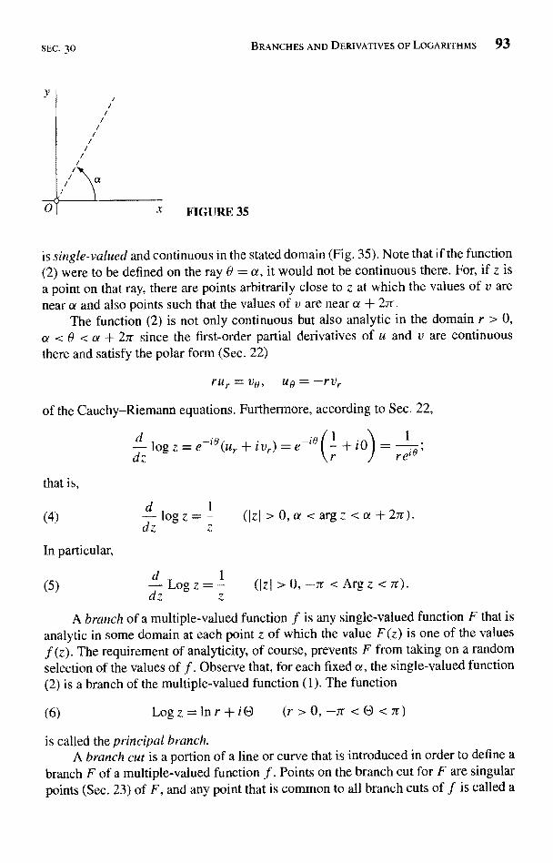
SEC. 30 BRANCHES AND DERIVATIVES OF LOGARITHMS 93
X FIGURE 35
ingle-valued and continuous in the stated domain (Fig. 35). Note that if the function(2) were to be defined on the ray 0 = a, it would not be continuous there. For, if z isa point on that ray, there are points arbitrarily close to z at which the values of v arenear a and also points such that the values of v are near a + 27c.
The function (2) is not only continuous but also analytic in the domain r > 0,a < 0 < a + 2n since the first-order partial derivatives of u and v are continuousthere and satisfy the polar form (Sec. 22)
rur = u0, u0 = -rvr
of the Cauchy-Riemann equations. Furthermore, according to Sec. 22,
d logV=e-i0(ur+ivr)=e-i0Q1 +i0) =1
dz r re
d log z=
1
d17 z0, a <argz <a+2Tr
Logz= (jz) > 0, -7r <Argz <7r).dz z
A branch of a multiple-valued function f is any single-valued function F that isanalytic in some domain at each point z of which the value F(z) is one of the valuesf (z). The requirement of analyticity, of course, prevents F from taking on a randomselection of the values of f. Observe that, for each fixed a, the single-valued function(2) is a branch of the multiple-valued function (1). The function
(6) Log z = In r + i(9 (r > 0, -rr < O < 7r)
is called the principal branch.A branch cut is a portion of a line or curve that is introduced in order to define a
branch F of a multiple-valued function f. Points on the branch cut for F are singularpoints (Sec. 23) of F, and any point that is common to all branch cuts of f is called a
94 ELEMENTARY FUNCTIONS CHAP. 3
branch point. The origin and the ray 6 = a make up the branch cut for the branch (2)of the logarithmic function. The branch cut for the principal branch (6) consists of theorigin and the ray O = 7r. The origin is evidently a branch point for branches of themultiple-valued logarithmic function.
EXERCISES
1. Show that
(a) Log(-ei) = 1- (b)Log(l-i)= 111n2-
n+4i.2. Verify that when n = 0, +1, ±2, . .
I(a)loge=I+2niri; (b)logi=(2n+-Irri;
(c)log(-l-1--i)=In 2+2 (n + )ni.2
3. Show that
(a) Log(1 + i)2 = 2 Log(1 + i); (b) Log(-l + i)2 A 2 Log(-1 + i).
4. Show that
(a) log(i2) = 2 log i when log z = In r + i BJr <0 <4 4
3rr 11Jr(b) log(i L) 54 2 log i when log z =1n r + i& (r > 0, < 0 <- 4
5. Show that
(a) the set of values of log(i 1/2) is (n + 41),7 i (n = 0, ±1, ±2, ...) and that the same istrue of (1/2) log i;
(b) the set of values of log(i2) is not the same as the set of values of 2 log i.
6. Given that the branch log z = In r + iB (r > 0, a < 0 < a + 27r) of the logarithmic func-tion is analytic at each point z in the stated domain, obtain its derivative by differentiatingeach side of the identity exp(log z) = z (Sec. 29) and using the chain rule.
7. Find all roots of the equation log z = iir/2.
Ans. z = i.
8. Suppose that the point z = x + iy lies in the horizontal strip a < y < a + 2n. Show thatwhen the branch log z =1n r + iB (r > 0, a < 0 < a + 21r) of the logarithmic functionis used, log(e`) = z.
9. Show that
(a) the function Log(z - i) is analytic everywhere except on the half line y = 1(x < 0);(b) the function
Log(z + 4)Z2 + i
is analytic everywhere except at the points + (1- i)/'12 and on the portion x < -of the real axis.
SEC. 31 SOME IDENTITIES INVOLVING LOGARITHMS 95
10. Show in two ways that the function ln(x2 + y2) is harmonic in every domain that doesnot contain the origin.
11. Show that
Re[log(z - 1)] = I ln[(x - .Y2] (z A 1)
Why must this function satisfy Laplace's equation when z ; 1?
. SOME IDENTITIES INVOLVING LOGARITHMS
As suggested by relations (3) and (4) in, Sec. 29, as well as Exercises 3, 4, and 5 withSec. 30, some identities involving logarithms in calculus carry over to complex analysisand others do not. In this section, we derive a few that do carry over, sometimes withqualifications as to how they are to be interpreted. A reader who wishes to pass to See.32 can simply refer to results here when needed.
If z1 and z2 denote any two nonzero complex numbers, it is straightforward toshow that
(1) log(z 1z2) = log Z I + log z2.
This statement, involving a multiple-valued function, is to be interpreted in the sameway that the statement
(2) arg(z 2 =argz1+argz2
was in Sec. 7. That is, if values of two of the three logarithms are specified, then thereis a value of the third logarithm such that equation (1) holds.
The proof of statement (1) can be based on statement (2) in the following way.Since 1Z Iz2I = 1Z 1 I I Z21 and since these moduli are all positive real numbers, we knowfrom experience with logarithms of such numbers in calculus that
In Izlz21 =In IziI + In Iz21.
So it follows from this and equation (2) that
(3) In Izlz21 + i arg(zIz2) = (In Iz1 I + i arg z1) + (In Iz21 + i arg z2).
Finally, because of the way in which equations (1) and (2) are to be interpreted,equation (3) is the same as equation (1).
EXAMPLE. To illustrate statement (1), write z1= Z2 = -l and note that ztz2 = 1.If the values log z1 = 7ri and log z2 = -7ri are specified, equation (1) is evidentlysatisfied when the value Iog(z1z2) = 0 is chosen.
Observe that, for the same numbers z1 and z2,
Log(zlz2 0 and Log z 1 + Log z2 = 2Tr i .
Thus statement (1) is not, in general, valid when log is replaced everywhere by Log.
96 ELEMENTARY FUNCTIONS CHAP. 3
Verification of the statement
(4) log (Z
I1 ) =log z 1 -log z2,
which is to be interpreted in the same way as statement (1), is left to the exercises.We include here two other properties of log z that will be of special interest in
Sec. 32. If z is a nonzero complex number, then
(5)Zn = en log z (n=0±1,±2,.
for any value of log z that is taken. When n = 1, this reduces, of course, to relation (3),Sec. 29. Equation (5) is readily verified by writing z = re`O and noting that each sidebecomes r"e`"O
It is also true that when z A 0,
(6 =exp log Z) (n =
That is, the term on the right here has n distinct values, and those values are the nthroots of z. To prove this, we write z = r exp(i O), where 19 is the principal value ofarg z. Then, in view of definition (2), Sec. 29, of log z,
N
exp(1
log z) = exp1
In r +i (O + 2k7r )
n In n
where k = 0, ±1, ±2, .... Thus
O 2k-r
(7) exp{n
log z r exp) i n+ k=0, ±1,±2,
Because exp(i2kn/n) has distinct values only when k = 0, 1, ... , n - 1, the right-hand side of equation (7) has only n values. That right-hand side is, in fact, anexpression for the nth roots of z (Sec. 8), and so it can be written z 1/". This establishesproperty (6), which is actually valid when n is a negative integer too (see Exercise 5).
EXERCISES
1. Show that ifRezl>0andRez2>0,then
Log(zlz2) = Log zl + Log z2.
2. Show that, for any two nonzero complex numbers z1 and z2,
Log(z1z2) = Log z1 + Log z2 + 2N7ri
where N has one of the values 0, ±1. (Compare Exercise 1.)
3. Verify expression (4), Sec. 31, for log(zl/z2) by
(a) using the fact that arg(zt/z2) = arg zI - arg z2 (Sec. 7);
SEC. 32 COMPLEX EXPONENTS 97
(b) showing that log(1/z) = - log z (z A 0), in the sense that log(l/z) and - log z havethe same set of values, and then referring to expression (1), Sec. 31, for log(ztz2).
4. By choosing specific nonzero values of zt and z2, show that expression (4). Sec. 31, forlog(z1/z2) is not always valid when log is replaced by Log.
5. Show that property (6), Sec. 31, also holds when n is a negative integer. Do this by writingzlln = (zt1'n)-l (m = -n), where n has any one of the negative values n = -1, -2, .. .(see Exercise 9, Sec. 9), and using the fact that the property is already known to be validfor positive integers.
6. Let z denote any nonzero complex number, written z = re`n (-Jr < 0 < rr), and let ndenote any fixed positive integer (n = 1, 2, ...). Show that all of the values of log(zlln)are given by the equation
log n) =1
In rC +2(pn+k)n--f- i
n n
where p = 0, E 1, ±2, ... and k = 0, 1, 2, ... , n - 1 . Then, after writing
-Iogz= I Inr+i(9 +2q7rn n n
where q = 0, ±1, , . . . , sh o w ow that the set of values of log(z 11 n) is the same as the setof values of (1/n) log z. Thus show that log(zlln) = (1/n) log z, where, correspondingto a value of log (z t/n) taken on the left, the appropriate value of log z is to be selected onthe right, and conversely. [The result in Exercise 5(a), Sec. 30, is a special case of thisone.]
Suggestion: Use the fact that the remainder upon dividing an integer by a positiveinteger n is always an integer between 0 and n - 1. inclusive; that is, when a positiveinteger n is specified, any integer q can be written q = pn + k, where p is an integer andk has one of the values k = 0, 1, 2, ... , n - 1.
32. COMPLEX EXPONENTS
When z 0 0 and the exponent c is any complex number, the function ZC is defined bymeans of the equation
(1) Z = ec log z
where log z denotes the multiple-valued logarithmic function. Equation (1) providesa consistent definition of z` in the sense that it is already known to be valid (see Sec.31) when c = n (n = 0, ±1, ±2, ...) and c = 1/n (n = ±1, f2, ...). Definition (1)is, in fact, suggested by those particular choices of c.
EXAMPLE 1. Powers of z are, in general, multiple-valued, as illustrated by writing
i-2" = exp(-2i log i)
98 ELEMENTARY FUNCTIONS
and then
logi =1n 1+i[ 2 +2n7r
This shows that \
(2) i-2i = exp[(4n
n=0,±1,±2,...
(n = 0, ±1, ±2,
CHAP. 3
Note that these values of i -2` are all real numbers.Since the exponential function has the property 1/ez = e-z, one can see that
1
=1
= exp(-c log z) = z-`zC exp(c log z)
and, in particular, that 1/ i2i = i -2i. According to expression (2), then,
1= exp[(4n + 1)7r] (n = 0, ±1, ±
If z = reie and a is any real number, the branch
logz=lnr+i8 (r>0,a <0 <a+2rr)
of the logarithmic function is single-valued and analytic in the indicated domain (Sec.30). When that branch is used, it follows that the function z` = exp(c log z) is single-valued and analytic in the same domain. The derivative of such a branch of z` is foundby first using the chain rule to write
zC= exp(c log z) = z exp(c log z)
and then recalling (Sec. 29) the identity z = exp(log z). That yields the result
d-z `
= cexp(c c exp[(c - 1) log z],eP(log z)
or
(4) ddzz` = Czc-1 (Izj > 0, a < arg z < a + 2.7r).
The principal value of zC occurs when log z is replaced by Log z in definition (1):
(5) P.v.z`= z
uation (5) also serves to define the principal branch of the function z` on the domainIzI>0,-rr<Argz<n.
SEC. 32
EXAMPLE 2. The principal value of (-
nexp[i Log(-i )] = exp I i ( In 1- i - ) I = exp - .
That is,
(6) P.V. (-i)` = exp-n
.
2
EXAMPLE 3. The principal branch of z2/3 can be written
exp( Log z = exp` 3 In r-
Thus
(7) P.V. z2
exp
.,., 2cos
Zd+ i V r2 sin
3
EXERCISES 99
This function is analytic in the domain r > 0, -rc < 0 < 7, as one can see directlyfrom the theorem in Sec. 22.
According to definition (1), the exponential function with base c, where c is anynonzero complex constant, is written
(8)CZ = ez log c
Note that although ez is, in general, multiple-valued according to definition (8), theusual interpretation of eZ occurs when the principal value of the logarithm is taken.For the principal value of log e is unity.
When a value of log c is specified, cz is an entire function of z. In fact,
dCZ = de" log e = ez log c log C;dz dz
and this shows that
(9)
EXERCISES
dC` = CZ log C.
dz
1. Show that when n = 0, f 1, f2, ... ,a (2' I 1}it n = eIn 2_ (b) (-1)+ 2nrrI exn(
. I I \ d / ` \2 I2. Find the principal value of
i`` (b)(C) i)4!
Ans. (a) exp(-7r/2); (b) - exp(2 2 (c) e'r[cos(2 in 2) + i sin(2 In 2)].
100 ELEMENTARY FUNCTIONS CHAP. 3
3. Use definition (1), Sec. 32, of z` to show that (-1 +i)3j2 = ± 2.4. Show that the result in Exercise 3 could have been obtained by writing
(a) (-1 + _"/3i)3/2 = [(-1 +.i) I/2]3 and first finding the square roots of - I + i ;
(b) (-1 + /3i)31/2 = [(-1 + /3i)311/2 and first cubing -1 + 3i.
5. Show that the principal nth root of a nonzero complex number z0, defined in Sec. 8, is
the same as the principal value of zO n, defined in Sec. 32.
6. Show that if z 0 and a is a real number, then jzaj = exp(a In jzj) = Izja, where theprincipal value of jzja is to be taken.
7. Let c = a + bi be a fixed complex number, where c * 0, ±1, ±2, . . . , and note that i`is multiple-valued. What restriction must be placed on the constant c so that the valuesof ji`'j are all the same?
Ans. c is real.
8. Let c, d, and z denote complex numbers, where z * 0. Prove that if all of the powersinvolved are principal values, then
(a) 1/z` = z (b) (z`)" = z" (n = 1, 2, ...(C) zlzd = zc+d; (d) zc/zd = z`-d
9. Assuming that f (z) exists, state the formula for the derivative of cfcz).
33. TRIGONOMETRIC FUNCTIONSEuler's formula (Sec. 6) tells us that
eix = cos x - i sin x and e-`X = cos x - i sin x
for every real number x, and it follows from these equations that
eiX - e-IX = 2i sin x and eix + e-i' = 2 cos x.
That is,
sin x =2i
e`X -and cos x
e
2
It is, therefore, natural to define the sine and cosine functions of a complex variable zas follows:
sin z =e`'Z
2icos z =
These functions are entire since they are linear combinations (Exercise 3, Sec. 24)of the entire functions e`z and e-`~. Knowing the derivatives of those exponentialfunctions, we find from equations (1) that
(2)dz
sin z = cos z,ti
cos z = - sin z.d
SEC. 33 TRIGONOMETRIC FUNCTIONS 101
It is easy to see from definitions (1) that
(3) sin(-z) = - sin z and Cos =cosz;
and a variety of other identities from trigonometry are valid with complex variables.
EXAMPLE. In order to show that
(4) 2 sin zr cos z2 = sin(zi z2) { sin(z - z2),
using definitions (1) and properties of the exponential function, we first write
- e-j7?2 sin z, cos z, =
Multiplication then reduces the right-hand side here to
ei(zi+z2) - e-i(z1+z2) ei(Z1-z2) - e-i(zl-z2)
2i 2i
or
and identity (4) is established.
sin(z1 + Z2) = sin zi cos Z2 + COS zi sin Z2,
Identity (4) leads to the identities (see Exercises 3 and 4)
(5)
(6) cOS(zl + z2) = cos z1 cos Z2 - sin Zl sin z2;
and from these it follows that
(7)
sin{zi z2) + sin(Z1 - z2);
sin- z cos2 z = 1,
sin 2z = 2 sin z cos z, cos 2z = cos2 z - sin2 z
(9) sin z + 2) = cos z, sin Cz - 2 = - cos Z.
When y is any real number, one can use definitions (1) and the hyperbolicfunctions
sinh
from calculus to write
and cosh y =_y
-e
2
(10) sin(iy) = i sinh y and cos(iy) = cosh y.
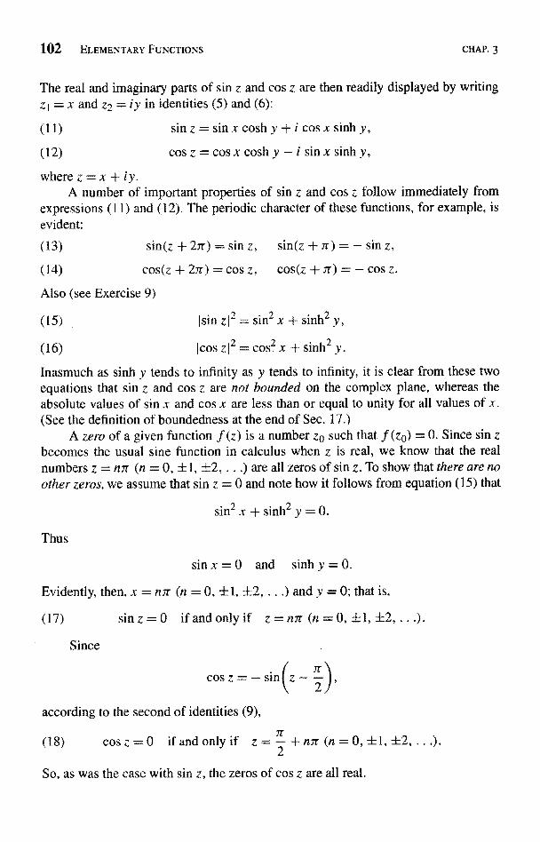
102 ELEMENTARY FUNCTIONS CHAP. 3
The real and imaginary parts of sin z and cos z are then readily displayed by writingz 1= x and z2 = iy in identities (5) and (6):
(11) sin z = sin x cosh y + i cos x sinh y,
(12) cos z = COS x cosh y - i sin x sink y,
where z = x + iy.A number of important properties of sin z and cos z follow immediately from
expressions (11) and (12). The periodic character of these functions, for example, isevident:
(13) sin(z + 2jr) = sin z, sin(-, + ,r) = - sin z,
(14) cos(z + 27r) = cos z, cos(z +;r) = - cos z.
Also (see Exercise 9)
(15)
(16)
I sin z I2 = sin2 x + sinh2 y,
,COs z12 = cost x + sinh2 Y.
Inasmuch as sinh y tends to infinity as y tends to infinity, it is clear from these twoequations that sin z and cos z are not bounded on the complex plane, whereas theabsolute values of sin x and cos x are less than or equal to unity for all values of x.(See the definition of boundedness at the end of Sec. 17.)
A zero of a given function f (z) is a number ze such that f (ze) = 0. Since sin zbecomes the usual sine function in calculus when z is real, we know that the realnumbers z = nrr (n = 0, +1, +2, . . .) are all zeros of sin z. To show that there are noother zeros, we assume that sin z = 0 and note how it follows from equation (15) that
sin2 x + sinh2 y = 0.
Thus
sin x = 0 and sink y = 0.
Evidently, then, x = nzr (n = 0, +1, ±2, ...) and y = 0; that is,
(17) sinz=0 if and only if z=nn (n=0,±1.±2,..
Since
cos z = - sin
according to the second of identities (9),
(18) COSz=0 if and only if z- +me(n=0,f1,f2,..
So, as was the case with sin z, the zeros of cos z are all real.
SEC. 33 EXERCISES 103
The other four trigonometric functions are defined in terms of the sine and cosinefunctions by the usual relations:
(19) tanz= sin z, cotz= cos z
cos z sin z
1 1
(20) sec -7 = , csc z = .
cos z sin z
Observe that the quotients tan z and sec z are analytic everywhere except at thesingularities (Sec. 23)
z = 2 + n7r (n = 0, ±1, ±2, .
which are the zeros of cos z. Likewise, cot z and csc z have singularities at the zerosof sin z, namely
z = n7r (n = 0, ±1, ±2, . .
By differentiating the right-hand sides of equations (19) and (20), we obtain theexpected differentiation formulas
(21) d tan z = sect z,d
cot z = - csc2 z,dz dz
(22) d sec z = sec z tan z,dz
d cscz=- csczcot z.dz
The periodicity of each of the trigonometric functions defined by equations (19) and(20) follows readily from equations (13) and (14). For example,
(23) tan(z + 7r) = tan z.
Mapping properties of the transformation w = sin z are especially important inthe applications later on. A reader who wishes at this time to learn some of thoseproperties is sufficiently prepared to read Sec. 89 (Chap. 8), where they are discussed.
EXERCISES
1. Give details in the derivation of expressions (2), Sec. 33, for the derivatives of sin z andcos Z.
2. Show that Euler's formula (Sec. 6) continues to hold when 8 is replaced by z:
ize =cost+i sin z.
Suggestion: To verify this, start with the right-hand side.
3. In Sec. 33, interchange zt and z2 in equation (4) and then add corresponding sides of theresulting equation and equation (4) to derive expression (5) for sin(zt + z2).
104 ELEMENTARY FUNCTIONS CHAP. 3
4. According to equation (5) in Sec. 33,
sin(z+z2)=SinzCOSz2+coszsinz2.
By differentiating each side here with respect to z and then setting z = z1, derive expres-Sion (6) for cos(zI + z2) in that section.
5. Verify identity (7) in Sec. 33 using
a identity (6) and relations (3) in that section;(b) the lemma in Sec. 26 and the fact that the entire function
f(z)=sin 2z+cos2z- 1
has zero values along the x axis.
6. Show how each of the trigonometric identities (8) and (9) in Sec. 33 follows from oneof the identities (5) and (6) in that section.
7. Use identity (7) in Sec. 33 to show that
(a) 1 + tan2 z = sect z; (b) I + cot2 z = csc2 Z.
8. Establish differentiation formulas (21) and (22) in Sec. 33.
9. In Sec. 33, use expressions (11) and (12) to derive expressions (15) and (16) for I sin z ( 2and icon zi`.
Suggestion: Recall the identities sin2 x + cost x = I and cosh2 y - sinh2 y = 1.
10. Point out how it follows from expressions (15) and (16) in Sec. 33 for isin z 12 and Icos z I2that
(a) Isin z1 > isin xj; (b) Icos zl > Icos xi.
11. With the aid of expressions (15) and (16) in See. 33 for isin z12 and I cos z12, show that
(a) Isinh yI < sin zI < cosh y; (b) Esinh yj < Icos zi < cosh y.
12. (a) Use definitions (1), Sec. 33, of sin z and cos z to show that
2 sin(z1 + z2) sin(zl - z2) = cos 2z2 - cos 2z1.
(b) With the aid of the identity obtained in part (a), show that if cos zI = cos z2, then atleast one of the numbers zI + z2 and zI z2 is an integral multiple of 27r.
13. Use the Cauchy-Riemann equations and the theorem in Sec. 20 to show that neither sin znor cos z is an analytic function of z anywhere.
14. Use the reflection principle (Sec. 27) to show that, for all z,
(a) sin z = sin z; (b) cos z = cos 4.
15. With the aid of expressions (11) and (12) in Sec. 33, give direct verifications of therelations obtained in Exercise 14.
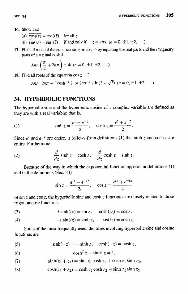
SEC. 34 HYPERBOLIC FUNCTIONS 105
16. Show that
(a) cos(iz) = cos(iz) for all z;
(b) sin(iz) = sin(iz) if and only if z = nrri (n = 0, ±1, ±2, ...).
17. Find all roots of the equation sin z = cosh 4 by equating the real parts and the imaginaryparts of sin z and cosh 4.
Ans. { + 2n7r { + 4i (n = 0, +1. +2, ...).
18. Find all roots of the equation cos z = 2.
Ans. 2nrr + i cosh-12, or 2nTr ± i ln(2 + ) (n=O,±],±2,..
34. HYPERBOLIC FUNCTIONSThe hyperbolic sine and the hyperbolic cosine of a complex variable are defined asthey are with a real variable; that is,
z
sinh - ez - e-coshz =
ez + e-z41
2 2
Since ez ande_z are entire, it follows from definitions (1) that sinh z and cosh z are
entire. Furthermore,
(2)
dsinh z = cosh z,
dcosh z = sinh z.
dz dz
Because of the way in which the exponential function appears in definitions (and in the definitions (Sec. 33)
etz - e-1z
sin z =2i
, cos z2
e-`z
of sin z and cos z, the hyperbolic sine and cosine functions are closely related to thosetrigonometric functions:
(3) -i sinh(iz) = sin z, cosh(iz) = cos z,
(4) -i sin(iz) = sinh z, cos(iz) = cosh Z.
Some of the most frequently used identities involving hyperbolic sine and cosinefunctions are
(5) sinh(-z) = - sinh z, cosh(-z) = cosh z,
(6) cosh2 z - sinh2 z = 1,
(7) sinh(zi + z2) = sinh z1 cosh Z2 + cosh zI sinh z2,
(8) cosh(zi + z2) = cosh z1 cosh Z2 + sinh z1 sinh z2
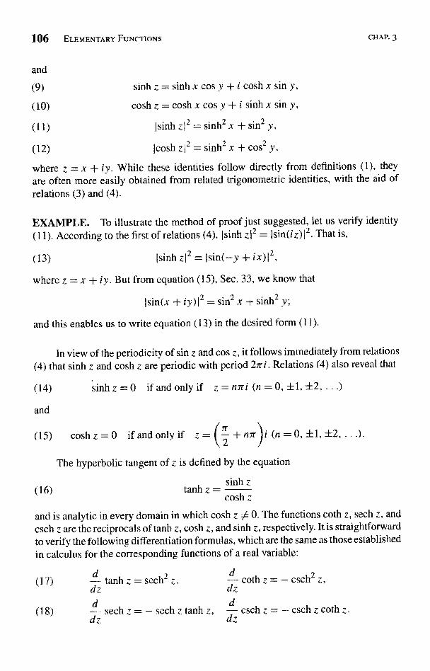
106 ELEMENTARY FUNCTIONS CHAP. 3
and
(9) sinh z = sinh x cosy + i cosh x sin y,
(10) cosh z = cosh x cosy + i sinh x sin y,
(11) Isinh zl2 = sinh2 x + sin` y,
(12) Icosh z 12 = sinh2 x + cost y,
where z = x + iv. While these identities follow directly from definitions (1), they
are often more easily obtained from related trigonometric identities, with the aid ofrelations (3) and (4).
EXAMPLE. To illustrate the method of proof just suggested, let us verify identity(11). According to the first of relations (4), (sinh z12 = Isin(iz)12. That is,
(13) Isinh z!2 = Isin(-y + ix)12,
where z = x + iv. But from equation (15), Sec. 33, we know that
Isin(x + iy)12 = sin 2 x + sinh2 y;
and this enables us to write equation (13) in the desired form (1 1).
In view of the periodicity of sin z and cos z, it follows immediately from relations(4) that sinh z and cosh z are periodic with period 21ri. Relations (4) also reveal that
(14) sinh z = 0 if and only if z = nni (n = 0, fl, +2, ...)
and
(15) cosh z = 0 if and only if z = (2 + nrr)i (n = 0, ±1, +2, .
(16)
The hyperbolic tangent of z is defined by the equation
tank z =sinh z
cosh z
and is analytic in every domain in which cosh z A 0. The functions coth z, sech z, andesch z are the reciprocals of tanh z, cosh z, and sinh z, respectively. It is straightforwardto verify the following differentiation formulas, which are the same asthose establishedin calculus for the corresponding functions of a real variable:
(17) tank z = sech` z,dz
(18) dz sechz=-sechztanhz,
d Goth z = - csch2 z,dzd
csch z = - csch z coth z.dz
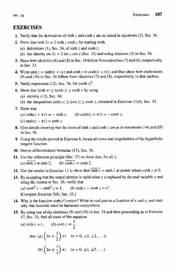
SEC. 34 EXERCISES 107
EXERCISES
1. Verify that the derivatives of sinh z and cosh z are as stated in equations (2), Sec. 34.
2. Prove that sinh 2z = 2 sinh z cosh z by starting with
(a) definitions (1), Sec. 34, of sinh z and cosh z;(b) the identity sin 2z = 2 sin z cos z (Sec. 33) and using relations (3) in Sec. 34.
3. Show how identities (6) and (8) in Sec. 34 follow from identities (7) and (6), respectively,in Sec. 33.
4. Write sinh z = sinh(x + iy) and cosh z = cosh(x + iy), and then show how expressions(9) and (10) in Sec. 34 follow from identities (7) and (8), respectively, in that section.
5. Verify expression (12), Sec. 34, for (cosh z12.
6. Show that Isinh xI < cosh zI < cosh x by using
(a) identity (12), Sec. 34;(b) the inequalities I sinh y I < cos z I cosh y, obtained in Exercise 11(b), Sec. 33.
7. Show that(a) sinh(z + ni) = - sinh z; (b) cosh(z + ni) cosh z;
(c) tanh(z + ni) = tanh z.
8. Give details showing that the zeros of sinh z and cosh z are as in statements (14) and (15)in Sec. 34.
9. Using the results proved in Exercise 8, locate all zeros and singularities of the hyperbolictangent function.
10. Derive differentiation formulas (17), Sec. 34.
11. Use the reflection principle (Sec. 27) to show that, for all z,
(a) sinh z = sinh z; (b) cosh z = cosh z.
12. Use the results in Exercise 11 to show that tanh z = tank z at points where cosh z 0 0.
13. By accepting that the stated identity is valid when z is replaced by the real variable x andusing the lemma in Sec. 26, verify that
(a) cosh` z - sinh2 z = 1; (b) sinh z + cosh z = e4.
[Compare Exercise 5(b), Sec. 33.]
14. Why is the function sinh(ez) entire? Write its real part as a function of x and y, and statewhy that function must be harmonic everywhere.
15. By using one of the identities (9) and (10) in Sec. 34 and then proceeding as in Exercise17, Sec. 33, find all roots of the equation
(a) sinh z = i ; (b) cosh z = 2I.
Ans. (a) (2n + 2} 7ri (n = 0, 11, ±2, .. .
1( 2 n (n=0,±l,±2,...).
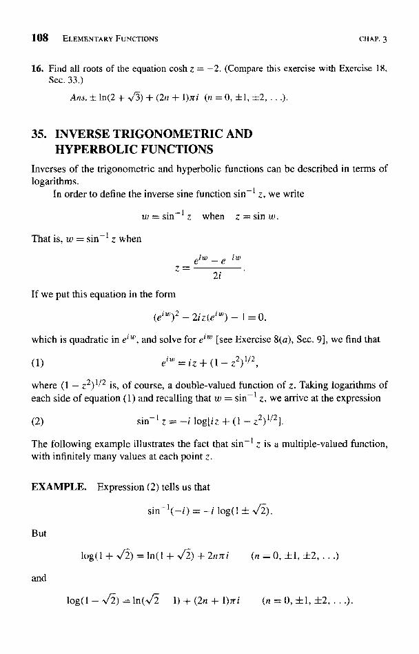
108 ELEMENTARY FUNCTIONS CHAP. 3
16. Find all roots of the equation cosh z = -2. (Compare this exercise with Exercise 18,Sec. 33.)
Ans. ±ln(2+ )+(2n+1)ni (n=0,±1,+2,...).
35. INVERSE TRIGONOMETRIC ANDHYPERBOLIC FUNCTIONS
Inverses of the trigonometric and hyperbolic functions can be described in terms oflogarithms.
In order to define the inverse sine function sin-1 z, we write
sin-1 z when z = sin w.
That is, w = sin-1 z when
z2i
If we put this equation in the form
(e'')2- 2iz(etw) - = 0,
which is quadratic in e' u', and solve for e`` [see Exercise 8(a), Sec. 9], we find that
(1) + (l -- z2)112,
where (1 - z2)112 is, of course, a double-valued function of z. Taking logarithms ofeach side of equation (1) and recalling that w = sin-1 z, we arrive at the expression
(2) sin-1 z = -i log[i z + (1 `2)1(2]
The following example illustrates the fact that sin-` z is a multiple-valued function,with infinitely many values at each point z.
EXAMPLE. Expression (2) tells us that
But
and
log(1 -,/2
sin-1(-i) = -i log(1 ± ).
=1n(1 + V) + 2n.rri (n = 0, ±1, ±2, ...)
log(1- )=ln(i- 1)+(2n+1)iri (n=0,±1,+2,...).
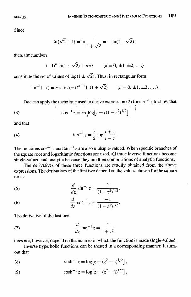
SEC. 35 INVERSE TRIGONOMETRIC AND HYPERBOLIC FUNCTIONS 109
Since
2 - l) = In In(l + ),
then, the numbers
(-1)"ln(I+/)+n7ri (n=0,+1,+2,...)
constitute the set of values of log(l ± ). Thus, in rectangular form,
sin-1(-i) = nJr + i (-l)"+I in(l + ) (n = 0, +1, ±2,
One can apply the technique used to derive expression (2) for sin-1 z to show that
cos-1 z = -i 1og[z + i(1 - z2)1/2]
and that
(4)- i
logi + z
2 i-zThe functions cos-1 z and tan-1 z are also multiple-valued. When specific branches ofthe square root and logarithmic functions are used, all three inverse functions becomesingle-valued and analytic because they are then compositions of analytic functions.
The derivatives of these three functions are readily obtained from the aboveexpressions. The derivatives of the first two depend on the values chosen for the squareroots:
(5)
(6)
dsin- 1 z =
1
dz (1- z2)1/2'
.
d _] -1COS z =
dz (I-z2)1/2
The derivative of the last one,
(7)d-tdz
-- 4 - 1+z2,
does not, however, depend on the manner in which the function is made single-valued.Inverse hyperbolic functions can be treated in a corresponding manner. It turns
out that
sinh-1 z = log [Z + (z2 + 2]
cosh-1 z = log [Z + (z2 - 1)1/211
0 ELEMENTARY FUNCTIONS CHAP. 3
and
(10) tank- Iz= Ilog i+z
Finally, we remark that common alternative notation for all of these inverse
functions is arcsin z, etc.
EXERCISES
1. Find all the values of
(a) tan -I(2i); (b) tan-I(1i
(c) cosh-I(-1); (d) tanh-I 0.
Ans. (a)(n+ 2r+ In3(n=0,+1,±2,-..);
(d) niri (n = 0. ±1, ±2, ...).
2. Solve the equation sin z = 2 for z by
(a) equating real parts and imaginary parts in that equation;
(b) using expression (2), Sec. 35, for sin- IZ.
Ans. (2n -1 )2r±i1n(2+3) (n = 0, ±l, ±2....).2)
3. Solve the equation cos z = -s./12 for z.
4. Derive formula (5), Sec. 35, for the derivative of sin- I
Z.
5. Derive expression (4), Sec. 35. for tan- IZ.
6. Derive formula (7), Sec. 35, for the derivative of tan -I z.
7. Derive expression (9), Sec. 35, for cosh-1 z.
CHAPTER
4INTEGRALS
Integrals are extremely important in the study of functions of a complex variable. Thetheory of integration, to be developed in this chapter, is noted for its mathematicalelegance. The theorems are generally concise and powerful, and most of the proofsare simple.
36. DERIVATIVES OF FUNCTIONS w(t)
In order to introduce integrals of f (z) in a fairly simple way, we need to first considerderivatives of complex-valued functions w of a real variable t. We write
(1) u(t)+iv
where the functions u and v are real-valued functions of t. The derivative w'(t), ord[w(t)]jdt, of the function (1) at a point t is defined as
(2) w'(t) = u'(t) + W (t),
provided each of the derivatives u' and v' exists at t.From definition (2), it follows that, for every complex constant zc = x0 + iy0,
d [zOw(t)]=[(x0+iy0)(u+iv)]'=[ - yov) + i (you + xov)]'
(xou - yov)` + i (you + xov)' = (xou' - yov) + i (you` + xcv)
112 INTEGRALS CHAP. 4
But
(xou' - You) + i (your + x0v') _ (xo + iY0)(u' + iv'
and so
(3) [zow(t)] = zowat
Another expected rule that we shall often use is
(4) eOt
= 4neZOtdt
where zo = xo + i yo. To verify this, we write
e"Ot _ ex0tety0t =e YOt cos yot + ieXOt sin yot
and refer to definition (2) to see that
dtezpt = WO' cos y0t)' + i (exOt sin y0t)'.
Znw'(t)I
Familiar rules from calculus and some simple algebra then lead us to the expression
dezOt = (xo + iYo)
or
dt
X cos yot + iexOt sin y0t),
ezO' = (xo + iyo)eXOte'YOt
This is, of course, the same as equation (4).Various other rules learned in calculus, such as the ones for differentiating sums
and products, apply just as they do for real-valued functions of t. As was the casewith property (3) and formula (4), verifications may be based on corresponding rulesin calculus. It should be pointed out, however, that not every rule for derivatives incalculus carries over to functions of type (1). The following example illustrates this.
EXAMPLE. Suppose that w(t) is continuous on an interval a < t < b; that is, itscomponent functions u(t) and v(t) are continuous there. Even if w'(t) exists whena < t < b, the mean value theorem for derivatives no longer applies. To be precise, itis not necessarily true that there is a number c in the interval a < t < b such that
,(e) _ w(b) - w(a)W
b-a
d
To see this, consider the function w(t) = e't on the interval 0 < t < 2ir. When thatfunction is used, I w'(t) I = Iieit f = 1; and this means that the derivative w'(t) is neverzero, while w (22r) - w (0) = 0.
SEC. 37 DEFINITE INTEGRALS OF FUNCTIONS W(t) 113
37. DEFINITE INTEGRALS OF FUNCTIONS w(t)
When w(t) is a complex-valued function of a real variable t and is written
w(t) = u(t)
where u and v are real-valued, the definite integral of w (t) over an interval a <is defined as
(2) j w(t)dt= j u(t)dt+i f v(t)dta a a
when the individual integrals on the right exist. Thus
b b
(3) Re I w(t) dt = I Re[w(t)] dt
EXAMPLE 1. For an illustration of definition (2),
fo
1
Improper integrals of w (t) over unbounded intervals are defined in a similar way.The existence of the integrals of u and v in definition (2) is ensured if those
functions are piecewise continuous on the interval a < t < b. Such a function iscontinuous everywhere in the stated interval except possibly for a finite number ofpoints where, although discontinuous, it has one-sided limits. Of course, only the right-hand limit is required at a; and only the left-hand limit is required at b. When both uand v are piecewise continuous, the function w is said to have that property.
Anticipated rules for integrating a complex constant times a function w(t), forintegrating sums of such functions, and for interchanging limits of integration are allvalid. Those rules, as well as the property
Ib
w(t) dt = j w(t) dt + j w(t) dt,
are easy to verify by recalling corresponding results in calculus.The fundamental theorem of calculus, involving antiderivatives, can, moreover,
be extended so as to apply to integrals of the type (2). To be specific, suppose that thefunctions
=u(t)+iv(t) and W(t)=U(t)+iV(t)
114 INTEGRALS CHAP. 4
are continuous on the interval a < t < b. If W(t) = w(t) when a < t < b, thenU'(t) = u(t) and V'(t) = ra(t). Hence, in view of definition (2),
b b b
f w(t) dt = U(t)j + iV(t)ja a a
= [U(b) + W WI -
That is,
L
EXAMPLE 2. Since
b
see Sec. 36),
nn/4 f4
ett dt = -ie't 1 = -ie'"/4 + i0
iV
We finish here with an important property of moduli of integrals. Namely,
(5)
fa
b
w(t) dt dt (a < b
This inequality clearly holds when the value of the integral on the left is zero, inparticular when a = b. Thus, in the verification, we may assume that its value is anonzero complex number. If rp is the modulus and 9fl is an argument of that constant,then
w dt = rpe`04
Solving for r0, we write
(6) e-`°0w dt.
Now the left-hand side of this equation is a real number, and so the right-hand side istoo. Thus, using the fact that the real part of a real number is the number itself andreferring to the first of properties (3), we see that the right-hand side of equation (6)can be rewritten in the following way:
.u dt = Re I e-` 0w dt = Re(e-"Ow) dt.
SEC. 37
Equation (6) then takes the form
(7)
But
Re(e-te0w)
and so, according to equation (7,
Re(e_`Oaw) dt.
-io0wI= le-`0°lI
wl dt.
EXERCISES 115
Because ro is, in fact, the left-hand side of inequality (5) when the value of the integralthere is nonzero, the verification is now complete.
With only minor modifications, the above discussion yields inequalities such as
(8) w(t) dt
provided both improper integrals exist.
dt,
EXERCISES
1. Use the corresponding rules in calculus to establish the following rules when
iv
is a complex-valued function of a real variable t and w(t) exists:d
t, evaluated at -t;d
at-w(-t) = -w'(-t), where w'(-t) denotes the derivative of w(t) with respect to
(b)dt
[w(t)j'=2w(t)w(t).
2. Evaluate the following integrals:2 (
Ans.
t
2 h/(
dt; (b) I et2t dt; (c) I e-Zt dt (Re z > 0).
2
3. Show that if m and n are integers,
o2x
Jo
nd df =
C1
z
0 when m 54tar when m =
4. According to definition (2), Sec. 37, of integrals of complex-valued functions of a realvariable,
X dx = / eX cos x dx + i I ex sin x dx.
116 INTEGRALS CHAP. 4
Evaluate the two integrals on the right here by evaluating the single integral on the leftand then using the real and imaginary parts of the value found.
Ans. -(1 + e")/2, (1 + e")/2,
5. Let w(t) be a continuous complex-valued function oft defined on an interval a < t < h.By considering the special case w(t) = ett on the interval 0 < t < 2n, show that it is notalways true that there is a number c in the interval a < t < b such that
Ia
h
w(t) dt = w(c)(b -
Thus show that the mean value theorem for definite integrals in calculus does not applyto such functions. (Compare the example in Sec. 36.)
6. Let w(t) = u(t) + iv(t) denote a continuous complex-valued function defined on aninterval -a < t < a.(a) Suppose that w(t) is even; that is, w (-t) = w(t) for each point tin the given interval.
Show that
r w(t) dt = 2 1 w(t) dt.J -a
a
(b) Show that if w(t) is an odd function, one where w(-t) = -w(t) for each point tinthe interval, then
-aw(t) dt =
Suggestion: In each part of this exercise, use the corresponding property ofintegrals of real-valued functions of t, which is graphically evident.
7. Apply inequality (5), Sec. 37, to show that for all values of x in the interval - i < x < 1,the functions*
P"(x)=-- (x+iv/1-x2cosO)'dO (n=0,1,2,..
satisfy the inequality IPP(x)I <
38. CONTOURSIntegrals of complex-valued functions of a complex variable are defined on curves inthe complex plane, rather than on just intervals of the real line. Classes of curves thatare adequate for the study of such integrals are introduced in this section.
* These functions are actually polynomials in x. They are known as Legendre polynomials and areimportant in applied mathematics. See, for example, Chap. 4 of the book by Lebedev that is listedin Appendix 1.
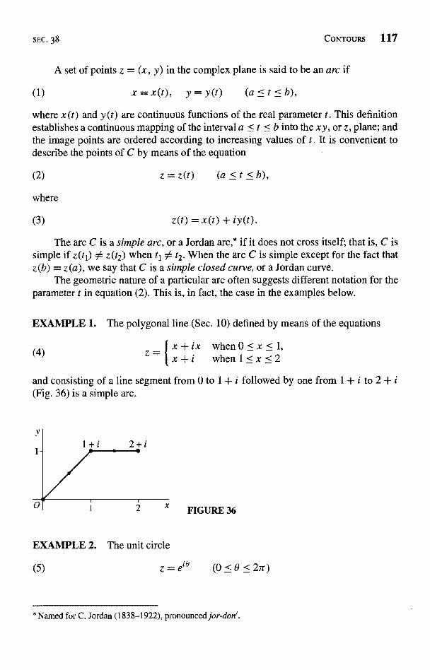
SEC, 38 CONTOURS 117
A set of points z = (x, y) in the complex plane is said to be an arc if
(1} x = x(t), y = y(t) (a < t < b),
where x(t) and y(t) are continuous functions of the real parameter t. This definitionestablishes a continuous mapping of the interval a < t < b into the xy, or z, plane; andthe image points are ordered according to increasing values of t. It is convenient todescribe the points of C by means of the equation
(2)
where
(3)
z=z(t) (a<t<b),
z(t) = x(t) + iy(t).
The are C is a simple arc, or a Jordan arc,* if it does not cross itself; that is, C issimple if z(tl) z(t2) when t1 t2. When the arc C is simple except for the fact thatz(b) = z(a), we say that C is a simple closed curve, or a Jordan curve.
The geometric nature of a particular arc often suggests different notation for theparameter t in equation (2). This is, in fact, the case in the examples below.
EXAMPLE 1. The polygonal line (Sec. 10) defined by means of the equations
(4)ix when 0 < x
x+i when I<x<2
and consisting of a line segment from 0 to 1 + i followed by one from 1 + i to 2 + i(Fig. 36) is a simple arc.
Y
1-I
XFIGURE 36
EXAMPLE 2. The unit circle
(5)
2+i0
2
* Named for C. Jordan (1838--1922), pronounced jor-don`.
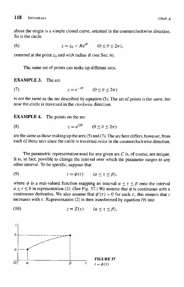
118 INTEGRALS CHAP. 4
about the origin is a simple closed curve, oriented in the counterclockwise direction.So is the circle
(6) z = zo + Re`' (0 < 9 < 27r),
centered at the point zu and with radius R (see Sec. 6).
The same set of points can make up different arcs.
EXAMPLE 3. The arc
(7)
is not the same as the arc described by equation (5). The set of points is the same, butnow the circle is traversed in the clockwise direction.
z=e-i8 (0<9<27r)
EXAMPLE 4. The points on the arc
(8) z = ei20 (0 < 0 < 27r)
are the same as those making up the arcs (5) and (7). The arc here differs, however, fromeach of those arcs since the circle is traversed twice in the counterclockwise direction.
The parametric representation used for any given arc C is, of course, not unique.It is, in fact, possible to change the interval over which the parameter ranges to anyother interval. To be specific, suppose that
(9) t = O (
where 0 is a real-valued function mapping an interval a < r < /3 onto the intervala < t < b in representation (2). (See Fig. 37.) We assume that 0 is continuous with acontinuous derivative. We also assume that 0'(r) > 0 for each r; this ensures that tincreases with T. Representation (2) is then transformed by equation (9) into
(10)
b
z=Z(v) (a<r</3)
FIGURE 37
SEC. 38 CONTOURS 119
where
(11) Z(r) = z10
This is illustrated in Exercise 3, where a specific function 0 (r) is found.Suppose now that the components x'(t) and y'(t) of the derivative (Sec. 36)
(12) z'(t) = x'(t) + iy'(t)
of the function (3), used to represent C, are continuous on the entire interval a < t < b.The arc is then called a differentiable arc, and the real-valued function
Iz'(t)I = [x7(t)]2 + [y'(t)]2
is integrable over the interval a < t < b. In fact, according to the definition of arc lengthin calculus, the length of C is the number
(13)
The value of L is invariant under certain changes in the representation for C thatis used, as one would expect. More precisely, with the change of variable indicated inequation (9), expression (13) takes the form [see Exercise 1(b)]
r) dr.
So, if representation (10) is used for C, the derivative (Exercise 4)
(14) Z'(
enables us to write expression (13) as
Z'(r)I dr.
Thus the same length of C would be obtained if representation (10) were to be used.If equation (2) represents a differentiable arc and if z(t) 0 anywhere in the
interval a < t < b, then the unit tangent vector
T z'(t)
IZV)
is well defined for all t in that open interval, with angle of inclination arg z'(t).Also, when T turns, it does so continuously as the parameter t varies over the entireinterval a < t < b. This expression for T is the one learned in calculus when z(t) is
120 INTEGRALS CHAP. 4
interpreted as a radius vector. Such an arc is said to be smooth. In referring to a smootharc z = z(t)(a < t < b), then, we agree that the derivative z'(t) is continuous on theclosed interval a < t < b and nonzero on the open interval a < t < b.
A contour, or piecewise smooth arc, is an arc consisting of a finite number ofsmooth arcs joined end to end. Hence if equation (2) represents a contour, z(t) iscontinuous, whereas its derivative z'(t) is piecewise continuous. The polygonal line(4) is, for example, a contour. When only the initial and final values of z(t) are thesame, a contour C is called a simple closed contour. Examples are the circles (5) and(6), as well as the boundary of a triangle or a rectangle taken in a specific direction.The length of a contour or a simple closed contour is the sum of the lengths of thesmooth arcs that make up the contour.
The points on any simple closed curve or simple closed contour C are boundarypoints of two distinct domains, one of which is the interior of C and is bounded. Theother, which is the exterior of C, is unbounded. It will be convenient to accept thisstatement, known as the Jordan curve theorem, as geometrically evident; the proof isnot easy.*
EXERCISES
1. Show that if w(t) - u
b
iv(t) is continuous on an interval a < t < b, then
(b) w(t) dt = dr, where 0 (r) is the function in equation (9),
Sec. 38.Suggestion: These identities can be obtained by noting that they are valid for
real-valued functions of t.
2. Let C denote the right-hand half of the circle I z I = 2, in the counterclockwise direction,and note that two parametric representations for C are
0
and
z=Z(y)= 4-y2+iy (-2<y<2).
* See pp. It 5-116 of the book by Newman or Sec. 13 of the one by Thron, both of which are cited inAppendix 1. The special case in which C is a simple closed polygon is proved on pp. 281-285 of Vol.1 of the work by Hille, also cited in Appendix 1.
SEC. 38
Verify that Z(y) = z[O(y)], where
(y) = arctan y - Z < arctanV4_ - yz
EXERCISES 121
Also, show that this function q5 has a positive derivative, as required in the conditionsfollowing equation (9), Sec. 38.
3. Derive the equation of the line through the points (a, a) and (f3, b) in the rt plane, shownin Fig. 37. Then use it to find the linear function 0 (r) which can be used in equation (9),Sec.'38, to transform representation (2) in that section into representation (10) there.
Ans. ¢5(r)=b - ar+ap - ba0 -a fl-a
4. Verify expression (14), Sec. 38, for the derivative of Z(r) = z[ O(Suggestion: Write Z(r) = x[0(r)] + iy[0(r)] and apply the chain rule for real-
valued functions of a real variable.
5. Suppose that a function f (z) is analytic at a point za = z(to) lying on a smooth arcz = z(t) (a < t < b). Show that if w(t) = f [z(t)], then
= .f'[z(t)]z
when t = to,Suggestion: Write f ( + i u(x, y) and z(t) = x(t) + iy(t), so that
y(t)] + iv[x(t), Y(01-
Then apply the chain rule in calculus for functions of two real variables to write
'+uyy')+i(vxx'+Vyy'),
and use the Cauchy-Riemann equations.
6. Let y(x) be a real-valued function defined on the interval 0 < x < I by means of theequations
yrr)
when 0 < x < 1,X
when x = 0.
Show that the equation
z=x+iy(x) (0<x<1)
represents an are C that intersects the real axis at the points z =1 jn (n = 1, 2,and z = 0, as shown in Fig. 38.
(b) Verify that the arc C in part (a) is, in fact, a smooth arc.Suggestion: To establish the continuity of y (x) at x = 0, observe that
x3Si
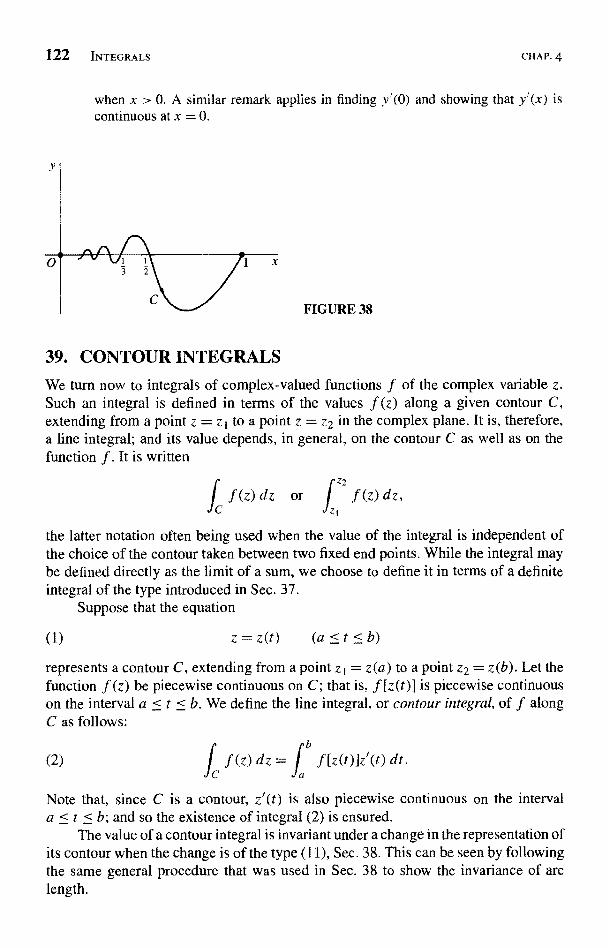
122 INTEGRALS CHAP. 4
0
when x > 0. A similar remark applies in finding y'(0) and showing that y'(x) iscontinuous at x = 0.
3 2
CFIGURE 38
39. CONTOUR INTEGRALSWe turn now to integrals of complex-valued functions f of the complex variable z.Such an integral is defined in terms of the values f (z) along a given contour C,extending from a point z = zt to a point z = z2 in the complex plane. It is, therefore,a line integral; and its value depends, in general, on the contour C as well as on thefunction f. It is written
~2fc f (z) dz orJ
f (z) dz,'1
the latter notation often being used when the value of the integral is independent ofthe choice of the contour taken between two fixed end points. While the integral maybe defined directly as the limit of a sum, we choose to define it in terms of a definiteintegral of the type introduced in Sec. 37.
Suppose that the equation
(1) z=z(t) (a<t<b)represents a contour C, extending from a point zl = z(a) to a point z2 = z(b). Let thefunction f (z) be piecewise continuous on C; that is, f [z(t)] is piecewise continuouson the interval a < t < b. We define the line integral, or contour integral, of f alongC as follows:
(2)L:
f (z) dz = I f[z(t)]z'(t) dt.
Note that, since C is a contour, z'(t) is also piecewise continuous on the intervala < t < b; and so the existence of integral (2) is ensured.
The value of a contour integral is invariant under a change in the representation ofits contour when the change is of the type (11), Sec. 38. This can be seen by followingthe same general procedure that was used in Sec. 38 to show the invariance of arclength.
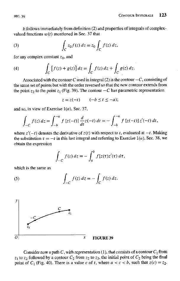
SEC. 39 CONTOUR INTEGRALS 123
It follows immediately from definition (2) and properties of integrals of complex-valued functions w(t) mentioned in Sec. 37 that
(3) Ic zcf(z)dz=ze jc f(z)dz,
for any complex constant ze, and
g(z) dz.(4) / [f (z) + g(z)] dz = / f (z) dz +Jc c
Associated with the contour C used in integral (2) is the contour -C, consisting ofthe same set of points but with the order reversed so that the new contour extends fromthe point z2 to the point zt (Fig. 39). The contour -C has parametric representation
z = z(-t) (-b <
and so, in view of Exercise 1(a), Sec. 37,
f_adz = f [z(-t)]
d z(-t) dt = - f [z(-t)] z'(-t) dt,-C,
` b dt b
where z'(-t) denotes the derivative of z(t) with respect to t, evaluated at -t. Makingthe substitution r = -t in this last integral and referring to Exercise l(a), Sec. 38, weobtain the expression
z) dz = - I .f [z(r)z(r) dr,
which is the same as
(5)
y
0
z)dz=- I f(z)dz.C
X FIGURE 39
Consider now a path C, with representation (1), that consists of a contour Ct fromzt to z2 followed by a contour C2 from z2 to z3, the initial point of C2 being the finalpoint of Cl (Fig. 40). There is a value c of t, where a < c < b, such that z(c) = z2.
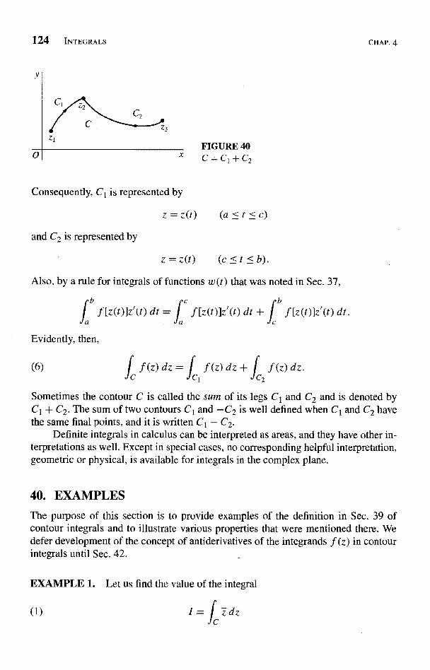
124 INTEGRALS CHAP. 4
FIGURE 40C=CI+C2
Consequently, C1 is represented by
z = z(t)
and C2 is represented by
z=z(t)
Also, by a rule for integrals of functions w(t) that was noted in Sec. 37,
ILz(t)]z'(t) dt + J f [z(t)]z'(t) dt.
b
f [z(t)]z'(t) dt =
Evidently, then,
(z) dz = I f (z) dzC C1 JC2
dz.
Sometimes the contour C is called the sum of its legs C1 and C2 and is denoted byC1 + C2. The sum of two contours C1 and -C2 is well defined when C1 and C2 havethe same final points, and it is written C1 - C2.
Definite integrals in calculus can be interpreted as areas, and they have other in-terpretations as well. Except in special cases, no corresponding helpful interpretation,geometric or physical, is available for integrals in the complex plane.
40. EXAMPLES
The purpose of this section is to provide examples of the definition in Sec. 39 ofcontour integrals and to illustrate various properties that were mentioned there. Wedefer development of the concept of antiderivatives of the integrands f (z) in contourintegrals until Sec. 42.
EXAMPLE 1. Let us find the value of the integral
(1) I =I z dz
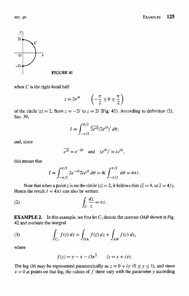
SEC. 40
FIGURE 41
when C is the right-hand half
EXAMPLES 125
of the circle Izi = 2, from z = -2i to z = 2i (Fig. 41), According to definition (2),Sec. 39,
dO;
and, since
and
this means that
i e`8
2 x/22e-`'2ier' dO = 4i r dO 47ri.
-7r/2 ar/2
Note that when a point z is on the circle 1z I = 2, it follows that zz = 4, or 4/z.Hence the result I = 47ri can also be written
(2)dz
Sri.C z
EXAMPLE 2. In this example, we first let C1 denote the contour OAB shown in Fig,42 and evaluate the integral
where
fc, Of(z)dz=f
A Af(z)dz+ f
8f(z)dz,
f(z)=y-x-13x2 (z=x+iy).
The leg OA may be represented parametrically as z = 0 + iy (0 < y < 1); and sincex = 0 at points on that leg, the values of f there vary with the parameter y according
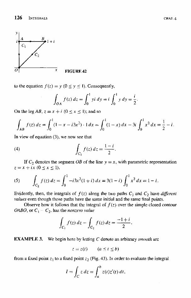
126 INTEGRALS
FIGURE 42
to the equation f (z) = y (0 < y < 1). Consequently,
JOAf(`)dz= J yi dy = i f ydy=Z.
On the leg AB, z = x + i (0 < x -< 1); and so J
f(z)dz= I (1-x-i3x`).ldx= j (1- x)dx_AB J0
In view of equation (3), we now see that
CHAP. 4
f(z) dz =1 2
(4)fc,
If C2 denotes the segment OB of the line y = x, with parametric representationz=x+ix(0<x<1),
(5) ff(z)dz=j -i3x2(l+i)dx=3(1-i)1 x2dxz a 0
Evidently, then, the integrals of f (z) along the two paths C, and C2 have differentvalues even though those paths have the same initial and the same final points.
Observe how it follows that the integral of f (z) over the simple closed contourOABO, or C t -- C2. has the nonzero value
ff(z)dz,
z)dz= -1+i2
EXAMPLE 3. We begin here by letting C denote an arbitrary smooth arc
z=z(t) (a<t<b)from a fixed point zl to a fixed point z2 (Fig. 43). In order to evaluate the integral
jbdz = 1 z(t)z'(t) dt,
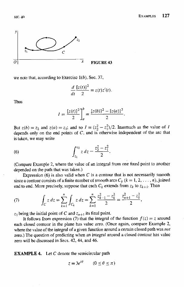
SEC. 40
X FIGURE 43
we note that, according to Exercise l(b), Sec. 37,
2d [Z (t)]= z(t)z'(t)
dt 2
Thus
EXAMPLES 127
But z(b) = z2 and z(a) = z1; and so I = (z2 - zi)/2. Inasmuch as the value of Idepends only on the end points of C, and is otherwise independent of the arc thatis taken, we may write
(6)
z2 2 2
zdz - Z2 2 1
2
(Compare Example 2, where the value of an integral from one fixed point to anotherdepended on the path that was taken.)
Expression (6) is also valid when C is a contour that is not necessarily smoothsince a contour consists of a finite number of smooth arcs Ck (k = 1, 2, ... , n), joinedend to end. More precisely, suppose that each Ck extends from Zk to zk+1. Then
(7) f(zdz= r zdz= 1k _ l1Ck - 2 2
zi being the initial point of C and zn+1 its final point.It follows from expression (7) that the integral of the function f (z) = z around
each closed contour in the plane has value zero. (Once again, compare Example 2,where the value of the integral of a given function around a certain closed path was notzero.) The question of predicting when an integral around a closed contour has valuezero will be discussed in Secs. 42, 44, and 46.
EXAMPLE 4. Let C denote the semicircular path
z=3e`d (Q<B<rr)
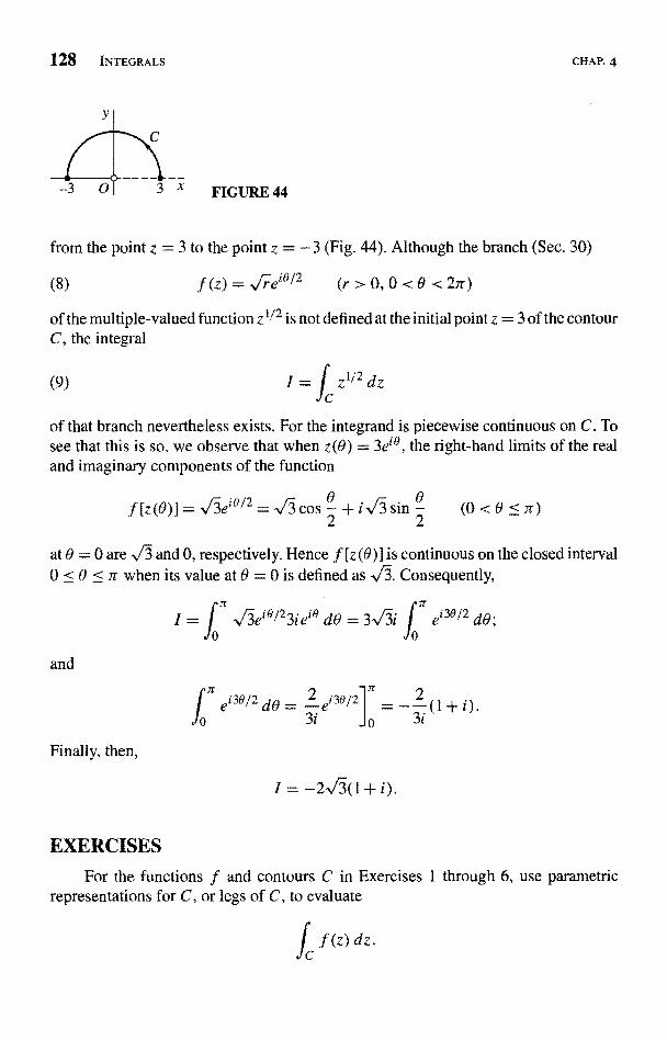
128 INTEGRALS CHAP. 4
FIGURE 44
from the point z = 3 to the point z = -3 (Fig. 44). Although the branch (Sec. 30)
(8) f (z) = /e°'2 (r > 0, 0 < 8 < 27r)
of the multiple-valued function z 1/2 is not defined at the initial point z = 3 of the contourC, the integral
/2 dz
of that branch nevertheless exists. For the integrand is piecewise continuous on C. Tosee that this is so, we observe that when z(O) = 3eie, the right-hand limits of the realand imaginary components of the function
f[z(8)]=V3ei1/2=Jcos 2 +iJsin (0<
at 8 = 0 are and 0, respectively. Hence f [z(8)] is continuous on the closed interval0 < 0 < n when its value at 0 = 0 is defined as . Consequently,
Jo,ei30/2 d8 = 2 ei30/2
3i
I = -2v(l + i).
(
For the functions f and contours C in Exercises I through 6, use parametricrepresentations for C, or legs of C, to evaluate
f(z) dz.C
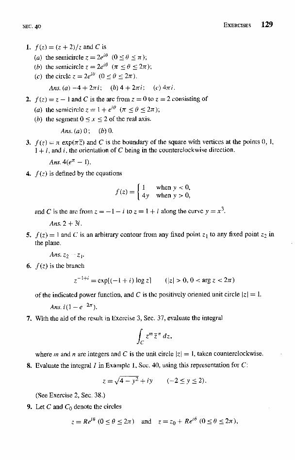
SEC. 40 EXERCISES 129
1. f (z) = (z + 2)/z and C is(a) the semicircle z = 2e`O (0 < 0 < 7r);(b) the semicircle z = 2e`$ (r < 6 < 2ir);(c) the circle z = 2ei° (0 < 0 < 2ir).
Ans. (a) -4 + 2iri; (b) 4 + 2iri; (c) 4.iri.
2. f(z)=z- landCisthearcfrom z=0toz=2 consisting of(a) the semicircle z = 1 + e'O (7r < 0 < 27r);(b) the segment 0 < x < 2 of the real axis.
Ans. (a) 0; (b) 0.
3. f (z) = 7 exp(7rz) and C is the boundary of the square with vertices at the points 0, 1,I + i, and i, the orientation of C being in the counterclockwise direction.
Ans.4(e' - 1).
4. f (z) is defined by the equations
f(z) =
and C is the are from z = -1 - i to z = 1 + i along the curve y = x'.
Ans. 2 + 3i.
5. f (z) = 1 and C is an arbitrary contour from any fixed point zI to any fixed painthe plane.
Ans, z2- zI.
6. f (z) is the branch
1 wheny < 0,4y wheny > 0,
=exp[(-1+i)logz] (IzI>0,0<argz<2rr)
of the indicated power function, and C is the positively oriented unit circle I z I =
Ans. i(1-e-7. With the aid of the result in Exercise 3, Sec. 37, evaluate the integral
L.Zm n dz,
z, In
where m and n are integers and C is the unit circle (zI = 1, taken counterclockwise.
8. Evaluate the integral I in Example 1, Sec. 40, using this representation for C:
z = 4-y2+iy(See Exercise 2, Sec. 38.)
9. Let C and CO denote the circles
(-2 < y < 2).
z=Re`s(0<0<27r) and z=zo+Re"'(0<6<2rr),
130 INTEGRALS
respectively. Use these parametric representations to show that
Jf(z)dz=f f(z - zo)dz
C n
CHAP. 4
when f is piecewise continuous on C.
10. Let Co denote the circle Iz - zol = R, taken counterclockwise. Use the parametricrepresentation z = zo + Re`o(-7r < 0 <,r) for Co to derive the following integrationformulas:
dz n 1dz=0 n=f1,±2,..co z - zo co
11. Use the parametric representation in Exercise 10 for the oriented circle Co there to showthat
'co
2 A(z-zo)a-1dz=i sin(a
a
where a is any real number other than zero and where the principal branch of the integrandand the principal value of Ra are taken. [Note how this generalizes Exercise 10(b).]
12. (a) Suppose that a function f (z) is continuous on a smooth are C, which has a parametricrepresentation z = z(t) (a < t < b); that is, f [z(t)] is continuous on the intervala < t < b. Show that if 0(r)(a < r < fl) is the function described in Sec. 38, then
f(b B
J f [z(t)]z'(t) dt = f f [Z(r)]Z'(r) dr,a a
where Z(r) z[O(r)].(b) Point out how it follows that the identity obtained in part (a) remains valid when C
is any contour, not necessarily a smooth one, and f (z) is piecewise continuous onC. Thus show that the value of the integral of f (z) along C is the same when therepresentation z = Z(r) (a < r < fi) is used, instead of the original one.
Suggestion: In part (a), use the result in Exercise 1(b), Sec. 38, and then referto expression (14) in that section.
41. UPPER BOUNDS FOR MODULIOF CONTOUR INTEGRALS
When C denotes a contour z = z(t)(a < t < b), we know from definition (2), Sec. 39,and inequality (5) in Sec. 37 that
fc f (z) dz f [z(t)]z'(t) dt .f[z(t)]I jz'(t) dt.
So, for any nonnegative constant M such that the values off on C satisfy the inequalityIf (Z) I < M.
fc f(z)dz
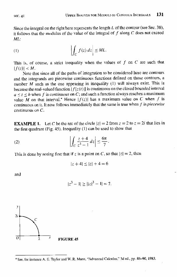
SEC. 41 UPPER BOUNDS FOR MODULI OF CONTOUR INTEGRALS 131
Since the integral on the right here represents the length L of the contour (see Sec. 38),it follows that the modulus of the value of the integral of f along C does not exceedML:
(z) dz <ML.
This is, of course, a strict inequality when the values of f on C are such thatIf (z)I < M.
Note that since all of the paths of integration to be considered here are contoursand the integrands are piecewise continuous functions defined on those contours, anumber M such as the one appearing in inequality (1) will always exist. This isbecause the real-valued function I f [z (t)] I is continuous on the closed bounded intervala < t < b when f is continuous on C; and such a function always reaches a maximumvalue M on that interval.* Hence I f (z) I has a maximum value on C when f iscontinuous on it. It now follows immediately that the same is true when f is piecewisecontinuous on C.
EXAMPLE 1. Let C be the arc of the circle I z I = 2 from z = 2 to z = 2i that lies inthe first quadrant (Fig. 45). Inequality (1) can be used to show that
(2)
This is done by noting first that if z is a point on C, so that I z I = 2, then
Iz+41 IzI+4=6
and
1z3
FIGURE 45
1
* See, for instance A. E. Taylor and W. R. Mann, "Advanced Calculus," 3d ed., pp. 86-90, 1983.
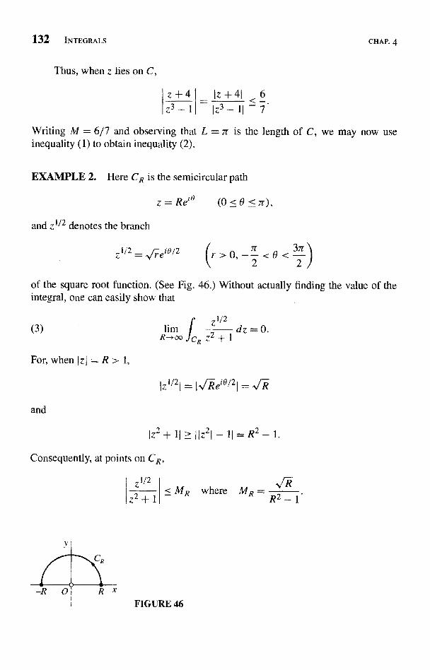
132 INTEGRALS
Thus, when z lies on C,
z+4Z3-1
CHAP. 4
Writing M = 6/7 and observing that L = n is the length of C, we may now useinequality (1) to obtain inequality (2).
EXAMPLE 2. Here CR is the semicircular path
z = Re'° (O < O < r),
and z 112 denotes the branch
zz 1/2 = ,Ir-e 2 (r>0,-2 <0
of the square root function. (See Fig. 46.) Without actually finding the value of theintegral, one can easily show that
Z1/2(3) lim I dz = O.
R->oo
For, when Izl=R>1,
Iz'121 = 1, Rei012
and
IIz21-11=R2-1.
Consequently, at points on CR,
z1/2 V -RMR where MR =z2+1 R2-1
FIGURE 46
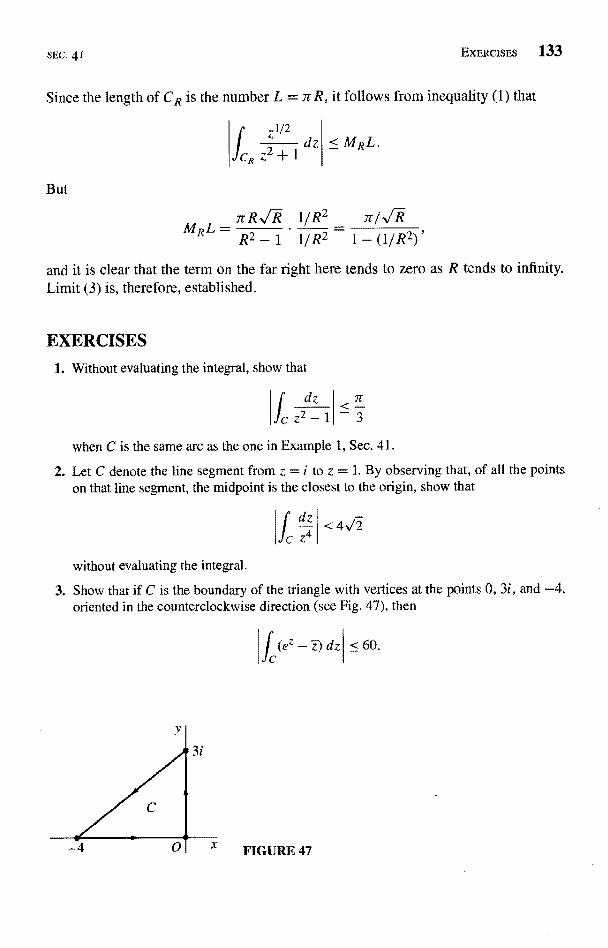
SEC. 41 EXERCISES 133
Since the length of CR is the number L = 7r R,
But
'0110 s from inequality (1) that
1/R2 _ 7/,/-RR2 - 1 1/R2 - 1- (1/R2)'
and it is clear that the term on the far right here tends to zero as R tends to infinity.Limit (3) is, therefore, established.
EXERCISES
1. Without evaluating the integral, show that
dz
2-1IT
_3
when C is the same arc as the one in Example 1, Sec. 41.
2. Let C denote the line segment from z = i to z = 1. By observing that, of all the pointson that line segment, the midpoint is the closest to the origin, show that
without evaluating the integral.
3. Show that if C is the boundary of the triangle with vertices at the points 0, 3i, and -oriented in the counterclockwise direction (see Fig. 47), then
fc- z)dz
FIGURE 47
<60.
134 INTEGRALS CHAP. 4
4. Let CR denote the upper half of the circle Iz I = R (R > 2), taken in the counterclockwisedirection. Show that
f2z2 - 1
drrR(2R2 + 1)
zR z4+5z2+4 (R2 - 1)(R2
Then, by dividing the numerator and denominator on the right here by R4, show that thevalue of the integral tends to zero as R tends to infinity.
5. Let CR be the circle I z I = R (R > 1), described in the counterclockwise direction. Showthat
Log z dz
f R Z2< 2ar
and then use l'Hospital's rule to show that the value of this integral tends to zero as Rtends to infinity.
6. Let Cp denote the circle IzI = p (0 < p < 1), oriented in the counterclockwise direction,and suppose that f (z) is analytic in the disk IzI 1. Show that if z-1/2 represents anyparticular branch of that power of z, then there is a nonnegative constant M, independentof p, such that
Z-112f(Z)
Cdz < 27r M
Thus show that the value of the integral here approaches 0 as p tends to 0.Suggestion: Note that since f (z) is analytic, and therefore continuous, throughout
the disk I z I < 1, it is bounded there (Sec. 17).
7. Let CN denote the boundary of the square formed by the lines
where N is a positive integer, and let the orientation of CN be counterclockwise.
(a) With the aid of the inequalities
Isinzj >_ IsinxI and Isinzl >_ Isinhy1,
obtained in Exercises 10(a) and 11(a) of Sec. 33, show that I sin z I >_ 1 on the verticalsides of the square and that Isin zI > sinh(7r/2) on the horizontal sides. Thus showthat there is a positive constant A, independent of N, such that I sin z I ? A for allpoints z lying on the contour CN.
(b) Using the final result in part (a), show that
dz
z2 sin z
16
(2N + 1)arA
and hence that the value of this integral tends to zero as N tends to infinity.
SEC. 42 ANTIDERIVATIVES 135
42. ANTIDERIVATIVES
Although the value of a contour integral of a function f (z) from a fixed point zt to afixed point z2 depends, in general, on the path that is taken, there are certain functionswhose integrals from z, to z2 have values that are independent of path. (CompareExamples 2 and 3 in Sec. 40.) The examples just cited also illustrate the fact thatthe values of integrals around closed paths are sometimes, but not always, zero. Thetheorem below is useful in determining when integration is independent of path and,moreover, when an integral around a closed path has value zero.
In proving the theorem, we shall discover an extension of the fundamental theo-rem of calculus that simplifies the evaluation of many contour integrals. That extensioninvolves the concept of an antiderivative of a continuous function f in a domain D,or a function F such that F'(z) = f (z) for all z in D. Note that an antiderivative is, ofnecessity, an analytic function. Note, too, that an antiderivative of a given function fis unique except for an additive complex constant. This is because the derivative of thedifference F (z) - G (z) of any two such antiderivatives F (z) and G (z) is zero; and,according to the theorem in Sec. 23, an analytic function is constant in a domain Dwhen its derivative is zero throughout D.
Theorem. Suppose that a function f (z) is continuous on a domain D. If any one ofthe following statements is true, then so are the others:
(i) f (z) has an antiderivative F(z) in D;(ii) the integrals of f (z) along contours lying entirely in D and extending from any
fixed point z i to any fixed point z2 all have the same value;the integrals of f (z) around closed contours lying entirely in D all have valuezero.
It should be emphasized that the theorem does not claim that any of thesestatements is true for a given function f and a given domain D. It says only thatall of them are true or that none of them is true. To prove the theorem, it is sufficientto show that statement (i) implies statement (ii), that statement (ii) implies statement(iii), and finally that statement (iii) implies statement (i).
Let us assume that statement (i) is true. If a contour C from zt to z2, lying in D, isjust a smooth arc, with parametric representation z = z(t)(a < t < b), we know fromExercise 5, Sec. 38, that
dtF[z(t)] = F'[z(t)]z'(t) = f [z(t)]z'(t)
Because the fundamental theorem of calculus can be extended so as to apply tocomplex-valued functions of a real variable (Sec. 37), it follows that .
dz = E f [z(t)]z'(t) dt = F[z(t)] = F[z(b)] - F[z(a)].a

136 INTEGRALS CHAP. 4
Since z(b) = z2 and z(a) = z1, the value of this contour integral is, then,
F(z2) - F(zt);
and that value is evidently independent of the contour C as long as C extends fromto z2 and lies entirely in D. That is,
(1)
(za'J( f (z) dz = F{z2} - F{zl} = F(z)
when C is smooth. Expression (1) is also valid when C is any contour, not necessarilya smooth one, that lies in D. For, if C consists of a finite number of smooth arcsCk (k = 1, 2, ... , n), each Ck extending from a point Zk to a point Zk+1, then
(z) dz = L /_ f (z) dz = > , [F(zk+t) - F(zk)] = F(zn+t) - F(zl).
(Compare Example 3, Sec. 40.) The fact that statement (ii) follows from statement (i)is now established.
To see that statement (ii) implies statement (iii), we let zl and z2 denote any twopoints on a closed contour C lying in D and form two paths, each with initial pointzt and final point z2, such that C = Ct - C2 (Fig. 48). Assuming that statement (ii) istrue, one can write
(2)
or
(3)
ICz)dz= I f(z)dz,
C
fc.f (z) dz + j f (z) dz =
J c2
That is, the integral of f {z} around the closed contour C = Ct - C2 has value zero.
It remains to show that statement (iii) implies statement (i). We do this byassuming that statement (iii) is true, establishing the validity of statement (ii), andthen arriving at statement (i). To see that statement (ii) is true, we let CI and C2 denoteany two contours, lying in D, from a point zt to a point z2 and observe that, in view of
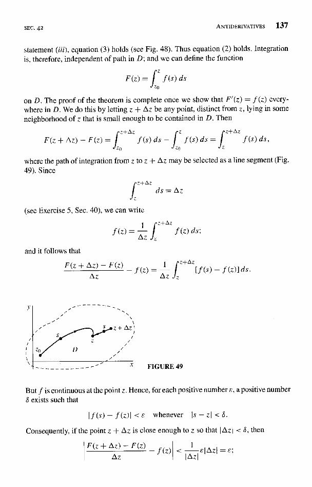
SEC. 42 ANTIDERIVATIVES 137
statement (iii), equation (3) holds (see Fig. 48). Thus equation (2) holds. Integrationis, therefore, independent of path in D; and we can define the function
F(z) = I f (s) dszO
on D. The proof of the theorem is complete once we show that F(z) = f (z) every-where in D. We do this by letting z + Az be any point, distinct from z, lying in someneighborhood of z that is small enough to be contained in D. Then
z+Az rz rz-t azF(z + ©z) - F(z) = 1 .f (s) ds
ZO
f(s)ds,
where the path of integration from z to z + Az may be selected as a line segment (Fig.49). Since
fz
z+Az
(see Exercise 5, Sec. 40), we can write
1z+Az
f (z) = az f (z) ds;
and it follows that
F(z + Az) - F(z) f _ 1
Az - (z)Az
f(z)] ds.
But f is continuous at the point z. Hence, for each positive number E, a positive number8 exists such that
f (z)I <c whenever Is - zI <8.
Consequently, if the point z + Az is close enough to z so that I Az I < 8, then
F(z + Az) - F(z)Az

138 INTEGRALS CHAP. 4
that is,
or F'(z) = f (z).
43. EXAMPLES
The following examples illustrate the theorem in Sec. 42 and, in particular, the use ofthe extension (1) of the fundamental theorem of calculus in that section.
EXAMPLE 1. The continuous function f (z) = z2 has an antiderivative F(z) = z3/3throughout the plane. Hence
I,.
1+i
for every contour from z = 0 to z =
EXAMPLE 2. The function f (z) = 1/Z2, which is continuous everywhere exceptat the origin, has an antiderivative F (z) = -1/z in the domain Iz > 0, consisting ofthe entire plane with the origin deleted. Consequently,
dz
c Z2
when C is the positively oriented circle (Fig. 50)
(1) z = 2eIII (-ar < 0 <,r
about the origin.Note that the integral of the function f (z) = 1/z around the same circle cannot
be evaluated in a similar way. For, although the derivative of any branch F (z) of log z
FIGURE 50
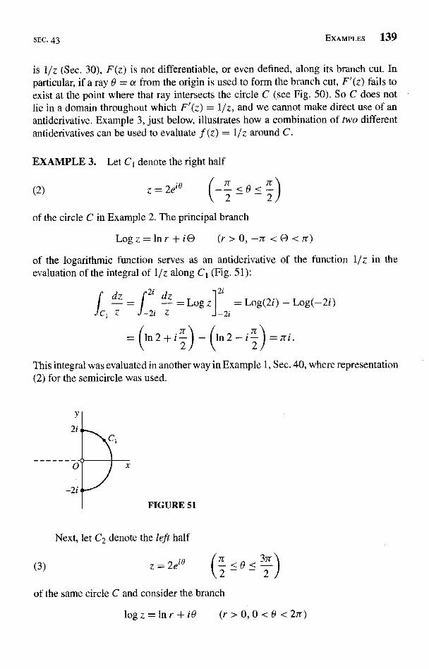
SEC. 43 EXAMPLES 139
is 1/z (Sec. 30), F(z) is not differentiable, or even defined, along its branch cut. Inparticular, if a ray 0 = a from the origin is used to form the branch cut, F(z) fails toexist at the point where that ray intersects the circle C (see Fig. 50). So C does notlie in a domain throughout which F(z) = l/z, and we cannot make direct use of anantiderivative. Example 3, just below, illustrates how a combination of two differentantiderivatives can be used to evaluate f (z) = l/z around C.
EXAMPLE 3. Let C1 denote the right half
(2) z = 2
of the circle C in Example 2. The principal branch
Log z = In r + K) (r > 0, -7r < 0 < 7r)
of the logarithmic function serves as an antiderivative of the function 1/z in theevaluation of the integral of 1/z along Ci (Fig. 51):
dz 21 dz21
- = I - = Log zi = Log(2iCI Z J 2i Z
_2i Log(-2i)
This integral was evaluated in another way in Example 1, Sec. 40, where representation(2) for the semicircle was used.
FIGURE 51
Next, let C2 denote the left half
2
of the same circle C and consider the branch
logz=lnr+iO (r>0,0<0 <2ir)
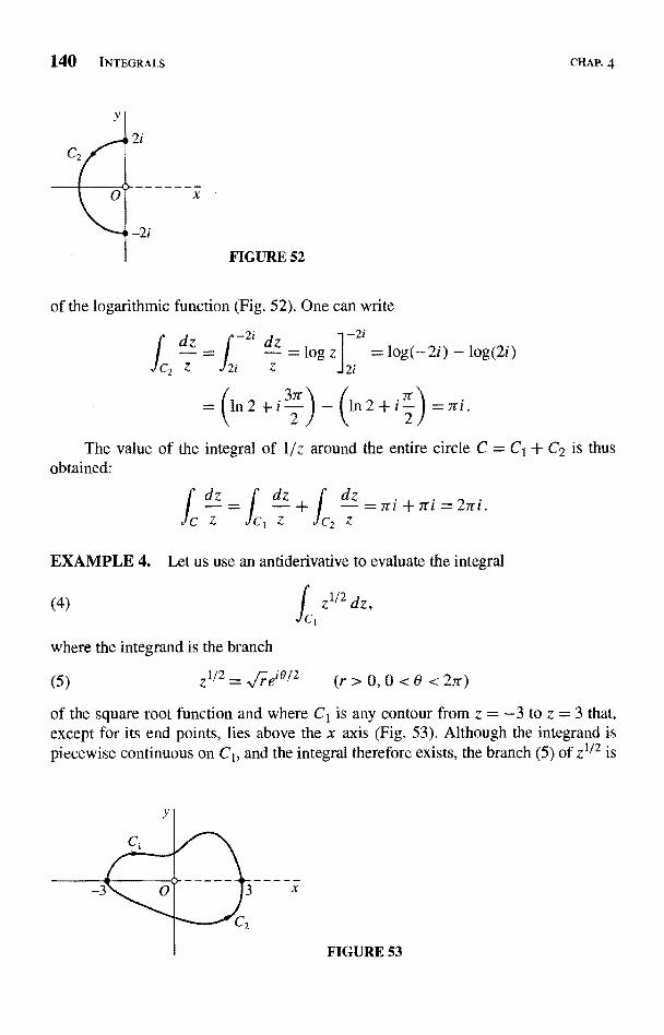
140 INTEGRALS CHAP. 4
FIGURE 52
of the logarithmic function (Fig. 52). One can write
f2dz - j-2i dz -2i
= log Z
I
= log(-2i) - log(2i)c, z i z JJJ zi
n2+i-' ) - In2+i21
=rri.
The value of the integral of I/z around the entire circle C = C1 + C2 is thusobtained:
C Z JCI Z JC2 Z
EXAMPLE 4. Let us use an antiderivative to evaluate the integral
f z1/2 dz,,
where the integrand is the branch
(5)zl/2= e'012 (r>0,0<6 <2n)
of the square root function and where C1 is any contour from z = -3 to z = 3 that,except for its end points, lies above the x axis (Fig. 53). Although the integrand ispiecewise continuous on C1, and the integral therefore exists, the branch (5) of z1/2 is
FIGURE 53
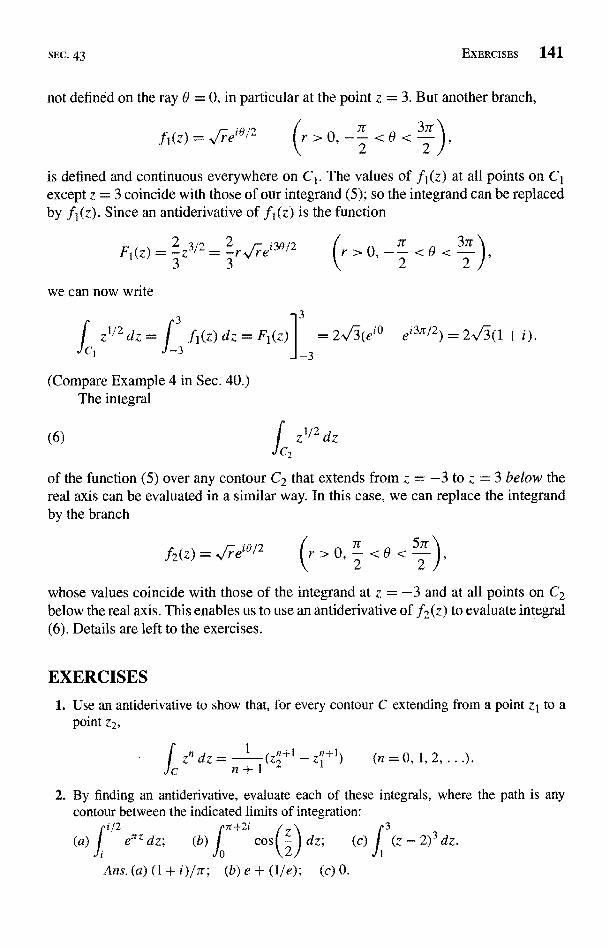
SEC. 43 EXERCISES 141
not defined on the ray 0 = 0, in particular at the point z = 3. But another branch,
Teia/2
is defined and continuous everywhere on C1. The values of f1(z) at all points on C1except z = 3 coincide with those of our integrand (5); so the integrand can be replacedby f1(z). Since an antiderivative of f1(z) is the function
F1(z)3
z3/23
we can now write
'Cl
1-ei 3012
3
z1/2 dz = / fl(z) dz = Fi(z) I = 2,13(eio - e'3.tr/2) = 2/(1 + i)3
Compare Example 4 in Sec. 40.)The integral
(6) fzhl2dzZ
of the function (5) over any contour C2 that extends from z = -3 to z = 3 below thereal axis can be evaluated in a similar way. In this case, we can replace the integrandby the branch
f2 (z) = TeiO/2
whose values coincide with those of the integrand at z = -3 and at all points on C2below the real axis. This enables us to use an antiderivative of f2(z) to evaluate integral(6). Details are left to the exercises.
EXERCISES
1. Use an antiderivative to show that, for every contour C extending from a point z1 to apoint z2,
f dz =n +
1(z2+t - zn+1) (n = 0, 1, 2,
2. By finding an antiderivative, evaluate each of these integrals, where the path is anycontour between the indicated limits of integration:
2
e?z dz; (b)
Ans. (a) (1
7r +21
cos(z) dz;0
(b) e + (1 f e); (c) 0.
142 INTEGRALS CHAP. 4
3. Use the theorem in Sec. 42 to show that
z0)r-1dz=0 (n=+1,±2, ...)
when Co is any closed contour which does not pass through the point z0. [CompareExercise 10(b), Sec. 40.1
4. Find an antiderivative F2(z) of the branch f2(z) of z172 in Example 4, Sec. 43, to showthat integral (6) there has value 2/(-1 + i). Note that the value of the integral of thefunction (5) around the closed contour C2 - C1 in that example is, therefore, -4-,,/-3.
5. Show that
z
z`=exp(iLogz) (Izi>0,-2T<Argz<rr)
and where the path of integration is any contour from z = -1 to z = 1 that, except for itsend points, lies above the real axis.
Suggestion: Use an antiderivative of the branch
z` = exp(i log z) IzI > 0, - 2 < arg z < 2
of the same power function.
44. CAUCHY-GOURSAT THEOREMIn Sec. 42, we saw that when a continuous function f has an antiderivative in a domainD, the integral of f (z) around any given closed contour C lying entirely in D has valuezero. In this section, we present a theorem giving other conditions on a function f,which ensure that the value of the integral of f (z) around a simple closed contour(Sec. 38) is zero. The theorem is central to the theory of functions of a complex variable;and some extensions of it, involving certain special types of domains, will be given inSec. 46.
We let C denote a simple closed contour z = z(t) (a < t < b), described in thepositive sense (counterclockwise), and we assume that f is analytic at each pointinterior to and on C. According to Sec. 39,
(1)
ICf (z) dz = )]z'(t) dt;
and if
Y x, y) and z(t) = x(t) + iy(t),
SEC. 44 CAUCHY-GOURSAT THEOREM 143
the integrand f [z(t)]z'(t) in expression (1) is the product of the functions
u[x(t), y(t)] + iv[x(t), y(t)], x'(t) + iy'(t)
of the real variable t. Thus
(2)C
(z) dz = I (ux' - vy') dt + i 1 (vx' + uy') dt.
In terms of line integrals of real-valued functions of two real variables, then,
(z)dz= j udx-vdy+i I vdx+udy.C JC C
Observe that expression (3) can be obtained formally by replacing f (z) and dz on theleft with the binomials
u+iv and dx+idy,
respectively, and expanding their product. Expression (3) is, of course, also valid whenC is any contour, not necessarily a simple closed one, and f [z(t)] is only piecewisecontinuous on it.
We next recall a result from calculus that enables us to express the line integralson the right in equation (3) as double integrals. Suppose that two real-valued functionsP(x, y) and Q (x, y), together with their first-order partial derivatives, are continuousthroughout the closed region R consisting of all points interior to and on the simpleclosed contour C. According to Green's theorem,
Pdx+ Qdy= f f (Qx-Py)dA...II .dt R
Now f is continuous in R, since it is analytic there. Hence the functions u andv are also continuous in R. Likewise, if the derivative f' of f is continuous in R, soare the first-order partial derivatives of u and v. Green's theorem then enables us torewrite equation (3) as
C R R(z)dz=f f(-vx-uy)dA+i [[(us -u)dA.
But, in view of the Cauchy-Riemann equations
uy = -vx,
the integrands of these two double integrals are zero throughout R. So, when f isanalytic in R and f' is continuous there,
(5) ( f(z)dz=O.C
This result was obtained by Cauchy in the early part of the nineteenth century.
144 INTEGRALS CHAP. 4
Note that, once it has been established that the value of this integral is zero, theorientation of C is immaterial. That is, statement (5) is also true if C is taken in theclockwise direction, since then
Ic f(z)dz=-JC f(z)dz=0.
EXAMPLE. If C is any simple closed contour, in either direction, then
Ic exp(z) dz = 0.
This is because the function f (z) = exp(z) is analytic everywhere and its derivative3z2 exp(z3) is continuous everywhere.
Goursat* was the first to prove that the condition of continuity on f' can beomitted. Its removal is important and will allow us to show, for example, that thederivative f' of an analytic function f is analytic without having to assume thecontinuity of f', which follows as a consequence, We now state the revised form ofCauchy's result, known as the Cauchy-Goursat theorem.
Theorem. If a function f is analytic at all points interior to and on a simple closedcontour C, then
fc f(z)dz=0.
The proof is presented in the next section, where, to be specific, we assume thatC is positively oriented. The reader who wishes to accept this theorem without proofmay pass directly to Sec. 46.
45. PROOF OF THE THEOREMWe preface the proof of the Cauchy-Goursat theorem with a lemma. We start byforming subsets of the region R which consists of the points on a positively orientedsimple closed contour C together with the points interior to C. To do this, we drawequally spaced lines parallel to the real and imaginary axes such that the distancebetween adjacent vertical lines is the same as that between adjacent horizontal lines.We thus form a finite number of closed square subregions, where each point of R liesin at least one such subregion and each subregion contains points of R. We refer tothese square subregions simply as squares, always keeping in mind that by a square we
* E. Goursat (1858-1936), pronounced gour-sah'.
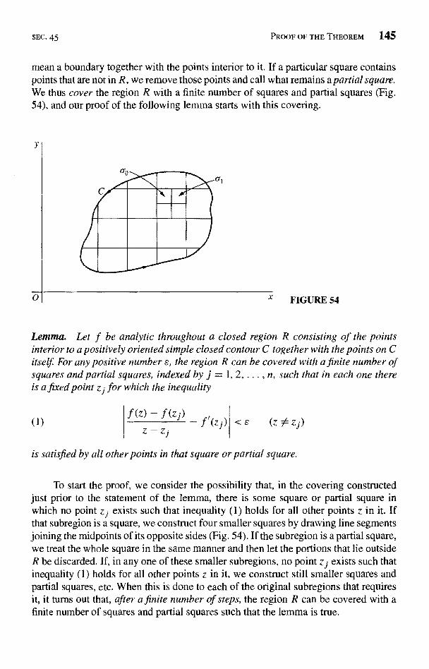
SEC. 45 PROOF OF THE THEOREM 145
mean a boundary together with the points interior to it. If a particular square containspoints that are not in R, we remove those points and call what remains a partial square.We thus cover the region R with a finite number of squares and partial squares (Fig.54), and our proof of the following lemma starts with this covering.
0 X FIGURE 54
Lemma. Let f be analytic throughout a closed region R consisting of the pointsinterior to a positively oriented simple closed contour C together with the points on Citself For any positive number s, the region R can be covered with a finite number ofsquares and partial squares, indexed by j = 1, 2, ... , n, such that in each one thereis a fixed point z1 for which the inequality
(1)
f(z)---f(z1) _fz-z1
<E
is satisfied by all other points in that square or partial square.
To start the proof, we consider the possibility that, in the covering constructedjust prior to the statement of the lemma, there is some square or partial square inwhich no point z1 exists such that inequality (1) holds for all other points z in it. Ifthat subregion is a square, we construct four smaller squares by drawing line segmentsjoining the midpoints of its opposite sides (Fig. 54). If the subregion is a partial square,we treat the whole square in the same manner and then let the portions that lie outsideR be discarded. If, in any one of these smaller subregions, no point z1 exists such thatinequality (1) holds for all other points z in it, we construct still smaller squares andpartial squares, etc. When this is done to each of the original subregions that requiresit, it turns out that, after a finite number of steps, the region R can be covered with afinite number of squares and partial squares such that the lemma is true.
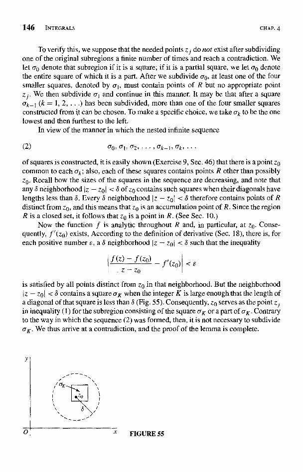
146 INTEGRALS CHAP. 4
To verify this, we suppose that the needed points zj do not exist after subdividingone of the original subregions a finite number of times and reach a contradiction. Welet ao denote that subregion if it is a square; if it is a partial square, we let ao denotethe entire square of which it is a part. After we subdivide ao, at least one of the foursmaller squares, denoted by a1, must contain points of R but no appropriate pointzj. We then subdivide a1 and continue in this manner. It may be that after a squareak_1 (k = 1, 2, ...) has been subdivided, more than one of the four smaller squaresconstructed from it can be chosen. To make a specific choice, we take ak to be the onelowest and then furthest to the left.
In view of the manner in which the nested infinite sequence
(2) ao,al,a2,...,ak-1,ak,..
of squares is constructed, it is easily shown (Exercise 9, Sec. 46) that there is a point zocommon to each ak; also, each of these squares contains points R other than possiblyz0. Recall how the sizes of the squares in the sequence are decreasing, and note thatany & neighborhood Iz - zoI < 8 of z0 contains such squares when their diagonals havelengths less than 8. Every E neighborhood Iz - zol < 8 therefore contains points of Rdistinct from z0, and this means that zo is an accumulation point of R. Since the regionR is a closed set, it follows that zo is a point in R. (See Sec. 10.)
Now the function f is analytic throughout R and, in particular, at zo. Conse-quently, f"(zo) exists, According to the definition of derivative (Sec. 18), there is, foreach positive number s, a 8 neighborhood (z - zoj < 8 such that the inequality
f (z) - .f(zo) - f'(zo). z - Zo
< 8
is satisfied by all points distinct from z4 in that neighborhood. But the neighborhood1z - zol < 8 contains a square UK when the integer K is large enough that the length ofa diagonal of that square is less than 8 (Fig. 55). Consequently, zo serves as the point zjin inequality (1) for the subregion consisting of the square UK or a part of aK . Contraryto the way in which the sequence (2) was formed, then, it is not necessary to subdivideaK. We thus arrive at a contradiction, and the proof of the lemma is complete.
Y,
01 X FIGURE 55
SEC. 45 PROOF OF THE THEOREM 147
Continuing with a function f which is analytic throughout a region R consistingof a positively oriented simple closed contour C and points interior to it, we are nowready to prove the Cauchy-Goursat theorem, namely that
(3) r. f(z)dz=0.
Given an arbitrary positive numbers, we consider the covering of R in thestatement of the lemma. Let us define on the jth square or partial square the followingfunction, where zl is the fixed point in that subregion for which inequality (1) holds:
f(z) - f(z1) ,
(4) 8;(z)= z - z;f (zj) when z
when z
According to inequality (1),
(5) 18f(z)I <s
at all points z in the subregion on which 8, (z) is defined. Also, the function 8j (z) iscontinuous throughout the subregion since f (z) is continuous there and
lira 8 (z) = f'(z3) - f'(z f) = 0.I
Next, let C; (j = 1, 2, . . . , n) denote the positively oriented boundaries of theabove squares or partial squares covering R. In view of definition (4), the value of fat a point z on any particular CJ can be written
f(z) = f (z;) - zjf'(z1) + f'(zf)z + (z - zj)SJ(z),
and this means that
(6) f f (z) dzC;
(z j)] / dz + f'(z,j) /_ z dz + / (z - zj)81(z) dz.
But
0 =z
fcj dz=0 and jzdz=0
since the functions 1 and z possess antiderivatives everywhere in the finite plane. Soequation (6) reduces to
(7) fcj f (z) dz = J (z - zj)8j (z) dz (j = 1, 2, n).C;
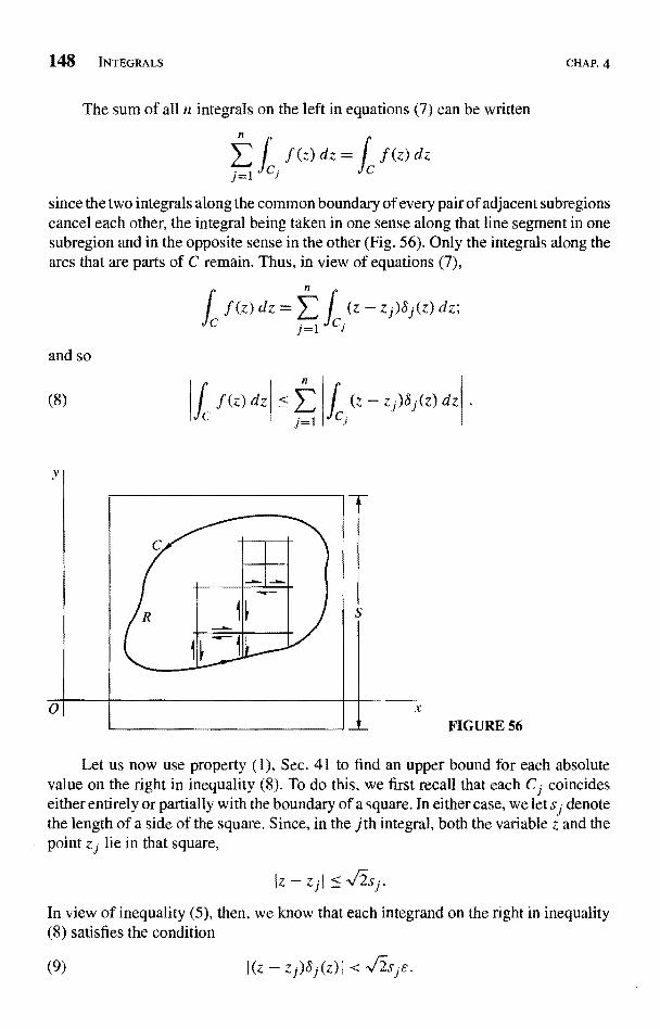
148 INTEGRALS
The sum of all n integrals on the left in equations (7) can be written
(z)dz=I f(z)dzc
CHAP. 4
since the two integrals along the common boundary of every pair of adjacent subregionscancel each other, the integral being taken in one sense along that line segment in onesubregion and in the opposite sense in the other (Fig. 56). Only the integrals along thearcs that are parts of C remain. Thus, in view of equations (7),
n
and so
(8)
0
Jf(z)dz=4 ( (z-zj)81(z)dz;
C C:
I z) dz z - zj)8j(z) dz
xFIGURE 56
Let us now use property (1). Sec. 41 to find an upper bound for each absolutevalue on the right in inequality (8). To do this, we first recall that each Ci coincideseither entirely or partially with the boundary of a square. In either case, we let sJ denotethe length of a side of the square. Since, in the jth integral, both the variable z and thepoint zj lie in that square,
Iz - ziI < v'2s1.
In view of inequality (5), then, we know that each integrand on the right in inequality(8) satisfies the condition
(9) 1(z - zj)8j(z)I < Js
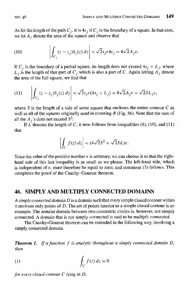
SEC. 46 SIMPLY AND MULTIPLY CONNECTED DOMAINS 149
As for the length of the path C j, it is 4s j if C1 is the boundary of a square. In that case,we let Al denote the area of the square and observe that
(10)IC
z - zj)dj(z) dz < V2sjE4sj =4/Ajs.
If C j is the boundary of a partial square, its length does not exceed 4s1 + L1, whereL1 is the length of that part of C1 which is also a part of C. Again letting Al denotethe area of the full square, we find that
J (z - z1)j (z) dzJ
< s j s (4s j + < 4,/2-A je + -SL js,
where S is the length of a side of some square that encloses the entire contour C aswell as all of the squares originally used in covering R (Fig. 56). Note that the sum ofall the A1's does not exceed S2.
If L denotes the length of C, it now follows from inequalities (8), (10), and (11)that
(z) dz <(4J s2+'.J SL)
Since the value of the positive number s is arbitrary, we can choose it so that the right-hand side of this last inequality is as small as we please. The left-hand side, whichis independent of e, must therefore be equal to zero; and statement (3) follows. Thiscompletes the proof of the Cauchy-Goursat theorem.
46. SIMPLY AND MULTIPLY CONNECTED DOMAINS
A simply connected domain D is a domain such that every simple closed contour withinit encloses only points of D. The set of points interior to a simple closed contour is anexample. The annular domain between two concentric circles is, however, not simplyconnected. A domain that is not simply connected is said to be multiply connected.
The Cauchy-Goursat theorem can be extended in the following way, involving asimply connected domain.
Theorem 1. If a function f is analytic throughout a simply connected domain D,then
(1) z) dz =
or every closed contour C lying in D.
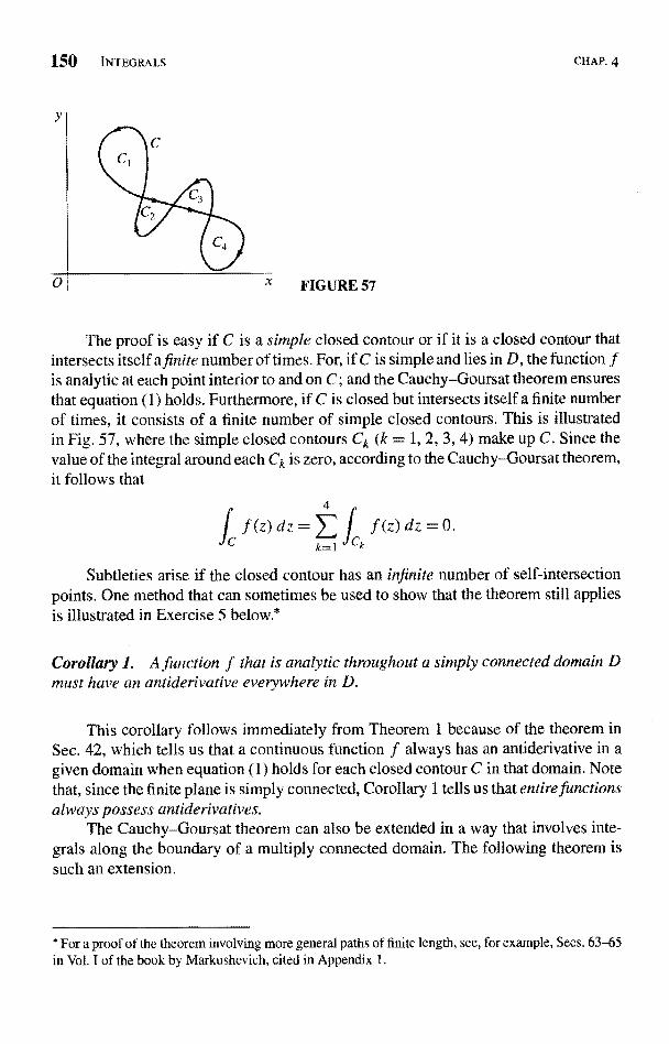
150 INTEGRALS CHAP. 4
FIGURE 57
The proof is easy if C is a simple closed contour or if it is a closed contour thatintersects itself a finite number of times. For, if C is simple and lies in D, the function fis analytic at each point interior to and on C; and the Cauchy-Goursat theorem ensuresthat equation (1) holds. Furthermore, if C is closed but intersects itself a finite numberof times, it consists of a finite number of simple closed contours. This is illustratedin Fig. 57, where the simple closed contours Ck (k = 1, 2, 3, 4) make up C. Since thevalue of the integral around each Ck is zero, according to the Cauchy-Goursat theorem,it follows that
C(z) dz = z) dz = 0.
Subtleties arise if the closed contour has an infinite number of self-intersectionpoints. One method that can sometimes be used to show that the theorem still appliesis illustrated in Exercise 5 below.*
Corollary 1. A function f that is analytic throughout a simply connected domain Dmust have an antiderivative everywhere in D.
This corollary follows immediately from Theorem 1 because of the theorem inSec. 42, which tells us that a continuous function f always has an antiderivative in agiven domain when equation (1) holds for each closed contour C in that domain. Notethat, since the finite plane is simply connected, Corollary 1 tells us that entire functionsalways possess antiderivatives.
The Cauchy-Goursat theorem can also be extended in a way that involves inte-grals along the boundary of a multiply connected domain. The following theorem issuch an extension.
* For a proof of the theorem involving more general paths of finite length, see, for example, Secs. 63-65in Vol. I of the book by Markushevich, cited in Appendix 1.
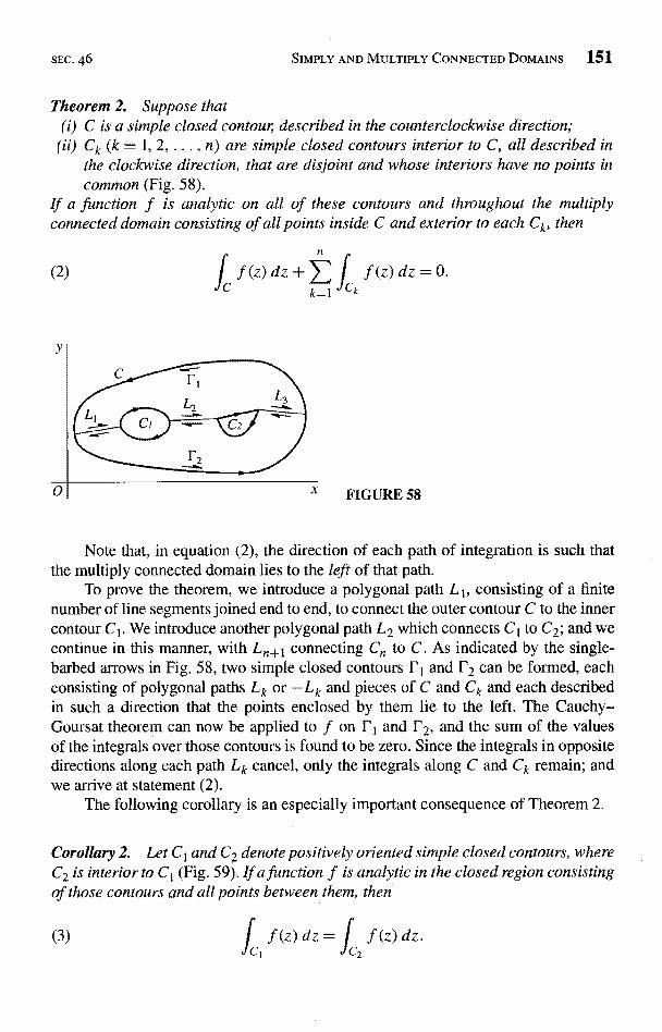
SEC. 46 SIMPLY AND MULTIPLY CONNECTED DOMAINS 151
Theorem 2. Suppose that(i) C is a simple closed contour, described in the counterclockwise direction;
Ck (k = 1, 2, ... , n) are simple closed contours interior to C, all described inthe clockwise direction, that are disjoint and whose interiors have no points incommon (Fig. 58).
nction f is analytic on all of these contours and throughout the multiplyconnected domain consisting of all points inside C and exterior to each Ck, then
n
(2)
k=1
z)dz+y J f(z)dz=
Note that, in equation (2), the direction of each path of integration is such thatthe multiply connected domain lies to the left of that path.
To prove the theorem, we introduce a polygonal path L 1, consisting of a finitenumber of line segments joined end to end, to connect the outer contour C to the innercontour C1. We introduce another polygonal path L2 which connects C1 to C2; and wecontinue in this manner, with L,+1 connecting Cn to C. As indicated by the single-barbed arrows in Fig. 58, two simple closed contours r1 and r2 can be formed, eachconsisting of polygonal paths Lk or -Lk and pieces of C and Ck and each describedin such a direction that the points enclosed by them lie to the left. The Cauchy-Goursat theorem can now be applied to f on F 1 and r2, and the sum of the valuesof the integrals over those contours is found to be zero. Since the integrals in oppositedirections along each path Lk cancel, only the integrals along C and Ck remain; andwe arrive at statement (2).
The following corollary is an especially important consequence of Theorem 2.
Corollary 2. Let C1 and C2 denote positively oriented simple closed contours, whereC2 is interior to C1 (Fig. 59). If a function f is analytic in the closed region consistingof those contours and all points between them, then
(3) fc, f (z) dz f (z) dz.c,
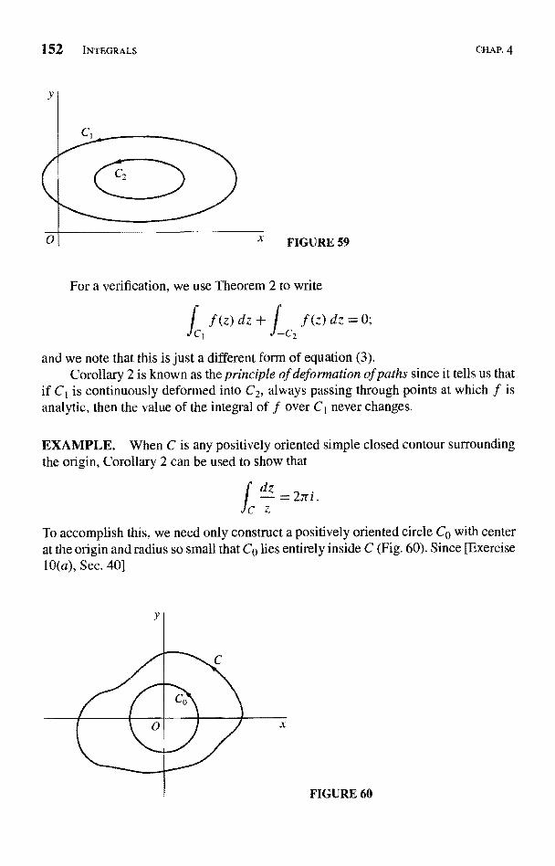
152 INTEGRALS CHAP. 4
FIGURE 59
For a verification, we use Theorem 2 to write
f( )dz = 0;dz+ JJ
_ 2c
and we note that this is just a different form of equation (3).Corollary 2 is known as the principle of deformation of pates since it tells us that
if C1 is continuously deformed into C2, always passing through points at which f isanalytic, then the value of the integral of f over C1 never changes.
EXAMPLE. When C is any positively oriented simple closed contour surroundingthe origin, Corollary 2 can be used to show that
To accomplish this, we need only construct a positively oriented circle Co with centerat the origin and radius so small that Co lies entirely inside C (Fig. 60). Since [Exercise10(a), Sec. 40]
FIGURE 60
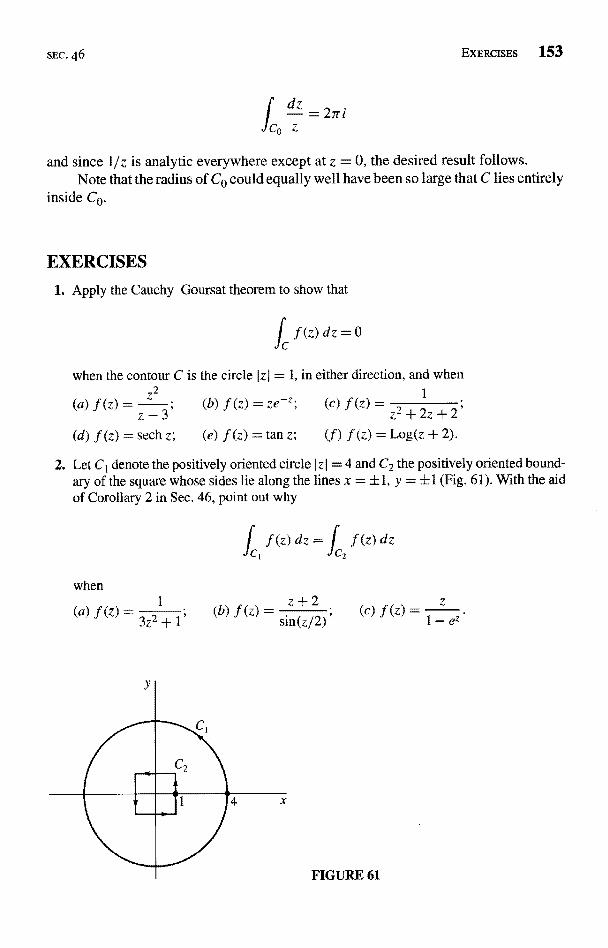
SEC. 46
dz_ 2ir i
Cn z
EXERCISES 153
and since 1/z is analytic everywhere except at z = 0, the desired result follows.Note that the radius of Co could equally well have been so large that C lies entirely
inside Co.
EXERCISES
1. Apply the Cauchy-Goursat theorem to show that
C(z) dz =
when the contour C is the circle 1zI = 1, in either direction, and when
(a) .f (z)z2
z-3'(d) 1(z) = sech z;
(b) .f (z) = ze-1;
z = tan z;
(c) .f (z) = .
z2 +2z+2'
(f) .f (z) = Log(z + 2).
2. Let C, denote the positively oriented circle IzI = 4 and C2 the positively oriented bound-ary of the square whose sides lie along the lines x = +1, y = +1 (Fig. 61). With the aidof Corollary 2 in Sec. 46, point out why
IC
when
(a) .f (z)1
(b) f (z) =sin(z/2)
FIGURE 61
1
z1-ez
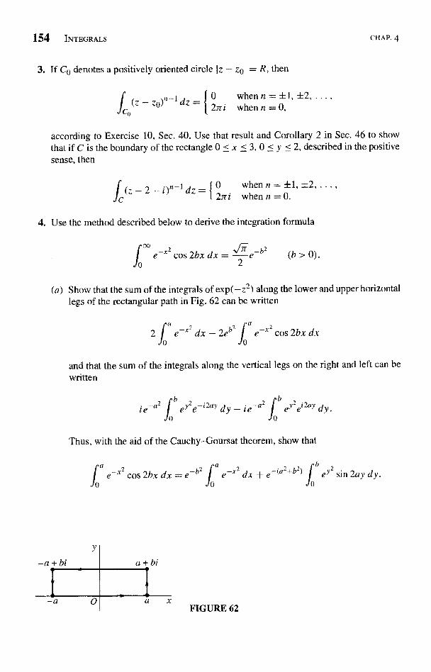
154 INTEGRALS CHAP. 4
3. If Co denotes a positively oriented circle Iz - 1701 = R, then
J(z - zo)n - when n =
according to Exercise 10, Sec. 40. Use that result and Corollary 2 in Sec. 46 to showthat if C is the boundary of the rectangle 0 < x < 3, 0 < y < 2, described in the positivesense,then
1,-2- n
41 -JO when n=f1,±2,..
27r i when n. = 0.
4. Use the method described below to derive the integration formula
l.,e-x cos 2bx dx = -- e-b2
(b > 0).
(a) Show that the sum of the integrals of exp(-z2) along the lower and upper horizontallegs of the rectangular path in Fig. 62 can be written
e_x2
0 whenn = f I, f2, .
2eb2 ja
e-x2 cos 2bx dx0
and that the sum of the integrals along the vertical legs on the right and left can bewritten
b zeye i 2ay dy - ie
bey2ei2ay
dy.
Thus, with the aid of the Cauchy-Goursat theorem, show that
y
-a + bi0 ------ .
ja ,cos 2bx dx = e-b2
e-x2dx + ea`+b2) ee sin 2ay dy.
a + bi0-a 01 a X
FIGURE 62
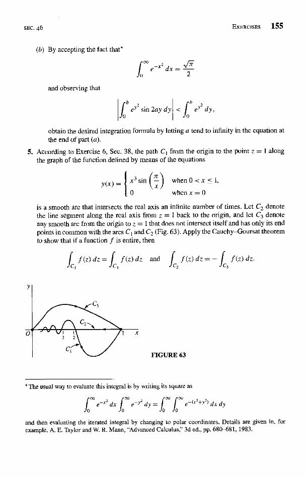
SEC. 46 EXERCISES 155
(b) By accepting the fact that*
and observing that
I:;
°C e-x2dx =
V 7
2
sin lay dy
obtain the desired integration formula by letting a tend to infinity in the equation atthe end of part (a).
5. According to Exercise 6, Sec. 38, the path CI from the origin to the point z = 1 alongthe graph of the function defined by means of the equations
yx3 sin ( -) when 0 < x < 1,
IX0 whenx=0
is a smooth arc that intersects the real axis an infinite number of times. Let C2 denotethe line segment along the real axis from z = i back to the origin, and let C3 denoteany smooth arc from the origin to z = 1 that does not intersect itself and has only its endpoints in common with the arcs CI and C2 (Fig. 63). Apply the Cauchy-Goursat theoremto show that if a function f is entire, then
C, C3
FIGURE 63
* The usual way to evaluate this integral is by writing its square as
e-xzdx
(z)dz= J f(z)dz and / f(z)dz=- I f(z)dz.
+yz) dx dy
and then evaluating the iterated integral by changing to polar coordinates. Details are given in, forexample, A. E. Taylor and W. R. Mann, "Advanced Calculus," 3d ed., pp. 680-681, 1983.
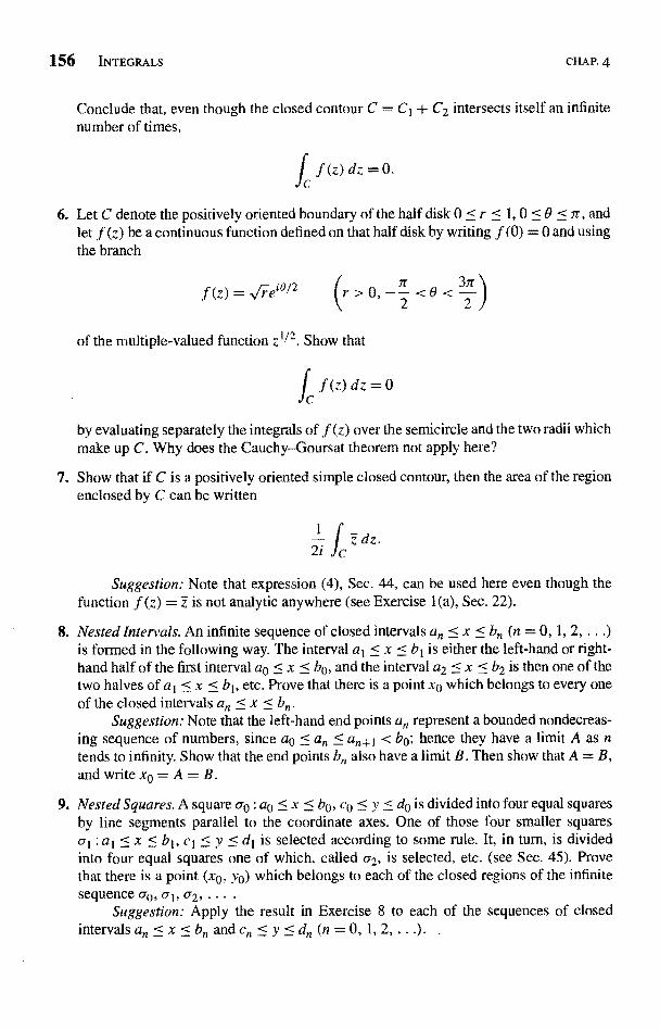
156 INTEGRALS CHAP. 4
Conclude that, even though the closed contour C = C1 + C2 intersects itself an infinitenumber of times,
Ic f(z)dz=0.
6. Let C denote the positively oriented boundary of the half disk 0 < r < 1, 0 < 9 < r, andlet f (z) be a continuous function defined on that half disk by writing f (0) = 0 and usingthe branch
,f (z) =e'0/2 -2<0< 2
of the multiple-valued function zl/2. Show that
1,f (z) dz = 0
by evaluating separately the integrals of f (z) over the semicircle and the two radii whichmake up C. Why does the Cauchy-Goursat theorem not apply here?
7. Show that if C is a positively oriented simple closed contour, then the area of the regionenclosed by C can be written
Cz dz.
Suggestion: Note that expression (4), Sec. 44, can be used here even though thefunction f (z) = z is not analytic anywhere (see Exercise 1(a), Sec. 22).
8. Nested Intervals. An infinite sequence of closed intervals an < x < bn (n = 0, 1, 2, ...)is formed in the following way. The interval a1 < x < b1 is either the left-hand or right-hand half of the first interval a0 < x < b0, and the interval a2 < x < b2 is then one of thetwo halves of a1 < x < b1, etc. Prove that there is a point x0 which belongs to every oneof the closed intervals an < x < bn
Suggestion: Note that the left-hand end points an represent a bounded nondecreas-ing sequence of numbers, since a0 < an < an+1 < b0; hence they have a limit A as ntends to infinity. Show that the end points bn also have a limit B. Then show that A = B,and write x0=A=B.
9. Nested Squares. A square a : a0 < x < b0, co < y < de is divided into four equal squaresby line segments parallel to the coordinate axes. One of those four smaller squareso't : at < x < b1, c1 < y < d1 is selected according to some rule. It, in turn, is dividedinto four equal squares one of which, called cr2, is selected, etc. (see Sec. 45). Provethat there is a point (x0, y0) which belongs to each of the closed regions of the infinitesequence cr0, or I, erg, ... .
Suggestion: Apply the result in Exercise 8 to each of the sequences of closedintervals an < x < bn and en < y < do (n = 0, 1, 2, ...). .
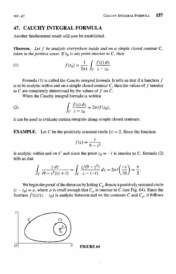
SEC. 47 CAUCHY INTEGRAL FORMULA 157
47. CAUCHY INTEGRAL FORMULA
Another fundamental result will now be established.
Theorem. Let f be analytic everywhere inside and on a simple closed contour C,taken in the positive sense. If zo is any point interior to C, then
(1) f (zo) _. 2rri Jc z - zo
Formula (1) is called the Cauchy integral formula. It tells us that if a function fis to be analytic within and on a simple closed contour C, then the values of f interiorto C are completely determined by the values of f on C.
When the Cauchy integral formula is written
f (z) dz = 27rif(z0),(2) fc z-zoit can be used to evaluate certain integrals along simple closed contours.
EXAMPLE. Let C be the positively oriented circle I z
f (z)z
9-
= 2. Since the function
is analytic within and on C and since the point zo = -i is interior to C, formula (2)tells us that
z dz - [ Z/(9 -C (9-z2)(z+i) Jc
z=2
We begin the proof of the theorem by letting Cp denote a positively oriented circleIz - zol = p, where p is small enough that Cp is interior to C (see Fig. 64). Since thefunction f (z)/(z - zo) is analytic between and on the contours C and Cp, it follows
y
01 x FIGURE 64
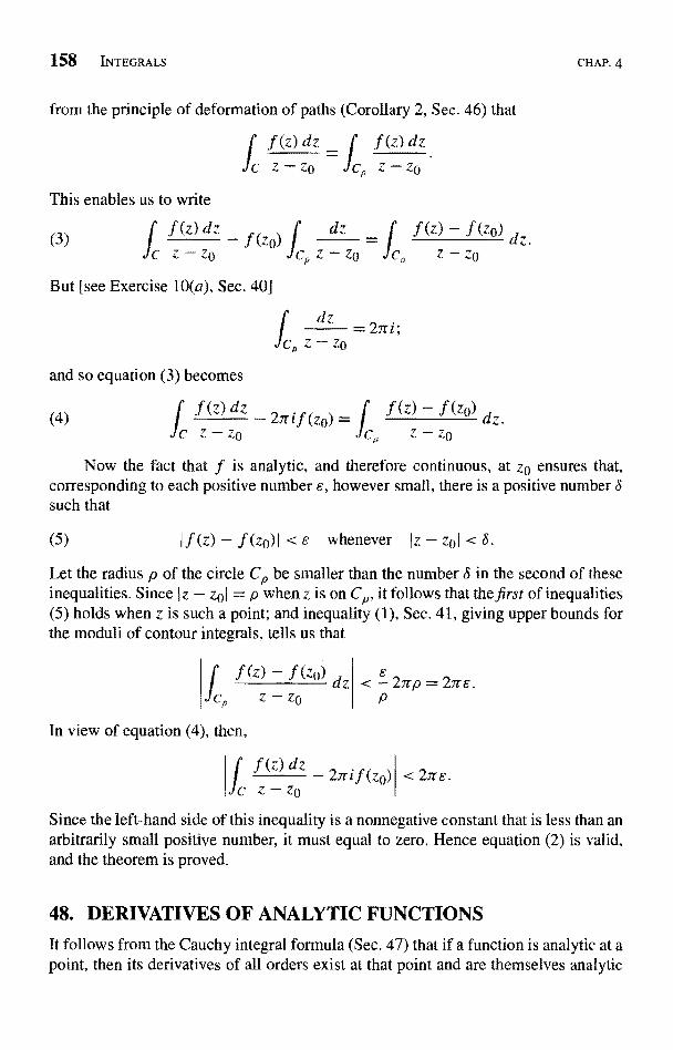
158 INTEGRALS
from the principle of deformation of paths (Corollary 2, Sec. 46) that
f f(z)dz _ l f(z)dzc z - zo
This enables us to write
(3)(z) dz - f,, dz .f (z) - f (zo) d) ! f '
ZVC Z - Zo : -Z0CZZo C
But [see Exercise 10(a), Sec. 40]
and so equation (3) becomes
dz =2rri;- zo
(4) f(z) dz - 27r if (zo) =c Z - zo
.f (z) - f (zo) dzz-z0
CHAP. 4
Now the fact that f is analytic, and therefore continuous, at zo ensures that,corresponding to each positive number E, however small, there is a positive number Ssuch that
(5) If (z) - f (zo)I <e whenever Iz - zol <6.
Let the radius p of the circle Cp be smaller than the number S in the second of theseinequalities. Since Iz - zol = p when z is on CP, it follows that the first of inequalities(5) holds when z is such a point; and inequality (1), Sec. 41, giving upper bounds forthe moduli of contour integrals, tells us that
f.f (z) - .f (zo)
,"z-zo
In view of equation (4), then,
dzE
< 27rp = 2Trs.p
VC
f (z) dz if (o)- 27ri z< 2,-r E.Z - zo
Since the left-hand side of this inequality is a nonnegative constant that is less than anarbitrarily small positive number, it must equal to zero. Hence equation (2) is valid,and the theorem is proved.
48. DERIVATIVES OF ANALYTIC FUNCTIONS
It follows from the Cauchy integral formula (Sec. 47) that if a function is analytic at apoint, then its derivatives of all orders exist at that point and are themselves analytic
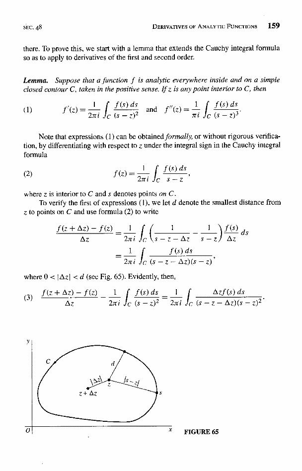
SEC. 48 DERIVATIVES OF ANALYTIC FUNCTIONS 159
there. To prove this, we start with a lemma that extends the Cauchy integral formulaso as to apply to derivatives of the first and second order.
Lemma. Suppose that a function f is analytic everywhere inside and on a simpleclosed contour C, taken in the positive sense. If z is any point interior to C, then
(1) f'(z)2Tri
and
Note that expressions (1) can be obtained formally, or without rigorous verifica-tion, by differentiating with respect to z under the integral sign in the Cauchy integralformula
where z is interior to C and s denotes points on C.To verify the first of expressions (1), we let d denote the smallest distance from
z to points on C and use formula (2) to write
+Az)-f(z)Az
2ni Jc
I
where 0 < IAz1 < d (see Fig. 65). Evidently, then,
(3) f (z + Az) - f (z) 1 f f (s) ds IAz 2iri c (s - z)2 2iri fc
bzf (s) dsz - Az)(s -
FIGURE 65
ds
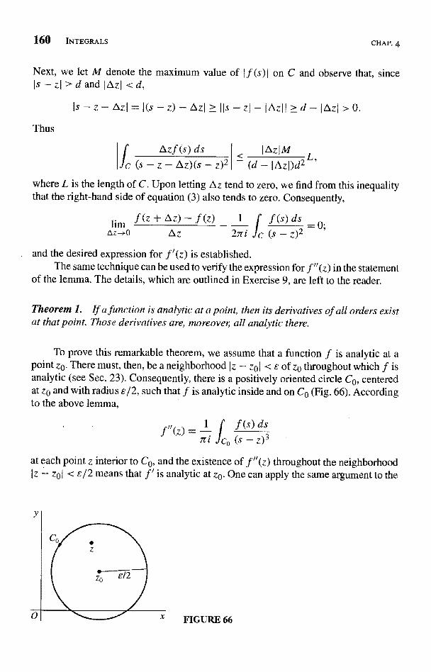
160 INTEGRALS CHAP. 4
Next, we let M denote the maximum value of If (s) I on C and observe that, sinceIs---zI>dandIAzI<d,
Is-z-AzI=I(s-z)--AzI>>-IIs
Thus
- (d - IAzl)d2
where L is the length of C. Upon letting Az tend to zero, we find from this inequalitythat the right-hand side of equation (3) also tends to zero. Consequently,
lim f (z -i- Az) - f (z) 1 [ f (s) dsAz 27ri c (s - z) 2
and the desired expression for f'(z) is established.The same technique can be used to verify the expression for f"(z) in the statement
of the lemma. The details, which are outlined in Exercise 9, are left to the reader.
Theorem 1. If a function is analytic at a point, then its derivatives of all orders existat that point. Those derivatives are, moreover, all analytic there.
To prove this remarkable theorem, we assume that a function f is analytic at apoint zo. There must, then, be a neighborhood Iz -- zol < s of zo throughout which f isanalytic (see Sec. 23). Consequently, there is a positively oriented circle CO, centeredat zo and with radius s/2, such that f is analytic inside and on Co (Fig. 66). Accordingto the above lemma,
f "(z)CO (s
at each point z interior to CO, and the existence of ,f"(z) throughout the neighborhoodIz - zol < s/2 means that f' is analytic at zo. One can apply the same argument to the
Azll>d-IAzI>0.
Azf (s) ds1
E 1AzIM L
FIGURE 66
SEC. 48 DERIVATIVES OF ANALYTIC FUNCTIONS 161
analytic function f' to conclude that its derivative f" is analytic, etc. Theorem 1 isnow established.
As a consequence, when a function
,f (z) = u(x, Y) + iv(x, Y)
is analytic at a point z = (x, y), the differentiability of f ensures the continuity of fthere (Sec. 18). Then, since
+ivx=vy-iuy,
we may conclude that the first-order partial derivatives of u and v are continuous atthat point. Furthermore, since f " is analytic and continuous at z and since
f"{z) = uxx + i vxx = vyx - ix,
etc., we arrive at a corollary that was anticipated in Sec. 25, where harmonic functionswere introduced,
Corollary. If a function f (z) = u(x, y) + iv(x, y) is defined and analytic at a pointz = (x, y) then the component functions u and v have continuous partial derivativesof all orders at that point.
One can use mathematical induction to generalize formulas (1) to
nt(4) f(n)(z)
2ni Jc(n=1,2,.
The verification is considerably more involved than for just n = 1 and n = 2, and werefer the interested reader to other texts for it.* Note that, with the agreement tha
.f (°) (z) - = .f (z) and 0! = 1,
expression (4) is also valid when n = 0, in which case it becomes the Cauchy integralformula (2).
When written in the form
(5) f f (z) dz=
2711 (n) (z°)(z - zo) +1 n!
expression (4) can be useful in evaluating certain integrals when f is analytic insideand on a simple closed contour C, taken in the positive sense, and z° is any pointinterior to C. It has already been illustrated in Sec. 47 when n = 0.
* See, for example, pp. 299-301 in Vol. I of the book by Markushevich, cited in Appendix 1.
162 INTEGRALS CHAP. 4
EXAMPLE 1. If C is the positively oriented unit circle lzI =I and
.f (z) = exp(2z),
then
exp(2z) dz _ ' f (z) dz = 8iri_ f (p) _C z4 c (z - 0)3+1 3! 3
EXAMPLE 2. Let ze be any point interior to a positively oriented simple closedcontour C. When f (z) = 1, expression (5) shows that
dz= 2rri
C z - zo
and
(Compare Exercise 10, Sec. 40.)
We conclude this section with a theorem due to E. Morera (1856-1909). The proofhere depends on the fact that the derivative of an analytic function is itself analytic, asstated in Theorem 1.
Theorem 2. Let f be continuous on a domain D. If
(6) / f (z) dz = 0C
for every closed contour C lying in D, then f is analytic throughout D.
In particular, when D is simply connected, we have for the class of continuousfunctions on D a converse of Theorem 1 in Sec. 46, which is the extension of theCauchy-Goursat theorem involving such domains.
To prove the theorem here, we observe that when its hypothesis is satisfied, thetheorem in Sec. 42 ensures that f has an antiderivative in D; that is, there exists ananalytic function F such that F'(z) = f (z) at each point in D. Since f is the derivativeof F, it then follows from Theorem 1 above that f is analytic in D.
EXERCISES
1. Let C denote the positively oriented boundary of the square whose sides lie along thelines x = + 2 and y = ± 2. Evaluate each of these integrals:
(a)e_zdz cost f zdz
1177
b)( Jc z - (rri J2)' c Z(Z2 + 8) - Jc 2z +
SEC. 48 EXERCISES 163
cosh z tan(z/2)
(d) Ic z4dz; (e) f (z - xO)2
dz (-2 x0 2).
Ans. (a) 2T; (b) 7ri/4; (c) -7ri/2; (d) 0; (e) irr sec2(x0/2).
2. Find the value of the integral of g(z) around the circle Iz - i I = 2 in the positive sensewhen
(a) g(z) = z2 + 4' (b) g(z) _ (z21
4)2
Ans. (a) 7r/2; (b) 7r/16.
3. Let C be the circle I z I = 3, described in the positive sense. Show that if
g(w) =_2z2 z - 2 dz (IwI 3),
then g(2) = 87ri. What is the value of g(w) when I w I > 3?
4. Let C be any simple closed contour, described in the positive sense in the z plane, andwrite
g(w)c (z - w)3
Show that g(w) = 67ri w when w is inside C and that g(w) = 0 when w is outside C.
5, Show that if f is analytic within and on a simple closed contour C and zc is not on C,then
f (z) dz [ f (z) dzc z - zp c (z - z0)2
6. Let f denote a function that is continuous on a simple closed contour C. Following aprocedure used in Sec. 48, prove that the function
1 f (s) dsg(z)=2ni c s-z
is analytic at each point z interior to C and that
1 f f (s) dsI
g (z) =2rri
at such a point.
7. Let C be the unit circle z = ezO(-rr < 0 < ze). First show that, for any real constant a,
2
Then write this integral in terms of 0 to derive the integration formula
Jea cos B cos(a sin 8) d8 =
0
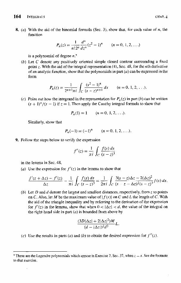
164 INTEGRALS CHAP. 4
8. (a) With the aid of the binomial formula (Sec. 3), show that, for each value of n, thefunction
n
Pn (z) =1 d
n' 2ndz
(z` - 1)n (n = 0, 1, 2,
is a polynomial of degree n.*
(b) Let C denote any positively oriented simple closed contour surrounding a fixedpoint z. With the aid of the integral representation (4), Sec. 48, for the nth derivativeof an analytic function, show that the polynomials in part (a) can be expressed in theform
f(S" - 1)nP (z) - ...).
2n+tn.i , (S - z)n+i ds (n = 0, 1, 2,
(c) Point out how the integrand in the representation for Pn(z) in part (b) can be written(s + 1)n/(s - 1) if z = 1. Then apply the Cauchy integral formula to show that
P11(I) = 1 (n = 0, 1, 2, ..).
Similarly, show that
n(-1) = (-1)n (n =0, 1, 2, ...).
9. Follow the steps below to verify the expression
f"(L) - ti JC (s - z)3
in the lemma in Sec. 48.
(a) Use the expression for f'(z) in the lemma to show that
f'(z + Az) - f'(z) 1 f (s) ds 1 f 3(s - z)Az -- 2(Az)2 f(s) ds.Az iri is (s - z)3 27ri Jc (s - z - Az)2(s - z)3
(b) Let D and d denote the largest and smallest distances, respectively, from z to pointson C. Also, let M be the maximum value of I f (s) I on C and L the length of C. Withthe aid of the triangle inequality and by referring to the derivation of the expressionfor f'(z) in the lemma, show that when 0 < I AzI < d, the value of the integral onthe right-hand side in part (a) is bounded from above by
(3DIAzI +21Az12)ML.(d - IAzI)2d3
Use the results in parts (a) and (b) to obtain the desired expression for it
* These are the Legendre polynomials which appear in Exercise 7. Sec. 37, when z = x. See the footnoteto that exercise.
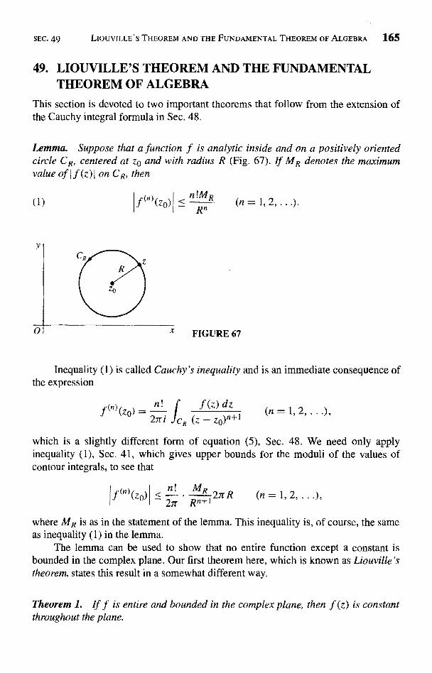
SEC. 49 LIOUVILLE'S THEOREM AND THE FUNDAMENTAL THEOREM OF ALGEBRA 165
49. LIOUVILLE'S THEOREM AND THE FUNDAMENTALTHEOREM OF ALGEBRA
This section is devoted to two important theorems that follow from the extension ofthe Cauchy integral formula in Sec. 48.
Lemma. Suppose that a function f is analytic inside and on a positively orientedcircle CR, centered at z0 and with radius R (Fig. 67). If MR denotes the maximumvalue of I f (z) ( on CR, then
(1) f (n) (Z0n !MR
Rn1,2,.
0 X FIGURE 67
Inequality (1) is called Cauchy's inequality and is an immediate consequence ofthe expression
f (n){z0)=
n!
27ri
f (,z) dz
(z - ZO)n+
which is a slightly different form of equation (5), Sec. 48. We need only applyinequality (1), Sec. 41, which gives upper bounds for the moduli of the values ofcontour integrals, to see that
f (fl)(z0)n!
c 27r .
Rn+127rR
where MR is as in the statement of the lemma. This inequality is, of course, the sameas inequality (1) in the lemma.
The lemma can be used to show that no entire function except a constant isbounded in the complex plane. Our first theorem here, which is known as Liouville'stheorem, states this result in a somewhat different way.
Theorem 1. If f is entire and bounded in the complex plane, then f (z) is constantthroughout the plane.
166 INTEGRALS CHAP. 4
To start the proof, we assume that f is as stated in the theorem and note that,since f is entire, Cauchy's inequality (1) with n = 1 holds for any choices of zo andR:
(2) If'(zo)R
Moreover, the boundedness condition in the statement of the theorem tells us that anonnegative constant M exists such that f (z) I < M for all z; and, because the constantMR in inequality (2) is always less than or equal to M, it follows that
(3) If'(zo)l < R
where zo is any fixed point in the plane and R is arbitrarily large. Now the number Min inequality (3) is independent of the value of R that is taken. Hence that inequalitycan hold for arbitrarily large values of R only if f'(zo) = 0. Since the choice of zo wasarbitrary, this means that f'(z) = 0 everywhere in the complex plane. Consequently,f is a constant function, according to the theorem in Sec. 23.
The following theorem, known as the fundamental theorem of algebra, followsreadily from Lionville's theorem.
Theorem 2. Any polynomial
P(z) = ao + a1z + a2z2 + ... + anzn (an 0 0)
of degree n (n > 1) has at least one zero. That is, there exists at least one pointzo suchthat P (zo) = 0.
The proof here is by contradiction. Suppose that P(z) is not zero for any valueof z. Then the reciprocal
f(z)=I
P (z)
is clearly entire, and it is also bounded in the complex plane.To show that it is bounded, we first write
(4)wao+ a1+ a2+...+an-1
z z1z 2
z
so that P(z) = (an + w)zn. We then observe that a sufficiently large positive numberR can be found such that the modulus of each of the quotients in expression (4) is lessthan the number Ian / (2n) when I z I > R. The generalized triangle inequality, appliedton complex numbers, thus shows that I w I < fan /2 for such values of z. Consequently,when f zI > R,
SEC. 50 MAXIMUM MODULUS PRINCIPLE 167
and this enables us to write
(5)IP(z)I=Ian+wIlznI> IzII
Evidently, then,
2whenever I z I >
2whenever Iz I > R.if (z) I = <
nIP(z)I IanlR
So f is bounded in the region exterior to the disk I z I < R. But f is continuous in thatclosed disk, and this means that f is bounded there too. Hence f is bounded in the
entire plane.It now follows from Liouville's theorem that f (z), and consequently P(z), is
constant. But P(z) is not constant, and we have reached a contradiction.*The fundamental theorem tells us that any polynomial P(z) of degree n (n > 1)
can be expressed as a product of linear factors:
(6) P (Z) = c(z - zi)(z - Z2)
where c and Zk (k = 1, 2, ... , n) are complex constants. More precisely, the theoremensures that P(z) has a zero zl. Then, according to Exercise 10, Sec. 50,
P(z) = (z - zl)Q1(z),
where Q1(z) is a polynomial of degree n - 1. The same argument, applied to Q1(z),reveals that there is a number z2 such that
P(z) = (z - zl)(z - z2)Q2(z),
where Q2(z) is a polynomial of degree n - 2. Continuing in this way, we arrive atexpression (6). Some of the constants Zk in expression (6) may, of course, appear morethan once, and it is clear that P(z) can have no more than n distinct zeros.
50. MAXIMUM MODULUS PRINCIPLEIn this section, we derive an important result involving maximum values of the moduliof analytic functions. We begin with a needed lemma.
Lemma. Suppose that I f (z) 1 1 f (za) I at each point z in some neighborhood1z - zoI < s in which f is analytic. Then f (z) has the constant value f (zp) throughoutthat neighborhood.
* For an interesting proof of the fundamental theorem using the Cauchy-Goursat theorem, see R. P.
Boas, Jr., Amer. Math. Monthly, Vol. 71, No. 2, p. 180, 1964.
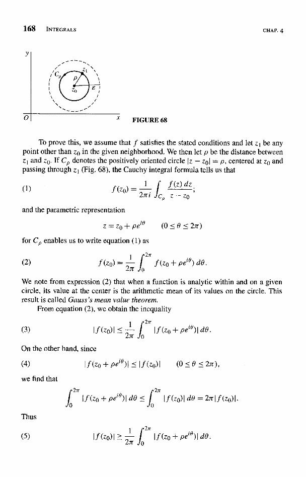
168 INTEGRALS
0 X FIGURE 68
CHAP. 4
To prove this, we assume that f satisfies the stated conditions and let zi be anypoint other than zo in the given neighborhood. We then let p be the distance betweenz1 and zo. If C. denotes the positively oriented circle Iz - zol = p, centered at zo andpassing through zl (Fig. 68), the Cauchy integral formula tells us that
(1) f (zo) = I Jf (z} dz
27ri c,, z -- zo
and the parametric representation
z=zo+peie (O<0 <2rr)
for C,, enables us to write equation (1) as
(2)
I f (zo +pet') dO.f (zo)
217r
We note from expression (2) that when a function is analytic within and on a givencircle, its value at the center is the arithmetic mean of its values on the circle. Thisresult is called Gauss's mean value theorem.
From equation (2), we obtain the inequality
12n
I I f (zo + pew) I dO.(3) I f (zo) I `-217r
On the other hand, since
(4)
we find that
Thus
f(zo+peL°')I<If(zo)I (0 <0<27r),
f (zo + pe'a)I dO T dO = 27r I f (zo) 1.
(5) I f (zo) I >_ = 1 If (zo + peter) I dO.2ir . n
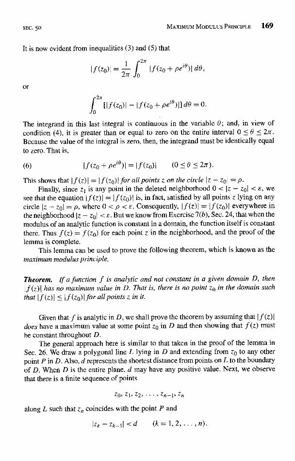
SEC. 50 MAXIMUM MODULUS PRINCIPLE 169
It is now evident from inequalities (3) and (5) that
Iif (zo + peI f (zo) I= 2n
or
2n
[If (zo) - If(zo+ pee)
d
Id9=0.
The integrand in this last integral is continuous in the variable 9; and, in view ofcondition (4), it is greater than or equal to zero on the entire interval 0 -< 0 <- 27r.Because the value of the integral is zero, then, the integrand must be identically equalto zero. That is,
(6) If(zo + pe`7)I 0 (0<9 <2r).
This shows that I f (z) I = I f (zo) I for all points z on the circle I z - zo I = p.Finally, since zI is any point in the deleted neighborhood 0 < Iz - zol < E, we
see that the equation I f (z) I = I f (zo) I is, in fact, satisfied by all points z lying on anycircle Iz - zoI = p, where 0 < p < E. Consequently, I f (z) I = I f (zo) I everywhere inthe neighborhood Iz - zo I < E. But we know from Exercise 7(b), Sec. 24, that when themodulus of an analytic function is constant in a domain, the function itself is constantthere. Thus f (z) = f (zo) for each point z in the neighborhood, and the proof of thelemma is complete.
This lemma can be used to prove the following theorem, which is known as theurn modulus principle.
Theorem. If' a function f is analytic and not constant in a given domain D, thenIf (z) I has no maximum value in D. That is, there is no point z0 in the domain such
that I f (z) I < I f (zo) I for all points z in it.
Given that f is analytic in D, we shall prove the theorem by assuming that I f (z) Idoes have a maximum value at some point z0 in D and then showing that f (z) mustbe constant throughout D.
The general approach here is similar to that taken in the proof of the lemma inSec. 26. We draw a polygonal line L lying in D and extending from z0 to any otherpoint P in D. Also, d represents the shortest distance from points on L to the boundaryof D. When D is the entire plane, d may have any positive value. Next, we observethat there is a finite sequence of points
Z0, ZI, Z2,
along L such that zn coincides with the point P and
Izk -zk-II <d (k= 1, 2, ...,
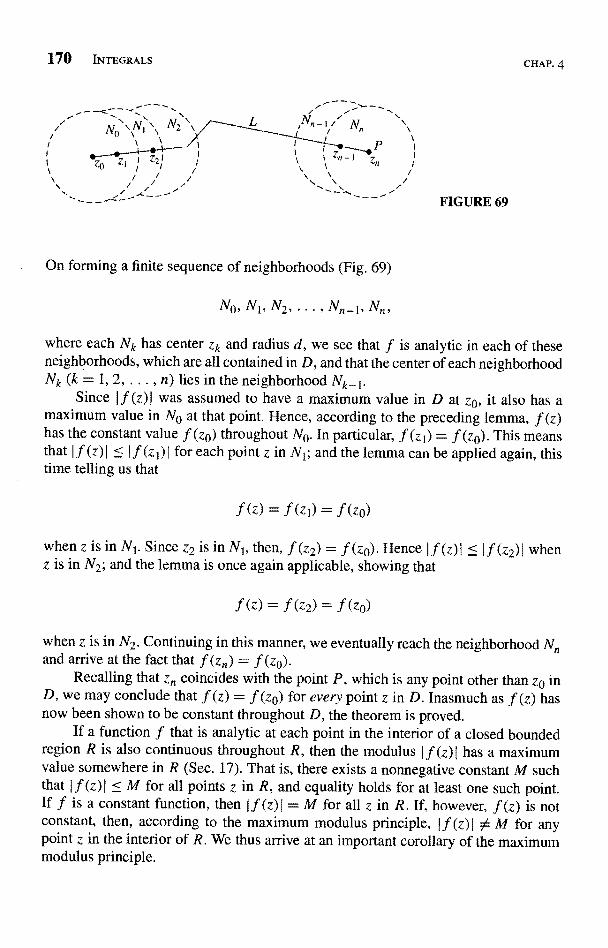
170 INTEGRALS
On forming a finite sequence of neighborhoods (Fig. 69)
No, N1,N2,...,Nn_
FIGURE 69
CHAP. 4
where each Nk has center zk and radius d, we see that f is analytic in each of theseneighborhoods, which are all contained in D, and that the center of each neighborhoodNk (k = 1, 2, . . . , n) lies in the neighborhood Nk_1.
Since I f (z) I was assumed to have a maximum value in D at z0, it also has amaximum value in No at that point. Hence, according to the preceding lemma, f (z)has the constant value f (za) throughout No. In particular, f (z1) = f (za). This meansthat I f (z) I I f (z 1) I for each point z in N1; and the lemma can be applied again, thistime telling us that
f(z)=f(z1)=f(z0)
when z is in N1. Since z2 is in N1, then, f (z2) = f (zo). Hence If (z) I { If (z2z is in N2; and the lemma is once again applicable, showing that
2) = f(ZO)
when
when z is in N2. Continuing in this manner, we eventually reach the neighborhoodand arrive at the fact that f (z,) = f (z0).
Recalling that z, coincides with the point P, which is any point other than z0 inD, we may conclude that f (z) = f (zp) for every point z in D. Inasmuch as f (z) hasnow been shown to be constant throughout D, the theorem is proved.
If a function f that is analytic at each point in the interior of a closed boundedregion R is also continuous throughout R, then the modulus If (z) I has a maximumvalue somewhere in R (Sec. 17). That is, there exists a nonnegative constant M suchthat If (z) I M for all points z in R, and equality holds for at least one such point.
is a constant function, then I f (z) I = M for all z in R. If, however, f (z) is notconstant, then, according to the maximum modulus principle, If (z) 10 M for anypoint z in the interior of R. We thus arrive at an important corollary of the maximummodulus principle.
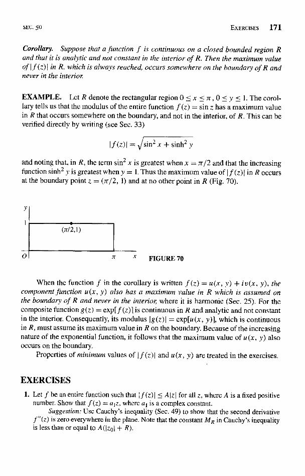
SEC. 50 EXERCISES 171
Corollary. Suppose that a function f is continuous on a closed bounded region Rand that it is analytic and not constant in the interior of R. Then the maximum valueof If (z) I in R, which is always reached, occurs somewhere on the boundary of R andnever in the interior.
EXAMPLE. Let R denote the rectangular region 0 < x < 7r, 0 < y < 1. The corol-lary tells us that the modulus of the entire function f (z) = sin z has a maximum valuein R that occurs somewhere on the boundary, and not in the interior, of R. This can beverified directly by writing (see Sec. 33)
If(z)I= /sin2 x + sinh2 y
and noting that, in R, the term sin2 x is greatest when x = 7r/2 and that the increasingfunction sinh2 y is greatest when y = 1. Thus the maximum value of If (z) I in R occursat the boundary point z = (7r/2, 1) and at no other point in R (Fig. 70).
X FIGURE 70
When the function f in the corollary is written f (z} = u(x, y) + iv(x, y), thecomponent function u (x, y) also has a maximum value in R which is assumed onthe boundary of R and never in the interior where it is harmonic (Sec. 25). For thecomposite function g(z) = exp[f (z)] is continuous in R and analytic and not constantin the interior. Consequently, its modulus Ig(z)l = exp[u(x, y)], which is continuousin R, must assume its maximum value in R on the boundary. Because of the increasingnature of the exponential function, it follows that the maximum value of u (x, y) alsooccurs on the boundary.
Properties of minimum values of If (z) I and u (x, y) are treated in the exercises.
EXERCISES
1. Let f be an entire function such that If (z) I < AIzI for all z, where A is a fixed positivenumber. Show that f'(z) = a1z, where a1 is a complex constant.
Suggestion: Use Cauchy's inequality (Sec. 49) to show that the second derivativef"(z) is zero everywhere in the plane. Note that the constant MR in Cauchy's inequalityis less than or equal to A(Izol + R).
172 INTEGRALS CHAP. 4
2. Suppose that f (z) is entire and that the harmonic function u(x, y) = Re[f (z)] has anupper bound u0; that is, u(x, y) < uq for all points (x, y) in the xy plane. Show thatu (x, y) must be constant throughout the plane.
Suggestion: Apply Liouville's theorem (Sec. 49) to the function g(z) = exp[f (z)].
3. Show that, for R sufficiently large, the polynomial P(z) in Theorem 2, Sec. 49, satisfiesthe inequality
IP(z)I < 21a,IIzI whenever Iz
[Compare the first of inequalities (5), Sec. 49.]Suggestion: Observe that there is a positive number R such that the modulus of
each quotient in expression (4), Sec. 49, is less than Ia,I /n when I z I > R.
4. Let a function f be continuous in a closed bounded region R, and let it be analytic andnot constant throughout the interior of R. Assuming that f (z) A 0 anywhere in R, provethat I f (z) I has a minimum value m in R which occurs on the boundary of R and neverin the interior. Do this by applying the corresponding result for maximum values (Sec.50) to the function g(z) =1Jf (z).
5. Use the function f (z) = z to show that in Exercise 4 the condition f (z) 0 anywherein R is necessary in order to obtain the result of that exercise. That is, show that If (z)
I
can reach its minimum value at an interior point when that minimum value is zero.
6. Consider the function f (z) _ (z + 1)2 and the closed triangular region R with verticesat the points z = 0, z = 2, and z = i. Find points in R where If (z) I has its maximum andminimum values, thus illustrating results in Sec. 50 and Exercise 4.
Suggestion: Interpret I f (z) I as the square of the distance between z and -1.
Ans. z=2,z=0.
7. Let f (z) = u (x, y) + i v (x, y) be a function that is continuous on a closed bounded regionR and analytic and not constant throughout the interior of R. Prove that the componentfunction u (x, y) has a minimum value in R which occurs on the boundary of R andneverin the interior. (See Exercise 4.)
8. Let f be the function f (z) = ez and R the rectangular region 0 < x < 1, 0 < y < 7r.Illustrate results in Sec. 50 and Exercise 7 by finding points in R where the componentfunction u(x, y) = Re[f (z)] reaches its maximum and minimum values.
Ans. z=1,z=1
9. Let the function f (z) = u(x, y) + iv(x, y) be continuous on a closed bounded regionR, and suppose that it is analytic and not constant in the interior of R. Show that thecomponent function v(x, y) has maximum and minimum values in R which are reachedon the boundary of R and never in the interior, where it is harmonic.
Suggestion: Apply results in Sec. 50 and Exercise 7 to the function g(z) - -if (z).10. Let za be a zero of the polynomial
P(z) = ao + alz + a2zL + ... + anz" (an 5 0)
SEC. 50
of degree n (n > 1). Show in the following way that
P (Z) = (z - zo) Q
where Q(z) is a polynomial of degree n - 1.
(a) Verify that
(z - zo(zx-1 + zx aza + ... + ZZa 2
EXERCISES 173
2,
(b) Use the factorization in part (a) to show that
P(z) - P(za) = (z - zo)Q(z),
where Q(z) is a polynomial of degree n - 1, and deduce the desired result from this.
CHAPTER
5SERIES
This chapter is devoted mainly to series representations of analytic functions. Wepresent theorems that guarantee the existence of such representations, and we developsome facility in manipulating series.
51. CONVERGENCE OF SEQUENCES
An infinite sequence
(1) Zlf z21 . . . , Zn, .
of complex numbers has a limit z if, for each positive number e, there exists a positiveinteger no such that
(2) (zn - zI < s whenever n > no.
Geometrically, this means that, for sufficiently large values of n, the points zn lie inany given s neighborhood of z (Fig. 71). Since we can chooses as small as we please,it follows that the points zn become arbitrarily close to z as their subscripts increase.Note that the value of no that is needed will, in general, depend on the value o
The sequence (1) can have at most one limit. That is, a limit z is unique if it exists(Exercise 5, Sec. 52). When that limit exists, the sequence is said to converge to z; andwe write
(3) lim zn = Z.n-too
If the sequence has no limit, it diverges.
175
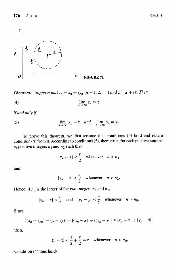
176 SERIES CHAP.5
y
n-+o,--
x
Theorem. Suppose that zn = xn + i yn (n = 1, 2, ...) and z = x + iy. Then
I'm Zn = Zn-roa
xn = x and = V.
To prove this theorem, we first assume that conditions (5) hold and obtaincondition (4) from it. According to conditions (5), there exist, for each positive numbere, positive integers n1 and n2 such that
Ixn - x (< 2 whenever n> n 1
and
IYnYI<2
FIGURE 71
whenever n > n2.
Hence, if no is the larger of the two integers n1 and n2,
s(xn - x j <- and
Since
then,
-y 6
2whenever n > no.
iYn)-(x+iy)l=I(Xn-x)+i(Yn-Y)I<- IXn-xI+lYn-Y1,
1Zn - zl < + - = e whenever n > no.
Condition (4) thus holds.
SEC. 51 CONVERGENCE OF SEQUENCES 177
Conversely, if we start with condition (4), we know that, for each positive numberthere exists a positive integer no such that
I(xn + iyn) - (x + iy)I < s whenever n > n0.
But
i(Yn-"Y)1=On+IYn)-(x+iY)I
IYn - YI On - x) + i(Yn - A = I(xn + IYn) - (x + iY)I;
and this means that
(xn - xI <E and Iyn - yl <E whenever n > n0.
That is, conditions (5) are satisfied.Note how the theorem enables us to write
lira (xn + iy,a) = I'm xn + i lim ynn-+CX n-+oo n-+oc
whenever we know that both limits on the right exist or that the one on the left exists.
EXAMPLE. The sequence
(n=1,2,
converges to i since
1lim-
1=0--i= limc n3 ++i nlimao
n ,o( +i
n- n 3r-
By writing
IZn-il=n3
one can also use definition (2) to obtain this result. More precisely, for each positivenumber s,
lIZn - i I <8 whenever n > ,--
178 SERIES
52. CONVERGENCE OF SERIES
An infinite series
(1)
00
EZn=Z1+Z2+...+Zn+n=1
of complex numbers converges to the sum S if the sequence
(2) SN=Lzn=Zl+z2+...+ZN (N=1,2,...)n=1
of partial sums converges to S; we then write
CHAP. 5
L Zn S.
n=1
Note that, since a sequence can have at most one limit, a series can have at most onesum. When a series does not converge, we say that it diverges.
Theorem. Suppose that zn = xn + i yn (n = 1, 2, ...) and S = X + i Y. Then
=S
Xn=X andn=1
1: yn=Y.n=1
This theorem tells us, of course, that one can write
whenever it is known that the two series on the right converge or that the one on the
left does.To prove the theorem, we first write the partial sums (2) as
(5) SN=XN+iYN,
where
XN=Lxn and YN=n=l
N
n=1
SEC. 52 CONVERGENCE OF SERIES 179
Now statement (3) is true if and only i
(6) lira SN = S;N-+oo
and, in view of relation (5) and the theorem on sequences in Sec. 51, limit (6) holds ifand only if
(7) lim XN = X andN +oc
lim YN = Y.N-* oc
Limits (7) therefore imply statement (3), and conversely. Since XN and YN are thepartial sums of the series (4), the theorem here is proved.
By recalling from calculus that the nth term of a convergent series of real numbersapproaches zero as n tends to infinity, we can see immediately from the theorems inthis and the previous section that the same is true of a convergent series of complexnumbers. That is, a necessary condition for the convergence of series (1) is that
(8) lim zn = 0.n- oc
The terms of a convergent series of complex numbers are, therefore, bounded. To bespecific, there exists a positive constant M such that j zn I < M for each positive integern. (See Exercise 9.)
For another important property of series of complex numbers, we assume thatseries (1) is absolutely convergent. That is, when Zn = xn + iyn, the series
Y2
of real numbers jx? + y converges. Since
and I yn
we know from the comparison test in calculus that the two series
n=1
and
oc
Yn I
n=1
must converge. Moreover, since the absolute convergence of a series of real numbersimplies the convergence of the series itself, it follows that there are real numbers X andY to which series (4) converge. According to the theorem in this section, then, series(1) converges. Consequently, absolute convergence of a series of complex numbersimplies convergence of that series.
In establishing the fact that the sum of a series is a given number S, it is oftenconvenient to define the remainder PN after N terms:
(9) PN = S - SN.
180 SERIES CHAP. 5
Thus S = SN + PN; and, since ISN - SI = I PN - 01, we see that a series convergesto a number S if and only if the sequence of remainders tends to zero. We shall makeconsiderable use of this observation in our treatment of power series. They are seriesof the form
n(z-zo)n=ao+a1(z-zo)+a2(z-zo)z+...+an(z-zon=0
where zo and the coefficients an are complex constants and z may be any point in astated region containing zo. In such series, involving a variable z, we shall denote sums,partial sums, and remainders by S(z), SN(z), and PN(z), respectively.
EXAMPLE. With the aid of remainders, it is easy to verify that
(10) whenever j z ( < 1.
We need only recall the identity (Exercise 10, Sec. 7)
1 _ Zn+11+z+z2+...+Zn=
-z
to write the part al sums
SN (Z)no
as
(z01)
n1-}-+z2+...+zN-1 (z01)
1-ZNSN (Z)
if
then,
Thus
pN(z) = S(z) - SN(z) = lzz
(z 0 D.
and it is clear from this that the remainders pN(z) tend to zero when I z I < 1 but notwhen 11-1 > 1. Summation formula (10) is, therefore, established.
SEC. 52 EXERCISES 181
EXERCISES
1. Show in two ways that the sequence
(_ I )nzn=-2+z (n=1,2,..
n
converges to -2.
2. Let rn denote the moduli and Qn the principal values of the arguments of the complexnumbers zn in Exercise 1. Show that the sequence rn (n = 1, 2, ...) converges but thatthe sequence Q, (n = 1, 2, ...) does not.
3. Show that
lim zn =z, then lim Izn1 = IzIn-), n
4. Write z = re'0, where 0 < r < 1, in the summation formula that was derived in theexample in Sec. 52. Then, with the aid of the theorem in Sec. 52, show that
r cos 9 -r 2 "" r sin 9rn cos n9 = and rn sin n9 =
n=11- 2r cos 0 + r2 n=1
1- 2r cos 9 + r2
when 0 < r < 1. (Note that these formulas are also valid when r = 0.)
5. Show that a limit of a convergent sequence of complex numbers is unique by appealingto the corresponding result for a sequence of real numbers.
6. Show that
if then
n=1n=1
7. Let c denote any complex number and show that
oa
zn = S, then E Czn = CS.
n=1
8. By recalling the corresponding result for series of real numbers and referring to the
theorem in Sec. 52, show that
oa oa
:--S and ) 'w,=T, then },(z, + wn) = S + T.n=1
9. Let a sequence z, (n = 1, 2, ...) converge to a number z. Show that there exists a positivenumber M such that the inequality IznI < M holds for all n. Do this in each of the waysindicated below.
(a) Note that there is a positive integer no such that
Iznl=Iz+(zn-z)I<IZI+1
whenever n > no.
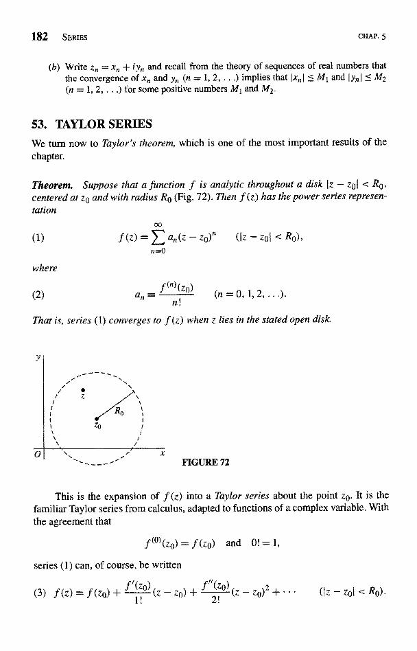
182 SERIES CHAP. 5
(b) Write z = x,a + iy, and recall from the theory of sequences of real numbers thatthe convergence of xn and yn (n = 1, 2, ...) implies that Ix I < MI and I yn I < M2(n = 1, 2, ...) for some positive numbers Ml and M2.
53. TAYLOR SERIESWe turn now to Taylor's theorem, which is one of the most important results of thechapter.
Theorem. Suppose that a function f is analytic throughout a disk Iz - zol < Ro,centered at zo and with radius Ro (Fig. 72). Then f (z) has the power series represen-tation
(1) f(z)= ) 'an(z-zo)n (Iz - zoI < Ro),n=0
where
(2) an = f (nl(zo)(n = 0, 1, 2, ...).
n!
That is, series (1) converges to f (z) when z lies in the stated open disk.
/z \
R4
zo
1 /
FIGURE 72
This is the expansion of f (z) into a Taylor series about the point zo. It is thefamiliar Taylor series from calculus, adapted to functions of a complex variable. Withthe agreement that
f(o)(zo) = f (zo) and 0! =
series (1) can, of course, be written
(3) f (z) _ .f (zo) +f o) (z - zo) + fo (z - zo)2 + ... (Iz - zoI < Ro).
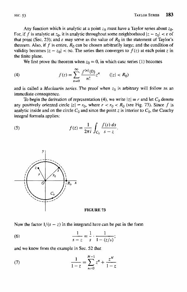
SEC. 53 TAYLOR SERIES 183
Any function which is analytic at a point z0 must have a Taylor series about z0.For, if f is analytic at z0, it is analytic throughout some neighborhood Iz - zoI < e ofthat point (Sec. 23); and s may serve as the value of R0 in the statement of Taylor'stheorem. Also, if f is entire, R0 can be chosen arbitrarily large; and the condition ofvalidity becomes Iz - zol < oo. The series then converges to f (z) at each point z inthe finite plane.
We first prove the theorem when z0 = 0, in which case series (1) becomes
(4) .f (z) =n=0
and is called a Maclaurin series. The proof when z0 is arbitrary will follow as animmediate consequence.
To begin the derivation of representation (4), we write I z I = r and let Co denoteany positively oriented circle Jzt = r0, where r < r0 < R0 (see Fig. 73). Since f isanalytic inside and on the circle Co and since the point z is interior to CO, the Cauchyintegral formula applies:
(5)
FIGURE 73
s 1 ds
Now the factor 1/(s - z) in the integrand here can be put in the form
(6)_1 1
s 1 - (z/s)'
and we know from the example in Sec. 52 that
(7)
tz) =
(n)(0) zn(fzl < RO)
nI
27r i J C, s - z
1N-1
ZnZN
n=O
184 SERIES CHAP.5
when z is any complex number other than unity. Replacing z by z/s in expression (7),then, we can rewrite equation (6) as
(8)N 1
s =- z n=0sn+1
LN(s - Z)s
Multiplying through this equation by f (s) and then integrating each side with respectto s around CO, we find that
f (s) ds = f (s) ds zn+ zN
.f (s) dsI o S - z J o sn+1 Co (S - Z)SN0n=
In view of expression (5) and the fact (Sec. 48) that
1 f (s) ds f (n) (0)(n = 0, 1, 2, .
27ri JC0 sn+1 n!
this reduces, after we multiply through by 1/ (27r i ), to
N-I{n)(0
(9) f (Z) = Y .f ) zn + hn(Z),
0
where
(10)
(11)
ni
N fPN(z) =
27ri fco (s (sZ)SN
Representation (4) now follows once it is shown that
lira pN (z) = 0.N-*oc
To accomplish this, we recall that Iz I = r and that Co has radius ro, where ro > r. Then,if s is a point on CO, we can see that
Is - zI? 11sl-Izli=r0-r.
Consequently, if M denotes the maximum value of If (s) I on CO,
rrN - JNIAN(z)I <27r (ro
M) rN
7rro =ro or \ JJJro
0
Inasmuch as (r/r0) < 1, limit (11) clearly holds.To verify the theorem when the disk of radius Ro is centered at an arbitrary point
Zo, we suppose that f is analytic when Iz - zol < Re and note that the compositefunction f (z + zo) must be analytic when I (z + zo) - zo I < R. This last inequalityis, of course, just IzI < Re; and, if we write g(z) = f (z + zo), the analyticity of g in
SEC. 54 EXAMPLES 185
the disk Iz I < Ro ensures the existence of a Maclaurin series representation:
tn1 O0g(z) = ` g zn (IzI < R0)
n=0
That is
0) -U/Zn (IZI < Ro).
n=0
After replacing z by z - zo in this equation and its condition of validity, we have thedesired Taylor series expansion (1).
54. EXAMPLESWhen it is known that f is analytic everywhere inside a circle centered at z0, conver-gence of its Taylor series about zo to f (z) for each point z within that circle is ensured;no test for the convergence of the series is required. In fact, according to Taylor's theo-rem, the series converges to f (z) within the circle about zo whose radius is the distancefrom zo to the nearest point zl where f fails to be analytic. In Sec. 59, we shall findthat this is actually the largest circle centered at zo such that the series converges tof (z) for all z interior to it,
Also, in Sec. 60, we shall see that if there are constants an (n = 0, 1, 2 ...) suchthat
oc1
z - z0),n
n=0
for all points z interior to some circle centered at zo, then the power series here mustbe the Taylor series for f about zo, regardless of how those constants arise. Thisobservation often allows us to find the coefficients an in Taylor series in more efficientways than by appealing directly to the formula an = f(n)(zo)/n! in Taylor's theorem.
In the following examples, we use the formula in Taylor's theorem to find theMaclaurin series expansions of some fairly simple functions, and we emphasize theuse of those expansions in finding other representations. In our examples, we shallfreely use expected properties of convergent series, such as those verified in Exercises7 and 8, Sec. 52.
EXAMPLE 1. Since the function f (z) = ez is entire, it has a Maclaurin seriesrepresentation which is valid for all z. Here f(n) (z) = ez; and, because f (n) (0) = 1, itfollows that
(1) ez = } ; = (IzI < CO.
186 SERIES
Note that if z = x + iO, expansion (1) becomes
xn <x<
- 1)ni nzn
n!
The entire function z2e3z also has a Maclaurin series expansion. The simplestway to obtain it is to replace z by 3z on each side of equation (1) and then multiplythrough the resulting equation by z2:
z2e3` =
n=
(IzI < oc).
Finally, if we replace n by n - 2 here, we have
2
(IzI <
EXAMPLE 2. One can use expansion (1) and the definition (Sec. 33)
sin z =
e-1z
2i
to find the Maclaurin series for the entire function f(z) = = sin z. To give the details,we refer to expansion (1) and write
sin 7
Butl-
Inasmuch as
this reduces to
(2)
CHAP. 5
(IzI < oc).
= 0 when n is even, and so we can replace n by 2n + 1 in this last series:
sin z
-1)2n+1= 2 and
sin zn=O
i 2n+rz2n+1
(2n + 1)!
Z2n+11)n
(2n + 1)!
(IzI < oo).
(IzI < oo
SEC. 54 EXAMPLES 187
Term by term differentiation will be justified in Sec. 59, Using that procedurehere, we differentiate each side of equation (2) and write
cos Z =
That is,
cos z OZI <
EXAMPLE 3. Because sinh z = -i sin(iz) (Sec. 34), we need only replace z by izon each side of equation (2) and multiply through the result by -i to see that
(4) sinh z = (Izl < oo).
Likewise, since cosh z = cos(iz), it follows from expansion (3) that
n=0
Observe that the Taylor series for cosh z about the point z0 = -2iri, for example,is obtained by replacing the variable z by z + 27ri on each side of equation (5) andthen recalling that cosh(z + 27ri) = cosh z for all z:
cosh z = ) . '" OZI < oc).n=
EXAMPLE 4. Another Maclaurin series representation is
1
1-zn=Q
OZI
The derivatives of the function f (z) = 1/(1 - z), which fails to be analytic at z =
n!1, 2,
and, in particular, f (n)(0) = W. Note that expansion (6) gives us the sum of an infinitegeometric series, where z is the common ratio of adjacent terms:
l+z+z2+z3+-
2ncoshz=) . OZI <oo).
1(IzI < 1).
188 SERIES CHAPS
This is, of course, the summation formula that was found in another way in the examplein Sec. 52.
If we substitute -z for z in equation (6) and its condition of validity, and notethat J z I < l when I - z I < 1, we see that
1
1+Z)nzn (IzI
W
n=O
If, on the other hand, we replace the variable z in equation (6) by 1- z, we havethe Taylor series representation
001 T-
nn=o
(Iz -11 < D.
This condition of validity follows from the one associated with expansion (6) sinceJ1-zl<1isthesame asIz-iJ<1.
EXAMPLE 5. For our final example, let us expand the function
1+2z2 1 2(l +z2) - 1 1 f.f (z) _ = = 2 -
z3+z5 - Z3 1 +Z2 Z3
into a series involving powers of z. We cannot find a Maclaurin series for f (z) sinceit is not analytic at z = 0. But we do know from expansion (6) that
1
I+z`Hence, when 0 < I z I < 1,
.f (z) _ 1 (2 -z
(Izl < 1).
We call such terms as 1/z3 and 1/z negative powers of z since they can be written z-3
and z-1, respectively. The theory of expansions involving negative powers of z - zowill be discussed in the next section.
EXERCISES*
1. Obtain the Maclaurin series representation
z cosh(z2) (Izl < oc).
*In these and subsequent exercises on series expansions, it is recommended that the reader use, whenpossible, representations (1) through (6) in Sec. 54.
SEC. 54
2. Obtain the Taylor series
I
for the function f (z) = ez by
a using f(n) (1) (n = 0, 1, 2, . . .); (b) writing ez = ez
3. Find the Maclaurin series expansion of the function
f(z)z z I
z4+9 9 1 + (z4/9)
n
Ans. YL-" z4n+1 (Iz) < /).
32n+2n=O
4. Show that if f (z) = sin z, then
EXERCISES 189
f(2n)(0) = 0 and f(2n+1)(0) _ (_1Y (n = 0, 1, 2, ...).
Thus give an alternative derivation of the Maclaurin series (2) for sin z in Sec. 54.
5. Rederive the Maclaurin series (3) in Sec. 54 for the function f (z) = cos z by
(a) using the definition
cos z2
in Sec. 33 and appealing to the Maclaurin series (1) for ez in Sec. 54;
(b) showing that
f(2n)(0) =( d (2n+1) (0) = 0 (n = 0, 1, 2, . .
6. Write the Maclaurin series representation of the function f (z) = sin(z2), and point outhow it follows that
0) = 0 and f (2n+1) (0) = 0 (n = 0, 1,
7. Derive the Taylor series representation
1
1-z
Suggestion: Start by writing
(Iz - i I < v'2).
1 1 1 1
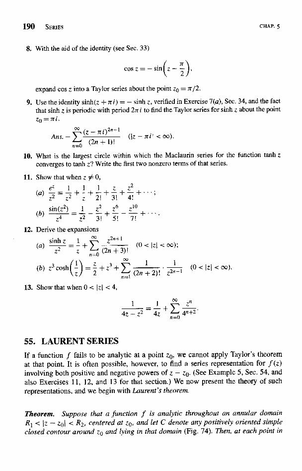
190 SERIES CHAP. 5
8. With the aid of the identity (see Sec. 33)
cos z = - sin
expand cos z into a Taylor series about the point z0 = 7r/2.
9. Use the identity sinh(z + iri) = - sinh z, verified in Exercise 7(a), Sec. 34, and the factthat sinh z is periodic with period 2n i to find the Taylor series for sinh z about the pointz0=ri.
00 (z - lrF 2n+1Ans. - (Iz - zri l < o0).
n-0 (2n + 1)!
10. What is the largest circle within which the Maclaurin series for the function tanh zconverges to tanh z? Write the first two nonzero terms of that series.
11. Show that when z 54 0,2-1 -(a) + +-
(b)
Z' Z' z Z! 3! 4!
sin(z2) _ 1z2 z6 z10
z4 z2 3! 5! 7!
12. Derive the expansions00 z2n+-1
(b) z3cosh ( z) 2 +..3
13. Show that when 0 < Izl < 4,
(0 < IzI < oc);
1 1 (0<Iz1 <oc).(2n + 2)! z2n-I
55. LAURENT SERIESIf a function f fails to be analytic at a point z0, we cannot apply Taylor's theoremat that point. It is often possible, however, to find a series representation for f (z)involving both positive and negative powers of z - zo (See Example 5, Sec. 54, andalso Exercises 11, 12, and 13 for that section.) We now present the theory of suchrepresentations, and we begin with Laurent's theorem.
Theorem. Suppose that a function f is analytic throughout an annular domainR1 < Iz - zol < R2, centered at zo, and let C denote any positively oriented simpleclosed contour around zo and lying in that domain (Fig. 74). Then, at each point in
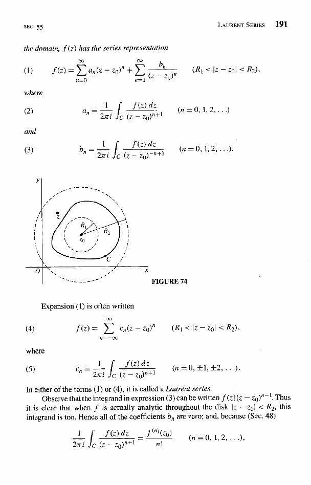
SEC. 55 LAURENT SERIES 191
the domain, f (z) has the series representation
(1) f(z)=Lan(Z-n=O n=
where
(2)
and
(3)
1 f (z) dz27ri c (z - zo)n+l
2
bn
1
C
f(z)dz (n=0,1,2,.n27ri (Z - zo)-n+l
R2),
FIGURE 74
Expansion (1) is often written
f (z) = > , cn(z - zo)n (RI < Iz - zol < R2),n=-cX
where
(5)f (z) dz
C (Z - Zo)n+l(n=0,±1,±2,
In either of the forms (1) or (4), it is called a Laurent series.Observe that the integrand in expression (3) can be written f (z) (z - zo)n-l. Thus
clear that when f is actually analytic throughout the disk Iz - zol < R2, thisintegrand is too. Hence all of the coefficients bn are zero; and, because (Sec. 48)
f (z) dz f(n)(z0) (n - 0 1 2 )2;ri C (z - ZO)n+l - n
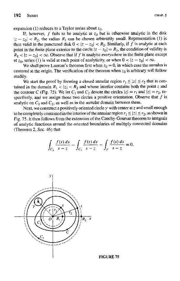
192 SERIES CHAP5
expansion (1) reduces to a Taylor series about z0.If, however, f fails to be analytic at z0 but is otherwise analytic in the disk
Iz - zol < R2, the radius RI can be chosen arbitrarily small. Representation (1) isthen valid in the punctured disk 0 < (z - z0I < R2. Similarly, if f is analytic at eachpoint in the finite plane exterior to the circle (z - zoo = R1, the condition of validity isR1 < Iz - z01 < oo. Observe that if f is analytic everywhere in the finite plane exceptat z0, series (1) is valid at each point of analyticity, or when 0 < 1z - z0) < exp.
We shall prove Laurent's theorem first when z0 = 0, in which case the annulus iscentered at the origin. The verification of the theorem when z0 is arbitrary will followreadily.
We start the proof by forming a closed annular region r1 < Izl < r2 that is con-tained in the domain R1 < Izi < R2 and whose interior contains both the point z andthe contour C (Fig. 75). We let C1 and C2 denote the circles IzI = r1 and I z I = r2, re-spectively, and we assign those two circles a positive orientation. Observe that f isanalytic on C1 and C2, as well as in the annular domain between them.
Next, we construct a positively oriented circle y with center at z and small enoughto be completely contained in the interior of the annular region r1 < Iz I < r2, as shown inFig. 75. It then follows from the extension of the Cauchy-Goursat theorem to integralsof analytic functions around the oriented boundaries of multiply connected domains(Theorem 2, Sec. 46) that
f f(s)ds f f(s)ds f f(s)ds -0C2 s - Z JC, s-Z Jy s-Z
FIGURE 75
SEC. 55 LAURENT SERIES 193
But, according to the Cauchy integral formula, the value of the third integral here is27ri if (z). Hence
f(z) = 1 f f(s) ds + 1 f f(s) d27ri c2 s-z 23ri cI z-s
Now the factor 1/(s - z) in the first of these integrals is the same as in expression(5), Sec. 53, where Taylor's theorem was proved; and we shall need here the expansion
(7)
1 1 n NZ
{-
Zs - z
n+1(s
n=O
which was used in that earlier section. As for the factor 1/(z - s) in the second integral,an interchange of s and z in equation (7) reveals that
eplace the index of summation n here by n - 1, this expansion takes the form
(8)
1
nZ - S It ' S-n+ 1 Zn
SN5
which is to be used in what follows.Multiplying through equations (7) and (8) by f (s)/(2rri) and then integrating
each side of the resulting equations with respect to s around C2 and C1, respectively,we find from expression (6) that
N-1 N
n
f (Z) _ anZ' + PN(Z)
where the numbers an (n = 0,by the equations
( 0)
and where
PN(Z) =ZN
27r iOrN
1 f sNf(s)dsZ) _
27rizN t Z - S
As N tends to oo, expression (9) evidently takes the proper form of a Laurentseries in the domain R1 < Izi < R2, provided that
, N - 1) and bn (n = 1, 2, . . . , N) are given
1) iim PN (z) = 0 and lim aN (Z) = 0.N--+oo Noo
194 SERIES CHAP. 5
These limits are readily established by a method already used in the proof of Taylor'stheorem in Sec. 53. We write IzI - r, so that r1 < r < r2, and let M denote themaximum value of If (s) I on C1 and C2. We also note that if s is a point on C2, thenIs - zI > r2 -- r; and if s is on C1, Iz - sI > r - r1. This enables us to write
IAN (Z) I <Mr2
r2 - r
Since (r 1r2) < 1 and (r1 1r) < 1, it is now clear that both PN(z) and UN(z) have thedesired property.
Finally, we need only recall Corollary 2 in Sec. 46 to see that the contours used inintegrals (10) may be replaced by the contour C. This completes the proof of Laurent'stheorem when zo = 0 since, if z is used instead of s as the variable of integration,expressions (10) for the coefficients a/z and bn are the same as expressions (2) and (3)when zo = 0 there.
To extend the proof to the general case in which zo is an arbitrary point in thefinite plane, we let f be a function satisfying the conditions in the theorem; and, justas we did in the proof of Taylor's theorem, we write g(z) = f (z + zo). Since f (z) isanalytic in the annulus R1 < Iz - zol < R2, the function f (z + zo) is analytic whenR1 < I (z + zo) - zol < R2. That is, g is analytic in the annulus Rl < IzI < R2, which iscentered at the origin. Now the simple closed contour C in the statement of the theoremhas some parametric representation z = z (t) (a < t < b), where
(12) R1 < Iz(t) - zol < R2
for all t in the interval a < t < b. Hence if F denotes the path
(13) z=z(t)-zo (a<t<b
r is not only a simple closed contour but, in view of inequalities (12), it lies in thedomain R1 < Iz I < R2. Consequently, g(z) has a Laurent series representation
00
(14) g(z) ' anzn + > (R1 < IzI < R2),
where
(15)
(16) bn =g(z) dz
r Z-n+l
n = 0, 1, 2, .
n=1,2,..
Representation (1) is obtained if we write f (z + zo) instead of g (z) in equation(14) and then replace z by z - zo in the resulting equation, as well as in the condition ofvalidity R1 < Izl < R2. Expression (15) for the coefficients an is, moreover, the same
SEC. 56 EXAMPLES 195
as expression (2) since
g(z) dz = 1b f[z(t)]z`(t) dt _ f (z) dz
r zn+1 a [z(t) - zeln+l c (z - zo)n+i `
Similarly, the coefficients bn in expression (16) are the same as those in expres-sion
56. EXAMPLESThe coefficients in a Laurent series are generally found by means other than byappealing directly to their integral representations. This is illustrated in the examplesbelow, where it is always assumed that, when the annular domain is specified, a Laurentseries for a given function in unique. As was the case with Taylor series, we defer theproof of such uniqueness until Sec. 60.
EXAMPLE 1. Replacing z by 1/z in the Maclaurin series expansion
(IzI < oc
we have the Laurent series representation
(0<`zI<oo
Note that no positive powers of z appear here, the coefficients of the positivepowers being zero. Note, too, that the coefficient of l/z is unity; and, according toLaurent's theorem in Sec. 55, that coefficient is the number
1/z dz,
where C is any positively oriented simple closed contour around the origin. Since
61 = 1, then,
dz=2rri.
This method of evaluating certain integrals around simple closed contours will bedeveloped in considerable detail in Chap. 6.
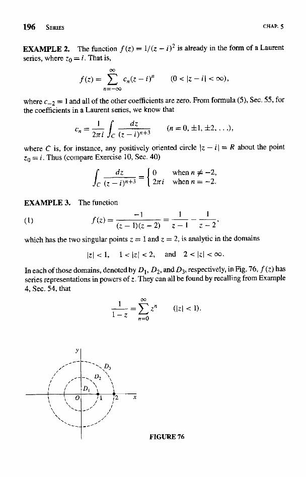
96 SERIES CHAP. 5
EXAMPLE 2. The function f (z) = 1/(z - i)2 is already in the form of a Laurentseries, where zQ = i. That is,
f(z) =00
n=-00z (0<Iz-i < 00
where c_2 = 1 and all of the other coefficients are zero. From formula (5), Sec. 55, fo
the coefficients in a Laurent series, we know that
dz
2iri Jc (z - i)n+3(n=0,±1,±2,.
where C is, for instance, any positively oriented circle Iz - i I = R about the pointze = i. Thus (compare Exercise 10, Sec. 40)
dz 0 when n i4 -2,
c ( Z 3 27ri whenn=-2.
EXAMPLE 3. The function
f(z)= (z - 1)(z - 2) z - 1 z - 2'
which has the two singular points z = 1 and z = 2, is analytic in the domains
Izl<1, 1<Izl<2, and 2<lzl<oo.
In each of those domains, denoted by D1, D2, and D3, respectively, in Fig. 76, f (z) hasseries representations in powers of z. They can all be found by recalling from Example4, Sec. 54, that
(IzI < D.
V
0 /i 1 ;/2 x
FIGURE 76
SEC. 56 EXAMPLES 197
The representation in D1 is a Maclaurin series. To find it, we write
f(z)=-llz+I.
and observe that, since Izl < 1 and Iz/21 < I in D1,
f (z)2-n-
1
2)
zn (IzI < 1).
As for the representation in D4, we write
1 1 1
f(z)= .
+.z
1-(1/z)2 1-(z/2)Since I I/zi < I and Iz/21 < 1 when 1 < IzI < 2, ollows that
f(z)= (1 < IzI < 2).
If we replace the index of summation n in the first of these series by n - 1 and theninterchange the two series, we arrive at an expansion having the same form as the onein the statement of Laurent's theorem (Sec. 55):
IzI<2
Since there is only one such representation for f (z) in the annulus 1 < IzI < 2,expansion (3) is, in fact, the Laurent series for f (z) there.
The representation of f (z) in the unbounded domain D3 is also a Laurent series.If we put expression (1) in the form
f(z) = z1 - (1/z) z 1 - (2/z)
and observe that I1/zl < 1 and 12/zl < 1 when 2 < IzI < oo, we find that
00 - 2n
f(z) )rni1 L n11 (2z . z
That is,
n=u n=
- 2n-1
(4) f (z) - (2 < IzI < oc).n=1 zn
198 SERIES
EXERCISES1. Find the Laurent series that represents the function
f(z)=z
in the domain 0 < I z J < oC.
1)n 1
.Ans. I+ (2n+1)! z4nI
2. Derive the Laurent series representation
ez 1
(z+1)2e00
n=
0<jz+11 <(Z + 1)n 1 1
(n+2)!+z+l+ (z+ )2
3. Find a representation for the function
1 _1 1
f(z)= 1+z z 1+(1/z)
in negative powers of z that is valid when 1 < Iz1 < oo.
Ansn=1
4. Give two Laurent series expansions in powers of z for the function
1
z2(1 - z)'
and specify the regions in which those expansions are valid.
Ans. zn+ + 1 (0<Izln=0 T.2
5. Represent the function
f (z) = z + 1z - 1
(1 < Izl < oo).
(a) by its Maclaurin series, and state where the representation is valid;
(b) by it Laurent series in the domain 1 < Iz I < oo.
Ans. (a) -1
6. Show that when 0 < Iz - 11 < 2,
z
- 1)(z - 3)z-1)n 1
2n+2 2(z - 1)n-0
CHAP. 5
SEC. 56 EXERCISES 199
7. Write the two Laurent series in powers of z that represent the function
f(7) 1
z(1 + z2)
in certain domains, and specify those domains.
Ans. )n+1z2n+1 + 1 (0 < IzI < 1);z
zI <
8. (a) Let a denote a real number, where -1 < a < 1, and derive the Laurent seriesrepresentation
I < Izl < 00).
(b) Write z = e`0 in the equation obtained in part (a) and then equate real partsimaginary parts on each side of the result to derive the summation formulas
00 acos0-aT, an cos n8 = and Y' an sin n6 =n-1 1- 2a cos 0 + a2
n=1
where -1 < a < 1. (Compare Exercise 4, Sec. 52.)
9. Suppose that a series
CO
Z-n
a sin 0
2a cos 9 +
converges to an analytic function X (z) in some annulus RI < I z I < R2. That sum X (z)is called the z-transform of x[n] (n = 0, ±1, ±2, ...).* Use expression (5), Sec. 55, forthe coefficients in a Laurent series to show that if the annulus contains the unit circleI z I = 1, then the inverse z-transform of X (z) can be written
inedO (n=0,±1,±2,..
10. (a) Let z be any complex number, and let C denote the unit circle
w = e"O (-7r < 0 < 7r )
in the w plane. Then use that contour in expression (5), Sec. 55, for the coefficientsin a Laurent series, adapted to such series about the origin in the w plane, to show
2
* The z-transform arises in studies of discrete-time linear systems. See, for instance, the book byOppenheim, Schafer, and Buck that is listed in Appendix 1.
200 SERIES CHAP. 5
that
expln(u' -- Jn(z)w (0<1wn=-oo
where
1n
Jn(z) = exp[-i (nor - z sin 0)] do (n = 0, ±1, 4-2....27r
).
(b) With the aid of Exercise 6, Sec. 37, regarding certain definite integrals of even andodd complex-valued functions of a real variable, show that the coefficients in part
(a) can be written*
Jn(z)= cos(no-zsinO)do (n=0,±l,42,...).0
11. (a) Let f (z) denote a function which is analytic in some annular domain about the origin
that includes the unit circle z = eiO (-7r < / < 7r). By taking that circle as the pathof integration in expressions (2) and (3), Sec. 55, for the coefficients an and bn in a
Laurent series in powers of z, show that
1
f (Z) = f (e`9) d6 27r n-I27r J_, `-'do
when z is any point in the annular domain.(b) Write u(6) = Re[f (ei°)], and show how it follows from the expansion in part
that
u(9)= 1
u(0) do27r ,0) cos[n(8 - 4)] do.
This is one form of the Fourier series expansion of the real-valued function u(0) onthe interval -7r < 0 < 7r. The restriction on u(6) is more severe than is necessary in
order for it to be represented by a Fourier series."
57. ABSOLUTE AND UNIFORM CONVERGENCEOF POWER SERIES
This section and the three following it are devoted mainly to various properties ofpower series. A reader who wishes to simply accept the theorems and any corollariesthere can easily skip their proofs in order to reach Sec. 61 more quickly.
*These coefficients J,4(z) are called Bessel functions of the first kind. They play a prominent role incertain areas of applied mathematics. See, for example, the authors' "Fourier Series and Boundary
Value Problems:' 6th ed., Chap. 8, 2001.t For other sufficient conditions, see Secs. 31 and 32 of the book cited in the footnote to Exercise 10.
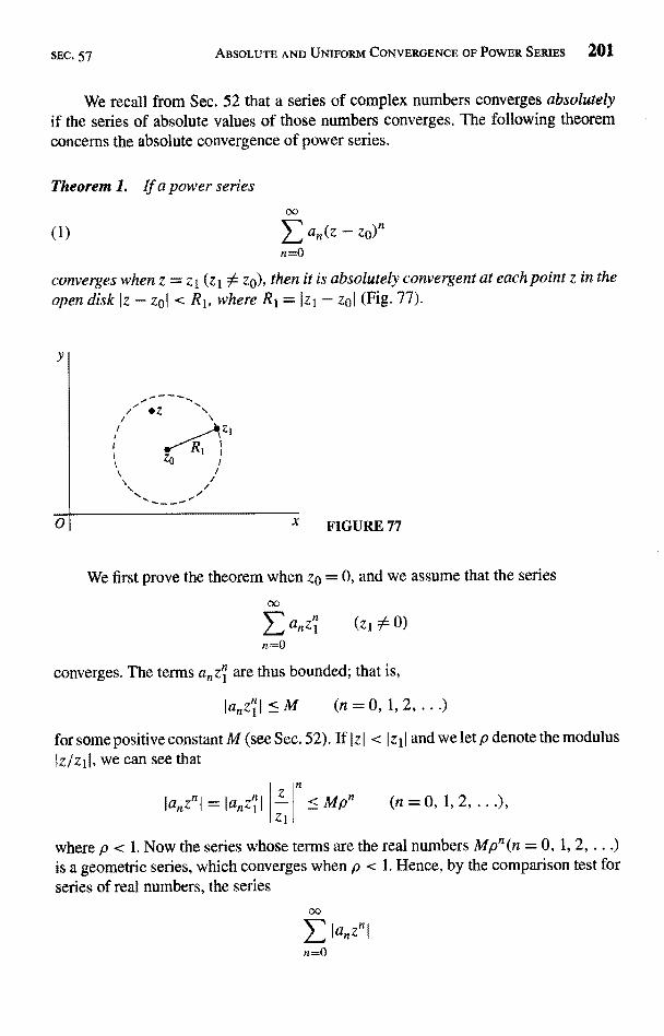
SEC. 57 ABSOLUTE AND UNIFORM CONVERGENCE OF POWER SERIES 201
We recall from Sec. 52 that a series of complex numbers converges absolutelyif the series of absolute values of those numbers converges. The following theoremconcerns the absolute convergence of power series.
Theorem 1. If a power series
an (z -n=0
converges when z = z1(z136 zo), then it is absolutely convergent at each point z in theopen disk Iz - zol < R1, where RI = Iz1- zol (Fig. 77).
I
zoRr
0
ZI
x FIGURE 77
We first prove the theorem when zo = 0, and we assume that the series
zl (zi 0 0)
n=0
converges. The terms anzl are thus bounded; that is,
I anz i I < M (n -= 0, 1, 2, ...)
f o r some positive constant M (see Sec. 52). If (z I < I z r I and we let p denote the modulusIz/zil, we can see that
lanznl = Ianz1I
where p < 1. Now the series whose terms are the real numbers Mpn(n = 0, 1, 2, ...)is a geometric series, which converges when p < 1. Hence, by the comparison test forseries of real numbers, the series
n=0
202 SERIES CHAP.5
converges in the open disk I z I < Iz 1 I; and the theorem is proved when zo = 0.When zo is any nonzero number, we assume that series (1) converges at z = z
(zt 0 zo). If we write w = z - zo, series (1) becomes
(2) E anwnn=0
and this series converges at w = zl - zo. Consequently, since the theorem is known to
be true when zo = 0, we see that series (2) is absolutely convergent in the open disk
Iwl < Izt - zol. Finally, by replacing w by z - zo in series (2) and this condition ofvalidity, as well as writing RI = Izi - zof, we arrive at the proof of the theorem as it
is stated.The theorem tells us that the set of all points inside some circle centered at zo
is a region of convergence for the power series (1), provided it converges at somepoint other than zo. The greatest circle centered at zo such that series (1) converges at
each point inside is called the circle of convergence of series (1). The series cannot
converge at any point Z2 outside that circle, according to the theorem; for if it did, itwould converge everywhere inside the circle centered at zo and passing through z2.The first circle could not, then, be the circle of convergence.
Our next theorem involves terminology that we must first define. Suppose thatthe power series (1) has circle of convergence Iz - zol = R, and let S(z) and SN(z)represent the sum and partial sums, respectively, of that series:
N
S(z) = F, an(z - zo)n, SN(z) = ) an(z - Zo)n (Iz - z0l < R).n=0
Then write the remainder function
(3) pN(z) = S(Z) - SN(Z) (Iz - zol < R).
Since the power series converges for any fixed value of z when Iz - zol < R, weknow that the remainder PN (z) approaches zero for any such z as N tends to infinity.According to definition (2), Sec. 51, of the limit of a sequence, this means that,corresponding to each positive number E, there is a positive integer NE such that
(4) IPN(z)I < s whenever N > Ne.
When the choice of N£ depends only on the value of e and is independent of the point
z taken in a specified region within the circle of convergence, the convergence is said
to be uniform in that region
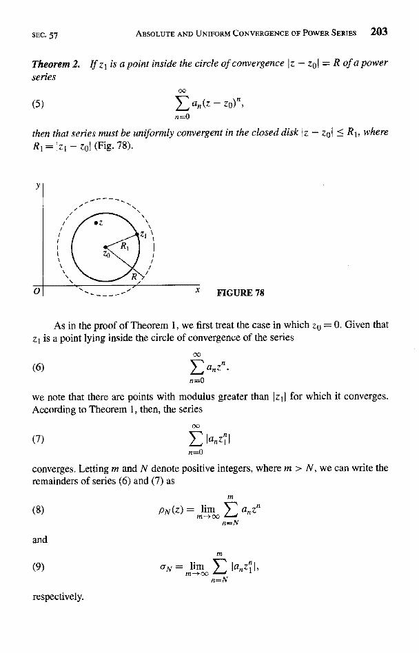
SEC. 57 ABSOLUTE AND UNIFORM CONVERGENCE OF POWER SERIEs 203
Theorem 2. If z1 is a point inside the circle of convergence Iz - zo1 -- R of a powerseries
(5) a,(z - zo)n,n=0
then that series must be uniformly convergent in the closed disk Iz - zol R1, where
R1= 1z1 - zo) (Fig. 78).
FIGURE 78
As in the proof of Theorem 1, we first treat the case in which zo = 0. Given thatz 1 is a point lying inside the circle of convergence of the series
(6)
n=0
we note that there are points with modulus greater than 1z11 for which it converges.According to Theorem 1, then, the series
(7) anZ11
n=0
converges. Letting m and N denote positive integers, where m > N, we can write theremainders of series (6) and (7) as
(8) PN (Z) =Zn
n=N
and
= lim > , Ian4I,n=N
respectively.
204 SERIES CHAP. 5
Now, in view of Exercise 3, Sec. 52,
IPN(Z)I =
when IzI
Y, anZnn=N n=N
Hence
(10) IPN(Z)I < ON when Iz1 < Izil
Since 6N are the remainders of a convergent series, they tend to zero as N tends toinfinity. That is, for each positive number e, an integer N. exists such that
(11) QN < e whenever N > NE .
Because of conditions (10) and (11), then, condition (4) holds for all points z in the disk
I z I Iz1I; and the value of Ne is independent of the choice of z. Hence the convergence
of series (6) is uniform in that disk.The extension of the proof to the case in which zo is arbitrary is, of course,
accomplished by writing w = z - zo in series (5). For then the hypothesis of thetheorem is that z 1 - zo is a point inside the circle of convergence I w I = R of the series
00
anwn.n=Q
Since we know that this series converges uniformly in the disk Iw1 < Izi - zol, theconclusion in the statement of the theorem is evident.
58. CONTINUITY OF SUMS OF POWER SERIES
Our next theorem is an important consequence of uniform convergence, discussed in
the previous section.
Theorem. A power series
n=o
represents a continuous function S(z) at each point inside its circle of convergence
Iz - zol=R.
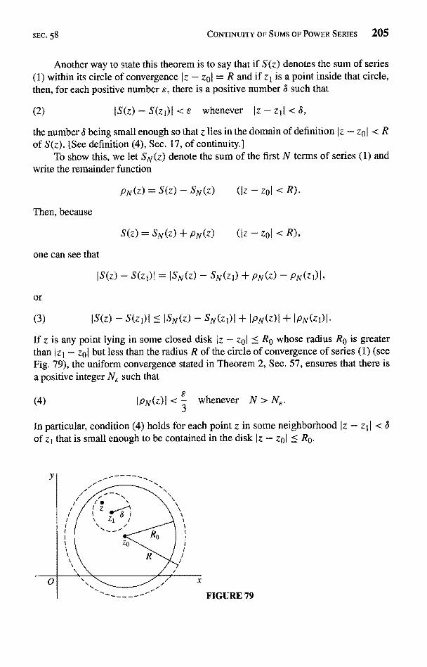
SEC. 58 CONTINUITY OF SUMS OF POWER SERIES 205
Another way to state this theorem is to say that if S(z) denotes the sum of series(1) within its circle of convergence I z - zoI = R and if zl is a point inside that circle,then, for each positive number s, there is a positive number 8 such that
(2) JS(z) - S(zi)I < s whenever Iz - z1) < 8,
the number 8 being small enough so that z lies in the domain of definition Iz - zo I < Rof S(z). [See definition (4), Sec. 17, of continuity.]
To show this, we let SN(z) denote the sum of the first N terms of series (1) anwrite the remainder function
PN(Z) = S(Z) - SN(Z) (Iz - zol < R).
Then, because
one can see that
S(Z) = SN(z) + PN(Z) (Iz - zol < R),
IS(z) - S(zi)I = ISN(z) - SN(Z1) + PN(Z) - PN(Zl)I,
or
(3) IS(z) - S(zl)l < ISN(z) - SN(zi)I + IpN(z)I + IPN(zt)I
If z is any point lying in some closed disk Iz - zol < Ro whose radius Ro is greaterthan Izr - zoI but less than the radius R of the circle of convergence of series (1) (seeFig. 79), the uniform convergence stated in Theorem 2, Sec. 57, ensures that there isa positive integer Ne such that
(4) I AN (z) I < - whenever N > NE .
In particular, condition (4) holds for each point z in some neighborhood Iz - ztl < 8of zI that is small enough to be contained in the disk Iz - zol E Ro.
FIGURE 79
206 SERIES CHAP. 5
Now the partial sum SN (z) is a polynomial and is, therefore, continuous at z 1 foreach value of N. In particular, when N = NN + 1, we can choose our 6 so small that
(5) ISN(z) - SN(z1)I < whenever Iz - z1) <8.
By writing N = NE + I in inequality (3) and using the fact that statements (4) and (5)are true when N = N£ + 1, we now find that
E E EIS(z) - S(zi)I <
3+
3+
3whenever Iz - z1I < 6.
This is statement (2), and the corollary is now established.By writing w = 1/(z - zo), one can modify the two theorems in the previous
section and the theorem here so as to apply to series of the type
(6)
If, for instance, series (6) converges at a point z 1(z I zo), the series
wnn
n=1
must converge absolutely to a continuous function when
1
(7) IwI <IZI - zol
Thus, since inequality (7) is the same as 3z - zol > Iz1 - zol, series (6) must convergeabsolutely to a continuous function in the domain exterior to the circle 1z - zoI = R1,where RI = Iz1 - zol. Also, we know that if a Laurent series representation
00
f (z) _ L an(z - ZQ)nn=o n=
bn
is valid in an annulus RI < Iz - zol.< R2, then both of the series on the right convergeuniformly in any closed annulus which is concentric to and interior to that region ofvalidity.
59. INTEGRATION AND DIFFERENTIATION OFPOWER SERIES
We have just seen that a power series
S(Z) _ an(z - z0)'n=0
SEC. 59 INTEGRATION AND DIFFERENTIATION OF POWER SERIES 207
represents a continuous function at each point interior to its circle of convergence. Inthis section, we prove that the sum S(z) is actually analytic within that circle. Ourproof depends on the following theorem, which is of interest in itself.
Theorem I. Let C denote any contour interior to the circle of convergence of thepower series (1), and let g (z) be any function that is continuous on C. The seriesformed by multiplying each term of the power series by g(z) can be integrated termby term over C; that is,
(2) dz = n dz.
To prove this theorem, we note that since both g (z) and the sum S(z) of the powerseries are continuous on C, the integral over C of the product
N-1
g(z)S(z)=Fangn=0
z - z0)" + g(z)pN(z),
where pN(z) is the remainder of the given series after N terms, exists. The terms ofthe finite sum here are also continuous on the contour C, and so their integrals overC exist. Consequently, the integral of the quantity g (z) PN (z) must exist; and we maywrite
N-1
g(z)S(z) dz = an J g(z)(z - zo)n dz + 1 g(z)pN(z) dz.n=0
Now let M be the maximum value of Ig(z)I on C, and let L denote the length ofC. In view of the uniform convergence of the given power series (Sec. 57), we knowthat for each positive numbers there exists a positive integer NN such that, for all pointsz on C,
IPN(Z)I < e whenever N > N.
Since N is independent of z, we find that
IC
that is,
g(z)pN(z) dz < MEL whenever N > N,e;
dz=0.
208 SERIES
It follows, therefore, from equation (3) that
) a,S(z) dz = limN-
n =O
g(z)(z -- z0)n dz.
CHAP. 5
This is the same as equation (2), and Theorem 1 is proved.If (g(z)j = 1 for each value of z in the open disk bounded by the circle of
convergence of power series (1), the fact that (z - z0)' is entire when n = 0, 1, 2, .. .ensures that
fc_ZO)Jc
) n
for every closed contour C lying in that domain. According to equation (2), then,
S(z) dz = 0c
for every such contour; and, by Morera's theorem (Sec. 48), the function S(z) isanalytic throughout the domain. We state this result as a corollary.
Corollary. The sum S(z) of power series (1) is analytic at each point z interior to thecircle of convergence of that series.
This corollary is often helpful in establishing the analyticity of functions and in
evaluating limits.
EXAMPLE 1. To illustrate, let us show that the function defined by the equations
(sin z)/z when z 0,f (z)
1 when z = 0
is entire. Since the Maclaurin series expansion
sin z =
represents sin z for every value of z, the series
(4)
oa
n=0
72n
ndz=0 (n=0, 1,2
= I2n + 1)!
obtained by dividing each term of that Maclaurin series by z, converges to f (z) when
z 36 0. But series (4) clearly converges to f (0) when z = 0. Hence f (z) is representedby the convergent power series (4) for all z. and f is, therefore, an entire function.
SEC. 59 INTEGRATION AND DIFFERENTIATION OF POWER SERIES 209
Note that, since f is continuous at z = 0 and since (sin z) /z = f (z) when z
lim sin z = lim f (z)z-O z z-O
f (0) = 1.
This is a result known beforehand because the limit here is the definition oderivative of sin z at z = 0.
We observed at the beginning of Sec. 54 that the Taylor series for a function fabout a point z0 converges to f (z) at each point z interior to the circle centered at z0and passing through the nearest point z1 where f fails to be analytic. In view of theabove corollary, we now know that there is no larger circle about z o such that at eachpoint z interior to it the Taylor series converges to f (z). For if there were such a circle,f would be analytic at z1; but f is not analytic at z1.
We now present a companion to Theorem 1.
Theorem 2. The power series (1) can be differentiated term by term. That is, at eachpoint z interior to the circle of convergence of that series,
S'(z) = Y. nan(z - zo)n-I
To prove this, let z denote any point interior to the circle of convergence of series(1), and let C be some positively oriented simple closed contour surrounding z andinterior to that circle. Also, define the function
(7) g
at each point s on C. Since g(s) is continuous on C, Theorem 1 tells us that
(8) fc
00
g(s)S(s) ds = an / g(s)(s - zo)' ds,n-a
Now S(s) is analytic inside and on C, and this enables us to write
ICg(s)S(s) ds
1
fcS(s) ds
= S'{z)2rti (s - z)2
with the aid of the integral representation for derivatives in Sec. 48. Furthermore,
)n ds z - zo)n (n = 0, 1,
210 SERIES
Thus equation (8) reduces to
S'(z) _ a,, d (z - Zo)n,n=o
which is the same as equation (6). This completes the proof.
EXAMPLE 2. In Example 4, Sec. 54, we saw that
1 = E(-1)n(zz n=o
0C
11<1).
Differentiation of each side of this equation reveals that
°O1
or
-1)nn(n=
(_1)n(n + 1)
< 1),
- 1)1 (IZ - 11 < 1).
CHAP. 5
60. UNIQUENESS OF SERIES REPRESENTATIONS
The uniqueness of Taylor and Laurent series representations, anticipated in Sees. 54and 56, respectively, follows readily from Theorem 1 in Sec. 59. We consider first theuniqueness of Taylor series representations.
Theorem I. If a series
(1) L an(Z - Zo)n
n=o
converges to f (z) at all points interior to some circle Iz - zol = R, then it is the Taylor
series expansion for f in powers of z - z0.
To prove this, we write the series representation
(2) f (z) _n=o
n (Iz - zoi < R
in the hypothesis of the theorem using the index of summation m:
f (z) _ L am(Z - zo)m (Iz - Zol < R).rn=o
SEC. 6o UNIQUENESS OF SERIES REPRESENTATIONS 211
Then, by appealing to Theorem 1 in Sec. 59, we may write
(3) g(z)f(z) dz =C
g(z)(z - zo)'n dz,
where g(z) is any one of the functions
(4) g(z) = 2ni (z -(n - 0, 1, 2, ...)
and C is some circle centered at zo and with radius less than R.In view of the generalized form (5), Sec. 48, of the Cauchy integral fo
also the corollary in Sec. 59), we find that
(5)f f(z) dz f (n) (zo)
JCg(z) f (z) dz = 2iri C (z - zo)n+i - n!
and, since (see Exercise 10, Sec. 40)
(6) f g(z)(z - zo)t dz = 1 fC 2,ri C
it is clear that
(7)
00
m=o
dz = 10)-m+l 1
g(z)(z - zo)t dz = aY,.C
Because of equations (5) and (7), equation (3) now reduces to
`) (zO)- an?
n!
when m i4 n,when m = n,
ula (see
and this shows that series (2) is, in fact, the Taylor series for f about the point zo.Note how it follows from Theorem 1 that if series (1) converges to zero throughout
some neighborhood of zo, then the coefficients aJZ must all be zero.Our second theorem here concerns the uniqueness of Laurent series representa-
tions.
Theorem 2. If a series
(8) Cn(Z - ZO)n = an(z - zO)n
n=-0Q n=O
converges to f (z) at all points in some annular domain about zo, then it is the Laurentseries expansion for f in powers of z - zO for that domain.
212 SERIES CHAP. 5
The method of proof here is similar to the one used in proving Theorem 1. Thehypothesis of this theorem tells us that there is an annular domain about zo such that
n=-00
for each point z in it. Let g(z) be as defined by equation (4), but now allow n to bea negative integer too. Also, let C be any circle around the annulus, centered at zoand taken in the positive sense. Then, using the index of summation m and adaptingTheorem 1 in Sec. 59 to series involving both nonnegative and negative powers ofz - zo (Exercise 10), write
IC
or
(9)
g(z)f (z) dz =
z) dzC g17)JC
27ri Jc0 dz.
Since equations (6) are also valid when the integers m and n are allowed to benegative, equation (9) reduces to
1 f (z) dz27ri c (z - zo)n+1
which is expression (5), Sec. 55, for coefficients in the Laurent series for f in theannulus.
EXERCISES
1. By differentiating the Maclaurin series representation
(Izl < 1),
obtain the expansions
) n 2 zn OzI <1).
SEC. 60
2. By substituting 1/(I - z) for z in the expansion
1)zn (IzI < 1),
found in Exercise 1, derive the Laurent series representation
1
z2
(Compare Example 2, Sec. 59.)
3. Find the Taylor series for the function
1 1
(1 < Iz -
EXERCISES 213
about the point zo = 2. Then, by differentiating that series term by term, show that
21 < 2).
4. With the aid of series, prove that the function f defined by means of the equations
.f (z) _
is entire.
5. Prove that if
.f (z) =
cos z
1
1)/z when zA0,when z =0
when z 5: ±/2 ,2 _ (x/2)2
when z = f7t/2,
then f is an entire function.
6. In the w plane, integrate the Taylor series expansion (see Example 4, Sec. 54)
along a contour interior to the circle of convergence from w = 1 to w = z to obtain therepresentation
Log z = L ' (z - 1)n Oz -
214 SERIES CHAP. 5
7. Use the result in Exercise 6 to show that if
Log zwhen z - 1 ,f(z)={ z-1when z = 1,
then f is analytic throughout the domain 0 < I z I < oa, -Jr < Arg z < ]r.
8. Prove that if f is analytic at zo and f (zo) = f'(zc) _ . = f (m) (zo) = 0, then thefunction g defined by the equations
g(z) =l) (ZO)
when z 0 zo,
when z = z
is analytic at zo.
9. Suppose that a function f (z) has a power series representation
.f (Z) = L a, (z - zo)"n=o
inside some circle Iz - zol = R. Use Theorem 2 in Sec. 59, regarding term by termdifferentiation of such a series, and mathematical induction to show that
k=O
n + k)1
kfan+k(Z - zo)k (n = 0,
when (z - zo t < R. Then, by setting z = zo, show that the coefficients an (n = 0, 1, 2, ...)are the coefficients in the Taylor series for f about zo. Thus give an alternative proof ofTheorem 1 in Sec. 60.
10. Consider two series
S1(z) _ 2 an(z - zo)", S2(z)
n=o
which converge in some annular domain centered at zo. Let C denote any contour lyingin that annulus, and let g(z) be a function which is continuous on C. Modify the proofof Theorem 1, Sec. 59, which tells us that
IC
to prove that
g(z)SI{z} dz
fcg(z)S2(z) dz =
f (z)Z - Z[))y"+l
g(z)dz.
(z - Zo)n
SEC. 61 MULTIPLICATION AND DIVISION OF POWER SERIES 215
Conclude from these results that if
00
S(z) = TCn(Z -
Z0)n = E an(Z - z0)n + Y'n=1
then
ICg(z)S(z) dz
11. Show that the function
f2(z)=z2+1 (z54 ±i)
is the analytic continuation (Sec. 26) of the function
.f1(Z) _)(-1)nZ2n (IzI < 1)
bn
- ZO)n
n=O
into the domain consisting of all points in the z plane except z = ± i.
12. Show that the function f2(z) =1/z2 (z ; 0) is the analytic continuation (Sec. 26) of thefunction
f1(z) -n=O
into the domain consisting of all points in the z plane except z = 0.
61. MULTIPLICATION AND DIVISION OF POWER SERIES
Suppose that each of the power series
(1)
00
z - zo)n and E bn(z - ,ZO)nn=0n=0
converges within some circle Iz - zoJ = R. Their sums f (z) and g(z), respectively,are then analytic functions in the disk `z - zol < R (Sec. 59), and the product of thosesums has a Taylor series expansion which is valid there:
00
(2) f(z)g(z) = E Cn(z - z0)n (Iz - zol < R).n=o
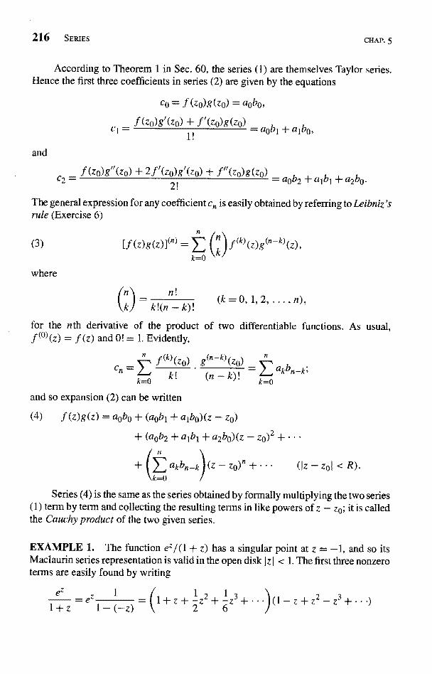
216 SERIES CHAP. 5
According to Theorem 1 in Sec. 60, the series (1) are themselves Taylor series.Hence the first three coefficients in series (2) are given by the equations
zo)g(zo) = a0b0,
Cl
and
0 g'(z0) + f'(zo)g(zo) = a0b, + aibo,
f (z0)g"(z0) + 2f'(z0)g'(z0) + f"(zo)g(zo)= a0b2 + alb, + a2b0.C2 =
2!
_
The general expression for any coefficient cn is easily obtained by referring to Leibniz'srule (Exercise 6)
(3) If (Z)g(z
where
n _ nS
k kl(n - k)! ),
for the nth derivative of the product of two differentiable functions. As usual,f (O) (z) = f (z) and 0! = 1. Evidently,
g(n-k)(Z),
n
ak(n - k,.
k=Ok=O
and so expansion (2) can be written
(4) f(z)g(z) = a0b0 + (aOb1 + alb0)(z - z0)
+ (aOb2 + aibl + a2b0)(z - zo)2 +
akbn- - ZO)n + ... (Pz - zoj < R).
Series (4) is the same as the series obtained by formally multiplying the two series(1) term by term and collecting the resulting terms in like powers of z - z0; it is calledthe Cauchy product of the two given series.
EXAMPLE 1. The function ez / (1 + z) has a singular point at z = -1, and so itsMaclaurin series representation is valid in the open disk Iz I < 1. The first three nonzeroterms are easily found by writing
Z+ 1Z2+ 34---
n""N f (k)(ZO)
g(n-k)(ZO)
1+ z 1-(-z) \ 2 6
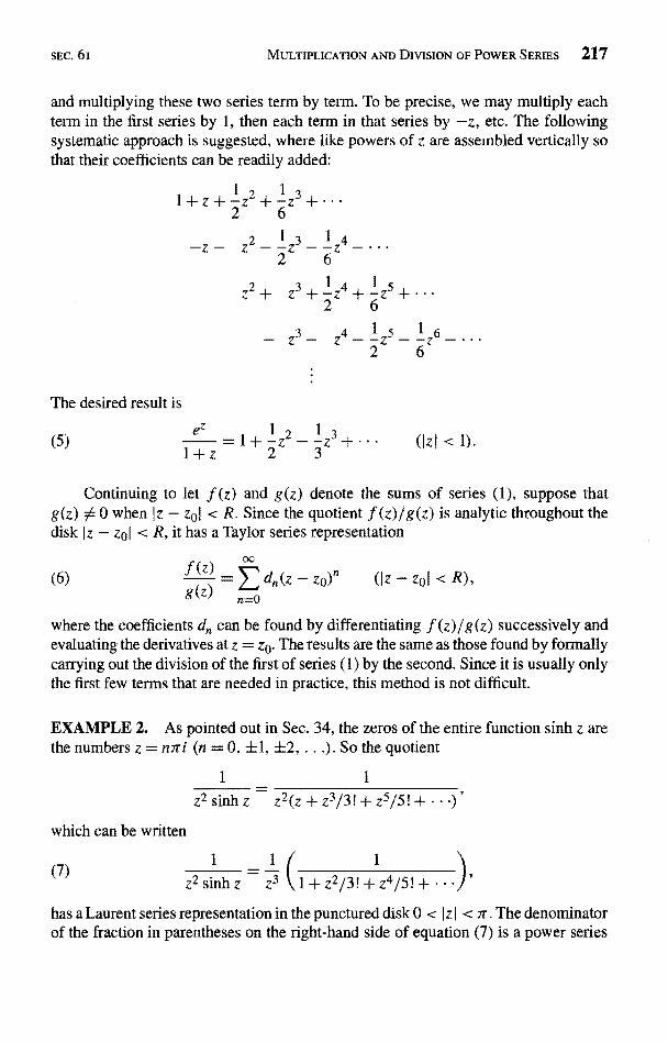
SEC. 6i MULTIPLICATION AND DIVISION OF POWER SERIES 217
and multiplying these two series term by term. To be precise, we may multiply eachterm in the first series by 1, then each term in that series by -z, etc. The followingsystematic approach is suggested, where like powers of z are assembled vertically sothat their coefficients can be readily added:
l+z+ 1z2+ 1z3+...2 6
_z _ z21_ z3 _
6
2z' + 6z' + .
The desired result is
(5)ez
+z(Izi < I).
Continuing to let f (z) and g(z) denote the sums of series (1), suppose thatg(z) A 0 when Iz - zol < R. Since the quotient f (z)/g(z) is analytic throughout thedisk Iz - zol < R, it has a Taylor series representation
(6)
f (z)
g(z) n=O
ZO) n(Iz zol < R),
where the coefficients do can be found by differentiating f (z) /g (z) successively andevaluating the derivatives at z = za. The results are the same as those found by formallycarrying out the division of the first of series (1) by the second. Since it is usually onlythe first few terms that are needed in practice, this method is not difficult.
EXAMPLE 2. As pointed out in Sec. 34, the zeros of the entire function sinh z arethe numbers z = nxri (n = 0, ±1, ±2, ...). So the quotient
sinhz z2(z+z3j3!+z5/5!+..
which can be written
(7)1
z2 sinhz z3 tl+z2/3!+z4/5!+has a Laurent series representation in the punctured disk 0 < I z I < 7r. The denominatorof the fraction in parentheses on the right-hand side of equation (7) is a power series
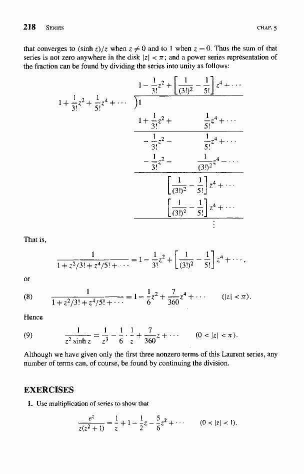
218 SERIES CHAP. 5
that converges to (sinh z)/z when z A 0 and to 1 when z = 0. Thus the sum of thatseries is not zero anywhere in the disk jzI < 7r; and a power series representation ofthe fraction can be found by dividing the series into unity as follows:
1
(
That is,
or
(8)
Hence
1 1=1-zI + z2/3! + z4/5! +- 3!
2
z4
1 1 2 7 41-z+z+.. (ICI<7Z1 + z2/3! + z4/5! + 6 360
1 1 1 1 7(9) _ (0<lzI<7r).
z2 sinh z z3 6 z 360'
Although we have given only the first three nonzero terms of this Laurent series, anynumber of terms can, of course, be found by continuing the division.
EXERCISES
1. Use multiplication of series to show that
5!
1 _4
(3!)2
z(z2+1) z+1- (0<Izl<1).2
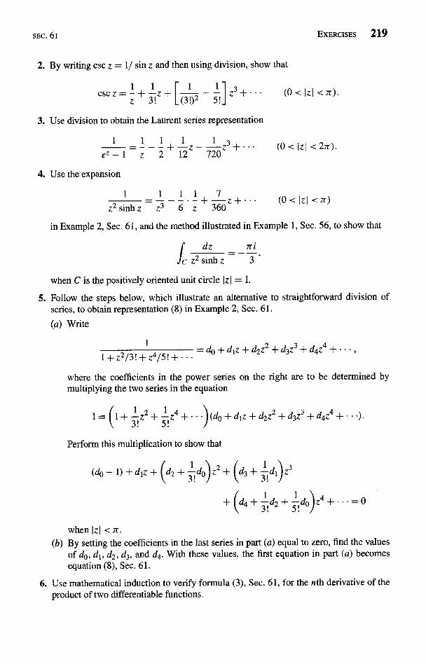
SEC. 6 i
2. By writing csc z = 1/ sin z and then using division, show that
1 1cscz-+-z+z 3! 2
EXERCISES 219
3. Use division to obtain the Laurent series representation
1 _1ez-1 z
4. Use the expansion
1
12Z
720z3 + ... (0 < IzC < 2n).
1 1 1 1 7Z+... (0<IZI<n)
z2 sinh z z3 6 z ' 360
in Example 2, Sec. 61, and the method illustrated in Example 1, Sec. 56, to show that
when C is the positively oriented unit circle Izl = 1.
5. Follow the steps below, which illustrate an alternative to straightforward division ofseries, to obtain representation (8) in Example 2, Sec. 61.
(a) Write
1 2 3 4
1 + z2/3! + z4/5! + . .
= do + diz + d2z + d3z + d4z +
where the coefficients in the power series on the right are to be determined bymultiplying the two series in the equation
1= (1+ z2+ 1 Z4+...}(de+diz+d2z2+d3z3+d4z4+..5!
Perform this multiplication to show that
(do-1)+diz+(d2+-do)z`+(d3+ 1
+[d4+-1 d2+ t
when Izl < n.(b) By setting the coefficients in the last series in part (a) equal to zero, find the values
of de, di, d2, d3, and d4. With these values, the first equation in part (a) becomesequation (8), Sec. 61.
6. Use mathematical induction to verify formula (3), Sec. 61, for the nth derivative of theproduct of two differentiable functions-
220 SERIES CHAP. 5
7. Let f (z) be an entire function that is represented by a series of the form.
f(z) =z+a2z2+a3z3+... (1z' <
(a) By differentiating the composite function g(z) = f [f (z)] successively, find the first
three nonzero terms in the Maclaurin series for g(z) and thus show that
f [f (z)] = z + 2a2z2 + 2(a2 + a3)z3 + .. (Iz) < oo).
(b) Obtain the result in part (a) in a formal manner by writing
2 +a3[f(z)f[f(Z)]=f(z)+a,[f(z)]replacing f (z) on the right-hand side here by its series representation, and thencollecting terms in like powers of z.
(c) By applying the result in part (a) to the function f (z) = sin z, show that
sin(sinz)=z- Iz3+... (Izl <oo).
8. The Euler numbers are the numbers E7z (n = 0, 1, 2, . . .) in the Maclaurin series repre-
sentation
I = ) -"Z" (IzI <7rI2).cosh z 0 n!Point out why this representation is valid in the indicated disk and why
E2,,+1 = 0 (n = 0, 1, 2, ...).
Then show that
E0 = 1, E2 = -1, E4 = 5, and E6 = -61.
CHAPTER
6RESIDUES AND POLES
The Cauchy-Goursat theorem (Sec. 44) states that if a function is analytic at all pointsinterior to and on a simple closed contour C, then the value of the integral of thefunction around that contour is zero. If, however, the function fails to be analytic at afinite number of points interior to C, there is, as we shall see in this chapter, a specificnumber, called a residue, which each of those points contributes to the value of theintegral. We develop here the theory of residues; and, in Chap. 7, we shall illustratetheir use in certain areas of applied mathematics.
62. RESIDUESRecall (Sec. 23) that a point z0 is called a singular point of a function f if f fails to beanalytic at z0 but is analytic at some point in every neighborhood of zo. A singular pointzo is said to be isolated if, in addition, there is a deleted neighborhood 0 < jz - zol < sof z0 throughout which f is analytic.
EXAMPLE 1. The function
z+z3(z2 + 1)
has the three isolated singular points z = 0 and z = ±i.
221
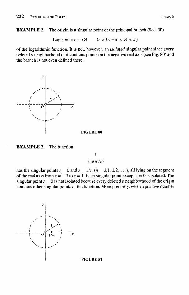
222 RESIDUES AND POLES CHAP. 6
EXAMPLE 2. The origin is a singular point of the principal branch (Sec. 30)
Logz=lnr+iO (r>0, -rr <O <rr)
of the logarithmic function. It is not, however, an isolated singular point since everydeleted s neighborhood of it contains points on the negative real axis (see Fig. 80) andthe branch is not even defined there.
Y
FIGURE 80
EXAMPLE 3. The function
I
sin(rr/z)
has the singular points z = 0 and z = l jn (n = ±1, ±2, ...), all lying on the segmentof the real axis from z = -I to z = 1. Each singular point except z = 0 is isolated. Thesingular point z = 0 is not isolated because every deleted s neighborhood of the origincontains other singular points of the function. More precisely, when a positive number
x
FIGURE 81
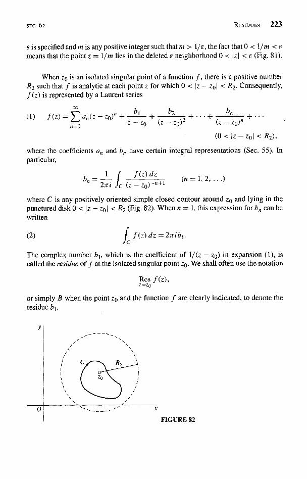
SEC. 62 RESIDUES 223
s is specified and in is any positive integer such that in > 1/s, the fact that 0 < l/m < smeans that the point z = 1/m lies in the deleted E neighborhood 0 < IzI < s (Fig. 81).
When zo is an isolated singular point of a function f , there is a positive numberR2 such that f is analytic at each point z for which 0 < Iz - zoI < R2. Consequently,f (z) is represented by a Laurent series
hb Z 2 + ... F n n + .. .l- +(1) f (y) y0)11 +LJ
)n=0
4 - bo {Z - Z0 k- 'C.0)
(0 < Iz - zol < R2),
where the coefficients an and bn have certain integral representations (Sec. 55). Inparticular,
7
b 2,-ri
f (n=1, 2,.,.)
where C is any positively oriented simple closed contour around zo and lying in thepunctured disk 0 < ?z - zol < R2 (Fig. 82). When n = 1, this expression for bn can bewritten
{IC
f (z) dz = 2,ribi.
The complex number bl, which is the coefficient of 1/(z - zo) in expansion (1), iscalled the residue of f at the isolated singular point zo. We shall often use the notation
Res f (z),z=z0
or simply B when the point z0 and the function f are clearly indicated, to denote theresidue b1.
i
0
t
1 Z0 I
4 t
1 //
I x
FIGURE 82
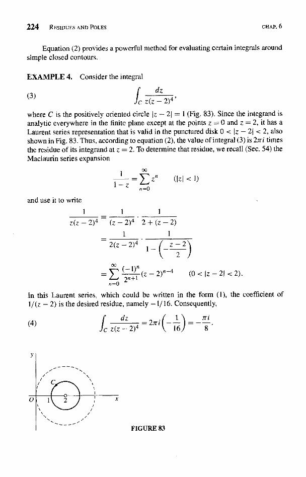
224 RESIDUES AND POLES CHAP. 6
Equation (2) provides a powerful method for evaluating certain integrals aroundsimple closed contours.
EXAMPLE 4. Consider the integral
dzz(3) fcz(z-2)'where C is the positively oriented circle Iz - 21 = 1 (Fig. 83). Since the integrand isanalytic everywhere in the finite plane except at the points z = 0 and z = 2, it has aLaurent series representation that is valid in the punctured disk 0 < Iz - 21 < 2, alsoshown in Fig. 83. Thus, according to equation (2), the value of integral (3) is 2n i timesthe residue of its integrand at z = 2. To determine that residue, we recall (Sec. 54) theMaclaurin series expansion
and use it to write
1 1 1
z(z - 2)4 Q-2)4 2+(z-2)1 1
2n+- 2)n-4 (0 < Iz - 21 < 2).
n=o
In this Laurent series, which could be written in the form (1), the coefficient of1/(z - 2) is the desired residue, namely -1/16. Consequently,
(4) dz
fc z(z-2=2n
FIGURE 83
SEC. 63
EXAMPLE 5. Let us show that
(5)
CAUCHY'S RESIDUE THEOREM 225
where C is the unit circle (z I = 1. Since 1/z2 is analytic everywhere except at the origin,
so is the integrand. The isolated singularpoint z = 0 is interior to C; and, with the aidof the Maclaurin series (Sec. 54)
31+... (Izi<oo
one can write the Laurent series expansion
ex1 1 1 1 1
Z 2! T 3! z
(0<IzI<oo).
The residue of the integrand at its isolated singular point z = 0 is, therefore, zero(b1= 0), and the value of integral (5) is established.
We are reminded in this example that, although the analyticity of a function withinand on a simple closed contour C is a sufficient condition for the value of the integralaround C to be zero, it is not a necessary condition.
63. CAUCHY'S RESIDUE THEOREMIf, except for a finite number of singular points, a function f is analyticinside a simpleclosed contour C, those singular points must be isolated (Sec. 62). The followingtheorem, which is known as Cauchy's residue theorem, is a precise statement of thefact that if f is also analytic on C and if C is positively oriented, then the value of theintegral off around C is 27ri times the sum of the residues off at the singular points
inside C.
Theorem. Let C be a simple closed contour, described in the positive sense. If afunction f is analytic inside and on C except for a finite number of singular points
Zk (k = 1, 2, . . . , n) inside C, then
C Z=Zk
To prove the theorem, let the points Zk (k = 1, 2, . . . , n) be centers of positivelyoriented circles Ck which are interior to C and are so small that no two of them havepoints in common (Fig. 84). The circles Ck, together with the simple closed contour C,form the boundary of a closed region throughout which f is analytic and whoseinterior
n
(z) dz = 27ri ) ' Res f (z).
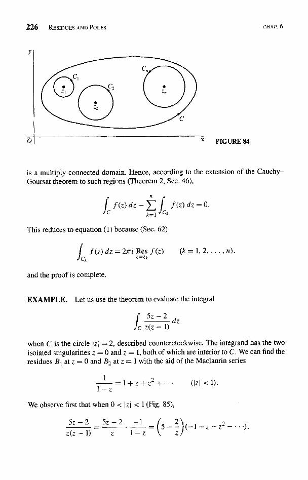
226 RESIDUES AND POLES
Y
x FIGURE 84
CHAP. 6
is a multiply connected domain. Hence, according to the extension of the Cauchy-Goursat theorem to such regions (Theorem 2, Sec. 46),
fcf(z)dz-) . I f(z)dz=0.
This reduces to equation (1) because (Sec. 62)
I f (z) dz = 27ri R_e s f (z) ( 1 r = 1 , 2, ... ,/Ck Z Zk
and the proof is complete.
EXAMPLE. Let us use the theorem to evaluate the integral
when C is the circle IzI = 2, described counterclockwise. The integrand has the twoisolated singularities z = 0 and z = 1, both of which are interior to C. We can find theresidues BI at z = 0 and B2 at z = 1 with the aid of the Maclaurin series
=1+z+z2+... (Izl
We observe first that when 0 < I z I < 1(Fig. 85),
5z-2 5z-z (z - 1) z
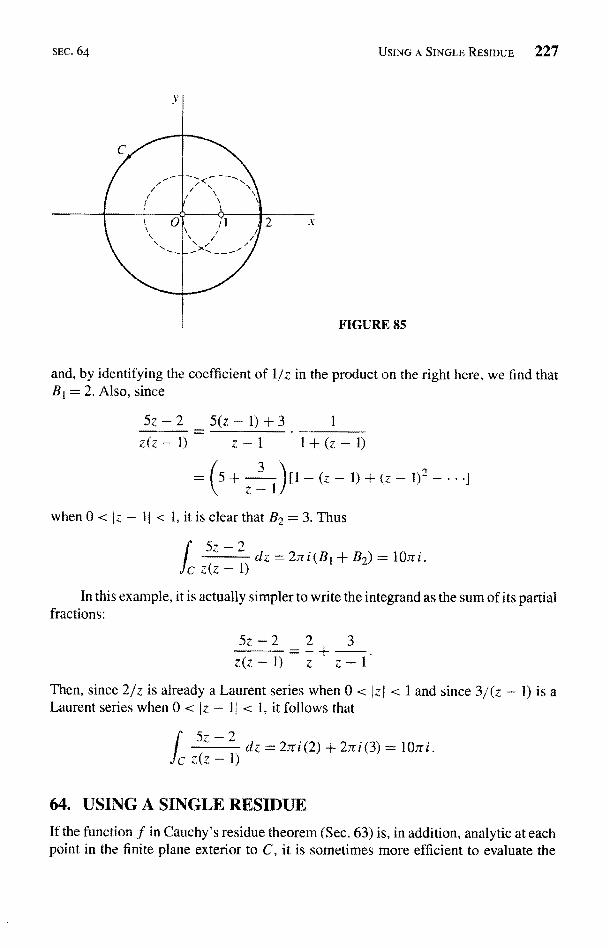
SEC. 64 USING A SINGLE RESIDUE 227
FIGURE 85
and, by identifying the coefficient of liz in the product on the right here, we find thatB1= 2. Also, since
5z - 2 5(z - 1) +
5+ (z - 1) + (z
when 0 < Iz - 11 < 1, it is clear that B2 ^ 3. Thus
5z - 2
c Z (z - 1)
z-1 1+(z-
dz=2nl(BI+B2)=10ri.
In this example, it is actually simpler to write the integrand as the sum of its partialfractions:
3
z(z - 1) z z -
Then, since 2/z is already a Laurent series when 0 < Jz1 < 1 and since 3/(z - 1) is aLaurent series when 0 < Iz - II < 1, it follows that
5z-2cz(z-1
dz = 2irl(2) + 2,rt(3) = 107ri.
64. USING A SINGLE RESIDUE
If the function f in Cauchy's residue theorem (Sec. 63) is, in addition, analytic at eachpoint in the finite plane exterior to C, it is sometimes more efficient to evaluate the
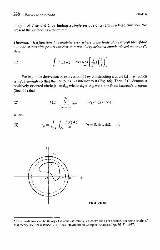
228 RESIDUES AND POLES CHAP, 6
integral of f around C by finding a single residue of a certain related function. Wepresent the method as a theorem.*
Theorem. If a junction f is analytic everywhere in the finite plane except for a finitenumber of singular points interior to a positively oriented simple closed contour C,then
(1) f (z) dz = 2.rci ResC z=O
We begin the derivation of expression (1) by constructing a circle Izi = R1 whichis large enough so that the contour C is interior to it (Fig. 86). Then if CO denotes apositively oriented circle I z I = R0, where Ra > R1, we know from Laurent's theorem(Sec. 55) that
(2) .f (z) _
where
(3) Cn =
(R1 < Izi < oc),
0, ±1, ±2, ..
FIGURE 86
* This result arises in the theory of residues at infinity, which we shall not develop. For some details ofthat theory, see, for instance, R. P. Boas, "Invitation to Complex Analysis," pp. 76-77, 1987.
SEC. 64
By writing n = -1 in expression (3), we find that
USING A SINGLE RESIDUE 229
(4) j f (z) dz = 2nic_j.JC4
Observe that, since the condition of validity with representation (2) is not of the type0 < I z I < R2, the coefficient c_I is not the residue of f at the point z = 0, which maynot even be a singular point of f. But, if we replace z by I /z in representation (2) andits condition of validity, we see that
Cn _ 'fin-2Zn+2 n=--too Zn
and hence that
Then, in view of equations (4
= Resz=O
d (5),
(z) dz = 27ri Resz=O
zl<R,
Finally, since f is analytic throughout the closed region bounded by C and CO, theprinciple of deformation of paths (Corollary 2, Sec. 46) yields the desired result (1).
EXAMPLE. In the example in Sec. 63, we evaluated the integral of
5z-2f(z)Z(z-1)
around the circle I z I = 2, described counterclockwise, by finding the residues of f (at z = 0 and z = 1. Since
(1) _ 5-2z 5-2z 1
z z(1-z) z 1-z
+3+3z+... (0<lzl<1),z
we see that the above theorem can also be used, where the desired residue is 5. Moreprecisely,
5z-2dz=27ri(5)=10.ira
230 RESIDUES AND POLES CHAP. 6
where C is the circle in question. This is, of course, the result obtained in the examplein Sec. 63.
EXERCISES
1. Find the residue at z = 0 of the function
(a) 1 (b) z cosz+Z2' Z
(c)z - sin z
z
Ans. (a) I ; (b) -1/2; (c) 0
2.
(d) cot z ; (e) sink z
z4 Z4(1 - z2)
(d) -1/45; (e) 7/6.
Use Cauchy's residue theorem (Sec. 63) to evaluate the integral of each of these functionsaround the circle Izl = 3 in the positive sense:
(d)z+1
Z2 - 2zexp(-z) (b) exp(-z)
Z2 (Z - 1)2 'Ans. (a) -2,ri; (b) -2ni/e; (c
3.
4.
3; (d) 2rri.
Use the theorem in Sec. 64, involving a single residue, to evaluate the integral of each ofthese functions around the circle Iz) = 2 in the positive sense:
5
(a)Z
(b) I ; (C)1-z3 1+Z2 Z
Ans. (a) -2rri; (b) 0; (c) 2n'i.
Let C denote the circle IzI = 1, taken counterclockwise, and follow the steps below toshow that
=2
(a) By using the Maclaurin series for ez and referring to Theorem 1 in Sec. 59, whichjustifies the term by term integration that is to be used, write the above integral as
`1 exp(l dz.z
(b) Apply the theorem in Sec. 63 to evaluate the integrals appearing in part (a) to arriveat the desired result.
5. Let the degrees of the polynomials
P(z) = aQ + alz + a2Z2 + ... + anZn (an A 0)
and
Q(Z) = bQ + blZ + b2Z` + ... + bmZm (bm A 0)
be such that m ? n + 2. Use the theorem in Sec. 64 to show that if all of the zeros ofQ(z) are interior to a simple closed contour C, then
P(Z) dz = 0.C Q(z)
[Compare Exercise 3(b).]
SEC. 65 THE THREE TYPES OF ISOLATED SINGULAR POINTS 231
65. THE THREE TYPES OF ISOLATED SINGULAR POINTS
We saw in Sec. 62 that the theory of residues is based on the fact that if f has anisolated singular point z0, then f (z) can be represented by a Laurent series
b b b(1) .f (z) = ) 'a, (z - z0)" + t + 2
2+ ... + ,2
n=o Z - Z0 (Z - Zo) (Z - Zo)n
in a punctured disk 0 < Iz - zol < R,. The portion
bt + b2
Z - ZO (z - zo)
b,x
- zo)n
of the series, involving negative powers of z - z0, is called the principal part of f atz0. We now use the principal part to identify the isolated singular point zp as one ofthree special types. This classification will aid us in the development of residue theorythat appears in following sections.
If the principal part of f at z0 contains at least one nonzero term but the numberof such terms is finite, then there exists a positive integer m such that
b,n 0 and b,n+1 = b, +2 =
That is, expansion (1) takes the form
bb
l`n -1- +')= } a (Z - Z )
n=O
b,n
Z - 10 (z - Z0) (Z - ZO
(2) (0 < Iz - zol < R2),
where bn 0. In this case, the isolated singular point z0 is called a pole of order m.*A pole of order m = 1 is usually referred to as a simple pole.
EXAMPLE 1. Observe that the function
zi-2z+3 z(z-2)+3 3 3-z+ =2+(z2)+z-2 z-2 z-2 z-2
(0<Iz-2
has a simple pole (m = 1) at zo = 2. Its residue bl there is 3.
< 00
"Reasons for the terminology pole are suggested on p. 70 of the book by R. P. Boas mentioned in thefootnote in See. 64.
232 RESIDUES AND POLES
EXAMPLE 2. The function
sinh z 1 z3 Z5 z7 1 1 1 z3zaZ
=- /z I } i f i
3! 5! 7!' --3+ i
ti 3.-z
++ 1 }5! 7!
CHAP. 6
(0<IZI <cx)
has a pole of order m = 3 at zo = 0, with residue bt = 1/6.
There remain two extremes, the case in which all of the coefficients in theprincipal part are zero and the one in which an infinite number of them are nonzero.
When all of the bn's are zero, so that
(3) f (z) zo)" = ao + a,(,, - zo) + a2(zn=0
(0<Iz-zol<R2),
the point zo is known as a removable singular point. Note that the residue at a remov-able singular point is always zero. If we define, or possibly redefine, f at zo so thatf (z0) = a0, expansion (3) becomes valid throughout the entire disk Iz - zol < R2.Since a power series always represents an analytic function interior to its circle ofconvergence (Sec. 59), it follows that f is analytic at zo when it is assigned the valueao there. The singularity at zo is, therefore, removed.
EXAMPLE 3. The point zo 0 is a removable singular point of the function
1-cost 1
f (z) = Z2Z2
2 41 z . Z
2! 4! 6!
(0<IzI<oo).
When the value f (0) = 1/2 is assigned, f becomes entire.
)1
When an infinite number of the coefficients bn in the principal part are nonzero,zo is said to be an essential singular point of f . An important result concerning thebehavior of a function near an essential singular point is due to Picard. It states thatin each neighborhood of an essential singular point, a function assumes every finitevalue, with one possible exception, an infinite number of times.*
* For a proof of Picard's theorem, see See. 51 in Vol. III of the book by Markushevich, cited inAppendix 1.

SEC. 65
EXAMPLE 4. The function
p(1) " 1 1 1 1 1
= 1Z n! Zn 1! z 2
EXERCISES 233
(0 < Izl < oo)
has an essential singular point at zo = 0, where the residue b t is unity. For an illustrationof Picard's theorem, let us show that exp(1/z) assumes the value -1 an infinite numberof times in each neighborhood of the origin. To do this, we recall from the example inSec. 28 that exp z = -1 when z = (2n + 1)7ri (n = 0, +1, +2, ...). This means thatexp(1/z) = -1 when
z = -(2n + 1),7 i i (2n + 1)7r(n = 0, +1, +2, . .
and an infinite number of these points clearly lie in any given neighborhood of theorigin. Since exp(1/z) 0 0 for any value of z, zero is the exceptional value in Picard'stheorem.
In the remaining sections of this chapter, we shall develop in greater depth thetheory of the three types of isolated singular points just described. The emphasis willbe on useful and efficient methods for identifying poles and finding the correspondingresidues.
EXERCISES
1. In each case, write the principal part of the function at its isolated singular point anddetermine whether that point is a pole, a removable singular point, or an essential singularpoint:
(a) z exu I = 1. (b) (C) ;
Z
(a) ;
1
3'I + Z Z Z
2. Show that the singular point of each of the following functions is a pole. Determine theorder m of that pole and the corresponding residue B.
1 - cosh z (b) 1 - exp(2z). () exp(2z)
Z3 Z4 (Z - 1)2
Ans. (a) m = 1, B = -1/2; (b) m = 3, B = -4/3; (c) m = 2, B = 2e2.
3. Suppose that a function f is analytic at Zp, and write g(z) = f (z)/(z - zo). Show that
(a) if f (zo) 0, then zO is a simple pole of g, with residue f (z0);
(b) if f (zo) = 0, then zo is a removable singular point of g.
Suggestion: As pointed out in Sec. 53, there is a Taylor series for f (z) about z0since f is analytic there. Start each part of this exercise by writing out a few terms ofthat series.
z sin z cos z
234 RESIDUES AND POLES
4. Write the function
as
z-ai ' (z-ai)2 (z-ai)3 z-ai
a > 0)
f (z) =0 (z) where O (z) _(z - ai)3
8a3z2
(z+ai)
CHAP. 6
Point out why 0 (z) has a Taylor series representation about z = ai, and then use it toshow that the principal part of f at that point is
0(ai) i/2 a/2+
66. RESIDUES AT POLES
When a function f has an isolated singularity at a point z0, the basic method foridentifying z0 as a pole and finding the residue there is to write the appropriate Laurentseries and to note the coefficient of 1/(z - z0). The following theorem provides analternative characterization of poles and another way of finding the correspondingresidues.
Theorem. An isolated singular point z0 of a function f is a pole of order m if andonly if f (z) can be written in the form
f(z)=
where
(2)
and
(3)
z
8a3z2(z2 + a2)3
O (z)
z - z0)m
is analytic and nonzero at zo. Moreover,
Res f (z) = O(zo)Z=ZO
Res f (z) _z=zo
Observe that expression (2) need not have been written separately since, with theconvention that (P (0) (z0) = 0(zo) and 0! = 1, expression (3) reduces to it when m = 1.
SEC. 66 RESIDUES AT POLES 235
To prove the theorem, we first assume that f (z) has the form (1) and recall (Sec.53) that since 0(z) is analytic at z0, it has a Taylor series representation
0 (z) = (Z0) +`()(z - zO) + "()(z _ z0)2 + . . . +
0(m-1)(za)
(z - ZO)m-1r
n=m
.I ! Z! ( - 1)
(n)ZO)n
(Z- ZO)
n.
in some neighborhood I z - zo < e of z0; and from expression (1) it follows that
6 (zo)12!$ (z0) $`(z.)11!+ +(4) f(z) =
z - ZO), (z - zo)m-1 (z - zo)m-2
n-m
Z - ZO
when 0 < Iz - zol < -. This Laurent series representation, together with the fact that¢,(zo) 0 0, reveals that zo is, indeed, a pole of order m of f (z). The coefficient of1/(z - zo) tells us, of course, that the residue of f (z) at zo is as in the statement of thetheorem.
Suppose, on the other hand, that we know only that zo is a pole of order m oor that f (z) has a Laurent series representation
f(Z)=n=O
b1 + b2 + ... + bm-1 + bm
z - zo (z - zo)2 (z - Z0)m (z - Z0)m
(bm 0 0)
which is valid in a punctured disk 0 < Iz - zol < R2. The function 0(z) defined bymeans of the equations
O(z)_
evidently has the power series representation
O (z) = bm + bm1(Z - Zo00
n=O
z -- ZO)m+n
when z zo,when z = zo
+ b2(z - ZO)m-2 + b1(z - ZO)m-1
throughout the entire disk I z - zo l < R2. Consequently, 4' (z) is analytic in that disk(Sec. 59) and, in particular, at zo. Inasmuch as 0 (zo) = bm ; 0, expression (1) isestablished; and the proof of the theorem is complete.
236 RESIDUES AND POLES CHAP. 6
67. EXAMPLESThe following examples serve to illustrate the use of the theorem in the previoussection.
EXAMPLE 1. The function f (z)at z = 3i and can be written as
O(z)
z - 3i
9) has an isolated singular point
where qi (
Since 0 (z) is analytic at z = 3i and 0 (3i) = (3 - i)/6 0 0, that point is a simple poleof the function f ; and the residue there is B1 = (3 - i)/6. The point z = -3i is also asimple pole of f, with residue B2 = (3 + i)/6.
EXAMPLE 2. If f (z) = (z3 + 2z)/(z - i)3, then
f (z) = 0(z) where (p (z) = z3 + 2z.(z - i)3
The function 0 (z) is entire, and 0 (i) = i ; 0. Hence f has a pole of order 3 at z = i .
The residue there is
B= =3i.2!
The theorem can, of course, be used when branches of multiple-valued functionsare involved.
EXAMPLE 3. Suppose that
.f (z) _ (logz)3
Z + 1
where the branch
logz=lnr+i6 (r>0,0<8<2mc)
of the logarithmic function is to be used. To find the residue off at z = i, we write
.f (z) =(z) where q, (z) = (log
Z)3
z-i z+iThe function 0(z) is clearly analytic at z = i; and, since
(logi)3 (In 1 l i r/2)3 = - n3-00,
2i 2i 16
the desired residue is B = qi (i) = -7r3/ 16.
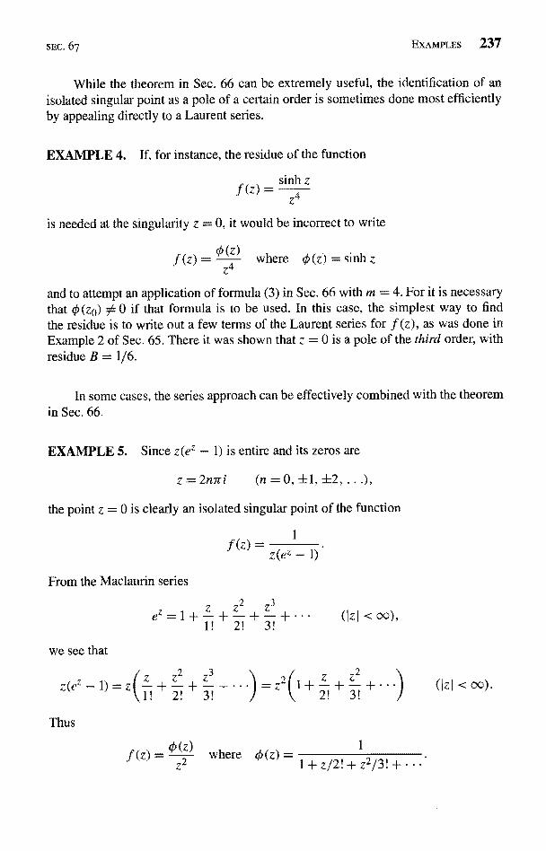
SEC. 67 EXAMPLES 237
While the theorem in Sec. 66 can be extremely useful, the identification of anisolated singular point as a pole of a certain order is sometimes done most efficientlyby appealing directly to a Laurent series.
EXAMPLE 4. If, for instance, the residue of the function
.f (z) =sink z
z4
is needed at the singularity z = 0, it would be incorrect to write
f (z) = 0() where O(z) = sinh zZ4
and to attempt an application of formula (3) in Sec. 66 with m = 4. For it is necessarythat $ (z0) ; 0 if that formula is to be used. In this case, the simplest way to findthe residue is to write out a few terms of the Laurent series for f (z), as was done inExample 2 of Sec. 65. There it was shown that z = 0 is a pole of the third order, withresidue B = 1/6.
In some cases, the series approach can be effectively combined with the theoremin Sec. 66.
EXAMPLE 5. Since z(ez - 1) is entire and its zeros are
z = 2n7ri (n = 0, +1, ±2, ...),
the point z = 0 is clearly an isolated singular point of the function
.f (z) =I
z(ez - 1)
From the Maclaurin series
Z Z2 3+ + Z
1! 2! 3!
f (z) _ 0 (z) where A (z)
(Izl < oo),
1
z2 1 + z/2! + z2/3!
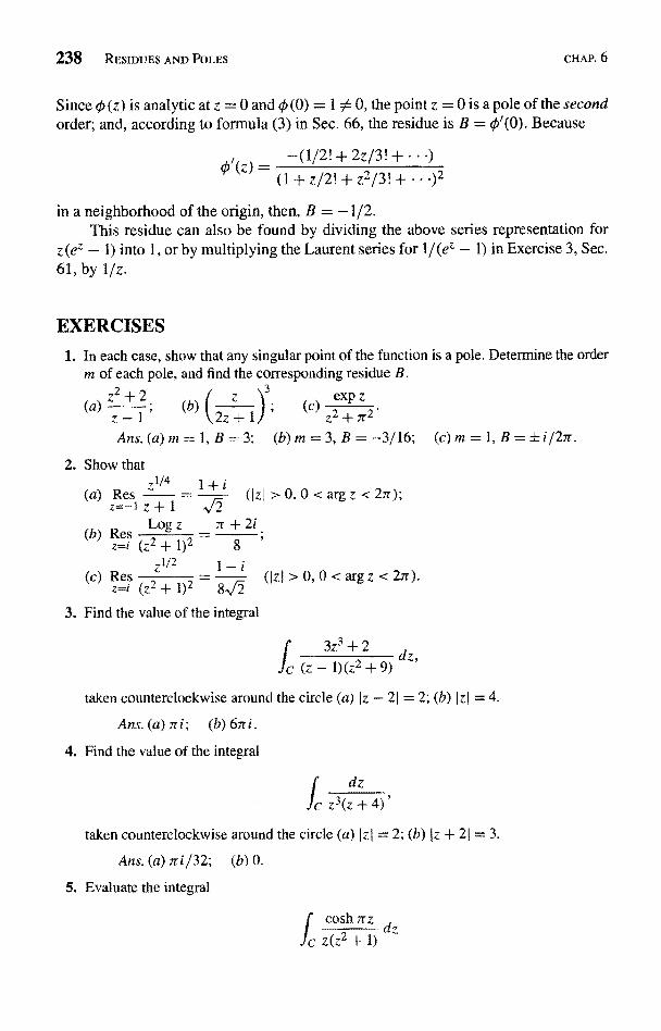
238 RESIDUES AND POLES CHAP. 6
Since 0 (z) is analytic at z = 0 and 0 (0) = I A 0, the point z = 0 is a pole of the secondorder; and, according to formula (3) in Sec. 66, the residue is B = 0'(0). Because
--(1/2! + 2z/3! + ...)(1 + z/2! + z2/3! + ...)2
in a neighborhood of the origin, then, B = -1/2.This residue can also be found by dividing the above series representation for
z(ez - 1) into 1, or by multiplying the Laurent series for 1/(ez - 1) in Exercise 3, Sec.61, by 1/z.
EXERCISES
1. In each case, show that any singular point of the function is a pole. Determine the orderm of each pole, and find the corresponding residue B.
z2+2 3z exp z
(a) z - l (b) \2z + lJ (c)z2+,72'
Ans.(a)m=1,B=3; (b) m = 3, B = -3/16; (c)m=1,B=ti/2n.2. Show that
az I/4 = 1+I
Res (Izl>0,0<argz<2z=-l z + 1
Log z rr + 2i(b) Res
z=i (z2 + 1)2 8
zlt2 1-iResz=j (z2 + 1)2 8
3. Find the value of the integral
(Iz.I>0,0<argz <21r).
3z3+2dz,
c (z - 1) (z2 + 9)
taken counterclockwise around the circle (a) (z - 21 = 2; (b) Izl = 4.
Ans. (a) ni; (b) 6iri.
4. Find the value of the integral
dz
Jc Z3(Z+4
taken counterclockwise around the circle (a)
Ans. (a) 7ri/32; (b) 0.
5. Evaluate the integral
zI=2;(b)Iz+2I=
f cosh rrz dzcJz(z2 + 1)
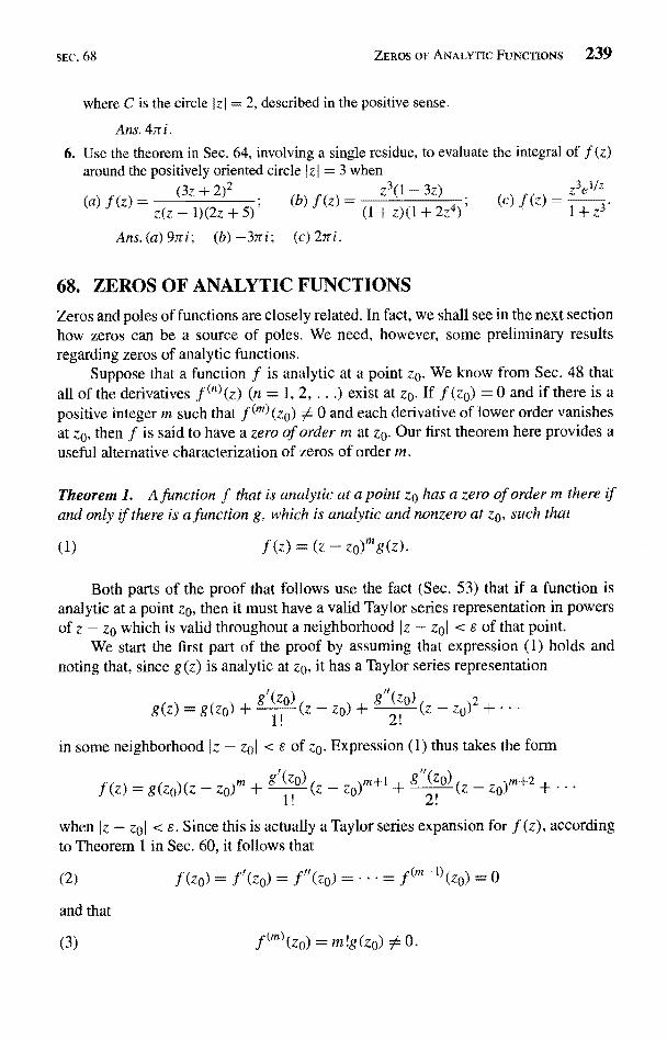
SEC, 68 ZEROS OF ANALYTIC FUNCTIONS 239
where C is the circle Izl = 2, described in the positive sense.
Ans. 4,7 i.
6. Use the theorem in Sec. 64, involving a single residue, to evaluate the integral ofaround the positively oriented circle I z I = 3 when
(a) f (z)(3z + 2)2
(b) f (z) =z3(l - 3z)
(c) f (z) =3elIz
4)z(z - l)(2z + 5) (l + z)(1 + 2z
Ans. (a) 9ni; (b) -3ni;
68. ZEROS OF ANALYTIC FUNCTIONSZeros and poles of functions are closely related. In fact, we shall see in the next sectionhow zeros can be a source of poles. We need, however, some preliminary resultsregarding zeros of analytic functions.
Suppose that a function f is analytic at a point zo. We know from Sec. 48 thatall of the derivatives f (")(z) (n = 1, 2, . . .) exist at zo. If f (zo) = 0 and if there is apositive integer m such that f (m)(zo) A 0 and each derivative of lower order vanishesat zo, then f is said to have a zero of order m at zo. Our first theorem here provides auseful alternative characterization of zeros of order m.
Theorem I. A function f that is analytic at a point zo has a zero of order m thereand only if there is a function g, which is analytic and nonzero at zo, such that
(1) f (z) = (z - zo)mg(z).
Both parts of the proof that follows use the fact (Sec. 53) that if a function isanalytic at a point zo, then it must have a valid Taylor series representation in powersof z - zo which is valid throughout a neighborhood Iz - zoI < 8 of that point.
We start the first part of the proof by assuming that expression (1) holds annoting that, since g(z) is analytic at zo, it has a Taylor series representation
g(z)=g(zo)+g (z-zo)+g (z-zo)2+...
in some neighborhood I z - zo I < 6 of zo. Expression (1) thus takes the form
f (z) = g (zo) (z - zo)t+ g` (zo) (z _ zo)m+1 + g" 2 o) (z _ zo),+z +
when I z - zo I < E. Since this is actually a Taylor series expansion for f (z), accordingto Theorem 1 in Sec. 60, it follows that
(2) f (zo) = f'(zo) _
and that
(3) f (m),
f(m-1)(zo) = 0
m!g(zo) 0 0 .
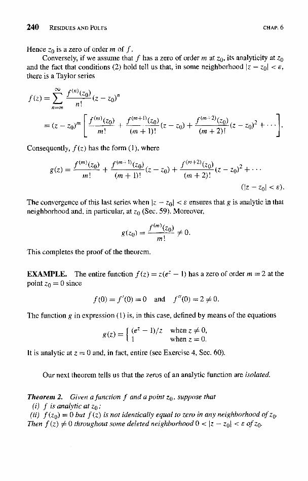
240 RESIDUES AND POLES CHAP. 6
Hence zo is a zero of order in of f .
Conversely, if we assume that f has a zero of order in at zo, its analyticity at zoand the fact that conditions (2) hold tell us that, in some neighborhood Iz - zol < E,there is a Taylor series
(n}
f(Z) _ f (zo)(z - Z0)n
n=m n!
Z0)mf(m)(z0)
m'.
fOn+1) (Z.) f (m+2) (Zn
Consequently, f (z) has the form (1), where
(m) '(m+l) ff (L0) ,f(Z0){Z0)
g(z) _ + (z - zo) + (---0)1+ ..
in! (m + 1)! (m + 2)!
(lz - zol < e).
The convergence of this last series when Iz - zol < e ensures that g is analytic in thatneighborhood and, in particular, at zo (Sec. 59). Moreover,
(m)f (zo)g(zo) _ A
Q
to !
This completes the proof of the theorem.
EXAMPLE. The entire function f Q) = z(ez - 1) has a zero of order m =2 at thepoint z0 = 0 since
f(O) = f'(0) = 0 and f"(0) =
The function g in expression (1) is, in this case, defined by means of the equations
g (z)when z 0,when z 0.
It is analytic at z = 0 and, in fact, entire (see Exercise 4, Sec. 60).
Our next theorem tells us that the zeros of an analytic function are isolated.
Theorem 2. Given a function f and a point z0, suppose that(i) f is analytic at zo ;
(ii) f (zo) = 0 but f (z) is not identically equal to zero in any neighborhood of zo.Then f (z) A 0 throughout some deleted neighborhood 0 < 14- - 1-01 < s of z0.
(m -}- 2) !
(m+2)
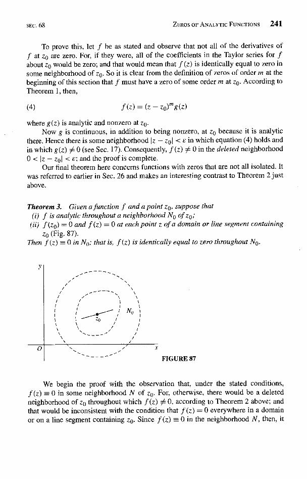
SEC. 68 ZEROS OF ANALYTIC FUNCTIONS 241
To prove this, let f be as stated and observe that not all of the derivatives off at zo are zero. For, if they were, all of the coefficients in the Taylor series for fabout zo would be zero; and that would mean that f (z) is identically equal to zero insome neighborhood of zo. So it is clear from the definition of zeros of order m at thebeginning of this section that f must have a zero of some order m at zo. According toTheorem 1, then,
(4) f(z)=(z-zo g(z)
where g(z) is analytic and nonzero at zo.Now g is continuous, in addition to being nonzero, at zo because it is analytic
there. Hence there is some neighborhood 1z - zol < e in which equation (4) holds andin which g(z) A 0 (see Sec. 17). Consequently, f (z) A 0 in the deleted neighborhood0 < Iz - zo) < e; and the proof is complete.
Our final theorem here concerns functions with zeros that are not all isolated. Itwas referred to earlier in Sec. 26 and makes an interesting contrast to Theorem 2 justabove.
Theorem 3. Given a function f and a point zo, suppose thatis analytic throughout a neighborhood No of zo;
(ii) f (zo) = 0 and f (z) = 0 at each point z of a domain or line segment containingzo (Fig. 87).
Then f (z) - 0 in No; that is, f (z) is identically equal to zero throughout No.
Y
0 x
FIGURE 87
We begin the proof with the observation that, under the stated conditions,f (z) - 0 in some neighborhood N of zo. For, otherwise, there would be a deletedneighborhood of zo throughout which f (z) A 0, according to Theorem 2 above; andthat would be inconsistent with the condition that f (z) = 0 everywhere in a domainor on a line segment containing zo. Since f (z) = 0 in the neighborhood N, then, it
242 RESIDUES AND POLES CHAP. 6
follows that all of the coefficients
a _ f (n) (zo) (n = 0, 1, 2, ...)n!
in the Taylor series for f (z) about zo must be zero. Thus f (z) - 0 in the neighborhoodNo, since Taylor series also represents f (z) in No. This completes the proof.
69. ZEROS AND POLESThe following theorem shows how zeros of order m can create poles of order m.
Theorem 1. Suppose that(1) two functions p and q are analytic at a point zo;
(ii) p(zo) 56 0 and q has a zero of order m at zo.Then the quotient p(z)/q (z) has a pole of order m at z
The proof is easy. Let p and q be as in the statement of the theorem. Since q hasa zero of order m at zo, we know from Theorem 2 in Sec. 68 that there is a deletedneighborhood of zo in which q (z) 56 0; and so zo is an isolated singular point of thequotient p(z)/q(z). Theorem 1 in Sec. 68 tells us, moreover, that
q(z) = (z - zc)mg(z),
where g is analytic and nonzero at z(>; and this enables us to write
(1) P(z) = P(z)/g(z)q (z) (z - zo)m
Since p(z)/g(z) is analytic and nonzero at zo, it now follows from the theorem in Sec.66 that zo is a pole of order m of p(z)/q(z).
EXAMPLE 1. The two functions
p(z)=l and q(z) = z(e` - 1)
are entire; and we know from the example in Sec. 68 that q has a zero of order m = 2at the point zo = 0. Hence it follows from Theorem I here that the quotient
P(z)_ 1
q (z) z(ez - 1)
has a pole of order 2 at that point. This was demonstrated in another way in Example 5,Sec. 67.
SEC. 69 ZEROS AND POLES 243
Theorem 1 leads us to another method for identifying simple poles and findingthe corresponding residues. This method is sometimes easier to use than the one inSec. 66.
Theorem 2. Let two functions p and q be analytic at a point 10.
P(zo) A 0, q(zo) = 0, and q'(zo) 560,
then zo is a simple pole of the quotient p(z)/q(z) and
(2)P(z0)P{z} -Res
z=z4 q(z) q'(z0)
To show this, we assume that p and q are as stated and observe that, because ofthe conditions on q, the point zo is a zero of order m = I of that function. Accordingto Theorem 1 in Sec. 68, then,
(3) q(z) _ (z - zo)g(z)
where g(z) is analytic and nonzero at zo. Furthermore, Theorem 1 in this section tellsus that z0 is a simple pole of p(z)/q(z); and equation (1) in its proof becomes
P(z) _ P(z)!g(z)q(z) z - zo
Now p(z) jg(z) is analytic and nonzero at z0, and it follows from the theorem in Sec.66 that
es p(z) = P(z0)
Z=zo q (z) g (zo)
But g(z0) = q'(z0), as is seen by differentiating each side of equation (3) and settingz = z0. Expression (4) thus takes the form (2).
EXAMPLE 2. Consider the function
COSzf(z)=cotz=sin z
which is a quotient of the entire functions p(z) = cos z and q(z) = sin z. The singu-larities of that quotient occur at the zeros of q, or at the points
z=n7r (n=0,±1,±2,..
Since
P(n7r) = (-1)" A0, q(nrr) = 0, and q'(nrr) = (-1)n A 0
244 RESIDUES AND POLES
each singular point z = n7r of f is a simple pole, with residue
B = p(n7r)
q'(n7r) 1)n
EXAMPLE 3. The residue of the function
f(z)tanh z sinh z
= -z2 z2 cosh z
at the zero z = 7ri /2 of cosh z (see Sec. 34) is readily found by writing
p(z) = sinh z and q(z)=Z2 cosh z.
Since
p(r i sinh(7ri 1= i sin r2 2 2
and
sinh
we find that z = 7ri /2 is a simple pole off and that the residue there is
B - p(7ri/2)q'(7ri/2)
4
EXAMPLE 4. One can find the residue of the function
Zf (Z) =
at the isolated singular point
+4
CHAP. 6
Za - /2e',,/4 = I + i
by writing p (z) = z and q (z) = z4 + 4. Since
0 0,P(zo) = za 0> q(ua) = 0, and q'(zo) _ 4z3
f has a simple pole at za. The corresponding residue is the number
BaP(za) = zo 1 1 i
= q (za) 4z3 4z02 8i 8
Although this residue could also be found by the method of Sec. 66, the computationwould be somewhat more involved.
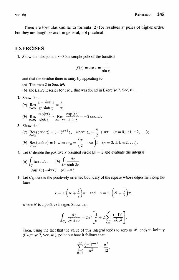
SEC. 69 EXERCISES 245
There are formulas similar to formula (2) for residues at poles of higher order,but they are lengthier and, in general, not practical.
EXERCISES
1. Show that the point z = 0 is a simple pole of the function
1f(z)=cscz=sin z
and that the residue there is unity by appealing to
(a) Theorem 2 in Sec. 69;(b) the Laurent series for csc z that was found in Exercise 2, Sec. 61.
2. Show that
(a) Res z - sinh z = i
z=7ri zz sinh z TC
(b) Resexp(zt)
+ Resexp(zt)
_ -2 cos ;r t.z=iri sinh z z=-rri sinh z
3. Show that
(a) ResZ=zn
where z,,, = - + n7t (n = 0, +1, +2, .
(b) Res(tanh z) = 1, where z _ (- + n7r )i (n =0, ±1, +2, ...).Z=Zn
4. Let C denote the positively oriented circle jz) = 2 and evaluate the integral
(a) I tan z dz: (b)dz
c Jc Sinn 2zAns. (a) -47ri; (b) -rri.
5. Let CN denote the positively oriented boundary of the square whose edges lie along thlines
N+ )7r and y=::LN+ 12
where N is a positive integer. Show that
dz =ar -2iz2sinz 6
Then, using the fact that the value of this integral tends to zero as N tends to infinity(Exercise 7, Sec. 41), point out how it follows that
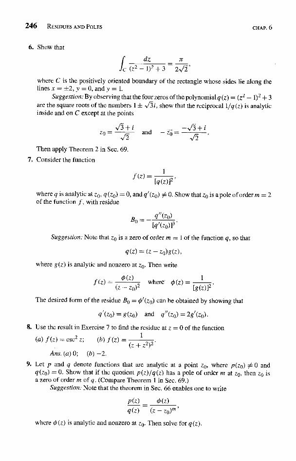
246 RESIDUES AND POLES
6. Show that
CHAP. 6
dz Tr- 2 yff ,c(z2-1)2+3where C is the positively oriented boundary of the rectangle whose sides lie along thelines x=+2,y=0,andy=1.
Suggestion: By observing that the four zeros of the polynomial q (z) = (z2 - 1)2 +3are the square roots of the numbers 1 ± i, show that the reciprocal 1/q (z) is analyticinside and on C except at the points
Z() =+
and - zp =
Then apply Theorem 2 in Sec. 69.
7. Consider the function
where q is analytic at zo, q (zo)of the function f , with residue
1
f(z)= [q(z)]2'
and q'(zo) A 0. Show that zo is a pole of order m = 2
q"(z0)
[q'(zo)]3 .
Suggestion: Note that zo is a zero of order m = 1 of the function q, so that
q(z) = (z - zo)g(z),
where g(z) is analytic and nonzero at zo. Then write
f (z) _ (ZZ)
o)2where q6(z) _
[g(z)]2
The desired form of the residue B0 = q'(zo) can be obtained by showing that
q'(zo) = g(zo) and q"(zo) = 2g'(zo).
8. Use the result in Exercise 7 to find the residue at z = 0 of the function
2 1(a) f (z) = csc z; (b) f (z) = (z+z2Ans. (a) 0; (b) -2.
9. Let p and q denote functions that are analytic at a point zo, where p(zo) A 0 andq (zo) = 0. Show that if the quotient p(z)/q(z) has a pole of order in at zo, then zo isa zero of order m of q. (Compare Theorem 1 in Sec. 69.)
Suggestion: Note that the theorem in See. 66 enables one to write
p(z) = 0(z)q (z) (z - zo)`
,
where 0 (z) is analytic and nonzero at zo. Then solve for q (z).
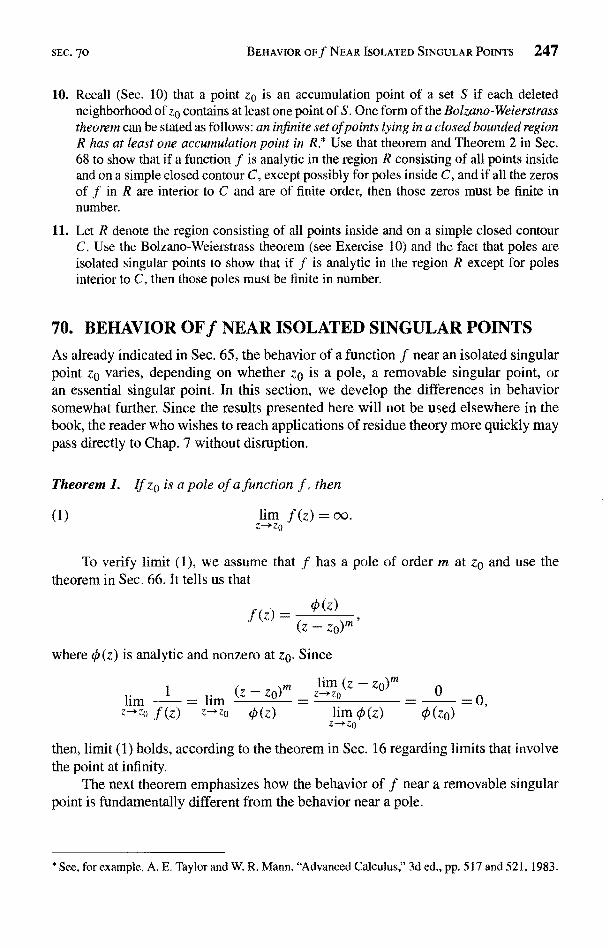
SEC. 70 BEHAVIOR OFf NEAR ISOLATED SINGULAR POINTS 247
10. Recall (Sec. 10) that a point z0 is an accumulation point of a set S if each deletedneighborhood of z0 contains at least one point of S. One form of the Bolzano-Weierstrasstheorem can be stated as follows: an infinite set of points lying in a closed bounded regionR has at least one accumulation point in R.* Use that theorem and Theorem 2 in Sec.68 to show that if a function f is analytic in the region R consisting of all points insideand on a simple closed contour C, except possibly for poles inside C, and if all the zerosof f in R are interior to C and are of finite order, then those zeros must be finite innumber.
11. Let R denote the region consisting of all points inside and on a simple closed contourC. Use the Bolzano-Weierstrass theorem (see Exercise 10) and the fact that poles areisolated singular points to show that if f is analytic in the region R except for polesinterior to C, then those poles must be finite in number.
70. BEHAVIOR OFf NEAR ISOLATED SINGULAR POINTS
As already indicated in Sec. 65, the behavior of a function f near an isolated singularpoint za varies, depending on whether Z0 is a pole, a removable singular point, oran essential singular point. In this section, we develop the differences in behaviorsomewhat further. Since the results presented here will not be used elsewhere in thebook, the reader who wishes to reach applications of residue theory more quickly maypass directly to Chap. 7 without disruption.
Theorem]. If,z0 is a pole of a function f , then
(1) lim f (z)Z--+Z0
To verify limit (1), we assume that f has a pole of order m at zc and use thetheorem in Sec. 66. It tells us that
(z)j(Z) = (z-zwhere 0 (z) is analytic and nonzero at Z. Since
1 lim(z-za),) Z-)Z(Z - Z a0 O --lim = lim - 0,
Z *Z0 f (z) Z- Z0 0 (z) lim 0 (z) 0 (za)z-a.Zo
then, limit (1) holds, according to the theorem in Sec. 16 regarding limits that involvethe point at infinity.
The next theorem emphasizes how the behavior of f near a removable singularpoint is fundamentally different from the behavior near a pole.
* See, for example, A. E. Taylor and W. R. Mann. "Advanced Calculus," 3d ed., pp. 517 and 521, 1983.
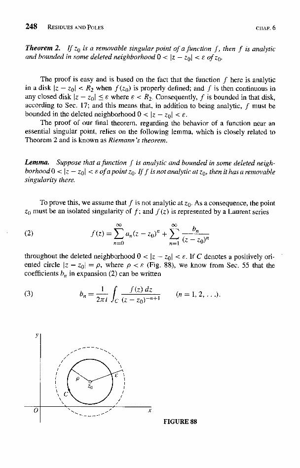
248 RESIDUES AND POLES CHAP. 6
Theorem 2. If zo is a removable singular point of a function f, then f is analyticand bounded in some deleted neighborhood 0 < Iz - zol < s of zo.
The proof is easy and is based on the fact that the function f here is analyticin a disk Iz - zol < R2 when f (zo) is properly defined; and f is then continuous inany closed disk Iz - zol < s where s < Rz. Consequently, f is bounded in that disk,according to Sec. 17; and this means that, in addition to being analytic, f must bebounded in the deleted neighborhood 0 < Iz - zoo < E.
The proof of our final theorem, regarding the behavior of a function near anessential singular point, relies on the following lemma, which is closely related toTheorem 2 and is known as Riemann's theorem.
Lemma. Suppose that a function f is analytic and bounded in some deleted neigh-borhood 0 < I z - zo I < s of a point zo. If f is not analytic at zo, then it has a removablesingularity there.
To prove this, we assume that f is not analytic at zo. As a consequence, the pointzo must be an isolated singularity of f ; and f (z) is represented by a Laurent series
(2) .f(z)=>,a,,(z-zo)"
00
n=O n=
bn
throughout the deleted neighborhood 0 < Iz - zol < s. If C denotes a positively ori-ented circle Iz - zol = p, where p < s (Fig. 88), we know from Sec. 55 that thecoefficients bn in expansion (2) can be written
(3)1
C
f (z) dz27r i (Z - Zo)-n+I
FIGURE 88
2,
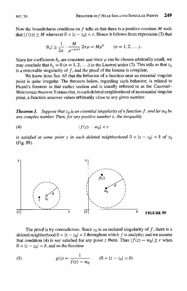
SEC. 70 BEHAVIOR OFf NEAR ISOLATED SINGULAR POINTS 249
Now the boundedness condition on f tells us that there is a positive constant M suchthat I f (z) I < M whenever 0 < Iz - zol < E. Hence it follows from expression (3) that
IbnI2rp_Mpn
(n2n p-n+1
Since the coefficients b. are constants and since p can be chosen arbitrarily small, wemay conclude that bn = 0 (n = 1, 2, . . .) in the Laurent series (2). This tells us that zais a removable singularity of f , and the proof of the lemma is complete.
We know from Sec. 65 that the behavior of a function near an essential singularpoint is quite irregular. The theorem below, regarding such behavior, is related toPicard's theorem in that earlier section and is usually referred to as the Casorati-Weierstrass theorem. It states that, in each deleted neighborhood of an essential singularpoint, a function assumes values arbitrarily close to any given number.
Theorem 3. Suppose that z0 is an essential singularity of a function f, and let w0 beany complex number. Then, for any positive number e, the inequality
(4) f(z) - woke
is satisfied at some point z in each deleted neighborhood 0 < Iz - zo(Fig. 89).
Y
0
V
x 0 u FIGURE 89
Zp
The proof is by contradiction. Since zo is an isolated singularity of f, there is adeleted neighborhood 0 < Iz - zol < S throughout which f is analytic; and we assumethat condition (4) is not satisfied for any point z there. Thus If (z) - w0I > s when0 < I z - zo I < S; and so the function
(5) g(z) = f(z)1-wp (0
<lz -
zoI <S)
250 RESIDUES AND POLES CHAP. 6
is bounded and analytic in its domain of definition. Hence, according to the abovelemma, zo is a removable singularity of g; and we let g be defined at zo so that it isanalytic there.
If g(zo) A 0, the function f (z), which can be written
(6) f (z) ` 1 + wog (z)
when 0 < I z - zo I < S, becomes analytic at zo if it is defined there as
1
f (zo)= g(zp)
+ wo.
But this means that zo is a removable singularity of f, not an essential one, and wehave a contradiction.
If g(zo) = 0, the function g must have a zero of some finite order m (Sec. 68) atzo because g(z) is not identically equal to zero in the neighborhood Iz - zol < S. Inview of equation (6), then, f has a pole of order m at zo (see Theorem 1 in Sec. 69).So, once again, we have a contradiction; and Theorem 3 here is proven.
CHAPTER
7APPLICATIONS OF RESIDUES
We turn now to some important applications of the theory of residues, which wasdeveloped in the preceding chapter. The applications include evaluation of certain typesof definite and improper integrals occurring in real analysis and applied mathematics.Considerable attention is also given to a method, based on residues, for locating zerosof functions and to finding inverse Laplace transforms by summing residues.
71. EVALUATION OF IMPROPER INTEGRALS
In calculus, the improper integral of a continuous function f (x) over the semi-infiniteinterval x > 0 is defined by means of the equation
(1)
When the limit on the right exists, the improper integral is said to converge to thatlimit. If f (x) is continuous for all x, its improper integral over the infinite interval-oo < x < oo is defined by writing
(2) j f(x)dx=limI
f(x)dx+l f(x)dx;Ri
R,
R2
and when both of the limits here exist, integral (2) converges to their sum. Anothervalue that is assigned to integral (2) is often useful. Namely, the Cauchy principal
251
252 APPLICATIONS OF RESIDUES CHAP. 7
value (P.V.) of integral (2) is the number
(3) P.V. / nf (x) dx = lim
R-a oo
provided this single limit exists.If integral (2) converges, its Cauchy principal value (3) exists; and that value is
the number to which integral (2) converges. This is because
and the limit as R -* oc of each of the integrals on the right exists when integral (2)converges. It is not, however, always true that integral (2) converges when its Cauchyprincipal value exists, as the following example shows.
EXAMPLE. Observe that
(4) RV. x dx = lim I x dx = limF00
R
R-aoo J R R-oo
On the other hand,
(5)
lim 0=0.R- roo
x dx
R2
0
RIB oo 2 R2R2Jim 1 + lim R2
2.
2'
and since these last two limits do not exist, we find that the improper integral (5) failsto exist.
But suppose that f (x) (-oc < x < ao) is an even function, one where
f -x) for all x.
The symmetry of the graph of y = f (x) with respect to the y axis enables us to write
fo
R
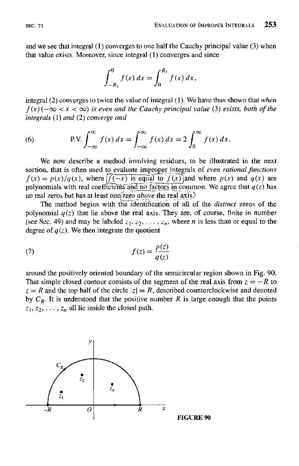
SEC. 7 I EVALUATION OF IMPROPER INTEGRALS 253
and we see that integral (1) converges to one half the Cauchy principal value (3) whenthat value exists. Moreover, since integral (1) converges and since
-R,
integral (2) converges to twice the value of integral (1). We have thus shown that whenf (x) (-oo < x < oo) is even and the Cauchy principal value (3) exists, both of theintegrals (1) and (2) converge and
(6) P. V. I f(x)dx= J f(x)dx=2 j f(x)dx.
We now describe a method involving residues, to be illustrated in the nextsection, that is often used to evaluate impro er integrals of even rational functionsf(x) = p(x)/q(x), where ff((-x) is equal to f(x) and where p(x) and q(x) arepolynomials with real coefficients and no factors in common. We agree that q (z) hasno real zeros but has at least on zero above the real axis)
The method begins with the identification of all of the distinct zeros of thepolynomial q (z) that lie above the real axis. They are, of course, finite in number(see Sec. 49) and may be labeled zI, z2, ... , zn, where n is less than or equal to thedegree of q (z). We then integrate the quotient
.f (z) =p (Z)
q (z)
around the positively oriented boundary of the semicircular region shown in Fig. 90.That simple closed contour consists of the segment of the real axis from z = -R toz = R and the top half of the circle I z I = R, described counterclockwise and denotedby CR. It is understood that the positive number R is large enough that the pointsZ1, z2, ... , z all lie inside the closed path.
FIGURE 90
254 APPLICATIONS OF RESIDUES CHAP. 7
The Cauchy residue theorem in Sec. 63 and the parametric representation z =- R < x < R) of the segment of the real axis just mentioned can be used to write
Or
R
LRf(x)dx+ ] f(z)dz=2 i }Res f(z),
k=Z=Zk
(8) J Rf(x)dx=2iRes f(z)-( f(z)dz.
kk=1 JCR
If
(z) dz = 0,
it then follows that
(9) P.V. / f(x)dx=27ri > 'Res f(z).=Zk
x) is even, equations (6) tell us, moreover, that
(10) dx=27ri) ;Res f(z)Z=Zk
and
Jo
n
(x) dx = 7ri ) ' Res f (z).Z=Zk
72. EXAMPLE
We turn now to an illustration of the method in Sec. 71 for evaluating improperintegrals.
EXAMPLE. In order to evaluate the integral
x6 + 1
we start with the observation that the function
z2f (z) = z6 +
has isolated singularities at the zeros of z6 + 1, which are the sixth roots of -1, and isanalytic everywhere else. The method in Sec. 8 for finding roots of complex numbers
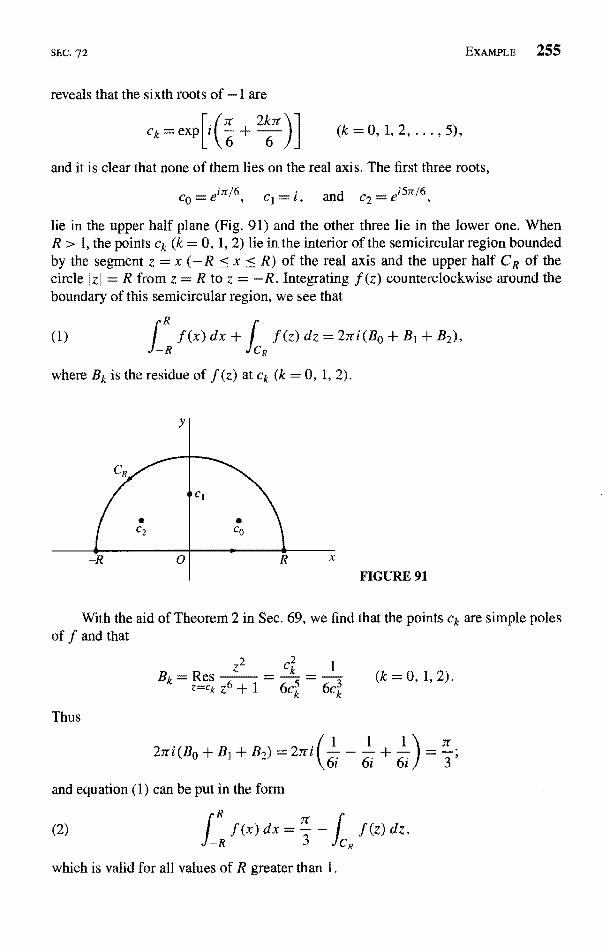
SEC. 72
reveals that the sixth roots of -1 are
EXAMPLE 255
and it is clear that none of them lies on the real axis. The first three roots,
co = einJ6, cl and c2 - ei5nJs
lie in the upper half plane (Fig. 91) and the other three lie in the lower one. WhenR > 1, the points ck (k = 0, 1, 2) lie in the interior of the semicircular region boundedby the segment z = x (-R < x < R) of the real axis and the upper half CR ocircle IzI = R from z = R to z = -R. Integrating f (z) counterclockwise around theboundary of this semicircular region, we see that
(1) dx + I f (z) dz = 27ri (Bo + BI + B2),-R C
where Bk is the residue of f (z) at Ck (k = 0, 1, 2).
FIGURE 91
With the aid of Theorem 2 in Sec. 69, we find that the points Ck are simple polesof f and that
2Z ck
6Ck
Thus
27ri (BO + BI + B2) = 27r
and equation (1) can be put in the form
6ck
7r
(k=0,1,2).
- I f (z) dz,(2) 1 f (x) dx =3
which is valid for all values of R greater than 1.
256 APPLICATIONS OF RESIDUES CHAP. 7
Next, we show that the value of the integral on the right in equation (2) tends to0 as R tends to oo. To do this, we observe that when IzI = R,
=Iz12=R2
and
Iz6+11>-IIZ16-lI=R6-1.
So, if z is any point on CR,
If(z)I = '- "IZ6 +11
and this means that
(3)
JCR
whereR2
R6 -
7r R being the length of the semicircle C. (See Sec. 41.) Since the number
MRJTR=R6-1
is a quotient of polynomials in R and since the degree of the numerator is less thanthe degree of the denominator, that quotient must tend to zero as R tends to oo. Moreprecisely, if we divide both numerator and denominator by R6 and write
MR Tr R
7r R3
Tr
R3
1-R6
evident that MR7r R tends to zero. Consequently,
It now follows from equation (2) that
(z)dz=0.
R x2lim dx =
R >cc> _R X6 + 1
or
n view of inequality (3
Tr
P. V.
°° x2
f-00dx
X6+1
SEC. 72EXERCISES 257
Since the integrand here is even, we know from equations (6) in Sec. 71 and thestatement in italics just prior to them that
(4) 1 . , dx =
EXERCISESUse residues to evaluate the improper integrals in Exercises 1 through 5.
x2 +Ans. n/2.
2. 00dx
.o
(x2+1)2
Ans. n/4.00 dx
3.p x4+1
Ans. 7r/(2J).
x2 dx)(x2+4).
5.
fo
Ans. 7r/6.
x2 dx(x2 + 9)(x2 + 4)2
Ans. ar/200.
Use residues to find the Cauchy principal values of the integrals in Exercises 6 and 7.
dx
00 x2+2x+2
7.0° xdx
J Oo (x2 + 1) (x2 + 2x + 2)
Ans. -Tr/5.
8. Use residues and the contour shown in Fig. 92, where R > 1, to establish the integrationformula
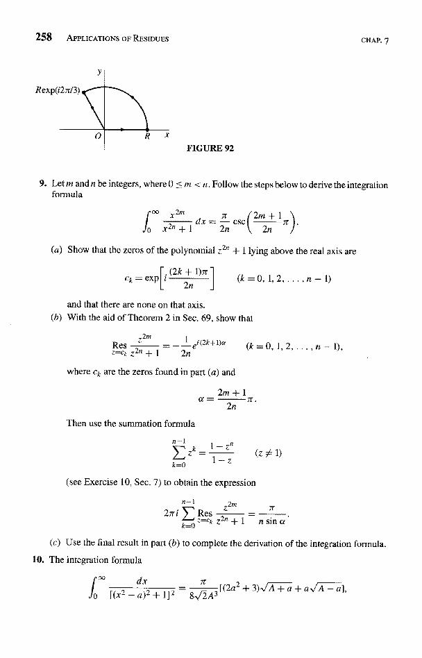
258 APPLICATIONS OF RESIDUES
Rexp(i270)
0
Y
CHAP. 7
9. Let m and n be integers, where 0 < m < n. Follow the steps below to derive the integrationformula
x2it + 1 dx 2ncsc
Show that the zeros of the polynom
(2k + 1)Ck=exp 2n (k=0,1,2,...,n-1)
R x
FIGURE 92
1 lying above the real axis are
and that there are none on that axis.(b) With the aid of Theorem 2 in Sec. 69, show that
ResZrm _ l
e`(2k+I)a (k=O, 1, 2, ... , n -Z=Ck Z2n + 1 2n
where ck are the zeros found in part (a) and
2m + Ir.
2n
Then use the summation formula
(Z 0 1)
see Exercise 10, Sec. 7) to obtain the expression
Z2m7C2rri )'Res =
2Z=Ck z n -{- 1 n sin ak_0
(c) Use the final result in p
10. The integration formula
dx
b) to complete the derivation of the integration formula.
SEC. 73 IMPROPER INTEGRALS FROM FOURIER ANALYSIS 259
where a is any real number and A = a2 + 1, arises in the theory of case-hardening ofsteel by means of radio-frequency heating.* Follow the steps below to derive it.
(a) Point out why the four zeros of the polynomial
q(z) = (zt - a)` + 1
are the square roots of the numbers a + i. Then, using the fact that the numbers
zo= ( A+a+i -,,/-A A --a)
and -zo are the square roots of a + i (Exercise 5, Sec. 9), verify that ±T0 are thesquare roots of a - i and hence that zo and -Toare the only zeros of q(z) in theupper half plane Im z > 0.
b) Using the method derived in Exercise 7, Sec. 69, and keeping in mind that z2 = a + ifor purposes of simplification, show that the point zo in part (a) is a pole of order 2of the function f (z) = 1/[q (z)]2 and that the residue BI at zo can be written
q"(zo) _ a - i(2a2 + 3)
[q'(zo)]3 16A2zo
After observing that q'(-"z) = -q'(z) and q"(-"z) = q"(z), use the same method toshow that the point -To in part (a) is also a pole of order 2 of the function f (z), withresidue
Then obtain the expression
1
I+B2=-a+i(2a2+3)
ZO$A2i
for the sum of these residues.(c) Refer to part (a) and show that Iq (z) I > (R - Iza 1 )4 if I Z I = R, where R > Izol. Then,
with the aid of the final result in part (b), complete the derivation of the integrationformula.
73. IMPROPER INTEGRALS FROM FOURIER ANALYSISResidue theory can be useful in evaluating convergent improper integrals of the form
(1) j f (x) sin ax dx or f00
(x) cos ax dx,
* See pp. 359-364 of the book by Brown, Hoyler, and Bierwirth that is listed in Appendix 1.
260 APPLICATIONS OF RESIDUES CHAP. 7
where a denotes a positive constant. As in Sec. 71, we assume that f (x) = p (x) f q(x),where p (x) and q (x) are polynomials with real coefficients and no factors in common.Also, q(z) has no real zeros. Integrals of type (1) occur in the theory and applicationof the Fourier integral.*
The method described in Sec. 71 and used in Sec. 72 cannot be applied directlyhere since (see Sec. 33)
and
More precisely, since
smh ay =
Isin az12 = sin2 ax + sinh2 ay
]cos ax 12 = cost ax + sinh2 ay.
Say - e-ay
2
the moduli Isin az) and Icos az) increase like eay as y tends to infinity. The modificationillustrated in the example below is suggested by the fact that
cos ax dx + i f (x) sin ax dx =-R -R J-R
together with the fact that the modulus
Ieia,l = leia(x+iy)) = Ie-ayeiax
is bounded in the upper half plane y ? 0.
EXAMPLE. Let us show that
(2)cos 3x
dx =27r-
-oo (x2 + 1)2 e3
tax dx,
Because the integrand is even, it is sufficient to show that the Cauchy principal valueof the integral exists and to find that value.
We introduce the function
.f (z) =1
(z2 + 1)2
and observe that the product f {z}ehiz is analytic everywhere on and above the realaxis except at the point z = i. The singularity z = i lies in the interior of the semi-circular region whose boundary consists of the segment -R < x < R of the real axis
* See the authors' "Fourier Series and Boundary Value Problems," 6th ed., Chap. 7, 2001.
SEC. 73 IMPROPER INTEGRALS FROM FOURIER ANALYSIS 261
and the upper half CR of the circle Iz I = R (R > 1) from z = R to z = R. Integrationof f (z)ei3z around that boundary yields the equation
R ei3z
(4) dx = 27ri Br ----R (x2 + 1) 2
where
Res[f (z)ez=i
Since
(z -where O (z) =
the point z = i is evidently a pole of order m = 2 of f (z)e`iz; and
1
By equating the real parts on each side of equation (4), then, we find that
ei3z dz.
Finally, we observe that when z is a point on CR,
I f(711 < M where M =
i3z 0(z)
1
R R 2 2(R - 1)
and that (e
(6)
Since the quantity
-3y < I for such a point. Consequently,
)ei3z dz We' .3z dz <MRnR.
tends to 0 as R tends to oo and because of inequalities (6), we need only let R tend tocoo in equation (5) to arrive at the desired result (2).
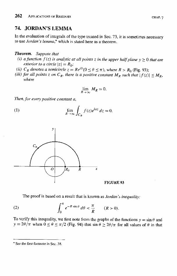
262 APPLICATIONS OF RESIDUES CHAP. 7
74. JORDAN'S LEMMA
In the evaluation of integrals of the type treated in Sec. 73, it is sometimes necessaryto use Jordan's lemma,* which is stated here as a theorem.
Theorem. Suppose that(i) a function f (z) is analytic at all points z in the upper half plane y > 0 that are
exterior to a circle I z) = R0,'CR denotes a semicircle z = Re`0(0 < 0 < ar), where R > R0 (Fig. 93);for all points z on CR, there is a positive constant MR such that I f (z) 1 c MR,where
R-+0C
Then, for every positive constant a,
(1)
= 0.
FIGURE 93
The proof is based on a result that is known as Jordan's inequality:
(2) e-R sin 8 dB
0 RR
To verify this inequality, we first note from the graphs of the functions y = sin 0 andy = 20/7r when 0 < 0 < 7r/2 (Fig. 94) that sin 0 > 20/7r for all values of 0 in that
* See the first footnote in Sec. 38.
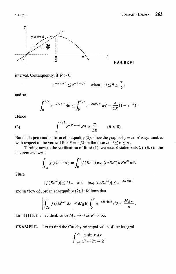
SEC. 74 JORDAN'S LEMMA 263
FIGURE 94
interval. Consequently, if R > 0,
e-R sin
and so
2R
2
e-R sin 8 d8 < 1 e-2R8Jn dO (1 - e-R)
-2R8/7r when
Hence
(3)
2e-R sin 8 dO <
2R(R > 0).
But this is just another form of inequality (2), since the graph of y = sin 0 is symmetricwith respect to the vertical line 0 = 7r/2 on the interval 0 < 0 < 7r.
Turning now to the verification of limit (1), we accept statements (i)-(iii) in thetheorem and write
Since
Z)eiaz dz = Reie) exp(iaRec8)iReie d8.
f(ReiB)f < MR and 1exp(iaRei9)1< e-aRsine
and in view of Jordan's inequality (2), it follows that
f (z)eiaz dz
ICR
e-aR sin 8 d$ < MR ITa
Limit (1) is then evident, since MR -* 0 as R -* coo.
EXAMPLE. Let us find the Cauchy principal value of the integral
264 APPLICATIONS OF RESIDUES CHAP. 7
As usual, the existence of the value in question will be established by our actuallyfinding it.
We write
.f (z) _Z
=Z
Z' + 2z + 2 (z - zl)(z - zl)'
where z1= -1+ i. The point z1, which lies above the z axis, is a simple pole of thefunction f (z)e`z, with residue
(4)z1 e`2I
z1
Hence, when R > and CR denotes the upper half of the positively oriented circleIzI=R,
1R xe`x dxJR x2+2x+2
and this means that
(5)
Now
r X sin x dx
-R x'2+2x+2
= 2iriB1 -
Z dz
and we note that, when z is a point on CR,
If (z) I < MR where
(z)e'z dz;
Z dz
R
(R -)2and that Ie`zI = e-y < 1 for such a point. By proceeding as we did in the examples inSecs. 72 and 73, we cannot conclude that the right-hand side of inequality (6), andhence the left-hand side, tends to zero as R tends to infinity. For the quantity
M srR= 7r R2 7r
R)
does not tend to zero. Limit (1) does, however, provide the desired result.So it does, indeed, follow from inequality (6) that the left-hand side there tends
to zero as R tends to infinity. Consequently, equation (5), together with expression (4)
SEC. 74
for the residue B1, tells us that
(7) P.V.
EXERCISES 265
2ariB1) _ (sin 1 + cos 1).
EXERCISES
Use residues to evaluate the improper integrals in Exercises 1 through 8.
(a > b > 0).
Ans_
dx(a>0) ,
x2 + 1TtAns. -e-'.2
cos ax
(cosb2)2 dx (a > 0, b > 0).
Ans. - -(l+ab)e-ab40
x sin 2xdx .
5. r
x2+3
Ans. 2 exp(-2V).
dx(a>()°O r -inaro, x4+4
7rAns. - e-a sin a.
2
X.5 sin axdx (a > 0)
7.
x4+4Ans. re"' cos a.
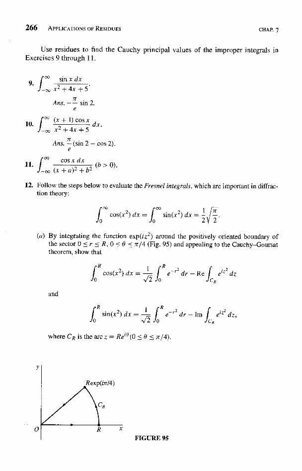
266 APPLICATIONS OF RESIDUES CHAP. 7
Use residues to find the Cauchy principal values of the improper integrals inExercises 9 through 11.
sin x dx9.
Ja.,x2+4x+57rAns. -- sin 2.e
f0c10. (x + 1) Cos x dx00 x2+4x+5
Ans. - (sin 2 - cos 2).e
0
12. Follow the steps below to evaluate the Fresnel integrals, which are important in diffrac-tion theory.
cos(x2) d x =
(a) By integrating the function exp(iz2) around the positively oriented boundary ofthe sector 0 <_ r < R, 0 <_ 0 < 7r/4 (Fig. 95) and appealing to the Cauchy-Goursattheorem, show that
1.
and
e`Zz
dz
sin(x2)dx= f e2 dr - Im f eizdz,,/2
0C
where CR is the arc z = Re
y
Rexp(iar/4)
CR
4
01 R X
FIGURE 95
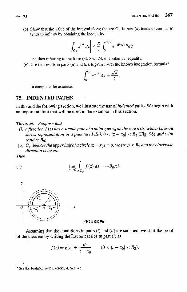
SEC. 75 INDENTED PATHS 267
(b) Show that the value of the integral along the arc CR in part (a) tends to zero as Rtends to infinity by obtaining the inequality
dz e-R2 sin OdO
and then referring to the form (3), Sec. 74, of Jordan's inequality.Use the results in parts (a) and (b), together with the known integration formula*
Ito complete the exercise.
04 2
e-X dx7t
75. INDENTED PATHSIn this and the following section, we illustrate the use of indented paths. We begin withan important limit that will be used in the example in this section.
Theorem. Suppose that(i) a function f (z) has a simple pole at a point z xa on the real axis, with a Laurent
series representation in a punctured disk 0 < Iz - xoI < R2 (Fig. 96) and withresidue Be;
(ii) C. denotes the upper ha lf of a circle I z - xp I = p, where p < R2 and the clockwisedirection is taken,
Then
(1) z)dz=-B0rri.
FIGURE 9b
Assuming that the conditions in parts (i) and (ii) are satisfied, we start the proofof the theorem by writing the Laurent series in part (i) as
Be
+.f (z) = 9(z) z - x0z - xe < R2),
* See the footnote with Exercise 4, Sec. 46.
268 APPLICATIONS OF RESIDUES CHAP, 7
where
g(z)= ,,,a,(z-x0)n (1z-xon=0
Thus
(2) f .f (z) dz = f ` g(z) dz + B0'A
R2),
Now the function g(z) is continuous when Iz - xol < R2, according to the theo-rem in Sec. 58. Hence if we choose a number pe such that p < pe < R2 (see Fig. 96), itmust be bounded on the closed disk Iz - xoI < pe, according to Sec. 17. That is, thereis a nonnegative constant M such that
I g (z) I< M whenever I z - xo l< po;
and, since the length L of the path C,, is L = np, it follows that
fcp g (z) dz
Consequently,
(3)P-0 Jc
<ML=M7rp.
g(z) dz =
Inasmuch as the semicircle -C, has parametric representation
z=xe+pe°
the second integral on the right in equation (2) has the value
Thus
(4)
"d9=-i I dB= -ijr.
Limit (1) now follows by letting p tend to zero on each side of equation (2) andreferring to limits (3) and (4).
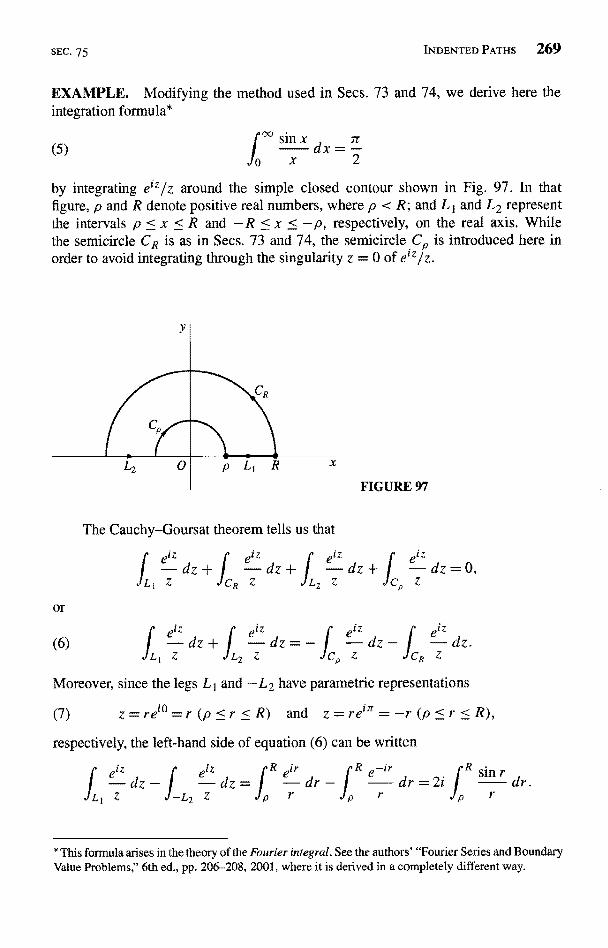
SEC. 75 INDENTED PATHS 269
EXAMPLE. Modifying the method used in Secs. 73 and 74, we derive here theintegration formula*
(5)fo
sin x 7t
xdx=
2
by integrating ecz/z around the simple closed contour shown in Fig. 97. In thatfigure, p and R denote positive real numbers, where p < R; and L 1 and L2 representthe intervals p < x < R and -R < x < -p, respectively, on the real axis. Whilethe semicircle CR is as in Secs. 73 and 74, the semicircle C,, is introduced here inorder to avoid integrating through the singularity z = 0 of etz/z.
FIGURE 97
The Cauchy-Goursat theorem tells us that
IL
or
(6)
dz+ I -dz+ I -dz+ I -dz=0,Cl? Z L, Z
Moreover, since the legs L1 and -L2 have parametric representations
(7) z=rer°=r(p<r<R) and z=rei"=-r(p<r<R),respectively, the left-hand side of equation (6) can be written
viz lR ,ir r, P-ir fR sin r-dz- I -dz= I -dr- I -dr=2r
* This formula arises in the theory of the Fourier integral. See the authors' "Fourier Series and BoundaryValue Problems," 6th ed., pp. 206-208, 2001, where it is derived in a completely different way.
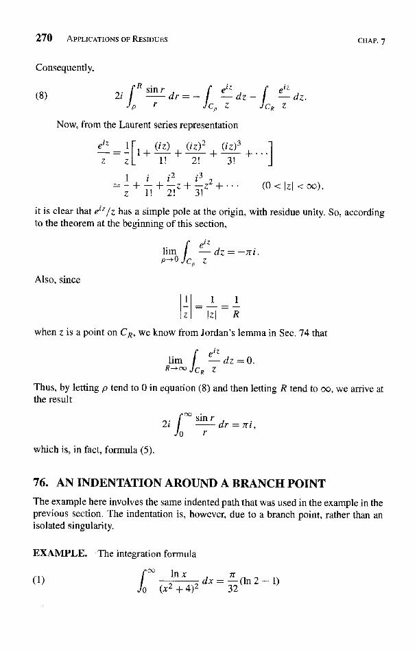
270 APPLICATIONS OF RESIDUES
Consequently,
Now, from the Laurent series representation
(iz) + (iz)2 + (iz)s1! 2! 3!
i2 i3+ Z +!z2 + .. . (0 < IzI < o©),
CHAP. 7
it is clear that e!z/z has a simple pole at the origin, with residue unity. So, accordingto the theorem at the beginning of this section,
=dz=-7ri.
Also, since
1
z
1 1
Izl R
when z is a point on CR, we know from Jordan's lemma in Sec. 74 that
Thus, by letting p tend to 0 in equation (8) and then letting R tend to oc, we arrive atthe result
°" sin r2i dr =
0 r
which is, in fact, formula (5).
76. AN INDENTATION AROUND A BRANCH POINT
The example here involves the same indented path that was used in the example in theprevious section. The indentation is, however, due to a branch point, rather than anisolated singularity.
EXAMPLE. The integration formula
(1)
P--+u JCP z
In xdx = (1n 2 - 1)2
32
SEC. 76 AN INDENTATION AROUND A BRANCH POINT 271
can be derived by considering the branch
log zf(z)=
Jrarg z
of the multiple-valued function (log z)/(z2 + 4)2, This branch, whose branch cutconsists of the origin and the negative imaginary axis, is analytic everywhere in theindicated domain except at the point z = 2i. In order that the isolated singularity 2ialways be inside the closed path, we require that p < 2 < R. See Fig. 98, where theisolated singularity and the branch point z = 0 are shown and where the same labelsL 1, L2, C., and CR as in Fig. 97 are used. According to Cauchy's residue theorem,
L f (z) dz -F jC
That is,
f(z)dz+ j f(z)dz+ J f(z)dz=2rriRes f(z).Z=2i
f(z) dz - f(z)dz.(2) j f(z) dz + I f(z) dz = 27ri Res f (z) -1Jz =2i Co CR
FIGURE 98
Since
Inr+i92ei20 + 4)2
the parametric representations
(3) z=re`Q=r(p{
(z = re
R) and z = re"' = (p<r{R)for the legs L 1 and -L2 can be used to write the left-hand side of equation (2) as
f(z)dz-j'
f(z)dz=fn lnr dr+L, L, P (r2 +4)2
272 APPLICATIONS OF RESIDUES
Also, since
.f (z) =0
(z) where 0 (z) = log z
(z - 2i)2 (z + 2i)2'
the singularity z = 2i of f (z) is a pole of order 2, with residue
+i1-1n2
64 32
Equation (2) thus becomes
In I+ 1101
and, by equating the real parts on each side here, we find that
Inr rr
In r zdr '=dr+iz // (In2-1)+i-4)2 h (r2 + 4)2 16 32
dr=-(1n2-1)-Re I f(z)dz-
It remains only to show that
(6) lim Rep-+a
f (z) dz = 0 and lim ReR-+oo
(z) dz = 0.
dz;
CHAP. 7
For, by letting p and R tend to 0 and oo, respectively, in equation (5), we then arriveat
2 °" Inr dr . n-(In 2 - 1),J0 (r2 + 4)2 16
which is the same as equation (1).Limits (6) are established as follows. First, we note that if p < I and z = pe
a point on Cp, then
llogzl=Ilnp+i81:5
and
Iz2+41 _ II
As a consequence,
dz dz
(z) dz -
- Inp+ir
p 2
- inp+i_ 7rp-plnp(4 - p2)2p (4 - p2)2
a
SEC. 77 INTEGRATION ALONG A BRANCH CUT 273
and, by 1'Hospital's rule, the product p in p in the numerator on the far right here tendsto 0 as p tends to 0. So the first of limits (6) clearly holds. Likewise, by writing
Re I f (z) dzIn R+7r "R -- (R2 - 4)2
and using i'Hospital's rule to show that the quotient (In R) JR tends to 0 as R tends tooc, we obtain the second of limits (6).
Note how another integration formula, n
(7) f°" dx
(x2 + 4)2
y
21
follows by equating imaginary, rather than real, parts on each side of equation (4):
(8) dz - Im I f (z) dz.CR
Formula (7) is then obtained by letting p and R tend to 0 and ova, respectively, since
(z) dz { (z) dz and z) dz
77. INTEGRATION ALONG A BRANCH CUT
Cauchy's residue theorem can be useful in evaluating a real integral when part of thepath of integration of the function f (z) to which the theorem is applied lies along abranch cut of that function.
EXAMPLE. Let x-a, where x > 0 and 0 < a < 1, denote the principal value of theindicated power of x; that is, x-Q is the positive real number exp(-a in x). We shallevaluate here the improper real integral
(1) f dx (0 < a < 1),0X+which is important in the study of the gamma function.* Note that integral (1) isimproper not only because of its upper limit of integration but also because its integrandhas an infinite discontinuity at x = 0. The integral converges when 0 < a < I since theintegrand behaves like x-Q near x = 0 and like x-a-1 as x tends to infinity. We do not,
* See, for example, p. 4 of the book by Lebedev cited in Appendix 1.
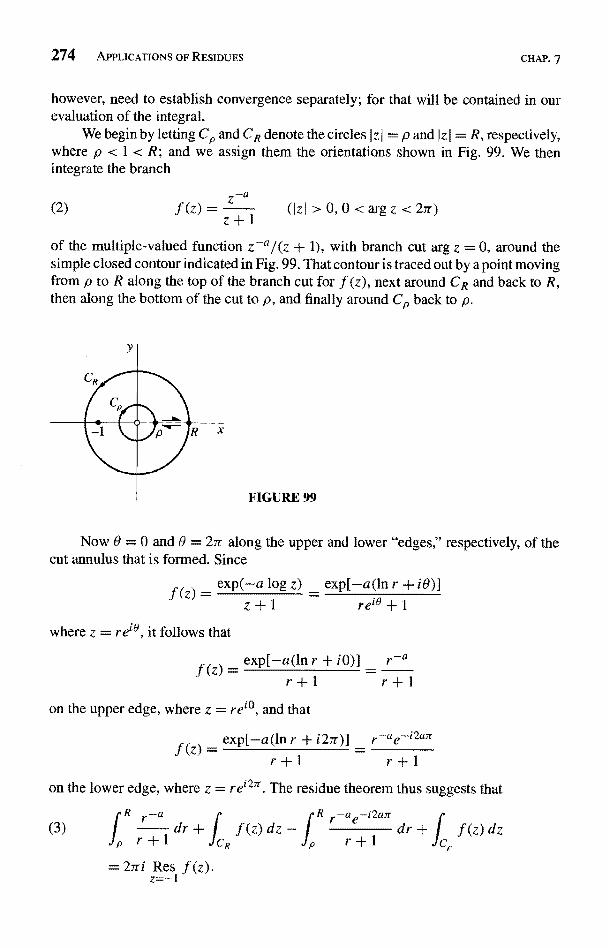
274 APPLICATIONS OF RESIDUES CHAP. 7
however, need to establish convergence separately; for that will be contained in ourevaluation of the integral.
We begin by letting C. and CR denote the circles lz I = p and Jz ( = R, respectively,where p < 1 < R; and we assign them the orientations shown in Fig. 99. We thenintegrate the branch
(2)f(z) z + 1
{Iz > 0, 0 < arg z < 27r)
of the multiple-valued function z-'/(z + 1), with branch cut arg z = 0, around thesimple closed contour indicated in Fig. 99. That contour is traced out by a point movingfrom p to R along the top of the branch cut for f (z), next around CR and back to R,then along the bottom of the cut to p, and finally around C,, back to p.
FIGURE 99
Now 9 = 0 and 9 = 27c along the upper and lower "edges," respectively, of thecut annulus that is formed. Since
exp(-a log z) = exp[-a(ln r + iBz+l rei$+1
where z = rein, it follows that
,f (z) =exp[-a(ln r + i0)] _ r
r+1on the upper edge, where z = reie, and that
r+l
exp[-a(ln r + i27r)] = r-ae-i2anf(z)r+1 r+l
]
on the lower edge, where z = rein. The residue theorem thus suggests that
R -a e_i2anrdr + I .f (z) dz - I d r + I .f (z) dzr + 1
= 27r Res f (z).Z=- I
SEC. 77 INTEGRATION ALONG A BRANCH CUT 275
Our derivation of equation (3) is, of course, only formal since f (z) is not analytic,or even defined, on the branch cut involved. It is, nevertheless, valid and can be fullyjustified by an argument such as the one in Exercise 8.
The residue in equation (3) can be found by noting that the function
0(z) = z-a = exp(-a log z) = exp[-a(ln r + i8)] (r > 0, 0 < 0 < 27r)
is analytic at z = -1 and that
= exp[-a(ln -Lair 0
This shows that the point z = -1 is a simple pole of the function f (z), defined byequation (2), and that
Res f (zz=- I
Equation (3) can, therefore, be written as
n -ar-i2an) J dr = 2 ie-ion - JC f (z) dz - J f (z) dz.P r+ 1p CR
Referring now to definition (2) of f (z), we see that
ff(z)dz 27r I,_ -a< 1- p27rp = I - pp
and
ICR< R-a 27rR =
27rR I
R-1 R-I RSince 0 < a < 1, the values of these two integrals evidently tend to 0 as p and R tendto 0 and oo, respectively. Hence, if we let p tend to 0 and then R tend to 00 in equation(4), we arrive at the result
l - e
or
dr = 27ri2i
r + I I- e-i2a7r eian eian - e-ion
This is, of course, the same as
r-a
I
dr = 27rie '-
00 x-a7r
(5) dx = 0 < afo x+1 sin air
276 APPLICATIONS OF RESIDUES
EXERCISES
In Exercises 1 through 4, take the indented contour in Fig. 97 (Sec. 75).
1. Derive the integration formula
°C cos(ax) - cos(bx) 7x2
dx= 1(b-a) (a>0,b>0).
CHAP. 7
Then, with the aid of the trigonometric identity 1- cos(2x) = 2 sine x, point out how itfollows that
2. Evaluate the improper integral
00
a
xadx, where - 1 < a < 3 and x' = exp(a In x2 + 1)2
Ans.(1-a)7r
4 cos(an/2)3. Use the function
z1/3 log z e(1/3) log z logZ
f (Z) z2+1 Z2+1
to derive this pair of integration formulas:
Jo
4. Use the function
to show that
f (Z)(log Z)2
f°° (In X)2
Jo x2+1dx =
argz< -
Suggestion: The integration formula obtained in Exercise 1, Sec. 72, is needed here.
5. Use the function
.f (z) =e(1/3) log z
(z+a)(z+b) (z+a)(z+b)
(zr >0,-2 <argz
(Izl>0,0<argz<27r)
and a closed contour similar to the one in Fig. 99 (Sec. 77) to show formally that
3x27e sa-
dx (a>b>0)-b) a - b
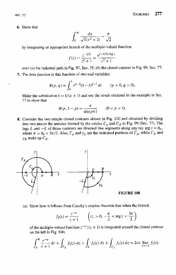
SEC. 77
6. Show that
ExrizcisEs 277
by integrating an appropriate branch of the multiple-valued function
z-1'2 e(-112)logz.f (z)
z2 + 1 z2 + 1
over (a) the indented path in Fig. 97, Sec. 75; (b) the closed contour in Fig. 99, Sec. 77.
7. The beta function is this function of two real variables:
0
Make the substitution t = 1/(x + 1) and use the result obtained in the example in See.77 to show that
B(p,l-p)= n (0<p<l).sin(p.Tr )
8. Consider the two simple closed contours shown in Fig. 100 and obtained by dividinginto two pieces the annulus formed by the circles Cp and CR in Fig. 99 (Sec. 77). Thelegs L and -L of those contours are directed line segments along any ray arg z = 80 ,where 7r < 00 < 37r/2. Also, FF and y,, are the indicated portions of C., while 1'R andYR make up CR.
FIGURE 100
(a) Show how it follows from Cauchy's residue theorem that when the branch
ft (Z) =z+ 1
2<argz<
2
of the multiple-valued function z-'/(z + 1) is integrated around the closed contouron the left in Fig. 100,
fl(z)dz=2ri Res fi(z).dr+I
fl(z)dz+I fl(z)dz+J
B(p, q) = ItP-1(1 - t)q-1dt (p > 0, q > 0).
fr+1 rA L r z=-l
z-d
278 APPLICATIONS OF RESIDUES
(b) Apply the Cauchy-Goursat theorem to the branch
5Z7r.f2(z)
+_Q
1(IzI>o4<argz<--)
of z`'/(z + 1), integrated around the closed contour on the right in Fig. 100, to showthat
z) dz - j f2 (z) dz + 2(z)dz=0.
Point out why, in the last lines in parts (a) and (b), the branches fl(z) and f2(z) ofz-a/(z + 1) can be replaced by the branch
,f(z)=z+1 (Izl>0,0<argz<2ar).
Then, by adding corresponding sides of those two lines, derive equation (3), Sec.77, which was obtained only formally there.
78. DEFINITE INTEGRALS INVOLVING SINES AND COSINES
The method of residues is also useful in evaluating certain definite integrals of the type
(1)
z=e`° (0<8<2r).
The fact that 0 varies from 0 to 2zr suggests that we consider 0 as an argument of apoint z on the circle C centered at the origin. Hence we write
(2)
Formally, then,
dz = ie`6 d8 = iz d8;
and the relations
z - z-` z+z_1 dz
2i
F(sin B, cos 8) d8.
cos8= , d8=-2 iz
enable us to transform integral (1) into the contour integral
- z-1 z + Z-1 dz
c \. 2i 2 iz
of a function of z around the circle C in the positive direction. The original integral (1)is, of course, simply a parametric form of integral (4), in accordance with expression(2), Sec. 39. When the integrand of integral (4) is a rational function of z, we can
SEC. 78 DEFINITE INTEGRALS INVOLVING SINES AND COSINES 279
evaluate that integral by means of Cauchy's residue theorem once the zeros of thepolynomial in the denominator have been located and provided that none lie on C.
EXAMPLE. Let us show that2" ds _ 2rr 1<a
0 1- -asin9 1-a2(-
This integration formula is clearly valid when a = 0, and we exclude that case in ourderivation. With substitutions (3), the integral takes the form
(6)(2ija)z - 1
where C is the positively oriented circle I z I = 1. The quadratic formula reveals that thedenominator of the integrand here has the pure imaginary zeros
So if f (z) denotes the integrand, then
f(z)
Note that, because la I < 1,
2/a
1+V-a2 > LIz21=lal
Also, since Iz1z2I = 1, it follows that Iz11 < 1. Hence there are no singular points on C,and the only one interior to it is the point z1. The corresponding residue B1 is foundby writing
.f (z) =0(z) where
z-z1This shows that z1 is a simple pole and that
Consequently,
0 (z
2/a 1
2/a dz=22riB1=(2i/a)z - I
2/az-Z2
27r
and integration formula (5) follows.
280 APPLICATIONS OF RESIDUES CHAP. 7
The method just illustrated applies equally well when the arguments of the sineand cosine are integral multiples of 0. One can use equation (2) to write, for example,
cos 20 =2
e i20
2
-2 z2 + z-22
EXERCISES
Use residues to evaluate the definite integrals in Exercises 1 through 7.
1.rzn d8
JJ0 5+4sin0'
Ans.2,,r
.
Ans. -,/2-7r.
c2n cost 38 d8,l0 5-4cos20
Ans.37r
.
I:;
dB
Ans.
1+a cos6
2,,r
Ans.an
(-1<a
7. I sin2n 6 d8 (n = 1, 2, ..
Am-(2n
22n (n!)
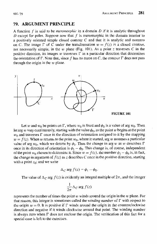
SEC. 79 ARGUMENT PRINCIPLE 281
79. ARGUMENT PRINCIPLEA function f is said to be meromorphic in a domain D if it is analytic throughoutD except for poles. Suppose now that f is meromorphic in the domain interior toa positively oriented simple closed contour C and that it is analytic and nonzeroon C. The image F of C under the transformation w = f (z) is a closed contour,not necessarily simple, in the w plane (Fig. 101). As a point z traverses C in thepositive direction, its images w traverses I' in a particular direction that determinesthe orientation of F. Note that, since f has no zeros on C, the contour F does not passthrough the origin in the w plane.
FIGURE 101
Let w and w0 be points on F, where wo is fixed and 00 is a value of arg w0. Thenlet arg w vary continuously, starting with the value 00, as the point w begins at the pointwo and traverses F once in the direction of orientation assigned to it by the mappingw = f (z). When w returns to the point wo, where it started, arg w assumes a particularvalue of arg wo, which we denote by 01. Thus the change in arg u) as w describes I'once in its direction of orientation is 01 - 00. This change is, of course, independentof the point wo chosen to determine it. Since w = f (z), the number 01 - 00 is, in fact,the change in argument of f (z) as z describes C once in the positive direction, startingwith a point z0; and we write
AC arg f(z)=0I-oho.
The value of A arg f (z) is evidently an integral multiple of 2,7, and the integer
1
27rAC arg f (z)
represents the number of times the point w winds around the origin in the w plane. Forthat reason, this integer is sometimes called the winding number of F with respect tothe origin w = 0. It is positive if F winds around the origin in the counterclockwisedirection and negative if it winds clockwise around that point. The winding numberis always zero when F does not enclose the origin. The verification of this fact for aspecial case is left to the exercises.
282 APPLICATIONS OF RESIDUES CHAP. 7
The winding number can be determined from the number of zeros and poles off interior to C. The number of poles is necessarily finite, according to Exercise 11,Sec. 69. Likewise, with the understanding that f (z) is not identically equal to zeroeverywhere else inside C, it is easily shown (Exercise 4, Sec. 80) that the zeros of fare finite in number and are all of finite order. Suppose now that f has Z zeros and Ppoles in the domain interior to C. We agree that f has mo zeros at a point zo if it has azero of order mo there; and if f has a pole of order mp at zo, that pole is to be countedmp times. The following theorem, which is known as the argument principle, statesthat the winding number is simply the difference Z - P.
Theorem. Suppose that(i) a function f (z) is meromorphic in the domain interior to a positively oriented
simple closed contour C;z) is analytic and nonzero on C;
counting multiplicities, Z is the number of zeros and P is the number of poles off (z) inside C.
Then
(1) - cargf(z)=Z-P.2,7
To prove this, we evaluate the integral of f'(z) jf (z) around C in two differentways. First, we let z = z(t) (a -< t -< b) be a parametric representation for C, so that
f f'(z) dz = [b f'[z(t)]z'(t) dt.C f (z) a f [z (t)]
Since, under the transformation w = f (z), the image r of C never passes throughthe origin in the w plane, the image of any point z = z(t) on C can be expressed inexponential form as w =,o(t) exp[io (t)]. Thus
(3) f [z(t)] = p(t)eio(t) (a < t < b);
and, along each of the smooth arcs making up the contour r, it follows that (seeExercise 5, Sec. 38)
io(t)(Pf(t)
Inasmuch as p(t) and 0'(t) are piecewise continuous on the interval a < t < b, wecan now use expressions (3) and (4) to write integral (2) as follows:
dt + i 1 (P'(t)dt=lnp(t)I +i(p(t)
SEC. 79 ARGUMENT PRINCIPLE
But
p(b)=p(a) and O(b)-O(a)=Acarg f(
Hence
(5)
f(z)=(z-zo
Another way to evaluate integral (5) is to use Cauchy's residue theorem. To bespecific, we observe that the integrand f'(z) jf (z) is analytic inside and on C exceptat the points inside C at which the zeros and poles of f occur. If f has a zero of ordermo at zo, then (Sec. 68)
(6)
where g(z) is analytic and nonzero at zo. Hence
f`(zo) = mo(z - zo)mo_lg(z) + (z - zo)m°g
(7)
=iAcarg
mo
+g'(z}
f (z) z - zo g (z)
Since g(z)1g(z) is analytic at zo, it has a Taylor series representation about that point;and so equation (7) tells us that f'(z) jf (z) has a simple pole at zo, with residue mo.If, on the other hand, f has a pole of order mp at zo, we know from the theorem inSec. 66 that
(8) f(z) = (z - zo)
where /(z) is analytic and nonzero at zo. Because expression (8) has the same formas expression (6), with the positive integer mo in equation (6) replaced by -m p, it isclear from equation (7) that f'(z) jf (z) has a simple pole at zo, with residue -m p.Applying the residue theorem, then, we find that
(z )f' dz = 27ri(Z - P).(9) f f(zc }
Expression (1) now follows by equating the right-hand sides of equations (5) and (9).
EXAMPLE. The only singularity of the function 1/z2 is a pole of order 2 at theorigin, and there are no zeros in the finite plane. In particular, this function is analyticand nonzero on the unit circle z - eis(0 < 0 < 2ir). If we let C denote that positivelyoriented circle, our theorem tells us that
284 APPLICATIONS OF RESIDUES CHAP. 7
That is, the image P of C under the transformation w = 1/z2 winds around the originw = 0 twice in the clockwise direction. This can be verified directly by noting that Phas the parametric representation w = e_z 20 (0 < 9 < 17).
f80. ROUCHE'S THEOREM
The main result in this section is known as Rouche's theorem and is a consequence ofthe argument principle, just developed in Sec. 79. It can be useful in locating regionsof the complex plane in which a given analytic function has zeros.
Theorem. Suppose that(i) two functions f (z) and g (z) are analytic inside and on a simple closed contour C;
(ii) I f (z) I > Ig(z) I at each point on C.Then f (z) and f (z) + g(z) have the same number of zeros, counting multiplicities,inside C.
The orientation of C in the statement of the theorem is evidently immaterial.Thus, in the proof here, we may assume that the orientation is positive. We begin withthe observation that neither the function f (z) nor the sum f (z) + g(z) has a zero onC, since
If(z)I > Ig(z) and f(z)+g(z)I >_ 11f W1 - Ig(z)II >
when z is on C.if Z f and Z f+g denote the number of zeros, counting multiplicities, of f (z) and
f (z) + g(z), respectively, inside C, we know from the theorem in Sec. 79 that
27rbeargf(z) and Zf+g IACarg[f(z)+g(z)].
2
Consequently, since
AC arg[f (z) + g
Z f+g
F(z) = 1
= Ac argS.f(z) 1+ g(z)
f(z) I
=ACar'gf(z)+Acarg
arg F(z),
1 + g(z)f (z)
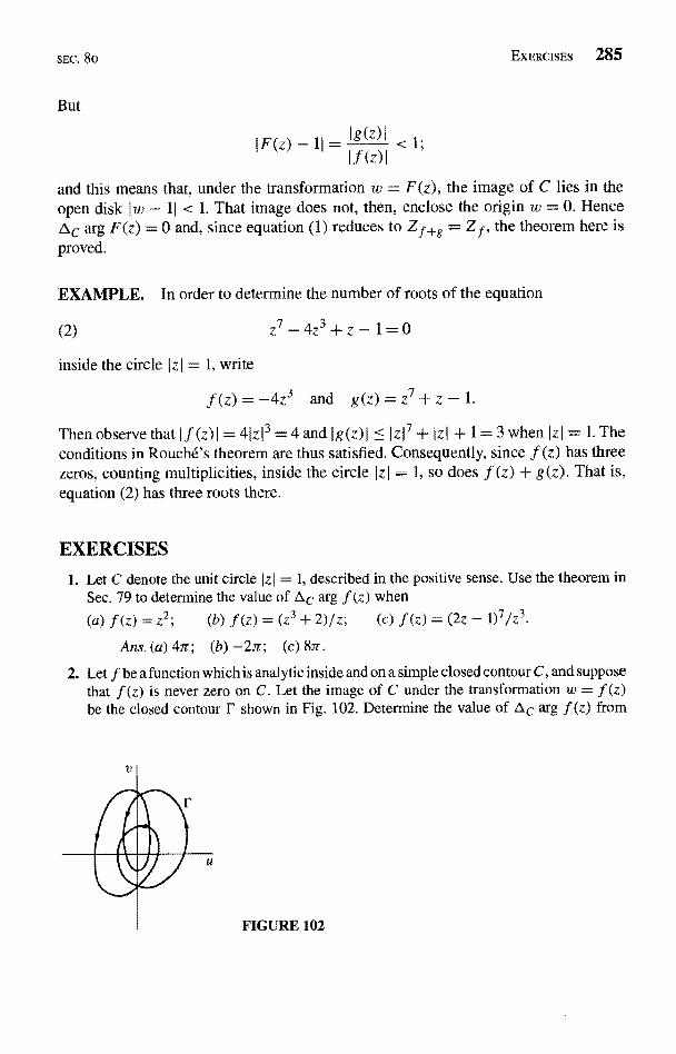
SEC. 80
But
Ig(z)IIFO - _
EXERCISES 285
and this means that, under the transformation w = F(z), the image of C lies in theopen disk I w - 1I < 1. That image does not, then, enclose the origin w = 0. HenceAC arg F(z) = 0 and, since equation (1) reduces to Z f+g = Z f, the theorem here isproved.
EXAMPLE. In order to determine the number of roots of the equation
(2)
inside the circle I z I = 1, write
z7-4z3+z-1=0
f (z) = -4z3 and g(z) = z7 + z - I.
Then observe that I f (z) I = 41z 13 = 4 and Ig{z}I < Iz17 + Izl + 1= 3 when Izl = 1. Theconditions in Rouche's theorem are thus satisfied. Consequently, since f (z) has threezeros, counting multiplicities, inside the circle zI = 1, so does f (z) + g(z). That is,equation (2) has three roots there.
EXERCISES1. Let C denote the unit circle Iz = 1, described in the positive sense. Use the theorem in
Sec. 79 to determine the value of i arg f (z) when
(a) f (z) = z2; (b) f (Z) = (z3 + 2)/z; (c) f (z) = (2z -
Ans. (a) 47e; (b) -27e; (c) 8n.
2. Let f be a function which is analytic inside and on a simple closed contour C, and supposethat f (z) is never zero on C. Let the image of C under the transformation w = f (z)be the closed contour r shown in Fig. 102. Determine the value of i arg f (z) from
FIGURE 102
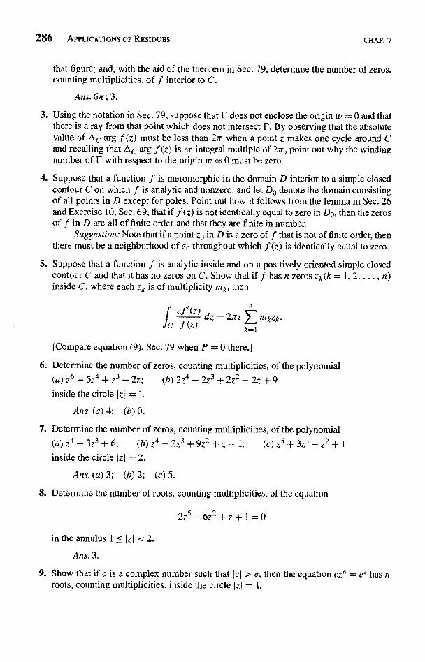
286 APPLICATIONS OF RESIDUES CHAP. 7
that figure; and, with the aid of the theorem in Sec. 79, determine the number of zeros,counting multiplicities, of f interior to C.
Arts. 6ir; 3.
3. Using the notation in Sec. 79, suppose that U' does not enclose the origin w = 0 and thatthere is a ray from that point which does not intersect P. By observing that the absolutevalue of AC arg f (z) must be less than 2ir when a point z makes one cycle around Cand recalling that AC arg f (z) is an integral multiple of 2ir, point out why the windingnumber of r with respect to the origin w = 0 must be zero.
4. Suppose that a function f is meromorphic in the domain D interior to a simple closedcontour C on which f is analytic and nonzero, and let Do denote the domain consistingof all points in D except for poles. Point out how it follows from the lemma in Sec. 26and Exercise 10, Sec. 69, that if f (z) is not identically equal to zero in Do, then the zerosof f in D are all of finite order and that they are finite in number.
Suggestion: Note that if a point zo in D is a zero off that is not of finite order, thenthere must be a neighborhood of zo throughout which f (z) is identically equal to zero.
5. Suppose that a function f is analytic inside and on a positively oriented simple closedcontour C and that it has no zeros on C. Show that if f has n zeros zk(k = 1, 2, . . . , n)inside C, where each Zk is of multiplicity Mk, then
'(7
c f(z)dz=2ir
k=
[Compare equation (9), Sec. 79 when P = 0 there.]
kzk
6. Determine the number of zeros, counting multiplicities, of the polynomial
(a) z6 - 5z4 + z3 - 2z; (b) 2z4 - 2z3 + 2z2 - 2z + 9inside the circle I z I = 1.
Ans. (a) 4; (b) 0.
7. Determine the number of zeros, counting multiplicities, of the polynomial
(a) z4 + 3z3 + 6; (b) z4 - 2z3 + 9z2 + z - 1; (c) z5 + 3z3 + z2 + 1inside the circle I zI = 2.
Ans. (a) 3; (b) 2; (c) 5.
8. Determine the number of roots, counting multiplicities, of the equation
2z5-6z2+z+1=0
in the annulus 1 < IzI < 2.
Ans. 3.
9. Show that if c is a complex number such that Icl > e, then the equation cz' = ez has nroots, counting multiplicities, inside the circle Izl = 1.
SEC. 8o EXERCISES 287
10. Write f (z) = zn and g(z) = ao + a1z + + an_Izn-1 and use Rouche's theorem toprove that any polynomial
P(z) = ao + a1z + ... + an-1Zn-1 + anzn (an A 0),
where n > 1, has precisely n zeros, counting multiplicities. Thus give an alternative proofof the fundamental theorem of algebra (Theorem 2, Sec. 49).
Suggestion: Note that one can let a be unity. Then show that I g (z) I < I f (z) I onthe circle Izl = R, where R is sufficiently large and, in particular, larger than
I + gaol + Ia1] + ... + ]an-1l.
11. Inequalities (5), Sec. 49, ensure that the zeros of a polynomial
P(z) = ao + a1z + ... + ar_1zn-I + anzn (a, A 0)
of degree n > I all lie inside some circle Iz I = R about the origin. Also, Exercise 4 abovetells us that they are all of finite order and that there is a finite number N of them. Useexpression (9), Sec. 79, and the theorem in Sec. 64 to show that
N=Res P'(1/z)z=O
z2P(l/z),
where multiplicities of the zeros are to be counted. Then evaluate this residue to showthat N = n. (Compare Exercise 10.)
12. Let two functions f and g be as in the statement of Rouche's theorem in Sec. 80, and letthe orientation of the contour C there be positive, Then define the function
q> (t) = 1
C
f'(z) +tg'(z) dz (0 <27t'i f (z) + tg(z)
and follow the steps below to give another proof of Rouche's theorem.
(a) Point out why the denominator in the integrand of the integral defining 4) (t) is neverzero on C. This ensures the existence of the integral.
(b) Let t and to be any two points in the interval 0 < t < 1 and show that
It-tolI (t)-C(to)l=
Then, after pointing out why
2'r Jfg' - f'g
(f + tg)(f + tog) dz
fg' - f'gf + tg)(f + tog)
at points on C, show that there is a positive constant A, which is independent of tand to, such that
Ic1(t) - (to)I < Alt - toy.
Conclude from this inequality that (D (t) is continuous on the interval 0 < t <
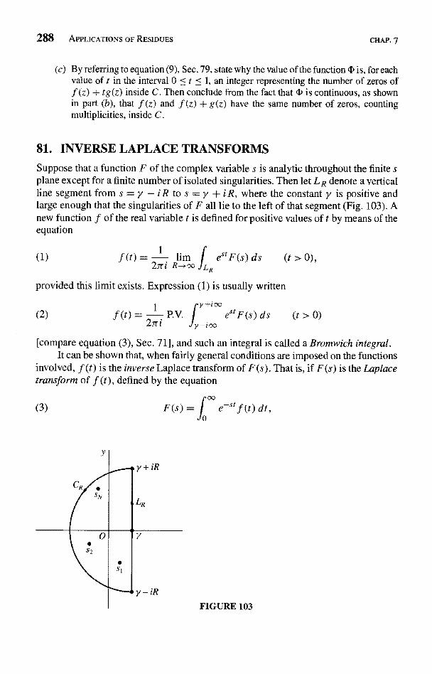
288 APPLICATIONS OF RESIDUES CHAP. 7
(c) By referring to equation (9), Sec. 79, state why the value of the function c is, for eachvalue of t in the interval 0 < t < 1, an integer representing the number of zeros off (z) + tg(z) inside C. Then conclude from the fact that D is continuous, as shownin part (b), that f (z) and f (z) + g(z) have the same number of zeros, countingmultiplicities, inside C.
81. INVERSE LAPLACE TRANSFORMS
Suppose that a function F of the complex variable s is analytic throughout the finite splane except for a finite number of isolated singularities. Then let LR denote a verticalline segment from s = y - iR to s = y + iR, where the constant y is positive andlarge enough that the singularities of F all lie to the left of that segment (Fig. 103). Anew function f of the real variable t is defined for positive values of t by means of theequation
(1) f(t)= lim estF(s) ds2rri R
provided this limit exists. Expression (1) is usually written
y+iooP.V. i estF(s) ds (t > 0)(2) f (t) = -f i
[compare equation (3), Sec. 71], and such an integral is called a Bromwich integral.It can be shown that, when fairly general conditions are imposed on the functions
involved, f (t) is the inverse Laplace transform of F(s). That is, if F(s) is the Laplacetransform of f (t), defined by the equation
F(s) = / e_st f(t) dt,
FIGURE 103
SEC. 81 INVERSE LAPLACE TRANSFORMS 289
then f (t) is retrieved by means of equation (2), where the choice of the positivenumber y is immaterial as long as the singularities of F all lie to the left of LR.*Laplace transforms and their inverses are important in solving both ordinary and partialdifferential equations.
Residues can often be used to evaluate the limit in expression (1) when thefunction F(s) is specified. To see how this is done, we let sn (n = 1, 2, . . . , N) denotethe singularities of F(s). We then let Ro denote the largest of their moduli and considera semicircle CR with parametric representation
(4) s=y -} Reio
where R > Ro + y. Note that, for each s, ,
Is,, -yI <Isnl+y <Ro+y <R.
Hence the singularities all lie in the interior of the semicircular region bounded by CRand LR (see Fig. 103), and Cauchy's residue theorem tells us that
(5) j eStF(s) ds = 27ri Res[es'F(s)] - L eStF(s) ds.R n=1
Suppose now that, for all points s on CR, there is a positive constant MR such thatI F(s) I < MR, where MR tends to zero as R tends to infinity. We may use the parametricrepresentation (4) for CR to write
ICR
3rr/2es'F(s) ds = / exp(yt + Rte
Then, since
lexp(yt + Rte
we find that
(6)
IC
2
F(y + Re`9)Rie'8 d8.
= eyteRtcos9 and JF(y + Re`s)) <
eS'F(s) ds
N
< eytMRR eRtcos0 dB.
* For an extensive treatment of such details regarding Laplace transforms, see R. V. Churchill, "Opera-tional Mathematics," 3d ed., 1972, where transforms F(s) with an infinite number of isolated singularpoints, or with branch cuts, are also discussed.
290 APPLICATIONS OF RESIDUES CHAP. 7
But the substitutionreveals that
2
2), together with Jordan's inequality (2), Sec. 74,
eRt cos 8 d9 _ I e-Rt sinRt
Inequality (6) thus becomes
(7)
and this shows that
(8)
.SCR
tF eYt MRYr
t
lim I e" F (s) ds = 0.A-+DQ tr
Letting R tend to co in equation (5), then, we see that the function f (t), defined byequation (1), exists and that it can be written
(9) f (t) =) : Res[e'F(s)] (t > 0n=1
s=sn
In many applications of Laplace transforms, such as the solution of partial differ-ential equations arising in studies of heat conduction and mechanical vibrations, thefunction F(s) is analytic for all values of s in the finite plane except for an infiniteset of isolated singular points sn (n = 1, 2, . . .) that lie to the left of some vertical lineRe s = y. Often the method just described for finding f (t) can then be modified insuch a way that the finite sum (9) is replaced by an infinite series of residues:
(10) f (t) = ) ' Res[e$tF(sn=
S=sn
The basic modification is to replace the vertical line segments LR by vertical linesegments LN (N = 1, 2, ...) from s = y -ibN to s = y + ibN. The circular arcs CRare then replaced by contours CN (N = 1, 2, ...) from y + ibN to y - ibN such that,for each N, the sum LN + CN is a simple closed contour enclosing the singular pointsS1, s2, ... , sN. Once it is shown that
(11) lim I estF(s) ds =N-+
expression (2) for f (t) becomes expression (10).The choice of the contours CN depends on the nature of the function F(s).
Common choices include circular or parabolic arcs and rectangular paths. Also, thesimple closed contour LN + CN need not enclose precisely N singularities. When, forexample, the region between LN + CN and LN+1 + CN+1 contains two singular points
SEC. 82 EXAMPLES 291
of F(s), the pair of corresponding residues of est F (s) are simply grouped together asa single term in series (10). Since it is often quite tedious to establish limit (11) in anycase, we shall accept it in the examples and related exercises below that involve aninfinite number of singularities.* Thus our use of expression (10) will be only formal.
82. EXAMPLESCalculation of the sums of the residues of est F(s) in expressions (9) and (10), Sec. 81,is often facilitated by techniques developed in Exercises 12 and 13 of this section. Wepreface our examples here with a statement of those techniques.
Suppose that F(s) has a pole of order m at a point se and that its Laurent seriesrepresentation in a punctured disk 0 < Is - sad < R2 has principal part
bm
Then
s0)m(bm V).
When the pole so is of the form sty = a + if3 (f 0 0) and F(s) = F(Ts) at points ofanalyticity of F(s) (see See. 27), the conjugate To = a - if3 is also a pole of order in.Moreover,
(2)
Res[estF(s)] + Res[estF(s)]s=SO s=so
= 2e" Re{etft [b1 + l'2t +1!
when t is real. Note that if so is a simple pole (m = 1), expressions (1) and (2) become
Res[estF(s)] = eSOt Res F(s)s=so s=so
(4)
respectively.
Res[estF(s)] + Res[eslF(s)] = teat Res=sp S=S')
e`Ot Res F(ss=so
I
* An extensive treatment of ways to obtain limit (11) appears in the book by R. V. Churchill that is citedin the footnote earlier in this section. In fact, the inverse transform to be found in Example 3 in the nextsection is fully verified on pp. 220-226 of that book.
292 APPLICATIONS OF RESIDUES CHAP. 7
EXAMPLE 1. Let us find the function f (t) that corresponds to
(5) F(s) -- s
The singularities of F(s) are the conjugate points
Upon writing
Fs + ai)2
we see that ¢ (s) is analytic and nonzero at so = a i. Hence se is a pole of order m = 2of F(s). Furthermore, F(s) = F() at points where F(s) is analytic, Consequently, TOis also a pole of order 2 of F(s); and we know from expression (2) that
(6) Res[es'F(s)] + Res[estF(s)] = 2 Re[e`at(bi + b2t)],S=SO s-Sp
where bI and b2 are the coefficients in the principal part
b, + b2
s - ai (s - ai)2
of F(s) at a i. These coefficients are readily found with the aid of the first two termsin the Taylor series for 0(s) about so = ai:
F (s
q (a(s - ai)2
s
0 < Is -ail < 2a).
It is straightforward to show that 0(ai) = -i/(4a) and 0'(ai) = 0, and we find thatbI = 0 and b2 = -i /(4a). Hence expression (6) becomes
Res[es(F(s)] + Res[estF(s)] = 2 Res=Sp s=SO
We can, then, conclude that
(7)
> 0).
se = ai and To = -ai.
f(t)=2a
1tsin at
eia l-t = --t sin at.a 2a
provided that F(s) satisfies the boundedness condition stated in italics in Sec. 81.To verify that boundedness condition, we let s be any point on the semicircle
Y Re`037r
2 1'
SEC. 82
where y > 0 and R > a + y; and we note that
Is=ly+Re`al<y+RSince
it follows that
IF(s)I =
and Re
where
Vy
y+R[(R - y)2 -
a2]2.
The desired boundedness condition is now established, since MR -* 0 as R
EXAMPLE 2. In order to find f (t) when
F(s) =tanh s sinh s
s2 cosh s'
we note that F(s) has isolated singularities at s = 0 and at the zeros (Sec. 34)
(n=0,+1,±2,.
of cosh s. We list those singularities as
(2n -and sn =
Then, formally,
2
(8) f (t) = Res[estF(s)] + Res[estF(s)] + Res[eS`F(S-So S=Sn S=Snn=
Division of Maclaurin series yields the Laurent series representation
F
which tells us that so = 0 is a simple pole of F(s), with residue unity. Thus
(9) Res[e''tF(s)]= Res F(s) = 1,s=so s=so
EXAMPLES 293
a.
according to expression (3).The residues of F (s) at the points sn (n = 1, 2, ...) are readily found by applying
the method of Theorem 2 in Sec. 69 for identifying simple poles and determining the
294 APPLICATIONS OF RESIDUES
residues at such points. To be specific, we write
F(s) = p(s) where p(s) = sinh s and q(s) = s2 cosh sq (s)
and observe that
sinh sn = sinh Ii ( nit
Then, since
p(sn) = sinh sn 0 0,
we find that
= i sin( nit -
q
i cos nit = n
and q'(sn) = sn sinh sn ; 0,
Res F(s) = p(sn) 1 4 . 1
S=Sn q'(sn)_
sn it (2n -
Compare Example 3 in Sec. 69.] The identities
sinh s = sinh s and cosh s = cosh s
,2
CHAP. 7
(see Exercise 11, Sec. 34) ensure that F(s) = F(s) at points of analyticity of F(s).Hence sn is also a simple pole of F(s), and expression (4) can be used to write
Res [estF(s)] + Res [esiF(s)]n
(10)7r2
1cos
(2n -2
Finally, by substituting expressions (9) and (10) into equation (8), we arrive atthe desired result:
1 (2n -cos-
n=1it2 L1 (2n - 1)z 2
EXAMPLE 3. We consider here the function
2)(Sinh (xs 1/2)
F(s) =s sinh(s1/2)
(0 <x
SEC. 82 EXAMPLES 295
where s1/2 denotes any branch of this double-valued function. We agree, however, touse the same branch in the numerator and denominator, so that
(13) F(s) _xs1/2 + (xs1/2)3/3! + .. .s[s1/2 + (51/2)3/3! + . . s+s2/6+...
when s is not a singular point of F(s). One such singular point is clearly s = 0. Withthe additional agreement that the branch cut of s 1/2 does not lie along the negative realaxis, so that sinh(s1/2) is well defined along that axis, the other singular points occurif s1/2 = ±nrri (n = 1, 2, ...). The points
so = 0 and sn = -n`rr` (n = 1, 2, ...)
thus constitute the set of singular points of F(s). The problem is now to evaluate theresidues in the formal series representation
(14) f (t) = Res[estF(s)] + Y. Res[estF(S=Sp S =Sn
n=1
Division of the power series on the far right in expression (13) reveals that so isa simple pole of F(s), with residue x. So expression (3) tells us that
(15) Res[esr F(S =SO
As for the residues of F(s) at the singular points s,write
, 2, ...), we
F(s) = P(s) where, p(s) = sinh(xs1/2) and q (s) = s sinh(sq
{s
Appealing to Theorem 2 in Sec. 69, as we did in Example 2, we note that
p(sn) = sinh(xs r`) ; 0, q(sn) = 0, and q'(sn) = _s 1/2 cosh
and this tells us that each sn is a simple pole of F(s), with residue
p{sn} 2Res F(s) =s=sn q (sn
So, in view of expression (3),
rr n
(16) Res[es`F(s)] = esnr Res F(s) =S=sn S=Sn It n
n
sin nirx.
Substituting expressions (15) and (16) into equation (14), we arrive at the function
(17) sin nrrx (t > 0).
296 APPLICATIONS OF RESIDUES CHAP. 7
EXERCISES
In Exercises 1 through 5, use the method described in See. 81 and illustrated in Example1, Sec. 82, to find the function f (t) corresponding to the given function F(s).
41. F(s) = S4.s3
2. F(s) =
3. F
Ans. f (t) = cosh 12-t + cos 12-t.
2s-2
Ans. f (t) = e-t(sin 2t + cos 2t - 1).
(s+1)(s2+2s+5)
12
S3+8
Ans. f (t) = sin J3 - Cos 13-t).
4. F(s)S2 -a2
_ (a > 0).(2 + a2)2
Ans. f (t) = t cos at.
a's8 _ ,(a > 0).5. F(s) =
Suggestion: Refer to Exercise 4, Sec. 65, for the principal part of F(s) at ai.
Ans. f (t) _ (1 + a2t2) sin at - at cos at.
In Exercises 6 through 11, use the formal method, involving an infinite series of residuesand illustrated in Examples 2 and 3 in Sec. 82, to find the function f (t) that correspondsto the given function F(s).
6. F(s) -sinh(xs)
(O < x <S2 cosh s
1) .
Ans. f (t) =
Ans.
2n - 1)Trx (2cos -2 2
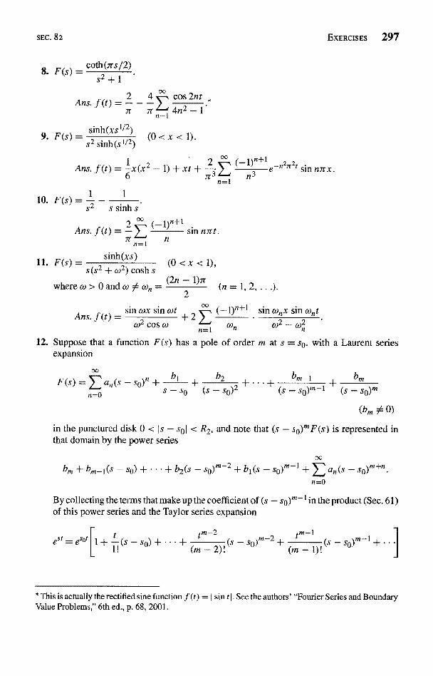
SEC. 82
8. F(s) =coth(7rs/2
2s
9. F (s
10. F (s
Ans. f (t)
sinh(xs 1/2)
s2 sinh(s 20<x<1).
Ans, f (t) = 1 X(x2 - 1) + xt
1 1
1) +isin n7rt.
n
Fsinh(xs)
s2 + w2) cosh s(0 < x < 1),
(2n 1}7rwhere w > 0 and cU 54 w n = (n = 1, 2, ...).
2
Ans. f(t)sin wx stn cut
+2_W2 Cos w
n=1
EXERCISES 297
Sin n7rx.
12. Suppose that a function F(s) has a pole of order m at s = so, with a Laurent seriesexpansion
F(s)_La,(s-so)nn=O
bi + b2
s-so (s - ibm-1 bm
so)m-
(bm 54 0)
in the punctured disk 0 < is - sod < R2, and note that (s - so)mF(s) is represented inthat domain by the power series
bm-i(s -so) +...+b2(s -so)'-L+b1(s---
n
By collecting the terms that makeup the coefficient of (s - so)'-' in the product (Sec. 61)of this power series and the Taylor series expansion
* This is actually the rectified sine function f (t) =I sin t I. See the authors' "Fourier Series and BoundaryValue Problems," 6th ed., p. 68, 2001.
298 APPLICATIONS OF RESIDUES
of the entire function est =
Res[est F(s)] _s=so
S. show that
bI+ bift+... tm-2 + bm tm-I(m - 1)!
CHAP, 7
as stated at the beginning of Sec. 82,
13. Let the point so = a + i,i (,B 54 0) be a pole of order m of a function F(s), which has aLaurent series representation
bb b 2 , -!- , , , + ,I + ,m (bm 0)F(s) = > , a,,(s - so)' +
n=0S-so 0
-so) M
in the punctured disk 0 < Is - so < R2. Also, assume that F (s) = F (-s) at points s whereF(s) is analytic.
(a) With the aid of the result in Exercise 6, Sec. 52, point out how it follows that
cc
n=0
b b2 bn I m-s0) +s-so+(s-so)2+...+(_-s
when 0 < 137 - sod < R2. Then replaces by s here to obtain a Laurent series repre-sentation for F(s) in the punctured disk 0 < Is - Sol < R2, and conclude that so is apole of order m of F(s).
(b) Use results in Exercise 12 and part (a) above to show that
Ress[est F(s)] + Res[eStF(s)] = 2e"t Re j [b1 + 1 t + ... + (mbm 1)! tm-a]In tt
when t is real, as stated at the beginning of Sec. 82.
14. Let F(s) be the function in Exercise 13, and write the nonzero coefficient bm there inexponential form as bm = rn exp(iOm). Then use the main result in part (b) of Exercise13 to show that when t is real, the sum of the residues of est F(s) at so = a + i,B (;8 54 0)and To contains a term of the type
2rm M-1 ate cos(f t + 6m).(m - 1) !
Note that if a > 0, the product tm-le«t here tends to oo as t tends to oo. When theinverse Laplace transform f (t) is found by summing the residues of eat F(s), the termdisplayed above is, therefore, an unstable component of f (t) if a > 0; and it is said tobe of resonance type. If m > 2 and a = 0, the term is also of resonance type.
CHAPTER
MAPPING BY ELEMENTARYFUNCTIONS
The geometric interpretation of a function of a complex variable as a mapping, ortransformation, was introduced in Secs. 12 and 13 (Chap. 2). We saw there how thenature of such a function can be displayed graphically, to some extent, by the mannerin which it maps certain curves and regions.
In this chapter, we shall see further examples of how various curves and regionsare mapped by elementary analytic functions. Applications of such results to physicalproblems are illustrated in Chaps. 10 and 11.
83. LINEAR TRANSFORMATIONS
To study the mapping
(1) w = Az,
where A is a nonzero complex constant and z A 0, we write A and z in exponentialform:
A = ae`a
Then
(2)
eio
and we see from equation (2) that transformation (1) expands or contracts the radiusvector representing z by the factor a = I A I and rotates it through an angle a = arg A
299
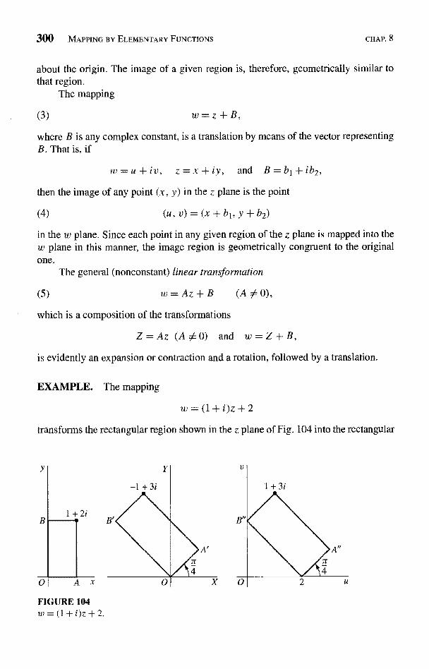
300 MAPPING BY ELEMENTARY FUNCTIONS CHAP. 8
about the origin. The image of a given region is, therefore, geometrically similar tothat region.
The mapping
(3) w=z+B,
where B is any complex constant, is a translation by means of the vector representingB. That is, if
iv, z=x+iy, and B=bl+ib2,
then the image of any point (x, y) in the z plane is the point
(4) (u, v) = (x + bt, y + b2)
in the w plane. Since each point in any given region of the z plane is mapped into thew plane in this manner, the image region is geometrically congruent to the originalone.
The general (nonconstant) linear transformation
(5) w=Az+B (A; 0),
which is a composition of the transformations
Z=Az (AA0) and w=Z+B,
is evidently an expansion or contraction and a rotation, followed by a translation.
EXAMPLE. The mapping
w=(1+i)z+2
transforms the rectangular region shown in the z plane of Fig. 104 into the rectangular
y
B1+2i
0
FIGURE 104w = (1+i)z+2.
SEC. 84 THE TRANSFORMATION W = llz 301
region shown in the w plane there. This is seen by writing it as a composition of thetransformations
Z=(1+i)z and w=Z+
Since 1+ i = exp(i 7r/4), the first of these transformations is an expansion by thefactor and a rotation through the angle 7r/4. The second is a translation two unitsto the right.
EXERCISES
1. State why the transformation w = iz is a rotation of the z plane through the angle 7r/2.Then find the image of the infinite strip 0 < x < 1.
Ans.0<v<1.
2. Show that the transformation w = iz + i maps the half plane x > 0 onto the half planev>1.
3. Find the region onto which the half plane y > 0 is mapped by the transformation
l+i)z
by using (a) polar coordinates; (b) rectangular coordinates. Sketch the region.
Ans. v>u.
4. Find the image of the half plane y > 1 under the transformation w = (1 - i)z.
5. Find the image of the semi-infinite strip x > 0, 0 < y < 2 when w = iz + 1. Sketch thestrip and its image.
Ans.-1<u< 1,v<0.
6. Give a geometric description of the transformation w = A(z + B), where A and B arecomplex constants and A 0.
84. THE TRANSFORMATION w = 1/z
The equation
(1)
establishes a one to one correspondence between the nonzero points of the z and thew planes. Since zz = Iz12, the mapping can be described by means of the successivetransformations
(2)
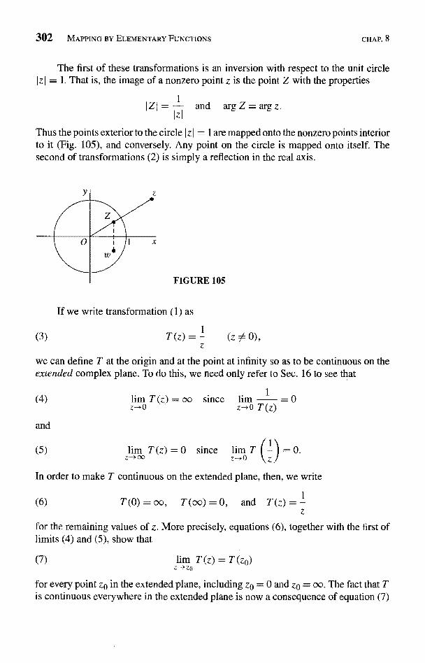
302 MAPPING BY ELEMENTARY FUNCTIONS CHAP. 8
The first of these transformations is an inversion with respect to the unit circleIz I = 1. That is, the image of a nonzero point z is the point Z with the properties
Iz
Thus the points exterior to the circle I z I = 1 are mapped onto the nonzero points interiorto it (Fig. 105), and conversely. Any point on the circle is mapped onto itself. Thesecond of transformations (2) is simply a reflection in the real axis.
FIGURE 105
e
(3)
ormation (1) as
we can define T at the origin and at the point at infinity so as to be continuous on theextended complex plane. To do this, we need only refer to Sec. 16 to see that
(4)
(5)
lim T (z) = oo since lira1
Z--),O z->0 T(z)
lim T (z) = 0 since lim T - -Z-+oo z--r0 z
l
In order to make T continuous on the extended plane, then, we write
(6) T (0) = oo, T (oo) = 0, and T (z)1
z
for the remaining values of z. More precisely, equations (6), together with the first oflimits (4) and (5), show that
(7) lim T(z) = T(z0)Z-- ZO
for every point z0 in the extended plane, including za = 0 and zo = oo. The fact that Tis continuous everywhere in the extended plane is now a consequence of equation (7)
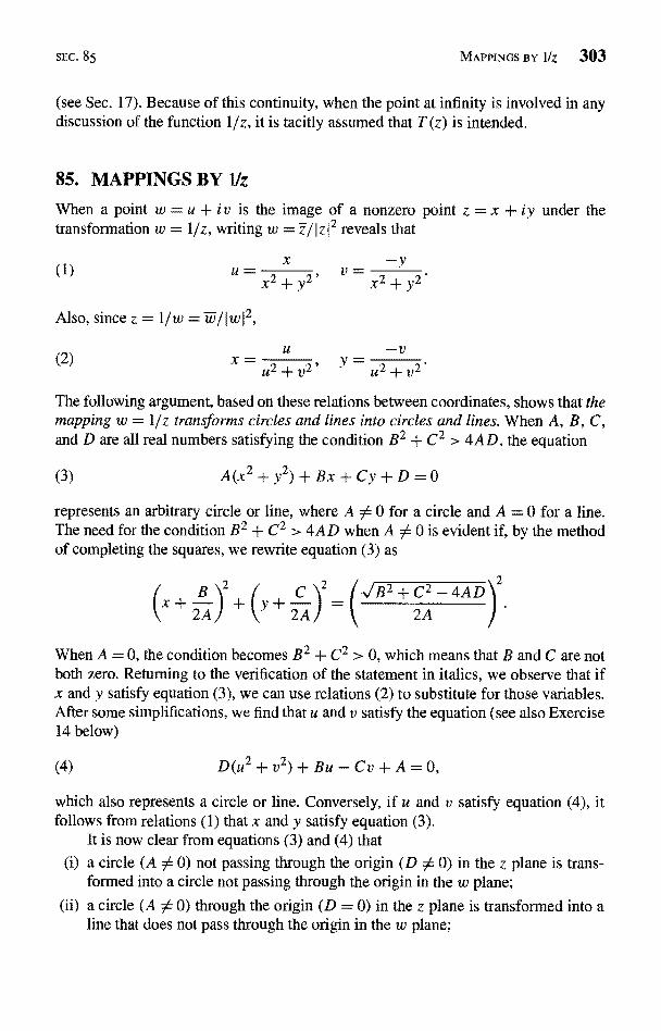
SEC, 85 MAPPINGS BY l/z 303
(see Sec. 17). Because of this continuity, when the point at infinity is involved in andiscussion of the function 1/z, it is tacitly assumed that T(z) is intended.
85. MAPPINGS BY lfz
When a point w = u + i v is the image of a nonzero point z = x + iy under thetransformation w = 1/z, writing w = z/IzI2 reveals that
+y2'-
x2-+2
-v
u2+ v2, u2+v
The following argument, based on these relations between coordinates, shows that themapping w = I /z transforms circles and lines into circles and lines. When A, B, C,and D are all real numbers satisfying the condition B2 + C2 > 4AD, the equation
(3)
represents an arbitrary circle or line, where A A 0 for a circle and A = 0 for a line.The need for the condition B2 + C2 > 4AD when A A 0 is evident if, by the methodof completing the squares, we rewrite equation (3) as
x
A(x2+y2)+Bx+Cy+D=0
_y
When A = 0, the condition becomes B2 + C2 > 0, which means that B and C are notboth zero. Returning to the verification of the statement in italics, we observe that ifx and y satisfy equation (3), we can use relations (2) to substitute for those variables.After some simplifications, we find that u and v satisfy the equation (see also Exercise14 below)
(4) D(u Bu-Cv+A=0,
which also represents a circle or line. Conversely, if u and v satisfy equation (4), itfollows from relations (1) that x and y satisfy equation (3).
It is now clear from equations (3) and (4) that
a circle (A A 0) not passing through the origin (D A 0) in the z plane is trans-formed into a circle not passing through the origin in the w plane;
a circle (A A 0) through the origin (D = 0) in the z plane is transformed into aline that does not pass through the origin in the w plane;
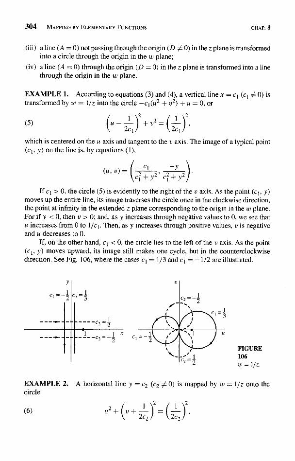
304 MAPPING BY ELEMENTARY FUNCTIONS CHAP. 8
) a line (A = 0) not passing through the origin (DO 0) in the z plane is transformedinto a circle through the origin in the w plane;
a line (A = 0) through the origin (D = 0) in the z plane is transformed into a linethrough the origin in the w plane.
EXAMPLE 1. According to equations (3) and (4), a vertical line x = c1 (c1 A 0) istransformed by w = 1/z into the circle -c1(u2 + v2) + u = 0, or
(5)1 2 l 1 \2
U
which is centered on the u axis and tangent to the v axis. The image of a typical point(c1, y) on the line is, by equations (1),
u, v) =
If cl > 0, the circle (5) is evidently to the right of the v axis. As the point (c1, y)moves up the entire line, its image traverses the circle once in the clockwise direction,the point at infinity in the extended z plane corresponding to the origin in the w plane.For if y < 0, then v > 0; and, as y increases through negative values to 0, we see thatu increases from 0 to 1/cl. Then, as y increases through positive values, v is negativeand u decreases to 0.
If, on the other hand, cl < 0, the circle lies to the left of the v axis. As the point(c1, y) moves upward, its image still makes one cycle, but in the counterclockwisedirection. See Fig. 106, where the cases c1= 1/3 and c1 = -1/2 are illustrated.
y
----C2 = I2
FIGURE106w=1/z.
EXAMPLE 2. A horizontal line y = c2 0) is mapped by w = 1/z onto the2circle
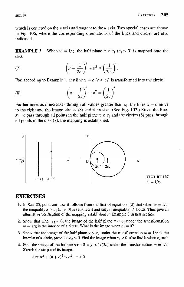
SEC. 85 EXERCISES 305
which is centered on the v axis and tangent to the u axis. Two special cases are shownin Fig. 106, where the corresponding orientations of the lines and circles are alsoindicated.
EXAMPLE 3. When w = 1/z, the half plane x > c1 (c1 > 0) is mapped onto thedisk
(7)
For, according to Example 1, any line x = c (c > c1) is transformed into the circle
I) +v2_(2c).
Furthermore, as c increases through all values greater than c1, the lines x = c moveto the right and the image circles (8) shrink in size. (See Fig. 107.) Since the linesx = c pass through all points in the half plane x > c1 and the circles (8) pass throughall points in the disk (7), the mapping is established.
x
FIGURE 107w = 1/z.
EXERCISES
1. In Sec. 85, point out how it follows from the first of equations (2) that when w = 1/z,the inequality x > c1 (c1 > 0) is satisfied if and only if inequality (7) holds. Thus give analternative verification of the mapping established in Example 3 in that section.
2. Show that when c1 < 0, the image of the half plane x < c1 under the transformationw = 1/z is the interior of a circle. What is the image when c1= 0?
3. Show that the image of the half plane y > c2 under the transformation w = 1/z is theinterior of a circle, provided c2 > 0. Find the image when c2 < 0; also find it when c2 = 0.
4. Find the image of the infinite strip 0 < y < 1/(2c) under the transformation w = 1/z.Sketch the strip and its image.
Ans. u2+(v+c)2>c2, v<0.
306 MAPPING BY ELEMENTARY FUNCTIONS CHAP. 8
5. Find the image of the quadrant x > 1, y > 0 under the transformation w = 1/z.
Ans. (u-21 I v2<(2 v<0.
6. Verify the mapping, where w = 1/z, of the regions and parts of the boundaries indicatedin (a) Fig. 4, Appendix 2; (b) Fig. 5, Appendix 2.
7. Describe geometrically the transformation w = 1/(z - 1).
8. Describe geometrically the transformation w = i /z. State why it transforms circles andlines into circles and lines.
9. Find the image of the semi-infinite strip x > 0, 0 < y < 1 when w = i/z. Sketch the stripand its image.
10. By writing w = p exp(ii), show that the mapping w = 1/z transforms the hyperbolax2 - y2 = 1 into the lemniscate p2 = cos 20. (See Exercise 15, Sec. 5.)
11. Let the circle IzI = 1 have a positive, or counterclockwise, orientation. Determineorientation of its image under the transformation w = 1/z.
12. Show that when a circle is transformed into a circle under the transformation w = 1/z,the center of the original circle is never mapped onto the center of the image circle.
13. Using the exponential form z = reie of z, show that the transformation
1w=z+-,z
which is the sum of the identity transformation and the transformation discussed in Secs.84 and 85, maps circles r = ro onto ellipses with parametric representations
cos0, v=(ro-= )sin0 (0<9<2ro
and foci at the points w = +2. Then show how it follows that this transformation mapsthe entire circle Iz I = 1 onto the segment -2 < u < 2 of the u axis and the domain outsidethat circle onto the rest of the w plane.
14. (a) Write equation (3), Sec. 85, in the form
2Azz+(B - Ci)z + (B + Ci)z+ 2D = 0,
where z = x + iy.(b) Show that when w = 1/z, the result in part (a) becomes
2Dww+(B+Ci)w+(B-Ci)w+2A=0.
Then show that if w = u + i v, this equation is the same as equation (4), Sec. 85.Suggestion: In part (a), use the relations (see Sec. 5)
x - z+z and v=z - z
SEC. 86 LINEAR FRACTIONAL TRANSFORMATIONS 307
86. LINEAR FRACTIONAL TRANSFORMATIONS
The transformation
(1)az + bw= (ad-bc 0),cz + d
where a, b, c, and d are complex constants, is called a linearfractional transformation,or Mobius transformation. Observe that equation (1) can be written in the form
Azw+Bz+Cw+D=O (AD-BC0 );
and, conversely, any equation of type (2) can be put in the form (1). Since thisalternative form is linear in z and linear in w, or bilinear in z and w, another namefor a linear fractional transformation is bilinear transformation.
When c = 0, the condition ad - be A 0 with equation (1) becomes ad 0; andwe see that the transformation reduces to a nonconstant linear function. When c 0 0,equation (1) can be written
(3) (ad - be 0
So, once again, the condition ad - be 0 ensures that we do not have a constantfunction. The transformation w = 1/z is evidently a special case of transformation (1)when c 0.
Equation (3) reveals that when c ; 0, a linear fractional transformation is acomposition of the mappings.
Z=cz+d, 1 a be - ad_-, w=*+ c (ad-be5,1- 0
It thus follows that, regardless of whether c is zero or nonzero, any linear fractionaltransformation transforms circles and lines into circles and lines because these speciallinear fractional transformations do. (See Sees. 83 and 85.)
Solving equation (1) for z, we find that
(4) z-dw+bcw - a
ad-bcA0).
When a given point w is the image of some point z under transformation (1), the pointz is retrieved by means of equation (4). If c = 0, so that a and d are both nonzero, eachpoint in the w plane is evidently the image of one and only one point in the z plane.The same is true if c 0 0, except when w = a/c since the denominator in equation(4) vanishes if w has that value. We can, however, enlarge the domain of definitionof transformation (1) in order to define a linear fractional transformation T on the
308 MAPPING BY ELEMENTARY FUNCTIONS CHAP. 8
extended z plane such that the point w = a lc is the image of z = oo when c ; 0. Wefirst write
(5)
We then write
and
T(cx)= c=0
T (oo) =a
andc
if c 0.
In view of Exercise 11, Sec. 17, this makes T continuous on the extended z plane.It also agrees with the way in which we enlarged the domain of definition of thetransformation w = 1/z in Sec. 84.
When its domain of definition is enlarged in this way, the linear fractionaltransformation (5) is a one to one mapping of the extended z plane onto the extendedw plane. That is, T(z1) ; T (Z2) whenever z 1 ; z2; and, for each point w in the secondplane, there is a point z in the first one such that T(z) = w. Hence, associated withthe transformation T, there is an inverse transformation T-1, which is defined on theextended w plane as follows:
T-`(w) = z if and only if T(z) = w.
From equation (4), we see that
(6) T--dw+bcw -a
(ad-bcA0).
Evidently, T-1 is itself a linear fractional transformation, where
T-1(
and
T-
c=0
and T - l (oo) = - -u if c ; 0.C
If T and S are two linear fractional transformations, then so is the composition S[T (z)].This can be verified by combining expressions of the type (5). Note that, in particular,T [T (z)] = z for each point z in the extended plane.
There is always a linear fractional transformation that maps three given distinctpoints z1, z2, and z3 onto three specified distinct points w1, w2, and w3, respectively.Verification of this will appear in Sec. 87, where the image w of a point z under sucha transformation is given implicitly in terms of z. We illustrate here a more directapproach to finding the desired transformation.
az+bT (z)
_cz +
d (ad - be A 0).
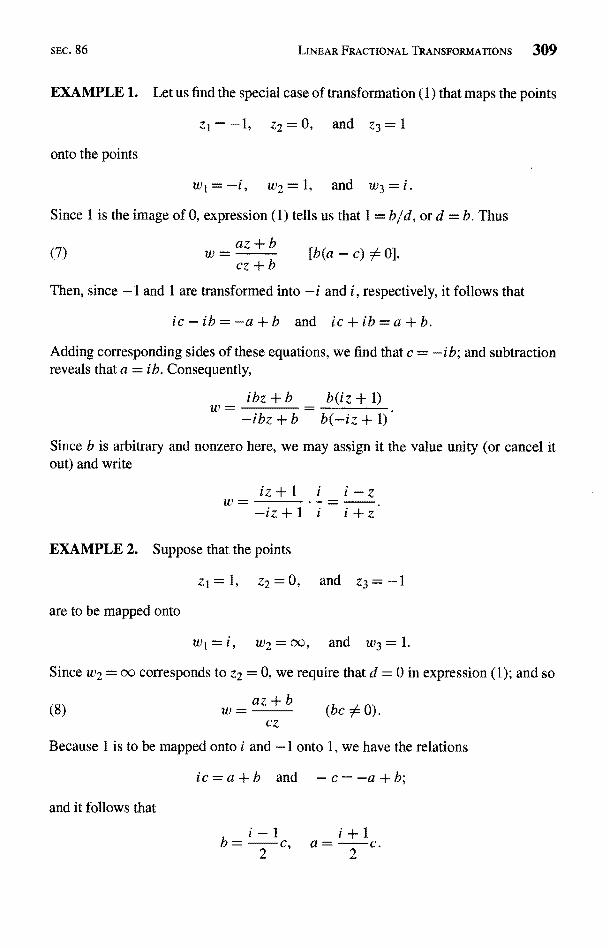
SEC. 86
EXAMPLE 1. Let us find the special case of transformation (1) that maps the points
zI--1, z2=0, and z3=1
onto the points
LINEAR FRACTIONAL TRANSFORMATIONS 309
wl=-i, w2=1, and w3=i,
Since 1 is the image of 0, expression (1) tells us that 1= b/d, or d = b. Thus
(7)az + bcz + b
[b(a -
Then, since -1 and 1 are transformed into -i and i, respectively, it follows that
ic-ib=-a+b and ic+ib=a+b.Adding corresponding sides of these equations, we find that c = -ib; and subtractionreveals that a = ib. Consequently,
w =ibz + b b(iz + 1)-
-ibz + b b(-iz + 1)
Since b is arbitrary and nonzero here, we may assign it the value unity (or cancel itout) and write
iz+1-iz+1 i i+z
EXAMPLE 2. Suppose that the points
zI=1, z2=0, and z3=-
are to be mapped onto
wl=i, w2=oo, and W3=1-
Since w2 = ao corresponds to z2 = 0, we require that d = 0 in expression (1); and so
(8)az + bw=
ezbe 0).
Because 1 is to be mapped onto i and -1 onto 1, we have the relations
b and -c---a+b:and it follows that
b_i-1c, a_i+lc.
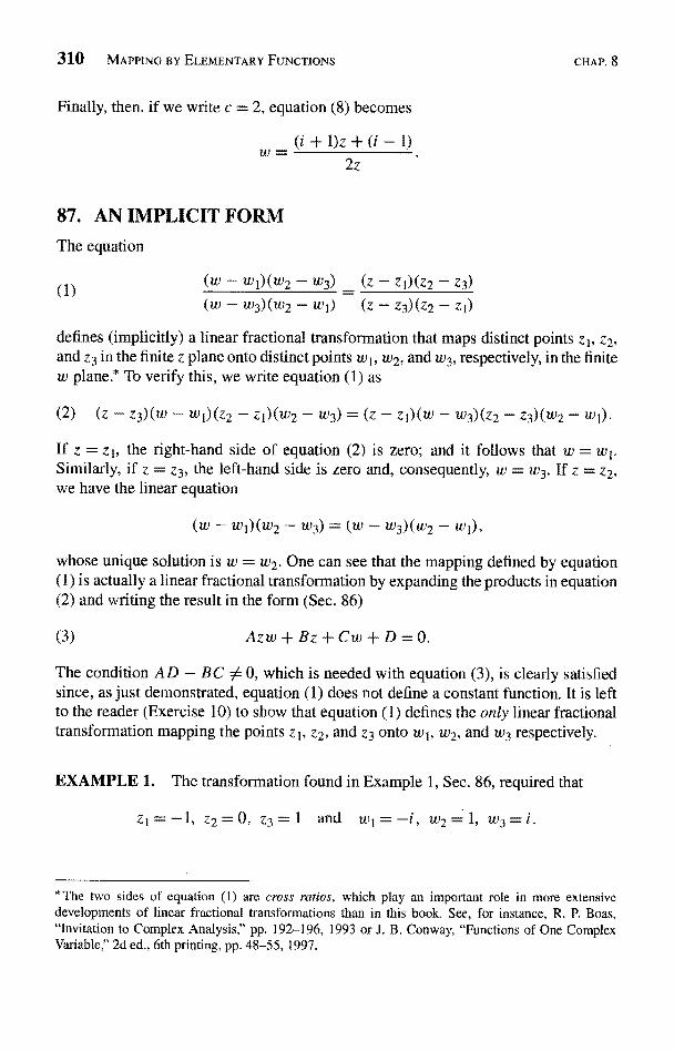
310 MAPPING BY ELEMENTARY FUNCTIONS CHAP. 8
Finally, then, if we write c = 2, equation (8) becomes
z -l
2z
87. AN IMPLICIT FORMThe equation
(1)wl)(w2 - w3)
(w - w3)(w2 - w1)
defines (implicitly) a linear fractional transformation that maps distinct points zI, z2,and z3 in the finite z plane onto distinct points wI, w2, and w3, respectively, in the finitew plane.* To verify this, we write equation (1) as
(2) (z - z3)(w - w1)(z2 - zi)(w2 - w3) = (z - zl)(w - w3)(z2 W'a'2 WI).
If z = zI, the right-hand side of equation (2) is zero; and it follows that w = wI.Similarly, if z = Z3, the left-hand side is zero and, consequently, w = w3. If z = z2,we have the linear equation
(w - w1)(w2 - w3) = (w - w3)(w2
whose unique solution is w = w2. One can see that the mapping defined by equation(1) is actually a linear fractional transformation by expanding the products in equation(2) and writing the result in the form (Sec. 86)
Azw+Bz+Cw+D=O.
The condition AD - BC 0, which is needed with equation (3), is clearly satisfiedsince, as just demonstrated, equation (1) does not define a constant function. It is leftto the reader (Exercise 10) to show that equation (1) defines the only linear fractionaltransformation mapping the points z1, z2, and z3 onto w1, w2, and w3 respectively.
EXAMPLE sformation found in Example 1, Sec. 86, required that
0, Z3=1 and wi=-i,
*The two sides of equation (1) are cross ratios, which play an important role in more extensivedevelopments of linear fractional transformations than in this book. See, for instance, R. P. Boas,"Invitation to Complex Analysis," pp. 192-196, 1993 or J. B. Conway, "Functions of One ComplexVariable,,, 2d ed., 6th printing, pp. 48-55, 1997.
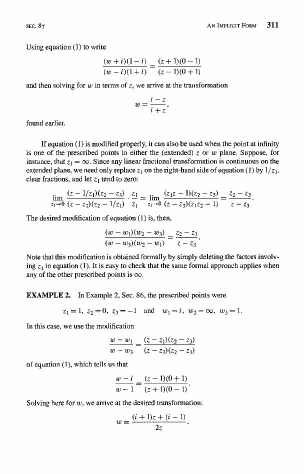
SEC. 8 7 AN IMPLICIT FORM 311
Using equation (1) to write
(z + WO - 1)(w - x)(1+ i) (z - 1)(0 + 1)
and then solving for w in terms of z, we arrive at the transformation
found earlier.
If equation (1) is modified properly, it can also be used when the point at infinityis one of the prescribed points in either the (extended) z or w plane. Suppose, forinstance, that z I = oo. Since any linear fractional transformation is continuous on theextended plane, we need only replace zI on the right-hand side of equation (1) by 1/z 1,clear fractions, and let z1 tend to zero:
zz-+O (z - Z3)(Z2 - 1/z1) z1 zI-*O (z - 23)(2122 - 1) z - Z3
The desired modification of equation (1) is, then,
(w - w1)(w2 - w3) z2 - z3(w - w3)(w2 - w1) z - z3
Note that this modification is obtained formally by simply deleting the factors involv-ing zi in equation (1). It is easy to check that the same formal approach applies whenany of the other prescribed points is oo.
EXAMPLE 2. In Example 2, Sec. 86, the prescribed points were
Z2=0, Z3==-l and
In this case, we use the modification
w - w1 _ (z - Zl)(Z2 - Z3)w-w3 (Z-23)(Z2-zi)
of equation (1), which tells us that
z-1)(0+1)z + 1) (0 - 1)
Solving here for w, we arrive at the desired transformation:
(i + 1)z + (i - 1)
lim (z - 1/ZI)(z2 - z3) . ZI __._ lira (ZIZ -1)(z2 - z3) - Z2 - Z3
2z
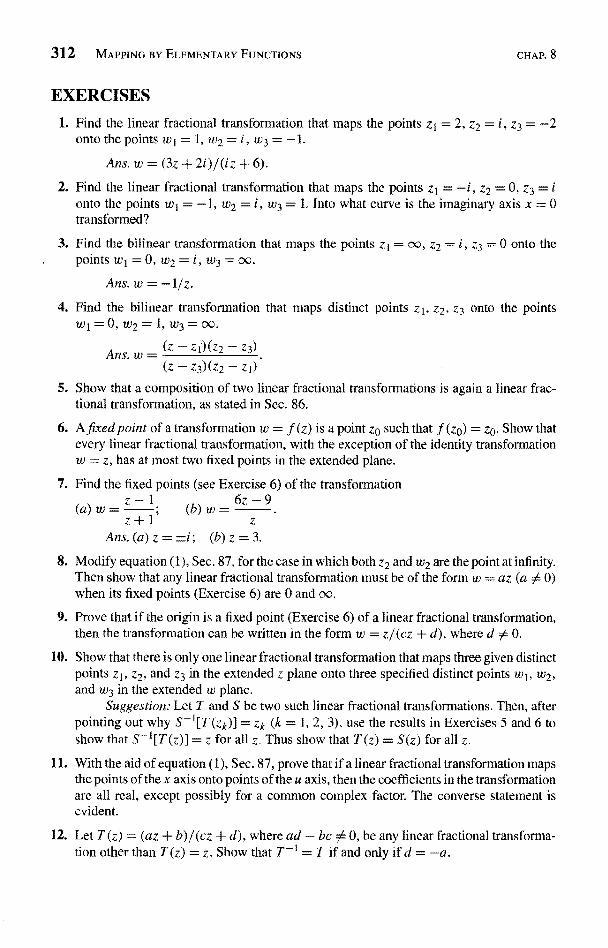
312 MAPPING BY ELEMENTARY FUNCTIONS CHAP. 8
EXERCISES
1. Find the linear fractional transformation that maps the points z1 = 2, z2 = i, z3 = -2onto the points wI = 1, w2 = i, w3 = -1.
Ans.w=(3z+2i)/(iz+6).2. Find the linear fractional transformation that maps the points z1 = -i, z2 = 0, z3 = i
onto the points w1= -1, w2 = i, w3 = 1. Into what curve is the imaginary axis x = 0transformed?
3. Find the bilinear transformation that maps the points zI = aa, z2 = i, z3 = 0 onto thepoints w1 = 0, w2 = i, w3 = 00.
Ans. w = z
4. Find the bilinear transformation that maps distinct points z1, z2, z3 onto the pointsw1= 0, W2 = 1, W3= CC-
Ans. w = (z - Zl)(22 - z3)(Z - 23)(22 - Z1)
5. Show that a composition of two linear fractional transformations is again a linear frac-tional transformation, as stated in Sec. 86.
6. A fixed point of a transformation w = f {z) is a point 20 such that f (zo) = z0. Show thatevery linear fractional transformation, with the exception of the identity transformationw = z, has at most two fixed points in the extended plane.
7. Find the fixed points (see Exercise 6) of the transformation
wz - l (b)w=6z-9
a =z+1' z
Ans.(a)z=±i; (b)z=3.
8. Modify equation (1), Sec. 87, for the case in which both z2 and w2 are the point at infinity.Then show that any linear fractional transformation must be of the form w = az (a 0 0)when its fixed points (Exercise 6) are 0 and oo.
9. Prove that if the origin is a fixed point (Exercise 6) of a linear fractional transformation,then the transformation can be written in the form w = z/(cz + d), where d 54 0.
10. Show that there is only one linear fractional transformation that maps three given distinctpoints zI, z2, and z3 in the extended z plane onto three specified distinct points wI, w2,and w3 in the extended w plane.
Suggestion: Let T and S be two such linear fractional transformations. Then, afterpointing out why S _ = zk (k = 1, 2, 3), use the results in Exercises 5 and 6 toshow that S-1[T(z)] = z for all z. Thus show that T(z) = S(z) for all z.
11. With the aid of equation (1), Sec. 87, prove that if a linear fractional transformation mapsthe points of the x axis onto points of the u axis, then the coefficients in the transformationare all real, except possibly for a common complex factor. The converse statement isevident.
12. Let T (z) _ (az + b)/(c2 + d), where ad - be 0 0, be any linear fractional transforma-tion other than T (z) = z. Show that T-I = T if and only if d = -a.
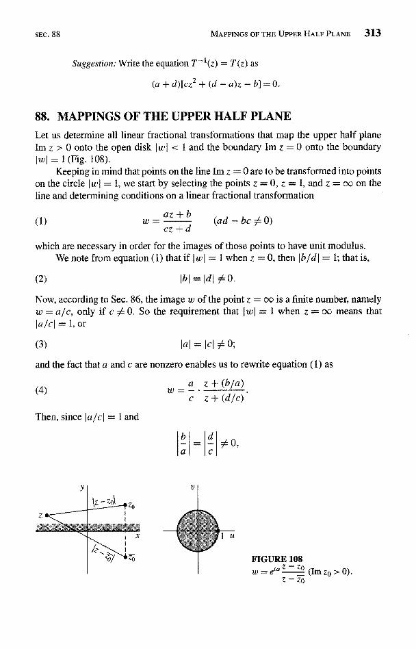
SEC. 88
lal = Icl A 0;
Suggestion: Write the equation T-1(z) = T(z) as
(a + d)[cz2 + (d - a) z - b] = 0.
88. MAPPINGS OF THE UPPER HALF PLANE
Let us determine all linear fractional transformations that map the upper half planeIm z > 0 onto the open disk I w I < 1 and the boundary Im z = 0 onto the boundaryw I = 1(Fig. 108).
Keeping in mind that points on the line Im z = 0 are to be transformed into pointson the circle I w I = 1, we start by selecting the points z = 0, z = 1, and z = oo on theline and determining conditions on a linear fractional transformation
(1) w _ az + b (ad - be 0)cz + d
which are necessary in order for the images of those points to have unit modulus.We note from equation (1) that if I w I = i when z = 0, then I bld I = 1; that is,
(2) IbI = Idl 0.
Now, according to Sec. 86, the image w of the point z = oo is a finite number, namelyw = a/c, only if c A 0. So the requirement that Iwl = I when z = oc means thatIa/cl = 1, or
(3)
and the fact that a and c are nonzero enables us to rewrite equation (1) as
(4)
Then, since l alcl = 1 and
MAPPINGS OF THE UPPER HALF PLANE 313
wa z + (b/a)=-c z + (d/c)
b d00,
c
FIGURE 108i,Z-Zp
w = eT
(IM z0 > 0).Z - zo
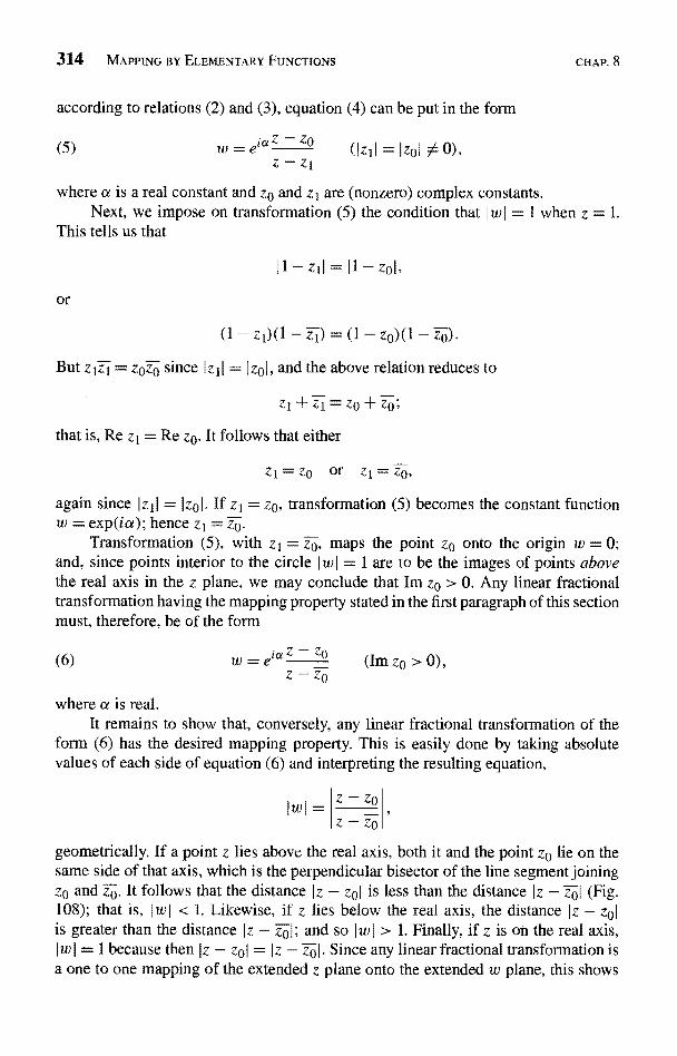
314 MAPPING BY ELEMENTARY FUNCTIONS CHAP. 8
according to relations (2) and (3), equation (4) can be put in the form
(5);a Z - zo
Z - Z1(1z11= Izol A O),
where a is a real constant and zo and z1 are (nonzero) complex constants.Next, we impose on transformation (5) the condition that I w I = 1 when z =
This tells us that
or
But zizl = zozo since
(I - z1)(1 - TO = 0 - zo)(1 - .
z 11 = I zo I, and the above relation reduces to
z1+Z1=zo+zo;
that is, Re zi = Re zo. It follows that either
z1 = zo or
again since Izil = Izol If z1 = zo, transformation (5) becomes the constant functionw = exp(ia); hence z1= To.
Transformation (5), with zi = za, maps the point zo onto the origin w = 0;and, since points interior to the circle I w I = 1 are to be the images of points abovethe real axis in the z plane, we may conclude that Im z0 > 0. Any linear fractionaltransformation having the mapping property stated in the first paragraph of this sectionmust, therefore, be of the form
(6)ja z - zo
z- z{1ZO > 0
where a is real.It remains to show that, conversely, any linear fractional transformation of the
form (6) has the desired mapping property. This is easily done by taking absolutevalues of each side of equation (6) and interpreting the resulting equation,
Z - ZO
Z - ZO
geometrically. If a point z lies above the real axis, both it and the point z0 lie on thesame side of that axis, which is the perpendicular bisector of the line segment joiningz0 and z0. It follows that the distance Iz - zol is less than the distance Iz - zol (Fig.108); that is, Iwl < 1. Likewise, if z lies below the real axis, the distance Iz - zolis greater than the distance I z - To 1; and so I w I > 1. Finally, if z is on the real axis,I w I = 1 because then Iz - zoI = Iz - zo1. Since any linear fractional transformation isa one to one mapping of the extended z plane onto the extended w plane, this shows
SEC. 88 MAPPINGS OF THE UPPER HALF PLANE 315
that transformation (6) maps the half plane Im z > 0 onto the disk I w I < 1 and theboundary of the half plane onto the boundary of the disk.
Our first example here illustrates the use of the result in italics just above.
EXAMPLE 1. The transformation
(7)i - z
+ zw=
in Examples 1 in Secs. 86 and 87 can be written
Hence it has the mapping property described in italics. (See also Fig. 13 in Appendix2, where corresponding boundary points are indicated.)
Images of the upper half plane Im z > 0 under other types of linear fractionaltransformations are often fairly easy to determine by examining the particular trans-formation in question.
EXAMPLE 2. By writing z = x + iy and w = u + i v, we can readily show that thetransformation
(8)
z-1z+1
maps the half plane y > 0 onto the half plane v > 0 and the x axis onto the u axis. Wefirst note that when the number z is real, so is the number w. Consequently, since theimage of the real axis y = 0 is either a circle or a line, it must be the real axis v = 0.Furthermore, for any point w in the finite w plane,
(z -- 1) (z + 1) 2y
z+1)(z+1) Iz+112(z -
The numbers y and v thus have the same sign, and this means that points above thex axis correspond to points above the u axis and points below the x axis correspondto points below the u axis. Finally, since points on the x axis correspond to pointson the u axis and since a linear fractional transformation is a one to one mapping ofthe extended plane onto the extended plane (Sec. 86), the stated mapping property oftransformation (8) is established.
Our final example involves a composite function and uses the mapping discussedin Example 2.
EXAMPLE 3. The transformation
(9) w = Log
316 MAPPING BY ELEMENTARY FUNCTIONS CHAP. 8
where the principal branch of the logarithmic function is used, is a composition of thefunctions
(10) Z = z - 1 and w = Log Z.z+lWe know from Example 2 that the first of transformations (10) maps the upper
half plane y > 0 onto the upper half plane Y > 0, where z = x + iy and Z = X + i Y.Furthermore, it is easy to see from Fig. 109 that the second of transformations (10)maps the half plane Y > 0 onto the strip 0 < v < 7r, where w = u + i v. More precisely,by writing Z = R exp(i 0) and
LogZ=inR+iO (R>0,-1r <0<7r),
we see that as a point Z = R exp(i O0) (0 < O0 < ir) moves outward from the originalong the ray 0 = O0, its image is the point whose rectangular coordinates in the wplane are (In R, O0). That image evidently moves to the right along the entire lengthof the horizontal line v = 00. Since these lines fill the strip 0 < v < Pr as the choice ofO0 varies between 00 = 0 to 00 = 7r, the mapping of the half plane Y > 0 onto thestrip is, in fact, one to one.
This shows that the composition (9) of the mappings (10) transforms the planey > 0 onto the strip 0 < v < 7r. Corresponding boundary points are shown in Fig. 19of Appendix 2.
V
0
FIGURE 109w=Logz.
EXERCISES
c
1. Recall from Example 1 in Sec. 88 that the transformation
Ira
0
maps the half plane Im z > 0 onto the disk I w I < 1 and the boundary of the half planeonto the boundary of the disk. Show that a point z = x is mapped onto the point
1-x2 . 2xw-1+x2+I1+x2,
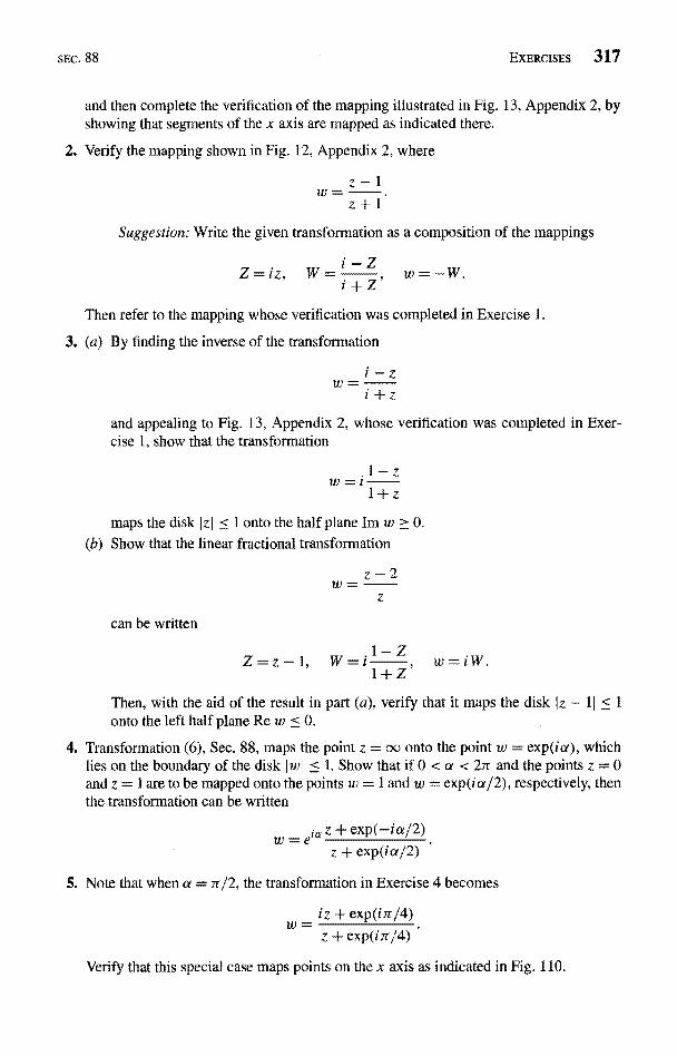
SEC. 88 EXERCISES 317
and then complete the verification of the mapping illustrated in Fig. 13, Appendix 2, byshowing that segments of the x axis are mapped as indicated there.
2. Verify the mapping shown in Fig. 12, Appendix 2, where
IV =z-1z+1
Suggestion: Write the given transformation as a composition of the mappings
-ZZ=iz, W= , w=+Z
Then refer to the mapping whose verification was completed in Exercise 1.
3. (a) By finding the inverse of the transformation
and appealing to Fig. 13, Appendix 2, whose verification was completed in Exer-cise 1, show that the transformation
.1-z+z
maps the disk I z I < I onto the half plane Im w > 0.(b) Show that the linear fractional transformation
z-2z
can be written
Z=z-1, W=i_ w=iW.+Z
Then, with the aid of the result in part (a), verify that it maps the disk Jz -onto the left half plane Re w < 0.
4. Transformation (6), Sec. 88, maps the point z = oo onto the point w = exp(ia), whichlies on the boundary of the disk J w I c 1. Show that if 0 < a < 2n and the points z = 0and z = 1 are to be mapped onto the points w = 1 and w = exp(ia/2), respectively, thenthe transformation can be written
z + exp(-ia/2z + exp(ia/2)
5. Note that when a = 7r/2, the transformation in Exercise 4 becomes
iz + exp(i7r/4)z + exp(i n/4)
Verify that this special case maps points on the x axis as indicated in Fig. 110.
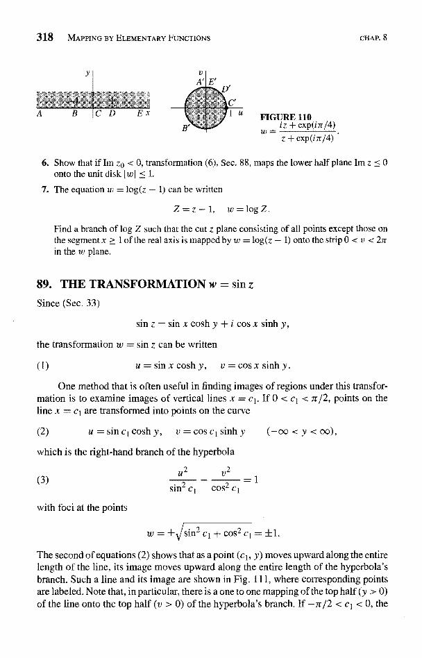
318 MAPPING BY ELEMENTARY FUNCTIONS
y
A C D FIGURE 110iz + exp (i rr/4)w=z + exp(iir/4)
CHAP. 8
6. Show that if Im zO < 0, transformation (6), Sec. 88, maps the lower half plane Im z < 0onto the unit disk I w I < 1.
7. The equation w = log(z - 1) can be written
Z=z-1, log Z.
Find a branch of log Z such that the cut z plane consisting of all points except those onthe segment x > I of the real axis is mapped by w = log(z - 1) onto the strip 0 < v < 2,7in the w plane.
89. THE TRANSFORMATION w = sin z
Since (Sec. 33)
sin z - sin x cosh y + i cos x sinh y,
the transformation w = sin z can be written
(1) u = sin x cosh y, v = cos x sinh y.
One method that is often useful in finding images of regions under this transfor-mation is to examine images of vertical lines x = cl. If 0 < cl < ir/2, points on theline x = c1 are transformed into points on the curve
(2) u = sin cl cosh y, v = Cos ci sinh y (-co < y < ao),
which is the right-hand branch of the hyperbola
(3)
with foci at the points
u2 V2
sing ci eos2 ci
n2 CI+COS2Cj=±1.
The second of equations (2) shows that as a point (c1, y) moves upward along the entirelength of the line, its image moves upward along the entire length of the hyperbola'sbranch. Such a line and its image are shown in Fig. 111, where corresponding pointsare labeled. Note that, in particular, there is a one to one mapping of the top half (y > 0)of the line onto the top half (v > 0) of the hyperbola's branch. If -ir/2 < c1 < 0, the
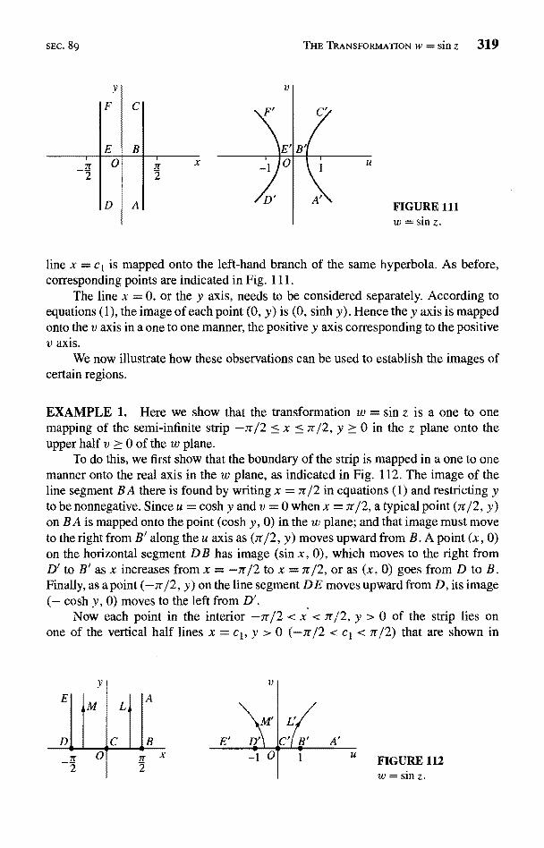
SEC. 89
Y
E0
D
B
A
x
FIGURE 111w = Sin z.
line x = c1 is mapped onto the left-hand branch of the same hyperbola. As before,corresponding points are indicated in Fig. 111.
The line x = 0, or the y axis, needs to be considered separately. According toequations (1), the image of each point (0, y) is (0, sinh y). Hence they axis is mappedonto the v axis in a one to one manner, the positive y axis corresponding to the positivev axis.
We now illustrate how these observations can be used to establish the images ofcertain regions.
EXAMPLE 1. Here we show that the transformation w = sin z is a one to onemapping of the semi-infinite strip -7r/2 < x < 7r/2, y > 0 in the z plane onto theupper half v > 0 of the w plane.
To do this, we first show that the boundary of the strip is mapped in a one to onemanner onto the real axis in the w plane, as indicated in Fig. 112. The image of theline segment BA there is found by writing x = 7/2 in equations (1) and restricting yto be nonnegative. Since u = cosh y and v = 0 when x = rr/2, a typical point (3r/2, y)on BA is mapped onto the point (cosh y, 0) in the w plane; and that image must moveto the right from B' along the u axis as (r/2, y) moves upward from B. A point (x, 0)on the horizontal segment DB has image (sin x, 0), which moves to the right fromD' to B' as x increases from x = -7r/2 to x = r/2, or as (x, 0) goes from D to B.Finally, as apoint (-7r/2, y) on the line segment DE moves upward from D, its image(- cosh y, 0) moves to the left from D.
Now each point in the interior -7r/2 < x < n/2, y > 0 of the strip lies onone of the vertical half lines x = cl, y > 0 (-7r/2 < cl < 7r/2) that are shown in
M
C0n_2
L
x
THE TRANSFORMATION w = sin z 319
FIGURE 112w=sinz.
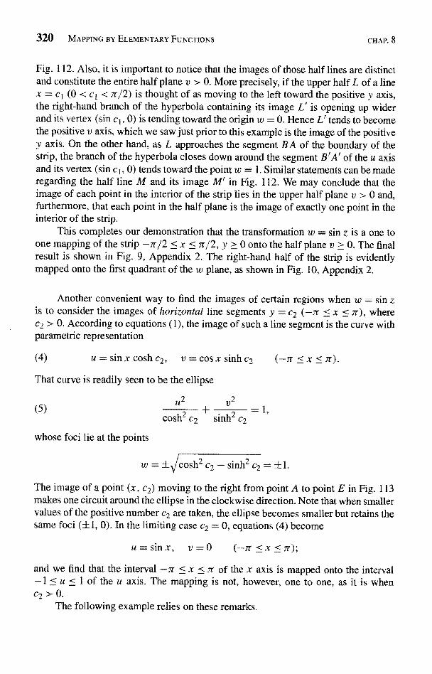
320 MAPPING BY ELEMENTARY FUNCTIONS CHAP. 8
Fig. 112. Also, it is important to notice that the images of those half lines are distinctand constitute the entire half plane v > 0. More precisely, if the upper half L of a linex = cI (0 < cI < 7r/2) is thought of as moving to the left toward the positive y axis,the right-hand branch of the hyperbola containing its image L' is opening up widerand its vertex (sin cI, 0) is tending toward the origin w = 0. Hence L' tends to becomethe positive v axis, which we saw just prior to this example is the image of the positivey axis. On the other hand, as L approaches the segment BA of the boundary of thestrip, the branch of the hyperbola closes down around the segment B'A' of the u axisand its vertex (sin cI, 0) tends toward the point w = 1. Similar statements can be maderegarding the half line M and its image M' in Fig. 112. We may conclude that theimage of each point in the interior of the strip lies in the upper half plane v > 0 and,furthermore, that each point in the half plane is the image of exactly one point in theinterior of the strip.
This completes our demonstration that the transformation w = sin z is a one toone mapping of the strip -7r/2 < x < r/2, y > 0 onto the half plane v > 0. The finalresult is shown in Fig. 9, Appendix 2. The right-hand half of the strip is evidentlymapped onto the first quadrant of the w plane, as shown in Fig. 10, Appendix 2.
Another convenient way to find the images of certain regions when w = sin zo consider the images of horizontal line segments y = c2 (-7t < x < ir), where
c2 > 0. According to equations (1), the image of such a line segment is the curve withparametric representation
(4) u = sin x cosh c2, v = cos x sinh c2 (-3r < x < n).
That curve is readily seen to be the ellipse
u2
2= 1,
(5) 2 +cosh sinhe2
whose foci lie at the points
w = ±\cosh2 c2 - sinh2 c2 = +1.
The image of a point (x, c2) moving to the right from point A to point E in Fig. 113makes one circuit around the ellipse in the clockwise direction. Note that when smallervalues of the positive number c2 are taken, the ellipse becomes smaller but retains thesame foci (±1, 0). In the limiting case c2 = 0, equations (4) become
u=sinx, v=0 (-3r <x <lr);
and we find that the interval -7r < x it of the x axis is mapped onto the intervalof the u axis. The mapping is not, however, one to one, as it is when
C2 > 0,
The following example relies on these remarks.
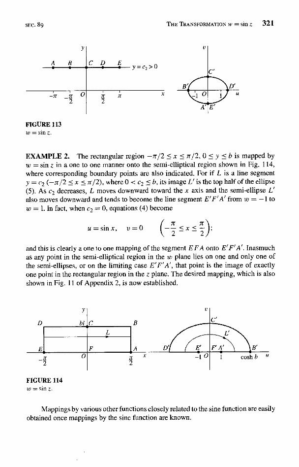
SEC. 89 THE TRANSFORMATION W= sin z 321
A
C2
FIGURE 113w = sin Z.
C D EY=C2>0
EXAMPLE 2. The rectangular region -ir/2 < x < r/2, 0 < y < b is mapped byw = sin z in a one to one manner onto the semi-elliptical region shown in Fig. 114,where corresponding boundary points are also indicated. For if L is a line segmenty = c2 (-ir/2 < x < r/2), where 0 < c2 < b, its image L` is the top half of the ellipse(5). As c2 decreases, L moves downward toward the x axis and the semi-ellipse L'also moves downward and tends to become the line segment E'F'A' from w = -1 tow = 1. In fact, when e2 = 0, equations (4) become
u =sin x, v = 0
and this is clearly a one to one mapping of the segment EFA onto E'F'A'. Inasmuchas any point in the semi-elliptical region in the w plane lies on one and only one ofthe semi-ellipses, or on the limiting case E'F'A', that point is the image of exactlyone point in the rectangular region in the z plane. The desired mapping, which is alsoshown in Fig. I 1 of Appendix 2, is now established.
FIGURE 114w=sinz.
Mappings by various other functions closely related to the sine function are easilyobtained once mappings by the sine function are known.
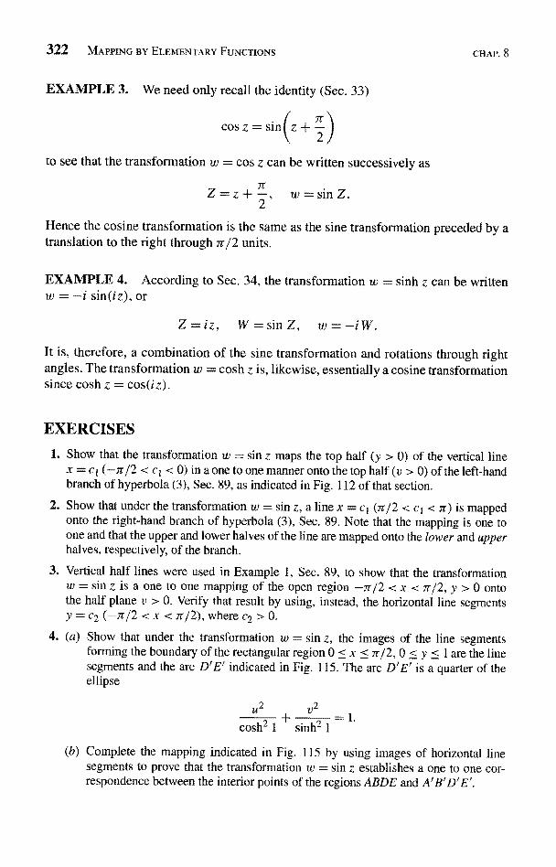
322 MAPPING BY ELEMENTARY FUNCTIONS
EXAMPLE 3. We need only recall the identity (Sec. 33)
cos z = sin
to see that the transformation w = cos z can be written successively as
CHAP. 8
Hence the cosine transformation is the same as the sine transformation preceded by atranslation to the right through 7r/2 units.
EXAMPLE 4. According to Sec. 34, the transformation w = sinh z can be writtenw = -i sin(iz), or
Z=iz, W=sinZ, w---It is, therefore, a combination of the sine transformation and rotations through rightangles. The transformation w = cosh z is, likewise, essentially a cosine transformationsince cosh z = cos(iz).
EXERCISES
1. Show that the transformation w = sin z maps the top half (y > 0) of the vertical linex = Cl (-7r/2 < ct < 0) in a one to one manner onto the top half (v > 0) of the left-handbranch of hyperbola (3), Sec. 89, as indicated in Fig. 112 of that section.
2. Show that under the transformation w = sin z, a line x = cl (7r/2 < cI < rr) is mappedonto the right-hand branch of hyperbola (3), Sec. 89. Note that the mapping is one toone and that the upper and lower halves of the line are mapped onto the lower and upperhalves, respectively, of the branch.
3. Vertical half lines were used in Example 1, Sec. 89, to show that the transformationw = sin z is a one to one mapping of the open region -7r/2 < x < 7r/2, y > 0 ontothe half plane v > 0. Verify that result by using, instead, the horizontal line segmentsy = c2 (-7r/2 < x < it/2), where c2 > 0.
4. (a) Show that under the transformation w = sin z, the images of the line segmentsforming the boundary of the rectangular region 0 < x < 7r/2, 0 < y < 1 are the linesegments and the arc D'E' indicated in Fig. 115. The arc D'E' is a quarter of theellipse
U2 V2
cosh2 1 sinh2 1
(b) Complete the mapping indicated in Fig. 115 by using images of horizontal linesegments to prove that the transformation w = sin z establishes a one to one cor-respondence between the interior points of the regions ABDE and A'B'D'E'.
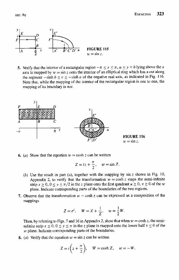
SEC. 89
FIGURE 115w = sin Z.
EXERCISES 323
5. Verify that the interior of a rectangular region -rr < x < r, a < y < b lying above the xaxis is mapped by w = sin z onto the interior of an elliptical ring which has a cut alongthe segment -sinh b < v < --sinh a of the negative real axis, as indicated in Fig. 116.Note that, while the mapping of the interior of the rectangular region is one to one, themapping of its boundary is not.
FIGURE 116w = sin z.
6. (a) Show that the equation w = cosh z can be written
Z=iz+, w=sin Z.2
(b) Use the result in part (a), together with the mapping by sin z shown in Fig. 10,Appendix 2, to verify that the transformation w = cosh z maps the semi-infinitestrip x > 0, 0 < y < 7r/2 in the z plane onto the first quadrant a > 0, v ? 0 of the w
plane. Indicate corresponding parts of the boundaries of the two regions.
7. Observe that the transformation w = cosh z can be expressed as a composition of themappings
Z=ez, W=Z+ I2
Then, by referring to Figs. 7 and 16 in Appendix 2, show that when w = cosh z, the semi-infinite strip x < 0, 0 < y < 7r in the z plane is mapped onto the lower half v < 0 of thew plane. Indicate corresponding parts of the boundaries.
8. (a) Verify that the equation w = sin z can be written
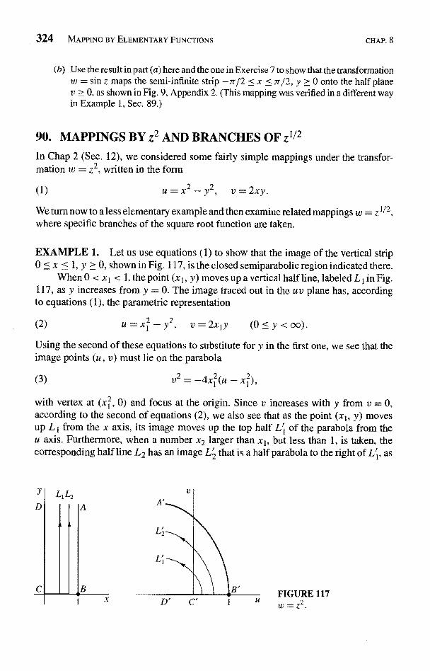
324 MAPPING BY ELEMENTARY FUNCTIONS CHAP. 8
(b) Use the result in part (a) here and the one in Exercise 7 to show that the transformationw = sin z maps the semi-infinite strip -7r/2 < x < 7r/2, y > 0 onto the half planev > 0, as shown in Fig. 9, Appendix 2. (This mapping was verified in a different wayin Example 1, Sec. 89.)
90. MAPPINGS BY z2 AND BRANCHES OF z1/2
In Chap 2 (Sec. 12), we considered some fairly simple mappings under the transfor-mation w = z2, written in the form
(1) v = 2xy.
We turn now to a less elementary example and then examine related mappings w =where specific branches of the square root function are taken.
EXAMPLE 1. Let us use equations (1) to show that the image of the vertical strip0 < x < 1, y > 0, shown in Fig. 117, is the closed semiparabolic region indicated there.
When 0 < x1 < 1, the point (x1= y) moves up a vertical half line, labeled L1 in Fig.117, as y increases from y = 0. The image traced out in the uv plane has, accordingto equations (1), the parametric representation
(2) u=xi -y2, v=2x1y (0<y<oo).Using the second of these equations to substitute for y in the first one, we see that theimage points (u, v) must lie on the parabola
(3) v2 = -4xi (u - xi ),
with vertex at (X2, 0) and focus at the origin. Since v increases with y from v = 0,according to the second of equations (2), we also see that as the point (x1, y) movesup L 1 from the x axis, its image moves up the top half L1 of the parabola from theu axis. Furthermore, when a number x2 larger than x1, but less than 1, is taken, thecorresponding half line L2 has an image L' that is a half parabola to the right of L1, as
y
A
B1
FIGURE 117w=z2.
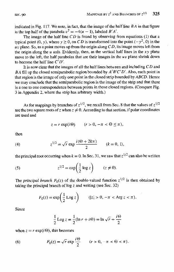
SEC. 90 MAPPINGS BY ZZ AND BRANCHES OF ZI/2 325
indicated in Fig. 117. We note, in fact, that the image of the half line BA in that figureis the top half of the parabola v2 = -4(u - 1), labeled B'A'.
The image of the half line CD is found by observing from equations (1) that atypical point (0, y), where y > 0, on CD is transformed into the point (-y2, 0) in theu v plane. So, as a point moves up from the origin along C D, its image moves left fromthe origin along the u axis. Evidently, then, as the vertical half lines in the xy planemove to the left, the half parabolas that are their images in the u v plane shrink downto become the half line C'D'.
It is now clear that the images of all the half lines between and including CD andBA fill up the closed semiparabolic region bounded by A'B'C'D'. Also, each point inthat region is the image of only one point in the closed strip bounded by ABCD. Hencewe may conclude that the semiparabolic region is the image of the strip and that thereis a one to one correspondence between points in those closed regions. (Compare Fig.3 in Appendix 2, where the strip has arbitrary width.)
As for mappings by branches of z112, we recall from Sec. 8 that the values of z112
are the two square roots of z when z A 0. According to that section, if polar coordinatesare used and
z = r exp(i®))
then
(4)z 1/2
= lr- eXp i (C) -I- 2k7r)(k = 0, 1),
2
the principal root occurring when k = 0. In Sec. 31, we saw that z112 can also be written
(5) z'/` = expf - log z I (z 54 0).
The principal branch F0(z) of the double-valued function z'1` is then obtained bytaking the principal branch of log z and writing (see Sec. 32)
F0(z) = exp( Log z (Iz
Since
I Log z = I(1nr+i02 2
when z = r exp(i C)), this becomes
(6) F0 (z) _ expiC}
2
>0,-rr<Argz<n).
iC)
2
-Tr < < Yr
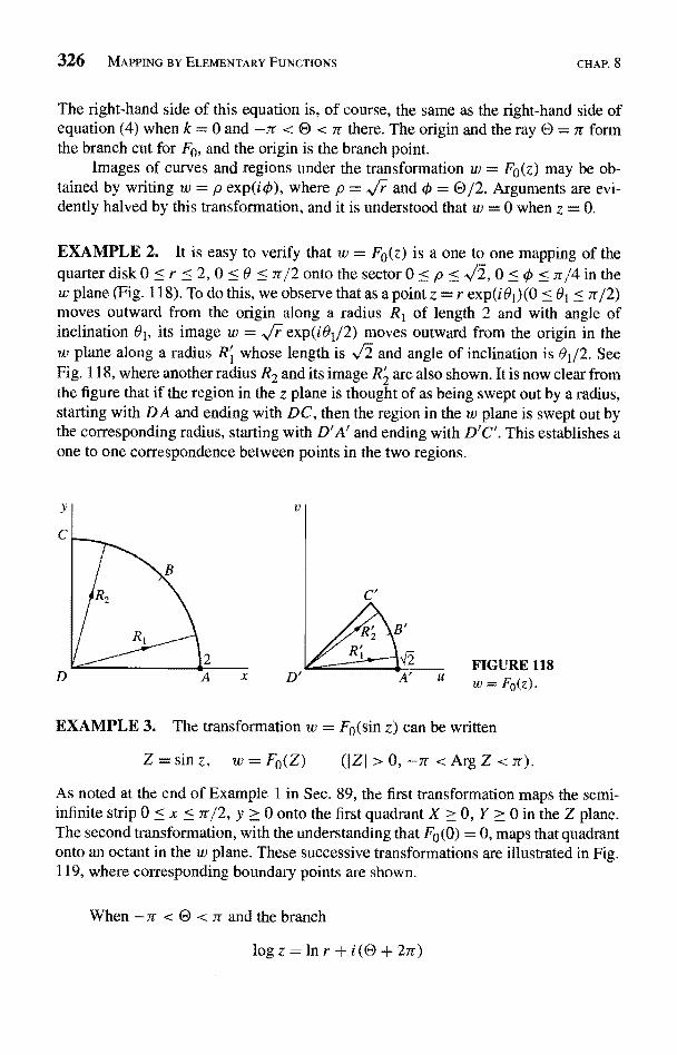
326 MAPPING BY ELEMENTARY FUNCTIONS CHAP. 8
The right-hand side of this equation is, of course, the same as the right-hand side ofequation (4) when k = 0 and -rc < E) < Tr there. The origin and the ray 0 = r formthe branch cut for F0, and the origin is the branch point.
Images of curves and regions under the transformation w = Fe(z) may be ob-tained by writing w = p exp(io), where p = 4 and 0 = 0/2. Arguments are evi-dently halved by this transformation, and it is understood that w = 0 when z = 0.
EXAMPLE 2. It is easy to verify that w = Fe(z) is a one to one mapping of thequarter disk 0 < r < 2, 0 < 6 < 7r/2 onto the sector 0 < p , 0 < 0 < 7r/4 in thew plane (Fig. 118). To do this, we observe that as a point z = r exp(i81) (0 < 81 nj2)moves outward from the origin along a radius R1 of length 2 and with angle ofinclination 81, its image w = 4 exp(i81 j2) moves outward from the origin in thew plane along a radius R1 whose length is and angle of inclination is 81/2. SeeFig. 118, where another radius R2 and its image R2 are also shown. It is now clear fromthe figure that if the region in the z plane is thought of as being swept out by a radius,starting with DA and ending with DC, then the region in the w plane is swept out bythe corresponding radius, starting with D'A' and ending with D'C'. This establishes aone to one correspondence between points in the two regions.
FIGURE 118w = F0(z).
EXAMPLE 3. The transformation w = F0(sin z) can be written
Z=sinz, w=F0(Z) (IZI >0, -rr <ArgZ <rr).
As noted at the end of Example 1 in Sec. 89, the first transformation maps the semi-infinite strip 0 < x < ir/2, y > 0 onto the first quadrant X > 0, Y > 0 in the Z plane.The second transformation, with the understanding that F0 (0) = 0, maps that quadrantonto an octant in the w plane. These successive transformations are illustrated in Fig.119, where corresponding boundary points are shown.
When -1r < O < .7 and the branch
log z = In r+i(O+2ir)
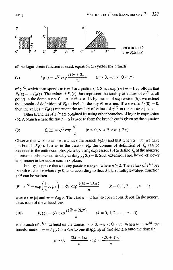
SEC. 90
Y
B' A' XFIGURE 119w = Fo(sin z).
of the logarithmic function is used, equation (5) yields the branch
+ 27r)(7) F1(z) = exp
i (O
2(r > 0, -7r < d < 7r)
of z1/2, which corresponds to k = 1 in equation (4). Since exp(i7r) = -1, it follows thatF1(z) = -F0(z). The values +F0(z) thus represent the totality of values of z1/2 at allpoints in the domain r > 0, -7r < C) < 7r. If, by means of expression (6), we extendthe domain of definition of F0 to include the ray C) = 7r and if we write FO(0) = 0,then the values ±F0(z) represent the totality of values of z1/2 in the entire z plane.
Other branches of z1/2 are obtained by using other branches of log z in expression(5). A branch where the ray 0 = a is used to form the branch cut is given by the equation
(8) f,, (z) = expi8 (r > 0, a < 0 < a + 27).
Observe that when a = -7r, we have the branch F0(z) and that when a = 7r, we havethe branch F1(z). Just as in the case of F0, the domain of definition of fa can beextended to the entire complex plane by using expression (8) to define f« at the nonzeropoints on the branch cut and by writing f,, (0) = 0. Such extensions are, however, nevercontinuous in the entire complex plane.
Finally, suppose that n is any positive integer, where n > 2. The values of z I/ n arethe nth roots of z when z 0; and, according to Sec. 31, the multiple-valued functionz1/n can be written
(9) z1/n = exp
MAPPINGS BY Z2 AND BRANCHES OF Z1/2 327
i(Q+2k7r)exp
n(k=0, 1,2,...,
where r = 1z I and C) = Arg z. The case n = 2 has just been considered. In the generalcase, each of the n functions
(10) Fk(z) = n r expi(C) -- 2k7r)
n(k=0, 1,2,...,n-1)
is a branch of z11", defined on the domain r > 0, -7r < C) < 7r. When w = pe`g', thetransformation w = Fk(z) is a one to one mapping of that domain onto the domain
p > 0, (2k - 1)7r < < (2k + 1)7r
n n
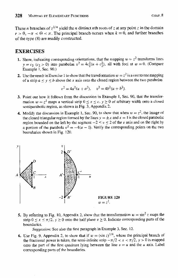
328 MAPPING BY ELEMENTARY FUNCTIONS CHAP. 8
These n branches of z I/ n yield the n distinct nth roots of z at any point z in the domainr > 0, -3r < O < rr. The principal branch occurs when k = 0, and further branchesof the type (8) are readily constructed.
EXERCISES1. Show, indicating corresponding orientations, that the mapping w = z22 transforms lines
y = c2 (c2 > 0) into parabolas v2 = 4c2(u + c2), all with foci at w = 0. (CompareExample 1, Sec. 90.)
2. Use the result in Exercise 1 to show that the transformation w = z2 is a one to one mappingof a strip a < y < b above the x axis onto the closed region between the two parabolas
v2 = 4a2(u + a2), v2 = 4b2(u + b2).
3. Point out how it follows from the discussion in Example 1, Sec. 90, that the transfor-mation w = z2 maps a vertical strip 0 < x < c, y > 0 of arbitrary width onto a closedsemiparabolic region, as shown in Fig. 3, Appendix 2.
4. Modify the discussion in Example 1, Sec. 90, to show that when w = z2. the image ofthe closed triangular region formed by the lines y = ±x and x = I is the closed parabolicregion bounded on the left by the segment -2 < v < 2 of the v axis and on the right bya portion of the parabola v2 = -4(u - 1). Verify the corresponding points on the twoboundaries shown in Fig. 120.
FIGURE 1202w=z
5. By referring to Fig. 10, Appendix 2, show that the transformation w = sin2 z maps thestrip 0 < x < ,r/2, y > 0 onto the half plane v > 0. Indicate corresponding parts of theboundaries.
Suggestion: See also the first paragraph in Example 3, Sec. 12.
6. Use Fig. 9, Appendix 2, to show that if w = (sin z)114, where the principal branch ofthe fractional power is taken, the semi-infinite strip -7r/2 < x < z j2, y > 0 is mappedonto the part of the first quadrant lying between the line v = u and the u axis. Labelcorresponding parts of the boundaries.
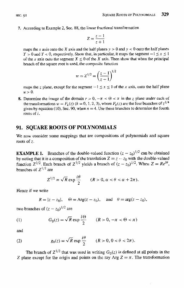
SEC. 91 SQUARE ROOTS OF POLYNOMIALS 329
7. According to Example 2, Sec. 88, the linear fractional transformation
Z= z-1
z+1maps the x axis onto the X axis and the half planes y > 0 and y < 0 onto the half planesY > 0 and Y < 0, respectively. Show that, in particular, it maps the segment -1 < x 1
of the x axis onto the segment X < 0 of the X axis. Then show that when the principalbranch of the square root is used, the composite function
2
maps the z plane, except for the segment -1 < x < 1 of the x axis, onto the half planeu>0.
8. Determine the image of the domain r > 0, -Tr < O < z in the z plane under each ofthe transformations w = Fk(z) (k = 0, 1, 2, 3), where Fk(z) are the four branches of z1/4given by equation (10), Sec. 90, when n = 4. Use these branches to determine the fourthroots of i.
91. SQUARE ROOTS OF POLYNOMIALS
We now consider some mappings that are compositions of polynomials and squareroots of z.
EXAMPLE 1, Branches of the double-valued function (z - zo)1/2 can be obtainedby noting that it is a composition of the translation Z = z - zo with the double-valuedfunction Z1/2. Each branch of Z1/2 yields a branch of (z - zo)1/2. When Z = ReZO,branches of Z1/2 are
Z1/2= expio (R>O,a <0 <a+27r).
Hence if we write
R=Iz - zol, O =Arg(z-zo), and 0=arg(z
two branches of (z - zo)1/2 are
(2)
Go(z) = exp (R>O,-n <4
go (z) =' exp i9(R > O, O < 0 < 2n
0
The branch of Z1/2 that was used in writing Go(z) is defined at all points in theZ plane except for the origin and points on the ray Arg Z = it. The transformation
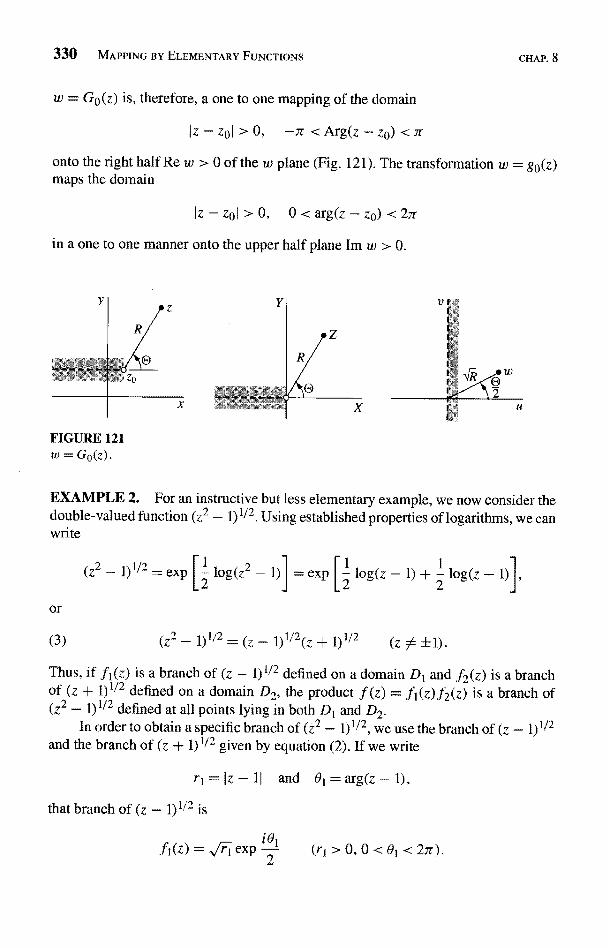
330 MAPPING BY ELEMENTARY FUNCTIONS CHAP. 8
w = G0(z) is, therefore, a one to one mapping of the domain
Iz -zol > 0, -Jr <Arg(z -zo) <m
onto the right half Re w > 0 of the w plane (Fig, 121). The transformation w = go(z)maps the domain
Iz-zol>0, 0<arg(z-zo) <27r
in a one to one manner onto the upper half plane Im w > 0.
FIGURE 121w = G0(z).
EXAMPLE 2. For an instructive but less elementary example, we now consider thedouble-valued function (z2 - 1)1/2. Using established properties of logarithms, we canwrite
(z2 - 1) 1/2 = exp log(z2 - 1)] = exp og(z - 1) + - log(z + 1)
or
(3) (z2 - 1)1/2 = (z - 1)1/2(z + 1)1/2 (z ±1).
Thus, if fl(z) is a branch of (z - 1)1/2 defined on a domain D1 and f2(z) is a branchof (z + 1) 1/2 defined on a domain D2, the product f(z) = f, (z) f2 (z) is a branch of(z2 - 1)1/2 defined at all points lying in both D1 and D2.
In order to obtain a specific branch of (z2 - 1)1/2, we use the branch of (z - 1)1/2and the branch of (z + 1)1/2 given by equation (2). If we write
ri=lz - 11 and 01=arg(z- 1),
that branch of (z - 1) 1/2 is
i91f1(z) = r_ exp
2(r1 > 0, 0 < 01 < 2n).
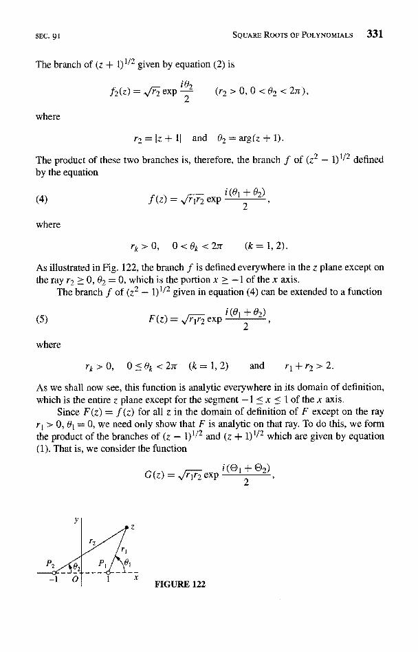
SEC. 91 SQUARE ROOTS OF POLYNOMIALS 331
The branch of (z + 1) 1/2 given by equation (2) is
f2(z) = r2expi02 (r2>0,0<02<2n),
where
The product of theseby the equation
where
r2= jz+ 11 and 92 = arg(z + 1).
o branches is, therefore, the branch f of (z2
f (z) = rlr2 expi(01 + 02)
2
I defined
rk > 0, 0 < Ok < 27r (k = 1, 2).
As illustrated in Fig. 122, the branch f is defined everywhere in the z plane except onthe ray r2 > 0, 92 = 0, which is the portion x > -1 of the x axis.
The branch f of (z2 - 1)1/2 given in equation (4) can be extended to a function
where
2
rk > 0, °-k<2 Tr (k=1,2) and r1 + r2 > 2.
As we shall now see, this function is analytic everywhere in its domain of definition,which is the entire z plane except for the segment -1 < x < 1 of the x axis.
Since F(z) = f (z) for all z in the domain of definition of F except on the rayr1 > 0, 81 = 0, we need only show that F is analytic on that ray. To do this, we formthe product of the branches of (z - 1)1/2 and (z + 1) 1/2 which are given by equation(1). That is, we consider the function
G(z) = rlr2 exp :
FIGURE 122
i(91+82)F(z) = rlr2 exp
2
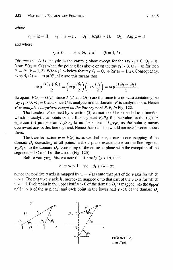
332 MAPPING BY ELEMENTARY FUNCTIONS CHAP. 8
where
r1 =
and where
z-11, r2=Iz+11, Arg(z - 1), O2 = Arg(z +
rk > 0, -n < Ok < r (k = 1, 2).
Observe that G is analytic in the entire z plane except for the ray r1 > 0, OI = n,Now F(z) = G(z) when the point z lies above or on the ray r1 > 0, O1 = 0; for then9k = Ok(k = 1, 2). When z lies below that ray, 9k = Ok + 27r (k = 1, 2). Consequently,exp(i9k/2) = -exp(i(DkJ2); and this means that
expI (012 92) _ exp i 01) (exp i 92) = exp i (O12 02)
So again, F(z) = G(z). Since F(z) and G(z) are the same in a domain containing theray r1 > 0, 01= 0 and since G is analytic in that domain, F is analytic there. HenceF is analytic everywhere except on the line segment P2 P1 in Fig. 122.
The function F defined by equation (5) cannot itself be extended to a functionwhich is analytic at points on the line segment P2P1; for the value on the right inequation (5) jumps from i rir2 to numbers near -i rlr2 as the point z movesdownward across that line segment. Hence the extension would not even be continuousthere.
The transformation w = F(z) is, as we shall see, a one to one mapping of thedomain DZ consisting of all points in the z plane except those on the line segmentP2P1 onto the domain D,,, consisting of the entire w plane with the exception of thesegment -1 < v { I of the v axis (Fig. 123).
Before verifying this, we note that if z = iy (y > 0), then
r1=r2> 1 and 91+92=7r;
hence the positive y axis is mapped by w = F(z) onto that part of the v axis for whichv > 1, The negative y axis is, moreover, mapped onto that part of the v axis for whichv < -1. Each point in the upper half y > 0 of the domain Dz is mapped into the upperhalf v > 0 of the w plane, and each point in the lower half y < 0 of the domain Dz
FIGURE 123w=F(z).
SEC. 91 SQUARE ROOTS OF POLYNOMIALS 333
is mapped into the lower half v < 0 of the w plane. The ray r1 > 0, 91= 0 is mappedonto the positive real axis in the w plane, and the ray r2 > 0, 02 = n is mapped ontothe negative real axis there.
To show that the transformation w = F (z) is one to one, we observe that ifF(z1) = F(z2), then z1 _I= z -- 1. From this, it follows that z1 = z2 or z1 = -Z2-However, because of the manner in which F maps the upper and lower halves of thedomain Dz, as well as the portions of the real axis lying in Dz, the case z1 = -z2 isimpossible. Thus, if F(z1) = F(z2), then z1= z2; and F is one to one.
We can show that F maps the domain Dz onto the domain D,,, by finding afunction H mapping D. , into Dz with the property that if z = H(w), then w = F(z).This will show that, for any point w in D,,,, there exists a point z in Dz such thatF(z) = w; that is, the mapping F is onto. The mapping H will be the inverse of F.
To find H, we first note that if w is a value of (z2 - 1)1/2 for a specific z, thenz2 - 1; and z is, therefore, a value of (w2 + 1)1/2 for that w. The function H will
be a branch of the double-valued function
1) 1/2 = (w - i)1/2(w + i)1/2
Following our procedure for obtaining the function F(z), we writeand w + i = P2 exp(i02). (See Fig. 123.) With the restrictions
Pk>0, 2<Ox<3 (k=
we then write
(6) H (w) = Pipe exp
- i = P1 exp(i41)
and P1+P2>2,
11
2
the domain of definition being D.. The transformation z = H(w) maps points of D"lying above or below the u axis onto points above or below the x axis, respectively. Itmaps the positive u axis into that part of the x axis where x > 1 and the negative u axisinto that part of the negative x axis where x < -1. If z = H(w), then z2 = w2 + 1;and so w2 = z2 - 1. Since z is in Dz and since F(z) and -F(z) are the two values of(z2 - 1)1/2 for a point in Dz, we see that w = F(z) or w = -F(z). But it is evidentfrom the manner in which F and H map the upper and lower halves of their domainsof definition, including the portions of the real axes lying in those domains, thatw = F(z).
Mappings by branches of double-valued functions
(7) w=(z2+Az+ B)1/2=[(z-zp)2_.z ]1l2 (zi 0
334 MAPPING BY ELEMENTARY FUNCTIONS CHAP, 8
where A = -2z0 and B = z2 = zz, can be treated with the aid of the results found forthe function F in Example 2 and the successive transformations
(8)Z=z-z0, w=(Z2-1)1/2, w=z
zt
EXERCISES
1. The branch F of (z2 - 1) 1/2 in Example 2, Sec. 91, was defined in terms of the coordinatesr1, r2, 81, 82. Explain geometrically why the conditions r1 > 0, 0 < 01 + 02 < 7r describethe quadrant x > 0, y > 0 of the z plane. Then show that the transformation w = F(z)maps that quadrant onto the quadrant u > 0, v > 0 of the w plane,
Suggestion: To show that the quadrant x > 0, y > 0 in the z plane is described, notethat 01 + 82 = 7r at each point on the positive y axis and that 81 + 82 decreases as a pointz moves to the right along a ray 82 = c (0 < c < 7r/2).
2. For the transformation w = F (z) of the first quadrant of the z plane onto the first quadrantof the w plane in Exercise 1, show that
u= /-Vrir2+x2-y2-1 and v= TUr1r2-
where
2 (x2 + y2 + 1)2 - 4x22
and that the image of the portion of the hyperbola x2 - y2 = 1 in the first quadrant is theray v = u (u > 0).
3. Show that in Exercise 2 the domain D that lies under the hyperbola and in the firstquadrant of the z plane is described by the conditions r1 > 0, 0 < 81 + 82 < 7r/2. Thenshow that the image of D is the octant 0 < v < u. Sketch the domain D and its image.
4. Let F be the branch of (z2 - 1)1/2 defined in Example 2, Sec. 91, and let zo = ro exp(i00)be a fixed point, where ro > 0 and 0 < 00 < 27r. Show that a branch F0 of (z2 - zo)112whose branch cut is the line segment between the points z0 and -z0 can be writtenF0(z) = z0F(Z), where Z = z/z0.
5. Write z - 1 = r1 exp(i91) and z + 1 = r2 exp(i 02), where
0<01 <27r and
to define a branch of the function
1)112;
z
1/2
In each case, the branch cut should consist of the two rays 81= 0 and 02 = 7r
6. Using the notation in Sec. 91, show that the function
w= p i(81 82)
2
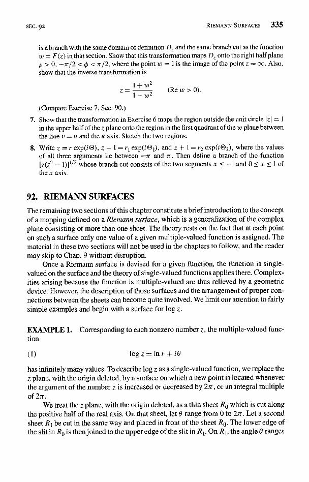
SEC, 92 RIEMANN SURFACES 335
is a branch with the same domain of definition DZ and the same branch cut as the functionw = F(z) in that section. Show that this transformation maps DZ onto the right half planep > 0, -7r/2 < 0 < 7r/2, where the point w = 1 is the image of the point z = 00. Also,show that the inverse transformation is
2
z= 1__w2 (Rew>0).
(Compare Exercise 7, Sec. 90.)
7. Show that the transformation in Exercise 6 maps the region outside the unit circle I z I = 1in the upper half of the z plane onto the region in the first quadrant of the w plane betweenthe line v = u and the u axis. Sketch the two regions.
8. Write z = r exp(i 0), z - 1 = rI exp(i 01), and z + 1 = r2 exp(i 02}, where the valuesof all three arguments lie between -7r and it, Then define a branch of the function[z(z2 - 1)]I/2 whose branch cut consists of the two segments x < -1 and 0 c x < 1 ofthe x axis.
92. RIEMANN SURFACES
The remaining two sections of this chapter constitute a brief introduction to the conceptof a mapping defined on a Riemann surface, which is a generalization of the complexplane consisting of more than one sheet. The theory rests on the fact that at each pointon such a surface only one value of a given multiple-valued function is assigned. Thematerial in these two sections will not be used in the chapters to follow, and the readermay skip to Chap. 9 without disruption.
Once a Riemann surface is devised for a given function, the function is single-valued on the surface and the theory of single-valued functions applies there. Complex-ities arising because the function is multiple-valued are thus relieved by a geometricdevice. However, the description of those surfaces and the arrangement of proper con-nections between the sheets can become quite involved. We limit our attention to fairlysimple examples and begin with a surface for log z.
EXAMPLE 1. Corresponding to each nonzero number z, the multiple-valued func-tion
(1) logz=lnr+i9
has infinitely many values. To describe log z as a single-valued function, we replace thez plane, with the origin deleted, by a surface on which a new point is located wheneverthe argument of the number z is increased or decreased by 2n, or an integral multipleof 27r.
We treat the z plane, with the origin deleted, as a thin sheet R0 which is cut alongthe positive half of the real axis. On that sheet, let 0 range from 0 to 27r. Let a secondsheet Rt be cut in the same way and placed in front of the sheet Re. The lower edge ofthe slit in R0 is then joined to the upper edge of the slit in R 1. On R1, the angle 0 ranges
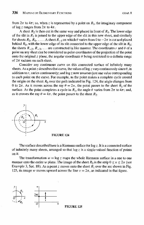
336 MAPPING BY ELEMENTARY FUNCTIONS CHAP. 8
from 2n to 4n; so, when z is represented by a point on RI, the imaginary componentof log z ranges from 27r to 47r.
A sheet R2 is then cut in the same way and placed in front of RI. The lower edgeof the slit in RI is joined to the upper edge of the slit in this new sheet, and similarlyfor sheets R3, R4, .... A sheet R_ I on which 9 varies from 0 to -2n is cut and placedbehind R0, with the lower edge of its slit connected to the upper edge of the slit in R0;the sheets R_2, R_3, ... are constructed in like manner. The coordinates r and 8 of apoint on any sheet can be considered as polar coordinates of the projection of the pointonto the original z plane, the angular coordinate 8 being restricted to a definite rangeof 27r radians on each sheet.
Consider any continuous curve on this connected surface of infinitely manysheets. As a point z describes that curve, the values of log z vary continuously since 8, inaddition to r, varies continuously; and log z now assumes just one value correspondingto each point on the curve. For example, as the point makes a complete cycle aroundthe origin on the sheet R0 over the path indicated in Fig. 124, the angle changes from0 to 2n. As it moves across the ray 0 = 27r, the point passes to the sheet RI of thesurface. As the point completes a cycle in R1, the angle 9 varies from 2n to 47r; and,as it crosses the ray 8 = 47r, the point passes to the sheet R2,
FIGURE 124
The surface described here is a Riemann surface for log z. It is a connected surfaceof infinitely many sheets, arranged so that log z is a single-valued function of pointson it.
The transformation w = log z maps the whole Riemann surface in a one to onemanner onto the entire w plane. The image of the sheet R0 is the strip 0 < v < 2nr (seeExample 3, Sec. 88). As a point z moves onto the sheet RI over the arc shown in Fig.125, its image w moves upward across the line v = 27r, as indicated in that figure.
v
2ni
FIGURE 125
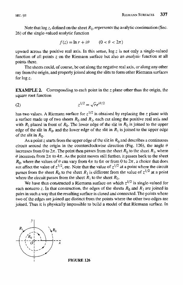
SEC. 92 RIEMANN SURFACES 337
Note that log z, defined on the sheet R1, represents the analytic continuation (Sec.26) of the single-valued analytic function
f(z) =lnr+i8 (0<0 <2n)
upward across the positive real axis. In this sense, log z is not only a single-valuedfunction of all points z on the Riemann surface but also an analytic function at allpoints there.
The sheets could, of course, be cut along the negative real axis, or along any otherray from the origin, and properly joined along the slits to form other Riemann surfacesfor log z.
EXAMPLE 2. Corresponding to each point in the z plane other than the origin, thesquare root function
(2) Z1/2 = freiO/2
has two values. A Riemann surface for z112 is obtained by replacing the z plane witha surface made up of two sheets RO and R1, each cut along the positive real axis andwith R1 placed in front of R0. The lower edge of the slit in R0 is joined to the upperedge of the slit in R1, and the lower edge of the slit in R1 is joined to the upper edgeof the slit in R0.
As a point z starts from the upper edge of the slit in Ro and describes a continuouscircuit around the origin in the counterclockwise direction (Fig. 126), the angle 0increases from 0 to 2n. The point then passes from the sheet RO to the sheet R1, where0 increases from 2Tr to 4n. As the point moves still further, it passes back to the sheetR0, where the values of 0 can vary from 47r to 67r or from 0 to 2ir, a choice that doesnot affect the value of z112, etc. Note that the value of z1"2 at a point where the circuitpasses from the sheet RO to the sheet R1 is different from the value of z1/2 at a pointwhere the circuit passes from the sheet R1 to the sheet R0.
We have thus constructed a Riemann surface on which z112 is single-valued foreach nonzero z. In that construction, the edges of the sheets RO and R1 are joined inpairs in such a way that the resulting surface is closed and connected. The points wheretwo of the edges are joined are distinct from the points where the other two edges arejoined, Thus it is physically impossible to build a model of that Riemann surface. In
FIGURE 126
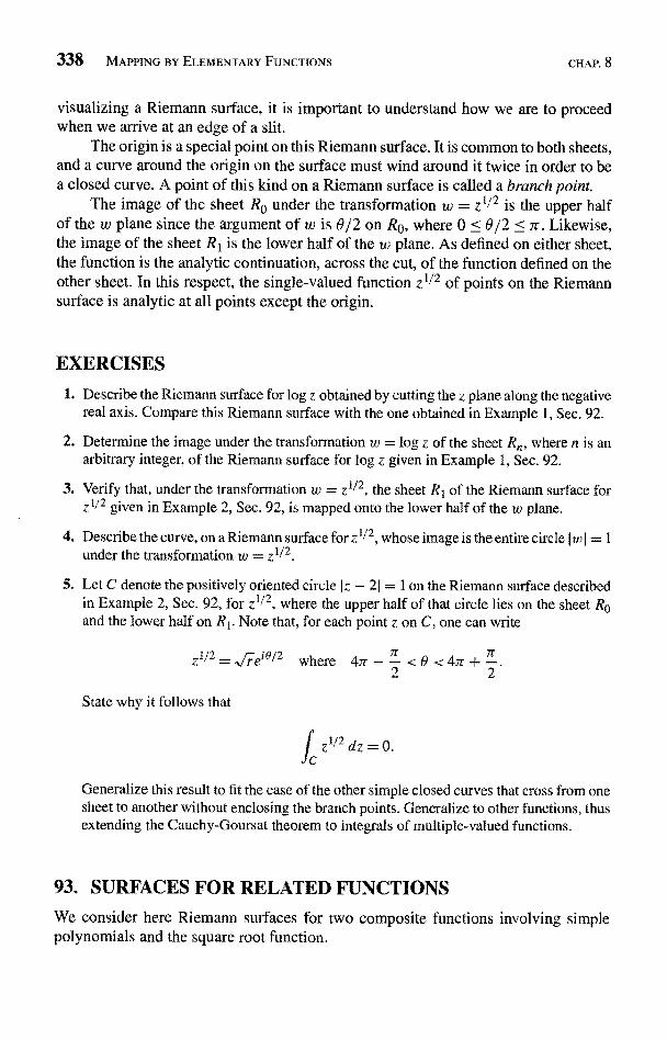
338 MAPPING BY ELEMENTARY FUNCTIONS CHAP. 8
visualizing a Riemann surface, it is important to understand how we are to proceedwhen we arrive at an edge of a slit.
The origin is a special point on this Riemann surface. It is common to both sheets,and a curve around the origin on the surface must wind around it twice in order to bea closed curve. A point of this kind on a Riemann surface is called a branch point.
The image of the sheet R0 under the transformation w = z"2 is the upper halfof the w plane since the argument of w is 0/2 on R0, where 0 < 8/2 < Tr. Likewise,the image of the sheet R1 is the lower half of the w plane. As defined on either sheet,the function is the analytic continuation, across the cut, of the function defined on theother sheet. In this respect, the single-valued function z 1/2 of points on the Riemannsurface is analytic at all points except the origin.
EXERCISES
1. Describe the Riemann surface for log z obtained by cutting the z plane along the negativereal axis. Compare this Riemann surface with the one obtained in Example 1, Sec. 92.
2. Determine the image under the transformation w = log z of the sheet R, where n is anarbitrary integer, of the Riemann surface for log z given in Example 1, Sec. 92.
3. Verify that, under the transformation w = z112, the sheet R1 of the Riemann surface forz 12 given in Example 2, Sec. 92, is mapped onto the lower half of the w plane.
4. Describe the curve, on a Riemann surface f o r z 112, whose image is the entire circle 1 w = 1under the transformation w = z1/2.
5. Let C denote the positively oriented circle Iz - 21 = 1 on the Riemann surface describedin Example 2, Sec. 92, for z1/2, where the upper half of that circle lies on the sheet Reand the lower half on RI. Note that, for each point z on C, one can write
2 where 47r -n
< 0 < 4n2
State why it follows that
CI/2 dz = 0.
Generalize this result to fit the case of the other simple closed curves that cross from onesheet to another without enclosing the branch points. Generalize to other functions, thusextending the Cauchy-Goursat theorem to integrals of multiple-valued functions.
93, SURFACES FOR RELATED FUNCTIONS
We consider here Riemann surfaces for two composite functions involving simplepolynomials and the square root function.
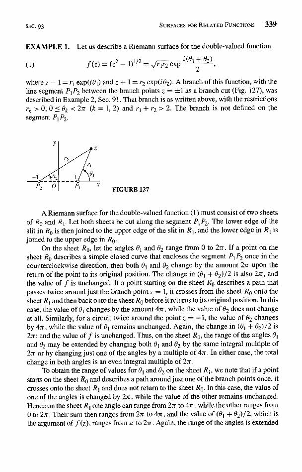
SEC. 93 SURFACES FOR RELATED FUNCTIONS 339
EXAMPLE 1. Let us describe a Riemann surface for the double-valued function
(1) f(z) = (z2_1)1/2= rlr2 expt(8
202)
where z - 1 = r1 exp(i01) and z + 1 = r2 exp(i02). A branch of this function, with theline segment P, P2 between the branch points z = ± I as a branch cut (Fig. 127), wasdescribed in Example 2, Sec. 91. That branch is as written above, with the restrictionsrk > 0, 0 < 6k < 27r (k = 1, 2) and rT + r2 > 2. The branch is not defined on thesegment PIP2.
FIGURE 127
A Riemann surface for the double-valued function (1) must consist of two sheetsof Ro and R1. Let both sheets be cut along the segment P1P2. The lower edge of theslit in Ro is then joined to the upper edge of the slit in R1, and the lower edge in RI isjoined to the upper edge in Ro.
On the sheet R0, let the angles 01 and 02 range from 0 to 27r. If a point on thesheet Ro describes a simple closed curve that encloses the segment PIP2 once in thecounterclockwise direction, then both 01 and 02 change by the amount 27r upon thereturn of the point to its original position. The change in (01 + 02)/2 is also 27r, andthe value of f is unchanged. If a point starting on the sheet Ro describes a path thatpasses twice around just the branch point z = 1, it crosses from the sheet Ro onto thesheet R1 and then back onto the sheet Ro before it returns to its original position. In thiscase, the value of 01 changes by the amount 47r, while the value of 02 does not changeat all. Similarly, for a circuit twice around the point z = -1, the value of 02 changesby 47r, while the value of 01 remains unchanged. Again, the change in (01 + 02)j2 is27r; and the value of f is unchanged. Thus, on the sheet R0, the range of the angles 01and 02 may be extended by changing both 01 and 62 by the same integral multiple of27r or by changing just one of the angles by a multiple of Oar. In either case, the totalchange in both angles is an even integral multiple of 27r.
To obtain the range of values for 01 and 02 on the sheet R1, we note that if a pointstarts on the sheet Ro and describes a path around just one of the branch points once, itcrosses onto the sheet R1 and does not return to the sheet R0. In this case, the value ofone of the angles is changed by 27r, while the value of the other remains unchanged.Hence on the sheet R 1 one angle can range from 27r to 47r, while the other ranges from0 to 27r. Their sum then ranges from 27r to 47r, and the value of (01 + 62)12, which isthe argument of f (z), ranges from 7r to 27r. Again, the range of the angles is extended
340 MAPPING BY ELEMENTARY FUNCTIONS CHAP. 8
by changing the value of just one of the angles by an integral multiple of 47r or bychanging the value of both angles by the same integral multiple of 27r.
The double-valued function (1) may now be considered as a single-valuedfunction of the points on the Riemann surface just constructed. The transformationw = f (z) maps each of the sheets used in the construction of that surface onto theentire w plane.
EXAMPLE 2. Consider the double-valued function
(2) .f (z) = [z(z2 - 1)]-1/2 = i (8 + 81 + 82)rrir2 exp
2
(Fig. 128). The points z = 0. i 1 are branch points of this function. We note that if thepoint z describes a circuit that includes all three of those points, the argument of f (z)changes by the angle 37r and the value of the function thus changes. Consequently, abranch cut must run from one of those branch points to the point at infinity in order todescribe a single-valued branch of f. Hence the point at infinity is also a branch point,as one can show by noting that the function f (1/z) has a branch point at z = 0.
Let two sheets be cut along the line segment L, from z = -1 to z = 0 and alongthe part LI of the real axis to the right of the point z = 1. We specify that each of thethree angles 8, 81, and 82 may range from 0 to 27r on the sheet Rp and from 27r to47r on the sheet RI. We also specify that the angles corresponding to a point on eithersheet may be changed by integral multiples of 27r in such a way that the sum of thethree angles changes by an integral multiple of 4n. The value of the function f is,therefore, unaltered.
A Riemann surface for the double-valued function (2) is obtained by joining thelower edges in RO of the slits along L1 and L2 to the upper edges in RI of the slitsalong L 1 and L2, respectively. The lower edges in R 1 of the slits along L 1 and L2 arethen joined to the upper edges in Rp of the slits along LI and L2. respectively. It isreadily verified with the aid of Fig. 128 that one branch of the function is representedby its values at points on Ra and the other branch at points on RI.
FIGURE 128
EXERCISES1. Describe a Riemann surface for the triple-valued function w = (z - 1) 113, and point out
which third of the w plane represents the image of each sheet of that surface.
SEC. 93 EXERCISES 341
2. Corresponding to each point on the Riemann surface described in Example 2, Sec. 93,for the function w = f (z) in that example, there is just one value of w. Show that,corresponding to each value of w, there are, in general, three points on the surface.
3. Describe a Riemann surface for the multiple-valued function
f (Z)
4. Note that the Riemann surface described in Example 1, Sec. 93, for (z2 - 1)1/2 is also aRiemann surface for the function
g (Z) = Z + (Z2 - 1)1/2.
Let fo denote the branch of (z2 - 1) 1/2 defined on the sheet Ro, and show that the branchesgo and g1 of g on the two sheets are given by the equations
go(z) =gl(z) =
z + .fo(z).
5. In Exercise 4, the branch fo of (z2 - 1) 1/2 can be described by means of the equation
.fo(z) = rlr2 (exp i11) (exp io
where 01 and 02 range from 0 to 27r and
z - 1 r1 exp(i01), z + 1 = r2 exp(i02).
Note that 2z = r1 exp(i91) + r2 exp(i02), and show that the branch go of the functiong(z) = z + (z2 - 1) 1/2 can be written in the form
iO lgo(z) = - ( rI exp +
2
Find go(z)go(z), and note that r1 + r2 > 2 and cos[(01 - 92)/2] > 0 for all z, to prove thatIgo(z) I > 1. Then show that the transformation w = z + (z2 - 1)1/2 maps the sheet Ro ofthe Riemann surface onto the region I w l > 1, the sheet R 1 onto the region I w I < 1, and thebranch cut between the points z = ± 1 onto the circle I w I = 1. Note that the transformationused here is an inverse of the transformation
z= - ( W +-

CHAPTER
9CONFORMAL MAPPING
In this chapter, we introduce and develop the concept of a conformal mapping, with em-phasis on connections between such mappings and harmonic functions. Applicationsto physical problems will follow in the next chapter.
94. PRESERVATION OF ANGLES
Let C be a smooth are (Sec. 38), represented by the equation
z = z(t) (a < t < b),
and let f (z) be a function defined at all points z on C. The equation
z < b)
is a parametric representation of the image F of C under the transformation w = f (z).Suppose that C passes through a point zo = z(to) (a < to < b) at which f is
analytic and that f'(zo) A 0. According to the chain rule given in Exercise 5, Sec.38, if w(t) = f [z(t)], then
.f`[z(ta)]z`(ta
and this means that (see Sec. 7)
(2) arg w`(to t o)j + arg z tta
343
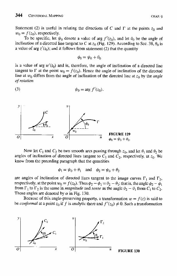
344 CONFORMAL MAPPING CHAP. 9
Statement (2) is useful in relating the directions of C and F at the points z0 andw0 = f (z0), respectively.
To be specific, let *0 denote a value of arg f'(z0), and let 00 be the angle ofinclination of a directed line tangent to C at z0 (Fig. 129). According to Sec. 38, 00 isa value of arg z'(t0); and it follows from statement (2) that the quantity
00-*0 +00is a value of arg w'(t0) and is, therefore, the angle of inclination of a directed linetangent to F at the point w0 = f (z0). Hence the angle of inclination of the directedline at w0 differs from the angle of inclination of the directed line at z0 by the angleof rotation
FIGURE 12900 = '0 + 00.
Now let C1 and C2 be two smooth arcs passing through z0, and let 01 and 02 beangles of inclination of directed lines tangent to C1 and C2, respectively, at z0. Weknow from the preceding paragraph that the quantities
01='0+01 and 02=*0+02are angles of inclination of directed lines tangent to the image curves F1 and F2,respectively, at the point w0 = f (z0). Thus 02 - fit= 02 - 01; that is, the angle q52 - 01from F1 to 1,2 is the same in magnitude and sense as the angle 02 - 01 from C1 to C2.Those angles are denoted by a in Fig. 130.
Because of this angle-preserving property, a transformation w = f (z) is said tobe conformal at a point z0 if f is analytic there and f'(z0) 0. Such a transformation
FIGURE 130
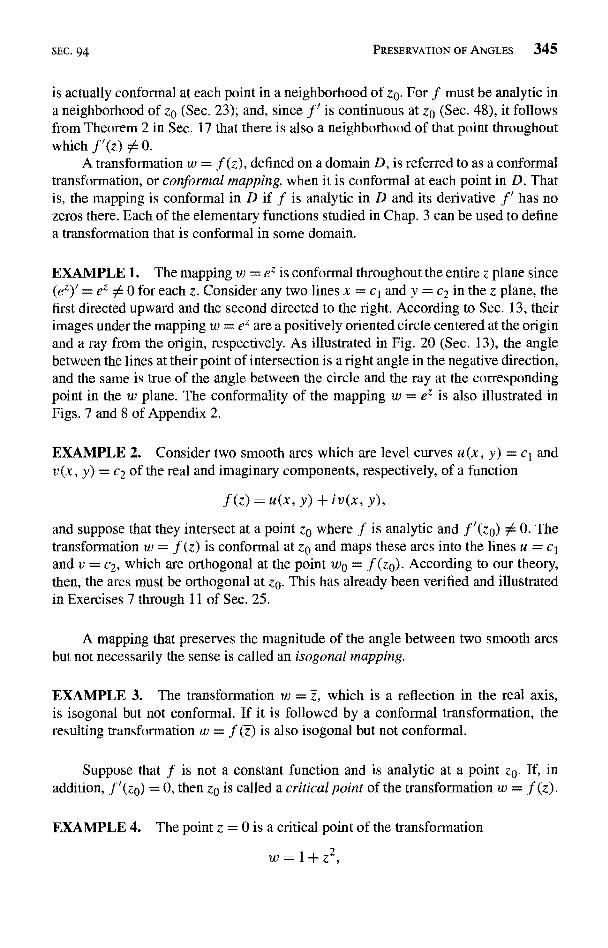
SEC. 94 PRESERVATION OF ANGLES 345
is actually conformal at each point in a neighborhood of z0. For f must be analytic ina neighborhood of za (Sec. 23); and, since f' is continuous at za (Sec. 48), it followsfrom Theorem 2 in Sec. 17 that there is also a neighborhood of that point throughoutwhich f'(z) A 0.
A transformation w = f (z), defined on a domain D, is referred to as a conformaltransformation, or conformal mapping, when it is conformal at each point in D. Thatis, the mapping is conformal in D if f is analytic in D and its derivative f has nozeros there. Each of the elementary functions studied in Chap. 3 can be used to definea transformation that is conformal in some domain.
EXAMPLE 1. The mapping w = eZ is conformal throughout the entire z plane since(ez)' = ez ,A 0 for each z. Consider any two lines x = cl and y = c2 in the z plane, thefirst directed upward and the second directed to the right. According to Sec. 13, theirimages under the mapping w = ez are a positively oriented circle centered at the originand a ray from the origin, respectively. As illustrated in Fig. 20 (Sec. 13), the anglebetween the lines at their point of intersection is a right angle in the negative direction,and the same is true of the angle between the circle and the ray at the correspondingpoint in the w plane. The conformality of the mapping w = eZ is also illustrated inFigs. 7 and 8 of Appendix 2.
EXAMPLE 2. Consider two smooth arcs which are level curves u (x, y) = cv(x, y) = c2 of the real and imaginary components, respectively, of a function
f (z) = u(x, y) + iv(x, y),
and suppose that they intersect at a point za where f is analytic and f'(zo) ; 0. Thetransformation w = f (z) is conformal at za and maps these arcs into the lines u = crand v = c2, which are orthogonal at the point wp = f (za). According to our theory,then, the arcs must be orthogonal at Z. This has already been verified and illustratedin Exercises 7 through 11 of Sec. 25.
A mapping that preserves the magnitude of the angle between two smooth arcsbut not necessarily the sense is called an isogonal mapping.
EXAMPLE 3. The transformation w = Z, which is a reflection in the real axis,is isogonal but not conformal. If it is followed by a conformal transformation, theresulting transformation w = f (z) is also isogonal but not conformal.
Suppose that f is not a constant function and is analytic at a point za. If, inaddition, f'(zo) = 0, then zo is called a critical point of the transformation w = f (z).
EXAMPLE 4. The point z = 0 is a critical point of the transformation
w=
346 CONFORMAL MAPPING
which is a composition of the mappings
Z=z2 and w=1+Z.
CHAP. 9
A ray 0 = a from the point z = 0 is evidently mapped onto the ray from the pointw = 1 whose angle of inclination is 2a. Moreover, the angle between any two raysdrawn from the critical point z = 0 is doubled by the transformation.
More generally, it can be shown that if zo is a critical point of a transformationw = f (z), there is an integer m (m > 2) such that the angle between any two smootharcs passing through zo is multiplied by m under that transformation, The integer m isthe smallest positive integer such that f (m) (zo) ; 0. Verification of these facts is leftto the exercises.
95. SCALE FACTORS
Another property of a transformation w = f (z) that is conformal at a point zo isobtained by considering the modulus of f'(zo). From the definition of derivative and aproperty of limits involving moduli that was derived in Exercise 7, Sec. 17, we knowthat
(1) If'(zo)I,f (z) - ,f (zo)
z - zo= lim I f (z) - .f (zo) I
z-zo Iz - zol
Now Iz - zol is the length of a line segment joining zo and z, and I f (z) - f (zo) I is thelength of the line segment joining the points f (zo) and f (z) in the w plane. Evidently,then, if z is near the point zo, the ratio
If(z) - f(zo)IIz - zoI
of the two lengths is approximately the number I f'(zo) I. Note that I f'(zo) I representsan expansion if it is greater than unity and a contraction if it is less than unity.
Although the angle of rotation arg f'(z) (Sec. 94) and the scale factor I f'(z)Ivary, in general, from point to point, it follows from the continuity of f' that theirvalues are approximately arg f'(zo) and I f'(zo)I at points z near zo. Hence the imageof a small region in a neighborhood of zo conforms to the original region in the sensethat it has approximately the same shape. A large region may, however, be transformedinto a region that bears no resemblance to the original one.
EXAMPLE. When f (z) = z2, the transformation
2-y2+i2xy
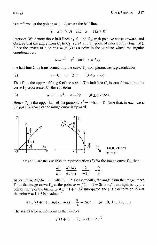
SEC. 95 SCALE FACTORS 347
is conformal at the point z = 1 + i, where the half lines
y=x(x>0) and x=1(x>O)intersect. We denote those half lines by C1 and C2, with positive sense upward, andobserve that the angle from C1 to C2 is irf4 at their point of intersection (Fig. 131).Since the image of a point z = (x, y) is a point in the w plane whose rectangularcoordinates are
u=x2-y2 and v=2xy,
the half line C1 is transformed into the curve F1 with parametric representation
(2) u=0, v=2x2 (0 <x
Thus F1 is the upper half v > 0 of the v axis. The half line C2 is transformed into thecurve 1 2 represented by the equations
(3) u=l-y2, v=2y (O<y<oo).
Hence 1 2 is the upper half of the parabola v2 = -4(u - 1). Note that, in each case,the positive sense of the image curve is upward.
FIGURE 131w = z°.
If u and v are the variables in representation (3) for the image curve F2, then
dv dvfdy 2 _ 2
du dufdy -2y v
In particular, d v Jdu = -1 when v = 2. Consequently, the angle from the image curve1', to the image curve F2 at the point w = f (1 + i) = 2i is 7r/4, as required by theconformality of the mapping at z = 1 + i. As anticipated, the angle of rotation ,7r/4 atthe point z = 1 + i is a value of
g[f`(1 + i)] = arg[2(l7r
42nir
The scale factor at that point is the number
I =12(l+i)I=2vt2.
348 CONFORMAL MAPPING CHAP. 9
To illustrate how the angle of rotation and the scale factor can change from pointto point, we note that they are 0 and 2, respectively, at the point z = I since f'(1) = 2.See Fig. 131, where the curves C2 and 1 2 are the ones just discussed and where thenonnegative x axis C3 is transformed into the nonnegative u axis F3.
96. LOCAL INVERSESA transformation w = f (z) that is conformal at a point z0 has a local inverse there. Thatis, if w0 = f (z0), then there exists a unique transformation z = g(w), which is definedand analytic in a neighborhood N of w0, such that g(w0) = z0 and f [g(w)] = w forall points w in N. The derivative of g(w) is, moreover,
1( ) g'f (z)
We note from expression (1) that the transformation z = g(w) is itself conformal atw0.
Assuming that w = f (z) is, in fact, conformal at z0, let us verify the existenceof such an inverse, which is a direct consequence of results in advanced calculus.* Asnoted in Sec. 94, the conformality of the transformation w = f (z) at z0 implies thatthere is some neighborhood of z0 throughout which f is analytic. Hence if we write
z = x + i y, z0 = x0 + iy0, and f (z) = u(x, y) + it) (x, y),
we know that there is a neighborhood of the point (x0, y0) throughout which thefunctions u(x, y) and v(x, y) along with their partial derivatives of all orders, arecontinuous (see Sec. 48).
Now the pair of equations
(2) u=u(x,y), v=v(x,y)
represents a transformation from the neighborhood just mentioned into the u v plane.Moreover. the determinant
uy= uxVy - vxuy>
Y
which is known as the Jacobian of the transformation, is nonzero at the point (x0, y0).For, in view of the Cauchy-Riemann equations ux = vy and uy = -vx, one can writeJ as
* The results from advanced calculus to be used here appear in, for instance, A. E. Taylor and W. R.
'(w)1
n, "Advanced Calculus," 3d ed., pp. 241-247,1983,
SEC. 96 LOCAL INVERSES 349
and f'(zo) 0 0 since the transformation w = f (z) is conformal at zo. The above con-tinuity conditions on the functions u(x, y) and v(x, y) and their derivatives, togetherwith this condition on the Jacobian, are sufficient to ensure the existence of a localinverse of transformation (2) at (xo, yo). That is, if
(3) uo = u (xo, yo) and vo = v (xo, yo),
then there is a unique continuous transformation
(4) X = x(u, v), y = y(u, v),
defined on a neighborhood N of the point (uo, vo) and mapping that point onto (xo, yo),such that equations (2) hold when equations (4) hold. Also, in addition to beingcontinuous, the functions (4) have continuous first-order partial derivatives satisfyingthe equations
(5)1 1 1 _ 1
xu= Jvy, fuy, Yu='--vx, yv=
throughout N.If we write w = u + iv and wo = uo + i vo, as well as
(6) g(w) = x(u, v) + iy(u, v),
the transformation z g (w) is evidently the local inverse of the original transformationw = f (z) at zo. Transformations (2) and (4) can be written
u-}-iv=u(x, y)+iv(x, y) and x+iy=x(u, v)-I-iy(u,
and these last two equations are the same as
z and z = g(w),
where g has the desired properties. Equations (5) can be used to show that g is analyticin N. Details are left to the exercises, where expression (1) for g(w) is also derived.
EXAMPLE. We saw in Example 1, Sec. 94, that if f (z) = ez, the transformationw = f (z) is conformal everywhere in the z plane and, in particular, at the pointzo = 2ni. The image of this choice of zo is the point wo = 1. When points in the wplane are expressed in the form w = p exp(irb), the local inverse at zo can be obtainedby writing g(w) = log w, where log w denotes the branch
logw=Inp+i i (p>0,ir <9 <
of the logarithmic function, restricted to any neighborhood of wo that does not containthe origin. Observe that
g(1)=In 1+i2n=2 i
350 CONFORMAL MAPPING
and that, when w is in the neighborhood,
f [g(w)] = exp(log w
Also,
g(w)=-logw
in accordance with equation (1).Note that, if the point zQ = 0 is chosen, one can use the principal branch
Log w =Inp+io (p > 0, -Tr <0 <
of the logarithmic function to define g. In this case, g(l) = 0.
CHAP. 9
EXERCISES
1. Determine the angle of rotation at the point z = 2 + i when the transformation is w = z2,and illustrate it for some particular curve. Show that the scale factor of the transformationat that point is 2,/5-.
2. What angle of rotation is produced by the transformation w = 1/z at the point
(a)z=1; (b)z=i?Ans. (a) 7r; (b) 0.
3. Show that under the transformation w = I/z, the images of the lines y = x - 1 andy = 0 are the circle u2 + v2 - u - v = 0 and the line v = 0, respectively. Sketch all fourcurves, determine corresponding directions along them, and verify the conformality ofthe mapping at the point z = 1.
4. Show that the angle of rotation at a nonzero point zo = r0 exp(i0v) under the transforma-tion w = zn (n = 1, 2, ...) is (n - 1)00. Determine the scale factor of the transformationat that point.
Ans. nra-I
5. Show that the transformation w = sin z is conformal at all points except
7rz =
2+ n7 (n = 0, ±1, ±2, .. ,).
Note that this is in agreement with the mapping of directed line segments shown in Figs.9, 10, and 1 I of Appendix 2.
6. Find the local inverse of the transformation w = z2 at the point
(a)z4=2; (b)z0= -2; (c)z0=-i.Ans. (a) w112 = /e"tt2 (p > 0, -Tr <,o < ir);
pei$12 (p>0,2Tr<q <4Tr).7. In Sec. 96, it was pointed out that the components x(u, v) and y(u, v) of the inverse
function g(w) defined by equation (6) are continuous and have continuous first-order
SEC. 97 HARMONIC CONJUGATES 351
partial derivatives in the neighborhood N. Use equations (5), Sec. 96, to show that theCauchy-Riemann equations x = y,,, x _ -yu hold in N. Then conclude that g(w) isanalytic in that neighborhood.
8. Show that if z = g(w) is the local inverse of a conformal transformation w = f (z) at apoint Z0, then
r9
1
at points w in the neighborhood N where g is analytic (Exercise 7).Suggestion: Start with the fact that f [g(w)] = w, and apply the chain rule for
differentiating composite functions.
9. Let C be a smooth arc lying in a domain D throughout which a transformation w = f (z)is conformal, and let F denote the image of C under that transformation. Show that r isalso a smooth arc.
10. Suppose that a function f is analytic at z0 and that
fff(z0) = ... = ftm-,U(zo) = 0, f(m)(z0) A 0
for some positive integer in (m > 1). Also, wo = f (z0)Use the Taylor series for f about the point zo to show that there is a neighborhoodof z0 in which the difference f (z) - w0 can be written
.f (z) - w0 = (z - zo).,sj [1 + g(z)],
(b)
where g(z) is continuous at zo and g(z0) = 0.Let F be the image of a smooth arc C under the transformation w = f (z), as shownin Fig. 129 (Sec. 94), and note that the angles of inclination 80 and 00 in that figureare limits of arg(z - z0) and arg[f (z) - w0], respectively, as z approaches zo alongthe arc C. Then use the result in part (a) to show that 80 and 00 are related by theequation
.00=m$0+arg z0).
(c) Let a denote the angle between two smooth arcs Ct and C2 passing through zo,as shown on the left in Fig. 130 (Sec. 94). Show how it follows from the relationobtained in part (b) that the corresponding angle between the image curves FI andF2 at the point w0 = f (zo) is ma. (Note that the transformation is conformal at z0when m = 1 and that zo is a critical point when m > 2.)
97. HARMONIC CONJUGATES
We saw in Sec. 25 that if a function
.f (z) = u(x, y) + i v(x, y)
352 CONFORMAL MAPPING CHAP. 9
is analytic in a domain D, then the real-valued functions u and v are harmonic in thatdomain. That is, they have continuous partial derivatives of the first and second orderin D and satisfy Laplace's equation there:
uzx + uyy = 0, vxz + VVV =0.
We had seen earlier that the first-order partial derivatives of u and v satisfy the Cauchy-Riemann equations
(2) ux = vy, uy
and, as pointed out in Sec. 25, v is called a harmonic conjugate of u.Suppose now that u(x, y) is any given harmonic function defined on a simply
connected (Sec. 46) domain D. In this section, we show that u(x, y) always has aharmonic conjugate v(x, y) in D by deriving an expression for v(x, y).
To accomplish this, we first recall some important facts about line integrals inadvanced calculus.* Suppose that P(x, y) and Q(x, y) have continuous first-orderpartial derivatives in a simply connected domain D of the xy plane, and let (xa, yo)and (x, y) be any two points in D. If P, = Qx everywhere in D, then the line integral
CP(s, t) ds + Q(s, t) d
from (x4, yo) to (x, y) is independent of the contour C that is taken as long as thecontour lies entirely in D, Furthermore, when the point (xa, yo) is keptfixed and (x, y)is allowed to vary throughout D, the integral represents a single-valued function
(a y)(3) F(x, y) = P(s, t) ds + Q(s, t) dt
of x and y whose first-order partial derivatives are given by the equations
(4) Fx(x, y) = P(x, y), Fy(x, y) = Q(x, y) -
Note that the value of F is changed by an additive constant when a different point(xa, yo) is taken.
Returning to the given harmonic function u(x, y), observe how it follows fromLaplace's equation uxx + uVV = 0 that
(-uy)V = (ux)x
everywhere in D. Also, the second-order partial derivatives of u are continuous in D;and this means that the first-order partial derivatives of -uy and ux are continuous
* See, for example, W. Kaplan, "Advanced Mathematics for Engineers," pp. 546-550, 1992.
SEC. 98 TRANSFORMATIONS OF HARMONIC FUNCTIONS 353
there. Thus, if (x0, y0) is a fixed point in D, the function
,Y)
(5) v(x, y) = J -ux(s, t) ds + us(s, t) dt(X0' YO)
is well defined for all (x, y) in D; and, according to equations (4),
(6) vx(x, y) = -uy(x, Y), vy(x, y) = ux(x, y).
These are the Cauchy-Riemann equations. Since the first-order partial derivatives ofu are continuous, it is evident from equations (6) that those derivatives of v are alsocontinuous. Hence (Sec. 21) u(x, y) + i v(x, y) is an analytic function in D; and v is,therefore, a harmonic conjugate of u.
The function v defined by equation (5) is, of course, not the only harmonicconjugate of u. The function v(x, y) + c, where c is any real constant, is also aharmonic conjugate of u. [Recall Exercise 2, Sec. 25.]
EXAMPLE. Consider the function a (x , y) = xy, which is harmonic throughout theentire xy plane. According to equation (5), the function
(x, y)
v(x,y)=f -sds+tdt11(0,0)
is a harmonic conjugate of u (x, y). The integral here is readily evaluated by inspection.It can also be evaluated by integrating first along the horizontal path from the point(0, 0) to the point (x, 0) and then along the vertical path from (x, 0) to the point (x, y).The result is
v(x, y) =
and the corresponding analytic function is
.f (z) = xY -
98. TRANSFORMATIONS OF HARMONIC FUNCTIONS
The problem of finding a function that is harmonic in a specified domain and satisfiesprescribed conditions on the boundary of the domain is prominent in applied mathe-matics. If the values of the function are prescribed along the boundary, the problemis known as a boundary value problem of the first kind, or a Dirichlet problem. If thevalues of the normal derivative of the function are prescribed on the boundary, theboundary value problem is one of the second kind, or a Neumann problem. Modifica-tions and combinations of those types of boundary conditions also arise.
The domains most frequently encountered in the applications are simply con-nected; and, since a function that is harmonic in a simply connected domain always
354 CONFORMAL MAPPING CHAP. 9
has a harmonic conjugate (Sec. 97), solutions of boundary value problems for suchdomains are the real or imaginary parts of analytic functions.
EXAMPLE 1. In Example 1, Sec. 25, we saw that the function
T(x, y) = e-y sin x
satisfies a certain Dirichlet problem for the strip 0 < x < it, y > 0 and noted that itrepresents a solution of a temperature problem. The function T (x, y), which is actuallyharmonic throughout the xy plane, is evidently the real part of the entire function
-y sin x - i e-ycos x.
It is also the imaginary part of the entire function ez.
Sometimes a solution of a given boundary value problem can be discovered byidentifying it as the real or imaginary part of an analytic function. But the success ofthat procedure depends on the simplicity of the problem and on one's familiarity withthe real and imaginary parts of a variety of analytic functions. The following theoremis an important aid.
Theorem. Suppose that an analytic function
(1) w=f(z)=u(x,y)+iv(x,y)maps a domain Dz in the z plane onto a domain Dw in the w plane. If h (u, v) is aharmonic function defined on D, then the function
(2) H(x, y) = h[u(x, y), v(x, y)]
is harmonic in D.
We first prove the theorem for the case in which the domain D,, is simplyconnected. According to Sec. 97, that property of Dw ensures that the given harmonicfunction h(u, v) has a harmonic conjugate g(u, v). Hence the function
(3) c(w) = h(u, v) + ig(u, v)
is analytic in Dw. Since the function f (z) is analytic in Dz, the composite function(D[f (z)] is also analytic in Dz. Consequently, the real part h[u(x, y), v(x, y)] of thiscomposition is harmonic in Dz.
If D W is not simply connected, we observe that each point w0 in D. has aneighborhood Iw - w0I < e lying entirely in Dw. Since that neighborhood is simplyconnected, a function of the type (3) is analytic in it. Furthermore, since f is continuousat a point zQ in Dz whose image is w0, there is a neighborhood I z - z0 I < S whose imageis contained in the neighborhood I w - wp I < e. Hence it follows that the composition
SEC. 99 TRANSFORMATIONS OF BOUNDARY CONDITIONS 355
(D[f (z)] is analytic in the neighborhood (z - zol < 8, and we may conclude thath[u(x, y), v(x, y)] is harmonic there. Finally, since w0 was arbitrarily chosen in Dwand since each point in Dz is mapped onto such a point under the transformationw = f (z), the function h[u(x, y), v(x, y)] must be harmonic throughout D.
The proof of the theorem for the general case in which Dw is not necessarilysimply connected can also be accomplished directly by means of the chain rule forpartial derivatives. The computations are, however, somewhat involved (see Exercise8, Sec. 99).
EXAMPLE 2. The function h(u, v) = e-" sin u is harmonic in the domain Dw con-sisting of all points in the upper half plane v > 0 (see Example 1). If the transformationis w = z2, then u (x, y) = x2 - y2 and v(x, y) = 2xy; moreover, the domain DZ in thez plane consisting of the points in the first quadrant x > 0, y > 0 is mapped onto thedomain Dw, as shown in Example 3, Sec. 12. Hence the function
H(x, y) = e-2xy sin(x2 - y2)
is harmonic in D.
EXAMPLE 3. Consider the function h(u, v) = Im w = v, which is harmonic inthe horizontal strip -7r/2 < v < 7r/2. We know from Example 3, Sec. 88, that thetransformation w = Log z maps the right half plane x > 0 onto that strip. Hence, bywriting
Log z = y2 arctan yx
where -ir/2 < arctan t <,7r/2, we find that the function
H(x, y) = arctan Y
x
is harmonic in the half plane x > 0.
99. TRANSFORMATIONS OF BOUNDARY CONDITIONS
The conditions that a function or its normal derivative have prescribed values alongthe boundary of a domain in which it is harmonic are the most common, although notthe only, important types of boundary conditions. In this section, we show that certainof these conditions remain unaltered under the change of variables associated with aconformal transformation. These results will be used in Chap. 10 to solve boundaryvalue problems. The basic technique there is to transform a given boundary valueproblem in the xy plane into a simpler one in the u v plane and then to use the theoremsof this and the preceding section to write the solution of the original problem in termsof the solution obtained for the simpler one.
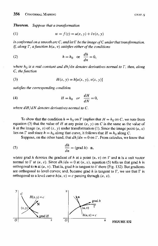
356 CONFORMAL MAPPING
Theorem. Suppose that a transformation
(1) z = u(x, Y) + iv(x, Y)
CHAP. 9
is conformal on a smooth arc C, and let r be the image of C under that transformation.If, along 1, a function h (u, v) satisfies either of the conditions
(2) h=h0 or n =0,d
where h0 is a real constant and dh jdn denotes derivatives normal to F, then, alongC, the function
(3) H(x, y) = h[u(x, y), v(x, y)]
satisfies the corresponding condition
(4) H = h0 or -N = 0,
where dHJdN denotes derivatives normal to C.
To show that the condition h = ho on F implies that H = h0 on C, we note fromequation (3) that the value of H at any point (x, y) on C is the same as the value ofh at the image (u, v) of (x, y) under transformation (1). Since the image point (u, v)lies on I and since h = h0 along that curve, it follows that H = h0 along C.
Suppose, on the other hand, that dh jdn = 0 on r. From calculus, we know that
(5)dh
do(grad h)
where grad h denotes the gradient of h at a point (u, v) on I' and n is a unit vectornormal to r at (u, v). Since dh jdn = 0 at (u, v), equation (5) tells us that grad h isorthogonal to n at (u, v). That is, grad h is tangent to F there (Fig. 132). But gradientsare orthogonal to level curves; and, because grad h is tangent to F, we see that r isorthogonal to a level curve h (u, v) = c passing through (u, v).
FIGURE 132
SEC. 99 TRANSFORMATIONS OF BOUNDARY CONDITIONS 357
Now, according to equation (3), the level curve H(x, y) = c in the z plane canbe written
h[u(x, y), v(x, y
and so it is evidently transformed into the level curve h(u, v) = c under transformation(1). Furthermore, since C is transformed into r and r is orthogonal to the level curveh(u, v) = c, as demonstrated in the preceding paragraph, it follows from the confor-mality of transformation (1) on C that C is orthogonal to the level curve H (x, y) = cat the point (x, y) corresponding to (u, v). Because gradients are orthogonal to levelcurves, this means that grad H is tangent to C at (x, y) (see Fig. 132). Consequently,if N denotes a unit vector normal to C at (x, y), grad H is orthogonal to N. That is,
(6) g
Finally, since
dHdN
grad H) N,
we may conclude from equation (6) that dH jdN = 0 at points on C.In this discussion, we have tacitly assumed that grad h 0 0. If grad h = 0, it
follows from the identity
(grad H(x, y) I = (grad h(u, v) I
derived in Exercise 10(a) below, that grad H = 0; hence dh f do and the correspondingnormal derivative d H f dN are both zero. We also assumed that
(i) grad h and grad H always exist;(ii) the level curve H(x, y) = c is smooth when grad h 0 0 at (u, v).
Condition (ii) ensures that angles between arcs are preserved by transformation(1) when it is conformal. In all of our applications, both conditions (i) and (ii) will besatisfied.
EXAMPLE. Consider, for instance, the function h(u, v) = v + 2. The transforma-tion
-2xy + i (x2 - y2)
is conformal when z 0 0. It maps the half line y = x (x > 0) onto the negative uaxis, where h = 2, and the positive x axis onto the positive v axis, where the normalderivative hu is 0 (Fig. 133). According to the above theorem, the function
H(x,y)=x2-y2-}-2
must satisfy the condition H = 2 along the half line y = x (x > 0) and Hy = 0 alongthe positive x axis, as one can verify directly.
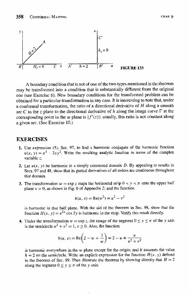
358 CONFORMAL MAPPING CHAP. 9
V
A' h=2
C'
h,, 0
B' FIGURE 133
A boundary condition that is not of one of the two types mentioned in the theoremmay be transformed into a condition that is substantially different from the originalone (see Exercise 6). New boundary conditions for the transformed problem can beobtained for a particular transformation in any case. It is interesting to note that, undera conformal transformation, the ratio of a directional derivative of H along a smootharc C in the z plane to the directional derivative of h along the image curve F at thecorresponding point in the w plane is If'(z)J; usually, this ratio is not constant alonga given arc. (See Exercise 10.)
EXERCISES1. Use expression (5), Sec. 97, to find a harmonic conjugate of the harmonic function
u(x, y) = x3 - 3xy2. Write the resulting analytic function in terms of the complexvariable z.
2. Let u(x, y) be harmonic in a simply connected domain D. By appealing to results inSecs. 97 and 48, show that its partial derivatives of all orders are continuous throughoutthat domain.
3. The transformation w = exp z maps the horizontal strip 0 < y < n onto the upper halfplane v > 0, as shown in Fig. 6 of Appendix 2; and the function
h(u, v) = Re(w2) = U2 - v2
is harmonic in that half plane. With the aid of the theorem in Sec. 98, show that thefunction H(x. y) = e2x cos 2y is harmonic in the strip. Verify this result directly.
4. Under the transformation w = exp z, the image of the segment 0 < y < n of the y axisis the semicircle u2 + v2 = 1, v > 0. Also, the function
1 uh(u,u)=Re 2-w I--)1=2-u+W u2 + v2
is harmonic everywhere in the w plane except for the origin; and it assumes the valueh = 2 on the semicircle. Write an explicit expression for the function H(x, y) definedin the theorem of Sec. 99. Then illustrate the theorem by showing directly that H = 2along the segment 0 < y < n of the y axis.
SEC. 99 EXERCISES 359
5. The transformation w = z2 maps the positive x and y axes and the origin in the z planeonto the u axis in the w plane. Consider the harmonic function
h(u, v) = Re(e-w) = e_ucos v,
and observe that its normal derivative h along the u axis is zero. Then illustrate thetheorem in Sec. 99 when f (z) = z2 by showing directly that the normal derivative of thefunction H (x, y) defined in that theorem is zero along both positive axes in the z plane.(Note that the transformation w = z2 is not conformal at the origin.)
6. Replace the function h (u, v) in Exercise 5 by the harmonic function
h(u, v) = Re(-2i w + e-') = 2v + e_ucos v.
Then show that h = 2 along the u axis but that Hy = 4x along the positive x axis andHx = 4y along the positive y axis. This illustrates how a condition of the type
dh _do
ho 0
is not necessarily transformed into a condition of the type dHJdN = ho.
7. Show that if a function H(x, y) is a solution of a Neumann problem (Sec. 98), thenH(x, y) + A, where A is any real constant, is also a solution of that problem.
8. Suppose that an analytic function w = f (z) = u(x, y) + iv(x, y) maps a domain DZ inthe z plane onto a domain D,,, in the w plane; and let a function h(u, v), with continuouspartial derivatives of the first and second order, be defined on D. Use the chain rule forpartial derivatives to show that if H(x, y) = h[u(x, y), v(x, y)], then
, y) + Hyy(x, y) = [huu(u, v) +h,,,,(u, v)]If`(z)I2
Conclude that the function H(x, y) is harmonic in DZ when h(u, v) is harmonic inD. This is an alternative proof of the theorem in Sec.98, even when the domain D,,, ismultiply connected.
Suggestion: In the simplifications, it is important to note that since f is analytic,the Cauchy-Riemann equations u, = vy, uy = -v4, hold and that the functions u and vboth satisfy Laplace's equation. Also, the continuity conditions on the derivatives of hensure that hu
9. Let p(u, v) be a function that has continuous partial derivatives of the first and secondorder and satisfies Poisson's equation
Puu(u, V) + PUV(u, v) = cI(u, v)
in a domain D. of the w plane, where cD is a prescribed function. Show how it followsfrom the identity obtained in Exercise 8 that if an analytic function
w= f(z)=u(x, y)+iv(x, y)
maps a domain DZ onto the domain D,,,, then the function
P(x, Y) = P[u(x, Y), v(x, Y)]
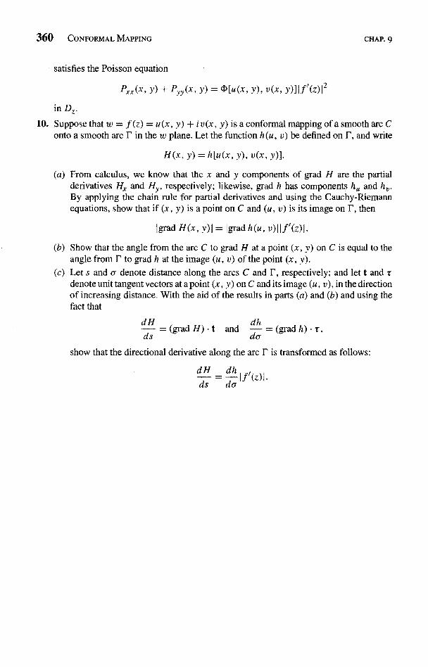
360 CONFORMAL MAPPING CHAP. 9
satisfies the Poisson equation
P"(x, Y) + Pyy(x, Y) = 4[u(x, Y), v(x, Y)]If'(z)I2
in D.10. Suppose that w = f (z) = u(x, y) + i v(x, y) is a conformal mapping of a smooth arc C
onto a smooth arc I' in the w plane. Let the function h(u, v) be defined on r, and write
H(x, y) = h[u(x, y), v(x, y)].
(a) From calculus, we know that the x and y components of grad H are the partialderivatives Hx and Hy, respectively; likewise, grad h has components h,, and h,,.By applying the chain rule for partial derivatives and using the Cauchy-Riemannequations, show that if (x, y) is a point on C and (u, v) is its image on r, then
grad H(x, Y)l = (grad h(u, v)Ilf'(z I.
(b) Show that the angle from the arc C to grad H at a point (x, y) on C is equal to theangle from F to grad h at the image (u, v) of the point (x, y).
(c) Let s and a denote distance along the arcs C and r, respectively; and let t and rdenote unit tangent vectors at a point (x, y) on C and its image (u, v), in the directionof increasing distance. With the aid of the results in parts (a) and (b) and using thefact that
dH =(gradH).t and a =(grad
show that the directional derivative along the arc F is transformed as follows:
CHAPTER
10APPLICATIONS OF
CONFORMAL MAPPING
We now use conformal mapping to solve a number of physical problems involvingLaplace's equation in two independent variables. Problems in heat conduction, elec-trostatic potential, and fluid flow will be treated. Since these problems are intended toillustrate methods, they will be kept on a fairly elementary level.
100. STEADY TEMPERATURES
In the theory of heat conduction, the, flux across a surface within a solid body at a pointon that surface is the quantity of heat flowing in a specified direction normal to thesurface per unit time per unit area at the point. Flux is, therefore, measured in suchunits as calories per second per square centimeter. It is denoted here by 4, and it varieswith the normal derivative of the temperature T at the point on the surface:
(1) (D -K T (K>0).d
Relation (1) is known as Fourier's law and the constant K is called the thermalconductivity of the material of the solid, which is assumed to be homogeneous.*
The points in the solid are assigned rectangular coordinates in three-dimensionalspace, and we restrict our attention to those cases in which the temperature T varies
* The law is named for the French mathematical physicist Joseph Fourier (1768-1830). A translation ofhis book, cited in Appendix 1, is a classic in the theory of heat conduction.
361
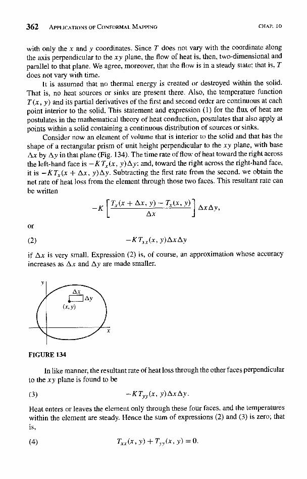
362 APPLICATIONS OF CONFORMAL MAPPING CHAP. 10
with only the x and y coordinates. Since T does not vary with the coordinate alongthe axis perpendicular to the xy plane, the flow of heat is, then, two-dimensional andparallel to that plane. We agree, moreover, that the flow is in a steady state; that is, Tdoes not vary with time.
It is assumed that no thermal energy is created or destroyed within the solid.That is, no heat sources or sinks are present there. Also, the temperature functionT (x, y) and its partial derivatives of the first and second order are continuous at eachpoint interior to the solid. This statement and expression (1) for the flux of heat arepostulates in the mathematical theory of heat conduction, postulates that also apply atpoints within a solid containing a continuous distribution of sources or sinks.
Consider now an element of volume that is interior to the solid and that has theshape of a rectangular prism of unit height perpendicular to the xy plane, with baseAx by Ay in that plane (Fig. 134). The time rate of flow of heat toward the right acrossthe left-hand face is - K Tx(x, y) Ay; and, toward the right across the right-hand face,it is -KTx(x + Ax, y)©y. Subtracting the first rate from the second, we obtain thenet rate of heat loss from the element through those two faces. This resultant rate canbe written
Ax Ay,
or
(2) -KTxx(x, y)AxAy
if Ax is very small. Expression (2) is, of course, an approximation whose accuracyincreases as Lix and Ay are made smaller.
FIGURE 134
In like manner, the resultant rate of heat loss through the other faces perpendicularto the xy plane is found to be
(3) -KTyy(x, y)©x©
Heat enters or leaves the element only through these four faces, and the temperatureswithin the element are steady. Hence the sum of expressions (2) and (3) is zero; thatis,
(4) T,.x(x, y) + Tyy(x, v) = 0.
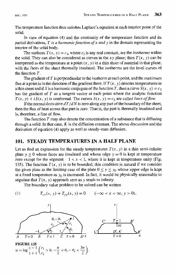
IoI STEADY TEMPERATURES IN A HALF PLANE 363
The temperature function thus satisfies Laplace's equation at each interior point of thesolid.
In view of equation (4) and the continuity of the temperature function and itspartial derivatives, T is a harmonic function of x and y in the domain representing theinterior of the solid body.
The surfaces T (x, y) = c1, where cr is any real constant, are the isotherms withinthe solid. They can also be considered as curves in the xy plane; then T(x, y) can beinterpreted as the temperature at a point (x, y) in a thin sheet of material in that plane,with the faces of the sheet thermally insulated. The isotherms are the level curves ofthe function T.
The gradient of T is perpendicular to the isotherm at each point, and the maximumflux at a point is in the direction of the gradient there. If T (x, y) denotes temperatures ina thin sheet and if S is a harmonic conjugate of the function T, then a curve S(x, y) czhas the gradient of T as a tangent vector at each point where the analytic functionT (x, y) + i S(_x, y) is conformal. The curves S(x, y) = c2 are called lines offlow.
If the normal derivative dT jdN is zero along any part of the boundary of the sheet,then the flux of heat across that part is zero. That is, the part is thermally insulated andis, therefore, a line of flow.
The function T may also denote the concentration of a substance that is diffusingthrough a solid. In that case, K is the diffusion constant. The above discussion and thederivation of equation (4) apply as well to steady-state diffusion.
101. STEADY TEMPERATURES IN A HALF PLANE
Let us find an expression for the steady temperatures T(x, y) in a thin semi-infiniteplate y > 0 whose faces are insulated and whose edge y = 0 is kept at temperaturezero except for the segment -1 < x < 1, where it is kept at temperature unity (Fig.135). The function T(x, y) is to be bounded; this condition is natural if we considerthe given plate as the limiting case of the plate 0 < y < yo whose upper edge is keptat a fixed temperature as yo is increased. In fact, it would be physically reasonable tostipulate that T (x, y) approach zero as y tends to infinity.
The boundary value problem to be solved can be written
(1) TXX(x, Y) + Tyy(x, y) = 0 (-oo < x < oo, y > 0),
FIGURE 135z- Iw=log 2 <01 2<32
V
T
D' A'T=0
364 APPLICATIONS OF CONFORMAL MAPPING CHAP. 10
T(x, 0) when Ix I < 1,0 when lxI > 1;
also, I T (x, y) I < M where M is some positive constant. This is a Dirichlet problemfor the upper half of the xy plane. Our method of solution will be to obtain a newDirichlet problem for a region in the uv plane. That region will be the image of thehalf plane under a transformation w = f (z) that is analytic in the domain y > 0 andthat is conformal along the boundary y = 0 except at the points (±1, 0), where it isundefined. It will be a simple matter to discover a bounded harmonic function satisfyingthe new problem. The two theorems in Chap. 9 will then be applied to transform thesolution of the problem in the u v plane into a solution of the original problem in the xyplane. Specifically, a harmonic function of u and v will be transformed into a harmonicfunction of x and y, and the boundary conditions in the uv plane will be preserved oncorresponding portions of the boundary in the xy plane. There should be no confusionif we use the same symbol T to denote the different temperature functions in the twop anes.
Let us write
z - 1= rt exp(i01) and z + 1= r2 exp(i02),
where 0 < 0k :5,7r (k = 1, 2). The transformation
(3) w = to
is defined on the upper half plane y > 0, except for the two points z = +1, since0 < 01 - 02 rr in the region. (See Fig. 135.) Now the value of the logarithm is theprincipal value when 0 < 01 - 02 < rr, and we recall from Example 3 in Sec. 88 thatthe upper half plane y > 0 is then mapped onto the horizontal strip 0 < v < ir in thew plane. As already noted in that example, the mapping is shown with correspondingboundary points in Fig. 19 of Appendix 2. Indeed, it was that figure which suggestedtransformation (3) here. The segment of the x axis between z = -1 and z = 1, where01- 02 = 7r, is mapped onto the upper edge of the strip; and the rest of the x axis, where01 - 02 = 0, is mapped onto the lower edge. The required analyticity and conformalityconditions are evidently satisfied by transformation (3).
A bounded harmonic function of u and v that is zero on the edge v = 0 of thestrip and unity on the edge v = 7r is clearly
(4)
it is harmonic since it is the imaginary part of the entire function (1/2r)w. Changingto x and y coordinates by means of the equation
z - I
z +1
SEC. 102 A RELATED PROBLEM 365
we find that
or
u = argx`+y`- 1+i2y
(x+1)2+y2
2yu = arctan I _
+y2-The range of the arctangent function here is from 0 to 7r since
z --- 1 __ gg z+1 1 -
0 _< 01 - 02 7r. Expression (4) now takes the form
(6)1 1' 2y
(0<arctant. y2 - 1
Since the function (4) is harmonic in the strip 0 < v < 7r and since transformation(3) is analytic in the half plane y > 0, we may apply the theorem in Sec. 98 to concludethat the function (6) is harmonic in that half plane. The boundary conditions for thetwo harmonic functions are the same on corresponding parts of the boundaries becausethey are of the type h = hg, treated in the theorem of Sec. 99. The bounded function (6)is, therefore, the desired solution of the original problem. One can, of course, verifydirectly that the function (6) satisfies Laplace's equation and has the values tending tothose indicated on the left in Fig. 135 as the point (x, y) approaches the x axis fromabove.
The isotherms T (x, y) = cl (0 < cl < 1) are arcs of the circles
x2 + (y - cot 7rc1)2 = csc2 7rc1,
passing through the points (± 1, 0) and with centers on the y axis.Finally, we note that since the product of a harmonic function by a constant is
also harmonic, the function
TO 2y-art tan
7r x2-I-y2-represents steady temperatures in the given half plane when the temperature T = 1along the segment -1 < x < 1 of the x axis is replaced by any constant temperatureT=To.
102. A RELATED PROBLEM
Consider a semi-infinite slab in the three-dimensional space bounded by the planesx = ±7r/2 and y = 0 when the first two surfaces are kept at temperature zero and the
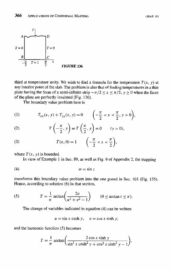
366 APPLICATIONS OF CONFORMAL MAPPING CHAP. IO
T=0
y
T=0
2x x
FIGURE 136
third at temperature unity. We wish to find a formula for the temperature T (x, y) atany interior point of the slab. The problem is also that of finding temperatures in a thinplate having the form of a semi-infinite strip -7r/2 < x < 7r/2, y > 0 when the facesof the plate are perfectly insulated (Fig. 136).
The boundary value problem here is
Txx(x, Y) + Tyy(x, y) = 0
(2)
(3) T(x, 0
IT<x< -,y>
y
where T(x, y) is bounded.In view of Example 1 in Sec. 89, as well as Fig. 9 of Appendix 2, the mapping
(4) sin z
transforms this boundary value problem into the one posed in Sec. 101 (Fig. 135).Hence, according to solution (6) in that section,
The change of variables indicated in equation (4) can be written
u =sinx cosh y, u=cosx sinhy;
and the harmonic function (5) becomes
T =1
arctan2 cos x sinh y--
r t sin2 x cosh2 _y -F Cos2 x sinh2 y -
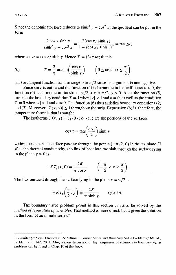
SEC. 102 A RELATED PROBLEM 367
Since the denominator here reduces to sinh2 y - cost x, the quotient can be put in theform
2 cos x sinh y 2(cos x/ sinh y)sinh2 y - cost x 1 - (cos x/ sinh y)2
where tan a = cos x/ sinh y. Hence T = (2/7r)a; that is
(6)2
_ - arctrr l sinh y
= tan 2a,
This arctangent function has the range 0 to 7r/2 since its argument is nonnegative.Since sin z is entire and the function (5) is harmonic in the half plane v > 0, the
function (6) is harmonic in the strip -ir/2 < x < ir/2, y > 0. Also, the function (5)satisfies the boundary condition T = 1 when (u < 1 and v = 0, as well as the conditionT = 0 when I u (> 1 and v = 0. The function (6) thus satisfies boundary conditions (2)and (3). Moreover, IT(x, y) I < 1 throughout the strip. Expression (6) is, therefore, thetemperature formula that is sought.
The isotherms T (x, y) = cl (0 < c1 < 1) are the portions of the surfaces
cos x =tan(= 1 ] sinhy
within the slab, each surface passing through the points (±ir/2, 0) in the xy plane. IfK is the thermal conductivity, the flux of heat into the slab through the surface lyingin the plane y = 0 is
The flux outward through the surface lying in the plane x = 7r/2 is
2K(y'>0).T (--,Y)- zrsinhy
The boundary value problem posed in this section can also be solved by themethod of separation of variables. That method is more direct, but it gives the solutionin the form of an infinite series.*
* A similar problem is treated in the authors' "Fourier Series and Boundary Value Problems," 6th ed.,Problem 7, p. 142, 2001. Also, a short discussion of the uniqueness of solutions to boundary valueproblems can be found in Chap. 10 of that book.
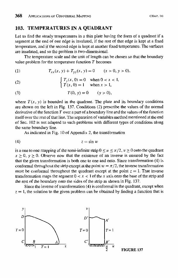
368 APPLICATIONS OF CONFORMAL MAPPING CHAP. IO
103. TEMPERATURES IN A QUADRANT
Let us find the steady temperatures in a thin plate having the form of a quadrant if asegment at the end of one edge is insulated, if the rest of that edge is kept at a fixedtemperature, and if the second edge is kept at another fixed temperature. The surfacesare insulated, and so the problem is two-dimensional.
The temperature scale and the unit of length can be chosen so that the boundaryvalue problem for the temperature function T becomes
(1) T,(x,y)+Tyy(x,y)=0 (x>O,y>0),
0)=0 when 0 < x < 1T(x ,,
O T (x, 0) = 1 when x > 1,
(3) T(O, y) = 0 (y > 0),
where T (x, y) is bounded in the quadrant. The plate and its boundary conditionsare shown on the left in Fig. 137. Conditions (2) prescribe the values of the normalderivative of the function T over a part of a boundary line and the values of the functionitself over the rest of that line. The separation of variables method mentioned at the endof Sec. 102 is not adapted to such problems with different types of conditions alongthe same boundary line.
As indicated in Fig. 10 of Appendix 2, the transformation
(4) z=sinw
is a one to one mapping of the semi-infinite strip 0 < u < re/2, v > 0 onto the quadrantx > 0, y > 0. Observe now that the existence of an inverse is ensured by the factthat the given transformation is both one to one and onto. Since transformation (4) isconformal throughout the strip except at the point w = 7c/2, the inverse transformationmust be conformal throughout the quadrant except at the point z = 1. That inversetransformation maps the segment 0 < x < 1 of the x axis onto the base of the strip andthe rest of the boundary onto the sides of the strip as shown in Fig. 137.
Since the inverse of transformation (4) is conformal in the quadrant, except whenz = 1, the solution to the given problem can be obtained by finding a function that is
V
D' r-"*-IA'
T=01 T=O
C`
T=1
B'
it u2 FIGURE 137
SEC. 103 TEMPERATURES IN A QUADRANT 369
harmonic in the strip and satisfies the boundary conditions shown on the right in Fig.137. Observe that these boundary conditions are of the types h = hg and dh/dn = 0in the theorem of Sec. 99.
The required temperature function T for the new boundary value problem isclearly
(5)Jr
u,
the function (2/7r)u being the real part of the entire function (2/7r)w. We must nowexpress T in terms of x and Y.
To obtain u in terms of x and y, we first note that, according to equation (4),
(6) x = sin u cosh v, y = cos u sinh v.
When 0 < u < 7r/2, both sin u and cos it are nonzero; and, consequently,
(7)x2
y2- = 1.
sin2 ecos2
u
Now it is convenient to observe that, for each fixed u, hyperbola (7) has foci at thpoints
cost u = ±
and that the length of the transverse axis, which is the line segment joining the twovertices, is 2 sin u. Thus the absolute value of the difference of the distances betweenthe foci and a point (x, y) lying on the part of the hyperbola in the first quadrant is
(x+1)2+y2- (x- 1)2 + y2 -2 sin u.
It follows directly from equations (6) that this relation also holds when u = 0 oru = 7/2. In view of equation (5), then, the required temperature function is
(8) T = arcsin1)2 -}- y2 - '(x - 1)2 + y
2
where, since 0 < u < n'/2, the arcsine function has the range 0 to 7r/2.If we wish to verify that this function satisfies boundary conditions (2), we must
remember that vr(x --1)2 denotes x - 1 when x > 1 and 1 - x when 0 < x < 1, thesquare roots being positive. Note, too, that the temperature at any point along theinsulated part of the lower edge of the plate is
T (x, 0) =2
aresin x (0 < xSr
It can be seen from equation (5) that the isotherms T (x, y) = ct (0 < ct < 1)are the parts of the confocal hyperbolas (7), where u = arcs/2, which lie in the first
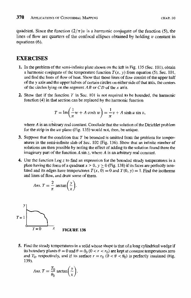
370 APPLICATIONS OF CONFORMAL MAPPING CHAP. 10
quadrant. Since the function (2j7r)v is a harmonic conjugate of the function (5), thelines of flow are quarters of the confocal ellipses obtained by holding v constant inequations (6).
EXERCISES
1. In the problem of the semi-infinite plate shown on the left in Fig. 135 (Sec. 101), obtaina harmonic conjugate of the temperature function T (x, y) from equation (5), Sec. 101,and find the lines of flow of heat. Show that those lines of flow consist of the upper halfof the y axis and the upper halves of certain circles on either side of that axis, the centersof the circles lying on the segment AB or CD of the x axis.
2. Show that if the function T in Sec. 101 is not required to be bounded, the harmonicfunction (4) in that section can be replaced by the harmonic function
lv + A sinh u sin v,x
where A is an arbitrary real constant. Conclude that the solution of the Dirichlet problemfor the strip in the uv plane (Fig. 135) would not, then, be unique.
3. Suppose that the condition that T be bounded is omitted from the problem for temper-atures in the semi-infinite slab of Sec. 102 (Fig. 136). Show that an infinite number ofsolutions are then possible by noting the effect of adding to the solution found there theimaginary part of the function A sin z, where A is an arbitrary real constant.
4. Use the function Log z to find an expression for the bounded steady temperatures in aplate having the form of a quadrant x > 0, y > 0 (Fig. 138) if its faces are perfectly insu-lated and its edges have temperatures T (x, 0) = 0 and T (0, y) = 1. Find the isothermsand lines of flow, and draw some of them.
Ans. T = 2 arctanxr
y
T=1
0
FIGURE 138T=0
5. Find the steady temperatures in a solid whose shape is that of a long cylindrical wedge ifits boundary planes 8 = 0 and 0 = 80 (0 < r < r0) are kept at constant temperatures zeroand To, respectively, and if its surface r = rp (0 < 8 < 8p) is perfectly insulated (Fig.139).
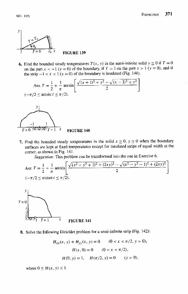
SEC. 103
FIGURE 139
EXERCISES 371
6. Find the bounded steady temperatures T (x, y) in the semi-infinite solid y > 0 if T =0
on the part x < -1 (y = 0) of the boundary, if T =1 on the part x > 1 (y = 0), and ifthe strip -1 < x < 1 (y = 0) of the boundary is insulated (Fig. 140).
Ans. T =1 + arcsin2 7r
(-ir/2 < arcsin t < it/2).
1)2+y-vJ(X - 1)2 + y
2
FIGURE 140
7. Find the bounded steady temperatures in the solid x > 0, y > 0 when the boundarysurfaces are kept at fixed temperatures except for insulated strips of equal width at the
corner, as shown in Fig. 141.Suggestion: This problem can be transformed into the one in Exercise 6.
Ans.1
[x2 - y2 + 1)2 + (2xy)2 - (x2 - y2 - 1)2 + (2xy
Ans. T = 2 + aresin2
(-ir/2 < arctan t < it/2).
T = 1 X FIGURE 141
8. Solve the following Dirichlet problem for a semi-infinite strip (Fig. 142):
Hxx(x,y)+Hyy(x,y)=0 (0<x{7r/2,y> 0),
H(x, 0) = 0 (0 < x < 7r/2),
H(0, y) = 1, H(r/2, y) = 0 (y > 0),
where 0<H(x,y)<1.
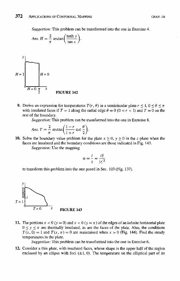
372 APPLICATIONS OF CONFORMAL MAPPING CHAP. IO
y
H= 1
0
Suggestion: This problem can be transformed into the one in Exercise 4.
Ans. H =2
arctan( tanh y
rr tan x
H=O
H=0 7r X2 FIGURE 142
9. Derive an expression for temperatures T (r, 8) in a semicircular plate r < 1, 0 < 0 < rrwith insulated faces if T = 1 along the radial edge 0 = 0 (0 < r < 1) and T = 0 on therest of the boundary.
Suggestion: This problem can be transformed into the one in Exercise 8.
l 1?Ans. T = acctrr
10. Solve the boundary value problem for the plate x > 0, y ? 0 in the z plane when thefaces are insulated and the boundary conditions are those indicated in Fig. 143.
Suggestion: Use the mapping
tz
12
to transform this problem into the one posed in Sec. 103 (Fig. 137).
T=
FIGURE 143
11. The portions x < 0 (y = 0) and x < 0 (y = Tr) of the edges of an infinite horizontal plate0 < y < rr are thermally insulated, as are the faces of the plate. Also, the conditionsT (x, 0) = I and T (x, 7r) = 0 are maintained when x > 0 (Fig. 144). Find the steadytemperatures in the plate.
Suggestion: This problem can be transformed into the one in Exercise 6.
12. Consider a thin plate, with insulated faces, whose shape is the upper half of the regionenclosed by an ellipse with foci (±1, 0). The temperature on the elliptical part of its
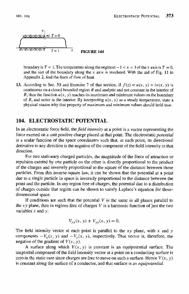
SEC. 1 04
FIGURE 144
ELECTROSTATIC POTENTIAL 373
boundary is T = 1. The temperature along the segment -1 < x < 1 of the x axis is T = 0,and the rest of the boundary along the x axis is insulated. With the aid of Fig. 11 inAppendix 2, find the lines of flow of heat.
13. According to Sec. 50 and Exercise 7 of that section, if f (z) = u(x, y) + iv(x, y) iscontinuous on a closed bounded region R and analytic and not constant in the interior ofR, then the function u (x, y) reaches its maximum and minimum values on the boundaryof R, and never in the interior. By interpreting u(x, y) as a steady temperature, state aphysical reason why that property of maximum and minimum values should hold true.
104. ELECTROSTATIC POTENTIAL
In an electrostatic force field, the field intensity at a point is a vector representing theforce exerted on a unit positive charge placed at that point. The electrostatic potentialis a scalar function of the space coordinates such that, at each point, its directionalderivative in any direction is the negative of the component of the field intensity in thatdirection.
For two stationary charged particles, the magnitude of the force of attraction orrepulsion exerted by one particle on the other is directly proportional to the productof the charges and inversely proportional to the square of the distance between thoseparticles. From this inverse-square law, it can be shown that the potential at a pointdue to a single particle in space is inversely proportional to the distance between thepoint and the particle. In any region free of charges, the potential due to a distributionof charges outside that region can be shown to satisfy Laplace's equation for three-dimensional space.
If conditions are such that the potential V is the same in all planes parallel tothe x y plane, then in regions free of charges V is a harmonic function of just the twovariables x and y:
Vxx(x, Y) + Vyy(x, y) = 0.
The field intensity vector at each point is parallel to the xy plane, with x and ycomponents -Vx(x, y) and -Vy(x, y), respectively. That vector is, therefore, thenegative of the gradient of V (x, y).
A surface along which V (x, y) is constant is an equipotential surface. Thetangential component of the field intensity vector at a point on a conducting surface iszero in the static case since charges are free to move on such a surface. Hence V (x, y)is constant along the surface of a conductor, and that surface is an equipotential.
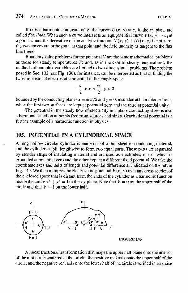
374 APPLICATIONS OF CONFORMAL MAPPING CHAP. 10
If U is a harmonic conjugate of V, the curves U(x, y) = e2 in the xy plane arecalled flux lines. When such a curve intersects an equipotential curve V (x, y) = cl ata point where the derivative of the analytic function V (x, y) + i U(x, y) is not zero,the two curves are orthogonal at that point and the field intensity is tangent to the fluxline there.
Boundary value problems for the potential V are the same mathematical problemsas those for steady temperatures T; and, as in the case of steady temperatures, themethods of complex variables are limited to two-dimensional problems. The problemposed in Sec. 102 (see Fig. 136), for instance, can be interpreted as that of finding the
o-dimensional electrostatic potential in the empty space
.7r 7r-2 <x< -,y>0
bounded by the conducting planes x = ±7r/2 and y = 0, insulated at their intersections,when the first two surfaces are kept at potential zero and the third at potential unity.
The potential in the steady flow of electricity in a plane conducting sheet is alsoa harmonic function at points free from sources and sinks. Gravitational potential is afurther example of a harmonic function in physics.
105. POTENTIAL IN A CYLINDRICAL SPACE
A long hollow circular cylinder is made out of a thin sheet of conducting material,and the cylinder is split lengthwise to form two equal parts. Those parts are separatedby slender strips of insulating material and are used as electrodes, one of which isgrounded at potential zero and the other kept at a different fixed potential. We take thecoordinate axes and units of length and potential difference as indicated on the left inFig. 145. We then interpret the electrostatic potential V (x, y) over any cross section ofthe enclosed space that is distant from the ends of the cylinder as a harmonic functioninside the circle x2 + y2 = I in the xy plane. Note that V = 0 on the upper half of thecircle and that V = 1 on the lower half.
y
V=1 FIGURE 145
A linear fractional transformation that maps the upper half plane onto the interiorof the unit circle centered at the origin, the positive real axis onto the upper half of thecircle, and the negative real axis onto the lower half of the circle is verified in Exercise
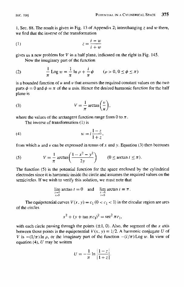
SEC. 105 POTENTIAL IN A CYLINDRICAL SPACE 375
1, Sec. 88. The result is given in Fig. 13 of Appendix 2; interchanging z and w there,we find that the inverse of the transformation
(1)I-wz= i+w
gives us a new problem for V in a half plane, indicated on the right in Fig. 145.Now the imaginary part of the function
l 1 i(2) (p>0,0<0<)
n 1r n
is a bounded function of u and v that assumes the required constant values on the twoparts 0 = 0 and _ 7r of the u axis. Hence the desired harmonic function for the halfplane is
(3) aretan IU
I ,717
where the values of the arctangent function range from 0 to it.The inverse of transformation (1) is
(4)<.w=r
1+:
from which u and v can be expressed in terms of x and y. Equation (3) then becomes
(5) (0 <arctant <zr).
The function (5) is the potential function for the space enclosed by the cylindricalelectrodes since it is harmonic inside the circle and assumes the required values on thesemicircles. If we wish to verify this solution, we must note that
lim arctan t = 0 and lim arctan t = 7r.t-.o t--:0t>0 1<0
The equipotential curves V (x, y) = ct (0 < ci < 1) in the circular region are arcsof the circles
x2 + (y + tan CI)2 =sec2 7rcl,
with each circle passing through the points (+ 1, 0). Also, the segment of the x axisbetween those points is the equipotential V (x, y) = 1/2. A harmonic conjugate U ofV is -(1/7r) In p, or the imaginary part of the function -(i/7r) Log w. In view ofequation (4), U may be written
1-z
1+z
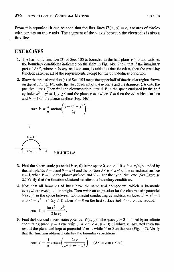
376 APPLICATIONS OF CONFORMAL MAPPING CHAP. 10
From this equation, it can be seen that the flux lines U(x, y) = c2 are arcs of circleswith centers on the x axis. The segment of the y axis between the electrodes is also aflux line.
EXERCISES
1. The harmonic function (3) of Sec. 105 is bounded in the half plane v > 0 and satisfiesthe boundary conditions indicated on the right in Fig. 145. Show that if the imaginarypart of Ae', where A is any real constant, is added to that function, then the resultingfunction satisfies all of the requirements except for the boundedness condition.
2. Show that transformation (4) of Sec. 105 maps the upper half of the circular region shownon the left in Fig. 145 onto the first quadrant of the w plane and the diameter C E onto thepositive v axis. Then find the electrostatic potential V in the space enclosed by the halfcylinder x2 + y2 = 1, y > 0 and the plane y = 0 when V = 0 on the cylindrical surfaceand V = I on the planar surface (Fig. 146).
Ans. V =2
arctan
Y
V=0
3. Find the electrostatic potential V (r, 0) in the space 0 < r < 1, 0 < 0 < 7r /4, bounded bythe half planes 0 = 0 and 0 = 7r/4 and the portion 0 < 0 < 7r/4 of the cylindrical surfacer = 1, when V = 1 on the planar surfaces and V = 0 on the cylindrical one. (See Exercise2.) Verify that the function obtained satisfies the boundary conditions.
4. Note that all branches of log z have the same real component, which is harmoniceverywhere except at the origin. Then write an expression for the electrostatic potentialV (x, y) in the space between two coaxial conducting cylindrical surfaces x2 + y2 = 1and x2 + y2 = rg (ra 1) when V = 0 on the first surface and V = I on the second.
Ans. V =+ y2)
2 in rp
5. Find the bounded electrostatic potential V (x, y) in the space y > 0 bounded by an infiniteconducting plane y = 0 one strip (-a < x < a, y = 0) of which is insulated from therest of the plane and kept at potential V = 1, while V = 0 on the rest (Fig. 147). Verifythat the function obtained satisfies the boundary conditions.
1Ans. V = arctan{ (0 < arctan t <n
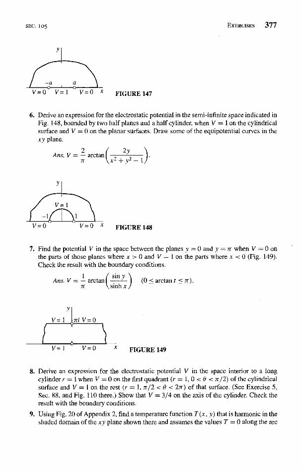
SEC. 1 05
FIGURE 147
EXERCISES 377
6. Derive an expression for the electrostatic potential in the semi-infinite space indicated inFig. 148, bounded by two half planes and a half cylinder, when V = 1 on the cylindricalsurface and V = 0 on the planar surfaces. Draw some of the equipotential curves in thexy plane.
21 2yarctanAns. V =
IT
7. Find the potential V in the space between the planes y = 0 and y = 7r when V = 0 onthe parts of those planes where x > 0 and V = 1 on the parts where x < 0 (Fig. 149).Check the result with the boundary conditions.
sin y1 1 (0 < arctanAns. V = arctanTr sinh x
Y
V=1 V=0
V=i V=0 FIGURE 149
8. Derive an expression for the electrostatic potential V in the space interior to a longcylinder r = 1 when V = 0 on the first quadrant (r = 1, 0 < 8 < 7r/2) of the cylindricalsurface and V = 1 on the rest (r = 1, 7r/2 < 0 < 2,r) of that surface. (See Exercise 5,Sec. 88, and Fig. 110 there.) Show that V = 3/4 on the axis of the cylinder. Check theresult with the boundary conditions.
9. Using Fig. 20 of Appendix 2, find a temperature function T (x, y) that is harmonic in theshaded domain of the xy plane shown there and assumes the values T = 0 along the arc
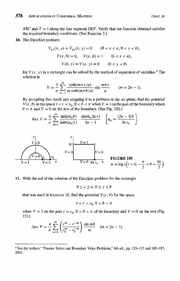
378 APPLICATIONS OF CONFORMAL MAPPING CHAP. 10
ABC and T = 1 along the line segment DEF. Verify that the function obtained satisfiesthe required boundary conditions. (See Exercise 2.)
10. The Dirichlet problem
Vxx(x,y)-i-Vyy(x,y)=0 (0 < x < a, 0 < y < b),
V(x,0)=0, V(x,b)=1 (0<x <a),
V(O, y) = V(a, y) = 0 (0<y<b)
for V (x, y) in a rectangle can be solved by the method of separation of variables.* Thesolution is
V= sinh(m,ry/a) . m7rx
m sinh(mrrbfa) an=Isin (m = 2n - 1).
By accepting this result and adapting it to a problem in the uv plane, find the potentialV (r, 0) in the space 1 < r < ro, 0 < 6 < 7t when V = 1 on the part of the boundary where0 = 7r and V = 0 on the rest of the boundary. (See Fig. 150.)
Ans. Vsinh(an&) sm(an in r) I ('2n - 1)ir
sinh (an Tr) 2n - 1 In ro
FIGURE 150
w=log zlr>0,-2 <0< 2
aid of the solution of the Dirichlet problem for the rectangle
0<x <a,0<y<bthat was used in Exercise 10, find the potential V (r, 6) for the space
1<r<ro,0<0<7r
when V = 1 on the part r = ro, 0 < 0 < it of its boundary and V = 0 on the rest (Fig.151).
Ans. V =
* See the authors' "Fourier Series and Boundary Value Problems," 6th ed., pp. 135-137 and 185-187,2001.
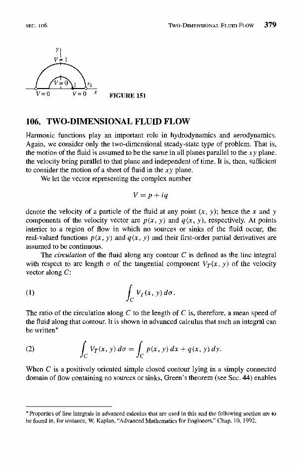
SEC. io6
v=o v=0 FIGURE 151
106. TWO-DIMENSIONAL FLUID FLOW
Harmonic functions play an important role in hydrodynamics and aerodynamics.Again, we consider only the two-dimensional steady-state type of problem. That is,the motion of the fluid is assumed to be the same in all planes parallel to the xy plane,the velocity being parallel to that plane and independent of time. It is, then, sufficientto consider the motion of a sheet of fluid in the x y plane.
We let the vector representing the complex number
V=p+iq
denote the velocity of a particle of the fluid at any point (x, y); hence the x and ycomponents of the velocity vector are p(x, y) and q(x, y), respectively. At pointsinterior to a region of flow in which no sources or sinks of the fluid occur, thereal-valued functions p (x, y) and q (x, y) and their first-order partial derivatives areassumed to be continuous.
The circulation of the fluid along any contour C is defined as the line integralwith respect to arc length or of the tangential component VT(x, y) of the velocityvector along C:
(1)
TWO-DIMENSIONAL FLUID FLOW 379
VT(x, y) da.
The ratio of the circulation along C to the length of C is, therefore, a mean speed ofthe fluid along that contour. It is shown in advanced calculus that such an integral canbe written*
(2) VT(x, y) do" = 1 p(x, y) dx -{- q(x, y) dy.C
When C is a positively oriented simple closed contour lying in a simply connecteddomain of flow containing no sources or sinks, Green's theorem (see Sec. 44) enables
* Properties of line integrals in advanced calculus that are used in this and the following section are tobe found in, for instance, W. Kaplan, "Advanced Mathematics for Engineers," Chap. 10, 1992,
380 APPLICATIONS OF CONFORMAL MAPPING CHAP. 10
us to write
fcp(x,y)dx+q(x,y)dy-ff qx(x, y) - py(x, y)] dA,
where R is the closed region consisting of points interior to and on C. Thus
(3) l VT(x, y) dcr = f + x, y) - py(x, y)] dA
for such a contourA physical interpretation of the integrand on the right in expression (3) for the
circulation along the simple closed contour C is readily given. We let C denote a circleof radius r which is centered at a point (xe, yo) and taken counterclockwise. The meanspeed along C is then found by dividing the circulation by the circumference 2irr,and the corresponding mean angular speed of the fluid about the center of the circle isobtained by dividing that mean speed by r:
1Rl [qx(x, y) - py(x, y)] dA.2
Now this is also an expression for the mean value of the function
(4) w(x, y) = I [qx(x, y) - py(x, y)]
over the circular region R bounded by C. Its limit as r tends to zero is the value ofto at the point (xa, yo). Hence the function w(x, y), called the rotation of the fluid,represents the limiting angular speed of a circular element of the fluid as the circleshrinks to its center (x, y), the point at which to is evaluated.
If to (x, y) = 0 at each point in some simply connected domain, the flow isirrotational in that domain. We consider only irrotational flows here, and we alsoassume that the fluid is incompressible and free from viscosity. Under our assumptionof steady irrotational flow of fluids with uniform density p, it can be shown that thefluid pressure P(x, y) satisfies the following special case of Bernoulli's equation:
P 1 2-+2IV
=constant.p
Note that the pressure is greatest where the speed I V I is least.Let D be a simply connected domain in which the flow is irrotational. According
to equation (4), py = qx throughout D. This relation between partial derivatives impliesthat the line integral
ds + q(s, t) dt
SEC. 107 THE STREAM FUNCTION 381
along a contour C lying entirely in D and joining any two points (xe, yo) and (x, y)in D is actually independent of path. Thus, if (xe= yo) is fixed, the function
(x,y)(5) 0(x,y)= p(s,t)ds+q(s,t)dt
fxo,yo)
is well defined on D; and, by taking partial derivatives on each side of this equation,we find that
(6) Ox (x, y) = p(x, y), fiy(x, y) = q(x, y).
From equations (6), we see that the velocity vector V = p + iq is the gradient of0; and the directional derivative of 0 in any direction represents the component of thevelocity of flow in that direction.
The function ¢r(x, y) is called the velocity potential. From equation (5), it isevident that 0 (x, y) changes by an additive constant when the reference point (xe, yo)is changed. The level curves O(x, y) = ci are called equipotentials. Because it is thegradient of O (x, y), the velocity vector V is normal to an equipotential at any pointwhere V is not the zero vector.
Just as in the case of the flow of heat, the condition that the incompressible fluidenter or leave an element of volume only by flowing through the boundary of thatelement requires that 0(x, y) must satisfy Laplace's equation
0xx(x, Y) + 0YY(x, y) = 0
in a domain where the fluid is free from sources or sinks. In view of equations (6)and the continuity of the functions p and q and their first-order partial derivatives, itfollows that the partial derivatives of the first and second order of 0 are continuous insuch a domain. Hence the velocity potential 0 is a harmonic function in that domain.
107. THE STREAM FUNCTIONAccording to Sec. 106, the velocity vector
(1) V = p(x, y) + iq(x, y)
for a simply connected domain in which the flow is irrotational can be written
(2) V =Ox(x, y) + i ry(x, y) =grad 0(x, y),
where 0 is the velocity potential. When the velocity vector is not the zero vectois normal to an equipotential passing through the point (x, y). If, moreover, +/r (x, y)denotes a harmonic conjugate of .0 (x, y) (see Sec. 97), the velocity vector is tangent toa curve *(x, y) = c2. The curves Vi (x, y) = c2 are called the streamlines of the flow,and the function Jr is the stream function. In particular, a boundary across which fluidcannot flow is a streamline.
382 APPLICATIONS OF CONFORMAL MAPPING
The analytic function
F(z) = O(x, y) + i /(x, y)
is called the complex potential of the flow. Note that
F'(z) = Ox (x, y) + i1x(x, y),
or, in view of the Cauchy-Riemann equations,
F'(z) = Ox (x, y) - iOy(x, y)
Expression (2) for the velocity thus becomes
(3) V = F'(z
The speed, or magnitude of the velocity, is obtained by writing
IV) = JF(z)I.
CHAP. 10
According to equation (5), Sec. 97, if 0 is harmonic in a simply connected domainD, a harmonic conjugate of ¢r there can be written
{x, Y)
t(x, y) = f -01(s, t) ds t) d{xo,Yo)
where the integration is independent of path. With the aid of equations (6), Sec. 106,we can, therefore, write
(4) 1r(x,y)= I -q(s,t)ds+p(s,t
where C is any contour in D from (xe, yo) to (x, y).Now it is shown in advanced calculus that the right-hand side of equation (4)
represents the integral with respect to arc length a along C of the normal componentVN(x, y) of the vector whose x and y components are p(x, y) and q(x, y), respec-tively. So expression (4) can be written
(5) f(x,y)= I VN(s,t)da.
Physically, then, iJr (x, y) represents the time rate of flow of the fluid across C. Moreprecisely, * (x, y) denotes the rate of flow, by volume, across a surface of unit heightstanding perpendicular to the xy plane on the curve C.
EXAMPLE. When the complex potential is the function
(6) F(z) = Az,
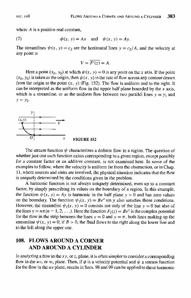
SEC. Io8 FLOWS AROUND A CORNER AND AROUND A CYLINDER 383
where A is a positive real constant,
(7) O(x, y) = Ax and *(x, y) = Ay.
The streamlines *(x, y) = c2 are the horizontal lines y = c2/A, and the velocity atany point is
V=F`(z)=A.
Here a point (x0, yo) at which Jr (x, y) = 0 is any point on the x axis. If the point(x0, yo) is taken as the origin, then Jr (x, y) is the rate of flow across any contour drawnfrom the origin to the point (x, y) (Fig. 152). The flow is uniform and to the right. Itcan be interpreted as the uniform flow in the upper half plane bounded by the x axis,which is a streamline, or as the uniform flow between two parallel lines y = yi andY=y2
y
(x,.Y)
D1 X FIGURE 152
The stream function * characterizes a definite flow in a region. The question ofwhether just one such function exists corresponding to a given region, except possiblyfor a constant factor or an additive constant, is not examined here. In some of theexamples to follow, where the velocity is uniform far from the obstruction, or in Chap.11, where sources and sinks are involved, the physical situation indicates that the flowis uniquely determined by the conditions given in the problem.
A harmonic function is not always uniquely determined, even up to a constantfactor, by simply prescribing its values on the boundary of a region. In this example,the function *(x, y) = Ay is harmonic in the half plane y > 0 and has zero valueson the boundary. The function VII(x, y) = Bex sin y also satisfies those conditions.However, the streamline *1(x, y) = 0 consists not only of the line y = 0 but also ofthe lines y = n7r(n = 1, 2, ...). Here the function F1(z) = Bez is the complex potentialfor the flow in the strip between the lines y = 0 and y = 7r, both lines making up thestreamline *(x, y) = 0; if B > 0, the fluid flows to the right along the lower line andto the left along the upper one.
108. FLOWS AROUND A CORNERAND AROUND A CYLINDER
In analyzing a flow in the xy, or z, plane, it is often simpler to consider a correspondingflow in the uv, or w, plane. Then, if 0 is a velocity potential and Jr a stream functionfor the flow in the uv plane, results in Secs. 98 and 99 can be applied to these harmonic
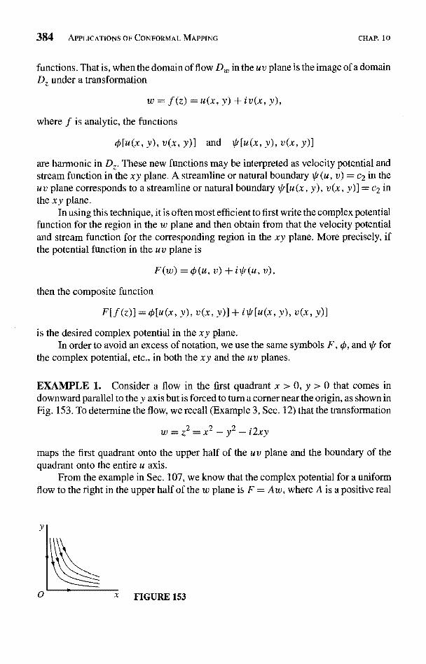
384 APPLICATIONS OF CONFORMAL MAPPING CHAP. 10
functions. That is, when the domain of flow D,,, in the u v plane is the image of a domainDz under a transformation
z) = u(x, y) + i v(x, y),
where f is analytic, the functions
0[u(x, y), v(x, y)] and tr[u(x, y), v(x, y)]
are harmonic in D. These new functions may be interpreted as velocity potential andstream function in the xy plane. A streamline or natural boundary *(u, v) = c2 in theuv plane corresponds to a streamline or natural boundary Ilr[u(x, y), v(x, y)] = c2 inthe xy plane.
In using this technique, it is often most efficient to first write the complex potentialfunction for the region in the w plane and then obtain from that the velocity potentialand stream function for the corresponding region in the xy plane. More precisely, ifthe potential function in the u v plane is
F(w) = 0(u, v) + ii/,(u, v),
then the composite function
F[.f (z)] = ([u(x, y), v(x, y)] + i J[u(x, y), v(x, y)]
is the desired complex potential in the xy plane.In order to avoid an excess of notation, we use the same symbols F, ¢r, and * fo
the complex potential, etc., in both the xy and the uv planes.
EXAMPLE 1. Consider a flow in the first quadrant x > 0, y > 0 that comes indownward parallel to they axis but is forced to turn a corner near the origin, as shown inFig. 153. To determine the flow, we recall (Example 3, Sec. 12) that the transformation
w=z2=x2-y2+i2xy
maps the first quadrant onto the upper half of the u v plane and the boundary of thequadrant onto the entire u axis.
From the example in Sec. 107, we know that the complex potential for a uniformflow to the right in the upper half of the w plane is F = Aw, where A is a positive real
y
0 X FIGURE 153
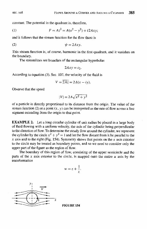
SEC. I08 FLOWS AROUND A CORNER AND AROUND A CYLINDER 385
constant. The potential in the quadrant is, therefore,
(1) F=Az2=A(x2-y2)+i2Axy,
and it follows that the stream function for the flow there is
(2) * = 2Axy.
This stream function is, of course, harmonic in the first quadrant, and it vanishes onthe boundary.
The streamlines are branches of the rectangular hyperbolas
2Axy = c2.
According to equation (3), Sec. 107, the velocity of the fluid is
V=2Az=2A(x-
Observe that the speed
V1 =2A + y2
of a particle is directly proportional to its distance from the origin. The value of thestream function (2) at a point (x, y) can be interpreted as the rate of flow across a linesegment extending from the origin to that point.
EXAMPLE 2. Let a long circular cylinder of unit radius be placed in a large bodyof fluid flowing with a uniform velocity, the axis of the cylinder being perpendicularto the direction of flow. To determine the steady flow around the cylinder, we representthe cylinder by the circle x2 + y2 = 1 and let the flow distant from it be parallel to thex axis and to the right (Fig. 154). Symmetry shows that points on the x axis exteriorto the circle may be treated as boundary points, and so we need to consider only theupper part of the figure as the region of flow.
The boundary of this region of flow, consisting of the upper semicircle and theparts of the x axis exterior to the circle, is mapped onto the entire u axis by thetransformation
1w=z+-.z
FIGURE 154
386 APPLICATIONS OF CONFORMAL MAPPING CHAP. IO
The region itself is mapped onto the upper half plane v > 0, as indicated in Fig. 17,Appendix 2. The complex potential for the corresponding uniform flow in that halfplane is F = A w, where A is a positive real constant. Hence the complex potential forthe region exterior to the circle and above the x axis is
(3) F=A z +1
j.
z
The velocity
(4) V=
approaches A as Izl increases. Thus the flow is nearly uniform and parallel to the xaxis at points distant from the circle, as one would expect. From expression (4), wesee that V (z) = V (z); hence that expression also represents velocities of flow in thelower region, the lower semicircle being a streamline.
According to equation (3), the stream function for the given problem is, in polarcoordinates,
(5)
The streamlines
sin 0 = c2
are symmetric to the y axis and have asymptotes parallel to the x axis. Note that whenc2 = 0, the streamline consists of the circle r = 1 and the parts of the x axis exteriorto the circle.
EXERCISES
1. State why the components of velocity can be obtained from the stream function by meansof the equations
p(x, y) = fv(x, y), 4(x, y) _ *x (x, y).
2. At an interior point of a region of flow and under the conditions that we have assumed,the fluid pressure cannot be less than the pressure at all other points in a neighborhoodof that point. Justify this statement with the aid of statements in Secs. 106, 107, and 50.
3. For the flow around a corner described in Example 1, Sec. 108, at what point of the regionx > 0, y > 0 is the fluid pressure greatest?
4. Show that the speed of the fluid at points on the cylindrical surface in Example 2, Sec.108, is 2A ( sin 61 and also that the fluid pressure on the cylinder is greatest at the pointsz = ± 1 and least at the points z = ± i.
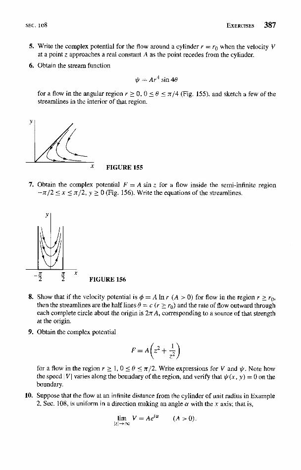
SEC. io8 EXERCISES 387
5. Write the complex potential for the flow around a cylinder r = r0 when the velocity Vat a point z approaches a real constant A as the point recedes from the cylinder.
6. Obtain the stream function
Vr = Ar4 sin 48
for a flow in the angular region r > 0, 0 < 8 < 7r/4 (Fig. 155), and sketch a few of thestreamlines in the interior of that region.
Y
6LFIGURE 155
7. Obtain the complex potential F = A sin z for a flow inside the semi-infinite region-7r/2 < x < n/2, y > 0 (Fig. 156). Write the equations of the streamlines.
Y
Jr2 FIGURE 156
x
8. Show that if the velocity potential is .0 = A In r (A > 0) for flow in the region r > r0,then the streamlines are the half lines 8 = c (r > r0) and the rate of flow outward througheach complete circle about the origin is 2JrA, corresponding to a source of that strengthat the origin.
9. Obtain the complex potential
F=A
for a flow in the region r > 1, 0 < 8 < ir/2. Write expressions for V and *. Note howthe speed I V ( varies along the boundary of the region, and verify that Vr(x, y) = 0 on theboundary.
10. Suppose that the flow at an infinite distance from the cylinder of unit radius in Example2, Sec. 108, is uniform in a direction making an angle et with the x axis; that is,
lim V = Ae`" (A > 0Izl-rx
388 APPLICATIONS OF CONFORMAL MAPPING CHAP. IO
Find the complex potential.
Ans. F = A
11. Write
z-2=riexp(i61), z+2=r2exp
and
where
0<01 <27r and 0<02 <27r.
The function (z2 - 4)1/2 is then single-valued and analytic everywhere except on thebranch cut consisting of the segment of the x axis joining the points z = ± 2. We know,moreover, from Exercise 13, Sec. 85, that the transformation
z=w+-w
maps the circle w E = 1 onto the line segment from z = -2 to z = 2 and that it maps thedomain outside the circle onto the rest of the z plane. Use all of the observations aboveto show that the inverse transformation, where I w I > 1 for every point not on the branchcut, can be written
i 2 1/21=1 tt/1 wW= [z+(z -4) ]=4 r1 exp + r2 exp2
The transformation and this inverse establish a one to one correspondence between pointsin the two domains.
12. With the aid of the results found in Exercises 10 and 11, derive the expression
F=A[zcosa-i(z2-4)1/2sina]
for the complex potential of the steady flow around a long plate whose width is 4 andwhose cross section is the line segment joining the two points z = ±2 in Fig. 157,assuming that the velocity of the fluid at an infinite distance from the plate is A exp(ia).The branch of (z2-4) 1/2 that is used is the one described in Exercise 11, and A > 0.
13. Show that if sin a A 0 in Exercise 12, then the speed of the fluid along the line segmentjoining the points z = ± 2 is infinite at the ends and is equal to Al cos a I at the midpoint.
14. For the sake of simplicity, suppose that 0 < a < 7r/2 in Exercise 12. Then show that thevelocity of the fluid along the upper side of the line segment representing the plate inFig. 157 is zero at the point x = 2 cos a and that the velocity along the lower side of thesegment is zero at the point x = -2 cos a.
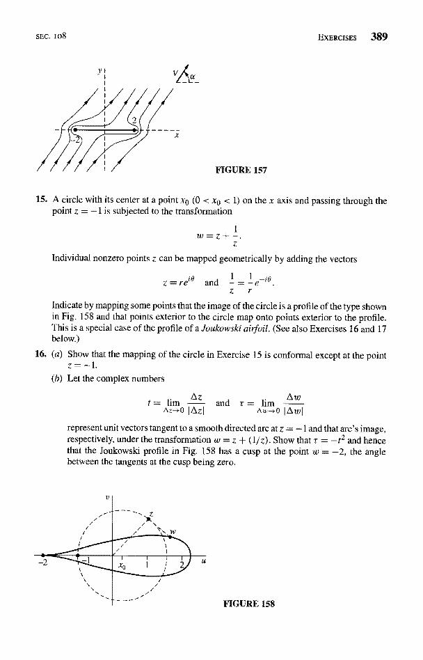
SEC. 1 08 EXERCISES 389
FIGURE 157
15. A circle with its center at a point xO (0 < xa < 1) on the x axis and passing through thepoint z = -1 is subjected to the transformation
1z+-.z
Individual nonzero points z can be mapped geometrically by adding the vectors
Z = reie and 1 = 1 e-i9z r
Indicate by mapping some points that the image of the circle is a profile of the type shownin Fig. 158 and that points exterior to the circle map onto points exterior to the profile.This is a special case of the profile of a Joukowski airfoil. (See also Exercises 16 and 17below.)
16. (a) Show that the mapping of the circle in Exercise 15 is conformal except at the pointz=-1.
(b) Let the complex numbers
t = lim Az and r = lim Awnz-+O IAz1 AW- O ItiwI
represent unit vectors tangent to a smooth directed arc at z = -1 and that arc's image,respectively, under the transformation w = z + (1/z). Show that r = -t2 and hencethat the Joukowski profile in Fig. 158 has a cusp at the point w = -2, the anglebetween the tangents at the cusp being zero.
FIGURE 158
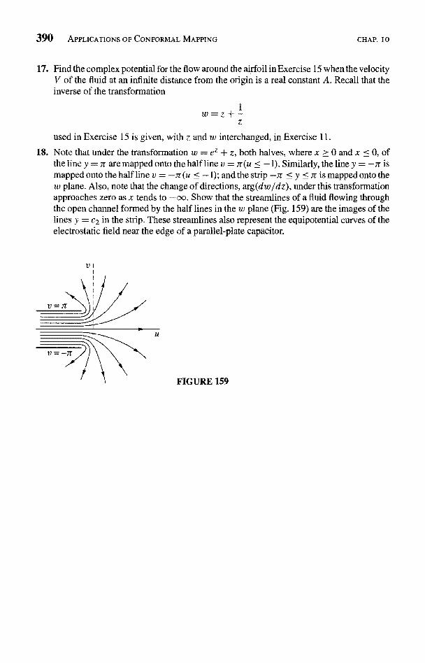
390 APPLICATIONS OF CONFORMAL MAPPING CHAP. TO
17. Find the complex potential for the flow around the airfoil in Exercise 15 when the velocityV of the fluid at an infinite distance from the origin is a real constant A. Recall that theinverse of the transformation
I
z
used in Exercise 15 is given, with z and w interchanged, in Exercise 11.
18. Note that under the transformation w = ez + z, both halves, where x > 0 and x < 0, ofthe line y = 7r are mapped onto the half line v = r (u < - 1). Similarly, the line y = -7r ismapped onto the half line v = -rr (u < -1); and the strip -ir < y < is mapped onto thew plane. Also, note that the change of directions, arg(dw/dz), under this transformationapproaches zero as x tends to -oo. Show that the streamlines of a fluid flowing throughthe open channel formed by the half lines in the w plane (Fig. 159) are the images of thelines y = c2 in the strip. These streamlines also represent the equipotential curves of theelectrostatic field near the edge of a parallel-plate capacitor.
P=ar
U
FIGURE 159
CHAPTER
11
THE SCHWARZ-CHRISTOFFELTRANSFORMATION
In this chapter, we construct a transformation, known as the Schwarz-Christoffeltransformation, which maps the x axis and the upper half of the z plane onto a givensimple closed polygon and its interior in the w plane. Applications are made to thesolution of problems in fluid flow and electrostatic potential theory.
109. MAPPING THE REAL AXIS ONTO A POLYGON
We represent the unit vector which is tangent to a smooth arc C at a point zo by thecomplex number t, and we let the number r denote the unit vector tangent to the imageI' of C at the corresponding point wo under a transformation w = f (z). We assumethat f is analytic at z0 and that f'(zo) ; 0. According to Sec. 94,
(1) arg r = arg f '(z0) + arg t.
In particular, if C is a segment of the x axis with positive sense to the right, then t = 1and arg t = 0 at each point zo = x on C. In that case, equation (1) becomes
(2) arg r = arg .f '(x)
If f'(z) has a constant argument along that segment, it follows that arg r is constant.Hence the image r of C is also a segment of a straight line.
Let us now construct a transformation w = f (z) that maps the whole x axis ontoa polygon of n sides, where xt, x2, ... , xn_ 1, and oo are the points on that axis whose
391
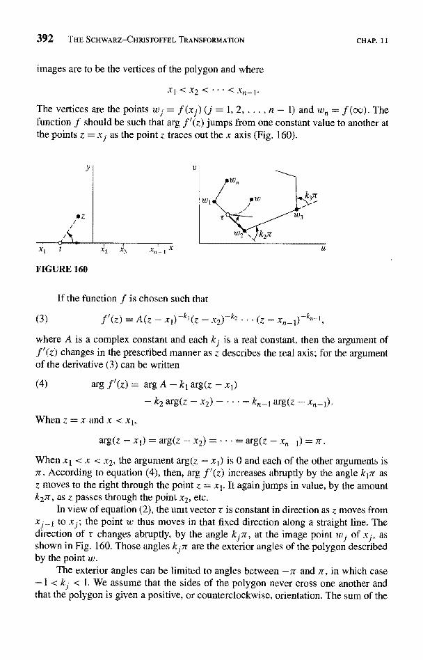
392 THE SCHWARZ-CHRISTOFFEL TRANSFORMATION CHAP. 11
mages are to be the vertices of the polygon and where
x1<x2<...<xn-1
The vertices are the points w1 = f (x1) (j = 1, 2, ... , n - 1) and wn = f (00). Thefunction f should be such that arg f(z) jumps from one constant value to another atthe points z = xj as the point z traces out the x axis (Fig. 160).
V
.zf
Txr
Tx2
FIGURE 160
If the function f is chosen such that
(3) z A(z - 2
where A is a complex constant and each k1 is a real constant, then the argument off'(z) changes in the prescribed manner as z describes the real axis; for the argumentof the derivative (3) can be written
(4) arg f(z) = arg A - kT arg(z - x1)
- k2 arg(z - x2) - ... - k,,-t arg(z -
x x < x1,
arg(z-x1) =arg(z-x2)=t =arg(z-xi-1)=7r.
When x1 < x < x2, the argument arg(z - x1) is 0 and each of the other arguments is7r. According to equation (4), then, arg f(z) increases abruptly by the angle k17r asz moves to the right through the point z = x1. It again jumps in value, by the amountk27r, as z passes through the point x2, etc.
In view of equation (2), the unit vector r is constant in direction as z moves fromxj_ 1 to xJ ; the point w thus moves in that fixed direction along a straight line. Thedirection of r changes abruptly, by the angle k17r, at the image point wj of xj, asshown in Fig. 160. Those angles kJ7r are the exterior angles of the polygon describedby the point w.
The exterior angles can be limited to angles between -7r and 7r, in which case-1 < ki < 1. We assume that the sides of the polygon never cross one another andthat the polygon is given a positive, or counterclockwise, orientation. The sum of the
SEC. 110 SCHWARZ-CHRISTOFFEL TRANSFORMATION 393
exterior angles of a closed polygon is, then, 27r; and the exterior angle at the vertexW., which is the image of the point z = oo, can be written
=tar - (k1+k2+...+kn-
Thus the numbers kJ must necessarily satisfy the conditions
(5) kI-I-k2-I-...+k,-1-I-kn =2, -1<k,<1 (j= 1,2,...
Note that kn = 0 if
(6) k1+ k2 -I- ..+ kn-1
This means that the direction of r does not change at the point wn. So wn is not avertex, and the polygon has n -- 1 sides.
The existence of a mapping function f whose derivative is given by equation (3)will be established in the next section.
110. SCHWARZ-CHRISTOFFEL TRANSFORMATION
In our expression (Sec. 109)
(1) f'(z)=A.(z-xi 2-1)-k"-t
for the derivative of a function that is to map the x axis onto a polygon, let the factors(z - xj)-ki represent branches of power functions with branch cuts extending belowthat axis. To be specific, write
(2) (z - xj)-"J = (z - xJ -Ki exp(-ikj91
where HJ = arg(z - xj) and j = 1, 2, ... , n - 1. Then f'(z) is analytic everywherein the half plane y ? 0 except at the n - I branch points x1.
If z0 is a point in that region of analyticity, denoted here by R, then the function
(3)
Zp
is single-valued and analytic throughout the same region, where the path of integrationfrom ze to z is any contour lying within R. Moreover, F'(z) = f(z) (see Sec. 42).
To define the function F at the point z = xI so that it is continuous there, we notethat (z - x1)-k' is the only factor in expression (1) that is not analytic at x1. Hence, if0 (z) denotes the product of the rest of the factors in that expression, 0 (z) is analytic atx1 and is represented throughout an open disk 1z - xI) < R1 by its Taylor series about
F(z) = I f(s) ds
394 THE SCHWARZ-CHRISTOFFEL TRANSFORMATION
x1. So we can write
f'(Z) = (z
=(z-x1
or
"x+ I) (Z - x,I)2 +
(4) f'(z) = t (xl){z - x1)-ki + (z -
CHAP. I I
where I/r is analytic and, therefore, continuous throughout the entire open disk. Since1 - k1 > 0, the last term on the right in equation (4) thus represents a continuousfunction of z throughout the upper half of the disk, where Im z > 0, if we assign itthe value zero at z = x1. It follows that the integral
S-xI)1-krf'(S) ds
of that last term along a contour from Z1 to z, where Z1 and the contour lie in the halfdisk, is a continuous function of z at z = x1. The integral
kl ds = 1 1 k [(z - x1)I-kl - (Z11
along the same path also represents a continuous function of z at x1 if we define thevalue of the integral there as its limit as z approaches x1 in the half disk. The integralof the function (4) along the stated path from Z1 to z is, then, continuous at z = x1; andthe same is true of integral (3) since it can be written as an integral along a contour inR from zo to ZI plus the integral from ZI to z.
The above argument applies at each of the n - 1 points xj to make F continuousthroughout the region y > 0.
From equation (1), we can show that, for a sufficiently large positive number R,a positive constant M exists such that if Im z > 0, then
(5) If`(z)IM
Iz12 °knwhenever Iz
Since 2 - k > 1, this order property of the integrand in equation (3) ensures theexistence of the limit of the integral there as z tends to infinity; that is, a numberW, exists such that
(6) Jim F(z) = W,, (Im z > 0).-z -+00
Details of the argument are left to Exercises 1 and 2.
SEC. I 10 SCHWARZ-CHRISTOFFEL TRANSFORMATION 395
Our mapping function, whose derivative is given by equation (1), can be written= F(z) + B, where B is a complex constant. The resulting transformation,
(7) x2)-k2 ... (s - ds + B,
is the Schwarz-Christoffel transformation, named in honor of the two German math-ematicians H. A. Schwarz (1843-1921) and E. B. Christoffel (1829-1900) who dis-covered it independently.
Transformation (7) is continuous throughout the half plane y > 0 and is con-formal there except for the points xj. We have assumed that the numbers kJ satisfyconditions (5), Sec. 109. In addition, we suppose that the constants xf and kf are suchthat the sides of the polygon do not cross, so that the polygon is a simple closed con-tour. Then, according to Sec. 109, as the point z describes the x axis in the positivedirection, its image u) describes the polygon P in the positive sense; and there is aone to one correspondence between points on that axis and points on P. According tocondition (6), the image w, of the point z = co exists and w, = W,, + B.
If z is an interior point of the upper half plane y ? 0 and x0 is any point on thex axis other than one of the xJ, then the angle from the vector t at x0 up to the linesegment joining x0 and z is positive and less than 7r (Fig. 160). At the image w0 of x0,the corresponding angle from the vector r to the image of the line segment joining x0and z has that same value. Thus the images of interior points in the half plane lie to theleft of the sides of the polygon, taken counterclockwise. A proof that the transformationestablishes a one to one correspondence between the interior points of the half planeand the points within the polygon is left to the reader (Exercise 3).
Given a specific polygon P, let us examine the number of constants in theSchwarz-Christoffel transformation that must be determined in order to map the xaxis onto P. For this purpose, we may write z0 = 0, A = 1, and B = 0 and simplyrequire that the x axis be mapped onto some polygon P similar to P. The size andposition of P' can then be adjusted to match those of P by introducing the appropriateconstants A and B.
The numbers kj are all determined from the exterior angles at the vertices of P.The n - 1 constants xi remain to be chosen. The image of the x axis is some polygonP that has the same angles as P. But if P' is to be similar to P, then n - 2 connectedsides must have a common ratio to the corresponding sides of P; this condition isexpressed by means of n - 3 equations in the n - 1 real unknowns xj. Thus two of thenumbers xi, or two relations between them, can be chosen arbitrarily, provided thosen - 3 equations in the remaining n - 3 unknowns have real-valued solutions.
When a finite point z = x. on the x axis, instead of the point at infinity, representsthe point whose image is the vertex w,,, it follows from Sec. 109 that the Schwarz-Christoffel transformation takes the form
(8) )-kl(s - x2)-k2 ... (S - ds + B,
396 THE SCHWARZ-CHRISTOFFEL TRANSFORMATION CHAP. I I
where k1 + k2 + - + kn = 2. The exponents k j are determined from the exteriorangles of the polygon. But, in this case, there are n real constants xj that must satisfythe n -- 3 equations noted above. Thus three of the numbers xj, or three conditions onthose n numbers, can be chosen arbitrarily in transformation (8) of the x axis onto agiven polygon.
EXERCISES
1. Obtain inequality (5), Sec. 110.Suggestion: Let R be larger than any of the numbers I xj I (j = 1, 2, .. , n - 1).
Note that if R is sufficiently large, the inequalities I z I /2 <I z --- x1 I< 21z I hold for eachxj when I z I > R. Then use equation (1), Sec. 110, along with conditions (5), Sec. 109.
2. Use condition (5), Sec. 110, and sufficient conditions for the existence of improperintegrals of real-valued functions to show that F(x) has some limit W as x tends toinfinity, where F(z) is defined by equation (3) in that section. Also, show that the integralof f'(z) over each arc of a semicircle IzI = R (Im z > 0) approaches 0 as R tends to oo.Then deduce that
3
lim F(z) = W, (Im z > 0),z-00
as stated in equation (6) of Sec. 110.
According to Sec. 79, the expression
N1
fg'(z)
27ri c g(z)
can be used to determine the number (N) of zeros of a function g interior to a positivelyoriented simple closed contour C when g(z) 0 0 on C and when C lies in a simplyconnected domain D throughout which g is analytic and g'(z) is never zero. In thatexpression, write g(z) = f (z) - w0, where f (z) is the Schwarz-Christoffel mappingfunction (7), Sec. 110, and the point w0 is either interior to or exterior to the polygon Pthat is the image of the x axis; thus f (z) 0 w0. Let the contour C consist of the upperhalf of a circle IzI = R and a segment -R < x < R of the x axis that contains all n - 1points x j, except that a small segment about each point xj is replaced by the upper halfof a circle I z - xj I = pJ with that segment as its diameter. Then the number of points zinterior to C such that f (z) = w0 is
NC = 1 f'(z) dz.c 2n if
f (z) - wo
Note that f (z) - w0 approaches the nonzero point W, - wo when I z I = R and R tendsto oc, and recall the order property (5), Sec. 110, for I f'(z)1. Let the p j tend to zero, andprove that the number of points in the upper half of the z plane at which f (z) = w0 is
N = 1 lim f x f '(X) dx.27ri R---oo
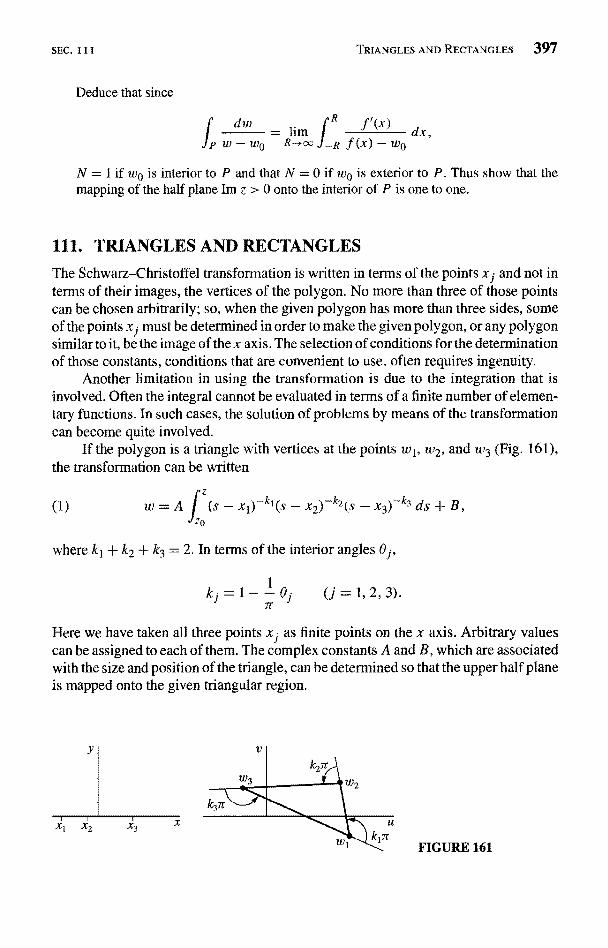
SEC. I I I
Deduce that since
N = 1 if wp is interior to P and that N = 0 if wp is exterior to P. Thus show that themapping of the half plane Im z > 0 onto the interior of P is one to one.
TRIANGLES AND RECTANGLES
The Schwarz-Christoffel transformation is written in terms of the points xj and not interms of their images, the vertices of the polygon. No more than three of those pointscan be chosen arbitrarily; so, when the given polygon has more than three sides, someof the points x1 must be determined in order to make the given polygon, or any polygonsimilar to it, be the image of the x axis. The selection of conditions for the determinationof those constants, conditions that are convenient to use, often requires ingenuity.
Another limitation in using the transformation is due to the integration that isinvolved. Often the integral cannot be evaluated in terms of a finite number of elemen-tary functions. In such cases, the solution of problems by means of the transformationcan become quite involved.
If the polygon is a triangle with vertices at the points wt, w2, and w3 (Fig. 161),the transformation can be written
(1) w = A I (s - xl)_k'(s - x2)-k2(s - x3)_kI ds + B,
TRIANGLES AND RECTANGLES 397
dx,
where kI + k2 + k3 = 2. In terms of the interior angles 8,,
7r(j =1,2 ).
Here we have taken all three points xi as finite points on the x axis. Arbitrary valuescan be assigned to each of them. The complex constants A and B, which are associatedwith the size and position of the triangle, can be determined so that the upper half planeis mapped onto the given triangular region.
Y
Txt
FIGURE 161
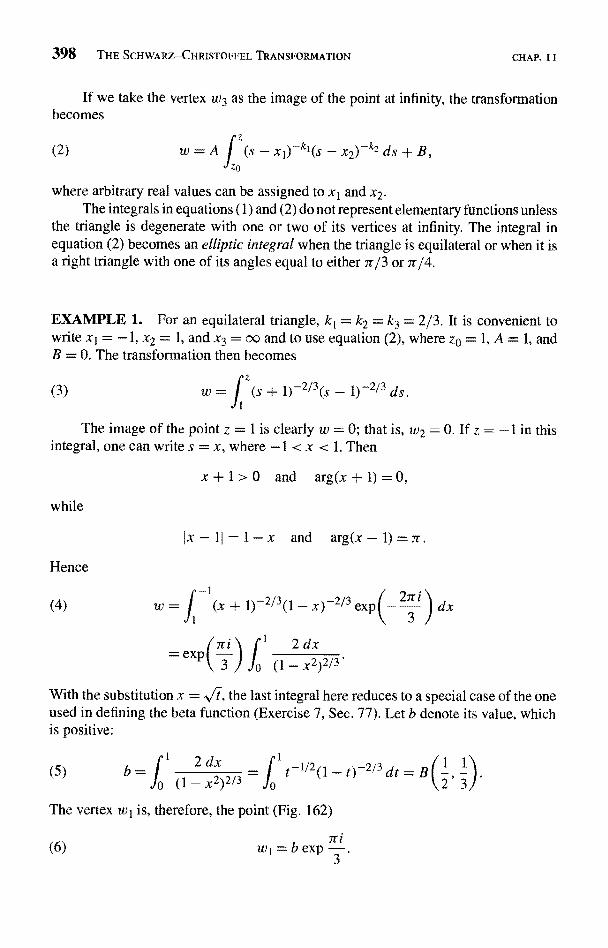
398 THE SCHWARZ-CHRISTOFFEL TRANSFORMATION CHAP. I I
If we take the vertex w3 as the image of the point at infinity, the transformationbecomes
(2) w = A / (S - xI)-ki(S - x2)-k2 ds + B,
where arbitrary real values can be assigned to x1 and x2.The integrals in equations (1) and (2) do not represent elementary functions unless
the triangle is degenerate with one or two of its vertices at infinity. The integral inequation (2) becomes an elliptic integral when the triangle is equilateral or when it isa right triangle with one of its angles equal to either 7r/3 or 7r/4.
EXAMPLE 1. For an equilateral triangle, k1 = k2 = k3 = 2/3. It is convenient towrite x1 = -1, x2 = 1, and x3 = oo and to use equation (2), where zo = 1, A = 1, andB = 0. The transformation then becomes
(3)
w=
1) -2/3
The image of the point z = 1 is clearly w = 0; that is, w2 = 0. If z = -1 in thisintegral, one can write s = x, where -1 < x < 1. Then
x+1>0 and arg(x+I)=0,
while
11 = 1- x and arg(x - 1) = 7r.
Hence
(4)
- 1)-2/3 ds.
-2/3 exp
7ri 1
=2 dxexp(3)
Jo (I - x2)2/3
With the substitution x = It, the last integral here reduces to a special case of the oneused in defining the beta function (Exercise 7, Sec. 77). Let b denote its value, whichis positive:
(5)
The vertex wI is, therefore, the point (Fig. 162)
dt=B
(6) w, = b exp i
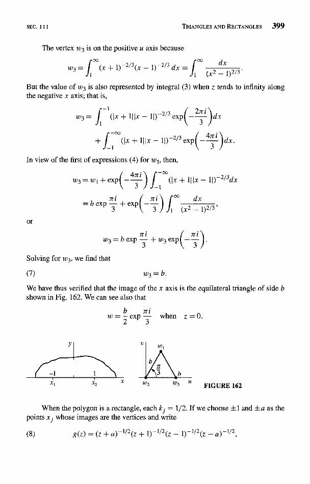
SEC. III TRIANGLES AND RECTANGLES 399
The vertex w3 is on the positive u axis because
)-2/3 dx =
But the value of w3 is also represented by integral (3) when z tends to infinity alongthe negative x axis; that is,
-2/3 exp
In view of the first of expressions (4) for w1, then,
+ exp
=bex
or
71w3=bexp-+w3exp
Solving for w3, we find that
(7) w3=b.
Ilx - lI)-2/3dx
We have thus verified that the image of the x axis is the equilateral triangle of side bshown in Fig. 162. We can see also that
b exp-
when z = 0.2 3
FIGURE 162
When the polygon is a rectangle, each ki = 1/2. If we choose ±1 and +a as thepoints xJ whose images are the vertices and write
(8) g(z) = (z + a)-1/2(z + 1)-1/2(z _ 1)-1/2(z - a) -1/2
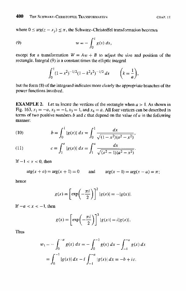
400 THE SCHWARZ-CHRISTOFFEL TRANSFORMATION CHAP. I I
where 0 < arg(z
(9)
the Schwarz-Christoffel transformation becomes
except for a transformation W = Aw + B to adjust the size and position of therectangle. Integral (9) is a constant times the elliptic integral
-1/2(1 -but the form (8) of the integrand indicates more clearly the appropriate branches of thepower functions involved.
EXAMPLE 2. Let us locate the vertices of the rectangle when a > 1. As shown inFig. 163, x1= -a, x2 = -1, x3 = 1, and x4 = a. All four vertices can be described interms of two positive numbers b and c that depend on the value of a in the followingmanner:
(10) b = 1 lg(x)) dx =
If - l < x < 0, then
Ig
-1/2 ds
dx =
arg(x + a) = arg(x + 1) = 0 and arg(x -
hence
x < -1, then
Thus
w1 =
0
g(x) _
) = arg
Ig(x)I = -1g(x)I
Ig =i1g
g(x) dx = - j g(x) dx - 1 g(x) dx
g(x)I dx - g(x) I dx = -b + ic.
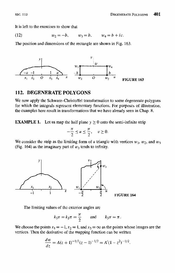
SEC, 112 DEGENERATE POLYGONS 401
It is left to the exercises to show that
(12) w2=-b, w3=b, w4=b+ic.
The position and dimensions of the rectangle are shown in Fig. 16
V
is
rw4
b
0 W3U
FIGURE 163
112. DEGENERATE POLYGONS
We now apply the Schwarz-Christoffel transformation to some degenerate polygonsfor which the integrals represent elementary functions. For purposes of illustration,the examples here result in transformations that we have already seen in Chap. 8.
EXAMPLE 1. Let us map the half plane y > 0 onto the semi-infinite strip
7r 7r-- <u< - v>0.2 - - 2 ,
We consider the strip as the limiting form of a triangle with vertices w1, w2, and w3(Fig. 164) as the imaginary part of w3 tends to infinity.
FIGURE 164
The limiting values of the exterior angles are
k17c = k2rc = 2 and k3ir
We choose the points x1= -1, x2 = 1, and x3 = oo as the points whose images are thevertices. Then the derivative of the mapping function can be written
dw= A(z + 1)-1J2(z - 1)-1/2 = Ar(1 - z2)-1J2 .
dz
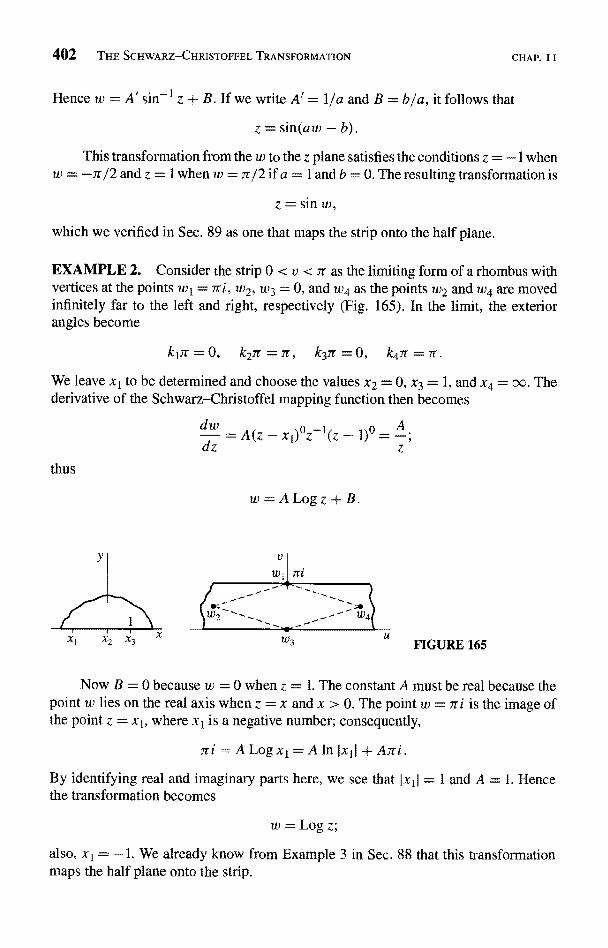
402 THE SCHWARZ-CHRISTOFFEL TRANSFORMATION CHAP. I I
Hence w = A' sin-1 z + B. If we write A' = 1/a and B = b/a, it follows that
z = sin(aw - b).
This transformation from the w to the z plane satisfies the conditions z = -1 when-7r/2 and z = 1 when w = it/2 if a = 1 and b = 0. The resulting transformation is
z = sin w,
which we verified in Sec. 89 as one that maps the strip onto the half plane.
EXAMPLE 2. Consider the strip 0 < v < it as the limiting form of a rhombus withvertices at the points w1= 7ri, w2, w3 = 0, and w4 as the points w2 and w4 are movedinfinitely far to the left and right, respectively (Fig. 165). In the limit, the exteriorangles become
k17r = 0, k27r = ir, k3ir = 0, k4Tr = 7r.
We leave x1 to be determined and choose the values x2 = 0, x3 = 1, and x4 = oo. Thederivative of the Schwarz-Christoffel mapping function then becomes
dw = A(z - xt)°z-1(z - 1)0 = Adz z
thus
= A Log z + B.
FIGURE 165
Now B = 0 because w = 0 when z = 1. The constant A must be real because thepoint w lies on the real axis when z = x and x > 0. The point w = Sri is the image ofthe point z = x1, where x1 is a negative number; consequently,
iri =ALogx1=AIn Jx1J+A7ri.
By identifying real and imaginary parts here, we see that Jx11 = 1 and A = 1. Hencethe transformation becomes
Log z;
also, x1 = -1. We already know from Example 3 in Sec. 88 that this transformationmaps the half plane onto the strip.
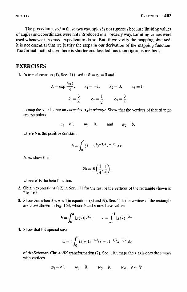
SEC. 112 EXERCISES 403
The procedure used in these two examples is not rigorous because limiting valuesof angles and coordinates were not introduced in an orderly way. Limiting values wereused whenever it seemed expedient to do so. But, if we verify the mapping obtained,it is not essential that we justify the steps in our derivation of the mapping function.The formal method used here is shorter and less tedious than rigorous methods.
EXERCISES
1. In transformation (1), Sec. 111, write B = zo = 0 and
A = exp
k1=4, k2=2, k3=4
to map the x axis onto an isosceles right triangle. Show that the vertices of that triangleare the points
w1=bi, w2=0, and w3=b,
where b is the positive constant
b= 1 (1- x2)-314x-IJ2 dx.
Also, show that
2b = B
where B is the beta function.
2. Obtain expressions (12) in Sec. 111 for the rest of the vertices of the rectangle shown inFig. 163.
3. Show that when 0 < a < 1 in equations (8) and (9), Sec. 111, the vertices of the rectangleare those shown in Fig. 163, where b and c now have values
b = I Ig(x)I dx,J
4. Show that the special case
w=
Ig(x)I dx.
J2 ds
of the Schwarz-Christoffel transformation (7), Sec. 110, maps the x axis onto the squarewith vertices
w1=bi, w2=0, w3=b, w4=b+ib,
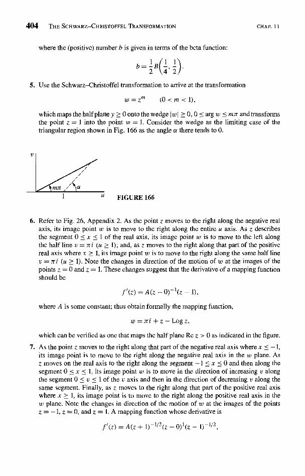
404 THE SCHWARZ-CHRISTOFFEL TRANSFORMATION
where the (positive) number b is given in terms of the beta function:
b=2
5. Use the Schwarz-Christoffel transformation to arrive at the transformation
w=zm (O<m<1),
CHAP. 11
which maps the half plane y > 0 onto the wedge I w I > 0, 0 < arg w < mir and transformsthe point z = 1 into the point w = 1. Consider the wedge as the limiting case of thetriangular region shown in Fig. 166 as the angle a there tends to 0.
FIGURE 166
6. Refer to Fig. 26, Appendix 2. As the point z moves to the right along the negative realaxis, its image point w is to move to the right along the entire u axis. As z describesthe segment 0 < x < 1 of the real axis, its image point w is to move to the left alongthe half line v = Jri (u > 1); and, as z moves to the right along that part of the positivereal axis where x > 1, its image point w is to move to the right along the same half linev = ni (u > 1). Note the changes in direction of the motion of w at the images of thepoints z = 0 and z = 1. These changes suggest that the derivative of a mapping functionshould be
f'(z) = A(z - 0)-'(z - 1),
where A is some constant; thus obtain formally the mapping function,
z - Logz,
which can be verified as one that maps the half plane Re z > 0 as indicated in the figure.
7. As the point z moves to the right along that part of the negative real axis where x < -1,its image point is to move to the right along the negative real axis in the w plane. Asz moves on the real axis to the right along the segment -1 < x < 0 and then along thesegment 0 c x < 1, its image point w is to move in the direction of increasing v alongthe segment 0 < v < 1 of the v axis and then in the direction of decreasing v along thesame segment. Finally, as z moves to the right along that part of the positive real axiswhere x > 1, its image point is to move to the right along the positive real axis in thew plane. Note the changes in direction of the motion of w at the images of the pointsz = -1, z = 0, and z = 1. A mapping function whose derivative is
.f'(z) = A(z + 1)-112(z _ 0)1(z _ 1)-3/2
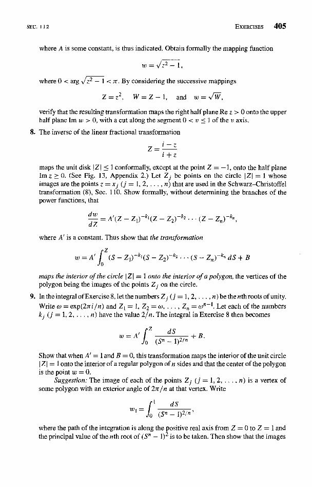
SEC. 112 EXERCISES 405
where A is some constant, is thus indicated. Obtain formally the mapping function
where 0 < arg z2 - 1 < n. By considering the successive mappings
Z=z2, W=Z---1, and w=-N/-W,
verify that the resulting transformation maps the right half plane Re z > 0 onto the upperhalf plane Im w > 0, with a cut along the segment 0 < v < 1 of the v axis.
8. The inverse of the linear fractional transformation
Zi - z
z
maps the unit disk I Z I < 1 conformally, except at the point Z = -1, onto the half planeIm z ? 0. (See Fig. 13, Appendix 2.) Let ZJ be points on the circle IZI = 1 whoseimages are the points z = xj (j = 1, 2, . . . , n) that are used in the Schwarz-Christoffeltransformation (8), Sec. 110. Show formally, without determining the branches of thepower functions, that
dw = A'(Z - ZI)-k1(Z - Z2)-k2 ... (Z - ZndZ
where A' is a constant. Thus show that the transformation
S - ZI)-k'(S - Z2) -k2 . (S - Z,,)-k- dS + B
maps the interior of the circle I ZI = I onto the interior of a polygon, the vertices of thepolygon being the images of the points Zi on the circle.
9. In the integral of Exercise 8, let the numbers Z1 (j = 1, 2, . . . , n) be the nth roots of unity.
Write w = exp(27ri/n) and ZI = 1, Z2 = c), . . . , Z, = w'''. Let each of the numberskJ (j = 1, 2, . . . , n) have the value 2/n. The integral in Exercise 8 then becomes
= A' dS(Sn - 1)2jn
+ B.
Show that when A' = 1 and B = 0, this transformation maps the interior of the unit circleI Z I = 1 onto the interior of a regular polygon of n sides and that the center of the polygonis the point w = 0.
Suggestion: The image of each of the points ZJ (j = 1, 2, ... , n) is a vertex ofsome polygon with an exterior angle of 2 r/n at that vertex. Write
dS
Sn - 1)2/n'
where the path of the integration is along the positive real axis from Z = 0 to Z = 1 andthe principal value of the nth root of (S' - 1)2 is to be taken. Then show that the images
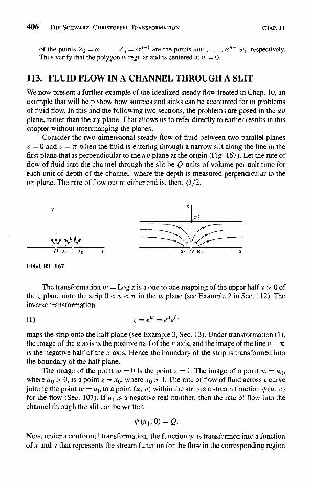
406 THE SCHWARZ-CHRISTOFFEL TRANSFORMATION CHAP. I I
of the points Z2 = a , ... , Z, = mn-I are the points cowl, ... , w"-Iwl, respectively.Thus verify that the polygon is regular and is centered at w = 0.
113. FLUID FLOW IN A CHANNEL THROUGH A SLIT
We now present a further example of the idealized steady flow treated in Chap. 10, anexample that will help show how sources and sinks can be accounted for in problemsof fluid flow. In this and the following two sections, the problems are posed in the uvplane, rather than the xy plane. That allows us to refer directly to earlier results in thischapter without interchanging the planes.
Consider the two-dimensional steady flow of fluid between two parallel planesv = 0 and v = n when the fluid is entering through a narrow slit along the line in thefirst plane that is perpendicular to the uv plane at the origin (Fig. 167). Let the rate offlow of fluid into the channel through the slit be Q units of volume per unit time foreach unit of depth of the channel, where the depth is measured perpendicular to theuv plane. The rate of flow out at either end is, then, Q/2.
Y
0
FIGURE 167
The transformation w = Log z is a one to one mapping of the upper half y > 0 ofthe z plane onto the strip 0 < v < it in the w plane (see Example 2 in Sec. 112). Theinverse transformation
(1) z = e
maps the strip onto the half plane (see Example 3, Sec. 13). Under transformation (1),the image of the u axis is the positive half of the x axis, and the image of the line v = itis the negative half of the x axis. Hence the boundary of the strip is transformed intothe boundary of the half plane.
The image of the point w = 0 is the point z = 1. The image of a point w = up,where uq > 0, is a point z = x0, where x0 > 1. The rate of flow of fluid across a curvejoining the point w = up to a point (u, v) within the strip is a stream function * (u, v)for the flow (Sec. 107). If uI is a negative real number, then the rate of flow into thechannel through the slit can be written
i'(u1, 0) = Q.
Now, under a conformal transformation, the function I/r is transformed into a functionof x and y that represents the stream function for the flow in the corresponding region
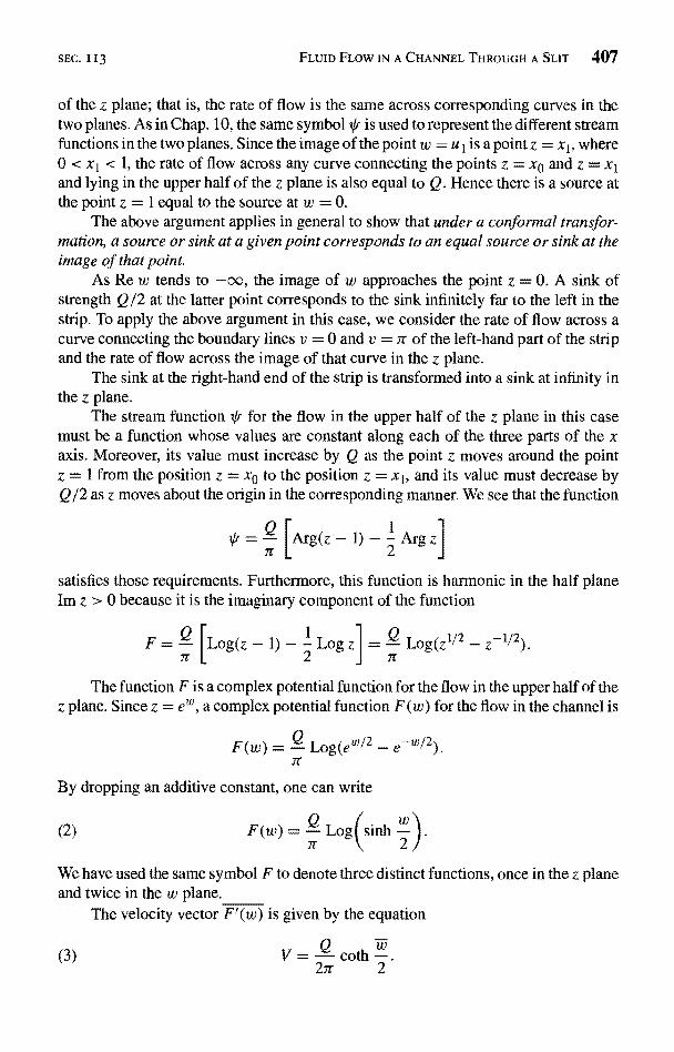
SEC. 113 FLUID FLOW IN A CHANNEL THROUGH A SLIT 407
of the z plane; that is, the rate of flow is the same across corresponding curves in thetwo planes. As in Chap. 10, the same symbol Vr is used to represent the different streamfunctions in the two planes. Since the image of the point w = u
1is a point z = x1, where
0 < x1 < 1, the rate of flow across any curve connecting the points z = x0 and z = x1and lying in the upper half of the z plane is also equal to Q. Hence there is a source atthe point z = 1 equal to the source at w = 0.
The above argument applies in general to show that under a conformal transfor-mation, a source or sink at a given point corresponds to an equal source or sink at theimage of that point.
As Re w tends to -oc, the image of w approaches the point z = 0. A sink ofstrength Q/2 at the latter point corresponds to the sink infinitely far to the left in thestrip. To apply the above argument in this case, we consider the rate of flow across acurve connecting the boundary lines v = 0 and v = it of the left-hand part of the stripand the rate of flow across the image of that curve in the z plane.
The sink at the right-hand end of the strip is transformed into a sink at infinity inthe z plane.
The stream function i/r for the flow in the upper half of the z plane in this casemust be a function whose values are constant along each of the three parts of the xaxis. Moreover, its value must increase by Q as the point z moves around the pointz = 1 from the position z = x0 to the position z = x1, and its value must decrease byQ/2 as z moves about the origin in the corresponding manner. We see that the function
Log(z112 - z-1/2Log(z - 1) - - Log z I =
Arg(z-1)-2Argz1
satisfies those requirements. Furthermore, this function is harmonic in the half planeIm z > 0 because it is the imaginary component of the function
qz 7r
The function F is a complex potential function for the flow in the upper half of thez plane. Since z = e'', a complex potential function F(w) for the flow in the channel is
F(w) = Q Log(e/2 -7r
By dropping an additive constant, one can write
(2)
2
F(w) _ ' Log (sink 2 .
We have used the same symbol F to denote three distinct functions, once in the z planeand twice in the w plane.
The velocity vector F'(w) is given by the equation
(3)
_ uV
27rcosh
2.
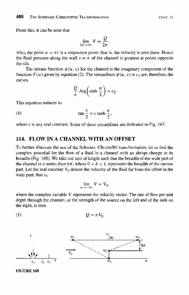
408 THE SCHWARZ-CHRISTOFFEL TRANSFORMATION
From this, it can be seen that
V2rr
CHAP. I I
Also, the point w = Tri is a stagnation point; that is, the velocity is zero there. Hencethe fluid pressure along the wall v = rr of the channel is greatest at points oppositethe slit.
The stream function Mfr (u, v) for the channel is the imaginary component of thefunction F(w) given by equation (2). The streamlines *(u, v) = c2 are, therefore, thecurves
Q Arg( sinh -2
This equation reduces to
(4)v u
tan2
= c tanh2
,
where c is any real constant. Some of these streamlines are indicated in Fig. 167.
114. FLOW IN A CHANNEL WITH AN OFFSET
To further illustrate the use of the Schwarz-Christoffel transformation, let us find thecomplex potential for the flow of a fluid in a channel with an abrupt change in itsbreadth (Fig. 168). We take our unit of length such that the breadth of the wide part ofthe channel is 7r units; then hrr, where 0 < h < 1, represents the breadth of the narrowpart. Let the real constant Va denote the velocity of the fluid far from the offset in thewide part; that is,
V = Va,
where the complex variable V represents the velocity vector. The rate of flow per unitdepth through the channel, or the strength of the source on the left and of the sink onthe right, is then
(1)
Y w4
h
1IFIGURE 168
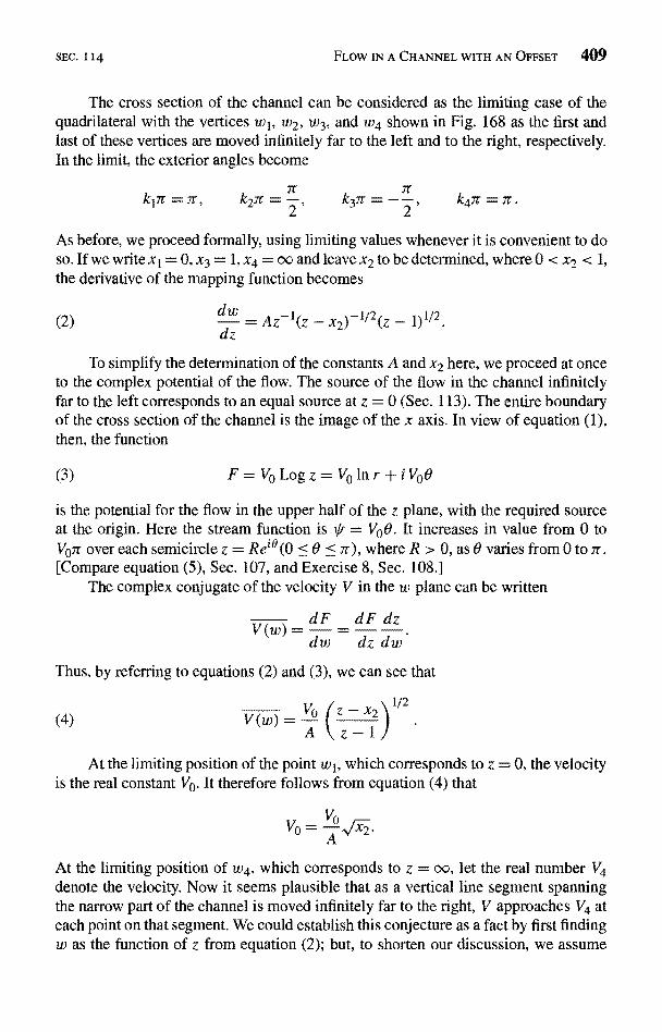
SEC. 1 14 FLOW IN A CHANNEL WITH AN OFFSET 409
The cross section of the channel can be considered as the limiting case of thequadrilateral with the vertices w1, W2, w3, and w4 shown in Fig, 168 as the first andlast of these vertices are moved infinitely far to the left and to the right, respectively.In the limit, the exterior angles become
It It
213, - 2'
k7r=-
As before, we proceed formally, using limiting values whenever it is convenient to doso. If we write x 1 = 0, x3 = 1, x4 = oc and leave x2 to be determined, where 0 < x2 < 1,
the derivative of the mapping function becomes
(2)dw
dz
x2)-1/2(z _ 1)1/2
To simplify the determination of the constants A and x2 here, we proceed at onceto the complex potential of the flow. The source of the flow in the channel infinitelyfar to the left corresponds to an equal source at z = 0 (Sec. 113). The entire boundaryof the cross section of the channel is the image of the x axis. In view of equation (1),then, the function
(3) F= V0Logz= V0lnr+iV0B
is the potential for the flow in the upper half of the z plane, with the required sourceat the origin. Here the stream function is fr = VO6. It increases in value from 0 toV0rc over each semicircle z = Re`0(0 < 0 < Ir), where R > 0, as 0 varies from 0 to It.[Compare equation (5), Sec. 107, and Exercise 8, Sec. 108.]
The complex conjugate of the velocity V in the w plane can be written
_dF_dFdzV(w)
dw dz dw
Thus, by referring to equations (2) and (3), we can see that
(4)
1/2
At the limiting position of the point wl, which corresponds to z = 0, the velocityis the real constant V0. It therefore follows from equation (4) that
VO
A
At the limiting position of w4, which corresponds to z -- oo, let the real number V4denote the velocity. Now it seems plausible that as a vertical line segment spanningthe narrow part of the channel is moved infinitely far to the right, V approaches V4 ateach point on that segment. We could establish this conjecture as a fact by first findingw as the function of z from equation (2); but, to shorten our discussion, we assume
410 THE SCHWARZ-CHRISTOFFEL TRANSFORMATION
that this is true, Then, since the flow is steady,
-r h V4= rr Vo = Q,
or V4 = Vo/ h. Letting z tend to infinity in equation (4), we find that
Vp Va
Thus
(5)
and
A = h,
CHAP. I I
From equation (6), we know that the magnitude V I of the velocity becomesinfinite at the corner w3 of the offset since it is the image of the point z = 1. Also,the corner w2 is a stagnation point, a point where V = 0. Along the boundary of thechannel, the fluid pressure is, therefore, greatest at w2 and least at w3.
To write the relation between the potential and the variable w, we must integrateequation (2), which can now be written
(7)
By substituting a new variables, where
z-h2z-1
one can show that equation (7) reduces to
Hence
(8) w=hLog 1+s -Log h+s1-s h -s
The constant of integration here is zero because when z = h2, the quantity s is zeroand so, therefore, is w.
In terms of s, the potential F of equation (3) becomes
F = Vo Logh2-s21-
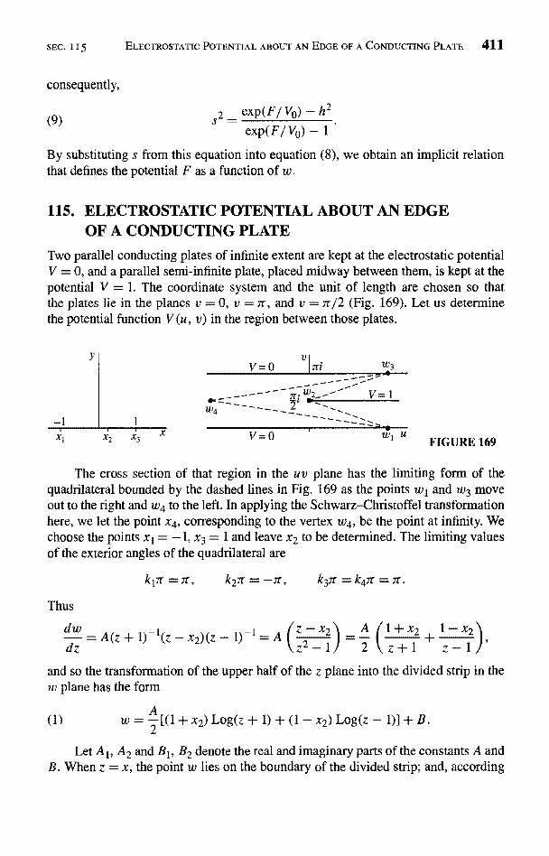
SEC. 1 15 ELECTROSTATIC POTENTIAL ABOUT AN EDGE OF A CONDUCTING PLATE 411
consequently,
(9)2 - exp(F/ Vo) - h2
exp(F/VO) - 1
By substituting s from this equation into equation (8), we obtain an implicit relationthat defines the potential F as a function o
115. ELECTROSTATIC POTENTIAL ABOUT AN EDGEOF A CONDUCTING PLATE
Two parallel conducting plates of infinite extent are kept at the electrostatic potentialV = 0, and a parallel semi-infinite plate, placed midway between them, is kept at thepotential V = 1. The coordinate system and the unit of length are chosen so thatthe plates lie in the planes v = 0, v = Tr, and v = 7r/2 (Fig. 169). Let us determinethe potential function V (u, v) in the region between those plates.
Yv=o
2- V=
xl
1-r'x3
4
v=o FIGURE 169
The cross section of that region in the uv plane has the limiting form of thequadrilateral bounded by the dashed lines in Fig. 169 as the points w1 and w3 moveout to the right and w4 to the left. In applying the Schwarz-Christoffel transformationhere, we let the point x4, corresponding to the vertex w4, be the point at infinity. Wechoose the points x1 = -1, x3 = 1 and leave x2 to be determined. The limiting valuesof the exterior angles of the quadrilateral are
k1ir = Tr, k2ar = -ar, k3ar = k4Tr =
Thus
dwdz =
A(z + I)-1(z - x2)(z - I)-1
z-
and so the transformation of the upper half of the z plane into the divided strip in thew plane has the form
{1} w=`[(1+x2)Log(z+1)+(I-x2)Log(z-1)]+B.
Let A 1, A2 and B1, B2 denote the real and imaginary parts of the constants A andB. When z = x, the point w lies on the boundary of the divided strip; and, according
412 THE SCHWARZ-C:HRISTOFFEL TRANSFORMATION CHAP. I I
to equation (1),
(2) u+iv=A1 iA2((I+x2)[inIx+11+iarg(x+1)]
+(l-x2)[lnIx-ii+iarg(x-1)]}+BI+iB2.To determine the constants here, we first note that the limiting position of the
line segment joining the points w1 and w4 is the u axis. That segment is the image ofthe part of the x axis to the left of the point x1= -1; this is because the line segmentjoining w3 and w4 is the image of the part of the x axis to the right of x3 = 1, andthe other two sides of the quadrilateral are the images of the remaining two segmentsof the x axis. Hence when v = 0 and u tends to infinity through positive values, thecorresponding point x approaches the point z = -1 from the left. Thus
arg(x+1)=ir, arg(x-1)=ar,
and In Ix + 1I tends to -oc. Also, since -1 < x2 < 1, the real part of the quantity insidethe braces in equation (2) tends to -oc. Since v = 0, it readily follows that A2 = 0;for, otherwise, the imaginary part on the right would become infinite. By equatingimaginary parts on the two sides, we now see that
Hence
x2)17 +(1-x2)r]+B2.
(3) -rrA1= B2, A2=0.
The limiting position of the line segment joining the points w1 and w2 is the halfline v = 7r/2 (u > 0). Points on that half line are images of the points z = x, where-1 < x -< x2; consequently,
arg(x + 1) = 0, arg(x - 1)
Identifying the imaginary parts on the two sides of equation (2), we thus arrive at therelation
(4)Jr - xi)ir + Bi.
Finally, the limiting positions of the points on the line segment joining w3 to w4are the points u + 7ti, which are the images of the points x when x > 1. By identifying,for those points, the imaginary parts in equation (2), we find that
7r= B2.
Then, in view of equations (3) and (4),
Al=-1,
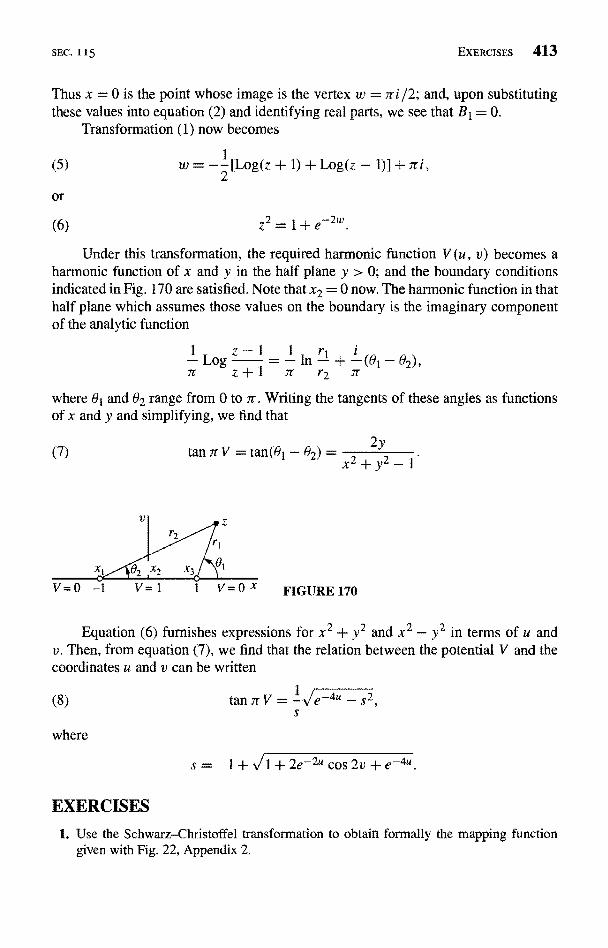
SEC. 1 15 EXERCISES 413
Thus x = 0 is the point whose image is the vertex w = rri J2; and, upon substitutingthese values into equation (2) and identifying real parts, we see that BI = 0.
Transformation (1) now becomes
(5) w = -2
[Log(z + 1) + Log(z -
or
(6) z2 = 1 + e-2w
Under this transformation, the required harmonic function V (u, v) becomes aharmonic function of x and y in the half plane y > 0; and the boundary conditionsindicated in Fig. 170 are satisfied. Note that x2 = 0 now. The harmonic function in thathalf plane which assumes those values on the boundary is the imaginary componentof the analytic function
Log z - 1 - In rl + a
-(01-02),r2 7It z + l it
where 81 and 02 range from 0 to jr. Writing the tangents of these angles as functionsof x and y and simplifying, we find that
(7)
FIGURE 170
Equation (6) furnishes expressions for x2 + y2 and x2 - y2 in terms of u andv. Then, from equation (7), we find that the relation between the potential V and thecoordinates u and v can be written
(8)
where
2ytan7rV =tan(81-02)=x2+y2-1
tan 7r V =
1 + 2e-2u cos 2v + e-4u
EXERCISES
1. Use the Schwarz-Christoffel transformation to obtain formally the mapping functiongiven with Fig. 22, Appendix 2.
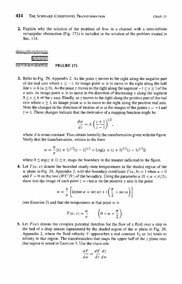
414 THE SCHWARZ-CHRISTOFFEL TRANSFORMATION CHAP. T I
2. Explain why the solution of the problem of flow in a channel with a semi-infiniterectangular obstruction (Fig. 171) is included in the solution of the problem treated inSee. 114.
FIGURE 171
3. Refer to Fig. 29, Appendix 2. As the point z moves to the right along the negative partof the real axis where x < -1, its image point w is to move to the right along the halfline v = h (u < 0). As the point z moves to the right along the segment -1 < x < I of thex axis, its image point u5 is to move in the direction of decreasing v along the segment0 < v < h of the v axis. Finally, as z moves to the right along the positive part of the realaxis where x > 1, its image point w is to move to the right along the positive real axis.Note the changes in the direction of motion of w at the images of the points z = - I andz = 1. These changes indicate that the derivative of a mapping function might be
d w _ Z +1)1/2
dzA
(z
- 1
where A is some constant. Thus obtain formally the transformation given with the figure.Verify that the transformation, written in the form
w = h {(z + 1)I1 '2 (z - 1)''2 + Log[z + (z + 1)''2{z - 1)1/2]}
where 0 < arg(z + 1) < 7r, maps the boundary in the manner indicated in the figure.
4. Let T(u, v) denote the bounded steady-state temperatures in the shaded region of thew plane in Fig. 29, Appendix 2, with the boundary conditions T (u, h) = 1 when u < 0and T = 0 on the rest (B'C'D') of the boundary. Using the parameter a (0 < a < 7r/2),show that the image of each point z = i tan a on the positive y axis is the point
w=- [In(tan a+see a)+i(2 +seca
(see Exercise 3) and that-the temperature at that point u) is
T(u,v)=- {0<a< ).7T 2
5. Let F(w) denote the complex potential function for the flow of a fluid over a step inthe bed of a deep stream represented by the shaded region of the w plane in Fig. 29,Appendix 2, where the fluid velocity V approaches a real constant Vp as (wi tends toinfinity in that region. The transformation that maps the upper half of the z plane ontothat region is noted in Exercise 3. Use the chain rule
dF dF dzdw dz dw
SEC. 115 EXERCISES 415
to show that
V(w) = Vp(z - 1)1/2(z + 1)-1/Z.
and, in terms of the points z = x whose images are the points along the bed of the stream,show that
I Vo
Note that the speed increases from I VoI along A'B' until I V I = oc at B', then diminishesto zero at C', and increases toward I Vol from C' to D'; note, too, that the speed is I Vol at
the point
between Band C.

CHAPTER
12INTEGRAL FORMULASOF THE POISSON TYPE
In this chapter, we develop a theory that enables us to obtain solutions to a variety ofboundary value problems where those solutions are expressed in terms of definite orimproper integrals. Many of the integrals occurring are then readily evaluated.
116. POISSON INTEGRAL FORMULALet Co denote a positively oriented circle, centered at the origin, and suppose that afunction f is analytic inside and on Co. The Cauchy integral formula (Sec. 47)
(1) f(z)
expresses the value off at any point z interior to Co in terms of the values off at pointss on Co. In this section, we shall obtain from formula (1) a corresponding formula forthe real part of the function f; and, in Sec. 117, we shall use that result to solve theDirichlet problem (Sec. 98) for the disk bounded by Co.
We let r0 denote the radius of Co and write z = r exp(i6), where 0 < r < ro(Fig. 172). The inverse of the nonzero point z with respect to the circle is the point z1lying on the same ray f r o m the origin as z and satisfying the condition I z 1 II z I = r2 ;
thus, ifs is a point on C0,
(2)
r2exp(iO) =
r
417
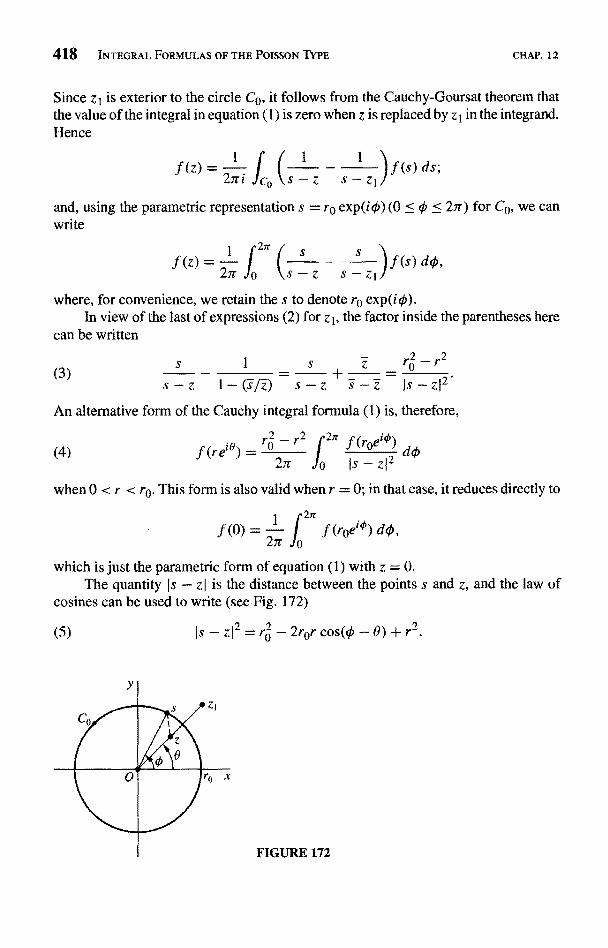
418 INTEGRAL FORMULAS OF THE POISSON TYPE CHAP. 12
Since z1 is exterior to the circle CO, it follows from the Cauchy-Goursat theorem thatthe value of the integral in equation (1) is zero when z is replaced by z 1 in the integrand.Hence
1 1.f (z) = ) .f (s) ds;2ni ]CO s-z s - zJ
and, using the parametric representation s = r4 exp(i gyp) (0 { 0 < 27r) for CO, we canwrite
1 2ir s S.f(z)=- --27r 0 s - z s -
where, for convenience, we retain the s to denote r0 exp(io).In view of the last of expressions (2) for z 1, the factor inside the parentheses here
can be written
An alternative form of the Cauchy integral formula (1) is, therefore,
eio
dpi(4) .f (ret4) =U J I2no s - z
when 0 < r < re. This form is also valid when r = 0; in that case, it reduces directly to
1
I2n
.f (0)2n
.f (rtle`1) dO,
which is just the parametric form of equation (1) with z = 0.The quantity Is - z I is the distance between the points s and z, and the law of
cosines can be used to write (see Fig. 172)
(5) Is-zI`=r.2 -2rercos(¢'-0)+r`
FIGURE 172
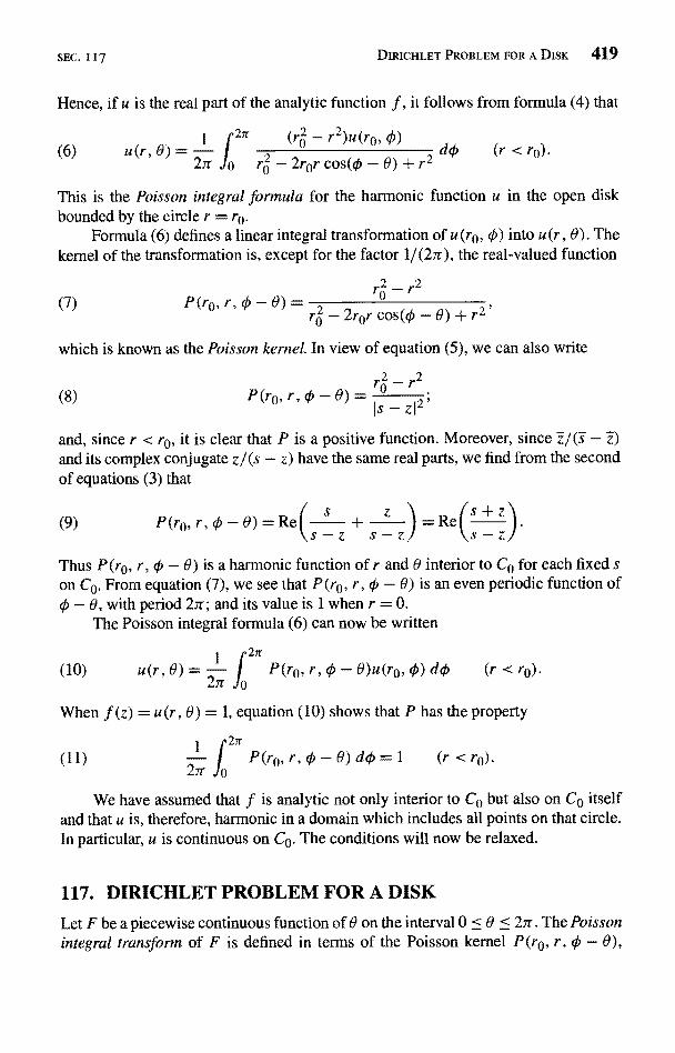
SEC. 117 DIRICHLET PROBLEM FOR A DISK 419
Hence, if u is the real part of the analytic function f, it follows from formula (4) that
r2)u(ro, 0dO (r < ro).(6) u(r, 8} = = 1 ,,
22ror cos(¢, - 0) + r
This is the Poisson integral formula for the harmonic function u in the open diskbounded by the circle r = re.
Formula (6) defines a linear integral transformation of u(ro, 0) into u (r, 0). Thekernel of the transformation is, except for the factor 1/(2n), the real-valued function
-0)= 0
roe - 2rer cos(¢ - 0) +r2'
which is known as the Poisson kernel. In view of equation (5), we can also write
(8) Pr2 - r20
- z12'
and, since r < ro, it is clear that P is a positive function. Moreover, since -Z/(s - z)and its complex conjugate z/ (s - z) have the same real parts, we find from the secondof equations (3) that
Thus P(ro, r, 0 - 0) is a harmonic function of r and 0 interior to Co for each fixed son Co. From equation (7), we see that P(ro, r, 0 - 0) is an even periodic function of
- 0, with period 2n; and its value is 1 when r = 0.The Poisson integral formula (6) can now be written
(10) u(r,0)=2n J0 P(ro,r,0h-0)u(ro,0)do
When f (z) = u(r, 0) = 1, equation (10) shows that P has the property
-I P(r0,r,0 - 1)do=
(11) 2
We have assumed that f is analytic not only interior to Co but also on Co itselfand that u is, therefore, harmonic in a domain which includes all points on that circle.In particular, u is continuous on Co. The conditions will now be relaxed.
117. DIRICHLET PROBLEM FOR A DISK
Let F be a piecewise continuous function of 0 on the interval 0 < 0 < 2nr. The Poissonintegral transform of F is defined in terms of the Poisson kernel P (ro,
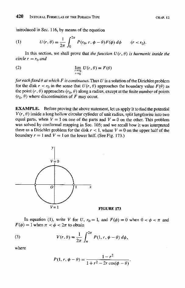
420 INTEGRAL FORMULAS OF THE POISSON TYPE
introduced in Sec. 116, by means of the equation
CHAP. 12
2n
(1) U(r,0)=27r j P(rc,r,0-8)F(O)d¢ (r <r4).
In this section, we shall prove that the function U (r, 0) is harmonic inside thecircle r = rc and
(2) lim Ur-rr0r<rp
0) = F(8)
for each fixed 0 at which F is continuous. Thus U is a solution of the Dirichlet problemfor the disk r < r0 in the sense that U(r, 0) approaches the boundary value F(0) asthe point (r, 0) approaches (rc, 0) along a radius, except at the finite number of points(rc, 0) where discontinuities of F may occur.
EXAMPLE. Before proving the above statement, let us apply it to find the potentialV (r, 0) inside a long hollow circular cylinder of unit radius, split lengthwise into twoequal parts, when V = 1 on one of the parts and V = 0 on the other. This problemwas solved by conformal mapping in Sec. 105; and we recall how it was interpretedthere as a Dirichlet problem for the disk r < 1, where V = 0 on the upper half of theboundary r = 1 and V = 1 on the lower half. (See Fig. 173.)
y
V=1 FIGURE 173
In equation (1), write V for U, r0 = 1, and F(0) = 0 when 0 < 0 < 7r andF(0) = 1 when 7r < 0 < 2ir to obtain
(3)
where
V(r,0)=- P(l,r,c -0)d¢,
P(1, r, 0 -0)=
SEC. 117 DIRICHLET PROBLEM FOR A DISK 421
An antiderivative of P(1, r,
(4) f P(1, r, IJr) difr = 2 arctan(1 +
1-rthe integrand here being the derivative with respect to IJr of the function on the right.So it follows from expression (3) that
f1[ tan
27r - B I - arctan1 + r
tanar -
ir V (r, 0) = arctan+ r
\1-r 2 /11 1-r 2
After simplifying the expression for tan[7r V (r, 8)] obtained from this last equation(see Exercise 3, Sec. 118), we find that
1(5) V (r, 0) = arctan
It Zr sin 8arctan t ,
where the stated restriction on the values of the arctangent function is physicallyevident. When expressed in rectangular coordinates, the solution here is the same assolution (5) in Sec. 105.
We turn now to the proof that the function U defined in equation (1) satisfies theDirichiet problem for the disk r < ro, as asserted just prior to this example. First ofall, U is harmonic inside the circle r = re because P is a harmonic function of r and0 there. More precisely, since F is piecewise continuous, integral (1) can be writtenas the sum of a finite number of definite integrals each of which has an integrand thatis continuous in r, 0, and 0. The partial derivatives of those integrands with respectto r and 0 are also continuous. Since the order of integration and differentiation withrespect to r and 0 can, then, be interchanged and since P satisfies Laplace's equation
r2Prr+rPr+ x'80=0
in the polar coordinates r and 6 (Exercise 5, Sec. 25), it follows that U satisfies thatequation too.
In order to verify limit (2), we need to show that if F is continuous at 0, therecorresponds to each positive number s a positive number & such that
(6) I U (r, 6) - F(0) J < s whenever 0 < ro - r <8.
We start by referring to property (11), Sec. 116, of the Poisson kernel and writing
U(r, 6) - F(8) = I P(ro, r, 0 - 6)[F(o) - F(8)] do.27r
For convenience, we let F be extended periodically, with period 27r, so that theintegrand here is periodic in 0 with that same period. Also, we may assume that0 < r < ro because of the nature of the limit to be established.
422 INTEGRAL FORMULAS OF THE POISSON TYPE CHAP. 12
Next, we observe that, since F is continuous at 0, there is a small positive numbera such that
(7) IF(O) - F(9)) < 2 whenever 10-
Evidently,
(8)
where
P(r0, r, 0 - 8)[F(o) - F(8)] do,
1 8 -a+2n
P(r0, r, 0 - 6)[F(o) - F(O)] do.- 2ar O+,,
The fact that P is a positive function (Sec. 116), together with the first ofinequalities (7) just above and property (11), Sec. 116, of that function, enables usto write
4Tr
P(ro, r, 0 - 0) IF(o) - F(0) I dry
2n
P(ro,r,0-O)do
As for the integral 12(r), one can see from Fig. 172 in Sec. 116 that the denominatorIs - z12 in expression (8) for P(ro, r, 0 - 6) in that section has a (positive) minimumvalue m as the argument 0 of s varies over the closed interval
9+a<0<0 -a+2n.So, if M denotes an upper bound of the piecewise continuous function IF(o) - F(O)1on the interval 0 < 0 < 27r, it follows that
112(r)I <
U(r, 8) - F(9) = 11(r) + 12(
27rm
whenever rn - r < S. where
(9)
2n<2M
0
ms
2
2
m 2
4Mr0
Finally, the results in the two preceding paragraphs tell us that
I U(r, 0) - F(9)
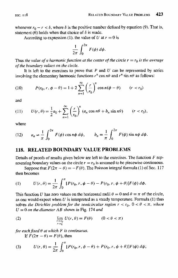
SEC. I 18 RELATED BOUNDARY VALUE PROBLEMS 423
whenever r0 - r < &, where & is the positive number defined by equation (9). That is,statement (6) holds when that choice of & is made.
According to expression (1), the value of U at r = 0 is
1
2Tr Jo
2
F(o) do.
Thus the value of a harmonic function at the center of the circle r = r0 is the averageof the boundary values on the circle.
It is left to the exercises to prove that P and U can be represented by seriesinvolving the elementary harmonic functions rn cos nO and r'1 sin nd as follows:
(10) P(ro,r, i-0)=1+2
and
(11) U(r, 0) = I a0 +
where
cosn(r -0)
ancosno+bn sin no) (r <r0
(12) an = - I F( o) cos no dry, bn = - j F(o) sin no do.
118. RELATED BOUNDARY VALUE PROBLEMS
Details of proofs of results given below are left to the exercises. The function F rep-resenting boundary values on the circle r = r0 is assumed to be piecewise continuous.
Suppose that F(2n - 0) = -F(0). The Poisson integral formula (1) of Sec. 117then becomes
1(1) U(r, 0) =
21r[P(ro, - 0) - P(r0, r, 0 + 0)]F(o) do.
This function U has zero values on the horizontal radii 0 = 0 and 0 = it of the circle,as one would expect when U is interpreted as a steady temperature. Formula (1) thussolves the Dirichlet problem for the semicircular region r < r0, 0 < 0 < Tr, whereU = 0 on the diameter AB shown in Fig. 174 and
(2) lim U(r, 0r-*r0r¢r0
F(O) (0<0<7r)
or each fixed 0 at which F is continuous.If F(2n - 0) = F(0), then
(3) U(r, 0) = + 0)]F(O) do;
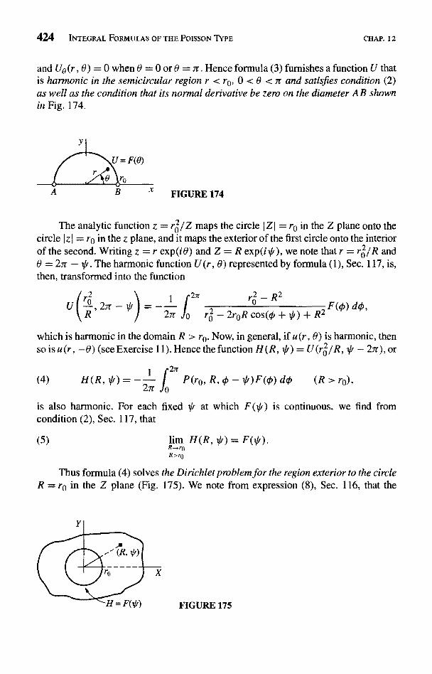
424 INTEGRAL FORMULAS OF THE POISSON TYPE CHAP. 12
and U0 (r, 0) = 0 when 0 = 0 or 0 = it. Hence formula (3) furnishes a function U thatis harmonic in the semicircular region r < ro, 0 < 6 < 7r and satisfies condition (2)as well as the condition that its normal derivative be zero on the diameter A B shownin Fig. 174.
FIGURE 174
The analytic function z = r jZ maps the circle Z (= ro in the Z plane onto thecircle I z ( = ro in the z plane, and it maps the exterior of the first circle onto the interiorof the second. Writing z = r exp(iO) and Z = R exp(i i), we note that r = r6 jR and0 = 2ir - s(i. The harmonic function U(r, 0) represented by formula (1), Sec. 117, is,then, transformed into the function
,2Tr- F(op) dO,
which is harmonic in the domain R > re. Now, in general, if u(r, 0) is harmonic, thenso is u (r, -0) (see Exercise 11). Hence the function H (R, IJi) = aJi -tar}, or
(4) H(R,27r J0 P(ro,R,0 -IJi)F(o)do (R>ro),
is also harmonic. For each fixed aji at which F(*) is continuous, we find fromcondition (2), Sec. 117, that
(5)R-.rpR>rd
H(R, afi) = F(IJI).
Thus formula (4) solves the Dirichlet problem for the region exterior to the circleR = ro in the Z plane (Fig. 175). We note from expression (8), Sec. 116, that the
FIGURE 175
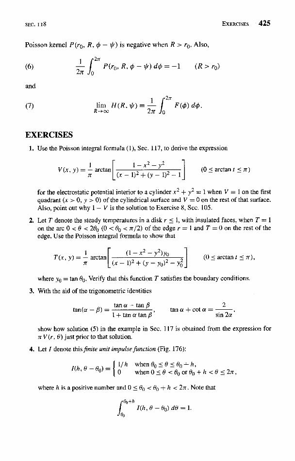
SEC. 118
Poisson kernel P (ro, R, is negative when R > r0. Also,
dpi= -
and
(7)R-aoo
R > ro
H(R,lG')_- I F(O)dcp.
EXERCISES 425
EXERCISES
1. Use the Poisson integral formula (1), Sec. 117, to derive the expression
(0 < arctan t < 7r)
for the electrostatic potential interior to a cylinder x2 + y2 = I when V = 1 on the firstquadrant (x > 0, y > 0) of the cylindrical surface and V = 0 on the rest of that surface.Also, point out why 1 - V is the solution to Exercise 8, Sec. 105.
2. Let T denote the steady temperatures in a disk r < 1, with insulated faces, when T = 1on the arc 0 < 9 < 20o (0 < 90 < 7r/2) of the edge r = 1 and T = 0 on the rest of theedge. Use the Poisson integral formula to show that
T(x, y) =1
arctan7r
- Y2)Yo
(x - 1)2 + (y - yo)2 -(0 < arctan t
where yo = tan 90. Verify that this function T satisfies the boundary conditions.
3. With the aid of the trigonometric identities
tan a - tan 6,tan{a - p) =
1+tanatan a + cot a =
2
sin 2a
show how solution (5) in the example in Sec. 117 is obtained from the expression forr V (r, 9) just prior to that solution.
4. Let I denote this finite unit impulse function (Fig. 176):
1/h when 90<9<00+h,1(h, 69 0 when 0<9 <00or00+h <9 <27r,
where h is a positive number and 0 < 90 < 90 + h < 27r. Note that
00+hI(h,0-90)d9=1.
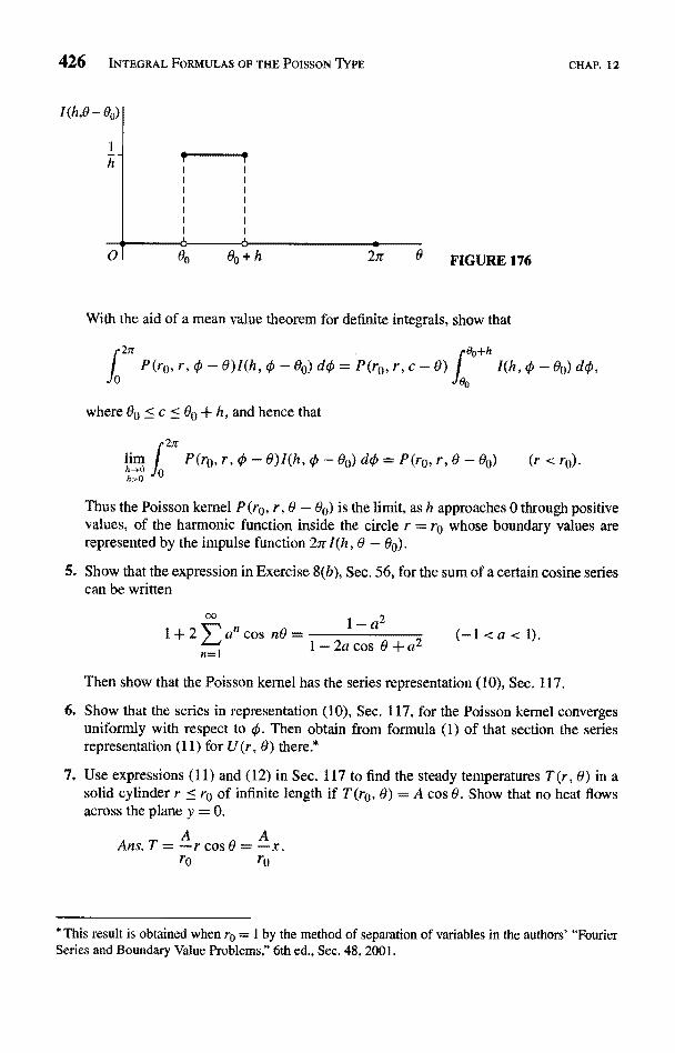
426 INTEGRAL FORMULAS OF THE POISSON TYPE CHAP. 12
1(h,8 - 80)
h
80 80 + h FIGURE 176
With the aid of a mean value theorem for definite integrals, show that
21r ('8p+hP(ro, r, O - 8)I(h, 0 - 8o) dO = P(ro, r, c - 0) ) I(h, 0 - 00) d4 ,
where Oo c < Oo + h, and hence that
I2rr
h>O
li m j P(r0,r,0-8)I(h,0-60)do=P(r0,r,0-80) (r<r0).
Thus the Poisson kernel P (ro, r, 8 - 80) is the limit, as h approaches 0 through positivevalues, of the harmonic function inside the circle r = r0 whose boundary values arerepresented by the impulse function 27r I(h, 8 - 8o).
5. Show that the expression in Exercise 8(b), Sec. 56, for the sum of a certain cosine seriescan be written
o©
1+2 an cos nOn=1
- a2
1-2acos 8+a2 a<
Then show that the Poisson kernel has the series representation (10), Sec. 117.
6. Show that the series in representation (10), Sec. 117, for the Poisson kernel convergesuniformly with respect to q5. Then obtain from formula (1) of that section the seriesrepresentation (11) for U(r, 0) there.*
7. Use expressions (11) and (12) in Sec. 117 to find the steady temperatures T(r, 8) in asolid cylinder r < r0 of infinite length if T (r0, 6) = A cos 8. Show that no heat flowsacross the plane y = 0.
AAns. T = Arcos0= Ax.ro ro
* This result is obtained when r0 = 1 by the method of separation of variables in the authors' "FourierSeries and Boundary Value Problems," 6th ed., Sec. 48, 2001.
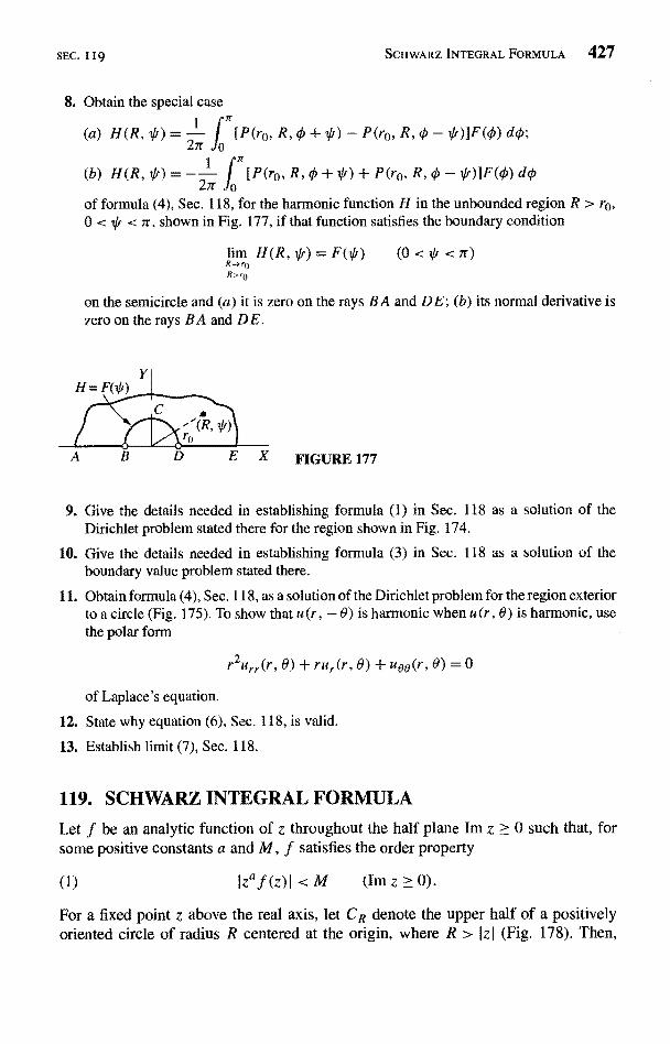
SEC. I 19 SCHWARZ INTEGRAL FORMULA 427
8. Obtain the special case
nI [P(ra, R, 0 + *) - P(ra, R, 0 - *)]F(4) do;(a) H(R, /) =
2
i J [P(ra, R, 0 + V'') + P(ra, R, t - ajf)]F(t) do(b) H(R, T/ r) = --of formula (4), Sec. 118, for the harmonic function H in the unbounded region R > ra,0 < T/r < sr, shown in Fig. 177, if that function satisfies the boundary condition
lim (0<Vr <n)R--. roR,ro
on the semicircle and (a) it is zero on the rays BA and DE; (b) its normal derivative iszero on the rays BA and DE.
9. Give the details needed in establishing formula (1) in Sec. 118 as a solution of theDirichiet problem stated there for the region shown in Fig. 174.
10. Give the details needed in establishing formula (3) in Sec. 118 as a solution of theboundary value problem stated there.
11. Obtain formula (4), Sec. 118, as a solution of the Dirichlet problem for the region exteriorto a circle (Fig. 175). To show that u(r, - 0) is harmonic when u(r, 0) is harmonic, usethe polar form
rur.( u00(r, 0) = 0
of Laplace's equation.
12. State why equation (6), Sec. 118, is valid.
13. Establish limit (7), Sec. 118.
119. SCHWARZ INTEGRAL FORMULA
Let f be an analytic function of z throughout the half plane Im z 0 such that, forsome positive constants a and M, f satisfies the order property
_
(1) Iza,f(z)) < M (Im z > 0).
For a fixed point z above the real axis, let CR denote the upper half of a positivelyoriented circle of radius R centered at the origin, where R > lzl (Fig. 178). Then,
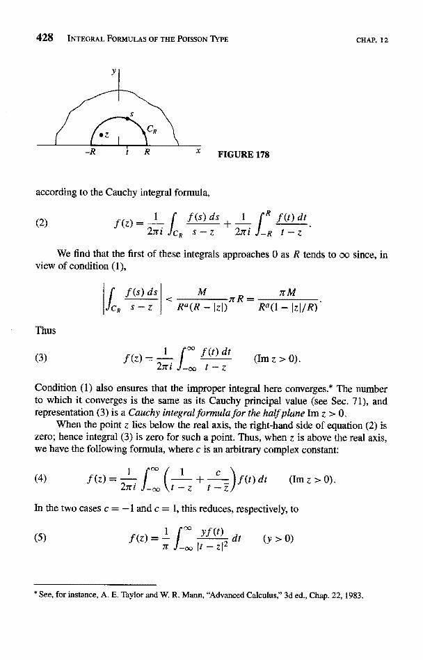
428 INTEGRAL FORMULAS OF THE POISSON TYPE CHAP. 12
FIGURE 178
according to the Cauchy integral formula,
1 f f(s) ds 1 f" f(tl dt{2) f(z) __27ri Jc, s - z " 27ri J-R t - z
We find that the first of these integrals approaches 0 as R tends to oc since, inview of condition (1),
nR= TrM
Ra(l - IzI/R)
Thus
(3) f(z) 27ri J-,, t - z(Imz>0).
Condition (1) also ensures that the improper integral here converges.* The numberto which it converges is the same as its Cauchy principal value (see Sec. 71), andrepresentation (3) is a Cauchy integral formula for the half plane Im z > 0.
When the point z lies below the real axis, the right-hand side of equation (2) iszero; hence integral (3) is zero for such a point. Thus, when z is above the real axis,we have the following formula, where c is an arbitrary complex constant:
(4) f (z)C
t-+ _ I f(t) dt (Im Z
In the two cases c = - I and c = 1, this reduces, respectively, to
(5) y>0
* See, for instance, A. E. Taylor and W. R. Mann, "Advanced Calculus," 3d ed., Chap. 22, 1983.
SEC. 120 DIRICHLET PROBLEM FOR A HALF PLANE 429
and
(6) f(z) dt (y > 0tIt - zi
If f (z) = u (x, y) + iv(x, y), it follows from formulas (5) and (6) that the har-monic functions u and v are represented in the half plane y > 0 in terms of the boundaryvalues of u by the formulas
yu(t O,.(7) u(x y) _
yu(t, 0)2 2
2zI
7r J-oa (t - x) y
and
- t)u(t 0)
at (y > 0)
2
dt (y > 0).(8) v(x, y) _ - j2x) +
y
Formula (7) is known as the Schwarz integral formula, or the Poisson integralformula for the half plane. In the next section, we shall relax the conditions for thevalidity of formulas (7) and (8).
120. DIRICHLET PROBLEM FOR A HALF PLANE
Let F denote a real-valued function of x that is bounded for all x and continuous exceptfor at most a finite number of finite jumps. When y > s and Ix I 11E, where s is anypositive constant, the integral
I(x v) =F(t) dt
r 2 2x) + y
converges uniformly with respect to x and y, as do the integrals of the partial derivativesof the integrand with respect to x and y. Each of these integrals is the sum of a finitenumber of improper or definite integrals over intervals where F is continuous; hencethe integrand of each component integral is a continuous function oft, x, and y wheny > E. Consequently, each partial derivative of I(x, y) is represented by the integralof the corresponding derivative of the integrand whenever y > 0.
We write U(x, y) = yI(x, y) 17r. Thus U is the Schwarz integral transform of F,suggested by the second of expressions (7), Sec. 119:
yF(t) 2dt (y > 0).X) Y
Except for the factor 117r, the kernel here is yf I t - z12. It is the imaginary componentof the function 11(t - z), which is analytic in z when y > 0. It follows that the kernelis harmonic, and so it satisfies Laplace's equation in x and y. Because the order ofdifferentiation and integration can be interchanged, the function (1) then satisfies thatequation. Consequently, U is harmonic when y > 0.
430 INTEGRAL FORMULAS OF THE POISSON TYPE
To prove that
(2) Jim U(x, y) = F(x)Y-0y>o
CHAP. 12
for each fixed x at which F is continuous, we substitute t = x + y tan r in formula (1)and write
(3) U(x,y)=- F(x+ytanr)dr (y>0).
Then, if
G(x,y,r)=F(x+ytan r)-F(x)
and a is some small positive constant,
2
(4) rr[U(x, y) - F(x)] = j G
where
(-zr/2)+aI1(y) = J G(x, y, r) dr,
n/2
13(Y) =
,y,r
2
2)-a
dr = II(Y 12(Y) + 13(Y),
(7r12)-aG(x, y, r) dr,
(-rr/2)+a
G(x, y, r) dr.
If M denotes an upper bound for IF(x)I, then IG(x, y, r)I 2M. For a givenpositive numbers, we select a so that 6Ma < E; and this means that
I11(Y)I < 2Ma < - and I'3(y)I < 2Ma < 3.
We next show that, corresponding to £, there is a positive number 3 such that
I12(Y)I <-
whenever3
<y<8.
To do this, we observe that, since F is continuous at x, there is a positive number ysuch that
IG(x, y, r)I < art whenever 0 < YI tan rl < y.
Now the maximum value of I tan r I as r ranges from (-nr/2) + a to (7r/2) - a istan[(rr/2) - a] = cot a. Hence, if we write 3 = y tan a, it follows that
112 (y) I <E (ir - 2a) < whenever 0 < y
SEC. 120 EXERCISES 4
We have thus shown that
I h (Y) I + 1 I2(Y) I + 113 (Y) I < s whenever 0 < y < 8.
Condition (2) now follows from this result and equation (4).Formula (1) therefore solves the Dirichlet problem for the half plane y > 0, with
the boundary condition (2). It is evident from the form (3) of expression (1) thatI U (x, y) I < M in the half plane, where M is an upper bound of I F(x) I; that is, Uis bounded. We note that U(x, y) = F0 when F(x) = F0, where F0 is a constant.
According to formula (8) of Sec. 119, under certain conditions of F the function
00
(5) V (X' y) = tx x)2 +(y2
dt (y > 0)n oo
is a harmonic conjugate of the function U given by formula (1). Actually, formula (5)furnishes a harmonic conjugate of U if F is everywhere continuous, except for at mosta finite number of finite jumps, and if F satisfies an order property
IxaF(x)I < M (a > 0).
For, under those conditions, we find that U and V satisfy the Cauchy-Riemannequations when y > 0.
Special cases of formula (1) when F is an odd or an even function are left to theexercises.
EXERCISES
1. Obtain as a special case of formula (1), Sec. 120, the expression
U (x, Y)= n Jo L (t - x)2 + y2 (t + x)2
+ y2 ] F(t) dt (x > 0, y > 0)
for a bounded function U that is harmonic in the first quadrant and satisfies the boundaryconditions
y-.oy>0
U(O,Y)=0 (Y>0),
U(x, y)=F(x) (x>O,x 54 xi
where F is bounded for all positive x and continuous except for at most a finite numberof finite jumps at the points x1 (j = 1, 2, ... , n).
2. Let T (x, y) denote the bounded steady temperatures in a plate x > 0, y > 0, withinsulated faces, when
lim T (x, y)= Fi(x) (x > 0),y-.0
Y'0
T(x, y)= F2(y) (Y > 0)
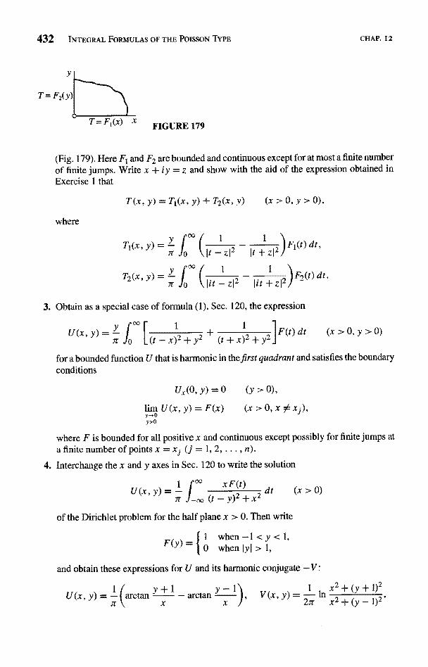
432 INTEGRAL FORMULAS OF THE POISSON TYPE CHAP. 12
FIGURE 179
(Fig. 179). Here Ft and F2 are bounded and continuous except for at most a finite numberof finite jumps. Write x + iy = z and show with the aid of the expression obtained inExercise 1 that
T (x, Y) = T1(x, Y) + T2(x, y) (x > 0, Y > 0),
where
T1(x,Y)=7t fo
T2(x,Y)=J
3. Obtain as a special case of formula (1), Sec. 120, the expression
1 1
+L(t-x)2+y2 Y2
F(t)dt (x>0,y>0)
for a bounded function U that is harmonic in the first quadrant and satisfies the boundaryconditions
Ux(0,Y) = 0 (Y > 0),
lim U(x, y) = F(x) (x > O, x 34 xj),y-r0y>o
where F is bounded for all positive x and continuous except possibly for finite jumps ata finite number of points x = xj (j = 1, 2, ... , n).
4. Interchange the x and y axes in Sec. 120 to write the solution
I f°° xF(t)U(x, Y) _ «, (t - y)z +x2
dt (x > O)
of the Dirichlet problem for the half plane x > 0. Then write
F(y)1 when-1<y<1,0 when IYI > 1,
and obtain these expressions for U and its harmonic conjugate ---V:
1U (x> y) (arctan y+l arctan y-1 V(x, y)
1nx2+(y+l)2_ - - , _ -2 2$
X X 27c x -1- (Y - 1)
SEC. 121
where -7r/2 < arctan t < it/2. Also, show that
V(x,y)+iU(x,y)=1[Log(z
7r
where z=x+iy.
2r22 - 2ror cos(o -
121. NEUMANN PROBLEMS
As in Sec. 116 and Fig. 172, we write s = ro exp(ire) and z = r exp(i8), where r <When s is fixed, the function
(1) 0-0)+r2Jis harmonic interior to the circle IzI = ro because it is the real component of-2ro log(,- - s), where the branch cut of log(z - s) is an outward ray from the points.If, moreover, r 0,
(2) Qr(ro,r,0-8)=-
ro
- 2ror cos(¢5 - 8) +
NEUMANN PROBLEMS 433
-Log(z-i)J,
P(ro,r,4) -8)-1],
where P is the Poisson kernel (7) of Sec. 116.These observations suggest that the function Q may be used to write an integral
representation for a harmonic function U whose normal derivative Ur on the circler = ro assumes prescribed values G(6).
If G is piecewise continuous and U0 is an arbitrary constant, the function
I f L,!
U(r, 8) =27r
/ Q(ro, r, 0 - 8)G(o) do + Uo (r < r0)
is harmonic because the integrated is a harmonic function of r and 8. If the mean valueof G over the circle I z I = ro is zero, or
(4)
then, in view of equation (2),
Ur(r, 8)I2
0
z,t
G(o) do = 0,
0) - 1JG(O) do
P(ro, r, ¢ - 8)G(r) do.
434 INTEGRAL FORMULAS OF THE POISSON TYPE CHAP. 12
Now, according to equations (1) and (2) of Sec. 117,
I P(ro, r, r - 0)G(0) dci = G(0).urn2 rr <r0
Hence
(5) lim Ur.(r, 8) =G(0)r <r0
for each value of 0 at which G is continuous.When G is piecewise continuous and satisfies condition (4), the formula
(6) U(r, 0)2-
n[r - 2ror 0) + r2] G(O) dpi + U0 0
therefore, solves the Neumann problem for the region interior to the circle r = ro,where G(0) is the normal derivative of the harmonic function U (r, 0) at the boundaryin the sense of condition (5). Note how it follows from equations (4) and (6) that, since
s constant, Ua is the value of U at the center r = 0 of the circle r = ro.The values U (r, 0) may represent steady temperatures in a disk r < ro with insu-
lated faces. In that case, condition (5) states that the flux of heat into the disk through itsedge is proportional to G(B). Condition (4) is the natural physical requirement that thetotal rate of flow of heat into the disk be zero, since temperatures do not vary with time.
A corresponding formula for a harmonic function H in the region exterior to thecircle r = rc can be written in terms of Q as
j Q(ro, R, 0 - f)G(o) drb + He (R > ro),(7) H (R, ,) _ - 2- a
where Ho is a constant. As before, we assume that G is piecewise continuous and thatcondition (4) holds. Then
R
and
(8)
H(R, 2/r)
lim HR (R, fir) = G(2/r)R +rpR>r0
for each * at which G is continuous. Verification of formula (7), as well as specialcases of formula (3) that apply to semicircular regions, is left to the exercises.
Turning now to a half plane, we let G(x) be continuous for all real x, exceptpossibly for a finite number of finite jumps, and let it satisfy an order property
(9) JxaG(x)t < M (a > 1)
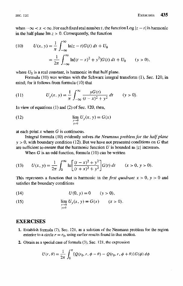
SEC. 121 EXERCISES 435
when -oo < x < oo. For each fixed real number t, the function Log I z - t I is harmonicin the half plane Im z > 0. Consequently, the function
(10) U(x,y)== I lnIz-tIG(t)dt+Uo
ln[(t - x)2 + Y2]G(t) dt + U0 (y > 0),
where U0 is a real constant, is harmonic in that half plane.Formula (10) was written with the Schwarz integral transform (1), Sec. 120, in
mind; for it follows from formula (10) that
(11) UU(x,y) _yG(t)- x)2 + y2
In view of equations (1) and (2) of Sec. 120, then,
(12) lim Uy(x, y) = Gy>0
dt (y > 0).
at each point x where G is continuous.Integral formula (10) evidently solves the Neumann problem for the half plane
y > 0, with boundary condition (12). But we have not presented conditions on G thatare sufficient to ensure that the harmonic function U is bounded as I z I increases.
When G is an odd function, formula (10) can be written
(13) U(x,y)=I (t-x)2+y2G(t) dt (x>0,y>0
(t+x)2+y2I
This represents a function that is harmonic in the first quadrant x > 0, y > 0 andsatisfies the boundary conditions
(14) U(0, y) = 0 (y > 0),
(15) lim U,,(x, y) = G(x) (x > 0).Y-0y>0
EXERCISES
1. Establish formula (7), Sec. 121, as a solution of the Neumann problem for the regionexterior to a circle r = ro, using earlier results found in that section.
2. Obtain as a special case of formula (3), Sec. 121, the expression
IU(r, 0) = j [Q(ro, r, 0 6)-Q(ro,r,0+0)]GG(0)do
2
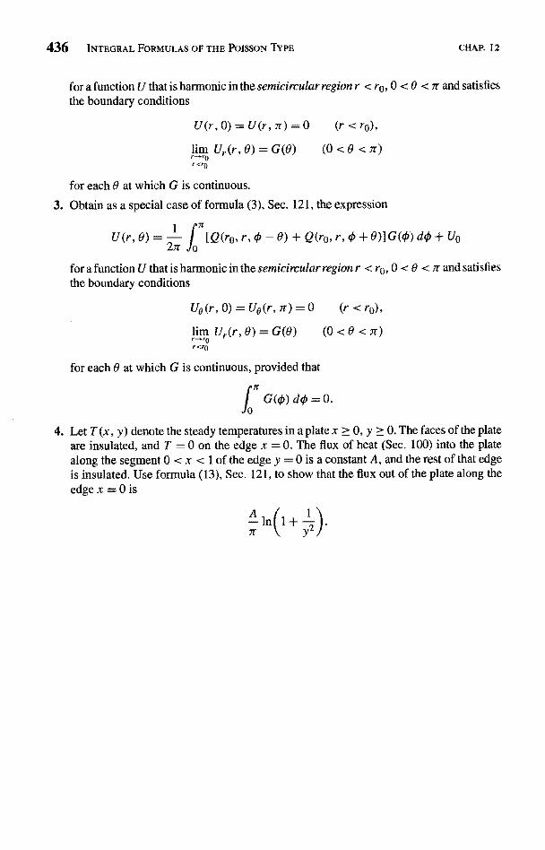
436 INTEGRAL FORMULAS OF THE POISSON TYPE CHAP. 12
for a function U that is harmonic in the semicircular region r < ro, 0 < 0 < 7r and satisfiesthe boundary conditions
U(r, 0) = U(r, 7r) = 0 (r<ro),
im Ur(r, 0) = G(0) (0 < 0 < ir)rv0
for each 0 at which G is continuous.
3. Obtain as a special case of formula (3), Sec. 121, the expression
U(r,8)= 1
a[Q(ro,r,-O-0)+Q(ro,r,O+8)]G(,O)do+Uo2rr
for a function U that is harmonic in the semicircular region r < ro, 0 < 0 < r and satisfiesthe boundary conditions
U0 (r, 0) = U6 (r, 7r) = 0 (r < ro),
U , G (0 < 0 < n)r-rror <rp
for each 0 at which G is continuous, provided that
G(O)dpi=0.
4. Let T (x, y) denote the steady temperatures in a plate x > 0, y ? 0. The faces of the plateare insulated, and T = 0 on the edge x = 0. The flux of heat (Sec. 100) into the platealong the segment 0 < x < 1 of the edge y = 0 is a constant A, and the rest of that edgeis insulated. Use formula (13), Sec. 121, to show that the flux out of the plate along theedge x = 0 is
APPENDIX
BIBLIOGRAPHY
The following list of supplementary books is far from exhaustive. Further referencescan be found in many of the books listed here.
THEORY
Ahlfors, L. V.: "Complex Analysis," 3d ed., McGraw-Hill Higher Education, Burr Ridge, IL, 1979.
Antimirov, M. Ya., A. A. Kolyshkin, and R. Vaillancourt: "Complex Variables," Academic Press, SanDiego, 1998.
Bak, J., and D. J. Newman: "Complex Analysis," 2d ed., Springer-Verlag, New York, 1997.
Bieberbach, L.: "Conformal Mapping," American Mathematical Society, Providence, RI, 2000.
Boas, R. P.: "Invitation to Complex Analysis," The McGraw-Hill Companies, New York, 1987.
: "Yet Another Proof of the Fundamental Theorem of Algebra," Amer. Math. Monthly, Vol. 71,No. 2, p. 180, 1964.
Caratheodory, C.: "Conformal Representation," Dover Publications, Inc., Mineola, NY, 1952.
:"Theory of Functions of a Complex Variable," American Mathematical Society, Providence,RI, 1954.
Conway, J. B.: "Functions of One Complex Variable," 2d ed., 6th Printing, Springer-Verlag, New York,1997.
Copson, E. T.: `Theory of Functions of a Complex Variable," Oxford University Press, London, 1962.
Evans, G. C.: "The Logarithmic Potential, Discontinuous Dirichlet and Neumann Problems," AmericanMathematical Society, Providence, RI, 1927.
Fisher, S. D.: "Complex Variables," 2d ed., Dover Publications, Inc., Mineola, NY, 1990.
437
438 BIBLIOGRAPHY APP. I
Flanigan, F. J.: "Complex Variables: Harmonic and Analytic Functions," Dover Publications, Inc.,Mineola, NY. 1983.
Hille, E.: "Analytic Function Theory," Vols. 1 and 2, 2d ed., Chelsea Publishing Co., New York, 1973.
Kaplan, W.: "Advanced Calculus," 5th ed., Addison-Wesley Higher Mathematics, Boston, MA, 2003.
: " Advanced Mathematics for Engineers," TechBooks, Marietta, OH, 1992.
Kellogg, O. D.: "Foundations of Potential Theory," Dover Publications, Inc., New York, 1953.
Knopp, K.: "Elements of the Theory of Functions," translated by F. Bagemihl, Dover Publications, Inc.,Mineola, NY, 1952.
"Problem Book in the Theory of Functions," Dover Publications, Inc., Mineola, NY, 2000.
Krantz, S. G.: "Complex Analysis: The Geometric Viewpoint," Carus Mathematical Monograph Series,The Mathematical Association of America, Washington, DC, 1990.
: "Handbook of Complex Variables," Birkhauser Boston, Cambridge, MA, 2000.
Krzyz, J. G.: "Problems in Complex Variable Theory," Elsevier Science, New York, 1972.
Lang, S.: "Complex Analysis," 3d ed., Springer-Verlag, New York, 1993.
Levinson, N., and R. M. Redheffer: "Complex Variables," The McGraw-Hill Companies, Inc., NewYork, 1988.
Markushevich, A. I.: "Theory of Functions of a Complex Variable." 3 vols. in one, 2d ed., AmericanMathematical Society, Providence, RI, 1977.
Marsden, J. E., and M. J. Hoffman: "Basic Complex Analysis," 2d ed., W. H. Freeman & Company,New York, 1987.
Mathews, J. H., and R. W. Howell: "Complex Analysis for Mathematics and Engineering," 4th ed., Jonesand Bartlett Publishers, Sudbury, MA, 2001.
Mitrinovic, D. S.: "Calculus of Residues," P. Noordhoff, Ltd., Groningen, 1966.
Nahin, P. J.: "An Imaginary Tale: The Story of ," Princeton University Press, Princeton, NJ, 1998.
Nehari, Z.: "Conformal Mapping," Dover Publications, Inc., Mineola, NY, 1975.
Newman, M. H. A.: "Elements of the Toplogy of Plane Sets of Points," 2d ed., Dover Publications, Inc.,Mineola, NY, 1999.
Pennisi, L. L.: "Elements of Complex Variables," 2d ed., Holt, Rinehart & Winston, Inc., Austin, TX,1976.
Rubenfeld, L. A.: "A First Course in Applied Complex Variables," John Wiley & Sons, Inc., New York,1985.
Saff, E. B., and A. D. Snider: "Fundamentals of Complex Analysis," 3d ed., Prentice-Hall PTR, Paramus,NJ, 2001.
Silverman, R. A.: "Complex Analysis with Applications," Dover Publications, Inc., Mineola, NY, 1984.
Springer, G.: "Introduction to Riemann Surfaces," 2d ed., American Mathematical Society, Providence,RI, 1981.
Taylor, A. E., and W. R. Mann: "Advanced Calculus," 3d ed., John Wiley & Sons, Inc., New York, 1983:
Thron, W. J.: "Introduction to the Theory of Functions of a Complex Variable," John Wiley & Sons,Inc., New York, 1953.
Titchmarsh, E. C.: "Theory of Functions," 2d ed., Oxford University Press, Inc., New York, 1976.
Volkovyskii, L. I., G. L. Lunts, and I. G. Aramanovich: "A Collection of Problems on Complex Analysis,"Dover Publications, Inc., Mineola, NY, 1992.
Whittaker, E. T., and G. N. Watson: "A Course of Modem Analysis," 4th ed., Cambridge UniversityPress, New York, 1996.
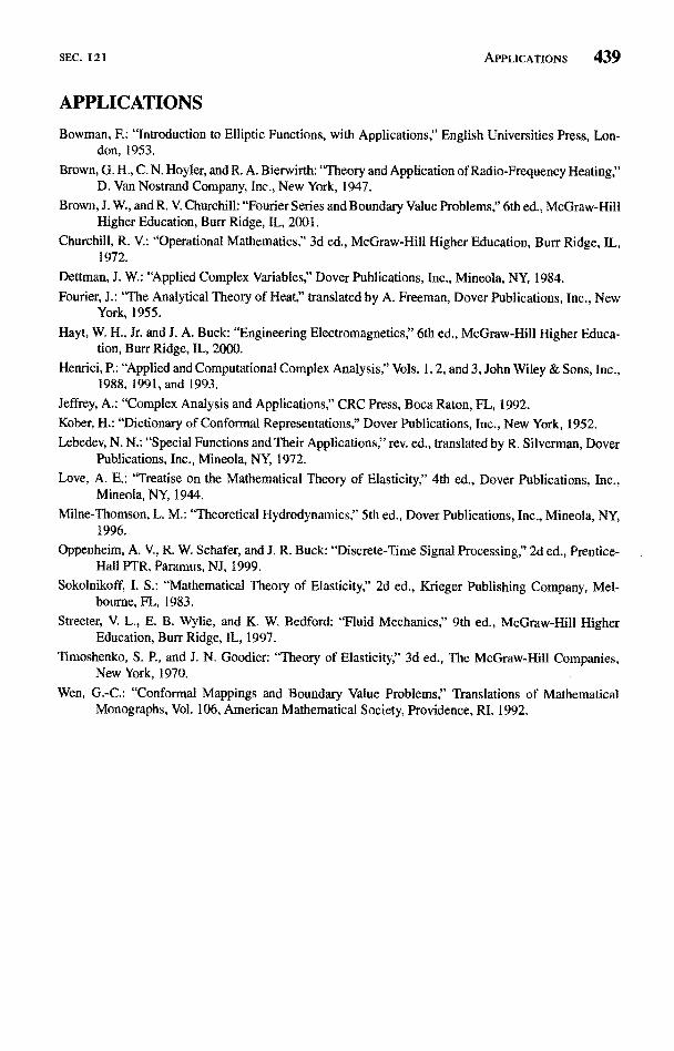
SEC. 121 APPLICATIONS 439
APPLICATIONS
Bowman, F.: "Introduction to Elliptic Functions, with Applications," English Universities Press, Lon-don, 1953.
Brown, G. H., C. N. Hoyler, and R. A. Bierwirth: "Theory and Application of Radio-Frequency Heating;'D. Van Nostrand Company, Inc., New York, 1947.
Brown, J. W., and R. V. Churchill: "Fourier Series and Boundary Value Problems," 6th ed., McGraw-HillHigher Education, Burr Ridge, IL, 2001.
Churchill, R. V.: "Operational Mathematics," 3d ed., McGraw-Hill Higher Education, Burr Ridge, IL,1972.
Dettman, J. W.: "Applied Complex Variables," Dover Publications, Inc., Mineola, NY11984.
Fourier, J.: "The Analytical Theory of Heat," translated by A. Freeman, Dover Publications, Inc., NewYork, 1955.
Hayt, W. H., Jr. and J. A. Buck: "Engineering Electromagnetics," 6th ed., McGraw-Hill Higher Educa-tion, Burr Ridge, IL, 2000.
Henrici, P.: "Applied and Computational Complex Analysis," Vols. 1, 2, and 3, John Wiley & Sons, Inc.,1988, 1991, and 1993.
Jeffrey, A.: "Complex Analysis and Applications," CRC Press, Boca Raton, FL, 1992.
Kober, H.: "Dictionary of Conformal Representations," Dover Publications, Inc., New York, 1952.
Lebedev, N. N.: "Special Functions and Their Applications," rev. ed., translated by R. Silverman, DoverPublications, Inc., Mineola, NY, 1972.
Love, A. E.: "Treatise on the Mathematical Theory of Elasticity," 4th ed., Dover Publications, Inc.,Mineola, NY, 1944.
Milne-Thomson, L. M.: "Theoretical Hydrodynamics," 5th ed., Dover Publications, Inc., Mineola, NY,1996.
Oppenheim, A. V., R. W. Schafer, and J. R. Buck: "Discrete-Time Signal Processing," 2d ed., Prentice-Hall PTR, Paramus, NJ, 1999.
Sokolnikoff, I. S.: "Mathematical Theory of Elasticity," 2d ed., Krieger Publishing Company, Mel-e, FL, 1983.
Streeter, V. L., E. B. Wylie, and K. W. Bedford: "Fluid Mechanics," 9th ed., McGraw-Hill HigherEducation, Burr Ridge, IL, 1997.
Timoshenko, S. P., and J. N. Goodier: "Theory of Elasticity," 3d ed., The McGraw-Hill Companies,New York, 1970.
Wen, G.-C.: "Conformal Mappings and Boundary Value Problems;' Translations of MathematicalMonographs, Vol. 106, American Mathematical Society, Providence, RI, 1992.
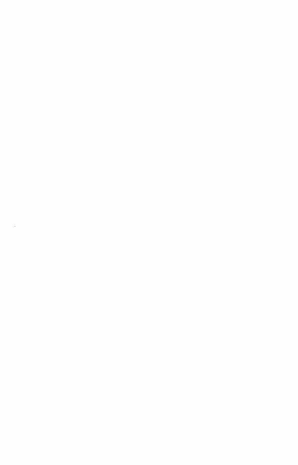
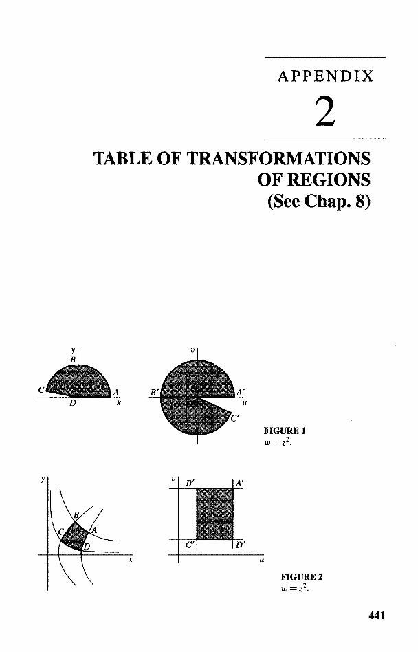
APPENDIX
2TABLE OF TRANSFORMATIONS
OF REGIONS(See Chap. 8)
FIGURE 1w = Z2.
FIGURE 2w=Z2.
441
442 TABLE OF TRANSFORMATIONS OF REGIONS APP. 2
Y
v
E
v
u
FIGURE 3w =Z2 ;
A'B' on parabola v2 = -4c2(u - c2).
FIGURE 4w = 1/z.
FIGURE 5w = 1/z.
E'D' C'B' A' u FIGURE 6w = exp z.
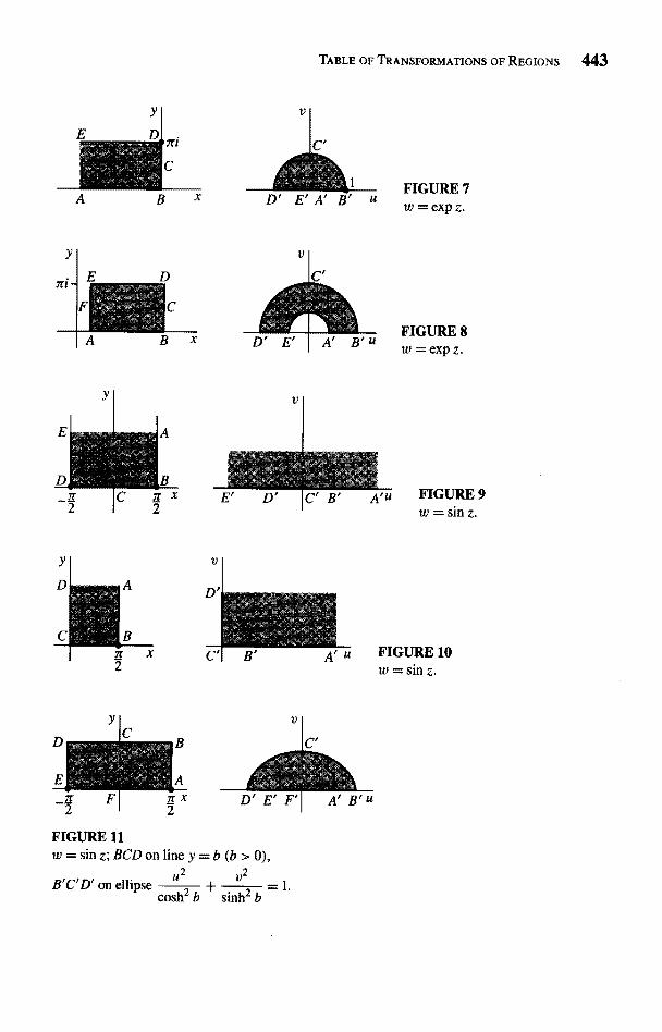
TABLE OF TRANSFORMATIONS OF REGIONS 443
FIGURE 7w = exp z.
FIGURE 8w = exp z.
FIGURE 9w = sin z.
FIGURE 10w = sin Z.
FIGURE 11w = sin z; BCD on line y = b (b > 0),
u2 v2B'C'D' on ellipse -
cosh2 b sinh2 b
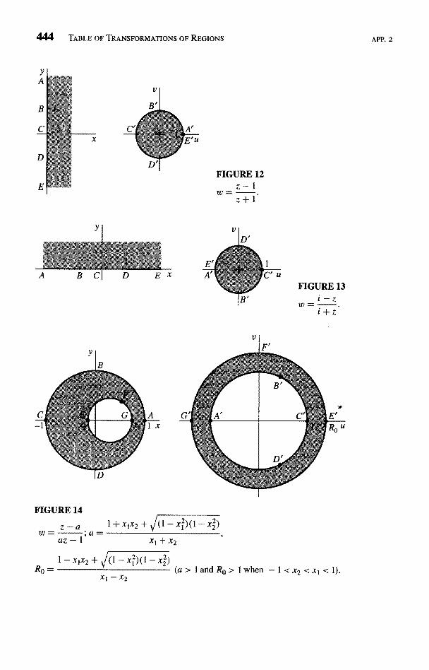
444 TABLE OF TRANSFORMATIONS OF REGIONS APP. 2
B
c
FIGURE 12z-1w=z+1
FIGURE 13i-z
FIGURE 14
z-a 1 + xix2
w= a=az - 1 xi +X2
1 - xlx2 /(1 - x2)(1 - x2)
R© (a > 1 and R0 > 1 when - 1 < x2 < x1 < 0-XI - x2
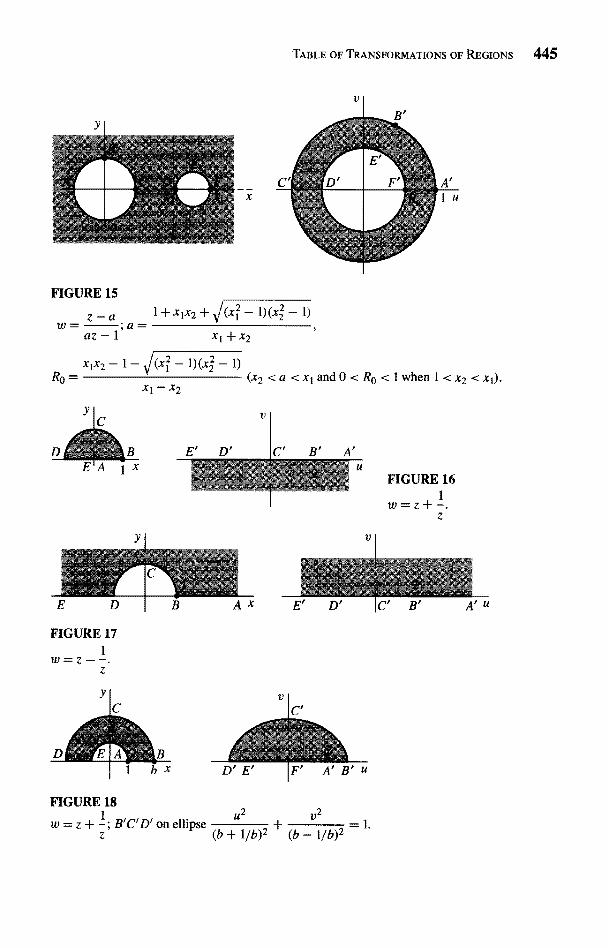
TABLE OF TRANSFORMATIONS OF REGIONS 445
FIGURE 15
z - a 1 + x1x2 + (x
w= ;a=az- 1'
R0 =
xl + x2
xlx2 - 1 - J(x, - 1)(x2 - 1)
X1 - x2(x2<a<x1 and0<R1}<1when 1<x2<x1).
FIGURE 161
z
v
FIGURE 171w=z+-.z
FIGURE 181 U2
W = z + -; B'C'D on ellipse +z (b + 1/b)2 (b - 1
E' D'
v2
b 2
At u

TABLE OF TRANSFORMATIONS OF REGIONS APP. 2
Dr C
A B IC D E x D' E'JA' B' U
FIGURE 19
-.Log z+ l ; z - coth
w
V
E`
A' B'
Sri D'
(ir - h)i C'
u
FIGURE 20zw= Logz+
ABC oncirclex2+(y+coth)2=csc2h (0<h <7r).
FIGURE 21
Logz + I; centers of circles at z = coth c, radii: csch c (n = 1, 2).z - I
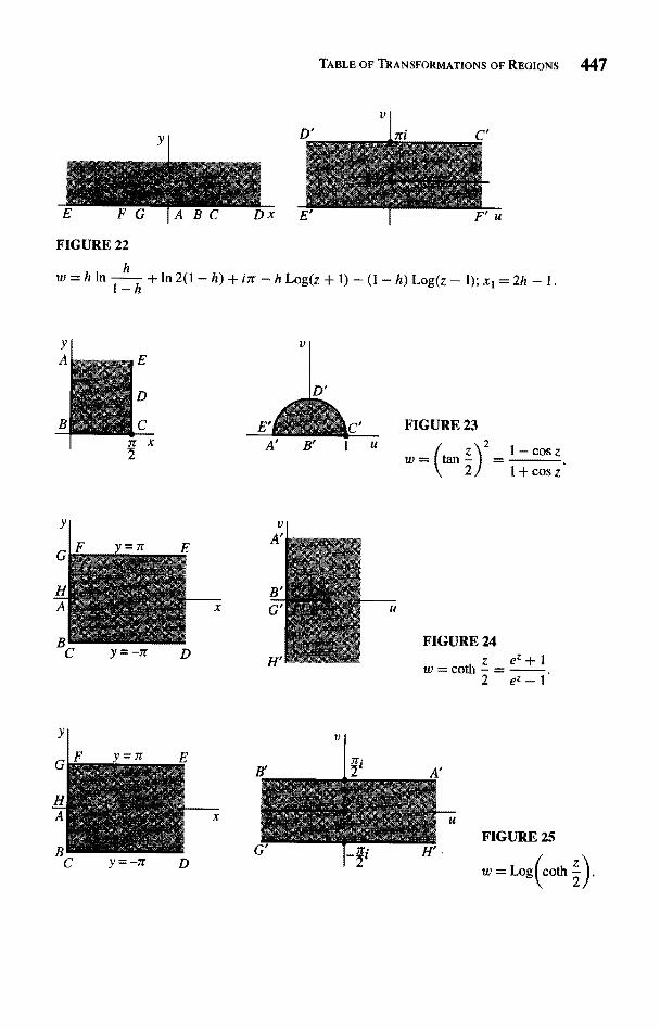
TABLE OF TRANSFORMATIONS OF REGIONS 447
V
C'
F' u
FIGURE 22
hin , hu
+1x12(1-h)+i7r-hLog(z+1)-(1-h)Log(z-1);x1=2h-
FIGURE 23
W= 1-cosz1+cosz
FIGURE 24
w = coth z = ez+ 1
2 ez-1
FIGURE 25
w =Log( coth
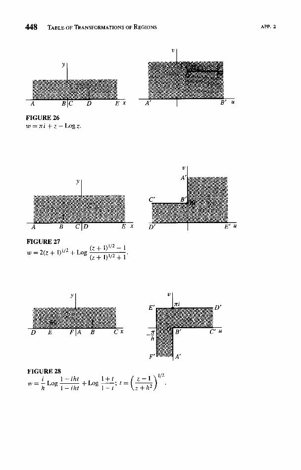
448 TABLE OF TRANSFORMATIONS OF REGIONS
Y
E X A'
FIGURE 26w =Tri+z-Logz.
FIGURE 27 Ij2 _w = 2{z + 1}IJ2 + Log
(Z +
+ 1)1/2 + 1
Y
E'
E F'IA B CX
FIGURE 28
w= i Log 1+iht+Log
1+t, t
h 1-iht 1--t
V
2
V
A'
I ni
B
E' U
D'
C u
APP. 2
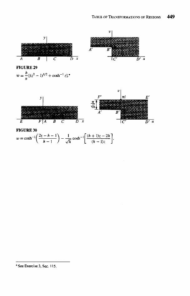
TABLE OF TRANSFORMATIONS OF REGIONS 449
FIGURE 29
w = h [(z2 - 1)1/2 + cosh-1 z} *7r
FIGURE 30
= cosh-1 2z-h- 1 "neh-hI(h + 1)z - 2h]h - 1 J 4lh L (h - 1)z
* See Exercise 3, Sec. 115.

INDEX
Absolute convergence, 179, 201-202Absolute value, 8-9Accumulation point, 31Aerodynamics, 379Analytic continuation, 81-82, 84-85Analytic function(s), 70-72
compositions of, 71derivatives of, 158-162products of, 71quotients of, 71, 242-243sums of, 71zeros of, 239-242, 246-247, 282-288
Angle:of inclination, 119, 344of rotation, 344
Antiderivative, 113, 135-138, 150Arc, 117
differentiable, 119simple, 117smooth, 120
Argument, 15Argument principle, 281-284
Bernoulli's equation, 380Bessel function, 200n.
Beta function, 277, 398Bibliography, 437-439Bilinear transformation, 307Binomial formula, 7Boas, R. P., Jr., 167n.Bolzano-Weierstrass theorem, 247Boundary conditions, 353
transformations of, 355-358Boundary point, 30Boundary value problem, 353-354, 417Bounded:
function, 53, 248set, 31
Branch cut, 93, 325-334, 338-340integration along, 273-275
Branch of function, 93principal, 93, 98, 325
Branch point, 93-94at infinity, 340
Bromwich integral, 288
Casorati-Weierstrass theorem, 249Cauchy, A. L., 62Cauchy-Goursat theorem, 142-144
converse of, 162
451
452 INDEX
Cauchy-Goursat theorem (continued)extensions of, 149-151proof of, 144-149
Cauchy integral formula, 157-158for half plane, 428
Cauchy principal value, 251-253Cauchy product, 216Cauchy-Riemann equations, 60-63
in complex form, 70in polar form, 65-68necessity of, 62sufficiency of, 63-65
Cauchy's inequality, 165Cauchy's residue theorem, 225Chebyshev polynomials, 22n.Christoffel, E. E., 395Circle of convergence, 202Circulation of fluid, 379Closed contour, 135, 149
simple, 120, 142, 151Closed curve, simple, 117Closed set, 30Closure of set, 30Complex conjugate, 11Complex exponents, 97-99Complex form of Cauchy-Riemann
equations, 70Complex number(s), 1
algebraic properties of, 3-7argument of, 15conjugate of, 11exponential form of, 15-17imaginary part of, 1modulus of, 8-11polar form of, 15powers of, 20, 96-99real part of, 1roots of, 22-24, 96
Complex plane, 1extended, 48, 302, 308regions in, 29-31
Complex potential, 382Complex variable, functions of, 33-35Composition of functions, 51, 58, 71Conductivity, thermal, 361
Conformal mapping, 343-358applications of, 361-386properties of, 343-350
Conformal transformation, 343-350angle of rotation of, 344local inverse of, 348scale factor of, 346
Conjugate:complex, 11harmonic, 77, 351-353
Connected open set, 30Continuity, 51-53Continuous function, 51Contour, 116-120
closed, 135, 149indented, 267simple closed, 120, 142, 151
Contour integral, 122-124Contraction, 299, 346Convergence of improper integral, 251-253Convergence of sequence, 175-177Convergence of series, 178-180
absolute, 179, 201-202circle of, 202uniform, 202
Coordinates:polar, 15, 34, 39, 65-68rectangular, 1
Critical point, 345Cross ratios, 310n.Curve:
Jordan, 117level, 79-80simple closed, 117
Definite integrals, 113-116, 278-280Deformation of paths, principle of, 152Deleted neighborhood, 30De Moivre's formula, 20Derivative, 54-57
directional, 71, 356-357existence of, 60--67
Differentiable arc, 119Differentiable function, 54Differentiation formulas, 57-59

INDEX 453
Diffusion, 363Directional derivative, 71, 356-357Dirichiet problem, 353
for disk, 419-423for half plane, 364, 429-431, 432for quadrant, 431for rectangle, 378for region exterior to circle, 424for semicircular region, 423for semi-infinite strip, 366-367
Disk, punctured, 30, 192, 217, 223Division of power series, 217-218Domain(s), 30
of definition of function, 33intersection of, 81multiply connected, 149-151simply connected, 149-150, 352union of, 82
Electrostatic potential, 373-374in cylinder, 374-376in half space, 376-377between planes, 377between plates, 390, 411
Elements of function, 82Elliptic integral, 398Entire function, 70, 165-166Equipotentials, 373, 381Essential singular point, 232
behavior near, 232, 249-250Euler numbers, 220Euler's formula, 16Even function, 116, 252-253Expansion, 299, 346Exponential form of complex numbers,
15-17Exponential function, 87-89, 99
inverse of, 349-350mapping by, 40-42
Extended complex plane, 48, 302,308
Exterior point, 30
Field intensity, 373Fixed point, 312
Fluid:circulation of, 379incompressible, 380pressure of, 380rotation of, 380velocity of, 379
Fluid flow:around airfoil, 390in angular region, 387in channel, 406-411circulation of, 379complex potential of, 382around corner, 383-385around cylinder, 385-386irrotational, 380around plate, 388in quadrant, 384-385in semi-infinite strip, 387over step, 414-415
Flux of heat, 361Flux lines, 374Formula:
binomial, 7Cauchy integral, 157-158de Moivre's, 20Euler's, 16Poisson integral, 417-435quadratic, 29Schwarz integral, 427-429(See also specific formulas, for example:
Differentiation formulas)Fourier, Joseph, 361n.Fourier integral, 260, 269n.Fourier series, 200Fourier's law, 361Fresnel integrals, 266Function(s):
analytic (See Analytic function)antiderivative of, 113, 135-138Bessel, 200n.beta, 277, 398bounded, 53, 248branch of, 93
principal, 93, 98, 325composition of, 51, 58, 71
454 INDEX
Function(s): (continued)continuous, 51derivatives of, 54-57differentiable, 54domain of definition of. 33elements of, 82entire, 70, 165-166even, 116, 252-253exponential (See Exponential function)gamma, 273harmonic (See Harmonic function)holomorphic, 70n.hyperbolic (See Hyperbolic functions)impulse, 425-426inverse, 308limit of, 43-48
involving point at infinity, 48-51local inverse of, 348logarithmic (See Logarithmic function)meromorphic, 281-282multiple-valued, 35, 335odd, 116piecewise continuous, 113, 122principal part of, 231range of, 36rational, 34, 253real-valued, 34, 111, 113, 120,
131
regular, 70n.stream, 381-383trigonometric (See Trigonometric
functions)value of, 33zeros of (See Zeros of functions)
Fundamental theorem:of algebra, 166of calculus, 113, 135
Gamma function, 273Gauss's mean value theorem, 168Geometric series, 187Goursat, E., 144Gradient, 71-72, 356-357, 360Green's theorem, 143, 379
Harmonic function, 75-78, 381conjugate of, 77, 351-353maximum and minimum values of,
171-172,373in quadrant, 435in semicircular region, 423-424, 436transformations of, 353-355
Holomorphic function, 70n.Hydrodynamics, 379Hyperbolic functions, 105-106
inverses of, 109-110zeros of, 106
Image of point, 36inverse, 36
Imaginary axis, 1Improper real integrals, 251-275Impulse function, 425 426Incompressible fluid, 380Independence of path, 127, 135Indented paths, 267-270Inequality:
Cauchy's, 165Jordan's, 262triangle, 10, 14
Infinity:point at, 48-49residues at, 228
Integral(s):Bromwich, 288Cauchy principal value of, 251-253contour, 122-124definite, 113-116, 27.8-280elliptic, 398Fourier, 260, 269n.Fresnel, 266improper real, 251-275line, 122, 352modulus of, 114, 130-133
Integral transformation, 419Interior point, 30Intersection of domains, 81Inverse:
function, 308image of point, 36
INDEX 455
Laplace transform, 288-291local, 348point, 302, 417z-transform, 199
Inversion, 302Irrotational flow, 380Isogonal mapping, 345Isolated singular point, 221Isolated zeros, 240Isotherms, 363
Jacobian, 348Jordan, C., 117Jordan curve, 117Jordan curve theorem, 120Jordan's inequality, 262Jordan's lemma, 262-265Joukowski airfoil, 389
Lagrange's trigonometric identity, 22Laplace transform, 288
inverse, 288-291Laplace's equation, 75, 79, 362-363, 381Laurent series, 190-195Laurent's theorem, 190Legendre polynomials, 116m., 164n.Level curves, 79-80Limit(s):
of function, 43-46involving point at infinity, 48-51
of sequence, 175theorems on, 46-48
Line integral, 122, 352Linear combination, 74Linear fractional transformation, 307-311Linear transformation, 299-301Lines of flow, 363Liouville's theorem, 165-166Local inverse, 348Logarithmic function, 90-96
branch of, 93mapping by, 316, 318principal branch of, 93principal value of, 92Riemann surface for, 335-337
Maclaurin series, 183Mapping, 36
conformal (See Conformaltransformation)
by exponential function, 40-42isogonal, 345by logarithmic function, 316, 318one to one (See One to one mapping)of real axis onto polygon, 391-393by trigonometric functions, 318-322(See also Transformation)
Maximum and minimum values, 130,167-171,373um modulus principle, 169
Meromorphic function, 281-282Modulus, 8-11
of integral, 114, 130-133Morera, E., 162Morera's theorem, 162Multiple-valued function, 35, 335Multiplication of power series, 215-217Multiply connected domain, 149-151
Neighborhood, 29-30deleted, 30of point at infinity, 49
Nested intervals, 156Nested squares, 146, 156Neumann problem, 353
for disk, 434for half plane, 435for region exterior to circle, 434for semicircular region, 436
Number:complex, Iwinding, 281
Odd function, 116One to one mapping, 37-40, 301, 308, 315,
318-321,325-326,332,336Open set, 30
Partial sum of series, 178Picard's theorem, 232, 249Piecewise continuous function, 113, 122
456 INDEx
Point at infinity, 48-49limits involving, 48-51neighborhood of, 49
Poisson integral formula, 417-435for disk, 419for half plane, 429
Poisson integral transform, 419-420Poisson kernel, 419Poisson's equation, 359Polar coordinates, 15, 34, 39, 65-68Polar form:
of Cauchy-Riemann equations, 65-68of complex numbers, 15
Pole(s):number of, 247, 282order of, 231, 234, 239, 242, 246, 282residues at, 234-235, 243simple, 231, 243, 267
Polynomial(s):Chebyshev, 22n.Legendre, 116n., 164n.zeros of, 166, 172, 286-287
Potential:complex, 382electrostatic (See Electrostatic potentialvelocity, 381
Power series, 180Cauchy product of, 216convergence of, 200-204differentiation of, 209division of, 217-218integration of, 207multiplication of, 215-217uniqueness of, 210
Powers of complex numbers, 20, 96-99Pressure of fluid, 380Principal branch of function, 93, 98, 325Principal part of function, 231Principal value:
of argument, 15Cauchy, 251-253of logarithm, 92of powers, 98
Principle:argument, 281-284
of deformation of paths, 152maximum modulus, 167-171reflection, 82-84
Product, Cauchy, 216Punctured disk, 30, 192, 217, 223Pure imaginary number, 1
Quadratic formula, 29
Radio-frequency heating, 259Range of function, 36Rational function, 34, 253Real axis, IReal-valued function, 34, 111, 113, 120,
131
Rectangular coordinates:Cauchy-Riemann equations in, 62complex number in, 8
Reflection, 11, 36, 82, 302Reflection principle, 82-84Regions in complex plane, 29-31Regular function, 70n.Remainder of series, 179-180Removable singular point, 232, 248Residue theorems, 225, 228Residues, 221-225
applications of, 251-295at infinity, 228n.at poles, 234-235, 243
Resonance, 298Riemann, G. P. B., 62Riemann sphere, 49Riemann surfaces, 335-340Riemann's theorem, 248Roots of complex numbers, 22-24, 96Rotation, 36, 299-301
angleof fluid, 380
Rouche's theorem, 284, 287
Scale factor, 346Schwarz, H. A., 395Schwarz-Christoffel transformation,
391-413onto degenerate polygon, 401-403
INDEx 457
onto rectangle, 400--401onto triangle, 397-399
Schwarz integral formula, 427-429Schwarz integral transform, 429Separation of variables, method of, 367,
378Sequence,175-177
limit of, 175Series, 175-220
Fourier, 200geometric, 187Laurent, 190-195Maclaurin, 183partial sum of, 178power (See Power series)remainder of, 179-180sum of, 178Taylor, 182-185(See also Convergence of series)
Simple arc, 117Simple closed contour, 120, 142, 151
positively oriented, 142Simple closed curve, 117Simple pole, 231, 243, 267Simply connected domain, 149-150, 352Singular point, 70
essential, 232, 249-250isolated, 221removable, 232, 248(See also Branch point; Pole)
Sink, 407, 408Smooth arc, 120Source, 407, 408Stagnation point, 408Stereographic projection, 49Stream function, 381-383Streamlines, 381Successive transformations, 300, 307,
315-318,322-324,333-334Sum of series, 178
Table of transformations, 441-449Taylor series, 182-185Taylor's theorem, 182
Temperatures, steady, 361-363in cylindrical wedge, 370-371in half plane, 363-365in infinite strip, 364, 372-373in quadrant, 368-370in semicircular plate, 372in semi-elliptical plate, 373in semi-infinite strip, 365-367
Thermal conductivity, 361Transform:
Laplace, 288inverse, 288-291
Poisson integral, 419-420Schwarz integral, 429z-transform, 199
Transformationbilinear, 307of boundary conditions, 355-358conformal, 343-350critical point of, 345of harmonic functions, 353-355integral, 419linear, 299-301linear fractional, 307-311Schwarz-Christoffel, 391-413successive, 300, 307, 315-318, 322-324,
333-334table of, 441-449(See also Mapping)
Translation, 35, 300Triangle inequality, 10, 14Trigonometric functions, 100-103
identities for, 101-102inverses of, 108-109mapping by, 318-322zeros of, 102
Two-dimensional fluid flow, 379-381
Unbounded set, 31Uniform convergence, 202Union of domains, 82Unity, roots of, 25-26Unstable component, 298
458 INDEX
Value, absolute, 8-9of function, 33
Vector field, 43Vectors, 8-9Velocity of fluid, 379Velocity potential, 381Viscosity, 380
Winding number, 281
Zeros of functions, 102, 166isolated, 240number of, 282, 284-288order of, 239, 242
z-transform, 199


![INDEX []€¦ · INDEX C.V.N.M. -2141905 ... COMPLEX VARIABLES AND NUMERICAL METHODS SUBJECT CODE: 2141905 ... Ablowitz and A.S. Fokas, Complex Variables-Introduction and Applications](https://img.pdfslide.net/doc/110x75/5b8fdecd09d3f2b01e8d1c81/index-index-cvnm-2141905-complex-variables-and-numerical-methods.jpg)
![Wunsch, A. D., Brown, M. - Complex Variables With Applications, 3rd Edition (Solutions Manual)[1]](https://img.pdfslide.net/doc/110x75/55cf9d80550346d033ade684/wunsch-a-d-brown-m-complex-variables-with-applications-3rd-edition.jpg)