Complexity of linear programming: outline - U-M …mepelman/teaching/IOE610/... · · 2013-11-05Algorithms for Solving (Optimization) Problems I It is reasonable to expect the running

Complexity of linear programming: outline

I Assessing computational e�ciency of algorithms

I Computational e�ciency of the Simplex method

I Ellipsoid algorithm for LP and its computational e�ciency

IOE 610: LP II, Fall 2013 Complexity of linear programming Page 139

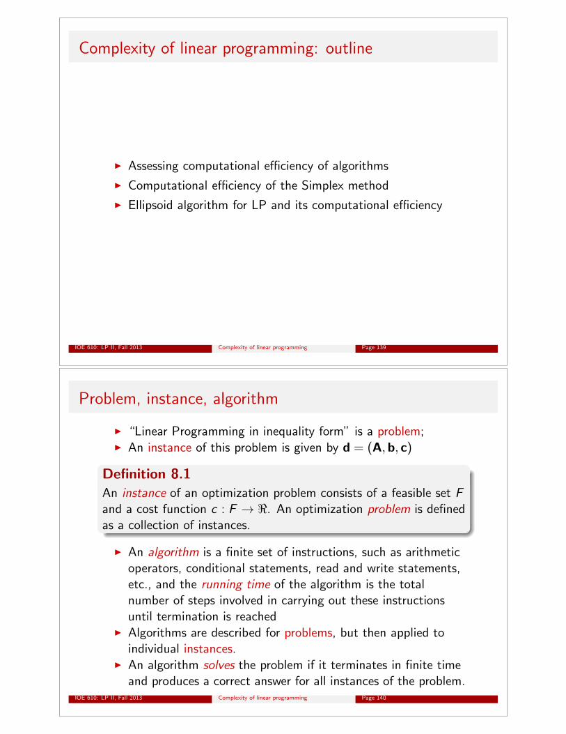
Problem, instance, algorithm

I “Linear Programming in inequality form” is a problem;I An instance of this problem is given by d = (A,b, c)

Definition 8.1An instance of an optimization problem consists of a feasible set Fand a cost function c : F ! <. An optimization problem is definedas a collection of instances.

I An algorithm is a finite set of instructions, such as arithmeticoperators, conditional statements, read and write statements,etc., and the running time of the algorithm is the totalnumber of steps involved in carrying out these instructionsuntil termination is reached

I Algorithms are described for problems, but then applied toindividual instances.

I An algorithm solves the problem if it terminates in finite timeand produces a correct answer for all instances of the problem.


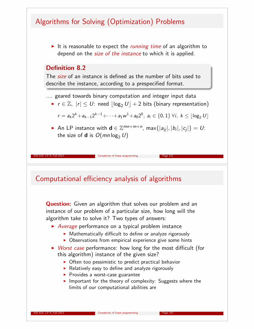
Algorithms for Solving (Optimization) Problems

I It is reasonable to expect the running time of an algorithm todepend on the size of the instance to which it is applied.

Definition 8.2The size of an instance is defined as the number of bits used todescribe the instance, according to a prespecified format.

.... geared towards binary computation and integer input dataI r 2 Z, |r | U: need blog2 Uc+ 2 bits (binary representation)

r = ak

2k+ak�12

k�1+· · ·+a1w1+a02

0, ai

2 {0, 1} 8i , k blog2 Uc

I An LP instance with d 2 Zmn+m+n, max{|aij

|, |bi

|, |cj

|} = U:the size of d is O(mn log2 U)


Computational e�ciency analysis of algorithms

Question: Given an algorithm that solves our problem and aninstance of our problem of a particular size, how long will thealgorithm take to solve it? Two types of answers:

I Average performance on a typical problem instanceI Mathematically di�cult to define or analyze rigorouslyI Observations from empirical experience give some hints

I Worst case performance: how long for the most di�cult (forthis algorithm) instance of the given size?

I Often too pessimistic to predict practical behaviorI Relatively easy to define and analyze rigorouslyI Provides a worst-case guaranteeI Important for the theory of complexity: Suggests where the

limits of our computational abilities are


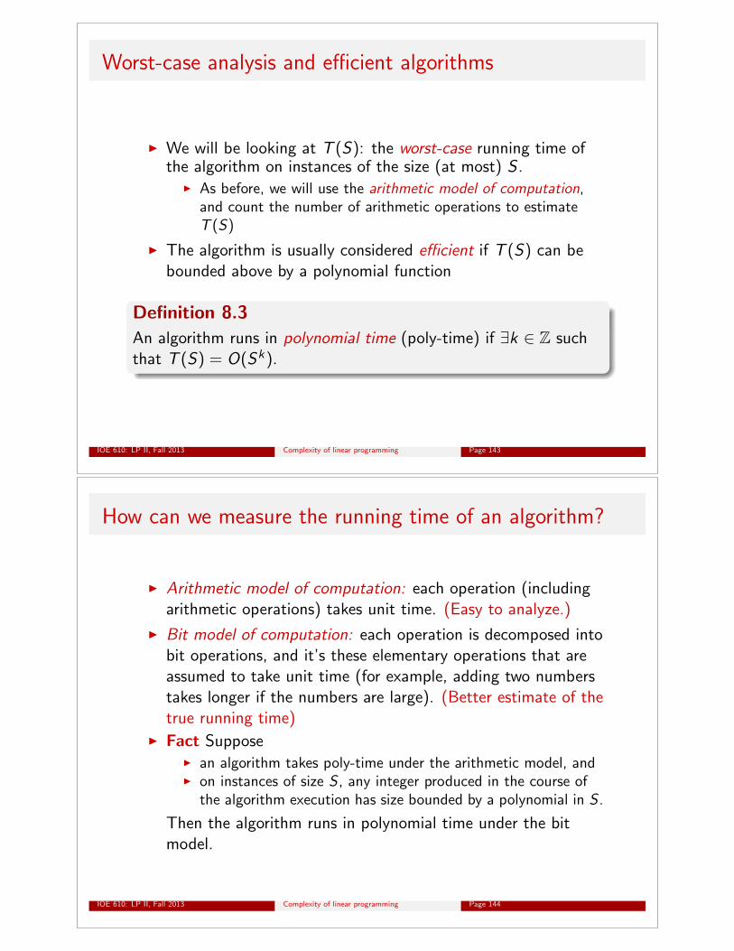
Worst-case analysis and e�cient algorithms

I We will be looking at T (S): the worst-case running time ofthe algorithm on instances of the size (at most) S .

I As before, we will use the arithmetic model of computation,and count the number of arithmetic operations to estimateT (S)

I The algorithm is usually considered e�cient if T (S) can bebounded above by a polynomial function

Definition 8.3An algorithm runs in polynomial time (poly-time) if 9k 2 Z suchthat T (S) = O(Sk).


How can we measure the running time of an algorithm?

I Arithmetic model of computation: each operation (includingarithmetic operations) takes unit time. (Easy to analyze.)

I Bit model of computation: each operation is decomposed intobit operations, and it’s these elementary operations that areassumed to take unit time (for example, adding two numberstakes longer if the numbers are large). (Better estimate of thetrue running time)

I Fact SupposeI an algorithm takes poly-time under the arithmetic model, andI on instances of size S , any integer produced in the course of

the algorithm execution has size bounded by a polynomial in S .

Then the algorithm runs in polynomial time under the bitmodel.


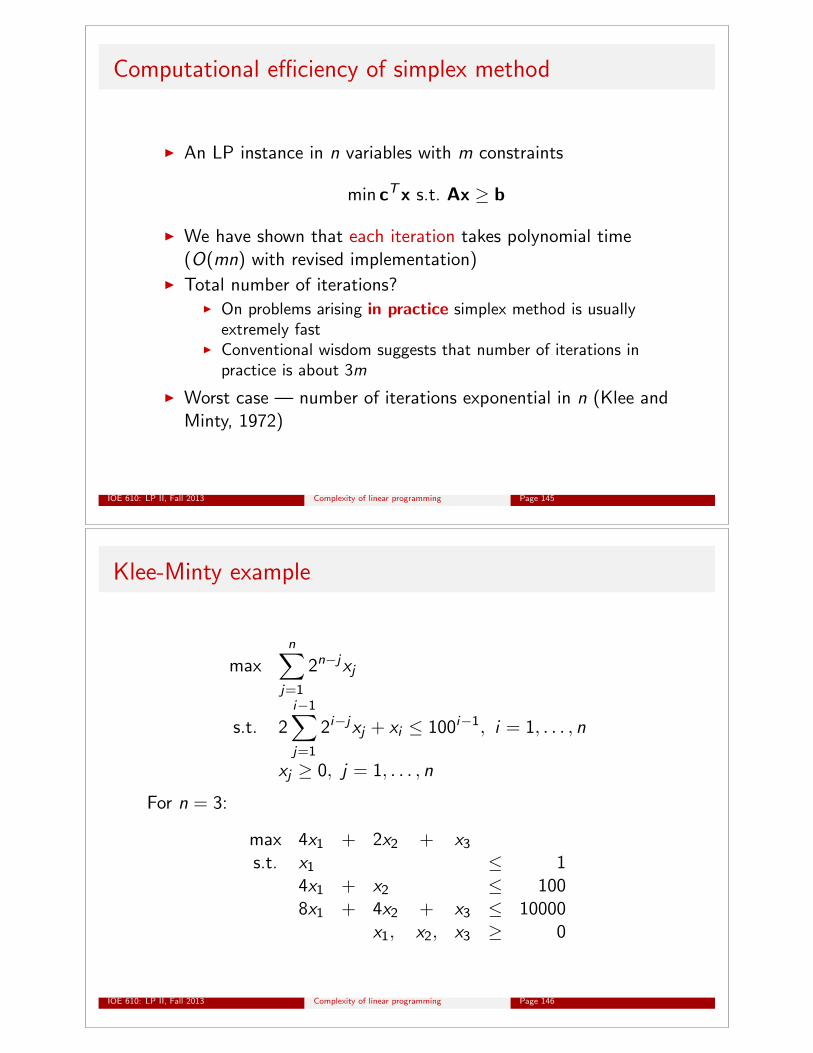
Computational e�ciency of simplex method

I An LP instance in n variables with m constraints

min cTx s.t. Ax � b

I We have shown that each iteration takes polynomial time(O(mn) with revised implementation)

I Total number of iterations?I On problems arising in practice simplex method is usually

extremely fastI Conventional wisdom suggests that number of iterations in

practice is about 3m

I Worst case — number of iterations exponential in n (Klee andMinty, 1972)


Klee-Minty example

maxn

X

j=1

2n�jxj

s.t. 2i�1X

j=1

2i�jxj

+ xi

100i�1, i = 1, . . . , n

xj

� 0, j = 1, . . . , n

For n = 3:

max 4x1 + 2x2 + x3s.t. x1 1

4x1 + x2 1008x1 + 4x2 + x3 10000

x1, x2, x3 � 0


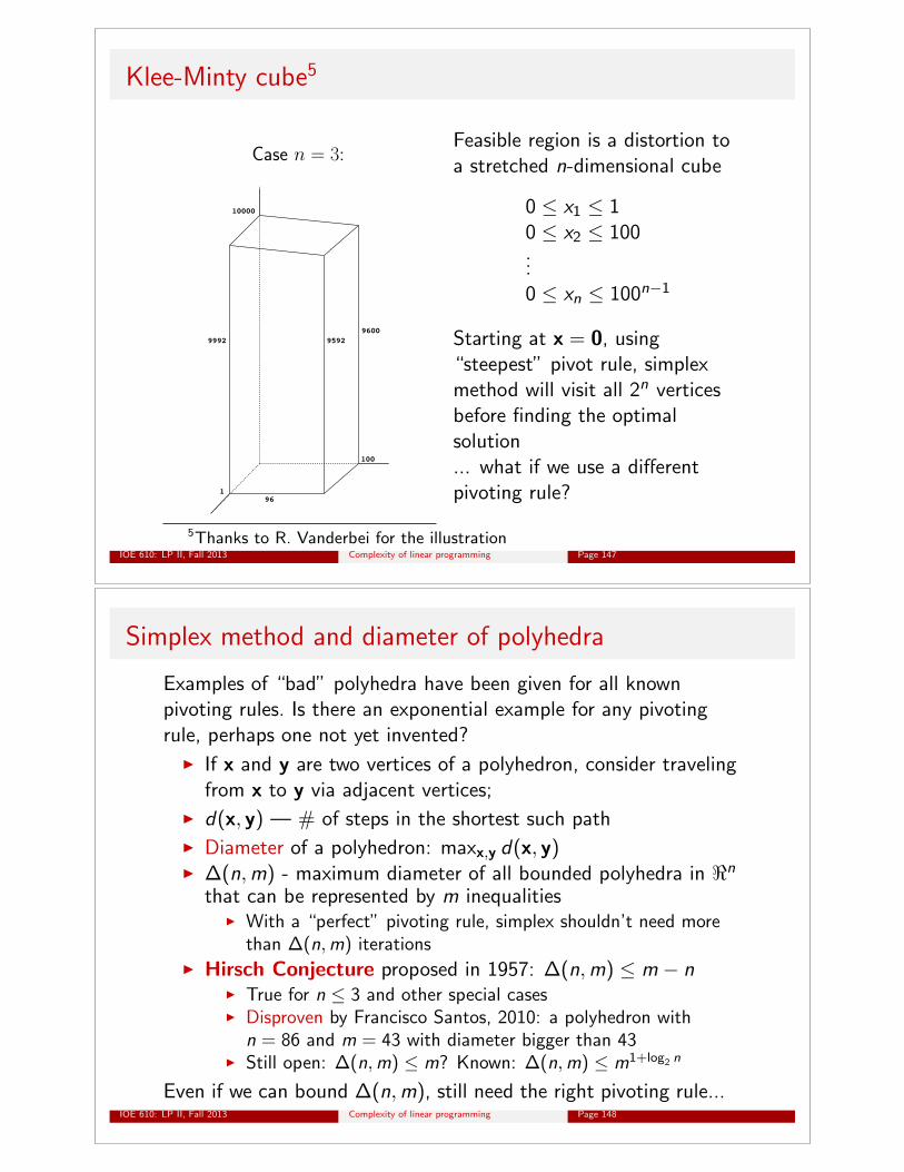
Klee-Minty cube5A Distorted Cube

Constraints represent a “minor” dis-tortion to an n-dimensional hyper-cube:

0 x1 10 x2 100

...0 xn 100n�1.

Case n = 3:

1

100

10000

96

9992 95929600

Feasible region is a distortion toa stretched n-dimensional cube

0 x1 10 x2 100...0 x

n

100n�1

Starting at x = 0, using“steepest” pivot rule, simplexmethod will visit all 2n verticesbefore finding the optimalsolution... what if we use a di↵erentpivoting rule?

5Thanks to R. Vanderbei for the illustrationIOE 610: LP II, Fall 2013 Complexity of linear programming Page 147

Simplex method and diameter of polyhedra

Examples of “bad” polyhedra have been given for all knownpivoting rules. Is there an exponential example for any pivotingrule, perhaps one not yet invented?

I If x and y are two vertices of a polyhedron, consider travelingfrom x to y via adjacent vertices;

I d(x, y) — # of steps in the shortest such pathI Diameter of a polyhedron: maxx,y d(x, y)I �(n,m) - maximum diameter of all bounded polyhedra in <n

that can be represented by m inequalitiesI With a “perfect” pivoting rule, simplex shouldn’t need more

than �(n,m) iterationsI Hirsch Conjecture proposed in 1957: �(n,m) m � n

I True for n 3 and other special casesI Disproven by Francisco Santos, 2010: a polyhedron with

n = 86 and m = 43 with diameter bigger than 43I Still open: �(n,m) m? Known: �(n,m) m1+log2 n

Even if we can bound �(n,m), still need the right pivoting rule...IOE 610: LP II, Fall 2013 Complexity of linear programming Page 148

Some LP history

I 1930’s — 1940’sI (Specialized) LP models and solution approaches developed

independently in the Soviet Union and the West for a varietyof optimal resource allocation and planning applications

I Late 1940’sI General LP theory (John Von Neumann) and solution method

(Simplex algorithm, George Dantzig) developed in USI Simplex runs quite fast in practice; LP used for military

operations and gains widespread use after the war

I 1972I Klee and Minty show that the simplex algorithm is not

e�cient, i.e., it does not run in polynomial time

I 1975: Nobel Prize in Economics is awarded for “for theircontributions to the theory of optimum allocation ofresources” via LP to Leonid V. Kantorovich and Tjalling C.Koopmans


LP history, continued

I 1970’sI THE BIG QUESTION: Does there exist an algorithm for

solving LPs that’s poly-time in the worst case?

I 1979, in the Soviet Union...I Leonid G. Khachiyan: YES, THERE IS — the Ellipsoid

algorithm!I NY Times publishes several articles about this discovery;

makes some mathematical blunders about the implications ofthe result and has to print retractions


Ellipsoid Algorithm for LP: outline

I Develop general ideas for the Ellipsoid algorithm

I Specify the algorithm for finding a point inP = {x 2 <n : Ax � b}

I Modify the algorithm for solving min cTx s.t. Ax � b

IOE 610: LP II, Fall 2013 Ellipsoid algorithm Page 151

Volumes and A�ne Transformations

DefinitionIf L ⇢ <n, the volume of L is

Vol(L) =

Z

x2Ldx

Definition 8.6

If D 2 <n⇥n is nonsingular and b 2 <n, the mappingS(x) = Dx+ b is an a�ne transformation.

I Note: by definition, a�ne transformation is invertible

Lemma 8.1Let L ⇢ <n. If S(x) = Dx+ b then Vol(S(L)) = | det(D)| · Vol(L).


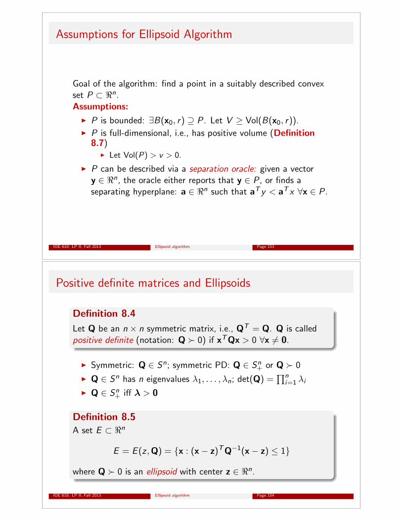
Assumptions for Ellipsoid Algorithm

Goal of the algorithm: find a point in a suitably described convexset P ⇢ <n.Assumptions:

I P is bounded: 9B(x0, r) ◆ P . Let V � Vol(B(x0, r)).I P is full-dimensional, i.e., has positive volume (Definition

8.7)I Let Vol(P) > v > 0.

I P can be described via a separation oracle: given a vectory 2 <n, the oracle either reports that y 2 P , or finds aseparating hyperplane: a 2 <n such that aT y < aT x 8x 2 P .


Positive definite matrices and Ellipsoids

Definition 8.4

Let Q be an n ⇥ n symmetric matrix, i.e., QT = Q. Q is calledpositive definite (notation: Q � 0) if xTQx > 0 8x 6= 0.

I Symmetric: Q 2 Sn; symmetric PD: Q 2 Sn

+ or Q � 0

I Q 2 Sn has n eigenvalues �1, . . . , �n

; det(Q) =Q

n

i=1 �i

I Q 2 Sn

+ i↵ � > 0

Definition 8.5A set E ⇢ <n

E = E (z ,Q) = {x : (x� z)TQ�1(x� z) 1}

where Q � 0 is an ellipsoid with center z 2 <n.


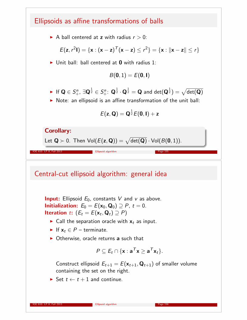
Ellipsoids as a�ne transformations of balls

I A ball centered at z with radius r > 0:

E (z, r2I) = {x : (x� z)T (x� z) r2} = {x : kx� zk r}

I Unit ball: ball centered at 0 with radius 1:

B(0, 1) = E (0, I)

I If Q 2 Sn

+, 9Q12 2 Sn

+: Q12 ·Q

12 = Q and det(Q

12 ) =

p

det(Q)

I Note: an ellipsoid is an a�ne transformation of the unit ball:

E (z,Q) = Q12E (0, I) + z

Corollary:

Let Q � 0. Then Vol(E (z,Q)) =p

det(Q) · Vol(B(0, 1)).


Central-cut ellipsoid algorithm: general idea

Input: Ellipsoid E0, constants V and v as above.Initialization: E0 = E (x0,Q0) ◆ P , t = 0.Iteration t: (E

t

= E (xt

,Qt

) ◆ P)

I Call the separation oracle with xt

as input.

I If xt

2 P – terminate.

I Otherwise, oracle returns a such that

P ✓ Et

\ {x : aTx � aTxt

}.

Construct ellipsoid Et+1 = E (x

t+1,Qt+1) of smaller volumecontaining the set on the right.

I Set t t + 1 and continue.


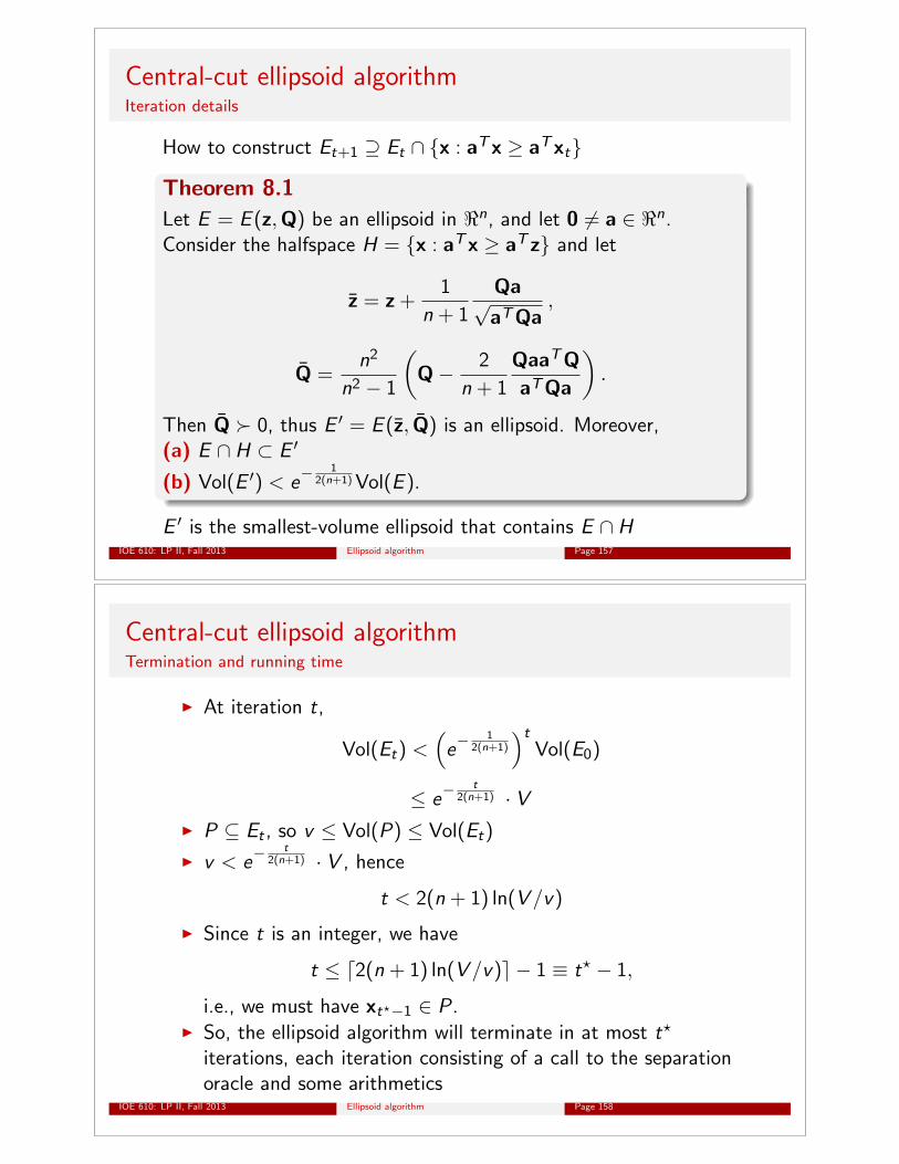
Central-cut ellipsoid algorithmIteration details

How to construct Et+1 ◆ E

t

\ {x : aTx � aTxt

}

Theorem 8.1Let E = E (z,Q) be an ellipsoid in <n, and let 0 6= a 2 <n.Consider the halfspace H = {x : aTx � aT z} and let

z = z+1

n + 1

QapaTQa

,

Q =n2

n2 � 1

✓

Q� 2

n + 1

QaaTQaTQa

◆

.

Then Q � 0, thus E 0 = E (z, Q) is an ellipsoid. Moreover,(a) E \ H ⇢ E 0

(b) Vol(E 0) < e�1

2(n+1)Vol(E ).

E 0 is the smallest-volume ellipsoid that contains E \ HIOE 610: LP II, Fall 2013 Ellipsoid algorithm Page 157

Central-cut ellipsoid algorithmTermination and running time

I At iteration t,

Vol(Et

) <⇣

e�1

2(n+1)

⌘

t

Vol(E0)

e�t

2(n+1) · VI P ✓ E

t

, so v Vol(P) Vol(Et

)

I v < e�t

2(n+1) · V , hence

t < 2(n + 1) ln(V /v)

I Since t is an integer, we have

t d2(n + 1) ln(V /v)e � 1 ⌘ t? � 1,

i.e., we must have xt

?�1 2 P .I So, the ellipsoid algorithm will terminate in at most t?

iterations, each iteration consisting of a call to the separationoracle and some arithmetics


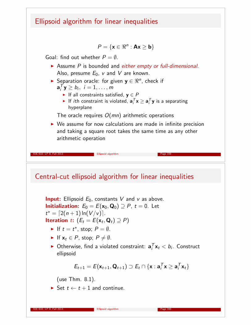
Ellipsoid algorithm for linear inequalities

P = {x 2 <n : Ax � b}

Goal: find out whether P = ;.I Assume P is bounded and either empty or full-dimensional.

Also, presume E0, v and V are known.I Separation oracle: for given y 2 <n, check if

aTi

y � bi

, i = 1, . . . ,mI If all constraints satisfied, y 2 PI If ith constraint is violated, aT

i

x � aTi

y is a separatinghyperplane

The oracle requires O(mn) arithmetic operations

I We assume for now calculations are made in infinite precisionand taking a square root takes the same time as any otherarithmetic operation


Central-cut ellipsoid algorithm for linear inequalities

Input: Ellipsoid E0, constants V and v as above.Initialization: E0 = E (x0,Q0) ◆ P , t = 0. Lett? = d2(n + 1) ln(V /v)e.Iteration t: (E

t

= E (xt

,Qt

) ◆ P)

I If t = t?, stop; P = ;.I If x

t

2 P , stop; P 6= ;.I Otherwise, find a violated constraint: aT

i

xt

< bi

. Constructellipsoid

Et+1 = E (x

t+1,Qt+1) � Et

\ {x : aTi

x � aTi

xt

}

(use Thm. 8.1).

I Set t t + 1 and continue.


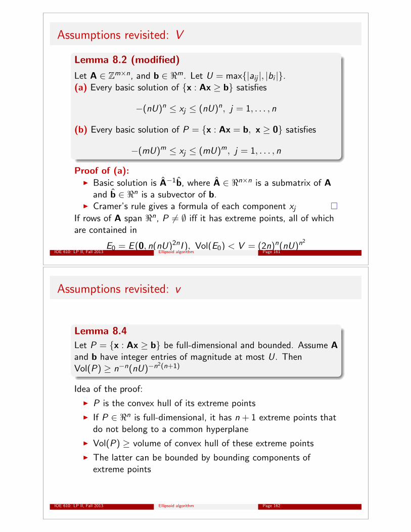
Assumptions revisited: V

Lemma 8.2 (modified)

Let A 2 Zm⇥n, and b 2 <m. Let U = max{|aij

|, |bi

|}.(a) Every basic solution of {x : Ax � b} satisfies

�(nU)n xj

(nU)n, j = 1, . . . , n

(b) Every basic solution of P = {x : Ax = b, x � 0} satisfies

�(mU)m xj

(mU)m, j = 1, . . . , n

Proof of (a):I Basic solution is A�1b, where A 2 <n⇥n is a submatrix of A

and b 2 <n is a subvector of b.I Cramer’s rule gives a formula of each component x

j

If rows of A span <n, P 6= ; i↵ it has extreme points, all of whichare contained in

E0 = E (0, n(nU)2nI ), Vol(E0) < V = (2n)n(nU)n2


Assumptions revisited: v

Lemma 8.4Let P = {x : Ax � b} be full-dimensional and bounded. Assume Aand b have integer entries of magnitude at most U. ThenVol(P) � n�n(nU)�n

2(n+1)

Idea of the proof:

I P is the convex hull of its extreme points

I If P 2 <n is full-dimensional, it has n + 1 extreme points thatdo not belong to a common hyperplane

I Vol(P) � volume of convex hull of these extreme points

I The latter can be bounded by bounding components ofextreme points


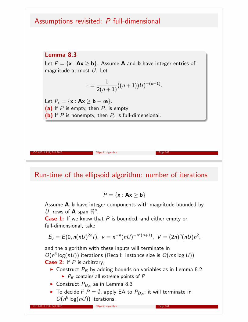
Assumptions revisited: P full-dimensional

Lemma 8.3Let P = {x : Ax � b}. Assume A and b have integer entries ofmagnitude at most U. Let

✏ =1

2(n + 1)((n + 1))U)�(n+1).

Let P✏ = {x : Ax � b� ✏e}.(a) If P is empty, then P✏ is empty(b) If P is nonempty, then P✏ is full-dimensional.


Run-time of the ellipsoid algorithm: number of iterations

P = {x : Ax � b}Assume A,b have integer components with magnitude bounded byU, rows of A span <n.Case 1: If we know that P is bounded, and either empty orfull-dimensional, take

E0 = E (0, n(nU)2nI ), v = n�n(nU)�n

2(n+1), V = (2n)n(nU)n2,

and the algorithm with these inputs will terminate inO(n4 log(nU)) iterations (Recall: instance size is O(mn logU))Case 2: If P is arbitrary,

I Construct PB

by adding bounds on variables as in Lemma 8.2I P

B

contains all extreme points of P

I Construct PB,✏ as in Lemma 8.3

I To decide if P = ;, apply EA to PB,✏; it will terminate in

O(n6 log(nU)) iterations.IOE 610: LP II, Fall 2013 Ellipsoid algorithm Page 164

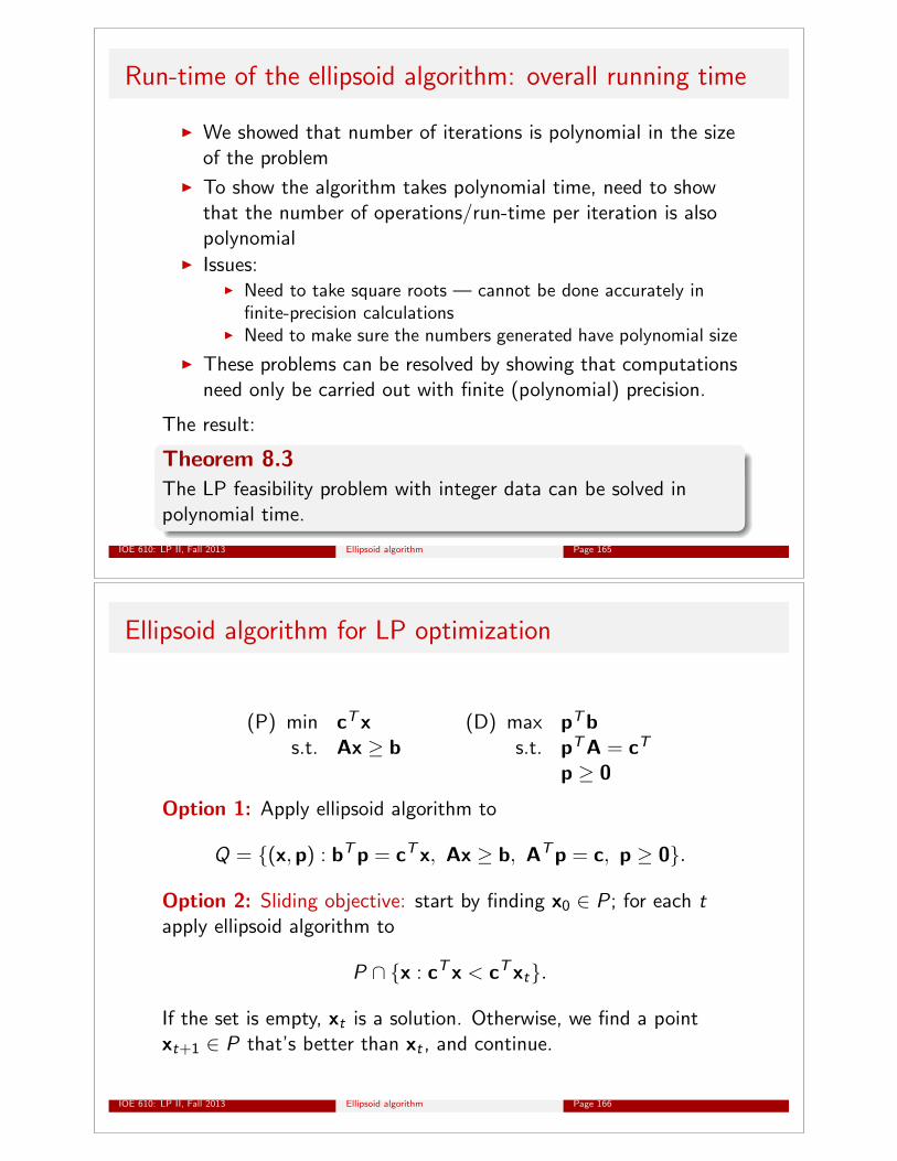
Run-time of the ellipsoid algorithm: overall running time

I We showed that number of iterations is polynomial in the sizeof the problem

I To show the algorithm takes polynomial time, need to showthat the number of operations/run-time per iteration is alsopolynomial

I Issues:I Need to take square roots — cannot be done accurately in

finite-precision calculationsI Need to make sure the numbers generated have polynomial size

I These problems can be resolved by showing that computationsneed only be carried out with finite (polynomial) precision.

The result:

Theorem 8.3The LP feasibility problem with integer data can be solved inpolynomial time.


Ellipsoid algorithm for LP optimization

(P) min cTx (D) max pTbs.t. Ax � b s.t. pTA = cT

p � 0

Option 1: Apply ellipsoid algorithm to

Q = {(x,p) : bTp = cTx, Ax � b, ATp = c, p � 0}.

Option 2: Sliding objective: start by finding x0 2 P ; for each tapply ellipsoid algorithm to

P \ {x : cTx < cTxt

}.

If the set is empty, xt

is a solution. Otherwise, we find a pointxt+1 2 P that’s better than x

t

, and continue.


Practical implications?

I Although a great theoretical accomplishment, Ellipsoidalgorithm never became a method of choice for solving LPs inpractice

I Its observed running time ⇡ its worst-case running time...

I ...unlike the simplex method

I ...or the Interior Point (Barrier) Methods


Documents

Complexity of linear programming: outline - U-M …mepelman/teaching/IOE610/... · · 2013-11-05Algorithms for Solving (Optimization) Problems I It is reasonable to expect the running