Compliance minimization of thin plates made of material with

Arch. Mech., 64, 2, pp. 111–135, Warszawa 2012

Compliance minimization of thin plates made of material

with predefined Kelvin moduli.

Part II. The effective boundary value problem

and exemplary solutions

G. DZIERŻANOWSKI, T. LEWIŃSKI

Faculty of Civil EngineeringWarsaw University of Technologyal. Armii Ludowej 1600-637 Warszawa, Polande-mails: [email protected]; [email protected]

The compliance minimization of transversely homogeneous plates with predefinedKelvin moduli leads to the equilibrium problem of an effective hyperelastic plate withthe hyperelastic potential expressed explicitly in terms of both the membrane andbending strain measures, as derived in Part I of the present paper. The aim of thissecond part of the paper is to show convexity of this potential and, consequently,uniqueness of solutions of the minimum compliance problem considered. Theoreticalresults are illustrated by numerically calculated optimal trajectories of the eigenstatecorresponding to the largest Kelvin modulus.

Key words: free material optimization, compliance minimization, anisotropic plates.

Copyright c© 2012 by IPPT PAN

1. Introduction

The free material optimization problem put forward in the first partof the present paper; namely minimize the compliance of a thin transversely

homogeneous plate of predefined Kelvin moduli of the elasticity tensor, meansthe optimal distribution of the eigenstates of the elasticity tensor to make theplate as stiff as possible. The problem has been reduced to the equilibrium prob-lem of an effective plate of specific hyperelastic properties. While the initialplate equilibrium problem is decoupled (the in-plane and bending problems canbe solved independently), the optimization process couples these deformations.The effective hyperelastic constitutive equations (3.59) in Dzierżanowski andLewiński [3] link the stress N and couple resultants M with the in-plane ε

and flexural κκκ strain measures. We shall prove that the underlying hyperelasticpotential is a homogeneous function of degree 2, bounded from both sides andstrictly convex. The latter property is crucial but fairly difficult to obtain. Itsproof is based on discussing of the positive definiteness of the Hessian.

112 G. Dzierżanowski, T. Lewiński

The results of the first part of the present paper were based on the assump-tion of possible interchanging the „min” and „max” operations in (I.2.19). Thecorrectness of this switching is substantiated in Sec. 3.4 below by utilizing the du-ality relations proved in Czarnecki and Lewiński [2], thus making the presenttwo-part paper complete.

According to the theorem by Minty [5], the relevant constitutive equationsare monotone and this property implies the uniqueness of a solution. However,the problem of its existence, linked with the regularity assumptions, will bediscussed elsewhere.

Theoretical considerations are illustrated by the examples of trajectories ofthe second-order symmetric tensor field ω1(x) corresponding to the greatestvalue of Kelvin modulus in the optimal constitutive tensor field A(x), relatedto the given strain fields obtained with the help of the Airy stress functions intwo-dimensional (plane) elasticity and the Navier and Levy’s infinite series, rep-resenting the deflection function in the theory of Kirchhoff plates. Consequently,components of the in-plane strain tensor and the curvature tensor of a plate inbending are calculated analytically and this step is followed by combining bothloading cases in the membrane-bending (M-B) problem. This in turn allows forsetting the variable coefficients of two ordinary differential equations whose so-lutions determine the families of orthogonal trajectories corresponding to theeigenvalues of ω1(x).

2. The effective hyperelastic problem (P ∗)

The problem of minimization of the plate compliance over possible eigenstatesof the elasticity tensor A, which determines both in-plane and bending stiff-nesses, reduces to problem (P ∗) or (I.2.22)–(I.2.24); the Roman numeral I refersto the Part I of the present paper, or to Dzierżanowski and Lewiński [3].The effective potential (I.2.23) has been reduced to the form (I.3.13), while theconstitutive equations have the form (I.3.59).

Assume that vectors ε, κ are not co-linear and, for the purpose of this sectiononly, set a basis (B.1), see Appendix B. Next, by making use of (I.3.50), (I.3.52)and (I.3.54), rewrite (I.3.59) in the form

(2.1)N =

1

2(λ1 + λ2) [(1 + ν φ(ε,κ)) ε + ν ψ(ε,κ) κ] ,

K =1

2(λ1 + λ2) [ν ψ(ε,κ) ε + (1 − ν φ(ε,κ))κ] .

Hence, contravariant representations of N and K in basis (B.1) are given byvectors

Compliance minimization of thin plates. . . 113

(2.2)

N1

N2

N3

=1

2(λ1 + λ2)

1 + ν φν ψ0

,

K1

K2

K3

=1

2(λ1 + λ2)

ν ψ1 − ν φ

0

.

Next, apply (I.3.50) in the representation of the constitutive tensor A in termsof G, φ and ψ. Rewriting (2.1) one obtains

(2.3) N = A ε, K = Aκ,

since it is clear that tensor A links both equations by D = (h2/12)A, see (I.2.2)and (I.2.3).

Formulae (2.3) can be rearranged in a form

(2.4) N = (Aij ei ⊗ ej) ε, K = (Ai

j ei ⊗ ej) κ,

thus leading to the mixed representation of tensor A given by

(2.5) [Aij ] =

1

2(λ1 + λ2)(1 + ν φ)

1

2(λ1 + λ2)ν ψ 0

1

2(λ1 + λ2)ν ψ

1

2(λ1 + λ2)(1 − ν φ) 0

0 0 λ3

.

Indeed, by introducing the basis and co-basis vectors (B.1) and (B.6) in (2.3)one obtains

A ε = (Aij ei ⊗ ej) ε = (Ai

j ei ⊗ ej) e1 = Aij δ

j1 ei(2.6)

= Ai1 ei = A1

1 ε +A21 κ,

Aκ = (Aij ei ⊗ ej) κ = (Ai

j ei ⊗ ej) e2 = Aij δ

j2 ei(2.7)

= Ai2 ei = A1

2 ε +A22 κ.

Comparing these formulae with those in (2.1) and taking into consideration thatω3 is perpendicular to the plane spanned by ε and κ, finally yields (2.5).

Upon solving the problem (I.2.22)–(I.2.24), with potential (I.3.13), one canfind optimal eigentensors P1, P2, P3 of the constitutive tensor A by using theEqs. (I.2.11) and (I.3.45), (I.3.46). Let us note that the eigentensors of A can becalculated as, see [8],

(2.8)

P1 =1

(λ1 − λ2)(λ1 − λ3)(A − λ2E) (A − λ3E) ,

P2 =1

(λ2 − λ1)(λ2 − λ3)(A − λ1E) (A − λ3E) ,

P3 =1

(λ3 − λ1)(λ3 − λ2)(A − λ1E) (A − λ2E) ,


where E represents the metric tensor, see Appendix B, or explicitly in the thebasis ej ⊗ ek

(2.9) [(P1)jk] =

1

2(1 + φ)

1

2ψ 0

1

2ψ

1

2(1 − φ) 0

0 0 0

,

(2.10) [(P2)jk] =

1

2(1 − φ) −1

2ψ 0

−1

2ψ

1

2(1 + φ) 0

0 0 0

,

and

(2.11) [(P3)jk] =

0 0 0

0 0 0

0 0 1

.

It is a simple matter to check that ‖Pi‖ = 1, i = 1, 2, 3.The projectors Pα, α = 1, 2, can be represented by

(2.12) Pα =αξ 1ε ⊗ ε +

αξ 3(ε ⊗ κ + κ ⊗ ε) +

αξ 2κ ⊗ κ

where, for α = 1,

(2.13)1ξ 1 =

(

γ1

‖ε‖

)2

,1ξ 2 =

(

γ2

‖κ‖

)2

,1ξ 3 =

√

1ξ 1

1ξ 2

and γ1, γ2, are given by (I.3.40), or, alternatively,

(2.14)

(γ1)2 =

1

2 sin2 α

(

1 + φ− ψε · κ‖κ‖2

)

,

(γ2)2 =

1

2 sin2 α

(

1 − φ− ψε · κ‖ε‖2

)

with

(2.15) sin2 α = 1 −(

ε · κ‖ε‖ ‖κ‖

)2

.

For α = 2, the coefficients2ξ j are given by (I.2.10) with γα replaced by δα.

If referred to the basis in R3 in the form (I.2.7), the tensors appearing in

(2.12) are represented by the matrices


ε ⊗ ε =

(ε11)2 ε11ε22

√2ε11ε12

ε22ε11 (ε22)2

√2ε22ε12√

2ε12ε11

√2ε12ε22 2 (ε12)

2

,(2.16)

ε ⊗ κ =

ε11κ11 ε11κ22

√2ε11κ12

ε22κ11 ε22κ22

√2ε22κ12√

2ε12κ11

√2ε12κ22 2 ε12κ12

,(2.17)

κ ⊗ κ =

(κ11)2 κ11κ22

√2κ11κ12

κ22κ11 (κ22)2

√2κ22κ12√

2κ12κ11

√2κ12κ22 2 (κ12)

2

,(2.18)

with ε ⊗ κ = (κ ⊗ ε)T .Let us now write the incremental form of the constitutive equations (2.1)

(2.19)

∆N =∂N

∂ε

∆ε +∂N

∂κ

∆κ,

∆K =∂K

∂ε

∆ε +∂K

∂κ

∆κ,

where

(2.20)

∂N

∂ε

=1

2(λ1 + λ2)

[

ν∂φ

∂ε

⊗ ε + ν∂ψ

∂ε

⊗ κ + (1 + ν φ) I4

]

,

∂N

∂κ

=1

2(λ1 + λ2)

[

ν∂φ

∂κ

⊗ ε + ν∂ψ

∂κ

⊗ κ + ν ψ I4

]

,

∂K

∂ε

=1

2(λ1 + λ2)

[

ν∂ψ

∂ε

⊗ ε − ν∂φ

∂ε

⊗ κ + ν ψ I4

]

,

∂K

∂κ

=1

2(λ1 + λ2)

[

ν∂ψ

∂κ

⊗ ε − ν∂φ

∂κ

⊗ κ + (1 − ν φ) I4

]

.

Here I4 stands for the unit tensor in E4s and

(2.21)

∂φ

∂ε

= 2ψ

G(ψ ε − φκ) ,

∂φ

∂κ

= −2ψ

G(φ ε + ψ κ) ,

∂ψ

∂ε

= −2φ

G(ψ ε − φκ) ,

∂ψ

∂κ

= 2φ

G(φ ε + ψ κ) .


3. Properties of (P ∗) problem

3.1. Strict convexity of Wλ

The aim of the present section is to show the strict convexity of potential Wλ

which was defined in (I.3.3), (I.3.4) and expressed explicitly in (I.3.13).Note first that Wλ is a homogeneous function of degree 2, or

(3.1) Wλ(αε, ακκκ) = α2Wλ(ε,κκκ)

for α ≥ 0. According to [7], the pointwise supremum of an arbitrary collectionof convex functions is also convex, but this theorem cannot be applied to (I.3.5),because tensors ωi are restricted by orthogonality conditions. It folows that con-vexity of Wλ cannot be inferred from (I.3.23), it must be deduced by examiningthe specific properties of the explicit expression (I.3.13) instead.

It is sufficient to prove convexity of U∗(ε,κ) in (I.3.52) with respect to botharguments. The proof of convexity consists in checking positive semidefinitenessof the Hessian matrix, see [7],

(3.2) F =

[

F11 F12

F21 F22

]

with

(3.3)

F11 =∂2U∗(ε,κ)

∂ε ⊗ ∂ε

, F12 =∂2U∗(ε,κ)

∂ε ⊗ ∂κ

,

F21 =∂2U∗(ε,κ)

∂κ ⊗ ∂ε

, F22 =∂2U∗(ε,κ)

∂κ ⊗ ∂κ

.

In the sequel it is proved that (3.2) is positive definite, which implies strictconvexity of U∗. From (I.3.58), (2.19), (2.20) and (2.21) one may deduce that

F11 = 2

[

(1 + νφ)I4 +2 ν

G(ψε − φκ) ⊗ (ψε − φκ)

]

,(3.4)

F12 = 2

[

νψI4 −2 ν

G(ψε − φκ) ⊗ (φε + ψκ)

]

,(3.5)

F22 = 2

[

(1 − νφ)I4 +2 ν

G(φε + ψκ) ⊗ (φε + ψκ)

]

,(3.6)

where I4 is the unit tensor in E4s, G = G(ε,κ), see (I.3.50), and F21 = (F12)T.

The task is now to prove that the following quadratic form:

(3.7) 2X(a,b) = a · (F11a) + a · (F12b) + b · (F21a) + b · (F22b)

is positive for arbitrary a, b ∈ E2s provided that ‖a‖2 + ‖b‖2 6= 0.


The first two terms on the r.h.s. of (3.7) can be expressed as

(3.8)1

2a · (F11a) = ‖a‖2 +

ν

G

[(

‖ε‖2 − ‖κ‖2)

‖a‖2 + 2(a · ε)2 + 2(a · κ)2]

− 2ν

G3

[(

‖ε‖2 − ‖κ‖2)

(a · ε) + 2(ε · κ)(a · κ)]2,

(3.9)1

2a · (F12b) =

2ν

G

[(a · κ)(b · ε) − (a · ε)(b · κ) + (ε · κ)(a · b)]

+1

G2[(

‖ε‖2 − ‖κ‖2)2

(b · κ)(a · ε) − 4(ε · κ)2(b · ε)(a · κ)]

+2

G2

(

‖κ‖2 − ‖ε‖2)

(ε · κ) [(a · ε)(b · ε) − (a · κ)(b · κ)]

.

The third term in (3.7) is exactly the same as (3.9), while the fourth one issimilar to (3.8), the only difference results in replacing a with b, ε with κ andκ with ε.

Substituting all terms in (3.7) one finds

(3.10) X(a,b) = X0(a,b) + ∆(a,b),

where

(3.11) X0(a,b) = ‖a‖2 + ‖b‖2 + ν[

φ(ε,κ)(

‖a‖2 − ‖b‖2)

+ 2ψ(ε,κ)(a · b)]

and

(3.12) ∆(a,b) = 2ν G(ε,κ) [φ(ε,κ)(a · κ + b · ε) − ψ(ε,κ)(a · ε − b · κ)]2 .

By virtue of ν > 0, one can estimate

(3.13) X(a,b) ≥ X0(a,b)

and the assumption ‖a‖2 + ‖b‖2 6= 0 leads to

(3.14) X(a,b) ≥(

‖a‖2 + ‖b‖2)

X1(a,b)

with

(3.15) X1(a,b) = 1 + νX2(a,b)

and

(3.16) X2(a,b) =‖a‖2 − ‖b‖2

‖a‖2 + ‖b‖2φ(ε,κ) +

2(a · b)

‖a‖2 + ‖b‖2ψ(ε,κ).

It remains to prove that

(3.17) X1(a,b) ≥ 1 − ν.


To this end, set the representations of a, b, ε, κ from E2s similarly to (I.2.8);

express ‖a‖ and ‖b‖ as

(3.18) ‖a‖ = R cosϑ, ‖b‖ = R sinϑ,

and let δ = ∢(a,b) or

(3.19) a · b = ‖a‖‖b‖ cos δ = R2 cosϑ sinϑ cos δ.

Next, by making use of the fact that φ2 + ψ2 = 1, see (I.3.50), express φ and ψin terms of a certain angle

(3.20) φ = cosϕ, ψ = sinϕ

and rewrite X2 in terms of ϑ and ϕ thus obtaining

(3.21) X2 = cos 2ϑ cosϕ+ sin 2ϑ sinϕ cos δ.

It is easily seen that

(3.22) min X2 | δ ∈ R = min cos(2ϑ− ϕ), cos(2ϑ+ ϕ) ,

hence,

(3.23) min X2 | δ ∈ R, ϑ ∈ R = −1

and the inequality X2 ≥ −1 implies (3.17).Estimates 1 − ν > 0 and (3.14) prove that X(a,b) > 0 if ‖a‖2 + ‖b‖2 6= 0,

thus completing the proof of strict convexity of the function (I.3.52) with respectto both arguments.

It is worth pointing out that U∗λ is bounded, i.e.

(3.24) λ3

(

‖ε‖2 + ‖κ‖2)

≤ 4U∗λ(ε,κ) ≤ λ1

(

‖ε‖2 + ‖κ‖2)

which follows from (I.3.5). To this end, one has to recall the estimates: λ1 >λ2 > λ3 > 0 and make use of (I.3.6).

3.2. Properties of the constitutive equations

Since Wλ is a homogeneous function of degree 2, see (3.1), the Euler theoremapplies and makes it possible to express this potential in terms of strains andstress resultants by the equation

(3.25) 2 · (2U∗λ)(ε,κ) = N · ε + K · κ.


This property can be checked by using (I.3.59). Indeed, by computing the scalarproducts

(3.26)N · ε =

1

2(λ1 + λ2)

[

‖ε‖2 + νL(ε,κ) · ε]

,

K · κ =1

2(λ1 + λ2)

[

‖κ‖2 + νL(κ, ε) · κ]

and making use of (I.3.57), one may note that

(3.27) L(ε,κ) · ε + L(κ, ε) · κ = G(ε,κ)

and this equality confirms (3.25). Since U∗λ is strictly convex, the constitutive

equations are strictly monotone, or

(3.28)

[

N( 1ε ,

1κ

)

−N( 2ε ,

2κ

)

]

·( 1ε− 2

ε

)

+

[

K( 1ε ,

1κ

)

−K( 2ε ,

2κ

)

]

·( 1κ− 2

κ

)

≥ 0

and the equality holds if and only if1ε =

2ε ,

1κ =

2κ .

This property is due to Minty [5], see also Ekeland and Temam [4]. It im-plies the uniqueness of solutions to the problem (P ∗) or (I.2.24). Indeed, assume

that two pairs (1u ,

1w ), (

2u ,

2w ) satisfy (I.2.6)

(3.29)

∫

Ω

[

N( 1ε ,

1κ

)

· ε(v) + K( 1ε ,

1κ

)

· κ(v)

]

dx = f(v, v),

∫

Ω

[

N( 2ε ,

2κ

)

· ε(v) + K( 2ε ,

2κ

)

· κ(v)

]

dx = f(v, v)

whereαε = ε(

αu ),

ακ = κ(

αw ). Suppose that (v, v) are common for both equa-

tions and subtract them to find

(3.30)∫

Ω

[(

N( 1ε ,

1κ

)

− N( 2ε ,

2κ

)

)

· ε(v)

]

dx

+

∫

Ω

[(

K( 1ε ,

1κ

)

−K( 2ε ,

2κ

)

)

· κ(v)

]

dx = 0.

Next, choose v =1u − 2

u , v =1w − 2

w . Then

(3.31) ε(v) =1ε − 2

ε , κ(v) =1κ − 2

κ .


By the strict monotonicity, see (3.28), the equality (3.30) can only be fulfilled

if1ε =

2ε and

1κ =

2κ which means that

( 1u ,

1w)

,( 2u ,

2w)

can differ only inthe terms describing a rigid body motion (with infinitesimal rotations). If both( αu ,

αw)

satisfy appropriate kinematic boundary conditions, these terms vanish

leading to the identities:1u =

2u ,

1w =

2w . This proves the uniqueness of solution

to the problem (P ∗), however the problem of its existence is not dealt with inthe present paper.

3.3. The variational formulation of (P ∗)

Note that

(3.32) N · ε(v) + M · κκκ(v) = N · ε(v) + K · κ(v).

Substitution of (I.3.59) into (I.2.6) gives

(3.33)1

2

∫

Ω

(λ1 + λ2) [ε(u) · ε(v) + κ(w) · κ(v)] dx

+1

2

∫

Ω

(λ1 − λ2) [L (ε(u),κ(w)) · ε(v) + L (κ(w), ε(u)) · κ(v)] dx

= f(v, v) ∀ (v, v) ∈ V.

This will be called a variational formulation of problem (P ∗).Consider the case of pure bending. Assume that the plate is subject only to

the transverse loading, i.e. f(v, v) = f(v). The goal is to check whether u = 0.Setting ε(u) = 0 in (3.33) and taking into account that

(3.34) L(κ,0) = κ, L(0,κ) = 0

gives

(3.35) N = 0, K =1

2(λ1 + λ2)(κ + νκ) = λ1κ,

thus Eq. (3.33) reduces to

(3.36)∫

Ω

λ1κ(w) · κ(v)dx = f(v)

and the conclusion that the pair (u = 0, w), w being solution to (3.36), solvesthe problem (I.2.6), (I.2.25) follows. Tensor A has the following representation:

(3.37) A = λ1κ ⊗ κ + λ2ω2 ⊗ ω2 + λ3ω3 ⊗ ω3


with ω2 ⊥ κ, ω3 = ω1 × ω2, κ given by (I.3.14) and the potential U∗λ reduces

to the expression given in (I.3.64). According to (3.28), the relevant solution(u = 0, w) is unique.

Next, assume that the plate is subjected to the in-plane forces only (mem-brane case), i.e. f(v, v) = f(v). By similar arguments one can show that w = 0in this case while u is the solution to the problem

(3.38)∫

Ω

λ1ε(u) · ε(v)dx = f(v).

Tensor A has the representation (3.37) with κ replaced by ε. Potential 2U∗λ

reduces to 12λ1‖ε‖2.

3.4. The primal formulation

All results of the paper are based on the equivalence of two expressions:(I.2.19) and (I.2.20). This equivalence property will be inferred by proving thatthe solution (u, w) of the problem (P ∗) or (I.2.24) is proportional to the solution(u, w) of the problem (P ) or – to the problem primal for (P ∗). We shall drawupon the results published in Czarnecki and Lewiński [2].

Let us introduce the function of arguments N,K ∈ E2s

(3.39) Uλ(N,K) =1

2

(

1

λ1+

1

λ2

)

(

‖N‖2 + ‖K‖2)

− 1

2

(

1

λ2− 1

λ1

)

G(N,K),

where G(·, ·) is defined by (I.3.50). According to (7.8) in [2], the potential (I.3.11)can be represented as

(3.40) U∗λ(ε,κ) = sup

N · ε + K · κ − Uλ(N,K)| (N,K) ∈ E2s

.

Therefore, the potential U∗λ is dual to Uλ.

Let∑

(Ω) denote the set of fields (N,M) given on Ω, satisfying the vari-ational equation (I.2.6). According to Castigliano’s theorem, the compliance isexpressed by

(3.41) C(A) = min(N,M)∈Σ(Ω)

∫

Ω

[

N · (A−1N) + M · (D−1M)]

dx,

where A, D are given by (I.2.2).Substitution of (3.41) into (I.2.15) leads to a new expression C0 for the op-

timal compliance. Minimization over A ∈ Tλ(Ω) can be performed analytically.By using the analogy with problem (3.2) in [2], we obtain the problem (P ):

(3.42) C0 = min(N,K)∈Σ(Ω)

∫

Ω

Uλ(N, K)dx,


where Uλ(N, K) is given by (3.39), see (4.48) in [2]. Note that C0 = C0, C0 beingdefined by (I.2.15). We shall prove that the problem dual to (P ) is just (P ∗) or(I.2.24).

Assume that (3.42) is solvable and one of the solutions is denoted by (N,M).Let us rewrite (3.42) as follows

(3.43)

C0 = min(N,K)∈Σ(Ω)

max(u,w)∈V

∫

Ω

Uλ(N, K)dx+ f(u, w) −∫

Ω

(N · ε + K · κ)dx

,

where ε = ε(u), κ = κ(w) and N, K defined on Ω are viewed as appropriatelyregular.

The stationarity conditions of (3.43) lead to the relations linking the unknownfields N, K with the unknown multipliers ε, κ:

(3.44)

ε =∂Uλ(N,K)

∂N

∣

∣

∣

∣

N=N,K=K

=

(

1

λ1+

1

λ2

)

(N− νL(N, K)),

κ =∂Uλ(N,K)

∂K

∣

∣

∣

∣

N=N,K=K

=

(

1

λ1+

1

λ2

)

(K − νL(K, N)).

Their inversions read

(3.45)

N =∂U∗

λ(ε,κ)

∂ε

∣

∣

∣

∣

ε=ε, κ=κ

,

K =∂U∗

λ(ε,κ)

∂κ

∣

∣

∣

∣

ε=ε, κ=κ

,

and, using (I.3.56), one finds

(3.46)N =

1

4(λ1 + λ2)(ε + νL(ε, κ)),

K =1

4(λ1 + λ2)(κ + νL(κ, ε)).

The fields u, w, ε, κ, N, K satisfy the constitutive equations (3.46) and the equa-tions of equilibrium (I.2.6) (upon the change (I.3.2) and K = (

√12/h)M) along

with appropriate kinematic boundary conditions. We note that this set of equa-tions is almost the same as the set of local equations of problem (P ∗) that canbe inferred from (3.33). It has been proved that the solution (u, w, ε, κ, N,M)to the problem (P ∗) is unique, provided it exists. The equations of problems (P )and (P ∗) differ in the coefficients of the constitutive equations, cf. (3.46) and


(2.1). We note that both the problems are uniquely solvable. The solution (u, w)of problem (P ) is linked with the solution (u, w) of problem (P ∗) by u = 2u,w = 2w, while N = N, K = K, since the moduli in (3.46) are two times smallerthan the moduli in (2.1). Since (N, K) is the minimizer of (3.42), one may write

(3.47) C0 =

∫

Ω

Uλ(N, K)dx

or

(3.48) C0 =

∫

Ω

Uλ(N, K)dx.

The equilibrium equation implies the identity

(3.49) f(u, w) =

∫

Ω

(N · ε + K · κ)dx

which makes it possible to rearrange (3.48) to the form

C0 =

∫

Ω

[

Uλ(N, K) − (N · ε + K · κ)]

dx+ f(u, w).(3.50)

By using (3.44) and (3.27), we compute

(3.51) N · ε + K · κ

= N ·(

1

2ε

)

+ K ·(

1

2κ

)

=1

2

(

1

λ1+

1

λ2

)

[

N ·(

N − νL(N, K))

+ K ·(

K − νL(K, N))]

= Uλ(N, K) = Uλ(N, K),

which gives C0 = f(u, w).Let us rearrange (I.2.24). The minimum is attained for (v, v) = (u, w), hence

(3.52) C0 = −2Jλ(u, w)

or

(3.53) C0 = 2f(u, w) −∫

Ω

2Wλ(x) (ε(u),κκκ(w)) dx.


The stationarity condition of Jλ(v, v) assumes the form of the equilibrium equa-tion (I.2.6) in which N = N, M = M, given by (I.2.25). Since

(3.54) N · ε(u) + M · κκκ(w) = 2Wλ(x) (ε(u),κκκ(w)) ,

see (3.25), we conclude that

(3.55) f(u, w) =

∫

Ω

2Wλ(x) (ε(u),κκκ(w)) dx

which gives C0 = f(u, w).Thus we have arrived at

(3.56) C0 = C0,

which ends the proof of possibility of switching the „min” and „max” operationsin (3.43). Let us rewrite (3.43) as

(3.57) C0 = max(u,w)∈V

∫

Ω

minN,K∈E2

s

[

Uλ(N, K) − (N · ε + K · κ)]

dx+ f(u, w)

,

hence

(3.58) C0 = max(u,w)∈V

−∫

Ω

maxN,K∈E2

s

[

N · ε + K · κ − Uλ(N, K)]

dx+ f(u, w)

.

We use (3.40) to find

(3.59) C0 = max(u,w)∈V

−∫

Ω

U∗λ(ε, κ)dx+ f(u, w)

.

By homogeneity of U∗λ and linearity of f(·, ·) we write

(3.60) C0 = 2 max(u,w)∈V

−∫

Ω

2U∗λ

(

1

2ε,

1

2κ

)

dx+ f

(

1

2u,

1

2w

)

,

hence

(3.61) C0 = −2 min(u,w)∈V

2

∫

Ω

U∗λ

(

1

2ε,

1

2κ

)

dx− f

(

1

2u,

1

2w

)

.


We introduce the notation (I.3.3):

(3.62) C0 = −2 min(u,w)∈V

∫

Ω

Wλ(x)

(

1

2ε,

1

2κ

)

dx− f

(

1

2u,

1

2w

)

and now we use the notation (I.2.22) to obtain

(3.63) C0 = −2 min(u,w)∈V

Jλ

(

1

2u,

1

2w

)

,

which can be written as, see (I.2.21),

(3.64) C0 = −2 min(u,w)∈V

maxA∈Tλ(Ω)

J

(

A,1

2u,

1

2w

)

.

Let us recall (I.2.19):

(3.65) C0 = −2 maxA∈Tλ(Ω)

min(u,w)∈V

J (A, u, w) .

Since C0 = C0 we confirm (3.56). Let (u, v) = (u, w) be the minimizer of (3.64)and (u, w) be the minimizer of (3.65). We confirm once again that 1

2 u = u,12 w = w. Thus the passage from (3.43) to (3.57) is justified.

4. Examples of optimal designs

4.1. Trajectories of the symmetric second-order tensor eigenvalues

Any symmetric second-order tensor a ∈ E2s admits a spectral decomposition

(4.1) a = α1 d ⊗ d + α2 d⊥ ⊗ d⊥

where d,d⊥ denotes the eigenbasis of a and forms an orthonormal (Cartesian)basis in R

2. The unit tensor in E2s is given by

(4.2) I2 = d⊗ d + d⊥ ⊗ d⊥,

thus we may re-write (4.1) in a form

(4.3) a =1

2(α1 + α2)I2 + t, t =

1

2(α1 − α2)(2d⊗ d− I2)

and it is a matter of straighforward calculations that I2 · t = 0. Equation (4.3)determines the isotropic decomposition of a, see e.g. [1], and t stands for itsdeviatoric (pure shear) part.


Let us introduce an angle ϕ as linking the arbitrary orthonormal basis i1, i2with the eigenbasis d,d⊥ by

(4.4) d = cosϕ i1 + sinϕ i2, d⊥ = sinϕ i1 − cosϕ i2.

Substituting (4.4) in (4.3) and making use of (I.2.7) leads to

(4.5) t =1

2(α1 − α2)

[

cos(2ϕ)(B1 −B2) +√

2 sin(2ϕ)B3

]

or

(4.6) t =1

2(a11 − a22)(B1 −B2) +

√2 a12B3,

see (I.2.8), by rotational invariance of the isotropic decomposition.Components of a depend on the spatial variables (x1, x2) ≡ (x, y), hence

comparing (4.5) with (4.6) allows for setting

(4.7) tan (2ϕ(x, y)) = 2a12(x, y)

a11(x, y) − a22(x, y),

thus establishing an equation determining the family of curves y = y(x). Conse-quently, d denotes a vector locally (i.e. at given x) tangent to a curve y(x) andϕ = ∢(d, i1), hence dy/dx = tanϕ. Making use of the trigonometric identity

(4.8) tan(2ϕ) =2 tanϕ

1 − tan2 ϕ,

we may re-write (4.7) in a form

(4.9)

(

dy

dx

)2

+a11 − a22

a12

(

dy

dx

)

− 1 = 0

whose solutions, known as trajectories of eigenvalues of a given tensor a, aregiven by

(4.10)dy

dx+a11 − a22

2 a12±((

a11 − a22

2 a12

)2

+ 1

)1/2

= 0.

The latter equations determine two families of curves which are orthogonal forevery (x, y) ∈ Ω. In most cases, functions y = y(x), solving the differentialequations in (4.10), cannot be computed analytically, thus in the sequel we makeuse of the numerical algorithm in MAPLE.


4.2. Numerical examples

In the following we will find the trajectories of ω1, i.e. the eigenstate of theoptimally oriented constitutive tensor A corresponding to the greatest Kelvinmodulus λ1 for given strain fields in some examples of membrane-bending loadcases. For this purpose, we will make use of the formula in (I.3.45). The results ofcalculations will be compared with those obtained for pure in-plane or bendingloadings. All numerical data for which the results in the sequel were obtainedare shown as measureless, but they correspond to a certain consistent system ofunits.

Example 1. In the first example, let us consider a rectangular plate withthe middle plane Ω whose dimensions 2a = 80 and 2b = 50 are shown in Fig. 1.The thickness of the plate is uniform and we set h = 1. For simplicity of thecalculations, we assume that the plate is made of the isotropic material such thatE = 205000 and ν = 0.3. Obviously, in such case λ1 > λ2 = λ3 and the optimaltensor A admits the form

(4.11) A = (λ1 − λ2)ω1 ⊗ ω1 + λ2I4,

see (I.2.10) and (I.2.13). Assume that in-plane displacements u1 = u2 = 0 alongA − B and the transversal displacement w = 0 along all the boundary of themiddle plane Ω. The plate is subjected to the in-plane tractions along C−D andthe magnitude of its resultant equals P = −50. The transversal load is uniformlyapplied to Ω and its intensity q = 1.

Fig. 1. Middle plane Ω of a plate.

For calculating the components of the plane strain tensor ε, let us make useof the Airy stress function


(4.12) F (x, y) = −3

2P x

y

2b− 2P (2a− x)

(

y

2b

)3

,

determining the components of the membrane force tensor N

(4.13) N11 =∂2F

∂(x2)2, N22 =

∂2F

∂(x1)2, N12 = − ∂2F

∂x1 ∂x2

satisfying the boundary conditions

(4.14) N12(x,±b) = 0, N22(x,±b) = 0,

b∫

−b

N12(2a, y) dy = P

and finally apply the constitutive relation

(4.15)

ε11

ε22

ε12

=

1

E h

1 −ν 0

−ν 1 0

0 0 1 + ν

N11

N22

N12

.

Components of the curvature tensor κ can be derived by assuming in (I.2.1)and (I.3.2) that

(4.16) w(x, y) =16 q

D π6f(x, y),

where

(4.17) D =E h3

12(1 − ν2)

and

(4.18) f(x, y) =∑

m=1,3,...

∑

n=1,3,...

1

mn

(

m2

(2a)2+

n2

(2b)2

)2 sinmπx

2asin

nπ(y + b)

2b.

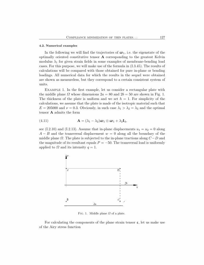
Next, we calculate the components of ω1 by (I.3.45) and we substituteaij = (ω1)ij , i, j = 1, 2, in (4.10), thus obtaining the formula for the trajec-tories corresponding to the eigenvalues of ω1, see Fig. 2.

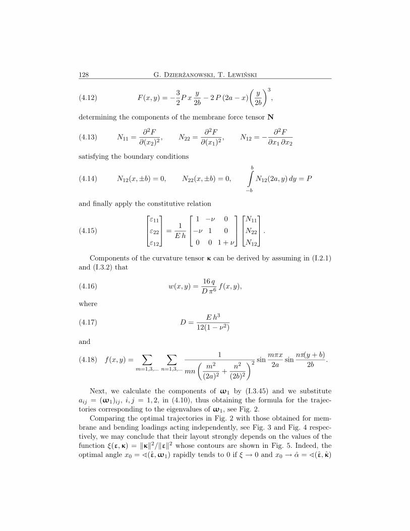
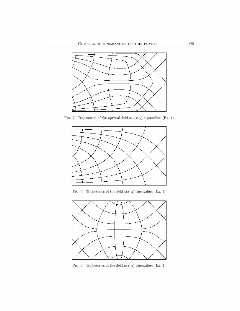
Comparing the optimal trajectories in Fig. 2 with those obtained for mem-brane and bending loadings acting independently, see Fig. 3 and Fig. 4 respec-tively, we may conclude that their layout strongly depends on the values of thefunction ξ(ε,κ) = ‖κ‖2/‖ε‖2 whose contours are shown in Fig. 5. Indeed, theoptimal angle x0 = ∢(ε,ω1) rapidly tends to 0 if ξ → 0 and x0 → α = ∢(ε, κ)


Fig. 2. Trajectories of the optimal field ω1(x, y) eigenvalues (Ex. 1).

Fig. 3. Trajectories of the field ε(x, y) eigenvalues (Ex. 1).

Fig. 4. Trajectories of the field κ(x, y) eigenvalues (Ex. 1).


Fig. 5. Contours ξ(ε, κ) = 0.2, ξ(ε, κ) = 1 and ξ(ε, κ) = 5, with ξ < 0.2 and ξ > 5,corresponding to white and black respectively (Ex. 1).

Fig. 6. Family of functions determining | cos x0| for varying values of ξ.

if ξ → +∞, see Fig. 6, where the lines corresponding to the varying valueξ ∈ [0,+∞) determine a set of plots

(4.19) | cosx0| =

√2

2

(

1 + φ(ξ, t) + ψ(ξ, t)√

ξ t)1/2


where t = cos α and

φ(ξ, t) = (1 − ξ)(

(1 − ξ)2 + 4ξt2)−1/2

,(4.20)

ψ(ξ, t) = 2√

ξ t(

(1 − ξ)2 + 4ξt2)−1/2

,(4.21)

see (I.3.50).

Example 2. Next, assume that the plate in Fig. 1 is subjected to the in-planeboundary conditions u1(0, 0) = u2(0, 0) = 0 and u2(2a, 0) = 0. The transversaldisplacement w = 0 along all the boundary of the middle plane and ∂w/∂n = 0along the edges A − D and B − C. Let p2 and q respectively denote the in-plane and transversal loadings uniformly applied to Ω. In what follows we setp2 = q = −10.

The Airy stress function assumed as

(4.22) F (x, y) = − 1

20

p2 y

b2

(

5 b2 (x− a)2 − 5 y2x (x− 2 a) − y2(

2 b2 − y2)

)

satisfies the boundary conditions

(4.23)

b∫

−b

N11(0, y) dy = 0,

b∫

−b

N11(0, y) dy = 0,

b∫

−b

yN11(0, y) dy = 0,

b∫

−b

yN11(2a, y) dy = 0,

b∫

−b

N12(0, y) dy = −2p2ab,

b∫

−b

N12(2a, y) dy = 2p2ab,

N12(x,±b) = 0, N22(x,±b) = 0,

and the components of a strain tensor ε are determined by making use of (4.13)and (4.15).

Next we calculate the curvature tensor representation by (I.2.1), (I.3.2) and

(4.24) w(x, y) =2qa4

3D

((

x

2a

)

− 2

(

x

2a

)3

+

(

x

2a

)4)

+ f(x, y),

where

(4.25) f(x, y) =2 q

D a

∑

m=1,3,...

1

(αm)5

[

2 sinh(αmb)

sinh(2αmb) + 2αmbαmy sinh(αmy)

−(

1 +2αmb sinh2(αmb)

sinh(2αmb) + 2αmb

)

cosh(αmy)

cosh(αmb)

]

and αm = (mπ)/(2a).


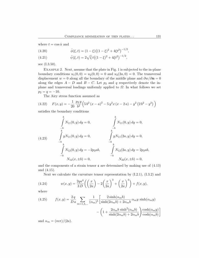
Fig. 7. Trajectories of the optimal field ω1(x, y) eigenvalues (Ex. 2).

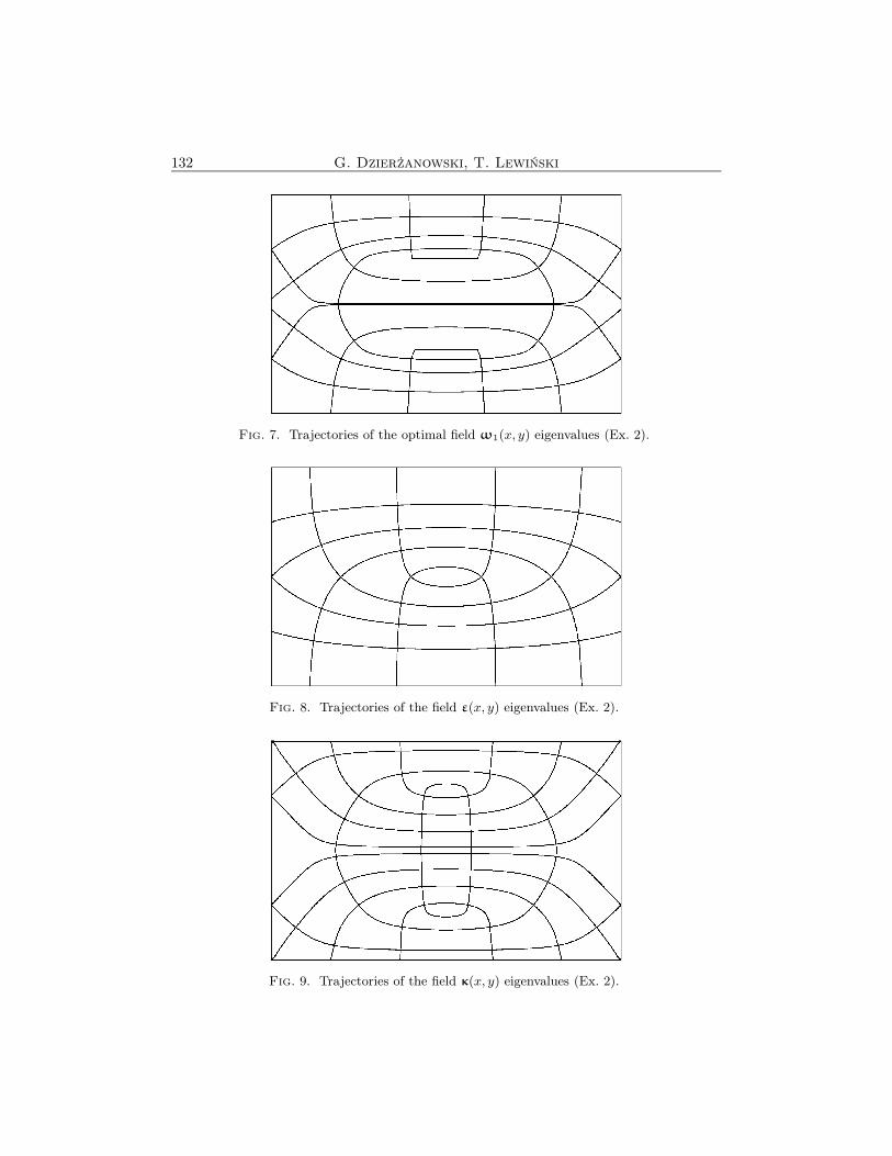
Fig. 8. Trajectories of the field ε(x, y) eigenvalues (Ex. 2).

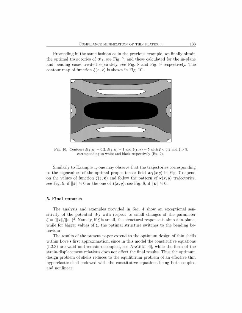
Fig. 9. Trajectories of the field κ(x, y) eigenvalues (Ex. 2).


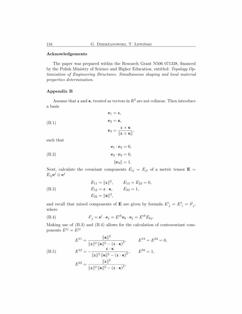
Proceeding in the same fashion as in the previous example, we finally obtainthe optimal trajectories of ω1, see Fig. 7, and these calculated for the in-planeand bending cases treated separately, see Fig. 8 and Fig. 9 respectively. Thecontour map of function ξ(ε,κ) is shown in Fig. 10.

Fig. 10. Contours ξ(ε, κ) = 0.2, ξ(ε, κ) = 1 and ξ(ε, κ) = 5 with ξ < 0.2 and ξ > 5,corresponding to white and black respectively (Ex. 2).

Similarly to Example 1, one may observe that the trajectories correspondingto the eigenvalues of the optimal proper tensor field ω1(x y) in Fig. 7 dependon the values of function ξ(ε,κ) and follow the pattern of κ(x, y) trajectories,see Fig. 9, if ‖ε‖ ≈ 0 or the one of ε(x, y), see Fig. 8, if ‖κ‖ ≈ 0.

5. Final remarks

The analysis and examples provided in Sec. 4 show an exceptional sen-sitivity of the potential Wλ with respect to small changes of the parameterξ = (‖κ‖/‖ε‖)2. Namely, if ξ is small, the structural response is almost in-plane,while for bigger values of ξ, the optimal structure switches to the bending be-haviour.

The results of the present paper extend to the optimum design of thin shellswithin Love’s first approximation, since in this model the constitutive equations(I.2.3) are valid and remain decoupled, see Naghdi [6], while the form of thestrain-displacement relations does not affect the final results. Thus the optimumdesign problem of shells reduces to the equilibrium problem of an effective thinhyperelastic shell endowed with the constitutive equations being both coupledand nonlinear.


Acknowledgements

The paper was prepared within the Research Grant N506 071338, financedby the Polish Ministry of Science and Higher Education, entitled: Topology Op-

timization of Engineering Structures. Simultaneous shaping and local material

properties determination.

Appendix B

Assume that ε and κ, treated as vectors in R3 are not colinear. Then introduce

a basis

e1 = ε,

e2 = κ,

e3 =ε × κ

‖ε × κ‖ ,(B.1)

such that

e1 · e3 = 0,

e2 · e3 = 0,

‖e3‖ = 1.

(B.2)

Next, calculate the covariant components Eij = Eji of a metric tensor E =Eije

i ⊗ ej

(B.3)

E11 = ‖ε‖2, E13 = E23 = 0,

E12 = ε · κ, E33 = 1,

E22 = ‖κ‖2,

and recall that mixed components of E are given by formula Eij = Ej

i = δij ,

where

(B.4) δij = ei · ej = Eikek · ej = EikEkj .

Making use of (B.3) and (B.4) allows for the calculation of contravariant com-ponents Eij = Eji

E11 =‖κ‖2

‖ε‖2 ‖κ‖2 − (ε · κ)2, E13 = E23 = 0,

E12 = − ε · κ‖ε‖2 ‖κ‖2 − (ε · κ)2

, E33 = 1,(B.5)

E22 =‖ε‖2

‖ε‖2 ‖κ‖2 − (ε · κ)2,


and co-basis vectors ei = Eij ej

e1 = E11 e1 +E12 e2

=‖κ‖2

‖ε‖2 ‖κ‖2 − (ε · κ)2ε − ε · κ

‖ε‖2 ‖κ‖2 − (ε · κ)2κ,

e2 = E21 e1 +E22 e2

= − ε · κ‖ε‖2 ‖κ‖2 − (ε · κ)2

ε +‖ε‖2

‖ε‖2 ‖κ‖2 − (ε · κ)2κ,

e3 = E33 e3 =ε × κ

‖ε × κ‖ .

In this notation, the mixed representation of E can be expressed by

(B.6) E = δij ei ⊗ ei.

References

1. A. Blinowski, J. Ostrowska-Maciejewska, J. Rychlewski, Two-dimensionalHooke’s tensors-isotropic decomposition, effective symmetry criteria, Arch. Mech., 48,325–345, 1996.

2. S. Czarnecki, T. Lewiński, The stiffest designs of elastic plates. Vector optimizationfor two loading conditions, Comp. Meth. Appl. Mech. Engrg., 200, 1708–1728, 2011.

3. G. Dzierżanowski, T. Lewiński, Compliance minimization of thin plates made of ma-terial with predefined Kelvin moduli. Part I. Solving the local optimization problem, Arch.Mech., 64, 21–40, 2012.

4. I. Ekeland, R. Temam, Convex Analysis and Variational Problems, North Holland,Amsterdam, 1976.

5. G.J. Minty, On the monotonicity of the gradient of a convex function, Pac. J. Math.,14, 243–247, 1964.

6. P.M. Naghdi, Foundations of elastic shell theory, [in:] Progress in Solid Mechanicsvol. IV, I.N. Sneddon, R. Hill (Eds.), North-Holland, Amsterdam, 1963.

7. R.T. Rockafellar, Convex Analysis, Princeton University Press, Princeton, 1970.

8. J. Rychlewski, On Hooke’s Law, Prikl. Mat. Mech., 48, 420–435, 1984 [in Russian].

Received January 21, 2011; revised version June 9, 2011.

Documents

Compliance minimization of thin plates made of material with