________________________________________________________

Composite Analysis of Atmospheric Bores during PECAN

Observed by Ground-Based Profiling Systems

________________________________________________________

David M. Loveless

A thesis submitted in partial fulfillment of

the requirements for the degree of

MASTER OF SCIENCE

(Atmospheric and Oceanic Sciences)

at the

UNIVERSITY OF WISCONSIN-MADISON

2017

Thesis Declaration and Approval I, David M. Loveless, declare that this thesis titled ‘Composite Analysis of Atmospheric Bores during PECAN

Observed by Ground-Based Profiling Systems’ and the work presented in it are my own.

David M. Loveless __________________________ _______________ Author Signature Date

I hereby approve and recommend for acceptance this work in partial fulfillment of the requirements for the

degree of Master of Science:

Steven A. Ackerman __________________________ _______________ Committee Chair Signature Date Jonathan Martin __________________________ _______________ Faculty Member Signature Date Ankur Desai __________________________ _______________ Faculty Member Signature Date

i

Abstract The Plains Elevated Convection At Night (PECAN) field project took place from 1

June to 15 July 2015 in the central Great Plains of the United States. As part of the project, a

vast suite of instrumentation was deployed that including mobile Doppler radars, aircraft, and

six fixed profiling sites and four mobile profiling units with high-temporal resolution

thermodynamic and kinematic profiling capabilities. The campaign focused on observations

of nocturnal elevated convection and phenomena thought to be mechanisms responsible for

the initiation and maintenance of elevated convective initiation. Atmospheric bores were a

focal point of intensive observation periods during the PECAN campaign, providing a

database of numerous bore passages.

Previous observational studies focused on bores in the context of a single case study,

which are typically extraordinary examples. Atmospheric Emitted Radiance Interferometer

(AERI) thermodynamic profiling at eight of the ten profiling platforms, combined with the

numerous bore passages observed during the PECAN campaign, allows for a unique

opportunity to combine multiple bore observations onto a uniform time and height grid. This

composite analysis is created using the observations of bore passages to document changes to

the boundary layer, with relevance to the convective initiation problem. This study combines

all bores, not only extraordinary cases, into a single analysis to determine typical

characteristics of bore passages.

The composite reveals a bore like structure, surface pressure jump, lower-

tropospheric cooling along with an updraft at the time of the bore, which gives confidence to

the methodology. Maximum composite mean quasi-permanent parcel displacements are on

ii

the order of 700 m, similar to observations in previous case studies. Time series of composite

mean convective indices are calculated. Convective Inhibition (CIN) and the Level of Free

Convection (LFC) is shown to decrease with the bore passage, while Convective Available

Potential Energy (CAPE) is shown to decrease. Results suggest that bores increase the

potential for convective initiation in the post-bore environment, but may cause convection to

be less intense than if convection occurred in a pre-bore environment.

iii

Acknowledgements Formally, I have to acknowledge that this thesis research is supported by National

Science Foundation (NSF) grant number 1359614 "Collaborative Research: Low-level Jets in

the Nocturnal Stable Boundary Layer: Structure, Evolution, and Interactions with Mesoscale

Atmospheric Disturbances”. However, there are countless individuals who have helped me to

finish this work and this degree, whether directly helping me with this project or convincing

me the world is not ending because I messed something up and generally helping me to keep

my life in order.

Being able to be get out in the field on a project like PECAN was amazing and I am

so grateful to everyone at SSEC for giving me the opportunity to have that experience. To

everyone who I got to enjoy being out in the field with, thank you for those moments, there

are memories that I will keep with me forever.

To Nadia, thank you for getting me spun up on the PECAN project and for helping

me to get acclimated to this new graduate school environment. To Tim, for all the discussion

and guidance and patience with me throughout this project. To Steve, for academic advising

and additional discussion on this project. To Ankur and Jon for their comments to help

improve this project.

To all my Oneonta friends, thank you for your support and encouragement, even

though we are hundreds to thousands of miles apart now. To Alex, Kate, Keiko, and Luke for

all those moments of our first year when we didn’t think we would make it but we still

managed to push each other through. To my officemates (past and present), thank you for

making it so much fun to come to school/work (I still don’t know what to call it) every day.

iv

To Skylar for ensuring there was never a dull moment in the last 2 years. To Michelle, thank

you for our walks together, for our meals together, for always supporting me, for being

someone I could walk with and grow in my faith with, and for being my best friend. Lastly to

my family, I cannot thank you enough for all the support and love you have given me. I

would never be writing this today without you all.

v

Table of Contents Abstract ..................................................................................................................................... i

Acknowledgements ................................................................................................................ iii Table of Contents .................................................................................................................... v

List of Figures ......................................................................................................................... vi I. Introduction ...................................................................................................................... 1

II. Atmospheric Bores ......................................................................................................... 5 III. Plains Elevated Convection At Night (PECAN) ....................................................... 14

IV. Instrumentation .............................................................................................................. 21 A. Atmospheric Emitted Radiance Interferometer (AERI) ....................................... 21 B. Wind Profilers ............................................................................................................ 22

V. AERIoe Retrieval Method ............................................................................................ 25

VI. Evaluating AERIoe Observations of Bore Passages ................................................ 30 VII. Composite Analysis .................................................................................................... 41

A. Developing the Composite ......................................................................................... 42 B. Composite Analysis Results ...................................................................................... 43 C. Convective Indices ..................................................................................................... 50

VIII. Case Study Comparison ........................................................................................... 61

IX. Summary and Conclusions ......................................................................................... 68 References .............................................................................................................................. 71

vi

List of Figures Figure 2.1: Schematic vertical cross-section of thunderstorm outflow, a type of gravity

current. (Adapted from Droegemeier and Wilhelmson 1987). .......................................... 6 Figure 2.2: Rottman and Simpson (1989) experimental design. Gravity current (salt water) is

hatched, stable layer (freshwater) is stippled. (Adapted from Rottman and Simpson 1989). ............................................................................................................................................ 6  

Figure 3.1: PECAN study domain, along with locations of WSR-88D radars, S-POL radar

and fixed profiling (FP) sites. Figure from the PECAN Operations Plan (available at: https://www.eol.ucar.edu/node/5784). ............................................................................. 15

Figure 3.2: 0.5° base reflectivity observed at Vance Air Force Base, Oklahoma (VNX) at

0557 UTC on 12 June 2015. Bore is seen as what is called a “fine line” ahead of the approaching MCS. ............................................................................................................ 17  

Figure 4.1: Example of AERI observed radiances with 0.5 cm-1 resolution observed at 2100

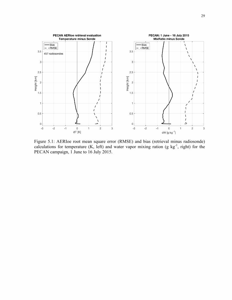
UTC in Hays, Kansas. ...................................................................................................... 22   Figure 5.1: AERIoe root mean square error (RMSE) and bias (retrieval minus radiosonde)

calculations for temperature (K, left) and water vapor mixing ration (g kg-1, right) for the PECAN campaign, 1 June to 16 July 2015. ..................................................................... 29  

Figure 6.1: AERIoe retrieved potential temperature time-height cross-section from FP4 in

Minden, NE from 20 June 2015 from 1000 UTC to 1600 UTC. Potential temperature is shaded, with isentropes outlined and labeled every 3 K. The bore start time is 1155 UTC, denoted by the black arrow. ............................................................................................. 31

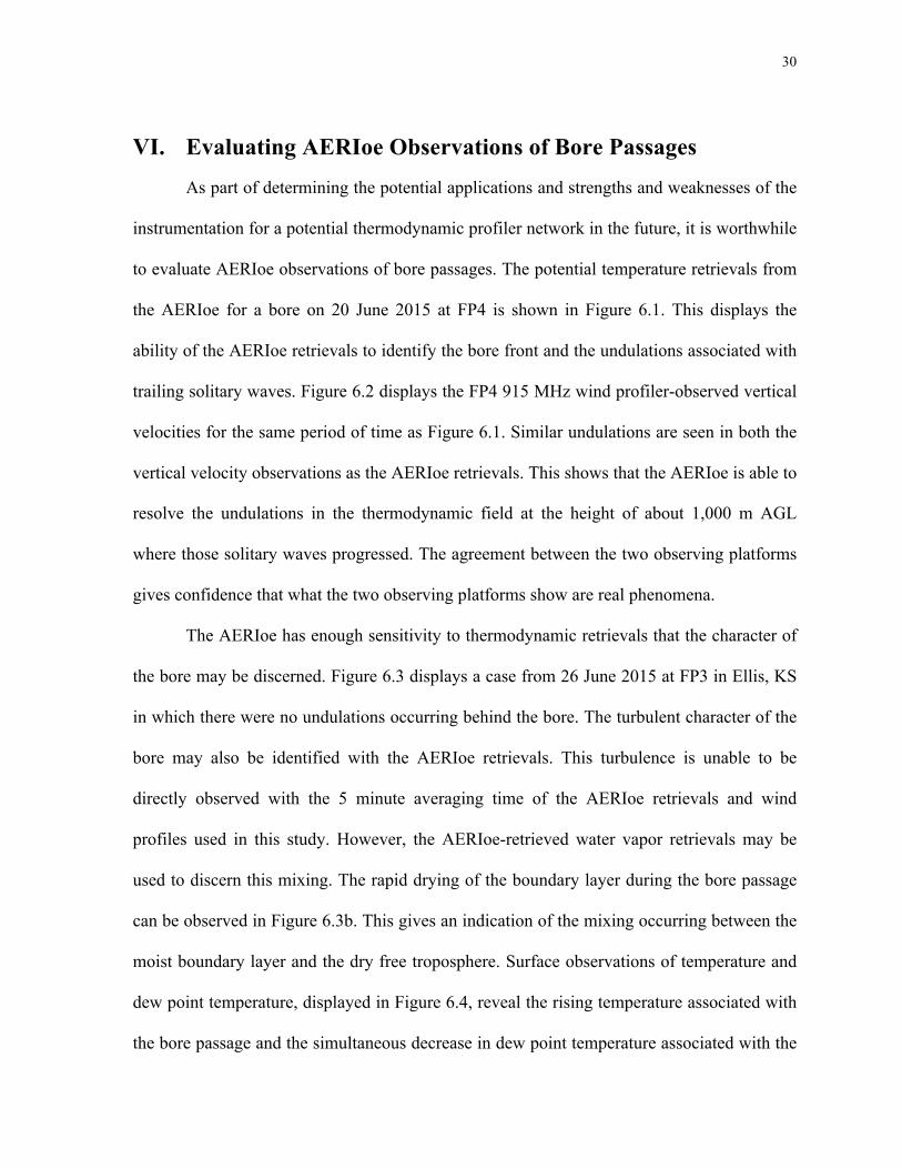
Figure 6.2: 915 MHz wind profiler retrieved 10 minute averaged vertical velocity with a 5

minute update cycle from 10 UTC to 16 UTC at FP4 on 20 June 2015. The bore start time is 1155 UTC, denoted by the black arrow. ............................................................... 32

Figure 6.3: AERIoe retrieved a) potential temperature and b) water vapor mixing ratio time-

height cross-section from FP3 in Ellis, KS from 26 June 2015 from 0200 UTC to 0700 UTC. Potential temperature and water vapor mixing ratio is shaded, with isentropes and isohumes outlined and labeled every 3 K and 3 g kg-1. The bore start time is 0455 UTC, denoted by the black arrows. There are no retrievals between 0615 and 0650 UTC due to rain. ................................................................................................................................... 33

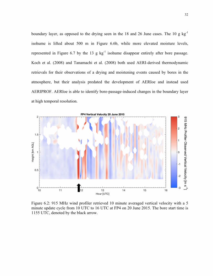
Figure 6.4: Surface temperature and dew point temperature [°C] from 00 to 08 UTC at FP3 in

Ellis, KS on 26 June 2015. The bore start time is 0455 UTC, denoted by the black arrow. .......................................................................................................................................... 34

vii

Figure 6.5: AERIoe retrieved a) potential temperature and b) water vapor mixing ratio time-height cross-section from FP3 in Ellis, KS from 18 June 2015 from 1200 UTC to 1600 UTC. Potential temperature and water vapor mixing ratio is shaded, with isentropes and isohumes outlined and labeled every 3 K and 3 g kg-1. The bore start time is 1355 UTC, denoted by the black arrows. ............................................................................................ 35

Figure 6.6: AERIoe retrieved a) potential temperature and b) water vapor mixing ratio time-

height cross-section from FP3 in Ellis, KS from 7 June 2015 from 0100 UTC to 0700 UTC. Potential temperature and water vapor mixing ratio is shaded, with isentropes and isohumes outlined and labeled every 3 K and 3 g kg-1. The bore start time is 0430 UTC, denoted by the black arrows. ............................................................................................ 38

Figure 6.7: Radiosonde temperature (thin, red) and dew point temperature (thin, teal)

comparison with AERIoe retrieved temperature (thick, red) and dew point temperature (thick, teal) skew-T/log-P graph for a pre-bore radiosonde on 26 June 2015 from MP3 (SPARC). Pre-bore inversion is located around 925 hPa, highlighted by the arrow. ...... 39

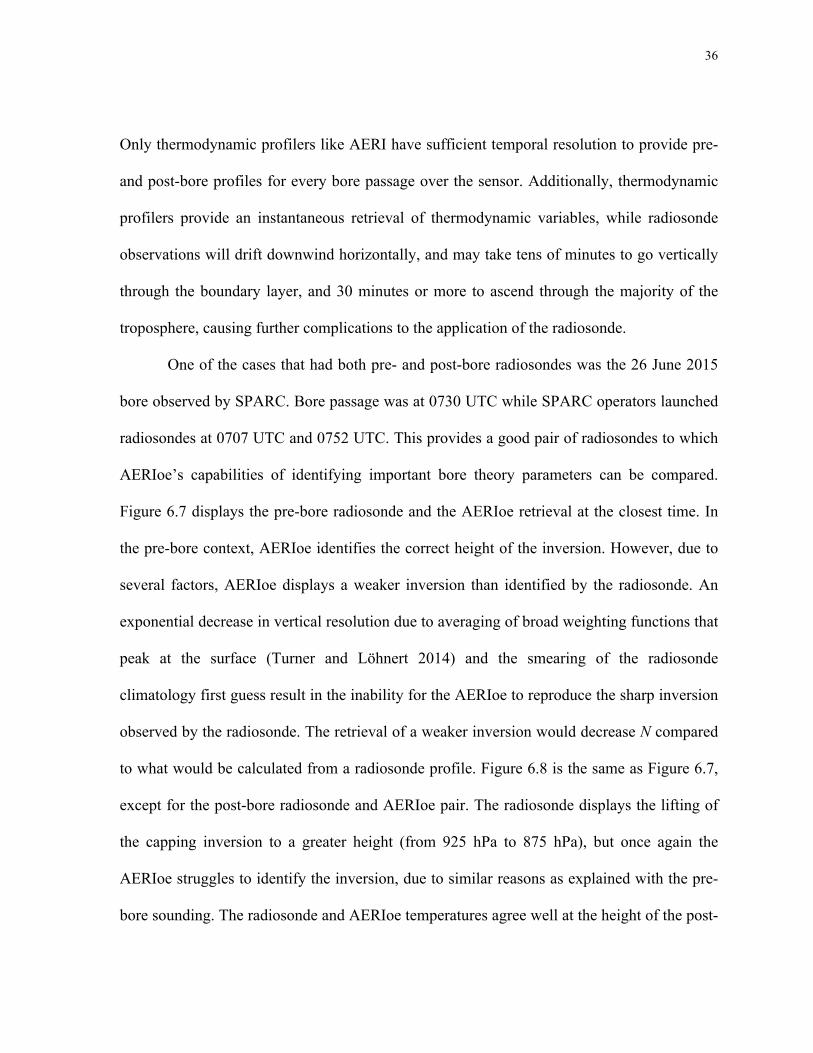
Figure 6.8: Radiosonde temperature (thin, red) and dew point temperature (thin, teal)

comparison with AERIoe retrieved temperature (thick, red) and dew point temperature (thick, teal) skew-T/log-P graph for a post-bore radiosonde on 26 June 2015 from MP3 (SPARC). Post-bore inversion is lifted to around 875 hPa, highlighted by the arrow. Near-surface inversion is a result of the gravity current arriving at the time of the radiosonde launch. ............................................................................................................ 40  

Figure 7.1: Composite mean change in potential temperature with time averaged over the 0.2

km to 1.0 km layer (plotted in black, left axis) and composite mean vertical velocity averaged over the 0.2 km to 1.0 km layer (plotted in red, right axis). ............................. 44

Figure 7.2: Composite mean AERIoe potential temperature retrieval. Isentropes labeled every

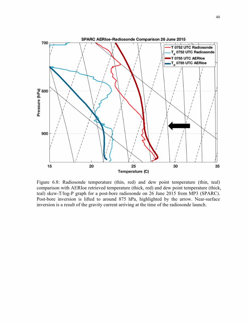
3 K. ................................................................................................................................... 45 Figure 7.3: Composite mean surface temperature (red) and dew point temperature (blue). .. 46 Figure 7.4: Pre-bore and post-bore surface temperature and dew point temperature are

averaged over the course of 1-hour prior to and after the bore, respectively. Differences are calculated taking post-bore variable average minus pre-bore variable average such that a positive change means that the bore is observed to induce an increase in the respective variable with its passage. Box edges are at the first quartile and third quartile, with median value plotted with a horizontal line, whiskers extend to the minimum and maximum of the sample. .................................................................................................. 46

Figure 7.5: Composite mean vertical velocity as measured by 449, 915 MHz wind profilers

and Doppler lidars. ........................................................................................................... 48 Figure 7.6: Composite mean surface pressure. ....................................................................... 48

viii

Figure 7.7: Composite mean horizontal wind speed as measured by 449, 915 MHz wind

profilers and Doppler lidars. ............................................................................................. 49 Figure 7. 8: Composite mean AERIoe retrieved water vapor. Isohumes labeled every 1 g kg-1.

.......................................................................................................................................... 50 Figure 7.9: Composite mean time series of surface-based (solid line) and most-unstable

parcel (dashed line) convective available potential energy (CAPE) relative to bore passage time. .................................................................................................................... 53

Figure 7.10: As in Figure 7.9 but for CIN. ............................................................................. 54 Figure 7.11: As in Figure 7.9 but for LCL height. .................................................................. 55 Figure 7.12: As in Figure 7.9 but for LFC height. .................................................................. 56 Figure 7.13: Pre-bore (0707 UTC, thin, light lines) and post-bore (0752 UTC, thick, dark

lines) SPARC radiosondes on 26 June 2015. Bore occurred at 0735 UTC. Temperature is plotted in red, dew point temperature plotted in teal. Post-bore radiosonde has a near-surface inversion due to the arrival of the bore’s parent gravity current at the time of the radiosonde launch. ............................................................................................................ 57

Figure 7.14: As in Figure 7.4 but for SBCAPE, MUCAPE, SBCIN, and MUCIN. .............. 59 Figure 7.15: As in Figure 7.4 except for SBLCL, MULCL, SBLFC, and MULFC height. ... 59   Figure 8.1: SBCAPE (solid line) and MUCAPE (dashed line) for a bore on 21 June 2015 at

FP4 (red line) and 26 June 2015 over FP3 (blue line). Time shown is relative to the time of the bore, using the bore start time algorithm from section 7A. The 21 June FP4 bore occurred at 1150 UTC, and the 26 June FP3 bore occurred at 0455 UTC. ...................... 62

Figure 8.2: As in Figure 8.1 but for CIN instead of CAPE. Note: CIN is undefined when

CAPE is zero. Large spikes in MUCIN for the 21 June case prior to the bore are likely due to noise in the AERIoe retrievals resulting in particularly large changes in the most-unstable parcel. ................................................................................................................. 63

Figure 8.3: As in Figure 8.1 but for LCL height instead of CAPE. Large spikes in MULCL

for the 21 June case prior to the bore are likely due to noise in the AERIoe retrievals resulting in particularly large changes in the most-unstable parcel. ................................ 64

Figure 8.4: As in Figure 8.1 but for LFC height instead of CAPE. LFC is not available when

CAPE is zero. ................................................................................................................... 65

ix

Figure 8.5: AERIoe retrieved a) potential temperature and b) water vapor mixing ratio time-height cross-section from FP4 in Minden, NE from 21 June 2015 from 0900 UTC to 1400 UTC. Potential temperature and water vapor mixing ratio is shaded, with isentropes and isohumes outlined and labeled every 3 K and 3 g kg-1. The bore start time is 1150 UTC, denoted by the black arrows. .................................................................................. 66

Figure 8.6: AERIoe retrieved a) potential temperature and b) water vapor mixing ratio time-

height cross-section from FP3 in Ellis, KS from 26 June 2015 from 0200 UTC to 0700 UTC. Potential temperature and water vapor mixing ratio is shaded, with isentropes and isohumes outlined and labeled every 3 K and 3 g kg-1. The bore start time is 0455 UTC, denoted by the black arrows. There are no retrievals between 0615 and 0650 UTC due to rain. ................................................................................................................................... 67  

x

List of Tables Table 1: Overview of PISA thermodynamic and kinematic profiling instrumentation. Fixed

PISA (FP) locations correspond with FP locations in Figure 3.1, mobile profiling units (MP) had different observing locations for each intensive observing period. ................. 18

Table 2: Uncertainties associated with each radiosonde type included in the AERIoe to

radiosonde evaluation. Radiosonde information can be found at: International Met Systems (2006) and Vaisala (2013, 2016). ...................................................................... 28

Table 3: List of bores included in this study. .......................................................................... 42  

1

I. Introduction Convective weather accounts for up to 70% of warm season (April – September)

precipitation in the central Great Plains of the United States (Fritsch et al. 1986). Many of

these locations have a well-documented nocturnal maximum in convective precipitation

(Wallace 1975, Heideman and Fritsch 1988, Colman 1990). Mesoscale convective systems

(MCS), a large cluster of multicellular thunderstorms that produce a continuous precipitation

area greater than 100 km (a commonly used definition noted by Houze 2004), are generally

the primary producer of this nocturnal precipitation in the plains states (Fritsch et al. 1986,

Heidman and Fritsch 1988, Houze 2004). The prominence of MCSs in producing flash floods

has been shown in both Maddox et al. (1979) and Ashley and Ashley (2008). Ashley and

Ashley (2008) found that MCSs were responsible for 36% of all flood fatalities in the United

States from 1996 to 2005.

MCSs, and nocturnal convection in general, occur with a stable surface layer and

elevated instability. Radiational cooling of the surface at night creates a stable nocturnal

boundary layer. As a result, convection is elevated, or decoupled from the surface, which

means that observed convection consists of rising parcels that originate above the nocturnal

stable boundary layer. Because of this, traditional daytime triggers for convection, like

differential diabatic heating, have limited application to the problem of elevated convection.

Several potential mechanisms exist with respect to explaining the initiation and

maintenance of such elevated convective systems. Tripoli and Cotton (1989a, 1989b) suggest

that gravity waves created by outflow from daytime convection in the Rocky Mountains play

a role in triggering elevated convection in the Plains. Raymond and Jiang (1990) used

2

numerical simulations to show the development of a mid-level potential vorticity (PV)

anomaly, due to modifications to the temperature profile through persistent convection. This

PV anomaly would be self-sustaining by generating additional lift ahead of or downshear of

the anomaly and descent behind the anomaly, thus maintaining the convection and

temperature profile modification to maintain and strengthen the PV anomaly. The nocturnal

low-level jet (LLJ) is also important in transporting high equivalent potential temperature

(θe) air from the Gulf of Mexico region into the MCS region in the Plains (Pu and Dickinson

2014). Tuttle and Davis (2006) found that MCSs are often found at the northern end of the

LLJ, a region associated with low-level convergence due to the decelerating flow.

An additional mechanism is the atmospheric bore, which is a type of gravity wave

that forms as a result of the interaction between a stable boundary layer and dense

evaporationally cooled air from thunderstorm outflow (e.g. Rottman and Simpson 1989,

Haase and Smith 1989). Model simulations of MCS-like systems by Parker (2008) suggest

that atmospheric bores play an important role in maintaining convection as the instability

becomes elevated. Numerous studies of individual bores (e.g. Weckwerth et al. 2004, Knupp

2006, Koch et al. 2008) have observed vertical parcel displacements of 200 m or greater as a

bore passes. Many studies have also observed convective initiation associated with a bore

passage (Karyampudi et al. 1995, Locatelli et al. 2002, Wilson and Roberts 2006, Koch et al.

2008, Coleman and Knupp 2011). A commonly held hypothesis is that a bore propagating

ahead of the MCS will either destabilize the boundary layer or initiate convection on its own,

generating new thunderstorm cells and contributing to the maintenance of the MCS (Parker

2008). The present study investigates the potential effects of bores with respect to

maintenance and initiation of convection using a composite analysis of numerous bore events.

3

Because elevated convection is decoupled from the surface, it is difficult to observe

processes occurring with respect to the initiation and maintenance of the convective activity

without vertical profiles. Radiosondes provide accurate in-situ profiles of temperature and

moisture above the surface; however, radiosonde stations are separated generally by more

than 500 km across the Plains states, and are only launched twice per day: 2300 and 1100

UTC (for 0000 and 1200 UTC numerical weather prediction assimilation cycles,

respectively). Meanwhile, in the United States, almost the entire life cycle of nocturnal

convection occurs during the period between 0000 and 1200 UTC. Thus, the radiosonde

network is extremely limited in capturing these proposed mechanisms for initiating and

sustaining elevated nocturnal convection. The Plains Elevated Convection At Night (PECAN,

Geerts et al. 2017) field campaign, which took place during the summer of 2015, deployed a

wide variety of fixed and mobile observing systems to study these mechanisms. An

additional theme of the PECAN campaign was to provide a testbed for a network of

thermodynamic and kinematic profilers in light of the National Research Council’s (NRC)

report in 2009 highlighting the need for a network that provides high-temporal resolution

thermodynamic and kinematic profiling of the boundary layer. A major feature of the

PECAN project (to be described further in the following section) was the creation and

utilization of an integrated sounding array of mobile and fixed observing platforms.

In this study, the ability of the instrumentation to observe bores will be qualitatively

assessed through the investigation of multiple cases. Additionally, the potential effects of

bores on destabilizing the boundary layer will be assessed in order to better understand the

role they have in the initiation and maintenance of elevated convection. To evaluate how the

boundary layer typically responds to bore passages, a composite analysis of bore events,

4

observed during the PECAN campaign, will be created. While previous studies have

investigated single events (eg. Koch et al. 1991, Koch and Clark 1999, Knupp 2006,

Coleman and Knupp 2011), the present study is the first to use uniform instrumentation and

methodology to composite bores on a uniform time and height scale.

5

II. Atmospheric Bores A gravity, or density current is the flow of a denser fluid beneath a less dense fluid as

a result of the difference in density between the two fluids in a system (Simpson 1982).

Thunderstorm outflow, cold pools, and sea breezes are typical gravity currents in the

atmosphere, while salt water moving upriver during high tide in a coastal estuary is a typical

form of a gravity current in ocean environments. Figure 2.1 displays a schematic diagram of

thunderstorm outflow as an example of the flows associated with the leading edge of gravity

currents. Internal bores are a type of gravity wave that form as a result of the interaction

between a gravity current and a stable fluid of lesser density which results in partially

blocked flow and allows the hydraulic jump, or bore, to form. In this partially blocked flow,

the gravity current is the object “blocking” the flow of the stable less dense fluid. In order for

the flow to be partially-blocked, the depth of the gravity current must be less than the depth

of the stable fluid.

Rottman and Simpson (1989) developed much of the hydraulic theory associated with

internal bores, using a laboratory experiments in a water channel to create an idealized two

layer model. Using methods originally developed by Wood and Simpson (1984), their

experiment consisted of towing a thin, rounded object along the bottom of the water channel

to generate a bore on the surface of the fluid. In this model, the water channel is the bottom

layer and represents a stable boundary layer in the atmosphere while the air is the top layer

and represents air above the stable boundary layer in the atmosphere. They also performed a

second set of experiments, replacing their rounded object with releases of salt water into their

two-layer channel, which simulated a gravity current (see Figure 2.2). Wood and Simpson

(1984) note that the character of the bore depends on the bore strength, the ratio h1/h0, where

6

h1 is the maximum depth of the fluid (crest of the hydraulic jump), and h0 is the depth of the

fluid before the bore passage (Rottman and Simpson 1989). In Figure 2.2, the salt water is

the gravity current and the bore is induced ahead of the gravity current. In the context of the

atmosphere, the bore would be initiated ahead of where an outflow boundary is traveling.

Figure 2.1: Schematic vertical cross-section of thunderstorm outflow, a type of gravity current. (Adapted from Droegemeier and Wilhelmson 1987).

Figure 2.2: Rottman and Simpson (1989) experimental design. Gravity current (salt water) is hatched, stable layer (freshwater) is stippled. (Adapted from Rottman and Simpson 1989).

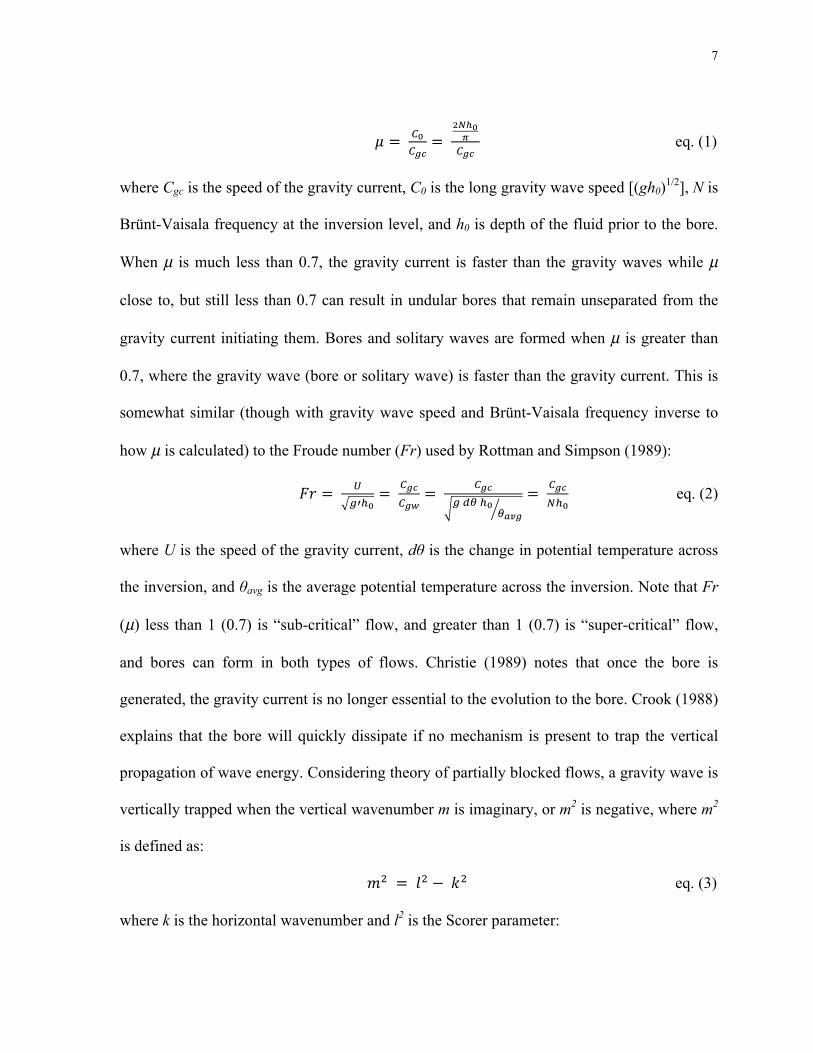
Haase and Smith (1989) ran numerical simulations of bores and used a non-

dimensional number µ to determine if bores will form, defined as:

7

𝜇 =   !!!!"

=  !!!!!!!"

eq. (1)

where Cgc is the speed of the gravity current, C0 is the long gravity wave speed [(gh0)1/2], N is

Brünt-Vaisala frequency at the inversion level, and h0 is depth of the fluid prior to the bore.

When µ is much less than 0.7, the gravity current is faster than the gravity waves while µ

close to, but still less than 0.7 can result in undular bores that remain unseparated from the

gravity current initiating them. Bores and solitary waves are formed when µ is greater than

0.7, where the gravity wave (bore or solitary wave) is faster than the gravity current. This is

somewhat similar (though with gravity wave speed and Brünt-Vaisala frequency inverse to

how µ is calculated) to the Froude number (Fr) used by Rottman and Simpson (1989):

𝐹𝑟 =   !!!!!

=   !!"!!"

=   !!"!  !"  !!

!!"#

=   !!"!!!

eq. (2)

where U is the speed of the gravity current, dθ is the change in potential temperature across

the inversion, and θavg is the average potential temperature across the inversion. Note that Fr

(µ) less than 1 (0.7) is “sub-critical” flow, and greater than 1 (0.7) is “super-critical” flow,

and bores can form in both types of flows. Christie (1989) notes that once the bore is

generated, the gravity current is no longer essential to the evolution to the bore. Crook (1988)

explains that the bore will quickly dissipate if no mechanism is present to trap the vertical

propagation of wave energy. Considering theory of partially blocked flows, a gravity wave is

vertically trapped when the vertical wavenumber m is imaginary, or m2 is negative, where m2

is defined as:

𝑚!  =   𝑙! −  𝑘! eq. (3)

where k is the horizontal wavenumber and l2 is the Scorer parameter:

8

𝑙!  =   !!

(!!!)!−  

!!!!"!

!!! eq. (4)

in which N is Brünt-Vaisala frequency, C is the speed of a gravity wave (or bore), and U is

the background wind in the direction of the bore propagation. The Scorer parameter will

determine the vertical trapping ability of the atmosphere. If the Scorer parameter decreases

with height, the wave energy will be trapped (Crook 1988). A low-level jet moving in the

opposite direction of bore propagation tends to act as a good trapping mechanism, given the

δ2U/δZ2 term (Crook 1988, Koch et al. 1991, Koch and Clark 1999).

Observational evidence for the existence of atmospheric bores has been observed as

early as Tepper (1950), who found that a squall line correlated with sharp increases in surface

pressure on the order of 2 hPa. He claimed that these pressure jumps were evidence of a

gravity wave propagating along a nocturnal temperature inversion. He proposed that this

gravity wave could be caused by temporary accelerations of the cold front into a low-level

stable layer, which would eventually propagate as a gravity wave downstream into the warm

sector of an extra-tropical cyclone. The idea of an atmospheric bore did not seem to exist at

the time of Tepper (1950), but the conditions observed and hypotheses are consistent with

what are today known as bores.

Since the Tepper (1950) study, bores have frequently been observed when cold air

from thunderstorm outflow interacts with a stable boundary layer (eg: Koch et al. 1991,

Locatelli et al. 1998; Knupp 2006, Koch et al. 2008, Coleman and Knupp 2011). Clarke et al.

(1981) identified the Morning Glory in the Gulf of Carpentaria to be a bore generated by the

interaction between a sea-breeze front and a nocturnal inversion. Wakimoto et al. (1995)

observed the formation of a bore as a result of a sea-breeze front colliding with an outflow

9

boundary. Following the Tepper (1950) hypothesis, cold fronts have also been observed to

act as a gravity current and result in bore formation in the presence of a stable boundary layer

(Koch et al. 1999, Hartung et al. 2010). Atmospheric bores will propagate along the

temperature inversion between the surface stable layer and the weakly stratified free

troposphere (Clarke et al. 1981, Koch et al. 1991, Koch et al. 1999), and will result in lifting

the inversion to a quasi-permanent greater height (Koch et al. 1991, Knupp 2006).

Atmospheric bore passages result in changes to surface conditions. A bore passage

will result in a surface pressure jump to a higher pressure that is sustained for a period of

time and a surface wind shift into the direction from which the bore is coming (Clarke et al.

1981; Smith 1988). The increase in surface pressure is due to the increase in the depth of the

surface layer caused by the bore passage. Surface temperature changes range from negligible

changes (Smith 1988; Mahapatra et al. 1991) to increases in temperature as a result of

adiabatic mixing of warm air at the level of the inversion down to the cooler surface (Clarke

et al. 1981, Koch et al. 1991). Surface drying and cooling will happen with the arrival of the

gravity current following the bore (Koch et al. 1991; Koch and Clark 1999).

The increase in the depth of the surface layer and level of the inversion results in

adiabatic lifting and cooling of the lower troposphere (Koch et al. 1991, Koch et al. 2008).

The magnitude of these displacements is variable, as Weckwerth et al. (2004) observed

vertical parcel displacements between 500 m and 900 m with a bore passage while Knupp

(2006) observed a bore that resulted in vertical parcel displacements up to 2000 m.

Mechanical lifting caused by bore passage frequently results in cloud formation (eg. Clarke

et al 1981, Smith et al. 1982, Knupp 2006, Coleman et al. 2010) and may trigger convective

initiation if the mechanical lifting can lift parcels to their level of free convection (LFC)

10

(Karyampudi et al. 1995, Locatelli et al 2002, Wilson and Roberts 2006, Koch et al. 2008,

Coleman and Knupp 2011). Mechanical lifting and mixing processes with bore passages

have been observed to weaken the capping inversion and destabilize the boundary layer

(Koch et al. 1991, Koch et al. 2008). Coleman and Knupp (2011) used temperature and

moisture retrievals from a microwave profiling radiometer to make time series of convective

available potential energy (CAPE) and convective inhibition (CIN) during a bore passage.

They observed a decrease in surface-based CIN from 180 J kg-1 to 75 J kg-1 with a bore

passage. Additionally, there was an increase in 300 m above ground level (AGL) CAPE from

75 J kg-1 to 300 J kg-1 at the time of the bore passage, which quickly decreased back to values

that were observed in the pre-bore environment. Convective initiation was observed in the

vicinity of this bore and soliton.

The International H2O Project (IHOP_2002) took place in the southern Great Plains

and while its goal was to investigate convective initiation processes in general, it provided

numerous observations of bores in particular. Wilson and Roberts (2006) provided a

summary of convective initiation episodes during IHOP_2002, classifying the episodes based

on their trigger mechanism (fronts, outflow boundaries, drylines, pressure troughs, colliding

boundaries, bores). Out of 112 episodes observed, bores triggered only three of the

convective initiation episodes. While other trigger mechanisms are responsible for more

frequent convective initiation (synoptic fronts and outflow boundaries were responsible for

most of these episodes), individual case studies have shown the role bores can have in major

initiation events. Numerical model simulations by Karyampudi et al. (1995) showed that a

bore originating in the Rocky Mountains was responsible for initiating a severe squall line in

western Kansas and Nebraska. Numerical simulations by Locatelli et al (2002) to study the

11

Super Outbreak storm from 2 – 5 April 1974 suggested that the first damaging squall line of

the system (but not the one that resulted in the most tornadoes) was initiated by an undular

bore. Koch and Clark (1999) showed that lifting from both a bore and gravity current resulted

in initiation of a severe convective event. Model simulations of squall lines by Parker (2008)

suggest that atmospheric bores play an important role in maintaining convection as the

instability becomes elevated.

Rottman and Simpson (1989) found that the turbulent mixing of the bore depended on

the bore strength (h1/ho). Turbulent processes began when bore strength was greater than 2,

with much more vigorous mixing occurring with bore strength greater than 4. Mixing by

bores with strength greater than 4 prevents trailing undulating solitary waves from forming,

thus making the bore have the appearance of a density current (see Figure 2.1). Koch et al.

(2008) used a combination of observations and numerical simulations to show that the

mixing processes of bores may also be tied to the life cycle of the bore. They identified an

“active phase” of the bore, during which turbulent processes are vigorous and the boundary

layer and free troposphere are mixed with each other. Given a sufficiently dry free

troposphere, an active phase bore can result in rapid drying of the boundary layer. Mixing

processes are weaker in the “dissipation stage”, which results in air being well-mixed

throughout the boundary layer due to updrafts and downdrafts caused by the bore passage,

but with minimal mixing between the boundary layer and free troposphere. The dissipation

stage case observed by Koch et al. (2008) resulted in moistening of the boundary layer.

Boundary layer rapid drying and moistening events were observed by Tanamachi et al.

(2008) and concluded to be caused by bore passages.

12

Tepper (1950) used one-minute synoptic maps and time series of surface pressure

observations at various stations to follow pressure jumps that formed ahead of a squall line.

Since then, observational studies of bores have utilized radiosonde soundings (eg. Koch et al.

1991, Koch et al. 2008), photography (Coleman et al. 2010), and ground-based profiling

instruments in addition to surface observations. Knupp (2006), Koch et al. (2008), and

Tanamachi et al. (2008) used AERIs in their observational analysis, similar to what is used in

this analysis, although these older studies used an older and less robust algorithm to retrieve

the thermodynamic profiles. Tanamachi et al. (2008) concluded that water vapor profiles

from instruments such as the AERI could indicate the presence of bores before they trigger

convection.

Again, while atmospheric bores do not result in as frequent convective initiation as

other mechanisms such as fronts or outflow boundaries, they have been shown in many

studies to initiate convection, including playing a role in major severe episodes. One of the

most significant, and surprising, results of the IHOP_2002 campaign was the frequent

presence of bores associated with nocturnal convective events (Weckwerth et al. 2004).

Additionally, their hypothesized importance to the maintenance of mesoscale convective

systems (Parker 2008) suggests further study of these phenomena. This resulted in bores

being one of the focal points in the Plains Elevated Convection At Night project (Geerts et al.

2017, to be described more in the next section).

Current literature on atmospheric bores has been limited to case studies of individual

bores from an observational and/or modeling perspective. This presents a problem, as there is

likely a selection bias that favors extraordinary cases. Additionally, there is no work that

attempts to characterize to the typical changes to the boundary layer with a bore passage in a

13

composite sense. Furthermore, no literature that addresses the difference between bores that

aid in convective initiation, and bores that do not. The present work addresses these

outstanding issues by incorporating a large sample of bores, regardless of their convective

initiation implications, into a single analysis to understand in general what changes a bore

makes to the boundary layer, as opposed to studying a single particularly notable event.

14

III. Plains Elevated Convection At Night (PECAN) The Plains Elevated Convection at Night (PECAN) campaign took place from 1 June

2015 to 15 July 2015 in the Great Plains region of the United States. Figure 3.1 displays the

PECAN study region, extending from southern Nebraska to northern Oklahoma, and from

Colorado to eastern Nebraska, Kansas, and Oklahoma. While this was the intended study

region, observations by mobile platforms during the campaign were made as far east as

Indiana and as far north as South Dakota. PECAN was designed to advance the scientific

understanding and forecast skill of the processes that initiate and maintain nocturnal

convection in the Great Plains. The campaign had four primary focal points: 1) initiation and

early evolution of elevated convection, 2) MCS internal structure and microphysics, 3) the

characterization of bores and other wave-like features, and 4) storm- and MCS-scale

numerical weather prediction. The study region was selected to cover a region that included

frequent low-level jet formation (pink lines in Figure 3.1 denote low-level jet frequency),

mesoscale convective system (MCS) formation (MCS climatology displayed as brown

dashed lines in Figure 3.1), along with frequent convective initiation and bore events.

The campaign was designed to test four overarching hypotheses, which correlate to

the four science objectives. These hypotheses are: 1) Nocturnal convection is more likely to

be initiated and sustained in regions of mesoscale convergence above the stable boundary

layer. 2) The microphysical and dynamical processes involved in the development and

maturing of nocturnal MCSs are critical to their maintenance and growth through the

structure and strength of cold pools, bores, and solitary waves that interact with the stable

boundary layer. 3) Bores and associated wave/solitary disturbances play a significant role in

maintaining or initiating elevated nocturnal MCSs by lifting parcels above the stable

15

boundary layer to their level of free convection. 4) The assimilation of a mesoscale network

of surface, boundary-layer and upper-level measurements into numerical weather prediction

models would significantly improve the prediction of convective initiation, and produce

improvements to the quantitative precipitation forecast (QPF).

Figure 3.1: PECAN study domain, along with locations of WSR-88D radars, S-POL radar and fixed profiling (FP) sites. Figure from the PECAN Operations Plan (available at: https://www.eol.ucar.edu/node/5784).

Previous field campaigns have taken observations that have some relevance to

PECAN science objectives, such as IHOP_2002 (International H2O Project, Weckwerth et al.

2004), BAMEX (Bow Echo and Mesoscale Convective Vortex Experiment, Davis et al.

2004), and MPEX (Mesoscale Predictability Experiment, Weisman et al. 2015). PECAN

differed from these experiments in two fundamental ways: first, it emphasized nocturnal

16

convection and environments; and second, it featured a much more diverse suite of

instrumentation.

Data collection during PECAN came from a set of six fixed observing sites, as well

observations from mobile platforms including profiling units, Doppler radars, mesonets, and

aircraft. The fixed profiling sites (denoted as FP in Figure 3.1) were located throughout the

study region, within 120 km of a S-band radar. While most of the fixed sites were located

within that radius of an operational National Weather Service WSR-88D radar, NCAR’s S-

POL radar was added near Hays, KS to cover a gap in central Kansas in the WSR-88D

network. The 120 km threshold for the S-band radars was determined to place each fixed

profiling site within the clear air return region of one of those radars, a region where outflow

boundaries, bores, solitary waves, and other non-precipitation features may be observed by

the radar returns. Figure 3.2 displays an example of a radar-observed bore in northern

Oklahoma where the bore is seen as what is commonly referred to as a “fine line” within the

clear air return region of the radar. The mobile vehicles and aircraft allowed for local, short

duration observing periods (3-12 hours) in specific regions that were forecasted to be

impacted by a phenomenon related to the science objectives with little advanced notice,

while fixed profiling sites took continuous observations for the entire campaign. In the early

morning hours following a deployment, the mobile units would position themselves

strategically to allow for rapid deployment for the next night’s operations given forecasted

phenomena.

17

Figure 3.2: 0.5° base reflectivity observed at Vance Air Force Base, Oklahoma (VNX) at 0557 UTC on 12 June 2015. Bore is seen as what is called a “fine line” ahead of the approaching MCS.

A novel concept for PECAN compared to previous campaigns was the creation of a

“PECAN Integrated Sounding Array” (PISA). The PISA consists of 10 units, the six fixed

sites and four mobile profiling units, which profile the kinematic and thermodynamic

structure of the lower troposphere. Each PISA facility had surface meteorology observations,

radiosonde launches, and remotely sensed profiles of wind and thermodynamics, although

exact instrumentation varied from one facility to the next. The instrumentation for each of the

profiling units in the PISA is displayed in Table 1. The thermodynamic and kinematic

18

profilers provided high-temporal resolution observations of low-level temperature, moisture,

and the three-dimensional wind field. This allowed for a complete observation of the

evolution of the lower troposphere during the targeted weather events, which enables the

assessment of the evolution of atmospheric stability (CIN, CAPE, etc.), moisture transport,

mesoscale convergence, and the structure and evolution of bores and solitary waves, all at

high temporal resolution. The PISA also serves as a testbed for the national network of

thermodynamic profilers described in the NRC 2009 report.

Table 1: Overview of PISA thermodynamic and kinematic profiling instrumentation. Fixed PISA (FP) locations correspond with FP locations in Figure 3.1, mobile profiling units (MP) had different observing locations for each intensive observing period.

Profiling Unit Location Thermodynamic Profiler(s)

Kinematic Profiler(s)

FP1 Lamont, OK 36.61°N, 97.49°W

AERI MWR

Doppler lidar 915 MHz WP

FP2 Greensburg, KS 37.61°N, 99.28°W

AERI MWR

Doppler lidar

FP3 Ellis, KS 38.96°N, 99.57°W

AERI MWR

Water vapor DIAL

Doppler lidar 449 MHz WP

Sodar FP4 Minden, NE

40.52°N, 98.95°W AERI 915 MHz WP

FP5 Brewster, KS 39.38°N, 101.37°W

AERI 915 MHz WP

FP6 Hesston, KS 38.14°N, 97.44°W

AERI MWR

Doppler lidar

MP1 “CLAMPS”

N/A AERI MWR

Doppler lidar

MP2 “MIPS”

N/A MWR Doppler lidar 915 MHz WP

MP3 “SPARC”

N/A AERI Doppler lidar

MP4 “MISS”

N/A N/A 915 MHz WP

19

Mobile mesonet units were utilized during PECAN to provide additional sources of

surface observations, and mobile GAUS units provided additional radiosonde measurements

to supplement where the PISA did not cover. These units would frequently move during each

intensive observation period in order to capture phenomena of concern as they were

happening. In addition to the fixed radars (WSR-88Ds and S-POL), eight mobile radars were

used with Doppler and dual-polarization capabilities to analyze storm-scale wind fields and

precipitation features in both clear air and precipitating environments. The three aircraft,

University of Wyoming King Air, NOAA P-3, and NASA DC-8, were used to provide

additional temperature, humidity, aerosol, and wind measurements near storm environments,

using a top-down approach. The mobility of the instrumentation allowed for units to be put in

position to observe necessary phenomena at short notice (as science team leaders may only

be certain about the forecast a few hours in advance), and to fill gaps within existing

instrumentation. Additional information on PECAN experimental design, deployment

strategies, and instrumentation can be found in Geerts et al (2017).

The work presented in this study utilizes observations from three fixed profiling sites

(Ellis, Kansas, Minden, Nebraska, and Brewster, Kansas) and two mobile profiling units, the

University of Oklahoma’s/National Severe Storms Laboratory’s Collaborative Lower

Atmosphere Mobile Profiling System (CLAMPS), and the University of Wisconsin-

Madison’s Space Science and Engineering Center (SSEC) Portable Atmosphere Research

Center (SPARC). These PISA units were selected because each used an Atmospheric

Emitted Radiance Interferometer (AERI, Knuteson et al. 2004a, 2004b) as its thermodynamic

profiling source in order to maintain uniformity in the thermodynamic observations across

the different observation platforms. While this does mean that different types of wind

20

profilers are used (both radar and lidar profilers), this study’s focus on the thermodynamic

characteristics of bore passages means that the wind profiles are secondary in importance.

The wind observations are interpolated to the AERI vertical and temporal observation grid.

Data issues with the AERIs at FP1 (Lamont, Oklahoma), FP2 (Greensburg, Kansas) and FP6

(Hesston, Kansas) did not allow those platforms to be included in this study; while FP6 had

two weeks of data available, no bore passages were recorded during that time. An overview

of the instrumentation from the platforms included in this study will be given in the next

section.

21

IV. Instrumentation A. Atmospheric Emitted Radiance Interferometer (AERI)

The Atmospheric Emitted Radiance Interferometer is a passive ground-based

interferometer that measures downwelling atmospheric radiation at 0.5 cm-1 resolution from

520 cm-1 to 3000 cm-1 (19.2 µm to 3.3 µm) (Knuteson et al. 2004a, 2004b). The instrument

was designed at the University of Wisconsin-Madison and then selected to be part of the

Department of Energy (DOE) Atmospheric Radiation Measurement (ARM) program (Stokes

and Schwartz 1994).

The instrument scans between three viewing states: two blackbodies, one at ambient

air temperature and one at 60°C, are used to calibrate the system before each upward sky

view. This allows the system to obtain radiometric accuracy greater than 1% of the ambient

radiance (Knuteson et al. 2004b). The interferometer was originally designed to make

radiance measurements across the AERI-observed spectra at a temporal resolution of 8

minutes (Knuteson et al. 2004a), but newer generations of AERIs are capable of making

observations every 20 s (Turner and Löhnert 2014). An example of AERI-observed radiances

is shown in Figure 4.1. From these radiances, thermodynamic profiles and trace gas

concentrations may be retrieved, utilizing hyperspectral measurements around trace gas

absorption bands (e.g. Smith et al. 1999, Turner and Löhnert 2014). The process of retrieving

thermodynamic profiles from AERI-observed radiances is discussed in Section V. High-

temporal resolution soundings provided by the AERI can observe dry lines and cold fronts

(Feltz et al. 1998), monitor convective indices during severe weather events (Feltz et al. 1999,

Wagner et al. 2008), and observe bore passages (Koch et al. 2008, Tanamachi et al. 2008).

22

Figure 4.1: Example of AERI observed radiances with 0.5 cm-1 resolution observed at 2100 UTC in Hays, Kansas.

B. Wind Profilers Doppler lidars, 449 MHz wind profilers, and 915 MHz wind profilers provided

kinematic observations of the boundary layer at the observing sites included in this study,

and supplement the analysis provided by the AERI retrieved thermodynamic variables.

The Streamline Doppler lidar (HALO Photonics, Great Britain; Pearson et al. 2009)

uses a 1.5 µm laser to remotely analyze wind speed and direction within the boundary layer.

The lidar emits pulses at a rate of 20 kHz. Aerosols and clouds backscatter the transmitted

pulses from the lidar. The along-beam component of the scatters’ velocity can be computed

23

by considering the Doppler shift of the backscattered light. This lidar uses a Doppler beam

steering method, a technique to steer the beam to point it in at least three different directions,

so that both the horizontal and vertical components of the wind in the boundary layer can be

computed. The depth over which the lidar can retrieve boundary layer winds is dependent on

the amount of aerosols present in the boundary layer, which can be highly variable depending

on both geographic location, atmospheric state, and synoptic meteorology conditions

(Pearson et al. 2009). While the unambiguous range of the lidar is 7.5 km (Pearson et al.

2009), the effective range is usually limited to around 1.5 km above ground level (AGL) due

to the lack of scatterers above that height. Since the optical depth of clouds at 1.5 µm is very

high, a cloud base less than 1.5 km AGL reduces the effective range for kinematic retrievals.

During PECAN, Doppler lidars were located with FP6, CLAMPS, and SPARC. Due to the

lack of bore passages at FP6 during the periods for which AERI was active, only profiles

form the latter two facilities are used in this study.

FP4 and FP5 utilized Scintec LAP-3000 915 MHz radar wind profilers to observe

three-dimensional wind vector profiles. The original design of the profiler is described in

Ecklund et al (1990). These radar wind profilers use a Doppler beam swinging technique to

make horizontal and vertical wind measurements, detecting backscatter from

inhomogeneities generated by turbulence. Data is post-processed using the NCAR Improved

Moments Algorithm (NIMA, Morse et al. 2002) to enable the retrieval of winds in weak or

noisy data. Its maximum unambiguous height is 5 km, but also had typical viewing heights of

up to 1.5 km for the 10 minute averaged data used in this study. This is because of a

combination of the reduction in signal to noise ratio, with higher temporal resolution data and

a lack of turbulent generated inhomogeneities above the boundary layer.

24

The 449 MHz multiple antenna profile radar was used at FP3, using a 7 antenna

module configuration. This system transmits and receives multiple pulses at once in different

directions as opposed to using the traditional Doppler beam swinging method. Similar to the

915 MHz profiler, the 449 MHz profiler detects backscatter from temperature and humidity

inhomogeneities generated by turbulence. The profiler can view up to 5 km, but the typical

maximum height of observations was 3 km for the 5 minute averaged data used in this study.

The phased array setup of the 449 MHz allows for better signal to noise ratio, allowing for

kinematic retrievals at greater heights and greater time resolution than the 915 MHz profiler.

A technical overview of the design and additional details on wind profiler performance may

be found in Lindseth et al. (2012).

25

V. AERIoe Retrieval Method As discussed in the previous chapter, the AERI measures downwelling infrared

radiation between 520 cm-1 and 3000 cm-1 every 20 s. To conduct noise filtering on the

radiances without resorting to averaging and thus maintaining the high temporal resolution,

raw spectra observations are noise filtered using a principal component analysis technique

(Turner et al. 2006). Since the downwelling spectrum at the surface is a function of the state

of the atmosphere above the surface, hyperspectral observations contain enough information

to retrieve profiles of temperature and moisture as well as trace gas concentrations. From the

filtered spectra, high-temporal resolution profiles of temperature and moisture can be

retrieved using a number of physical and/or statistical approaches. This study uses

thermodynamic retrievals made by an optimal estimation retrieval technique referred to as

AERIoe (Turner and Löhnert 2014).

The optimal estimation approach used in the AERIoe is similar to the optimal

estimation approach originally developed by Rodgers (2000). The optimal estimation

equation used (equation 1 in Turner and Löhnert 2014) is as follows:

𝐗!!! =  𝐗! + (𝛾𝐒!!! + 𝐊!!𝐒!!!𝐊!)!!𝐊!!𝐒!!![𝐘− 𝐹 𝐗! + 𝐊! 𝐗! − 𝐗! ] eq. (5)

where K is the Jacobian or weighting function matrix:

𝐊! =  !" 𝐗!

!𝐗! eq. (6)

Xn is the current state vector at iteration n, Xa is the a priori, Y is the observation vector, F is

a forward model, Sa is the a priori covariance matrix, and Se is the observation error

covariance matrix. Equation 5 differs slightly from the version derived in Rodgers (2000) in

that the parameter γ, as added by Turner and Löhnert (2014), is included to change the

26

relative weight between the prior information and the observation. It is adjusted to smaller

values with each iteration, which allows the algorithm to converge even with a poor first

guess; with the addition of the γ parameter, AERIoe usually converges in approximately

seven iterations.

AERIoe requires an external observation of cloud base height to calculate the liquid

water path, which is necessary to produce temperature and moisture profiles in the presence

of clouds. In this study, cloud base height is provided through backscatter profiles of the

Doppler lidars on the mobile units (CLAMPS and SPARC), water-vapor Differential

Absorption Lidar (DIAL) at FP3, and ceilometers located at or near FP4 and FP5. The ability

to retrieve profiles in the presence of clouds is a notable advantage of AERIoe over the

previously used AERIPROF thermodynamic retrieval algorithm (Smith et al. 1999, Turner et

al. 2000, Feltz et al. 2003). Being able to retrieve profiles in cloudy sky conditions allows for

more continuous profiling, with only precipitation preventing the thermodynamic retrievals,

which improves the applications to weather observations.

According to the original version in Turner and Löhnert (2014), the retrieval is

constrained using a first guess that is a 10-year-long radiosonde climatology from the ARM

Southern Great Plains (SGP) site in Lamont, OK. The original version of AERIoe has less

than 0.2 K and 0.3 g kg-1 mean bias in the lowest 2 km of the atmosphere in clear sky

conditions compared to radiosondes at the ARM Southern Great Plains site. AERIoe also can

retrieve concentrations of trace gases that absorb and emit within the AERI-observed

wavelengths (eg. CO, CO2, CH4, etc.), but will not be utilized in this investigation.

The newest version of AERIoe, used in this study, uses profiles derived from the

Rapid Refresh Model (RAP, Benjamin et al. 2016) as both a first guess and as a solution

27

constraint for observations above 4 km. This assumes RAP provides a better estimate of the

atmosphere above 4 km than an unconstrained retrieval; as AERI information content peaks

in the lower troposphere (Turner and Löhnert 2014), observed radiances contain little

information about the profile above 4 km. This also improves performance of the algorithm

in the lower troposphere by effectively setting the thermodynamic state of the middle and

upper troposphere as known, which allows the available information content in the radiances

to be applied to the near-surface atmosphere instead of to the whole atmospheric column,

which increases the ability of the algorithm to retrieve atmospheric structure in the regions

with greatest variability. Accuracy above 4 km is also improved, as the RAP profile is more

likely to accurately represent the upper atmospheric state than radiance observations that

contain little information from those levels or a climatology of radiosonde observations.

Through the use of RAP profiles as first guesses and the resulting increase in accuracy of the

thermodynamic observations throughout the troposphere, the retrieval of thermodynamic

indices like Convective Available Potential Energy (CAPE) is improved.

Each of the FP and mobile profiling platforms with AERIs made radiosonde launches

during PECAN. SPARC, FP4, FP5, and FP6 used Vaisala RS92-SGP radiosondes, FP3 used

Vaisala RS41-SGP radiosondes, and CLAMPS used IMET-1 radiosondes. This provides a

dataset of collocated radiosonde observations with AERI retrievals from which an evaluation

study could be done for the PECAN campaign. Using radiosonde observations and AERIoe

retrievals from CLAMPS, SPARC, FP3, FP4, FP5, and FP6, there were a total of 457 profile-

to-profile comparisons. Of the 457 total comparisons, 252 are Vaisala RS92, 130 are Vaisala

RS41, and 75 are IMET1. The AERIoe retrieval selected for the comparison was the retrieval

closest in time to the average time between the radiosonde launch and the time the

28

radiosonde reached 4 km above ground level. The AERIoe retrieval also had to be within 15

minutes of that average time in order to be included in the comparison.

Figure 5.1 displays the root mean square error (RMSE) and bias (calculated as

AERIoe retrieval minus radiosonde, thus a positive bias indicates the retrieval is warmer or

more moist than the radiosonde observation) for temperature and water vapor mixing ratio.

Each of the radiosondes has its own set of uncertainties, displayed in Table 2. From the

RMSE, it can be determined that AERIoe is typically within 2.0 K of the radiosonde

measurement in the lowest 2.0 km of the atmosphere, with near zero bias compared to the

radiosonde. Above 2.0 km, a warm bias compared to the radiosonde is present in the

retrievals, and RMSE increases to 2.5 K by 3.0 km above ground level. Similarly, AERIoe is

generally within 1.5 g kg-1 of the radiosonde up to 1.5 km, also with near zero bias. Water

vapor mixing ratio displays less than 1 g kg-1 bias compared to the radiosonde throughout the

entire profile while RMSE exceeds 2 g kg-1 at places in the profile. These results are different

than what was recorded in Turner and Löhnert (2014) because this includes all comparisons,

not only clear sky profiles. This evaluation allows for the results presented in this study to be

put into context given the performance of the retrieval algorithm.

Table 2: Uncertainties associated with each radiosonde type included in the AERIoe to radiosonde evaluation. Radiosonde information can be found at: International Met Systems (2006) and Vaisala (2013, 2016).

Radiosonde Type Pressure Uncertainty

Temperature Uncertainty

Relative Humidity

Uncertainty IMET-1 0.5 hPa 0.2°C 5%

Vaisala RS41-SGP 0.4 hPa 0.3°C 5% Vaisala RS92-SGP 1.0 hPa 0.5°C 4%

29

Figure 5.1: AERIoe root mean square error (RMSE) and bias (retrieval minus radiosonde) calculations for temperature (K, left) and water vapor mixing ration (g kg-1, right) for the PECAN campaign, 1 June to 16 July 2015.

30

VI. Evaluating AERIoe Observations of Bore Passages As part of determining the potential applications and strengths and weaknesses of the

instrumentation for a potential thermodynamic profiler network in the future, it is worthwhile

to evaluate AERIoe observations of bore passages. The potential temperature retrievals from

the AERIoe for a bore on 20 June 2015 at FP4 is shown in Figure 6.1. This displays the

ability of the AERIoe retrievals to identify the bore front and the undulations associated with

trailing solitary waves. Figure 6.2 displays the FP4 915 MHz wind profiler-observed vertical

velocities for the same period of time as Figure 6.1. Similar undulations are seen in both the

vertical velocity observations as the AERIoe retrievals. This shows that the AERIoe is able to

resolve the undulations in the thermodynamic field at the height of about 1,000 m AGL

where those solitary waves progressed. The agreement between the two observing platforms

gives confidence that what the two observing platforms show are real phenomena.

The AERIoe has enough sensitivity to thermodynamic retrievals that the character of

the bore may be discerned. Figure 6.3 displays a case from 26 June 2015 at FP3 in Ellis, KS

in which there were no undulations occurring behind the bore. The turbulent character of the

bore may also be identified with the AERIoe retrievals. This turbulence is unable to be

directly observed with the 5 minute averaging time of the AERIoe retrievals and wind

profiles used in this study. However, the AERIoe-retrieved water vapor retrievals may be

used to discern this mixing. The rapid drying of the boundary layer during the bore passage

can be observed in Figure 6.3b. This gives an indication of the mixing occurring between the

moist boundary layer and the dry free troposphere. Surface observations of temperature and

dew point temperature, displayed in Figure 6.4, reveal the rising temperature associated with

the bore passage and the simultaneous decrease in dew point temperature associated with the

31

drying of the boundary layer. This is likely an “active phase” bore according to Koch et al

(2008) terminology, but its type cannot be determined exactly due to the inability to calculate

turbulent kinetic energy from the available instrumentation. Figure 6.5 displays the AERIoe

retrievals of potential temperature and water vapor mixing ratio for a more dramatic

boundary layer drying event with a bore passage from 18 June 2015. However, in this case

the gravity current which follows closely behind the bore contributes to the drying, and not

just the bore causing the drying on its own.

Figure 6.1: AERIoe retrieved potential temperature time-height cross-section from FP4 in Minden, NE from 20 June 2015 from 1000 UTC to 1600 UTC. Potential temperature is shaded, with isentropes outlined and labeled every 3 K. The bore start time is 1155 UTC, denoted by the black arrow.

In contrast to the 18 and 26 June 2015 cases at FP3, Figure 6.6 displays the AERIoe

retrieved potential temperature and water vapor mixing ratio for 7 June 2015 at FP3. As

shown in Figure 6.6a, the thermal structure of the 7 June bore appears similar to the 26 June

bore (Figure 6.3a). However, Figure 6.6b displays the lofting of moisture throughout the

32

boundary layer, as opposed to the drying seen in the 18 and 26 June cases. The 10 g kg-1

isohume is lifted about 500 m in Figure 6.6b, while more elevated moisture levels,

represented in Figure 6.7 by the 13 g kg-1 isohume disappear entirely after bore passage.

Koch et al. (2008) and Tanamachi et al. (2008) both used AERI-derived thermodynamic

retrievals for their observations of a drying and moistening events caused by bores in the

atmosphere, but their analysis predated the development of AERIoe and instead used

AERIPROF. AERIoe is able to identify bore-passage-induced changes in the boundary layer

at high temporal resolution.

Figure 6.2: 915 MHz wind profiler retrieved 10 minute averaged vertical velocity with a 5 minute update cycle from 10 UTC to 16 UTC at FP4 on 20 June 2015. The bore start time is 1155 UTC, denoted by the black arrow.

33

Figure 6.3: AERIoe retrieved a) potential temperature and b) water vapor mixing ratio time-height cross-section from FP3 in Ellis, KS from 26 June 2015 from 0200 UTC to 0700 UTC. Potential temperature and water vapor mixing ratio is shaded, with isentropes and isohumes outlined and labeled every 3 K and 3 g kg-1. The bore start time is 0455 UTC, denoted by the black arrows. There are no retrievals between 0615 and 0650 UTC due to rain.

34

Figure 6.4: Surface temperature and dew point temperature [°C] from 00 to 08 UTC at FP3 in Ellis, KS on 26 June 2015. The bore start time is 0455 UTC, denoted by the black arrow.

Internal bore theory deals heavily with the depth of the fluid layers: the depth of the

stable fluid (h0), the depth of the gravity current (d0), and the depth of the fluid at the peak of

the hydraulic jump (h1) are all critical for defining characteristics of the bore. In order to

make comparisons of observation to theory, these parameters must be observed. Additionally,

the Brünt-Vaisala frequency (N) across the inversion is needed in the calculation of the

Scorer Parameter (equation 4). Radiosondes have higher vertical resolution than surface-

based profilers which allows for it to resolve finer scale features, and, if launched at the

correct time, would be the ideal source for identifying these parameters. However, outside of

field experiments, the radiosonde network does not offer sufficient temporal density to

provide both pre- and post-bore thermodynamic profiles. Even during field campaigns, pre-

35

and post-bore radiosonde launches are difficult to come by: only 6 of the 20 bore cases in this

study have both pre- and post-bore radiosonde launches within an hour of the bore passage.

Figure 6.5: AERIoe retrieved a) potential temperature and b) water vapor mixing ratio time-height cross-section from FP3 in Ellis, KS from 18 June 2015 from 1200 UTC to 1600 UTC. Potential temperature and water vapor mixing ratio is shaded, with isentropes and isohumes outlined and labeled every 3 K and 3 g kg-1. The bore start time is 1355 UTC, denoted by the black arrows.

36

Only thermodynamic profilers like AERI have sufficient temporal resolution to provide pre-

and post-bore profiles for every bore passage over the sensor. Additionally, thermodynamic

profilers provide an instantaneous retrieval of thermodynamic variables, while radiosonde

observations will drift downwind horizontally, and may take tens of minutes to go vertically

through the boundary layer, and 30 minutes or more to ascend through the majority of the

troposphere, causing further complications to the application of the radiosonde.

One of the cases that had both pre- and post-bore radiosondes was the 26 June 2015

bore observed by SPARC. Bore passage was at 0730 UTC while SPARC operators launched

radiosondes at 0707 UTC and 0752 UTC. This provides a good pair of radiosondes to which

AERIoe’s capabilities of identifying important bore theory parameters can be compared.

Figure 6.7 displays the pre-bore radiosonde and the AERIoe retrieval at the closest time. In

the pre-bore context, AERIoe identifies the correct height of the inversion. However, due to

several factors, AERIoe displays a weaker inversion than identified by the radiosonde. An

exponential decrease in vertical resolution due to averaging of broad weighting functions that

peak at the surface (Turner and Löhnert 2014) and the smearing of the radiosonde

climatology first guess result in the inability for the AERIoe to reproduce the sharp inversion

observed by the radiosonde. The retrieval of a weaker inversion would decrease N compared

to what would be calculated from a radiosonde profile. Figure 6.8 is the same as Figure 6.7,

except for the post-bore radiosonde and AERIoe pair. The radiosonde displays the lifting of

the capping inversion to a greater height (from 925 hPa to 875 hPa), but once again the

AERIoe struggles to identify the inversion, due to similar reasons as explained with the pre-

bore sounding. The radiosonde and AERIoe temperatures agree well at the height of the post-

37

bore inversion, but AERIoe is unable to sufficiently resolve enough structure at that height

level to identify the post-bore inversion. There can be noise in AERIoe retrievals, with

variations occurring from retrieval to retrieval that are not necessarily physical, but these

problems identified in the pre- and post-bore comparisons remain the same for AERIoe

retrievals +/- 10 minutes of the radiosonde time.

While the AERIoe struggles to reproduce finer scale features in the thermodynamic

profiles like the inversion strength and height, the AERIoe is able to capture temporal

changes in the boundary layer due to the bore passage. Quasi-permanent parcel

displacements may be observed and time series of retrievals can reveal information about the

turbulent mixing occurring in the bores. Observing the changes to the boundary layer caused

by the bore passage are important for determining the possibility of the bore producing

convective initiation. Monitoring changes to the thermodynamic field in the boundary layer

allows for the ability to observe changes to the instability of the atmosphere. As will be

shown in the next section, AERIoe is able to observe temporal changes in severe index

calculations which allows for the changes in instability and potential for convective initiation

to be quantified.

38

Figure 6.6: AERIoe retrieved a) potential temperature and b) water vapor mixing ratio time-height cross-section from FP3 in Ellis, KS from 7 June 2015 from 0100 UTC to 0700 UTC. Potential temperature and water vapor mixing ratio is shaded, with isentropes and isohumes outlined and labeled every 3 K and 3 g kg-1. The bore start time is 0430 UTC, denoted by the black arrows.

39

Figure 6.7: Radiosonde temperature (thin, red) and dew point temperature (thin, teal) comparison with AERIoe retrieved temperature (thick, red) and dew point temperature (thick, teal) skew-T/log-P graph for a pre-bore radiosonde on 26 June 2015 from MP3 (SPARC). Pre-bore inversion is located around 925 hPa, highlighted by the arrow.

40

Figure 6.8: Radiosonde temperature (thin, red) and dew point temperature (thin, teal) comparison with AERIoe retrieved temperature (thick, red) and dew point temperature (thick, teal) skew-T/log-P graph for a post-bore radiosonde on 26 June 2015 from MP3 (SPARC). Post-bore inversion is lifted to around 875 hPa, highlighted by the arrow. Near-surface inversion is a result of the gravity current arriving at the time of the radiosonde launch.

41

VII. Composite Analysis One of the drawbacks of current available literature available on bores is that all

observational studies have been case studies focused on a single bore. Previous studies have

focused on bores that result in boundary layer transitions favorable for convective initiation

and bores that result in convective initiation, primarily because they have the largest impacts

and are most interesting for the sake of a case study. By creating a composite including both

bores that are favorable and bores that are unfavorable for convective initiation, the mean

changes within the boundary layer caused by a bore passage can be identified and the role of

bores in convective initiation can be better identified. Since the composite will average

conditions in both pre- and post-bore environments and show changes relative to the time

that the bore passed overhead, the time of the bore passage must be defined through the use

of an objective procedure.

A total of 20 bores were observed by the FP3, FP4, FP5, CLAMPS, and SPARC

observing platforms during PECAN. There were likely more bores to pass over these sites,

but they either occurred in proximity to rain or were too close to the density current to be

distinguished as a bore. Table 3 displays the 20 bores included in this study from these

observation platforms; note that the same bore observed at different times by multiple

platforms is counted as an additional case.

42

Table 3: List of bores included in this study.

Date Time [UTC] Platform 2 June 0800 FP4 2 June 0940 FP3 3 June 1145 FP3 4 June 1025 FP3 7 June 0430 FP3 7 June 0530 FP4 8 June 0351 CLAMPS 8 June 0455 SPARC 17 June 0405 SPARC 17 June 0447 CLAMPS 18 June 1400 FP3 20 June 1155 FP4 21 June 1150 FP4 26 June 0455 FP3 26 June 0651 CLAMPS 26 June 0735 SPARC 1 July 0945 SPARC 12 July 0340 FP3 14 July 0545 FP5 16 July 0445 SPARC

A. Developing the Composite By considering factors related to bores, such as surface pressure, vertical velocity

profiles, horizontal wind speed and direction (at the surface and profiles), and potential

temperature profiles, a time range is identified in which a bore occurred. This time range is

manually determined given knowledge of expected temporal changes in these atmospheric

variables. Given the time range, thermodynamic retrievals from the AERIoe can be used to

determine the exact time of bore passage by finding the time that the temporal rate of change

of potential temperature is most negative between 200 m and 1000 m AGL. Potential

temperature is averaged across that height range, and a time series of average potential

43

temperature between 200 m and 1000 m is created. A center difference averaging method is

used to calculate the rate of cooling:

!"!"

𝑡! =   ! !! !  !(!!)!!!  !!

eq. (7)

where t1 < t2 < t3. The time of greatest cooling (minimum in !"!"

) is declared to be the time of

the bore passage. By identifying a specific time range in which a bore may have passed,

gravity currents and precipitation are excluded, which would otherwise result in cooling rates

similar to or greater than those caused by bore passages. While a more sophisticated bore

identification procedure could be developed, including objective analysis of surface pressure

changes and wind shifts, which is beyond the scope of this research.

B. Composite Analysis Results With a technique to identify the time of the bore passage, composite means can be

calculated. Figure 7.1 displays the composite mean change in potential temperature with time

(using Equation 7 above) averaged across the 0.2 km to 1.0 km layer, along with the

composite mean average vertical velocity across the same vertical layer. Since the minimum

in the change in potential temperature with time was the defining criterion for the time of the

bore, vertical velocity has no bearing on the determination of the time of the bore and is

measured by a different instrument from the AERI. The peak in vertical velocity, across the

0.2 km to 1.0 km layer, coincides with the minimum in the change in potential temperature

(greatest cooling) at time zero (the objectively determined time of bore passage). This

engenders confidence in the compositing method, as the wind profilers independently

identify the bore’s leading updraft at the same time the AERI has been identifying cooling.

44

Figure 7.1: Composite mean change in potential temperature with time averaged over the 0.2 km to 1.0 km layer (plotted in black, left axis) and composite mean vertical velocity averaged over the 0.2 km to 1.0 km layer (plotted in red, right axis).

Figure 7.2 displays the time-height cross-section of the composite mean AERIoe-

retrieved potential temperature, and reveals isentropic ascent at the time of the bore passage.

Maximum composite mean parcel displacements are on the order of 700 m, similar to parcel

displacements observed in previous case studies (e.g. Weckwerth et al. 2004). This

composite structure qualitatively resembles a bore, which gives confidence in the

compositing technique. The AERIoe potential temperature retrieval composite reveals near-

surface cooling of about 1 K with the bore passage while the surface temperature composite

(measured with surface meteorology stations, and not the AERIoe), displayed in Figure 7.3,

shows negligible temperature changes with the bore passage. This aligns with previous

observations, which have shown that bores are characterized by either warming at the surface

(Clarke et al. 1981), or negligible surface temperature changes (Mahapatra et al. 1991).

45

Figure 7.2 shows more significant cooling approximately one hour after the bore passage,

which would be from gravity currents trailing the bores.

Figure 7.2: Composite mean AERIoe potential temperature retrieval. Isentropes labeled every 3 K.

Figure 7.4 displays the variability of changes in surface temperature and dew point

temperature. This is calculated by averaging the variable for 1 hour before and after the bore,

and finding the difference between the two averages. The mean differences are very close to

zero change in both surface temperature and dew point temperature. Additionally, the

majority of cases have changes within ± 1 °C. However, some cases do exhibit changes

greater than ± 2 °C across the one hour averaging periods, which is somewhat more

significant warming/cooling and moistening/drying than the composite alone indicates.

Surface warming and negligible surface temperature changes are typical of bores, but they

should not result in cooling. The cooling would be due to the arrival of gravity currents

behind the bore, resulting in cooler temperatures being included in the one hour averaging.

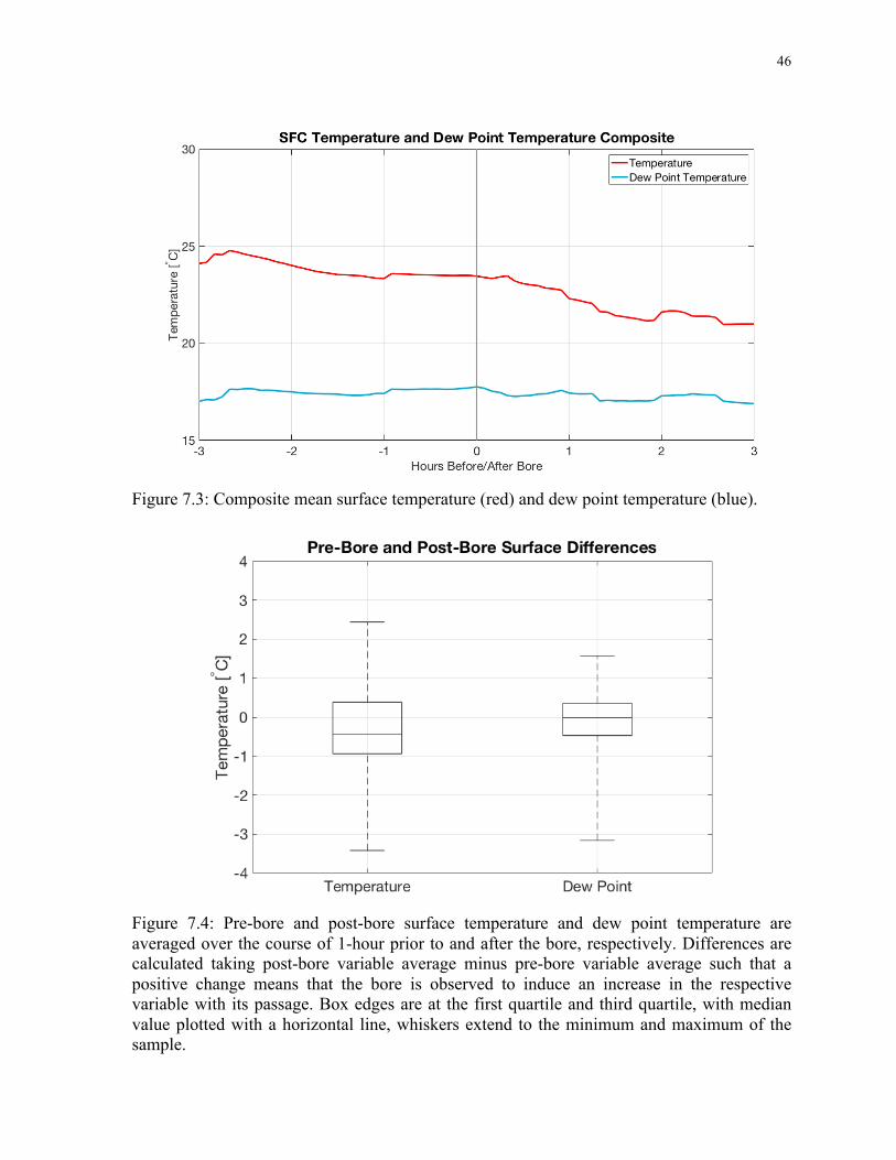
46

Figure 7.3: Composite mean surface temperature (red) and dew point temperature (blue).

Figure 7.4: Pre-bore and post-bore surface temperature and dew point temperature are averaged over the course of 1-hour prior to and after the bore, respectively. Differences are calculated taking post-bore variable average minus pre-bore variable average such that a positive change means that the bore is observed to induce an increase in the respective variable with its passage. Box edges are at the first quartile and third quartile, with median value plotted with a horizontal line, whiskers extend to the minimum and maximum of the sample.

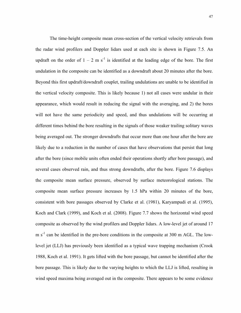
47

The time-height composite mean cross-section of the vertical velocity retrievals from

the radar wind profilers and Doppler lidars used at each site is shown in Figure 7.5. An

updraft on the order of 1 – 2 m s-1 is identified at the leading edge of the bore. The first

undulation in the composite can be identified as a downdraft about 20 minutes after the bore.

Beyond this first updraft/downdraft couplet, trailing undulations are unable to be identified in

the vertical velocity composite. This is likely because 1) not all cases were undular in their

appearance, which would result in reducing the signal with the averaging, and 2) the bores

will not have the same periodicity and speed, and thus undulations will be occurring at

different times behind the bore resulting in the signals of those weaker trailing solitary waves

being averaged out. The stronger downdrafts that occur more than one hour after the bore are

likely due to a reduction in the number of cases that have observations that persist that long

after the bore (since mobile units often ended their operations shortly after bore passage), and

several cases observed rain, and thus strong downdrafts, after the bore. Figure 7.6 displays

the composite mean surface pressure, observed by surface meteorological stations. The

composite mean surface pressure increases by 1.5 hPa within 20 minutes of the bore,

consistent with bore passages observed by Clarke et al. (1981), Karyampudi et al. (1995),

Koch and Clark (1999), and Koch et al. (2008). Figure 7.7 shows the horizontal wind speed

composite as observed by the wind profilers and Doppler lidars. A low-level jet of around 17

m s-1 can be identified in the pre-bore conditions in the composite at 300 m AGL. The low-

level jet (LLJ) has previously been identified as a typical wave trapping mechanism (Crook

1988, Koch et al. 1991). It gets lifted with the bore passage, but cannot be identified after the

bore passage. This is likely due to the varying heights to which the LLJ is lifted, resulting in

wind speed maxima being averaged out in the composite. There appears to be some evidence

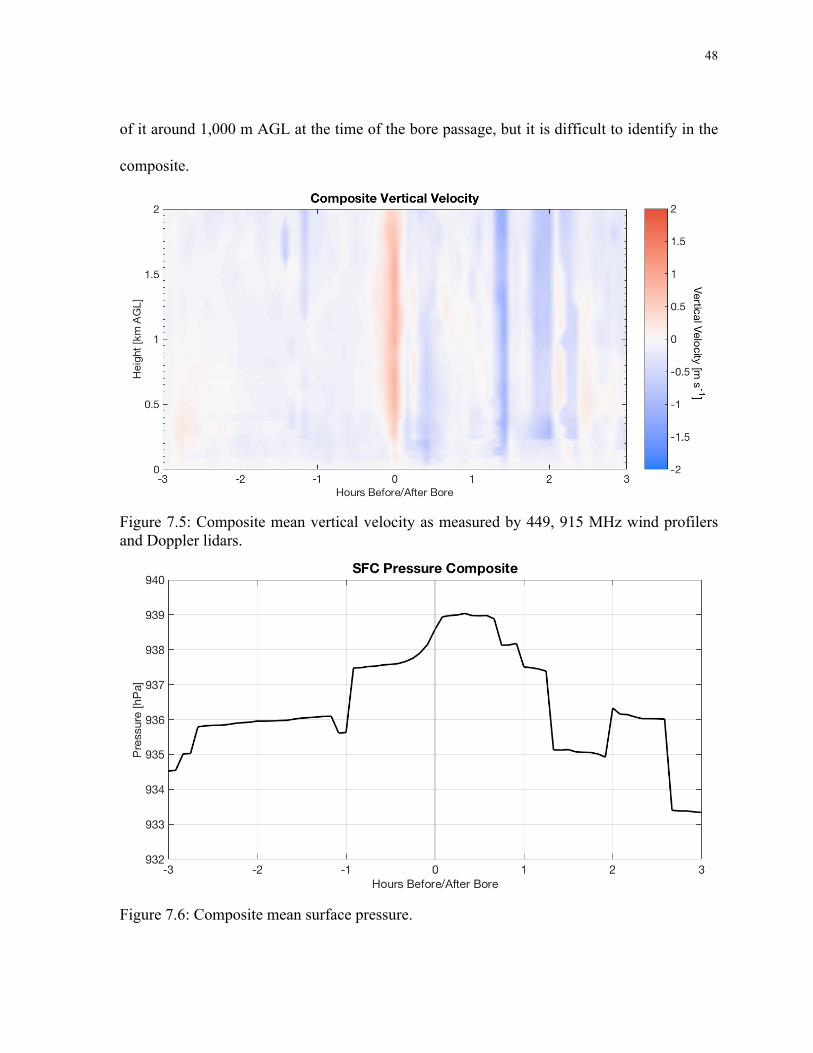
48

of it around 1,000 m AGL at the time of the bore passage, but it is difficult to identify in the

composite.

Figure 7.5: Composite mean vertical velocity as measured by 449, 915 MHz wind profilers and Doppler lidars.

Figure 7.6: Composite mean surface pressure.

49

Figure 7.7: Composite mean horizontal wind speed as measured by 449, 915 MHz wind profilers and Doppler lidars.

The composite mean water vapor retrieval from the AERIoe is displayed in Figure 7.8.

As was shown in both the previous section and Koch et al. (2008), bores can result in a rapid

moistening or drying of the boundary layer. Figure 7.8 shows that there is an increase in

moisture in the boundary layer with the bore passage. The 12 g kg-1 isohume is lifted about

200 m with the bore passage. This is much less than the 7 June 2015 case observed at FP3,

shown in Figure 6.6 in the previous section. This is to be expected since the averaging

includes bores that both moisten the boundary layer (e.g. 7 June 2015, shown in Figure 6.6)

with those that rapidly dry the boundary layer (e.g. 18 June 2015, shown in Figures 6.5).

With this composite, it can be inferred that of the 20 bores identified and included in the

study during PECAN, bores were somewhat more likely to result in lofting of moisture in the

boundary layer than rapidly drying the boundary layer. Koch et al. (2008) identified that the

stronger mixing – which would result in drying of the boundary layer by mixing dry air from

50

the free troposphere down to the surface – occurs earlier in the bore’s life cycle while weaker

mixing, and thus moistening throughout the boundary layer, occurs near the end of the bore’s

life cycle. Given that bores early in their life cycle are more likely to be located near their

parent gravity current and the precipitation that engendered it, and that AERI is unable to

observe radiances in the presence of precipitation, this composite is likely biased towards

late-life-cycle bores that have propagated away from the parent convection. Additionally, the

stronger mixing cases will only result in rapid drying of the boundary layer if the free

troposphere is sufficiently dry, which may not have always been the case for the bores

included in this study.

Figure 7. 8: Composite mean AERIoe retrieved water vapor. Isohumes labeled every 1 g kg-1.

C. Convective Indices AERIoe-derived thermodynamic soundings provide the opportunity to assess trends

in convective indices at high-temporal resolution. There is historical precedence for using

51

AERI-derived retrievals to monitor trends in convective indices, for using AERIs in bore

studies, and monitoring time series of convective indices in bore case studies (albeit without

an AERI). Feltz et al. (2002) used AERI-derived thermodynamic profiles to calculate severe

indices during the 3 May 1999 Kansas and Oklahoma tornado outbreak. Wagner et al. (2008)

observed the temporal evolution in severe convective indices for tornadic and non-tornadic

supercell environments, from 1999 to 2003, using AERI-derived thermodynamic profiles.

Coleman and Knupp (2011) showed time series of CAPE, CIN, and LFC height with a bore

and soliton passage, using thermodynamic variables derived from a microwave radiometer.

AERIoe would likely have a more accurate calculation of convective indices than microwave

radiometers, given the increased vertical resolution as a result of a greater number of

absorption bands in the infrared compared to the microwave. While severe index calculations

using AERIoe profiles are unlikely to be exactly the same as coincident radiosondes due to

smoothing and vertical resolution differences outlined earlier, trends in observed stability are

still useful.

Using the same compositing method, we can analyze trends in convective indices to

assess whether or not the bore passage is making the environment more or less likely to

produce convection. To do this, the convective available potential energy (CAPE),

convective inhibition (CIN), lifted condensation level (LCL), and level of free convection

(LFC) are calculated for each individual case using the SHARPpy program (Blumberg et al.

2017) and then averaged together to form a composite time series. SHARPpy is a

meteorological Python package available online (https://github.com/sharppy/SHARPpy) that

uses the same methods to calculate severe indices as the National Oceanographic and

52

Atmospheric Administration’s (NOAA) Storm Prediction Center’s (SPC) operational

forecasting software.

The composite time series of surface-based and most-unstable parcel CAPE is shown

in Figure 7.9. Surface-based calculated indices use the surface parcel, while the most-

unstable calculated indices finds the parcel that has the greatest CAPE and calculates the

indices from that level. Surface-based CAPE (SBCAPE) has a gradual decrease throughout

the time period of analysis, likely due to radiational cooling since all of the cases occurred

during the overnight hours. With the passage of the bore, SBCAPE decreases at a slightly

greater rate than prior to the bore. A similar trend is observed in the most-unstable parcel

CAPE (MUCAPE), where the bore passage results in a greater rate of decrease than with

SBCAPE. The most-unstable level does not change at all with the bore passage, staying at

870 m AGL around the time of the bore. It is unclear whether this is a product of the AERIoe

retrievals or a real phenomenon as an insufficient number of pre- and post-bore radiosondes

were available to determine this. As such, changes in MUCAPE are due to the changes at the

most-unstable level and above, and not due to changes in the altitude of the most-unstable

parcel.

53

Figure 7.9: Composite mean time series of surface-based (solid line) and most-unstable parcel (dashed line) convective available potential energy (CAPE) relative to bore passage time.

Time series of surface-based and most-unstable CIN (SBCIN and MUCIN) are shown

in Figure 7.10. SHARPpy outputs CIN as a negative value, but SBCIN and MUCIN are

shown as absolute value of those quantities. For both SBCIN and MUCIN, there is a decrease

of 50 to 100 J kg-1 immediately after the bore passage. After that, SBCIN increases back to

pre-bore levels. MUCIN slowly increases again after the bore. Coleman and Knupp (2011)

showed a rapid decrease in SBCIN coincident with an increase in SBCAPE as a bore passed.

The decrease in SBCIN with the bore passage would allow for the environment to be more

conducive to convection, but the decrease in SBCAPE would suggest any convection that

initiated after the bore would be less intense than convection initiated in the pre-bore

environment. The decrease in SBCIN is expected as a typical characteristic of bores is the

54

lifting, cooling, and weakening of the capping inversion (Koch et al. 1991, Koch and Clark

1999, Koch et al. 2008, Coleman and Knupp 2011).

Figure 7.10: As in Figure 7.9 but for CIN.

Surface-based and most-unstable parcel LCL (SBLCL and MULCL) heights are

displayed in Figure 7.11. SBLCL has a very gradual decrease over the time of the composite,

decreasing from 1 km AGL to 0.7 km AGL, but the bore does not have an impact on the

trend. The reason for this can be understood when considering the composite surface

temperature and dew point temperature in Figure 7.3. While dew point temperature does not

change over the time series, the temperature slowly decreases, which results in the persistent

lowering of the SBLCL. The MULCL does decrease 300 m with the bore passage, likely due

to the lower-level cooling associated with the bore. Additionally, the lofting of water vapor

could play some role in lowering the MULCL. The composite mean water vapor retrievals

(Figure 7.8) indicate more bores that loft moisture and moisten the boundary layer were

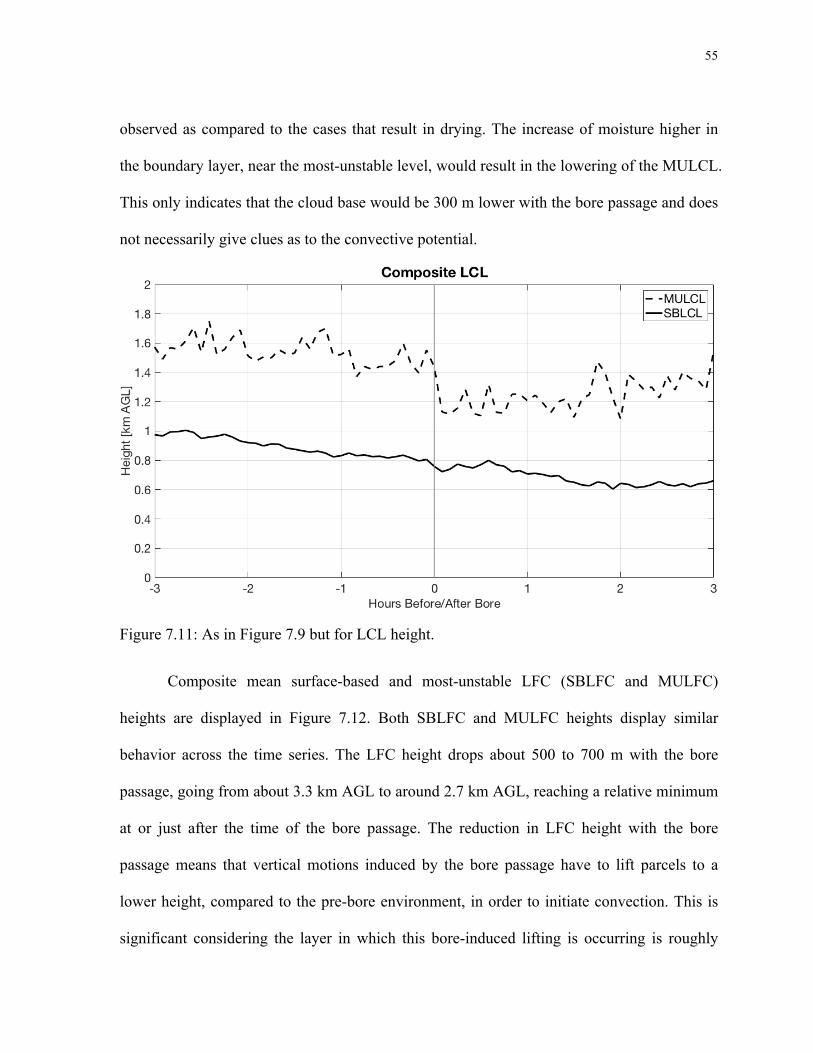
55

observed as compared to the cases that result in drying. The increase of moisture higher in

the boundary layer, near the most-unstable level, would result in the lowering of the MULCL.

This only indicates that the cloud base would be 300 m lower with the bore passage and does

not necessarily give clues as to the convective potential.

Figure 7.11: As in Figure 7.9 but for LCL height.

Composite mean surface-based and most-unstable LFC (SBLFC and MULFC)

heights are displayed in Figure 7.12. Both SBLFC and MULFC heights display similar

behavior across the time series. The LFC height drops about 500 to 700 m with the bore

passage, going from about 3.3 km AGL to around 2.7 km AGL, reaching a relative minimum

at or just after the time of the bore passage. The reduction in LFC height with the bore

passage means that vertical motions induced by the bore passage have to lift parcels to a

lower height, compared to the pre-bore environment, in order to initiate convection. This is

significant considering the layer in which this bore-induced lifting is occurring is roughly

56

within the bottom 2 km AGL of the atmosphere. It is in this layer where low-level

convergence (Figure 7.7) and vertical motions (Figure 7.5) are occurring. 3.3 km AGL would

likely prove to be too high for bore induced lifting, but 2.7 km AGL is notably closer to the

level where lifting is occurring. This decrease in LFC height is also expected since once

again, lifting, cooling, and weakening of the capping inversion results a lower LFC height

just as it does for reduced CIN (Koch et al. 1991, Koch and Clark 1999, Koch et al. 2008,

Coleman and Knupp 2011).

Figure 7.12: As in Figure 7.9 but for LFC height.

Figure 7.13 displays both a pre-bore radiosonde and a post-bore radiosonde launched

by SPARC operators on 26 June 2015. The pre-bore radiosonde was launched at 0707 UTC

while the post-bore radiosonde was launched at 0752 UTC, while the bore occurred at 0735

UTC. The pre-bore inversion is located at 925 hPa. In the post-bore sounding, the pre-bore

inversion has been lifted dry adiabatically about 0.5 km to 875 hPa. These two radiosondes

57

are a great example of a bore lifting, cooling, and weakening the capping inversion, resulting

in a decrease in CIN and LFC height, and thus increasing the potential for convective

initiation behind the bore.

Figure 7.13: Pre-bore (0707 UTC, thin, light lines) and post-bore (0752 UTC, thick, dark lines) SPARC radiosondes on 26 June 2015. Bore occurred at 0735 UTC. Temperature is plotted in red, dew point temperature plotted in teal. Post-bore radiosonde has a near-surface inversion due to the arrival of the bore’s parent gravity current at the time of the radiosonde launch.

Pre-bore and post-bore index differences were also investigated by averaging index

values for the one hour periods that preceded and followed bore passage in order to compute

an average pre- and post-bore index; these averages were calculated using each individual

case instead of calculating indices from composite values. The difference was then defined as

58

post-bore minus pre-bore so that a positive difference would imply an increase in the

particular severe index, similar to Figure 7.4. Figures 7.14 and 7.15 display the variability of

changes to CAPE and CIN, and LCL and LFC height respectively. It is seen that the most-

unstable parcel indices have greater variability than the surface-based parcel indices. In the

majority of cases, SBCIN and MUCIN decrease with the bore passage, as do the MULCL

and MULFC heights. SBCAPE and MUCAPE, along with SBLCL, have median differences

near zero. It is shown that several cases exhibited positive trends in these indices, and several

cases also exhibited negative trends. These indices also displayed little trend in the composite

mean analysis, as previously shown in Figures 7.8 and 7.10. SBLFC also has a median value

near zero, with most cases on the negative side of the zero-line, but the first quartile extends

to the positive side of the zero-line. The slight downward trend with the bore passage,

observed in the composite mean in Figure 7.12, could perhaps be partly explained by the

very negative outlier, as shown in Figure 7.15. In general, Figures 7.14 and 7.15 show that

bores tend to result in decreases in CIN and LFC height and MULCL heights, but can be

quite variable with respect to changes in CAPE.

59

Figure 7.14: As in Figure 7.4 but for SBCAPE, MUCAPE, SBCIN, and MUCIN.

Figure 7.15: As in Figure 7.4 except for SBLCL, MULCL, SBLFC, and MULFC height.

Overall, the results presented here are mixed with respect to the problem of bores and

convective initiation. The reduced CAPE, according to the composite mean analysis, would

characterize weaker convection. However, Figures 7.10, 7.12, 7.14 and 7.15 display a greater

60

signal with the bore passage, and indicate most cases exhibit a reduction in LFC height and

CIN. This trend would increase the potential for convective initiation to occur. Thus, in this

composite mean sense, it appears that bores are likely to increase the potential for convective

initiation but the reduced CAPE, in many of the cases, may indicate that the convection in the

post-bore environment will be weaker in the pre-bore environment. It is important to note

that a composite mean does not represent all bores, and individual bores have been observed

to induce severe convection (eg. Karyampudi et al. 1995, Locatelli et al. 2002). However, it

is also observed here that bores can stabilize the atmosphere, which has not necessarily been

communicated in the literature.

61

VIII. Case Study Comparison The large variability in changes to CAPE displayed in Figure 7.14, and especially the

preference toward decreasing CAPE, is an interesting result. Both Koch et al. (2008) and

Coleman and Knupp (2011) observed a “modest” increase of surface-based CAPE with a

bore passage and Coleman and Knupp also observed an increase in 300 m CAPE. While a

few cases exhibit an increase in CAPE, the majority of cases result in a decrease, something

that has not been previously documented in the literature. In order to try to understand the

large differences in SBCAPE with the bore passage, the events with the maximum SBCAPE

difference (21 June FP4) and the minimum CAPE difference (26 June FP3) are examined in

greater detail.

Figures 8.1 through 8.4 display time series of surface-based and most-unstable parcel

calculations for CAPE (8.1), CIN (8.2), LCL height (8.3), and LFC height (8.4) for both the

21 June FP4 case and the 26 June FP3 case. As shown in Figure 8.1, SBCAPE increased by

1000 J kg-1 with the bore passage in the 21 June case, while MUCAPE increased to a

maximum ahead of the bore, but then decreased again after the bore. For the 26 June case,

SBCAPE and MUCAPE gradually decreased with time, with the appearance that the bore

accelerated the rate at which CAPE decreased, similar to what was seen in the composite

analysis in the previous section (Figure 7.9).

Figure 8.2 displays SBCIN and MUCIN for both cases. Note that SBCIN was

undefined for the 21 June case prior to the bore, as there was zero SBCAPE at that time and

CIN is undefined without positive CAPE. On 21 June, MUCIN decreased from about 600 J

kg-1 to about 100 J kg-1 within the hour prior to the bore passage. The 26 June case exhibits

62

little change with the bore passage, with a short 10 – 15 minute time period of reduced CIN

right after the bore passage.

Figure 8.1: SBCAPE (solid line) and MUCAPE (dashed line) for a bore on 21 June 2015 at FP4 (red line) and 26 June 2015 over FP3 (blue line). Time shown is relative to the time of the bore, using the bore start time algorithm from section 7A. The 21 June FP4 bore occurred at 1150 UTC, and the 26 June FP3 bore occurred at 0455 UTC.

63

Figure 8.2: As in Figure 8.1 but for CIN instead of CAPE. Note: CIN is undefined when CAPE is zero. Large spikes in MUCIN for the 21 June case prior to the bore are likely due to noise in the AERIoe retrievals resulting in particularly large changes in the most-unstable parcel.

SBLCL height (Figure 8.3) changed little for both cases. MULCL height for the 26

June case shows negligible changes with the bore passage, but the 21 June case had a

decrease of about 500 m for the 30 minutes following the bore passage. Figure 8.4 displays

SBLFC and MULFC heights for both cases. LFC height cannot be calculated when CAPE is

zero, so the 21 June case had no surface-based LFC height prior to the bore passage. In the

26 June case, the MULFC height stayed very similar in height across the bore passage, with

an increase of about 500 m in the surface-based LFC height. We can only observe the time

series of the MULFC height in the 21 June case because of the lack of pre-bore SBCAPE for

that case. The 21 June case had a decrease of 3000 m in the hour prior to the bore passage;

recall the gradual increase in most-unstable CAPE and decrease in MUCIN in that time

64

frame. This was due to surface heating as the bore is occurring at 1150 UTC (6:50 am local

time) while sunrise was at 1105 UTC. Overall, the 21 June bore, coupled with diabatic

surface heating, destabilized the environment while the 26 June bore stabilized it.

Figure 8.3: As in Figure 8.1 but for LCL height instead of CAPE. Large spikes in MULCL for the 21 June case prior to the bore are likely due to noise in the AERIoe retrievals resulting in particularly large changes in the most-unstable parcel.

The changes in severe indices shown in Figures 8.1 through 8.4 could be put into

perspective when considering the AERIoe potential temperature and water vapor mixing

ratio retrievals. Figures 8.5a and 8.6a display the potential temperature retrievals from the

AERIoe for 21 June and 26 June respectively, while Figures 8.5b and 8.6b display the

corresponding water vapor mixing ratios. The potential temperature retrievals show the bore

front at 1150 UTC and 0455 UTC respectively. The real difference between the two cases is

seen in the water vapor mixing ratio retrievals as the 21 June case resulted in lofting of

moisture in the boundary layer, while the 26 June case resulted in a drying of the boundary

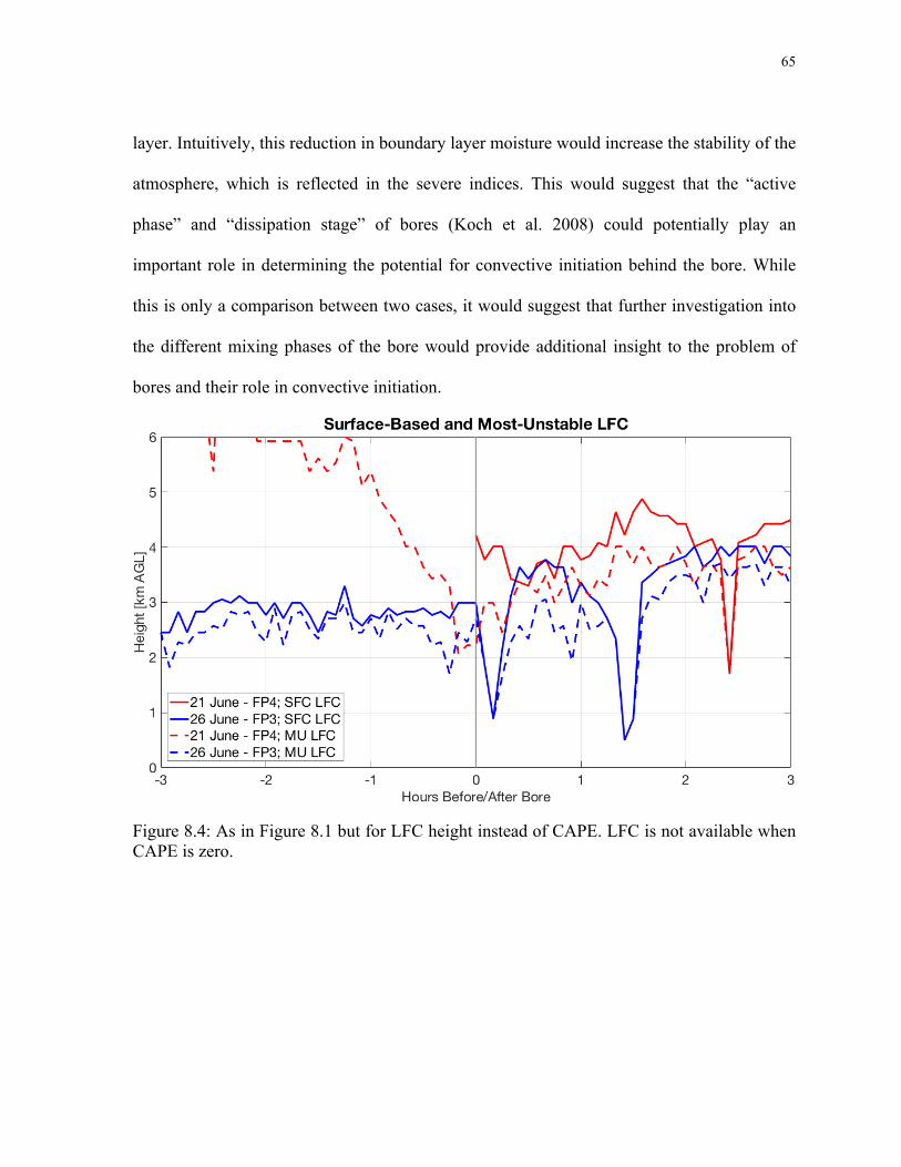
65

layer. Intuitively, this reduction in boundary layer moisture would increase the stability of the

atmosphere, which is reflected in the severe indices. This would suggest that the “active

phase” and “dissipation stage” of bores (Koch et al. 2008) could potentially play an

important role in determining the potential for convective initiation behind the bore. While

this is only a comparison between two cases, it would suggest that further investigation into

the different mixing phases of the bore would provide additional insight to the problem of

bores and their role in convective initiation.

Figure 8.4: As in Figure 8.1 but for LFC height instead of CAPE. LFC is not available when CAPE is zero.

66

Figure 8.5: AERIoe retrieved a) potential temperature and b) water vapor mixing ratio time-height cross-section from FP4 in Minden, NE from 21 June 2015 from 0900 UTC to 1400 UTC. Potential temperature and water vapor mixing ratio is shaded, with isentropes and isohumes outlined and labeled every 3 K and 3 g kg-1. The bore start time is 1150 UTC, denoted by the black arrows.

67

Figure 8.6: AERIoe retrieved a) potential temperature and b) water vapor mixing ratio time-height cross-section from FP3 in Ellis, KS from 26 June 2015 from 0200 UTC to 0700 UTC. Potential temperature and water vapor mixing ratio is shaded, with isentropes and isohumes outlined and labeled every 3 K and 3 g kg-1. The bore start time is 0455 UTC, denoted by the black arrows. There are no retrievals between 0615 and 0650 UTC due to rain.

68

IX. Summary and Conclusions This study developed a method to create a composite mean of 20 different bore events

observed by AERIs during the PECAN campaign. Using this composite mean, the average

character of a bore passage is analyzed. High-temporal resolution thermodynamic sounding

retrievals from the AERIoe algorithm allow for the monitoring of the evolution of severe

indices with the bore passage to assess the impact of the bore on potential convective

initiation after passage. Two short case studies were conducted to assess the extremes in

variability in overall CAPE trends among the 20 cases used in the study.

No other studies in the literature combine multiple bores with uniform

instrumentation within a single methodology. Previous observational studies focused on one

or two bores on the same day in the same area in the context of a case study. This

combination of many bores into a single composite average allows for the general boundary

layer trends of bores to be documented, along with their implications for convective initiation.

This knowledge is presently lacking in the literature, as case studies of bores are likely

picked due to their convective initiation potential; null convection cases are rarely

investigated with the same depth. This study fills that gap in the literature and provides a

general overview of typical conditions with bore passages, and makes progress at

categorizing the variability of some of the changes that can occur with bore passages.

Key findings can be summarized as follows:

• The compositing method was proven to be useful to create a composite mean of

pressure, temperature, water vapor mixing ratio, and wind variables and recreate a

bore-like structure in time series of those atmospheric variables.

69

• A composite mean time series of convective indices was developed, which identified

reductions in CIN and LFC height with the bore passage. This would favor future

convective initiation behind the bore.

• Changes in CAPE were found to be highly variable, with the majority of cases

resulting in decreased CAPE behind the bore, something that has not been frequently

documented in previous case studies.

• The comparison of the two case studies provides evidence for active phase and

dissipation stage bores to have differing influences on the potential for convective

initiation. This result suggests that better understanding the differences between the

two stages/phases should be a topic of further research.

Bores have been found to frequently result in decreases in CIN and LFC height.

Another boundary trailing the bore could provide enough lift, given the bore’s modification

to the LFC height, to initiate convection, as was the case in Koch and Clark (1999). The

lower CIN and LFC height would increase the potential for convective initiation, but the

decrease in CAPE would reduce the severity of convection that may form in the post-bore

environment. This is an important finding because without a nation-wide network of

thermodynamic profilers in place or more frequent radiosonde launches from operational

sites, the only method of identifying bores is using National Weather Service Doppler Radars

(WSR-88Ds). Thus, the boundary layer transitions occurring with the bore passage are

difficult to know; surface observations can only provide limited insight. While each

individual bore seems to have a unique set of transitions associated with it, the results

presented here provide forecasters with a general idea of what trends they can expect when

they observe bores on radar. The average vertical parcel displacement as shown in the

70

composite was approximately 700 m. These results have important implications that can be

applied to real-time forecasting of potential convective initiation, even given that operational

forecasters have minimal knowledge of the bore.

Future work could include compositing bores based on active phase versus

dissipation stages of their life cycles and the impacts on convection that follow from those

changes if an objective way of discriminating between those bore types using typical

instrumentation can be determined. The short case studies of the 21 June and 26 June bores at

FP4 and FP3 presented in section 8 revealed the potential importance of active phase and

dissipation stage bores, identified by Koch et al. (2008). The rapid drying of the boundary

layer could potentially be a major source of stabilization behind active phase bores, while

dissipation stage bores and their lofting of moisture could result in further destabilization of

the boundary layer. Koch et al. (2008) identified the differences between the two bores based

on their turbulent kinetic energy (TKE), which was modeled. TKE is difficult to observe with

the instruments deployed at the various facilities during PECAN, and an obvious

differentiation between the two bore types cannot be made to create a composite analysis

focused on this difference. Furthermore, the drying and moistening of the boundary layer is

only evidence of the differences in mixing between bore types, but it is dependent on the

assumption of a sufficiently dry free troposphere, which is not always the case. The more

vigorous mixing associated with active phase bores is also a result of stronger updrafts,

which can make direct convective initiation by the bore more likely. Given the results of this

study, it may be worthwhile for future work on the problem of bores and convective initiation

to further investigate the differences between these two types of bores and their potential

different implications for convective initiation.

71

References Ashley, S. T., and W. S. Ashley, 2008: Flood fatalities in the United States. J. Appl. Meteor.

Climatol., 47, 805-818. Benjamin, S. G., and Coauthors, 2016: A North American hourly assimilation and model

forecast cycle: The Rapid Refresh. Mon. Wea. Rev., 144, 1669-1694. Blumberg, W. G., K. Halbert, T. Supinie, P. Marsh, R. Thompson, and J. Hart, 2017:

SHARPpy: An open source sounding analysis toolkit for the atmospheric sciences. Bull. Amer. Meteor. Soc., doi:10.1175/BAMS-D-15-00309.1, in press.

Christie, D. R., 1989: Long nonlinear waves in the lower atmosphere. J. Atmos. Sci., 46,

1462-1491. Clarke, R. H, R. K. Smith, and D. G. Reid, 1981: The Morning Glory of the Gulf of

Carpentaria: an atmospheric undular bore. Mon. Wea. Rev., 109, 1726-1750. Coleman, T. A., K. R. Knupp, and D. E. Herzmann, 2010: An undular bore and gravity

waves illustrated by dramatic time-lapse photography. J. Atmos. Oceanic Technol., 27 1355-1361.

____, and K. R. Knupp, 2011: Radiometer and profiler analysis of the effects of a bore and a

solitary wave on the stability of the nocturnal boundary layer. Mon. Wea. Rev., 139, 211-223.

Colman, B. R., 1990: Thunderstorms above frontal surfaces in environments without positive

CAPE. Part I: A climatology. Mon. Wea. Rev., 118, 1103-1121. Crook, N. A. 1988: Trapping of low-level internal gravity waves. J. Atmos. Sci., 45, 1533-

1541. Davis, C. A., and Coauthors, 2004: The Bow Echo and MCV Experiment: observations and

opportunities. Bull. Amer. Meteor. Soc., 85, 1075-1093. Droegemeier, K. K., and R. B. Wilhelmson, 1987: Numerical simulation of thunderstorm

outflow dynamics. Part I: Outflow sensitivity experiments and turbulence dynamics. J. Atmos. Sci., 44, 1180-1210.

Ecklund, W. L., D. A. Carter, B. B. Balsley, P. E. Currier, J. L. Green, B. L. Weber, and K. S.

Gage, 1990: Field tests of a lower tropospheric wind profiler. Radio Sci., 25, 899-906. Feltz, W. F., W. L. Smith, R. O. Knuteson, H. E. Revercomb, H. M. Woolf, and H. B.

Howell, 1998: Meteorological applications of temperature and water vapor retrievals

72

from the ground-based atmospheric emitted radiance interferometer (AERI). J. Appl. Meteor., 37, 857-875.

____, and J. R. Mecikalski, 2002: Monitoring high-temporal resolution convective stability

indices using the ground-based atmospheric emitted radiance interferometer (AERI) during the 3 May 1999 Oklahoma-Kansas tornado outbreak. Wea. Forecasting, 17, 445-455.

____, W. L. Smith, H. B. Howell, R. O. Knuteson, H. Woolf, and H. E. Revercomb, 2003:

Near-continuous profiling of temperature, moisture, and atmospheric stability using the atmospheric emitted radiance interferometer (AERI). J. Appl. Meteor., 42, 584-597.

Fritsch, J. M., R. J. Kane, and C. R. Chelius, 1986: The contribution of mesoscale convective

weather systems to the warm-season precipitation in the United States. J. Clim. Appl. Meteor., 25, 1333-1345.

Geerts, B., and Coauthors, 2017: The 2015 Plains Elevated Convection At Night (PECAN)

field project. Bull. Amer. Meteor. Soc., 98, 767-786. Haase, S. P., and R. K. Smith, 1989: The numerical simulation of atmospheric gravity

currents. Part II: Environments with stable layers. Geophys. Astrophys. Fluid Dyn., 46, 35-51.

Hartung, D. C., J. A. Otkin, J. E. Martin, D. D. Turner, 2010: The life cycle of an undular

bore and its interaction with a shallow, intense cold front. Mon. Wea. Rev., 138, 886-908.

Heideman, K. F. and J. M. Fritsch, 1988: Forcing mechanism and other characteristics of

significant summertime precipitation. Wea. Forecasting, 3, 115-130. Houze, R. A., 2004: Mesoscale convective systems. Rev. Geophys., 42, 1-43. International Met Systems, 2006: iMet-1-ABxn Radiosonde. International Met Systems, 1 pp.

[Available online at: http://intermetsystems.com/ee/pdf/202060_iMet-1-ABxn _Data_161006.pdf].

Karyampudi, V. M., S. E. Koch, C. Chen, J. W. Rottman, 1995: The influence of the Rocky

Mountains on the 13 – 14 April 1986 severe weather outbreak. Part II: Evolution of a prefrontal bore and its role in triggering a squall line. Mon. Wea. Rev., 123, 1423-1446.

Knupp, K. R., 2006: Observational analysis of a gust front to bore to solitary wave transition

within an evolving nocturnal boundary layer. J. Atmos. Sci., 63, 2016-2035.

73

Knuteson, R. O., and Coauthors, 2004a: Atmospheric emitted radiance interferometer (AERI). Part I: Instrument design. J. Atmos. Oceanic Technol., 21, 1763-1776.

____, and Coauthors, 2004b: Atmospheric emitted radiance interferometer (AERI). Part II:

Instrument performance. J. Atmos. Oceanic Technol., 21, 1777-1789. Koch, S. E., P. B. Dorian, R. Ferrare, S. H. Melfi, W. C. Skillman, and D. Whiteman, 1991:

Structure of an internal bore and dissipating gravity current as revealed by Raman lidar. Mon. Wea. Rev., 119, 857-887.

____, and W. L. Clark, 1999: A nonclassical cold front observed during COPS-91: Frontal

structure and the process of severe storm initiation. J. Atmos. Sci., 56, 2862-2890. ____, W. F. Feltz, F. Fabry, M. Pagowski, B. Geerts, K. M. Bedka, D. O. Miller, and J. W.

Wilson, 2008: Turbulent mixing processes in atmospheric bores and solitary waves deduced from profiling systems and numerical simulation. Mon. Wea. Rev., 136, 1373-1400.

Lindseth, B., W. O. J. Brown, J. Jordan, D. Law, T. Hock, S. A. Cohn, and Z. Popović, 2012:

A new portable 449-MHz spaced antenna wind profiler radar. IEEE Trans. Geosci. Remote Sens., 50, 3544-3553.

Locatelli, J. D., M. T. Stoelinga, P. V. Hobbs, and J. Johnson, 1998: Structure and evolution

of an undular bore on the High Plains and its effects on migrating birds. Bull. Amer. Meteor. Soc., 79, 1043-1060.

____, ____, ____, 2002: A new look at the Super Outbreak of tornadoes on 3 – 4 April 1974.

Mon. Wea. Rev., 130, 1633-1651. Maddox, R. A., C. F. Chappell, and L. R. Hoxit, 1979: Synoptic and meso-α scale aspects of

flash flood events. Bull. Amer. Meteor. Soc., 60, 115-123. Mahapatra, P. R., R. J. Doviak, and D. S. Zrnic, 1991: Multisensor observation of an

atmospheric undular bore. Bull. Amer. Meteor. Soc., 72, 1468-1480. Morse, C. S., R. K. Goodrich, and L. B. Cornman, 2002: The NIMA method for improved

moment estimation from Doppler spectra. J. Atmos. Oceanic Technol., 19, 274-295. Parker, M. D., 2008: Response of simulated squall lines to low-level cooling. J. Atmos. Sci.,

65, 1323-1341. Pearson, G., F. Davies, and C. Collier, 2009: An analysis of the performance of the EFAM

pulsed Doppler lidar for observing the boundary layer. J. Atmos. Oceanic Technol., 26, 240-250.

74

Pu, B. and R. E. Dickinson, 2014: Diurnal spatial variability of Great Plains summer precipitation related to the dynamics of the low-level jet. J. Atmos. Sci., 71, 1807-1817.

Raymond, D. J., and H. Jiang, 1990: A theory for long-lived mesoscale convective systems. J.

Atmos. Sci., 47, 3067-3077. Rodgers, C. D., 2000: Inverse Methods for Atmospheric Sounding: Theory and Practice.

Series on Atmospheric, Oceanic and Planetary Physics, Vol. 2, World Scientific, 238 pp.

Rottman, J. W., and J. E. Simpson, 1989: The formation of internal bores in the atmosphere:

A laboratory model. Quart. J. Roy. Meteor. Soc., 108, 941-963. Simpson, J. E., 1982: Gravity currents in the laboratory, atmosphere, and ocean. Ann. Rev.

Fluid. Mech., 14, 213-234. Smith. R. K, N. Crook, and G. Roff, 1982: The Morning Glory: an extraordinary atmospheric

undular bore. Quart. J. Roy. Meteor. Soc., 108, 937-956. Smith, R. K., 1988: Travelling waves and bores in the lower atmosphere: The ‘Morning

Glory’ and related phenomena. Earth-Sci. Rev., 25, 267-290. Smith, W. L., W.F. Feltz, R. O. Knuteson, H. E. Revercomb, H. M. Woolf, and H. B.

Howell, The retrieval of planetary boundary layer structure using ground-based infrared spectral radiance measurements. J. Atmos. Oceanic Technol., 16, 323-333.

Tanamachi, R. L., W. F. Feltz, and M. Xue, 2008: Observations and numerical simulation of

upper boundary layer rapid drying and moistening events during the International H2O Project (IHOP_2002). Mon. Wea. Rev., 136, 3106-3120.

Tepper, M., 1950: A proposed mechanism of squall lines: the pressure jump line. J. Meteor.,

7, 21-29. Tripoli, G. J. and W. R. Cotton, 1989a: Numerical study of an observed orogenic mesoscale

convective system. Part I: Simulated genesis and comparison with observations. Mon. Wea. Rev., 117, 273-304.

____, and ____, 1989b: Numerical study of an observed orogenic mesoscale convective

system. Part II: Analysis of governing dynamics. Mon. Wea. Rev., 117, 305-328. Turner, D. D, W. F. Feltz, and R. A. Ferrare, 2000: Continuous water vapor profiles from

operational ground-based active and passive remote sensors. Bull. Amer. Meteor. Soc., 81, 1301-1317.

75

____, R. O. Knuteson, H. E. Revercomb, C. Lo, and R. G. Dedecker, 2006: Noise reduction of Atmospheric Emitted Radiance Interferometer (AERI) observations using principal component analysis. J. Atmos. Oceanic Technol., 23, 1223-1238.

____, and U. Löhnert, 2014: Information content and uncertainties in thermodynamic profiles

and liquid cloud properties retrieved from the ground-based atmospheric emitted radiance interferometer (AERI). J. Appl. Meteor. and Climatol., 53, 752-771.

Tuttle, J. D., and C. A. Davis, 2006: Corridors of warm season precipitation in the central

United States. Mon. Wea. Rev., 134, 2297-2317. Vaisala, 2013: Vaisala Radiosonde RS92-SGP. Vaisala, 2 pp. [Available online at:

http://www.vaisala.com/Vaisala%20Documents/Brochures%20and%20Datasheets/RS92SGP-Datasheet-B210358EN-F-LOW.pdf].

____, 2016: Vaisala Radiosonde RS41-SGP. Vaisala, 2 pp. [Available online at:

http://www.vaisala.com/Vaisala%20Documents/Brochures%20and%20Datasheets/WEA-MET-RS41SGP-Datasheet-B211444EN.pdf].

Wagner, T. J., W. F. Feltz, and S. A. Ackerman, 2008: The temporal evolution of convective

indices in storm-producing environments. Wea. Forecasting, 23, 786-794. Wakimoto, R. M, and D. E. Kingsmill, 1995: Structure of an atmospheric undular bore

generated from colliding boundaries during CAPE. Mon. Wea. Rev., 123, 1374-1393. Wallace, J. M., 1975: Diurnal variations in precipitation and thunderstorm frequency over the

conterminous United States. Mon. Wea. Rev., 103, 406-419. Weckwerth, T. M., and Coauthors, 2004: An overview of the International H2O Project

(IHOP_2002) and some preliminary highlights. Bull. Amer. Meteor. Soc., 85, 253-277. Weisman, M. L., and Coauthors, 2015: The Mesoscale Predictability Experiment (MPEX).

Bull. Amer. Meteor. Soc., 96, 2127-2149. Wilson, J. W., and R. D. Roberts, 2006: Summary of convective storm initiation and

evolution during IHOP: Observational and modeling perspective. Mon. Wea. Rev., 134, 23-47.

Wood, I. R., and J. E. Simpson, 1984: Jumps in layered miscible fluids. J. Fluid Mech., 140,

329-342.