1

Lecture 4.

Composition and structure of the atmospheres.

Basic properties of gases, aerosols, and clouds that are important for

radiative transfer modeling. Objectives:

1. Basic properties of planetary atmospheres, structure of the Earth’s atmosphere and

radiative transfer modeling.

2. Atmospheric gases.

3. Aerosols.

4. Clouds.

5. Refractive indices of atmospheric particulates (aerosol and clouds).

Required reading:

L02: 3.1, 5.1, pp.169-176

Additional reading:

Boer, G.J., I.N. Sokolik, and S.T. Martin, Infrared optical constants of aqueous sulfate-nitrate-ammonium multi-component tropospheric aerosols from attenuated total reflectance measurements: Part I. Results and analysis of spectral absorbing features. J. Quant. Specrtrocs. Radiat. Transfer, doi:10.1016/j.jqsrt.2007.02.017, 2007. Boer, G.J., I.N. Sokolik, and S.T. Martin, Infrared optical constants of aqueous sulfate-nitrate-ammonium multi-component tropospheric aerosols from attenuated total reflectance measurements: Part II. An examination of mixing rules. J. Quant. Specrtrocs. Radiat. Transfer, doi:10.1016/j.jqsrt.2007.02.018, 2007.

1. Basic properties of planetary atmospheres. Structure of the Earth’s atmosphere

and radiative transfer modeling.

Propagation of the electromagnetic radiation in an atmosphere is affected by its

state (temperature, pressure, air density) and composition (gases and particulates)

Interactions of atmospheric constituents with radiation:

Gases – all scatter radiation, and some can absorb (and emit) radiation depending

on their molecular structure

2

Particulates (aerosol and clouds) – all scatter radiation, and some can absorb (and

emit) radiation depending on their refractive indices (determined by composition)

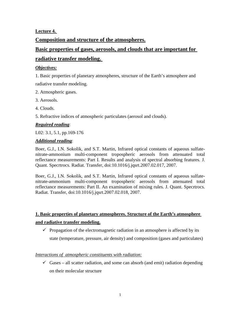
Radiative transfer in the Earth (or other planets) atmosphere is commonly solved in one

dimension (1D) based on the concept of the plane parallel atmosphere (see figure 2.1 in

Lecture 2) (e.g., in numerical weather prediction (NWP) models and GCMs)

EXAMPLE: In global and regional models, radiative transfer is solved in each column

defined by the model grid size. The vertical resolution is the same as the number of

vertical layers in the model.

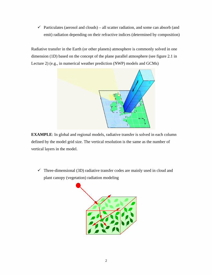
Three-dimensional (3D) radiative transfer codes are mainly used in cloud and

plant canopy (vegetation) radiation modeling

3

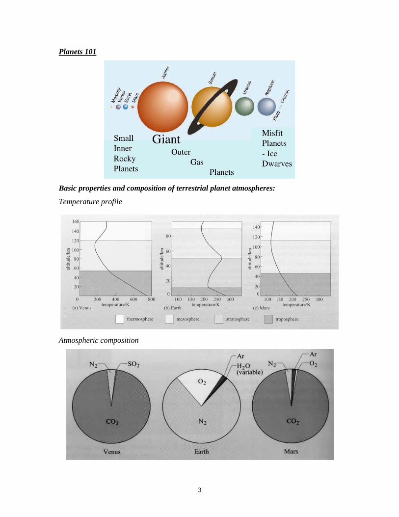
Planets 101

Basic properties and composition of terrestrial planet atmospheres:

Temperature profile

Atmospheric composition

4

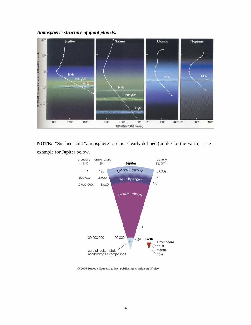
Atmospheric structure of giant planets:

NOTE: “Surface” and “atmosphere” are not clearly defined (unlike for the Earth) – see

example for Jupiter below.

5

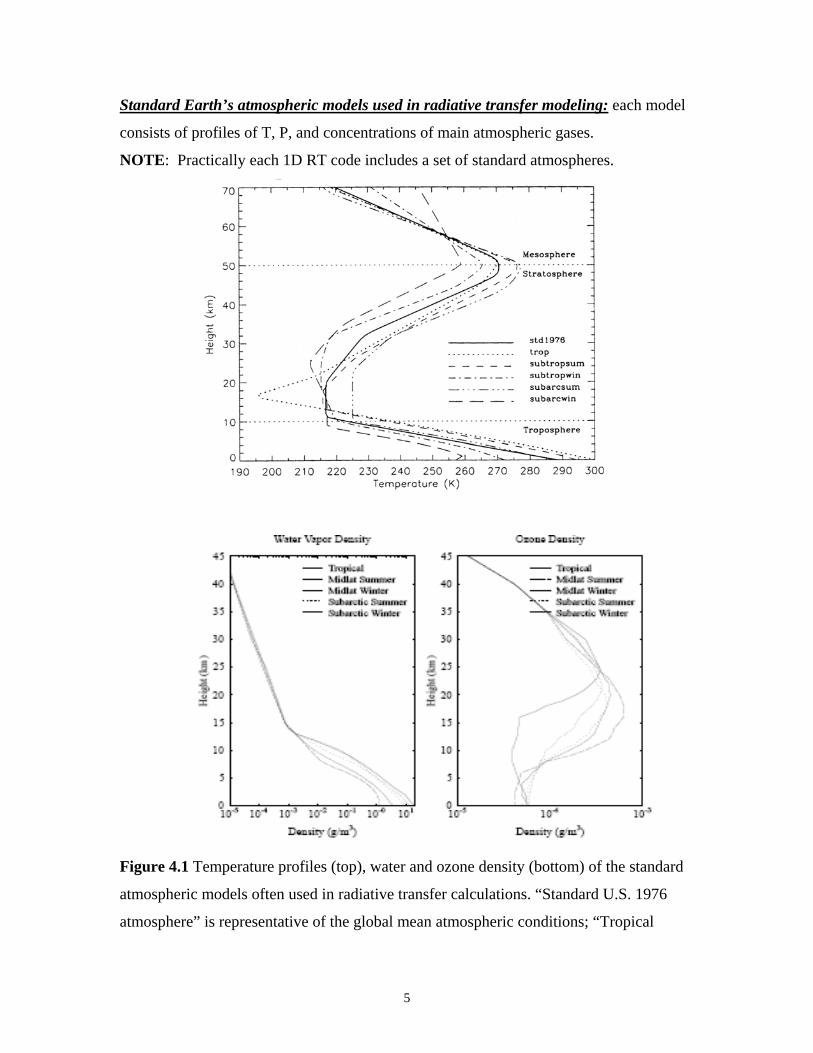
Standard Earth’s atmospheric models used in radiative transfer modeling: each model

consists of profiles of T, P, and concentrations of main atmospheric gases.

NOTE: Practically each 1D RT code includes a set of standard atmospheres.

Figure 4.1 Temperature profiles (top), water and ozone density (bottom) of the standard

atmospheric models often used in radiative transfer calculations. “Standard U.S. 1976

atmosphere” is representative of the global mean atmospheric conditions; “Tropical

6

atmosphere” is for latitudes < 300; “Subtropical atmosphere” is for latitudes between 300

and 450; “Subarctic atmosphere” is for latitudes between 450 and 600; and “Arctic

atmosphere” is for latitudes > 600.

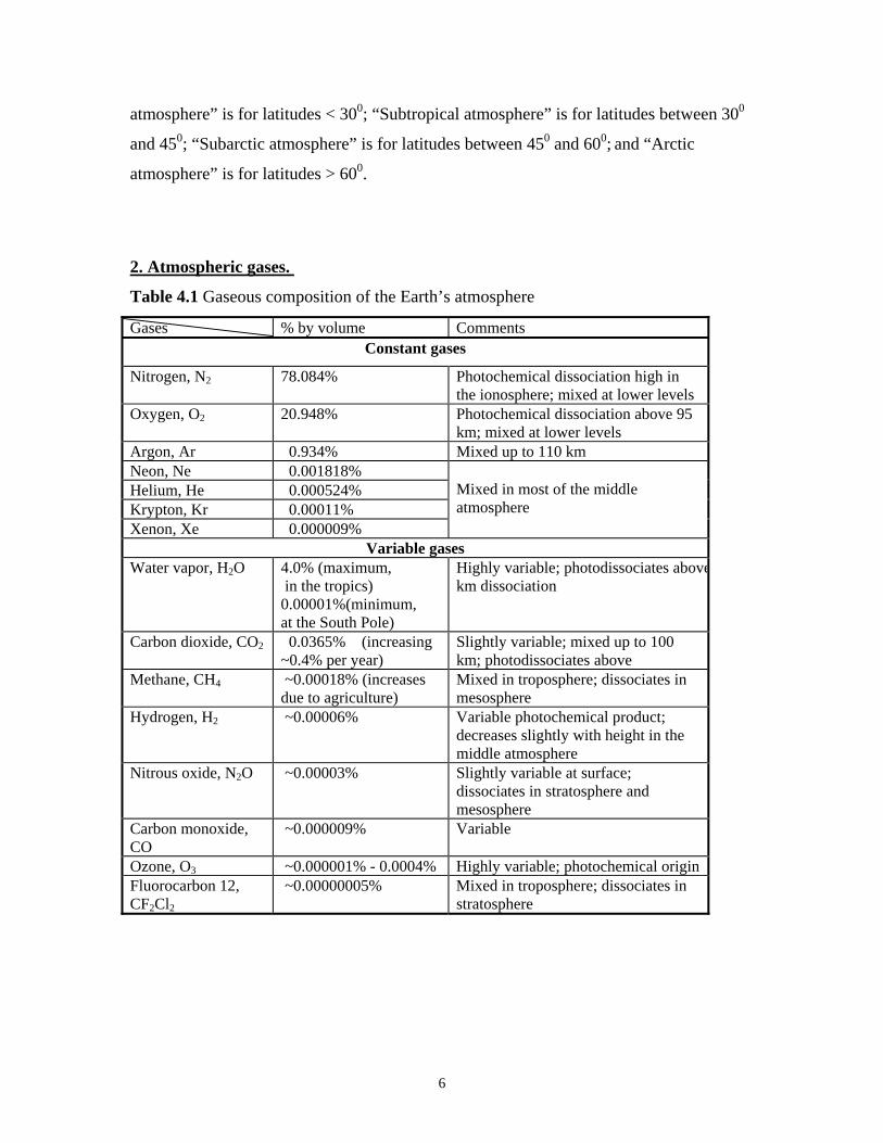
2. Atmospheric gases.

Table 4.1 Gaseous composition of the Earth’s atmosphere

Gases % by volume Comments Constant gases

Nitrogen, N2 78.084% Photochemical dissociation high in the ionosphere; mixed at lower levels

Oxygen, O2 20.948% Photochemical dissociation above 95 km; mixed at lower levels

Argon, Ar 0.934% Mixed up to 110 km Neon, Ne 0.001818%

Mixed in most of the middle atmosphere

Helium, He 0.000524% Krypton, Kr 0.00011% Xenon, Xe 0.000009%

Variable gases Water vapor, H2O 4.0% (maximum,

in the tropics) 0.00001%(minimum, at the South Pole)

Highly variable; photodissociates abovekm dissociation

Carbon dioxide, CO2 0.0365% (increasing ~0.4% per year)

Slightly variable; mixed up to 100 km; photodissociates above

Methane, CH4 ~0.00018% (increases due to agriculture)

Mixed in troposphere; dissociates in mesosphere

Hydrogen, H2 ~0.00006% Variable photochemical product; decreases slightly with height in the middle atmosphere

Nitrous oxide, N2O ~0.00003% Slightly variable at surface; dissociates in stratosphere and mesosphere

Carbon monoxide, CO

~0.000009% Variable

Ozone, O3 ~0.000001% - 0.0004% Highly variable; photochemical origin Fluorocarbon 12, CF2Cl2

~0.00000005% Mixed in troposphere; dissociates in stratosphere

7

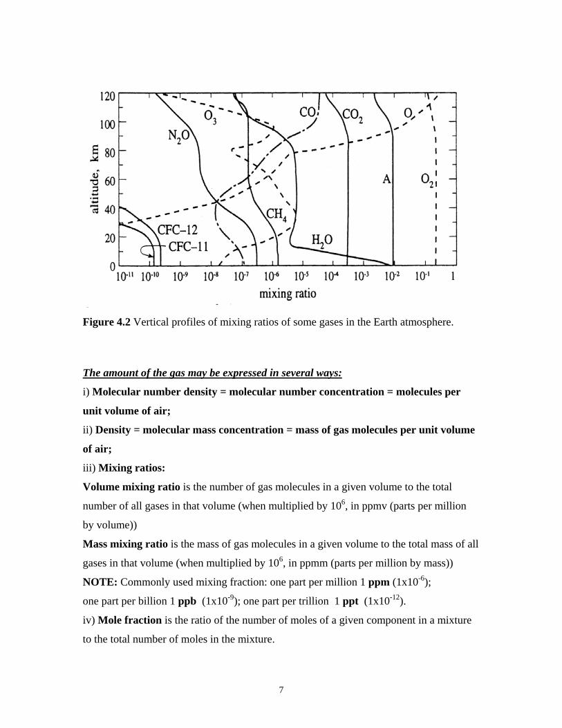
Figure 4.2 Vertical profiles of mixing ratios of some gases in the Earth atmosphere. The amount of the gas may be expressed in several ways:

i) Molecular number density = molecular number concentration = molecules per

unit volume of air;

ii) Density = molecular mass concentration = mass of gas molecules per unit volume

of air;

iii) Mixing ratios:

Volume mixing ratio is the number of gas molecules in a given volume to the total

number of all gases in that volume (when multiplied by 106, in ppmv (parts per million

by volume))

Mass mixing ratio is the mass of gas molecules in a given volume to the total mass of all

gases in that volume (when multiplied by 106, in ppmm (parts per million by mass))

NOTE: Commonly used mixing fraction: one part per million 1 ppm (1x10-6);

one part per billion 1 ppb (1x10-9); one part per trillion 1 ppt (1x10-12).

iv) Mole fraction is the ratio of the number of moles of a given component in a mixture

to the total number of moles in the mixture.

8

NOTE: mole fraction is equivalent to the volume fraction.

NOTE: The equation of state can be written in several forms:

using molar concentration of a gas, c= µ/v: P = c T R

using number concentration of a gas, N = c NA: P = N T R/NA or P = N T kB

using mass concentration of a gas, q = c mg: P = q T R /mg

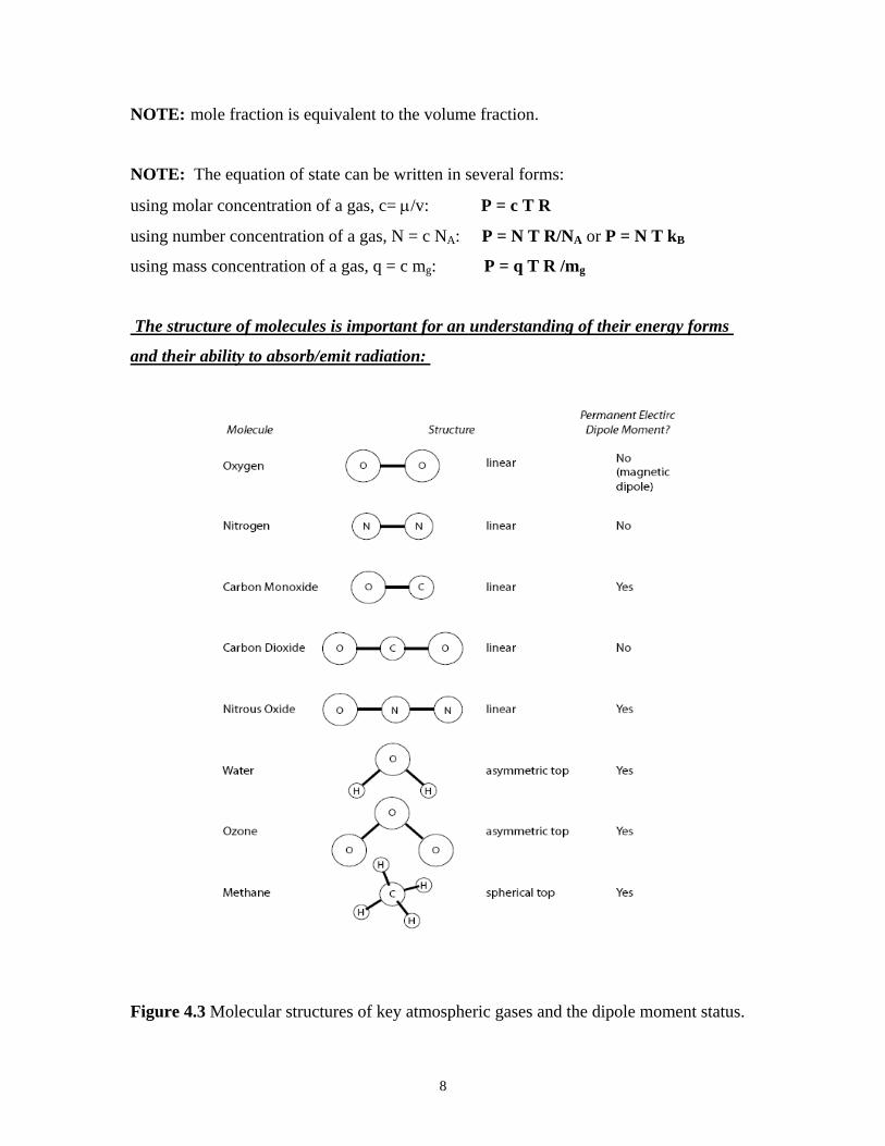
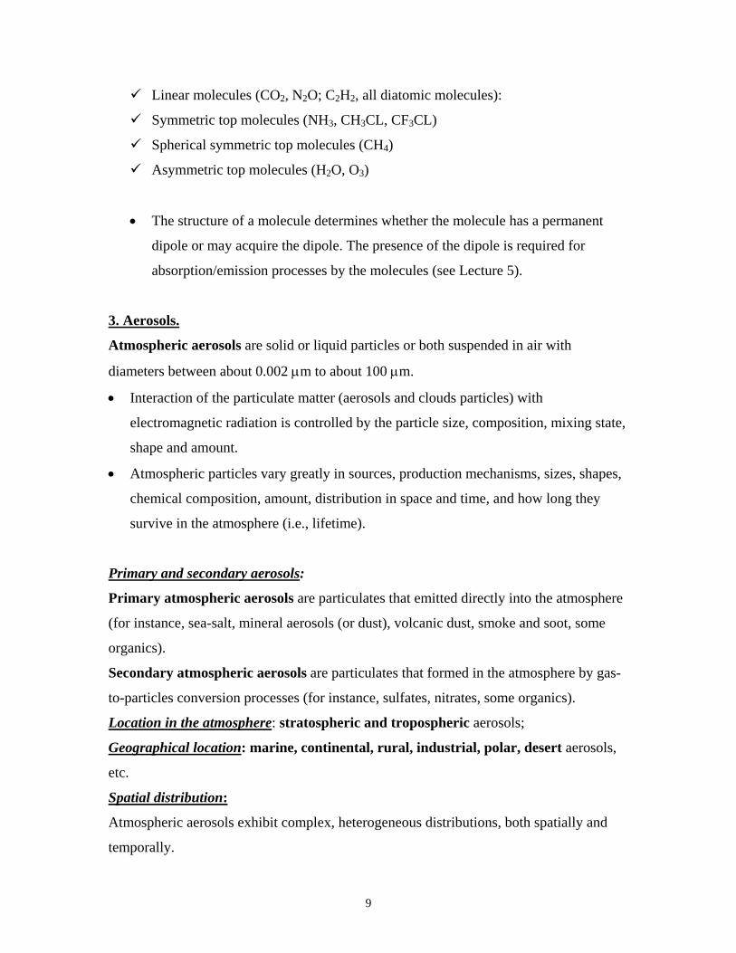
The structure of molecules is important for an understanding of their energy forms

and their ability to absorb/emit radiation:

Figure 4.3 Molecular structures of key atmospheric gases and the dipole moment status.

9

Linear molecules (CO2, N2O; C2H2, all diatomic molecules):

Symmetric top molecules (NH3, CH3CL, CF3CL)

Spherical symmetric top molecules (CH4)

Asymmetric top molecules (H2O, O3)

• The structure of a molecule determines whether the molecule has a permanent

dipole or may acquire the dipole. The presence of the dipole is required for

absorption/emission processes by the molecules (see Lecture 5).

3. Aerosols.

Atmospheric aerosols are solid or liquid particles or both suspended in air with

diameters between about 0.002 µm to about 100 µm.

• Interaction of the particulate matter (aerosols and clouds particles) with

electromagnetic radiation is controlled by the particle size, composition, mixing state,

shape and amount.

• Atmospheric particles vary greatly in sources, production mechanisms, sizes, shapes,

chemical composition, amount, distribution in space and time, and how long they

survive in the atmosphere (i.e., lifetime).

Primary and secondary aerosols:

Primary atmospheric aerosols are particulates that emitted directly into the atmosphere

(for instance, sea-salt, mineral aerosols (or dust), volcanic dust, smoke and soot, some

organics).

Secondary atmospheric aerosols are particulates that formed in the atmosphere by gas-

to-particles conversion processes (for instance, sulfates, nitrates, some organics).

Location in the atmosphere: stratospheric and tropospheric aerosols;

Geographical location: marine, continental, rural, industrial, polar, desert aerosols,

etc.

Spatial distribution:

Atmospheric aerosols exhibit complex, heterogeneous distributions, both spatially and

temporally.

10

Anthropogenic (man-made) and natural aerosols:

Anthropogenic sources: various (biomass burning, gas to particle conversion; industrial

processes; agriculture’s activities)

Natural sources: various (sea-salt, dust storm, biomass burning, volcanic debris, gas to

particle conversion).

Chemical composition:

Individual chemical species: sulfate (SO42-), nitrate (NO3

-), soot (elemental carbon),

sea-salt (NaCl); minerals (e.g., quartz, SiO4).

Multi-component (MC) aerosols: complex make-up of many chemical species (called

internally mixed particles)

Particle size distribution:

• The particle size distribution of aerosols are commonly approximated by the

analytical functions (such as log-normal, power law, or gamma function)

Log-normal function:

))ln(2)/ln(

exp()ln(2

)( 2

2

σσπorr

rNorN −= [4.1]

Normalization:

0)( NdrrN =∫ [4.2]

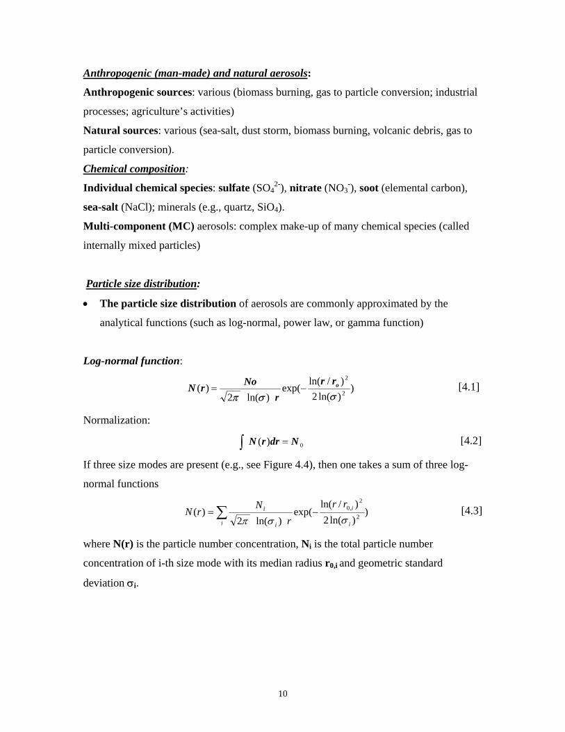
If three size modes are present (e.g., see Figure 4.4), then one takes a sum of three log-

normal functions

∑ −=i i

i

i

i rrr

NrN )

)ln(2)/ln(

exp()ln(2

)( 2

2,0

σσπ [4.3]

where N(r) is the particle number concentration, Ni is the total particle number

concentration of i-th size mode with its median radius r0,i and geometric standard

deviation σi.

11

NOTE: Surface area or volume (mass) size distributions can be found using the k-

moment of the lognormal distribution (k=2 or k=3, respectively):

)2/)(lnexp()( 2200 σkrNdrrNr kk =∫ [4.4]

Figure 4.4 A “classical view” of the distribution of particle mass of atmospheric aerosols

(from Whitby and Cantrell, 1976).

NOTE: Fine mode (d < ~ 2.5 µm) and coarse mode (d > ~ 2.5 µm); fine mode is divided

on the nuclei mode (about 0.005 µm < d < 0.1 µm) and accumulation mode (0.1µm < d <

2.5 µm).

12

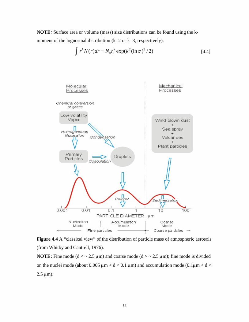
Shapes of aerosol particles : many are spherical but not all!

4. Clouds.

Major characteristics are cloud type, cloud coverage and distribution, liquid water

content of cloud, cloud droplet concentration, and cloud droplet size.

Cloud droplet sizes vary from a few micrometers to 100 micrometers with

average diameter in 10 to 20 µm range.

Cloud droplet concentration varies from about 10 cm-3 to 1000 cm-3 with average

droplet concentration of a few hundred cm-3.

The liquid water content of typical clouds, often abbreviated LWC, varies from

approximately 0.05 to 3 g(water) m-3, with most of the observed values in the 0.1

to 0.3 g(water) m-3 region.

13

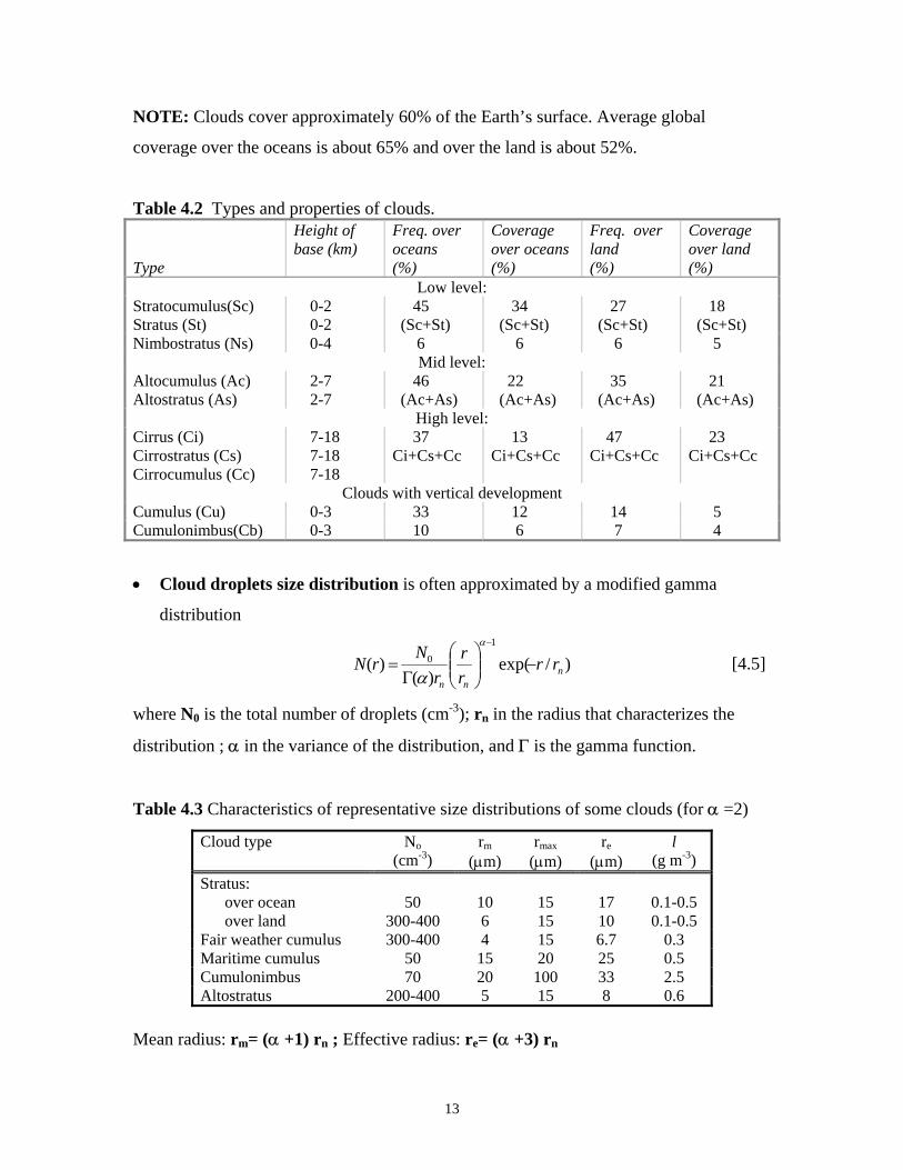
NOTE: Clouds cover approximately 60% of the Earth’s surface. Average global

coverage over the oceans is about 65% and over the land is about 52%.

Table 4.2 Types and properties of clouds. Type

Height of base (km)

Freq. over oceans (%)

Coverage over oceans (%)

Freq. over land (%)

Coverage over land (%)

Low level: Stratocumulus(Sc) Stratus (St)

0-2 0-2

45 (Sc+St)

34 (Sc+St)

27 (Sc+St)

18 (Sc+St)

Nimbostratus (Ns) 0-4 6 6 6 5 Mid level:

Altocumulus (Ac) Altostratus (As)

2-7 2-7

46 (Ac+As)

22 (Ac+As)

35 (Ac+As)

21 (Ac+As)

High level: Cirrus (Ci) Cirrostratus (Cs) Cirrocumulus (Cc)

7-18 7-18 7-18

37 Ci+Cs+Cc

13 Ci+Cs+Cc

47 Ci+Cs+Cc

23 Ci+Cs+Cc

Clouds with vertical development Cumulus (Cu) 0-3 33 12 14 5 Cumulonimbus(Cb) 0-3 10 6 7 4

• Cloud droplets size distribution is often approximated by a modified gamma

distribution

)/exp()(

)(1

0n

nn

rrrr

rN

rN −⎟⎟⎠

⎞⎜⎜⎝

⎛Γ

=−α

α [4.5]

where N0 is the total number of droplets (cm-3); rn in the radius that characterizes the

distribution ; α in the variance of the distribution, and Γ is the gamma function.

Table 4.3 Characteristics of representative size distributions of some clouds (for α =2)

Cloud type No (cm-3)

rm

(µm) rmax

(µm) re

(µm) l

(g m-3) Stratus: over ocean

50

10

15

17

0.1-0.5

over land 300-400 6 15 10 0.1-0.5 Fair weather cumulus 300-400 4 15 6.7 0.3 Maritime cumulus 50 15 20 25 0.5 Cumulonimbus 70 20 100 33 2.5 Altostratus 200-400 5 15 8 0.6

Mean radius: rm= (α +1) rn ; Effective radius: re= (α +3) rn

14

• For many practical applications, the optical properties of water clouds are

parameterized as a function of the effective radius and liquid water content

(LWC).

The effective radius is defined as

∫∫=

drrNr

drrNrre )(

)(2

3

π

π [4.6]

where N(r) is the droplet size distribution.

The liquid water content (LWC) is defined as

drrNrVLWC ww )(34 3∫== πρρ [4.7]

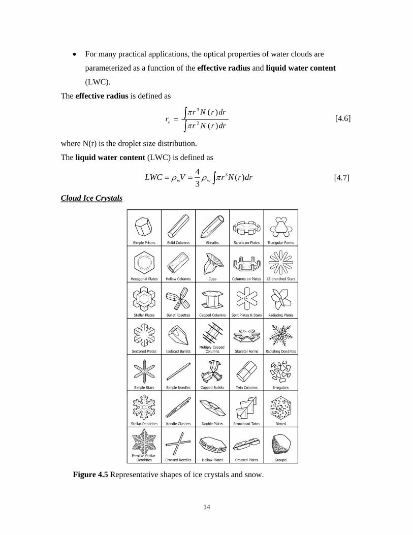
Cloud Ice Crystals

Figure 4.5 Representative shapes of ice crystals and snow.

15

Ice crystals present in clouds found in the atmosphere are often six-sided. However,

there are variations in shape: plates - nearly flat hexagon; columns - elongated, flat

bottoms; needles - elongated, pointed bottoms; dendrites - elongated arms (six),

snowflake shape.

Ice crystal shapes depend on temperature and relative humidity. Also, crystal shapes

can be changed due to collision and coalescence processes in the clouds.

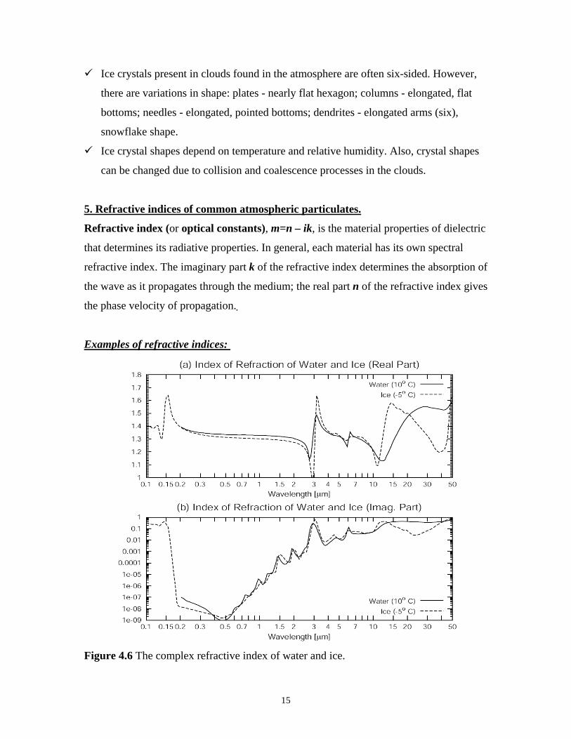
5. Refractive indices of common atmospheric particulates.

Refractive index (or optical constants), m=n – ik, is the material properties of dielectric

that determines its radiative properties. In general, each material has its own spectral

refractive index. The imaginary part k of the refractive index determines the absorption of

the wave as it propagates through the medium; the real part n of the refractive index gives

the phase velocity of propagation..

Examples of refractive indices:

Figure 4.6 The complex refractive index of water and ice.

16

It is believed that the refractive indices of the (bulk material apply down to the

smallest atmospheric aerosol particles.

The refractive index is a function of wavelength. Each substance has a specific

spectrum of the refractive index.

Particles of different sizes, shapes and indices of refraction will have different

scattering and absorbing properties.

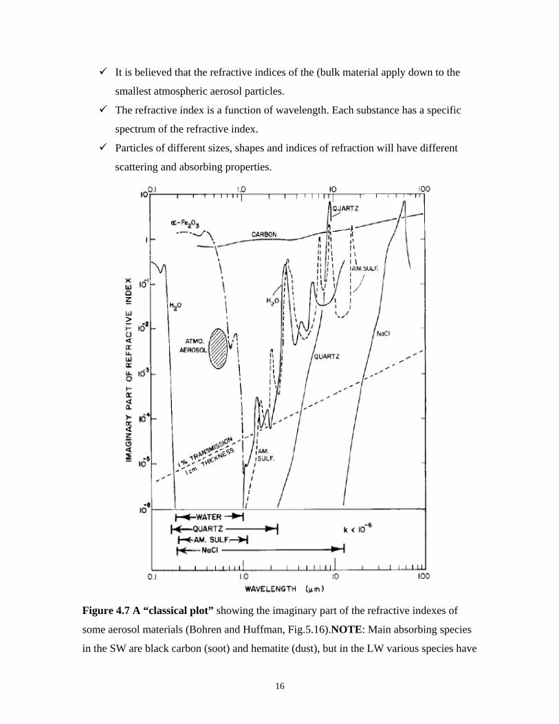
Figure 4.7 A “classical plot” showing the imaginary part of the refractive indexes of

some aerosol materials (Bohren and Huffman, Fig.5.16).NOTE: Main absorbing species

in the SW are black carbon (soot) and hematite (dust), but in the LW various species have

17

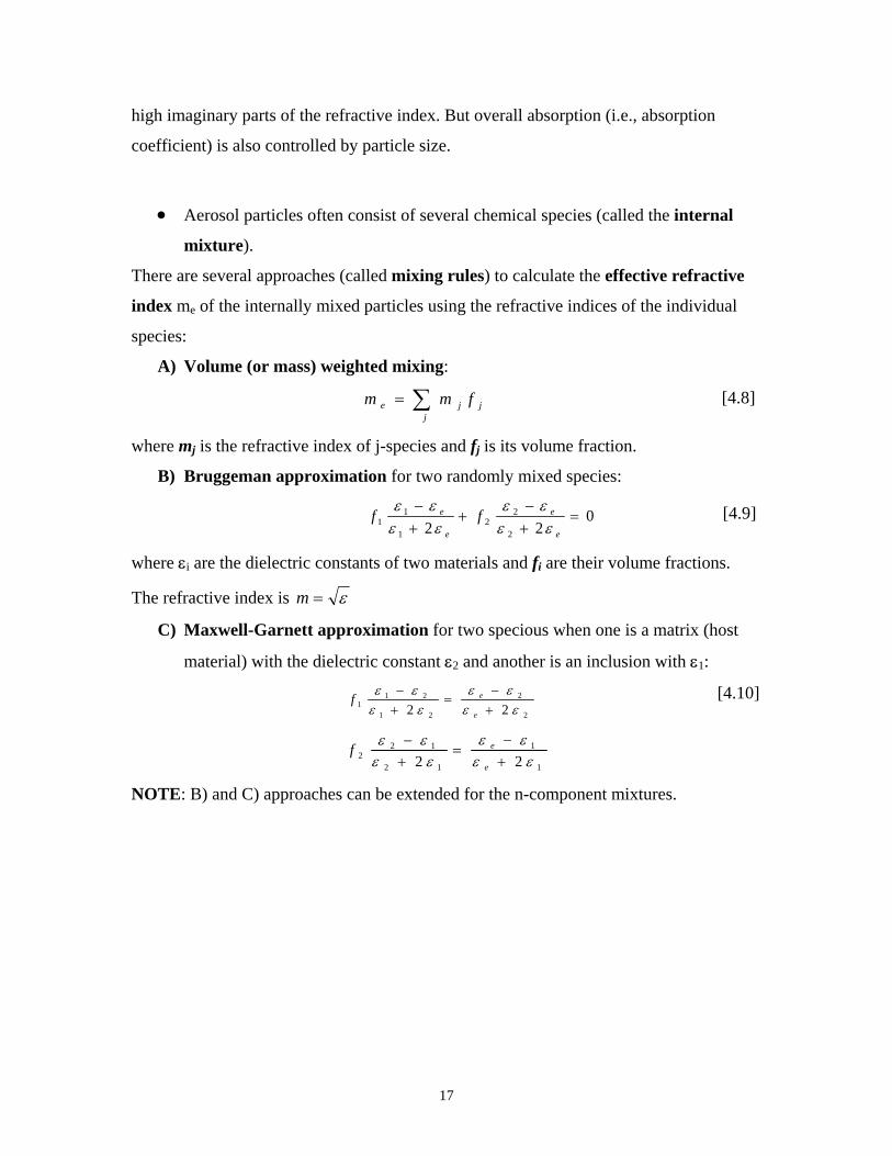
high imaginary parts of the refractive index. But overall absorption (i.e., absorption

coefficient) is also controlled by particle size.

• Aerosol particles often consist of several chemical species (called the internal

mixture). There are several approaches (called mixing rules) to calculate the effective refractive

index me of the internally mixed particles using the refractive indices of the individual

species:

A) Volume (or mass) weighted mixing:

∑=j

jje fmm [4.8]

where mj is the refractive index of j-species and fj is its volume fraction.

B) Bruggeman approximation for two randomly mixed species:

022 2

22

1

11 =

+−

++−

e

e

e

e ffεεεε

εεεε [4.9]

where εi are the dielectric constants of two materials and fi are their volume fractions.

The refractive index is ε=m

C) Maxwell-Garnett approximation for two specious when one is a matrix (host

material) with the dielectric constant ε2 and another is an inclusion with ε1:

2

2

21

211 22 εε

εεεεεε

+−

=+−

e

ef [4.10]

1

1

12

122 22 εε

εεεεεε

+−

=+−

e

ef

NOTE: B) and C) approaches can be extended for the n-component mixtures.