Embed Size (px)
Citation preview
University of Central Florida University of Central Florida
STARS STARS
Electronic Theses and Dissertations, 2020-
2020
Compressibility of Fine-Grained Soil in Central Florida Compressibility of Fine-Grained Soil in Central Florida
Andre Kruk University of Central Florida
Part of the Geotechnical Engineering Commons, and the Structural Engineering Commons
Find similar works at: https://stars.library.ucf.edu/etd2020
University of Central Florida Libraries http://library.ucf.edu
This Masters Thesis (Open Access) is brought to you for free and open access by STARS. It has been accepted for
inclusion in Electronic Theses and Dissertations, 2020- by an authorized administrator of STARS. For more
information, please contact [email protected].
STARS Citation STARS Citation Kruk, Andre, "Compressibility of Fine-Grained Soil in Central Florida" (2020). Electronic Theses and Dissertations, 2020-. 80. https://stars.library.ucf.edu/etd2020/80
COMPRESSIBILITY OF FINE-GRAINED SOIL IN CENTRAL FLORIDA
by
ANDRE KRUK B.S. University of Central Florida, 2019
A thesis submitted in partial fulfillment of the requirements for the degree of Master of Sciences
in the Department of Civil, Environmental, and Construction Engineering at the College of Engineering and Computer Science
at the University of Central Florida Orlando, Florida
Spring Term 2020
ii
@ 2020 Andre Kruk
iii
ABSTRACT
Settlement is a limiting design aspect in most geotechnical projects. Fine-grained cohesive soils
are typically responsible for the majority of site settlements through a time dependent process known
as consolidation. For this reason, it is desirable to accurately determine the degree of consolidation,
referred to in the report as soil compressibility, of the fine-grained layers impacted by loading. Soil
compressibility is commonly determined from the Oedometer test; however, this test is time
consuming, expensive, highly susceptible to soil disturbance, and represents a very small zone of the soil
layer. An alternative method to estimate the compressibility would be correlations with index
properties which can be performed for all soil layers at a low cost and with quick turnover. Other
methods include in-situ testing techniques such as Standard Penetration Testing (SPT), Cone Penetration
Testing (CPT), Dilatometer Testing (DMT), and Pressuremeter Testing (PMT). The CPT is the most ideal
test as it is repeatable, continuous, and commonly used. For this reason, this study utilizes an empirical
method to refine correlations to index properties for local soils and estimate the compressibility via CPT.
It was found that compressibility can be accurately estimated via CPT for soils with relatively high
activity and moisture content. Index test correlations, when refined for the local geology, performed
better than the generic correlations. The results for both techniques are not accurate enough to
completely replace better in-situ or laboratory tests. However, it is this authors opinion that accurate
determination of preconsolidation pressure is more important for accurate settlement estimation than
compressibility indices. If the preconsolidation pressure is well defined for the site, the small error in the
compressibility indices will have a minimal impact on the overall estimation of settlement.
Consequently, this study will recommend a refined model for preconsolidation pressure in the
conclusion chapter.

iv
ACKNOWLEDGMENTS
I would like to thank my advisor, Dr. Boo Hyun Nam, for patiently guiding and supporting me
throughout this process. I also sincerely appreciate my committee members, Dr. Manoj Chopra, Dr.
Arboleda Monslave and Dr. Dingbao Wang for reviewing this work. The following members have not
only guided me through this research but have shared their knowledge of Geotechnical Engineering
through teaching, office hours, and presentations. The support from my co-workers at Ardaman and
Associates and S&ME has made this research possible by providing data points, and technically stronger
by fielding questions.
v
TABLE OF CONTENTS
LIST OF FIGURES ........................................................................................................................................... vii
LIST OF TABLES ............................................................................................................................................... x
CHAPTER 1 INTRODUCTION ...................................................................................................................... 1
1.1 Purpose .......................................................................................................................................... 4
1.2 Methodology ................................................................................................................................. 4
1.3 Thesis Outline ................................................................................................................................ 5
CHAPTER 2 LITERATURE REVIEW .............................................................................................................. 6
2.1 Introduction ................................................................................................................................... 6
2.2 Important Concepts ....................................................................................................................... 6
2.3 Central Florida Geology ................................................................................................................. 8
2.4 Estimation of Compressibility from Index Properties ................................................................... 8
2.5 Compressibility and Cone Penetration Test ................................................................................ 12
2.5.1 Elastic Derivation and Calibration Constant ........................................................................ 12
2.5.2 Constrained Modulus .......................................................................................................... 16
2.6 Estimation of Preconsildation Pressure ....................................................................................... 18
2.7 Literature Review Conclusion ...................................................................................................... 20
CHAPTER 3 INDEX PROPERTIES AND COMPRESSIBILITY......................................................................... 22
3.1 Introduction ................................................................................................................................. 22
3.2 Methodology ............................................................................................................................... 25
3.2.1 Data Base ............................................................................................................................. 25
3.2.2 Analysis ................................................................................................................................ 25
3.3 Results and Discussion ................................................................................................................. 26
3.3.1 Correlations from Charts ..................................................................................................... 26
3.3.2 Recommended Models and Discussion ............................................................................... 32
3.4 Conclusion .................................................................................................................................... 34
CHAPTER 4 CONE PENETRATION TEST BASED CORRELATION ANALYSIS ............................................... 35
4.1 Introduction ................................................................................................................................. 35
4.2 Methodology ............................................................................................................................... 38
4.2.1 Cone Penetration Test Data Base ........................................................................................ 38
4.2.2 Data Processing Procedure .................................................................................................. 38
vi
4.2.3 Data Processing Procedure: Example ................................................................................. 41
4.2.4 Analysis ................................................................................................................................ 50
4.3 Results .......................................................................................................................................... 52
4.3.1 Correlations from Charts ..................................................................................................... 52
4.3.2 Recommended Model and Discussion ................................................................................ 57
4.4 Conclusion .................................................................................................................................... 63
CHAPTER 5 CONE PENETRATION TEST BASED CORRELATIONS – DIVIDED DATA BASE FOR ACTIVITY
AND MOISTURE CONTENT ........................................................................................................................... 64
5.1 Introduction ................................................................................................................................. 64
5.2 Methodology ............................................................................................................................... 69
5.3 Results .......................................................................................................................................... 69
5.3.1 Correlations from Charts ..................................................................................................... 70
5.3.2 Recommended Models and Discussion ............................................................................... 77
5.4 Conclusion .................................................................................................................................... 80
CHAPTER 6 CONCLUSION........................................................................................................................ 81
6.1 Summary ...................................................................................................................................... 81
6.2 Recommendations ....................................................................................................................... 81
6.2.1 Compression Index Recommendation................................................................................. 81
6.2.2 OCR Recommendation......................................................................................................... 82
6.3 Limitations and Future Works ..................................................................................................... 83
APPENDIX A – INDEX PROPERTY CORRELATIONS ........................................................................................ 85
APPENDIX B – CONE PENETRATION TEST BASED CORRELATIONS (UNDIVIDED) ........................................ 96
APPENDIX C - CONE PENETRATION TEST BASED CORRELATIONS (DIVIDED) ............................................ 107
APPENDIX D – SNIPPET OF UCF DATA BASE .............................................................................................. 120
APPENDIX E – SNIPPET OF CPT DATA BASE ............................................................................................... 122
LIST OF REFERENCES .................................................................................................................................. 124
vii
LIST OF FIGURES
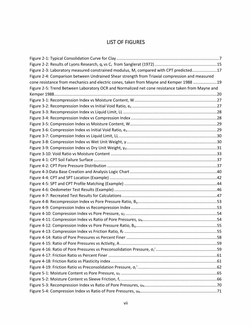
Figure 2-1: Typical Consolidation Curve for Clay ........................................................................................... 7
Figure 2-2: Results of Lyons Research, qc vs Cc from Sanglerat (1972) ....................................................... 15
Figure 2-3: Laboratory measured constrained modulus, M, compared with CPT predicted...................... 17
Figure 2-4: Comparison between Undrained Shear strength from Triaxial compression and measured
cone resistance from mechanics and electric cones, taken from Mayne and Kemper 1988 ..................... 19
Figure 2-5: Trend Between Laboratory OCR and Normalized net cone resistance taken from Mayne and
Kemper 1988 ................................................................................................................................................ 20
Figure 3-1: Recompression Index vs Moisture Content, W ......................................................................... 27
Figure 3-2: Recompression Index vs Initial Void Ratio, eo ........................................................................... 27
Figure 3-3: Recompression Index vs Liquid Limit, LL ................................................................................... 28
Figure 3-4: Recompression Index vs Compression Index ............................................................................ 28
Figure 3-5: Compression Index vs Moisture Content, W............................................................................. 29
Figure 3-6: Compression Index vs Initial Void Ratio, eo ............................................................................... 29
Figure 3-7: Compression Index vs Liquid Limit, LL ....................................................................................... 30
Figure 3-8: Compression Index vs Wet Unit Weight, γ ................................................................................ 30
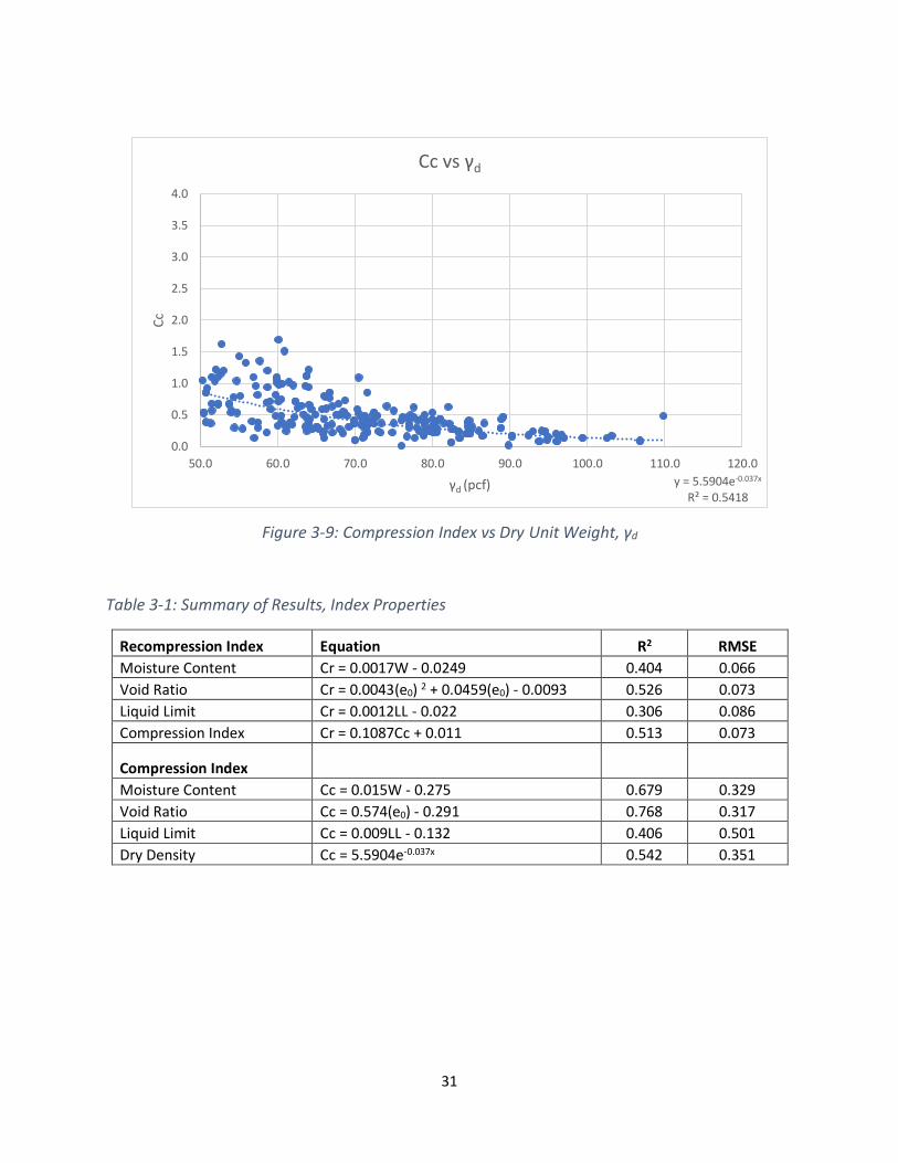
Figure 3-9: Compression Index vs Dry Unit Weight, γd ................................................................................ 31
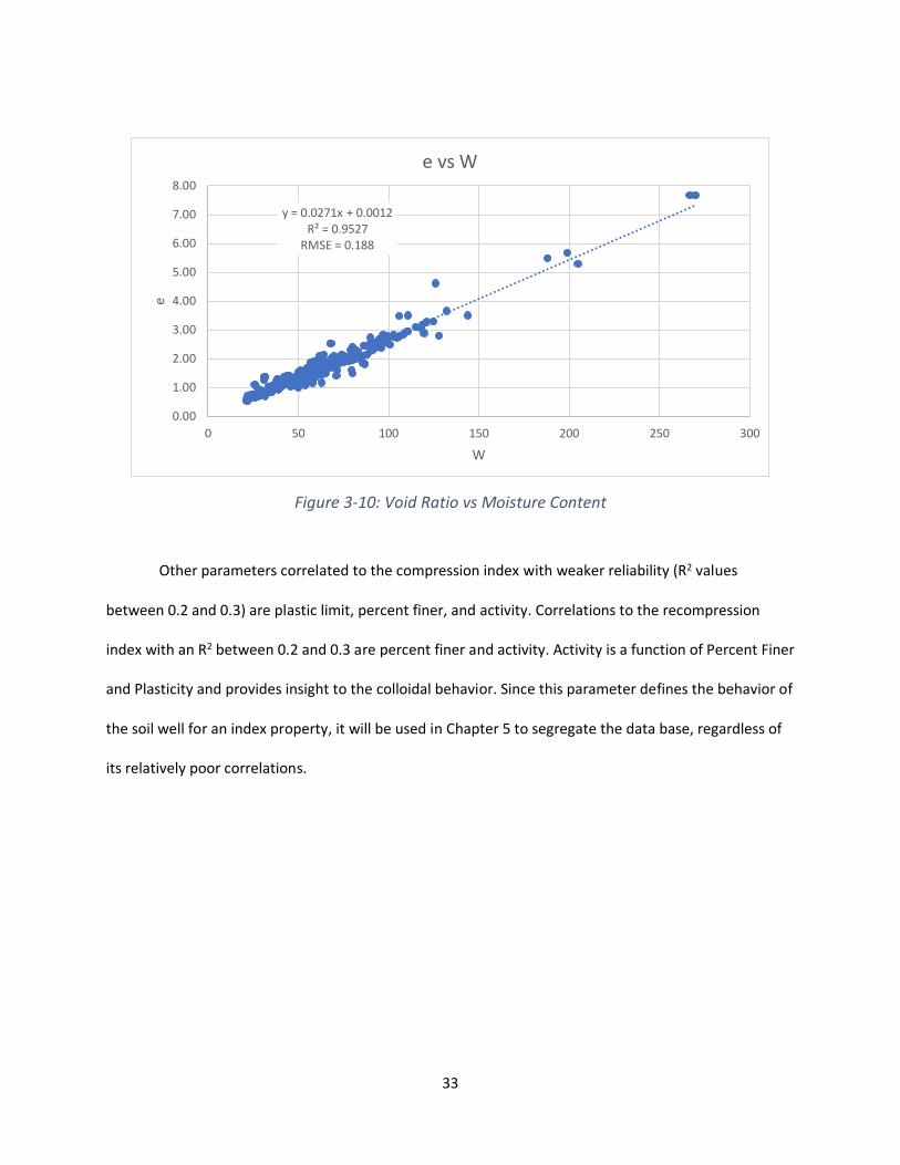
Figure 3-10: Void Ratio vs Moisture Content .............................................................................................. 33
Figure 4-1: CPT Soil Failure Surface ............................................................................................................. 37
Figure 4-2: CPT Pore Pressure Distribution ................................................................................................. 37
Figure 4-3:Data Base Creation and Analysis Logic Chart ............................................................................. 40
Figure 4-4: CPT and SPT Location (Example) ............................................................................................... 42
Figure 4-5: SPT and CPT Profile Matching (Example) .................................................................................. 44
Figure 4-6: Oedometer Test Results (Example) ........................................................................................... 46
Figure 4-7: Recreated Test Results for Calculations .................................................................................... 47
Figure 4-8: Recompression Index vs Pore Pressure Ratio, Bq ...................................................................... 53
Figure 4-9: Compression Index vs Recompression Index ............................................................................ 53
Figure 4-10: Compression Index vs Pore Pressure, u2 ................................................................................. 54
Figure 4-11: Compression Index vs Ratio of Pore Pressures, uN.................................................................. 54
Figure 4-12: Compression Index vs Pore Pressure Ratio, Bq........................................................................ 55
Figure 4-13: Compression Index vs Friction Ratio, Rf .................................................................................. 55
Figure 4-14: Ratio of Pore Pressures vs Percent Finer ................................................................................ 58
Figure 4-15: Ratio of Pore Pressures vs Activity, A ...................................................................................... 59
Figure 4-16: Ratio of Pore Pressures vs Preconsolidation Pressure, σc' ...................................................... 59
Figure 4-17: Friction Ratio vs Percent Finer ................................................................................................ 61
Figure 4-18: Friction Ratio vs Plasticity index .............................................................................................. 61
Figure 4-19: Friction Ratio vs Preconsolidation Pressure, σc' ...................................................................... 62
Figure 5-1: Moisture Content vs Pore Pressure, u2 ..................................................................................... 65
Figure 5-2: Moisture Content vs Sleeve Friction, fs ..................................................................................... 66
Figure 5-3: Recompression Index vs Ratio of Pore Pressures, uN ................................................................ 70
Figure 5-4: Compression Index vs Ratio of Pore Pressures, uN.................................................................... 71
viii
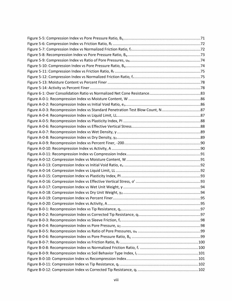
Figure 5-5: Compression Index vs Pore Pressure Ratio, Bq.......................................................................... 71
Figure 5-6: Compression Index vs Friction Ratio, Rf .................................................................................... 72
Figure 5-7: Compression Index vs Normalized Friction Ratio, fr .................................................................. 72
Figure 5-8: Recompression Index vs Pore Pressure Ratio, Bq ...................................................................... 73
Figure 5-9: Compression Index vs Ratio of Pore Pressures, uN.................................................................... 74
Figure 5-10: Compression Index vs Pore Pressure Ratio, Bq........................................................................ 74
Figure 5-11: Compression Index vs Friction Ratio, Rf .................................................................................. 75
Figure 5-12: Compression Index vs Normalized Friction Ratio, fr................................................................ 75
Figure 5-13: Moisture Content vs Percent Finer ......................................................................................... 78
Figure 5-14: Activity vs Percent Finer .......................................................................................................... 78
Figure 6-1: Over Consolidation Ratio vs Normalized Net Cone Resistance................................................. 83
Figure A-0-1: Recompression Index vs Moisture Content, W ..................................................................... 86
Figure A-0-2: Recompression Index vs Initial Void Ratio, eo........................................................................ 86
Figure A-0-3: Recompression Index vs Standard Penetration Test Blow Count, N ..................................... 87
Figure A-0-4: Recompression Index vs Liquid Limit, LL................................................................................ 87
Figure A-0-5: Recompression Index vs Plasticity Index, PI .......................................................................... 88
Figure A-0-6: Recompression Index vs Effective Vertical Stress.................................................................. 88
Figure A-0-7: Recompression Index vs Wet Density, γ ................................................................................ 89
Figure A-0-8: Recompression Index vs Dry Density, γd ................................................................................ 89
Figure A-0-9: Recompression Index vs Percent Finer, -200 ......................................................................... 90
Figure A-0-10: Recompression Index vs Activity, A ..................................................................................... 90
Figure A-0-11: Recompression Index vs Compression Index....................................................................... 91
Figure A-0-12: Compression Index vs Moisture Content, W ....................................................................... 91
Figure A-0-13: Compression Index vs Initial Void Ratio, eo ......................................................................... 92
Figure A-0-14: Compression Index vs Liquid Limit, LL ................................................................................. 92
Figure A-0-15: Compression Index vs Plasticity Index, PI ............................................................................ 93
Figure A-0-16: Compression Index vs Effective Vertical Stress, σ' .............................................................. 93
Figure A-0-17: Compression Index vs Wet Unit Weight, γ .......................................................................... 94
Figure A-0-18: Compression Index vs Dry Unit Weight, γd .......................................................................... 94
Figure A-0-19: Compression Index vs Percent Finer .................................................................................... 95
Figure A-0-20: Compression Index vs Activity, A ......................................................................................... 95
Figure B-0-1: Recompression Index vs Tip Resistance, qc............................................................................ 97
Figure B-0-2: Recompression Index vs Corrected Tip Resistance, qt ........................................................... 97
Figure B-0-3: Recompression Index vs Sleeve Friction, fs ............................................................................ 98
Figure B-0-4: Recompression Index vs Pore Pressure, u2 ............................................................................ 98
Figure B-0-5: Recompression Index vs Ratio of Pore Pressures, uN ............................................................ 99
Figure B-0-6: Recompression Index vs Pore Pressure Ratio, Bq .................................................................. 99
Figure B-0-7: Recompression Index vs Friction Ratio, Rf ........................................................................... 100
Figure B-0-8: Recompression Index vs Normalized Friction Ratio, fr ........................................................ 100
Figure B-0-9: Recompression Index vs Soil Behavior Type Index, Ic .......................................................... 101
Figure B-0-10: Compression Index vs Recompression Index ..................................................................... 101
Figure B-0-11: Compression Index vs Tip Resistance, qc ........................................................................... 102
Figure B-0-12: Compression Index vs Corrected Tip Resistance, qt .......................................................... 102
ix
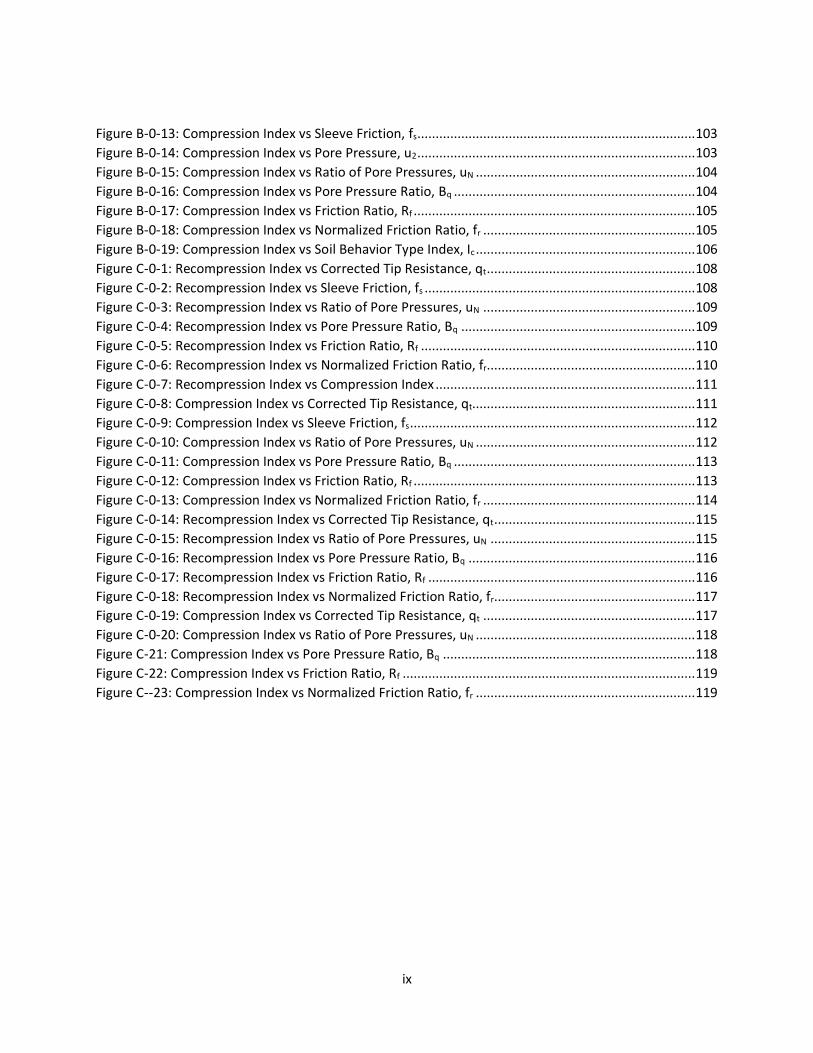
Figure B-0-13: Compression Index vs Sleeve Friction, fs............................................................................ 103
Figure B-0-14: Compression Index vs Pore Pressure, u2 ............................................................................ 103
Figure B-0-15: Compression Index vs Ratio of Pore Pressures, uN ............................................................ 104
Figure B-0-16: Compression Index vs Pore Pressure Ratio, Bq .................................................................. 104
Figure B-0-17: Compression Index vs Friction Ratio, Rf ............................................................................. 105
Figure B-0-18: Compression Index vs Normalized Friction Ratio, fr .......................................................... 105
Figure B-0-19: Compression Index vs Soil Behavior Type Index, Ic ............................................................ 106
Figure C-0-1: Recompression Index vs Corrected Tip Resistance, qt ......................................................... 108
Figure C-0-2: Recompression Index vs Sleeve Friction, fs .......................................................................... 108
Figure C-0-3: Recompression Index vs Ratio of Pore Pressures, uN .......................................................... 109
Figure C-0-4: Recompression Index vs Pore Pressure Ratio, Bq ................................................................ 109
Figure C-0-5: Recompression Index vs Friction Ratio, Rf ........................................................................... 110
Figure C-0-6: Recompression Index vs Normalized Friction Ratio, fr......................................................... 110
Figure C-0-7: Recompression Index vs Compression Index ....................................................................... 111
Figure C-0-8: Compression Index vs Corrected Tip Resistance, qt............................................................. 111
Figure C-0-9: Compression Index vs Sleeve Friction, fs .............................................................................. 112
Figure C-0-10: Compression Index vs Ratio of Pore Pressures, uN ............................................................ 112
Figure C-0-11: Compression Index vs Pore Pressure Ratio, Bq .................................................................. 113
Figure C-0-12: Compression Index vs Friction Ratio, Rf ............................................................................. 113
Figure C-0-13: Compression Index vs Normalized Friction Ratio, fr .......................................................... 114
Figure C-0-14: Recompression Index vs Corrected Tip Resistance, qt ....................................................... 115
Figure C-0-15: Recompression Index vs Ratio of Pore Pressures, uN ........................................................ 115
Figure C-0-16: Recompression Index vs Pore Pressure Ratio, Bq .............................................................. 116
Figure C-0-17: Recompression Index vs Friction Ratio, Rf ......................................................................... 116
Figure C-0-18: Recompression Index vs Normalized Friction Ratio, fr....................................................... 117
Figure C-0-19: Compression Index vs Corrected Tip Resistance, qt .......................................................... 117
Figure C-0-20: Compression Index vs Ratio of Pore Pressures, uN ............................................................ 118
Figure C-21: Compression Index vs Pore Pressure Ratio, Bq ..................................................................... 118
Figure C-22: Compression Index vs Friction Ratio, Rf ................................................................................ 119
Figure C--23: Compression Index vs Normalized Friction Ratio, fr ............................................................ 119
x
LIST OF TABLES
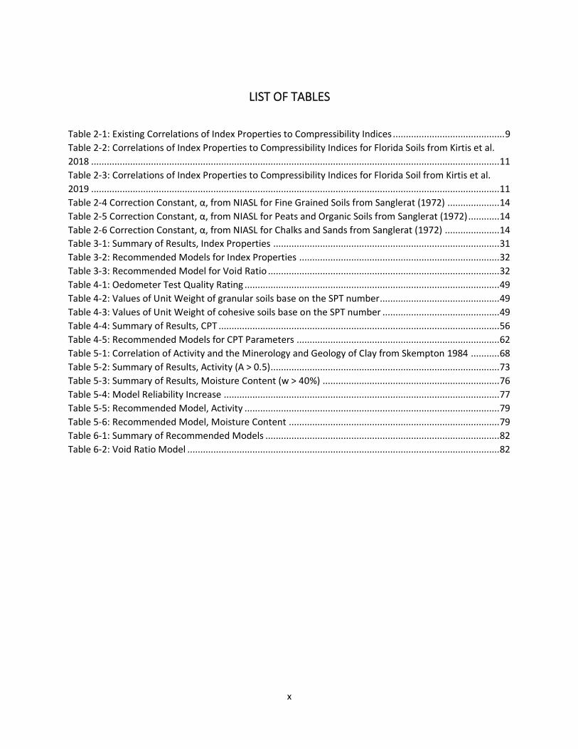
Table 2-1: Existing Correlations of Index Properties to Compressibility Indices ........................................... 9
Table 2-2: Correlations of Index Properties to Compressibility Indices for Florida Soils from Kirtis et al.
2018 ............................................................................................................................................................. 11
Table 2-3: Correlations of Index Properties to Compressibility Indices for Florida Soil from Kirtis et al.
2019 ............................................................................................................................................................. 11
Table 2-4 Correction Constant, α, from NIASL for Fine Grained Soils from Sanglerat (1972) .................... 14
Table 2-5 Correction Constant, α, from NIASL for Peats and Organic Soils from Sanglerat (1972) ............ 14
Table 2-6 Correction Constant, α, from NIASL for Chalks and Sands from Sanglerat (1972) ..................... 14
Table 3-1: Summary of Results, Index Properties ....................................................................................... 31
Table 3-2: Recommended Models for Index Properties ............................................................................. 32
Table 3-3: Recommended Model for Void Ratio ......................................................................................... 32
Table 4-1: Oedometer Test Quality Rating .................................................................................................. 49
Table 4-2: Values of Unit Weight of granular soils base on the SPT number.............................................. 49
Table 4-3: Values of Unit Weight of cohesive soils base on the SPT number ............................................. 49
Table 4-4: Summary of Results, CPT ............................................................................................................ 56
Table 4-5: Recommended Models for CPT Parameters .............................................................................. 62
Table 5-1: Correlation of Activity and the Minerology and Geology of Clay from Skempton 1984 ........... 68
Table 5-2: Summary of Results, Activity (A > 0.5)........................................................................................ 73
Table 5-3: Summary of Results, Moisture Content (w > 40%) .................................................................... 76
Table 5-4: Model Reliability Increase .......................................................................................................... 77
Table 5-5: Recommended Model, Activity .................................................................................................. 79
Table 5-6: Recommended Model, Moisture Content ................................................................................. 79
Table 6-1: Summary of Recommended Models .......................................................................................... 82
Table 6-2: Void Ratio Model ........................................................................................................................ 82
1
CHAPTER 1 INTRODUCTION
In most Geotechnical projects a major design consideration is settlement. The magnitude of
settlement is estimated by defining the soil’s compressibility, which is dependent on composition
(stress) and structure (void ratio).
The in-situ stress and void ratio define the current compressive state of the soil. The in-situ
effective vertical stress consists of the total vertical stress and the pore pressure, implying the effective
stress is time-dependent. This time-dependent compression is known as consolidation which is the
transfer of stress from the pore pressure to the soil skeleton. Any combination of composition and
structure that allows a soil to exist at a high volume of voids, as indicated by a high natural water
content or void ratio, results in the potential for large volume changes. The change in stress (change in
stress from pre-post construction) results in the reconfiguration of the structure into a decreased void
ratio. (Terzaghi et al. 1996). The pre- construction stress state, also known as the preconsolidation
pressure, can be defined as the amount of maximum pressure previously experienced by the soil
through geologic conditions and marks the stress level at which the soil switches from elastic to plastic
behavior.
Volume change within the elastic region is strongly influenced by the natural soil structure,
however, once the preconsolidation pressure is exceeded the change in volume is more influenced by
the loading. Within the elastic region the soil skeleton accommodates the stress with little interparticle
displacements, which are recoverable, resulting from minor slips at interparticle contacts. Within the
plastic region major particle rearrangement, which is not recoverable, is required to develop
interparticle resistance to the increased effective stress. This resistance must accommodate the stress
applied as well as compensate for the destroyed interparticle bond resistance. (Terzaghi et al. 1996)
2
The elastic region is occupied by over consolidated (OC) soils, a soil which has experienced a
stress greater than the current stress and is commonly referred to as the over consolidation line (OCL).
These soils could be overconsolidated due to natural causes such as erosion and groundwater
fluctuation, or unnatural causes such as surcharging and previous construction. The plastic response
occurs in normally consolidated (NC) soil, a soil which has never experienced the current magnitude of
stress and is referred to as the virgin or normally consolidated line (NCL) of the compression response
curve.
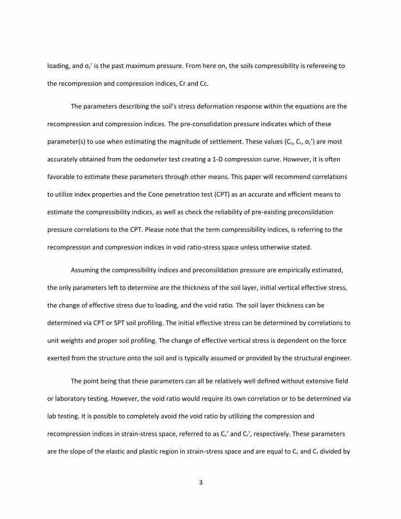
The stress path (change in stress from pre to post construction loading) determines which
equation to utilize to estimate the magnitude of consolidation (Das 2002). Equation (1) is used for an OC
soil that remains on the OCL after loading (i.e. never exceeds its past maximum pressure). Equation (2) is
used for an OC soil that exceeds the past-maximum pressure and now acts on the NCL. Equation (3) is
for a NC soil. The stress history of the soil can be changed with unloading; however, this is not within the
scope of the current research.
𝑆𝐶 = 𝐶𝑟𝐻𝐶
1+𝑒0𝑙𝑜𝑔 (
𝜎0′+∆𝜎′
𝜎𝑜′) ( 1 )
𝑆𝐶 = 𝐶𝑟𝐻𝐶
1+𝑒0𝑙𝑜𝑔 (
𝜎𝑐′
𝜎𝑜′) +
𝐶𝐶𝐻𝐶
1+𝑒0𝑙𝑜𝑔 (
𝜎0′+∆𝜎′
𝜎𝑜′) ( 2 )
𝑆𝐶 = 𝐶𝐶𝐻𝐶
1+𝑒0𝑙𝑜𝑔 (
𝜎0′+∆𝜎′
𝜎𝑜′) ( 3 )
These equations state that settlement is a direct function of compressibility, stress states, and
the drainage path. Where Sc is the settlement from loading, Cr is the recompression index (slope of
OCL), Cc is the compression index (slope of NCL), e0 is the soils initial ratio of voids to solids in terms of
volume of the soil, Hc is the thickness of soil layer between drainage paths, σ0’ is the initial vertical
effective stress at the midpoint of the soil layer, Δσ0’ is the change in vertical effective stress due to
3
loading, and σc’ is the past maximum pressure. From here on, the soils compressibility is refereeing to
the recompression and compression indices, Cr and Cc.
The parameters describing the soil’s stress deformation response within the equations are the
recompression and compression indices. The pre-consolidation pressure indicates which of these
parameter(s) to use when estimating the magnitude of settlement. These values (Cc, Cr, σc’) are most
accurately obtained from the oedometer test creating a 1-D compression curve. However, it is often
favorable to estimate these parameters through other means. This paper will recommend correlations
to utilize index properties and the Cone penetration test (CPT) as an accurate and efficient means to
estimate the compressibility indices, as well as check the reliability of pre-existing preconsildation
pressure correlations to the CPT. Please note that the term compressibility indices, is referring to the
recompression and compression indices in void ratio-stress space unless otherwise stated.
Assuming the compressibility indices and preconsildation pressure are empirically estimated,
the only parameters left to determine are the thickness of the soil layer, initial vertical effective stress,
the change of effective stress due to loading, and the void ratio. The soil layer thickness can be
determined via CPT or SPT soil profiling. The initial effective stress can be determined by correlations to
unit weights and proper soil profiling. The change of effective vertical stress is dependent on the force
exerted from the structure onto the soil and is typically assumed or provided by the structural engineer.
The point being that these parameters can all be relatively well defined without extensive field
or laboratory testing. However, the void ratio would require its own correlation or to be determined via
lab testing. It is possible to completely avoid the void ratio by utilizing the compression and
recompression indices in strain-stress space, referred to as Cc’ and Cr’, respectively. These parameters
are the slope of the elastic and plastic region in strain-stress space and are equal to Cc and Cr divided by
4
(1+e0). This transformation equation from void ratio- to strain – stress space is utilized in equations 1
through 3. The correlations to compressibility indices provided in this study will be presented in strain-
stress space where applicable or in void- stress space with an accompanying correlation to void ratio.
With void ratio now accounted for, everything needed to estimate settlement in Central Florida can be
determined cost effectively and accurately via CPT and/or index testing techniques.
1.1 Purpose
The purpose of this research is to estimate the compressibility of fine-grained cohesive soils via
index properties and the Cone penetration test (CPT) in the Central Florida region. Strong correlations
between certain index properties and compressibility have been previously defined. This study will
refine these correlations to the local geology. Correlations between compressibility and CPT for elastic
soil behavior have also been well defined, however, correlations for plastic behavior have not. This study
will refine elastic compressibility (recompression index) correlations and propose a model for estimation
of plastic compressibility (compression index). The yielding point at which soil behavior transitions from
elastic to plastic, also known as preconsolidation pressure, is required to estimate settlement. As a
result, a pre-exisiting model from Mayne and Kemper (1988) will be refined for the local soil.
1.2 Methodology
Two data bases will be utilized to recommend a model for index properties and CPT parameters.
The first data base, created for the CPT correlations, consists of 24 coupled Oedometer and Cone
penetration tests. The first step in creating this data base is to locate projects in the Central Florida area
in which both CPT and Oedometer tests have been performed. Next, the CPT and Oedometer test
results will be checked for reliability and then, if deemed to be of good quality, the couple is added to
the data base. Once enough data has been collected to produce statistically reliable correlations, each
5
parameter will be plotted against the compressibility coefficients to recommend a model. This data set
will be utilized to recommend models for CPT and compressibility for the entire data base in Chapter 4,
as well as CPT outputs and compressibility for the specific soil categories. The second data base consists
of 393 coupled Oedometer and Index test results. This data base is a combined set of the first data set,
discussed above, and the University of Central Florida’s data set created by Scott Kirtis. This data set will
be used to recommend a model to estimate compressibility from index properties. Since this study
utilizes an empirical method, it is important to provide a theoretical justification for each model.
1.3 Thesis Outline
Chapter 2 will review relevant studies; including two papers regarding empirical analysis of index
properties, three works regarding the CPT for both elastic and plastic compressibility, one paper
summarizing the preconsildation equation refined in the conclusion, and one work explaining the
Central Florida geology. Chapter 3 will relate the recompression and compression indices to index
properties via regression analysis from the combined data set. Chapter 4 will recommend a model to
estimate compressibility via CPT parameters and provide an in-depth explanation of the CPT data base
creation. Chapter 5 will be similar to chapter 4 but it will recommend a model for soils with relatively
high activity and high moisture content to give insight into the effect of varying index properties.
Chapter 6 will summarize all the findings, recommend a refined preconsolidation pressure equation,
provide insight to future studies, and discuss possible sources of error within the data base.
6
CHAPTER 2 LITERATURE REVIEW
2.1 Introduction
This chapter will discuss important concepts, summarize previous research on index properties
and CPT correlations to compressibility and preconsolidation pressure. Section 2.2 will review
information about the Cone penetration test, Soil Behavior, and the Oedometer Test. Section 2.3 will
explain the relative aspects of the local geology. Section 2.4 will cover previous research relative to
index properties and soil compressibility. Section 2.5 will discuss previous research relative to CPT and
compressibility correlations and section 2.6 will summarize the derivation of the correlation between
CPT and preconsolidation pressure. The purpose of this section is to inform the reader on the current
state of the practice and provide insight into the methods previously utilized as they will be emulated in
this study.
2.2 Important Concepts
The Cone penetration test is an in-situ test which pushes a penetrometer into the earth at a
constant rate as it records the tip resistance (qc), sleeve friction (fs), and pore pressure (u2). These
readings are continuous, repeatable, and efficient. For this reason, many correlations arise relating CPT
readings to soil parameters such as soil behavior type, elastic compressibility, overconsolidation ratio,
undrained shear strength, friction angle, and many more.
The soil being studied consists primarily of clayey soils. These soil types exhibit a non-linear
stress strain relationship, recoverable and unrecoverable deformation, and a memory of previous stress
states. Therefore, the compression curve this study aims to approximate displays elastic-plastic behavior
as well as a yield value dependent on the past maximum stress. The primary cause of compression is
consolidation, the process of stress transfer from pore pressure to the soil skeleton via the dissipation of
7
water from the voids, and results in a denser configuration. The magnitude and rate of consolidation
vary for each soil type, soil stratigraphy, and stress path, and is best determined via oedometer testing.
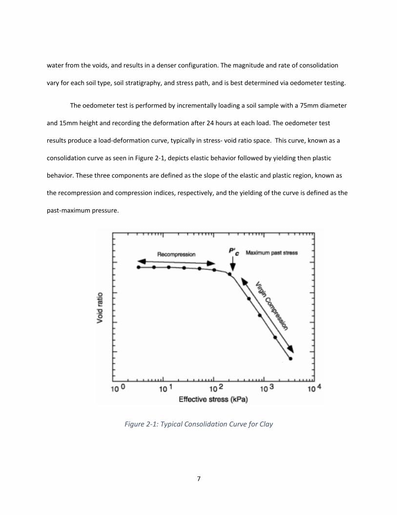
The oedometer test is performed by incrementally loading a soil sample with a 75mm diameter
and 15mm height and recording the deformation after 24 hours at each load. The oedometer test
results produce a load-deformation curve, typically in stress- void ratio space. This curve, known as a
consolidation curve as seen in Figure 2-1, depicts elastic behavior followed by yielding then plastic
behavior. These three components are defined as the slope of the elastic and plastic region, known as
the recompression and compression indices, respectively, and the yielding of the curve is defined as the
past-maximum pressure.
Figure 2-1: Typical Consolidation Curve for Clay
8
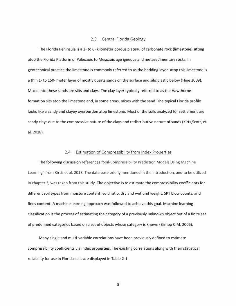
2.3 Central Florida Geology
The Florida Peninsula is a 2- to 6- kilometer porous plateau of carbonate rock (limestone) sitting
atop the Florida Platform of Paleozoic to Mesozoic age igneous and metasedimentary rocks. In
geotechnical practice the limestone is commonly referred to as the bedding layer. Atop this limestone is
a thin 1- to 150- meter layer of mostly quartz sands on the surface and siliciclastic below (Hine 2009).
Mixed into these sands are silts and clays. The clay layer typically referred to as the Hawthorne
formation sits atop the limestone and, in some areas, mixes with the sand. The typical Florida profile
looks like a sandy and clayey overburden atop limestone. Most of the soils analyzed for settlement are
sandy clays due to the compressive nature of the clays and redistributive nature of sands (Kirts,Scott, et
al. 2018).
2.4 Estimation of Compressibility from Index Properties
The following discussion references “Soil-Compressibility Prediction Models Using Machine
Learning” from Kirtis et al. 2018. The data base briefly mentioned in the introduction, and to be utilized
in chapter 3, was taken from this study. The objective is to estimate the compressibility coefficients for
different soil types from moisture content, void ratio, dry and wet unit weight, SPT blow counts, and
fines content. A machine learning approach was followed to achieve this goal. Machine learning
classification is the process of estimating the category of a previously unknown object out of a finite set
of predefined categories based on a set of objects whose category is known (Bishop C.M. 2006).
Many single and multi-variable correlations have been previously defined to estimate
compressibility coefficients via index properties. The existing correlations along with their statistical
reliability for use in Florida soils are displayed in Table 2-1.
9
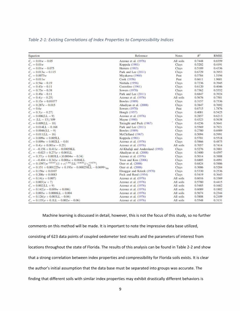
Table 2-1: Existing Correlations of Index Properties to Compressibility Indices
Machine learning is discussed in detail, however, this is not the focus of this study, so no further
comments on this method will be made. It is important to note the impressive data base utilized,
consisting of 623 data points of coupled oedometer test results and the parameters of interest from
locations throughout the state of Florida. The results of this analysis can be found in Table 2-2 and show
that a strong correlation between index properties and compressibility for Florida soils exists. It is clear
the author’s initial assumption that the data base must be separated into groups was accurate. The
finding that different soils with similar index properties may exhibit drastically different behaviors is
10
useful. This supports hypothesis’ utilized within Chapter 5 stating that one soil type must be utilized
(cohesive, fine-grained) and should be further categorized by some specific soil property. Three distinct
soil classes were suggested within this study, coarse grained, fine grained and organic peat. It should be
noted that both coarse-grained and organic peat performed exceptionally well, while the fine-grained
model was on par with existing correlations. Highly compressible organics and predominately sandy soils
are plentiful in Florida, so this was a useful finding for local practitioners. Another important note is that
plasticity indices were not utilized in this study but were added in for future research. As seen in Table 2-
2 and 2-3, there was no major increase in the reliability of this correlation when plasticity indices were
introduced. This does not agree with the correlations shown in Table 2-1. Further investigation is
needed to determine the effects of plasticity indices on compressibility. The reference discussed below
expands upon these correlations.
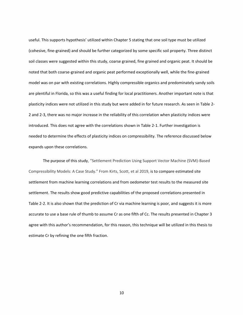
The purpose of this study, “Settlement Prediction Using Support Vector Machine (SVM)-Based
Compressibility Models: A Case Study.” From Kirts, Scott, et al 2019, is to compare estimated site
settlement from machine learning correlations and from oedometer test results to the measured site
settlement. The results show good predictive capabilities of the proposed correlations presented in
Table 2-2. It is also shown that the prediction of Cr via machine learning is poor, and suggests it is more
accurate to use a base rule of thumb to assume Cr as one fifth of Cc. The results presented in Chapter 3
agree with this author’s recommendation, for this reason, this technique will be utilized in this thesis to
estimate Cr by refining the one fifth fraction.
11
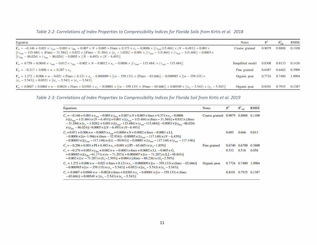
Table 2-2: Correlations of Index Properties to Compressibility Indices for Florida Soils from Kirtis et al. 2018
Table 2-3: Correlations of Index Properties to Compressibility Indices for Florida Soil from Kirtis et al. 2019
12
2.5 Compressibility and Cone Penetration Test
Research that estimates the compressibility of soils via cone penetration testing is presented
within this section. Correlations for granular soils, idealized as an elastic material, have been
mathematically, empirically, and theoretically justified. An attempt is made to relate elastic correlations
to elastic- plastic soil behaviors. The error with this approach is that the assumptions made for the
elastic material cannot be applied to plastic material, which makes it difficult to defend mathematically.
For this reason, all research referenced in this section utilizes empirical methods to determine a soil type
specific parameter to estimate compressibility. This parameter, referred from here on as the calibration
constant, is multiplied by tip resistance to estimate the stiffness of the soil. This approach allows the
originally derived correlation for elastic material to be applied to an elastic-plastic material.
2.5.1 Elastic Derivation and Calibration Constant
The method discussed in this section references “The Static Penetrometer and the Prediction of
Settlements” from Sanglerat, G. (1972) and is based on a mathematical derivation of an equation to
estimate compressibility from cone tip resistance. Keverling Buisman derived an equation in 1940 to
estimate compressibility of elastic materials. The derivation is founded upon the assumption that the
volume decrease occurs at the point of the penetrometer, implying tip resistance is only a function of
soil compression and the constrained modulus is constant due to the small loading area. Since the
constrained modulus is assumed constant, it is implied very small levels of strain occur as well as an
elastic response. Boussinesq’s solution (Boussinesq 1885) were utilized to determine stress at any point
from the cone tip. These assumptions were utilized for the solution shown in (4). When this solution was
tested against actual parameters specifically for sandy soils, it was shown to be the upper bounds of
settlement and a conservative estimation.
13
𝐶 =3
2(
𝑞𝑐
𝜎𝑣0) ( 4 )
Sangleret and others proposed altering Buisman’s solution to work for cohesive soils by
replacing 3/2 shown above in (4) with a constant dependent on soil classification, α, as seen below in
(5). The theoretical error in the application of this derivation to soft soils is that Buisman originally
assumed an elastic response. Implying that for clays the correlation is theoretically only applicable to
estimate the recompression index.
𝐶 = 𝛼 (𝑞𝑐
𝜎𝑣0) ( 5 )
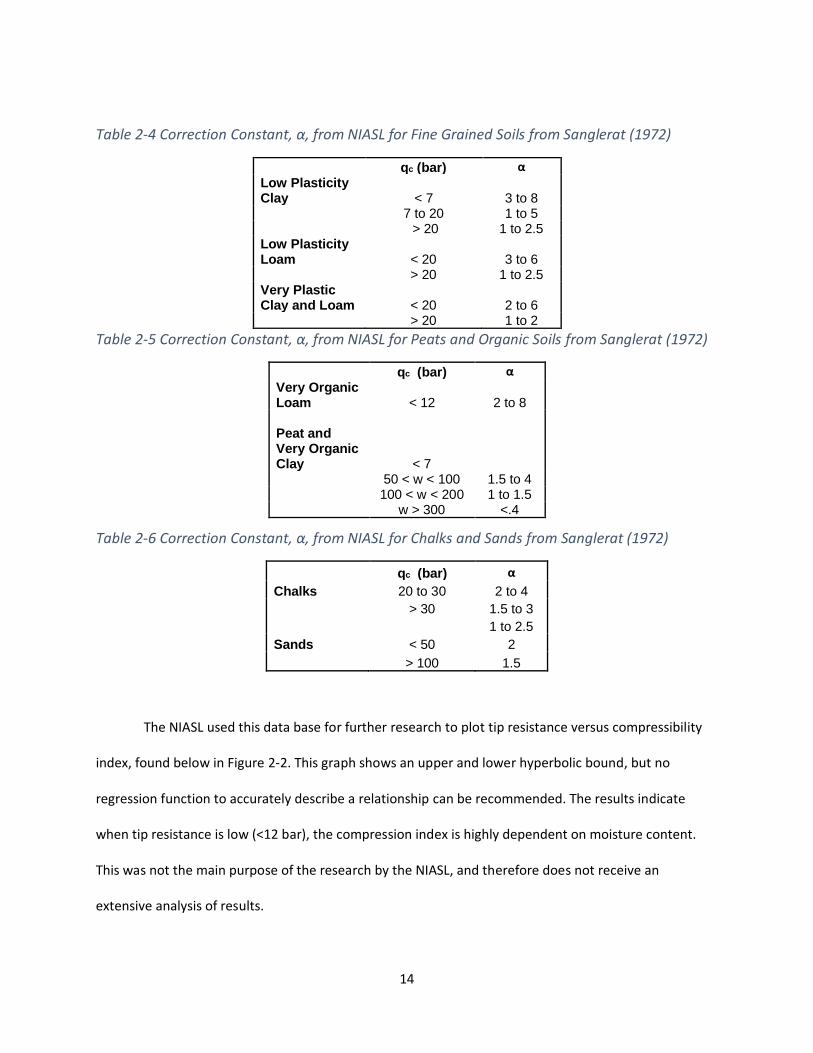
The National Institute of Applied Sciences of Lyons (NIASL) determined the values of α for
different soil types through extensive data collection. The process used by the NIASL was to acquire the
compressibility constant from oedometer testing and the tip resistance from cone penetration testing.
Since the compressibility constant C, tip resistance (qc), and vertical stress (σv0) are known, α can be
assigned. The NIASL utilized 600 comparative couples for fine grained soils (>50% fines) to create tables
of α for different soil behavior types shown in Table 2-4, which also includes information on water
content.
14
Table 2-4 Correction Constant, α, from NIASL for Fine Grained Soils from Sanglerat (1972)
qc (bar) α Low Plasticity Clay < 7 3 to 8 7 to 20 1 to 5 > 20 1 to 2.5 Low Plasticity Loam < 20 3 to 6 > 20 1 to 2.5 Very Plastic Clay and Loam < 20 2 to 6 > 20 1 to 2
Table 2-5 Correction Constant, α, from NIASL for Peats and Organic Soils from Sanglerat (1972)
qc (bar) α Very Organic Loam < 12 2 to 8 Peat and Very Organic Clay < 7 50 < w < 100 1.5 to 4 100 < w < 200 1 to 1.5 w > 300 <.4
Table 2-6 Correction Constant, α, from NIASL for Chalks and Sands from Sanglerat (1972)
qc (bar) α
Chalks 20 to 30 2 to 4
> 30 1.5 to 3
1 to 2.5
Sands < 50 2
> 100 1.5
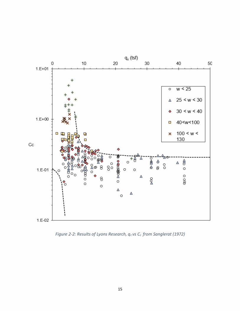
The NIASL used this data base for further research to plot tip resistance versus compressibility
index, found below in Figure 2-2. This graph shows an upper and lower hyperbolic bound, but no
regression function to accurately describe a relationship can be recommended. The results indicate
when tip resistance is low (<12 bar), the compression index is highly dependent on moisture content.
This was not the main purpose of the research by the NIASL, and therefore does not receive an
extensive analysis of results.
15
Figure 2-2: Results of Lyons Research, qc vs Cc from Sanglerat (1972)
16
2.5.2 Constrained Modulus
The following section references “Interpretation of cone penetration tests - a unified approach”
from Robertson, P. K. (2009). This study presents a method to estimate the constrained modulus (stress:
strain response with no net lateral displacement) via the Cone penetration test. This modulus can be
analogous to the compressibility indices as it is a means to describe soil deformation due to loading.
Robertson’s previous research into Normalized Soil Behavior Type (SBTn) enables one to create a soil
profile and identify transition zones from the CPT. The SBTn graph is also useful as a tool to better relate
CPT parameters to soil parameters, in this case to the constrained modulus.
In short, Robertson accomplished this correlation via multiple empirical relationships. First, the
CPT is correlated to the shear wave velocity, which is directly related to the small shear modulus. The
small shear modulus is then correlated to the constrained modulus.
Initially, a set of normalized shear wave velocity (Vsl) contours are plotted on the SBTn chart
from over 100 SCPT profiles. Then, a function that best approximates the Vsl contours is used to relate
shear wave velocity to cone tip resistance and soil behavior type. This relationship is theoretically
justified since both of these parameters are dependent on the soil’s relative density, effective stress
state, age, and cementation.
Small strain shear modulus (Go) is a soil stiffness parameter that describes the material’s
deformation response to shear stress in the linear elastic zone (shear levels less than 10-4 %). Since Go is
a direct function of shear velocity it can be contoured on the SBTn chart and become a function of tip
resistance, sleeve friction ratio, and soil type. This step is controversial as the small shear strain modulus
describes the stiffness in the elastic zone. However, there is a small error in the results, shown below in
Figure 2-3, when these contours were extended into the plastic region of the SBTn chart.
17
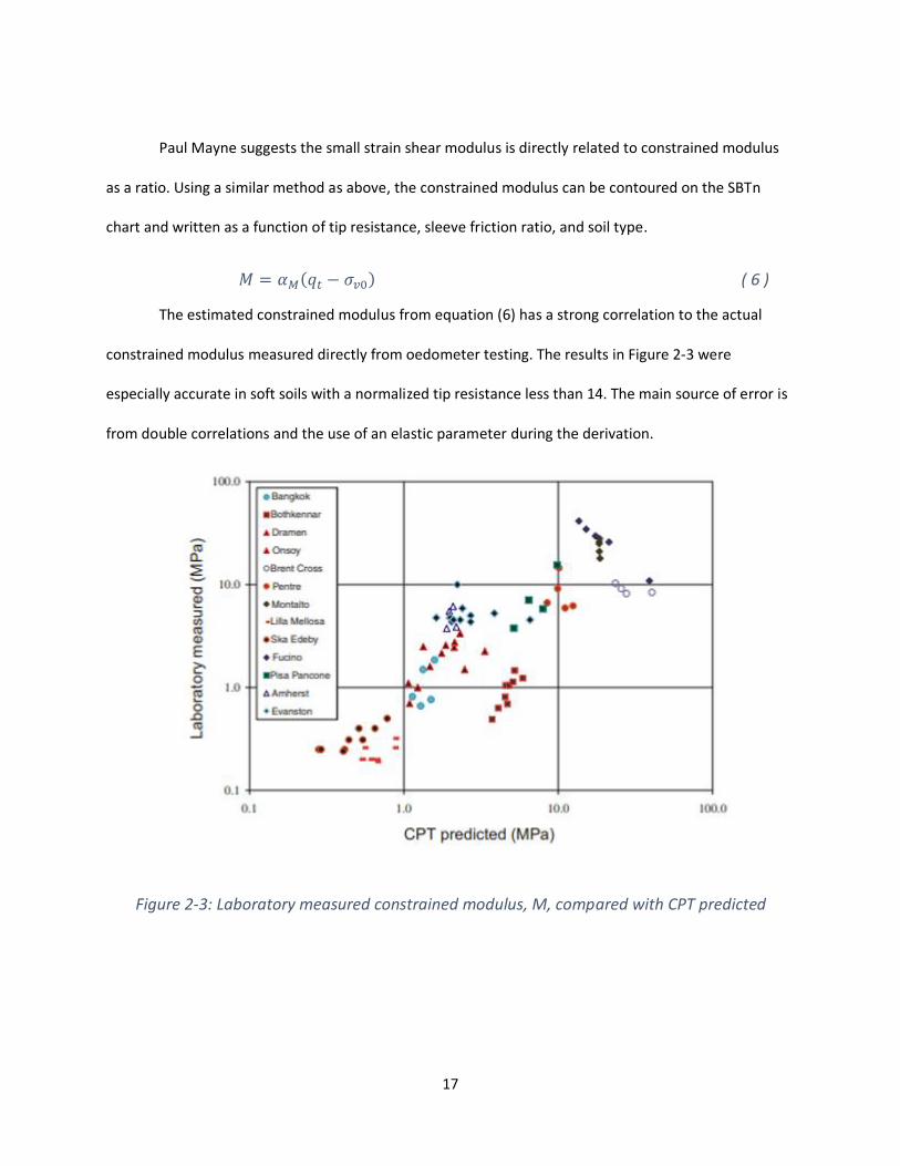
Paul Mayne suggests the small strain shear modulus is directly related to constrained modulus
as a ratio. Using a similar method as above, the constrained modulus can be contoured on the SBTn
chart and written as a function of tip resistance, sleeve friction ratio, and soil type.
𝑀 = 𝛼𝑀(𝑞𝑡 − 𝜎𝑣0) ( 6 )
The estimated constrained modulus from equation (6) has a strong correlation to the actual
constrained modulus measured directly from oedometer testing. The results in Figure 2-3 were
especially accurate in soft soils with a normalized tip resistance less than 14. The main source of error is
from double correlations and the use of an elastic parameter during the derivation.
Figure 2-3: Laboratory measured constrained modulus, M, compared with CPT predicted
18
2.6 Estimation of Preconsildation Pressure
This section presents are reliable semi-empirical model to estimate the preconsolidation pressure
from the CPT. This compressibility parameter is required to define the soils compressibility and estimate
settlements. A model will not be proposed within the analysis of this thesis as more reliable correlations
already exist.
The reference discussed below, “Profiling OCR in stiff clays by CPT and SPT” by Mayne & Kemper
(1988), utilizes a semi - empirical methodology to estimate OCR from the CPT. In short, the cone
penetration test is commonly used to estimate undrained shear strength which is dependent on the
soils stress history. Relating undrained shear strength to stress history allows continuous profiling of
overconsolidation ratio from tip resistance.
The data base utilized consists of CPT data from 40 different clays with a plasticity index ranging
from 3 to 9 and an OCR ranging from normally consolidated to heavily overconsolidated. These clays
have been deposited in a variety of geologic environments including terrestrial, marine, glacial and
alluvial, implying this correlation is generic and not refined to a specific geology. Since the data is from
different sites the CPT and oedometer test equipment and technician likely vary, which makes it difficult
to control the quality and consistency of each point.
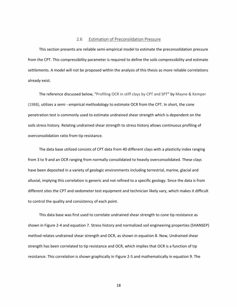
This data base was first used to correlate undrained shear strength to cone tip resistance as
shown in Figure 2-4 and equation 7. Stress history and normalized soil engineering properties (SHANSEP)
method relates undrained shear strength and OCR, as shown in equation 8. Now, Undrained shear
strength has been correlated to tip resistance and OCR, which implies that OCR is a function of tip
resistance. This correlation is shown graphically in Figure 2-5 and mathematically in equation 9. The
19
calibration parameter in equation (10), kc, is dependent on soil type and stress path. This parameters
makes it possible to refine the model to the local geology.
𝑆𝑢
𝜎0′=
𝑞𝑐−𝛾𝑧
𝑁𝑘𝜎0′ ( 7 )
𝑂𝐶𝑅 = (
𝑆𝑢
𝜎0′𝑆𝑢
𝜎𝑐′
)1
𝛬 ( 8 )
𝑂𝐶𝑅 = 0.37(𝑞𝑐−𝛾𝑧
𝜎0′)1.01 ( 9 )
𝑂𝐶𝑅 = 𝑘𝑐(𝑞𝑐−𝛾𝑧
𝜎0′) ( 10 )
Figure 2-4: Comparison between Undrained Shear strength from Triaxial compression and measured cone resistance from mechanics and electric cones, taken from Mayne and Kemper
1988

20
Figure 2-5: Trend Between Laboratory OCR and Normalized net cone resistance taken from Mayne and Kemper 1988
2.7 Literature Review Conclusion
Index properties have been shown empirically to have a strong correlation to the compression
index and a poor correlation to the recompression index. It was then suggested a ratio from the
compression index to estimate the recompression index may be more accurate. It was also shown that
different soil types require different correlations.
21
Robertson and Buisman’s derivation of the coefficient of compressibility utilizes elastic theory
and therefore is not theoretically sound for prediction of elastic-plastic soil behavior. However,
Robertson’s correlation compared very well to estimated values and Buisman’s equation can be applied
to clays after receiving a correction constant, α, dependent on the soil behavior type. A derivation using
elastic and plastic theory would be ideal, but properly selected calibration parameters determined via
empirical methods have proven accurate.
The derivation and justification of the CPT correlation to past maximum pressure is sound. There
is no need to propose a new model in this paper. Instead, the accuracy of the model will be checked and
the proper correction factor, Kc, for Central Florida soils will be recommended.
22
CHAPTER 3 INDEX PROPERTIES AND COMPRESSIBILITY
3.1 Introduction
The objective of this chapter is to provide a model to estimate the compressibility of fine-
grained soils in the Central Florida region via index properties. Previous researchers have demonstrated
that index properties can accurately estimate the compressibility of the soil, however, most of these
models are generic and no refined for specific geologies. This section will differ from Kirtis et al., which
studied Central Florida Soils, by building upon their data base and by recommending a single variable
model. Since this is an empirical method, any firm with adequate data can create a data base and
perform the following analysis, allowing more accurate estimation of compressibility via index
properties in their specific area.
The specific index properties compared with compressibility include moisture content (W),
Liquid Limit (LL), Plasticity index (PI), Liquidity Index (LI), Percent Finer (-200), Activity (A), moist unit
weight (γ), dry unit weight (γd), and Initial Void Ratio (e0). Moisture content describes the ratio by weight
of water to solids. The Liquid and Plastic limits are defined as the moisture content required to change
the behavior to a liquid and to a solid state, respectively. The Plasticity index is the range between the
plastic and liquid limit and describes the soil’s ability to hold water as well as it’s susceptibility to volume
change via shrinking and swelling. The Liquidity Index scales the Atterberg limits to the moisture
content. Percent Finer is the percentage of particles less than 75μm, which are referred to as fine-
grained soil and are typically clays and silts. Activity is the ratio of plasticity index to percent finer. This
parameter “normalizes” the plasticity index and describes the colloidal properties of the soil providing
information into the soil behavior, geology and strength (Skempton 1988). The moist unit weight is
measured from the Shelby tube before sample extraction by measuring the volume and total weight
minus weight of Shelby tube then multiplying this density by gravity. The dry unit weight is equal to the
23
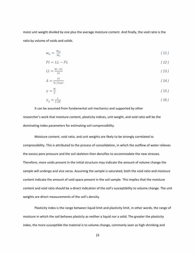
moist unit weight divided by one plus the average moisture content. And finally, the void ratio is the
ratio by volume of voids and solids.
𝑤𝑛 = 𝑊𝑤
𝑊𝑠 ( 11 )
𝑃𝐼 = 𝐿𝐿 − 𝑃𝐿 ( 12 )
𝐿𝐼 =𝑊−𝑃𝐿
𝑃𝐼 ( 13 )
𝐴 =𝑃𝐼
% 𝑓𝑖𝑛𝑒𝑟 ( 14 )
𝛾 =𝑊
𝑉 ( 15 )
𝛾𝑑 =𝛾
1+𝑊 ( 16 )
It can be assumed from fundamental soil mechanics and supported by other
researcher’s work that moisture content, plasticity indices, unit weight, and void ratio will be the
dominating index parameters for estimating soil compressibility.
Moisture content, void ratio, and unit weights are likely to be strongly correlated to
compressibility. This is attributed to the process of consolidation, in which the outflow of water relieves
the excess pore pressure and the soil skeleton then densifies to accommodate the new stresses.
Therefore, more voids present in the initial structure may indicate the amount of volume change the
sample will undergo and vice versa. Assuming the sample is saturated, both the void ratio and moisture
content indicate the amount of void space present in the soil sample. This implies that the moisture
content and void ratio should be a direct indication of the soil’s susceptibility to volume change. The unit
weights are direct measurements of the soil’s density.
Plasticity index is the range between liquid limit and plasticity limit, in other words, the range of
moisture in which the soil behaves plasticly as neither a liquid nor a solid. The greater the plasticity
index, the more susceptible the material is to volume change, commonly seen as high shrinking and

24
swelling potential. Since this index provides insight into the soil’s ability to change volume with
moisture, it is likely that it will be strongly correlated to compressibility indices. By association, the liquid
limit and plastic limit may also show strong correlations.
25
3.2 Methodology
3.2.1 Data Base
The data base utilized in this chapter is a combination of UCF’s data base and the CPT data base
created for use in Chapters 4 and 5. UCF’s data base consists of 350 oedometer test and index test
results for fine-grained soil. All the data is from Florida soils and majority is from FDOT district five. The
CPT data base was created from scratch. It originally consisted of thirty-five data points, of which
twenty-three were accepted. The removal of data points was in accordance with the filters discussed in
Chapter 4 which was done to ensure a high quality, reliable data base. Of the twenty-three accepted
points twenty-one are clays with more than 50 % fines and two are clayey sands with 40 to 50 % fines.
The combination of the two data bases total 375 couples of index properties and compressibility
parameters.
3.2.2 Analysis
A regression analysis is utilized in which each index property is plotted against the
recompression and compression indices. Then, the parameters indicating a strong correlation indicated
by statistical quantifiers (R2 and RMSE) will be interpreted and presented as a viable model. The
correlation with the highest statistical reliability that is also theoretically justifiable will be
recommended as the final model to estimate compressibility. All correlations are in Appendix A, the
reliable correlations are presented in section 3.3.1, and the final recommended model is in section 3.3.2
This analysis will recommend compressibility indices in void ratio – stress space and a
correlation to estimate void ratio will be provided. The analysis in strain – stress space yielded weaker
correlations, so it has been deemed more accurate to utilize a double correlation.
26
3.3 Results and Discussion
The strong correlations will be discussed and summarized within this section. A strong correlation
was an R2 greater than 0.3 for the recompression index and 0.4 for the compression index. The R2 value
is the initial statistical parameter utilized to quantify the correlations strength. For the relatively strong
correlations, the root mean squares error (RMSE) is also determined to further quantify the correlations
reliability. The R2 parameter represents the portion of observed values which can be captured using the
proposed model. The RMSE describes how concentrated the data is around the line of best fit with 0
being a perfect fit. It is important to note that R2 is a dimensionless parameter while RMSE is dependent
on the dimension of the parameter. Therefore, RMSE will have the dimensions of compression or
recompression index, where deemed applicable. The equation for the line of best fit and the statistical
parameters are found within each graph and summarized in Table 3-2. The subsections will display each
correlation, discuss the results and recommend the best model to estimate the compressibility of
cohesive soil in the Central Florida area.
3.3.1 Correlations from Charts
This section presents the strongest correlations between index properties and compressibility
indices. The weaker correlations not shown in this section are in Appendix A. The parameters which
correlated well are moisture content, void ratio, liquid limit and dry unit weight. Moisture content, void
ratio and dry unit weight provide insight into the in-situ soil structure, and liquid limit indicates the soil
behavior. The correlations are presented and summarized below in figures 3-1 to 3-9 and table 3-1,
respectively, and further discussed in section 3.3.2.
27
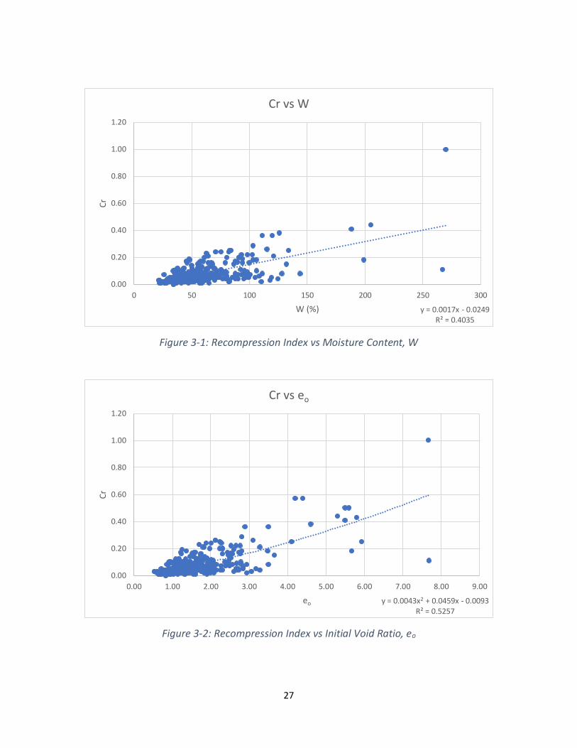
Figure 3-1: Recompression Index vs Moisture Content, W
Figure 3-2: Recompression Index vs Initial Void Ratio, eo
y = 0.0017x - 0.0249R² = 0.4035
0.00
0.20
0.40
0.60
0.80
1.00
1.20
0 50 100 150 200 250 300
Cr
W (%)
Cr vs W
y = 0.0043x2 + 0.0459x - 0.0093R² = 0.5257
0.00
0.20
0.40
0.60
0.80
1.00
1.20
0.00 1.00 2.00 3.00 4.00 5.00 6.00 7.00 8.00 9.00
Cr
eo
Cr vs eo
28
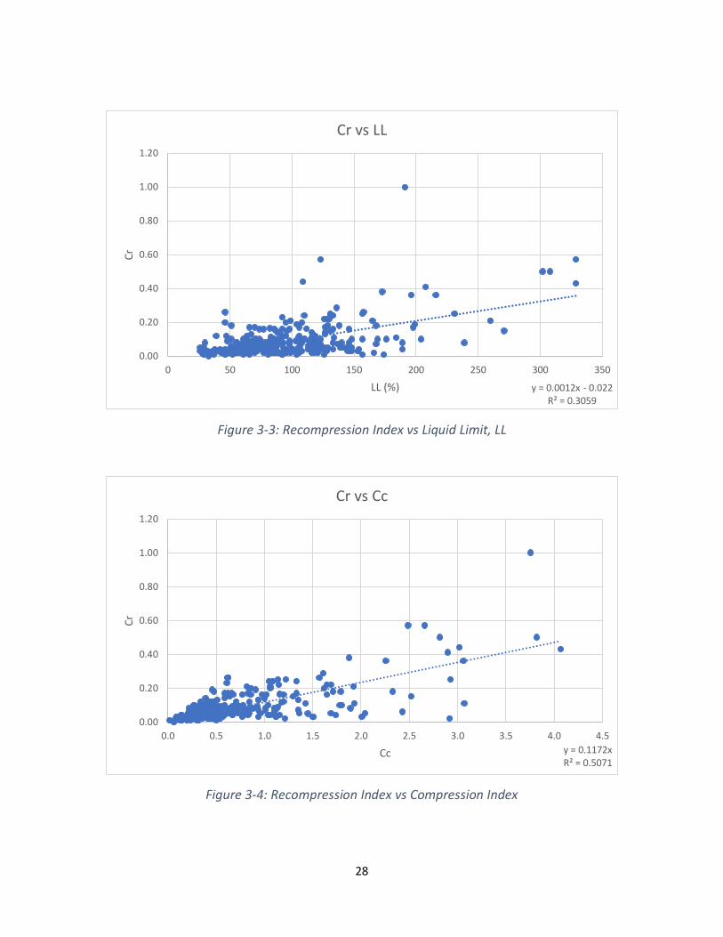
Figure 3-3: Recompression Index vs Liquid Limit, LL
Figure 3-4: Recompression Index vs Compression Index
y = 0.0012x - 0.022R² = 0.3059
0.00
0.20
0.40
0.60
0.80
1.00
1.20
0 50 100 150 200 250 300 350
Cr
LL (%)
Cr vs LL
y = 0.1172xR² = 0.5071
0.00
0.20
0.40
0.60
0.80
1.00
1.20
0.0 0.5 1.0 1.5 2.0 2.5 3.0 3.5 4.0 4.5
Cr
Cc
Cr vs Cc
29
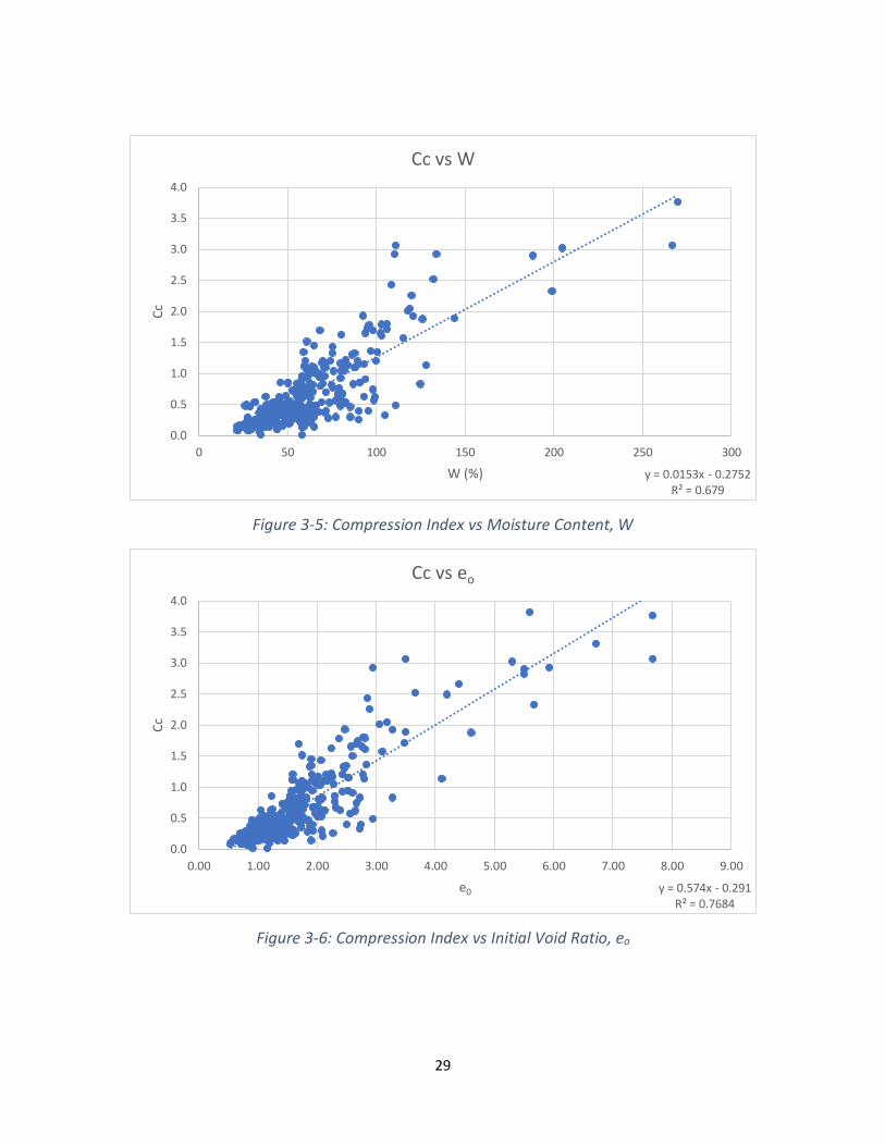
Figure 3-5: Compression Index vs Moisture Content, W
Figure 3-6: Compression Index vs Initial Void Ratio, eo
y = 0.0153x - 0.2752R² = 0.679
0.0
0.5
1.0
1.5
2.0
2.5
3.0
3.5
4.0
0 50 100 150 200 250 300
Cc
W (%)
Cc vs W
y = 0.574x - 0.291R² = 0.7684
0.0
0.5
1.0
1.5
2.0
2.5
3.0
3.5
4.0
0.00 1.00 2.00 3.00 4.00 5.00 6.00 7.00 8.00 9.00
Cc
e0
Cc vs eo
30
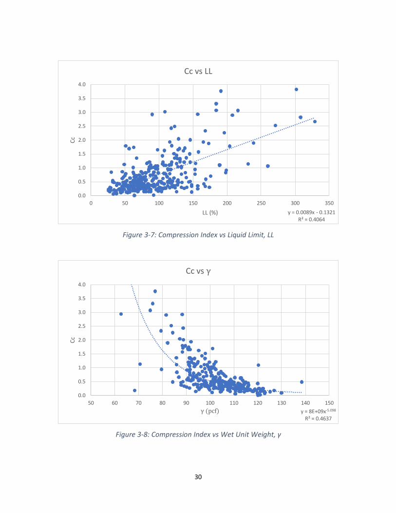
Figure 3-7: Compression Index vs Liquid Limit, LL
Figure 3-8: Compression Index vs Wet Unit Weight, γ
y = 0.0089x - 0.1321R² = 0.4064
0.0
0.5
1.0
1.5
2.0
2.5
3.0
3.5
4.0
0 50 100 150 200 250 300 350
Cc
LL (%)
Cc vs LL
y = 8E+09x-5.098
R² = 0.4637
0.0
0.5
1.0
1.5
2.0
2.5
3.0
3.5
4.0
50 60 70 80 90 100 110 120 130 140 150
Cc
γ (pcf)
Cc vs γ
31
Figure 3-9: Compression Index vs Dry Unit Weight, γd
Table 3-1: Summary of Results, Index Properties
Recompression Index Equation R2 RMSE
Moisture Content Cr = 0.0017W - 0.0249 0.404 0.066
Void Ratio Cr = 0.0043(e0) 2 + 0.0459(e0) - 0.0093 0.526 0.073
Liquid Limit Cr = 0.0012LL - 0.022 0.306 0.086
Compression Index Cr = 0.1087Cc + 0.011 0.513 0.073
Compression Index
Moisture Content Cc = 0.015W - 0.275 0.679 0.329
Void Ratio Cc = 0.574(e0) - 0.291 0.768 0.317
Liquid Limit Cc = 0.009LL - 0.132 0.406 0.501
Dry Density Cc = 5.5904e-0.037x 0.542 0.351
y = 5.5904e-0.037x
R² = 0.5418
0.0
0.5
1.0
1.5
2.0
2.5
3.0
3.5
4.0
50.0 60.0 70.0 80.0 90.0 100.0 110.0 120.0
Cc
γd (pcf)
Cc vs γd
32
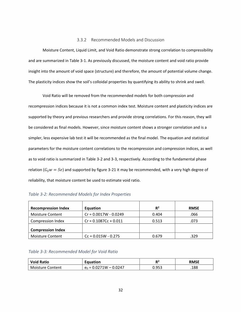
3.3.2 Recommended Models and Discussion
Moisture Content, Liquid Limit, and Void Ratio demonstrate strong correlation to compressibility
and are summarized in Table 3-1. As previously discussed, the moisture content and void ratio provide
insight into the amount of void space (structure) and therefore, the amount of potential volume change.
The plasticity indices show the soil’s colloidal properties by quantifying its ability to shrink and swell.
Void Ratio will be removed from the recommended models for both compression and
recompression indices because it is not a common index test. Moisture content and plasticity indices are
supported by theory and previous researchers and provide strong correlations. For this reason, they will
be considered as final models. However, since moisture content shows a stronger correlation and is a
simpler, less expensive lab test it will be recommended as the final model. The equation and statistical
parameters for the moisture content correlations to the recompression and compression indices, as well
as to void ratio is summarized in Table 3-2 and 3-3, respectively. According to the fundamental phase
relation (𝐺𝑆𝑤 = 𝑆𝑒) and supported by figure 3-21 it may be recommended, with a very high degree of
reliability, that moisture content be used to estimate void ratio.
Table 3-2: Recommended Models for Index Properties
Recompression Index Equation R2 RMSE
Moisture Content Cr = 0.0017W - 0.0249 0.404 .066
Compression Index Cr = 0.1087Cc + 0.011 0.513 .073
Compression Index
Moisture Content Cc = 0.015W - 0.275 0.679 .329
Table 3-3: Recommended Model for Void Ratio
Void Ratio Equation R2 RMSE
Moisture Content e0 = 0.0271W – 0.0247 0.953 .188
33
Figure 3-10: Void Ratio vs Moisture Content
Other parameters correlated to the compression index with weaker reliability (R2 values
between 0.2 and 0.3) are plastic limit, percent finer, and activity. Correlations to the recompression
index with an R2 between 0.2 and 0.3 are percent finer and activity. Activity is a function of Percent Finer
and Plasticity and provides insight to the colloidal behavior. Since this parameter defines the behavior of
the soil well for an index property, it will be used in Chapter 5 to segregate the data base, regardless of
its relatively poor correlations.
y = 0.0271x + 0.0012R² = 0.9527
RMSE = 0.188
0.00
1.00
2.00
3.00
4.00
5.00
6.00
7.00
8.00
0 50 100 150 200 250 300
e
W
e vs W
34
3.4 Conclusion
This study has provided strong correlation to moisture content and Atterberg limits for cohesive
soil in Central Florida. The soil index properties have been proven by previous researchers and
supported by this study to accurately estimate the compressibility. The recommended correlations
between moisture content and compressibility are more accurate than the correlations utilizing
moisture content summarized in Table 2-1.
These models, although accurate, are still a crude way to determine the compressibility of soil. For
sites where settlement needs to be well defined it is best to use a combination of Oedometer testing,
experience, as well as these correlations. It is also important to note that the definition of OCR is as
important as the definition of compressibility. Misjudging the range of the stress levels for the
recompression and compression index will be responsible for much more error than a slightly inaccurate
definition of compressibility indices. For this reason, if the OCR is well defined from other correlations
(see Mayne & Kemper 1988), then the usage of crude estimations of compressibility is acceptable. An
OCR model is recommended for the local soil in Chapter 6.
35
CHAPTER 4 CONE PENETRATION TEST BASED CORRELATION ANALYSIS
4.1 Introduction
The objective of this chapter is to recommend a model to estimate the compressibility of fine-
grained cohesive soils in the Central Florida region via the Cone Penetration Test. Previous researchers,
as mentioned in the literature review, have shown that it is difficult and not theoretically sound to
estimate the compressibility of an elastic-plastic material from the CPT. For this reason, the CPT has
been primarily used to estimate elastic stiffness moduli (recompression index, elastic modulus, small
shear strain modulus, etc.) which applies to granular material and the elastic zone of clays. Two things
will be done differently from previous researchers to present new findings: the pore pressure will be
incorporated into the analysis and each data point will be carefully filtered. Previously, only tip
resistance has been correlated, and massive data bases were created making it difficult to perform
quality control.
Since this is an empirical method, any firm with an adequate quantity of reliable data can
recreate this analysis to define correlations refined to their location. These results may be useful for
firms in the Central Florida region, or areas with similar geology, but will mainly show how the CPT can
be used to estimate compressibility of soft, elastic-plastic materials.
Based on previous findings and soil mechanics it is expected that the tip and sleeve friction will
accurately estimate the compressibility in the elastic zone, known as the recompression index. It is also
expected that the pore pressure reading in the u2 position will be the controlling parameter for
estimating the compression index. This hypothesis is made because the deformation pre yielding is due
to soil structure while the deformation post-yielding is due to composition (stress). Therefore, the
36
process of consolidation, transfer of stress from the pore water to the soil skeleton, will be the main
mechanism occurring in the compression index.
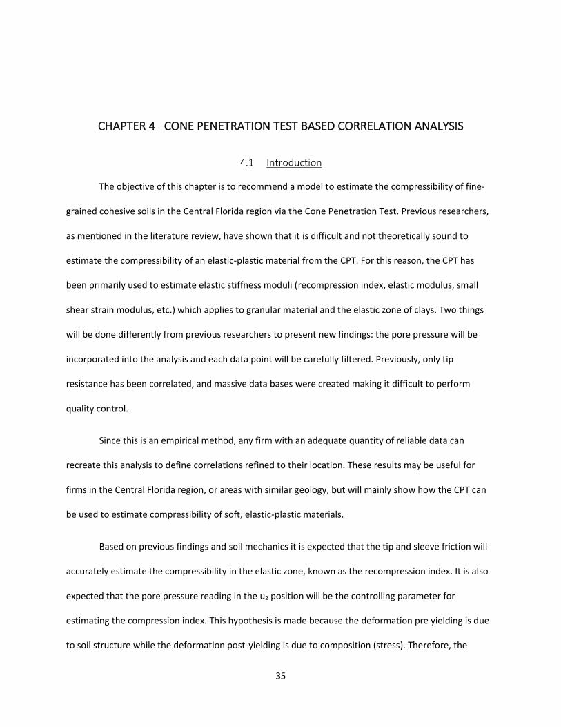
It is important to first discuss the mechanisms causing the CPT readings of tip resistance, sleeve
friction, and pore pressure. The penetrometer is shearing the soil to failure to maintain the constant
rate of push; therefore, the tip and sleeve resistance is the amount of force the penetrometer must
exert to maintain that constant rate. Following this logic, it is reasonable that tip and sleeve resistance
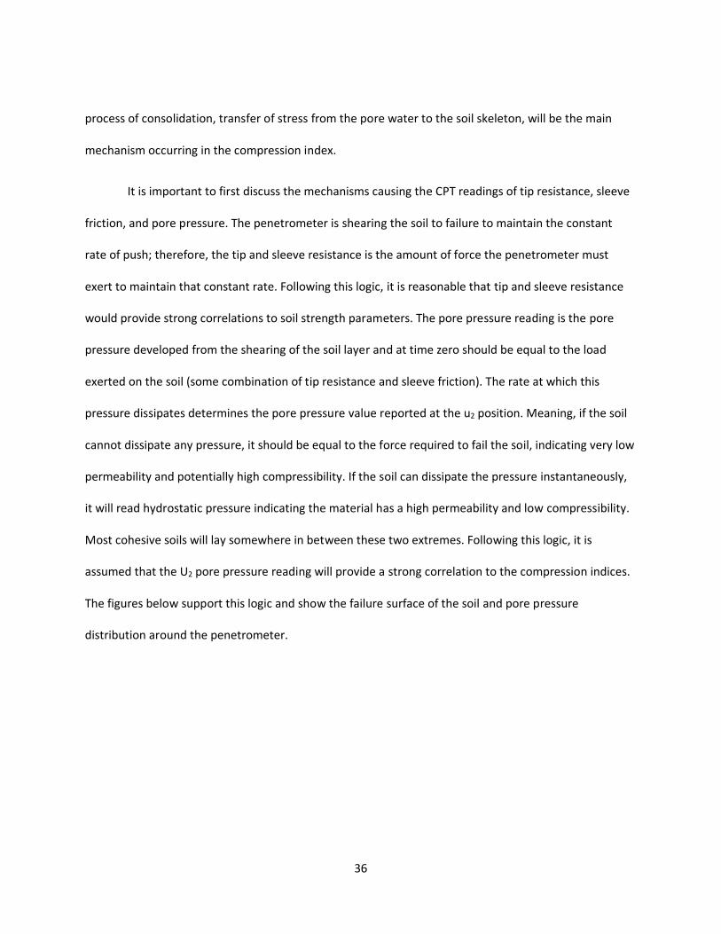
would provide strong correlations to soil strength parameters. The pore pressure reading is the pore
pressure developed from the shearing of the soil layer and at time zero should be equal to the load
exerted on the soil (some combination of tip resistance and sleeve friction). The rate at which this
pressure dissipates determines the pore pressure value reported at the u2 position. Meaning, if the soil
cannot dissipate any pressure, it should be equal to the force required to fail the soil, indicating very low
permeability and potentially high compressibility. If the soil can dissipate the pressure instantaneously,
it will read hydrostatic pressure indicating the material has a high permeability and low compressibility.
Most cohesive soils will lay somewhere in between these two extremes. Following this logic, it is
assumed that the U2 pore pressure reading will provide a strong correlation to the compression indices.
The figures below support this logic and show the failure surface of the soil and pore pressure
distribution around the penetrometer.
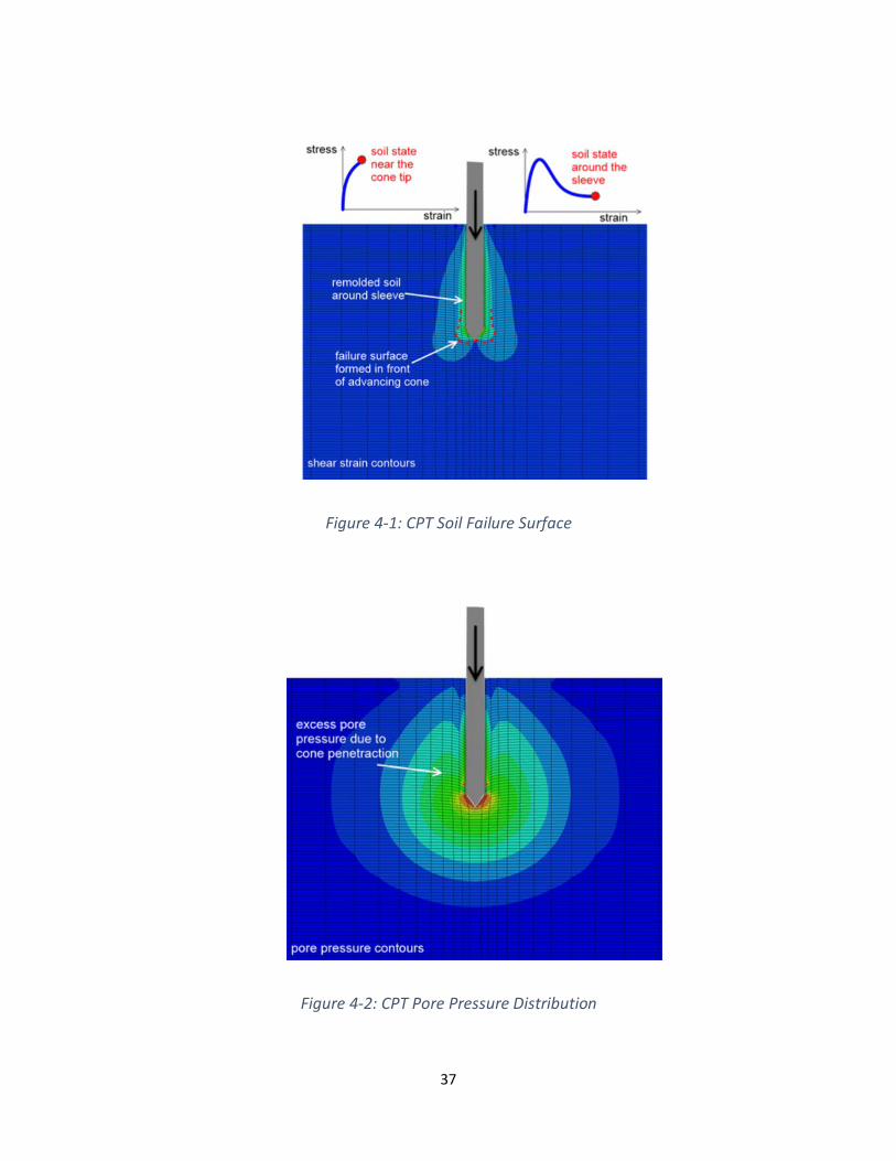
37
Figure 4-1: CPT Soil Failure Surface
Figure 4-2: CPT Pore Pressure Distribution
38
4.2 Methodology
4.2.1 Cone Penetration Test Data Base
The following section describes, in detail, the creation of the CPT data base, followed by an
example of data selection, and the analysis process performed in this chapter. In order to create the
data base, information from local projects with Oedometer testing and CPTs performed must be
acquired. The data is then filtered and a data base with adequate points is created. A description of each
test, the filtering process, and the CPT analysis process is covered in the following section. A logic chart
(Figure 4-3) summarizing the methodology can be found at the end of this section.
4.2.2 Data Processing Procedure
The data utilized for this data base include oedometer test results, CPT results, and index
properties (moisture content, void ratio, liquid and plastic limits, and percent finer). All test results must
be interpreted and if deemed unreliable, removed.
The correlations are aimed to estimate the compressibility of soil, specifically the recompression
and compression indices obtained from the oedometer test. This test is utilized to determine the
response of soil in 1-D compression. For soft soils this response is non-linear, elastic-plastic and
dependent on the material’s past maximum pressure. Soils of this nature deform due to a time
dependent process known as consolidation. Defining parameters from this test are the slopes of elastic
response or OCL (swelling index), the slope of the plastic response or NCL (compression index), and the
vertical stress at yielding (preconsildation pressure). The elastic response turns into a plastic response at
the preconsildation pressure. This is important because simple elastic analysis may be performed up to
this point while a more complex definition is required after this point. The oedometer test is highly
39
sensitive to soil sample disturbance, therefore, quality rating suggested by Terzaghi et al (1996) and
Lunne et all (1997a) is utilized to check for disturbance and help attain a reliable data base (Table 3-1).
The Cone Penetration Test is performed near the Shelby tube borehole to capture the soil layer
in which the oedometer sample is taken. Checks implemented for the CPT results are to confirm that the
rate of push is around 2 cm/s, the inclination of push is less than 2 degrees, and that all readings agree.
This last part is important as a highly plastic clay with no nearby drainage should indicate low tip,
relatively high friction, and some pore pressure. If there is a contradiction with what is expected, a more
detailed check of the profile is performed and justifications made. Robertson’s normalized soil behavior
type is then used to compare the CPT soil behavior type profile with the Shelby tube boring visually
classified soil profile to confirm the soil stratum is similar within the couple. This step is crucial as soil in
this geology can be highly variable, meaning a CPT and SPT boring performed nearby can display
different soil profiles and fail to capture the oedometer sample layer.
If the oedometer and cone penetration tests are acceptable and agree with one another, the
couple is added to the data base. Next, the depth of representative values of cone tip resistance, sleeve
friction and pore water pressure are designated with extreme care as selection of the proper values is
key to the success of the research. The depth of CPT readings is ideally at or near the depth of the
Shelby tube. The exact location of the sample extraction within the Shelby tube has not been provided
with the oedometer results, limiting the precision of the representative readings. However, from
experience working at Ardaman and Associates’ Soil Testing Laboratory the sample is not extracted from
the bottom 3 in. or top 9 in. as the sample is disturbed in these zones. Minimizing the zone of the
sample location is important as the CPT outputs can experience a high range of values over the length of
the Shelby tube. On top of refining the sample extraction zone to 1 ft., an arbitrary filter requiring all
data points to have a range of less than half the average value for each CPT output will be applied.
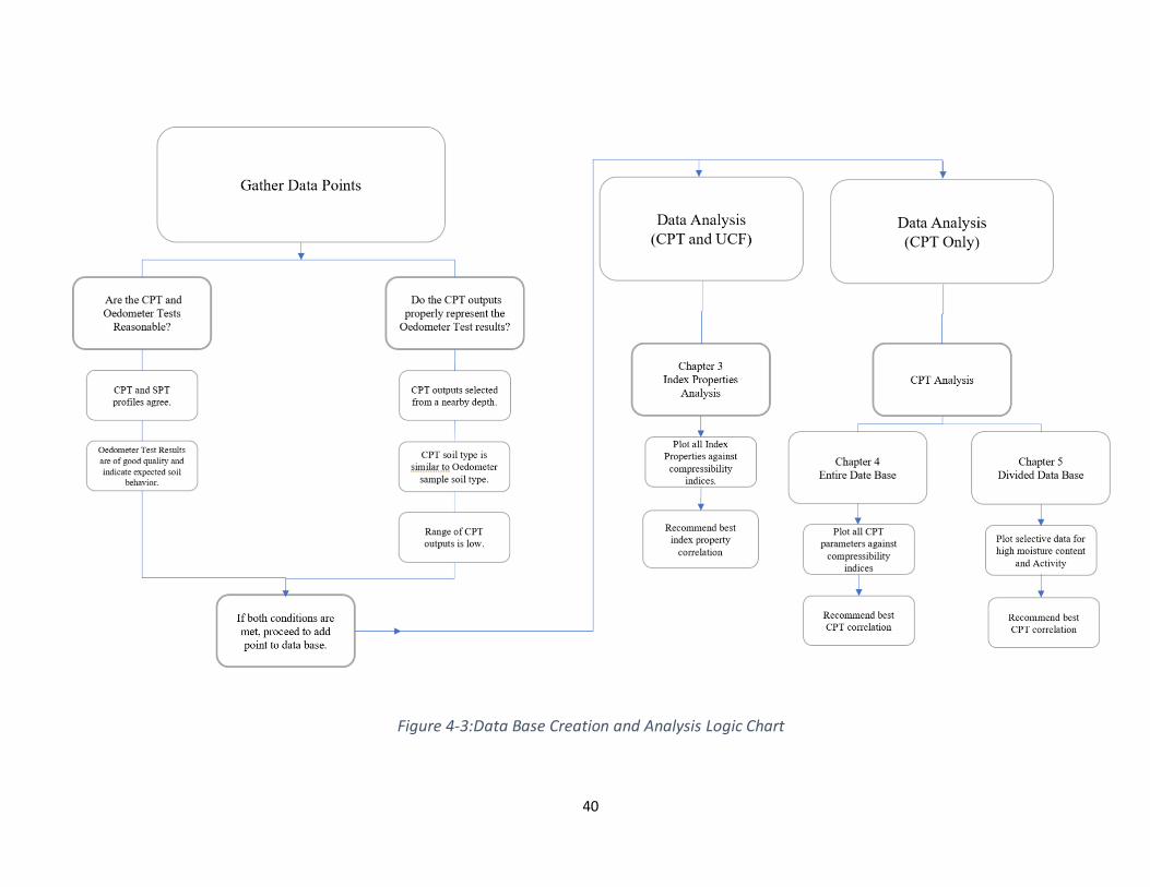
40
Figure 4-3:Data Base Creation and Analysis Logic Chart
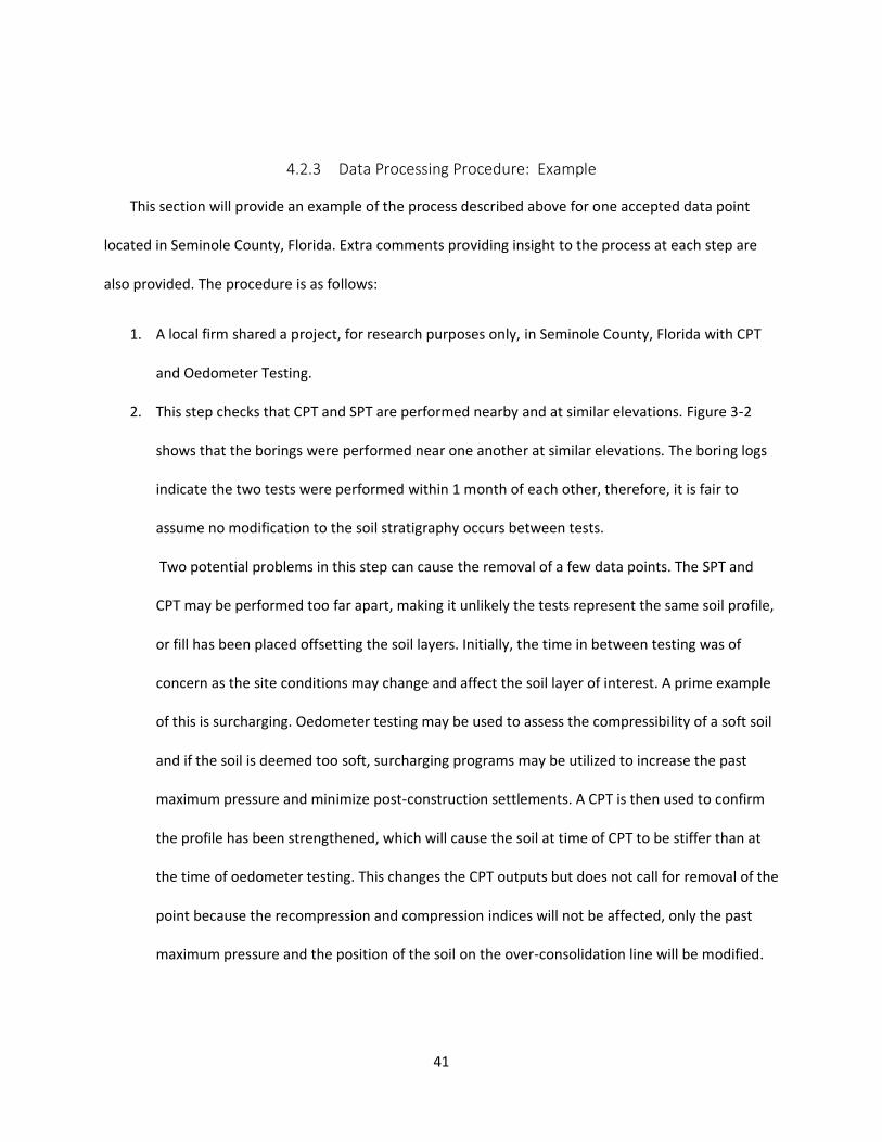
41
4.2.3 Data Processing Procedure: Example
This section will provide an example of the process described above for one accepted data point
located in Seminole County, Florida. Extra comments providing insight to the process at each step are
also provided. The procedure is as follows:
1. A local firm shared a project, for research purposes only, in Seminole County, Florida with CPT
and Oedometer Testing.
2. This step checks that CPT and SPT are performed nearby and at similar elevations. Figure 3-2
shows that the borings were performed near one another at similar elevations. The boring logs
indicate the two tests were performed within 1 month of each other, therefore, it is fair to
assume no modification to the soil stratigraphy occurs between tests.
Two potential problems in this step can cause the removal of a few data points. The SPT and
CPT may be performed too far apart, making it unlikely the tests represent the same soil profile,
or fill has been placed offsetting the soil layers. Initially, the time in between testing was of
concern as the site conditions may change and affect the soil layer of interest. A prime example
of this is surcharging. Oedometer testing may be used to assess the compressibility of a soft soil
and if the soil is deemed too soft, surcharging programs may be utilized to increase the past
maximum pressure and minimize post-construction settlements. A CPT is then used to confirm
the profile has been strengthened, which will cause the soil at time of CPT to be stiffer than at
the time of oedometer testing. This changes the CPT outputs but does not call for removal of the
point because the recompression and compression indices will not be affected, only the past
maximum pressure and the position of the soil on the over-consolidation line will be modified.
42
Figure 4-4: CPT and SPT Location (Example)
3. Next, the CPT and SPT profiles are compared to ensure there is not much variability in the soil
stratums between borings. As seen in figure 3-3, the majority of the soil profiles from each test
agree and both indicate clayey soils at the Shelby tube depth. However, the top of Shelby tube
depth is a transition zone, so the data point was taken to be in the middle to lower portion of
the Shelby tube requiring a small shift down of about 3 inches. This matching still provides a
high degree of reliability that the selected CPT output depth represents the oedometer test
sample.
In the scenario in which the profile has been offset due to fill or simply different soil stratum
thicknesses, judgment must be used to best match these profiles and select the representative
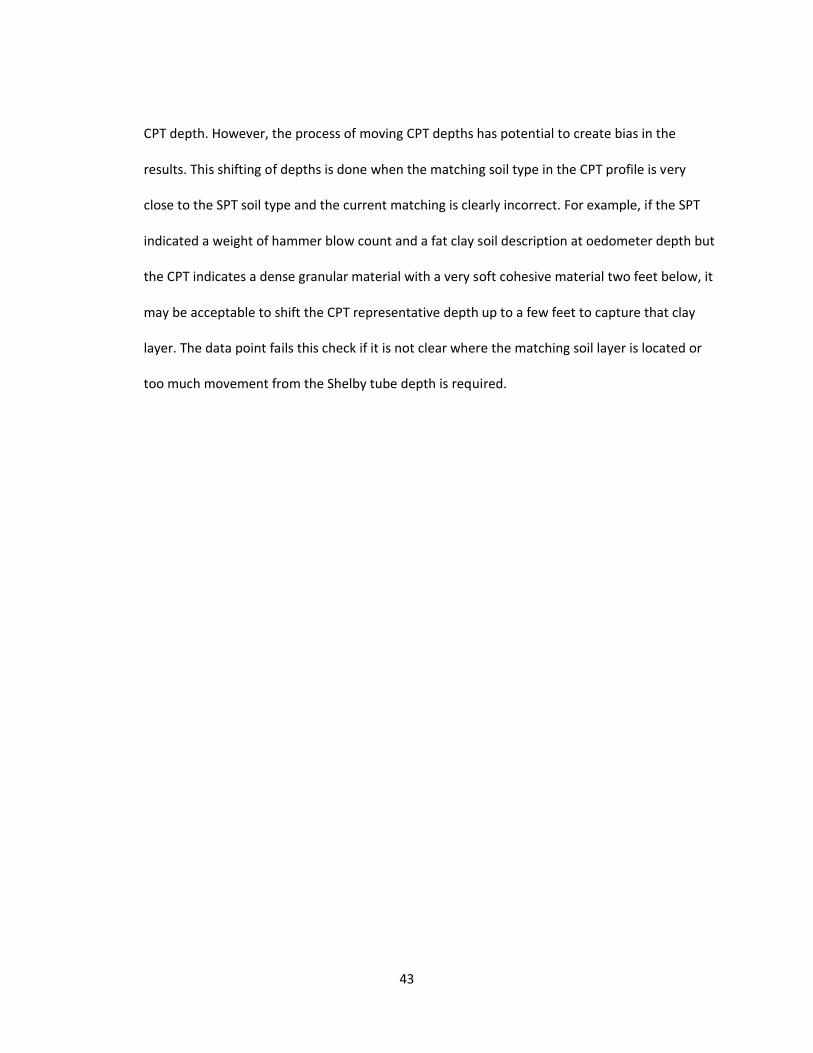
43
CPT depth. However, the process of moving CPT depths has potential to create bias in the
results. This shifting of depths is done when the matching soil type in the CPT profile is very
close to the SPT soil type and the current matching is clearly incorrect. For example, if the SPT
indicated a weight of hammer blow count and a fat clay soil description at oedometer depth but
the CPT indicates a dense granular material with a very soft cohesive material two feet below, it
may be acceptable to shift the CPT representative depth up to a few feet to capture that clay
layer. The data point fails this check if it is not clear where the matching soil layer is located or
too much movement from the Shelby tube depth is required.
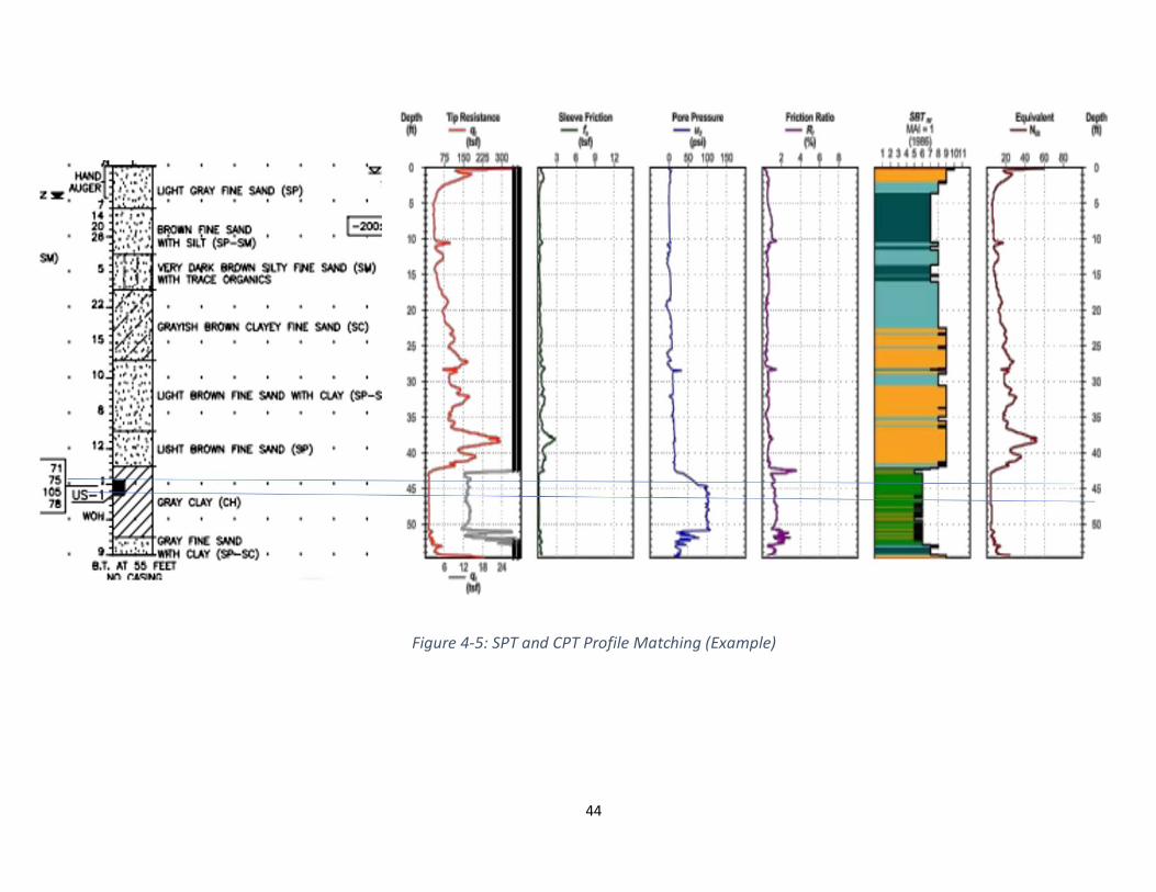
44
Figure 4-5: SPT and CPT Profile Matching (Example)
45
4. The final step performed before adding the point to the data base is to analyze the oedometer
test results. This involves selecting the recompression and compression indices, as well as
checking the overall quality of the test. The first check is that the sample represents the soil type
labeled in the SPT profile log. If not, any adjustments made to the CPT depth to match the
Oedometer sample depth may have been presumptuous and incorrect, requiring the previous
step to be redone. This test always depicts a gentle slope defined as the recompresison index, a
preconsolidation pressure, and a steep slope defined as the compresison index, as well as
displayed hysterosis behavior during unloading and reloading cycles. These responses, as well as
the high moisture content, plasticity index, percent passing and void ratio, confirm that the
sample matches the SPT profile as a high plasticity clay (CH).
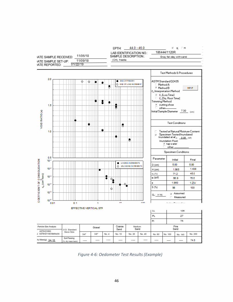
46
Figure 4-6: Oedometer Test Results (Example)
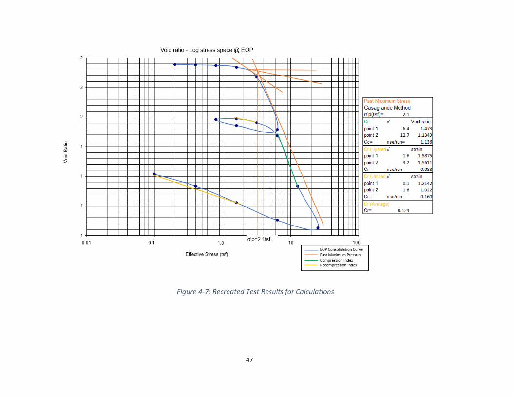
47
Figure 4-7: Recreated Test Results for Calculations
48
Next, the degree of sample disturbance is checked using the quality rating technique shown in
table 4-1. This is done by checking the amount of volume change (in terms of strain or void
ratio) that occurrs between the start of loading and the in-situ effective stress conditions. In
order to be enter into this table, the in-situ effective stress must be calculated. This is done by
estimating the unit weight of each soil layer using soil type and number of blows from the SPT
(correlations found in table 4-2 and 4-3) to calculate the total stress then subtracting the
hydrostatic pressure to obtain the effective stress. The quality rating table also considers over
consolidation ratio (OCR), therefore the past maximum pressure must be determined. This was
done by the Casagrande Method as this charts range allows for a crude estimation. The
casagrande method is a simple visual method with a relatively low degree of accuracy, however,
since the preconsoldiation pressure is only being used to check sample quaility this method is
acceptable. This sample has an OCR of 1.6, effective stress of 1.35 tsf, and a void ratio at the
effective stress of approximately 1.945, indicating an excellent quality sample with minimal
sample disturbance. This research requires high quality data as the purpose is to estimate
compression indices. For this reason any data point with a quality rating less than poor (lunne)
or D (Terizaghi) from Table 4-1 will be removed.
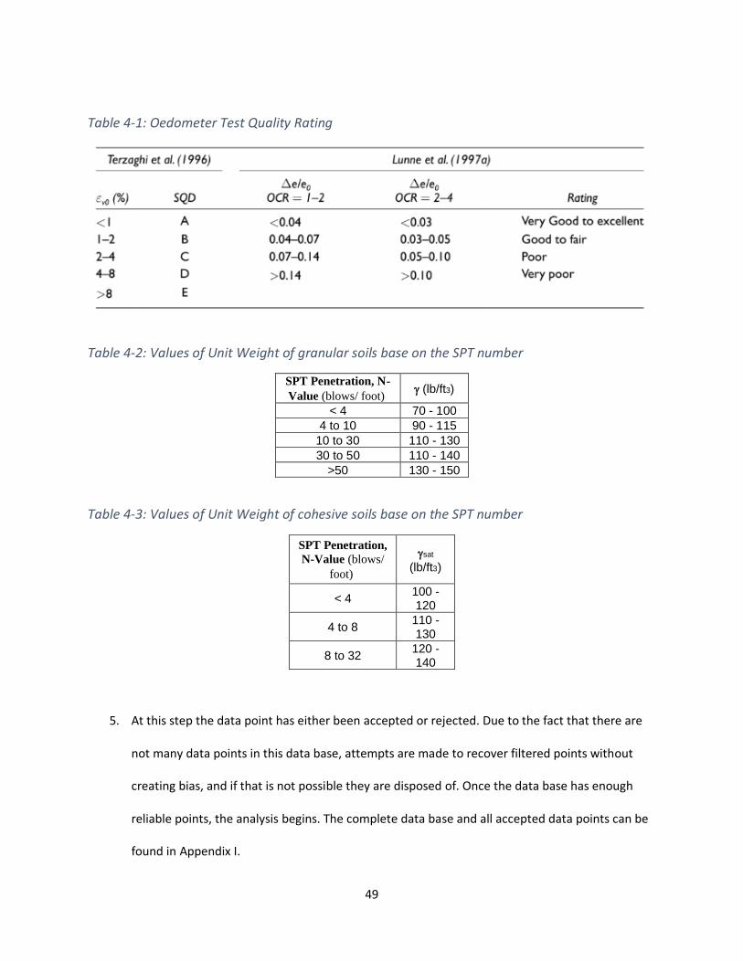
49
Table 4-1: Oedometer Test Quality Rating
Table 4-2: Values of Unit Weight of granular soils base on the SPT number
SPT Penetration, N-
Value (blows/ foot) (lb/ft3)
< 4 70 - 100
4 to 10 90 - 115
10 to 30 110 - 130
30 to 50 110 - 140
>50 130 - 150
Table 4-3: Values of Unit Weight of cohesive soils base on the SPT number
SPT Penetration,
N-Value (blows/
foot)
sat
(lb/ft3)
< 4 100 - 120
4 to 8 110 - 130
8 to 32 120 - 140
5. At this step the data point has either been accepted or rejected. Due to the fact that there are
not many data points in this data base, attempts are made to recover filtered points without
creating bias, and if that is not possible they are disposed of. Once the data base has enough
reliable points, the analysis begins. The complete data base and all accepted data points can be
found in Appendix I.
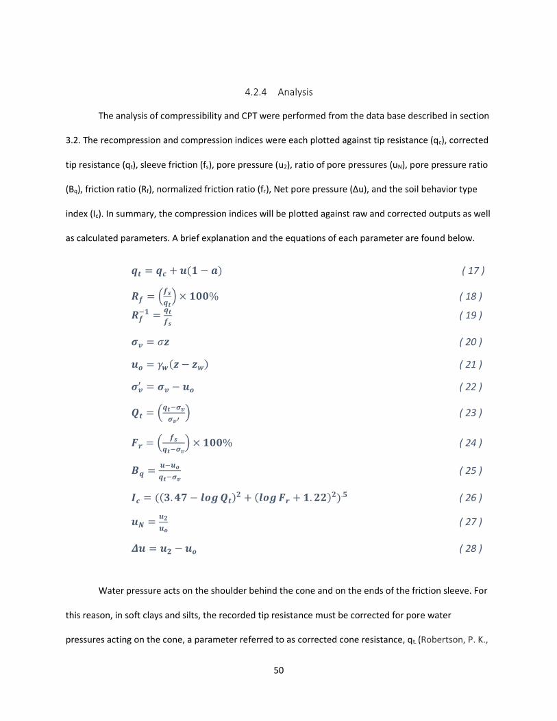
50
4.2.4 Analysis
The analysis of compressibility and CPT were performed from the data base described in section
3.2. The recompression and compression indices were each plotted against tip resistance (qc), corrected
tip resistance (qt), sleeve friction (fs), pore pressure (u2), ratio of pore pressures (uN), pore pressure ratio
(Bq), friction ratio (Rf), normalized friction ratio (fr), Net pore pressure (Δu), and the soil behavior type
index (Ic). In summary, the compression indices will be plotted against raw and corrected outputs as well
as calculated parameters. A brief explanation and the equations of each parameter are found below.
𝒒𝒕 = 𝒒𝒄 + 𝒖(𝟏 − 𝒂) ( 17 )
𝑹𝒇 = (𝒇𝒔
𝒒𝒕) × 𝟏𝟎𝟎% ( 18 )
𝑹𝒇−𝟏 =
𝒒𝒕
𝒇𝒔 ( 19 )
𝝈𝒗 = 𝜎𝒛 ( 20 )
𝒖𝒐 = 𝛾𝒘(𝒛 − 𝒛𝒘) ( 21 )
𝝈𝒗′ = 𝝈𝒗 − 𝒖𝒐 ( 22 )
𝑸𝒕 = (𝒒𝒕−𝝈𝒗
𝝈𝒗′) ( 23 )
𝑭𝒓 = (𝒇𝒔
𝒒𝒕−𝝈𝒗) × 𝟏𝟎𝟎% ( 24 )
𝑩𝒒 =𝒖−𝒖𝒐
𝒒𝒕−𝝈𝒗 ( 25 )
𝑰𝒄 = ((𝟑. 𝟒𝟕 − 𝒍𝒐𝒈 𝑸𝒕)𝟐 + (𝒍𝒐𝒈 𝑭𝒓 + 𝟏. 𝟐𝟐)𝟐).𝟓 ( 26 )
𝒖𝑵 =𝒖𝟐
𝒖𝒐 ( 27 )
𝜟𝒖 = 𝒖𝟐 − 𝒖𝒐 ( 28 )
Water pressure acts on the shoulder behind the cone and on the ends of the friction sleeve. For
this reason, in soft clays and silts, the recorded tip resistance must be corrected for pore water
pressures acting on the cone, a parameter referred to as corrected cone resistance, qt. (Robertson, P. K.,
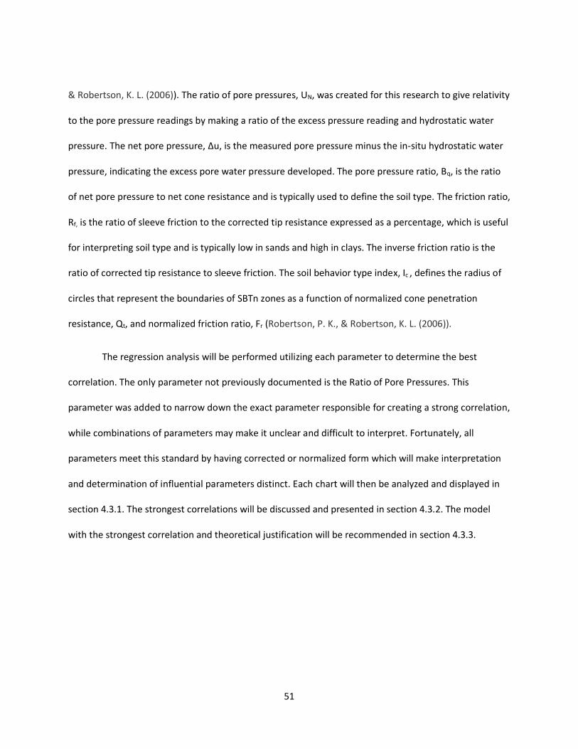
51
& Robertson, K. L. (2006)). The ratio of pore pressures, UN, was created for this research to give relativity
to the pore pressure readings by making a ratio of the excess pressure reading and hydrostatic water
pressure. The net pore pressure, Δu, is the measured pore pressure minus the in-situ hydrostatic water
pressure, indicating the excess pore water pressure developed. The pore pressure ratio, Bq, is the ratio
of net pore pressure to net cone resistance and is typically used to define the soil type. The friction ratio,
Rf, is the ratio of sleeve friction to the corrected tip resistance expressed as a percentage, which is useful
for interpreting soil type and is typically low in sands and high in clays. The inverse friction ratio is the
ratio of corrected tip resistance to sleeve friction. The soil behavior type index, Ic , defines the radius of
circles that represent the boundaries of SBTn zones as a function of normalized cone penetration
resistance, Qt, and normalized friction ratio, Fr (Robertson, P. K., & Robertson, K. L. (2006)).
The regression analysis will be performed utilizing each parameter to determine the best
correlation. The only parameter not previously documented is the Ratio of Pore Pressures. This
parameter was added to narrow down the exact parameter responsible for creating a strong correlation,
while combinations of parameters may make it unclear and difficult to interpret. Fortunately, all
parameters meet this standard by having corrected or normalized form which will make interpretation
and determination of influential parameters distinct. Each chart will then be analyzed and displayed in
section 4.3.1. The strongest correlations will be discussed and presented in section 4.3.2. The model
with the strongest correlation and theoretical justification will be recommended in section 4.3.3.
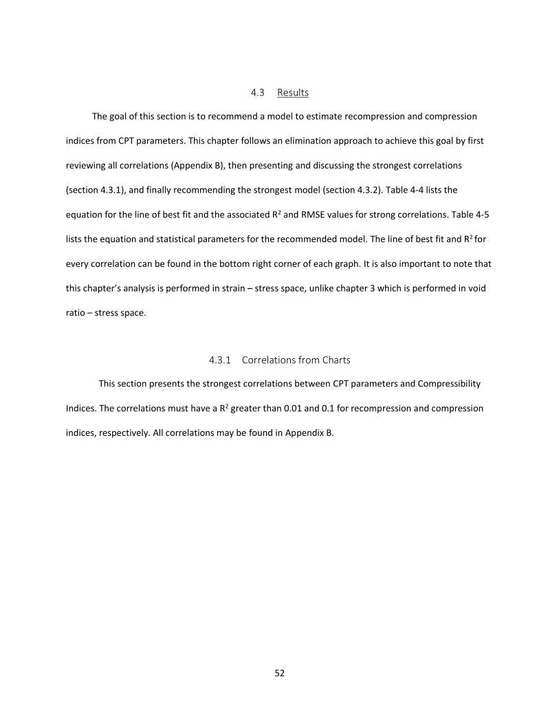
52
4.3 Results
The goal of this section is to recommend a model to estimate recompression and compression
indices from CPT parameters. This chapter follows an elimination approach to achieve this goal by first
reviewing all correlations (Appendix B), then presenting and discussing the strongest correlations
(section 4.3.1), and finally recommending the strongest model (section 4.3.2). Table 4-4 lists the
equation for the line of best fit and the associated R2 and RMSE values for strong correlations. Table 4-5
lists the equation and statistical parameters for the recommended model. The line of best fit and R2 for
every correlation can be found in the bottom right corner of each graph. It is also important to note that
this chapter’s analysis is performed in strain – stress space, unlike chapter 3 which is performed in void
ratio – stress space.
4.3.1 Correlations from Charts
This section presents the strongest correlations between CPT parameters and Compressibility
Indices. The correlations must have a R2 greater than 0.01 and 0.1 for recompression and compression
indices, respectively. All correlations may be found in Appendix B.
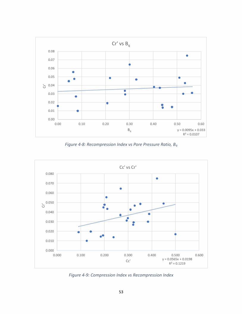
53
Figure 4-8: Recompression Index vs Pore Pressure Ratio, Bq
Figure 4-9: Compression Index vs Recompression Index
y = 0.0095x + 0.033R² = 0.0107
0.00
0.01
0.02
0.03
0.04
0.05
0.06
0.07
0.08
0.00 0.10 0.20 0.30 0.40 0.50 0.60
Cr'
Bq
Cr' vs Bq
y = 0.0565x + 0.0198R² = 0.1219
0.000
0.010
0.020
0.030
0.040
0.050
0.060
0.070
0.080
0.000 0.100 0.200 0.300 0.400 0.500 0.600
Cr'
Cc'
Cc' vs Cr'
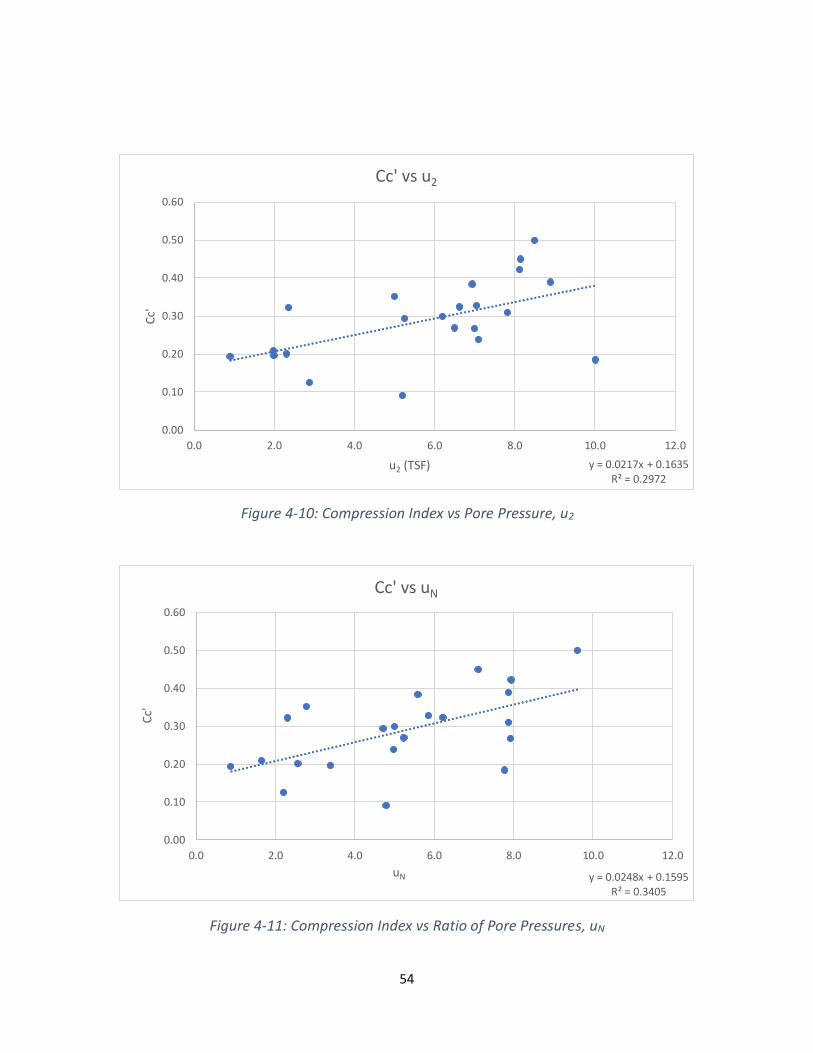
54
Figure 4-10: Compression Index vs Pore Pressure, u2
Figure 4-11: Compression Index vs Ratio of Pore Pressures, uN
y = 0.0217x + 0.1635R² = 0.2972
0.00
0.10
0.20
0.30
0.40
0.50
0.60
0.0 2.0 4.0 6.0 8.0 10.0 12.0
Cc'
u2 (TSF)
Cc' vs u2
y = 0.0248x + 0.1595R² = 0.3405
0.00
0.10
0.20
0.30
0.40
0.50
0.60
0.0 2.0 4.0 6.0 8.0 10.0 12.0
Cc'
uN
Cc' vs uN
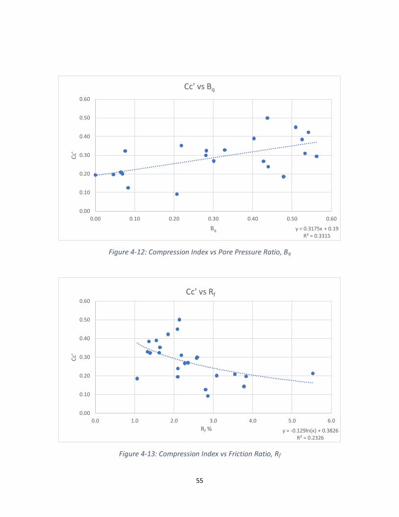
55
Figure 4-12: Compression Index vs Pore Pressure Ratio, Bq
Figure 4-13: Compression Index vs Friction Ratio, Rf
y = 0.3175x + 0.19R² = 0.3315
0.00
0.10
0.20
0.30
0.40
0.50
0.60
0.00 0.10 0.20 0.30 0.40 0.50 0.60
Cc'
Bq
Cc' vs Bq
y = -0.129ln(x) + 0.3826R² = 0.2326
0.00
0.10
0.20
0.30
0.40
0.50
0.60
0.0 1.0 2.0 3.0 4.0 5.0 6.0
Cc'
Rf %
Cc' vs Rf
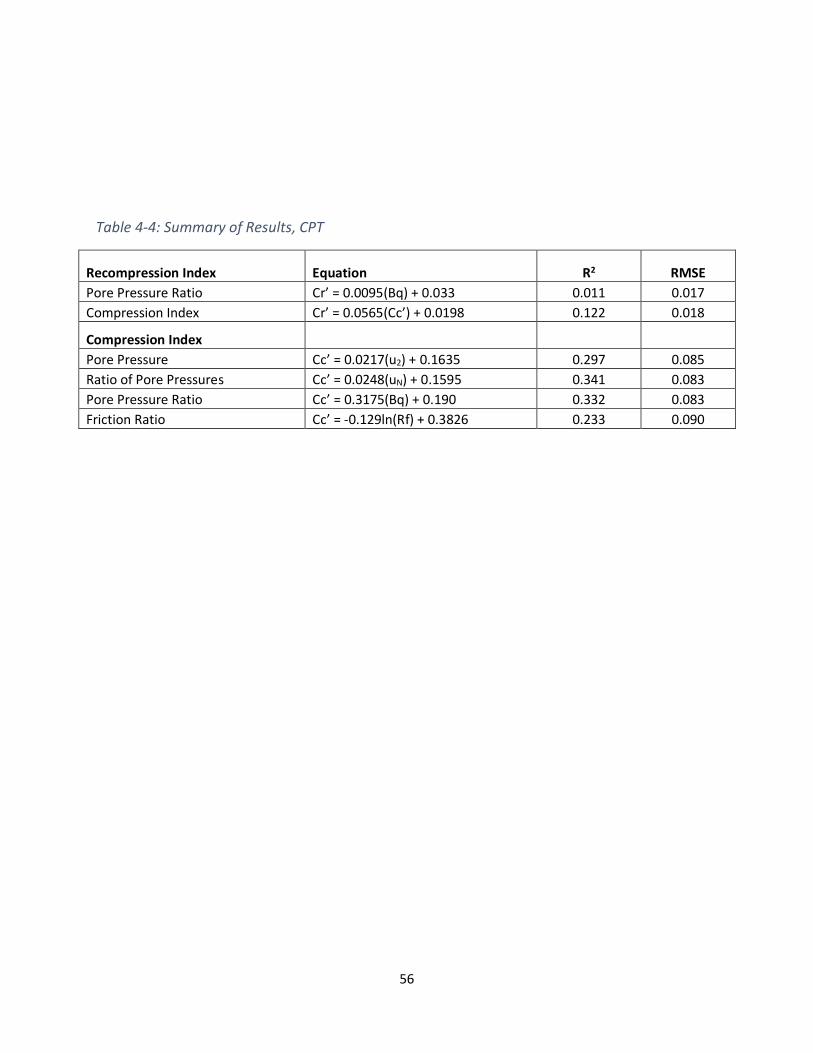
56
Table 4-4: Summary of Results, CPT
Recompression Index Equation R2 RMSE
Pore Pressure Ratio Cr’ = 0.0095(Bq) + 0.033 0.011 0.017
Compression Index Cr’ = 0.0565(Cc’) + 0.0198 0.122 0.018
Compression Index
Pore Pressure Cc’ = 0.0217(u2) + 0.1635 0.297 0.085
Ratio of Pore Pressures Cc’ = 0.0248(uN) + 0.1595 0.341 0.083
Pore Pressure Ratio Cc’ = 0.3175(Bq) + 0.190 0.332 0.083
Friction Ratio Cc’ = -0.129ln(Rf) + 0.3826 0.233 0.090
57
4.3.2 Recommended Model and Discussion
The findings of this study show relatively good correlations of the compression index to friction
and pore pressure parameters. These findings will be condensed to avoid redundancy by defining all
pore pressure correlations using only the Ratio of Pore Pressures (uN) and all friction correlations using
the Friction Ratio (Rf).
Of these correlations the ratio of pore pressures is the strongest. This relationship is positive,
indicating as the ratio of excess pore water pressure (PWP) to hydrostatic PWP increases, the
compressibility increases.
It was mentioned in the introduction that the pore pressure reading (u2) is dependent on the
rate of dissipation. In the extreme example, clays will dissipate pore pressure much slower than sands,
which is why sands record hydrostatic pressures and clays record some net pore pressure. It is also
understood that sands have a lower compressibility than clays. There are varying dissipation rates for
clays as the drainage behavior is heavily influenced by stress history, sand content, and mineral type.
The effects of each factors are further examined in figures 4-14 to 4-16. Figure 4-14 shows a strong
positive correlation between percent finer and pore pressure. This indicates that the sand content
decreases the pore pressures by increasing the drainage rate. Figure 4-15 shows a strong correlation
between Plasticity index and pore pressure. This shows that as the colloidal properties become more
pronounced that soil’s dissipation rate decreases. Figure 4-16 shows a weak positive correlation to
preconsolidation pressure. This parameter is influential for stress-strain response; however, the
mechanism of the CPT is that the penetrometer is quickly failing the soil not slowly straining it. Due to
this violent loading scenario, the preconsolidation pressure is likely quickly surpassed and does not
heavily impact the CPT outputs. This is not to say the CPT cannot estimate preconsolidation pressure but
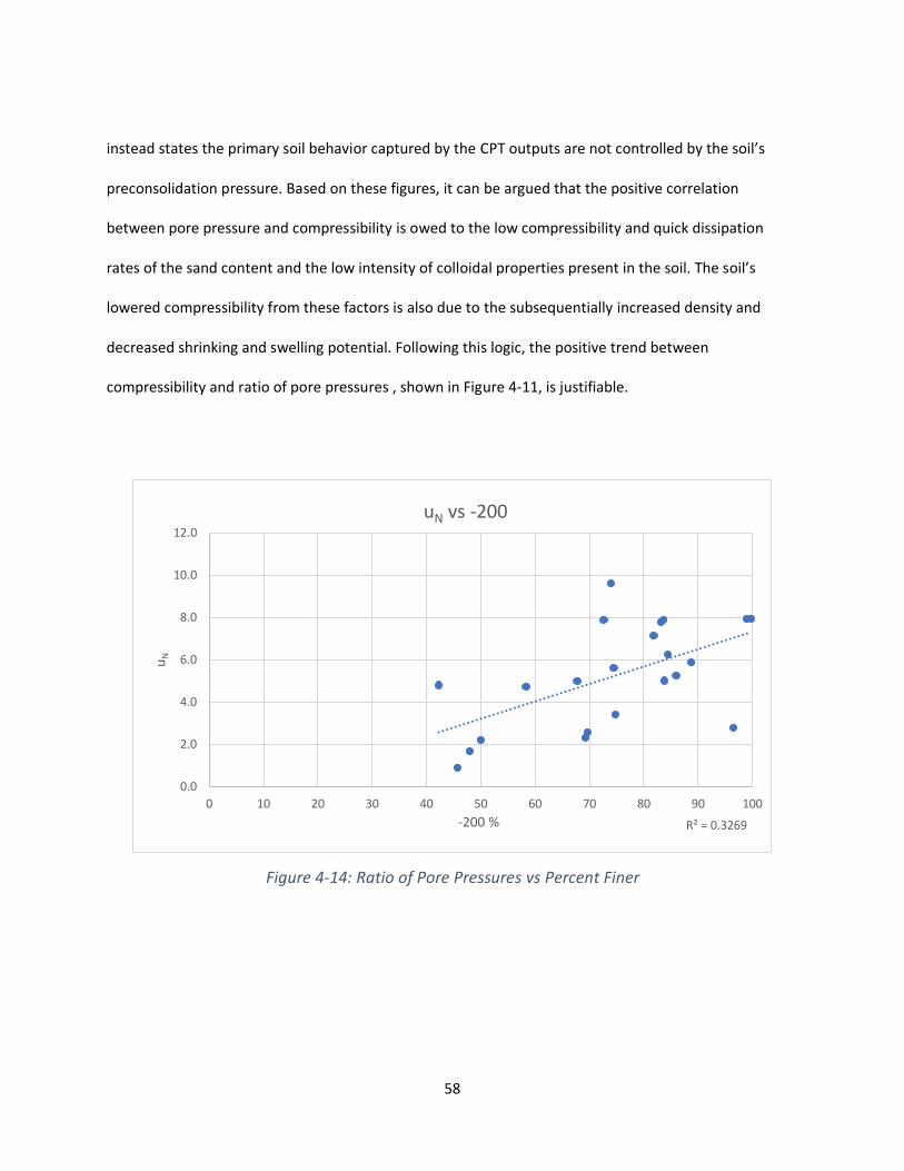
58
instead states the primary soil behavior captured by the CPT outputs are not controlled by the soil’s
preconsolidation pressure. Based on these figures, it can be argued that the positive correlation
between pore pressure and compressibility is owed to the low compressibility and quick dissipation
rates of the sand content and the low intensity of colloidal properties present in the soil. The soil’s
lowered compressibility from these factors is also due to the subsequentially increased density and
decreased shrinking and swelling potential. Following this logic, the positive trend between
compressibility and ratio of pore pressures , shown in Figure 4-11, is justifiable.
Figure 4-14: Ratio of Pore Pressures vs Percent Finer
R² = 0.3269
0.0
2.0
4.0
6.0
8.0
10.0
12.0
0 10 20 30 40 50 60 70 80 90 100
uN
-200 %
uN vs -200
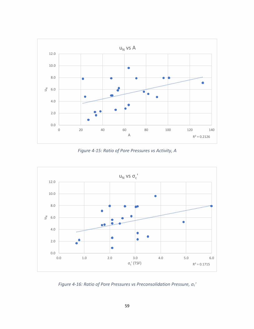
59
Figure 4-15: Ratio of Pore Pressures vs Activity, A
Figure 4-16: Ratio of Pore Pressures vs Preconsolidation Pressure, σc'
R² = 0.2126
0.0
2.0
4.0
6.0
8.0
10.0
12.0
0 20 40 60 80 100 120 140
uN
A
uN vs A
R² = 0.1715
0.0
2.0
4.0
6.0
8.0
10.0
12.0
0.0 1.0 2.0 3.0 4.0 5.0 6.0
uN
σc' (TSF)
uN vs σc'
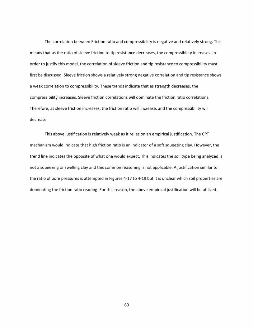
60
The correlation between Friction ratio and compressibility is negative and relatively strong. This
means that as the ratio of sleeve friction to tip resistance decreases, the compressibility increases. In
order to justify this model, the correlation of sleeve friction and tip resistance to compressibility must
first be discussed. Sleeve friction shows a relatively strong negative correlation and tip resistance shows
a weak correlation to compressibility. These trends indicate that as strength decreases, the
compressibility increases. Sleeve friction correlations will dominate the friction ratio correlations.
Therefore, as sleeve friction increases, the friction ratio will increase, and the compressibility will
decrease.
This above justification is relatively weak as it relies on an empirical justification. The CPT
mechanism would indicate that high friction ratio is an indicator of a soft squeezing clay. However, the
trend line indicates the opposite of what one would expect. This indicates the soil type being analyzed is
not a squeezing or swelling clay and this common reasoning is not applicable. A justification similar to
the ratio of pore pressures is attempted in Figures 4-17 to 4-19 but it is unclear which soil properties are
dominating the friction ratio reading. For this reason, the above empirical justification will be utilized.
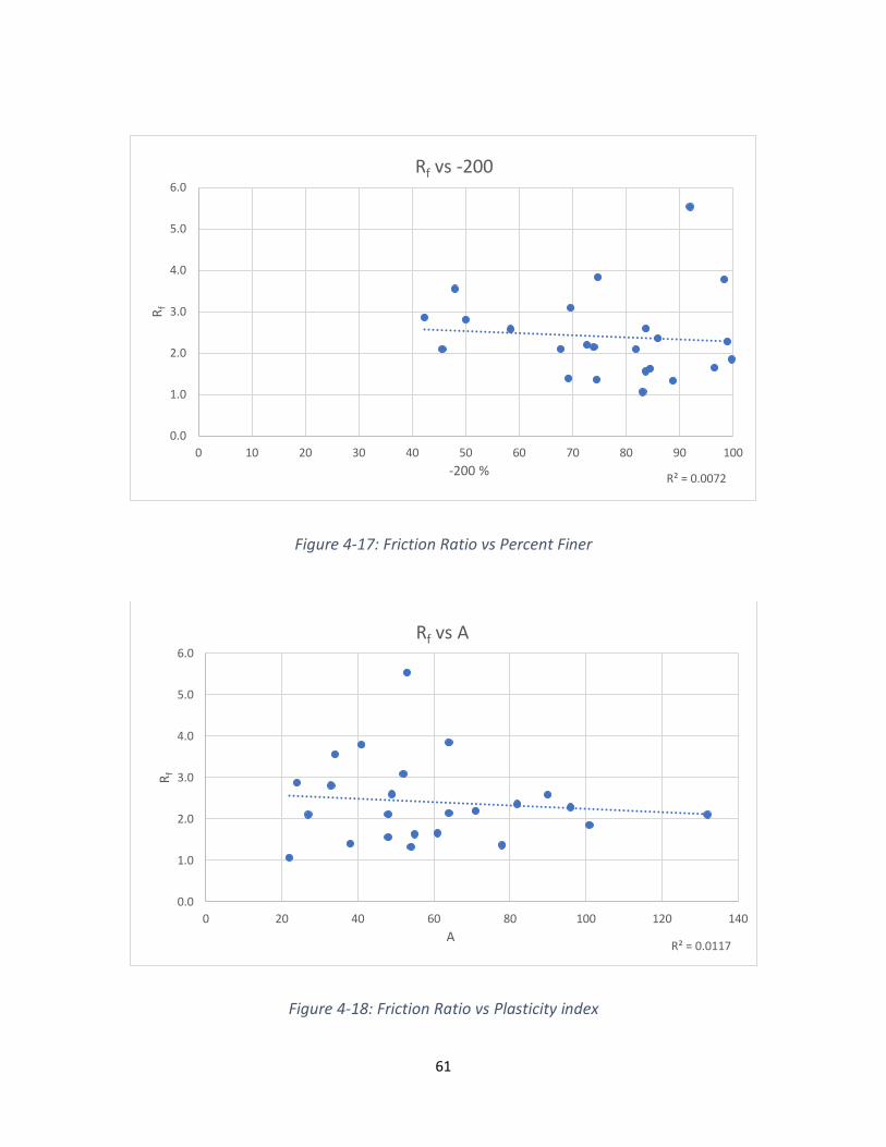
61
Figure 4-17: Friction Ratio vs Percent Finer
Figure 4-18: Friction Ratio vs Plasticity index
R² = 0.0072
0.0
1.0
2.0
3.0
4.0
5.0
6.0
0 10 20 30 40 50 60 70 80 90 100
Rf
-200 %
Rf vs -200
R² = 0.0117
0.0
1.0
2.0
3.0
4.0
5.0
6.0
0 20 40 60 80 100 120 140
Rf
A
Rf vs A
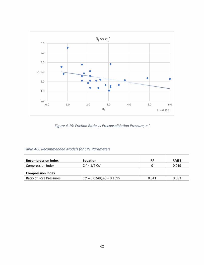
62
Figure 4-19: Friction Ratio vs Preconsolidation Pressure, σc'
Table 4-5: Recommended Models for CPT Parameters
Recompression Index Equation R2 RMSE
Compression Index Cr’ = 1/7 Cc’ 0 0.019
Compression Index
Ratio of Pore Pressures Cc’ = 0.0248(uN) + 0.1595 0.341 0.083
R² = 0.156
0.0
1.0
2.0
3.0
4.0
5.0
6.0
0.0 1.0 2.0 3.0 4.0 5.0 6.0
Rf
σc'
Rf vs σc'
63
4.4 Conclusion
The recommended model to estimate the compressibility of fine-grained soils via CPT is shown
below in Table 4.5. The model and discussion above demonstrate a relationship between CPT pore
pressure reading and compression index exists. The correlations to the recompression index were poor,
indicating the recompression index cannot be estimated from the CPT parameters. This finding is
contradicting to the literature review which show elastic correlations from the CPT to compressibility for
elastic behavior. The reason for this finding is that some error within the recompression index value
exists within the data base. Another possible reason could be owed to the mechanism of the CPT failing
the soil column in shear and quickly exceeding the preconsolidation pressure. This process would likely
cause the CPT outputs to correlate better to the compression index than the recompression index. For
this reason, the “one-fifth rule” discussed in the literature review and utilized in chapter 3 will also be
utilized in this chapter. A refined ratio for the CPT data base is recommended in Table 4-5.
These findings indicate it is possible to create a continuous compressibility profile from a commonly
utilized field test. However, the data base would have to be expanded and more rigorous filters applied
in order to produce any reliable models for use in practice. The purpose of the filter applied in the
following section is to support the findings of this chapter and determine the effectiveness of the CPT on
soils at varying levels of index properties.
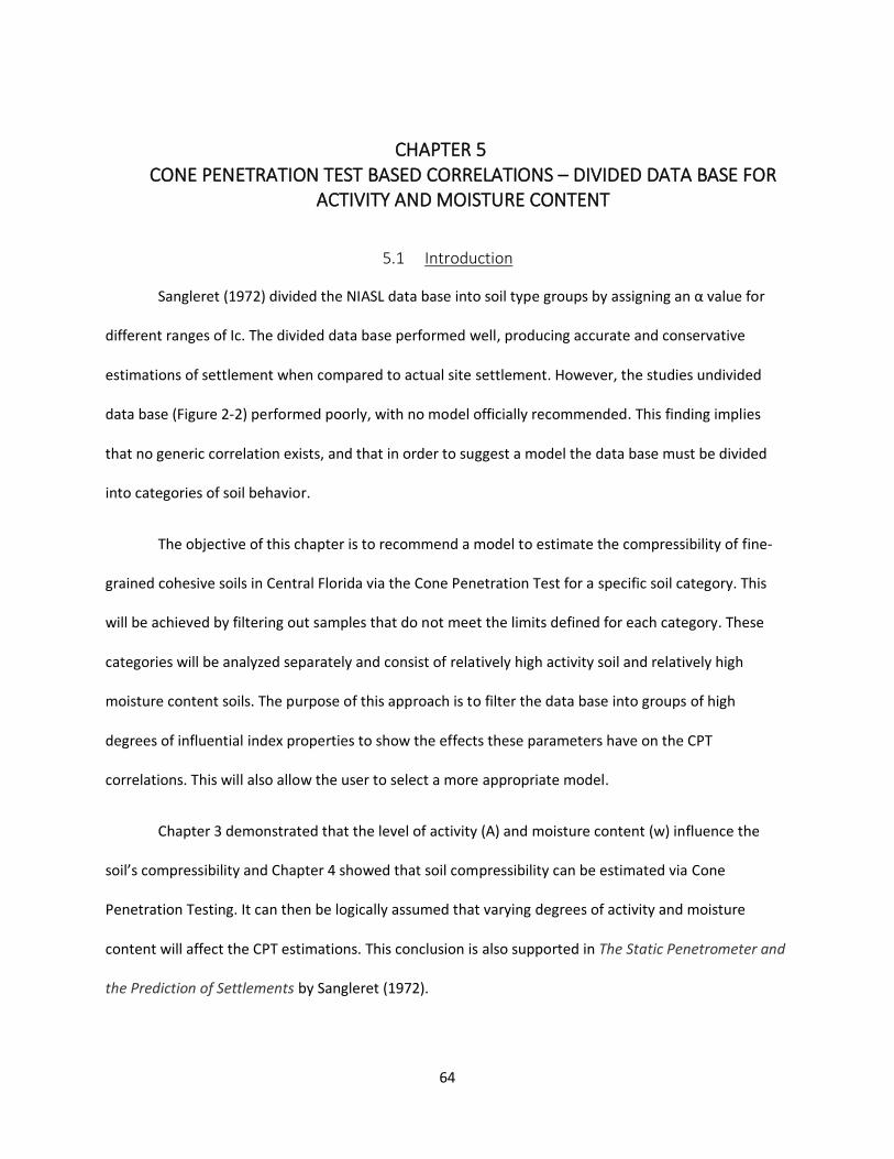
64
CHAPTER 5 CONE PENETRATION TEST BASED CORRELATIONS – DIVIDED DATA BASE FOR
ACTIVITY AND MOISTURE CONTENT
5.1 Introduction
Sangleret (1972) divided the NIASL data base into soil type groups by assigning an α value for
different ranges of Ic. The divided data base performed well, producing accurate and conservative
estimations of settlement when compared to actual site settlement. However, the studies undivided
data base (Figure 2-2) performed poorly, with no model officially recommended. This finding implies
that no generic correlation exists, and that in order to suggest a model the data base must be divided
into categories of soil behavior.
The objective of this chapter is to recommend a model to estimate the compressibility of fine-
grained cohesive soils in Central Florida via the Cone Penetration Test for a specific soil category. This
will be achieved by filtering out samples that do not meet the limits defined for each category. These
categories will be analyzed separately and consist of relatively high activity soil and relatively high
moisture content soils. The purpose of this approach is to filter the data base into groups of high
degrees of influential index properties to show the effects these parameters have on the CPT
correlations. This will also allow the user to select a more appropriate model.
Chapter 3 demonstrated that the level of activity (A) and moisture content (w) influence the
soil’s compressibility and Chapter 4 showed that soil compressibility can be estimated via Cone
Penetration Testing. It can then be logically assumed that varying degrees of activity and moisture
content will affect the CPT estimations. This conclusion is also supported in The Static Penetrometer and
the Prediction of Settlements by Sangleret (1972).
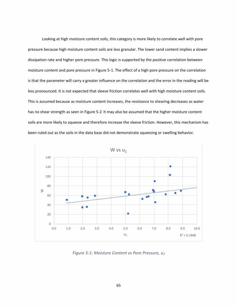
65
Looking at high moisture content soils, this category is more likely to correlate well with pore
pressure because high moisture content soils are less granular. The lower sand content implies a slower
dissipation rate and higher pore pressure. This logic is supported by the positive correlation between
moisture content and pore pressure in Figure 5-1. The effect of a high pore pressure on the correlation
is that the parameter will carry a greater influence on the correlation and the error in the reading will be
less pronounced. It is not expected that sleeve friction correlates well with high moisture content soils.
This is assumed because as moisture content increases, the resistance to shearing decreases as water
has no shear strength as seen in Figure 5-2. It may also be assumed that the higher moisture content
soils are more likely to squeeze and therefore increase the sleeve friction. However, this mechanism has
been ruled out as the soils in the data base did not demonstrate squeezing or swelling behavior.
Figure 5-1: Moisture Content vs Pore Pressure, u2
R² = 0.1848
0
20
40
60
80
100
120
140
0.0 1.0 2.0 3.0 4.0 5.0 6.0 7.0 8.0 9.0 10.0
W
u2
W vs u2
66
Figure 5-2: Moisture Content vs Sleeve Friction, fs
Activity is the ratio of plasticity index and percent finer. The plasticity index indicates the range
between liquid and solid consistencies. In more relative words, the plasticity index indicates the soils
ability to change volume with varying moisture contents. Percent finer represents the number of fines
present in the soil mixture. These fines could be kaolinite, illite, montmorillonite, and/or silt. Therefore,
the percent finer, when used alone, does not quantify the soil behavior. This implied test is most
valuable when used in conjunction with more testing. In the case for the Activity parameter, the
plasticity index is combined with the percent finer to describe the soils mineralogy (Skempton 1988).
Table 5-1 from Skempton (1988) states that soils with activity less than 0.75 are inactive and
predominately kaolinite and illite. Clays with activity from 0.75 to 1.25 are normal and predominately
illite. Clays greater than 1.25 are active illite and clays greater than 2 are active montmorillonite.
R² = 0.2546
0
20
40
60
80
100
120
140
0.0 0.2 0.4 0.6 0.8 1.0 1.2 1.4
W
fs
W vs fs

67
From Skempton’s findings and an understanding of the plasticity and percent finer tests it is
assumed that Activity will be a strong indicator of soil behavior. Soils with relatively high Activity (A>0.5)
will have a strong correlation to pore pressure and friction parameters. This hypothesis is made because
high activity soils are likely to squeeze and develop higher pore pressures, making the sleeve friction and
pore pressure readings more pronounced. Neither of these hypotheses are supported through
correlation such as the ones utilized within the moisture content discussion. Since Activity has not been
seen to correlate well with any parameters within this study, the theoretical hypothesis will be accepted
over the graphical hypothesis.
The filters applied to the data base were briefly mentioned above but will formally be
summarized within this paragraph. Samples with activity less than 0.5 are removed. As mentioned above
the ideal filter would be for soils with activity less than 0.75, however, the limited data points made this
filter impractical. This applied limit of 0.5 resulted in the removal of only two data points. For the next
analysis samples with moisture content less than 40% are removed, resulting in the removal of three
data points. The method used to select the limits is discussed in the following section.

68
Table 5-1: Correlation of Activity and the Minerology and Geology of Clay from Skempton 1984
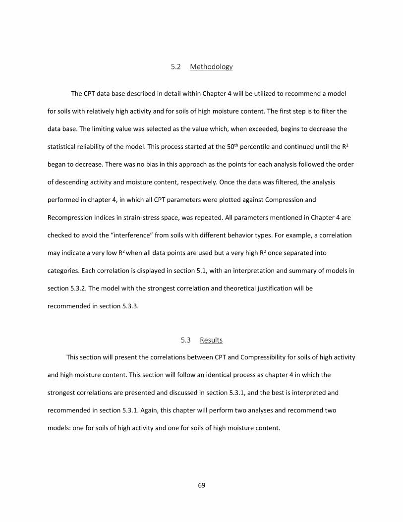
69
5.2 Methodology
The CPT data base described in detail within Chapter 4 will be utilized to recommend a model
for soils with relatively high activity and for soils of high moisture content. The first step is to filter the
data base. The limiting value was selected as the value which, when exceeded, begins to decrease the
statistical reliability of the model. This process started at the 50th percentile and continued until the R2
began to decrease. There was no bias in this approach as the points for each analysis followed the order
of descending activity and moisture content, respectively. Once the data was filtered, the analysis
performed in chapter 4, in which all CPT parameters were plotted against Compression and
Recompression Indices in strain-stress space, was repeated. All parameters mentioned in Chapter 4 are
checked to avoid the “interference” from soils with different behavior types. For example, a correlation
may indicate a very low R2 when all data points are used but a very high R2 once separated into
categories. Each correlation is displayed in section 5.1, with an interpretation and summary of models in
section 5.3.2. The model with the strongest correlation and theoretical justification will be
recommended in section 5.3.3.
5.3 Results
This section will present the correlations between CPT and Compressibility for soils of high activity
and high moisture content. This section will follow an identical process as chapter 4 in which the
strongest correlations are presented and discussed in section 5.3.1, and the best is interpreted and
recommended in section 5.3.1. Again, this chapter will perform two analyses and recommend two
models: one for soils of high activity and one for soils of high moisture content.
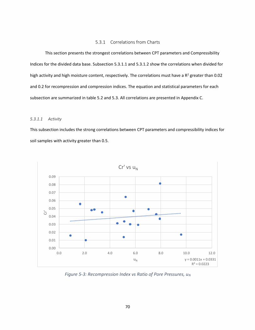
70
5.3.1 Correlations from Charts
This section presents the strongest correlations between CPT parameters and Compressibility
Indices for the divided data base. Subsection 5.3.1.1 and 5.3.1.2 show the correlations when divided for
high activity and high moisture content, respectively. The correlations must have a R2 greater than 0.02
and 0.2 for recompression and compression indices. The equation and statistical parameters for each
subsection are summarized in table 5.2 and 5.3. All correlations are presented in Appendix C.
5.3.1.1 Activity
This subsection includes the strong correlations between CPT parameters and compressibility indices for
soil samples with activity greater than 0.5.
Figure 5-3: Recompression Index vs Ratio of Pore Pressures, uN
y = 0.0011x + 0.0331R² = 0.0223
0.00
0.01
0.02
0.03
0.04
0.05
0.06
0.07
0.08
0.09
0.0 2.0 4.0 6.0 8.0 10.0 12.0
Cr'
uN
Cr' vs uN
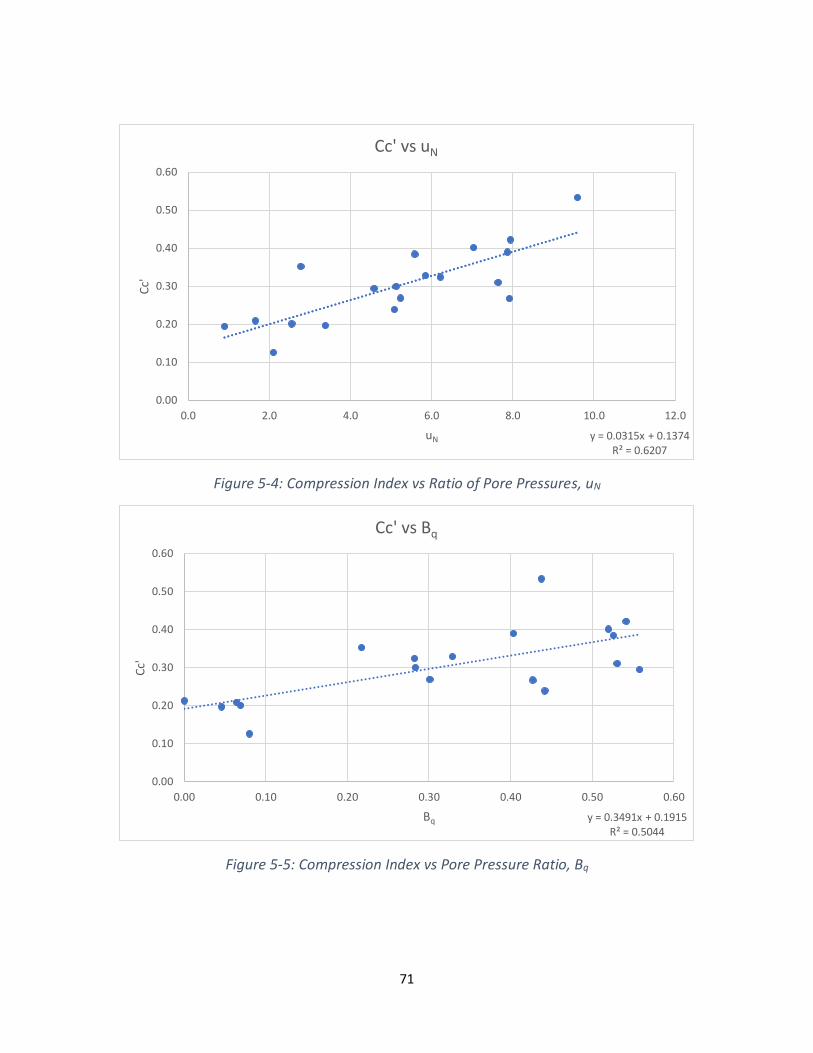
71
Figure 5-4: Compression Index vs Ratio of Pore Pressures, uN
Figure 5-5: Compression Index vs Pore Pressure Ratio, Bq
y = 0.0315x + 0.1374R² = 0.6207
0.00
0.10
0.20
0.30
0.40
0.50
0.60
0.0 2.0 4.0 6.0 8.0 10.0 12.0
Cc'
uN
Cc' vs uN
y = 0.3491x + 0.1915R² = 0.5044
0.00
0.10
0.20
0.30
0.40
0.50
0.60
0.00 0.10 0.20 0.30 0.40 0.50 0.60
Cc'
Bq
Cc' vs Bq
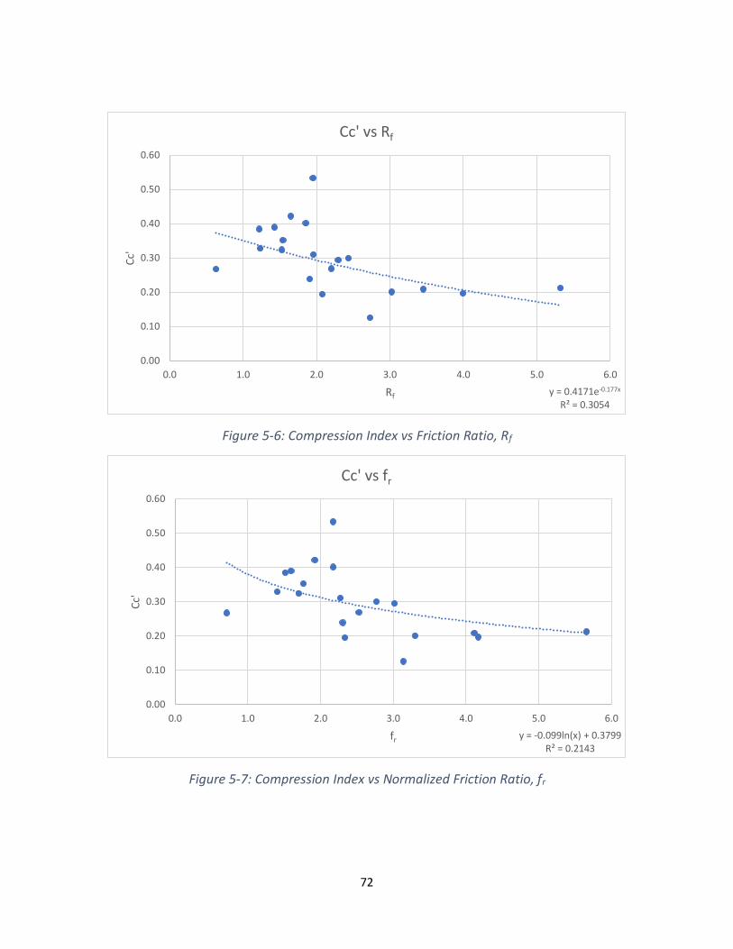
72
Figure 5-6: Compression Index vs Friction Ratio, Rf
Figure 5-7: Compression Index vs Normalized Friction Ratio, fr
y = 0.4171e-0.177x
R² = 0.3054
0.00
0.10
0.20
0.30
0.40
0.50
0.60
0.0 1.0 2.0 3.0 4.0 5.0 6.0
Cc'
Rf
Cc' vs Rf
y = -0.099ln(x) + 0.3799R² = 0.2143
0.00
0.10
0.20
0.30
0.40
0.50
0.60
0.0 1.0 2.0 3.0 4.0 5.0 6.0
Cc'
fr
Cc' vs fr
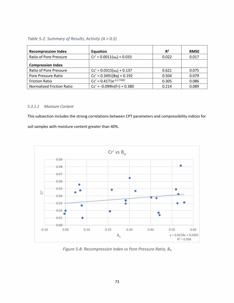
73
Table 5-2: Summary of Results, Activity (A > 0.5)
Recompression Index Equation R2 RMSE
Ratio of Pore Pressure Cr’ = 0.0011(uN) + 0.033 0.022 0.017
Compression Index Ratio of Pore Pressure Cc’ = 0.0315(uN) + 0.137 0.621 0.075
Pore Pressure Ratio Cc’ = 0.3491(Bq) + 0.192 0.504 0.079
Friction Ratio Cc’ = 0.4171e-0.177(Rf) 0.305 0.086 Normalized Friction Ratio Cc’ = -0.099ln(Fr) + 0.380 0.214 0.089
5.3.1.2 Moisture Content
This subsection includes the strong correlations between CPT parameters and compressibility indices for
soil samples with moisture content greater than 40%.
Figure 5-8: Recompression Index vs Pore Pressure Ratio, Bq
y = 0.0218x + 0.0302R² = 0.058
0.00
0.01
0.02
0.03
0.04
0.05
0.06
0.07
0.08
0.09
-0.10 0.00 0.10 0.20 0.30 0.40 0.50 0.60
Cr'
Bq
Cr' vs Bq
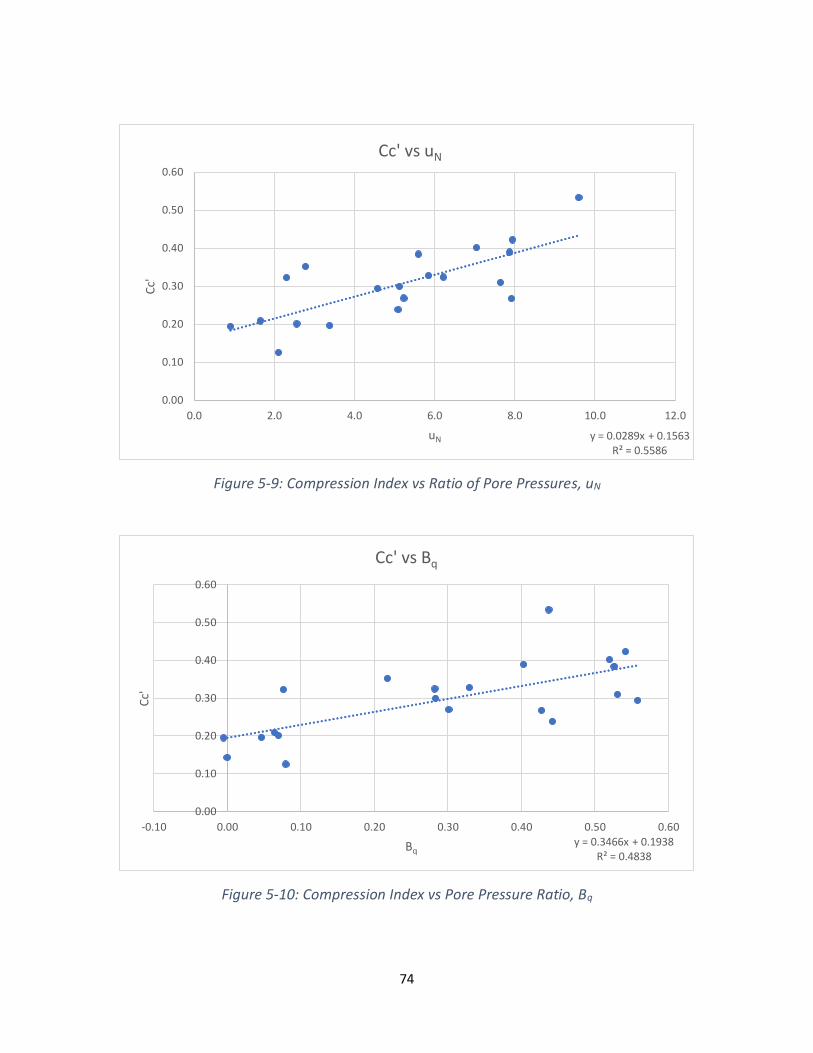
74
Figure 5-9: Compression Index vs Ratio of Pore Pressures, uN
Figure 5-10: Compression Index vs Pore Pressure Ratio, Bq
y = 0.0289x + 0.1563R² = 0.5586
0.00
0.10
0.20
0.30
0.40
0.50
0.60
0.0 2.0 4.0 6.0 8.0 10.0 12.0
Cc'
uN
Cc' vs uN
y = 0.3466x + 0.1938R² = 0.4838
0.00
0.10
0.20
0.30
0.40
0.50
0.60
-0.10 0.00 0.10 0.20 0.30 0.40 0.50 0.60
Cc'
Bq
Cc' vs Bq
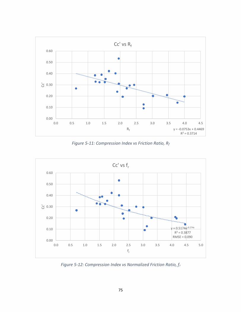
75
Figure 5-11: Compression Index vs Friction Ratio, Rf
Figure 5-12: Compression Index vs Normalized Friction Ratio, fr
y = -0.0753x + 0.4469R² = 0.3714
0.00
0.10
0.20
0.30
0.40
0.50
0.60
0.0 0.5 1.0 1.5 2.0 2.5 3.0 3.5 4.0 4.5
Cc'
Rf
Cc' vs Rf
y = 0.5174e-0.274x
R² = 0.3877RMSE = 0.090
0.00
0.10
0.20
0.30
0.40
0.50
0.60
0.0 0.5 1.0 1.5 2.0 2.5 3.0 3.5 4.0 4.5 5.0
Cc'
fr
Cc' vs fr
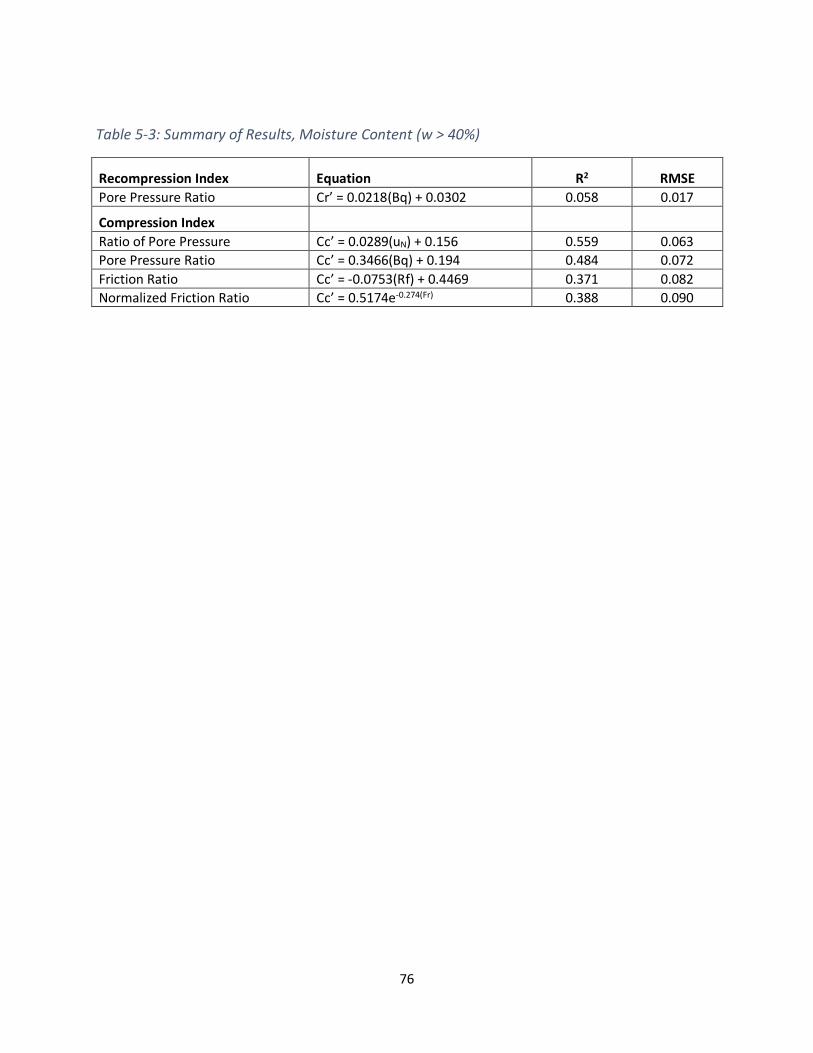
76
Table 5-3: Summary of Results, Moisture Content (w > 40%)
Recompression Index Equation R2 RMSE
Pore Pressure Ratio Cr’ = 0.0218(Bq) + 0.0302 0.058 0.017
Compression Index
Ratio of Pore Pressure Cc’ = 0.0289(uN) + 0.156 0.559 0.063
Pore Pressure Ratio Cc’ = 0.3466(Bq) + 0.194 0.484 0.072
Friction Ratio Cc’ = -0.0753(Rf) + 0.4469 0.371 0.082
Normalized Friction Ratio Cc’ = 0.5174e-0.274(Fr) 0.388 0.090
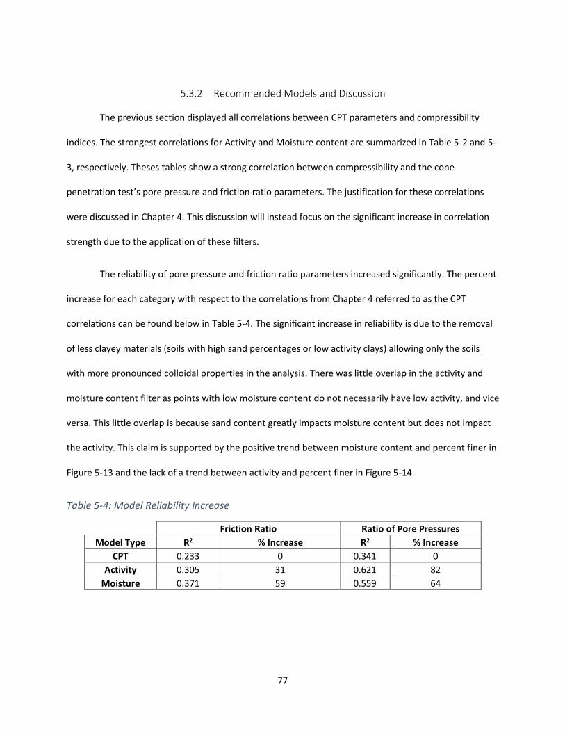
77
5.3.2 Recommended Models and Discussion
The previous section displayed all correlations between CPT parameters and compressibility
indices. The strongest correlations for Activity and Moisture content are summarized in Table 5-2 and 5-
3, respectively. Theses tables show a strong correlation between compressibility and the cone
penetration test’s pore pressure and friction ratio parameters. The justification for these correlations
were discussed in Chapter 4. This discussion will instead focus on the significant increase in correlation
strength due to the application of these filters.
The reliability of pore pressure and friction ratio parameters increased significantly. The percent
increase for each category with respect to the correlations from Chapter 4 referred to as the CPT
correlations can be found below in Table 5-4. The significant increase in reliability is due to the removal
of less clayey materials (soils with high sand percentages or low activity clays) allowing only the soils
with more pronounced colloidal properties in the analysis. There was little overlap in the activity and
moisture content filter as points with low moisture content do not necessarily have low activity, and vice
versa. This little overlap is because sand content greatly impacts moisture content but does not impact
the activity. This claim is supported by the positive trend between moisture content and percent finer in
Figure 5-13 and the lack of a trend between activity and percent finer in Figure 5-14.
Table 5-4: Model Reliability Increase
Friction Ratio Ratio of Pore Pressures
Model Type R2 % Increase R2 % Increase
CPT 0.233 0 0.341 0
Activity 0.305 31 0.621 82
Moisture 0.371 59 0.559 64
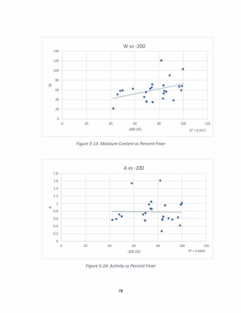
78
Figure 5-13: Moisture Content vs Percent Finer
Figure 5-14: Activity vs Percent Finer
R² = 0.1671
0
20
40
60
80
100
120
140
0 20 40 60 80 100 120
W
-200 (%)
W vs -200
R² = 0.0004
0
0.2
0.4
0.6
0.8
1
1.2
1.4
1.6
1.8
0 20 40 60 80 100 120
A
-200 (%)
A vs -200
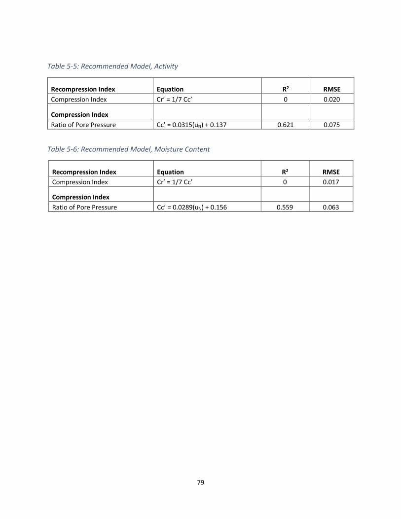
79
Table 5-5: Recommended Model, Activity
Recompression Index Equation R2 RMSE
Compression Index Cr’ = 1/7 Cc’ 0 0.020
Compression Index
Ratio of Pore Pressure Cc’ = 0.0315(uN) + 0.137 0.621 0.075
Table 5-6: Recommended Model, Moisture Content
Recompression Index Equation R2 RMSE
Compression Index Cr’ = 1/7 Cc’ 0 0.017
Compression Index
Ratio of Pore Pressure Cc’ = 0.0289(uN) + 0.156 0.559 0.063
80
5.4 Conclusion
The findings of this chapter indicate that the CPT should be utilized to estimate virgin
compressibility of fine-grained soils with pronounced colloidal properties. Tables 5-5 and 5-6 summarize
the recommended models for high activity and high moisture content soils, respectively. These tables
show improved models to compression index, as well as a refined ratio to estimate recompression
index. It should be noted that only an activity and moisture content filter was applied, however, it is
likely that any index property filter would increase the CPT model’s reliability.
This study expanded upon chapter 4 to show that the CPT test can estimate compressibility.
These findings should demonstrate the proper methodology and analysis required to relate the CPT to
compressibility, however, a larger data base is required to recommend a model for use in practice.
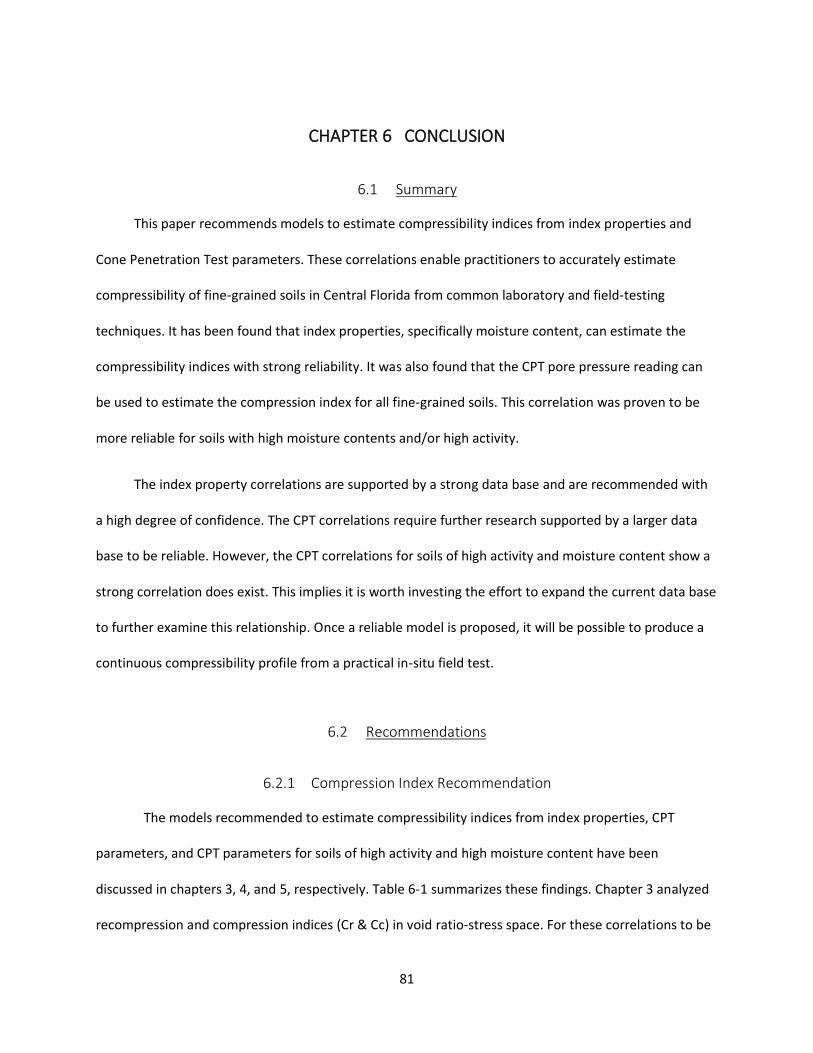
81
CHAPTER 6 CONCLUSION
6.1 Summary
This paper recommends models to estimate compressibility indices from index properties and
Cone Penetration Test parameters. These correlations enable practitioners to accurately estimate
compressibility of fine-grained soils in Central Florida from common laboratory and field-testing
techniques. It has been found that index properties, specifically moisture content, can estimate the
compressibility indices with strong reliability. It was also found that the CPT pore pressure reading can
be used to estimate the compression index for all fine-grained soils. This correlation was proven to be
more reliable for soils with high moisture contents and/or high activity.
The index property correlations are supported by a strong data base and are recommended with
a high degree of confidence. The CPT correlations require further research supported by a larger data
base to be reliable. However, the CPT correlations for soils of high activity and moisture content show a
strong correlation does exist. This implies it is worth investing the effort to expand the current data base
to further examine this relationship. Once a reliable model is proposed, it will be possible to produce a
continuous compressibility profile from a practical in-situ field test.
6.2 Recommendations
6.2.1 Compression Index Recommendation
The models recommended to estimate compressibility indices from index properties, CPT
parameters, and CPT parameters for soils of high activity and high moisture content have been
discussed in chapters 3, 4, and 5, respectively. Table 6-1 summarizes these findings. Chapter 3 analyzed
recompression and compression indices (Cr & Cc) in void ratio-stress space. For these correlations to be
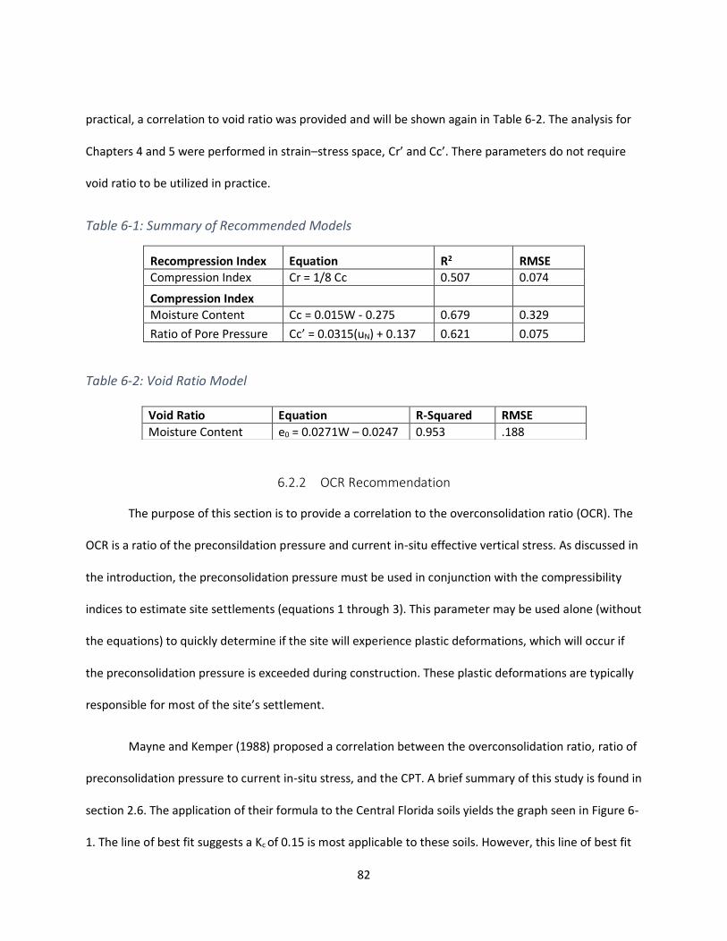
82
practical, a correlation to void ratio was provided and will be shown again in Table 6-2. The analysis for
Chapters 4 and 5 were performed in strain–stress space, Cr’ and Cc’. There parameters do not require
void ratio to be utilized in practice.
Table 6-1: Summary of Recommended Models
Recompression Index Equation R2 RMSE Compression Index Cr = 1/8 Cc 0.507 0.074
Compression Index Moisture Content Cc = 0.015W - 0.275 0.679 0.329
Ratio of Pore Pressure Cc’ = 0.0315(uN) + 0.137 0.621 0.075
Table 6-2: Void Ratio Model
6.2.2 OCR Recommendation
The purpose of this section is to provide a correlation to the overconsolidation ratio (OCR). The
OCR is a ratio of the preconsildation pressure and current in-situ effective vertical stress. As discussed in
the introduction, the preconsolidation pressure must be used in conjunction with the compressibility
indices to estimate site settlements (equations 1 through 3). This parameter may be used alone (without
the equations) to quickly determine if the site will experience plastic deformations, which will occur if
the preconsolidation pressure is exceeded during construction. These plastic deformations are typically
responsible for most of the site’s settlement.
Mayne and Kemper (1988) proposed a correlation between the overconsolidation ratio, ratio of
preconsolidation pressure to current in-situ stress, and the CPT. A brief summary of this study is found in
section 2.6. The application of their formula to the Central Florida soils yields the graph seen in Figure 6-
1. The line of best fit suggests a Kc of 0.15 is most applicable to these soils. However, this line of best fit
Void Ratio Equation R-Squared RMSE
Moisture Content e0 = 0.0271W – 0.0247 0.953 .188
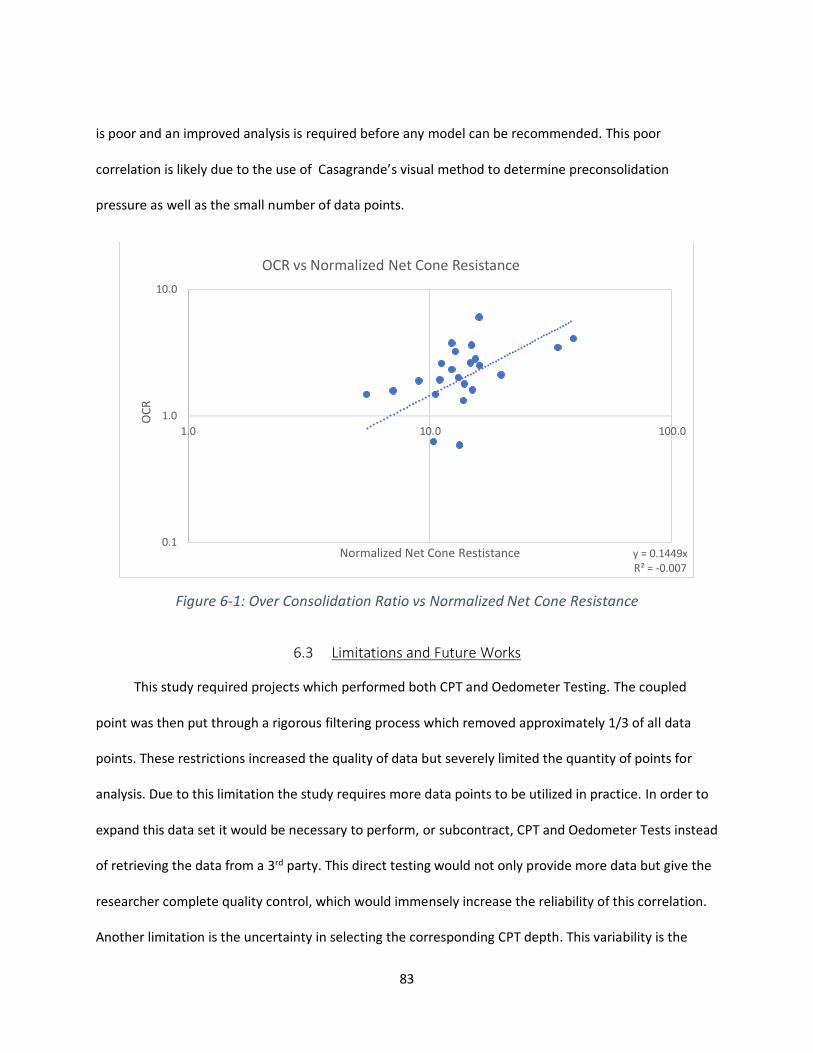
83
is poor and an improved analysis is required before any model can be recommended. This poor
correlation is likely due to the use of Casagrande’s visual method to determine preconsolidation
pressure as well as the small number of data points.
Figure 6-1: Over Consolidation Ratio vs Normalized Net Cone Resistance
6.3 Limitations and Future Works
This study required projects which performed both CPT and Oedometer Testing. The coupled
point was then put through a rigorous filtering process which removed approximately 1/3 of all data
points. These restrictions increased the quality of data but severely limited the quantity of points for
analysis. Due to this limitation the study requires more data points to be utilized in practice. In order to
expand this data set it would be necessary to perform, or subcontract, CPT and Oedometer Tests instead
of retrieving the data from a 3rd party. This direct testing would not only provide more data but give the
researcher complete quality control, which would immensely increase the reliability of this correlation.
Another limitation is the uncertainty in selecting the corresponding CPT depth. This variability is the
y = 0.1449xR² = -0.007
0.1
1.0
10.0
1.0 10.0 100.0
OC
R
Normalized Net Cone Restistance
OCR vs Normalized Net Cone Resistance

84
nature of soil and some uncertainty will always remain; however, it could be minimized by directly
overseeing the CPT and Oedometer Testing.
Once a stronger data base is provided, the analysis could improve as well. This would consist of
strengthening the current correlations to compressibility indices, as well as performing a similar trial and
error regression analysis for the Preconsolidation Pressure (σc’). The coefficient of consolidation (Cv) is
utilized to estimate the rate of consolidation. This design consideration is equally important as the
estimation of the magnitude of consolidation. However, this parameter can be directly measured from
the CPT dissipation test. The dissipation test is common, relatively inexpensive, reliable, and relatively
time efficient. For this reason, the scope of the future works will remain focused on the magnitude of
consolidation.
This report provides a strong correlation between recompression and compression indices and
moisture content. The moisture content is the most ideal index property to correlate to as the test is
cost and time effective, and there is minimal room for error. The report also provides a strong
correlation between CPT pore pressure and compression index. This suggest the CPT can be used to
create continuous and repeatable soil compressibility profiles. Future works will consist of improving the
CPT correlations to compressibility indices and preconsolidation pressure.

85
APPENDIX A – INDEX PROPERTY CORRELATIONS
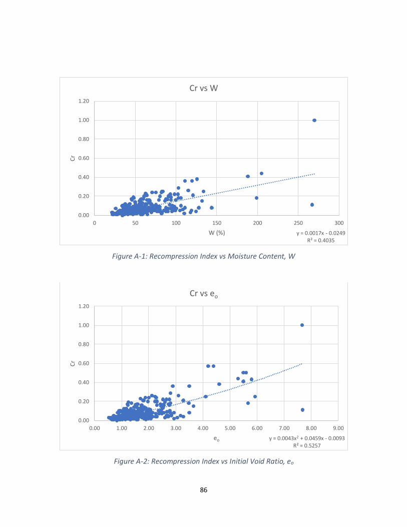
86
Figure A-1: Recompression Index vs Moisture Content, W
Figure A-2: Recompression Index vs Initial Void Ratio, eo
y = 0.0017x - 0.0249R² = 0.4035
0.00
0.20
0.40
0.60
0.80
1.00
1.20
0 50 100 150 200 250 300
Cr
W (%)
Cr vs W
y = 0.0043x2 + 0.0459x - 0.0093R² = 0.5257
0.00
0.20
0.40
0.60
0.80
1.00
1.20
0.00 1.00 2.00 3.00 4.00 5.00 6.00 7.00 8.00 9.00
Cr
eo
Cr vs eo
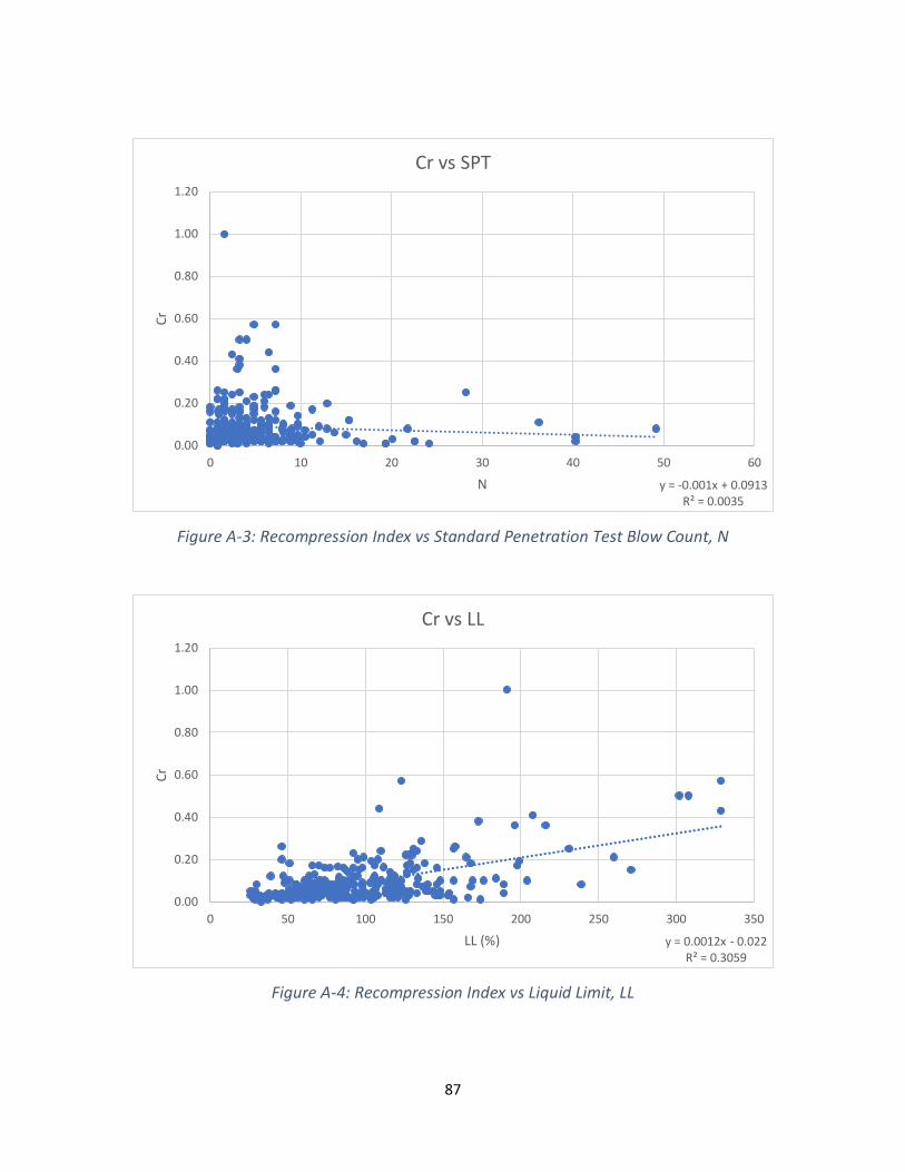
87
Figure A-3: Recompression Index vs Standard Penetration Test Blow Count, N
Figure A-4: Recompression Index vs Liquid Limit, LL
y = -0.001x + 0.0913R² = 0.0035
0.00
0.20
0.40
0.60
0.80
1.00
1.20
0 10 20 30 40 50 60
Cr
N
Cr vs SPT
y = 0.0012x - 0.022R² = 0.3059
0.00
0.20
0.40
0.60
0.80
1.00
1.20
0 50 100 150 200 250 300 350
Cr
LL (%)
Cr vs LL
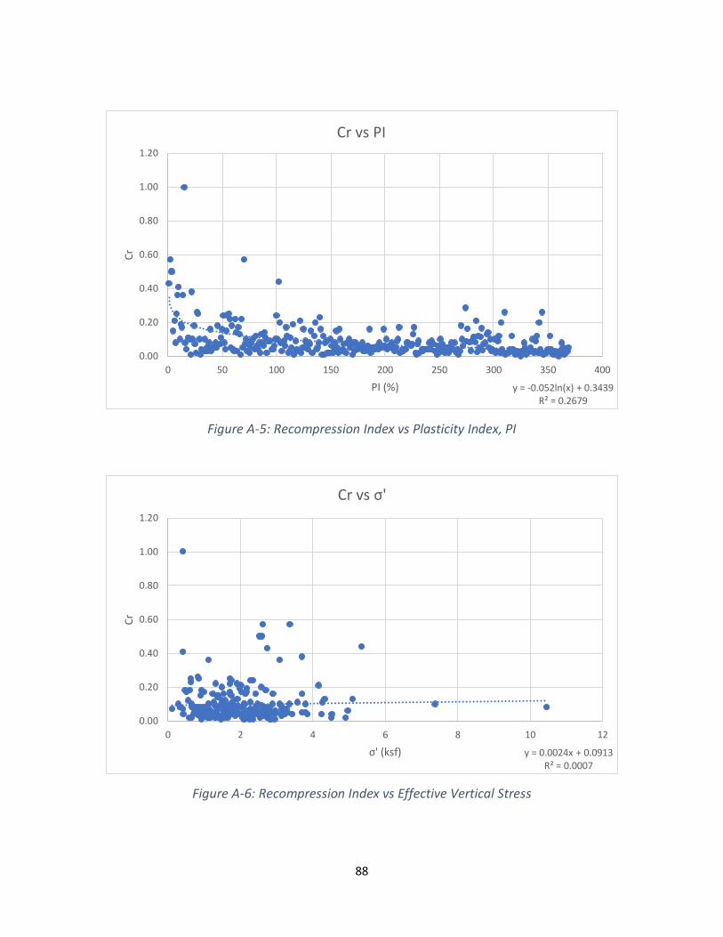
88
Figure A-5: Recompression Index vs Plasticity Index, PI
Figure A-6: Recompression Index vs Effective Vertical Stress
y = -0.052ln(x) + 0.3439R² = 0.2679
0.00
0.20
0.40
0.60
0.80
1.00
1.20
0 50 100 150 200 250 300 350 400
Cr
PI (%)
Cr vs PI
y = 0.0024x + 0.0913R² = 0.0007
0.00
0.20
0.40
0.60
0.80
1.00
1.20
0 2 4 6 8 10 12
Cr
σ' (ksf)
Cr vs σ'
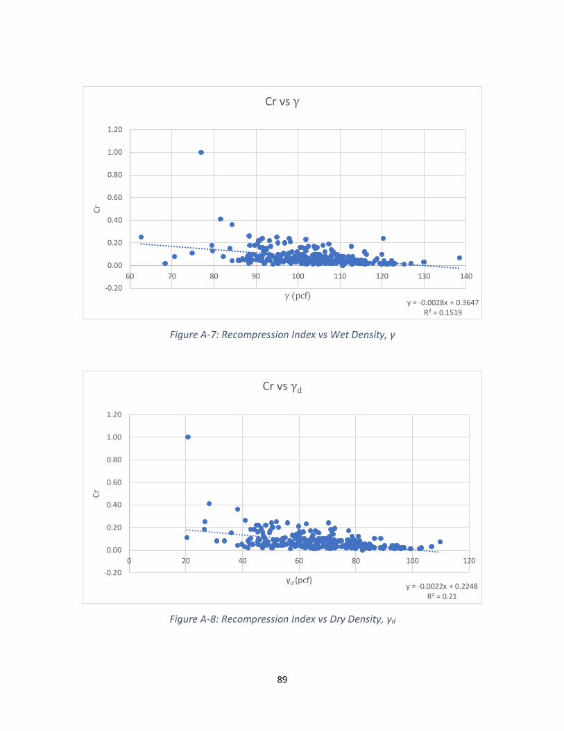
89
Figure A-7: Recompression Index vs Wet Density, γ
Figure A-8: Recompression Index vs Dry Density, γd
y = -0.0028x + 0.3647R² = 0.1519
-0.20
0.00
0.20
0.40
0.60
0.80
1.00
1.20
60 70 80 90 100 110 120 130 140
Cr
γ (pcf)
Cr vs γ
y = -0.0022x + 0.2248R² = 0.21
-0.20
0.00
0.20
0.40
0.60
0.80
1.00
1.20
0 20 40 60 80 100 120
Cr
γd (pcf)
Cr vs γd
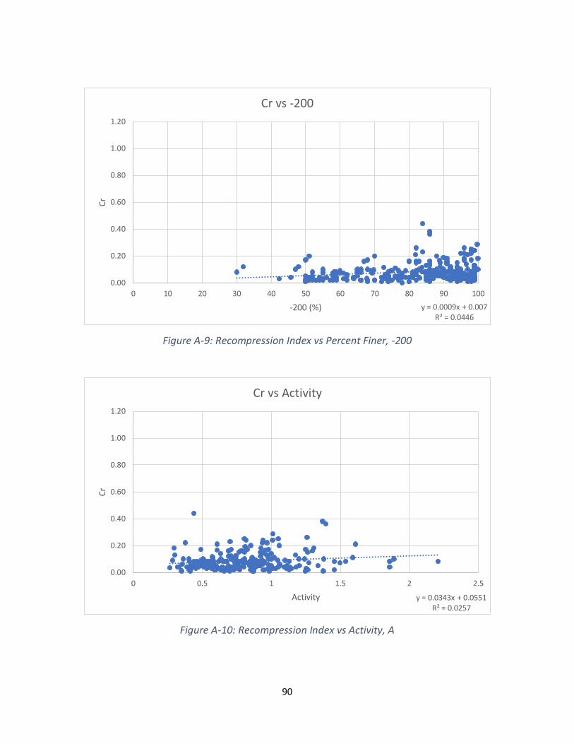
90
Figure A-9: Recompression Index vs Percent Finer, -200
Figure A-10: Recompression Index vs Activity, A
y = 0.0009x + 0.007R² = 0.0446
0.00
0.20
0.40
0.60
0.80
1.00
1.20
0 10 20 30 40 50 60 70 80 90 100
Cr
-200 (%)
Cr vs -200
y = 0.0343x + 0.0551R² = 0.0257
0.00
0.20
0.40
0.60
0.80
1.00
1.20
0 0.5 1 1.5 2 2.5
Cr
Activity
Cr vs Activity
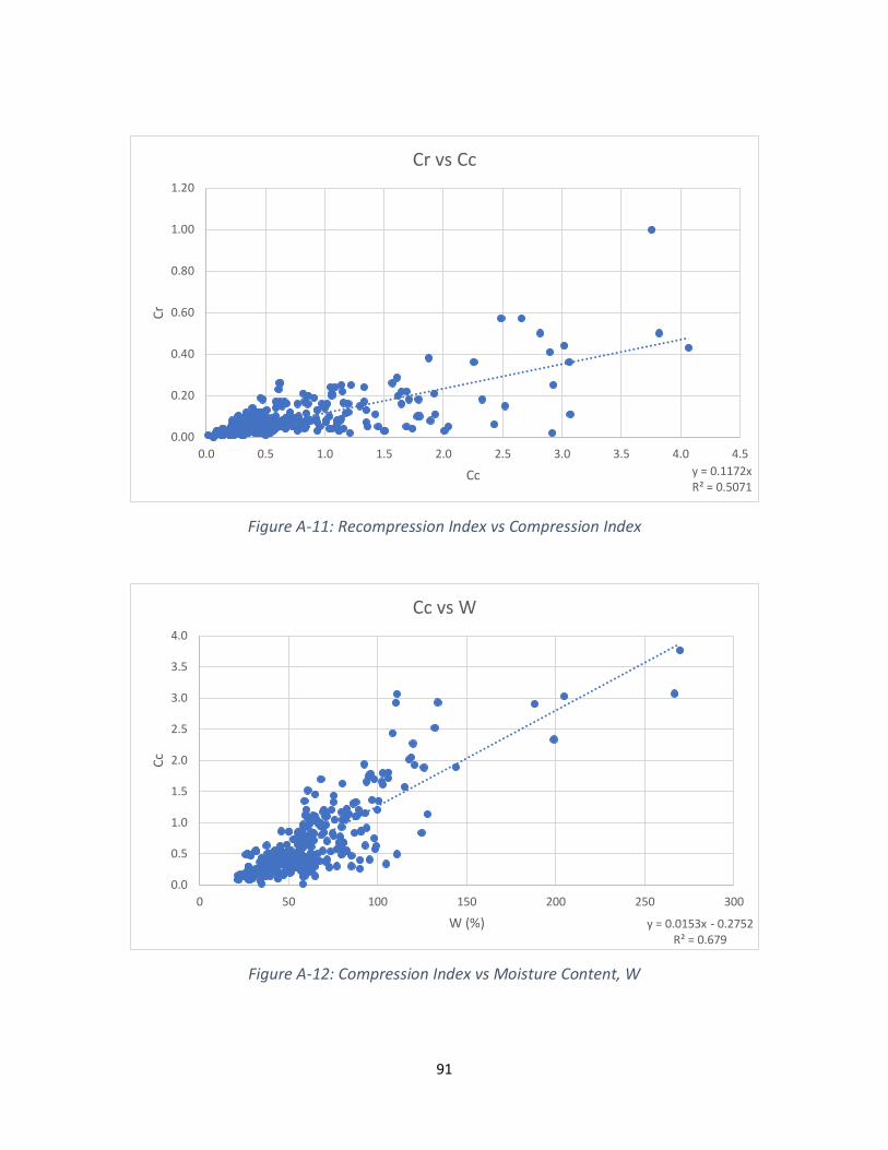
91
Figure A-11: Recompression Index vs Compression Index
Figure A-12: Compression Index vs Moisture Content, W
y = 0.1172xR² = 0.5071
0.00
0.20
0.40
0.60
0.80
1.00
1.20
0.0 0.5 1.0 1.5 2.0 2.5 3.0 3.5 4.0 4.5
Cr
Cc
Cr vs Cc
y = 0.0153x - 0.2752R² = 0.679
0.0
0.5
1.0
1.5
2.0
2.5
3.0
3.5
4.0
0 50 100 150 200 250 300
Cc
W (%)
Cc vs W
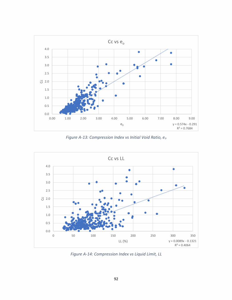
92
Figure A-13: Compression Index vs Initial Void Ratio, eo
Figure A-14: Compression Index vs Liquid Limit, LL
y = 0.574x - 0.291R² = 0.7684
0.0
0.5
1.0
1.5
2.0
2.5
3.0
3.5
4.0
0.00 1.00 2.00 3.00 4.00 5.00 6.00 7.00 8.00 9.00
Cc
e0
Cc vs eo
y = 0.0089x - 0.1321R² = 0.4064
0.0
0.5
1.0
1.5
2.0
2.5
3.0
3.5
4.0
0 50 100 150 200 250 300 350
Cc
LL (%)
Cc vs LL
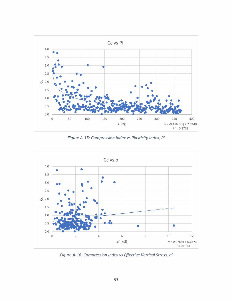
93
Figure A-15: Compression Index vs Plasticity Index, PI
Figure A-16: Compression Index vs Effective Vertical Stress, σ'
y = -0.416ln(x) + 2.7448R² = 0.3762
0.0
0.5
1.0
1.5
2.0
2.5
3.0
3.5
4.0
0 50 100 150 200 250 300 350 400
Cc
PI (%)
Cc vs PI
y = 0.0783x + 0.6373R² = 0.0161
0.0
0.5
1.0
1.5
2.0
2.5
3.0
3.5
4.0
0 2 4 6 8 10 12
Cc
σ' (ksf)
Cc vs σ'
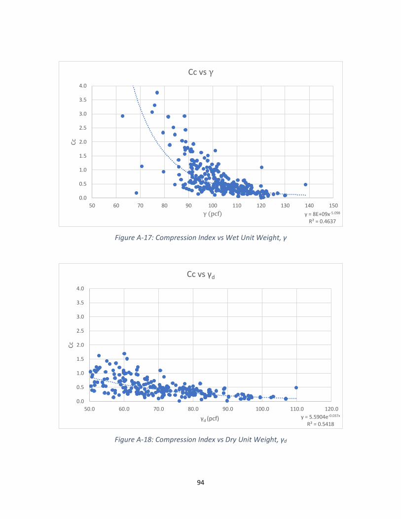
94
Figure A-17: Compression Index vs Wet Unit Weight, γ
Figure A-18: Compression Index vs Dry Unit Weight, γd
y = 8E+09x-5.098
R² = 0.4637
0.0
0.5
1.0
1.5
2.0
2.5
3.0
3.5
4.0
50 60 70 80 90 100 110 120 130 140 150
Cc
γ (pcf)
Cc vs γ
y = 5.5904e-0.037x
R² = 0.5418
0.0
0.5
1.0
1.5
2.0
2.5
3.0
3.5
4.0
50.0 60.0 70.0 80.0 90.0 100.0 110.0 120.0
Cc
γd (pcf)
Cc vs γd
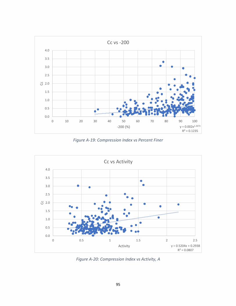
95
Figure A-19: Compression Index vs Percent Finer
Figure A-20: Compression Index vs Activity, A
y = 0.002x1.2673
R² = 0.1235
0.0
0.5
1.0
1.5
2.0
2.5
3.0
3.5
4.0
0 10 20 30 40 50 60 70 80 90 100
Cc
-200 (%)
Cc vs -200
y = 0.5204x + 0.2938R² = 0.0807
0.0
0.5
1.0
1.5
2.0
2.5
3.0
3.5
4.0
0 0.5 1 1.5 2 2.5
Cc
Activity
Cc vs Activity

96
APPENDIX B – CONE PENETRATION TEST BASED CORRELATIONS (UNDIVIDED)

97
Figure B-1: Recompression Index vs Tip Resistance, qc
Figure B-2: Recompression Index vs Corrected Tip Resistance, qt
y = -0.0003x + 0.0397R² = 0.0083
0.00
0.01
0.02
0.03
0.04
0.05
0.06
0.07
0.08
0.0 5.0 10.0 15.0 20.0 25.0 30.0 35.0
Cr'
qc
Cr' vs qc
y = -0.0003x + 0.0401R² = 0.007
0.00
0.01
0.02
0.03
0.04
0.05
0.06
0.07
0.08
0.0 5.0 10.0 15.0 20.0 25.0 30.0 35.0
Cr'
qt
Cr' vs qt
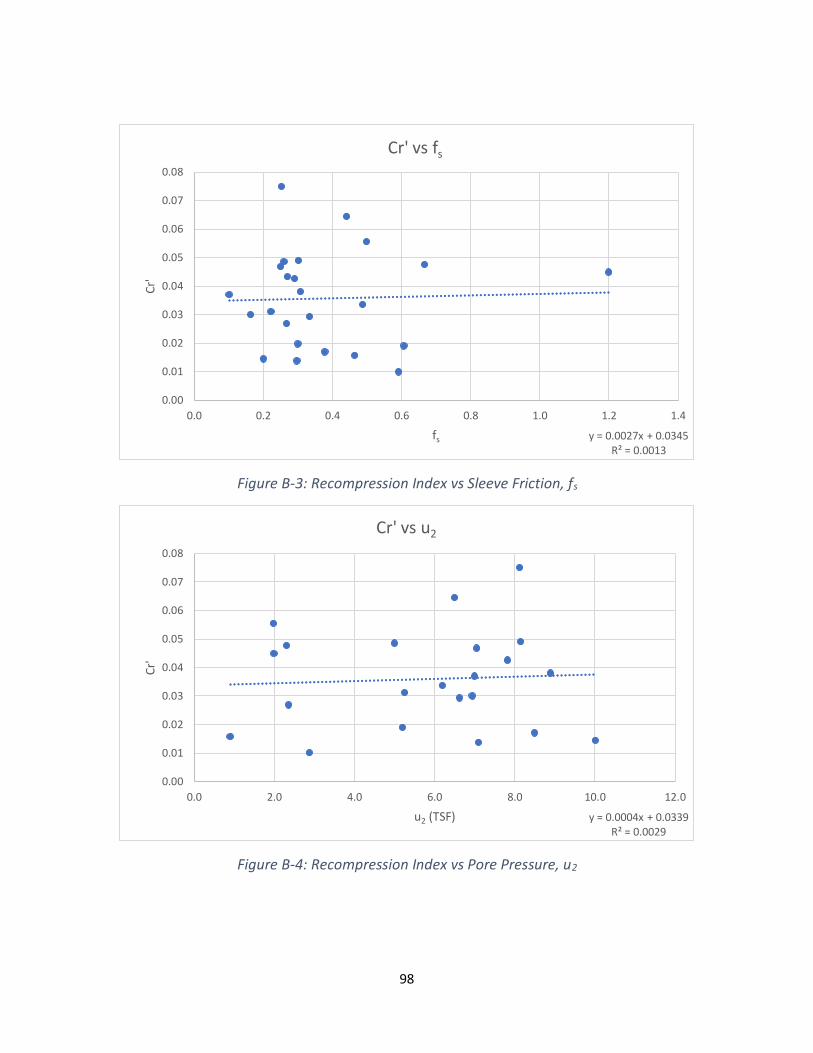
98
Figure B-3: Recompression Index vs Sleeve Friction, fs
Figure B-4: Recompression Index vs Pore Pressure, u2
y = 0.0027x + 0.0345R² = 0.0013
0.00
0.01
0.02
0.03
0.04
0.05
0.06
0.07
0.08
0.0 0.2 0.4 0.6 0.8 1.0 1.2 1.4
Cr'
fs
Cr' vs fs
y = 0.0004x + 0.0339R² = 0.0029
0.00
0.01
0.02
0.03
0.04
0.05
0.06
0.07
0.08
0.0 2.0 4.0 6.0 8.0 10.0 12.0
Cr'
u2 (TSF)
Cr' vs u2
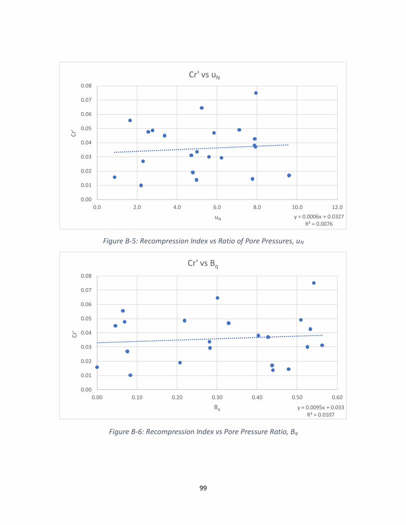
99
Figure B-5: Recompression Index vs Ratio of Pore Pressures, uN
Figure B-6: Recompression Index vs Pore Pressure Ratio, Bq
y = 0.0006x + 0.0327R² = 0.0076
0.00
0.01
0.02
0.03
0.04
0.05
0.06
0.07
0.08
0.0 2.0 4.0 6.0 8.0 10.0 12.0
Cr'
uN
Cr' vs uN
y = 0.0095x + 0.033R² = 0.0107
0.00
0.01
0.02
0.03
0.04
0.05
0.06
0.07
0.08
0.00 0.10 0.20 0.30 0.40 0.50 0.60
Cr'
Bq
Cr' vs Bq
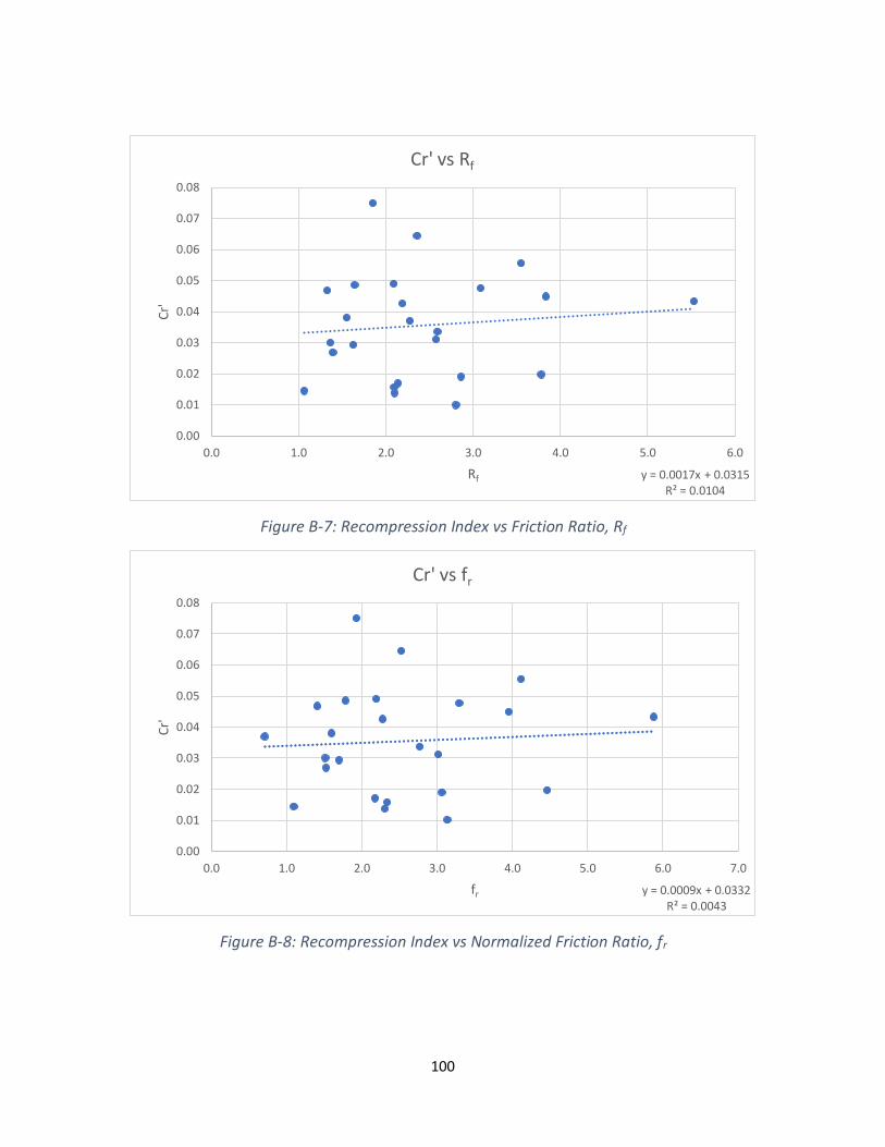
100
Figure B-7: Recompression Index vs Friction Ratio, Rf
Figure B-8: Recompression Index vs Normalized Friction Ratio, fr
y = 0.0017x + 0.0315R² = 0.0104
0.00
0.01
0.02
0.03
0.04
0.05
0.06
0.07
0.08
0.0 1.0 2.0 3.0 4.0 5.0 6.0
Cr'
Rf
Cr' vs Rf
y = 0.0009x + 0.0332R² = 0.0043
0.00
0.01
0.02
0.03
0.04
0.05
0.06
0.07
0.08
0.0 1.0 2.0 3.0 4.0 5.0 6.0 7.0
Cr'
fr
Cr' vs fr
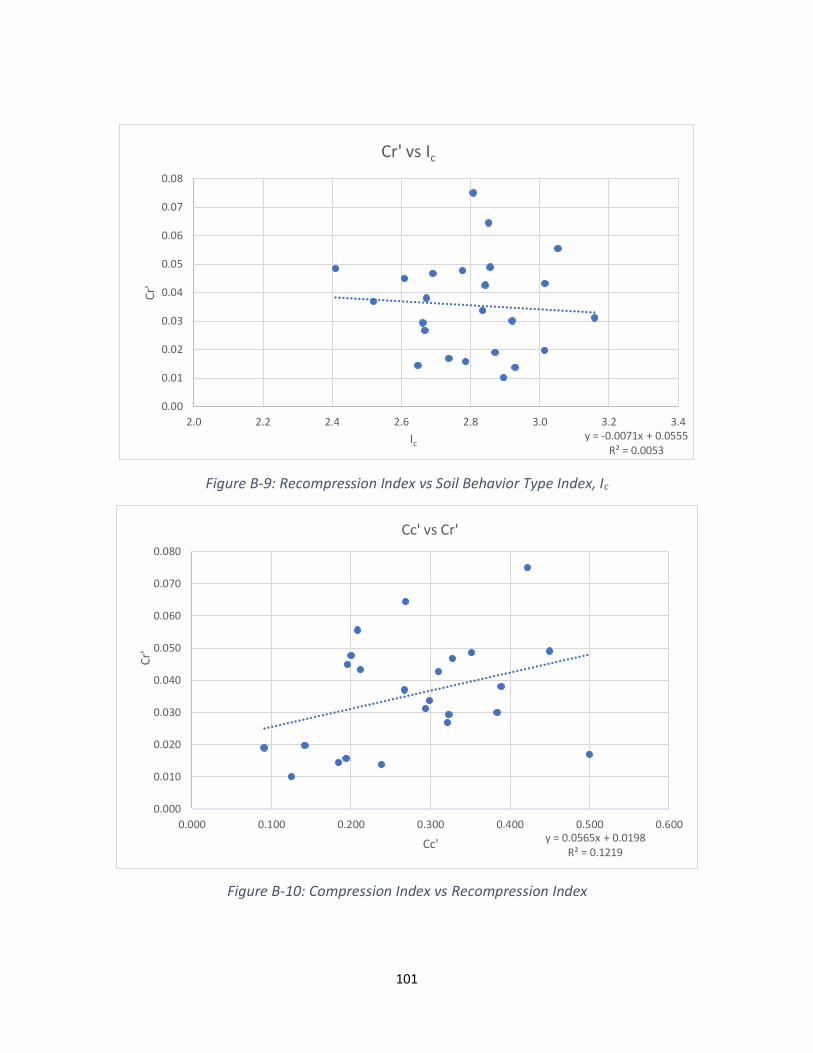
101
Figure B-9: Recompression Index vs Soil Behavior Type Index, Ic
Figure B-10: Compression Index vs Recompression Index
y = -0.0071x + 0.0555R² = 0.0053
0.00
0.01
0.02
0.03
0.04
0.05
0.06
0.07
0.08
2.0 2.2 2.4 2.6 2.8 3.0 3.2 3.4
Cr'
Ic
Cr' vs Ic
y = 0.0565x + 0.0198R² = 0.1219
0.000
0.010
0.020
0.030
0.040
0.050
0.060
0.070
0.080
0.000 0.100 0.200 0.300 0.400 0.500 0.600
Cr'
Cc'
Cc' vs Cr'
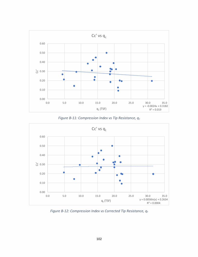
102
Figure B-11: Compression Index vs Tip Resistance, qc
Figure B-12: Compression Index vs Corrected Tip Resistance, qt
y = -0.0024x + 0.3182R² = 0.019
0.00
0.10
0.20
0.30
0.40
0.50
0.60
0.0 5.0 10.0 15.0 20.0 25.0 30.0 35.0
Cc'
qc (TSF)
Cc' vs qc
y = 0.0056ln(x) + 0.2634R² = 0.0004
0.00
0.10
0.20
0.30
0.40
0.50
0.60
0.0 5.0 10.0 15.0 20.0 25.0 30.0 35.0
Cc'
qt (TSF)
Cc' vs qt
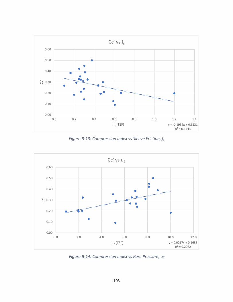
103
Figure B-13: Compression Index vs Sleeve Friction, fs
Figure B-14: Compression Index vs Pore Pressure, u2
y = -0.1936x + 0.3531R² = 0.1743
0.00
0.10
0.20
0.30
0.40
0.50
0.60
0.0 0.2 0.4 0.6 0.8 1.0 1.2 1.4
Cc'
fs (TSF)
Cc' vs fs
y = 0.0217x + 0.1635R² = 0.2972
0.00
0.10
0.20
0.30
0.40
0.50
0.60
0.0 2.0 4.0 6.0 8.0 10.0 12.0
Cc'
u2 (TSF)
Cc' vs u2
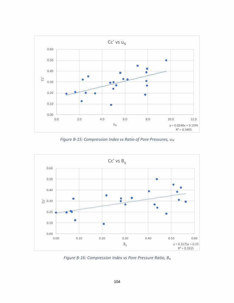
104
Figure B-15: Compression Index vs Ratio of Pore Pressures, uN
Figure B-16: Compression Index vs Pore Pressure Ratio, Bq
y = 0.0248x + 0.1595R² = 0.3405
0.00
0.10
0.20
0.30
0.40
0.50
0.60
0.0 2.0 4.0 6.0 8.0 10.0 12.0
Cc'
uN
Cc' vs uN
y = 0.3175x + 0.19R² = 0.3315
0.00
0.10
0.20
0.30
0.40
0.50
0.60
0.00 0.10 0.20 0.30 0.40 0.50 0.60
Cc'
Bq
Cc' vs Bq
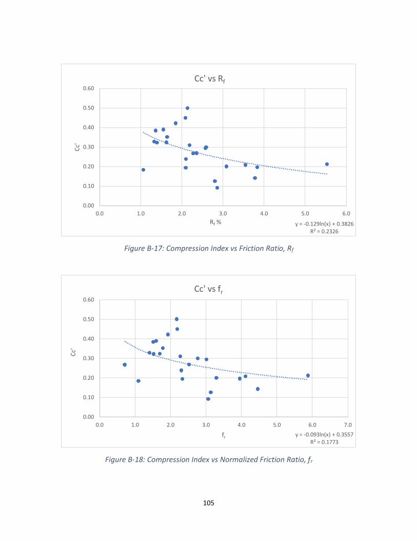
105
Figure B-17: Compression Index vs Friction Ratio, Rf
Figure B-18: Compression Index vs Normalized Friction Ratio, fr
y = -0.129ln(x) + 0.3826R² = 0.2326
0.00
0.10
0.20
0.30
0.40
0.50
0.60
0.0 1.0 2.0 3.0 4.0 5.0 6.0
Cc'
Rf %
Cc' vs Rf
y = -0.093ln(x) + 0.3557R² = 0.1773
0.00
0.10
0.20
0.30
0.40
0.50
0.60
0.0 1.0 2.0 3.0 4.0 5.0 6.0 7.0
Cc'
fr
Cc' vs fr
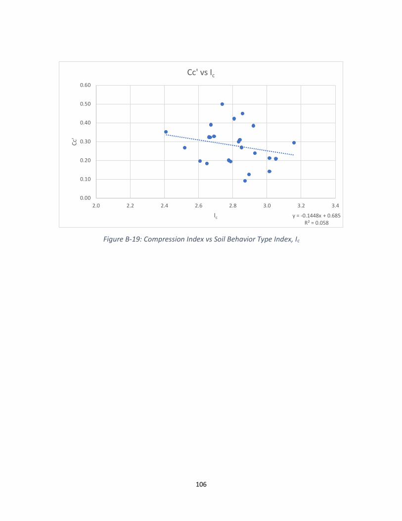
106
Figure B-19: Compression Index vs Soil Behavior Type Index, Ic
y = -0.1448x + 0.685R² = 0.058
0.00
0.10
0.20
0.30
0.40
0.50
0.60
2.0 2.2 2.4 2.6 2.8 3.0 3.2 3.4
Cc'
Ic
Cc' vs Ic
107
APPENDIX C - CONE PENETRATION TEST BASED CORRELATIONS (DIVIDED)
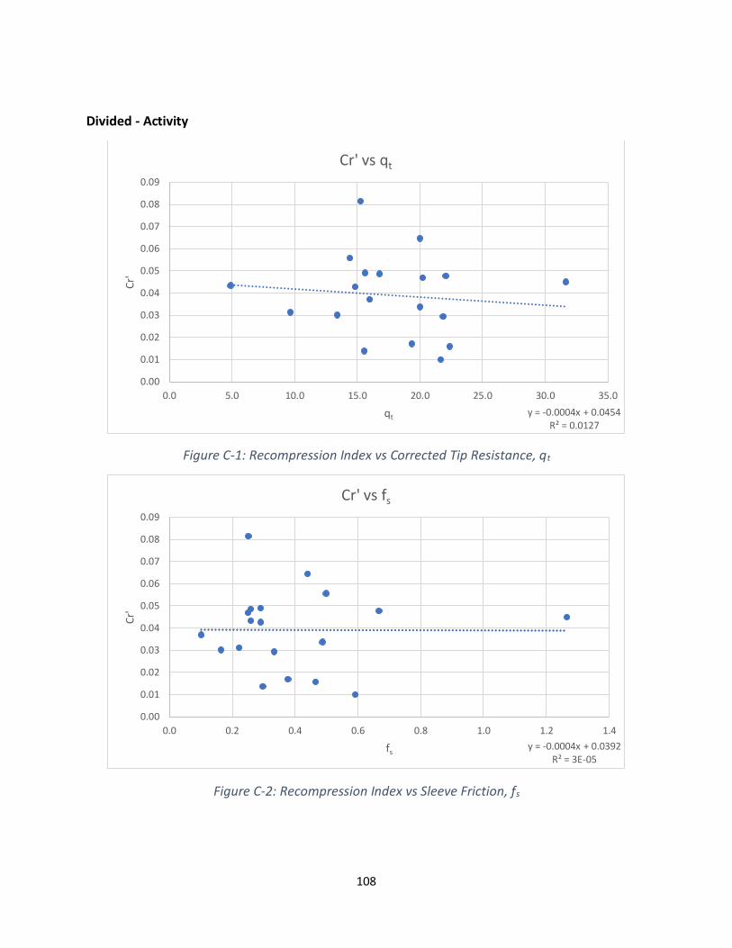
108
Divided - Activity
Figure C-1: Recompression Index vs Corrected Tip Resistance, qt
Figure C-2: Recompression Index vs Sleeve Friction, fs
y = -0.0004x + 0.0454R² = 0.0127
0.00
0.01
0.02
0.03
0.04
0.05
0.06
0.07
0.08
0.09
0.0 5.0 10.0 15.0 20.0 25.0 30.0 35.0
Cr'
qt
Cr' vs qt
y = -0.0004x + 0.0392R² = 3E-05
0.00
0.01
0.02
0.03
0.04
0.05
0.06
0.07
0.08
0.09
0.0 0.2 0.4 0.6 0.8 1.0 1.2 1.4
Cr'
fs
Cr' vs fs

109
Figure C-3: Recompression Index vs Ratio of Pore Pressures, uN
Figure C-4: Recompression Index vs Pore Pressure Ratio, Bq
y = 0.0011x + 0.0331R² = 0.0223
0.00
0.01
0.02
0.03
0.04
0.05
0.06
0.07
0.08
0.09
0.0 2.0 4.0 6.0 8.0 10.0 12.0
Cr'
uN
Cr' vs uN
y = 0.0092x + 0.0363R² = 0.0106
0.00
0.01
0.02
0.03
0.04
0.05
0.06
0.07
0.08
0.09
-0.10 0.00 0.10 0.20 0.30 0.40 0.50 0.60
Cr'
Bq
Cr' vs Bq

110
Figure C-5: Recompression Index vs Friction Ratio, Rf
Figure C-6: Recompression Index vs Normalized Friction Ratio, fr
y = 0.0013x + 0.0361R² = 0.006
0.00
0.01
0.02
0.03
0.04
0.05
0.06
0.07
0.08
0.09
0.0 1.0 2.0 3.0 4.0 5.0 6.0
Cr'
Rf
Cr' vs Rf
y = 0.0011x + 0.0362R² = 0.0048
0.00
0.01
0.02
0.03
0.04
0.05
0.06
0.07
0.08
0.09
0.0 1.0 2.0 3.0 4.0 5.0 6.0
Cr'
fr
Cr' vs fr
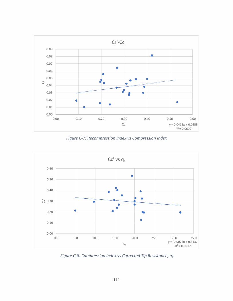
111
Figure C-7: Recompression Index vs Compression Index
Figure C-8: Compression Index vs Corrected Tip Resistance, qt
y = 0.0416x + 0.0255R² = 0.0609
0.00
0.01
0.02
0.03
0.04
0.05
0.06
0.07
0.08
0.09
0.00 0.10 0.20 0.30 0.40 0.50 0.60
Cr'
Cc'
Cr'-Cc'
y = -0.0026x + 0.3437R² = 0.0217
0.00
0.10
0.20
0.30
0.40
0.50
0.60
0.0 5.0 10.0 15.0 20.0 25.0 30.0 35.0
Cc'
qt
Cc' vs qt
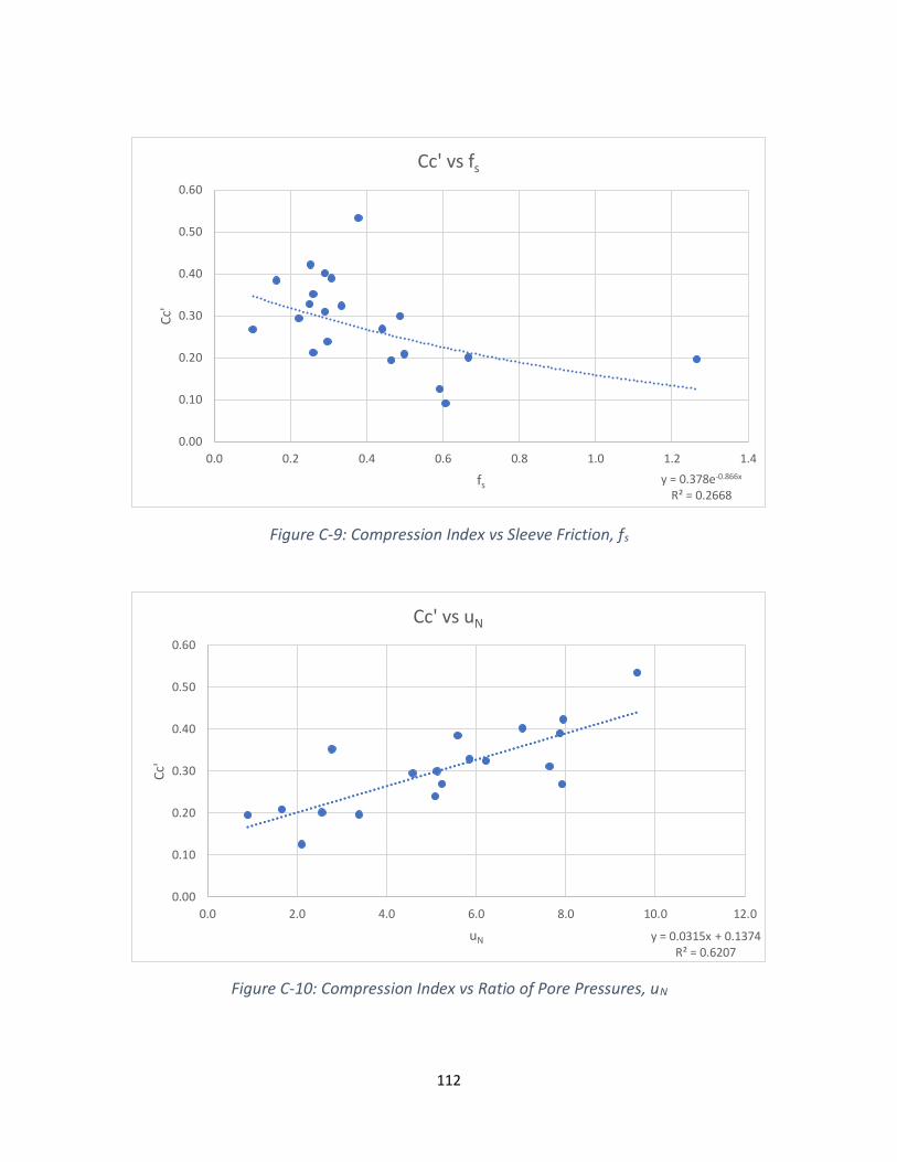
112
Figure C-9: Compression Index vs Sleeve Friction, fs
Figure C-10: Compression Index vs Ratio of Pore Pressures, uN
y = 0.378e-0.866x
R² = 0.2668
0.00
0.10
0.20
0.30
0.40
0.50
0.60
0.0 0.2 0.4 0.6 0.8 1.0 1.2 1.4
Cc'
fs
Cc' vs fs
y = 0.0315x + 0.1374R² = 0.6207
0.00
0.10
0.20
0.30
0.40
0.50
0.60
0.0 2.0 4.0 6.0 8.0 10.0 12.0
Cc'
uN
Cc' vs uN
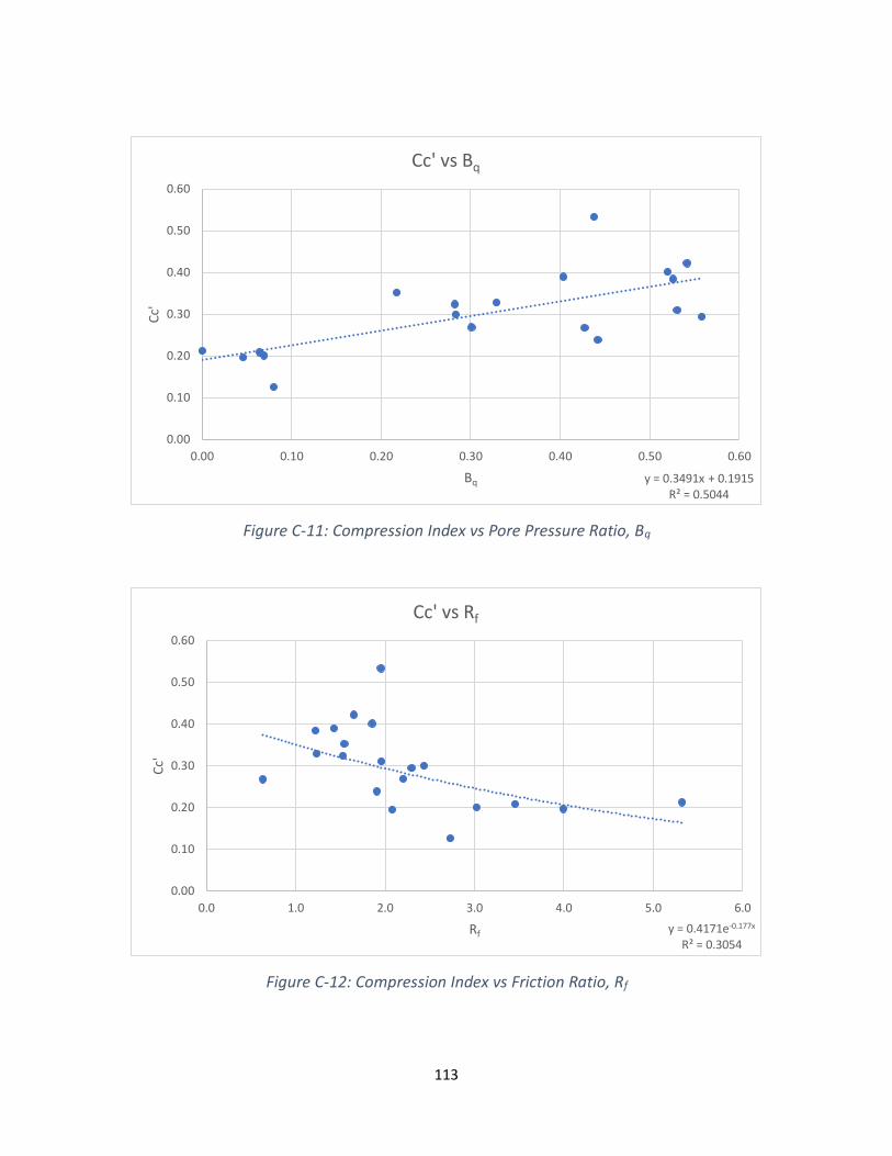
113
Figure C-11: Compression Index vs Pore Pressure Ratio, Bq
Figure C-12: Compression Index vs Friction Ratio, Rf
y = 0.3491x + 0.1915R² = 0.5044
0.00
0.10
0.20
0.30
0.40
0.50
0.60
0.00 0.10 0.20 0.30 0.40 0.50 0.60
Cc'
Bq
Cc' vs Bq
y = 0.4171e-0.177x
R² = 0.3054
0.00
0.10
0.20
0.30
0.40
0.50
0.60
0.0 1.0 2.0 3.0 4.0 5.0 6.0
Cc'
Rf
Cc' vs Rf
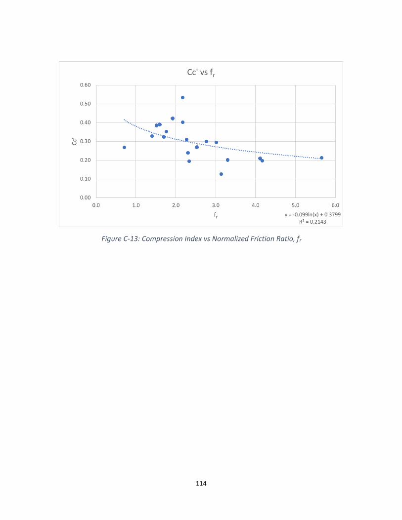
114
Figure C-13: Compression Index vs Normalized Friction Ratio, fr
y = -0.099ln(x) + 0.3799R² = 0.2143
0.00
0.10
0.20
0.30
0.40
0.50
0.60
0.0 1.0 2.0 3.0 4.0 5.0 6.0
Cc'
fr
Cc' vs fr
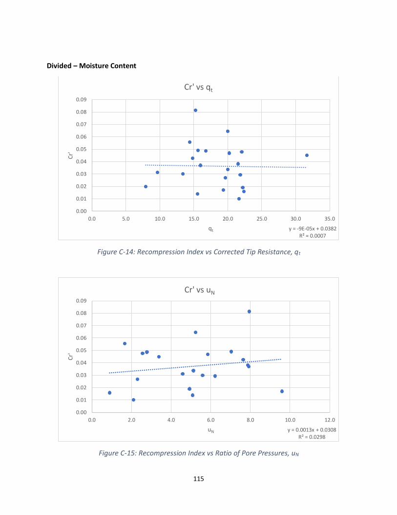
115
Divided – Moisture Content
Figure C-14: Recompression Index vs Corrected Tip Resistance, qt
Figure C-15: Recompression Index vs Ratio of Pore Pressures, uN
y = -9E-05x + 0.0382R² = 0.0007
0.00
0.01
0.02
0.03
0.04
0.05
0.06
0.07
0.08
0.09
0.0 5.0 10.0 15.0 20.0 25.0 30.0 35.0
Cr'
qt
Cr' vs qt
y = 0.0013x + 0.0308R² = 0.0298
0.00
0.01
0.02
0.03
0.04
0.05
0.06
0.07
0.08
0.09
0.0 2.0 4.0 6.0 8.0 10.0 12.0
Cr'
uN
Cr' vs uN
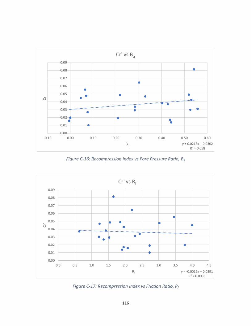
116
Figure C-16: Recompression Index vs Pore Pressure Ratio, Bq
Figure C-17: Recompression Index vs Friction Ratio, Rf
y = 0.0218x + 0.0302R² = 0.058
0.00
0.01
0.02
0.03
0.04
0.05
0.06
0.07
0.08
0.09
-0.10 0.00 0.10 0.20 0.30 0.40 0.50 0.60
Cr'
Bq
Cr' vs Bq
y = -0.0012x + 0.0391R² = 0.0036
0.00
0.01
0.02
0.03
0.04
0.05
0.06
0.07
0.08
0.09
0.0 0.5 1.0 1.5 2.0 2.5 3.0 3.5 4.0 4.5
Cr'
Rf
Cr' vs Rf
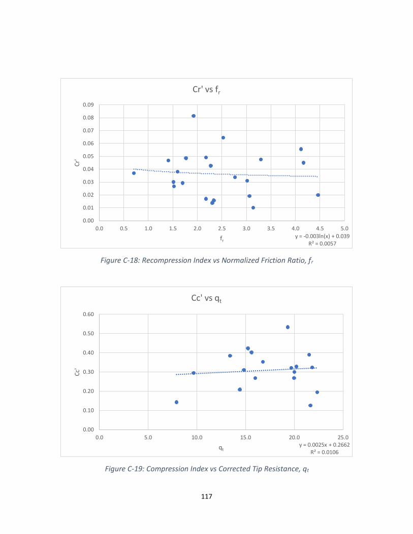
117
Figure C-18: Recompression Index vs Normalized Friction Ratio, fr
Figure C-19: Compression Index vs Corrected Tip Resistance, qt
y = -0.003ln(x) + 0.039R² = 0.0057
0.00
0.01
0.02
0.03
0.04
0.05
0.06
0.07
0.08
0.09
0.0 0.5 1.0 1.5 2.0 2.5 3.0 3.5 4.0 4.5 5.0
Cr'
fr
Cr' vs fr
y = 0.0025x + 0.2662R² = 0.0106
0.00
0.10
0.20
0.30
0.40
0.50
0.60
0.0 5.0 10.0 15.0 20.0 25.0
Cc'
qt
Cc' vs qt
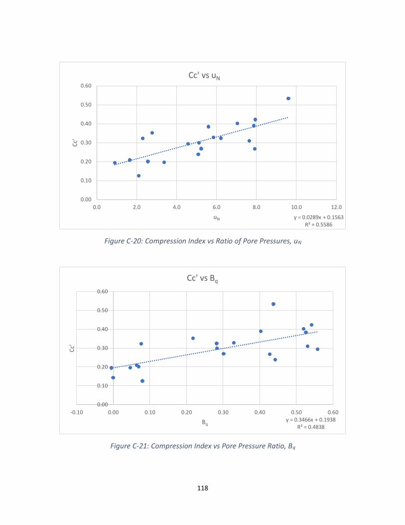
118
Figure C-20: Compression Index vs Ratio of Pore Pressures, uN
Figure C-21: Compression Index vs Pore Pressure Ratio, Bq
y = 0.0289x + 0.1563R² = 0.5586
0.00
0.10
0.20
0.30
0.40
0.50
0.60
0.0 2.0 4.0 6.0 8.0 10.0 12.0
Cc'
uN
Cc' vs uN
y = 0.3466x + 0.1938R² = 0.4838
0.00
0.10
0.20
0.30
0.40
0.50
0.60
-0.10 0.00 0.10 0.20 0.30 0.40 0.50 0.60
Cc'
Bq
Cc' vs Bq
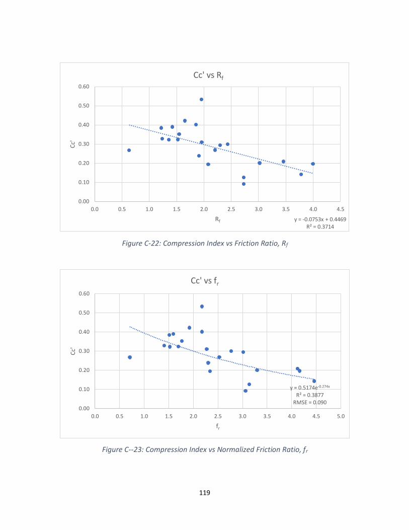
119
Figure C-22: Compression Index vs Friction Ratio, Rf
Figure C--23: Compression Index vs Normalized Friction Ratio, fr
y = -0.0753x + 0.4469R² = 0.3714
0.00
0.10
0.20
0.30
0.40
0.50
0.60
0.0 0.5 1.0 1.5 2.0 2.5 3.0 3.5 4.0 4.5
Cc'
Rf
Cc' vs Rf
y = 0.5174e-0.274x
R² = 0.3877RMSE = 0.090
0.00
0.10
0.20
0.30
0.40
0.50
0.60
0.0 0.5 1.0 1.5 2.0 2.5 3.0 3.5 4.0 4.5 5.0
Cc'
fr
Cc' vs fr

120
APPENDIX D – SNIPPET OF UCF DATA BASE
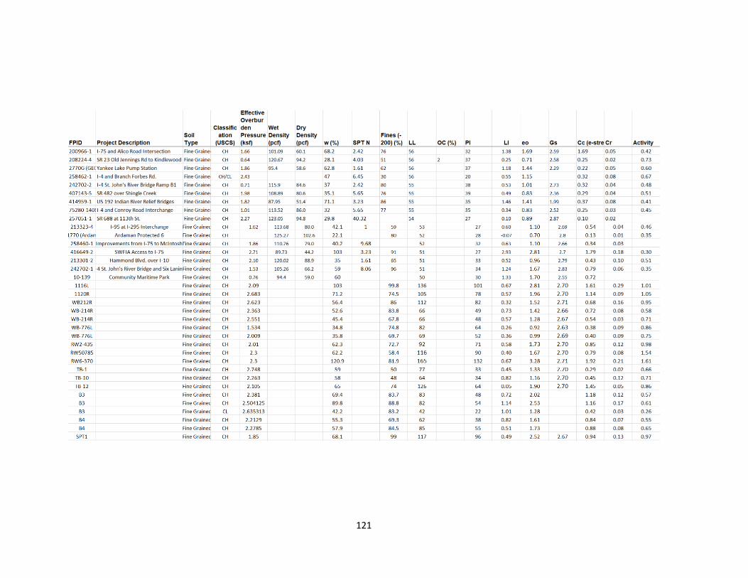
121

122
APPENDIX E – SNIPPET OF CPT DATA BASE
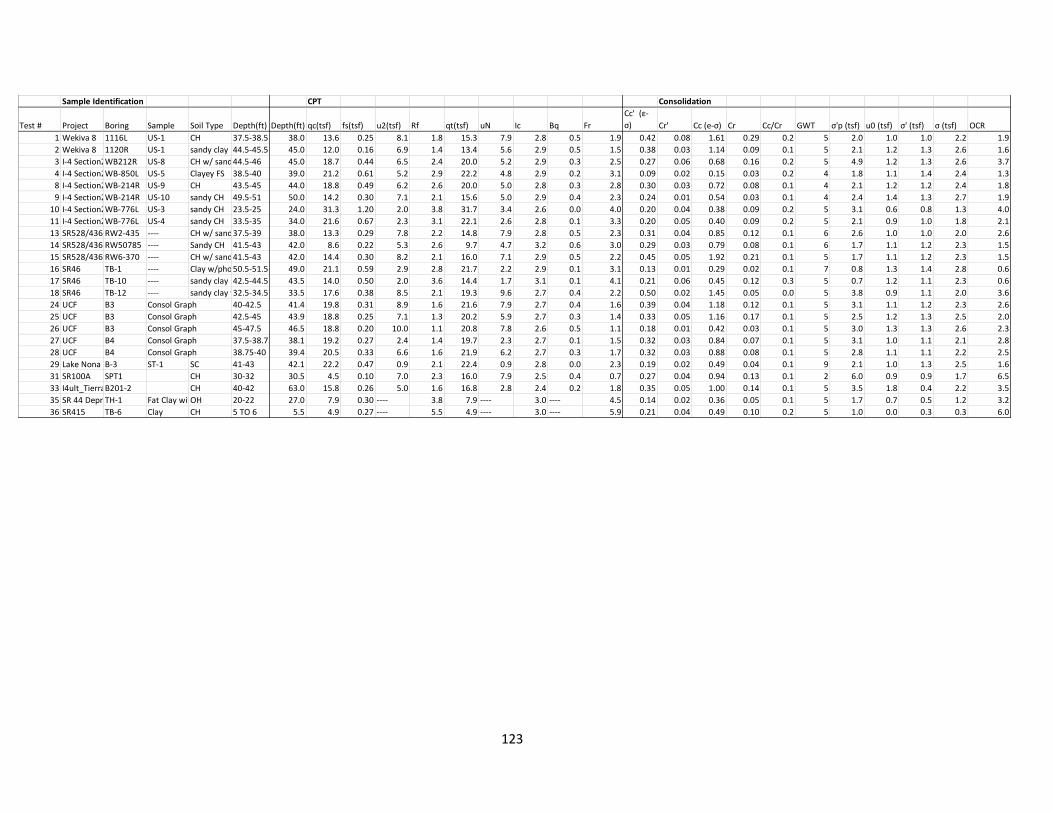
123
Sample Identification CPT Consolidation
Test # Project Boring Sample Soil Type Depth(ft) Depth(ft) qc(tsf) fs(tsf) u2(tsf) Rf qt(tsf) uN Ic Bq Fr
Cc' (ε-
σ) Cr' Cc (e-σ) Cr Cc/Cr GWT σ'p (tsf) u0 (tsf) σ' (tsf) σ (tsf) OCR
1 Wekiva 8 1116L US-1 CH 37.5-38.5 38.0 13.6 0.25 8.1 1.8 15.3 7.9 2.8 0.5 1.9 0.42 0.08 1.61 0.29 0.2 5 2.0 1.0 1.0 2.2 1.9
2 Wekiva 8 1120R US-1 sandy clay 44.5-45.5 45.0 12.0 0.16 6.9 1.4 13.4 5.6 2.9 0.5 1.5 0.38 0.03 1.14 0.09 0.1 5 2.1 1.2 1.3 2.6 1.6
3 I-4 Section2WB212R US-8 CH w/ sand44.5-46 45.0 18.7 0.44 6.5 2.4 20.0 5.2 2.9 0.3 2.5 0.27 0.06 0.68 0.16 0.2 5 4.9 1.2 1.3 2.6 3.7
4 I-4 Section2WB-850L US-5 Clayey FS 38.5-40 39.0 21.2 0.61 5.2 2.9 22.2 4.8 2.9 0.2 3.1 0.09 0.02 0.15 0.03 0.2 4 1.8 1.1 1.4 2.4 1.3
8 I-4 Section2WB-214R US-9 CH 43.5-45 44.0 18.8 0.49 6.2 2.6 20.0 5.0 2.8 0.3 2.8 0.30 0.03 0.72 0.08 0.1 4 2.1 1.2 1.2 2.4 1.8
9 I-4 Section2WB-214R US-10 sandy CH 49.5-51 50.0 14.2 0.30 7.1 2.1 15.6 5.0 2.9 0.4 2.3 0.24 0.01 0.54 0.03 0.1 4 2.4 1.4 1.3 2.7 1.9
10 I-4 Section2WB-776L US-3 sandy CH 23.5-25 24.0 31.3 1.20 2.0 3.8 31.7 3.4 2.6 0.0 4.0 0.20 0.04 0.38 0.09 0.2 5 3.1 0.6 0.8 1.3 4.0
11 I-4 Section2WB-776L US-4 sandy CH 33.5-35 34.0 21.6 0.67 2.3 3.1 22.1 2.6 2.8 0.1 3.3 0.20 0.05 0.40 0.09 0.2 5 2.1 0.9 1.0 1.8 2.1
13 SR528/436 RW2-435 ---- CH w/ sand37.5-39 38.0 13.3 0.29 7.8 2.2 14.8 7.9 2.8 0.5 2.3 0.31 0.04 0.85 0.12 0.1 6 2.6 1.0 1.0 2.0 2.6
14 SR528/436 RW50785 ---- Sandy CH 41.5-43 42.0 8.6 0.22 5.3 2.6 9.7 4.7 3.2 0.6 3.0 0.29 0.03 0.79 0.08 0.1 6 1.7 1.1 1.2 2.3 1.5
15 SR528/436 RW6-370 ---- CH w/ sand41.5-43 42.0 14.4 0.30 8.2 2.1 16.0 7.1 2.9 0.5 2.2 0.45 0.05 1.92 0.21 0.1 5 1.7 1.1 1.2 2.3 1.5
16 SR46 TB-1 ---- Clay w/phosphates50.5-51.5 49.0 21.1 0.59 2.9 2.8 21.7 2.2 2.9 0.1 3.1 0.13 0.01 0.29 0.02 0.1 7 0.8 1.3 1.4 2.8 0.6
17 SR46 TB-10 ---- sandy clay 42.5-44.5 43.5 14.0 0.50 2.0 3.6 14.4 1.7 3.1 0.1 4.1 0.21 0.06 0.45 0.12 0.3 5 0.7 1.2 1.1 2.3 0.6
18 SR46 TB-12 ---- sandy clay w/shell32.5-34.5 33.5 17.6 0.38 8.5 2.1 19.3 9.6 2.7 0.4 2.2 0.50 0.02 1.45 0.05 0.0 5 3.8 0.9 1.1 2.0 3.6
24 UCF B3 Consol Graph 40-42.5 41.4 19.8 0.31 8.9 1.6 21.6 7.9 2.7 0.4 1.6 0.39 0.04 1.18 0.12 0.1 5 3.1 1.1 1.2 2.3 2.6
25 UCF B3 Consol Graph 42.5-45 43.9 18.8 0.25 7.1 1.3 20.2 5.9 2.7 0.3 1.4 0.33 0.05 1.16 0.17 0.1 5 2.5 1.2 1.3 2.5 2.0
26 UCF B3 Consol Graph 45-47.5 46.5 18.8 0.20 10.0 1.1 20.8 7.8 2.6 0.5 1.1 0.18 0.01 0.42 0.03 0.1 5 3.0 1.3 1.3 2.6 2.3
27 UCF B4 Consol Graph 37.5-38.75 38.1 19.2 0.27 2.4 1.4 19.7 2.3 2.7 0.1 1.5 0.32 0.03 0.84 0.07 0.1 5 3.1 1.0 1.1 2.1 2.8
28 UCF B4 Consol Graph 38.75-40 39.4 20.5 0.33 6.6 1.6 21.9 6.2 2.7 0.3 1.7 0.32 0.03 0.88 0.08 0.1 5 2.8 1.1 1.1 2.2 2.5
29 Lake Nona HospitalB-3 ST-1 SC 41-43 42.1 22.2 0.47 0.9 2.1 22.4 0.9 2.8 0.0 2.3 0.19 0.02 0.49 0.04 0.1 9 2.1 1.0 1.3 2.5 1.6
31 SR100A SPT1 CH 30-32 30.5 4.5 0.10 7.0 2.3 16.0 7.9 2.5 0.4 0.7 0.27 0.04 0.94 0.13 0.1 2 6.0 0.9 0.9 1.7 6.5
33 I4ult_TierraB201-2 CH 40-42 63.0 15.8 0.26 5.0 1.6 16.8 2.8 2.4 0.2 1.8 0.35 0.05 1.00 0.14 0.1 5 3.5 1.8 0.4 2.2 3.5
35 SR 44 DepressionTH-1 Fat Clay with organicsOH 20-22 27.0 7.9 0.30 ---- 3.8 7.9 ---- 3.0 ---- 4.5 0.14 0.02 0.36 0.05 0.1 5 1.7 0.7 0.5 1.2 3.2
36 SR415 TB-6 Clay CH 5 TO 6 5.5 4.9 0.27 ---- 5.5 4.9 ---- 3.0 ---- 5.9 0.21 0.04 0.49 0.10 0.2 5 1.0 0.0 0.3 0.3 6.0
124
LIST OF REFERENCES
Bishop, C.M. (2006) Pattern recognition and machine learning. Springer, New York
Boussinesq, J., Applications des potentiels à l’étude de l’équilibre et mouvement des solides elastiques, Gauthier–Villard, Paris, 1885
Das, B. M. (2002). Principles of geotechnical engineering, Thomson Learning, Urbana, IL.
Hine, Albert C. Geology of Florida. Brooks/Cole, 2009, www.cengage.com/custom/enrichment_modules.bak/data/1426628390_Florida-LowRes_watermarked.pdf
Kirts, S., Nam, B. H., Panagopoulos, O., Xanthopoulos, P., "Settlement prediction using support vector
machine (SVM)-based compressibility models: a case study," International Journal of Civil Engineering,
Vol. 17, Issue 10, pp 1547-1557
Kirts, S., Nam, B. H., Panagopoulos, O., Xanthopoulos, P., “Soil-Compressibility Prediction Models Using Machine Learning.” Journal of Computing in Civil Engineering”
Mayne, P. W., & Kemper, J. B. (1988). Profiling OCR in stiff clays by CPT and SPT. Geotechnical Testing Journal, 11(2), 139–147.
Robertson, P. K., & Robertson, K. L. (2006). Guide to cone penetration testing and its application to geotechnical engineering. Signal Hill, CA: Gregg Drilling & Testing, Inc.
Robertson, P. K. (2009). Interpretation of cone penetration tests - a unified approach. Can. Geotechnical, 26, 1337–1352.
Sanglerat, G. (1972). The Static Penetrometer and the Prediction of Settlements. The Penetrometer and Soil Exploration, 337–405.
Skempton, A. W. “The Colloidal ‘Activity’ of Clays.” Selected Papers On Soil Mechanics, 1984.
Teh, C. I., & Houlsby, G. T. (1992). An analytical study of the cone penetration test in clay. Géotechnique, 41(1), 17–34.

![PHYSICAL AND MECHANICAL PROPERTIES OF COAL FUEL …[MPa] – fine-grained ashes, (4) [MPa] – coarse-grained ashes. (5) Fig.3 The compressibility of ashes The results are unexpected](https://img.pdfslide.net/doc/110x75/5fb01c361679ad2ae2770be5/physical-and-mechanical-properties-of-coal-fuel-mpa-a-fine-grained-ashes-4.jpg)


![Fine-Grained Classification of Product Images Based on ...For fine-grained classification, Yao [7] presented a codebook-free and annota-tion-free approach for fine-grained image categorization](https://img.pdfslide.net/doc/110x75/604cb33cad8012213a236236/fine-grained-classification-of-product-images-based-on-for-fine-grained-classification.jpg)