Compressible Boundary Layer Predictions at High Reynolds ... · NASA Langley Research Center, Hampton, VA 27695-7910 Simulations of compressible boundary layer flow at three different

American Institute of Aeronautics and Astronautics

1 of 17

Compressible Boundary Layer Predictions at High Reynolds Number using Hybrid LES/RANS Methods

Jung-Il Choi1 and Jack R. Edwards2 Department of Mechanical and Aerospace Engineering

North Carolina State University, Raleigh, NC 27695-7910

Robert A. Baurle3 Hypersonic Airbreathing Propulsion Branch

NASA Langley Research Center, Hampton, VA 27695-7910

Simulations of compressible boundary layer flow at three different Reynolds numbers (Reδ = 5.59×104, 1.78×105, and 1.58×106) are performed using a hybrid large-eddy/Reynolds-averaged Navier-Stokes method. Variations in the recycling/rescaling method, the higher-order extension, the choice of primitive variables, the RANS/LES transition parameters, and the mesh resolution are considered in order to assess the model. The results indicate that the present model can provide good predictions of the mean flow properties and second-moment statistics of the boundary layers considered. Normalized Reynolds stresses in the outer layer are found to be independent of Reynolds number, similar to incompressible turbulent boundary layers.

Nomenclature a1 = turbulence model constant A = constant in van Driest transformation Asst = turbulence model constant B = constant in van Driest transformation C = logarithmic-law wall intercept Cf = skin friction Ckleb = constant in Klebanoff intermittency function Cμ = turbulence model constant d = distance to nearest wall (m) d+ = wall coordinate based on local kinematic viscosity dw

+ = wall coordinate based on wall kinematic viscosity F = interface flux vector F2 = blending function k = turbulence kinetic energy (m/s)2 M = Mach number p = pressure (N/m2) Prt = turbulent Prandtl number q = subgrid kinetic energy Re = Reynolds number S = strain rate (1/s) T = temperature (K) u, v, w = velocity in x, y, z directions (m/s) uvd = van Driest-transformed velocity (m/s) uτ = friction velocity (m/s) V = primitive variable vector 1 Research Assistant Professor, Department of Mechanical and Aerospace Engineering, AIAA Member 2 Professor, Department of Mechanical and Aerospace Engineering, AIAA Associate Fellow 3 Aerospace Engineer, AIAA Senior Member

https://ntrs.nasa.gov/search.jsp?R=20080023891 2020-05-29T02:56:27+00:00Z


2 of 17

r = wall recovery factor t = time (s) x, y, z = streamwise, wall-normal and spanwise directions in Cartesian coordinates (m) α = model constant χ = Taylor microscale (m) δ = boundary layer thickness (m) Δ = filter width, grid size (m) η = ratio of turbulence length scales γ = ratio of specific heats Γ = blending function Γkleb = Klebanoff intermittency function κ = von Karman constant μt = eddy viscosity (kg/(m⋅ s)) ν = kinematic viscosity (m2/s) νt = kinematic eddy viscosity (m2/s) ω = turbulence frequency (1/s) Ω = vorticity magnitude (1/s) φ = turbulence model constant П = wake parameter ρ = density (kg/m3) θ = boundary layer momentum thickness (m) Subscripts ∞ = free stream o = stagnation conditions 0 = reference condition for boundary layer thickness Superscripts ΄ = fluctuations

I. Introduction ECENTLY, high-fidelity models, such as direct numerical simulation (DNS), large eddy simulation (LES), and hybrid large-eddy/Reynolds-averaged Navier-Stokes (LES/RANS) techniques, have been developed to predict

turbulent shock / boundary layer interactions.1-3 These methods have shown an ability to capture directly the unsteadiness of the interactions and to improve our understanding of the underlying physics of complicated high-speed flows. Predictions of high Reynolds-number flows still remain a challenging issue in DNS or LES due to the large computational requirements necessary to resolve near-wall turbulence. Because of their use of near-wall modeling, hybrid LES/RANS methods3-6 offer the potential to compute flows at high Reynolds number with much less expense than LES or DNS. Accurate predictions would appear to require that most of the boundary layer be computed as a large-eddy simulation, but there has been little work done in determining exactly how well the boundary layer structure is predicted using these techniques, particularly for high Reynolds numbers.

The objective of the present work is to examine the effects of various modeling and algorithmic parameters on the ability of a representative hybrid LES/RANS method3 to predict mean-flow and second-moment statistics for a selection of well-characterized compressible turbulent boundary layers. The baseline model utilizes a flow-dependent blending function to shift the closure from a RANS model (Menter’s BSL)7 near solid surfaces to a large-eddy simulation approach further away. A key to the performance of the method is the precise embedding of the RANS component of the closure within the boundary layer and the use of recycling / re-scaling techniques3,6,8-11 to sustain the development of larger turbulent structures in the outer layer. To assess the effects of different variations in the formulation, we perform parametric studies based on the flat-plate boundary layer experiment of Luker et al.12 (Reδ=1.78×105 and M ∞=2.80). These studies vary the position of the average RANS-to-LES transition, the mesh resolution, the higher-order extension, and the choice of recycling / re-scaling strategy. Finally, the model is used to simulate experiments of Elena and Lacharme13 (Reδ=5.59×104 and M ∞=2.32) and Smits and Muck14 (Reδ=1.58×106 and M ∞=2.79) in order to assess the Reynolds-number independence of the formulation. The numerical methods and physical models used in the investigation are presented in Section II. The results of the assessment of the hybrid LES/RANS model and the effects of Reynolds number on turbulent boundary layer development are discussed in Sections III and IV, respectively, and some conclusions are presented in Section V.

R


3 of 17

II. Numerical Methods The governing compressible Navier-Stokes equations are discretized in a finite-volume framework15. Inviscid

fluxes are discretized using a low-diffusion flux-splitting scheme (LDFSS)16, while viscous and diffusive fluxes are discretized using second-order central differences. A dual-time stepping implicit method is used to advance the equations in time. At each time step, a Crank-Nicholson discretization of the equations is solved to a prescribed tolerance using a sub-iteration procedure. The matrix system resulting from the linearization of the equation system is approximately solved using a planar relaxation procedure at each sub-iteration. To enhance computational efficiency, matrix elements are evaluated and factored every second time step and are held fixed over the duration of the sub-iterations.

A. Turbulence Closure The hybrid LES/RANS model used in the present study3 is based on Menter’s εω −− kk / model7 and only

involves modifications to the eddy viscosity description:

( ) ⎟⎟

⎠

⎞⎜⎜⎝

⎛Γ−+

ΩΓ== Mt

ssttt FAa

ka,

21

1 )1(,max

νω

ρρνμ (1)

As the blending function Γ approaches one, the closure approaches its RANS description, and as it approaches zero, a subgrid eddy viscosity is obtained. This work uses a mixed-scale model17 for the subgrid eddy viscosity, defined as

06.0,)( 2/34/122/1, =Δ= MMMt CqSCν and

21

2~

32~~~~

⎥⎥⎦

⎤

⎢⎢⎣

⎡⎟⎟⎠

⎞⎜⎜⎝

⎛∂∂

−∂∂

∂∂

+∂∂

∂∂

=i

i

j

i

j

i

i

j

j

i

xu

xu

xu

xu

xuS (2)

An estimate of the subgrid kinetic energy is obtained by test-filtering the resolved-scale velocity data:

22 )~~(21

kk uuq −= (3)

The blending function Γ is based on the ratio of the wall distance d to a modeled form of the Taylor micro-scale:

⎟⎟

⎠

⎞

⎜⎜

⎝

⎛+−−=Γ ))1(5tanh[1

21 2 φηκ

μC and

αχη d

= (4)

where φ is set to )98.0(tanh 1− in order to fix the balancing position (where μκη C=2 ) to Γ = 0.99, and the

Taylor micro-scale is defined as ωνχ μC= . The constant α is chosen to enforce the average LES to RANS transition ( Γ = 0.99 position) for equilibrium boundary layers at the point where the wake law starts to deviate from the log law. To determine α for a particular inflow boundary layer, the following procedure is used.3 First, a prediction of the equilibrium boundary layer is obtained, given free-stream properties, a specified wall condition (adiabatic or isothermal) and a value for the boundary layer thickness, from Coles’ Law of the Wall / Wake along with the van Driest transformation:

)2

(sin2)ln(1 2

δπ

κκτ

dCduu

wvd Π

++= + , w

w

dudν

τ=+ (5)

with

,4

sin4

/2sin22

1

22

21

⎪⎭

⎪⎬⎫

⎪⎩

⎪⎨⎧

⎥⎦

⎤⎢⎣

⎡

++⎥

⎦

⎤⎢⎣

⎡

+

−= −∞−∞

ABB

ABBuuA

Auuvd (6)

,Pr2

)1( 2

wt T

TMA ∞∞

−=

γ 12

)1(Pr1 22/1 −⎥⎦⎤

⎢⎣⎡ −

+= ∞∞

wt T

TMB γ

An initial estimate for the outer extent of the log layer is defined by finding the value of +wd such that

98.0/)ln(1=⎟⎟

⎠

⎞⎜⎜⎝

⎛⎟⎠⎞

⎜⎝⎛ ++

τκ uuCd vd

w . (7)

The value of ντ /dud =+ that corresponds to this value of +wd is then found through the use of Walz’s formula for

the static temperature distribution within the boundary layer:


4 of 17

2

2

2)1()(

⎟⎟⎠

⎞⎜⎜⎝

⎛−−

−+=

∞

∞

∞∞∞∞ uuMr

uu

TTT

TT

TT waww γ (8)

The model constant is then found by the equivalence 2α=+d , which arises from the use of inner-layer scaling arguments for k andω . It should be noted that this approach is not universal, as the wake law is not universal. In this investigation, we use a spatially-varying form of the model constant )(xαα = by applying the above procedure to the boundary-layer thickness distribution as determined by a RANS simulation. B. Interface Flux Reconstruction We consider two methods for extending the baseline first-order upwind method16 to higher order in this study. The baseline scheme is the piecewise parabolic method (PPM)18, which reduces to a fourth-order approximation to the interface flux:

),( 2/1,2/1,2/12/1 ++++ = iRiLii VVFFrr

, (9) with

)(121)(

127

1212/1,2/1, −++++ +−+== iiiiiRiL VVVVVVrrrrrr

(10)

if the data is sufficiently smooth. The PPM enforces local monotonicity by resetting left-and right-state values if local extrema are detected. Specifically, the following limiting procedure is performed:

ifendifend

23then)(elseif

23then)(if

)]([6 C

else

then,1)])(( sgn[ if

2/1,2/1,

2/1,2/1,

2/1,2/1,21

2/1,2/1,

2/1,2/1,

2/1,2/1,

−+

+−

−+

−+

−+

−+

−=>−

−=>

+−=

−=

==

−=−−

iRiiL

iLiiR

iRiLi

iRiL

iiRiL

iRiiiL

VVVDCCC

VVVCCDC

VVVDVV

VVVVVVV

rrr

rrr

rrr

rr

rrr

rrrr

(11)

The first ‘if’ block in Eq. (11) resets the interpolation function to a constant if iVr

is a local maximum or minimum. The second ‘if’ block in Eq. (11) resets either the left-state value at interface 2/1+i or the right-state value at interface 2/1−i so that the interpolation parabola that connects the interface states with the state at the cell center is monotonically increasing or decreasing. It is also possible to enforce physical constraints (such as positive pressures and densities) at the cell interfaces by a similar cell-by-cell resetting algorithm. We also test the use of 5th order upwind-biased interpolations as a replacement for Eq. (10):

32112/1,

21122/1,

602

6013

6047

6027

603

603

6027

6047

6013

602

+++−+

++−−+

+−++−=

−++−=

iiiiiiR

iiiiiiL

VVVVVV

VVVVVVrrrrrr

rrrrrr

(12)

We also consider different choices for the variable vector used in the reconstruction: TkTwvuV ],,,,,,[ ωρ=r

and TkTwvupV ],,,,,,[ ω=

r In the discussion that follows, the use of the first set of variables will be denoted as

SCHEME(ρ,T) (SCHEME being PPM4 or PPM5), while the second is denoted as SCHEME(p,T). The PPM requires a seven point stencil in each coordinate direction for both the 4th and 5th order variants.

C. Inflow Generation Methods A key element of the hybrid LES/RANS formulation is the use of recycling/rescaling techniques to initiate and

sustain grid-resolved turbulent structures in the outer part of the boundary layer. Among recycling / rescaling techniques recently proposed in the literature for compressible flows,3,6,8-11 we consider three variants in the present study. In the first method, the recycled and rescaled velocity, temperature, and density fluctuations are imposed onto the RANS mean inflow.3,6 The density fluctuations are adjusted so that a specified rms value (2% in this work)


5 of 17

for the pressure fluctuations is maintained, and the temperature fluctuations are also scaled so that Morkovin’s hypothesis is not violated.3 In the second method, we separately recycle and rescale the mean and fluctuating velocity and temperature fields. The density field is obtained by enforcing a constant-pressure condition at the inflow.8 In the third approach, recycled and rescaled mean and fluctuating density fields are also imposed as inflow conditions without assuming that the pressure remains constant.9

The current technique also includes an intermittency function for preventing recycled fluctuations from affecting the free-stream regions and in some cases, from accumulating too much energy in the outer part of the boundary layer. In this, recycled and rescaled fluctuations are multiplied by a Klebanoff-type intermittency function19:

16 ))(1()( −+=Γ inklebkleb Cdd δ (13) where klebC is a model constant and inδ is the inflow boundary layer thickness, before being added to the mean profile. Our baseline value for klebC is 1.1; other choices for klebC are considered in the present study. Turbulence variables ( Γ,,ωk ) are recycled and rescaled without decomposing them into mean and fluctuating components.3

D. Computational Details Three different high Reynolds number flows developing on flat plates are considered in the present study. For

each case, the boundary layer properties corresponding to the reference experiments are shown in Table 1. The Reynolds numbers (based on the boundary layer thickness) range from 5.59×104 to 1.58×106. The incoming Mach number ranges from 2.32 to 2.80. Mean-flow and second-moment data for these boundary layers have been reported in Ref. 12-14, 20 and 21. Based on the thickness ( 0δ ) of the boundary layer at the measurement station, the sizes of the computational domain are 010δ , 05δ , and 04.6 δ in streamwise, wall-normal and spanwise directions, respectively. The baseline meshes are generated so that approximately 20 uniformly-spaced cells per incoming boundary layer thickness are present in the streamwise and spanwise directions, and each mesh contains 200128200 ×× cells (5.12 million) in the streamwise, spanwise, and wall-normal directions, respectively. The grids are clustered to the surface in the wall-normal direction using a hyperbolic tangent stretching function so that the minimum grid spacing in wall units is less than one.

The incoming boundary layer is generated by using the three different recycling/rescaling methods described in the previous section. The recycling station is located at 05.7 δ downstream of the inlet. Supersonic outflow boundary conditions are used at the far-field and outlet, while no slip boundary condition is used at the wall. A constant wall temperature of 276 K is specified for the Smits and Muck14 case, while an adiabatic wall condition is used for the other cases. Periodic boundary conditions are used in the spanwise direction. The initial condition is a RANS 2-D flat-plate solution, to which a re-scaled fluctuation field from an earlier calculation is super-imposed.3 Following a period of about 5 flow-through-times to remove initial transients, time- and span-averaged statistics are collected over a minimum of 10 flow through times ( ∞U/100 0δ ). The computational time step ranged from 0.25-0.4 μs, with the differences in time step being related to variations in the mesh sizes discussed later.

III. Assessment of the Hybrid LES/RANS Method If the LES/RANS model of Edwards et al.3 operates as designed, the outer layer will be computed as a large-

eddy simulation and will force the development of the inner layer so that a uniform boundary layer structure will emerge in the time- and span-average. The sensitivity of this response to various factors should be determined, however, in order to understand the limitations of the approach and to establish practices that consistently lead to acceptable boundary-layer predictions. For this purpose, we characterize the effect of modeling and algorithm parameters on turbulent statistics through comparisons with experimental data of Luker et al.12 Table 2 shows the numerical parameters for the cases computed as part of this assessment as well as those for the Elena and Lacharme13 and Smits and Muck14 experiments. Note that the characters L, E, and S represent the Luker et al.,12 Elena and Lacharme,13 and Smits and Muck14 experiments, respectively. Predictions at the target location are compared with mean-flow velocity profiles and Reynolds-stress measurements from the references. Reynolds shear-stress predictions are normalized by the wall shear stress at the measurement location, whereas Reynolds streamwise and wall-normal stresses are presented as rms fluctuation intensities rmsu′ and rmsv′ , which are normalized by the edge velocity. Distances from the wall are normalized by the target (experimental) boundary layer thickness so that the ability of the methods to predict the growth rate of the boundary layer can be assessed more clearly. Velocities are normalized by the predicted edge velocity.


6 of 17

A. Effect of Model Constant for LES/RANS Transition First, we focus on the effect of model constant α , which shifts the target position of the midpoint of the

LES/RANS transition region. The procedure in Section II-A, when applied to the 2-D flat plate boundary layer as predicted by the RANS model, gives a spatially-varying constant that may be regressed as a linear distribution

)/(145.0276.22)( 0δα xx += . This distribution is used as the baseline and is designated as )(0 xα . This choice is designed to force the time-averaged LES/RANS transition to occur at the point where the wake law just begins to depart from the logarithmic law. With this choice, the entire logarithmic region is heavily influenced by the RANS closure even though some turbulence structure and significant unsteadiness is still present. Another possible choice of the model constant is to use the midpoint of the logarithmic layer as the average transition location. A regression equation for the second choice is )/(036.0771.12)( 0δα xxm += . Figure 1 compares the mean velocity profile and Reynolds stresses obtained using the baseline )(0 xα distribution and the )(xmα distribution. Other modeling parameters are given in Table 2. Specifically, the 4th order PPM scheme with pressure and temperature reconstruction at the interface is used, the model constant 1.1=klebC , and the Edwards et al.3 recycling / rescaling procedure is used on the baseline grid. The predictions obtained using the baseline distribution )(0 xα are in good agreement with experimental results (Figure 1a), while the second choice )(xmα leads to an overly-energetic near wall velocity profile (Figure 1c). The Reynolds shear stresses are over-predicted in the entire boundary layer for the )(xmα distribution (Figure 1a), reaching values well in excess of the wall shear stress, but the predictions of the Reynolds normal stresses in the near wall region show slightly better agreement with experimental results when the

)(xmα distribution is used. In Figure 1a and in subsequent ones, the modeled component of the Reynolds shear stress is indicated toward the left axis ( 0/δy → 0). The modeled component decays nearly to zero through the action of the blending function (though a sub-grid component remains) and is supplanted by the resolved Reynolds stress in the outer layer. The total Reynolds stress can be estimated by summing the modeled and resolved components. The modeled components of the Reynolds normal stresses are neglected in Figure 1b and in subsequent ones. In our code, we absorb the trace of the modeled Reynolds-stress tensor into the effective pressure. The remaining normal-stress components are very small in the near-wall region when the Boussinesq hypothesis is invoked, and as such, high accuracy in normal stress predictions near the surface cannot be expected. The boundary layer thickness as indicated by the Reynolds-stress measurements is over-predicted for both cases. This example shows that a precise embedding of the RANS component of the LES/RANS model is a critical factor in achieving accurate turbulent statistics for very high Reynolds number flows.

B. Effect of Interface Flux Reconstruction Years of experience with DNS and LES methods have shown that higher-order, minimally dissipative numerical

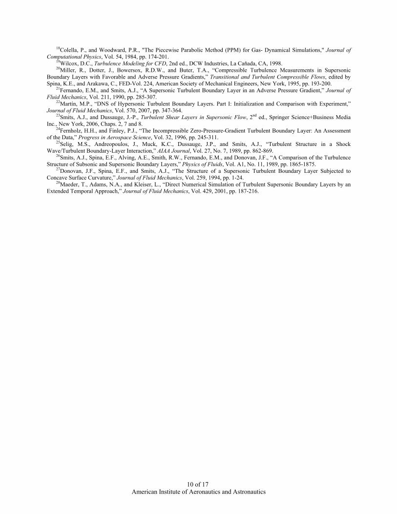
methods with high bandwidth efficiency are required to sustain turbulent eddy structures. When shocks are considered, then it becomes more difficult to meet these requirements, as they conflict with the need to maintain monotone capturing of discontinuities to avoid numerical instabilities. We consider two aspects of the reconstruction procedure in the context of the baseline PPM scheme presented in Section II B. The effects of the choice of the variable vector (PPM4(ρ,T) or PPM4(p,T)) used in the reconstruction are shown in Figure 2. Other modeling parameters are the same as those of the baseline case. The shape of the mean velocity profile is not very sensitive to this choice, while the levels of Reynolds shear and wall-normal stresses are increased significantly in the outer part of the boundary layer for the PPM4(ρ,T) reconstruction, relative to that provided by the PPM4(p,T) reconstruction. This might be explained by the following two factors. First, the interface pressure, for the PPM4 (ρ,T) reconstruction, will be obtained as a product of the interface density and temperature. The difference in the pressure gradient as calculated from this formulation and that obtained directly from the PPM4(p,T) reconstruction can be interpreted as a blend of diffusive and anti-diffusive terms, and it is possible that these additional transport mechanisms give rise to the amplification of transverse-velocity components. Another factor is that the PPM limiting procedure may act more strongly on the pressure than it does on the density and temperature. This could mean that grid-scale noise in the pressure field is damped more strongly in the PPM4 (p,T) reconstruction, leading to a suppression of similar noise in the transverse velocity components. More smaller-scale structures are captured for PPM4(ρ,T), particularly toward the outer part of the boundary layer, as shown in the tranverse-velocity magnitude snapshots of Figure 2c. The energy contained in these structures appears to be in excess of that expected, based on the comparisons with experimental data, and this behavior can lead to unphysical levels of boundary-layer growth if the spatial domain is long enough.


7 of 17

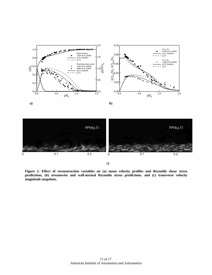
Next, we compare two different variable-extrapolation techniques, PPM4(p,T) and PPM5(p,T), for the reconstruction of the fluid properties at the interface. The PPM4 scheme can be viewed as a central-differencing scheme that is stabilized through the local use of monotonicity-preserving techniques. Such schemes may be subject to aliasing due to the non-linearity inherent in the flux functions. The fifth-order, upwind-biased extrapolations used in PPM5 should be less susceptible to aliasing effects. Figure 3 shows that there are no essential differences in the predictions of the mean velocity profile and second-moment quantities provided by PPM4(p,T) and PPM5(p,T).

C. Effect of Inflow Generation Method The effects of the three inflow generation methods described in Section II-C are described in this section. The

interface fluxes are reconstructed by PPM4(p,T), the baseline model-constant distribution )(0 xα is used, and the constant klebC in the intermittency function is set to 1.1. Figure 4 illustrates the effect of the Urbin and Knight procedure8 for rescaling the mean inflow profile as compared with the use of a RANS inflow profile3 and the Stolz and Adams procedure.9 The results indicate that rescaling the mean and fluctuating fields using the Stolz and Adams procedure9 yields slightly better predictions for the mean velocity profile, particularly in the inner region. The resolved Reynolds stresses for all cases fall within the data ranges of the experiments. In detail, some differences in Reynolds shear stresses are observed in the inner region, while no significant difference is found in the outer region. The predictions of the Reynolds normal stresses show no significant difference among the methods. All cases show that the boundary layer thickness at the target location is over-estimated, with this quantity being reduced slightly when the fixed RANS mean inflow is used. All methods result in a transition region near the inlet (extending ~ 03δ downstream)9 where the flow attempts to adjust to the imposed inflow condition through the generation of various compression / expansion waves. The growth of the boundary layer is delayed in this transition region until these waves are attenuated.

To prevent recycled fluctuations from affecting the free-stream regions, we utilize a Klebanoff-type intermittency function to damp recycled fluctuations. The extent of the intermittency function is controlled by the model constant klebC . Figure 5 shows the effect of klebC on the mean velocity profile and Reynolds-stress distributions. Increasing klebC allows more amplification of turbulent fluctuations in the outer region, leading to more growth of the boundary layer. The shapes of the profiles do not change significantly except near the outer edge of the boundary layer, where the wake region expands in accord with the increase in klebC . The choice of

1.1=klebC provides better predictions based on the experimental results. Recently, Sagaut et al.11 reported that existing inflow-generation methods cannot sustain target values for boundary-layer integral properties over long integration times, and this observation is confirmed in our work. The intermittency function appears to help maintain a target boundary layer thickness while also isolating the free-stream region from being affected by the recycling procedure.

D. Effect of Spatial Resolution The spatial resolution in the wall-transverse directions (streamwise and spanwise directions) is also expected to

influence predictions of the boundary layer structure. For the hybrid LES/RANS methods, the mesh should be generated so that the outer layer is resolved adequately. We use the Escudier mixing length (~0.1 0δ )19 as an upper bound for the mesh spacing and choose half of this value as the baseline mesh spacing ( 20/ =Δδ ). To examine the effects of mesh resolution on the predicted quantities, we consider three levels of mesh refinement (10 cells / 0δ , 20 cells / 0δ , and 30 cells / 0δ ) as shown in Table 2. Figure 6 shows that mean velocity profile and Reynolds stresses for the baseline grid simulation are in good agreement with those for the fine-grid simulation. The wall-normal Reynolds stress and the resolved Reynolds shear stress are under-predicted for the coarse-mesh simulation. The under-prediction of the resolved Reynolds shear stress is partially compensated for by an increase in the modeled Reynolds shear stress, and as such, the mean velocity profile is relatively unaffected by the mesh resolution. This result is encouraging as it indicates that acceptable results might be obtained on marginally resolved meshes for the present hybrid LES/RANS technique.

IV. Compressible Boundary Layer Flows at High Reynolds Numbers Using the baseline parameters (PPM4(p,T), klebC = 1.1, Edwards, et al. recycling / rescaling3, 20 cells / 0δ ), we apply the method to experiments13,14 conducted at Reynolds numbers lower and higher than the baseline12 to test the Reynolds-number independence of the present model and to illustrate the effect of the Reynolds number on the


8 of 17

mean turbulent flow structure. The boundary layer properties for each case are listed in Table 1 and the corresponding numerical parameters are shown in Table 2.

A. Mean Velocity and Reynolds Stress Figure 7 compares results from the hybrid LES/RANS computations with hot-wire and LDA measurements

reported in Elena and Lacharme13. The regression equation for the model constant α is extracted from a prior RANS computation: )/(100.0409.13)( 0δα xx += . The results show good agreement with the experimental data. Compared to recent DNS data of this case22, the Reynolds stresses are comparable in the outer part of boundary layer but differ near the wall due to the presence of the RANS component in the turbulence closure. Figure 8 shows mean velocity profile and Reynolds-stress predictions for the present method as applied to the Smits and Muck14 experiment. For the model constantα , a regression equation )/(356.0389.72)( 0δα xx += from the initial RANS computation is used. Good agreement with the experimental data is evidenced, though the wall-normal Reynolds stress is slightly under-predicted. The results shown in Figures 1, 7 and 8 indicate that the present hybrid LES/RANS method is able to provide a degree of Reynolds number independence in the predictions of the boundary layer structure.

Figure 9 plots van Driest transformed velocity profiles for the different Reynolds-number cases. As expected, the extent of the logarithmic layer increases with the increase in Reynolds number. Figures 10 and 11 show the effect of Reynolds number on the Reynolds stresses. The wall normal coordinate is normalized by the predicted boundary layer thickness at 05.7 δ downstream location. The peak positions of the Reynolds stresses move toward the wall as the Reynolds number increases. This might be related to the effect of the RANS closure. In the outer layer, there is no significant variation in the Reynolds-stress distributions with respect to Reynolds numbers. These results indicate that, given similar Mach numbers23, the outer-layer scaling of the turbulent statistics has no dominant dependence on Reynolds number, similar to observations in incompressible flows.24

B. Boundary Layer Properties The time-averaged skin-friction coefficient ( fC ) is determined from the averaged streamwise velocity and the

molecular viscosity computed according to Sutherland’s law using the averaged temperature.23 Figure 12 (a) shows a comparison of the present fC with several experimental results12,13,21,25-28 as a function of Reynolds number based on momentum thickness. Variations of fC in the computational domain are marked as error bars. A theoretical prediction of the skin-friction variation for incompressible flows24 is also shown in the figure. The present results are in excellent agreement with a regression (based on power law) of the experimental data. Figure 12 (b) shows the time-averaged streamwise evolution of the boundary thickness for the different Reynolds-number cases. Empirical correlations based on power-law relations for the boundary layer integral parameters23 are also shown in the figure. The growth rates of the boundary layer in the correlations are re-adjusted to the incoming boundary layer thickness used in the present simulations. The present growth rates indicate two distinct features. First, the initial growth rates for all cases are under-estimated, relative to the empirical correlations. Secondly, after a transition region of 03~ δ (discussed earlier), the boundary layer re-develops, and the corresponding growth rate maintains the empirical rates except for the case corresponding to Elena and Lacharme’s experiment.12 The predicted boundary layer thicknesses at the target location are larger than the experimental values by 1% to 6%.

V. Conclusions Simulations of compressible boundary layer flows at three different Reynolds numbers (Reδ = 5.59×104,

1.78×105, and 1.58×106) have been performed using a hybrid large-eddy/Reynolds-averaged Navier-Stokes method. The model uses a flow-dependent RANS-to-LES transition function to shift the closure from Menter’s two equation RANS model near walls to a mixed subgrid-scale model in the outer part of boundary layer. To assess the present hybrid LES/RANS model, the effects of various modeling and algorithmic parameters on the predictions of mean-flow and second moment statistics have been investigated, and the following conclusions may be stated:

1) the RANS/LES blending function should be designed to transition to LES toward the outer part of the logarithmic region for accurate predictions of the composite structure of the boundary layer and the Reynolds-shear stress levels,

2) reconstructing the interface flux from extrapolated pressure and temperature (as opposed to extrapolated density and temperature) is more effective in suppressing grid-scale noise in the transverse velocity components, and this leads to better predictions of the outer-layer turbulent structure,


9 of 17

3) the choice of variable-extrapolation method (4th order central versus 5th order upwind-biased) does not significantly influence predictions of the low-order turbulent statistics,

4) the choice of recycling / rescaling strategy for the inflow properties does not significantly affect the predictions. All result in a adjustment distance of approximately 03~ δ before the boundary layer begins to grow, and all over-estimate the target boundary layer thickness at the recycle-plane location.

5) the use of a Klebanoff-type intermittency function to attenuate fluctuations in the outer part of the boundary layer helps keep the boundary layer growth within the target range.

6) a resolution metric of 20 cells / boundary layer thickness in the wall-transverse directions yields predictions almost identical to those obtained using 30 cells / boundary layer thickness. Results obtained using only 10 cells / boundary layer thickness in the wall-transverse directions are not grossly inferior to the refined-mesh results (at least for the Reynolds number tested), indicating that acceptable predictions of the boundary layer structure might be obtained on meshes scaled according to the Escudier mixing length.

7) in general, the present hybrid LES/RANS model provides good predictions of mean-flow and second-moment boundary layer statistics and exhibits a degree of Reynolds-number independence. Reynolds stress distributions plotted using outer-layer scaling are found to be independent of Reynolds number, similar to observations in incompressible flows.

Acknowledgments This work is supported by NASA under Cooperative Agreement NNX07AC27A-S01. Computer resources have

been provided by the High Performance Computing component of North Carolina State University’s Information Technology division.

References 1Wu, M., and Martín, M.P., “Analysis of Shock Motion in Shockwave and Turbulent Boundary Layer Interaction using

Direct Numerical Simulation Data,” Journal of Fluid Mechanics, Vol. 594, 2008, pp. 71-83. 2Loginov, M.S., Adams, N.A., and Zheltovodov, A., “Large-Eddy Simulation of Shock-Wave/Turbulent-Boundary-Layer

Interaction,” Journal of Fluid Mechanics, Vol. 565, 2006, pp. 135-169. 3Edwards. J.R., Choi, J.-I., and Boles, J.A., “Hybrid LES/RANS Simulation of a Mach 5 Compression-Corner Interaction,”

AIAA Journal, Vol. 46, No. 4, 2008, pp. 977-991. 4Baurle, R.A., Tam, J., Edwards, J.R., and Hassan, H.A., “Hybrid RANS/LES Approach for Cavity Flows: Blending,

Algorithm, and Boundary Treatment Issues,” AIAA Journal, Vol. 41, No. 8, 2003, pp. 1463-1480. 5Fan, T.C., Edwards, J.R., Hassan, H.A., and Baurle, R.A., “Hybrid Large-Eddy / Reynolds-Averaged Navier-Stokes

Simulations of Shock-Separated Flows,” Journal of Spacecraft and Rockets, Vol. 41, No. 6, 2004, pp.897-906. 6Xiao, X., Edwards, J.R., Hassan, H.A., and Baurle, R.A., “Inflow Boundary Conditions for Hybrid Large-Eddy / Reynolds-

Averaged Navier-Stokes Simulations,” AIAA Journal, Vol. 41, No. 8, 2003, pp. 1481-1490. 7Menter, F.R., “Two-Equation Eddy-Viscosity Turbulence Models for Engineering Applications,” AIAA Journal, Vol. 32, No.

8, 1994, pp. 1598-1605. 8Urbin, G., and Knight, D., “Large Eddy Simulation of a Supersonic Boundary Layer using an Unstructured Grid,” AIAA

Journal, Vol. 29, No. 7, 2001, pp. 1288-1295. 9Stolz, S., and Adams, N.A., “Large-Eddy Simulation of High-Reynolds-Number Supersonic Boundary Layers using the

Approximate Deconvolution Model and a Rescaling and Recycling Technique,” Physics of Fluids, Vol. 15, No. 8, 2003, pp. 2398-2412.

10Xu, S., and Martín, M.P., “Assessment of Inflow Boundary Conditions for Compressible Turbulent Boundary Layers,” Physics of Fluids, Vol. 16, No. 7, 2004, pp. 2623-2639.

11Sagaut, P., Garnier, E., Tromeur, E., Larchevêque, L., and Labourasse, E., “Turbulent Inflow Conditions for Large-Eddy Simulation of Compressible Wall-Bounded Flows,” AIAA Journal, Vol. 42, No. 3, 2004, pp. 469-477.

12Luker, J.J., Bowersox, R.D.W., and Buter, T.A., “Influence of Curvature-Driven Favorable Pressure Gradient on Supersonic Turbulent Boundary Layer,” AIAA Journal, Vol. 38, 2000, pp. 1351-1359.

13Elena, M., and Lacharme, J.P., “Experimental Study of a Supersonic Turbulent Boundary Layer using a Laser Doppler Anemometer,” Journal of Theoretical and Applied Mechanics, Vol. 7, No. 2, 1988, pp. 175-190.

14Smits, A.J., and Muck, K.-C., “Experimental Study of Three Shock-Wave/Turbulent Boundary Layer Interactions,” Journal of Fluid Mechanics, Vol. 182, 1987, pp. 291-314.

15Roy, C.J., and Edwards, J.R., “Numerical Simulation of a Three-Dimensional Flame/Shock Wave Interaction,” AIAA Journal, Vol. 38, No. 5, 2000, pp. 745-760.

16Edwards, J.R., “A Low-Diffusion Flux-Splitting Scheme for Navier-Stokes Calculations,” Computers & Fluids, Vol. 26, No. 6, 1997, pp. 635-659.

17Lenormand, E., Sagaut, P., Ta Phuoc, L., and Comte, P., “Subgrid-Scale Models for Large-Eddy Simulations of Compressible, Wall-Bounded Flows,” AIAA Journal, Vol. 38, 2000, pp. 1340-1350.


10 of 17

18Colella, P., and Woodward, P.R., "The Piecewise Parabolic Method (PPM) for Gas- Dynamical Simulations," Journal of Computational Physics, Vol. 54, 1984, pp. 174-201.

19Wilcox, D.C., Turbulence Modeling for CFD, 2nd ed., DCW Industries, La Caňada, CA, 1998. 20Miller, R., Dotter, J., Bowersox, R.D.W., and Buter, T.A., “Compressible Turbulence Measurements in Supersonic

Boundary Layers with Favorable and Adverse Pressure Gradients,” Transitional and Turbulent Compressible Flows, edited by Spina, K.E., and Arakawa, C., FED-Vol. 224, American Society of Mechanical Engineers, New York, 1995, pp. 193-200.

21Fernando, E.M., and Smits, A.J., “A Supersonic Turbulent Boundary Layer in an Adverse Pressure Gradient,” Journal of Fluid Mechanics, Vol. 211, 1990, pp. 285-307.

22Martín, M.P., “DNS of Hypersonic Turbulent Boundary Layers. Part I: Initialization and Comparison with Experiment,” Journal of Fluid Mechanics, Vol. 570, 2007, pp. 347-364.

23Smits, A.J., and Dussauge, J.-P., Turbulent Shear Layers in Supersonic Flow, 2nd ed., Springer Science+Business Media Inc., New York, 2006, Chaps. 2, 7 and 8.

24Fernholz, H.H., and Finley, P.J., “The Incompressible Zero-Pressure-Gradient Turbulent Boundary Layer: An Assessment of the Data,” Progress in Aerospace Science, Vol. 32, 1996, pp. 245-311.

25Selig, M.S., Andreopoulos, J., Muck, K.C., Dussauge, J.P., and Smits, A.J., “Turbulent Structure in a Shock Wave/Turbulent Boundary-Layer Interaction,” AIAA Journal, Vol. 27, No. 7, 1989, pp. 862-869.

26Smits, A.J., Spina, E.F., Alving, A.E., Smith, R.W., Fernando, E.M., and Donovan, J.F., “A Comparison of the Turbulence Structure of Subsonic and Supersonic Boundary Layers,” Physics of Fluids, Vol. A1, No. 11, 1989, pp. 1865-1875.

27Donovan, J.F., Spina, E.F., and Smits, A.J., “The Structure of a Supersonic Turbulent Boundary Layer Subjected to Concave Surface Curvature,” Journal of Fluid Mechanics, Vol. 259, 1994, pp. 1-24.

28Maeder, T., Adams, N.A., and Kleiser, L., “Direct Numerical Simulation of Turbulent Supersonic Boundary Layers by an Extended Temporal Approach,” Journal of Fluid Mechanics, Vol. 429, 2001, pp. 187-216.


11 of 17

Table 1. Turbulent boundary layer properties for the referenced experiments

Case M 0δ , mm ∞U , m/s δRe oP , pa oT , K Ref. experiment

E0 2.32 10 (12)* 552 5.59×104 5.0×104 291 Elena and Lacharme (1988)

L0 2.80 9.9 602 1.78×105 2.1×105 298 Luker et al. (2000)

S0 2.79 25 562 1.58×106 6.9×106 263 Smits and Muck (1987)

Note that * is based on 99.9% of freestream velocity.

Table 2. Numerical parameters of the present Hybrid/LES simulations.

Case α klebC Recon. variables Scheme Δ/δ Inflow method

L0 0α 1.1 Tp, PPM4 20 Edwards et al. (2008)

L1 mα 1.1 Tp, PPM4 20 Edwards et al. (2008)


L3 0α 1.1 T,ρ PPM4 20 Edwards et al. (2008)


L5 0α 1.1 Tp, Sonic-A 20 Edwards et al. (2008)



L8 0α 1.1 Tp, PPM4 10 Urbin & Knight (2001)

L9 0α 1.1 Tp, PPM4 10 Stolz & Adams (2003)

E0 0α 1.1 Tp, PPM4 20 Edwards et al. (2008)

S0 0α 1.1 Tp, PPM4 20 Edwards et al. (2008)


12 of 17

y/δ0

U/U

e

-ρu’

v’/τ

w0.0 0.5 1.0 1.5

0.0

0.2

0.4

0.6

0.8

1.0

0.0

0.5

1.0

1.5

2.0

Mean velocityLuker et al. (2000)α0, baselineαm

Reynolds shear stressLuker et al. (2000)Miller et al. (1995)α0, baselineαm

y/δ0

(u’) rm

s/Ue,

(v’) rm

s/Ue

0.0 0.5 1.0 1.50.00

0.02

0.04

0.06

0.08

0.10

(u’)rms/Ue

Luker et al. (2000)α0, baselineαm

(v’)rms/Ue

Luker et al. (2000)α0, baselineαm

a) b)

y+

UV

D+

10-1 100 101 102 103 104 1050

5

10

15

20

25

30

35

α0, baselineαm

Law of the wallUVD

+=y+ and UVD+=2.5 log y+ + 5.2

c)

Figure 1. Effect of model constant α on (a) mean velocity profiles and Reynolds shear stress predictions, (b) streamwise and wall-normal Reynolds stress predictions, and (c) velocity profiles in wall coordinates.


13 of 17

y/δ0

U/U

e

-ρu’

v’/τ

w

0.0 0.5 1.0 1.50.0

0.2

0.4

0.6

0.8

1.0

0.0

0.5

1.0

1.5

2.0

Mean velocityLuker et al. (2000)(p,T), baseline(ρ,T)

Reynolds shear stressLuker et al. (2000)Miller et al. (1995)(p,T), baseline(ρ,T)

y/δ0

(u’) rm

s/Ue,

(v’) rm

s/Ue

0.0 0.5 1.0 1.50.00

0.02

0.04

0.06

0.08

0.10

(u’)rms/Ue

Luker et al. (2000)(p,T), baseline(ρ,T)

(v’)rms/Ue

Luker et al. (2000)(p,T), baseline(ρ,T)

a) b) c) Figure 2. Effect of reconstruction variables on (a) mean velocity profiles and Reynolds shear stress predictions, (b) streamwise and wall-normal Reynolds stress predictions, and (c) transverse velocity magnitude snapshots.

PPM(p,T) PPM(ρ,T)


14 of 17

y/δ0

U/U

e

-ρu’

v’/τ

w

0.0 0.5 1.0 1.50.0

0.2

0.4

0.6

0.8

1.0

0.0

0.5

1.0

1.5

2.0

Mean velocityLuker et al. (2000)PPM4, baselinePPM5

Reynolds shear stressLuker et al. (2000)Miller et al. (1995)PPM4, baselinePPM5

y/δ0

(u’) rm

s/Ue,

(v’) rm

s/Ue

0.0 0.5 1.0 1.50.00

0.02

0.04

0.06

0.08

0.10

(u’)rms/Ue

Luker et al. (2000)PPM4, baselinePPM5

(v’)rms/Ue

Luker et al. (2000)PPM4, baselinePPM5

a) b) Figure 3. Effect of reconstruction method on (a) mean velocity profiles and Reynolds shear stress predictions, and (b) streamwise and wall-normal Reynolds stress predictions.

y/δ0

U/U

e

-ρu’

v’/τ

w

0.0 0.5 1.0 1.50.0

0.2

0.4

0.6

0.8

1.0

0.0

0.5

1.0

1.5

2.0

Mean velocityLuker et al. (2000)Edwards et al. (2008), baselineUrbin & Knight (2001)Stolz & Adams (2003)

Reynolds shear stressLuker et al. (2000)Miller et al. (1995)Edwards et al. (2008), baselineUrbin & Knight (2001)Stolz & Adams (2003)

y/δ0

(u’) rm

s/Ue,

(v’) rm

s/Ue

0.0 0.5 1.0 1.50.00

0.02

0.04

0.06

0.08

0.10(u’)rms/Ue

Luker et al. (2000)Edwards et al. (2008), baselineUrbin & Knight (2001)Stolz & Adams (2003)

(v’)rms/Ue

Luker et al. (2000)Edwards et al. (2008), baselineUrbin & Knight (2001)Stolz & Adams (2003)

a) b) Figure 4. Effect of inflow method on (a) mean velocity profiles and Reynolds shear stress predictions, and (b) streamwise and wall-normal Reynolds stress predictions.

y/δ0

U/U

e

-ρu’

v’/τ

w

0.0 0.5 1.0 1.50.0

0.2

0.4

0.6

0.8

1.0

0.0

0.5

1.0

1.5

2.0

Mean velocityLuker et al. (2000)Ckleb=1.1, baselineCkleb=2.0Ckleb=∞

Reynolds shear stressLuker et al. (2000)Miller et al. (1995)Ckleb=1.1, baselineCkleb=2.0Ckleb=∞

y/δ0

(u’) rm

s/Ue,

(v’) rm

s/Ue

0.0 0.5 1.0 1.50.00

0.02

0.04

0.06

0.08

0.10(u’)rms/Ue

Luker et al. (2000)Ckleb=1.1, baselineCkleb=2.0Ckleb=∞

(v’)rms/Ue

Luker et al. (2000)Ckleb=1.1, baselineCkleb=2.0Ckleb=∞

a) b) Figure 5. Effect of model constant Ckleb on (a) mean velocity profiles and Reynolds shear stress predictions, and (b) streamwise and wall-normal Reynolds stress predictions.


15 of 17

y/δ0

U/U

e

-ρu’

v’/τ

w

0.0 0.5 1.0 1.50.0

0.2

0.4

0.6

0.8

1.0

0.0

0.5

1.0

1.5

2.0

Mean velocityLuker et al. (2000)δ/Δ=30δ/Δ=20, baselineδ/Δ=10

Reynolds shear stressLuker et al. (2000)Miller et al. (1995)δ/Δ=30δ/Δ=20, baselineδ/Δ=10

y/δ0

(u’) rm

s/Ue,

(v’) rm

s/Ue

0.0 0.5 1.0 1.50.00

0.02

0.04

0.06

0.08

0.10

(u’)rms/Ue

Luker et al. (2000)δ/Δ=30δ/Δ=20, baselineδ/Δ=10

(v’)rms/Ue

Luker et al. (2000)δ/Δ=30δ/Δ=20, baselineδ/Δ=10

a) b) Figure 6. Effect of streamwise and spanwise grid size on (a) mean velocity profiles and Reynolds shear stress predictions, and (b) streamwise and wall-normal Reynolds stress predictions.

y/δ0

U/U

e

-ρu’

v’/τ

w

0.0 0.5 1.0 1.50.0

0.2

0.4

0.6

0.8

1.0

0.0

0.5

1.0

1.5

2.0

Mean velocityElena & Lacharme (1988)Present

Reynolds shear stressElean & Lacharme (1988), LDAElena & Lacharme (1988), HWAJohnson & Rose (1975)Robinson et al. (1983)Present, ResolvedPresent, Modeled

y/δ0

(u’) rm

s/Ue,

(v’) rm

s/Ue

0.0 0.5 1.0 1.50.00

0.02

0.04

0.06

0.08

0.10(u’)rms/Ue

Elena & Lacharme (1988), LDAElena & Lacharme (1988), HWAPresent

(v’)rms/Ue

Elena & Lacharme (1988), LDAPresent

a) b) Figure 7. (a) Mean velocity profiles and Reynolds shear stress predictions, and (b) streamwise and wall-normal Reynolds stress predictions for Elena and Lacharme (1988) case.

y/δ0

U/U

e

-ρu’

v’/τ

w

0.0 0.5 1.0 1.50.0

0.2

0.4

0.6

0.8

1.0

0.0

0.5

1.0

1.5

2.0

Mean velocitySmits & Muck (1987)Present

Reynolds shear stressSmits & Muck (1987)Present, ResolvedPresent, Modeled

y/δ0

(u’) rm

s/Ue,

(v’) rm

s/Ue

0.0 0.5 1.0 1.50.00

0.02

0.04

0.06

0.08

0.10

(u’)rms/Ue

Smits & Muck (1987)Fernando & Smits (1990)Present

(v’)rms/Ue

Fernando & Smits (1990)Present

a) b) Figure 8. (a) Mean velocity profiles and Reynolds shear stress predictions, and (b) streamwise and wall-normal Reynolds stress predictions for Smits and Muck (1987) case.


16 of 17

y+

UV

D+

10-1 100 101 102 103 104 1050

5

10

15

20

25

30

35Present, Elena & Lacharme (1988)Present, Luker et al. (2000)Present, Smits & Muck (1987)Law of the wallUVD

+=y+ and UVD+=2.5 log y+ + 5.2

Figure 9. Mean velocity profiles for the present hybrid LES/RANS simulations of three different Reynolds number flows.

y/δ

-ρu’

v’/τ

w

0.0 0.5 1.0 1.50.0

0.2

0.4

0.6

0.8

1.0

1.2

Present, Elena & Lacharme (1988)Present, Luker et al. (2000)Present, Smits & Muck (1987)

y/δ

(u’) rm

s/uτ,

(v’) rm

s/uτ

0.0 0.5 1.0 1.50.0

0.5

1.0

1.5

2.0

2.5

Present, Elena & Lacharme (1988)Present, Luker et al. (2000)Present, Smits & Muck (1987)

a) b) Figure 10. The effect of Reynolds number on (a) Reynolds shear stress and (b) streamwise and wall-normal Reynolds stress distributions.


17 of 17

×

×

×

×

××

××

Reθ

Cf×

103

103 104 105 1060

1

2

3

Present simulationsSmits group (1989a, 1989b, 1990, 1994)Luker et al. (2000)Elena & Lacharme (1988)Coles and Mabey from Maeder et al. (2001)Exp. regression, Cf=0.0064 Reθ

-0.154

Fernholz & Finley (1996), incompressible flow

×

x/δ0

δ/δ 0

0 2 4 6 8 100.8

0.9

1.0

1.1

1.2

Present, Elena & Lacharme (1988)Present, Luker et al. (2000)Present, Smits & Muck (1987)Empirical correlations, Elena & Lacharme (1988)Empirical correlations, Luker et al. (2000)Empirical correlations, Smits & Muck (1987)

a) b) Figure 11. The effect of Reynolds number on (a) skin-friction coefficient and (b) boundary layer growth rates.

Documents

Compressible Boundary Layer Predictions at High Reynolds ... · NASA Langley Research Center, Hampton, VA 27695-7910 Simulations of compressible boundary layer flow at three different