Embed Size (px)
Citation preview
Noname manuscript No.(will be inserted by the editor)
Compressive Mining: Fast and Optimal Data Miningin the Compressed Domain
Michail Vlachos · Nikolaos M. Freris · Anastasios Kyrillidis
Received: date / Accepted: date
Abstract Real-world data typically contain repeatedand periodic patterns. This suggests that they can beeffectively represented and compressed using only afew coefficients of an appropriate basis (e.g., Fourier,Wavelets, etc.). However, distance estimation when thedata are represented using different sets of coefficientsis still a largely unexplored area. This work studies theoptimization problems related to obtaining the tightestlower/upper bound on Euclidean distances when eachdata object is potentially compressed using a differentset of orthonormal coefficients. Our technique leads tobetter distance estimates, which translates into moreaccurate search, learning and mining operations di-
rectly in the compressed domain.
We establish the properties of optimal solutions,and leverage the theoretical analysis to develop a fastalgorithm to obtain an exact solution to the problem.The suggested solution provides the tightest provableestimation of the L2-norm or the correlation. We showthat typical data-analysis operations, such as k-NNsearch or k-Means clustering, can operate more accu-rately using the proposed compression and distancereconstruction technique. We compare it with manyother prevalent compression and reconstruction tech-niques, including random projections and PCA-basedtechniques. We highlight a surprising result, namelythat when the data are highly sparse in some basis, our
M. Vlachos and A. KyrillidisIBM-Research Zurich, Saumerstrasse 4, CH-8803, Ruschlikon,SwitzerlandE-mail: {mvl,nas}@zurich.ibm.com
N. FrerisSchool of Computer and Communication Sciences, Ecole Poly-technique Federale de Lausanne (EPFL), CH-1015 Lausanne,SwitzerlandE-mail: [email protected]
technique may even outperform PCA-based compres-sion.
The contributions of this work are generic as ourmethodology is applicable to any sequential or high-dimensional data as well as to any orthogonal datatransformation used for the underlying data compres-sion scheme.
Keywords: Data Compression, Compressive Sensing,Fourier, Wavelets, Water-filling algorithm, ConvexOptimization
1 Introduction
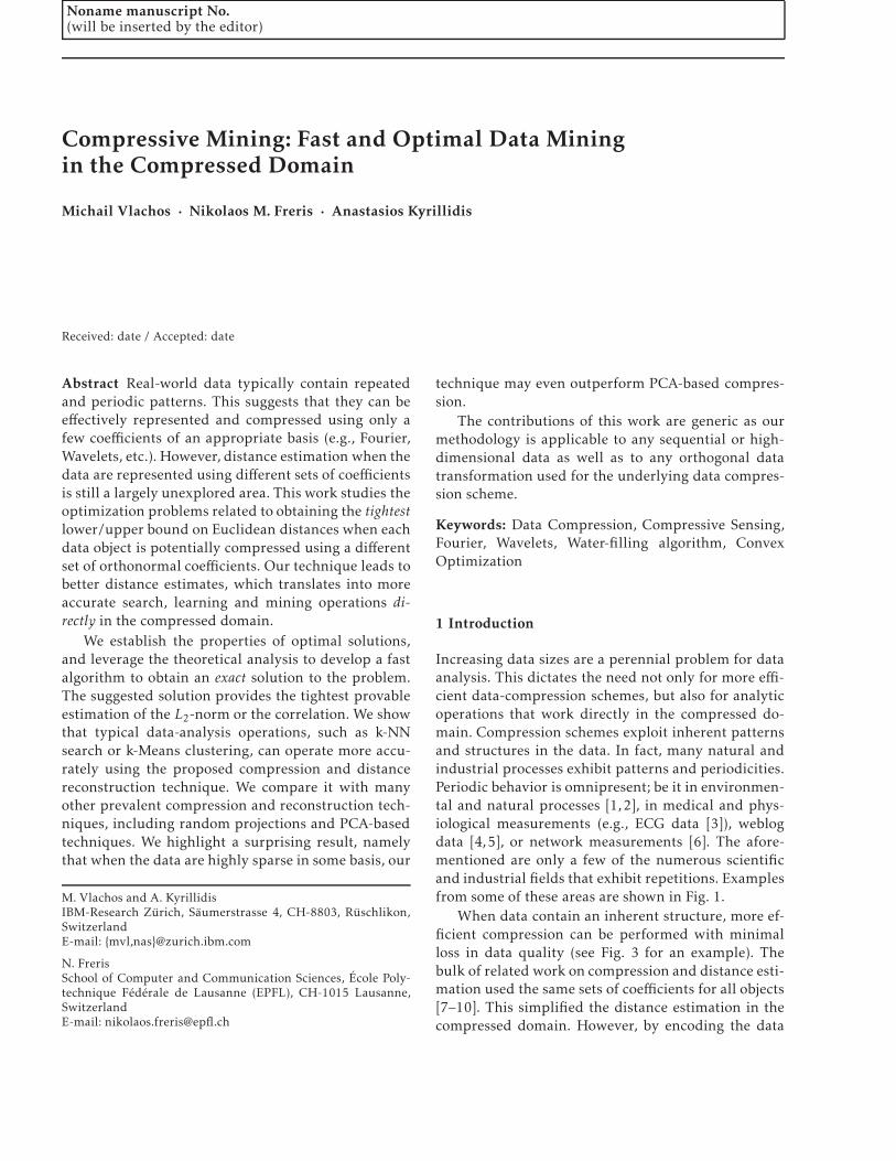
Increasing data sizes are a perennial problem for dataanalysis. This dictates the need not only for more effi-cient data-compression schemes, but also for analyticoperations that work directly in the compressed do-main. Compression schemes exploit inherent patternsand structures in the data. In fact, many natural andindustrial processes exhibit patterns and periodicities.Periodic behavior is omnipresent; be it in environmen-tal and natural processes [1,2], in medical and phys-iological measurements (e.g., ECG data [3]), weblogdata [4,5], or network measurements [6]. The afore-mentioned are only a few of the numerous scientificand industrial fields that exhibit repetitions. Examplesfrom some of these areas are shown in Fig. 1.
When data contain an inherent structure, more ef-ficient compression can be performed with minimalloss in data quality (see Fig. 3 for an example). Thebulk of related work on compression and distance esti-mation used the same sets of coefficients for all objects[7–10]. This simplified the distance estimation in thecompressed domain. However, by encoding the data
2 Michail Vlachos et al.
Fig. 1: Many scientific fields entail periodic data. Ex-amples from medical, industrial, web and astronomi-cal measurements.
using only a few and potentially disjoint sets of high-energy coefficients in an orthonormal basis, one canachieve better reconstruction performance. Nonethe-less, it was not known how to compute tight distanceestimates using such a representation. Our work ex-actly addresses this issue: given data that are com-pressed using disjoint coefficient sets of an orthonor-mal basis (for reasons of higher fidelity), how can dis-
tances among the compressed objects be estimated with thehighest fidelity?
Here, we provide the tightest possible upper andlower bounds on the original distances, based onlyon the compressed objects. By tightest, we mean that,given the information available, no better estimate canbe derived. Distance estimation is fundamental fordata mining: the majority of mining and learning tasksare distance-based, including clustering (e.g. k-Meansor hierarchical), k-NN classification, outlier detection,pattern matching, etc. This work focuses on the casewhere the distance is the widely used Euclidean dis-tance (L2-norm), but makes no assertions on the un-derlying transform used to compress the data: As longas the transform is orthonormal, our methodology isapplicable. In the experimental section, we use bothFourier and Wavelets Decomposition as a data com-pression technique. Our main contributions are sum-marized below:
- We formulate the problem of tight distance esti-mation in the compressed domain as two optimizationproblems for obtaining lower/upper bounds. We showthat both problems can be solved simultaneously bysolving a single convex optimization program.
- We derive the necessary and sufficient Karush-Kuhn-Tucker (KKT) conditions and study the proper-ties of optimal solutions. We use the analysis to devise
exact closed-form solution algorithms for the optimaldistance bounds.
- We evaluate our analytical findings experimen-tally; we compare the proposed algorithms with preva-lent distance estimation schemes, and demonstratesignificant improvements in terms of estimation accu-racy. We further compare the performance of our opti-mal algorithm with that of a numerical scheme basedon convex optimization, and show that our scheme isat least two orders of magnitude faster, while also pro-viding more accurate results.
- We also provide extensive evaluations with min-ing tasks in the compressed domain using our ap-proach and many other prevalent compression anddistance reconstruction schemes used in the literature(random projections, SVD, etc).
2 Related Work
We briefly position our work in the context of othersimilar approaches in the area. The majority of data-compression techniques for sequential data use thesame set of low-energy coefficients whether usingFourier [7,8], Wavelets [9,10] or Chebyshev polynomi-als [13] as the orthogonal basis for representation andcompression. Using the same set of orthogonal coeffi-cients has several advantages: a) it is straightforwardto compare the respective coefficients; b) space parti-tioning and indexing structures (such as R-trees) canbe directly used on the compressed data; c) there isno need to store also the indices (position) of the basisfunctions to which the stored coefficients correspond.The disadvantage is that both object reconstructionand distance estimation may be far from optimal fora given fixed compression ratio.
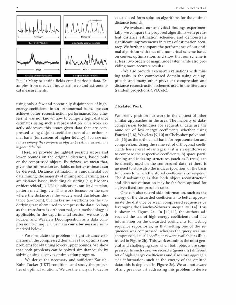
One can also record side information, such as theenergy of the discarded coefficients, to better approx-imate the distance between compressed sequences byleveraging the Cauchy–Schwartz inequality [14]. Thisis shown in Figure 2a). In [12,11], the authors ad-vocated the use of high-energy coefficients and sideinformation on the discarded coefficients for weblogsequence repositories; in that setting one of the se-quences was compressed, whereas the query was un-compressed, i.e., all coefficients were available as illus-trated in Figure 2b). This work examines the most gen-eral and challenging case when both objects are com-pressed. In such case, we record a (generally) differentset of high-energy coefficients and also store aggregateside information, such as the energy of the omitteddata; this is depicted in Figure 2c). We are not awareof any previous art addressing this problem to derive
Compressive Mining 3
e
ee
ee
QXQX QX
a) b) c)Fig. 2: Comparison with previous work. Distance estimation between a compressed sequence (X) and a query(Q) represented in any complete orthonormal basis. A compressed sequence is represented by a set of storedcoefficients (gray) as well as the error e incurred because of compression (yellow). a) Both X,Q are compressed bystoring the first coefficients. b) The highest-energy coefficients are used for X, whereas Q is uncompressed as in[11,12]. c) The problem we address: both sequences are compressed using the highest-energy coefficients; notethat in general for each object a different set of coefficients is used.
either optimal or suboptimal bounds on distance esti-mation.
The above approaches consider determining dis-tance estimation in the compressed domain. There isalso a big body of work that considers probabilisticdistance estimation via low-dimensional embeddings.Several projection techniques for dimensionality re-duction can preserve the geometry of the points [15,16]. These results heavily depend on the work of John-son and Lindenstrauss [17], according to which anyset of points can be projected onto a logarithmic (inthe cardinality of the data points) dimensional sub-space, while still retaining the relative distances be-tween the points, thus preserving an approximation oftheir nearest neighbors [18,19] or clustering [20,21].Both random [22] and deterministic [23] constructionshave been proposed in the literature.
This paper extends and expands the work of [24].Here we include additional experiments that showthe performance of our methodology for k-NN-search,and k-Means clustering directly in the compressed do-main. We also compare our approach with the per-formance of Principal Components and Random Pro-jection techniques (both in the traditional and in thecompressive sensing setting). Finally, we also conductexperiments using other orthonormal bases (namely,wavelets) to demonstrate the generality of our tech-nique. In the experimental section of this work, wecompare our methodology to both deterministic andprobabilistic techniques.
3 Searching Data Using Distance Estimates
We consider a databaseDB that stores sequences asN-dimensional complex vectors x(i) ∈ CN , i = 1, . . . ,V .A search problem that we examine is abstracted as fol-lows: a user is interested in finding the k most ‘simi-lar’ sequences to a given query sequence q ∈ DB, un-der a certain distance metric d(·, ·) : CN×N → R+. Thisis an elementary, yet fundamental operation known ask-Nearest-Neighbor (k-NN)-search. It is a core func-tion in database-querying, data-mining and machine-learning algorithms including classification (NN clas-sifier), clustering, etc.
In this paper, we focus on the case where d(·, ·)is the Euclidean distance. We note that other mea-sures, e.g., time-invariant matching, can be formu-lated as Euclidean distance on the periodogram [25].Correlation can also be expressed as an instance ofEuclidean distance on properly normalized sequences[26]. Therefore, our approach is applicable on a widerange of distance measures with little or no modifica-tion. However, for ease of exposition, we focus on theEuclidean distance as the most used measure in the lit-erature [27].
Search operations can be quite costly, especially forcases when the dimensionality N of data is high: se-quences need to be retrieved from the disk for com-parison against the query q. An effective way to mit-igate this is to retain a compressed representation ofthe sequences to be used as an initial pre-filteringstep. The set of compressed sequences could be smallenough to keep in-memory, hence enabling a signifi-cant performance speedup. In essence, this is a mul-
4 Michail Vlachos et al.
tilevel filtering mechanism. With only the compressedsequences available, we obviously cannot infer the ex-act distance between the query q and a sequence x(i)
in the database. However, it is still plausible to obtainlower and upper bounds of the distance. Using thesebounds, one might request a superset of the k-NN an-swers, which will be then verified using the uncom-pressed sequences that will need to be fetched andcompared with the query, so that the exact distancescan be computed. Such filtering ideas are used in themajority of the data-mining literature for speeding upsearch operations [7,8,28].
4 Notation
Consider an N-dimensional sequence x =[x1 x2 . . . xN ]T ∈ R
N . For compression purposes,x is first transformed using a sparsity-inducing(i.e., compressible) basis F (·) in R
N or CN , such
that X = F (x). We denote the forward linear map-ping x → X by F , whereas the inverse linear mapX → x is denoted by F −1, i.e., we say X = F (x) andx = F −1(X). A nonexhaustive list of invertible lineartransformations includes Discrete Fourier Transform(DFT), Discrete Cosine Transform, Discrete WaveletTransform, etc.
As a running example for this paper, we assumethat a sequence is compressed using DFT. In this case,the basis represent sinusoids of different frequencies,and the pair (x,X) satisfies
Xl =1√N
N∑
k=1
xkei2π(k−1)(l−1)/N , l = 1, . . . ,N
xk =1√N
N∑
l=1
Xlei2π(k−1)(l−1)/N , k = 1, . . . ,N
where i is the imaginary unit i2 = −1.Given the above, we assume the L2-norm as the dis-
tance between two sequences x, q, which can easily betranslated into distance in the frequency domain be-cause of Parseval’s theorem [29]:
d(x,q) := ||x−q||2 = ||X−Q||2In the experimental section, we also show applica-
tions of our methodology when wavelets are used asthe signal decomposition transform.
5 Motivation
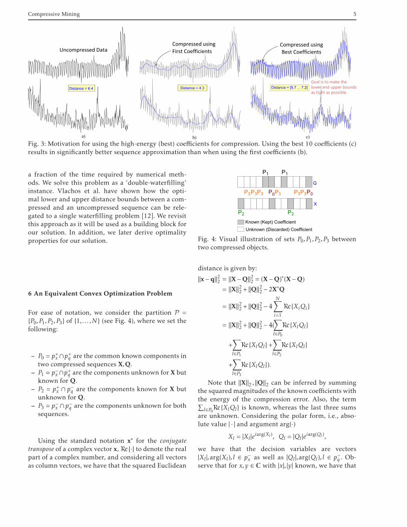
The choice of which coefficients to use has a direct im-pact on the data approximation quality. Although it
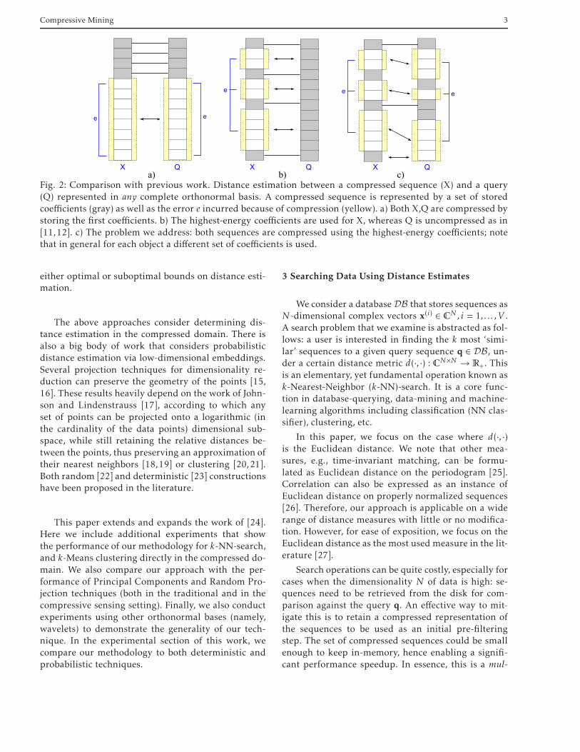
has long been recognized that sequence approxima-tion is indeed superior when using high-energy (i.e.,best) coefficients [30,12] - see also Figure 3 for an il-lustrative example - a barrier still has to be overcome:the efficiency of solution for distance estimation.
Consider a sequence represented using its high-energy coefficients. Then, the compressed sequencewill be described by a set of Cx coefficients that holdthe largest energy. We denote the vector describing thepositions of those coefficients in X as p+x , and the posi-tions of the remaining ones as p−x (that is, p+x ∪ p−x ={1, . . . ,N }). For any sequence X, we store the vectorX(p+x ) in the database, which we denote simply byX+ := {Xi}i∈p+x . We denote the vector of discarded co-efficients by X− := {Xi }i∈p−x . In addition to the best co-efficients of a sequence, we can also record one addi-tional value for the energy of the compression error,ex = ||X−||22, i.e., the sum of squared magnitudes of theomitted coefficients.
Then, one needs to solve the following minimiza-tion (maximization) problem for calculating the lower(upper) bounds on the distance between two se-quences based on their compressed versions:
min(max)
X−∈C|p−x |, Q−∈C|p−q |
||X−Q||2
s.t. |X−l | ≤minj∈p+x|Xj |, ∀l ∈ p−x
|Q−l | ≤minj∈p+q|Qj |, ∀l ∈ p−q
∑
l∈p−x|X−l |2 = ex,
∑
l∈p−q|Q−l |2 = eq
(1)
The inequality constraints are due to the fact that weuse the high-energy components for the compression.Hence, any of the omitted components must have anenergy lower than the minimum energy of any keptcomponent.
The optimization problem presented is a complex-valued program: we show a single real-valued convex
program that is equivalent to both theminimization andmaximization problems. This program can be solvedefficiently with numerical methods [31], cf. Sec. 8.1.However, as we show in the experimental section, eval-uating an instance of this problem is not efficient inpractice, even for a single pair of sequences. There-fore, although a solution can be found numerically,it is generally costly and not suitable for large min-ing tasks, where one would like to evaluate thousandsor millions of lower/upper bounds on compressed se-quences.
In this paper, we show how solve this problem an-alytically by exploiting the derived optimality con-ditions. In this manner we can solve the problem in
Compressive Mining 5
a) b) c)
Distance = 6.4 Distance = 4.3 Distance = [5.7 ... 7.2]
Uncompressed DataCompressed using
First Coefficients
Compressed using
Best Coefficients
Goal is to make the
lower and upper bounds
as tight as possible
Fig. 3: Motivation for using the high-energy (best) coefficients for compression. Using the best 10 coefficients (c)results in significantly better sequence approximation than when using the first coefficients (b).
a fraction of the time required by numerical meth-ods. We solve this problem as a ‘double-waterfilling’instance. Vlachos et al. have shown how the opti-mal lower and upper distance bounds between a com-pressed and an uncompressed sequence can be rele-gated to a single waterfilling problem [12]. We revisitthis approach as it will be used as a building block forour solution. In addition, we later derive optimalityproperties for our solution.
6 An Equivalent Convex Optimization Problem
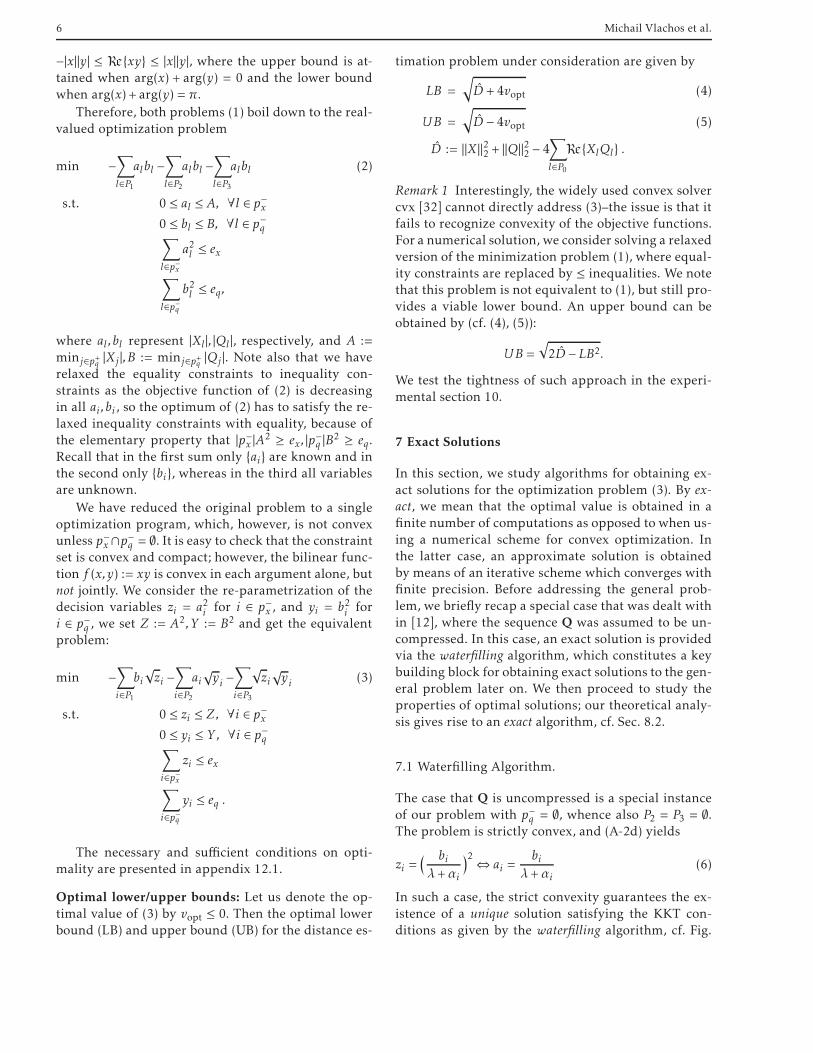
For ease of notation, we consider the partition P ={P0,P1,P2,P3} of {1, . . . ,N } (see Fig. 4), where we set thefollowing:
– P0 = p+x ∩p+q are the common known components intwo compressed sequences X,Q.
– P1 = p−x ∩p+q are the components unknown forX butknown for Q.
– P2 = p+x ∩ p−q are the components known for X butunknown for Q.
– P3 = p−x ∩p−q are the components unknown for bothsequences.
Using the standard notation x∗ for the conjugatetranspose of a complex vector x,ℜ{·} to denote the realpart of a complex number, and considering all vectorsas column vectors, we have that the squared Euclidean
Q
X
Unknown (Discarded) Coefficient
Known (Kept) Coefficient
P0
P1
P2
P3 P0
P1
P2
P3P3 P3 P3P3
Fig. 4: Visual illustration of sets P0,P1,P2,P3 betweentwo compressed objects.
distance is given by:
||x−q||22 = ||X−Q||22 = (X−Q)∗(X−Q)
= ||X||22 + ||Q||22 − 2X∗Q
= ||X||22 + ||Q||22 − 4N∑
i=1
ℜ{XiQi }
= ||X||22 + ||Q||22 − 4(∑
l∈P0ℜ{XlQl }
+∑
l∈P1ℜ{XlQl}+
∑
l∈P2ℜ{XlQl}
+∑
l∈P3ℜ{XlQl}).
Note that ||X||2 , ||Q||2 can be inferred by summingthe squared magnitudes of the known coefficients withthe energy of the compression error. Also, the term∑
l∈P0ℜ{XlQl} is known, whereas the last three sumsare unknown. Considering the polar form, i.e., abso-lute value | · | and argument arg(·)
Xl = |Xl |eiarg(Xl ), Ql = |Ql |eiarg(Ql ),
we have that the decision variables are vectors|Xl |,arg(Xl ), l ∈ p−x as well as |Ql |,arg(Ql ), l ∈ p−q . Ob-serve that for x,y ∈ C with |x|, |y| known, we have that
6 Michail Vlachos et al.
−|x||y| ≤ ℜ{xy} ≤ |x||y|, where the upper bound is at-tained when arg(x) + arg(y) = 0 and the lower boundwhen arg(x) + arg(y) = π.
Therefore, both problems (1) boil down to the real-valued optimization problem
min −∑
l∈P1albl −
∑
l∈P2albl −
∑
l∈P3albl (2)
s.t. 0 ≤ al ≤ A, ∀l ∈ p−x0 ≤ bl ≤ B, ∀l ∈ p−q∑
l∈p−xa2l ≤ ex
∑
l∈p−qb2l ≤ eq,
where al ,bl represent |Xl |, |Ql |, respectively, and A :=minj∈p+q |Xj |,B := minj∈p+q |Qj |. Note also that we haverelaxed the equality constraints to inequality con-straints as the objective function of (2) is decreasingin all ai ,bi , so the optimum of (2) has to satisfy the re-laxed inequality constraints with equality, because ofthe elementary property that |p−x |A2 ≥ ex , |p−q |B2 ≥ eq.Recall that in the first sum only {ai} are known and inthe second only {bi }, whereas in the third all variablesare unknown.
We have reduced the original problem to a singleoptimization program, which, however, is not convexunless p−x∩p−q = ∅. It is easy to check that the constraintset is convex and compact; however, the bilinear func-tion f (x,y) := xy is convex in each argument alone, butnot jointly. We consider the re-parametrization of thedecision variables zi = a2i for i ∈ p−x , and yi = b2i fori ∈ p−q , we set Z := A2,Y := B2 and get the equivalentproblem:
min −∑
i∈P1bi√zi −
∑
i∈P2ai√yi −
∑
i∈P3
√zi√yi (3)
s.t. 0 ≤ zi ≤ Z, ∀i ∈ p−x0 ≤ yi ≤ Y, ∀i ∈ p−q∑
i∈p−xzi ≤ ex
∑
i∈p−qyi ≤ eq .
The necessary and sufficient conditions on opti-mality are presented in appendix 12.1.
Optimal lower/upper bounds: Let us denote the op-timal value of (3) by vopt ≤ 0. Then the optimal lowerbound (LB) and upper bound (UB) for the distance es-
timation problem under consideration are given by
LB =
√
D +4vopt (4)
UB =√
D − 4vopt (5)
D := ||X ||22 + ||Q||22 − 4∑
l∈P0ℜ{XlQl} .
Remark 1 Interestingly, the widely used convex solvercvx [32] cannot directly address (3)–the issue is that itfails to recognize convexity of the objective functions.For a numerical solution, we consider solving a relaxedversion of the minimization problem (1), where equal-ity constraints are replaced by ≤ inequalities. We notethat this problem is not equivalent to (1), but still pro-vides a viable lower bound. An upper bound can beobtained by (cf. (4), (5)):
UB =√
2D − LB2.
We test the tightness of such approach in the experi-mental section 10.
7 Exact Solutions
In this section, we study algorithms for obtaining ex-act solutions for the optimization problem (3). By ex-act, we mean that the optimal value is obtained in afinite number of computations as opposed to when us-ing a numerical scheme for convex optimization. Inthe latter case, an approximate solution is obtainedby means of an iterative scheme which converges withfinite precision. Before addressing the general prob-lem, we briefly recap a special case that was dealt within [12], where the sequence Q was assumed to be un-compressed. In this case, an exact solution is providedvia the waterfilling algorithm, which constitutes a keybuilding block for obtaining exact solutions to the gen-eral problem later on. We then proceed to study theproperties of optimal solutions; our theoretical analy-sis gives rise to an exact algorithm, cf. Sec. 8.2.
7.1 Waterfilling Algorithm.
The case that Q is uncompressed is a special instanceof our problem with p−q = ∅, whence also P2 = P3 = ∅.The problem is strictly convex, and (A-2d) yields
zi =( biλ+αi
)2⇔ ai =bi
λ+αi(6)
In such a case, the strict convexity guarantees the ex-istence of a unique solution satisfying the KKT con-ditions as given by the waterfilling algorithm, cf. Fig.
Compressive Mining 7
5. The algorithm progressively increases the unknowncoefficients ai until saturation, i.e., until they reach A,in which case they are fixed. The set C is the set of nonsaturated coefficients at the beginning of each itera-tion, whereas R denotes the “energy reserve,” i.e., theenergy that can be used to increase the non saturatedcoefficients; vopt denotes the optimal value.
Waterfilling algorithmInputs: {bi }i∈p−x , ex ,AOutputs: {ai }i∈p−x ,λ, {αi }i∈p−x ,vopt,R1. Set R = ex , C = p−x2. while R > 0 and C , ∅ do3. set λ =
√
∑
i∈C b2iR , ai =
biλ , i ∈ C
4. if for some i ∈ C, ai > A then5. ai = A, C← C − {i}6. else break;7. end if8. R = ex − (|p−x | − |C|)A2
9. end while10. Set vopt = −
∑
i∈p−x aibi and
αi =
{
0, if ai < AbiA −λ, if ai = A
Fig. 5: Waterfilling algorithm for optimal distance es-timation between a compressed and an uncompressedsequence
As a shorthand notation, we write a =waterfill(b, ex ,A). Note that in this case the prob-lem (2) for P2 = P3 = ∅ is convex, so the solution canbe obtained via the KKT conditions to (2), whichare different from those for the re-parameterizedproblem (3); this was done in [12]. The analysis andstraightforward extensions are summarized in Lemma1.
Lemma 1 (Exact solutions)
1. If either p−x = ∅ or p−q = ∅ (i.e., when at least one of
the sequences is uncompressed) we can obtain an ex-act solution to the optimization problem (2) via the
waterfilling algorithm.
2. If P3 = p−x ∩ p−q = ∅, i.e., when the two compressed
sequences do not have any common unknown coeffi-cients, the problem is decoupled in a,b, and the water-
filling algorithm can be used separately to obtain exact
solutions to both unknown vectors.
3. If P1 = P2 = ∅, i.e., when both compressed sequences
have the same discarded coefficients, the optimal valueis simply equal to −√ex√eq, but there is no unique so-lution for a,b.
Proof The first two cases are obvious. For thethird one, note that it follows immediately fromthe Cauchy–Schwartz inequality that −∑l∈P3 albl ≥−√ex√eq, and in this is case this is also attainable. Just
consider for example, al =√
ex|P3 | ,bl =
√
eq|P3 | , which is
feasible because |p−x |A2 ≥ ex, |p−q |B2 ≥ eq, as follows bycompression with the high-energy coefficients. �
We have shown how to obtain exact optimal solu-tions for special cases. To derive efficient algorithmsfor the general case, we first study end establish someproperties of the optimal solution of (3).
Theorem 1 (Properties of optimal solutions)Let an augmented optimal solution of (2) be denoted by
(aopt,bopt); where aopt := {aopti }i∈p−x∪p−q denotes the optimal
solution extended to include the known values |Xl |l∈P2 ,and bopt := {bopti }i∈p−x∪p−q denotes the optimal solution ex-
tended to include the known values |Ql |l∈P1 . Let us furtherdefine e′x = ex −
∑
l∈P1 a2l , e′q = eq −
∑
l∈P2 b2l . We then have
the following:
1. The optimal solution satisfies1
aopt = waterfill (bopt, ex,A), (7a)
bopt = waterfill (aopt, eq ,B). (7b)
In particular, it follows that aopti > 0 iff b
opti > 0 and
that {aopti }, {bopti } have the same ordering. In addition,
minl∈P1 al ≥maxl∈P3 al ,minl∈P2 bl ≥maxl∈P3 bl .2. If at optimality it holds that e′xe′q > 0 there exists
a multitude of solutions. One solution (a,b) satisfies
al =√
e′x|P3 | ,bl =
√
e′q|P3 | for all l ∈ P3, whence
λ =
√
e′qe′x
µ =
√
e′xe′q, (8a)
αi = βi = 0 ∀i ∈ P3. (8b)
In particular, λµ = 1 and the values e′x, e′q need to be
solutions to the following set of nonlinear equations:
∑
l∈P1min
(
b2le′xe′q,A2
)
= ex − e′x, (9a)
∑
l∈P2min
(
a2le′qe′x,B2
)
= eq − e′q. (9b)
3. At optimality, it is not possible to have e′xe′q = 0 unless
e′x = e′q = 0.
1 This has a natural interpretation as the Nash equilibrium ofa 2-player game [33] in which Player 1 seeks to minimize theobjective of (3) with respect to z, and Player 2 seeks to minimizethe same objective with respect to y.
8 Michail Vlachos et al.
4. Consider the vectors a,b with al = |Xl |, l ∈ P2,al =|Xl |, l ∈ P1 and
{al}l∈P1 = waterfill ({bl }l∈P1 , ex,A), (10a)
{bl}l∈P2 = waterfill ({al}l∈P2 , eq ,B). (10b)
If ex ≤ |P1|A2 and eq ≤ |P2|B2, whence e′x = e′q = 0, thenby defining al = bl = 0 for l ∈ P3, we obtain a globallyoptimal solution (a,b).
Proof See appendix 12.2.
Remark 2 One may be tempted to think that an op-timal solution can be derived by waterfilling for thecoefficients of {al}l∈P1 , {bl }l∈P2 separately, and then allo-cating the remaining energies e′x, e
′q to the coefficients
in {al ,bl }l∈P3 leveraging the Cauchy–Schwartz inequal-
ity, the value being −√
e′x√
e′q. However, the third and
fourth parts of Theorem 1 state that this is not optimalunless e′x = e′q = 0.
We have shown that there are two possible cases foran optimal solution of (2): either e′x = e′q = 0 or e′x, e
′q >
0. The first case is easy to identify by checking whether(10) yields e′x = e′q = 0. If this is not the case, we are inthe latter case and need to find a solution to the set ofnonlinear equations (9).
Consider the mapping T : R2+→ R
2+ defined by
T ((x1,x2)) :=
(
ex −∑
l∈P1min
(
b2lx1x2
,A2)
, eq −∑
l∈P2min
(
a2lx2x1
,B2)
)
(11)
The set of nonlinear equations of (9) corresponds to apositive fixed point of T , i.e., (e′x , e′q) = T (e′x , e′q), e′x, e′q >0. Calculating a fixed point of T may at first seem in-volved, but it turns out that this can be accomplishedexactly and with minimal overhead. The analysis canbe found in appendix 12.3, where we prove that thisproblem is no different from the simplest numericalproblem: finding the root of a scalar linear equation.
Remark 3 We note that coefficients {al}P2 , {bl }P1 arealready sorted because of the way we performcompression–by storing high-energy coefficients. It isplain to check that all other operations can be effi-ciently implemented, with the average complexity be-ing linear (Θ(N ))–hence the term minimum-overhead
algorithm.
Remark 4 (Extensions) It is straightforward to see thatour approach can be applied without modification tothe case that each point is compressed using a differentnumber of coefficients. Additionally, we note here twoimportant extensions of our problem formulation andoptimal algorithm.
1. Consider the case that a data point is a countably in-finite sequence. For example, wemay express a con-tinuous function via its Fourier series, or Cheby-shev polynomials expansion. In that case, surpris-ingly enough, our algorithm can be applied with-out any alteration. This is because P0,P1,P2 are fi-nite sets as defined above, whereas P3 is now infi-nite. The energy allocation in P3 can be computedexactly by the same procedure (cf. appendix 12.3)and then in P3 the Cauchy–Schwartz inequality isagain applied2.
2. Of particular interest is the case that data are com-pressed using an over-complete basis (also knownas frame in the signal-processing literature [29]);this approach has recently become popular in thecompressed-sensing framework [34]. Our methodcan be extended to handle this important gen-eral case, by storing the compression errors corre-sponding to each given basis, and calculating thelower/upper bounds in each one separately usingour approach. We leave this direction for future re-search work.
8 Algorithm for Optimal Distance Estimation
In this section, we present an algorithm for obtain-ing the exact optimal upper and lower bounds on thedistance between the original sequences, when fullyleveraging all information available given their com-pressed counterparts. First, we present a simple nu-merical scheme using a convex solver such as cvx [32]and then use our theoretical findings to derive an ana-lytical algorithm which we call ‘double-waterfilling’.
8.1 Convex Programming
We let M := N − |P0|, and consider the nontrivial caseM > 0. Following the discussion in Sec. 6, we set the2M ×1 vector v = ({al}l∈P1∪P2∪P3 , {bl }l∈P1∪P2∪P3 ) and con-sider the following convex problem directly amenableto a numerical solution via a solver such as cvx:
min∑
l∈P1∪P2∪P3 (al − bl )2s.t. al ≤ A, ∀l ∈ p−x , bl ≤ B, ∀l ∈ p−q
∑
l∈p−x a2l ≤ ex,
∑
l∈p−q b2l ≤ eq
al = |Xl |, ∀l ∈ P2, bl = |Ql |, ∀l ∈ P12 The proof of optimality in this case assumes a finite subset
of P3 and applies the same conditions of optimality that wereleveraged before; in fact particular selection of the subset is notof importance, as long as its cardinality is large enough to ac-commodate the computed energy allocation (e′x , e
′q).
Compressive Mining 9
The lower bound (LB) can be obtained by adding D′ :=∑
l∈P0 |Xl −Ql |2 to the optimal value of (1) and takingthe square root; then the upper bound is given byUB =√2D′ − LB2, cf. (4).
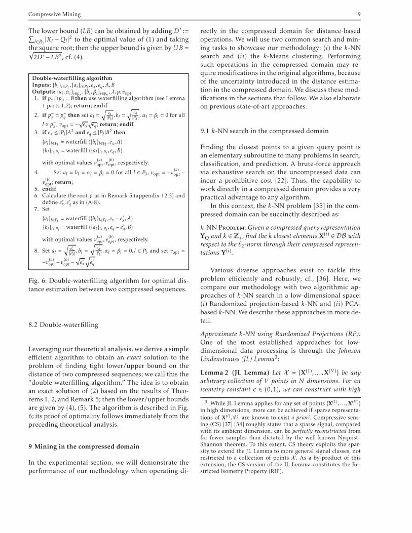
Double-waterfilling algorithmInputs: {bi }i∈P1 , {ai }i∈P2 , ex , eq ,A,BOutputs: {ai ,αi }i∈p−x , {bi ,βi }i∈p−q ,λ,µ,vopt1. if p−x ∩p−q = ∅ then use waterfilling algorithm (see Lemma
1 parts 1,2); return; endif
2. if p−x = p−q then set al =√
ex|P3 | ,bl =
√
eq|P3 | , αl = βl = 0 for all
l ∈ p−x , vopt = −√ex√eq ; return; endif
3. if ex ≤ |P1|A2 and eq ≤ |P2 |B2 then
{al }l∈P1 = waterfill ({bl }l∈P1 , ex ,A){bl }l∈P2 = waterfill ({al }l∈P2 , eq ,B)
with optimal values v(a)opt,v
(b)opt, respectively.
4. Set al = bl = αl = βl = 0 for all l ∈ P3, vopt = −v(a)opt −v(b)opt; return;
5. endif6. Calculate the root γ as in Remark 5 (appendix 12.3) and
define e′x , e′q as in (A-8).
7. Set
{al }l∈P1 = waterfill ({bl }l∈P1 , ex − e′x ,A){bl }l∈P2 = waterfill ({al }l∈P2 , eq − e′q ,B)
with optimal values v(a)opt ,v
(b)opt , respectively.
8. Set al =√
e′x|P3 | ,bl =
√
e′q|P3 | ,αl = βl = 0, l ∈ P3 and set vopt =
−v(a)opt − v(b)opt −
√
e′x√
e′q
Fig. 6: Double-waterfilling algorithm for optimal dis-tance estimation between two compressed sequences.
8.2 Double-waterfilling
Leveraging our theoretical analysis, we derive a simpleefficient algorithm to obtain an exact solution to theproblem of finding tight lower/upper bound on thedistance of two compressed sequences; we call this the“double-waterfilling algorithm.” The idea is to obtainan exact solution of (2) based on the results of Theo-rems 1, 2, and Remark 5; then the lower/upper boundsare given by (4), (5). The algorithm is described in Fig.6; its proof of optimality follows immediately from thepreceding theoretical analysis.
9 Mining in the compressed domain
In the experimental section, we will demonstrate theperformance of our methodology when operating di-
rectly in the compressed domain for distance-basedoperations. We will use two common search and min-ing tasks to showcase our methodology: (i) the k-NNsearch and (ii) the k-Means clustering. Performingsuch operations in the compressed domain may re-quire modifications in the original algorithms, becauseof the uncertainty introduced in the distance estima-tion in the compressed domain. We discuss these mod-ifications in the sections that follow. We also elaborateon previous state-of-art approaches.
9.1 k-NN search in the compressed domain
Finding the closest points to a given query point isan elementary subroutine to many problems in search,classification, and prediction. A brute-force approachvia exhaustive search on the uncompressed data canincur a prohibitive cost [22]. Thus, the capability towork directly in a compressed domain provides a verypractical advantage to any algorithm.
In this context, the k-NN problem [35] in the com-pressed domain can be succinctly described as:
k-NN Problem: Given a compressed query representation
YQ and k ∈Z+, find the k closest elements X(i) ∈ DB withrespect to the ℓ2-norm through their compressed represen-
tations Y(i).
Various diverse approaches exist to tackle thisproblem efficiently and robustly; cf., [36]. Here, wecompare our methodology with two algorithmic ap-proaches of k-NN search in a low-dimensional space:(i) Randomized projection-based k-NN and (ii) PCA-based k-NN.We describe these approaches in more de-tail.
Approximate k-NN using Randomized Projections (RP):
One of the most established approaches for low-dimensional data processing is through the Johnson
Lindenstrauss (JL) Lemma3:
Lemma 2 (JL Lemma) Let X = {X(1), . . . ,X(V )} be anyarbitrary collection of V points in N dimensions. For an
isometry constant ǫ ∈ (0,1), we can construct with high
3 While JL Lemma applies for any set of points {X(1) , . . . ,X(V )}in high dimensions, more can be achieved if sparse representa-
tions of X(i) ,∀i, are known to exist a priori. Compressive sens-ing (CS) [37] [34] roughly states that a sparse signal, comparedwith its ambient dimension, can be perfectly reconstructed fromfar fewer samples than dictated by the well-known Nyquist–Shannon theorem. To this extent, CS theory exploits the spar-sity to extend the JL Lemma to more general signal classes, notrestricted to a collection of points X . As a by-product of thisextension, the CS version of the JL Lemma constitutes the Re-stricted Isometry Property (RIP).
10 Michail Vlachos et al.
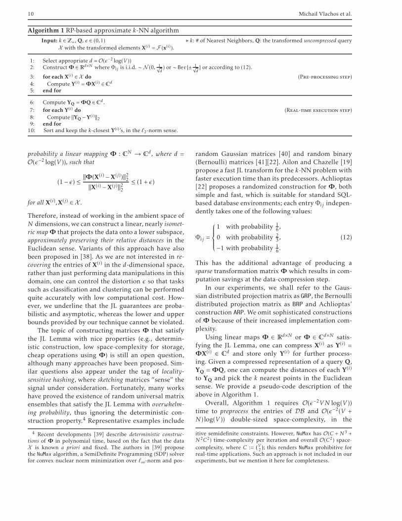
Algorithm 1 RP-based approximate k-NN algorithm
Input: k ∈Z+, Q, ǫ ∈ (0,1) ⊲ k: # of Nearest Neighbors, Q: the transformed uncompressed query
X with the transformed elements X(i) = F (x(i)).
1: Select appropriate d = O(ǫ−2 log(V ))2: ConstructΦ ∈Rd×N where Φij is i.i.d. ∼N (0, 1√
d) or ∼ Ber{± 1√
d} or according to (12).
3: for each X(i) ∈ X do (Pre-processing step)
4: Compute Y(i) =ΦX(i) ∈Cd
5: end for
6: Compute YQ =ΦQ ∈Cd .
7: for each Y(i) do (Real-time execution step)
8: Compute ‖YQ −Y(i)‖29: end for10: Sort and keep the k-closest Y(i)’s, in the ℓ2-norm sense.
probability a linear mapping Φ : CN → Cd , where d =
O(ǫ−2 log(V )), such that
(1− ǫ) ≤ ‖Φ(X(i) −X(j))‖22‖X(i) −X(j)‖22
≤ (1 + ǫ)
for all X(i),X(j) ∈ X .
Therefore, instead of working in the ambient space ofN dimensions, we can construct a linear, nearly isomet-ric mapΦ that projects the data onto a lower subspace,approximately preserving their relative distances in theEuclidean sense. Variants of this approach have alsobeen proposed in [38]. As we are not interested in re-covering the entries of X(i) in the d-dimensional space,rather than just performing data manipulations in thisdomain, one can control the distortion ǫ so that taskssuch as classification and clustering can be performedquite accurately with low computational cost. How-ever, we underline that the JL guarantees are proba-bilistic and asymptotic, whereas the lower and upperbounds provided by our technique cannot be violated.
The topic of constructing matrices Φ that satisfythe JL Lemma with nice properties (e.g., determin-istic construction, low space-complexity for storage,cheap operations using Φ) is still an open question,although many approaches have been proposed. Sim-ilar questions also appear under the tag of locality-
sensitive hashing, where sketching matrices “sense” thesignal under consideration. Fortunately, many workshave proved the existence of random universal matrixensembles that satisfy the JL Lemma with overwhelm-
ing probability, thus ignoring the deterministic con-struction property.4 Representative examples include
4 Recent developments [39] describe deterministic construc-tions of Φ in polynomial time, based on the fact that the dataX is known a priori and fixed. The authors in [39] proposethe NuMax algorithm, a SemiDefinite Programming (SDP) solverfor convex nuclear norm minimization over ℓ∞-norm and pos-
random Gaussian matrices [40] and random binary(Bernoulli) matrices [41][22]. Ailon and Chazelle [19]propose a fast JL transform for the k-NN problem withfaster execution time than its predecessors. Achlioptas[22] proposes a randomized construction for Φ, bothsimple and fast, which is suitable for standard SQL-based database environments; each entry Φij indepen-dently takes one of the following values:
Φij =
1 with probability 16 ,
0 with probability 23 ,
−1 with probability 16 .
(12)
This has the additional advantage of producing asparse transformation matrix Φ which results in com-putation savings at the data-compression step.
In our experiments, we shall refer to the Gaus-sian distributed projectionmatrix as GRP, the Bernoullidistributed projection matrix as BRP and Achlioptas’construction ARP. We omit sophisticated constructionsof Φ because of their increased implementation com-plexity.
Using linear maps Φ ∈ Rd×N or Φ ∈ C
d×N satis-fying the JL Lemma, one can compress X(i) as Y(i) =ΦX(i) ∈ C
d and store only Y(i) for further process-ing. Given a compressed representation of a query Q,YQ = ΦQ, one can compute the distances of each Y(i)
to YQ and pick the k nearest points in the Euclideansense. We provide a pseudo-code description of theabove in Algorithm 1.
Overall, Algorithm 1 requires O(ǫ−2VN log(V ))time to preprocess the entries of DB and O(ǫ−2(V +N ) log(V )) double-sized space-complexity, in the
itive semidefinite constraints. However, NuMax has O(C +N3 +N2C2) time-complexity per iteration and overall O(C2) space-
complexity, where C :=(V2
)
; this renders NuMax prohibitive forreal-time applications. Such an approach is not included in ourexperiments, but we mention it here for completeness.
Compressive Mining 11
Gaussian case. In the other two cases, the space com-plexity can be further reduced thanks to the binaryrepresentation of Φ. Given a query YQ, Algorithm 1requires O(max{V ,N } · ǫ−2 log(V )) time-cost.
Approximate k-Nearest Neighbors using PCA: Instead ofprojecting onto a randomly chosen low-dimensionalsubspace, one can use the most informative sub-spaces to construct a projection matrix, based on X .PCA-based k-NN relies on this principle: let X :=[X(1) X(1) . . . X(V )] ∈ CN×n be the data matrix. GivenX, one can compute the Singular Value Decomposi-tion (SVD) X =UΣVT to identify the d most importantsubspaces of X, spanned by the d dominant singularvectors in U. In this case, Φ := U(1 : d, :) works as alow-dimensional linear map, biased by the informa-tion contained in X.
The main shortcoming of PCA-based k-NN searchis the computation of the SVD of X; generally, such anoperation has cubic complexity in the number of en-tries in X. Moreover, PCA-based projection providesno guarantees on the order of distortion in the com-pressed domain: While in most cases Φ := U(1 : d, :)outperforms RP-based approaches with JL guarantees,one can construct test cases where the pairwise pointdistances are heavily distorted such that points in Xmight be mapped to a single point [22] [39]. Finally,note that computation of the SVD requires the pres-ence of the entire dataset, whereas approaches such asours operate on a per-object basis.
Optimal bounds-based k-NN: Our approach can easilybe adapted to perform k-NN search operations in thecompressed domain. Similar to Algorithm 1, insteadof computing randomprojectionmatrices, we keep thelargest coefficients for each transformed signal repre-sentation X(i) (in Fourier, Wavelet or other basis) andalso record the total discarded energy per object. Fol-lowing a similar approach to compress the input queryQ, say YQ, we perform the optimal bounds procedureto obtain upper (ub) and lower bounds (ℓb) of the dis-tance in the original domain. Therefore, we do nothave only one distance, but can compute three distanceproxies based on the upper and lower bounds on thedistance.
(i) We use the lower bound ℓb as indicator of howclose the uncompressed x(i) is to the uncompressedquery q.
(ii) We use the upper bound ub as indicator of howclose the uncompressed x(i) is to the uncompressedquery q.
(iii) We define the average metric ℓb+ub2 as indicator of
how close the uncompressed x(i) is to the uncom-pressed query q.
In the experimental section, we evaluate the per-formance of these three metrics, and show that the lastmetric based on the average distance bound providesthe most robust performance.
9.2 k-Means clustering in the compressed domain
Clustering is a rudimentary mining task for summa-rizing and visualizing large amounts of data. Specifi-cally, the k-clustering problem is defined as follows:
k-Clustering Problem: Given a DB containing V com-
pressed representations of x(i),∀i, and a target number ofclusters k, group the compressed data into k clusters in an
accurate way through their compressed representations.
This is an assignment problem and is in fact NP-hard [42]. Many approximations to this problem ex-ist, one of the most widely-used algorithms being thek-Means clustering algorith [43]. Formally, k-Meansclustering involves partitioning the V vectors into kclusters, i.e., into k disjoint subsets G(t) (1≤t≤k) with∪tG(t) = V , such that the sum of intraclass variances
V :=
k∑
t=1
∑
x(i)∈G(t)
||x(i) −C(t)||2, (13)
is minimized, where C(t) is the centroid of the k-th clus-ter.
There also exist other formalizations for data clus-tering, based on either hierarchical clustering (“top-down” and “bottom-up” constructions, cf. [44]); flat orcentroid-based clustering, or on spectral-based clus-tering [45]. In our subsequent discussions, we focuson the k-Means algorithm because of its widespreaduse and fast runtime. Note also that k-Means is eas-ily amenable for use by our methodology owning toits computation of distances between objects and thederived centroids.
Similar to the k-NN problem case, we considerlow-dimensional embedding matrices based on bothPCA and randomized constructions [46][15] [20]. Wenote that [20] theoretically proves that a specific ran-dom matrix construction achieves a (2 + ǫ)-optimalk-partition of the points in the compressed domainin O(VN k
ǫ2 log(N )) time. Based on simulated annealing
clustering heuristics, [21] proposes an iterative pro-cedure where sequential k-means clustering is per-formed, with increasing projection dimensions d, forbetter clustering performance. We refer the reader to[20] for a recent discussion of the above approaches.
Similar, in spirit, to our approach is the work of[42]. There, the authors propose 1-bit MinimumMean
12 Michail Vlachos et al.
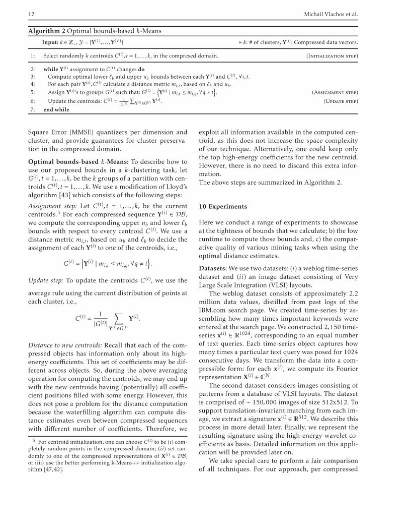
Algorithm 2 Optimal bounds-based k-Means
Input: k ∈Z+, Y = {Y(1) , . . . ,Y(V )} ⊲ k: # of clusters, Y(i) : Compressed data vectors.
1: Select randomly k centroids C(t), t = 1, . . . , k, in the compresed domain. (Initialization step)
2: while Y(i) assignment to C(t) changes do
3: Compute optimal lower ℓb and upper ub bounds between each Y(i) and C(t), ∀i, t.4: For each pair Y(i) ,C(t) calculate a distance metric mi,t , based on ℓb and ub .
5: Assign Y(i)’s to groups G(t) such that: G(t) ={
Y(i) | mi,t ≤mi,q ,∀q , t}
. (Assignment step)
6: Update the centroids: C(t) = 1|G(t) |
∑
Y(i)∈G(t) Y(i). (Update step)
7: end while
Square Error (MMSE) quantizers per dimension andcluster, and provide guarantees for cluster preserva-tion in the compressed domain.
Optimal bounds-based k-Means: To describe how touse our proposed bounds in a k-clustering task, letG(t), t = 1, . . . ,k, be the k groups of a partition with cen-troids C(t), t = 1, . . . ,k. We use a modification of Lloyd’salgorithm [43] which consists of the following steps:
Assignment step: Let C(t), t = 1, . . . ,k, be the currentcentroids.5 For each compressed sequence Y(i) ∈ DB,we compute the corresponding upper ub and lower ℓbbounds with respect to every centroid C(t). We use adistance metric mi,t , based on ub and ℓb to decide theassignment of each Y(i) to one of the centroids, i.e.,
G(t) ={
Y(i) | mi,t ≤mi,q ,∀q , t}
.
Update step: To update the centroids C(t), we use the
average rule using the current distribution of points ateach cluster, i.e.,
C(t) =1
|G(t)|∑
Y(i)∈G(t)
Y(i).
Distance to new centroids: Recall that each of the com-pressed objects has information only about its high-energy coefficients. This set of coefficients may be dif-ferent across objects. So, during the above averagingoperation for computing the centroids, we may end upwith the new centroids having (potentially) all coeffi-cient positions filled with some energy. However, thisdoes not pose a problem for the distance computationbecause the waterfilling algorithm can compute dis-tance estimates even between compressed sequenceswith different number of coefficients. Therefore, we
5 For centroid initialization, one can choose C(t) to be (i) com-pletely random points in the compressed domain; (ii) set ran-
domly to one of the compressed representations of X(i) ∈ DB,or (iii) use the better performing k-Means++ initialization algo-rithm [47,42].
exploit all information available in the computed cen-troid, as this does not increase the space complexityof our technique. Alternatively, one could keep onlythe top high-energy coefficients for the new centroid.However, there is no need to discard this extra infor-mation.
The above steps are summarized in Algorithm 2.
10 Experiments
Here we conduct a range of experiments to showcasea) the tightness of bounds that we calculate; b) the lowruntime to compute those bounds and, c) the compar-ative quality of various mining tasks when using theoptimal distance estimates.
Datasets:We use two datasets: (i) a weblog time-seriesdataset and (ii) an image dataset consisting of VeryLarge Scale Integration (VLSI) layouts.
The weblog dataset consists of approximately 2.2million data values, distilled from past logs of theIBM.com search page. We created time-series by as-sembling how many times important keywords wereentered at the search page.We constructed 2,150 time-series x(i) ∈ R1024, corresponding to an equal numberof text queries. Each time-series object captures howmany times a particular text query was posed for 1024consecutive days. We transform the data into a com-pressible form: for each x(i), we compute its Fourierrepresentation X(i) ∈CN .
The second dataset considers images consisting ofpatterns from a database of VLSI layouts. The datasetis comprised of ∼ 150,000 images of size 512x512. Tosupport translation-invariant matching from each im-age, we extract a signature x(i) ∈R512. We describe thisprocess in more detail later. Finally, we represent theresulting signature using the high-energy wavelet co-efficients as basis. Detailed information on this appli-cation will be provided later on.
We take special care to perform a fair comparisonof all techniques. For our approach, per compressed
Compressive Mining 13
0 1 2 3
[a] First Coeff.
[b] Best Coeff.
Numerical
Optimal bounds
1.94
2.13
1.96
1.94
Coefficients = 4 Improvement over [a] = 0.08%Improvement over [b] = 8.98%
PCA-based
0 1 2 3
1.78
1.96
1.74
1.70
Coefficients = 8 Improvement over [a] = 4.88%Improvement over [b] = 13.38%
0 1 2 3
1.68
1.67
1.44
1.39
Coefficients = 16 Improvement over [a] = 17.21%Improvement over [b] = 16.56%
0 1 2 3
1.59
1.43
1.21
1.15
Coefficients = 32 Improvement over [a] = 27.32%Improvement over [b] = 19.12%
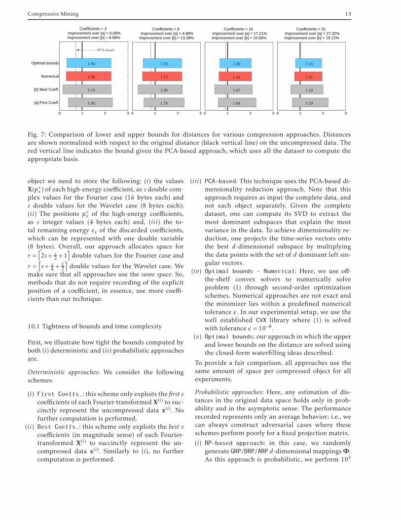
Fig. 7: Comparison of lower and upper bounds for distances for various compression approaches. Distancesare shown normalized with respect to the original distance (black vertical line) on the uncompressed data. Thered vertical line indicates the bound given the PCA-based approach, which uses all the dataset to compute theappropriate basis.
object we need to store the following: (i) the valuesX(p+x ) of each high-energy coefficient, as s double com-plex values for the Fourier case (16 bytes each) ands double values for the Wavelet case (8 bytes each);(ii) The positions p+x of the high-energy coefficients,as s integer values (4 bytes each) and, (iii) the to-tal remaining energy ex of the discarded coefficients,which can be represented with one double variable(8 bytes). Overall, our approach allocates space for
r =⌈
2s + s2 +1
⌉
double values for the Fourier case and
r =⌈
s + s4 +
12
⌉
double values for the Wavelet case. Wemake sure that all approaches use the same space. So,methods that do not require recording of the explicitposition of a coefficient, in essence, use more coeffi-cients than our technique.
10.1 Tightness of bounds and time complexity
First, we illustrate how tight the bounds computed byboth (i) deterministic and (ii) probabilistic approachesare.
Deterministic approaches: We consider the followingschemes:
(i) First Coeffs.: this scheme only exploits the first scoefficients of each Fourier-transformed X(i) to suc-cinctly represent the uncompressed data x(i). Nofurther computation is performed.
(ii) Best Coeffs.: this scheme only exploits the best scoefficients (in magnitude sense) of each Fourier-transformed X(i) to succinctly represent the un-compressed data x(i). Similarly to (i), no furthercomputation is performed.
(iii) PCA-based. This technique uses the PCA-based di-mensionality reduction approach. Note that thisapproach requires as input the complete data, andnot each object separately. Given the completedataset, one can compute its SVD to extract themost dominant subspaces that explain the mostvariance in the data. To achieve dimensionality re-duction, one projects the time-series vectors ontothe best d-dimensional subspace by multiplyingthe data points with the set of d dominant left sin-gular vectors.
(iv) Optimal bounds - Numerical: Here, we use off-the-shelf convex solvers to numerically solveproblem (1) through second-order optimizationschemes. Numerical approaches are not exact andthe minimizer lies within a predefined numericaltolerance ǫ. In our experimental setup, we use thewell established CVX library where (1) is solvedwith tolerance ǫ = 10−8.
(v) Optimal bounds: our approach in which the upperand lower bounds on the distance are solved usingthe closed-form waterfilling ideas described.
To provide a fair comparison, all approaches use thesame amount of space per compressed object for allexperiments.
Probabilistic approaches: Here, any estimation of dis-tances in the original data space holds only in prob-ability and in the asymptotic sense. The performancerecorded represents only an average behavior; i.e., wecan always construct adversarial cases where theseschemes perform poorly for a fixed projection matrix.
(i) RP-based approach: in this case, we randomlygenerate GRP/BRP/ARP d-dimensional mappingsΦ.As this approach is probabilistic, we perform 103
14 Michail Vlachos et al.
0 1 2 3
RP−based
Optimal bounds
1.30
1.94
Coefficients = 4
PCA-based
0 1 2 3
0.97
1.70
Coefficients = 8
0 1 2 3
0.70
1.39
Coefficients = 16
0 1 2 3
0.49
1.15
Coefficients = 32
0 0.5 1 1.5 2 2.5
RP−based
Optimal bounds
1.08
0.82
Coefficients = 4
PCA-based
0 0.5 1 1.5 2 2.5
0.86
0.77
Coefficients = 8
0 0.5 1 1.5 2 2.5
0.65
0.72
Coefficients = 16
0 0.5 1 1.5 2 2.5
0.47
0.63
Coefficients = 32
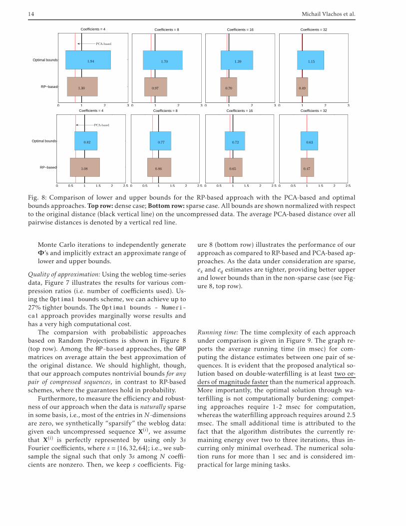
Fig. 8: Comparison of lower and upper bounds for the RP-based approach with the PCA-based and optimalbounds approaches.Top row: dense case; Bottom row: sparse case. All bounds are shown normalizedwith respectto the original distance (black vertical line) on the uncompressed data. The average PCA-based distance over allpairwise distances is denoted by a vertical red line.
Monte Carlo iterations to independently generateΦ’s and implicitly extract an approximate range oflower and upper bounds.
Quality of approximation: Using the weblog time-seriesdata, Figure 7 illustrates the results for various com-pression ratios (i.e. number of coefficients used). Us-ing the Optimal bounds scheme, we can achieve up to27% tighter bounds. The Optimal bounds - Numeri-
cal approach provides marginally worse results andhas a very high computational cost.
The comparsion with probabilistic approachesbased on Random Projections is shown in Figure 8(top row). Among the RP-based approaches, the GRP
matrices on average attain the best approximation ofthe original distance. We should highlight, though,that our approach computes nontrivial bounds for anypair of compressed sequences, in contrast to RP-basedschemes, where the guarantees hold in probability.
Furthermore, to measure the efficiency and robust-ness of our approach when the data is naturally sparsein some basis, i.e., most of the entries inN-dimensionsare zero, we synthetically “sparsify” the weblog data:given each uncompressed sequence X(i), we assumethat X(i) is perfectly represented by using only 3sFourier coefficients, where s = {16,32,64}; i.e., we sub-sample the signal such that only 3s among N coeffi-cients are nonzero. Then, we keep s coefficients. Fig-
ure 8 (bottom row) illustrates the performance of ourapproach as compared to RP-based and PCA-based ap-proaches. As the data under consideration are sparse,ex and eq estimates are tighter, providing better upperand lower bounds than in the non-sparse case (see Fig-ure 8, top row).
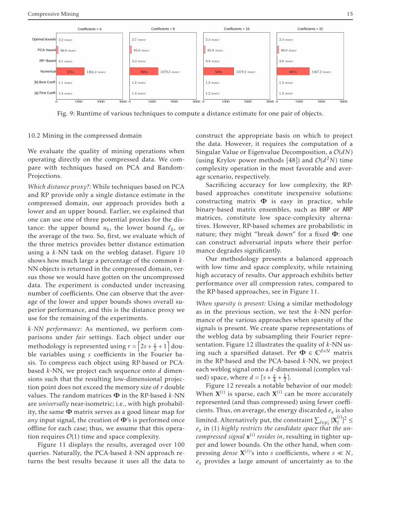
Running time: The time complexity of each approachunder comparison is given in Figure 9. The graph re-ports the average running time (in msec) for com-puting the distance estimates between one pair of se-quences. It is evident that the proposed analytical so-lution based on double-waterfilling is at least two or-ders of magnitude faster than the numerical approach.More importantly, the optimal solution through wa-terfilling is not computationally burdening: compet-ing approaches require 1-2 msec for computation,whereas the waterfilling approach requires around 2.5msec. The small additional time is attributed to thefact that the algorithm distributes the currently re-maining energy over two to three iterations, thus in-curring only minimal overhead. The numerical solu-tion runs for more than 1 sec and is considered im-practical for large mining tasks.
Compressive Mining 15
0 1000 2000 3000
[a] First Coeff.
[b] Best Coeff.
Numerical
RP−Based
PCA−based
Optimal bounds
1.3 msec
1.1 msec
1264.4 msec
3.1 msec
86.0 msec
2.2 msec
573x
Coefficients = 4
0 1000 2000 3000
1.3 msec
1.2 msec
1279.3 msec
3.4 msec
85.6 msec
2.7 msec
469x
Coefficients = 8
0 1000 2000 3000
1.2 msec
1.3 msec
1379.2 msec
8.8 msec
85.8 msec
2.3 msec
588x
Coefficients = 16
0 1000 2000 3000
1.3 msec
1.3 msec
1467.2 msec
8.0 msec
86.0 msec
2.4 msec
607x
Coefficients = 32
Fig. 9: Runtime of various techniques to compute a distance estimate for one pair of objects.
10.2 Mining in the compressed domain
We evaluate the quality of mining operations whenoperating directly on the compressed data. We com-pare with techniques based on PCA and Random-Projections.
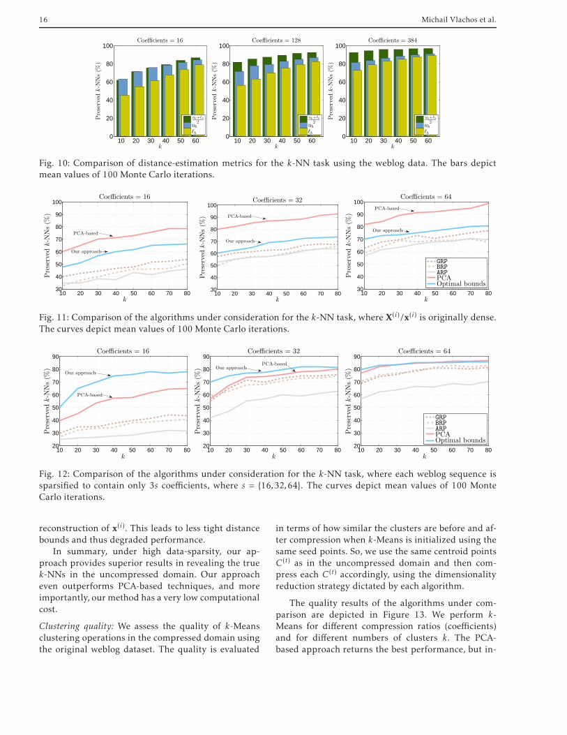
Which distance proxy?:While techniques based on PCAand RP provide only a single distance estimate in thecompressed domain, our approach provides both alower and an upper bound. Earlier, we explained thatone can use one of three potential proxies for the dis-tance: the upper bound ub, the lower bound ℓb, orthe average of the two. So, first, we evaluate which ofthe three metrics provides better distance estimationusing a k-NN task on the weblog dataset. Figure 10shows how much large a percentage of the common k-NN objects is returned in the compressed domain, ver-sus those we would have gotten on the uncompresseddata. The experiment is conducted under increasingnumber of coefficients. One can observe that the aver-age of the lower and upper bounds shows overall su-perior performance, and this is the distance proxy weuse for the remaining of the experiments.
k-NN performance: As mentioned, we perform com-parisons under fair settings. Each object under our
methodology is represented using r =⌈
2s + s2 +1
⌉
dou-ble variables using s coefficients in the Fourier ba-sis. To compress each object using RP-based or PCA-based k-NN, we project each sequence onto d dimen-sions such that the resulting low-dimensional projec-tion point does not exceed the memory size of r doublevalues. The random matrices Φ in the RP-based k-NNare universally near-isometric; i.e., with high probabil-ity, the same Φ matrix serves as a good linear map forany input signal, the creation ofΦ’s is performed onceoffline for each case; thus, we assume that this opera-tion requires O(1) time and space complexity.
Figure 11 displays the results, averaged over 100queries. Naturally, the PCA-based k-NN approach re-turns the best results because it uses all the data to
construct the appropriate basis on which to projectthe data. However, it requires the computation of aSingular Value or Eigenvalue Decomposition, a O(dN )(using Krylov power methods [48]) and O(d2N ) timecomplexity operation in the most favorable and aver-age scenario, respectively.
Sacrificing accuracy for low complexity, the RP-based approaches constitute inexpensive solutions:constructing matrix Φ is easy in practice, whilebinary-based matrix ensembles, such as BRP or ARP
matrices, constitute low space-complexity alterna-tives. However, RP-based schemes are probabilistic innature; they might “break down” for a fixed Φ: onecan construct adversarial inputs where their perfor-mance degrades significantly.
Our methodology presents a balanced approachwith low time and space complexity, while retaininghigh accuracy of results. Our approach exhibits betterperformance over all compression rates, compared tothe RP-based approaches, see in Figure 11.
When sparsity is present: Using a similar methodologyas in the previous section, we test the k-NN perfor-mance of the various approaches when sparsity of thesignals is present. We create sparse representations ofthe weblog data by subsampling their Fourier repre-sentation. Figure 12 illustrates the quality of k-NN us-ing such a sparsified dataset. Per Φ ∈ C
d×N matrixin the RP-based and the PCA-based k-NN, we projecteachweblog signal onto a d-dimensional (complex val-ued) space, where d = ⌈s + s
4 +12 ⌉.
Figure 12 reveals a notable behavior of our model:When X(i) is sparse, each X(i) can be more accuratelyrepresented (and thus compressed) using fewer coeffi-cients. Thus, on average, the energy discarded ex is also
limited. Alternatively put, the constraint∑
l∈p−x |X(i)l |2 ≤
ex in (1) highly restricts the candidate space that the un-
compressed signal x(i) resides in, resulting in tighter up-per and lower bounds. On the other hand, when com-pressing dense X(i)’s into s coefficients, where s ≪ N ,ex provides a large amount of uncertainty as to the
16 Michail Vlachos et al.
10 20 30 40 50 600
20
40
60
80
100
k
Preserved
k-N
Ns(%
)
Coefficients = 16
ub+ℓb
2ub
ℓb
10 20 30 40 50 600
20
40
60
80
100
k
Preserved
k-N
Ns(%
)
Coefficients = 128
ub+ℓb
2ub
ℓb
10 20 30 40 50 600
20
40
60
80
100
k
Preserved
k-N
Ns(%
)
Coefficients = 384
ub+ℓb
2ub
ℓb
Fig. 10: Comparison of distance-estimation metrics for the k-NN task using the weblog data. The bars depictmean values of 100 Monte Carlo iterations.
10 20 30 40 50 60 70 8030
40
50
60
70
80
90
100
k
Preserved
k-N
Ns(%
)
Coefficients = 16
Our approach
PCA-based
10 20 30 40 50 60 70 8030
40
50
60
70
80
90
100
k
Preserved
k-N
Ns(%
)Coefficients = 32
Our approach
PCA-based
10 20 30 40 50 60 70 8030
40
50
60
70
80
90
100
k
Preserved
k-N
Ns(%
)
Coefficients = 64
GRP
BRP
ARP
PCAOptimal bounds
Our approach
PCA-based
Fig. 11: Comparison of the algorithms under consideration for the k-NN task, where X(i)/x(i) is originally dense.The curves depict mean values of 100 Monte Carlo iterations.
10 20 30 40 50 60 70 8020
30
40
50
60
70
80
90
k
Preserved
k-N
Ns(%
)
Coefficients = 16
PCA-based
Our approach
10 20 30 40 50 60 70 8020
30
40
50
60
70
80
90
k
Preserved
k-N
Ns(%
)
Coefficients = 32
PCA-basedOur approach
10 20 30 40 50 60 70 8020
30
40
50
60
70
80
90
k
Preserved
k-N
Ns(%
)Coefficients = 64
GRP
BRP
ARP
PCAOptimal bounds
Fig. 12: Comparison of the algorithms under consideration for the k-NN task, where each weblog sequence issparsified to contain only 3s coefficients, where s = {16,32,64}. The curves depict mean values of 100 MonteCarlo iterations.
reconstruction of x(i). This leads to less tight distancebounds and thus degraded performance.
In summary, under high data-sparsity, our ap-proach provides superior results in revealing the truek-NNs in the uncompressed domain. Our approacheven outperforms PCA-based techniques, and moreimportantly, our method has a very low computationalcost.
Clustering quality: We assess the quality of k-Meansclustering operations in the compressed domain usingthe original weblog dataset. The quality is evaluated
in terms of how similar the clusters are before and af-ter compression when k-Means is initialized using thesame seed points. So, we use the same centroid pointsC(t) as in the uncompressed domain and then com-press each C(t) accordingly, using the dimensionalityreduction strategy dictated by each algorithm.
The quality results of the algorithms under com-parison are depicted in Figure 13. We perform k-Means for different compression ratios (coefficients)and for different numbers of clusters k. The PCA-based approach returns the best performance, but in-
Compressive Mining 17
0 50 100 150 200 2500
20
40
60
80
100
CoefficientsPreserved
Cluster
Assignments
(%)
Clusters = 5
Our approachPCA-based
0 50 100 150 200 2500
20
40
60
80
100
CoefficientsPreserved
Cluster
Assignments
(%)
Clusters = 10
Our approach
PCA-based
0 50 100 150 200 2500
20
40
60
80
100
CoefficientsPreserved
Cluster
Assignments
(%)
Clusters = 20
GRP
BRP
ARP
PCAOptimal bounds
Our approach
PCA-based
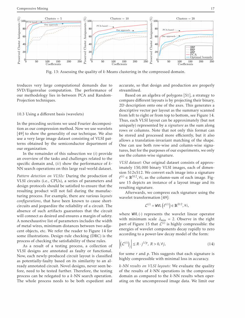
Fig. 13: Assessing the quality of k-Means clustering in the compressed domain.
troduces very large computational demands due toSVD/Eigenvalue computation. The performance ofour methodology lies in-between PCA and Random-Projection techniques.
10.3 Using a different basis (wavelets)
In the preceding sections we used Fourier decomposi-tion as our compression method. Now we use wavelets[49] to show the generality of our technique. We alsouse a very large image dataset consisting of VLSI pat-terns obtained by the semiconductor department ofour organization.
In the remainder of this subsection we (i) providean overview of the tasks and challenges related to thespecific domain and, (ii) show the performance of k-NN search operations on this large real-world dataset.
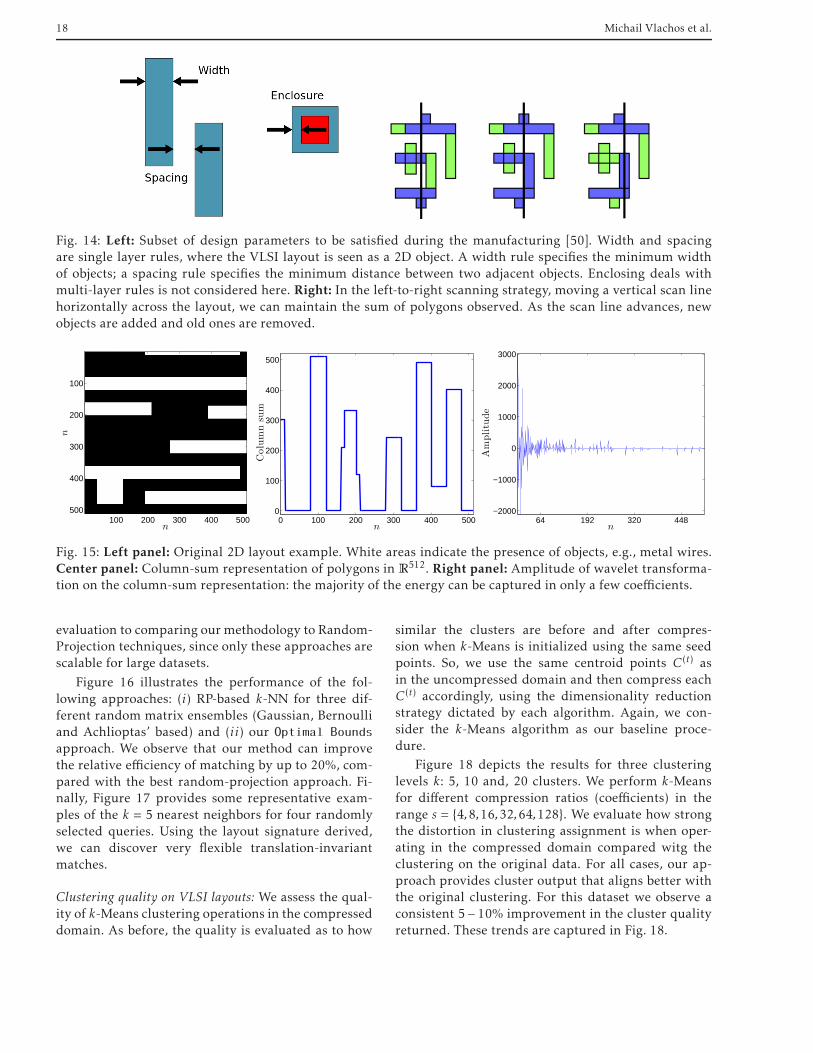
Pattern detection on VLSIs: During the production ofVLSI circuits (i.e., CPUs), a series of parameters anddesign protocols should be satisfied to ensure that theresulting product will not fail during the manufac-turing process. For example, there are various layoutsconfigurations, that have been known to cause short-circuits and jeopardize the reliability of a circuit. Theabsence of such artifacts guarantees that the circuitwill connect as desired and ensures a margin of safety.A nonexhaustive list of parameters includes the widthof metal wires, minimum distances between two adja-cent objects, etc. We refer the reader to Figure 14 forsome illustrations. Design-rule checking (DRC) is theprocess of checking the satisfiability of these rules.
As a result of a testing process, a collection ofVLSI designs are annotated as faulty or functional.Now, each newly-produced circuit layout is classifiedas potentially-faulty based on its similarity to an al-ready annotated circuit. Novel designs, never seen be-fore, need to be tested further. Therefore, the testingprocess can be relegated to a k-NN search operation.The whole process needs to be both expedient and
accurate, so that design and production are properlystreamlined.
Based on an algebra of polygons [51], a strategy tocompare different layouts is by projecting their binary,2D description onto one of the axes. This generates adescriptive vector per layout as the summary scannedfrom left to right or from top to bottom, see Figure 14.Thus, each VLSI layout can be approximately (but notuniquely) represented by a signature as the sum alongrows or columns. Note that not only this format canbe stored and processed more efficiently, but it alsoallows a translation-invariant matching of the shape.One can use both row-wise and column-wise signa-tures, but for the purposes of our experiments, we onlyuse the column-wise signature.
VLSI dataset: Our original dataset consists of approx-imately 150,000 binary VLSI images, each of dimen-sion 512x512. We convert each image into a signatureℓ(i) ∈ R
512,∀i, as the column-sum of each image. Fig-ure 15 depicts an instance of a layout image and itsresulting signature.
Afterwards, we compress each signature using thewavelet transformation [49]:
L(i) = WVL(
ℓ(i))
∈R512,∀i,
where WVL (·) represents the wavelet linear operatorwith minimum scale Jmin = 2. Observe in the rightpart of Figure 15 that L(i) is highly compressible: theenergies of wavelet components decay rapidly to zeroaccording to a power-law decay model of the form:∣
∣
∣
∣
∣
(
L(i))
j
∣
∣
∣
∣
∣
≤ R · j1/p , R > 0,∀j, (14)
for some r and p. This suggests that each signature ishighly compressible with minimal loss in accuracy.
k-NN results on VLSI layouts: We evaluate the qualityof the results of k-NN operations in the compresseddomain as compared to the k-NN results when oper-ating on the uncompressed image data. We limit our
18 Michail Vlachos et al.
Fig. 14: Left: Subset of design parameters to be satisfied during the manufacturing [50]. Width and spacingare single layer rules, where the VLSI layout is seen as a 2D object. A width rule specifies the minimum widthof objects; a spacing rule specifies the minimum distance between two adjacent objects. Enclosing deals withmulti-layer rules is not considered here. Right: In the left-to-right scanning strategy, moving a vertical scan linehorizontally across the layout, we can maintain the sum of polygons observed. As the scan line advances, newobjects are added and old ones are removed.
n
n
100 200 300 400 500
100
200
300
400
5000 100 200 300 400 500
0
100
200
300
400
500
n
Columnsum
64 192 320 448−2000
−1000
0
1000
2000
3000
n
Amplitude
Fig. 15: Left panel: Original 2D layout example. White areas indicate the presence of objects, e.g., metal wires.Center panel: Column-sum representation of polygons in R
512. Right panel: Amplitude of wavelet transforma-tion on the column-sum representation: the majority of the energy can be captured in only a few coefficients.
evaluation to comparing our methodology to Random-Projection techniques, since only these approaches arescalable for large datasets.
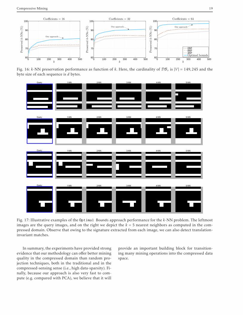
Figure 16 illustrates the performance of the fol-lowing approaches: (i) RP-based k-NN for three dif-ferent random matrix ensembles (Gaussian, Bernoulliand Achlioptas’ based) and (ii) our Optimal Bounds
approach. We observe that our method can improvethe relative efficiency of matching by up to 20%, com-pared with the best random-projection approach. Fi-nally, Figure 17 provides some representative exam-ples of the k = 5 nearest neighbors for four randomlyselected queries. Using the layout signature derived,we can discover very flexible translation-invariantmatches.
Clustering quality on VLSI layouts: We assess the qual-ity of k-Means clustering operations in the compresseddomain. As before, the quality is evaluated as to how
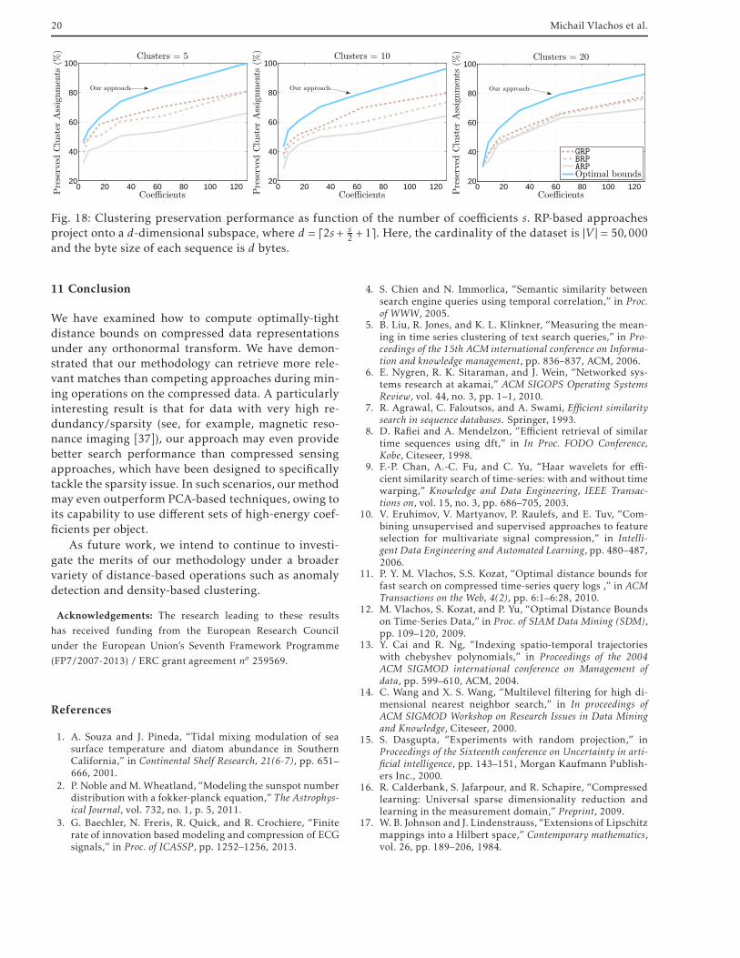
similar the clusters are before and after compres-sion when k-Means is initialized using the same seedpoints. So, we use the same centroid points C(t) asin the uncompressed domain and then compress eachC(t) accordingly, using the dimensionality reductionstrategy dictated by each algorithm. Again, we con-sider the k-Means algorithm as our baseline proce-dure.
Figure 18 depicts the results for three clusteringlevels k: 5, 10 and, 20 clusters. We perform k-Meansfor different compression ratios (coefficients) in therange s = {4,8,16,32,64,128}. We evaluate how strongthe distortion in clustering assignment is when oper-ating in the compressed domain compared witg theclustering on the original data. For all cases, our ap-proach provides cluster output that aligns better withthe original clustering. For this dataset we observe aconsistent 5− 10% improvement in the cluster qualityreturned. These trends are captured in Fig. 18.
Compressive Mining 19
0 100 200 300 400 50060
70
80
90
100
k
Preserved
k-N
Ns(%
)Coefficients = 16
Our approach
0 100 200 300 400 50060
70
80
90
100
k
Preserved
k-N
Ns(%
)
Coefficients = 32
Our approach
0 100 200 300 400 50060
70
80
90
100
k
Preserved
k-N
Ns(%
)
Coefficients = 64
GRP
BRP
ARP
Optimal bounds
Our approach
Fig. 16: k-NN preservation performance as function of k. Here, the cardinality of DBr is |V | = 149,245 and thebyte size of each sequence is d bytes.
4-NN 5-NN1-NN 2-NN 3-NN
3-NN 4-NN 5-NNQuery 1-NN 2-NN
4-NN 5-NNQuery 1-NN 2-NN 3-NN
4-NN 5-NNQuery 1-NN 2-NN 3-NN
Query
Fig. 17: Illustrative examples of the Optimal Bounds approach performance for the k-NN problem. The leftmostimages are the query images, and on the right we depict the k = 5 nearest neighbors as computed in the com-pressed domain. Observe that owing to the signature extracted from each image, we can also detect translation-invariant matches.
In summary, the experiments have provided strongevidence that our methodology can offer better miningquality in the compressed domain than random pro-jection techniques, both in the traditional and in thecompressed-sensing sense (i.e., high data-sparsity). Fi-nally, because our approach is also very fast to com-pute (e.g. compared with PCA), we believe that it will
provide an important building block for transition-ing many mining operations into the compressed dataspace.
20 Michail Vlachos et al.
0 20 40 60 80 100 12020
40
60
80
100
CoefficientsPreserved
Cluster
Assignments
(%)
Clusters = 5
Our approach
0 20 40 60 80 100 12020
40
60
80
100
CoefficientsPreserved
Cluster
Assignments
(%)
Clusters = 10
Our approach
0 20 40 60 80 100 12020
40
60
80
100
CoefficientsPreserved
Cluster
Assignments
(%)
Clusters = 20
GRP
BRP
ARP
Optimal bounds
Our approach
Fig. 18: Clustering preservation performance as function of the number of coefficients s. RP-based approachesproject onto a d-dimensional subspace, where d = ⌈2s + s
2 +1⌉. Here, the cardinality of the dataset is |V | = 50,000and the byte size of each sequence is d bytes.
11 Conclusion
We have examined how to compute optimally-tightdistance bounds on compressed data representationsunder any orthonormal transform. We have demon-strated that our methodology can retrieve more rele-vant matches than competing approaches during min-ing operations on the compressed data. A particularlyinteresting result is that for data with very high re-dundancy/sparsity (see, for example, magnetic reso-nance imaging [37]), our approach may even providebetter search performance than compressed sensingapproaches, which have been designed to specificallytackle the sparsity issue. In such scenarios, ourmethodmay even outperform PCA-based techniques, owing toits capability to use different sets of high-energy coef-ficients per object.
As future work, we intend to continue to investi-gate the merits of our methodology under a broadervariety of distance-based operations such as anomalydetection and density-based clustering.
Acknowledgements: The research leading to these results
has received funding from the European Research Council
under the European Union’s Seventh Framework Programme
(FP7/2007-2013) / ERC grant agreement no 259569.
References
1. A. Souza and J. Pineda, “Tidal mixing modulation of seasurface temperature and diatom abundance in SouthernCalifornia,” in Continental Shelf Research, 21(6-7), pp. 651–666, 2001.
2. P. Noble andM.Wheatland, “Modeling the sunspot numberdistribution with a fokker-planck equation,” The Astrophys-ical Journal, vol. 732, no. 1, p. 5, 2011.
3. G. Baechler, N. Freris, R. Quick, and R. Crochiere, “Finiterate of innovation based modeling and compression of ECGsignals,” in Proc. of ICASSP, pp. 1252–1256, 2013.
4. S. Chien and N. Immorlica, “Semantic similarity betweensearch engine queries using temporal correlation,” in Proc.of WWW, 2005.
5. B. Liu, R. Jones, and K. L. Klinkner, “Measuring the mean-ing in time series clustering of text search queries,” in Pro-ceedings of the 15th ACM international conference on Informa-tion and knowledge management, pp. 836–837, ACM, 2006.
6. E. Nygren, R. K. Sitaraman, and J. Wein, “Networked sys-tems research at akamai,” ACM SIGOPS Operating SystemsReview, vol. 44, no. 3, pp. 1–1, 2010.
7. R. Agrawal, C. Faloutsos, and A. Swami, Efficient similaritysearch in sequence databases. Springer, 1993.
8. D. Rafiei and A. Mendelzon, “Efficient retrieval of similartime sequences using dft,” in In Proc. FODO Conference,Kobe, Citeseer, 1998.
9. F.-P. Chan, A.-C. Fu, and C. Yu, “Haar wavelets for effi-cient similarity search of time-series: with and without timewarping,” Knowledge and Data Engineering, IEEE Transac-tions on, vol. 15, no. 3, pp. 686–705, 2003.
10. V. Eruhimov, V. Martyanov, P. Raulefs, and E. Tuv, “Com-bining unsupervised and supervised approaches to featureselection for multivariate signal compression,” in Intelli-gent Data Engineering and Automated Learning, pp. 480–487,2006.
11. P. Y. M. Vlachos, S.S. Kozat, “Optimal distance bounds forfast search on compressed time-series query logs ,” in ACMTransactions on the Web, 4(2), pp. 6:1–6:28, 2010.
12. M. Vlachos, S. Kozat, and P. Yu, “Optimal Distance Boundson Time-Series Data,” in Proc. of SIAM Data Mining (SDM),pp. 109–120, 2009.
13. Y. Cai and R. Ng, “Indexing spatio-temporal trajectorieswith chebyshev polynomials,” in Proceedings of the 2004ACM SIGMOD international conference on Management ofdata, pp. 599–610, ACM, 2004.
14. C. Wang and X. S. Wang, “Multilevel filtering for high di-mensional nearest neighbor search,” in In proceedings ofACM SIGMOD Workshop on Research Issues in Data Miningand Knowledge, Citeseer, 2000.
15. S. Dasgupta, “Experiments with random projection,” inProceedings of the Sixteenth conference on Uncertainty in arti-ficial intelligence, pp. 143–151, Morgan Kaufmann Publish-ers Inc., 2000.
16. R. Calderbank, S. Jafarpour, and R. Schapire, “Compressedlearning: Universal sparse dimensionality reduction andlearning in the measurement domain,” Preprint, 2009.
17. W. B. Johnson and J. Lindenstrauss, “Extensions of Lipschitzmappings into a Hilbert space,” Contemporary mathematics,vol. 26, pp. 189–206, 1984.
Compressive Mining 21
18. P. Indyk and A. Naor, “Nearest-neighbor-preserving em-beddings,” ACM Transactions on Algorithms (TALG), vol. 3,no. 3, p. 31, 2007.
19. N. Ailon and B. Chazelle, “Approximate nearest neighborsand the fast Johnson-Lindenstrauss transform,” in Proceed-ings of the thirty-eighth annual ACM symposium on Theory ofcomputing, pp. 557–563, ACM, 2006.
20. C. Boutsidis, A. Zouzias, and P. Drineas, “Random Projec-tions for k-means Clustering,” in Advances in Neural Infor-mation Processing Systems, pp. 298–306, 2010.
21. A. Cardoso and A. Wichert, “Iterative random projectionsfor high-dimensional data clustering,” Pattern RecognitionLetters, vol. 33, no. 13, pp. 1749–1755, 2012.
22. D. Achlioptas, “Database-friendly random projections,” inProc. of ACM PODS, pp. 274–281, 2001.
23. E. Bingham and H. Mannila, “Random projection in dimen-sionality reduction: applications to image and text data,” inProceedings of the seventh ACM SIGKDD international confer-ence on Knowledge discovery and data mining, pp. 245–250,ACM, 2001.
24. N. M. Freris, M. Vlachos, and S. S. Kozat, “Optimal dis-tance estimation between compressed data series.,” in SDM,pp. 343–354, 2012.
25. M. Vlachos, P. Yu, and V. Castelli, “On periodicity detectionand structural periodic similarity,” in SIAM InternationalConference on Data Mining, pp. 449–460, 2005.
26. A. Mueen, S. Nath, and J. Liu, “Fast approximate correla-tion for massive time-series data,” in Proceedings of the 2010ACM SIGMOD International Conference on Management ofdata, pp. 171–182, ACM, 2010.
27. E. Keogh and S. Kasetty, “On the Need for Time Series DataMining Benchmarks: A Survey and Empirical Demonstra-tion,” in Proc. of KDD, 2002.
28. A. Mueen, E. J. Keogh, and N. B. Shamlo, “Finding TimeSeries Motifs in Disk-Resident Data,” in Proc. of ICDM,pp. 367–376, 2009.
29. A. V. Oppenheim, R. W. Schafer, J. R. Buck, et al., Discrete-time signal processing, vol. 5. Prentice Hall Upper SaddleRiver, 1999.
30. E. Keogh, K. Chakrabarti, S. Mehrotra, and M. Pazzani,“Locally Adaptive Dimensionality Reduction for IndexingLarge Time Series Databases,” in Proc. of ACM SIGMOD,pp. 151–162, 2001.
31. S. Boyd and L. Vandenberghe, Convex Optimization. Cam-bridge University Press, 1st ed., 2004.
32. M. Grant and S. Boyd, “Graph Implementations for Nons-mooth Convex Programs,” Recent Advances in Learning andControl, Springer, pp. 95–110, 2008.
33. T. Basar and G. J. Olsder,Dynamic Noncooperative Game The-ory. Academic Press, 2nd ed., 1995.
34. D. L. Donoho, “Compressed sensing,” Information Theory,IEEE Transactions on, vol. 52, no. 4, pp. 1289–1306, 2006.
35. T. Cover and P. Hart, “Nearest neighbor pattern classifi-cation,” Information Theory, IEEE Transactions on, vol. 13,no. 1, pp. 21–27, 1967.
36. P. W. Jones, A. Osipov, and V. Rokhlin, “Randomized ap-proximate nearest neighbors algorithm,” Proceedings of theNational Academy of Sciences, vol. 108, no. 38, pp. 15679–15686, 2011.
37. E. J. Candes, J. K. Romberg, and T. Tao, “Stable signal recov-ery from incomplete and inaccurate measurements,” Com-munications on pure and applied mathematics, vol. 59, no. 8,pp. 1207–1223, 2006.
38. E. Kushilevitz, R. Ostrovsky, and Y. Rabani, “Efficient searchfor approximate nearest neighbor in high dimensionalspaces,” SIAM Journal on Computing, vol. 30, no. 2, pp. 457–474, 2000.
39. C. Hegde, A. Sankaranarayanan, W. Yin, and R. Baraniuk,“A convex approach for learning near-isometric linear em-beddings,” preprint, August, 2012.
40. S. Dasgupta, “Learning mixtures of Gaussians,” in Founda-tions of Computer Science, 1999. 40th Annual Symposium on,pp. 634–644, IEEE, 1999.
41. R. I. Arriaga and S. Vempala, “An algorithmic theory oflearning: Robust concepts and randomprojection,” in Foun-dations of Computer Science, 1999. 40th Annual Symposiumon, pp. 616–623, IEEE, 1999.
42. N. M. Freris, M. Vlachos, and D. S. Turaga, “Cluster-Aware Compression with Provable K-means Preservation,”in SDM, pp. 82–93, 2012.
43. S. Lloyd, “Least squares quantization in PCM,” InformationTheory, IEEE Transactions on, vol. 28, no. 2, pp. 129–137,1982.
44. A. Tanay, R. Sharan, and R. Shamir, “Biclustering algo-rithms: A survey,” Handbook of computational molecular bi-ology, vol. 9, pp. 26–1, 2005.
45. I. S. Dhillon, “Co-clustering documents and words usingbipartite spectral graph partitioning,” in Proceedings of theseventh ACM SIGKDD international conference on Knowledgediscovery and data mining, pp. 269–274, ACM, 2001.
46. P. J. Huber, “Projection pursuit,” The annals of Statistics,pp. 435–475, 1985.
47. D. Arthur and S. Vassilvitskii, “k-Means++: The Advantagesof Careful Seeding,” in Proc. of Symposium of Discrete Anal-ysis, 2005.
48. J. K. Cullum and R. A. Willoughby, Lanczos Algorithms forLarge Symmetric Eigenvalue Computations: Volume 1, Theory.No. 41, SIAM, 2002.
49. S. Mallat, A wavelet tour of signal processing. Elsevier, 1999.50. Wikipedia, “http://en.wikipedia.org/wiki/Design_
rule_checking.”51. B. Crawford, “Design rules checking for integrated circuits
using graphical operators,” in Proceedings of the 2nd annualconference on Computer graphics and interactive techniques,pp. 168–176, ACM, 1975.
12 Appendix
12.1 Existence of solutions and necessary andsufficient conditions for optimality
The constraint set is a compact convex set, in fact, acompact polyhedron. The function g(x,y) := −√x√y isconvex but not strictly convex on R
2+. To see this, note
that the Hessian exists for all x,y > 0 and equals
▽2g =
1
4
x−32 y−
12 −x− 1
2 y−12
−x− 12 y−
12 x−
12 y−
32
with eigenvalues 0, 1√xy (
1x + 1
y ), and hence is positive
semi-definite, which in turn implies that g is convex[31]. Furthermore, −√x is a strictly convex function ofx so that the objective function of (3) is convex, andstrictly convex only if p−x ∩ p−q = ∅. It is also a continu-
ous function so solutions exist, i.e., the optimal valueis bounded and is attained. It is easy to check thatthe Slater condition holds, whence the problem satis-fies strong duality and there exist Lagrange multipli-ers [31]. We skip the technical details for simplicity,
22 Michail Vlachos et al.
but we want to highlight that this property is crucialbecause it guarantees that the Karush–Kuhn–Tucker(KKT) necessary conditions [31] for Lagrangian opti-mality are also sufficient. Therefore, if we can find asolution that satisfies the KKT conditions for the prob-lem, we have found an exact optimal solution and theexact optimal value of the problem. The Lagrangian is
L(y,z,λ,µ,α,β) := −2∑
i∈P1bi√zi − 2
∑
i∈P2ai√yi − 2
∑
i∈P3
√zi√yi (A-1)
+λ(∑
i∈p−x(zi − ex)
)
+µ(∑
i∈p−q(yi − eq)
)
+∑
i∈p−xαi (zi −Z) +
∑
i∈p−qβi (yi −Y ) .
The KKT conditions are as follows6:
0 ≤ zi ≤ Z, 0 ≤ yi ≤ Y , (PF) (A-2a)∑
i∈p−xzi ≤ ex ,
∑
i∈p−xzi ≤ eQ
λ,µ,αi ,βi ≥ 0 (DF) (A-2b)
αi (zi −Z) = 0, βi (yi −Y ) = 0 (CS) (A-2c)
λ(∑
i∈p−x(zi − ex)
)
= 0, µ(∑
i∈p−q(yi − eq)
)
= 0
i ∈ P1 :∂L
∂zi= − bi√
zi+λ+αi = 0 (O) (A-2d)
i ∈ P2 :∂L
∂yi= − ai√
yi+µ+ βi = 0
i ∈ P3 :∂L
∂zi= −√yi√zi
+λ+αi = 0
∂L
∂yi= −√zi√yi
+µ+ βi = 0 ,
where we use shorthand notation for Primal Feasibil-
ity (PF), Dual Feasibility (DF), Complementary Slackness
(CS), and Optimality (O) [31].
12.2 Proof of theorem 1
For the first part, note that problem (3) is a doubleminimization problem over {zi }i∈p−x and {yi }i∈p−q . If wefix one vector in the objective function of (3), then theoptimal solution with respect to the other one is givenby the waterfilling algorithm. In fact, if we considerthe KKT conditions (A-2) or the KKT conditions to (2),they correspond exactly to (7). The waterfilling algo-rithm has the property that if a = waterfill (b, ex ,A),then bi > 0 implies ai > 0. Furthermore, it has a mono-tonicity property in the sense that bi ≤ bj impliesai ≤ aj . Assume that, at optimality, al1 < al2 for somel1 ∈ P1, l2 ∈ P3. Because bl1 ≥ B ≥ bl3 we can swap thesetwo values to decrease the objective function, which is
6 The condition (A-2d) excludes the cases that for some i zi =0, or yi = 0, which will be treated separately.
a contradiction. The exact same argument applies for{bl}, so minl∈P1 al ≥maxl∈P3 al ,minl∈P2 bl ≥maxl∈P3 bl .
For the second part, note that −∑i∈P3√zi√yi ≥
−√
e′x√
e′q. If e′xe′q > 0, then at optimality this is attained
with equality for the particular choice of {al ,bl }l∈P3 .It follows that all entries of the optimal solution{al ,bl }l∈p−x∪p−q are strictly positive, hence (A-2d) impliesthat
ai =bi
λ+αi, i ∈ P1 (A-3a)
bi =ai
µ+ βi, i ∈ P2 (A-3b)
ai = (µ+ βi )bi , i ∈ P3 (A-3c)
bi = (λ+αi )ai , i ∈ P3.
For the particular solution with all entries in
P3 equal(
al =√
e′x/ |P3|,bl =√
e′q/ |P3|)
, (8a) is an im-
mediate application of (A-3.c). The optimal entries{al}l∈P1 , {bl }l∈P2 are provided by waterfilling with avail-able energies ex − e′x, eq − e′q, respectively, so (9) imme-diately follows.
For the third part, note that the cases that eithere′x = 0, e′q > 0 or e′x > 0, e′q = 0 are excluded at optimalityby the first part, cf. (7).
For the last part, note that when e′x = e′q = 0, equiv-
alently al = bl = 0 for l ∈ P3, it is not possible to takederivatives with respect to any coefficient in P3, so thelast two equations of (A-2) do not hold. In that case,we need to perform a standard perturbation analy-sis. Let ǫ := {ǫl}l∈P1∪P2 be a sufficiently small positivevector. As the constraint set of (3) is linear in zi ,yi ,any feasible direction (of potential decrease of the ob-jective function) is of the form zi ← zi − ǫi , i ∈ P1,yi ← yi − ǫi , i ∈ P2, and zi ,yi ≥ 0, i ∈ P3 such that∑
i∈P3 zi =∑
i∈P1 ǫi ,∑
i∈P3 yi =∑
i∈P2 ǫi . The change in the
objective function is then equal to (modulo an o(||ǫ||2)term)
g(ǫ) ≈ 1
2
∑
i∈P1
bi√ziǫi +
1
2
∑
i∈P2
ai√yi
ǫi −∑
i∈P3
√zi√yi (A-4)
≥ 1
2
∑
i∈P1
bi√ziǫi +
1
2
∑
i∈P2
ai√yi
ǫi −√
∑
i∈P1ǫi
√
∑
i∈P2ǫi
≥ 1
2mini∈P1
bi√ziǫ1 +
1
2mini∈P2
ai√yi
ǫ2 −√ǫ1ǫ2,
where the first inequality follows from an applicationof the Cauchy–Schwartz inequality to the last term,and in the second one we have defined ǫj =
∑
i∈Pj ǫi , i =
1,2. Let us define ǫ :=√ǫ1/ǫ2. From the last expres-
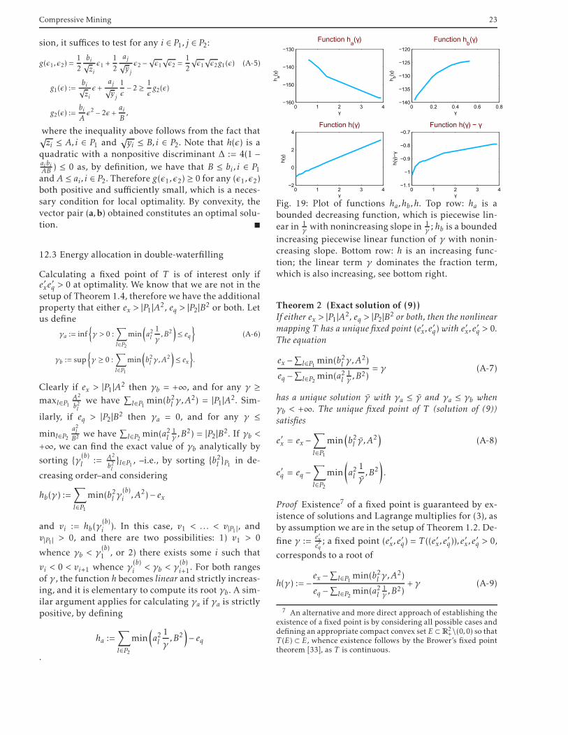
Compressive Mining 23
sion, it suffices to test for any i ∈ P1, j ∈ P2:
g(ǫ1,ǫ2) =1
2
bi√ziǫ1 +
1
2
aj√yj
ǫ2 −√ǫ1√ǫ2 =
1
2
√ǫ1√ǫ2g1(ǫ) (A-5)
g1(ǫ) :=bi√ziǫ +
aj√yj
1
ǫ− 2 ≥ 1
ǫg2(ǫ)
g2(ǫ) :=biAǫ2 − 2ǫ + ai
B,
where the inequality above follows from the fact that√zi ≤ A,i ∈ P1 and
√yi ≤ B,i ∈ P2. Note that h(ǫ) is a
quadratic with a nonpositive discriminant ∆ := 4(1 −aibiAB ) ≤ 0 as, by definition, we have that B ≤ bi , i ∈ P1and A ≤ ai , i ∈ P2. Therefore g(ǫ1,ǫ2) ≥ 0 for any (ǫ1,ǫ2)both positive and sufficiently small, which is a neces-sary condition for local optimality. By convexity, thevector pair (a,b) obtained constitutes an optimal solu-tion. �
12.3 Energy allocation in double-waterfilling
Calculating a fixed point of T is of interest only ife′xe′q > 0 at optimality. We know that we are not in the
setup of Theorem 1.4, therefore we have the additionalproperty that either ex > |P1|A2, eq > |P2|B2 or both. Letus define
γa := inf{
γ > 0 :∑
l∈P2min
(
a2l1
γ,B2
)
≤ eq
}
(A-6)
γb := sup{
γ ≥ 0 :∑
l∈P1min
(
b2l γ,A2)
≤ ex
}
.
Clearly if ex > |P1|A2 then γb = +∞, and for any γ ≥maxl∈P1
A2
b2lwe have
∑
l∈P1 min(b2l γ,A2) = |P1|A2. Sim-
ilarly, if eq > |P2|B2 then γa = 0, and for any γ ≤minl∈P2
a2lB2
we have∑
l∈P2 min(a2l1γ ,B
2) = |P2|B2. If γb <
+∞, we can find the exact value of γb analytically by
sorting {γ (b)l := A2
b2l}l∈P1 , –i.e., by sorting {b2l }P1 in de-
creasing order–and considering
hb(γ) :=∑
l∈P1min(b2l γ
(b)i ,A2)− ex
and vi := hb(γ(b)i ). In this case, v1 < . . . < v|P1 |, and
v|P1| > 0, and there are two possibilities: 1) v1 > 0
whence γb < γ(b)1 , or 2) there exists some i such that
vi < 0 < vi+1 whence γ(b)i < γb < γ
(b)i+1. For both ranges
of γ , the function h becomes linear and strictly increas-ing, and it is elementary to compute its root γb. A sim-ilar argument applies for calculating γa if γa is strictlypositive, by defining
ha :=∑
l∈P2min
(
a2l1
γ,B2
)
− eq.
0 1 2 3 4−160
−150
−140
−130
γ
ha(γ
)
Function ha(γ)
0 0.2 0.4 0.6 0.8−140
−135
−130
−125
−120
γ
hb(γ
)
Function hb(γ)
0 1 2 3 4−2
0
2
4
γ
h(γ
)
Function h(γ)
0 1 2 3 4−1.1
−1
−0.9
−0.8
−0.7
γ
h(γ
)−γ
Function h(γ) − γ
Fig. 19: Plot of functions ha,hb ,h. Top row: ha is abounded decreasing function, which is piecewise lin-ear in 1
γ with nonincreasing slope in 1γ ; hb is a bounded
increasing piecewise linear function of γ with nonin-creasing slope. Bottom row: h is an increasing func-tion; the linear term γ dominates the fraction term,which is also increasing, see bottom right.
Theorem 2 (Exact solution of (9))If either ex > |P1|A2, eq > |P2|B2 or both, then the nonlinear
mapping T has a unique fixed point (e′x, e′q)with e′x, e′q > 0.The equation
ex −∑
l∈P1 min(b2l γ,A2)
eq −∑
l∈P2 min(a2l1γ ,B
2)= γ (A-7)
has a unique solution γ with γa ≤ γ and γa ≤ γb when
γb < +∞. The unique fixed point of T (solution of (9))
satisfies
e′x = ex −∑
l∈P1min
(
b2l γ ,A2)
(A-8)
e′q = eq −∑
l∈P2min
(
a2l1
γ,B2
)
.
Proof Existence7 of a fixed point is guaranteed by ex-istence of solutions and Lagrange multiplies for (3), asby assumption we are in the setup of Theorem 1.2. De-
fine γ :=e′xe′q; a fixed point (e′x , e′q) = T ((e′x , e′q)), e′x , e′q > 0,
corresponds to a root of
h(γ) := −ex −
∑
l∈P1 min(b2l γ,A2)
eq −∑
l∈P2 min(a2l1γ ,B
2)+γ (A-9)
7 An alternative and more direct approach of establishing theexistence of a fixed point is by considering all possible cases anddefining an appropriate compact convex set E ⊂ R
2+\(0,0) so that
T (E) ⊂ E, whence existence follows by the Brower’s fixed pointtheorem [33], as T is continuous.
24 Michail Vlachos et al.
For the range γ ≥ γa and γ ≤ γb, if γb < +∞, we havethat h(γ) is continuous and strictly increasing. The factthat limγցγa h(γ) < 0, limγրγb h(γ) > 0 shows the exis-tence of a unique root γ of h corresponding to a uniquefixed point of T , cf. (A-8). �
Remark 5 (Exact calculation of a root of h) We seek tocalculate the root of h exactly and efficiently. In doingso, consider the points {γl}l∈P1∪P2 , where γl :=
Ab2l, l ∈
P1, γl :=a2lB , l ∈ P2. Then, note that for any γ ≥ γl , l ∈ P1
we have that min(b2l γ,A2) = A2. Similarly, for any
γ ≤ γl , l ∈ P2, we have that min(a2l1γ ,B
2) = B2. We or-
der all such points in increasing order, and considerthe resulting vector γ′ := {γ ′i } excluding any points be-low γa or above γb. Let us define hi := h(γ ′i ). If for somei, hi = 0 we are done. Otherwise there are three possi-bilities: 1) there is an i such that hi < 0 < hi+1; 2) h1 > 0,or 3) hN < 0. In all cases, the numerator (denominator)of h is linear in γ ( 1γ ) for the respective range of γ .
Therefore, γ is obtained by solving the linear equation
f (γ) := ex−∑
l∈P1min(b2l γ,A
2)−γ
eq −∑
l∈P2min
(
a2l1
γ,B2
)
.
(A-10)
Note that there is no need for further computation toset this into the form f (γ) = αγ + β for some α,β. In-stead, we use the elementary property that a linearfunction f on [x0,x1] with f (x0)f (x1) < 0 has a uniqueroot given by
x = x0 −x1 − x0
f (x1)− f (x0)f (x0) .