Embed Size (px)
Citation preview

CompSci 516Data Intensive Computing Systems
Lecture 11Parallel DBMS
andMap-‐Reduce
Instructor: Sudeepa Roy
1Duke CS, Spring 2016 CompSci 516: Data Intensive Computing Systems

Announcements
• Map-‐Reduce and Parallel DBMS have been moved earlier in the schedule– will be helpful for HW3 (and HW4)
• An anonymous poll will be posted soon– please give your feedback
2Duke CS, Spring 2016 CompSci 516: Data Intensive Computing Systems

What will we learn?
• Last lecture:–We finished query execution and query optimization
• Next:– Parallel DBMS and Map Reduce (MR)–Will discuss some more MR in the next lecture
3Duke CS, Spring 2016 CompSci 516: Data Intensive Computing Systems

Reading Material• [RG]
– Chapter 22.1-‐22.5• [GUW]
– Chapter 20.1-‐20.2
• Recommended readings:– Chapter 2 (Sections 1,2,3) of Mining of Massive Datasets, by Rajaraman and
Ullman: http://i.stanford.edu/~ullman/mmds.html– Original Google MR paper by Jeff Dean and Sanjay Ghemawat, OSDI’ 04:
http://research.google.com/archive/mapreduce.html
4
Acknowledgement: The following slides have been created adapting theinstructor material of the [RG] book provided by the authorsDr. Ramakrishnan and Dr. Gehrke.
Duke CS, Spring 2016 CompSci 516: Data Intensive Computing Systems

Parallel DBMS
Duke CS, Spring 2016 CompSci 516: Data Intensive Computing Systems 5

Basics of Parallelism
• Units: a collection of processors– assume always have local cache– may or may not have local memory or disk (next)
• A communication facility to pass information among processors– a shared bus or a switch
Duke CS, Spring 2016 CompSci 516: Data Intensive Computing Systems 6

Parallel vs. Distributed DBMSParallel DBMS
• Parallelization of various operations– e.g. loading data,
building indexes, evaluating queries
• Data may or may not be distributed initially
• Distribution is governed by performance considertaion
Duke CS, Spring 2016 CompSci 516: Data Intensive Computing Systems 7
Distributed DBMS
• Data is physically stored across different sites– Each site is typically managed by an
independent DBMS
• Location of data and autonomy of sites have impact on Query opt., Conc. Control and recovery
• Also governed by other factors:– increased availability for system
crash – local ownership and access
later, after we do transactions
today

Why Parallel Access To Data?
At 10 MB/s1.2 days to scan
1,000 x parallel1.5 minute to scan.
Parallelism:divide a big problem into many smaller onesto be solved in parallel.
Duke CS, Spring 2016 CompSci 516: Data Intensive Computing Systems 8
1 TB Data
1 TB Data

Parallel DBMS• Parallelism is natural to DBMS processing– Pipeline parallelism: many machines each doing one step in a multi-‐step process.
– Data-‐partitioned parallelism: many machines doing the same thing to different pieces of data.
– Both are natural in DBMS!
PipelineAny
SequentialProgram
Any SequentialProgram
Partition SequentialSequential SequentialSequential Any SequentialProgram
Any SequentialProgram
outputs split N ways, inputs merge M waysDuke CS, Spring 2016 CompSci 516: Data Intensive Computing Systems 9
DBMS: The parallel Success Story
• DBMSs are the most successful application of parallelism– Teradata (1979), Tandem (1974, later acquired by HP),..– Every major DBMS vendor has some parallel server
• Reasons for success:– Bulk-‐processing (= partition parallelism)– Natural pipelining– Inexpensive hardware can do the trick– Users/app-‐programmers don’t need to think in parallel
Duke CS, Spring 2016 CompSci 516: Data Intensive Computing Systems 10

Some || Terminology
• Speed-‐Up– More resources means proportionally less time for given amount of data.
• Scale-‐Up– If resources increased in proportion to increase in data size, time is constant.
#CPUs(degree of ||-‐ism)
#ops/sec.
(throughput)
Ideal:linear speed-‐up
sec./op
(response time)
#CPUs + size of databasedegree of ||-‐ism
Ideal:linear scale-‐up
Ideal graphs
Duke CS, Spring 2016 CompSci 516: Data Intensive Computing Systems 11

Some || Terminology
• Due to overhead in parallel processing
• Start-‐up costStarting the operation on many processor, might need to distribute data
• InterferenceDifferent processors may compete for the same resources
• SkewThe slowest processor (e.g. with a huge fraction of data) may become the bottleneck
#CPUs(degree of ||-‐ism)
#ops/sec.
(throughput)
#CPUs + size of databasedegree of ||-‐ism
sec./op
(response time)
In practice
Ideal:linear speed-‐up
Ideal:linear scale-‐up
Actual: sub-‐linear speed-‐up
Actual: sub-‐linear scale-‐up
Duke CS, Spring 2016 CompSci 516: Data Intensive Computing Systems 12

Architecture for Parallel DBMS
• Among different computing units
–Whether memory is shared–Whether disk is shared
Duke CS, Spring 2016 CompSci 516: Data Intensive Computing Systems 13

Shared Memory
Duke CS, Spring 2016 CompSci 516: Data Intensive Computing Systems 14
Interconnection Network
P P P
D D D
Global Shared Memorysharedmemory

Shared Disk
Duke CS, Spring 2016 CompSci 516: Data Intensive Computing Systems 15
P P P
M
D
M
D
M
D
Interconnection Network
localmemory
shared disk

Shared Nothing
Duke CS, Spring 2016 CompSci 516: Data Intensive Computing Systems 16
Interconnection Network
P P P
M
D
M
D
M
D
localmemoryand disk
no two CPU can access the samestorage area
all communicationthrough a network connection

Architecture: At A GlanceShared Memory
(SMP)Shared Disk Shared Nothing
(network)
CLIENTS CLIENTSCLIENTS
MemoryProcessors
• Easy to program• Expensive to build• Low communication overhead: shared mem.
• Difficult to scaleup(memory contention)
• Hard to program and design parallel algos
• Cheap to build• Easy to scaleup and speedup
• Considered to be the best architecture
Sequent, SGI, Sun VMScluster, Sysplex Tandem, Teradata, SP2
• Trade-off but still interference like shared-memory (contention of memory and nw bandwidth)
we will assume shared nothing
Duke CS, Spring 2016 CompSci 516: Data Intensive Computing Systems 17

What Systems Worked This Way
Shared NothingTeradata: 400 nodesTandem: 110 nodesIBM / SP2 / DB2: 128 nodesInformix/SP2 48 nodesATT & Sybase ? nodes
Shared DiskOracle 170 nodesDEC Rdb 24 nodes
Shared MemoryInformix 9 nodes RedBrick ? nodes
CLIENTS
MemoryProcessors
CLIENTS
CLIENTS
NOTE: (as of 9/1995)!
Duke CS, Spring 2016 CompSci 516: Data Intensive Computing Systems 18

Different Types of DBMS Parallelism• Intra-‐operator parallelism
– get all machines working to compute a given operation (scan, sort, join)
– OLAP (decision support)
• Inter-‐operator parallelism– each operator may run concurrently on a
different site (exploits pipelining)– For both OLAP and OLTP
• Inter-‐query parallelism– different queries run on different sites– For OLTP
• We’ll focus on intra-‐operator parallelism
⨝
𝝲
⨝
𝝲
⨝
𝝲
⨝
𝝲
Duke CS, Spring 2016 CompSci 516: Data Intensive Computing Systems 19
Ack:Slide by Prof. Dan Suciu

Data PartitioningHorizontally Partitioning a table (why horizontal?):Range-partition Hash-partition Block-partition
or Round Robin
Shared disk and memory less sensitive to partitioning, Shared nothing benefits from "good" partitioning
A...E F...J K...N O...S T...Z A...E F...J K...N O...S T...Z A...E F...J K...N O...S T...Z
• Good for equijoins, range queries, group-by• Can lead to data skew
• Good for equijoins• But only if hashed on that attribute
• Can lead to data skew
• Send i-th tuple to i-mod-n processor
• Good to spread load
• Good when the entire relation is accessed
Duke CS, Spring 2016 CompSci 516: Data Intensive Computing Systems 20

Example
• R(Key, A, B)
• Can Block-‐partition be skewed?– no, uniform
• Can Hash-‐partition be skewed?– on the key: uniform with a good hash function– on A: may be skewed, • e.g. when all tuples have the same A-‐value
Duke CS, Spring 2016 CompSci 516: Data Intensive Computing Systems 21

Parallelizing Sequential Evaluation Code
• “Streams” from different disks or the output of other operators– are “merged” as needed as input to some operator– are “split” as needed for subsequent parallel processing
• Different Split and merge operations appear in addition to relational operators
• No fixed formula for conversion• Next: parallelizing individual operations
Duke CS, Spring 2016 CompSci 516: Data Intensive Computing Systems 22

Parallel Scans
• Scan in parallel, and merge.• Selection may not require all sites for range or hash partitioning– but may lead to skew– Suppose σA = 10R and partitioned according to A– Then all tuples in the same partition/processor
• Indexes can be built at each partition
Duke CS, Spring 2016 CompSci 516: Data Intensive Computing Systems 23

Parallel Sorting
Idea: • Scan in parallel, and range-‐partition as you go– e.g. salary between 10 to 210, #processors = 20– salary in first processor: 10-‐20, second: 21-‐30, third: 31-‐40, ….
• As tuples come in, begin “local” sorting on each• Resulting data is sorted, and range-‐partitioned• Visit the processors in order to get a full sorted order• Problem: skew!• Solution: “sample” the data at start to determine partition points. Duke CS, Spring 2016 CompSci 516: Data Intensive Computing Systems 24
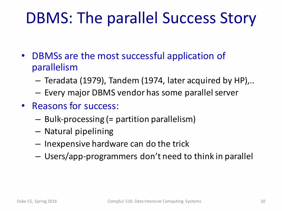
Parallel Joins
• Need to send the tuples that will join to the same machine– also for GROUP-‐BY
• Nested loop:– Each outer tuple must be compared with each inner tuple that might join.
– Easy for range partitioning on join cols, hard otherwise
• Sort-‐Merge:– Sorting gives range-‐partitioning– Merging partitioned tables is local
Duke CS, Spring 2016 CompSci 516: Data Intensive Computing Systems 25

Parallel Hash Join
• In first phase, partitions get distributed to different sites:– A good hash function automatically distributes work evenly
• Do second phase at each site.• Almost always the winner for equi-‐join
Original Relations(R then S)
OUTPUT
2
B main memory buffers DiskDisk
INPUT1
hashfunction
hB-1
Partitions
12
B-1. . .
Phase 1
Duke CS, Spring 2016 CompSci 516: Data Intensive Computing Systems 26

Dataflow Network for parallel Join
• Good use of split/merge makes it easier to build parallel versions of sequential join code.
Duke CS, Spring 2016 CompSci 516: Data Intensive Computing Systems 27

Jim Gray & Gordon Bell: VLDB 95 Parallel Database Systems Survey
Parallel Aggregates
A...E F...J K...N O...S T...Z
A Table
Count Count Count Count Count
Count
• For each aggregate function, need a decomposition:– count(S) = Σ count(s(i)), ditto for sum()– avg(S) = (Σ sum(s(i))) / Σ count(s(i))– and so on...
• For group-‐by:– Sub-‐aggregate groups close to the source.– Pass each sub-‐aggregate to its group’s site.
• Chosen via a hash fn.
Duke CS, Spring 2016 CompSci 516: Data Intensive Computing Systems 28
Which SQL aggregate operators are not good for parallel execution?

• Why?• Trivial counter-‐example:– Table partitioned with local secondary index at two nodes
– Range query: all of node 1 and 1% of node 2.– Node 1 should do a scan of its partition.– Node 2 should use secondary index.
Best serial plan may not be best ||
N..Z
TableScan
A..M
Index Scan
Duke CS, Spring 2016 CompSci 516: Data Intensive Computing Systems 29

Map-‐Reduce
Duke CS, Spring 2016 CompSci 516: Data Intensive Computing Systems 30

The Map-‐Reduce Framework
• A high level programming paradigm– allows many important data-‐oriented processes to be written simply
• A master controller – divides the data into chunks– assigns different processors to execute the map function on each chunk
– other/same processors execute the reduce functions on the outputs of the map functions
Duke CS, Spring 2016 CompSci 516: Data Intensive Computing Systems 31

Storage Model
• Data is stored in large files (TB, PB)– e.g. market-‐basket data (more when we do data mining)
– or web data• Files are divided into chunks– typically many MB (64 MB)– sometimes each chunk is replicated for fault tolerance (later)
Duke CS, Spring 2016 CompSci 516: Data Intensive Computing Systems 32

Map-‐Reduce Steps
• Input is typically (key, value) pairs– but could be objects of any type
• Map and Reduce are performed by a number of processes– physically located in some processors
Duke CS, Spring 2016 CompSci 516: Data Intensive Computing Systems 33
same key
Map ReduceShuffleInputkey-‐value pairs
outputlistssort by key

Map-‐Reduce Steps
1. Read Data2. Map – extract some info of interest
in (key, value) form3. Shuffle and sort
– send same keys to the same reduce process
Duke CS, Spring 2016 CompSci 516: Data Intensive Computing Systems 34
same key
Map ReduceShuffleInputkey-‐value pairs
outputlistssort by key
4. Reduce– operate on the values of the same key– e.g. transform, aggregate, summarize,
filter5. Output the results (key, final-‐result)

Simple Example: Map-‐Reduce
• Word counting• Inverted indexes
Ack:Slide by Prof. Shivnath Babu
Duke CS, Spring 2016 CompSci 516: Data Intensive Computing Systems 35

Map Function
• Each map process works on a chunk of data• Input: (input-‐key, value)• Output: (intermediate-‐key, value) -‐-‐may not be the same as input key value• Example: list all doc ids containing a word
– output of map (word, docid) – emits each such pair– word is key, docid is value– duplicate elimination can be done at the reduce phase
Duke CS, Spring 2016 CompSci 516: Data Intensive Computing Systems 36
same key
Map ReduceShuffleInputkey-‐value pairs
outputlistssort by key
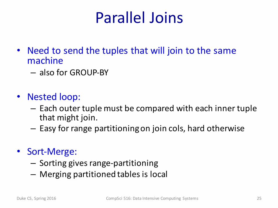
Reduce Function
• Input: (intermediate-‐key, list-‐of-‐values-‐for-‐this-‐key) – list can include duplicates– each map process can leave its output in the local disk, reduce process can retrieve its
portion• Output: (output-‐key, final-‐value)• Example: list all doc ids containing a word
– output will be a list of (word, [doc-‐id1, doc-‐id5, ….])– if the count is needed, reduce counts #docs, output will be a list of (word, count)
Duke CS, Spring 2016 CompSci 516: Data Intensive Computing Systems 37
same key
Map ReduceShuffleInputkey-‐value pairs
outputlistssort by key

More Terminology
• A Map-‐Reduce “Job”– e.g. count the words in all docs– complex queries can have multiple MR jobs
• Map or Reduce “Tasks”– A group of map or reduce “functions”– scheduled on a single “worker”
• Worker – a process that executes one task at a time– one per processor, so 4-‐8 per machine
Duke CS, Spring 2016 CompSci 516: Data Intensive Computing Systems 38
however, there is no uniformterminology across systems
Ack:Slide by Prof. Dan Suciu

Examples
Duke CS, Spring 2016 CompSci 516: Data Intensive Computing Systems 39

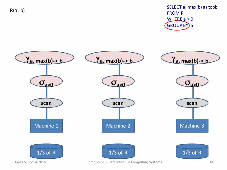
Example problem: Parallel DBMSR(a,b) is horizontally partitioned across N = 3 machines.
Each machine locally stores approximately 1/N of the tuples in R.
The tuples are randomly organized across machines (i.e., R is block partitioned across machines).
Show a RA plan for this query and how it will be executed across the N = 3 machines.
Pick an efficient plan that leverages the parallelism as much as possible.
• SELECT a, max(b) as topb• FROM R• WHERE a > 0• GROUP BY a
Duke CS, Spring 2016 CompSci 516: Data Intensive Computing Systems 40

1/3 of R 1/3 of R 1/3 of R
Machine 1 Machine 2 Machine 3
SELECT a, max(b) as topbFROM RWHERE a > 0GROUP BY a
R(a, b)
Duke CS, Spring 2016 CompSci 516: Data Intensive Computing Systems 41

1/3 of R 1/3 of R 1/3 of R
Machine 1 Machine 2 Machine 3
SELECT a, max(b) as topbFROM RWHERE a > 0GROUP BY a
R(a, b)
scan scan scan
If more than one relation on a machine, then “scan S”, “scan R” etc
Duke CS, Spring 2016 CompSci 516: Data Intensive Computing Systems 42

1/3 of R 1/3 of R 1/3 of R
Machine 1 Machine 2 Machine 3
SELECT a, max(b) as topbFROM RWHERE a > 0GROUP BY a
R(a, b)
scan scan scan
σa>0 σa>0 σa>0
Duke CS, Spring 2016 CompSci 516: Data Intensive Computing Systems 43
1/3 of R 1/3 of R 1/3 of R
Machine 1 Machine 2 Machine 3
SELECT a, max(b) as topbFROM RWHERE a > 0GROUP BY a
R(a, b)
scan scan scan
σa>0 σa>0 σa>0
γa, max(b)-‐> b γa, max(b)-‐> b γa, max(b)-‐> b
Duke CS, Spring 2016 CompSci 516: Data Intensive Computing Systems 44

1/3 of R 1/3 of R 1/3 of R
Machine 1 Machine 2 Machine 3
SELECT a, max(b) as topbFROM RWHERE a > 0GROUP BY a
R(a, b)
scan scan scan
σa>0 σa>0 σa>0
γa, max(b)-‐> b γa, max(b)-‐> b γa, max(b)-‐> b
Hash on a Hash on a Hash on a
Duke CS, Spring 2016 CompSci 516: Data Intensive Computing Systems 45

1/3 of R 1/3 of R 1/3 of R
Machine 1 Machine 2 Machine 3
SELECT a, max(b) as topb FROM RWHERE a > 0 GROUP BY aR(a, b)
scan scan scan
σa>0 σa>0 σa>0
γa, max(b)-‐> b γa, max(b)-‐> b γa, max(b)-‐> b
Hash on a Hash on a Hash on a
Duke CS, Spring 2016 CompSci 516: Data Intensive Computing Systems 46

1/3 of R 1/3 of R 1/3 of R
Machine 1 Machine 2 Machine 3
SELECT a, max(b) as topb FROM RWHERE a > 0 GROUP BY aR(a, b)
scan scan scan
σa>0 σa>0 σa>0
γa, max(b)-‐> b γa, max(b)-‐> b γa, max(b)-‐> b
Hash on a Hash on a Hash on a
γa, max(b)-‐>topb γa, max(b)-‐>topb γa, max(b)-‐>topb
Duke CS, Spring 2016 CompSci 516: Data Intensive Computing Systems 47

Same Example Problem: Map Reduce
Explain how the query will be executed in MapReduce
• SELECT a, max(b) as topb• FROM R• WHERE a > 0• GROUP BY a
Specify the computation performed in the map and the reduce functionsDuke CS, Spring 2016 CompSci 516: Data Intensive Computing Systems 48

Map
• Each map task– Scans a block of R– Calls the map function for each tuple– The map function applies the selection predicate to the tuple
– For each tuple satisfying the selection, it outputs a record with key = a and value = b
SELECT a, max(b) as topb FROM RWHERE a > 0GROUP BY a
•When each map task scans multiple relations, it needs to output something like key = a and value = (‘R’, b) which has the relation name ‘R’
Duke CS, Spring 2016 CompSci 516: Data Intensive Computing Systems 49

Shuffle
• The MapReduce engine reshuffles the output of the map phase and groups it on the intermediate key, i.e. the attribute a
SELECT a, max(b) as topb FROM RWHERE a > 0GROUP BY a
•Note that the programmer has to write only the map and reduce functions, the shuffle phase is done by the MapReduce engine (although the programmer can rewrite the partition function), but you should still mention this in your answers
Duke CS, Spring 2016 CompSci 516: Data Intensive Computing Systems 50

ReduceSELECT a, max(b) as topbFROM RWHERE a > 0GROUP BY a
• Each reduce task• computes the aggregate value max(b) = topb for each group
(i.e. a) assigned to it (by calling the reduce function) • outputs the final results: (a, topb)
•Multiple aggregates can be output by the reduce phase likekey = a and value = (sum(b), min(b)) etc.
• Sometimes a second (third etc) level of Map-‐Reduce phase might be needed
A local combiner can be used to compute local max before data gets reshuffled (in the map tasks)
Duke CS, Spring 2016 CompSci 516: Data Intensive Computing Systems 51

Benefit of hash-‐partitioning
• What would change if we hash-‐partitioned R on R.a before executing the same query on the previous parallel DBMS and MR
• First Parallel DBMS
SELECT a, max(b) as topbFROM R
WHERE a > 0GROUP BY a
Duke CS, Spring 2016 CompSci 516: Data Intensive Computing Systems 52

1/3 of R 1/3 of R 1/3 of R
Machine 1 Machine 2 Machine 3
SELECT a, max(b) as topb FROM RWHERE a > 0 GROUP BY aPrev: block-‐partition
scan scan scan
σa>0 σa>0 σa>0
γa, max(b)-‐> b γa, max(b)-‐> b γa, max(b)-‐> b
Hash on a Hash on a Hash on a
γa, max(b)-‐>topb γa, max(b)-‐>topb γa, max(b)-‐>topb
Duke CS, Spring 2016 CompSci 516: Data Intensive Computing Systems 53

• It would avoid the data re-‐shuffling phase• It would compute the aggregates locally
SELECT a, max(b) as topbFROM R
WHERE a > 0GROUP BY a
Duke CS, Spring 2016 CompSci 516: Data Intensive Computing Systems 54

1/3 of R 1/3 of R 1/3 of R
Machine 1 Machine 2 Machine 3
SELECT a, max(b) as topb FROM RWHERE a > 0 GROUP BY aHash-‐partition on a for R(a, b)
scan scan scan
σa>0 σa>0 σa>0
γa, max(b)-‐>topb γa, max(b)-‐>topb γa, max(b)-‐>topb
Duke CS, Spring 2016 CompSci 516: Data Intensive Computing Systems 55

Benefit of hash-‐partitioning
• For MapReduce– Logically, MR won’t know that the data is hash-‐partitioned
– MR treats map and reduce functions as black-‐boxes and does not perform any optimizations on them
• But, if a local combiner is used– Saves communication cost:
• fewer tuples will be emitted by the map tasks– Saves computation cost in the reducers:
• the reducers would have to do anything
SELECT a, max(b) as topbFROM R
WHERE a > 0GROUP BY a
Duke CS, Spring 2016 CompSci 516: Data Intensive Computing Systems 56