Comput. Methods Appl. Mech. Engrg. - vahabonline.comvahabonline.com/wp-content/uploads/2016/03/An... · tially the whole of the problem domain is modelled using the FEM. During an

Comput. Methods Appl. Mech. Engrg. 267 (2013) 111–132

Contents lists available at ScienceDirect

Comput. Methods Appl. Mech. Engrg.

journal homepage: www.elsevier .com/ locate/cma

An adaptive finite element/meshless coupled method basedon local maximum entropy shape functions for linear andnonlinear problems

0045-7825/$ - see front matter � 2013 Elsevier B.V. All rights reserved.http://dx.doi.org/10.1016/j.cma.2013.07.018

⇑ Corresponding author. Tel.: +44 1913342504.E-mail address: [email protected] (C.E. Augarde).

Z. Ullah, W.M. Coombs, C.E. Augarde ⇑School of Engineering and Computing Sciences, Durham University, Durham DH1 3LE, UK

a r t i c l e i n f o a b s t r a c t

Article history:Received 26 April 2013Received in revised form 5 July 2013Accepted 29 July 2013Available online 19 August 2013

Keywords:Meshless methodMaximum entropy shape functionsFE–EFGM couplingError estimationAdaptivitySuperconvergent patch recovery

In this paper, an automatic adaptive coupling procedure is proposed for the finite elementmethod (FEM) and the element-free Galerkin method (EFGM) for linear elasticity and forproblems with both material and geometrical nonlinearities. In this new procedure, ini-tially the whole of the problem domain is modelled using the FEM. During an analysis,those finite elements which violate a predefined error measure are automatically con-verted to an EFG zone. This EFG zone can be further refined by adding nodes, thus avoidingcomputationally expensive FE remeshing. Local maximum entropy shape functions areused in the EFG zone of the problem domain for two reasons: their weak Kronecker deltaproperty at the boundaries allows straightforward imposition of essential boundary condi-tions and also provides a natural way to couple the EFG and FE regions compared to the useof moving least squares basis functions. The Zienkiewicz and Zhu error estimation proce-dure with the superconvergent patch method for strains and stresses recovery is used inthe FE region of the problem domain, while the Chung and Belytschko error estimationprocedure is used in the EFG region.

� 2013 Elsevier B.V. All rights reserved.

1. Introduction

Meshless methods remain of interest in the computational mechanics community, in particular the element-free Galerkinmethod (EFGM) [1], because in these methods only a set of nodes is required for the problem discretisation, making themideal for modelling problems with large deformation, material damage, projectile penetration, fragmentation, crack growthand moving boundaries, the details of which can be found in [2–12]. However it is well-known that they tend to be morecomputationally expensive than finite element methods (FEMs) set the same job. It makes sense therefore to look at coupledmodelling, where meshless discretisation is used in regions of a domain which most benefit from their greater accuracy andlack of a mesh, while maintaining a finite element discretisation elsewhere in the domain. In most of the coupling proceduresproposed to date it is necessary to specify FE and EFG regions in the problem domain at the start of simulation, in the pre-processing stage. These regions are fixed in the problem domain, and performance is then highly user dependent. For prac-tical engineering problems, it will be very difficult, especially for an inexperienced user, to decide on appropriate FE and EFGregions in a given problem domain. For problems with both geometric and material nonlinearities, this problem is even moreintractable, as geometry is changing during the simulation. To overcome these problems, an automatic adaptive FE–EFGMcoupled method is proposed in this paper for linear and nonlinear problems where initially the whole of the problem domain

http://crossmark.crossref.org/dialog/?doi=10.1016/j.cma.2013.07.018&domain=pdf

http://dx.doi.org/10.1016/j.cma.2013.07.018

mailto:[email protected]

http://dx.doi.org/10.1016/j.cma.2013.07.018

http://www.sciencedirect.com/science/journal/00457825

http://www.elsevier.com/locate/cma

112 Z. Ullah et al. / Comput. Methods Appl. Mech. Engrg. 267 (2013) 111–132

is modelled using the FEM. During an analysis those finite elements which violate a predefined error measure are automat-ically converted to an EFG zone. This zone can be further refined by adding nodes, thus achieving adaptivity without any(computationally expensive) FE remeshing.

Proper FE–EFGM coupling is an important issue in the development of meshless methods, and different coupling strate-gies are available in the literature. The most prominent at present is probably that proposed in [13], in which interface/tran-sition elements are used between the FE and the EFG regions of the problem domain. In that procedure moving least squares(MLS) shape functions are used in the EFG region of the problem domain, while hybrid shape functions, combining both MLSand FE shape functions, are used in the interface region. Other commonly used methods for FE–EFGM coupling are the con-tinuous blending method in [14,15], methods based on Lagrange multipliers [16,17], on transition or bridge regions [18] andmethods based on a collocation approach [19]. A comprehensive review of different FE–EFGM coupling procedures up to2005 can be found in [20]. A new coupling procedure for FE–EFGM has recently been proposed by the authors in [21] forlinear elastic and geometrically nonlinear problems. In this coupling procedure, max-ent shape functions are used in theEFG region of the problem domain. Their weak Kronecker delta property allows imposition of the essential boundary con-ditions directly and a direct coupling of the FE and the EFG regions without transition/interface elements or any of the otherspecial techniques used previously. In this paper we extend this work into an adaptive framework as well as into materiallynonlinear problems. Only a very limited literature is available for adaptive FE-meshless coupling, for instance references[22,23] deal only with two-dimensional problems without proper error estimation and with no further adaptivity in themeshless zone.

The method presented here uses a total Lagrangian formulation for modelling finite deformation due to its computationalefficiency, and performance with material nonlinearity is demonstrated using the Prandtl–Reuss constitutive model (the vonMises yield function with perfect plasticity and associated flow) although any similar constitutive model could be used. Forlinear elastic problems, the well-established error estimation procedure of Zienkiewicz and Zhu [24] with the superconver-gent convergent patch recovery (SPR) method for recovery of the nodal stresses [25,26] is used in the FE region to determinethe elements requiring conversion to EFG regions. The Chung and Belytschko [27] error estimator is used in the EFG regionfor further adaptive refinement. For nonlinear problems, incremental forms of the Zienkiewicz and Zhu error estimator [28]and the Chung and Belytschko error estimator [29] are used. Full details of each component are given below, organized asfollows. The theoretical background and detailed formulation of the max-ent shape functions are presented in Section 2.These shape functions are then used in the EFGM, for which the modified formulations are given in Section 3. The detailsof the coupling between the FE and EFG region based on max-ent shape functions are given in Section 4. The adaptiveFE–EFGM coupling procedure for linear elastic and nonlinear problems is described in Section 5, including error estimationprocedures for both FEM and EFGM in Section 5.1. The corresponding refinement strategy is then given in Section 5.2 and thefull adaptively coupled FE–EFGM algorithm is described in Section 5.3. Numerical examples are given in Section 6 to showthe implementation and performance of the proposed adaptive FE–EFGM method. Concluding remarks follow in Section 7.

2. Maximum entropy shape functions

Max-ent shape functions, based on the idea of informational entropy [30,31] and the principle of max-ent [32,33], wereintroduced in [34] to formulate interpolants for polygons. These shape functions are not however suitable to be directly usedfor meshless methods as they extend to the global problem domain. More useful shape functions termed as ‘‘local’’, whichcan be defined for a set of nodes, were first introduced in [35], where their weak Kronecker delta property was also high-lighted. Compact support shape functions were then derived using Gaussian weight functions (or priors) in [35], work whichwas extended in [36] to any weight function (or generalized prior). First-order consistent max-ent shape functions [36] werethen extended to second order in [37] and higher order in [38] and max-ent was used in [39] for the automatic calculation ofthe nodal domain of influence within a meshless method.

The max-ent concept comes from information theory [31] where a measure of the amount of information or uncertaintyof a finite scheme is termed information entropy and is given as

Hðp1; . . . ;pnÞ ¼ �Xn

i¼1

pi log pi; ð1Þ

where p1; . . . :; pn are probabilities of n mutually independent events. The most likely probability distribution is obtained byusing Jaynes’ principle of max-ent [33], i.e. maximising (1) subject to constraints

Pni¼1pi ¼ 1 and

Pni¼1pigr xið Þ ¼ grðxÞh i, where

grðxÞh i is the expectation of a function grðxÞ. The max-ent approach can be used to derive shape functions by seeing an anal-ogy between the probabilities above and the shape function values themselves. A useful local shape function formulation canbe obtained [36] by incorporating prior distributions wi which can be regarded as weight functions that provide compact orlocal support, and then maximising the following

Hð/;wÞ ¼ �Xn

i¼1

/i log/i

wi

� �; ð2Þ

subject to the standard constant and linearly reproducing constraints

Z. Ullah et al. / Comput. Methods Appl. Mech. Engrg. 267 (2013) 111–132 113

Xn

i¼1

/i ¼ 1;Xn

i¼1

/ixi ¼ x;Xn

i¼1

/iyi ¼ y andXn

i¼1

/izi ¼ z: ð3Þ

Shape functions can be derived as

/i ¼Zi

Z; ð4Þ

where

Zi ¼ wie�k1~xi�k2~yi�k3~zi and Z ¼Xn

j¼1

Zj; ð5Þ

in which wi is the weight function associated with node i, evaluated at point x ¼ x; yð ÞT ; exi ¼ xi � x; eyi ¼ yi � y and ezi ¼ zi � zare shifted coordinates. n is the number of nodes in support at x and k1; k2 and k3 are Lagrange multipliers which can befound from

k1; k2; k3ð Þ ¼ argmin F k1; k2; k3ð Þ where F k1; k2; k3ð Þ ¼ logðZÞ: ð6Þ

F is a convex function and Newton’s method is used to solve (6) to find the Lagrange multipliers which can then be used inthe expressions for the shape functions. The shape function derivatives follow as [40]

r/i ¼ /i rfi �Xn

i¼1

/irfi

!; ð7Þ

where

rfi ¼rwi

wiþ kþ exi H�1 � H�1A

h iand A ¼

Xn

k¼1

/kexk �rwk

wk; ð8Þ

where H is the Hessian matrix and the dyadic product � of two vector a and b is a second order tensor, i.e. a� b defined asa� b ¼ abT .

3. Element-free Galerkin method

The element-free Galerkin method was proposed in [1], based on a global weak form. It is one of the most commonly usedmeshless methods and is based on the earlier diffuse element method [41]. In the EFGM, moving least squares (MLS) shapefunctions are used for the approximation of the field variables, background integration cells are used for numerical integra-tion and Lagrange multipliers are used for the imposition of essential boundary conditions.

Three-dimensional formulations are given here for the EFGM with max-ent shape functions, but it is straightforward tomodify for one- and two-dimensional cases. Consider a three-dimensional problem defined in the domain X and bounded byC. The equilibrium equations at a point x are written as

$Trþ bf ¼ 0 in X; ð9Þ

where r ¼ rxx ryy rzz rxy ryz rxzf gT is the Cauchy stress vector, bf ¼ bf x bf y bf z

� �Tis the body force vector,

where bf x; bf y and bf z are the body forces in x; y and z directions respectively and $ is the differential operator and is writtenas

$ ¼

@@x 0 00 @

@y 0

0 0 @@z

@@y

@@x 0

0 @@z

@@y

@@z 0 @

@x

26666666664

37777777775:

The boundary conditions associated with (9) are

u ¼ �u on Cu; ð10aÞ

rn ¼ t on Ct; ð10bÞ

where (10a) is the essential or Dirichlet boundary condition and (10b) is the natural or Neumann boundary condition. Hereu ¼ ux uy uzf gT is the displacement vector, where ux;uy and uz are the displacements in x; y and z directions, andn ¼ nx ny nzf gT is the outward unit normal to the boundary C; t is the prescribed traction on the traction boundary,


Ct , and �u is the prescribed displacement on the essential boundaries, Cu. Due to the use of MLS shape functions, which do notposses the Kronecker delta property, a constrained Galerkin weak form with Lagrange multipliers is used in [1] but due to theuse of max-ent shape functions here a Galerkin weak form is used directly, which is written as
Z
Xd ruð ÞT D ruð ÞdX�

ZX

duT bf dX�Z

Ct

duT�tdC ¼ 0; ð11Þ

where D is the material stiffness matrix. After discretising the problem with a set of nodes, displacement at a point of interestx is written as

uh xð Þ ¼ux

uy

uz

8><>:9>=>; ¼

Xn

i¼1

/i 0 00 /i 00 0 /i

264375 uxi

uyi

uzi

8><>:9>=>; ¼

Xn

i¼1

/iui; ð12Þ

where uh xð Þ is an approximation of the displacement at a point x;n is the number of nodes in the support of point x; /i is amatrix of the max-ent shape functions for node i at a point x and ui are known as fictitious nodal values or nodal parameters.Using (12) in (11) and after simplification, the final discrete system of linear equations is written as

Ku ¼ f; ð13Þ

where

Kij ¼Z

XBT

i DBjdX; ð14Þ

f i ¼Z

Ct

/itdCþZ

X/ibf dX; ð15Þ

Bi ¼

@/i@x 0 0

0 @/i@y 0

0 0 @/i@z

@/i@y

@/i@x 0

@/i@z 0 @/i

@x

0 @/i@z

@/i@y

2666666666664

3777777777775ð16Þ

and

D ¼ E1þ mð Þ 1� 2mð Þ

1� m m m 0 0 0m 1� m m 0 0 0m m 1� m 0 0 00 0 0 1�2m

2 0 00 0 0 0 1�2m

2 00 0 0 0 0 1�2m

2

2666666664

3777777775; ð17Þ

where m is the Poisson’s ratio and E is the modulus of elasticity. To perform the integrations in (14) and (15) numerically, theproblem domain X and traction boundary Ct are divided into a number of non-overlapping background cells.

In the case of nonlinear problems, a total Lagrangian formulation is used here to model finite deformation, in which all thekinematical variables are referred back to the original or undeformed configuration and for modelling elasto-plasticity, thePrandtl–Reuss constitutive model is used. Here the deformation gradient is used, which is the fundamental measure ofdeformation, providing the relationship between the current and reference configurations, that is

F ¼ @x@X

; ð18Þ

where x and X are the coordinates of a point in the current and reference configurations respectively. The work-conjugatestress and strain measures used in this paper are logarithmic strain e and Kirchhoff stress s [42], which are given as [43]

e ¼ 12

ln b; s ¼ Jr; ð19Þ

where r is the Cauchy stress, b is the left Cauchy–Green tensor and J is the determinant of the deformation gradient F. Intotal Lagrangian formulations, there is no need to update the geometry, the shape functions and the corresponding deriva-tives are calculated and stored at the start of the simulation and are used in every solution step in each Newton–Raphsoniteration. In this case, the deformation gradient Fnþ1 for increment nþ 1 is calculated from the total nodal parameters or


fictitious nodal values ui and the increment in the deformation gradient DF is then calculated using the deformation gradientFn of the previous converged iteration, i.e.

DF ¼ Fnþ1 F�1n ; Fnþ1 ¼ Iþ

Xn

i¼1

ui

@/@X@/@Y@/@Z

26643775

T

i

; ð20Þ

where I is a 3� 3 identity matrix, n is the number of nodes in support and the shape function derivatives are calculated withreference to the original geometry. The trial elastic left Cauchy–Green strain matrix be

tr is written as

betr ¼ DFbe

n DFT ; ð21Þ

where ben is the value of the elastic left Cauchy-Green strain matrix at the end of previous increment and is obtained by rear-

ranging (19) in terms of b and using e ¼ een, where ee

n is the elastic strain from the previously converged load step. (21) can beused in (19) to calculate the trial elastic strain ee

tr , which is input to the constitutive model, the output of which includeselastic strain ee, stress r and consistent or algorithmic tangent Dalg . A Newton–Raphson incremental-iterative procedureis used, i.e. load is applied incrementally in steps and convergence is sought for each increment, using

f intnþ1 unþ1ð Þ � fext

nþ1 ¼ oobfnþ1 ¼ 0; ð22Þ

where nþ 1 is the global Newton–Raphson iteration counter, f intnþ1 and fext

nþ1 are the global internal and external force vectorsrespectively, oobfnþ1 is the residual or out-of-balance force and unþ1 is a vector of nodal parameters or fictitious nodal values.The expression for the internal forces for an increment nþ 1 are given as

f intnþ1 ¼

ZX

GT PdX ¼Xng

i¼1

GTi Pi Jij jwi; ð23Þ

where ng are the total number of Gauss points in the problem domain, Ji and wi are the Jacobian and weights associated witheach Gauss points respectively, G is the 9-component strain–displacement matrix, consisting of the shape function deriva-tives with respect to the original configuration and is written as

Gi ¼

@/i@X 0 0

0 @/i@Y 0

0 0 @/i@Z

@/i@Y 0 0

0 @/i@X 0

0 @/i@Z 0

0 0 @/i@Y

0 0 @/i@X

@/i@Z 0 0

266666666666666666664

377777777777777777775

ð24Þ

and P is the nine component non-symmetric first Piola–Kirchhoff stress and is given as

P ¼ JrF�T ¼ sF�T : ð25Þ

The equation for the global stiffness matrix in this case is written as

K ¼Z

XGT eAGdX; ð26Þ

where eA is the isotropic material stiffness tangent and is written as

eA ¼ @P@F¼ @sF�T

@F: ð27Þ

The partial derivative is expressed as (index notation is used here for better presentation)

eAijkl ¼@sipF�1

jp

@Fkl¼ @sip

@FklF�1

jp � PikF�1jk : ð28Þ

After using the chain rule, the partial derivative @sip

@Fklis written as

@sip

@Fkl¼ @sip

@ eetð Þab

@ eet

� �ab

@ bet

� �cd

@ bet

� �cd

@Fkl; ð29Þ


where @sip

@ eetð Þab

¼ Dalgipab is the infinitesimal consistent or algorithmic tangent and

@ eetð Þab

@ betð Þcd

¼ Labcd is the partial derivative of the log-

arithm of bet with respect to its components and is written as

@ bet

� �cd

@Fkl¼ dck F�1

n

� lw

ben

� �wvDFdv

� þ dck DFcw be

n

� �wv F�1

n

� lv

� : ð30Þ

Effective plastic strain is used as one of the measures to evaluate the performance of the proposed model and is given as

ep ¼ffiffiffiffiffiffiffiffiffiffiffiffiffiffiffiffiffiffiffiffiffiffi23

epð ÞT epð Þr

; ð31Þ

where ep is plastic strain.

4. FE–EFGM coupling using max-ent shape functions

In the FE–EFGM coupling based on interface elements [13], MLS shape functions are used in the EFG zone for theapproximation of the field variables. The MLS shape functions do not possess the Kronecker delta property like FE shapefunctions and due to this reason interface elements are introduced between the FE and the EFG zones [13], to properly couplethe two regions. The shape functions for the interface elements are hybrid shape functions of the FE and the EFG shape func-tions to make the displacement continuous across the FE–EFGM interface. The details of the FE–EFGM coupling based on theinterface elements is not given here and can be found in the relevant literature. In this paper, max-ent shape functions areused in the EFG region of the problem domain, which provides a natural way to couple the FEM and the EFGM without usinginterface elements or transition regions between the FE and EFG zones because of the weak Kronecker delta property at theboundaries. A sample mixed FE and EFG discretization is shown in Fig. 1, where XE and XF are the EFG and the FE regions andC is the boundary between these two regions. The nodes on the boundary C between the EFG and FE regions, shown in greenin Fig. 1, are used in the displacement approximation for both the EFG and the FE regions. Displacement can be approximatedat point x in a similar way in the two regions, i.e.

uh xð Þ ¼Xn

i¼1

eNi xð Þui; ð32Þ

where uh xð Þ is the approximate displacement component at point x; eNi xð Þ is either the FE or the EFG shape function for node ievaluated at point x;n is the number of nodes in support of point x and ui are either nodal displacements in the case of theFEM, or nodal parameters in case of the EFGM.

5. Adaptive FE–EFGM

All analyses using this method start with a domain discretised entirely with finite elements. An error estimator is used toflag elements which require conversion to EFG zones. The refinement strategy then comprises changing the nodes on theseelements to become EFG nodes, and the original finite element regions become the integration cells for the EFGM. By thisprocess the method uses the finite element grid to form the integration cells and avoids generating a separate cell layout.Refinement is not confined to this conversion from FE to EFG: further refinement of EFG regions is also included.

Fig. 1. FE–EFGM coupling using max-ent shape functions.


5.1. Error estimation

The Zienkiewicz and Zhu [25] error estimator with the SPR method for recovery of stresses and strain are used in the FEregion of the problem domain, while the Chung and Belytschko [27] error estimation is used in the EFG region of the problemdomain. The basic idea of both of these error estimation procedure is to use the difference between projected and the directnumerical solutions and are similar to the conventional recovery type error estimation method in the FEM [26]. Despite thedifferences in calculation of nodal stresses and strains, the error estimation procedures for the FE and EFG regions work sim-ilarly, i.e. in FE and EFG regions the procedure goes element-wise and background cells-wise respectively.

The exact error in stress or strain fields at a point x is the difference between the exact and numerical values, i.e.

re xð Þ ¼ r xð Þ � rh xð Þ and ee xð Þ ¼ e xð Þ � eh xð Þ; ð33Þ

where re xð Þ and ee xð Þ are the exact error in the stress and strain at a point x respectively, r xð Þ and e xð Þ are the exact stressand strain at a point x while rh xð Þ and eh xð Þ are the numerical stress and strain at a point x. The error for the individual celland for the whole domain can then be found using an appropriate norm; error in energy norm is used in this paper. In thiscase, the exact local error in energy norm eek k and the corresponding exact local energy norm Uek k for either an individual FEor EFG background cell Xe are given by

eek k ¼Z

Xe

re xð Þð ÞT D�1 re xð Þð ÞdXe

� �12

and Uek k ¼Z

Xe

r xð Þð ÞT D�1 r xð Þð ÞdXe

� �12

; ð34Þ

where subscript e shows an individual FE or EFG background cell with domain Xe. As the exact stresses and strains are notavailable for real-life problems, so the projected stress rp xð Þ and projected strain ep xð Þ are used in (33) and (34) instead of theexact stress and exact strain respectively and the calculated error in energy norm ep

e

�� is then known as the estimated errorin energy norm. Equations for the global error in energy norm and the corresponding global energy norm for the problemdomain X are then written as

epk k2 ¼Xne

i¼1

epe

�� 2i

and Uk k2 ¼Xne

i¼1

Uek k2i ; ð35Þ

where for linear elastic problems ne is the number of FEs in the first iteration and the number of EFG background cells in theconsecutive iterations. Global relative percentage error g and permissible local error in an individual FE or EFG backgroundcells eek k are then written as

g ¼ epk kUk k � 100 and eek k ¼

g100

Uk k2

ne

!12

; ð36Þ

where g is the global permissible relative error for the whole problem domain. The adaptive procedure is triggered by theglobal relative error, i.e. when g > g and the conversion of FEs to EFG background cells or further refinement of EFG back-

ground cells is performed whenep

ek keek k

> 1.

Recovery type error estimation procedures have already been used by other researchers in the literature for nonlinearproblems in adaptive analysis. The Zienkiewicz and Zhu error estimation procedure was extended to nonlinear problemsfor the first time in [28] and was used for two-dimensional problems subjected to small strain elasto-plasticity, in whichfor each solution step, incremental error in energy norm was calculated from nodal stresses and nodal incremental strainsrecovered using the recovery by equilibrium in patches [44] and SPR method respectively. Further applications of the Zie-nkiewicz and Zhu error estimation procedure in two-dimensional nonlinear problems can be found in a number of refer-ences, e.g. in [45], the SPR method was used to estimate error for two-dimensional footings on soil problems, subjectedto large deformation with elasto-plasticity. 6-node triangular elements with three Gauss points per element were used todiscretise the problems and the L2 norm of error in strain was used for the adaptive analysis. In [46], recovery of the Cauchystress was performed by the SPR method for two-dimensional problems with large deformation using hyperelasticity as amaterial model. The improved SPR method was introduced for two-dimensional large deformation problems in [47], inwhich integration points were used as sampling points and bilinear 4-node quadrilateral elements with ð2� 2Þ Gauss pointswere used in the analysis. It was shown in [48,49] that the SPR method can perform well, even if the sampling points used forstress recovery are not the superconvergent points. This information is very helpful to extend the SPR method originally pro-posed for linear problems to nonlinear problems, where most of the path dependent variables are available at the integrationpoints, which are generally not superconvergent. The use of integration points as sampling points also allows the inclusion ofmore terms in the polynomial of the least squares fitting over the patch of elements, which is normally impossible with thesuperconvergent points, because they are few in number. The nonexistence of superconvergent points in the case of nonlin-ear problems was also mentioned in [46], where it was concluded that using (2� 2) integration points in linear 4-node quad-rilateral elements as sampling points led to better performance than using one superconvergent Gauss point. Gauss pointswere also used as sampling points in [47] for problems subjected to large deformation.


The Zienkiewicz and Zhu error estimation procedure with the SPR method for stress recovery has also been used in anumber of linear and nonlinear three-dimensional problems. In [50], the SPR method was used to calculate error inthree-dimensional h-adaptive analysis for linear-elastic problems. Adaptive FEA based on the modified SPR method was usedto model curved cracks in three-dimensional problems in [51]. In [52], the SPR method was used for error estimation inthree-dimensional nonlinear problems, involving liquefaction of soil due to seismic effects. The incremental L2 norm of errorin strain for each solution step was used here in h-adaptive analysis, while linear 8-node hexahedral elements were used todiscretise the problems’ domains. The SPR method was extended to three-dimensional nonlinear problems, and its applica-tions were explored in the transferring of the path dependent variables in [53–55]. Tetrahedral elements were used in theanalysis, and different polynomials were used in the least squares fitting for the SPR method, possessing C0; C1 and C2 con-tinuity. In [56], an improvement of the SPR method, i.e. minimal patch recovery (MPR), was introduced in which there wasno need to calculate the nodal stresses. The recovered solutions at Gauss points were calculated directly from theleast squares projection of the Gauss points belonging to the neighbouring elements. The method was applied to three-dimensional elasticity and metal forming problems with tetrahedral elements.

The same incremental procedure for the error estimation, used for the adaptive FEM in [28] and for the adaptive EFGM in[29] is used here, i.e. incremental global relative error in energy norm is calculated for each solution step, and checkedagainst a permissible value. For solution step n, equations for the incremental error in energy norm and the correspondingenergy norm for either an individual FE or EFG background cell Xe are given as

epe

�� ¼ ZXe

spn xð Þ � sh

n xð Þ� �T

Depn xð Þ � Deh

n xð Þ� �� dXe

�12

and Uek k ¼Z

Xe

spn xð Þ

� �TDep

n xð Þ� �� dXe

�12

; ð37Þ

where the subscript e shows an individual FE or EFG background cell, spn xð Þ and sh

n xð Þ are the projected and numericalKirchhoff stresses respectively at a Gauss point x for solution step n, while Dep

n xð Þ and Dehn xð Þ are the projected and numerical

incremental logarithmic strains at a Gauss point x for the solution step n. Projected Kirchhoff stresses and the projectedlogarithmic strains in this case are calculated using the Zienkiewicz and Zhu and Chung and Belytschko procedures in theFE and the EFG region of the problem domain respectively. Equations for the error in energy norm and the correspondingenergy norm for the problem domain X are then written as

epk k2 ¼XnFE

i¼1

epFE

�� 2i þ

XnEFG

j¼1

epEFG

�� 2j and Uk k2 ¼

XnFE

i¼1

UFEk k2i þ

XnEFG

j¼1

UEFGk k2j ; ð38Þ

where nFE and nEFG are the total numbers of FEs and EFG background cells respectively in the problem domain. Similarly to(36) incremental global relative percentage error and incremental permissible error in an individual FE or EFG backgroundcell are written as

g ¼ epk kUk k � 100 and eek k ¼

g100

Uk k2

n

!12

; ð39Þ

where n ¼ nFE þ nEFG and g is a permissible relative error for the whole problem domain.

5.1.1. Calculation of nodal stressesThe procedures to calculate nodal strains and stresses are now given separately for both FE and EFG regions.

5.1.2. Finite elementFor the FEM, the SPR method was developed by Zienkiewicz and Zhu [25] to calculate the nodal stresses and strains from

the nodal displacements. In this procedure stresses and strains are initially calculated at the superconvergent points, whichare then used to calculate stresses and strains at the nodes. It was shown that, in the cases of linear and cubic elements therecovered nodal stresses and strains are superconvergent (one order more accurate or OðhPþ1Þ), where h is the element sizewheras ultraconvergence, i.e. OðhPþ2ÞÞ or two orders higher accuracy was obtained in the case of quadratic elements. Thedirectly calculated nodal stresses and strains from the nodal displacements using the shape function derivatives are howeverless accurate and discontinuous. Different strategies have been suggested in the literature to calculate accurate nodal stres-ses. One of the commonly used methods is averaging or local projection techniques, in which stresses are calculated at thenodes by extrapolation from the superconvergent sampling points, which are then averaged to get a single value. The accu-racy of the stresses from this method is highly dependent on the existence of the superconvergent points in the FEs. Furtherdetail and theoretical background of the superconvergent points within FEs and the averaging or local projection method canbe found in, e.g. [57]. Other procedures for nodal stress recovery can also be found in the literature, including global projec-tion [58] and extraction and other alternatives [59]. In all the above-mentioned nodal stress recovery methods, the nodalstresses obtained, are generally not superconvergent. In the SPR method, nodal stresses are calculated by using a discreteor local least square fitting over a set of superconvergent points in a patch of elements, assembled at a common node.The SPR method is superior to other stress recovery procedures because the recovered stresses are generally superconver-gent or even ultraconvergent for the case of quadratic elements as stated above.


The objective of the SPR method is to find the nodal stresses r�i such that a continuous and accurate stress field r� isobtained, i.e.

r� ¼Xn

i¼1

Nir�i ; ð40Þ

where Ni is the same elemental shape function used in the displacement interpolation. Here the stress field r� is smooththroughout the problem domain and is more accurate than the corresponding directly calculated stress field rh. In theSPR method, nodal stresses r�i are obtained by the least squares fitting of the complete basis as used in the displacementapproximation over a patch of elements surrounding an assembly node. The polynomial expansion of the stress componentr�p is written as

r�p ¼ P xð Þa ð41Þ

where P xð Þ is a monomial basis function, x are spatial coordinates and a is a vector of unknown coefficients. For three-dimensional linear and quadratic elements P xð Þ and corresponding a are

P xð Þ ¼ 1; x; y; zf g; a ¼ a1; � � � ; a4f gT; ð42aÞ

P xð Þ ¼ 1; x; y; z; xy; yz; zx; x2; y2; z2� �

; a ¼ a1; � � � ; a10f gT: ð42bÞ

In (41), unknown coefficients a are determined separately for each patch by least squares fitting to the stresses at the super-convergent points. For the least squares fitting, the following equation is minimized w.r.t. a

FðaÞ ¼Xn

i¼1

rh xið Þ � r�p xið Þ� 2

¼Xn

i¼1

rh xið Þ � P xið Þa� �2

; ð43Þ

where n is the total number of superconvergent points in a single patch of elements, xi are the spatial coordinates of super-convergent points, rh xið Þ are the stresses calculated directly by the FEM at the superconvergent points and r�p xið Þ are therecovered stresses at the same points using least square fitting. Minimization of (43) w.r.t. a gives

Aa ¼ b or a ¼ A�1b; ð44Þ

where

A ¼Xn

i¼1

PT xið ÞP xið Þ and b ¼Xn

i¼1

PT xið Þrh xið Þ: ð45Þ

After calculating a, nodal stresses are calculated from (41), i.e. using the nodal coordinates. The size of matrices A and b arevery small and depend on P. b should be determined separately for each stress component, while A�1 is the same for allstress components and is determined only once.

For the three-dimensional case, patches are shown in Figs. 2(a) and 2(b) for 8-node and 20-node hexahedral elementsrespectively. In both patches, eight elements are joined at a common patch assembly node. In Fig. 2(a) there is only onesuperconvergent point per element, and the patch is used to recover the stresses only at patch assembly nodes. InFig. 2(b) there are eight superconvergent points per element and patches are used to recover stresses at the patch assemblynodes as well as internal nodes, which are inside these patches, shown as solid circles. In Fig. 2(b), internal nodes normallybelong to more than one patch, and stresses are recovered at these nodes from each patch, and the final stresses are thencalculated by averaging. To recover stresses at boundary nodes, including essential/traction as well as the interface betweenFE and EFG regions, internal or boundary patches can be used. Accuracy is the same, if stresses are recovered either from theboundary or internal patches [25]. In some situations, however, sufficient elements and superconvergent points are notavailable to construct patches at the boundary. Even if sufficient elements and superconvergent points are available, the con-struction of these boundary patches involves extra unnecessary work, as the stresses at boundary nodes can be recoveredfrom the already constructed internal patches. To avoid these complications, in this paper internal patches are used torecover stresses at the boundary nodes.

5.1.3. Element-free Galerkin methodAs there are no elements in the EFGM, so there is no issue of strain and stress discontinuity, and the procedure used for

the FEM is not directly applicable to the EFGM, because the derived stress and strain fields are already smooth. The errorestimation procedure proposed for the EFGM in [27] is used, in which projected stresses are calculated from the nodal stres-ses based on reduced domains of influence. It was also shown in [27] that the error estimator performs well when the do-main of influence for stress projection is as small as possible but at the same time must be large enough to have sufficientnodes in support of each Gauss point required for the shape functions calculation. In the case of the EFGM, the stress andstrain vector returned at any point x is written as

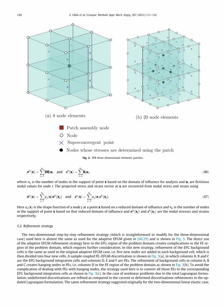
Fig. 2. SPR three-dimensional elements patches.


rh xð Þ ¼Xna

i¼1

DBiui and eh xð Þ ¼Xna

i¼1

Biui; ð46Þ

where na is the number of nodes in the support of point x based on the domain of influence for analysis and ui are fictitiousnodal values for node i. The projected stress and strain vector at x are recovered from nodal stress and strain using

rp xð Þ ¼Xnp

j¼1

wj xð Þrh xj� �

and ep xð Þ ¼Xnp

j¼1

wj xð Þeh xj� �

: ð47Þ

Here wj xð Þ is the shape function of a node j at a point x based on a reduced domain of influence and np is the number of nodesin the support of point x based on that reduced domain of influence and rh xj

� �and eh xj

� �are the nodal stresses and strains

respectively.

5.2. Refinement strategy

The two-dimensional step-by-step refinement strategy (which is straightforward to modify for the three-dimensionalcase) used here is almost the same as used for the adaptive EFGM given in [60,29] and is shown in Fig. 3. The direct useof the adaptive EFGM refinement strategy here in the EFG region of the problem domain creates complications in the FE re-gion of the problem domain, which requires further consideration. In this new strategy, refinement of the EFG backgroundcells is the same as used in the original adaptive EFGM case, i.e. five new nodes are added in each background cell, which isthen divided into four new cells. A sample coupled FE–EFGM discretisation is shown in Fig. 3(a), in which columns A, B and Care the EFG background integration cells and columns D, E and F are FEs. The refinement of background cells in column A, Band C creates hanging nodes in FEs, i.e. columns D in the FE region of the problem domain as shown in Fig. 3(b). To avoid thecomplication of dealing with FEs with hanging nodes, the strategy used here is to convert all those FEs to the correspondingEFG background integration cells as shown in Fig. 3(c). In the case of nonlinear problems due to the total Lagrangian formu-lation, undeformed discretisations are refined as compared to the current or deformed discretisations refinements in the up-dated Lagrangian formulation. The same refinement strategy suggested originally for the two-dimensional linear elastic case,

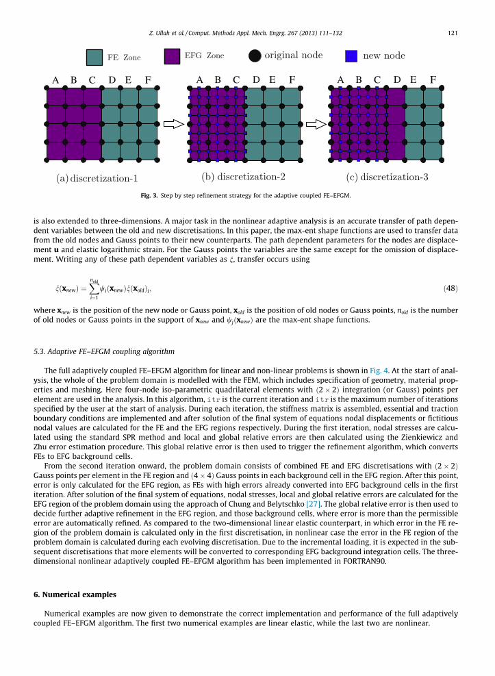
Fig. 3. Step by step refinement strategy for the adaptive coupled FE–EFGM.


is also extended to three-dimensions. A major task in the nonlinear adaptive analysis is an accurate transfer of path depen-dent variables between the old and new discretisations. In this paper, the max-ent shape functions are used to transfer datafrom the old nodes and Gauss points to their new counterparts. The path dependent parameters for the nodes are displace-ment u and elastic logarithmic strain. For the Gauss points the variables are the same except for the omission of displace-ment. Writing any of these path dependent variables as n, transfer occurs using

n xnewð Þ ¼Xnold

i¼1

wi xnewð Þn xoldð Þi; ð48Þ

where xnew is the position of the new node or Gauss point, xold is the position of old nodes or Gauss points, nold is the numberof old nodes or Gauss points in the support of xnew and wj xnewð Þ are the max-ent shape functions.

5.3. Adaptive FE–EFGM coupling algorithm

The full adaptively coupled FE–EFGM algorithm for linear and non-linear problems is shown in Fig. 4. At the start of anal-ysis, the whole of the problem domain is modelled with the FEM, which includes specification of geometry, material prop-erties and meshing. Here four-node iso-parametric quadrilateral elements with ð2� 2Þ integration (or Gauss) points perelement are used in the analysis. In this algorithm, itr is the current iteration and itr is the maximum number of iterationsspecified by the user at the start of analysis. During each iteration, the stiffness matrix is assembled, essential and tractionboundary conditions are implemented and after solution of the final system of equations nodal displacements or fictitiousnodal values are calculated for the FE and the EFG regions respectively. During the first iteration, nodal stresses are calcu-lated using the standard SPR method and local and global relative errors are then calculated using the Zienkiewicz andZhu error estimation procedure. This global relative error is then used to trigger the refinement algorithm, which convertsFEs to EFG background cells.

From the second iteration onward, the problem domain consists of combined FE and EFG discretisations with ð2� 2ÞGauss points per element in the FE region and ð4� 4Þ Gauss points in each background cell in the EFG region. After this point,error is only calculated for the EFG region, as FEs with high errors already converted into EFG background cells in the firstiteration. After solution of the final system of equations, nodal stresses, local and global relative errors are calculated for theEFG region of the problem domain using the approach of Chung and Belytschko [27]. The global relative error is then used todecide further adaptive refinement in the EFG region, and those background cells, where error is more than the permissibleerror are automatically refined. As compared to the two-dimensional linear elastic counterpart, in which error in the FE re-gion of the problem domain is calculated only in the first discretisation, in nonlinear case the error in the FE region of theproblem domain is calculated during each evolving discretisation. Due to the incremental loading, it is expected in the sub-sequent discretisations that more elements will be converted to corresponding EFG background integration cells. The three-dimensional nonlinear adaptively coupled FE–EFGM algorithm has been implemented in FORTRAN90.

6. Numerical examples

Numerical examples are now given to demonstrate the correct implementation and performance of the full adaptivelycoupled FE–EFGM algorithm. The first two numerical examples are linear elastic, while the last two are nonlinear.

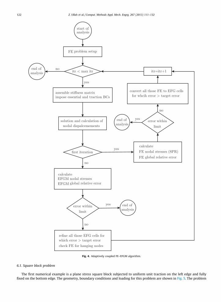
Fig. 4. Adaptively coupled FE–EFGM algorithm.


6.1. Square block problem

The first numerical example is a plane stress square block subjected to uniform unit traction on the left edge and fullyfixed on the bottom edge. The geometry, boundary conditions and loading for this problem are shown in Fig. 5. The problem

Fig. 5. Geometry, boundary condition and loading for the square block problem.

Fig. 6. Step by step discretisations for the square block problem.


is solved with E ¼ 1� 103; m ¼ 0:3; damax ¼ 1:5; dp

max ¼ 1:2 and g ¼ 6:0%, all in compatible units, where damax and dp

max are thescaling parameters for the domain of influence for analysis and projection respectively. The evolving step by step adaptivelycoupled FE–EFGM discretisations in this case are shown in Fig. 6. The FE mesh at the start of analysis with 225ð15� 15Þ ele-ments and 256 ð16� 16Þ nodes is shown in Fig. 6(a). The converted FEs to corresponding EFG background cells based on theZienkiewicz and Zhu error estimation at the end of first iteration are shown in Fig. 6(b). During this first FEs to EFG back-ground cells conversion the number of nodes is constant. Subsequent refinements in the EFG regions of the problem domain,based on the Chung and Belytschko error estimation procedure, are shown in Fig. 6(c). It can also be seen in Fig. 6(c) that inthe EFG zone on the right-hand side, all new nodes are added within the EFG region and there is no issue of hanging nodes inthe FE region of the problem domain. However, in the EFG zone on the left-hand side, four more FEs at the top of EFG zoneare converted to EFG background cells, to avoid hanging nodes in the FE region of the problem domain. As expected, theadaptively coupled FE–EFGM algorithm, initially converts the high-stress zones in the problem domain to the correspondingEFG zones and then adds nodes to the high-stress EFG zones. The contours of the von Mises rVM stress over the problemdomain after the first FE iteration are shown in Fig. 7, which are obtained from the SPR method’s recovered nodal stressesusing

rVM ¼ r2xx þ r2

yy � rxxryy þ 3rxy

h i12; ð49Þ

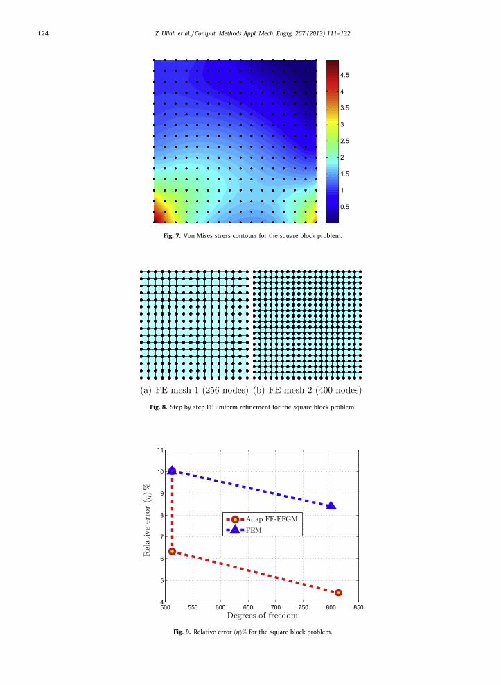
Fig. 7. Von Mises stress contours for the square block problem.

(a) FE mesh-1 (256 nodes) (b) FE mesh-2 (400 nodes)

Fig. 8. Step by step FE uniform refinement for the square block problem.

500 550 600 650 700 750 800 8504

5

6

7

8

9

10

11

Degrees of freedom

Rel

ativ

eer

ror

(η)%

Adap FE-EFGM

FEM

Fig. 9. Relative error ðgÞ% for the square block problem.



where rxx and ryy are the normal stresses in x and y directions and rxy is the shear stress. For comparison, the same problemis also solved with uniformly refined FE meshes with almost the same number of nodes as shown in Fig. 6(a) and (c). Theuniformly refined meshes in this case with 256ð16� 16Þ and 400ð20� 20Þ nodes are shown in Fig. 8(a) and (b) respectively.Comparison of the relative error (g) for the adaptively coupled FE–EFGM case and uniformly refined FEM case are shown inFig. 9, in which three data points are available for the adaptively coupled FE–EFGM case and only two data points are avail-able in the uniformly refined FEM case. In Fig. 9, it is clear that the decrease in the relative error is greater in the case of theadaptively coupled FE–EFGM as compared to the uniformly refined FEM case.

6.2. L-shaped plate

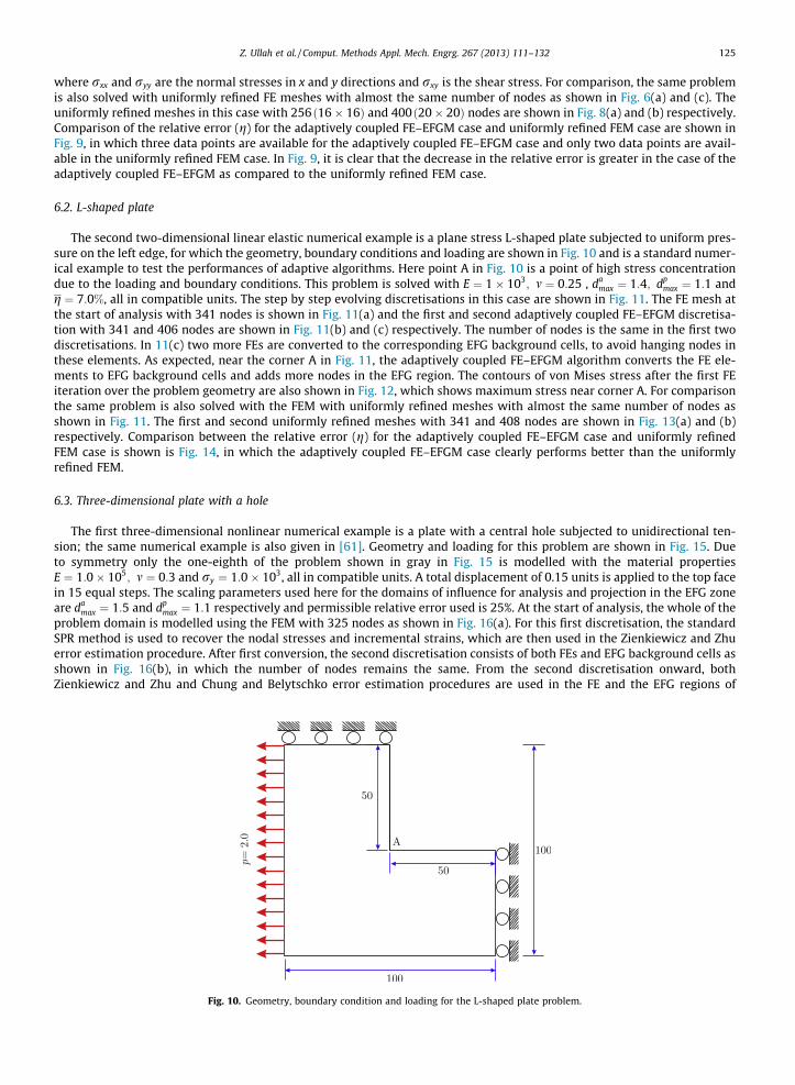
The second two-dimensional linear elastic numerical example is a plane stress L-shaped plate subjected to uniform pres-sure on the left edge, for which the geometry, boundary conditions and loading are shown in Fig. 10 and is a standard numer-ical example to test the performances of adaptive algorithms. Here point A in Fig. 10 is a point of high stress concentrationdue to the loading and boundary conditions. This problem is solved with E ¼ 1� 103; m ¼ 0:25 , da

max ¼ 1:4; dpmax ¼ 1:1 and

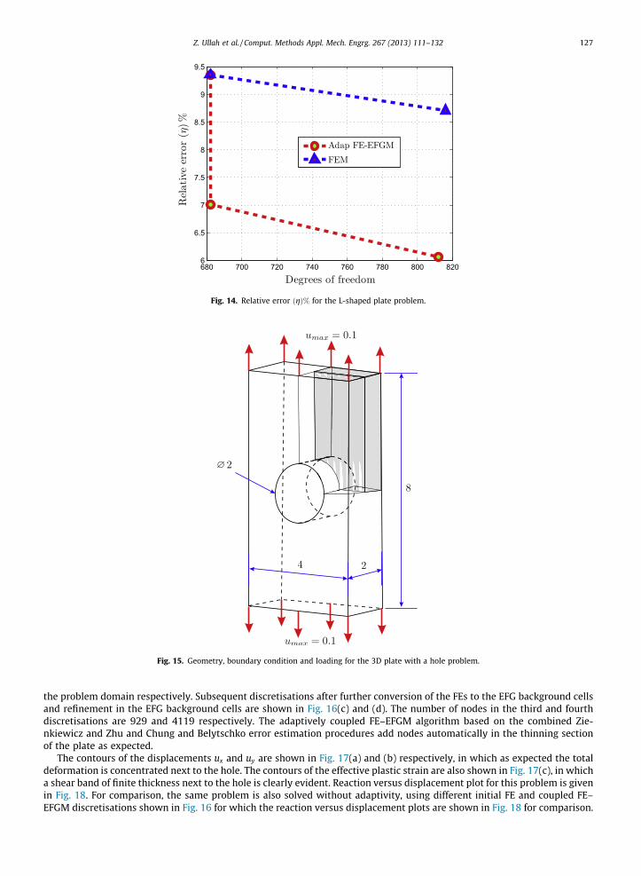
g ¼ 7:0%, all in compatible units. The step by step evolving discretisations in this case are shown in Fig. 11. The FE mesh atthe start of analysis with 341 nodes is shown in Fig. 11(a) and the first and second adaptively coupled FE–EFGM discretisa-tion with 341 and 406 nodes are shown in Fig. 11(b) and (c) respectively. The number of nodes is the same in the first twodiscretisations. In 11(c) two more FEs are converted to the corresponding EFG background cells, to avoid hanging nodes inthese elements. As expected, near the corner A in Fig. 11, the adaptively coupled FE–EFGM algorithm converts the FE ele-ments to EFG background cells and adds more nodes in the EFG region. The contours of von Mises stress after the first FEiteration over the problem geometry are also shown in Fig. 12, which shows maximum stress near corner A. For comparisonthe same problem is also solved with the FEM with uniformly refined meshes with almost the same number of nodes asshown in Fig. 11. The first and second uniformly refined meshes with 341 and 408 nodes are shown in Fig. 13(a) and (b)respectively. Comparison between the relative error (g) for the adaptively coupled FE–EFGM case and uniformly refinedFEM case is shown is Fig. 14, in which the adaptively coupled FE–EFGM case clearly performs better than the uniformlyrefined FEM.

6.3. Three-dimensional plate with a hole

The first three-dimensional nonlinear numerical example is a plate with a central hole subjected to unidirectional ten-sion; the same numerical example is also given in [61]. Geometry and loading for this problem are shown in Fig. 15. Dueto symmetry only the one-eighth of the problem shown in gray in Fig. 15 is modelled with the material propertiesE ¼ 1:0� 105; m ¼ 0:3 and ry ¼ 1:0� 103, all in compatible units. A total displacement of 0.15 units is applied to the top facein 15 equal steps. The scaling parameters used here for the domains of influence for analysis and projection in the EFG zoneare da

max ¼ 1:5 and dpmax ¼ 1:1 respectively and permissible relative error used is 25%. At the start of analysis, the whole of the

problem domain is modelled using the FEM with 325 nodes as shown in Fig. 16(a). For this first discretisation, the standardSPR method is used to recover the nodal stresses and incremental strains, which are then used in the Zienkiewicz and Zhuerror estimation procedure. After first conversion, the second discretisation consists of both FEs and EFG background cells asshown in Fig. 16(b), in which the number of nodes remains the same. From the second discretisation onward, bothZienkiewicz and Zhu and Chung and Belytschko error estimation procedures are used in the FE and the EFG regions of

Fig. 10. Geometry, boundary condition and loading for the L-shaped plate problem.

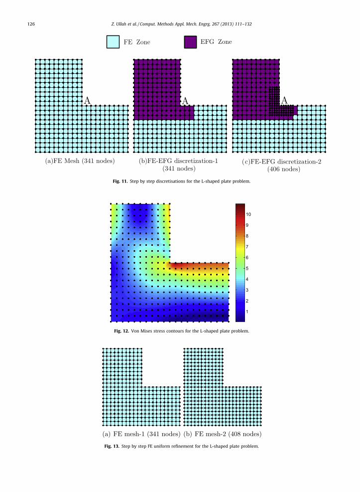
Fig. 11. Step by step discretisations for the L-shaped plate problem.

Fig. 12. Von Mises stress contours for the L-shaped plate problem.

Fig. 13. Step by step FE uniform refinement for the L-shaped plate problem.


680 700 720 740 760 780 800 8206

6.5

7

7.5

8

8.5

9

9.5

Degrees of freedom

Rel

ativ

eer

ror

(η)%

Adap FE-EFGM

FEM

Fig. 14. Relative error ðgÞ% for the L-shaped plate problem.

Fig. 15. Geometry, boundary condition and loading for the 3D plate with a hole problem.


the problem domain respectively. Subsequent discretisations after further conversion of the FEs to the EFG background cellsand refinement in the EFG background cells are shown in Fig. 16(c) and (d). The number of nodes in the third and fourthdiscretisations are 929 and 4119 respectively. The adaptively coupled FE–EFGM algorithm based on the combined Zie-nkiewicz and Zhu and Chung and Belytschko error estimation procedures add nodes automatically in the thinning sectionof the plate as expected.

The contours of the displacements ux and uy are shown in Fig. 17(a) and (b) respectively, in which as expected the totaldeformation is concentrated next to the hole. The contours of the effective plastic strain are also shown in Fig. 17(c), in whicha shear band of finite thickness next to the hole is clearly evident. Reaction versus displacement plot for this problem is givenin Fig. 18. For comparison, the same problem is also solved without adaptivity, using different initial FE and coupled FE–EFGM discretisations shown in Fig. 16 for which the reaction versus displacement plots are shown in Fig. 18 for comparison.

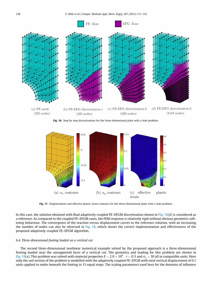
Fig. 16. Step by step discretisations for the three-dimensional plate with a hole problem.

(a) ux contours (b) uy contours (c) effective plasticstrain

Fig. 17. Displacements and effective plastic strain contours for the three-dimensional plate with a hole problem.


In this case, the solution obtained with final adaptively coupled FE–EFGM discretisation shown in Fig. 16(d) is considered asa reference. As compared to the coupled FE–EFGM cases, the FEM response is relatively rigid without obvious geometric soft-ening behaviour. The convergence of the reaction versus displacement curves to the reference solution, with an increasingthe number of nodes can also be observed in Fig. 18, which shows the correct implementation and effectiveness of theproposed adaptively coupled FE–EFGM algorithm.

6.4. Three-dimensional footing loaded on a vertical cut

The second three-dimensional nonlinear numerical example solved by the proposed approach is a three-dimensionalfooting loaded near the unsupported faces of a vertical cut. The geometry and loading for this problem are shown inFig. 19(a). This problem was solved with material properties E ¼ 2:0� 104; m ¼ 0:3 and ry ¼ 30 all in compatible units. Hereonly the soil section of the problem is modelled with the adaptively coupled FE–EFGM with total vertical displacement of 0.1units applied to nodes beneath the footing in 15 equal steps. The scaling parameters used here for the domains of influence

0 0.02 0.04 0.06 0.08 0.1 0.12 0.14 0.160

200

400

600

800

1000

1200

Displacement

Rea

ctio

n FEFE-EFG-1FE-EFG-2FE-EFG-3FE-EFG Adaptive

Fig. 18. Reaction versus displacement for the three-dimensional plate with a hole problem.

Fig. 19. Step by step discretisations for the three-dimensional vertical cut problem.


(a) uy contours (b) Effective plastic strain

Fig. 20. Displacement uy and effective plastic strain contours for the three-dimensional vertical cut problem.

0 0.02 0.04 0.06 0.08 0.10

200

400

600

800

1000

1200

1400

1600

1800

2000

Displacement

Rea

ctio

n

FEFE-EFG-1FE-EFG-2FE-EFG-3FE-EFG Adaptive

Fig. 21. Reaction versus displacement for the three-dimensional vertical cut problem.


for analysis and projection in the EFG zone are damax ¼ 1:5 and dp

max ¼ 1:1 respectively and permissible relative error used is25%. The FE mesh at the start of the analysis is shown in Fig. 19(b) and the step by step conversion of the FEs to the EFGbackground cells and subsequent refinements of the EFG background cells are shown in Fig. 19(c)–(e). The number of nodesused in the first two discretisations is 729, while in the subsequent discretisations, the number of nodes increases to 1215and 2950. For this problem, failure is expected in the soil below the footing, where FEs are automatically converted to theEFG background cells, which are refined in the subsequent discretisations. The contours of uy and effective plastic strain arealso shown in Fig. 20(a) and (b) respectively. It can be seen in Fig. 20(a), that the total displacement is concentrated belowthe footing and a very clear shear band of finite thickness can also be seen in Fig. 20. A reaction versus displacement plot forthis problem is shown in Fig. 21. For comparison, the same problem is also solved with different starting discretisationsshown in Fig. 19 without adaptivity and plots for the reaction versus displacement are shown also in Fig. 21. The solutionwith discretisation 19(e) is considered as a reference solution in this case. Convergence of the adaptively coupled FE–EFGMcase and all other cases to the reference solution is clear in Fig. 21. It is obvious from the plot that the adaptive solution has anumber of jumps in the curve. The jumps represent points where rediscretisation is taking place and mapping has been car-ried out. These changes are due to recalculation of the equilibrium state of the domain due to the altered discretisation. Theyshould not be confused with jumps in displacements. These plots show results from successive analysis not a singlecalculation.

7. Concluding remarks

In this paper, a new numerical method is developed for solid mechanics in which initially, the whole of the problem do-main is modelled using the FEM and during the analysis adaptive refinement changes FE regions to EFG regions. Two estab-


lished error estimation procedures have been adapted for use here, one for FEs and the other for the EFGM regions. Refine-ment of the created EFG regions is also included. The full implementation and performance of the linear elastic adaptivelycoupled FE–EFGM algorithm is demonstrated with the help of two two-dimensional numerical examples. Results are alsocompared with the FEM uniform refinement case, and it is shown that the proposed method performs better in terms of de-crease in the relative error. The adaptively coupled FE–EFGM algorithm is also extended to challenging three-dimensionalcases with both material and geometrical nonlinearities. Total Lagrangian formulations are used instead of updated Lagrang-ian formulations to model finite deformation due to computational efficiency. Incremental forms of the Zienkiewicz and Zhuerror estimation procedure and the Chung and Belytschko’s error estimation procedures are used in this case in the FE andEFG region of the problem domain. The implementation and performance of the nonlinear adaptively coupled FE–EFGMalgorithm is also demonstrated with two three-dimensional numerical examples.

Acknowledgement

The first author was supported by an Overseas Research Students Awards Scheme award from Durham University duringthe research which led to this paper.

References

[1] T. Belytschko, Y.Y. Lu, L. Gu, Element-free Galerkin methods, Int. J. Numer. Methods Eng. 37 (1994) 229–256.[2] T. Rabczuk, T. Belytschko, Cracking particles: a simplified meshfree method for arbitrary evolving cracks, Int. J. Numer. Methods Eng. 61 (13) (2004)

2316–2343.[3] T. Rabczuk, G. Zi, A meshfree method based on the local partition of unity for cohesive cracks, Comput. Mech. 39 (6) (2007) 743–760.[4] T. Rabczuk, T. Belytschko, A three dimensional large deformation meshfree method for arbitrary evolving cracks, Comput. Methods Appl. Mech. Eng.

196 (29–30) (2007) 2777–2799.[5] T. Rabczuk, S. Bordas, G. Zi, A three-dimensional meshfree method for continuous multiple crack initiation, nucleation and propagation in statics and

dynamics, Comput. Mech. 40 (3) (2007) 473–495.[6] S. Bordas, T. Rabczuk, G. Zi, Three-dimensional crack initiation, propagation, branching and junction in non-linear materials by extrinsic discontinuous

enrichment of meshfree methods without asymptotic enrichment, Eng. Fract. Mech. 75 (5) (2008) 943–960.[7] T. Rabczuk, G. Zi, S. Bordas, H. Nguyen-Xuan, A geometrically non-linear three dimensional cohesive crack method for reinforced concrete structures,

Eng. Fract. Mech. 75 (16) (2008) 4740–4758.[8] T. Rabczuk, J. Eibl, L. Stempniewski, Simulation of high velocity concrete fragmentation using SPH/MLSPH, Int. J. Numer. Methods Eng. 56 (10) (2003)

1421–1444.[9] X. Zhuang, C.E. Augarde, S.P. Bordas, Accurate fracture modelling using meshless methods, the visibility criterion and level sets: formulation and 2D

modelling, Int. J. Numer. Methods Eng. 86 (2) (2011) 249–268.[10] X. Zhuang, C.E. Augarde, K.M. Mathisen, Fracture modeling using meshless methods and level sets in 3D: framework and modeling, Int. J. Numer.

Methods Eng. 92 (2012) 969–998.[11] X. Zhuang, C.E. Heaney, C.E. Augarde, On error control in the element-free Galerkin method, Eng. Anal. Boundary Elem. 36 (3) (2012) 351–360.[12] X. Zhuang, C.E. Augarde, Aspects of the use of orthogonal basis functions in the element-free Galerkin method, Int. J. Numer. Methods Eng. 81 (3)

(2010) 366–380.[13] T. Belytschko, D. Organ, Y. Krongauz, A coupled finite element-element-free Galerkin method, Comput. Mech. 17 (1995) 186–195.[14] S. Fernández-Méndez, A. Huerta, Enrichment and coupling of the finite element and meshless methods, Int. J. Numer. Methods Eng. 48 (2000) 1615–

1636.[15] A. Huerta, S. Fernández-Méndez, W.K. Liu, A comparison of two formulations to blend finite elements and mesh-free methods, Comput. Methods Appl.

Mech. Eng. 193 (2004) 1105–1117.[16] D. Hegen, Element-free Galerkin methods in combination with finite element approaches, Comput. Methods Appl. Mech. Eng. 135 (1–2) (1996) 143–

166.[17] T. Rabczuk, T. Belytschko, Application of particle methods to static fracture of reinforced concrete structures, Int. J. Fract. 137 (2006) 19–49.[18] Y.T. Gu, L.C. Zhang, Coupling of the meshfree and finite element methods for determination of the crack tip fields, Eng. Fract. Mech. 75 (5) (2008) 986–

1004.[19] Q. Xiao, M. Dhanasekar, Coupling of FE and EFG using collocation approach, Adv. Eng. Softw. 33 (2002) 507–515.[20] T. Rabczuk, S.P. Xiao, M. Sauer, Coupling of mesh-free methods with finite elements: basic concepts and test results, Commun. Numer. Methods Eng. 22

(10) (2006) 1031–1065.[21] Z. Ullah, C. Augarde, W. Coombs, Local maximum entropy shape functions based FE–EFGM coupling, Int. J. Numer. Methods Eng., submitted for

publication.[22] H. Karutz, R. Chudoba, W. Krätzig, Automatic adaptive generation of a coupled finite element/element-free Galerkin discretization, Finite Elem. Anal.

Des. 38 (11) (2002) 1075–1091.[23] L. Liu, X. Dong, C. Li, Adaptive finite element-element-free Galerkin coupling method for bulk metal forming processes, J. Zhejiang Univ. Sci. A 10 (2009)

353–360.[24] O.C. Zienkiewicz, J.Z. Zhu, A simple error estimator and adaptive procedure for practical engineering analysis, Int. J. Numer. Methods Eng. 24 (1987)

337–357.[25] O.C. Zienkiewicz, J.Z. Zhu, The superconvergent patch recovery and a posteriori error estimates. Part 1: The recovery technique, Int. J. Numer. Methods

Eng. 33 (7) (1992) 1331–1364.[26] O.C. Zienkiewicz, J.Z. Zhu, The superconvergent patch recovery and a posteriori error estimates. Part 2: Error estimates and adaptivity, Int. J. Numer.

Methods Eng. 33 (7) (1992) 1365–1382.[27] H.-J. Chung, T. Belytschko, An error estimate in the EFG method, Comput. Mech. 21 (1998) 91–100.[28] B. Boroomand, O. Zienkiewicz, Recovery procedures in error estimation and adaptivity. Part II: Adaptivity in nonlinear problems of elasto-plasticity

behaviour, Comput. Methods Appl. Mech. Eng. 176 (1–4) (1999) 127–146.[29] Z. Ullah, C. Augarde, Finite deformation elasto-plastic modelling using an adaptive meshless method, Comput. Struct. 118 (2013) 39–52.[30] C.E. Shannon, A mathematical theory of communication, Bell Syst. Tech. J. 27 (1948) 379–423.[31] A.I. Khinchin, Mathematical foundation of information theory, Dover Publications, Inc., New York, 1957.[32] E.T. Jaynes, Information theory and statistical mechanics, Phys. Rev. 106 (1957) 620–630.[33] E.T. Jaynes, Information theory and statistical mechanics – II, Phys. Rev. 108 (1957) 171–190.[34] N. Sukumar, Construction of polygonal interpolants: a maximum entropy approach, Int. J. Numer. Methods Eng. 61 (2004) 2159–2181.

http://refhub.elsevier.com/S0045-7825(13)00194-1/h0005























































[35] M. Arroyo, M. Ortiz, Local maximum-entropy approximation schemes: a seamless bridge between finite elements and meshfree methods, Int. J.Numer. Methods Eng. 65 (2006) 2167–2202.

[36] N. Sukumar, R.W. Wright, Overview and construction of meshfree basis functions: from moving least squares to entropy approximants, Int. J. Numer.Methods Eng. 70 (2007) 181–205.

[37] C.J. Cyron, M. Arroyo, M. Ortiz, Smooth, second order, non-negative meshfree approximants selected by maximum entropy, Int. J. Numer. Methods Eng.79 (13) (2009) 1605–1632.

[38] D. González, E. Cueto, M. Doblaré, A higher order method based on local maximum entropy approximation, Int. J. Numer. Methods Eng. 83 (6) (2010)741–764.

[39] A. Rosolen, D. Millán, M. Arroyo, On the optimum support size in meshfree methods: a variational adaptivity approach with maximum-entropyapproximants, Int. J. Numer. Methods Eng. 82 (7) (2010) 868–895.

[40] N. Sukumar, Fortran 90 Library for Maximum-Entropy Basis Functions. User’s Reference Manual Version 1.4. Code, 2008. <http://www.imechanica.org/node/3424>.

[41] B. Nayroles, G. Touzot, P. Villon, Generalizing the finite element method: diffuse approximation and diffuse elements, Comput. Mech. 10 (1992) 307–318.

[42] W. Ji, A.M. Waas, Z.P. Bazant, Errors caused by non-work-conjugate stress and strain measures and necessary corrections in finite element programs, J.Appl. Mech. 77 (4) (2010) 044504 (1–5).

[43] W.M. Coombs, R.S. Crouch, C.E. Augarde, 70-line 3D finite deformation elastoplastic finite-element code, in: Proc. Numerical Methods in GeotechnicalEngineering (NUMGE), Trondheim, Norway, June 3–5 2010, pp. 151–156.

[44] B. Boroomand, O.C. Zienkiewicz, Recovery by equilibrium in patches (REP), Int. J. Numer. Methods Eng. 40 (1) (1997) 137–164.[45] Y. Hu, M.F. Randolph, H-adaptive FE analysis of elasto-plastic non-homogeneous soil with large deformation, Comput. Geotech. 23 (1–2) (1998) 61–83.[46] M. Kitanmra, H. Gu, H. Nobukawa, A study of applying the superconvergent patch recovery (SPR) method to large deformation problem, J. Soc. Naval

Architects Jpn. (187) (2000) 201–208.[47] H. Gu, Z. Zong, K. Hung, A modified superconvergent patch recovery method and its application to large deformation problems, Finite Elem. Anal. Des.

40 (2004) 665–687.[48] I. Babuška, T. Strouboulis, C.S. Upadhyay, S.K. Gangaraj, K. Copps, Validation of a posteriori error estimators by numerical approach, Int. J. Numer.

Methods Eng. 37 (7) (1994) 1073–1123.[49] M. Ainsworth, J.T. Oden, A Posteriori Error Estimation in Finite Element Analysis, John Wiley & Sons, New York, 2000.[50] C.K. Choi, N.H. Lee, A 3D adaptive mesh refinement using variable-node solid transition elements, Int. J. Numer. Methods Eng. 39 (9) (1996) 1585–

1606.[51] H. Moslemi, A. Khoei, 3D adaptive finite element modeling of non-planar curved crack growth using the weighted superconvergent patch recovery

method, Eng. Fract. Mech. 76 (11) (2009) 1703–1728.[52] T. Xiaowei, S. Tadanobu, Adaptive mesh refinement and error estimate for 3-D seismic analysis of liquefiable soil considering large deformation, J. Nat.

Disaster Sci. 26 (1) (2004) 37–48.[53] A. Khoei, S. Gharehbaghi, The superconvergence patch recovery technique and data transfer operators in 3D plasticity problems, Finite Elem. Anal. Des.

43 (8) (2007) 630–648.[54] S. Gharehbaghi, A. Khoei, Three-dimensional superconvergent patch recovery method and its application to data transferring in small-strain plasticity,

Comput. Mech. 41 (2008) 293–312.[55] A. Khoei, S. Gharehbaghi, Three-dimensional data transfer operators in large plasticity deformations using modified-SPR technique, Appl. Math.

Modell. 33 (7) (2009) 3269–3285.[56] R. Boussetta, L. Fourment, A posteriori error estimation and three-dimensional adaptive remeshing: application to error control of non-steady metal

forming simulations, AIP Conf. Proc. 712 (1) (2004) 2246–2251.[57] O. Zienkiewicz, R. Taylor, The Finite Element Method Set, Elsevier Science, 2005.[58] O.C. Zienkiewicz, X.K. Li, S. Nakazawa, Iterative solution of mixed problems and the stress recovery procedures, Commun. Appl. Numer. Methods 1 (1)

(1985) 3–9.[59] I. Babuška, A. Miller, The post-processing approach in the finite element method – Part I: Calculation of displacements, stresses and other higher

derivatives of the displacements, Int. J. Numer. Methods Eng. 20 (6) (1984) 1085–1109.[60] T. Rabczuk, T. Belytschko, Adaptivity for structured meshfree particle methods in 2D and 3D, Int. J. Numer. Methods Eng. 63 (11) (2005) 1559–1582.[61] Y.T. Feng, D. Peric, Coarse mesh evolution strategies in the Galerkin multigrid method with adaptive remeshing for geometrically non-linear problems,

Int. J. Numer. Methods Eng. 49 (4) (2000) 547–571.











http://www.imechanica.org/node/3424

http://www.imechanica.org/node/3424






































Documents

Comput. Methods Appl. Mech. Engrg. - vahabonline.comvahabonline.com/wp-content/uploads/2016/03/An... · tially the whole of the problem domain is modelled using the FEM. During an