Embed Size (px)
Citation preview

Computation and Deduction
Frank PfenningCarnegie Mellon University
Draft of March 6, 2001
Notes for a course given at Carnegie Mellon University during the Spring semesterof 2001. Please send comments to [email protected]. These notes are to be publishedby Cambridge University Press.
Copyright c© Frank Pfenning 1992–2001

ii

Contents
1 Introduction 1
1.1 The Theory of Programming Languages . . . . . . . . . . . . . . . . 2
1.2 Deductive Systems . . . . . . . . . . . . . . . . . . . . . . . . . . . . 3
1.3 Goals and Approach . . . . . . . . . . . . . . . . . . . . . . . . . . . 6
2 The Mini-ML Language 9
2.1 Abstract Syntax . . . . . . . . . . . . . . . . . . . . . . . . . . . . . 9
2.2 Substitution . . . . . . . . . . . . . . . . . . . . . . . . . . . . . . . . 12
2.3 Operational Semantics . . . . . . . . . . . . . . . . . . . . . . . . . . 13
2.4 Evaluation Returns a Value . . . . . . . . . . . . . . . . . . . . . . . 18
2.5 The Type System . . . . . . . . . . . . . . . . . . . . . . . . . . . . . 21
2.6 Type Preservation . . . . . . . . . . . . . . . . . . . . . . . . . . . . 24
2.7 Further Discussion . . . . . . . . . . . . . . . . . . . . . . . . . . . . 28
2.8 Exercises . . . . . . . . . . . . . . . . . . . . . . . . . . . . . . . . . 31
3 Formalization in a Logical Framework 37
3.1 The Simply-Typed Fragment of LF . . . . . . . . . . . . . . . . . . . 38
3.2 Higher-Order Abstract Syntax . . . . . . . . . . . . . . . . . . . . . 40
3.3 Representing Mini-ML Expressions . . . . . . . . . . . . . . . . . . . 45
3.4 Judgments as Types . . . . . . . . . . . . . . . . . . . . . . . . . . . 50
3.5 Adding Dependent Types to the Framework . . . . . . . . . . . . . . 53
3.6 Representing Evaluations . . . . . . . . . . . . . . . . . . . . . . . . 56
3.7 Meta-Theory via Higher-Level Judgments . . . . . . . . . . . . . . . 63
3.8 The Full LF Type Theory . . . . . . . . . . . . . . . . . . . . . . . . 71
3.9 Canonical Forms in LF . . . . . . . . . . . . . . . . . . . . . . . . . . 74
3.10 Summary and Further Discussion . . . . . . . . . . . . . . . . . . . . 76
3.11 Exercises . . . . . . . . . . . . . . . . . . . . . . . . . . . . . . . . . 79
iii
iv CONTENTS
4 The Elf Programming Language 834.1 Concrete Syntax . . . . . . . . . . . . . . . . . . . . . . . . . . . . . 844.2 Type and Term Reconstruction . . . . . . . . . . . . . . . . . . . . . 864.3 A Mini-ML Interpreter in Elf . . . . . . . . . . . . . . . . . . . . . . 894.4 An Implementation of Value Soundness . . . . . . . . . . . . . . . . 974.5 Input and Output Modes . . . . . . . . . . . . . . . . . . . . . . . . 1004.6 Exercises . . . . . . . . . . . . . . . . . . . . . . . . . . . . . . . . . 104
5 Parametric and Hypothetical Judgments 1075.1 Closed Expressions . . . . . . . . . . . . . . . . . . . . . . . . . . . . 1085.2 Function Types as Goals in Elf . . . . . . . . . . . . . . . . . . . . . 1185.3 Negation . . . . . . . . . . . . . . . . . . . . . . . . . . . . . . . . . . 1215.4 Representing Mini-ML Typing Derivations . . . . . . . . . . . . . . . 1235.5 An Elf Program for Mini-ML Type Inference . . . . . . . . . . . . . 1275.6 Representing the Proof of Type Preservation . . . . . . . . . . . . . 1335.7 Exercises . . . . . . . . . . . . . . . . . . . . . . . . . . . . . . . . . 139
6 Compilation 1456.1 An Environment Model for Evaluation . . . . . . . . . . . . . . . . . 1466.2 Adding Data Values and Recursion . . . . . . . . . . . . . . . . . . . 1596.3 Computations as Transition Sequences . . . . . . . . . . . . . . . . . 1706.4 Complete Induction over Computations . . . . . . . . . . . . . . . . 1826.5 A Continuation Machine . . . . . . . . . . . . . . . . . . . . . . . . . 1836.6 Type Preservation and Progress . . . . . . . . . . . . . . . . . . . . . 1936.7 Contextual Semantics . . . . . . . . . . . . . . . . . . . . . . . . . . 2016.8 Exercises . . . . . . . . . . . . . . . . . . . . . . . . . . . . . . . . . 201
Bibliography 207

Chapter 1
Introduction
Now, the question, What is a judgement? is no small question,because the notion of judgement is just about the first of all thenotions of logic, the one that has to be explained before all the oth-ers, before even the notions of proposition and truth, for instance.
— Per Martin-LofOn the Meanings of the Logical Constants and the
Justifications of the Logical Laws [ML96]
In everyday computing we deal with a variety of different languages. Some of themsuch as C, C++, Ada, ML, or Prolog are intended as general purpose languages.Others like Emacs Lisp, Tcl, TEX, HTML, csh, Perl, SQL, Visual Basic, VHDL, orJava were designed for specific domains or applications. We use these examples toillustrate that many more computer science researchers and system developers areengaged in language design and implementation than one might at first suspect. Weall know examples where ignorance or disregard of sound language design principleshas led to languages in which programs are much harder to write, debug, compose,or maintain than they should be. In order to understand the principles which guidethe design of programming languages, we should be familiar with their theory. Onlyif we understand the properties of complete languages as opposed to the propertiesof individual programs, do we understand how the pieces of a language fit togetherto form a coherent (or not so coherent) whole.
As these notes demonstrate, the theory of programming languages does not re-quire a deep and complicated mathematical apparatus, but can be carried out in aconcrete, intuitive, and computational way. With only a few exceptions, the ma-terial in these notes has been fully implemented in a meta-language, a so-calledlogical framework. This implementation encompasses the languages we study, thealgorithms pertaining to these languages (for example, compilation), and the proofsof their properties (for example, compiler correctness). This allows hands-on exper-
1
2 CHAPTER 1. INTRODUCTION
imentation with the given languages and algorithms and the exploration of variantsand extensions. We now briefly sketch our approach and the organization of thesenotes.
1.1 The Theory of Programming Languages
The theory of programming languages covers diverse aspects of languages and theirimplementations. Logically first are issues of concrete syntax and parsing. Thesehave been relatively well understood for some time and are covered in numerousbooks. We therefore ignore them in these notes in order to concentrate on deeperaspects of languages.
The next question concerns the type structure of a language. The importance ofthe type structure for the design and use of a language can hardly be overempha-sized. Types help to sort out meaningless programs and type checking catches manyerrors before a program is ever executed. Types serve as formal, machine-checkeddocumentation for an implementation. Types also specify interfaces to modulesand are therefore important to obtain and maintain consistency in large softwaresystems.
Next we have to ask about the meanings of programs in a language. The mostimmediate answer is given by the operational semantics which specifies the behaviorof programs, usually at a relatively high level of abstraction.
Thus the fundamental parts of a language specification are the syntax, the typesystem, and the operational semantics. These lead to many meta-theoretic questionsregarding a particular language. Is it effectively decidable if an input expression iswell-typed? Do the type system and the operational semantics fit together? Aretypes needed during the execution of a program? In these notes we investigate suchquestions in the context of small functional and logic programming languages. Manyof the same issues arise for realistic languages, and many of the same solutions stillapply.
The specification of an operational semantics rarely corresponds to an efficientlanguage implementation, since it is designed primarily to be easy to reason about.Thus we also study compilation, the translation from a source language to a targetlanguage which can be executed more efficiently by an abstract machine. Of coursewe want to show that compilation preserves the observable behavior of programs.Another important set of questions is whether programs satisfy some abstract speci-fication, for example, if a particular function really computes the integer logarithm.Similarly, we may ask if two programs compute the same function, even thoughthey may implement different algorithms and thus may differ operationally. Thesequestions lead to general type theory and denotational semantics, which we con-sider only superficially in these notes. We concentrate on type systems and theoperational behavior of programs, since they determine programming style and are

1.2. DEDUCTIVE SYSTEMS 3
closest to the programmer’s intuition about a language. They are also amenableto immediate implementation, which is not so direct, for example, for denotationalsemantics.
The principal novel aspect of these notes is that the operational perspectiveis not limited to the programming languages we study (the object language), butencompasses the meta-language, that is, the framework in which we carry out ourinvestigation. Informally, the meta-language is centered on the notions of judgmentand deductive system explained below. They have been formalized in a logicalframework (LF) [HHP93] in which judgments can be specified at a high level ofabstraction, consistent with informal practice in computer science. LF has beengiven an operational interpretation in the Elf meta-programming language [Pfe91a,Pfe94], thus providing means for a computational meta-theory. Implementations ofthe languages, algorithms, and proofs of meta-theorems in these notes are availableelectronically and constitute an important supplement to these notes. They providethe basis for hands-on experimentation with language variants, extensions, proofsof exercises, and projects related to the formalization and implementation of othertopics in the theory of programming languages. The most recent implementationof both LF and Elf is called Twelf [PS99], available from the Twelf home page athttp://www.cs.cmu.edu/~twelf/.
1.2 Deductive Systems
In logic, deductive systems are often introduced as a syntactic device for establishingsemantic properties. We are given a language and a semantics assigning meaningto expressions in the language, in particular to a category of expressions calledformulas. Furthermore, we have a distinguished semantic property, such as truth ina particular model. A deductive system is then defined through a set of axioms (all ofwhich are true formulas) and rules of inference which yield true formulas when giventrue formulas. A deduction can be viewed as a tree labelled with formulas, wherethe axioms are leaves and inference rules are interior nodes, and the label of theroot is the formula whose truth is established by the deduction. This naturally leadsto a number of meta-theoretic questions concerning a deductive system. Perhapsthe most immediate are soundness: “Are the axioms true, and is truth preserved bythe inference rules?” and completeness: “Can every true formula be deduced?”. Adifficulty with this general approach is that it requires the mathematical notion ofa model, which is complex and not immediately computational.
An alternative is provided by Martin-Lof [ML96, ML85] who introduces the no-tion of a judgment (such as “A is true”) as something we may know by virtue ofa proof. For him the notions of judgment and proof are thus more basic than thenotions of proposition and truth. The meaning of propositions is explained via therules we may use to establish their truth. In Martin-Lof’s work these notions are

4 CHAPTER 1. INTRODUCTION
mostly informal, intended as a philosophical foundation for constructive mathemat-ics and computer science. Here we are concerned with actual implementation andalso the meta-theory of deductive systems. Thus, when we refer to judgments wemean formal judgments and we substitute the synonyms deduction and derivationfor formal proof. The term proof is reserved for proofs in the meta-theory. We calla judgment derivable if (and only if) it can be established by a deduction, usingthe given axioms and inference rules. Thus the derivable judgments are definedinductively. Alternatively we might say that the set of derivable judgments is theleast set of judgments containing the axioms and closed under the rules of inference.The underlying view that axioms and inference rules provide a semantic definitionfor a language was also advanced by Gentzen [Gen35] and is sometimes referredto as proof-theoretic semantics. A study of deductive systems is then a semanticinvestigation with syntactic means. The investigation of a theory of deductionsoften gives rise to constructive proofs of properties such as consistency (not everyformula is provable), which was one of Gentzen’s primary motivations. This is alsoan important reason for the relevance of deductive systems in computer science.
The study of deductive systems since the pioneering work of Gentzen has arrivedat various styles of calculi, each with its own concepts and methods independentof any particular logical interpretation of the formalism. Systems in the style ofHilbert [HB34] have a close connection to combinatory calculi [CF58]. They arecharacterized by many axioms and a small number of inference rules. Systemsof natural deduction [Gen35, Pra65] are most relevant to these notes, since theydirectly define the meaning of logical symbols via inference rules. They are alsoclosely related to typed λ-calculi and thus programming languages via the so-calledCurry-Howard isomorphism [How80]. Gentzen’s sequent calculus can be consid-ered a calculus of proof search and is thus relevant to logic programming, wherecomputation is realized as proof search according to a fixed strategy.
In these notes we concentrate on calculi of natural deduction, investigating meth-ods for
1. the definition of judgments,
2. the implementation of algorithms for deriving judgments and manipulatingdeductions, and
3. proving properties of deductive systems.
As an example of these three tasks, we show what they might mean in the contextof the description of a programming language.
Let e range over expressions of a statically typed programming language, τ rangeover types, and v over those expressions which are values. The relevant judgmentsare
. e : τ e has type τe ↪→ v e evaluates to v

1.2. DEDUCTIVE SYSTEMS 5
1. The deductive systems that define these judgments fix the type system andthe operational semantics of our programming language.
2. An implementation of these judgments provides a program for type inferenceand an interpreter for expressions in the language.
3. A typical meta-theorem is type preservation, which expresses that the typesystem and the operational semantics are compatible:
If . e : τ is derivable and e ↪→ v is derivable, then . v : τ is derivable.
In this context the deductive systems define the judgments under considerations:there simply exists no external, semantical notion against which our inference rulesshould be measured. Different inference systems lead to different notions of evalu-ation and thus to different programming languages.
We use standard notation for judgments and deductions. Given a judgment Jwith derivation D we write
DJ
or, because of its typographic simplicity,D :: J . An application of a rule of inferencewith conclusion J and premises J1, . . . , Jn has the general form
J1 . . . Jnrule name.
J
An axiom is simply an inference rule with no premises (n = 0) and we still showthe horizontal line. We use script letters D, E ,P,Q, . . . to range over deductions.Inference rules are almost always schematic, that is, they contain meta-variables.A schematic inference rule stands for all its instances which can be obtained byreplacing the meta-variables by expressions in the appropriate syntactic category.We usually drop the byword “schematic” for the sake of simplicity.
Deductive systems are intended to provide an explicit calculus of evidence forjudgments. Sometimes complex side conditions restrict the set of possible instancesof an inference rule. This can easily destroy the character of the inference rules inthat much of the evidence for a judgment may be implicit in the side conditions. Wetherefore limit ourselves to side conditions regarding legal occurrences of variablesin the premises. It is no accident that our formalization techniques directly accountfor such side conditions. Other side conditions as they may be found in the literaturecan often be converted into explicit premises involving auxiliary judgments. Thereare a few standard means to combine judgments to form new ones. In particular,we employ parametric and hypothetical judgments. Briefly, a hypothetical judgmentexpresses that a judgment J may be derived under the assumption or hypothesisJ ′. If we succeed in constructing a deduction D′ of J ′ we can substitute D′ in
6 CHAPTER 1. INTRODUCTION
every place where J ′ was used in the original, hypothetical deduction of J to obtainunconditional evidence for J . A parametric judgment J is a judgment containing ameta-variable x ranging over some syntactic category. It is judged evident if we canprovide a deduction D of J such that we can replace x in D by any expression in theappropriate syntactic category and obtain a deduction for the resulting instance ofJ .
In the statements of meta-theorems we generally refer to a judgment J as deriv-able or not derivable. This is because judgments and deductions have now becomeobjects of study and are themselves subjects of judgments. However, using thephrase “is derivable” pervasively tends to be verbose, and we will take the libertyof using “J” to stand for “J is derivable” when no confusion can arise.
1.3 Goals and Approach
We pursue several goals with these notes. First of all, we would like to convey acertain style of language definition using deductive systems. This style is standardpractice in modern computer science and students of the theory of programminglanguages should understand it thoroughly.
Secondly, we would like to impart the main techniques for proving properties ofprogramming languages defined in this style. Meta-theory based on deductive sys-tems requires surprisingly few principles: induction over the structure of derivationsis by far the most common technique.
Thirdly, we would like the reader to understand how to employ the LF logicalframework [HHP93] and the Twelf system [PS99] in order to implement these def-initions and related algorithms. This serves several purposes. Perhaps the mostimportant is that it allows hands-on experimentation with otherwise dry definitionsand theorems. Students can get immediate feedback on their understanding of thecourse material and their ideas about exercises. Furthermore, using a logical frame-work deepens one’s understanding of the methodology of deductive systems, sincethe framework provides an immediate, formal account of informal explanations andpractice in computer science.
Finally, we would like students to develop an understanding of the subject mat-ter, that is, functional and logic programming. This includes an understandingof various type systems, operational semantics for functional languages, high-levelcompilation techniques, abstract machines, constructive logic, the connection be-tween constructive proofs and functional programs, and the view of goal-directedproof search as the foundation for logic programming. Much of this understanding,as well as the analysis and implementation techniques employed here, apply to otherparadigms and more realistic, practical languages.
The notes begin with the theory of Mini-ML, a small functional language includ-ing recursion and polymorphism (Chapter 2). We informally discuss the language

1.3. GOALS AND APPROACH 7
specification and its meta-theory culminating in a proof of type preservation, alwaysemploying deductive systems. This exercise allows us to identify common conceptsof deductive systems which drive the design of a logical framework . In Chapter 3 wethen incrementally introduce features of the logical framework LF, which is our for-mal meta-language. Next we show how LF is implemented in the Elf programminglanguage (Chapter 4). Elf endows LF with an operational interpretation in the styleof logic programming, thus providing a programming language for meta-programssuch as interpreters or type inference procedures. Our meta-theory will always beconstructive and we observe that meta-theoretic proofs can also be implementedand executed in Elf, although at present they cannot be verified completely. Nextwe introduce the important concepts of parametric and hypothetical judgments(Chapter 5) and develop the implementation of the proof of type preservation. Atthis point the basic techniques have been established, and we devote the remainingchapters to case studies: compilation and compiler correctness (Chapter 6), naturaldeduction and the connection between constructive proofs and functional programs(Chapter ??), the theory of logic programming (Chapter ??), and advanced typesystems (Chapter ??).

8 CHAPTER 1. INTRODUCTION

Chapter 2
The Mini-ML Language
Unfortunately one often pays a price for [languages which imposeno discipline of types] in the time taken to find rather inscrutablebugs—anyone who mistakenly applies CDR to an atom in LISPand finds himself absurdly adding a property list to an integer, willknow the symptoms.
— Robin MilnerA Theory of Type Polymorphism in Programming [Mil78]
In preparation for the formalization of Mini-ML in a logical framework, we beginwith a description of the language in a common mathematical style. The versionof Mini-ML we present here lies in between the language introduced in [CDDK86,Kah87] and call-by-value PCF [Plo75, Plo77]. The description consists of threeparts: (1) the abstract syntax, (2) the operational semantics, and (3) the typesystem. Logically, the type system would come before the operational semantics,but we postpone the more difficult typing rules until Section 2.5.
2.1 Abstract Syntax
The language of types centrally affects the kinds of expression constructs that shouldbe available in the language. The types we include in our formulation of Mini-ML are natural numbers, products, and function types. Many phenomena in thetheory of Mini-ML can be explored with these types; some others are the subjectof Exercises 2.7, 2.8, and 2.10. For our purposes it is convenient to ignore certainquestions of concrete syntax and parsing and present the abstract syntax of thelanguage in Backus Naur Form (BNF). The vertical bar “|” separates alternativeson the right-hand side of the definition symbol “::=”. Definitions in this style
9

10 CHAPTER 2. THE MINI-ML LANGUAGE
can be understood as inductive definitions of syntactic categories such as types orexpressions.
Types τ ::= nat | τ1 × τ2 | τ1 → τ2 | α
Here, nat stands for the type of natural numbers, τ1×τ2 is the type of pairs withelements from τ1 and τ2, τ1 → τ2 is the type of functions mapping elements of typeτ1 elements of type τ2. Type variables are denoted by α. Even though our languagesupports a form of polymorphism, we do not explicitly include a polymorphic typeconstructor in the language; see Section 2.5 for further discussion of this issue. Wefollow the convention that × and → associate to the right, and that × has higherprecendence than→. Parentheses may be used to explicitly group type expressions.For example,
nat× nat→ nat→ nat
denotes the same type as
(nat× nat)→ (nat→ nat).
For each concrete type (excluding type variables) we have expressions that allowus to construct elements of that type and expressions that allow us to destructelements of that type. We choose to separate the languages of types and expressionsso we can define the operational semantics without recourse to typing. We have inmind, however, that only well-typed programs will ever be executed.
Expressions e ::= z | s e | (case e1 of z⇒ e2 | s x⇒ e3) Natural numbers| 〈e1, e2〉 | fst e | snd e Pairs| lam x. e | e1 e2 Functions| letval x = e1 in e2 Definitions| letname x = e1 in e2
| fix x. e Recursion| x Variables
Most of these constructs should be familiar from functional programming lan-guages such as ML: z stands for zero, s e stands for the successor of e. A case-expression chooses a branch based on whether the value of the first argument iszero or non-zero. Abstraction, lam x. e, forms functional expressions. It is oftenwritten λx. e, but we will reserve “λ” for the formal meta-language. Application ofa function to an argument is denoted simply by juxtaposition.
Definitions introduced by let val provide for explicit sequencing of computation,while letname introduces a local name abbreviating an expression. The latterincorporates a form of polymorphism. Recursion is introduced via the fixed pointconstruct fix x. e explained below using the example of addition.

2.1. ABSTRACT SYNTAX 11
We use e, e′, . . ., possibly subscripted, to range over expressions. The lettersx, y, and occasionally u, v, f and g, range over variables. We use a boldface fontfor language keywords. Parentheses are used for explicit grouping as for types.Juxtaposition associates to the left. The period (in lam x. and fix x. ) and thekeywords in and of act as a prefix whose scope extends as far to the right as possiblewhile remaining consistent with the present parentheses. For example, lam x. x zstands for lam x. (x z) and
letval x = z in case x of z⇒ y | s x′ ⇒ f x′ x
denotes the same expression as
letval x = z in (case x of z⇒ y | s x′ ⇒ ((f x′) x)).
As a first example, consider the following implementation of the predecessorfunction, where the predecessor of 0 is defined to be 0.
pred = lam x. case x of z⇒ z | s x′ ⇒ x′
Here “=” introduces a definition in our mathematical meta-language.As a second example, we develop the definition of addition that illustrates the
fixed point operator in the language. We begin with an informal recursive specifi-cation of the behavior or plus1.
plus1 z m = mplus1 (s n′) m = s (plus1 n
′ m)
In order to express this within our language, we need to perform several transforma-tions. The first is to replace the two clauses of the specification by one, expressingthe case distinction in Mini-ML.
plus1 n m = case n of z⇒ m | s x′ ⇒ s (plus1 x′ m)
In the second step we explicitly abstract over the arguments of plus1.
plus1 = lam x. lam y. case x of z⇒ y | s x′⇒ s (plus1 x′ y)
At this point we have an equation of the form
f = e(. . . f . . .)
where f is a variable (plus1) and e(. . . f . . .) is an expression with some occurrencesof f . If we think of e as a function that depends on f , then f is a fixed point ofe since e(. . . f . . .) = f . The Mini-ML language allows us to construct such a fixedpoint directly.
f = fix x. e(. . . x . . .)

12 CHAPTER 2. THE MINI-ML LANGUAGE
In our example, this leads to the definition
plus1 = fix add . lam x. lam y. case x of z⇒ y | s x′ ⇒ s (add x′ y).
Our operational semantics will have to account for the recursive nature of computa-tion in the presence of fixed point expressions, including possible non-termination.
The reader may want to convince himself now or after the detailed presentationof the operational semantics that the following are correct alternative definitions ofaddition.
plus2 = lam y. fix add . lam x. case x of z⇒ y | s x′ ⇒ s (add x′)plus3 = fix add . lam x. lam y. case x of z⇒ y | s x′ ⇒ add x′ (s y)
2.2 Substitution
The concepts of free and bound variable are fundamental in this and many otherlanguages. In Mini-ML variables are scoped as follows:
case e1 of z⇒ e2 | s x⇒ e3 binds x in e3,lam x. e binds x in e,let val x = e1 in e2 binds x in e2,let name x = e1 in e2 binds x in e2,fix x. e binds x in e.
An occurrence of variable x in an expression e is a bound occurrence if it lies withinthe scope of a binder for x in e, in which case it refers to the innermost enclosingbinder. Otherwise the variable is said to be free in e. For example, the two non-binding occurrences of x and y below are bound, while the occurrence of u is free.
letname x = lam y. y in x u
The names of bound variables may be important to the programmer’s intuition,but they are irrelevant to the formal meaning of an expression. We therefore donot distinguish between expressions that differ only in the names of their boundvariables. For example, lam x. x and lam y. y both denote the identity function.Of course, variables must be renamed “consistently”, that is, corresponding variableoccurrences must refer to the same binder. Thus
lam x. lam y. x = lam u. lam y. u
butlam x. lam y. x 6= lam y. lam y. y.
When we wish to be explicit, we refer to expressions that differ only in the names oftheir bound variables as α-convertible and the renaming operation as α-conversion.
2.3. OPERATIONAL SEMANTICS 13
Languages in which meaning is invariant under variable renaming are said to belexically scoped or statically scoped, since it is clear from program text, withoutconsidering the operational semantics, where a variable occurrence is bound. Lan-guages such as Lisp that permit dynamic scoping for some variables are semanticallyless transparent and more difficult to describe formally and reason about.
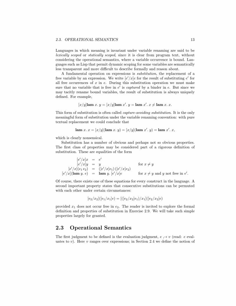
A fundamental operation on expressions is substitution, the replacement of afree variable by an expression. We write [e′/x]e for the result of substituting e′ forall free occurrences of x in e. During this substitution operation we must makesure that no variable that is free in e′ is captured by a binder in e. But since wemay tacitly rename bound variables, the result of substitution is always uniquelydefined. For example,
[x/y]lam x. y = [x/y]lam x′. y = lam x′. x 6= lam x. x.
This form of substitution is often called capture-avoiding substitution. It is the onlymeaningful form of substitution under the variable renaming convention: with puretextual replacement we could conclude that
lam x. x = [x/y](lam x. y) = [x/y](lam x′. y) = lam x′. x,
which is clearly nonsensical.Substitution has a number of obvious and perhaps not so obvious properties.
The first class of properties may be considered part of a rigorous definition ofsubstitution. These are equalities of the form
[e′/x]x = e′
[e′/x]y = y for x 6= y[e′/x](e1 e2) = ([e′/x]e1) ([e′/x]e2)
[e′/x](lam y. e) = lam y. [e′/x]e for x 6= y and y not free in e′.
Of course, there exists one of these equations for every construct in the language. Asecond important property states that consecutive substitutions can be permutedwith each other under certain circumstances:
[e2/x2]([e1/x1]e) = [([e2/x2]e1)/x1]([e2/x2]e)
provided x1 does not occur free in e2. The reader is invited to explore the formaldefinition and properties of substitution in Exercise 2.9. We will take such simpleproperties largely for granted.
2.3 Operational Semantics
The first judgment to be defined is the evaluation judgment, e ↪→ v (read: e eval-uates to v). Here v ranges over expressions; in Section 2.4 we define the notion of

14 CHAPTER 2. THE MINI-ML LANGUAGE
a value and show that the result of evaluation is in fact a value. For now we onlyinformally think of v as representing the value of e. The definition of the evaluationjudgment is given by inference rules. Here, and in the remainder of these notes, wethink of axioms as inference rules with no premises, so that no explicit distinctionbetween axioms and inference rules is necessary. A definition of a judgment viainference rules is inductive in nature, that is, e evaluates to v if and only if e ↪→ vcan be established with the given set of inference rules. We will make use of this in-ductive structure of deductions throughout these notes in order to prove propertiesof deductive systems.
This approach to the description of the operational semantics of programminglanguages goes back to Plotkin [Plo75, Plo81] under the name of structured oper-ational semantics and Kahn [Kah87], who calls his approach natural semantics.Our presentation follows the style of natural semantics.
We begin with the rules concerning the natural numbers.
ev zz ↪→ z
e ↪→ vev s
s e ↪→ s v
The first rule expresses that z is a constant and thus evaluates to itself. The secondexpresses that s is a constructor, and that its argument must be evaluated, that is,the constructor is eager and not lazy. For more on this distinction, see Exercise 2.13.Note that the second rule is schematic in e and v: any instance of this rule is valid.
The next two inference rules concern the evaluation of the case construct. Thesecond of these rules requires substitution as introduced in the previous section.
e1 ↪→ z e2 ↪→ vev case z
(case e1 of z⇒ e2 | s x⇒ e3) ↪→ v
e1 ↪→ s v′1 [v′1/x]e3 ↪→ vev case s
(case e1 of z⇒ e2 | s x⇒ e3) ↪→ v
The substitution of v′1 for x in case e1 evaluates to s v′1 eliminates the need forenvironments which are present in many other semantic definitions. These rulesare declarative in nature, that is, we define the operational semantics by declaringrules of inference for the evaluation judgment without actually implementing aninterpreter. This is exhibited clearly in the two rules for the conditional: in aninterpreter, we would evaluate e1 and then branch to the evaluation of e2 or e3,depending on the value of e1. This interpreter structure is not contained in theserules; in fact, naive search for a deduction under these rules will behave differently(see Section 4.3).
As a simple example that can be expressed using only the four rules given sofar, consider the derivation of (case s (s z) of z ⇒ z | s x′ ⇒ x′) ↪→ s z. This

2.3. OPERATIONAL SEMANTICS 15
would arise as a subdeduction in the derivation of pred (s (s z)) with the earlierdefinition of pred .
ev zz ↪→ z
ev ss z ↪→ s z
ev ss (s z) ↪→ s (s z)
ev zz ↪→ z
ev ss z ↪→ s z
ev case s(case s (s z) of z⇒ z | s x′⇒ x′) ↪→ s z
The conclusion of the second premise arises as [(s z)/x′]x′ = s z. We refer to adeduction of a judgment e ↪→ v as an evaluation deduction or simply evaluation ofe. Thus deductions play the role of traces of computation.
Pairs do not introduce any new ideas.
e1 ↪→ v1 e2 ↪→ v2ev pair
〈e1, e2〉 ↪→ 〈v1, v2〉
e ↪→ 〈v1, v2〉ev fst
fst e ↪→ v1
e ↪→ 〈v1, v2〉ev snd
snd e ↪→ v2
This form of operational semantics avoids explicit error values: for some ex-pressions e there simply does not exist any value v such that e ↪→ v would bederivable. For example, when trying to construct a v and a deduction of the ex-pression (case 〈z, z〉 of z ⇒ z | s x′ ⇒ x′) ↪→ v, one arrives at the followingimpasse:
ev zz ↪→ z
ev zz ↪→ z
ev pair〈z, z〉 ↪→ 〈z, z〉 ?
?case 〈z, z〉 of z⇒ z | s x′ ⇒ x′ ↪→ v
There is no inference rule “?” which would allow us to fill v with an expression andobtain a valid deduction. This particular kind of example will be excluded by thetyping system, since the argument which determines the cases here is not a naturalnumber. On the other hand, natural semantics does not preclude a formulationwith explicit error elements (see Exercise 2.10).
In programming languages such as Mini-ML functional abstractions evaluate tothemselves. This is true for languages with call-by-value and call-by-name seman-tics, and might be considered a distinguishing characteristic of evaluation compared

16 CHAPTER 2. THE MINI-ML LANGUAGE
to normalization.
ev lamlam x. e ↪→ lam x. e
e1 ↪→ lam x. e′1 e2 ↪→ v2 [v2/x]e′1 ↪→ vev app
e1 e2 ↪→ v
This specifies a call-by-value discipline for our language, since we evaluate e2 andthen substitute the resulting value v2 for x in the function body e′1. In a call-by-name discipline, we would omit the second premise and the third premise would be[e2/x]e′1 ↪→ v (see Exercise 2.13).
The inference rules above have an inherent inefficiency: the deduction of a judg-ment of the form [v2/x]e′1 ↪→ v may have many copies of a deduction of v2 ↪→ v2.In an actual interpreter, we would like to evaluate e′1 in an environment where x isbound to v2 and simply look up the value of x when needed. Such a modification inthe specification, however, is not straightforward, since it requires the introductionof closures. We make such an extension to the language as part of the compilationprocess in Section 6.1.
The rules for let are straightforward, given our understanding of function ap-plication. There are two variants, depending on whether the subject is evaluated(let val) or not (let name).
e1 ↪→ v1 [v1/x]e2 ↪→ vev letv
let val x = e1 in e2 ↪→ v
[e1/x]e2 ↪→ vev letn
let name x = e1 in e2 ↪→ v
The letval construct is intended for the computation of intermediate results thatmay be needed more than once, while the let name construct is primarily intendedto give names to functions so they can be used polymorphically. For more on thisdistinction, see Section 2.5.
Finally, we come to the fixed point construct. Following the considerations inthe example on page 11, we arrive at the rule
[fix x. e/x]e ↪→ vev fix.
fix x. e ↪→ v
Thus evaluation of a fixed point construct unrolls the recursion one level and eval-uates the result. Typically this uncovers a lam-abstraction which evaluates to
2.3. OPERATIONAL SEMANTICS 17
itself. This rule clearly exhibits another situation in which an expression does nothave a value: consider fix x. x. There is only one rule with a conclusion of theform fix x. e ↪→ v, namely ev fix. So if fix x. x ↪→ v were derivable for some v,then the premise, namely [fix x. x/x]x ↪→ v would also have to be derivable. But[fix x. x/x]x = fix x. x, and the instance of ev fix would have to have the form
fix x. x ↪→ vev fix.
fix x. x ↪→ v
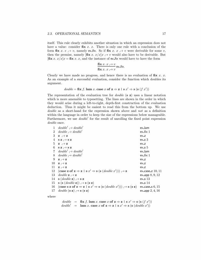
Clearly we have made no progress, and hence there is no evaluation of fix x. x.As an example of a successful evaluation, consider the function which doubles itsargument.
double = fix f. lam x. case x of z⇒ z | s x′ ⇒ s (s (f x′))
The representation of the evaluation tree for double (s z) uses a linear notationwhich is more amenable to typesetting. The lines are shown in the order in whichthey would arise during a left-to-right, depth-first construction of the evaluationdeduction. Thus it might be easiest to read this from the bottom up. We usedouble as a short-hand for the expression shown above and not as a definitionwithin the language in order to keep the size of the expressions below manageable.Furthermore, we use double′ for the result of unrolling the fixed point expressiondouble once.
1 double′ ↪→ double′ ev lam2 double ↪→ double′ ev fix 13 z ↪→ z ev z4 s z ↪→ s z ev s 35 z ↪→ z ev z6 s z ↪→ s z ev s 57 double′ ↪→ double′ ev lam8 double ↪→ double′ ev fix 19 z ↪→ z ev z
10 z ↪→ z ev z11 z ↪→ z ev z12 (case z of z⇒ z | s x′ ⇒ s (s (double x′))) ↪→ z ev case z 10, 1113 double z ↪→ z ev app 8, 9, 1214 s (double z) ↪→ s z ev s 1315 s (s (double z)) ↪→ s (s z) ev s 1416 (case s z of z⇒ z | s x′⇒ s (s (double x′))) ↪→ s (s z) ev case s 6, 1517 double (s z) ↪→ s (s z) ev app 2, 4, 16
where
double = fix f. lam x. case x of z⇒ z | s x′ ⇒ s (s (f x′))double′ = lam x. case x of z⇒ z | s x′ ⇒ s (s (double x′))

18 CHAPTER 2. THE MINI-ML LANGUAGE
The inefficiencies of the rules we alluded to above can be seen clearly in thisexample: we need two copies of the evaluation of s z, one of which should in principlebe unnecessary, since we are in a call-by-value language (see Exercise 2.12).
2.4 Evaluation Returns a Value
Before we discuss the type system, we will formulate and prove a simple meta-theorem. The set of values in Mini-ML can be described by the BNF grammar
Values v ::= z | s v | 〈v1, v2〉 | lam x. e.
This kind of grammar can be understood as a form of inductive definition of asubcategory of the syntactic category of expressions: a value is either z, the successorof a value, a pair of values, or any lam-expression. There are alternative equivalentdefinition of values, for example as those expressions which evaluate to themselves(see Exercise 2.14). Syntactic subcategories (such as values as a subcategory ofexpressions) can also be defined using deductive systems. The judgment in thiscase is unary: e Value. It is defined by the following inference rules:
val zz Value
e Valueval s
s e Value
e1 Value e2 Valueval pair
〈e1, e2〉 Valueval lam
lam x. e Value
Again, this definition is inductive: an expression e is a value if and only if e Valuecan be derived using these inference rules. It is common mathematical practice touse different variable names for elements of the smaller set in order to distinguishthem in the presentation. But is it justified to write e ↪→ v with the understandingthat v is a value? This is the subject of the next theorem. The proof is instructiveas it uses an induction over the structure of a deduction. This is a central techniquefor proving properties of deductive systems and the judgments they define. Thebasic idea is simple: if we would like to establish a property for all deductions of ajudgment we show that the property is preserved by all inference rules, that is, weassume the property holds of the deduction of the premises and we must show thatthe property holds of the deduction of the conclusion. For an axiom (an inferencerule with no premises) this just means that we have to prove the property outright,with no assumptions. An important special case of this induction principle is aninversion principle: in many cases the form of a judgment uniquely determinesthe last rule of inference which must have been applied, and we may conclude theexistence of a deduction of the premise.

2.4. EVALUATION RETURNS A VALUE 19
Theorem 2.1 (Value Soundness) For any two expressions e and v, if e ↪→ v isderivable, then v Value is derivable.
Proof: The proof is by induction over the structure of the deduction D :: e ↪→ v.We show a number of typical cases.
Case: D = ev z.z ↪→ z
Then v = z is a value by the rule val z.
Case:
D =
D1
e1 ↪→ v1ev s.
s e1 ↪→ s v1
The induction hypothesis on D1 yields a deduction of v1 Value. Using theinference rule val s we conclude that s v1 Value.
Case:
D =
D1
e1 ↪→ zD2
e2 ↪→ vev case z.
(case e1 of z⇒ e2 | s x⇒ e3) ↪→ v
Then the induction hypothesis applied to D2 yields a deduction of v Value,which is what we needed to show in this case.
Case:
D =
D1
e1 ↪→ s v′1
D3
[v′1/x]e3 ↪→ vev case s.
(case e1 of z⇒ e2 | s x⇒ e3) ↪→ v
Then the induction hypothesis applied to D3 yields a deduction of v Value,which is what we needed to show in this case.
Case: If D ends in ev pair we reason similar to cases above.
Case:
D =
D′e′ ↪→ 〈v1, v2〉
ev fst.fst e′ ↪→ v1
Then the induction hypothesis applied to D′ yields a deduction P ′ of thejudgment 〈v1, v2〉 Value. By examining the inference rules we can see that P ′

20 CHAPTER 2. THE MINI-ML LANGUAGE
must end in an application of the val pair rule, that is,
P ′ =
P1
v1 ValueP2
v2 Valueval pair
〈v1, v2〉 Value
for some P1 and P2. Hence v1 Value must be derivable, which is what weneeded to show. We call this form of argument inversion.
Case: If D ends in ev snd we reason similar to the previous case.
Case: D = ev lam.lam x. e ↪→ lam x. e
Again, this case is immediate, since v = lam x. e is a value by rule val lam.
Case:
D =
D1
e1 ↪→ lam x. e′1
D2
e2 ↪→ v2
D3
[v2/x]e′1 ↪→ vev app.
e1 e2 ↪→ v
Then the induction hypothesis on D3 yields that v Value.
Case: D ends in ev letv. Similar to the previous case.
Case: D ends in ev letn. Similar to the previous case.
Case:
D =
D1
[fix x. e/x]e ↪→ vev fix.
fix x. e ↪→ v
Again, the induction hypothesis on D1 directly yields that v is a value.
2
Since it is so pervasive, we briefly summarize the principle of structural inductionused in the proof above. We assume we have an arbitrary derivation D of e ↪→ vand we would like to prove a property P of D. We show this by induction on thestructure of D: For each inference rule in the system defining the judgment e ↪→ vwe show that the property P holds for the conclusion under the assumption thatit holds for every premise. In the special case of an inference rule with no premiseswe have no inductive assumptions; this therefore corresponds to a base case of theinduction. This suffices to establish the property P for every derivation D since itmust be constructed from the given inference rules. In our particular theorem theproperty P states that there exists a derivation P of the judgment that v is a value.
2.5. THE TYPE SYSTEM 21
2.5 The Type System
In the presentation of the language so far we have not used types. Thus typesare external to the language of expressions and a judgment such as . e : τ maybe considered as establishing a property of the (untyped) expression e. This viewof types has been associated with Curry [Cur34, CF58], and systems in this styleare often called type assignment systems. An alternative is a system in the styleof Church [Chu32, Chu33, Chu41], in which types are included within expressions,and every well-typed expression has a unique type. We will discuss such a systemin Section ??.
Mini-ML as presented by Clement et al. [CDDK86] is a language with somelimited polymorphism in that it explicitly distinguishes between simple types andtype schemes with some restrictions on the use of type schemes. This notion ofpolymorphism was introduced by Milner [Mil78, DM82]. We will refer to it asschematic polymorphism. In our formulation, we will be able to avoid using typeschemes completely by distinguishing two forms of definitions via let, one of which ispolymorphic. A formulation in this style orginates with Hannan and Miller [HM89,Han91, Han93].
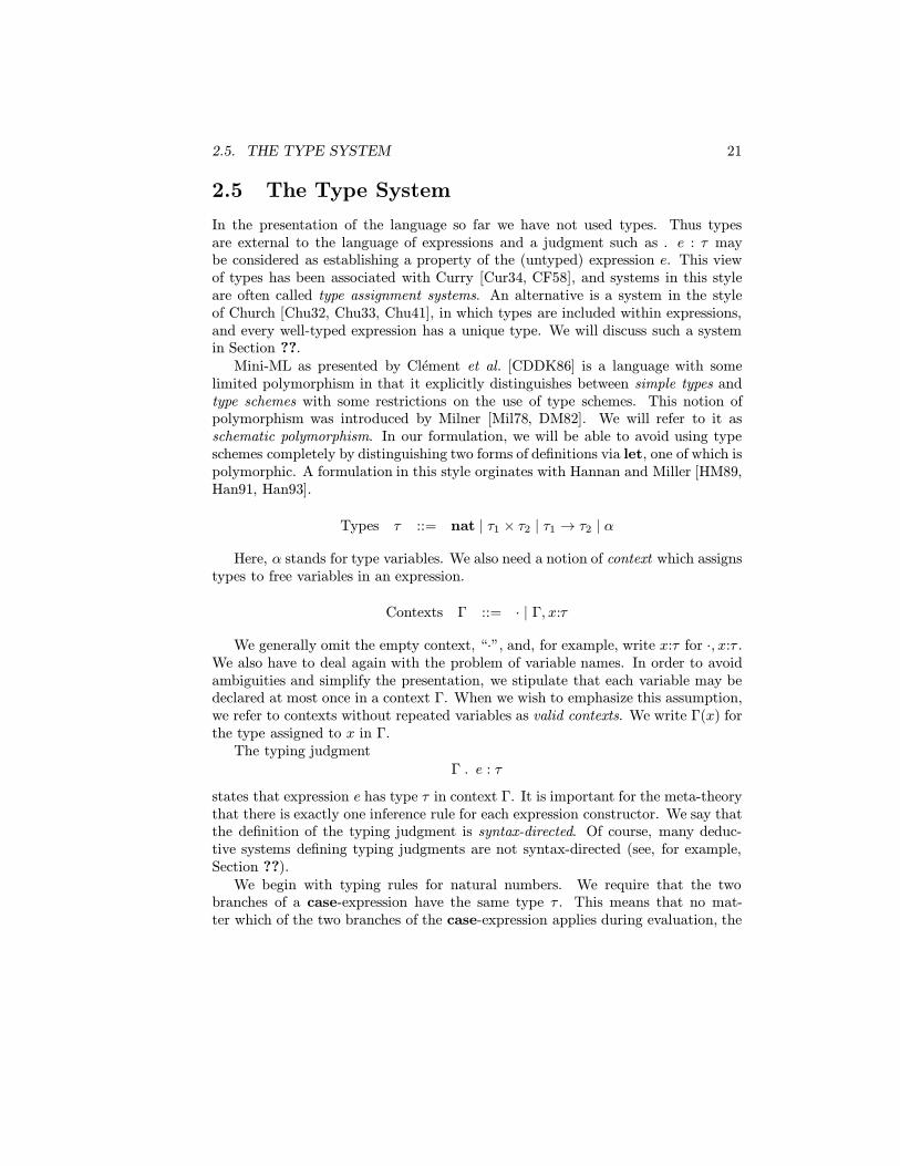
Types τ ::= nat | τ1 × τ2 | τ1 → τ2 | α
Here, α stands for type variables. We also need a notion of context which assignstypes to free variables in an expression.
Contexts Γ ::= · | Γ, x:τ
We generally omit the empty context, “·”, and, for example, write x:τ for ·, x:τ .We also have to deal again with the problem of variable names. In order to avoidambiguities and simplify the presentation, we stipulate that each variable may bedeclared at most once in a context Γ. When we wish to emphasize this assumption,we refer to contexts without repeated variables as valid contexts. We write Γ(x) forthe type assigned to x in Γ.
The typing judgmentΓ . e : τ
states that expression e has type τ in context Γ. It is important for the meta-theorythat there is exactly one inference rule for each expression constructor. We say thatthe definition of the typing judgment is syntax-directed. Of course, many deduc-tive systems defining typing judgments are not syntax-directed (see, for example,Section ??).
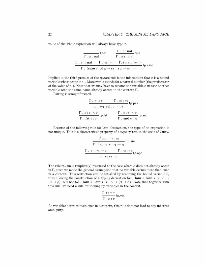
We begin with typing rules for natural numbers. We require that the twobranches of a case-expression have the same type τ . This means that no mat-ter which of the two branches of the case-expression applies during evaluation, the
22 CHAPTER 2. THE MINI-ML LANGUAGE
value of the whole expression will always have type τ .
tp zΓ . z : nat
Γ . e : nattp s
Γ . s e : nat
Γ . e1 : nat Γ . e2 : τ Γ, x:nat . e3 : τtp case
Γ . (case e1 of z⇒ e2 | s x⇒ e3) : τ
Implicit in the third premise of the tp case rule is the information that x is a boundvariable whose scope is e3. Moreover, x stands for a natural number (the predecessorof the value of e1). Note that we may have to rename the variable x in case anothervariable with the same name already occurs in the context Γ.
Pairing is straightforward.
Γ . e1 : τ1 Γ . e2 : τ2tp pair
Γ . 〈e1, e2〉 : τ1 × τ2Γ . e : τ1 × τ2
tp fstΓ . fst e : τ1
Γ . e : τ1 × τ2tp snd
Γ . snd e : τ2
Because of the following rule for lam-abstraction, the type of an expression isnot unique. This is a characteristic property of a type system in the style of Curry.
Γ, x:τ1 . e : τ2tp lam
Γ . lam x. e : τ1 → τ2
Γ . e1 : τ2 → τ1 Γ . e2 : τ2tp app
Γ . e1 e2 : τ1
The rule tp lam is (implicitly) restricted to the case where x does not already occurin Γ, since we made the general assumption that no variable occurs more than oncein a context. This restriction can be satisfied by renaming the bound variable x,thus allowing the construction of a typing derivation for . lam x. lam x. x : α →(β → β), but not for . lam x. lam x. x : α → (β → α). Note that together withthis rule, we need a rule for looking up variables in the context.
Γ(x) = τtp var
Γ . x : τ
As variables occur at most once in a context, this rule does not lead to any inherentambiguity.

2.5. THE TYPE SYSTEM 23
Our language incorporates a let val expression to compute intermediate values.This is not strictly necessary, since it may be defined using lam-abstraction andapplication (see Exercise 2.20).
Γ . e1 : τ1 Γ, x:τ1 . e2 : τ2tp letv
Γ . letval x = e1 in e2 : τ2
Even though e1 may have more than one type, only one of these types (τ1) can beused for occurrences of x in e2. In other words, x can not be used polymorphically,that is, at various types.
Schematic polymorphism (or ML-style polymorphism) only plays a role in thetyping rule for let name. What we would like to achieve is that, for example, thefollowing judgment holds:
. let name f = lam x. x in 〈f z, f (lam y. s y)〉 : nat× (nat→ nat)
Clearly, the expression can be evaluated to 〈z, (lam y. s y)〉, since lam x. x can actas the identity function on any type, that is, both
. lam x. x : nat→ nat,and . lam x. x : (nat→ nat)→ (nat→ nat)
are derivable. In a type system with explicit polymorphism a more general judg-ment might be expressed as . lam x. x : ∀α. α → α (see Section ??). Here, weuse a different device by allowing different types to be assigned to e1 at differentoccurrences of x in e2 when type-checking let name x = e1 in e2. We achieve thisby substituting e1 for x in e2 and checking only that the result is well-typed.
Γ . e1 : τ1 Γ . [e1/x]e2 : τ2tp letn
Γ . letname x = e1 in e2 : τ2
Note that τ1, the type assigned to e1 in the first premise, is not used anywhere.We require such a derivation nonetheless so that all subexpressions of a well-typedterm are guaranteed to be well-typed (see Exercise 2.21). The reader may want tocheck that with this rule the example above is indeed well-typed.
Finally we come to the typing rule for fixed point expressions. In the evaluationrule, we substitute [fix x. e/x]e in order to evaluate fix x. e. For this to be well-typed, the body e must be well-typed under the assumption that the variable x hasthe type of whole fixed point expression. Thus we are lead to the rule
Γ, x:τ . e : τtp fix.
Γ . fix x. e : τ
24 CHAPTER 2. THE MINI-ML LANGUAGE
More general typing rules for fixed point constructs have been considered in theliterature, most notably the rule of the Milner-Mycroft calculus which is discussedin Section ??.
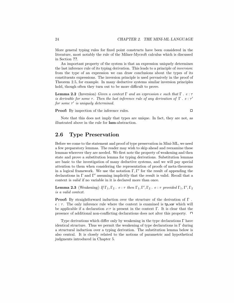
An important property of the system is that an expression uniquely determinesthe last inference rule of its typing derivation. This leads to a principle of inversion:from the type of an expression we can draw conclusions about the types of itsconstituents expressions. The inversion principle is used pervasively in the proof ofTheorem 2.5, for example. In many deductive systems similar inversion principleshold, though often they turn out to be more difficult to prove.
Lemma 2.2 (Inversion) Given a context Γ and an expression e such that Γ . e : τis derivable for some τ . Then the last inference rule of any derivation of Γ . e : τ ′
for some τ ′ is uniquely determined.
Proof: By inspection of the inference rules. 2
Note that this does not imply that types are unique. In fact, they are not, asillustrated above in the rule for lam-abstraction.
2.6 Type Preservation
Before we come to the statement and proof of type preservation in Mini-ML, we needa few preparatory lemmas. The reader may wish to skip ahead and reexamine theselemmas wherever they are needed. We first note the property of weakening and thenstate and prove a substitution lemma for typing derivations. Substitution lemmasare basic to the investigation of many deductive systems, and we will pay specialattention to them when considering the representation of proofs of meta-theoremsin a logical framework. We use the notation Γ,Γ′ for the result of appending thedeclarations in Γ and Γ′ assuming implicitly that the result is valid. Recall that acontext is valid if no variable in it is declared more than once.
Lemma 2.3 (Weakening) If Γ1,Γ2 . e : τ then Γ1,Γ′,Γ2 . e : τ provided Γ1,Γ
′,Γ2
is a valid context.
Proof: By straightforward induction over the structure of the derivation of Γ .e : τ . The only inference rule where the context is examined is tp var which willbe applicable if a declaration x:τ is present in the context Γ. It is clear that thepresence of additional non-conflicting declarations does not alter this property. 2
Type derivations which differ only by weakening in the type declarations Γ haveidentical structure. Thus we permit the weakening of type declarations in Γ duringa structural induction over a typing derivation. The substitution lemma below isalso central. It is closely related to the notions of parametric and hypotheticaljudgments introduced in Chapter 5.

2.6. TYPE PRESERVATION 25
Lemma 2.4 (Substitution) If Γ . e′ : τ ′ and Γ, x:τ ′,Γ′ . e : τ then Γ,Γ′ . [e′/x]e :τ .
Proof: By induction over the structure of the derivation D :: (Γ, x:τ ′,Γ′ . e : τ).The result should be intuitive: wherever x occurs in e we are at a leaf in the typingderivation of e. After substitution of e′ for x, we have to supply a derivation showingthat e′ has type τ ′ at this leaf position, which exists by assumption. We only showa few cases in the proof in detail; the remaining ones follow the same pattern.
Case: D =(Γ, x:τ ′,Γ′)(x) = τ ′
tp var.Γ, x:τ ′,Γ′ . x : τ ′
Then [e′/x]e = [e′/x]x = e′, so the lemma reduces to showing Γ,Γ′ . e′ : τ ′
from Γ . e′ : τ ′ which follows by weakening.
Case: D =(Γ, x:τ ′,Γ′)(y) = τ
tp var,Γ, x:τ ′,Γ′ . y : τ
where x 6= y.
In this case, [e′/x]e= [e′/x]y = y and hence the lemma follows from
(Γ,Γ′)(y) = τtp var.
Γ,Γ′ . y : τ
Case: D =
D1
Γ, x:τ ′,Γ′ . e1 : τ2 → τ1
D2
Γ, x:τ ′,Γ′ . e2 : τ2tp app.
Γ, x:τ ′,Γ′ . e1 e2 : τ1
Then we construct a deduction
E1Γ,Γ′ . [e′/x]e1 : τ2 → τ1
E2Γ,Γ′ . [e′/x]e2 : τ2
tp appΓ,Γ′ . ([e′/x]e1) ([e′/x]e2) : τ1
where E1 and E2 are known to exist from the induction hypothesis appliedto D1 and D2, respectively. By definition of substitution, [e′/x](e1 e2) =([e′/x]e1) ([e′/x]e2), and the lemma is established in this case.
Case: D =
D1
Γ, x:τ ′,Γ′, y:τ1 . e2 : τ2tp lam
Γ, x:τ ′,Γ′ . lam y. e2 : τ1 → τ2.
In this case we need to apply the induction hypothesis by using Γ′, y:τ1 for Γ′.This is why the lemma is formulated using the additional context Γ′. From

26 CHAPTER 2. THE MINI-ML LANGUAGE
the induction hypothesis and one inference step we obtain
E1Γ,Γ′, y:τ1 . [e′/x]e2 : τ2
tp lamΓ,Γ′ . lam y. [e′/x]e2 : τ1 → τ2
which yields the lemma by the equation [e′/x](lam y. e2) = lam y. [e′/x]e2 ify is not free in e′ and distinct from x. We can assume that these conditionsare satisfied, since they can always be achieved by renaming bound variables.
2
The statement of the type preservation theorem below is written in such a waythat the induction argument will work directly.
Theorem 2.5 (Type Preservation) For any e and v, if e ↪→ v is derivable, thenfor any τ such that . e : τ is derivable, . v : τ is also derivable.
Proof: By induction on the structure of the deduction D of e ↪→ v. The justification“by inversion” refers to Lemma 2.2. More directly, from the form of the judgmentestablished by a derivation we draw conclusions about the possible forms of thepremise, which, of course, must also derivable.
Case: D = ev z.z ↪→ z
Then we have to show that for any type τ such that . z : τ is derivable, . z : τis derivable. This is obvious.
Case: D =
D1
e1 ↪→ v1ev s.
s e1 ↪→ s v1
Then
. s e1 : τ By assumption
. e1 : nat and τ = nat By inversion
. v1 : nat By ind. hyp. on D1
. s v1 : nat By rule tp s
Case: D =
D1
e1 ↪→ zD2
e2 ↪→ vev case z.
(case e1 of z⇒ e2 | s x⇒ e3) ↪→ v
. (case e1 of z⇒ e2 | s x⇒ e3) : τ By assumption
. e2 : τ By inversion
. v : τ By ind. hyp. on D2
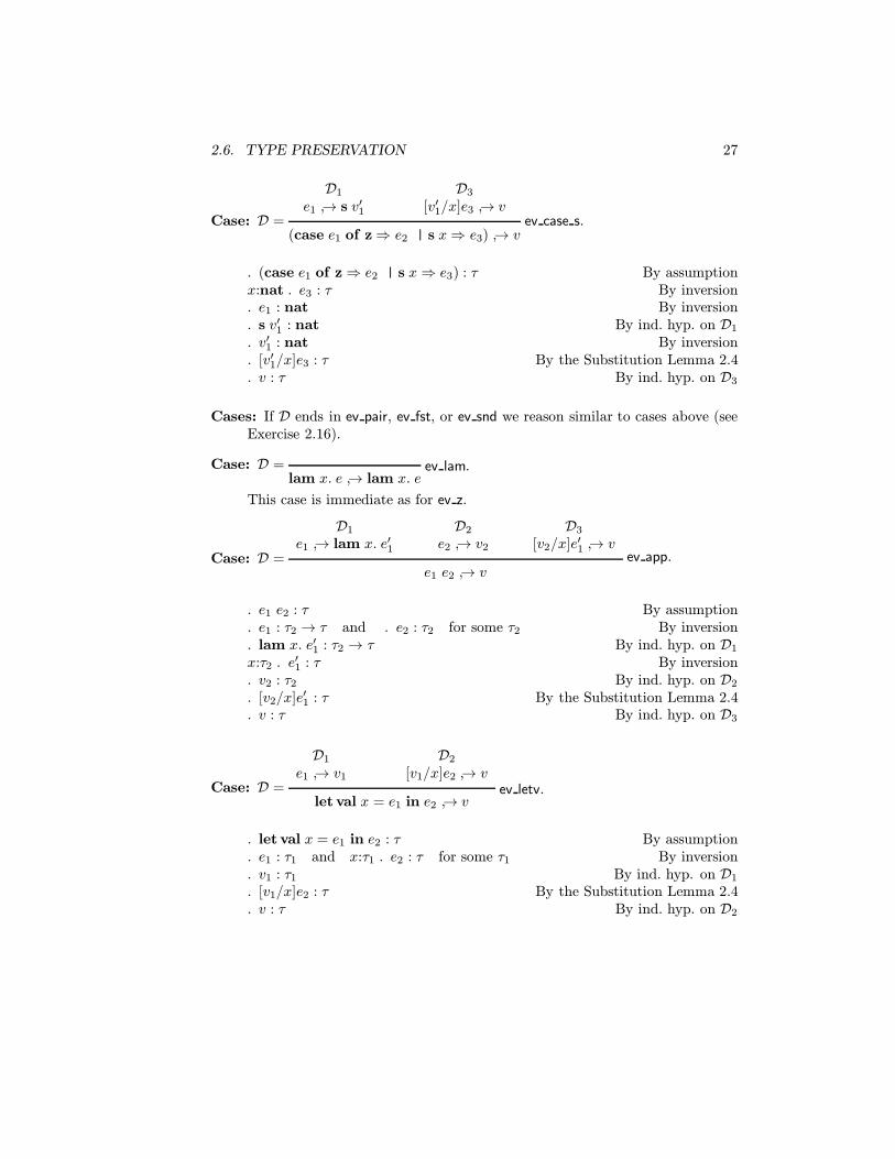
2.6. TYPE PRESERVATION 27
Case: D =
D1
e1 ↪→ s v′1
D3
[v′1/x]e3 ↪→ vev case s.
(case e1 of z⇒ e2 | s x⇒ e3) ↪→ v
. (case e1 of z⇒ e2 | s x⇒ e3) : τ By assumptionx:nat . e3 : τ By inversion. e1 : nat By inversion. s v′1 : nat By ind. hyp. on D1
. v′1 : nat By inversion
. [v′1/x]e3 : τ By the Substitution Lemma 2.4
. v : τ By ind. hyp. on D3
Cases: If D ends in ev pair, ev fst, or ev snd we reason similar to cases above (seeExercise 2.16).
Case: D = ev lam.lam x. e ↪→ lam x. e
This case is immediate as for ev z.
Case: D =
D1
e1 ↪→ lam x. e′1
D2
e2 ↪→ v2
D3
[v2/x]e′1 ↪→ vev app.
e1 e2 ↪→ v
. e1 e2 : τ By assumption
. e1 : τ2 → τ and . e2 : τ2 for some τ2 By inversion
. lam x. e′1 : τ2 → τ By ind. hyp. on D1
x:τ2 . e′1 : τ By inversion
. v2 : τ2 By ind. hyp. on D2
. [v2/x]e′1 : τ By the Substitution Lemma 2.4
. v : τ By ind. hyp. on D3
Case: D =
D1
e1 ↪→ v1
D2
[v1/x]e2 ↪→ vev letv.
let val x = e1 in e2 ↪→ v
. let val x = e1 in e2 : τ By assumption
. e1 : τ1 and x:τ1 . e2 : τ for some τ1 By inversion
. v1 : τ1 By ind. hyp. on D1
. [v1/x]e2 : τ By the Substitution Lemma 2.4
. v : τ By ind. hyp. on D2

28 CHAPTER 2. THE MINI-ML LANGUAGE
Case: D =
D2
[e1/x]e2 ↪→ vev letn.
let name x = e1 in e2 ↪→ v
. let name x = e1 in e2 : τ By assumption
. [e1/x]e2 : τ By inversion
. v : τ By ind. hyp. on D2
Case: D =
D1
[fix x. e1/x]e1 ↪→ vev fix.
fix x. e1 ↪→ v
. fix x. e1 : τ By assumptionx : τ . e1 : τ By inversion. [fix x. e1/x]e1 : τ By the Substitution Lemma 2.4. v : τ By ind. hyp. on D1
2
It is important to recognize that this theorem cannot be proved by induction onthe structure of the expression e. The difficulty is most pronounced in the cases forlet and fix: The expressions in the premises of these rules are in general much largerthan the expressions in the conclusion. Similarly, we cannot prove type preservationby an induction on the structure of the typing derivation of e.
2.7 Further Discussion
Ignoring details of concrete syntax, the Mini-ML language is completely specifiedby its typing and evaluation rules. Consider a simple simple model of an interactionwith an implementation of Mini-ML consisting of two phases: type-checking andevaluation. During the first phase the implementation only accepts expressionse that are well-typed in the empty context, that is, . e : τ for some τ . In thesecond phase the implementation constructs and prints a value v such that e ↪→ vis derivable. This model is simplistic in some ways, for example, we ignore thequestion which values can actually be printed or observed by the user. We willreturn to this point in Section ??.
Our self-contained language definition by means of deductive systems does notestablish a connection between types, values, expressions, and mathematical objectssuch as partial functions. This can be seen as the subject of denotational semantics.For example, we understand intuitively that the expression
ss = lam x. s (s x)

2.7. FURTHER DISCUSSION 29
denotes the function from natural numbers to natural numbers that adds 2 to itsargument. Similarly,
pred0 = lam x. case x of z⇒ fix y. y | s x′ ⇒ x′
denotes the partial function from natural numbers to natural numbers that returnsthe predecessor of any argument greater or equal to 1 and is undefined on 0. Butis this intuitive interpretation of expressions justified? As a first step, we establishthat the result of evaluation (if one exists) is unique. Recall that expressions thatdiffer only in the names of their bound variables are considered equal.
Theorem 2.6 (Uniqueness of Values) If e ↪→ v1 and e ↪→ v2 are derivable thenv1 = v2.
Proof: Straightforward (see Exercise 2.17). 2
Intuitively the type nat can be interpreted by the set of natural numbers. Wewrite vnat for values v such that . v : nat. It can easily be seen by induction on thestructure of the derivation of vnat Value that vnat could be defined inductively by
vnat ::= z | s vnat.
The meaning or denotation of a value vnat, [[vnat]], can be defined almost trivially as
[[z]] = 0[[s vnat]] = [[vnat]] + 1.
It is immediate that this is a bijection between closed values of type nat and thenatural numbers. The meaning of an arbitrary closed expression enat of type natcan then be defined by
[[enat]] =
{[[v]] if enat ↪→ v is derivableundefined otherwise
Determinism of evaluation (Theorem 2.6) tells us that v, if it exists, is uniquelydefined. Value soundness 2.1 tells us that v is indeed a value. Type preservation(Theorem 2.5) tells us that v will be a closed expression of type nat and thus thatthe meaning of an arbitrary expression of type nat, if it is defined, is a uniquenatural number. Furthermore, we are justified in overloading the [[·]] notation forvalues and arbitrary expressions, since values evaluate to themselves (Exercise 2.14).
Next we consider the meaning of expressions of functional type. Intuitively, if. e : nat → nat, then the meaning of e should be a partial function from naturalnumbers to natural numbers. We define this as follows:
[[e]](n) =
{[[v2]] if e v1 ↪→ v2 and [[v1]] = nundefined otherwise

30 CHAPTER 2. THE MINI-ML LANGUAGE
This definition is well-formed by reasoning similar to the above, using the observa-tion that [[·]] is a bijection between closed values of type nat and natural numbers.
Thus we were justified in thinking of the type nat → nat as consisting ofpartial functions from natural numbers to natural numbers. Partial functions inmathematics are understood in terms of their input/output behavior rather than interms of their concrete definition; they are viewed extensionally. For example, theexpressions
ss = lam x. s (s x) andss ′ = fix f. lam x. case x of z⇒ s (s z) | s x′⇒ s (f x′)
denote the same function from natural numbers to natural numbers: [[ss]] = [[ss ′]].Operationally, of course, they have very different behavior. Thus denotational se-mantics induces a non-trivial notion of equality between expressions in our language.On the other hand, it is not immediately clear how to take advantage of this equal-ity due to its non-constructive nature. The notion of extensional equality betweenpartial recursive function is not recursively axiomatizable and therefore we cannotwrite a complete deductive system to prove functional equalities. The denotationalapproach can be extended to higher types (for example, functions that map func-tions from natural numbers to natural numbers to functions from natural numbersto natural numbers) in a natural way.
It may seem from the above development that the denotational semantics ofa language is uniquely determined. This is not the case: there are many choices.Especially the mathematical domains we use to interpret expressions and the struc-ture we impose on them leave open many possibilites. For more on the subject ofdenotational semantics see, for example, [Gun92].
In the approach above, the meaning of an expression depends on its type. Forexample, for the expression id = lam x. x we have . id : nat → nat and by thereasoning above we can interpret it as a function from natural numbers to naturalnumbers. We also have . id : (nat → nat) → (nat → nat), so it also mapsevery function between natural numbers to itself. This inherent ambiguity is dueto our use of Curry’s approach where types are assigned to untyped expressions. Itcan be remedied in two natural ways: we can construct denotations independentlyof the language of types, or we can give meaning to typing derivations. In thefirst approach, types can be interpreted as subsets of a universe from which themeanings of untyped expressions are drawn. The disadvantage of this approach isthat we have to give meanings to all expressions, even those that are intuitivelymeaningless, that is, ill-typed. In the second approach, we only give meaning toexpressions that have typing derivations. Any possible ambiguity in the assignmentof types is resolved, since the typing derivation will choose are particular type for theexpression. On the other hand we may have to consider coherence: different typingderivations for the same expression and type should lead to the same meaning. Atthe very least the meanings should be compatible in some way so that arbitrary

2.8. EXERCISES 31
decisions made during type inference do not lead to observable differences in thebehavior of a program. In the Mini-ML language we discussed so far, this propertyis easily seen to hold, since an expression uniquely determines its typing derivation.For more complex languages this may require non-trivial proof. Note that theambiguity problem does not usually arise when we choose a language presentationin the style of Church where each expression contains enough type information touniquely determine its type.
2.8 Exercises
Exercise 2.1 Write Mini-ML programs for multiplication, exponentiation, sub-traction, and a function that returns a pair of (integer) quotient and remainder oftwo natural numbers.
Exercise 2.2 The principal type of an expression e is a type τ such that any typeτ ′ of e can be obtained by instantiating the type variables in τ . Even though typesin our formulation of Mini-ML are not unique, every well-typed expression has aprincipal type [Mil78]. Write Mini-ML programs satisfying the following informalspecifications and determine their principal types.
1. compose f g to compute the composition of two functions f and g.
2. iterate n f x to iterate the function f n times over x.
Exercise 2.3 Write down the evaluation of plus2 (s z) (s z), given the definitionof plus2 in the example on page 11.
Exercise 2.4 Write out the typing derivation that shows that the function doubleon page 17 is well-typed.
Exercise 2.5 Explore a few alternatives to the definition of expressions given inSection 2.1. In each case, give the relevant inference rules for evaluation and typing.
1. Add a type of Booleans and replace the constructs concerning natural numbersby
e ::= . . . | z | s e | pred e | zerop e
2. Replace the constructs concerning pairs by
e ::= . . . | pair | fst | snd
3. Replace the constructs concerning pairs by
e ::= . . . | 〈e1, e2〉 | split e1 as 〈x1, x2〉 ⇒ e2
32 CHAPTER 2. THE MINI-ML LANGUAGE
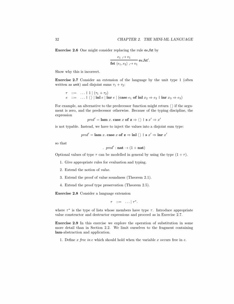
Exercise 2.6 One might consider replacing the rule ev fst by
e1 ↪→ v1ev fst′.
fst 〈e1, e2〉 ↪→ v1
Show why this is incorrect.
Exercise 2.7 Consider an extension of the language by the unit type 1 (oftenwritten as unit) and disjoint sums τ1 + τ2:
τ ::= . . . | 1 | (τ1 + τ2)e ::= . . . | 〈 〉 | inl e | inr e | (case e1 of inl x2 ⇒ e2 | inr x3 ⇒ e3)
For example, an alternative to the predecessor function might return 〈 〉 if the argu-ment is zero, and the predecessor otherwise. Because of the typing discipline, theexpression
pred ′ = lam x. case x of z⇒ 〈 〉 | s x′ ⇒ x′
is not typable. Instead, we have to inject the values into a disjoint sum type:
pred ′ = lam x. case x of z⇒ inl 〈 〉 | s x′ ⇒ inr x′
so that. pred ′ : nat→ (1 + nat)
Optional values of type τ can be modelled in general by using the type (1 + τ).
1. Give appropriate rules for evaluation and typing.
2. Extend the notion of value.
3. Extend the proof of value soundness (Theorem 2.1).
4. Extend the proof type preservation (Theorem 2.5).
Exercise 2.8 Consider a language extension
τ ::= . . . | τ∗.
where τ∗ is the type of lists whose members have type τ . Introduce appropriatevalue constructor and destructor expressions and proceed as in Exercise 2.7.
Exercise 2.9 In this exercise we explore the operation of substitution in somemore detail than in Section 2.2. We limit ourselves to the fragment containinglam-abstraction and application.
1. Define x free in e which should hold when the variable x occurs free in e.

2.8. EXERCISES 33
2. Define e =α e′ which should hold when e and e′ are alphabetic variants, that
is, they differ only in the names assigned to their bound variables as explainedin Section 2.2.
3. Define [e′/x]e, the result of substituting e′ for x in e. This operation shouldavoid capture of variables free in e′ and the result should be unique up torenaming of bound variables.
4. Prove [e′/x]e =α e if x does not occur free in e′.
5. Prove [e2/x2]([e1/x1]e) =α [([e2/x2]e1)/x1]([e2/x2]e), provided x1 does notoccur free in e2.
Exercise 2.10 In this exercise we will explore different ways to treat errors in thesemantics.
1. Assume there is a new value error of arbitary type and modify the operationalsemantics appropriately. You may assume that only well-typed expressions areevaluated. For example, evaluation of s (lam x. x) does not need to result inerror.
2. Add an empty type 0 (often called void) containing no values. Are thereany closed expressions of type 0? Add a new expression form abort e whichhas arbitrary type τ whenever e has type 0, but add no evaluation rules forabort. Do the value soundness and type preservation properties extend tothis language? How does this language compare to the one in item 1.
3. An important semantic property of type systems is often summarized as “well-typed programs cannot go wrong.” The meaning of ill-typed expressions suchas fst z would be defined as a distinguished semantic value wrong (in contrastto intuitively non-terminating expressions such as fix x. x) and it is thenshown that no well-typed expression has meaning wrong. A related phraseis that in statically typed languages “no type-errors can occur at runtime.”Discuss how these properties might be expressed in the framework presentedhere and to what extent they are already reflected in the type preservationtheorem.
Exercise 2.11 In the language Standard ML [MTH90], occurrences of fixed pointexpressions are syntactially restricted to the form fix x. lam y. e. This means thatevaluation of a fixed point expression always terminates in one step with the valuelam y. [fix x. lam y. e/x]e.
It has occasionally been proposed to extend ML so that one can construct re-cursive values. For example, ω = fix x. s x would represent a “circular value”s (s . . .) which could not be printed finitely. The same value could also be defined,for example, as ω′ = fix x. s (s x).

34 CHAPTER 2. THE MINI-ML LANGUAGE
In our language, the expressions ω and ω′ are not values and, in fact, they donot even have a value. Intuitively, their evaluation does not terminate.
Define an alternative semantics for the Mini-ML language that permits recursivevalues. Modify the definition of values and the typing rules as necessary. Sketch therequired changes to the statements and proofs of value soundness, type preservation,and uniqueness of values. Discuss the relative merits of the two languages.
Exercise 2.12 Explore an alternative operational semantics in which expressionsthat are known to be values (since they have been evaluated) are not evaluatedagain. State and prove in which way the new semantics is equivalent to the onegiven in Section 2.3.Hint: It may be necessary to extend the language of expressions or explicitlyseparate the language of values from the language of expressions.
Exercise 2.13 Specify a call-by-name operational semantics for our language,where function application is given by
e1 ↪→ lam x. e′1 [e2/x]e′1 ↪→ vev app.
e1 e2 ↪→ v
We would like constructors (successor and pairing) to be lazy, that is, they shouldnot evaluate their arguments. Consider if it still makes sense to have let val andlet name and what their respective rules should be. Modify the affected inferencerules, define the notion of a lazy value, and prove that call-by-name evaluationalways returns a lazy value. Furthermore, write a function observe : nat → natthat, given a lazy value of type nat, returns the corresponding eager value if itexists.
Exercise 2.14 Prove that v Value is derivable if and only if v ↪→ v is derivable.That is, values are exactly those expressions that evaluate to themselves.
Exercise 2.15 A replacement lemma is necessary in some formulations of the typepreservation theorem. It states:
If, for any type τ ′, . e′1 : τ ′ implies . e′2 : τ ′, then . [e′1/x]e : τ implies. [e′2/x]e : τ .
Prove this lemma. Be careful to generalize as necessary and clearly exhibit thestructure of the induction used in your proof.
Exercise 2.16 Complete the proof of Theorem 2.5 by giving the cases for ev pair,ev fst, and ev snd.
Exercise 2.17 Prove Theorem 2.6.

2.8. EXERCISES 35
Exercise 2.18 (Non-Determinism) Consider a non-deterministic extension of Mini-ML with two new expression constructors ◦ and e1 ⊕ e2 with the evaluation rules
e1 ↪→ vev choice1
e1 ⊕ e2 ↪→ v
e2 ↪→ vev choice2
e1 ⊕ e2 ↪→ v
Thus, ⊕ signifies non-deterministic choice, while ◦ means failure (choice betweenzero alternatives).
1. Modify the type system and extend the proofs of value soundness and typepreservation.
2. Write an expression that may evaluate to an arbitrary natural number.
3. Write an expression that may evaluate precisely to the numbers that are notprime.
4. Write an expression that may evaluate precisely to the prime numbers.
Exercise 2.19 (General Pattern Matching) Patterns for Mini-ML can be definedby
Patterns p ::= x | z | s p | 〈p1, p2〉.Devise a version of Mini-ML where case (for natural numbers), fst, and snd arereplaced by a single form of case-expression with arbitrarily many branches. Eachbranch has the form p⇒ e, where the variables in p are bound in e.
1. Define an operational semantics.
2. Define typing rules.
3. Prove type preservation and any lemmas you may need. Show only the criticalcases in proofs that are very similar to the ones given in the notes.
4. Is your language deterministic? If not, devise a restriction that makes yourlanguage deterministic.
5. Does your operational semantics require equality on expressions of functionaltype? If yes, devise a restriction that requires equality only on observabletypes—in this case (inductively) natural numbers and products of observabletype.
Exercise 2.20 Prove that the expressions let val x = e1 in e2 and (lam x. e2) e1
are equivalent in sense that
1. for any context Γ, Γ . let val x = e1 in e2 : τ iff Γ . (lam x. e2) e1 : τ , and
2. letval x = e1 in e2 ↪→ v iff (lam x. e2) e1 ↪→ v.
36 CHAPTER 2. THE MINI-ML LANGUAGE
Is this sufficient to guarantee that if we replace one expression by the other some-where in a larger program, the value of the whole program does not change?
Exercise 2.21 Carefully define a notion of subexpression for Mini-ML and provethat if Γ . e : τ then every subexpression e′ of e is also well-typed in an appropriatecontext.

Chapter 3
Formalization in a LogicalFramework
We can look at the current field of problem solving by computersas a series of ideas about how to present a problem. If a problemcan be cast into one of these representations in a natural way, thenit is possible to manipulate it and stand some chance of solving it.
— Allen Newell,Limitations of the Current Stock of Ideas for Problem Solving [New65]
In the previous chapter we have seen a typical application of deductive systemsto specify and prove properties of programming languages. In this chapter wepresent techniques for the formalization of the languages and deductive systemsinvolved. In the next chapter we show how these formalization techniques can leadto implementations.
The logical framework we use in these notes is called LF and sometimes ELF (forEdinburgh Logical Framework), not to be confused with Elf, which is the program-ming language based on the LF logical framework we introduce in Chapter 4. LFwas introduced by Harper, Honsell, and Plotkin [HHP93]. It has its roots in similarlanguages used in the project Automath [dB68, NGdV94]. LF has been explicitlydesigned as a meta-language for high-level specification of languages in logic andcomputer science and thus provides natural support for many of the techniques wehave seen in the preceding chapter. For example, it can capture the convention thatexpressions that differ only in the names of bound variables are identified. Similarly,contexts and variable lookup as they arise in the typing judgment can be modelledconcisely. The fact that these techniques are directly supported by the logical frame-work is not just a matter of engineering an implementation of the deductive systemsin question, but it will be a crucial factor for the succinct implementation of proofs
37
38 CHAPTER 3. FORMALIZATION IN A LOGICAL FRAMEWORK
of meta-theorems such as type preservation.By codifying formalization techniques into a meta-language, a logical framework
also provides insight into principles of language presentation. Just as it is interestingto know if a mathematical proof depends on the axiom of choice or the law ofexcluded middle, a logical framework can be used to gauge the properties of thesystems we are investigating.
The formalization task ahead of us consists of three common stages. The firststage is the representation of abstract syntax of the object language under investi-gation. For example, we need to specify the languages of expressions and types ofMini-ML. The second stage is the representation of the language semantics. Thisincludes the static semantics (for example, the notion of value and the type system)and the dynamic semantics (for example, the operational semantics). The thirdstage is the representation of meta-theory of the language (for example, the proof oftype preservation). Each of these uses its own set of techniques, some of which areexplained in this chapter using the example of Mini-ML from the preceding chapter.
In the remainder of this chapter we introduce the framework in stages, alwaysmotivating new features using our example. The final summary of the system isgiven in Section 3.8 at the end of this chapter.
3.1 The Simply-Typed Fragment of LF
For the representation of the abstract syntax of a language, the simply-typed λ-calculus (λ→) is usually adequate. When we tackle the task of representing inferencerules, we will have to refine the type system by adding dependent types. The readershould bear in mind that λ→ should not be considered as a functional programminglanguage, but only as a representation language. In particular, the absence ofrecursion will be crucial in order to guarantee adequacy of representations. Ourformulation of the simply-typed λ-calculus has two levels: the level of types and thelevel of objects, where types classify objects. Furthermore, we have signatures whichdeclare type and object constants, and contexts which assign types to variables.Unlike Mini-ML, the presentation is given in the style of Church: every objectwill have a unique type. This requires that types appear in the syntax of objectsto resolve the inherent ambiguity of certain functions, for example, the identityfunction. We let a range over type constants, c over object constants, and x overvariables.
Types A ::= a | A1 → A2
Objects M ::= c | x | λx:A. M |M1 M2
Signatures Σ ::= · | Σ, a:type | Σ, c:AContexts Γ ::= · | Γ, x:A
We make the general restriction that constants and variables can occur at most

3.1. THE SIMPLY-TYPED FRAGMENT OF LF 39
once in a signature or context, respectively. We will write Σ(c) = A if c:A occursin Σ and Σ(a) = type if a:type occurs in Σ. Similarly Γ(x) = A if x:A occurs in Γ.We will use A and B to range over types, and M and N to range over objects. Werefer to type constants a as atomic types and types of the form A→ B as functiontypes.
The judgments defining λ→ are
Σ A : type A is a valid type
Γ Σ M : A M is a valid object of type A in context Γ
` Σ Sig Σ is a valid signature
Σ Γ Ctx Γ is a valid context
They are defined via the following inference rules.
Σ(c) = Acon
Γ Σ c : A
Γ(x) = Avar
Γ Σ x : A
Σ A : type Γ, x:A Σ M : Blam
Γ Σ λx:A. M : A→ B
Γ Σ M : A→ B Γ Σ N : Aapp
Γ Σ M N : B
Σ(a) = typetcon
Σ a : type
Σ A : type Σ B : typearrow
Σ A→ B : type
esig` · Sig
` Σ Sigtconsig
` Σ, a:type Sig
` Σ Sig Σ A : typeconsig
` Σ, c:A Sig
ectxΣ · Ctx
Σ Γ Ctx Σ A : typevarctx
Σ Γ, x:A Ctx
40 CHAPTER 3. FORMALIZATION IN A LOGICAL FRAMEWORK
The rules for valid objects are somewhat non-standard in that they contain nocheck whether the signature Σ or the context Γ are valid. These are often added tothe base cases, that is, the cases for variables and constants. We can separate thevalidity of signatures, since the signature Σ does not change in the rules for validtypes and objects, Furthermore, the rules guarantee that if we have a derivationD :: Γ Σ M : A and Γ is valid, then every context appearing in D is also valid. Thisis because the type A in the lam rule is checked for validity as it is added to thecontext. For an alternative formulation see Exercise 3.1.
Our formulation of the simply-typed λ-calculus above is parameterized by asignature in which new constants can be declared. In contrast, our formulation ofMini-ML has only a fixed set of constants and constructors. So far, we have leftthe dynamic semantics of λ→ unspecified. We later consider canonical forms asan analogue to Mini-ML values and conversion to canonical form as an analogueto evaluation. However, every well-typed λ→ object has a canonical form, whilenot every well-typed Mini-ML expression evaluates to a value. Moreover, we willstart with a notion of definitional equality rather than an operational semantics.These differences illustrate that the similarity between Mini-ML as a programminglanguage and λ→ as a representation language are rather superficial.
The notion of definitional equality for objects in λ→, written as M ≡ N , can bebased on three conversions. The first is α-conversion: two objects are consideredidentical if they differ only in the names of their bound variables. The second isβ-conversion: (λx:A. M) N ≡ [N/x]M . It employs substitution [N/x]M whichrenames bound variables to avoid variable capture. The third is derived from anextensionality principle. Roughly, two objects of functional type should be equal ifapplying them to equal arguments yields equal results. This can be incorporatedby the rule of η-conversion: (λx:A. M x) ≡ M provided x does not occur freein M . The conversion rules can be applied to any subobject of an object M toobtain an object M ′ that is definitionally equal to M . Furthermore the relationof definitional equality is assumed to be an equivalence relation. We define theconversion judgment more formally in Section 3.8, once we have seen which role itplays in the logical framework.
3.2 Higher-Order Abstract Syntax
The first task in the formalization of a language in a logical framework is the rep-resentation of its expressions. We base the representation on abstract (rather thanconcrete) syntax in order to expose the essential structure of the object language sowe can concentrate on semantics and meta-theory, rather than details of lexical anal-ysis and parsing. The representation technique we use is called higher-order abstractsyntax. It is supported by the simply-typed fragment λ→ of the logical frameworkLF. The idea of higher-order abstract syntax goes back to Church [Chu40] and has

3.2. HIGHER-ORDER ABSTRACT SYNTAX 41
since been employed in a number of different contexts and guises. Church observedthat once λ-notation is introduced into a language, all constructs that bind vari-ables can be reduced to λ-abstraction. If we apply this principle in a setting wherewe distinguish a meta-language (the logical framework) from an object language(Mini-ML, in this example) then variables in the object language are representedby variables in the meta-language. Variables bound in the object language (by con-structs such as case, lam, let, and fix) will be bound by λ in the meta-language.This has numerous advantages and a few disadvantages over the more immediatetechnique of representing variables by strings; some of the trade-offs are discussedin Section 3.10.
In the development below it is important not to confuse the typing of Mini-ML expressions with the type system employed by the logical framework, eventhough some overloading of notation is unavoidable. For example, “:” is used inboth systems. For each (abstract) syntactic category of the object language weintroduce a new type constant in the meta-language via a declaration of the forma:type. Thus, in order to represent Mini-ML expressions we declare a type exp inthe meta-language. Since the representation techniques do not change when wegeneralize from the simply-typed λ-calculus to LF, we refer to the meta-languageas LF throughout.
exp : type
We intend that every LF object M of type exp represents a Mini-ML expressionand vice versa. The Mini-ML constant z is now represented by an LF constant zdeclared in the meta-language to be of type exp.
z : exp
The successor s is an expression constructor. It is represented by a constant offunctional type that maps expressions to expressions so that, for example, s z hastype exp.
s : exp→ exp
We now introduce the function p·q which maps Mini-ML expressions to theirrepresentation in the logical framework. Later we will use p·q generically for repre-sentation functions. So far we have
pzq = zps eq = s peq.
We would like to achieve that peq has type exp in LF, given appropriate declara-tions for constants representing Mini-ML expression constructors. The constructsthat do not introduce bound variables can be treated in a straightforward manner.
42 CHAPTER 3. FORMALIZATION IN A LOGICAL FRAMEWORK
pzq = z z : expps eq = s peq s : exp→ exp
p〈e1, e2〉q = pair pe1q pe2q pair : exp→ exp→ exppfst eq = fst peq fst : exp→ exppsnd eq = snd peq snd : exp→ exp
pe1 e2q = app pe1q pe2q app : exp→ exp→ exp
Traditionally, one might now represent lam x. e by lam pxq peq, where pxqmaybe a string or have some abstract type of identifier. This approach leads to a rela-tively low-level representation, since renaming of bound variables, capture-avoidingsubstitution, etc. as given in Section 2.2 now need to be axiomatized explicitly. Us-ing higher-order abstract syntax means that variables of the object language (thelanguage for which we are designing a representation) are represented by variables inthe meta-language (the logical framework). Variables bound in the object languagemust then be bound correspondingly in the meta-language. As a first and immedi-ate benefit, expressions which differ only in the names of their bound variables willbe α-convertible in the meta-language. This leads to the representation
pxq = xplam x. eq = lam (λx:exp. peq) lam : (exp→ exp)→ exp.
Recall that LF requires explicit types wherever variables are bound by λ, and freevariables must be assigned a type in a context. Note also that the two occurrencesof x in the first line above represent two variables with the same name in differentlanguages, Mini-ML and LF. One can allow explicit renaming in the translation,but it complicates the presentation unnecessarily. The four remaining Mini-MLconstructs, case, letval, let name, and fix, also introduce binding operators. Theirrepresentation follows the scheme for lam, taking care that variables bound in Mini-ML are also bound at the meta-level and have proper scope. For example, therepresentation of letval x = e1 in e2 reflects that x is bound in e2 but not in e1.
pcase e1 of z⇒ e2 | s x⇒ e3q = case pe1q pe2q (λx:exp. pe3q)pletval x = e1 in e2q = letv pe1q (λx:exp. pe2q)
plet name x = e1 in e2q = letn pe1q (λx:exp. pe2q)pfix x. eq = fix (λx:exp. peq)
Hence we have
case : exp→ exp→ (exp→ exp)→ expletv : exp→ (exp→ exp)→ expletn : exp→ (exp→ exp)→ expfix : (exp→ exp)→ exp.

3.2. HIGHER-ORDER ABSTRACT SYNTAX 43
As an example, consider the program double from page 17.
pfix f. lam x. case x of z⇒ z | s x′ ⇒ s (s (f x′))q= fix (λf :exp. lam (λx:exp. case x z (λx′:exp. s (s (app f x′)))))
One can easily see that the object on the right-hand side is valid and has type exp,given the constant declarations above.
The next step will be to formulate (and later prove) what this representationaccomplishes, namely that every expression has a representation, and every LFobject of type exp constructed with constants from the signature above represents anexpression. In practice we want a stronger property, namely that the representationfunction is a compositional bijection, something we will return to later in this chapterin Section 3.3.
Recall that Σ is the typing judgment of LF. We fix the signature E to containall declarations above starting with exp:type through fix:(exp → exp) → exp. Atfirst it might appear that we should be able to prove:
1. For any Mini-ML expression e, E peq : exp.
2. For any LF object M such that E M : exp, there is a Mini-ML expression esuch that peq = M .
As stated, neither of these two propositions is true. The first one fails due to thepresence of free variables in e and therefore in peq (recall that object-languagevariables are represented as meta-language variables). The second property failsbecause there are many objects M of type exp that are not in the image of p·q.Consider, for example, (λx:exp. x) z for which it is easy to show that
E (λx:exp. x) z : exp.
Examining the representation function reveals that the resulting LF objects containno β-redices, that is, no objects of the form (λx:A. M) N .
A more precise analysis later yields the related notion of canonical form. Tak-ing into account free variables and restricting ourselves to canonical forms (yet tobe defined), we can reformulate the proposition expressing the correctness of therepresentation.
1. Let e be a Mini-ML expression with free variables among x1, . . . , xn. Thenx1:exp, . . . , xn:exp E peq : exp, and peq is in canonical form.
2. For any canonical form M such that x1:exp, . . . , xn:exp E M : exp there is aMini-ML expression e with free variables among x1, . . . , xn such that peq = M .
It is a deep property of LF that every valid object is definitionally equal to a uniquecanonical form. Thus, if we want to answer the question which Mini-ML expression

44 CHAPTER 3. FORMALIZATION IN A LOGICAL FRAMEWORK
is represented by a non-canonical object M of type exp, we convert it to canonicalform M ′ and determine the expression e represented directly by M ′.
The definition of canonical form is based on two observations regarding theinverse of the representation function. The first is that if we are considering an LFobject M of type exp we can read off the top-level constructor (the alternative inthe definition of Mini-ML expressions) if the term has the form c M1 . . .Mn, wherec is one of the LF constants in the signature defining Mini-ML expressions. Forexample, if M has the form (s M1) we know that M represents an expression of theform s e1, where M1 is the representation of e1.
The second observation is less obvious. Let us consider an LF object of typeexp → exp. Such objects arise in the representation, for example, in the secondargument to letv, which has type exp→ (exp→ exp)→ exp. For example,
pletval x = s z in 〈x, x〉q = letv (s z) (λx:exp. pair x x).
The argument (λx:exp. pair x x) represents the body of the let-expression, ab-stracted over the let-bound variable x. Since we model the scope of a boundvariable in the object language by the scope of a corresponding λ-abstraction in themeta-language, we always expect an object of type exp→ exp to be a λ-abstraction.As a counterexample consider the object
letv (pair (s z) z) fst
which is certainly well-typed in LF and has type exp, since fst : exp → exp. Thisobject is not the image of any expression e under the representation function p·q.However, there is an η-equivalent object, namely
letv (pair (s z) z) (λx:exp. fst x)
which represents let val x = 〈s z, z〉 in fst x.We can summarize these two observations as the following statement constrain-
ing our definition of canonical forms.
1. A canonical object of type exp should either be a variable or have the formc M1 . . .Mn, where M1, . . . ,Mn are again canonical; and
2. a canonical object of type exp→ exp should have the form λx:exp. M1, whereM1 is again canonical.
Returning to an earlier counterexample, ((λx:exp. x) z), we notice that it is notcanonical, since it is of atomic type (exp), but does not have the form of a constantapplied to some arguments. In this case, there is a β-equivalent object which iscanonical form, namely z. In general each valid object has a βη-equivalent objectin canonical form, but this is a rather deep theorem about LF.

3.3. REPRESENTING MINI-ML EXPRESSIONS 45
For the representation of more complicated languages, we have to generalize theobservations above and allow an arbitrary number of type constants (rather thanjust exp) and allow arguments to variables. We write the general judgment as
Γ Σ M ⇑ A M is canonical of type A.
This judgment is defined by the following inference rules. Recall that a standsfor constants at the level of types.
Σ A : type Γ, x:A Σ M ⇑ Bcarrow
Γ Σ λx:A. M ⇑ A→ B
Σ(c) = A1 → · · · → An → a Γ Σ M1 ⇑ A1 . . . Γ Σ Mn ⇑ Anconapp
Γ Σ c M1 . . .Mn ⇑ a
Γ(x) = A1 → · · · → An → a Γ Σ M1 ⇑ A1 . . . Γ Σ Mn ⇑ Anvarapp
Γ Σ x M1 . . .Mn ⇑ a
This judgment singles out certain valid objects, as the following theorem shows.
Theorem 3.1 (Validity of Canonical Objects) Let Σ be a valid signature and Γ acontext valid in Σ. If Γ Σ M ⇑ A then Γ Σ M : A.
Proof: See Exercise 3.2 and Section 3.9. 2
The simply-typed λ-calculus we have introduced so far has some importantproperties. In particular, type-checking is decidable, that is, it is decidable if a givenobject is valid. It is also decidable if a given object is in canonical form, and everywell-typed object can effectively be converted to a unique canonical form. Furtherdiscussion and proof of these and other properties can be found in Section ??.
3.3 Representing Mini-ML Expressions
In order to obtain a better understanding of the representation techniques, it isworthwile to state in full detail and carry out the proofs that the representation ofMini-ML introduced in this chapter is correct. First, we summarize the representa-tion function and the signature E defining the abstract syntax of Mini-ML.

46 CHAPTER 3. FORMALIZATION IN A LOGICAL FRAMEWORK
pzq = zps eq = s peq
pcase e1 of z⇒ e2 | s x⇒ e3q = case pe1q pe2q (λx:exp. pe3q)p〈e1, e2〉q = pair pe1q pe2qpfst eq = fst peqpsnd eq = snd peq
plam x. eq = lam (λx:exp. peq)pe1 e2q = app pe1q pe2q
pletval x = e1 in e2q = letv pe1q (λx:exp. pe2q)plet name x = e1 in e2q = letn pe1q (λx:exp. pe2q)
pfix x. eq = fix (λx:exp. peq)pxq = x
exp : typez : exps : exp→ expcase : exp→ exp→ (exp→ exp)→ exppair : exp→ exp→ expfst : exp→ expsnd : exp→ explam : (exp→ exp)→ expapp : exp→ exp→ explet : exp→ (exp→ exp)→ expfix : (exp→ exp)→ exp
Lemma 3.2 (Validity of Representation) For any context Γ = x1:exp, . . . , xn:expand Mini-ML expression e with free variables among x1, . . . , xn,
Γ E peq ⇑ exp
Proof: The proof is a simple induction on the structure of e. We show threerepresentative cases—the others follow similarly.
Case: e = z. Then pzq = z and Γ E z ⇑ exp.
Case: e = e1 e2. Then peq = app pe1q pe2q. By induction hypothesis there arederivations
D1 :: Γ E pe1q ⇑ exp, andD2 :: Γ E pe2q ⇑ exp.

3.3. REPRESENTING MINI-ML EXPRESSIONS 47
Since E(app) = exp→ exp→ exp we can apply rule conapp from the definitionof canonical forms to D1 and D2 to conclude that
Γ E app pe1q pe2q ⇑ exp
is derivable.
Case: e = (letval x = e1 in e2). Then peq = let pe1q (λx:exp. pe2q). Notethat if e has free variables among x1, . . . , xn, then e2 has free variables amongx1, . . . , xn, x. Hence, by induction hypothesis, we have derivations
D1 :: Γ E pe1q ⇑ exp, andD2 :: Γ, x:exp E pe2q ⇑ exp.
Applying rule carrow yields the derivation
E(exp) = typecon
E exp : typeD2
Γ, x:exp E pe2q ⇑ expcarrow
Γ E λx:exp. pe2q ⇑ exp→ exp
Using this derivation, E(let) = exp→ (exp → exp) → exp, derivation D1 andrule conapp yields a derivation of
Γ E let pe1q (λx:exp. pe2q) ⇑ exp,
which is what we needed to show.
2
Next we define the inverse of the representation function, x·y. We need to keepin mind that it only needs to be defined on canonical forms of type exp.
xzy = zxs My = s xMy
xcase M1 M2 (λx:exp. M3)y = case xM1y of z⇒ xM2y | s x⇒ xM3yxpair M1 M2y = 〈xM1y, xM2y〉
xfst My = fst xMyxsnd My = snd xMy
xlam (λx:exp. M)y = lam x. xMyxapp M1 M2y = xM1y xM2y
xletv M1 (λx:exp. M2)y = letval x = xM1y in xM2yxletn M1 (λx:exp. M2)y = letname x = xM1y in xM2y
xfix (λx:exp. M)y = fix x. xMyxxy = x

48 CHAPTER 3. FORMALIZATION IN A LOGICAL FRAMEWORK
Lemma 3.3 For any Γ = x1:exp, . . . , xn:exp and M such that Γ E M ⇑ exp, xMyis defined and yields a Mini-ML expression such that pxMyq = M .
Proof: The proof is by induction on the structure of the derivation D of Γ E M ⇑exp. Note that D cannot end with an application of the carrow rule, since exp isatomic.
Case: D ends in varapp. From the form of Γ we know that x = xi for some i andx has no arguments. Hence xMy = xxy = x is defined.
Case: D ends in conapp. Then c must be one of the constants in E. We nowfurther distinguish subcases, depending on c. We only show three subcases;the others follow similarly.
Subcase: c = z. Then c has no arguments and xMy = xzy = z, which is aMini-ML expression. Furthermore, pzq = z.
Subcase: c = app. Then c has two arguments, xMy = xapp M1 M2y =xM1y xM2y, and, suppressing the premise E(app) = exp → exp → exp,D has the form
D1
Γ E M1 ⇑ expD2
Γ E M2 ⇑ expconapp
Γ E app M1 M2 ⇑ exp
By the induction hypothesis on D1 and D2, xM1y and xM2y are definedand therefore xMy = xM1y xM2y is also defined. Furthermore, pxMyq =pxM1y xM2yq = app pxM1yq pxM2yq = app M1 M2, where the lastequality follows by the induction hypothesis on M1 and M2.
Subcase: c = letv. Then c has two arguments and, suppressing the premiseE(letv) = exp→ (exp→ exp)→ exp, D has the form
D1
Γ E M1 ⇑ expD2
Γ E M2 ⇑ exp→ expconapp
Γ E letv M1 M2 ⇑ exp
There is only one inference rule which could have been used as the lastinference in D2, namely carrow. Hence, by inversion, D2 must have theform
D′2Γ, x:exp E M
′2 ⇑ exp
carrowΓ E λx:exp. M ′2 ⇑ (exp→ exp)
where M2 = λx:exp. M ′2. Then
xMy = xletv M1 (λx:exp. M ′2)y = (let val x = xM1y in xM ′2y)
3.3. REPRESENTING MINI-ML EXPRESSIONS 49
which is a Mini-ML expression by induction hypothesis on D1 and D′2.We reason as in the previous cases that here, too, pxMyq = M .
2
Lemma 3.4 For any Mini-ML expression e, xpeqy = e.
Proof: The proof is a simple induction over the structure of e (see Exercise 3.3).2
The final lemma of this section asserts compositionality of the representationfunction, connecting meta-level substitution with object-level substitution. We onlystate this lemma for substitution of a single variable, but other, more general vari-ants are possible. This lemma gives a formal expression to the statement that therepresentation of a compound expression is constructed from the representations ofits immediate constituents. Note that in the statement of the lemma, the substitu-tion on the left-hand side of the equation is substitution in the Mini-ML languageas defined in Section 2.2, while on the right-hand side we have substitution at thelevel of the framework.
Lemma 3.5 (Compositionality) p[e1/x]e2q = [pe1q/x]pe2q.
Proof: The proof is by induction on the structure of e2. We show three cases—theremaining ones follow the same pattern.
Case: e2 = x. Then
p[e1/x]e2q = p[e1/x]xq = pe1q = [pe1q/x]x = [pe1q/x]pe2q.
Case: e2 = y and y 6= x. Then
p[e1/x]e2q = p[e1/x]yq = y = [pe1q/x]y = [pe1q/x]pe2q.
Case: e2 = (let val y = e′2 in e′′2 ), where y 6= x and y is not free in e1. Note thatthis condition can always be achieved via renaming of the bound variable y.Then
= p[e1/x]e2q= p[e1/x](letval y = e′2 in e′′2 )q= pletval y = [e1/x]e′2 in [e1/x]e′′2q= letv p[e1/x]e′2q (λy:exp. p[e1/x]e′′2q)= letv ([pe1q/x]pe′2q) (λy:exp. [pe1q/x]pe′′2q) by induction hypothesis= [pe1q/x](letv pe′2q (λy:exp. pe′′2q))= [pe1q/x]pletval y = e′2 in e′′2q= [pe1q/x]pe2q.

50 CHAPTER 3. FORMALIZATION IN A LOGICAL FRAMEWORK
2
We usually summarize Lemmas 3.2, 3.3, 3.4, and 3.5 into a single adequacytheorem, whose proof is is immediate from the preceding lemmas.
Theorem 3.6 (Adequacy) There is a bijection p·q between Mini-ML expressionswith free variables among x1, . . . , xn and (canonical) LF objects M such that
x1:exp, . . . , xn:exp E M ⇑ exp
is derivable. The bijection is compositional in the sense that
p[e1/x]e2q = [pe1q/x]pe2q.
3.4 Judgments as Types
So far, we have only discussed the representation of the abstract syntax of a lan-guage, taking advantage of the expressive power of the simply-typed λ-calculus.The next step is the representation of deductions. The general approach is to rep-resent deductions as objects and judgments as types. For example, given closedexpressions e and v and a deduction
De ↪→ v
we would like to establish that
EV pDq ⇑ pe ↪→ vq,
where p·q is again a representation function and EV is an LF signature from whichthe constants in pDq are drawn. That is, the representation of D is a canonicalobject of type pe ↪→ vq. The main difficulty will be achieving the converse, namelythat if
EV M ⇑ pe ↪→ vq
then there is a deduction D such that pDq = M .As a first approximation, assume we declare a type eval of evaluations, similar
to the way we declared a type exp of Mini-ML expressions.
eval : type
An axiom would simply be represented as a constant of type eval. An inference rulecan be viewed as a constructor which, given deductions of the premises, yields a

3.4. JUDGMENTS AS TYPES 51
deduction of the conclusion. For example, the rules
ev zz ↪→ z
e ↪→ vev s
s e ↪→ s v
e1 ↪→ z e2 ↪→ vev case z
(case e1 of z⇒ e2 | s x⇒ e3) ↪→ v
would be represented by
ev z : evalev s : eval→ evalev case z : eval→ eval→ eval.
One can easily see that this representation is not faithful: the declaration of aconstant in the signature contains much less information than the statement of theinference rule. For example,
EV ev case z (ev s ev z) ev z ⇑ eval
would be derivable, but the object above does not represent a valid evaluation. Theproblem is that the first premise of the rule ev case z must be an evaluation yieldingz, while the corresponding argument to ev case z, namely (ev s ev z), represents anevaluation yielding s z.
One solution to this representation problem is to introduce a validity predicateand define when a given object of type eval represents a valid deduction. This is,for example, the solution one would take in a framework such as higher-order Hornclauses or hereditary Harrop formulas. This approach is discussed in a number ofpapers [MNPS91, Pau86] and also is the basis for the logic programming languageλProlog [NM99] and the theorem prover Isabelle [Pau94]. Here we take a differentapproach in that we refine the type system instead in such a way that only therepresentations of valid deductions (evaluations, in this example) will be well-typedin the meta-language. This has a number of methodological advantages. Perhapsthe most important is that checking the validity of a deduction is reduced to a type-checking problem in the logical framework. Since LF type-checking is decidable, thismeans that checking deductions of the object language is automatically decidable,once a suitable representation in LF has been chosen.
But how do we refine the type system so that the counterexample above isrejected as ill-typed? It is clear that we have to subdivide the type of all evaluationsinto an infinite number of subtypes: for any expression e and value v there should bea type of deductions of e ↪→ v. Of course, many of of these types should be empty.For example, there is no deduction of the judgment s z ↪→ z. These considerationslead to the view that eval is a type family indexed by representations of e and v.

52 CHAPTER 3. FORMALIZATION IN A LOGICAL FRAMEWORK
Following our representation methodology, both of these will be LF objects of typeexp. Thus we have types, such as (eval z z) which depend on objects, a situationwhich can easily lead to an undecidable type system. In the case of LF we canpreserve decidability of type-checking (see Section 3.5). A first approximation to arevision of the representation for evaluations above would be
eval : exp→ exp→ typeev z : eval z zev s : eval E V → eval (s E) (s V )ev case z : eval E1 z→ eval E2 V → eval (case E1 E2 E3) V.
The declarations of ev s and ev case z are schematic in the sense that they areintended to represent all instances with valid objects E, E1, E2, E3, and V ofappropriate type. With these declarations the object (ev case z (ev s ev z) ev z)is no longer well-typed, since (ev s ev z) has type eval (s z) (s z), while the firstargument to ev case z should have type eval E1 z for some E1.
Although it is not apparent in this example, allowing unrestricted schematicdeclarations would lead to an undecidable type-checking problem for LF, since itwould require a form of higher-order unification. Instead we add E1, E2, E3, andV as explicit arguments to ev case z. In practice this is often unnecessary andthe Elf programming language allows schematic declarations in the form aboveand performs type reconstruction. A simple function type (formed by →) is notexpressive enough to capture the dependencies between the various arguments. Forexample,
ev case z : exp→ exp→ (exp→ exp)→ exp→ eval E1 z→ eval E2 V → eval (case E1 E2 E3) V
does not express that the first argument is supposed to be E1, the second argumentE2, etc. Thus we must explicitly label the first four arguments: this is what thedependent function type constructor Π achieves. Using dependent function types wewrite
ev case z : ΠE1:exp. ΠE2:exp. ΠE3:exp→ exp. ΠV :exp.eval E1 z→ eval E2 V → eval (case E1 E2 E3) V.
Note that the right-hand side is now a closed type since Π binds the variable itquantifies. The function ev case z is now a function of six arguments.
Before continuing the representation, we need to extend the simply-typed frame-work as presented in Section 3.1 to account for the two new phenomena we haveencountered: type families indexed by objects and dependent function types.
3.5. ADDING DEPENDENT TYPES TO THE FRAMEWORK 53
3.5 Adding Dependent Types to the Framework
We now introduce type families and dependent function types into the simply-typedfragment, although at this point not in the full generality of LF.
The first change deals with type families: it is now more complicated to check ifa given type is well-formed, since types depend on objects. Moreover, we must beable to declare the type of the indices of type families. This leads to the introductionof kinds, which form another level in the definition of the framework calculus.
Kinds K ::= A1 → . . .→ An → typeTypes A ::= a M1 . . .Mn | A1 → A2 | Πx:A1. A2
Objects M ::= c | x | λx:A. M |M1 M2
Signatures Σ ::= · | Σ, a:K | Σ, c:AContexts Γ ::= · | Γ, x:A
Note that the level of objects has only changed insofar as the types occurringin λ-abstractions may now be more general. Indeed, all functions which can beexpressed in this version of the framework could already be expressed in the simply-typed fragment. This highlights our motivation and intuition behind this extension:we refine the type system so that objects that do not represent deductions will beill-typed. We are not interested in extending the language so that, for example,more functions would be representable.
Type families can be declared via a:K in signatures and instantiated to types asa M1 . . .Mn. We refer to such types as atomic types, to types of the form A1 → A2
as simple function types, and to types of the form Πx:A1. A2 as dependent functiontypes. We also need to extend the inference rules for valid types and objects. Wenow have the basic judgments
Γ Σ A : type A is a valid type
Γ Σ M : A M is a valid object of type A
and auxiliary judgments
` Σ Sig Σ is a valid signature
Σ Γ Ctx Γ is a valid context
Γ Σ K : kind K is a valid kind
Γ Σ M ≡ N : A M is definitionally equal to N at type A
Γ Σ A ≡ B : type A is definitionally equal to B

54 CHAPTER 3. FORMALIZATION IN A LOGICAL FRAMEWORK
The judgments are now mutually dependent to a large degree. For example, inorder to check that a type is valid, we have to check that the objects occuring inthe indices of a type family are valid. The need for the convertibility judgmentswill be motivated below. Again, there are a variety of possibilities for defining thesejudgments. The one we give below is perhaps not the most convenient for the meta-theory of LF, but it reflects the process of type-checking fairly directly. We beginwith the rules defining the valid types.
Σ(a) = A1 → · · · → An → type Γ Σ M1 : A1 . . . Γ Σ Mn : Anatom
Γ Σ a M1 . . .Mn : type
Γ Σ A : type Γ Σ B : typearrow
Γ Σ A→ B : type
Γ Σ A : type Γ, x:A Σ B : typepi
Γ Σ Πx:A. B : type
The basic rules for valid objects are as before, except that we now have to allowfor dependency. The typing rule for applying a function with a dependent typerequires some thought. Recall, from the previous section,
ev case z : ΠE1:exp. ΠE2:exp. ΠE3:exp→ exp. ΠV :exp.eval E1 z→ eval E2 V → eval (case E1 E2 E3) V.
The Π construct was introduced to express the dependency between the first argu-ment and the type of the fifth argument. This means, for example, that we wouldexpect
EV ev case z z z (λx:exp. x) z: eval z z→ eval z z→ eval (case z z (λx:exp. x)) z
to be derivable. We have instantiated E1 with z, E2 with z, E3 with (λx:exp. x)and V with z. Thus the typing rule
Γ Σ M : Πx:A. B Γ Σ N : Aapp
Γ Σ M N : [N/x]B
emerges. In this rule we can see that the type (and not just the value) of anapplication of a function M to an argument N may depend on N . This is thereason why Πx:A. B is called a dependent function type. For different reasons it isalso sometimes referred to as the dependent product. The rule for λ-abstraction and

3.5. ADDING DEPENDENT TYPES TO THE FRAMEWORK 55
the other rules do not change significantly.
Σ(c) = Acon
Γ Σ c : A
Γ(x) = Avar
Γ Σ x : A
Γ Σ A : type Γ, x:A Σ M : Blam
Γ Σ λx:A. M : Πx:A. B
The prior rules for functions of simple type are still valid, with the restriction thatx may not occur free in B in the rule lam′′. This restriction is necessary, since it isnow possible for x to occur in B because objects (including variables) can appearinside types.
Γ Σ A : type Γ, x:A Σ M : Blam′′
Γ Σ λx:A. M : A→ B
Γ Σ M : A→ B Γ Σ N : Aapp′′
Γ Σ M N : B
The type system as given so far has a certain redundancy and is also no longersyntax-directed. That is, there are two rules for λ-abstraction (lam and lam′′) andapplication. It is convenient to eliminate this redundancy by allowing A → B as anotation for Πx:A. B whenever x does not occur in B. It is easy to see that underthis convention, the rules lam′′ and app′′ are valid rules of inference, but are nolonger necessary since any of their instances are also instances of lam and app.
The rules for valid signatures, contexts, and kinds are straightforward and leftas Exercise 3.10. They are a special case of the rules for full LF given in Section 3.8.
One rule which is still missing is the rule of type conversion. Type conversionintroduces a major complication into the type system and is difficult to motivateand illustrate with the example as we have developed it so far. We take a briefexcursion and introduce another example to illustrate the necessity for the typeconversion rule. Consider a potential application of dependent types in functionalprogramming, where we would like to index the type of vectors of integers by thelength of the vector. That is, vector is a type family, indexed by integers.
int : typeplus : int→ int→ intvector : int→ type
Furthermore, assume we can assign the following type to the function which con-catenates two vectors:
concat : Πn:int. Πm:int. vector n→ vector m→ vector (plus n m).

56 CHAPTER 3. FORMALIZATION IN A LOGICAL FRAMEWORK
Then we would obtain the typings
concat 3 2 〈1, 2, 3〉 〈4, 5〉 : vector (plus 3 2)〈1, 2, 3, 4, 5〉 : vector 5.
But since the first expression presumably evaluates to the second, we would expect〈1, 2, 3, 4, 5〉 to have type vector (plus 3 2), or the first expression to have typevector 5—otherwise the language would not preserve types under evaluation.
This example illustrates two points. The first is that adding dependent typesto functional languages almost invariably leads to an undecidable type-checkingproblem, since with the approach above one could easily encode arbitrary arithmeticequations. The second is that we need to allow conversion between equivalent types.In the example above, vector (plus 3 2) ≡ vector 5. Thus we need a notion ofdefinitional equality and add the rule of type conversion to the system we haveconsidered so far.
Γ Σ M : A Γ Σ A ≡ B : typeconv
Γ Σ M : B
It is necessary to check the validity of B in the premise, since we have followedthe standard technique of formulating definitional equality as an untyped judgment,and a valid type may be convertible to an invalid type. As hinted earlier, the notionof definitional equality that is most useful for our purposes is based on β- and η-conversion. We postpone the full definition until the need for these conversions isbetter motivated from the example.
3.6 Representing Evaluations
We summarize the signature for evaluations as we have developed it so far, takingadvantage of type families and dependent types.
eval : exp→ exp→ typeev z : eval z zev s : ΠE:exp. ΠV :exp. eval E V → eval (s E) (s V )ev case z : ΠE1:exp. ΠE2:exp. ΠE3:exp→ exp. ΠV :exp.
eval E1 z→ eval E2 V → eval (case E1 E2 E3) V
The representation function on derivations using these rules is defined induc-tively on the structure of the derivation.
pev z
z ↪→ z
q= ev z
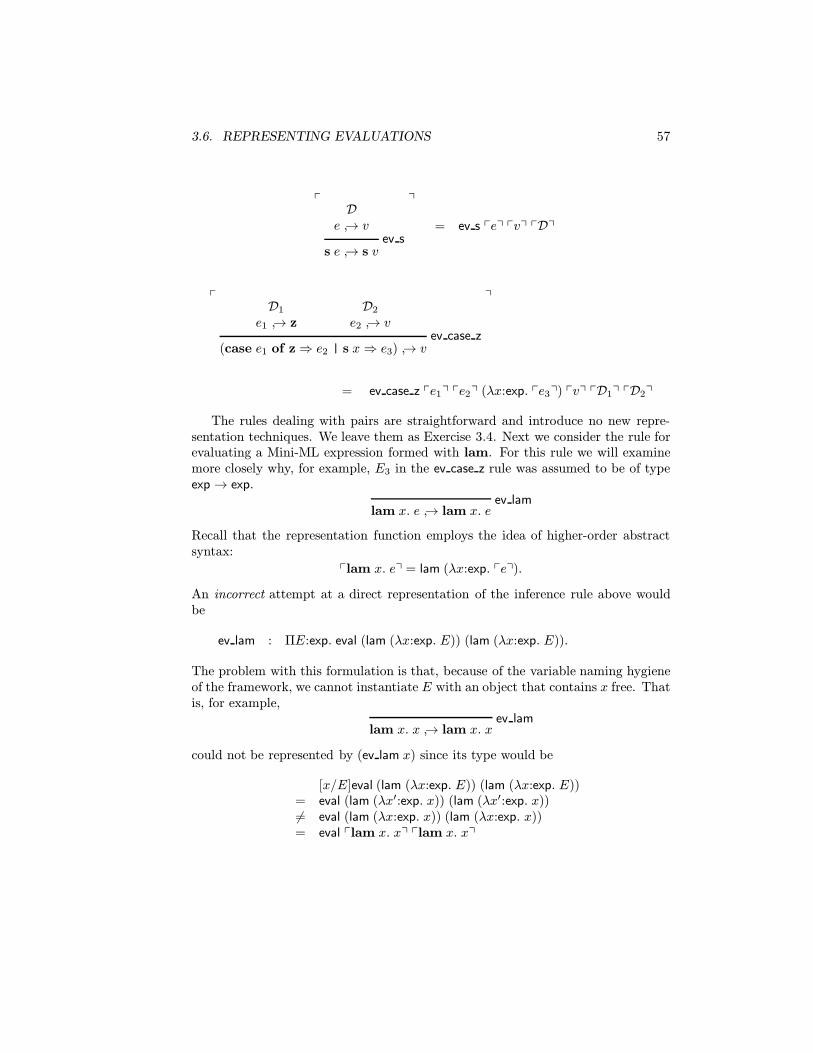
3.6. REPRESENTING EVALUATIONS 57
pD
e ↪→ vev s
s e ↪→ s v
q
= ev s peq pvq pDq
pD1
e1 ↪→ zD2
e2 ↪→ vev case z
(case e1 of z⇒ e2 | s x⇒ e3) ↪→ v
q
= ev case z pe1q pe2q (λx:exp. pe3q) pvq pD1q pD2q
The rules dealing with pairs are straightforward and introduce no new repre-sentation techniques. We leave them as Exercise 3.4. Next we consider the rule forevaluating a Mini-ML expression formed with lam. For this rule we will examinemore closely why, for example, E3 in the ev case z rule was assumed to be of typeexp→ exp.
ev lamlam x. e ↪→ lam x. e
Recall that the representation function employs the idea of higher-order abstractsyntax:
plam x. eq = lam (λx:exp. peq).
An incorrect attempt at a direct representation of the inference rule above wouldbe
ev lam : ΠE:exp. eval (lam (λx:exp. E)) (lam (λx:exp. E)).
The problem with this formulation is that, because of the variable naming hygieneof the framework, we cannot instantiate E with an object that contains x free. Thatis, for example,
ev lamlam x. x ↪→ lam x. x
could not be represented by (ev lam x) since its type would be
[x/E]eval (lam (λx:exp. E)) (lam (λx:exp. E))= eval (lam (λx′:exp. x)) (lam (λx′:exp. x))6= eval (lam (λx:exp. x)) (lam (λx:exp. x))= eval plam x. xq plam x. xq

58 CHAPTER 3. FORMALIZATION IN A LOGICAL FRAMEWORK
for some new variable x′. Instead, we have to bundle the scope of the bound variablewith its binder into a function from exp to exp, the type of the argument to lam.
ev lam : ΠE:exp→ exp. eval (lam E) (lam E).
Now the evaluation of the identity function above would be correctly representedby (ev lam (λx:exp. x)) which has type
[(λx:exp. x)/E]eval (lam E) (lam E)= eval (lam (λx:exp. x)) (lam (λx:exp. x)).
To summarize this case, we have
pev lam
lam x. e ↪→ lam x. e
q= ev lam (λx:exp. peq).
Yet another new technique is introduced in the representation of the rule whichdeals with applying a function formed by lam to an argument.
e1 ↪→ lam x. e′1 e2 ↪→ v2 [v2/x]e′1 ↪→ vev app
e1 e2 ↪→ v
As in the previous example, e′1 must be represented with its binder as a functionfrom exp to exp. But how do we represent [v2/x]e′1? Compositionality (Lemma 3.5)tell us that
p[v2/x]e′1q = [pv2q/x]pe′1q.The right-hand side is β-convertible to (λx:exp. pe′1q) pv2q. Note that the functionpart of this application, (λx:exp. pe′1q) will be an argument to the constant repre-senting the rule, and we can thus directly apply it to the argument representing v2.These considerations lead to the declaration
ev app : ΠE1:exp. ΠE2:exp. ΠE′1:exp→ exp. ΠV2:exp. ΠV :exp.eval E1 (lam E′1)→ eval E2 V2
→ eval (E′1 V2) V→ eval (app E1 E2) V
where
pD1
e1 ↪→ lam x. e′1
D2
e2 ↪→ v2
D3
[v2/x]e′1 ↪→ vev app
e1 e2 ↪→ v
q
= ev app pe1q pe2q (λx:exp. pe′1q) pv2q pvq pD1q pD2q pD3q.

3.6. REPRESENTING EVALUATIONS 59
Consider the evaluation of the Mini-ML expression (lam x. x) z:
ev lamlam x. x ↪→ lam x. x
ev zz ↪→ z
ev zz ↪→ z
ev app(lam x. x) z ↪→ z
Note that the third premise is a deduction of [z/x]x ↪→ z which is z ↪→ z. Thewhole deduction is represented by the LF object
ev app (lam (λx:exp. x)) z (λx:exp. x) z z(ev lam (λx:exp. x))ev zev z.
But why is this well-typed? The crucial question arises with the last argument toev app. By substitution into the type of ev app we find that the last argument isrequired to have type (eval ((λx:exp. x) z) z), while the actual argument, ev z, hastype eval z z. The rule of type conversion allows us to move from one type to theother provided they are definitionally equal. Thus our notion of definitional equalitymust include β-conversion in order to allow the representation technique wherebyobject-level substitution is represented by meta-level β-reduction.
In the seminal paper on LF [HHP93], definitional equality was based only onβ-reduction, due to technical problems in proving the decidability of the systemincluding η-conversion. The disadvantage of the system with only β-reduction isthat not every object is convertible to a canonical form using only β-conversion (seethe counterexample on page 44). This property holds once η-conversion is added.The decidability of the system with both βη-conversion has since been proven usingfour different techniques [Sal90, Coq91, Geu92, HP00].
The remaining rules of the operational semantics of Mini-ML follow the patternof the previous rules.
e1 ↪→ s v′1 [v′1/x]e3 ↪→ vev case s
(case e1 of z⇒ e2 | s x⇒ e3) ↪→ v
ev case s : ΠE1:exp. ΠE2:exp. ΠE3:exp→ exp. ΠV ′1 :exp. ΠV :exp.eval E1 (s V ′1)→ eval (E3 V
′1) V → eval (case E1 E2 E3) V
e1 ↪→ v1 [v1/x]e2 ↪→ vev letv
let val x = e1 in e2 ↪→ v
ev letv : ΠE1:exp. ΠE2:exp→ exp. ΠV1:exp. ΠV :exp.eval E1 V1 → eval (E2 V1) V → eval (letv E1 E2) V

60 CHAPTER 3. FORMALIZATION IN A LOGICAL FRAMEWORK
[e1/x]e2 ↪→ vev letn
let name x = e1 in e2
ev letn : ΠE1:exp. ΠE2:exp→ exp. ΠV :exp.eval (E2 E1) V → eval (letn E1 E2) V
For the fixpoint construct, we have to substitute a compound expression andnot just a variable.
[fix x. e/x]e ↪→ vev fix
fix x. e ↪→ v
ev fix : ΠE:exp→ exp. ΠV :exp.eval (E (fix E)) V → eval (fix E) V
Again we are taking advantage of compositionality in the form
p[fix x. e/x]eq = [pfix x. eq/x]peq ≡ (λx:exp. peq) pfix x. eq.
The succession of representation theorems follows the pattern of Section 3.3.Note that we postulate that e and v be closed, that is, do not contain any freevariables. We state this explicitly, because according to the earlier inference rules,there is no requirement that lam x. e be closed in the ev lam rule. However, wewould like to restrict attention to closed expressions e, since they are the onlyones which will be well-typed in the empty context within the Mini-ML typingdiscipline. The generalization of the canonical form judgment to LF in the presenceof dependent types is given in Section 3.9.
Lemma 3.7 Let e and v be closed Mini-ML expressions, and D a derivation ofe ↪→ v. Then
EV pDq ⇑ eval peq pvq.
Proof: The proof proceeds by induction on the structure of D. We show only onecase—the others are similar and simpler.
Case: D =
D1
e1 ↪→ lam x. e′1
D2
e2 ↪→ v2
D3
[v2/x]e′1 ↪→ vev app
e1 e2 ↪→ v. Then
pDq = ev app pe1q pe2q (λx:exp. pe′1q) pv2q pvq pD1q pD2q pD3q
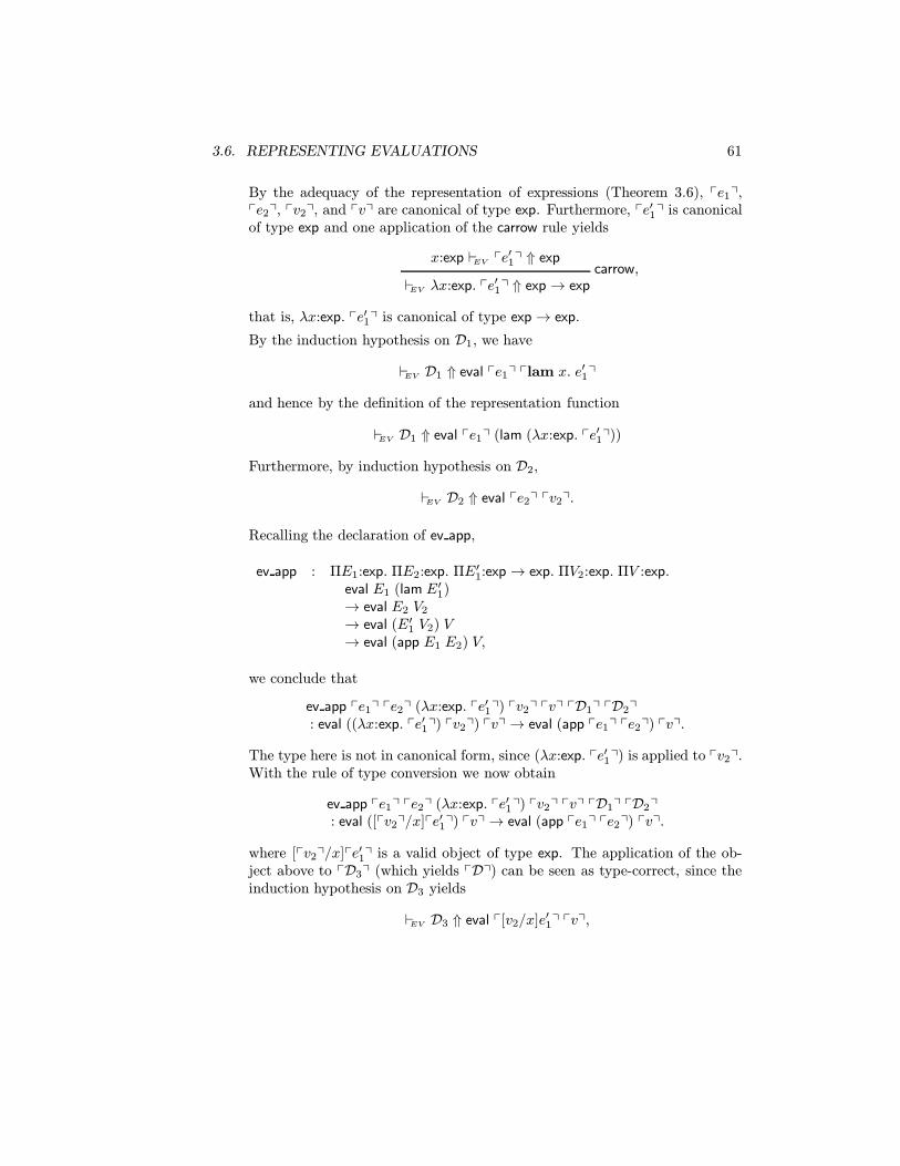
3.6. REPRESENTING EVALUATIONS 61
By the adequacy of the representation of expressions (Theorem 3.6), pe1q,pe2q, pv2q, and pvq are canonical of type exp. Furthermore, pe′1q is canonicalof type exp and one application of the carrow rule yields
x:exp EV pe′1q ⇑ expcarrow,
EV λx:exp. pe′1q ⇑ exp→ exp
that is, λx:exp. pe′1q is canonical of type exp→ exp.
By the induction hypothesis on D1, we have
EV D1 ⇑ eval pe1q plam x. e′1q
and hence by the definition of the representation function
EV D1 ⇑ eval pe1q (lam (λx:exp. pe′1q))
Furthermore, by induction hypothesis on D2,
EV D2 ⇑ eval pe2q pv2q.
Recalling the declaration of ev app,
ev app : ΠE1:exp. ΠE2:exp. ΠE′1:exp→ exp. ΠV2:exp. ΠV :exp.eval E1 (lam E′1)→ eval E2 V2
→ eval (E′1 V2) V→ eval (app E1 E2) V,
we conclude that
ev app pe1q pe2q (λx:exp. pe′1q) pv2q pvq pD1q pD2q: eval ((λx:exp. pe′1q) pv2q) pvq→ eval (app pe1q pe2q) pvq.
The type here is not in canonical form, since (λx:exp. pe′1q) is applied to pv2q.With the rule of type conversion we now obtain
ev app pe1q pe2q (λx:exp. pe′1q) pv2q pvq pD1q pD2q: eval ([pv2q/x]pe′1q) pvq→ eval (app pe1q pe2q) pvq.
where [pv2q/x]pe′1q is a valid object of type exp. The application of the ob-ject above to pD3q (which yields pDq) can be seen as type-correct, since theinduction hypothesis on D3 yields
EV D3 ⇑ eval p[v2/x]e′1q pvq,

62 CHAPTER 3. FORMALIZATION IN A LOGICAL FRAMEWORK
and from compositionality (Lemma 3.5) we know that
p[v2/x]e′1q = [pv2q/x]pe′1q.
Furthermore, D is canonical, since it is atomic and all the arguments to ev appare in canonical form.
2
Lemma 3.8 For any LF objects E, V , and M such that EV E ⇑ exp, EV V ⇑ expand EV M ⇑ eval E V , there exist unique Mini-ML expressions e and v and adeduction D :: e ↪→ v such that peq = E, pvq = V and pDq = M .
Proof: The proof is by structural induction on the derivation of EV M ⇑ eval E V(see Exercise 3.12). 2
A compositionality property does not arise here in the same way as it arosefor expressions since evaluations are closed. However, as we know from the use ofLemma 2.4 in the proof of type preservation (Theorem 2.5), a substitution lemmafor Mini-ML typing derivations plays an important role. We will return to this inSection 5.4. As before, we summarize the correctness of the representation into anadequacy theorem. It follows directly from Lemmas 3.7 and 3.8.
Theorem 3.9 (Adequacy) There is a bijection between deductions of e ↪→ v forclosed Mini-ML expressions e and v and canonical LF objects M such that
EV M ⇑ eval peq pvq
As a second example for the representation of deductions we consider the judg-ment e Value, defined in Section 2.4. Again, the judgment is represented as a typefamily, value, indexed by the representation of the expression e. That is,
value : exp→ type
Objects of type value peq then represent deductions, and inference rules are encodedas constructors for objects of such types.
val z : value zval s : ΠE:exp. value E → value (s E)val pair : ΠE1:exp. ΠE2:exp. value E1→ value E2 → value (pair E1 E2)val lam : ΠE:exp→ exp. value (lam E)
In the last rule, the scope of the binder lam is represented as a function fromexpressions to expressions. We refer to the signature above (including the signatureE representing Mini-ML expressions) as V . We omit the obvious definition of therepresentation function on value deductions. The adequacy theorem only refers toits existence implicitly.

3.7. META-THEORY VIA HIGHER-LEVEL JUDGMENTS 63
Theorem 3.10 (Adequacy) For closed expressions e there is a bijection betweendeductions P :: e Value and canonical LF objects M such that V M ⇑ value peq isderivable.
Proof: See Exercise 3.13. 2
3.7 Meta-Theory via Higher-Level Judgments
So far we have completed two of the tasks we set out to accomplish in this chapter:the representation of abstract syntax and the representation of deductive systemsin a logical framework. This corresponds to the specification of a language and itssemantics. The third task now before us is the representation of the meta-theory ofthe language, that is, proofs of properties of the language and its semantics.
This representation of meta-theory should naturally fit within the framework wehave laid out so far. It should furthermore reflect the structure of the informal proofas directly as possible. We are thus looking for a formal language and methodologyfor expressing a given proof, and not for a system or environment for finding such aproof. Once such a methodology has been developed it can also be helpful in proofsearch, but we would like to emphasize that this is a secondary consideration. Inorder to design a proof representation we must take stock of the proof techniqueswe have seen so far. By far the most pervasive is structural induction. Structuralinduction is applied in various forms: we have used induction over the structure ofexpressions, and induction over the structure of deductions. Within proofs of thelatter kind we have also frequent cause to appeal to inversion, that is, from theform of a derivable judgment we make statements about which inference rule musthave been applied to infer it. Of course, as is typical in mathematics, we breakdown a proof into a succession of lemmas leading up to a main theorem. A kind oflemma which arises frequently when dealing with deductive systems is a substitutionlemma.
We first consider the issue of structural induction and its representation in theframework. At first glance, this seems to require support for logical reasoning, thatis, we need quantifiers and logical connectives to express a meta-theorem, and log-ical axioms and inference rules to prove it. Our framework does not support thisdirectly—we would either have to extend it very significantly or encode the logicwe are attempting to model just like any other deductive system. Both of theseapproaches have some problems. The first does not mesh well with the idea ofhigher-order abstract syntax, basically because the types (such as the type exp ofMini-ML expressions) are not inductively defined in the usual sense. The problemarises from the negative occurrences of exp in the type of case, lam, let, and fix.Similar problems arise when encoding deductive systems employing parametric and

64 CHAPTER 3. FORMALIZATION IN A LOGICAL FRAMEWORK
hypothetical judgments such as the Mini-ML typing judgment. The second ap-proach, that is, to first define a logical system and then reason within it, incurs atremendous overhead in additional machinery to be developed. Furthermore, theconnection between the direct representations given in the previous sections of thischapter and this indirect method is problematic.
Thus we are looking for a more direct way to exploit the expressive power of theframework we have developed so far. We will use Theorem 2.1 (value soundness forMini-ML) and its proof as a motivating example. Recall that the theorem statesthat whenever e ↪→ v is derivable, then v Value is also derivable. The proof proceedsby an induction on the structure of the derivation of e ↪→ v.
A first useful observation is that the proof is constructive in the sense thatit implicitly contains a method for constructing a deduction P of the judgmentv Value, given a deduction D of e ↪→ v. This is an example of the relation-ship between constructive proofs and programs considered further in Sections ??through ??. Could we exploit the converse, that is, in what sense might thefunction f for constructing P from D represent a proof of the theorem? Such afunction f , if it were expressible in the framework, would presumably have typeΠE:exp. ΠV :exp. eval E V → value V . If it were guaranteed that a total functionof this type existed, our meta-theorem would be verified. Unfortunately, such afunction is not realizable within the logical framework, since it would have to bedefined by a form of recursion on an object of type eval E V . Attempting to ex-tend the framework in a straightforward way to encompass such function definitionsinvalidates our approach to abstract syntax and hypothetical judgments.
But we have one further possibility: why not represent the connection betweenD :: e ↪→ v and P :: v Value as a judgment (defined by inference rules) rather than afunction? This technique is well-known from logic programming, where predicates(defined via Horn clauses) rather than functions give rise to computation. A relatedoperational interpretation for LF signatures (which properly generalize sets of Hornclauses) forms the basis for the Elf programming language discussed in Chapter 4.To restate the idea: we represent the essence of the proof of value soundness asa judgment relating deductions D :: e ↪→ v and P :: v Value. Judgments relatingdeductions are not uncommon in the meta-theory of logic. An important example isthe judgment that a natural deduction reduces to another natural deduction, whichwe will discuss in Section ??.
In order to illustrate this approach, we quote various cases in the proof of valuesoundness and try to extract the inference rules for the judgment we motivatedabove. We write the judgment as
De ↪→ v
=⇒ Pv Value
and read it as “D reduces to P.” Following this analysis, we give its representationin LF. Recall that the proof is by induction over the structure of the deduction

3.7. META-THEORY VIA HIGHER-LEVEL JUDGMENTS 65
D :: e ↪→ v.
Case: D = ev z.z ↪→ z
Then v = z is a value by the rule val z.
This gives rise to the axiom
vs zev z
z ↪→ z=⇒ val z
z Value
Case:
D =
D1
e1 ↪→ v1
ev s.s e1 ↪→ s v1
The induction hypothesis on D1 yields a deduction of v1 Value. Using theinference rule val s we conclude that s v1 Value.
This case in the proof is represented by the following inference rule.
D1
e1 ↪→ v1=⇒ P1
v1 Valuevs s
D1
e1 ↪→ v1ev s
s e1 ↪→ s v1
=⇒
P1
v1 Valueval s
s v1 Value
Here, the appeal to the induction hypothesis on D1 has been represented in thepremise, where we have to establish that D1 reduces to P1.
Case:
D =
D1
e1 ↪→ zD2
e2 ↪→ vev case z.
(case e1 of z⇒ e2 | s x⇒ e3) ↪→ v
Then the induction hypothesis applied to D2 yields a deduction of v Value,which is what we needed to show in this case.

66 CHAPTER 3. FORMALIZATION IN A LOGICAL FRAMEWORK
In this case, the appeal to the induction hypothesis immediately yields the cor-rect deduction; no further inference is necessary.
D2
e2 ↪→ v=⇒ P2
v Valuevs case z
D1
e1 ↪→ zD2
e2 ↪→ vev case z
(case e1 of z⇒ e2 | s x⇒ e3) ↪→ v=⇒ P2
v Value
Case:
D =
D1
e1 ↪→ s v′1
D3
[v′1/x]e3 ↪→ vev case s.
(case e1 of z⇒ e2 | s x⇒ e3) ↪→ v
Then the induction hypothesis applied to D3 yields a deduction of v Value,which is what we needed to show in this case.
This is like the previous case.
D3
[v′1/x]e3 ↪→ v=⇒ P3
v Valuevs case s
D1
e1 ↪→ s v′1
D3
[v′1/x]e3 ↪→ vev case s
(case e1 of z⇒ e2 | s x⇒ e3) ↪→ v=⇒ P3
v Value
If D ends in ev pair we reason similar to cases above.
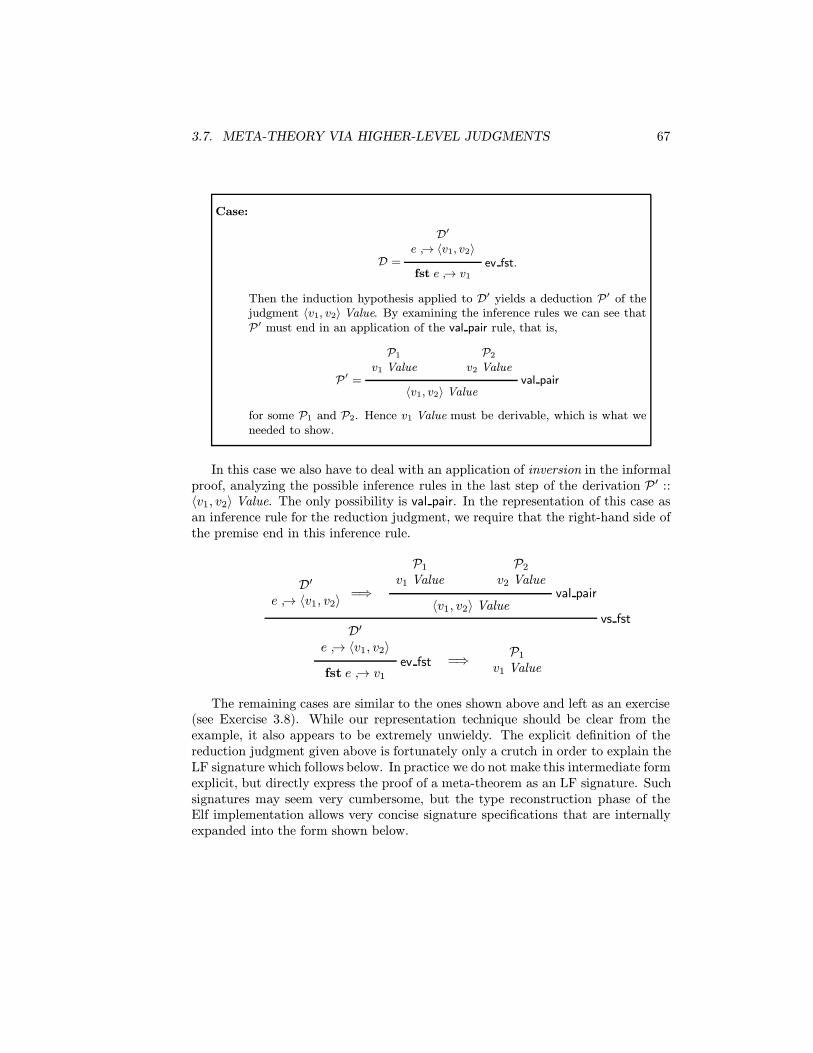
3.7. META-THEORY VIA HIGHER-LEVEL JUDGMENTS 67
Case:
D =
D′e ↪→ 〈v1, v2〉
ev fst.fst e ↪→ v1
Then the induction hypothesis applied to D′ yields a deduction P ′ of thejudgment 〈v1, v2〉 Value. By examining the inference rules we can see thatP ′ must end in an application of the val pair rule, that is,
P ′ =
P1
v1 ValueP2
v2 Valueval pair
〈v1, v2〉 Value
for some P1 and P2. Hence v1 Value must be derivable, which is what weneeded to show.
In this case we also have to deal with an application of inversion in the informalproof, analyzing the possible inference rules in the last step of the derivation P ′ ::〈v1, v2〉 Value. The only possibility is val pair. In the representation of this case asan inference rule for the reduction judgment, we require that the right-hand side ofthe premise end in this inference rule.
D′e ↪→ 〈v1, v2〉
=⇒
P1
v1 ValueP2
v2 Valueval pair
〈v1, v2〉 Valuevs fst
D′e ↪→ 〈v1, v2〉
ev fstfst e ↪→ v1
=⇒ P1
v1 Value
The remaining cases are similar to the ones shown above and left as an exercise(see Exercise 3.8). While our representation technique should be clear from theexample, it also appears to be extremely unwieldy. The explicit definition of thereduction judgment given above is fortunately only a crutch in order to explain theLF signature which follows below. In practice we do not make this intermediate formexplicit, but directly express the proof of a meta-theorem as an LF signature. Suchsignatures may seem very cumbersome, but the type reconstruction phase of theElf implementation allows very concise signature specifications that are internallyexpanded into the form shown below.

68 CHAPTER 3. FORMALIZATION IN A LOGICAL FRAMEWORK
The representation techniques given so far suggest that we represent the judg-ment
De ↪→ v
=⇒ Pv Value
as a type family indexed by the representation of the deductions D and P, that is,
vs : eval E V → value V → type
Once again we need to resolve the status of the free variables E and V in orderto achieve (in general) a decidable type reconstruction problem. Before, we usedthe dependent function type constructor Π to turn them into explicit arguments toobject level constants. Here, we need to index the type family vs explicitly by Eand V , both of type exp. Thus we need to extend the language for kinds (whichclassify type families) to admit dependencies and allow the declaration
vs : ΠE:exp. ΠV :exp. eval E V → value V → type.
The necessary generalization of the system from Section 3.5 is given in Section 3.8.The main change is a refinement of the language for kinds by admitting dependen-cies, quite analogous to the previous refinement of the language of types when wegeneralized the simply-typed fragment of Section 3.1.
We now consider the representation of some of the rules of the judgment D =⇒ Pas LF objects. The axiom
vs zev z
z ↪→ z=⇒ val z
z Value
is represented as
vs z : vs z z ev z val z.
The instantiation of the type family vs is valid, since ev z : eval z z and val z : value z.The second rule we considered arose from the case where the evaluation ended
in the rule for successor.
D1
e1 ↪→ v1=⇒ P1
v1 Valuevs s
D1
e1 ↪→ v1ev s
s e1 ↪→ s v1
=⇒
P1
v1 Valueval s
s v1 Value
Recall the declarations for ev s and val s.

3.7. META-THEORY VIA HIGHER-LEVEL JUDGMENTS 69
ev s : ΠE:exp. ΠV :exp. eval E V → eval (s E) (s V )val s : ΠE:exp. value E → value (s E)
The declaration corresponding to vs s:
vs s : ΠE1:exp. ΠV1:exp.ΠD1:eval E1 V1. ΠP1:value V1.
vs E1 V1 D1 P1 → vs (s E1) (s V1) (ev s E1 V1 D1) (val s V1 P1).
We consider one final example, where inversion was employed in the informalproof.
D′e ↪→ 〈v1, v2〉
=⇒
P1
v1 ValueP2
v2 Valueval pair
〈v1, v2〉 Valuevs fst
D′e ↪→ 〈v1, v2〉
ev fstfst e ↪→ v1
=⇒ P1
v1 Value
We recall the types for the inference rule encodings involved here:
val pair : ΠE:exp. ΠE2:exp. value E1 → value E2→ value (pair E1 E2)ev fst : ΠE:exp. ΠV1:exp. ΠV2:exp.
eval E (pair V1 V2)→ eval (fst E) V1
The rule above can then be represented as
vs fst : ΠE1:exp. ΠV1:exp. ΠV2:exp.ΠD′:eval E (pair V1 V2). ΠP1:value V1. ΠP2:value V2.
vs E (pair V1 V2) D′ (val pair V1 V2 P1 P2)→ vs (fst E) V1 (ev fst E V1 V2 D
′) P1
What have we achieved with this representation of the proof of value soundnessin LF? The first observation is the obvious one, namely a representation theoremrelating this signature to the judgment D =⇒ P. Let P be the signature containingthe declaration for expressions, evaluations, value deductions, and the declarationsabove encoding the reduction judgment via the type family vs.
Theorem 3.11 (Adequacy) For closed expressions e and v, there is a composi-tional bijection between deductions of
De ↪→ v
=⇒ Pv Value
and canonical LF objects M such that
P M ⇑ vs peq pvq pDq pPqis derivable.
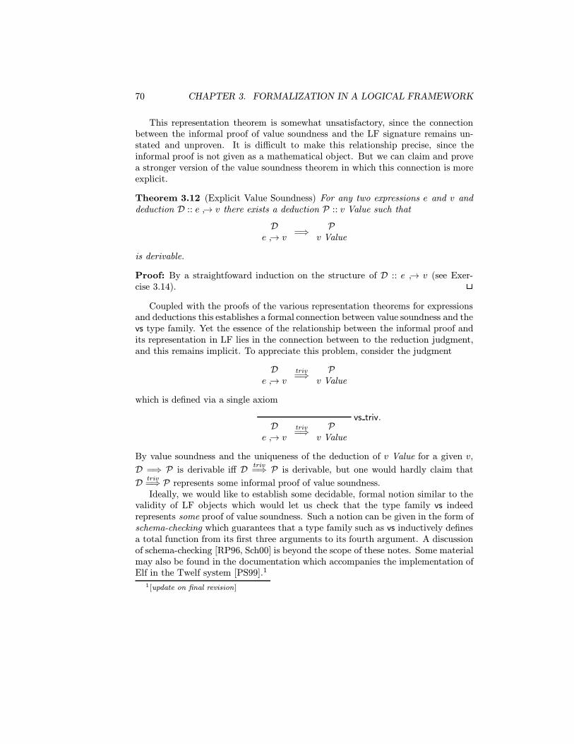
70 CHAPTER 3. FORMALIZATION IN A LOGICAL FRAMEWORK
This representation theorem is somewhat unsatisfactory, since the connectionbetween the informal proof of value soundness and the LF signature remains un-stated and unproven. It is difficult to make this relationship precise, since theinformal proof is not given as a mathematical object. But we can claim and provea stronger version of the value soundness theorem in which this connection is moreexplicit.
Theorem 3.12 (Explicit Value Soundness) For any two expressions e and v anddeduction D :: e ↪→ v there exists a deduction P :: v Value such that
De ↪→ v
=⇒ Pv Value
is derivable.
Proof: By a straightfoward induction on the structure of D :: e ↪→ v (see Exer-cise 3.14). 2
Coupled with the proofs of the various representation theorems for expressionsand deductions this establishes a formal connection between value soundness and thevs type family. Yet the essence of the relationship between the informal proof andits representation in LF lies in the connection between to the reduction judgment,and this remains implicit. To appreciate this problem, consider the judgment
De ↪→ v
triv=⇒ P
v Value
which is defined via a single axiom
vs triv.D
e ↪→ vtriv=⇒ P
v Value
By value soundness and the uniqueness of the deduction of v Value for a given v,
D =⇒ P is derivable iff D triv=⇒ P is derivable, but one would hardly claim that
D triv=⇒ P represents some informal proof of value soundness.Ideally, we would like to establish some decidable, formal notion similar to the
validity of LF objects which would let us check that the type family vs indeedrepresents some proof of value soundness. Such a notion can be given in the form ofschema-checking which guarantees that a type family such as vs inductively definesa total function from its first three arguments to its fourth argument. A discussionof schema-checking [RP96, Sch00] is beyond the scope of these notes. Some materialmay also be found in the documentation which accompanies the implementation ofElf in the Twelf system [PS99].1
1[update on final revision]

3.8. THE FULL LF TYPE THEORY 71
3.8 The Full LF Type Theory
The levels of kinds and types in the system from Section 3.5 were given as
Kinds K ::= type | A1 → · · · → An → KTypes A ::= a M1 . . .Mn | A1 → A2 | Πx:A1. A2
We now make two changes: the first is a generalization in that we allow dependentkinds Πx:A. K. The kind of the form A → K is then a special case of the newconstruct where x does not occur in K. The second change is to eliminate themultiple argument instantiation of type families. This means we generalize to alevel of families, among which we distinguish the types as families of kind “type.”
Kinds K ::= type | Πx:A. KFamilies A ::= a | A M | Πx:A1. A2
Objects M ::= c | x | λx:A. M |M1 M2
Signatures Σ ::= · | Σ, a:K | Σ, c:AContexts Γ ::= · | Γ, x:A
This system differs only minimally from the one given by Harper, Honsell, andPlotkin in [HHP93]. They also allow families to be formed by explicit abstraction,that is, λx:A1. A2 is a legal family. These do not occur in normal forms and wehave thus chosen to omit them from our system. As mentioned previously, it alsodiffers in that we allow β and η-conversion between objects as the basis for ournotion of definitional equality, while in [HHP93] only β-conversion is considered.The judgments take a slightly different form than in Section 3.5, in that we nowneed to introduce a judgment to explicitly classify families.
Γ Σ A : K A is a valid family of kind K
Γ Σ M : A M is a valid object of type A
Γ Σ K : kind K is a valid kind
` Σ Sig Σ is a valid signature
Σ Γ Ctx Γ is a valid context
Γ Σ M ≡ N : A M is definitionally equal to N at type A
Γ Σ A ≡ B : K A is definitionally equal to B at kind K
Γ Σ K ≡ K′ : kind kind K is definitionally equal to K′
These judgments are defined via the following inference rules.

72 CHAPTER 3. FORMALIZATION IN A LOGICAL FRAMEWORK
Σ(a) = Kfamcon
Γ Σ a : K
Γ Σ A : Πx:B. K Γ Σ M : Bfamapp
Γ Σ A M : [M/x]K
Γ Σ A : type Γ, x:A Σ B : typefampi
Γ Σ Πx:A. B : type
Σ(c) = Aobjcon
Γ Σ c : A
Γ(x) = Aobjvar
Γ Σ x : A
Γ Σ A : type Γ, x:A Σ M : Bobjlam
Γ Σ λx:A. M : Πx:A. B
Γ Σ M : Πx:A. B Γ Σ N : Aobjapp
Γ Σ M N : [N/x]B
Γ Σ M : A Γ Σ A ≡ B : typetypcnv
Γ Σ M : B
kndtypΓ Σ type : kind
Γ Σ A : type Γ, x:A Σ K : kindkndpi
Γ Σ Πx:A. K : kind
Γ Σ A : K Γ Σ K ≡K′ : kindkndcnv
Γ Σ A : K′
ctxempΣ · Ctx
Σ Γ Ctx Γ Σ A : typectxobj
Σ Γ, x:A Ctx

3.8. THE FULL LF TYPE THEORY 73
sigemp` · Sig
` Σ Sig Σ K : kindsigfam
` Σ, a : K Sig
` Σ Sig Σ A : typesigobj
` Σ, c : A Sig
For definitional equality, we have several classes of rules. The first rules intro-duces β-conversion.
Γ Σ A : type Γ, x:A Σ M : B Γ Σ N : Abeta
Γ Σ (λx:A. M) N ≡ [N/x]M : [N/x]B
We verify the validity of the objects and types involved in order to guarantee thatΓ Σ M ≡ N : A implies Γ Σ M : A and Γ Σ N : A. The second rule isextensionality: two objects of function type are equal, if they are equal on anarbitrary argument x.
Γ Σ A : type Γ, x:A Σ M x ≡ N x : Bext
Γ Σ M ≡ N : Πx:A. B
This rule is equivalent to η-conversion
Γ Σ M : Πx:A. Beta∗.
Γ Σ (λx:A. M x) ≡M : Πx:A. B
where η is restricted to the case the x is not free in M . The second class of rulesspecifies that ≡ is an equivalence, satisfying reflexivity, symmetry, and transitivityat each level. We only show the rules for objects; the others are obvious analogues.
Γ Σ M : Aobjrefl
Γ Σ M ≡M : A
Γ Σ N ≡M : Aobjsym
Γ Σ M ≡ N : A
Γ Σ M ≡ O : A Γ Σ O ≡ N : Aobjtrans
Γ Σ M ≡ N : A

74 CHAPTER 3. FORMALIZATION IN A LOGICAL FRAMEWORK
Finally we require rules to ensure that ≡ is a congruence, that is, conversion can beapplied to subterms. Technically, we use the notion of a simultaneous congruencethat allows simultaneous conversion in all subterms of a given term. We only showthe congruence rules at the levels of objects.
Σ(c) = Acngobjcon
Γ Σ c = c : A
Γ(x) = Acngobjvar
Γ Σ x = x : A
Γ Σ M1 ≡ N1 : Πx:A2. A1 Γ Σ M2 ≡ N2 : A2cngobjapp
Γ Σ M1 M2 ≡ N1 N2 : [M2/x]A1
Γ Σ A′ ≡ A : type Γ Σ A
′′ ≡ A : type Γ, x:A Σ M ≡ N : Bcngobjlam
Γ Σ λx:A′. M ≡ λx:A′′. N : Πx:A. B
In addition we also need type and kind conversion rules for the same reason theyare needed in the typing judgments (see Exercise 3.15). Some important propertiesof the LF type theory are stated at the end of next section.
3.9 Canonical Forms in LF
The notion of a canonical form, which is central to the representation theoremsfor LF encodings, is somewhat more complicated in full LF than in the simplytyped fragment given in Section 3.1. In particular, we need to introduce auxil-iary judgments for canonical types. At the same time we replace the rules withan indeterminate number of premises by using another auxiliary judgment whichestablishes that an object is atomic, that is, of the form x M1 . . .Mn or c M1 . . .Mn,and its arguments M1, . . . ,Mn are again canonical. An analogous judgment existsat the level of families. Thus we arrive at the judgments
Γ Σ M ⇑ A M is canonical of type A
Γ Σ A ⇑ type A is a canonical type
Γ Σ M ↓ A M is atomic of type A
Γ Σ A ↓ K A is atomic of kind K
These are defined by the following inference rules.
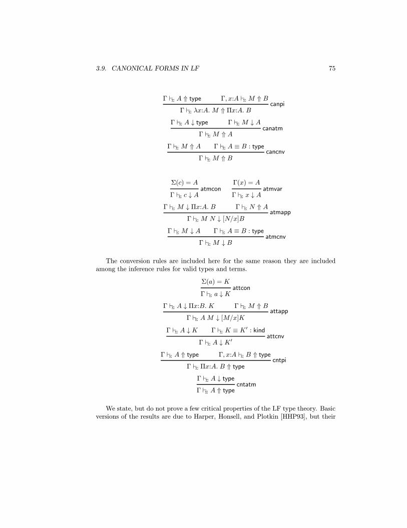
3.9. CANONICAL FORMS IN LF 75
Γ Σ A ⇑ type Γ, x:A Σ M ⇑ Bcanpi
Γ Σ λx:A. M ⇑ Πx:A. B
Γ Σ A ↓ type Γ Σ M ↓ Acanatm
Γ Σ M ⇑ A
Γ Σ M ⇑ A Γ Σ A ≡ B : typecancnv
Γ Σ M ⇑ B
Σ(c) = Aatmcon
Γ Σ c ↓ A
Γ(x) = Aatmvar
Γ Σ x ↓ A
Γ Σ M ↓ Πx:A. B Γ Σ N ⇑ Aatmapp
Γ Σ M N ↓ [N/x]B
Γ Σ M ↓ A Γ Σ A ≡ B : typeatmcnv
Γ Σ M ↓ B
The conversion rules are included here for the same reason they are includedamong the inference rules for valid types and terms.
Σ(a) = Kattcon
Γ Σ a ↓ K
Γ Σ A ↓ Πx:B. K Γ Σ M ⇑ Battapp
Γ Σ AM ↓ [M/x]K
Γ Σ A ↓ K Γ Σ K ≡ K′ : kindattcnv
Γ Σ A ↓ K′
Γ Σ A ⇑ type Γ, x:A Σ B ⇑ typecntpi
Γ Σ Πx:A. B ⇑ type
Γ Σ A ↓ typecntatm
Γ Σ A ⇑ type
We state, but do not prove a few critical properties of the LF type theory. Basicversions of the results are due to Harper, Honsell, and Plotkin [HHP93], but their
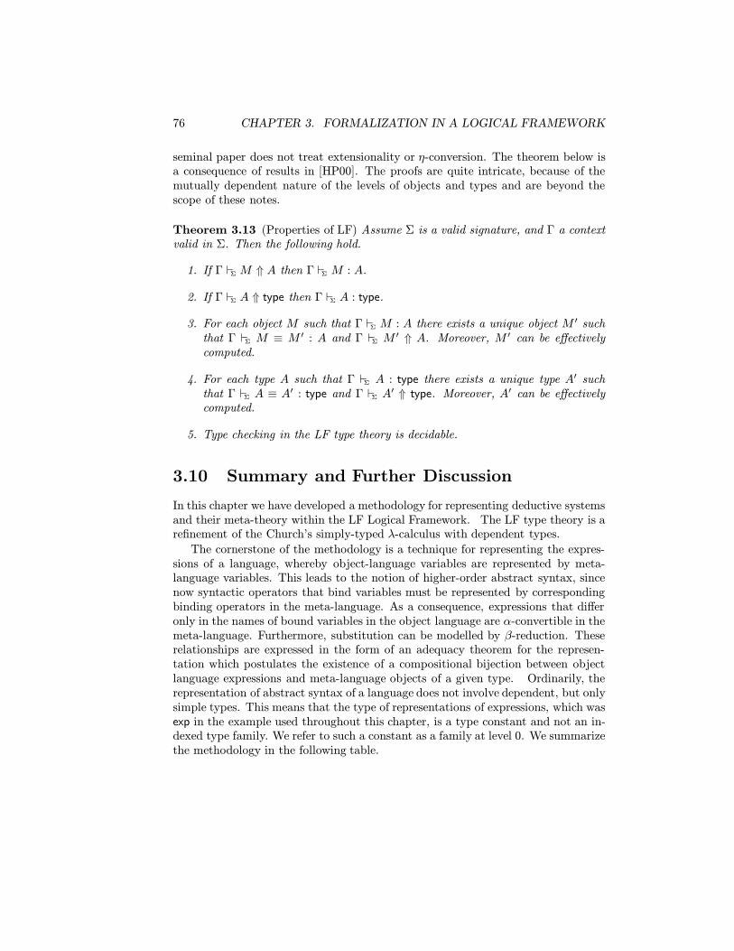
76 CHAPTER 3. FORMALIZATION IN A LOGICAL FRAMEWORK
seminal paper does not treat extensionality or η-conversion. The theorem below isa consequence of results in [HP00]. The proofs are quite intricate, because of themutually dependent nature of the levels of objects and types and are beyond thescope of these notes.
Theorem 3.13 (Properties of LF) Assume Σ is a valid signature, and Γ a contextvalid in Σ. Then the following hold.
1. If Γ Σ M ⇑ A then Γ Σ M : A.
2. If Γ Σ A ⇑ type then Γ Σ A : type.
3. For each object M such that Γ Σ M : A there exists a unique object M ′ suchthat Γ Σ M ≡ M ′ : A and Γ Σ M ′ ⇑ A. Moreover, M ′ can be effectivelycomputed.
4. For each type A such that Γ Σ A : type there exists a unique type A′ suchthat Γ Σ A ≡ A′ : type and Γ Σ A′ ⇑ type. Moreover, A′ can be effectivelycomputed.
5. Type checking in the LF type theory is decidable.
3.10 Summary and Further Discussion
In this chapter we have developed a methodology for representing deductive systemsand their meta-theory within the LF Logical Framework. The LF type theory is arefinement of the Church’s simply-typed λ-calculus with dependent types.
The cornerstone of the methodology is a technique for representing the expres-sions of a language, whereby object-language variables are represented by meta-language variables. This leads to the notion of higher-order abstract syntax, sincenow syntactic operators that bind variables must be represented by correspondingbinding operators in the meta-language. As a consequence, expressions that differonly in the names of bound variables in the object language are α-convertible in themeta-language. Furthermore, substitution can be modelled by β-reduction. Theserelationships are expressed in the form of an adequacy theorem for the represen-tation which postulates the existence of a compositional bijection between objectlanguage expressions and meta-language objects of a given type. Ordinarily, therepresentation of abstract syntax of a language does not involve dependent, but onlysimple types. This means that the type of representations of expressions, which wasexp in the example used throughout this chapter, is a type constant and not an in-dexed type family. We refer to such a constant as a family at level 0. We summarizethe methodology in the following table.

3.10. SUMMARY AND FURTHER DISCUSSION 77
Object Language Meta-Language
Syntactic Category Level 0 Type FamilyExpressions exp : type
Variable Variablex x
Constructor Constant〈e1, e2〉 pair pe1q pe2q, where
pair : exp→ exp→ expBinding Constructor Second-Order Constantlet val x = e1 in e2 letv pe1q (λx:exp. pe2q), where
letv : exp→ (exp→ exp)→ exp
An alternative approach, which we do not pursue here, is to use terms in a first-order logic to represent Mini-ML expressions. For example, we may have a binaryfunction constant pair and a ternary function constant letv . We then define a pred-icate exp which is true for expressions and false otherwise. This predicate is definedvia a set of axioms. For example, ∀e1. ∀e2. exp(e1) ∧ exp(e1) ⊃ exp(pair(e1, e2)).Similarly, ∀x. ∀e1. ∀e2. var (x) ∧ exp(e1) ∧ exp(e2) ⊃ exp(letv(x, e1, e2)), where varis another predicate which is true on variables and false otherwise. Since first-order logic is undecidable, we must then impose some restriction on the possibledefinitions of predicates such as exp or var in order to guarantee decidable rep-resentations. Under appropriate restrictions such predicates can then be seen todefine types. A commonly used class are regular tree types. Membership of a termin such a type can be decided by a finite tree automaton [GS84]. This approachto representation and types is the one usually taken in logic programming whichhas its roots in first-order logic. For a collection of papers describing this and re-lated approaches see [Pfe92]. The principal disadvantage of regular tree types in afirst-order term language is that it does not admit representation techniques suchas higher-order abstract syntax. Its main advantage is that it naturally permitssubtypes. For example, we could easily define the set of Mini-ML values as a sub-type of expressions, while the representation of values in LF requires an explicitjudgment. Thus, we do not capture in LF that it is decidable if an expression is avalue. Some initial work towards combining regular tree types and function typesis reported in [FP91] and [Pfe93].
The second representation technique translates judgments to types and deduc-tions to objects. This is often summarized by the motto judgments-as-types. Thiscan be seen as a methodology for formalizing the semantics of a language, sincesemantic judgments (such as evaluation or typing judgments) can be given conve-niently and elegantly as deductive systems. The goal is now to reduce checking ofdeductions to type-checking within the framework (which is decidable). For thisreduction to work correctly, the simply-typed framework which is sufficient for ab-

78 CHAPTER 3. FORMALIZATION IN A LOGICAL FRAMEWORK
stract syntax in most cases, needs to be refined by type families and dependentfunction types. The index objects for type families typically are representations ofexpressions, which means that they are typed at level 0. We refer to a family whichis indexed by objects typed at level 0 as a level 1 family. We can summarize thisrepresentation technique in the following table.
Object Language Meta-Language
Semantic Judgment Level 1 Type Familye ↪→ v eval : exp→ exp→ type
Inference Rule Constant Declaration
e ↪→ vev s
s e ↪→ s v
ev s :ΠE:exp. ΠV :exp.eval E V→ eval (s E) (s V )
Deduction Well-Typed ObjectDeductive System Signature
An alternative to dependent types (which we do not pursue here) is to definepredicates in a higher-order logic which are true of valid deductions and false oth-erwise. The type family eval, indexed by two expressions, then becomes a simpletype eval and we additionally require a predicate valid . The logics of higher-orderHorn clauses [NM98] and hereditary Harrop formulas [MNPS91] support this ap-proach and the use of higher-order abstract syntax. They have been implementedin the logic programming language λProlog [NM99] and the theorem prover Is-abelle [Pau94]. The principal disadvantage of this approach is that checking thevalidity of a deduction is reduced to theorem proving in the meta-logic. Thus de-cidability is not guaranteed by the representation and we do not know of any workto isolate decidable classes of higher-order predicates which would be analogous toregular tree types. Hereditary Harrop formulas have a natural logic programminginterpretation, which permits them to be used as the basis for implementing pro-grams related to judgments specified via deductive systems. For example, programsfor evaluation or type inference in Mini-ML can be easily and elegantly expressedin λProlog. In Chapter 4 we show that a similar operational interpretation is alsopossible for the LF type theory, leading to the language Elf.
The third question we considered was how to represent the proofs of propertiesof deductive systems. The central idea was to formulate the functions implicit in aconstructive proof as a judgment relating deductions. For example, the proof thatevaluation returns a value proceeds by induction over the structure of the deductionD :: e ↪→ v. This gives rise to a total function f , mapping each D :: e ↪→ v into adeduction P :: v Value. We then represent this function as a judgment D =⇒ Psuch that D =⇒ P is derivable if and only if f(D) = P. A strong adequacy theorem,however, is not available, since the mathematical proof is informal, and not itself

3.11. EXERCISES 79
introduced as a mathematical object. The judgment between deductions is thenagain represented in LF using the idea of judgments-as-types, although now theindex objects to the representing family represent deductions. We refer to a familyindexed by objects whose type is constructed from a level 1 family as a level 2 family.The technique for representing proofs of theorems about deductive systems whichhave been formalized in the previous step is summarized in the following table.
Object Language Meta-Language
Informal Proof Level 2 Type Family
Value Soundnessvs : ΠE:exp. ΠV :exp.
eval E V → value V → typeCase in Structural Induction Constant Declaration
Base Case for Axioms Constant of Atomic TypeInduction Step Constant of Functional Type
A decidable criterion on when a given type family represents a proof of a theoremabout a deductive system is subject of current research [RP96, Sch00].2
An alternative to this approach is to work in a stronger type theory with explicitinduction principles in which we can directly express induction arguments. Thisapproach is taken, for example, in the Calculus of Inductive Constructions [PM93]which has been implemented in the Coq system [DFH+93]. The disadvantage ofthis approach is that it does not coexist well with the techniques of higher-orderabstract syntax and judgments-as-types, since the resulting representation types(for example, exp) are not inductively defined in the usual sense.
3.11 Exercises
Exercise 3.1 Consider a variant of the typing rules given in Section 3.1 where therules var, con, lam, tcon, and ectx are replaced by the following rules.
Σ Γ Ctx Σ(c) = Acon′
Γ Σ c : A
Σ Γ Ctx Γ(x) = Avar′
Γ Σ x : A
Γ, x:A Σ M : Blam′
Γ Σ λx:A. M : A→ B
` Σ Sig Σ(a) = typetcon′
Σ a : type
` Σ Sigectx
Σ · Ctx
In what sense are these two systems equivalent? Formulate and carefully prove anappropriate theorem.
2[update in final revision ]

80 CHAPTER 3. FORMALIZATION IN A LOGICAL FRAMEWORK
Exercise 3.2 Prove Theorem 3.1.
Exercise 3.3 Prove Lemma 3.4
Exercise 3.4 Give LF representations of the natural semantics rules ev pair, ev fst,and ev snd (see Section 2.3).
Exercise 3.5 Reconsider the extension of the Mini-ML language by unit and dis-joint sum type (see Exercise 2.7). Give LF representation for
1. the new expression constructors,
2. the new rules in the evaluation and value judgments, and
3. the new cases in the proof of value soundness.
Exercise 3.6 Give the LF representation of the evaluations in Exercise 2.3. Youmay need to introduce some abbreviations in order to make it feasible to write itdown.
Exercise 3.7 Complete the definition of the representation function for evaluationsgiven in Section 3.6.
Exercise 3.8 Complete the definition of the judgment
De ↪→ v
=⇒ Pv Value
given in Section 3.7 and give the LF encoding of the remaining inference rules.
Exercise 3.9 Formulate and prove a theorem which expresses that the rules lam′′
and app′′ in Section 3.5 are no longer necessary, if A → B stands for Πx:A. B forsome x which does not occur in B.
Exercise 3.10 State the rules for valid signatures, contexts, and kinds which wereomitted in Section 3.8.
Exercise 3.11 Formulate an adequacy theorem for the representation of evalua-tions which is more general than Theorem 3.9 by allowing free variables in theexpressions e and v.
Exercise 3.12 Show the case for ev app in the proof of Lemma 3.8.
Exercise 3.13 Prove Theorem 3.10.
Exercise 3.14 Prove Theorem 3.12.

3.11. EXERCISES 81
Exercise 3.15 Complete the rules defining the full LF type theory.
Exercise 3.16 Prove items 1 and 2 of Theorem 3.13.
Exercise 3.17 In Exercise 2.13 you were asked to write a function observe : nat→nat that, given a lazy value of type nat returns the corresponding eager value if itexists.
1. Carefully state and prove the correctness of your function observe.
2. Explain the meaning of your proof as a higher-level judgment (without nec-essarily giving all details).

82 CHAPTER 3. FORMALIZATION IN A LOGICAL FRAMEWORK

Chapter 4
The Elf ProgrammingLanguage
Elf, thou lovest best, I think,The time to sit in a cave and drink.
— William AllinghamIn Fairy Land [All75]
In Chapter 2 we have seen how deductive systems can be used systematically tospecify aspects of the semantics of programming languages. In later chapters, wewill see many more examples of this kind, including some examples from logic. InChapter 3 we explored the logical framework LF as a formal meta-language for therepresentation of programming languages, their semantics, and their meta-theory.An important motivation behind the development of LF has been to provide aformal basis for the implementation of proof-checking and theorem proving tools,independently of any particular logic or deductive system. Note that search in thecontext of LF is the dual of type-checking: given a type A, find a closed objectM of type A. If such an object M exists we refer to A as inhabited. Since typesrepresent judgments and objects represent deductions, this is a natural formulationof the search for a deduction of a judgment via its representation in LF. Unliketype-checking, of course, the question whether a closed object of a given type existsis in general undecidable. The question of general search procedures for LF hasbeen studied by Elliott [Ell89, Ell90] and Pym and Wallen [PW90, Pym90, PW91,Pym92], including the question of unification of LF objects modulo βη-conversion.
In the context of the study of programming languages, we encounter problemsthat are different from general proof search. For example, once a type system hasbeen specified as a deductive system, how can we implement a type-checker or
83

84 CHAPTER 4. THE ELF PROGRAMMING LANGUAGE
a type inference procedure for the language? Another natural question concernsthe operational semantics: once specified as a deductive system, how can we takeadvantage of this specification to obtain an interpreter for the language? In bothof these cases we are in a situation where algorithms are known and need to beimplemented. The problem of proof search can also be phrased in these terms:given a logical system, implement algorithms for proof search that are appropriateto the system at hand.
Our approach to the implementation of algorithms is inspired by logic program-ming: specifications and programs are written in the same language. In traditionallogic programming, the common basis for specifications and implementations hasbeen the logic of Horn clauses; here, the common basis will be the logical frameworkLF. We would like to emphasize that specifications and programs are generally notthe same: many specifications are not useful if interpreted as programs, and manyprograms would not normally be considered specifications. In the logic program-ming paradigm, execution is the search for a derivation of some instance of a query.The operational semantics of the logic programming language specifies preciselyhow this search will be performed, given a list of inference rules that constitutethe program. Thus, if one understands this operational reading of inference rules,the programmer can obtain the desired execution behavior by defining judgmentsappropriately. We explain this in more detail in Section ?? and investigate it moreformally in Chapter ??.
Elf is a strongly typed language, since it is directly based on LF. The Elfinterpreter must thus perform type reconstruction on programs and queries beforeexecuting them. Because of the complex type system of LF, this is a non-trivial task.In fact, it has been shown by Dowek [Dow93] that the general type inference problemfor LF is undecidable, and thus not all types may be omitted from Elf programs.The algorithm for type reconstruction which is used in the implementation [Pfe91a,Pfe94] is based on the same constraint solving algorithm employed during execution.
The current implementation of Elf is within the Twelf system [PS99]. The readershould consult an up-to-date version of the User’s Guide for further informationregarding the language, its implementation, and its use. Sources, binaries for variousarchitectures, examples, and other materials are available from the Twelf homepage [Twe98].
4.1 Concrete Syntax
The concrete syntax of Elf is very simple, since we only have to model the relativelyfew constructs of LF. While LF is stratified into the levels of kinds, families, andobjects, the syntax is overloaded in that, for example, the symbol Π constructsdependent function types and dependent kinds. Similarly, juxtaposition is concretesyntax for instantiation of a type family and application of objects. We maintain this

4.1. CONCRETE SYNTAX 85
overloading in the concrete syntax for Elf and refer to expressions from any of thethree levels collectively as terms. A signature is given as a sequence of declarations.We describe here only the core language which corresponds very closely to LF.The main addition is a form of declaration id : term1 = term2 that introduces anabbreviation id for term2.
Terms term ::= id a or c or x| {id:term1}term2 Πx:A1. A2 or Πx:A. K| [id:term1]term2 λx:A. M| term1 term2 A M or M1 M2
| type type| term1 -> term2 A1 → A2
| term1 <- term2 A2 → A1
| {id}term | [id]term | _ omitted terms| term1:term2 type ascription| (term) grouping
Declarations decl ::= id : term. a:K or c:A| id : term1 = term2. c:A = M
The terminal id stands either for a bound variable, a free variable, or a constantat the level of families or objects. Bound variables and constants in Elf can bearbitrary identifiers, but free variables in a declaration or query must begin with anuppercase letter (a free, undeclared lowercase identifier is flagged as an undeclaredconstant). An uppercase identifier is one which begins with an underscore _ ora letter in the range A through Z; all others are considered lowercase, includingnumerals. Identifiers may contain all characters except (){}[]:.% and whitespace.In particular, A->B would be a single identifier, while A -> B denotes a functiontype. The left-pointing arrow as in B <- A is a syntactic variant and parsed into thesame representation as A -> B. It improves the readability of some Elf programs.Recall that A -> B is just an abbreviation for {x:A} B where x does not occur inB.
The right-pointing arrow -> is right associative, while the left-pointing arrow <-
is left associative. Juxtaposition binds tighter than the arrows and is left associative.The scope of quantifications {x : A} and abstractions [x : A] extends to the nextclosing parenthesis, bracket, brace or to the end of the term. Term reconstructionfills in the omitted types in quantifications {x} and abstractions [x] and omittedtypes or objects indicated by an underscore _ (see Section 4.2). In case of essentialambiguity a warning or error message results.
Single-line comments begin with % and extend through the end of the line. Adelimited comment begins with %{ and ends with the matching }%, that is, delimitedcomments may be properly nested. The parser for Elf also supports infix, prefix,and postfix declarations.
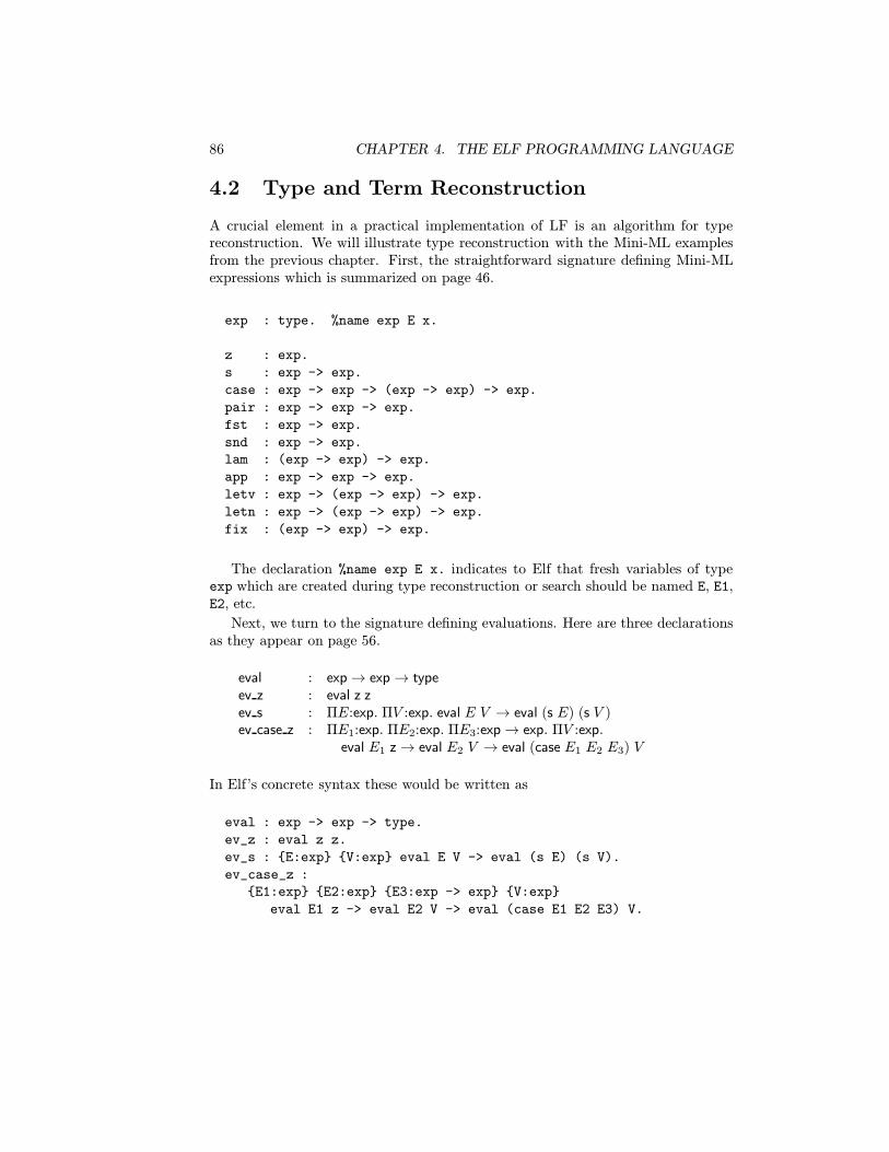
86 CHAPTER 4. THE ELF PROGRAMMING LANGUAGE
4.2 Type and Term Reconstruction
A crucial element in a practical implementation of LF is an algorithm for typereconstruction. We will illustrate type reconstruction with the Mini-ML examplesfrom the previous chapter. First, the straightforward signature defining Mini-MLexpressions which is summarized on page 46.
exp : type. %name exp E x.
z : exp.
s : exp -> exp.
case : exp -> exp -> (exp -> exp) -> exp.
pair : exp -> exp -> exp.
fst : exp -> exp.
snd : exp -> exp.
lam : (exp -> exp) -> exp.
app : exp -> exp -> exp.
letv : exp -> (exp -> exp) -> exp.
letn : exp -> (exp -> exp) -> exp.
fix : (exp -> exp) -> exp.
The declaration %name exp E x. indicates to Elf that fresh variables of typeexp which are created during type reconstruction or search should be named E, E1,E2, etc.
Next, we turn to the signature defining evaluations. Here are three declarationsas they appear on page 56.
eval : exp→ exp→ typeev z : eval z zev s : ΠE:exp. ΠV :exp. eval E V → eval (s E) (s V )ev case z : ΠE1:exp. ΠE2:exp. ΠE3:exp→ exp. ΠV :exp.
eval E1 z→ eval E2 V → eval (case E1 E2 E3) V
In Elf’s concrete syntax these would be written as
eval : exp -> exp -> type.
ev_z : eval z z.
ev_s : {E:exp} {V:exp} eval E V -> eval (s E) (s V).
ev_case_z :
{E1:exp} {E2:exp} {E3:exp -> exp} {V:exp}
eval E1 z -> eval E2 V -> eval (case E1 E2 E3) V.

4.2. TYPE AND TERM RECONSTRUCTION 87
A simple deduction, such as
ev zz ↪→ z
ev zz ↪→ z
ev ss z ↪→ s z
ev case zcase z of z⇒ s z | s x⇒ z
is represented in Elf as
ev_case_z z (s z) ([x:exp] z) (s z) ev_z (ev_s z z ev_z).
The Elf implementation performs type checking and reconstruction; later we willsee how the user can also initiate search. In order to check that the object aboverepresents a derivation of case z of z⇒ s z | s x⇒ z, we construct an anonymousdefinition
_ = ev_case_z z (s z) ([x:exp] z) (s z) ev_z (ev_s z z ev_z)
: eval (case z (s z) ([x:exp] z)) (s z).
The interpreter re-prints the declaration, which indicates that the given judgmentholds, that is, the object to the left of the colon has type type to the right of thecolon in the current signature. The current signature is embodied in the state ofthe Twelf system and comprises all loaded files. Please see the Twelf User’s Guidefor details.
We now reconsider the declaration of ev_case_z. The types of E1, E2, E3, andV are unambiguously determined by the kind of eval and the type of case. Forexample, E1 must have type exp, since the first argument of eval must have typeexp. This means, the declaration of ev_case_z could be replaced by
ev_case_z :
{E1} {E2} {E3} {V}
eval E1 z -> eval E2 V -> eval (case E1 E2 E3) V.
It will frequently be the case that the types of the variables in a declaration canbe determined from the context they appear in. To abbreviate declarations furtherwe allow the omission of the explicit Π-quantifiers. Consequently, the declarationabove can be given even more succinctly as
ev_case_z : eval E1 z -> eval E2 V -> eval (case E1 E2 E3) V.
This second step introduces a potential problem: the order of the quantifiers is notdetermined by the abbreviated declaration. Therefore, we do not know which argu-ment to ev_case_z stands for E1, which for E2, etc. Fortunately, these arguments(which are objects) can be determined from the context in which ev_case_z occurs.Let E1, E2, E3, V, E’ and V’ stand for objects yet to be determined and considerthe incomplete object

88 CHAPTER 4. THE ELF PROGRAMMING LANGUAGE
ev_case_z E1 E2 E3 V (ev_z) (ev_s E’ V’ (ev_z)).
The typing judgment
ev_case_z E1 E2 E3 V
: eval E1 z -> eval E2 V -> eval (case E1 E2 E3) V
holds for all valid objects E1, E2, E3, and V of appropriate type. The next argument,ev_z has type eval z z. For the object to be well-typed we must thus have
eval E1 z = eval z z
where = represents definitional equality. Thus E1 = z. We can similarly determinethat E2 = s z, V = s z, E’ = z, and V’ = z. However, E3 is as yet undetermined.But if we also know the type of the whole object, namely
eval (case z (s z) ([x:exp] z)) (s z),
then E3 = [x:exp] z also follows. Since it will generally be possible to determinethese arguments (up to conversion), we omit them in the input. We observe a strictcorrespondence between implicit quantifiers in a constant declaration and implicitarguments wherever the constant is used. This solves the problem that the order ofimplicit arguments is unspecified. With the abbreviated declarations
eval : exp -> exp -> type.
ev_z : eval z z.
ev_s : eval E V -> eval (s E) (s V).
ev_case_z :
eval E1 z -> eval E2 V -> eval (case E1 E2 E3) V.
the derivation above is concisely represented by
ev_case_z (ev_z) (ev_s (ev_z))
: eval (case z (s z) ([x:exp] z)) (s z).
While arguments to an object of truly dependent function type (Πx:A. B wherex occurs free in B) are often redundant, there are examples where arguments cannotbe reconstructed unambiguously. It is a matter of practical experience that the greatmajority of arguments to dependently typed functions do not need to be explicitlygiven, but can be reconstructed from context. The Elf type reconstruction algorithmwill give a warning when an implicit quantifier in a constant declaration is likely tolead to essential ambiguity later.
For debugging purposes it is sometimes useful to know the values of recon-structed types and objects. The front-end of the Elf implementation can thus printthe internal and fully explicit form of all the declarations if desired. Type recon-struction is discussed in further detail in the documentation of the implementation.For the remainder of this chapter, the main feature to keep in mind is the dualitybetween implicit quantifiers and implicit arguments.

4.3. A MINI-ML INTERPRETER IN ELF 89
4.3 A Mini-ML Interpreter in Elf
Let us recap the signatureEV defining evaluation as developed so far in the previoussection.
eval : exp -> exp -> type.
ev_z : eval z z.
ev_s : eval E V -> eval (s E) (s V).
ev_case_z :
eval E1 z -> eval E2 V -> eval (case E1 E2 E3) V.
One can now follow follow the path of Section 3.6 and translate the LF signatureinto Elf syntax. Our main concern in this section, however, will be to implementan executable interpreter for Mini-ML in Elf. In logic programming languages ingeneral computation is search for a derivation. In Elf, computation is search fora derivation of a judgment according to a particular operational interpretation ofinference rules. In the terminology of the LF type theory, this translates to thesearch for an object of a given type over a particular signature.
To consider a concrete example, assume we are given a Mini-ML expression e.We would like to find an object V and a closed object D of type eval peq V. Thus,we are looking simultaneously for a closed instance of a type, eval peq V, and aclosed object of this instance of the type. How would this search proceed? As anexample, consider e = case z of z ⇒ s z | s x ⇒ z. The query would have theform
?- D : eval (case z (s z) ([x:exp] z)) V.
where V is a free variable. Now the Elf interpreter will attempt to use each of theconstants in the given signature in turn in order to construct a canonical object ofthis type. Neither ev_z nor ev_s are appropriate, since the types do not match.However, there is an instance of the last declaration
ev_case_z : eval E1 z -> eval E2 V -> eval (case E1 E2 E3) V.
whose conclusion eval (case E1 E2 E3) V matches the current query by instanti-ating E1 = z, E2 = (s z), E3 = ([x:exp] z), and V = V. Thus, solutions to thesubgoals
?- D2 : eval (s z) V.
?- D1 : eval z z.
would provide a solution D = ev_case_z D1 D2 to the original query. At this pointduring the search, the incomplete derivation in mathematical notation would be
D1
z ↪→ zD2
s z ↪→ vev case z
(case z of z⇒ s z | s x⇒ z) ↪→ v

90 CHAPTER 4. THE ELF PROGRAMMING LANGUAGE
where D1, D2, and v are still to be filled in. Thus computation in Elf corresponds tobottom-up search for a derivation of a judgment. We solve the currently unsolvedsubgoals going through the partial deduction in a depth-first, left-to-right manner.So the next step would be to solve
?- D1 : eval z z.
We see that only one inference rule can apply, namely ev z, instantiating D1 toev_z. Now the subgoal D2 can be matched against the type of ev_s, leading to thefurther subgoal
?- D3 : eval z V1.
while instantiating V to s V1 for a new variable V1 and D2 to ev_s D3. In mathe-matical notation, the current state of search would be the partial derivation
ev zz ↪→ z
D3
z ↪→ v1ev s
s z ↪→ s v1ev case z.
(case z of z⇒ s z | s x⇒ z) ↪→ s v1
The subgoals D3 can be solved directly by ev_z, instantiating V1 to z. We obtainthe following cumulative substitution:
D = ev_case_z D1 D2
D2 = ev_s D3,
V = s V1,
D3 = ev_z,
V1 = z,
D1 = ev_z.
Eliminating the intermediate variables we obtain the same answer that Elf wouldreturn.
?- D : eval (case z (s z) ([x:exp] z)) V.
V = s z,
D = ev_case_z ev_z (ev_s ev_z).
One can see that the matching process which is required for this search proceduremust allow instantiation of the query as well as the declarations. The problem offinding a common instance of two terms is called unification. A unification algorithmfor terms in first-order logic was first sketched by Herbrand [Her30]. The first fulldescription of an efficient algorithm for unification was given by Robinson [Rob65],

4.3. A MINI-ML INTERPRETER IN ELF 91
which has henceforth been a central building block for automated theorem prov-ing procedures and logic programming languages. In Elf, Robinson’s algorithm isnot directly applicable because of the presence of types and λ-abstraction. Huetshowed that unification in the simply-typed λ-calculus is undecidable [Hue73], aresult later sharpened by Goldfarb [Gol81]. The main difficulty stems from thenotion of definitional equality, which can be taken as β or βη-convertibility. Ofcourse, the simply-typed λ-calculus is a subsystem of the LF type theory, and thusunifiability is undecidable for LF as well. A practical semi-decision procedure forunifiability in the simply-typed λ-calculus has been proposed by Huet [Hue75] andused in a number of implementations of theorem provers and logic programminglanguages [AINP88, Pfe91a, Pau94]. However, the procedure has the drawbackthat it may not only diverge but also branch, which is difficult to control in logicprogramming. Thus, in Elf, we have adopted the approach of constraint logic pro-gramming languages first proposed by Jaffar and Lassez [JL87], whereby difficultunification problems are postponed and carried along as constraints during execu-tion. We will say more about the exact nature of the constraint solving algorithmemployed in Elf in Section ??. In this chapter, all unification problems encounteredwill be essentially first-order.
We have not payed close attention to the order of various operations duringcomputation. In the first approximation, the operational semantics of Elf can bedescribed as follows. Assume we are given a list of goals A1, . . . , An with somefree variables. Each type of an object-level constant c in a signature has the formΠy1:B1 . . .Πym:Bm. C1 → · · · → Ck → C, where C is an atomic type. We call Cthe target type of c. Also, in analogy to logic programming, we call c a clause, C thehead of the clause c. Recall, that some of these quantifiers may remain implicit inElf. We instantiate y1, . . . , ym with fresh variables Y1, . . . , Ym and unify the resultinginstance of C ′ with A1, trying each constant in the signature in turn until unificationsucceeds. Unification may instantiate C1, . . . , Ck to C ′1, . . . , C
′k. We now set these
up as subgoals, that is, we obtain the new list of goals C ′k, . . . , C′1, A2, . . . , An. The
object we were looking for will be c Y1 . . . Yn M1 . . .Mk, where M1, . . . ,Mk are theobjects of type C ′1, . . . , C
′k, respectively, yet to be determined. We say that the goal
A1 has been resolved with the clause c and refer to the process as back-chaining.Note that the subgoals will be solved “from the inside out,” that is, C ′k is the firstone to be considered. If unification should fail and no further constants are availablein the signature, we backtrack, that is, we return to the most recent point where agoal unified with a clause head (that is, a target type of a constant declaration ina signature) and further choices were available. If there are no such choice points,the overall goal fails.
Logic programming tradition suggests writing the (atomic) target type C firstin a declaration, since it makes is visually much easier to read a program. Wefollow the same convention here, although the reader should keep in mind thatA -> B and B <- A are parsed to the same representation: the direction of the arrow

92 CHAPTER 4. THE ELF PROGRAMMING LANGUAGE
has no semantic significance. The logical reading of B <- A is “B if A,” althoughstrictly speaking it should be “B is derivable if A is derivable.” The left-pointingarrow is left associative so that C <- B <- A, (C <- B) <- A, A -> (B -> C), andA -> B -> C are all syntactically different representations for the same type. Sincewe solve innermost subgoals first, the operational interpretation of the clause
ev_case_z :
eval E1 z -> eval E2 V -> eval (case E1 E2 E3) V.
would be: “To solve a goal of the form eval (case E1 E2 E3) V, solve eval E2 V
and, if successful, solve eval E1 z.” On the other hand, the clause
ev_case_z : eval (case E1 E2 E3) V
<- eval E1 z
<- eval E2 V.
reads as: “to solve a goal of the form eval (case E1 E2 E3) V, solve eval E1 z
and, if successful, eval E2 V.” Clearly this latter interpretation is desirable fromthe operational point of view, even though the argument order to ev_case_z isreversed when compared to the LF encoding of the inference rules we have used sofar. This serves to illustrate that a signature that is adequate as a specification ofa deductive system is not necessarily adequate for search. We need to pay closeattention to the order of the declarations in a signature (since they will be tried insuccession) and the order of the subgoals (since they will be solved from the insideout).
We now complete the signature describing the interpreter for Mini-ML in Elf.It differs from the LF signature in Section 3.6 only in the order of the argumentsto the constants. First the complete rules concerning natural numbers.
ev_z : eval z z.
ev_s : eval (s E) (s V)
<- eval E V.
ev_case_z : eval (case E1 E2 E3) V
<- eval E1 z
<- eval E2 V.
ev_case_s : eval (case E1 E2 E3) V
<- eval E1 (s V1’)
<- eval (E3 V1’) V.
Recall that the application (E3 V1’) was used to implement substitution inthe object language. We discuss how this is handled operationally below whenconsidering ev_app. Pairs are straightforward.
ev_pair : eval (pair E1 E2) (pair V1 V2)
<- eval E1 V1

4.3. A MINI-ML INTERPRETER IN ELF 93
<- eval E2 V2.
ev_fst : eval (fst E) V1
<- eval E (pair V1 V2).
ev_snd : eval (snd E) V2
<- eval E (pair V1 V2).
Abstraction and function application employ the notion of substitution. Recallthe inference rule and its representation in LF:
e1 ↪→ lam x. e′1 e2 ↪→ v2 [v2/x]e′1 ↪→ vev app
e1 e2 ↪→ v
ev app : ΠE1:exp. ΠE2:exp. ΠE′1:exp→ exp. ΠV2:exp. ΠV :exp.eval E1 (lam E′1)→ eval E2 V2
→ eval (E′1 V2) V→ eval (app E1 E2) V.
As before, we transcribe this (and the trivial rule for evaluating λ-expressions) intoElf.
ev_lam : eval (lam E) (lam E).
ev_app : eval (app E1 E2) V
<- eval E1 (lam E1’)
<- eval E2 V2
<- eval (E1’ V2) V.
The operational reading of the ev_app rule is as follows. In order to evaluate anapplication e1 e2 we evaluate e1 and match the result against lam x. e′1. If thissucceeds we evaluate e2 to the value v2. Then we evaluate the result of substitutingv2 for x in e′1. The Mini-ML expression lam x. e′1 is represented as in LF aslam (λx:exp. pe′1q), and the variable E1’ : exp -> exp will be instantiated to([x:exp] pe′1q). In the operational semantics of Elf, an application which is not incanonical form (such as (E1’ V2) after instantiation of E1’ and V2) will be reduceduntil it is in head-normal form (see Section ??)—in this case this means performingthe substitution of V2 for the top-level bound variable in E1’. As an example,consider the evaluation of (lam x. x) z which is given by the deduction
ev lamlam x. x ↪→ lam x. x
ev zz ↪→ z
ev zz ↪→ z
ev app.(lam x. x) z ↪→ z
The first goal is

94 CHAPTER 4. THE ELF PROGRAMMING LANGUAGE
?- D : eval (app (lam [x:exp] x) z) V.
This is resolved with the clause ev_app, yielding the subgoals
?- D1 : eval (lam [x:exp] x) (lam E1’).
?- D2 : eval z V2.
?- D3 : eval (E1’ V2) V.
The first subgoal will be resolved with the clause ev_lam, instantiating E1’ to([x:exp] x). The second subgoal will be resolved with the clause ev_z, instan-tiating V2 to z. Thus, by the time the third subgoal is considered, it has beeninstantiated to
?- D3 : eval (([x:exp] x) z) V.
When this goal is unified with the clauses in the signature, (([x:exp] x) z) isreduced to z. It thus unifies with the head of the clause ev_z, and V is instantiatedto z to yield the answer
V = z.
D = ev_app ev_z ev_z ev_lam.
Note that because of the subgoal ordering, ev_lam is the last argument to ev_app.Evaluation of let-expressions follows the same schema as function application,
and we again take advantage of meta-level β-reduction in order to model object-levelsubstitution.
ev_letv : eval (letv E1 E2) V
<- eval E1 V1
<- eval (E2 V1) V.
ev_letn : eval (letn E1 E2) V
<- eval (E2 E1) V.
The Elf declaration for evaluating a fixpoint construct is again a direct tran-scription of the corresponding LF declaration. Recall the rule
[fix x. e/x]e ↪→ vev fix
fix x. e ↪→ v
ev_fix : eval (fix E) V
<- eval (E (fix E)) V.
This declaration introduces non-terminating computations into the interpreter. Re-consider the example from page 17, fix x. x. Its representation in Elf is given byfix ([x:exp] x). Attempting to evaluate this expression leads to the followingsequence of goals.

4.3. A MINI-ML INTERPRETER IN ELF 95
?- D : eval (fix ([x:exp] x)) V.
?- D1 : eval (([x:exp] x) (fix ([x:exp] x))) V.
?- D1 : eval (fix ([x:exp] x)) V.
The step from the original goal to the first subgoal is simply the back-chaining step,instantiating E to [x:exp] x. The second is a β-reduction required to transformthe goal into canonical form, relying on the rule of type conversion. The third goalis then a renaming of the first one, and computation will diverge. This correspondsto the earlier observation (see page 17) that there is no v such that the judgmentfix x. x ↪→ v is derivable.
It is also possible that evaluation fails finitely, although in our formulation ofthe language this is only possible for Mini-ML expressions that are not well-typedaccording to the Mini-ML typing rules. For example,
?- D : eval (fst z) V.
no
The only subgoal considered is D’ : eval z (pair V V2) after resolution withthe clause ev_fst. This subgoal fails, since there is no rule that would permit aconclusion of this form, that is, no clause head unifies with eval z (pair V V2).
As a somewhat larger example, we reconsider the evaluation which doubles thenatural number 1, as given on page 17. Reading the justifications of the lines 1–17from the bottom-up yields the same sequence of inference rules as reading the objectD below from left to right.
%query 1 *
D : eval (app
(fix [f:exp] lam [x:exp]
(case x z ([x’:exp] s (s (app f x’)))))
(s z))
V.
This generates the following answer:
V = s (s z),
D =
ev_app
(ev_case_s
(ev_s (ev_s (ev_app (ev_case_z ev_z ev_z)
ev_z (ev_fix ev_lam))))
(ev_s ev_z))
(ev_s ev_z) (ev_fix ev_lam).
The example above exhibits another feature of the Elf implementation. We canpose query in the form %query n k A. which solves the query A and verifies that
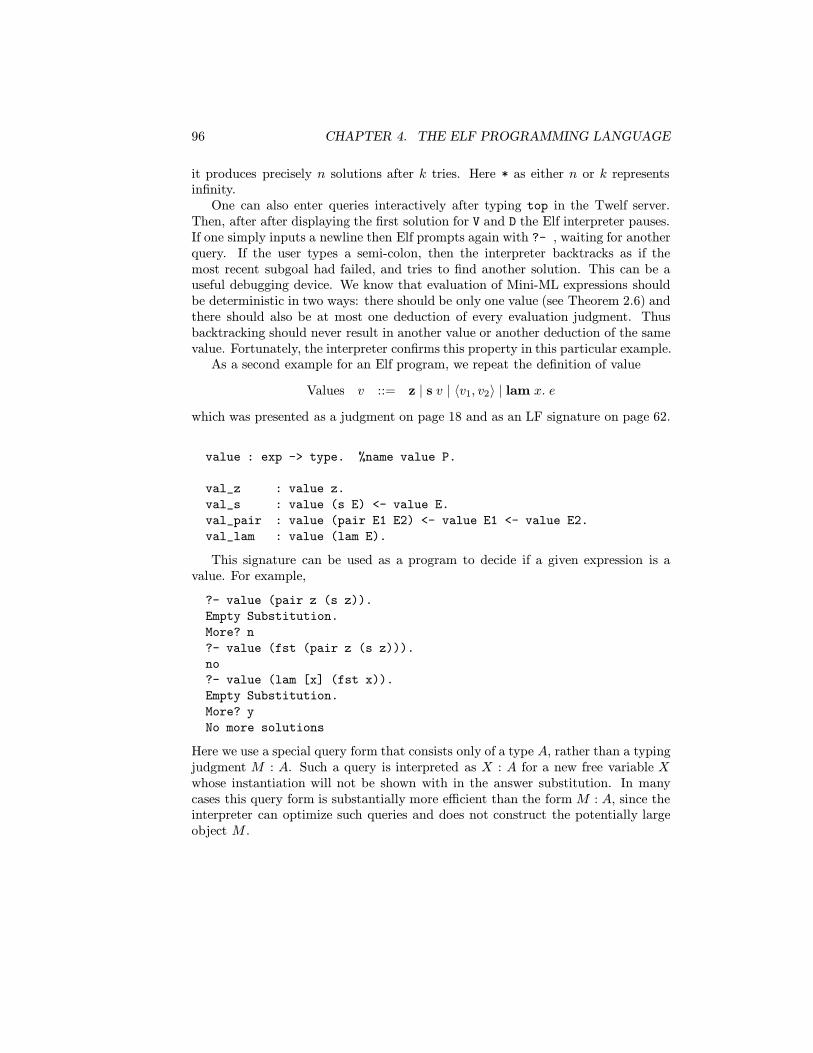
96 CHAPTER 4. THE ELF PROGRAMMING LANGUAGE
it produces precisely n solutions after k tries. Here * as either n or k representsinfinity.
One can also enter queries interactively after typing top in the Twelf server.Then, after after displaying the first solution for V and D the Elf interpreter pauses.If one simply inputs a newline then Elf prompts again with ?- , waiting for anotherquery. If the user types a semi-colon, then the interpreter backtracks as if themost recent subgoal had failed, and tries to find another solution. This can be auseful debugging device. We know that evaluation of Mini-ML expressions shouldbe deterministic in two ways: there should be only one value (see Theorem 2.6) andthere should also be at most one deduction of every evaluation judgment. Thusbacktracking should never result in another value or another deduction of the samevalue. Fortunately, the interpreter confirms this property in this particular example.
As a second example for an Elf program, we repeat the definition of value
Values v ::= z | s v | 〈v1, v2〉 | lam x. e
which was presented as a judgment on page 18 and as an LF signature on page 62.
value : exp -> type. %name value P.
val_z : value z.
val_s : value (s E) <- value E.
val_pair : value (pair E1 E2) <- value E1 <- value E2.
val_lam : value (lam E).
This signature can be used as a program to decide if a given expression is avalue. For example,
?- value (pair z (s z)).
Empty Substitution.
More? n
?- value (fst (pair z (s z))).
no
?- value (lam [x] (fst x)).
Empty Substitution.
More? y
No more solutions
Here we use a special query form that consists only of a type A, rather than a typingjudgment M : A. Such a query is interpreted as X : A for a new free variable Xwhose instantiation will not be shown with in the answer substitution. In manycases this query form is substantially more efficient than the form M : A, since theinterpreter can optimize such queries and does not construct the potentially largeobject M .

4.4. AN IMPLEMENTATION OF VALUE SOUNDNESS 97
4.4 An Implementation of Value Soundness
We now return to the proof of value soundness which was first given in Section 2.4and formalized in Section 3.7. The theorem states that evaluation always returnsa value. The proof of the theorem proceeds by induction over the structure of thederivation D of the judgment e ↪→ v, that is, the evaluation of e. The first step inthe formalization of this proof is to formulate a judgment between deductions,
De ↪→ v
=⇒ Pv Value
which relates every D to some P and whose definition is based on the structureof D. This judgment is then represented in LF as a type family vs, following thejudgments-as-types principle.
vs : ΠE:exp. ΠV :exp. eval E V → value V → type.
Each of the various cases in the induction proof gives rise to one inference rulefor the =⇒ judgment, and each such inference rule is represented by a constantdeclaration in LF. We illustrate the Elf implementation with the case where Dends in the rule ev fst and then present the remainder of the signature in Elf moretersely.
Case:
D =
D′e′ ↪→ 〈v1, v2〉
ev fst.fst e′ ↪→ v1
Then the induction hypothesis applied to D′ yields a deduction P ′ of thejudgment 〈v1, v2〉 Value. By examining the inference rules we can see thatP ′ must end in an application of the val pair rule, that is,
P ′ =
P1
v1 ValueP2
v2 Valueval pair
〈v1, v2〉 Value
for some P1 and P2. Hence v1 Value must be derivable, which is what weneeded to show.

98 CHAPTER 4. THE ELF PROGRAMMING LANGUAGE
This is represented by the following inference rule for the =⇒ judgment.
D′e′ ↪→ 〈v1, v2〉
=⇒
P1
v1 ValueP2
v2 Valueval pair
〈v1, v2〉 Valuevs fst
D′e ↪→ 〈v1, v2〉
ev fstfst e′ ↪→ v1
=⇒ P1
v1 Value
Its representation in LF is given by
vs fst : ΠE′:exp. ΠV1:exp. ΠV2:exp.ΠD′:eval E′ (pair V1 V2). ΠP1:value V1. ΠP2:value V2.
vs E (pair V1 V2) D′ (val pair V1 V2 P1 P2)→ vs (fst E′) V1 (ev fst E V1 V2 D
′) P1
This may seem unwieldy, but Elf’s type reconstruction comes to our aid. In thedeclaration of vs, the quantifiers on E and V can remain implicit:
vs : eval E V -> value V -> type.
The corresponding arguments to vs now also remain implicit. We also repeat thedeclarations for the inference rules involved in the deduction above.
ev_fst : eval (fst E) V1 <- eval E (pair V1 V2).
val_pair : value (pair E1 E2) <- value E1 <- value E2.
Here is the declaration of the vs fst constant:
vs_fst : vs (ev_fst D’) P1 <- vs D’ (val_pair P2 P1).
Note that this declaration only has to deal with deductions, not with expressions.Term reconstruction expands this into
vs_fst :
{E:exp} {E1:exp} {E2:exp} {D’:eval E (pair E1 E2)}
{P2:value E2} {P1:value E1}
vs E (pair E1 E2) D’ (val_pair E2 E1 P2 P1)
-> vs (fst E) E1 (ev_fst E E1 E2 D’) P1.
Disregarding the order of quantifiers and the choice of names, this is the LF dec-laration given above. We show the complete signature which implements the proofof value soundness without further comment. The declarations can be derived fromthe material and the examples in Sections 2.4 and 3.7.

4.4. AN IMPLEMENTATION OF VALUE SOUNDNESS 99
vs : eval E V -> value V -> type.
% Natural Numbers
vs_z : vs (ev_z) (val_z).
vs_s : vs (ev_s D1) (val_s P1)
<- vs D1 P1.
vs_case_z : vs (ev_case_z D2 D1) P2
<- vs D2 P2.
vs_case_s : vs (ev_case_s D3 D1) P3
<- vs D3 P3.
% Pairs
vs_pair : vs (ev_pair D2 D1) (val_pair P2 P1)
<- vs D1 P1
<- vs D2 P2.
vs_fst : vs (ev_fst D’) P1
<- vs D’ (val_pair P2 P1).
vs_snd : vs (ev_snd D’) P2
<- vs D’ (val_pair P2 P1).
% Functions
vs_lam : vs (ev_lam) (val_lam).
vs_app : vs (ev_app D3 D2 D1) P3
<- vs D3 P3.
% Definitions
vs_letv : vs (ev_letv D2 D1) P2
<- vs D2 P2.
vs_letn : vs (ev_letn D2) P2
<- vs D2 P2.
% Recursion
vs_fix : vs (ev_fix D1) P1
<- vs D1 P1.
This signature can be used to transform evaluations into value deductions. Forexample, the evaluation of case z of z ⇒ s z | s x ⇒ z considered above is givenby the Elf object
ev_case_z (ev_s ev_z) ev_z
of type
eval (case z (s z) ([x:exp] z)) (s z).
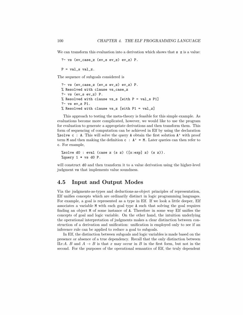
100 CHAPTER 4. THE ELF PROGRAMMING LANGUAGE
We can transform this evaluation into a derivation which shows that s z is a value:
?- vs (ev_case_z (ev_s ev_z) ev_z) P.
P = val_s val_z.
The sequence of subgoals considered is
?- vs (ev_case_z (ev_s ev_z) ev_z) P.
% Resolved with clause vs_case_z
?- vs (ev_s ev_z) P.
% Resolved with clause vs_s [with P = val_s P1]
?- vs ev_z P1.
% Resolved with clause vs_z [with P1 = val_z]
This approach to testing the meta-theory is feasible for this simple example. Asevaluations become more complicated, however, we would like to use the programfor evaluation to generate a appropriate derivations and then transform them. Thisform of sequencing of computation can be achieved in Elf by using the declaration%solve c : A. This will solve the query A obtain the first solution A’ with proofterm M and then making the definition c : A’ = M. Later queries can then refer toc. For example,
%solve d0 : eval (case z (s z) ([x:exp] z) (s z)).
%query 1 * vs d0 P.
will construct d0 and then transform it to a value derivation using the higher-leveljudgment vs that implements value soundness.
4.5 Input and Output Modes
Via the judgments-as-types and deductions-as-object principles of representation,Elf unifies concepts which are ordinarily distinct in logic programming languages.For example, a goal is represented as a type in Elf. If we look a little deeper, Elfassociates a variable M with each goal type A such that solving the goal requiresfinding an object M of some instance of A. Therefore in some way Elf unifies theconcepts of goal and logic variable. On the other hand, the intuition underlyingthe operational interpretation of judgments makes a clear distinction between con-struction of a derivation and unification: unification is employed only to see if aninference rule can be applied to reduce a goal to subgoals.
In Elf, the distinction between subgoals and logic variables is made based on thepresence or absence of a true dependency. Recall that the only distinction betweenΠx:A. B and A → B is that x may occur in B in the first form, but not in thesecond. For the purposes of the operational semantics of Elf, the truly dependent

4.5. INPUT AND OUTPUT MODES 101
function type Πx:A. B where x does in fact occur somewhere in B is treated bysubstituting a new logic variable for x which is subject to unification. The non-dependent function type A→ B is treated by introducing A as a subgoal necessaryfor the solution of B.
Therefore, a typical constant declaration which has the form
c : Πx1:A1 . . .Πxn:An. B1 → · · · → Bm. C
for an atomic type C, introduces logic variables X1, . . . , Xn, then finds most generalcommon instance between the goal G and C (possibly instantiating X1, . . . , Xn andthen solves Bm, . . . , B1 as subgoals, in that order. Note that in practical programs,the quantifiers on x1, . . . , xn are often implicit.
When writing a program it is important to kept this interpretation in mind. Inorder to illustrate it, we write some simple programs.
First, the declaration of natural numbers. We declare s, the successor function,as a prefix operator so we can write 2, for example, as s s 0 without additionalparentheses. Note that without the prefix declaration this term would be associatedto the left and parsed incorrectly as ((s s) 0).
nat : type. %name nat N.
0 : nat.
s : nat -> nat. %prefix 20 s.
The prefix declaration has the general form %prefix prec id1 . . . idn and gives theconstants id1, . . . , idn precedence prec. The second declaration introduces lists ofnatural numbers. We declare “;” as a right-associative infix constructor for lists.
list : type. %name list L.
nil : list.
; : nat -> list -> list. %infix right 10 ;.
For example, (0 ; s 0 ; s s 0 ; nil) denotes the list of the first three naturalnumbers; (0 ; ((s 0) ; ((s (s 0)) ; nil))) is its fully parenthesized version,and (; 0 (; (s 0) (; (s (s 0)) nil))) is the prefix form which would have tobe used if no infix declarations had been supplied.
The definition of the append program is straightforward. It is implementedas a type family indexed by three lists, where the third list must be the result ofappending the first two. This can easily be written as a judgment (see Exercise 4.6).
append : list -> list -> list -> type.
%mode append +L +K -M.
ap_nil : append nil K K.
ap_cons : append (X ; L) K (X ; M)
<- append L K M.

102 CHAPTER 4. THE ELF PROGRAMMING LANGUAGE
The mode declaration
%mode append +L +K -M.
specifies that, for the operational reading, we should consider the first two argumentL and K as given input, while the third argument M is to be constructed by theprogram as output. To make this more precise, we define that a term is ground if itdoes not contain any logic variables. With the above mode declaration we specifythat first two arguments l and k to append should always be ground when a goal ofthe form append l k m is to be solved. Secondly, it expresses that upon success, thethird argument m should always be ground. The Elf compiler verifies this propertyas each declaration is read and issues an appropriate error message if it is violated.
This mode verification proceeds as follows. We first consider
ap_nil : append nil K K.
We may assume that the first two arguments are ground, that is, nil and K will beground when append is invoked. Therefore, if this rule succeeds, the third argumentK will indeed be ground.
Next we consider the second clause.
ap_cons : append (X ; L) K (X ; M)
<- append L K M.
We may assume that the first two arguments are ground when append is invoked.Hence X, L, and K may be assumed to be ground. This is necessary to know that therecursive call append L K M is well-moded: L and K are indeed ground. Inductively,we may now assume that M is ground if this subgoal succeeds, since the third argu-ment to M was designated as an output argument. Since we also already know thatX is ground, we thus conclude that (X ; M) is ground. Therefore the declaration iswell-moded.
This program exhibits the expected behavior when given ground lists as the firsttwo arguments. It can also be used to split a list when the third argument is giventhe first two are variables. For example,
?- append (0 ; s 0 ; nil) (s s 0 ; nil) M.
M = 0 ; s 0 ; s s 0 ; nil.
We can also use the same implementation to split a list into two parts by posinga query of the form append L K m for a given list m. This query constitutes a useof append in the mode
%mode append -L -K +M.

4.5. INPUT AND OUTPUT MODES 103
The reader may wish to analyze append to see why append also satisfies this modedeclaration. We can now use the %query construct to verify that the actual andexpected number of solutions coincide.
%query 4 *
append L K (0 ; s 0 ; s s 0 ; nil).
---------- Solution 1 ----------
K = 0 ; s 0 ; s s 0 ; nil;
L = nil.
---------- Solution 2 ----------
K = s 0 ; s s 0 ; nil;
L = 0 ; nil.
---------- Solution 3 ----------
K = s s 0 ; nil;
L = 0 ; s 0 ; nil.
---------- Solution 4 ----------
K = nil;
L = 0 ; s 0 ; s s 0 ; nil.
Mode-checking is a valuable tool for the programmer to check the correct def-inition and use of predicate. Incorrect use often leads to non-termination. Forexample, consider the following definition of the even numbers.
even : nat -> type.
%mode even +N.
even_ss : even (s (s N)) <- even N.
even_0 : even 0.
The mode declaration indicates that it should be used only to verify if a given(ground) natural numbers is even. Indeed, the query
?- even N.
will fail to terminate without giving a single answer. It is not mode-correct, since N
is a logic variable in an input position. To see why this fails to terminate, we stepthrough the execution:
?- even N.
Solving...
% Goal 1:
even N.
% Resolved with clause even_ss
N = s s N1.
% Solving subgoal (1) of clause even_ss

104 CHAPTER 4. THE ELF PROGRAMMING LANGUAGE
% Goal 2:
even N1.
% Resolved with clause even_ss
N1 = s s N2.
% Solving subgoal (1) of clause even_ss
% Goal 3:
even N2.
...
If definition of even was intended to enumerate all even numbers instead, we wouldexchange the order of the two declarations even_0 and even_ss. We call this newfamily even*.
even* : nat -> type.
%mode even* -N.
even*_0 : even* 0.
even*_ss : even* (s (s N)) <- even* N.
The mode declaration now indicates that the argument of even* is no longer aninput, but an output. Since the declarations are tried in order, execution nowsucceeds infinitely many times, starting with 0 as the first answer. The query
%query * 10 even* N.
enumerates the first 10 answers and then stops.It is also possible to declare variables to be neither input nor output by using
the pattern *X for an argument X. This kind of pattern is used, for example, inthe implementation of type inference in Section 5.5.
4.6 Exercises
Exercise 4.1 Show the sequence of subgoals generated by the query which at-tempts to evaluate the Mini-ML expression (lam x. x x) (lam x. x x). Also showthat this expression is not well-typed in Mini-ML, although its representation is ofcourse well-typed in LF.
Exercise 4.2 The Elf interpreter for Mini-ML contains some obvious redundancies.For example, while constructing an evaluation of case e1 of z ⇒ e2 | s x ⇒ e3,the expression e1 will be evaluated twice if its value is not zero. Write a programfor evaluation of Mini-ML expressions in Elf that avoids this redundant computa-tion and prove that the new interpreter and the natural semantics given here areequivalent. Implement this proof as a higher-level judgment relating derivations.
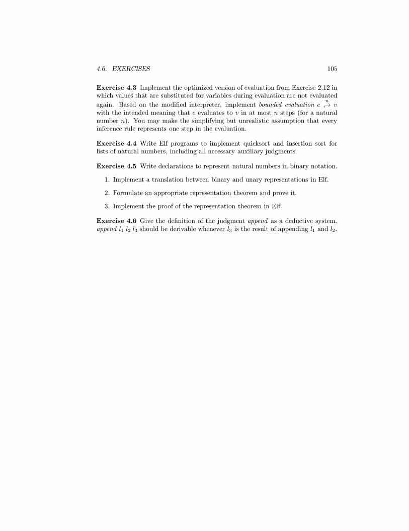
4.6. EXERCISES 105
Exercise 4.3 Implement the optimized version of evaluation from Exercise 2.12 inwhich values that are substituted for variables during evaluation are not evaluated
again. Based on the modified interpreter, implement bounded evaluation en↪→ v
with the intended meaning that e evaluates to v in at most n steps (for a naturalnumber n). You may make the simplifying but unrealistic assumption that everyinference rule represents one step in the evaluation.
Exercise 4.4 Write Elf programs to implement quicksort and insertion sort forlists of natural numbers, including all necessary auxiliary judgments.
Exercise 4.5 Write declarations to represent natural numbers in binary notation.
1. Implement a translation between binary and unary representations in Elf.
2. Formulate an appropriate representation theorem and prove it.
3. Implement the proof of the representation theorem in Elf.
Exercise 4.6 Give the definition of the judgment append as a deductive system.append l1 l2 l3 should be derivable whenever l3 is the result of appending l1 and l2.

106 CHAPTER 4. THE ELF PROGRAMMING LANGUAGE

Chapter 5
Parametric and HypotheticalJudgments
Many deductive systems employ reasoning from hypotheses. We have seen an exam-ple in Section 2.5: a typing derivation of a Mini-ML expression requires assumptionsabout the types of its free variables. Another example occurs in the system of natu-ral deduction in Chapter ??, where a deduction of the judgment that A⊃B is truecan be given as a deduction of B is true from the hypothesis A is true. We refer toa judgment that J is derivable under a hypothesis J ′ as a hypothetical judgment. Itscritical property is that we can substitute a derivation D of J ′ for every use of thehypothesis J ′ to obtain a derivation which no longer depends on the assumption J ′.
Related is reasoning with parameters, which also occurs frequently. The systemof natural deduction provides once again a typical example: we can infer that∀x. A is true if we can show that [a/x]A is true, where a is a new parameter whichdoes not occur in any undischarged hypothesis. Similarly, in the typing rules forMini-ML we postulate that every variable is declared at most once in a context Γ,that is, in the rule
Γ, x:τ1 . e : τ2tp lam
Γ . lam x. e : τ1 → τ2
the variable x is new with respect to Γ (which represents the hypotheses of thederivation). This side condition can always be fulfilled by tacitly renaming thebound variable. We refer to a judgment that J is derivable with parameter x as aparametric judgment. Its critical property is that we can substitute an expressiont for x throughout a derivation of a parametric judgment to obtain a derivationwhich no longer depends on the parameter x.
Since parametric and hypothetical judgments are common, it is natural to askif we can directly support them within the logical framework. The answer is
107

108 CHAPTER 5. PARAMETRIC AND HYPOTHETICAL JUDGMENTS
affirmative—the key is the notion of function provided in LF. Briefly, the derivationof a hypothetical judgment is represented by a function which maps a derivation ofthe hypothesis to a derivation of the conclusion. Applying this function correspondsto substituting a derivation for appeals to the hypothesis. Similarly, the derivationof a parametric judgment is represented by a function which maps an expression toa derivation of the instantiated conclusion. Applying this function corresponds tosubstituting an expressions for the parameter throughout the parametric derivation.
In the remainder of this chapter we elaborate the notions of parametric andhypothetical judgment and their representation in LF. We also show how to ex-ploit them to arrive at a natural and elegant representation of the proof of typepreservation for Mini-ML.
5.1 Closed Expressions
When employing parametric and hypothetical judgments, we must formulate therepresentation theorems carefully in order to avoid paradoxes. As a simple example,we consider the judgment e Closed which expresses that e has no free variables.Expression constructors which do not introduce any bound variables are treated ina straightforward manner.
clo zz Closed
e Closedclo s
s e Closed
e1 Closed e2 Closedclo pair
〈e1, e2〉 Closed
e Closedclo fst
fst e Closed
e Closedclo snd
snd e Closed
e1 Closed e2 Closedclo app
e1 e2 Closed
In order to give a concise formulation of the judgment whenever variables arebound we use hypothetical judgments. For example, in order to conclude thatlam x. e is closed, we must show that e is closed under the assumption that xis closed. The hypothesis about x may only be used in the deduction of e, butnot elsewhere. Furthermore, in order to avoid confusion between different boundvariables with the same name, we would like to make sure that the name x is notalready used, that is, the judgment should be parametric in x. The hypothetical
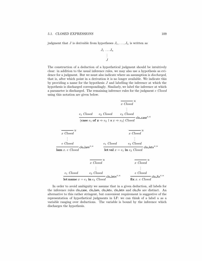
5.1. CLOSED EXPRESSIONS 109
judgment that J is derivable from hypotheses J1, . . . , Jn is written as
J1 . . . Jn...J
The construction of a deduction of a hypothetical judgment should be intuitivelyclear: in addition to the usual inference rules, we may also use a hypothesis as evi-dence for a judgment. But we must also indicate where an assumption is discharged,that is, after which point in a derivation it is no longer available. We indicate thisby providing a name for the hypothesis J and labelling the inference at which thehypothesis is discharged correspondingly. Similarly, we label the inference at whicha parameter is discharged. The remaining inference rules for the judgment e Closedusing this notation are given below.
e1 Closed e2 Closed
ux Closed
...e3 Closed
clo casex,u(case e1 of z⇒ e2 | s x⇒ e3) Closed
ux Closed
...e Closed
clo lamx,u
lam x. e Closed
e1 Closed
ux Closed
...e2 Closed
clo letvx,u
letval x = e1 in e2 Closed
e1 Closed
ux Closed
...e2 Closed
clo letnx,u
letname x = e1 in e2 Closed
ux Closed
...e Closed
clo fixx,u
fix x. e Closed
In order to avoid ambiguity we assume that in a given deduction, all labels forthe inference rules clo case, clo lam, clo letv, clo letn and clo fix are distinct. Analternative to this rather stringent, but convenient requirement is suggestive of therepresentation of hypothetical judgments in LF: we can think of a label u as avariable ranging over deductions. The variable is bound by the inference whichdischarges the hypothesis.
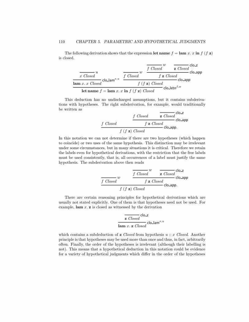
110 CHAPTER 5. PARAMETRIC AND HYPOTHETICAL JUDGMENTS
The following derivation shows that the expression let name f = lam x. x in f (f z)is closed.
ux Closed
clo lamx,u
lam x. x Closed
wf Closed
wf Closed
clo zz Closed
clo appf z Closed
clo appf (f z) Closed
clo letnf,wlet name f = lam x. x in f (f z) Closed
This deduction has no undischarged assumptions, but it contains subderiva-tions with hypotheses. The right subderivation, for example, would traditionallybe written as
f Closed
f Closedclo z
z Closedclo app
f z Closedclo app.
f (f z) Closed
In this notation we can not determine if there are two hypotheses (which happento coincide) or two uses of the same hypothesis. This distinction may be irrelevantunder some circumstances, but in many situations it is critical. Therefore we retainthe labels even for hypothetical derivations, with the restriction that the free labelsmust be used consistently, that is, all occurrences of a label must justify the samehypothesis. The subderivation above then reads
wf Closed
wf Closed
clo zz Closed
clo appf z Closed
clo app.f (f z) Closed
There are certain reasoning principles for hypothetical derivations which areusually not stated explicitly. One of them is that hypotheses need not be used. Forexample, lam x. z is closed as witnessed by the derivation
clo zz Closed
clo lamx,u
lam x. z Closed
which contains a subdeduction of z Closed from hypothesis u :: x Closed. Anotherprinciple is that hypotheses may be used more than once and thus, in fact, arbitrarilyoften. Finally, the order of the hypotheses is irrelevant (although their labelling isnot). This means that a hypothetical deduction in this notation could be evidencefor a variety of hypothetical judgments which differ in the order of the hypotheses
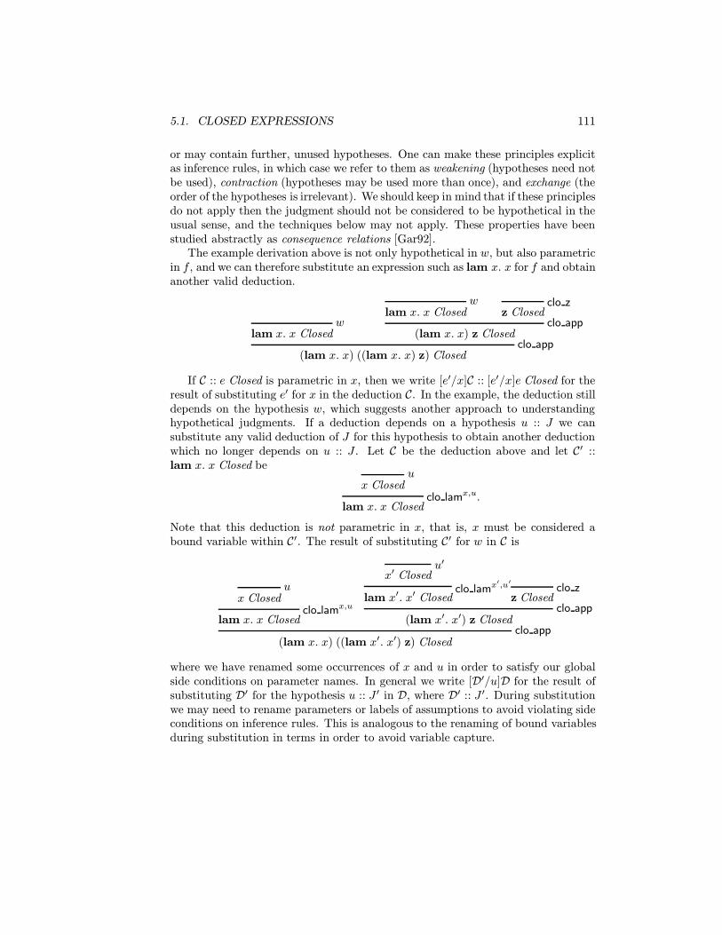
5.1. CLOSED EXPRESSIONS 111
or may contain further, unused hypotheses. One can make these principles explicitas inference rules, in which case we refer to them as weakening (hypotheses need notbe used), contraction (hypotheses may be used more than once), and exchange (theorder of the hypotheses is irrelevant). We should keep in mind that if these principlesdo not apply then the judgment should not be considered to be hypothetical in theusual sense, and the techniques below may not apply. These properties have beenstudied abstractly as consequence relations [Gar92].
The example derivation above is not only hypothetical in w, but also parametricin f , and we can therefore substitute an expression such as lam x. x for f and obtainanother valid deduction.
wlam x. x Closed
wlam x. x Closed
clo zz Closed
clo app(lam x. x) z Closed
clo app(lam x. x) ((lam x. x) z) Closed
If C :: e Closed is parametric in x, then we write [e′/x]C :: [e′/x]e Closed for theresult of substituting e′ for x in the deduction C. In the example, the deduction stilldepends on the hypothesis w, which suggests another approach to understandinghypothetical judgments. If a deduction depends on a hypothesis u :: J we cansubstitute any valid deduction of J for this hypothesis to obtain another deductionwhich no longer depends on u :: J . Let C be the deduction above and let C′ ::lam x. x Closed be
ux Closed
clo lamx,u.lam x. x Closed
Note that this deduction is not parametric in x, that is, x must be considered abound variable within C′. The result of substituting C′ for w in C is
ux Closed
clo lamx,u
lam x. x Closed
u′x′ Closed
clo lamx′,u′
lam x′. x′ Closedclo z
z Closedclo app
(lam x′. x′) z Closedclo app
(lam x. x) ((lam x′. x′) z) Closed
where we have renamed some occurrences of x and u in order to satisfy our globalside conditions on parameter names. In general we write [D′/u]D for the result ofsubstituting D′ for the hypothesis u :: J ′ in D, where D′ :: J ′. During substitutionwe may need to rename parameters or labels of assumptions to avoid violating sideconditions on inference rules. This is analogous to the renaming of bound variablesduring substitution in terms in order to avoid variable capture.

112 CHAPTER 5. PARAMETRIC AND HYPOTHETICAL JUDGMENTS
The representation of the judgment e Closed in LF follows the judgment-as-typesprinciple: we introduce a type family ‘closed’ indexed by an expression.
closed : exp→ type
The inference rules that do not employ hypothetical judgments are representedstraightforwardly.
clo z : closed zclo s : ΠE:expclosed E → closed (s E)clo pair : ΠE1:exp. ΠE2:exp.
closed E1 → closed E2 → closed (pair E1 E2)clo fst : ΠE:exp. closed E → closed (fst E)clo snd : ΠE:exp. closed E → closed (snd E)clo app : ΠE1:exp. ΠE2:exp.
closed E1 → closed E2 → closed (app E1 E2)
Now we reconsider the rule clo lam.
ux Closed
...e Closed
clo lamx,u
lam x. e Closed
The judgment in the premiss is parametric in x and hypothetical in x Closed.We thus consider it as a function which, when applied to an e′ and a deductionC :: e′ Closed yields a deduction of [e′/x]e Closed.
clo lam : ΠE:exp→ exp.(Πx:exp. closed x→ closed (E x))→ closed (lam E)
Recall that it is necessary to represent the scope of a binding operator in the lan-guage of expressions as a function from expressions to expressions. Similar declara-tions are necessary for the hypothetical judgments in the premisses of the clo letv,clo letn, and clo fix rules.
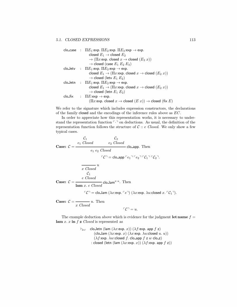
5.1. CLOSED EXPRESSIONS 113
clo case : ΠE1:exp. ΠE2:exp. ΠE3:exp→ exp.closed E1 → closed E2
→ (Πx:exp. closed x→ closed (E3 x))→ closed (case E1 E2 E3)
clo letv : ΠE1:exp. ΠE2:exp→ exp.closed E1 → (Πx:exp. closed x→ closed (E2 x))→ closed (letv E1 E2)
clo letn : ΠE1:exp. ΠE2:exp→ exp.closed E1 → (Πx:exp. closed x→ closed (E2 x))→ closed (letn E1 E2)
clo fix : ΠE:exp→ exp.(Πx:exp. closed x→ closed (E x))→ closed (fix E)
We refer to the signature which includes expression constructors, the declarationsof the family closed and the encodings of the inference rules above as EC.
In order to appreciate how this representation works, it is necessary to under-stand the representation function p·q on deductions. As usual, the definition of therepresentation function follows the structure of C :: e Closed. We only show a fewtypical cases.
Case: C =
C1e1 Closed
C2e2 Closed
clo appe1 e2 Closed
. Then
pCq = clo app pe1q pe2q pC1q pC2q.
Case: C =
ux ClosedC1
e Closedclo lamx.u
lam x. e Closed. Then
pCq = clo lam (λx:exp. peq) (λx:exp. λu:closed x. pC1q).
Case: C = ux Closed
. Then
pCq = u.
The example deduction above which is evidence for the judgment letname f =lam x. x in f z Closed is represented as
EC clo letn (lam (λx:exp. x)) (λf :exp. app f z)(clo lam (λx:exp. x) (λx:exp. λu:closed u. u))(λf :exp. λw:closed f. clo app f z w clo z)
: closed (letn (lam (λx:exp. x)) (λf :exp. app f z))
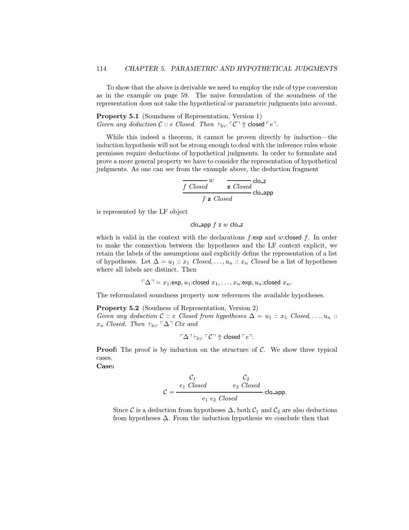
114 CHAPTER 5. PARAMETRIC AND HYPOTHETICAL JUDGMENTS
To show that the above is derivable we need to employ the rule of type conversionas in the example on page 59. The naive formulation of the soundness of therepresentation does not take the hypothetical or parametric judgments into account.
Property 5.1 (Soundness of Representation, Version 1)Given any deduction C :: e Closed. Then EC pCq ⇑ closed peq.
While this indeed a theorem, it cannot be proven directly by induction—theinduction hypothesis will not be strong enough to deal with the inference rules whosepremisses require deductions of hypothetical judgments. In order to formulate andprove a more general property we have to consider the representation of hypotheticaljudgments. As one can see from the example above, the deduction fragment
wf Closed
clo zz Closed
clo appf z Closed
is represented by the LF object
clo app f z w clo z
which is valid in the context with the declarations f :exp and w:closed f . In orderto make the connection between the hypotheses and the LF context explicit, weretain the labels of the assumptions and explicitly define the representation of a listof hypotheses. Let ∆ = u1 :: x1 Closed, . . . , un :: xn Closed be a list of hypotheseswhere all labels are distinct. Then
p∆q = x1:exp, u1:closed x1, . . . , xn:exp, un:closed xn.
The reformulated soundness property now references the available hypotheses.
Property 5.2 (Soudness of Representation, Version 2)Given any deduction C :: e Closed from hypotheses ∆ = u1 :: x1 Closed, . . . , un ::xn Closed. Then EC p∆q Ctx and
p∆q EC pCq ⇑ closed peq.
Proof: The proof is by induction on the structure of C. We show three typicalcases.
Case:
C =
C1e1 Closed
C2e2 Closed
clo app.e1 e2 Closed
Since C is a deduction from hypotheses ∆, both C1 and C2 are also deductionsfrom hypotheses ∆. From the induction hypothesis we conclude then that

5.1. CLOSED EXPRESSIONS 115
1. p∆q EC pC1q ⇑ closed pe1q, and
2. p∆q EC pC2q ⇑ closed pe2q
are both derivable. Thus, from the type of clo app,
p∆q EC clo app pe1q pe2q pC1q pC2q ⇑ closed (app pe1q pe2q).
It remains to notice that pe1 e2q = app pe1q pe2q.Case:
C =
ux ClosedC1
e Closedclo lamx,u.
lam x. e Closed
Then C1 is a deduction from hypotheses ∆, u :: x Closed, and
p∆, u :: x Closedq = p∆q, x:exp, u:closed x.
By the induction hypothesis on C1 we thus conclude that
p∆q, x:exp, u:closed x EC pC1q ⇑ closed peq
is derivable. Hence, by two applications of the canpi rule for canonical forms,
p∆q EC λx:exp. λu:closed x. pC1q ⇑ Πx:exp. Πu:closed x. closed peq
is also derivable.
By the representation theorem for expressions (Theorem 3.6) and the weak-ening for LF we also know that
p∆q EC λx:exp. peq ⇑ exp→ exp
is derivable. From this and the type of clo lam we infer
p∆q EC clo lam (λx:exp. peq)↓ (Πx:exp. Πu:closed x. closed ((λx:exp. peq) x))
→ closed (lam (λx:exp. peq)).
By the rule atmcnv, using one β-conversion in the type above, we conclude
p∆q EC clo lam (λx:exp. peq)↓ (Πx:exp. Πu:closed x. closed peq)
→ closed (lam (λx:exp. peq)).

116 CHAPTER 5. PARAMETRIC AND HYPOTHETICAL JUDGMENTS
Using the rules atmapp and cancon which are now applicable we infer
p∆q EC clo lam (λx:exp. peq) (λx:exp. λu:closed x. pC1q)⇑ closed (lam (λx:exp. peq)),
which is the desired conclusion since plam x. eq = lam (λx:exp. peq).
Case:
C = u.x Closed
Then pCq = u, to which p∆q assigns type closed x = closed pxq, which iswhat we needed to show.
2
The inverse of the representation function, x·y, is defined on canonical objects Cof type closed E for some E of type exp. This is sufficient for the adequacy theorembelow—one can extend it to arbitrary valid objects via conversion to canonical form.Again, we only show three critical cases.
xclo app E1 E2 C1 C2y =xC1y xC2y
clo appxE1y xE2y Closed
xclo lam (λx:exp. E) (λx:exp. λu:closed x. C1)y =
ux ClosedxC1y
xEy Closedclo lamx,u
lam x. xEy Closed
xuy =u
x Closed
The last case reveals that the inverse of the representation function should be param-eterized by a context so we can find the x which is assumed to be closed accordingto hypothesis u. Alternatively, we can assume that we always know the type ofthe canonical object we are translating to a deduction. Again, we are faced withthe problem that the natural theorem regarding the function x·y cannot be proveddirectly by induction.
Property 5.3 (Completeness of Representation, Version 1) Given LF objects Eand C such that EC E ⇑ exp and EC C ⇑ closed E. Then xCy :: xEy Closed.

5.1. CLOSED EXPRESSIONS 117
In order to prove this, we generalize it to allow appropriate contexts. Thesecontexts need to be translated to an appropriate list of hypotheses. Let Γ be acontext of the form x1:exp, u1:closed x1, . . . , xn:closed xn. Then xΓy is the list ofhypotheses u1 :: x1 Closed, . . . , un :: xnClosed.
Property 5.4 (Completeness of Representation, Version 2) Given a context Γ =x1:exp, u1:closed x1, . . . , xn:closed xn and LF objects E and C such that Γ EC E ⇑exp and Γ EC C ⇑ closed E. Then xCy :: xEy Closed is a valid deduction fromhypotheses xΓy. Moreoever, xpCqy = C and xp∆qy = ∆ for deductions C :: e Closedand hypotheses ∆.
Proof: By induction on the structure of the derivation Γ EC C ⇑ closed E. Therestriction to contexts Γ of a certain form is crucial in this proof (see Exercise 5.1).2
The usual requirement that p·q be a compositional bijection can be understoodin terms of substitution for deductions. Let C :: e Closed be a deduction fromhypothesis u :: x closed. Then compositionality of the representation functionrequires
p[C′/u][e′/x]Cq = [pC′q/u][pe′q/x]pCqwhenever C′ :: e′ Closed. Note that the substitution on the left-hand side is substi-tution for undischarged hypotheses in a deduction, while substitution on the rightis at the level of LF objects. Deductions of parametric and hypothetical judgmentsare represented as functions in LF. Applying such functions means to substitute fordeductions, which can be exhibited if we rewrite the right-hand side of the equationabove, preserving definitional equality.
[pC′q/u][pe′q/x]pCq ≡ (λx:exp. λu:closed x. pCq) pe′q pC′q
The discipline of dependent function types ensures the validity of the object on theright-hand side:
(λx:exp. λu:closed x. pCq) pe′q : [pe′q/x](closed x→ closed peq).
Hence, by compositionality of the representation for expressions,
(λx:exp. λu:closed x. pCq) pe′q : closed pe′q→ closed p[e′/x]eq
and the application of this object to pC′q is valid and of the appropriate type.
Theorem 5.5 (Adequacy) There is a bijection between deductions C :: e Closedfrom hypotheses u1 :: x1 Closed, . . . , un :: xn Closed and LF objects C such that
x1:exp, u1:closed x1, . . . , xn:exp, un:closed xn EC C ⇑ closed peq.

118 CHAPTER 5. PARAMETRIC AND HYPOTHETICAL JUDGMENTS
The bijection is compositional in the sense that for an expression ei and a deductionCi :: ei Closed, we have
p[Ci/ui][ei/xi]Cq = [pCiq/ui][peiq/xi]pCq
Proof: Properties 5.2 and 5.4 show the existence of the bijection. To show that itis compositional we reason by induction over the structure of C (see Exercise 5.2).2
5.2 Function Types as Goals in Elf
Below we give the transcription of the LF signature above in Elf.
closed : exp -> type. %name closed U u.
% Natural Numbers
clo_z : closed z.
clo_s : closed (s E)
<- closed E.
clo_case : closed (case E1 E2 E3)
<- closed E1
<- closed E2
<- ({x:exp} closed x -> closed (E3 x)).
% Pairs
clo_pair : closed (pair E1 E2)
<- closed E1
<- closed E2.
clo_fst : closed (fst E)
<- closed E.
clo_snd : closed (snd E)
<- closed E.
% Functions
clo_lam : closed (lam E)
<- ({x:exp} closed x -> closed (E x)).
clo_app : closed (app E1 E2)
<- closed E1
<- closed E2.
% Definitions
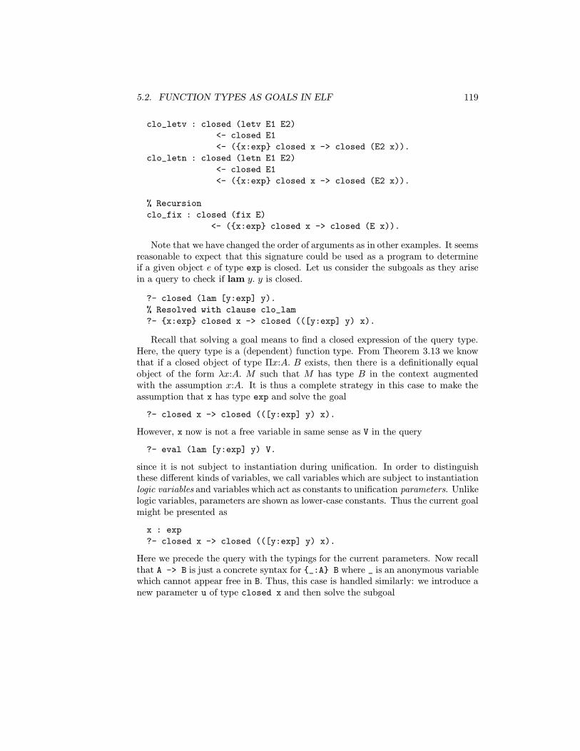
5.2. FUNCTION TYPES AS GOALS IN ELF 119
clo_letv : closed (letv E1 E2)
<- closed E1
<- ({x:exp} closed x -> closed (E2 x)).
clo_letn : closed (letn E1 E2)
<- closed E1
<- ({x:exp} closed x -> closed (E2 x)).
% Recursion
clo_fix : closed (fix E)
<- ({x:exp} closed x -> closed (E x)).
Note that we have changed the order of arguments as in other examples. It seemsreasonable to expect that this signature could be used as a program to determineif a given object e of type exp is closed. Let us consider the subgoals as they arisein a query to check if lam y. y is closed.
?- closed (lam [y:exp] y).
% Resolved with clause clo_lam
?- {x:exp} closed x -> closed (([y:exp] y) x).
Recall that solving a goal means to find a closed expression of the query type.Here, the query type is a (dependent) function type. From Theorem 3.13 we knowthat if a closed object of type Πx:A. B exists, then there is a definitionally equalobject of the form λx:A. M such that M has type B in the context augmentedwith the assumption x:A. It is thus a complete strategy in this case to make theassumption that x has type exp and solve the goal
?- closed x -> closed (([y:exp] y) x).
However, x now is not a free variable in same sense as V in the query
?- eval (lam [y:exp] y) V.
since it is not subject to instantiation during unification. In order to distinguishthese different kinds of variables, we call variables which are subject to instantiationlogic variables and variables which act as constants to unification parameters. Unlikelogic variables, parameters are shown as lower-case constants. Thus the current goalmight be presented as
x : exp
?- closed x -> closed (([y:exp] y) x).
Here we precede the query with the typings for the current parameters. Now recallthat A -> B is just a concrete syntax for {_:A} B where _ is an anonymous variablewhich cannot appear free in B. Thus, this case is handled similarly: we introduce anew parameter u of type closed x and then solve the subgoal

120 CHAPTER 5. PARAMETRIC AND HYPOTHETICAL JUDGMENTS
x : exp
u : closed x
?- closed (([y:exp] y) x).
By an application of β-conversion this is transformed into the equivalent goal
x : exp
u : closed x
?- closed x.
Now we can use the parameter u as the requested object of type closed x and thequery succeeds without further subgoals.
We now briefly consider, how the appropriate closed object of the originalquery, namely ?- closed (lam [y:exp] y). would be constructed. Recall thatif Γ, x:A Σ M : B then Γ Σ λx:A. M : Πx:A. B. Using this we can now throughthe trace of the search in reverse, constructing inhabiting objects as we go alongand inserting conversions where necessary.
u : closed x.
[u:closed x] u : closed x -> closed x.
[x:exp][u:closed x] u : {x:exp} closed x -> closed x.
[x:exp][u:closed x] u : {x:exp} closed x -> closed (([y:exp] y) x).
clo_lam ([x:exp][u:closed x] u)
: closed (lam [y:exp] y).
Just as in Prolog, search proceeds according to a fixed operational semantics.This semantics specifies that clauses (that is, LF constant declarations) are triedin order from the first to the last. Before referring to the fixed signature, however,the temporary hypotheses are consulted, always considering the most recently in-troduced parameter first. After all of them have been considered, then the currentsignature is traversed. In this example the search order happens to be irrelevant asthere will always be at most one assumption available for any expression parameter.
The representations of parametric and hypothetical judgments can also be givendirectly at the top-level. Here are two examples: the first to find the representationof the hypothetical deduction of f (f z) closed from the hypothesis f closed, thesecond to illustrate failure when given an expression (〈x, x〉) which is not closed.
?- Q : {f:exp} closed f -> closed (app f (app f z)).
Q = [f:exp] [u:closed f] clo_app (clo_app clo_z u) u.
More? y
no more solutions
?- Q : {x:exp} closed (pair x x).
no
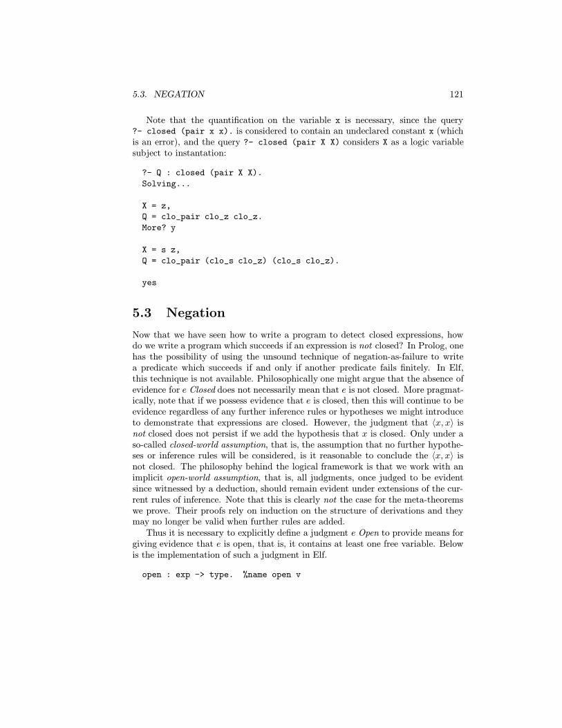
5.3. NEGATION 121
Note that the quantification on the variable x is necessary, since the query?- closed (pair x x). is considered to contain an undeclared constant x (whichis an error), and the query ?- closed (pair X X) considers X as a logic variablesubject to instantation:
?- Q : closed (pair X X).
Solving...
X = z,
Q = clo_pair clo_z clo_z.
More? y
X = s z,
Q = clo_pair (clo_s clo_z) (clo_s clo_z).
yes
5.3 Negation
Now that we have seen how to write a program to detect closed expressions, howdo we write a program which succeeds if an expression is not closed? In Prolog, onehas the possibility of using the unsound technique of negation-as-failure to writea predicate which succeeds if and only if another predicate fails finitely. In Elf,this technique is not available. Philosophically one might argue that the absence ofevidence for e Closed does not necessarily mean that e is not closed. More pragmat-ically, note that if we possess evidence that e is closed, then this will continue to beevidence regardless of any further inference rules or hypotheses we might introduceto demonstrate that expressions are closed. However, the judgment that 〈x, x〉 isnot closed does not persist if we add the hypothesis that x is closed. Only under aso-called closed-world assumption, that is, the assumption that no further hypothe-ses or inference rules will be considered, is it reasonable to conclude the 〈x, x〉 isnot closed. The philosophy behind the logical framework is that we work with animplicit open-world assumption, that is, all judgments, once judged to be evidentsince witnessed by a deduction, should remain evident under extensions of the cur-rent rules of inference. Note that this is clearly not the case for the meta-theoremswe prove. Their proofs rely on induction on the structure of derivations and theymay no longer be valid when further rules are added.
Thus it is necessary to explicitly define a judgment e Open to provide means forgiving evidence that e is open, that is, it contains at least one free variable. Belowis the implementation of such a judgment in Elf.
open : exp -> type. %name open v

122 CHAPTER 5. PARAMETRIC AND HYPOTHETICAL JUDGMENTS
% Natural Numbers
open_s : open (s E) <- open E.
open_case1 : open (case E1 E2 E3) <- open E1.
open_case2 : open (case E1 E2 E3) <- open E2.
open_case3 : open (case E1 E2 E3) <- ({x:exp} open (E3 x)).
% Pairs
open_pair1 : open (pair E1 E2) <- open E1.
open_pair2 : open (pair E1 E2) <- open E2.
open_fst : open (fst E) <- open E.
open_snd : open (snd E) <- open E.
% Functions
open_lam : open (lam E) <- ({x:exp} open (E x)).
open_app1 : open (app E1 E2) <- open E1.
open_app2 : open (app E1 E2) <- open E2.
% Definitions
open_letv1 : open (letv E1 E2) <- open E1.
open_letv2 : open (letv E1 E2) <- ({x:exp} open (E2 x)).
open_letn1 : open (letn E1 E2) <- open E1.
open_letn2 : open (letn E1 E2) <- ({x:exp} open (E2 x)).
% Recursion
open_fix : open (fix E) <- ({x:exp} open (E x)).
One curious fact about this judgment is that there is no base case, that is,without any hypotheses any query of the form ?- open peq. will fail! That is,with a given query we must provide evidence that any parameters which may occurin it are open. For example,
?- Q : {x:exp} open (pair x x).
no
?- Q : {x:exp} open x -> open (pair x x).
Empty Substitution.
Q = [x:exp] [v:open x] open_pair1 v.
More? y
Empty Substitution.
Q = [x:exp] [v:open x] open_pair2 v.
More? y
No more solutions

5.4. REPRESENTING MINI-ML TYPING DERIVATIONS 123
?- Q : {x:exp} open x -> open (lam [x:exp] pair x x).
no
5.4 Representing Mini-ML Typing Derivations
In this section we will show a natural representation of Mini-ML typing derivationsin LF. In order to avoid confusion between the contexts of LF and the contexts ofMini-ML, we will use ∆ throughout the remainder of this chapter to designate aMini-ML context. The typing judgment of Mini-ML then has the form
∆ . e : τ
and expresses that e has type τ in context ∆. We observe that this judgmentcan be interpreted as a hypothetical judgment with hypotheses ∆. There is thusan alternative way to describe the judgment e : τ which employs hypotheticaljudgments without making assumptions explicit.
∆, x:τ1 . e : τ2tp lam
∆ . lam x. e : τ1 → τ2
u. x : τ1
.... e : τ2
tp lamx,u
. lam x. e : τ1 → τ2
The judgment in the premiss in the formulation of the rule on the right is parametricin x and hypothetical in u :: x:τ1. On the left, all available hypothesis are repre-sented explicitly. The restriction that each variable may be declared at most oncein a context and bound variables may be renamed tacitly encodes the parametricitywith respect to x.
First, however, the representation of Mini-ML types. We declare an LF typeconstant, tp, for the representation of Mini-ML types. Recall, from Section 2.5,
Types τ ::= nat | τ1 × τ2 | τ1 → τ2 | α
It is important to bear in mind that → is overloaded here, since it stands for thefunction type constructor in Mini-ML and in LF. It should be clear from the contextwhich constructor is meant in each instance. The representation function and theLF declarations are straightforward.
tp : typepαq = αpnatq = nat nat : tp
pτ1 × τ2q = cross pτ1q pτ2q cross : tp→ tp→ tppτ1 → τ2q = arrow pτ1q pτ2q arrow : tp→ tp→ tp

124 CHAPTER 5. PARAMETRIC AND HYPOTHETICAL JUDGMENTS
Here α on the right-hand side stands for a variable named α in the LF type theory.We refer to the signature in the right-hand column as T . We briefly state (withoutproof) the representation theorem.
Theorem 5.6 (Adequacy) The representation function p·q is a compositional bi-jection between Mini-ML types and canonical LF objects of type tp over the signatureT .
Now we try to apply the techniques for representing hypothetical judgmentsdeveloped in Section 5.1 to the representation of the typing judgment (for an al-ternative, see Exercise 5.6). The representation will be as a type family ‘of’ suchthat
p∆q ` pPq : of peq pτqwhenever P is a deduction of ∆ . e : τ . Thus,
of : exp→ tp→ type
with the representation for Mini-ML contexts ∆ as LF contexts p∆q.
p·q = ·p∆, x:τq = p∆q, x:exp, u:of x pτq
Here u must be chosen to be different from x and any other variable in p∆q inorder to satisfy the general assumption about LF contexts. This assumption canbe satisfied since we made a similar assumption about ∆.
For typing derivation themselves, we only show three critical cases in the defi-nition of pPq for P :: ∆ . e : τ . The remainder is given directly in Elf later. Thetype family of : exp→ tp→ type represents the judgment e : τ .
Case:
P =
P1
∆ . e1 : τ2 → τ1
P2
∆ . e2 : τ2tp app.
∆ . e1 e2 : τ1
In this simple case we let
pPq = tp app pτ1q pτ2q pe1q pe2q pP1q pP2q
where
tp app : ΠT1:tp. ΠT2:tp. ΠE1:exp. ΠE2:expof E1 (arrow T2 T1)→ of E2 T2 → of (app E1 E2) T1

5.4. REPRESENTING MINI-ML TYPING DERIVATIONS 125
Case:
P =
P ′∆, x:τ1 . e : τ2
tp lam.∆ . lam x. e : τ1 → τ2
In this case we view P ′ as a deduction of a hypothetical judgment, that is, aderivation of e : τ2 from the hypothesis x:τ1. We furthermore note that P ′ isparametric in x and choose an appropriate functional representation.
pPq = tp lam pτ1q pτ2q (λx:exp. peq) (λx:exp. λu:of x pτ1q. pP ′q)
The constant tp lam must thus have the following type:
tp lam : ΠT1:tp. ΠT2:tp. ΠE:exp→ exp.(Πx:exp. of x T1 → of (E x) T2)→ of (lam E) (arrow T1 T2).
Representation of a deduction P with hypotheses ∆ requires unique labels forthe various hypotheses, in order to return the appropriate variable wheneveran hypothesis is used. While we left this correspondence implicit, it should beclear that in the case of pP ′q above, the hypothesis x:τ1 should be consideredas labelled by u.
Case:
P =∆(x) = τ
tp var.∆ . x : τ
This case is not represented using a fixed inference rule, but we will have avariable u of type ‘of x pτq’ which implicitly provides a label for the assump-tion x. We simply return this variable.
pPq = u
The adequacy of this representation is now a straightforward exercise, given inthe following two properties. We refer to the full signature (which includes thesignatures T for Mini-ML types and E for Mini-ML expressions) as TD.
Property 5.7 (Soundness) If P :: ∆ . e : τ then TD p∆q Ctx and
p∆q TD pPq ⇑ of peq pτq.

126 CHAPTER 5. PARAMETRIC AND HYPOTHETICAL JUDGMENTS
Property 5.8 (Completeness) Let ∆ be a Mini-ML context and Γ = p∆q. If
TD E ⇑ exp, TD T ⇑ tp, and
Γ TD P ⇑ of E T
then there exist e, τ , and a derivation P :: ∆ . e : τ such that peq = E, pTq = τ ,and pPq = P .
It remains to understand the compositionality property of the bijection. Wereconsider the substitution lemma (Lemma 2.4):
If ∆ . e1 : τ1 and ∆, x1:τ1 . e2 : τ2 then ∆ . [e1/x1]e2 : τ2.
The proof is by induction on the structure of P2 :: (∆, x1:τ1 . e2 : τ2). Whereverthe assumption x1:τ1 is used, we substitute a version of the derivation P1 :: ∆ . e1 :τ1 where some additional (and unused) typing assumptions may have been addedto ∆. A reformulation using the customary notation for hypothetical judgmentsexposes the similarity to the considerations for the judgment e Closed considered inSection 5.1.
If
u1
. x1:τ1P2
. e2:τ2
andP1
. e1:τ1then
P1u1
. e1:τ1[e1/x1]P2
. [e1/x1]e2 : τ2
Here, [e1/x1]P2 is the substitution of e1 for x1 in the deduction P2, which is legalsince P2 is a deduction of a judgment parametric in x1. Furthermore, the deductionP1 has been substituted for the hypotheses labelled u in P2, indicated by writingP1 above the appropriate hypothesis. Using the conventions established for hypo-thetical and parametric judgments, the final deduction above can also be writtenas [P1/u1][e1/x1]P2. Compositionality of the representation then requires
p[P1/u1][e1/x1]P2q = [pP1q/u1][pe1q/x1]pP2q≡ (λx1:exp. λu1:of x1 pτ1q. pP2q) pe1q pP1q
After appropriate generalization, this is proved by a straightforward induction overthe structure of P2, just as the substitution lemma for typing derivation which liesat the heart of this property.
Theorem 5.9 (Adequacy) There is a bijection between deductions
Px1:τ1, . . . , xn:τn . e : τ

5.5. AN ELF PROGRAM FOR MINI-ML TYPE INFERENCE 127
and LF objects P such that
x1:exp, u1:of x1 pτ1q, . . . , xn:exp, un:of xn pτnq TD P ⇑ of peq pτq.
The bijection is compositional in the sense that for an expression ei and deductionPi :: ∆i . ei : τi we have
p[Pi/ui][ei/xi]Pq = [pPiq/ui][peiq/xi]pPq
where ∆i = x1:exp, u1:of x1 pτ1q, . . . , xi:exp, ui:of xi pτiq.
Proof: As usual, by induction on the given derivations in each direction combinedwith verifying that correctness of the inverse of the representation function. Com-positionality follows by induction on the structure of P. 2
5.5 An Elf Program for Mini-ML Type Inference
We now complete the signature from the previous section by transcribing the rulesfrom the previous section and Section 2.5 into Elf. The notation will be suggestiveof a reading of this signature as a program for type inference. First, the declarationsof Mini-ML types.
tp : type. %name tp T.
nat : tp.
cross : tp -> tp -> tp.
arrow : tp -> tp -> tp.
Next, the typing rules.
of : exp -> tp -> type. %name of P u.
%mode of +E *T.
% Natural Numbers
tp_z : of z nat.
tp_s : of (s E) nat
<- of E nat.
tp_case : of (case E1 E2 E3) T
<- of E1 nat
<- of E2 T
<- ({x:exp} of x nat -> of (E3 x) T).
% Pairs
tp_pair : of (pair E1 E2) (cross T1 T2)

128 CHAPTER 5. PARAMETRIC AND HYPOTHETICAL JUDGMENTS
<- of E1 T1
<- of E2 T2.
tp_fst : of (fst E) T1
<- of E (cross T1 T2).
tp_snd : of (snd E) T2
<- of E (cross T1 T2).
% Functions
tp_lam : of (lam E) (arrow T1 T2)
<- ({x:exp} of x T1 -> of (E x) T2).
tp_app : of (app E1 E2) T1
<- of E1 (arrow T2 T1)
<- of E2 T2.
% Definitions
tp_letv : of (letv E1 E2) T2
<- of E1 T1
<- ({x:exp} of x T1 -> of (E2 x) T2).
tp_letn : of (letn E1 E2) T2
<- of E1 T1
<- of (E2 E1) T2.
% Recursion
tp_fix : of (fix E) T
<- ({x:exp} of x T -> of (E x) T).
As for evaluation, we take advantage of compositionality in order to represent sub-stitution of an expression for a bound variable in representation of tp letn,
∆ . e1 : τ1 ∆ . [e1/x]e2 : τ2tp letn.
∆ . letname x = e1 in e2 : τ2
Since we are using higher-order abstract syntax, e2 is represented together withits bound variable as a function of type exp → exp. Applying this function to therepresentation of e1 yields the representation of [e1/x]e2.
The Elf declarations above are suggestive of an operational interpretation as aprogram for type inference. The idea is to pose queries of the form ?- of peq T.
where T is a free variable subject to instantiation and e is a concrete Mini-MLexpression. We begin by considering a simple example: lam x. 〈x, s x〉. For thispurpose we assume that of has been declared dynamic and exp and tp are static.This means that free variables of type exp and tp may appear in an answer.
?- of (lam [x] pair x (s x)) T.

5.5. AN ELF PROGRAM FOR MINI-ML TYPE INFERENCE 129
Resolved with clause tp_lam
?- {x:exp} of x T1 -> of (pair x (s x)) T2.
In order to perform this first resolution step, the interpreter performed the substi-tutions
E = [x:exp] pair x (s x),
T1 = T1,
T2 = T2,
T = arrow T1 T2.
where E, T1, and T2 come from the clause tp_lam, and T appears in the originalquery. Now the interpreter applies the rules for solving goals of functional type andintroduces a new parameter x.
Introducing new parameter x : exp
x : exp
?- of x T1 -> of (pair x (s x)) T2.
Introducing new parameter u : of x T1.
x : exp,
u : of x T1
?- of (pair x (s x)) T2.
Resolved with clause tp_pair
This last resolution again requires some instantiation. We have
E1 = x,
E2 = (s x),
T2 = cross T21 T22.
Here, E1, E2, T21, and T22 come from the clause (the latter two renamed from T1 andT2, respectively). Now we have to solve two subgoals, namely ?- of x T21. and?- of (s x) T22. The first subgoal immediately succeeds by using the assump-tion u, which requires the instantiation T21 = T1 (or vice versa).
x : exp,
u : of x T1
?- of x T21.
Resolved with clause u
Here is the remainder of the computation.
x : exp,
u : of x T1
?- of (s x) T22.
Resolved with clause tp_s
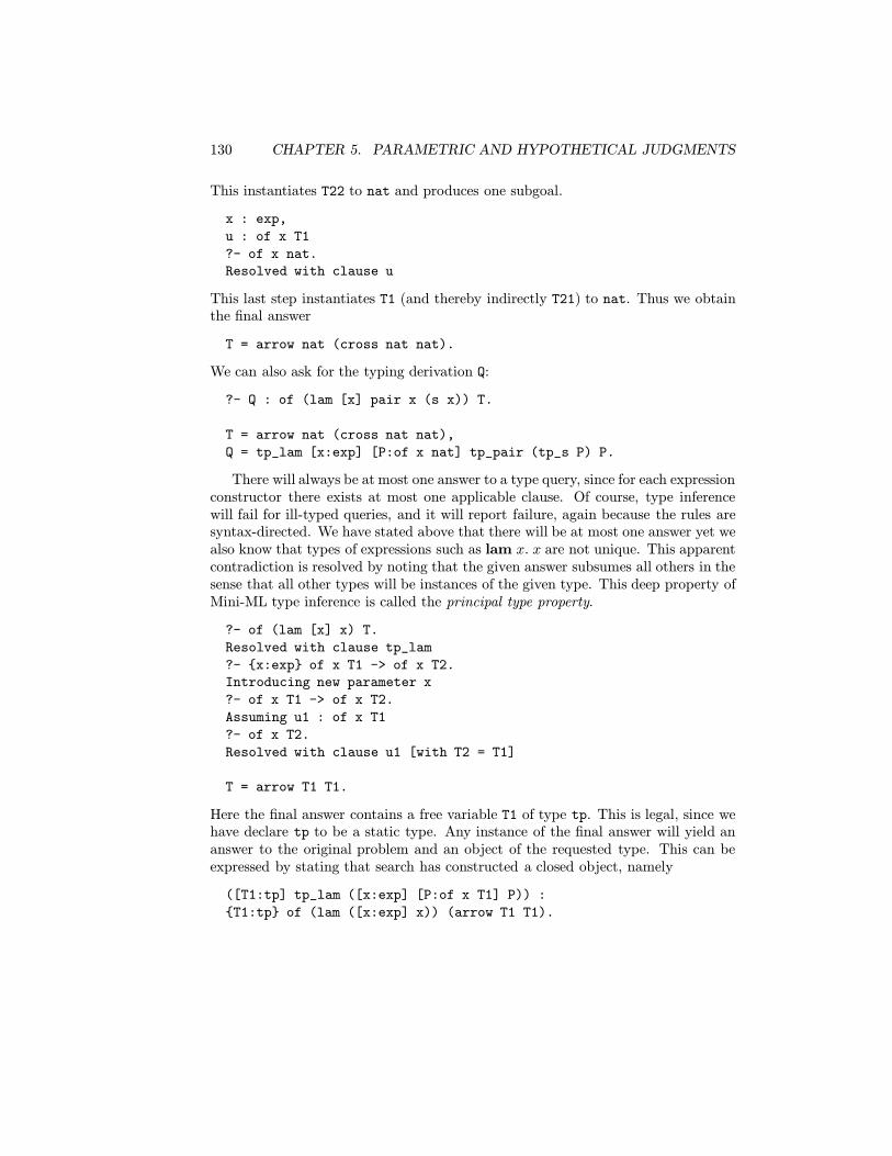
130 CHAPTER 5. PARAMETRIC AND HYPOTHETICAL JUDGMENTS
This instantiates T22 to nat and produces one subgoal.
x : exp,
u : of x T1
?- of x nat.
Resolved with clause u
This last step instantiates T1 (and thereby indirectly T21) to nat. Thus we obtainthe final answer
T = arrow nat (cross nat nat).
We can also ask for the typing derivation Q:
?- Q : of (lam [x] pair x (s x)) T.
T = arrow nat (cross nat nat),
Q = tp_lam [x:exp] [P:of x nat] tp_pair (tp_s P) P.
There will always be at most one answer to a type query, since for each expressionconstructor there exists at most one applicable clause. Of course, type inferencewill fail for ill-typed queries, and it will report failure, again because the rules aresyntax-directed. We have stated above that there will be at most one answer yet wealso know that types of expressions such as lam x. x are not unique. This apparentcontradiction is resolved by noting that the given answer subsumes all others in thesense that all other types will be instances of the given type. This deep property ofMini-ML type inference is called the principal type property.
?- of (lam [x] x) T.
Resolved with clause tp_lam
?- {x:exp} of x T1 -> of x T2.
Introducing new parameter x
?- of x T1 -> of x T2.
Assuming u1 : of x T1
?- of x T2.
Resolved with clause u1 [with T2 = T1]
T = arrow T1 T1.
Here the final answer contains a free variable T1 of type tp. This is legal, since wehave declare tp to be a static type. Any instance of the final answer will yield ananswer to the original problem and an object of the requested type. This can beexpressed by stating that search has constructed a closed object, namely
([T1:tp] tp_lam ([x:exp] [P:of x T1] P)) :
{T1:tp} of (lam ([x:exp] x)) (arrow T1 T1).
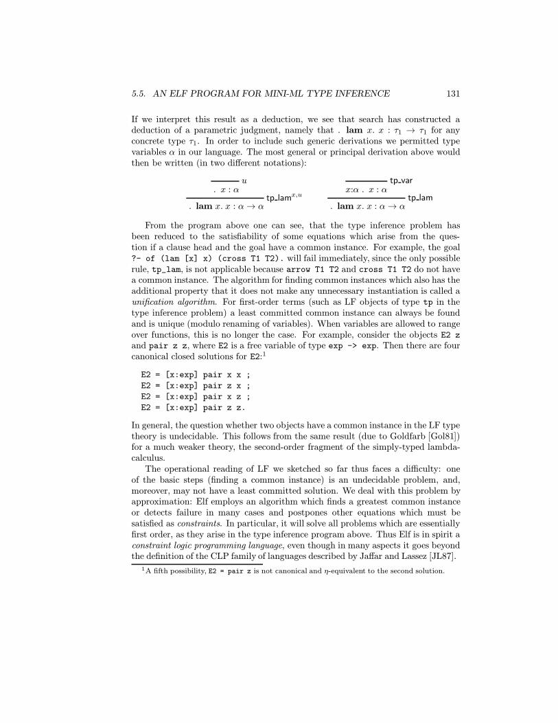
5.5. AN ELF PROGRAM FOR MINI-ML TYPE INFERENCE 131
If we interpret this result as a deduction, we see that search has constructed adeduction of a parametric judgment, namely that . lam x. x : τ1 → τ1 for anyconcrete type τ1. In order to include such generic derivations we permitted typevariables α in our language. The most general or principal derivation above wouldthen be written (in two different notations):
u. x : α
tp lamx,u
. lam x. x : α→ α
tp varx:α . x : α
tp lam. lam x. x : α→ α
From the program above one can see, that the type inference problem hasbeen reduced to the satisfiability of some equations which arise from the ques-tion if a clause head and the goal have a common instance. For example, the goal?- of (lam [x] x) (cross T1 T2). will fail immediately, since the only possiblerule, tp_lam, is not applicable because arrow T1 T2 and cross T1 T2 do not havea common instance. The algorithm for finding common instances which also has theadditional property that it does not make any unnecessary instantiation is called aunification algorithm. For first-order terms (such as LF objects of type tp in thetype inference problem) a least committed common instance can always be foundand is unique (modulo renaming of variables). When variables are allowed to rangeover functions, this is no longer the case. For example, consider the objects E2 z
and pair z z, where E2 is a free variable of type exp -> exp. Then there are fourcanonical closed solutions for E2:1
E2 = [x:exp] pair x x ;
E2 = [x:exp] pair z x ;
E2 = [x:exp] pair x z ;
E2 = [x:exp] pair z z.
In general, the question whether two objects have a common instance in the LF typetheory is undecidable. This follows from the same result (due to Goldfarb [Gol81])for a much weaker theory, the second-order fragment of the simply-typed lambda-calculus.
The operational reading of LF we sketched so far thus faces a difficulty: oneof the basic steps (finding a common instance) is an undecidable problem, and,moreover, may not have a least committed solution. We deal with this problem byapproximation: Elf employs an algorithm which finds a greatest common instanceor detects failure in many cases and postpones other equations which must besatisfied as constraints. In particular, it will solve all problems which are essentiallyfirst order, as they arise in the type inference program above. Thus Elf is in spirit aconstraint logic programming language, even though in many aspects it goes beyondthe definition of the CLP family of languages described by Jaffar and Lassez [JL87].
1A fifth possibility, E2 = pair z is not canonical and η-equivalent to the second solution.

132 CHAPTER 5. PARAMETRIC AND HYPOTHETICAL JUDGMENTS
The algorithm, originally discovered by Miller in the simply-typed λ-calculus [Mil91]has been generalized to dependent and polymorphic types in [Pfe91b]. The precisemanner in which it is employed in Elf is described in [Pfe91a].2. Here we contentourselves with a simple example which illustrates how constraints may arise.
?- of (lam [x] x) ((F:tp -> tp) nat).
F = F.
(( arrow T1 T1 = F nat ))
Here the remaining constraint is enclosed within double parentheses. Any solutionto this equation yields an answer to the original query. It is important to realizethat this constitutes only a conditional success, that is, we can in general not besure that the given constraint set is indeed be satisfiable. In the example above,this is obvious: there are infinitely many solutions of which we show two.
F = [T:tp] arrow T1 T1,
T1 = T1 ;
F = [T:tp] arrow (arrow T T) (arrow T T),
T1 = arrow nat nat.
The same algorithm is also employed during Elf’s term reconstruction phase. Inpractice this means that Elf term reconstruction may also terminate with remainingconstraints which, in this case, is considered an error and accompanied by a requestto the programmer to supply more type information.
The operational behavior of the program above may not be satisfactory from thepoint of view of efficiency, since expressions bound to a variable by a let name aretype-checked once for each occurrence of the variable in the body of the expression.The following is an example for a derivation involving let name in Elf.
?- Q : of (letn (lam [y] y) ([f] pair (app f z) (app f (pair z z)))) T.
Solving...
T = cross nat (cross nat nat),
Q =
tp_letn
(tp_pair
(tp_app (tp_pair tp_z tp_z)
(tp_lam [x:exp] [P:of x (cross nat nat)] P))
(tp_app tp_z (tp_lam [x:exp] [P:of x nat] P)))
(tp_lam [x:exp] [P:of x T1] P).
More? y
no more solutions
2[further discussion of unification elsewhere? ]

5.6. REPRESENTING THE PROOF OF TYPE PRESERVATION 133
Notice the two occurrences of tp_lam which means that (lam [y] y) was type-checked twice. Usually, ML’s type system is defined with explicit constructors forpolymorphic types so that we can express . lam x. x : ∀t. t → t. The typeinference algorithm can then instantiate such a most general type in the body e2 of alet name-expression let name x = e1 in e2 without type-checking e1 again. This isthe essence of Milner’s algorithmW in [Mil78]. It is difficult to realize this algorithmdirectly in Elf. Some further discussion and avenues towards a possible solutionare given in [Har90], [DP91], and [Lia95]. . Theoretically, however, algorithm Wof [Mil78] is not more efficient compared to the algorithm presented above as shownby [Mai92].
5.6 Representing the Proof of Type Preservation
We now return to the proof of type preservation from Section 2.6. In order to preparefor its representation in Elf, we reformulate the theorem to explicitly mention thedeductions involved.
For any e, v, τ , D :: e ↪→ v, and P :: . e : τ there exists a Q :: . v : τ .
The proof is by induction on the structure of D and relies heavily on inversionto predict the shape of P from the structure of e. The techniques from Section 3.7suggest casting this proof as a higher-level judgment relating D, P, and Q. Thishigher-level judgment can be represented in LF and then be implemented in Elf asa type family. We forego the intermediate step and directly map the informal proofinto Elf, calling the type family tps.
tps : eval E V -> of E T -> of V T -> type.
%mode tps +D +P -Q.
All of the cases in the induction proof now have a direct representation in Elf. Theinteresting cases involve appeals to the substitution lemma (Lemma 2.4).
Case: D = ev z.z ↪→ z
Then we have to show that for any type τ such that . z : τ is derivable,. z : τ is derivable. This is obvious.
There are actually two slightly different, but equivalent realizations of this case.The first uses the deduction P :: . z : τ that exists by assumption.
tps_z0 : tps (ev_z) P P.
The second, which we prefer, uses inversion to conclude that P must be tp z, sinceit is the only rule which assigns a type to z.
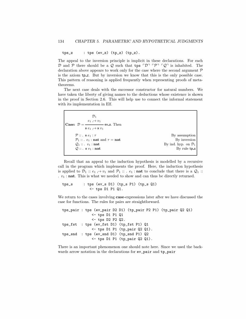
134 CHAPTER 5. PARAMETRIC AND HYPOTHETICAL JUDGMENTS
tps_z : tps (ev_z) (tp_z) (tp_z).
The appeal to the inversion principle is implicit in these declarations. For eachD and P there should be a Q such that tps pDq pPq pQq is inhabited. Thedeclaration above appears to work only for the case where the second argument Pis the axiom tp z. But by inversion we know that this is the only possible case.This pattern of reasoning is applied frequently when representing proofs of meta-theorems.
The next case deals with the successor constructor for natural numbers. Wehave taken the liberty of giving names to the deductions whose existence is shownin the proof in Section 2.6. This will help use to connect the informal statementwith its implementation in Elf.
Case: D =
D1
e1 ↪→ v1
ev s.s e1 ↪→ s v1
Then
P :: . s e1 : τ By assumptionP1 :: . e1 : nat and τ = nat By inversionQ1 :: . v1 : nat By ind. hyp. on D1
Q :: . s v1 : nat By rule tp s
Recall that an appeal to the induction hypothesis is modelled by a recursivecall in the program which implements the proof. Here, the induction hypothesisis applied to D1 :: e1 ↪→ v1 and P1 :: . e1 : nat to conclude that there is a Q1 ::. v1 : nat. This is what we needed to show and can thus be directly returned.
tps_s : tps (ev_s D1) (tp_s P1) (tp_s Q1)
<- tps D1 P1 Q1.
We return to the cases involving case-expressions later after we have discussed thecase for functions. The rules for pairs are straightforward.
tps_pair : tps (ev_pair D2 D1) (tp_pair P2 P1) (tp_pair Q2 Q1)
<- tps D1 P1 Q1
<- tps D2 P2 Q2.
tps_fst : tps (ev_fst D1) (tp_fst P1) Q1
<- tps D1 P1 (tp_pair Q2 Q1).
tps_snd : tps (ev_snd D1) (tp_snd P1) Q2
<- tps D1 P1 (tp_pair Q2 Q1).
There is an important phenomenon one should note here. Since we used the back-wards arrow notation in the declarations for ev_pair and tp_pair

5.6. REPRESENTING THE PROOF OF TYPE PRESERVATION 135
ev_pair : eval (pair E1 E2) (pair V1 V2)
<- eval E1 V1
<- eval E2 V2.
tp_pair : of (pair E1 E2) (cross T1 T2)
<- of E1 T1
<- of E2 T2.
their arguments are reversed from what one might expect. This is why we called thefirst argument to ev_pair above D2 and the second argument D1, and similiary fortp_pair. The case for lam-expressions is simple, since they evaluate to themselves.For stylistic reasons we apply inversion here as in all other cases.
tps_lam : tps (ev_lam) (tp_lam P) (tp_lam P).
The case for evaluating an application e1 e2 is more complicated than the casesabove. The informal proof appeals to the substitution lemma.
Case: D =
D1
e1 ↪→ lam x. e′1
D2
e2 ↪→ v2
D3
[v2/x]e′1 ↪→ vev app
e1 e2 ↪→ v.
P :: . e1 e2 : τ1 By assumptionP1 :: . e1 : τ2 → τ1 and P2 :: . e2 : τ2 for some τ2 By inversionQ1 :: . lam x. e′1 : τ2 → τ1 By ind. hyp. on D1
Q′1 :: x:τ2 . e′1 : τ1 By inversion
Q2 :: . v2 : τ2 By ind. hyp. on D2
P3 :: . [v2/x]e′1 : τ1 By the Substitution Lemma 2.4Q3 :: . v : τ1 By ind. hyp. on D3
We repeat the declarations of the ev_app and tp_lam clauses here with somevariables renamed in order to simplify the correspondence to the names used above.
ev_lam : eval (app E1 E2) V
<- eval E1 (lam E1’)
<- eval E2 V2
<- eval (E1’ V2) V.
tp_lam : of (lam E1’) (arrow T2 T1)
<- ({x:exp} of x T2 -> of (E1’ x) T1).
The deduction Q1 is a deduction of a parametric and hypothetical judgment (para-metric in x, hypothetical in . x:τ2). In Elf this is represented as a functionwhich, when applied to V2 and an object Q2 : of V2 T2 yields an object of typeof (E1’ V2) T1, that is

136 CHAPTER 5. PARAMETRIC AND HYPOTHETICAL JUDGMENTS
Q1’ : {x:exp} of x T2 -> of (E1’ x) T1.
The Elf variable E1’ : exp -> exp represents λx:exp. pe′1q, and V2 represents v2.Thus the appeal to the substitution lemma has been transformed into a functionapplication using Q1’, that is, P3 = Q1’ V2 Q2.
tps_app : tps (ev_app D3 D2 D1) (tp_app P2 P1) Q3
<- tps D1 P1 (tp_lam Q1’)
<- tps D2 P2 Q2
<- tps D3 (Q1’ V2 Q2) Q3.
This may seem like black magic—where did the appeal to the substitution lemmago? The answer is that it is hidden in the proof of the adequacy theorem for therepresentation of typing derivations (Theorem 5.9) combined with the substitutionlemma for LF itself! We have thus factored the proof effort: in the proof of theadequacy theorem, we establish that the typing judgment employs parametric andhypothetical judgments (which permit weakening and substitution). The implemen-tation above can then take this for granted and model an appeal to the substitutionlemma simply by function application.
One very nice property is the conciseness of the representation of the proofs ofthe meta-theorems in this fashion. Each case in the induction proof is representeddirectly as a clause, avoiding explicit formulation and proof of many properties ofsubstitution, variable occurrences, etc. This is due to the principles of higher-orderabstract syntax, judgments-as-types, and hypothetical judgments as functions. An-other important factor is the Elf type reconstruction algorithm which eliminates theneed for much redundant information. In the clause above, for example, we needto refer explicitly to only one expression (the variable V2). All other constraintsimposed on applications of inferences rules can be inferred in a most general way inall of these examples. To illustrate this point, here is the fully explicit form of theabove declaration, as generated by Elf’s term reconstruction.
tps_app :
{E:exp -> exp} {V2:exp} {E1:exp} {T:tp} {D3:eval (E V2) E1}
{T1:tp} {Q1’:{E1:exp} of E1 T1 -> of (E E1) T} {Q2:of V2 T1}
{Q3:of E1 T} {E2:exp} {D2:eval E2 V2} {P2:of E2 T1} {E3:exp}
{D1:eval E3 (lam E)} {P1:of E3 (arrow T1 T)}
tps (E V2) E1 T D3 (Q1’ V2 Q2) Q3 -> tps E2 V2 T1 D2 P2 Q2
-> tps E3 (lam E) (arrow T1 T) D1 P1 (tp_lam T1 E T Q1’)
-> tps (app E3 E2) E1 T (ev_app E V2 E1 E2 E3 D3 D2 D1)
(tp_app E2 T1 E3 T P2 P1) Q3.
We skip the two cases for case-expressions and only show their implementation.The techniques we need have all been introduced.

5.6. REPRESENTING THE PROOF OF TYPE PRESERVATION 137
tps_case_z: tps (ev_case_z D2 D1) (tp_case P3 P2 P1) Q2
<- tps D2 P2 Q2.
tps_case_s: tps (ev_case_s D3 D1) (tp_case P3 P2 P1) Q3
<- tps D1 P1 (tp_s Q1’)
<- tps D3 (P3 V1 Q1’) Q3.
Next, we come to the cases for definitions. For let val-expressions, no newconsiderations arise.
Case: D =
D1
e1 ↪→ v1
D2
[v1/x]e2 ↪→ vev letv.
let val x = e1 in e2 ↪→ v
P :: . let val x = e1 in e2 : τ By assumptionP1 :: . e1 : τ1 andP2 :: x:τ1 . e2 : τ for some τ1 By inversionQ1 :: . v1 : τ1 By ind. hyp. on D1
P ′2 :: . [v1/x]e2 : τ By the Substitution Lemma 2.4Q2 :: . v : τ By ind. hyp. on D2
tps_letv : tps (ev_letv D2 D1) (tp_letv P2 P1) Q2
<- tps D1 P1 Q1
<- tps D2 (P2 V1 Q1) Q2.
let name-expressions may at first sight appear to be the most complicated case.However, the substitution at the level of expressions is dealt with via composition-ality as in evaluation, so the representation of this case is actually quite simple.
Case: D =
D2
[e1/x]e2 ↪→ vev letn.
let name x = e1 in e2 ↪→ v
P :: . let name x = e1 in e2 : τ By assumptionP2 :: . [e1/x]e2 : τ By inversionQ2 :: . v : τ By ind. hyp. on D2
tps_letn : tps (ev_letn D2) (tp_letn P2 P1) Q2
<- tps D2 P2 Q2.
The case of fixpoint follows the same general pattern as the case for applicationin that we need to appeal to the substitution lemma. The solution is analogous.
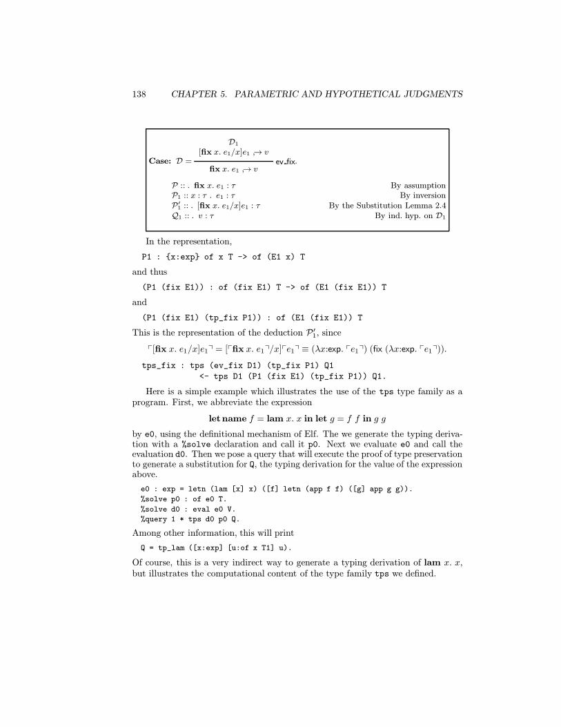
138 CHAPTER 5. PARAMETRIC AND HYPOTHETICAL JUDGMENTS
Case: D =
D1
[fix x. e1/x]e1 ↪→ vev fix
fix x. e1 ↪→ v.
P :: . fix x. e1 : τ By assumptionP1 :: x : τ . e1 : τ By inversionP ′1 :: . [fix x. e1/x]e1 : τ By the Substitution Lemma 2.4Q1 :: . v : τ By ind. hyp. on D1
In the representation,
P1 : {x:exp} of x T -> of (E1 x) T
and thus
(P1 (fix E1)) : of (fix E1) T -> of (E1 (fix E1)) T
and
(P1 (fix E1) (tp_fix P1)) : of (E1 (fix E1)) T
This is the representation of the deduction P ′1, since
p[fix x. e1/x]e1q = [pfix x. e1q/x]pe1q ≡ (λx:exp. pe1q) (fix (λx:exp. pe1q)).tps_fix : tps (ev_fix D1) (tp_fix P1) Q1
<- tps D1 (P1 (fix E1) (tp_fix P1)) Q1.
Here is a simple example which illustrates the use of the tps type family as aprogram. First, we abbreviate the expression
letname f = lam x. x in let g = f f in g g
by e0, using the definitional mechanism of Elf. The we generate the typing deriva-tion with a %solve declaration and call it p0. Next we evaluate e0 and call theevaluation d0. Then we pose a query that will execute the proof of type preservationto generate a substitution for Q, the typing derivation for the value of the expressionabove.
e0 : exp = letn (lam [x] x) ([f] letn (app f f) ([g] app g g)).
%solve p0 : of e0 T.
%solve d0 : eval e0 V.
%query 1 * tps d0 p0 Q.
Among other information, this will print
Q = tp_lam ([x:exp] [u:of x T1] u).
Of course, this is a very indirect way to generate a typing derivation of lam x. x,but illustrates the computational content of the type family tps we defined.

5.7. EXERCISES 139
5.7 Exercises
Exercise 5.1 Carry out three representative cases in the proof of Property 5.4.Where do we require the assumption that Γ must be of a certain form? Construct acounterexample which shows the falsehood of careless generalization of the theoremto admit arbitary contexts Γ.
Exercise 5.2 Carry out three representative cases in the proof of the AdequacyTheorem 5.5.
Exercise 5.3 Modify the natural semantics for Mini-ML such that only closed λ-expressions have a value. How does this affect the proof of type preservation?
Exercise 5.4 Write Elf programs
1. to count the number of occurrences of bound variables in a Mini-ML expres-sion;
2. to remove all vacuous let-bindings from a Mini-ML expression;
3. to rewrite all occurrences of expressions of the form (lam x. e2) e1 to let x =e1 in e2.
Exercise 5.5 For each of the following statements, prove them informally andrepresent the proof in Elf, or give a counterexample if the statement is false.
1. For any expressions e1 and e2, evaluation of (lam x. e2) e1 yields a value v ifand only if evaluation of let val x = e1 in e2 yields v.
2. For any expressions e1 and e2, evaluation of (lam x. e2) e1 yields a value v ifand only if evaluation of let name x = e1 in e2 yields v.
3. For values v1, the expression (lam x. e2) v1 has type τ if and only if theexpression letval x = v1 in e2 has type τ .
4. For values v1, the expression (lam x. e2) v1 has type τ if and only if theexpression letname x = v1 in e2 has type τ .
5. Evaluation is deterministic, that is, whenever e ↪→ v1 and e ↪→ v2 then v1 = v2
(modulo renaming of bound variables, as usual).
Exercise 5.6 Give an LF representation of the fragment of Mini-ML which includespairing, first and second projection, functions and application, and definitions withlet val without using hypothetical judgments. Thus the typing judgment should berepresented as a ternary type family, say, hastype, indexed by a representation of the

140 CHAPTER 5. PARAMETRIC AND HYPOTHETICAL JUDGMENTS
context ∆ and representations of e and τ . We would then look for a representationfunction p·q which satisfies
Γ ` pPq : hastype p∆q peq pτq
for a suitable Γ, whenever P is a valid deduction of ∆ . e : τ .
Exercise 5.7 Illustrate by means of an example why declaring the type tp asdynamic might lead to undesirable backtracking and unexpected answers duringtype inference for Mini-ML with the program in Section 5.5. Can you construct asituation where the program diverges on a well-typed Mini-ML expression? Howabout on a Mini-ML expression which is not well-typed?
Exercise 5.8 Extend the implementation of the Mini-ML interpreter, type infer-ence, and proof of type preservation to include
1. unit, void, and disjoint sum types (see Exercise 2.7),
2. lists (see Exercise 2.8).
Exercise 5.9 Consider the call-by-name version of Mini-ML with lazy constructorsas sketched in Exercise 2.13. Recall that neither the arguments to functions, northe arguments to constructors (s and 〈·, ·〉) should be evaluated.
1. Implement an interpreter for the language and show a few expressions thathighlight the differences in the operational semantics.
2. Implement type inference.
3. Define and implement a suitable notion of value.
4. Prove value soundness and implement your proof.
5. Prove type preservation and implement your proof.
Discuss the main differences between the development for Mini-ML and its call-by-name variant.
Exercise 5.10 The definition of the judgment e Closed follows systematically fromthe representation of expressions in higher-order abstract syntax, because object-level variables are represented by meta-level variables. This exercise explores ageneralization of this fact. Assume we have a signature Σ0 in the simply-typedlambda-calculus that declares exactly one type constant a and some unspecifiednumber of object constants c1, . . . , cn. Define an LF signature Σ1 that extends Σ0
by a new family
closed : a→ type

5.7. EXERCISES 141
such that
Σ0N : a
if and only ifΓ Σ1
N : a and Γ Σ1M : closed N
provided Γ no has declaration of the form u:Πy1:A1 . . .Πym:Am. closed P .
Exercise 5.11 Write Elf programs to determine if a Mini-ML expression is free ofthe recursion operation fix and at the same time
1. linear (every bound variable occurs exactly once);
2. affine (every bound variable occurs at most once);
3. relevant (every bound variable occurs at least once).
Since only one branch in a case statement will be taken during evaluation, a boundvariable must occur exactly once in each branch in a linear expression, may occurat most once in each branch in an affine expression, and must occur at least oncein each branch in a relevant expression.
Exercise 5.12 Instead of substituting in the typing rule for letname-expressionswe could extend contexts to record the definitions for variables bound with letname.
Contexts ∆ ::= · | ∆, x:τ | ∆, x = e
Variables must still occur at most once in a context (no variable may be declaredand defined). We would replace the rule tp letn by the following two rules.
∆ . e1 : τ1 ∆, x = e1 . e2 : τ1tp letn0
∆ . letname x = e1 in e2 : τ2
x = e in ∆ ∆ . e : τtp var0
∆ . x : τ
There are at least two ways we can view this modification for representation in theframework.
1. We use a new judgment, x = e, which is introduced only as a hypothesis intoa derivation.
2. We view a hypothesis x = e as the assumption of an inference rule. We mightwrite this as
. e1 : τ1
. e1 : τuτ
. x : τ...
. e2 : τ2tp letx,u.
. let name x = e1 in e2
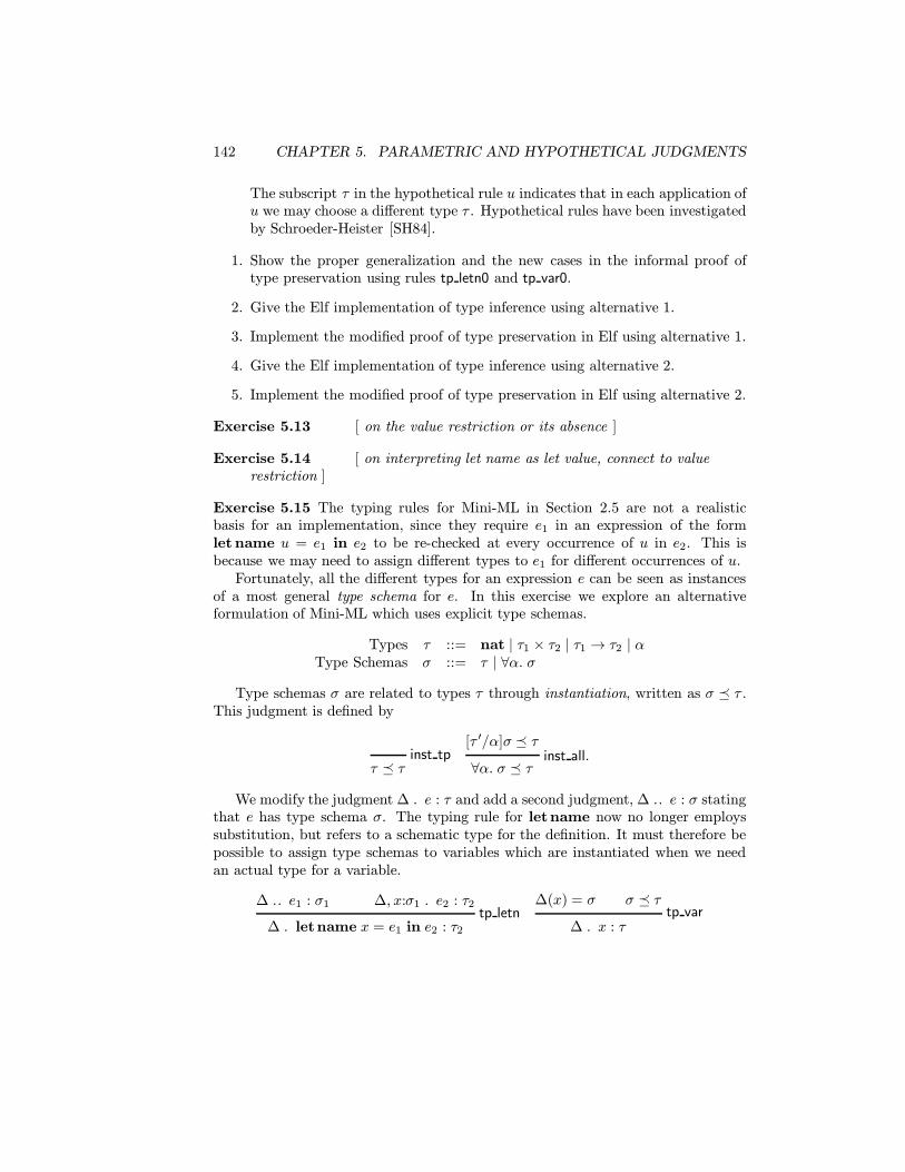
142 CHAPTER 5. PARAMETRIC AND HYPOTHETICAL JUDGMENTS
The subscript τ in the hypothetical rule u indicates that in each application ofu we may choose a different type τ . Hypothetical rules have been investigatedby Schroeder-Heister [SH84].
1. Show the proper generalization and the new cases in the informal proof oftype preservation using rules tp letn0 and tp var0.
2. Give the Elf implementation of type inference using alternative 1.
3. Implement the modified proof of type preservation in Elf using alternative 1.
4. Give the Elf implementation of type inference using alternative 2.
5. Implement the modified proof of type preservation in Elf using alternative 2.
Exercise 5.13 [ on the value restriction or its absence ]
Exercise 5.14 [ on interpreting let name as let value, connect to valuerestriction ]
Exercise 5.15 The typing rules for Mini-ML in Section 2.5 are not a realisticbasis for an implementation, since they require e1 in an expression of the formlet name u = e1 in e2 to be re-checked at every occurrence of u in e2. This isbecause we may need to assign different types to e1 for different occurrences of u.
Fortunately, all the different types for an expression e can be seen as instancesof a most general type schema for e. In this exercise we explore an alternativeformulation of Mini-ML which uses explicit type schemas.
Types τ ::= nat | τ1 × τ2 | τ1 → τ2 | αType Schemas σ ::= τ | ∀α. σ
Type schemas σ are related to types τ through instantiation, written as σ � τ .This judgment is defined by
inst tpτ � τ
[τ ′/α]σ � τinst all.
∀α. σ � τ
We modify the judgment ∆ . e : τ and add a second judgment, ∆ .. e : σ statingthat e has type schema σ. The typing rule for letname now no longer employssubstitution, but refers to a schematic type for the definition. It must therefore bepossible to assign type schemas to variables which are instantiated when we needan actual type for a variable.
∆ .. e1 : σ1 ∆, x:σ1 . e2 : τ2tp letn
∆ . letname x = e1 in e2 : τ2
∆(x) = σ σ � τtp var
∆ . x : τ

5.7. EXERCISES 143
Type schemas can be derived for expressions by means of quantifying over free typevariables.
∆ . e : τtpsc tp
∆ .. e : τ
∆ .. e : σtpsc allα
∆ .. e : ∀α. σ
Here the premiss of the tpsc allα rule must be parametric in α, that is, α must notoccur free in the context ∆.
In the proofs and implementations below you may restrict yourself to the frag-ment of the language with functions and let name, since the changes are orthogonalto the other constructs of the language.
1. Give an example which shows why the restriction on the tpsc all rule is nec-essary.
2. Prove type preservation for this formulation of Mini-ML. Carefully writeout and prove any substitution lemmas you might need, but you may takeweakening and exchange for granted.
3. State the theorem which asserts the equivalence of the new typing rules whencompared to the formulation in Section 2.5.
4. Prove the easy direction of the theorem in item 3. Can you conjecture thecritical lemma for the opposite direction?
5. Implement type schemas, schematic instantiation, and the new typing judg-ments in Elf.
6. Unlike our first implementation, the new typing rules do not directly providean implementation of type inference for Mini-ML in Elf. Show the difficultyby means of an example.
7. Implement the proof of type preservation from item 2 in Elf.
8. Implement one direction of the equivalence proof from item 3 in Elf.
Exercise 5.16 [ about the Milner-Mycroft calculus with explicit typesfor polymorphic let and recursion ]

144 CHAPTER 5. PARAMETRIC AND HYPOTHETICAL JUDGMENTS
Chapter 6
Compilation
The model of evaluation introduced in Section 2.3 and formalized in Section 3.6builds only on the expressions of the Mini-ML language itself. This leads verynaturally to an interpreter in Elf which is given in Section 4.3. Our specification ofthe operational semantics is in the style of natural semantics which very often lendsitself to direct, though inefficient, execution. The inefficiency of the interpreterin 4.3 is more than just a practical issue, since it is clearly the wrong model if wewould like to reason about the complexity of functions defined in Mini-ML. One canrefine the evaluation model in two ways: one is to consider more efficient interpreters(see Exercises 2.12 and 4.2), another is to consider compilation. In this chapter wepursue the latter possibility and describe and prove the correctness of a compilerfor Mini-ML.
In order to define a compiler we need a target language for compilation, that is,the language into which programs in the source language are translated. This targetlanguage has its own operational semantics, and we must show the correctness ofcompilation with respect to these two languages and their semantics. The ultimatetarget language for compilation is determined by the architecture and instructionset of the machine the programs are to be run on. In order to insulate compilersfrom the details of particular machine architectures it is advisable to design anintermediate language and execution model which is influenced by a set of targetarchitectures and by constructs of the source language. We refer to this intermedi-ate level as an abstract machine. Abstract machine code can then itself either beinterpreted or compiled further to actual machine code. In this chapter we take astepwise approach to compilation, using two intermediate forms between Mini-MLand a variant of the SECD machine [Lan64] which is also related to the CategoricalAbstract Machine (CAM) [CCM87]. This decomposition simplifies the correctnessproofs and localizes ideas which are necessary to understand the compiler in itstotality.
145

146 CHAPTER 6. COMPILATION
The material presented in this chapter follows work by Hannan [HM90, Han91],both in general approach and in many details. An extended abstract that alsoaddresses correctness issues and methods of formalization can be found in [HP92].A different approach to compilation using continuations may be found in Section ??.
6.1 An Environment Model for Evaluation
The evaluation judgment e ↪→ v requires that all information about the state of thecomputation is contained in the Mini-ML expression e. The application of a functionformed by λ-abstraction, lam x. e, to an argument v thus requires the substitutionof v for x in e and evaluation of the result. In order to avoid this substitutionit may seem reasonable to formulate evaluation as a hypothetical judgment (e isevaluated under the hypothesis that x evaluates to v) but this attempt fails (seeExercise 6.1). Instead, we allow free variables in expressions which are given valuesin an environment, which is explicitly represented as part of a revised evaluationjudgment. Variables are evaluated by looking up their value in the environment;previously we always eliminated them by substitution, so no separate rule wasrequired. However, this leads to a problem with the scope of variables. Considerthe expression lam y. x in an environment that binds x to z. According to ournatural semantics the value of this expression should be lam y. z, but this requiresthe substitution of z for x. Simply returning lam y. x is incorrect if this valuemay later be interpreted in an environment in which x is not bound, or boundto a different value. The practical solution is to return a closure consisting of anenvironment η and an expression lam y. e. η must contain at least all the variablesfree in lam y. e. We ignore certain questions of efficiency in our presentation andsimply pair up the complete current environment with the expression to form theclosure.
This approach leads to the question how to represent environments and closures.A simple solution is to represent an environment as a list of values and a variableas a pointer into this list. It was de Bruijn’s idea [dB72] to implement such pointersas natural numbers where n refers to the nth element of the environment list. Thisworks smoothly if we also represent bound variables in this fashion: an occurenceof a bound variable points backwards to the place where it is bound. This pointertakes the form of a positive integer, where 1 refers to the innermost binder and 1is added for every binding encountered when going upward through the expression.For example
lam x. lam y. x (lam z. y z)
would be written asΛ (Λ (2 (Λ (2 1))))
where Λ binds an (unnamed) variable. In this form expressions that differ onlyin the names of their bound variables are syntactically identical. If we restrict

6.1. AN ENVIRONMENT MODEL FOR EVALUATION 147
attention to pure λ-terms for the moment, this leads to the definition
de Bruijn Expressions D ::= n | ΛD | D1 D2
de Bruijn Indices n ::= 1 | 2 | . . .
Instead of using integers and general arithmetic operations on them, we use onlythe integer 1 to refer to the innermost element of the environment and the operator↑ (read: shift, written in post-fix notation) to increment variable references. Thatis, the integer n+ 1 is represented as
1 ↑ · · · ↑︸ ︷︷ ︸n times
.
But ↑ can also be applied to other expressions, in effect raising each integer in theexpression by 1. For example, the expression
lam x. lam y. x x
can be represented byΛ (Λ ((1↑) (1↑)))
orΛ (Λ ((1 1)↑)).
This is a very simple form of a λ-calculus with explicit substitutions where ↑ is theonly available substitution (see [ACCL91]).
Modified de Bruijn Expressions F ::= 1 | F↑ | ΛF | F1 F2
We use the convention that the postfix operator ↑ binds stronger than applicationwhich in turn binds stronger that the prefix operator Λ. Thus the two examplesabove can be written as Λ Λ 1↑ 1↑ and Λ Λ (1 1)↑, respectively.
The next step is to introduce environments. These depend on values and viceversa, since a closure is a pair of an environment and an expression, and an envi-ronment is a list of values. This can be carried to the extreme: in the CategoricalAbstract Machine (CAM), for example, environments are built as iterated pairs andare thus values. Our representation will not make this identification. Since we havesimplified our language to a pure λ-calculus, the only kind of value which can ariseis a closure.
Environments η ::= · | η,WValues W ::= {η;F}
We write w for parameters ranging over values. During the course of evaluation, onlyclosures over Λ-expressions will arise, that is, all closures have the form {η; ΛF ′}(see Exercise 6.2).
The specification of modified de Bruijn expressions, values, and environmentsis straightforward. The abstract syntax is now first-order, since the language doesnot contain any name binding constructs.
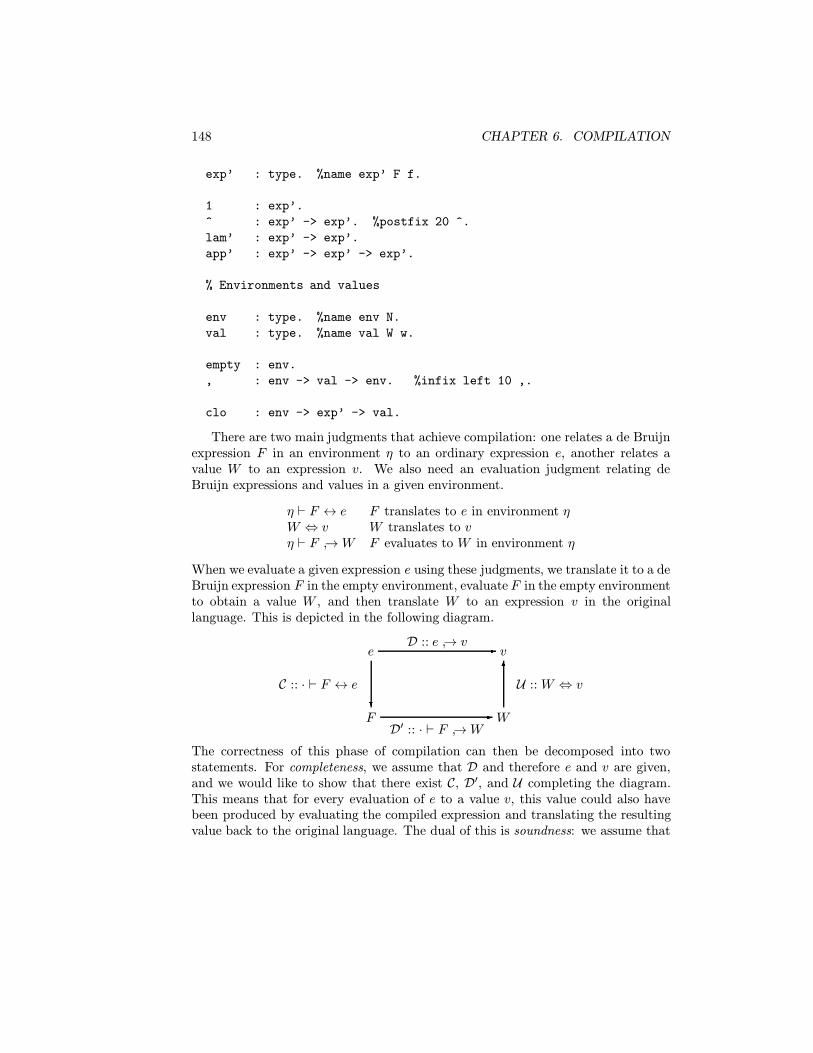
148 CHAPTER 6. COMPILATION
exp’ : type. %name exp’ F f.
1 : exp’.
^ : exp’ -> exp’. %postfix 20 ^.
lam’ : exp’ -> exp’.
app’ : exp’ -> exp’ -> exp’.
% Environments and values
env : type. %name env N.
val : type. %name val W w.
empty : env.
, : env -> val -> env. %infix left 10 ,.
clo : env -> exp’ -> val.
There are two main judgments that achieve compilation: one relates a de Bruijnexpression F in an environment η to an ordinary expression e, another relates avalue W to an expression v. We also need an evaluation judgment relating deBruijn expressions and values in a given environment.
η ` F ↔ e F translates to e in environment ηW ⇔ v W translates to vη ` F ↪→W F evaluates to W in environment η
When we evaluate a given expression e using these judgments, we translate it to a deBruijn expression F in the empty environment, evaluate F in the empty environmentto obtain a value W , and then translate W to an expression v in the originallanguage. This is depicted in the following diagram.
e
F W
v
?
C :: · ` F ↔ e
-
D′ :: · ` F ↪→W
6
U :: W ⇔ v
-
D :: e ↪→ v
The correctness of this phase of compilation can then be decomposed into twostatements. For completeness, we assume that D and therefore e and v are given,and we would like to show that there exist C, D′, and U completing the diagram.This means that for every evaluation of e to a value v, this value could also havebeen produced by evaluating the compiled expression and translating the resultingvalue back to the original language. The dual of this is soundness: we assume that

6.1. AN ENVIRONMENT MODEL FOR EVALUATION 149
C, D′ and U are given and we have to show that an evaluation D exists. Thatis, every value which can be produced by compilation and evaluation of compiledexpressions can also be produced by direct evaluation.
We will continue to restrict ourselves to expressions built up only from ab-straction and application. When we generalize this later only the case of fixpointexpressions will introduce an essential complication. First we define evaluation ofde Bruijn expressions in an environment η, written as η ` F ↪→ W . The vari-able 1 refers to the first value in the environment (counting from right to left); itsevaluation just returns that value.
fev 1η,W ` 1 ↪→W
The meaning of an expression F↑ in an environment η,W is the same as the meaningof F in the environment η. Intuitively, the environment references from F into ηare shifted by one. The typical case is one where a reference to the nth value in ηis represented by the expression 1↑ · · · ↑, where the shift operator is applied n − 1times.
η ` F ↪→Wfev ↑
η,W ′ ` F↑ ↪→W
A functional abstraction usually immediately evaluates to itself. Here this is in-sufficient, since an expression ΛF may contain references to the environment η.Thus we need to combine the environment η with ΛF to produce a closed (andself-contained) value.
fev lamη ` ΛF ↪→ {η; ΛF}
In order to evaluate F1 F2 in an environment η we evaluate both F1 and F2 in thatenvironment, yielding the closure {η′; ΛF ′1} and value W2, respectively. We thenadd W2 to the environment η′, in effect binding the variable previously bound byΛ in ΛF ′1 to W2 and then evaluate F ′1 in the extended environment to obtain theoverall value W .
η ` F1 ↪→ {η′; ΛF ′1} η ` F2 ↪→W2 η′,W2 ` F ′1 ↪→Wfev app
η ` F1 F2 ↪→W
Here is the implementation of this judgment as the type family feval in Elf.
feval : env -> exp’ -> val -> type. %name feval D’.
%mode feval +N +F -W.
% Variables
fev_1 : feval (N , W) 1 W.
fev_^ : feval (N , W’) (F ^) W

150 CHAPTER 6. COMPILATION
<- feval N F W.
% Functions
fev_lam : feval N (lam’ F) (clo N (lam’ F)).
fev_app : feval N (app’ F1 F2) W
<- feval N F1 (clo N’ (lam’ F1’))
<- feval N F2 W2
<- feval (N’ , W2) F1’ W.
We have written this signature in a way that emphasizes its operational reading,because it serves as an implementation of an interpreter. As an example, considerthe evaluation of the expression (Λ (Λ (1↑))) (Λ 1), which is a representation of(lam x. lam y. x) (lam v. v).
?- D : feval empty (app’ (lam’ (lam’ (1 ^))) (lam’ 1)) W.
W = clo (empty , clo empty (lam’ 1)) (lam’ (1 ^)).
D’ = fev_app fev_lam fev_lam fev_lam.
The resulting closure, {(·, {·,Λ1}); Λ(1↑)}, represents the de Bruijn expressionsΛ(Λ1), since (1↑) refers to the first value in the environment.
The translation between ordinary and de Bruijn expressions is specified by thefollowing rules which employ a parametric and hypothetical judgment.
η ` F1 ↔ e1 η ` F2 ↔ e2tr app
η ` F1 F2 ↔ e1 e2
uw⇔ x
...η, w ` F ↔ e
tr lamw,x,u
η ` ΛF ↔ lam x. e
W ⇔ etr 1
η,W ` 1↔ e
η ` F ↔ etr ↑
η,W ` F↑ ↔ e
where the rule tr lam is restricted to the case where w and x are new parametersnot free in any other hypothesis, and u is a new label. The translation of values isdefined by a single rule in this language fragment.
η ` ΛF ↔ lam x. evtr lam
{η; ΛF} ⇔ lam x. e
As remarked earlier this translation can be non-deterministic if η and e are givenand F is to be generated. This is the direction in which this judgment would beused for compilation. Here is an example of a translation.

6.1. AN ENVIRONMENT MODEL FOR EVALUATION 151
uw ⇔ x
tr 1·, w ` 1↔ x
tr ↑·, w, w′ ` 1↑ ↔ x
tr lamw,′,y,u′
·, w ` Λ1↑ ↔ lam y. xtr lamw,x,u
· ` ΛΛ1↑ ↔ lam x. lam y. x
u′′w′′ ⇔ v
tr 1·, w′′ ` 1↔ v
tr lamw′′,v,u′′
· ` Λ1↔ lam v. vtr app
· ` (ΛΛ1↑) (Λ1)↔ (lam x. lam y. x) (lam v. v)
The representation of the translation judgment relies on the standard techniquefor representing deductions of hypothetical judgments as functions.
trans : env -> exp’ -> exp -> type. %name trans C.
vtrans : val -> exp -> type. %name vtrans U.
% can be used in different directions
%mode trans +N +F -E.
%mode vtrans +W -V.
% Functions
tr_lam : trans N (lam’ F) (lam E)
<- ({w:val} {x:exp}
vtrans w x -> trans (N , w) F (E x)).
tr_app : trans N (app’ F1 F2) (app E1 E2)
<- trans N F1 E1
<- trans N F2 E2.
% Variables
tr_1 : trans (N , W) 1 E
<- vtrans W E.
tr_^ : trans (N , W) (F ^) E
<- trans N F E.
% Values
vtr_lam : vtrans (clo N (lam’ F)) (lam E)
<- trans N (lam’ F) (lam E).
The judgmentu
w⇔ x...
η, w ` F ↔ e

152 CHAPTER 6. COMPILATION
in the premiss of the tr lam is parametric in the variables w and x and hypotheticalin u. It is represented by a function which, when given a value W ′, an expressione′, and a deduction U ′ :: W ′ ⇔ e′ returns a deduction D′ :: η,W ′ ` F ↔ [e′/x]e.This property is crucial in the proof of compiler correctness.
The signature above can be executed as a non-deterministic program for trans-lation between de Bruijn and ordinary expressions in both directions. For thecompilation of expressions it is important to keep the clauses tr_1 and tr_^ in thegiven order so as to avoid unnecessary backtracking. This non-determinism arises,since the expression E in the rules tr_1 and tr_^ does not change in the recursivecalls. For other possible implementations see Exercise 6.3. Here is an executionwhich yields the example deduction above.
?- C : trans empty F (app (lam [x] lam [y] x) (lam [z] z)).
F = app’ (lam’ (lam’ (1 ^))) (lam’ 1).
C =
tr_app (tr_lam ([w:val] [x:exp] [u3:vtrans w x] tr_1 u3))
(tr_lam
([w:val] [x:exp] [u1:vtrans w x]
tr_lam ([w1:val] [x1:exp] [u2:vtrans w1 x1]
tr_^ (tr_1 u1)))).
It is not immediately obvious that every source expression e can in fact becompiled using this judgment. This is the subject of the following theorem.
Theorem 6.1 For every closed expression e there exists a de Bruijn expression Fsuch that · ` F ↔ e.
Proof: A direct attempt at an induction argument fails—a typical situation whenproving properties of judgments which involve hypothetical reasoning. However,the theorem follows immediately from Lemma 6.2 below. 2
Lemma 6.2 Let w1, . . . , wn be parameters ranging over values and let η be theenvironment ·, wn, . . . , w1. Furthermore, let x1, . . . , xn range over expression vari-ables. For any expression e with free variables among x1, . . . , xn there exists a deBruijn expression F and a deduction C of η ` F ↔ e from hypotheses u1 :: w1 ⇔x1, . . . , un :: wn ⇔ xn.
Proof: By induction on the structure of e.
Case: e = e1 e2. By induction hypothesis on e1 and e2, there exist F1 and F2 anddeductions C1 :: η ` F1 ↔ e1 and C2 :: η ` F2 ↔ e2. Applying the rule tr appto C1 and C2 yields the desired deduction C :: η ` F1 F2 ↔ e1 e2.

6.1. AN ENVIRONMENT MODEL FOR EVALUATION 153
Case: e = lam x. e1. Here we apply the induction hypothesis to the expressione1, environment η, w for a new parameter w, and hypotheses u1 :: w1 ⇔x1, . . . , un :: wn ⇔ xn, u :: w ⇔ x to obtain an F1 and a deduction
uw ⇔ xC1
η, w ` F1 ↔ e1
possibly also using hypotheses labelled u1, . . . , un. Note that e1 is an ex-pression with free variables among x1, . . . , xn, x. Applying the rule tr lamdischarges the hypothesis u and we obtain the desired deduction
C =
uw ⇔ xC1
η, w ` F1 ↔ e1
tr lamu
η ` ΛF1 ↔ lam x. e1
Case: e = x. Then x = xi for some i between 1 and n and we let F = 1 ↑ · · · ↑︸ ︷︷ ︸i−1 times
and
C =
uiwi ⇔ xi
tr 1·, wn, . . . , wi ` 1↔ xi
tr ↑· · ·
tr ↑·, wn, . . . , w1 ` 1↑ · · · ↑ ↔ xi
2
This proof cannot be represented directly in Elf because we cannot employ theusual technique for representing hypothetical judgments as functions. The difficultyis that the order of the hypotheses is important for returning the correct variable1↑ · · · ↑, but hypothetical judgments are generally invariant under reordering of hy-potheses. Hannan [Han91] has suggested a different, deterministic translation forwhich termination is relatively easy to show, but which complicates the proofs of theremaining properties of compiler correctness. Thus our formalization does not cap-ture the desirable property that compilation always terminates. All the remainingparts, however, are implemented. The first property states that translation followedby evaluation leads to the same result as evaluation followed by translation. Wegeneralize this for arbitrary environments η in order to allow a proof by induction.

154 CHAPTER 6. COMPILATION
This property is depicted in the following diagram.
e
η;F W
v
?
C :: η ` F ↔ e
-
D :: e ↪→ v
. . . . . . . . . . . . . . . . . . .-D′ :: η ` F ↪→W
..
..
..
..6U :: W ⇔ v
The solid lines indicate deductions that are assumed, dotted lines represent thedeductions whose existence we assert and prove below.
Lemma 6.3 For any closed expressions e and v, environment η, de Bruijn expres-sion F , deductions D :: e ↪→ v and C :: η ` F ↔ e, there exist a value W anddeductions D′ :: η ` F ↪→W and U :: W ⇔ v.
Proof: By induction on the structures of D :: e ↪→ v and C :: η ` F ↔ e. Inthis induction we assume the induction hypothesis on the premisses of D and forarbitrary C and on the premisses of C, but for the same D. This is sometimes calledlexicographic induction on the pair consisting of D and C. It should be intuitivelyclear that this form of induction is valid. We represent this proof as a judgmentrelating the four deductions involved in the diagram.
map_eval : eval E V -> trans N F E
-> feval N F W -> vtrans W V -> type.
%mode map_eval +D +C -D’ -U.
Case: C ends in an application of the tr 1 rule.
C =
U1
W1 ⇔ etr 1
η1,W1 ` 1↔ e
D :: e ↪→ v AssumptionC1 :: η′1 ` ΛF ′1 ↔ e and W1 = {η′1; ΛF ′1} By inversion on U1
e = lam x. e1 By inversion on C1v = lam x. e1 = e By inversion on D
Then W = W1, U = U1 :: W1 ⇔ e and D′ = fev 1 :: η1,W1 ` 1 ↪→ W1 satisfythe requirements of the theorem. This case is captured in the clause
mp_1 : map_eval (ev_lam) (tr_1 (vtr_lam (tr_lam C2)))
(fev_1) (vtr_lam (tr_lam C2)).
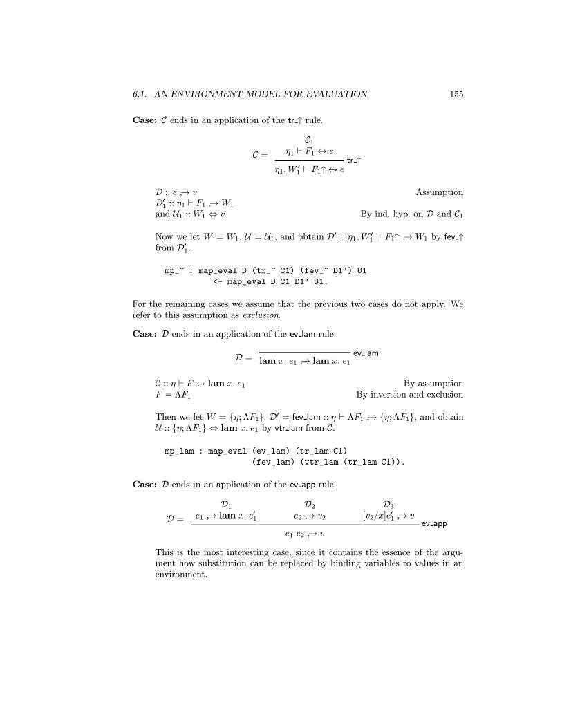
6.1. AN ENVIRONMENT MODEL FOR EVALUATION 155
Case: C ends in an application of the tr ↑ rule.
C =
C1η1 ` F1 ↔ e
tr ↑η1,W
′1 ` F1↑ ↔ e
D :: e ↪→ v AssumptionD′1 :: η1 ` F1 ↪→W1
and U1 :: W1 ⇔ v By ind. hyp. on D and C1
Now we let W = W1, U = U1, and obtain D′ :: η1,W′1 ` F1↑ ↪→ W1 by fev ↑
from D′1.
mp_^ : map_eval D (tr_^ C1) (fev_^ D1’) U1
<- map_eval D C1 D1’ U1.
For the remaining cases we assume that the previous two cases do not apply. Werefer to this assumption as exclusion.
Case: D ends in an application of the ev lam rule.
D = ev lamlam x. e1 ↪→ lam x. e1
C :: η ` F ↔ lam x. e1 By assumptionF = ΛF1 By inversion and exclusion
Then we let W = {η; ΛF1}, D′ = fev lam :: η ` ΛF1 ↪→ {η; ΛF1}, and obtainU :: {η; ΛF1} ⇔ lam x. e1 by vtr lam from C.
mp_lam : map_eval (ev_lam) (tr_lam C1)
(fev_lam) (vtr_lam (tr_lam C1)).
Case: D ends in an application of the ev app rule.
D =
D1
e1 ↪→ lam x. e′1
D2
e2 ↪→ v2
D3
[v2/x]e′1 ↪→ vev app
e1 e2 ↪→ v
This is the most interesting case, since it contains the essence of the argu-ment how substitution can be replaced by binding variables to values in anenvironment.
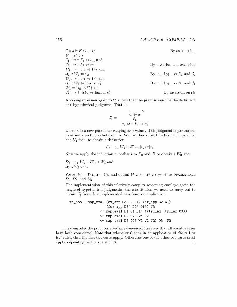
156 CHAPTER 6. COMPILATION
C :: η ` F ↔ e1 e2 By assumptionF = F1 F2,C1 :: η ` F1 ↔ e1, andC2 :: η ` F2 ↔ e2 By inversion and exclusionD′2 :: η ` F2 ↪→W2 andU2 :: W2 ⇔ v2 By ind. hyp. on D2 and C2D′1 :: η ` F1 ↪→W1 andU1 :: W1 ⇔ lam x. e′1 By ind. hyp. on D1 and C1W1 = {η1; ΛF ′1} andC′1 :: η1 ` ΛF ′1 ↔ lam x. e′1 By inversion on U1
Applying inversion again to C′1 shows that the premiss must be the deductionof a hypothetical judgment. That is,
C′1 =
uw ⇔ xC3
η1, w ` F ′1 ↔ e′1
where w is a new parameter ranging over values. This judgment is parametricin w and x and hypothetical in u. We can thus substitute W2 for w, v2 for x,and U2 for u to obtain a deduction
C′3 :: η1,W2 ` F ′1 ↔ [v2/x]e′1.
Now we apply the induction hypothesis to D3 and C′3 to obtain a W3 and
D′3 :: η1,W2 ` F ′1 ↪→W3 andU3 :: W3 ⇔ v.
We let W = W3, U = U3, and obtain D′ :: η ` F1 F2 ↪→ W by fev app fromD′1, D′2, and D′3.
The implementation of this relatively complex reasoning employs again themagic of hypothetical judgments: the substitution we need to carry out toobtain C′3 from C3 is implemented as a function application.
mp_app : map_eval (ev_app D3 D2 D1) (tr_app C2 C1)
(fev_app D3’ D2’ D1’) U3
<- map_eval D1 C1 D1’ (vtr_lam (tr_lam C3))
<- map_eval D2 C2 D2’ U2
<- map_eval D3 (C3 W2 V2 U2) D3’ U3.
This completes the proof once we have convinced ourselves that all possible caseshave been considered. Note that whenever C ends in an application of the tr 1 ortr ↑ rules, then the first two cases apply. Otherwise one of the other two cases mustapply, depending on the shape of D. 2
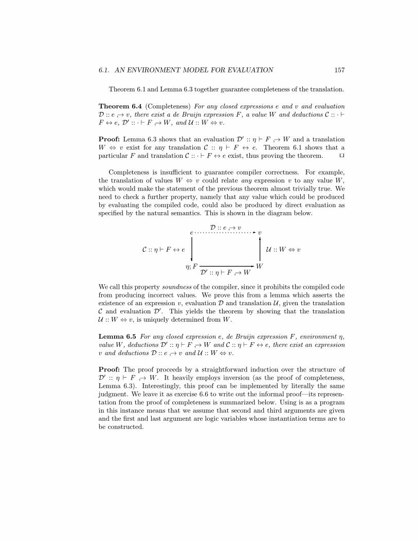
6.1. AN ENVIRONMENT MODEL FOR EVALUATION 157
Theorem 6.1 and Lemma 6.3 together guarantee completeness of the translation.
Theorem 6.4 (Completeness) For any closed expressions e and v and evaluationD :: e ↪→ v, there exist a de Bruijn expression F , a value W and deductions C :: · `F ↔ e, D′ :: · ` F ↪→W , and U :: W ⇔ v.
Proof: Lemma 6.3 shows that an evaluation D′ :: η ` F ↪→ W and a translationW ⇔ v exist for any translation C :: η ` F ↔ e. Theorem 6.1 shows that aparticular F and translation C :: · ` F ↔ e exist, thus proving the theorem. 2
Completeness is insufficient to guarantee compiler correctness. For example,the translation of values W ⇔ v could relate any expression v to any value W ,which would make the statement of the previous theorem almost trivially true. Weneed to check a further property, namely that any value which could be producedby evaluating the compiled code, could also be produced by direct evaluation asspecified by the natural semantics. This is shown in the diagram below.
e
η;F W
v
?
C :: η ` F ↔ e
-
D′ :: η ` F ↪→W
6
U :: W ⇔ v
. . . . . . . . . . . . . . . . . . . . . .-D :: e ↪→ v
We call this property soundness of the compiler, since it prohibits the compiled codefrom producing incorrect values. We prove this from a lemma which asserts theexistence of an expression v, evaluation D and translation U , given the translationC and evaluation D′. This yields the theorem by showing that the translationU :: W ⇔ v, is uniquely determined from W .
Lemma 6.5 For any closed expression e, de Bruijn expression F , environment η,value W , deductions D′ :: η ` F ↪→W and C :: η ` F ↔ e, there exist an expressionv and deductions D :: e ↪→ v and U :: W ⇔ v.
Proof: The proof proceeds by a straightforward induction over the structure ofD′ :: η ` F ↪→ W . It heavily employs inversion (as the proof of completeness,Lemma 6.3). Interestingly, this proof can be implemented by literally the samejudgment. We leave it as exercise 6.6 to write out the informal proof—its represen-tation from the proof of completeness is summarized below. Using is as a programin this instance means that we assume that second and third arguments are givenand the first and last argument are logic variables whose instantiation terms are tobe constructed.
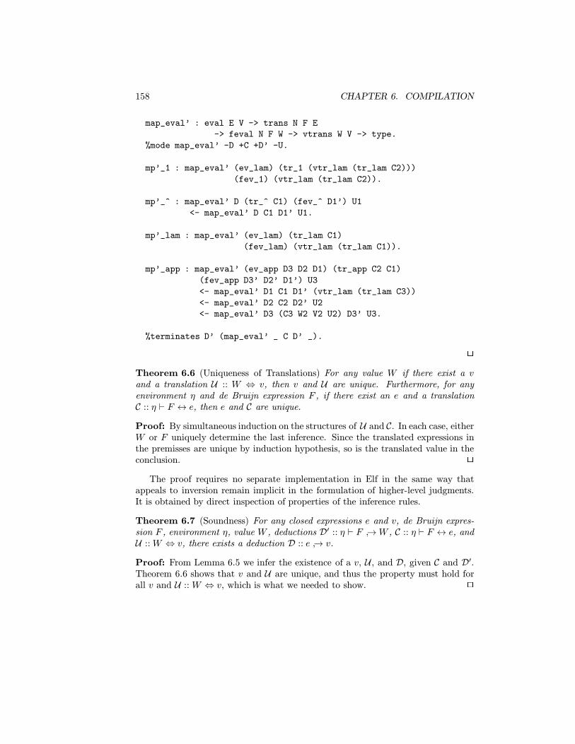
158 CHAPTER 6. COMPILATION
map_eval’ : eval E V -> trans N F E
-> feval N F W -> vtrans W V -> type.
%mode map_eval’ -D +C +D’ -U.
mp’_1 : map_eval’ (ev_lam) (tr_1 (vtr_lam (tr_lam C2)))
(fev_1) (vtr_lam (tr_lam C2)).
mp’_^ : map_eval’ D (tr_^ C1) (fev_^ D1’) U1
<- map_eval’ D C1 D1’ U1.
mp’_lam : map_eval’ (ev_lam) (tr_lam C1)
(fev_lam) (vtr_lam (tr_lam C1)).
mp’_app : map_eval’ (ev_app D3 D2 D1) (tr_app C2 C1)
(fev_app D3’ D2’ D1’) U3
<- map_eval’ D1 C1 D1’ (vtr_lam (tr_lam C3))
<- map_eval’ D2 C2 D2’ U2
<- map_eval’ D3 (C3 W2 V2 U2) D3’ U3.
%terminates D’ (map_eval’ _ C D’ _).
2
Theorem 6.6 (Uniqueness of Translations) For any value W if there exist a vand a translation U :: W ⇔ v, then v and U are unique. Furthermore, for anyenvironment η and de Bruijn expression F , if there exist an e and a translationC :: η ` F ↔ e, then e and C are unique.
Proof: By simultaneous induction on the structures of U and C. In each case, eitherW or F uniquely determine the last inference. Since the translated expressions inthe premisses are unique by induction hypothesis, so is the translated value in theconclusion. 2
The proof requires no separate implementation in Elf in the same way thatappeals to inversion remain implicit in the formulation of higher-level judgments.It is obtained by direct inspection of properties of the inference rules.
Theorem 6.7 (Soundness) For any closed expressions e and v, de Bruijn expres-sion F , environment η, value W , deductions D′ :: η ` F ↪→W , C :: η ` F ↔ e, andU :: W ⇔ v, there exists a deduction D :: e ↪→ v.
Proof: From Lemma 6.5 we infer the existence of a v, U , and D, given C and D′.Theorem 6.6 shows that v and U are unique, and thus the property must hold forall v and U :: W ⇔ v, which is what we needed to show. 2

6.2. ADDING DATA VALUES AND RECURSION 159
6.2 Adding Data Values and Recursion
In the previous section we treated only a very restricted core language of Mini-ML. In this section we will extend the compiler to the full Mini-ML language aspresented in Chapter 2. The main additions to the core language which affect thecompiler are data values (such as natural numbers and pairs) and recursion. Thelanguage of de Bruijn expressions is extended by allowing constructors that parallelordinary expressions. We maintain a similar syntax, but mark de Bruijn expressionconstructors with a prime (′).
Expressions F ::= | z′ | s′ F | case′ F1 F2 F3 Natural Numbers| 〈F1, F2〉′ | fst′ F | snd′ F Pairs| ΛF | F1 F2 Functions| let′ val F1 in F2 Definitions| let′ name F1 in F2
| fix′ F Recursion| 1 | F↑ Variables
Expressions of the form F↑ are not necessarily variables (where F is a sequence ofshifts applied to 1), but it may be intuitively helpful to think of them that way.In the representation we need only first-order constants, since this language has noconstructs binding variables by name.
exp’ : type. %name exp’ F f.
1 : exp’.
^ : exp’ -> exp’. %postfix 20 ^.
z’ : exp’.
s’ : exp’ -> exp’.
case’ : exp’ -> exp’ -> exp’ -> exp’.
pair’ : exp’ -> exp’ -> exp’.
fst’ : exp’ -> exp’.
snd’ : exp’ -> exp’.
lam’ : exp’ -> exp’.
app’ : exp’ -> exp’ -> exp’.
letv’ : exp’ -> exp’ -> exp’.
letn’ : exp’ -> exp’ -> exp’.
fix’ : exp’ -> exp’.
Next we need to extend the language of values. While data values can beadded in a straightforward fashion, let name and recursion present some difficulties.Consider the evaluation rule for fixpoints.
[fix x. e/x]e ↪→ vev fix
fix x. e ↪→ v

160 CHAPTER 6. COMPILATION
We introduced the environment model of evaluation in order to eliminate the needfor explicit substitution, where an environment is a list of values. In the case of thefixpoint construction we would need to bind the variable x to the expression fix x. ein the environment in order to avoid substutition, but fix x. e is not a value. Theevaluation rules for de Bruijn expressions take advantage of the invariant that anenvironment contains only values. In particular, the rule
fev 1η,W ` 1 ↪→W
requires that an environment contain only values. We will thus need to add anew environment constructor η+F in order to allow unevaluated expressions in theenvironment. These considerations yield the following mutually recursive definitionsof environments and values. We mark data values with a star (∗) to distinguish themfrom expressions and de Bruijn expressions with the same name.
Environments η ::= · | η,W | η + FValues W ::= | z∗ | s∗ W Natural Numbers
| 〈W1,W2〉∗ Pairs| {η;F} Closures
The Elf representation is direct.
env : type. %name env N.
val : type. %name val W w.
empty : env.
, : env -> val -> env. %infix left 10 ,.
+ : env -> exp’ -> env. %infix left 10 +.
z* : val.
s* : val -> val.
pair* : val -> val -> val.
clo : env -> exp’ -> val.
In the extension of the evaluation rule to this completed language, we mustexercise care in the treatment of the new environment constructor for unevaluatedexpression: when such an expression is looked up in the environment, it must beevaluated.
η ` F ↪→Wfev 1+
η + F ` 1 ↪→W
η ` F ↪→Wfev ↑+
η + F ′ ` F↑ ↪→W

6.2. ADDING DATA VALUES AND RECURSION 161
The rules involving data values generally follow the patterns established in thenatural semantics for ordinary expressions. The main departure from the earlierformulation is the separation of values from expressions. We show only four of therelevant rules.
fev zη ` z′ ↪→ z∗
η ` F ↪→Wfev s
η ` s′ F ↪→ s∗ W
η ` F1 ↪→ z∗ η ` F2 ↪→Wfev case z
η ` case′ F1 F2 F3 ↪→W
η ` F1 ↪→ s∗ W ′1 η,W ′1 ` F3 ↪→Wfev case s
η ` case′ F1 F2 F3 ↪→W
Evaluating a let val-expression also binds a variable to value by extending theenvironment.
η ` F1 ↪→W1 η,W1 ` F2 ↪→Wfev letv
η ` let val′ F1 in F2 ↪→W
Evaluating a let name-expression binds a variable to an expression and thus re-quires the new environment constructor.
η + F1 ` F2 ↪→Wfev letn
η ` letname′ F1 in F2 ↪→W
Fixpoint expressions are similar, except that the variable is bound to the fix ex-pression itself.
η + fix′ F ` F ↪→Wfev fix
η ` fix′ F ↪→W
For example, fix x. x (considered on page 17) is represented by fix′ 1. Intuitively,evaluation of this expression should not terminate. An attempt to construct anevaluation leads to the sequence
...fev fix
· ` fix′ 1 ↪→Wfev 1+
·+fix′ 1 ` 1 ↪→Wfev fix.
· ` fix′ 1 ↪→W
The implementation of these rules in Elf poses no particular difficulties. Weshow only the rules from above.
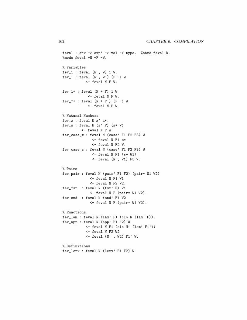
162 CHAPTER 6. COMPILATION
feval : env -> exp’ -> val -> type. %name feval D.
%mode feval +N +F -W.
% Variables
fev_1 : feval (N , W) 1 W.
fev_^ : feval (N , W’) (F ^) W
<- feval N F W.
fev_1+ : feval (N + F) 1 W
<- feval N F W.
fev_^+ : feval (N + F’) (F ^) W
<- feval N F W.
% Natural Numbers
fev_z : feval N z’ z*.
fev_s : feval N (s’ F) (s* W)
<- feval N F W.
fev_case_z : feval N (case’ F1 F2 F3) W
<- feval N F1 z*
<- feval N F2 W.
fev_case_s : feval N (case’ F1 F2 F3) W
<- feval N F1 (s* W1)
<- feval (N , W1) F3 W.
% Pairs
fev_pair : feval N (pair’ F1 F2) (pair* W1 W2)
<- feval N F1 W1
<- feval N F2 W2.
fev_fst : feval N (fst’ F) W1
<- feval N F (pair* W1 W2).
fev_snd : feval N (snd’ F) W2
<- feval N F (pair* W1 W2).
% Functions
fev_lam : feval N (lam’ F) (clo N (lam’ F)).
fev_app : feval N (app’ F1 F2) W
<- feval N F1 (clo N’ (lam’ F1’))
<- feval N F2 W2
<- feval (N’ , W2) F1’ W.
% Definitions
fev_letv : feval N (letv’ F1 F2) W

6.2. ADDING DATA VALUES AND RECURSION 163
<- feval N F1 W1
<- feval (N , W1) F2 W.
fev_letn : feval N (letn’ F1 F2) W
<- feval (N + F1) F2 W.
% Recursion
fev_fix : feval N (fix’ F) W
<- feval (N + (fix’ F)) F W.
Next we need to extend the translation between expressions and de Bruijn ex-pressions and values. We show a few interesting cases in the extended judgmentsη ` F ↔ e and W ⇔ v. The case for let val is handled just like the case for lam,since we will always substitute a value for the variable bound by the let duringexecution.
tr zη ` z′ ↔ z
η ` F ↔ etr s
η ` s′ F ↔ s e
η ` F1 ↔ e1
uw⇔ x
...η, w ` F2 ↔ e2
tr letvw,x,u
η ` let val′ F1 in F2 ↔ let x = e1 in e2
where the right premiss of tr let is parametric in w and x and hypothetical in u.In order to preserve the basic structure of the proofs of lemmas 6.3 and 6.5, wemust treat the let name and fix constructs somewhat differently: we extend theenvironment with an expression parameter (not a value parameter) using the new
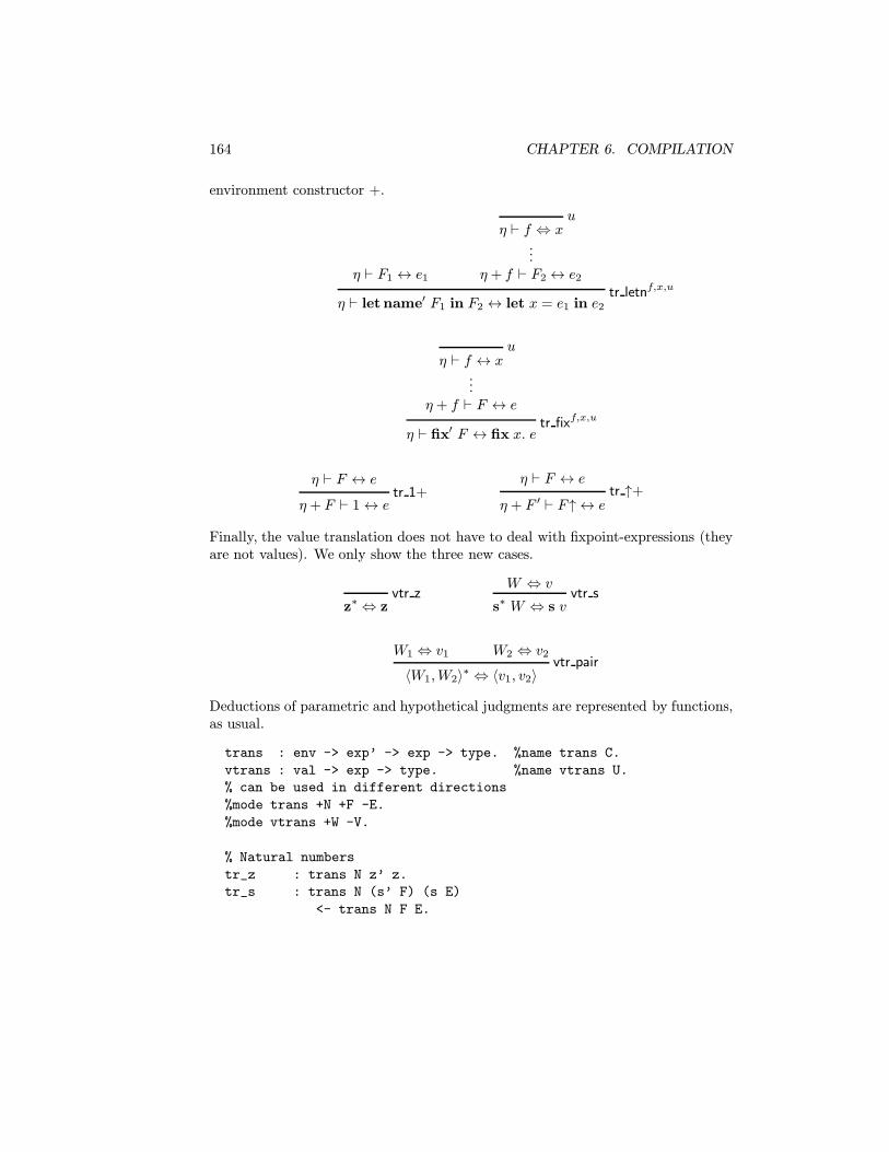
164 CHAPTER 6. COMPILATION
environment constructor +.
η ` F1 ↔ e1
uη ` f ⇔ x
...η + f ` F2↔ e2
tr letnf,x,uη ` let name′ F1 in F2 ↔ let x = e1 in e2
uη ` f ↔ x
...η + f ` F ↔ e
tr fixf,x,uη ` fix′ F ↔ fix x. e
η ` F ↔ etr 1+
η + F ` 1↔ e
η ` F ↔ etr ↑+
η + F ′ ` F↑ ↔ e
Finally, the value translation does not have to deal with fixpoint-expressions (theyare not values). We only show the three new cases.
vtr zz∗ ⇔ z
W ⇔ vvtr s
s∗ W ⇔ s v
W1 ⇔ v1 W2 ⇔ v2vtr pair
〈W1,W2〉∗ ⇔ 〈v1, v2〉
Deductions of parametric and hypothetical judgments are represented by functions,as usual.
trans : env -> exp’ -> exp -> type. %name trans C.
vtrans : val -> exp -> type. %name vtrans U.
% can be used in different directions
%mode trans +N +F -E.
%mode vtrans +W -V.
% Natural numbers
tr_z : trans N z’ z.
tr_s : trans N (s’ F) (s E)
<- trans N F E.

6.2. ADDING DATA VALUES AND RECURSION 165
tr_case : trans N (case’ F1 F2 F3) (case E1 E2 E3)
<- trans N F1 E1
<- trans N F2 E2
<- ({w:val} {x:exp}
vtrans w x -> trans (N , w) F3 (E3 x)).
% Pairs
tr_pair : trans N (pair’ F1 F2) (pair E1 E2)
<- trans N F1 E1
<- trans N F2 E2.
tr_fst : trans N (fst’ F1) (fst E1)
<- trans N F1 E1.
tr_snd : trans N (snd’ F1) (snd E1)
<- trans N F1 E1.
% Functions
tr_lam : trans N (lam’ F) (lam E)
<- ({w:val} {x:exp}
vtrans w x -> trans (N , w) F (E x)).
tr_app : trans N (app’ F1 F2) (app E1 E2)
<- trans N F1 E1
<- trans N F2 E2.
% Definitions
tr_letv: trans N (letv’ F1 F2) (letv E1 E2)
<- trans N F1 E1
<- ({w:val} {x:exp}
vtrans w x -> trans (N , w) F2 (E2 x)).
tr_letn: trans N (letn’ F1 F2) (letn E1 E2)
<- trans N F1 E1
<- ({f:exp’} {x:exp}
trans N f x -> trans (N + f) F2 (E2 x)).
% Recursion
tr_fix : trans N (fix’ F) (fix E)
<- ({f:exp’} {x:exp}
trans N f x -> trans (N + f) F (E x)).
% Variables
tr_1 : trans (N , W) 1 E <- vtrans W E.
tr_^ : trans (N , W) (F ^) E <- trans N F E.

166 CHAPTER 6. COMPILATION
tr_1+ : trans (N + F) 1 E <- trans N F E.
tr_^+ : trans (N + F’) (F ^) E <- trans N F E.
% Natural number values
vtr_z : vtrans z* z.
vtr_s : vtrans (s* W) (s V)
<- vtrans W V.
% Pair values
vtr_pair : vtrans (pair* W1 W2) (pair V1 V2)
<- vtrans W1 V1
<- vtrans W2 V2.
% Function values
vtr_lam : vtrans (clo N (lam’ F)) (lam E)
<- trans N (lam’ F) (lam E).
In order to extend the proof of compiler correctness in Section 6.1 we need toextend various lemmas.
Theorem 6.8 For every closed expression e there exists a de Bruijn expression Fsuch that · ` F ↔ e.
Proof: We generalize analogously to Lemma 6.2 and prove the modified lemma byinduction on the structure of e (see Exercise 6.7). 2
Lemma 6.9 If W ⇔ e is derivable, then e Value is derivable.
Proof: By a straightforward induction on the structure of U :: W ⇔ e. 2
Lemma 6.10 If e Value and e ↪→ v are derivable then e = v.
Proof: By a straightforward induction on the structure of P :: e Value. 2
The Elf implementations of the proofs of Lemmas 6.9 and 6.10 is straightforwardand can be found in the on-line material that accompanies these notes. The typefamilies are
vtrans_val : vtrans W E -> value E -> type.
%mode vtrans_val +U -P.
val_eval : value E -> eval E E -> type.
%mode val_eval +P -D.

6.2. ADDING DATA VALUES AND RECURSION 167
The next lemma is the main lemma is the proof of completeness, that is, everyvalue which can obtained by direct evaluation can also be obtained by compilation,evaluation of the compiled code, and translation of the returned value to the originallanguage.
Lemma 6.11 For any closed expressions e and v, environment η, de Bruijn ex-pression F , deduction D :: e ↪→ v and C :: η ` F ↔ e, there exist a value W anddeductions D′ :: η ` F ↪→W and U :: W ⇔ v.
Proof: By induction on the structure of D :: e ↪→ v and C :: η ` F ↔ e. In thisinduction, as in the proof of Lemma 6.3, we assume the induction hypothesis on thepremisses of D and for arbitrary C, and on the premisses of C if D remains fixed.The implementation is an extension of the previous higher-level judgment,
map_eval : eval E V -> trans N F E
-> feval N F W -> vtrans W V -> type.
%mode map_eval +D +C -D’ -U.
We show only some of the typical cases—the others are straightforward and left tothe reader or remain unchanged from the proof of Lemma 6.3
Case: C ends in an application of the tr 1 rule.
C =
U1
W1 ⇔ etr 1
η1,W1 ` 1↔ e
This case changes from the previous proof, since there we applied simpleinversion (there was only one possible kind of value) to conclude that e = v.Here we need two lemmas from above.
D :: e ↪→ v AssumptionP :: e Value By Lemma 6.9 from U1
e = v By Lemma 6.10 from P
Hence we can let W be W1, U be U1, and D′ be fev 1 :: η1,W1 ` 1 ↪→ W1.The implementation explicitly appeals to the implementations of the lemmas.
mp_1 : map_eval D (tr_1 U1) (fev_1) U1
<- vtrans_val U1 P
<- val_eval P D.
Case: C ends in an application of the tr ↑ rule. This case proceeds as before.
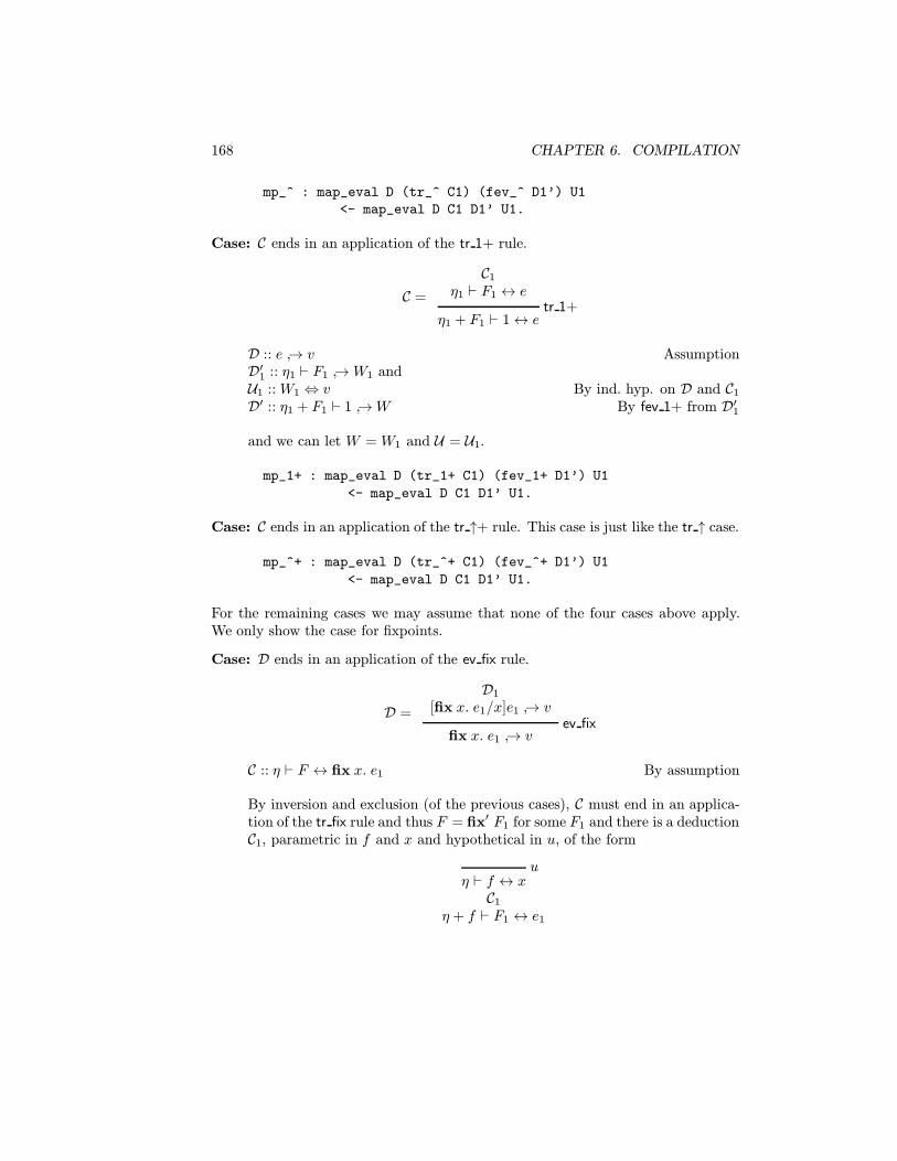
168 CHAPTER 6. COMPILATION
mp_^ : map_eval D (tr_^ C1) (fev_^ D1’) U1
<- map_eval D C1 D1’ U1.
Case: C ends in an application of the tr 1+ rule.
C =
C1η1 ` F1 ↔ e
tr 1+η1 + F1 ` 1↔ e
D :: e ↪→ v AssumptionD′1 :: η1 ` F1 ↪→W1 andU1 :: W1 ⇔ v By ind. hyp. on D and C1D′ :: η1 + F1 ` 1 ↪→W By fev 1+ from D′1
and we can let W = W1 and U = U1.
mp_1+ : map_eval D (tr_1+ C1) (fev_1+ D1’) U1
<- map_eval D C1 D1’ U1.
Case: C ends in an application of the tr ↑+ rule. This case is just like the tr ↑ case.
mp_^+ : map_eval D (tr_^+ C1) (fev_^+ D1’) U1
<- map_eval D C1 D1’ U1.
For the remaining cases we may assume that none of the four cases above apply.We only show the case for fixpoints.
Case: D ends in an application of the ev fix rule.
D =
D1
[fix x. e1/x]e1 ↪→ vev fix
fix x. e1 ↪→ v
C :: η ` F ↔ fix x. e1 By assumption
By inversion and exclusion (of the previous cases), C must end in an applica-tion of the tr fix rule and thus F = fix′ F1 for some F1 and there is a deductionC1, parametric in f and x and hypothetical in u, of the form
uη ` f ↔ xC1
η + f ` F1 ↔ e1
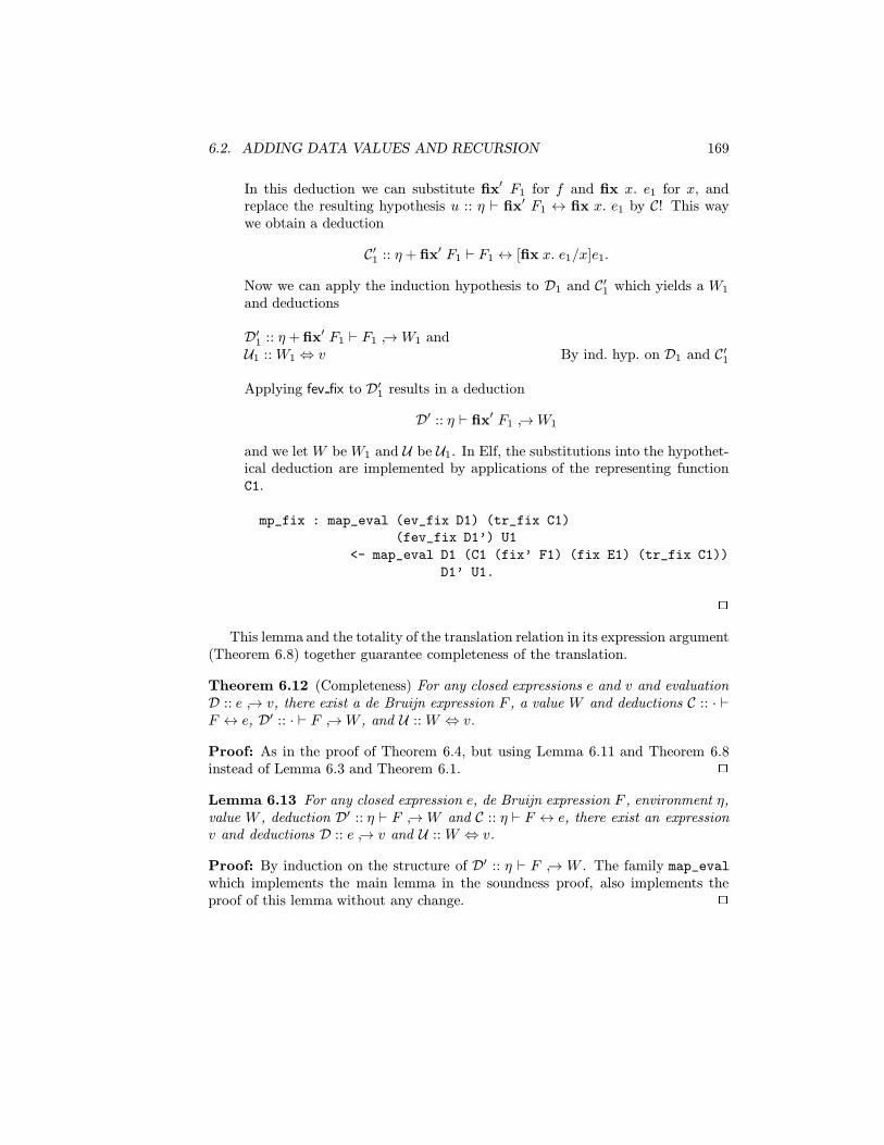
6.2. ADDING DATA VALUES AND RECURSION 169
In this deduction we can substitute fix′ F1 for f and fix x. e1 for x, andreplace the resulting hypothesis u :: η ` fix′ F1 ↔ fix x. e1 by C! This waywe obtain a deduction
C′1 :: η + fix′ F1 ` F1 ↔ [fix x. e1/x]e1.
Now we can apply the induction hypothesis to D1 and C′1 which yields a W1
and deductions
D′1 :: η + fix′ F1 ` F1 ↪→W1 andU1 :: W1 ⇔ v By ind. hyp. on D1 and C′1
Applying fev fix to D′1 results in a deduction
D′ :: η ` fix′ F1 ↪→W1
and we let W be W1 and U be U1. In Elf, the substitutions into the hypothet-ical deduction are implemented by applications of the representing functionC1.
mp_fix : map_eval (ev_fix D1) (tr_fix C1)
(fev_fix D1’) U1
<- map_eval D1 (C1 (fix’ F1) (fix E1) (tr_fix C1))
D1’ U1.
2
This lemma and the totality of the translation relation in its expression argument(Theorem 6.8) together guarantee completeness of the translation.
Theorem 6.12 (Completeness) For any closed expressions e and v and evaluationD :: e ↪→ v, there exist a de Bruijn expression F , a value W and deductions C :: · `F ↔ e, D′ :: · ` F ↪→W , and U :: W ⇔ v.
Proof: As in the proof of Theorem 6.4, but using Lemma 6.11 and Theorem 6.8instead of Lemma 6.3 and Theorem 6.1. 2
Lemma 6.13 For any closed expression e, de Bruijn expression F , environment η,value W , deduction D′ :: η ` F ↪→W and C :: η ` F ↔ e, there exist an expressionv and deductions D :: e ↪→ v and U :: W ⇔ v.
Proof: By induction on the structure of D′ :: η ` F ↪→ W . The family map_eval
which implements the main lemma in the soundness proof, also implements theproof of this lemma without any change. 2

170 CHAPTER 6. COMPILATION
Theorem 6.14 (Uniqueness of Translations) For any value W if there exist a vand a translation U :: W ⇔ v, then v and U are unique. Furthermore, for anyenvironment η and de Bruijn expression F , if there exist an e and a translationC :: η ` F ↔ e, then e and C are unique.
Proof: As before, by a simultaneous induction on the structures of U and C. 2
Theorem 6.15 (Soundness) For any closed expressions e and v, de Bruijn expres-sion F , environment η, value W , deductions D′ :: η ` F ↪→W , C :: η ` F ↔ e, andU :: W ⇔ v, there exists a deduction D :: e ↪→ v.
Proof: From Lemma 6.13 we infer the existence of a v, U , and D, given C and D′.Theorem 6.14 shows that v and U are unique, and thus the property must hold forall v and U :: W ⇔ v, which is what we needed to show. 2
6.3 Computations as Transition Sequences
So far, we have modelled evaluation as the construction of a deduction of the eval-uation judgment. This is true for evaluation based on substitution in Section 2.3and for evaluation based on environments in Section 6.1. In an abstract machine(and, of course, in an actual machine) a more natural model for computation is asequence of states. In this section we will develop the CLS machine, an abstractmachine similar in scope to the SECD machine [Lan64]. The CLS machine still in-terprets expressions, so the step from environment based evaluation to this abstractmachine does not involve any compilation. Instead, we flatten evaluation trees tosequences of states that describe the computation. This flattening involves somerather arbitrary decisions about which subcomputations should be performed first.We linearize the evaluation deductions beginning with the deduction of the leftmostpremiss.
Throughout the remainder of this chapter, we will drop the prime (′) from theexpression constructors. This should not lead to any confusion, since we no longerneed to refer to the original expressions. Now consider the rule for evaluating pairsas a simple example where an evaluation tree has two branches.
η ` F1 ↪→W1 η ` F2 ↪→W2fev pair
η ` 〈F1, F2〉 ↪→ 〈W1,W2〉∗
An abstract machine would presumably start in a state where it is given theenvironment η and the expression 〈F1, F2〉. The final state of the machine shouldsomehow indicate the final value 〈W1,W2〉∗. The computation naturally decomposesinto three phases: the first phase computes the value of F1 in environment η, thesecond phase computes the value of F2 in environment η, and the third phase
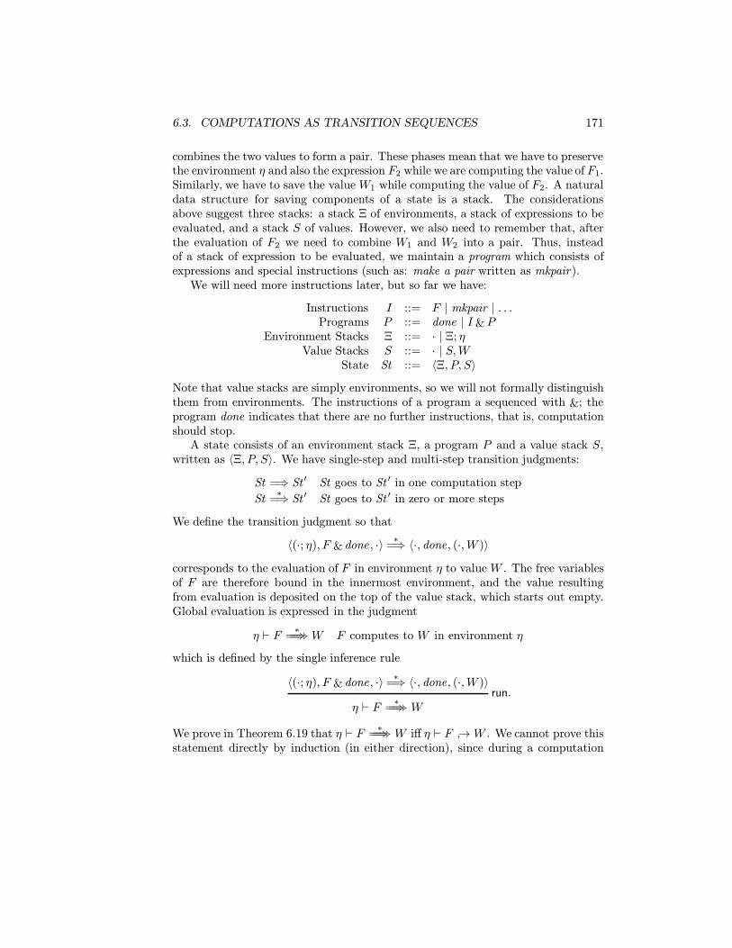
6.3. COMPUTATIONS AS TRANSITION SEQUENCES 171
combines the two values to form a pair. These phases mean that we have to preservethe environment η and also the expression F2 while we are computing the value of F1.Similarly, we have to save the value W1 while computing the value of F2. A naturaldata structure for saving components of a state is a stack. The considerationsabove suggest three stacks: a stack Ξ of environments, a stack of expressions to beevaluated, and a stack S of values. However, we also need to remember that, afterthe evaluation of F2 we need to combine W1 and W2 into a pair. Thus, insteadof a stack of expression to be evaluated, we maintain a program which consists ofexpressions and special instructions (such as: make a pair written as mkpair).
We will need more instructions later, but so far we have:
Instructions I ::= F | mkpair | . . .Programs P ::= done | I &P
Environment Stacks Ξ ::= · | Ξ; ηValue Stacks S ::= · | S,W
State St ::= 〈Ξ, P, S〉
Note that value stacks are simply environments, so we will not formally distinguishthem from environments. The instructions of a program a sequenced with &; theprogram done indicates that there are no further instructions, that is, computationshould stop.
A state consists of an environment stack Ξ, a program P and a value stack S,written as 〈Ξ, P, S〉. We have single-step and multi-step transition judgments:
St =⇒ St ′ St goes to St ′ in one computation step
St∗
=⇒ St ′ St goes to St ′ in zero or more steps
We define the transition judgment so that
〈(·; η), F & done , ·〉 ∗=⇒ 〈·, done, (·,W )〉
corresponds to the evaluation of F in environment η to value W . The free variablesof F are therefore bound in the innermost environment, and the value resultingfrom evaluation is deposited on the top of the value stack, which starts out empty.Global evaluation is expressed in the judgment
η ` F ∗=⇒=⇒W F computes to W in environment η
which is defined by the single inference rule
〈(·; η), F & done , ·〉 ∗=⇒ 〈·, done, (·,W )〉run.
η ` F ∗=⇒=⇒ W
We prove in Theorem 6.19 that η ` F ∗=⇒=⇒ W iff η ` F ↪→W . We cannot prove this
statement directly by induction (in either direction), since during a computation

172 CHAPTER 6. COMPILATION
situations arise where the environment stack consists of more than a single envi-ronment, the remaining program is not done , etc. In one direction we generalize itto
〈(Ξ; η), F &P, S〉 ∗=⇒ 〈Ξ, P, (S,W )〉
if η ` F ↪→W . This is the subject of Lemma 6.16. A slightly modified form of theconverse is given in Lemma 6.18.
The transition rules and the remaining instructions can be developed system-atically from the intuition provided above. First, we reconsider the evaluation ofpairing. The first rule decomposes the pair expression and saves the environment ηon the environment stack.
c pair :: 〈(Ξ; η), 〈F1, F2〉&P, S〉 =⇒ 〈(Ξ; η; η), F1 &F2 & mkpair &P, S〉
Here c pair labels the rule and can be thought of as the deduction of the giventransition judgment. The evaluation of F1, if it terminates, leads to a state
〈(Ξ; η), F2 & mkpair &P, (S,W1)〉,
and the further evaluation of F2 then leads to a state
〈Ξ,mkpair &P, (S,W1,W2)〉.
Thus, the mkpair instruction should cause the machine to create a pair from thefirst two elements on the value stack and deposit the result again on the value stack.That is, we need as another rule:
c mkpair :: 〈Ξ,mkpair &P, (S,W1,W2)〉 =⇒ 〈Ξ, P, (S, 〈W1,W2〉∗)〉.
We consider one other construct in detail: application. To evaluate an appli-cation F1 F2 we first evaluate F1 and then we evaluate F2. If the value of F1 is aclosure, we have to bind its variable to the value of F2 and continue evaluation inan extended environment. The instruction that unwraps the closure and extendsthe environment is called apply .
c app :: 〈(Ξ; η), F1 F2 &P, S〉 =⇒ 〈(Ξ; η; η), F1 &F2 & apply &P, S〉c apply :: 〈Ξ, apply &P, (S, {η′; ΛF ′1},W2)〉 =⇒ 〈(Ξ; (η′,W2)), F ′1 &P, S〉
The rules for applying zero and successor are straightforward, but they necessitatea new operator add1 to increment the first value on the stack.
c z :: 〈(Ξ; η), z&P, S〉 =⇒ 〈Ξ, P, (S, z∗)〉c s :: 〈(Ξ; η), s F &P, S〉 =⇒ 〈(Ξ; η), F & add1 &P, S〉
c add1 :: 〈Ξ, add1 &P, (S,W )〉 =⇒ 〈Ξ, P, (S, s∗ W )〉
For expressions of the form case F1 F2 F3, we need to evaluate F1 and then evaluateeither F2 or F3, depending on the value of F1. This requires a new instruction,

6.3. COMPUTATIONS AS TRANSITION SEQUENCES 173
branch , which either goes to the next instructions or skips the next instruction.In the latter case it also needs to bind a new variable in the environment to thepredecessor of the value of F1.
c case :: 〈(Ξ; η), case F1 F2 F3 &P, S〉=⇒ 〈(Ξ; η; η), F1 & branch &F2 &F3 &P, S〉
c branch z :: 〈(Ξ; η), branch &F2 &F3 &P, (S, z∗)〉 =⇒ 〈(Ξ; η), F2 &P, S〉c branch s :: 〈(Ξ; η), branch &F2 &F3 &P, (S, s∗ W )〉
=⇒ 〈(Ξ; (η,W )), F3 &P, S〉
Rules for fst and snd require new instructions to extract the first or secondelement of the value on the top of the stack.
c fst :: 〈(Ξ; η), fst F &P, S〉 =⇒ 〈(Ξ; η), F & getfst &P, S〉c getfst :: 〈Ξ, getfst &P, (S, 〈W1,W2〉∗)〉 =⇒ 〈Ξ, P, (S,W1)〉
c snd :: 〈(Ξ; η), snd F &P, S〉 =⇒ 〈(Ξ; η), F & getsnd &P, S〉c getsnd :: 〈Ξ, getsnd &P, (S, 〈W1,W2〉∗)〉 =⇒ 〈Ξ, P, (S,W2)〉
In order to handle let val we introduce another new instruction bind , eventhough it is not strictly necessary and could be simulated with other instructions(see Exercise 6.10).
c let :: 〈(Ξ; η), let F1 in F2 &P, S〉 =⇒ 〈(Ξ; η; η), F1 & bind &F2 &P, S〉c bind :: 〈(Ξ; η), bind &F2 &P, (S;W1)〉 =⇒ 〈(Ξ; (η,W1)), F2 &P, S〉
We leave the rules for recursion to Exercise 6.11. The rules for variables andabstractions thus complete the specification of the single-step transition relation.
c 1 :: 〈(Ξ; (η,W )), 1 &P, S〉 =⇒ 〈Ξ, P, (S,W )〉c ↑ :: 〈(Ξ; (η,W ′)), F↑&P, S〉 =⇒ 〈(Ξ; η), F &P, S〉
c lam :: 〈(Ξ; η),ΛF &P, S〉 =⇒ 〈Ξ, P, (S, {η; ΛF})〉
The set of instructions extracted from these rules is
Instructions I ::= F | add1 | branch | mkpair | getfst | getsnd | apply | bind .
We view each of the transition rules for the single-step transition judgment asan axiom. Note that there are no other inference rules for this judgment. A partialcomputation is defined as a multi-step transition. This is easily defined via thefollowing two inference rules.
idSt
∗=⇒ St
St =⇒ St ′ St ′∗
=⇒ St ′′step
St∗
=⇒ St ′′
This definition guarantees that the end state of one transition matches the beginningstate of the remaining transition sequence. Without the aid of dependent types we

174 CHAPTER 6. COMPILATION
would have to define a computation as a list states and ensure externally that theend state of each transition matches the beginning state of the next. This use ofdependent types to express complex constraints is one of the reasons why simplelists do not arise very frequently in Elf programming.
Deductions of the judgment St∗
=⇒ St ′ have a very simple form: They all consistof a sequence of single steps terminated by an application of the id rule. We willfollow standard practice and use a linear notation for sequences of steps:
St1 =⇒ St2 =⇒ · · · =⇒ Stn
Similarly, we will mix multi-step and single-step transitions in sequences, with theobvious meaning. We write C1 ◦C2 for the result of appending computations C1 andC2. This only makes sense if the final state of C1 is the same as the start state ofC2. The ◦ operator is associative (see Exercise 6.12).
Recall that a complete computation was defined as a sequence of transitionsfrom an initial state to a final state. The latter is characterized by the programdone , and empty environment stack, and a value stack containing exactly one value,namely the result of the computation.
〈(·; η), F & done , ·〉 ∗=⇒ 〈·, done, (·,W )〉run
η ` F ∗=⇒=⇒ W
The representation of the abstract machine and the computation judgmentspresent no particular difficulties. We begin with the syntax.
instruction : type. %name instruction I.
program : type. %name program P.
envstack : type. %name envstack Ns.
state : type. %name state St.
% Instructions
ev : exp’ -> instruction.
add1 : instruction.
branch : instruction.
mkpair : instruction.
getfst : instruction.
getsnd : instruction.
apply : instruction.
bind : instruction.
% Programs
done : program.
& : instruction -> program -> program.

6.3. COMPUTATIONS AS TRANSITION SEQUENCES 175
%infix right 10 &.
% Environment stacks
emptys : envstack.
; : envstack -> env -> envstack.
%infix left 10 ;.
% States
st : envstack -> program -> env -> state.
The computation rules are also a straightforward transcription of the rules above.The judgment St
∗=⇒ St ′ is represented by a type St => St’ where => is a type
family indexed by two states and written in infix notation. We show only threeexample rules.
=> : state -> state -> type. %name => R.
%infix none 10 =>.
%mode => +St -St’.
c_z : st (Ns ; N) (ev z’ & P) S => st Ns P (S , z*).
c_app : st (Ns ; N) (ev (app’ F1 F2) & P) S
=> st (Ns ; N ; N) (ev F1 & ev F2 & apply & P) S.
c_apply : st Ns (apply & P) (S , clo N’ (lam’ F1’) , W2)
=> st (Ns ; (N’ , W2)) (ev F1’ & P) S.
The multi-step transition is defined by the transcription of its two inferencerules. We write ~ in infix notation rather than step since it leads to a concise andreadable notation for sequences of computation steps.
=>* : state -> state -> type. %name =>* C.
%infix none 10 =>*.
% no mode---this is not operational.
id : St =>* St.
~ : St => St’
-> St’ =>* St’’
-> St =>* St’’.
%infix right 10 ~.
Complete computations appeal directly to the multi-step computation judgment.We write ceval K F W for η ` F ∗
=⇒=⇒W .

176 CHAPTER 6. COMPILATION
ceval : env -> exp’ -> val -> type.
% no mode---this is not operational
run : st (emptys ; N) (ev F & done) (empty)
=>* st (emptys) (done) (empty , W)
-> ceval N F W.
While this representation is declaratively adequate it has a serious operational defectwhen used for evaluation, that is, when η and F are given andW is to be determined.The declaration for step (written as ~) solves the innermost subgoal first, that is
we reduce the goal of finding a computation C′′ :: St∗
=⇒ St ′′ to finding a state St ′
and computation of C′ :: St ′∗
=⇒ St ′′ and only then a single transition R :: St =⇒St ′. This leads to non-termination, since the interpreter is trying to work its waybackwards through the space of possible computation sequences. Instead, we canget linear, backtracking-free behavior if we first find the single step R :: St =⇒ St ′
and then the remainder of the computation C′ :: St ′∗
=⇒ St ′′. Since there is exactlyone rule for any instruction I and id will apply only when the program P is done ,finding a computation now becomes a deterministic process. Executable versionsof the last two judgments are given below. They differ from the one above only inthe order of the recursive calls and it is a simple matter to relate the two versionsformally.
>=>* : state -> state -> type.
%infix none 10 >=>*.
%mode >=>* +St -St’.
id< : St >=>* St.
<=< : St >=>* St’’
<- St => St’
<- St’ >=>* St’’.
%infix left 10 <=<.
>ceval : env -> exp’ -> val -> type.
%mode >ceval +N +F -W.
>run : >ceval N F W
<- st (emptys ; N) (ev F & done) (empty)
>=>* st (emptys) (done) (empty , W).
This example clearly illustrates that Elf should be thought of a uniform language inwhich one can express specifications (such as the computations above) and imple-mentations (the operational versions below), but that many specifications will notbe executable. This is generally the situation in logic programming languages.

6.3. COMPUTATIONS AS TRANSITION SEQUENCES 177
In the informal development it is clear (and not usually separately formulatedas a lemma) that computation sequences can be concatenated if the final state ofthe first computation matches the initial state of the second computation. In theformalization of the proofs below, we will need to explicitly implement a type familythat appends computation sequences. It cannot be formulated as a function, sincesuch a function would have to be recursive and is thus not definable in LF.
append : st Ns P S =>* st Ns’ P’ S’
-> st Ns’ P’ S’ =>* st Ns’’ P’’ S’’
-> st Ns P S =>* st Ns’’ P’’ S’’
-> type.
%mode append +C +C’ -C’’.
The defining clauses are left as Exercise 6.12.We now return to the task of proving the correctness of the abstract machine.
The first lemma states the fundamental motivating property for this model of com-putation.
Lemma 6.16 Let η be an environment, F an expression, and W a value such thatη ` F ↪→W . Then, for any environment stack Ξ, program P and stack S,
〈(Ξ; η), F &P, S〉 ∗=⇒ 〈Ξ, P, (S,W )〉
Proof: By induction on the structure of D :: η ` F ↪→ W . We will construct adeduction of C :: 〈(Ξ; η), F &P, S〉 ∗
=⇒ 〈Ξ, P, (S,W )〉. The proof is straightforwardand we show only two typical cases. The implementation in Elf takes the form of ahigher-level judgment subcomp that relates evaluations to computation sequences.
subcomp : feval N F W
-> st (Ns ; N) (ev F & P) S =>* st Ns P (S , W)
-> type.
%mode +{N:env} +{F:exp’} +{W:val} +{Ns:envstack} +{P:program} +{S:env}
+{D:feval N F W} -{C:st (Ns ; N) (ev F & P) S =>* st Ns P (S , W)}
subcomp D C.
Note that the mode declaration here is in the “full” form in order to express that theimplicitly quantified variables Ns, P, and S are input arguments rather than outputarguments. The system would have inferred the latter from the simpler declaration%mode subcomp +D -C.
Case: D ends in an application of the rule fev z.
D = fev z.η ` z ↪→ z∗
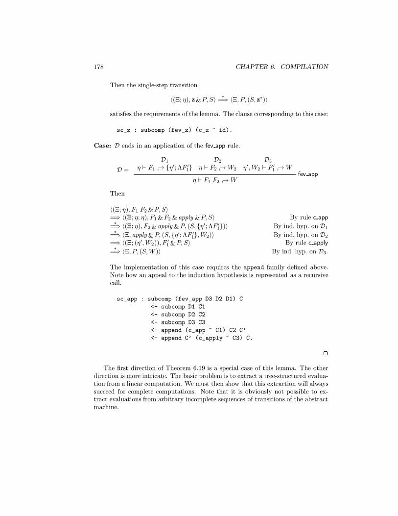
178 CHAPTER 6. COMPILATION
Then the single-step transition
〈(Ξ; η), z&P, S〉 ∗=⇒ 〈Ξ, P, (S, z∗)〉
satisfies the requirements of the lemma. The clause corresponding to this case:
sc_z : subcomp (fev_z) (c_z ~ id).
Case: D ends in an application of the fev app rule.
D =
D1
η ` F1 ↪→ {η′; ΛF ′1}D2
η ` F2 ↪→W2
D3
η′,W2 ` F ′1 ↪→Wfev app
η ` F1 F2 ↪→W
Then
〈(Ξ; η), F1 F2 &P, S〉=⇒ 〈(Ξ; η; η), F1 &F2 & apply &P, S〉 By rule c app∗
=⇒ 〈(Ξ; η), F2 & apply &P, (S, {η′; ΛF ′1})〉 By ind. hyp. on D1∗
=⇒ 〈Ξ, apply &P, (S, {η′; ΛF ′1},W2)〉 By ind. hyp. on D2
=⇒ 〈(Ξ; (η′,W2)), F ′1 &P, S〉 By rule c apply∗
=⇒ 〈Ξ, P, (S,W )〉 By ind. hyp. on D3.
The implementation of this case requires the append family defined above.Note how an appeal to the induction hypothesis is represented as a recursivecall.
sc_app : subcomp (fev_app D3 D2 D1) C
<- subcomp D1 C1
<- subcomp D2 C2
<- subcomp D3 C3
<- append (c_app ~ C1) C2 C’
<- append C’ (c_apply ~ C3) C.
2
The first direction of Theorem 6.19 is a special case of this lemma. The otherdirection is more intricate. The basic problem is to extract a tree-structured evalua-tion from a linear computation. We must then show that this extraction will alwayssucceed for complete computations. Note that it is obviously not possible to ex-tract evaluations from arbitrary incomplete sequences of transitions of the abstractmachine.

6.3. COMPUTATIONS AS TRANSITION SEQUENCES 179
In order to write computation sequences more concisely, we introduce somenotation. Let R :: St =⇒ St ′ and C :: St ′
∗=⇒ St ′′. Then we write
R ∼ C :: St =⇒ St ′′
for the computation which begins with R and then proceeds with C. Such a com-putation exists by the step inference rule. This corresponds directly to the notationin the Elf implementation.
For the proof of the central lemma of this section, we will need a new formof induction often referred to as complete induction. During a proof by completeinduction we assume the induction hypothesis not only for the immediate premissesof the last inference rule, but for all proper subderivations. Intuitively, this isjustified, since all proper subderivations are “smaller” than the given derivation.For a more formal discussion of the complete induction principle for derivations seeSection 6.4. The judgment C < C′ (C is a proper subcomputation of C′) is definedby the following inference rules.
sub immC < R ∼ C
C < C′sub med
C < R ∼ C′
It is easy to see that the proper subcomputation relation is transitive.
Lemma 6.17 If C1 < C2 and C2 < C3 then C1 < C3.
Proof: By a simple induction (see Exercise 6.12). 2
The implementation of this ordering and the proof of transitivity are immediate.
< : (st Ns1 P1 S1) =>* (st Ns P S)
-> (st Ns2 P2 S2) =>* (st Ns P S)
-> type.
%infix none 8 <.
sub_imm : C < R ~ C.
sub_med : C < C’
-> C < R ~ C’.
The representation of the proof of transitivity is left to Exercise 6.12.We are now prepared for the lemma that a complete computation with an appro-
priate initial state can be translated into an evaluation followed by another completecomputation.
Lemma 6.18 If
C :: 〈(Ξ, η), F &P, S〉 ∗=⇒ 〈·, done, (·,W ′)〉
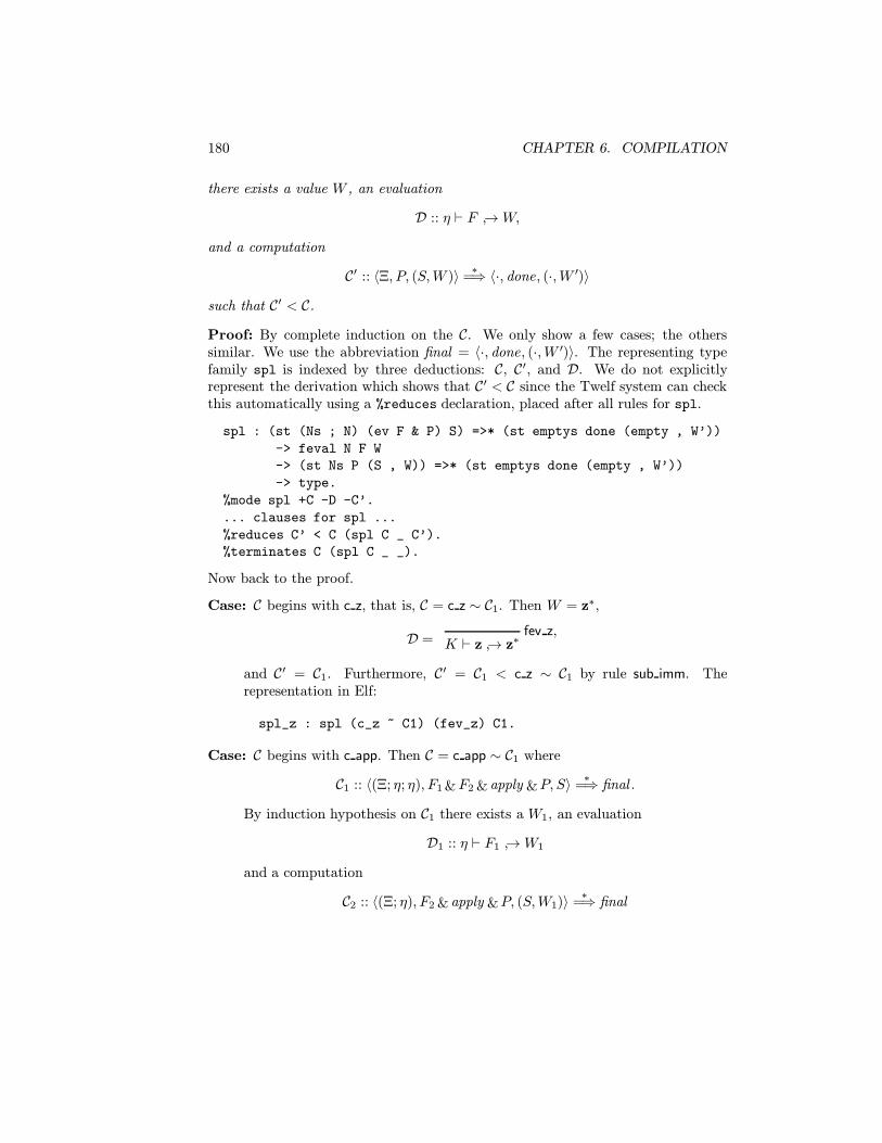
180 CHAPTER 6. COMPILATION
there exists a value W , an evaluation
D :: η ` F ↪→W,
and a computation
C′ :: 〈Ξ, P, (S,W )〉 ∗=⇒ 〈·, done, (·,W ′)〉
such that C′ < C.
Proof: By complete induction on the C. We only show a few cases; the otherssimilar. We use the abbreviation final = 〈·, done, (·,W ′)〉. The representing typefamily spl is indexed by three deductions: C, C′, and D. We do not explicitlyrepresent the derivation which shows that C′ < C since the Twelf system can checkthis automatically using a %reduces declaration, placed after all rules for spl.
spl : (st (Ns ; N) (ev F & P) S) =>* (st emptys done (empty , W’))
-> feval N F W
-> (st Ns P (S , W)) =>* (st emptys done (empty , W’))
-> type.
%mode spl +C -D -C’.
... clauses for spl ...
%reduces C’ < C (spl C _ C’).
%terminates C (spl C _ _).
Now back to the proof.
Case: C begins with c z, that is, C = c z ∼ C1. Then W = z∗,
D =fev z,
K ` z ↪→ z∗
and C′ = C1. Furthermore, C′ = C1 < c z ∼ C1 by rule sub imm. Therepresentation in Elf:
spl_z : spl (c_z ~ C1) (fev_z) C1.
Case: C begins with c app. Then C = c app ∼ C1 where
C1 :: 〈(Ξ; η; η), F1 &F2 & apply &P, S〉 ∗=⇒ final .
By induction hypothesis on C1 there exists a W1, an evaluation
D1 :: η ` F1 ↪→W1
and a computation
C2 :: 〈(Ξ; η), F2 & apply &P, (S,W1)〉 ∗=⇒ final
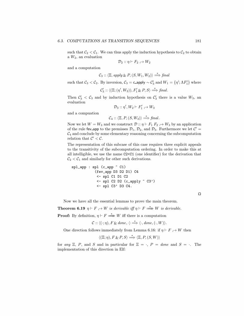
6.3. COMPUTATIONS AS TRANSITION SEQUENCES 181
such that C2 < C1. We can thus apply the induction hypothesis to C2 to obtaina W2, an evaluation
D2 :: η ` F2 ↪→W2
and a computation
C3 :: 〈Ξ, apply &P, (S,W1,W2)〉 ∗=⇒ final
such that C3 < C2. By inversion, C3 = c apply ∼ C′3 and W1 = {η′; ΛF ′1} where
C′3 :: 〈(Ξ; (η′,W2)), F ′1 &P, S〉 ∗=⇒ final .
Then C′3 < C3 and by induction hypothesis on C′3 there is a value W3, anevaluation
D3 :: η′,W2 ` F ′1 ↪→W3
and a compuationC4 :: 〈Ξ, P, (S,W3)〉 ∗
=⇒ final .
Now we let W = W3 and we construct D :: η ` F1 F2 ↪→W3 by an applicationof the rule fev app to the premisses D1, D2, and D3. Furthermore we let C′ =C4 and conclude by some elementary reasoning concerning the subcomputationrelation that C′ < C.The representation of this subcase of this case requires three explicit appealsto the transitivity of the subcomputation ordering. In order to make this atall intelligible, we use the name C2<C1 (one identifier) for the derivation thatC2 < C1 and similarly for other such derivations.
spl_app : spl (c_app ~ C1)
(fev_app D3 D2 D1) C4
<- spl C1 D1 C2
<- spl C2 D2 (c_apply ~ C3’)
<- spl C3’ D3 C4.
2
Now we have all the essential lemmas to prove the main theorem.
Theorem 6.19 η ` F ↪→W is derivable iff η ` F ∗=⇒=⇒ W is derivable.
Proof: By definition, η ` F ∗=⇒=⇒ W iff there is a computation
C :: 〈(·; η), F & done , ·〉 ∗=⇒ 〈·, done, (·,W )〉.
One direction follows immediately from Lemma 6.16: if η ` F ↪→W then
〈(Ξ; η), F &P, S〉 ∗=⇒ 〈Ξ, P, (S,W )〉
for any Ξ, P , and S and in particular for Ξ = ·, P = done and S = ·. Theimplementation of this direction in Elf:

182 CHAPTER 6. COMPILATION
cev_complete : feval N F W -> ceval N F W -> type.
%mode cev_complete +D -C.
cevc : cev_complete D (run C) <- subcomp D C.
%terminates [] (cev_complete D _).
For the other direction, assume there is a deduction C of the form shown above.By Lemma 6.18 we know that there exist a W ′, an evaluation
D′ :: η ` F ↪→W ′
and a computation
C′ :: 〈·, done, (·,W ′)〉 ∗=⇒ 〈·, done, (·,W )〉
such that C′ < C. Since there is no transition rule for the program done , C′ mustbe id and W = W ′. Thus D = D′ fulfills the requirements of the theorem. This isimplemented as follows.
cls_sound : ceval N F W -> feval N F W -> type.
%mode cls_sound +C -D.
clss : cls_sound (run C) D <- spl C D (id).
%terminates [] (cls_sound C _).
2
6.4 Complete Induction over Computations
Here we briefly justify the principle of complete induction used in the proof ofLemma 6.18. We repeat the definition of proper subcomputations and also definea general subcomputation judgment which will be useful in the proof.
C < C′ C is a proper subcomputation of C′, andC ≤ C′ C is a subcomputation of C′.
These judgments are defined via the following inference rules.
sub immC < R ∼ C
C < C′sub med
C < R ∼ C′
C < C′leq sub
C ≤ C′leq eq
C ≤ C
We only need one simple lemma regarding the subcomputation judgment.
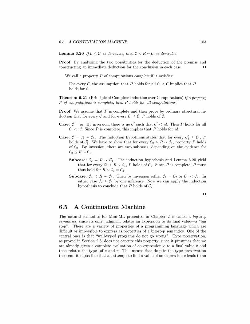
6.5. A CONTINUATION MACHINE 183
Lemma 6.20 If C ≤ C′ is derivable, then C < R ∼ C′ is derivable.
Proof: By analyzing the two possibilities for the deduction of the premiss andconstructing an immediate deduction for the conclusion in each case. 2
We call a property P of computations complete if it satisfies:
For every C, the assumption that P holds for all C′ < C implies that Pholds for C.
Theorem 6.21 (Principle of Complete Induction over Computations) If a propertyP of computations is complete, then P holds for all computations.
Proof: We assume that P is complete and then prove by ordinary structural in-duction that for every C and for every C′ ≤ C, P holds of C.
Case: C = id . By inversion, there is no C′ such that C′ < id . Thus P holds for allC′ < id . Since P is complete, this implies that P holds for id .
Case: C = R ∼ C1. The induction hypothesis states that for every C′1 ≤ C1, Pholds of C′1. We have to show that for every C2 ≤ R ∼ C1, property P holdsof C2. By inversion, there are two subcases, depending on the evidence forC2 ≤ R ∼ C1.
Subcase: C2 = R ∼ C1. The induction hypothesis and Lemma 6.20 yieldthat for every C′1 < R ∼ C1, P holds of C1. Since P is complete, P mustthus hold for R ∼ C1 = C2.
Subcase: C2 < R ∼ C1. Then by inversion either C1 = C2 or C1 < C2. Ineither case C2 ≤ C1 by one inference. Now we can apply the inductionhypothesis to conclude that P holds of C2.
2
6.5 A Continuation Machine
The natural semantics for Mini-ML presented in Chapter 2 is called a big-stepsemantics, since its only judgment relates an expression to its final value—a “bigstep”. There are a variety of properties of a programming language which aredifficult or impossible to express as properties of a big-step semantics. One of thecentral ones is that “well-typed programs do not go wrong”. Type preservation,as proved in Section 2.6, does not capture this property, since it presumes that weare already given a complete evaluation of an expression e to a final value v andthen relates the types of e and v. This means that despite the type preservationtheorem, it is possible that an attempt to find a value of an expression e leads to an
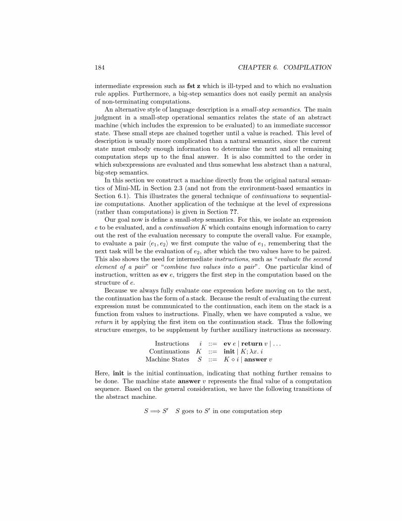
184 CHAPTER 6. COMPILATION
intermediate expression such as fst z which is ill-typed and to which no evaluationrule applies. Furthermore, a big-step semantics does not easily permit an analysisof non-terminating computations.
An alternative style of language description is a small-step semantics. The mainjudgment in a small-step operational semantics relates the state of an abstractmachine (which includes the expression to be evaluated) to an immediate successorstate. These small steps are chained together until a value is reached. This level ofdescription is usually more complicated than a natural semantics, since the currentstate must embody enough information to determine the next and all remainingcomputation steps up to the final answer. It is also committed to the order inwhich subexpressions are evaluated and thus somewhat less abstract than a natural,big-step semantics.
In this section we construct a machine directly from the original natural seman-tics of Mini-ML in Section 2.3 (and not from the environment-based semantics inSection 6.1). This illustrates the general technique of continuations to sequential-ize computations. Another application of the technique at the level of expressions(rather than computations) is given in Section ??.
Our goal now is define a small-step semantics. For this, we isolate an expressione to be evaluated, and a continuation K which contains enough information to carryout the rest of the evaluation necessary to compute the overall value. For example,to evaluate a pair 〈e1, e2〉 we first compute the value of e1, remembering that thenext task will be the evaluation of e2, after which the two values have to be paired.This also shows the need for intermediate instructions, such as “evaluate the secondelement of a pair” or “combine two values into a pair”. One particular kind ofinstruction, written as ev e, triggers the first step in the computation based on thestructure of e.
Because we always fully evaluate one expression before moving on to the next,the continuation has the form of a stack. Because the result of evaluating the currentexpression must be communicated to the continuation, each item on the stack is afunction from values to instructions. Finally, when we have computed a value, wereturn it by applying the first item on the continuation stack. Thus the followingstructure emerges, to be supplement by further auxiliary instructions as necessary.
Instructions i ::= ev e | return v | . . .Continuations K ::= init | K; λx. i
Machine States S ::= K � i | answer v
Here, init is the initial continuation, indicating that nothing further remains tobe done. The machine state answer v represents the final value of a computationsequence. Based on the general consideration, we have the following transitions ofthe abstract machine.
S =⇒ S′ S goes to S′ in one computation step

6.5. A CONTINUATION MACHINE 185
st initinit � return v =⇒ answer v
st returnK; λx. i � return v =⇒ K � [v/x]i
Further rules arise from considering each expression constructor in turn, possiblyadding new special-purpose intermediate instructions. We will write the rules in theform label :: S =⇒ S′ as a more concise alternative to the format used above. Themeaning, however, remains the same: each rules is an axiom defining the transitionjudgment. First, the constructors:
st z :: K � ev z =⇒ K � return zst s :: K � ev (s e) =⇒ K; λx. return (s x) � e
Second, the corresponding destructor:
st case :: K � ev (case e1 of z⇒ e2 | s x⇒ e3)=⇒ K; λx1. case1 x1 of z⇒ e2 | s x⇒ e3 � ev e1
st case1 z :: K � case1 z of z⇒ e2 | s x⇒ e3 =⇒ K � ev e2
st case1 s :: K � case1 s v1 of z⇒ e2 | s x⇒ e3 =⇒ K � ev [v′1/x]e3
We can see that the case construct requires a new instruction of the formcase1 v1 of z⇒ e2 | s x⇒ e3. This is distinct from case e1 of z⇒ e2 | s x⇒ e3
in that the case subject is known to be a value. Without an explicit new construct,computation could get into an infinite loop since every value is also an expressionwhich evaluates to itself. It should now be clear how pairs and projections arecomputed; the new instructions are 〈v1, e2〉1, fst1, and snd1.
st pair :: K � ev 〈e1, e2〉 =⇒ K; λx1. 〈x1, e2〉1 � ev e1
st pair1 :: K � 〈v1, e2〉1 =⇒ K; λx1. return 〈v1, x2〉 � ev e2
st fst :: K � ev (fst e) =⇒ K; λx. fst1 x � ev est fst1 :: K � fst1 〈v1, v2〉 =⇒ K � return v1
st snd :: K � ev (snd e) =⇒ K; λx. snd1 x � ev est snd1 :: K � snd1 〈v1, v2〉 =⇒ K � return v2
Neither functions, nor definitions or recursion introduce any essentially newideas. We add two new forms of instructions, app1 and app2, for the intermediateforms while evaluating applications.
st lam :: K � ev (lam x. e) =⇒ K � return lamx. est app :: K � ev (e1 e2) =⇒ K; λx1. app1 x1 e2 � ev e1
st app1 :: K � app1 v1 e2 =⇒ K; λx2. app2 v1 x2 � ev e2
st app2 :: K � app2 (lam x. e′1) v2 =⇒ K � ev ([v2/x]e′1)
st letv :: K � letval x = e1 in e2 =⇒ K; λx1. [x1/x]e2 � ev e1
st letn :: K � letname u = e1 in e2 =⇒ K � ev ([e1/x]e2)
st fix :: K � fix u. e =⇒ K � ev ([fix u. e/u]e)
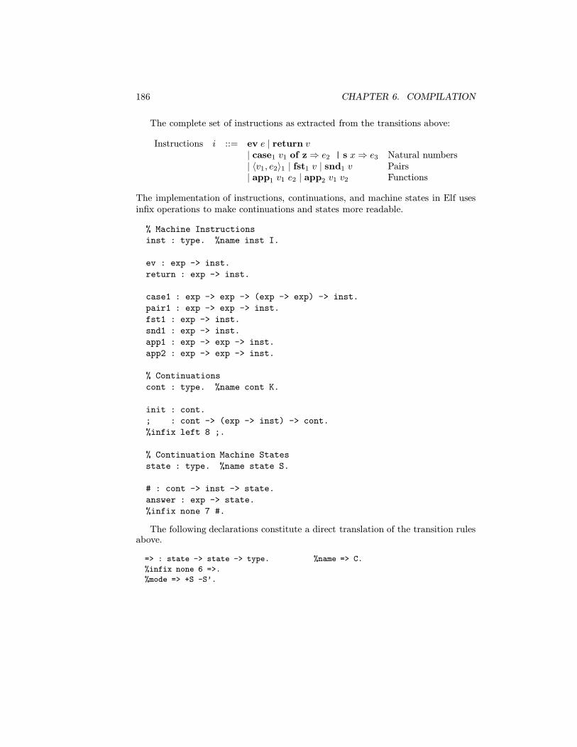
186 CHAPTER 6. COMPILATION
The complete set of instructions as extracted from the transitions above:
Instructions i ::= ev e | return v| case1 v1 of z⇒ e2 | s x⇒ e3 Natural numbers| 〈v1, e2〉1 | fst1 v | snd1 v Pairs| app1 v1 e2 | app2 v1 v2 Functions
The implementation of instructions, continuations, and machine states in Elf usesinfix operations to make continuations and states more readable.
% Machine Instructions
inst : type. %name inst I.
ev : exp -> inst.
return : exp -> inst.
case1 : exp -> exp -> (exp -> exp) -> inst.
pair1 : exp -> exp -> inst.
fst1 : exp -> inst.
snd1 : exp -> inst.
app1 : exp -> exp -> inst.
app2 : exp -> exp -> inst.
% Continuations
cont : type. %name cont K.
init : cont.
; : cont -> (exp -> inst) -> cont.
%infix left 8 ;.
% Continuation Machine States
state : type. %name state S.
# : cont -> inst -> state.
answer : exp -> state.
%infix none 7 #.
The following declarations constitute a direct translation of the transition rulesabove.
=> : state -> state -> type. %name => C.
%infix none 6 =>.
%mode => +S -S’.

6.5. A CONTINUATION MACHINE 187
% Natural Numbers
st_z : K # (ev z) => K # (return z).
st_s : K # (ev (s E’)) => (K ; [x’] return (s x’)) # (ev E’).
st_case : K # (ev (case E1 E2 E3)) => (K ; [x1] case1 x1 E2 E3) # (ev E1).
st_case1_z : K # (case1 (z) E2 E3) => K # (ev E2).
st_case1_s : K # (case1 (s V1’) E2 E3) => K # (ev (E3 V1’)).
% Pairs
st_pair : K # (ev (pair E1 E2)) => (K ; [x1] pair1 x1 E2) # (ev E1).
st_pair1 : K # (pair1 V1 E2) => (K ; [x2] return (pair V1 x2)) # (ev E2).
st_fst : K # (ev (fst E’)) => (K ; [x’] fst1 x’) # (ev E’).
st_fst1 : K # (fst1 (pair V1 V2)) => K # (return V1).
st_snd : K # (ev (snd E’)) => (K ; [x’] snd1 x’) # (ev E’).
st_snd1 : K # (snd1 (pair V1 V2)) => K # (return V2).
% Functions
st_lam : K # (ev (lam E’)) => K # (return (lam E’)).
st_app : K # (ev (app E1 E2)) => (K ; [x1] app1 x1 E2) # (ev E1).
st_app1 : K # (app1 V1 E2) => (K ; [x2] app2 V1 x2) # (ev E2).
st_app2 : K # (app2 (lam E1’) V2) => K # (ev (E1’ V2)).
% Definitions
st_letv : K # (ev (letv E1 E2)) => (K ; [x1] ev (E2 x1)) # (ev E1).
st_letn : K # (ev (letn E1 E2)) => K # (ev (E2 E1)).
% Recursion
st_fix : K # (ev (fix E’)) => K # (ev (E’ (fix E’))).
% Return Instructions
st_return : (K ; [x] I x) # (return V) => K # (I V).
st_init : (init) # (return V) => (answer V).
Multi-step computation sequences could be represented as lists of single steptransitions. However, we would like to use dependent types to guarantee that, ina valid computation sequence, the result state of one transition matches the startstate of the next transition. This is difficult to accomplish using a generic type oflists; instead we introduce specific instances of this type which are structurally justlike lists, but have strong internal validity conditions.
S∗
=⇒ S′ S goes to S′ in zero or more steps
ec↪→ v e evaluates to v using the continuation machine

188 CHAPTER 6. COMPILATION
stopS∗
=⇒ S
S =⇒ S′ S′∗
=⇒ S′′step
S∗
=⇒ S′′
init � ev e∗
=⇒ answer vcev
ec↪→ v
We would like the implementation to be operational, that is, queries of theform ?- ceval peq V. should compute the value V of a given e. This means theS =⇒ S′ should be the first subgoal and hence the second argument of the steprule. In addition, we employ a visual trick to display computation sequences in areadable format by representing the step rule as a left associative infix operator.
=>* : state -> state -> type. %name =>* C*.
%infix none 5 =>*.
%mode =>* +S -S’.
stop : S =>* S.
<< : S =>* S’’
<- S => S’
<- S’ =>* S’’.
%infix left 5 <<.
% Because of evaluation order, computation sequences are displayed
% in reverse, using "<<" as a left-associative infix operator.
ceval : exp -> exp -> type. %name ceval CE.
%mode ceval +E -V.
cev : ceval E V
<- (init) # (ev E) =>* (answer V).
We then get a reasonable display of the sequence of computation steps whichmust be read from right to left.
?- C* : init # (ev (app (lam [x] x) z)) =>* answer V.
Solving...
V = z.
C* =
stop << st_init << st_z << st_app2 << st_return << st_z << st_app1
<< st_return << st_lam << st_app.
The overall task now is to prove that e ↪→ v if and only if ec↪→ v. In one
direction we have to find a translation from tree-structured derivations D :: e ↪→ vto sequential computations C :: init � ev e
∗=⇒ answer v. In the other direction

6.5. A CONTINUATION MACHINE 189
we have to find a way to chop a sequential computation into pieces which can bereassembled into a tree-structured derivation.
We start with the easier of the two proofs. We assume that e ↪→ v and try to show
that ec↪→ v. This immediately reduces to showing that init � ev e
∗=⇒ answer v.
This does not follow directly by induction, since subcomputations will neither startfrom the initial computation nor return the final answer. If we generalize the claimto state that for all continuations K we have that K � ev e
∗=⇒ K � return v,
then it follows directly by induction, using some simple lemmas regarding the con-catenation of computation sequences (see Exercise 6.17).
We can avoid explicit concatenation of computation sequences and obtain a moredirect proof (and more efficient program) if we introduce an accumulator argument.This argument contains the remainder of the computation, starting from the stateK � return v. To the front of this given computation we add the computationfrom K � ev e
∗=⇒ K � return v, passing the resulting computation as the next
value of the accumulator argument. Translating this intuition to a logical statementrequires explicitly universally quantifying over the accumulator argument.
Lemma 6.22 For any closed expression e, value v and derivation D :: e ↪→ v, ifC′ :: K � return v
∗=⇒ answer w for any K and w, then C :: K � ev e
∗=⇒
answer w.
Proof: The proof proceeds by induction on the structure of D. Since the accumu-lator argument must already hold the remainder of the overall computation uponappeal to the induction hypothesis, we apply the induction hypothesis on the im-mediate subderivations of D in right-to-left order.
The proof is implemented by a type family
ccp : eval E V
-> K # (return V) =>* (answer W)
-> K # (ev E) =>* (answer W)
-> type.
%mode ccp +D +C’ -C.
Operationally, the first argument is the induction argument, the second argumentthe accumlator, and the last the output argument.
We only show a couple of cases in the proof; the others follow in a similarmanner.
Case:
D = ev lamlam x. e1 ↪→ lam x. e1
C′ :: K � return lam x. e1∗
=⇒ answer w AssumptionC :: K � ev(lam x. e1) =⇒ answer w By st lam followed by C′
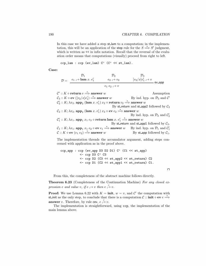
190 CHAPTER 6. COMPILATION
In this case we have added a step st lam to a computation; in the implemen-tation, this will be an application of the step rule for the S
∗=⇒ S′ judgment,
which is written as << in infix notation. Recall that the reversal of the evalu-ation order means that computations (visually) proceed from right to left.
ccp_lam : ccp (ev_lam) C’ (C’ << st_lam).
Case:
D =
D1
e1 ↪→ lam x. e′1
D2
e2 ↪→ v2
D3
[v2/x]e′1 ↪→ vev app
e1 e2 ↪→ v
C′ :: K � return v∗
=⇒ answer w Assumption
C3 :: K � ev ([v2/x]e′1)∗
=⇒ answer w By ind. hyp. on D3 and C′C′2 :: K; λx2. app2 (lam x. e′1) x2 � return v2
∗=⇒ answer w
By st return and st app2 followed by C3C2 :: K; λx2. app2 (lam x. e′1) x2 � ev e2
∗=⇒ answer w
By ind. hyp. on D2 and C′2C′1 :: K; λx1. app1 x1 e2 � return lam x. e′1
∗=⇒ answer w
By st return and st app1 followed by C2.
C1 :: K; λx1. app1 x1 e2 � ev e1∗
=⇒ answer w By ind. hyp. on D1 and C′1C :: K � ev (e1 e2)
∗=⇒ answer w By st app followed by C1.
The implementation threads the accumulator argument, adding steps con-cerned with application as in the proof above.
ccp_app : ccp (ev_app D3 D2 D1) C’ (C1 << st_app)
<- ccp D3 C’ C3
<- ccp D2 (C3 << st_app2 << st_return) C2
<- ccp D1 (C2 << st_app1 << st_return) C1.
2
From this, the completeness of the abstract machine follows directly.
Theorem 6.23 (Completeness of the Continuation Machine) For any closed ex-
pression e and value v, if e ↪→ v then ec↪→ v.
Proof: We use Lemma 6.22 with K = init, w = v, and C′ the computation withst init as the only step, to conclude that there is a computation C :: init � ev e
∗=⇒
answer v. Therefore, by rule cev, ec↪→ v.
The implementation is straightforward, using ccp, the implementation of themain lemma above.

6.5. A CONTINUATION MACHINE 191
cpm_complete : eval E V -> ceval E V -> type.
%mode cpm_complete +D -C.
cpmcp : cpm_complete D (cev C)
<- ccp D (stop << st_init) C.
2
Now we turn our attention to the soundness of the continuation machine: when-ever it produces a value v then the natural semantics can also produce the value vfrom the same expression. This is more difficult to prove than completeness. Thereason is that in the completeness proof, every subderivation of D :: e ↪→ v caninductively be translated to a sequence of computation steps, but not every se-quence of computation steps corresponds to an evaluation. For example, the partialcomputation
K � ev (e1 e2)∗
=⇒ K; λx1. app1 x1 e2 � ev e1
represents only a fragment of an evaluation. In order to translate a computationsequence we must ensure that it is sufficiently long. A simple way to accomplish thisis to require that the given computation goes all the way to a final answer. Thus, wehave a state K � ev e at the beginning of a computation sequence C to a final answerw, there must be some initial segment of C′ which corresponds to an evaluation of eto a value v, while the remaining computation goes from K � return v to the finalanswer w. This can then be proved by induction.
Lemma 6.24 For any continuation K, closed expression e and value w, if C ::K � ev e
∗=⇒ answer w then there is a value v a derivation D :: e ↪→ v, and a
subcomputation C′ of C of the form K � return v∗
=⇒ answer w.
Proof: By complete induction on the structure of C. Here complete induction, asopposed to a simple structural induction, means that we can apply the inductionhypothesis to any subderivation of C, not just to the immediate subderivations.It should be intuitively clear that this is a valid induction principle (see also Sec-tion 6.4).
In the implementation we have chosen not to represent the evidence for theassertion that C′ is a subderivation of C. This can be added, either directly to theimplementation or as a higher-level judgment (see Exercise ??). This informationis not required to execute the proof on specific computation sequences, although itis critical for seeing that it always terminates.
csd : K # (ev E) =>* (answer W)
-> eval E V
-> K # (return V) =>* (answer W)
-> type.
%mode csd +C -D -C’.
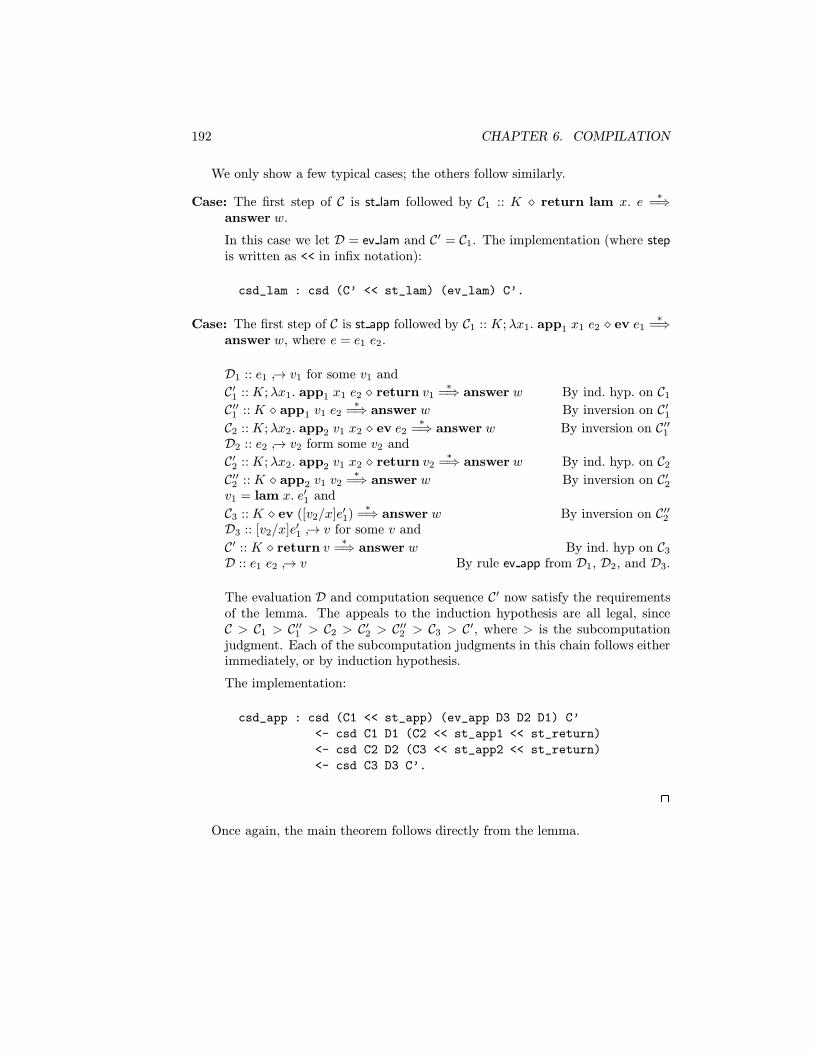
192 CHAPTER 6. COMPILATION
We only show a few typical cases; the others follow similarly.
Case: The first step of C is st lam followed by C1 :: K � return lam x. e∗
=⇒answer w.
In this case we let D = ev lam and C′ = C1. The implementation (where stepis written as << in infix notation):
csd_lam : csd (C’ << st_lam) (ev_lam) C’.
Case: The first step of C is st app followed by C1 :: K; λx1. app1 x1 e2 � ev e1∗
=⇒answer w, where e = e1 e2.
D1 :: e1 ↪→ v1 for some v1 and
C′1 :: K; λx1. app1 x1 e2 � return v1∗
=⇒ answer w By ind. hyp. on C1C′′1 :: K � app1 v1 e2
∗=⇒ answer w By inversion on C′1
C2 :: K; λx2. app2 v1 x2 � ev e2∗
=⇒ answer w By inversion on C′′1D2 :: e2 ↪→ v2 form some v2 and
C′2 :: K; λx2. app2 v1 x2 � return v2∗
=⇒ answer w By ind. hyp. on C2C′′2 :: K � app2 v1 v2
∗=⇒ answer w By inversion on C′2
v1 = lam x. e′1 and
C3 :: K � ev ([v2/x]e′1)∗
=⇒ answer w By inversion on C′′2D3 :: [v2/x]e′1 ↪→ v for some v and
C′ :: K � return v∗
=⇒ answer w By ind. hyp on C3D :: e1 e2 ↪→ v By rule ev app from D1, D2, and D3.
The evaluation D and computation sequence C′ now satisfy the requirementsof the lemma. The appeals to the induction hypothesis are all legal, sinceC > C1 > C′′1 > C2 > C′2 > C′′2 > C3 > C′, where > is the subcomputationjudgment. Each of the subcomputation judgments in this chain follows eitherimmediately, or by induction hypothesis.
The implementation:
csd_app : csd (C1 << st_app) (ev_app D3 D2 D1) C’
<- csd C1 D1 (C2 << st_app1 << st_return)
<- csd C2 D2 (C3 << st_app2 << st_return)
<- csd C3 D3 C’.
2
Once again, the main theorem follows directly from the lemma.

6.6. TYPE PRESERVATION AND PROGRESS 193
Theorem 6.25 (Soundness of the Continuation Machine) For any closed expres-
sion e and value v, if ec↪→ v then e ↪→ v.
Proof: By inversion, C :: init � ev e∗
=⇒ answer v. By Lemma 6.24 there is aderivation D :: e ↪→ v′ and C′ :: init � return v′
∗=⇒ answer v for some v′. By
inversion on C′ we see that v = v′ and therefore D satisfies the requirements of thetheorem.
cpm_sound : ceval E V -> eval E V -> type.
%mode cpm_sound +C -D.
cpmsd : cpm_sound (cev C) D
<- csd C D (stop << st_init).
%terminates {} (cpm_sound C D).
2
6.6 Type Preservation and Progress
So far we have concentrated on operational aspects of the translation from a big-stepto a small-step semantics; now we turn to issues of typing. The first property is typepreservation—a reprise of the same property for the big-step semantics. But thereformulation of the semantics also allows us to express new language properties,still at a high level of abstraction. One of the most important ones is progress. Itstates that in any valid abstract machine state we can have one of two situations:either we have already computed the final answer of the program, or we can makeprogress by taking a further step.
Type preservation and progress together express that well-typed programs can-not go wrong, a phrase coined by Milner [Mil78]. In our setting, “going wrong”corresponds to reaching a machine state in which no further transition rules appli-cable. Note that type preservation for the big-step semantics does not express this,since it only talks about completed evaluations, not about intermediate states. Ofcourse, even in the small-step semantics an expression can fail to have a value, butfrom the progress theorem we know that this is only due to non-termination.
We begin by giving the typing rules for the continuation-passing machine. Onecomplication as compared to the typing rules for expressions is that certain machinestates only make sense when components of instructions are values. For example,the instruction app2 v1 v2 requires both arguments to be values. If this restrictionis not enforced, the progress theorem clearly fails, because there is no transition fora state K � app2 ((lam x. x) (lam y. y)) z even though the arguments to app2
are correctly typed. This introduces a further complication: since continuations
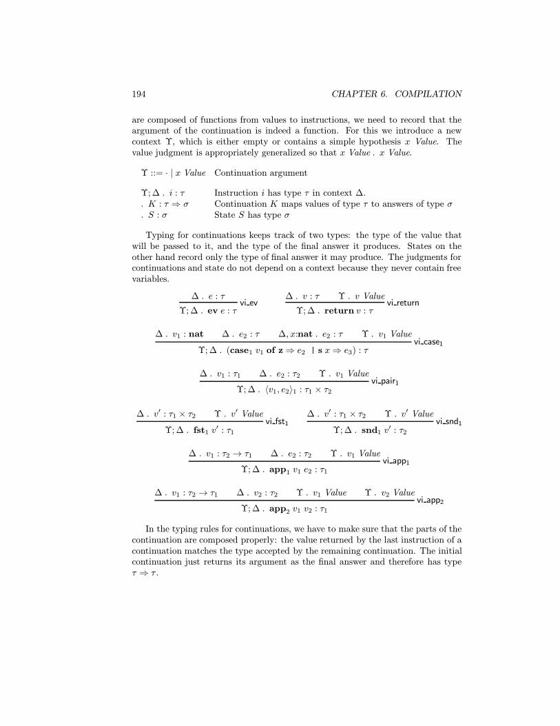
194 CHAPTER 6. COMPILATION
are composed of functions from values to instructions, we need to record that theargument of the continuation is indeed a function. For this we introduce a newcontext Υ, which is either empty or contains a simple hypothesis x Value. Thevalue judgment is appropriately generalized so that x Value . x Value.
Υ ::= · | x Value Continuation argument
Υ; ∆ . i : τ Instruction i has type τ in context ∆.. K : τ ⇒ σ Continuation K maps values of type τ to answers of type σ. S : σ State S has type σ
Typing for continuations keeps track of two types: the type of the value thatwill be passed to it, and the type of the final answer it produces. States on theother hand record only the type of final answer it may produce. The judgments forcontinuations and state do not depend on a context because they never contain freevariables.
∆ . e : τvi ev
Υ; ∆ . ev e : τ
∆ . v : τ Υ . v Valuevi return
Υ; ∆ . return v : τ
∆ . v1 : nat ∆ . e2 : τ ∆, x:nat . e2 : τ Υ . v1 Valuevi case1
Υ; ∆ . (case1 v1 of z⇒ e2 | s x⇒ e3) : τ
∆ . v1 : τ1 ∆ . e2 : τ2 Υ . v1 Valuevi pair1
Υ; ∆ . 〈v1, e2〉1 : τ1 × τ2
∆ . v′ : τ1 × τ2 Υ . v′ Valuevi fst1
Υ; ∆ . fst1 v′ : τ1
∆ . v′ : τ1 × τ2 Υ . v′ Valuevi snd1
Υ; ∆ . snd1 v′ : τ2
∆ . v1 : τ2 → τ1 ∆ . e2 : τ2 Υ . v1 Valuevi app1
Υ; ∆ . app1 v1 e2 : τ1
∆ . v1 : τ2 → τ1 ∆ . v2 : τ2 Υ . v1 Value Υ . v2 Valuevi app2
Υ; ∆ . app2 v1 v2 : τ1
In the typing rules for continuations, we have to make sure that the parts of thecontinuation are composed properly: the value returned by the last instruction of acontinuation matches the type accepted by the remaining continuation. The initialcontinuation just returns its argument as the final answer and therefore has typeτ ⇒ τ .

6.6. TYPE PRESERVATION AND PROGRESS 195
vk init. init : τ ⇒ τ
xValue; ·, x:τ . i : τ ′ . K : τ ′ ⇒ σvk ;
. K; λx. i : τ ⇒ σ
For a state we verify that the type of the instruction to be executed matchesthe one expected by the continuation, and assign the type of the final answer to thestate.
·; · . i : τ . K : τ ⇒ σvs �
. (K � i) : σ
· . v : σ · . v Valuevs answer
. answer v : σ
The typing judgments for instructions, continuations, and states admit morestates as valid than can be reached from an initial state of the form init � ev e (seeExercise 6.19). However, they are accurate enough to permit proof of preservationand progress and is therefore appropriate for our purposes.
The implementation of the judgments in the logical framework is straightfor-ward. The fact that we need at most one value variable is not explicitly represented.Instead, we use the usual techniques for parametric and hypothetical judgments byassuming value x for a new parameter x. The declarations below can be executedin Elf in order to check the validity of instructions, continuations and states andinfer their most general types.
%%% Instructions
valid : inst -> tp -> type. %name valid VL.
%mode valid +I *T.
% Evaluation and return
vi_ev : valid (ev E) T
<- of E T.
vi_return : valid (return V) T
<- of V T
<- value V.
% Natural Numbers
vi_case1 : valid (case1 V1 E2 E3) T
<- of V1 nat
<- of E2 T
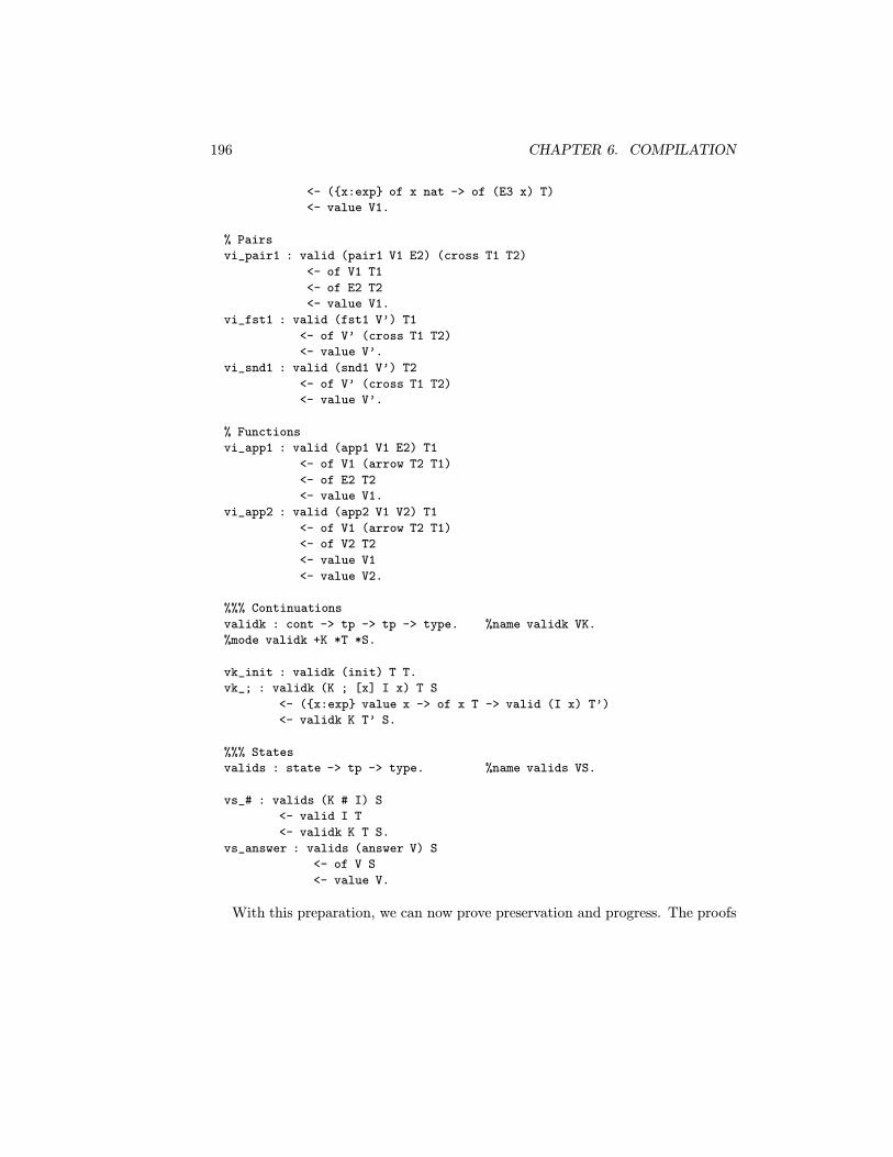
196 CHAPTER 6. COMPILATION
<- ({x:exp} of x nat -> of (E3 x) T)
<- value V1.
% Pairs
vi_pair1 : valid (pair1 V1 E2) (cross T1 T2)
<- of V1 T1
<- of E2 T2
<- value V1.
vi_fst1 : valid (fst1 V’) T1
<- of V’ (cross T1 T2)
<- value V’.
vi_snd1 : valid (snd1 V’) T2
<- of V’ (cross T1 T2)
<- value V’.
% Functions
vi_app1 : valid (app1 V1 E2) T1
<- of V1 (arrow T2 T1)
<- of E2 T2
<- value V1.
vi_app2 : valid (app2 V1 V2) T1
<- of V1 (arrow T2 T1)
<- of V2 T2
<- value V1
<- value V2.
%%% Continuations
validk : cont -> tp -> tp -> type. %name validk VK.
%mode validk +K *T *S.
vk_init : validk (init) T T.
vk_; : validk (K ; [x] I x) T S
<- ({x:exp} value x -> of x T -> valid (I x) T’)
<- validk K T’ S.
%%% States
valids : state -> tp -> type. %name valids VS.
vs_# : valids (K # I) S
<- valid I T
<- validk K T S.
vs_answer : valids (answer V) S
<- of V S
<- value V.
With this preparation, we can now prove preservation and progress. The proofs
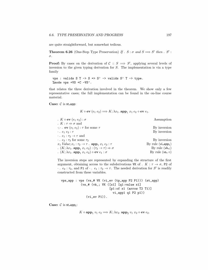
6.6. TYPE PRESERVATION AND PROGRESS 197
are quite straightforward, but somewhat tedious.
Theorem 6.26 (One-Step Type Preservation) If . S : σ and S =⇒ S′ then . S′ :σ.
Proof: By cases on the derivation of C :: S =⇒ S′, applying several levels ofinversion to the given typing derivation for S. The implementation is via a typefamily
vps : valids S T -> S => S’ -> valids S’ T -> type.
%mode vps +VS +C -VS’.
that relates the three derivation involved in the theorem. We show only a fewrepresentative cases; the full implementation can be found in the on-line coursematerial.
Case: C is st app:
K � ev (e1 e2) =⇒ K; λx1. app1 x1 e2 � ev e1.
. K � ev (e1 e2) : σ Assumption
. K : τ ⇒ σ and·; · . ev (e1 e2) : τ for some τ By inversion· . e1 e2 : τ By inversion· . e1 : τ2 → τ and· . e2 : τ2 for some τ2 By inversionx1 Value; x1 : τ2 → τ . app1 x1 e2 : τ By rule (vi app1). (K; λx1. app1 x1 e2) : (τ2 → τ)⇒ σ By rule (vk ;). (K; λx1. app1 x1 e2) � ev e1 : σ By rule (vs �)
The inversion steps are represented by expanding the structure of the firstargument, obtaining access to the subderivations VK of . K : τ → σ, P2 of· . e2 : τ2, and P1 of · . e1 : τ2 → τ . The needed derivation for S′ is readilyconstructed from these variables.
vps_app : vps (vs_# VK (vi_ev (tp_app P2 P1))) (st_app)
(vs_# (vk_; VK ([x1] [q1:value x1]
[p1:of x1 (arrow T2 T1)]
vi_app1 q1 P2 p1))
(vi_ev P1)).
Case: C is st app1:
K � app1 v1 e2 =⇒ K; λx2. app2 v1 x2 � ev e2.

198 CHAPTER 6. COMPILATION
. K � app1 v1 e2 : σ Assumption
. K : τ ⇒ σ and·; · . app1 v1 e2 : τ for some τ By inversion· . v1 : τ2 → τ and· . e2 : τ2 form some τ2 and· . v1 Value By inversionx2 Value; x2 : τ2 .. app2 v1 x2 : τ By rule (vi app2). (K; λx2. app1 v1 e2) : τ2 ⇒ σ By rule (vk ;). (K; λx1. app2 v1 x2) � ev e2 : σ By rule vs cpm
In the representation we decompose the first argument as before. This nowgives as also Q1 which is the derivation of v1 Value.
vps_app1 : vps (vs_# VK (vi_app1 Q1 P2 P1)) (st_app1)
(vs_# (vk_; VK ([x2] [q2:value x2] [p2:of x2 T2]
vi_app2 q2 Q1 p2 P1))
(vi_ev P2)).
Case: C is st app2:
K � app2 (lam x. e′1) v2 =⇒ K � ev ([v2/x]e′1).
. (K � app2 (lam x. e′1) v2) : σ Assumption
. K : τ1 ⇒ σ and·; · . app2 (lam x. e′1) v2) : τ1 for some τ1 By inversion· . (lam x. e′1) : τ2 → τ1 and· . v2 : τ2 for some τ2 and· . (lam x. e′1) Value and· . v2 Value By inversionx:τ2 . e
′1 : τ1 By inversion
· . [v2/x]e′1 : τ1 By substitution property (2.4)·; · . ev ([v2/x]e′1) : τ1 By rule (vi ev). K � ev ([v2/x]e′1) : σ By rule (vs cpm)
By applying inversion as above we obtained
P ′1 :: (x:τ2 . e′1 : τ1)
which is represented by the variable
P1’ : {x:exp} of x T2 -> of (E1’ x) T1.

6.6. TYPE PRESERVATION AND PROGRESS 199
The appeal to the substitution principle is implemented by applying this func-tion to the representation of v2 and the typing derivation P2 :: (· . v2 : τ2).Note that we do not need the derivation Q2 which is evidence that v2 is avalue.
vps_app2 : vps (vs_# VK (vi_app2 Q2 (val_lam) P2 (tp_lam P1’)))
(st_app2) (vs_# VK (vi_ev (P1’ V2 P2))).
2
The multi-step type preservation theorem is a direct consequence of the one-steppreservation.
Theorem 6.27 (Multi-Step Type Preservation) If . S : σ and S∗
=⇒ S′ then. S′ : σ
Proof: By straightforward induction on the structure of the derivation C∗ :: (S∗
=⇒S′). We only show the implementation.
vps* : valids S T -> S =>* S’ -> valids S’ T -> type.
%mode vps* +VS +C* -VS’.
vps*_stop : vps* VS (stop) VS.
vps*_<< : vps* VS (C2* << C1) VS2
<- vps VS C1 VS1
<- vps* VS1 C2* VS2.
2
Finally, we come to the progress theorem: we can make a transition from everystate that is not a final state. Recall that the only final states are of the formanswer v.
Theorem 6.28 (Progress) If . (K � i) : σ then there is a state S′ such thatK � i =⇒ S′.
Proof: We know by inversion that
. K : τ ⇒ σ and
. i : τ for some τ .
We apply case analysis on i. In each case we can either directly make a transition,or we need to apply several inversions on an available typing or value derivationuntil each subcase can be seen to be impossible or a transition rule applies. For areturn instruction, we also need to distinguish cases on the shape of K. We showonly a few cases.
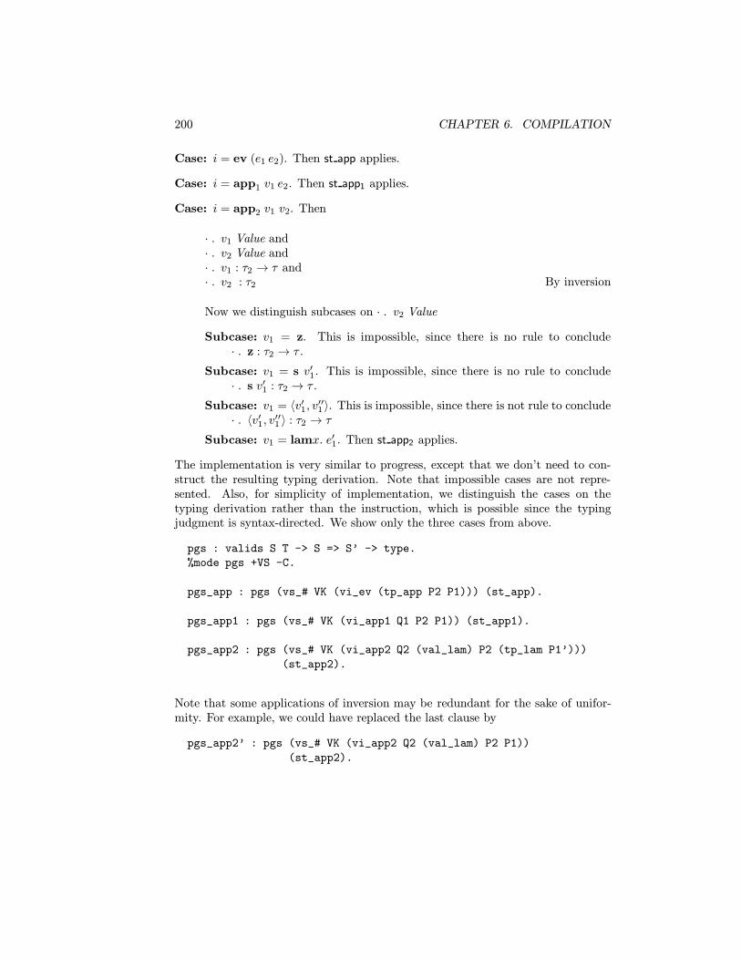
200 CHAPTER 6. COMPILATION
Case: i = ev (e1 e2). Then st app applies.
Case: i = app1 v1 e2. Then st app1 applies.
Case: i = app2 v1 v2. Then
· . v1 Value and· . v2 Value and· . v1 : τ2 → τ and· . v2 : τ2 By inversion
Now we distinguish subcases on · . v2 Value
Subcase: v1 = z. This is impossible, since there is no rule to conclude· . z : τ2 → τ .
Subcase: v1 = s v′1. This is impossible, since there is no rule to conclude· . s v′1 : τ2 → τ .
Subcase: v1 = 〈v′1, v′′1 〉. This is impossible, since there is not rule to conclude· . 〈v′1, v′′1 〉 : τ2 → τ
Subcase: v1 = lamx. e′1. Then st app2 applies.
The implementation is very similar to progress, except that we don’t need to con-struct the resulting typing derivation. Note that impossible cases are not repre-sented. Also, for simplicity of implementation, we distinguish the cases on thetyping derivation rather than the instruction, which is possible since the typingjudgment is syntax-directed. We show only the three cases from above.
pgs : valids S T -> S => S’ -> type.
%mode pgs +VS -C.
pgs_app : pgs (vs_# VK (vi_ev (tp_app P2 P1))) (st_app).
pgs_app1 : pgs (vs_# VK (vi_app1 Q1 P2 P1)) (st_app1).
pgs_app2 : pgs (vs_# VK (vi_app2 Q2 (val_lam) P2 (tp_lam P1’)))
(st_app2).
Note that some applications of inversion may be redundant for the sake of unifor-mity. For example, we could have replaced the last clause by
pgs_app2’ : pgs (vs_# VK (vi_app2 Q2 (val_lam) P2 P1))
(st_app2).

6.7. CONTEXTUAL SEMANTICS 201
Nonetheless, the inversion on the value derivation is necessary, and
pgs_app2’’ : pgs (vs_# VK (vi_app2 Q2 Q1 P2 P1))
(st_app2).
would be incorrect as a proof case because it is not apparent from the first argumentthat st app2 indeed applies. 2
6.7 Contextual Semantics
[ This section discusses a contextual semantics as an alternative small-step machine to the CPM machine. This still has to be revised from anolder version. ]
6.8 Exercises
Exercise 6.1 If we replace the rule ev app in the natural semantics of Mini-ML(see Section 2.3) by
e1 ↪→ lam x. e′1 e2 ↪→ v2
ux ↪→ v2
...e′1 ↪→ v
ev app′x,u
e1 e2 ↪→ v
in order to avoid explicitly substituting v2 for x, something goes wrong. Whatis it? Can you suggest a way to fix the problem which still employs hypotheticaljudgments?
(Note: We assume that the third premiss of the modified rule is parametric in xand hypothetical in u which is discharged as indicated. This implies that we assumethat x is not already free in any other hypothesis and that all labels for hypothesesare distinct—so this is not the problem you are asked to detect.)
Exercise 6.2 Define the judgment W RealVal which restricts closures W to Λ-abstractions. Prove that · ` F ↪→ W then W RealVal and represent this proof inElf.
Exercise 6.3 In this exercise we try to eliminate some of the non-determinism incompilation.
1. Define a judgment F std which should be derivable if the de Bruijn expressionF is in the standard form in which the ↑ operator is not applied to applicationsor abstractions.
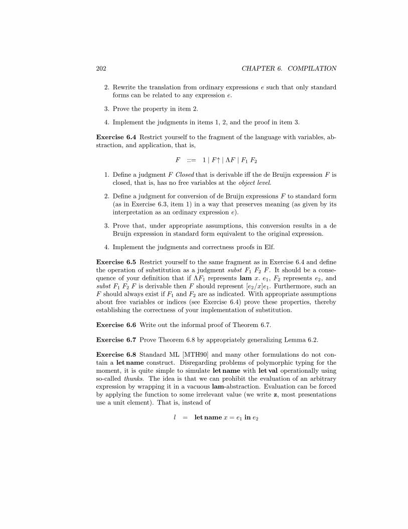
202 CHAPTER 6. COMPILATION
2. Rewrite the translation from ordinary expressions e such that only standardforms can be related to any expression e.
3. Prove the property in item 2.
4. Implement the judgments in items 1, 2, and the proof in item 3.
Exercise 6.4 Restrict yourself to the fragment of the language with variables, ab-straction, and application, that is,
F ::= 1 | F↑ | ΛF | F1 F2
1. Define a judgment F Closed that is derivable iff the de Bruijn expression F isclosed, that is, has no free variables at the object level.
2. Define a judgment for conversion of de Bruijn expressions F to standard form(as in Exercise 6.3, item 1) in a way that preserves meaning (as given by itsinterpretation as an ordinary expression e).
3. Prove that, under appropriate assumptions, this conversion results in a deBruijn expression in standard form equivalent to the original expression.
4. Implement the judgments and correctness proofs in Elf.
Exercise 6.5 Restrict yourself to the same fragment as in Exercise 6.4 and definethe operation of substitution as a judgment subst F1 F2 F . It should be a conse-quence of your definition that if ΛF1 represents lam x. e1, F2 represents e2, andsubst F1 F2 F is derivable then F should represent [e2/x]e1. Furthermore, such anF should always exist if F1 and F2 are as indicated. With appropriate assumptionsabout free variables or indices (see Exercise 6.4) prove these properties, therebyestablishing the correctness of your implementation of substitution.
Exercise 6.6 Write out the informal proof of Theorem 6.7.
Exercise 6.7 Prove Theorem 6.8 by appropriately generalizing Lemma 6.2.
Exercise 6.8 Standard ML [MTH90] and many other formulations do not con-tain a letname construct. Disregarding problems of polymorphic typing for themoment, it is quite simple to simulate letname with let val operationally usingso-called thunks. The idea is that we can prohibit the evaluation of an arbitraryexpression by wrapping it in a vacuous lam-abstraction. Evaluation can be forcedby applying the function to some irrelevant value (we write z, most presentationsuse a unit element). That is, instead of
l = letname x = e1 in e2

6.8. EXERCISES 203
we writel′ = let val x′ = lam y. e1 in [x′ z/x]e2
where y is a new variable not free in e1.
1. Show a counterexample to the conjecture “If l is closed, l ↪→ v, and l′ ↪→ v′
then v = v′ (modulo renaming of bound variables)”.
2. Show a counterexample to the conjecture “. l : τ iff . l′ : τ”.
3. Define an appropriate congruence e ∼= e′ such that l ∼= l′ and if e ∼= e′, e ↪→ vand e′ ↪→ v′ then v ∼= v′.
4. Prove the properties in item 3.
5. Prove that if the values v and v′ are natural numbers, then v ∼= v′ iff v = v′.
We need a property such as the last one to make sure that the congruence we definedoes not identify all expressions. It is a special case of a so-called observationalequivalence (see ??).
Exercise 6.9 The rules for evaluation in Section 6.2 have the drawback that look-ing up a variable in an environment and evaluation are mutually recursive, sincethe environment contains unevaluated expressions. Such expressions may be addedto the environment during evaluation of a letname or fix construct. In the defi-nition of Standard ML [MTH90] this problem is avoided by disallowing let name(see Exercise 6.8) and by syntactically restricting occurrences of the fix construct.When translated into our setting, this restriction states that all occurrences of fix-point expressions must be of the form fix x. lam y. e. Then we can dispense withthe environment constructor + and instead introduce a constructor ∗ that builds arecursive environment. More precisely, we have
Environments η ::= · | η,W | η ∗ F
The evaluation rules fev 1+, fev ↑+, and fev fix on page 161 are replaced by
fev fix∗K ` fix′ F ↪→ {K ∗ F ;F}
fev 1∗K ∗ F ` 1 ↪→ {K ∗ F ;F}
K ` F ↪→Wfev ↑∗
K ∗ F ′ ` F↑ ↪→W

204 CHAPTER 6. COMPILATION
1. Implement this modified evaluation judgment in Elf.
2. Prove that under the restriction that all occurrences of fix′ in de Bruijn ex-pressions have the form fix′ ΛF for some F , the two sets of rules define anequivalent operational semantics. Take care to give a precise definition of thenotion of equivalence you are considering and explain why it is appropriate.
3. Represent the equivalence proof in Elf.
4. Exhibit a counterexample which shows that some restriction on fixpoint ex-pressions (as, for example, the one given above) is necessary in order to pre-serve equivalence.
5. Under the syntactic restriction from above we can also formulate a semanticswhich requires no new constructor for environments by forming closures overfixpoint expressions. Then we need to add another rule for application ofan expression which evaluates to a closure over a fixpoint expression. Writeout the rules and prove its equivalence to either the system above or theoriginal evaluation judgment for de Bruijn expressions (under the appropriaterestriction).
Exercise 6.10 Show how the effect of the bind instruction can be simulated in theCLS machine using the other instructions. Sketch the correctness proof for thissimulation.
Exercise 6.11 Complete the presentation of the CLS machine by adding recursion.In particular
1. Complete the computation rules on page 173.
2. Add appropriate cases to the proofs of Lemmas 6.16, and 6.18.
Exercise 6.12 Prove the following carefully.
1. The concatenation operation “◦” on computations is associative.
2. The subcomputation relation “<” is transitive (Lemma 6.17).
Show the implementation of your proofs as type families in Elf.
Exercise 6.13 The machine instructions from Section 6.3 can simply quote ex-pressions in de Bruijn form and consider them as instructions. As a next step inthe (abstract) compilation process, we can convert the expressions to lower-levelcode which simulates the effect of instructions on the environment and value stacksin smaller steps.
1. Design an appropriate language of operations.
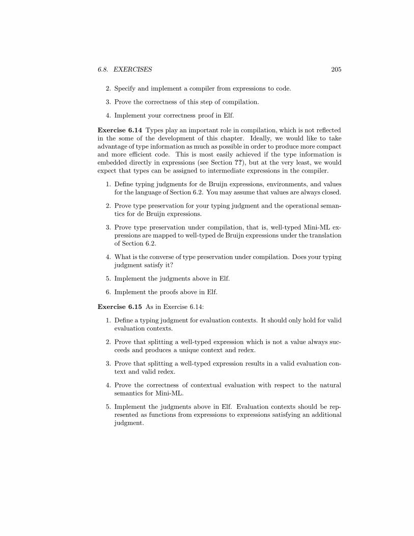
6.8. EXERCISES 205
2. Specify and implement a compiler from expressions to code.
3. Prove the correctness of this step of compilation.
4. Implement your correctness proof in Elf.
Exercise 6.14 Types play an important role in compilation, which is not reflectedin the some of the development of this chapter. Ideally, we would like to takeadvantage of type information as much as possible in order to produce more compactand more efficient code. This is most easily achieved if the type information isembedded directly in expressions (see Section ??), but at the very least, we wouldexpect that types can be assigned to intermediate expressions in the compiler.
1. Define typing judgments for de Bruijn expressions, environments, and valuesfor the language of Section 6.2. You may assume that values are always closed.
2. Prove type preservation for your typing judgment and the operational seman-tics for de Bruijn expressions.
3. Prove type preservation under compilation, that is, well-typed Mini-ML ex-pressions are mapped to well-typed de Bruijn expressions under the translationof Section 6.2.
4. What is the converse of type preservation under compilation. Does your typingjudgment satisfy it?
5. Implement the judgments above in Elf.
6. Implement the proofs above in Elf.
Exercise 6.15 As in Exercise 6.14:
1. Define a typing judgment for evaluation contexts. It should only hold for validevaluation contexts.
2. Prove that splitting a well-typed expression which is not a value always suc-ceeds and produces a unique context and redex.
3. Prove that splitting a well-typed expression results in a valid evaluation con-text and valid redex.
4. Prove the correctness of contextual evaluation with respect to the naturalsemantics for Mini-ML.
5. Implement the judgments above in Elf. Evaluation contexts should be rep-resented as functions from expressions to expressions satisfying an additionaljudgment.

206 CHAPTER 6. COMPILATION
6. Implement the proofs above in Elf.
Exercise 6.16 Show that the purely expression-based natural semantics of Sec-tion 2.3 is equivalent to the one based on a separation between expressions andvalues in Section 6.5. Implement your proof, including all necessary lemmas, in Elf.
Exercise 6.17 Carry out the alternative proof of completeness of the continuationmachine sketched on page 189. Implement the proof and all necessary lemmas inElf.
Exercise 6.18 Do the equivalence proof in Lemma 6.22 and the alternative in Ex-ercise 6.17 define the same relation between derivations? If so, exhibit the bijectionin the form of a higher-level judgment relating the Elf implementations. Be carefulto write out necessary lemmas regarding concatenation. You may restrict yourselfto functional abstraction, application, and the necessary computation rules.
Exercise 6.19 Not every valid state of the CPM machine (according to the typingjudgments in Section 6.6) can be reached by a computation starting from someinitial state of the form init � ev e where · ` e : τ .
1. Exhibit a valid, but unreachable state.
2. Modify the validity judgments so that every valid machine state can in factbe reached from some initial state.
3. Prove this property.
4. Implement your proof in Elf.

Bibliography
[ACCL91] Martın Abadi, Luca Cardelli, Pierre-Louis Curien, and Jean-JacquesLevy. Explicit substitutions. Journal of Functional Programming,1(4):375–416, October 1991.
[AINP88] Peter B. Andrews, Sunil Issar, Daniel Nesmith, and Frank Pfenning.The TPS theorem proving system. In Ewing Lusk and Russ Overbeek,editors, 9th International Conference on Automated Deduction, pages760–761, Argonne, Illinois, May 1988. Springer-Verlag LNCS 310. Sys-tem abstract.
[All75] William Allingham. In Fairy Land. Longmans, Green, and Co., London,England, 1875.
[CCM87] Guy Cousineau, Pierre-Louis Curien, and Michel Mauny. The categori-cal abstract machine. Science of Computer Programming, 8, May 1987.
[CDDK86] Dominique Clement, Joelle Despeyroux, Thierry Despeyroux, and GillesKahn. A simple applicative language: Mini-ML. In Proceedings of the1986 Conference on LISP and Functional Programming, pages 13–27.ACM Press, 1986.
[CF58] H. B. Curry and R. Feys. Combinatory Logic. North-Holland, Amster-dam, 1958.
[Chu32] A. Church. A set of postulates for the foundation of logic I. Annals ofMathematics, 33:346–366, 1932.
[Chu33] A. Church. A set of postulates for the foundation of logic II. Annals ofMathematics, 34:839–864, 1933.
[Chu40] Alonzo Church. A formulation of the simple theory of types. Journalof Symbolic Logic, 5:56–68, 1940.
[Chu41] Alonzo Church. The Calculi of Lambda-Conversion. Princeton Univer-sity Press, Princeton, New Jersey, 1941.
207
208 BIBLIOGRAPHY
[Coq91] Thierry Coquand. An algorithm for testing conversion in type theory.In Gerard Huet and Gordon Plotkin, editors, Logical Frameworks, pages255–279. Cambridge University Press, 1991.
[Cur34] H. B. Curry. Functionality in combinatory logic. Proceedings of theNational Academy of Sciences, U.S.A., 20:584–590, 1934.
[dB68] N.G. de Bruijn. The mathematical language AUTOMATH, its usage,and some of its extensions. In M. Laudet, editor, Proceedings of the Sym-posium on Automatic Demonstration, pages 29–61, Versailles, France,December 1968. Springer-Verlag LNM 125.
[dB72] N. G. de Bruijn. Lambda-calculus notation with nameless dummies: atool for automatic formula manipulation with application to the Church-Rosser theorem. Indag. Math., 34(5):381–392, 1972.
[DFH+93] Gilles Dowek, Amy Felty, Hugo Herbelin, Gerard Huet, Chet Murthy,Catherine Parent, Christine Paulin-Mohring, and Benjamin Werner.The Coq proof assistant user’s guide. Rapport Techniques 154, INRIA,Rocquencourt, France, 1993. Version 5.8.
[DM82] Luis Damas and Robin Milner. Principal type schemes for functionalprograms. In Conference Record of the 9th ACM Symposium on Princi-ples of Programming Languages (POPL’82), pages 207–212. ACM Press,1982.
[Dow93] Gilles Dowek. The undecidability of typability in the lambda-pi-calculus.In M. Bezem and J.F. Groote, editors, Proceedings of the InternationalConference on Typed Lambda Calculi and Applications, pages 139–145,Utrecht, The Netherlands, March 1993. Springer-Verlag LNCS 664.
[DP91] Scott Dietzen and Frank Pfenning. A declarative alternative to assert inlogic programming. In Vijay Saraswat and Kazunori Ueda, editors, In-ternational Logic Programming Symposium, pages 372–386. MIT Press,October 1991.
[Ell89] Conal Elliott. Higher-order unification with dependent types. In N. Der-showitz, editor, Rewriting Techniques and Applications, pages 121–136,Chapel Hill, North Carolina, April 1989. Springer-Verlag LNCS 355.
[Ell90] Conal M. Elliott. Extensions and Applications of Higher-Order Unifi-cation. PhD thesis, School of Computer Science, Carnegie Mellon Uni-versity, May 1990. Available as Technical Report CMU-CS-90-134.

BIBLIOGRAPHY 209
[FP91] Tim Freeman and Frank Pfenning. Refinement types for ML. In Pro-ceedings of the SIGPLAN ’91 Symposium on Language Design and Im-plementation, pages 268–277, Toronto, Ontario, June 1991. ACM Press.
[Gar92] Philippa Gardner. Representing Logics in Type Theory. PhD thesis,University of Edinburgh, July 1992. Available as Technical Report CST-93-92.
[Gen35] Gerhard Gentzen. Untersuchungen uber das logische Schließen. Mathe-matische Zeitschrift, 39:176–210, 405–431, 1935. English translation inM. E. Szabo, editor, The Collected Papers of Gerhard Gentzen, pages68–131, North-Holland, 1969.
[Geu92] Herman Geuvers. The Church-Rosser property for βη-reduction in typedλ-calculi. In A. Scedrov, editor, Seventh Annual IEEE Symposium onLogic in Computer Science, pages 453–460, Santa Cruz, California, June1992.
[Gol81] Warren D. Goldfarb. The undecidability of the second-order unificationproblem. Theoretical Computer Science, 13:225–230, 1981.
[GS84] Ferenc Gecseg and Magnus Steinby. Tree Automata. Akademiai Kiado,Budapest, 1984.
[Gun92] Carl A. Gunter. Semantics of Programming Languages. MIT Press,Cambridge, Massachusetts, 1992.
[Han91] John J. Hannan. Investigating a Proof-Theoretic Meta-Language forFunctional Programs. PhD thesis, University of Pennsylvania, January1991. Available as Technical Report MS-CIS-91-09.
[Han93] John Hannan. Extended natural semantics. Journal of Functional Pro-gramming, 3(2):123–152, April 1993.
[Har90] Robert Harper. Systems of polymorphic type assignment in LF. Tech-nical Report CMU-CS-90-144, Carnegie Mellon University, Pittsburgh,Pennsylvania, June 1990.
[HB34] David Hilbert and Paul Bernays. Grundlagen der Mathematik. Springer-Verlag, Berlin, 1934.
[Her30] Jacques Herbrand. Recherches sur la theorie de la demonstration.Travaux de la Societe des Sciences et de Lettres de Varsovic, 33, 1930.
[HHP93] Robert Harper, Furio Honsell, and Gordon Plotkin. A framework fordefining logics. Journal of the Association for Computing Machinery,40(1):143–184, January 1993.

210 BIBLIOGRAPHY
[HM89] John Hannan and Dale Miller. A meta-logic for functional programming.In H. Abramson and M. Rogers, editors, Meta-Programming in LogicProgramming, chapter 24, pages 453–476. MIT Press, 1989.
[HM90] John Hannan and Dale Miller. From operational semantics to abstractmachines: Preliminary results. In M. Wand, editor, Proceedings ofthe 1990 ACM Conference on Lisp and Functional Programming, pages323–332, Nice, France, 1990.
[How80] W. A. Howard. The formulae-as-types notion of construction. In J. P.Seldin and J. R. Hindley, editors, To H. B. Curry: Essays on Combina-tory Logic, Lambda Calculus and Formalism, pages 479–490. AcademicPress, 1980. Hitherto unpublished note of 1969, rearranged, corrected,and annotated by Howard.
[HP92] John Hannan and Frank Pfenning. Compiler verification in LF. InAndre Scedrov, editor, Seventh Annual IEEE Symposium on Logic inComputer Science, pages 407–418, Santa Cruz, California, June 1992.
[HP00] Robert Harper and Frank Pfenning. On equivalence and canonical formsin the LF type theory. Technical Report CMU-CS-00-148, Departmentof Computer Science, Carnegie Mellon University, July 2000.
[Hue73] Gerard Huet. The undecidability of unification in third order logic.Information and Control, 22(3):257–267, 1973.
[Hue75] Gerard Huet. A unification algorithm for typed λ-calculus. TheoreticalComputer Science, 1:27–57, 1975.
[JL87] Joxan Jaffar and Jean-Louis Lassez. Constraint logic programming. InProceedings of the Fourteenth Annual ACM Symposium on Principlesof Programming Languages, pages 111–119, Munich, Germany, January1987. ACM Press.
[Kah87] Gilles Kahn. Natural semantics. In Proceedings of the Symposium onTheoretical Aspects of Computer Science, pages 22–39. Springer-VerlagLNCS 247, 1987.
[Lan64] P. J. Landin. The mechanical evaluation of expressions. ComputerJournal, 6:308–320, 1964.
[Lia95] Chuck Liang. Object-Level Substitutions, Unification and Generalizationin Meta Logic. PhD thesis, University of Pennsylvania, December 1995.
[Mai92] H.G. Mairson. Quantifier elimination and parametric polymorphism inprogramming languages. Journal of Functional Programming, 2(2):213–226, April 1992.

BIBLIOGRAPHY 211
[Mil78] Robin Milner. A theory of type polymorphism in programming. JournalOf Computer And System Sciences, 17:348–375, August 1978.
[Mil91] Dale Miller. A logic programming language with lambda-abstraction,function variables, and simple unification. Journal of Logic and Com-putation, 1(4):497–536, 1991.
[ML85] Per Martin-Lof. On the meanings of the logical constants and the jus-tifications of the logical laws. Technical Report 2, Scuola di Specializ-zazione in Logica Matematica, Dipartimento di Matematica, Universitadi Siena, 1985.
[ML96] Per Martin-Lof. On the meanings of the logical constants and the jus-tifications of the logical laws. Nordic Journal of Philosophical Logic,1(1):11–60, 1996.
[MNPS91] Dale Miller, Gopalan Nadathur, Frank Pfenning, and Andre Scedrov.Uniform proofs as a foundation for logic programming. Annals of Pureand Applied Logic, 51:125–157, 1991.
[MTH90] Robin Milner, Mads Tofte, and Robert Harper. The Definition of Stan-dard ML. MIT Press, Cambridge, Massachusetts, 1990.
[New65] Allen Newell. Limitations of the current stock of ideas about problemsolving. In A. Kent and O. E. Taulbee, editors, Electronic InformationHandling, pages 195–208, Washington, D.C., 1965. Spartan Books.
[NGdV94] R.P. Nederpelt, J.H. Geuvers, and R.C. de Vrijer, editors. Selected Pa-pers on Automath, volume 133 of Studies in Logic and the Foundationsof Mathematics. North-Holland, 1994.
[NM98] Gopalan Nadathur and Dale Miller. Higher-order logic programming.In D.M. Gabbay, C.J. Hogger, and J.A. Robinson, editors, Handbookof Logic in Artificial Intelligence and Logic Programming, volume 5,chapter 8. Oxford University Press, 1998.
[NM99] Gopalan Nadathur and Dustin J. Mitchell. System description:Teyjus—a compiler and abstract machine based implementation oflambda Prolog. In H. Ganzinger, editor, Proceedings of the 16th Interna-tional Conference on Automated Deduction (CADE-16), pages 287–291,Trento, Italy, July 1999. Springer-Verlag LNCS.
[Pau86] Lawrence C. Paulson. Natural deduction as higher-order resolution.Journal of Logic Programming, 3:237–258, 1986.

212 BIBLIOGRAPHY
[Pau94] Lawrence C. Paulson. Isabelle: A Generic Theorem Prover. Springer-Verlag LNCS 828, 1994.
[Pfe91a] Frank Pfenning. Logic programming in the LF logical framework. InGerard Huet and Gordon Plotkin, editors, Logical Frameworks, pages149–181. Cambridge University Press, 1991.
[Pfe91b] Frank Pfenning. Unification and anti-unification in the Calculus of Con-structions. In Sixth Annual IEEE Symposium on Logic in ComputerScience, pages 74–85, Amsterdam, The Netherlands, July 1991.
[Pfe92] Frank Pfenning, editor. Types in Logic Programming. MIT Press, Cam-bridge, Massachusetts, 1992.
[Pfe93] Frank Pfenning. Refinement types for logical frameworks. In HermanGeuvers, editor, Informal Proceedings of the Workshop on Types forProofs and Programs, pages 285–299, Nijmegen, The Netherlands, May1993.
[Pfe94] Frank Pfenning. Elf: A meta-language for deductive systems. InA. Bundy, editor, Proceedings of the 12th International Conferenceon Automated Deduction, pages 811–815, Nancy, France, June 1994.Springer-Verlag LNAI 814. System abstract.
[Plo75] G. D. Plotkin. Call-by-name, call-by-value and the λ-calculus. Theoret-ical Computer Science, 1:125–159, 1975.
[Plo77] G. D. Plotkin. LCF considered as a programming language. TheoreticalComputer Science, 5(3):223–255, 1977.
[Plo81] Gordon D. Plotkin. A structural approach to operational seman-tics. Technical Report DAIMI FN-19, Computer Science Department,Aarhus University, Aarhus, Denmark, September 1981.
[PM93] Christine Paulin-Mohring. Inductive definitions in the system Coq:Rules and properties. In M. Bezem and J.F. Groote, editors, Pro-ceedings of the International Conference on Typed Lambda Calculi andApplications, pages 328–345, Utrecht, The Netherlands, March 1993.Springer-Verlag LNCS 664.
[Pra65] Dag Prawitz. Natural Deduction. Almquist & Wiksell, Stockholm, 1965.
[PS99] Frank Pfenning and Carsten Schurmann. System description: Twelf —a meta-logical framework for deductive systems. In H. Ganzinger, edi-tor, Proceedings of the 16th International Conference on Automated De-duction (CADE-16), pages 202–206, Trento, Italy, July 1999. Springer-Verlag LNAI 1632.

BIBLIOGRAPHY 213
[PW90] David Pym and Lincoln Wallen. Investigations into proof-search ina system of first-order dependent function types. In M.E. Stickel, edi-tor, Proceedings of the 10th International Conference on Automated De-duction, pages 236–250, Kaiserslautern, Germany, July 1990. Springer-Verlag LNCS 449.
[PW91] David Pym and Lincoln A. Wallen. Proof search in the λΠ-calculus. InGerard Huet and Gordon Plotkin, editors, Logical Frameworks, pages309–340. Cambridge University Press, 1991.
[Pym90] David Pym. Proofs, Search and Computation in General Logic. PhDthesis, University of Edinburgh, 1990. Available as CST-69-90, alsopublished as ECS-LFCS-90-125.
[Pym92] David Pym. A unification algorithm for the λΠ-calculus. InternationalJournal of Foundations of Computer Science, 3(3):333–378, September1992.
[Rob65] J. A. Robinson. A machine-oriented logic based on the resolution prin-ciple. Journal of the ACM, 12(1):23–41, January 1965.
[RP96] Ekkehard Rohwedder and Frank Pfenning. Mode and termination check-ing for higher-order logic programs. In Hanne Riis Nielson, editor, Pro-ceedings of the European Symposium on Programming, pages 296–310,Linkoping, Sweden, April 1996. Springer-Verlag LNCS 1058.
[Sal90] Anne Salvesen. The Church-Rosser theorem for LF with βη-reduction.Unpublished notes to a talk given at the First Workshop on LogicalFrameworks in Antibes, France, May 1990.
[Sch00] Carsten Schurmann. Automating the Meta Theory of Deductive Sys-tems. PhD thesis, Department of Computer Science, Carnegie MellonUniversity, August 2000. Available as Technical Report CMU-CS-00-146.
[SH84] Peter Schroeder-Heister. A natural extension of natural deduction. TheJournal of Symbolic Logic, 49(4):1284–1300, December 1984.
[Twe98] Twelf home page. Available at http://www.cs.cmu.edu/~twelf, 1998.


![Deduction, Collection and Recovery of · PDF file28 Deduction, Collection and Recovery of Tax 28.1 Deduction and Collection of Tax at Source and Advance Payment [Section 190] The total](https://img.pdfslide.net/doc/110x75/5aadf0d27f8b9adb688bae6c/deduction-collection-and-recovery-of-deduction-collection-and-recovery-of-tax.jpg)


![ADVANCE TAX, TAX DEDUCTION AT SOURCE AND … · advance tax [Section 207 to 208] Collection of tax at source [Section 206C] Computation of advance tax [Section 209] Installments of](https://img.pdfslide.net/doc/110x75/5fa63a289ca1172a0e527830/advance-tax-tax-deduction-at-source-and-advance-tax-section-207-to-208-collection.jpg)