Computation of 3D Weld Pool Surface from the Slope Field and Point Tracking of Laser Beams

G. Saeed, M. Lou, Y.M. Zhang Center for Manufacturing and Department of Electrical and Computer Engineering

College of Engineering, University of Kentucky Lexington, KY 40506, U.S.A.

Abstract – A novel computation method of the 3D weld pool surface from specular

reflection of laser beams is presented in this paper. The mathematical model for the three-dimensional surface measurement technique has been developed. Structured pattern of laser is projected on the weld pool in molten state and the reflection observed using a CCD camera. These reflected patterns can be tracked using image processing techniques including optical flow and moving point tracking. A simulation model has been developed implementing these techniques. The movement of reflected laser during welding process is indicative of change in state of weld pool. The surface slope field is calculated from law of reflection and is used to compute the 3D surface of the weld pool. The measurement technique is tested on objects with a priori knowledge of geometry having specular surface to test the effectiveness of the measurement technique.

1. Introduction

Welding has become indispensable tool for many industries because of the basic role of materials joining in manufacturing industry. Some welding techniques, such as Gas Tungsten Arc Welding (GTAW) produce high quality welds. For critical and accurate joining where the weld quality must be ensured such as for the root pass and for the welding of advanced materials, GTAW is often used in such applications to produce high-quality weld because of its capability in precision control of the fusion process [1]. In an arc welding process, the electric arc heats the work piece and the molten pool. The temperature gradient on the pool surface creates difference in the surface tension that drives the liquid metal flow. The electromagnetic force associated with the welding current flow also drives the liquid metal flow. The fluid flow driven convection which is the major heat transfer form in the weld pool, controls the geometry of the fusion zone. Further, the geometry of the fusion zone determines how the weld pool surface is deformed under arc pressure and gravity. The deformation of the weld pool is a determining factor for the distribution of the arc and the distribution of the current flow (thus the electromagnetic force). Finally, the surface tension depends on the deformation of the weld pool surface and the distribution of the arc (heat input flux and the temperature field). Hence, a chain reaction and strong coupling of heat transfer, fluid flow, and geometrical deformation exists in the weld pool. The physical processes occurring in the weld pool are very complicated.

Due to the extreme complexity, analytic methods in general cannot adequately describe the physical phenomena associated with arc welding processes. Numerical analysis has been a powerful tool in modeling these phenomena and revealing their fundamentals. However, in order to confirm the effectiveness of the numerical models, the calculated results must be compared

with experimental data. Ideally, experimental data for temperature field [2, 3], fluid flow [4, 5], fusion zone geometry [6, 7], and pool surface deformation [4, 8, 9, 10, 11] are all required.

Although the temperature field and the fusion zone geometry can be measured using

existing methods, the observation and measurement of the deformation of the pool surface and the fluid flow in the weld pool remains difficult. The strong illumination from the arc disqualifies most visual technologies for possible applications in arc welding. The specular surface of the weld pool adds another difficulty. Hence, despite the importance of observation and measurement of fluid flow and pool surface, only limited solutions have been obtained to date. This paper will focus on the measurement of the surface of the weld pool which will significantly benefit the development of the numerical models.

To measure the three-dimensional surface of the weld pool, a sensing system was

developed at the University of Kentucky using a specific high shutter speed camera system and a specific optic grid which consists of a grid and a frosted glass [12, 13]. A recent study has been done to mathematically model this sensing system in order to optimize the design [14]. While this measurement system can visualize the three-dimensional pool surface by the deformed laser stripes projected through the specific optic grid, it requires the specific camera system whose shutter is synchronized with a pulsed laser so that the intensity of the laser stripes is much stronger than that of the arc during imaging. The acquired quality image of the weld pool surface makes this system suitable for laboratory studies, but the high capital investment of the specific camera system affects its affordability in real-time control applications. To develop a cost-effect system for real-time control applications, this paper proposes a novel sensing technique which only uses a high-speed digital camera and laser and requires no synchronization between the camera and laser. Band pass filters centering at the laser beam’s wave-length are mounted on camera to remove the arc light, and other light sources from entering the camera.

This paper is organized as follows: section Two provides a description of the sensing

technique. In section Three, the mathematical model of weld pool will be ascertained. In section Four, the optical flow tracking method will be introduced. Section Five, will use the optical flow concepts from image processing to analyze the optical points moving in the plane. The reflected points will be used to calculate the slope field of the weld pool surface and the 3D- surface reconstructed from the slope field in section Six. Section seven will conclude all of the above work and present ideas for future work. 2. Description of Proposed Sensing Technique

In the proposed sensing technique, a laser is used to illuminate the weld pool surface. The

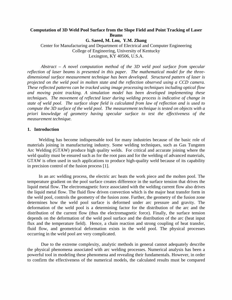
corresponding reflected rays are completely determined by the slope of the weld pool interface and the point where they hit the weld pool (also called the intersection points). Figure 1 illustrates the sensing mechanism used. By tracking the reflected rays and computing the slope field of the weld pool surface, the three-dimensional weld pool shape can be restituted.

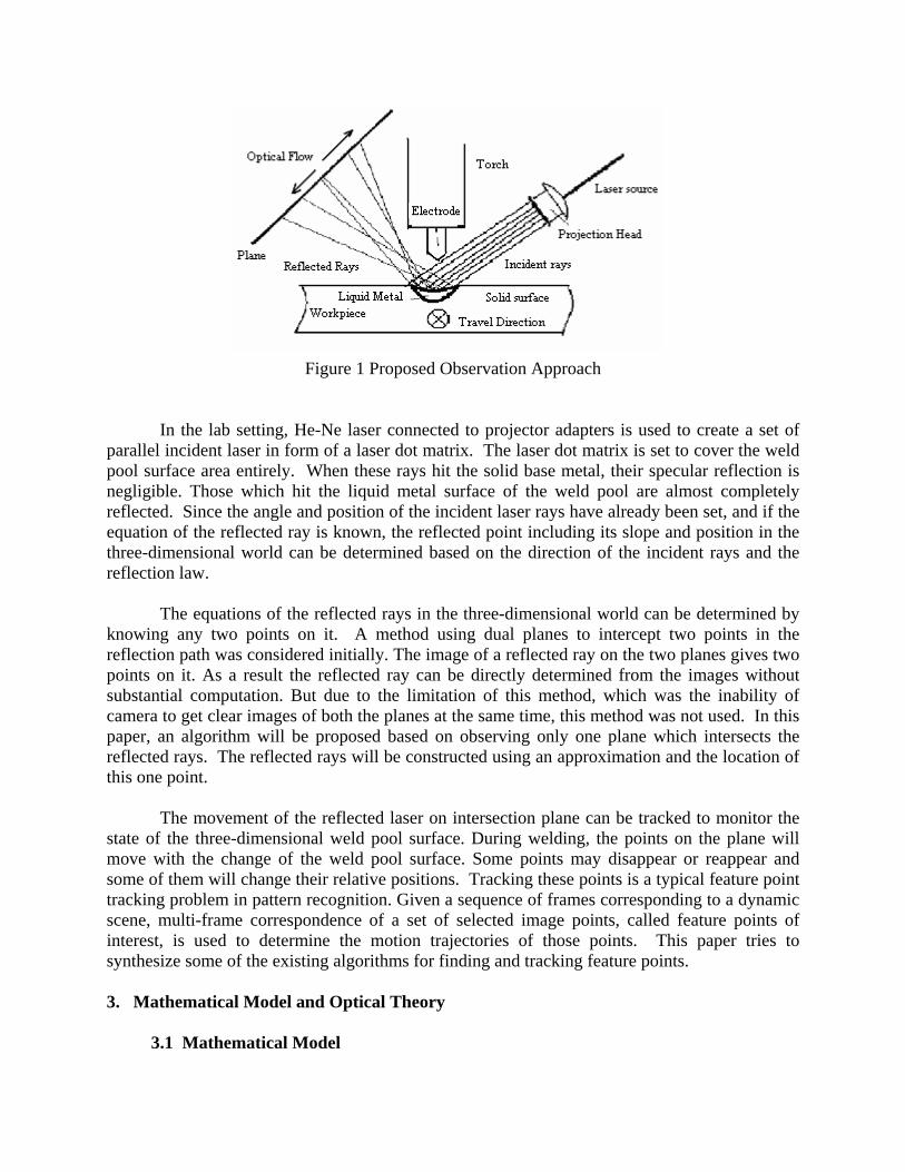
Figure 1 Proposed Observation Approach

In the lab setting, He-Ne laser connected to projector adapters is used to create a set of

parallel incident laser in form of a laser dot matrix. The laser dot matrix is set to cover the weld pool surface area entirely. When these rays hit the solid base metal, their specular reflection is negligible. Those which hit the liquid metal surface of the weld pool are almost completely reflected. Since the angle and position of the incident laser rays have already been set, and if the equation of the reflected ray is known, the reflected point including its slope and position in the three-dimensional world can be determined based on the direction of the incident rays and the reflection law.

The equations of the reflected rays in the three-dimensional world can be determined by

knowing any two points on it. A method using dual planes to intercept two points in the reflection path was considered initially. The image of a reflected ray on the two planes gives two points on it. As a result the reflected ray can be directly determined from the images without substantial computation. But due to the limitation of this method, which was the inability of camera to get clear images of both the planes at the same time, this method was not used. In this paper, an algorithm will be proposed based on observing only one plane which intersects the reflected rays. The reflected rays will be constructed using an approximation and the location of this one point.

The movement of the reflected laser on intersection plane can be tracked to monitor the

state of the three-dimensional weld pool surface. During welding, the points on the plane will move with the change of the weld pool surface. Some points may disappear or reappear and some of them will change their relative positions. Tracking these points is a typical feature point tracking problem in pattern recognition. Given a sequence of frames corresponding to a dynamic scene, multi-frame correspondence of a set of selected image points, called feature points of interest, is used to determine the motion trajectories of those points. This paper tries to synthesize some of the existing algorithms for finding and tracking feature points. 3. Mathematical Model and Optical Theory 3.1 Mathematical Model

The welding electrode is considered to be above the work piece in the z direction and it moves in the x direction at a constant speed u . A moving coordinate system is so chosen that its origin is at the center of the welding electrode. The equation that governs the balance at the liquid-vapor and solid-liquid interface under the quasi-steady state condition is used to obtain the shapes of these interfaces [4, 8, 9, 10, 11]. The solid-liquid interface ),( yxSs is given below as:

( ))2exp(

)2(2exp

32),( 2

2

2

231

32

ss

so

o

ompm

m

ss L

yd

PeRxR

TTCLv

APL

KyxS −⎟⎟

⎠

⎞⎜⎜⎝

⎛ +−⎟⎟

⎠

⎞⎜⎜⎝

⎛ −+⎟⎟⎠

⎞⎜⎜⎝

⎛=

πρ (1)

where 02RLd ss −= if soPeRx 2−≥ , else 02RLd ss += , sK and sL are given by

31

2

)]([3

;)]([

)]([⎟⎟⎠

⎞⎜⎜⎝

⎛

−++=

−++

−+=

ompmb

os

ompmbm

ompms TTCLLv

APRL

TTCLLLTTCL

Kπρ

, and sPe is defined as the

Peclete parameter and is given by s

s avR

Pe 0= . [14]

The other parameters with their values are summarized in the table below.

Table 1 Values of Parameters Used in Weld Pool Equation

Name and Notation Values of thermo physical properties

Power, P 2000 )(W

Density, ρ 7500(7000)kg 3−m liquid(solid) state

Melting temperature, mT 1810K

Boiling temperature, bT 3342K

Work piece Initial Temperature, oT 50K

Specific heat capacitance, pC 678.5 (636.7)Jkg 11 −− K

Latent heat of fusion, mL 151072.2 −× Jkg

Latent heat of boiling, bL 16103.6 −× Jkg

Diffusivity for the liquid state, lα 12610223.5 −−× sm

Diffusivity for the solid state, sα 12610435.6 −−× sm Radius or arc/laser, oR 0.0003 )(m Speed of welding, v 0.02 )/( sm

The width of the weld is typically considered to be the width of the solid-liquid interface

profile at the surface of the work piece. Figure 2 shows a Matlab simulation of Equation 1 to obtain the three dimension solid-liquid weld pool interface.

It should be pointed out that the above analytical models are derived from laser welding. Although laser weld pools are in general different from those of gas tungsten arc, shallow laser weld pools generated by low power, defocused (large diameter) beam should be similar to those of gas tungsten arc. Further, the focus of the present research is to measure three-dimensional surfaces of weld pool and the measurement system is modeled to study the effect of the system parameters on measurement results. The surface of the weld pool is given only as input parameters. More importantly and practically, limited work has been done to establish analytical models for gas tungsten arc weld pools. Hence, the analytical models derived from laser welding are used to approximate gas tungsten weld pool surfaces using energy beam wider than typical laser applications in this paper.

Figure 2 Three dimensional Solid-liquid Weld Pool (Front View). The weld pool surface is

shallow because its depth is 0.05 mm while its width is 4 mm.

3.2 Optical Geometry 3.2.1. Incident line

The incident laser rays are described by direction vectors and the coordinates of laser

source point. tpxtx xjiji ×+= )0()( ,, , tpyty yjiji ×+= )0()( ,, tpztz zjiji ×+= )0()( ,, 2

Where [ )0(, jix , )0(, jiy )0(, jiz ] represents the coordinates of a laser source in real world, [ ]zyx ppp ,, is the direction vector of laser beam. The parameter t is independent variable.

3.2.2 Normal line [15,16]

Suppose S is a surface with Equation nzyxF =),,( . Let ),,( 000 zyxP = be a point on S . Let C be any curve that lies on the surface S and passes through the point P. The curve C is described by a continuous vector function ( ))(),(),()( tztytxtr = . Let ot be the parameter value corresponding to P ; that is ),,()( 0000 zyxtr = Since C lies on S , any point ( ))(),(),( tztytx must satisfy the Equation for S , that is,

( ) ntztytxF =)(),(),( 3

If x , y and z are differentiable functions of t and F is also differentiable, then Chain Rule can be used to differentiate both sides as follows:

0=∂∂

+∂∂

+∂∂

dtdz

zF

dtdy

yF

dtdx

xF 4

However, since ( )zyx FFFF ,,=∇ and ( ))(),(),()( tztytxtr ′′′=′ , the above Equation can be written in terms of a dot product as 0)( =′•∇ trF . In particular, when 0tt = ,

( )0000 ,,)( zyxtr = then,

0)(),,( 0000 =′•∇ trzyxF 5

It implies that the gradient vector ),,( 000 zyxF∇ at P , is tangent to vector )( 0tr′ at any curve C on S that passes through P . Since 0),,( 000 ≠∇ zyxF , it is natural to define tangent plane to ( ))(),(),( tztytxF = k at P as the plane that passes through P and has normal vector ),,( 000 zyxF∇ . The normal line to S at P is the line passing through P and perpendicular to tangent plane. The direction of normal line is therefore given by the gradient vector ),,( 000 zyxF∇ and its symmetric equations thus are

),(),(),( 00,0

0

00,0

0

00,0

0

zyxFzz

zyxFyy

zyxFxx

zyx

−=

−=

− 6

In the special case in which the equation of a surface S is of the form ),( yxfz = (that is, S is a function f of two variables), the equation can be rewritten as:

0),(),,( =−= zyxfzyxF 7

and considering S as a weld pool surface with Equation ),( yxfz = . Then

1),()(),()(),(

00,0

0,000,0

0,000,0

−=

=

=

zyxFyxfzyxFyxfzyxF

z

yy

xx

8

3.2.3. Reflected Line

The reflected lines were calculated based on law of reflection, which states that the incident angle of a light beam is equal to the angle of reflection. Figure 3, illustrates this concept where iθ is equal to rθ .

From Figure 3, suppose ik is the angle of the incident ray measured from the horizon and θ is the slope angle of the weld pool interface. Then,

θπθθ +−== iir k2

9

The angle of the reflected line from horizon is: rir kk θπ 2+−= 10

Figure 3 Reflected Rays from Weld Pool Interface.

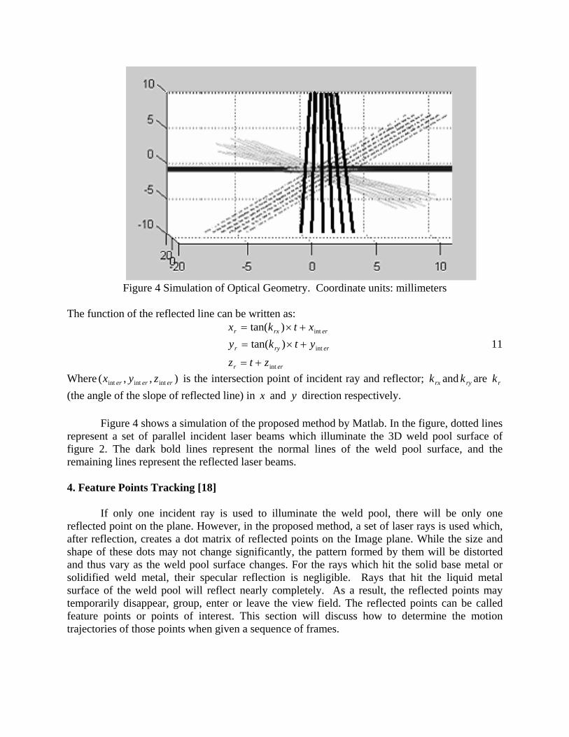
Figure 4 Simulation of Optical Geometry. Coordinate units: millimeters

The function of the reflected line can be written as:

err

erryr

errxr

ztz

ytkyxtkx

int

int

int

)tan()tan(

+=

+×=+×=

11

Where ),,( intintint ererer zyx is the intersection point of incident ray and reflector; rxk and ryk are rk (the angle of the slope of reflected line) in x and y direction respectively.

Figure 4 shows a simulation of the proposed method by Matlab. In the figure, dotted lines

represent a set of parallel incident laser beams which illuminate the 3D weld pool surface of figure 2. The dark bold lines represent the normal lines of the weld pool surface, and the remaining lines represent the reflected laser beams.

4. Feature Points Tracking [18]

If only one incident ray is used to illuminate the weld pool, there will be only one reflected point on the plane. However, in the proposed method, a set of laser rays is used which, after reflection, creates a dot matrix of reflected points on the Image plane. While the size and shape of these dots may not change significantly, the pattern formed by them will be distorted and thus vary as the weld pool surface changes. For the rays which hit the solid base metal or solidified weld metal, their specular reflection is negligible. Rays that hit the liquid metal surface of the weld pool will reflect nearly completely. As a result, the reflected points may temporarily disappear, group, enter or leave the view field. The reflected points can be called feature points or points of interest. This section will discuss how to determine the motion trajectories of those points when given a sequence of frames.

Typically, the characteristics of the motion of feature points are classified and described using different motion models, such as the average deviation conditioned by competition and alternative model [17], smooth motion model [20], and the proximal uniformity model [17]. Many algorithms or methods are provided based on the motion models. Feature point based motion tracking, in long image sequences algorithm in which dynamic scenes with multiple independently moving objects are considered in which feature points may temporarily disappear enter and leave the view field, was used. Most of the existing approaches to feature point tracking have limited capabilities in handling incomplete trajectories especially when the number of points and their speeds are large and trajectory ambiguities are frequent. The basic matching algorithm has three basic steps [18-20]: initialization, processing of consecutive frames, and post-processing. The initialization procedure operates on the first three frames and induces the tracking process. The points in Frame 2 are linked to the corresponding points in Frame 1 and Frame 3. Starting from Frame 3, a different matching procedure is applied. When all frames have been matched, a post–processing procedure is used to reconsider the points that temporarily disappeared and later re-appeared. This procedure attempts to connect the corresponding endpoints of the broken trajectories.

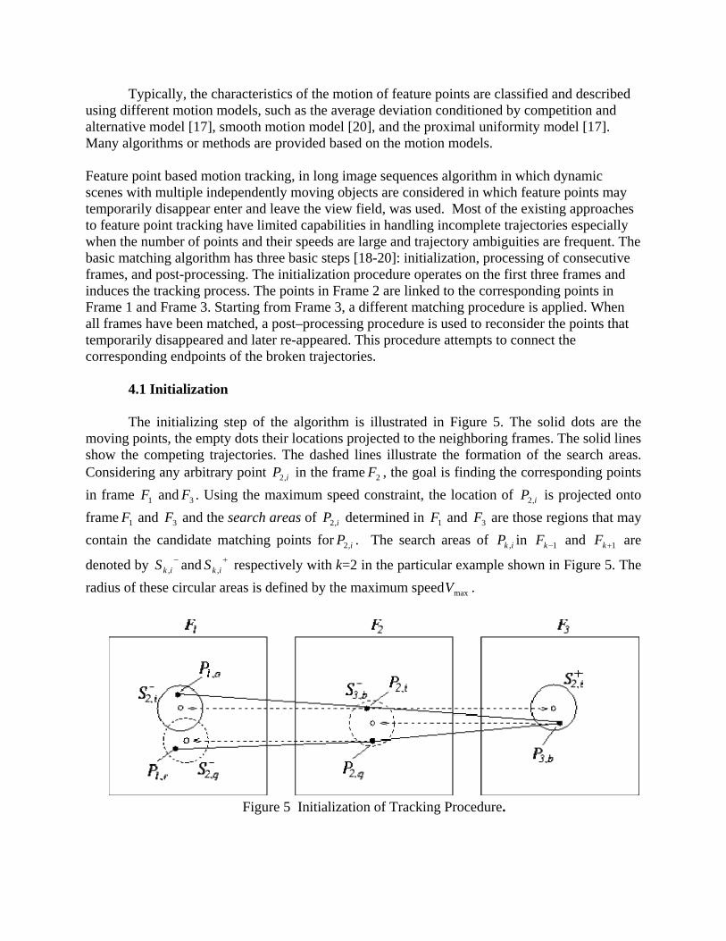
4.1 Initialization The initializing step of the algorithm is illustrated in Figure 5. The solid dots are the

moving points, the empty dots their locations projected to the neighboring frames. The solid lines show the competing trajectories. The dashed lines illustrate the formation of the search areas. Considering any arbitrary point iP ,2 in the frame 2F , the goal is finding the corresponding points in frame 1F and 3F . Using the maximum speed constraint, the location of iP ,2 is projected onto frame 1F and 3F and the search areas of iP ,2 determined in 1F and 3F are those regions that may contain the candidate matching points for iP ,2 . The search areas of ikP , in 1−kF and 1+kF are

denoted by −ikS , and +

ikS , respectively with k=2 in the particular example shown in Figure 5. The radius of these circular areas is defined by the maximum speed maxV .

Figure 5 Initialization of Tracking Procedure.

Next by considering all possible triplets of points ( )min PPP ,3,2,1 ,, , −∈ in SP ,2,1

and +∈ im SP ,2,3 , that contain the point iP ,2 the triplet ),,( ,3,2,1 bia PPP can be found that minimizes for 2=k the cost function ),,( ,1,,1 mkiknk PPP +−δ based on smooth motion models as introduced by Sethi and Jain [20].

A cost function evaluates the local deviation from smoothness and penalizes changes in

both direction and magnitude of the velocity vector. Its value is normalized so as to span the range [ ]1,0 , with 0 meaning no change at all. The smooth motion is formulated quantitatively as:

[ ]⎟⎟⎟

⎠

⎞

⎜⎜⎜

⎝

⎛

+

⋅−+

⎟⎟⎟

⎠

⎞

⎜⎜⎜

⎝

⎛

⋅

⋅−=

+−

+−

+−

+−+−

mkikiknk

mkikiknk

mkikiknk

mkikiknkmkiknk

PPPP

PPPPw

PPPP

PPPPwPPP

,1,,,1

2/1

,1,,,12

,1,,,1

,1,,,11,1,,1

211),,(δ 12

Here iknk PP ,,1− and mkik PP ,1, + denote the vectors pointing from nkP ,1− to ikP , and from ikP , to mkP ,1+ , respectively. The first term in cost function penalizes changes in the direction, the second in the magnitude of the speed vector. The weights 1w and 2w , 121 =+ ww , are used to balance the two components of the cost function.

The triplet ),,( ,3,2,1 bia PPP is selected as the initial hypothesis and the remaining triplets ranked according to their cost values. (The triplets with maxδδ < are considered only, maxδ is maximum cost and is further discussed in section 4.3) The initial hypothesis is tested by scanning −

bS ,3 , the search area of bP ,3 in 2F . Let qP ,2 be a point in −bS ,3 . (See Figure 5). If −

qS ,2 has a point rP ,1 such that ),,( ,3,2,1 bqr PPPδ < ),,( ,3,2,1 bia PPPδ , then the initial hypothesis is rejected and the second ranking hypothesis is considered and tested. Otherwise, the testing of the initial hypothesis proceeds with checking aP ,1 in the same way. If this check is also successful, ),,( ,3,2,1 bia PPP is output as the initial part of the trajectory of aP ,1 . The correspondences established are not altered during further processing.

If all hypotheses for iP ,2 have been rejected, then the point is not linked to 1F and 3F . It is

still possible that iP ,2 will be linked to 3F when the latter is processed. In such case iP ,2 first appear at fame 2 and begins a trajectory starting from frame 2.

When all points of 2F have been processed, some points in the neighboring frames may

remain unmatched. A point in 1F that is not linked to any point in 2F disappears, that is, either leaves the view field or temporarily disappears within the image, e.g., due to occlusion. An unmatched point in 3F may later open a trajectory.

In the above description of the hypothesis testing procedure, original hypothesis is

rejected immediately when a `stronger' triple ),,( ,3,2,1 bqr PPP is found. However, ),,( ,3,2,1 bqr PPP

can itself be overruled by still another triple if the verification proceeds by testing ),,( ,3,2,1 bqr PPP in a similar way, that is, by switching back to 2F and 3F .

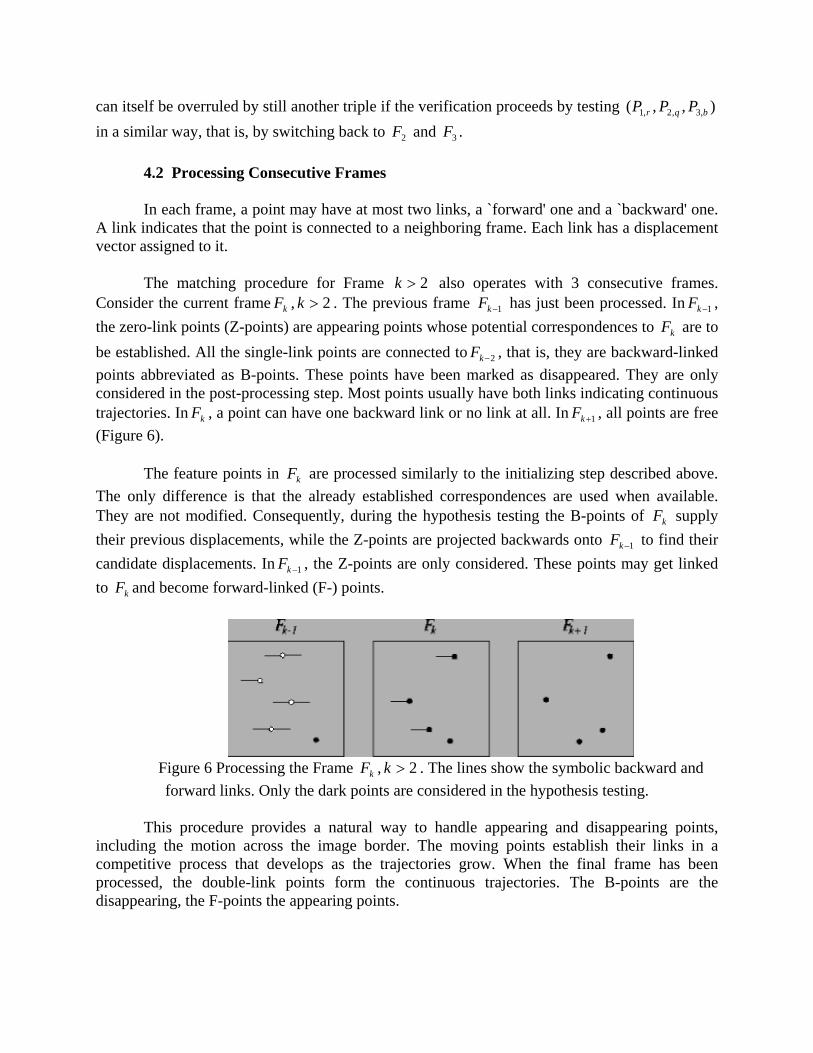
4.2 Processing Consecutive Frames In each frame, a point may have at most two links, a `forward' one and a `backward' one.

A link indicates that the point is connected to a neighboring frame. Each link has a displacement vector assigned to it.

The matching procedure for Frame 2>k also operates with 3 consecutive frames.

Consider the current frame kF , 2>k . The previous frame 1−kF has just been processed. In 1−kF , the zero-link points (Z-points) are appearing points whose potential correspondences to kF are to be established. All the single-link points are connected to 2−kF , that is, they are backward-linked points abbreviated as B-points. These points have been marked as disappeared. They are only considered in the post-processing step. Most points usually have both links indicating continuous trajectories. In kF , a point can have one backward link or no link at all. In 1+kF , all points are free (Figure 6).

The feature points in kF are processed similarly to the initializing step described above.

The only difference is that the already established correspondences are used when available. They are not modified. Consequently, during the hypothesis testing the B-points of kF supply their previous displacements, while the Z-points are projected backwards onto 1−kF to find their candidate displacements. In 1−kF , the Z-points are only considered. These points may get linked to kF and become forward-linked (F-) points.

Figure 6 Processing the Frame kF , 2>k . The lines show the symbolic backward and forward links. Only the dark points are considered in the hypothesis testing.

This procedure provides a natural way to handle appearing and disappearing points,

including the motion across the image border. The moving points establish their links in a competitive process that develops as the trajectories grow. When the final frame has been processed, the double-link points form the continuous trajectories. The B-points are the disappearing, the F-points the appearing points.

4.3 Post-Processing of Occlusion This procedure attempts to connect the broken trajectories. In Figure 7, a broken

trajectory is shown along with two possible continuations and a separate, continuous trajectory. Consider a B-point Pe with the incoming velocity ev and an F-point Ps with the outgoing velocity sv . A candidate occluded point is searched in the intersection of two search areas Se+ and Ss-.

The search areas are basically defined by cost function, cost limit and the speed limit. In

addition, this procedure makes use of the fact that simultaneous occlusion and drastic turn are rare, since both are relatively rare events compared to the high-speed camera which has 1000 frames/sec picture grabbing ability. To ensure directional continuity of broken trajectories

−+ ∩ se SS is more constrained than it is prescribed by the cost limit alone.

Figure 7 Post-processing of Broken Trajectories. A broken trajectory is shown along with two

alternative continuations and a separate, continuous trajectory. The occluded point is searched in the filled region.

If −+ ∩ se SS is empty, the trajectory remains broken. Otherwise, a point is found that minimizes the cost for the interpolated trajectory. This is done by exhaustive search of

−+ ∩ se SS with a suitable spatial resolution. To account for possible two-frame occlusions, each

point of −+ ∩ se SS is expanded in the same way into a search area in the next (previous) frame, and the average cost is minimized. As discussed above, less deviation from smoothness is allowed for a hypothetical occluded point than for an actual point being observed.

Mathematically, directional continuity of broken trajectories is enforced by limiting the unweighted terms rather than weighted terms. Under these constraints, it is easy to derive that

)1arccos( max2,1 δθθ −= me 13

2max

2maxmax

2,1 )1())2(1(

δδδ

−

−=

mevv 14

Here eθ is the direction, ev the magnitude of the incoming velocity vector.

From these equations, the maximum allowed direction change for broken trajectories is 2/π , when maxδ =1. When maxδ =0.5, the turn limit is 3/π . evv ≤≤ 10 , while evv ≥2 . When

maxδ is set close to 1, 01 ≈v and evv >>2 .

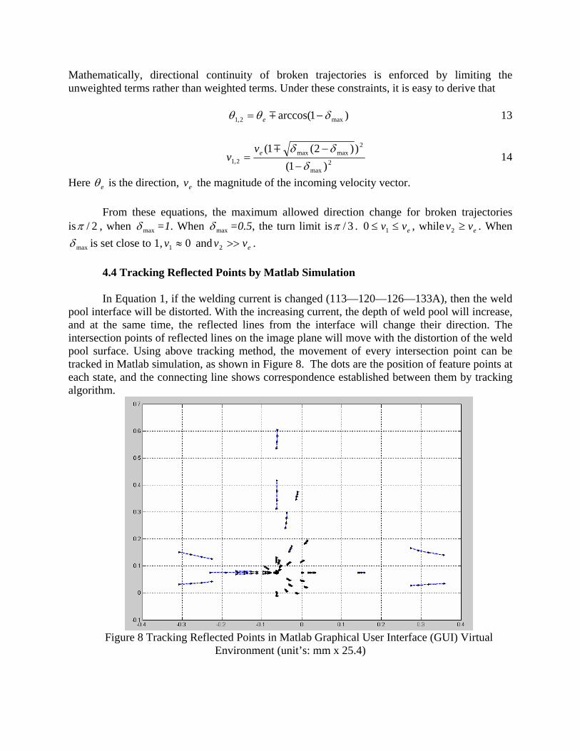
4.4 Tracking Reflected Points by Matlab Simulation

In Equation 1, if the welding current is changed (113—120—126—133A), then the weld pool interface will be distorted. With the increasing current, the depth of weld pool will increase, and at the same time, the reflected lines from the interface will change their direction. The intersection points of reflected lines on the image plane will move with the distortion of the weld pool surface. Using above tracking method, the movement of every intersection point can be tracked in Matlab simulation, as shown in Figure 8. The dots are the position of feature points at each state, and the connecting line shows correspondence established between them by tracking algorithm.

Figure 8 Tracking Reflected Points in Matlab Graphical User Interface (GUI) Virtual

Environment (unit’s: mm x 25.4)

5. Optical Flow [21, 22, 23, 24]

Optical flow is the apparent motion of brightness patterns across the image plane of a computer vision system or across the retina of the eye in a biological vision system. Optical flow arises from movement of objects in the scene or from movement of the camera (or eye) through the scene.

Calculation of the optical flow is used as a cue to aid the processing of video segmentation. In this case, since the illuminating laser source is fixed for its position and angle during experiment, the movement of the feature points created by reflected beams can be seen as optical flow, or in other words, the motion field.

5.1 Estimation of Optical Flow

Assume the weld pool surface is stationary and can be modeld by a mathmatical equation,

which can be written as a fuction ( ),,, zyxF , and assume that Χ is the coordinate matrix of

projected pattern (the 3D space position of a set of parallel laser beams), and Χ′ the coordinate

matrix after refection, then the warp between Χ and Χ′ can be obtained from the following

equations:

),( Χ′Χ∇=∂∂

xFxf , ),( Χ′Χ∇=

∂∂

yFyf , ),( Χ′Χ∇=

∂∂

zFzf 15

where ),(),,( XXFzyxf ′=

Further assume that the weld pool surface shape may be modelled by an 4D (3D Cartesian and time) function, ( )tzyxf ,,, , which varies continuously with position and time.

If the intensity function is expanded in a Taylor series, one may obtain

K+∂∂

+∂∂

+∂∂

+∂∂

+=++++ dttfdz

zfdy

yfdx

xftzyxfdttdzzdyydxxf ),,,(),,,(

By ignoring the higher order terms: ),,,(),,,( tzyxfdttdzzdyydxxff −++++=∆

dtdtdfdz

dzdfdy

dydfdx

dxdf

+++= 16

Substituting (15) into Equation (16) we get

dtXFdzXXFdyXXFdxXXFf tzyx )'()',()',()',(→

∇+∇+∇+∇=∆ 17

Hence, f∆ can be calculated from Χ (coordinate matrix of projected pattern), Χ′ (coordinate

matrix after refection from weld pool surface) and →

'X (a vector which represents the track of these feature points).

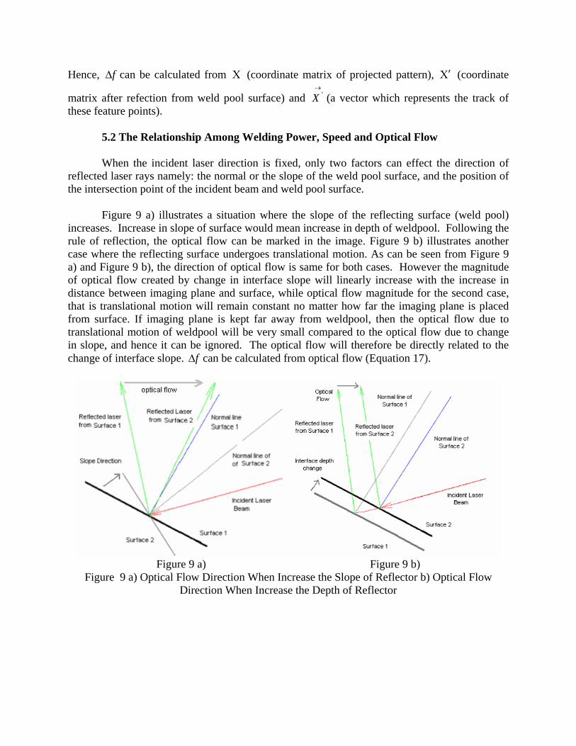
5.2 The Relationship Among Welding Power, Speed and Optical Flow

When the incident laser direction is fixed, only two factors can effect the direction of reflected laser rays namely: the normal or the slope of the weld pool surface, and the position of the intersection point of the incident beam and weld pool surface.

Figure 9 a) illustrates a situation where the slope of the reflecting surface (weld pool)

increases. Increase in slope of surface would mean increase in depth of weldpool. Following the rule of reflection, the optical flow can be marked in the image. Figure 9 b) illustrates another case where the reflecting surface undergoes translational motion. As can be seen from Figure 9 a) and Figure 9 b), the direction of optical flow is same for both cases. However the magnitude of optical flow created by change in interface slope will linearly increase with the increase in distance between imaging plane and surface, while optical flow magnitude for the second case, that is translational motion will remain constant no matter how far the imaging plane is placed from surface. If imaging plane is kept far away from weldpool, then the optical flow due to translational motion of weldpool will be very small compared to the optical flow due to change in slope, and hence it can be ignored. The optical flow will therefore be directly related to the change of interface slope. f∆ can be calculated from optical flow (Equation 17).

Figure 9 a) Figure 9 b)

Figure 9 a) Optical Flow Direction When Increase the Slope of Reflector b) Optical Flow Direction When Increase the Depth of Reflector

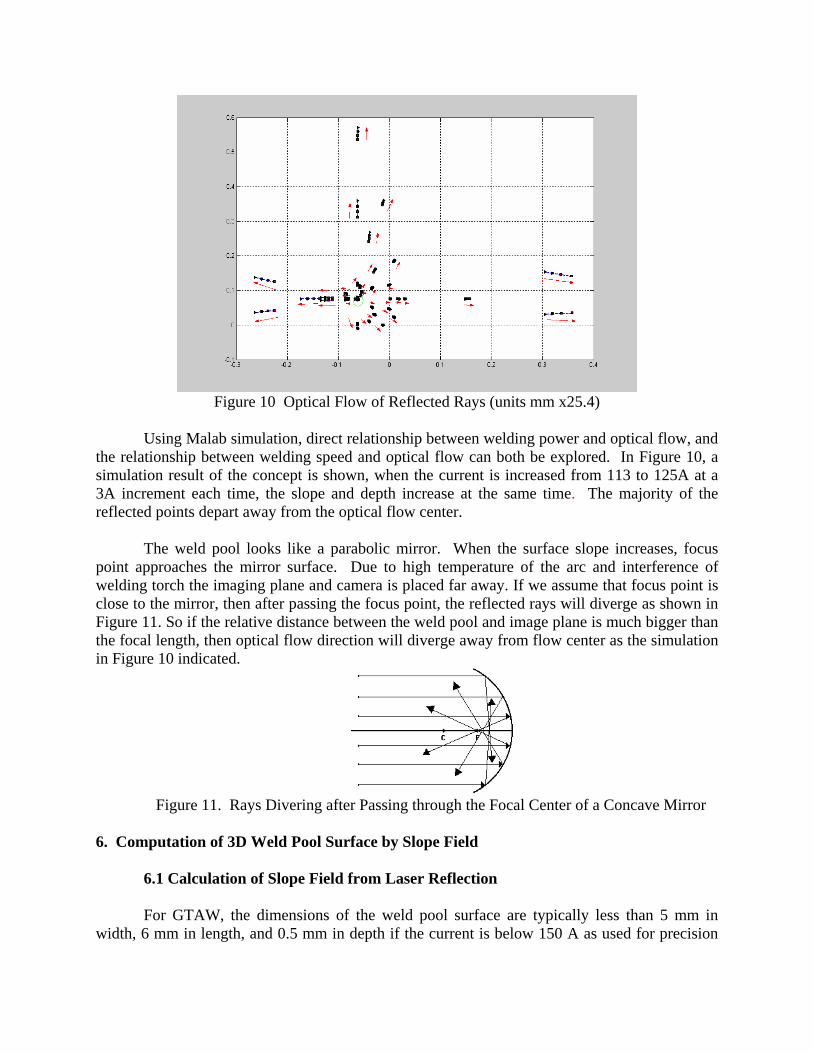
Figure 10 Optical Flow of Reflected Rays (units mm x25.4)

Using Malab simulation, direct relationship between welding power and optical flow, and

the relationship between welding speed and optical flow can both be explored. In Figure 10, a simulation result of the concept is shown, when the current is increased from 113 to 125A at a 3A increment each time, the slope and depth increase at the same time. The majority of the reflected points depart away from the optical flow center.

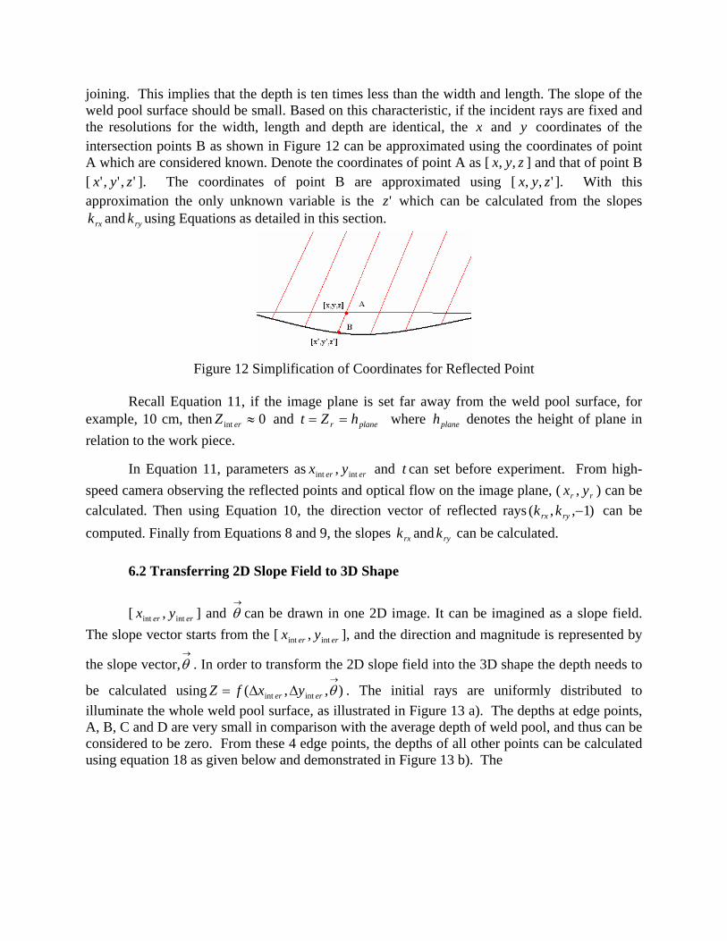
The weld pool looks like a parabolic mirror. When the surface slope increases, focus

point approaches the mirror surface. Due to high temperature of the arc and interference of welding torch the imaging plane and camera is placed far away. If we assume that focus point is close to the mirror, then after passing the focus point, the reflected rays will diverge as shown in Figure 11. So if the relative distance between the weld pool and image plane is much bigger than the focal length, then optical flow direction will diverge away from flow center as the simulation in Figure 10 indicated.

Figure 11. Rays Divering after Passing through the Focal Center of a Concave Mirror

6. Computation of 3D Weld Pool Surface by Slope Field

6.1 Calculation of Slope Field from Laser Reflection

For GTAW, the dimensions of the weld pool surface are typically less than 5 mm in width, 6 mm in length, and 0.5 mm in depth if the current is below 150 A as used for precision

joining. This implies that the depth is ten times less than the width and length. The slope of the weld pool surface should be small. Based on this characteristic, if the incident rays are fixed and the resolutions for the width, length and depth are identical, the x and y coordinates of the intersection points B as shown in Figure 12 can be approximated using the coordinates of point A which are considered known. Denote the coordinates of point A as [ zyx ,, ] and that of point B [ ',',' zyx ]. The coordinates of point B are approximated using [ ',, zyx ]. With this approximation the only unknown variable is the 'z which can be calculated from the slopes

rxk and ryk using Equations as detailed in this section.

Figure 12 Simplification of Coordinates for Reflected Point

Recall Equation 11, if the image plane is set far away from the weld pool surface, for

example, 10 cm, then 0int ≈erZ and planer hZt == where planeh denotes the height of plane in relation to the work piece.

In Equation 11, parameters as erer yx intint , and t can set before experiment. From high-speed camera observing the reflected points and optical flow on the image plane, ( rr yx , ) can be calculated. Then using Equation 10, the direction vector of reflected rays )1,,( −ryrx kk can be computed. Finally from Equations 8 and 9, the slopes rxk and ryk can be calculated. 6.2 Transferring 2D Slope Field to 3D Shape

[ erer yx intint , ] and →

θ can be drawn in one 2D image. It can be imagined as a slope field. The slope vector starts from the [ erer yx intint , ], and the direction and magnitude is represented by

the slope vector,→

θ . In order to transform the 2D slope field into the 3D shape the depth needs to

be calculated using ),,( intint

→

∆∆= θerer yxfZ . The initial rays are uniformly distributed to illuminate the whole weld pool surface, as illustrated in Figure 13 a). The depths at edge points, A, B, C and D are very small in comparison with the average depth of weld pool, and thus can be considered to be zero. From these 4 edge points, the depths of all other points can be calculated using equation 18 as given below and demonstrated in Figure 13 b). The

[ ][ ] [ ]eryjierxji

jieryjierxji

ji

eryjierxjiji

eryjierxjiji

ji

ybxaybxa

ybxaybxa

Z

int,int,7

44

1int,int,

7

44

7

int,int,1

44

7int,int,

1

44

1

,

)tan())tan()tan()tan(

)tan())tan())tan()tan((

∆××+∆××∑∑+∆××+∆××∑∑+

∆××+∆××∑∑+∆××+∆××∑∑=

====

====

θθθθ

θθθθ

rrrr

rrrr

Where 25.0,, =+ jiji ba if ( 4, =ji ), otherwise 1,, =+ jiji ba when ( 4, ≠ji )

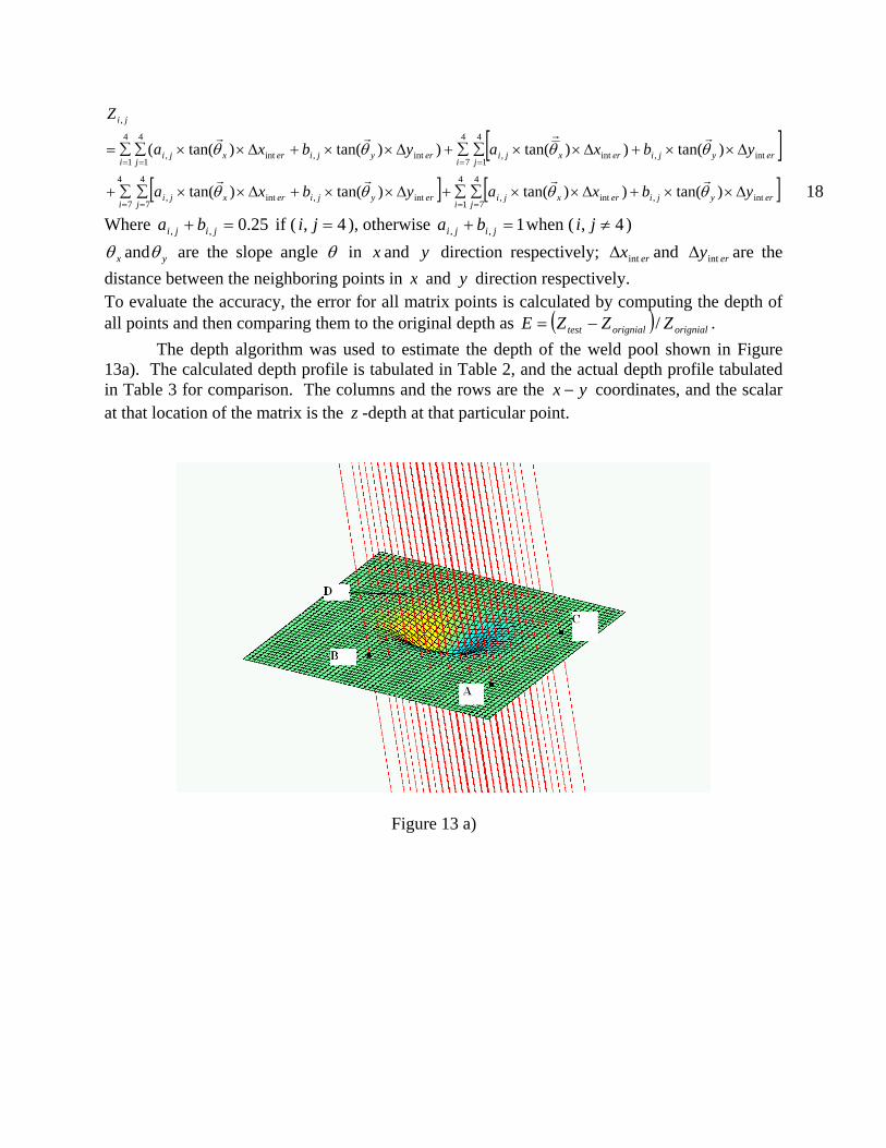
xθ and yθ are the slope angle θ in x and y direction respectively; erxint∆ and eryint∆ are the distance between the neighboring points in x and y direction respectively. To evaluate the accuracy, the error for all matrix points is calculated by computing the depth of all points and then comparing them to the original depth as ( ) orignialorignialtest ZZZE /−= .

The depth algorithm was used to estimate the depth of the weld pool shown in Figure 13a). The calculated depth profile is tabulated in Table 2, and the actual depth profile tabulated in Table 3 for comparison. The columns and the rows are the yx − coordinates, and the scalar at that location of the matrix is the z -depth at that particular point.

Figure 13 a)

18

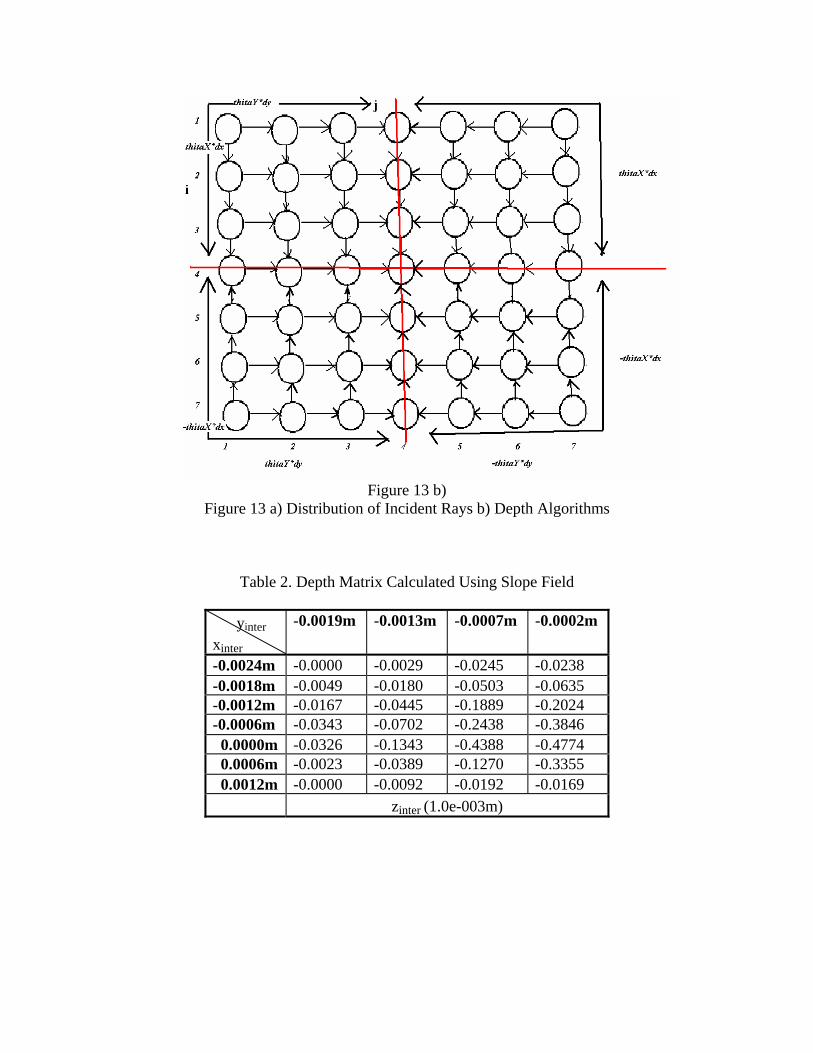
Figure 13 b)

Figure 13 a) Distribution of Incident Rays b) Depth Algorithms

Table 2. Depth Matrix Calculated Using Slope Field

yinter xinter

-0.0019m -0.0013m -0.0007m -0.0002m

-0.0024m -0.0000 -0.0029 -0.0245 -0.0238 -0.0018m -0.0049 -0.0180 -0.0503 -0.0635 -0.0012m -0.0167 -0.0445 -0.1889 -0.2024 -0.0006m -0.0343 -0.0702 -0.2438 -0.3846 0.0000m -0.0326 -0.1343 -0.4388 -0.4774 0.0006m -0.0023 -0.0389 -0.1270 -0.3355 0.0012m -0.0000 -0.0092 -0.0192 -0.0169 zinter (1.0e-003m)

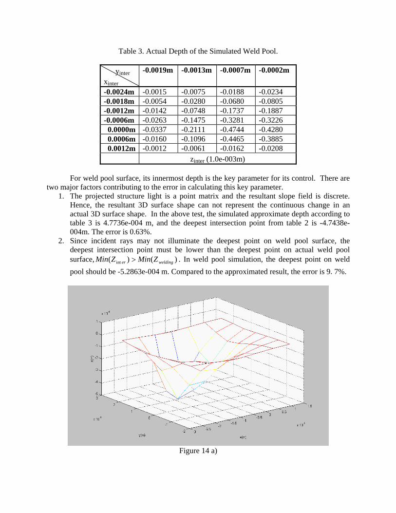
Table 3. Actual Depth of the Simulated Weld Pool.

yinter xinter

-0.0019m -0.0013m -0.0007m -0.0002m

-0.0024m -0.0015 -0.0075 -0.0188 -0.0234 -0.0018m -0.0054 -0.0280 -0.0680 -0.0805 -0.0012m -0.0142 -0.0748 -0.1737 -0.1887 -0.0006m -0.0263 -0.1475 -0.3281 -0.3226 0.0000m -0.0337 -0.2111 -0.4744 -0.4280 0.0006m -0.0160 -0.1096 -0.4465 -0.3885 0.0012m -0.0012 -0.0061 -0.0162 -0.0208 zinter (1.0e-003m)

For weld pool surface, its innermost depth is the key parameter for its control. There are

two major factors contributing to the error in calculating this key parameter. 1. The projected structure light is a point matrix and the resultant slope field is discrete.

Hence, the resultant 3D surface shape can not represent the continuous change in an actual 3D surface shape. In the above test, the simulated approximate depth according to table 3 is 4.7736e-004 m, and the deepest intersection point from table 2 is -4.7438e-004m. The error is 0.63%.

2. Since incident rays may not illuminate the deepest point on weld pool surface, the deepest intersection point must be lower than the deepest point on actual weld pool surface, )()( int weldinger ZMinZMin > . In weld pool simulation, the deepest point on weld pool should be -5.2863e-004 m. Compared to the approximated result, the error is 9.7%.

Figure 14 a)

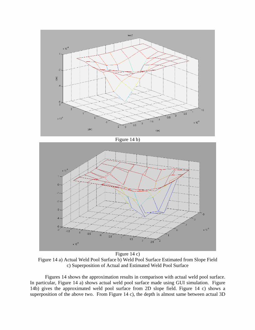
Figure 14 b)

Figure 14 c)

Figure 14 a) Actual Weld Pool Surface b) Weld Pool Surface Estimated from Slope Field c) Superposition of Actual and Estimated Weld Pool Surface

Figures 14 shows the approximation results in comparison with actual weld pool surface.

In particular, Figure 14 a) shows actual weld pool surface made using GUI simulation. Figure 14b) gives the approximated weld pool surface from 2D slope field. Figure 14 c) shows a superposition of the above two. From Figure 14 c), the depth is almost same between actual 3D

shape and approximated 3D shape. However, due to the above approximation method, especially in x and y coordinates, the approximated shape has a little distortion in x and y direction.

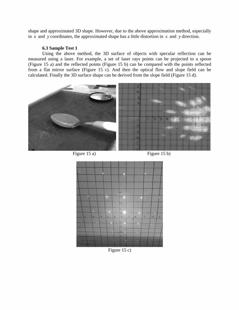
6.3 Sample Test 1 Using the above method, the 3D surface of objects with specular reflection can be

measured using a laser. For example, a set of laser rays points can be projected to a spoon (Figure 15 a) and the reflected points (Figure 15 b) can be compared with the points reflected from a flat mirror surface (Figure 15 c). And then the optical flow and slope field can be calculated. Finally the 3D surface shape can be derived from the slope field (Figure 15 d).

Figure 15 a) Figure 15 b)

Figure 15 c)

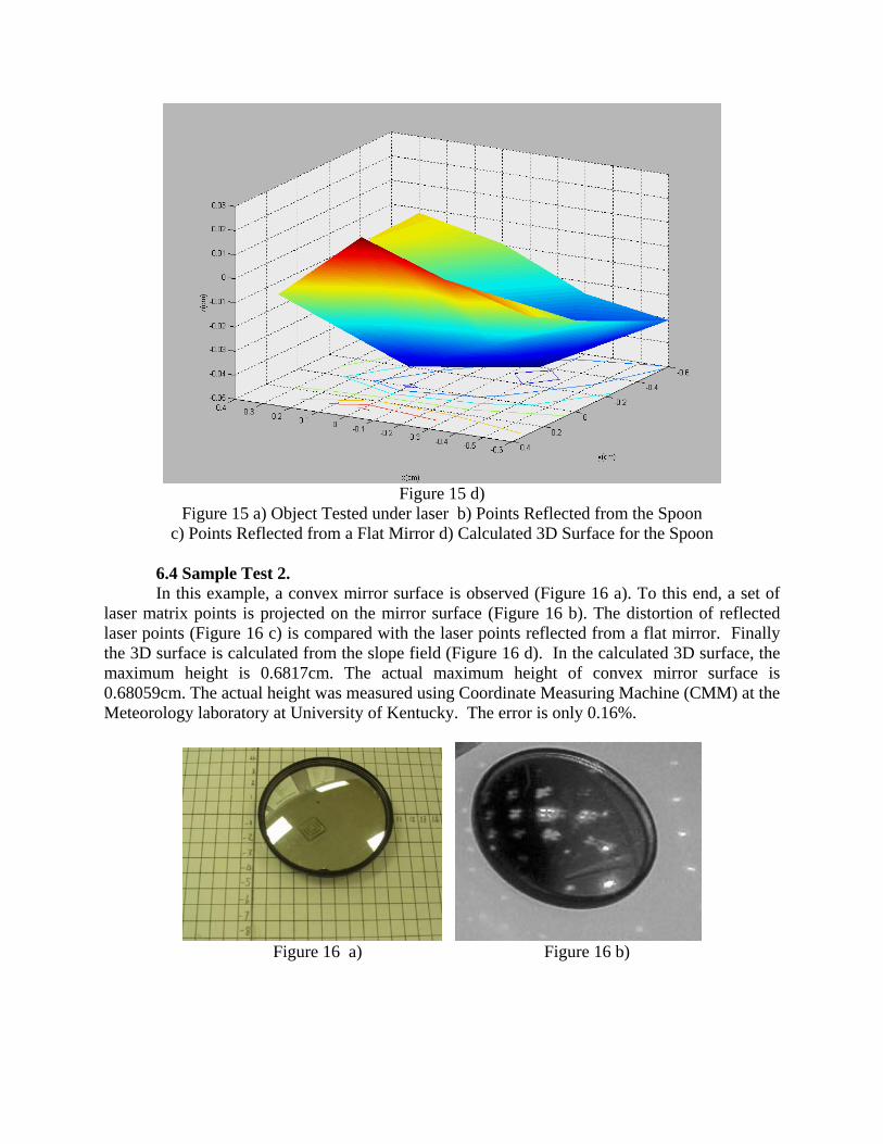
Figure 15 d)

Figure 15 a) Object Tested under laser b) Points Reflected from the Spoon c) Points Reflected from a Flat Mirror d) Calculated 3D Surface for the Spoon

6.4 Sample Test 2. In this example, a convex mirror surface is observed (Figure 16 a). To this end, a set of

laser matrix points is projected on the mirror surface (Figure 16 b). The distortion of reflected laser points (Figure 16 c) is compared with the laser points reflected from a flat mirror. Finally the 3D surface is calculated from the slope field (Figure 16 d). In the calculated 3D surface, the maximum height is 0.6817cm. The actual maximum height of convex mirror surface is 0.68059cm. The actual height was measured using Coordinate Measuring Machine (CMM) at the Meteorology laboratory at University of Kentucky. The error is only 0.16%.

Figure 16 a) Figure 16 b)

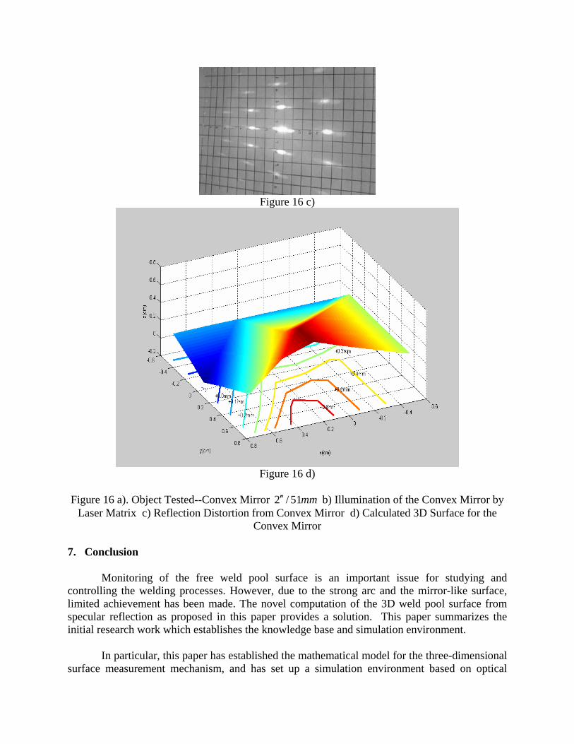
Figure 16 c)

Figure 16 d)

Figure 16 a). Object Tested--Convex Mirror mm51/2 ′′ b) Illumination of the Convex Mirror by

Laser Matrix c) Reflection Distortion from Convex Mirror d) Calculated 3D Surface for the Convex Mirror

7. Conclusion

Monitoring of the free weld pool surface is an important issue for studying and controlling the welding processes. However, due to the strong arc and the mirror-like surface, limited achievement has been made. The novel computation of the 3D weld pool surface from specular reflection as proposed in this paper provides a solution. This paper summarizes the initial research work which establishes the knowledge base and simulation environment.

In particular, this paper has established the mathematical model for the three-dimensional

surface measurement mechanism, and has set up a simulation environment based on optical

geometry and imaging processing technique utilizing concepts including optical flow, structured light, and feature points tracking. The simulation environment can describe the relationship between the resultant image (optical flow of reflected points), the slope field of the weld pool surface, and the three-dimensional surface of the weld pool. This technique can also be used for studying the oscillations on the surface of the weld pool which are in the order of less than 100Hz, provided that the camera is fast enough to capture the movement of the feature points. This method is however limited to the GTAW and cannot be used in processes like keyhole establishment.

With this virtual environment, the parameters of the image system can also be optimized

such that the measurement system will be optimally designed to achieve accurate measurement under various weld pool surface shapes. By simulation and measurement of sample objects, the effectiveness of the proposed specular reflection and optical flow based method for 3D specular surface has been confirmed.

Acknowledgements

This work is funded by the National Science Foundation under Grant DMI-01144982 and the University of Kentucky Center for Manufacturing.

References

1. W. Swaim, 1998. “Gas tungsten arc welding made easy,” Welding Journal, 77(9): 51-52. 2. D. Farson, X.C. Li, R. Richardson, 1998. “Infrared Measurement of Gas Tungsten Arc Weld Temperatures,” Welding Journal, 77(9): 396s-401s. 3. H. G. Kraus, 1987. “Optical spectral radiometric method for noninvasive measurement of weld pool surface temperatures,” Optical Engineering, 26(12): 1183-1190. 4. T. DebRoy, 1995. “Role of Interfacial Phenomena in Numerical Analysis of Weldability,” in Mathematical Modelling of Weld Phenomena II, The Institute of Materials, London, pp. 3-21. 5. D. R. Atthey, 1980. “A mathematical model for fluid flow in a weld pool at high current,” Journal of Fluid Mechanics, 98(June): 787-801. 6. Y. M. Zhang and S. B. Zhang, 1998. “Double-sided arc welding increases weld joint penetration,” Welding Journal, 77(6): 57-61. 7. S. Missori and C. Koerber, 1997. “Laser beam welding of austenitic-ferritic transition joints,” Welding Journal, 76: 125s-134s. 8. P. Solana and J. L. Ocana, 1997. “A mathematical model for penetration laser welding as a free-boundary problem,” J.Phys.D: Apply. Phys. 30: 1300-1313. 9. W. Pecharapa and A. Kar, 1997. “Effects of phase changes on weld pool shape in laser welding,” J.Phys.D: Apply. Phys. 30: 3322-3329.

10. K.N. Lankalapalli, J.F. Tu and M. Gartner, 1996. “A model for estimating penetration depth of laser welding processes,” J. Phys.D: Apply. Phys. 30: 1831-1814. 11. T. J. Colla, M. Vicanek, and G. Simon, 1994. “Heat transport in melt flowing past the keyhole in deep penetration welding,” J. Phys.D: Apply. Phys. 27: 2035-2040. 12. R. Kovacevic and Y. M. Zhang, 1996. "Sensing free surface of arc weld pool using specular reflection: principle and analysis," Proceedings of the Institution of Mechanical Engineers, Part B, Journal of Engineering Manufacturing, 210(6): 553-564. 13. R. Kovacevic and Y. M. Zhang, 1997. "Real-time image processing for monitoring of free weld pool surface," ASME Journal of Manufacturing Science and Engineering, 119(2): 161-169. 14. G. Saeed and Y. M. Zhang. “Mathematical formulation and simulation of specular reflection based measurement system for gas tungsten arc weld pool surface,” Measurement Science Journal. 14(9) 1671-1682. 15. R. E. Larson and R. P. Hostetler, 1997. Calculus with Analytic Geometry, D. C. Heath and Company, Lexington, Massachusetts. 16. G. Bertoline, et al, 2000. Fundamentals of Graphics Communication, 3rd Edition, McGraw-Hill, New York. 17. K. Rangarajan and M. Sha, 1991. “Establishing motion correspondence,” CVGIP: Image Understanding, 24(6): 56-73. 18. D. Chetverikov and J. Verestoy, 1999. “Feature Point Tracking for Incomplete Trajectories” Computing, vol.62, 321-338. 19. V. Salari and I. K. Sethi, 1990. “Feature point correspondence in the presence of occlusion,” IEEE Transactions on Pattern Analysis and Machine Intelligence, 12(1): 97-91. 20. I. K. Sethi and R. Jain, 1987. “Finding trajectories of feature points in a monocular image sequence,” IEEE Transactions on Pattern Analysis and Machine Intelligence, 9(1): 56-73. 21. A.-T. Tsao, C.-S. Fuh, 1997. “Ego-motion estimation using optical flow fields observed from multiple cameras,” Conference on Computer Vision and Pattern Recognition (CVPR '97), Puerto Rico, June 17-19. 22. A. Verri and T. Poggio, 1989. “Motion field and optical flow: qualitative properties,” IEEE Transactions on Pattern Analysis and Machine Intelligence, 11(5): 490-498. 23. D. DeCarlo and D. Metaxas, 2002. “Adjusting shape parameters using model-based optical flow residuals,” IEEE Transactions on Pattern Analysis and Machine Intelligence, 24(6): 814-823.

24. S.S. Beauchemin and J. L. Barron, 1995. “The computation of optical flow,” ACM Computing Surveys, 27(3): 433-467.