Computation of free-surface flows and fluid–object ... of free-surface flows and fluid–object interactionswith the CIP method based on adaptive meshless soroban grids 2.2.1

Comput MechDOI 10.1007/s00466-006-0093-2

ORIGINAL PAPER

Computation of free-surface flows and fluid–object interactionswith the CIP method based on adaptive meshless soroban grids

Kenji Takizawa · Takashi Yabe · Yumiko Tsugawa ·Tayfun E. Tezduyar · Hiroki Mizoe

Received: 2 March 2006 / Accepted: 28 May 2006© Springer-Verlag 2006

Abstract The CIP Method [J comput phys 61:261–268,1985; J comput phys 70:355–372, 1987; Comput physcommun 66:219–232, 1991; J comput phys 169:556–593,2001] and adaptive Soroban grid [J comput phys194:57–77, 2004] are combined for computation of three-dimensional fluid–object and fluid–structure interactions,while maintaining high-order accuracy. For the robustcomputation of free-surface and multi-fluid flows, weadopt the CCUP method [Phys Soc Japan J 60:2105–2108,1991]. In most of the earlier computations, the CCUPmethod was used with a staggered-grid approach. Here,because of the meshless nature of the Soroban grid, weuse the CCUP method with a collocated-grid approach.We propose an algorithm that is stable, robust and accu-rate even with such collocated grids. By adopting theCIP interpolation, the accuracy is largely enhanced com-pared to linear interpolation. Although this grid systemis unstructured, it still has a very simple data structure.

K. TakizawaNational Maritime Research Institute,6-38-1, Shinkawa, Mitaka-shi,Tokyo 181-0004, Japan

T. Yabe(B) · Y. TsugawaTokyo Institute of Technology,O-okayama, Meguro, Tokyo 152-8552, Japane-mail: [email protected]

T. E. TezduyarMechanical Engineering, Rice University,MS 321, Houston, Texas 77005, USA

H. MizoeTohoku Electric Power Company, Inc.,Sendai 981-0952, Japan

1 Introduction

Computation of fluid–object and fluid–structureinteractions poses a number of numerical challenges.These challenges include the accuracy of the flow fieldnear solid surfaces, accurate advection of the vortexfields, grid generation and motion, and computationalefficiency. The numerical challenges become even moreformidable when the problem, in addition to fluid–objectand fluid–structure interactions, involves free-surface ormulti-fluid flows. While the boundary layers near solidsurfaces need to be accurately resolved, free surfacesand two-fluid interfaces need to be calculated in a ro-bust, accurate and efficient fashion.

A number of very effective finite element interface-tracking (mesh moving) methods have been developedin recent decades for computation of fluid–object andfluid–structure interactions (see for example the meth-ods and computations reported in [7–16]). The MixedInterface-Tracking/Interface-Capturing Technique(MITICT) was introduced in [17] for computationsinvolving both fluid–solid interfaces that need to beaccurately tracked with a moving mesh method andfluid–fluid interfaces that are too complex or unsteadyto be tracked and therefore require an interface-captur-ing technique. As far as these finite element approachesare concerned, there is a clear need for more freedomfrom mesh moving and distortion issues, and there isalso still some room for improvements in accuracy andefficiency. On the other hand, Adaptive Mesh Refine-ment (AMR) [18] with Cartesian grids can be accurateonly when the interpolation inside a cell is effective, butthe AMR cannot place grid points on the boundariesand resolve the thin boundary layers. The cut-cell [19]approach is an alternative, but its application to moving

Comput Mech

objects is not so easy because of the presence of ex-tremely small-size cells. Besides these approaches, theuse of the particles [20,21] in capturing interfaces wouldbe among the challenging and interesting future tech-niques.

The Constrained Interpolation Profile/Cubic Interpo-lated Pseudo-particle (CIP) technique, which was devel-oped by Yabe et al. [1–4] for solving hyperbolicequations, has attracted a great deal of attention. Thistechnique would become even more powerful and prac-tical if it is combined with a special mesh system, “Soro-ban grid”, that allows accurate computations withunstructured grids. It would be a robust, accurate andefficient way of computing fluid–object and fluid–struc-ture interactions in the presence of free surfaces andtwo-fluid interfaces. It would accurately resolve theboundary layers near solid surfaces and also calculate, ina robust fashion, even the most complex and unsteadyfree surfaces and two-fluid interfaces. In this paper wepropose such a combined CIP/Adaptive Soroban gridmethod and apply it to a number of problems in multidimensions.

2 Grid system

2.1 Structure of the Soroban grid system

The Soroban grid is composed of planes, lines and gridpoints as shown in Fig. 1. Parallel planes can freely movein the z direction. Each plane is composed of lines andgrid points as shown in the bottom part of Fig. 1. Theparallel lines can freely move in the y direction and thegrid points on each line can move along each line whichis directed in the x-direction. We note that the number ofgrid points on different lines are not necessarily equal.Therefore the number of grid points on each line canvary depending on the required resolution. Such flexi-bility of the Soroban grid could increase the possibilityof grid arrangement. Most importantly, finding neigh-boring points becomes very easy and fast because ofthis structure, as will be shown in later sections.

Since the number of grid points may change on eachline, it would be better to employ a one-dimensionalarray for storing the grid points and changing their num-ber during a computation. For example, when the firstline has 30 grid points and the second line has 20 gridpoints, we need 50 grid points. Even if both lines have25 grid points in the next time step, the first and secondlines can share the memory and we do not need memoryre-allocation.

The index of the grid point number is unique forall the grid points on all the lines and planes. There-

=3k

x

yz 1

2

=10j

9

8

717 18

19 21

=23i

x

y

Fig. 1 (Top) Full view of a three dimensional Soroban grid. Theblack spheres represent the grid points. (Bottom) Line and gridarrangement on one of the planes. The symbols k, j, and i denotethe indices for the planes, lines and grid points, respectively

fore it starts from the first grid point along the firstline on the first plane and increases along the first line,then continuously increases along the second line andso on. Similarly the index of the line number is alsoone-dimensional and starts from the first line on the firstplane, and continuously increases to the next planes. Inthis way we can use only one-dimensional arrays and wecan change the number of grid points on each line, num-ber of lines on each plane, and the number of planes.The details of how the grid positions are specified aredescribed in Appendix 6.1.

2.2 Grid generation

Using the Soroban grids, grid points can be placed adap-tively around any complex shape, and can be changedeach time step with little computational cost. Since weuse a one-dimensional array for indexing, grid pointsare not inserted but all points are replaced. As shownin the next section, this will cause no problem for thecalculations. We choose a simple method for the gridgeneration. This is an old-fashioned way, but it is easyto implement in multi dimensions. First, we explain thegrid-generation method for a one-dimensional non-reg-ular grid.


2.2.1 Non-regular grids in one dimension

We define a monitoring function M(x, t). This functionshould give the information on which part of thecalculation domain should be refined. For this purpose,we propose a form:

M(x, t) =√

1 + α

(∂φ

∂x

)2

+ β

∣∣∣∣∂2φ

∂x2

∣∣∣∣ , (1)

where α and β are some scaling coefficients, and φ rep-resents the solution value, such as the density, velocityor pressure. Since the minimum of M(x, t) is 1, we definein advance the maximum of M(x, t), Mmax, so that wecan determine the grid interval ratio between the maxi-mum and minimum intervals. Therefore the monitoringfunction is re-written as follows:

M(x, t)

= min

⎛⎝

√1 + α

(∂φ

∂x

)2

+ β

∣∣∣∣∂2φ

∂x2

∣∣∣∣ , Mmax

⎞⎠ . (2)

Then we introduce the accumulated function I by inte-grating M as

I(x, t) =x∫

xS

M(x, t)dx, (3)

where xS is the start position of the system. If we dividethe accumulated function into equal regions, the bound-aries of each region give the grid points as shown inFig. 2. Let L be the number of grid points. Then theposition of each grid point is calculated as follows:

xn+1i = I−1

(i × I(xE)

Ln+1 − 1

), (4)

where xE is the end position of the system and I−1 meansthe inverse function of I. Since I is a monotonicallyincreasing function, the inverse of I can be easily esti-mated by linear interpolation as follows. First, we searchi that satisfies Ii ≤ I < Ii+1, and then calculate as

xn+1i =

(In

i+1 − I)

xni + (

I − Ini)

xni+1

Ini+1 − In

i, (5)

where Ii is the value of I at the old grid point xni .

We allow the number of grid points to vary in timeand hence Ln+1 represents the number of the grid pointsat time step n + 1. Although we can choose any Ln+1,we adopt the following rule.

Ln+1 = int(

I(xE)

�xmax

)+ 1, (6)

M(x) I(x)

x x

Integrate

Fig. 2 (Left) Monitoring function. (Right) Accumulated function

where int(x) is the round-off function and �xmax is themaximum grid interval. This means that all intervalsbecome �xmax when M(x) = 1 for all parts of cal-culation domain. Moreover, the minimum interval is�xmax/Mmax. In this way a non-regular grid is gener-ated, then we apply it to the Soroban grid.

2.2.2 Application to the Soroban grid

Since the Soroban grid is composed of the grid pointsalong straight lines, it is easy to apply the above methodto the Soroban grids in multi-dimensions by directionalsplitting. In two dimensions, we rearrange the line loca-tion on a plane at first according to the above-mentionedmethod, then rearrange the grid location on a line withthe same method. However, we have to change the defi-nition of the monitoring function as follows:

M(x, y, t) =√√√√1 + α

((∂φ

∂x

)2

+(∂φ

∂y

)2)

+ β

(∣∣∣∣∂2φ

∂x2

∣∣∣∣ +∣∣∣∣∂2φ

∂y2

∣∣∣∣)

. (7)

In order to determine the line location in the y direction,we must define My(y, t) like in the one-dimensional case.We propose two methods for calculating My(y, t) fromM(x, y, t). One is to use the maximum of the monitoringfunction along the line. It means,

My(y, t)max = max {M(x, y, t)|xS ≤ x ≤ xE} . (8)

Another approach is to average the monitoring functionas follows:

My(y, t)ave = 1xE − xS

xE∫xS

M(x, y, t)dx. (9)

Then we use a combination of these two definitions:

My(y, t) = qMy(y, t)max + (1 − q)My(y, t)ave. (10)

Here 0 ≤ q ≤ 1 is the weighting function.

Comput Mech

As is easily understood,∫ xE

xSM(x, y, t)dx is a function

of y, and therefore the number of grid points on differentlines do not need to be equal. In the second step, the gridpoints along a line are rearranged along the line usingMjL(x, t), which should be M(x, y[jL], t), y[jL] being theline location. In three dimensions, we first rearrange theplanes, then the lines and grid points, and the monitoringfunction includes the spatial derivative in the z direction.

3 Computational strategy

3.1 Discretization

In this section, we discretize the three-dimensional fluiddynamics equations:

∂ρ

∂t+ (u · ∇) ρ = −ρ∇ · u, (11)

∂u∂t

+ (u · ∇) u = − 1ρ

∇p + µ

ρ∇2u + F, (12)

∂p∂t

+ (u · ∇) p = −ρC2s ∇ · u, (13)

where Cs is the local acoustic speed, which is√γp/ρ

for ideal gases. The symbols ρ, u, p denote the density,velocity and pressure, µ is the viscosity, and F is theexternal force such as gravity. Equations (11)–(13) areput into a common form as

∂φ

∂t+ (u · ∇) φ = G, (14)

where φ is ρ, u and p. Then we use a fractional stepmethod as follows:

φ∗ − φn

�t+ (u · ∇) φ = 0, (15)

φn+1 − φ∗

�t= G. (16)

Equations (15) and (16) show, in the fractional-steptreatment of a generic form represented by Eq. (14),how the spatial operator is split into two components.How each component is handled is explained in theremainder of this section. The advection part Eq. (15)is solved by the method of characteristics based on theCIP method [1–4]:

φ∗ = φn

⎛⎜⎝x∗ −

tn+1∫tn

udt

⎞⎟⎠ . (17)

In Eq. (17), the form φn(x∗−∫ tn+1

tn udt) represents evalu-

ation ofφn at x∗−∫ tn+1

tn udt. What is important in Eq. (17)is the definition of the values on the Soroban grids. The

values denoted by the superscript n are defined on theSoroban grid at the time step n, but the values denotedby the superscript n + 1 and ∗ are defined on a newSoroban grid at the next time step. This new Sorobangrid can be generated without any relation to the grid atstep n. In this way, we can dynamically change the gridto adapt to the solution.

Since φn is defined on the grid at step n, φ(x) inbetween the grid points can be calculated by the CIPinterpolation from φ defined on the grid point xn. Itis important to note that we move the grid at the timeof the advection process. Therefore the new grid pointx∗ in the argument of Eq. (17) is not necessarily thesame as xn, and x∗ − un+1(x∗)�t becomes the upstreampoint. The advection needs the interpolated value at theupstream point in between grid points, and the valueat the new grid points is also given by the interpola-tion from the values at xn. Therefore, by this procedure,the interpolation for both processes is performed byonly a single interpolation procedure. The CIP methodshows excellent performance for the advection processfor fixed grids. This means that the CIP interpolationgives very accurate prediction of the value in betweengrid points. For example, as shown in Fig. 17, we cal-culate the value by using the CIP1D function given inAppendix 6.2. The bottom values are estimated by

φBS = CIP1D(φ

[iG00

],φ

[iG00 + 1

],

x0 − x[iG00

], x

[iG00 + 1

] − x[iG00

]) , (18)

φBN = CIP1D(φ

[iG10

],φ

[iG10 + 1

],

x0 − x[iG10

], x

[iG10 + 1

] − x[iG10

]) , (19)

where BS and BN are positions with coordinates (x0,y[jL], z[kP]) and (x0, y[jL +1], z[kP]), respectively. Then,

φB = CIP1D(φBS,φBN , y0 − y[jL], y[jL + 1] − y[jL]

),

(20)

where B is the position with coordinates (x0, y0, z[kP]).Similarly, φT, with coordinates (x0, y0, z[kP + 1]), is cal-culated. Then,

φ0 = CIP1D(φB,φT , z0 − z[kP], z[kP + 1] − z[kP]

).

(21)

In addition to φ∗ in Eq. (17), we need the updatedderivatives for the CIP. Thus we differentiate Eq. (15)in the x-direction.

∂xφ∗ − ∂xφ

n

�t+ (u · ∇) ∂xφ = −

(∂

∂xu · ∇

)φn, (22)

where ∂xφ is an independent variable and is the spatialderivative in the x-direction.


Then, with the same idea used in Eq. (17), the deriv-atives are:

∂xφ∗ =∂xφ

n

⎛⎜⎝x∗ −

tn+1∫tn

udt

⎞⎟⎠−

tn+1∫tn

(∂

∂xu · ∇

)φndt. (23)

The second term on the right-hand-side is calculated bythe finite differences.

The non-advection parts of Eqs. (11)–(13) are ex-pressed as follows:

ρn+1 − ρ∗

�t= −ρ∗∇ · un+1, (24)

un+1 − u∗

�t= − 1

ρ∗ ∇pn+1 + µ

ρ∗ ∇2u + F, (25)

pn+1 − p∗

�t= −ρ∗C2

s ∇ · un+1. (26)

We use the same idea as the CCUP method [6] and ICE[22] to solve the part related to the acoustic wave asfollows. From Eq. (25),

∇ · un+1 = −∇ ·(

1ρ∗ ∇pn+1

)�t + ∇ · u∗

+∇ ·(µ

ρ∗ ∇2u + F)�t, (27)

pn+1 − p∗

ρ∗C2s�t2

= ∇ ·(

1ρ∗ ∇pn+1

)− ∇ · u∗

�t

−∇ ·(µ

ρ∗ ∇2u + F)

. (28)

In a previous paper [23], Eq. (28) was re-written like theSMAC method,

u(∗+1) = u∗ −(∇p∗

ρ∗ − µ

ρ∗ ∇2u(∗+θ) − F∗)�t, (29)

where 0 < θ ≤ 1, and if θ equals 0, it becomes an explicitmethod,

�pρ∗C2

s�t2= ∇ ·

(1ρ∗ ∇�p

)− ∇ · u(∗+1)

�t, (30)

where u(∗+1) is the predicted velocity and�p is pn+1−p∗.After the pressure is calculated, the divergence of thevelocity is calculated from Eq. (26) as follows:

∇ · un+1 = − �pρ∗C2

s�t. (31)

Using this expression in Eq. (24), we estimate the den-sity evolution. Then the velocity is accelerated and thepressure is updated as follows:

un+1 = u(∗+1) − ∇�pρ∗ �t, (32)

pn+1 = p∗ +�p. (33)

In summary, we use Eq. (24) and Eqs. (29)–(33). Whenwe deal with incompressible flows, we use Eqs. (29)(without p∗), (30) (with Cs → ∞) and (32), and inthose equations �p is replaced with pn+1.

For the time evolution of the spatial derivatives, wealready treated the term related to advection in Eq. (23).The other terms are estimated by taking the spatialderivative of Eq. (16) in x, as

∂xφn+1 − ∂xφ

∗

�t= ∂G∂x

. (34)

Instead of using finite differences for ∂G/∂x on the right-hand-side, we use Eq. (16) for this calculation, becausethe effect of G is already included in the change of φ:

∂G∂x�t = ∂φn+1

∂x− ∂φ∗

∂x. (35)

Thus Eq. (34) is written as

∂xφn+1 = ∂xφ

∗ + ∂

∂x(φn+1 − φ∗). (36)

Although Eq. (36) looks like a tautology, the actual cal-culation is different. The symbol ∂xφ denotes the inde-pendent variable but ∂φ/∂x is estimated by the finitedifference of φ [2]. All in all, the time evolution of ∂xφ

in the non-advection part is estimated by the time evo-lution of finite differences approximation of φ expectedfrom the G term.

3.2 Finite differences on the Soroban grid

The spatial discretization is based on finite differenceapproximations on the Soroban grid. The preliminaryconcepts of the finite differences on the Soroban gridare given in Appendix 6.3.

3.2.1 Time evolution of the spatial derivatives

When we update the spatial derivatives according toEq. (36), we already know φ∗, ∂xφ

∗, ∂yφ∗ and φn+1 and

therefore we obtain ∂xφn+1 and ∂yφ

n+1 by the followingprocedure.

(1) The calculations of ∂φn+1/∂x and ∂φ∗/∂x are doneby just using finite differences along the line, whichis the same as Eq. (90).

(2) In the calculation of ∂φn+1/∂y and ∂φ∗/∂y, as ex-plained before, there exist no corresponding pointswith the same x in the y-direction. We need to cal-culate these values as accurately as possible. Usingφ and ∂xφ, the values at S and N shown in Fig. 19are estimated by the CIP method.

Comput Mech

If we use the CIP Type-C [24] method, we can calculate∂φn+1

xy as the 3rd step. Since we already know the ∂yφn+1

and ∂yφ∗, we can apply the CIP method to the x-deriv-

ative of ∂yφ instead of φ along the line to get ∂xyφ. Seerefs. [24] and [5] for detailed procedure.

3.2.2 Implicit solution of the equations

In Sect. 3.1, we omitted the details of how we treatedthe viscous term and F. These terms are∂u∂t

= µ

ρ∇2u + F. (37)

Frequently, the viscous term needs to be treated implic-itly. In such cases, the above equation is very similar toEq. (30). These are put into a common form:

�φ

�t= κ∇ · (

H∇ (θ�φ + φ∗)) + , (38)

where �φ is φn+1 − φ∗, and φ is u or p. Here 0 < θ ≤ 1,and if θ equals 0, it becomes an explicit method. To solvethe equation for θ �= 0, we have to solve the matrix equa-tion in terms of �φ.

In a conventional method, we need to solve a ma-trix system only for �φ. In the proposed method inSect. 3.2.1, however, we need the spatial derivativesof �φ for interpolation. In order to avoid solving theaugmented matrix both for φ and its derivatives, weintroduce the following iteration process by separatingEq. (38) as follows:

�φ(m−1) + δφ(m)

�t= κ∇ ·

(H∇

(θ�φ(m−1) + φ∗))

+κ∇ ·(

H∇(θδφ(m)

))+ , (39)

where (m) denotes the number of iteration step and

�φ(m) =(m)∑k=0

δφk, (40)

which is the predicted solution at the (m)-th iteration.The above equation is implicitly solved in terms of δφ(m).Since ∂x�φ

(m−1),∂y�φ(m−1), ∂xy�φ

(m−1) are alreadyknown explicitly, κ∇ · (

H∇ (θ�φ(m−1) + φ∗)) is calcu-

lated by the finite difference with the values interpolatedby the CIP method as shown in Sect. 3.2. In most of theexamples in Sect. 4, the maximum m for convergence isabout 3.

In contrast, δφ(m) is solved by the linear interpolation.Suppose the ∇ · (H∇) operator is written as follows:

∇ · (H∇)δφ(m) =∑

χlδφ(m)l , (41)

where l symbolically represents C or N or S and so onshown in Fig. 19, and χl are the coefficients stemming

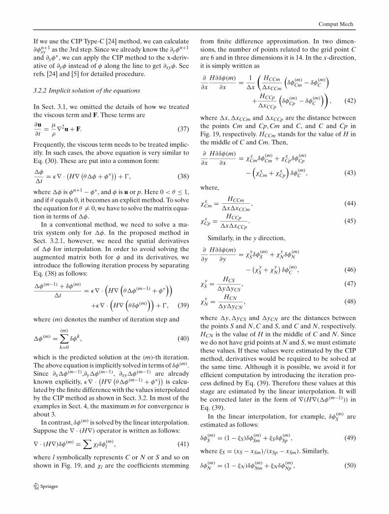
from finite difference approximation. In two dimen-sions, the number of points related to the grid point Care 6 and in three dimensions it is 14. In the x-direction,it is simply written as

∂

∂xH∂δφ(m)

∂x= 1�x

(HCCm

�xCCm

(δφ

(m)Cm − δφ

(m)C

)

+ HCCp

�xCCp

(δφ

(m)Cp − δφ

(m)C

)), (42)

where �x,�xCCm and �xCCp are the distance betweenthe points Cm and Cp, Cm and C, and C and Cp inFig. 19, respectively. HCCm stands for the value of H inthe middle of C and Cm. Then,

∂

∂xH∂δφ(m)

∂x= χx

Cmδφ(m)Cm + χx

Cpδφ(m)Cp

−(χx

Cm + χxCp

)δφ

(m)C , (43)

where,

χxCm = HCCm

�x�xCCm, (44)

χxCp = HCCp

�x�xCCp. (45)

Similarly, in the y direction,

∂

∂yH∂δφ(m)

∂y= χ

ySδφ

(m)S + χ

yNδφ

(m)N

− (χ

yS + χ

yN

)δφ

(m)C , (46)

χyS = HCS

�y�yCS, (47)

χyN = HCN

�y�yCN, (48)

where �y,�yCS and �yCN are the distances betweenthe points S and N, C and S, and C and N, respectively.HCN is the value of H in the middle of C and N. Sincewe do not have grid points at N and S, we must estimatethese values. If these values were estimated by the CIPmethod, derivatives would be required to be solved atthe same time. Although it is possible, we avoid it forefficient computation by introducing the iteration pro-cess defined by Eq. (39). Therefore these values at thisstage are estimated by the linear interpolation. It willbe corrected later in the form of ∇(H∇(�φ(m−1))) inEq. (39).

In the linear interpolation, for example, δφ(m)S areestimated as follows:

δφ(m)S = (1 − ξS)δφ

(m)Sm + ξSδφ

(m)Sp , (49)

where ξS = (xS − xSm)/(xSp − xSm). Similarly,

δφ(m)N = (1 − ξN)δφ

(m)Nm + ξNδφ

(m)Np , (50)


where ξN = (xN − xNm)/(xNp − xNm). These equationsare substituted into Eq. (46). For the calculation of ∇ ·(H∇(θ�φ(m−1)+φ∗)), we use the technique proposed inSect. 3.2, and thus �φ(m−1)

S and �φ(m−1)N are estimated

by the CIP interpolation defined by Eqs. (92) and (93).Similarly, in the z direction:

∂

∂zH∂δφ(m)

∂z= χz

CBδφ(m)B + χz

Tδφ(m)T

− (χz

B + χzT

)δφ

(m)C , (51)

χzB = HCB

�z�zCB, (52)

χzT = HCT

�z�zCT, (53)

where �z,�zCB and �zCT are the distances betweenthe points B and T, C and B, and C and T. By the samereason, B and T are estimated by using neighboringpoints. In this case, however, we need two steps to deter-mine the values. First, these points are estimated by BSand BN as follows:

δφ(m)B = (1 − ηB)δφ

(m)BS + ηBδφ

(m)BN , (54)

where ηB = (zB − zBS)/(zBN − zBS). Next, δφ(m)BS and

δφ(m)BN are linearly interpolated in the x direction:

δφ(m)BS = (1 − ξBS)δφ

(m)BSm + ξBSδφ

(m)BSp, (55)

where ξBS = (xBS − xBSm)/(xBSp − xBSm). Similarly,

δφ(m)BN = (1 − ξBN)δφ

(m)BNm + ξBNδφ

(m)BNp. (56)

These equations are substituted into Eq. (51).In this way Eq. (39) is modified as follows:

1�tδφ

(m)C − κθ

∑χlδφ

(m)l

= − 1�t�φ

(m−1)C + κ∇ ·

(H∇

(θ�φ(m−1)+φ∗))

+ .

(57)

This equation is solved in terms of δφm by using theBiCGSTAB matrix solver [28–30].

By using this notation, Eq. (30) is calculated as fol-lows:

δp(m)C

ρC2s�t2

−∑

χlδp(m)l

= −�p(m−1)C

ρC2s�t2

+∇ ·(

1ρ

∇(�p(m−1) + p∗))

+ ∇ · u∗+1

�t.

(58)

Here ∇ ·u∗+1 is estimated in a form of average flux ofthe control volume. This means that ∂u/∂x is estimatedas follows:

Fig. 3 Control volume around a central point in pressure calcu-lations

∂u∂x

= 2xCp − xCm

(u

(xC + xCp

2, yC, zC

)

−u(

xC + xCm

2, yC, zC

)), (59)

where u(x, y, z) is estimated by the CIP. In addition, thiscontrol volume does not overlap each other and thesevolumes cover the entire space. Figure 3 shows a two-dimensional control volume. Then y and z directions arecalculated as follows:

∂v∂y

= 2yN − yS

(v(

xC,yC + yN

2, zC

)

− v(

xC,yC + yS

2, zC

)), (60)

∂w∂z

= 2zT − zB

(w

(xC, yC,

zC + zT

2

)

− w(

xC, yC,zC + zB

2

)). (61)

3.2.3 Velocity update

The non-advection part of the momentum equation alsoincludes the pressure gradient (see Eq. (32)). For sta-ble calculations, these need to be estimated like it isdone with staggered grids. Thus, the two gradients ofthe pressure are calculated in the middle of C and Cmand Cp and C, and the pressure gradient at C is esti-mated by the linear combination of these two gradientsas follows:

∂u∂t

= −(�xCCp

�x(pC − pCm)

ρCCm�xCCm

+�xCCm

�x(pCp − pC)

ρCCp�xCCp

). (62)

Comput Mech

Similarly,

∂v∂t

= −(�yCN

�y(pC − p(xC, yS, zC))

ρCS�yCS

+ �yCS

�y(p(xC, yN , zC)− pC)

ρCN�yCN

), (63)

∂w∂t

= −(�zCT

�z(pC − p(xC, yC, zB))

ρCB�zCB

+ �zCB

�z(p(xC, yC, zT)− pC)

ρCT�zCT

), (64)

where p(x, y, z) is estimated by the CIP interpolation.

3.2.4 Improvement of the temporal accuracy

Using a semi-Lagrangian method [25] and an implicitmethod, we can choose any time-step size. The problemthat we have to consider is the accuracy in time. We usu-ally assume that there is no velocity change during theadvection process in Eq. (17). If the velocity changes intime, then it should be estimated as follows:

u(x, t) = (t − tn)un+1(x)+ (tn+1 − t)un(x)tn+1 − tn

. (65)

Unfortunately, however, the velocity at the next timestep is not yet determined, and thus we propose toapproximate it by the following iteration process. Atfirst, we define:

l = 0, (66)

un+1,(l) = un, (67)

φn+1,(l) = φn, (68)

where l is the iteration counter. Here φ represents vari-ous physical quantities that vary in time. Thus the advec-tion velocity is estimated as follows:

u(x, t) = (t − tn)un+1,(l)(x)+ (tn+1 − t)un(x)tn+1 − tn

. (69)

At every iteration, we regenerate a new grid becausethe surface of the moving structure will be in a differentposition during the iterations within a time step. There-fore, x in Eq. (69) is the location of the new grid points.Since un+1,(l) and un are on the old grids, the CIP inter-polation is used to estimate them.

Using Eq. (69), Eqs. (15) and (16) are calculated,and the calculated values are stored as data with thesuperscript n + 1, (l + 1). Then (l) is incremented by oneand we return to the procedure for generating a newgrid. As shown in a later section, only one iteration issufficient. In summary, φn+1,(0) = φn is used as the ini-tial guess. At every iteration counted by the iterationcounter (l), (a) we generate a new grid, (b) calculate φ∗

by using Eqs. (17) and (69), (c) solve for pressure byusing Eq. (30), and (d) solve for other φn+1,(l+1).

4 Test calculations

4.1 Two dimensions

4.1.1 Compressible flow

We first test the proposed scheme on a compressible flowproblem. The purpose of this calculation is to confirm thedirectional independence of the calculation because thelines in the Soroban grid is directed to a specific directionand thus the directional dependence might be expected.A high density and high pressure fluid is placed at thecenter like a circular cylinder, then this fluid should radi-ally explode away. The calculation area is 0 ≤ x ≤ 1 and0 ≤ y ≤ 1, with ρ = 0.1, P = 0.1 for R > 0.08 andρ = 1.0, P = 3.0 for R < 0.08, where R is the distancefrom the center. In this calculation, we set γ = 1.4. Weadopt the scalar numerical viscosity proposed by Ogataand Yabe [26] to avoid the directional dependence ofthe viscosity for variable grid size. If ∇ · u ≤ 0,

q = −ρcv

(Cs − γ + 1

2λ∇ · u

)λ∇ · u, (70)

otherwise, q = 0, where cv = 0.55, Cs is the local acous-tic speed and λ is (�x�y)1/2. Here �x and �y are thelocal grid spacings.

Figure 4 is the result after 150 steps (�t = 5.0×10−5).Figure 4(a) is the result with the Cartesian grid and 4(b)is the result with the Soroban grid, where the physicalquantity used for the monitor is the density, and α = 7.1and β = 1.1. Although the Soroban grid is not symmet-rical, the cylindrical symmetry is not deteriorated. Thegrid was controlled so that the maximum grid spacing is0.04 and the minimum spacing is 0.0027.

The number of grid points varies with time as shownin Fig. 5, and the grid location at the final step is shownin Fig. 6. The Soroban grid describes the shock wavemore sharply with a number of grid points compara-ble to the number of grid points for the Cartesian grid.Furthermore, the profiles at x = y = 0.3 or 0.7 is moresymmetrical. It is important to note that the CPU timefor the Soroban grid and the Cartesian grid are 195 [s]and 290 [s] , respectively. The Soroban grid is provento be faster than non-Soroban grids despite the extracalculation related to the grid generation. The reason ispartly because the computational cost is small for gridgeneration and partly because the number of grid pointsis smaller for most of the calculation as shown in Fig. 5.


(a)

Y0.00 1.00

X

1.00

0.00 0.1

0.12

0.14

0.16

0.18

0.2

0.22

0.24

0.26

0 0.2 0.4 0.6 0.8 1

xy

xy

(b)

Y0.00 1.00

X

1.00

0.00 0.1

0.12

0.14

0.16

0.18

0.2

0.22

0.24

0.26

0 0.2 0.4 0.6 0.8 1

xy

xy

Fig. 4 Explosion of a point. (Left) Density contours at t = 7.5 ×10−2, after 150 steps. (Right) Cross-section along x = 0.5, y = 0.5and y = x. The grid system for (a) is a Cartesian grid with

�x = �y = 0.01 and for (b) is the Soroban grid with the numberof grid points less than the number grid points of the Cartesiangrid, which is 101 × 101

Fig. 5 Time evolution of the number of grid points

4.1.2 Incompressible flow

The next example is incompressible flow past a circularcylinder. The dimension of the computational domain is60×16, which is normalized by the diameter of the cylin-der. The cylinder is located at (8, 8), and the location ofthe cylinder and the lateral dimension of the domain arethe same as those reported in [27]. The initial Sorobangrid is shown in Fig. 7. The Soroban lines are parallel tothe vertical (y) axis, and the grid points are placed oneach line in a way to refine the grid where it is needed.

We also put grid points inside the cylinder, otherwisethe interpolations become more complicated. The gridsin this case are generated from the monitoring functionsthat depend on the distance from the surface and thevorticity:

M1(x, y) = 10.005 + 0.1 × min(5, D(x, y))

, (71)

D(x, y) =√(x − 8)2 + (y − 8)2 − 0.5, (72)

M2(x, y, t) = 1 + 50 ×∣∣∣∣∂v∂x

− ∂u∂y

∣∣∣∣ , (73)

M(x, y, t) = min

(∑Nk=1 Mk(x, y)

N,�xmax

�xmin

). (74)

The no-slip boundary condition is imposed on the cylin-der surface, and inside the cylinder the velocities are setto u = v = 0. We employed the second-order implicit

Comput Mech

Fig. 6 Grid arrangement for the Soroban grid

Fig. 7 Initial grid arrangement. The Soroban lines are parallelto the vertical (y) axis. All other lines are for visualization pur-pose only. (Top) Entire grid image. (Bottom) Local view near thecylinder

method (i.e. θ = 1/2 in Eq. (38)) for the viscous term.The Reynolds number is 100.

The drag coefficient CD and lift coefficient CL aredefined as follows:

CD = FD12ρU2∞D

, (75)

CL = FL12ρU2∞D

, (76)

where FD and FL are the drag and lift forces, respec-tively. Initially the number grid points is about 4,000,

Fig. 8 Time history of the drag coefficient CD and lift coefficientCL for the flow past a cylinder at Re = 100

and it is eventually increased up to 9,000 points. Figure 8shows the time history of the drag and lift coefficients.The drag coefficient is 1.375 ± 0.009 and the lift coeffi-cient is ±0.27. The computed Strouhal number is about0.16. These values are in good agreement with thosereported in [27].

Figure 9 is a snapshot of the adaptive grids. The num-ber of grid points changes in time as shown in Fig. 10.After t = 80, the number of grid points stays at the samevalue, because the number of wake vortices remainsalmost constant in the computational domain. We com-pared the calculation with the fine grids as shown in thebottom of Fig. 9. The grid spacing is the same as it is inthe finest part of the Soroban grids. The number of gridpoints is 45,000. Figure 11 shows the maximum vortic-ity on each line(y direction). This figure indicates thatSoroban grids can work very well without introducingany additional diffusion.

Next, we tested the dependence of the solution on thenumber of iterations used in Eq. (69). Figure 12 showsthe lift coefficient in which ‘Iteration 1’ means l = 1.We cannot see a difference between l = 1 and l = 2.Therefore, it is sufficient to use Eq. (69) only once.

In Fig. 12, we also depict the results from linear inter-polation. As explained in Sect. 3.2.2, we normally usethe CIP method for interpolation. The figure shows thatthe use of linear interpolation instead of the CIP givesrise to a large dissipation error as well as error in Strou-hal number, which is 0.14 for linear interpolation, whileit is 0.164, 0.165, 0.165 for l = 0, 1, 2. Thus, accurateinterpolation is a key issue in the Soroban grid system.

Since both the semi-Lagrangian technique for theadvection terms and the implicit procedure for the pres-sure and viscous terms make the scheme free from CFLconstraints, we can use any time-step size. This becomesvery important for locally refined grids that limit thetime-step size in conventional schemes. Actually, the


Fig. 9 (Top) Snapshot of the adaptive grid. (Bottom) Fixed fine grid

2000

4000

6000

8000

10000

12000

14000

16000

0 20 40 60 80 100 120 140 160 180

Fig. 10 Time history of the number of grid points in the adaptivecalculation

time-step size was set to �t = 0.05 regardless of thegrid size, and the maximum CFL number is about 10.

4.2 Three dimensions

In this section, we examine a three dimensional case.The CCUP method can calculate compressible flow andincompressible flow at the same time. Then, we added acolor function ψ , where ψ = 1 for water and ψ = 0 forair. The advection ofψ is solved by the tangent-functionCIP [31]. Then this ψ is used for the calculation of thephysical values at grid points as follows:

0.001

0.01

0.1

1

10

100

0 10 20 30 40 50 60

Max

imum

vor

ticity

alo

ng e

ach

line

x

adaptive gridfine grid

Fig. 11 Maximum magnitude of the vorticity along each Sorobanline, given by the adaptive and fixed fine grids

Rgrid = Rwaterψ + Rair(1 − ψ), (77)

where Rgrid, Rwater and Rair are the physical values atthe grid point, and for water and air. In the calculation,the acoustic speed and viscosity of the mixed states aresimilarly calculated by using this color function.

As a test calculation, we adopt a skimmer (stone-skipping) simulation. The coupling technique we use indealing with the interaction between the solid and fluidis explained in [32]. At every iteration, (a) we move theobject with fluid forces based on the pressure valuescalculated by using the pressure versions of Eqs. (17)

Comput Mech

Fig. 12 Time history of thelift coefficient at Re = 100

-0.4

-0.3

-0.2

-0.1

0

0.1

0.2

0.3

0.4

160 170 180

Lift Coefficient

Time

No iterationIteration 1

Iteration 2Linear Interoplation

and (69), (b) generate a new grid, (c) calculate φ∗ byusing Eqs. (17) and (69), (d) solve for pressure by usingEq. (30), and (e) solve for other φn+1,(l+1). We havealready performed experiments, and the detailed move-ment was visualized by a high-speed camera as shownin Fig. 13 [32]. In the experiment, the disk made of alu-minum was used instead of a stone. The feature of thisphenomenon is that the disk goes through thin waterfilm, which is generated by the collision of the disk andwater surface.

In order to capture such phenomena, the Sorobangrid points were collected near the interface of the waterand air and also, to a lesser extent, near the solid sur-faces. Figures 14 and 15 show the computed results inwhich the initial velocity of the aluminum disk is set to(u, v, w) = (5, −1.2, 0) m/s, and the angle-of-attack is 10degrees. The disk is 5 cm in diameter and 1 cm in thick-ness, rotating with a speed of 20 rad/s. The domain size inthe simulation is 0.4×0.14×0.14 m, and the water depthis 0.05 m. The number of grid points is not constant butis about 120,000.

The calculation was efficiently advanced by automati-cally repeating grid generation. Figure 16 shows the gridarrangement. A vertical plane shows the grid arrange-ment where we connected the grid points, like it is ina finite element method, but the connectivity is for thepurpose of visualization only. Also for visualization pur-pose, grid points in three dimensions are depicted byspheres whose size depends on the density and hencethe grid points in the air are not visible.

5 Concluding remarks

We have proposed, for fluid–object and fluid–structureinteractions, the Soroban CCUP method, which uses a

collocated-grid approach. Multi-fluid flows with densityratios reaching 1000 and fluid–object interactions werecomputed robustly and accurately. The use of the CIPinterpolation in the estimation of the values from theneighboring points enhances the accuracy compared tousing linear interpolation. In solving the matrix systems,we avoided the inclusion of the derivatives and proposedan efficient iteration procedure.

By using a semi-Lagrangian CIP technique and bytreating the viscous terms implicitly, we removed thetime-step size limitations to a large extent, and in somecases we were able to compute with the CFL numberreaching 10. Therefore, we are able to use large time-step sizes even with very small mesh sizes in refined-mesh areas.

Because of somewhat limited movement of the Soro-ban grid and the resulting ease in memory management,searching for the neighboring points is very fast andhence the time required for dynamical grid generationis negligibly small. The Soroban grid technique we cur-rently have imposes, for the sake of computational effi-ciency, fine grid resolution (in directions perpendicularto the Soroban grid lines and planes) even in locationsfar from the solid objects. This is one of the aspects of themethod that we plan to improve in the future, withoutsignificantly compromising the efficiency.

6 Appendix

6.1 Specifying the grid point locations

The location of a grid point is specified by the Carte-sian coordinate (x, y, z) in the three-dimensional space.However, the grid points along a line has the same value


Fig. 13 Skimmer experiment

of y and z. Therefore, we specify the plane by the indexkP and call it the k-th plane. Similarly the line is specifiedby the index jL. Since jL is a one-dimensional index and

Fig. 14 Skimmer simulation (side view)

continuously increases over all the planes, we need tointroduce the starting index JLS[kP], which means thatthe line index jL starts from JLS[kP] on the kP plane.

Similarly, the grid point is specified by the index iG,which is also a one-dimensional index and continuouslyincreases over all the lines, and we introduce the startingindex IGS[jL] on the jL line. The grid points are stored ina one-dimensional array in the order shown in Table 1.

In the calculation described in the next section, weneed to know where the point (x0, y0, z0) is locatedin this system. First, z0 is specified by two planes asfollows:

Comput Mech

Fig. 15 Skimmer simulation (front view)

Fig. 16 Grid points used in the simulation. The vertical planeshows the grid arrangement. For visualization, grid points in threedimensions are depicted by spheres whose sizes represent the den-sity

Table 1 JLS denotes the start index for the lines on each plane.IGS denotes the start index for the grid points on each line. Forexample, the number of grid points is 2 and 3 for the 7-th and 8-thlines. See also Fig. 1

Plane number 1 2 3 ...

JLS 1 4 7 ...

Line number ... 7 8 9 10 ...

IGS ... 17 19 22 24 ...

z[kP] ≤ z0 < z[kP + 1], (78)

as shown in Fig. 17. There would be several methods ofsearching the kP as proposed in our previous paper [5],but in this paper, we use the binary search tree algo-rithm since the cost of computation is very small in aone-dimensional search. Since the system is arranged as


B

BS

BN

T

iG00

( )x , y , z 0 0 0

jL

kP

z

y

x

G

iG

iG

i01

11

10

Fig. 17 Location of a point (x0, y0, z0) in the Soroban grid. Thefirst and second subscripts of iG specify the line and plane num-bers, respectively

h 1

φ i−1 φ i φ i+1

h 2x i−1 x i+1x iFig. 18 One-dimensional non-regular grid

in Fig. 17, we need to find two lines on the kP plane andanother two lines on the kP + 1 plane so that

y[jL] ≤ y0 < y[jL + 1] (79)

is satisfied. We note that there are two jLs; one is for thekP plane and the other is for the kP + 1 plane.

Similarly, we search for x0 on the jL-th line:

x[iG] ≤ x0 < x[iG + 1]. (80)

We note that there are four iGs shown in Fig. 17.

6.2 One-dimensional CIP Interpolation

CIP1D is to estimate the function by the CIP method.In fact we use the spatial derivatives as follows,

CIP1D (φ0,φ1, X, D) = CIP(φ0, ∂xφ0,φ1, ∂xφ1, X, D)

(81)

CIP(φ0, ∂xφ0,φ1, ∂xφ1, X, D) = �3k=0CkXk (82)

∂xCIP(φ0, ∂xφ0,φ1, ∂xφ1, X, D) = �3k=1k · CkXk−1 (83)

C0 = φ0, (84)

C1 = ∂xφ0, (85)

C2 = 3(φ0 + φ1)

D2 − 2∂xφ0 − ∂xφ1

D3 , (86)

C3 = ∂xφ0 + ∂φ1

D2 + 2(φ0 − φ1)

D3 . (87)

This is x directional estimation, when we calculate alongthe y direction, spatial derivatives of y direction are re-quired.

6.3 Preliminary concepts of finite differenceson the Soroban grid

In estimating the finite difference of ∂φ/∂x and the termsin G , we need special consideration because for exam-ple as shown in Fig. 17, all the points in general are notalways on a straight line. In this paper, we interpolatethe values needed for finite differences by using the gridpoints. Usually the interpolation deteriorates the accu-racy. As already demonstrated in a previous paper [5],the CIP method can very accurately retrieve a profilebetween the grid points.

We should just consider two derivatives. One is thefirst spatial derivative, the other is the second derivative.In one dimension, it is just using finite differences overnon-regular grids.

For example,

h1 = xi − xi−1, (88)

h2 = xi+1 − xi, (89)∂φi

∂x= 1

h1 + h2

(h1φi+1 − φi

h2− h2

φi − φi−1

h1

), (90)

∂2φi

∂x2 = 2h1 + h2

(φi − φi−1

h1+ φi+1 − φi

h2

). (91)

In two dimensions, shown in the bottom-left part ofFig. 19, estimation of the derivative at C needs the valuesat N and S along the vertical line, but these two pointsdo not in general coincide with the grid points. Then weuse CIP interpolation like we do in the advection part.

The value at S can be estimated by the values at Smand Sp. This is symbolically written as

φS = CIP1D(φSm,φSp, xS − xSm, xSp − xSm

). (92)

Similarly at N,

φN = CIP1D(φNm,φNp, xN − xNm, xNp − xNm

). (93)

In this way, we get φS,φN , h1 = yj − yj−1, h2 = yj+1 − yj.Then, we can calculate the spatial derivative in they-direction at C.

Comput Mech

Fig. 19 Black points are thegrid points. Circles are thepoints that must be estimatedfrom the grid points on a lineor plane. The shaded circlesinside the circles at T and Bshow the location of the pointC in other planes. The symbolC denotes center, N and Sdenote north and south, andB and T denote bottom andtop. Lower case m and p arethe minus and plus sidesalong a line

The derivatives in the z direction are also estimatedby φB and φT on the neighboring planes. φB are esti-mated by φBS and φBN as follows:

φB = CIP1D (φBS,φBN , yB − yBS, yBN − yBS) , (94)

where φBN and φBS are estimated like N and S. Forexample,

φBS = CIP1D(φBSm,φBSp, xBS − xBSm, xBSp − xBSm

).

(95)

References

1. Takewaki H, Nishiguchi A, Yabe T (1985) The cubic-inter-polated pseudo-particle (CIP) method for solving hyperbolic-type equations. J Comput Phys 61:261–268

2. Takewaki H, Yabe T (1987) Cubic-interpolated pseudo parti-cle (CIP) method – Application to nonlinear or multi-dimen-sional problems. J Comput Phys 70:355–372

3. Yabe T, Aoki T (1991) A universal solver for hyperbolic-equa-tions by cubic-polynomial interpolation. I. One-dimensionalsolver. Comput Phys Commun 66:219–232

4. Yabe T, Xiao F, Utsumi T (2001) Constrained interpola-tion profile method for multiphase analysis. J Comput Phys169:556–593

5. Yabe T, Mizoe H, Takizawa K, Moriki H, Im H, Ogata Y(2004) Higher-order schemes with CIP method and adap-tive Soroban grid towards mesh-free scheme. J Comput Phys194:57–77

6. Yabe T, Wang PY (1991) Unified numerical procedurefor compressible and incompressible fluid. Phys Soc Jpn J60:2105–2108

7. Tezduyar TE, Behr M, Liou J (1992) A new strat-egy for finite element computations involving movingboundaries and interfaces – The deforming-spatial-domain/space–time procedure: I. The concept and the pre-liminary numerical tests. Comput Methods Appl Mech Eng94:339–351

8. Tezduyar TE, Behr M, Mittal S, Liou J (1992) A newstrategy for finite element computations involvingmoving boundaries and interfaces – The deforming-spa-tial-domain/space–time procedure: II. Computation offree-surface flows, two-liquid flows, and flows with driftingcylinders. Comput Methods Appl Mech Eng 94:353–371

9. Johnson AA, Tezduyar TE (1996) Simulation of multiplespheres falling in a liquid-filled tube. Comput Methods ApplMech Eng 134:351–373

10. Johnson AA, Tezduyar TE (1997) 3D simulation of fluid-par-ticle interactions with the number of particles reaching 100.Comput Methods Appl Mech Eng 145:301–321

11. Mittal S, Tezduyar TE (1995) Parallel finite element simula-tion of 3D incompressible flows – Fluid-structure interactions.Int J Numerical Methods Fluids 21:933–953

12. Stein K, Benney R, Kalro V, Tezduyar TE, Leonard J, AccorsiM (2000) Parachute fluid–structure interactions: 3-D Compu-tation. Comput Methods Appl Mech Eng 190:373–386

13. Wall W (1999) Fluid–Structure Interaction with Stabilized Fi-nite Elements. Ph.D. thesis, University of Stuttgart

14. Heil M (2004) An efficient solver for the fully coupled solu-tion of large-displacement fluid–structure interaction prob-lems. Comput Methods Appl Mech Eng 193:1–23


15. Hubner B, Walhorn E, Dinkler D (2004) A monolithic ap-proach to fluid–structure interaction using space–time finiteelements. Comput Methods Appl Mech Eng 193:2087–2104

16. Dettmer W (2004) Finite element modeling of fluid flow withmoving free surfaces and interfaces including fluid–solid inter-action. Ph.D. thesis, University of Wales Swansea

17. Tezduyar TE (2001) Finite element methods for flow prob-lems with moving boundaries and interfaces. Arch ComputMethods Eng 8:83–130

18. Berger MJ, Oliger J (1984) Adaptive mesh refinement forhyperbolic partial differential equations. J Comput Phys53:484–512

19. Kirkpatrick MP, Armfield SW, Kent JH (2003) A representa-tion of curved boundaries for the solution of the Navier-Stokesequations on a staggered three-dimensional Cartesian grid. JComput Phys 184:1–36

20. Unverdi SO, Tryggvasson GA (1992) A front-tracking methodfor viscous, incompressible, multi-fluid flows. J Comput Phys100:25–37

21. Enright D, Fedkiw R, Ferziger J, Mitchell I (2002) A hybridparticle level set method for improved interface capturing. JComput Phys 183:83–116

22. Harlow FH, Amsden AA (1968) Numerical calculation ofalmost incompressible flow. J Comput Phys 3:80–93

23. Yoon SY, Yabe T (1999) The unified simulation for incom-pressible and compressible flow by the predictor-correctorscheme based on the CIP method. Comput Phys Commun119:149–158

24. Aoki T (1995) Multi-dimensional advection of CIP (cubic-interpolate propagation) scheme. CFD J 4:279–291

25. Staniforth A, Côté J (1991) Semi-Lagrangian integrationscheme for atmospheric models - A review. Mon WeatherRev 119:2206–2223

26. Ogata Y, Yabe T (1999) Shock capturing with improvednumerical viscosity in primitive Euler representation. Com-put Phys Commun 119:1799–193

27. Tezduyar TE, Liou J, Ganjo DK (1990) Incompressible flowcomputations based on the vorticity-stream function andvelocity-pressure formulations. Comput Struct 35:445–472

28. van der Vorst HA (1992) Bi-CGSTAB: a fast and smoothlyconverging variant of Bi-CG for the solution of non symmetriclinear systems. SIAM J Sci Stat Comput 13:631–644

29. Lee J, Zhang J, Lu C (2003) Incomplete LU preconditioningfor large scale dense complex linear systems from electromag-netic wave scattering problems. J Comput Phys 185:158–175

30. Show E, Saad Y (1997) Experimental study of ILUpreconditioners for indefinite matrices. J Comput ApplMath 86:387–414

31. Yabe T, Xiao F (1993) Description of complex and sharp inter-face during shock wave interaction with liquid drop. Phys SocJpn J 62:2537–2540

32. Takizawa K, Yabe T, Chino M, Kawai T, Wataji K, Hoshino H,Watanabe T (2005) Simulation and experiment on swimmingfish and skimmer by CIP method. Comput Struct 83:397–408

Documents

Computation of free-surface flows and fluid–object ... of free-surface flows and fluid–object interactionswith the CIP method based on adaptive meshless soroban grids 2.2.1