1

Computation of Turbulent Viscous Flow around Submarine Hull Using Unstructured Grid

M. M. Karim1, M. M. Rahman2 and M. A. Alim3

1Dept. of Naval Architecture and Marine Engineering, Bangladesh University of Engineering and Technology, Email: mmkarim@name.buet.ac.bd, 2Department of Natural Science, Stamford University, Bangladesh, Email: mahbub_stamford@yahoo.com, 3Dept. of Mathematics, Bangladesh University of Engineering and Technology, Email: maalim@math.buet.ac.bd

Abstract This paper presents finite volume method based on Reynolds-averaged Navier-Stokes (RANS) equations for computation of 2D axisymmetric flow around bare submarine hull using unstructured grid. The body used for this purpose is a standard DREA (Defence Research Establishment Atlantic) bare submarine hull. Shear Stress Transport (SST) k-ω model has been used to simulate turbulent flow past the hull surface. Finally, computed results using unstructured grid are compared with those using structured grid and also with published experimental measurements. The computed results show good agreement with the experimental measurements. Keywords: axisymmetric body of revolution, underwater vehicle, unstructured grid, viscous drag, CFD, turbulence model 1. Introduction Applications of computational fluid dynamics (CFD) to the maritime industry continue to grow as this advanced technology takes advantage of the increasing speed of computers. In the last two decades, different areas of incompressible flow modeling including grid generation techniques, solution algorithms and turbulence modeling, and computer hardware capabilities have witnessed tremendous development. In view of these developments, computational fluid dynamics (CFD) can offer a cost-effective solution to many problems in underwater vehicle hull forms. However, effective utilization of CFD for marine hydrodynamics depends on proper selection of turbulence model, grid generation and boundary resolution.

Turbulence modeling is still a necessity as even with the emergence of high performance computing since analysis of complex flows by direct numerical simulations (DNS) is untenable. The peer approach, the large-Eddy simulation (LES), still remains expensive. Hence, simulation of underwater hydrodynamics continues to be based on the solution of the Reynolds-averaged Navier-Stokes (RANS) equations. Various researchers used turbulence modeling to simulate flow around axisymmetric bodies since late seventies. Patel and Chen [1] made an extensive review of the simulation of flow past axisymmeric bodies. Choi and Chen [2] gave calculation method for the solution of RANS equation, together with k-ε

2

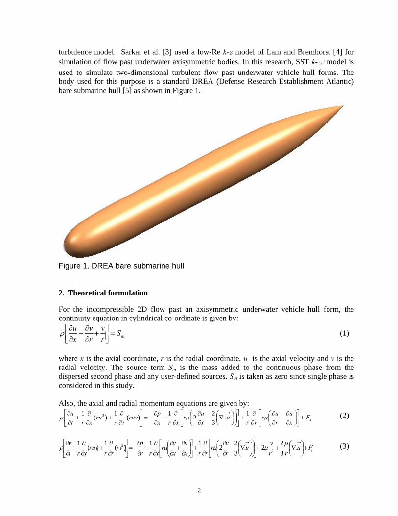
turbulence model. Sarkar et al. [3] used a low-Re k-ε model of Lam and Bremhorst [4] for simulation of flow past underwater axisymmetric bodies. In this research, SST k-ω model is used to simulate two-dimensional turbulent flow past underwater vehicle hull forms. The body used for this purpose is a standard DREA (Defense Research Establishment Atlantic) bare submarine hull [5] as shown in Figure 1.

Figure 1. DREA bare submarine hull 2. Theoretical formulation

For the incompressible 2D flow past an axisymmetric underwater vehicle hull form, the continuity equation in cylindrical co-ordinate is given by:

mSrv

rv

xu

=⎥⎦⎤

⎢⎣⎡ +

∂∂

+∂∂ρ (1)

where x is the axial coordinate, r is the radial coordinate, u is the axial velocity and v is the radial velocity. The source term Sm is the mass added to the continuous phase from the dispersed second phase and any user-defined sources. Sm is taken as zero since single phase is considered in this study. Also, the axial and radial momentum equations are given by:

xFxu

rur

rru

xur

xrxpruv

rrru

xrtu

+⎥⎦

⎤⎢⎣

⎡⎟⎠⎞

⎜⎝⎛

∂∂

+∂∂

∂∂

+⎥⎦

⎤⎢⎣

⎡⎟⎠

⎞⎜⎝

⎛⎟⎠⎞

⎜⎝⎛∇−

∂∂

∂∂

+∂∂

−=⎥⎦

⎤⎢⎣

⎡∂∂

+∂∂

+∂∂ →

µµρ 1.3221)(1)(1 2 (2)

rFurr

vurvr

rrxu

xvr

xrrprv

rrruv

xrtv

+⎟⎠⎞

⎜⎝⎛∇+−⎥

⎦

⎤⎢⎣

⎡⎟⎠

⎞⎜⎝

⎛⎟⎠⎞

⎜⎝⎛∇−

∂∂

∂∂

+⎥⎦

⎤⎢⎣

⎡⎟⎠⎞

⎜⎝⎛

∂∂

+∂∂

∂∂

+∂∂

−=⎥⎦

⎤⎢⎣

⎡∂∂

+∂∂

+∂∂ →→

.322.

32211)(1)(1

22 µ

µµµρ (3)

3

Where, p = static pressure, µ = molecular viscosity, ρ = density, Fx & Fr are external body

forces and rv

rv

xuu +

∂∂

+∂∂

=⋅∇→

. However, Fx & Fr are taken as zero since no external body

force is used here.

2.1 The Shear-Stress Transport (SST) k-ω model

The SST k-ω turbulence model is a two-equation eddy-viscosity model developed by Menter [6] to effectively blend the robust and accurate formulation of the k-ω model in the near-wall region with the free-stream independence of the k-e model in the far field. To achieve this, the k-e model is converted into a k-ω formulation. The SST k-ω model is similar to the standard k-ω model, but includes the following refinements: • The standard k-ω model and the transformed k-e model are both multiplied by a blending

function and both models are added together. • The blending function is designed to be one in the near-wall region, which activates the

standard k-ω model, and zero away from the surface, which activates the transformed k-e model.

• The SST model incorporates a damped cross-diffusion derivative term in the ω equation. • The definition of the turbulent viscosity is modified to account for the transport of the

turbulent shear stress. • The modeling constants are different.

These features make the SST k-ω model more accurate and reliable for a wider class of flows (e.g., adverse pressure gradient flows, airfoils, transonic shock waves) than the standard k-ω model.

The shear-stress transport (SST) k-ω model is so named because the definition of the turbulent viscosity is modified to account for the transport of the principal turbulent shear stress. The use of a k-ω formulation in the inner parts of the boundary layer [7] makes the model directly usable all the way down to the wall through the visous sub-layer, hence the SST k-ω model can be used as a Low-Re turbulence model without any extra damping functions. The SST formulation also switches to a k-ε behaviour in the free-stream and thereby avoids the common k-ω problem that the model is too sensitive to the inlet free-stream turbulence properties. It is this feature that gives the SST k-ω model an advantage in terms of performance over both the standard k-ω model and the standard k-ε model. Other modifications include the addition of a cross-diffusion term in the ω equation and a blending function to ensure that the model equations behave appropriately in both the near-wall and far-field zones. Transport equations for the SST k-ω model are given by:

kkkj

kj

ii

SYGxk

xku

xk

t+−+⎟

⎟⎠

⎞⎜⎜⎝

⎛

∂∂

Γ∂∂

=∂∂

+∂∂ ~)()( ρρ (4)

4

ωωωωωωρωρω SDYGxx

uxt jj

ii

++−+⎟⎟⎠

⎞⎜⎜⎝

⎛

∂∂

Γ∂∂

=∂∂

+∂∂ )()( (5)

In these equations,

kG~ represents the generation of turbulence kinetic energy due to mean velocity gradients, Gω represents the generation of ω, Гk and Гω represent the effective diffusivity of k and ω, respectively, Yk and Yω represent the dissipation of k and ω due to turbulence, Dω represents the cross-diffusion term, Sk and Sω are user-defined source terms. 2.2 Boundary conditions Since the geometry of an axisymmetric underwater hull is, in effect, a half body section rotated about an axis parallel to the free stream velocity, the bottom boundary of the domain is modeled as an axis boundary. Additionally, the left and top boundaries of the domain are modeled as velocity inlet, the right boundary was modeled as an outflow boundary, and the surface of the body itself was modeled as a wall.

2.3 Viscous drag The viscous drag of a body is generally derivable from the boundary-layer flow either on the basis of the local forces acting on the surface of the body or on the basis of the velocity profile of the wake far downstream. The local hydrodynamic force on a unit of surface area is resolvable into a surface shearing stress or local skin friction tangent to the body surface and a pressure p normal to the surface. The summation over the whole body surface of the axial components of the local skin friction and of the pressure gives, respectively, the skin-friction drag Df and the pressure drag Dp which for a body of revolution in axisymmetric flow become

∫= ex

wwf dxrD0

cos2 ατπ ; ∫= ex

wp dxprD0

sin2 απ

where, rw is the radius from the axis to the body surface, α is the arc length along the meridian profile, and xe is the total arc length of the body from nose to tail.

The sum of the two drags then constitutes the total viscous drag, D or D=Df +Dp

The drag coefficient CD and the pressure coefficient, Cp based on some appropriate reference area A are given by:

AUDC D 25.0 ∞

=ρ

and AU

ppC p 25.0 ∞

∞−=

ρ

where, p∞ is pressure of free stream and U∞ is free stream velocity.

5

3. Methodology 3.1 Computational method and domain The 2D axisymmetric problem with appropriate boundary conditions is solved over a finite computational domain. The computational domain extended 1.0L upstream of the leading edge of the axisymmetric body, 1.0L above the body surface and 2.0L downstream from the trailing edge; where L is the overall length of the body. The solution domain is found large enough to capture the entire viscous-inviscid interaction and the wake development.

A finite volume method [8, 9] is employed to obtain a solution of the Reynolds averaged Navier-Stokes equations. The coupling between the pressure and velocity fields was achieved using PISO algorithm [8]. A second order upwind scheme was used for the convection and the central-differencing scheme for diffusion terms. 3.2 Geometry of bare submarine hull DREA

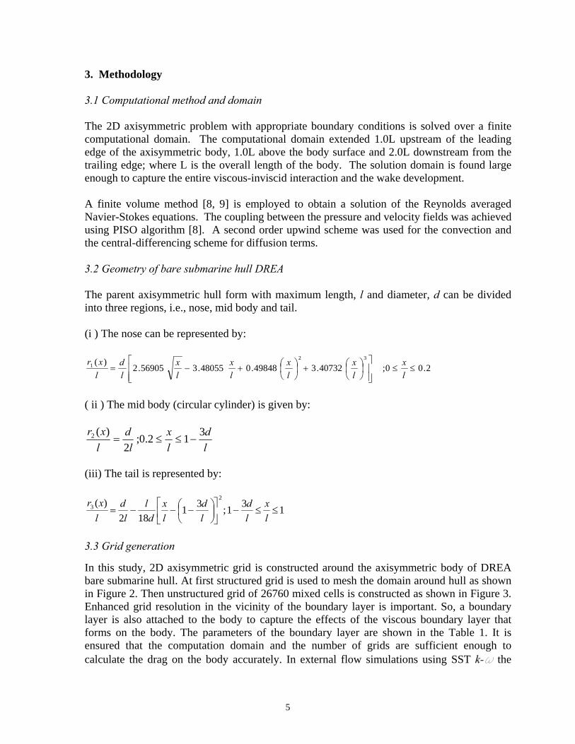
The parent axisymmetric hull form with maximum length, l and diameter, d can be divided into three regions, i.e., nose, mid body and tail. (i ) The nose can be represented by:

2.00;40732.349848.048055.356905.2)( 32

1 ≤≤⎥⎥⎦

⎤⎟⎠⎞

⎜⎝⎛+

⎢⎢⎣

⎡⎟⎠⎞

⎜⎝⎛+−=

lx

lx

lx

lx

lx

ld

lxr

( ii ) The mid body (circular cylinder) is given by:

ld

lx

ld

lxr 312.0;

2)(2 −≤≤=

(iii) The tail is represented by:

131;31182

)( 23 ≤≤−⎥

⎦

⎤⎢⎣

⎡⎟⎠⎞

⎜⎝⎛ −−−=

lx

ld

ld

lx

dl

ld

lxr

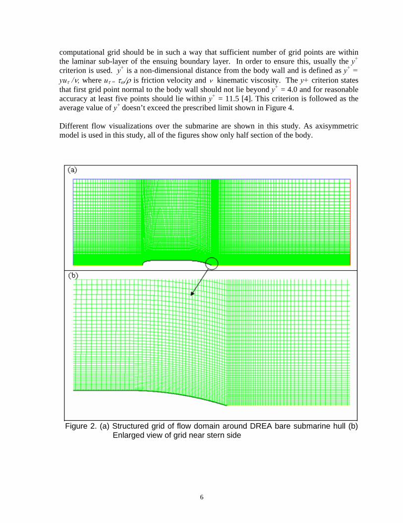
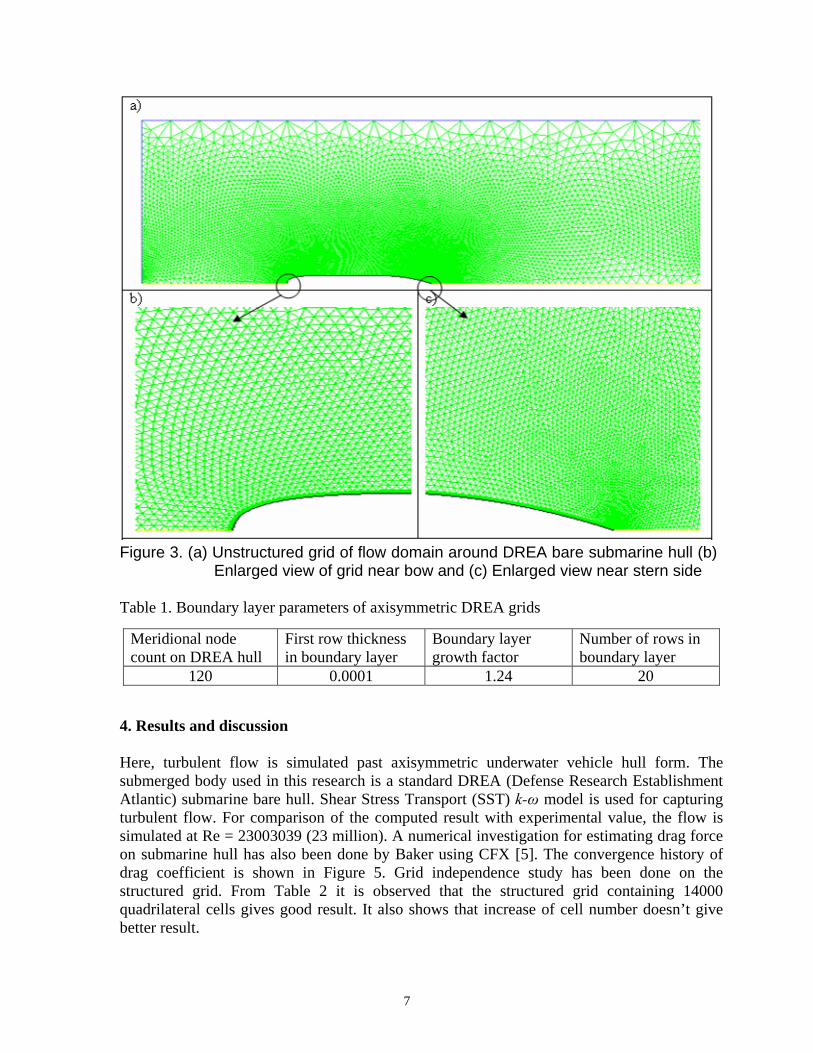
3.3 Grid generation In this study, 2D axisymmetric grid is constructed around the axisymmetric body of DREA bare submarine hull. At first structured grid is used to mesh the domain around hull as shown in Figure 2. Then unstructured grid of 26760 mixed cells is constructed as shown in Figure 3. Enhanced grid resolution in the vicinity of the boundary layer is important. So, a boundary layer is also attached to the body to capture the effects of the viscous boundary layer that forms on the body. The parameters of the boundary layer are shown in the Table 1. It is ensured that the computation domain and the number of grids are sufficient enough to calculate the drag on the body accurately. In external flow simulations using SST k-ω the

6

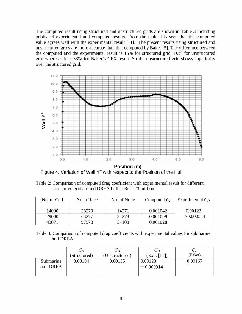
computational grid should be in such a way that sufficient number of grid points are within the laminar sub-layer of the ensuing boundary layer. In order to ensure this, usually the y+ criterion is used. y+ is a non-dimensional distance from the body wall and is defined as y+ = yuτ /ν, where uτ = τω/ρ is friction velocity and ν kinematic viscosity. The y+ criterion states that first grid point normal to the body wall should not lie beyond y+ = 4.0 and for reasonable accuracy at least five points should lie within y+ = 11.5 [4]. This criterion is followed as the average value of y+ doesn’t exceed the prescribed limit shown in Figure 4. Different flow visualizations over the submarine are shown in this study. As axisymmetric model is used in this study, all of the figures show only half section of the body.

Figure 2. (a) Structured grid of flow domain around DREA bare submarine hull (b) Enlarged view of grid near stern side

7

Figure 3. (a) Unstructured grid of flow domain around DREA bare submarine hull (b) Enlarged view of grid near bow and (c) Enlarged view near stern side

Table 1. Boundary layer parameters of axisymmetric DREA grids

Meridional node count on DREA hull

First row thickness in boundary layer

Boundary layer growth factor

Number of rows in boundary layer

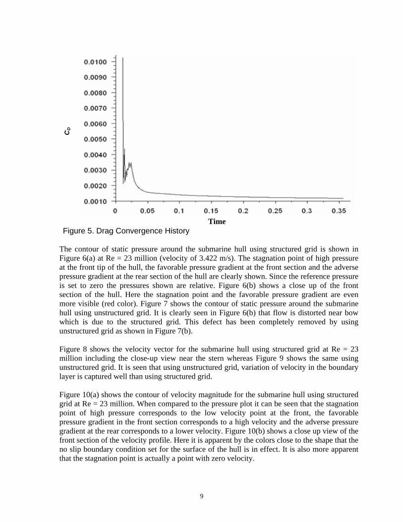
120 0.0001 1.24 20 4. Results and discussion Here, turbulent flow is simulated past axisymmetric underwater vehicle hull form. The submerged body used in this research is a standard DREA (Defense Research Establishment Atlantic) submarine bare hull. Shear Stress Transport (SST) k-ω model is used for capturing turbulent flow. For comparison of the computed result with experimental value, the flow is simulated at Re = 23003039 (23 million). A numerical investigation for estimating drag force on submarine hull has also been done by Baker using CFX [5]. The convergence history of drag coefficient is shown in Figure 5. Grid independence study has been done on the structured grid. From Table 2 it is observed that the structured grid containing 14000 quadrilateral cells gives good result. It also shows that increase of cell number doesn’t give better result.

8

The computed result using structured and unstructured grids are shown in Table 3 including published experimental and computed results. From the table it is seen that the computed value agrees well with the experimental result [11]. The present results using structured and unstructured grids are more accurate than that computed by Baker [5]. The difference between the computed and the experimental result is 15% for structured grid, 10% for unstructured grid where as it is 33% for Baker’s CFX result. So the unstructured grid shows superiority over the structured grid.

Wal

l Y+

Position (m)

Figure 4. Variation of Wall Y+ with respect to the Position of the Hull Table 2: Comparison of computed drag coefficient with experimental result for different

structured grid around DREA hull at Re = 23 million

No. of Cell No. of face No. of Node Computed CD

Experimental CD

14000 28270 14271 0.001042 29000 63277 34278 0.001009 43871 97978 54108 0.001028

0.00123 +/-0.000314

Table 3: Comparison of computed drag coefficients with experimental values for submarine

hull DREA

CD (Structured)

CD (Unstructured)

CD (Exp. [11])

CD (Baker)

Submarine hull DREA

0.00104 0.00135 0.00123 ±0.000314

0.00167

9

CD

Time Figure 5. Drag Convergence History

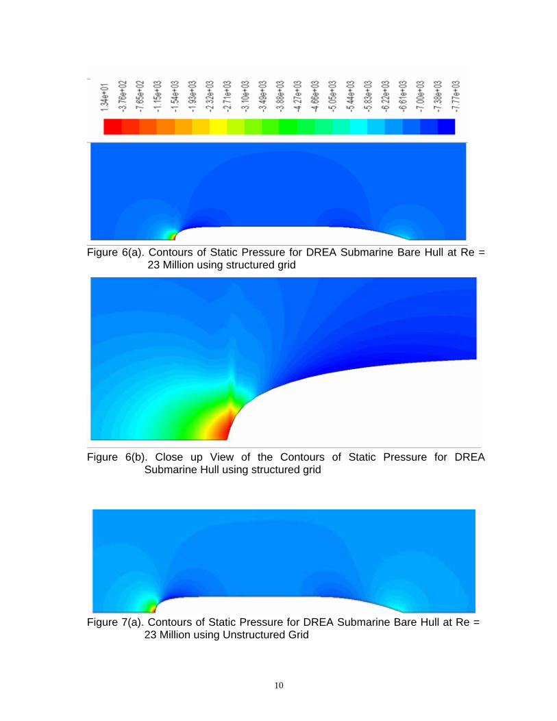
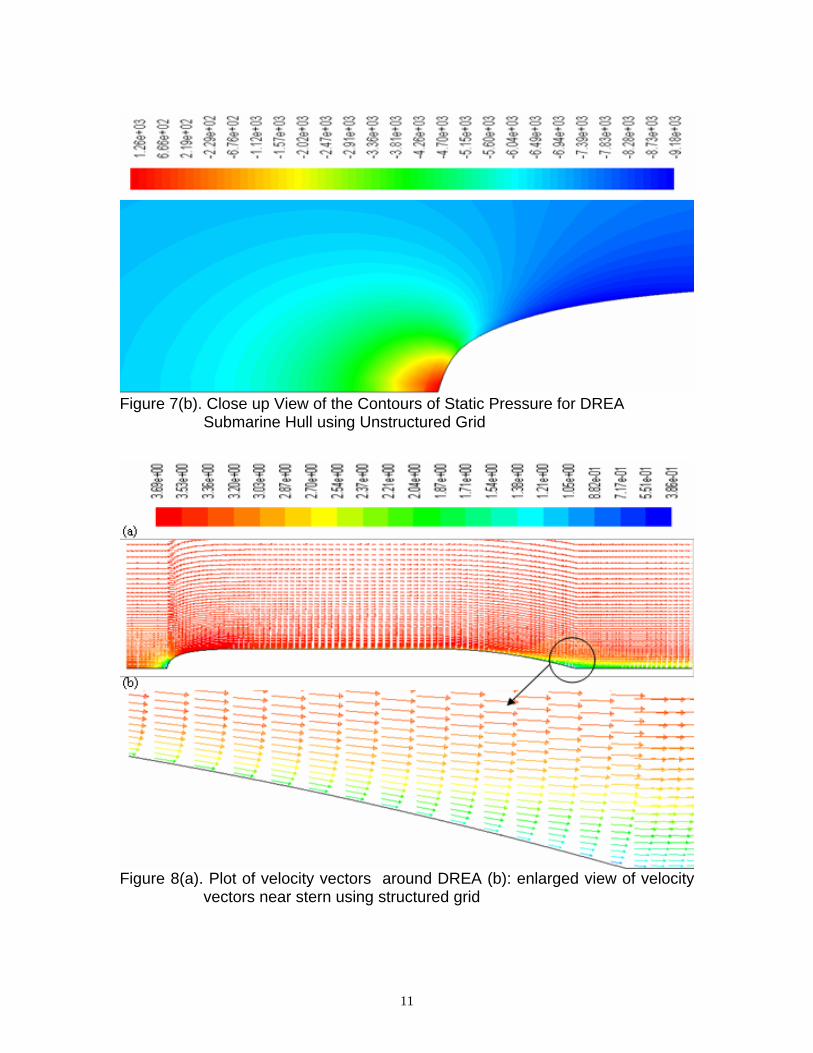
The contour of static pressure around the submarine hull using structured grid is shown in Figure 6(a) at Re = 23 million (velocity of 3.422 m/s). The stagnation point of high pressure at the front tip of the hull, the favorable pressure gradient at the front section and the adverse pressure gradient at the rear section of the hull are clearly shown. Since the reference pressure is set to zero the pressures shown are relative. Figure 6(b) shows a close up of the front section of the hull. Here the stagnation point and the favorable pressure gradient are even more visible (red color). Figure 7 shows the contour of static pressure around the submarine hull using unstructured grid. It is clearly seen in Figure 6(b) that flow is distorted near bow which is due to the structured grid. This defect has been completely removed by using unstructured grid as shown in Figure 7(b). Figure 8 shows the velocity vector for the submarine hull using structured grid at Re = 23 million including the close-up view near the stern whereas Figure 9 shows the same using unstructured grid. It is seen that using unstructured grid, variation of velocity in the boundary layer is captured well than using structured grid. Figure 10(a) shows the contour of velocity magnitude for the submarine hull using structured grid at Re = 23 million. When compared to the pressure plot it can be seen that the stagnation point of high pressure corresponds to the low velocity point at the front, the favorable pressure gradient in the front section corresponds to a high velocity and the adverse pressure gradient at the rear corresponds to a lower velocity. Figure 10(b) shows a close up view of the front section of the velocity profile. Here it is apparent by the colors close to the shape that the no slip boundary condition set for the surface of the hull is in effect. It is also more apparent that the stagnation point is actually a point with zero velocity.

10

Figure 6(a). Contours of Static Pressure for DREA Submarine Bare Hull at Re =

23 Million using structured grid

Figure 6(b). Close up View of the Contours of Static Pressure for DREA Submarine Hull using structured grid

Figure 7(a). Contours of Static Pressure for DREA Submarine Bare Hull at Re = 23 Million using Unstructured Grid

11

Figure 7(b). Close up View of the Contours of Static Pressure for DREA

Submarine Hull using Unstructured Grid

Figure 8(a). Plot of velocity vectors around DREA (b): enlarged view of velocity

vectors near stern using structured grid

12

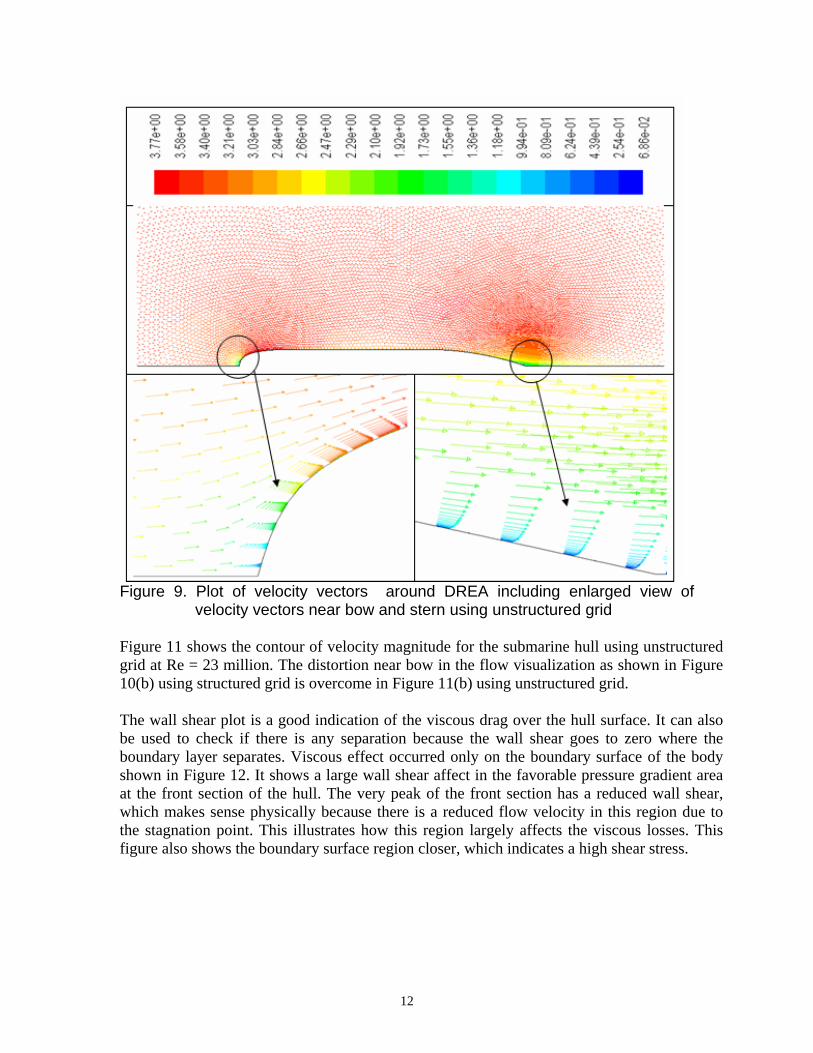
Figure 9. Plot of velocity vectors around DREA including enlarged view of

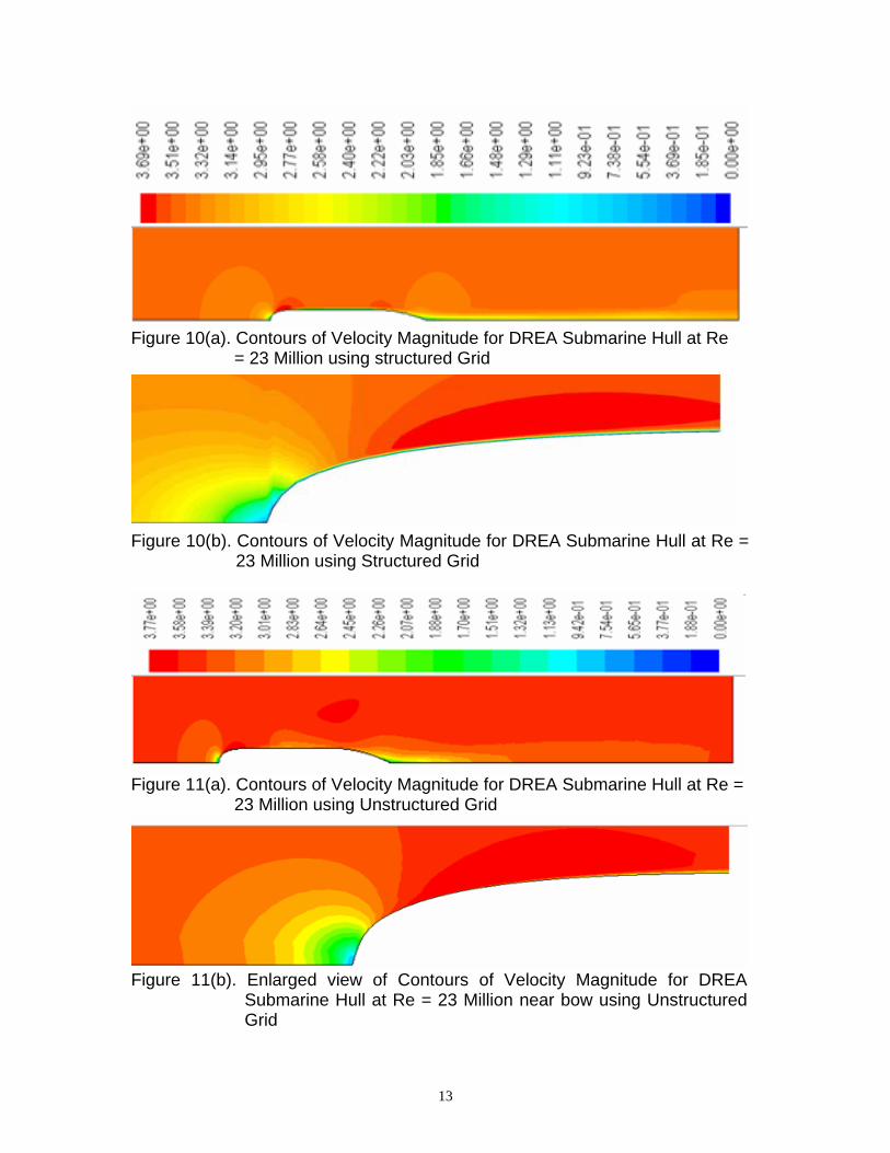
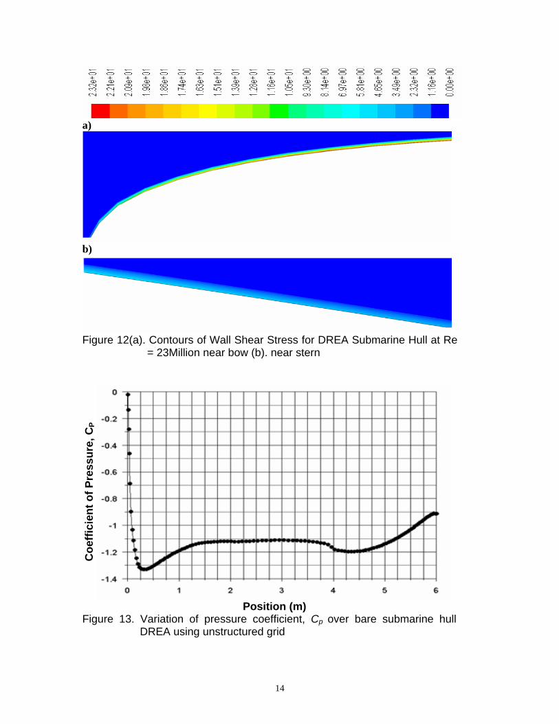
velocity vectors near bow and stern using unstructured grid Figure 11 shows the contour of velocity magnitude for the submarine hull using unstructured grid at Re = 23 million. The distortion near bow in the flow visualization as shown in Figure 10(b) using structured grid is overcome in Figure 11(b) using unstructured grid. The wall shear plot is a good indication of the viscous drag over the hull surface. It can also be used to check if there is any separation because the wall shear goes to zero where the boundary layer separates. Viscous effect occurred only on the boundary surface of the body shown in Figure 12. It shows a large wall shear affect in the favorable pressure gradient area at the front section of the hull. The very peak of the front section has a reduced wall shear, which makes sense physically because there is a reduced flow velocity in this region due to the stagnation point. This illustrates how this region largely affects the viscous losses. This figure also shows the boundary surface region closer, which indicates a high shear stress.

13

Figure 10(a). Contours of Velocity Magnitude for DREA Submarine Hull at Re = 23 Million using structured Grid

Figure 10(b). Contours of Velocity Magnitude for DREA Submarine Hull at Re =

23 Million using Structured Grid

Figure 11(a). Contours of Velocity Magnitude for DREA Submarine Hull at Re =

23 Million using Unstructured Grid

Figure 11(b). Enlarged view of Contours of Velocity Magnitude for DREA Submarine Hull at Re = 23 Million near bow using Unstructured Grid

14

a)

b)

Figure 12(a). Contours of Wall Shear Stress for DREA Submarine Hull at Re

= 23Million near bow (b). near stern

Coe

ffici

ent o

f Pre

ssur

e, C

P

Position (m)

Figure 13. Variation of pressure coefficient, Cp over bare submarine hull DREA using unstructured grid

15

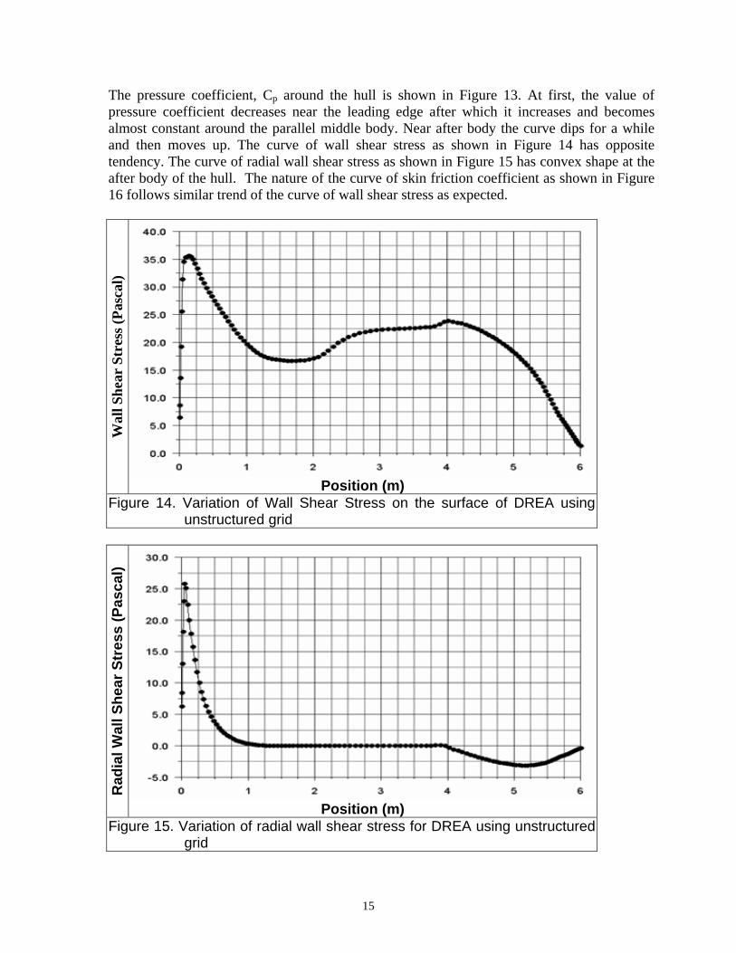
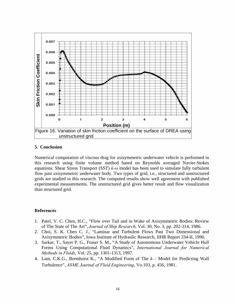
The pressure coefficient, Cp around the hull is shown in Figure 13. At first, the value of pressure coefficient decreases near the leading edge after which it increases and becomes almost constant around the parallel middle body. Near after body the curve dips for a while and then moves up. The curve of wall shear stress as shown in Figure 14 has opposite tendency. The curve of radial wall shear stress as shown in Figure 15 has convex shape at the after body of the hull. The nature of the curve of skin friction coefficient as shown in Figure 16 follows similar trend of the curve of wall shear stress as expected.

Wal

l She

ar S

tres

s (Pa

scal

)

Position (m) Figure 14. Variation of Wall Shear Stress on the surface of DREA using

unstructured grid

Rad

ial W

all S

hear

Str

ess

(Pas

cal)

Position (m) Figure 15. Variation of radial wall shear stress for DREA using unstructured

grid

16

Skin

Fric

tion

Coe

ffici

ent

Position (m) Figure 16. Variation of skin friction coefficient on the surface of DREA using

unstructured grid 5. Conclusion Numerical computation of viscous drag for axisymmetric underwater vehicle is performed in this research using finite volume method based on Reynolds averaged Navier-Stokes equations. Shear Stress Transport (SST) k-ω model has been used to simulate fully turbulent flow past axisymmetric underwater body. Two types of grid, i.e., structured and unstructured grids are studied in this research. The computed results show well agreement with published experimental measurements. The unstructured grid gives better result and flow visualization than structured grid. References 1. Patel, V. C. Chen, H.C., “Flow over Tail and in Wake of Axisymmetric Bodies: Review

of The State of The Art”, Journal of Ship Research, Vol. 30, No. 3, pp. 202-314, 1986. 2. Choi, S. K. Chen C. J., “Laminar and Turbulent Flows Past Two Dimensional and

Axisymmetric Bodies”, Iowa Institute of Hydraulic Research, IIHR Report 334-II, 1990. 3. Sarkar, T., Sayer P. G., Fraser S. M., “A Study of Autonomous Underwater Vehicle Hull

Forms Using Computational Fluid Dynamics”, International Journal for Numerical Methods in Fluids, Vol. 25, pp. 1301-1313, 1997.

4. Lam, C.K.G., Bremhorst K., “A Modified Form of The k-e Model for Predicting Wall Turbulence”, ASME Journal of Fluid Engineering, Vo.103, p. 456, 1981.

17

5. Baker, C., “Estimating Drag Forces on Submarine Hulls”, Report DRDC Atlantic CR 2004-125, Defence R&D Canada – Atlantic, 2004.

6. Menter, F. R., “Two-Equation Eddy-Viscosity Turbulence Models for Engineering Applications”, AIAA Journal, Vol. 32, No. 8, pp.1598-1605, August, 1994.

7. Schlichting, H.,Boundary Layer Theory, McGraw-Hill, New York, 1966. 8. Versteeg, H. K. and Malalasekera, W., An Introduction to Computational Fluid

Dynamics- The Finite Volume Method, Longman Scientific & Technical, England, 1995. 9. Cebeci, T., Shao, J.R., Kafyeke, F., Laurendeau, E., Computational Fluid Dynamics for

Engineers, Horizons Publishing Inc., Long Beach, California 2005. 10. Baldwin, B.S., Lomax, H., “Thin layer approximation and algebraic model for separated

turbulent flows”, AIAA 16th Aerospace Sciences Meeting, 1978. 11. Department of Research and Development Canada- Atlantic, National Defense, “Fall

1988 Wind Tunnel Test of the DREA Six Meter Long Submarine Model- Force Data Analysis”, Ottawa, 1988.

Authors’ biography DR. MD. MASHUD KARIM Dr. Md. Mashud Karim graduated in Naval Architecture and Marine Engineering (NAME) from Bangladesh University of Engineering and Technology (BUET) in 1992. He also completed M. Sc in NAME from BUET in 1996. Finally, he obtained Ph. D degree in Naval Architecture and Ocean Engineering from Yokohama National University, Japan in 2001. Dr. Karim joined BUET as Lecturer in 1994, as Assistant Professor in 1996 and as Associate Professor in 2004. He has research interest on Computational Geometry, Hydrodynamics, Resistance, Propulsion and Stability of Ship, Design optimization, Genetic Algorithms etc. He is now Associate Member of SNAME and Life Member of IEB, ANAME, NOAMI and JUAAB. He is the Editor-in-Chief of the Journal of Naval Architecture and Marine Engineering. MD. MAHBUBAR RAHMAN Mr. Md. Mahbubar Rahman completed B.Sc and M.Sc in Mathematics from Jahangirnagar University, Dhaka, Bangladesh in 1997 & 1998 respectively. He obtained M. Phil. Degree in Mathematics from Bangladesh University of Engineering and Technology in 2008. Mr. Rahman joined Department of Natural Science, Stamford University, Bangladesh as Lecturer in 2004 and as Assistant Professor in 2007. Now he is doing his postgraduate research in the Hull Form Design Lab of Prof. Yasuyuki Toda, Department of Naval Architecture and Ocean Engineering, Division of Global Architecture, Graduate School of Engineering, Osaka University, Osaka, Japan under Monbukagakusho (Japanese Government) Scholarship.

18

DR. MD. ABDUL ALIM Dr. Md. Abdul Alim completed B.Sc. (Hons) in Mathematics from Department of Mathematics, Dhaka University, Dhaka in 1992 and M.Sc. in Applied Mathematics from the same department in 1994. He obtained M.Phil. degree in Mathematics/Fluid Dynamics from Department of Mathematics, Bangladesh University of Engineering and Technology (BUET), in 2000 and Ph.D degree in Mechanical Engineering from Loughborough University, Loughborough, Leicestershire, UK, with specialization in Computational Fluid Dynamics (CFD), Combustion and Heat Transfer in 2004. Dr. Alim joined Department of Mathematics, BUET as lecturer in 1996, as Assistant Professor in 2005 and Associate Professor in 2008. He is also the assistant provost of Shahid Smrity Hall (Student Hostel), BUET since 2005. Dr. Alim is the member of Bangladesh Association for the Advancement of Science (BAAS) and Life Member of Bangladesh Mathematical society. He is also the member of editorial board of the Journal of Naval Architecture and Marine Engineering.