1

Special Issue of The Aeronautical Journal celebrating the 150th anniversary of the Royal Aeronautical Society

Computational aerodynamics:

advances and challenges Dimitris Drikakis

University of Strathclyde

Glasgow, UK

and

Dochan Kwak and Cetin C. Kiris

NASA Ames Research Center,

Moffett Field CA 94035, USA

ABSTRACT

Computational aerodynamics, which complement more expensive empirical approaches, are critical for

developing aerospace vehicles. During the past three decades, computational aerodynamics capability has

improved remarkably, following advances in computer hardware and algorithm development. However, most of

the fundamental computational capability realized in recent applications is derived from earlier advances, where

specific gaps in solution procedures have been addressed only incrementally. The present paper presents our

view of the state-of-the-art in computational aerodynamics and assessment of the issues that drive future

aerodynamics and aerospace vehicle development. Requisite capabilities for perceived future needs are

discussed, and associated grand challenge problems are presented.

2

1.0 INTRODUCTION

Computational aerodynamics research can be traced back to more than a century ago; (For example, see the

landmark paper by Richardson(1).) However, much of the groundbreaking work for the modern-day electronic

computations was performed during the 1960s at Los Alamos Scientific Laboratory (now Los Alamos National

Laboratory). Since the 1970s, computational technology for flow analysis has developed rapidly, in parallel with

advances in computing hardware. During the 1980s and 1990s, flow simulation tools of varying fidelity were

developed for aerodynamics applications. Numerous individuals contributed to algorithm research and many

organizations developed computational tools in such areas as meteorology or aerospace vehicle development. It

is an almost impossible task to review these activities comprehensively and give proper credits to all major

contributors in this review. For a more comprehensive historical review, readers are referred to existing literature

such as Roache(2), Tannehill et al.(3), and Chapman(4). In this review we focus on the advances in computational

aerodynamics, or more narrowly, on the computational fluid dynamics (CFD) that impacted aerospace

engineering and sciences. We also discuss what challenges need to be addressed to support aerospace

engineering for the foreseeable future.

Computational flow analysis complements the experimental approach. As the computational aerodynamics

technology became more developed in parallel with advances in computing hardware, computational flow

analysis became a key element in providing data for fluid engineering and fundamentally changed how airplanes

and spacecraft are designed. In aeronautics, airplane design demands high precision and rapid design cycles,

requiring integrated work with other disciplines such as structures and control. Johnson et al.(5) summarizes how

computational analysis became an indispensable part of airplane design.

In the space exploration area, however, applications of computational aerodynamics have lagged

aeronautics, partially because space-related flow problems involve largely time-dependent and complex flow

phenomena, which require advanced unsteady flow algorithm and physical modeling (for example, see Kiris et

al.(6-7)). Moreover, limited amount of experimental and flight data are available for validation, especially, for new

vehicle configurations. Advanced computational technology suitable for space transportation vehicle

development requires maturation through experiences in realistic applications. When a new vehicle concept like

the Space Shuttle launch vehicle was on the drawing board, flow simulation capabilities or CFD tools were not

mature enough to make significant impacts. Therefore, until recently, most operational space vehicles were

designed heavily relying on empiricism. Later, the CFD technology suitable for space applications was

developed in parallel with vehicles’ operational period. Subsequently, CFD became useful to support operational

aspects, to retrofit for improved components, and to investigate accidents. Since post-Shuttle human space

exploration requires new or replacement vehicles, conceptual design evaluations rely on databases generated by

CFD, which has not, however, been thoroughly validated for the types of flow encountered in new vehicle

concepts. Therefore, the so-called “best practices” protocols have been developed in conjunction with new

vehicle development tasks. In this report, the state-of-the-art in computational aerodynamics and requisite

capabilities for supporting future tasks are discussed with a list of grand challenge problems.

Regarding the development of requisite capabilities for aerospace problem solving, steady investment has

been made, especially during the 1980s and 1990s, to develop flow simulation tools of varying fidelity. As a

result, computational technology has become an indispensable part of the design and operation of aerospace

vehicles. However, there are several fundamental elements of these tools that need continued advances such as

efficient algorithms, geometry definition and grid generation procedures, boundary condition procedures,

physical modeling, and pre- and post-processing methods. Furthermore, in a practical problem solving

environment, computer architecture, data management tools and networking play a very important role in

producing results in a timely manner. To obtain solutions within a reasonable turn-around time, approximate

formulations and simplified geometries were utilized first. Then, in the 1980s and 1990s, increasing the fidelity

of formulation and inclusion of more complete geometry were the focus largely in a single discipline. The high-

speed scientific computing environment has grown to the point that vehicles and components are to some degree

amenable to computer simulations. Despite these advances, unsolved problems still exist in several areas critical

to aerospace mission successes. For example, high-fidelity simulation of unsteady flow for the prediction of

vibration loads on launch vehicles and prediction of massively separated flow are among the remaining

challenges. Of course, CFD-related issues can vary depending on primary flow features of interest, and resolving

all scales and features of complex problems is not necessarily needed in all flow analyses or in all tasks.

Following the early successes in developing solution algorithms and flow solvers, reduction of solution time

has been realized more through computer hardware speed-up than algorithm advancement. Thus, the parallel

computing methods and associated data management schemes have played an important role in utilizing compute

resources. As problem sizes continue to grow, development of both advanced methods and advanced computer

hardware remain very importance.

It is to be noted that successful application of computational technology requires the synergy of computing

facility, software, simulation tools, data analysis tools, and networks, coupled with a combined knowledge of

3

engineering, flow physics, and computer science. Contrary to the common impression that CFD is mature

enough to the point that it is usable by non-experts, available tools still lack prediction capability in many critical

areas and require experts in order to conduct successful simulation of surprisingly many problems in aerospace

vehicle applications. Thus, it is necessary to advance the state-of-the-art in CFD as well as to gain critical skills

in both numerical methods and physics. Lack of support has been listed as a main culprit for the slow progress in

advancing the state-of-the-art in CFD. However, the primary questions to ask are what advances can be made

given resources? Is the slow progress due to limited resources or limited innovations? Or do we simply wait for

the computing hardware to increase its capability by several orders of magnitude compared to current computers?

In this article, a brief summary of the state-of-the-art in computational aerodynamics will be given first,

followed by a discussion on what needs to be done realistically to solve grand challenge problems we face today

in supporting aeronautics and space exploration. Some features are crosscutting in nature for both exploration

and aeronautics. The examples selected are based primarily on our experience. We will discuss best practices

utilizing current and projected tools and computers rather than based on conjectures about the new but uncertain

“revolutionary” computational technology.

2.0 STATE-OF THE ART IN COMPUTATIONAL AERODYNAMICS

In this section, we will review the state-of-the-art (SOA) in computational aerodynamics from the flow

simulation capability point of view. This assessment can then be used to determine the areas that need further

advances in order to produce credible and predictive results for the flow analysis of a wide range of vehicle

configurations and operating scenarios.

2.1 RANS modeling for viscous flow simulation

Key areas for describing computational capabilities for viscous flow simulations are listed below based on our

observations.

2.1.1 Flow solver capabilities

Many viscous flow solvers were developed primarily by research organizations such as government laboratories,

and later distributed to industries and software developers. Subsequently, many variations of vendor-developed

software or flow simulation codes became available to users. More recently, there are open-source solvers

available such as openFoam or SU2. In general, the capabilities of these and other in-house viscous codes in

research laboratories can be characterized as below.

a) Simulation of attached flows:

Steady-state solutions for attached flows about complex configurations are routinly solved reliably and are being

used for aerospace vehicle development and operations. Supercomputers are now readily available, and thus

simulations with hundred million grid points are fairly common. Unsteady or time-dependent flow can be solved

when the flow is primarily attached about relatively simple geometries.

b) Simulation of massively separated or unsteady/transient flow involving complex geometry:

Massively separated flows and vortex dominated flows are difficult to solve accurately. For more complex

geometries, unsteady simulations require guidelines on spatial and temporal resolutions. For good convergence,

accuracy and reliability, best practice guidelines are required on mesh resolution and time step size.

c) Grid generation:

Dependence on grid quality continues to be an important factor to get consistent and accurate CFD predictions.

Many grid generators are available, but to utilize beneficial grid characteristics of different grid topologies it is

desirable to be able to seamlessly couple different grids in simulation. Also, at the present time, grid generation

typically requires an expert for more than a week to go from CAD to grid. Therefore, more automation is highly

desirable.

d) Post-processing:

Post-processing massive datasets for extracting aerodynamic loads is routinely done, but flow feature extraction,

especially for unsteady flow, still remains challenging.

4

2.1.2 Physical modeling capabilities

Physical modeling is of major importance for obtaining accurate and reliable solutions. The following lists

provide a summary of current physical modeling status for engineering-level viscous flow simulation.

a) Turbulence models

Details of current turbulence modeling practices will be presented in the next sub-section. A short summary is

listed below:

Engineering-level turbulence models exist, but the modeling approach has not been improved much since

the early days of CFD. To be economically viable, 1- or 2-equation models are frequently used in

conjunction with aerospace flight vehicles.

Current models are not capable of predicting massively separated and unsteady flows.

Separated flows need ad hoc tuning or can be more accurately computed by utilizing large eddy simulation

(LES) variants such as hybrid RANS-LES, Wall-Modeled LES, Wall-Resolved LES or Implicit LES (ILES)

approaches (e.g. DES-based models are gaining popularity, despite accuracy issues in the wall region).

Internal flow applications of existing turbulence models, most of which are tuned for external flows, are not

very well evaluated, and may require the development and calibration of models using new approaches.

Accurate models for transition are practically non-existent for engineering; for multi-phase or multi-material

flow models are further behind in producing even engineering-level solutions.

b) Criteria for engineering models of turbulence

Current models, which are mostly tuned to boundary layer flow, have been successfully used in many vehicle

calculations where flow is largely attached and steady-state solutions are the main quantities of interest. Users of

legacy CFD codes may not have in-depth knowledge of turbulence modeling. Following are some of the issues

which need to be considered when selecting turbulence models for mission computing.

- Sensitivity: Impact of the model on the accuracy of the overall computed results need to be assessed relative

to the impact on the accuracy stemming from algorithm and grid quality.

- Consistency and robustness: It should be usable by non-experts.

- Range of applicability: Most engineering-level models are tuned for limited cases, and therefore the

applicable range needs to be defined.

With advances in computer hardware, resolution and turn-around time have improved substantially, but there are

problems that require advanced algorithm and enhanced methods such as in- and out-flow boundary condition

procedures. Algorithms for the RANS approach may need to be reevaluated for applications to turbulent eddy

simulation, which may offer a possibility for obtaining more physical and consistent solutions(8). Turbulent eddy

simulations will be discussed in the next sub-section.

2.2 Turbulent flow simulations

Although RANS will continue to be used in the computation of flows around and inside complex geometries,

more researchers and practitioners will increasingly use Large Eddy Simulations (LES) and hybrid methods,

which combine LES and near wall RANS-type modeling. Direct Numerical Simulations (DNS) will also

continue to be used on finely resolved meshes. Note that DNS should not be considered as validation data but

rather as a benchmark, and as a simulation result must contain some assessment of the numerical errors. A brief

overview of the above approaches with particular focus on channel flows where there is an extensive body of

work is given below.

A recent overview of the progress made regarding Direct Numerical Simulation (DNS) of wall-bounded

turbulent flows with particular emphasis on channel and pipe flow geometries is given in (8-11) and references

therein. Most of the DNS studies have used finite differences, Legendre polynomials and/or spectral methods

based on Fourier representations or Chebychev-tau formulations. More recently, Discontinuous Galerkin (DG)

methods have also been applied to DNS of turbulent channel flow(12-13).

Incompressible DNS of fully developed channel flow has been published(14-21). These studies shed light on

the turbulent flow physics, as well as provide data for the validation of numerical methods and turbulence

models. A recent study(22) compared two fundamentally different DNS codes to assess the accuracy and

reproducibility of standard and non-standard turbulence statistics, showing that the maximum relative deviations

were below 0.2% for the mean flow, below 1% for the root-mean-square velocity, and pressure fluctuations, and

below 2% for the three components of the turbulent dissipation. In comparison to incompressible DNS, there is

5

only a limited number of compressible DNS studies and those have primarily been conducted for supersonic

flows(23-26).

The DNS data obtained by Tsuji et al.(27) and Philip et al.(28) were initially verified against experimental

results, and then used to further probe and shed light on the turbulent flow physics. Other studies tried to

ascertain the differences between channel and pipe turbulent flows through numerical computations(29-30) and

experiments(31-32). Monty et al.(31) presented a comparison of experimental data with well-documented high

Reynolds number (Reτ=934) DNS(17). An excellent agreement for the streamwise velocity statistics between the

two data sets was reported. Although the energy spectra were very similar, the DNS predicted a lower energy

value in the logarithmic region, possibly due to the (shorter) dimension of the DNS box. The high computational

cost required to successfully resolve all turbulent length-scales limits the applicability of DNS to relatively low

Reynolds numbers and the incompressible Navier-Stokes equations. Note that DNS should be used (cautiously)

as a benchmark rather than validation data. As a simulation result must ideally contain some assessment of the

numerical errors and an error bar; however, this is not the case in the literature.

There are several research studies concerning LES both classical and implicit. One of the early Implicit

Large-Eddy Simulations (ILES) concepts was originated from the observations made by Boris et al.(33) that the

embedded dissipation of a certain class of numerical methods can be used in lieu of explicit sub-grid scale (SGS)

models in classical Large-Eddy Simulation (LES) of turbulent flows. Modified equation analysis (MEA) was

developed(34) in an effort to determine the stability of a difference equation by examining the truncation errors.

The process begins from reducing a differential equation to a discretised equation by expanding each of its terms

in a Taylor series. Such an analysis has been performed for the truncation error of certain schemes(35-41) leading

to a better understanding of the implicit sub-grid dissipation. In ILES, the Navier–Stokes equations (NSE) are

discretised using high-resolution/high-order non-oscillatory methods without involving a low-pass filtering

operation which gives rise to sub-grid scale (SGS) terms that require additional modelling. Instead, only the

(implicit) de facto filtering introduced through the finite volume integration of the NSE over the grid cells is

utilised in conjunction with non-linear numerical schemes that adhere to a number of principles; see (42, 43), and

reviews (40, 44, 45). It has been shown(35) that ILES methods need to be carefully(13) designed, optimised, and

validated for the particular differential equation to be solved. Direct MEA of high-resolution schemes for the

Navier–Stokes equations is extremely difficult to perform, thus understanding of the numerical properties of

these methods to date still relies on performing computational experiments.

Classical LES studies have dealt with the development of SGS models and error contributions from SGS

modeling (Stolz et al.(46-47), Hickel et al.(48-49) and references therein) and numerical schemes(50-54); error control

through explicit filtering(53, 55-56); and the effects of different filtering procedures(57-59). Recent developments of

explicit SGS models include the approximate deconvolution model (ADM)(46), which is an approximation of the

non-filtered field by means of a truncated series expansion of the inverse filter operator. For an incompressible

channel flow, ADM compared well against DNS data and showed a significant improvement(47) over the results

obtained from typical SGS models such as the classical and dynamic Smagorinsky model. An evolution of the

ADM is the adaptive local deconvolution model (ALDM)(48). The ALDM is based on a non-linear discretisation

scheme, which contains several free deconvolution parameters that allow control of the truncation error. The

ALDM was applied to incompressible, turbulent channel flow to analyze its implicit SGS modeling capability in

wall-bounded turbulence(49). In the framework of classical LES, the accuracy of the SGS model is strongly

influenced by the numerical contamination of the smallest resolved turbulent structures near the filter cut-off length(51-52, 60).

Furthermore, it was found that the numerical error and SGS model interact with each other(50, 52-54). It was

reported(50) that for low-order finite-difference schemes, the truncation errors can exceed in magnitude the

contribution of the SGS term. High-order numerical schemes are thus important in resolving the large energy-

containing scales more accurately. However, they can also lead to contamination of the smallest resolved scales

by truncation errors, in particular when using non-spectral methods. It was shown(56) that these errors could be

controlled using an explicit filter. Nonetheless, mesh refinement still improved the results at a faster rate than the

explicit filter size. Furthermore, previous studies(53) have shown that a minimum ratio of explicit filter-width to

cell-size is necessary to be defined in order to prevent numerical errors from becoming larger than the

contribution of the SGS turbulence closure terms and consequently saturating the solution period.

The influence of the numerical errors and SGS models in LES of channel flows, with and without explicit

filtering was studied by Gullbrand et al.(61,62). When comparing to LES without explicit filtering, the difference in

the mean velocity profiles was not large; however, the turbulence intensities were improved when explicit

filtering was used. Gullbrand(62) investigated various dynamic SGS models to obtain the true filtered LES

solution for an incompressible turbulent channel flow. It was hypothesized that the true LES solution should

depend only on the filter width, regardless of the grid resolution. On the other hand, in ILES the solution

converges towards DNS as the grid is refined because the filter width is implicitly and directly connected to the

grid spacing. The effect of the different filtering methods was also examined in a subsequent study(58) showing

that three-dimensional filtering gives better results than two-dimensional filtering. Brandt(59) reported that the

6

effect of filtering can be significant, with smooth filters increasing the total simulation error. Recently, Bose et

al.(57) investigated the use of explicit filtering in LES for obtaining grid independent numerical solutions similar

to the work of Gullbrand(62). The convergence of the simulations was analysed for a turbulent channel flow at

various friction Reynolds numbers (Reτ =180, 395, and 640), and it was shown that by using an explicit filter, the

turbulent statistics and energy spectra became independent of mesh resolution. Other LES approaches include

spectral-based LES(63) and “variational multiscale residual-based turbulence modeling”(64-65).

Although LES is computationally less demanding than DNS, it still requires significant computational

resources for simulating near wall turbulence at high Reynolds numbers. An alternative to LES is to make use of

wall-layer models near the wall and use LES to resolve the outer region of the boundary layer, thus “relaxing”

the grid resolution requirements near the wall. The wall-layer models can be broadly classified as: (i)

equilibrium laws based on the logarithmic law, or some other assumed velocity profile (wall functions); (ii) zonal

models, in which the turbulent boundary-layer equations (TBLE) are solved, weakly coupled to the outer-layer

LES; and (iii) hybrid methods employing a Reynolds-Averaged Navier-Stokes (RANS)-based turbulence model

near the wall and LES in the outer layer. A thorough review of the above is provided by Piomelli(66). The best-

known realisation of the hybrid framework is the Detached Eddy Simulation (DES) method by Spalart et al.(67).

In DES the interface location is dictated by the grid parameters through a switching condition. Nikitin et al.(68)

used DES in the simulation of a turbulent channel flow. The results showed a non-physical boundary layer

developing near the RANS/LES interface caused by the misalignment of the log layers between the RANS and

LES regions. Due to the log-layer mismatch, the skin-friction coefficient was under-predicted by approximately

15%. In the most commonly used DES implementation, the entire boundary layer is modeled by RANS(69-70).

Using the k-ε model, Hamba(69-70) carried out hybrid simulations of channel flow and introduced additional

filtering at the interface to reduce the log-layer mismatch. Although these methods are promising, the amplitude

of the stochastic forcing and the width of the additional filtering need both to be determined empirically. Piomelli

et al.(71) applied a stochastic backscatter model to the wall-modeled DES of a channel flow showing

improvements in the prediction of the mean velocity profile.

Other DES studies(72-73) also reported issues in coupling the modeled and LES resolved regions, especially

when more complex geometries and flows were considered in comparison to a plane flat surface(74-77). More

recently, a dynamic slip wall boundary condition for wall-modeled LES(78) was proposed, which gave

encouraging results for separated flows over aerofoils. Chen et al.(79) showed that both ILES and the immersed-

interface treatment of the wall boundaries provide high computational efficiency on very coarse meshes for

backward-facing step and periodic hill flows. Another category of near-wall models has been proposed(80) which

has been used in RANS, but may also prove promising for DES. Although there is an extensive body of

published research regarding the solution of turbulent channel flows using DNS, classical LES and DES, ILES

investigations are still limited in number(81-84). Previous research(81-84) has indicated that ILES is capable of

reproducing first and second order statistical moments of the velocity field. Reviews examining the accuracy of

ILES in other canonical problems such as the turbulence decay in a Taylor-Green vortex have also been

published(85-86). Despite the above literature, there has been no systematic attempt to investigate the behavior of

different high-order compressible ILES methods in compressible turbulent channel flows.

3.0 MULTI-PHYSICS MODELING

Modeling and simulation is increasingly becoming a powerful tool in designing and manufacturing of new

aerospace products. Multi-physics simulations involve continuum and/or atomistic methods for a range of

temporal and spatial scales and physical processes involved. Multi-physics consists of three main attributes:

“multi-field”, “multi-domain” and “multi-scale”(87). The combination of these attributes can lead to the

understanding of the natural behavior of physical systems by generating relational mathematical and

computational models.

Product development requires extended investigation of its behavior in various environmental conditions,

which may include thermal, mechanical and humidity stimuli. Coupling techniques to address this type of multi-

physics (also known as multi-field) problems include electrodynamic and thermoelasticity. Multi-field theories

have also been extended to three-fields that includes thermo-electroelasticity (88,89) and hygro-thermoelasticity (90). Multi-domain modeling refers to the physical problems that focus on the interaction of continuum systems

characterized by different properties, such as multi-phase flows, liquid-solid interaction, and moving boundaries.

A typical example of multi-domain modeling application is the field of aeroelasticity. Coupled formulations have

been developed (91) for cases where i) neither domain can be solved separately from each other; ii) neither set of

dependent variables can be explicitly eliminated. The first attempts to study aeroelasticity were based on linear

mathematical models (92). Linear aeroelastic models have successfully managed to predict the basic features of

aeroelastic behavior of a structure both in the subsonic(93,94) and in the supersonic regimes (95). However, the

advances in the aircraft industry have pushed towards critical design conditions in the transonic regime in terms

of flutter, which linear models failed to predict.

7

Nowadays, nonlinear CFD and Computational Structural Dynamics (CSD) are widely used in aeroelastic

simulations. CFD is used for the estimation of the flow temperature, pressure and density by solving the Navier-

Stokes equations. On the other hand, CSD is used for modeling the nonlinear geometrical and material behaviour

of solids. However, the solution of such a dynamic problem requires the constant exchange of input information

between CFD and CSD, as the latter one needs information on the airflow while CFD requires the knowledge of

the temperature or the deformation of the solid. Coupling CFD and CSD is one of the most challenging tasks.

There are two main coupling strategies, namely the monolithic approach (96,97) and the partitioned energy

approach (98,99). In the monolithic approach, the coupled system is regarded as a whole and ensures convergence

provided that the nonlinearities of the subsystems can be resolved. On the other hand, in the partitioned solution

approach, solid and structure are spatially decomposed and the different physical fields (partitions) interact

through the exchange of boundary conditions. In the case of very weak fluid-solid interaction, partitioned solvers

are more effective than the monolithic ones as they converge in fewer time steps. On the contrary, for strongly

coupled problems partitioned solvers can hardly converge and monolithic ones become essential (100).

Continuum Models (e.g. CFD, FEA) have been the staple of computational simulations of many engineering

problems. However, the development of nano-devices such as micro-electromechanical systems (MEMS) over

the last few decades created the need to study micro/nanoscale systems, where many of the laws of continuum

mechanics break down (101). Fortunately, recent advances in computing have made the investigation of the

mechanics of fluids and materials on nanoscales feasible with the use of molecular models. Molecular models

can be simulated using two techniques: Molecular Dynamics (102) and Monte Carlo (103). The computational

expense limits the use of these methods to a number of atoms relatively small compared to macroscale problems.

Multi-scale methods (Fig. 1) attempt to bridge the accurate microscopic models with efficient continuum ones.

Multi-scale methods can be divided into two groups: the meso-scale and the hybrid ones. Meso-scale

methods work with intermediate resolution, i.e. a single solver that can simulate large physical phenomena taking

into account the essential detail of the molecular interactions. This is achieved by replacing an atomic description

by larger particles while averaging fine detail out. The most common meso-scale methods are: a) Lattice Gas

Cellular Automata (LGA)(104,105), b) the Lattice-Boltzmann (LB) method (106,107), c) Dissipative Particle Dynamics

(DPD) (108), and d) Direct Simulation Monte Carlo (DSMC) (109,110). On the other hand, hybrid models employ two

solvers, a molecular (e.g. Molecular Dynamics, Monte Carlo) and a continuum one (e.g. CFD, FEA). The

challenge in such an approach is the transparent exchange of information between the two. Hybrid models can be

classified into Geometric Decomposition (GD) and Embedded based techniques (EBT) depending on how the

length scales are decoupled (111-118).

Figure 1. Multi-scale modelling of materials and multi-material interfaces across length scales.

It is expected that in the future the interface between the three basic components needed to address multi-

scale problems, governing equations, experimental data and simulation software, will become integrated. This

will enhance the accuracy of the existing modeling methods and lead to the evolution of the design of aerospace

8

products intended to operate under complex environmental conditions. As far as multi-domain systems are

concerned, current modeling software should be evolved and become capable of handling a larger number of

domains so as to represent effectively real environmental and operating conditions.

Multi-scale methods need to be further developed to enable the fabrication of devices that incorporate design

characteristics ranging from nano- to macro-scale, such as the aircraft skin(119-120). In the future, new, more robust

methods efficiently linking the atomistic and the continuum domains should be developed. This will enable

modeling of materials for particular applications. For example, selecting and designing a proper material for a

morphing skin of an aircraft is not a trivial task, as candidate materials should be able to withstand the

aerodynamic loads and simultaneously be flexible enough to alter their shape during flight. Therefore, a large

number of experiments should be carried out to identify the most suitable choice. An alternative and cost-

effective approach would be to perform multi-physics simulations based on an integrated framework.

Besides multi-scale material modeling, hybrid multi-scale simulations have been extended to static and

quasi-static physical problems, where relaxation time scales in atomic models can be matched by the continuum

ones, but not to fully dynamic problems where the macroscopic evolution in time affects the molecular structure

of a system. Such cases include adsorption, sedimentation, fouling and fatigue. For example, in the case of a flow

over an elastic surface, the long time scales over which the structure of the surface is deformed cannot be

simulated by a molecular solver and the dynamics of the build-up, which are being calculated by a continuum

solver, cannot be fed into the molecular domain, as a re-initialisation of the molecular solver would be required.

Therefore, the development of integrated hybrid approaches capable of linking macroscopic changes with the

molecular structure and meso-scale methods need to be developed. Other challenges that have to be addressed in

the future involve parallelization of hybrid codes, which in combination with complex geometries poses a

number of challenges regarding the molecular solver and the boundary conditions at multi-material interfaces.

4.0 VISION

Computational aerodynamics can play a significant role for developing aerospace vehicles during the conceptual

design and trade study phases. This requires consistency in computed results and quick turn-around to evaluate

different ideas. In applying current simulation tools to determine fluid dynamic loads on aerospace vehicles, flow

physics such as turbulence are approximated by models. Modeling which assures prediction of the proper non-

linear physical phenomena is crucially important. Predictive simulation capability, usually with a range of

limited applicability, will alleviate the need for extensive ground- or flight-testing. The requisite capabilities

listed below are the ones needed for enhancing aerodynamics analysis for developing the next-generation

vehicles. The list is intended to identify the major advances in computational aerodynamics required in the near

or medium-term future. This will help minimize the expensive “test-fail-fix” cycle of past practices.

4.1 Requisite capabilities

Some of the capabilities required for computational aerodynamics facing current and mid-term future

applications are:

Quantification of grid effects relative to physics model sensitivity, and versatile grid generation

capability to couple various grid topologies as needed.

Advanced algorithms, such as space-time correlation, and high-accuracy methods especially for

unsteady flows.

Guidelines for selecting turbulence modeling approach for real-world applications such as RANS, DES

variants, LES, Hybrid wall modeled or wall-resolved LES, ILES suitable for flow solvers in use.

Aeroacoustics modeling and computation capability.

Simulation capability for integrated vehicle-propulsion configuration. For launch vehicle design

applications such as for determining structural loading and for designing guidance and control system,

computed results using clean vehicles without plume and protuberances seem adequate. However, with

plume or wake, the prediction capability for separated region can drastically be reduced.

Practical model for predicting combustion instability.

Parallel implementation of flow solver codes on ever evolving high-performance computer architecture.

Improved speed of CAD to solution so that CFD can be utilized in post-concept trades for revising the

design with very specific gorals.

4.2 Target research areas

Selected research areas are listed below where requisite capabilities discussed above can be advanced.

4.2.1 Unsteady and separated flow research

9

To improve current practices for establishing CFD application procedures, advances in algorithms will be

desired, such as enhanced time integration schemes/procedures combined with high-accuracy and grid adaption

schemes.

4.2.2 Range of applicability for turbulence models

Even though intensive research on turbulence physics has been performed for several decades, models useful for

vehicle development and operations have been developed by CFD practitioners at engineering level. To meet the

near-term needs, it will be necessary to enhance CFD tools to simulate turbulent flow more consistently.

Therefore, establishing a usable recipe for turbulence modeling will be very valuable possibly using existing

models and/or enhanced versions.

4.2.3 Practical turbulent eddy simulation method

Uncertainties in turbulent flow simulation can be reduced by modeling small eddies only. However, the

computing requirements for turbulent eddy simulation is still an issue. In 1979 Chapman(4) projected that a full

aircraft can be solved using LES in 1990s. This projection has been delayed more than 10 years now, and most

simulations are still performed with wall models. Now computers are at petaflop level, but only if the entire

system of a supercomputing facility can be allocated to one user. In reality it is reasonable to assume that about

10% or less of a system will be available to solve one problem. Therefore, it will make practical sense to develop

efficient new methods while computer hardware is being advanced further.

4.2.4 Engineering-level physics model

No usable guidelines are available for multi-phase, cavitation and combustion instability. However, in a number

of important applications, such as the turbopump, cavitation phenomena need to be included in CFD simulation.

In propulsion simulation, prediction of combustion instability has been a major challenge, and still requires a

longer-term research combined with systematic validation experiments.

4.3 Outlook for organized or directed research

Research in many of the areas discussed above is already in progress but lacks coordination. Strategic

investments are rare because of the erroneous assumption that CFD has reached its maximum potential and

further development will result in only incremental improvement at best. However, CFD is not accurate enough

for many major design decisions except in limited regions of operational conditions in aerodynamics and

engineering and largely not reliable when extrapolated to un-experimented flow regimes. It is to be noted that

CFD has made a profound impact on airplane design, especially, commercial transport airplane. Similar impacts

can be expected in aerospace sciences and engineering in general when “prediction” capability is improved to

produce consistent and credible results. To close the current gap in computational aerodynamics, strategic

investment at a fundamental technology level would be desirable.

5.0 GRAND CHALLENGE APPLICATIONS

The goal of Grand Challenge (GC) problems is to develop several key capabilities of computational

aerodynamics procedures to handle current bottleneck issues. Therefore, we are looking at medium term, three to

five year, realistic advances to facilitate development of computational capability for aerodynamics analysis and

vehicle development. The GC cases presented here are to advance several realistic and practical capabilities.

There are also open-ended issues not extensively discussed here, such as developing general turbulence models

applicable to a wide variety of flows.

Our assumptions in selecting these GC problems are that (1) we do not anticipate significant long-term

research and technology development funding to generally advance fundamental CFD capability, and (2) there

are immediate needs for developing specific capabilities to make tangible impacts on current missions. Typically,

aerospace vehicles once developed will be in operation for a long time. Therefore, the impacts of computational

aerodynamics will be the greatest during the conceptual and preliminary design phases. Significant impacts will

be made in the subsequent applications for retrofitting and operational support. For example, the Space Shuttle

was designed without much help from CFD and has flown for 30 years since its maiden flight. Subsequent

advances in CFD and computer hardware have made major impacts on many aspects of retrofitting, operational

support and accident investigation.

10

Grand Challenge # 1 (GC1): Simulation of a full aircraft configuration

Accurate CFD simulations around a full aircraft configuration still remain a major CFD challenge. Although

RANS simulations on relatively fine grids are feasible, achieving acceptable accuracy at take off and landing

conditions is an extremely difficult task. The RANS prediction uncertainties at high angles of attack are

associated with the inherent inability of RANS methods to capture flow unsteadiness, in general, and unsteady

flow separation and turbulent wakes, in particular. Some of these challenges have been discussed in the AIAA

high-lift workshops(121). The computational challenges include i) an accurate representation of the full aircraft

configuration. Usually, the simulations are preformed on simplified geometries that do not include the slat-track

and flap-track fairings and the slat pressure tubes. ii) High aspect ratio skewed elements with non-planar face

definition are often present, thus increasing the complexity in implementing high-order spatial discretization

schemes, which are more sensitive to grid quality issues compared to second-order schemes. iii) Accurate

prediction of the drag coefficient, which have been partially attributed to installations effects of the model in the

wind tunnel but also to the turbulence modeling as well as numerical accuracy particularly in the flow separation

regions and in the wake. Large eddy simulations of a full aircraft configuration, including the near wall region at

adequate mesh resolution, are unlikely to be performed at least within the next decade. However, the use of high-

order methods in conjunction with hybrid approaches may increasingly allow the use of LES, and implicit LES

(ILES) more specifically, to model flows around full aircraft configurations.

Figure 2 shows the hybrid unstructured mesh around the DLR-F6 geometry, which had been proposed as test

problem in the 2nd-AIAA CFD Drag Prediction Workshop(122). The RANS version of a high-order code(123-125)

was implemented in the simulation of the DLR-F6 geometry from the 2nd-AIAA CFD Drag Prediction

Workshop. The flow conditions were: Mach number of 0.75, zero angle of attack, and Reynolds number of 3x106

based on the mean aerodynamic chord.

(a) (b)

Figure 2. Computational grid for the DLR-F6 geometry; a) surface mesh of the DLR-F6 quadrature points; b) corresponding

quadrature points.

Figure 3. Predicted drag coefficient (CD) error for DLR-F6 obtained from 2nd and 3rd order methods and comparison with the

mean values of the solutions of the 2nd Drag Prediction Workshop. The blue line (labeled as present) has been obtained using

a high-order RANS code (Azure)(123) in conjunction with the 2nd order MUSCL and 3rd order WENO schemes on the coarsest

grid.

11

The objective of this study was to assess the uncertainty associated with different numerical schemes with

respect to the drag coefficient prediction. In Fig. 3 the results on the coarsest mesh, which consists of

approximately 5 million elements, are shown in conjunction with different numerical schemes namely 2nd order

MUSCL and 3rd order WENO schemes. The reduction of error in the drag prediction is faster when increasing

the numerical order of the scheme than increasing the grid size (Fig. 3). This is also reflected on the computing

time, where the coarse grid simulation using the WENO-3rd order scheme requires less time than the standard

MUSCL 2nd-order scheme on the medium size grid. The present results are compared with the mean values of

drag from all the available solutions of the 2nd-AIAA CFD Drag Prediction Workshop.

In light of these results, this GC should perform simulation of a full aircraft configuration.

Grand Challenge # 2 (GC2): Rotorcraft flow simulation.

The simulations of the flow field of a rotorcraft in hover as well as in forward flight involve blade-vortex

interactions and turbulence modeling for near and far wake. Even though fine resolution simulations are possible

with advances in computer hardware, there are many challenging issues for routine simulations. Local grid

resolution, grid adaptation, and turbulence modeling for near and far wake are some of the pacing issues in

simulation.

Figure 4 illustrates the latest simulation capability using Overflow code by Chaderjian et al.(126,127). In Fig.

4(a) the CFD generated flow is visualized using an iso-surface of the q-criterion, and colored by vorticity

magnitude, where red is high and blue is low. In Fig. 4(b) the green turbulent structures show vortex stretching as

the boundary layer wake shear layers that form at the blade trailing edge descend and interact with the vortices.

(a) UH-60: M∞

=0.236, m =M∞ Mup=0.37 (advance ratio) (b) V22 Osprey isolated rotor in hover

Figure 4: Rotorcraft flow simulations in top view in forward flight and hover.

Grand Challenge #3 (GC3): Integration of multiple grid topologies for complex

geometry simulation.

One of the most important first steps for CFD simulation is grid generation. For example, surface grid is

important in representing geometry accurately. The selection of grid topology is directly related to the type of

flow being simulated whether it is a boundary layer type, free shear layer, or wake flow. Grid quality has been an

important issue from the early days of CFD, but rigorous guidelines such as the criteria for determining the grid

density, optimum distribution, stretching rates and allowable skewness have not been established yet

Currently the most commonly used grids are Cartesian, unstructured or overset structured grids. Each

approach is well developed, but it is desirable to be able to combine these to benefit form the best features of

each. GC2 call for an automated high-fidelity multiple-grid technique using conservative overset grid approach.

Three representative samples of different grid approaches are shown in Fig. 5 for launch vehicle simulation

as discussed by Moini-Yekta et al.(128). These are Cartesian (Fig. 5 a), unstructured (Fig. 5b) and overset

structured grids (Fig. 5c). Benefits and shortcomings of each are listed in the figure for comparison.

The proposed task is to apply the grid integration technology developed under GC3 to generate a combined

grid and compare grid generation efficiency and flow solution accuracy to other single-grid approaches.

12

Figure 5. Examples of three different grid topology for launch environment simulation.

Grand Challenge #4 (GC4): Space-time resolution guideline for unsteady flow

simulation.

For unsteady flow simulation, space-time convergence is a major issue. Current practices require establishing

guidelines for temporal and spatial resolution. However, it is very expensive and case-dependent to

computationally determine the sensitivity related to space-time resolution as well as to establish sub-iteration

requirement for a dual-time stepping approach. The goal of GC4 is to establish a guideline for space-time

resolution and then test this criterion against well-established test cases. A suitable test case for GC4 is to apply

the criterion developed to the experimental study case by Nakanishi et al.(129). The geometry and the probe

locations for comparing experiments and computed results are indicated in Fig. 6.

Figure 6. Geometry and point probe locations for jet impingement test case for space-time convergence study. Flow

conditions are from the experiment by Nakanishi et al.(129): Nozzle exit temperature=300K, jet Mach number, M=1.8.

Brehm et al.(130) used this case to study space-time convergence as illustrated in Fig. 7. Results from the

space-time resolution guideline can then be compared with the best practice results by Brehm et al.(130)

13

(a) Probe A (b) Probe B (c) Probe C

Figure 7. Spatial convergence study for 2D case(129) .

Grand Challenge # 5 (GC5): Effects of turbulence models on simulation accuracy.

Several issues need to be considered with respect to turbulence models required for mission support involving

complex geometry and time-dependent turbulent flows. For attached boundary layer flows, turbulence scale is

small and the usual RANS-based model works well. In general, the major bottleneck for flow simulation stems

from uncertainties in modeling turbulence and transition. Especially for massively separated flows and unsteady

shear layer interaction problems such as jet-plume interaction problem, adequacy of the particular turbulence

model in use needs to be examined. When RANS models, such as Spalart-Allmaras (S-A)(131), Baldwin-Barth (B-

B)(132), or SST(133), have difficulties, large eddy simulation (LES) or LES-RANS hybrid model might offer an

avenue to overcome these difficulties. However, they are expensive and have their own limitations, especially

for wall-bounded flows.

The goal of Grand Challenge #5 is to evaluate LES, DES and ILES and assess the pros and cons of these

approaches. The results of these evaluations and assessments are then expected to provide directions on what

needs to be developed further to mature these modeling approaches to a wider range of flows.

Basic test cases for GC5 are to compare LES, various versions of DES, and ILES for a selected number of

basic flows such as the decaying box turbulence, flow over a cylinder and back step flow. Then, to test model

performances in real world situation, simulation of plume-induced flow separation (PIFS) for Apollo 6 flight is

proposed where flight data and RANS computed results are available (Gusman et al.(134)). This test case offers

the opportunity to examine in detail the performance of DNS- and LES-based modeling approaches, which are

particularly relevant to complex geometry applications such as separated flow, shear-layer interaction, plume-

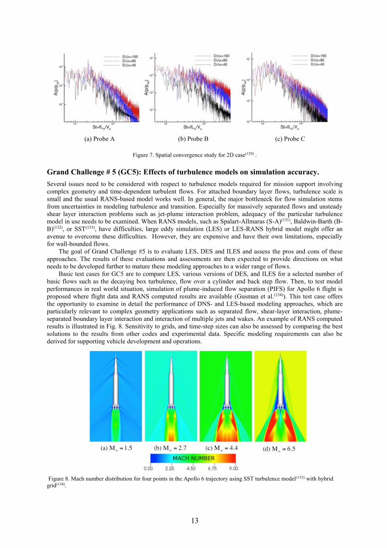
separated boundary layer interaction and interaction of multiple jets and wakes. An example of RANS computed

results is illustrated in Fig. 8. Sensitivity to grids, and time-step sizes can also be assessed by comparing the best

solutions to the results from other codes and experimental data. Specific modeling requirements can also be

derived for supporting vehicle development and operations.

Figure 8. Mach number distribution for four points in the Apollo 6 trajectory using SST turbulence model(133) with hybrid

grid(134).

14

Grand Challenge # 6 (GC6): Aeroacoustics – computational issues.

Requirements for aero-acoustic computations are different from CFD. For example, numerical dispersion and

dissipation errors can cause major errors in acoustic wave propagation. Spatial and temporal discretization

schemes and far field non-reflecting boundary conditions play very important roles.

For acoustics involving complex geometry, it is a common practice to develop an acoustic surface about a

RANS solution and apply Lighthill’s method for propagation to the far field. To study noise generation

mechanisms associated with jets and jet-solid interfaces, fine scale turbulence computations are needed (at the

DNS or LES level). The primary question to be answered is whether we can compute noise sources directly and

accurately propagate acoustic radiation with a wave propagation model. This approach can be compared to

RANS-acoustic surface modeling combination such as reported by Kiris et al.(135) and Brehm et al.(136)

6.0 CONCLUDING REMARKS

The opinions presented in this paper are based on the authors’ experience related to computational aerodynamics

and engineering, and may represent only a small portion of the flow simulation challenges we face today. Those

requisite capabilities listed above, if made available in the near term, can significantly impact the next generation

of air- and space-vehicle development and operations. We also believe that longer-term strategic research and

development, especially for the development of more universally applicable turbulence and possibly transition

models, will have far-reaching impacts on computational fluid engineering for flight vehicles as well as

aerospace engineering in general.

REFERENCES

1. Richardson, L. F., The approximate arithmetical solution by finite differences of physical problems

involving differential equations, with an application to the stresses in a masonry dam, Philosophical

Transactions of the Royal Society of London. Series A, Vol. 210, 1910, pp307-357.

2. Roache, P.J., Computational Fluid Dynamics, Hermosa Publisher, Alburquerque, NM 1976 (and

subsequent editions in 1972 and 1998).

3. Tannehill, J.C., Anderson, D.A., and Pletcher, R.H., Computational fluid mechanics and heat transfer, 2nd

ed. Taylor & Francis, Philadelphia, PA, 1997.

4. Chapman, D.R., Computational aerodynamics development and outlook, AIAA J. vol. 17, no. 12,

December 1979.

5. Johnson, F.T., Tinoco, E.N., and Yu, N.J., Thirty years of Development and application of CFD at Boeing

Commercial Airplane, Seattle, Computers and Fluids 34, 2005, pp1115-1151.

6. Kiris, C., Housman, J.A., and Kwak, D., Space/time convergence analysis of a ignition overpressure in the

flame trench, CFD Review 2010, World Scientific, 2010.

7. Kiris, C., Housman, J., Gusman, M., Schauerhamer, D., Deere, K., Elmiligui, A., Abdol-Hamid, K.,

Parlette, E., Andrews, M., and Belvins, J., Best Practices for Aero-Database CFD Simulations of Ares V

ascent, 49th AIAA Aerospace Sciences Meeting, January 4-7, 2011.

8. Leschziner, M.A. and Drikakis, D. Turbulence and turbulent-flow computation in aeronautics, The

Aeronautical Journal, 2729, 349-384, 2002.

9. Jiménez, J. Near-wall turbulence, Physics of Fluids (1994-present), 2013, 25, (10), pp. 101302.

10. Jiménez, J. How linear is wall-bounded turbulence? Physics of Fluids (1994-present), 2013, 25, (11), pp.

110814.

11. Cimarelli, A., De Angelis, E., and Casciola, C. Paths of energy in turbulent channel flows, J.Fluid Mech.,

2013, 715, pp. 436-451.

12. Wei, L., and Pollard, A. Direct numerical simulation of compressible turbulent channel flows using the

discontinuous Galerkin method, Comput.Fluids, 2011, 47, (1), pp. 85-100.

13. Chapelier, J., De La Llave Plata, M, Renac, F. Evaluation of a high-order discontinuous Galerkin method

for the DNS of turbulent flows, Comput.Fluids, 2014, 95, pp. 210-226.

14. Kim, J., Moin, P., and Moser, R. Turbulence statistics in fully developed channel flow at low Reynolds

number, J.Fluid Mech., 1987, 177, pp. 133-166.

15. Mansour, N., Kim, J., and Moin, P. Reynolds-stress and dissipation-rate budgets in a turbulent channel

flow, J.Fluid Mech., 1988, 194, pp. 15-44.

16. Moser, R.D., Kim, J., and Mansour, N.N. Direct numerical simulation of turbulent channel flow up to Re=

590, Phys.Fluids, 1999, 11, (4), pp. 943-945.

17. Del Alamo, J.C., Jiménez, J., Zandonade, P. Scaling of the energy spectra of turbulent channels, J.Fluid

Mech., 2004, 500, pp. 135-144.

18. Abe, H., Kawamura, H., and Matsuo, Y. Surface heat-flux fluctuations in a turbulent channel flow up to Re

τ= 1020 with Pr= 0.025 and 0.71, Int J Heat Fluid Flow, 2004, 25, (3), pp. 404-419.

15

19. Hoyas, S., and Jiménez, J. Scaling of the velocity fluctuations in turbulent channels up to Reτ= 2003,

Physics of Fluids (1994-present), 2006, 18, (1), pp. 011702.

20. Jiménez, J., Hoyas, S., Simens, M.P. Turbulent boundary layers and channels at moderate Reynolds

numbers, J.Fluid Mech., 2010, 657, pp. 335-360.

21. Wu, X., and Moin, P. Transitional and turbulent boundary layer with heat transfer, Physics of Fluids (1994-

present), 2010, 22, (8), pp. 085105.

22. Vreman, A., and Kuerten, J. Comparison of direct numerical simulation databases of turbulent channel flow

at Reτ= 180, Physics of Fluids (1994-present), 2014, 26, (1), pp. 015102.

23. Coleman, G.N., Kim, J., and Moser, R. A numerical study of turbulent supersonic isothermal-wall channel

flow, J.Fluid Mech., 1995, 305, pp. 159-183.

24. MorinishI, Y., Tamano, S., and Nakabayashi, K. Direct numerical simulation of compressible turbulent

channel flow between adiabatic and isothermal walls, J.Fluid Mech., 2004, 502, pp. 273-308.

25. Duan, L., Beekman, I., and Martin, M. Direct numerical simulation of hypersonic turbulent boundary

layers. Part 2. Effect of wall temperature, J.Fluid Mech., 2010, 655, pp. 419-445.

26. Taieb, D., and Ribert, G. Direct Numerical Simulation and Large-Eddy Simulation of Supersonic Channel

Flow, J.Propul.Power, 2013, 29, (5), pp. 1064-1075.

27. Tsuji, Y., Imayama, S., Schlatter, P. Pressure fluctuation in high-Reynolds-number turbulent boundary

layer: results from experiments and DNS, Journal of Turbulence, 2012, (13), pp. N50.

28. Philip, J., Baidya, R., Hutchins, N. Spatial averaging of streamwise and spanwise velocity measurements in

wall-bounded turbulence using∨ -and×-probes, Measurement Science and Technology, 2013, 24, (11), pp.

115302.

29. Ghosh, S., Foysi, H., and Friedrich, R. Compressible turbulent channel and pipe flow: similarities and

differences, J.Fluid Mech., 2010, 648, pp. 155-181.

30. Chin, C., Monty, J., and Ooi, A. Reynolds number effects in DNS of pipe flow and comparison with

channels and boundary layers, Int J Heat Fluid Flow, 2014, 45, pp. 33-40.

31. Monty, J., and Chong, M. Turbulent channel flow: comparison of streamwise velocity data from

experiments and direct numerical simulation, J.Fluid Mech., 2009, 633, pp. 461-474.

32. Ng, H., Monty, J., Hutchins, N. Comparison of turbulent channel and pipe flows with varying Reynolds

number, Exp.Fluids, 2011, 51, (5), pp. 1261-1281.

33. Boris, J., Grinstein, F., Oran, E. New insights into large eddy simulation, Fluid Dyn.Res., 1992, 10, (4-6),

pp. 199.

34. Hirt, C. Heuristic stability theory for finite-difference equations, Journal of Computational Physics, 1968,

2, (4), pp. 339-355.

35. Domaradzki, J.A., and Radhakrishnan, S. Effective eddy viscosities in implicit modeling of decaying high

Reynolds number turbulence with and without rotation, Fluid Dyn.Res., 2005, 36, (4), pp. 385-406.

36. Margolin, L.G., and Rider, W.J. A rationale for implicit turbulence modelling, Int.J.Numer.Methods Fluids,

2002, 39, (9), pp. 821-841.

37. Rider, W.J., and Margolin, L. From numerical analysis to implicit subgrid turbulence modeling, AIAA

paper, 2003, 4101, pp. 2003.

38. Margolin, L., and Rider, W. The design and construction of implicit LES models, Int.J.Numer.Methods

Fluids, 2005, 47, (10‐11), pp. 1173-1179.

39. Margolin, L., Rider, W., and Grinstein, F. Modeling turbulent flow with implicit LES, Journal of

Turbulence, 2006, (7), pp. N15.

40. Drikakis, D., and Rider, W. High-resolution methods for incompressible and low-speed flows, Springer

Science & Business Media, 2006.

41. Grinstein, F.F., Margolin, L.G., and Rider, W.J. Implicit large eddy simulation: computing turbulent fluid

dynamics, Cambridge university press, 2007.

42. Harten, A. High resolution schemes for hyperbolic conservation laws, Journal of computational physics,

1983, 49, (3), pp. 357-393.

43. Harten, A. High resolution schemes for hyperbolic conservation laws, Journal of Computational Physics,

1997, 135, (2), pp. 260-278.

44. Toro, E.F. Riemann solvers and numerical methods for fluid dynamics: a practical introduction, Springer

Science & Business Media, 2009.

45. Drikakis, D. Advances in turbulent flow computations using high-resolution methods, Prog.Aerospace Sci.,

2003, 39, (6), pp. 405-424.

46. Stolz, S., and Adams, N. An approximate deconvolution procedure for large-eddy simulation, Physics of

Fluids (1994-present), 1999, 11, (7), pp. 1699-1701.

47. Stolz, S., Adams, N., and Kleiser, L. An approximate deconvolution model for large-eddy simulation with

application to incompressible wall-bounded flows, Physics of Fluids (1994-present), 2001, 13, (4), pp. 997-

1015.

16

48. Hickel, S., Adams, N.A., and Domaradzki, J.A. An adaptive local deconvolution method for implicit LES,

Journal of Computational Physics, 2006, 213, (1), pp. 413-436.

49. Hickel, S., and Adams, N. On implicit subgrid-scale modeling in wall-bounded flows, Physics of Fluids

(1994-present), 2007, 19, (10), pp. 105106.

50. Kravchenko, A., and Moin, P. On the effect of numerical errors in large eddy simulations of turbulent

flows, Journal of Computational Physics, 1997, 131, (2), pp. 310-322.

51. Ghosal, S. An analysis of numerical errors in large-eddy simulations of turbulence, Journal of

Computational Physics, 1996, 125, (1), pp. 187-206.

52. Geurts, B.J., and Fröhlich, J. A framework for predicting accuracy limitations in large-eddy simulation,

Physics of Fluids (1994-present), 2002, 14, (6), pp. L41-L44.

53. Chow, F.K., and Moin, P. A further study of numerical errors in large-eddy simulations, Journal of

Computational Physics, 2003, 184, (2), pp. 366-380.

54. Meyers, J., Geurts, B.J., and Baelmans, M. Database analysis of errors in large-eddy simulation, Physics of

Fluids (1994-present), 2003, 15, (9), pp. 2740-2755.

55. Lund, T., and Kaltenbach, H. Experiments with explicit filtering for LES using a finite-difference method,

Annual Research Briefs, 1995, pp. 91-105.

56. Lund, T. On the use of discrete filters for large eddy simulation, Annual Research Briefs, 1997, pp. 83-95.

57. Bose, S.T., Moin, P., and You, D. Grid-independent large-eddy simulation using explicit filtering, Physics

of Fluids (1994-present), 2010, 22, (10), pp. 105103.

58. Gullbrand, J. Dynamic modeling in large-eddy simulation of turbulent channel flow: Investigation of two-

dimensional versus three-dimensional test filtering, Int.J.Numer.Methods Heat Fluid Flow, 2004, 14, (4),

pp. 467-492.

59. Brandt, T.T. Usability of explicit filtering in large eddy simulation with a low‐order numerical scheme and

different subgrid‐scale models, Int.J.Numer.Methods Fluids, 2008, 57, (7), pp. 905-928.

60. Klein, M. An attempt to assess the quality of large eddy simulations in the context of implicit filtering,

Flow, Turbulence and Combustion, 2005, 75, (1-4), pp. 131-147.

61. Gullbrand, J., and Chow, F.K. The effect of numerical errors and turbulence models in large-eddy

simulations of channel flow, with and without explicit filtering, J.Fluid Mech., 2003, 495, pp. 323-341.

62. Gullbrand, J., Grid-independent large-eddy simulation in turbulent channel flow using three-dimensional

explicit filtering, DTIC Document, Grid-independent large-eddy simulation in turbulent channel flow using

three-dimensional explicit filtering, 2003.

63. Hughes, T.J., Oberai, A.A., and Mazzei, L. Large eddy simulation of turbulent channel flows by the

variational multiscale method, Physics of Fluids (1994-present), 2001, 13, (6), pp. 1784-1799.

64. Bazilevs, Y., Calo, V., Cottrell, J. Variational multiscale residual-based turbulence modeling for large eddy

simulation of incompressible flows, Comput.Methods Appl.Mech.Eng., 2007, 197, (1), pp. 173-201.

65. Oberai, A.A., Liu, J., Sondak, D. A residual based eddy viscosity model for the large eddy simulation of

turbulent flows, Comput.Methods Appl.Mech.Eng., 2014, 282, pp. 54-70.

66. Piomelli, U. Wall-layer models for large-eddy simulations, Prog.Aerospace Sci., 2008, 44, (6), pp. 437-

446.

67. Spalart, P., Jou, W., Strelets, M. Comments on the feasibility of LES for wings, and on a hybrid

RANS/LES approach, Advances in DNS/LES, 1997, 1, pp. 4-8.

68. Nikitin, N., Nicoud, F., Wasistho, B. An approach to wall modeling in large-eddy simulations, Physics of

Fluids (1994-present), 2000, 12, (7), pp. 1629-1632.

69. Hamba, F. A hybrid RANS/LES simulation of turbulent channel flow, Theor.Comput.Fluid Dyn., 2003, 16,

(5), pp. 387-403.

70. Hamba, F. A hybrid RANS/LES simulation of high-Reynolds-number channel flow using additional

filtering at the interface, Theor.Comput.Fluid Dyn., 2006, 20, (2), pp. 89-101.

71. Piomelli, u., balaras, E., Pasinato, H. The inner–outer layer interface in large-eddy simulations with wall-

layer models, Int J Heat Fluid Flow, 2003, 24, (4), pp. 538-550.

72. Tessicini, F., Temmerman, L., and Leschziner, M. Approximate near-wall treatments based on zonal and

hybrid RANS–LES methods for LES at high Reynolds numbers, Int J Heat Fluid Flow, 2006, 27, (5), pp.

789-799.

73. Walters, D., Bhushan, S., Alam, M. Investigation of a dynamic hybrid RANS/LES modelling methodology

for finite-volume CFD simulations, Flow, turbulence and combustion, 2013, 91, (3), pp. 643-667.

74. Temmerman, L., Hadžiabdić, M., Leschziner, M. A hybrid two-layer URANS–LES approach for large

eddy simulation at high Reynolds numbers, Int J Heat Fluid Flow, 2005, 26, (2), pp. 173-190.

75. Abe, K. A hybrid LES/RANS approach using an anisotropy-resolving algebraic turbulence model, Int J

Heat Fluid Flow, 2005, 26, (2), pp. 204-222.

76. Duprat, C., Balarac, G., Métais, O. A wall-layer model for large-eddy simulations of turbulent flows

with/out pressure gradient, Physics of Fluids (1994-present), 2011, 23, (1), pp. 015101.

17

77. Davidson, L. The PANS k–ε model in a zonal hybrid RANS–LES formulation, Int J Heat Fluid Flow, 2014,

46, pp. 112-126.

78. Bose, S., and Moin, P. A dynamic slip boundary condition for wall-modeled large-eddy simulation, Physics

of Fluids (1994-present), 2014, 26, (1), pp. 015104.

79. Chen, Z.L., Hickel, S., Devesa, A. Wall modeling for implicit large-eddy simulation and immersed-

interface methods, Theor.Comput.Fluid Dyn., 2014, 28, (1), pp. 1-21.

80. Utyuzhnikov, S. Towards development of unsteady near-wall interface boundary conditions for turbulence

modeling, Comput.Phys.Commun., 2014, 185, (11), pp. 2879-2884.

81. Fureby, C., and Grinstein, F.F. Large eddy simulation of high-Reynolds-number free and wall-bounded

flows, Journal of Computational Physics, 2002, 181, (1), pp. 68-97.

82. Kokkinakis, I. and Drikakis, D. Implicit Large Eddy Simulation of Weakly-Compressible Turbulent

Channel Flow, Computer Methods in Applied Mechanics and Engineering, 287, 229–261, 2015.

83. Grinstein, F., Fureby, C., and Devore, C. On MILES based on flux‐limiting algorithms,

Int.J.Numer.Methods Fluids, 2005, 47, (10‐11), pp. 1043-1051.

84. Fureby, C. Towards the use of large eddy simulation in engineering, Prog.Aerospace Sci., 2008, 44, (6), pp.

381-396.

85. Drikakis, D., Fureby, C., Grinstein, F.F., D. Youngs Simulation of transition and turbulence decay in the

Taylor–Green vortex, Journal of Turbulence, 2007, (8), pp. N20.

86. Domaradzki, J. Large eddy simulations without explicit eddy viscosity models, International Journal of

Computational Fluid Dynamics, 2010, 24, (10), pp. 435-447.

87. Michopoulos, J.G., Farhat, C., and Fish, J. Modeling and simulation of multiphysics systems, Journal of

Computing and Information Science in Engineering, 2005, 5, (3), pp. 198-213.

88. Tiersten, H. On the nonlinear equations of thermo-electroelasticity, Int.J.Eng.Sci., 1971, 9, (7), pp. 587-

604.

89. XU, K., NOOR, A.K., and TANG, Y.Y. Three-dimensional solutions for coupled thermoelectroelastic

response of multilayered plates, Comput.Methods Appl.Mech.Eng., 1995, 126, (3), pp. 355-371.

90. Sih, G.C., Michopoulos, J., and Chou, S. Hygrothermoelasticity, Springer Science & Business Media,

2012.

91. Zienkiewicz, O., and Chan, A. Coupled problems and their numerical solution, Advances in Computational

Nonlinear Mechanics, Springer, 1989.

92. Wright, J.R., and Cooper, J.E. Introduction to aircraft aeroelasticity and loads, John Wiley & Sons, 2008.

93. Albano, E., and Rodden, W.P. A doublet-lattice method for calculating lift distributions on oscillating

surfaces in subsonic flows. AIAA J., 1969, 7, (2), pp. 279-285.

94. Hassig, H.J. An approximate true damping solution of the flutter equation by determinant iteration. J.Aircr.,

1971, 8, (11), pp. 885-889.

95. Ashley, H. Piston theory-a new aerodynamic tool for the aeroelastician, Journal of the Aeronautical

Sciences (Institute of the Aeronautical Sciences), 2012, 23, (12).

96. Hübner, B., Walhorn, E., and Dinkler, D. A monolithic approach to fluid–structure interaction using space–

time finite elements, Comput.Methods Appl.Mech.Eng., 2004, 193, (23), pp. 2087-2104.

97. Ishihara, D., and Yoshimura, S. A monolithic approach for interaction of incompressible viscous fluid and

an elastic body based on fluid pressure Poisson equation, Int J Numer Methods Eng, 2005, 64, (2), pp. 167-

203.

98. Wüchner, R., Kupzok, A., and Bletzinger, K. A framework for stabilized partitioned analysis of thin

membrane–wind interaction, Int.J.Numer.Methods Fluids, 2007, 54, (6‐8), pp. 945-963.

99. Cerqueira, S., and Chaineray, G. Multi-Physics Coupling Approaches for Aerospace Numerical

Simulations, AerospaceLab, 2, 2011.

100. Heil, M., Hazel, A.L., and Boyle, J. Solvers for large-displacement fluid–structure interaction problems:

segregated versus monolithic approaches, Comput.Mech., 2008, 43, (1), pp. 91-101.

101. Gad-El-Hak, M. Gas and liquid transport at the microscale, Heat Transfer Eng., 2006, 27, (4), pp. 13-29.

102. Marx, D., and Hutter, J. Ab initio molecular dynamics: basic theory and advanced methods, Cambridge

University Press, 2009.

103. Ohno, K., Esfarjani, K., and Kawazoe, Y. Computational materials science: from ab initio to Monte Carlo

methods, Springer Science & Business Media, 2012.

104. Frisch, U., Hasslacher, B., and Pomeau, Y. Lattice-gas automata for the Navier-Stokes equation,

Phys.Rev.Lett., 1986, 56, (14), pp. 1505.

105. Mcnamara, G.R., and Zanetti, G. Use of the Boltzmann equation to simulate lattice-gas automata,

Phys.Rev.Lett., 1988, 61, (20), pp. 2332.

106. Wolf-Gladrow, D.A. Lattice-gas cellular automata and lattice Boltzmann models: An Introduction,

Springer Science & Business Media, 2000.

18

107. Chen, S., and Doolen, G.D. Lattice Boltzmann method for fluid flows, Annu.Rev.Fluid Mech., 1998, 30,

(1), pp. 329-364.

108. Groot, R.D., and Warren, P.B. Dissipative particle dynamics: Bridging the gap between atomistic and

mesoscopic simulation, J.Chem.Phys., 1997, 107, (11), pp. 4423.

109. Garcia, A.L., Bell, J.B., Crutchfield, W.Y. Adaptive mesh and algorithm refinement using direct simulation

Monte Carlo, Journal of computational Physics, 1999, 154, (1), pp. 134-155.

110. Oran, E., Oh, C., and Cybyk, B. Direct simulation Monte Carlo: recent advances and applications 1,

Annu.Rev.Fluid Mech., 1998, 30, (1), pp. 403-441.

111. Kalweit, M., and Drikakis, D. Multiscale methods for micro/nano flows and materials, Journal of

Computational and Theoretical Nanoscience, 2008, 5, (9), pp. 1923-1938.

112. Kalweit, M., and Drikakis, D. Multiscale simulation strategies and mesoscale modelling of gas and liquid

flows, IMA journal of applied mathematics, 2011, 76, (5), pp. 661-671.

113. O’Connell, S.T., and Thompson, P.A. Molecular dynamics–continuum hybrid computations: a tool for

studying complex fluid flows, Physical Review E, 1995, 52, (6), pp. R5792.

114. Kalweit, M., and Drikakis, D. Coupling strategies for hybrid molecular—continuum simulation methods,

Proc.Inst.Mech.Eng.Part C, 2008, 222, (5), pp. 797-806.

115. Darbandi, M., and Roohi, E. Applying a hybrid DSMC/Navier–Stokes frame to explore the effect of splitter

catalyst plates in micro/nanopropulsion systems, Sensors and actuators A: Physical, 2013, 189, pp. 409-

419.

116. Farber, K., Farber, P., Gräbel, J. Development and validation of a coupled Navier–Stokes/DSMC

simulation for rarefied gas flow in the production process for OLEDs, Applied Mathematics and

Computation, 2015.

117. Wu, J., Lian, Y., Cheng, G. Development and verification of a coupled DSMC–NS scheme using

unstructured mesh, Journal of Computational Physics, 2006, 219, (2), pp. 579-607.

118. Asproulis, N., Kalweit, M., and Drikakis, D. A hybrid molecular continuum method using point wise

coupling, Adv.Eng.Software, 2012, 46, (1), pp. 85-92.

119. Balasubramanian, A.K., Miller, A.C., and Rediniotis, O.K. Microstructured hydrophobic skin for

hydrodynamic drag reduction, AIAA J., 2004, 42, (2), pp. 411-414.

120. Ghoniem†, N.M., Busso, E.P., Kioussis, N. Multiscale modelling of nanomechanics and micromechanics:

an overview, Philosophical magazine, 2003, 83, (31-34), pp. 3475-3528.

121. Rumsey, C. and Slotnicky, J., Overview and summary of the second AIAA High Lift Prediction Workshop.

52nd Aerospace Sciences Meeting, National Harbor; United States; p37-40, 13-17 January 2014.

122. Brodersen, O., and Sturmer, A. Drag prediction of engine-airframe interference effects using unstructured

Navier-Stokes calculations, 19th AIAA Applied Aerodynamics Conference, AIAA, Ed., Anaheim

California, 2001, pp. 2001–2041.

123. Antoniadis, A., Tsoutsanis, P., Rana, Z., Kokkinakis, I., Drikakis, D. Azure: An Advanced CFD Software

Suite Based on High-Resolution and High-Order Methods, Session FD-21, CFD Methods IV, AIAA,

Aerospace SciTech Conference 2015.

124. Drikakis, D., Hahn, M., Mosedale, A. and Thornber, B. Large Eddy Simulation Using High Resolution and

High Order Methods, Philosophical Transactions Royal Society A, 367, 2985-2997, 2009.

125. Tsoutsanis, P., Antoniadis, A.F., Drikakis, D. WENO schemes on arbitrary unstructured meshes for

laminar, transitional and turbulent flow, Journal of Computational Physics, 256, 254-276, 2014.

126. Chaderjian, N., and Buning, P. High resolution Navier-Stokes simulation of rotor wakes, Proceedings of

the American Helicopter Society 67th Annual Forum, 2011.

127. Chaderjian, N.M., and Ahmad, J.U. Detached Eddy Simulation of the UH-60 Rotor Wake Using Adaptive

Mesh Refinement, Proceedings of the 68th Annual Forum of the American Helicopter Society, Forth

Worth, TX, 2012.

128. Moini-yekta, S., Barad, M., Sozer, E., Housman, J. Towards Hybrid Grid Simulations of the Launch

Environment, Seventh International Conference on CFD, ICCFD7, 2012.

129. Nakanishi, Y., Okamoto, K., Teramoto, S., and Okunuki, T. Acoustic characteristics of correctly-expanded

supersonic jet impinging to an inclined plate, Asian Joint Conference on Propulsion and Power, 2012.

130. Brehm, C., Sozer, E., Moini-yekta, S., Housman, J.A. Computational Prediction of Pressure Environment

in the Flame Trench, 2013.

131. Spalart, P., and Allmaras, S. A one-equation turbulence model for aerodynamic flows, AIAA-92-0439,

AIAA 30th Aerospace Sciences Meeting, 1992.

132. Baldwin, B.S., and Barth, T.J. A one-equation turbulence transport model for high Reynolds number wall-

bounded flows, AIAA paper 91-0610, 1991.

133. Menter, F.R., Zonal two equation k-turbulence models for aerodynamic flows, AIAA paper 93-2906, AIAA

paper, 1993.

19

134. Gusman, M., Housman, J., and Kiris, C. Best Practices for CFD Simulations of Launch Vehicle Ascent

with Plumes-OVERFLOW Perspective, 49th AIAA Aerospace Sciences Meeting, AIAA Paper, 2011.

135. Kiris, C., Barad, M., Housman, J. The LAVA Computational Fluid Dynamics Solver, AIAA 2014-0070,

AIAA SciTech, 2014.

136. Brehm, C., Housman, J.A., kiris, C.C., and Hutcheson, F.V. Noise Characteristics of a Four-Jet

Impingement Device Inside a Broadband Engine Noise Simulator, AIAA 2015-2211, AIAA 21st

AIAA/CEAS Aeroacoustics Conference, 2015.