Embed Size (px)
Citation preview

Rochester Institute of Technology Rochester Institute of Technology
RIT Scholar Works RIT Scholar Works
Theses
8-1-1996
Computational analysis and revision of the Nayatani et al. Computational analysis and revision of the Nayatani et al.
appearence model appearence model
John Rahill
Follow this and additional works at: https://scholarworks.rit.edu/theses
Recommended Citation Recommended Citation Rahill, John, "Computational analysis and revision of the Nayatani et al. appearence model" (1996). Thesis. Rochester Institute of Technology. Accessed from
This Thesis is brought to you for free and open access by RIT Scholar Works. It has been accepted for inclusion in Theses by an authorized administrator of RIT Scholar Works. For more information, please contact [email protected].

COMPUTATIONAL ANALYSIS AND REVISION OF
THE NAYATANI ET AL. COLOR APPEARANCE MODEL
John F. Rahill
B.S. Chemistry
Rochester Institute of Technology
(1986)
A thesis submitted in partial fulfillmentof the requirements for the M.S. in the Chester F Carlson
Center for Imaging Science in the College of Scienceat the Rochester Institute of Technology
August 1996
Signature of Author
Accepted by Harry E. Rhody._--
Coordinator, M.S. Degree Program

COllEGE OF SCIENCEROCHFSfER INSTITUTE OF TECHNOLOGY
ROCHESTER,NY
CERTIFICATE OF APPROVAL
M. S. DEGREE THESIS
The M.S. Degree Thesis of John F. Rahillhas been examined and approved by the thesis committe
as satisfactory for the thesis requirement for theMaster of Science degree in Imaging Science.
Dr. Mark D. Fairchild
Dr. Roy S. Berns
Ms. Paula J. Alessi
Date

THESIS RELEASE PERMISSION
ROCHESTER INSTITUTE OF TECHNOLOOY
ROCHESTER, NY
COMPUTATIONAL ANALYSIS AND REVISION OF
THE NAYATANI Ef AL. COLOR APPEARANCE MODEL
I, John F. Rahill, hereby grant permission to the Wallace Memorial Library of
R.I.T. to reproduce my thesis in whole or in part. Any reproduction will not be
for commercial use or profit.
John F. Rahill
-----~~~~----------------------Date

Computational Analysis and Revision of
the Nayatani et al. Color Appearance Model
John F. Rahill
Submitted to the Center for Imaging Science
in partial fulfillment of the requirements for the
Master of Science degree in Imaging Science at the
Rochester Institute of Technology
August 1996
ABSTRACT
A literature search showed Nayatani 's color appearance model to be inferior to
Hunt's model. The goal of this research was to determine what modifications
could be made to improve Nayatani's model. Thecoefficients'
!;, T|, and C, in
Nayatani's model represent the chromaticity coordinates of the illuminant in
the fundamental primary system. These coefficients were used in calculating
the effective adapting level for each cone and act as normalizing factors i n
the calculation of Nayatani color space. The CSAJ data set was used to determine
a baseline for Nayatani's model, and results from modifications were compared
relative to Hunt. Nayatani's Ml model set thecoefficients'
equal to 1, and
Illuminant A was used to normalize the estimates of the fundamental
primaries. Nayatani's results were compared to the CSAJ D65 reference data.
The average AE*ab error was essentially equal for Munsell Value 3/, 5/, and 7/,
while the total AE*ab error was reduced from 7.19 to 6.3. In addition, light
colors shifted yellow and dark colors shifted blue for all three Value levels.
This correctly predicts the Helson-Judd effect, and the results appear to match
the Hunt model. The exponents of Nayatani's nonlinear p functions were
rounded to the hundredths place to test the relevance of four significant
figures. The AL*, Aa*,Ab*
and AE*ab errors were the identical to those i n
Nayatani's standard model for all Value levels. Thus there is no justification
for specifying exponents to four decimal places. Variations in the adapting
luminance showed AE*ab errors to be nonlinear at low luminance levels.

Acknowledgments
The are very few times in our lives where we can openly thank those who
have helped us reach our goals. There are friends, family, teachers, co
workers, and professionals who have not only helped along the way but
influenced my life as well. To some the payback is immediate, to others it will
show as I live out my life. Hopefully I can thank them all.
To the health care, lawyer, pharmacist, banker, and quality professionals who
are my real life brothers and sisters, a toast to you. Thanks for setting the
standards. To my nephews and nieces who taught me how to be a father.
To the teachers. Dana set me straight. Roy drove me to always bring out the
best. Mark was the rock. No matter how bizarre the question or distant the
tangent. Paula gave me the goal, guidance and perspective.
To my golf partner. Always. To Nathan, Elizabeth and Tim. May a light guide
you wherever you go. To my Mom who will always be a Mom. To Dad, I did it!
To the Doctors. Tim Quill, Stephen Rauh, Janet Reiser, and Joe Leberer. I have
my life back thanks to you. To the Crohn's and Colitis Foundation of America
and the American Cancer Society, may you find new paths to cure an old foe.

Mostly, to Gail and Meghan. My true friends, my two loves. Though my heart
pounds, my feet dance, my hands touch, my ears hear, and my eyes see. it
would be nothing if not for you. Life is not whole until your loved ones make
you laugh until you cry. Being scared makes us sure we are alive.

1
Table of Contents
Table of Contents
List of Figures i v
List of Tables vi
Introduction 1
Literature Review 3
Goal of Thesis 16
Basic Review of Hunt and Nayatani Models 17
Hunt Model 17
Nayatani Model 19
von Kries transformation 23
P Functions 23
Nayatani Color Space 28
CSAJ Data Used to Test Validity of Models 29
Code 29
Characteristics and Computational Parameters 29
Nayatani Model Verification using CSAJ Data 30
CIELAB Analysis for Nayatani Standard Model 30
Helson-Judd Modification: Ml 37
CIELAB Analysis of Nayatani Ml Model 38
Helson-Judd Modification: M2 45
CIELAB Analysis of Nayatani M2 Model 45
Comparison of Nayatani and Hunt Models using CSAJ Data Set 53
CIELAB Analysis for Hunt Model 53

CIELAB Analysis of Nayatani and Hunt Models 60
Verification of Modifications using Independent Data Set 70
Characteristics of Breneman Data Set 70
CIELAB Analysis of Nayatani Standard Model 71
CIELAB Analysis of Nayatani M2 Model 74
CIELAB Analysis of Hunt Model 76
Comparison of Nayatani and Hunt Models using Breneman Data 78
Nayatani Model: Significant Figures for Nonlinear Exponents 83
CIELAB Analysis using CSAJ Data 84
Nayatani Model: Nonlinearity at Low Luminance Levels 88
CIELAB Analysis using CSAJ Data 88
Summary of Results 93
Helson-Judd Modification 93
Independent Data Study 95
Nonlinear Exponents 97
Luminance Adaptation 98
Conclusions and Recommendations 98
Appendix A: Source Code 100
Appendix B: CSAJ Data 111
Appendix CI: CSAJ using Nayatani Standard Model 113
Appendix C2: CSAJ using Nayatani Ml Model 115
Appendix C3: CSAJ using Nayatani M2 Model 117
Appendix D: CSAJ using Hunt Model 119
Appendix E: Breneman Data 121

Appendix Fl: Breneman Data using Nayatani Standard Model 122
Appendix F2: Breneman Data using Nayatani M2 Model 123
Appendix F3: Breneman Data using Hunt Model 124
Appendix Gl: CSAJ Data w/ Nayatani Standard Model; r,g=.4, b=.5128 125
Appendix G2: CSAJ Data w/ Nayatani Standard Model; r,g=4495, b=.5 127
Appendix G3: CSAJ Data w/ Nayatani Standard Model; r,g=4, b=.5 129
Appendix G4: CSAJ Data w/ Nayatani Standard Model; r,g=4495, b=.51 131
Appendix G5: CSAJ Data w/ Nayatani Standard Model; r,g=45, b=.5128 133
Appendix G6: CSAJ Data w/ Nayatani Standard Model; r,g=.45, b=.51 135
Appendix HI: CSAJ Data w/ Nayatani Standard Model; 25 cd/mA2 137
Appendix H2: CSAJ Data w/ Nayatani Standard Model; 50 cd/mA2 139
Appendix H3: CSAJ Data w/ Nayatani Standard Model; 100 cd/mA2 141
Appendix H4: CSAJ Data w/ Nayatani Standard Model; 300 cd/mA2 143
Appendix H5: CSAJ Data w/ Nayatani Standard Model; 500 cd/mA2 145
Appendix H6: CSAJ Data w/ Nayatani Standard Model; 1000 cd/mA2 147
Appendix H7: CSAJ Data w/ Nayatani Standard Model; 3000 cd/mA2 149
Appendix H8: CSAJ Data w/ Nayatani Standard Model; 5000 cd/mA2 151
Appendix H9: CSAJ Data w/ Nayatani Standard Model; 10000 cd/mA2 153
References 155
ui

List of Figures
Fig. 1. Mean Visual Lightness for Hunt and Nayatani Model Predictions 3
Fig. 2. Mean Visual Hue for Hunt and Nayatani Model Predictions (240 cd/mA2) 4
Fig. 3. Mean Visual Hue for Hunt and Nayatani Model Predictions (40 cd/mA2) 5
Fig. 4. CIELAB a*
vsb* for Nayatani, von Kries, Hunt Model Predictions 7
Fig. 5. Observed Achromatic Lightness vs. Nayatani Model Predictions 9
Fig. 6. Observed Increase in Chroma vs. Nayatani Model Predictions 1 0
Fig. 7. Observed Helson-Judd Effect vs. Nayatani Model Predictions 1 1
Fig. 8. Z-scores for Daylight Luminance Levels (71, 214, 642 cd/mA2) 12-13
Fig. 9. Munsell N5 Patch for Fairchild, Hunt, Nayatani Models 1 5
Fig. 10. Nayatani Two-Stage Nonlinear Model 2 0
Fig. 11. Comparison of Hunt, Stevens, Breneman Nonlinear Cone Functions 2 5
Fig. 12. Nayatani Beta Functions for Red, Green, Blue Cones 2 6
Fig. 13. Cone Response Function of Boynton and Nayatani 2 6
Fig. 14. CIE a*
vs.b* CSAJ Value 3/ for Nayatani Standard model 3 3
Fig. 15. CIE a*vs.
b* CSAJ Value 5/ for Nayatani Standard model 3 4
Fig. 16. CIE a*vs.
b* CSAJ Value 7/ for Nayatani Standard model 3 5
Fig. 17. CIE C*vs.
L* CSAJ Value 3/, 5/, 7/ for Nayatani Standard model 3 6
Fig. 18. CIE a*
vs.b* CSAJ Value 3/ for Nayatani Ml model 4 1
Fig. 19. CIE a*
vs.b* CSAJ Value 5/ for Nayatani Ml model 4 2
Fig. 20. CIE a*
vs.b* CSAJ Value 7/ for Nayatani Ml model 4 3
Fig. 21. CIEC*
vs.L* CSAJ Value 3/, 5/, 7/ for Nayatani Ml model 4 4
Fig. 22. Cffi a* vs.b* CSAJ Value 3/ for Nayatani M2 model 4 9
IV

Fig. 23. CIE a*
vs.b* CSAJ Value 5/ for Nayatani M2 model 5 0
Fig. 24. CIE a*
vs.b* CSAJ Value 7/ for Nayatani M2 model 5 1
Fig. 25. CIE C*vs.
L* CSAJ Value 3/, 5/, 7/ for Nayatani M2 model 5 2
Fig. 26. CIE a*
vs.b* CSAJ Value 3/ for Hunt model 5 6
Fig. 27. CIE a*
vs.b* CSAJ Value 5/ for Hunt model 5 7
Fig. 28. CIE a*
vs.b* CSAJ Value 7/ for Hunt model 5 8
Fig. 29. CIE C*vs.
L* CSAJ Value 3/, 5/, 7/ Hunt model 5 9
Fig. 30. CIE a*
vs.b* CSAJ Value 3/ Nayatani Ml vs. Hunt model 6 1
Fig. 31. CIE a*
vs.b* CSAJ Value 5/ Nayatani Ml vs. Hunt model 6 2
Fig. 32. CIE a*
vs.b* CSAJ Value 7/ Nayatani Ml vs. Hunt model 6 3
Fig. 33. CIE C*vs.
L* CSAJ Value 3/, 5/, 7/ Nayatani Ml vs. Hunt model 6 4
Fig. 34. CIE a*
vs.b* CSAJ Value 3/ Nayatani M2 vs. Hunt model 6 6
Fig. 35. CIE a*
vs.b* CSAJ Value 5/ Nayatani M2 vs. Hunt model 6 7
Fig. 36. CIE a*vs.
b* CSAJ Value 7/ Nayatani M2 vs. Hunt model 6 8
Fig. 37. CIE C*vs.
L* CSAJ Value 3/, 5/, 7/ Nayatani M2 vs. Hunt model 6 9
Fig. 38. CIE a*
vs.b* Nayatani Std. model vs. Breneman D65 Reference 7 3
Fig. 39. CIE a*
vs.b* Nayatani M2 model vs. Breneman D65 Reference 7 5
Fig. 40. CIE a*
vs.b* Hunt model vs. Breneman D65 Reference 7 7
Fig. 41. CIE a*
vs.b* Breneman: Nayatani Std vs. Hunt model 8 0
Fig. 42. CIE a*
vs.b* Breneman: Nayatani M2 vs. Hunt model 8 2
Fig. 43. CIE a*vs.
b* CSAJ Value 3/, 5/, 7/ Log Luminance vs.AL* 9 0
Fig. 44. CIE a*vs.
b* CSAJ Value 3/, 5/, 7/ Log Luminance vs. AE*ab 9 2

List of Tables
Table I. CIELAB Deltas': CSAJ with Nayatani Standard Model 31
Table II. CIELAB Deltas': CSAJ with Nayatani Ml Model 40
Table III. CIELAB Deltas': CSAJ with Nayatani M2 Model 46
Table IV. CIELAB Deltas': CSAJ with Hunt Model 53
Table V. CIELAB Deltas': Breneman with Nayatani Standard Model 72
Table VI. CIELAB Deltas': Breneman with Nayatani M2 Model 74
Table VII. CIELAB Deltas': Breneman with Hunt Model 76
Table VIII. CIELAB Deltas': CSAJ with Nayatani Std Model; rg=.4, b=.5128 84
Table IX. CIELAB Deltas': CSAJ with Nayatani Std Model; rgb exp mod 1 85
Table X. CIELAB Deltas': CSAJ with Nayatani Std Model; rgb exp mod 2 87
Table XI. CIE AL* & AE*, CSAJ Value 3/ with varying Luminance 88
Table XII. CIE AL* & AE*, CSAJ Value 7/ with varying Luminance 89
VI

Introduction
While the human visual system adapts routinely under various conditions,
capturing and re-creating images for commercial applications is quite a
different story. The use of color critical images in the commercial field has
increased exponentially in the past decade. This has led to the need for
accurate color appearance models to optimize device and system performance.
For example, consider a professional photographer capturing a scene in his
studio on slide film for a national ad campaign. He chooses a mixture of
daylight and amber gel lighting, in a 2:1 luminance level ratio, and proofs his
images on a light box in a dim surround. Yet when the image is displayed i n
magazines, they are typically viewed under tungsten or cool white fluorescent
lighting. The image displayed in the magazine was also scanned which raises
concerns over dye gamut mismatches. The spectral sensitivity of the dyes used
in the film will not match those of the scanner nor the colorants used in the
inks for printing. Thus the need for accurate color appearance models to
optimize device and system performance becomes an important issue. How
accurate do color appearance models and imaging systems need to be today to
generate an exact reproduction of the captured image?
The critical use of color modeling in the imaging field also includes:
generation of prints from prints utilizing hardcopy/hardcopy matching,
desktop publishing using photo quality images for hardcopy/softcopy
matching,
film based images (negatives or transparencies) scanned onto PhotoCD
Disks for storage or print generation,
electronic cameras with CCD sensors are utilized for computer displayed
images.
The various types of image capture formats, intermediate image processing
algorithms, and output devices and media can further change the appearance
of the original image.
In addition to the previous commercial applications, both the CIE and ISCC need
to recommend a color-appearance model that is applicable for resolvingcolor-
rendering issues when artificial lighting is involved. The Hunt (1) and
Nayatani (2) models have dominated the field for predicting the appearance of
images and objects under various adapting illuminants and luminance levels.
Both models use non-linear functions to model the three cone responses, and
incorporate a von Kries (3) type adaptation transformation. The models also
apply factors to account for illuminant and luminance level adaptation, and
predict the Helson-Judd effect (4). However, the models are quite different. The
discussions on literature searches that follow, have indicated that Hunt's model
was preferred to Nayatani's in both numerical and psychophysical judgments.
Throughout this paper, Illuminants D65, D50, CWF and A refer to CIE the
Standard Illuminants.

Literature Review: Luo
Luo (5,6,7,8) et al., attempted to develop a color appearance model for the
graphic art industry. During this project, workers studied different viewing
conditions including change of illuminant, varying the luminance level of
the source, luminous reflectance of the background, and media type. Six
different color appearance models were compared in these experiments,
among them Hunt (1) and Nayatani (2).
10 20 30 40 50 60 70 80 90 100 0 10 20 30 40 50 60 70
CIE Hunt's 87
90 100 0 10 20 30 40 50 60 70 80 90 100
Nayatani et al
90
80
70
60
50
40 /*30
20
10
u
10 20 30 40 50 60 70 80 90 100 0 10 20 30 40 50 60 70 80 90 100
CMC(1:1) Hunt's91
Figurel. Comparison of mean visual lightness results vs predicted
lightness for CIE L*, Hunt's 87, Nayatani, and Hunt's 91 models.
Figure 1 represents the visual lightness results for gray backgrounds at a
high luminance level (240 cd/mA2) for Illuminant D50. The results show

Hunt's model has better correlation Nayatani when comparing visual
lightness to the lightness predicted by the models. For perfect correlation, all
the data would lie on the 45-degree line. Figure's 2 and 3 show the
experimental results for hue vs. the predicted hue using the Hunt and
Nayatani models. These results are for gray backgrounds at high (Figure 2)
and low (Figure 3) luminance levels under Illuminants D65, D50, CWF, and A.
Luo et al., reported the appearance of a systematic scattering pattern, where
less scattering occurs for Illuminants D65 and D50 than for CWF and A. He also
reported that Hunt's model appears to give less scattering than Nayatani's.
D65 D50
O 10 20 30 40 SO 60 70 BO 90 100 110 120 0 10 20 30 40 30 60 TO tO 90 100 1 10 120 0 10 30 30 40 50 60 70 BO 93 100 110 120 0 10 20 30 40 50 60 70 KO 90 100 110 120
Nayatani et al
0 10 20 30 40 50 60 70 10 90 100 1 10 120 0 10 20 30 40 50 60 70 SO 90 100 1 10 120 0 10 20 30 40 50 60 70 BO 90 100 110 120 0 10 20 30 40 50 60 70 KO 90 100 110 120
Hunt
Figure 2. Comparison of mean visual hue vs predicted hue for Nayatani and Hunt models,
under high (240 cd/mA2) luminance level of D65, D50, CWF, and A.

Luo noted that Nayatani's model gave reasonable correlation to hue results for
high luminance D50 as well as both luminance levels for D50 and D65. Yet,
Nayatani's model performed poorly for nondaylight low luminance sources.
The report made two suggestions. First, that Nayatani's model be restricted for
use with light gray to white backgrounds under high luminance daylight
sources. Secondly, Nayatani's model does not give good correlation to results
obtained under non-daylight sources. It was suggested that the error in hue
prediction could be caused by the models use of logarithmic functions with the
adaptation coefficients. Lastly, Luo felt both Hunt and Nayatani's models
overpredicted colorfulness at both high and low luminance levels.
D65 D50 WF
10 20 30 40 50 60 70 SO 90 100 110 120 0 10 20 30 40 50 60 70 SO 90 100 1 10 120 0 10 20 30 40 SO 60 70 SO 90 100 110 120 0 10 20 30 40 SO 60 70 SO 90 100 110 120
Nayatani et al
0 10 20 30 40 50 60 70 80 90 100110 120 0 10 20 30 40 SO 60 70 BO 90 100110120 0 10 20 30 40 50 60 70 SO 90 100 110 120 0 10 20 30 40 50 60 70 SO 90 100110 120
Hunt
Figure 3. Comparison of mean visual hue vs predicted hue for Nayatani and Hunt models,under low (40 cd/mA2) luminance level of D65, D50, CWF, and A.

: Mori
The Color Science Association of Japan (CSAJ) formed a committee to prepare
test data for Nayatani's chromatic adaptation formula, which was conducted by
Mori (9) for the CIE. A large number of observers (208) were used to test four
color perception effects. The color perceptions studied were:
adaptive color shift from Illuminant D65 to Illuminant A
Stevens (10) effect,
Hunt (11) effect,
Helson-Judd effect.
The Stevens effect occurs when the whites appear whiter and the blacks
appear blacker as the adapting illuminance level (lux) increases. The Hunt
effect occurs when colors appear more saturated as the adaptating luminance
level increases. The Helson-Judd effect is a phenomenon that occurs when, i n
colored illumination, light colors appear to be tinged in the hue of the
illuminant and dark colors appear tinged with the complimentary hue.
In this experiment a tungsten-halogen lamp was used for Illuminant A and
special fluorescent lamps were used for Illuminant D65. The test samples were
color chips with nominal Munsell renotations placed in a test field with a
neutral mask, while a JIS Color Atlas was used in the reference field with a n
identical mask. The JIS Color Atlas samples are based on CIE standard
Illuminant Cand were converted to Illuminant D65 by Sobagaki, and spectral
radiance factors were measured for all test samples and backgrounds.

The published figures are CIELAB in nature, making it difficult to
quantitatively determine which of the models tested perform best. For the D65-
to-A adaptation, the Nayatani, von Kries, and Hunt models results were
compared against observed data at three Munsell Value levels, 3/, 5/, and II.
V/C: 3/2.3/4,3/6
A VA-
<
V/C:
- '
1 1
3/Z.3/4.3/6
^1My-aY*s
-60 -40 -20 20 40 00 20 "io ao ~* "* "w
4a 4b 4c
Figure 4 (a-c). CIELAB a*
vsb* diagram for Munsell Value Levels V=3, 5, and 7.
Mean observed corresponding colors versus predictions by Nayatani (4a),
von Kries (4b), and Hunt (4c). Solid line=observed, dotted line=model.
Figure's 4a-c show the CIELAB a*
vsb* diagram for the mean observed
corresponding color vs those predicted by nayatani's, von Kries, and Hunt's

models. The reported results for the test-colors of Value 5/, state that slight
differences were seen between the Nayatani and von Kries models.
Mori also reported that Nayatani's Value 7/ showed an achromatic shift
towards yellow, and Value 3/ showed an achromatic shift towards blue, which
supported theobservers'
results. This incorrectly predicts the Helson-Judd
effect. Mori further stated that Hunt's model appears to desaturate samples
with a reddish hue. While this is true from the figures shown, Nayatani's
observed results for corresponding colors are higher in Value and Chroma
than the model predicts. Mori defended this by stating the systematic
differences between the observed and predicted results were due to observer
error. It is difficult to believe that over-prediction for Nayatani's model was
due to observer error while those attested to Hunt's model were model error.
Figure 5 shows Nayatani's model predicted increased contrast as the luminance
level increases, thus correctly predicting the Stevens effect. However, the
observers also indicated that both light and dark samples appeared lighter as
the luminance level increased. The observer's perception is contrary to the
Stevens effect.

100 J2N 8
:N6.5
GO 200 1000 3000
ILLUMINANCE Uoo jcau) Ix
Figure 5. Stevens effect. Mean observed achromatic lightness vs Nayatani
model predictions. Solid line=observed, dotted line=model.
Figure 6 shows Nayatani's model predictions for the Hunt effect, where highly
chromatic samples appear more saturated as the luminance level increases.
However, while the green, yellow, red, and purple hue lines appear to b e
linear with increased luminance, both the observed and modeled blue line
appears to have a hue shift towards purple.
The observed results showed slightly higher chroma than Nayatani's model,
which could not be attributed to by the author. In addition Nayatani's model
predicts yellow and blue hue shifts when compared to the observed data.

60
60
40
20
3000
1000
200
; 5Y 5/6
"*^
~i1-
*f
/R
-20
-40
-CO
\* P
-GO -40 -20 O
a
20 40 60
Figure 6. Hunt Effect. Mean observed increase in chroma vs Nayatani
model predictions. Solid line=observed, dotted line=model.
Figure 7 shows Nayatani's model predictions for the Helson-Judd effect. While
the differences between the observed and predicted data appear rather large,
the author feels they are quite small. Yet, the observed data shows much
higher chroma changes than the model predicts. In addition, there appears to
be hue changes under the red, green, and blue illuminant. The author did note
a large uncertainty in the observation of this experiment.
10

GO
40
20
b"o
-20
1 1 1
YNB? X-O.6.7
\ Y-0.4 7 6
*N 5
V*
N8
NC f>
/ R
N 2/
X-0.703
y-0.28 1
. . i
40b
N8
a \20 . \
0G '\ N G
-20
X-0.207
y-0.B9 1>K N 2
"tl
-401 .
N8'
-40 -JO
N 2 .
7FX-O.l 3 B
y-o.i ob
Bo
a"
20 <I0 -40 20 40
Figure 7. Helson-Judd Effect. Mean observed achromatic results vs Nayatani model
predictions under highly saturated red, yellow, green and blue illuminants.
Solid line=observed, dotted line=model.
The report concludes by stating the data support the Nayatani model while the
von Kries model failed for all perceptions. However, predictions for von Kries
were only shown for adaptation from D65-to-A. For each of the perceptions
studied, the observed data did not truely match Nayatani's model. While Mori
attributes these differences to the observers, unknowns, or differences being
perceived as small, the differences are consistent and appear to be real.
Lastly, Mori feels Hunt's model is rather complex, yet the figures show Hunt's
model predicts all of the perceptions that were tested. Further, computer power
and speed make any complex model a simple matter of science and logic.
11

: Kim
A psychophysical paired comparison experiment using pictorial images was
conducted by Kim (12) to compare eight different color appearance models,
including Hunt and Nayatani. The reference field used tungsten bulbs to
simulate Illuminant A, while the test field used fluorescent tubes whose
chromaticities were approximately Illuminant D65. The luminance level for
the reference field was 214 cd/mA2. The test field used three luminance levels,
71, 214, and 642 cd/mA2. The background and surround were N5. The images
used were selected from the IT8 standard image set. These images were titled
Fruit Basket, Orchid, Musicians, and Candles.
_ Error Bar : 2a -
Tl I T
ft h ii k vp T
I 11
Total 11O Frui; Basket Jj_o Orchid ^1
A Musicians -L
o Candles
5CO
<
s2
<
"? 8
Tf ?I f
hT1
Error Bar : 2o
%YK TT
mJLTI A
i1
Total
Fruit Basket
Orchid
Musicians
Candles
i
To
1
to
<
Iol
1
Figure 8 a Figure 8b
Figure 8 (a-c). Z-scores for daylight test field luminance levels; 1/3 (8a),same (8b), and 3x (8c) luminance level of reference illuminant field.
12

Figures 8a-c show the Z-score results for eight different color appearance
models at three different adapting luminance levels. Though the model order
changed slightly with change in adapting luminance level, Kim reported the
differences were not statistically significant. Kim also noted that for this
experiment, the observers were judging the relative appearance attributes
(hue, lightness, chroma) and not the absolute attributes (hue, brightness,
colorfulness). The results show a distinct trend when Hunt and Nayatani were
compared at each luminance level. The Hunt model was preferred in three out
of four images at the low luminance level, three out of four images at an equal
luminance level, and for all four images at the high luminance level. Kim felt
the"Orchid"
image yielded poor performance because of its dark-blue
background.
tI Tf1 T
# h TlT t
1 1 * It1* It
T J-TI A
Error Bar : 2o
O
o
A
o
I 1
Total
Fruit Basket
Orchid
Musicians
Candles
3
<?J
I
I
OS
Figure 8c
T
JitA
1
13
Nayatani (13) stated that his model correctly predicts the Helson-Judd as well
as the Stevens effect. However, the observers in this experiment felt these
predictions were not detected, causing poor performance by the model. Kim
also noted a reduction in contrast that was viewed as tone reproduction, but
may have been color contrast as well. If the latter were true, it would further
emphasize the failure of Nayatani's model to correctly predict the Helson-Judd
effect.
: Pirrotta
Pirrotta (14) tested the performance of chromatic adaptation models using
object colors in a successive-ganzfeld haploscopic, paired comparison,
matching experiment. A mathematical analysis was performed on several
chromatic adaptation models to define the focal area for psychophysical
testing.
The 40 Munsell samples tested contained four unique hues, and varied in three
levels of lightness and chroma. The test, illuminant used was D65, while the
reference illuminants were D65, D50, F2 and A. The test and reference field
luminance levels were varied from 31.83, 318.3, and 3183 cd/mA2. The
background relative luminance level was 20. When Pirotta compared the Hunt
and Nayatani models for D65-to-A adaptation, Nayatani's model performed
poorly at the high and low luminance levels.
14

0 0-
-15.0-
-30.0-
i 8
m
ffl
to
/LAB, LUV
vk, HNU2
Fh, He
-45.0-
-60.0-
-75.0-
I
h
m
I I I I
e Fh
o Fs
? He
A Hi
m N
-9.0 -7.5 -6.0 -4.5 -3.0 -1.5 0.0
a"
Figure 9. Munsell N5 patch at low (1), medium (m), and high (h)
luminance levels for Fairchild, Hunt, and Nayatani models.
Figure 9 shows Nayatani's model predicts an approximate 20 Ab* between the
low and medium luminance level for the Munsell N5 patch, and a 60 Ab *
between the low and high luminance level. These differences can be detected
visually and the magnitudes seen are not shown for other models.
When Munsell N3, N5, and N7 patches were compared at the mid luminance
level, the Hunt predictions appeared to remain neutral. However, Nayatani's
N3 prediction appears bluer than N5, and N7 appears yellower than N5. While
this suggests correctly predicting the Helson-Judd effect, more data at the low
and high lumiannce levels is required.
15

: Braun
Braun (15) reported that the CIELAB, von Kries, RLAB (a model derived by
Fairchild and Berns (16)), and Hunt models were better predictors than
Nayatani for D65-to-A chromatic adaptation. Braun also reported that similar
results were found by the CIE Technical Committee 1-34. This Committee tested
color appearance models in order to predict corresponding colors using data
supplied by the Color Science Association of Japan, herein noted as CSAJ.
Goal of Thesis
The literature cited previously showed Nayatani's model to be inferior i n
several categories. With these works in mind, this researcher decided to
conduct an independent test to determine what modifications could be made, if
any, to improve Nayatani's model. The goals of this thesis were to:
review the basics of the Hunt and Nayatani models,
describe the CSAJ data set used in testing the validity of the models,
perform Nayatani Model verification,
discuss the approach and outline steps used in modifying parameters to
correctly predict Helson-Judd effect for Nayatani's model (note;
modifications made on the basis of one data set may not apply globally),
compare Nayatani's results to Hunt's results for CSAJ data set,
discuss the nature of Brenemans data, and use to verify the changes made,
compare Nayatani's results to Hunt's results for Breneman data set.
16

Additionally, two independent tests were conducted that:
varied the nonlinear exponents to determine the relevance of significant
figures as expressed in the Nayatani model,
varied the adapting illuminance of the test colors to determine presence of
nonlinearity at low luminance levels.
I. Review the Basics of the Hunt and Nayatani Models
A. Hunt Model
While there are many color appearance models in use today, most if not all
models are grounded in some aspect of Hunt's work regarding color vision that
have been developed over the past 50 years. The heart of any color appearance
model is the formulation of chromatic adaptation. Hunt's (17) model of cone
responses after adaptation is expressed as:
pa = Bp[fn(FLFpp/pw) + pD] + l [1]
Ta= BY[fn(FLFY y/yj + Yd] + 1 [2]
Pa = Bp[fn(FLFpp/pw) + PD] + i [3]
The factors p/pw, y/Yw. and p/pw represent a von Kries transformation where
pw, Yw> and pw are values for the reference white. These factors have been
transformed from tristimulus to fundamental-primary space. The
17

transformation to fundamental-primary space was derived from a new set of
primaries based on the work of Estevez (18). These primaries are intended to
predict the spectral responses of the cones from the CIE 1931 color matching
functions. These are referred to as the Estevez-Hunt-Pointer primaries.
The von Kries adaptation factors are cascaded with a luminance level
adaptation factor (FL) and chromatic adaptation factors (Fp, Fr Fp). The former
accounts for the level of illumination in the adapting field, while the latter
describes the decrease in adaptation as the purity of the color of the
illuminant increases. This also describes the increase in adaptation as the
luminance increases. These cascaded values are scaled by the hyperbolic cone
response function (fn), which was based on the work of Boynton (19), Valeton
(20), and Seim (21).
The factors (pD, Yd. Pd) are added to account for changes in the neutral due to
the Helson-Judd effect. Lastly, cone bleaching factors (Bp,BY, B3) are applied to
account for reduced cone response at extremely high levels of illumination.
As noted earlier, Hunt's model is complex, and while not easily reversed as
many matrix operations, it can be iteratively reversed to produce
corresponding colors from a given set of color appearance data. Hunt also
defined criteria for unique hues and hue-angle, and specified relationships
for hue quadrature and composition as well as colorfulness and saturation. The
Hunt model includes not only color difference signals, but achromatic signals
18

as well. Hunt developed the achromatic response sent by the retina to the
brain to include a scotopic luminance-level adaptation factor for predicting
the rod receptor response as well as photopic response factors for the cones.
The Hunt model also developed equations for yellowness-blueness,redness-
greenness, brightness, lightness, chroma and whiteness-blacknes.
B. Nayatani Model
Nayatani's model for nonlinear chromatic adaptation was first presented
during the CDE 19th proceedings in Kyoto, 1979 (22). The model is based o n
brightness and achromatic constancy for non-selective object colors. Figure
10 represents Nayatani's two stage nonlinear model. The model represents an
opponent-color theory for color vision where the red, green, and blue
receptors undergo a von Kries type transformation. This is essentially a
sensitivity change induced by the adapting illuminant and the background.
This is followed by a non-linear transformation which models the compression
of responses from the eye to the brain.
19

r r
IAL
VR.
5 PI
IR + R
AL AL
>-
0 DG + G
-
0 B
iB + B.
R= R + R
R+ R0 B
aO B>
N3.
l_ L
-
G =
G + G
G+ G0 o
'
BB + BBB+ B
j-ZEZ- -AEIZ.- --1--
^ = [G]P.tfV
=
P,(M8
R + R
R+ R0 B
9 - [B*]WW
=
P.KVIogG + G
G+ G0 a
3 =
P^logB + B
0 B
Figure 10. Nayatani's two stage model non-linear model.
Nayatani's model requires five types of input data for predict corresponding
colors:
chromaticity coordinates of the test illuminant,
tristimulus values of the test samples,
adapting illuminance of the test sample and background,
normalized illuminance,
level of the achromatic background.
Since opponent-color theory is based in a fundamental primary system, the
adapting illuminants are transformed from their CIE xy coordinates to their
20

fundamental primary coordinates; xi, eta, and zeta. These were formally
proposed to the CIE by Nayatani in 1986 (23) and are expressed by
k = (0.48105*x + 0.78841*y 0.08081) / y [4]
ti = (-0.27200*x + 1.11962*y + 0.04570) / y [5]
C = 0.91822*(1 x y) / y [6]
The tristimulus values of the test sample must also be transformed to
fundamental RGB values. This transformation was also proposed to the CIE by
Nayatani in the paper cited previously.
The adapting illuminance is cascaded with the achromatic level of the
background and the fundamental primary coordinate for each cone to
generate the effective adapting level for each cone. These functions are
combined with Nayatani's so called p functions to form the second part of a two
stage nonlinear adaptation model. The first stage depicts a logarithmic
expression for normalizing the tristimulus values of the test sample using the
fundamental primaries of the test illuminant. These functions for predicting
the adapted cone responses are expressed by
21

R = pi (Ro) log ((R^ +1) / (Yo^ +1)) [7]
G = pi (Go) log ((Grel +1) / (Yon +1)) [8]
B = pi (Bo) log ((Brel +1) / (YoC +1)) [9]
Nayatani (24) suggested that this requires a normalization of the object colors
tristimulus values by those of the background and not the tristimulus values of
white point for the reference illuminant. Nayatani also found a parallel
between his nonlinear adaptation model and the retinex theory by Land (25).
The importance of neighboring colors upon the RGB cone response was
expressed by
R = p(RJ log (R + Rn/R0 + Rn) [10]
where R is the response for the red cone, and o is the background viewing
condition. For Nayatani's modified von Kries transformation, R would be
replaced by the relative RGB tristimulus value in the fundamental system and
R0 would be replaced by Yo, the level of the background reflectance.
In the next section, equations [7, 8, 9] will be used to describe the von Kries
type transformation for the first stage of the model. This will be followed by a
22

description of the p functions which model the nonlinear characteristics
between the adapting luminance and the respective RGB cone responses.
von Kries
The first stage of Nayatani's nonlinear adaptation model uses a logarithmic
function to account for the Stevens and Helson-Judd effects. As you may recall,
Stevens predicted an increase in achromatic contrast by increasing the
adapting luminance of the source. The Helson-Judd effect applies to nearly
achromatic samples viewed under colored illumination. Under these
conditions, light samples are perceived as having the hue of the illuminant
and dark samples are perceived as having the complimentary hue. Both of
these effects underscore the importance of the viewing background when
judging the appearance of object colors. In Nayatani's model the relative
tristimulus value in the fundamental system is normalized using the
background reflectance instead of the white point of the reference
illuminant.
Beta Functions
The second stage of Nayatani's nonlinear adaptation model uses p functions, pi
(Ro), pi (Go), and pi (Bo), to represent the nonlinear characteristics between
the effective adapting luminance (Ro, Go, Bo) and the output response for each
cone. The P functions were based on the experiments of Hunt (11, 25), Stevens
(10), Breneman (26), and Boynton(27).
23

As noted earlier, Hunt reported that the colorfulness of an object color
increases when the adapting luminance of the source is raised. This can be
expressed in terms of a power function where the adapting luminance is
raised to some exponential power. Secondly, Hunt reported that the perceived
color of an object moved in the blue direction by increasing the luminance.
Stevens asked observers to estimate the magnitude of brightness and lightness
and found that a power-law relationship exists between the luminance of a n
object and the corresponding subjective magnitude observed. This can be
expressed in Nayatani's equations as the log of the background luminance, Yo.
Breneman used a test and matching colorimeter to generate corresponding
colors under various adaptation conditions. In the adaptation phase of
Breneman's experiment his observers adapted to a different illuminant in
each eye. The distinguishing element of these data is that chromatic adaptation
effects were generated by the individual observers, thus the perfect chromatic
adaptation model. Breneman reported that at low illuminance levels the
chromatic adaptation transforms appeared to be nonlinear, while at high
illuminance levels the results were similar to the linear von Kries adaptation
transforms.
Figure 11 shows Nayatani comparison of Hunt's power function, the log
function model of Stevens, and the Breneman physiological function that was
non-linear at low and medium illuminance and approached a linear von Kries
transformation a thigh illuminance. These functions correspond to the non-
24

linear characteristics between the efective adapting luminance and the output
for each cone. Nayatani recommended the physiological function, which h e
calls S-type, based upon physiological requirements.
2ir
Figure 11. Comparison of Hunt, Stevens, Breneman non-linear cone functions
Hunt showed that corresponding colors shifted blue by raising the Y
tristimulus value of the sample. This effect requires the p function of the blue
cones must be different than the red and green cones. Figure 12 show the p
functions chosen by Nayatani. The exponents used in his P function was based
on the work of Boynton. The four factors Boynton used to model cone response
functions were luminance level, pupil dilation, bleaching of the cones, and
the cones nonlinear response.
25

2.0 r
1.5
POO
1.0
0.5 -
0.0
-
\^^^
J*^- PnPg
1 1 1
logx
Figure 12. Nayatani beta function for red, green, blue cone.
Nayatani found that he could approximate Boynton 's model by using exponents
of 0.4, or 0.5. Figure 13 shows the comparison of Nayatani's exponents with
Boynton.
0.2--
Res. --
LogL
Figure 13. Cone response functions of Boynton, and Nayatani.
Solid=Boynton, dotted=Nayatani (0.4), dot-dash=Nayatani (0.5).
26

Based on the similarity of the curves, Nayatani chose the values 0.4495 for Ro
and Go and 0.5128 for Bo. The p functions are then expressed as
pl(Ro) = (6.469 + 6.362(Ro)A'4495) / (6.469 + (Ro)A'4495
[11]
pl(Go) = (6.469 + 6.362(Go)A'4495) / (6.469 + (Go)A4495
[12]
pi(Bo) = 0.7844(8.414 + 8.091(Ro)A'5128) / (8.414 + (Ro)A'5128
[13]
The last parameters that need to be described are the eccentricity factor
developed by Hunt (28), factors for e(R) and e(G), and the normalizing
illuminance, pi (Lor). The eccentricity factor, es, was first proposed by Hunt to
give different weights to metric colorfulness for different hues of object
colors. Thus specific factors for any hue angle can be linearly interpolated b y
using the eccentricity factor from the two neighboring unique hues.
Relative to e(R) and e(G), Nayatani (29) believed that the perceived differences
between Munsell Value 9/ and 5/, would be approximately equal to the
differences for Values 5/ and 1/. The ratio between the two perceptive
differences was derived using his equation for brightness under D65
adaptation and constant adapting illuminance.
27

The results showed that the difference between Value 9/ and 5/ was 1.7 times
smaller than the difference between Value 5/ and Value 1/. Thus the
achromatic response between gray and white for the red and green channels
was multiplied by a factor of 1.785. The normalizing luminance factor was
derived so that the metric lightness would approximate the CIE L* function for
achromatic samples under D65 illuminant.
Nayatani Color Space
After the adapting illuminant and test samples are transformed to fundamental
RGB space, and the p functions have been calculated, the metrics for lightness,
redness-greenness, and yellowness-blueness, can be calculated. Nayatani's
equations for lightness, Q, redness-greenness, T, and yellowness-blueness, P,
are expressed as
Q = 41.69/ pl(Lor) 2/3 pi(Ro) e(R) log (Rrel + 1/20 $ + 1)
+ 1/3 pl(Go) e(G) log (Grel + 1/20 n + 1) [14]
T = 488.93/ pi (Lor) es(<|>) [pl(Ro) log (Rrel + 1/Yo \ + 1)
12/11 pl(Go) log (Grel + 1/Yo r\ + 1)
+ 1/11 p2(Bo) log (Brel + 1/Yo + 1)] [15]
P = 488.93/ pi (Lor) es(0) [1/9 pl(Ro) log (Rrel + 1/Yo % + 1)
+ l/9pl(Go) log (Grel + 1/Yo t\ + 1)
2/9 p2(Bo) log (Brel + 1/Yo + 1)] [16]
28

The fundamental primaries of the corresponding color can be computed by
inverting equations [14, 15, 16]. The fundamental primaries of the
corresponding color are then transformed to CIE tristimulus values. This
transformation matrix was also proposed by Nayatani (22) to the CIE in 1986.
II. CSAJ Data Set used to Test Validity of Models
A. Code
The code for Nayatani's model was written in C language, based on notes from
Nayatani and Mark Fairchild. The author combined the forward and reverse
model into one program, and added calculations for CIE L*, a*, b*. The code was
written in a manner such that data sets could be submitted as whole files. The
file format allows for each test point to have some form of identification
followed by the CIE tristimulus values of the test color then the tristimulus
value of the reference color. This is true regardless of the number of
corresponding colors. The code is provided in Appendix A.
B. Characteristics & Computational Parameters
The CSAJ data used was composed of two sets of Munsell patches whose
tristimulus values were used to determine corresponding colors for
Illuminants A and D65. There were 87 patches in the CSAJ data set. These were
split into segments of Munsell patches for Value 3/, 5/, and 7/. The background
and surround were N5 (Yo=20%) and the normalizing illuminance was 1000 lux.
The test illuminant used was source A, the reference illuminant was D65, and
29

the adapting illuminance for both sources was 1000 cd/mA2. Thus the output
from the model is transformed to D65 conditions, whose white point was 95.05,
100.0, and 108.91. The data set used is shown in Appendix B. All computational
analysis was performed in CIELAB space.
III. Nayatani Model Verification
A. CIELAB Analysis of Nayatani Standard Model using CSAJ Data
The CSAJ data set was used initially to verify that the code had been written
properly. Since modifications will be made to Nayatani's model, I will refer to
the verification as using the Nayatani Standard model. Verification was made
using data supplied by Mark Fairchild. Once verification was complete the data
were analyzed for average, minimum, maximum, and standard deviation for
AL*, Aa*, Ab*, and AEab*. The CIELAB calculations used for verification of the
CSAJ data set using the Nayatani Standard model are listed in Appendix CI.
CSAJ Illuminant A :
XYZ Reference Data
Color Appearance Models:
Conversion toXYZ'
to predict
Corresponding Colors (D65)
]CSAJ Illuminant D65:IXYZ Reference Data
CIELAB Analysis: Illuminant D65XYZ'
Model Predictions vs
CSAJ XYZ Reference Data
Diagram 1. Flowchart for Analyzing CSAJ Model data.
30

Diagram 1 shows the approach used to analyze the corresponding color
predictions for each model using the CSAJ data set. The data were analyzed,
both in tabular and graphical form, in three groups, Value 3/, Value 5/, and
Value II. The goal for analyzing the data was to determine whether any
systematic trends existed within the entire data set. Numerically, the AE*ab
errors between Nayatani's predicted results and the D65 reference values for
Value 3/ and Value 7/ were larger than those of Value 5/. Table I shows the
CIELAB calculations for the standard Nayatani model, where the average AL*,
Aa*, Ab*, and AE*ab were 1.3, 0.7, -0.08, and 7.19 respectively.
AL* Aa* Ab* AE*
Value 3/ Average 0.41 1.91 -9.49 9.87
Min 0.05 0.31 -6.12 6.77
Max 3.31 4.57 -11.83 12.32
Std Dev 1.67 0.86 1.3 1.26
Value 5/ Average 2.76 -0.40 0.2 3.42
Min 0.74 0.01 0.02 0.77
Max 7.32 2.01 3.65 7.97
Std Dev 1.97 1.46 1.62 2.14
Value 11 Average 0.66 0.70 8.1 8.54
Min 0.07 0.01 5.12 5.37
Max 5.51 2.68 11.26 12.76
Std Dev 2.6 0.81 1.64 1.87
Total Average 1.3 0.70 -0.08 7.19
Min 0.05 0.01 0.02 0.77
Max 7.32 4.57 -11.83 12.76
Std Dev 2.35 1.43 7.31 3.32
Table I. CIE AL*, Aa*, Ab*, andAE* for the CSAJ data
using the Nayatani Standard Model
31

A closer look at each Value level shows that Value 5/ results have correlation
for each CIELAB metric. The averageAL*
results for Value 3/ and Value 7 /
were 0.41 and 0.66 respectively. This indicates that Nayatani's model shows
good correlation with CIE L*. However, the averageAb*
results for Value 3 /
and Value 7/ were 9.87 and 8.54 respectively. This indicates a distinct bias i n
Nayatani's predictions. Figure's 14-16 represent Cffi a* vs.b*
plots that show
the corresponding color predictions, based on Nayatani's model, for the CSAJ
data set. In each Figure, the + refers to the CIE D65 reference color and the tip
of the vector represents corresponding color predicted by Nayatani's model.
Figure 14 corresponds to the results from Value 3/, Figure 15 from Value 5/,
and Figure 16 from Value 7/. Figure 14 shows that all of the Value 3 /
corresponding colors predicted by Nayatani's model shifted blue. Figure 16
shows that all of the Value 7/ corresponding colors predicted by Nayatani's
model shifted yellow. These results incorrectly predict the Helson-Judd effect.
Colors on the lighter portion of theb*
axis should shift yellow and those o n
the darker portion should shift blue, indicative of the Illuminants A and D65.
Figure 17 shows the CIE C*vs.
L*results that correspond to Figures 1-3. While
the Value 3/ and Value 7/ results look random in nature, the Value 5/ results
indicate an increased lightness for many of the corresponding colors. Table 1
verifies the fact that the averageAL*
errors for Value 5/ were greater than
Value 3/ or Value II.
32

VERSUS B*
Figure 14. CIELAB a*
vs.b* for Munsell Value 3/ Corresponding
Colors. Nayatani Standard Model vs. CSAJ D65 Reference Data.
33

VERSUS BX
Figure 15. CIELAB a*vs.
b* for Munsell Value 5/ Corresponding
Colors. Nayatani Standard Model vs. CSAJ D65 Reference Data.
34

VERSUS B*
Figure 16. CIELAB a*
vs.b* for Munsell Value 7/ Corresponding
Colors. Nayatani Standard Model vs. CSAJ D65 Reference Data.
35

o-
o.
00
CIELAB CX VERSUS Lx
o.r~.
o.ID
>K o_l
m"
j?l
o.
A Al / Hvl
j2t_l--
o
cu
10
- J
20 30
I-"
40 50
-T-
60
r-
70
~ r~
80
CX
Figure 17. CIELAB C*vs.
L* for Munsell Value 3/, 5/, 7/ Corresponding
Colors. Nayatani Standard Model vs. CSAJ D65 Reference Data.
36
These results indicated an error in predicting the Helson-Judd effect. Thus the
first set of modifications made to Nayatani's model will attempt to correctly
predict the Helson-Judd effect. These results will be compared to the results
predicted using Hunt's model. Remember that Luo, Kim, and Pirrotta showed
that the Hunt model was preferred to Nayatani's model. By making these
modifications it is hoped that the results improve the status of Nayatani's
model.
IV. Helson-Judd Modifications
1A. Modification Ml:
Normalize Fundamental Primaries using Reference Illuminant
Set Coefficients ,n>C =1
As discussed previously, Nayatani's model uses the background level to
normalize the fundamental primaries The first modification to Nayatani's
model was completed in two steps. First, the estimates of the fundamental
primaries were normalized using the white point of reference Illuminant A
instead of the background level. These primaries are transformed from the
tristimulus values of the sample, allowing for adaptation to the color of the
illuminant.
Second, theparameters'
%, n, and C, that represent the chromaticity coordinate
of the illuminant were set equal to one. These values are used to calculate the
effective adapting level for each cone response, Ro, Go, Bo, and are used as
normalizing factors in the calculation of Nayatani Color Space (Q, T, P). These
37

values are also used when the equations for Q, T, and P are inverted. The
parameters'
%, r\, and , the chromaticity coordinates of the illuminant, are
already imbedded in the tristimulus values of the CSAJ data set. Thus having
the model normalize for a characteristic already accounted for in the data was
felt as form of double jeopardy. The normalization factors used were based o n
expressions by Hunt (30). These are expressed as
R = (0.40024* X + 0.7076*Y 0.08081*Z) * (0.8940) [17]
G = (-0.22630*X + 1. 16532*Y + 0.04570*Z)* (1.0718) [18]
B = (0.91822*Z)* (3.0600) [19]
IB. CIELAB Analysis of Nayatani Ml Model using CSAJ Data
The CSAJ data set was re-run through the first modification to Nayatani's
model, hereafter called Nayatani's Ml model, generating CIELAB data and
plots. The CIELAB calculations for Nayatani's Ml model are listed in Appendix
C2.
Table II shows the CIELAB calculations for the Nayatani's Ml model, where the
average AL*, Aa*, Ab*, and AE*ab errors were 1.3, -0.65, -2.05 and 6.3
respectively. The averageAE*
and associated standard deviations appear to b e
equal for each Value level. The averageAb*
error for the Value 3/ level
38

decreased from -9.49 to 0.44 while its associated standard deviation increased
from 1.3 to 3.80. The nominal decrease in averageAb* error for Value 3/ is a
factor greater than 20. For the Value 7/ level, the averageAb* error decreased
from 8.1 to -4.06 and its associated standard deviation increased from 1.64 to
4.18. The nominal decrease in average Ab*error for Value 7/ is a factor of 2.
Figure's 18-20 represent CIE a*
vs.b*
plots that show the corresponding color
predictions, based on Nayatani's Ml model. Figure 18 shows that Value 3/
corresponding colors shifted in both the yellow and blue directions, primarily
along the CIE b*axis. The colors having a larger yellow component shifted
yellow and those having a larger blue component shifted blue.
Figure 19 shows that Value 5/ corresponding colors also shifted in both the
yellow and blue directions along the CEE b*axis. Samples with the largest
yellow component shifted the greatest while those with the smallest
component shifted the least. A similar result is found for samples on the blue
portion of the axis, where the color shift is blue.
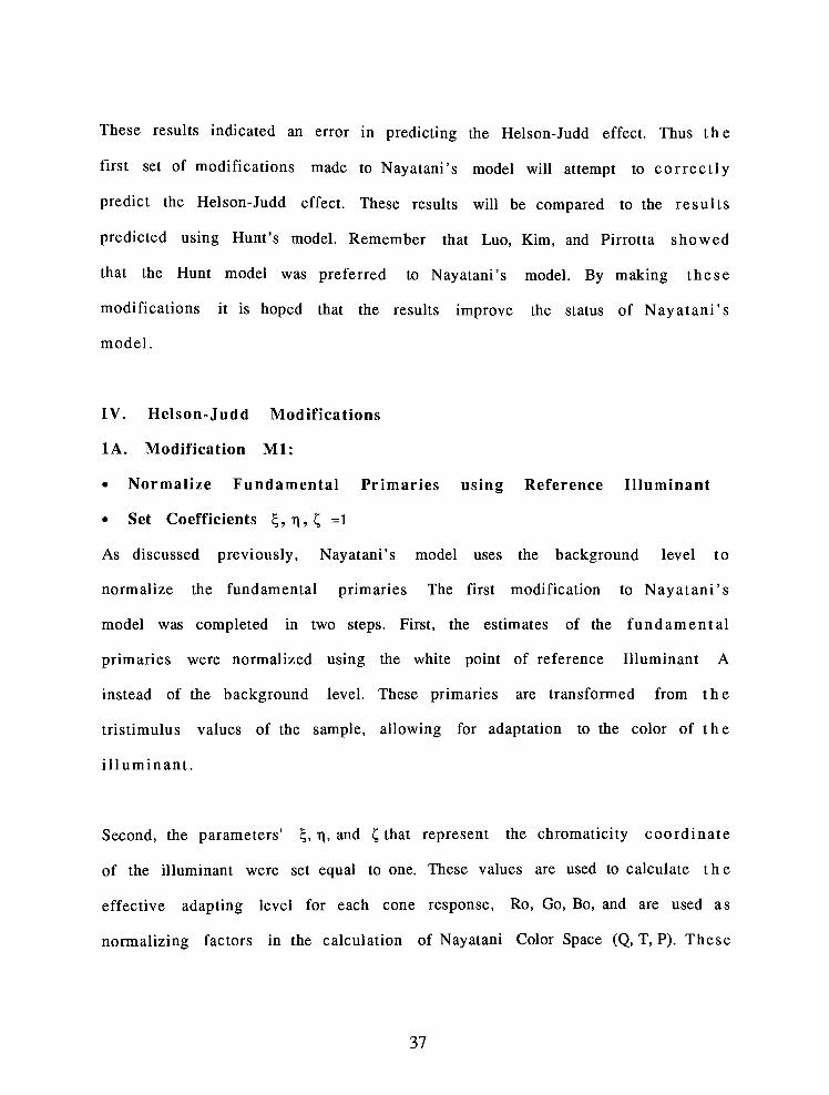
Figure 20 shows that Value 7/ corresponding colors on the yellow portion of
the CIE b*axis shifted green, while those on the blue axis shifted blue. The
results show the Helson-Judd effect has been corrected, where most colors
along the yellow portion of theb*
axis shifted yellow and those on the blue
portion of the axis shifted blue. In addition, there appears to be hue rotation
errors that would be detected by the standard observer.
39

Figure 21 shows the CIE C*vs.
L*results that correspond to Figures 18-20.
While the Value 3/ and Value 7/ results look random in nature, portions of the
Value 5/ results indicate an increased lightness for many of the
corresponding colors. Table II verifies the fact that the averageAL*
errors for
Value 5/ were greater than Value 3/ or Value II. This was the same result for
the standard Nayatani Model.
AL* Aa* Ab* AE*
Value 3/ Average 0.39 -0.2 0.44 5.08
Min -0.14 -0.04 0.02 0.87
Max 3.34 12.91 -7.21 15.04
Std Dev 1.64 4.68 3.8 3.56
Value 5/ Average 2.76 -1.08 -2.29 6.86
Min 0.7 0.26 -0.12 2.83
Max 7.45 13.77 -12.24 18.65
Std Dev 2.04 5.27 4.04 3.76
Value 11 Average 0.67 -0.64 -4.06 6.84
Min 0.2 0.06 -0.02 1.32
Max 5.34 10.31 -12.92 16.06
Std Dev 2.54 4.2 4.18 3.32
Total Average 1.3 -0.65 -2.05 6.3
Min -0.14 -0.04 0.02 0.87
Max 7.45 13.77 -12.92 18.65
Std Dev 2.35 4.7 4.37 3.6
Table II. CIE AL*, Aa*, Ab*, andAE* for the CSAJ data
using the Nayatani Ml Model
40

VERSUS BX
Figure 18. CIELAB a*vs.
b* for Munsell Value 3/ CorrespondingColors. Nayatani Ml Model vs. CSAJ D65 Reference Data.
41

Missing Page
o-
o.as
o.(O
CIELAB AX
'"^23
j?4
J4 S
VERSUS BX
13
22
Figure 20. CIELAB a*
vs.b* for Munsell Value 7/ Corresponding
Colors. Nayatani Ml Model vs. CSAJ D65 Reference Data.
43

o
o.cn
o.
o.to
CIELAB CX VERSUS Lx
_1
in-1
_
o.ro
o_
6?S*t >^Vi
**
,27
fr*
r-
10
\
20
- r-
30 40
- r-
50
- r~
60 70
- r-
80
CX
Figure 21. CIELAB C*vs.
L* for Munsell Value 3/, 5/, 7/ Corresponding
Colors. Nayatani Ml Model vs. CSAJ D65 Reference Data.
44

IV Helson-Judd Modifications
2A. Modification M2:
Normalize Fundamental Primaries using Reference Illuminant
Set Coefficients ,n,C =1 for Calculating Q, T, P
A second modification was made to Nayatani's model to attempt to correct for
the Helson-Judd effect. This was also accomplished in two steps. As noted
previously, thecoefficients'
%, n, and C, are used in calculating the effective
adapting level for each cone response, and as normalizing factors in the
calculation of Q, T, and P for Nayatani color space. If the perceived adapting
level changes are performed in the fundamental primary system then the
coefficients cj, r\, and C chromaticity coordinates of the illuminant, should be
used in calculating the effective adapting level for each cone response. Thus
the first step should be using thecoefficients'
%, r\, and L, to calculate the
effective adapting level for each cone response.
However, when calculating Q, T, and P for Nayatani color space, normalization
is already being performed with Illuminant A. Therefore, the second step
would be setting the coefficients %, n, and C equal to one for calculating Q, T,
and P (equations [14, 15, 16]). This was the second modification to Nayatani's
model, herein called Nayatani's M2 model.
2B. CIELAB Analysis of Nayatani M2 Model using CSAJ Data
The CSAJ data set was run through Nayatani's M2 model. The models predicted
results and the reference D65 CSAJ data were used to calculate CIELAB data and
45

plots. The CIELAB calculations for the CSAJ data set using Nayatani's M2 model
are listed in Appendix C3. Table III shows the CIELAB calculations for
Nayatani's M2 model, where the average AL*, Aa*, Ab*, and AE*ab were 1.3,
0.46, -2.5 and 5.8 respectively.
AL* Aa* Ab* AE*
Value 3/ Average 0.4 0.16 -5.45 6.46
Min -0.10 0.19 -3.36 3.77
Max 3.34 10.46 -8.69 13.88
Std Dev 1.64 3.5 1.4 2.16
Value 5/ Average 2.76 -1.17 -3.46 5.94
Min 0.71 0.09 0.02 2.07
Max 7.43 8.6 -8.82 12.64
Std Dev 2.03 3.52 1.98 2.38
Value 11 Average 0.66 -0.32 1.12 5.09
Min 0.18 -0.05 0.14 1.7
Max 5.34 6.65 9.48 11.5
Std Dev 2.54 2.65 4.22 2.53
Total Average 1.3 -0.46 -2.5 5.8
Min -0.1 -0.05 0.02 1.7
Max 7.43 10.46 9.48 13.88
Std Dev 2.35 3.25 3.94 2.4
Table III. CIE AL*, Aa*, Ab*, andAE* for the CSAJ
data using the Nayatani M2 Model
As in the previous modification, the averageAE*
and associated standard
deviations appear to be equal for each Value level. The averageAb*
error and
its associated standard deviation for the Value 3/ level decreased from -9.49 and
1.3 to -5.45 and 1.4 respectively, when compared to Nayatani's standard model.
46

However, when compared to Nayatani's Ml model, the averageAb*
error
increased by a factor of 12. The average Ab*error for Value 5/ corresponding
colors were larger (-3.46) than the standard Nayatani (0.2), or the Nayatani (
2.29) Ml model. For Value 7/ corresponding colors, the averageAb*
error was
1.12. This result is smaller than either the standard Nayatani (8.1), or Nayatani
(-4.06) Ml model.
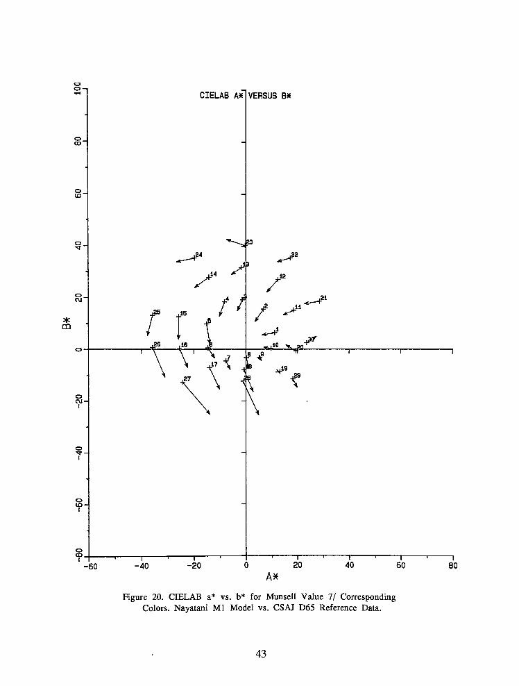
Figure's 22-24 represent CIE a*
vs.b*
plots that show the corresponding color
predictions, based on Nayatani's M2 model. Figure 22 shows that all Value 3 /
corresponding colors predicted by Nayatani's model shifted in the blue
direction. The colors having a larger blue component appear to have a larger
shift than those having a smaller component.
The Value 5/ corresponding colors in Figure 23 show a variation of Figure 19,
where most of the corresponding colors appear shifted in the blue direction.
For the Value 7/ corresponding colors in Figure 24, only 1/3 of the colors
appear to have a significant shift applied to them. Low chroma, magenta-red
colors were shifted yellow, while mid-chroma green-blue colors were shifted
blue. These results appear to incorrectly predict the Helson-Judd effect. Again,
there appears to be hue rotation errors that would be detected by the standard
observer.
Figure 25 shows the CEE C*vs.
L*results that correspond to Figures 22-24.
While the Value 3/ and Value 7/ results look random in nature, portions of the
47

Value 5/ results indicate an increased lightness for many of the
corresponding colors. Table III verifies the fact that the averageAL*
errors
for Value 5/ were greater than Value 3/ or Value II. Again, this was the same
result for the Nayatani's standard and Ml model.
48

VERSUS Bx
Figure 22. CIELAB a*
vs.b* for Munsell Value 3/ Corresponding
Colors. Nayatani M2 Model vs. CSAJ D65 Reference Data.
49

VERSUS BX
Figure 23. CIELAB a*vs.
b* for Munsell Value 5/ Corresponding
Colors. Nayatani M2 Model vs. CSAJ D65 Reference Data.
50

VERSUS BX
Figure 24. CIELAB a*
vs.b* for Munsell Value 7/ Corresponding
Colors. Nayatani M2 Model vs. CSAJ D65 Reference Data.
51

oo-
o
cn
CIELAB CX VERSUS Lx
S *% 21
''Sjae
o
CO
.19
_l
in-
o
WlV> I
^\^*^p.
124
o
O.
o_
- r
10
I-
20
- r-
30
- J
40
- r-
50 60
- r~
70
~r-
80
C*
Figure 25. CIELAB C*vs.
L* for Munsell Value 3/, 5/, 7/ CorrespondingColors. Nayatani M2 Model vs. CSAJ D65 Reference Data.
52

V. Comparison of Nayatani Model Results to Hunt Model Results
A. CIELAB Analysis of Hunt Model using CSAJ Data
The Hunt model results are being presented in order to compare them to the
results from Nayatani's models. The CSAJ data set was run through the '94 Hunt
model and results were computed by Hauf (31). The CIELAB calculations are
listed in Appendix D for the CSAJ data set using Hunt's model. Table IV shows
the CIELAB calculations Hunt's model, where the average AL*, Aa*, Ab*, and
AE*ab were 1.18, -0.57, -2.01 and 6.32 respectively. The averageAEab*
and
associated standard deviations appear to be equal for each Value level.
AL* Aa* Ab* AE*
Value 3/ Average 0.28 -0.06 0.52 5.26
Min -0.19 0.2 -0.01 1.4
Max 3.2 13.1 7.39 15.07
Std Dev 1.65 4.89 3.63 3.38
Value 5/ Average 2.63 -1.03 -2.28 6.83
Min 0.63 -0.63 -0.09 2.65
Max 7.27 13.87 -12.02 18.54
Std Dev 2.02 5.36 3.92 3.69
Value 11 Average 0.52 -0.57 -4.03 6.78
Min 0.04 0.06 0.01 1.19
Max -5.34 10.35 -12.84 16.02
Std Dev 2.54 4.2 4.14 3.33
Total Average 1.18 -0.57 -2.01 6.32
Min 0.04 0.06 0.01 1.19
Max 7.27 13.87 -12.84 18.54
Std Dev 2.35 4.8 4.29 3.51
Table IV. CIE AL*, Aa*, Ab*, andAE* for the CSAJ data using the Hunt Model
53

Table IV shows the averageAb*
errors are smaller for Value 3/, 0.52, than for
Value 5/, -2.28, or for Value II, -4.03. The errors in Lightness, AL*, also show a
trend where the errors are smaller for Value 3/, 0.28, and Value II, 0.52, than
for Value 5/, 2.63. The lightness errors for both Hunt and Nayatani, including
modifications, are of the same magnitude and direction.
Figure's 26-28 represent CIE a*
vs.b*
plots that show the corresponding color
predictions, for Hunt's model. Figure 26 shows that Value 3/ corresponding
colors predicted by Hunt's model shift in the yellow and blue direction. Colors
having a larger yellow component appear to have a larger yellow shift, while
the same trend holds true for blue colors. The Value 5/ corresponding colors of
Figure 27 show that the more saturated colors have the larger shifts.
Corresponding colors with a yellowb*
component appear to be shifted yellow-
green, and colors with a blue b*component appear to be shifted magenta-
blue.
In Figure 28, the Value 7/ corresponding colors have a larger shift than either
Value 3/ or Value 5/. While lighter colors along the yellow component of the
b*axis appear shifted yellow-green, darker colors are shifted blue. Practically
all of the samples along the blue component of theb*
axis are shifted blue. As
with the first modification to Nayatani's models, there is evidence of correctly
predicting the Helson-Judd effect.
54

Figure 29 shows the CDE C*vs.
L*results. While the Value 3/ and Value 7 /
results look random in nature, portions of the Value 5/ results indicate a n
increased lightness for many of the corresponding colors. This is verified b y
the data in Table IV.
55

VERSUS BX
Figure 26. CIELAB a*vs.
b* for Munsell Value 3/ CorrespondingColors. Hunt Model vs. CSAJ D65 Reference Data.
56

CIELAB Ax VERSUS BX
CD-
_to
-
-
Vf23
\. ^s.j.22
"
12 r >"
cu
^(
*
/'
CD
^ *%
^^-30
-.20
^10
*-.-
1
.26< V
.17
^
a*
'
IB *
\ . f8
\
i 1
oc\i-
1
\hF
\ ;Hi
o
i
o(O-
1
OGO
1
60
1
-40 -20 (
i |.
| .
) 20 40 60
1
80
A*
Figure 27. CIELAB a*vs.
b* for Munsell Value 5/ CorrespondingColors. Hunt Model vs. CSAJ D65 Reference Data.
57

VERSUS BX
Figure 28. CIELAB a*
vs.b* for Munsell Value 7/ Corresponding
Colors. Hunt Model vs. CSAJ D65 Reference Data.
58

oo-
o.CO
o
CO
o.
o.CO
_|
in"
o_
o.CM
o_
CIELAB CX VERSUS Lx
fH*'V^
"'^^B
[1
"^FEz^
J21
*?*,27
-2V2
- r-
10 20
- T-
30
- r-
40
T-
50 60
- r
70
T
80
CX
Figure 29. CIELAB C*vs.
L* for Munsell Value 3/, 5/, 7/ CorrespondingColors. Hunt Model vs. CSAJ D65 Reference Data.
59

B. Compare Nayatani Model Modifications to Hunt Model Results
: CIELAB Analysis of Nayatani & Hunt Models using CSAJ Data
The first comparison will be made using the CSAJ data set. The changes made to
Nayatani's model were designed to modify the functions for predicting the
adapted cone responses, primarily the Helson-Judd effect. These changes were
to be compared to the Hunt model, since the literature indicated Hunt's model
to be superior.
It was argued previously that the parameters cj, n and t, which represent the
chromaticity coordinates of the illuminant in the fundamental primary
system, were already imbedded in the CSAJ data set. These values are used i n
calculating the adapting level for each cone as well as normalizing factors i n
calculating Nayatani's or Q, T, and P color space. The first modification
normalized with illuminant A, and set theparameters'
cj, n> and C, equal to 1. By
plotting the results of Nayatani's vs. Hunt's predictions of corresponding
colors, we can determine if improvements were made to Nayatani's model.
Figures 30-32 represent CIE a*vs.
b*plots that show Nayatani's vs Hunt's
predictions. In each Figure, the + refers to Hunt's predicted corresponding
color and the tip of the vector represents the corresponding color predicted by
Nayatani's Ml model. Surprisingly, the data appears to be an exact match for
all three Value levels.
60

VERSUS BX
Figure 30. CIELAB a*vs.
b* for Munsell Value 3/ CorrespondingColors. Nayatani Ml vs. Hunt Model for CSAJ D65 Reference Data.
61

VERSUS BX
Figure 31. CIELABa*
vs.b* for Munsell Value 5/ Corresponding
Colors. Nayatani Ml vs. Hunt Model for CSAJ D65 Reference Data.
62

VERSUS BX
Figure 32. CIELAB a*
vs.b* for Munsell Value 7/ Corresponding
Colors. Nayatani Ml vs. Hunt Model for CSAJ D65 Reference Data.
63

oo-
cn
oCO
o
to
o.
o.
o.CM
CIELAB CX VERSUS Lx
"fm*
S* * "
38->*" >^+ '
,
*
<%,,
4^ yf5-*
1
10
1
20
I
30 40
I
50
CX
I
60
I
70
1
80
Figure 33. CIELAB C*vs.
L* for Munsell Value 3/, 5/, 7/ CorrespondingColors. Nayatani Ml vs. Hunt Model for CSAJ D65 Reference Data.
64

Figure 33 shows the CIE C*vs.
L*results that correspond to Figures 30-32. The
Value 3/, Value 5/, and Value 7/ results appear to match as well. If we page
back to Tables II and IV, we see that while that data are not the same they
appear to be statistically equal. This indicates, quantitatively and qualitatively,
that the Nayatani Ml and Hunt models are identical.
The second modification used thecoefficients'
cj, n> and C as m Nayatani's
standard model for calculating the effective adapting level for each cone.
However, the coefficients were set equal to 1 when used as normalizing factors
for calculating Nayatani color space.
Figure's 34-36 represent CIE a*
vs.b*
plots that show the corresponding color
predictions from the Hunt and Nayatani M2 models. Figure 37 shows the CLE C*
vs.L*
results that correspond to Figures 34-36. The Value 3/ corresponding
colors shift primarily blue, while Value 7/ corresponding colors shift
primarily yellow. The Value 5/ high chroma colors appear to have shifted the
most. The yellow colors show a large shift towards blue while blue colors
exhibit a small shift towards yellow. The data in Tables III and IV point out that
Nayatani has greaterAb*
errors at Value 3/ while Hunt has greaterAb*
errors
at Value II. Both the data and the plots indicate a good match at Value 5/ only.
Thus the second modification proved to be inadequate.
65
VERSUS BX
Figure 34. CIELAB a*
vs.b* for Munsell Value 3/ Corresponding
Colors. Nayatani M2 vs. Hunt Model for CSAJ D65 Reference Data.
66

VERSUS BX
Figure 35. CIELAB a*
vs.b* for Munsell Value 5/ Corresponding
Colors. Nayatani M2 vs. Hunt Model for CSAJ D65 Reference Data.
67

CIELAB AX
o.CO
CO
o_
o.CM
OQ
23
H*
Is l t
**
VERSUS BX
H
Figure 36. CIELAB a*
vs.b* for Munsell Value 7/ Corresponding
Colors. Nayatani M2 vs. Hunt Model for CSAJ D65 Reference Data.
68

o
o,o>
o.CO
o.
o.CO'
5tC o
_1
in"
O
T
o
CD
oCM^
CIELAB CX VERSUS Lx
$^S^uL^m**-
& 23
j.23
+
j28 9R J?
j?l
^Mi^irf^
-
1 1 1 I 1 1r-
10 20 30 40 50 60 70
CX
Figure 37. CIELAB C*vs.
L* for Munsell Value 3/, 5/, 7/ CorrespondingColors. Nayatani M2 vs. Hunt Model for CSAJ D65 Reference Data.
69

VI. Verification of Changes using Independent Data Set
A. Characteristics of Breneman Data Set
An independent data set was used to assess the Nayatani model modifications
and compare them to the Hunt model results. The independent data set used was
experiment #4 from Breneman (26). The Illuminants were A and D65, the
luminance of the white was 75 cd/mA2, the normalizing illuminance used was
1000 lux, and the average surround was Yo=30%.
Although the data were given inu'v'
coordinates, the samples were converted
to xy coordinates using the relationships provided by Hunt (29). The
luminance, or Y tristimulus components for the samples were reported in the
body of Breneman's paper. The luminances for samples red, brown, foliage,
green, blue, and purple corresponded to Y= 9, and samples grey, skin, orange,
yellow, blue-green, and sky corresponded to Y=27. The converted(u'v'
to XYZ
tristimulus) data are shown in Appendix E.
The test Illuminant used was A and the reference Illuminant was D65. The
white point for Illuminant D65, based on theu'v'
coordinates in Breneman's
report, was 95.86, 100.0, 110.41. The white point for Illuminant A was 110.99,
100.0, 36.59. The normalizing coefficients were calculated as follows
70

R = (0.40024* X + 0.7076*Y 0.0808 1*Z)* (0.8911) [20]
G = (-0.22630*X + 1. 16532*Y + 0.04570*Z) * (1. 0742) [21]
B = (0.91822*Z)* (2.9762) [22]
B. CIELAB Analysis of Nayatani Std. Model using Breneman Data
The Breneman data were run through Nayatani's standard model and CIELAB
calculations and plots were generated. The CIELAB calculations for the
Breneman data set using Nayatani's standard model are listed in Appendix Fl.
Table V shows the CIELAB calculations for Nayatani's standard model, where
the average AL*, Aa*, Ab*, and AE*ab were 0.06, -0.17, -5.16, and 5.20
respectively.
Breneman Exp. 4:
Illuminant A XYZ
Reference Data
1Color Appearance Models:
Conversion toXYZ'
to predict
Corresponding Colors (D65)
Breneman Exp. 4:
Illuminant D65 XYZ
Reference Data
CIELAB Analysis: Illuminant D65
Model predictions vs
Breneman XYZ Reference Data
Diagram 2. Flowchart for Analyzing Breneman Model Data
71

Total
AL* Aa* Ab* AE*
Average 0.06 -0.17 -5.16 5.20
Min 0.04 -0.13 -.502 0.52
Max 0.08 -1.24 -15.35 15.35
Std Dev 0.01 0.62 5.42 5.42
Table V. CIE AL*, Aa*, Ab*, andAE* for Breneman Exp. 4 data using
the Nayatani Standard Model
Diagram 2 shows the approach used to analyze the corresponding color
predictions for each model using the Breneman data set. Figure 38 represents
CIE a*vs.
b*plots for corresponding colors using Nayatani's standard model
vs. Breneman's D65 reference data.Colors'
1-6 corresponds toL* 30 and colors
7-12 corresponds toL* 60. The results are similar to Figures 14 and 15. All of
the colors atL* 30 have shifted blue, while those at
L* 60 have not moved. The
standard Nayatani model seems reasonably adequate for predicting
corresponding colors for Breneman's data set. However, for the Helson-Judd
effect, the lighter colors should appear in the hue of the illuminant and
darker colors should appear in the complimentary hue. Since the lighter
colors appear shifted towards the complimentary hue, Nayatani's standard
model incorrectly predicts the Helson-Judd effect.
72

CIELAB AX
o
CO
o.CO
o
O
CM
CQAl
VERSUS BX
.10 4?
ir t
oCM-
I
O
i
oco-
CO.i
20 40
r
60 80-60
AX
Figure 38. CIELAB a*
vs.b* Nayatani Standard Model
vs. Breneman Reference Data.
73

C. CIELAB Analysis of Nayatani M2 Model using Breneman Data
Next, the Breneman data were run through Nayatani's M2 model and CIELAB
calculations and plots were generated. The CIELAB calculations for the
Breneman data set using Nayatani's M2 model are listed in Appendix F2. Table
VI shows the CIELAB calculations Nayatani's M2 model, where the average AL*,
Aa*, Ab*, and AE*ab were 0.00, 2.11, -15.40, and 17.19 respectively.
The results show an approximate 3x increase in Ab*, and AE*ab error when
compared to Nayatani's standard model results. The Ab*error suggests the
Helson-Judd effect. However, Figure 39 shows that all corresponding colors
have shifted blue regardless of their lightness level. Thus, this modification is
not only a poor predictor for corresponding colors, the Helson-Judd effect has
been incorrectly predicted as well.
Total
AL* Aa* Ab* AE*
Average 0 2.11 -15.4 17.19
Min 0.01 1.06 -11.13 11.51
Max -0.37 22.8 -24.95 33.8
Std Dev 0.19 9.07 4.92 6.91
Table VI. CIE AL*, Aa*, Ab*, andAE* for Breneman
Exp. 4 data using the Nayatani M2 Model
74

o_CD^
CO^
O
CIELAB AX VERSUS BX
r /
Figure 39. CIELAB a*
vs.b* Nayatani M2 Model
vs. Breneman Reference Data.
75

D. CIELAB Analysis of Hunt Model using Breneman Data Set
The Breneman data was also run through the Hunt model and CIELAB
calculations and plots were generated. The CIELAB calculations for the
Breneman data set using the Hunt model are listed in Appendix F3. Table VII
shows the CIELAB calculations for the Hunt model, where the average AL*,
Aa*, Ab*, and AE*ab were -0.19, 4.21, -8.50, and 17.15 respectively. Again, the
Ab*, and AE*ab errors are large.
Total
AL* Aa* Ab* AE*
Average -0.19 4.21 -8.5 17.15
Min 0.03 -0.12 3.24 3.27
Max -4.33 28.78 -27.64 39.46
Std Dev 0.14 11.69 14.6 11.28
Table VII. CIE AL*, Aa*, Ab*, andAE* for Breneman Exp. 4 data using the Hunt Model
The Ab*error suggests the Helson-Judd effect, and Figure 40 shows a good
approximation to this effect. The plot shows that lighter colors along the b *
axis shifted yellow and darker colors shifted blue. However, the magnitude of
the vectors suggests large errors in predicting corresponding colors.
76

VERSUS BX
Figure 40. CIELAB a*
vs.b* Hunt Model
vs. Breneman Reference Data.
77

VII. Comparison of Nayatani and Hunt Models using Breneman Data
Before comparing the Hunt and Nayatani results, a major difference between
the CSAJ and Breneman data sets should be noted. The CSAJ data is a series of
Munsell patches that were designed for Illuminants A and D65 at 1000 cd/mA2.
Breneman carried out two different series of experiments. The first was
comprised of nine chromatic adaptation experiments using mixed Illuminants
at the same illuminance level. In the second, three experiments were
performed where the Illuminants were chromatically equal but the
illuminance level was increased by factors ranging from 13 to 18.
The results of these experiments showed that the adaptation of the observers
was incomplete, and that the extent of the adaptation is dependent on the level
of illumination. Breneman further reported that the proportionate extent of
adaptation was less at lower levels of illumination, and the adaptation for the
blue receptor mechanism was less than that for red or green.
The comparison of Nayatani and Hunt models using the Breneman data set
show that neither Nayatani's standard nor M2 models are good predictors for
Helson-Judd, while Hunt's model predicts this effect quite well. Yet only
Nayatani's standard model appears to be a good predictor for corresponding
colors. This indicates either an error in the models or in the data. As stated
previously, Breneman noted that incomplete adaptation occurred at low levels
of luminance. The luminance of the white for Breneman's experiment #4 was
75 cd/mA2, which was considered a low level of illuminance for his
78
experiments. Thus when predicting corresponding colors, depending on
extent of chromatic adaptation in the color appearance model, incomplete
adaptation should result from use of this data set.
Before analyzing Nayatani vs. Hunt for the Breneman data, a quick review of
each models results are in order. Figure 38 showed that Nayatani's model was a
good predictor for corresponding colors at L*60 but a poor predictor at L*30.
In addition, the Nayatani model incorrectly predicted the Helson-Judd effect.
In Figure 40, Hunt correctly predicted the direction for the Helson-Judd effect,
but the magnitude of the vector indicates a relatively large error when
predicting corresponding colors.
Figure 41 is a plot of Nayatani's standard model vs. Hunt that represents the
vector difference between Figures 38 and 40. The Hunt model predictions are
represented by the + sign and Nayatani's predictions are represented by the
tip of the vector. Nayatani's predictions are attributable to incomplete
adaptations at low illuminance levels and incorrectly predicting the Helson-
Judd effect. Hunt's model shows more complete adaptation at low luminance
levels and correctly predicts the Helson-Judd effect.
79

VERSUS BX
Figure 41. CIELAB a*
vs.b* Nayatani Standard vs.
Hunt Model for Breneman Reference Data.
80

Figure 42 is a plot of Nayatani's M2 model vs. Hunt which represents the vector
difference between Figures 39 and 40. The lighter colors show a significant
shift towards blue, while the darker colors show good correlation to Hunt's
model. These results are similar to those found in Figure's 34-35 using the CSAJ
data set. Again, incomplete adaptation plays a major role in the poor
performance of Nayatani's M2 model. Hunt's model predicted the Helson-Judd
effect fairly well on its own, yet when compared to Nayatani's M2 model the
errors are quite large. Thus, Nayatani's M2 model is a poor predictor for the
Helson-Judd effect as well.
81

VERSUS BX
Figure 42. CIELAB a*vs.
b* Nayatani M2 vs.
Hunt Model for Breneman Reference Data.
82

VIII. Nayatani Standard Model:
A. Relevance of Significant Figures for Nonlinear Exponents
The exponents in Nayatani's model were varied to determine the relevance of
values expressed to 4 significant figures. Nayatani uses nonlinear p functions,
pi (Ro), pi (Go), and pi (Bo) to represent the nonlinear characteristics between
the effective adapting luminance (Ro, Go, Bo) and the output response for each
cone. The exponents in these equations [11, 12, 13], are stated to have 4
significant figures. However, no published evidence exists to signify the
exactness of these figures.
Thus an additional test was undertaken to examine variations in these
exponents. The exponents for the red and green channel are reported as
0.4495, while the blue channel is reported at 0.5128. These exponents were
rounded down to 0.4, and 0.5 respectively. Three variations of the standard
Nayatani model were run where the exponents were given the trials listed
below
1
2
3
t-g b
0.4 0.5128
0.4495 0.5
0.4 0.5
83

B. CIELAB Analysis using CSAJ Data
The CIELAB calculations for the CSAJ data set using trial 1 for Nayatani's model
are listed in Appendix Gl. Table VIII shows the CIELAB calculations for the
Standard Nayatani model, where the average AL*, Aa*, Ab*, and AE*ab were
1.89, 0.31, 0.31, and 8.06 respectively. The Aa*, Ab*, and AE*ab errors are of the
same order of magnitude as the standard Nayatani model where the r, g
exponents are =0.4495. However, the Value 3/ and Value IIAL*
errors are a
factor of 10 larger when the exponent is set equal to 0.4.
AL* Aa* Ab* AE*
Value 3/ Average -4.33 1.52 -8.43 9.86
Min 0.05 0.31 -6.12 7.51
Max -1.27 3.05 -11.83 12.1
Std Dev 1.87 0.7 1.69 1.25
Value 5/ Average 2.72 -0.39 0.27 3.36
Min 0.74 0.01 0.02 0.69
Max 6.68 2.15 3.57 7.46
Std Dev 1.8 1.47 1.55 1.99
Value 11 Average 6.67 -0.08 8.22 11.25
Min 0.17 0.04 4.19 5.18
Max 12.75 -23.52 36.01 43.67
Std Dev 3.06 4.49 5.62 6.99
Total Average 1.89 0.31 0.31 8.06
Min 0.05 0.01 0.02 0.69
Max 12.75 -23.52 36.01 43.67
Std Dev 5.07 2.89 7.62 5.5
Table VIII. CIE AL*, Aa*, Ab*, andAE* for CSAJ data using the Standard
Nayatani Model where r,g exponents = 0.4, b exponent = 0.5128
84

The second and third trial results were very similar to the first. The CIELAB
calculations for the CSAJ data set using the second and third trials for
Nayatani's model are listed in Appendices G2 and G3 respectively. Data i n
Appendix G show the CIELAB calculations for the Standard Nayatani model. The
average AL*, Aa*, Ab*, and AE*ab were 1.84, 0.43, -0.13, and 7.0 respectively for
trial two, and 1.90, 0.57, -0.02, and 7.62 respectively for trial three.
While the data show the AE*error for trials 2 and 3 were similar for Nayatani's
model, an additionalAL*
error was again introduced for the Value 3/ and Value
7/ corresponding colors. However, the corresponding colors for Value 5/ i n
Table IX are essentially the same for each trial.
AL* Aa* Ab* AE*
r,g=
.4 Average 2.72 -0.39 0.27 3.36
b =.5128 Min 0.74 0.01 0.02 0.69
Max 6.69 2.15 3.57 7.46
Std Dev 1.8 1.47 1.55 1.99
r,g=
.4495 Average 2.72 -0.45 0.28 3.34
b=.5 Min 0.74 0.01 0.02 0.7
Max 6.74 1.99 3.6 7.49
Std Dev 1.8 1.49 1.47 2.01
r,g=
.4 Average 2.72 -0.4 0.28 3.36
b =.5 Min 0.74 0.01 0.02 0.69
Max 6.68 2.15 3.57 7.46
Std Dev 1.8 1.47 1.54 2
Table IX. CIE AL*, Aa*, Ab*, andAE* for CSAJ data for Value 5/ corresponding
colors using the Standard Nayatani Model
85

Thus the rounding of exponents for Value 5/ corresponding colors appear
justified while simultaneously introducing errors for Value 3/ and Value 7/
corresponding colors.
Since these results indicate that rounding the exponents to the tenth's place
produces additional error, it was decided to further investigate whether
rounding to the hundredths place provides any additional insight. The
exponents were rounded to 0.45, and 0.51 respectively. Three variations of the
Standard Nayatani model were run with the exponents listed below
1
2
3
I-g b
0.4495 0.51
0.45 0.5128
0.45 0.51
The CffiLAB calculations for the CSAJ data set for each trial using Nayatani's
standard model are listed in Appendix G4-G6. The data shows that there is n o
statistical difference between the trial data. Table X shows an example of the
CIELAB calculations for the Standard Nayatani model, where the average AL*,
Aa*, Ab*,and AE*ab were 1.30, 0.70, -0.08, and 7.19 respectively.
86

AL* Aa* Ab* AE*
Value 3/ Average 0.41 1.91 -9.50 9.88
Min 0.05 0.30 -6.12 6.79
Max 3.31 4.60 -11.83 12.32
Std Dev 1.67 0.86 1.30 1.26
Value 5/ Average 2.76 -0.40 0.20 3.42
Min 0.74 0.01 0.02 0.77
Max 7.32 -4.98 3.65 7.98
Std Dev 1.97 1.45 1.62 2.14
Value 11 Average 0.66 0.70 8.11 8.54
Min 0.07 0.01 5.13 5.37
Max 5.51 2.68 11.25 12.75
Std Dev 2.60 0.81 1.63 1.86
Total Average 1.30 0.70 -0.08 7.19
Min 0.05 0.01 0.02 0.77
Max 7.32 -4.98 -11.83 12.75
Std Dev 2.36 1.43 7.32 3.33
Table X. CIE AL*, Aa*, Ab*, andAE* for CSAJ data using the Standard Nayatani Model
where r,g exponents = 0.4495, b exponent = 0.51
The data from Appendix G4-G6 and Appendix CI (data generated using
Nayatani's original exponents) were reviewed. The data appears to be one and
the same. Thus there appears to be no justification for expressing the
nonlinear exponents to four decimal places, since twodecimals'
places
produces the same data.
87

IX. Nayatani Standard Model:
A. Nonlinearity at Low Luminance Levels
The adapting luminance levels were varied in order to determine the presence
of nonlinearity at low luminance levels. Recall Pirrotta (14) reported a
luminance compression in Nayatani's model, based on chromatic adaptation
from D65-to-A. Her results showed that Nayatani's model performed poorly at
the low and high luminance level. Thus an additional test was conducted using
the CSAJ data to determine the significance of lightness errors. The adapting
luminance for illuminant A was varied from 25 cd/mA2 to 10,000 cd/mA2. The
data files are listed in Appendix H1-H9.
B. CIELAB Analysis using CSAJ Data
The AL*and AE*ab results for Value 3/ and Value 5/ are shown in Table XI and
Table XII respectively. Table XI shows AL* has a negative slope moving from
9.55 at 25 cd/mA2 through a minimum to -3.93 at 10,000 cd/mA2.
cd/mA2AL* AE*
Value 3/ 25 9.55 13.44
50 8.01 12.71
100 6.3 11.99
300 3.44 10.91
500 2.11 10.44
1000 0.41 9.87
3000 -1.95 9.25
5000 -2.87 9.11
10000 -3.93 9.05
Table XL CIE AL*, andAE* for CSAJ data for Value 3/ using varying
adaptation luminance for Illuminant A for the Standard Nayatani Model
88

Table XI shows AL* has a positive slope moving from of -9.1 at 25 cd/mA2
through a minimum to 6.15 at 10,000 cd/mA2.
cd/mA2 AL* AE*
11 25 -9.1 10.77
50 -7.6 10.05
100 -5.89 9.45
300 -2.83 8.84
500 -1.34 8.68
1000 0.66 8.54
3000 3.57 8.61
5000 4.75 8.76
10000 6.15 9.08
Table XII. CIE AL*, andAE* for CSAJ data for Value 7/ using varying
adaptation luminance for Illuminant A for the Standard Nayatani Model
These nonlinearities for Value 3/ and Value II corresponding colors are more
clearly shown in Figure 43. The Value 5/ colors show linearity throughout the
luminance range, and a minimum is detected at 1000 cd/mA2 for all Value
levels.
89

o~
rs
o
r~r""J
1
o>k Delta I* Value :J/
Potto If v<jLiue*
ylO-
_______
Delta l Value'
V
o
*1
c
I'I
1
q
/
vo-
1
q
1
o
l i1.0 1
I.5 2.0 23 s. .0 3 .5 4 .0 4-.5 5.0 5.5
iog luminance (cd/m?2) Illuminant A
Figure 43. Log Luminance vs.AL* for
CSAJ Data at Munsell Value 3/, 5/, 7/.
90

Figure 44 shows the AE*ab changes as the luminance level increases from 25
to 10,000 cd/mA2. The AE*ab errors for Value 5/ remain linear over the entire
luminance range. However, the Value 3/ errors continually drift lower while
the Value 7/ results pass through a minimum only to increase after 1000
cd/mA2. Both Figures indicate that the greatest percentage of error lies in the
low luminance range, from 25 to 1000 cd/mA2.
91

O"
Jg
o
t -
V
o
i
Delta E* Value 3/
(N D.eJtoSXj^SliiiA.p^
Delta Ex Value W
o
d-
Lu
D ni
+5 00
0
oVO~
o<+"
ors-
o
o_
1.0 1.5 2.0 2 .5 2 .0 : .5 4.0 4 .5 5.0 5.5
log luminance (cd/m?2) Illuminant A
Figure 44. Log Luminance vs. AE*ab for
CSAJ Data at Munsell Value 3/, 5/, 7/.
92

X. Summary of Results
The search of the literature showed several references to Hunt's color
appearance model being preferred to Nayatani's. The intent of this thesis was
to determine the degree and nature of the model differences, and attempt to
improve Nayatani's model if possible. The CSAJ data were used to form a
baseline for making such improvements. These data are composed of two sets
of CIE XYZ tristimulus values for predicting corresponding colors under
illuminants A and D65. In testing Nayatani's model using the CSAJ data, the
results showed larger AE*ab errors at Munsell Value 3/ and 7/ than at Value
5/. The AE*ab errors were 9.87 and 8.54 for Value 3/ and Value II, while only
3.42 for Value 5/.Figures'
1-3 also showed that all of the predicted
corresponding colors for Value 3/ shifted blue, while all of the colors for
Value 7/ shifted yellow. This incorrectly predicts the Helson-Judd effect,
where, under colored illumination, light colors appear tinted in the hue of the
illuminant and dark colors appear tinted in the complimentary hue. Thus the
first attempt to modify Nayatani's model was to improve the predictions for the
Helson-Judd effect.
A. Helson-Judd
In Nayatani's model, thecoefficients'
%, t\, and represent the chromaticity
coordinates of the illuminant in the fundamental primary system. They are
used in calculating the effective adapting level for each cone and as
normalizing factors in the calculation of Nayatani color space. Nayatani's Ml
model set thecoefficients'
\, i\, and C, equal to 1, and Illuminant A was used to
93

normalize the estimates of the fundamental primaries. The results showed that
the average AE*ab error was essentially equal for each Munsell Value level,
and the overall AE*ab error was reduced from 7.19 to 6.3. Yet theAb*
error was
larger for Value 7/ colors than for any other level.Figures'
18-20 showed that
light color shifted yellow and dark colors shifted blue for all three Value
levels. This correctly predicts the Helson-Judd effect.
Nayatani's M2 model used thecoefficients'
%, T|, and to calculate the effective
adapting level for each cone, but they were not used as normalizing factors for
Nayatani color space. Illuminant A was used to normalize the estimates of the
fundamental primaries. The results showed that the average AE*ab errors
were essentially equal for each Munsell Value level, and the overall AE*ab
error was reduced again from 6.3 to 5.8. The Ab*error was now larger for
Value 3/ colors than for any other level. However, Figures 22-24 showed that
all Value 3/ colors shifted blue, the Value 5/ colors shifted predominately blue,
while only a handful of Value 7/ colors shifted albeit incorrectly. This
modification incorrectly predicts the Helson-Judd effect, even though the
overall AE*ab error was reduced.
The Hunt model was also used to determine corresponding colors using the
CSAJ data set. The results showed that the AE*ab errors were relatively equal
for each Munsell Value level, while the overall AE*ab error was 6.32. The Ab *
error was higher for Value 7/ than for any other level. Figures 26-28 showed
94
that light colors shifted yellow and dark colors shifted blue for all three Value
levels. This model correctly predicts the Helson-Judd effect.
Comparisons of Nayatani's modifications to Hunt's results were extremely
different in nature. The first modification, labeled the Nayatani Ml model,
appears to be a match with the Hunt model. The CIELAB errors are almost
identical, and Figure's 30-32 supported these results. This indicates a
quantitative match to Hunt's model, which based on the reports from
literature, would improve Nayatani's model. The second modification, labeled
the Nayatani M2 model, does not match the Hunt model. Figure's 34-36 showed
that Value 3/ colors shifted blue while Value 7/ colors shifted yellow. Thus the
second modification proved to be inferior.
B. Independent Data
An independent set was used to test the findings from using the CSAJ data base.
The data that were used were taken from Breneman's series of experiments on
corresponding colors for different states of adaptation. This data set was
unique in that Breneman showed that adaptation to chromatically different
illuminants was incomplete, and that the extent of the adaptation was
dependent on the level of illuminance. The proportionate extent of adaptation
was less at lower levels of illuminance, and the adaptation for the blue
receptor mechanism was less than that for red or green.
95

Both Nayatani's standard and M2 models along with the Hunt model were used
to test the Breneman data. Nayatani's standard model showed to be fairly
reasonable at predicting corresponding colors, but was unable to correctly
predict the Helson-Judd effect. The Nayatani M2 model showed that the AE*ab
errors increased by a factor of 3, and that all of the colors shifted blue. Thus
this model was a poor predictor for both corresponding colors and the Helson-
Judd effect.
The Hunt model results were similar to Nayatani's M2 model, where the AE*ab
errors increased by a factor of 3, which showed poor predictability of
corresponding colors. However, Hunt showed good correlation at predicting
the Helson-Judd effect. Comparison of the Hunt model to Nayatani's models
produced different effects yet again. Figure 41 shows the comparison of
Nayatani's standard model to Hunt. Nayatani's standard model was a good
predictor for corresponding colors because of the good correlation between
the model and incomplete chromatic adaptation at low luminance levels.
However, Nayatani incorrectly predicted the Helson-Judd effect. The larger
vector errors mimic Hunt's poor prediction for corresponding colors, while
the Helson-Judd effect correctly predicted by Hunt shifted blue. Figure 42
shows the comparison of Nayatani's M2 model to Hunt. These results
correspond to Figures 34 and 35, which compared these models using the CSAJ
data base. The major source of error for Nayatani's model was incorrectly
predicting the Helson-Judd effect, which was more predominant for lighter
colors.
96

The common thread among these comparisons was that Hunt's results were
similar to Nayatani's Ml and M2 models and different from Nayatani's standard
model. The CSAJ data set showed that increased modification led to decreased
errors. Breneman's data set indicated that Nayatani's standard model showed
incomplete chromatic adaptation at low levels of illuminance, and incorrectly
predicted the Helson-Judd effect. While Hunt's model produced relatively large
errors, it also showed more complete adaptation and correctly predicted the
Helson-Judd effect.
C. Nonlinear Exponents
The exponents of Nayatani's nonlinear p functions were rounded down to test
the relevance of data extended to four significant figures. Three trials were
conducted using the CSAJ data set, varying the r,g, and b exponents. The
results showed that no additional error was introduced for Munsell Value 5 /
colors. The errors were essentially equal regardless of the exponent variation
used. However, an increase in theAL*
error for Munsell Value 3/ and 7/ were
found. The results show that rounding to the tenth's place creates additional
error at certain levels, and it was decided to round the exponents to the nearest
hundredth place. The results for the three trials showed that the data was
essentially the same as the data using Nayatani's original exponents. Thus
there was no justification for using exponents specific to four decimal places.
97
D. Luminance Adaptation
Reports from the literature showed that Nayatani's model performed poorly at
low and high luminance levels. The adapting luminance for Illuminant A was
varied from 25 to 10000 cd/mA2 to determine if a relationship exists between
lightness errors and luminance. Figure 43 shows that as luminance increases,
AL* decreases from 9.55 to -3.93 for Value 3/. The opposite is true for Value II,
whereAL* increases from AL*
-9.1 to 6.15. The AL* for Value 5/ remains
constant over the luminance range. The minimum error for all Value levels
appears to correspond to 1000 cd/mA2. Additionally, Figure 44 shows a plot of
AE*ab as the luminance level increases. The errors for Value 5/ remain linear,
while Value 3/ and Value Tl errors decrease nonlinearly. This supports the
reports found in the literature, where the largest source of error appears to be
in the low luminance area, ranging from 25 to 1000 cd/mA2.
XI. Conclusions and Recommendations
This thesis was undertaken to determine what parameters could be changed i n
Nayatani's model to improve it's performance. The criteria used to judge
changes to Nayatani's model were the CSAJ data set and their performance in
relation to Hunt's model. Thecoefficients'
!_,, r\, and in Nayatani's Ml model
were set equal to 1, and Illuminant A was used to normalize the estimates of the
fundamental primaries. Results showed That Nayatani's Ml model performs
exactly as Hunt's. Considering the review of the literature, this appears to be a
significant improvement to Nayatani's model. The second modification
introduced additional errors and was not viewed as a positive improvement.
98

Expressing the exponents for the effective adapting luminance to four decimal
places proved to be unwarranted. Expressing the exponents to two decimal
places produced the same results. Nonlinearity was a factor for AL*and AE*ab
errors at low luminance.
Though improvements were made to Nayatani's model, the errors using the
CSAJ data set are still large. Breneman noted that, except for low illuminance
levels, a linear von Kries transformation characterized the relationships
between the corresponding chromaticities and the degree of adaptation.
Further work should be conducted using power, physiological and log
functions to model the nonlinear characteristics between the effective
adapting illuminance and the output of each cone at low, medium, and high
illuminance levels.
However, the numerical improvement shown can only be substantiated by
performing psychophysical experiments. It is recommended here that tests be
conducted using Hunt's, Nayatani's standard model, and Ml model. These tests
should include a uniform sampling of color and lightness space as well as an
appropriate range of luminance. It would be interesting to determine whether
Nayatani's nonlinearity has improved using the new modification.
99

/* APPENDIX A: C Code for Nayatani Standard model
/*
/* Nayatani Model to XYZ & CIELAB 4/11/96/* */
/* */
#include <stdio.h>
#include <stdlib.h>
#include <string.h>
#include <math.h>
#define PI 3.14159265
#define OK 1
#defme NOT_OK 0
#define SEPCHARS"\t"
#define BUFF_SIZE 256
#defme NUM_TOKENS 7
#define SAMPLE 0
#define XYZ1JJ 1
#define XYZ1_1 2
#define XYZ1_2 3
#define XYZ2_0 4
#define XYZ2_1 5
#define XYZ2_2 6
int isanum(char *string);
void XYZToLAB (double *XYZ2, double *lab, double *refWhite);
int calcColorAppO;
double XYZ1[3];
double XYZ2[3];
double lab[3];
double refWhite[3]={95.05, 100.00, 108.91};
char sample[BUFF_SIZE];
FILE *outputFile;
main(int argc,char*
argv[])
{FILE *inputFile;
char line[BUFF_SIZE];
int status;
int i;
100

int debug_f = 0;int num_lines = 0;char *token [NUMJTOKENS];char *check_tabs;
/*-
Should we do'?'
help?
-*/
if ((argc < 2) II (*argv [1] == '?')){
printf("
This program processes color space information\n");printf("Use a
'&'
in the first column to stop processingW);
printf("The data MUST be of the form:\n");printf("
xx yy t ff t ff t ff t ff t ff t ff\n");printf("
Where: xx and yy fields are seperated by spaces and Y\n");printf("
is a TAB character\n\n");
printf("\n Syntax is: testMod in_file out_file <-d>\n");
printf("\n");printf("
Where: -d-
Debug flagW);
exit(99);
}
/*
Open the input and output files
*/
if (KoutputFile = fopen(argv [2], "w+")))
{printf("Could not open output file %s\n", argv [2]);
exit(-l);
}
if (!(inputFile = fopen(argv [1], "r")))
{printf("Could not open input file %s\n", argv [1]);
exit(-l);
}
Check the option flags
*/
for (i = 0; i < argc; i++)
{if (strcmp(argv [i], "-d") = 0) debug_f = 1;
}/** End for **/
/*-
Process until end of file. Other tests are done internally to
101

stop processing too
*/
for(;!feof(inputFile);){
fgets(line, BUFF_SIZE, inputFile);num_lines++;
/*-
Remove the extra carriage control character
*/if (strlen(line)) line [strlen(line)-l] = 0;
if (debug_f)
{printf("Input line %d: %s\n", numjines, line);
}
/*
Make sure that there is enough to tokenize, there needs to be
exactly 6 tab characters
*/
check_tabs = line;for (i = 0; i < 8; i++)
{if ((check_tabs = strchr(check_tabs, \t')) == NULL) break;
check_tabs++;
}
/*
Check to see if we should stop processing.
- */
if ((line[0] == '&') I (i != 6))
{break;
}
token [SAMPLE] = strtok(line, SEPCHARS);
token [XYZ1_0] = strtok(\0', SEPCHARS);
token [XYZ1_1] = strtok(\0', SEPCHARS);
token [XYZ1_2] = strtok(\0', SEPCHARS);
token [XYZ2_0] = strtok(\0', SEPCHARS);
token [XYZ2_1] = strtok(\0', SEPCHARS);
token [XYZ2_2] = strtok(\0', SEPCHARS);
if (debug_f)
{printf("Parsed line :
'%s' '%s' '%s' '%s' '%s' '%s'
'%s\n",
token [SAMPLE], token [XYZ1_0], token [XYZ1_1], token [XYZ1_2],
102
token [XYZ2_0], token [XYZ2_1], token [XYZ2_2]);
}
/*
Make sure all the data is a valid type
for (i = 1; i< NUM_TOKENS; i++)
{if (!isanum(token [i]))
{printf("Error on line %d, %s is not a valid numberAn",
numjines, token [i]);
exit(-l);
1
}
/*
Convert the tokens
strcpy(sample, token [SAMPLE]);
XYZ1[0] = atof(token [XYZ1_0]);
XYZ1[1] = atof(token [XYZ1_1]);
XYZ1[2] = atof(token [XYZ1_2]);
XYZ2[0] = atof(token [XYZ2_0]);
XYZ2[1] = atof(token [XYZ2_1]);
XYZ2[2] = atof(token [XYZ2_2]);
if (debug_f)
{printf("Data : [%s] %f %f %f %f %f %f\n\n", sample,
XYZ1[0], XYZ1[1], XYZ1[2], XYZ2[0], XYZ2[1], XYZ2[2]);
}status = calcColorAppO;
}/** End for **/
printf("%d lines read\n", num_lines);
int calcColorAppO
{double L01, L02, YO, E01, E02, EOr;
double suml, sum2, xl, x2, yl, y2, R01, G01, B01, R02, G02, B02, LOr;
double xil, etal, zetal, xi2, eta2, zeta2;
double betalROl, betalGOl, beta2B01, betalR02, betalG02, beta2B02, betalLOr;
103

double RGB1[3], RGB2[3], Ql, eR, eG, Ties, Pies, theta, es;double Tl, PI, q2, t2, p2, KR, KG, KB, tmp, sum3, x3, y3;
L01 = 1000.0;L02 = 1000.0;EOr = 1000.0;Y0 = 20.0;
/*-
._ */
/* Calculate E01 and E02 - - - *//*
- .- */
E01 = PI * L01;E02 = PI * L02;
/**/
/* Convert XYZ'z to xy's - - *//*
*/
suml = (XYZ1[0] + XYZ1[1] + XYZ1[2]);
xl = XYZl[0]/suml;yl = XYZl[l]/suml;
sum2 = (XYZ2[0] + XYZ2[1] + XYZ2[2]);
x2 = XYZ2[0]/sum2;
y2 = XYZ2[l]/sum2;
/* */
/* Calculate the xi's eta's and zeta's *//* */
xil = (0.48105 *xl + 0.78841 *
yl 0.08081) / yl;
etal = (-0.27200 *xl + 1.11962 *
yl + 0.04570) / yl;
zetal = 0.91822 * (1.0 xl yl) / yl;
xi2 = (0.48105 *x2 + 0.78841 *
y2 0.08081) / y2;
eta2 = (-0.27200 *x2 + 1.11962 *
y2 + 0.04570) / y2;
zeta2 = 0.91822 * (1.0 x2 y2) / y2;
104

/* Calculate RGB's - *//*
-
*/
R01 = (YO * EOl *xil) / (100.0
*PI);
G01 = (YO * EOl *etal) / (100.0
*PI);
B01 = (YO * EOl *zetal) / (100.0
*PI);
R02 = (YO * E02 *xi2) / (100.0
*PI);
G02 = (YO * E02 *eta2) / (100.0
*PI);
B02 = (YO * E02 *zeta2) / (100.0
*PI);
/*_. __ *j
I* Calculate most of the beta's *//*
_. ._ ..__. */
betalROl = (6.469 + 6.362 *powfROl, 0.4495)) / (6.469 + pow(R01, 0.4495));
betalGOl = (6.469 + 6.362 *pow(G01, 0.4495)) / (6.469 + pow(G01, 0.4495));
beta2B01 = 0.7844*((8.414+8.091*pow(B01, 0.5128))/(8.414 + pow(B01, 0.5128)));
betalR02 = (6.469 + 6.362 *pow(R02, 0.4495)) / (6.469 + pow(R02, 0.4495));
betalG02 = (6.469 + 6.362 *pow(G02, 0.4495)) / (6.469 + pow(G02, 0.4495));
beta2B02 = 0.7844*((8.414+8.091*pow(B02, 0.5128))/(8.414 + pow(B02, 0.5128)));
/**/
/* Calculate normalizing illuminance *//*
*/
LOr = (YO *EOr) / (100
*PI);
/* */
/* Calculate the last beta --- *//* */
betalLOr = (6.469 + 6.362 *pow(LOr, 0.4495)) / (6.469 + pow(LOr, 0.4495));
/* *//* Calculate RGB1 (Fundamental Primaries) of test sample from TSV
*//* */
if(XYZl[l] < 0.5)
XYZ1[1] = 0.5;
105

RGB1[0] = (0.40024*XYZ1[0] + 0.70760*XYZ1[1] 0.08081*XYZ1[2]);
RGBlfl] = (-0.22630*XYZ1[0] + 1.16532*XYZ1[1] + 0.04570*XYZ1[2]);
RGB1[2] = (0.91822*XYZ1[2]);
if (RGB1[0] < 0.0 ) RGB1[0] = 0.000000001
if (RGB1[1] < 0.0 ) RGB1[1] = 0.000000001
if (RGB1[2] < 0.0 ) RGB1[2] = 0.000000001
/**/
/* Calculate Red eR and Green eG Factors for G/W & G/B ratios- */
/*- */
if(RGBl[0] >= 20.0*xil)eR = 1.758;
else eR = 1.0;
if(RGBl[l] >= 20.0*etal)eG = 1.758;
else eG = 1.0;
/* */
/* Calculate Ql - *//* */
Ql = (41.69/betalLOr)
*((2.0/3.0)*betalR01*eR*loglO((RGBl[0]+1.0)/(20.0*xil+1.0))
+ 1.0/3.0*betalG01*eG*loglO((RGBl[l]+1.0)/(20.0*etal+1.0)));
/* *//* Calculate Ties (Tl/es) and Pies (Pl/es) - *//* */
Ties = (488.93/betalLOr)
*((betalR01)*logl0((RGBl[0]+1.0)/(Y0*xil+1.0))
(12.0/11.0*betalG01)*logl0((RGBl[l]+1.0)/(Y0*etal+1.0))
+ (1.0/1 1.0*beta2B01)*logl0((RGBl[2]+1.0)/(Y0*zetal+1.0)));
Pies = (488.93/betalLOr)
*((1.0/9.0*betalR01)*logl0((RGBl[0]+1.0)/(Y0*xil+1.0))
+ (1.0/9.0*betalG01)*logl0((RGBl[l]+1.0)/(Y0*etal+1.0))
(2.0/9.0*beta2B01)*logl0((RGBl[2]+1.0)/(Y0*zetal+1.0)));
/* _-
- *//* Calculate theta
-- - - */
106

/*- */
theta = atan2(Ples, Tles)*(180.0/PI);if(theta < 0) theta = 360.0 + theta;
/*-
_. _*/
/* Calculate es -- -- */
/*- */
if(theta >= 0.0 && theta < 20.14)es = ((theta +360.0 231.0)*0.8 + (20.14 theta)* 1.2)/149. 14;
else if(theta >= 20.14 && theta < 90.0)es = ((theta 20.14)*0.7 + (90.0 theta)*0.8)/69.86;
else if(theta >= 90.0 && theta < 164.25)es = ((theta 90.0)*1.0 + (164.25 theta)*0.7)/74.25;
else if(theta >= 164.25 && theta < 231.0)es = ((theta 164.25)* 1.2 + (231.0 theta)*
1.0)/66.75;
else
es = ((theta 231.0)*0.8 + (20.14 + 360.0 theta)*1.2)/149.14;
/**/
/* Calculate Tl and PI - *//* */
Tl = Ties *es;
PI = Pies *es;
/* */
/* Calculate q2, t2, and p2 - *//* */
q2 = (3.0*Ql*betalL0r)/41.69
(2.0*betalR02*eR*logl0((Y0*xi2+1.0)/(20.0*xi2+1.0))
+ betalG02*eG*logl0((Y0*eta2+1.0)/(20.0*eta2+1.0)));
t2 = (11.0*Tl*betalL0r)/(488.93*es);
p2 = (9.0*Pl*betalL0r)/(488.93*es);
/* - *//* Calculate KR, KG, and KB - */
107
/*-
*/
KR = (23.0*q2 + (2.0*t2 + p2)*eG)/(23.0*(2.0*eR + eG));
KG = (23.0*q2 2.0*(2.0*t2 + p2)*eR)/(23.0*(2.0*eR + eG));
KB = (23.0*q2 (2.0*eR-eG)*t2 (24.0*eR+11.0*eG)*p2)/(23.0*(2.0*eR + eG));
/*-
_ _ *//* Calculate RGB2 - - *//*
--
*/
tmp = pow(10.0, KR/betalR02);
RGB2[0] = tmp*(Y0*xi2 + 1.0) 1.0;
tmp = pow(10.0, KG/betalG02);
RGB2[1] = tmp*(Y0*eta2 + 1.0) 1.0;
tmp= pow(10.0, KB/beta2B02);
RGB2[2] = tmp*(Y0*zeta2 + 1.0) 1.0;
/* *//* Calculate XYZ2 *//* */
XYZ2[0] = (1.8599*RGB2[0] 1.1294*RGB2[1] + 0.2199*RGB2[2]);
XYZ2[1] = (0.3612*RGB2[0] + 0.6388*RGB2[1]);
XYZ2[2] = (1.0891*RGB2[2]);
XYZToLAB(XYZ2, lab, refWhite);
fprintf(outputFile, "\t%s\tXYZ2(%.3f, %.3f, %.3f)\tlab(%.3f, %.3f, %.3f)\n'\
sample, XYZ2[0], XYZ2[1], XYZ2[2], lab[0], lab[l], lab[2]);
retum(OK);
}
/*
Function Name: int isanum(char *string)
108

Purpose: Checks the string is a valid floating point number.
Parameters:
Input: char *string The input string, limited to 255 characters
Output: none
Return Values: int isanum 1 for matches, 0 otherwise
*/int isanum(char *string)
{/*
This contains the length of the input string
*/int len_in_string;
/*
This contains a copy of the input string
*/char in_string [256];
/*
A counter
*/
int i;
/*- -
Copy the input string from the first non-blank character
*/
while ((*string != 0x00) && (*string =='
')) string ++;
strcpy(in_string, string);
/*
Remove any trailing spaces
*/
if (!strlen(in_string)) return(O);
string= &in_string [strlen(in_string)-l];
while ((*string =='
') && (string != in_string))
{
*string = 0x00;
string-;
}
/*
Get the length
*/
109

len_in_string = strlen(in_string);
/*
Search the string for the
*/
for (i = 0; i < len_in_string; i++)
{if ((in_string [i] != '.') &&
( (in_string [i] < '0') II (in_string [i] > '9'))) retum(O);
]/** End for i **/
retum(l);
}/** End isanum **/
/* Calculate L*, a*,b*
coordinates-
void XYZToLAB (double *XYZ2, double *lab, double *refWhite)
{double nXYZ[3];
double fXYZ[3];
short i;
for (i=0; i<3; i++)
{
nXYZ[i]= XYZ2[i] / refWhite[i];
if (nXYZ[i] > 0.008856)
fXYZ[i] = pow (nXYZ[i], 1.0/3.0);
else
fXYZ[i] = 7.787 *nXYZ[i] + 16.0/116.0;
}
if (nXYZ[l] <= 0.008856)
lab[0] = 903.3 *nXYZ[l];
else
lab[0] = 116.0 * fXYZ[l] 16;
lab[l] = 500 * (fXYZ[0] fXYZ[l]);
lab[2] = 200 * (fXYZ[l] fXYZ[2]);
return;
}
/* End XYZToLAB
110

/* APPENDIX B: Color Science Association of Japan Data Set
/* CSAJ Data Set/ */
5R 3/2 9.31 7.33 2.12 8.77 7.74 7.66
5YR 3/2 8.85 7.26 1.73 6.95 6.35 4.90
5Y 3/2 7.57 6.72 1.45 5.99 6.10 4.57
5GY 3/2 6.93 6.78 1.81 4.96 5.67 5.12
5G 3/2 6.10 6.41 2.17 5.35 6.63 6.54
5BG 3/2 5.89 6.36 2.65 4.80 6.07 7.99
5B 3/2 5.96 6.24 3.14 4.95 5.82 8.86
5PB 3/2 6.60 6.21 3.24 6.49 6.70 10.05
5P 3/2 8.13 6.74 3.12 7.10 6.40 9.05
5RP 3/2 9.29 7.46 2.71 8.16 7.21 8.64
5R 3/4 11.21 7.78 1.73 10.12 7.77 6.19
5YR 3/4 9.76 7.28 1.07 7.19 5.95 3.49
5Y 3/4 8.52 7.32 0.89 6.24 6.29 3.14
5GY 3/4 6.48 6.77 1.10 4.25 5.45 3.58
5G 3/4 4.75 5.99 1.93 4.15 6.39 6.27
5BG 3/4 4.28 5.55 2.83 3.65 5.31 8.00
5B 3/4 4.88 5.80 3.97 4.24 5.58 10.53
5PB 3/4 6.15 5.98 4.26 5.30 5.52 10.78
5P 3/4 8.85 6.81 3.74 7.30 5.99 9.67
5RP 3/4 10.74 7.76 2.68 9.06 7.14 8.16
5R 3/6 13.58 8.66 1.58 12.59 9.02 6.22
5G 3/6 3.88 5.80 1.83 3.41 6.38 6.12
5BG 3/6 3.14 4.99 3.10 3.39 5.91 9.50
5B 3/6 3.83 5.35 4.93 4.37 6.49 14.01
5PB 3/6 5.73 5.80 5.43 6.12 6.46 14.59
5P 3/6 9.92 7.23 4.52 9.24 7.00 12.35
5RP 3/6 12.28 7.66 2.66 12.37 8.28 9.58
5R 5/2 25.06 20.96 6.42 20.84 19.47 17.48
5YR 5/2 24.39 20.65 5.50 20.52 19.97 15.56
5Y 5/2 22.85 20.46 5.04 17.95 18.87 13.46
5GY 5/2 20.84 19.87 5.33 16.73 19.02 14.41
5G 5/2 19.00 19.45 6.67 15.11 18.56 17.76
5BG 5/2 18.49 19.08 7.53 13.85 16.88 18.59
5B 5/2 19.44 19.34 8.58 12.84 14.70 18.58
5PB 5/2 20.25 18.84 8.35 15.46 16.23 21.03
5P 5/2 23.50 20.47 8.20 18.35 17.94 20.99
5RP 5/2 24.98 21.02 7.25 20.73 19.54 20.59
5R 5/4 28.00 21.26 5.27 24.01 20.37 14.97
5YR 5/4 27.66 21.94 4.20 22.25 20.15 11.38
5Y 5/4 23.88 20.89 3.26 18.58 19.43 9.77
5GY 5/4 19.65 19.72 3.75 15.34 19.08 10.87
5G 5/4 16.48 18.87 6.21 10.40 15.01 13.50
5BG 5/4 15.78 18.46 8.10 10.10 14.32 17.10
5B 5/4 16.39 17.92 9.86 10.06 12.55 18.34
111

5PB 5/4
5P 5/4
5RP 5/4
5R 5/8
5YR 5/8
5Y 5/8
5GY 5/8
5G 5/8
5BG 5/8
5B 5/8
5PB 5/8
5P 5/8
5RP 5/8
5R 7/2
5YR 7/2
5Y 7/2
5GY 7/2
5G 7/2
5BG 7/2
5B 7/2
5PB 7/2
5P 7/2
5RP 7/2
5R 7/4
5YR 7/4
5Y 7/4
5GY 7/4
5G 7/4
5BG 7/4
5B 7/4
5PB 7/4
5P 7/4
5RP 7/4
5R 7/6
5YR 7/6
5Y 7/6
5GY 7/6
5G 7/6
5BG 7/6
5B 7/6
5PB 7/6
5P 7/6
5RP 7/6
18.81
24.53
28.10
36.31
32.47
25.96
16.94
11.51
10.66
11.81
16.48
26.75
35.94
51.48
52.10
49.35
45.88
42.03
38.92
41.21
45.21
48.11
51.28
55.86
56.48
50.94
44.30
37.51
35.35
37.26
43.24
49.20
55.55
63.57
59.61
52.37
41.84
33.71
30.22
33.26
41.99
53.44
63.08
17.89
20.27
21.73
23.75
23.05
22.33
19.34
17.13
16.24
15.73
16.69
20.01
23.61
44.17
44.99
44.23
43.36
42.04
39.17
40.22
41.75
42.48
44.35
44.57
46.28
45.06
43.47
40.86
39.12
38.70
40.67
41.81
45.18
47.85
46.66
45.89
42.37
40.09
36.68
37.35
40.27
44.07
47.24
9.97
9.32
7.13
4.25
2.04
1.40
1.51
5.43
9.11
13.45
14.05
11.24
7.31
13.98
12.77
11.47
11.77
14.30
14.89
16.66
17.15
16.43
15.45
11.95
10.25
8.49
8.99
13.42
16.03
18.63
19.79
17.63
15.45
11.77
7.81
6.15
7.00
12.81
16.27
21.58
23.06
20.61
15.10
14.58
23.44
24.43
29.12
25.70
19.89
9.61
6.53
7.37
9.57
13.72
23.68
29.51
43.34
43.78
44.21
40.65
38.32
32.11
38.98
43.62
40.75
42.61
43.17
46.65
38.26
34.81
33.01
30.57
32.63
42.63
42.05
47.89
47.12
42.13
38.50
31.31
26.30
23.84
31.25
45.41
47.26
46.57
15.47
21.56
20.67
20.58
20.61
20.78
14.59
12.65
13.00
13.83
14.62
18.32
21.06
41.78
43.71
46.97
45.63
45.45
38.20
43.62
45.82
41.11
41.51
39.17
44.59
40.82
41.16
42.94
39.89
38.59
45.11
39.86
43.37
39.62
38.60
40.60
38.91
37.82
34.60
40.31
48.18
43.19
40.73
22.75
28.03
20.70
11.19
6.69
4.73
3.67
11.15
18.47
28.15
31.12
29.34
19.12
39.82
34.40
34.41
33.89
40.58
41.15
51.86
53.16
47.70
44.84
30.70
27.01
21.58
23.98
35.96
43.02
48.48
57.17
51.62
47.71
28.64
18.17
17.02
18.40
30.96
37.11
56.29
65.84
58.59
42.09
112

markref_nayv0.xl
APPENDIX CI: CIELAB Calculations for Navatani Stannary Mode(
Nayatani Standard Model
A-to-D65. adapting luminance 1000 cd/m' 2
L* (Test) a (Test) b* (Test) L* (Naya vO)a* (Naya vO)
b* (Naya vO)DL* Da* Db* DE*
33.435 12.852 2.672 32.573 14.174 -7.273 -0.862 1.322 -9.945 10.069
30.279 9.603 8.653 32.412 11.382 -0.723 2.133 1.779 -9.376 9.77929.663 2.148 9.227 31.181 3.818 -1.662 1.518 1.670 -10.889 11.120
28.564 -5.243 4.648 31.318 -3.871 -5.705 2.754 1.372 -10.353 10.801
30.949 -10.749 2.623 30.438 -9.543 -6.946 -0.511 1.206 -9.569 9.658
29.588 -11.688 -5.130 30.318 -9.907 -15.223 0.730 1.781 -10.093 10.275
28.954 -7.047 -9.159 30.025 -5.023 -18.887 1.071 2.024 -9.728 9.994
31.114 1.285 -9.153 29.956 3.141 -17.974 -1.158 1.856 -8.821 9.088
30.400 10.574 -7.280 31.233 12.655 -16.513 0.833 2.081 -9.233 9.501
32.280 12.467 -2.700 32.857 14.376 -11.921 0.577 1.909 -9.221 9.434
33.499 23.622 8.443 33.550 24.919 -1.504 0.051 1.297 -9.947 10.031
29.286 16.262 14.550 32.460 19.034 3.709 3.174 2.772 -10.841 11.631
30.133 2.856 18.208 32.545 4.120 7.030 2.412 1.264 -11.178 11.505
27.980 -12.103 11.757 31.293 -11.166 -0.075 3.313 0.937 -11.832 12.323
30.376 -23.833 2.728 29.393 -21.633 -7.896 -0.983 2.200 -10.624 10.894
27.600 -19.245 -8.592 28.250 -16.504 -18.886 0.650 2.741 -10.294 10.672
28.327 -13.738 -15.374 28.909 -11.884 -24.348 0.582 1.854 -8.974 9.182
28.168 0.642 -16.370 29.380 2.587 -25.268 1.212 1.945 -8.898 9.188
29.387 16.899 -10.976 31.400 19.410 -19.943 2.013 2.511 -8.967 9.527
32.124 20.971 -1.348 33.507 23.089 -10.306 1.383 2.118 -8.958 9.308
36.023 30.639 12.670 35.354 30.945 3.116 -0.669 0.306 -9.554 9.582
30.352 -34.885 3.307 28.901 -31.655 -7.658 -1.451 3.230 -10.965 11.523
29.184 -30.176 -10.800 26.697 -25.603 -19.518 -2.487 4.573 -8.718 10.154
30.616 -21.812 -20.594 27.703 -19.000 -26.716 -2.913 2.812 -6.122 7.340
30.545 -0.221 -22.092 28.914 1.164 -28.510 -1.631 1.385 -6.418 6.765
31.807 23.838 -14.385 32.354 25.807 -22.140 0.547 1.969 -7.755 8.020
34.559 35.454 -1.781 33.302 36.028 -10.799 -1.257 0.574 -9.018 9.123
51.233 11.703 7.222 52.905 11.968 7.854 1.672 0.265 0.632 1.807
51.803 7.692 12.341 52.564 7.777 12.791 0.761 0.085 0.450 0.888
50.535 0.075 15.087 52.353 0.082 15.721 1.818 0.007 0.634 1.925
50.711 -7.335 13.099 51.690 -7.452 13.237 0.979 -0.117 0.138 0.996
50.168 -14.351 4.810 51.210 -14.593 4.642 1.042 -0.242 -0.168 1.083
48.108 -13.221 -0.418 50.781 -13.776 -0.845 2.673 -0.555 -0.427 2.763
45.221 -7.330 -5.377 51.083 -8.021 -6.186 5.862 -0.691 -0.809 5.958
47.275 0.197 -6.512 50.501 0.249 -7.382 3.226 0.052 -0.870 3.342
49.423 6.981 -2.734 52.364 7.275 -2.635 2.941 0.294 0.099 2.957
51.313 10.825 1.263 52.970 11.052 1.789 1.657 0.227 0.526 1.753
52.253 21.876 14.455 53.232 22.179 15.264 0.979 0.303 0.809 1.306
52.006 15.019 23.046 53.961 15.488 24.629 1.955 0.469 1.583 2.559
51.187 0.583 26.303 52.828 0.630 27.417 1.641 0.047 1.114 1.984
50.781 -15.623 22.361 51.519 -15.818 22.473 0.738 -0.195 0.112 0.772
45.648 26.577 6.563 50.535 -28.744 6.580 4.887 -2.167 0.017 5.346
44.688 -24.764 -3.268 50.050 -26.965 -4.231 5.362 -2.201 -0.963 5.876
42.077 -13.822 -10.317 49.400 -15.500 -12.499 7.323 -1.678 -2.182 7.823
46.271 -0.758 -11.311 49.364 -0.734 -12.759 3.093 0.024 -1.448 3.415
53.557 13.734 -7.300 52.141 13.442 -7.026 -1.416 -0.292 0.274 1.472
52.586 22.271 3.254 53.738 22.572 4.136 1.152 0.301 0.882 1.482
52.487 41.866 24.401 55.833 43.875 27.365 3.346 2.009 2.964 4.901
52.520 27.974 39.220 55.121 29.119 42.428 2.601 1.145 3.208 4.286
52.708 0.691 48.157 54.373 0.914 50.633 1.665 0.223 2.476 2.992
45.067 -30.291 40.685 51.083 -33.372 44.335 6.016 -3.081 3.650 7.682
42.231 -46.215 6.831 48.423 -51.200 6.195 6.192 -4.985 -0.636 7.975
42.763 -40.079 -9.395 47.287 -42.980 -11.687 4.524 -2.901 -2.292 5.843
43.988 -25.962 -23.979 46.618 -26.874 -26.638 2.630 -0.912 -2.659 3.850
45.109 -1.119 -26.378 47.869 -0.936 -28.878 2.760 0.183 -2.500 3.728
49.882 30.641 -15.588 51.849 31.550 -16.042 1.967 0.909 -0.454 2.214
53.015 41.086 6.997 55.690 42.613 8.880 2.675 1.527 1.883 3.610
70.719 11.053 6.494 72.327 11.157 15.386 1.608 0.104 8.892 9.037
72.034 6.682 15.570 72.869 7.475 24.036 0.835 0.793 8.466 8.544
74.171 -1.266 19.240 72.367 -0.198 27.137 -1.804 1.068 7.897 8.171
73.305 -8.225 18.437 71.786 -7.093 25.913 -1.519 1.132 7.476 7.712
73.187 -15.058 9.845 70.888 -13.881 16.683 -2.299 1.177 6.838 7.310
68.168 -14.562 0.520 68.864 -14.362 7.357 0.696 0.200 6.837 6.875
71.974 -7.719 -4.508 69.615 -7.603 2.825 -2.359 0.116 7.333 7.704
73.429 0.201 -3.294 70.685 0.172 4.338 -2.744 -0.029 7.632 8.110
Page 113

markref_nayv0.xl
70.253 5.238 -3.182 71.185 5.249 4.998 0.932 0.011 8.180 8.233
70.532 9.687 0.397 72.445 9.643 9.461 1.913 0.044 9.064 9.264
68.874 18.501 15.191 72.589 19.781 24.507 3.715 1.280 9.316 10.111
72.621 12.412 27.132 73.708 13.822 36.016 1.087 1.410 8.884 9.061
70.050 -1.727 31.756 72.915 -0.115 41.278 2.865 1.612 9.522 10.073
70.288 -14.202 27.995 71.862 -13.190 36.584 1.574 1.012 8.589 8.790
71.514 -25.763 12.644 70.071 -24.540 19.020 -1.443 1.223 6.376 6.651
69.391 -25.494 0.472 68.832 -24.990 6.775 -0.559 0.504 6.303 6.348
68.453 -13.923 -7.108 68.526 -13.970 -1.014 0.073 -0.047 6.094 6.095
72.964 -0.738 -7.959 69.933 -0.729 -1.083 -3.031 0.009 6.876 7.514
69.370 13.012 -8.757 70.723 12.752 -0.718 1.353 -0.260 8.039 8.156
71.805 19.392 -0.516 72.991 19.214 9.093 1.186 -0.178 9.609 9.684
69.198 28.487 18.751 74.709 30.718 29.558 5.511 2.231 10.807 12.334
68.461 17.173 35.514 73.951 19.850 46.714 5.490 2.677 11.200 12.757
69.895 -0.289 40.360 73.458 1.402 51.620 3.563 1.691 11.260 11.931
68.686 -19.712 35.440 71.115 -18.737 44.365 2.429 0.975 8.925 9.301
67.888 -35.770 13.121 69.529 -35.704 19.805 1.641 0.066 6.684 6.883
65.436 -35.695 0.707 67.033 -35.885 5.830 1.597 -0.190 5.123 5.370
69.690 -24.260 -12.772 67.534 -23.504 -7.232 -2.156 0.756 5.540 5.993
74.938 -1.102 -12.331 69.652 -1.075 -5.764 -5.286 0.027 6.567 8.430
71.684 18.164 -11.492 72.256 17.921 -3.207 0.572 -0.243 8.285 8.308
69.986 23.543 2.563 74.312 25.411 13.049 4.326 1.868 10.486 11.496
Value3 Mean 0.409 1.907 -9.492 9.870
Min 0.050 0.310 -6.120 6.765
Max 3.313 4.573 -11.830 12.323
STDEV 1.673 0.860 1.304 1.262
Value5 Mean 2.757 -0.398 0.201 3.419
Min 0.738 0.007 0.017 0.772
Max 7.323 2.009 3.650 7.975
STDEV 1.969 1.455 1.619 2.142
Value7 Mean 0.659 0.698 8.103 8.541
Min 0.073 0.009 5.123 5.370
Max 5.511 2.677 11.260 12.757
STDEV 2.598 0.811 1.636 1.868
Total Mean 1.305 0.695 -0.082 7.188
Min 0.050 0.007 0.017 0.772
Max 7.323 4.573 -11.830 12.757
STDEV 2.359 1.427 7.314 3.325
Page 114

markref_nayv1.xl
AFPENDKC2 CIELAB Calculations for Na, atani Ml Mod il
Nayatani Model: A-to-D65. 000 lux
Version 1 Modification; xi. eta. zeta =1.0 1 formalize w/Ill A
L*(Test) a* (Test) b* (Test) L* (Naya vl)
a* (Naya vl) b* (Naya vl) DL* Da* Db* DE*
33.435 12.852 2.672 32.469 9.637 5.459 -0.966 -3.215 2.787 4.36330.279 9.603 8.653 32.331 4.747 10.330 2.052 -4.856 1.677 5.53229.663 2.148 9.227 31.138 -2.345 12.453 1.475 -4.493 3.226 5.72428.564 -5.243 4.648 31.324 -8.291 7.494 2.760 -3.048 2.846 5.00130.949 -10.749 2.623 30.481 -11.032 1.421 -0.468 -0.283 -1.202 1.32129.588 -11.688 -5.130 30.376 -10.336 -4.182 0.788 1.352 0.948 1.83028.954 -7.047 -9.159 30.078 -5.417 -9.591 1.124 1.630 -0.432 2.02731.114 1.285 -9.153 29.963 2.440 -10.724 -1.151 1.155 -1.571 2.26430.400 10.574 -7.280 31.172 10.133 -7.515 0.772 -0.441 -0.235 0.92032.280 12.467 -2.700 32.771 10.188 -0.683 0.491 -2.279 2.017 3.083
33.499 23.622 8.443 33.363 18.868 12.117 -0.136 -4.754 3.674 6.01029.286 16.262 14.550 32.317 10.153 21.117 3.031 -6.109 6.567 9.46730.133 2.856 18.208 32.477 -2.700 25.096 2.344 -5.556 6.888 9.15527.980 -12.103 11.757 31.318 -16.938 18.818 3.338 -4.835 7.061 9.186
30.376 -23.833 2.728 29.503 -23.873 2.751 -0.873 -0.040 0.023 0.874
27.600 -19.245 -8.592 28.383 -18.356 -9.482 0.783 0.889 -0.890 1.48228.327 -13.738 -15.374 29.026 -7.650 -18.645 0.699 6.088 -3.271 6.946
28.168 0.642 -16.370 29.417 5.532 -20.260 1.249 4.890 -3.890 6.372
29.387 16.899 -10.976 31.304 18.120 -12.821 1.917 1.221 -1.845 2.927
32.124 20.971 -1.348 33.355 18.654 0.639 1.231 -2.317 1.987 3.291
36.023 30.639 12.670 35.098 26.380 17.283 -0.925 -4.259 4.613 6.346
30.352 -34.885 3.307 29.063 -34.986 3.324 -1.289 -0.101 0.017 1.293
29.184 -30.176 -10.800 26.896 -24.989 -14.697 -2.288 5.187 -3.897 6.87930.616 -21.812 -20.594 27.894 -8.901 -27.803 -2.722 12.911 -7.209 15.036
30.545 -0.221 -22.092 28.989 8.969 -29.302 -1.556 9.190 -7.210 11.784
31.807 23.838 -14.385 32.233 24.643 -17.370 0.426 0.805 -2.985 3.121
34.559 35.454 -1.781 33.049 31.368 0.322 -1.510 -4.086 2.103 4.837
51.233 11.703 7.222 52.842 7.375 5.688 1.609 -4.328 -1.534 4.866
51.803 7.692 12.341 52.504 4.254 10.780 0.701 -3.438 -1.561 3.840
50.535 0.075 15.087 52.329 -3.017 13.562 1.794 -3.092 -1.525 3.886
50.711 -7.335 13.099 51.708 -8.981 10.528 0.997 -1.646 -2.571 3.211
50.168 -14.351 4.810 51.277 -13.037 1.542 1.109 1.314 -3.268 3.693
48.108 -13.221 -0.418 50.858 -11.370 -3.902 2.750 1.851 -3.484 4.809
45.221 -7.330 -5.377 51.146 -5.465 -8.706 5.925 1.865 -3.329 7.047
47.275 0.197 -6.512 50.522 1.398 -8.659 3.247 1.201 -2.147 4.074
49.423 6.981 -2.734 52.340 6.721 -4.782 2.917 -0.260 -2.048 3.574
51.313 10.825 1.263 52.916 8.311 1.142 1.603 -2.514 -0.121 2.984
52.253 21.876 14.455 53.089 16.394 13.310 0.836 -5.482 -1.145 5.662
52.006 15.019 23.046 53.845 8.920 22.320 1.839 -6.099 -0.726 6.411
51.187 0.583 26.303 52.778 -4.413 28.427 1.591 -4.996 2.124 5.657
50.781 -15.623 22.361 51.558 -18.324 22.016 0.777 -2.701 -0.345 2.832
45.648 -26.577 6.563 50.659 -25.012 3.170 5.011 1.565 -3.393 6.251
44.688 -24.764 -3.268 50.196 -21.447 -7.979 5.508 3.317 -4.711 7.971
42.077 -13.822 -10.317 49.523 -9.700 -17.409 7.446 4.122 -7.092 11.078
46.271 -0.758 -11.311 49.411 3.864 -18.086 3.140 4.622 -6.775 8.782
53.557 13.734 -7.300 52.087 14.858 -10.563 -1.470 1.124 -3.263 3.751
52.586 22.271 3.254 53.619 17.540 3.006 1.033 -4.731 -0.248 4.849
52.487 41.866 24.401 55.548 33.434 24.871 3.061 -8.432 0.470 8.983
52.520 27.974 39.220 54.900 18.892 45.129 2.380 -9.082 5.909 11.093
52.708 0.691 48.157 54.300 -6.816 53.189 1.592 -7.507 5.032 9.177
45.067 -30.291 40.685 51.177 -38.491 46.068 6.110 -8.200 5.383 11.556
42.231 -46.215 6.831 48.653 -49.701 4.601 6.422 -3.486 -2.230 7.640
42.763 -40.079 -9.395 47.548 -36.980 -17.421 4.785 3.099 -8.026 9.845
43.988 -25.962 -23.979 46.857 -12.192 -36.223 2.869 13.770 -12.244 18.648
45.109 -1.119 -26.378 47.981 9.162 -36.405 2.872 10.281 -10.027 14.645
49.882 30.641 -15.588 51.733 29.506 -19.418 1.851 -1.135 -3.830 4.403
53.015 41.086 6.997 55.427 37.647 5.148 2.412 -3.439 -1.849 4.589
70.719 11.053 6.494 72.284 6.279 5.742 1.565 -4.774 -0.752 5.080
72.034 6.682 15.570 72.828 3.562 11.033 0.794 -3.120 -4.537 5.563
74.171 -1.266 19.240 72.353 -3.290 15.211 -1.818 -2.024 -4.029 4.862
73.305 -8.225 18.437 71.815 -10.199 13.098 -1.490 -1.974 -5.339 5.884
73.187 -15.058 9.845 70.969 -13.884 2.365 -2.218 1.174 -7.480 7.890
68.168 -14.562 0.520 68.953 -12.044 -3.113 0.785 2.518 -3.633 4.489
71.974 -7.719 -4.508 69.688 -6.136 -7.553 -2.286 1.583 -3.045 4.124
73.429 0.201 -3.294 70.717 1.046 -7.286 -2.712 0.845 -3.992 4.899
Page 115

markref_nayv1.xl
70.253 5.238 -3.182 71.179 5.934 -4.264 0.926 0.696 -1.082 1.585
70.532 9.687 0.397 72.416 6.879 1.005 1.884 -2.808 0.608 3.436
68.874 18.501 15.191 72.476 14.476 13.536 3.602 -4.025 -1.655 5.649
72.621 12.412 27.132 73.611 8.050 22.425 0.990 -4.362 -4.707 6.493
70.050 -1.727 31.756 72.880 -5.490 29.204 2.830 -3.763 -2.552 5.356
70.288 -14.202 27.995 71.909 -19.545 24.140 1.621 -5.343 -3.855 6.785
71.514 -25.763 12.644 70.206 -25.854 4.141 -1.308 -0.091 -8.503 8.603
69.391 -25.494 0.472 68.986 -22.459 -6.779 -0.405 3.035 -7.251 7.871
68.453 -13.923 -7.108 68.649 -10.203 -15.238 0.196 3.720 -8.130 8.943
72.964 -0.738 -7.959 69.989 2.721 -16.207 -2.975 3.459 -8.248 9.426
69.370 13.012 -8.757 70.691 13.071 -8.781 1.321 0.059 -0.024 1.323
71.805 19.392 -0.516 72.907 15.573 1.852 1.102 -3.819 2.368 4.627
69.198 28.487 18.751 74.533 22.757 17.784 5.335 -5.730 -0.967 7.889
68.461 17.173 35.514 73.803 12.252 34.199 5.342 -4.921 -1.315 7.381
69.895 -0.289 40.360 73.406 -7.304 42.750 3.511 -7.015 2.390 8.201
68.686 -19.712 35.440 71.178 -26.542 33.997 2.492 -6.830 -1.443 7.412
67.888 -35.770 13.121 69.716 -37.687 5.519 1.828 -1.917 -7.602 8.050
65.436 -35.695 0.707 67.243 -31.055 -10.547 1.807 4.640 -11.254 12.306
69.690 -24.260 -12.772 67.718 -13.954 -24.937 -1.972 10.306 -12.165 16.065
74.938 -1.102 -12.331 69.734 4.823 -25.247 -5.204 5.925 -12.916 15.133
71.684 18.164 -11.492 72.205 19.937 -14.626 0.521 1.773 -3.134 3.638
69.986 23.543 2.563 74.153 27.224 5.152 4.167 3.681 2.589 6.133
Value 3 Mean 0.392 -0.198 0.437 5.077
Min -0.136 -0.040 0.017 0.874
Max 3.338 12.911 -7.210 15.036
StDev 1.635 4.682 3.796 3.556
Value 5 Mean 2.757 -1.081 -2.286 6.860
Min 0.701 0.260 -0.121 2.832
Max 7.446 13.770 -12.244 18.648
StDev 2.040 5.274 4.043 3.757
Value 7 Mean 0.674 -0.637 -4.055 6.837
Min 0.196 0.059 -0.024 1.323
Max 5.342 10.306 -12.916 16.065
StDev 2.536 4.199 4.175 3.324
Total Mean 1.305 -0.654 -2.051 6.299
Min -0.136 -0.040 0.017 0.874
Max 7.446 13.770 -12.916 18.648
StDev 2.349 4.699 4.372 3.604
Page 116

markref_nayv2.xl
APPENDDC C3: CIELAB Calculations for Navatani M2 Mod il
Nayatani Model; A-to-D65. adapting lumii ance 1000 cdj mA2
Version 3 Modification xi, eta, zeta as std; 01. Ties, Pies, q2, RGB2rxi.eta.zetal a t = 1.0; Norm; lize w/Ill. A
L* (Test) a* (Test) b* (Test) L* (Naya v3)a* (Naya v3)
b* (Nava v3)DL* Da* Db* DE(ab)
33.435 12.852 2.672 32.492 10.672 -1.397 -0.943 -2.180 -4.069 4.712
30.279 9.603 8.653 32.350 6.235 2.645 2.071 -3.368 -6.008 7.192
29.663 2.148 9.227 31.152 -0.700 3.542 1.489 -2.848 -5.685 6.531
28.564 -5.243 4.648 31.331 -7.049 -0.089 2.767 -1.806 -4.737 5.776
30.949 -10.749 2.623 30.482 -10.436 -4.454 -0.467 0.313 -7.077 7.099
29.588 -11.688 -5.130 30.372 -10.316 -9.365 0.784 1.372 -4.235 4.520
28.954 -7.047 -9.159 30.076 -5.747 -13.737 1.122 1.300 -4.578 4.889
31.114 1.285 -9.153 29.970 2.219 -14.545 -1.144 0.934 -5.392 5.591
30.400 10.574 -7.280 31.190 10.260 -11.771 0.790 -0.314 -4.491 4.571
32.280 12.467 -2.700 32.791 10.837 -6.058 0.511 -1.630 -3.358 3.768
33.499 23.622 8.443 33.395 20.274 3.816 -0.104 -3.348 -4.627 5.712
29.286 16.262 14.550 32.342 12.321 9.484 3.056 -3.941 -5.066 7.109
30.133 2.856 18.208 32.494 -0.492 12.141 2.361 -3.348 -6.067 7.321
27.980 -12.103 11.757 31.322 -14.837 7.372 3.342 -2.734 -4.385 6.154
30.376 -23.833 2.728 29.493 -23.064 -3.831 -0.883 0.769 -6.559 6.663
27.600 -19.245 -8.592 28.368 -18.455 -13.961 0.768 0.790 -5.369 5.481
28.327 -13.738 -15.374 29.010 -9.196 -21.372 0.683 4.542 -5.998 7.555
28.168 0.642 -16.370 29.417 4.204 -22.643 1.249 3.562 -6.273 7.321
29.387 16.899 -10.976 31.327 17.796 -16.045 1.940 0.897 -5.069 5.501
32.124 20.971 -1.348 33.385 19.370 -4.844 1.261 -1.601 -3.496 4.047
36.023 30.639 12.670 35.140 27.739 8.009 -0.883 -2.900 -4.661 5.560
30.352 -34.885 3.307 29.046 -33.943 -3.482 -1.306 0.942 -6.789 6.977
29.184 -30.176 -10.800 26.873 -25.495 -18.248 -2.311 4.681 -7.448 9.095
30.616 -21.812 -20.594 27.868 -11.352 -29.286 -2.748 10.460 -8.692 13.875
30.545 -0.221 -22.092 28.983 6.778 -30.426 -1.562 6.999 -8.334 10.995
31.807 23.838 -14.385 32.259 24.026 -19.597 0.452 0.188 -5.212 5.235
34.559 35.454 -1.781 33.093 32.057 -5.186 -1.466 -3.397 -3.405 5.028
51.233 11.703 7.222 52.848 7.897 5.001 1.615 -3.806 -2.221 4.693
51.803 7.692 12.341 52.510 5.193 9.082 0.707 -2.499 -3.259 4.167
50.535 0.075 15.087 52.331 -1.863 11.310 1.796 -1.938 -3.777 4.609
50.711 -7.335 13.099 51.706 -8.062 8.673 0.995 -0.727 -4.426 4.594
50.168 -14.351 4.810 51.269 -12.952 1.111 1.101 1.399 -3.699 4.105
48.108 -13.221 -0.418 50.849 -11.873 -3.556 2.741 1.348 -3.138 4.379
45.221 -7.330 -5.377 51.138 -6.503 -7.488 5.917 0.827 -2.111 6.336
47.275 0.197 -6.512 50.520 0.456 -7.598 3.245 0.259 -1.086 3.432
49.423 6.981 -2.734 52.343 6.244 -3.816 2.920 -0.737 -1.082 3.200
51.313 10.825 1.263 52.922 8.438 1.280 1.609 -2.387 0.017 2.879
52.253 21.876 14.455 53.102 17.457 11.312 0.849 -4.419 -3.143 5.489
52.006 15.019 23.046 53.855 10.535 18.853 1.849 -4.484 -4.193 6.411
51.187 0.583 26.303 52.783 -2.302 23.108 1.596 -2.885 -3.195 4.591
50.781 -15.623 22.361 51.554 -16.540 17.845 0.773 -0.917 -4.516 4.673
45.648 -26.577 6.563 50.643 -24.853 2.292 4.995 1.724 -4.271 6.794
44.688 -24.764 -3.268 50.177 -22.604 -7.200 5.489 2.160 -3.932 7.089
42.077 -13.822 -10.317 49.508 -11.914 -15.427 7.431 1.908 -5.110 9.218
46.271 -0.758 -11.311 49.406 1.872 -16.028 3.135 2.630 -4.717 6.245
53.557 13.734 -7.300 52.094 13.828 -8.756 -1.463 0.094 -1.456 2.066
52.586 22.271 3.254 53.630 17.823 3.037 1.044 -4.448 -0.217 4.574
52.487 41.866 24.401 55.567 34.930 21.368 3.080 -6.936 -3.033 8.173
52.520 27.974 39.220 54.917 21.337 36.191 2.397 -6.637 -3.029 7.679
52.708 0.691 48.157 54.306 -3.963 42.121 1.598 -4.654 -6.036 7.788
45.067 -30.291 40.685 51.167 -35.667 36.356 6.100 -5.376 -4.329 9.211
42.231 -46.215 6.831 48.626 -49.500 2.893 6.395 -3.285 -3.938 8.197
42.763 -40.079 -9.395 47.517 -39.731 -16.053 4.754 0.348 -6.658 8.188
43.988 -25.962 -23.979 46.825 -17.365 -32.802 2.837 8.597 -8.823 12.641
45.109 -1.119 -26.378 47.966 4.629 -32.440 2.857 5.748 -6.062 8.829
49.882 30.641 -15.588 51.746 27.582 -16.318 1.864 -3.059 -0.730 3.656
53.015 41.086 6.997 55.451 38.060 5.374 2.436 -3.026 -1.623 4.210
70.719 11.053 6.494 72.277 6.714 11.503 1.558 -4.339 5.009 6.808
72.034 6.682 15.570 72.820 4.817 15.706 0.786 -1.865 0.136 2.028
74.171 -1.266 19.240 72.344 -1.413 19.022 -1.827 -0.147 -0.218 1.846
73.305 -8.225 18.437 71.802 -8.604 17.006 -1.503 -0.379 -1.431 2.110
73.187 -15.058 9.845 70.951 -13.504 7.666 -2.236 1.554 -2.179 3.487
68.168 -14.562 0.520 68.935 -12.367 2.772 0.767 2.195 2.252 3.237
71.974 -7.719 -4.508 69.671 -7.215 -0.603 -2.303 0.504 3.905 4.561
73.429 0.201 -3.294 70.704 0.074 -0.101 -2.725 -0.127 3.193 4.200
Page 117

markref_nayv2.xl
70.253 5.238 -3.182 71.170 5.485 2.886 0.917 0.247 6.068 6.142
70.532 9.687 0.397 72.408 6.882 7.816 1.876 -2.805 7.419 8.150
68.874 18.501 15.191 72.474 15.848 17.820 3.600 -2.653 2.629 5.187
72.621 12.412 27.132 73.608 10.387 25.262 0.987 -2.025 -1.870 2.928
70.050 -1.727 31.756 72.872 -2.339 30.556 2.822 -0.612 -1.200 3.127
70.288 -14.202 27.995 71.894 -16.820 26.931 1.606 -2.618 -1.064 3.250
71.514 -25.763 12.644 70.184 -25.423 8.779 -1.330 0.340 -3.865 4.102
69.391 -25.494 0.472 68.962 -23.508 -0.647 -0.429 1.986 -1.119 2.320
68.453 -13.923 -7.108 68.628 -12.456 -7.953 0.175 1.467 -0.845 1.702
72.964 -0.738 -7.959 69.974 0.551 -8.340 -2.990 1.289 -0.381 3.278
69.370 13.012 -8.757 70.685 11.923 -0.886 1.315 -1.089 7.871 8.054
71.805 19.392 -0.516 72.904 15.656 8.866 1.099 -3.736 9.382 10.158
69.198 28.487 18.751 74.534 24.286 22.014 5.336 -4.201 3.263 7.534
68.461 17.173 35.514 73.803 15.394 34.917 5.342 -1.779 -0.597 5.662
69.895 -0.289 40.360 73.399 -3.290 41.554 3.504 -3.001 1.194 4.765
68.686 -19.712 35.440 71.163 -23.063 33.842 2.477 -3.351 -1.598 4.463
67.888 -35.770 13.121 69.690 -37.192 9.790 1.802 -1.422 -3.331 4.045
65.436 -35.695 0.707 67.214 -32.687 -4.833 1.778 3.008 -5.540 6.550
69.690 -24.260 -12.772 67.691 -17.614 -17.086 -1.999 6.646 -4.314 8.172
74.938 -1.102 -12.331 69.717 1.409 -16.812 -5.221 2.511 -4.481 7.324
71.684 18.164 -11.492 72.200 18.113 -5.525 0.516 -0.051 5.967 5.989
69.986 23.543 2.563 74.161 28.529 12.044 4.175 4.986 9.481 11.497
Value3 Mean 0.401 0.161 -5.447 6.455
Min -0.104 0.188 -3.358 3.768
Max 3.342 10.460 -8.692 13.875
StDev 1.641 3.500 1.400 2.156
ValueS Mean 2.755 -1.173 -3.460 5.937
Min 0.707 0.094 0.017 2.066
Max 7.431 8.597 -8.823 12.641
StDev 2.032 3.525 1.983 2.384
Value7 Mean 0.663 -0.316 1.125 5.089
Min 0.175 -0.051 0.136 1.702
Max 5.342 6.646 9.481 11.497
StDev 2.541 2.651 4.224 2.529
Total Mean 1.303 -0.463 -2.496 5.805
Min -0.104 -0.051 0.017 1.702
Max 7.431 10.460 9.481 13.875
StDev 2.349 3.251 3.945 2.407
Page 118

markrefjiunt.xl
APPENDIX D: CIELAB Calcu ations for Hur Model
Hunt Model; data from C. Hi uf
A-to-D65. 1000 lux
L*(Test) a* (Test) b*
(Test) L* (Hunt) a* (Hunt) b* (Hunt) DL* Da* Db* DE (ab)33.435 12.852 2.672 32.381 9.293 5.163 -1.054 -3.559 2.491 4.470
30.279 9.603 8.653 32.216 4.652 9.914 1.937 -4.951 1.261 5.464
29.663 2.148 9.227 31.102 -2.343 12.608 1.439 -4.491 3.381 5.803
28.564 -5.243 4.648 31.179 -7.950 7.038 2.615 -2.707 2.390 4.458
30.949 -10.749 2.623 30.335 -9.885 1.266 -0.614 0.864 -1.357 1.722
29.588 -11.688 -5.130 30.241 -9.011 -3.958 0.653 2.677 1.172 2.994
28.954 -7.047 -9.159 29.927 -5.052 -9.165 0.973 1.995 -0.006 2.220
31.114 1.285 -9.153 29.844 2.268 -10.255 -1.270 0.983 -1.102 1.948
30.400 10.574 -7.280 31.099 9.370 -7.115 0.699 -1.204 0.165 1.402
32.280 12.467 -2.700 32.742 9.268 -0.580 0.462 -3.199 2.120 3.865
33.499 23.622 8.443 33.313 18.506 11.918 -0.186 -5.116 3.475 6.187
29.286 16.262 14.550 32.241 10.013 20.702 2.955 -6.249 6.152 9.254
30.133 2.856 18.208 32.438 -2.624 25.596 2.305 -5.480 7.388 9.483
27.980 -12.103 11.757 31.179 -16.600 18.336 3.199 -4.497 6.579 8.587
30.376 -23.833 2.728 29.329 -22.600 2.708 -1.047 1.233 -0.020 1.618
27.600 -19.245 -8.592 28.218 -16.940 -9.361 0.618 2.305 -0.769 2.507
28.327 -13.738 -15.374 28.846 -7.381 -18.253 0.519 6.357 -2.879 6.998
28.168 0.642 -16.370 29.282 5.322 -19.849 1.114 4.680 -3.479 5.937
29.387 16.899 -10.976 31.240 17.402 -12.468 1.853 0.503 -1.492 2.432
32.124 20.971 -1.348 33.320 17.920 0.684 1.196 -3.051 2.032 3.856
36.023 30.639 12.670 35.058 26.120 17.174 -0.965 -4.519 4.504 6.453
30.352 -34.885 3.307 28.886 -33.533 3.267 -1.466 1.352 -0.040 1.995
29.184 -30.176 -10.800 26.721 -23.582 -14.546 -2.463 6.594 -3.746 7.974
30.616 -21.812 -20.594 27.700 -8.716 -27.450 -2.916 13.096 -6.856 15.067
30.545 -0.221 -22.092 28.837 8.777 -28.946 -1.708 8.998 -6.854 11.439
31.807 23.838 -14.385 32.163 24.034 -17.051 0.356 0.196 -2.666 2.697
34.559 35.454 -1.781 33.048 30.906 0.412 -1.511 -4.548 2.193 5.270
51.233 11.703 7.222 52.741 7.223 5.581 1.508 -4.480 -1.641 5.004
51.803 7.692 12.341 52.390 4.224 10.617 0.587 -3.468 -1.724 3.917
50.535 0.075 15.087 52.241 -2.998 13.748 1.706 -3.073 -1.339 3.761
50.711 -7.335 13.099 51.568 -8.829 10.343 0.857 -1.494 -2.756 3.250
50.168 -14.351 4.810 51.120 -12.544 1.510 0.952 1.807 -3.300 3.881
48.108 -13.221 -0.418 50.699 -10.823 -3.933 2.591 2.398 -3.515 4.982
45.221 -7.330 -5.377 50.984 -5.234 -8.523 5.763 2.096 -3.146 6.892
47.275 0.197 -6.512 50.383 1.337 -8.423 3.108 1.140 -1.911 3.822
49.423 6.981 -2.734 52.233 6.349 -4.607 2.810 -0.632 -1.873 3.436
51.313 10.825 1.263 52.840 7.999 1.169 1.527 -2.826 -0.094 3.214
52.253 21.876 14.455 53.002 16.233 13.199 0.749 -5.643 -1.256 5.829
52.006 15.019 23.046 53.741 8.869 22.127 1.735 -6.150 -0.919 6.456
51.187 0.583 26.303 52.698 -4.352 28.619 1.511 -4.935 2.316 5.657
50.781 -15.623 22.361 51.415 -18.136 21.821 0.634 -2.513 -0.540 2.647
45.648 -26.577 6.563 50.497 -24.607 3.143 4.849 1.970 -3.420 6.252
44.688 -24.764 -3.268 50.025 -20.891 -7.971 5.337 3.873 -4.703 8.100
42.077 -13.822 -10.317 49.344 -9.494 -17.217 7.267 4.328 -6.900 10.916
46.271 -0.758 -11.311 49.262 3.790 -17.872 2.991 4.548 -6.561 8.525
53.557 13.734 -7.300 51.993 14.483 -10.372 -1.564 0.749 -3.072 3.528
52.586 22.271 3.254 53.560 17.217 3.051 0.974 -5.054 -0.203 5.151
52.487 41.866 24.401 55.469 33.190 24.697 2.982 -8.676 0.296 9.179
52.520 27.974 39.220 54.812 18.753 44.753 2.292 -9.221 5.533 10.995
52.708 0.691 48.157 54.194 -6.758 52.972 1.486 -7.449 4.815 8.993
45.067 -30.291 40.685 51.025 -38.201 45.777 5.958 -7.910 5.092 11.135
42.231 -46.215 6.831 48.471 -49.137 4.571 6.240 -2.922 -2.260 7.251
42.763 -40.079 -9.395 47.357 -36.278 -17.325 4.594 3.801 -7.930 9.922
43.988 -25.962 -23.979 46.646 -12.094 -35.995 2.658 13.868 -12.016 18.541
45.109 -1.119 -26.378 47.810 9.082 -36.179 2.701 10.201 -9.801 14.402
49.882 30.641 -15.588 51.632 29.264 -19.225 1.750 -1.377 -3.637 4.265
53.015 41.086 6.997 55.361 37.213 5.169 2.346 -3.873 -1.828 4.883
70.719 11.053 6.494 72.154 6.352 5.762 1.435 -4.701 -0.732 4.969
72.034 6.682 15.570 72.697 3.598 11.082 0.663 -3.084 -4.488 5.486
74.171 -1.266 19.240 72.219 -3.230 15.028 -1.952 -1.964 -4.212 5.041
73.305 -8.225 18.437 71.648 -10.177 13.132 -1.657 -1.952 -5.305 5.891
73.187 -15.058 9.845 70.805 -13.866 2.386 -2.382 1.192 -7.459 7.920
68.168 -14.562 0.520 68.795 -12.031 -3.074 0.627 2.531 -3.594 4.440
71.974 -7.719 -4.508 69.540 -6.178 -7.511 -2.434 1.541 -3.003 4.161
73.429 0.201 -3.294 70.553 1.218 -7.328 -2.876 1.017 -4.034 5.058
Page 119

markref_hunt.xl
70.253 5.238 -3.182 71.033 6.057 -4.259 0.780 0.819 -1.077 1.562
70.532 9.687 0.397 72.279 6.977 0.998 1.747 -2.710 0.601 3.280
68.874 18.501 15.191 72.318 14.500 13.525 3.444 -4.001 -1.666 5.536
72.621 12.412 27.132 73.457 8.059 22.424 0.836 -4.353 -4.708 6.466
70.050 -1.727 31.756 72.755 -5.436 29.009 2.705 -3.709 -2.747 5.350
70.288 -14.202 27.995 71.741 -19.435 25.052 1.453 -5.233 -2.943 6.177
71.514 -25.763 12.644 70.032 -25.707 4.147 -1.482 0.056 -8.497 8.625
69.391 -25.494 0.472 68.816 -22.355 -6.726 -0.575 3.139 -7.198 7.874
68.453 -13.923 -7.108 68.490 -10.188 -15.171 0.037 3.735 -8.063 8.886
72.964 -0.738 -7.959 69.837 2.802 -16.172 -3.127 3.540 -8.213 9.474
69.370 13.012 -8.757 70.557 13.111 -8.750 1.187 0.099 0.007 1.191
71.805 19.392 -0.516 72.763 15.610 1.857 0.958 -3.782 2.373 4.566
69.198 28.487 18.751 74.398 22.724 17.735 5.200 -5.763 -1.016 7.828
68.461 17.173 35.514 73.671 12.232 34.121 5.210 -4.941 -1.393 7.314
69.895 -0.289 40.360 73.279 -7.252 42.557 3.384 -6.963 2.197 8.047
68.686 -19.712 35.440 70.999 -26.353 33.811 2.313 -6.641 -1.629 7.218
67.888 -35.770 13.121 69.524 -37.392 5.518 1.636 -1.622 -7.603 7.944
65.436 -35.695 0.707 67.058 -30.866 -10.471 1.622 4.829 -11.178 12.284
69.690 -24.260 -12.772 67.545 -13.911 -24.817 -2.145 10.349 -12.045 16.025
74.938 -1.102 -12.331 69.583 4.867 -25.175 -5.355 5.969 -12.844 15.142
71.684 18.164 -11.492 72.080 19.943 -14.574 0.396 1.779 -3.082 3.581
69.986 23.543 2.563 74.029 27.177 5.146 4.043 3.634 2.583 6.019
Value 3 Mean 0.285 -0.064 0.520 5.263
Min -0.186 0.196 -0.006 1.402
Max 3.199 13.096 7.388 15.067
StDev 1.650 4.892 3.626 3.378
Value 5 Mean 2.630 -1.031 -2.276 6.826
Min 0.634 -0.632 -0.094 2.647
Max 7.267 13.868 -12.016 18.541
StDev 2.015 5.364 3.925 3.694
Value 7 Mean 0.523 -0.573 -4.032 6.779
Min 0.037 0.056 0.007 1.191
Max -5.355 10.349 -12.844 16.025
StDev 2.543 4.196 4.139 3.334
Total Mean 1.176 -0.573 -2.014 6.325
Min 0.037 0.056 0.007 1.191
Max 7.267 13.868 -12.844 18.541
StDev 2.347 4.799 4.291 3.509
Page 120

breneman_4.xl
APPENDIXE: CIELAB Calculations for Brene nan Exd. < Data
Breneman #4 A to D65 Luminance of white = 75 cd/i n"2
Test Colorsu' v'
X V X Y z X/Xn Y/Yn Z/Zn L a* b*
red 0.460 0.521 0.644 0.324 17.879 9.000 0.864 0.161 0.090 0.024 35.988 47.984 32.256
brown 0.350 0.541 0.579 0.398 13.101 9.000 0.541 0.118 0.090 0.015 35.988 21.197 40.551
foliage 0.258 0.543 0.478 0.447 9.622 9.000 1.517 0.087 0.090 0.041 35.988 -2.783 20.413
green 0.193 0.543 0.389 0.486 7.198 9.000 2.325 0.065 0.090 0.064 35.988 -23.190 9.824
blue 0.185 0.445 0.278 0.297 8.419 9.000 12.868 0.076 0.090 0.352 35.988 -12.419 -51.541
purple 0.278 0.455 0.392 0.285 12.373 9.000 10.216 0.111 0.090 0.279 35.988 16.566 -41.091
gray 0.257 0.524 0.448 0.406 29.795 27.000 9.648 0.268 0.270 0.264 58.978 -0.619 1.015
skin 0.308 0.526 0.510 0.387 35.572 27.000 7.135 0.320 0.270 0.195 58.978 19.007 13.288
orange 0.360 0.544 0.594 0.399 40.202 27.000 0.496 0.362 0.270 0.014 58.978 33.250 81.567
yellow 0.317 0.550 0.559 0.431 35.014 27.000 0.601 0.315 0.270 0.016 58.978 17.208 78.415
blue-green 0.180 0.516 0.336 0.428 21.192 27.000 14.913 0.191 0.270 0.408 58.978 -35.248 -19.017
sky 0.225 0.490 0.368 0.356 27.895 27.000 21.008 0.251 0.270 0.574 58.978 -7.626 -36.958
Matching Colors
u' v"
X V X Y Z X/Xn Y/Yn Z/Zn L* a* b*
red 0.416 0.501 0.578 0.309 16.814 9.000 3.287 0.175 0.090 0.030 35.988 55.799 27.645
brown 0.296 0.527 0.499 0.394 11.374 9.000 2.442 0.119 0.090 0.022 35.988 21.607 33.492
foliage 0.203 0.520 0.373 0.425 7.905 9.000 4.288 0.082 0.090 0.039 35.988 -6.448 21.904
green 0.142 0.516 0.278 0.449 5.573 9.000 5.468 0.058 0.090 0.050 35.988 -30.390 16.188
blue 0.151 0.394 0.206 0.239 7.761 9.000 20.941 0.081 0.090 0.190 35.988 -7.782 -25.271
purple 0.229 0.388 0.288 0.217 11.952 9.000 20.604 0.125 0.090 0.187 35.988 25.699 -24.651
gray 0.205 0.495 0.347 0.373 25.159 27.000 20.250 0.262 0.270 0.183 58.978 -3.058 15.643
skin 0.253 0.503 0.416 0.368 30.556 27.000 15.848 0.319 0.270 0.144 58.978 18.365 24.556
orange 0.303 0.541 0.528 0.419 34.024 27.000 3.381 0.355 0.270 0.031 58.978 30.826 66.697
yellow 0.260 0.547 0.487 0.455 28.876 27.000 3.455 0.301 0.270 0.031 58.978 11.986 66.244
blue-green 0.140 0.484 0.247 0.380 17.572 27.000 26.498 0.183 0.270 0.240 58.978 -39.149 4.988
sky 0.180 0.448 0.274 0.303 24.408 27.000 37.667 0.255 0.270 0.341 58.978 -6.273 -10.470
Dl. A 0.258 0.523 0.448 0.404 110.994 100.000 36.616
D65 0.199 0.467 0.313 0.326 95.878 100.000 110.439
Page 121

breneman_nay01_cie.xl
APPENDIX FJ CIELAB Calculations for Navatani Standard Model using Breneman Dats
Breneman Exp #4
Reference Data; Matching CI SLAB Nayatani Standard Model
A-to-D65; Adapting 111. 785. Norm 111. = 10 00 lux : Y=30
L* a* b* L* a* b* DL* Da* Db* DE*
35.988 55.799 27.645 36.035 56.856 13.980 0.047 1.057 -13.665 13.706
35.988 21.607 33.492 36.050 22.010 18.144 0.062 0.403 -15.348 15.353
35.988 -6.448 21.904 36.055 -6.904 11.540 0.067 -0.456 -10.364 10.375
35.988 -30.390 16.188 36.055 -31.629 8.028 0.067 -1.239 -8.160 8.254
35.988 -7.782 -25.271 36.057 -8.956 -28.830 0.069 -1.174 -3.559 3.748
35.988 25.699 -24.651 36.064 26.001 -29.950 0.076 0.302 -5.299 5.308
58.978 -3.058 15.643 59.045 -3.208 14.973 0.067 -0.150 -0.670 0.690
58.978 18.365 24.556 59.033 18.230 23.823 0.055 -0.135 -0.733 0.747
58.978 30.826 66.697 59.023 30.661 65.066 0.045 -0.165 -1.631 1.640
58.978 11.986 66.244 59.031 11.786 64.707 0.053 -0.200 -1.537 1.551
58.978 -39.149 4.988 59.055 -39.347 4.480 0.077 -0.198 -0.508 0.551
58.978 -6.273 -10.470 59.055 -6.405 -10.972 0.077 -0.132 -0.502 0.525
Mean 0.063 -0.174 -5.165 5.204
Min 0.045 -0.132 -0.502 0.525
Max 0.077 -1.239 -15.348 15.353
Std Dev 0.011 0.625 5.423 5.421
Page 122
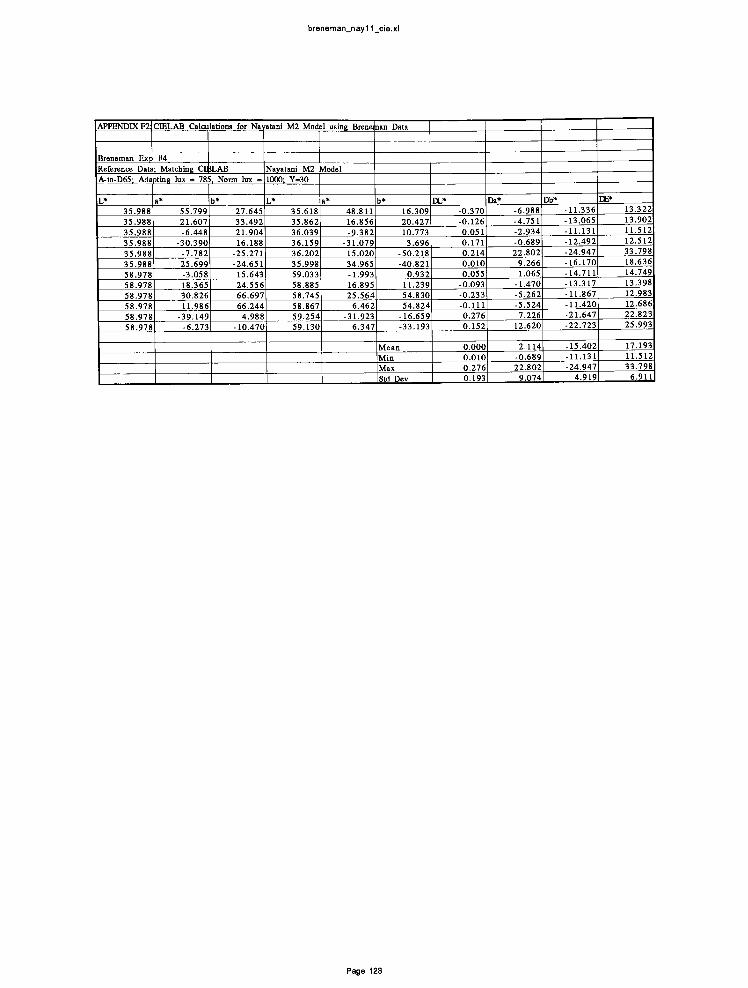
breneman_nay11_cie.xl
APPENDIX F2: CIELAB Calculations for Nayatani M2 Model using Brenenan Data
Reference Data; Matching CIJLAB Naya ani M2 Vlodel
A-to-D65; Adapting lux = 785. Norm lux = 1000; Y=30
L* a* b* L* a* b* DL* Da* Db* DE*
35.988 55.799 27.645 35.618 48.811 16.309 -0.370 -6.988 -11.336 13.322
35.988 21.607 33.492 35.862 16.856 20.427 -0.126 -4.751 -13.065 13.902
35.988 -6.448 21.904 36.039 -9.382 10.773 0.051 -2.934 -11.131 11.512
35.988 -30.390 16.188 36.159 -31.079 3.696 0.171 -0.689 -12.492 12.512
35.988 -7.782 -25.271 36.202 15.020 -50.218 0.214 22.802 -24.947 33.798
35.988 25.699 -24.651 35.998 34.965 -40.821 0.010 9.266 -16.170 18.636
58.978 -3.058 15.643 59.033 -1.993 0.932 0.055 1.065 -14.711 14.749
58.978 18.365 24.556 58.885 16.895 11.239 -0.093 -1.470 -13.317 13.398
58.978 30.826 66.697 58.745 25.564 54.830 -0.233 -5.262 -11.867 12.983
58.978 11.986 66.244 58.867 6.462 54.824 -0.111 -5.524 -11.420 12.686
58.978 -39.149 4.988 59.254 -31.923 -16.659 0.276 7.226 -21.647 22.823
58.978 -6.273 -10.470 59.130 6.347 -33.193 0.152 12.620 -22.723 25.993
Mean 0.000 2.114 -15.402 17.193
Min 0.010 -0.689 -11.131 11.512
Max 0.276 22.802 -24.947 33.798
t Std Dev 0.193 9.074 4.919 6.911
Page 123

breneman_huntest.xl
APPENDTXF3: CIELAB Calculations for Hunt Model using Breneman Dat
Breneman Exp. #4
Reference Matching Colors HUNT Model Data
A-to-D65. 75 cd/mA2
L* a* b* L* a* b* DL* Da* Db* DE (ab)
35.988 55.799 27.645 35.555 48.084 30.886 -0.433 -7.715 3.241 8.379
35.988 21.607 33.492 35.735 16.007 39.339 -0.253 -5.600 5.847 8.100
35.988 -6.448 21.904 35.870 -8.729 19.566 -0.118 -2.281 -2.338 3.269
35.988 -30.390 16.188 35.916 -28.632 9.138 -0.072 1.758 -7.050 7.266
35.988 -7.782 -25.271 35.955 20.993 -52.269 -0.033 28.775 -26.998 39.457
35.988 25.699 -24.651 35.790 39.255 -42.140 -0.198 13.556 -17.489 22.128
58.978 -3.058 15.643 58.829 0.668 -0.060 -0.149 3.726 -15.703 16.139
58.978 18.365 24.556 58.704 18.241 11.832 -0.274 -0.124 -12.724 12.727
58.978 30.826 66.697 58.581 24.506 79.956 -0.397 -6.320 13.259 14.693
58.978 11.986 66.244 58.685 5.468 76.755 -0.293 -6.518 10.511 12.371
58.978 -39.149 4.988 59.009 -26.621 -19.882 0.031 12.528 -24.870 27.847
58.978 -6.273 -10.470 58.903 12.499 -38.113 -0.075 18.772 -27.643 33.415
Average -0.189 4.213 -8.496 17.149
Min 0.031 -0.124 -2.338 3.269
Max -0.433 28.775 -27.643 39.457
StDev 0.145 11.691 14.603 11.282
Page 124

csaj_nle_4_51 28_cie.xl
APPENDIXOl CIELAB Calculations for Nav D. =.4. b exn =.5128
Nayatani Standard Model
A-to-D65, adapting luminance 1000 cd/m' 2
L*(Test) a*
(Test) b* (Test) L* (Nava vO)a* (Naya vO)
b* (Naya vO)DL* Da* Db* DE*
33.435 12.852 2.672 28.143 13.864 -6.236 -5.292 1.012 8.908 10.411
30.279 9.603 8.653 27.951 11.257 -0.013 -2.328 1.654 -8.666 9.124
29.663 2.148 9.227 26.476 3.887 -1.059 -3.187 1.739 -10.286 10.908
28.564 -5.243 4.648 26.639 -3.965 -4.763 -1.925 1.278 -9.411 9.691
30.949 -10.749 2.623 25.587 -9.824 -5.800 -5.362 0.925 -8.423 10.028
29.588 -11.688 -5.130 25.444 -10.360 -13.760 -4.144 1.328 -8.630 9.665
28.954 -7.047 -9.159 25.094 -5.508 -17.323 -3.860 1.539 -8.164 9.161
31.114 1.285 -9.153 25.009 2.689 -16.465 -6.105 1.404 -7.312 9.628
30.400 10.574 -7.280 26.537 12.134 -15.045 -3.863 1.560 -7.765 8.812
32.280 12.467 -2.700 28.482 13.913 -10.652 -3.798 1.446 -7.952 8.930
33.499 23.622 8.443 29.319 24.593 -0.857 -4.180 0.971 -9.300 10.242
29.286 16.262 14.550 28.012 19.173 3.576 -1.274 2.911 -10.974 11.425
30.133 2.856 18.208 28.110 4.775 6.437 -2.023 1.919 -11.771 12.097
27.980 -12.103 11.757 26.609 -10.680 0.004 -1.371 1.423 -11.753 11.918
30.376 -23.833 2.728 24.342 -22.250 -6.732 -6.034 1.583 -9.460 11.332
27.600 -19.245 -8.592 22.978 -17.370 -17.290 -4.622 1.875 -8.698 10.027
28.327 -13.738 -15.374 23.765 -12.350 -22.750 -4.562 1.388 -7.376 8.783
28.168 0.642 -16.370 24.322 2.273 -23.693 -3.846 1.631 -7.323 8.431
29.387 16.899 -10.976 26.737 18.794 -18.424 -2.650 1.895 -7.448 8.129
32.124 20.971 -1.348 29.265 22.519 -9.115 -2.859 1.548 -7.767 8.420
36.023 30.639 12.670 31.492 30.655 3.422 -4.531 0.016 -9.248 10.298
30.352 -34.885 3.307 23.758 -32.850 -6.506 -6.594 2.035 -9.813 11.997
29.184 -30.176 -10.800 21.127 -27.130 -18.020 -8.057 3.046 -7.220 11.239
30.616 -21.812 -20.594 22.331 -19.310 -25.390 -8.285 2.502 -4.796 9.895
30.545 -0.221 -22.092 23.767 1.201 -27.156 -6.778 1.422 -5.064 8.579
31.807 23.838 -14.385 27.880 25.089 -20.668 -3.927 1.251 -6.283 7.514
34.559 35.454 -1.781 29.026 35.165 -9.569 -5.533 -0.289 -7.788 9.558
51.233 11.703 7.222 53.194 11.986 7.797 1.961 0.283 0.575 2.063
51.803 7.692 12.341 52.760 7.781 12.761 0.957 0.089 0.420 1.049
50.535 0.075 15.087 52.492 0.078 15.703 1.957 0.003 0.616 2.052
50.711 -7.335 13.099 51.651 -7.451 13.243 0.940 -0.116 0.144 0.958
50.168 -14.351 4.810 51.042 -14.590 4.679 0.874 -0.239 -0.131 0.916
48.108 -13.221 -0.418 50.500 -13.780 -0.775 2.392 -0.559 -0.357 2.482
45.221 -7.330 -5.377 50.882 -8.029 -6.130 5.661 -0.699 -0.753 5.753
47.275 0.197 -6.512 50.146 0.225 -7.280 2.871 0.028 -0.768 2.972
49.423 6.981 -2.734 52.506 7.286 -2.672 3.083 0.305 0.062 3.099
51.313 10.825 1.263 53.277 11.076 1.716 1.964 0.251 0.453 2.031
52.253 21.876 14.455 53.610 22.205 15.214 1.357 0.329 0.759 1.589
52.006 15.019 23.046 54.541 15.483 24.607 2.535 0.464 1.561 3.013
51.187 0.583 26.303 53.096 0.601 27.427 1.909 0.018 1.124 2.215
50.781 -15.623 22.361 51.434 -15.800 22.477 0.653 -0.177 0.116 0.686
45.648 -26.577 6.563 50.190 -28.730 6.650 4.542 -2.153 0.087 5.027
44.688 -24.764 -3.268 49.577 -26.960 -4.105 4.889 -2.196 -0.837 5.425
42.077 -13.822 -10.317 48.759 -15.520 -12.310 6.682 -1.698 -1.993 7.177
46.271 -0.758 -11.311 48.713 -0.777 -12.568 2.442 -0.019 -1.257 2.747
53.557 13.734 -7.300 52.223 13.450 -7.048 -1.334 -0.284 0.252 1.387
52.586 22.271 3.254 54.255 22.633 4.020 1.669 0.362 0.766 1.872
52.487 41.866 24.401 56.936 44.017 27.348 4.449 2.151 2.947 5.754
52.520 27.974 39.220 56.023 29.070 42.718 3.503 1.096 3.498 5.070
52.708 0.691 48.157 55.068 0.742 50.990 2.360 0.051 2.833 3.688
45.067 -30.291 40.685 50.882 -33.300 44.258 5.815 -3.009 3.573 7.459
42.231 -46.215 6.831 47.533 -51.200 6.377 5.302 -4.985 -0.454 7.292
42.763 -40.079 -9.395 46.113 -43.040 -11.350 3.350 -2.961 -1.955 4.880
43.988 -25.962 -23.979 45.278 -26.830 -26.240 1.290 -0.868 -2.261 2.744
45.109 -1.119 -26.378 46.838 -0.962 -28.556 1.729 0.157 -2.178 2.785
49.882 30.641 -15.588 51.852 31.551 -16.043 1.970 0.910 -0.455 2.217
53.015 41.086 6.997 56.754 42.819 8.668 3.739 1.733 1.671 4.447
70.719 11.053 6.494 78.719 11.460 14.293 8.000 0.407 7.799 11.180
72.034 6.682 15.570 79.455 7.520 23.214 7.421 0.838 7.644 10.687
74.171 -1.266 19.240 78.774 -0.397 26.484 4.603 0.869 7.244 8.627
73.305 -8.225 18.437 77.989 -7.345 25.223 4.684 0.880 6.786 8.292
73.187 -15.058 9.845 76.776 -14.000 15.721 3.589 1.058 5.876 6.966
68.168 -14.562 0.520 74.055 -14.360 6.275 5.887 0.202 5.755 8.235
71.974 -7.719 -4.508 75.063 -7.439 1.583 3.089 0.280 6.091 6.835
73.429 0.201 -3.294 76.503 0.432 3.057 3.074 0.231 6.351 7.060
Page 125

csaj_nle_4_512B_cie.xl
70.253 5.238 -3.182 77.177 5.568 3.672 6.924 0.330 6.854 9.748
70.532 9.687 0.397 78.091 -13.828 36.412 7.559 -23.515 36.015 43.671
68.874 18.501 15.191 79.072 20.044 23.739 10.198 1.543 8.548 13.396
72.621 12.412 27.132 80.592 13.694 35.697 7.971 1.282 8.565 11.770
70.050 -1.727 31.756 79.517 -0.709 41.330 9.467 1.018 9.574 13.503
70.288 -14.202 27.995 78.091 -13.820 36.412 7.803 0.382 8.417 11.484
71.514 -25.763 12.644 75.674 -24.790 18.171 4.160 0.973 5.527 6.986
69.391 -25.494 0.472 74.010 -25.040 5.705 4.619 0.454 5.233 6.995
68.453 -13.923 -7.108 73.601 -13.840 -2.193 5.148 0.083 4.915 7.118
72.964 -0.738 -7.959 75.490 -0.443 -2.364 2.526 0.295 5.595 6.146
69.370 13.012 -8.757 76.554 13.272 -2.158 7.184 0.260 6.599 9.758
71.805 19.392 -0.516 79.619 19.786 7.736 7.814 0.394 8.252 11.371
69.198 28.487 18.751 81.950 31.187 28.907 12.752 2.700 10.156 16.524
68.461 17.173 35.514 80.920 19.543 47.084 12.459 2.370 11.570 17.167
69.895 -0.289 40.360 80.253 0.468 52.594 10.358 0.757 12.234 16.048
68.686 -19.712 35.440 77.082 -19.670 44.696 8.396 0.042 9.256 12.497
67.888 -35.770 13.121 74.944 -36.020 19.009 7.056 -0.250 5.888 9.193
65.436 -35.695 0.707 71.603 -35.970 4.896 6.167 -0.275 4.189 7.460
69.690 -24.260 -12.772 72.273 -23.470 -8.354 2.583 0.790 4.418 5.178
74.938 -1.102 -12.331 75.112 -0.788 -7.009 0.174 0.314 5.322 5.334
71.684 18.164 -11.492 78.625 18.592 -4.788 6.941 0.428 6.704 9.659
69.986 23.543 2.563 81.416 25.966 11.734 11.430 2.423 9.171 14.853
Value3 Mean -4.333 1.519 -8.430 9.861
Min 0.050 0.310 -6.120 7.514
Max -1.274 3.046 -11.830 12.097
STDEV 1.871 0.698 1.694 1.252
Value5 Mean 2.717 -0.391 0.269 3.362
Min 0 738 0.007 0.017 0.686
Max 6 682 2.151 3.573 7.459
STDEV 1.795 1.469 1.554 1.994
Value7 Mean 6.668 -0.081 8.218 11.125
Mm 0.174 0.042 4.189 5.178
Max 12.752 -23.515 36.015 43.671
STDEV 3.058 4.486 5.621 6.994
Total Mean 1.891 0.309 0.310 8 056
Min 0.050 0.007 0.017 0.686
Max 12.752 -23.515 36.015 43.671
STDEV 5.065 2.889 7 624 5.505
Page 126

csaj_nle_4495_5_cie.xl
APPENDIXG2 CIELAB Calculations for Navatani Standard Model w/ ro e p. =.4495. b 5XP. = .5
Nayatani Standard Model
A-to-D65. adapting luminance 1000 cd/m' 2
L* (Test) a*
(Test) b* (Test) L* (Naya vO)a* (Naya vO)
b* (Naya vO)DL* Da* Db* DE*
33.435 12.852 2.672 28.518 13.972 -5.509 -4.917 1.120 -8.181 9.610
30.279 9.603 8.653 28.329 11.393 0.707 -1.950 1.790 -7.946 8.375
29.663 2.148 9.227 26.874 3.913 -0.311 -2.789 1.765 -9.538 10.093
28.564 -5.243 4.648 27.034 -4.158 -4.002 -1.530 1.085 -8.650 8.851
30.949 -10.749 2.623 25.997 -10.200 -4.984 -4.952 0.549 -7.607 9.093
29.588 -11.688 -5.130 25.856 -10.970 -12.920 -3.732 0.718 -7.790 8.668
28.954 -7.047 -9.159 25.510 -6.170 -16.461 -3.444 0.877 -7.302 8.121
31.114 1.285 -9.153 25.427 2.235 -15.593 -5.687 0.950 -6.440 8.644
30.400 10.574 -7.280 26.933 11.974 -14.231 -3.467 1.400 -6.951 7.893
32.280 12.467 -2.700 28.853 13.914 -9.916 -3.427 1.447 -7.216 8.118
33.499 23.622 8.443 29.679 24.941 -0.181 -3.820 1.319 -8.624 9.524
29.286 16.262 14.550 28.389 19.505 4.258 -0.897 3.243 -10.292 10.828
30.133 2.856 18.208 28.485 4.958 7.105 -1.648 2.102 -11.103 11.420
27.980 -12.103 11.757 27.005 -10.860 0.725 -0.975 1.243 -11.032 11.145
30.376 -23.833 2.728 24.769 -22.980 -5.889 -5.607 0.853 -8.617 10.316
27.600 -19.245 -8.592 23.425 -18.520 -16.360 -4.175 0.725 -7.768 8.849
28.327 -13.738 -15.374 24.200 -13.540 -21.810 -4.127 0.198 -6.436 7.648
28.168 0.642 -16.370 24.749 1.504 -22.771 -3.419 0.862 -6.401 7.308
29.387 16.899 -10.976 27.131 18.675 -17.599 -2.256 1.776 -6.623 7.219
32.124 20.971 -1.348 29.624 22.695 -8.403 -2.500 1.724 -7.055 7.681
36.023 30.639 12.670 31.821 31.123 4.028 -4.202 0.484 -8.642 9.622
30.352 -34.885 3.307 24.194 -33.920 -5.648 -6.158 0.965 -8.955 10.911
29.184 -30.176 -10.800 21.601 -28.930 -17.000 -7.583 1.246 -6.200 9.874
30.616 -21.812 -20.594 22.787 -21.170 -24.370 -7.829 0.642 -3.776 8.716
30.545 -0.221 -22.092 24.203 0.147 -26.181 -6.342 0.368 -4.089 7.555
31.807 23.838 -14.385 28.259 25.016 -19.861 -3.548 1.178 -5.476 6.630
34.559 35.454 -1.781 29.389 35.540 -8.850 -5.170 0.086 -7.069 8.758
51.233 11.703 7.222 53.169 11.977 7.748 1.936 0.274 0.526 2.025
51.803 7.692 12.341 52.743 7.773 12.728 0.940 0.081 0.387 1.020
50.535 0.075 15.087 52.480 0.075 15.680 1.945 0.000 0.593 2.033
50.711 -7.335 13.099 51.654 -7.451 13.249 0.943 -0.116 0.150 0.962
50.168 -14.351 4.810 51.057 -14.590 4.708 0.889 -0.239 -0.102 0.926
48.108 -13.221 -0.418 50.525 -13.790 -0.725 2.417 -0.569 -0.307 2.502
45.221 -7.330 -5.377 50.899 -8.043 -6.094 5.678 -0.713 -0.717 5.767
47.275 0.197 -6.512 50.176 0.209 -7.217 2.901 0.012 -0.705 2.985
49.423 6.981 -2.734 52.494 7.287 -2.697 3.071 0.306 0.037 3.086
51.313 10.825 1.263 53.251 11.070 1.663 1.938 0.245 0.400 1.994
52.253 21.876 14.455 53.577 22.175 15.150 1.324 0.299 0.695 1.525
52.006 15.019 23.046 54.490 15.436 24.513 2.484 0.417 1.467 2.915
51.187 0.583 26.303 53.073 0.586 27.385 1.886 0.003 1.082 2.174
50.781 -15.623 22.361 51.442 -15.800 22.491 0.661 -0.177 0.130 0.697
45.648 -26.577 6.563 50.220 -28.760 6.710 4.572 -2.183 0.147 5.069
44.688 -24.764 -3.268 49.618 -27.020 -4.021 4.930 -2.256 -0.753 5.474
42.077 -13.822 -10.317 48.814 -15.610 -12.190 6.737 -1.788 -1.873 7.217
46.271 -0.758 -11.311 48.770 -0.825 -12.449 2.499 -0.067 -1.138 2.747
53.557 13.734 -7.300 52.216 13.450 -7.063 -1.341 -0.284 0.237 1.391
52.586 22.271 3.254 54.210 22.606 3.931 1.624 0.335 0.677 1.791
52.487 41.866 24.401 56.839 43.857 27.169 4.352 1.991 2.768 5.529
52.520 27.974 39.220 55.944 28.946 42.581 3.424 0.972 3.361 4.895
52.708 0.691 48.157 55.007 0.681 50.887 2.299 -0.010 2.730 3.569
45.067 -30.291 40.685 50.899 -33.300 44.288 5.832 -3.009 3.603 7.487
42.231 -46.215 6.831 47.610 -51.360 6.529 5.379 -5.145 -0.302 7.450
42.763 -40.079 -9.395 46.214 -43.350 -11.130 3.451 -3.271 -1.735 5.062
43.988 -25.962 -23.979 45.394 -27.210 -25.980 1.406 -1.248 -2.001 2.746
45.109 -1.119 -26.378 46.927 -1.134 -28.358 1.818 -0.015 -1.980 2.688
49.882 30.641 -15.588 51.851 31.551 -16.044 1.969 0.910 -0.456 2.217
53.015 41.086 6.997 56.661 42.695 8.485 3.646 1.609 1.488 4.254
70.719 11.053 6.494 78.146 11.273 13.166 7.427 0.220 6.672 9.986
72.034 6.682 15.570 78.864 7.267 22.063 6.830 0.585 6.493 9.442
74.171 -1.266 19.240 78.200 -0.597 25.377 4.029 0.669 6.137 7.372
73.305 -8.225 18.437 77.434 -7.411 24.146 4.129 0.814 5.709 7.093
73.187 -15.058 9.845 76.250 -13.840 14.670 3.063 1.218 4.825 5.843
68.168 -14.562 0.520 73.592 -14.120 5.343 5.424 0.442 4.823 7.272
71.974 -7.719 -4.508 74.577 -7.208 0.595 2.603 0.511 5.103 5.751
73.429 0.201 -3.294 75.983 0.545 2.000 2.554 0.344 5.294 5.888
Page 127

csaj_nle_4495_5_cie.xl
70.253 5.238 -3.182 76.641 5.569 2.595 6.388 0.331 5.777 8.619
70.532 9.687 0.397 78.304 9.908 7.018 7.772 0.221 6.621 10.212
68.874 18.501 15.191 78.491 19.606 22.615 9.617 1.105 7.424 12.199
72.621 12.412 27.132 79.974 13.195 34.527 7.353 0.783 7.395 10.458
70.050 -1.727 31.756 78.926 -1.071 40.231 8.876 0.656 8.475 12.290
70.288 -14.202 27.995 77.533 -13.920 35.366 7.245 0.282 7.371 10.339
71.514 -25.763 12.644 75.174 -24.490 17.175 3.660 1.273 4.531 5.962
69.391 -25.494 0.472 73.548 -24.610 4.763 4.157 0.884 4.291 6.039
68.453 -13.923 -7.108 73.149 -13.440 -3.134 4.696 0.483 3.974 6.171
72.964 -0.738 -7.959 74.994 -0.215 -3.398 2.030 0.523 4.561 5.020
69.370 13.012 -8.757 76.033 13.250 -3.214 6.663 0.238 5.543 8.670
71.805 19.392 -0.516 79.025 19.528 6.561 7.220 0.136 7.077 10.111
69.198 28.487 18.751 81.298 30.515 27.660 12.100 2.028 8.909 15.162
68.461 17.173 35.514 80.294 18.845 45.937 11.833 1.672 10.423 15.857
69.895 -0.289 40.360 79.643 -0.011 51.502 9.748 0.278 11.142 14.807
68.686 -19.712 35.440 76.549 -19.760 43.721 7.863 -0.048 8.281 11.419
67.888 -35.770 13.121 74.461 -35.570 18.050 6.573 0.200 4.929 8.218
65.436 -35.695 0.707 71.197 -35.400 4.054 5.761 0.295 3.347 6.669
69.690 -24.260 -12.772 71.851 -22.850 -9.255 2.161 1.410 3.517 4.362
74.938 -1.102 -12.331 74.625 -0.445 -8.050 -0.313 0.657 4.281 4.342
71.684 18.164 -11.492 78.055 18.545 -5.962 6.371 0.381 5.530 8.445
69.986 23.543 2.563 80.778 25.440 10.482 10.792 1.897 7.919 13.519
Value3 Mean -3.932 1.138 -7.621 8.943
Min 0.050 0.310 -6.120 6.630
Max -0.897 3.243 -11.830 11.420
STDEV 1.851 0.662 1.770 1.286
Value5 Mean 2.720 -0.455 0.280 3.340
Min 0.738 0.007 0.017 0.697
Max 6.737 1.991 3.603 7.487
STDEV 1.803 1.492 1.466 2.009
Value7 Mean 6.154 0.683 6.212 8.918
Min 0.073 0.009 3.347 4.342
Max 12.100 2.028 11.142 15.857
STDEV 3.022 0.536 1.943 3.242
Total Mean 1.840 0.432 -0.126 7.002
Min 0.050 0.007 0.017 0.697
Max 7.323 4.573 -11.830 15.857
STDEV 4.736 1.197 5.887 3.542
Page 128

csaj_nle_4_5_cie.xl
APPENDTXG3 CIELAB Calculationd for Navatani Standard Model w/ re e -
.5
Nayatani Standard Model
A-to-D65, adapting luminance 1000 cd/m' 2
L* (Test) a* (Test) b*(Test) L* (Naya vO)
a* (Nava vO)b* (Nava vO)
DL* Da* Db* DE*
33.435 12.852 2.672 28.143 13.816 -6.155 -5.292 0.964 -8.827 10.337
30.279 9.603 8.653 27.951 11.221 0.055 -2.328 1.618 -8.598 9.053
29.663 2.148 9.227 26.476 3.852 -0.997 -3.187 1.704 -10.224 10.844
28.564 -5.243 4.648 26.639 -4.019 -4.684 -1.925 1.224 -9.332 9.607
30.949 -10.749 2.623 25.587 -9.906 -5.691 -5.362 0.843 -8.314 9.929
29.588 -11.688 -5.130 25.444 -10.480 -13.630 -4.144 1.208 -8.500 9.533
28.954 -7.047 -9.159 25.094 -5.645 -17.179 -3.860 1.402 -8.020 9.010
31.114 1.285 -9.153 25.009 2.561 -16.314 -6.105 1.276 -7.161 9.496
30.400 10.574 -7.280 26.537 12.039 -14.915 -3.863 1.465 -7.635 8.681
32.280 12.467 -2.700 28.482 13.849 -10.554 -3.798 1.382 -7.854 8.833
33.499 23.622 8.443 29.319 24.566 -0.800 -4.180 0.944 -9.243 10.188
29.286 16.262 14.550 28.012 19.160 3.608 -1.274 2.898 -10.942 11.391
30.133 2.856 18.208 28.110 4.766 6.458 -2.023 1.910 -11.750 12.075
27.980 -12.103 11.757 26.609 -10.710 0.042 -1.371 1.393 -11.715 11.877
30.376 -23.833 2.728 24.342 -22.340 -6.626 -6.034 1.493 -9.354 11.231
27.600 -19.245 -8.592 22.978 -17.550 -17.130 -4.622 1.695 -8.538 9.856
28.327 -13.738 -15.374 23.765 -12.570 -22.560 -4.562 1.168 -7.186 8.592
28.168 0.642 -16.370 24.322 2.085 -23.507 -3.846 1.443 -7.137 8.235
29.387 16.899 -10.976 26.737 18.686 -18.278 -2.650 1.787 -7.302 7.971
32.124 20.971 -1.348 29.265 22.466 -9.023 -2.859 1.495 -7.675 8.326
36.023 30.639 12.670 31.492 30.639 3.461 -4.531 0.000 -9.209 10.263
30.352 -34.885 3.307 23.758 -32.960 -6.400 -6.594 1.925 -9.707 11.892
29.184 -30.176 -10.800 21.127 -27.390 -17.820 -8.057 2.786 7.020 11.043
30.616 -21.812 -20.594 22.331 -19.650 -25.150 -8.285 2.162 -4.556 9.699
30.545 -0.221 -22.092 23.767 0.951 -26.931 -6.778 1.172 -4.839 8.410
31.807 23.838 -14.385 27.880 24.977 -20.514 -3.927 1.139 -6.129 7.368
34.559 35.454 -1.781 29.026 35.116 -9.476 -5.533 -0.338 -7.695 9.484
51.233 11.703 7.222 53.194 11.989 7.791 1.961 0.286 0.569 2.062
51.803 7.692 12.341 52.760 7.782 12.757 0.957 0.090 0.416 1.047
50.535 0.075 15.087 52.492 0.079 15.701 1.957 0.004 0.614 2.051
50.711 -7.335 13.099 51.651 -7.451 13.243 0.940 -0.116 0.144 0.958
50.168 -14.351 4.810 51.042 -14.590 4.682 0.874 -0.239 -0.128 0.915
48.108 -13.221 -0.418 50.500 -13.780 -0.767 2.392 -0.559 -0.349 2.481
45.221 -7.330 -5.377 50.882 -8.033 -6.124 5.661 -0.703 -0.747 5.753
47.275 0.197 -6.512 50.146 0.218 -7.270 2.871 0.021 -0.758 2.969
49.423 6.981 -2.734 52.506 7.288 -2.676 3.083 0.307 0.058 3.099
51.313 10.825 1.263 53.277 11.080 1.709 1.964 0.255 0.446 2.030
52.253 21.876 14.455 53.610 22.208 15.207 1.357 0.332 0.752 1.587
52.006 15.019 23.046 54.541 15.486 24.600 2.535 0.467 1.554 3.010
51.187 0.583 26.303 53.096 0.602 27.425 1.909 0.019 1.122 2.214
50.781 -15.623 22.361 51.434 -15.800 22.478 0.653 -0.177 0.117 0.687
45.648 -26.577 6.563 50.190 -28.730 6.658 4.542 -2.153 0.095 5.027
44.688 -24.764 -3.268 49.577 -26.970 -4.091 4.889 -2.206 -0.823 5.426
42.077 -13.822 -10.317 48.759 -15.540 -12.280 6.682 -1.718 -1.963 7.173
46.271 -0.758 -11.311 48.713 -0.793 -12.546 2.442 -0.035 -1.235 2.737
53.557 13.734 -7.300 52.223 13.452 -7.051 -1.334 -0.282 0.249 1.386
52.586 22.271 3.254 54.255 22.639 4.009 1.669 0.368 0.755 1.868
52.487 41.866 24.401 56.936 44.020 27.336 4.449 2.154 2.935 5.749
52.520 27.974 39.220 56.023 29.070 42.717 3.503 1.096 3.497 5.070
52.708 0.691 48.157 55.068 0.741 50.992 2.360 0.050 2.835 3.689
45.067 -30.291 40.685 50.882 -33.300 44.258 5.815 -3.009 3.573 7.459
42.231 -46.215 6.831 47.533 -51.210 6.396 5.302 -4.995 -0.435 7.297
42.763 -40.079 -9.395 46.113 -43.080 -11.310 3.350 -3.001 -1.915 4.888
43.988 -25.962 -23.979 45.278 -26.890 -26.180 1.290 -0.928 -2.201 2.715
45.109 -1.119 -26.378 46.838 -1.003 -28.512 1.729 0.116 -2.134 2.749
49.882 30.641 -15.588 51.852 31.551 -16.043 1.970 0.910 -0.455 2.217
53.015 41.086 6.997 56.754 42.827 8.646 3.739 1.741 1.649 4.442
70.719 11.053 6.494 78.719 11.524 14.154 8.000 0.471 7.660 11.086
72.034 6.682 15.570 79.455 7.575 23.081 7.421 0.893 7.511 10.596
74.171 -1.266 19.240 78.774 -0.349 26.367 4.603 0.917 7.127 8.534
73.305 -8.225 18.437 77.989 -7.293 25.103 4.684 0.932 6.666 8.200
73.187 -15.058 9.845 76.776 -13.930 15.577 3.589 1.128 5.732 6.856
68.168 -14.562 0.520 74.055 -14.280 6.140 5.887 0.282 5.620 8.144
71.974 -7.719 -4.508 75.063 -7.351 1.433 3.089 0.368 5.941 6.706
73.429 0.201 -3.294 76.503 0.521 2.896 3.074 0.320 6.190 6.919
Page 129

csaj_nle_4_5_cie.xl
70.253 5.238 -3.182 77.177 5.651 3.518 6.924 0.413 6.700 9.644
70.532 9.687 0.397 78.881 10.090 8.012 8.349 0.403 7.615 11.307
68.874 18.501 15.191 79.072 20.091 23.617 10.198 1.590 8.426 13.324
72.621 12.412 27.132 80.592 13.729 35.592 7.971 1.317 8.460 11.698
70.050 -1.727 31.756 79.517 -0.683 41.251 9.467 1.044 9.495 13.449
70.288 -14.202 27.995 78.091 -13.790 36.327 7.803 0.412 8.332 11.423
71.514 -25.763 12.644 75.674 -24.720 18.037 4.160 1.043 5.393 6.890
69.391 -25.494 0.472 74.010 -24.950 5.558 4.619 0.544 5.086 6.892
68.453 -13.923 -7.108 73.601 -13.740 -2.355 5.148 0.183 4.753 7.009
72.964 -0.738 -7.959 75.490 -0.336 -2.543 2.526 0.402 5.416 5.990
69.370 13.012 -8.757 76.554 13.360 -2.316 7.184 0.348 6.441 9.655
71.805 19.392 -0.516 79.619 19.857 7.586 7.814 0.465 8.102 11.266
69.198 28.487 18.751 81.950 31.230 28.783 12.752 2.743 10.032 16.455
68.461 17.173 35.514 80.920 19.561 47.017 12.459 2.388 11.503 17.124
69.895 -0.289 40.360 80.253 0.478 52.553 10.358 0.767 12.193 16.017
68.686 -19.712 35.440 77.082 -19.650 44.640 8.396 0.062 9.200 12.455
67.888 -35.770 13.121 74.944 -35.950 18.883 7.056 -0.180 5.762 9.112
65.436 -35.695 0.707 71.603 -35.880 4.755 6.167 -0.185 4.048 7.379
69.690 -24.260 -12.772 72.273 -23.340 -8.528 2.583 0.920 4.244 5.053
74.938 -1.102 -12.331 75.112 -0.660 -7.211 0.174 0.442 5.120 5.142
71.684 18.164 -11.492 78.625 18.699 -4.979 6.941 0.535 6.513 9.533
69.986 23.543 2.563 81.416 26.033 11.582 11.430 2.490 9.019 14.771
Value3 Mean -4.333 1.413 -8.313 9.749
Min 0.050 0.310 -6.120 7.368
Max -1.274 2.898 -11.830 12.075
STDEV 1.871 0.669 1.746 1.281
ValueS Mean 2.717 -0.397 0.275 3.359
Min 0.738 0.007 0.017 0.687
Max 6.682 2.154 3.573 7.459
STDEV 1.795 1.474 1.541 1.995
Value7 Mean 6.694 0.782 7.143 9.954
Min 0.073 0.009 4.048 5.053
Max 12.752 2.743 12.193 17.124
STDEV 3.069 0.723 2.038 3.372
Total Mean 1.901 0.571 -0.022 7.616
Min 0.050 0.007 0.017 0.687
Max 7.323 4.573 -11.830 17.124
STDEV 5.076 1.269 6.531 3.915
Page 130

csaj_nle_4495_51_cle.xl
APPENDrX04 CIELAB Calculations for Navatani Standard Model w/ re e n. =.4495. b
Nayatani Standard Model
A-to-D65, adapting luminance 1000 cd/m' 2
L* (Test) a* (Test) b*(Test) L* (Naya vO)
a* (Nava vO)b* (Naya vO)
DL* Da* Db* DE*
33.435 12.852 2.672 32.573 14.175 -7.275 -0.862 1.323 -9.947 10.072
30.279 9.603 8.653 32.412 11.381 -0.722 2.133 1.778 -9.375 9.778
29.663 2.148 9.227 31.181 3.816 -1.66 1.518 1.668 -10.887 11.118
28.564 -5.243 4.648 31.318 -3.871 -5.706 2.754 1.372 -10.354 10.801
30.949 -10.749 2.623 30.438 -9.541 -6.949 -0.511 1.208 -9.572 9.661
29.588 -11.688 -5.130 30.318 -9.9 -15.231 0.730 1.788 -10.101 10.284
28.954 -7.047 -9.159 30.025 -5.013 -18.898 1.071 2.034 -9.739 10.007
31.114 1.285 -9.153 29.956 3.15 -17.985 -1.158 1.865 -8.832 9.101
30.400 10.574 -7.280 31.233 12.662 -16.523 0.833 2.088 -9.243 9.512
32.280 12.467 -2.700 32.857 14.38 -11.926 0.577 1.913 -9.226 9.440
33.499 23.622 8.443 33.55 24.918 -1.503 0.051 1.296 -9.946 10.030
29.286 16.262 14.550 32.46 19.032 3.716 3.174 2.770 -10.834 11.624
30.133 2.856 18.208 32.545 4.117 7.038 2.412 1.261 -11.170 11.497
27.980 -12.103 11.757 31.293 -11.17 -0.069 3.313 0.933 -11.826 12.317
30.376 -23.833 2.728 29.393 -21.63 -7.899 -0.983 2.203 -10.627 10.897
27.600 -19.245 -8.592 28.25 -16.49 -18.89 0.650 2.755 -10.298 10.680
28.327 -13.738 -15.374 28.909 -11.86 -24.36 0.582 1.878 -8.986 9.199
28.168 0.642 -16.370 29.38 2.604 -25.284 1.212 1.962 -8.914 9.207
29.387 16.899 -10.976 31.4 19.419 -19.955 2.013 2.520 -8.979 9.541
32.124 20.971 -1.348 33.507 23.092 -10.31 1.383 2.121 -8.962 9.313
36.023 30.639 12.670 35.354 30.943 3.119 -0.669 0.304 -9.551 9.579
30.352 -34.885 3.307 28.901 -31.65 -7.66 -1.451 3.235 -10.967 11.526
29.184 -30.176 -10.800 26.697 -25.58 -19.53 -2.487 4.596 -8.730 10.175
30.616 -21.812 -20.594 27.703 -18.97 -26.73 -2.913 2.842 -6.136 7.363
30.545 -0.221 -22.092 28.914 1.184 -28.529 -1.631 1.405 -6.437 6.787
31.807 23.838 -14.385 32.354 25.816 -22.153 0.547 1.978 -7.768 8.035
34.559 35.454 -1.781 33.302 36.03 -10.804 -1.257 0.576 -9.023 9.128
51.233 11.703 7.222 52.905 11.968 7.854 1.672 0.265 0.632 1.807
51.803 7.692 12.341 52.564 7.777 12.791 0.761 0.085 0.450 0.888
50.535 0.075 15.087 52.353 0.082 15.721 1.818 0.007 0.634 1.925
50.711 -7.335 13.099 51.69 -7.452 13.237 0.979 -0.117 0.138 0.996
50.168 -14.351 4.810 51.21 -14.59 4.642 1.042 -0.239 -0.168 1.082
48.108 -13.221 -0.418 50.781 -13.77 -0.845 2.673 -0.549 -0.427 2.762
45.221 -7.330 -5.377 51.083 -8.021 -6.186 5.862 -0.691 -0.809 5.958
47.275 0.197 -6.512 50.501 0.249 -7.383 3.226 0.052 -0.871 3.342
49.423 6.981 -2.734 52.364 7.275 -2.635 2.941 0.294 0.099 2.957
51.313 10.825 1.263 52.97 11.052 1.79 1.657 0.227 0.527 1.754
52.253 21.876 14.455 53.232 22.179 15.264 0.979 0.303 0.809 1.306
52.006 15.019 23.046 53.961 15.488 24.629 1.955 0.469 1.583 2.559
51.187 0.583 26.303 52.828 0.63 27.417 1.641 0.047 1.114 1.984
50.781 -15.623 22.361 51.519 -15.81 22.473 0.738 -0.187 0.112 0.770
45.648 -26.577 6.563 50.535 -28.74 6.58 4.887 -2.163 0.017 5.344
44.688 -24.764 -3.268 50.05 -26.96 -4.231 5.362 -2.196 -0.963 5.874
42.077 -13.822 -10.317 49.4 -15.5 -12.5 7.323 -1.678 -2.183 7.824
46.271 -0.758 -11.311 49.364 -0.733 -12.76 3.093 0.025 -1.449 3.416
53.557 13.734 -7.300 52.141 13.442 -7.025 -1.416 -0.292 0.275 1.472
52.586 22.271 3.254 53.738 22.572 4.137 1.152 0.301 0.883 1.482
52.487 41.866 24.401 55.833 43.875 27.364 3.346 2.009 2.963 4.900
52.520 27.974 39.220 55.121 29.119 42.426 2.601 1.145 3.206 4.284
52.708 0.691 48.157 54.373 0.915 50.632 1.665 0.224 2.475 2.991
45.067 -30.291 40.685 51.083 -33.37 44.335 6.016 -3.079 3.650 7.681
42.231 -46.215 6.831 48.423 -51.2 6.195 6.192 -4.985 -0.636 7.975
42.763 -40.079 -9.395 47.287 -42.97 -11.69 4.524 -2.891 -2.295 5.839
43.988 -25.962 -23.979 46.618 -26.86 -26.64 2.630 -0.898 -2.661 3.848
45.109 -1.119 -26.378 47.869 -0.933 -28.881 2.760 0.186 -2.503 3.731
49.882 30.641 -15.588 51.849 31.55 -16.042 1.967 0.909 -0.454 2.214
53.015 41.086 6.997 55.69 42.613 8.88 2.675 1.527 1.883 3.610
70.719 11.053 6.494 72.327 11.156 15.388 1.608 0.103 8.894 9.039
72.034 6.682 15.570 72.869 7.474 24.036 0.835 0.792 8.466 8.544
74.171 -1.266 19.240 72.367 -0.198 27.136 -1.804 1.068 7.896 8.170
73.305 -8.225 18.437 71.786 -7.092 25.913 -1.519 1.133 7.476 7.712
73.187 -15.058 9.845 70.888 -13.88 16.686 -2.299 1.178 6.841 7.312
68.168 -14.562 0.520 68.864 -14.36 7.361 0.696 0.202 6.841 6.879
71.974 -7.719 -4.508 69.615 -7.607 2.831 -2.359 0.112 7.339 7.710
73.429 0.201 -3.294 1 70.685 0.168 4.345 -2.744 -0.033 7.639 8.117
Page 131

csaj_nle_4495_51_cie.xl
70.253 5.238 -3.182 71.185 5.246 5.004 0.932 0.008 8.186 8.239
70.532 9.687 0.397 72.445 9.641 9.466 1.913 -0.046 9.069 9.269
68.874 18.501 15.191 72.589 19.781 24.506 3.715 1.280 9.315 10.110
72.621 12.412 27.132 73.708 13.824 36.012 1.087 1.412 8.880 9.057
70.050 -1.727 31.756 72.915 -0.114 41.273 2.865 1.613 9.517 10.069
70.288 -14.202 27.995 71.862 -13.19 36.579 1.574 1.012 8.584 8.786
71.514 -25.763 12.644 70.071 -24.54 19.021 -1.443 1.223 6.377 6.652
69.391 -25.494 0.472 68.832 -25 6.78 -0.559 0.494 6.308 6.352
68.453 -13.923 -7.108 68.526 -13.97 -1.007 0.073 -0.047 6.101 6.102
72.964 -0.738 -7.959 69.933 -0.733 -1.075 -3.031 0.005 6.884 7.522
69.370 13.012 -8.757 70.723 12.748 -0.709 1.353 -0.264 8.048 8.165
71.805 19.392 -0.516 72.991 19.212 9.098 1.186 -0.180 9.614 9.689
69.198 28.487 18.751 74.709 30.719 29.556 5.511 2.232 10.805 12.333
68.461 17.173 35.514 73.951 19.852 46.706 5.490 2.679 11.192 12.751
69.895 -0.289 40.360 73.458 1.404 51.61 3.563 1.693 11.250 11.922
68.686 -19.712 35.440 71.115 -18.73 44.359 2.429 0.982 8.919 9.296
67.888 -35.770 13.121 69.529 -35.7 19.806 1.641 0.070 6.685 6.884
65.436 -35.695 0.707 67.033 -35.88 5.835 1.597 -0.185 5.128 5.374
69.690 -24.260 -12.772 67.534 -23.51 -7.223 -2.156 0.750 5.549 6.000
74.938 -1.102 -12.331 69.652 -1.081 -5.755 -5.286 0.021 6.576 8.437
71.684 18.164 -11.492 72.256 17.915 -3.196 0.572 -0.249 8.296 8.319
69.986 23.543 2.563 74.312 25.409 13.053 4.326 1.866 10.490 11.499
Value3 Mean 0.409 1.914 -9.497 9.877
Min 0.051 0.304 -6.136 6.787
Max 3.313 4.596 -11.826 12.317
STDEV 1.673 0.865 1.298 1.256
Value5 Mean 2.757 -0.396 0.201 3.419
Min 0.738 0.007 0.017 0.770
Max 7.323 -4.985 3.650 7.975
STDEV 1.969 1.454 1.619 2.142
Value7 Mean 0.659 0.697 8.106 8.544
Min 0.073 0.005 5.128 5.374
Max 5.511 2.679 11.250 12.751
STDEV 2.598 0.813 1.632 1.865
Total Mean 1.305 0.698 -0.083 7.190
Min 0.050 0.005 0.017 0.770
Max 7.323 -4.985 -11.830 12.751
STDEV 2.359 1.429 7.317 3.326
Page 132

csaj_nle_45_5128_cie.xl
APPENDDCG5 CIELAB Calculations for Nayatani Standard Model w/ re e D. = .45. b ex p. = .5128
Nayatani Stan tard Model
A-to-D65, adapting luminance 1000 cd/m' 2
L* (Test) a* (Test) b* (Test) L* (Naya vO)a* (Naya vO)
b* (Naya vO)DL* Da* Db* DE*
33.435 12.852 2.672 32.573 14.176 -7.275 -0.862 1.324 -9.947 10.072
30.279 9.603 8.653 32.412 11.382 -0.722 2.133 1.779 -9.375 9.778
29.663 2.148 9.227 31.181 3.817 -1.66 1.518 1.669 -10.887 11.118
28.564 -5.243 4.648 31.318 -3.87 -5.706 2.754 1.373 -10.354 10.802
30.949 -10.749 2.623 30.438 -9.54 -6.949 -0.511 1.209 -9.572 9.662
29.588 -11.688 -5.130 30.318 -9.899 -15.231 0.730 1.789 -10.101 10.284
28.954 -7.047 -9.159 30.025 -5.012 -18.898 1.071 2.035 -9.739 10.007
31.114 1.285 -9.153 29.956 3.151 -17.985 -1.158 1.866 -8.832 9.101
30.400 10.574 -7.280 31.233 12.663 -16.523 0.833 2.089 -9.243 9.513
32.280 12.467 -2.700 32.857 14.381 -11.926 0.577 1.914 -9.226 9.440
33.499 23.622 8.443 33.55 24.919 -1.503 0.051 1.297 -9.946 10.030
29.286 16.262 14.550 32.46 19.032 3.716 3.174 2.770 -10.834 11.624
30.133 2.856 18.208 32.545 4.117 7.038 2.412 1.261 -11.170 11.497
27.980 -12.103 11.757 31.293 -11.16 -0.069 3.313 0.943 -11.826 12.317
30.376 -23.833 2.728 29.393 -21.62 -7.899 -0.983 2.213 -10.627 10.899
27.600 -19.245 -8.592 28.25 -16.49 -18.89 0.650 2.755 -10.298 10.680
28.327 -13.738 -15.374 28.909 -11.86 -24.36 0.582 1.878 -8.986 9.199
28.168 0.642 -16.370 29.38 2.605 -25.284 1.212 1.963 -8.914 9.208
29.387 16.899 -10.976 31.4 19.42 -19.955 2.013 2.521 -8.979 9.541
32.124 20.971 -1.348 33.507 23.092 -10.31 1.383 2.121 -8.962 9.313
36.023 30.639 12.670 35.354 30.944 3.119 -0.669 0.305 -9.551 9.579
30.352 -34.885 3.307 28.901 -31.65 -7.66 -1.451 3.235 -10.967 11.526
29.184 -30.176 -10.800 26.697 -25.58 -19.53 -2.487 4.596 -8.730 10.175
30.616 -21.812 -20.594 27.703 -18.97 -26.73 -2.913 2.842 -6.136 7.363
30.545 -0.221 -22.092 28.914 1.185 -28.529 -1.631 1.406 -6.437 6.788
31.807 23.838 -14.385 32.354 25.817 -22.153 0.547 1.979 -7.768 8.035
34.559 35.454 -1.781 33.302 36.031 -10.804 -1.257 0.577 -9.023 9.128
51.233 11.703 7.222 52.905 11.968 7.854 1.672 0.265 0.632 1.807
51.803 7.692 12.341 52.564 7.777 12.791 0.761 0.085 0.450 0.888
50.535 0.075 15.087 52.353 0.082 15.721 1.818 0.007 0.634 1.925
50.711 -7.335 13.099 51.69 -7.452 13.237 0.979 -0.117 0.138 0.996
50.168 -14.351 4.810 51.21 -14.59 4.642 1.042 -0.239 -0.168 1.082
48.108 -13.221 -0.418 50.781 -13.77 -0.845 2.673 -0.549 -0.427 2.762
45.221 -7.330 -5.377 51.083 -8.021 -6.186 5.862 -0.691 -0.809 5.958
47.275 0.197 -6.512 50.501 0.249 -7.383 3.226 0.052 -0.871 3.342
49.423 6.981 -2.734 52.364 7.275 -2.635 2.941 0.294 0.099 2.957
51.313 10.825 1.263 52.97 11.052 1.79 1.657 0.227 0.527 1.754
52.253 21.876 14.455 53.232 22.179 15.264 0.979 0.303 0.809 1.306
52.006 15.019 23.046 53.961 15.488 24.629 1.955 0.469 1.583 2.559
51.187 0.583 26.303 52.828 0.63 27.417 1.641 0.047 1.114 1.984
50.781 -15.623 22.361 51.519 -15.81 22.473 0.738 -0.187 0.112 0.770
45.648 -26.577 6.563 50.535 -28.74 6.58 4.887 -2.163 0.017 5.344
44.688 -24.764 -3.268 50.05 -26.96 -4.231 5.362 -2.196 -0.963 5.874
42.077 -13.822 -10.317 49.4 -15.5 -12.5 7.323 -1.678 -2.183 7.824
46.271 -0.758 -11.311 49.364 -0.733 -12.76 3.093 0.025 -1.449 3.416
53.557 13.734 -7.300 52.141 13.441 -7.025 -1.416 -0.293 0.275 1.472
52.586 22.271 3.254 53.738 22.571 4.137 1.152 0.300 0.883 1.482
52.487 41.866 24.401 55.833 43.875 27.364 3.346 2.009 2.963 4.900
52.520 27.974 39.220 55.12 29.119 42.426 2.600 1.145 3.206 4.284
52.708 0.691 48.157 54.373 0.914 50.632 1.665 0.223 2.475 2.991
45.067 -30.291 40.685 51.083 -33.37 44.335 6.016 -3.079 3.650 7.681
42.231 -46.215 6.831 48.423 -51.19 6.195 6.192 -4.975 -0.636 7.968
42.763 -40.079 -9.395 47.287 -42.97 -11.69 4.524 -2.891 -2.295 5.839
43.988 -25.962 -23.979 46.618 -26.86 -26.64 2.630 -0.898 -2.661 3.848
45.109 -1.119 -26.378 47.869 -0.933 -28.881 2.760 0.186 -2.503 3.731
49.882 30.641 -15.588 51.849 31.55 -16.042 1.967 0.909 -0.454 2.214
53.015 41.086 6.997 55.69 42.613 8.88 2.675 1.527 1.883 3.610
70.719 11.053 6.494 72.327 11.155 15.388 1.608 0.102 8.894 9.039
72.034 6.682 15.570 72.869 7.473 24.036 0.835 0.791 8.466 8.544
74.171 -1.266 19.240 72.367 -0.199 27.136 -1.804 1.067 7.896 8.169
73.305 -8.225 18.437 71.786 -7.094 25.913 -1.519 1.131 7.476 7.712
73.187 -15.058 9.845 70.888 -13.88 16.686 -2.299 1.178 6.841 7.312
68.168 -14.562 0.520 68.864 -14.36 7.361 0.696 0.202 6.841 6.879
71.974 -7.719 -4.508 69.615 -7.608 2.831 -2.359 0.111 7.339 7.710
73.429 0.201 -3.294 70.685 0.167 4.345 -2.744 -0.034 7.639 8.117
Page 133

csaj_nle_46_6128_cie.xl
70.253 5.238 -3.182 71.185 5.245 5.004 0.932 0.007 8.186 8.239
70.532 9.687 0.397 72.445 9.64 9.466 1.913 -0.047 9.069 9.269
68.874 18.501 15.191 72.589 19.78 24.506 3.715 1.279 9.315 10.110
72.621 12.412 27.132 73.708 13.823 36.012 1.087 1.411 8.880 9.057
70.050 -1.727 31.756 72.915 -0.115 41.273 2.865 1.612 9.517 10.069
70.288 -14.202 27.995 71.862 -13.19 36.579 1.574 1.012 8.584 8.786
71.514 -25.763 12.644 70.071 -24.54 19.021 -1.443 1.223 6.377 6.652
69.391 -25.494 0.472 68.832 -25 6.78 -0.559 0.494 6.308 6.352
68.453 -13.923 -7.108 68.526 -13.97 -1.007 0.073 -0.047 6.101 6.102
72.964 -0.738 -7.959 69.933 -0.734 -1.075 -3.031 0.004 6.884 7.522
69.370 13.012 -8.757 70.723 12.746 -0.709 1.353 -0.266 8.048 8.165
71.805 19.392 -0.516 72.991 19.21 9.098 1.186 -0.182 9.614 9.689
69.198 28.487 18.751 74.709 30.718 29.556 5.511 2.231 10.805 12.333
68.461 17.173 35.514 73.951 19.851 46.706 5.490 2.678 11.192 12.750
69.895 -0.289 40.360 73.458 1.403 51.61 3.563 1.692 11.250 11.921
68.686 -19.712 35.440 71.115 -18.73 44.359 2.429 0.982 8.919 9.296
67.888 -35.770 13.121 69.529 -35.7 19.806 1.641 0.070 6.685 6.884
65.436 -35.695 0.707 67.033 -35.88 5.835 1.597 -0.185 5.128 5.374
69.690 -24.260 -12.772 67.534 -23.51 -7.223 -2.156 0.750 5.549 6.000
74.938 -1.102 -12.331 69.652 -1.082 -5.755 -5.286 0.020 6.576 8.437
71.684 18.164 -11.492 72.256 17.914 -3.196 0.572 -0.250 8.296 8.319
69.986 23.543 2.563 74.312 25.407 13.053 4.326 1.864 10.490 11.499
Value3 Mean 0.409 1.915 -9.497 9.877
Min 0.051 0.306 -6.116 6.788
Max 3.313 4.596 -11.832 12.317
STDEV 1.673 0.864 1.298 1.256
Value5 Mean 2.757 -0.396 0.201 3.419
Min 0.738 0.007 0.017 0.770
Max 7.323 -4.985 3.650 7.968
STDEV 1.969 1.453 1.619 2.142
Value7 Mean 0.659 0.697 8.106 8.544
Min 0.073 0.008 5.128 5.374
Max 5.511 2.678 11.250 12.750
STDEV 2.598 0.813 1.632 1.865
Total Mean 1.305 0.698 -0.083 7.190
Min 0.051 0.007 0.017 0.770
Max 7.323 -4.985 -11.832 12.750
STDEV 2.359 1.429 7.317 3.326
Page 134

csaj_nle_45_51_cle.xl
APPENDTXG6 CIELAB Calculations for Nav ttani Standard vlodel w re ex 3. = .45. h exp=.51
Nayatani Standard Model
A-to-D65, adapting luminance 1000 cd/m' 2
L* (Test) a*
(Test) b* (Test) L* (Naya vO)a* (Naya vO)
b* (Naya vO)DL* Da* Db* DE*
33.435 12.852 2.672 32.573 14.176 -7.275 -0.862 1.324 -9.947 10.072
30.279 9.603 8.653 32.412 11.382 -0.722 2.133 1.779 -9.375 9.778
29.663 2.148 9.227 31.181 3.817 -1.66 1.518 1.669 -10.887 11.118
28.564 -5.243 4.648 31.318 -3.87 -5.706 2.754 1.373 -10.354 10.802
30.949 -10.749 2.623 30.438 -9.54 -6.949 -0.511 1.209 -9.572 9.662
29.588 -11.688 -5.130 30.318 -9.899 -15.231 0.730 1.789 -10.101 10.284
28.954 -7.047 -9.159 30.025 -5.012 -18.898 1.071 2.035 -9.739 10.007
31.114 1.285 -9.153 29.956 3.151 -17.985 -1.158 1.866 -8.832 9.101
30.400 10.574 -7.280 31.233 12.663 -16.523 0.833 2.089 -9.243 9.513
32.280 12.467 -2.700 32.857 14.381 -11.926 0.577 1.914 -9.226 9.440
33.499 23.622 8.443 33.55 24.919 -1.503 0.051 1.297 -9.946 10.030
29.286 16.262 14.550 32.46 19.032 3.716 3.174 2.770 -10.834 11.624
30.133 2.856 18.208 32.545 4.117 7.038 2.412 1.261 -11.170 11.497
27.980 -12.103 11.757 31.293 -11.16 -0.069 3.313 0.943 -11.826 12.317
30.376 -23.833 2.728 29.393 -21.62 -7.899 -0.983 2.213 -10.627 10.899
27.600 -19.245 -8.592 28.25 -16.49 -18.89 0.650 2.755 -10.298 10.680
28.327 -13.738 -15.374 28.909 -11.86 -24.36 0.582 1.878 -8.986 9.199
28.168 0.642 -16.370 29.38 2.605 -25.284 1.212 1.963 -8.914 9.208
29.387 16.899 -10.976 31.4 19.42 -19.955 2.013 2.521 -8.979 9.541
32.124 20.971 -1.348 33.507 23.092 -10.31 1.383 2.121 -8.962 9.313
36.023 30.639 12.670 35.354 30.944 3.119 -0.669 0.305 -9.551 9.579
30.352 -34.885 3.307 28.901 -31.65 -7.66 -1.451 3.235 -10.967 11.526
29.184 -30.176 -10.800 26.697 -25.58 -19.53 -2.487 4.596 -8.730 10.175
30.616 -21.812 -20.594 27.703 -18.97 -26.73 -2.913 2.842 -6.136 7.363
30.545 -0.221 -22.092 28.914 1.185 -28.529 -1.631 1.406 -6.437 6.788
31.807 23.838 -14.385 32.354 25.817 -22.153 0.547 1.979 -7.768 8.035
34.559 35.454 -1.781 33.302 36.031 -10.804 -1.257 0.577 -9.023 9.128
51.233 11.703 7.222 52.905 11.968 7.854 1.672 0.265 0.632 1.807
51.803 7.692 12.341 52.564 7.777 12.791 0.761 0.085 0.450 0.888
50.535 0.075 15.087 52.353 0.082 15.721 1.818 0.007 0.634 1.925
50.711 -7.335 13.099 51.69 -7.452 13.237 0.979 -0.117 0.138 0.996
50.168 -14.351 4.810 51.21 -14.59 4.642 1.042 -0.239 -0.168 1.082
48.108 -13.221 -0.418 50.781 -13.77 -0.845 2.673 -0.549 -0.427 2.762
45.221 -7.330 -5.377 51.083 -8.021 -6.186 5.862 -0.691 -0.809 5.958
47.275 0.197 -6.512 50.501 0.249 -7.383 3.226 0.052 -0.871 3.342
49.423 6.981 -2.734 52.364 7.275 -2.635 2.941 0.294 0.099 2.957
51.313 10.825 1.263 52.97 11.052 1.79 1.657 0.227 0.527 1.754
52.253 21.876 14.455 53.232 22.179 15.264 0.979 0.303 0.809 1.306
52.006 15.019 23.046 53.961 15.488 24.629 1.955 0.469 1.583 2.559
51.187 0.583 26.303 52.828 0.63 27.417 1.641 0.047 1.114 1.984
50.781 -15.623 22.361 51.519 -15.81 22.473 0.738 -0.187 0.112 0.770
45.648 -26.577 6.563 50.535 -28.74 6.58 4.887 -2.163 0.017 5.344
44.688 -24.764 -3.268 50.05 -26.96 -4.231 5.362 -2.196 -0.963 5.874
42.077 -13.822 -10.317 49.4 -15.5 -12.5 7.323 -1.678 -2.183 7.824
46.271 -0.758 -11.311 49.364 -0.733 -12.76 3.093 0.025 -1.449 3.416
53.557 13.734 -7.300 52.141 13.441 -7.025 -1.416 -0.293 0.275 1.472
52.586 22.271 3.254 53.738 22.571 4.137 1.152 0.300 0.883 1.482
52.487 41.866 24.401 55.833 43.875 27.364 3.346 2.009 2.963 4.900
52.520 27.974 39.220 55.12 29.119 42.426 2.600 1.145 3.206 4.284
52.708 0.691 48.157 54.373 0.914 50.632 1.665 0.223 2.475 2.991
45.067 -30.291 40.685 51.083 -33.37 44.335 6.016 -3.079 3.650 7.681
42.231 -46.215 6.831 48.423 -51.19 6.195 6.192 -4.975 -0.636 7.968
42.763 -40.079 -9.395 47.287 -42.97 -11.69 4.524 -2.891 -2.295 5.839
43.988 -25.962 -23.979 46.618 -26.86 -26.64 2.630 -0.898 -2.661 3.848
45.109 -1.119 -26.378 47.869 -0.933 -28.881 2.760 0.186 -2.503 3.731
49.882 30.641 -15.588 51.849 31.55 -16.042 1.967 0.909 -0.454 2.214
53.015 41.086 6.997 55.69 42.613 8.88 2.675 1.527 1.883 3.610
70.719 11.053 6.494 72.327 11.155 15.388 1.608 0.102 8.894 9.039
72.034 6.682 15.570 72.869 7.473 24.036 0.835 0.791 8.466 8.544
74.171 -1.266 19.240 72.367 -0.199 27.136 -1.804 1.067 7.896 8.169
73.305 -8.225 18.437 71.786 -7.094 25.913 -1.519 1.131 7.476 7.712
73.187 -15.058 9.845 70.888 -13.88 16.686 -2.299 1.178 6.841 7.312
68.168 -14.562 0.520 68.864 -14.36 7.361 0.696 0.202 6.841 6.879
71.974 -7.719 -4.508 69.615 -7.608 2.831 -2.359 0.111 7.339 7.710
73.429 0.201 -3.294 70.685 0.167 4.345 -2.744 -0.034 7.639 8.117
Page 135

csai_nle_46_51_cie.xl
70.253 5.238 -3.182 71.185 5.245 5.004 0.932 0.007 8.186 8.239
70.532 9.687 0.397 72.445 9.64 9.466 1.913 -0.047 9.069 9.269
68.874 18.501 15.191 72.589 19.78 24.506 3.715 1.279 9.315 10.110
72.621 12.412 27.132 73.708 13.823 36.012 1.087 1.411 8.880 9.057
70.050 -1.727 31.756 72.915 -0.115 41.273 2.865 1.612 9.517 10.069
70.288 -14.202 27.995 71.862 -13.19 36.579 1.574 1.012 8.584 8.786
71.514 -25.763 12.644 70.071 -24.54 19.021 -1.443 1.223 6.377 6.652
69.391 -25.494 0.472 68.832 -25 6.78 -0.559 0.494 6.308 6.352
68.453 -13.923 -7.108 68.526 -13.97 -1.007 0.073 -0.047 6.101 6.102
72.964 -0.738 -7.959 69.933 -0.734 -1.075 -3.031 0.004 6.884 7.522
69.370 13.012 -8.757 70.723 12.746 -0.709 1.353 -0.266 8.048 8.165
71.805 19.392 -0.516 72.991 19.21 9.098 1.186 -0.182 9.614 9.689
69.198 28.487 18.751 74.709 30.718 29.556 5.511 2.231 10.805 12.333
68.461 17.173 35.514 73.951 19.851 46.706 5.490 2.678 11.192 12.750
69.895 -0.289 40.360 73.458 1.403 51.61 3.563 1.692 11.250 11.921
68.686 -19.712 35.440 71.115 -18.73 44.359 2.429 0.982 8.919 9.296
67.888 -35.770 13.121 69.529 -35.7 19.806 1.641 0.070 6.685 6.884
65.436 -35.695 0.707 67.033 -35.88 5.835 1.597 -0.185 5.128 5.374
69.690 -24.260 -12.772 67.534 -23.51 -7.223 -2.156 0.750 5.549 6.000
74.938 -1.102 -12.331 69.652 -1.082 -5.755 -5.286 0.020 6.576 8.437
71.684 18.164 -11.492 72.256 17.914 -3.196 0.572 -0.250 8.296 8.319
69.986 23.543 2.563 74.312 25.407 13.053 4.326 1.864 10.490 11.499
Value3 Mean 0.409 1.915 -9.497 9.877
Min 0.051 0.305 -6.136 6.788
Max 3.313 4.596 -11.826 12.317
STDEV 1.673 0.864 1.298 1.256
ValueS Mean 2.757 -0.396 0.201 3.419
Min 0.738 0.007 0.017 0.770
Max 7.323 -4.975 3.650 7.968
STDEV 1.969 1.453 1.619 2.142
Value7 Mean 0.659 0.697 8.106 8.544
Min 0.073 0.004 5.128 5.374
Max 5.511 2.678 11.250 12.750
STDEV 2.598 0.813 1.632 1.865
Total Mean 1.305 0.698 -0.083 7.190
Min 0.051 0.007 0.017 0.770
Max 7.323 -4.975 -11.826 12.750
STDEV 2.359 1.429 7.317 3.326
Page 136

csa]_cle25lx.xl
APPENDIX HI CIELAB Calciilnrinnri for Ni valani Stanclar Model w/ a,( 2
Chromatic Adaptation Data; XYZ Reference Data Convcrlet to CIELAB
A-to-D65; adaptinu luminance for A = 25 =d/m"2
L*(Test) a*
(Test) b*(Test) L* NavvO d* NayvO b* NavvO DL* Da* Db* DE*ab
33.44 12.85 2.67 41.07 15.42 -4,99 7.63 2.56 -7.66 11.11
30.28 9.60 8.65 40.97 12.09 2.86 10.69 2.49 -5.79 12.41
29.66 2 15 9.23 40 24 3.23 2.72 10.58 1.08 -6.51 12.47
28.56 -5.24 4.65 40.33 -5.18 -2.70 11.76 0.06 -7.35 13.87
30.95 -10.75 2.62 39.80 -10.92 -5.20 8.86 -0.17 -7.83 1 1.82
29.59 -11.69 -5.13 39.73 -11.13 -15.11 10.14 0.56 -9.98 14.24
28.95 -7.05 -9.16 39.56 -5.18 -20.06 10.60 1.87 -10.91 15.32
31.11 1.29 -9.15 39.52 4.23 -19.28 8.40 2.95 -10.12 13.48
30.40 10.57 -7.28 40.28 14.62 -17.09 9.88 4.05 -9 81 14.49
32.28 12.47 -2.70 41.24 15.94 -11.06 8.96 3.47 -8 36 12.73
33.50 23.62 8.44 41.63 27.16 2.15 8.14 3.54 -6.29 10.88
29.29 16.26 14.55 40.99 20.04 9.93 11.71 3.78 -4.62 13.14
30.13 2.86 18.21 41.05 3.12 14.24 10.92 0.26 -3 97 11.62
27.98 -12.10 11.76 40.31 -14.44 5.94 12.33 -2.34 -5.X2 13.84
30.38 -23.83 2.73 39.18 -25.09 -5.78 8.80 -1.26 -8.51 12.30
27.60 -19.25 -8.59 38.49 -18.48 -20.15 10.89 0.77 -1 1.56 15.90
28.33 -13.74 -15.37 38.89 -11.91 -27.64 10.56 1.83 -12.27 16.29
28.17 0.64 -16.37 39.17 4.51 -28.79 11.00 3.87 -12.42 17.04
29.39 16.90 -10.98 40.37 22.65 -21.61 10.99 5.75 -10.64 16.34
32.12 20.97 -1.35 41.61 25.63 -9.18 9.49 4.66 -7.83 13.15
36.02 30.64 12.67 42.69 33.60 7.37 6.66 2.96 -5.30 9.01
30.35 -34.89 3.31 38.88 -36.72 -5.33 8.53 -1.84 -8.64 12.28
29.18 -30.18 -10.80 37.54 -28.14 -22.02 8.36 2.04 -1 1.22 14.14
30.62 -21.81 -20.59 38.15 -18.84 -31.79 7.54 2.97 -1 1.20 13.82
30.55 -0.22 -22.09 38.89 3.78 -33.62 8.35 4.00 -1 1.53 14.78
31.81 23.84 -14.39 40.94 29.93 -24.49 9.13 6.09 -10.10 14.91
34.56 35.45 -1.78 41.48 40.25 -9.73 6.92 4.80 -7.95 1 1.58
51.23 11.70 7.22 52.40 11.89 7.72 1.17 0.19 0.50 1.28
51.80 7.69 12.34 52.22 7.74 12.67 0.42 0.05 0.33 0.53
50.54 0.08 15.09 52.11 0.08 15.62 1.57 0.00 0.53 1 .66
50.71 -7.34 13.10 51.76 -7 46 13.26 1.05 -0.12 0.16 1.07
50.17 -14.35 4.81 51.51 -14.62 4.70 1.34 -0 27 -0.1 1 1.37
48.11 -13.22 -0.42 51.28 -13.81 -0 80 3.17 -0.59 -0.38 3.25
45.22 -7.33 -5.38 5 1 .44 -8.02 -6.18 6.22 -0.69 -0.81 6.31
47.28 0.20 -6.51 51.13 0.30 -7.38 3.86 0.10 -0.87 3.95
49.42 6.98 -2.73 52.12 7.24 -2.65 2.69 0.26 0.08 2.71
51.31 10.83 1.26 52.43 10.97 1.70 1.12 0.14 0.43 1.21
52.25 21.88 14.46 52.57 22.01 15 00 0.32 0.13 0.54 0.64
52.01 15.02 23.05 52.95 15.32 24.05 0.94 0.30 1.01 1.41
51.19 0.58 26.30 52.36 0.64 27.09 1.17 0.05 0.79 1.41
50.78 -15.62 22.36 51.67 -15.84 22.56 0.89 -0.22 0.20 0.94
45.65 -26.58 6.56 51 15 -28.89 6.72 5.50 -2.31 0.16 5.97
44.69 -24.76 -3 27 50.89 -27.12 -4.21 6.20 -2.36 -0.94 6.70
42.08 -13.82 -10.32 50.54 -15.54 -12.64 8.47 -1.72 -2.32 8.95
46.27 -0.76 -11.31 50.52 -0.59 -12.92 4.25 0.16 -1.61 4.55
53.56 13.73 -7.30 52.00 13.41 -7.02 -1.56 -0.33 0.28 1 .62
52.59 22.27 3.25 52.83 22.32 3.95 0.25 0.05 0.69 0.74
52.49 41.87 24.40 53.92 42.98 26.20 1.44 1.11 1.80 2.5 6
52.52 27.97 39.22 53.55 28.68 40.88 1.03 (1 70 1.66 2.(17
52.71 0.69 48.16 53.16 0.94 49.25 0.46 0 25 1.09 1 .21
45.07 -30 29 40.69 51.44 -33.51 44.71 6.37 -3.22 4.02 X 19
42.23 -46.22 6.83 50.02 -52.01 6.59 7.79 -5 80 -0.24 9 71
42.76 -40.08 -9.40 49.41 -43.67 -1 1.97 6.64 -3.59 -2.58 7.98
43.99 -25.96 -23.98 49.04 -27.01 -27.66 5.05 -1.05 -3.68 6.34
45.1 1 -1.12 -26.38 49 72 -0.57 -29.68 4.61 0.55 -3.30 5.70
49 88 30.64 -15.59 51 84 31.55 -16.04 1.96 0.91 -0.45 2.21
53.02 41.09 7.00 53.85 41.69 8.40 0.83 0.61 1.40 1.74
70.72 11.05 6.49 62.03 9.71 12.59 -8.69 -1.35 6.09 10.70
72.03 6.68 15.57 62.29 6.31 20.27 -9.75 -0.37 4.70 10.83
74.17 -1.27 19.24 62.05 -0.60 22.91 -12.12 0.67 3.67 12.68
73.31 -8.23 18.44 61.77 -6.89 22.06 -11.53 1.33 3.63 12.16
73.19 -15.06 9.85 61.35 -13.33 14.34 -11.84 1.73 4.50 12.78
68.17 -14.56 0.52 60.38 -13.91 6.05 -7.78 0.65 5.5 3 9.57
71.97 -7.72 -4.51 60.74 -7.71 2.00 -1 1.23 0.01 6.5 1 12.98
73.43 0.20 -3.29 61.25 -0.59 3.35 -12.18 -0.80 6 65 13.89
Page 137

csaj_cie25lx.xl
70.25 5.24 -3.18 61.49 4.09 3.70 -8.76 -1.15 6.88 1 1.20
70.53 9.69 0.40 62.09 8.21 7.37 -8.45 -1.48 6.97 1 1 .05
68.87 18.50 15.19 62.16 17.57 20.50 -6.72 -0.93 5.31 8,61
72.62 12.41 27.13 62.68 12.14 30.39 -9.94 -0.27 3.26 10.46
70.05 -1.73 31.76 62.31 -0.36 34.89 -7.74 1.37 3.14 8,47
70.29 -14.20 28.00 61.81 -12.22 31.09 -8.48 1.98 3.09 9-24
71.51 -25.76 12.64 60.96 -23.10 16.55 -10.55 2.66 3.90 1 1.56
69.39 -25.49 0.47 60.37 -23.83 5.78 -9.02 1.66 5.31 10.60
68.45 -13.92 -7.11 60.22 -13.79 -1.09 -8.23 0.13 6.02 10.20
72.96 -0.74 -7.96 60.90 -1.62 -I. 12 -12.07 -0.88 6 84 13.90
69.37 13.01 -8.76 61.27 10.93 -1.35 -8.10 -2.08 7.41 11.17
71.81 19.39 -0.52 62.34 16.89 6.88 -9.46 -2.51 7 39 12.27
69.20 28.49 18.75 63.15 27.29 24.47 -6.05 -1.20 5.72 8.41
68.46 17.17 35.51 62.80 17.69 39.26 -5.66 0.52 3.74 6.81
69.90 -0.29 40.36 62.56 1.25 43.07 -7.33 1.54 2 71 7.97
68.69 -19.71 35.44 61.46 -17.19 37.86 -7.23 2.52 2.42 8.03
67.89 -35.77 13.12 60.70 -33.39 17.27 -7.19 2.38 4.15 8.63
65.44 -35.70 0.71 59.50 -34.23 5.24 -5.93 1.47 4,53 7.61
69.69 -24.26 -12.77 59.75 -22.97 -6.45 -9.95 1.29 6.33 11.86
74.94 -1.10 -12.33 60.76 -2.12 -4.99 -14.18 -1.02 7.34 16.00
71.68 18.16 -11.49 62.00 15.32 -3.31 -9.69 -2.85 8.19 13.00
69.99 23.54 2.56 62.96 22.15 10.15 -7.02 -1.39 7.59 10.43
Value3 Mean 9.55 2.25 -8.67 13.44
Mm 6.66 0.06 -3.97 9.01
Max 12.33 6.09 -12.42 17.04
StdError 1.54 2. 211 2.43 1.88
;
ValucS Mean 2.84 -0 5 6 -0.05 3.47
Min 0.25 0.00 0.08 0.53
--
max 8.47 -5.80 4.02 9.71
StdError 2.63 1.52 1.56 2.82
Valuc7 Mean -9.10 0.12 5.32 10.77
Min -5.66 0.01 2.42 6.81
Max -14.18 -2.85 8.19 16.00
StdError 2.15 1.56 1.68 2.17
Total Mean 0.81 0.55 -0.88 9.08
Min 0.25 0.00 0.08 0.5 3
Max -14.12 6.09 -12.42 17.04
StdError 2.18 1.61 1.73 2.26
Page 138

csa|_cie50lx.xl
APPENDIX H2 CIELAB Calculations for Navalan, SmnHnr, Model w/ A< "1
Chromatic Adaptation Data; XYZ Reference Data Convert to CIELAB
A-to-D65; adapting luminance for A = 50 cd/mA2
L*(Test) a*
(Test) b* (Test) L* NavvO a* NavvO b* NavvO DL* Da* Db* DE*ab
33.44 12.85 2.67 39.64 15.08 -5.89 6.20 2.23 -8.56 10.80
30.28 9.60 8.65 39.53 1 1.82 1.75 9.25 2.22 -6.91 1 1.76
29.66 2.15 9.23 38.72 3.25 1.44 9.05 1.11 -7.79 1 1.99
28.56 -5.24 4.65 38.81 -4.86 -3.75 10.25 0.38 -8.40 13.25
30.95 -10.75 2.62 38.22 -10.46 -6.05 7.27 0.29 -8.67 1 1.32
29.59 -11.69 -5.13 38.14 -10.58 -15.66 8.55 1.11 -10.53 13.61
28.95 -7.05 -9.16 37.95 -4.84 -20.36 8 99 2 21 -1 1.20 14.53
31.11 1.29 -9.15 37.90 4.21 -19.54 6,79 2.93 -10.39 12.75
30.40 10.57 -7.28 38.75 14.29 -17.48 8.35 3.71 -10.20 13.70
32.28 12.47 -2.70 39.83 15.61 -1 1.70 7.55 3.15 -9.00 12.16
33.50 23.62 8.44 40.28 26.49 1.05 6.78 2.87 -7.39 10.43
29.29 16.26 14.55 39.56 19.55 8.41 10.27 3.29 -6.14 12.41
30.13 2.86 18.21 39.62 3.06 12.59 9.49 0.20 -5.62 1 1.03
27.98 -12.10 11.76 38.79 -13.82 4.41 10.81 -1.72 -7.35 13.19
30.38 -23.83 2.73 37.52 -24.00 -6.72 7.15 -0.17 -9.45 11.85
27.60 -19.25 -8.59 36.75 -17.49 -20.46 9.15 1.76 -I 1.87 15.09
28.33 -13.74 -15.37 37.20 -11.40 -27.48 8.87 2.34 -12.11 15.19
28.17 0.64 -16.37 37.51 4.39 -28.57 9.35 3.75 -12.20 15.82
29.39 16.90 -10.98 38.86 22.03 -21.77 9 47 5.13 -10.80 15.25
32.12 20.97 -1.35 40.25 25.02 -9.85 8.13 4.05 -8.50 12.44
36.02 30.64 12.67 41.46 32.79 6 23 5.44 2.15 -6 44 8.70
30.35 -34.89 3.31 37.19 -35.08 -6.33 6.84 -0.20 -9.63 1 1.81
29.18 -30.18 -10.80 35.70 -26.73 -22.06 6.51 3.45 -1 1.26 13.46
30.62 -21.81 -20.59 36.38 -18.22 -31.17 5.76 3.59 -10.58 12.57
30.55 -0.22 -22.09 37.20 3.52 -32.98 6.66 3.75 -10.89 13.30
31.81 23.84 -14,39 39.49 29.10 -24.47 7.69 5.26 -10.09 13 73
34.56 35.45 -1.78 40.11 39.22 -10.40 5.55 3.77 -8.62 10.92
51.23 11.70 7.22 52.48 11.91 7.77 1.25 0.21 0.55 1.38
51.80 7.69 12.34 52.27 7.75 12.71 (1.47 0.06 0.37 0.60
50.54 0.08 15.09 52.15 0.08 15.65 1.61 0.01 0.56 1.71
50.71 -7.34 13.10 51.75 -7.46 13.25 1.04 -0.12 0.15 1 .06
50.17 -14.35 4.81 51.46 -14.61 4.68 1.29 -0.26 -0.14 1.32
48.11 -13.22 -0.42 51.20 -13.80 -0.83 3 09 -0.58 -0.41 3.17
45.22 -7.33 -5.38 51.38 -8.02 -6.20 6.16 -0.69 -0.83 6.25
47.28 0.20 -6 51 51.03 0.30 -7.41 3.75 0.10 -0.90 3.86
49.42 6.98 -2.73 52.15 7.25 -2.64 2 73 0.26 0.10 2 75
51.31 10.83 1.26 52.52 10.99 1.74 1.21 0.16 0.48 1.31
52.25 21.88 14.46 52.68 22.06 15.08 0 42 0.18 0 62 0.77
52.01 15.02 23.05 53.11 15.38 24.20 1.11 0.36 1.15 1.64
51.19 0.58 26.30 52.43 0.65 27.17 1.25 0.06 0.87 1.52
50.78 -15.62 22.36 51.65 -15.84 22.54 0.86 -0.22 0.18 0.91
45.65 -26.58 6.56 51.05 -28.85 6.66 5.40 -2.27 0.10 5.86
44.69 -24.76 -3.27 50.76 -27.07 -4.26 6.07 -2.31 -0.99 6.57
42.08 -13.82 -10.32 50.36 -15.50 -12.67 8.28 -1.68 -2.35 8.77
46.27 -0.76 -11.31 50.34 -0.60 -12.95 4.07 0.16 -1.64 4.39
53.56 13.73 -7.30 52.02 13.41 -7.02 -1.54 -0.32 0.28 1.60
52.59 22.27 3.25 52.98 22.38 4.03 0.39 0.11 0.77 0.87
52.49 41.87 24.40 54.23 43.21 26.49 1.74 1 35 2.09 3.03
52.52 27.97 39.22 53.80 28.83 41.19 1.28 0.85 1.97 2.50
52.71 0.69 48.16 53.36 0.98 49.51 0.65 0.29 1.35 1.5 3
45.07 -30.29 40.69 51.38 -33.49 44.63 6.32 -3.20 3.95 8.1 1
42.23 -46.22 6.83 49.76 -51.78 6.44 7.53 -5.57 -0.39 9 37
42.76 -40.08 -9.40 49.06 -43.40 -12.02 6.30 -3.32 -2.63 7 59
43.99 -25.96 -23.98 48.65 -26.86 -27.56 4.66 -0.90 -3.58 5.95
45.11 -1.12 -26.38 49.42 -0.59 -29.61 4.31 0.53 -3.23 5.41
49.88 30.64 -15.59 51.84 31.55 -16.04 1.96 0.91 -0.45 2.21
53.02 41.09 7.00 54.14 41.91 8.58 1.13 0.82 1.5 8 2.1 1
70.72 11.05 6.49 63.60 10.05 13.54 -7.12 -1.00 7.05 10.06
72.03 6.68 15.57 63.90 6.65 21.38 -8.14 -0 04 5.81 10.00
74.17 -1.27 19.24 63.62 -0.41 24.08 -10.55 0.86 4.84 1 1.64
73.31 -8.23 18.44 63.30 -6.86 23.16 -10.00 1.37 4.72 11.14
73.19 -15.06 9.85 62.81 -13.46 15.18 -10.38 1.60 5.34 11.78
68.17 -14.56 0.52 61.69 -14.06 6.68 -6.48 0.50 6.16 8.95
71.97 -7.72 -4.51 62.11 -7.77 2.56 -9.87 -0.05 7.07 12.14
73.43 0.20 -3.29 62.70 -0.48 3.97 -10.73 -0.68 7 26 12.98
Page 139

csaj_cie50lx.xl
70 25 5 24 -3.18 62.97 4.31 4.38 -7.28 -0 9 3 7.57 10.54
70 53 9 69 0.40 63.67 8.52 8.21 -6.87 -1.17 7.82 10.47
68.87 18 50 15.19 63.75 18.15 21.65 -5.12 -0.35 6.45 8.25
72.62 12 41 27.13 64.36 12.68 31.80 -8.26 0.26 4.66 9.49
70.05 -1 73 31.76 63.92 -0.10 36.39 -6.13 1.62 4.63 7.85
70.29 -14.20 28.00 63.35 -12.29 32.43 -6.94 1.91 4.43 8.46
7 1.51 -25.76 12 64 62.36 -23.43 17.39 -9.16 2.33 4.74 10.57
69.39 -25.49 0.47 61.67 -24.18 6.35 -7.72 1.31 5.87 9.79
68.45 -13.92 -7.1 1 61.50 -13.95 -0.69 -6.95 -0.03 6.42 9.47
72.96 -0.74 -7.96 62.28 -1.52 -0.70 -10.68 -0.78 7.26 12.94
69.37 13.01 -8.76 62.72 1 1.27 -0.79 -6.65 -1.74 7.97 10.53
71.81 19.39 -0.52 63.97 17.40 7.76 -7.84 -2.00 8.27 1 1 57
69.20 28.49 18.75 64.91 28.17 25.83 -4.29 -0.32 7.08 8.28
68.46 17.17 35.51 64.50 18.40 40.92 -3.97 1.23 5.41 6.82
69.90 -0.29 40.36 64.22 1.55 44.86 -5.67 1.84 4.50 7 47
68.69 -19.71 35.44 62.93 -17.34 39.32 -5.75 2.37 3.88 7.33
67.89 -35.77 13.12 62.06 -33.94 18.10 -5.83 1.83 4.98 7.88
65.44 -35.70 0.71 60.67 -34.72 5.69 -4.77 0 98 4.98 6.97
69.69 -24.26 -12.77 60.95 -23.26 -6.24 -8.74 1.00 6.54 10.96
74.94 -1.10 -12.33 62.13 -2.03 -4.73 -12.81 -0.93 7.60 14.93
71.68 18.16 -11.49 63.56 15.81 -2.81 -8.12 -2.36 8.69 12.12
69.99 23.54 2.56 64.69 22.93 1 1.17 -5.30 -0.61 8.61 10.13
Valuc3 Mean 8.01 2.32 -9.28 12.71
Min 5.44 -0.17 -5.62 8.70
Max 10.81 5.26 -12.20 15.82
StdError 1.53 1.73 1.87 1 .66
Valuc5 Mean 2.83 -0.50 -0.01 3 47
Min 0.39 0.01 0.10 0 60
Max 8.28 -5.57 3.95 9.37
StdError 2.51 1.49 1.59 2.67
Valuc7 Mean -7.60 0.27 6.22 1 0 05
Min -3.97 -0.04 3.88 6 82
Max -12.81 2.37 8.69 14.93
StdError 2.19 1.33 1.41 1 99
Total Mean 0 84 0.64 -0.74 8.61
Min 0.39 0.01 0.10 0.60
Max -12.81 5.26 -12.20 15 82
StdError 6.84 1.91 6.52 4.45
Page 140

csaj_cie1 OOlx.xl
APPENDIX H3 CJELAB_Calculations for Navalani .Stanrh.rr
iA,
:a aI
Chromatic Adaptation Data; XYZ Reference Data rnnv.-rt<.r to CIELAB
A-10-D65; adapting luminance for A = 100 cd/mA2
L*(Test) a*
(Test) b*(Test) L* NavvO a* NavvO h* NavvO DL* Da* Db*
,DE'ab
10 5933.44 12.85 2.67 38.06 14.78 -6.66 4.62 1 .93 -9 33
30.28 9.60 8.65 37.94 1 1 62 0.73 7.66 2.02 -7.93 1121
29.66 2.15 9.23 37.03 3.34 0.25 7.36 1.20 -8.98 1 1 68
28.56 -5.24 4.65 37 13 -4.53 -4.68 8 57 0.71 -9.33 12.69
30.95 -10.75 2.62 36.48 -10.05 -6.73 5.53 0.70 -9.36 10 89
29.59 -11.69 -5.13 36.39 -10.12 -16.02 6.80 1.57 -10 89 12.93
28.95 -7.05 -9.16 36 17 -4.61 -20.44 7.21 2.44 -1 1.28 13 61
31.1 1 1.29 -9.15 36.12 4.10 -19.58 5.00 2.82 -10.43 1 1 .90
30.40 10.57 -7.28 37.07 13.92 -17.68 6.67 3.35 -10.40 12.79
32.28 12.47 -2.70 38.27 15.29 -12.18 5.99 2.83 -9.48 1 1.56
33.50 23.62 8.44 38.78 25.90 0.03 5.28 2.28 -8.41 10.19
29.29 16.26 14.55 37.97 19.19 6.91 8.68 2.93 -7.64 1 1.93
30.13 2.86 18.21 38.04 3.13 10.93 7.91 0.28 -7.28 10.75
27.98 -12.10 11.76 37.11 -13.13 2.92 9.13 -1.03 -8.84 12.75
30.38 -23.83 2.73 35.69 -23.00 -7.50 5.32 0.83 -10.23 1 1.56
27.60 -19.25 -8.59 34.84 -16.71 -20.54 7.24 2.54 -11.95 14.20
28.33 -13.74 -15.37 35.33 -11.11 -27.08 7.00 2.63 -1 1.71 13.89
28.17 0.64 -16.37 35.69 4.13 -28.10 7.52 3.49 -11.73 14.37
29.39 16.90 -10.98 37.18 21.37 -21.72 7.79 4.47 -10.74 14.00
32.12 20.97 -1.35 38.75 24.45 -10.37 6.62 3,48 -9.03 1 1.72
36.02 30.64 12.67 40.10 32.08 5.14 4.08 1.44 -7.53 8.68
30.35 -34.89 3.31 35.32 -33.61 -7.15 4.97 1.28 -10.46 1 1.65
29.18 -30.18 -10.80 33.66 -25.65 -21.85 4.48 4.5 3 -11.05 12.75
30.62 -21.81 -20.59 34 42 -17.90 -30.31 3 81 3.91 -9.72 1 1 14
30.55 -0.22 -22.09 35.34 3.10 -32.10 4.79 3.32 -10.01 1 1.58
31.81 23.84 -14.39 37.90 28.23 -24.25 6.09 4.40 -9.87 12.40
34.56 35.45 -1.78 38.59 38.24 -10 92 4.03 2.79 -9.14 10.37
51.23 11.70 7.22 52.57 1 1.93 7.81 1.34 0.22 0.59 1.48
51.80 7.69 12.34 52.34 7.76 12.74 0.53 0.07 0.40 0.67
50.54 0.08 15.09 52.19 0.08 15.68 1.66 0.01 0.59 1.76
50.71 -7.34 13.10 51.74 -7.46 13.25 1.03 -0.12 0.15 1.04
50.17 -14.35 4.81 51.41 -14.60 4 65 1.24 -0.25 -0.16 1.27
48.1 1 -13.22 -0.42 51.11 -13.78 -0.85 3.00 -0.56 -0.43 3.0 8
45.22 -7 33 -5.38 51.32 -8.01 -6.21 6.10 -0.68 -0.84 6.19
47.28 0.20 -6.51 50.92 0.29 -7.44 3.64 0 09 -0.92 3.76
49.42 6.98 -2.73 52.20 7.25 -2.63 2.78 0.27 0.1 1 2.79
51.31 10.83 1.26 52.62 11.00 1.78 1.30 0.18 0.51 1.41
52.25 21.88 14.46 52.80 22.10 15.15 0.54 0.22 0.70 0.91
52.01 15.02 23.05 53.29 15.43 24.34 1.29 0.41 1.30 1.87
51.19 0.58 26.30 52.52 0.65 27.25 1.33 0.07 0.94 1.63
50.78 -15.62 22.36 51.62 -15.83 22.52 0.84 -0.21 0.15 0.88
45.65 -26.58 6.56 50.94 -28.81 6.62 5.29 -2.23 0.05 5.74
44.69 -24.76 -3.27 50.60 -27.02 -4.29 5.92 -2.26 -1.02 6.41
42.08 -13.82 -10.32 50.15 -15.48 -12 68 8.07 -1.66 -2.36 8.57
46.27 -0.76 -11.31 50.13 -0.62 -12.95 3.86 0.14 -1 64 4.19
53.56 13.73 -7.30 52.05 13.42 -7.01 -1.51 -0.31 0.29 1.57
52.59 22.27 3.25 53.14 22.44 4.09 0.56 0.16 0.84 1 02
52.49 41.87 24.40 54.57 43.44 26.77 2.08 1.57 2.37 3 "S2
52.52 27.97 39.22 54 09 28.96 41.52 1.57 0.98 2.3(1 2 95
1.8852.71 0.69 48.16 53 58 1.01 49.79 0.87 0.32 1.64
45.07 -30.29 40.69 51.32 -33.46 44.56 6.25 -3 17 3.87 8 (II
42.23 -46.22 6.83 49.47 -51.57 6.30 7.24 -5 36 -0.53 9.02
42.76 -40.08 -9.40 48.68 -43.18 -12.03 5.91 -3 10 -2 64 7.18
43.99 -25.96 -23.98 48.21 -26.76 -27.41 4.22 -0.80 -3 43 5.50
45.11 -1.12 -26.38 49.08 -0.64 -29.49 3.98 0.48 -3 1 1 5.07
49.88 30.64 -15.59 51.85 31.55 -16.04 1.96 0.91 -0.45 2.21
53.02 41.09 7.00 54.47 42.12 8.74 1.46 1.04 1.74 2.49
70.72 11.05 6.49 65.41 10.39 14.41 -5.31 -0.66 7.92 9.56
72.03 6.68 15.57 65.76 6.96 22.44 -6.28 0.28 6.87 9.31
74.17 -1.27 19.24 65.44 -0.25 25.21 -8.74 1.02 5.97 10.63
73.31 -8.23 18.44 65.07 -6.85 24.21 -8.24 1.37 5.77 10.15
73.19 -15.06 9.85 64.49 -13.58 15.94 -8.70 1.48 6.09 10.72
68 17 -14.56 0.52 63.19 -14.19 7.21 -4.98 0.37 6.69 8.35
71.97 -7.72 -4.51 63.67 -7.79 3.01 -8.30 -0.07 7.52 1 1.20
73.43 0.20 -3.29 64.36 -0.35 4.46 -9.07 -0.55 7.76 1 1.95
Page 141

csaj_cie100lx.xl
70.25 5.24 -3.18 64.68 4.55 4.95 -5.57 -0.69 8.13 9.88
70.53 9.69 0.40 65.49 8.83 8.96 -5.05 -0.86 8.56 9.97
68.87 18.50 15.19 65.58 18.71 22.74 -3.29 0.20 7.55 8.24
72.62 12.41 27.13 66.30 13.16 33.20 -6.33 0.75 6.07 8.80
70.05 -1.73 31.76 65.79 0.08 37.90 -4.26 1.81 6.15 7.69
70.29 -14.20 28.00 65 1 1 -12.41 33.77 -5.18 1.79 5.78 7.96
7 1. 51 -25.76 12.64 63.96 -23.77 18.15 -7.55 1.99 5.51 9.56
69.39 -25.49 0.47 63.17 -24.50 6.81 -6.23 0.99 6.34 8,94
68.45 -13.92 -7.11 62.97 -14.06 -0.41 -5.49 -0.14 6.70 8.66
72.96 -0.74 -7.96 63.88 -1.38 -0.41 -9.09 -0.65 7.55 11.83
69.37 13.01 -8.76 64.38 11.64 -0.35 -4.99 -1.38 8.41 9.87
71.81 19.39 -0.52 65.84 17.92 8.54 -5.97 -1.48 9.05 10.94
69.20 28.49 18.75 66.94 29.01 27.16 -2.26 0.52 8.41 8.72
68.46 17.17 35.51 66.45 19.04 42.64 -2.01 1.87 7.13 7.64
69.90 -0.29 40.36 66.13 1.77 46.75 -3.76 2.06 6.39 7.69
68.69 -19.71 35.44 64.64 -17.56 40.82 -4 05 2.15 5.38 7.07
67.89 -35.77 13.12 63.62 -34.49 18.87 -4.27 1.28 5.75 7.28
65.44 -35.70 0.71 62.00 -35.18 6.04 -3.44 0.52 5.33 6 36
69.69 -24.26 -12.77 62.33 -23.49 -6,16 -7.37 0.77 6 61 9 93
74.94 -1.10 -12.33 63.69 -1.88 -4.62 -11.24 -0.78 7.71 13.65
71.68 18.16 -I 1.49 65.37 16.33 -2.46 -6.32 -1.83 8.69 10.90
69.99 23.54 2.56 66 68 23.70 12.10 -3.31 0.16 9.54 10.10
|
Value3 Mean 6 30 2 34 -9.73 1 1 .99
Mm 3.81 0.28 -7.28 8.68
Max 9.13 4.53 -11.95 14.37
StdError 1.54 1.37 1.30 1.36
Value5 Mean 2.81 -0.45 0.03 3 47
Min 0.53 0.01 0.05 0 67
Max 8.07 -5.36 3.87 9.02
StdError 2.37 1.47 1.62 2.52
Value7 Mean -5.89 0.41 7.04 9.45
--
Mm -2.01 -0.07 5.33 6.36
Max -11.24 2.15 9.54 13.65
StdError 2 25 1.14 1.19 1.64
|Total Mean 0 89 0.71 -0.58 8.18
Min 0.53 0.01 5.33 0.67
Max -1 1 .24 -5.36 -1 1.95 14.37
StdError 5 55 1.75 6.97 4.06
Page 142

csaj_cie300lx.xl
APPENDIX H4 CIELAB Calculations for Navatani Standar dModel w/ Ad lance = 300 cd/mA2
Chromatic Adaptation Data ; XYZ Reference Data Converted to CIELAB
A-to-D65; adapting luminance for A = 300 cd/ma2
L*(Test) a*
(Test) b*(Test) L* NayvO a* NayvO b* NayvO DL* Da* Db* DE*ab
33.44 12.85 2.67 35.40 14.43 -7.38 1.96 1.58 -10.05 10.36
30.28 9.60 8.65 35.26 11.44 -0.42 4.98 1.84 -9.07 10.51
29.66 2.15 9.23 34.19 3.58 -1.16 4.52 1.43 -10.38 1 1.41
28.56 -5.24 4.65 34.31 -4.09 -5.63 5.74 1.16 -10.28 11.83
30.95 -10.75 2.62 33.54 -9.60 -7.26 2.59 1.15 -9.89 10.28
29.59 -11.69 -5.13 33.43 -9.75 -16.01 3.85 1.93 -10.88 11.70
28.95 -7.05 -9.16 33.18 -4.59 -20.01 4.23 2.45 -10.85 11.90
31.11 1.29 -9.15 33.12 3.73 -19.11 2.01 2.44 -9.95 10.44
30.40 10.57 -7.28 34.23 13.30 -17.45 3.83 2.72 -10.17 11.20
32.28 12.47 -2.70 35.64 14.82 -12.43 3.36 2.35 -9.73 10.56
33.50 23.62 8.44 36.24 25.25 -1.14 2.74 1.63 -9.58 10.10
29.29 16.26 14.55 35.29 18.94 4.91 6.01 2.67 -9.64 1 1.67
30.13 2.86 18.21 35.37 3.51 8.61 5.24 0.65 -9.60 10.96
27.98 -12.10 11.76 34.28 -12.04 0.99 6.30 0.06 -10.77 12.48
30.38 -23.83 2.73 32.63 -21.91 -8.15 2.25 1.92 -10.88 11.27
27.60 -19.25 -8.59 31.63 -16.14 -20.07 4.03 3.11 -11.48 12.55
28.33 -13.74 -15.37 32.20 -11.19 -25.95 3.88 2.55 -10.58 11.55
28.17 0.64 -16.37 32.62 3.46 -26.90 4.45 2.82 -10.53 1 1.78
29.39 16.90 -10.98 34.38 20.33 -21.13 4.99 3.43 -10.16 11.82
32.12 20.97 -1.35 36.21 23.68 -10.71 4.08 2.71 -9.37 10.57
36.02 30.64 12.67 37.80 31.29 3.77 1.78 0.65 -8.90 9.10
30.35 -34.89 3.31 32.20 -32.00 -7.87 1.84 2.89 -11.18 11.69
29.18 -30.18 -10.80 30.27 -24.95 -20.97 1.08 5.23 -10.17 1 1.49
30.62 -21.81 -20.59 31.15 -18.09 -28.60 0.53 3.72 -8.01 8.84
30.55 -0.22 -22.09 32.21 2.17 -30.39 1.67 2.39 -8.30 8.80
31.81 23.84 -14.39 35.21 26.92 -23.44 3.40 3.08 -9.06 10.15
34.56 35.45 -1.78 36.02 36.95 -11.24 1.46 1.50 -9.46 9.68
51.23 11.70 7.22 52.73 11.95 7.86 1.50 0.25 0.63 1.64
51.80 7.69 12.34 52.45 7.77 12.78 0.64 0.08 0.44 0.78
50.54 0.08 15.09 52.27 0.09 15.71 1.73 0.01 0.62 1.84
50.71 -7.34 13.10 51.71 -7.45 13.24 1. 00 -0.12 0.14 1.02
50.17 -14.35 4.81 51.31 -14.59 4.64 1.14 -0.24 -0.18 1.18
48.11 -13.22 -0.42 50.95 -13.77 -0.87 2.85 -0.55 -0.45 2.93
45.22 -7.33 -5.38 51.21 -8.01 -6.22 5.99 -0.68 -0.84 6.08
47.28 0.20 -6.51 50.72 0.27 -7.44 3.44 0.08 -0.92 3.56
49.42 6.98 -2.73 52.28 7.26 -2.62 2.86 0.28 0.12 2.87
51.31 10.83 1.26 52.78 11.03 1.81 1.47 0.21 0.54 1.58
52.25 21.88 14.46 53.00 22.15 15.24 0.75 0.27 0.78 1.12
52.01 15.02 23.05 53.61 15.48 24.53 1.61 0.46 1.48 2.23
51.19 0.58 26.30 52.67 0.65 27.35 1.48 0.07 1.05 1.81
50.78 -15.62 22.36 51.57 -15.82 22.49 0.79 -0.20 0.13 0.82
45.65 -26.58 6.56 50.75 -28.77 6.57 5.10 -2.19 0.01 5.55
44.69 -24.76 -3.27 50.34 -26.97 -4.29 5.65 -2.21 -1.03 6.15
42.08 -13.82 -10.32 49.79 -15.47 -12.63 7.72 -1.65 -2.31 8.22
46.27 -0.76 -11.31 49.76 -0.67 -12.90 3.49 0.09 -1.59 3.84
53.56 13.73 -7.30 52.09 13.43 -7.01 -1.47 -0.30 0.29 1.52
52.59 22.27 3.25 53.43 22.51 4.16 0.84 0.24 0.90 1.26
52.49 41.87 24.40 55.17 43.71j 27.15 2.68 1.85 2.75 4.26
52.52 27.97 39.22 54.58 29.09 42.02 2.06 1.12 2.80 3.65
52.71 0.69 48.16 53.95 1.00 50.24 1.25 0.31 2.08 2.45
45.07 -30.29 40.69 51.21 -33.42 44.44 6.14 -3.13 3.75 7.84
42.23 -46.22 6.83 48.97 -51.31 6.18 6.74 -5.10 -0.65 8.47
42.76 -40.08 -9.40 48.01 -42.97 -11.93 5.25 -2.89 -2.54 6.5 1
43.99 -25.96 -23.98 47.45 -26.74 -27.07 3.46 -0.78 -3.09 4.70
Page 143

csaj_cie300lx.xl
45.1 1 -1.12 -26.38 48.50 -0.77 -29.22 3.39 0.35 -2.85 4.44
49.88 30.64 -15.59 5 1.85 31.55 -16.04 1.97 0.91 -0.45 2.21
53.02 41.09 7.00 55.05 42.41 8.89 2.04 1.32 1.89 3.08
70.72 11.05 6.49 68.64 10.85 15.34 -2.08 -0.21 8.85 9.09
72.03 6.68 15.57 69.08 7.33 23.68 -2.96 0.64 8.11 8.66
74.17 -1.27 19.24 68.67 -0.13 26.61 -5.50 1.14 7.37 9.26
73.31 -8.23 18.44 68.21 -6.92 25.48 -5.10 1.30 7.05 8.80
73.19 -15.06 9.85 67.48 -13.76 16.71 -5.71 1.30 6.87 9.02
68.17 -14.56 0.52 65.85 -14.33 7.64 -2.32 0.23 7.12 7.49
71.97 -7.72 -4.51 66.45 -7.75 3.29 -5.52 -0.03 7.80 9.55
73.43 0.20 -3.29 67.32 -0.10 4.79 -6.11 -0.31 8.09 10.14
70.25 5.24 -3.18 67.72 4.92 5.39 -2.53 -0.32 8.57 8.94
70.53 9.69 0.40 68.74 9.28 9.66 -1.80 -0.40 9.26 9.44
68.87 18.50 15.19 68.85 19.40 24.07 -0.02 0.90 8.88 8.92
72.62 12.41 27.13 69.75 13.69 35.05 -2.87 1.28 7.92 8.52
70.05 -1.73 31.76 69.11 0.16 40.00 -0.94 1.88 8.25 8.5 1
70.29 -14.20 28.00 68.27 -12.73 35.58 -2.02 1.47 7.59 7.99
71.51 -25.76 12.64 66.82 -24.23 18.97 -4.69 1.53 6.32 8.02
69.39 -25.49 0.47 65.82 -24.87 7.14 -3.57 0.62 6.67 7.59
68.45 -13.92 -7.11 65.57 -14.11 -0.39 -2.88 -0.19 6.72 7.31
72.96 -0.74 -7.96 66.71 -1.09 -0.39 -6.25 -0.36 7.57 9.82
69.37 13.01 -8.76 67.35 12.22 -0.14 -2.02 -0.80 8.62 8.89
71.81 19.39 -0.52 69.18 18.65 9.28 -2.63 -0.74 9.80 10.17
69.20 28.49 18.75 70.5 6 30.10 28.84 1.36 1.61 10.09 10.31
68.46 17.17 35.51 69.95 19.73 45.09 1.49 2.55 9.57 10.02
69.90 -0.29 40.36 69.55 1.82 49.54 -0.34 2.11 9.18 9.43
68.69 -19.71 35.44 67.67 -18.06 42.95 -1.02 1.65 7.51 7.76
67.89 -35.77 13.12 66.38 -35.23 19.71 -1.50 0.54 6.59 6.78
65.44 -35.70 0.71 64.36 -35.70 6.23 -1.07 -0.01 5.53 5.63
69.69 -24.26 -12.77 64.77 -23.64 -6.43 -4.92 0.62 6.35 8.06
74.94 -1.10 -12.33 66.48 -1.53 -4.88 -8.46 -0.43 7.45 11.28
71.68 18.16 -11.49 68.58 17.17 -2.42 -3.10 -0.99 8.69 9.28
69.99 23.54 2.56 70.24 24.74 13.07 0.25 1.19 10.51 10.58
Value3 Mean 3.44 2.22 -9.96 10.91
Min 0.5 3 0.06 -8.01 8.80
Max 6.30 5.23 -11.18 12.55
StdError 1.59 1.08 0.84 1.03
ValueS Mean 2.78 -0.40 0.12 3.46
Min 0.64 0.01 0.01 0.78
Max 7.72 -5.10 3.75 8.47
StdError 2.16 1.45 1.65 2.31
Value7 Mean -2.83 0.59 7.96 8.84
Min -0.02 -0.01 5.53 5.63
Max -8.46 2.55 10.51 11.28
StdError 2.39 0.96 1.22 1.21
Total Mean 1.05 0.76 -0.30 7.63
Min -0.02 -0.01 0.01 0.78
Max -8.46 5.23 -11.18 12.55
StdError 3.51 1.59 7.40 3 5 5
Page 144

csaj_cie500lx.xl
APPENDIX H5 CIELAB Calculations for Navatani Slandnr, ice- 500 cd/ n"2
1
|Chromatic Adaptation Data; XYZ Reference Data Convertet to CIELAB
A-to-D65; adapling luminance for A = 50( cd/m"2
L*(Test) a* (Test) b* (Test) L* NavvO a* NavvO b* NavvO DL* Da* Db* DE*ab
33.44 12.85 2.67 34.16 14.31 -7.44 0.73 1.45 -10.12 10.25
30.28 9.60 8.65 34.01 1 1.41 -0.67 3.74 1.80 -9.33 10.21
29.66 2.15 9.23 32.87 3.69 -1.51 3.21 1.55 -10.74 11.31
28.56 -5.24 4.65 33.00 -3.95 -5.79 4.44 1.29 -10.44 1 1.41
30.95 -10.75 2.62 32.19 -9.52 -7.24 1.24 1.23 -9.86 10.01
29.59 -1 1.69 -5.13 32.07 -9.75 -15.76 2.49 1.93 -10.63 1 1 09
28.95 -7.05 -9.16 31.80 -4.73 -19.59 2.85 2.32 -10.43 11.06
31.11 1.29 -9.15 31.74 3.49 -18.68 0.62 2.20 -9.53 9.80
30.40 10.57 -7.28 32.92 13.01 -17.12 2.52 2.44 -9.84 10.44
32.28 12.47 -2.70 34.43 14.62 -12.30 2.15 2.15 -9.60 10.07
33.50 23.62 8.44 35.07 25.07 -1.42 1.57 1.44 -9.86 10.09
29.29 16.26 14.55 34.06 18.94 4.26 4.77 2.68 -10.30 1 1 .66
30.1.3 2.86 18.21 34.14 3.76 7.79 4.01 0.91 -10.42 1 1.20
27.98 -12.10 1 1.76 32.98 -1 1.61 0.39 5.00 0.49 -1 1.37 12.43
30.38 -23.83 2 73 31.21 -21.67 -8 16 0.84 2.16 -10.89 11.13
27.60 -19.25 -8.59 30.15 -16.18 -19.63 2.55 3 07 -1 1.04 1 1 74
28.33 -13.74 -15.37 30.76 -11.43 -25.28 2.44 2.31 -9.91 10.46
28.17 0.64 -16.37 31.20 3.08 -26.22 3.04 2.44 -9.85 10.59
29.39 16.90 -10.98 33.08 19.90 -20.67 3.69 3.00 -9.70 10.80
32.12 20.97 -1.35 35.03 23.39 -10.63 2.90 2 42 -9.29 10.03
36.02 30.64 12.67 36.73 31.09 3.37 0.71 0.45 -9.30 9.34
30.35 -34.89 3.31 30.76 -31.67 -7.90 0.40 3 22 -1 1.21 1 1.67
29.18 -30 18 -10.80 28.71 -25.07 -20.39 -0.48 5 1 1 -9.59 10.88
30.62 -21.81 -20.59 29.64 -18.41 -27.77 -0.98 3.40 -7.18 8.00
30.55 -0.22 -22.09 30.77 1.72 -29.56 0.22 1.94 -7.47 7.72
31.81 23.84 -14.39 33.96 26.39 -22.92 2.15 2.55 -8.54 9.16
34.56 35.45 -1.78 34.84 36.49 -1 1.14 0.28 1.04 -9.36 9.42
51.23 11.70 7.22 52.81 11.96 7.86 1.57 0.26 0.64 1.72
51.80 7.69 12.34 52.50 7.78 12.79 0.69 0.08 0.45 0.83
50.54 0.08 15.09 52.31 0.08 15.72 1.77 0.01 0.63 1.88
50.71 -7.34 13.10 51.70 -7.45 13.24 0.99 -0.12 0.14 1.01
50.17 -14.35 4.81 51.27 -14.59 4.63 1.10 -0.24 -0.18 1.14
48.11 -13.22 -0.42 50.88 -13.77 -0.87 2.77 -0.55 -0.45 2.86
45.22 -7.33 -5.38 51.15 -8.02 -6.21 5.93 -0.69 -0.83 6.03
47.28 0.20 -6.51 50.62 0.26 -7.42 3.35 0.07 -0.91 3.47
49.42 6.98 -2.73 52.32 7.27 -2.62 2.89 0.29 0.1 1 2.91
51.31 10.83 1.26 52.87 11.04 1.81 1.55 0.22 0.54 1.66
52.25 21.88 14.46 53.10 22.17 15.26 0.85 0.29 0.80 1.20
52.01 15.02 23.05 53.76 15.49 24.59 1.76 0.47 1.54 2.38
51.19 0.58 26.30 52.74 0.64 27.39 1.55 0.06 1.08 1.89
50.78 -15.62 22.36 51.55 -15.82 22.48 0.77 -0.20 0.12 0.80
45.65 -26.58 6.56 50.66 -28.75 6.57 5.01 -2.17 0.00 5.46
44.69 -24.76 -3.27 50.21 -26.96 -4.28 5.53 -2.20 -1.01 6.03
42.08 -13.82 -10.32 49.62 -15 48 -12.58 7.55 -1.66 -2.26 8.05
46.27 -0.76 -11.31 49.59 -0.70 -12.85 3.32 0.06 -1.54 3.66
53.56 13.73 -7.30 52.11 13.44 -7.02 -1.44 -0.30 0.28 1.50
52.59 22.27 3.25 53.56 22.54 4.16 0.97 0.27 0.91 1.36
52.49 41.87 24.40 55.46 43.80 27.27 2,97 1.94 2.87 4.56
52.52 27.97 39.22 54.81 29.12 42.22 2.29 1.15 3.00 3.94
52.71 0.69 48.16 54.14 0.97 50.43 1.43 0.28 2.27 2.69
45.07 -30.29 40.69 51.15 -33.40 44.39 6.09 -3.11 3.70 7.77
42 23 -46.22 6.83 48.73 -51.24 6.17 6.50 -5.03 -0.67 8.24
42 76 -40.08 -9.40 47.70 -42.94 -11.84 4.93 -2.86 -2.45 6.21
43 99 -25.96 -23.98 47.09 -26.78 -26.89 3.10 -0.82 -2.91 4 33
45 1 1 -1.12 -26.38 48.23 -0.84 -29.08 3.12 0.28 -2.70 4 13
49 8 8 30.64 -15.59 51.85 31.55 -16.04 1.97 0.91 -0.45 2.21
5 3 02 4 1.09 7.00 55.33 42 51 8.91 2.31 1.43 1.91 3.32
70 72 1 1.05 6.49 70.21 11.01 15.50 -0.50 -0.05 9.00 9.02
72 03 6.68 15.57 70.70 7.42 23.98 -1.34 0.74 8.41 8.55
74 17 -1.27 19.24 70.25 -0.13 26.98 -3.92 1.13 7.74 8.75
73 31 -8.23 18 44 69.73 -6.99 25.81 -3.57 1.24 7.37 8.28
73.191 -15 06 9.85 68 94 -13 82 16.82 -4.25 1.24 6.97 8.26
68.17 -14 56 0.52 67.14 -14.36 7.62 -1.03 0.20 7.10 7.18
7 1 97 -7 72 -4 51 67.81 -7.70 3.19 -4.17 0.02 7.70 8.75
71 43i 0.201 -3 29 68.76 0.02 4 70 -4.67 -0.19 8.00 9.26
Page 145

csaj_cie500lx.xl
70.25 5.24 -3.18 69.20 5.07 5.34 -1.05 -0 17 8.52 8 58
70.53 9.69 0.40 70.32 9.46 9.70 -0.21 -0 23 9.31 9.31
68.87 18.50 15.19 70.45 19.62 24,40 1.58 1.12 9.21 9.41
72.62 12.41 27.13 71.44 13.81 35,63 -1.18 1.40 8.49 8.69
70.05 -1.73 31.76 70.74 0.08 40.71 0.69 1.81 8.95 9.16
70.29 -14.20 28.00 69.80 -12.92 36.16 -0.49 1 28 8.16 8.28
71.51 -25.76 12.64 68.21 -24.39 19.11 -3.30 1.37 6.46 7.39
69.39 -25.49 0.47 67.11 -24.96 7.08 -2.28 0.53 6.61 7.01
68.45 -13.92 -7.1 1 66.84 -14.07 -0.58 -1.62 -0.15 6.53 6.73
72.96 -0.74 -7.96 68.09 -0.94 -0 60 -4 88 -0 20 7 36 8.83
69.37 13.01 -8.76 68 79 12.46 -0.28 -0.58 -0.55 8.48 8.51
71.81 19.39 -0 52 70.80 18.93 9.34 -1.00 -0.46 9.85 9.91
69.20 28.49 18.75 72 33 30.44 29.31 3.13 1.96 10.56 11.19
68.46 17.17 35.51 71.66 19.86 45.95 3.20 2.69 10.44 1 1.24
69.90 -0.29 40.36 71.22 1.70 50.59 1.32 1.99 10.23 10.51
68.69 -19.71 35.44 69.14 -18.34 43.70 0,45 1.37 8.26 8.39
67.89 -35.77 13.12 67 73 -35.48 19.87 -0.16 0.29 6.75 6.75
65.44 -35.70 0 71 65.51 -35.83 6.14 0.07 -0.13 5.43 5.43
69 69 -24.26 -12.77 65.95 -23.61 -6.71 -3.74 0.65 6.06 7.15
74 94 -1.10 -12.33 67.84 -1.34 -5.19 -7.10 -0.23 7.14 10.07
71 68 18 16 -11.49 70 15 17.52 -2.65 -1.53 -0.64 8.69 8.84
69.99 23.54 2.56 71.98 25.09 13.21 1.99 1 .55 10.65 10.94
Valuc3 Mean 2 1 1 2.1 1 -9.84 10.44
Min 0 23 0.45 -7.18 7 72
Max 5.00 5.1 1 -1 1.21 12.43
StdError 1.62 0 99 0.99 1 .09
Value5 Mean 2.77 -0.40 0.16 3.44
Mm 0.69 0.01 0.0(1 0.80
Max 7.55 -5.03 3.70 8.24
StdError 2.07 1.45 1.64 2.23
Value7 Mean -1 34 0 65 8.15 8.68
Min 0.07 0.02 5.43 5.43
Max -7.10 2.69 10.65 1 1.24
StdError 2.47 0.90 1.39 1.37
Total Mean 1.15 0.74 -0.19 7 42
Min 0.07 0.01 0.00 0.80
Max 7 55 5.11 -1 1.21 12.43
StdError 2.77 1.52 7.44 3.41
Page 146

csaj_cie1 OOOIx.xl
AEEENJ2IXH6 CIELAB Calculations for Navatnni Siandan Model w/ At antine l^mjp.v ce = 1000 cd mA2
Navatani Standard Model
A-lo-D65, adapting luminance 1000 cd/m' 2
L*(Test) a* (Test) b*
(Test) L* (Naya vO)b* (Naya vO)
DL* Da* Db* DE*
33.44 12.85 2.67 32.57 14.17 -7.27 -0.86 1.32 -9.95 10.07
30.28 9.60 8.65 32.41 1 1.38 -0.72 2.13 1.78 -9.38 9.78
29.66 2.15 9.23 31.18 3.82 -1.66 1.52 1.67 -10.89 11.12
28.56 -5.24 4.65 31.32 -3.87 -5.71 2.75 1.37 -10.35 10.80
30.95 -10.75 2.62 30.44 -9.54 -6.95 -0.51 1.21 -9.57 9.66
29.59 -11.69 -5.13 30.32 -9.91 -15 22 0.73 1.78 -10.09 10.27
28.95 -7.05 -9.16 30.03 -5.02 -18.89 1.07 2.02 -9.73 9.99
31.11 1.29 -9.15 29.96 3.14 -17.97 -1.16 1.86 -8.82 9.09
30.40 10.57 -7.28 31.23 12.66 -16.51 0.83 2.08 -9.23 9.50
32.28 12.47 -2.70 32.86 14.38 -11.92 0.58 1.91 -9.22 9.43
33.50 23.62 8.44 33.55 24.92 -1.50 0.05 1.30 -9.95 10.03
29.29 16.26 14.55 32.46 19.03 3.71 3.17 2.77 -10.84 1 1.63
30.13 2.86 18.21 32.55 4.12 7.03 2.41 1.26 -11.18 1 1 .50
27.98 -12.10 11.76 31.29 -11.17 -0.08 3.31 0.94 -1 1 83 12.32
30.38 -23.83 2.73 29.39 -21.63 -7.90 -0.98 2.20 -10.62 10.89
27.60 -19.25 -8.59 28.25 -16.50 -18.89 0.65 2.74 -10.29 10.67
28,33 -13.74 -15.37 28.91 -1 1.88 -24.35 0.58 1.85 -8.97 9.18
28.17 0.64 -16.37 29.38 2.59 -25.27 1.21 1.95 -8.90 9.19
29.39 16.90 -10.98 31.40 19.41 -19.94 2.01 2.51 -8.97 9.53
32.12 20.97 -1.35 33.51 23.09 -10.31 1.38 2.12 -8.96 9 31
36.02 30.64 12.67 35.35 30.95 3.12 -0.67 0.31 -9.55 9.58
30.35 -34.89 3.31 28.90 -31.66 -7.66 -1.45 3.23 -10.97 11.52
29.18 -30.18 -10.80 26.70 -25.60 -19.52 -2.49 4.57 -8.72 10.15
30.62 -21 81 -20.59 27.70 -19.00 -26.72 -2.91 2.81 -6.12 7.34
30.55 -0.22 -22.09 28.91 1.16 -28.51 -1.63 1.39 -6.42 6.77
31.81 23.84 -14.39 32.35 25.81 -22.14 0.55 1.97 -7.76 8.02
34.56 35.45 -1.78 33.30 36.03 -10.80 -1.26 0.57 -9.02 9.12
51.23 1 1.70 7 22 52.91 11.97 7.85 1.67 0.27 0.63 1.81
51.80 7.69 12.34 52.56 7.78 12.79 0.76 0.09 0.45 0.89
50.54 0.08 15.09 52.35 0.08 15.72 1.82 0.01 0.63 1.93
50.71 -7.34 13.10 51.69 -7.45 13.24 0.98 -0.12 0.14 1.00
50.17 -14.35 4.81 51.21 -14.59 4.64 1.04 -0.24 -0.17 1.08
48.1 1 -13.22 -0.42 50.78 -13.78 -0.85 2.67 -0.56 -0.43 2.76
45.22 -7.33 -5.3 8 51.08 -8.02 -6.19 5.86 -0.69 -0.81 5.96
47.28 0.20 -6 51 50.50 0 25 -7.38 3.23 0.05 -0.87 3.34
49.42 6.98 -2.73 52.36 7.28 -2.64 2.94 0.29 0.10 2.96
51.31 10.83 1.26 52.97 11.05 1.79 1.66 0.23 0.53 1.75
52.25 21.88 14.46 53.23 22.18 15.26 0.98 0.30 0.81 1.31
52.01 15.02 23.05 53.96 15.49 24.63 1.96 0.47 1.58 2.56
51.19 0.58 26.30 52.83 0.63 27 42 1.64 0.05 1.1 1 1.98
50.78 -15.62 22.36 51.52 -15.82 22.47 0.74 -0.20 0.1 1 0.77
45.65 -26.58 6.56 50.54 -28.74 6.58 4.89 -2.17 0.02 5 35
44.69 -24.76 -3.27 50.05 -26.97 -4.23 5.36 -2.20 -0.96 5.88
42.08 -13.82 -10.32 49.40 -15 50 -12.50 7.32 -1.68 -2.18 7.82
46.27 -0.76 -11.31 49.36 -0.73 -12.76 3.09 0.02 -1.45 3.42
53.56 13.73 -7.30 52.14 13.44 -7 03 -1.42 -0.29 0.27 1.47
52.59 22.27 3.25 53.74 22.57 4 14 1.15 0.30 0.88 1.48
52.49 41.87 24.40 55.83 43.88 27.37 3.35 2.01 2.96 4.90
52.52 27.97 39.22 55.12 29.12 42.43 2.60 1.15 3.21 4.29
52.71 0.69 48.16 54.37 0.91 50.63 1.67 0.22 2.48 2.99
45.07 -30.29 40.69 51.08 -33.37 44.34 6.02 -3.08 3.65 7.68
42.23 -46.22 6.83 48.42 -51.20 6.20 6.19 -4.99 -0.64 7.97
42.76 -40.08 -9.40 47.29 -42.98 -11.69 4.52 -2.90 -2.29 5.84
43.99 -25.96 -23.98 46.62 -26.87 -26.64 2.63 -0.91 -2.66 3.85
45.11 -1.12 -26.38 47.87 -0.94 -28.88 2.76 0.18 -2.50 3.73
49.88 30.64 -15.59 51.85 31.55 -16.04 1.97 0.91 -0.45 2.21
53.02 41.09 7.00 55.69 42.61 8.88 2.68 1.53 1.88 3.61
70.72 11.05 6.49 72.33 1 1.16 15.39 1.61 0.10 8.89 9.04
72.03 6.68 15.57 72.87 7.48 24.04 0.83 0.79 8.47 8.54
74.17 -1.27 19.24 72.37 -0.20 27.14 -1.80 1.07 7.90 8.17
73.31 -8.23 18.44 71.79 -7.09 25.91 -1.52 1.13 7.48 7.71
73.19 -15.06 9.85 70.89 -13.88 16.68 -2 30 1.18 6.84 7.31
68.17 -14.56 0.52 68.86 -14.36 7.36 0.70 0.20 6.84 6.88
71.97 -7.72 -4.51 69.62 -7.60 2.83 -2.36 0.12 7.33 7.70
73.43 0.20 -3.29 70.69 0.17 4.34 -2.74 -0.03 7.63 8.1 1
Page 147

csaj_cie 1 0OOIx.xl
70.25 5.24 -3.18 71.19 5.25 5.00 0 9 3 0.01 8.18 8.23
70.53 9.69 0 40 72.45 9.64 9 46 1 9 1 -0.04 9.06 9.26
68.87 18.50 15.19 72.59 19.78 24.51 3 72 1.28 9.32 10.1 1
72.62 12.41 27.13 73.71 13.82 36.02 1 09 1.41 8.88 9.06
70.05 -1.73 31.76 72.92 -0.12 41.28 2.87 1.61 9.52 10.07
70.29 -14.20 28.00 71.86 -13.19 36.58 1 57 1 01 8.59 8.79
71.51 -25.76 12.64 70.07 -24.54 19.02 -1.44 1.22 6.38 6.65
69.39 -25.49 0.47 68.83 -24.99 6.78 -0.56 0.50 6.30 6.35
68.45 -13.92 -7.11 68.53 -13.97 -1.01 0 07 -0.05 6.09 6.09
72.96 -0.74 -7.96 69.93 -0.73 -1.08 -3.03 0.01 6.88 7.51
69.37 13.01 -8.76 70.72 12.75 -0.72 1.35 -0.26 8.04 8.16
71.81 19.39 -0.52 72.99 19.21 9.09 1.19 -0.18 9.61 9.68
69.20 28.49 18.75 74.71 30.72 29.5 6 5.51 2.23 10 81 12.33
68.46 17.17 35.51 73.95 19.85 46.71 5.49 2.68 11.20 12.76
69.90 -0.29 40.36 73.46 1.40 51.62 3.5 6 1.69 11.26 1 1.93
68.69 -19.71 35.44 71.12 -18.74 44.37 2.43 0.98 8.93 9.30
67.89 -35.77 13.12 69.53 -35.70 19.81 1.64 0.07 6.68 6.88
65.44 -35.70 0.71 67.03 -35.89 5.83 1.60 -0.19 5.12 5.37
69.69 -24.26 -12.77 67.53 -23.50 -7.23 -2 16 0.76 5.54 5.99
74.94 -1.10 -12.33 69.65 -1.08 -5.76 -5.29 0.03 6.57 8.43
71.68 18.16 -11.49 72.26 17.92 -3.21 0.57 -0.24 8.29 8.31
69.99 23.54 2.56 74.31 25.41 13.05 4.33 1.87 10.49 11.50
Value3 Mean 0.41 1.91 -9.49 9.87
Min 0.05 0.31 -6.12 6.77
Max 3.31 4.57 -1 1.83 12.32
StdError 1.67 0.86 1.30 1.26
Value5 Mean 2.76 -0.40 0.20 3.42
Min 0.74 0.01 0.02 0.77
Max 7 32 -4.99 3.65 7.97
StdError 1.97 1.45 1.62 2.14
Valuc7 Mean 0.66 0.70 8.10 8.54
Min 0.07 0.01 5.12 5.37
Max 5.51 2.68 1 1.26 12.76
StdError 2.60 0.81 1.64 1.87
Total
Mean 1.30 0.70 -0.08 7.19
Min 0.05 0.01 0.02 0.77
Max 7 32 -4.99 -11. 83 12.76
StdError 2.36 1.43 7 31 3 33
Page 148

csaj_cie3000lx.xl
APPENDIX H7 CIELAB calculations for Nayatani Standard Model w/ Adapting Luminance = 30 30 cd/mA2
Chromatic Adaptation Data ; XYZ Reference Data Converted tc CIELAB
A-to-D65; adapting luminance for A = 3000 cd/mA2
L*(Test)
a*
(Test)b*
(Test)L* NayvO a* NayvO b* NayvO DL* Da* Db* DE*ab
33.44 12.85 2.67 30.37 14.04 -6.56 -3.06 1.19 -9.23 9.80
30.28 9.60 8.65 30.19 11.38 -0.24 -0.09 1.78 -8.90 9.07
29.66 2.15 9.23 28.84 3.92 -1.26 -0.82 1.77 -10.49 10.67
28.56 -5.24 4.65 28.99 -3.93 -5.06 0.43 1.31 -9.71 9.80
30.95 -10.75 2.62 28.02 -9.79 -6.11 -2.93 0.96 -8.73 9.26
29.59 -11.69 -5.13 27.89 -10.36 -14.14 -1.70 1.33 -9.01 9.26
28.95 -7.05 -9.16 27.57 -5.57 -17.69 -1.38 1.48 -8.53 8.76
31.11 1.29 -9.15 27.49 2.66 -16.79 -3.62 1.37 -7.64 8.56
30.40 10.57 -7.28 28.90 12.25 -15.41 -1.50 1.67 -8.13 8.43
32.28 12.47 -2.70 30.68 14.10 -11.02 -1.60 1.63 -8.32 8.63
33.50 23.62 8.44 31.45 24.87 -1.08 -2.05 1.25 -9.52 9.82
29.29 16.26 14.55 30.25 19.27 3.62 0.96 3.00 -10.93 11.38
30.13 2.86 18.21 30.34 4.61 6.66 0.21 1.76 -11.55 11.69
27.98 -12.10 11.76 28.96 -10.82 -0.03 0.98 1.28 -11.79 1 1.90
30.38 -23.83 2.73 26.88 -22.08 -7.05 -3.50 1.75 -9.78 10.53
27.60 -19.25 -8.59 25.63 -17.36 -17.63 -1.97 1.89 -9.04 9.44
28.33 -13.74 -15.37 26.35 -12.67 -23.01 -1.98 1.07 -7.64 7.96
28.17 0.64 -16.37 26.86 1.98 -23.94 -1.31 1.34 -7.57 7.80
29.39 16.90 -10.98 29.08 18.92 -18.76 -0.31 2.02 -7.79 8.05
32.12 20.97 -1.35 31.40 22.81 -9.47 -0.73 1.84 -8.12 8.36
36.02 30.64 12.67 33.44 30.96 3.31 -2.59 0.32 -9.37 9.72
30.35 -34.89 3.31 26.34 -32.43 -6.82 -4.01 2.46 -10.13 11.17
29.18 -30.18 -10.80 23.93 -26.99 -18.21 -5.26 3.19 -7.41 9.63
30.62 -21.81 -20.59 25.03 -19.99 -25.41 -5.59 1.82 -4.82 7.60
30.55 -0.22 -22.09 26.35 0.58 -27.22 -4.19 0.80 -5.12 6.67
31.81 23.84 -14.39 30.13 25.26 -20.96 -1.68 1.42 -6.58 6.94
34.56 35.45 -1.78 31.18 35.64 -9.94 -3.38 0.19 -8.16 8.83
51.23 11.70 7.22 53.05 11.98 7.81 1.81 0.27 0.59 1.93
51.80 7.69 12.34 52.66 7.78 12.77 0.86 0.08 0.43 0.96
50.54 0.08 15.09 52.42 0.08 15.71 1.89 0.00 0.62 1.99
50.71 -7.34 13.10 51.67 -7.45 13.24 0.96 -0.12 0.14 0.98
50.17 -14.35 4.81 51.13 -14.59 4.67 0.96 -0.24 -0.14 1.00
48.11 -13.22 -0.42 50.64 -13.78 -0.79 2.54 -0.56 -0.38 2.62
45.22 -7.33 -5.38 50.98 -8.03 -6.14 5.76 -0.70 -0.77 5.86
47.28 0.20 -6.51 50.33 0.23 -7.31 3.05 0.03 -0.80 3.15
49.42 6.98 -2.73 52.43 7.28 -2.66 3.01 0.30 0.07 3.03
51.31 10.83 1.26 53.12 11.06 1.74 1.81 0.24 0.47 1.88
52.25 21.88 14.46 53.42 22.18 15.23 1.16 0.31 0.77 1.43
52.01 15.02 23.05 54.25 15.47 24.61 2.24 0.45 1.57 2.77
51.19 0.58 26.30 52.96 0.61 27.42 1.77 0.03 1.12 2.10
50.78 -15.62 22.36 51.48 -15.81 22.48 0.70 -0.19 0.11 0.73
45.65 -26.58 6.56 50.37 -28.74 6.63 4.72 -2.16 0.07 5.19
44.69 -24.76 -3.27 49.82 -26.98 -4.14 5.13 -2.22 -0.87 5.66
42.08 -13.82 -10.32 49.09 -15.55 -12.35 7.01 -1.73 -2.03 7.50
46.27 -0.76 -11.31 49.04 -0.78 -12.61 2.77 -0.03 -1.30 3.06
53.56 13.73 -7.30 52.18 13.45 -7.04 -1.38 -0.29 0.26 1.43
52.59 22.27 3.25 53.99 22.60 4.05 1.41 0.33 0.80 1.65
52.49 41.87 24.40 56.37 43.90 27.35 3.88 2.04 2.95 5.28
52.52 27.97 39.22 55.56 29.05 42.60 3.04 1.08 3.38 4.67
52.71 0.69 48.16 54.71 0.80 50.84 2.01 0.11 2.68 3.35
45.07 -30.29 40.69 50.98 -33.33 44.29 5.92 -3.04 3.61 7.57
42.23 -46.22 6.83 47.99 -51.23 6.33 5.76 -5.01 -0.50 7.65
Page 149

csaj_cie30001x.xl
42.76 -40.08 -9.40 46.71 -43.12 -11.41 3.95 -3.04 -2.02 5.37
43.99 -25.96 -23.98 45.96 -27.02 -26.29 1.97 -1.06 -2.31 3.22
45.11 -1.12 -26.38 47.36 -1.05 -28.60 2.25 0.07 -2.23 3.17
49.88 30.64 -15.59 51.85 31.55 -16.04 1.97 0.91 -0.46 2.22
53.02 41.09 7.00 56.21 42.69 8.73 3.20 1.60 1.73 3.97
70.72 11.05 6.49 75.41 11.26 14.58 4.69 0.21 8.09 9.35
72.03 6.68 15.57 76.04 7.41 23.41 4.01 0.73 7.84 8.83
74.17 -1.27 19.24 75.45 -0.39 26.64 1.28 0.88 7.40 7.56
73.31 -8.23 18.44 74.78 -7.28 25.38 1.47 0.95 6.95 7.16
73.19 -15.06 9.85 73.73 -13.91 15.94 0.54 1.15 6.09 6.22
68.17 -14.56 0.52 71.37 -14.29 6.54 3.21 0.27 6.02 6.82
71.97 -7.72 -4.51 72.25 -7.43 1.88 0.27 0.29 6.39 6.40
73.43 0.20 -3.29 73.49 0.37 3.36 0.06 0.17 6.65 6.65
70.25 5.24 -3.18 74.08 5.44 4.01 3.82 0.20 7.19 8.15
70.53 9.69 0.40 75.55 9.82 8.51 5.01 0.13 8.11 9.54
68.87 18.50 15.19 75.71 19.79 23.93 6.84 1.28 8.74 11.17
72.62 12.41 27.13 77.02 13.59 35.74 4.40 1.18 8.61 9.74
70.05 -1.73 31.76 76.10 -0.57 41.26 6.05 1.16 9.50 1 1.32
70.29 -14.20 28.00 74.87 -13.61 36.42 4.58 0.59 8.42 9.60
71.51 -25.76 12.64 72.78 -24.61 18.36 1.26 1.15 5.71 5.96
69.39 -25.49 0.47 71.33 -24.89 5.94 1.94 0.60 5.47 5.83
68.45 -13.92 -7.11 70.98 -13.74 -1.96 2.53 0.18 5.15 5.74
72.96 -0.74 -7.96 72.62 -0.46 -2.11 -0.35 0.28 5.85 5.86
69.37 13.01 -8.76 73.54 13.06 -1.79 4.17 0.05 6.96 8.12
71.81 19.39 -0.52 76.18 19.45 8.11 4.38 0.06 8.63 9.67
69.20 28.49 18.75 78.19 30.77 29.06 8.99 2.28 10.31 13.87
68.46 17.17 35.51 77.31 19.47 46.89 8.84 2.30 11.38 14.59
69.90 -0.29 40.36 76.73 0.74 52.17 6.84 1.03 11.81 13.69
68.69 -19.71 35.44 73.99 -19.31 44.53 5.31 0.40 9.09 10.53
67.89 -35.77 13.12 72.15 -35.78 19.19 4.26 -0.01 6.06 7.41
65.44 -35.70 0.71 69.25 -35.75 5.07 3.81 -0.05 4.37 5.79
69.69 -24.26 -12.77 69.83 -23.23 -8.18 0.14 1.03 4.59 4.71
74.94 -1.10 -12.33 72.29 -0.74 -6.83 -2.65 0.36 5.51 6.12
71.68 18.16 -1 1.49 75.33 18.33 -4.43 3.64 0.16 8.69 9.42
69.99 23.54 2.56 77.73 25.57 12.10 7.74 2.02 9.54 12.45
Value3 Mean -1.95 1.55 -8.67 9.25
min -5.59 0.19 -4.82 6.67
Max 0.98 3.19 -11.82 11.90
StdError 1.76 0.66 1.66 1.37
Value5 Mean 2.74 -0.42 0.25 3.38
Min 0.70 0.00 0.07 0.73
Max 7.01 -5.02 3.61 7.65
StdError 1.86 1.47 1.56 2.05
Value7 Mean 3.57 0.70 7.50 8.61
Min 0.06 -0.01 4.37 4.71
Max 8.99 2.30 11.81 14.59
StdError 2.81 0.66 1.91 2.69
Total Mean 1.57 0.58 -0.01 7.00
Min 0.06 0.00 0.07 0.73
Max 8.99 -5.02 -11.82 14.59
StdError 3.24 1.29 6.79 3.39
Page 150

csaj_cie5000lx.xl
APPENDIX H8 CIELAB Calculations for Navatani Standard Model w/ Adapting Lum nance = 5000 cd/mA2
Chromatic Adaptation Data ; XYZ Reference Data Converted tc) CIELAB
A-to-D65; adapting luminance for A = 5000 cd/ nA2
L*(Test)
a*
(Test) b*(Test) L* NayvO a* NayvO b* NayvO DL* Da* Db* DE*ab
33.44 12.85 2.67 29.51 14.02 -6.15 -3.92 1.17 -8.82 9.72
30.28 9.60 8.65 29.33 11.39 0.12 -0.95 1.79 -8.54 8.77
29.66 2.15 9.23 27.93 3.94 -0.91 -1.74 1.79 -10.14 10.44
28.56 -5.24 4.65 28.08 -4.00 -4.65 -0.48 1.24 -9.30 9.39
30.95 -10.75 2.62 27.08 -9.93 -5.66 -3.87 0.82 -8.29 9.18
29.59 -11.69 -5.13 26.95 -10.59 -13.64 -2.64 1.10 -8.51 8.98
28.95 -7.05 -9.16 26.61 -5.79 -17.18 -2.34 1.25 -8.02 8.45
31.11 1.29 -9.15 26.54 2.50 -16.30 -4.58 1.21 -7.15 8.57
30.40 10.57 -7.28 27.99 12.14 -14.93 -2.42 1.56 -7.65 8.17
32.28 12.47 -2.70 29.83 14.02 -10.57 -2.45 1.56 -7.87 8.39
33.50 23.62 8.44 30.63 24.90 -0.74 -2.87 1.27 -9.18 9.71
29.29 16.26 14.55 29.39 19.38 3.82 0.10 3.12 -10.73 11.17
30.13 2.86 18.21 29.48 4.79 6.77 -0.65 1.93 -11.44 11.62
27.98 -12.10 11.76 28.05 -10.79 0.22 0.07 1.31 -11.53 1 1.61
30.38 -23.83 2.73 25.90 -22.41 -6.59 -4.48 1.42 -9.32 10.44
27.60 -19.25 -8.59 24.60 -17.80 -17.11 -3.00 1.45 -8.52 9.14
28.33 -13.74 -15.37 25.35 -12.98 -22.51 -2.98 0.76 -7.14 7.77
28.17 0.64 -16.37 25.88 1.81 -23.46 -2.29 1.17 -7.09 7.54
29.39 16.90 -10.98 28.18 18.82 -18.28 -1.21 1.92 -7.31 7.65
32.12 20.97 -1.35 30.58 22.76 -9.04 -1.55 1.78 -7.69 8.05
36.02 30.64 12.67 32.69 31.02 3.56 -3.34 0.38 -9.11 9.71
30.35 -34.89 3.31 25.34 -32.99 -6.36 -5.01 1.90 -9.67 1 1.05
29.18 -30.18 -10.80 22.85 -27.72 -17.72 -6.34 2.46 -6.92 9.70
30.62 -21.81 -20.59 23.99 -20.39 -24.99 -6.63 1.42 -4.40 8.08
30.55 -0.22 -22.09 25.36 0.45 -26.80 -5.19 0.67 -4.71 7.04
31.81 23.84 -14.39 29.26 25.16 -20.51 -2.55 1.32 -6.12 6.76
34.56 35.45 -1.78 30.35 35.58 -9.50 -4.21 0.13 -7.72 8.79
51.23 11.70 7.22 53.10 11.98 7.79 1.87 0.27 0.57 1.97
51.80 7.69 12.34 52.70 7.77 12.75 0.90 0.08 0.41 0.99
50.54 0.08 15.09 52.45 0.08 15.70 1.91 0.00 0.61 2.01
50.71 -7.34 13.10 51.66 -7.45 13.24 0.95 -0.12 0.15 0.97
50.17 -14.35 4.81 51.10 -14.59 4.68 0.93 -0.24 -0.13 0.97
48.11 -13.22 -0.42 50.59 -13.78 -0.77 2.48 -0.56 -0.35 2.57
45.22 -7.33 -5.38 50.95 -8.04 -6.12 5.72 -0.71 -0.75 5.82
47.28 0.20 -6.51 50.26 0.22 -7.27 2.98 0.02 -0.76 3.08
49.42 6.98 -2.73 52.46 7.28 -2.68 3.04 0.30 0.06 3.05
51.31 10.83 1.26 53.18 11.07 1.71 1.87 0.24 0.45 1.94
52.25 21.88 14.46 53.49 22.18 15.20 1.24 0.30 0.74 1.48
52.01 15.02 23.05 54.36 15.46 24.58 2.35 0.44 1.53 2.84
51.19 0.58 26.30 53.01 0.60 27.41 1.83 0.02 1.11 2.14
50.78 -15.62 22.36 51.46 -15.80 22.48 0.68 -0.18 0.12 0.71
45.65 -26.58 6.56 50.30 -28.74 6.66 4.65 -2.16 0.10 5.13
44.69 -24.76 -3.27 49.73 -27.00 -4.09 5.04 -2.24 -0.82 5.57
42.08 -13.82 -10.32 48.96 -15.57 -12.28 6.88 -1.75 -1.96 7.37
46.27 -0.76 -11.31 48.92 -0.80 -12.55 2.65 -0.04 -1.23 2.92
53.56 13.73 -7.30 52.20 13.45 -7.05 -1.36 -0.29 0.25 1.41
52.59 22.27 3.25 54.09 22.60 4.01 1.51 0.33 0.75 1.72
52.49 41.87 24.40 56.59 43.89 27.29 4.10 2.02 2.89 5.41
52.52 27.97 39.22 55.74 29.01 42.61 3.22 1.04 3.39 4.79
52.71 0.69 48.16 54.85 0.75 50.88 2.14 0.06 2.72 3.46
45.07 -30.29 40.69 50.95 -33.31 44.28 5.88 -3.02 3.60 7.52
42.23 -46.22 6.83 47.81 -51.28 6.40 5.58 -5.07 -0.43 7.55
Page 151

csaj_cie5000lx.xl
42.76 -40.08 -9.40 46.48 -43.21 -11.30 3.72 -3.13 -1.91 5.22
43.99 -25.96 -23.98 45.70 -27.08 -26.17 1.71 -1.12 -2.19 3.00
45.11 -1.12 -26.38 47.16 -1.08 -28.50 2.05 0.04 -2.13 2.96
49.88 30.64 -15.59 51.85 31.55 -16.04 1.97 0.91 -0.46 2.22
53.02 41.09 7.00 56.42 42.70 8.64 3.40 1.61 1.64 4.11
70.72 11.05 6.49 76.66 11.26 14.05 5.94 0.20 7.56 9.62
72.03 6.68 15.57 77.33 7.34 22.92 5.30 0.66 7.35 9.09
74.17 -1.27 19.24 76.71 -0.50 26.19 2.54 0.77 6.95 7.44
73.31 -8.23 18.44 75.99 -7.36 24.94 2.69 0.87 6.50 7.09
73.19 -15.06 9.85 74.88 -13.91 15.47 1.70 1.15 5.62 5.98
68.17 -14.56 0.52 72.39 -14.24 6.08 4.22 0.32 5.56 6.99
71.97 -7.72 -4.51 73.31 -7.36 1.38 1.34 0.36 5.89 6.05
73.43 0.20 -3.29 74.63 0.42 2.84 1.21 0.22 6.13 6.25
70.25 5.24 -3.18 75.25 5.48 3.47 5.00 0.24 6.65 8.32
70.53 9.69 0.40 76.81 9.84 7.94 6.28 0.16 7.55 9.82
68.87 18.50 15.19 76.98 19.71 23.46 8.11 1.21 8.27 11.64
72.62 12.41 27.13 78.37 13.42 35.33 5.75 1.01 8.20 10.07
70.05 -1.73 31.76 77.39 -0.80 40.93 7.34 0.93 9.18 11.79
70.29 -14.20 28.00 76.09 -13.77 36.07 5.80 0.43 8.07 9.95
71.51 -25.76 12.64 73.88 -24.60 17.92 2.36 1.16 5.28 5.90
69.39 -25.49 0.47 72.35 -24.81 5.49 2.96 0.68 5.02 5.86
68.45 -13.92 -7.11 71.97 -13.65 -2.41 3.52 0.27 4.70 5.88
72.96 -0.74 -7.96 73.71 -0.38 -2.61 0.74 0.36 5.35 5.41
69.37 13.01 -8.76 74.68 13.13 -2.35 5.31 0.12 6.41 8.32
71.81 19.39 -0.52 77.48 19.48 7.52 5.68 0.09 8.04 9.84
69.20 28.49 18.75 79.61 30.67 28.57 10.42 2.19 9.82 14.48
68.46 17.17 35.51 78.67 19.21 46.61 10.21 2.04 11.10 15.22
69.90 -0.29 40.36 78.06 0.40 52.03 8.17 0.69 11.67 14.26
68.69 -19.71 35.44 75.16 -19.53 44.29 6.48 0.18 8.85 10.97
67.89 -35.77 13.12 73.21 -35.74 18.77 5.32 0.03 5.65 7.76
65.44 -35.70 0.71 70.14 -35.65 4.69 4.71 0.05 3.98 6.16
69.69 -24.26 -12.77 70.76 -23.11 -8.60 1.07 1.15 4.18 4.46
74.94 -1.10 -12.33 73.36 -0.64 -7.30 -1.58 0.46 5.03 5.30
71.68 18.16 -11.49 76.58 18.41 -5.03 4.89 0.25 8.69 9.97
69.99 23.54 2.56 79.12 25.52 11.49 9.14 1.98 8.93 12.93
value3 Mean -2.87 1.40 -8.25 9.11
min 0.07 0.13 -4.40 6.76
Max -6.34 3.12 -11.53 1 1.62
StdError 1.80 0.61 1.72 1.34
Value5 Mean 2.73 -0.43 0.27 3.36
Min 0.07 0.00 0.06 0.71
Max 6.88 -5.07 3.60 7.55
StdError 1.83 1.48 1.52 2.03
Value7 Mean 4.75 0.67 7.07 8.76
Min 0.74 0.03 3.98 4.46
Max 10.42 2.19 11.67 15.22
StdError 2.90 0.60 1.96 2.97
Total Mean 1.69 0.52 -0.03 7.01
Min 0.07 0.00 0.06 0.71
Max 10.42 -5.07 11.67 15.22
SrdError 3.89 1.24 6.47 3.46
Page 152

csaj_cie10000lx.xl
APPENDIX H9 CIELAB Calculations for Navatani Standard M odel w/ Adaptina Lum nance = 10 000 cd/mA2
Chromatic Adaptation Data; XYZ Reference Data Converted tc CIELAB
A-to-D65; adapting luminance for A = 10000 cd /mA2
L*(Test) a*
(Test) b*(Test)
L* NayvO a* NayvO b* NayvO DL* Da* Db* DE*ab
33.44 12.85 2.67 28.52 14.02 -5.59 -4.92 1.17 -8.26 9.68
30.28 9.60 8.65 28.33 1 1.43 0.64 -1.95 1.82 -8.01 8.45
29.66 2.15 9.23 26.87 3.95 -0.37 -2.79 1.80 -9.60 10.16
28.56 -5.24 4.65 27.03 -4.11 -4.08 -1.53 1.14 -8.73 8.93
30.95 -10.75 2.62 26.00 -10.12 -5.09 -4.95 0.63 -7.72 9.19
29.59 -11.69 -5.13 25.86 -10.86 -13.05 -3.73 0.83 -7.92 8.79
28.95 -7.05 -9.16 25.51 -6.04 -16.61 -3.44 1.01 -7.45 8.27
31.11 1.29 -9.15 25.43 2.36 -15.74 -5.69 1.08 -6.59 8.77
30.40 10.57 -7.28 26.93 12.07 -14.36 -3.47 1.49 -7.08 8.02
32.28 12.47 -2.70 28.85 13.98 -10.01 -3.43 1.51 -7.31 8.22
33.50 23.62 8.44 29.68 24.97 -0.24 -3.82 1.35 -8.68 9.58
29.29 16.26 14.55 28.39 19.52 4.23 -0.90 3.26 -10.32 10.86
30.13 2.86 18.21 28.49 4.97 7.09 -1.65 2.11 -11.12 11.44
27.98 -12.10 11.76 27.01 -10.83 0.69 -0.98 1.27 -11.07 11.19
30.38 -23.83 2.73 24.77 -22.88 -6.00 -5.61 0.95 -8.72 10.41
27.60 -19.25 -8.59 23.43 -18.35 -16.52 -4.18 0.90 -7.93 9.00
28.33 -13.74 -15.37 24.20 -13.32 -22.00 -4.13 0.42 -6.63 7.82
28.17 0.64 -16.37 24.75 1.69 -22.96 -3.42 1.05 -6.59 7.49
29.39 16.90 -10.98 27.13 18.78 -17.74 -2.26 1.88 -6.77 7.38
32.12 20.97 -1.35 29.62 22.75 -8.50 -2.50 1.78 -7.15 7.78
36.02 30.64 12.67 31.82 31.14 3.99 -4.20 0.50 -8.68 9.66
30.35 -34.89 3.31 24.19 -33.81 -5.75 -6.16 1.08 -9.06 11.01
29.18 -30.18 -10.80 21.60 -28.67 -17.20 -7.58 1.51 -6.40 10.04
30.62 -21.81 -20.59 22.79 -20.84 -24.60 -7.83 0.97 -4.01 8.85
30.55 -0.22 -22.09 24.20 0.39 -26.41 -6.34 0.62 -4.31 7.69
31.81 23.84 -14.39 28.26 25.13 -20.02 -3.55 1.29 -5.63 6.78
34.56 35.45 -1.78 29.39 35.59 -8.94 -5.17 0.13 -7.16 8.83
51.23 11.70 7.22 53.17 11.97 7.75 1.94 0.27 0.53 2.03
51.80 7.69 12.34 52.74 7.77 12.73 0.94 0.08 0.39 1.02
50.54 0.08 15.09 52.48 0.07 15.68 1.95 0.00 0.60 2.03
50.71 -7.34 13.10 51.65 -7.45 13.25 0.94 -0.12 0.15 0.96
50.17 -14.35 4.81 51.06 -14.59 4.70 0.89 -0.24 -0.11 0.93
48.11 -13.22 -0.42 50.53 -13.79 -0.73 2.42 -0.57 -0.32 2.50
45.22 -7.33 -5.38 50.90 -8.04 -6.10 5.68 -0.71 -0.72 5.77
47.28 0.20 -6.51 50.18 0.22 -7.23 2.90 0.02 -0.72 2.99
49.42 6.98 -2.73 52.49 7.29 -2.69 3.07 0.30 0.04 3.09
51.31 10.83 1.26 53.25 11.07 1.67 1.94 0.24 0.41 2.00
52.25 21.88 14.46 53.58 22.17 15.16 1.32 0.30 0.70 1.53
52.01 15.02 23.05 54.49 15.43 24.52 2.48 0.41 1.47 2.92
51.19 0.58 26.30 53.07 0.59 27.39 1.89 0.00 1.08 2.18
50.78 -15.62 22.36 51.44 -15.80 22.49 0.66 -0.18 0.13 0.70
45.65 -26.58 6.56 50.22 -28.75 6.70 4.57 -2.17 0.14 5.06
44.69 -24.76 -3.27 49.62 -27.01 -4.04 4.93 -2.25 -0.77 5.47
42.08 -13.82 -10.32 48.81 -15.59 -12.21 6.74 -1.77 -1.89 7.22
46.27 -0.76 -11.31 48.77 -0.81 -12.47 2.50 -0.05 -1.16 2.76
53.56 13.73 -7.30 52.22 13.45 -7.06 -1.34 -0.29 0.24 1.39
52.59 22.27 3.25 54.21 22.60 3.94 1.62 0.33 0.69 1.79
52.49 41.87 24.40 56.84 43.85 27.18 4.35 1.99 2.78 5.53
52.52 27.97 39.22 55.94 28.95 42.58 3.42 0.97 3.36 4.90
52.71 0.69 48.16 55.01 0.68 50.89 2.30 -0.01 2.73 3.57
45.07 -30.29 40.69 50.90 -33.30 44.29 5.83 -3.01 3.60 7.49
42.23 -46.22 6.83 47.61 -51.35 6.51 5.38 -5.14 -0.32 7.44
153

csaj_cie10000lx.xl
42.76 -40.08 -9.40 46.21 -43.31 -11.17 3.45 -3.23 -1.78 5.05
43.99 -25.96 -23.98 45.39 -27.15 -26.04 1.41 -1.19 -2.06 2.76
45.11 -1.12 -26.38 46.93 -1.09 -28.40 1.82 0.03 -2.03 2.72
49.88 30.64 -15.59 51.85 31.55 -16.04 1.97 0.91 -0.46 2.22
53.02 41.09 7.00 56.66 42.69 8.51 3.65 1.60 1.51 4.26
70.72 11.05 6.49 78.15 11.21 13.31 7.43 0.16 6.81 10.08
72.03 6.68 15.57 78.86 7.21 22.20 6.83 0.53 6.63 9.53
74.17 -1.27 19.24 78.20 -0.65 25.49 4.03 0.62 6.25 7.47
73.31 -8.23 18.44 77.43 -7.46 24.27 4.13 0.76 5.83 7.18
73.19 -15.06 9.85 76.25 -13.92 14.81 3.06 1.14 4.97 5.95
68.17 -14.56 0.52 73.59 -14.20 5.48 5.42 0.36 4.96 7.36
71.97 -7.72 -4.51 74.58 -7.30 0.75 2.60 0.42 5.25 5.88
73.43 0.20 -3.29 75.98 0.46 2.16 2.55 0.25 5.46 6.03
70.25 5.24 -3.18 76.64 5.49 2.75 6.39 0.25 5.93 8.72
70.53 9.69 0.40 78.30 9.83 7.17 7.77 0.15 6.77 10.31
68.87 18.50 15.19 78.49 19.56 22.74 9.62 1.06 7.55 12.27
72.62 12.41 27.13 79.97 13.16 34.63 7.35 0.75 7.50 10.53
70.05 -1.73 31.76 78.93 -1.10 40.31 8.88 0.63 8.55 12.34
70.29 -14.20 28.00 77.53 -13.95 35.45 7.25 0.25 7.46 10.40
71.51 -25.76 12.64 75.17 -24.56 17.31 3.66 1.20 4.67 6.05
69.39 -25.49 0.47 73.55 -24.70 4.91 4.16 0.79 4.44 6.13
68.45 -13.92 -7.11 73.15 -13.55 -2.97 4.70 0.37 4.14 6.27
72.96 -0.74 -7.96 74.99 -0.32 -3.22 2.03 0.42 4.74 5.17
69.37 13.01 -8.76 76.03 13.16 -3.06 6.66 0.15 5.70 8.77
71.81 19.39 -0.52 79.03 19.46 6.71 7.22 0.06 7.23 10.22
69.20 28.49 18.75 81.30 30.47 27.78 12.10 1.99 9.03 15.23
68.46 17.17 35.51 80.29 18.83 46.01 11.83 1.65 10.49 15.90
69.90 -0.29 40.36 79.64 -0.02 51.54 9.75 0.27 11.18 14.84
68.69 -19.71 35.44 76.55 -19.78 43.78 7.86 -0.07 8.34 1 1.46
67.89 -35.77 13.12 74.46 -35.64 18.18 6.57 0.13 5.06 8.29
65.44 -35.70 0.71 71.20 -35.50 4.20 5.76 0.20 3.49 6.74
69.69 -24.26 -12.77 71.85 -22.98 -9.08 2.16 1.28 3.69 4.47
74.94 -1.10 -12.33 74.63 -0.57 -7.85 -0.31 0.53 4.48 4.52
71.68 18.16 -11.49 78.06 18.44 -5.77 6.37 0.27 8.69 10.78
69.99 23.54 2.56 80.78 25.37 10.63 10.79 1.83 8.07 13.60
Value3 Mean -3.93 1.24 -7.74 9.05
Min -0.90 0.13 -4.01 6.78
Max -7.83 3.26 -11.12 11.44
StdError 1.85 0.63 1.72 1.25
Value5 Mean 2.72 -0.45 0.27 3.34
Min 0.66 0.00 0.04 0.70
Max 6.74 -5.14 3.60 7.49
StdError 1.80 1.49 1.48 2.01
Value7 Mean 6.15 0.61 6.44 9.08
Min -0.31 0.06 3.49 4.47
Max 11.83 1.99 11.18 15.90
StdError 3.02 0.54 1.96 3.23
Total Mean 1.84 0.44 -0.08 7.09
Min -0.31 0.00 0.04 0.70
Max 11.83 -5.14 11.18 15.90
I StdError 4.74 1.20 6.02 3.58
154

References
1. Hunt, R. W. G. Revised colour-appearance model for related and
unrelated Colours, Color Res. Appl. 16, 146-165 (1991).
2. Nayatani, Y., Takahama, K., Sobagaki, H., Color-appearance model and
chromatic-adaptation transform, Color Res. Appl. 15, 210-221 (1990b).
3. von Kries, J., Chromatic adaptation, Festschrift der Albrecht-Ludwig-
Universitat, (1902).
4. Helson, H., Judd, D., Warren M., Object-Color changes from daylight to
incandescent filament illumination, Illuminating Engineering, 221-
233, (1952).
Luo, M. R., Clarke, A. A., Rhodes, P. A., Schappo, A., Scrinener, S. A. R.,
Tait, C. J., Quantifying colour appearance. Part I. LUTCHI Colour
appearance data, Color Res. Appl. 16, 166-180 (1991b).
6. Luo, M. R., Clarke, A. A., Rhodes, P. A., Schappo, A., Scrinener, S. A. R.,
Tait, C. J., Quantifying colour appearance. Part II. Testing colour models
performance using LUTCHI colour appearance data, Color Res. Appl. 16.
181-197 (1991a).
7. Luo, M. R., Clarke, A. A., Rhodes, P. A., Schappo, A., Scrinener, S. A. R.,
Tait, C. J., Quantifying Colour Appearance. Part III. SupplementaryLUTCHI colour appearance data, Color Res. Appl. 18, 98-113 (1993a).
8. Luo, M. R., Clarke, A. A., Rhodes, P. A., Schappo, A., Scrinener, S. A. R.,
Tait, C. J., Quantifying Colour Appearance. Part IV. Transmissive media,
Color Res. Appl. 18, 191-209 (1993b).
9. Mori, L., Sobagaki, H., Komatsubara, H., Ikeda, K., Field trials on CIE
chromatic adaptation formula, Proceedings of the 22nd Session of the
CIE (), 55-58 (1986).
10. Stevens, S. S., To honor Fechner and repeal his law, Science 133, 80-86
(1960).
155
11. Hunt, R. W. G., The effects of daylight and tungsten light adaptation on
colour perception, J. Opt. Soc. Am. 40, 362-371 (1950).
12. Kim, T. G., Berns, R. S., and Fairchild, M. D., Comparing appearance
models using pictorial images, IS&T/SID Color Imaging Conference, 72-
77 (1993).
13. Nayatani, Y., Takahama, K., Sobagaki, H., On exponents of a nonlinear
model of chromatic adaptation, Color Res. Appl. 7, 34-45 (1982).
14. Pirotta, E., and Fairchild, M. D., Directly testing chromatic-adaptation
models using object colors, Proceedings of the 23rd Session of the CIE,
(New Delhi) 1, 77-78 (1995).
15. Braun, K. M., and Fairchild, M. D., Color-appearance modeling for cross-
media image reproduction, Ph. D. Thesis, Rochester Institute of
Technology, Rochester, New York, 1996.
16. Fairchild, M. D., Berns, R. S., Image color-appearance specification
through extension of CIELAB, Color Res. Appl. 18, 178-190 (1993).
17. Hunt, R. W. G., Measuring Colour, 2nd ed., Ellis Horwood, England, 1991.
18. Estevez, O., On the Fundamental data-base of Normal and Dichromatic
Color Vision, Ph. D. Thesis, University of Amsterdam, 1979.
19. Boynton, R. M., and Whitten, D. N., Visual adaptation in monkey cones:
recordings of late receptor potentials, Science, 170, 1423-1426 (1970).
20. Valeton, J. M., and Van Norren, D., Light adaptation in primate cones: An
analysis based on extracelluar data, Vision Res. 23, 1539-1547 (1983).
21. Seim, T., and Valberg A., Color Res. Appl. 11, 11 (1986).
156

22. Nayatani, Y., Takahama, K., Sobagaki, H., Estimation of adaptation effects
by use of a theoretical nonlinear model, Proceedings of the 19th Session
of the CIE (Kyoto), 490-494 (1979).
23. Research Note, CIE-Journal, 5, 16-18, (1986).
24. Nayatani, Y., "On the nonlinear color appearance model", Symposium
notes from Paula Alessi.
25. Land, E. H., The retinex theory of color vision, Scientific American, 218
(6), 108-128 (1977).
26. Hunt, R. W. G., Light and dark adaptation and the perception of color, J.
Opt. Soc. Am. 42, 190-199 (1952).
27. Breneman, E. J., Corresponding chromaticities for different states of
adaptation to complex visual fields, J. Opt. Soc. Am. 4, 1115-1129 (1987).
28. Boynton, R. M., Human Color Vision, Limited ed. , Optical Society of
America, USA, 1992.
29. Hunt, R. W. G., Measuring Colour, 2nd ed., Ellis Horwood, England, 1991.
30. Nayatani, Y., Hashimoto, K., Takahama, K., Sobagaki, H., White-
Blackness and brightness response in a nonlinear color-appearance
model, Color Res. Appl. 12, 121-127 (1987).
31. Hunt, R. W. G., The reproduction of colour in photography, printing and
television, 4th ed., Fountain, England (1987).
32. Hauf, C, Masters Thesis, Rochester Institute of Technology,
Rochester, New York, 1996.
157