Embed Size (px)
Citation preview

Computational & Applied MathematicsUnderstanding our World
0 0.5 1 1.5 2
0
0.5
1
1.5
2
Martin J. GanderDepartment of Mathematics and Statistics
McGill UniversityOn leave at the University of Geneva, 2002/2003
Computational and Applied Mathematics – p.1/31

Optimal Intercept Time
Suspect Vessel: speed v
Police Boat: speed u
y
xx0
y0
What direction does the police boat have to choose
to approach the suspect vessel up to a distance R as
quickly as possible ?Computational and Applied Mathematics – p.2/31

Geometric Solutiony
x0x
R
y0
Imagine the police boat going into all directions at thesame time =⇒ y2
0 + (vt − x0)2 = (ut + R)2.
In “Note on the Optimal Intercept Time of Vessels to a Nonzero Range”
G, SIAM Review Vol. 40, No. 3, 1998.
Computational and Applied Mathematics – p.3/31

The Donut Problem
Top View
Side View
What is the maximum number of pieces one can getfrom a donut when cutting it with three planar cuts ?
Starting with an apple, how many pieces can we get ?
Computational and Applied Mathematics – p.4/31

First Cut
Top view First cut
The most we can get with a single planar cut is twopieces.
Computational and Applied Mathematics – p.5/31

Second Cut
Top view
First and second cut
We get six pieces in total, each of the first two is cut
twice.
Computational and Applied Mathematics – p.6/31

Third Cut
How many pieces do we have now ?
Computational and Applied Mathematics – p.7/31

The Total Number of Pieces isUpper right octant:
1
2
3
4
5
6
7
8
9
10
11
12
13
14
15
3 pieces
Upper top octant:
Lower top octant:
1 piece
Lower left octant:
2 pieces
Upper left octant:
2 pieces 1 piece
Lower right octant:
1 piece
Lower bottom octant:
2 pieces
Upper bottom octant:
3 pieces
15 Pieces with 3 planar cuts.
Computational and Applied Mathematics – p.8/31

Is this Solution Really Correct ?The answer is NO, the maximum number of piecesone can get is 13 ! How ?
An article by Martin Gardner in the “ScientificAmerican” contains the general result for a torus in ndimensions and m cuts along hyperplanes.
Suppose you are allowed to move the pieces betweenthe cuts, what is now the maximum number of piecesyou can get ?
Computational and Applied Mathematics – p.9/31

Circular Billiard
In which direction do you have to push the red ball sothat it bounces of the rim exactly once and then hitsthe blue ball ?
Is there more than one solution ?Computational and Applied Mathematics – p.10/31
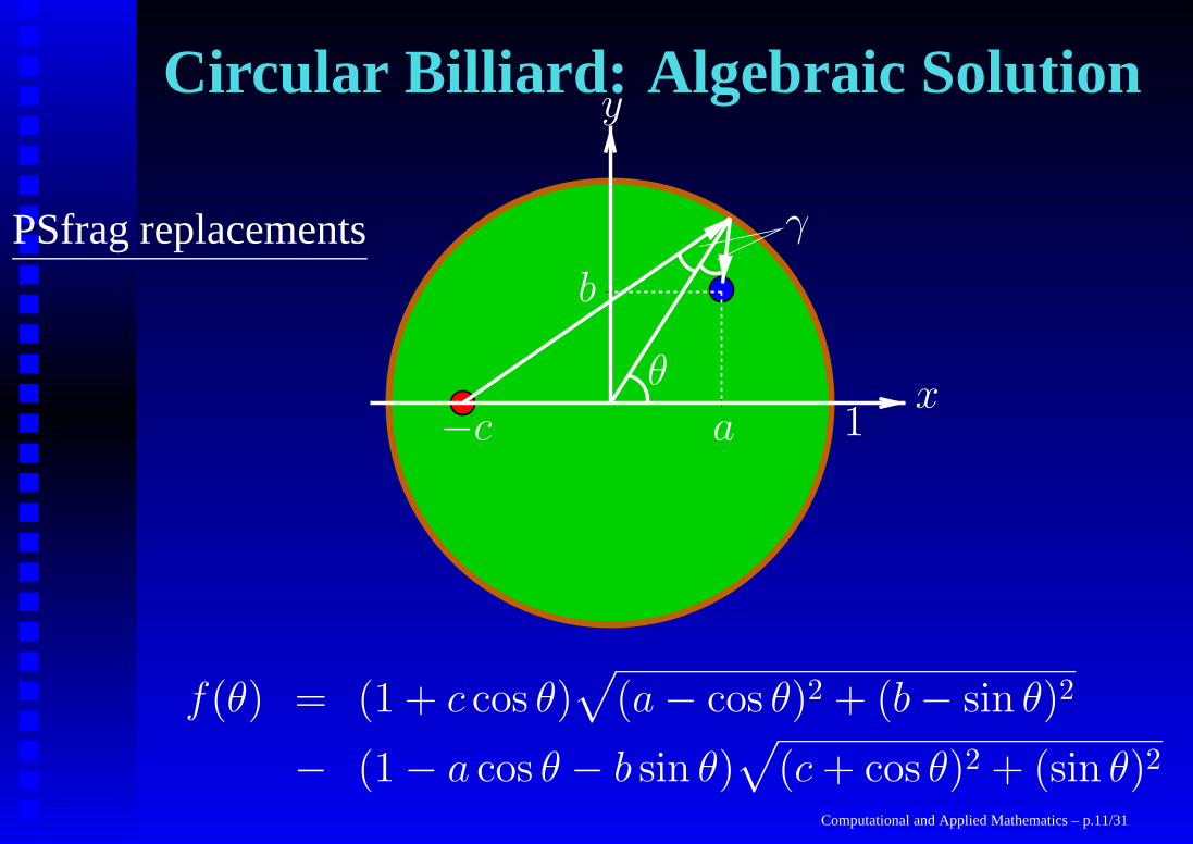
Circular Billiard: Algebraic Solution
PSfrag replacements γ
θx
y
−c a
b
1
f(θ) = (1 + c cos θ)√
(a − cos θ)2 + (b − sin θ)2
− (1 − a cos θ − b sin θ)√
(c + cos θ)2 + (sin θ)2
Computational and Applied Mathematics – p.11/31

Solution for the Given Example
0 1 2 3 4 5 6 7−0.3
−0.2
−0.1
0
0.1
0.2
0.3
0.4
PSfrag replacements
θ
f(θ
)
0.2
0.4
0.6
0.8
1
30
210
60
240
90
270
120
300
150
330
180 0
PSfrag replacements
θ
f(θ)
Are there always four solutions ?
Computational and Applied Mathematics – p.12/31

The Geometric Point of View
PSfrag replacements
1
x
y
e−e m1
m2
α
θ
We need to find an ellipse which touches the circle tan-
gentially.Computational and Applied Mathematics – p.13/31

Number of Solutions
An example with 4 solutions and one with 2 only.
Q(u) = (m2−m2m1)u4+(2m1−2m2
1+2e2+2m22)u
3+6u2m2m1
+ (−2m22 + 2m2
1 + 2m1 − 2e2)u − m2m1 − m2 = 0
where θ = 2 arctan(u). Q(u) is a 4th degreepolynomial, there can not be more than four solutions.
Computational and Applied Mathematics – p.14/31

Dependence on the Ball PositionA numerical experiment: fixing the position of oneball and varying the position of the second ball.Counting the number of solutions gives the grayshade:
Computational and Applied Mathematics – p.15/31

Dependence on the Ball Position
The separatrix (x,y) can be computed analytically (t parameter):
x(t)=−c
h
[
(1 + c)t6 + 3(1 + 3c)t4 + 3(1 − 3c)t2 + (1 − c)]
,
y(t) =16
hc2t3, h = (1 + 3c + 2c2)t6 + 3(1 + c + 2c2)t4+
+3(1 − c + 2c2)t2 + (1 − 3c + 2c2)
where c is the position of the fixed ball on the x axis.Computational and Applied Mathematics – p.16/31

Dependence on the Ball Position
Top view of a coffee mug with a point source of lightemulating the circular billiard game
(Drexler and G, SIAM review Vol. 40, No. 2, 1998)
Computational and Applied Mathematics – p.17/31

Digital Signal ProcessingA periodic signal f(t) can be decomposed into itsFourier components:
f(t) =∞
∑
k=−∞
fkeikt.
Discrete version: for the vector f of length n, wherefj := f(tj), tj = j∆t, ∆t = 2π/n, we have
fj =n−1∑
k=0
fkeiktj .
What if the signal is an image, or a piece of music?Computational and Applied Mathematics – p.18/31

Population Dynamics
Joint work with Antonio Steiner, Il Volterriano1997-2003
Computational and Applied Mathematics – p.19/31

The Lotka Volterra SystemWe consider rabbits and foxes living in a commonhabitat. If x denotes the rabbit population and y thefox population, the Lotka Volterra model states
x = x − xy
y = −y + xy
Approximating the derivative using its definition:
x(tn+1) − x(tn)
∆t= x(tn) − x(tn)y(tn)
y(tn+1) − y(tn)
∆t= −y(tn) + x(tn)y(tn)
We get a discrete dynamical system.Computational and Applied Mathematics – p.20/31

SolutionsThe exact solutions are cycles, but in general exact
solutions can not be found. Numerical solutionsspiral:
0 0.5 1 1.5 2 2.50
0.5
1
1.5
2
2.5
x
y
0 0.5 1 1.5 2 2.5 30
0.5
1
1.5
2
2.5
3
x
y
Computational and Applied Mathematics – p.21/31

A Symplectic MethodA very small change in the original method, instead of
x(tn+1) − x(tn)
∆t= x(tn) − x(tn)y(tn)
y(tn+1) − y(tn)
∆t= −y(tn) + x(tn)y(tn)
changing in the second line tn to tn+1,
x(tn+1) − x(tn)
∆t= x(tn) − x(tn)y(tn)
y(tn+1) − y(tn)
∆t= −y(tn) + x(tn+1)y(tn)
leads to a method for which one can prove that the
approximate solution is cyclic like the exact solution.Computational and Applied Mathematics – p.22/31

Success...
−1 0 1 2 3 4 5 60
0.5
1
1.5
2
2.5
3
3.5
4
The approximate solutions are also cycles, like the
mathematically exact or “biological” ones.Computational and Applied Mathematics – p.23/31

and Failure of the new method
−25 −20 −15 −10 −5 0 5 10−2
−1
0
1
2
3
4
−1 0 1 2 3 4 5 60
0.5
1
1.5
2
2.5
3
3.5
4
But here, in spite of the proof of cyclic behavior, the
method failed. On the right one can see why with the
zoom!
Computational and Applied Mathematics – p.24/31

So When does the Method Work?
0 0.5 1 1.5 2
0
0.5
1
1.5
2
The boundary beteween where the method works andwhere it does not is very complicated: it is a fractal.
Computational and Applied Mathematics – p.25/31

Room Temperature in Montreal
∂u
∂t(x, t) =
∂2u
∂x2(x, t)+
∂2u
∂y2(x, t)+
∂2u
∂z2(x, t)+f(x, t)
Room temperaturein our living roomin Montreal (outsidetemperature up to -47degrees): the heat equa-tion.
Insulated walls, notwell insulated windowsand doors.
Computational and Applied Mathematics – p.26/31
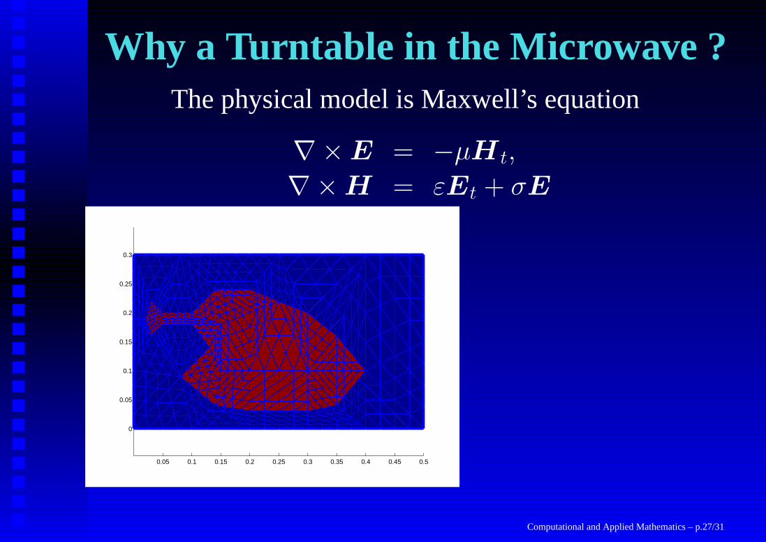
Why a Turntable in the Microwave ?The physical model is Maxwell’s equation
∇× E = −µH t,
∇× H = εEt + σE
0.05 0.1 0.15 0.2 0.25 0.3 0.35 0.4 0.45 0.5
0
0.05
0.1
0.15
0.2
0.25
0.3
0.05 0.1 0.15 0.2 0.25 0.3 0.35 0.4 0.45 0.5
0
0.05
0.1
0.15
0.2
0.25
0.3
Computational and Applied Mathematics – p.27/31
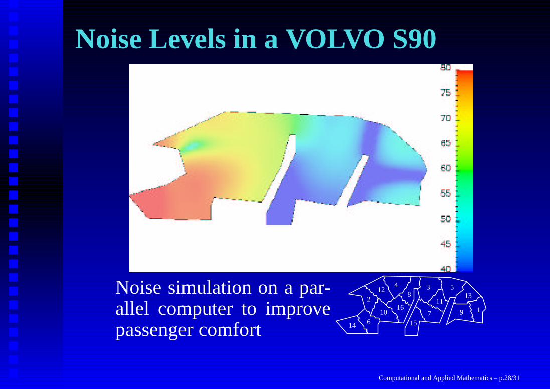
Noise Levels in a VOLVO S90
Noise simulation on a par-allel computer to improvepassenger comfort
1
212
4 3 513
9
15
11
716
10
14 6
8
Computational and Applied Mathematics – p.28/31

Radiation Therapy for Cancer
For cancer treatment it is important to have a very pre-
cise model of the body part that will be exposed to ra-
diation.Computational and Applied Mathematics – p.29/31

Aircraft Industry: B-747 in Flight
Simulation of a B-747 flying through athunderstorm, com-putation of the iceaccumulation on thewings and aroundthe engine intake.
Computational and Applied Mathematics – p.30/31

The Fundamental Role of CAM
0.1
0.2
0.3
0.4
0.5
0.6
0.7
0.8
0.9
0 0.2 0.4 0.6 0.8 10
0.1
0.2
0.3
0.4
0 0.5 1 1.5 2
0
0.5
1
1.5
2
− Fluid Dynamics
− Radiation− Particle Physics
− Aero Dynamics
Engineering:
− Active Noise Cancellation− Cellular Phone Systems
− Population Dynamics− Antibiotics− Micromachines
Physics:
Applied Mathematics
Pure Mathematics:− Geometry− Asymptotics− Existence
ANDComputational
Biology:
− Circuits Simulation
See also: www.math.mcgill.ca/mganderComputational and Applied Mathematics – p.31/31


![1.5 Installation Manual Version 0.5[1]](https://img.pdfslide.net/doc/110x75/577d36c81a28ab3a6b940224/15-installation-manual-version-051.jpg)
