Embed Size (px)
Citation preview

Computational Approaches to Modeling the Conserved
Structural Core Among Distantly Homologous Proteins
by
Matthew Ewald Menke
Submitted to the Department of Electrical Engineering and ComputerScience
in partial fulfillment of the requirements for the degree of
Doctor of Philosophy in Computer Science
at the
MASSACHUSETTS INSTITUTE OF TECHNOLOGY
September 2009
© Massachusetts Institute of Technology 2009. All rights reserved.
ARCHIVES
AuthorDepartment of Electrical Engineering and Computer Science
August 19, 2009
Certified byBonnie Berger
Professor of Applied MathematicsThesis Supervisor
/7 /-,
Accepted by......Professor Terry P. Orlando
Chair, Department Committee on Graduate Students
MASSACHUSETTS INSTr'IJTEOF TECHNOLOGY
SEP 3 0 2009
LIBRARIES


Computational Approaches to Modeling the Conserved Structural
Core Among Distantly Homologous Proteins
by
Matthew Ewald Menke
Submitted to the Department of Electrical Engineering and Computer Scienceon May 29, 2009, in partial fulfillment of the
requirements for the degree ofDoctor of Philosophy in Computer Science and Engineering
Abstract
Modem techniques in biology have produced sequence data for huge quantities of proteins,and 3-D structural information for a much smaller number of proteins. We introduce severalalgorithms that make use of the limited available structural information to classify and an-notate proteins with structures that are unknown, but similar to solved structures. The firstalgorithm is actually a tool for better understanding solved structures themselves. Namely,we introduce the multiple alignment algorithm Matt (Multiple Alignment with Transla-tions and Twists), an aligned fragment pair chaining algorithm that, in intermediate steps,allows local flexibility between fragments. Matt temporarily allows small translations androtations to bring sets of fragments into closer alignment than physically possible underrigid body transformation. The second algorithm, BetaWrapPro, is designed to recognizesequences of unknown structure that belong to specific all-beta fold classes. BetaWrap-Pro employs a "wrapping" algorithm that uses long-distance pairwise residue preferencesto recognize sequences belonging to the beta-helix and the beta-trefoil classes. It useshand-curated beta-strand templates based on solved structures. Finally, SMURF (Struc-tural Motifs Using Random Fields) combines ideas from both these algorithms into a gen-eral method to recognize beta-structural motifs using both sequence information and long-distance pairwise correlations involved in beta-sheet formation. For any beta-structuralfold, SMURF uses Matt to automatically construct a template from an alignment of solved3-D structures. From this template, SMURF constructs a Markov random field that com-bines a profile hidden Markov model together with pairwise residue preferences of thetype introduced by BetaWrapPro. The efficacy of SMURF is demonstrated on three beta-propeller fold classes.
Thesis Supervisor: Bonnie BergerTitle: Professor of Applied Mathematics

Acknowledgments
I am grateful to Lenore Cowen for her help in designing, and, particularly, in evaluating
and writing up the algorithms discussed in this paper.
Many thanks to my advisor, Bonnie Berger, for all her technical guidance and finding
me funding for all these years. Thanks also to Akamai, Merck, and the National Institute
of Health for providing the aforementioned funding.
I would also like to thank my parents for their financial and moral support and, more
importantly, for not repeatedly asking me when I was finally going to graduate.
I also want to thank Phil Bradley, Andrew McDonnell, Nathan Palmer, and Jonathan
King for their contributions to the development of the BetaWrap and BetaWrapPro algo-
rithms.
Roland L. Dunbrack, Jr. generously assisted with with SCWRL.
Much of the work in Chapter 2 of this thesis appeared as "Matt: Local Flexibility Aids
Protein Multiple Structure Alignment" in PLoS Computational Biology in 2008. Most of
Chapter 3 was published as "Prediction and comparative modeling of sequences directing
beta-sheet proteins by profile wrapping" in Proteins: Structure, Function, and Bioinfor-
matics in 2006, volume 63. Chapter 4 has yet to be published. I thank my coauthors for
their permission to include our joint work in this thesis.
I would also like to the members of my thesis committee.

Contents
1 Introduction
1.1 Protein Structural Alignment . ............
1.2 Protein Superfamily Recognition from Sequence . .
1.2.1 Protein Profile Hidden Markov Models . . .
1.2.2 Threading ...................
1.3 Our Contribution ...................
1.3.1 M att . . . . . . . . . . . . . . . . . . . . . .
1.3.2 BetaW rapPro .................
1.3.3 SM URF ....................
1.3.4 Conclusions ..................
2 Matt: Local Flexibility Aids Protein Multiple Structure
2.1 Introduction ......................
2.1.1 Performance Metrics . ............
2.1.2 Our Contribution . ..............
2.1.3 Related Work .................
2.1.4 Matt Implementation ..............
2.2 Algorithm Overview .................
2.3 Results. . .................. .....
2.3.1 The Benchmark Datasets . ..........
2.3.2 The Programs to Which Matt Is Compared
2.3.3 Performance .................
2.3.4 p-Value Calculation . .............
Alignment
. . . o..
.° .° . . °..

2.4 Methods.............
2.4.1 Pairwise alignment .
2.4.2 Multiple Alignment.
2.5 Discussion. ..........
3 BetaWrapPro
3.1 Introduction . . . . . . . . . . . . . . . . . . . .
3.2 The Algorithm . . . . . . . . . . . . . . . . . .
3.3 Results. .................... ....
3.3.1 Recognition and Alignment of Sequences
3.3.2 Comparison to Other Methods ......
3.3.3 Recognition of Unknown Sequences . . .
with Known
. . . ° . .
. . . ° . . .
3.4 Materials and Methods . . . . . . .
3.4.1 Sequence Databases . . . .
3.4.2 Pairwise Residue Databases
3.4.3 Structure Databases .....
3.4.4 Training and Testing . . . .
3.4.5 Running Time . . . . . . .
3.5 Discussion ..............
3.5.1 Biological Implications . . .
3.5.2 Web Server .........
4 An Integrated Markov Random Field Method for Recognizing Beta-Structural
Motifs
4.1 Introduction . . . . . . . . . . . . . . . . . . . . . . . . . . . . . . . . . .
4.2 A lgorithm . . . . . . . . . . . . . . . . . . . . . . . . . . . . . . . . . . .
4.3 R esults . . . . . . . . . . . . . . . . . . . . . . . . . . . . . . . . . . . . .
4.4 M ethods . . . . . . . . . . . . . . . . . . . . . . . . . . . . . . . . . . . .
4.5 D iscussion . . . . . . . . . . . . . . . . . . . . . . . . . . . . . . . . . . .
8
44
44
48
51
Structures
. . .
.° . °. °
~-l-X---- -----'*-'~-*-1XY- '"--*--L-'"~ _-~-jili~i.^*:-in~i.I-r;- ~--r~.^rs~---^ --- -r~----~--^rr~-^--r~-w~;i,_i~,,,i--~ -;I; =i;n4~-%.^;;xI~nllr ~1;-1-~,-~ -
5 Conclusions 87
5.1 Discussion and Future Work ......................... 87
A Pairwise Tables 89


List of Figures
1-1 HMMER hidden Markov model ........................ 19
2-1 Overview of the Matt algorithm ....................... 30
2-2 Matt SABmark performance tradeoff ................... .. 37
2-3 Matt Homstrad performance tradeoff ................... .. 38
2-4 Comparative beta-propeller alignment . .............. . . . . . 40
2-5 Comparative beta-helix alignment ................ . . . . . 41
2-6 Distinguishing alignable structures from decoys . .............. 42
2-7 Assembling sequential block pairs ................... ... 45
3-1 The beta-helix and beta-trefoil folds ................... .. 54
3-2 Side-chain packing example ......................... 62
4-1 A 7-bladed beta-propeller ................... ........ 75
4-2 HMMER hidden Markov model ....................... 76
4-3 Anti-parallel beta-strand dependencies . ................. .. 77
4-4 Template construction ............................ . 81

List of Tables
2.1 Homstrad performance comparison . . . . . . . . . . . . . . . . .
2.2 SABmark superfamily performance comparison . . . . . . . . . .
2.3 SABmark twilight zone performance comparison . . . . . . . . .
2.4 Sample multiple structure alignments from SABmark benchmark .
2.5 Discrimination performance on the SABmark superfamily set . . .
2.6 Discrimination performance on the SABmark twilight zone set . .
3.1
3.2
3.3
3.4
3.5
. . . . 36
. . . . 38
. . . . 38
. . . . 41
. . . . 43
Beta-helix cross-validation . . . . . . . . .
Beta-trefoil cross-validation . . . . . . . .
Beta-helix alignment accuracy comparison .
Beta-trefoil alignment accuracy comparison
New beta-helices ..............
4.1 Our results versus HMMer 3.0 . . . . . . . . . . . . . . . . . . . . . . .
4.2 Selected SMURF predictions . . . . . . . . . . . . . . . . . . . . . . . .
A. 1 Solvent inaccessible beta residue conditional probabilities . . . . . . . . .
A.2 Solvent accessible beta residue conditional probabilities . . . . . . . . . .
A.3 Solvent inaccessible twisted beta-strand residue conditional probabilities .
A.4 Solvent accessible twisted beta-strand residue conditional probabilities . .
A.5 Solvent inaccessible twisted beta-strand one-off residue conditional proba-
bilities . . . . . . . . . . . . . . . . . . . . . . . . . . . . . . . . . . . .
. . . 61
. . . 61
. . . 64
. . . 64
... 67


Chapter 1
Introduction
A single protein chain consists of an ordered set of the twenty different amino acids, typ-
ically from 50 to 1000 residues in length. Proteins are termed homologous if they share
a common evolutionary origin; since evolution was not observed over time, homology is
generally inferred by similarity. Homology can be inferred by sequence similarity when
proteins are evolutionarily close, but as their evolutionary relationship becomes more dis-
tance, direct inference of protein homology from sequence can become difficult. However,
when 3-D structural information is also available, it can be easier to classify proteins. Pro-
teins whose folded 3-D structure is known are termed solved protein structures.
The solved protein structures have been grouped together in hierarchical classification
schemes such as the Structural Classification of Proteins (SCOP) [73] and CATH (Class,
Architecture, Topology, Homologous superfamily) [76]. At the top level of the SCOP
hierarchy, proteins are subdivided based on their predominant type of secondary structure:
predominantly alpha, predominantly beta, or a combination of the two. Within these broad
groups, there is a further subdivision into the fold, superfamily, and family levels of the
SCOP hierarchy. Each successive level contains proteins that share progressively greater
structural similarity.
In SCOP, at the 'family' level, this translates into a sufficient level of sequence similar-
ity to clearly indicate an evolutionary relationship. The level of pairwise sequence identity
at the family level is generally 30% or greater. At the 'superfamily' level, sequence identity
is significantly lower, but structural and functional similarities indicate a probable common

ancestor. Proteins in the same 'fold' have the same basic arrangement of secondary struc-
ture, but may have significant differences in intervening regions. Such proteins may not
have an evolutionary relationship.
This thesis is largely concerned with the goals of recognizing, and aligning proteins that
belong to the same SCOP superfamily or fold class. We consider two main subproblems: 1)
aligning proteins in the same superfamily whose three-dimensional structures are known,
so that the similar parts are matched, and 2) predicting when a protein whose sequence
is known but whose structure is not should be placed in the same superfamily as a set
of proteins whose 3-D structure is known. In some cases, we not only recognize that
the protein folds into the appropriate family, but we also predict the sequence-structure
alignment.
1.1 Protein Structural Alignment
The problem of constructing accurate protein multiple structure alignments has been stud-
ied in computational biology almost as long as the better-known multiple sequence align-
ment problem [71]. The main goal for both problems is to provide an alignment of residue-
residue correspondences in order to identify homologous residues. When applied to closely
related proteins, sequence-based and structure-based alignments typically give consistent
answers even though most sequence alignment methods are measuring statistical models
of amino acid substitution rates, whereas most structure-based methods are seeking to su-
perimpose alpha-carbon atoms from corresponding backbone 3-D coordinates while mini-
mizing geometric distance. However, as has been known for some time [15], these answers
can diverge when aligning distantly related proteins; most relevant, it is still possible to find
good structural alignments when sequence similarity has evolutionarily diverged into "the
twilight zone" [83]. In the twilight zone, distantly related proteins can still share a common
core structure containing regions, including conserved secondary-structure elements and
binding sites, in which the chains retain the folding topology (see [25] for a recent survey).
Structural information can align the residues in this common core, even after the sequences
have diverged too far for successful sequence-based alignment, because structural similar-
~~~~-

ity is typically more evolutionarily conserved [1, 28, 106]. (While divergent sequence with
conserved structure is the typical case and the one that structural alignment algorithms that
respect backbone order such as Matt seek to handle, there are also well-known examples
where structure has diverged more rapidly than sequence; see, for example, Kinch and
Grishin [55] and Grishin [37].)
Applications of multiple structure alignment programs include understanding evolu-
tionary conservation and divergence, functional prediction through the identification of
structurally conserved active sites in homologous proteins [42], construction of bench-
mark datasets on which to test multiple sequence alignment programs [28], and automatic
construction of profiles and threading templates for protein structure prediction [25, 78].
It has also recently been suggested that multiple structure alignment algorithms may soon
become an important component in the best multiple sequence alignment programs. As
more protein structures are solved, there is an ever-increasing chance that a given set of
sequences to be aligned will contain a subset with structural information available. To
date, however, only a handful of multiple sequence alignment programs are set up to take
advantage of any available structural data [28, 77].
Pairwise structure alignment programs fall into three broad classes: the first class, to
which Matt belongs, are aligned fragment pair (AFP) chaining methods [91, 110] which do
an all-against-all best transformation of short protein fragments from one protein structure
onto another, and then assemble these in a geometrically consistent fashion. The second
class (which includes the popular Dali [40]), look at pairwise distances or contacts within
each structure separately, then try to find a maximum set of corresponding residues that
obey the same distance or contact relationships in pairs of structures- these are called dis-
tance matrix or contact map methods. The third class consists of everything else, from
geometric hashing [74] borrowed from computer vision to an abstraction of the problem to
secondary structural elements [23]. Some protein structure alignment programs are non-
sequential; that is, they allow residue alignments that are inconsistent with the linear pro-
gression of the protein sequence [24, 57, 107, 115]. Most enforce an alignment consistent
with the sequential ordering of the residues along the backbone- Matt belongs to the class
of sequential protein aligners. There are strengths to both approaches: most useful protein
alignments are sequential; however, non-sequential protein aligners can handle cases where
there is a reordering of domains, and circular permutations [37].
Multiple structure alignment programs are typically built on top of pairwise structural
alignment programs. Even simplified variants of structure alignment are known to be NP-
hard [35, 105]; important progress has been recently been made in theoretically rigorous
approximation guarantees [59] for pairwise structural alignment using a class of single opti-
mality criteria scores such as the Structal score [71], and also in provably fast parameterized
algorithms for the pairwise structural alignment problem in the non-sequential case [107].
1.2 Protein Superfamily Recognition from Sequence
We consider the following set of problems. Given a set of proteins from a particular SCOP
superfamily, can we predict if a new protein sequence, of unknown 3-D structure, also
belongs to the same SCOP superfamily?
If sequence similarity to one of the solved structures is high, this is an easy problem.
In fact, structural information need not be used at all. Protein sequence alignment algo-
rithms, such as BLAST [2] and ClustalW [102], attempt to align protein sequences directly
and return one or more of the highest scoring alignments using some metric. Generally,
the scoring function penalizes unaligned gap positions and rewards aligning similar amino
acids. Amino acid similarity can be calculated from a set of alignments assumed to be
correct. Designed for searching through large databases, BLAST looks for similar subse-
quences and extends them to longer sequence alignments. Slower dynamic programming
algorithms, such as ClustalW, tend to return better results. While these methods can be very
accurate when two proteins are in the same SCOP family, they can fail at the superfamily
level due to insufficient sequence similarity.
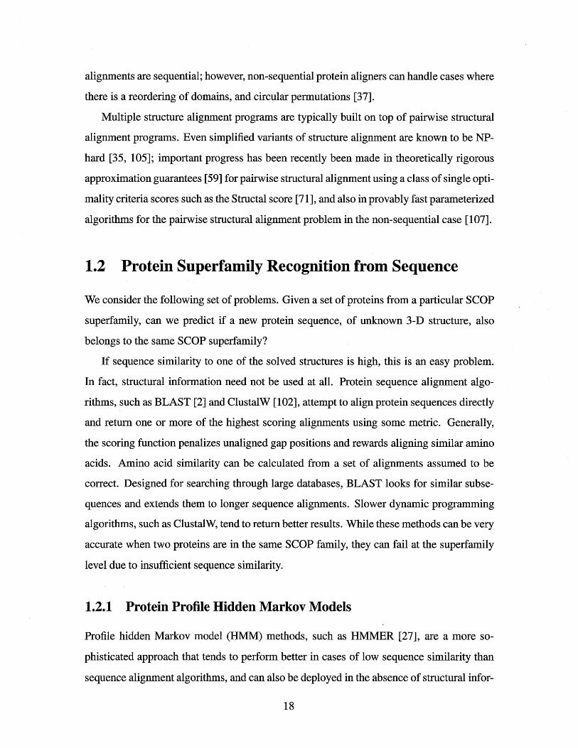
1.2.1 Protein Profile Hidden Markov Models
Profile hidden Markov model (HMM) methods, such as HMMER [27], are a more so-
phisticated approach that tends to perform better in cases of low sequence similarity than
sequence alignment algorithms, and can also be deployed in the absence of structural infor-
--" r--_-~~~~l l'ii~~*--ri;^ ~~ijr. ;;~; ;; ~;,-;-~-~-I---11 ;~~;~_:;i-;-~;~ll~F;-~-;ii-;~;; %;~ii ~"~-. I*;w"i--~--'ri~;;~;ii:-;~;i~l:~;;~~~~,-

Figure 1-1: HMMER hidden Markov model
HMM generated by HMMER, with states for matching multiple domains removed. Square states always
output a residue, round states never do. The grayed out states are removed from the model, as no paths from
Begin to End include them.
mation. Profile HMMs model a set of homologous proteins as a probabilistic walk through
a directed graph which generates member protein sequences. Each edge has a learned
probability of being taken. Some of the nodes, or states, output residues with a position-
dependent probabilities.
HMMER constructs a profile HMM as follows (see Figure 1-1): Given a multiple align-
ment of homologous protein sequences, pick the most highly conserved positions to use in
the HMM. For each of these positions, the model has three states: A match state, an in-
sertion state, and a deletion state. Each match state corresponds to the conserved position
itself, and has transitions to its own insertion state and the next position's match and dele-
tion states. The deletion state corresponds to a particular protein not containing any residue
in that particular position, and has transitions to the next match and deletion states. The
insertion state corresponds to the residues between one conserved position and the next,
and has transitions to itself and the next match state. Both the insertion and match states
always output a single residue, and the deletion state outputs no residue. The HMM also
has begin and end states. The begin state has a transition to each of the match states, and
each of the match states has a transition to the end state. Both the transition probabilities
and the probabilities of outputting each of the 20 residues at each insertion and match state
are calculated based on the input alignment. In general, a profile HMM is any HMM with
match, insertion, and deletion states arranged as described above with position-specific

residue output probabilities. HMMer also uses five other states that allow it to recognize
multiple instances of the motif in a single protein sequence.
After constructing a profile HMM, HMMER uses both the Viterbi and forward algo-
rithms [104, 82] to calculate the probability of the HMM generating a given sequence. The
Viterbi algorithm returns the path through the HMM most likely to generate a specific se-
quence, along with its probability. The path taken corresponds to an alignment of the input
sequence to the original multiple sequence alignment. The slower Forward algorithm re-
turns the probability that any path through the HMM returns the input sequence. HMMER
3.0 uses the score of the Viterbi algorithm as a filter to determine whether or not to run the
Forward algorithm.
1.2.2 Threading
While the above methods only require sequence information, threading methods make use
of protein structural information in order to identify even more distantly homologous pro-
teins. Currently, the most successful methods for fold recognition at the superfamily level
of similarity fall within the paradigm of protein threading [48, 14, 45, 93, 108]. In the
most general sense, protein threading algorithms work by searching for the higest-scoring
alignment of a sequence of unknown structure onto the previously solved structure of an-
other protein. Ideally a threading algorithm is sensitive enough to not only give a yes/no
answer for the fold recognition problem, but also to generate sequence-structure alignment
and possibly a putative structure as well.
Some threaders use scoring functions that have no pairwise interaction component and
find the best fit using dynamic programming. Algorithms that use scoring functions with
pairwise components tend to perform better, but finding the best hit in the general case has
been proven to be NP-complete [61]. As a result, these threading methods tend to be quite
slow, particularly when threading onto tightly packed template structures.
Unfortunately, there is no general-purpose threading method that can reliably identify
even a large subset of SCOP superfamily classes.

1.3 Our Contribution
1.3.1 Matt
In Chapter 2 we introduce the program Matt ("Multiple Alignment with Translations and
Twists"), an AFP fragment chaining method for pairwise and multiple sequence alignment,
and test its performance on standard benchmark datasets. At the heart of our approach is
a relaxation of the traditional rigid protein backbone transformations for protein superim-
position, that allows protein structures flexibility to bend or rotate in order to come into
alignment. While flexibility has been introduced into the study of protein folding in the
context of docking [9, 26], and particularly for the modeling of ligand binding [62] and
most recently in decoy construction for ab initio folding algorithms [86, 92], it has only re-
cently been incorporated into general-purpose pairwise [87, 110] and multiple [111] struc-
ture alignment programs. There are two reasons it makes sense to introduce flexibility
into protein structure alignment: the first is the main reason that's been addressed in previ-
ous work, namely, proteins that do not align well by means of rigid body transformations
because their structures have been determined in different conformational states: a well-
known example is that the fold of a protein will change depending on whether it is bound
to a ligand or not [62]. Matt is designed to also address the second reason to introduce
flexibility into protein structure alignment, namely to handle structural distortions as we
align proteins whose structural environment becomes increasingly divergent outside the
conserved core.
1.3.2 BetaWrapPro
In Chapter 3 we introduce the program BetaWrapPro that recognizes, and gives sequence-
structure alignments for, proteins that are members of the single-stranded right-handed
pectin lyase-like beta-helix superfamily, and several beta-trefoil superfamilies. BetaWrap-
Pro uses sequence profiles, pairwise beta-strand hydrogen bonding preferences, and com-
parative modeling to recognize proteins that lie in these superfamilies. Given a sequence,
BetaWrapPro uses BLAST to create a sequence profile containing information about which
residues tend to align at each position of the input sequence. Dynamic programming
is then used to locate the highest scoring matches to a template consisting only of gap
length ranges and hydrogen-bonded beta-strands pairs. The score is the combination of
pairwise hydrogen-bonding propensities of residues in beta-strands, gap penalties, and
residue preferences learned from the proteins in the superfamily used to create the tem-
plate. The highest scoring hits are then threaded onto the backbone of known structures
using SCWRL [90], and those that are not good fits are removed. One important feature
of the BetaWrapPro algorithm is that the hydrogen-bonding propensities, which are the
primary component of the score, are learned from superfamilies other than the one be-
ing recognized. BetaWrapPro is a generalization of our previous work: BetaWrap [12]
and Wrap-and-Pack [69]- programs that introduced the threading method we employ with
scoring based on pairwise beta-strand hydrogen bonding preferences (Wrap-and-Pack is
Menke's masters thesis and he worked on BetaWrap as an undergraduate). BetaWrapPro
extends this to profiles, and by the incorporation of side-chain packing. It is shown that
BetaWrapPro performs better than HMMs or the Raptor [108] threader on recognition and
sequence-structure alignment of the beta-helices and beta-trefoils.
1.3.3 SMURF
Finally, in Chapter 4 we introduce SMURF ("Structural Motifs Using Random Fields"),
a method that uses Markov random fields (MRFs) [72], an extension of Markov models,
to train a model to identify a set of homologous proteins. SMURF uses the beta-strand
propensities much like BetaWrapPro, but learns the model autonomously and learns in-
dividual residue probabilities from the input alignment. Given a multiple structure align-
ment generated by Matt, SMURF generates a Markov random field much like the HMMs
generated by HMMER. The generated MRFs have match, insertion, and deletion states
with the same connections HMMs created by HMMER have. In addition, the MRF has
long-distance probability dependencies on match states corresponding to pairs of residues
hydrogen-bonded to each other across a beta-sheet. Because of these additional dependen-
cies, an HMM is no longer sufficient for the model. SMURF then trains the MRF just like
HMMer, though it uses the BetaWrapPro tables for pairwise emission probabilities of the
hydrogen-bonded beta residue pairs, because of sparse data. Sequences of unknown struc-
ture are then run against the MRF using dynamic programming, much like an HMM. The
pairwise dependencies between hydrogen bonded beta-strands can result in significantly
improved discrimination in predominantly beta structures. Because of the long range de-
pendencies, significantly more memory and computation time is needed by SMURF than
by HMM-based algorithms. We demonstrate that SMURF has significantly better perfor-
mance than ordinary HMM methods on the six, seven, and eight-bladed beta-propeller
folds.
1.3.4 Conclusions
We show in this thesis, that better structural alignments (Matt), capture of statistical de-
pendencies of hydrogen-bonded beta residue pairs, profiles, and extensions of HMMs to
a MRF framework can improve structural motif recognition for SCOP beta-structural su-
perfamilies. We discuss future work, limitations of the methods, and open problems in
Chapter 5.

Chapter 2
Matt: Local Flexibility Aids Protein
Multiple Structure Alignment
2.1 Introduction
Proteins fold into complicated highly asymmetrical 3-D shapes. When a protein is found
to fold in a shape that is sufficiently similar to other proteins whose functional roles are
known, this can significantly aid in predicting function in the new protein. In addition, the
areas where structure is highly conserved in a set of such similar proteins may indicate
functional or structural importance of the conserved region. Given a set of protein struc-
tures, the protein structural alignment problem is to determine the superimposition of the
backbones of these protein structures that places as much of the structures as possible into
close spatial alignment.
We introduce an algorithm that allows local flexibility in the structures which allows it
to bring them into closer alignment. The algorithm performs as well as its competitors when
the structures to be aligned are highly similar, and outperforms them by a larger and larger
margin as similarity decreases. In addition, for the related classification problem that asks if
the degree of structural similarity between two proteins implies if they likely evolved from
a common ancestor, a scoring function assesses, based on the best alignment generated for
each pair of protein structures, whether they should be declared sufficiently structurally
similar or not. This score can be used to predict when two proteins have sufficiently similar

shapes to likely share functional characteristics.
2.1.1 Performance Metrics
There are two related problems that protein structure alignment programs are designed to
address. The first we will call the alignment problem, where the input is a set of k proteins
that have a conserved structural common core, where the common core is defined as in
Eidhammer et al. [29] as a set of residues that can be simultaneously superimposed with
small structural variation. The desired output consists of a superimposition of the proteins
in 3-D space, coupled with the list of which amino acid residues are declared to be in
alignment and part of the core. The second problem, which we will call the discrimination
problem, takes as input a pair of protein structures, and the output a yes/no answer, together
with an associated score or confidence value, as to whether a good alignment can be found
for these two protein structures or not. We discuss how to measure performance on the
alignment problem first, and then on the discrimination problem below.
The classical geometric way to measure the quality of a protein structural alignment
involves two parameters: the number of amino acid residue positions that are found to
participate in the alignment (and are therefore found to be part of the conserved structural
core), as well as the average pairwise root mean squared deviation (RMSD) (where RMSD
is calculated from the best rigid body transformation using least squares minimization [52])
between backbone alpha-carbons placed in alignment in the conserved core. Clearly, this
is a bi-criteria optimization problem: the goal is to minimize the RMSD of the conserved
core while maximizing the number of residues placed in the conserved core.
We first take a traditional geometric approach: reporting for all programs and all bench-
mark datasets, the average number of residues placed into the common core structure,
alongside the average RMS of the pairwise RMSDs among all pairs of residues that partici-
pate in a multiple alignment of a set of structures. In addition, results are compared against
Homstrad reference alignments. This approach follows Godzik and Ye's evaluation of their
multiple structure alignment program, POSA [111].
More sophisticated geometric scoring measures have also been suggested, some to col-
lapse the bi-criteria optimization problem into a single score to be optimized [58], such as
the Structal score [71], others to incorporate more environmental information into the sim-
ilarity measure, such as secondary structure, or solvent accessibility [51, 99]. The p-value
score that we develop to handle the discrimination problem, described below, is a collapse
of the bi-criteria optimization problem into one score that provides a single lens on pairwise
alignment quality.
An alternative approach to measuring the performance of a structure alignment algo-
rithm comes from the discrimination problem directly. Here, the measure is typically re-
ceiver operating characteristic (ROC) curves; looking for the ratio of true and false positives
and negatives from a "gold-standard" classification for what is alignable or not, based either
on decoy structures or a classification scheme such as SCOP or CATH. Indeed, a possible
concern with adding flexibility to protein structure would be that the added flexibility in our
alignment might lead to an inability to distinguish structures that should have good align-
ments from those that do not. We therefore test our ability to distinguish true alignable
structures from decoys on the SABmark dataset (which comes with a ready-made set of
decoy structures) as compared to competitor programs.
2.1.2 Our Contribution
We introduce the program Matt (Multiple Alignment with Translations and Twists), an
AFP fragment chaining method for pairwise and multiple sequence alignment that out-
performs existing popular multiple structure alignment methods when tested on standard
benchmark datasets. At the heart of Matt is a relaxation of the traditional rigid protein
backbone transformations for protein superimposition, which allows protein structures flex-
ibility to bend or rotate in order to come into alignment. While flexibility has been intro-
duced into the study of protein folding in the context of docking [9, 26], particularly for
the modeling of ligand binding [62], and more recently in decoy construction for ab initio
folding algorithms [86, 92], it has only recently been incorporated into general-purpose
pairwise [87, 110] and multiple [111] structure alignment programs. There are two reasons
it makes sense to introduce flexibility into protein structure alignment. The first is the main

reason that has been addressed in previous work, namely, aligning proteins that do not align
well by means of rigid body transformations because their structures have been determined
in different conformational states: a well-known example is that the fold of a protein will
change depending on whether it is bound to a ligand or not [62]. Matt is designed to also
address the second reason to introduce flexibility into protein structure alignment, namely
to handle structural distortions as we align proteins whose shape becomes increasingly
divergent outside the conserved core.
We find that at each fixed value for number of aligned residues, Matt is competitive
with other recent multiple structure alignment programs in average RMSD on the popu-
lar Homstrad [70] and outperforms them on the SABmark [103] benchmark datasets (see
Tables 2.1, 2.2 and 2.3). We emphasize again that this is an apples-to-apples comparison
of the best (i.e., the standard least squares RMSD minimization) rigid body transformation
for Matt's alignments, just as it is for the other programs- while Matt allows impossible
bends and breaks in intermediate stages of the algorithm, it is stressed that the final Matt
alignments and RMSD scores come from legal, allowable "unbent" rigid body transforma-
tions. We also present RMSD/alignment length tradeoffs for Matt performance on the same
datasets. In the case of Homstrad, where a manually curated "correct" structural alignment
is made available as part of the benchmark, Matt alignments are also measured against
the reference alignments, where we are again competitive with or outperforming previous
structure alignment programs (see Table 2.1).
In addition, Matt's ability to distinguish truly alignable folds from decoy folds is tested
with the standard benchmark SABmark set of alignments and decoys [103]. The SABmark
decoy set was constructed to contain, for each alignable subset, decoy structures that belong
to a different SCOP superfamily, but whose sequences align reasonably well according to
BLAST [103]. Thus, they may be more similar at the local level to the true positive ex-
amples, and thus fool a structure alignment program better than a random structure. Here,
we tested both the "unbent" Matt alignments described above, but also the "bent" Matt
alignments, where the residues are aligned allowing the impossible bends and breaks. We
test Matt's performance both against the decoy set and also against random structures taken
from the Protein Data Bank (PDB; http://www.rcsb.org/pdb). We use Matt's performance

on the truly random structures to generate a p-value score for pairwise Matt alignments.
Rather than choose from among the large number of competitor pairwise structural align-
ment programs, Matt was instead tested against other multiple structure aligners, in fact
the same programs we used for measuring how well they aligned protein families known
to have good alignments. The exception was that we also tested the FlexProt program [87],
a purely pairwise structure alignment program that was of special interest because it also
claims to handle flexibility in protein structures.
We have made Matt's source code along with its structural alignments available at
http://groups.csail.mit.edu/cb/matt and http://matt.cs.tufts.edu so anyone can additionally
compute any alternate alignment quality scores they favor.
2.1.3 Related Work
The only general protein structure alignment programs that previously tried to model flexi-
bility are FlexProt [87] and Ye and Godzik's FATCAT [110] (both for pairwise alignment),
and FATCAT's generalization to multiple structure alignment, POSA [111]. FATCAT is
also an AFP chaining algorithm, except it allows a globally minimized number of transla-
tions or bends in the structure if it improves the overall alignment. In this way, it is able
to capture homologous proteins with hinges, or other discrete points of flexibility, due to
conformational change. Our program Matt is fundamentally different: it instead allows
flexibilities everywhere between short fragments- that is, it does not seek to globally min-
imize the number of bends, but rather allows continuous small local perturbations in order
to better match the "bent" RMSD between structures. Because Matt allows these flexi-
bilities, it can put strict tolerance limits on "bent" RMSD, so it only keeps fragments that
locally have very tight alignments. Up until the last step, Matt allows the dynamic pro-
gram to assemble fragments in ways that are structurally impossible- one chain may have
to break or rotate beyond the physical constraints imposed by the backbone molecules in
order to simultaneously fit the best transformation. This is repaired in a final step, when
the residue to residue alignment produced by this unrealistic "bent" transformation is re-
tained; the best rigid-body transformation that preserves that alignment is found, and then
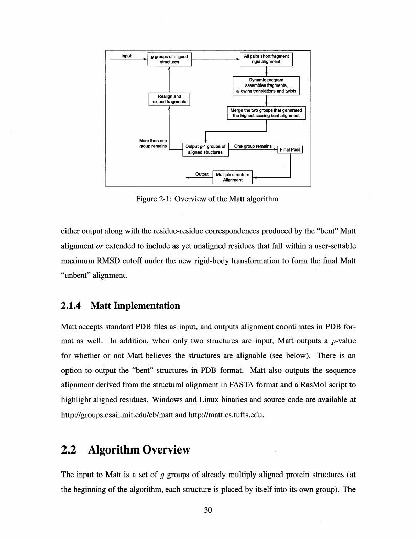
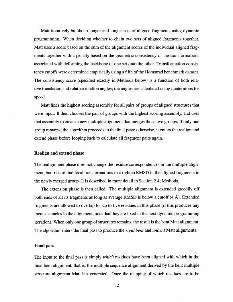
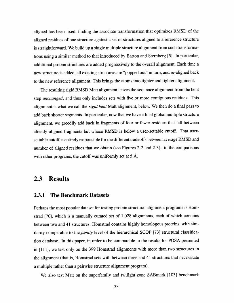
Figure 2-1: Overview of the Matt algorithm
either output along with the residue-residue correspondences produced by the "bent" Matt
alignment or extended to include as yet unaligned residues that fall within a user-settable
maximum RMSD cutoff under the new rigid-body transformation to form the final Matt
"unbent" alignment.
2.1.4 Matt Implementation
Matt accepts standard PDB files as input, and outputs alignment coordinates in PDB for-
mat as well. In addition, when only two structures are input, Matt outputs a p-value
for whether or not Matt believes the structures are alignable (see below). There is an
option to output the "bent" structures in PDB format. Matt also outputs the sequence
alignment derived from the structural alignment in FASTA format and a RasMol script to
highlight aligned residues. Windows and Linux binaries and source code are available at
http://groups.csail.mit.edu/cb/matt and http://matt.cs.tufts.edu.
2.2 Algorithm Overview
The input to Matt is a set of g groups of already multiply aligned protein structures (at
the beginning of the algorithm, each structure is placed by itself into its own group). The
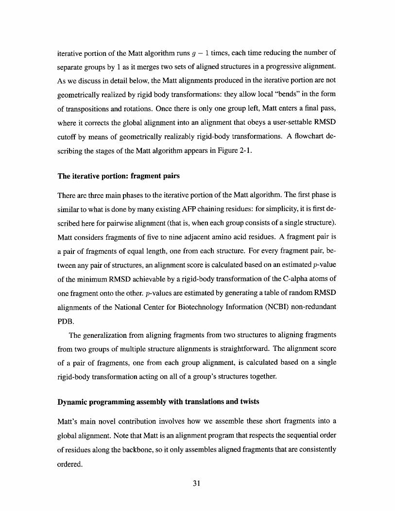
iterative portion of the Matt algorithm runs g - 1 times, each time reducing the number of
separate groups by 1 as it merges two sets of aligned structures in a progressive alignment.
As we discuss in detail below, the Matt alignments produced in the iterative portion are not
geometrically realized by rigid body transformations: they allow local "bends" in the form
of transpositions and rotations. Once there is only one group left, Matt enters a final pass,
where it corrects the global alignment into an alignment that obeys a user-settable RMSD
cutoff by means of geometrically realizably rigid-body transformations. A flowchart de-
scribing the stages of the Matt algorithm appears in Figure 2-1.
The iterative portion: fragment pairs
There are three main phases to the iterative portion of the Matt algorithm. The first phase is
similar to what is done by many existing AFP chaining residues: for simplicity, it is first de-
scribed here for pairwise alignment (that is, when each group consists of a single structure).
Matt considers fragments of five to nine adjacent amino acid residues. A fragment pair is
a pair of fragments of equal length, one from each structure. For every fragment pair, be-
tween any pair of structures, an alignment score is calculated based on an estimated p-value
of the minimum RMSD achievable by a rigid-body transformation of the C-alpha atoms of
one fragment onto the other. p-values are estimated by generating a table of random RMSD
alignments of the National Center for Biotechnology Information (NCBI) non-redundant
PDB.
The generalization from aligning fragments from two structures to aligning fragments
from two groups of multiple structure alignments is straightforward. The alignment score
of a pair of fragments, one from each group alignment, is calculated based on a single
rigid-body transformation acting on all of a group's structures together.
Dynamic programming assembly with translations and twists
Matt's main novel contribution involves how we assemble these short fragments into a
global alignment. Note that Matt is an alignment program that respects the sequential order
of residues along the backbone, so it only assembles aligned fragments that are consistently
ordered.
Matt iteratively builds up longer and longer sets of aligned fragments using dynamic
programming. When deciding whether to chain two sets of aligned fragments together,
Matt uses a score based on the sum of the alignment scores of the individual aligned frag-
ments together with a penalty based on the geometric consistency of the transformations
associated with deforming the backbone of one set onto the other. Transformation consis-
tency cutoffs were determined empirically using a fifth of the Homstrad benchmark dataset.
The consistency score (specified exactly in Methods below) is a function of both rela-
tive translation and relative rotation angles; the angles are calculated using quaternions for
speed.
Matt finds the highest scoring assembly for all pairs of groups of aligned structures that
were input. It then chooses the pair of groups with the highest scoring assembly, and uses
that assembly to create a new multiple alignment that merges those two groups. If only one
group remains, the algorithm proceeds to the final pass; otherwise, it enters the realign and
extend phase before looping back to calculate all fragment pairs again.
Realign and extend phase
The realignment phase does not change the residue correspondences in the multiple align-
ment, but tries to find local transformations that tighten RMSD in the aligned fragments in
the newly merged group. It is described in more detail in Section 2.4, Methods.
The extension phase is then called. The multiple alignment is extended greedily off
both ends of all its fragments as long as average RMSD is below a cutoff (4 A). Extended
fragments are allowed to overlap for up to five residues in this phase (if this produces any
inconsistencies in the alignment, note that they are fixed in the next dynamic programming
iteration). When only one group of structures remains, the result is the bent Matt alignment.
The algorithm enters the final pass to produce the rigid bent and unbent Matt alignments.
Final pass
The input to the final pass is simply which residues have been aligned with which in the
final bent alignment; that is, the multiple sequence alignment derived by the bent multiple
structure alignment Matt has generated. Once the mapping of which residues are to be
aligned has been fixed, finding the associate transformation that optimizes RMSD of the
aligned residues of one structure against a set of structures aligned to a reference structure
is straightforward. We build up a single multiple structure alignment from such transforma-
tions using a similar method to that introduced by Barton and Sternberg [5]. In particular,
additional protein structures are added progressively to the overall alignment. Each time a
new structure is added, all existing structures are "popped out" in turn, and re-aligned back
to the new reference alignment. This brings the atoms into tighter and tighter alignment.
The resulting rigid RMSD Matt alignment leaves the sequence alignment from the bent
step unchanged, and thus only includes sets with five or more contiguous residues. This
alignment is what we call the rigid bent Matt alignment, below. We then do a final pass to
add back shorter segments. In particular, now that we have a final global multiple structure
alignment, we greedily add back in fragments of four or fewer residues that fall between
already aligned fragments but whose RMSD is below a user-settable cutoff. That user-
settable cutoff is entirely responsible for the different tradeoffs between average RMSD and
number of aligned residues that we obtain (see Figures 2-2 and 2-3)- in the comparisons
with other programs, the cutoff was uniformly set at 5 A.
2.3 Results
2.3.1 The Benchmark Datasets
Perhaps the most popular dataset for testing protein structural alignment programs is Hom-
strad [70], which is a manually curated set of 1,028 alignments, each of which contains
between two and 41 structures. Homstrad contains highly homologous proteins, with sim-
ilarity comparable to the family level of the hierarchical SCOP [73] structural classifica-
tion database. In this paper, in order to be comparable to the results for POSA presented
in [111], we test only on the 399 Homstrad alignments with more than two structures in
the alignment (that is, Homstrad sets with between three and 41 structures that necessitate
a multiple rather than a pairwise structure alignment program).
We also test Matt on the superfamily and twilight zone SABmark [103] benchmark

datasets. The superfamily set contains 3,645 domains sorted into 426 subsets represent-
ing structures at the superfamily level of the SCOP hierarchy, a set designed to be well-
distributed in known protein space, and presumably containing more remote homologs than
Homstrad. The twilight zone set contains 1,740 domains sorted into 209 subsets whose ho-
mology is even more remote than the superfamily set. Both the superfamily and twilight
zone sets have subsets containing between three and 25 structures.
Since the "correct" alignments provided by SABmark are generated automatically from
existing structure alignment programs, we do not report the percentage of "correctly"
aligned residue pairs as we did for the manually curated Homstrad, but rather report only
the objective geometric measures of alignment quality (number of residues placed in the
conserved core, and average pairwise RMSD among residues placed in the combined core).
SABmark additionally provides a set of decoy structures for nearly all its 462 sets of
alignable superfamily (and 209 alignable twilight zone) sets of structures. We constructed
a decoy discrimination test suite as follows. Each SABmark superfamily (or twilight zone)
test set comes with an equal number of decoy structures with high sequence similarity
(see [103]). For each test set, a random pair of structures in the positive set (that belong to
the same SCOP superfamily and are supposed to align) and a random decoy was selected.
Then a random discrimination test suite was similarly constructed, the only difference be-
ing that the decoy was chosen to be a random structure in a different SABmark set, not a
decoy structure that was specifically chosen to have high sequence similarity to the positive
set.
2.3.2 The Programs to Which Matt Is Compared
On Homstrad, we compare Matt to three recent multiple structure alignment programs:
listed in alphabetical order, they are MultiProt [88], Mustang [60], and POSA [111]. Note
that MultiProt has sequential and non-sequential alignment options; we compare against
the option that, like Matt, respects sequence order. MultiProt is an AFP program that uses
rigid body superimposition. Mustang uses a combination of short fragment alignment, con-
tact maps, and consensus-based methods. We were particularly eager to test Matt against
i
POSA, because it is the only other multiple structure alignment program that allows flex-
ibility, though as discussed in the Introduction, POSA's flexibility is more limited. POSA
outputs two different structural alignments: one comes from the version of POSA that dis-
allows bends, and the other from the version with limited bends allowed. We test both
versions, and results appear in Table 2.1.
We were not able to obtain POSA code. (Our statistics on Homstrad come from POSA
alignments provided by the authors as supplementary data). Because we were not able to
obtain POSA code, we were not able to test POSA on all of SABmark, but we do compare
Mustang and MultiProt to Matt on the entire SABmark benchmark. On the other hand,
we were able to submit individual sets of SABmark structures to the POSA online server;
POSA sometimes did nearly as well as Matt on the examples we tested, but other times, it
missed finding alignable structures entirely. We show both cases in two in-depth examples:
Figure 2-4 shows alignments of Matt, MultiProt, Mustang, and POSA on a seven-bladed
beta-propeller, and Figure 2-5 shows alignments of the four programs on a set of left-
handed beta-helix structures. POSA and Matt are the only algorithms that successfully
align all seven blades of the beta-propeller. POSA, however, entirely misses the alignable
regions in the beta-helix fold.
For the discrimination problem, Matt is compared against MultiProt and Mustang again,
but also against FlexProt [87]. FlexProt has an option to allow from zero to four bends in
the aligned structure, which is specified at runtime. FlexProt scores each of these structures
by length of the alignment found. On each structure, the alignment with the number of
bends that produces the highest-scoring alignment is output. In the case of both POSA
and FlexProt, the "bent" alignment outputs the (best rigid-body transformation) RMSD of
the aligned structures with bends allowed, and the "unbent," or regular, version outputs
the RMSD of the best rigid-body transformation that places the same set of residues in
alignment as the bent version.

Program Name Average Core Size Average Normalized Correct Pairs Average RMSDMultiProt 142.331 132.350 1.347Mustang 171.363 155.932 2.669
POSA (unbent) 165.160 152.475 2.004POSA (bent) 167.847 154.482 2.224
Matt 172.276 155.352 2.044
Table 2.1: Homstrad performance comparison
2.3.3 Performance
Table 2.1 shows the following quantities for each program on the 399 Homstrad reference
alignments that contain at least three structures each (this is the identical set of reference
alignments on which POSA was tested). The first field is the average number of residues
placed in the common core. The second is "average normalized correct pairs" computed
according to the Homstrad reference alignments. This quantity is computed as follows: for
each set of structures, we look at every pair of aligned residues that also participate in a
Homstrad correct alignment. Then, we normalize based on the number of structures in the
set (so the alignments in the set of 41 structures do not weight more heavily than the align-
ments in the set of three structures), dividing by the number of pairs of distinct structures in
the reference set. (Note that, as discussed in [60], having additional pairs placed into align-
ment that Homstrad does not consider part of the "gold-standard" alignment is a positive,
not a negative, if RMSD remains low. This is because declaring a pair of nearly aligned
residues "aligned" or not is a judgment call that Homstrad makes partially based on older
multiple structure alignment programs whose performance is weaker than the most recent
programs.) The second column is the same "average RMSD" measure that POSA reports:
the average RMS of the pairwise RMSDs among all pairs of residues that participate in a
multiple alignment in a set of structures.
We downloaded and ran MultiProt and Mustang and computed RMSD statistics our-
selves. POSA is only accessible as a web server; however, Homstrad alignments are
available online at http://fatcat.bumham.org/POSA/POSAvsHOM.html. POSA's website
provides two sets of multiple alignments: one derived from running their algorithm allow-
ing geometrically impossible bends, and one running an unbent version of their algorithm.
Note that for POSA's bent alignments, we had to recalculate RMSD from the multiple se-

2.8
2.7
2.6
2.5
2.1
2
80 85 90 95 100 105
Aligned residues
Figure 2-2: Matt SABmark performance tradeoff
Average pairwise RMSD versus average number of residue positions placed in the common core.
quence alignment provided from their bent alignments, because unbent RMSD based on
bent alignments was not provided on their website. It is of independent interest that, as
expected, POSA's unbent version has better RMSD, while POSA's bent version finds more
residues participating in the alignments overall.
Matt scores slightly better than POSA on Homstrad. Matt's average core size is com-
parable with that of Mustang, but Matt has a lower RMSD. The size of the alignments that
MultiProt finds are much smaller than for the other programs (though its average RMSD is
therefore much lower): this becomes even more pronounced on the more distant structures
in SABmark (see Figure 2-2). Note that the core-size/RMSD tradeoff of Matt is very sen-
sitive to cutoffs set in the last pass of the Matt algorithm, when it is decided what segments
of less than five consecutive residues are added back into the alignment. Throughout this
paper, the results reported in our tables come from setting the cutoff at 5 A. By compari-
son, if the cutoff is set at 3.5 A, Matt achieves 168.038 average core size, 153.362 average
normalized pairs correct, and 1.862 average RMSD on Homstrad. Full tradeoff results on
RMSD versus number of residues based on changing the last pass cutoff appear in Fig-
ure 2-3. Note that Matt's cutoffs for allowable bends were trained on a random 20% of the
Homstrad dataset.

2-
t1.7
150 155 160 165 170 175
Aligned residues
Figure 2-3: Matt Homstrad performance tradeoff
Average pairwise RMSD versus average number of residue positions placed in the common core
Program Name Average Core Size Average RMSDMultiProt 68.701 1.498Mustang 104.162 4.146
Matt 104.692 2.639
Table 2.2: SABmark superfamily performance comparison
Program Name Average Core Size Average RMSDMultiProt 36.354 1.536Mustang 66.833 5.035
Matt 66.967 2.916
Table 2.3: SABmark twilight zone performance comparison
While Matt competes favorably with the other programs on Homstrad, Matt was de-
signed for sets of more distantly related proteins than appear in the Homstrad benchmark.
Thus, the best demonstration of the advantage of the Matt approach appears on the more
distantly related proteins in the SABmark benchmark sets. Here, Matt is seen to do exactly
what was hoped: by detouring through bent structures, it finds rigid RMSD alignments
that place as many residues in the conserved alignment as Mustang does (and more than
50% more than MultiProt does) while reducing the average RMSD from that of Mustang
by more than 1.4 A (see Tables 2.2 and 2.3). It should again be emphasized that none of
Matt's parameters were trained on SABmark.
Looking by hand through the alignments, MultiProt consistently aligns small subsets of
residues correctly, but leaves large regions unaligned that both Mustang and Matt believe
to be alignable. Mustang, on the other hand, frequently misaligns regions, particularly in
the case when there are many alpha-helices tightly packed in the structure. On two of the
twilight zone sets, Mustang fails to find anything in the common core. Altogether on the
twilight zone set, there are four sets of structures for which Mustang fails to find at least
three residues in the common core (and there is one set of structures in the superfamily
set where Mustang also fails to find anything in the common core). Though the effect is
negligible, these four sets are removed from Mustang's average RMSD calculation.
Although these tables show overall performance, it is also helpful to look at actual
examples. We pulled two example reference sets out of the SABmark superfamily bench-
mark. Figure 2-4 shows the Matt alignment versus MultiProt, POSA, and Mustang align-
ments of the SABmark structures in the set labeled Group 137 (beta-propellers; PDB IDs
dlnr0al, dlnr0a2, d1p22a2, and dltbga). POSA does second best to Matt here, and in fact,
the overall alignment of the structures in POSA is most similar to Matt- the same propeller
blades are overlaid in both alignments. Although it is hard to see in the picture, Mustang is
superimposing the wrong blades, which accounts for the terrible RMSD. MultiProt makes a
similar error, but then gets a low RMSD by aligning less of the structure. Figure 2-5 shows
a Matt alignment of the SABmark structures in the set labeled Group 144 (beta-helices;
PDB IDs dlhm9al, dlkk6a, dlkrra, dllxa, dlocxa, dlqrea, dlxat, and d3tdt). Here, POSA
does very poorly, only finding a very small set of residues to align. MultiProt again aligns

Figure 2-4: Comparative beta-propeller alignment
The four SABmark domains in the set Group 137, consisting of seven-bladed beta-propellers as aligned by
POSA, Mustang, MultiProt, and Matt. Backbone atoms that participate in the common core of the alignment
show up colored as red (PDB ID dlnr0al), green (PDB ID dlnr0a2), blue (PDB ID dlp22a2), and magenta
(PDB ID dltbga); residues in all four chains that are not placed into the alignment by the tested algorithm are
shown in gray. These pictures were generated by the Swiss PDB Viewer (DeepView) [38].
the portion that it declares in the common core very tightly (this is a theme throughout
the SABmark dataset), but it only places five rungs in the common core. Both these fig-
ures were generated using the Swiss PDB Viewer (DeepView) [38]. Core size and RMSD
comparisons on both these reference sets appear in Table 2.4.
We then turn to the discrimination problem. Matt, FlexProt, Mustang, and MultiProt
were tested on the SABmark superfamily and SABmark twilight zone decoy test suites
described in the previous section. Using a method similar to what Gerstein and Levitt [34]
did to systematically assess structure alignment programs against a gold standard, length of
alignment versus RMSD for the true positives and true negatives were plotted in the plane
r ~~- - -1 -7 ~1 --~- ------ i
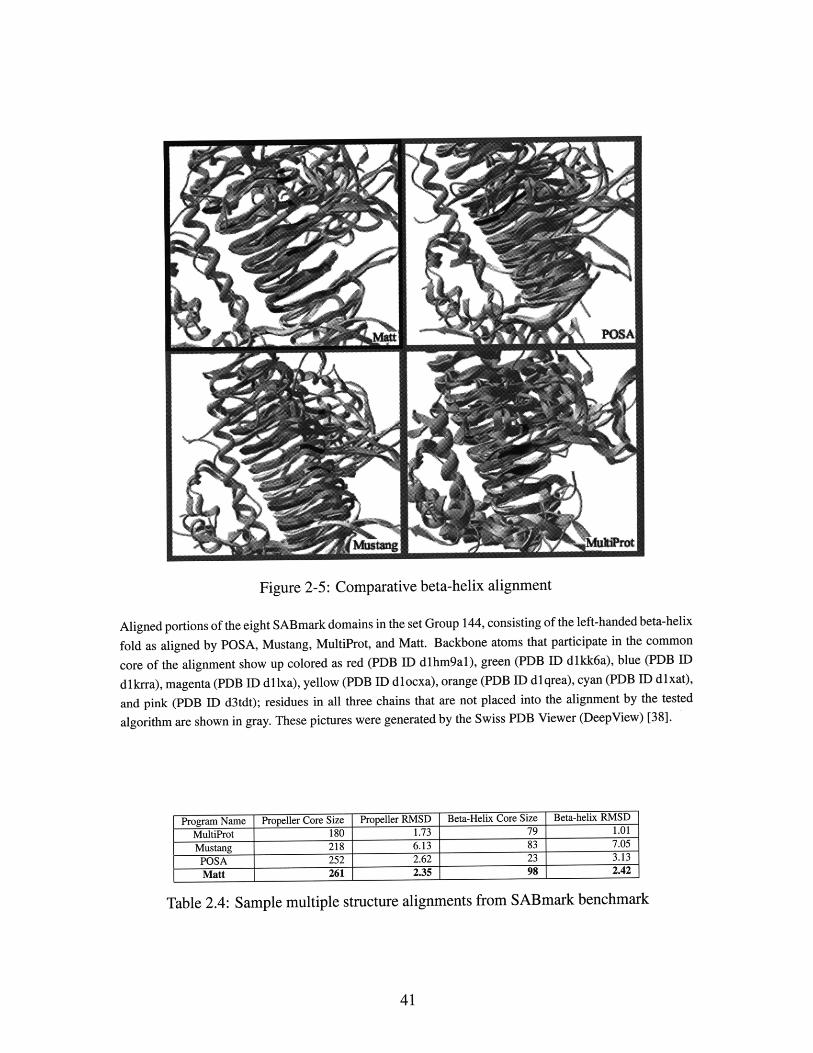
Figure 2-5: Comparative beta-helix alignment
Aligned portions of the eight SABmark domains in the set Group 144, consisting of the left-handed beta-helix
fold as aligned by POSA, Mustang, MultiProt, and Matt. Backbone atoms that participate in the common
core of the alignment show up colored as red (PDB ID dlhm9al), green (PDB ID dlkk6a), blue (PDB ID
dlkrra), magenta (PDB ID dllxa), yellow (PDB ID dlocxa), orange (PDB ID dlqrea), cyan (PDB ID dlxat),
and pink (PDB ID d3tdt); residues in all three chains that are not placed into the alignment by the tested
algorithm are shown in gray. These pictures were generated by the Swiss PDB Viewer (DeepView) [38].
Propeller Core Size180218252261
Propeller RMSD Beta-Helix Core Size1.73 796.13 832.62 232.35 98
Beta-helix RMSD1.017.053.132.42
Table 2.4: Sample multiple structure alignments from SABmark benchmark
Program NameMultiProtMustangPOSAMatt
_ I L __ __

M.a. t... FI.exFt
S0 .I
Figure 2-6: Distinguishing alignable structures from decoys
Positive (blue) and SABmark decoy (red) pairwise alignments plotted by RMSD versus number of residuesfor Matt, FlexProt, MultiProt, and Mustang on the SABmark superfamily set.
for all programs. Figure 2-6 displays the results on the SABmark superfamily set versus
SABmark decoys. The separating line marks where the true positive and true negative
percentages are roughly equal.
When comparing ROC curves over the four different programs, we find that Matt con-
sistently dominates both FlexProt and MultiProt at almost every fixed true positive rate.
Mustang does as well. Interestingly, Matt and Mustang are incomparable- on the Super-
family sets, Matt does better than Mustang when the true positive rate is fixed over 93%
(90% for the random decoy set), and Mustang does better thereafter. For the twilight zone
set, the situation is reversed: SABmark does better than Matt when the true positive rate is
between 93% and 98%, but Matt does better between 70% and 92% true positives; then,
performance reverses, and Mustang does better below 70% true positive rates. Sample
percentages for the four programs near the line where the true positive and true negative
percentages are roughly equal appear in Tables 5 and 6 on the superfamily and twilight
zone family sets, respectively.
Unsurprisingly, for all four programs, the SABmark decoy set was more difficult to
'VOL. .$~Wwai
41 4
I -- - --- -- - ----- --- - --- --- - ~ I I
p:*-~ '- ' ir t:t'":Q''
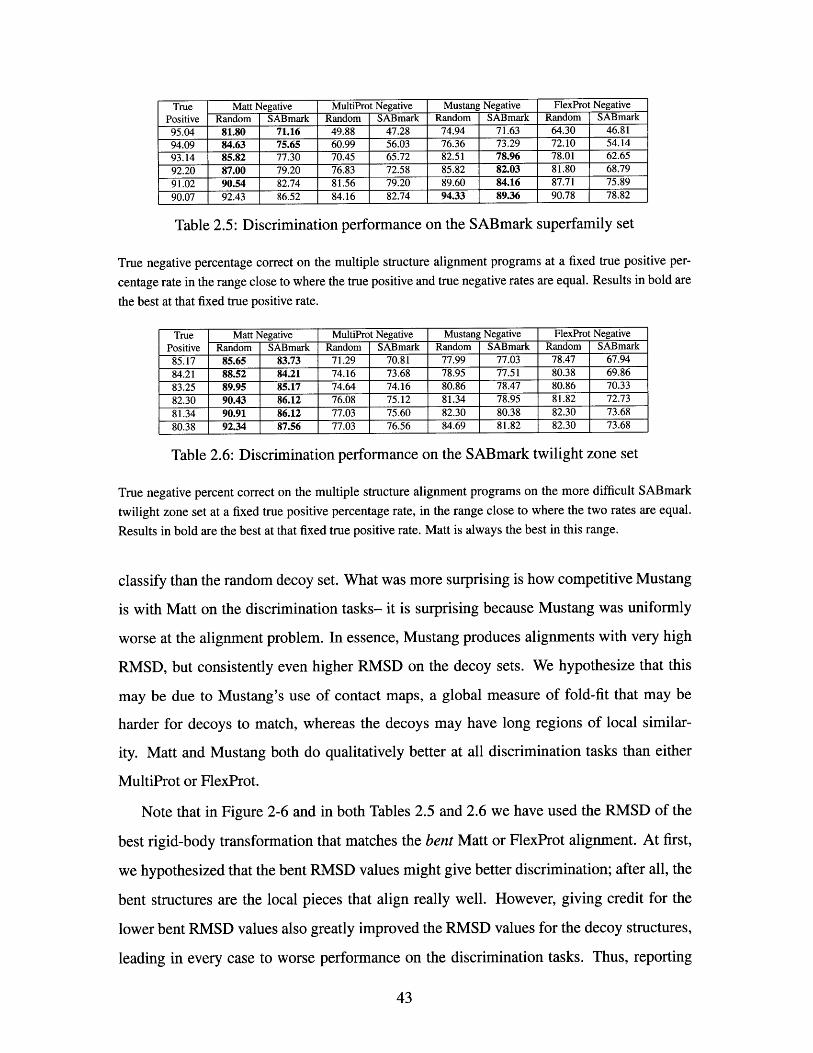
True Matt Negative MultiProt Negative Mustang Negative FlexProt NegativePositive Random SABmark Random SABmark Random SABmark Random SABmark
95.04 81.80 71.16 49.88 47.28 74.94 71.63 64.30 46.8194.09 84.63 75.65 60.99 56.03 76.36 73.29 72.10 54.1493.14 85.82 77.30 70.45 65.72 82.51 78.96 78.01 62.6592.20 87.00 79.20 76.83 72.58 85.82 82.03 81.80 68.7991.02 90.54 82.74 81.56 79.20 89.60 84.16 87.71 75.89
90.07 92.43 86.52 84.16 82.74 94.33 89.36 90.78 78.82
Table 2.5: Discrimination performance on the SABmark superfamily set
True negative percentage correct on the multiple structure alignment programs at a fixed true positive per-
centage rate in the range close to where the true positive and true negative rates are equal. Results in bold are
the best at that fixed true positive rate.
True Matt Negative MultiProt Negative Mustang Negative FlexProt NegativePositive Random SABmark Random SABmark Random SABmark Random SABmark
85.17 85.65 83.73 71.29 70.81 77.99 77.03 78.47 67.9484.21 88.52 84.21 74.16 73.68 78.95 77.51 80.38 69.8683.25 89.95 85.17 74.64 74.16 80.86 78.47 80.86 70.3382.30 90.43 86.12 76.08 75.12 81.34 78.95 81.82 72.7381.34 90.91 86.12 77.03 75.60 82.30 80.38 82.30 73.6880.38 92.34 87.56 77.03 76.56 84.69 81.82 82.30 73.68
Table 2.6: Discrimination performance on the SABmark twilight zone set
True negative percent correct on the multiple structure alignment programs on the more difficult SABmark
twilight zone set at a fixed true positive percentage rate, in the range close to where the two rates are equal.
Results in bold are the best at that fixed true positive rate. Matt is always the best in this range.
classify than the random decoy set. What was more surprising is how competitive Mustang
is with Matt on the discrimination tasks- it is surprising because Mustang was uniformly
worse at the alignment problem. In essence, Mustang produces alignments with very high
RMSD, but consistently even higher RMSD on the decoy sets. We hypothesize that this
may be due to Mustang's use of contact maps, a global measure of fold-fit that may be
harder for decoys to match, whereas the decoys may have long regions of local similar-
ity. Matt and Mustang both do qualitatively better at all discrimination tasks than either
MultiProt or FlexProt.
Note that in Figure 2-6 and in both Tables 2.5 and 2.6 we have used the RMSD of the
best rigid-body transformation that matches the bent Matt or FlexProt alignment. At first,
we hypothesized that the bent RMSD values might give better discrimination; after all, the
bent structures are the local pieces that align really well. However, giving credit for the
lower bent RMSD values also greatly improved the RMSD values for the decoy structures,
leading in every case to worse performance on the discrimination tasks. Thus, reporting

an RMSD value for the rigid superimposition that minimized the RMSD of the residues
placed into a bent alignment produced the best separation of true alignments from decoys.
2.3.4 p-Value Calculation
p-values for pairwise Matt alignments are calculated based on our 2-D alignment versus
RMSD graphs. To calculate p-values, we find the slope m of a line in the alignment length
versus RMSD graph that maximizes the number of elements from the random negative set
on one side and has at least 90% of the SABmark positives on the other. This value was
chosen because it allows roughly the same percentage of the negative set to be on the other
side. These were then used to calculate z-scores of the distribution of RMSD - m x length
of the random negative set. These are fit to a standard Gaussian distribution to calculate
p-values for pairwise alignments.
2.4 Methods
2.4.1 Pairwise alignment
First, it is useful consider Matt's behavior on pairwise alignments. In what follows, we
assume structures are sequentially ordered from their N terminal to their C terminal.
Notation and Definitions
Definition 2.4.1 A block denotes the C-alpha atoms of a set offive to nine adjacent amino
acid residues in a protein structure. For block B, let bh denote the first residue and bt
denote the last residue of the block. A block pair is a pair of blocks of equal length, one
from each of a pair of structures.
For block pair BC, define TCB to be the minimum RMSD transformation that is applied
to C to align its C-alpha carbons against those of B, and let RMSDBc denote the RMSD
of the two blocks under TCB. Minimum transformations are calculated using the standard
classical singular value decomposition method of Kabsch [52].
;:ii

B D
Figure 2-7: Assembling sequential block pairs
Two Sequential Block Pairs that could form part of an assembly. Block pair BC precedes block pair DE
because B precedes D and C precedes E in their respective protein sequences.
Definition 2.4.2 For block pair BC,
Score(BC) = - log Pr[RMSDBc]
Here, p-values are estimated by generating a table of random five-residue RMSD align-
ments of the NCBI non-redundant PDB [39] (update dated 7 May 2007) with a BLAST
E-value cutoff of 10- 7. For longer block pairs, negative log p-values for a given RMSD
are assumed to increase linearly with respect to alignment length. (This assumption was
verified empirically to be approximately true in the relevant range.)
Definition 2.4.3 Let S be a set of block pairs. Two block pairs BC and DE are sequential
if bt precedes dh (and cr precedes eh) and there is no block pair with any residue that lies
between them in S.
Definition 2.4.4 A set of block pairs is called an assembly if it consists of block pairs P1,
P 2, ... , Pn such that Pi and Pi+l are sequential.
Note that the definition of sequential means that the Pi will be non-overlapping and
seen in both structures in precisely this order; see Figure 2-7.
L

Matt Assembly
A Matt pass uses dynamic programming to create an assembly of block pairs. A pass
takes an assembly and three cutoff values as input and outputs a new assembly. The new
assembly contains all the block pairs of the original assembly. The three cutoffs are a
maximum block-pair RMSD cutoff and maximum values for the displacement and relative
angles for each sequential pair of blocks (the "translations" and "twists," respectively, of
Matt's acronym). Using multiple passes and relaxing cutoffs in each successive pass results
in favoring strongly conserved regions while still detecting more weakly conserved regions.
All Matt results in this paper use a three-pass algorithm. All three passes use a cutoff
of 45 on the angle between the transformations of two sequential block pairs. The first
pass is restricted to block pairs with a minimum negative log p-value of 2.0, and sequential
block pairs must have a displacement no greater than 4. The second pass uses a minimum
negative log p-value of 1.6 and a maximum displacement of sequential pairs of 5. The last
pass uses cutoffs of 0.6 and 10, respectively. The values of these cutoffs were determined
by training on a random 20% of the Homstrad benchmark dataset.
More formally, the score of a set of block pairs S is the sum of the alignment scores of
the individual block pairs and a bonus based on how consistent the transformations associ-
ated with the two block pairs are. This score is used internally throughout the construction
of the alignment, but is not used to determine the p-value, which is instead computed di-
rectly based on length and RMSD of the resulting alignments; see the section on calculating
p-values at the end of Section 2.1.
Score(S) = EBCes - log(Pvalue(RMSDBc)) +
ZBC,DE sequential in s - log(SolidAngle(Angle(TcB, TED))/2) +
ZBC,DE sequential in s -Displacement(BC, DE)
where
Displacement(BC, DE) = (Length(TB (Ct) - TED (Ct)) +Length(TCB(eh) - TED (eh)))/2
and Length is defined to be ordinary Euclidean distance, Angle is the angle of TCBT,J
in axis-angle form, and SolidAngle is the solid angle associated with an angle, measured as
a fraction of the sphere. SolidAngle(q) ranges from 0 to 1 and is the probability of a given
ray and a random point in 3-D space forming an angle less than q. To prevent overflow, if
Angle has a value below 0.1 radians, it is set to 0.1 radians.
We note that a naive implementation of dynamic programming would use O(n 4) time
(where n is the length of the longer string), as there are O(n2 ) block pairs. We reduce
this to an O(n3 log n) algorithm by incorporating geometric knowledge of the structural
transformations to reduce the search space. In particular, for each of structure two's C-alpha
atoms, an oct-tree [43] that partitions Euclidean space based on the transformed positions
of that C-alpha atom is created. Each transformation comes from a previously considered
block pair that ends with the C-alpha atom in question. When the dynamic program is
assembling a block pair starting with the kth C-alpha atom in structure two, it searches the
oct-trees for all of structure two's C-alpha atoms before k for compatible transformations
(meaning the associated transformations of the atom are within the distance cutoff).
Final Output
The final output is an assembly A, a bent assembly A' (only output with a command-line
option), BentRMSD(A'), UnbentRMSD(A), and a p-value for the assembly.
The result of the dynamic programming algorithm described above gives the bent align-
ment A', together with a set of local transformations (allowing translations and rotations)
that produced the alignment. Its associated RMSD is BentRMSD(A').
To produce the unbent alignment, the set of which residues are to be placed into align-
ment is retained from A', and all geometric information is discarded. Then, the best global
rigid-body transformation that minimizes the RMSD of this alignment is found using the
classical SVD method of Kabsch [52]. The result is the rigid-bent RMSD, which is not
output explicitly, but implicitly forms the basis for the p-value calculation (as described
in the p-value section at the end of Section 2.1, the Introduction). Note that so far the
sequence alignment from the bent step is unchanged, and thus only includes sets of con-
tiguous residues that are at least 5 A in length. A final pass then greedily adds back shorter

segments of four or fewer residues that fall between already aligned fragments but whose
RMSD under the global transformation falls below a user-settable cutoff. The resulting
alignment is A, with its associated unbent RMSD(A).
2.4.2 Multiple Alignment
In this subsection, we extend the definitions of assemblies to sets of more than two struc-
tures in the natural way. The input to each iteration of the Matt multiple alignment algo-
rithm is the set of structures to be aligned that have been partitioned into sets, where the
structures in each set are multiply aligned in an assembly. The output of the iteration leaves
all but two sets unchanged; the structures in those two sets are merged into a single set with
a new multiple alignment assembly. (The initial iteration of Matt places each structure into
its own set and is equivalent to the pairwise alignment algorithm described above.)
Analogous to blocks, we define block-tuples.
Definition 2.4.5 A block-tuple is an aligned set of equal-length blocks. A block-tuple pair
is a set of two block-tuples, one from each of two sets of aligned structures.
At each iteration, for every pair of sets in the partition, Matt uses the merge procedure
detailed below to combine the two assemblies into a single assembly and computes its
score. It then chooses the highest-scoring pair of sets to merge in that iteration. Matt
terminates when all structures have been aligned into a single assembly, outputting the
assembly, bent RMSD, and unbent RMSD.
Merging
Here is a high-level description of the steps of the merge procedure. The merge procedure
take as input two assemblies, each possibly containing multiple structures. Each step is
explained in more detail:
1. Find the pair of structures, ao from assembly A and bo from assembly B, that have
the highest-scoring pairwise structural alignment, according to the pairwise structural
alignment algorithm of the previous section.
i ~iTa~i~i~L-iir?-~i--~;--; I - ~i;l-- ;~;; ------ ~-~~~-1~1--1;-U~- i; -- ~ ; ;- ;--- ; ;;;i--;- - ?;;- -I-1------- --- --~-- ~ acui~~;-r;~~i;~;c;.r-i;s;~~~ ~1;.1 :

2. For each block b of a0o, let Tb denote the transformation of b back to its original atomic
coordinates. Transform every block in the block-tuple associated with b in A by Tb.
Do the same for each block of bo and its associated block-tuple.
3. Within each of A and B separately, realign all blocks within each block-tuple to
reduce RMSD using the LocalOpt procedure (described below).
4. Still within each of A and B separately, an extension step is performed than can
lengthen block-tuples into unaligned regions or other block-tuples. Note that this
step may temporarily produce overlapping blocks, but that this is corrected later, and
only non-overlapping block-tuples are returned at the end of the merge procedure.
5. Taking the set of all aligned block-tuples of A, we consider all sets of five to nine
adjacent residues entirely contained within one of these block-tuples by sliding a
window of appropriate length. We do the same for the block-tuples of B. These
become the building blocks of new block-tuple pairs in the merged assembly. Just
as in the pairwise case, all equal-length building blocks, one each from A and B,
are pairwise aligned and scored. Note that the RMSD algorithm easily generalizes
to align sets of aligned residues by treating each aligned k-length set of m structures
against n structures as a single RMSD alignment of kmn residues. Let TBA(r, S)
be the transformation that produces the lowest RMSD on the block-tuple pair r C
A, sE B.
6. Dynamic programming is used to find the optimal assembly of pairs of new block-
tuples. The dynamic programming algorithm in the multiple structural case has the
same form as in the pairwise case. The angle penalty is calculated as before from
TBA (r, s). The displacement penalty is calculated slightly differently. In each residue
position, an average C-alpha atom position is calculated for both A and B. The
displacement is calculated using the averages as if they were positions of atoms of
single structures in a pairwise alignment. Note that as in the pairwise case, this
algorithm does not allow block-tuples to overlap, so the final set of block-tuples that
are aligned by the merge procedure will be a legal assembly.

The merge procedure has now been specified except for LocalOpt and the extension
procedure. We now explain both these steps in detail.
LocalOpt
LocalOpt acts independently on A and B; therefore, it is described here only on A. The
intuition for the LocalOpt step comes from merges in the previous iterations. The block-
tuple alignment that an assembly inherits is the result of a global RMSD alignment of the
block-tuple of potentially many protein structures. Therefore, while keeping the residue
alignments fixed, it is often still possible to transform the coordinates of the C-alpha atoms
to improve bent RMSD. LocalOpt acts separately on each block-tuple in the assembly. In
particular, if a0o, al, ... , ar are the structures within a block-tuple (where ao is the reference
structure as defined by merge), each ai is removed in turn and then realigned to minimize
RMSD to the other r structures for each block-tuple.
Extension phase
In the extension phase, both ends of block-tuples of five to nine residues are explored in
order to determine if additional adjacent residues have a good multiple alignment. The
LocalOpt transformations associated with each block-tuple in each structure are applied to
the residues immediately before and after the block-tuple. If the average distance between
all pairs of residues in all structures before or after a block-tuple is less than 5 A, the
residues are added to the block-tuple. This is done in a greedy fashion. Note that this
allows block-tuples to be longer than nine residues or even to overlap (though in practice,
we do not allow them to overlap by any more than five residues to bound computational
time).
Final output
When only one assembly remains, as in the pairwise case, this produces the bent alignment.
As before, a final realignment and extension phase is done in which additional i-residue
segments are greedily added to the common core, for i = 4 down to 1, provided their
--- -------

average RMSD lies below a (user-settable) cutoff. This cutoff is solely responsible for
the size of common core/RMSD tradeoff found in Figures 2-2 and 2-3. All residues that
were aligned in the iterative phase are kept in the final alignments. Block-tuples are not
allowed to overlap in the final extension phase. A new RMSD alignment of the original
unbent structures is done, aligning residues according to the extended block-tuples. This
assembly, its RMSD, and the sets of aligned residues are the algorithm's unbent output. A
p-value is not output when a group of more than two structures is to be aligned.
2.5 Discussion
We introduced the program Matt, which showed that detouring through local flexibility in
an AFP alignment algorithm could aid in protein multiple structure alignment. We suggest
that looking at local bends in protein structure captures similarity well for fundamental
biological as well as mathematical reasons. In particular, Matt may be both capturing
flexibility inherent naturally in some protein structures themselves and modeling structural
distortions in the common core that arise as proteins become more evolutionarily distant.
Matt runs in O(k2 n3 log n) time, where k is the number of sequences participating in
the alignment and n is the length of the longest sequence in the alignment. Compared with
Mustang and MultiProt, Matt takes about the same amount of time to complete running
on the benchmark datasets. We find that Matt is typically several times slower on most
sets of structures; however, there are a small percentage of sets of substructures in both
benchmark datasets where both Mustang and MultiProt take orders of magnitude more
time to complete their alignments than they do on the typical set of structures. Matt is
saved in these difficult cases with lots of self-similar substructures by its implementation
of the oct-trees, which allows for better pruning of the search space. Matt also supports a
multithreaded implementation, which is faster still. Matt is sufficiently fast that it should
be feasible to construct a set of reference alignments for similar fold classes based on Matt,
covering the space of all known folds, which we intend to do.
Examining some of the Matt alignments by hand, the program seems to typically do a
better job of aligning the ends of alpha-helices and beta-strands than its competitors; we

therefore suggest that Matt may be a useful tool for construction of better sequence profiles
for protein structure prediction, and for the construction of better templates for protein
threading libraries. For these applications, both Matt's rigid unbent alignments and the
geometrically impossible bent alignments may be of interest.
Finally, looking at how Matt (or the other structure aligners) performs on the two SAB-
mark benchmarks raises again the philosophical question of how far into the twilight zone
it makes sense to align protein structures. Clearly at the superfamily level, there is typically
substantial structural similarity. At the twilight zone level, there is much increased diver-
gence. Examining these alignments in more details may help develop our intuition about
the limits of comparative modeling for protein structure prediction as we go further into the
twilight zone.
_ ̂___~_____^_~_ltli___;_;~__~i;__~_t ___ II; //_jl__ _ ii__;_ /j_;iiiii_/iiil___;___r__jr _____~__~

Chapter 3
BetaWrapPro
3.1 Introduction
Successful computational prediction of protein structural motifs from sequence remains
a very challenging problem. It is most difficult in the case of proteins whose secondary
structure is "mainly beta," meaning that many of the amino acid residue participate in
beta-sheet formation. While there is evidence that residues involved in beta-sheet forma-
tion that are close in space exhibit strong statistical biases [75, 98], these residues may
be difficult to discover due to being a variable and potentially long distance apart in the
protein sequence. In fact, simply predicting the correct annotation of secondary structure
of these folds can be problematic: even the best secondary structure predictors such as
PHD [84] and PSIPRED [47] predict alpha-helices more accurately than beta-strands [64].
It has been our experience that general secondary structure predictors do not suffice even
to correctly determine the number of beta-strands in a sequence that folds into one of these
motifs, never mind finding the ends of the strands. Tertiary structure predictors such as
Rosetta [11] and LINUS [95] while performing well on all-alpha and alpha/beta proteins,
are also challenged by topologically complex all-beta proteins [11, 95]. Many threading
programs also have particular problems recognizing and then threading beta-sheet topolo-
gies correctly once sequences fall into the so-called "twilight zone" [83] of less than fifteen
percent sequence homology to known structures.
The stabilizing interactions from a beta-sheet's side-chains, generally pointing orthog-

Cap
Tl B1
B2 T2 Barrel
A. Beta-helix rung B. Beta-helix (1plu) C. Beta-trefoil leaf D. Beta-trefoil (lbff)
Figure 3-1: The beta-helix and beta-trefoil folds
The beta-helix fold is characterized by a repeating pattern of parallel beta-strands in a triangular prism
shape [112]. The cross-section, or rung, of a beta-helix consists of three beta-strands connected by variable-
length turn regions (A); the backbone folds in a helical fashion with beta-strands from adjacent rungs stacking
on top of each other (B) from lplu [113]. The beta-trefoil fold consists of three leaves (C) around an axis
of three-fold symmetry. Two beta-strands from each leaf form a 6-stranded anti-parallel barrel and two more
from each leaf form a cap at one end of the barrel (D) from ibff [54]. In all figures, the darkened regions
correspond to the positions the templates.
onal to the strand axis, involve contacts with residues that are often very distant in the lin-
ear amino acid sequence. For beta-sandwich structures the packings between sheets show
very little structural organization and considerable packing diversity [16, 17]. Higher or-
der features such as the "ridges-into-grooves" that characterize alpha-helix-to-alpha-helix
packings within proteins are absent. Beta-sheet proteins do preserve the general packing
pattern of a buried core dominated by hydrophobic side-chains, and a mosaic surface that
mixes polar with hydrophobic side-chains.
Our computational approach to this problem has been focused initially on two classes
of beta-sheet proteins that have some topological regularity: beta-helices and beta-trefoils.
The pectin lyase-like single-stranded right-handed beta-helix superfamily l is a coiled fold
wherein each rung is composed primarily of beta-strands (Figure 3-1A and B). Beta-helices
are elongated molecules in which the N-terminal and C-terminal are far apart, and form
characteristic hydrophobic stacks between rungs [112]. The largest group of these folds
with solved structures are involved with complex polysaccharide metabolism, either recog-
1SCOP classification; henceforth referred to as the beta-helix fold.
-3 1 C~1 ~CI

nizing and binding to such molecules or involved in their synthesis or remodeling. Rather
than having a crevice or pocket as an active site, the elongated lateral surface of the beta-
helix provides the recognition and catalytic elements [44]. A number of these proteins are
virulence factors for bacterial and fungal pathogens, including pertactin from Bordetella
pertussis and pectate lyase from Erwinia chrysanthemi. Because of the extended nature
of the active sites, they cannot currently be recognized from examination of amino acid
sequence alone. The ability to predict the fold from sequence alone would be of consid-
erable value in medical microbiology. The beta-trefoil SCOP [73] fold2 consists of three
mainly-beta leaves folded around an axis of three-fold symmetry (Figure 3-1C and D).
Their functions are diverse, including neurotoxins, inhibitors, and cytokines.
Both motifs have repeating structural segments: the rungs in the beta-helix and the
leaves in the beta-trefoil. However, unlike coiled-coils, collagen, or leucine-rich repeats,
they do not have a characteristic signature at the sequence level. Their intracellular folding
process may have a progressive or sequential aspect, through which the sequence directs
the native fold. We have been involved in developing algorithms that have a "wrapping"
component, which may capture the processes that have an initiation stage followed by
progressive interaction of the sequence with the already-formed motifs.
Fold recognition and sequence-structure alignment are difficult problems for both these
protein folds, just as they are for many protein folds that lie in the "mainly-beta" top level
of the SCOP hierarchy. The difficulty comes from the fact that there is insufficient se-
quence similarity to apply standard homology-based approaches. Both the beta-helix and
the beta-trefoil folds lie in the so-called "twilight zone" of sequence homology [83], with
sequence identity between members of the fold class lower than 15%. While there is evi-
dence that residues involved in beta-sheet formation that are close in space exhibit strong
statistical biases [75, 98], these residues may be difficult to discover due to being a variable
and potentially long distance apart in the protein sequence. In fact, simply predicting the
correct annotation of secondary structure of these folds can be problematic: even the best
secondary structure predictors such as PHD [84] and PSIPRED [47] predict alpha-helices
2Here, we consider the STI-like and cytokine SCOP superfamilies, for reasons explained in Section 3.4,and refer specifically to them with the term beta-trefoil.
more accurately than beta-strands [63]. Tertiary structure predictors such as Rosetta [11]
and LINUS [95], while performing well on all-alpha and alpha/beta proteins, are also chal-
lenged by topologically complex all-beta proteins [11, 95].
Various researchers have found that considering interactions between pairs of residues
can lead to improvements in beta-strand prediction. An information theoretic approach to
the problem of determining the correct alignment between interacting beta-strands in par-
allel and anti-parallel beta-sheets [98] suggests that when it is possible to limit the search
to a window of sequence around suspected interacting strands, consideration of inter-strand
residue-residue pairings can be of significant value in determining the correct alignment be-
tween beta-strands. Similarly, Olmea et al. [84] note that exploiting information contained
in the correlation between residue pairs seems to be a promising method for modeling the
constraints that govern the folding process. Recognition tools for various folds have been
built using pairwise interaction probabilities, including the coiled-coils [7, 31]. Previous
studies [13, 21, 69] took a somewhat different approach, namely to search for secondary
and supersecondary structure at the same time. These produced the BetaWrap program
for recognizing the motif characteristic of the pectin lyase-like superfamily of the single-
stranded right-handed beta-helix SCOP fold class, and Wrap-and-Pack, for recognizing the
beta-trefoil motif. Other recent work [66] studied recognition of the beta-helix fold using
Markov random fields. However, these programs are strictly fold recognizers. For exam-
ple, BetaWrap predicts a structure to be in the template class if the average score of the top
five alignments produced for overlapping sub-regions is good; it does not output a single
global alignment of the putative structure to the motif.
Sequence profiles have previously been used for structure prediction in various ways.
The profile encodes information about residue conservation (which locations are conserved,
which are variable) and what types of substitutions are found at each location [36]. This
additional information allows more distant homologies to be found by aligning profiles
rather than sequences [114]. Strongly conserved residues are often of structural importance,
as demonstrated by programs such as PSIPRED, which uses profiles for secondary structure
prediction, and GenThreader [46], which uses this prediction as an input to its neural-
network based threader. Sequence profiles have also been used to detect disulfide bonds
based in part on Cys-Cys conservation [19]. Panchenko et al. [78] present a method for
threading a sequence onto a profile of a structural template and its homologs. In some
sense our approach is the opposite, in that we wrap a sequence profile onto a structural
template.
We introduce the program BetaWrapPro, which performs both fold recognition and
sequence-structure alignment for the beta-helix and beta-trefoil motifs. The algorithm is
based on the fold recognition algorithms of BetaWrap and Wrap-and-Pack, which use sta-
tistical correlations between pairs of residues in adjacent beta-strands to decide if a query
sequence aligns well to the abstract structural template for a motif. We generalize this
method to take advantage of the additional data provided by sequence profiles and by pair-
wise correlations of non-adjacent residues, and extend it to predict structure alignments for
the conserved region of the motif.
To further support the utility of this method, we note that a list of the highest-scoring
two hundred sequences with no known structure was provided with the first BetaWrap
paper [13]. Since then, six have had their structure determined, and all were found to form
the beta-helix fold (see Table 3.5).
3.2 The Algorithm
BetaWrapPro "wraps" a profile of a target sequence onto the abstract supersecondary struc-
tural template for a beta-helix (Figure 3-1A) or beta-trefoil (Figure 3-1C) derived from
structural alignments with the dynamic programming algorithms of BetaWrap [13] and
Wrap-and-Pack [69]. They were extended in this work to operate on sequence profiles, and
the BetaWrap algorithm was also changed to include data on cater-corner residues. The
concept behind the algorithm is that there is a statistically significant difference in residue
pairing probabilities between aligned beta-strands and other structure [98]. This statisti-
cal signature can be used in conjunction with an abstract structural template to recognize
supersecondary structure. The templates introduce constraints reflecting fold characteris-
tics derived from structural alignments of known structures. The algorithms were extended
to deal with sequence profiles rather than individual sequences, and BetaWrap was also

modified to take into account diagonally adjacent residues, as described below.
A profile for a sequence n residues in length can be represented as a 20-by-n matrix
that encodes some statistic of the amino acid composition for each position in the target
sequence. This is based on the substitutions that occur in each position in a sequence align-
ment of the target to a number of other sequences 3. Each row of the matrix corresponds to
one of the 20 amino acids, and each column corresponds to a position in the target sequence.
An entry in the matrix thus presents information concerning the chance of observing a spe-
cific amino acid in that position, based on a number of similar sequences. Logically, each
residue pairing can be scored based on the distribution, rather than a particular amino acid.
To create this matrix, PSI-BLAST is run on the non-redundant NCBI BLAST sequence
database from July 18, 2005 for two iterations.
Wrapping mimics the progressive manner in which these folds may form: the struc-
ture is built around an initial structural segment, or seed. For beta-helices, the seed is a
B2-T2-B3 rung section which matches a hydrophobic-residue sequence pattern common
to the fold. The beta-trefoil search requires two phases, the first starting from two aligned
beta-strands to build an individual leaf, and then to combine the leaves into a complete tre-
foil. In either case, the profile is searched forward and backward from the initial segment
for neighboring segments based on a beta-strand alignment score. The score is primarily
based on observed correlations between pairs of residues in adjacent beta-strands, and also
incorporates information on turn lengths and observed residue stacking preferences. The
correlations are derived from similar beta-sheets taken from the PDB, excluding the tem-
plate fold class. The probability that a residue of type X will align with a residue of type
Y is determined by the pairwise frequency of X and Y aligning over the frequency of X
appearing, conditional on whether X is exposed or buried. Conditional probabilities are
defined for stacking residues in adjacent beta-strands and for cater-corner residue pairs, i.e.
those residues one off from a vertical alignment in either direction. Probabilities used for
beta-trefoil scoring are given in Tables A.1 and A.2, and for the beta-trefoils in Tables A.4,
A.3, and A.5.
The exact formula for computing the interaction probability between positions i and j
3Columns involving a gap in the target are ignored.

in a sequence is given in Equation 3.1, where d varies over each of the twenty amino acids,
Pr[ri, d] is the log probability of the residue in position i interacting with d, and f(d, j)
is the frequency with which residue d appears in position j of the profile. The weight
w assigned to the interaction is based on the relative locations of i and j: for beta-helix
scoring, inward-pointing adjacent residues have a weight of 1, outward of 0.5, and one-off
of 0.25, which reflects that there are twice as many one-off residues as adjacent residues.
All beta-trefoil adjacent residues are weighted 1, and one-off residues 0.5. There are several
score adjustments reflecting fold-specific knowledge. The beta-helices receive a penalty of
-1 for each standard deviation away from the mean number of residues between rungs,
-1 for each large hydrophobic residue at positions that bound the beta-strands, and a +1
bonus for each pair of stacked aliphatic, aromatic, and polar residues. The trefoils are also
penalized according to gap length, and given a +1 bonus for each residue predicted to be a
beta-strand by PSIPRED.
20
Pr[i,j] = w Pr[ri, d] f (d,j) (3.1)d=1
The final beta-trefoil wrap is the one with the best score. The five-rung beta-helix wrap
is taken as a consensus by combining pairs of adjacent rungs from each of the ten highest-
scoring wraps and finding the four overlapping rung pairs which appear most frequently.
This alignment of the target to a structural template can then be passed to standard pack-
ing [50] methods to determine putative atomic coordinates for the structurally conserved
regions. In fact, BetaWrapPro uses SCWRL [90] to place side-chains onto several repre-
sentative backbones, and the structure with the lowest SCWRL energy score is presented
in PDB format. The energy score is a measure of how well the sequence fits the backbone
template: a high energy score implies that many atoms are too close to one another, and
thus the sequence is unlikely to form the target fold, either because it forms another fold or
because it is poorly aligned to the structural template. Note that only a partial structure is
output, for those regions that correspond to the template not including loops. This is similar
to the outputs of other fold recognition programs such as PROSPECT [109].

3.3 Results
3.3.1 Recognition and Alignment of Sequences with Known Struc-
tures
On the positive and negative test databases described in Section 3.4, Materials and Methods,
BetaWrapPro recognizes the beta-helix fold with 100% sensitivity at 99.7% specificity in
cross-validation and with 100% sensitivity at 92.5% specificity in cross-validation for the
beta-trefoils. This is an improvement over the results for BetaWrap (100.0% sensitivity,
95.0% specificity) and Wrap-and-Pack (88.9%, 96.3% resp. on the same databases). Given
the improvement in specificity achieved by BetaWrapPro, over 300 false positives reported
by BetaWrap as hits in the PDB-minus have been eliminated.
BetaWrapPro also produces accurate alignments of the target sequence onto the struc-
tural template. In sequence-heterogeneous motifs such as those BetaWrapPro predicts,
this is difficult to accomplish by the common sequence similarity methods. However, the
profile wrapping technique proves to be successful at predicting alignment to a supersec-
ondary structure template across diverse sequence families. All results stated in this section
are from the leave-family-out cross-validation described in Section 3.4. In particular, we
are always packing onto a backbone from a different SCOP family.
On the twelve beta-helices in our database, the sequence-structure alignment is accurate
for 88% of predicted residues. The beta-trefoil alignments are 89% accurate4 . To verify that
the additional information available in a sequence profile assists in wrapping, the original
motif recognizers were modified to also produce a sequence-structure alignment. We find
meaningful improvements: BetaWrap's beta-helix wraps are 67% accurate, and Wrap-and-
Pack achieves 75% accuracy on the beta-trefoils.
Because of the quality of sequence-structure alignment, BetaWrapPro is able to use
SCWRL to generate accurate 3-D structures of its template motifs. The accurately aligned
regions of the beta-helix template average less than 2.0 A RMSD (Table 3.1). The side-
chain predictions placed onto the backbone by SCWRL are consistent with SCWRL's re-
4We treat a residue as accurately aligned if it is within four position shifts of the exact position.

PDB p-score Alignment acc RMSD (A) X1 correct X1+2 correct % identity BLAST score
lair 0.0001 1.00 1.21 0.63 0.23 18 0.06lbn8 0.0009 1.00 1.31 0.62 0.43 22 0.06lee6 0.0032 1.00 1.70 0.55 0.24 14 0.04
ljta 0.0001 1.00 1.45 0.71 0.32 12 0.02
lbhe 0.0001 0.80 0.97 0.67 0.34 19 0.03lczf 0.0005 1.00 1.43 0.72 0.46 11 0.18lrmg 0.0002 0.94 1.29 0.54 0.36 17 0.07
idab 0.0001 1.00 1.39 0.60 0.41 18 1.0
ldbg 0.0001 1.00 2.83 0.66 0.45 14 0.02
lqjv 0.0012 0.66 2.13 0.45 0.29 11 0.82
lidk 0.0014 1.00 1.47 0.55 0.35 16 2.8
1h80 0.0015 0.14 1.40 0.67 0.50 11 0.23
Average 0.0023 0.88 1.55 0.61 0.42 16 -
Table 3.1: Beta-helix cross-validation
Cross-validation score and modeling accuracy for the beta-helix structures in the database as packed onto the
minimum-energy template structure from outside its own SCOP family. Families are separated by a single
line. The p-score is the BetaWrapPro score of the sequence. RMSD, dihedral angle correctness, and aligned
sequence identity are calculated only on the accurately aligned residues of the structure. Aligned sequence
identity is the identity between the target and template structure it was aligned to by BetaWrapPro; BLAST
E-score is the expectation score bl2seq [101] gives to its best alignment between the entire target and template
sequences.
PDB p-score Alignment acc RMSD (A) X1 correct X1+2 correct % identity BLAST score
lbff 0.111 1.00 3.79 0.52 0.39 10 0.011Ig82 0.041 1.00 6.23 0.56 0.50 7 2.6
2ilb 0.012 1.00 5.59 0.47 0.22 13 1.1lirp 0.011 1.00 4.12 0.36 0.34 12 0.0772ila 0.010 1.00 5.65 - - 7 no hitsiwba 0.038 1.00 3.58 0.51 0.55 7 0.99ltie 0.041 1.00 2.51 0.46 0.35 15 1.7
3bta 0.013 0.08 - - 13 3.2la8d 0.009 none - - - 5 0.23
average 0.038 0.89 4.50 0.48 0.39 10
Table 3.2: Beta-trefoil cross-validation
Cross-validation score and modeling accuracy for the beta-trefoil structures in the database as packed onto
the minimum-energy template structures from outside its own SCOP family. Superfamilies are separated
by double lines, families by single lines. For an explanation of each column, see Table 3.1. Note that the
structure 2ila in the PDB does not include side-chain coordinates. We do not report structure prediction result
for 3bta because only four residues are accurately aligned.
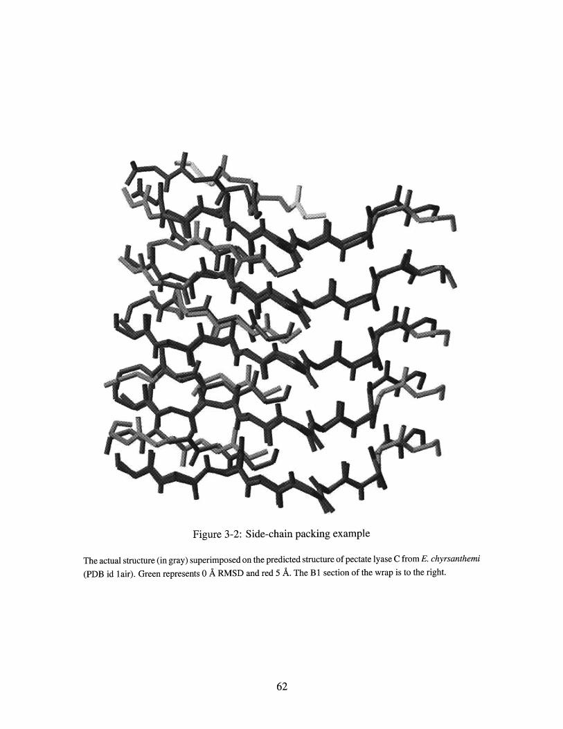
Figure 3-2: Side-chain packing example
The actual structure (in gray) superimposed on the predicted structure of pectate lyase C from E. chyrsanthemi
(PDB id lair). Green represents 0 A RMSD and red 5 A. The B 1 section of the wrap is to the right.
62
_

ported performance on near-native backbones [10, 49, 41], with 61% of X1 and 42% of
X1+2 angles correct 5. Figure 3-2 shows a sample model superimposed on the solved struc-
ture. The aligned regions of the beta-trefoils average 4.5 A RMSD (Table 3.2). Much of
this deviation is due to the fact that some beta-strands are often seven residues long in the
structure, whereas they are five long in the template. This leads to various off-by-two errors
in the alignment, but with the advantage of predicting both those trefoils with five-residue
and seven-residue strands. In addition, because the beta-trefoil predictions are made across
both superfamilies and families, with at most only one structure available from within the
same superfamily (rather than just family as in the beta-helices), there is greater struc-
tural deviation between the template backbones and the actual structure. The X1 angles are
predicted correctly for 48% of residues, and X1+2 for 39%. The decrease in X accuracy
compared to the beta-helices is to be expected, given the larger backbone deviation. Impor-
tantly, Tables 3.1 and 3.2 show that even when there is very low sequence identity between
the target sequence and the structure used to model it, BetaWrapPro is able to predict an
accurate structure for the aligned region.
3.3.2 Comparison to Other Methods
We compare BetaWrapPro to several popular methods for fold recognition and sequence-
structure alignment. We expect BetaWrapPro will perform better because it is tailored
to the beta-structural folds, and this indeed turns out to be the case. As reported previ-
ously [12, 69], neither PSI-BLAST nor HMMer succeed in recognizing these folds across
families. PSI-BLAST failed to recognize beta-helices in a leave-family-out cross-validation
(with the exceptions of the pectate lyase and pectin lyase families, and a couple exam-
ples across these families and the galacturonase family), and HMMER performed slightly
worse. PSI-BLAST and HMMer perform even more poorly on the beta-trefoils. For
alignment accuracy, we compared the output of PSI-BLAST, PROSPECT Version 2 [109]
and RAPTOR [108]. In all cases, we recreated the leave-family-out testing method used
throughout this work, excluding from the PSI-BLAST database or the PROSPECT and
RAPTOR template libraries all proteins in the same SCOP family as the target sequence.
5Dihedral angles are counted as correct if they are within 400 of the angle in the solved structure.

BetaWrapPro PSI-BLAST PROSPECT RAPTORPDB Exact Within 4 Exact Within 4 Exact Within 4 Exact Within 4lair 0.88 1.00 0.76 0.95 0.78 0.90 0.87 0.95
1bn8 0.94 1.00 0.78 0.78 0.88 0.95 0.88 0.95lee6 1.00 1.00 none none 0.29 0.32 0.35 0.43ljta 0.94 1.00 0.74 0.75 0.74 0.80 0.87 0.81lidk 0.94 1.00 0.77 0.81 0.74 0.83 0.88 0.94lbhe 0.80 0.80 none none none 0.08 0.50 0.58lczf 1.00 1.00 none none 0.24 0.34 0.54 0.58lrmg 0.94 0.94 none none 0.38 0.59 0.50 0.58Idab 1.00 1.00 none none 0.35 0.37 none none
ldbg 0.94 1.00 none none 0.22 0.37 0.59 0.671h80 none 0.14 none none 0.20 0.43 none 0.25lqjv 0.66 0.66 none none 0.20 0.27 none 0.17total 0.91 0.88 0.76 0.81 0.44 0.52 0.66 0.62
Table 3.3: Beta-helix alignment accuracy comparison
Percent of sequence-structure alignment correct for several programs on the beta-helices.
that no residues were correctly aligned.
BetaWrapPro PSI-BLAST PROSPECT RAPTORPDB Exact Within 4 Exact Within 4 Exact Within 4 Exact Within 4lbfg 0.33 1.00 0.15 0.45 0.22 0.87 0.38 1.001g82 0.17 1.00 none none 0.35 0.57 none none21bi 0.33 1.00 0.15 0.45 0.48 0.57 none 0.40lirp 0.33 1.00 none none none none 0.75 1.002ila 0.33 1.00 none none 0.47 0.73 0.40 0.62iwba 0.50 1.00 none none 0.08 0.42 none 1.00Itie 0.58 1.00 none none 0.23 0.68 0.25 0.58
3bta none 0.08 none none none none none nonela8d none none none none none 0.03 none nonetotal 0.30 0.89 0.15 0.45 0.30 0.77 0.45 0.78
Table 3.4: Beta-trefoil alignment accuracy comparison
Percent of sequence-structure alignment correct for several programs on the beta-trefoils.
that no residues were correctly aligned.
"None" denotes
"None" denotes
PSI-BLAST was run on the PDB data set described in Section 3.4, Materials and Methods,
filtered to 90 percent sequence identity. The default E-score cutoff for inclusion of 0.001
was used, and all searches converged within three rounds. PROSPECT was run using sec-
ondary structure prediction and evolutionary information from the same PDB90 used for
PSI-BLAST, and z-scores were calculated with the -reliab option. RAPTOR was run with
all default options.
As Tables 3.3 and 3.4 show, BetaWrapPro produces more accurate sequence-structure
alignments to the template across the entire range of the folds than more general methods
. BetaWrapPro finds an alignment with at least some residues correct for all but one tested
sequence while the other tested programs often fail to align anything. In fact, on the beta-

helices, PSI-BLAST fails to produce any alignment at all on 67% of the tested structures.
While PROSPECT and RAPTOR do find alignments for most of the beta-helices, their
alignment quality is substantially worse than BetaWrapPro. PSI-BLAST fails to align 88%
of the beta-trefoils, PROSPECT 22%, and RAPTOR 33%. We remark that the percent-
age of correctly aligned residues for the beta-trefoils are exactly comparable between all
methods because they are each searching for a motif that is exactly 60 residues long. In
the case of the beta-helices, BetaWrapPro alignments are for a 65-residue motif, while the
alignments of other programs may be longer or shorter.
Finally, we mention that Liu et al. [66] have recently produced a fold recognizer tai-
lored, like BetaWrapPro, specifically for the beta-helix fold, and achieve 100% sensitivity.
They report 100% specificity on an unspecified version of PDB25 and have not made their
program available, so it is not possible to perform a direct comparison to BetaWrapPro.
3.3.3 Recognition of Unknown Sequences
BetaWrapPro identifies a number of putative beta-helices in the SWISS-PROT data set (see
Section 3.4, Materials and Methods). These include a number of bacterial autotransporters,
including probable outer membrane proteins in Chlamydia pneumoniae (SWISS-PROT ID
Q9Z8 13), Chlamydia muridarum (Q9PL47), and Bordetella parapertusis (P24328); AcfD
from Vibrio cholerae (Q9KTQ4); adhesion and penetration protein precursor (P44596) and
a putative surface exposed virulence protein from Haemophilus influenzae (P25927); and
C5 epimerase from Pseudomonas aeruginosa (Q51371). We further note that while 44% of
the sequences in SWISS-PROT are derived from mammals, mammalian sequences make up
only 12% of the beta-helix sequences that BetaWrapPro identifies from the same database,
supporting preliminary species distribution claims [12, 22].
BetaWrapPro also successfully identifies the newly-solved beta-helical protein Jun a
1 [22] (PDB ID lpxz), an allergen from Juniperus ashei, with a p-score of 0.0001, and fil-
amentous hemagglutinin [18] (lrwr) from Bordetella pertussis (p-score = 0.0014), despite
a lack of significant sequence identity to previously solved beta-helix structures. These
proteins were not included in the training set, as the structures were not available at the

time.
Among putative beta-trefoils identified are the Kunitz-type proteinase inhibitor BbCI
(P83051) from Bauhinia bauhinioides, agglutinin-like protein 3 (P46590) from Candida
albicans, and protein B17 (P33878), a proposed virulence factor in the smallpox virus [89].
Complete lists of high-scoring sequences detected and their BetaWrapPro scores can be
found at the same location as our web server.
3.4 Materials and Methods
3.4.1 Sequence Databases
As our basic sequence database, we use the June 8, 2004 release of the NCBI non-redundant
PDB data set, filtered to exclude sequences with more than 25% sequence identity. All
positive and negative sequence databases for evaluating BetaWrapPro are derived from this
database.
The beta-helix database is made up of sequences that are part of the pectin lyase-like
superfamily of the single-stranded right-handed beta-helix SCOP fold. This superfamily is
comprised of eight individual SCOP families, represented by 12 unique sequences in our
database. Although the beta-helix fold class contains four additional SCOP superfamilies,
these only contain one or two representative structures. For this reason, and because several
of the structures (e.g. lhf2 and lk4z, by visual inspection and PDB coordinates) do not map
directly onto the single-stranded right-handed beta-helix template that we consider in this
study, these superfamilies were omitted from the main portion of this study.
In addition, it has been observed [21] that the leucine-rich repeat and single-stranded
left-handed beta-helix folds are detected by BetaWrap, since they are also beta-helical-like
folds, albeit not those of interest in this work. These were filtered out on the grounds
that they conform to well-characterized repeat patterns and are easily detected (Pfam [6]
families LRR and Hexapep, respectively). Since the last revision of SCOP, four beta-
helices have been identified (PDB ids lpxz, lrwr, logm, lru4 in Table 3.5). As the new
structures have not yet been classified into a SCOP superfamily, they were also excluded

PDB Description Species BLAST hit BetaWrap BetaWrapProlpxz Major pollen allergen Juniperus ashei lpcl (1 x 10-20) 0.00074 0.00046lru4 Pectate lyase 9A Erwinia chrysanthemi ldbg (4 x 10- 4 ) 0.0021 0.0047logo Dextranase Penicillium minioluteum lrmg (0.052) 0.0022 0.00015lgq8 Pectin Methylesterase Daucus carota lqjv (2 x 10-30) 0.0046 0.00015lee6 Pectate lyase Bacillus sp. Iczf (0.005) 0.011 0.0032lh80 iota-carageenase Alteromonas sp. lqjv (0.004) 0.021 0.0023lrwr Filamentous Hemagglutinin Bordetella pertussis Itsp (1.8) 0.041 0.0020
Table 3.5: New beta-helices
Beta-helix structures deposited in the PDB since the original BetaWrap appeared, and their P-values accord-
ing to BetaWrap and BetaWrapPro. Also given is the protein from the original BetaWrap training set that
is most similar (by BLAST [2] alignment), and the bl2seq [101] E-score of the best alignment of the two
sequences.
from our beta-helix database, although BetaWrapPro does recognize them as beta-helices.
In addition, we removed the beta-helix structure from the tailspike of bacteriophage P22
(PDB id ltsp). Unlike all other known beta-helices, Itsp is a trimer in its natural state,
which gives it a significantly different surface exposure pattern than other helices. As such,
although BetaWrapPro recognizes it as a beta-helix, we do not include it in this study.
The PDB-minus set of non-beta-helical proteins is composed of the 6566 sequences in the
PDB which are not described above. Of course, this PDB-minus includes the beta-trefoil
sequences.
The beta-trefoil database is composed of members of the SCOP beta-trefoil fold that
appear in our basic sequence database. Beta-trefoil structures from SCOP superfamilies
other than the two we concern ourselves with (STI-like, cytokine) were also filtered out
of the trefoil database. Although BetaWrapPro does recognize these sequences correctly,
most of the structures contain multiple trefoils. Because of the limited number of hydrogen-
bonded residues between leaves, BetaWrapPro is has difficulty distinguishing accurately
between leaves in adjacent trefoils. The PDB-minus of non-beta-trefoil sequences consists
of the 6564 sequences which are not in the classes above, but naturally also contains the
beta-helix sequences.
Potential new beta-helices and beta-trefoils were identified from the SWISS-PROT se-
quence database (Release 44.0 of 05 July, 2004), which was filtered to a 40% sequence
identity non-redundant set of representatives, containing 48,269 sequences. Redundancy
filtering was accomplished using the CD-HIT program [65].

3.4.2 Pairwise Residue Databases
Pairwise residue correlations for beta-trefoil prediction were taken from Menke et al. [69].
Beta-helix residue correlations were derived by the same method as in Berger et al. [7],
from a beta structure database from the PDB-minus. STRIDE [32] was used to detect
parallel and anti-parallel beta-sheets whose residue surface accessibility values alternated
between values below 0.05 and above 0.15. 3211 protein chains contributed to the statistics.
3.4.3 Structure Databases
A database of template backbone structures was assembled from representative structures.
For the beta-helices, a five-rung section corresponding to the rung template was extracted
from a representative of each SCOP family. This also included a "buffer" residue on the
open end of each strand (which is not included in the final structure), yielding a template
backbone of 85 residues, reduced to 65 residues for output. The buffer was found to in-
crease side-chain prediction accuracy, presumably by providing more of the physical re-
straints found in the true structure. The backbones were taken from PDB structures ljta,
1k5c, lqcx, lgq8, ldbg, 1dab, lh80, and ltsp. The beta-trefoil database was constructed
with one representative structure from each SCOP family. The structures contain only the
60 residues in the beta-strands in the trefoil template, as there is often, but not always, only
one residue between adjacent strands. The backbones come from structures lijt, ln4k,
labr, 1jly, lwba and ldfc.
3.4.4 Training and Testing
BetaWrapPro also uses BetaWrap as a quick filter for probable false positive results. Pos-
sible beta-helices with a BetaWrap alignment score of less than -25 (corresponding to a
BetaWrap p-score of about 0.070) are discarded. This allows for faster execution by not
requiring a PSI-BLAST search for every sequence.
Score thresholds were learned by training on the positive beta-helix and beta-trefoil
databases against the corresponding negative database. In all cases, we performed leave-
family-out training, both for learning the statistical profiles and for structure prediction,
I -------r~-- rri r~~*- ~~li-;~---r--rr- . ~,....~...~ ~_.....,..~.~.~_1. ....~..~.~...1.~...._.:ir;c _;^^i\;l;.;i
i.e. never packing a sequence onto a backbone from its own SCOP family. From this, we
derive a probability, the p-score, which is a measure of what percent of non-beta-helix or
non-beta-trefoil proteins score above a particular pairwise structural alignment score.
Structure prediction accuracy was tested by a leave-family-out cross-validation on the
known structures listed above. We ensured that each sequence was packed only onto struc-
tures from a different SCOP family. Fold recognition and alignment quality were tested on
the sequence and structure databases described above.
3.4.5 Running Time
The main limiting factor for BetaWrapPro execution speed is the PSI-BLAST search per-
formed for each input sequence, which requires time proportional to the size of the search
database and the length of the query sequence. This can be avoided in some cases (when
searching for only the beta-helix fold) by using BetaWrap as a quick filter for probable false
positive results. The second greatest performance limitation is side-chain packing, which
may require anything from a few seconds to several minutes per backbone. In this experi-
ment, about 40 hours of computer time were required to process the PDB used. This figure
could be improved substantially by running PSI-BLAST searches and side-chain packing
in parallel.
3.5 Discussion
Our results indicate that evolutionary information in the form of profiles generated by se-
quence alignments, when used in conjunction with statistics about pairwise residue-residue
interactions occurring between adjacent beta-strands on an abstract structural template can
allow accurate fold recognition and sequence-structure alignment for the beta-helix and
beta-trefoil folds. Even when undetectable by straightforward sequence similarity searches
across a SCOP superfamily or fold, selective pressure on residues that stabilize a fold ought
to constrain evolutionary substitution at these locations and evidence of the amino acid sub-
stitutions compatible with the fold should be present within the profile. We take advantage
of the fact that beta-strand interactions act as a stabilizing mechanism for the beta-helices

and beta-trefoils by considering the potential mutations suggested by the target's profile
when evaluating pairwise beta-strand alignments.
We thus obtain a novel recognition and alignment method devised specifically for di-
verse sequence mainly-beta structural supersecondary motifs, which allows 3-D modeling
between a sequence and structure that have very low sequence similarity. The improved
specificity of the BetaWrapPro method gives us greater confidence in the prediction of
beta-helices and beta-trefoils. Moreover, our program's ability to produce 3-D structures
of newly predicted beta-helices and beta-trefoils is useful in identifying novel structures,
predicting functional residues, and designing mutational studies that could in turn lend
support to the prediction.
We have found that sequences with a beta-helix p-score of less than 0.002 have a strong
likelihood of forming the fold, and those with a p-score of less than 0.01 may. For the
trefoils, sequences with a p-score of less than 0.05 are likely to form the fold.
3.5.1 Biological Implications
The majority of the beta-helical protein structures deposited in the Protein Data Bank
(PDB) are carbohydrate binding proteins involved in host cell recognition, infection, or
penetration. One large beta-helix family is the pectate lyase family, required for virulence
in soft rot plant disease. Initial sequence homology studies have suggested that these pro-
teins are representatives of a large class of virulence factors not limited to plant disease: ho-
mologous sequences are found, for example, in Yersinia pseudotuberculosis. Right-handed
beta-helix domains have also been found among the virulence factors and adhesins of mi-
croorganisms, including Salmonella typhimurium phage P22 [97], the plant pathogen As-
pergillus niger [67], and the whooping cough pathogen Bordetella pertussis [30]. Thus the
accurate prediction of beta-helices in microbial or viral sequences is likely to be a useful
early warning method for identifying proteins playing a role in cell attachment and pene-
tration.
In addition, beta-helices may be novel targets of anti-bacterial agents. It is known
that beta-helices use the lateral surface of the helix to bind polysaccharides and related

molecules. We suspect that this function is particularly important for bacteria and viruses
that bind to cell surfaces. Insights into the details of the mechanism of glycolysis and the
specific amino acid residues involved for both lyases and hydrolases are aided by crystal-
lographic structures of these proteins complexed with their carbohydrate substrates. The
active site is located in a groove on the elongated lateral surface in the B3-T3-B1 region
of the domain [96]. This general use of an elongated surface rather than a crevice is quite
different from the active site clefts in conventional enzymes and may underlie the selection
for this elongated fold. By locating this region in an unsolved sequence, researchers can
focus their efforts on a much smaller section of the protein. Since parallel beta-helices
appear to be relatively rare in mammals and humans, such inhibitors may be very specific
for their protein substrates. In addition, since they will be sugar analogues, solubility and
transport problems should be relatively easy to overcome.
The prediction and subsequent confirmation of the beta-helical conformation of a pollen
allergen is of particular interest. Given the role of beta-helices as microbial virulence fac-
tors and toxins, it is not surprising that the immune system mounts an efficient response to
these proteins. It may be that where a plant pollen surface protein has evolved a beta-helical
fold for dealing with polysaccharide metabolism, the immune system responds as if to a
microbial pathogen.
The beta-trefoil SCOP superfamilies that BetaWrapPro was tested with include the
interleukin- 1 cytokines, promoters of mammalian immune system response, appetite regu-
lation [80], and insulin secretion [20], among other functions. The same superfamily con-
tains the fibroblast growth factors, important for cell growth and differentiation. The STI-
like superfamily includes neurotoxins produced by both Clostridium tetani and Clostridium
botulinum, and homologues of Salmonella typhimurium-derived T-cell inhibitor, which acts
to subvert the host's immune response to invaders [4]. Rather than acting as enzymes like
the beta-helices, the beta-trefoils interact with receptor proteins to induce specific behaviors
in a cell.
As with the beta-helices, the ability to recognize and model the beta-trefoils has various
uses for the scientific community, including working towards a better understanding of the
structure-function relationship of new trefoils. This may be useful for structural studies,

identifying new trefoils, and drug discovery and design.
3.5.2 Web Server
A BetaWrapPro server is available at http://betawrappro.csail.mit.edu.
i ~ __ ~~_____1_____ 1 ~I_;(___~__1I1~___ -.illLiliil_

Chapter 4
An Integrated Markov Random Field
Method for Recognizing Beta-Structural
Motifs
4.1 Introduction
One of the most successful and powerful methods for the prediction of protein struc-
tural motifs to date has been profile Hidden Markov Methods. There are several success-
ful HMM packages that are widely used in structural motif recognition including HM-
Mer [27, 94] and SAM [53]. However, HMMs have a fundamental limitation that they can-
not capture long-range dependencies- a particular problem for beta-structural motifs, be-
cause hydrogen-bonded residues in beta-strands can be a long way, and a variable distance
apart in sequence. In previous work, we therefore introduced several alternative methods
to identify particular beta-structural motifs from sequence. BetaWrap [12, 21] recognizes
right-handed pectate lyase-like parallel beta-helices; Wrap-and-Pack [69] recognizes beta-
trefoils, and BetaWrapPro (see Chapter 3), built on the previous two programs, presents
an improved method to recognize both folds. All these methods were particular types of
threaders that were specifically tailored to beta-structural motifs: they searched for residues
that could be hydrogen-bonded pairs forming beta-sheets in a template. It was shown that

they outperformed other motif-recognition methods such as PSI-BLAST [3], HMMs [27]
and threaders such as Raptor [108] on these particular folds. While the beta-sheet signal
these methods recovered proved to be a powerful statistical signal, our previous methods
ignored information in other sequence positions, such as could be captured in an HMM.
For folds where a strong one-dimensional sequence signal is also present (like some of the
beta-propeller folds, discussed below), it is clear that this discards important information
that could improve the quality of motif recognition.
In this chapter, we present the best of both worlds, i.e. a general method that is able to
capture local sequence information as an HMM, but at the same time, discover residues that
interact in beta-strands that participate in beta-sheet formation. We do both at once using a
special set of Markov random fields (MRFs) [72], a generalization of HMMs that allows for
arbitrary statistical dependencies. However, we restrict the type of MRF that we consider
to those that calculate only pairwise dependencies between beta-strand pairs. When not
too many pairs of adjacent beta-strands interleave in the one-dimensional sequence order,
this results in a MRF whose optimal scoring function can be tractably computed using
multi-dimensional dynamic programming.
The method we introduce, SMURF (Sequence Motifs Using Random Fields) is appli-
cable to most parallel and anti-parallel beta-structural motifs. Here, we test it on three fold
classes- namely, the six, seven and eight-stranded beta-propeller fold. The propeller fold
classes make a good test case for our method, because several families have a strong se-
quence signature. We find that our method outperforms ordinary HMMs in cross-validation
on the beta-propeller superfamilies on the NCBI non-redundant subset of the Protein Data
Bank (PDB) [8].
Previous work. We note that the idea of using a random field for protein structural motif
recognition did not originate with us; Liu et al. [66] proposed a conditional random field
framework for incorporating long-distance features into Markov-type models. They built
a CRF predictor for the right-handed parallel beta-helix motif, that performed somewhat
better than our original BetaWrap algorithm (though not than its successor, BetaWrap-
Pro [68]). However, Liu et al's approach used the same hand-generated template and many

Figure 4-1: A 7-bladed beta-propeller
of the hand-generated features of BetaWrap, and these features were all specific only to the
beta-helix fold and no others. On the other hand, this paper presents a general, automated
method that can be applied to all beta-structural motifs. For our new method, template con-
struction is automatic from a protein multiple structure alignment and requires no human
intervention.
The beta-propeller folds. The beta-propeller folds are noted for their extreme sequence,
functional, and phylogenetic diversity [33, 79, 81]. They are found throughout the tree of
life, and their functions range from signaling, to transport, to cell-cycle, to ligand binding,
to involvement in mediating protein-protein interactions. One superfamily, the neuramin-
dases, are particularly important to human health in that they are often virulence factors.
Best known as a virulence factor in influenza (and several of the anti-virals used to treat
influenza are neuramindase inhibitors), they are also virulence factors for many bacteria.
Beta-propellers are often observed as part of multi-domain proteins. Each propeller
has between a four and eight-fold access of symmetry: the repeating motif is termed a
blade of the propeller. In addition, some propellers have an open topology, and others
are closed. Each blade is formed by a twisted four-stranded anti-parallel beta-sheet motif.
I I _ I

Figure 4-2: HMMER hidden Markov model
HMM generated by HMMER, with states for matching multiple domains removed. Square states output a
residue, round states do not. The grayed out states are removed from the model, as no paths from Begin to
End include them.
Some families of beta-propellers have characteristic sequence repeats; the best known of
these is the Pfam family of WD40 repeats (also known as WD or beta-transducin repeats).
Here the repeating units serve as a rigid scaffolding for protein interactions while coordi-
nating multi-protein complex assemblies; the specificity of the proteins is determined by
the sequences outside the repeats themselves. In this paper, we consider the six, seven and
eight-bladed propeller folds. There are also a handful of four-bladed and five bladed pro-
pellers known; We do not examine the four-bladed propellers because there are insufficient
solved structures in the PDB for a cross-validation experiment.
While HMM-based methods can identify WD40 repeats with high success rates, finding
a model that will recognize other beta-propeller folds is a much more difficult problem.
4.2 Algorithm
The diagram in Figure 4-2 shows how a profile HMM is typically designed for protein
motif recognition. In addition to begin and end states, there are match states corresponding
to each sequence position, insertion states, and deletion states.
In our MRF, the main difference is that we do not allow insertions or deletions in posi-
tions corresponding to match states along a beta-strand: that is, once we match a residue in
sequence with the first residue in a beta-strand, subsequent residues must match to the fol-
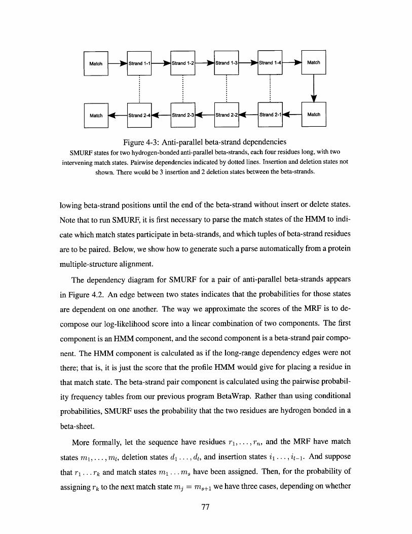
Figure 4-3: Anti-parallel beta-strand dependenciesSMURF states for two hydrogen-bonded anti-parallel beta-strands, each four residues long, with two
intervening match states. Pairwise dependencies indicated by dotted lines. Insertion and deletion states not
shown. There would be 3 insertion and 2 deletion states between the beta-strands.
lowing beta-strand positions until the end of the beta-strand without insert or delete states.
Note that to run SMURF, it is first necessary to parse the match states of the HMM to indi-
cate which match states participate in beta-strands, and which tuples of beta-strand residues
are to be paired. Below, we show how to generate such a parse automatically from a protein
multiple-structure alignment.
The dependency diagram for SMURF for a pair of anti-parallel beta-strands appears
in Figure 4.2. An edge between two states indicates that the probabilities for those states
are dependent on one another. The way we approximate the scores of the MRF is to de-
compose our log-likelihood score into a linear combination of two components. The first
component is an HMM component, and the second component is a beta-strand pair compo-
nent. The HMM component is calculated as if the long-range dependency edges were not
there; that is, it is just the score that the profile HMM would give for placing a residue in
that match state. The beta-strand pair component is calculated using the pairwise probabil-
ity frequency tables from our previous program BetaWrap. Rather than using conditional
probabilities, SMURF uses the probability that the two residues are hydrogen bonded in a
beta-sheet.
More formally, let the sequence have residues rl, ... , rn, and the MRF have match
states mi, ... , mi, deletion states d, ... , dl, and insertion states i ... , il_ 1. And suppose
that r, ... rk and match states mi ... m have been assigned. Then, for the probability of
assigning rk to the next match state mj = ms+ we have three cases, depending on whether
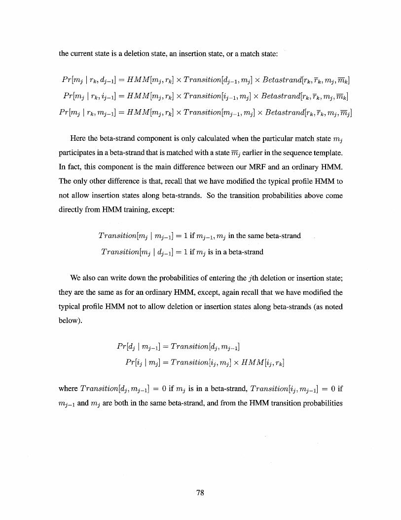
the current state is a deletion state, an insertion state, or a match state:
Pr[mj , dj-1] = HMM[mj, rk] Transition [dj_, mj] x Betastrand[rk, Tk, m , Tk]
Pr[mj Irk, ij-1] = HMM[mj, rk] X Transition[ijl, mj] X Betastrand[rk, rk, m , Tk]
Pr[mj I Trk, nj-11 = HMM[mj, rk] x Transition[mjl, mj] x Betastrand[rk, Tk, mj, j]
Here the beta-strand component is only calculated when the particular match state mj
participates in a beta-strand that is matched with a state Tj earlier in the sequence template.
In fact, this component is the main difference between our MRF and an ordinary HMM.
The only other difference is that, recall that we have modified the typical profile HMM to
not allow insertion states along beta-strands. So the transition probabilities above come
directly from HMM training, except:
Transition[mj I mj-1] = 1 if mj-1, mj in the same beta-strand
Transition[mj I dj- 1] = 1 if mj is in a beta-strand
We also can write down the probabilities of entering the jth deletion or insertion state;
they are the same as for an ordinary HMM, except, again recall that we have modified the
typical profile HMM not to allow deletion or insertion states along beta-strands (as noted
below).
Pr[dj I myl ] = Transition[dj, mj-1]
Pr[ij I my] = Transition[ij, my] x HMM[ij, rk]
where Transition[dj, mj-1] = 0 if my is in a beta-strand, Transition[i, myj1] = 0 if
mj_l and mj are both in the same beta-strand, and from the HMM transition probabilities
I _ i
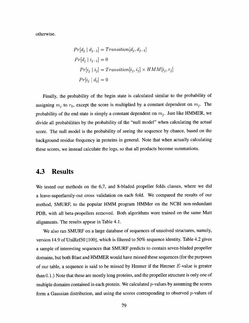
otherwise.
Pr[dj dj_l] = Transition[dj, dj- 1]
Pr[dj ij-1] = 0
Pr[ij | ij] = Transition[is, ij] x HMM[is, rj]
Pr[ij I dj] = 0
Finally, the probability of the begin state is calculated similar to the probability of
assigning mj to rk, except the score is multiplied by a constant dependent on mj. The
probability of the end state is simply a constant dependent on mj. Just like HMMER, we
divide all probabilities by the probability of the "null model" when calculating the actual
score. The null model is the probability of seeing the sequence by chance, based on the
background residue frequency in proteins in general. Note that when actually calculating
these scores, we instead calculate the logs, so that all products become summations.
4.3 Results
We tested our methods on the 6,7, and 8-bladed propeller folds classes, where we did
a leave-superfamily-out cross validation on each fold. We compared the results of our
method, SMURF, to the popular HMM program HMMer on the NCBI non-redundant
PDB, with all beta-propellers removed. Both algorithms were trained on the same Matt
alignments. The results appear in Table 4.1.
We also ran SMURF on a large database of sequences of unsolved structures, namely,
version 14.9 of UniRef50 [100], which is filtered to 50% sequence identity. Table 4.2 gives
a sample of interesting sequences that SMURF predicts to contain seven-bladed propeller
domains, but both Blast and HMMER would have missed these sequences (for the purposes
of our table, a sequence is said to be missed by Hmmer if the Hmmer E-value is greater
than 0.1.) Note that these are mostly long proteins, and the propeller structure is only one of
multiple domains contained in each protein. We calculated p-values by assuming the scores
form a Gaussian distribution, and using the scores corresponding to observed p-values of
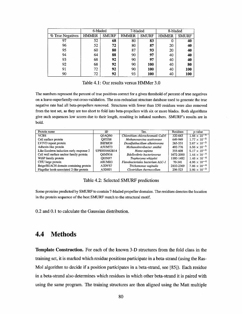
6-bladed 7-bladed 8-bladed% True Negatives HMMER SMURF HMMER SMURF HMMER SMURF
97 52 68 80 83 0 4096 52 72 80 87 20 4095 60 80 87 93 20 4094 64 88 90 97 40 4093 68 92 90 97 40 4092 68 92 90 100 40 8091 72 92 90 100 40 10090 72 92 93 100 40 100
Table 4.1: Our results versus HMMer 3.0
The numbers represent the percent of true positives correct for a given threshold of percent of true negativeson a leave-superfamily-out cross-validation. The non-redundant structure database used to generate the truenegative rate had all beta-propellers removed. Structures with fewer than 150 residues were also removedfrom the test set, as they are too short to fold into beta-propellers with six or more
give such sequences low scores due to their length, resulting in inflated numbers.bold.
blades. Both algorithms
SMURF's results are in
Protein name ID Tax. Residues p-valueVCBS Q3AQB0 Chlorobium chlorochromatii CaD3 320-643 1.88 x 10-
Cell surface protein Q8TJS8 Methanosarcina acetivorans 649-949 1.77 x 10- 5
LVIVD repeat protein B8FMG9 Desulfatibacillum alkenivorans 265-551 2.67 x 10- 5
Adhesin-like protein A5UMT3 Methanobrevibacter smithii 492-776 3.56 x 10- 5
Like Esoderm induction early response 2 UPI0001662B14 Homo sapiens 355-608 5.17 x 10- 5
Cell wall surface anchor family protein Q6MN16 Bdellovibrio bacteriovorus 1672-2000 1.44 x 10- 4
WiSP family protein Q83NF7 Tropheryma whipplei 1180-1482 1.46 x 10- 4
CHU large protein A8UMR3 Flavobacteriales bacterium ALC-1 70-341 4.96 x 10- 4
Beige/BEACH domain containing protein A2DVS7 Trichomonas vaginalis 2110-2369 7.86 x 10- 4
Flagellar hook-associated 2-like protein A3DHJ1 Clostridium thermocellum 206-523 2.86 x 10- 3
Table 4.2: Selected SMURF predictions
Some proteins predicted by SMURF to contain 7-bladed propeller domains. The residues denotes the locationin the protein sequence of the best SMURF match to the structural motif.
0.2 and 0.1 to calculate the Gaussian distribution.
4.4 Methods
Template Construction. For each of the known 3-D structures from the fold class in the
training set, it is marked which residue positions participate in a beta-strand (using the Ras-
Mol algorithm to decide if a position participates in a beta-strand, see [85]). Each residue
in a beta-strand also determines which residues in which other beta-strand it is paired with
using the same program. The training structures are then aligned using the Matt multiple
I Ii i _; ;i__;_~__ill_~~_l___i______~_llj_ 111__;I___I_____LiI_~~i i~~.i---i.i.-~i_

Before:Seql ...VVDGD-ALLV--GFSEGSVN-YLYDG-GET-KLR--ING. ..
Seq2 ...VVDGDK--LLV-GFSEGSLQ-SMYDS-GETVKLR--ING...Seq3 ... LD-GDLIA--FVS----RGQAFIQDSVGTYVL--KVL--...Seq4 .. .VI-GDL--IAFVS----RGY----DSVGTYVLKV--L--...Seq5 .. .VI-GDL--IAF-S----AGY--IQDSVGTY-LKV--L--...
1 2345 5432 1
After:Seql .. .VVDGD- LV--GFSEGSVN-YLYDG-GET-KLR ING...
Seq2 .. .VVDGDK LLV-GFSEGSLQ-SMYDS-GETVKLR ING...Seq3 ... LD-GDL -- FVS----RGQAFIQDSVGTYVL-- L--...
Seq4 ... VI-GDL IAFVS----RGY----DSVGTYVLKV L--...
Seq5 ...VI-GDL IAF-S----AGY--IQDSVGTY-LKV L--...1 234 432 1
Figure 4-4: Template construction
Example of the template construction phase modifying a pair of hydrogen-bonded anti-parallel beta-strands in
Matt alignment containing five structures. The positions labeled with the same number are hydrogen-bonded
to each other, in all sequences with a residue in corresponding numbered positions. Intervening residues are
removed from the four-residue consensus beta-strand pair. Fewer than half the structures have a residue in
position five in the first strand, so both position fives are removed from the beta-strand. Residues outside all
consensus beta-strand pairs are never removed.
structure alignment program (see Chapter 2), and we call a position in the alignment beta-
conserved if more than half the structures in the alignment mark that position as participat-
ing in a beta-sheet. A pair of positions in the alignment is a beta-conserved pair if more
than half the structures in the alignment mark both positions as being hydrogen bonded with
each other in the beta-sheet. Two beta-conserved pairs AB and CD are said to be adjacent
if in more than half the structures of the alignment, A is adjacent to C and B is adjacent to
D, and AB and CD are hydrogen-bonded to each other in the same beta-sheet. Template
beta-conserved strands consist of the maximal contiguous sets of adjacent beta-conserved
strand pairs, together with the information of which residue positions are hydrogen bonded.
Note that since these template positions may only be occupied by positions that are identi-
fied as beta-strands in a majority of the structures, there could be residues in other structures
between these positions in the Matt alignment, creating gap positions in the structural align-
ment in the middle of the template beta-conserved strands. This is undesirable, so we will
remove these positions; this includes possibly deleting residues from sequences when we
remove the corresponding position from the template structural alignment. In the resulting
alignment, the beta-conserved template strands are always contiguous.

The output of this phase is a sequence alignment derived from the Matt structural align-
ment with annotated beta-strand residue positions and the residue positions to which they
are paired. See Figure 4-4 for an example the template construction phase on an alignment.
This multiple sequence alignment, together with the locations of the template beta-strands
is the input to the next training phase.
Model Training Phase. The training phase trains both an HMM on the multiple se-
quence alignment, and also, pairwise probabilities on the paired residue positions in the
template beta-strands. The HMM portion of the training is exactly the default HMM train-
ing from HMMer version 3, except that every template beta-strand position is always in-
cluded in the output model. For the pairwise probabilities in the template beta-strands, the
"in" and "out" pairwise probability tables from the program BetaWrap are considered [12].
it is determined for each residue position, whether the sum of the pairwise probabilities
of seeing the pairs in the training alignment, summed over all structures in the alignment,
was more probable from the "buried" or the "exposed" probability table. The position is
then labeled buried or exposed accordingly. Note that, while the names buried and exposed
come from the solvent accessibility of residue positions in the original BetaWrap algo-
rithm, no claim about solvent accessibility or consistency of solvent accessibility is made
in our context. In our case, in a structurally oblivious way, we are simply determining
based on the training data which of the two models best predicts the set of residue pairs
we see. The output is an HMM where certain states are marked as beta-strand states, and,
pairings of hydrogen-bonded beta-strand states are also given. Since the score includes a
component from these pairs, and not just the linear score of the HMM component, it is no
longer a simple HMM, but rather a MRF, because of the non-linear dependencies between
the paired states in constructing the score.
Score. For a given test sequence, we seek the parse of the sequence to the states of the
training HMM that optimizes the particular score. The score we seek to optimize, over all
ways to map the sequence to the states of the MRF model is
a! x log (HMM score) + P x log (pairwise score)

where the HMM score represents the conditional probability of seeing the sequence given
the HMM portion of the model. Experimentally, using a value of one for both a and 3
provided the best results on cross-validation (see Table 4.1). The details of how a particular
parse of sequence to the states of the MRF is scored has already been given above, in the
section on the algorithm. The score of the sequence is then the maximum score obtained
over all possible ways to parse the sequence onto the states of the MRF. We next explain
how to compute this maximum score.
Computing the Score. The maximum score of a sequence is computed by multi-
dimensional dynamic programming. The dynamic programming takes place on the MRF
described above- it has the same beginning states, ending states, match states, insertion
states and deletion states as does HMMer HMMs, except some of the states are special
beta-strand states. Recall that the beta-strand states consist of sets of contiguous states with
no insertion or deletion states allowed between them (the beta-strands), and furthermore,
beta-strands are paired with other beta-strands. In particular, the pairwise probabilities for
paired beta-strands can only be calculated for the second paired beta-strand, once it has
been fixed what residue will be occupying the first position of the pair. Thus, each time
we reach a state in the HMM that corresponds to the first residue of the first beta-strand
in a set of paired beta-strands, we need to keep track of multiple cases, depending on
what sequence position is mapped to that state in the dynamic program. We keep track
of this using a multi-dimensional array. For arbitrary gap lengths, this quickly becomes
computationally infeasible, so a maximum gap length is defined (and for our purposes is set
to the longest gap seen in the training alignment plus 20). When paired beta-strands follow
each other in sequence with no interleaving beta-strands between them (which is usually
the case for the beta-propellers) the number of dimensions in the table for the portion of the
dynamic program that parses the parts of the HMM between the two beta-strands is directly
proportional to the maximum gap length.
We now introduce some notation that will help describe the algorithm and analyze its
complexity for interleaving pairs of beta-strands. When we look, in order of sequence, at
the states in the template MRF, mark the first of a pair of beta-strands with consecutive
numbers 1,2,3, and so on, and mark its corresponding paired beta-strand with the same

number. Thus if we have n pairs of beta-strands, we get a sequence that contains precisely
two occurrences of each of the numbers from 1 to n. Now replace the first occurrence of
each number with a left parenthesis and the second occurrence with a right parenthesis.
Starting with the number 0, walk along the sequence, adding one for every left parenthesis,
and subtracting one for every right parenthesis. The maximum size of this total at any
intermediate point we call the interleaving number of this sequence. We call the last MRF
state for the first of each pair of beta-strands the "split" state, and the first MRF state for
the second of that pair of beta-strands the "join" state.
At every split state, the number of dimensions of the dynamic program will be multi-
plied by the maximum gap length, since the dynamic program has to keep track of scores
for each possible sequence position (up to maximum gap length) that could be mapped to
that state. At the corresponding join state, the number of dimensions will be reduced by the
maximum gap length, since the scoring function can calculate all the pairwise probabilities
(and hence the score) of placing that residue into the join state, and then simply take the
maximum of all ways to have placed its paired residue into the split state. Thus the number
of elements in the multi-dimensional table is never more than sequence length times the
maximum gap length raised to the interleaving number power. As noted above, when there
are few or no interleaving beta-strand pairs, as is the case with the strand topology of the
beta-propellers, this is very computationally feasible. On the other hand, the algorithm may
become computationally infeasible for structures with many interleaving beta-strands, such
as the parallel beta-helix structures.
4.5 Discussion
A major challenge in protein threading has been to find a tractable way to integrate local
sequence information with higher-order structural dependencies in an integrated, compu-
tationally tractable, energy function. We have presented a framework, SMURF (Structural
Motifs Using Random Fields), that integrates long-distance pairwise correlations involving
beta-sheet formation with an HMM using a random field, and tested it on three fold classes,
namely the five, six, and seven-bladed propellers. There is nothing in the method, however,
that restricts it to propellers. The method can be applied to any beta-structural motif where
there is enough training data, and the number of interleaved pairs of beta-strands is not too
great. We will be applying SMURF to additional classes of beta-structural motifs in the
future.


Chapter 5
Conclusions
5.1 Discussion and Future Work
We have introduced the program Matt and demonstrated that its use of local flexibility
yields high-quality multiple structure alignments even when proteins are more distantly ho-
mologous. We have introduced the program BetaWrapPro which combines long-distance
pairwise correlations involved in beta-sheet formation with sequence profiles and a back-
bone dependent rotamer library to successfully recognize beta-helices and beta-trefoils
from hand-constructed templates of solved structures. Finally, we introduced the program
SMURF which can combines automatic template construction using Matt, pairwise beta-
sheet probabilities in a manner similar to BetaWrapPro, and profile hidden Markov models
into a general method for recognize beta-structural motifs. We now discuss what is yet to
be done and future directions.
As a stand alone structure alignment program, Matt is probably the current state of the
art for aligning proteins that are distant homologs. However, it may still be possible to
improve Matt. For example, Matt currently only uses alpha-carbon coordinates in its align-
ments. Adding sequence information to its scoring function may well improve alignment
accuracy as well as allow it to handle cases where some residues lack alpha-carbon coordi-
nates in the input structures, as is often the case in PDB files. Adding the option to weight
structures by either their sequence or structure similarity would reduce the problem of bias
when some of the input structures are significantly more similar to each other than others.

Based on X-ray scattering results [56], beta-helices are a possible structure for many
prions and amyloids. We are are actively working to apply the methods developed for
BetaWrapPro to combine sequence information with CD spectral, X-ray scattering, and
electron microscopy data to model and investigate the observed properties of prion tendrils.
However, most of our future research is going to be focused on SMURF. SMURF has
yet to be trained and tested on any folds other than the beta-propellers. Running on a
broader set of structures will undoubtedly highlight any weaknesses in the current algo-
rithm, and provide more information on what types of beta structures it works well on,
and for which structures its memory requirements are prohibitively high. Incorporating
profiles of input sequences and adding a side-chain packing algorithm as a post process
may increase the accuracy of SMURF as they did with BetaWrapPro. Adding support for
multiple hits in a single sequence and improving handling of very long sequences, both of
which HMMER already supports, could improve SMURF's results with a minimal impact
on runtime and memory usage. Support for other long range dependencies, such as disul-
fide bonds, could also be added to SMURF. It's also possible to decrease its memory usage
significantly. An implementation capable of disk caching or using 64-bit addressing would
also make memory usage less of an issue.
Protein structural motif recognition is an easy problem for proteins that are close ho-
mologs to proteins of solved structure. For distant homologs, it remains an incredibly
challenging problem. Hopefully this thesis has significantly extended the class of protein
structures for which we can solve this problem, particularly in the case of beta-structural
motifs.

Appendix A
Pairwise Tables

Residue A C D E F G H I K L M N P Q R S T V W YA 5.8 5.5 8.9 19.5 7.5 3.6 12.6 7.8 5.5 8.8 5.4 10.0 6.9 4.6 2.9 6.7 8.4 7.8 7.9 7.4C 2.2 11.1 3.5 2.4 2.8 4.3 3.1 2.5 5.5 2.8 1.4 3.3 13.9 2.3 2.9 4.3 4.2 2.2 6.1 3.0D 1.0 1.0 0.8 0.8 0.6 2.1 1.5 0.8 0.8 0.3 0.9 5.0 4.6 0.8 5.8 3.0 0.6 0.8 0.8 0.3E 1.6 0.5 0.6 4.8 0.9 0.3 3.1 0.6 11.1 0.4 1.4 0.6 0.6 0.6 0.6 1.2 0.6 0.1 0.6 0.6F 9.9 9.0 7.1 14.6 11.9 13.8 11.1 8.4 11.1 9.1 11.8 5.0 11.6 13.9 8.8 14.1 11.4 9.0 8.8 11.1G 2.0 6.0 10.7 2.4 5.9 6.5 7.9 3.6 4.3 3.6 2.9 1.6 13.9 2.3 2.9 3.0 6.0 4.4 2.6 5.2H 1.6 1.0 1.7 4.8 1.1 1.8 6.3 0.6 0.9 0.6 0.9 1.6 0.9 2.3 0.9 3.7 1.2 0.2 0.8 0.9I 17.6 14.1 16.0 17.0 14.3 14.1 11.1 20.5 16.6 17.8 18.8 11.6 9.3 13.9 5.8 15.4 8.4 17.7 15.9 15.7
K 0.2 0.5 0.2 4.8 0.3 0.2 0.2 0.2 0.2 0.4 0.2 0.2 0.2 2.3 2.9 0.6 0.2 0.2 0.2 0.2L 18.9 14.6 7.1 12.1 14.7 13.8 11.1 17.0 27.7 18.0 16.8 13.3 9.3 11.6 5.8 13.5 15.0 16.0 13.2 16.6M 2.2 1.5 3.5 7.3 3.7 2.1 3.1 3.5 3.1 3.3 5.9 1.6 2.3 9.3 2.9 0.6 4.2 2.9 2.6 3.3N 1.2 1.0 5.3 0.9 0.4 0.3 1.5 0.6 0.9 0.7 0.4 0.9 2.3 4.6 2.9 1.2 3.6 0.7 4.4 0.3P 0.6 3.0 3.5 0.6 0.7 2.1 0.6 0.3 0.6 0.3 0.4 1.6 0.6 2.3 0.6 1.2 0.6 0.2 3.5 0.6Q 0.4 0.5 0.6 0.6 0.9 0.3 1.5 0.5 5.5 0.4 1.9 3.3 2.3 0.6 2.9 1.8 0.6 0.6 1.7 0.3R 0.2 0.5 3.5 0.5 0.4 0.3 0.5 0.1 5.5 0.1 0.4 1.6 0.5 2.3 0.5 0.6 2.4 0.6 1.7 1.5S 2.2 3.5 8.9 4.8 3.6 1.8 9.5 2.3 5.5 2.1 0.4 3.3 4.6 6.9 2.9 8.6 0.6 1.6 4.4 2.1T 2.9 3.5 1.7 2.4 2.9 3.6 3.1 1.2 2.5 2.4 3.4 10.0 2.3 2.3 11.7 0.6 2.4 3.0 1.7 3.3V 22.2 15.1 21.4 4.8 19.3 22.1 6.3 22.2 16.6 21.1 19.8 16.6 6.9 20.9 26.4 13.5 25.3 25.4 12.3 19.7W 1.8 3.5 1.7 1.7 1.5 1.0 1.5 1.6 1.7 1.4 1.4 8.3 9.3 4.6 5.8 3.0 1.2 1.0 3.5 2.7Y 4.9 5.0 1.7 4.8 5.6 6.1 4.7 4.7 5.0 5.2 5.4 1.6 4.6 2.3 14.7 4.3 6.6 4.7 7.9 4.9
Table A.1: Solvent inaccessible beta residue conditional probabilitiesPairwise conditional probability tables of solvent inaccessible residue pairs used by BetaWrapPro to detect beta-helices. The value in row i, column j is the
probability of residue i appearing in a beta-strand given that it is aligned with residue j. They were calculated from a hand annotated set of amphipathic parallel
and anti-parallel beta-sheets from a subset of the PDB containing no beta-helices.

Residue A C D E F G H I K L M N P Q R S T V W YA 5.4 7.6 4.0 2.9 5.0 4.0 4.7 5.0 2.8 5.5 4.4 3.6 3.1 2.0 4.1 3.4 2.7 5.4 2.1 5.9C 2.3 10.2 0.4 0.2 2.5 0.5 0.9 0.8 0.9 1.2 0.8 1.0 1.5 0.3 1.6 1.4 1.2 1.0 2.1 1.8D 3.8 1.2 2.4 2.1 2.5 4.0 5.2 3.5 6.7 3.2 3.5 3.6 1.5 4.8 6.4 5.3 3.7 2.1 4.3 2.7E 5.4 1.2 4.0 5.1 7.6 4.0 5.6 5.7 15.8 6.4 10.6 9.3 7.9 7.3 13.0 5.1 8.0 6.0 7.6 4.6F 4.6 7.6 2.4 3.8 6.7 7.6 7.1 2.4 2.6 4.0 7.0 2.5 3.1 2.7 1.1 5.3 3.6 2.9 4.3 3.7G 2.7 1.2 2.8 1.4 5.5 3.5 4.2 3.0 0.7 4.0 6.1 4.1 1.5 1.7 2.9 2.9 1.8 2.0 3.2 3.7H 3.8 2.5 4.5 2.5 6.3 5.2 2.8 2.8 3.0 3.0 4.4 2.0 4.7 2.7 2.2 3.4 3.3 3.4 2.1 4.9I 8.9 5.1 6.5 5.5 4.6 8.1 6.1 13.1 6.9 9.4 9.7 5.1 6.3 6.6 6.8 7.0 5.4 7.6 7.6 5.9
K 5.8 6.4 14.7 17.9 5.9 2.3 7.5 8.1 8.6 7.7 10.6 8.8 3.1 9.4 5.9 5.3 7.2 6.5 9.8 11.8L 10.0 7.6 6.1 6.4 8.0 11.1 6.6 9.6 6.7 10.3 5.3 3.1 14.2 6.2 5.2 6.5 4.8 10.9 7.6 6.5M 1.9 1.2 1.6 2.5 3.3 4.0 2.3 2.4 2.2 1.2 3.5 1.5 1.5 1.3 2.0 1.4 1.0 1.4 1.0 0.6N 2.7 2.5 2.8 3.8 2.1 4.6 1.8 2.1 3.2 1.2 2.6 3.1 3.1 4.5 4.5 3.1 3.7 1.8 4.3 4.0P 0.7 1.2 0.4 1.0 0.8 0.5 1.4 0.8 0.3 1.9 0.8 1.0 1.0 0.6 1.1 0.4 0.7 1.2 2.1 2.4
Q 2.3 1.2 5.7 4.4 3.3 2.9 3.7 4.1 5.0 3.8 3.5 6.7 3.1 8.3 3.4 3.9 5.9 4.5 6.5 4.6R 6.9 8.9 11.4 12.2 2.1 7.6 4.7 6.5 4.9 4.9 7.9 10.3 7.9 5.2 2.7 6.8 8.4 8.2 10.9 5.9S 5.4 7.6 9.0 4.4 9.3 7.0 6.6 6.3 4.1 5.7 5.3 6.7 3.1 5.5 6.4 8.7 10.3 4.5 5.4 6.8T 6.9 10.2 10.2 11.3 10.1 7.0 10.4 7.9 9.0 6.8 6.1 12.9 7.9 13.6 12.8 16.5 15.7 11.3 2.1 4.3V 11.6 7.6 4.9 7.0 6.7 6.4 9.0 9.2 6.7 12.8 7.0 5.1 11.1 8.7 10.3 6.0 9.3 11.3 9.8 9.3W 0.7 2.5 1.6 1.4 1.6 1.7 0.9 1.5 1.6 1.5 0.8 2.0 3.1 2.0 2.2 1.2 0.3 1.6 2.1 1.2Y 7.3 7.6 3.6 3.2 5.0 7.0 7.5 4.1 7.1 4.5 1.7 6.7 12.6 5.2 4.3 5.3 2.1 5.4 4.3 8.6
Table A.2: Solvent accessible beta residue conditional probabilitiesPairwise conditional probability tables of solvent accessible residue pairs used by BetaWrapPro to detect beta-helices. The value in row i, column j is the probability
of residue i appearing in a beta-strand given that it is aligned with residue j. They were calculated from a hand annotated set of amphipathic parallel and anti-parallel
beta-sheets from a subset of the PDB containing no beta-helices.

Residue A C D E F G H I K L M N P Q R S T V W YA 5.8 4.3 10.0 8.3 5.8 5.2 5.4 6.7 5.9 8.0 7.4 5.9 6.1 6.4 5.4 5.5 7.9 8.6 4.9 4.4C 2.4 18.4 2.9 3.3 2.8 4.7 4.7 2.5 3.3 2.5 2.3 7.1 4.6 3.7 3.7 3.3 2.7 2.4 15.6 3.9D 3.2 1.7 3.3 2.2 1.4 1.3 4.7 1.9 3.2 1.1 2.0 5.3 1.8 1.6 3.7 2.7 2.7 2.6 2.4 1.1E 3.2 2.3 2.7 2.1 2.3 1.3 2.9 2.0 4.0 2.1 2.5 5.0 2.5 4.4 5.9 3.3 4.0 2.0 3.8 2.8F 6.2 5.4 4.8 6.4 9.3 9.5 5.8 8.9 5.3 6.4 10.1 3.4 6.1 6.0 7.4 6.0 5.3 7.7 8.2 8.4G 3.2 5.3 2.5 2.1 5.5 6.5 4.7 4.2 1.7 4.0 3.2 4.3 6.4 3.3 2.2 4.8 4.0 4.8 4.5 4.2H 1.0 1.6 2.7 1.4 1.0 1.4 2.2 1.0 1.0 1.1 1.8 1.5 2.1 1.5 1.9 1.3 2.1 0.8 0.4 1.8I 12.1 8.1 10.4 9.5 15.0 12.3 9.8 17.4 11.5 14.2 7.9 5.9 6.4 13.0 9.5 9.2 9.2 12.2 10.7 10.3
K 2.7 2.7 4.6 4.8 2.3 1.3 2.5 3.0 2.9 1.9 3.1 3.1 1.1 4.8 2.2 4.5 4.3 3.4 5.3 6.2L 15.1 8.4 6.5 10.0 11.2 12.1 10.9 14.8 7.5 17.0 12.7 10.8 11.1 12.3 9.8 10.9 9.9 14.7 9.1 9.7M 2.7 1.6 2.3 2.4 3.5 1.9 3.6 1.6 2.4 2.5 6.1 3.7 5.7 1.5 4.0 1.9 3.5 2.1 1.6 2.4N 1.3 2.7 3.5 2.8 0.7 1.5 1.8 0.7 1.4 1.3 2.2 4.3 1.8 2.6 2.1 1.6 2.9 0.8 1.1 1.5P 1.1 1.6 1.0 1.2 1.1 1.9 2.2 0.7 0.4 1.1 2.9 1.5 2.9 0.7 0.8 1.3 1.4 1.0 3.8 2.2Q 2.3 2.4 1.9 4.1 2.1 1.9 2.9 2.6 3.7 2.4 1.4 4.3 1.4 1.5 2.4 3.0 1.6 2.1 1.1 5.1R 2.3 2.7 4.8 6.4 2.9 1.5 4.3 2.2 2.0 2.2 4.5 4.0 1.8 2.7 2.6 2.5 4.2 2.2 3.3 5.5S 2.5 2.6 3.8 3.8 2.5 3.4 3.3 2.3 4.3 2.6 2.3 3.4 3.2 3.7 2.7 6.3 4.4 3.1 3.3 3.0T 5.2 3.2 5.6 6.9 3.3 4.3 7.6 3.4 6.2 3.5 6.3 9.0 5.0 2.9 6.7 6.5 6.8 3.8 1.6 6.0V 22.4 11.1 21.5 13.4 18.7 20.2 11.6 17.7 18.9 20.5 14.7 9.9 13.9 15.2 13.8 17.7 14.8 19.8 10.2 15.1W 1.5 8.4 2.3 2.9 2.3 2.2 0.7 1.8 3.4 1.5 1.3 1.5 6.1 0.9 2.4 2.2 0.7 1.2 2.2 2.4Y 3.5 5.6 2.7 5.9 6.3 5.5 8.0 4.6 10.8 4.2 5.2 5.6 9.6 11.2 10.6 5.4 7.3 4.7 6.5 3.7
Table A.3: Solvent inaccessible twisted beta-strand residue conditional probabilitiesPairwise conditional probability tables of solvent inaccessible residue pairs used by BetaWrapPro to detect beta-trefoils. The value in row i, column j is the
probability of residue i appearing in a beta-strand given that it is aligned with residue j. They were calculated using an automated search for twisted amphipathic
strands in a non-redundant structure database with the beta-trefoils removed.
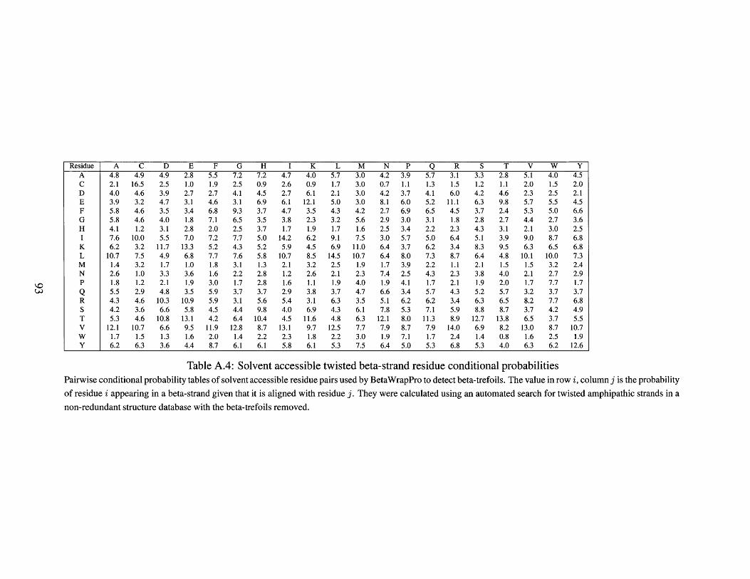
Residue A C D E F G H I K L M N P Q R S T V W YA 4.8 4.9 4.9 2.8 5.5 7.2 7.2 4.7 4.0 5.7 3.0 4.2 3.9 5.7 3.1 3.3 2.8 5.1 4.0 4.5C 2.1 16.5 2.5 1.0 1.9 2.5 0.9 2.6 0.9 1.7 3.0 0.7 1.1 1.3 1.5 1.2 1.1 2.0 1.5 2.0D 4.0 4.6 3.9 2.7 2.7 4.1 4.5 2.7 6.1 2.1 3.0 4.2 3.7 4.1 6.0 4.2 4.6 2.3 2.5 2.1E 3.9 3.2 4.7 3.1 4.6 3.1 6.9 6.1 12.1 5.0 3.0 8.1 6.0 5.2 11.1 6.3 9.8 5.7 5.5 4.5F 5.8 4.6 3.5 3.4 6.8 9.3 3.7 4.7 3.5 4.3 4.2 2.7 6.9 6.5 4.5 3.7 2.4 5.3 5.0 6.6G 5.8 4.6 4.0 1.8 7.1 6.5 3.5 3.8 2.3 3.2 5.6 2.9 3.0 3.1 1.8 2.8 2.7 4.4 2.7 3.6H 4.1 1.2 3.1 2.8 2.0 2.5 3.7 1.7 1.9 1.7 1.6 2.5 3.4 2.2 2.3 4.3 3.1 2.1 3.0 2.5I 7.6 10.0 5.5 7.0 7.2 7.7 5.0 14.2 6.2 9.1 7.5 3.0 5.7 5.0 6.4 5.1 3.9 9.0 8.7 6.8
K 6.2 3.2 11.7 13.3 5.2 4.3 5.2 5.9 4.5 6.9 11.0 6.4 3.7 6.2 3.4 8.3 9.5 6.3 6.5 6.8L 10.7 7.5 4.9 6.8 7.7 7.6 5.8 10.7 8.5 14.5 10.7 6.4 8.0 7.3 8.7 6.4 4.8 10.1 10.0 7.3M 1.4 3.2 1.7 1.0 1.8 3.1 1.3 2.1 3.2 2.5 1.9 1.7 3.9 2.2 1.1 2.1 1.5 1.5 3.2 2.4N 2.6 1.0 3.3 3.6 1.6 2.2 2.8 1.2 2.6 2.1 2.3 7.4 2.5 4.3 2.3 3.8 4.0 2.1 2.7 2.9P 1.8 1.2 2.1 1.9 3.0 1.7 2.8 1.6 1.1 1.9 4.0 1.9 4.1 1.7 2.1 1.9 2.0 1.7 7.7 1.7Q 5.5 2.9 4.8 3.5 5.9 3.7 3.7 2.9 3.8 3.7 4.7 6.6 3.4 5.7 4.3 5.2 5.7 3.2 3.7 3.7R 4.3 4.6 10.3 10.9 5.9 3.1 5.6 5.4 3.1 6.3 3.5 5.1 6.2 6.2 3.4 6.3 6.5 8.2 7.7 6.8S 4.2 3.6 6.6 5.8 4.5 4.4 9.8 4.0 6.9 4.3 6.1 7.8 5.3 7.1 5.9 8.8 8.7 3.7 4.2 4.9T 5.3 4.6 10.8 13.1 4.2 6.4 10.4 4.5 11.6 4.8 6.3 12.1 8.0 11.3 8.9 12.7 13.8 6.5 3.7 5.5V 12.1 10.7 6.6 9.5 11.9 12.8 8.7 13.1 9.7 12.5 7.7 7.9 8.7 7.9 14.0 6.9 8.2 13.0 8.7 10.7W 1.7 1.5 1.3 1.6 2.0 1.4 2.2 2.3 1.8 2.2 3.0 1.9 7.1 1.7 2.4 1.4 0.8 1.6 2.5 1.9Y 6.2 6.3 3.6 4.4 8.7 6.1 6.1 5.8 6.1 5.3 7.5 6.4 5.0 5.3 6.8 5.3 4.0 6.3 6.2 12.6
Table A.4: Solvent accessible twisted beta-strand residue conditional probabilitiesPairwise conditional probability tables of solvent accessible residue pairs used by BetaWrapPro to detect beta-trefoils. The value in row i, column j is the probability
of residue i appearing in a beta-strand given that it is aligned with residue j. They were calculated using an automated search for twisted amphipathic strands in a
non-redundant structure database with the beta-trefoils removed.

Residue A C D E F G H I K L M N P Q R S T V W YA 4.9 4.8 4.1 3.5 4.5 5.7 7.8 4.5 2.9 4.4 4.3 4.1 4.4 3.8 3.2 5.2 4.7 4.6 6.7 3.8C 1.6 2.3 3.1 2.4 1.9 1.6 2.4 1.5 2.6 1.3 1.5 1.5 1.3 1.6 2.6 3.6 1.9 1.7 2.7 2.2D 3.6 3.9 2.2 2.0 4.1 3.9 3.1 3.4 3.1 3.6 3.7 5.6 4.0 2.1 2.5 3.4 3.3 3.4 2.2 2.8E 5.5 5.5 5.7 4.3 6.5 6.9 4.5 6.8 6.1 6.8 7.5 4.1 4.2 4.7 5.7 4.7 5.4 7.2 5.5 5.6F 4.6 4.4 4.2 5.5 4.1 5.0 6.7 5.8 3.3 4.6 5.1 3.0 4.2 4.3 6.0 5.4 4.7 4.2 5.7 4.4G 5.0 3.9 4.0 5.6 3.2 6.1 4.5 3.5 4.6 4.0 1.7 4.4 5.0 5.3 4.8 5.2 5.5 3.8 4.0 5.3H 2.9 3.2 1.2 1.8 3.3 2.1 2.0 2.3 1.8 2.8 2.5 1.8 2.5 2.1 2.0 3.0 2.8 2.5 2.6 1.6I 8.1 5.9 9.0 9.8 6.9 7.3 10.5 7.6 8.2 6.1 6.9 7.7 7.5 6.1 7.9 6.9 9.6 6.9 6.8 6.5
K 6.6 7.7 6.8 6.3 6.9 6.1 5.8 7.3 8.3 6.8 5.7 7.7 5.8 8.2 6.1 3.9 5.0 6.6 5.6 8.2L 9.6 5.2 11.3 9.6 6.8 8.8 7.6 8.8 7.9 8.9 8.0 7.9 8.5 7.4 10.1 11.2 9.7 8.7 6.3 7.0M 2.3 1.4 1.7 3.1 1.6 2.1 2.4 2.0 1.9 1.9 2.3 2.0 3.7 1.6 2.1 1.3 2.7 1.7 1.7 1.9N 3.1 4.8 2.7 2.2 3.4 3.5 3.6 2.9 2.0 2.5 4.0 2.0 2.3 5.0 3.2 3.7 2.2 3.0 1.4 2.7P 2.8 2.0 2.4 2.3 1.8 1.6 1.6 1.8 2.4 2.0 2.6 2.1 2.9 3.2 2.1 1.9 2.0 2.5 3.1 2.0Q 4.6 3.2 3.8 2.3 4.2 3.6 3.8 4.4 4.1 4.5 4.3 4.3 2.3 2.2 3.5 2.7 3.7 4.1 6.4 5.5R 5.8 5.0 6.8 6.1 7.1 5.1 5.1 5.7 6.2 6.4 4.8 7.2 6.2 7.6 5.4 5.0 4.4 6.4 5.6 5.9S 5.3 7.5 5.2 5.7 7.5 6.8 4.7 6.7 3.4 6.4 4.4 6.3 5.2 6.8 4.1 4.1 3.4 5.1 5.1 6.1T 7.4 9.6 6.7 5.7 9.7 8.0 6.0 7.9 9.5 9.0 8.8 6.4 6.7 7.4 6.6 8.4 8.3 9.5 6.3 9.0V 8.9 9.1 13.3 13.1 9.9 8.8 10.7 9.5 9.7 11.0 13.2 11.2 11.8 11.1 11.2 11.4 11.7 11.4 7.7 9.8W 1.4 1.7 1.9 3.0 1.8 1.1 2.7 1.9 2.3 2.0 1.3 3.0 1.3 1.6 3.2 1.4 2.2 1.5 1.3 1.2Y 6.0 8.9 3.7 5.9 4.8 5.8 4.5 5.8 9.6 5.0 7.3 7.6 9.8 7.9 7.7 7.5 6.6 5.1 13.1 8.4
Table A.5: Solvent inaccessible twisted beta-strand one-off residue conditional probabilitiesPairwise conditional probability tables of off-by-one residue pairs used by BetaWrapPro to detect beta-trefoils. The value in row i, column j is the probability
of solvent inaccessible residue i appearing in a beta-strand given that it is aligned with a residue adjacent to j. They were calculated using an automated search
for twisted amphipathic strands in a non-redundant structure database with the beta-trefoils removed. Note that the table with solvent accessibility of the row and
column residues exchanged can be calculated from this table.

Bibliography
[1] R.A. Abagyan and S. Batalov. Do aligned sequences share the same fold? J. Mol.Biol., 273(1):355-368, 1997.
[2] S.F. Altschul, W. Gish, W. Miller, E.W. Myers, and D.J. Lipman. Basic local align-ment search tool. J. Mol. Biol., 215:403-410, 1990.
[3] S.F. Altschul, T.L. Madden, A.A. Schaffer, J. Zhang, Z. Zhang, W. Miller, and L.J.Lipman. Gapped BLAST and PSI-BLAST: a new generation of protein databasesearch programs. Nucleic Acids Res., 25:3389-3402, 1997.
[4] T. Arai and K. Matsui. A purified protein from Salmonella typhimurium inhibitshigh-affinity interleukin-2 receptor expression on CTLL-2 cells. FEMS Immunol.Med. Microbiol., 17:155-160, 1997.
[5] G.J. Barton and M.J. Sternberg. A strategy for the rapid multiple alignment of pro-tein sequences. confidence levels from tertiary structure comparisons. J. Mol. Biol.,198:327-337, 1987.
[6] A. Bateman, L. Coin, R. Durbin, R.D. Finn, V. Hollich, S. Griffiths-Jones,A. Khanna, M. Marshall, S. Moxon, E.L.L. Sonnhammer, D.J.Stud holme, C. Yeats,and S.R. Eddy. The pfam protein families database. Nucleic Acids Res., 32:D138-D141, 2004.
[7] B. Berger, D.B. Wilson, E. Wolf, T. Tonchev, M. Milla, and P.S. Kim. Predictingcoiled coils by use of pairwise residue correlations. Proc. Natl. Acad. Sci. U.S.A.,92:8259-8263, August 1995.
[8] H.M. Berman, J. Westbrook, Z. Feng, G. Gilliland, T.N. Bhat, H. Weissig, I.N.Shindyalov, and P.E. Bourne. The protein data bank. Nucleic Acids Res., 28:235-242, 2000.
[9] A.M. Bonvin. Flexible protein-protein docking. Curr Opin. Struct. Biol., 16:194-200, 2006.
[10] M.J. Bower, F.E. Cohen, and R.L. Dunbrack Jr. Prediction of protein side-chainrotamers from a backbone-dependent rotamer library: A new homology modelingtool. J. Mol. Biol., 267:1268-1282, 1997.
[11] P. Bradley, D. Chivian, J. Meiler, K. Misura, and W. Schief C. Rohl, W. Wedemeyer,O. Schueler-Furman, P Murphy, J. Schonbrun, C. Strauss, and D. Baker. Rosettapredictions in CASP5: Successes, failures, and prospects for complete automation.Proteins, 53:457-68, 2003.
[12] P. Bradley, L. Cowen, M. Menke, J. King, and B. Berger. Betawrap: Successful pre-diction of parallel 3-helices from primary sequence reveals an association with manymicrobial pathogens. Proc. Natl. Acad. Sci. U.S.A., 98(26):14819-14824, 2001.
[13] P. Bradley, L. Cowen, M. Menke, J. King, and B. Berger. BETAWRAP: Successfulprediction of parallel 0-helices from primary sequence reveals an association withmany microbial pathogens. Proc. Natl. Acad. Sci. U.S.A., 98:14819-14824, 2001.
[14] S.H. Bryant. Evaluation of threading specificity and accuracy. Proteins, 26:172-185,1996.
[15] C. Chothia and A.M.Lesk. The relation between sequence and structure in proteins.EMBO J., 5:823-826, 1986.
[16] C. Chothia and J. Janin. Relative orientation of close-packed beta-pleated sheets inproteins. Proc. Natl. Acad. Sci. U.S.A., 78(7):4146-4150, 1981.
[17] C. Chothia and J. Janin. Orthogonal packing of beta-pleated sheets in proteins.Biochemistry, 21(17):3955-3965, 1982.
[18] B. Clantin, H. Hodak, E. Willery, C. Locht, F. Jacob-Dubuisson, and V. Villeret. Thecrystal structure of filamentous hemagglutinin secretion domain and its implicationsfor the two-partner secretion pathway. PNAS, 101(16):6194-6199, 2004.
[19] P. Clote. Performance comparison of generalized PSSM in signal peptide cleavagesite and disulfide bond recognition. In BIBE'03, pages 37-44, 2003.
[20] P.G. Comens, B.A. Wolf, E.R. Unanue, PE. Lacy, and M.L. McDaniel. Interleukin1 is potent modulator of insulin secretion from isolated rat islets of Langerhans.Diabetes, 36:963-970, 1987.
[21] L. Cowen, P. Bradley, M. Menke, J. King, and B. Berger. Predicting the beta-helixfold from protein sequence data. J. Comput. Biol., 9(2):261-276, 2002.
[22] E.W. Czerwinski, T. Midoro-Horiuti, M.A. White, E.G. Brooks, and R.M. Gold-blum. Crystal structure of jun a 1, the major cedar pollen allergen from juniperusashei, reveals a parallel beta-helical core. J. Biol. Chem., 280:3740-3746, 2005.
[23] O. Dror, H. Benyamini, R. Nussinov, and H. Wolfson. MASS: multiple structuralalignment by secondary structures. Bioinformatics, 19:95-104, 2003.
[24] O. Dror, H. Benyamini, R. Nussinov, and H.J. Wolfson. Multiple structure alignmentby secondary structures: algorithm and applications. Protein Sci., 12:2492-2507,2003.
[25] R.L. Dunbrack. Sequence comparison and protein structure prediction. Curr. Opin.Struct. Biol., 16(3):274-84, 2006.
[26] N. Echols, D. Milburn, and M. Gerstein. MolMovDB: analysis and visualization ofconformational change and structural flexibility. Nucleic Acids Res., 31:478-482,2003.
[27] S.R. Eddy. Profile hidden Markov models. Bioinformatics, 14:755-763, 1998.
[28] R.C. Edgar and S. Batzoglou. Multiple sequence alignment. Curr. Opin. Struct. Bio.,16:368-373, 2006.
[29] I. Eidhammer, I. Jonassen, and W. R. Taylor. Structure comparison and structurepatterns. J. Comput. Biol., 7:685-716, 2000.
[30] P. Emsley, I.G. Charles, N.F. Fairweather, and N.W. Isaacs. Structure of bordetellapertussis virulence factor p.69 pertactin. Nature, 381:90-92, 1996.
[31] J. Fong, A. Keating, and M. Singh. Predicting specificity in bZIP coiled-coil proteininteractions. Genome Biol, 5(2):R11, 2004.
[32] D. Frishman and P. Argos. Knowledge-based protein secondary structure assign-ment. Proteins, 23(4):556-579, 1995.
[33] V. Fullop and D.T. Jones. Beta propellers: Structural rigidity and functional diver-sity. Curr Opin. Struct. Biol., 9(6):715-721, 1999.
[34] M. Gerstein and M. Levitt. Comprehensive assessment of automatic structural align-ment against a manual standard, the SCOP classification of proteins. Prot. Sci.,7:445-456, 1998.
[35] D. Goldman, S. Istrail, and C.H. Papadimitriou. Algorithmic aspects of proteinstructure similarity. In FOCS, pages 512-522, 1999.
[36] M. Gribskov, R. Lithy, and D. Eisenberg. Profile analysis. Meth. Enzymol.,183:146-159, 1990.
[37] N.V. Grishin. Fold change in evolution of protein structures. J. Struct. Biol., 134(3-4):167-185, 2001.
[38] N. Guex and M.C. Peitsch. SWISS-MODEL and the Swiss-PdbViewer: An envi-ronment for comparative protein modeling. Electrophoresis, 18:2714-2723, 1997.
[39] U. Hobohm and C. Sander. Enlarged representative set of protein structures. ProteinSci., 3:522-524, 1994.
[40] L. Holm and J. Park. DaliLite workbench for protein structure comparison. Bioin-formatics, 16:566-567, 2000.
[41] E.S. Huang, P. Koehl, M. Levitt, R.V. Pappu, and J.W. Ponder. Accuracy of side-chain prediction upon near-native protein backbones generated by ab initio foldingmethods. Proteins, 33:204-217, 1998.
[42] J.A. Irving, J.C. Whisstock, and A.M. Lesk. Protein structural alignments and func-tional genomics. Proteins, 42(3):378-382, 2001.
[43] C.L. Jackins and S.L. Tanimoto. Quad-trees, Oct-trees, and K-trees: A general-ized approach to recursive decomposition of euclidean space. Pattern Matching andMachine Intelligence, 5(5):533-539, September 1983.
[44] J. Jenkins and R. Pickersgill. The architecture of parallel beta-helices and relatedfolds. Prog. Biophys. Mol. Biol., 77:111-175, 2001.
[45] D.T. Jones. GenTHREADER: an efficient and reliable protein fold recognitionmethod for genomic sequences. J. Mol. Biol., 287:797-815, 1999.
[46] D.T. Jones. Genthreader: an efficient and reliable protein fold recognition methodfor genomic sequences. J. Mol. Biol., 287:797-815, 1999.
[47] D.T. Jones. Protein secondary structure prediction based on position-specific scoringmatrices. J. Mol. Biol., 292:195-202, 1999.
[48] D.T. Jones, W.R. Taylor, and J.M. Thornton. A new approach to protein fold recog-nition. Nature, 358:86-89, 1992.
[49] R.L. Dunbrack Jr. Comparative modeling of casp3 targets using psi-blast and scwrl.Proteins, Suppl 3:81-87, 1999.
[50] R.L. Dunbrack Jr. and M. Karplus. A backbone dependent rotamer library for pro-teins: application to side-chain prediction. J. Mol. Biol., 230:543-571, 1993.
[51] J. Jung and B. Lee. Protein structure alignment using environmental profiles. ProteinEng., 13:535-543, 2000.
[52] W. Kabsh. A discussion of the solution for the best rotation to relate two sets ofvectors. Acta. Crystallogr A, 34:827-828, 1978.
[53] K. Karplus, C. Barrett, and R. Hughey. Hidden markov models for detecting remoteprotein homologies. Bioinformatics, 14(10):846-856, 1998.
[54] J.S. Kastrup, E.S. Eriksson, H. Dalboge, and H. Flodgaard. X-ray structure of the154-amino-acid form of recombinant human basic fibroblast growth factor. compar-ison with the truncated 146-amino-acid form. Acta Crystallogr D Biol. Crystallogr.,D56:160-168, 1997.
[55] L.N. Kinch and N.V. Grishin. Evolution of protein structures and functions. CurrOpin. Struct. Biol., 12(3):400-408, 2002.
( __ II_ ; _~_1) I _ ~~__I_

[56] A. Kishimoto, K. Hasegawa, H. Suzuki, H. Taguchi, K. Namba, and M. Yoshida. /-helix is a likely core structure of yeast prion sup35 and amyloid fibers. Biochemicaland Biophysical Research Communications, 315:739-745, 2004.
[57] B. Kolbeck, P. May, T. Schmidt-Goenner, T. Steinke, and Ernst-Walter Knappl.Connectivity independent protein-structure alignment: a hierarchical approach.BMC Bioinformatics, page 510, 2006.
[58] R. Kolodny, P. Koehl, and M. Levitt. Comprehensive evaluation of protein structurealignment methods: scoring by geometric measures. J. Mol. Biol., 346:1173-1188,2005.
[59] R. Kolodny and N. Linial. Approximate protein structural alignment in polynomialtime. Proc. Natl. Acad. Sci. U.S.A., 101:12201-12206, 2004.
[60] A.S. Konagurthu, J.C. Whisstock, P.J. Stuckey, and A.M. Lesk. MUSTANG: Amultiple structural alignment algorithm. Proteins, 64:559-574, 2006.
[61] R.H. Lathrop. The protein threading problem with sequence amino acid interactionpreferences is np-complete. Protein Eng., 7(9):1059-1068, 1994.
[62] C. Lemmen, T. Lengauer, and G. Klebe. FlexS: A method for fast flexible ligandsuperposition. J. Med. Chem., pages 4502-4520, 1998.
[63] A.M. Lesk, L. Lo Conte, and T.J. Hubbard. Assessment of novel fold targets incasp4: predictions of three-dimensional structures, secondary structures and inter-residue contacts. Proteins, Suppl 5:98-118, 2001.
[64] A.M. Lesk, L. LoConte, and T. Hubbard. Assessment of novel fold predictions inCASP4. Proteins, 45(Suppl 5):98-118, 2001.
[65] W. Li, L. Jaroszewski, and A. Godzik. Clustering of highly homologous sequencesto reduce the size of large protein databases. Bioinformatics, 17:282-283, 2001.
[66] Y. Liu, J. Carbonell, P. Weigele, and V. Gopalakrishnan. Segmentation conditionalrandom fields (SCRFs): A new approach for protein fold recognition. In Proc. ofACM RECOMB '05, volume 9, pages 408-422, 2005.
[67] 0. Mayans, M. Scott, I. Connerton, T. Gravesen, J. Benen, J. Visser, R. Pickersgill,and J. Jenkins. Two crystal structures of pectin lyase A from Aspergillus reveal a pHdriven conformational change and striking divergence in the substrate-binding cleftsof pectin and pectate lyases. Structure, 5:677, 1997.
[68] A. McDonnell, M. Menke, N. Palmer, J. King, L. Cowen, and B. Berger. Foldrecognition and accurate sequence-structure alignment of sequences directing beta-sheet proteins. Proteins, 63(4):976-985, 2006.
[69] M. Menke, J. King B. Berger, and L. Cowen. Wrap-and-pack: A new paradigmfor beta structural motif recognition with application to recognizing beta trefoils. J.Comput. Biol., 12(6):261-276, 2005.

[70] K. Mizuguchi, C.M. Deane, T.L. Blundell, and J.P. Overington. HOMSTRAD: adatabase of protein structure alignments for homologous families. Protein Sci..,11:2469-2471, 1998.
[71] M.Levitt and M. Gerstein. A unified statistical framework for sequence comparisonand structure comparison. Proc. Natl. Acad. Sci. U.S.A., 95(11):5913-20, 1998.
[72] J. Moussouris. Gibbs and markov random systems with constraints. J. Stat. Phys.,10(1):11-33, 1974.
[73] A.G. Murzin, S.F. Brenner, T. Hubbard, and C. Chothia. SCOP: a structural classifi-cation of proteins database for the investigation of sequences and structures. J. Mol.Biol., 297:536-540, 1995.
[74] R. Nussinov and H. Wolfson. Efficient detection of three-dimensional structuralmotifs in biological macromolecules by computer vision techniques. Proc. Natl.Acad. Sci., 88:10495-10499, 1991.
[75] 0. Olmea, B. Rost, and A. Valencia. Effective use of sequence correlation andconservation in fold recognition. J. Mol. Biol., 293:1221-1239, 1999.
[76] C.A. Orengo, A.D. Michie, S. Jones, D.T. Jones, M.B. Swindells, and J.M. Thornton.Cath- a hierarchic classification of protein domain structures. Structure, 5(8): 1093-1108, 1997.
[77] 0. O'Sullivan, K. Suhre, C. Abergel, D.G. Higgins D.G., and C. Notredame. 3DCof-fee: combining protein sequences and structures within multiple sequence align-ments. J. Mol. Biol., 340:385-395, 2004.
[78] A. Panchenko, A. Marchler-Bauer, and S.H. Bryant. Threading with explicit modelsfor evolutionary conservation of structure and sequence. Proteins, Suppl 3:133-140,1999.
[79] M. Paoli. Protein folds propelled by diversity. Prog. Biophys. Mol. Biol., 76(1-2):103-130, 2001.
[80] C.R. Plata-Salaman. Meal patterns in response to the intracerebroventricular admin-istration of interleukin-1 beta in rats. Physiol. Behav., 55:727-733, 1994.
[81] T. Pons, R. Gomez, G. Chinea, and A. Valencia. Beta-propellers: associated func-tions and their role in human diseases. Currt Med. Chem., 10(6):505-524, 2003.
[82] L.R. Rabiner. A tutorial on hidden markov models and selected applications inspeech recognition. Proceedings of the IEEE, 77(2):257-286, 1989.
[83] B. Rost. Twilight zone of protein sequence alignments. Protein Eng., 12(2):85-94,1999.
[84] B. Rost and C. Sander. Prediction of protein secondary structure at better than 70%accuracy. J. Mol. Biol., 232:584-599, 1993.
100
i L ~I_~ __ ___~_ _ __

[85] R. Sayle and E. James Milner-White. RASMOL: Biomolecular graphics for all.Trends Biochem. Sci., 20(9):374, 1995.
[86] 0. Schueler-Furman, C. Wang, P. Bradley, K. Misura, and D. Baker. Re-view:progress in modeling of protein structures and interactions. Science, 310:638-642, 2005.
[87] M. Shatsky, R. Nussinov, and H.J. Wolfson. Flexible protein alignment and hingedetection. Proteins, pages 242-256, 2002.
[88] M. Shatsky, R. Nussinov, and H.J. Wolfson. A method for simultaneous alignmentof multiple protein structures. Proteins, pages 143-156, 2004.
[89] S.N. Shchelkunov, V.M. Blinov, and L.S. Sandakhchiev. Genes of variola and vac-cinia viruses necessary to overcome the host protective mechanisms. FEBS Lett.,319:80-83, 1993.
[90] A.A. Shelenkov, A.A. Shelenkov, and R.L. Dunbrak Jr. A graph-theory algorithmfor rapid protein side-chain prediction. Protein Sci., 9:2001-2014, 2003.
[91] I.N. Shindyalov and P.E. Bourne. Protein structure alignment by incremental com-binatorial extension (CE) of the optimal path. Protein Eng., 11:739-47, 1998.
[92] R. Singh and B. Berger. ChainTweak: Sampling from the neighbourhood of a proteinconformation. In Pac. Symp. Biocomput., pages 54-65, 2005.
[93] T.F. Smith, L. Lo Conte, J. Bienkowska, B. Rogers, C. Gaitatzes, and R. Lathrop.The threading approach to the inverse protein folding problem. In Proc. of ACMRECOMB '97, pages 287-292, 1997.
[94] E. Sonnhamer, S. Eddy, E. Bimey, A. Bateman, and R. Durbin. Pfam: multiplesequence alignments and HMM-profiles of protein domains. Nucleic Acids Res.,26(1):320-322, 1998.
[95] R. Srinivasan and G.D. Rose. Ab initio prediction of protein structure using LINUS.Proteins, 47(4):489-495, 2002.
[96] S. Steinbacher, U. Baxa, S. Miller, A. Weintraub, R. Seckler, and R. Huber. Crystalstructure of phage p22 tailspike protein complexed with salmonella sp. o-antigenreceptors. Proc. Natl. Acad. Sci. U.S.A., 93:10584-10588, 1996.
[97] S. Steinbacher, R. Seckler, S. Miller, B. Steipe, R. Huber, and P. Reinemer. Crystalstructure of p22 tailspike protein: interdigitated subunits in a thermostable trimer.Science, 265:383-386, 1994.
[98] R.E. Steward and J.M. Thornton. Prediction of strand pairing in antiparallel andparallel beta-sheets using information theory. Proteins, 48(2):178-191, 2002.
[99] M. Suyama, Y. Matsuo, and K. Nishikawa. Comparison of protein structures using3D profile alignment. J. Mol. Evol., 44 Suppl 1:S163-173, 1997.
101

[100] B.E. Suzek, H. Huang, P. McGarvey, R. Mazumder, and C.H. Wu. Uniref: Com-prehensive and non-redundant uniprot reference clusters. Bioinformatics, 23:1282-1288, 2009.
[101] T.A. Tatusova and T.L. Madden. Blast 2 sequences - a new tool for comparingprotein and nucleotide sequences. FEMS Microbiol. Lett., 174:247-250, 1999.
[102] J.D. Thompson, D.G. Higgins, and T.J. Gibson. CLUSTAL W: improving thesensitivity of progressive multiple sequence alignment through sequence weight-ing, position-specific gap penalties and weight matrix choice. Nucleic Acids Res.,22:4673-4680, 1994.
[103] I. VanWalle, I. Lasters, and L. Wyns. SABmark- a benchmark for sequence align-ment that covers the entire known fold space. Bioinformatics, 21:1267-1268, 2005.
[104] A.J. Viterbi. Error bounds for convolutional codes and an asymptotically optimumdecoding algorithm. IEEE Trans. Inf. Theory., 13(2):260-269, 1967.
[105] L. Wang and T. Jiang. On the complexity of multiple sequence alignment. J. Comput.Biol., 1:512-522, 1994.
[106] J.C. Whisstock and A.M. Lesk. Prediction of protein function from protein sequenceand structure. Q. Rev. Biophys., 36(3):307-340, 2003.
[107] J. Xu, E Jiao, and B. Berger. A parameterized algorithm for protein structurealignment. In Proceedings of the Tenth International Conference on ComputationalMolecular Biology (RECOMB), pages 488-499, April 2006.
[108] J. Xu, M. Li, D. Kim, and Y. Xu. RAPTOR: optimal protein threading by linearprogramming. J. Bioinform. Comput. Biol., 1:95-117, 2003.
[109] Y. Xu and D. Xu. Protein threading using prospect: Design and evaluation. Proteins,40:343-354, 2000.
[110] Y. Ye and A. Godzik. Flexible structure alignment by chaining aligned fragmentpairs allowing twists. Bioinformatics, Suppl 2:11246-11255, 2003.
[111] Y. Ye and A. Godzik. Multiple flexible structure alignment using partial ordergraphs. Bioinformatics, 21:2362-2369, 2005.
[112] M. Yoder, S. Lietzke, and E Jurnak. Unusual structural features in the parallel beta-helix in pectate lyases. Structure, 1:241-251, 1993.
[113] M.D. Yoder and EA. Jurnak. The refined three-dimensional structure of pectate lyasec from erwinia chrysanthemi at 2.2 angstrom resolution. Plany Phsiol., 107(2):349-364, 1995.
[114] G. Yona and M. Levitt. Within the twilight zone: A sensitive profile-profile compar-ison tool based on information theory. J. Mol. Biol., 315:1257-1275, 2002.
102
[115] X. Yuan and C. Bystroff. Non-sequential structure-based alignments revealtopology-independent core packing arrangements in proteins. Bioinformatics,21:1010-1019, 2005.
103