Computational Biology, Part 23

Segmentation and Feature Calculation for Automated

Interpretation of Subcellular Patterns

Computational Biology, Part 23

Segmentation and Feature Calculation for Automated

Interpretation of Subcellular PatternsRobert F. MurphyRobert F. Murphy

Copyright Copyright 1996, 1999, 1996, 1999, 2000-2009.2000-2009.

All rights reserved.All rights reserved.

This is a micro-tubule pattern

Assign proteins to major subcellular structures using fluorescent microscopy

Initial GoalInitial Goal

PreprocessingPreprocessing

Correction for/Removal of camera Correction for/Removal of camera defectsdefects

Background correctionBackground correction Autofluorescence correctionAutofluorescence correction Illumination correctionIllumination correction DeconvolutionDeconvolution

PreprocessingPreprocessing

RegistrationRegistration Not critical if only using DNA or Not critical if only using DNA or membrane referencesmembrane references

Intensity scaling (constant scale Intensity scaling (constant scale or contrast stretched for each or contrast stretched for each cell)cell)

Feature levels and granularityFeature levels and granularity

Objectfeatures

SingleObject

SingleCell

SingleField

Cellfeatures

Fieldfeatures

Granularity: 2D, 3D, 2Dt, 3Dt

Aggregate/average operator

Cell SegmentationCell Segmentation

Single cell segmentation approaches

Single cell segmentation approaches

VoronoiVoronoi WatershedWatershed Seeded WatershedSeeded Watershed Level Set MethodsLevel Set Methods Graphical ModelsGraphical Models

Voronoi diagramVoronoi diagram

Seed

Edge

Vertex

Given a set of seeds, draw vertices and edges such that each seed is enclosed in a single polygon where each edge is equidistant from the seeds on either side.

Voronoi Segmentation ProcessVoronoi Segmentation Process• Threshold DNA image (downsample?)Threshold DNA image (downsample?)• Find the objects in the imageFind the objects in the image• Find the centers of the objectsFind the centers of the objects• Use as seeds to generate Voronoi Use as seeds to generate Voronoi

diagramdiagram• Create a mask for each region in Create a mask for each region in

the Voronoi diagramthe Voronoi diagram• Remove regions whose object that Remove regions whose object that

does not have does not have intensity/size/shape of nucleusintensity/size/shape of nucleus

Original DNA image

After thresholding and removing small objects

After triangulation

After removing edge cells and filtering

Final regions masked onto original image

Watershed SegmentationWatershed Segmentation

Intensity of an Intensity of an image ~ image ~ elevation in a elevation in a landscapelandscape Flood from minimaFlood from minima Prevent merging Prevent merging of “catchment of “catchment basins”basins”

Watershed borders Watershed borders built at contacts built at contacts between basinsbetween basins

http://www.ctic.purdue.edu/KYW/glossary/whatisaws.htmlhttp://www.ctic.purdue.edu/KYW/glossary/whatisaws.html

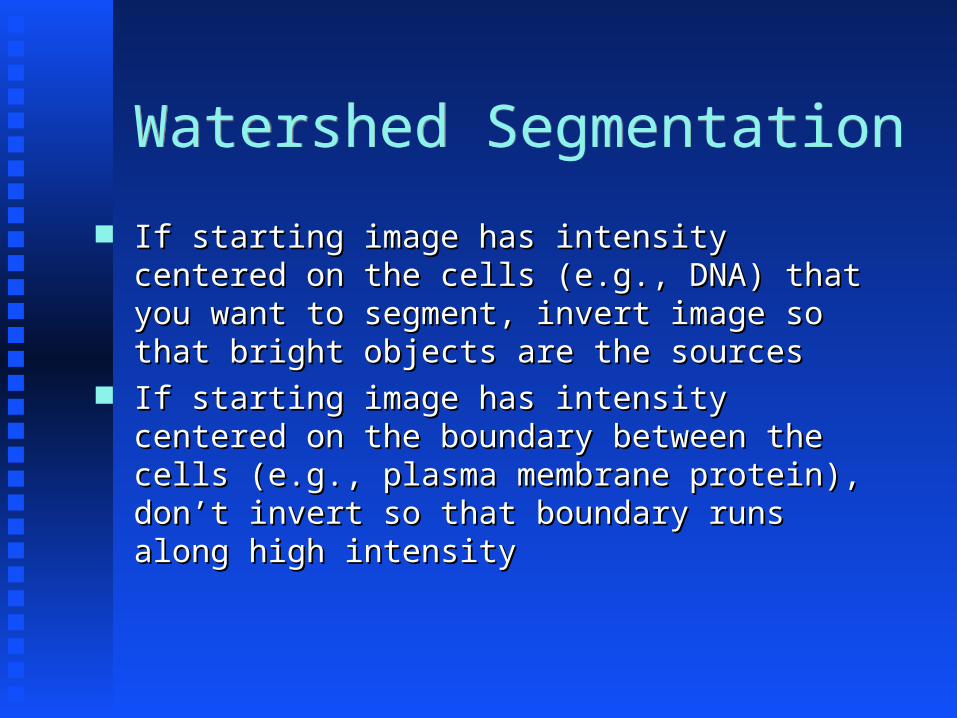
Watershed SegmentationWatershed Segmentation

If starting image has intensity If starting image has intensity centered on the cells (e.g., DNA) that centered on the cells (e.g., DNA) that you want to segment, invert image so you want to segment, invert image so that bright objects are the sourcesthat bright objects are the sources

If starting image has intensity If starting image has intensity centered on the boundary between the centered on the boundary between the cells (e.g., plasma membrane protein), cells (e.g., plasma membrane protein), don’t invert so that boundary runs don’t invert so that boundary runs along high intensityalong high intensity

Seeded Watershed SegmentationSeeded Watershed Segmentation

Drawback is that the number of regions Drawback is that the number of regions may not correspond to the number of may not correspond to the number of cellscells

Seeded watershed allows water to rise Seeded watershed allows water to rise only from predefined sources (seeds)only from predefined sources (seeds)

If DNA image available, can use same If DNA image available, can use same approach to generate these seeds as approach to generate these seeds as for Voronoi segmentationfor Voronoi segmentation

Can use seeds from DNA image but use Can use seeds from DNA image but use total protein image for watershed total protein image for watershed segmentationsegmentation

Seeded Watershed SegmentationSeeded Watershed Segmentation

Original image

Seeds and boundary

Applied directly to protein image (no DNA image)

Note non-linear boundaries

Feature ExtractionFeature Extraction

Morphological FeaturesMorphological Features

Morphological features require Morphological features require some method for defining objectssome method for defining objects

Most common approach is global Most common approach is global thresholdingthresholding

Alternatives include locally Alternatives include locally adaptive thresholdingadaptive thresholding

2D FeaturesMorphological Features2D FeaturesMorphological Features

DescriptionDescription

The number of fluorescent objects in the The number of fluorescent objects in the imageimage

The Euler number of the imageThe Euler number of the image

The average number of above-threshold The average number of above-threshold pixels per objectpixels per object

The variance of the number of above-The variance of the number of above-threshold pixels per objectthreshold pixels per object

The ratio of the size of the largest The ratio of the size of the largest object to the smallestobject to the smallest

The average object distance to the The average object distance to the cellular center of fluorescence(COF)cellular center of fluorescence(COF)

The variance of object distances from The variance of object distances from the COFthe COF

The ratio of the largest to the smallest The ratio of the largest to the smallest object to COF distanceobject to COF distance

2D FeaturesMorphological Features2D FeaturesMorphological Features

DescriptionDescription

The average object distance from the COF of the DNA The average object distance from the COF of the DNA imageimage

The variance of object distances from the DNA COFThe variance of object distances from the DNA COF

The ratio of the largest to the smallest object to The ratio of the largest to the smallest object to DNA COF distanceDNA COF distance

The distance between the protein COF and the DNA COFThe distance between the protein COF and the DNA COF

The ratio of the area occupied by protein to that The ratio of the area occupied by protein to that occupied by DNAoccupied by DNA

The fraction of the protein fluorescence that co-The fraction of the protein fluorescence that co-localizes with DNAlocalizes with DNA

DNA features (objects relative to DNA reference)

2D FeaturesMorphological Features2D FeaturesMorphological Features

DescriptionDescription

The average length of the morphological skeleton of The average length of the morphological skeleton of objectsobjects

The ratio of object skeleton length to the area of The ratio of object skeleton length to the area of the convex hull of thethe convex hull of the

skeleton, averaged over all objectsskeleton, averaged over all objects

The fraction of object pixels contained within the The fraction of object pixels contained within the skeletonskeleton

The fraction of object fluorescence contained within The fraction of object fluorescence contained within the skeletonthe skeleton

The ratio of the number of branch points in the The ratio of the number of branch points in the skeleton to the length ofskeleton to the length of

skeletonskeleton

Skeleton features

Illustration – SkeletonIllustration – Skeleton

Edge FeaturesEdge Features

DescriptionDescription

The fraction of the non-zero pixels that are along The fraction of the non-zero pixels that are along an edgean edge

Measure of edge gradient intensity homogeneityMeasure of edge gradient intensity homogeneity

Measure of edge direction homogeneity 1Measure of edge direction homogeneity 1

Measure of edge direction homogeneity 2Measure of edge direction homogeneity 2

Measure of edge direction differenceMeasure of edge direction difference

Zernike Moment FeaturesZernike Moment Features

left: Zernike polynomialsA: Z(2,0)B: Z(4,4)C: Z(10,6)

right: lamp2 image

• Shape similarity of protein image to Zernike polynomials Z(n,l)• 49 polynomials and 49 features

Haralick Texture FeaturesHaralick Texture Features Correlations of adjacent pixels in Correlations of adjacent pixels in gray level imagesgray level images

Start by calculating co-occurrence Start by calculating co-occurrence matrix P:matrix P:

N by N matrix, N=number of gray N by N matrix, N=number of gray level.level.Element P(i,j) is the probability of Element P(i,j) is the probability of pixels with value i being adjacent pixels with value i being adjacent with pixels with value jwith pixels with value j

Four directions in which a pixel can Four directions in which a pixel can be adjacentbe adjacent

331122

223344114433004400334444003322110033001144332211

221133334411443300333333441122330011001144332211

442244114422663300334433661122110011221144332211

222233224422224411334444442222

001144332211

4 2 2 2 41 2 4 1 13 4 4 4 22 2 3 3 23 3 3 2 4

Co-occurrence Matrix

Pixel Resolution and Gray LevelsPixel Resolution and Gray Levels Texture features are influenced Texture features are influenced by the number of gray levels by the number of gray levels and pixel resolution of the and pixel resolution of the imageimage

Optimization for each image Optimization for each image dataset requireddataset required

Alternatively, features can be Alternatively, features can be calculated for many resolutionscalculated for many resolutions

Fourier featuresFourier features

Frequency representationFrequency representation Any signal may be represented Any signal may be represented as the sum of many sinusoids.as the sum of many sinusoids.

As more sinusoids are added to As more sinusoids are added to the sum, the representation of the sum, the representation of the original signal becomes the original signal becomes more and more accurate.more and more accurate.

Frequency representationFrequency representation On the left below is a square wave.On the left below is a square wave. On the right is a single sinusoid with a DC offset On the right is a single sinusoid with a DC offset

which begins to approximate the original data.which begins to approximate the original data.

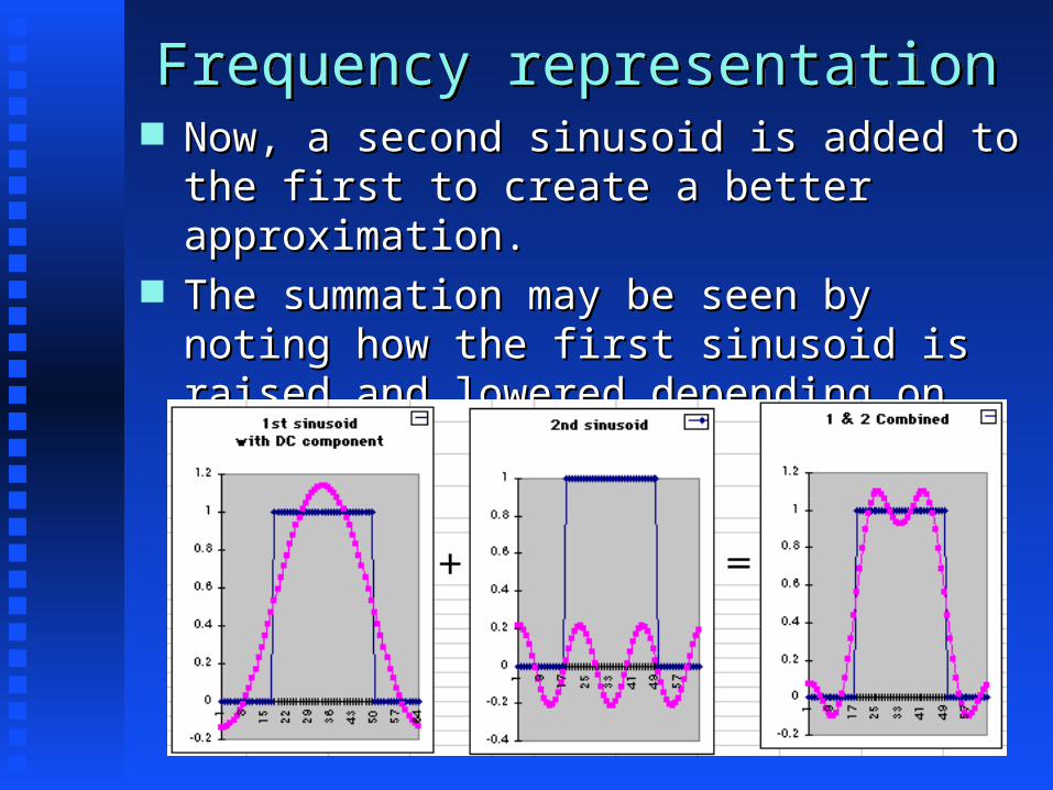
Frequency representationFrequency representation Now, a second sinusoid is added to the first to Now, a second sinusoid is added to the first to

create a better approximation.create a better approximation. The summation may be seen by noting how the The summation may be seen by noting how the

first sinusoid is raised and lowered depending on first sinusoid is raised and lowered depending on whether the second is positive or negative.whether the second is positive or negative.

Frequency representationFrequency representation Adding still another sinusoid further improves the Adding still another sinusoid further improves the

approximation.approximation.

Frequency representationFrequency representation Any discrete distribution can be represented in a Any discrete distribution can be represented in a

completely reversible manner (to numerical completely reversible manner (to numerical accuracy) by as many sinusoids as there are points accuracy) by as many sinusoids as there are points in the distributionin the distribution

Demonstration spreadsheetDemonstration spreadsheet

DemoC3.xlsDemoC3.xls

MATLAB demonstrationMATLAB demonstration

fftillustrator.mfftillustrator.m

Fourier featuresFourier features

Amount of signal at various Amount of signal at various spatial frequencies can be spatial frequencies can be used as image featuresused as image features

Wavelet Transformation - 1DWavelet Transformation - 1D

A: approximation (low frequency)

D: detail (high frequency)

X=A3+D3+D2+D1

2D Wavelets - intuition2D Wavelets - intuition Apply some filter to detect Apply some filter to detect edges (horizontal; vertical; edges (horizontal; vertical; diagonal)diagonal)

After Christos Faloutsos

2D Wavelets - intuition2D Wavelets - intuition RecurseRecurse

Slide courtesy of Christos Faloutsos

2D Wavelets - intuition2D Wavelets - intuition Edges (horizontal; vertical; Edges (horizontal; vertical; diagonal)diagonal)

http://www331.jpl.nasa.gov/http://www331.jpl.nasa.gov/public/wave.htmlpublic/wave.html

Slide courtesy of Christos Faloutsos

Daubechies D4 decompositionDaubechies D4 decomposition

Original image Wavelet Transformation

Wavelet Feature CalculationWavelet Feature Calculation PreprocessingPreprocessing

Background subtraction and thresholdingBackground subtraction and thresholding Translation and rotationTranslation and rotation

Wavelet transformationWavelet transformation The Daubechies 4 waveletThe Daubechies 4 wavelet 10 level decomposition10 level decomposition Use the average energy of the three high-Use the average energy of the three high-frequency components at each level as frequency components at each level as featuresfeatures

WaveletsWavelets

Many wavelet basis functions Many wavelet basis functions (filters):(filters): HaarHaar Daubechies (-4, -6, -20)Daubechies (-4, -6, -20) GaborGabor ......

Slide courtesy of Christos Faloutsos

Feature selectionFeature selection

Having too many features can Having too many features can confuse a classifierconfuse a classifier

Can use comparison of feature Can use comparison of feature distributions between classes to distributions between classes to choose a subset of features that choose a subset of features that gets rid of uninformative or gets rid of uninformative or redundant featuresredundant features

Feature Selection MethodsFeature Selection Methods Principal Components AnalysisPrincipal Components Analysis Non-Linear Principal Components Non-Linear Principal Components AnalysisAnalysis

Independent Components AnalysisIndependent Components Analysis Information GainInformation Gain Stepwise Discriminant AnalysisStepwise Discriminant Analysis Genetic AlgorithmsGenetic Algorithms

Matlab demonstrationsMatlab demonstrations

Example data files: Example data files: EndoAndLysoImages.tgzEndoAndLysoImages.tgz

(use tar xzf (use tar xzf EndoAndLysoImages.tgz)EndoAndLysoImages.tgz)

20 images of a lysosomal protein 20 images of a lysosomal protein (LAMP2, stained with antibody (LAMP2, stained with antibody h4b4)h4b4)

20 images of an endosomal protein 20 images of an endosomal protein (TfR)(TfR)

Matlab demonstrationsMatlab demonstrations

exampleclassif.m (uses exampleclassif.m (uses finddecisionboundary.m)finddecisionboundary.m)

showthresh.mshowthresh.m (call with name of file(s) to display, (call with name of file(s) to display, can include wildcards)can include wildcards)

realdata.m (train classifier to realdata.m (train classifier to distinguish lysosomes and endosomes)distinguish lysosomes and endosomes)

realWave.m (show wavelet decomposition realWave.m (show wavelet decomposition for endosome and lysosome images)for endosome and lysosome images)