Computational chemistry forcomplex systems: open-shell

molecules to conjugated organicmaterials

Peter Repiščák

Submitted for the degree of Doctor of Philosophy(Chemistry)

Heriot-Watt University

School of Engineering and Physical Sciences

July 2017

The copyright in this thesis is owned by the author. Any quotation from thethesis or use of any of the information contained in it must acknowledge this thesis

as the source of the quotation or information.

Abstract

This thesis focuses on two different, but equally challenging, areas ofcomputational chemistry: transition metal organic molecule interactionsand parameterisation of organic conjugated polymers for molecular dy-namics simulations. The metal-binding properties are important for un-derstanding of biomolecular action of type 2 diabetes drug and develop-ment of novel protocols for redox calculations of copper systems. In thisarea the challenge is mainly related to the complex electronic structureof the open-shell transition metals. The main challenges for the param-eterisation of conjugated polymers are due to the size of the studiedsystems, their conjugated nature and inclusion of environment.

Metal-binding properties as well as electronic structures of copper com-plexes of type 2 diabetes drug metformin (Metf) and other similar, butoften inactive, compounds were examined using DFT method. It wasfound that for neutral compounds it is not possible to explain the differ-ences in their biological effects solely by examining the copper-bindingproperties. Further, the proposed mechanism potentially explaining thedifference in the biomolecular mode of action involves a possible depro-tonation of biguanide and Metf compounds under higher mitochondrialpH which would lead to formation of more stable copper complexes andpotentially affecting the mitochondrial copper homeostasis. In addition,redox properties of copper-biguanide complexes could interfere with thesensitive redox chemistry or interact with important metalloproteins inthe mitochondria.

Understanding the copper-binding properties is also important for a sys-tematic development and testing of computational protocols for calcula-tions of reduction potentials of copper complexes. Copper macrocycliccomplexes previously used as model systems for redox-active metalloen-zymes and for which experimentally determined redox potentials areavailable were used as model systems. First adequacy of using single-reference methods such as DFT was examined for these systems and thenvarious DFT functionals and basis sets were tested in order to developaccurate redox potential protocol. It was shown that good relative cor-

relations were obtained for several functionals while the best absoluteagreement was obtained with either the M06/cc-pVTZ functional withthe SMD or either M06L or TPSSTPSS functional with cc-pVTZ basisset and the PCM solvation model.

Organic conjugated polymers have a great potential due to their applica-tion in organic optoelectronics. Various wavefunction and DFT methodsare utilized in order to systematically develop parameterisation schemethat can be used to derive selected force-field parameters such as tor-sional potentials between monomer units that are critical for these sys-tems and partial charges. Moreover, critical points of such a parameter-isation are addressed in order to obtain accurate MD simulations thatcould provide valuable insight into material morphology and conforma-tion that affect their optical properties and conductivity. It was shownthat a two step approach of geometry optimisation with CAM-B3LYP/6-31G* and single point (SP) energy scan with CAM-B3LYP/cc-pVTZ isable to yield accurate dihedral potentials in agreement with the poten-tials calculated using higher level methods such as MP2 and CBS limitCCSD(T). Further, investigating partial charge distribution for increas-ing backbone length of fluorene and thiophene it has been found that itis possible to obtain a three residue model of converged charge distribu-tions using the RESP scheme. The three partial charge residues can bethen used to build and simulate much longer polymers without the needto re-parametrize charge distributions. In the case of side-chains, it wasfound that it is not possible to obtain converged charge sets for side-chain lengths of up to 10 carbons due to the strong asymmetry betweenthe side-chain ends. Initial validation of derived force-field parametersperformed by simulations of 32mers of fluorene with octyl side-chains(PF8) and thiophene with hexyl side-chains (P3HT) in chloroform andcalculation of persistence lengths and end-to-end lengths showed closecorrespondence to experimentally obtained values.

Acknowledgements

I would like to express my deepest gratitude to all those who made thisthesis and underlying work possible. Especially, I would like to thankmy supervisor Prof. Martin Paterson for his guidance, expertise andinfinite support and patience that helped me through the PhD. Further,I would like to thank all of my colleagues and friends for many valuablediscussions and whose stimulating suggestions and guidance helped meduring my research and writing of this thesis.

Most importantly, I would like to thank my family, and especially my wifeBarbora for her patience, support and supply of hot food and beverages.Having you by my side makes my life wonderful.

Contents

Contents v

1 Introduction to Computational Chemistry 1

2 Methods 62.1 Ab initio Methods . . . . . . . . . . . . . . . . . . . . . . . . . . . . 6

2.1.1 Schrödinger Equation . . . . . . . . . . . . . . . . . . . . . . . 62.1.2 The Adiabatic and Born-Oppenheimer Approximation . . . . 82.1.3 Hartree-Fock Method . . . . . . . . . . . . . . . . . . . . . . . 112.1.4 Configuration Interaction . . . . . . . . . . . . . . . . . . . . . 182.1.5 Many Body Perturbation Theories . . . . . . . . . . . . . . . 202.1.6 Coupled Cluster . . . . . . . . . . . . . . . . . . . . . . . . . . 242.1.7 Multi-Configuration Self-Consistent Field . . . . . . . . . . . . 272.1.8 Basis Sets . . . . . . . . . . . . . . . . . . . . . . . . . . . . . 282.1.9 Local Methods . . . . . . . . . . . . . . . . . . . . . . . . . . 312.1.10 Frequency Calculations . . . . . . . . . . . . . . . . . . . . . . 322.1.11 Thermochemistry . . . . . . . . . . . . . . . . . . . . . . . . . 33

2.2 Density Functional Theory . . . . . . . . . . . . . . . . . . . . . . . . 362.2.1 The Hohenberg-Kohn Theorems . . . . . . . . . . . . . . . . . 372.2.2 Orbital Free Approaches . . . . . . . . . . . . . . . . . . . . . 382.2.3 Kohn-Sham Self-consistent Field Methodology . . . . . . . . . 382.2.4 Approximations to the Exchange-correlation Functional . . . . 392.2.5 Dispersion correction DFT (D-DFT) . . . . . . . . . . . . . . 41

2.3 Molecular Dynamics . . . . . . . . . . . . . . . . . . . . . . . . . . . 422.3.1 Force fields . . . . . . . . . . . . . . . . . . . . . . . . . . . . 432.3.2 Potential Energy and Equations of Motion . . . . . . . . . . . 442.3.3 Molecular Dynamics Simulations . . . . . . . . . . . . . . . . 45

2.4 Hybrid QM/MM Methods . . . . . . . . . . . . . . . . . . . . . . . . 47References . . . . . . . . . . . . . . . . . . . . . . . . . . . . . . . . . . . . 48

3 Biomolecular mode of action of Metformin 513.1 Introduction . . . . . . . . . . . . . . . . . . . . . . . . . . . . . . . . 51

v

3.2 Copper Binding Properties . . . . . . . . . . . . . . . . . . . . . . . . 533.3 Computational Details . . . . . . . . . . . . . . . . . . . . . . . . . . 553.4 Results . . . . . . . . . . . . . . . . . . . . . . . . . . . . . . . . . . . 56

3.4.1 Comparision of X-ray Structures and Computed Complexes . 563.4.2 Binding Energies of CuI/II Complexes . . . . . . . . . . . . . . 603.4.3 Electronic Properties . . . . . . . . . . . . . . . . . . . . . . . 633.4.4 ESP Maps . . . . . . . . . . . . . . . . . . . . . . . . . . . . . 653.4.5 Discussion and Conclusion . . . . . . . . . . . . . . . . . . . . 66

References . . . . . . . . . . . . . . . . . . . . . . . . . . . . . . . . . . . . 68

4 Protocols for Understanding the Redox Behaviour of Copper Con-taining systems 714.1 Introduction . . . . . . . . . . . . . . . . . . . . . . . . . . . . . . . . 714.2 Computational Electrochemistry . . . . . . . . . . . . . . . . . . . . . 734.3 Results and Discussion . . . . . . . . . . . . . . . . . . . . . . . . . . 76

4.3.1 Assessing Appropriateness of DFT for Redox Potential Cal-culations. . . . . . . . . . . . . . . . . . . . . . . . . . . . . . 77

4.3.2 Basis Set Dependence of Calculated Redox Potentials . . . . . 784.3.3 Solvation Models . . . . . . . . . . . . . . . . . . . . . . . . . 874.3.4 Effect of S for N substitution . . . . . . . . . . . . . . . . . . 90

4.4 Conclusion . . . . . . . . . . . . . . . . . . . . . . . . . . . . . . . . . 934.5 Appendix: Comparison of X-ray Structures and Computed Complexes 95References . . . . . . . . . . . . . . . . . . . . . . . . . . . . . . . . . . . . 102

5 Development of general low-cost parameterisation scheme for MDsimulations of conjugated materials 1075.1 Introduction . . . . . . . . . . . . . . . . . . . . . . . . . . . . . . . . 1075.2 Generating Molecular Dynamics Parameters . . . . . . . . . . . . . . 1105.3 Determination of the Appropriate Methodology. . . . . . . . . . . . . 113

5.3.1 Technical Details . . . . . . . . . . . . . . . . . . . . . . . . . 1135.3.2 Results of Methodology Testing . . . . . . . . . . . . . . . . . 1155.3.3 Results of Basis Set Testing . . . . . . . . . . . . . . . . . . . 1235.3.4 Results of Dispersion Corrected DFT . . . . . . . . . . . . . . 1265.3.5 Discussion and Conclusion . . . . . . . . . . . . . . . . . . . . 127

5.4 Determining Dihedral Profiles . . . . . . . . . . . . . . . . . . . . . . 1285.5 Partial Charge Calculations . . . . . . . . . . . . . . . . . . . . . . . 1335.6 Force-Field Implementation . . . . . . . . . . . . . . . . . . . . . . . 1365.7 Molecular Dynamics Results . . . . . . . . . . . . . . . . . . . . . . . 1415.8 Discussion and Conclusion . . . . . . . . . . . . . . . . . . . . . . . . 145References . . . . . . . . . . . . . . . . . . . . . . . . . . . . . . . . . . . . 146

6 Summary and Future Work 152

vi

Chapter 1

Introduction to ComputationalChemistry

Computational chemistry is a research field which uses a broad range of computa-tional techniques, ranging from quantum mechanics to more empirical methods, inorder to solve chemically related problems. Nowadays, computational chemistry isan invaluable tool not only able to complement experiments and provide detailedinsight into experimental results, but also make novel predictions and help to designnew materials and reactions. For example, it can be applied to predict NMR, EPR,rotational, vibrational and electronic spectra. Further, calculating thermodynamicquantities can provide information about activation energies of reactions, bindingaffinities of complexes, reduction potentials and pKa values.

The choice of technique strongly depends on the many aspects of the system of inter-est as well as question asked. Different levels of details about the studied system arerequired when studying, for example, reaction mechanisms, spectroscopic transitionenergies and intensities, solvent diffusion and protein folding. The first two wouldrequire a detailed understanding of electronic structure, whereas atomistic or evenmore approximate coarse-grain picture may be sufficient for the question of solventdiffusion and protein folding. Moreover, some systems and calculations can posechallenges due to complex electronic structure such as open-shell states, low-spinmetal complexes and excited states; and therefore more approximate methods maynot able to address these challenges. On the other hand, system size and the needto account for environmental effects can be the limiting factor for other systems.

Ideally, solving the non-relativistic time-dependent Schrödinger equation it wouldbe possible to obtain the information about a molecular system with a very highaccuracy, however, anything more complex than the smallest few electron system

1

cannot be handled at this ab initio level. Therefore, in order to solve more complexand chemically interesting systems some approximations need to be introduced.For example, a full configuration interaction (CI) which is able to yield exact non-relativistic description of the many electron system would be a suitable candidate.Unfortunately, a full CI is computationally extremely expensive method for any butthe smallest gas phase molecules. For instance, if the full CI is applied to a watermolecule more than 3.8x108 configurations would need to be calculated. Thus, inorder to reduce the CI space and at the same time being able to accurately calculate,for example, open-shell systems or excited state phenomena with multi-referencecharacter (different configurations have similar importance) methods such as Multi-reference CI (MRCI), Restricted Active Space SCF (RASSCF), Complete ActiveSpace Self-Consistent (CASSCF) and Monte Carlo CI must be applied. Although,these methods can potentially yield approximate CI wavefunctions and energiesthat are as close as possible to the exact values, they can still be used only forsmall systems. Moreover, the first three are not black-box methods and can beespecially challenging to use and when defining the important configurations (activespaces). In the case when one dominant configuration is able to accurately describethe system a single reference methods such as truncated CI (CISD), Møller–Plesset(MP2) or coupled-cluster (CCSD, CCSD(T)) may be applied to small to mediumsized systems (tens of atoms). Using local variants of some of these methods suchas local MP2, CCSD, CCSD(T) it may be possible to extend them to study largersystems, however, at the same time these methods become less black-box and morechallenging to use. Density Functional Theory (DFT), which uses the electronicdensity as a central variable, is very popular single-reference method applicable tolarge systems (potentially hundreds of atoms). However, due to the fact that theexact functionals are unknown and there is usually no systematic way of improvingobtained results by, for example, improving the size of basis set one needs to performa benchmark of various functionals in order to assess their accuracy and adequacyfor the studied system.

As mentioned previously size of the studied system is another important aspect toconsider when deciding which method to use. For example, highly accurate ab initiomethods can be applied to system of few atoms, but as the system size increasesmore approximations need to be introduced or even replaced by empirical parame-ters. Force-field methods is a family of methods using either experimentally or abinitio derived parameters to describe atomic interaction and the classical mechan-ics to describe the motion of atoms. These methods are applicable to simulationsof molecular systems potentially consisting of thousands of atoms. However, dueto the quantum phenomena being usually neglected in force-field methods thesecannot be used to study, for example, photochemistry and events such as bondformation/breaking.

2

Environmental effects is yet another aspect one needs to consider when designingcomputational experiment. For instance, environment surrounding a photoactivechromophore, whether the photoactive molecule is in a solvent or embedded in aprotein, can significantly affect spectroscopic and photodynamical properties. Theelectronic and molecular structure of a solute, can be influenced either directlythrough electrostatic interaction (e.g. polarisation by environment) or indirectly byimposed steric constraints on the solute geometry. It is possible to include someenvironmental effects in the quantum mechanics calculations usually in a form ofimplicit solvation where solvent is defined as a structureless dielectric continuum. Inthe case of force-field calculations, such as molecular dynamics simulations, a solventis commonly included as explicit solvent or a combination of explicit/implicit solvent.

In order to realistically model, for example, complex biological systems with all thenecessary environmental effects and to avoid unreasonable computational costs aso-called hybrid schemes are often employed. The hybrid techniques allow a morerobust way of considering the active site (e.g. chromophore) and the surroundingenvironment (e.g. protein) by treating a system of interest at different levels oftheory. For example, a part where (photo)chemical reaction occurs is investigatedwith more accurate QM method and the rest with computationally cheaper andusually less accurate QM, molecular mechanical, semi-empirical methods or evenhybrid explicit/implicit solvent setup. Hybrid methods allow to apply advantagesfrom both worlds and treat much larger systems than it would be possible withQM alone and study, for example, reactions and photochemical processes, whichwould not be possible with force-field methods on their own. However, the maindisadvantage of these methods is they are not black-box and therefore require moreexpertise and deeper insight into the studied system.

Another important aspect is whether one is interested in static equilibrium prop-erties or dynamic properties of a system. Most of the methods mentioned aboveallow description of important stationary points of a studied system on a potentialenergy surface(s) and adiabatic (potentially also non-adiabatic) events connectingthem. However, in order to follow, for example, the excited state reaction path indetails, explore the configurational space and determine the time scales of variousphenomena it is necessary to reach for methods able to simulate the dynamic pro-cesses. In photochemistry, two main classes of methods based on whether the nucleiare treated as classical (often with the inclusion of quantum effects in semi-classicalapproaches) or quantum particles are trajectory-based approaches and wavepacketdynamics. The wavepacket propagation methods are computationally very demand-ing due to the complete QM solution given in full dimensionality and thus appli-cable only to small number of nuclear coordinates. From the force-field methods,for example, molecular dynamics allows to explore the configurational space and

3

generate ensembles from which various properties can be calculated. However, clas-sical molecular dynamics with predefined potentials is facing some drawbacks suchas need to account for all the different interatomic interactions of the studied sys-tem as well as inability to account for quantum effects. Therefore, a family of abinitio molecular dynamics methods is unifying molecular dynamics and ab initiomethods by computing the forces acting on the nuclei using, for example, DFTmethod. These forces are calculated "on-the-fly" as the molecular dynamics tra-jectory is generated. Although, these methods present some advantages over theclassical molecular dynamics, usually much smaller systems and shorter timescalescan be studied.

In this thesis two different areas on the scale of computational chemistry are ex-plored. The first is related to understanding of transition metal organic moleculeinteractions which are important in drug research and development of new proto-cols for redox potential calculations of copper systems. In this part the focus is onusing accurate ab initio methods and the complexity mainly comes from open-shelltransition metal systems with potential multi-reference character. The second areafocuses on the development of schemes for molecular dynamics parameter deriva-tion of conjugated materials in order to advance the field by allowing dynamicssimulation to start to understand how conformation affects morphology. This isespecially important as, for example, optical properties and conductivity are sen-sitive to intra-molecular conjugation and excitation transfer dynamics is affectedby the inter-molecular alignment and separation. In this part the challenges andcomplexity mainly comes from the size of the studied systems and inclusion of theenvironment.

In the chapter 3 computational techniques of quantum chemistry are applied in orderto examine metal-binding properties of important type 2 diabetes drug metforminand structurally similar compounds. The work in this chapter follows a previouslypublished experimental study which points toward the important link between thecopper-binding properties of these compounds and their biological effect. This chap-ter answers some of the observed effects by examining the electronic structures ofthe studied compounds and their copper-binding energies. Further, potential mech-anisms involving metformin deprotonation and metformin-copper redox propertiesare proposed that could explain the specific biological effects of metformin drug anddirect the future research.

Chapter 4 focuses on a systematic development and testing of computational proto-col for calculation of reduction potentials of copper complexes. This chapter followsthe need for accurate redox potential calculations of copper-binding complexes andindirectly stems from the discovery of previous chapter where redox properties are

4

implied as one of a potential mechanism explaining biological effects of the met-formin. Copper macrocyclic complexes previously used as model systems for redox-active metalloenzymes, such as blue copper proteins involved in the photosynthesisin green plants, and for which experimentally determined redox potentials are avail-able were used as model systems in this chapter. Further, some aspects of accuratecalculations of redox potentials of copper complexes are addressed and discussed.This involves, for example, potential multi-reference character of metal-binding sys-tems, spin contamination of open-shell molecules and appropriate choice of method,basis set and solvation.

Chapter 5 is distinct from the previous chapters as its main focus is developmentof scheme that can be used to obtain force-field parameters for simulations of largeorganic conjugated polymers with potential application in opto-electronic materi-als. These polymers are of great interest in rapidly expanding field of organic-basedopto-electronics. However, due to the size of studied system (hundreds of atoms)techniques of classical molecular dynamics are more appropriate in order to un-derstand and predict macroscopic properties based on the detailed knowledge ofstructure-property relationship at atomic level. This chapter first systematicallytests and establish various ab initio computational methods required in order toobtain accurate critical force-field parameters. In the next step, after force-fieldparameters are obtained these are validated against available experimental data.

5

Chapter 2

Methods

In the following chapter basic computational theory used in the experimental partis introduced. The first part describes ab initio wave function based methods. Inthe second part Density Functional Theory is introduced. The chapter finishes withthe basic concepts of molecular dynamics theory and hybrid approaches combiningquantum mechanical and classical mechanical methods.

2.1 Ab initio Methods

Ab initio ("from the beginning" or "from first principles") methods apply the theoryof quantum mechanics in order to predict the properties of atomic and molecularsystems and to solve problems in chemistry. In quantum chemistry the wave func-tion, Ψ , is a central variable that contains all the measurable information abouta chemical system. It is used in the Schrödinger equation which plays the role ofthe equation of motion (Newton’s laws in classical mechanics) and describes theevolution of QM system in time.1

2.1.1 Schrödinger Equation

The time-dependent Schrödinger equation (TDSE) involves differentiation with re-spect to both time and position:

H(r, t)︷ ︸︸ ︷[− ~2

2m∆ + V (r, t)

]Ψ(r, t) = i

∂Ψ(r, t)

∂t(2.1)

6

where H(r, t) is the Hamiltonian operator†, the Laplacian is: ∆ = ∇2 ≡ ∂2

∂x2+

∂2

∂y2+ ∂2

∂z2. In most cases, such as systems mainly composed of the first and the

second row elements, it is sufficient to take the non-relativistic Hamiltonian as thevelocities are small enough for the relativistic effects to be neglected.2 The wavefunction Ψ(r, t) is a function of particle position, it is not an observable quantity,but the square modulus of the wave function (the product of the wave functionwith its complex conjugate), |Ψ |2 = |Ψ ∗Ψ |, yields the probability of finding theparticle at that position r at a given time t. In addition, the normalized integral ofthis probability density over all space must be unity (which simply means that theparticle must be somewhere in space). And in order to obtain a physically relevantsolution of the SE, the wave function must also be continuous, single-valued andantisymmetric with respect to the interchange of electrons.3

In the case of a time-independent potential energy operator we can separate thewave function into a spatial and a phase factor part, Ψ(r, t) = Ψ(r)e−iEt, and afterneglecting the phase factor we obtain the time-independent Schrödinger equation(TISE, or in the rest of the text just SE):

H(r)Ψ(r) = E(r)Ψ(r) (2.2)

The H contains the sum of terms for nuclei and electron kinetic energies and poten-tial energy terms: Coulomb repulsion and attraction of charged particles:

H =

(−∑A

~2

2mA

∇2A −

∑i

~2

2me

∇2i

)+

e2

4πε0

(∑A<B

ZAZB|RA −RB|

+

+∑i<j

1

|ri − rj|−∑i

∑A

ZA|RA − ri|

) (2.3)

where A and B run over all nuclei, i and j run over all electrons, ~ is Planck’sconstant divided by 2π, mA is the mass of the nucleus A, me is the mass of electron,e is the charge on an electron, Z is an atomic number and |RA − ri| = riA is therelative distance between the position of nucleus and electron.4 The above equationcan be expressed symbolically as:

H = (TN + Te) + (VNN + Vee + VNe) (2.4)†Operators (e.g. Hamiltonian operator, corresponding to the total energy of the system) are

associated with each measurable parameter and when they carry out a mathematical operation ontheir eigenfunction (e.g. the wave function Ψ) they produce the same eigenfunction multiplied bya scalar value, eigenvalue (e.g. energy E) of the selected operator.

7

Although the time-independent SE (eq. (2.2)) simplifies the problem, we are stillable to solve it only for the smallest one electron systems (e.g. hydrogen atom).Hence, approximations have to be introduced for the Hamiltonian H as well as forthe wave function Ψ in order to solve the SE for many-electron systems. Note thatthe units used throughout this report are a so called atomic units. In this systemof units: the electric charge e, electron mass me and reduced Planck constant ~ areequal to 1. Then the units for distance and energy become bohrs (a0) and hartrees(Eh), respectively.

2.1.2 The Adiabatic and Born-Oppenheimer Approximation

The total wave function depends on the positions of all particles and their spins,however in the adiabatic approximation,it can be expressed as a product of a nuclearand an electronic wave function

The Born-Oppenheimer approximation (BO) is one of the most important approxi-mations that simplifies the molecular Hamiltonian by separating the electronic andnuclear motions allowing definitions of concepts such as bond-lengths, bond-angles,equilibrium structures and reaction barriers. This separation can be easily justi-fied when we realize there is a large mass difference between electrons and nuclei(a proton is ∼1836 times heavier than an electron). As a consequence, electronsin a molecule react instantaneously to displacements of nuclei and to a good ap-proximation can be considered to be moving in the field of fixed nuclei. In thisapproximation, the nuclear kinetic operator TN = 0 is omitted from eq. (2.4) andthe potential energy operator for nuclei-nuclei repulsion VNN can be considered forthe selected molecular geometry to be constant5:

He = (Te) + (VNN + Vee + VNe) (2.5)

where He is the electronic Hamiltonian. And after solving SE for the electronicHamiltonian:

HeΨi(r;R) = Ei(R)Ψi(r;R) (2.6)

we obtain the electronic wave function Ψi(r;R) which explicitly depends on theelectronic coordinates and parametrically on the nuclear coordinates as does theelectronic energies Ei(R).

In the modern derivation of the BO approximation, the wave functions are adiabaticelectronic states† (ground state (i = 0), first excited state (i = 1), second excited

†The adiabatic wave functions are orthonormal,∫∞−∞ Ψ∗i (r,R)Ψj(r,R)dr = δij , where δij is

Kronecker delta function (for i = j is 1 and 0 ortherwise)

8

state (i = 1),). Then the total (exact) wave function can be written as a sum ofproducts of the nuclear and the electronic wave functions:

Ψ(r;R) =∑n

χn(R)Ψn(r;R) (2.7)

where the expansion coefficients χn(R) are the nuclear wave functions. This in-serted into the SE and expanded, followed by multiplication by the adiabatic elec-tronic wave function Ψ ∗i (r;R) from the left (using the orthonormality of the Ψi)and integration over the electron coordinates, we obtain the following set of coupledequations2,6: ∑

j

Hij(R)χj(R) = E(R)χi(R) (2.8)

Here Hij(R) = [TN + Vi(R)]δij − Λij(R) with the kinetic energy operator TN =

−∑

k1

2Mk∇2

Rk(expressed in atomic units), where 2Mk is the mass of nucleus k, and

the non-adiabatic operator elements Λij(R) are defined as:

Λij(R) =∑k

Fkij(R)︷ ︸︸ ︷(1

Mk

〈Ψi(r;R)|∇Rk|Ψj(r;R)〉

)∇Rk

+

Gij(R)︷ ︸︸ ︷(∑k

1

2Mk

〈Ψi(r;R)|∇2Rk|Ψj(r;R)〉

)(2.9)

where F kij(R) and Gij(R) are the first- and the second-order non-adiabatic coupling

elements, respectively, expressed in the Dirac bracket notation (〈|〉). These couplingelements connect individual electronic states via nuclear motion. In the adiabaticapproximation, where the nuclei move only on a single electronic potential surface,F kij(R) and Gij(R) are very small and can be neglected. However, another crucial

requirement for these terms to vanish is that there must be a mass difference andalso electronic states must not be too close in energy to one another. Although,coupling elements are ignored here, they play a very important role in the photo-chemical reactions where the system involves more than one electronic surface andthis will be discussed later on in the section about conical intersections. In the BOapproximation, Hij is assumed to be diagonal and the resulting equation has theform of SE:

[TN + Vi(R)]χj(R) = Etotχj(R) (2.10)

Here the nuclei move on a potential energy surface (PES) Vi(R) of a given electronicstate i which is a solution to the electronic SE. Further, solving equation (2.10) forthe nuclear wave function yields the vibrational, rotational and translational statesof the nuclei.7 The first-order correction to the Born-Oppenheimer electronic energydue to the nuclear motion is the Born-Oppenheimer diagonal correction (BODC):

EDBOC = 〈Ψi(r;R)|TN|Ψi(r;R)〉 (2.11)

9

This correction is especially important for molecules with light atoms (e.g. hydrogen-containing molecules) and its effect becomes smaller for heavier nuclei.6

Figure 2.1 shows an example a PES, a very important concept in chemistry, fromwhere we can obtain information about the minimum and transition state geometriesof the studied system.

Figure 2.1: Example of a PES (figure taken from8).

Conical intersections (CoIn) are a products of a so called nonadiabatic phenom-ena, which are frequently found in photochemical and photobiological mechanisms.During ground state reactions, thermal chemistry typically plays significant role,where the excited state is usually several eV higher and the BO nonadiabatic cou-pling terms, which depend not only on the mass but also on the energy differencebetween electronic states, are neglected. However, in photochemistry one must dealwith situations where energy gaps between electronic states get smaller and smaller,reaching the same magnitude of energy difference as vibrational states. This resultsin stronger coupling between nuclear motion and electronic configuration changes(vibronic coupling).2 Ultimately, there are CoIn points with infinitely large cou-pling at ∆EPES=0. At this points, the Born-Oppenheimer approximation that rep-resents powerful simplification applicable for the nuclei movement on a single PES,breaks down. In other words, when we recall the nonadiabatic coupling operatorsΛij, where Gii(R) corresponds to the nonadiabatic correction to a single PES andF kij((R)) is the derivative coupling vector (of dimension equal to the number of

nuclear coordinates) that can expressed in the terms of energy difference as:

F kij(R) =

1

Mk

〈Ψi(r;R)|∇RkHe|Ψj(r;R)〉

Vj − Vi(2.12)

10

which for zero energy difference becomes infinity and provide the most efficient wayfor radiationless transition between states.9

The topology of CoIn is that of a double cone, with a so called branching space at theapex. The branching space is spanned by the energy difference gradient gij, and hij

which represents the interstate coupling gradient and is parallel to the nonadiabaticcoupling10:

gij =∂(Ej − Ei)

∂ξ(2.13)

hij = 〈Ci|∂H

∂ξ|Cj〉 (2.14)

where Ci, Cj are configuration interaction eigenvectors, H is the Hamiltonian andξ is a vector of Cartesian displacements.

Orthogonal to the branching space is a so called intersection seam, which lies for amolecule with N int internal degrees of freedom on the N int−2 dimensional subspaceformed by an infinite number of connected CoIns.

2.1.3 Hartree-Fock Method

The Hartree-Fock method (HF), also known as self-consistent field (or SCF method),is a central ab initio method able to solve the electronic SE (eq. (2.6)) of a many-electron system. The HF is often a starting point leading after some improvementstowards more accurate methods or after additional approximations to semi-empiricalmethods.6

The key aspect of the HF approximation is the assumption that the exact N -electronwave function and associated energy of a system can be approximated by a singleexpression of N spin-orbitals that is derived by applying the variational principle.But before we establish HF theory in more details a few theoretical concepts needto be presented.

First a spatial orbital φi(r) is defined as a wave function that describes the spa-tial distribution of an electron and depends on the position vector r, such that|φi(r)|2dr is the probability of finding the selected electron within small volume drsurrounding r. Further, in context of neglecting the non-relativistic effects and inorder to complete the description of an electron, we introduce electron spin. Thespin of an electron can be in one of the two states α (spin up) and β (spin down)and these two functions obey the orthonormal conditions (〈α|α〉 = 〈β|β〉 = 0 and〈α|β〉 = 〈β|α〉 = 1).6 Two spinorbitals χ(x) = φi(r)α or χ(x) = φi(r)β can be

11

formed combining spatial orbital and either the spin function α or β. In the case ofsolving the electronic SE for a molecule, the term molecular orbitals is used for thewave functions of electrons in a molecule.

After neglecting electron-electron repulsion a many-electron wave function, termedas Hartree product, can be expressed as a product of spinorbitals for each electron:

ΨHP(x1, x1, . . . , xN) = χi(x1)χj(x2) · · ·χk(xN) (2.15)

However, the Hartree product is inadequate since it is required for the electronic wavefunction to be antisymmetric (change sign) with respect to interchange of any twoelectron space and spin coordinates (since electrons are fermions with spin quantumnumber of 1/2). Hence, an antisymmetric wave function is introduced in the formof a so called Slater determinant 5:

Ψ(x1, x1, . . . , xN) =1√N !

∣∣∣∣∣∣∣∣∣∣χi(x1) χj(x1) · · · χk(x1)

χi(x2) χj(x2) · · · χk(x2)...

... . . . ...χi(xN) χj(xN) · · · χk(xN)

∣∣∣∣∣∣∣∣∣∣. (2.16)

where 1√N !

is a normalization factor and in each row all possible assignments ofelectron i to all molecular spinorbital combinations are presented.

Now, we will proceed with derivation of Hartree-Fock equations. First, the simplestantisymmetric wave function, Ψguess, able to describe the ground state of an N-electron system is taken as a trial wave function (as the exact wave function isunknown) in a form of a single Slater determinant. Given the trial wave function,the expectation value E[Ψguess] of the full electronic Hamiltonian He is expressed as:

E[Ψguess] = 〈Ψguess|He|Ψguess〉 (2.17)

where in this case the energy E[Ψguess] is a function of the trial wave funcion, whichis in turn a function of molecular spinorbitals. Further, in order to minimize theenergy the vartiational theorem for a normalized wave functions is applied:

Eapprox = 〈Ψguess|He|Ψguess〉 ≥ Eexact (2.18)

Thus, we have a tool to judge the quality of an approximate wave function andfurther improve our guess towards the limit of an exact wave function E0 by alteringthe spinorbitals, but they must still remain orthonormal.

In the process of finding such spinorbitals χi that would lead to E0, an eigenvalue

12

Hartree-Fock equation (in typical form for closed-shell systems) is derived, whichdetermines the optimal spinorbitals5:

f(i)χ(xi) = εχ(xi) (2.19)

where f(i) is the one-electron Fock operator defined as:

f(i) =

Te︷ ︸︸ ︷−1

2∇2i

VNe︷ ︸︸ ︷−

M∑A=1

ZAriA

+V HFi {j} (2.20)

Here, the electron-electron repulsion is substituted with the interaction of ith elec-tron with the mean-field, V HF

i {j}, created by other electrons occupying orbitals{j} (i.e. charge density associated with orbital χj). Hence, the complicated many-electron problem is replaced by the one-electron problem. However, this impliesthat mutual correlation of electron motion (electron correlation) is ignored. Theaverage potential V HF

i {j} has the form V HFi {j} =

∑j 6=i Jj − Kj, with the Coulomb

operator Jj defined as6:

Jjχi(x1) =

(∫|χj(x2)|2

r12

dx2

)χi(x1) =

(∫ρjr12

dx2

)χi(x1) (2.21)

and the Exchange operator Kj:

Kjχi(x1) =

(∫χ∗j(x2)χi(x2)

r12

dx2

)χj(x1) (2.22)

From the above equations we can see that V HFi {j} depends on the spinorbitals of

other electrons (i.e. Fock operator depends on its own eigenfunctions) and thus thisnonlinear problem must be solved iteratively using a so called Self-consistent fieldmethod (SCF).

Finally, we can evaluate the energy of a Slater determinant composed of an optimisedset of molecular orbitals obtained from SCF as:

EHF =elec.∑i

hci +

elec.pairs∑i<j

(Jij −Kij) (2.23)

with hci being one-electron integrals, i.e. electron kinetic energy and electron-nucleusrepulsion.

In modern chemistry an unknown molecular orbital (MO) (guess wave function) Ψiis constructed as a linear combination of known atomic orbitals (MO LCAO), i.e.

13

an expansion of MOs in terms of the known basis functions φµ 5,6:

Ψi =

Kbasis∑µ=1

Cµiφµ (2.24)

where Cµi are the molecular orbital expansion coefficients and φµ are basis functionschosen to be normalized. More on a mathematical form of basis functions will bediscussed in the section about basis sets.

In the atomic orbital approximation in order to solve the Hartree-Fock equations nu-merically for molecular systems the operator eigenvalue equations eq. (2.19) are con-verted to a matrix representation by first substituting the linear expansion eq. (2.24)to obtain:

f(r1)

Kbasis∑µ=1

Cµiφµ = εi

Kbasis∑µ=1

Cµiφµ (2.25)

Multiplying the above equations by a specific basis function on the left and inte-grating yields matrix equations, a so-called Roothaan-Hall equations11,12:

Kbasis∑µ=1

Cµi〈φν |f(r1)|φµ〉 = εi

Kbasis∑µ=1

Cµi〈φν |φµ〉 (2.26)

These can be compactly written as a single matrix equation:

FC = SCε (2.27)

where F is the Fock matrix, S is the overlap matrix of overlap elements betweenbasis functions and C is a K ×K matrix of the expansion coefficients. Further, adensity matrix which is needed in the SCF calculation is obtained from the totalcharge density:

ρ(r) = 2

N/2∑i

= |ψi(r)|2 (2.28)

by inserting the MO expansion (eq. (2.25)) into the above equation and then thecharge density matrix is defined as:

ρ(r) = 2

N/2∑i

∑ν

C∗νiφ∗ν(r)

∑µ

Cµiφµ(r)

=∑µν

2

N/2∑i

CµiC∗νi

φµ(r)φ∗ν(r)

=∑µν

Pµνφµ(r)φ∗ν(r)

(2.29)

14

Initial guess ofdensity matrix P(0)

Construct the Fockmatrix and solve

Hartree-Fock equation

Form a new den-sity matrix fromoccupied MOs

Determine whetherthe new density

matrix is the sameas the previousdensity matrix

ReplaceP(n−1)

with P(n)

Figure 2.2: Illustration of the SCF procedure.

where Pµν is a density matrix related to expansion coefficients C by Pµν = 2∑N/2

i CµiC∗νi.

The density matrix is used in the SCF procedure together with the one- and two-electron integrals to construct the Fock matrix:

Fµν = Tµν + V nuclµν︸ ︷︷ ︸

Hcoreµν

+∑λσ

Pλσ[(µν|σλ)− 1

2(µλ|σν)]︸ ︷︷ ︸

Gµν

(2.30)

In the equation (2.30) Hcoreµν is the core-Hamiltonian matrix, which involves the

kinetic energy integrals Tµν and the nuclear attraction integrals V nuclµν and Gµν is the

two-electron part of the Fock matrix involving the density matrix P and a set oftwo-electron integrals.

The SCF procedure, illustrated in the Figure 2.2, is iterated until the new densitymatrix is sufficiently similar (converges to within a selected treshold) to the previousdensity matrix.

In the basis set approximation improving the quality of a basis set of atomic orbitalsleads to a lower and lower expectation value E0, converging ultimately to the basisset limit of the method, the so called HF limit. We have neglected the electroncorrelation effect, but the HF limit is only a small step away from the exact (non-relativistic) energy (in most cases it accounts for ∼ 99% of total energy) and theremainder of the energy is called the correlation energy Ecorr = Eexact − EHF.

15

The correlation energy can be further divided into a static and dynamic electroncorrelation. In order to understand the difference between these two correlations weintroduce an improvement to HF wave function (single slater determinant) by con-structing a wave function as a linear combination of multiple slater determinants4:

Ψ = c0ΨHF + c1Ψ1 + c2Ψ2 + · · · (2.31)

where the coefficients c represents weights of each determinant in the expansion aswell as ensures normalization. For most systems the HF wave function dominatesthe linear expansion and the main contribution to correlation energy is due to the dy-namic correlation, which is related to the instantaneous correlation of the movementof electrons and tends to be made up from a sum of individually small contributionsfrom other determinants. However, static correlation takes place in situations wheredifferent determinants have similar weights (i.e. configurations have similar ener-gies) and thus a single configuration becomes inappropriate for an accurate systemdescription, e.g. stretched bonds and excited states.

There are various approaches trying to include the dynamic and static electroncorrection into the HF calculation, referred to as electron correlation methods orPost-HF methods. Some of these methods are, for example, Configuration Interac-tion (CI), Coupled cluster, Møller-Plesset perturbation theory (MPn, where n is theorder of correction), multi-configurational self-consistent field (MCSCF) and cou-pled cluster theory (CC). Density functional theory (DFT), which will be coveredin more details in a separate chapter, is yet another approach capable of recoveringsome of the correlation energy.

Solving the Hartree-Fock eigenvalue equation an unique set of spin orbitals, whichare called canonical spinorbitals, is obtained. These orbitals are diagonal matrixrepresentation of 〈ψi|f |ψj〉 = εiδij and also include the unoccupied spinorbitals asadditional eigenfunctions of f . The canonical spinorbitals are generally delocalized,but since the Hartree-Fock state is invariant to unitary transformations among theoccupied spinorbitals Ψi, i = 1, 2, ..., N and canonical spin orbitals are just one pos-sible choice of spinorbitals for the optimized N -particle state it is possible by unitarytransformation to generate an alternative more chemically intuitive picture of or-bitals localized to individual bonds or atoms. The non− canonical representationof the HF solution leads to a block-diagonal matrix form of the Fock operator withtwo non-diagonal blocks that belong to the occupied and unoccupied spinorbitals,respectively.13

There are several variants of the HF method depending on whether any restrictionsare imposed on the spinorbitals used to build the trial wave function. For a closed-shell systems near their equilibrium geometry, a Restricted Hartree-Fock (RHF)

16

approach is usually used which allows to simplify the problem by restricting pairs ofα and β spinorbitals to the same spatial orbital. In the case of open shell systemsthere is a possibility to restrict only the spatial part of the doubly occupied orbitalsin a Restricted Open-shell Hartree-Fock (ROHF).6 Other option for the open shellsystems is to use the Unrestricted Hartree-Fock (UHF) which uses two complete setsof orbitals, one for the α and one for the β electrons. The advantage of UHF is thatit can perform very efficiently for an open-shell system and yields lower or equalenergy to a corresponding R(O)HF. On the other hand, the UHF wave functionis no longer an eigenfunction of the total spin operator, S2, which results in anincorrect wave function that has some other spin states mixed in (a so called spincontamination error).

Koopmans’ theorem provides a physical interpretation of the orbital energies εi, itstates that energies associated with orbitals χi are approximations to the ionizationenergies of the system.5 Given two systems one with N -electron Hartree-Fock sin-gle determinant and other with (N − 1)-electron determinant, where electron wasremoved from χa, will have in general different orbitals. But when we assume theorbitals are identical ("frozen" orbitals), all the one electron terms cancel out ex-cept for the unoccupied orbital χa (removed orbital) in the N − 1 electron system.Also, majority of the two-body terms cancel as well except for the ones involvingthe removed orbital χa:

EN − EN−1 = ha +1

2

Nelec∑i=1

(Jia −Kia) +1

2

Nelec∑j=1

(Jaj −Kaj) (2.32)

The last two terms are identical and the ionization energy is given as:

EN − EN−1 = ha +Nelec∑i=1

(Jia −Kia) = εa (2.33)

From the above equation it can be seen that −εa is the HF approximation to theionization energy. Similarly, it can be shown that −εr of virtual spin orbital χr isthe HF approximation to electron affinity when, for example, an (N + 1)-electronsystem is generated from an N -electron system. The error in this approximation isdue to the fact that orbital relaxation was neglected and this error becomes moresignificant when more and more electrons are removed. Moreover, including thecorrelation effects can correct further the Koopmans’ results for calculated ionizationpotentials and electron affinities.

17

2.1.4 Configuration Interaction

Configuration Interaction (CI), which is based on the variational principle, is in com-parison to other correlation methods conceptually the simplest one.5 Even thoughwithout proper denoting, CI’s form has already been introduced in eq. (2.31). Theprinciple of the CI method is that it augments ground state HF wave function byincluding additional configurations, i.e. it utilizes virtual (empty) orbitals whereelectrons from occupied HF orbitals can be substituted (equivalent to exciting elec-tron to a higher energy orbital). This has the effect that electrons can partiallyspread across virtual orbitals and we can recover part of the correlation energy.And thus the exact wave function can be constructed as a linear combination of allthe possible substitutions (configurations):

ΨCI = c0ΨHF +

Singles∑cSi

cSi ΨSi +

Doubles∑cDi

cDi ΨDi +

Triples∑cTi

cTi ΨTi + · · ·+

N−folds∑cNi

cNi ΨNi (2.34)

where c represents the weight of each determinant in the expansion, the first termis the fully occupied HF ground state and the rest of terms represent, respectively,orbitals that are Singly (sum of all the single substitutions), Doubly (D), Triply (T),etc., excited relative to the HF configuration.6 For the excited configurations ini-tial MOs are taken from HF calculation and their coefficients held fixed. eq. (2.34)represents a Full CI, the most complete non-relativistic treatment of the many elec-tron system, within the limitations imposed by chosen basis set (i.e. Full CI yieldsexact correlation energy for an infinite basis set). The full CI is well-defined, size-consistent, size-extensive† and variational, however very computationally expensiveand feasible only for the smallest systems.7 In practice, only truncated CI is used,e.g. CIS that consists of the HF determinant with inclusion of single excitations,CISD adds singles and doubles, etc. Unfortunately, a major disadvantage of trun-cated CI methods is that they are not size-consistent nor size-extensive.

Brillouin theorem states that the Hamiltonian matrix elements between the HFdeterminant and the singly excited determinants are zero (〈ΦHF|H|Φa

i 〉 = 0), inother words there is no mixing between the HF ground state and the singly exciteddeterminants. Although HF and singles are decoupled there is an indirect mixingthrough higher excited states, for example, through double excited determinants.One of the results of the Brillouin’s theorem is that single excitations in CI expansionprovide no improvement over the HF. Therefore, it is possible to eliminate thecontribution of singles completely by a suitable transformation involving mixing of

†Size-consistency : the energy calculated for a system of infinitely separated molecules shouldbe equal to the sum of the energies for individual molecules. Size-extensivity : the energy scaleslinearly with the size of the system.

18

occupied and unoccupied orbitals that produces a so called Brueckner orbitals. Thistransformation in terms of T1 = 0 is applied in the Bruckner theory 14,15, which is avariation of the coupled cluster theory.

Natural orbitals and reduced density matrix are important concepts potentially lead-ing to more rapidly convergent CI expansion and are often used in evaluation ofwhich orbitals should be included in, for example, MCSCF wave function. Thereduced density function for a single electron in an N -electron system, defined asthe probability of finding an electron in dx1 at x1 independent of position of otherelectrons, has the following form:

ρ(x1) = N

∫Φ∗(x1, ..., xN)Φ(x1, ..., xN)dx2 · · · dxN (2.35)

where N is the normalization factor ensuring the integral of the density equals thetotal number of electrons and Φ is a normalized wave function. From there, thefirst-order reduced density matrix γ(x1, x

′1) is defined as:

γ(x1, x′1) = N

∫Φ∗(x′1, x2, ..., xN)Φ(x1, x2, ..., xN)dx2 · · · dxN (2.36)

In the above equation the diagonal element is the density of electrons γ(x1, x1) =

ρ(x1). The equation (2.36) can be generalized to define the reduced density matrixof order k, γk 6,16:

γk(x1, ...xk, x′1, ...x

′k)

=

(Nelec

k

)∫Φ∗(x′1, ...x

′k, xk+1...xNelec

)

∫Φ(x1, ...xk, xk+1...xNelec

)dxk+1 · · · dxNelec

(2.37)

The first-order density matrix defined in the basis of HF spin orbitals may be diago-nalized to obtain eigenvectors a so called Natural orbitals and eigenvalues a so calledOccupation Numbers. For the single-determinant HF the occupation numbers (di-agonal elements) are ones for occupied spin orbitals and zeros for unocuppied spinorbitals (alternatively 2 or 0 in the case of RHF).5 The occupation numbers mayhave fractional values between 0 and 2 in the case of multi-determinant wave func-tion (CI, MP, CC, MCSCF).6

When the configurations in the CI expansion are constructed from natural orbitalswith the largest occupation numbers this leads to fewer configurations required (ata given accuracy) and hence much faster convergence of the expansion. Anotherapplication of the natural orbitals is, for example, in the MCSCF active space con-struction when importance of included orbitals is evaluated.

19

2.1.5 Many Body Perturbation Theories

Many body perturbation methods is yet another family of methods trying to bring inthe missing dynamic electron correlation and improve the hartree-fock solution. Incontrast to, for example, truncated CI energy calculated by most of the perturbationmethods scales correctly with the system size and therefore they are size-extensive.13

Further, effects of higher order excitations can be included more efficiently than inthe case of configuration interaction by combination of contributions of most im-portant high order excitations with low order excitations. The main disadvantagesof many body perturbation methods are in many cases slow convergence and thatthey are in general non-variational.

The main idea behind the perturbational approach is to apply a small perturbation(V ) to the well described non-perturbed system (H0) in order to estimate solutionto a more complete perturbed system. This can be expressed as:

H = H0 + λV (2.38)

where λ is a dimensionless parameter that determines the strength of perturbation.The zero-order unperturbed Schrödinger equation has the following form:

H0Φn = E(0)n Φn (2.39)

The solution to the unperturbed SE form an orthonormal complete set 〈Φm|Φn〉 =

δmn. Considering the time-independent perturbation and a non-degenerate refer-ence wave function the perturbed SE can be written as:

HΨn = EnΨn (2.40)

At the limit of λ → 0 Ψ(0)n = Φn and En = E

(0)n . Increasing the perturbation to

a finite value energy and wave function must also change continuously and can beexpanded in series of λ:

Ψn = Φn + χn = Ψ(0)n + λΨ(1)

n + λ2Ψ(2)n + · · ·

En = E(0)n + ∆En = E(0)

n + λE(1)n + λ2E(2)

n + · · ·(2.41)

Substituting eqs. (2.41) into SE eq. (2.40) with the perturbed hamiltonian expressedas in equation (2.38) and collecting terms with the same power of λ gives the fol-

20

lowing equations13:

(H0 − E(0)n )Ψ(0)

n = 0 (zero order)

(H0 − E(0)n )Ψ(1)

n = (E(1)n − V )Ψ(0)

n (first order)

(H0 − E(0)n )Ψ(2)

n = (E(1)n − V )Ψ(1)

n + E(2)n Ψ(0)

n (second order)

(H0 − E(0)n )Ψ(m)

n = (E(1)n − V )Ψ(m−1)

n +m−2∑l=0

E(m−l)n Ψ(l)

n (mth-order)

(2.42)

The mth-order equation can also be rewritten as:

(E(0)n − H0)Ψ(m)

n = VΨ(m−1)n +

m−1∑l=0

E(m−l)n Ψ(l)

n (2.43)

For example, in order to solve the first order equation for λ1 to obtain expression forE

(1)n , 〈Φn| is applied to the equation and after integrating it results in the following

equation:〈(H0 − E(0)

n )Φn︸ ︷︷ ︸=0

|Ψ(1)n 〉 = E(1)

n − 〈Φn|V |Φn〉︸ ︷︷ ︸Vnn

(2.44)

and from there the first-order correction to the energy is obtained as:

E(1)n = Vnn (2.45)

Similarly, it is possible to obtain each E(m)n without the knowledge of Ψ

(m)n using the

previous Ψ(m−1)n and then solve the inhomogeneous differential equation for Ψ

(m)n .13

A condition of intermediate normalization 〈Φn|Ψ(m)n 〉 = 0 (m > 0) is applied for

each order in order to achieve that correction terms are orthogonal to the referencewave function.

In order to solve the inhomogeneous differential equation to calculate the mth-ordercorrection to the wave function Ψ

(m)n this unknown function is expanded in terms of

known zero-order solutions Φk.

Ψ(m)n =

∑k

a(m)kn Φk =

∑k

|Φk〉〈Φk|Ψ(m)n 〉 (2.46)

where a(m)kn = 〈Φk|Ψ(m)

n 〉 are expansion coefficients to be determined. In order tocalculate a(m)

kn the mth-order equation is multiplied by 〈Φk| and integrated to yield:

〈Φk|E(0)n − H(0)|︸ ︷︷ ︸

=(E(0)n −E

(0)k )〈Φk|

Ψ(m)n 〉 = 〈Φk|V |Ψ(m−1)

n 〉︸ ︷︷ ︸∑j〈Φk|V |Φj〉〈Φj |Ψ

(m−1)n 〉

−m−1∑l=0

Em−ln 〈Φk|Ψ(l)

n 〉︸ ︷︷ ︸=a

(l)kn

(2.47)

21

which becomes

(E(0)n − E

(0)k )a

(m)kn =

∑j

Vkja(m−1)jn −

m−1∑l=0

E(m−l)n a

(l)kn (2.48)

and since the overlap integrals between different solutions of the same SE are 0,the l=0 contributions are a(0)

kn = 〈Φk|Φn〉 = δkn. The above equation leads to seriesof equations for the a(m)

kn coefficients, which are solved order by order. One thingto notice is that the choice of intermediate normalization for each order results ina

(m)nn = δm0. The first-order equation is defined as (since a(0)

kn = δkn):

(E(0)n − E

(0)k )a

(1)kn = Vkn − E(1)

n a(0)kn = Vkn (n 6= k)

(2.49)

and from there the first-order coefficient becomes:

a(1)kn =

Vkn

E(0)n − E(0)

k

(n 6= k)

(2.50)

substitutting the above solution into the equation (2.46) yields the first-order cor-rection to the wave function:

Ψ(1)n =

∑k

Vkn

E(0)n − E(0)

k

Φk (n 6= k)

(2.51)

which can be used to obtain the second-order energy correction as:

E(2)n = 〈Φn|V |Ψ(1)

n 〉 =∑k

a(1)knVnk (2.52)

=|Vkn|2

E(0)n − E(0)

k

(n 6= k)

These steps can be repeated in order to calculate higher order corrections to theenergy and wave function. The knowledge of the mth-order wave function Ψ

(l)n for

l = 1, 2, ...,m actually allows a calculation of the (2m + 1)th-order energy by ap-plying a so called Wigner’s rule.13

The general theory introduced above is also known as Rayleigh-Schrödinger per-turbation theory. In order to use this theory for calculations of correlation energyan unperturbed Hamiltonian has to be selected. Møller-Plesset perturbation theory

22

uses the partitioning of the Hamiltonian based on the HF reference function and theFock operator. The unperturbed hamiltonian has the form of H0 =

∑Neleci=1 Fi and

the perturbation operator is defined as the exact electron-electron repulsion oper-ator minus twice the averaged electron–electron repulsion V = Vee − 2〈Vee〉.6 Thetotal energy with correction up to order m can be expressed in MPm notation as:

MP0 = E(MP0) =

Nelec∑i=1

εi (2.53)

MP1 = E(MP0) + E(MP1) = E(HF ) (2.54)

In this partitioning the zeroth-order wave function is the HF determinant and thezeroth-order energy is described as a sum of molecular orbital energies. The first-order energy correction brings in a correction for counting the electron-electronrepulsion twice at the zeroth-order and is exactly the HF energy. Since MP1 doesnot provide improvement beyond the HF level in determining the energy at leastthe second-order correction must be used in order to obtain estimate of correlationenergy. In order to evaluate the second-order correction within a finite basis setapproximation all possible excited Slater determinants are constructed from the HFreference. After application of Slater-Condon rules, which is a set of rules for matrixelements evaluation between Slater determinants, to matrix elements involving twodifferent Slater determinants and also applying Brillouin theorem (〈ΦHF |H|Φa

i 〉 = 0,where Φa

i is a singly excited determinant) the second-order energy correction onlyinvolves a sum over doubly excited determinants and can be obtained as follows:

E(MP2) =occ∑i<j

vir∑a<b

(〈φiφj|φaφb〉 − 〈φiφj|φbφa〉)εi + εj − εa − εb

(2.55)

As mentioned previously perturbation methods are in general non-variational andtherefore obtained energy may fluctuate around the exact value (i.e. may be evenlower than the exact energy). Moreover, calculations may suffer with convergenceproblems when the HF reference is a poor zeroth-order approximation. On theother hand, the main advantage of MP2 is that it is size-extensive method. More-over, MP2, which is able to recover 80-90% of the correlation energy, is one of thecomputationally cheapest methods for the correlation energy calculation.6

23

2.1.6 Coupled Cluster

Coupled cluster (CC) theory is an elegant technique for estimating the electroncorrelation energy of small to medium-sized molecules. The main idea behind CCis using the exponential ansatz for the excitation operator T , which leads to the full-CI wave function within the basis set approximation and thus provides the exactsolution to the time-independent SE.

The excitation operator T is defined as:

T = T1 + T2 + T3 + · · ·+ TNelec(2.56)

where Ti is an excitation operator generating ith excited Slater determinants froma HF reference wave function6:

T1Φ0 =occ∑i

vir∑a

taiΦai (2.57)

T2Φ0 =occ∑i<j

vir∑a<b

tabij Φabij (2.58)

where t are the expansion coefficients also often called amplitudes. For example,in the above equations T1 and T2 generates all singly and doubly excited states,respectively. In the case of CI theory CI wave function is generated from a HFwave function by excitation operator as:

ΨCI = (1 + T )Φ0 = (1 + T1 + T2 + T3 + · · · )Φ0 (2.59)

In contrast the CC wave function ΨCC = eTΦ0 is generate by applying an exponentialoperator:

eT = 1 + T +1

2T 2 +

1

6T 3 + · · · =

∞∑k=0

1

k!T k (2.60)

Substituting the excitation operator defined in eq. (2.56) into the above equationand rearranging the excitation exponential operator can be written as:

eT = 1 + T1 + (T2 +1

2T 2

1 ) + (T3 + T2T1 +1

6T 3

1 ) + · · · (2.61)

The first term generates the reference HF, the second all singly excited states andfollowing terms higher order excited states. For example, the first paranthesis gen-erates all doubly excited states, the second paranthesis all triply excited states andso on. Further, terms in paranthesis can be divided into "true" or a so called con-nected (T2, T3,...) terms and "product" or a so called disconnected (T 2

1 , T2T1, T31 ,...)

terms.6 The connected terms represent and instantenous interaction of n number of

24

electrons (e.g. four electrons for T4) and disconnected terms, such as T 22 , represent

two non-interacting pairs of interacting electrons. At each excitation level the CCwave function, in contrast to the CI wave function, contains additional terms forproducts of excitations. Solving the Schrödinger equation with the coupled clusterwave function variationally the energy and the amplitudes are determined as:

EvarCC =

〈(1 + T + 12T 2 · · · 1

N !TN)Φ0|H|(1 + T + 1

2T 2 · · · 1

N !TN)Φ0〉

〈(1 + T + 12T 2 · · · 1

N !TN)Φ0|(1 + T + 1

2T 2 · · · 1

N !TN)Φ0〉

(2.62)

However, using the variational approach leads to a series of non-vanishing terms upto order Nelec, which is difficult to solve for all but the smallest systems.17 Instead,in the standard formulation of CC a more manageable approach is applied where theCC SE, HeTΦ0 = EeTΦ0, is projected onto the reference wave function, multipliedfrom the left by Φ∗0 and integrated to eventually obtain the equation for the CCenergy:

〈Φ0|HeT |Φ0〉 = ECC〈Φ0|eTΦ0〉 (2.63)

ECC = 〈Φ0|HeT |Φ0〉 (2.64)

Inserting eq. (2.60) into the above equation and after using the fact that the Hamil-tonian contains only one- and two-electron operators the following equation areobtained6:

ECC = 〈Φ0|H(1 + T1 + T2 +1

2T 2

1 )|Φ0〉 (2.65)

ECC = 〈Φ0|H|Φ0〉+ 〈Φ0|H|T1Φ0〉+ 〈Φ0|H|T2Φ0〉〉+1

2〈Φ0|H|T 2

1 Φ0〉 (2.66)

ECC = E0 +occ∑i

vir∑a

tai 〈Φ0|H|Φai 〉︸ ︷︷ ︸

=0

+occ∑i<j

vir∑a<b

(tabij + tai tbj − tbitaj )〈Φ0|H|Φab

ij 〉 (2.67)

where the second term in the last equation is equal to zero due to the applica-tion of Brillouin’s theorem when HF orbitals are used for constructing Slater de-terminants. Further, the third term 〈Φ0|H|Φab

ij 〉 represents two-electron integrals as〈φiφj|φaφb〉−〈φiφj|φbφa〉. From the above it can be seen that in order to determinethe coupled cluster correlation energy the singles, doubles amplitudes and the twoelectron integrals need to be calculated. One way to determine amplitudes is toapply a similarity transformation of the Hamiltonian operator:

e−T HeTΦ0 = ECCΦ0 (2.68)

where CC SE was multiplied by deexcitation operator e−T from the left. From therethe projected energy equation and amplitude equations are obtained by multiplying

25

with the reference state and an excited state, respectively, as:

〈Φ0|e−T HeT |Φ0〉 = ECC (2.69)

〈Φem|e−T HeT |Φ0〉 = 0 (2.70)

〈Φefmn|e−T HeT |Φ0〉 = 0 (2.71)

... (2.72)

In the first equation since e−T is deexcitating the reference function, which is impos-sible, 〈Φ0|e−T = 〈Φ0|. The second equation describes e−T acting on singly exciteddeterminants Φe

m which results in:

〈Φem(1− T1)|H|(1 + T1 + (T2 +

1

2T 2

1 ) + (T3 + T2T1 +1

6T 3

1 ))Φ0〉 = 0 (2.73)

where from the infinite expansion only certain terms survive using again the fact thatthe Hamiltonian operator contains only one- and two-electron terms and due to Bril-louin’s theorem terms involving singly excited states and the reference wave functionare zero. The eq. (2.73) represents a coupled set of equations for single, double andtriple amplitudes. Similarly, when the deexitation operator e−T is working on Φef

mn

the reference HF, singly and doubly excited states are generated and the resultingequation contains additional terms for quadruple amplitudes and connected terms.Following this procedure equations for higher order amplitudes and additional con-necting amplitudes can be generated by projecting the deexcitation operator againsthigher excited determinants. However, in practical calculations it is not possible toinclude all cluster operators up to TN , which would lead to the coupled cluster wavefunction equivalent to the full CI wave function, and thus a truncation to the clusteroperator expansion has to be introduced. Truncating the T operator leads to thecoupled cluster energy being approximate due to some of the derived amplitudesnot being exact. The impact of truncation on the calculated energy depends onthe excitation level at which truncation is introduced and importance of this levelcontribution to the overall energy. For example, truncating at double substitutionsfrom the Hartree-Fock determinant (T = T2) leads to the lowest level of approxima-tion often referred to as Coupled Cluster Doubles (CCD).6 A popular CCSD includeboth single and double substitutions (T = T1 + T2). Higher order truncations suchas CCSDT are rarely used but for the smallest systems and rather, such as in thecase of a more popular CCSD(T), a full treatment of singles and doubles is includedtogether with an estimate to the connected triples contribution.

When comparison is made between CC and CI, in both methods we are trying to

26

generate full CI from the reference HF wave function by applying (1+T ) in thecase of CI and eT in the case of CC. The advantage of using the exponential of Tbecomes apparent when truncation of T is introduded in both CI and CC. As anexample, when excitation operator is truncated at double substitutions (T2), theTaylor expansion of the exponential function leads to CCD:

ΨCCD = eTΨHF =

(1 + T2 +

T 22

2!+T 3

2

3!+ · · ·

)ΨHF (2.74)

In the above equation the 1 + T2 terms define the configuration interaction withall double substitutions (CID) method and the remaining terms involve products ofexcitation operators (quadruple, hextuple substitutions,...). The inclusion of theseproducts of excitation operators is the reason for size-consistency of CC method.4

Moreover, with increasing number of electrons method such as CCSD is thanks tothe disconnected terms able to recover higher percentage of the correlation energythan CISD.

2.1.7 Multi-Configuration Self-Consistent Field

Another class of methods able to recover part of the HF missing electron correlationenergy, in this case static correlation, are multi-configuration self-consistent field(MCSCF) methods. They are in principle CI methods that in addition to calculationof expansion coefficient also optimize MOs used for construction of the determinantsin order to minimize the energy for a given CI wave function. They achieve this,similarly as in HF method, by using the SCF procedure. In the original HF theory,there are only two types of orbitals, occupied and unoccupied (virtual). In MCSCFan orbital space is partitioned into different sub-spaces, in order to obtain the mostimportant configurations, where the electrons obey rules specified for that particularsub-space.18

One of the most common approaches is the Complete Active Space Self-ConsistentField (CASSCF) method. In the CASSCF, orbitals are divided into inactive (coreorbitals), active and virtual orbitals. Here, the inactive orbitals are always doublyoccupied, the active space orbitals typically include choosen valence orbitals togetherwith some of the lowest unoccupied MOs, and virtual orbitals represent the restof the unnoccupied orbitals. A full CI expansion is performed within the activespace orbitals which yields accurate representation of the potential energy surfacefor virtually any type of electronic state: closed or open shell, ground or excitedstate, neutral or ionic, etc.18 This also allows to recover a major part of the staticcorrelation, if the active orbitals are chosen well.19 However, the choice of active

27

orbitals is not a trivial task and knowledge about the studied system and relatedchemistry is needed. Furthermore, we are limited in the size of the active space asinclusion of all the valence electrons is impossible for all but the smallest systems.

A mean to overcome the problem with the size of the active space is presented ina so called Restricted Active Space Self-Consistent Field (RASSCF) method, whichdivides orbitals into three sections RAS1, RAS2 and RAS3.6 Here, RAS1 and RAS3represent in the HF reference doubly occupied and unnocupied orbitals, respectively.Further, both RAS1 and RAS2 have limitations on the allowed excitation levels(occupation numbers), i.e. only n number of excitations are allowed from RAS1and to RAS3 (e.g. CISD). RAS2 is similar to the CASSCF active space whereusually all the excitation are permitted (the Full CI). Sometimes an additional stepis included by freezing the shapes of the core orbitals to the initial HF orbitals. Acomparison of different orbital space partitioning is depicted in the Figure 2.3.

Figure 2.3: Illustrating orbital partitions for HF, CASSCF and RASSCF methods.

MCSCFmethods provide a very powerfull tool for investigation of multi-configurationalstates and conical intersections typical in, for example, photochemical reactions.Moreover, where needed it is possible to include some dynamic correlation to theCASSCF calculation by complementing it with, for example, the second order per-turbation theory (MP2) in a so called CASPT2 method.

2.1.8 Basis Sets

In order to approximate the unknown molecular orbitals these are expressed asan expansion of known mathematical functions, denoted as basis functions. Moremathematical functions are used, lower are restrictions on an electron location in

28

space thus simulating the true quantum nature of being anywhere in space, and itresults in better description of orbitals. In principle any type of basis functions maybe used, such as Gaussian, plane waves, etc., but when it comes to the choice ofbasis functions they should agree with the physics of the problem and be able toadequately describe the studied system. For example, for atomic and molecular sys-tems functions such as Slater functions (exp(-ζr)), denoted also as STO (Slater-typeorbitals), and Gaussian functions (exp(-ζr2)), which is similarly denoted as GTO,are suitable choice as both of these functions and go towards zero with the increasingdistance between the nucleus and the electron. On the other hand, the use of planewaves may be more appropriate for the use with periodic systems. Further, whenchoosing basis functions it should be easy to solve the required integrals with thechosen functions and they should converge relatively quickly.

Slater-type functions expressed in cartesian coordinates have the following form:

φ(r) = xlymzne−ζr (2.75)

where r =√x2 + y2 + z2 and L = l + m + n is similar to the angular momentum

(L = 0,1,2,3,... as s, p, d, f, ...). These type of functions are useful for calculationson atoms as, for example, s-type Slater functions are similar to hydrogenic orbitalsand have proper analytical structure with good description at singularities (nuclearcusp) and exponential decay. However, it is very difficult to compute matrix ele-ments for molecular systems with the Slater type orbitals. Therefore, other type ofbasis functions such as atom-centered Gaussian functions are commonly used. TheGaussian functions, also referred to as primitive GTO, in the cartesian coordinatescan be expressed as:

φ(r) = xlymzne−αr2 (2.76)

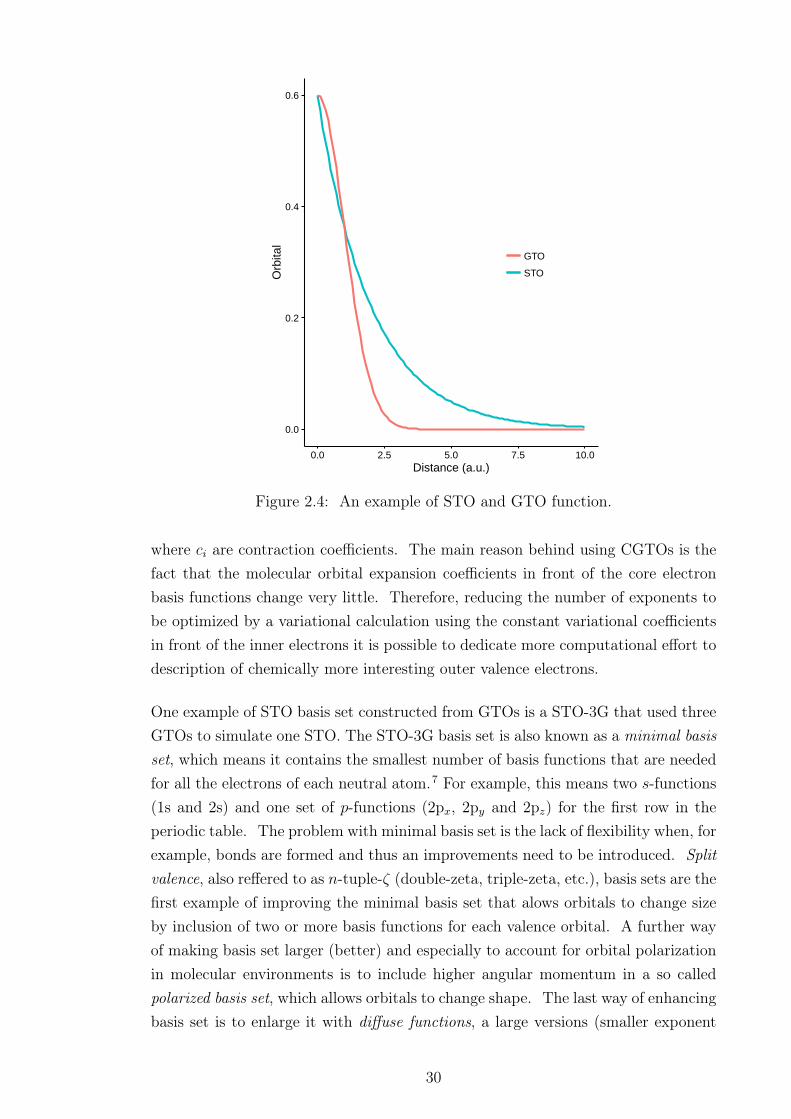
where L = l+m+n is referred to as the angular momentum. These functions tendto decay at infinity faster than Slater functions and s-type Gaussians are missingnuclear cusp, but it is much easier to compute matrix elements using Gaussians.An example of STO and GTO function is depicted in the Figure 2.4.

As mentioned previously, although STO functions have better description for elec-tron density they are computationally more expensive and hence this problem iscircumvented by constructing the STO basis function as a linear combination ofcomputationally more convenient gaussian functions. In practice, a so called con-tracted GTOs (CGTOs) are used, which are smaller sets of functions formed fromfixed linear combinations of primitive GTOs:

χ(r) =n∑i=1

ciφi(r) (2.77)

29

0.0

0.2

0.4

0.6

0.0 2.5 5.0 7.5 10.0Distance (a.u.)

Orb

ital

GTO

STO

Figure 2.4: An example of STO and GTO function.

where ci are contraction coefficients. The main reason behind using CGTOs is thefact that the molecular orbital expansion coefficients in front of the core electronbasis functions change very little. Therefore, reducing the number of exponents tobe optimized by a variational calculation using the constant variational coefficientsin front of the inner electrons it is possible to dedicate more computational effort todescription of chemically more interesting outer valence electrons.

One example of STO basis set constructed from GTOs is a STO-3G that used threeGTOs to simulate one STO. The STO-3G basis set is also known as a minimal basisset, which means it contains the smallest number of basis functions that are neededfor all the electrons of each neutral atom.7 For example, this means two s-functions(1s and 2s) and one set of p-functions (2px, 2py and 2pz) for the first row in theperiodic table. The problem with minimal basis set is the lack of flexibility when, forexample, bonds are formed and thus an improvements need to be introduced. Splitvalence, also reffered to as n-tuple-ζ (double-zeta, triple-zeta, etc.), basis sets are thefirst example of improving the minimal basis set that alows orbitals to change sizeby inclusion of two or more basis functions for each valence orbital. A further wayof making basis set larger (better) and especially to account for orbital polarizationin molecular environments is to include higher angular momentum in a so calledpolarized basis set, which allows orbitals to change shape. The last way of enhancingbasis set is to enlarge it with diffuse functions, a large versions (smaller exponent

30

ζ) of standard valence-size functions that enables orbitals to occupy a larger areaof space. The diffuse functions are especially important for systems with looselybound electrons such as anions, Rydberg states and excited states.

An example of an actual basis set commonly used is 6-31+G(d,p), which contains 6GTOs for core orbitals, 3 GTOs for the first STO of the valence orbital and 1 GTOfor the second STO description. Moreover, it contains d orbital functions on heavyatoms and p orbital functions on hydrogen atoms. This basis set is completed byadding diffuse function to heavy atoms only. The above introduced STO-3G and6-31+G(d,p) basis sets are from a family of Pople style basis sets developed by JohnPople and co-workers.

Correlation consistent (cc) basis sets developed by Dunning and co-workers representa family of basis sets which should be mostly used with correlated calculations suchas coupled cluster and Møller-plesset methods. In contrast to, for example, Poplebasis sets which are optimized by variational procedure at the HF level the cc basissets are optimized using correlated (CISD) wave functions and thus are designed torecover the correlation energy of the valence electrons. These basis sets are designedto converge smoothly towards the complete basis set limit. The cc are commonlydenoted as (aug)-cc-pVXZ, which stands for correlation consistent polarized valenceX-zeta (X=D, T, Q, 5, etc.) basis set. Optionally a prefix "aug" in front of thebasis set means that it was augmented by inclusion of diffuse functions.

Another type of basis sets used within this work are all-electron split valence def2-xVP (x = S, TZ, QZ) basis sets originally developed by Ahlrich and co-workers20.These are property-optimized (specifically dipole polarizabilities) split valence, po-larized, n-zeta basis sets and, for example, Def2-TZVPD21 basis set is also aug-mented with diffuse functions.

2.1.9 Local Methods

Treatment of electron correlation at high level of ab initio calculations is essen-tial for an accurate description of molecular structures, energetics and properties.Computational cost of conventional electron correlation methods, such as, CCSD(CCSD(T)) increases very steeply with the number of electrons and become pro-hibitively expensive for anything but small molecules. One of the reasons of thisunfavourable scaling is that usually canonical molecular orbitals, which are generallydelocalized over the whole system, are used as a basis for these calculations. Onthe other hand, localizing the molecular orbitals allows us to reduce the number ofelectron pairs to be correlated since there are small correlation effects coming from

31

interaction of distant electrons. Furthermore, this reduces the steep increase in thenumber of virtual orbitals needed.

In the case of local method, such as LCCSD, it is formulated in a basis of nonorthog-onal local correlation functions.22 Excitations are made from localized molecularorbitals into subspaces (domains) of the local basis in order to significantly reducethe number of amplitudes to be optimized in LCCSD calculations. Moreover, thisallows to completely neglect (or treat in a simplified way, e.g. MP2) the correlationof distant electrons. Local correlation methods have a potential to approach linearscaling with molecular size and to suffer less from the basis set superposition er-ror.23,24 The basis set superposition error is often encountered in the case of weaklybound clusters where it leads to an artificial overestimation of the binding energyand shortening of inter-molecular distances. The reason is, due to finite basis setsbeing used, when monomers are approaching each other they can utilize extra basisfunctions from each other and thus improve their description of electron distribution.The error is coming from the fact that this electron distribution improvement is in-consistent, happening especially at shorter inter-molecular distances, which leads toinconsistent treatment of monomers at different inter-molecular distances.

2.1.10 Frequency Calculations

The following section, which mainly follows the Vibrational Analysis in Gaussianarticle by Ochterski25, gives a short introduction to the frequency calculations.

Frequency calculations are not only important in order to predict the IR/Ramanspectra, but also in order to characterize stationary points on the potential energysurface, for example, identifying a minimum, transition state or a higher order saddlepoint. Moreover, frequencies are needed for calculations of various thermochemicalvalues, such as enthalpies, entropies and zero-point vibration and thermal energycorrections to the total energy.

Vibrational frequencies are calculated at the stationary point geometries by deter-mining the second derivatives of the energy with respect to the cartesian nuclearcoordinates and then transforming to mass weighted coordinates. This starts withcalculation of the Hessian matrix, which contains the second partial derivatives of theenergy with respect to displacement of the atoms in cartesian coordinates under thecondition that the first derivatives with respect to displacement of the atoms are zero.These force constants are then converted to mass weighted cartesian coordinates.Next step is diagonalization of mass weighted force constant matrix which yields aset of 3N eigenvalues (the fundamental frequencies) and eigenvectors (the normal

32

modes). The eigenvectors are initially discarded and recalculated again after the ro-tation and translation modes are separated out leaving 3N−6 or 3N−5 vibrationalmodes. This is done by finding the transformation matrix, which is used to trans-form mass weighted cartesian coordinates to internal coordinates where rotationand translation modes are separated out. After the transformation the Nvib ×Nvib

submatrix, which represents the force constants internal coordinates, is diagonalizedand yields Nvib eigenvalues λ = 4π2v2 and Nvib eigenvectors. These eigenvalues arethen converted to frequencies in units of reciprocal centimeters.

2.1.11 Thermochemistry

In the following section basic concepts and equations for computing thermochemicalquantities, specifically as defined in Gaussian program but applicable in general,are introduced in order to understand how these are obtained. This section mainlyfollows the paper on computing thermochemistry in Gaussian by Ochterski26, whichin return refers to equations from the textbook by McQuarrie and Simon27.

All of these equations are derived under the special case of ideal gas approximation,therefore particles have no potential energy of interaction of any kind. Further, itis assumed that excitation energies even to the first electronically excited state aremuch higher than kBT at room termperature and thus there is usually no electronicenergy contribution to the internal energy from occupation of electronically excitedstates.

In the following section equations describing how partition functions q(V, T ) fromtranslational, electronic, rotational and vibrational motion components are used todetermine entropy contribution, internal thermal energy and heat capacity. Thefollowing relation can be used to determine the entropy contribution:

S = NkB +NkBln

(q(V, T )

N

)+NkBT

(∂lnq

∂T

)V

(2.78)

In Gaussian package, special form of the above equation is used where molar valuesare given, so after division by n = N/NA, substitution of NAkB = R and movingthe first term into the logarithm (as e), it yields (with N = 1):

S = R +Rln (q(V, T )) +RT

(∂lnq

∂T

)V

= R

(ln(qtqeqrqve) + T

(∂lnq

∂T

)V

) (2.79)

33

Further, the partition function can be used to obtain the internal thermal energyE:

E = NkBT2

(∂lnq

∂T

)V

(2.80)

And this equation can be used to obtain the heat capacity:

C =

(∂E

∂T

)N,V

(2.81)

In the following paragraph individual partition functions, as defined in Gaussian

package, are introduced. Their definition may be slightly different and simplifiedin comparison to the usual definitions commonly found in textbooks. For example,contribution from the translation partition function qt is defined as:

qt =

(2πmkBT

h2

)3/2kBT

P(2.82)

which when substituted to eq. (2.79) (and partially derived with respect to T to getthe third term) yields the translational entropy:

St = R

(ln(qte) +

(3

2

))(2.83)

In the above equation factor e comes from Stirling’s approximation. Similarly, trans-lational contribution to the internal thermal energy can be derived as:

Et = NAkbT2

(∂lnq

∂T

)V

=3

2RT (2.84)

and the constant volume heat capacity as:

Ct =∂Et

∂T=

3

2R (2.85)

In the case of contribution from electronic partition function, it is assumed there isno contribution from the first and higher excited states, as these lie much higher inenergy than kBT . This assumption together with treating the ground state energyas a reference value of zero greatly simplifies the electronic partition function intocontribution only from ground state degeneracy of the system qe = ω0. Since thereare no temperature dependent terms, this results in the electronic heat capacity andthe internal thermal energy due to the electronic partition function being both zeroand the electronic entropy of Se = R(lnqe).

In the general case of a nonlinear polyatomic molecule rotational partition function

34

has the following form:

qr =π1/2

σr

(T 3/2

(Θr,xΘr,yΘr,z)1/2

)(2.86)

where Θr,n, n = x, y, z are the rotational temperatures defined as Θr = h2/8π2InkB, n =

x, y, z for three values of the moment of inertia In for three rotation axes. The con-tribution arising from rotational partition function for entropy is Sr = R(lnqr +3/2),to the internal thermal energy is Er = 3/2RT and finally 3/2R for the heat capacity.When compared with the average contribution to the entropy, the internal energyand heat capacity in the case of a linear polyatomic molecule, which has only tworotational degrees of freedom, it is 1/2RT less for the internal thermal energy, 1/R

for the entropy and heat capacity.

Contributions from vibrational motion are represented as a product of the contribu-tions from each real vibrational mode K, ignoring imaginary (minus sign) frequen-cies. There is a characteristic vibrational temperature, Θv,K = hvK/kB, for each ofthe 3N−6 or 3N−5 modes for linear molecules. In the case when zero-point energycontributions are computed separately and bottom of the internuclear potential en-ergy well is taken as zero energy reference point, then vibrational partition functionis expressed as a product of individual partition functions for each vibrational modeK:

qv =∏K

e−Θv,K/2T

1− e−Θv,K/T(2.87)

After using the above partition function to calculate entropy and few algebraicoperations the total vibrational entropy has the following form:

Sv = R∑K

(Θv,K/T

eΘv,K/T − 1− ln(1− e−Θv,K/T )

)(2.88)

Similarly, contribution to the internal energy from vibrational modes can be calcu-lated as follows:

Ev = R∑K

Θv,K

(1

2+

1

eΘv,K − 1

)(2.89)

And finally contribution to the heat capacity is calculated as:

Cv = R∑K

eΘv,K/T

(Θv,K/T

e−Θv,K/T − 1

)2

(2.90)

The above defined terms for partition functions, entropies and energies are used in

35

calculation of, for example, the Gibbs free energy defined as:

∆G =

∆H︷ ︸︸ ︷Eelec + EZPE + Etot + kBT −TStot (2.91)

where Eelec is electronic energy calculated at a given level of theory relative toseparate nuclei and electrons. EZPE is zero-point energy correction , correcting forvibrational motion of the system described by a harmonic oscillator at 0 K andcomputed as a sum of contributions from all non-imaginary K vibrational modesEZPE =

∑K 1/2hcvK . In the eq. (2.91) Etot = Et + Er + Ev + Ee represents

correction to the internal thermal energy at given temperature T and calculated asa sum over contributions from individual partition functions. Similarly, Stot is givenas a sum of contributions from translational, rotational, vibrational and electronicdegrees of freedom.

The Gibbs free energies calculated using the eq. (2.91) can be used, for example,in calculations of binding energies from free energies of reactants and products (seeChapter 3) and in calculations of reduction potentials using the thermodynamiccycle (see Chapter 4).

2.2 Density Functional Theory

Researchers have intensively tried to find a simplificating substitution for the verycomplex many-body wave function, which depends on 4N coordinates (three spatialand one spin coordinate for each of N electrons in the system). A suitable candidateseems to be the electronic density, a central variable in the Density FunctionalTheory (DFT), which is a simple function that depends solely on the three spatialvariables (or in the case of systems including spin polarisation, such as open-shellsystems, a spin-polarized formalism is used and the density is divided into spin up(ρα) and spin down (ρβ) density). Moreover, in contrast to wave function methods,the density is an observable quantity that can be obtained from experiments, e.g.X-ray diffraction.

One of the advantages of DFT methods is their ability to directly include some ofthe effects of electron correlation (less expensively than post-Hartree-Fock correlatedmethods), in comparison to Hartree-Fock method that considers these effects onlyin an average sense. The best DFT methods achieve significantly greater accuracythan HF theory at only a modest increase in computational cost.7 On the otherhand, the biggest disadvantage of DFT is that it is an exact method with theapproximated functionals (as the real functionals are not known) and cannot be

36

further systematically improved, e.g. with increasing basis set. In the followingsection the basic theory behind DFT will be introduced.

The ultimate goal of the DFT method is the calculation of the total energy ofthe system and the ground-state electron density distribution without using thewave function of the system.1 Starting from the Born-Oppenheimer approximationa relation between a central quantity in the DFT method, the electron density ρ,and the electronic wave function can be established:

ρ(r) =∑

σ1=− 12, 12

∫|Ψ0(r, σ1, r2, σ2, . . . , rN , σN)|2dτ2dτ3 . . . dτN (2.92)

where Ψ0 is a ground state wave function and τ is a spatial-spin coordinate. Fromthe above equation a function of the position of electron 1 in space ρ(r) is obtainedafter integration of the square of |Ψ0|2 over spin-space coordinates and summationover electron 1 spin coordinate.4

2.2.1 The Hohenberg-Kohn Theorems

The Hohenberg-Kohn Existence Theorem:Hohenberg-Kohn in their existence theorem proved that for a ground state the elec-tron density uniquely determines the Hamiltonian operator and thus all propertiesof the system.1 This can be shown by constructing a Hamiltionian operator as inthe following equation using only the density:

H =N∑j=1

(− ~2

2me

∇2j −

M∑A=1

ZAe2

|~rj − ~RA|+

1

2

N∑k 6=j

e2

|~rj − ~rk|

)(2.93)

where the number of electrons (N) is defined by the integral of the density overthe whole space. Further, searching for the positions of potential spikes, number ofspikes and steepness of each spike on the ρ0(r) landscape we obtain positions (~RA),number (M) and charge (ZA) of the nuclei, respectively.The Hohenberg-Kohn Variational Theorem:This theorem states that for a given number of electrons N and an external potentialVext(r) (substituting for the interaction of electrons with nuclei) there exists anenergy functional† of electron density EHK which obeys the following variationalprinciple:

EHK[ρguess] ≥ EHK[ρ0] = E0 (2.94)

†the functional is a function that takes a function for its input argument

37

where ρ0 is the exact electronic density distribution for the ground state energy E0.Unfortunately, the major goal of the method to find out the mathematical form ofthis functional has not yet been successful.

2.2.2 Orbital Free Approaches

Early orbital free approaches to define the energy functional considered the systemto be classical and the energy consist of separable kinetic and potential components.6

In a so-called Thomas-Fermi (TF) model, the density is derived from an uniformelectron gas and equations are based on fermion statistical mechanics. The electron-electron repulsion (Eee) is with reference to the Hartree approximation divided intoa Coulomb (J [ρ]) and exchange part (K[ρ]), and nuclear-nuclear repulsion is con-stant within the BO approximation. Finally, the total electronic energy functionalE0,TF[ρ] has the following form:

E0,TF[ρ] =

TTF[ρ]︷ ︸︸ ︷CF

∫ρ5/3(r)dr

Een[ρ]︷ ︸︸ ︷−

Nnuclei∑A=1

∫ZA(RA)ρ(r)

|RA − r|dr+

J [ρ]︷ ︸︸ ︷1

2

∫∫ρ(r)ρ(r′)

|r − r′|drdr′ (2.95)

where CF = 310

(3π2)2/3, TTF refers to the Thomas-Fermi approximate kinetic energy,Een is the exact expression for electron-nuclei attraction. Further, inclusion of theexchange energy termKD[ρ] = −Cx

∫ρ4/3(r)dr, with Cx = 3

4( 3π)1/3, derived by Dirac

into the above equation (2.95) forms a Thomas-Fermi-Dirac model. Limitations ofthese models are, for instance, the approximate kinetic energy term, self-interactionterm in Eee as well as missing electron correlation effects. Although there have beensome improvements in these orbital free models and some of the ideas and equationsderived from uniform electron gas models are used in the so-called Local DensityApproximation that will be discussed further below, their accuracy is still too lowto be of general use.

2.2.3 Kohn-Sham Self-consistent Field Methodology

Kohn and Sham (KS) realised that the main flaw of orbital free models (i.e. theThomas-Fermi model) is connected with the way the kinetic energy is determined.28

In their report from 1965 they introduced an approach to the unknown universalfunctional, mentioned in the second Hohenberg-Kohn theorem, in a form of a fic-tious non-interacting system of electrons. In this non-interacting system the totalHamiltonian is expressed as a sum of one-electron operators (

(−1

2∆ + Vext

)) where

electrons are subject to an external potential Vext ingeniously tailored such that

38

the overall density ρ is same as the ground-state density ρ0 of a real system. Theeigenfunction for the total Hamiltonian is a KS determinant ΨKS (similar form asSlater determinant) constructed from KS spinorbitals φKS

i and the electronic densitycan be expressed as ρexact(r) =

∑i ni|ΨKS

i (r)|2 with ni = 0, 1, 2 denoting orbitaloccupancy in the KS determinant. The total energy functional is written as:

EDFT[ρ(r)] = Tni[ρ(r)] + Vne[ρ(r)] + Vee[ρ(r)] + Exc[ρ(r)] (2.96)

where the terms on the r.h.s. refer, respectively, to the kinetic energy of the non-interacting electrons, standard Coulomb electron-nuclei interaction, the classicalCoulomb electron-electron repulsion and Exc includes quantum in nature exchange,electron-electron correlation terms, correction for the classical self-interaction energyand the difference in the kinetic energy between the non-interacting and the realsystem. The problem with the kinetic energy was partially solved by splitting it intoa major fraction that can be computed exactly (equation (2.97)) and a small partthat is merged into a so called exchange-correlation energy Exc together with allnon-classical corrections to the electron-electron repulsion energy.

Tni[ρ(r)] =N∑i=1

⟨φi| −

1

2∇2i |φi⟩

(2.97)

Kohn-Sham orbitals are expressed within a basis set of functions φi and individualorbital coefficients are determined by solving a secular equation (analogous to HFtheory) which is done iteratively using SCF procedure:

Kµν =

⟨φµ| −

1

2∇2 −

nuclei∑k

Zk|r − rk|

+

∫ρ(r′)

|r − r′|d3r′ + Vxc|φν

⟩(2.98)

Here, Vxc = δExc

δρis a potential corresponding to the exchange-correlation energy

Exc, and Kµν is similar to Fµν from the HF method.4,28 Most of the terms on r.h.sof the equation (2.98) can be solved exactly except for the Vxc and thus Exc partsfor which approximations have to be introduced.

2.2.4 Approximations to the Exchange-correlation Functional

The electronic density distribution can be described locally within a small volumeapproximated as homogenous. Following this assumption the exchange-correlationenergy can be estimated as a sum of contributions from infinitesimally small volumesusing the uniform electron gas model.1 The Thomas-Fermi-Dirac model, introduced

39

in section 2.2.2, is an example of total electronic energy in Local Density Approx-imations (LDA). In the LDA, the term "local" means that the energy is given asa functional which depends only on ρ(r) at points in space but not on ρ(r) atmore than one point in space or on spatial derivatives of ρ(r). Unfortunately, theuniform electron gas approximation is insufficient especially in the region near thenuclei where the electron densities vary rather strongly. This inhomogeneity of theelectron density can be taken into account using non-local corrections, GeneralizedGradient Approximations (GGA), involving gradient of ρ(r), ∇ρ(r).

In most cases a gradient corrected functional is constructed by adding a gradientcorrection to the LDA functional:

EGGAXC = ELDA

XC +

∫BXC(ρ,∇ρ)d3r (2.99)

where the exchange-correlation function BXC is carefully selected as a function of ρand its gradient in order to:

• reproduce experimental properties of atoms and molecules (training sets ofmolecules)

• reproduce properties of exchange and correlation effects resulting from quan-tum mechanical equations (limiting values for high and low electron densities,properties of the exchange "hole")

Typically, complete exchange-correlation functionals are built as a combination ofcorrelation and exchange GGA functionals, for instance, a BLYP functional is acombination of Becke’s (B) GGA exchange with the GGA correlation functional ofLee, Yang, and Parr (LYP).4

Additional improvement to the GGA functionals is an inclusion of the second deriva-tive of the density (the Laplacian operator, ∆ρ) or the kinetic energy density, definedas τ(r) =

∑occupiedi=1

12|∇Ψi(r)|2, in a so-called meta-GGA functionals. For example,

TPSS29 and M06-L30 (in the rest of the text written as M06L) are examples ofmeta-GGA functionals.

Another family of exchange-correlation approximations are hybrid functionals, whichdefine the exchange functional by mixing exact HF with DFT (LDA and/or GGA)exchange term and this functional is then combined with a local and/or gradient-corrected correlation functional. This is theoretically justified by the adiabatic con-nection theorem, which connects the non-interacting (KS) and fully interacting (ex-act) system.

EhybridXC = α(EHF

X − EDFTX ) + EDFT

XC (2.100)

40

An example of one of the most popular three-parameter hybrid functional B3LYPhas the following form for EXC:

EB3LYPXC = ELDA

X + c0(EHFX −ELDA

X )+ cXEB88X +EVWN3

C + cC(ELYPC −EVWN3

C ) (2.101)

where the c parameters were obtained fitting into experimental data. The parameterc0 = 0.20 controls admixture of HF and LDA local exchange and exchange functionalis further supplemented with gradient-corrected Becke’s (B88) functional, scaled bythe parameter cX = 0.72. Finally, exchange-correlation functional is completed byaddition of the Vosko-Wilk-Nusair (VWN3) local correction functional, which can beoptionally corrected by the LYP correlation correction via the parameter cC = 0.81.7

A major drawback of DFT is that we are not able to systematically improve thecurrent methods to yield the exact results, not even when a complete basis set is used,since the functional form of the exact exchange-correlation energy is not known.Moreover, we cannot use DFT (in the Hohenberg-Kohn ground state theory) on itsown to probe processes in photochemistry and to predict excited state properties.Although it was shown that the density contains information about excited stateproperties, as we are able to construct a Hamiltonian operator (wave function) fromthe density, there is no practical way to extract this information so far.28

2.2.5 Dispersion correction DFT (D-DFT)

One of the areas where the current DFT functionals usually perform poorly is aso called dispersion energy problem. This problem is related to inability of mod-ern functionals to describe contribution that stem from dispersion forces and poseschallenge especially when studying weakly bound systems such as rare gas dimers,hydrogen bonded complexes and complexes dominated by π-π-stacking. Dispersionforces, sometimes also referred to as London forces, are long-range attractive forcesarising from the induced dipole-induced dipole interaction generated as a result ofinstantaneous correlation of electronic motion. The induced dipole-induced dipoleinteraction, which is usually dominating the interaction, decays with the inversesixth power (1/R6) of the intermolecular distance.

The main reason for the missing dispersion forces is that the exchange-correlationpotential VXC(r) at a point r is determined by the density exactly at this point.28

This means that if there is no overlap of electron densities between the local andanother distant system, which means that these are not directly bonded to eachother, only the local exchange-correlation energy is considered. Therefore some kindof improvement has to be introduced in order to account for this nonlocal long-range

41

correlation effects.

There are several approaches trying to address the dispersion energy problem. Forexample, time-dependent DFT based approaches31, vdW-Density Functional method32,33

which uses the electron density to compute the dispersion energy and DFT-D meth-ods34–37 utilizing a damped, atom-pair wise potential which is added to a standardKohn-Sham DFT.

The GD3BJ dispersion correction, which is used in this work, belongs to the family ofDFT-D methods and uses the D3 version of Grimme’s dispersion with Becke-Johnson(BJ) finite-damping to ensure more physically correct short-range behavior.38 TheDFT-D3 is atom pairwise additive scheme in which the dispersion energy is definedas:

ED3(BJ)disp = −1

2

∑A 6=B

s6CAB

6

R6AB + [f(R0

AB)]6+ s8

CAB8

R8AB + [f(R0

AB)]8(2.102)

where the sum runs over all atom pairs in the system and f(R0AB) = a1R

0AB + a2

contains free fit parameters a1 and a2 introduced by BJ. Further, R0AB is defined as

R0AB =

√CAB

8 /CAB6 .39

2.3 Molecular Dynamics

Molecular dynamics (MD) is an advanced computational method based on a rathersimple physical model that can provide insight into the structural dynamics and en-ergetics of molecular systems at atomic level. It belongs to the family of a so-calledforce-field methods (or sometimes referred to as Molecular Mechanics methods)where the step of obtaining a potential energy surface by calculating the electronicenergy is greatly simplified by using the parametric functions of the electronic energywith parameters fitted to usually ab initio calculations or experimental data. Thesmallest building blocks are typically atoms or groups of atoms in the case of, forexample, Coarse-Grained Molecular Dynamics. Force-field based methods do nottake into account electrons and hence the bonding information must be part of theparameters provided for the system. Potential energy surface is sampled using theclassical mechanics (Newton’s second law), which means that quantum phenomenaare neglected and events such as bond formation/breaking and quantum tunnellingcannot be observed.

Molecular dynamics simulations are performed in order to provide conformationalsampling, to understand structure-energy relationship and to estimate equilibrium

42

and non-equilibrium properties of molecular systems. One of the major advantagesof MD simulations over, for example, Monte-Carlo method is the possibility to studytime-dependent properties, using a so called time-correlation functions, due to thetime connection between simulation steps.40 Macroscopic properties that can bestudied by MD are, for example, the radial distribution function of a solvent, vis-cosity of a liquid, reaction kinetics and diffusion processes.

2.3.1 Force fields

Force fields used in MD are simple analytical atomistic functions relating structurewith potential energy. In MD a set of approximations is introduced to the molecularsystem. For example, parameters for both bond-stretching and angle-bending arepresent in the form of spring constants describing generally a harmonic potential.These are further supplemented by torsion profiles for dihedral angles. Atoms areapproximated as Lennard-Jones spheres with constant point partial charges local-ized at the atomic centres. The partial charges are normally derived based on fittingto the molecular electrostatic potential calculated using an ab initio method. It isthe quality of these partial charges that determine the accuracy of MD calculationsespecially for polar molecules where the electrostatic terms will dominate the poten-tial function.6 Moreover, the partial charges are geometry dependent and this has tobe taken into account during their derivation. The force fields commonly used arepair-additive, neglect explicit polarization and charge-transfer effects though thesecontributions are included indirectly by some parameters. The result is that someimportant effects are not well described, for example, inclusion of divalent ions,hydrogen bonding and solute polarization by solvent.41

There are various types of force-fields designed for different purposes and can differin aspects such as6:

• Potential energy functional form

• Number of cross terms† included

• Type of information used for fitting the parameters

For example, in the case of force fields designed to treat large systems, such asnucleic acids or proteins, the harmonic form of potentials for bonds and angles areused. Furthermore, a Lennard-Jones potential is used for the Van der Waals termand the cross term is not present.6 Force fields are usually designed to work for

†in general all kind of terms that couple two (or more) of the bonded terms

43

specific systems of interest. For instance, the OPLS42,43 force field was developedfor organic liquids simulations, the AMBER force field mainly to work with nucleicacids and proteins in comparison to the CHARMM that is used mainly for proteins.One of the key ideas that is often used during force-field parametrization is thatstructural units (bond-stretching, angle-bending, etc.) defined for similar chemicalenvironments are transferable between different molecules. An overview of some ofthe available force fields can be found in, for example, Introduction to ComputationalChemistry by Jensen6 and Essentials of Computational Chemistry by Cramer4.Below generic aspects of force fields are given.

2.3.2 Potential Energy and Equations of Motion

Propagation of the studied system in time is acquired by calculating the Newton’sequations of motion (2.103) for a system of N interacting atoms:

fi = mi∂ri∂t2

= −∂U∂ri

(2.103)

where forces fi acting on the atoms are usually derived from a potential energy U

which is given as a sum of individual energy terms for covalent and noncovalentcontributions eq. (2.104):

U = Ucovalent + Unoncovalent (2.104)

Continuing to discuss, for simplicity, a system composed of atoms with coordinatesr1, · · · , rN and potential energy U(r1, · · · , rN), we introduce an atomic momentap1, · · · , pN, in terms of which the kinetic energy may be written as K(p1, · · · , pN) =∑N

i=1 |pi|2/2mi. The covalent part of the potential energy consists of bond-stretching,angle-bending and dihedral (torsion) angle contributions. Illustrative figure of co-valent contibutions is shown in Figure 2.5 and the related equations (2.105):

Ucovalent =1

2

∑bonds

kij(rij − rij0)2

+1

2

∑bendangles

kijk(θijk − θijk0)2 (2.105)

+1

2

∑torsionangles

∑n

kijkl(1 + cos(nφijkl − φijkl0))

44

Figure 2.5: Illustrating picture for the definition of bond rij (interatomic distance),bend angle θijk and torsion angle φijkl.

The noncovalent part of potential energy is in the form of a pair-additive poten-tial where three-body and higher order interactions are neglected. A model of pairpotential can be seen in eq. (2.106) and a real noncovalent potential used in simu-lations eq. (2.107) consist of a VdW part, which has the form of the Lennard-Jonespotential, and a Coulomb part for electrostatic charges.

U(r1, · · · , rN) =∑i<j

u(ri, rj) (2.106)

Unoncovalent = 4ε

[(σ

rij

)12

−(σ

rij

)6]

︸ ︷︷ ︸Lennard−Jones potential

+1

4πε0

qiqjrij︸ ︷︷ ︸

Coulomb potential

(2.107)

2.3.3 Molecular Dynamics Simulations

The MD simulations are carried out from a starting set of atomic coordinates, whichare usually obtained from X-ray crystallography or NMR experiments. The highquality starting structure is of an essential importance for MD sampling a proxim-ity of X-ray potential minimum on a potential energy surface. The reason is thatfor most of the simulations due to a limited simulation time only a small confor-mational space is sampled around the crystal structure minimum. Moreover, MDcannot overcome large energy barriers due to usually limited kinetic energy relatedto reasonable simulation temperatures.41,44

In a typical MD simulation, an initial geometry of the studied system is placed inthe environment of solvent (e.g. water) and ions. Immersing the structure into asolvent box with ions, we are trying to get as close as possible to real conditions.

45

Initial velocities are assigned to each of the atoms according to randomly selectingfrom a Maxwell-Boltzmann distribution at the simulated temperature:

p(vix) =

(mi

2πkBT

)1/2

exp

[−1

2

miv2ix

kBT

](2.108)

where at a given temperature T atom i of mass mi is asigned a velocity vix in the xdirection.

When MD is performed without temperature and pressure coupling this generatesNVE (constant moles, constant volume and constant energy) ensemble. However,most desired quantities are commonly calculated from MD simulations performedin the constant temperature NVT or constant pressure NPT ensemble. The NVTensemble is usually achieved by coupling the system to a heat bath and there are var-ious schemes available to simulate the constant temperature or if needed to controlthe temperature of the system. For example, since the temperature of the systemis related to the time averaged kinetic energy as 〈Ek〉NV T = 3/2NkBT an obviousscheme would adjust the temperature by re-scaling the velocities of particles. Sucha scheme is the Berendsen thermostat45 that corrects a deviation of the system tem-perature by weak coupling to an external heat bath with reference temperature T0

using the following equation:

dT

dt=T0 − Tτ

(2.109)

which assures that a temperature deviation decays exponentially with a constantcoupling time τ . However, this termostat does not generate a correct canonicalensemble and therefore this is achieved by more advanced thermostats such asvelocity-rescaling46 or Nosé-Hoover scheme47,48. For the generation of the NPT en-sembles the constant pressure is maintained by changing the volume of the simula-tion cell by scalling the coordinates and simulation box vectors. The Berendsen45

or the Parrinello-Rahman49,50 scheme are examples of common pressure couplingalgorithms used to ensure the constant-pressure simulations.

MD run generates a series of time-correlated configurations, or "snapshots" of thesimulated system at a given time, which form a trajectory of the system. The timestep is one of the limiting factors of MD and is determined by the rate of thefastest molecular motions, which are usually vibrations involving hydrogen atoms.Therefore, the maximum time step is typically of the order of femtoseconds (10−15s).Another issue is that the classical harmonic oscillator approach is unsuitable forhigh frequency motions with ν � kBT/h. Around the room temperature of 300K this corresponds to the wavenumber of approximately 208 cm−1. Therefore, inorder to achieve longer time steps and thus longer simulation times it is common to

46

remove the highest frequencies by treating the bonds and angles (typically involvinghydrogen) as constraints.6

Most MD calculations use leap-frog algorithm51, which step-by-step numerically in-tegrate coupled differential equations of motion (2.110) and (2.111). In the case ofleapfrog, positions are defined at times ti, ti+1, ti+2, . . . , spaced at constant inter-vals dt, while the velocities are defined at times halfway in between, indicated byti−1/2, ti+1/2, ti+3/2, . . . .

r(t+ δt) = r(t) + v(t+1

2δt)δt (2.110)

v(t+1

2δt) = v(t− 1

2δt) +

1

mF(t)δt (2.111)

The analysis of the outcome from simulations may provide detailed informationabout all aspects of the time evolution (with sub-ps time resolution) of the three-dimensional structure and interactions within studied system.41 Despite the enor-mous advance of MD in recent years, the method still encounters two basic limita-tions. The first one deals with problems of short simulation timescales, which re-sult in limited sampling of conformational space. However, this limitation is slowlywaning with faster computers, use of graphic cards for some of the calculations andimprovements in the codes used in MD. The second, more critical limitation thatcannot be easily overcome, is because of the approximate nature of the force fieldsused in MD. In comparison to more accurate quantum mechanical calculations, how-ever MD is able to work with larger systems with reasonable computational cost andprovide dynamical, not just static molecular information.

2.4 Hybrid QM/MM Methods

Hybrid QM/MM methods treat a system of interest at multiple levels of theory,combining high accuracy of quantum mechanical (QM) calculations with the lowcomputational cost of empirical molecular mechanical (MM) approach. A challengefor computational chemistry at present is to study reactions and photochemicalprocesses in large systems or molecules in a realistically modeled environment ofchemical and/or biological interest. However, this goal is currently out of reachof traditional electronic structure methods for which the computational costs scaleunfavourably with the size of the system, typically limiting them to small modelsystems in vacuo. In contrast, methods of molecular mechanics have the advantageof lower computational requirements than QM methods, but on the other hand

47

suffer from several limitations, as they are not able to describe the details of bondbreaking/forming or electron transfer reactions.4,44 The QM/MM approach providesa means for overcoming these limitations by partitioning the studied system into two(or more) parts, which are calculated with different computational methods and arecoupled with each other.

In a typical approach a part of the molecule where a (photo)chemical reaction takesplace, denoted as QM core, is investigated with a reliable QM method (ab initio orDFT), semi-empirical, or Empirical Valence Bond (EVB) level. The remainder ofthe molecule, which impose sterical and polarization constraints on the QM core,is included using a lower level of theory, typically using molecular mechanics (MMregion). The result is that the complete Hamiltonian and thus the total energy ofthe system must be some kind of hybrid of QM and MM.

References

[1] Piela, L. Ideas of Quantum Chemistry; Elsevier, 2007.

[2] Groenhof, G.; Boggio Pasqua, M.; Schäfer, L. V.; Robb, M. A. In Combin-ing Quantum Mechanics and Molecular Mechanics. Some Recent Progresses inQM/MM Methods; Sabin, J. R., Brändas, E., Eds., Vol. 59; Academic Press,2010; pages 181–212.

[3] Young, D. Computational Chemistry: A Practical Guide for Applying Tech-niques to Real World Problems; John Wiley & Sons, 2001.

[4] Cramer, C. Essentials of computational chemistry: theories and models; J.Wiley, 2002.

[5] Szabo, A.; Ostlund, N. Modern Quantum Chemistry: Introduction to AdvancedElectronic Structure Theory; Dover Publications, 1996.

[6] Jensen, F. Introduction to Computational Chemistry; John Wiley & Sons, 2007.

[7] Foresman, J.; Frisch, A.; Gaussian, I. Exploring chemistry with electronic struc-ture methods; Gaussian, Inc., 1996.

[8] Schlegel, H. B. WIREs Comput Mol Sci 2011, 1(5), 790–809.

[9] Matsika, S.; Krause, P. Annu. Rev. Phys. Chem. 2011, 62(1), 621–643.

[10] Paterson, M. J.; Bearpark, M. J.; Robb, M. A.; Blancafort, L.; Worth, G. A.Phys. Chem. Chem. Phys. 2005, 7(10), 2100–2115.

48

[11] Roothaan, C. C. J. Rev. Mod. Phys. 1951, 23, 69–89.

[12] Hall, G. G. Proc. R. Soc. A 1951, 205(1083), 541–552.

[13] Shavitt, I.; Bartlett, R. J.Many-Body Methods in Chemistry and Physics; Cam-bridge University Press, 2009.

[14] Nesbet, R. K. Phys. Rev. 1958, 109, 1632–1638.

[15] Löwdin, P.-O. J. Math. Phys. 1962, 3(6), 1171–1184.

[16] Parr, R.; Weitao, Y. Density-Functional Theory of Atoms and Molecules, Inter-national Series of Monographs on Chemistry; Oxford University Press, 1989.

[17] Van Voorhis, T.; Head-Gordon, M. J. Chem. Phys. 2000, 113(20), 8873–8879.

[18] Roos, B. O. In Theory and Applications of Computational Chemistry; Dyk-stra, C. E., Frenking, G., Kim, K. S., Gustavo E. Scuseria., Eds.; Elsevier:Amsterdam, 2005; pages 725–764.

[19] Robb, M. A.; Bernardi, F.; Kluwer Academic Publishers, 1991; Vol. 339of NATO ASI series: Mathematical and physical sciences; chapter Ab-InitioModelling of Chemical Reactivity using MC-SCF and VB Methods.

[20] Weigend, F.; Ahlrichs, R. Phys. Chem. Chem. Phys. 2005, 7, 3297–3305.

[21] Rappoport, D.; Furche, F. J. Chem. Phys. 2010, 133(13).

[22] Hampel, C.; Werner, H.-J. J. Chem. Phys 1996, 104(16), 6286–6297.

[23] Murphy, R. B.; Beachy, M. D.; Friesner, R. A.; Ringnalda, M. N. J. Chem.Phys 1995, 103(4), 1481–1490.

[24] DuBay, K. H.; Hall, M. L.; Hughes, T. F.; Wu, C.; Reichman, D. R.; Friesner,R. A. J. Chem. Theory Comput. 2012, 8(11), 4556–4569.

[25] Ochterski, J. W. Gaussian Inc, Pittsburgh, PA 1999, pages 1–17.

[26] Ochterski, J. W. Gaussian Inc, Pittsburgh, PA 2000, pages 1–17.

[27] McQuarrie, D.; Simon, J. Molecular Thermodynamics; University ScienceBooks, 1999.

[28] Koch, W.; Holthausen, M. A chemist’s guide to density functional theory;Wiley-VCH, 2000.

[29] Tao, J.; Perdew, J. P.; Staroverov, V. N.; Scuseria, G. E. Phys. Rev. Lett. 2003,91, 146401.

49

[30] Zhao, Y.; Truhlar, D. G. J. Chem. Phys. 2006, 125(19), 194101–18.

[31] Heßelmann, A.; Jansen, G. Chem. Phys. Lett. 2003, 367(5–6), 778 – 784.

[32] Dion, M.; Rydberg, H.; Schröder, E.; Langreth, D. C.; Lundqvist, B. I. Phys.Rev. Lett. 2004, 92, 246401.

[33] Lee, K.; Murray, E. D.; Kong, L.; Lundqvist, B. I.; Langreth, D. C. Phys. Rev.B 2010, 82, 081101.

[34] Grimme, S.; Antony, J.; Ehrlich, S.; Krieg, H. J. Chem. Phys. 2010, 132(15).

[35] Grimme, S. J. Comput. Chem. 2004, 25(12), 1463–1473.

[36] Jurecka, P.; Cerny, J.; Hobza, P.; Salahub, D. R. J. Comput. Chem. 2007,28(2), 555–569.

[37] Grimme, S. WIREs Comput, Mol. Sci. 2011, 1(2), 211–228.

[38] Grimme, S.; Ehrlich, S.; Goerigk, L. J. Comput. Chem. 2011, 32(7), 1456–1465.

[39] Johnson, E. R.; Becke, A. D. J. Chem. Phys. 2006, 124(17).

[40] Leach, A. Molecular Modelling: Principles and Applications, Pearson Educa-tion; Prentice Hall, 2001.

[41] Ditzler, M. A.; Otyepka, M.; Sponer, J.; Walter, N. G. Acc Chem Res 2010,43(1), 40–7.

[42] Jorgensen, W. L.; Maxwell, D. S.; Tirado-Rives, J. J. Am. Chem. Soc. 1996,118(45), 11225–11236.

[43] Kaminski, G. A.; .; Friesner, R. A.; Tirado-Rives, J.; Jorgensen, W. L. J. Phys.Chem. B 2001, 105(28), 6474–6487.

[44] Banas, P.; Jurecka, P.; Walter, N. G.; Sponer, J.; Otyepka, M. Methods 2009,49(2), 202–16.

[45] Berendsen, H. J. C.; Postma, J. P. M.; van Gunsteren, W. F.; DiNola, A.;Haak, J. R. J. Chem. Phys. 1984, 81(8), 3684–3690.

[46] Bussi, G.; Donadio, D.; Parrinello, M. J. Chem. Phys. 2007, 126(1).

[47] Nosé, S. Mol. Phys. 1984, 52(2), 255–268.

[48] Hoover, W. G. Phys. Rev. A 1985, 31, 1695–1697.

[49] Parrinello, M.; Rahman, A. J. Appl. Phys. 1981, 52(12), 7182–7190.

[50] Nosé, S.; Klein, M. Mol. Phys. 1983, 50(5), 1055–1076.

[51] Hockney, R.; Goel, S.; Eastwood, J. J. Comp. Phys. 1974, 14(2), 148 – 158.

50

Chapter 3

Biomolecular mode of action ofMetformin

3.1 Introduction

The following chapter presents a project studying metal-binding properties of type2 diabetes drug metformin and structurally closely related compounds. This studywas done in collaboration with Stefan Erhardt and a group of Graham Rena andwas published in 2014 in the journal of Biochemistry.1

Type 2 diabetes (T2D), which covers 90% of all diabetes patients, is characterizedby hyperglycaemia due to insulin resistance in peripheral tissues. One of the mosteffective and commonly used antihyperglycemic T2D drugs is metformin, which isthe first-line treatment because of better long-term outcomes compared with those ofother therapies such as insulin secretagogues.2 Metformin [N ,N -dimethylbiguanide,Metf (for its chemical structure, see Figure 3.2) belongs to the biguanide familythat also includes other compounds, such as phenformin and buformin, with antihy-perglycemic properties. Metf and other biguanide derivatives have been developedafter it was discovered that the blood glucose-lowering ingredient in Goat’s Rue isguanidine and other guanidine derivatives such as galegine. In attempt to mimicproperties of guanidine a synthetic diguanide drug Synthalin was developed, whichwas more potent and showed lower toxicity. However, the liver damage caused byboth guanidine and diguanides stimulated a search for safer alternatives, which ledto the development of biguanides as T2D drugs.2

Although, metformin has been in use as well as studied for decades its exact molec-ular mechanism of therapeutic action and direct target are poorly understood. One

51

suggested mechanism of action is suppression of mitochondrial respiration by inhi-bition of complex I;3,4 however, the precise mechanism of this inhibition remainsunclear.

It has been shown recently that the cellular effects of metformin significantly dependon its metal-binding properties, particularly towards copper.5 In the above studyit was found that both Metf and biguanide (BG) show antihyperglycemic proper-ties and no free copper CuII levels after drug treatment could be detected by aCuII specific fluorescence probe. In contrast propanediimidamide (PDI) showed noantihyperglycemic effect and free CuII was detected. Interestingly, Metf does notlower the urinal copper concentration which in T2D patients is increased, whereastriethylenetetramine (trien) decreases the urinal copper concentration, but has noantihyperglycemic effect.

It remained unclear whether Metf binds to CuI or CuII. In water CuII is the morestable oxidation state. However, in living organisms a complex machinery of cupricreductase, a CuI specific membrane transport protein, and chaperone proteins withinthe cells exist which effectively does not allow free copper ions at cellular level.6–12

The chaperone proteins play a vital role in the copper transport system and arenot only abundant in the cell but also in the mitochondria where the biomoleculareffects of metformin are observed. Moreover, copper metalloenzymes, where theunique copper redox chemistry is needed, are able to bind both CuI and CuII. Theidea of potential metformin interaction with the redox active parts inside the cellis further supported by a study of the antimicrobial properties of binary metforminmetal complexes.13,14 In that study among other physico-chemical properties, thecyclic voltammogram of [CuII(Metf)2]2+ was measured against a Ag/AgCl electrodeand showed a reduction peak at 320mV and oxidation peak at 490mV giving a E1/2

of +405 mV, which is in the range of the reduction potentials of copper containingenzymes.15 Therefore, there are various possibilities of drug interaction with CuI/II

proteins and Metf could potentially interact with protein bound CuI/II ions.

The study presented in this chapter builds upon the previous work of our collab-orators on the cellular response to T2D drugs and in particular on the observedvariations of free copper levels after drug treatment. It provides deeper insight intothe copper binding properties of BG and Metf with focus on possible differences toPDI, which may be important for their different biological antihyperglycemic prop-erties. In the first part of this chapter, the differences in copper-binding propertiesof studied compounds are discussed. In the second part, the optimized structuresare compared to known crystal structures and binding energies are computed. Thelast part investigates and discuss the electronic properties such as molecular orbitalsand electrostatic potentials of these molecules.

52

3.2 Copper Binding Properties

In order to understand in details copper-binding properties of Metf and similar com-pounds, an initial computational study of copper complexes of Metformin (Metf),Biguanidine (BG), Propanediimidamide (PDI), Ethylenediamine (en) and Triethylenete-tramine (trien), see Figure 3.1, was conducted. In this section the differences incopper-binding between the studied compounds is first examined from the theoret-ical point of view.

NH

NHNH

H2N NH2 CH2

NRNR

R RNH

NHNH

Me2N NH2

H2NNH2

HN

NH

H2NNH2

biguanide(BG)

1,1'-dimethylbiguanide(metformin, Metf)

propanediimidamide(PDI)

triethylenetetramine(trien)

ethylenediamine(en)

Figure 3.1: Compounds used as ligands.

A sp2 hybridised N1 (for atom labels see Figure 3.2) is the ligand atom for BG, Metfand PDI. This means that π-backbonding can occur and stabilize the lower CuI

oxidation state by transferring electron density into the π-orbitals of the ligands,see Figure 3.3. This type of molecular orbital (MO) interaction may also be impor-tant for CuI/II as its 3d orbitals are almost filled up. The methylene CH2 moietyin PDI compared to the secondary amine N2 in BG and Metf causes a disruptionof the π-system, whereas the lone-pair of N2 can contribute electron density intothe adjacent carbon pz-orbital in BG and Metf, which results in a planar molecularstructure for the latter ones and a nonplanar geometry for PDI in the complex.This is similar to the stabilisation effect detected in peptide bonds.

Additionally, the N2H group contains a protic hydrogen whereas the methylene hy-drogens cannot undergo proton exchange in aqueous media. Deprotonated metalcomplexes of PDI are known, however, those are synthesised in non-protic solventsunder conditions that prevent any water contamination.16–18 Due to the protic hy-drogen, the most stable neutral form of BG and Metf in water is a tautomer inwhich the N2H proton is formally transferred to N1 or N3.19 This leads to a fullyconjugated π-system in the ligands. However, only the N2 can then act as a donoratom as has been observed with a similar ligand in a known AgI complex.20

53

X

HN

HN

N

NH2

M

C1'

X2

C1 N1H

N1'H

N3'H2

N3

R

R

R

R

BG: R=H, X=NHMetf: R=Me, X=NHPDI: R=Me, X=CH2

Figure 3.2: Numbering of atoms in X-ray and computed structures.

Biguanides formally belong to the 1,3,5-triazapentadienyl21,22 (also known as imi-doylamidine) ligand family and PDI is a member of the 1,5-diazapentadienyl15,18

(also known as β-diketiminate) ligand class, each of which are well established asmetal ion ligands in inorganic coordination chemistry. However, their structure andchemistry is mainly established in nonaqueous solvents; hence, their properties can-not be transferred directly to aqueous environments, particularly biosystems withvery sensitive pH range.

Figure 3.3: Schematic representation of possible orbital interactions Cu complexeswith BG, Metf and PDI (A) and with en and trien (B).

The protonation equilibria of BG have been studied along with complex formationwith CuII at a pH range of 2-12.23,24 First, BG predominately exists in an equilib-rium between its monoprotonated and neutral forms at physiological pH, and no

54

deprotonated BG-H was reported for the given pH range. Second, the formation of[CuII(OH)(BG)]+ was observed to be the major Cu-BG complex; however, binaryCuII-BG complexes such as [Cu(BG)2]2+, [Cu(BG)(BG-H)]+ and [Cu(BG-H)2]0 werealso observed at slightly higher pH values. The pKa value of 6.88 was reported for[Cu(OH)(BG)]+, hence indicating the possibility of deprotonated BG while being co-ordinated to CuII. Neither Metf nor PDI has been studied in this detail. However,these results are at least qualitatively transferred to Metf.

3.3 Computational Details

Geometries of all the computed structures were optimized using B3LYP25–29 with all-electron Def2-TZVPD30 basis set and the calculations were performed using Gaus-sian0931 (A.02 and C.01). Further, frequency analysis was performed in order toverify that each structure is a true minimum by the absence of imaginary frequen-cies. Spin multiplicities considered were singlet and doublet for Cu(I) and Cu(II),respectively. In the case of open-shell species spin contamination was found to benegligible. Other DFT functionals tested were BP8627,32, M0633 and M06L34. Ascan be seen in Table 3.1 and Table 3.2, although standard deviation in calculatedbinding energies between functionals can be up to ≈ 10 kcal/mol, the overall trendsin binding energies of the BG and PDI Cu complexes are not changing betweendifferent functionals used. Therefore, mainly B3LYP results are presented in thischapter. Natural bond orbital (NBO) charges were calculated using NBO 3.135 toolintegrated within Gaussian09.

Table 3.1: Mean and standard deviation (STD) of B3LYP, BP86, M06, M06L calcu-lated binding energies (in kcal/mol) for BG and PDI [CuI/II(L)2] and [CuI/II(L-H)2]complexes.

BG PDIMean STD Mean STD

[CuI(L)2]+ 115.9 6.9 134.8 7.2[CuII(L)2]2+ 398.1 7.5 412.8 9.5

[CuI(L-H)2]1− 230.2 6.9 228.1 7.1[CuII(L-H)2] 686.0 7.3 687.5 7.5

55

Table 3.2: Binding Energies (in kcal/mol) of BG and PDI [CuI/II(L)2] and [CuI/II(L-H)2] complexes calculated using B3LYP, BP86, M06 and M06L with Def2-TZVPDbasis set.

L B3LYP BP86 M06 M06L[CuI(L)2]+ BG 106.0 118.3 117.2 122.0

PDI 124.8 139.7 134.4 140.4

[CuII(L)2]2+ BG 391.6 408.8 395.9 396.1PBI 406.0 426.8 408.6 409.9

[CuI(L-H)2]1− BG 220.5 233.3 230.3 236.7PBI 218.2 231.8 228.0 234.5

[CuII(L-H)2] BG 678.7 696.0 685.9 683.7PBI 680.1 697.9 686.3 685.5

3.4 Results

3.4.1 Comparision of X-ray Structures and Computed Com-

plexes

There are several crystal structures known for bisbiguanide-copper complexes. Threedescribe the [Cu(BG)2]2+ complex and contain different counterions.36–38 These com-plexes are planar and non-symmetric in terms of their bond lengths. Table 3.3, Ta-ble 3.5 and Table 3.6 present a comparison between critical structural parameters ofcalculated and crystal structures. Numbers in brackets for crystal structure bondlengths, where available, are estimated standard deviations or in the case where thebond length was averaged these represent the standard errors. The standard errors(SE) are calculated by propagating estimated standard deviations and dividing bythe square root of number of averaged values. Further, uncertainty in calculatedaverage values are presented. The uncertainties are calculated as (max −min)/2,which accounts for the best and worst case scenario for the averaged bond length.In Table 3.3 an average over all three structures is presented and compared to theDFT optimized structure. This table also contains a published structure for theneutral complex Cu(BG-H)2 which has the deprotonated biguanide (BG-H).39

The observed Cu-N1 bond length of 1.945 Å is in the normal range of CuII-N ligandbonds. The computed Cu-N bond distance of 1.980 Å is slightly longer, even thoughthis is outside the range of crystal structure average bond length with uncertainty,as can be seen in the Table 3.4 the calculated Cu-N bond lengths vary significantlybetween functionals tested. Moreover, the individual Cu-N bond lengths in the

56

Table 3.3: Comparison of critical bondsa (distance in angstroms) of[CuII(BG)2]X1,2 {X = CO2−

3 , Cl−, or [CuII(C5H7O2)(Cl)]−} and CuII(BG-H)2

crystal structures and computed [CuII(BG/BG-H)2]2+/0 complexes.

BG CSD code X Cu-N N1-C1 C1-N2 C1-N3X-ray BGCUCB36 CO2−

3 1.951(7) 1.296(10) 1.374(9) 1.351(10)COBMAH37 [CuII(C5H7O2)(Cl)]− 1.936(3) 1.286(3) 1.373(4) 1.337(4)ZZZDZQ0138 Cl− 1.949(5) 1.291(7) 1.374(8) 1.342(8)∅b{[Cu(BG)2]2+} 1.945 1.291 1.373 1.343SEc 0.005 0.007 0.007 0.008Uncertaintyd 0.014 0.020 0.020 0.022

B3LYP [Cu(BG)2]2+ 1.980 1.299 1.383 1.344X-ray SAPFUL39 - 1.941(4) 1.320(4) 1.355(4) 1.360(4)B3LYP Cu(BG-H)2 1.971 1.318 1.337 1.383aExperimental bond lengths are averaged for each crystal structure (BGCUCB C1 sym-metry, COBMAH Ci symmetry, and ZZZDZQ01 C1 symmetry).bAverage of all [CuII(BG)2]X1,2 structures.cStandard error of averaged bond lengthdUncertainty in averaged bond length

different crystal structures can vary from 1.933 Å to 1.958 Å for complexes with theneutral BG ligand. The most symmetrical, coplanar X-ray structure COBMAH37

is Ci symmetric with Cu-N distances of 1.933 and 1.939 Å. The same feature isobserved in the DFT calculated structure with slightly longer Cu-N bonds of 1.978and 1.982 Å. Interestingly, the computed minimum structure is slightly twisted andhas C2 symmetry with regards to the heavy atoms which is abolished by the non-planar H-atoms of the amine groups. The coplanar, D2h symmetrical geometry is infact computed to be a rotational transition state in the gas phase with a negligiblebarrier ∆E‡ of 1.04 kcal/mol and a ∆G‡ of 3.65 kcal/mol.

The observed N1-C1 bond length (X-rayav: 1.291 Å; DFT: 1.299 Å) is slightly longerthan a pure C-N double bond and whereas the C1-N2 (X-rayav: 1.373 Å; DFT:1.383 Å) and C1-N3 (X-rayav: 1.343 Å; DFT: 1.344 Å) are much shorter than aC-N single bond, which indicates conjugation of the N2-lone pairs into the N1-C1double bound. The computed N-C bonds are within the range of uncertainties ofobserved bond lengths and in much better agreement with the crystal structurecompared to the metal-ligand bond because these bonds are less affected by crystalpacking. Particularly, the changes upon deprotonation of the secondary amine N2Hgroup in the N1-C1 and C1-N2 bonds that indicate a delocalization of the negativecharge within the ligand bonds that form the metallacycle is very well reproducedin the computed structure. The observed differences between the different X-raystructures could be explained by the different counterions present. The axially po-sitioned counterions could potentially affect equatorial bond lengths through a so

57

called Jahn-Teller effect. The Jahn-Teller effect describes a geometrical distortion ofnon-linear molecules with a degenerate electronic state that stabilizes the moleculesby removing that degeneracy and leads to a system of lower symmetry and energy.This is typically observed in transition metal octahedral complexes with, for exam-ple, d9 Cu2+ centres. The result of such a distortion is that the octahedral complexwill either elongate with the axial bonds being longer than the equatorial bonds orcompress with the equatorial bonds being longer than the axial bonds. The typeand strength of distortion varies depending on the type of metal and ligands and aredictated by the amount of overlap between the metal and ligand orbitals. Interest-ingly, almost negligible shortening of -0.003 Å for the Cu-N bond length is observedfor the Cu(BG-H)2

39 neutral complex compared to the average of the cationic com-plexes, whereas in the case of the DFT structure a stronger reduction of -0.009 Å isobserved, indicating a slightly larger increase in the Cu-N bond strength than theexperimental results are suggesting. As can be seen in the Table 3.4, although Cu-N bond lengths calculated using different functionals can vary up to ≈0.02 Å, theobserved shortening of -0.009 Å between the neutral and cationic BG complexes isconsistent across the functionals tested.

Table 3.4: Mean Cu-N bond lengths and bond length difference (in Å) for Cu(BG)2

neutral and cationic complexes calculated using B3LYP, BP86, M06 and M06Lfunctionals with Def2TZVPD basis set.

Mean Cu-N bond length [Å]Functional [CuII(BG-H)2] [CuII(BG)2]2+ Bond length differenceB3LYP 1.971 1.980 -0.009BP86 1.961 1.969 -0.009M06 1.954 1.960 -0.006M06L 1.966 1.974 -0.009

In the case of the Metf-Cu complexes, there are in total five crystal structuresknown, see Table 3.5, three include the neutral Metf14,40,41 and two the deproto-nated metformin (Metf-H)40,41 with CuII. Some differences compared to the BG-Cu complexes in the bond distances can be observed which are due to the methylgroups that abolish the symmetry of the BG complex. The N1-C1 bond becomesslightly longer (X-rayav: 1.305 Å; DFT: 1.307 Å) and the N1’-C1’ slightly shorter(X-rayav: 1.276 Å; DFT: 1.298 Å) compared to the N1-C1 bond (X-rayav: 1.291 Å;DFT: 1.299 Å) in the BG complex. This alteration is also observed in the computedcomplex, although the decrease in the N1’-C1’ bond is only marginal. The asym-metrical nature of the ligand is also noticeable in different Cu-N bond distances ofCu-N1 1.941 Å and Cu-N1’ 1.932 Å, surprisingly the DFT computed Cu-N bonddistances show an opposite trend with 1.973 Å and 1.980 Å, which might be due tocrystal packing effects compared to the gas-phase computed, single-molecule struc-ture. However, the other bond distances are either in excellent agreement or wellwithin the estimated uncertainty of the average crystal bond lengths.

58

Table 3.5: Comparison of critical bondsa (distance in angstroms) of [CuII(Metf)2]X1,2(X = ClO−4 ,CO2−

3 , or Cl−) and CuII(Metf-H)2 crystal and computed Structures.

Metf CSD code X Cu-N1 Cu-N1’ N1-C1 N1’-C1’ C1-N2 C1’-N2 C1-N3 C1’-N3’X-ray AJUHUJ14 ClO4− 1.944 1.944 1.303 1.268 1.374 1.384 1.354 1.344

HIBPOX42 CO2−3 1.931(4) 1.920(4) 1.305(6) 1.282(6) 1.364(6) 1.392(6) 1.342(6) 1.323(6)

HIHDUX43 Cl− 1.948(7) 1.932(7) 1.308(11) 1.278(11) 1.376(11) 1.379(13) 1.342(12) 1.343(12)∅([Cu(Metf)2]2+) 1.941 1.932 1.305 1.276 1.371 1.385 1.346 1.337SEb 0.006 0.006 0.009 0.009 0.009 0.010 0.009 0.009Uncertaintyc 0.011 0.011 0.017 0.017 0.017 0.019 0.018 0.018

B3LYP [Cu(Metf)2]2+ 1.973 1.980 1.307 1.298 1.389 1.379 1.346 1.348X-ray EFIXUM40 — 1.943(1) 1.921(1) 1.313(2) 1.306(2) 1.372(2) 1.350(2) 1.365(2) 1.386(2)

ETOFOI41-Aa — 1.938(2) 1.928(2) 1.324(3) 1.320(3) 1.358(3) 1.350(3) 1.368(3) 1.371(3)ETOFOI41-Ba — 1.950(2) 1.923(2) 1.315(3) 1.310(3) 1.371(3) 1.342(3) 1.357(3) 1.391(3)∅(Cu(Metf-H)2) 1.944 1.924 1.317 1.312 1.367 1.347 1.363 1.383SEb 0.002 0.002 0.003 0.003 0.003 0.003 0.003 0.003Uncertaintyc 0.005 0.005 0.008 0.008 0.008 0.008 0.008 0.008

B3LYP Cu(Metf-H)2 1.970 1.967 1.323 1.320 1.343 1.332 1.383 1.388aThe unit cell of ETOFOI contains two Cu(Metf-H)2 molecules.bStandard error of averaged bond lengthcUncertainty in averaged bond length

The two crystal structures CuII(Metf-H)2·H2O (ETOFOI)[41 and Cu(Metf-H)2·8H2O(EFIXUM)40 were synthesized under basic conditions. The ETOFOI structure com-plex contains two CuII(Metf-H)2 molecules in the unit cell, with ETOFOI-A resem-bling the CuII(BG-H)2 more closely than ETOFOI-B and EFIXUM. The best agree-ment with the DFT optimized Cu(Metf-H)2 structure is also with ETOFOI-A. Thelengthened N1-C1 and N1’-C1’ double bond is particularly well reproduced by theB3LYP optimized structure.

Interestingly, in EFIXUM and ETOFOI-B, hardly any increase in the N1-C1 bondand decrease in the C1-N2 bond is observed, which most likely is due to strongH-bonding of crystal water in the proximity of N2. Two crystal waters are close toN2− in EFIXUM at a distance of 2.86 Å and 2.91 Å (N2-O distance), whereas onewater is found in ETOFOI-B to be 2.84 Å away from N2−.

Overall, the crystal structures of the neutral complex CuII(Metf-H)2 indicate thepossibility of the formation of stable CuII complex with deprotonated metformin atbasic conditions.

Only one crystal structure for the homoleptic PDI complex is known.44 The com-puted Cu-N bond is longer, similarly to the BG Cu-N bond length, than the observedcrystal structure bond length. When comparing PDI and BG Cu-N bond lengthsthe Cu-N bond 1.956 Å in the [CuII(PDI)2]2+ complex is slightly longer than in theBG complex 1.945 Å, which is also observed in the computed structure with 1.999Å compared to 1.980 Å, for PDI and BG respectively. In contrast to the BG com-plexes the C1-C2 bond (1.504(2) Å) in the PDI complex is much longer comparedto the C1-N2 bond (1.373 Å) in [CuII(BG)2]2+ and closer to a pure single C-C bond

59

than a double bond.

In order to investigate this long C1-C2 bond the rotational barrier of the free, neutralligand of 2.42 kcal/mol for PDI and 18.20 kcal/mol for BG were calculated. Themuch higher rotational barrier for BG gives an indication about the strength of theconjugation of the N2 lone pair into the adjacent N1-C1 double bond.

Table 3.6: Comparison of critical structural parameters (bond distances inangstroms and angles in degrees) of [CuII(PDI)2][ClO4]2 crystal structures and com-puted [CuII(PDI/PDI-H)2]2+/0 complexes.

Structure Cu-N N1-C1 C1-C2 C1-N3 ] N1-N1’-C1’-C2X-ray MALDOU44 1.956(1) 1.289(2) 1.504(2) 1.333(2) 21.6B3LYP [Cu(PDI)2]2+ 1.999 1.297 1.514 1.336 22.1

[Cu(PDI-H)2]0 1.976 1.321 1.403 1.394 1.4

3.4.2 Binding Energies of CuI/II Complexes

The binding energies related to the gas phase structures that are presented in Ta-ble 3.7 were computed in two different ways. The interaction energy ∆Eint corre-sponds to the binding energy of the Cu-centre or CuOH fragment with the ligandin its geometry found in the optimized complex structure. On the other hand, thebinding free energy ∆Gint is determined using the lowest energy tautomer and con-former of the ligands. The negative ∆Gint is equal to the dissociation energy De.The difference between the energy of the ligand in its complex geometry and itslowest tautomer and conformer is called preparation energy ∆Eprep.

The binding energies were computed for CuI and CuII complexes of the mono-Lcomplexes, the homoleptic, bis-L complexes, and the mixed [CuI/II(OH)(L)]0/+ com-plexes. The latter is particular important in aqueous media as this is the majorCuII-BG species at physiological pH in most biological compartments. In addition,the complexes with deprotonated ligands were also calculated as these might becomeimportant at higher physiological pH, occurring for example inside the mitochondria.

Firstly, the [CuI/II(L)]+/2+ complexes are discussed. Among all ligands Metf showsthe strongest interaction energy with CuI, however, due to lower ∆Eprep PDI formsthe strongest [CuI(L)]+ complex. Interestingly, for BG and PDI ∆Eprep is almostequal. En binds around 25-30 kcal/mol weaker to CuI compared to the other ligands,but De is only 6-16 kcal weaker, which as well is due to a small preparation energy.The weaker binding of en is possibly due to the lack of π-backbonding to the sp3-hydridized N centres of this ligand. Differences in ring strain ( Figure 3.4) may alsomake a contribution.

60

Table 3.7: Binding Energies (in kcal/mol) of Cu Complexes calculated usingB3LYP/Def2-TZVPD.

BG Metf PDI en trien[CuI(L)]+ ∆Eint -119.77 -125.07 -120.74 -95.15

∆G (=-De) -84.71 -87.45 -94.18 -78.60[CuII(L)]2+ ∆Eint -331.77 -347.81 -332.66 -270.92

∆G (=-De) -286.23 -299.91 -296.49 -250.70

[CuI(L)2]+ ∆Eint -183.80 -187.80 -186.28 -154.32 -151.04∆G (=-De) -105.97 -106.64 -124.85 -112.52 -117.58

[CuII(L)2]2+ ∆Eint -489.52 -505.09 -488.51 -410.06 -409.90∆G (=-De) -391.59 -402.19 -405.96 -355.32 -364.10

[CuI(OH)(L)] ∆Eint -50.88 -47.80 -51.05 -42.10∆G (=-De) -16.26 -12.02 -34.12 -24.60

[CuCuII(OH)(L)]+ ∆Eint -138.25 -144.61 -138.73 -112.33∆G (=-De) -97.37 -101.23 -105.93 -88.99

[CuI(L-H)] ∆Eint -229.86 -231.38 -234.86∆G (=-De) -200.71 -201.60 -203.80

[CuII(L-H)]1− ∆Eint -555.26 -561.38 -566.70∆G (=-De) -511.20 -518.40 -530.24

[CuI(L-H)2]1− ∆Eint -353.80 -351.71 -359.31∆G (=-De) -220.55 -220.70 -218.21

[CuII(L-H)2] ∆Eint -836.32 -837.06 -846.10∆G (=-De) -678.65 -680.45 -680.12

61

The CuII complexes for BG, Metf and PDI are more than 200 kcal/mol more stablethan the CuI complex, which is due to stronger Coulomb and orbital interactions,whereas the en complex does not receive as strong a stabilisation compared to theother ligands. This could be due to the σ-bonding with the N lone pair beingsmaller in the sp3 hybrid N compared to the slightly larger sp2 hybrid lone pair withmore s-character. Although, overall Metf binds strongest, the De of PDI is only 3.4kcal/mol lower.

Figure 3.4: BG, PDI and en [CuI(L)]+ structures optimized with B3LYP/Def2-TZVPD.

Secondly, the homoleptic [CuI/II(L)2]+/2+ complexes are discussed. For BG, Metfand PDI complexes similar trends are observed as in the mono-complexes, with aneven stronger stabilisation for PDI compared to BG and Metf due to a much larger∆Eprep for the latter ones. Trien is also included in this group of complexes. Sincetrien is tetradentate, its chelating properties are superior to those of BG, Metf andPDI at equal molarity. However, here it is included in the group for comparisonof its binding properties to copper-ligand complexes with a saturated copper ligandsphere. Trien has almost the same ∆Eint than en, but a larger De due to entropiceffects by 5 kcal/mol with CuI and by ≈ 10 kcal/mol with CuII which agrees withthe experimentally observed stronger stabilisation of trien with CuII.

Next, the binding of BG, Metf, PDI and en in a mixed complex with Cu(OH), whereOH is a stronger ligand than the neutral bidentate ligands, is investigated and dis-cussed. The CuI cation forms a strong bond with the hydroxide anion, which resultsin weak binding of a second, non-anionic ligand. Here a surprising order is observedfor the CuI complexes, with PDI (De = 34.12 kcal/mol) forming the strongest mixedcomplexes, en (De = 24.60 kcal/mol) following as the second strongest, then BG(De = 16.26 kcal/mol) and Metf (De = 12.02 kcal/mol) forming the weakest com-plex. The differences between the ligands is again mainly due to the larger ∆Eprep

for BG and Metf compared to low ∆Eprep for PDI and en.

The mixed CuII(OH)(L) complexes are slightly stronger than the CuI(L) complexes,with very similar trends and similar stabilities for BG, Metf and PDI.

In addition to the complexes with neutral ligands, the binding energies for the

62

deprotonated BG-H, Metf-H and PDI-H were also calculated. It is important topoint out here that at higher pH BG and Metf can be deprotonated in aqueousmedium, on the other hand PDI, even when in a metal complex which lowers its pKa,will only be deprotonated above pH 14 in non-aqueous medium as the methylenegroup in PDI cannot be deprotonated by bases in aqueous media.

These anionic ligands bind much stronger than the neutral counterparts as theyhave much larger ionic bonding contributions than the neutral ligands. Also, theCuII complexes receive an even stronger stabilization than the CuI complexes. Thiscould indicate an easier oxidation compared to the neutral ligands when a CuI ionis extracted from a protein by Metf-H. In addition, these deprotonated forms of thebiguanides alone might be a strong enough as ligands to extract CuI from proteinswith thiolate ligands. This modelling indicates that any copper-dependent effectsof the drug may be restricted to or most prominent in the mitochondria and othercompartments in the body where physiological pH is above the typical range, al-lowing deprotonation of the drug. Such pH-dependent activation or priming couldpotentially explain why metformin is almost invariably found in the biological lit-erature to act on the mitochondria, with very few effects reported in other cellularcompartments.

3.4.3 Electronic Properties

In order to gain a deeper understanding about the biguanide type ligands in com-parison to the PDI the molecular orbitals (MO) of these ligands in their geometryin a complex are investigated, see Figure 3.5. For simplicity the main focus is onthe π-orbitals and the MOs with the N1 lone pairs.

The lowest lying MOs with π-character in BG and PDI are the MO-19. PDI, whichis not planar, still shows a π-like plane with one σ-C2-H bond above and the otherσ-C2-H bond mixing with the N1-C1 double bond plus contribution from the N3lone pairs. The MO-19 in BG, which is only 0.01 eV lower in energy than the PDIM0-19, is a mix of π and σ character. The lone pairs of N2 and N3 are mixing withthe pz AO of the sp2 hybridized C1, plus σ-character from the N1-H bond. For BGthe MO-21 looks very similar to the MO-19 with σ- and π-character, except that itis the negative combination of the AOs and therefore higher in energy. The MO-21in PDI is 1.04 eV higher than the BG MO-21 and only shows σ-character, whichexplains the much lower rotational barrier for PDI compared to BG. The MO-22looks basically the same for both molecules, however the MO-22 in PDI lies 0.47eV higher. MO-23 in BG, which lies 1.70 eV higher than MO-23 in PDI, is a purecombination of N2 and N3 lone pairs, whereas in PDI as there is no lone pair on C2

63

Figure 3.5: Molecular orbitals for BG and PDI and the corresponding energies inhartrees.

this MO is a mix of π-MO with contributions from the N1-C1 double bonds and theN3 lone pairs plus out-of plane C2-H σ-bond character. The MO-24 is the positivecombination of the N1 lone pairs which is responsible for bonding to the empty 4sAO of Cu. In the BG the MO-24 lies 0.18 eV lower in energy than the correspondingPDI orbital. The next two MOs 25 and 26 are very close in energy (0.17 eV and0.11 eV, respectively) for BG and PDI and are pure π-MOs. The HOMO, MO-27,is the negative combination of the N1 lone pairs and donate electron density intothe empty 4p AO of Cu. The HOMO orbitals of BG and PDI are energetically only0.08 eV apart. These MOs show that the electron density on N1 is very similar inBG and PDI which explains the strong similarities in the observed binding energiesfor these ligands with Cu.

Table 3.8: NBO charges for [CuII(L)]2+, L=BG, PDI and en.

BG PDI ENCuII +1.38 +1.34 +1.30N1 -0.87 -0.84 -0.80

To emphasise this point further the NBO charges are calculated and compared forthe [Cu(L)]2+ complexes. As can be seen from Table 3.8, the charge on Cu decreasesfrom +1.87, +1.84 to +1.80 for BG, PDI and en, respectively. This is consistentwith a decreasing negative charge on the ligand N1 atoms of these ligands from -

64

0.87, -0.84 to -0.80 for BG, PDI and en, respectively. Further, Figure 3.3 illustratespossible orbital interactions for the sp2-type N in BG, Metf and PDI compared tothe sp3-type N in en and trien. From this figure it can be seen that BG, Metf incomparison to en and trien are capable of stronger bonds due to σ-donation while atthe same time receiving electron density from the metal centre via π-backdonation,these two types of bonding have a synergistic effect and reinforce each other. Onthe other hand, the pure σ-donor ligands en and trien cannot accept electron densityin π-MOs, which results in weaker binding. The small difference between BG andPDI can be due to either slightly larger σ-donation or smaller π-backdonation inPDI or a combination of both.

3.4.4 ESP Maps

The electrostatic potential (ESP) maps for BG and PDI in their neutral forms arepresented in Figure 3.6. Interestingly, the PDI-A shows a slightly more negativepotential than BG-A around the N1 atoms which will form coordination bondstoward Cu. This means that PDI is a slightly stronger Lewis base than BG-A andis consistent with the findings that the PDI has a larger ∆Eint. It has to be pointedout here that the presented structure PDI-A is not a minimum energy structure,but a transition state structure, and therefore not stable in nature; however, thisis the conformation that will bind to a metal center in a bidentate binding mode.BG-A, on the other hand, is a local minimum energy structure, which also is in onesense surprising as the two N1 lone pairs should strongly repel each other; however,it seems that the p-stabilisation as shown by the MOs exceeds the steric repulsion.Also, the methylene moiety causes a greater part of PDI-A to be hydrophobic (green)compared to BG-A, which could be important in terms of molecular recognitionwhen binding to a Cu centre of a protein. Therefore, PDI not only causes greatersteric hindrance due to its lack of planarity but also introduces repulsive or at leastweaker interactions with H-bond acceptors.

The PDI-B represents the lowest energy conformer of the neutral PDI. An internalH-bond in PDI-B results in a very weak hydrophilicity, with strong, large areas thatcan be described as lipophilic. In contrast the BG-B, which is a minimum energyconformer, but not the lowest tautomer of BG, shows much more pronounced nega-tive (red) and positive (blue) moieties which results in H-bond donor and acceptorproperties that are stronger than those of PDI-B. This is suggestive evidence thatPDI may be able to penetrate cell membranes, whereas BG and Metf need to betaken up via transmembrane transporters.

The lowest energy conformer and tautomer of BG-C shows qualitatively slightly

65

Figure 3.6: Electrostatic potential maps for BG and PDI. Red negative, green neu-tral and blue positive ESP values. BG-A and BG-B are local minimum energy con-formers where BG-A is in the conformation that will bind to a metal center. BG-Cis the lowest energy conformer and tautomer. PDI-A is a transition state structurein the conformation that will bind to a metal center and PDI-B is the lowest en-ergy conformer. Color range: from -0.06 (Red) to +0.06 (Blue). Red: H-acceptor;Blue: H-donor; Green: neutral ≈ hydrophobic.

smaller Lewis acid (blue) sites, but at the same time more intense Lewis basic(red) sites; however, there are also fewer hydrophobic areas above the plane of themolecules, which means that solvation and stabilisation due to H-bonding can bestronger not only on the edges of the molecules but also along the molecular plane.

3.4.5 Discussion and Conclusion

In this chapter copper binding properties of Metformin and structurally similar com-pounds were investigated. It was found that differences in the biologically observed

66

effects of neutral biguanide compounds (BG and Metf) and PDI cannot be solelyexplained by different Cu-binding energies. When examining the molecular orbitalsit was shown that these ligands are electronically too similar and the substitution ofthe secondary amine to methylene has no negative effect on the complex formationvia the N1 atoms for PDI. One of the possible mechanism explaining the differencein the biomolecular mode of action of biguanidines is that the secondary aminecan be deprotonated in aqueous medium as the pKa value is reduced when BG orMetf are coordinated to CuI/II. It is known that the mitochondrial matrix pH ishigher than normal cellular or serum pH. Therefore, inside the mitochondria theequilibrium is potentially shifted towards the CuI/II(Metf-H) complex. Moreover, itis possible that biguanidines could potentially extract redox active CuI ions fromproteins inside the mitochondria which after subsequent oxidation to CuII would fur-ther stabilise the complex. This suggests that metformin could act in cells at leastin part as a copper-binding prodrug, becoming activated by elevated mitochondrialpH values. Further, this is consistent with the strong emphasis on the mitochon-drial effects of metformin often found in the biological literature. In addition, thispotentially explains the differences between mitochondrial responses to metforminand PDI, as the latter agent only becomes deprotonated at much higher pH values.There is a possibility that high binding affinities of Metf-H to copper could signifi-cantly affect the mitochondrial copper pool, which would probably have an impacton metal homeostasis of other metals and lead to mis-metallation of important met-alloproteins.45 The redox properties of such copper complexes may interfere withthe sensitive redox chemistries occurring inside the cell, such as the mitochondrialelectron transport chain.

Furthermore, ESP maps show that molecular recognition processes, which are copper-independent, could play a vital role in explaining the different drug properties ofbiguanides and PDI. Further work will establish if the much stronger hydrophilicityof BG facilitates its mitochondrial activity. On the other hand, in the case of PDIthe higher lipophilicity might enable it to penetrate cell membranes without relyingon membrane transport proteins.

In summary, the pH-dependent complex formation of BG with a pKa within thephysiological pH range23,24 together with the strongly hydrophilic character as shownby ESP maps demonstrate that BG potentially works as a pH-sensitive copper-binding agent. Together, these properties, which are at least qualitatively transfer-able to metformin, should be able to distinguish it from the other copper-bindingagents studied, and these are also likely to account for many of the biological/therapeuticresponses to the drug.

67

References

[1] Repiščák, P.; Erhardt, S.; Rena, G.; Paterson, M. J. Biochemistry 2014, 53(4),787–795.

[2] Rena, G.; Pearson, E. R.; Sakamoto, K. Diabetologia 2013, 56(9), 1898–1906.

[3] El-Mir, M. Y.; Nogueira, V.; Fontaine, E.; Averet, N.; Rigoulet, M.; Leverve,X. J. Biol. Chem. 2000, 275(1), 223–228.

[4] Owen, M. R.; Doran, E.; Halestrap, A. P. Biochem. J. 2000, 348, 607–614.

[5] Logie, L.; Harthill, J.; Patel, K.; Bacon, S.; Hamilton, D. L.; Macrae, K.;McDougall, G.; Wang, H. H.; Xue, L.; Jiang, H.; Sakamoto, K.; Prescott,A. R.; Rena, G. Diabetes 2012, 61(6), 1423–33.

[6] Puig, S.; Thiele, D. J. Curr. Opin. Chem. Biol. 2002, 6(2), 171–180.

[7] Bertini, I.; Rosato, A. PNAS 2003, 100(7), 3601–3604.

[8] Nose, Y.; Rees, E. M.; Thiele, D. J. Trends Biochem. Sci. 2006, 31(11), 604–607.

[9] Horn, D.; Barrientos, A. IUBMB Life 2008, 60(7), 421–429.

[10] Boal, A. K.; Rosenzweig, A. C. Chem. Rev. 2009, 109(10), 4760–4779.

[11] Wang, Y.; Hodgkinson, V.; Zhu, S.; Weisman, G. A.; Petris, M. J. Adv. Nutr.2011, 2(2), 129–137.

[12] Rubino, J. T.; Franz, K. J. J. Inorg. Biochem. 2012, 107(1), 129–143.

[13] Olar, R.; Badea, M.; Marinescu, D.; Chifiriuc, C. M.; Bleotu, C.; Grecu, M. N.;Iorgulescu, E. E.; Bucur, M.; Lazar, V.; Finaru, A. Eur. J. Med. Chem. 2010,45(7), 2868–2875.

[14] Olar, R.; Badea, M.; Marinescu, D.; Chifiriuc, M.-C.; Bleotu, C.; Grecu, M. N.;Iorgulescu, E.-E.; Lazar, V. Eur. J. Med. Chem. 2010, 45(7), 3027–3034.

[15] Solomon, E. I.; Szilagyi, R. K.; DeBeer George, S.; Basumallick, L. Chem. Rev.2004, 104(2), 419–458.

[16] Feldman, J.; McLain, S. J.; Parthasarathy, A.; Marshall, W. J.; Calabrese,J. C.; Arthur, S. D. Organometallics 1997, 16(8), 1514–1516.

[17] Holland, P. L.; Tolman, W. B. J. Am. Chem. Soc. 1999, 121(31), 7270–7271.

68

[18] Randall, D. W.; George, S. D.; Holland, P. L.; Hedman, B.; Hodgson, K. O.;Tolman, W. B.; Solomon, E. I. J. Am. Chem. Soc. 2000, 122(47), 11632–11648.

[19] Bharatam, P. V.; Patel, D. S.; Iqbal, P. J. Med. Chem. 2005, 48(24), 7615–22.

[20] Dias, H. V. R.; Singh, S. Inorg. Chem. 2004, 43(23), 7396–7402.

[21] Flores, J. A.; Dias, H. V. R. Inorg. Chem. 2008, 47(11), 4448–4450.

[22] Kopylovich, M. N.; Pombeiro, A. J. Coord. Chem. Rev. 2011, 255(1–2), 339–355.

[23] Barman, T. R.; Mukherjee, G. N. J. Chem. Sci. (Bangalore, India) 2006,118(5), 411–418.

[24] Barman, T. R.; Mukherjee, G. N. Indian J. Chem., Sect. A: Inorg., Bio-inorg.,Phys., Theor. Anal. Chem. 2009, 48(1), 38–44.

[25] Becke, A. D. J. Chem. Phys. 1993, 98(7), 5648–5652.

[26] Stephens, P. J.; Devlin, F. J.; Chabalowski, C. F.; Frisch, M. J. J. Phys. Chem.1994, 98(45), 11623–11627.

[27] Becke, A. D. Phys. Rev. A 1988, 38(6), 3098–3100.

[28] Vosko, S. H.; Wilk, L.; Nusair, M. Can. J. Phys. 1980, 58(8), 1200–1211.

[29] Lee, C.; Yang, W.; Parr, R. G. Phys. Rev. B 1988, 37(2), 785–789.

[30] Rappoport, D.; Furche, F. J. Chem. Phys. 2010, 133(13), 134105–11.

[31] Gaussian 09 Revision A.02. Frisch, M. J.; Trucks, G. W.; Schlegel, H. B.;Scuseria, G. E.; Robb, M. A.; Cheeseman, J. R.; Scalmani, G.; Barone, V.;Mennucci, B.; Petersson, G. A.; Nakatsuji, H.; Caricato, M.; Li, X.; Hratchian,H. P.; Izmaylov, A. F.; Bloino, J.; Zheng, G.; Sonnenberg, J. L.; Hada, M.;Ehara, M.; Toyota, K.; Fukuda, R.; Hasegawa, J.; Ishida, M.; Nakajima, T.;Honda, Y.; Kitao, O.; Nakai, H.; Vreven, T.; Montgomery, Jr., J. A.; Peralta,J. E.; Ogliaro, F.; Bearpark, M.; Heyd, J. J.; Brothers, E.; Kudin, K. N.;Staroverov, V. N.; Kobayashi, R.; Normand, J.; Raghavachari, K.; Rendell,A.; Burant, J. C.; Iyengar, S. S.; Tomasi, J.; Cossi, M.; Rega, N.; Millam,J. M.; Klene, M.; Knox, J. E.; Cross, J. B.; Bakken, V.; Adamo, C.; Jaramillo,J.; Gomperts, R.; Stratmann, R. E.; Yazyev, O.; Austin, A. J.; Cammi, R.;Pomelli, C.; Ochterski, J. W.; Martin, R. L.; Morokuma, K.; Zakrzewski, V. G.;Voth, G. A.; Salvador, P.; Dannenberg, J. J.; Dapprich, S.; Daniels, A. D.;Farkas, O.; Foresman, J. B.; Ortiz, J. V.; Cioslowski, J.; Fox, D. J.

[32] Perdew, J. P. Phys. Rev. B 1986, 33(12), 8822–8824.

69

[33] Zhao, Y.; Truhlar, D. Theor. Chem. Acc. 2008, 120(1-3), 215–241.

[34] Zhao, Y.; Truhlar, D. G. J. Chem. Phys. 2006, 125(19), 194101–18.

[35] Nbo version 3.1. Glendening, E. D.; Reed, A. E.; Carpenter, J. E.; Weinhold,F.

[36] Coghi, L.; Lanfranchi, M.; Pelizzi, G.; Tarasconi, P. Transition Met. Chem.(Dordrecht, Neth.) 1978, 3(1), 69–76.

[37] Hota, S. K.; Saha, C. R.; Pritzkow, H. J. Coord. Chem. 1984, 13(2), 131–142.

[38] Kennard, C. H. L.; Smith, G.; O’Reilly, E. J. Inorg. Chim. Acta 1983, 77(0),L113–L115.

[39] Su, Y. L.; Lu, L. P.; Li, X. M.; Zhu, M. L. Acta Crystallogr. E61 2005, 61,m910–m912.

[40] Zhu, M.; Lu, L.; Yang, P.; Jin, X. Acta Crystallogr. E58 2002, 58, m217–m219.

[41] Lu, L. P.; Yang, P.; Qin, S. D.; Zhu, M. L. Acta Crystallogr. C60 2004, 60,M219–M220.

[42] Viossat, B.; Tomas, A.; Dung, N.-H. Acta Cryst. C 1995, 51(2), 213–215.

[43] Lemoine, P.; Chiadmi, M.; Bissery, V.; Tomas, A.; Viossat, B. Acta Crystallogr.C52 1996, 52(6), 1430–1436.

[44] Schwarzenbach, D.; Schmelczer, R. Acta Crystallogr. B34 1978, 34(Jun), 1827–1833.

[45] Pierrel, F.; Cobine, P. A.; Winge, D. R. Biometals 2007, 20(3-4), 675–682.

70

Chapter 4

Protocols for Understanding theRedox Behaviour of CopperContaining systems

4.1 Introduction

Many fundamental chemical reactions include steps involving electron transfer fromone reacting partner to another. Reduction and oxidation potentials are thermody-namic quantities that quantitatively describe the tendency of a chemical compoundsto lose or acquire electrons. Experimentally, techniques such as cyclic voltamme-try provide an experimental means for the measurement of redox potentials for thereversible electron-transfer processes. However, for measurement of experimentallymore complicated non-reversible reactions use of rapid spectrophotometric tech-niques such as pulse radiolysis may be needed in order to obtain accurate redoxpotentials.1 Moreover, a lot of information, such as structure-property relationship,is hidden due to the complex nature of experimental settings. On the other handcomputational approaches provide deeper insight into the redox potential chemistryby, for example, separating various effects and breaking down the structural com-plexity into smaller building blocks.

Computational approach for redox potential calculations rely on the application ofaccurate quantum chemistry methods for electron affinity (ionization potential) cal-culations on the solute combined with a dielectric continuum models to account forthe solvent effects. In general, a thermodynamic cycle that includes the free ener-gies of products and reactants in the gas phase and their free energies of solvation isused in order to estimate the standard-state Gibbs free energy of the corresponding

71

half-reaction, which is then used to calculate the reduction potential. Solvation freeenergies are calculated using implicit solvent models, often referred to as contin-uum solvation models. Here, solute molecule is usually placed inside the suitablyshaped cavity surrounded by the solvent in a form of an uniform structureless di-electric medium characterized by macroscopic (fixed or adaptive dielectric constantε, density) and sometimes also by microscopic properties (molecule polarizabilityand an effective solvent radius). This approach, which mainly accounts for bulkelectrostatic effects, is often sufficient and much computationally cheaper, whichenables focusing computational resources on the higher theoretical level calculationsof the solute. In the case when interaction with solvation sphere or encapsulatingprotein environment needs to be accounted for there is a possibility to include mul-tiple layers treated at different levels of theory in a so called QM/QM or QM/MMapproach. This would involve, for example, treating the active site (solute) at thehigh QM level (CC, MP2, DFT), first solvation sphere at the lower level (DFT,semi-empirical or molecular mechanical level) and if needed more extended environ-ment beyond first solvation sphere at the MM level. However, this can eventuallylead to computationally and technically more demanding calculations.

DFT in conjuction with continuum solvation models was successfully applied instudies involving the prediction of redox potentials of organic molecules, such asanilines2 and polycyclic aromatic hydrocarbons3; transition metal complexes, suchas ferricinium/ferrocene couple4,5 and copper complexes6,7. A more detailed recentreview by Marenich et al.8 discusses many more examples of successful applicationof DFT and other computational methods in calculations of reduction potentials.

In spite of encouraging results from DFT redox calculations, the redox potentialstudies often lack a more systematic approach in order to understand fundamentalelements of the redox potential calculation in depth. Moreover, use of a huge varietyof different functional and basis set combinations across the literature and insufficientbenchmarking may lead to an unnecessarily difficult task for a new user to calculateredox potentials and assess their accuracy.

In general redox potential calculations of transition metal complexes present a chal-lenge, because of usually large structural difference between oxidized and reducedform of the complex, excess charge of the complex and potential multireference char-acter of the transition metal wave function. Some of these issues can be addressedby use of higher level methods or use of multiple conformers. Matsui et al.9 pro-posed a scheme to address the metal complexes with excess charge by putting animage counterion distribution around the charged complex in order to neutralize thesystem and improve often poor description of solvation energy.

72

Copper complexes play an essential role in living systems involving, for example,electron transfer, O2 binding and various enzymatic reactions.10,11 Therefore, de-tailed understanding of the redox chemistry of copper-binding complexes can providedeeper insight into the mechanisms of copper metalloproteins and copper trafickingwhich is important in regulation of normal human physiology and homeostasis12,13.Moreover, redox properties of copper-binding drugs, such as metformin (see chap-ter 3), may play a crucial role in the biomolecular function of these drugs as theycan, for example, interfere with the sensitive redox chemistries occurring inside thecell, such as the mitochondrial electron transport chain.

The effect of coordination geometry, nature of the donor atoms of the ligands aswell as number of substituents have been shown to affect the redox potential of theCu(II)/Cu(I) couple.14–16 For example, there is a dependence of the Cu(II/I) redoxpotential on the relative number of N and S donor atoms, mainly guided by theCu(II) preference for amine nitrogen relative to thioether sulfur.17 Moreover, thereduction of Cu(II) to Cu(I) is facilitated in the case of ligands containing bothunsaturated nitrogen and thioether sulfur atoms.18

Comparison of the calculated geometries with the solid state structures obtainedusing X-ray diffraction and then trying to find correlation with electrochemical be-haviour may give misleading results. The main reason is that the electrochemicalbehaviour may correspond to completely different geometries in solution. Here, the-oretical calculations offer a possibility to study electrochemical mechanisms of thesolution-phase structures.

4.2 Computational Electrochemistry

The thermodynamic (Born-Haber) cycle, as illustrated in the Figure 4.1, was usedin the calculation of equilibrium redox potentials. The top part represents thecondensed-phase free-energy changes associated with the reduction of metal com-plex and the bottom part relevant gas-phase processes. The thermodynamic cycleis completed with parts connecting gas phase and condensed phase, which repre-sent differential solvation free energies of the oxidized and reduced species. Afterneglecting the free electron in the thermodynamic cycle, it is sufficient to compute agas-phase free-energy change (at 0 K this would typically correspond to an electronaffinity (EA) as an analog for reduction potential and an ionization potential (IP)for oxidation potential) and free energies of solvation.

Following the thermodynamic cycle absolute half-cell standard reduction potentials

73

Figure 4.1: Born-Haber cycle for calculation of redox potential.

E0Abs were calculated using the following equation:

E0Abs = −

∆Gred(aq)

nF− 0.03766 eV (4.1)

with the last term representing a free electron correction at 298 K,19 the Faradayconstant F = 23.06 kcal/mol.V, n = 1 the number of electrons involved in the redoxcouple and the Gibbs free energy change ∆Gred(aq) due to the reduction of coppercomplex in aqueous solution, computed as follows:

∆Gred(aq) = ∆Gred(g) + ∆Gsolv(I)−∆Gsolv(II) (4.2)

In the eq. (4.2), the ∆Gred(g) = G(g)([CuIILx]y)−G(g)([CuILx]

y) in the gas phase andthe solvation ∆Gsolv = E(elec,solv) − E(elec,g) were calculated as a difference betweenelectronic energies in the implicit solvent and in the gas phase. Further, a correctionto the gas-phase Gibbs energy of reaction, ≈ 1.89 kcal/mol, placing it from theinitial reference state of 1 atm to 1 mol/L, is included in the calculation. However,neglecting this correction would lead to a relatively small error of 80 mV to thecalculated absolute potentials.

Absolute reduction potentials are reported as well as relative potentials referencedto a standard hydrogen electrode (SHE). In order to reference against SHE, a sug-gested absolute SHE potential value of +4.28 V,20 which is in good agreement withexperimentally determined value of +4.29 V,21 is substracted from the calculatedabsolute potentials.

The following approach was used for reduction potential calculations. Minimumgeometries of all the computed structures were obtained by gas phase optimization

74

at the DFT level of theory using various functionals and each structure was verifiedto be a true minimum by the absence of imaginary frequencies in the vibrationalanalysis. For each calculation stability of the wave function was tested. Basis setsused were Def2-TZVPD22 and cc-pVTZ23,24. Calculations were performed usingGaussian09 (A.02 version)25. Implicit solvent calculations were computed by usingthe standard self-consistent reaction field (SCRF) approach with PCM26–30, theintegral equation formalism variant (IEFPCM), and SMD31 solvation model, andwater as a solvent.

Calculations were carried out using the following funcionals SVWN32–35, BP8636,37,B3LYP35,38–40 (as implemented in Gaussian 09), B3PW9135,38,41–44, CAM-B3LYP45,B97D46, ωB97xD47, TPSSTPSS48, PBE1PBE (PBE0)49–51 and Minnesota function-als with different % HF exchange included (in brackets): M06-L52 (0%), M0653

(27%), M06-2X53 (54%), M06-HF54 (100%).

SVWN is a local spin density functional with the Slater exchange, ρ4/3 with the-oretical coefficient of 2/3 and Vosko, Wilk, and Nusair 1980 correlation functional(III) fitting the RPA solution to the uniform electron gas. BP86 represents func-tional from generalized gradient approximation (GGA), which incorporates Becke’s1988 exchange functional B with Perdew’s 1986 correlation functional P86, familyof functionals. B3LYP is the hybrid functional, which incorporates Becke’s three-parameter exchange functional B3 with the Lee, Yang, and Parr correlation func-tional LYP. The B3PW91 is similar to the B3LYP functional, but the non-local cor-relation is provided by Perdew/Wang 91. B97D is the GGA exchange-correlationfunctional including dispersion. TPSSTPSS represents the τ -dependent gradient-corrected functional and PBE1PBE (PBE0) is the hybrid functional that uses 25%exact exchange and 75% DFT exchange. Minnesota functionals contain M06-L func-tional, which is a fully local meta-GGA functional, accounts implicitly for dispersioneffects, and should perform well for systems containing transition metals. In thesame family of functionals M06, M06-2X and M06-HF represent the global hybridfunctionals. In addition, inclusion of Grimme’s GD3 dispersion with Becke-Johnsondamping55 was tested with the B3LYP, B3PW91 and BP86 functionals. In theabove functionals the long-range electron-electron exchange part typically dies offtoo rapidly and becomes very inaccurate at large distances, making these functionalsunsuitable for modeling processes such as electron excitations and charge transferstates. Long range corrected functionals such as ωB97xD and CAM-B3LYP weredesigned to address these problems by separating the two-electron operator, 1

r12,

into the short-range and long-range parts using the standard error function erf .The commonly used CAM-B3LYP functional uses 19% exact HF and 81% Becke’s1988 exchange interaction at short-range, and 65% HF and 35% Becke’s 1988 atlong-range. The intermediate region is smoothly described by the parameter µ =

75

0.33 controlling the partitioning of the inter-electronic distance.

4.3 Results and Discussion

Computational protocol for calculation of reduction potentials of copper complexesis being developed and tested on the series of 14-membered quadridentate macro-cyclic polyamino polyether ligands, see Figure 4.2. These molecules represent avalid copper-binding model systems, previously used as a model for blue copperbinding sites. Moreover, in these series effect of thioether sulfur substitution foramine nitrogen on the electrochemical properties is examined. Although, in theoriginal experimental paper by Rorabacher17 these macrocyclic complexes serve asmodel compounds for blue copper protein binding sites, their application as modelsystems can be potentially extended to other important copper binding complexes(e.g. metfomin copper complex).

S S

S S

NHH

S

S S

NHH

NHH

S S

NHH

S

NHH

S

NHH

NHH

NHH

S

NHH

NHH

NHH

NHH

[14]aneS4 [14]aneNS3 [14]aneN2S2

[14]aneNSSN [14]aneN3S [14]aneN4

Figure 4.2: Macrocyclic ligands used in the reduction potentials study.

Experimental reduction potentials, listed in Table 4.1, are obtained from the articleby Rorabacher17 and these were originally derived using the cyclic voltammetricmeasurements on aqueous CuIIL solutions at 25 °C. For the empirical estimation ofpotential values of the N3S complex the following equation was used17:

Ef = E◦aq −2.303RT

nFlog

KCuIIL

KCuIL

(4.3)

where the E◦aq is the standard electrode potential, in terms of molar concentrations,for the Cu2+

aq /Cu+aq couple of the aqueous Cu(II/I). In the original reference17 it was

76

measured as E◦aq ≈ 0.13V at 25 °C.

Table 4.1: Experimental E1/2 potentials for studied NxS4−x (x = 0, 1, 2, 3, 4) com-plexes.

NxS4−x E1/2a [mV]

N4 -0.66 (est)bN3S ≤-0.24 (est)cN2S2 0.04 (pH > 5.0)NSSN -0.01 (pH > 5.0)NS3 0.38 (pH > 3.5)S4 0.58a Experimentally determined E1/2 should be accurate to within ±0.01 V17

b Values estimated from the trend of methanolic potentials of copper complexes withrelated 14-membered macrocyclic N4 ligands containing unsaturated nitrogen56 assumingEfH2O = EfMeOH - 0.060 V.57,58c Value estimated using Equation 4.3 assuming KCuIIL ≥ 1× 1020 and KCuIL ≈ 4× 1013

(see main text).

4.3.1 Assessing Appropriateness of DFT for Redox Potential

Calculations.

In order to assess the correctness and reliability of the single reference DFT for thereduction potential calculations of the copper macrocycles following steps were con-sidered. Multi-reference character of the wave function was assessed using T1

59–62

diagnostics value calculated at the CCSD/cc-pVDZ level, spin contamination bylooking at the expectation value of the total spin <S2> and the wave function sta-bility63–65.

The T1 diagnostics, which uses the Frobenius norm of the t1 amplitudes of the CCSDwave function, provide an averaged indicator of the quality of a single-referencecouple-cluster, but may fail to indicate a small problem region of a large molecule.A criteria of T1 > 0.05 were proposed to identify 3d transition metal species with sub-stantial nondynamical correlation, for which results obtained from a single-referencequantum method may suffer from large errors and unpredictable behaviour.66 TheT1 diagnostic has not been used on many large copper complexes and so data islimited to only small copper complexes. In general, the T1 values for small coppercomplexes tend to be lower than 0.05 and the only cases of large T1 noted in theliterature are small coordinately unsaturated species where multi-reference charac-ter would be expected.66,67 For the macrocyclic complexes presented in this chapterthe T1 diagnostic was calculated for completeness as it is readily available from thefinal CC wave function, however there is no a priori reason to expect large values.

77

The spin contamination is a result of unrestricted wave function being no longer aneigenfunction of the total spin <S2> and therefore the desired spin state may sufferfrom having other spin states mixed in (being spin contaminated), which may resultin some errors, e.g. increase in the total energy.

Finally, the stability test ensures that resulting single-determinant wave function isa local minimum with respect to relaxing various constraints, e.g. allowing an RHFdeterminant to become UHF, allowing orbitals to become complex and reducing thesymmetry of the orbitals.

Examining the T1 values in the Table 4.2, all of the studied complexes and copperoxidation states exhibit T1 values lower than the 0.05 criteria and thus should beaccurately described by a single-reference method. Further, there is a slight increasein T1 for the NxS4−x series where more thioether sulfur is substituted for aminenitrogen for the CuI complex as opposed to a slight decrease of T1 values for theCuII complexes.

Table 4.2: Multireference character measured using T1 diagnostics values. Calcu-lated at CCSD/cc-pVDZ level using M06/cc-pVTZ geometry.

NxS4−x CuI CuII

S4 0.016 0.026N1S3 0.017 0.024N2S2 0.016 0.022NSSN 0.017 0.023N1S3 0.018 0.021N4 0.019 0.019

Looking at the eigenfunctions of the total spin <S2> for all of the unrestrictedcalculations it can be concluded that a spin contamination, if present, was completelyremoved after a spin annihilation step and the calculated wave functions representpure spin states, <S2> = 0.75 (CuII). Lastly, the stability tests showed none of thecalculations suffered with any stability problems.

4.3.2 Basis Set Dependence of Calculated Redox Potentials

In this subsection, convergence of the reduction potential results for M06 func-tional with the increase in the basis set quality is examined. Single point energycalculations are performed on the cc-pVTZ geometries using Dunning’s correlation-consistent basis sets, cc-pVnZ23,24,68–70 with n=D,T,Q (D=double,T=Triple,Q=Quadruple)and 5 (5=Quintuple) zeta basis sets. The effect on EA, ∆Gsolv(I) and ∆Gsolv(II)

components of the thermodynamic cycle and on the overall calculated reduction

78

potentials is examined. Reduction potentials for the cc-pVnZ series were calculatedusing the electronic energy calculated at the given basis set and the thermal cor-rection to the Gibbs free energy (Gcorr = Etot + kBT − TStot, see subsection 2.1.11)obtained with the cc-pVTZ basis set as a frequency calculation using larger basissets would be prohibitively expensive. At the end of the subsection performance ofDef2-TZVPD basis set, which is a triple-zeta-valence basis set with polarization anddiffuse basis functions, as taken from the EMSL Basis Set Library71,72 is presented.The Def2-TZVPD is from a family of property-optimized (in this case optimized fordipole polarizabilities) diffuse augmented basis sets of the Karlsruhe def2-TZVP73

basis sets, which are smaller and less diffuse than augmented Dunning basis sets andare well-known for their robustness and their excellent cost-to-performance ratio inlarge-scale DFT calculations.22 For these calculations the Gcorr to the electronicenergies for the reduction potentials were calculated with the Def2-TZVPD basisset.

As can be seen from figs. 4.3 to 4.8, solvation components (∆Gsolv(I), ∆Gsolv(II))for both the SMD and PCM model very quickly converge to the cc-pV5Z basis setresults with the largest deviation at the cc-pVTZ basis set not larger than 10 mV.In the case of calculated electron affinities (EA) there is much slower convergencetowards more positive values with the basis set size, with the largest deviation of-36 mV at the cc-pVTZ for the S4 complex.

For SMD solvation model, there is increase in the ∆Gsolv(I) solvation energies withthe improvement of the basis set and exponential convergence to the cc-pV5Z resultindependent of the copper environment as opposed to the ∆Gsolv(II) componentwhere the solvation energies decrease with improvement in the basis set for S4,N1S3, N2S2 and NSSN complexes, but increase for the N3S1 and N4 complexes.Similar environment dependence can be observed for both solvation componentswhen calculated using the PCM solvation model. Improving basis set there is anoscillatory convergence of ∆Gsolv(II) for both SMD and PCM and in the case of∆Gsolv(I) for PCM only. This behaviour is observed for most of the complexes withan exception of N1S3 (∆Gsolv(II), SMD) and S4 complexes.

Overall effect of improvement in the basis set quality on the calculated reductionpotentials is that the absolute values of reduction potentials decrease with increasein the basis set size. This applies to both SMD and PCM solvation model and ismainly due to the largest change with increase in the basis set size affecting theEA component. At the cc-pVTZ basis set the results are already very close tothe cc-pV5Z reduction potentials with the largest deviation no more than 32 mV(S4, SMD) and 33 mV (S4, PCM). As can be seen in Table 4.3 there is basicallyno effect of the basis set improvement on the mean absolute deviation (MAD) of

79

calculated reduction potentials for the SMD model, but a more significant effect onthe MAD when PCM solvation is used. This again points to the fact that already atthe cc-pVTZ basis set the calculated reduction potentials are well converged. Themaximum absolute deviation is 173 mV, 139 mV, 105 mV and 113 mV for the N1S3

complex at the cc-pVDZ, cc-pVTZ, cc-pVQZ and cc-pV5Z, respectively.

Table 4.3: Effect of basis set improvement on the MAD (mV) of calculated reductionpotentials.

MAD [mV]cc-pVnZ SMD PCM

2 75 5683 75 5274 75 4925 76 499

Table 4.4: Absolute deviations of calculated reduction potentials (mV) for cc-pVTZand Def2-TZVPD basis sets with SMD solvation model.

Absolute deviation [mV]NxS4−x cc-pVTZ Def2-TZVPD

S4 22 10N1S3 139 171N2S2 50 3NSSN 95 142N3S1 75 131N4 70 7

Using the Def2-TZVPD basis set produces a MAD of 77 mV for reduction poten-tials calculated with the SMD model, which is comparable to MAD of 75 mV cal-culated using the cc-pVTZ basis set. Interestingly, for S4, N2S2 and N4 complexesDef2-TZVPD yields absolute deviations from the experimental values that are sig-nificantly smaller than the corresponding cc-PVTZ values, see Table 4.4. It may bepossible to lower the absolute deviations of the problematic complexes by optimizingthem with the Def2-TZVPD rather than using the cc-pVTZ basis set geometries.However, this will be part of the follow up future study where structure-redox rela-tionship will be examined in more details together with more detailed examinationof the optimized geometries. The overall better performance of the Def2-TZVPDbasis set may be attributed to the improved basis set convergence and thus smallerbasis set error.

80

-90

-80

-70

-60

-50

-40

-30

-20

-10

0

10

20

2 3 4 5

Rel. E

nerg

y [m

V]

cc-pVnZ

EASMD dGsolv(I)

SMD dGsolv(II)PCM dGsolv(I)

PCM dGsolv(II)

(a)

500

550

600

650

700

750

800

850

900

2 3 4 5

Reduction p

ote

ntial vs S

HE

[m

V]

cc-pVnZ

Exp.SMDPCM

(b)

Figure 4.3: Convergence of (a) EA, ∆Gsolv(I) and ∆Gsolv(II); and (b) calculatedreduction potentials with cc-pVnZ basis set for S4 complex.

81

-100

-80

-60

-40

-20

0

20

2 3 4 5

Rel. E

nerg

y [m

V]

cc-pVnZ

EASMD dGsolv(I)

SMD dGsolv(II)PCM dGsolv(I)

PCM dGsolv(II)

(a)

300

400

500

600

700

800

900

1000

1100

2 3 4 5

Reduction p

ote

ntial vs S

HE

[m

V]

cc-pVnZ

Exp.SMDPCM

(b)

Figure 4.4: Convergence of (a) EA, ∆Gsolv(I) and ∆Gsolv(II); and (b) calculatedreduction potentials with cc-pVnZ basis set for N1S3 complex.

82

-100

-80

-60

-40

-20

0

20

40

2 3 4 5

Rel. E

nerg

y [m

V]

cc-pVnZ

EASMD dGsolv(I)

SMD dGsolv(II)PCM dGsolv(I)

PCM dGsolv(II)

(a)

-100

0

100

200

300

400

500

600

2 3 4 5

Reduction p

ote

ntial vs S

HE

[m

V]

cc-pVnZ

Exp.SMDPCM

(b)

Figure 4.5: Convergence of (a) EA, ∆Gsolv(I) and ∆Gsolv(II); and (b) calculatedreduction potentials with cc-pVnZ basis set for N2S2 complex.

83

-80

-60

-40

-20

0

20

40

2 3 4 5

Rel. E

nerg

y [m

V]

cc-pVnZ

EASMD dGsolv(I)

SMD dGsolv(II)PCM dGsolv(I)

PCM dGsolv(II)

(a)

-100

0

100

200

300

400

500

600

700

2 3 4 5

Reduction p

ote

ntial vs S

HE

[m

V]

cc-pVnZ

Exp.SMDPCM

(b)

Figure 4.6: Convergence of (a) EA, ∆Gsolv(I) and ∆Gsolv(II); and (b) calculatedreduction potentials with cc-pVnZ basis set for NSSN complex.

84

-70

-60

-50

-40

-30

-20

-10

0

10

20

30

2 3 4 5

Rel. E

nerg

y [m

V]

cc-pVnZ

EASMD dGsolv(I)

SMD dGsolv(II)PCM dGsolv(I)

PCM dGsolv(II)

(a)

-300

-200

-100

0

100

200

300

400

500

2 3 4 5

Reduction p

ote

ntial vs S

HE

[m

V]

cc-pVnZ

Exp.SMDPCM

(b)

Figure 4.7: Convergence of (a) EA, ∆Gsolv(I) and ∆Gsolv(II); and (b) calculatedreduction potentials with cc-pVnZ basis set for N3S1 complex.

85

-80

-60

-40

-20

0

20

40

2 3 4 5

Rel. E

nerg

y [m

V]

cc-pVnZ

EASMD dGsolv(I)

SMD dGsolv(II)PCM dGsolv(I)

PCM dGsolv(II)

(a)

-800

-700

-600

-500

-400

-300

-200

-100

0

2 3 4 5

Reduction p

ote

ntial vs S

HE

[m

V]

cc-pVnZ

Exp.SMDPCM

(b)

Figure 4.8: Convergence of (a) EA, ∆Gsolv(I) and ∆Gsolv(II); and (b) calculatedreduction potentials with cc-pVnZ basis set for N4 complex.

86

4.3.3 Solvation Models

As can be seen in Figure 4.9, overall the best performing functional is the M06 (27%HF exchange) with MAD = 75 mV when used with SMD implicit solvation. Onthe other hand, this functional is one of the worst performing for PCM solvationwhere the best performing functionals are pure local M06L (27% HF) and meta-GGA TPSSTPSS, both with MAD = 94 mV. Average MAD using SMD is 320 mVwith the maximum MAD of 529 mV for M06HF functional. In the case of PCMsolvation average MAD is 277 mV and the maximum MAD of 759 mV corresponds tothe SVWN functional. However, when the local SVWN functional, which performsthe worst in the PCM, is removed from the series the averaged MAD drops to 236mV and the maximum MAD of 527 mV corresponds to the M06 functional. ThisSVWN removal could be justified as SVWN represents the simplest approximationto the density functional approximation. For the SMD solvation there is no obviouscandidate that could be considered for removal from the series in order to lowerthe overall MAD. Therefore, when the SVWN is not considered, the PCM solvationmodel has better overall performance than the SMD solvation model with the loweraverage and maximum MAD from the experimental reduction potentials.

0

100

200

300

400

500

600

700

800

SVWN

BP86

B3LYP

B3PW91

CAM

B3LYP

M06L

M06

M062X

M06H

F

B97D

wB97xD

PBE1PBE

TPSSTPSS

MA

D [

mV

]

SMDPCM

Figure 4.9: Overview of Mean Absolute Deviation (MAD) of theoretical values fromexperimental values for different functionals using cc-pVTZ basis set.

When we examine effect of functional improvement (climbing a so called "Jacob’sladder" of density functional approximations) on the calculated redox potentials

87

with SMD solvation, surprisingly, LDA (SVWN) performs slightly better than mostof the GGA and hybrid functionals for the SMD model. In the case of PCM modelthere is a huge decrease in the MAD when further improvements to the functionalapproximations are included, e.g. gradient correction, moving from SVWN to BP86.

In the same Figure 4.9, it is shown that including long-range correction to B3LYP(CAM-B3LYP) decreases the MAD by ≈ 87 mV for the SMD, but increases theMAD by ≈ 93 mV for the PCM.

Including Grimme’s dispersion with Becke-Johnson damping (GD3BJ)55 to theBP86, B3LYP and B3PW91 functionals, tables 4.5 and 4.6, has a minor effect on theMAD in both solvent models. Dispersion corrected functionals used with the SMDsolvation, Table 4.5, increase the absolute deviation from the experimental valuesfor S4 and N2S2 complexes, have mixed effect in the case of N1S3, but decrease thisdeviation when more thioether sulfurs are substituted for amine nitrogens in the caseof N3S1 and N4. NSSN complex represents an exception as it has the same amountof sulfur for nitrogen substitutions as N2S2, but exhibit decrease in the absolute de-viations. For PCM solvation model, Table 4.6, there seems to be exactly oppositetrend when dispersion is considered, with exceptions of S4 (BP86, B3PW91) andN1S3 (BP86, B3PW91).

Table 4.5: Effect of dispersion correction [in mV] on absolute deviation from ex-perimental value of reduction potential for SMD water model. Using GD3BJ withBP86, B3LYP and B3PW91 and cc-pVTZ basis set.

S4 N1S3 N2S2 NSSN N3S1 N4

BP86 26 -11 29 -37 -30 -26B3LYP 43 11 46 -17 -8 -6B3PW91 40 -5 42 -29 -20 -14

Table 4.6: Effect of dispersion correction [in mV] on absolute deviation from ex-perimental value of reduction potential for PCM water model. Using GD3BJ withBP86, B3LYP and B3PW91 and cc-pVTZ basis set.

S4 N1S3 N2S2 NSSN N3S1 N4

BP86 32 21 -20 35 32 31B3LYP -57 -1 -40 13 9 9B3PW91 46 15 -32 26 21 16

Examining the performance of the M06 family of functionals, Figure 4.10, there isa strong dependence of calculated reduction potential on the percentage of exactHF exchange included in the functional with the opposite trend for SMD and PCMsolvation models. The optimal value for the SMD model seems to be around 27%HF exchange corresponding to the M06 functional and increasing this value in either

88

direction increases the MAD. On the other hand, in the case of PCM model M06is the worst performing functional and the M06L (0% HF) and M06HF (100% HF)produce the lowest MAD for reduction potentials. The difference between the MADof the worst and best performing functionals of the M06 family is 454 mV (SMD)and 408 mV (PCM). This points towards a huge importance of %HF exchange usedin a functional and solvation model used in the calculations. A possible explanationof the strong dependence of redox potentials on the % HF exchange stems from thefact that functionals with a high %HF exchange are not suitable especially for open-shell transition-metal systems due to potential multireference character. Although,this trend is observed for the SMD solvation it is not present in the case of PCM.This may be due to complex cancellation of errors present and thus further detailedinvestigation is required. Another possible explanation of the great performanceof M06 functional with SMD solvation model is that electron affinities were usedduring its parametrization and that SMD solvation model was specifically designedand tested on the M06 family of functionals.

50

100

150

200

250

300

350

400

450

500

550

M06L (0)

M06 (27)

M062X (54)

M06H

F (100)

MA

D [

mV

]

SMDPCM

Figure 4.10: Performance of M06 family of functionals with varying %HF exchange(in brackets) is compared in SMD and PCM solvent model.

A table of variances of individual components of the thermodynamic cycle, Table 4.7,is presented in order to identify errors in these components and their sensitivity tothe choice of functional. From this table it can be seen that electron affinities (EAor ∆Gred(g) in Figure 4.1) carry the biggest variation across the functionals, followed

89

by solvation energies of open-shell systems, ∆Gsolv(II). The solvation energies ofclosed-shell systems are the least sensitive to the choice of the functional. In thesame table it is also shown that the functional sensitivity of the PCM solvationmodel is half of that of the SMD model for both ∆Gsolv(I) and ∆Gsolv(II).

Table 4.7: Standard deviation (in mV) of EA (∆Gred(g) in fig. 4.1), ∆Gsolv(I) and∆Gsolv(II) taken from the average over all functionals.

Standard deviation [mV]dGsolv(I) dGsolv(II)

EA SMD PCM SMD PCM

S4 227 34 16 89 58NS3 192 25 9 103 56N2S2 180 26 12 101 53NSSN 195 26 9 108 58N3S 204 19 9 100 52N4 211 15 8 98 48

4.3.4 Effect of S for N substitution

In agreement with the experimental study by Rorabacher et al.17, for most of thefunctionals used the calculated reduction potentials show a fairly linear relationshipwith the value of x in the NxS4−x series. In the article by Rorabacher17 it was shownthat each substitution of a nitrogen donor atom for a thioether sulfur donor atomresulted in an average decrease in the E1/2 value ≈ 300 mV per nitrogen. As can beseen from Figure 4.11, the M06 with SMD closely follows the experimental profileand has the slope of -326 mV which is in the closest agreement to the experimentallyobserved slope. Further, the slope for M06L = -358 mV, M062X = -468 mV andM06HF = -523 mV deviates more significantly and this can also be related to theiroverall worse performance for SMD (as seen in Figure 4.10). In the case of PCMsolvation none of the observed slopes (M06L = -264 mV, M06 = -235 mV, M062X= -361 mV, M06HF = -417 mV) is in as close agreement as M06/SMD decrease.However, it is interesting that the trend in slopes with the increasing %HF exchangeis similar to the one observed for SMD.

Examining the calculated trends in the case of SMD the M06 functional closelyfollows the experimental curve, while the M06L curve also follows the shape of theexperimental one it is shifted by a factor. In the case of M062X and M06HF func-tionals the calculated curves diverge from the experimental curve with the increasein the number of nitrogen substitutions. In the case of PCM solvation model theM06L curve is more closely following the experimental curve, however together withthe M06 functional, these have a more distinct shape from the experimental one.

90

-2000

-1500

-1000

-500

0

500

1000

0 1 2 3 4

Reduction p

ote

ntial vs S

HE

[m

V]

NxS4-x

Exp.M06LM06

M062XM06HF

(a)

-2000

-1500

-1000

-500

0

500

1000

0 1 2 3 4

Reduction p

ote

ntial vs S

HE

[m

V]

NxS4-x

Exp.M06LM06

M062XM06HF

(b)

Figure 4.11: Comparison of calculated and experimental reduction potentials forthe NxS4−x series. Performance of the M06 family of functionals with varying %HFexchange is compared using (a) SMD and (b) PCM solvent model. Note that NSSNwas omitted for simplicity from this comparison as its redox potential is close to thatof N2S2.

91

-1400

-1200

-1000

-800

-600

-400

-200

0

200

400

600

0 1 2 3 4

Reduction p

ote

ntial vs S

HE

[m

V]

NxS4-x

Exp.BP86

B3LYPM06LM06

TPSSTPSS

(a)

-800

-600

-400

-200

0

200

400

600

800

1000

0 1 2 3 4

Reduction p

ote

ntial vs S

HE

[m

V]

NxS4-x

Exp.BP86

B3LYPM06LM06

TPSSTPSS

(b)

Figure 4.12: Comparison of calculated and experimental reduction potentials forthe NxS4−x series in the (a) SMD and (b) PCM solvent model. Performance ofthe BP86, B3LYP functionals and the best performing functionals in terms of thelowest MAD either in the SMD (M06) or the PCM (M06L, TPSSTPSS) solvationmodel. Note that NSSN was omitted for simplicity from this comparison as its redoxpotential is close to that of N2S2.

92

The M062X and M06HF functional trends tend to slowly converge towards the ex-perimental curve with the increase in the number of nitrogen substitutions with theM06HF intersecting the experimental profile at x = 3. Further, Figure 4.12 showsa comparison of reduction potential trends calculated using BP86, B3LYP and thebest performing functionals in terms of the lowest MAD either in the SMD (M06) orthe PCM (M06L, TPSSTPSS) solvation model. The SMD profiles calculated withBP86, B3LYP, M06L and TPSSTPSS have similar shape to the M06 curve whichas mentioned above is closely following the experimental curve, but are shifted inrespect to the experimental profile by a factor. Similarly, in the case of the PCMall of the functionals have similar profiles, however for PCM it is the M06L andTPSSTPSS that follow the experimental curve more closely.

The above findings raise a question whether trying lots of methods and choosingthe one with the lowest MAD is any better than taking a different method withthe best trend and adding an empirical correction. Indeed, it would be possible toadd a correction to the calculated reduction potentials in the case of, for example,M06L/SMD in order to produce more accurate potentials. However, estimating anuniversal empirical correction may prove to be problematic and its applicability forother copper complexes would be questionable. On the other hand, a scheme suchas M06/SMD is not just closely following the experimental profile and at the sametime producing the lowest MAD, but seems to be potentially more robust to thesmall changes in the chemical environment and thus avoiding the need to derive anyempirical correction.

4.4 Conclusion

This chapter described development and testing of computational protocol for cal-culation of reduction potentials of copper complexes. The series of 14-memberedquadridentate macrocyclic polyamino polyether ligands were used as models sys-tems in order to assess the limits of the computational protocol using DFT andimplicit solvation.

It was found that the single-reference DFT is a suitable method for redox potentialcalculations of the studied copper macrocyclic complexes. This is further supportedby no spin-contamination and wave function instabilities observed for the studiedsystems as well as no significant multireference character present. When examin-ing the effect of improvement in the cc-pVnZ basis set series on calculated redoxpotentials (with the cc-pVTZ geometries), the results are already converged at thecc-pVTZ level. The all-electron Def2-TZVPD basis set is a suitable choice of a basis

93

set for the redox potential calculation part (geometries optimized with the cc-pVTZbasis set) potentially leading to smaller absolute deviations from the experimentalredox potential. This would be beneficial for a scheme where smaller basis sets areused for expensive parts of geometry optimization and frequency calculations andlarger basis sets for more accurate redox calculations. However, a more thoroughtesting is needed. It was found the biggest error in the calculated redox potentialsis coming from computed electron affinities. This points to the potential way ofimproving calculated results by using higher levels of theory for electron affinitycalculations. When it comes to the choice of solvation model the PCM seems to beless sensitive to the choice of functional (excluding local functionals) in comparisonto the SMD solvation model. Further, there is a strong dependence of accuracy ofcalculated redox potentials on the %HF exchange included in the functional and onthe solvation model used. From the preliminary analysis of obtained geometries itseems that most of the functionals yield comparable geometries (see Appendix sec-tion 4.5) and thus critical steps in the redox calculations are the single-point energycalculations and the gibbs free energy correction calculations. Overall, the bestperforming functionals are M06 for the SMD and M06L and TPSSTPSS function-als for the PCM model. Summarizing the above findings a proposed scheme forredox potential calculations of copper macrocycles is using M06/cc-pVTZ with theSMD solvation or either M06L or TPSSTPSS functional/cc-pVTZ with the PCMsolvation methods.

94

4.5 Appendix: Comparison of X-ray Structures and

Computed Complexes

Examining the gas phase optimized geometries it seems that most of the function-als yield similar geometries. In the case of CuII complexes, tables 4.9, 4.11, 4.13,4.15, 4.17 and 4.19, the standard deviation of copper nitrogen or copper sulfur dis-tance and corresponding critical angles between functionals is less than 0.027 Å and1.3°, respectively. Further, in cases where X-ray structures are available and CuII

complex has the square-planar geometry, tables 4.9 and 4.19, the DFT calculatedvalues of critical bonds are within 0.05 Å of the X-ray values and calculated angleshave negligible deviation from the square-planarity. All of the calculated struc-tures show angles between the opposing ligands of 180.00 when rounded up to twodecimal places. This may seem a bit odd since no symmetry was imposed duringoptimization, but at the same time the angles for both the N4-CuII and S4-CuII

X-ray structures are also very close to 180.00 degrees or are actually 180.00 degreesto within decimal places considered. In the case of mixed coordination, table 4.13,although, the DFT calculated values of critical bonds are still within 0.05 Å of theX-ray values the corresponding angles deviates more significantly. In the case ofCuI complexes, tables 4.8, 4.10, 4.12, 4.14, 4.16 and 4.18, more significant devia-tions are observed between the values of critical bonds and angles calculated usingvarious functionals as well as available X-ray structure ( table 4.10). This points to-wards more complex coordination chemistry for these complexes. However, a moredetailed study in the future work is required in order to address this points.

Figure 4.13: Illustrative drawing of labelling system for the critical bonds and anglesof the X-ray and computed structures. The bond angles are defined between theX1-Cu-X3 and X2-Cu-X4.

95

Table 4.8: Comparison of critical bonds (distances in angstroms) and angles (in de-grees) of X-ray structures and structures calculated using DFT for S4-CuI complexes.DFT structures were optimized with cc-pVTZ basis set. Average and standard de-viation (STD) are only over all of the DFT functionals.

Structure CSD code X S1-Cu S2-Cu S3-Cu S4-Cu S1-Cu-S3 S2-Cu-S4

HF 2.597 2.565 2.565 2.597 158.4 158.4SVWN 2.959 2.157 2.289 2.211 173.2 158.7BP86 3.114 2.223 2.358 2.274 172.3 157.7B3LYP 2.937 2.288 2.455 2.333 170.6 162.2CAMB3LYP 3.019 2.257 2.399 2.305 169.9 159.3B3PW91 2.785 2.281 2.432 2.324 172.3 165.3M06L 3.013 2.238 2.416 2.290 171.0 160.5M06 2.923 2.261 2.441 2.304 170.2 162.4M062X 2.572 2.466 2.512 2.507 165.0 165.6M06HF 2.547 2.498 2.520 2.517 161.4 163.6B97D 3.166 2.235 2.414 2.301 170.0 158.6ωB97xD 3.020 2.254 2.407 2.302 169.5 159.9PBE1PBE 2.652 2.308 2.446 2.352 172.0 167.7TPSSTPSS 2.970 2.236 2.377 2.284 173.0 160.9

AVERAGE 2.898 2.285 2.420 2.331 170.0 161.7STD 0.199 0.095 0.061 0.087 3.4 3.1

Table 4.9: Comparison of critical bonds (distances in angstroms) and angles (indegrees) of X-ray structures and structures calculated using DFT for S4-CuII com-plexes. DFT structures were optimized with cc-pVTZ basis set. Average and stan-dard deviation (STD) are only over all of the DFT functionals.

Structure CSD code X S1-Cu S2-Cu S1-Cu-S3

X-ray VIMDOK74 2x(ClO4)− 2.292(1) 2.312(1) 179.97THCDCU75 2x(ClO4)− 2.297(1) 2.308(1) 179.97AVERAGE 2.288 2.309 179.97

STD 0.009 0.001 0.00HF 2.396 180.00SVWN 2.266 180.00BP86 2.333 180.00B3LYP 2.347 180.00CAMB3LYP 2.320 180.00B3PW91 2.321 180.00M06L 2.334 180.00M06 2.332 180.00M062X 2.364 180.00M06HF 2.368 180.00B97D 2.366 180.00ωB97xD 2.319 180.00PBE1PBE 2.314 180.00TPSSTPSS 2.326 180.00

AVERAGE 2.331 180.00STD 0.027 0.00

96

Table 4.10: Comparison of critical bonds (distances in angstroms) and angles (indegrees) of X-ray structures and structures calculated using DFT for N1S3-CuI com-plexes. DFT structures were optimized with cc-pVTZ basis set. Average and stan-dard deviation (STD) are only over all of the DFT functionals.

Structure CSD code X N1-Cu S2-Cu S3-Cu S4-Cu N1-Cu-S3 S2-Cu-S4

X-ray SOZZAI17 (ClO4)− 2.061(5) 2.254(2) 2.277(2) 2.240(2) 114.2(2) 137.25(8)HF 2.210 2.422 2.556 2.443 106.5 160.4SVWN 2.033 2.209 2.233 2.218 115.1 134.8BP86 2.115 2.279 2.315 2.287 118.4 136.6B3LYP 2.142 2.314 2.374 2.325 117.0 141.4CAMB3LYP 2.111 2.297 2.347 2.309 117.2 140.6B3PW91 2.114 2.289 2.328 2.299 118.8 138.8M06L 2.133 2.282 2.363 2.293 113.1 141.6M06 2.122 2.294 2.368 2.306 113.7 140.9M062X 2.159 2.389 2.468 2.406 114.2 146.8M06HF 2.147 2.412 2.471 2.433 113.9 149.9B97D 2.162 2.293 2.354 2.300 111.1 140.5ωB97xD 2.122 2.289 2.354 2.300 113.2 142.5PBE1PBE 2.108 2.285 2.326 2.295 117.8 139.5TPSSTPSS 2.099 2.277 2.308 2.287 119.4 135.6

AVERAGE 2.121 2.301 2.354 2.312 115.6 140.7STD 0.033 0.051 0.063 0.054 2.6 4.2

Table 4.11: Comparison of critical bonds (distances in angstroms) and angles (indegrees) of X-ray structures and structures calculated using DFT for N1S3-CuII

complexes. DFT structures were optimized with cc-pVTZ basis set. Average andstandard deviation (STD) are only over all of the DFT functionals.

Structure CSD code X N1-Cu S2-Cu S3-Cu S4-Cu N1-Cu-S3 S2-Cu-S4

HF 2.096 2.441 2.398 2.404 166.6 173.9SVWN 2.023 2.292 2.246 2.280 169.7 169.9BP86 2.091 2.358 2.310 2.341 170.7 169.9B3LYP 2.089 2.375 2.330 2.355 170.2 170.8CAMB3LYP 2.060 2.348 2.306 2.330 170.3 170.9B3PW91 2.069 2.348 2.305 2.330 170.9 170.4M06L 2.081 2.375 2.309 2.344 169.4 171.5M06 2.056 2.357 2.313 2.341 170.0 170.5M062X 2.068 2.396 2.360 2.376 169.0 172.1M06HF 2.061 2.405 2.370 2.379 168.2 172.4B97D 2.124 2.393 2.330 2.373 168.2 172.2ωB97xD 2.064 2.350 2.303 2.329 169.8 171.2PBE1PBE 2.060 2.342 2.300 2.324 170.7 170.7TPSSTPSS 2.075 2.351 2.307 2.335 171.0 169.7

AVERAGE 2.071 2.361 2.315 2.341 169.9 170.9STD 0.023 0.029 0.030 0.026 0.9 0.9

97

Table 4.12: Comparison of critical bonds (distances in angstroms) and angles (indegrees) of X-ray structures and structures calculated using DFT for N2S2-CuI com-plexes. DFT structures were optimized with cc-pVTZ basis set. Average and stan-dard deviation (STD) are only over all of the DFT functionals.

Structure CSD code X N1-Cu N4-Cu S2-Cu S3-Cu N1-Cu-S3 N4-Cu-S2

HF 2.545 2.531 2.263 2.285 172.7 147.8SVWN 2.155 2.068 2.296 2.215 167.6 156.1BP86 2.256 2.156 2.379 2.300 171.3 156.9B3LYP 2.205 2.252 2.395 2.406 174.3 154.5CAMB3LYP 2.195 2.193 2.400 2.370 174.3 154.7B3PW91 2.212 2.189 2.383 2.341 173.2 155.8M06L 2.147 2.289 2.329 2.400 172.1 152.8M06 2.199 2.180 2.399 2.364 172.6 156.1M062X 2.211 2.221 2.495 2.462 176.8 153.1M06HF 2.204 2.210 2.513 2.477 177.9 152.1B97D 2.214 2.255 2.370 2.382 172.4 154.1ωB97xD 2.190 2.242 2.373 2.377 174.1 153.5PBE1PBE 2.204 2.183 2.380 2.338 173.5 155.4TPSSTPSS 2.231 2.152 2.372 2.303 171.2 156.7

AVERAGE 2.202 2.199 2.391 2.364 173.2 154.7STD 0.028 0.057 0.058 0.069 2.6 1.6

Table 4.13: Comparison of critical bondsa (distances in angstroms) and angles (indegrees) of X-ray structures and structures calculated using DFT for N2S2-CuII

complexes. DFT structures were optimized with cc-pVTZ basis set.

Structure CSD code X N1-Cu S2-Cu N1-Cu-S3 N4-Cu-S2

X-ray ZUDSOG76 2x(ClO4)− 2.073(7) 2.344(3) 148.6(2) 178.6(2)HF 2.071 2.411 173.3 162.7SVWN 2.012 2.249 167.6 165.4BP86 2.072 2.319 169.0 167.2B3LYP 2.068 2.341 170.1 166.9CAMB3LYP 2.041 2.315 169.7 166.5B3PW91 2.050 2.315 169.4 167.3M06L 2.066 2.321 170.1 165.6M06 2.042 2.317 169.1 166.3M062X 2.054 2.371 171.0 164.3M06HF 2.047 2.381 170.9 163.2B97D 2.101 2.336 170.3 164.6ωB97xD 2.044 2.314 169.8 165.7PBE1PBE 2.041 2.310 169.4 166.9TPSSTPSS 2.059 2.316 169.1 167.6

AVERAGE 2.053 2.323 169.6 166.0STD 0.021 0.032 0.9 1.3

a Experimental/Calculated bond lengths are averaged for each crystal/calculated structure.

98

Table 4.14: Comparison of critical bonds (distances in angstroms) and angles (indegrees) of X-ray structures and structures calculated using DFT for NSSN-CuI

complexes. DFT structures were optimized with cc-pVTZ basis set. Average andstandard deviation (STD) are only over all of the DFT functionals.

Structure CSD code X N1-Cu N2-Cu S3-Cu S4-Cu N1-Cu-S3 N2-Cu-S4

HF 2.140 2.095 2.306 2.376 144.9 119.9SVWN 2.038 2.018 2.201 2.241 138.3 119.8BP86 2.118 2.092 2.263 2.309 140.1 122.1B3LYP 2.144 2.105 2.305 2.371 145.1 120.5CAMB3LYP 2.114 2.082 2.292 2.351 144.4 120.3B3PW91 2.116 2.092 2.280 2.323 142.3 122.0M06L 2.146 2.083 2.259 2.376 147.6 114.8M06 2.133 2.067 2.284 2.385 147.9 114.8M062X 2.163 2.118 2.389 2.492 153.7 113.8M06HF 2.149 2.138 2.430 2.489 155.6 114.2B97D 2.168 2.112 2.268 2.373 146.7 114.9ωB97xD 2.121 2.083 2.283 2.356 145.8 117.2PBE1PBE 2.110 2.086 2.278 2.322 143.0 121.3TPSSTPSS 2.104 2.083 2.262 2.304 139.3 122.5

AVERAGE 2.125 2.089 2.292 2.361 145.4 118.3STD 0.033 0.029 0.058 0.070 5.1 3.4

Table 4.15: Comparison of critical bonds (distances in angstroms) and angles (indegrees) of X-ray structures and structures calculated using DFT for NSSN-CuII

complexes. DFT structures were optimized with cc-pVTZ basis set. Average andstandard deviation (STD) are only over all of the DFT functionals.

Structure CSD code X N1-Cu S3-Cu N1-Cu-S3

HF 2.054 2.385 (2.383) 148.4 (132.2)SVWN 2.023 2.268 177.3BP86 2.081 2.332 177.7B3LYP 2.078 2.347 177.5CAMB3LYP 2.053 2.321 177.4B3PW91 2.061 2.322 177.5M06L 2.073 2.332 177.5M06 2.054 2.331 177.1M062X 2.065 2.372 177.1M06HF 2.059 2.381 176.9B97D 2.110 2.351 178.3ωB97xD 2.057 2.319 177.8PBE1PBE 2.053 2.316 177.5TPSSTPSS 2.069 2.327 177.4

AVERAGE 2.064 2.332 177.5STD 0.020 0.028 0.3

99

Table 4.16: Comparison of critical bonds (distances in angstroms) and angles (indegrees) of X-ray structures and structures calculated using DFT for N3S1-CuI com-plexes. DFT structures were optimized with cc-pVTZ basis set. Average and stan-dard deviation (STD) are only over all of the DFT functionals.

Structure CSD code X N1-Cu N2-Cu N4-Cu S3-Cu N2-Cu-N4 N1-Cu-S3

HF 2.149 2.146 2.080 2.248 123.7 149.2SVWN 2.059 2.053 2.019 2.183 123.3 144.7BP86 2.149 2.146 2.080 2.234 123.5 149.4B3LYP 2.183 2.179 2.100 2.280 121.4 154.7CAMB3LYP 2.149 2.143 2.084 2.274 122.3 152.7B3PW91 2.147 2.144 2.086 2.256 123.5 151.3M06L 2.178 2.170 2.082 2.234 117.6 155.0M06 2.162 2.150 2.077 2.270 119.9 154.2M062X 2.187 2.172 2.145 2.393 121.1 157.3M06HF 2.174 2.163 2.160 2.434 121.8 158.1B97D 2.181 2.187 2.108 2.246 116.4 156.3ωB97xD 2.178 2.165 2.079 2.258 118.3 156.0PBE1PBE 2.140 2.137 2.083 2.256 123.0 151.6TPSSTPSS 2.132 2.127 2.076 2.235 124.6 147.6

AVERAGE 2.155 2.149 2.091 2.273 121.3 153.0STD 0.034 0.034 0.034 0.067 2.6 4.0

Table 4.17: Comparison of critical bonds (distances in angstroms) and angles (indegrees) of X-ray structures and structures calculated using DFT for N3S1-CuII

complexes. DFT structures were optimized with cc-pVTZ basis set. Average andstandard deviation (STD) are only over all of the DFT functionals.

Structure CSD code X N1-Cu N2-Cu N4-Cu S3-Cu N2-Cu-N4 N1-Cu-S3

HF 2.047 2.055 2.050 2.299 145.9 149.0SVWN 2.026 2.006 2.020 2.250 173.2 172.1BP86 2.083 2.059 2.080 2.312 173.4 172.7B3LYP 2.076 2.057 2.077 2.332 173.4 173.2CAMB3LYP 2.050 2.034 2.053 2.308 173.5 173.3B3PW91 2.060 2.041 2.061 2.308 173.7 173.1M06L 2.072 2.057 2.071 2.315 173.5 173.2M06 2.050 2.038 2.048 2.319 173.5 172.8M062X 2.064 2.053 2.068 2.365 173.6 173.7M06HF 2.063 2.048 2.069 2.374 173.4 173.9B97D 2.104 2.080 2.101 2.326 172.6 173.3ωB97xD 2.052 2.037 2.056 2.305 173.2 173.0PBE1PBE 2.051 2.034 2.053 2.304 173.7 173.2TPSSTPSS 2.070 2.051 2.068 2.310 173.6 172.7

AVERAGE 2.063 2.046 2.063 2.318 173.4 173.1STD 0.018 0.017 0.019 0.030 0.3 0.5

100

Table 4.18: Comparison of critical bondsa (distances in angstroms) and angles (indegrees) of X-ray structures and structures calculated using DFT for N4-CuI com-plexes. DFT structures were optimized with cc-pVTZ basis set.

Structure CSD code X N1-Cu N2-Cu N1-Cu-N3 N2-Cu-N4

HF 2.227 2.180 115.9 174.0SVWN 2.070 1.993 123.8 152.7BP86 2.171 2.047 122.3 159.3B3LYP 2.198 2.070 120.8 163.1CAMB3LYP 2.161 2.062 122.3 160.5B3PW91 2.157 2.062 123.3 159.4M06L 2.218 2.040 114.7 167.6M06 2.194 2.038 116.9 165.6M062X 2.194 2.129 119.7 165.4M06HF 2.172 2.163 121.9 164.6B97D 2.204 2.063 116.3 166.6ωB97xD 2.186 2.057 118.7 164.2PBE1PBE 2.148 2.060 122.8 159.5TPSSTPSS 2.150 2.041 122.9 157.2

AVERAGE 2.171 2.063 120.5 162.0STD 0.038 0.042 3.0 4.3

a Experimental/Calculated bond lengths are averaged for each crystal/calculated structure.

Table 4.19: Comparison of critical bondsa (distances in angstroms) and angles (indegrees) of X-ray structures and structures calculated using DFT for N4-CuII com-plexes. DFT structures were optimized with cc-pVTZ basis set.

Structure CSD code X N1-Cu N1-Cu-N3

X-ray HAFSUC77 2x(BH4)−1 2.021 179.97IPEYUX78 2x(C7H5O2)−1,2xH2O 1.969 180.00IPEZAE78 2x(C11H13O2)−1,2xH2O 2.011 180.00AVERAGE 2.000 179.99

STD 0.028 0.01HF 2.071 179.99SVWN 2.009 180.00BP86 2.062 180.00B3LYP 2.060 180.00CAMB3LYP 2.038 180.00B3PW91 2.044 180.00M06L 2.055 180.00M06 2.036 180.00M062X 2.057 180.00M06HF 2.059 180.00B97D 2.077 180.00ωB97xD 2.040 180.00PBE1PBE 2.037 180.00TPSSTPSS 2.054 180.00

AVERAGE 2.048 180.00STD 0.017 0.00

a Experimental/Calculated bond lengths are averaged for each crystal/calculated structure.

101

References

[1] Wardman, P. J. Phys. Chem. Ref. Data 1989, 18(4), 1637–1755.

[2] Winget, P.; Weber, E. J.; Cramer, C. J.; Truhlar, D. G. Phys. Chem. Chem.Phys. 2000, 2(6), 1231–1239.

[3] Méndez-Hernández, D. D.; Tarakeshwar, P.; Gust, D.; Moore, T. a.; Moore,A. L.; Mujica, V. J. Mol. Model. 2013, 19(7), 2845–2848.

[4] Namazian, M.; Lin, C. Y.; Coote, M. L. J. Chem. Theory Comput. 2010, 6(9),2721–2725.

[5] Baik, M.-H.; Friesner, R. A. J. Phys. Chem. A 2002, 106(32), 7407–7412.

[6] Cañon Mancisidor, W.; Spodine, E.; Venegas-Yazigi, D.; Rojas, D.; Manzur,J.; Alvarez, S. Inorg. Chem. 2008, 47(9), 3687–3692.

[7] Arca, M.; Azimi, G.; Demartin, F.; Devillanova, F. a.; Escriche, L.; Garau,A.; Isaia, F.; Kivekas, R.; Lippolis, V.; Muns, V.; Perra, A.; Shamsipur, M.;Sportelli, L.; Yari, A. Inorg. Chim. Acta. 2005, 358(7), 2403–2412.

[8] Marenich, A. V.; Ho, J.; Coote, M. L.; Cramer, C. J.; Truhlar, D. G. Phys.Chem. Chem. Phys. 2014, 16(29), 15068–106.

[9] Matsui, T.; Kitagawa, Y.; Shigeta, Y.; Okumura, M. J. Chem. Theory Comput.2013, 9(7), 2974–2980.

[10] Festa, R. A.; Thiele, D. J. Curr. Biol. 2011, 21(21), R877–R883.

[11] Solomon, E. I.; Heppner, D. E.; Johnston, E. M.; Ginsbach, J. W.; Cirera, J.;Qayyum, M.; Kieber-Emmons, M. T.; Kjaergaard, C. H.; Hadt, R. G.; Tian,L. Chem. Rev. 2014, 114(7), 3659–3853.

[12] Lutsenko, S. Curr. Opin. Chem. Biol. 2010, 14(2), 211–217.

[13] Leary, S. C.; Cobine, P. A.; Nishimura, T.; Verdijk, R. M.; de Krijger, R.;de Coo, R.; Tarnopolsky, M. A.; Winge, D. R.; Shoubridge, E. A. Mol. Biol.Cell 2013, 24(6), 683–691.

[14] Karlin, K. D.; Hayes, J. C.; Juen, S.; Hutchinson, J. P.; Zubieta, J. Inorg.Chem. 1982, 21(11), 4106–4108.

[15] Navon, N.; Golub, G.; Cohen, H.; Paoletti, P.; Valtancoli, B.; Bencini, A.;Meyerstein, D. Inorg. Chem. 1999, 38(15), 3484–3488.

102

[16] Taylor, M. K.; Reglinski, J.; Berlouis, L. E.; Kennedy, A. R. Inorg. Chim. Acta2006, 359(8), 2455–2464.

[17] Bernardo, M. M.; Heeg, M. J.; Schroeder, R. R.; Ochrymowycz, L.; Rorabacher,D. Inorg. Chem. 1992, 31(2), 191–198.

[18] Kanters, R. P.; Ru, Y.; Addison, A. W. Inorg. Chim. Acta 1992, 196(1), 97–103.

[19] Davis, A. P.; Fry, A. J. J. Phys. Chem. A 2010, 114(46), 12299–12304.

[20] Isse, A. A.; Gennaro, A. J. Phys. Chem. B 2010, 114(23), 7894–7899.

[21] Donald, W. A.; Leib, R. D.; O’Brien, J. T.; Williams, E. R. Chem. Eur. J.2009, 15(24), 5926–5934.

[22] Rappoport, D.; Furche, F. J. Chem. Phys. 2010, 133(13), 134105.

[23] Kendall, R. A.; Dunning, T. H.; Harrison, R. J. J. Chem. Phys. 1992, 96(9),6796–6806.

[24] Davidson, E. R. Chem. Phys. Lett. 1996, 260(3), 514 – 518.

[25] Gaussian 09 Revision A.02. Frisch, M. J.; Trucks, G. W.; Schlegel, H. B.;Scuseria, G. E.; Robb, M. A.; Cheeseman, J. R.; Scalmani, G.; Barone, V.;Mennucci, B.; Petersson, G. A.; Nakatsuji, H.; Caricato, M.; Li, X.; Hratchian,H. P.; Izmaylov, A. F.; Bloino, J.; Zheng, G.; Sonnenberg, J. L.; Hada, M.;Ehara, M.; Toyota, K.; Fukuda, R.; Hasegawa, J.; Ishida, M.; Nakajima, T.;Honda, Y.; Kitao, O.; Nakai, H.; Vreven, T.; Montgomery, Jr., J. A.; Peralta,J. E.; Ogliaro, F.; Bearpark, M.; Heyd, J. J.; Brothers, E.; Kudin, K. N.;Staroverov, V. N.; Kobayashi, R.; Normand, J.; Raghavachari, K.; Rendell,A.; Burant, J. C.; Iyengar, S. S.; Tomasi, J.; Cossi, M.; Rega, N.; Millam,J. M.; Klene, M.; Knox, J. E.; Cross, J. B.; Bakken, V.; Adamo, C.; Jaramillo,J.; Gomperts, R.; Stratmann, R. E.; Yazyev, O.; Austin, A. J.; Cammi, R.;Pomelli, C.; Ochterski, J. W.; Martin, R. L.; Morokuma, K.; Zakrzewski, V. G.;Voth, G. A.; Salvador, P.; Dannenberg, J. J.; Dapprich, S.; Daniels, A. D.;Farkas, O.; Foresman, J. B.; Ortiz, J. V.; Cioslowski, J.; Fox, D. J.

[26] Miertuš, S.; Scrocco, E.; Tomasi, J. Chem. Phys. 1981, 55(1), 117–129.

[27] Cances, E.; Mennucci, B.; Tomasi, J. J. Chem. Phys. 1997, 107(8), 3032–3041.

[28] Mennucci, B.; Tomasi, J. J. Chem. Phys 1997, 106(12), 5151–5158.

[29] Mennucci, B.; Cances, E.; Tomasi, J. J. Phys. Chem. B 1997, 101(49), 10506–10517.

103

[30] Tomasi, J.; Mennucci, B.; Cammi, R. Chem. Rev. 2005, 105(8), 2999–3094.

[31] Marenich, A. V.; Cramer, C. J.; Truhlar, D. G. J. Phys. Chem. B 2009, 113(18),6378–6396.

[32] Hohenberg, P.; Kohn, W. Phys. Rev. 1964, 136, B864–B871.

[33] Kohn, W.; Sham, L. J. Phys. Rev. 1965, 140, A1133–A1138.

[34] The self-consistent field for molecular and solids, quantum theory of molecularand solids, vol. 4. Slater, J. 1974.

[35] Vosko, S.; Wilk, L.; Nusair, M. Can. J. Phys. 1980, 58(8), 1200–1211.

[36] Becke, A. D. Phys. Rev. A 1988, 38(6), 3098.

[37] Perdew, J. P. Phys. Rev. B 1986, 33(12), 8822.

[38] Becke, A. D. J. Chem. Phys. 1993, 98(7), 5648–5652.

[39] Lee, C.; Yang, W.; Parr, R. G. Phys. Rev. B 1988, 37, 785–789.

[40] Stephens, P.; Devlin, F.; Chabalowski, C.; Frisch, M. J. J. Phys. Chem. 1994,98(45), 11623–11627.

[41] Perdew, J. P.; Chevary, J.; Vosko, S.; Jackson, K. A.; Pederson, M. R.; Singh,D.; Fiolhais, C. Phys. Rev. B 1992, 46(11), 6671.

[42] Perdew, J. P.; Chevary, J.; Vosko, S.; Jackson, K. A.; Pederson, M. R.; Singh,D.; Fiolhais, C. Phys. Rev. B 1993, 48(7), 4978.

[43] Perdew, J. P.; Burke, K.; Wang, Y. Physical Review B 1996, 54(23), 16533.

[44] Electronic density function theory: Recent progress and new directions, eds. jfdobson, g. vignale, mp das. Burke, K.; Perdew, J.; Wang, Y. 1998.

[45] Yanai, T.; Tew, D. P.; Handy, N. C. Chem. Phys. Lett. 2004, 393(1–3), 51–57.

[46] Grimme, S. J. Comput. Chem. 2006, 27(15), 1787–1799.

[47] Chai, J.-D.; Head-Gordon, M. Phys. Chem. Chem. Phys. 2008, 10(44), 6615–6620.

[48] Tao, J.; Perdew, J. P.; Staroverov, V. N.; Scuseria, G. E. Phys. Rev. Lett. 2003,91(14), 146401.

[49] Perdew, J. P.; Burke, K.; Ernzerhof, M. Phys. Rev. Lett. 1996, 77(18), 3865.

[50] Perdew, J. P.; Burke, K.; Ernzerhof, M. Phys. Rev. Lett. 1997, 78, 1396–1396.

104

[51] Adamo, C.; Barone, V. J. Chem. Phys. 1999, 110(13), 6158–6170.

[52] Zhao, Y.; Truhlar, D. G. J. Chem. Phys. 2006, 125(19), 194101.

[53] Zhao, Y.; Truhlar, D. G. Theor. Chem. Acc. 2008, 120(1-3), 215–241.

[54] Zhao, Y.; Truhlar, D. G. J. Phys. Chem. A 2006, 110(49), 13126–13130.

[55] Grimme, S.; Ehrlich, S.; Goerigk, L. J. Comput. Chem. 2011, 32(7), 1456–1465.

[56] Fabbrizzi, L.; Lari, A.; Poggi, A.; Seghi, B. Inorg. Chem. 1982, 21(5), 2083–2085.

[57] Addison, A. W. Inorg. Chim. Acta 1989, 162(2), 217–220.

[58] Lever, A. B. P. Inorg. Chem. 1990, 29(6), 1271–1285.

[59] Lee, T. J.; Rice, J.; Scuseria, G. E.; Schaefer, Henry F., I. Theor. Chim. Acta1989, 75(2), 81–98.

[60] Lee, T. J.; Taylor, P. R. Int. J. of Quantum Chem. 1989, 36(S23), 199–207.

[61] Jayatilaka, D.; Lee, T. J. J. Chem. Phys. 1993, 98(12), 9734–9747.

[62] Lee, T. J.; Scuseria, G. E. In Quantum Mechanical Electronic Structure Calcu-lations with Chemical Accuracy; Langhoff, S. R., Ed., Vol. 13 of UnderstandingChemical Reactivity; Springer Netherlands, 1995; pages 47–108.

[63] Seeger, R.; Pople, J. A. J. Chem. Phys. 1977, 66(7), 3045–3050.

[64] Schlegel, H.; McDouall, J. In NATO ASI Series; Ögretir, C., Csizmadia, I.,Eds., Vol. 330; Springer Netherlands, 1991; pages 167–185.

[65] Bauernschmitt, R.; Ahlrichs, R. J. Chem. Phys. 1996, 104(22), 9047–9052.

[66] Jiang, W.; DeYonker, N. J.; Wilson, A. K. J. Chem. Theory Comput. 2012,8(2), 460–468.

[67] Niu, S.; Huang, D.-L.; Dau, P. D.; Liu, H.-T.; Wang, L.-S.; Ichiye, T. JCTC2014, 10(3), 1283–1291.

[68] Dunning, T. H. J. Chem. Phys. 1989, 90(2), 1007–1023.

[69] Woon, D. E.; Dunning, T. H. J. Chem. Phys. 1993, 98(2), 1358–1371.

[70] Peterson, K. A.; Woon, D. E.; Dunning, T. H. J. Chem. Phys. 1994, 100(10),7410–7415.

[71] Feller, D. J. Comput. Chem. 1996, 17(13), 1571–1586.

105

[72] Schuchardt, K. L.; Didier, B. T.; Elsethagen, T.; Sun, L.; Gurumoorthi, V.;Chase, J.; Li, J.; Windus, T. L. J. Chem. Inf. Model. 2007, 47(3), 1045–1052.

[73] Weigend, F.; Ahlrichs, R. Phys. Chem. Chem. Phys. 2005, 7(18), 3297–3305.

[74] Desper, J. M.; Gellman, S. H. J. Am. Chem. Soc. 1991, 113(2), 704–706.

[75] Glick, M. D.; Gavel, D. P.; Diaddario, L. L.; Rorabacher, D. B. Inorg. Chem.1976, 15(5), 1190–1193.

[76] Hörmann, E.; Riesen, P. C.; Neuburger, M.; Zehnder, M.; Kaden, T. A. Helv.Chim. Acta. 1996, 79(1), 235–243.

[77] A.S.Antsyshkina.; M.A.Porai-Koshits.; V.D.Makhaev.; A.P.Borisov.;N.S.Kedrova.; N.N.Mal’tseva. Koord.Khim.(Russ.)(Coord.Chem.) 1992,18, 474–480.

[78] Lindoy, L. F.; Mahinay, M. S.; Skelton, B. W.; White, A. H. J.Coord.Chem.2003, 56(14), 1203–1213.

106

Chapter 5

Development of general low-costparameterisation scheme for MDsimulations of conjugated materials

5.1 Introduction

The following chapter presents a step-by-step development of general scheme thatcan be applied to obtain classical molecular dynamics force-field parameters of conju-gated polymers. Critical steps of such parametrization are identified and addressedtogether with the choice of appropriate computational methodology for calculationsof, for example, accurate inter-monomer dihedral potentials and partial charges.Further, a two-step protocol of geometry optimisation and single-point energy calcu-lations using DFT method was tested for production of accurate dihedral potentialscomparable with high level theory calculations. In addition, the effects of varyingthe conjugated backbone length and alkyl side-chain lengths on the dihedral profilesand partial charges distributions were examined in order to determine the existenceof converged lengths above which universality is observed in the force-field parametersets. This could potentially allow extension of simulations to layers of conjugatedpolymers with relatively cheap parametrization step required. This study was donein collaboration with Jack Wildman and a group of Ian Galbraith and was recentlypublished in the Journal of Chemical Theory and Computation.1

Semiconducting conjugated polymer materials have a great potential in organic-based opto-electronics with several advantages over, for example, inorganic semicon-ductors including light-weight, flexibility, low toxicity and inexpensive fabricationfor applications such as photovoltaic cells and light-emitting diodes.2–4 However,

107

there are some challenges for viable devices construction when using organic poly-mers such as ability to achieve sufficient power conversion efficiencies and durability.One of the key reasons behind this is the important role of material morphology andconformation within such materials.5

Detailed understanding of conjugated polymers morphology and conformation al-lows new modifications of existing materials as well as design of new materials withthe desirable properties. For example, this can lead to more control over solubil-ity, allowing solution processing and low bulk modulus accounting for flexibility2.However, at the same time the polymeric nature of individual molecules and thestatistical nature of their mixing may lead to the existence of phenomena such asdeep-tail trap-states which can inhibit the conductivity.6 This is primarily due tothe delicate physics of both intra-molecular conjugation - its sensitivity to local dis-tortions along the backbone of a polymer7 and the effect this has on the resultingoptical absorption and emission dynamics7–9 - and the inter-molecular excitationtransfer dynamics - the interplay of alignment and separation of conjugated seg-ments or ’chromophores’ and their spectral overlaps with the Förster-type10 transferof excitons and polarons.11,12

Molecular Dynamics (MD) is a suitable method to address the questions of theinterplay of the dynamics and statistical mechanics of conjugated polymer-basedmaterials. It helps to understand and predict macroscopic properties of these sys-tems based on the detailed knowledge on atomic scale. In MD simulations, theclassical dynamics of molecules are generated using force-fields which describe theaveraged effect of the molecular electrons on the covalent bonding and the Van derWaals type forces. Treating the system classically as well as using the predefinedforce-fields greatly reduces the computational expense of analysing questions of con-formational properties and allows for the simulations of reasonably long chains.13–16

It is important that the force-fields used are able to reproduce experimental be-haviour with sufficiently high accuracy. Historically, MD force-fields were mainlydesigned for applications in biochemical simulations of, for example, large proteinsand DNA/RNA molecules. There exists a number of available force fields17–25 whichare parameterised in order to yield accurate results for the specific task. These force-fields usually contain many parameters transferable to the conjugated polymer sys-tems, however, there are certain aspects that require a careful re-parameterisationdue to the conjugated nature of the molecular physics involved. The key challengeis to utilise as many transferable parameters as is possible while identifying criticalparameters that require further attention and re-parameterisation.

In the case of organic conjugated polymers one of the most important terms to be

108

considered is the energetic profile of the dihedral between monomers in a conjugatedsystem. The excited-state landscape of conjugated molecules is governed by thedihedral angles26; therefore accurate modelling of the dihedral profiles and energybarriers between conformers is of critical importance when studying the opticalproperties of polymer materials as these are crucially dependent on the torsionalprofiles.

Another key aspect to consider is how interatomic electrostatic interactions, whicharise due to local deviations in electronic charge densities, are described. The mostcommon implementation in MD force-fields is in a form of atom centred ’partialcharges’. Derivation of these charges usually requires fitting atomic charges to thecalculated electrostatic potentials of the molecule. While there exist a number ofsuch fitting schemes27–30, the RESP scheme31 is generally considered to be one ofthe more robust and accurate procedures for this task.

There are already some methodological approaches15,32,33 available for generatingMD parameters for simulations of conjugated polymers. However, there is often alack of systematic parameter development and benchmarking of given methodologyand many of these sources provide conflicting viewpoints on the appropriate levelsof quantum chemical theory required. This leads to a large degree of ambiguity inthe accuracy of a given method as well as whether or not a described computa-tional scheme could be replaced by a significantly less computationally expensiveone. Given the wide range of organic molecules which are of potential interest forapplications in organic opto-electronics the computational cost and complexity ofobtaining parameters is yet another aspect one needs to consider when aiming tosimulate these systems using MD.

Additional point that has, to date, been neglected is how sensitive a given parame-terisation scheme is to variation in length of molecules and lengths of their associatedalkyl side chains. A typical solution-cast mixture of conjugated polymers requiresthe attachment of branched alkyl side chains to provide solubility. It has also beenshown that these side chains and their interference with the intrinsic molecular mo-tion of the conjugated backbone of the molecule has a key role in effects such as theinhibition of excitonic diffusion6 as well as the emergence of exotic bulk behavioursuch as the well-studied β-phase of poly-fluorene34.

For the above reasons, the work presented here establishes a systematic approach tothe force-field parameterisation. Further, applicability of a given set of parametersfor molecules of varying length and varying length of side chain is investigated andcases in which the universality of given parameters to these variations is broken arediscussed. This results in a parameterisation protocol which conforms sufficiently

109

to both established benchmarks of accuracy; avoids unnecessarily computationally-intensive calculation methods; and in theory could be applied to any type of conju-gated system with alkyl side chains.

5.2 Generating Molecular Dynamics Parameters

As described in the section 2.3 a set of force-field parameters typically containsparameters of five types: three describing the energetics due to covalent bondingbetween atoms and two describing non-covalent interactions. The covalent terms ac-count for the bond-stretching, the angle bending and changes in the dihedral anglesbetween four atoms. These are modelled by functions ranging from quadratic (par-ticularly for two-atom vibrations) to Fourier-based functions for the angular types.Non-covalent interactions are of the form of Lennard-Jones and Coulomb poten-tials which account for London dispersion, Pauli repulsion and, in the case of theCoulomb potentials, electrostatic interactions between local variations in electronicdensity.

The OPLS18–24 force-field (as implemented in Gromacs 4.6.535,36) was chosen asa starting point for the parameterisation due to the availability of parameters formany atoms in a multitude of different molecular frameworks as well as its use inprevious works parameterising conjugated polymers.15,33,37

Thiophene and fluorene oligomers with and without alkyl side-chains were chosen asmodel systems (see Figure 5.1). One of the reasons behind this choice is that thesemolecules are experimentally34,38–40 well-characterised conjugated systems. The sec-ond reason is that there are already some parameters available for these moleculeswithin the OPLS force-field, which greatly simplifies the task at hand.

In order to parameterise a given molecule, the first step is to build on the appropriateparameters found within OPLS for a monomer. In the case of thiophene and fluorenethe OPLS parameters for monomers were already available. This leads to need todetermine only the bonds, angles, and dihedrals associated with the linking bondbetween two connected units of thiophene/fluorene (hereafter referred to as a 2merand, for molecules with x connected units, as an xmer) and partial charges. This isillustrated in Figure 5.2.

An initial expectation is that bond-stretching and angle-bending within the monomersare reliably parameterised by the existing OPLS force-field terms thus this leaves theinter-monomer dihedral profile as the primary unknown from the covalent terms. Inthe case of non-bonding interactions, existing Lennard-Jones terms are used without

110

�

�

(a)

(b)

Figure 5.1: Schematic of (a) fluorene and (b) thiophene 2mers with the associateddihedral angle, φ, highlighted in each case.

Figure 5.2: Schematic highlighting the required new parameters in going from aparameter set for thiophene to di-thiophene. The missing force-field parameters arethe bond-stretching term between the two carbons circled in red; angle-bending termbetween each combination of three blue-circled atoms (two from one unit and onefrom the other); and the dihedral angle term for each combination of four blue-circledatoms (two from one unit and two from the other).

any modifications, and the main focus is on partial charge generation and validation.

In order to generate sufficiently accurate dihedral potentials at low computationalexpense, a two-step Scan - Single Point (SP) approach33,41 was adopted. The mainidea behind this approach is to use a computationally inexpensive lower level oftheory such as DFT to perform geometry optimisations over the span of a dihedralrotation (Scan) and subsequently refine these results with a higher level of theory,for example, local methods (MP2, CCSD, CCSD(T)) or DFT with a larger basis setto obtain more accurate SP energies.

111

In the first step, the Scan, involves determining, by relaxed scan geometry optimisa-tion, a series of molecular geometries for different values of dihedral angle betweenthe units of 2mer. Geometry optimisation can become computationally very expen-sive task, especially when large molecules are considered. However, it is possible toobtain reliable geometries in the case of many conjugated molecules using moderatelevel of theory, such as DFT, as previously shown by DuBay el al.33 and Bhatta elal.37

While it is possible to obtain accurate geometries in the Scan step, as will be shown,the energies obtained from this step are often quite inaccurate. This is why thesecond step, the SP step, using higher levels of theory in order to obtain accurateenergetic profiles is necessary.

Partial charges are generated using the RESP31 scheme with input electronic den-sities calculated at the above SP step. Further, effects of varying backbone lengthon the net charges of the internal monomer units were studied in order to investi-gate a possibility to determinine a length at which the net charges go to zero andthus to obtain converged charge distributions which are generalisable to any lengthof molecule. Furthermore, similar possibility to generalise charges with respect tovariations of side-chains was examined.

Once the appropriate partial charges have been determined, these are directly im-plemented into the force-field. The dihedral profile, on the other hand, must be im-plemented by means of a ’subtraction’ method so as to ensure that energetic termsalready described by the force-field and partial charges are not double-counted.This involves performing a dihedral scan using the force-field parameters (withoutthe required dihedral) in order to obtain the contribution already accounted for bythe force-field and subtracting this from the calculated DFT profile. The resulting’subtracted’ profile is then implemented into the force-field.

Throughout this work the ’polymer convention’ for dihedral angle labelling is used.This convention casts the trans conformation at 0° and the cis conformation at 180°.Dihedral potentials taken from other works have been transformed so as to fit withthis convention.

112

5.3 Determination of the Appropriate Methodol-

ogy.

The most important terms identified in the organic conjugated systems parametriza-tion are the torsional (dihedral) profiles between monomers and the partial charges.In order to obtain accurate torsional potentials it is necessary to fit the torsionalprofiles to potentials obtained from a high level ab initio calculation.

Some of the methodology for computational studies of conjugated systems in the lit-erature involved using the second-order Møller-Plesset perturbation theory (MP2)15,41–44,local MP2 (LMP2)33, coupled cluster theory (CCSD(T))41,42 and DFT41,42,44–47.The following section examines performance of some of these methods as well asthe possibility to obtain highly accurate torsional profiles using moderate levels oftheory.

In the first part, performance of wave function based methods, such as MP2, CCSD(T)and their local variations such as LMP2 and LCCSD(T), were examined for the SPstep of dihedral calculations. This is followed by testing various DFT functionalssuch as SVWN, BP86, B3LYP, CAM-B3LYP, ωB97X, ωB97X-D and the family ofM06 functionals (M06L, M06, M062X, M06HF). These calculations were mainlyperformed for thiophene dihedral profiles and the results were also compared to theCCSD(T)/CBS result of Bloom et al.41.

Once, the appropriate functional was determined the effects of basis set choice onthe Scan step of the dihedral profile calculation were examined. Further, the effectsof including dispersion correction GD3BJ48,49 were also investigated for thiopheneand fluorene 2mers with no-, methyl- and ethyl-side-chains.

5.3.1 Technical Details

Following procedures were employed when performing calculations presented in thissection, geometries for both thiophene and fluorene dimer were generated using re-laxed scan geometry optimization at the B3LYP/6-31+G(d,p) level for structureswith dihedral angle ranging from 0° (trans) to 180° (cis) with 10° step. Generatedgeometries were used for a Single-Point energy (SP) calculations using cc-pVTZ asbasis set. All DFT calculations presented were performed in Gaussian 09 (Revi-sion D.01)50 and all other calculations, such as canonical MP2, CCSD(T) and theirlocal variants, were performed in Molpro 201251,52. The CCSD(T)/CBS result ofBloom et al.41, which was used as a benchmark profile for thiophene dihedral, uses

113

geometries obtained at the MP2/aug-cc-pVTZ level. Further, the possibility of us-ing density fitting to approximate the integrals, was tested as a potential option todecrease the computational cost of some of the calculations.

Two settings were modified in local methods (e.g. LCCSD(T) and LMP2) in orderto control the size of local domains, mainly the threshold for selecting atoms con-tributing to orbital domains utilising the Boughton - Pulay algorithm (THRBP)53,54

and MERGEDOM directive (MDom).

Domains are geometry dependent as a result of the restriction of the virtual spacein local calculations and this may result in discontinuities on the potential energysurface. For this reason, the MERGEDOM directive was employed to generate aug-mented (merged) domains, that are appropriate for a whole range of geometries inthe scan. Further, the THRBP criterion is somewhat basis set dependent with thedefault selection criterion value of 0.98, which should work usually well for small basissets like cc-pVDZ. For larger basis sets like cc-pVTZ and cc-pVQZ a slightly largervalues of 0.985 and 0.990, respectively, are recommended to ensure that enoughatoms are included in each domain. For illustration, in the case of THRBP=1.0this includes all atoms into each orbital domain, i.e. leads to full domains, and ifno pairs are neglected, this should theoretically yield the canonical MP2 energy.

The following calculations were performed in this section in order to address differentquestions:

• MP2 and density-fitted MP2 (DF-MP2) to see the effect of density fitting ondihedral profiles.

• Density-fitted local MP2 (DF-LMP2) calculations were performed in orderto assess the performance of DF-LMP2, specifically different choices of do-main size. These results were then compared to canonical DF-MP2. Variousmergedom (MDom) and THRBP values were tested; such as MDom=0, 1, 2,3 and THRBP=0.980, 0985, 0990, 0995.

• Results of DF-LCCSD(T) calculations with the optimal choice of THRBP andMDom were compared with the canonical CCSD(T) calculations.

• Various DFT functionals such as: SVWN, BP86, B3LYP, CAM-B3LYP, ωB97X,ωB97X-D and the family of M06 functionals (M06L, M06, M062X, M06HF)were tested and compared against CCSD(T)/CBS.

• Performance of CAM-B3LYP with various combinations of Scan step basissets and with further SP calculation with cc-pVTZ were examined for fluorene

114

and thiophene.

• The effects of GD3BJ dispersion correction with the Scan CAM-B3LYP/6-31G* and SP CAM-B3LYP/cc-pVTZ were investigated for thiophene and flu-orene 2mers with no-, methyl- and ethyl-side-chains.

Most of the functionals used in this section were already described in the previouschapters. From the new ones the ωB97X55 and ωB97X-D56 are both long-range(LC) corrected hybrid functional that also include a small fraction of exact short-range exchange (16%) and in the case of ωB97X-D also empirical dispersion is in-cluded.

5.3.2 Results of Methodology Testing

Examining the results for thiophene, as shown in the Figure 5.3, introduction ofthe density fitting (DF-MP2) into MP2 calculation to approximate the integralshas no noticable effect on the dihedral profile, other than speeding up the calcu-lations (on average 20% speedup in the case of bithiophene dihedral scan). Theprofile obtained using the Density-Fitted Local-MP2 (DF-LMP2) was calculatedusing THRBP=0.985 and MDom=1, more on this choice will be discussed below.From the same figure it can be seen that MP2 dihedral profiles (MP2, DF-MP2and DF-LMP2) are closely copying CCSD(T)/CBS calculated profile with slightlyshifted trans minimum and the largest deviation of ≈ 0.6 kJ/mol (' 0.2 RT ) (DF-LMP2) for the trans minimum to trans planar structure barrier which is deemedto be modest deviation. In general, deviations in the calculated torsional profilesfrom the CCSD(T)/CBS profile affect the population distribution of conformers at agiven simulation temperature. The ratio of probabilities of two populations whichdiffer by ∆E is defined as N2

N1= exp(−∆E/RT ). When the energy difference is

affected by an error d, where d is the error in energy difference in units of RT,the population ratio would be affected by a factor of exp(−d). In the situation ofd = 1 RT (RT = 2.479 kJ/mol at T = 298K), this leads to a factor of change inthe population ratio larger than 0.6.

Testing various THRBP (THRBP=0.980, 0.985, 0.990 and 0.995) and mergedom(MDom=0-3) options, figs. 5.4 to 5.7, in the cases where augmented domains arenot used (MDom=0) this gives poorly converged results across all THRBP choicesand leads to discontinuities in the calculated dihedral potentials. On the other hand,augmented domains with MDom=1 and 2 give results close to the canonical MP2,with almost identical profile to that of MP2 in the case of THRBP=0.995. It wasfound, generally, that MDom=3 gives slightly poorer results than MDom=1 or 2

115

●

●

●

●●

●

●

●

●

●

●

●

●

●

●

●

●

●

●

●

●

●

●●

●

●

●

●

●

●

●

●

●

●

●

●

●

●

●●

●

●

●

●

●●

●

●

●

●

●

●

●

●

●

●●

●

●

●

●

●

●

●

●

●

●

●

●●●

●

●●●

●

●

●

●●

●

●

●

●

●

●

●

●

●

●

●

●

●

●

0

1

2

3

4

5

6

7

8

9

0 20 40 60 80 100 120 140 160 180

Dihedral Angle (°)

Rel

. E (

kJ/m

ol)

Method●

●

●

●

DF−LMP2

DF−MP2

MP2

CCSD(T)−CBS

Figure 5.3: Dihedral profiles of thiophene dimers calculated using DF-LMP2 (us-ing THRBP=0.985 and MDom=1), DF-MP2 and MP2 with cc-pVTZ basis set.CCSD(T)/CBS results of Bloom et al 41 is used for comparison.

for all THRBP values except THRBP=0.995. For THRBP=0.995, the choice ofMDom=3 results in unphysical domain formation which is reflected in the resultingprofile. Given that THRBP=0.985 and MDom=1 provides the least computation-ally intensive and suitably accurate choice, the subsequent DF-LCCSD(T) calcula-tions were performed using these parameters.

Finally, as can be seen in Figure 5.8, using the THRBP=0.985 and MDom=1 leads tothe dihedral profile for DF-LCCSD(T) almost exactly copying canonical CCSD(T)profile. Compared to CCSD(T)/CBS, the CCSD(T)/cc-pVTZ result over-estimatesthe cis minimum slightly by ≈ 0.8 kJ/mol (' 0.3 RT ) while at the same time un-derestimating the 90° barrier by ≈ 1.3 kJ/mol (' 0.5 RT ), which leads to an overallreduction of ≈ 2.1 kJ/mol (' 0.9 RT ) in the cis to 90° conformation barrier. Giventhe scale of this overall deviation, it would be expected that this would considerablyaffect the resulting dynamics. Further, Table 5.1 shows some illustrative timingresults between canonical methods and their local versions. Note, however, thattiming benchmark in the table is very limited as there may be more optimal settingssuch as number of procesors, memory and using integral-direct calculations (recom-puting two-electron integrals in the AO basis whenever needed and avoiding the

116

●

●

●

●●

●

●

●

●

●

●

●

●

●

●

●

●

●

●

●

●

●

●●

●

●

●

●

●

●

●

●

●

●

●

●

●

●

●

●

●

●●

●

●

●

●

●

●

●

●

●

●

●

●

●

●

●

●

●

●●

●

●

●

●

●

●

●

●

●

●

●

●

●

●

●

●

●

●●

●

●

●

●

●

●

●

●

●

●

●

●

●

●

0

1

2

3

4

5

6

7

8

9

0 20 40 60 80 100 120 140 160 180

Dihedral Angle (°)

Rel

. E (

kJ/m

ol)

Method●

●

●

●

●

DF−LMP2 MD=0

DF−LMP2 MD=1

DF−LMP2 MD=2

DF−LMP2 MD=3

DF−MP2

THRBP=0.980

Figure 5.4: Dihedral profiles of thiophene dimers calculated using DF-MP2 andDF-LMP2 with THRBP=0.980 and varying mergedom (MDom) value; MDom =0,1,2,3.

●

●

●

●●

●

●

●

●

●

●

●

●

●

●

●

●

●

●

●

●

●

●●

●

●

●

●

●

●

●

●

●

●

●●

●

●

●

●

●

●●

●

●

●

●

●

●

●

●

●

●

●

●

●

●

●

●

●

●●

●

●

●

●

●

●

●

●

●

●

●

●

●

●

●

●

●

●●

●

●

●

●

●

●

●

●

●

●

●

●

●

●

0

1

2

3

4

5

6

7

8

9

10

0 20 40 60 80 100 120 140 160 180

Dihedral Angle (°)

Rel

. E (

kJ/m

ol)

Method●

●

●

●

●

DF−LMP2 MD=0

DF−LMP2 MD=1

DF−LMP2 MD=2

DF−LMP2 MD=3

DF−MP2

THRBP=0.985

Figure 5.5: Dihedral profiles of thiophene dimers calculated using DF-MP2 andDF-LMP2 with THRBP=0.985 and varying mergedom (MDom) value; MDom =0,1,2,3.

117

●

●

●

●●

●

●

●

●

●

●

●

●

●

●

●

●

●

●

●

●

●

●

●

●

●

●

●

●

●

●

●

●

●

●

●

●

●

●

●

●

●●

●

●

●

●

●

●

●

●

●

●

●

●

●

●

●

●

●

●●

●

●

●

●

●

●

●

●

●

●

●

●

●

●

●

●

●

●●

●

●

●

●

●

●

●

●

●

●

●

●

●

●

0

1

2

3

4

5

6

7

8

9

0 20 40 60 80 100 120 140 160 180

Dihedral Angle (°)

Rel

. E (

kJ/m

ol)

Method●

●

●

●

●

DF−LMP2 MD=0

DF−LMP2 MD=1

DF−LMP2 MD=2

DF−LMP2 MD=3

DF−MP2

THRBP=0.990

Figure 5.6: Dihedral profiles of thiophene dimers calculated using DF-MP2 andDF-LMP2 with THRBP=0.990 and varying mergedom (MDom) value; MDom =0,1,2,3.

●

●

●

●●

●

●

●

●

●

●

●

●

●

●

●●

●●

●

●

●

●●

●

●

●

●

●

●

●

●

●

●

●●

●

●

●

●

●

●●

●

●

●

●

●

●

●

●

●

●

●●

●

●

●

●

●

●●

●

●

●

●

●

●

●

●

●

●

●●

●

●

●

●

●

●●

●

●

●

●

●

●

●

●

●

●

●●

●

●0

2

4

6

8

10

12

14

16

18

20

22

0 20 40 60 80 100 120 140 160 180

Dihedral Angle (°)

Rel

. E (

kJ/m

ol)

Method●

●

●

●

●

DF−LMP2 MD=0

DF−LMP2 MD=1

DF−LMP2 MD=2

DF−LMP2 MD=3

DF−MP2

THRBP=0.995

Figure 5.7: Dihedral profiles of thiophene dimers calculated using DF-MP2 andDF-LMP2 with THRBP=0.995 and varying mergedom (MDom) value; MDom =0,1,2,3.

118

●

●

●

●●

●

●

●

●

●

●

●

●

●

●

●●

●

●

●

●

●

●●

●

●

●

●

●

●

●

●

●

●

●●

●

●

●●

●

●

●

●

●●

●

●

●

●

●

●

●

●

●

●●

●

●

●

●

●

●

●

●

●

●

●

●●●

●

●●●

0

1

2

3

4

5

6

7

8

9

0 20 40 60 80 100 120 140 160 180

Dihedral Angle (°)

Rel

. E (

kJ/m

ol)

Method●

●

●

DF−LCCSD(T)

CCSD(T)

CCSD(T)−CBS

Figure 5.8: Dihedral profiles of thiophene dimers calculated using CCSD(T) andDF-LCCSD(T) (THRBP=0.985 and MDom=1) with cc-pVTZ basis set. These arecompared against CCSD(T)/CBS results of Bloom et al.41.

bottleneck of storing these quantities on disk). Nevertheless, from this table it canbe seen that DF-LCCSD(T) runtime is ≈ 70% of the canonical CCSD(T) runtime.

Table 5.1: Average runtime (Real) time in minutes, averaged over runtimes for allthe points along the dihedral potential, for different methods with cc-pVTZ basisset. All of the calculations were run at 6 processors with ≈ 7.5GB memory perprocessor (5 processors, since one is helper processor). Local methods were runwith THRBP=0.985 and MDom=1.

Method Runtime [minutes]CCSD(T) 378DF-LCCSD(T) 264MP2 10DF-MP2 8DF-LMP2 9

Both the Figure 5.8 and Table 5.1 point to very promising results for local methodssince for thiophene dimer they are able to achieve accuracy comparable to that ofcanonical methods at the reduced computational cost. However, as can be seenin Table 5.2, trying to apply local methods to larger conjugated systems such asfluorene monomer the deviation from MP2 energies are in order of tenths of kJ/mol

119

and only at much larger THRBP=0.995 and MDom=2 it is possible to achieveaccuracy of the canonical MP2. In the case of fluorene dimer, Table 5.3, it was notpossible to achieve the accuracy of canonical MP2 not even at THRBP=0.995 andMDom=0. Further, for values beyond THRBP=0.995 and MDom=0 the domainsize becomes prohibitevely too expensive and localization procedure convergenceproblems were encountered. Further, Figure 5.8 shows that even if local methodsare able to achieve accuracy of their canonical counterparts both the CCSD(T) andDF-LCCSD(T) with cc-pVTZ result in a considerably different profile from that ofthe CCSD(T)/CBS. This appears to be the result of basis set incompleteness and,in comparison to results using DFT, the generally slower convergence to CBS limitof Coupled-Cluster methods.

Table 5.2: Relative energies of single fluorene unit againstcanonical MP2 and running time in seconds. In the brack-ets are the values when DF-HF is used.

cc-pVTZ Method Relat. to RealMP2 [kJ/mol] time [sec]

HF DF-MP2 0.0 (1.3) 555 (70)Full doma HF DF-LMP2 0.0 805Full domb HF DF-LMP2 0.0 730

THRB=0.980MDom=0 HF DF-LMP2 84.5 716MDom=1 HF DF-LMP2 73.4 762MDom=2 HF DF-LMP2 73.4 760MDom=3 HF DF-LMP2 73.4 761

THRB=0.985MDom=0 HF DF-LMP2 80.1 1063MDom=1 HF DF-LMP2 70.3 704MDom=2 HF DF-LMP2 70.3 698MDom=3 HF DF-LMP2 70.3 667

THRB=0.990MDom=0 HF DF-LMP2 72.0 751MDom=1 HF DF-LMP2 51.7 1226MDom=2 HF DF-LMP2 51.7 1220MDom=3 HF DF-LMP2 59.3 854

THRB=0.995MDom=0 HF DF-LMP2 40.7 867MDom=1 HF DF-LMP2 0.0 (1.3) 3160(2753)MDom=2 HF DF-LMP2 0.0 3745MDom=3 HF DF-LMP2 11.5 2434arepresents full domain (THRBP=1) with and b without verydistant pairs being neglected.

From Figure 5.9, it can be seen that for DFT results improving the functional ap-proximation by moving from local SVWN to gradient corrected BP86 and to hybridfunctionals leads to a significant improvement of not only the important energy

120

Table 5.3: Relative energies against canonical MP2 and running time in seconds fora minimum structure of fluorene dimer (39.3°). In the brackets are the values whenDF-HF is used.

cc-pVTZ Method Relat. to RealMP2 [kJ/mol] time [sec]

HF DF-MP2 0.0 (2.6) 2876 (672)THRB=0.980

MDom=0 HF DF-LMP2 182.8 3152MDom=1 HF DF-LMP2 159.4 3984MDom=2 HF DF-LMP2 159.4 4016MDom=3 HF DF-LMP2 159.4 3779

THRB=0.985MDom=0 HF DF-LMP2 171.7 3199MDom=1 HF DF-LMP2 152.9 3501MDom=2 HF DF-LMP2 152.9 3500MDom=3 HF DF-LMP2 152.9 3528

THRB=0.990MDom=0 HF DF-LMP2 146.9 3549MDom=1 HF DF-LMP2 102.3 13141MDom=2 HF DF-LMP2 102.3 11268MDom=3 HF DF-LMP2 123.8 4272

THRB=0.995MDom=0 HF DF-LMP2 81.9 4659MDom=1 HF DF-LMP2 * *MDom=2 HF DF-LMP2 * *MDom=3 HF DF-LMP2 * *

barriers of calculated profiles of thiophene dimers, but also of the overall shape ofthe profiles. Further, including long-range correction in the case of CAM-B3LYPprovides dihedral profile with accuracy close to the benchmark CCSD(T)/CBS re-sult. The only notable deviation between CAM-B3LYP and CCSD(T)/CBS profileis that CAM-B3LYP modestly over-estimates the energy of the cis minimum by ≈0.8 kJ/mol (' 0.3 RT ), which is similar to the CCSD(T)/cc-pVTZ over-estimationof this minimum. Testing the choice of different long-range corrected ωB97X func-tional, Figure 5.10, also results in a highly accurate profile, however in comparisonto CAM-B3LYP slightly more underestimating the perpendicular barrier height.Further, inclusion of empirical dispersion in the case of ωB97XD does not provideany significant improvement over the ωB97X, but actually makes it a little worsefor the perpendicular barrier height and trans minimum to trans planar barriers.Examining the effects of different %HF exchange included, Figure 5.11, it can beseen that the M06-2X gives the closest agreement to the CCSD(T)/CBS result. Onthe other hand, the M06-L is not able to identify any of the minima and the overalldihedral profile deviates the most from the CCSD(T)/CBS profile. Further, thisfigure points to a strong dependence of the dihedral profile shape and energetics onthe %HF exchange included in the functional.

121

●●

●

●

●

●●●

●

●

●

●

●

●

●

●

●

●●●

●

●

●

●

●

●

●

●

●

●

●●●

●●

●●

●●

●

●

●

●

●

●

●

●

●

●

●

●

●

●

●●●

●

●

●●

●

●

●

●

●

●

●

●

●

●

●

●

●●●

●

●

●

●

●

●

●

●

●

●

●

●

●

●

●

●●

●●

●

●

●

●●

●

●

●

●

●

●

●

●

●

●

●●

●

●

0

1

2

3

4

5

6

7

8

9

10

11

12

13

14

15

16

0 20 40 60 80 100 120 140 160 180

Dihedral Angle (°)

Rel

. E (

kJ/m

ol)

Method●

●

●

●

●

SVWN

BP86

B3LYP

CAMB3LYP

CCSD(T)/CBS

Figure 5.9: Comparison of thiophene dimer dihedral profiles calculated using variousDFT functionals with cc-pVTZ basis set and CCSD(T)/CBS profile.

●●

●

●

●

●

●●

●

●

●

●

●

●

●

●

●

●●

●

●

●

●

●

●

●

●

●

●

●

●●●

●

●●●

●

●

●

●●

●

●

●

●

●

●

●

●

●

●

●●

●

●

●

●

●

●●

●

●

●

●

●

●

●

●

●

●

●●

●

●

●

●

●

●

●

●

●

●

●

●

●

●

●

●

●

●

●

●

●

0

1

2

3

4

5

6

7

8

9

0 20 40 60 80 100 120 140 160 180

Dihedral Angle (°)

Rel

. E (

kJ/m

ol)

Method●

●

●

●

CAMB3LYP

ωB97X

ωB97XD

CCSD(T)/CBS

Figure 5.10: Comparison of thiophene dimer dihedral profiles calculated using thelong-range corrected functionals with cc-pVTZ basis set and CCSD(T)/CBS profile.

122

●●

●

●

●

●●●

●

●

●

●

●

●

●

●

●

●●●

●

●

●

●

●

●

●

●

●

●●●●

●●

●●

●●●

●

●

●

●

●

●

●

●

●

●

●

●

●

●

●

●

●

●

●●

●

●

●

●

●

●

●

●

●

●

●

●

●●●

●

●

●

●●

●

●

●

●

●

●

●

●

●

●

●

●●

●

●

●

●

●

●

●

●

●

●●

●

●

●

●

●●

●

●

●

0

2

4

6

8

10

12

14

16

18

20

0 20 40 60 80 100 120 140 160 180

Dihedral Angle (°)

Rel

. E (

kJ/m

ol)

Method●

●

●

●

●

M06L (0%)

M06 (27%)

M062X (54%)

M06HF (100%)

CCSD(T)/CBS

Figure 5.11: Comparison of thiophene dimer dihedral profiles calculated using theM06 family of functionals with increasing value of %HF exchange (in brackets) andCCSD(T)/CBS profile. All calculations are performed with cc-pVTZ basis set.

Summary of some of the key results for thiophene is given in the Figure 5.12 and Ta-ble 5.4. In addition, these results show that CCSD(T) and MP2 with cc-pVTZ basisset provide comparable bitiophene dihedral profiles, with MP2 predicting a slightlylarger trans to cis barrier and lower lying cis minimum and cis planar structure.Moreover, MP2/cc-pVTZ is overall in better agreement with CCSD(T)/CBS dihe-dral profile taken from the article by Bloom et al.41, which was obtained at theMP2/aug-cc-pVTZ geometries.

Table 5.4: Relative energies (E, in kJ.mol−1) and dihedral angles (φ, in deg) for sta-tionary points along dihedral potential of bitiophene calculated using different methodswith cc-pVTZ basis set.

trans TS cis barrier to planarityMethod E φ E φ E φ trans cisCCSD(T)/CBSa 0.0 ≈ 25.0 9.10 ≈90.0 1.85 ≈ 150.0 0.49 1.72CCSD(T) 0.0 <30.0 7.97 ≈ 90.0 2.17 >140.0 0.80 2.40MP2 0.0 <30.0 8.94 ≈ 90.0 1.79 <150.0 1.09 2.11CAM-B3LYP 0.0 <30.0 8.70 ≈ 90.0 2.28 >140.0 0.72 2.00aCCSD(T)/CBS values, calculated at the MP2/aug-cc-pVTZ geometries, were taken from thearticle by Bloom et al.41.

5.3.3 Results of Basis Set Testing

In order to examine effects of basis set choice on the 2mer dihedral profile calculationsusing Scan-SP approach various basis sets from the 6-31G57–66 family with added

123

0 30 60 90 120 150 180Dihedral Angle (º)

0

2

4

6

8

10En

ergy

(kJ/

mol

)

0 30 60 90 120 150 180Dihedral Angle (º)

0 30 60 90 120 150 180Dihedral Angle (º)

0

2

4

6

8

10

Ener

gy (k

J/m

ol)

MP2DF-LMP2CAM-B3LYPCCSD(T)CCSD(T)/CBS

0 30 60 90 120 150 180Dihedral Angle (º)

0

2

4

6

8

10

Ener

gy (k

J/m

ol)

MP2DF-LMP2CAM-B3LYPCCSD(T)CCSD(T)/CBS

0 30 60 90 120 150 180Dihedral Angle (º)

B3LYPωB97XM06-2XCAM-B3LYPCCSD(T)CCSD(T)/CBS

0 30 60 90 120 150 180Dihedral Angle (º)

B3LYPωB97XM06-2XCAM-B3LYPCCSD(T)CCSD(T)/CBS(a) (b)

Figure 5.12: Dihedral profiles of thiophene dimers for various choices of SP calcula-tion methods. In (a), results for MP2 and DF-LMP2 are presented with (b) contain-ing results for B3LYP, ωB97X, and M06-2X. In each graph, results for CAM-B3LYPand CCSD(T) are also provided for comparison as well as the CCSD(T)/CBS re-sults of Bloom et al 41. All geometries are obtained at the B3LYP/6-31G(d,p) levelexcept for the CCSD(T)/CBS which were obtained at the MP2/aug-cc-pVTZ level.

polarization and diffuse functions for scans and the cc-pVTZ67 basis set for SPcalculations were tested. For both fluorene and thiophene, comparisons are madeagainst a scan performed using cc-pVTZ for both Scan and SP (herein referred toas the cc-pVTZ result), and further comparison is made against the benchmarkCBS-limit CCSD(T) calculations of Bloom et al41 for thiophene. The CBS-limitCCSD(T) calculations, which are further referred to as the CCSD(T)/CBS result,were performed with MP2/aug-cc-pVTZ for the Scan and CCSD(T) in the CompleteBasis Set (CBS) limit for the SP.

Figure 5.13 gives an overview of perfomance of the basis sets tested. It can be seenfrom Figure 5.13(b) that the cc-pVTZ result of thiophene is in good agreement withthe CCSD(T)/CBS result. As performing such a high-level calculation as that ofBloom et al for as large a molecule as fluorene is computationally prohibitive, thecc-PVTZ result is used as a benchmark in the case of fluorene.

From the results for fluorene, Figure 5.13(a), it is observed that the energetics ofthe geometry optimisation alone are quite inaccurate when compared to the cc-pVTZ result. In the case of basis sets without diffuse functions a considerable over-estimation (≈ 2 kJ/mol or 0.8 RT ) of both the planar conformations barrier and thebarrier at 90° is present. On the other hand, the basis sets with diffuse functionsover-estimate the planar barrier but considerably underestimate the 90° barrier toa similar degree.

For thiophene, Figure 5.13(b), inclusion of diffuse functions in the basis set pro-

124

0

2

4

6

8

10

12En

ergy

(kJ/

mol

)

0 30 60 90 120 150 180Dihedral Angle (º)

0

2

4

6

8

10

12

Ener

gy (k

J/m

ol)

0

2

4

6

8

10

12

Ener

gy (k

J/m

ol)

6-31G*6-31+G**6-31G* (SP)6-31+G** (SP)cc-PVTZ

0 30 60 90 120 150 180Dihedral Angle (º)

0

2

4

6

8

10

12

Ener

gy (k

J/m

ol)

6-31G*6-31+G**6-31G* (SP)6-31+G** (SP)cc-PVTZCCSD(T)/CBS

(a)

(b)

Figure 5.13: Dihedral profiles from geometry scans for CAM-B3LYP with variousbasis sets in (a) fluorene and (b) thiophene 2mers. Those with additional cc-pVTZsingle-point calculations are labelled (SP). Full geometry optimisations using cc-pVTZ are also included and in (b) comparison is made to the CCSD(T)/CBS thio-phene result of Bloom et al 41.

125

vide considerably less accurate results when compared to results without diffusefunctions. In details, using the diffuse functions, the energetics of conjugation bar-rier (≈ 90°) appear to be underestimated when compared to the cc-pVTZ andCCSD(T)/CBS results. This difference is ≈ 3 kJ/mol (' 1.2 RT ) which at ≈ 20-30% of the barrier itself, is a significant discrepancy. However, it is also observedthat none of the 6-31G-type basis sets exhibit suitable accuracy as both overestimatethe height of the 180° energy barrier in thiophene by ≈ 2 kJ/mol (' 0.8 RT ).

Note that while there exists significant deviation in the energetic barrier heightsdue to the inclusion of diffuse functions, upon performing SP calculations with cc-pVTZ this difference becomes negligible. This implies that all the above discussedchoices of basis-set provide very similar geometries and that the final accuracy ofthe dihedral profile is more dependent on the choice of basis set for the following SPcalculation. It follows from this that 6-31G* basis set for the geometry optimisationis an appropriate choice providing accurate enough geometries at much cheapercomputational cost.

Further, it was found that utilising a subsequent SP calculation offers a significantimprovement to the resulting potentials. In thiophene, it is observed that the errorin the SP curves is ≈ 50% of that of the initial 6-31G* calculation when comparedto the CCSD(T) curve. For the largest deviation, at the 180° barrier, this trans-lates to a reduction of the absolute error to < 1 kJ/mol (' 0.4 RT ) from ≈ 2kJ/mol (' 0.8 RT ). When compared to the 6-31+G** curve, this error reductionis considerably greater.

Finally, when comparison is made to the results of a full optimisation using cc-pVTZ(i.e. performing the Scan step with cc-pVTZ without any further SP calculation)it is shown that the results of the Scan-SP approach are almost identical to that ofusing cc-pVTZ for geometry optimisation. This is yet another proof that reliablegeometries are obtained from basis set choices as low as 6-31G*. With the above inmind, the choice of CAM-B3LYP/6-31G* Scans and CAM-B3LYP/cc-pVTZ SP’sis well justified.

5.3.4 Results of Dispersion Corrected DFT

The results of dihedral profiles with and without the dispersion correction GD3BJ48,49

for 2mers with no- , methyl- and ethyl-side-chains are summarized in Figure 5.14.In the case of fluorene 2mers, Figure 5.14(a), the use of dispersion correction hasessentially no effect for all side-chains considered. On the other hand, in the caseof thiophene, Figure 5.14(b), it is found that there is little effect only for no and

126

0 30 60 90 120 150 180Dihedral Angle (º)

0

2

4

6

8

10

12

Ener

gy (k

J/m

ol)

0 30 60 90 120 150 180Dihedral Angle (º)

HCH3C2H5H DispCH3 DispC2H5 Disp

(a) (b)

Figure 5.14: Dihedral energetics from DFT with and without dispersion correctionfor 2mers of (a) fluorene, and (b) thiophene. For each molecule, the profile with noside-chains, with methyls, and with ethyls is given.

methyl-side-chains. However, ethyl-thiophene is affected in two ways. Firstly, thereis a slight variation of certain energies of ≈ 0.5 kJ/mol (' 0.2 RT ) - particularlythose at the planar points. Secondly, the overall profile is far less smooth than thosegiven without dispersion.

One of the reasons is that the inclusion of dispersion interactions in DFT calculationsof this type often lead to convergence problems as the relatively high flexibility ofthe side chains allows for many possible local minimal conformations. Due to this,the calculations both become increasingly computationally expensive and generateresults which are strongly-dependent on initial conditions; resulting in ambiguity intheir translation into force-field parameters. The second reason is that by effectivelyremoving the side chain - side chain interactions, what is observed is the effectof the presence of the side chains on the electronic properties of the backbone.For the purposes of generating good force-fields for MD calculations, this is thecrucial point as this determines whether or not, in principle, the bare dihedralsalong the molecular backbone require modification due to the presence of the sidechain. Therefore, the dispersion correction is not used in the force-field schemepresented here.

5.3.5 Discussion and Conclusion

The main result is that two step approach with CAM-B3LYP/6-31G* Scans andCAM-B3LYP/cc-pVTZ SP performs with accuracy close to that of the benchmarkCCSD(T)/CBS result of Bloom et al. While it was found that MP2 and DF-LMP2(with the above MDom and THRBP choices) give slightly better agreement thanCAM-B3LYP, given that the method used will be applied to longer molecules andmolecules of larger constituent unit size (for example, fluorene in this work), a

127

strongly performing DFT functional will provide highly accurate results with muchbetter scaling with the system size. Further, although local methods gives us thepossibility for a systematic improvement of calculated results and minimization ofbasis set superposition error at lower computational costs, as opposed to their canon-ical counterparts these methods are not black-box methods. They depend on thechoice of the domain for the local calculations. Furthermore, domains are geome-try dependent and restriction of the virtual space in local calculations may resultin discontinuities on the potential energy surface. For this reason domains have tobe defined that are appropriate for a whole range of geometries in order to obtainsmooth potential energy profile along the scan coordinate.

In the case of strongly conjugated systems local methods may suffer due to theintrinsic delocalisation of the conjugated molecular orbitals, which results in thenecessity of impractically large domains. Another problem one may encounter forstrongly conjugated systems is a poor localization of molecular orbitals or that thelocalization procedure does not converge at all. Therefore, for the above reasons,better scaling of DFT when applied to longer polymer chains and side-chains andfor the consistency with the subsequent optical studies CAM-B3LYP was used forthe dihedral modelling in this study. Further, it was shown that basis set choices aslow as 6-31G* are sufficient in order to provide reliable geometries. Furthermore,it was demonstrated that two step approach using CAM-B3LYP/6-31G* Scans andCAM-B3LYP/cc-pVTZ SP is needed in order to obtain accurate dihedral profiles.

5.4 Determining Dihedral Profiles

Now, with the above established methodology it is possible to examine the effects ofneighbouring dihedral angles, position of the dihedral along the conjugated backboneand the length of conjugated backbone on the dihedral energetics. Examining theeffect of neighbouring dihedral angles, as can be seen from individual graphs inFigure 5.15 and Figure 5.16, in the case of fluorene there is no difference betweendihedral profiles for all neighbouring values while in the case of thiophene there existsa slight deviation of ≈ 0.5 kJ/mol (' 0.2 RT ) in the barrier height. In the samefigures when comparison is made between dihedral profiles on the left (a) and right(b), a set of curves corresponding to a different position along the conjugated chain,the differences observed are in both cases small. The above findings point to theinvariance of the dihedral energetic profiles to the value of the neighbouring dihedralangle and its position along a chain longer than a 2mer. With this in mind it ispossible to examine the sensitivity of dihedral profile to the length of the conjugatedbackbone by performing a scan over one dihedral for any chosen values of the others

128

in various lengths of molecule.

0 30 60 90 120 150 180Dihedral Angle, φ1 (º)

0

2

4

6

8

10

12

Ener

gy (k

J/m

ol)

φ2=0°φ2=90°φ2=180°

0 30 60 90 120 150 180Dihedral Angle, φ2 (º)

φ1=0°φ1=90°φ1=180°

0 30 60 90 120 150 180Dihedral Angle, φ1 (º)

0

2

4

6

8

10

Ener

gy (k

J/m

ol)

φ2=0°φ2=90°φ2=180°

0 30 60 90 120 150 180Dihedral Angle, φ2 (º)

φ1=0°φ1=90°φ1=180°

(a) (b)

Figure 5.15: Dihedral profiles obtained from scans of 4mers of fluorene. The profilesobtained for (a) the end-most dihedral, φ1, and (b) the second dihedral, φ2 , werecalculated for various values of the other dihedral (φ2 and φ1, respectively). Thethird dihedral, φ3, is optimised to its minimal value in all cases.

0 30 60 90 120 150 180Dihedral Angle, φ1 (º)

0

2

4

6

8

10

12

Ener

gy (k

J/m

ol)

φ2=0°φ2=90°φ2=180°

0 30 60 90 120 150 180Dihedral Angle, φ2 (º)

φ1=0°φ1=90°φ1=180°

0 30 60 90 120 150 180Dihedral Angle, φ1 (º)

0

2

4

6

8

10

Ener

gy (k

J/m

ol)

φ2=0°φ2=90°φ2=180°

0 30 60 90 120 150 180Dihedral Angle, φ2 (º)

φ1=0°φ1=90°φ1=180°

(a) (b)

Figure 5.16: Dihedral profiles obtained from scans of tetramers of thiophene. Theprofiles obtained for (a) the end-most dihedral, φ1, and (b) the second dihedral, φ2,were calculated for various values of the other dihedral (φ2 and φ1 respectively).The third dihedral, φ3, is optimised to its minimal value in all cases.

Figure 5.17 demonstrates the invariance of the calculated dihedral profile of the end-most inter-monomer junction for both molecules over a backbone length range of2-10 units. In fluorene, there is almost no dependence on the chain length while inthiophene there is a very slight deviation of <≈ 1 kJ/mol (' 0.4 RT ) in the energeticbarrier heights. The above results suggest it is possible to utilise the same dihedralenergy profile for all inter-monomer dihedrals within any length of molecule. Thisgreatly reduces the amount of parameterisation required for MD simulations.

In order to examine the influence of alkyl side chains on the dihedral energy profilesscans have been performed for side chains of lengths varying from 1-10 units. In thecase of fluorene, initial geometries with side chains on opposing sides of the moleculewere used.

129

!

!!

!

0

2

4

6

8

10

Ener

gy (k

J/m

ol)

2 Units4 Units10 Units

0 30 60 90 120 150 180Dihedral Angle (º)

0

2

4

6

8

10

Ener

gy (k

J/m

ol)

(b)

(a)

Figure 5.17: Dihedral profiles for various backbone lengths of (a) fluorene and (b)thiophene. (Legend applies to both graphs.)

With the above considered, Figure 5.18(a) gives the resulting dihedral profiles calcu-lated for fluorene with various lengths of side-chains. It is observed that increasingside-chain length has very little effect on the energetics of the dihedral. However,in the case of thiophene ( Figure 5.18(b)), the problem becomes considerably morecomplex due to the dihedral energetics being strongly influenced by steric repulsionof the side-chain in close proximity to the dihedral. This is illustrated in Figure 5.19.In the case of fluorene side-chains are much further from the centre of dihedral rota-tion than in the case of thiophene. Therefore, the notion of separating long-rangeinteractions from those due to the electronic conjugation is considerably more com-plicated for thiophene while it does not pose any issues in fluorene.

130

Fluorene

Thiophene

‘Mirrored’ Thiophene

!!

!!

!

0

2

4

6

8

10

12

Ener

gy (k

J/m

ol) H1

C1H3C2H5C3H7C5H11

0

2

4

6

8

10

12

Ener

gy (k

J/m

ol)

0 30 60 90 120 150 180Dihedral Angle (º)

0

2

4

6

8

10

12

Ener

gy (k

J/m

ol)

(a)

(b)

(c)

Figure 5.18: Dihedral profiles for 2mers of: (a) fluorene, (b) thiophene, and (c)’mirrored’ thiophene for varying lengths of side-chain(s). The side-chain(s) are la-belled by chemical formula e.g. H1 and C5H11 refer to no side-chain(s) and pentylside-chain(s) respectively. Each graph has a schematic of the associated moleculeto the right. (Legend in (a) applies to all graphs.)

The issue of this unavoidable steric repulsion creates a problem in interpreting thedihedral profiles. The parameterisation is built on the ability to transfer parametersfor long-range dispersive forces, the steric contribution to the dihedral profile dueto the side-chains is captured by the existing terms in the force-field. Therefore, a’mirrored’ thiophene 2mer ( Figure 5.18(c)) approximation is introduced in orderto investigate the effect of the side-chain on the covalently-bound component of thedihedral rotation, i.e. the effect it has on orbital conjugation, as it is this componentwhich comprises the required parameters in the force-field.

In the mirrored 2mer, in order to remove the steric conflict the side-chain of oneunit is moved from the 3 carbon position to the 2 carbon position. The nature ofthe approximation is that the effect of the side-chain on the conjugation-dependentcomponent of the dihedral energetics are the same in both cases. The idea behind

131

Figure 5.19: Schematic highlighting the difference in the location of the alkyl side-chains in 2mers of fluorene and thiophene. The blue area represents the location ofthe inter-monomer dihedral; the green the alkyl side-chain; and, in thiophene, thered area highlights the steric conflict involved.

this approximation is justified by agreement of the fundamental transition energies( Table 5.5) and transition densities ( Figure 5.20) between thiophene dimers withno side-chains and with ethyl side-chains in the normal and mirrored case.

Both the transition densities and energies suggest that there is very little effect onthe excitations in all cases. This implies that the side-chains have little effect on theproperties of the orbital conjugation along the backbone. Between the cases withside-chains and without, the transition energies deviate by ∼ 0.05% of the excitationenergy and between the two side-chain cases, the deviation is ∼ 0.1%.

0-1 Transition Energies: Thiophene DimersNone 4.5632 eVNormal 4.5873 eVMirrored 4.5434 eV

Table 5.5: Transition energies of the fundamental bright transition of thiophenedimers in the three cases shown in Figure 5.20.

132

(a) (b) (c)

Figure 5.20: 0-1 transition densities of thiophene dimers with (a) no side-chains,(b) 3-position side-chains (the normal case), and (c) ‘mirrored’ side-chains.

With the above in mind, it can be seen from Figure 5.18(c) that the presence ofside-chains introduces only a small deviation (≈ 1 kJ/mol) to the dihedral energeticprofile of the mirrored thiophene. This deviation is attributed, in a similar man-ner to those seen in Figure 5.17, to small remaining dispersive forces between themirrored side-chain and the neighbouring unit. These results strongly suggest thatany variance in the dihedral energetics on account of the inclusion of side-chainsis mediated entirely by known long-range, non-covalent interactions. This suggeststhat the dihedral profile is invariant to the addition of side-chains and this is furtheranalysed in section 5.6.

5.5 Partial Charge Calculations

Partial charges are obtained using the RESP scheme31 within the Antechamberprogram, which is a part of the AmberTools 14 suite68. The choice of this schemeis based both on consistency with the recommended methodology for OPLS pa-rameterisation as well as the robustness of the method to slight perturbations ingeometry as opposed to, for example, ESP charges. Not only does this result inmore accurate partial charges for utilisation within MD force-field, the robustnessof the method also allows to accurately determine variations due to the changesin molecular environment. Input electronic densities for the RESP calculations areobtained from SP calculations with CAM-B3LYP/cc-pVTZ using geometries takenfrom CAM-B3LYP/6-31G* optimisation.

When generating parameters for MD simulations of repeating structures of manyunits, such as polymers or oligomers, partial charges are often implemented using a’three residue’ model in which three sets of charges are built: one for each end unitand one for the central unit. In order to build such a model that is fully scalableto a variety of lengths, a first pre-requisite is the requirement that the net chargefor each individual central residue and the sum of the end residues have a net zerocharge. This ensures the overall charge neutrality of the molecule and that this

133

neutrality will remain when generating longer molecules by inserting extra centralunits. As it is possible for the end residues to have a non-zero net charge, if onewishes for a model with which scaling to many lengths is possible, it is necessaryto determine the length of molecule at which the above criteria are met. Only formolecule lengths greater than this length will the application of the three-residuemodel be valid.

As an example, Figure 5.21 presents the total charge of each monomer unit for9mer of fluorene, 9,9-dioctyl-fluorene, thiophene, and 3-hexyl-thiophene. For thefirst three of these, the total charge for each monomer is close to zero across theentire molecule, whereas for hexyl-thiophene, there is a small but notable residualcharge on the two end units. The key feature that distinguishes hexyl-thiophenefrom the other molecules is the breaking of reflection symmetry between each end ofthe molecule. At one end of the hexyl-thiophene molecule, the hexyl side-chain ison the side of the thiophene nearest the neighbouring unit while, at the other end,the side-chain is on the side further from the neighbouring unit. This asymmetryof molecular structure forms an intrinsic asymmetry in the charge distribution ofeach end of the molecule which leads to a small net charge difference (≈ 0.1 e), i.e.resulting in a dipole. Therefore, in order to build a three-residue model for hexyl-thiophene with accurate partial charges, the end residues must encompass two unitsof the molecule. In doing so, these two end residues will each have a non-zero netcharge which cancel each other.

1 2 3 4 5 6 7 8 9Unit Index

-0.04

-0.02

0

0.02

0.04

0.06

Tota

l Cha

rge

(e)

FluoreneFluorene w/ OctylsThiopheneThiophene w/ Hexyls

Figure 5.21: Total charge on each monomer unit of 9mers of fluorene, dioctyl-fluorene, thiophene, and hexyl-thiophene. The end monomers of hexyl-thiopheneretain a considerably larger net charge than those of the other molecules.

In order to build a partial charges model generalisable to all lengths of side-chainthere must exist a length of side-chain beyond which the charge distribution of

134

0 2 4 6 8 10Side-Chain Length (No. of Carbons)

-0.2

-0.1

0

0.1

0.2

Tota

l Cha

rge

(e)

FluoreneThiophene

Figure 5.22: Relationship of the total charge, excluding side-chains, of monomersof dialkyl-fluorene and 3-alkyl thiophene of various lengths of alkyl chain. Eachdisplay a convergence to near zero at around 6 carbons side-chain length.

the conjugated backbone is invariant. Further, it must be possible to generate astandardised methylene (CH2) and methyl (CH3) groups which allows addition ofthese groups in order to create longer structures. The first requirement is inves-tigated by analysing the charge distributions of a monomer with varying lengthsof side chain, Figure 5.22. From this figure it can be seen that for both fluoreneand thiophene the total charge on the main conjugated component excluding theside chain converge near zero at around six carbons side-chain length. This im-plies that the charges on this part of the molecule are invariant to the side-chainlength beyond this point. Examining the charge distributions of the side-chains inthe case of monomer of alkyl-thiophene, Figure 5.23, suggests that at the lengthsof side chain considered (up to 10 carbons) it is not possible to satisfy the secondrequirement to generate standardised charge groups for methylene. The reason isthat while there are convergences in the end-most and inner-most groups on a givenside-chain, the charge on the methylene group in the middle of a long chain stillfluctuates considerably as side-chain length is varied. This can be attributed to thestrong asymmetry between each end of the side-chain - one is connected to a largemolecule while the other is terminated only by a hydrogen. However, as can beseen in Figure 5.24, the overall effect of the residual partial charges would not beas dramatic as these are balanced by the neighbouring carbons. It may be possi-ble to generate a sufficiently accurate standardised methylene group charges usingmuch longer side-chains. However, since lengths of side chains greater than 12 arenot often used in practical settings, it remains that if one wishes to include partialcharges for use with side-chains, it is necessary to compute these charges for each

135

length of side-chain required.

4 5 6 7 8 9 10Side-Chain Length (No. of Carbons)

-0.4

-0.2

0

0.2

0.4

0.6

Parti

al C

harg

e (e

)

1st (C)1st (H)End (C)End (H)Mid (C)Mid (H)

Figure 5.23: Sample of beginning, middle, and end side-chain charges for variouslengths of side-chain in a monomer of alkyl-thiophene. It is observed that, in con-trast to the end groups, the charge of the carbon on the inner methylene group(yellow triangles) does not converge with increased side-chain length.

-0.20

0.20.4

q (e

)

C1H1C2H2C3H3C4H4C5H5C6H6

2 3 4 5 6 7 8Backbone Length (N)

-0.20

0.20.4

q (e

)

C1H1H2C3H3C4H4C5H5C6H6

-0.20

0.20.4

q (e

)

4 5 6 7 8Backbone Length (N)

-0.20

0.20.4

q (e

)

4 5 6 7 8Backbone Length (N)

(a) 3rd Unit (b) 4th Unit

(c) 5th Unit (d) 6th Unit

Hexyl-Thiophene (Mid Units, Side-Chain)

Figure 5.24: Individual atomic charges of the side-chain atoms of the third throughsixth units ((a) through (d) respectively) of hexyl-thiophenes of various backbonelengths.

5.6 Force-Field Implementation

Force-field parameters for molecular building blocks of fluorene and thiophene aregenerated using pre-existing bond-stretching and angle-bending terms for monomer

136

Table 5.6: Comparison of the un-modified and modified OPLS force-fields (MD0

and MD1 respectively) with DFT calculations for 2mers of fluorene (F0), methyl-fluorene (F1), thiophene (T0), and ethyl-thiophene (T2). The properties comparedare: the difference in energy between the cis and trans minima (∆E); the dihedralangle of each minimum (φ); and the end-end length associated with each minimum(lEE).

∆E (kJ/mol) φtrans (°) φcis (°) lEE,trans (Å) lEE,cis (Å)DFT MD0 MD1 DFT MD0 MD1 DFT MD0 MD1 DFT MD0 MD1 DFT MD0 MD1

F0 0.04 0.00 0.08 39 39 40 141 135 140 15.3 15.2 15.4 15.1 15.0 15.2F1 -0.05 0.03 0.05 39 41 38 141 139 142 15.3 15.2 15.4 15.1 15.0 15.2T0 2.23 2.23 2.09 26 31 28 147 145 145 6.4 6.4 6.4 6.3 6.3 6.3T2 0.84 1.43 0.86 45 20 50 129 129 135 6.4 6.5 6.4 6.3 6.5 6.3

units from the OPLS force-field. In the case of fluorene also parameters for thebonds and angles around the inter-monomer junction are available. However, sinceinter-monomer parameters are lacking for oligo-thiophenes, the fluorene inter-monomerparameters are used.

Partial charges which were generated following the procedure described in section 5.5are directly implemented in the force-field parameter set. However, in the case ofdihedral potentials these require the extra ’substraction’ step, as already describedin section 5.2, before implementation in the force-field (FF). This is to avoid adouble-counting of interactions, such as dispersive and electrostatic interaction, thatare already described by the existing FF terms.

It was found that in order to achieve better agreement between the DFT and MDresults the equilibrium bond lengths and angles of the parameters taken from theOPLS force-field need to modified while keeping the original force-constants. Equi-librium values were taken from the global minimal geometries obtained from theCAM-B3LYP/6-31G* optimisation. Table 5.6 contains a breakdown of these changeson: the resulting minimal energy difference, ∆E; the values of each dihedral min-imum, φtrans/cis; and the end-to-end length of each minimal geometry, lEE,trans/cis.In all cases, it was found that there is either improvement in particular values orchanges which are negligible (∼ 0.1 kJ/mol, 1°, 0.1 Å in each value).

In the case of fluorene with and without methyl-side chains (F0 and F1, respec-tively), it was found that the only slight improvement is in the location of φcis ofF0. While there are other values which seem to agree less well after modification,these deviations are generally negligible as mentioned above. Overall, there is goodcorrespondence between F0 and F1 values.

In the case of thiophene with and without ethyl-side chains (T0, T2), there aresome substantial improvements introduced by this modification as the changes are

137

made to the inter-monomer junction parameters. While there are significant im-provements in ∆E and φtrans for T2, the deviation of φcis slightly increased by ≈ 6°.For the T0 there is a small improvement in the φtrans, but on the other hand the ∆E

value is worsened. This may play a role when considering properties of more mi-croscopic interest (e.g. if utilising geometries for optical calculations). Overall, theimprovements made in T2 are substantial and the energetic improvement stronglyimpacts the resulting dynamics.

The force-field contribution to the dihedral potential is isolated by performing adihedral scan using the FF parameters (without the required dihedral) over intervalsof 10° from 0° to 180° in a manner analogous to that of the scans performed usingDFT. In order to isolate all interactions relevant in the dihedral rotation which arenot the covalent interaction and also to restrain the dihedral at each value in thescan, the four covalent energetic functions at each inter-monomer juncture are usedto impose restraints.

The effective restraints at a given angle, φ0, are generated by placing each of thefour dihedral terms under the influence of a periodic potential, VR, given by:

VR(φ) = kc[1− cos(φ− φ0)]. (5.1)

When it comes to the choice value kc care must be taken so as to find a balancebetween forming an effective restraint without inducing any unwanted distortion tothe molecule. For example, for molecules with methyl or no side-chains, the choiceof kc = 5× 104 kJ/mol is suitable. However, in the case of ethyl-thiophene, a largereduction is necessary kc = 103 kJ/mol which may be attributed to the prevalenceof large forces in the side-chain - dihedral area. For each point along the scan thegeometry is then optimised in vacuum using the conjugate-gradients minimisationalgorithm within Gromacs 4.6.535,36 and the total energy of each point is used togenerate the corresponding profile.

With the FF contribution isolated, the required dihedral profile is obtained by sub-tracting the FF contribution from the DFT scan. The resulting ’subtracted’ profileis then fit to a 5th order Ryckaert-Bellmans function:

VRB(φ) = 45∑

n=0

cn[± cos(φ)]n (5.2)

The fit function described in Equation 5.2 yields two sets of parameters. This results

138

from the difference of 180° between one pair of dihedral angles and another of thefour used. For example, for a dihedral angle of 0° in the polymer convention, thedihedral angle of the two pairs of four atoms in the trans position is φ° while thetwo pairs in the cis position have a (φ+ 180)° dihedral angle. As such, the functioncosine terms in Equation 5.2 must be modified to cos(φ + 180) = − cos(φ) in orderto yield the appropriate energy.

0 30 60 90 120 150 180Dihedral Angle (º)

-6

-4

-2

0

2

4

6

8

10

Ener

gy (k

J/m

ol)

(b)

0 30 60 90 120 150 180Dihedral Angle (º)

-15

-10

-5

0

5

10

15

20

25

Ener

gy (k

J/m

ol)

-15

-10

-5

0

5

10

15

20

25

30

Ener

gy (k

J/m

ol)

DFT ProfileFF ContributionSubtractionFitted ProfileFit + FF Contribution

(a)

(c)

(b)

(c)

Figure 5.25: Subtraction profiles for (a) fluorene, (b) thiophene and (c) ethyl-thiophene. Each figure displays the calculated DFT profile; the profile obtainedfrom the MD ’scan’; the resulting subtracted profile; the fit of the subtracted profileto a 5th order Ryckaert-Bellmans function; and the resulting ’effective’ profile givenby the addition of the MD scan profile and the fitted profile. (Legend applies to allgraphs.)

Figure 5.25 provides examples of the curves obtained in the subtraction process for2mers of fluorene, thiophene, and ethyl-thiophene. In the cases with no side-chains,Figure 5.25(a) and (b), it can be seen that this procedure and the fitting with the

139

Table 5.7: Height of the energetic barriers at 0° (E0) and 180° (E180) for 2mersethyl-thiophene, methyl-thiophene, and thiophene using fitted profiles obtained fromscans using different side-chain lengths. Each barrier is calculated relative to theclosest local minimum (i.e. the trans minimum for ∆E0 and the cis minimum for∆E180). The labels Tx (Ty) denote the energies of a 2mer with an x-yl side-chainwith energetic profile taken from a y-yl side-chain scan. The DFT values shown arethose from the dihedral scan of the Tx molecule.

∆E0 (kJ/mol) ∆E180 (kJ/mol)DFT MD DFT MD

T0 (T0) 0.59 0.33 2.02 1.75T1 (T0) 1.20 5.35 7.21T1 (T1) 1.20 1.33 4.65 5.00T2 (T0) 4.02 11.07 6.71 12.00T2 (T1) 4.02 6.67 6.71 9.18T2 (T2) 4.02 3.90 6.71 7.66

Ryckaert-Bellemans function result in a force-field which quantitatively mimics theDFT dihedral potential to a very high degree of accuracy.

It is noted that this procedure results in a far less smooth fit for ethyl-thiophene, Fig-ure 5.25(c). As discussed with respect to the DFT scans, the introduction of side-chains is a potential source of inconsistency in the calculations due to the relativefreedom of side-chains. To minimise this inconsistency, the starting geometries aretaken from the DFT calculations so as to reproduce the side-chain conformations aswell as possible. However, this does not, in all cases, lead to a perfect agreement inthe side-chain conformations between the DFT and FF scans.

As seen from the DFT results for alkyl-fluorenes, Figure 5.18(a), addition of methylside-chains to fluorene has no effect on the dihedral profile which means no fur-ther modification are needed. In the case of alkyl-thiophenes, section 5.4, it wasargued that the steric interactions responsible for large changes in dihedral po-tential should be already accounted for by the force-field. However, as is shownin Table 5.7, utilising the dihedral potential fitted from a thiophene with a shorterside-chain leads to drastically overestimated barriers at the planar positions. Assuch, reparameterisation of the dihedral term must be performed to accomodate forthis. Therefore, given the tendency for inconsistency observed in ethyl-thiophenedue to the side-chain degrees of freedom and that the difference in DFT dihedralpotential between ethyl and propyl-thiophene is small (≈ 0.5 kJ/mol at the pla-nar barriers, Figure 5.18(b)), the ethyl-thiophene potential is used for thiophenemolecules with longer side-chains.

140

5.7 Molecular Dynamics Results

All MD simulations were carried out using Gromacs 4.6.535,36 with an integratorstep-size of 2 fs and system coordinates sampled every 10 ps. Each simulation wasperformed at ambient temperature and pressure (298.15 K, 1.01325 bar). In allcases, the following measures have been taken prior to the MD run: steepest-descentminimisation; followed by 0.5 ns of both NVT and NPT ensemble equilibrationwith position restraints on the heavy atoms of the molecule followed by 5 ns ofunrestrained NPT equilibration.

Calculations were performed in a fully-solvated manner i.e. in a periodic cubic boxlarge enough to avoid any possible interactions of periodic images. This conditionleads, in the case of the largest molecules simulated (32 units in length), to themajority of computational effort being spent on calculating the solvent dynamics.Simulations were performed with chloroform as a solvent. The solvent parameterswere obtained from the molecule database at virtualchemistry.org69,70.

Long-range electrostatics in all of the simulations have been treated using theReaction-Field (RF) scheme71 with a dielectric constant εRF of 4.81 for chloro-form.The RF method for treating the coulomb interaction assumes a constant di-electric environment beyond the cut-off rc with a dielectric constant of εrf . Thisleads to the modified Coulomb potential of the following form:

VRF (rij) = fqiqjεrrij

[1 +

εrf − εr2εrf + εr

r3ij

r3c

]− f qiqj

εrrc

3εrf2εrf + εr

(5.3)

where the constant expression on the right ensures that the potential VRF is zero atthe cut-off rc. The relative dielectric constant εr describes the dielectric behaviourwithin a volume defined by the cut-off radius and is usually set to εr = 1 whichrepresents a vacuum dielectric environment with local dielectrics emerging from theexplicit short-range electrostatics. The εrf defines the dielectric effects within thecut-off volume due to the electrostatics of the solvent used in the simulation.

Table 5.8 summarizes some of the simulation details of 16mers and 32mers of thio-phene with hexyl side-chains and fluorene with octyl side-chains. In this table it canbe seen that both the temperature and pressure are stable during the simulation andare well within the target values.

As an initial test of derived parameters simulations in chloroform of 32mers of fluo-rene with octyl side-chains (PF8) and thiophene with hexyl side-chains (P3HT) were

141

Table 5.8: Simulation details of 16mers and 32mers of thiophene withhexyl side-chains (T6) and fluorene with octyl side-chains (F8). Allstatistics are over first 50 ns of the simulation time.

Molecule Chloroform Box dimensions Density Temperature Pressure– length molecules (x=y=z) [nm] [kg/m3] [K] [ bar]

T6 – 16mer 3289 7.684 ± 0.000 1446.9 ± 0.1 298.14 ± 0.00 0.98 ± 0.06T6 – 32mer 18621 13.743 ± 0.000 1425.6 ± 0.1 298.12 ± 0.00 0.99 ± 0.03F8 – 16mer 20750 14.240 ± 0.000 1428.0 ± 0.1 298.11 ± 0.00 1.03 ± 0.02F8 – 32mer 151644 27.689 ± 0.001 1417.0 ± 0.1 298.09 ± 0.00 1.01 ± 0.01

performed over the course of 50 ns and 100 ns, respectively. Simulations were anal-ysed and persistence lengths, np (in number of monomer units) and lp (in nm) werecalculated in order to assess the accuracy of derived parameters. The quantity ofpersistence length provides a length along the chain over which the tangent vectors ofthe chain become de-correlated, i.e. it defines how long a straight segment ’persists’for and provides an intuitive measure of the overall rigidity of a polymer. For a verylarge polymer (L � lp), a persistent chain effectively behaves like a freely-jointedchain and the persistence length is one half of a so-called Kuhn statistical length(l2K), which is the length of hypothetical Kuhn segment in an ideal chain of freelyjoined segments. Moreover, the persistence length can be inferred from the exper-imental dynamic light scattering measurements of the radius of gyration (Rg) ofpolymers in solution. The Rg is defined as a mean-squared quantity that measuresthe average squared distance of each mass in the molecule from the centre of masspoint and for a freely-jointed chain is given as R2

g = 〈R2〉/6 with 〈R2〉 = NK l2K rep-

resenting the mean square end-to-end distance and NK , lK representing the Kuhnsegment and Kuhn length, respectively. The persistence length calculations wereperformed by generating vectors, vi, across the first and last carbon of unit i andgenerating a correlation function, A(θn), of the angles between each pair of vectors,θn:

A(θn) =〈vi · vi+n〉〈vi · vi〉

= 〈cos(θn)〉. (5.4)

The persistence length72,73 is defined by the e−1-point of A(θn) i.e.,

A(θn) = 〈cos(θn)〉 ≈ exp(−n/np). (5.5)

The correlation curves for fluorene and thiophene with their respective side-chains

142

0 2 4 6 8 10 12 14Monomer Index

0

0.2

0.4

0.6

0.8

1

<cos

(θn)>

F8 32merT6 32mer

Figure 5.26: Angle correlation functions, A(θn), of 32mers of dioctyl-fluorene (F8)and hexyl-thiophene (T6) simulated in chloroform. Each calculated correlationfunction is given along with their respective fitted curves (solid lines, given byeq. 5.5). From the fitted curves, np, indicated by arrows corresponding to the cross-ing of the fitted curve and the e−1 line, is found to be 12.9 and 8.5 respectively.

are shown in Figure 5.26. By fitting these to the exponential decay function givenin Equation 5.5, the persistence lengths are np = 12.9 and np = 8.5 units, respec-tively. In order to recast these into nm, the average unit length, l, are calculatedfrom the MD simulation to be l = 0.832 nm for PF8 and l = 0.397 nm for P3HTwhich gives lp = 10.8 nm and lp = 3.4 nm respectively. As a means of comparison,persistence lengths for the polymer in each case have been reported as lp = 8±1 nmfor PF838,39 and lp = 2.4± 0.3 nm for P3HT40; both measured by a combination ofgel permeation chromatography and light scattering in THF solution.

Although the calculated persistence lengths were obtained from MD simulations inchloroform they show a remarkable agreement with experimental persistence lengthsobtained in THF solution. The main reason behind the choice of chloroform in sim-ulations was that simulations with THF are ≈ 5 times more expensive computation-ally. This stems from the fact when calculations are performed in a fully-solvatedmanner i.e. in a periodic cubic box large enough to avoid any possible interactionsof periodic images, ≈ 2 × 105 and 2 × 104 solvent molecules per simulation areneeded for fluorene and thiophene, respectively. Furthermore, in order to obtaina converged result it was found that it is necessary to use molecules considerablylarger than the persistence length. For example, simulating only a 16mer of fluo-rene resulted in ≈ 2 times larger value of lp = 19.5 units which corresponds to 16.24nm in comparison to the value obtained for the 32mer. Similar behaviour, but to aconsiderably lesser extent, was observed for thiophenes with simulation lengths near

143

0.2 0.4 0.6 0.8 1End-to-End Length

0

2

4

6

8

Prob

abili

ty D

ensit

y

F8 16merF8 32merT6 16merT6 32mer

Figure 5.27: End-to-end length distributions (solid lines) for a 16mer of dioctyl-fluorene (F8) and a 16mer and 32mer hexyl-thiophene (T6) in chloroform. The end-to-end length is scaled to give each length as a fraction of the fully extended length ofeach molecule. Comparison is given for each distribution to the distribution r2Pee(r)obtained using Equation 5.6 (dashed lines)74,75 with a curve for an F8 32mer givenbased on the calculated persistence length.

the persistence-length (e.g. lp = 9.5 units for a 5mer).

Figure 5.27 shows distributions of end-to-end length computed from simulations for16mers of dioctyl-fluorene and 16mers and 32mers of hexyl-thiophene in chloroform.The distributions for 32mers of dioctyl-fluorene have not been shown as, while thetangent correlation curves were converged, after 50ns the end-to-end length distri-butions were far from converged. In each example, the end-to-end length is givenas a fraction, r, of the straight length of the molecule, Nl, where N is the numberof units and l is the mean unit length given above.

When a comparison is made between each length of thiophene, it can be seen thatthe 32mer has a much wider distribution which peaks at a lower length fraction(0.7) than that of the 16mer which is narrower and peaked at ≈ 0.85. Given theshorter persistence length calculated, the distribution for the 16mer of fluorene isless spread and peaked at a higher length fraction ≈ 0.9 than the 16mer and 32merof thiophene. The distribution obtained for the 16mer of fluorene are consistentwith measurements performed by Muls et al. Using end-marked hexyl-fluorenes ofa similar length scale (≈ 42 monomer units with a polydispersity of 1.8) in an inertZeonex matrix, they measured end-end length distributions which are centred at alength fraction (based on the fully-extended 42mer) of ≈ 0.8976.

144

Both the progression of the distributions and the difference in overall spread betweenfluorene and largely spread thiophene can be understood qualitatively by consider-ing the increase in conformational entropy with increasing length and is consistentwith the persistence lengths calculated previously. For a quantitative insight, wehave also calculated the end-to-end length distributions, Pee(r), using the expres-sion derived by a path-integral approach for semi-flexible polymers by Wilhelm andFrey74,75:

Pee(r) = N

∞∑k=1

(−1)k+1k2π2e−k2π2ξ(1−r) (5.6)

Where r is the end-to-end length fraction, ξ = np/N is the persistence length frac-tion, and N is the normalisation constant such that

∫ 1

0drr2Pee(r) = 1. The values

of ξ used are ξ = 1.219, 0.403, 0.531, 0.266 for the 16mer and 32mer of fluorene,and the 16mer and 32mer of thiophene respectively. For each fluorene, the corre-sponding persistence length was used due to the large difference for both lengths (asdescribed above). The value calculated for the 32mer was used for both thiophenes.For all the distributions calculated, each MD distribution agrees well with the cor-responding calculated result and we expect that this behaviour would be replicatedby a fully converged fluorene 32mer distribution.

5.8 Discussion and Conclusion

It was shown, for the two systems considered, that it is possible to reproduce dihe-dral profiles obtained at high level of theory using a much more economical two-stepapproach with CAM-B3LYP/6-31G* and CAM-B3LYP/cc-pVTZ for geometry op-timisation scans and single-point energy calculations, respectively. Further, it hasbeen found that dihedral potentials are invariant to the length of the molecular con-jugated backbone and that any effect due to the inclusion of side-chains seems tostem from long-range interactions alone.

When it comes to the partial charge distributions it was shown that these convergequickly with varying length of molecule. However, one must take into account po-tential deviations in end monomer distributions for molecules which do not possessend-to-end reflection symmetry. In terms of varying side-chains, it seems that thereis no simple way of generalising the inclusion of partial charges to this variation.

Utilising the above findings a parameterisation scheme has been developed which ispotentially applicable to a wide range of conjugated molecules. This scheme assumes

145

pre-existing parameters for monomeric units (e.g. bond-stretching, angle-bendingparameters and L-J terms) where some of the missing parameters can derived fromsimilar chemical groups. For example, substituting internal dihedrals, which arenot specified, with the dihedral potential for four aromatic carbons. In the nextstep dihedral profiles are generated using two-step CAM-B3LYP/6-31G∗//CAM-B3LYP/cc-pVTZ approach for 2mer without side-chains for molecules with side-chains far from the inter-monomer junction. In the case of molecules with side-chains close to the inter-monomer junction, such as in 3-alkyl-thiophenes, a moredetailed re-parameterisation may be needed due to potential high steric contibu-tions of these side-chains to the dihedral energetics. The following step involvespartial charges calculation with electron density calculated at the CAM-B3LYP/cc-pVTZ SP step. This step involves calculating partial charges using the three residuemodel with the RESP scheme, finding a convergence length for total charges of thebackbone units and derive partial charges for side-chains. The final step involvesimplementing the above derived parameters either directly as in the case of partialcharges or using the substraction procedure as in the case of dihedral profile.

Preliminary results of persistence lengths and end-to-end lengths calculations usingthe MD simulations with newly derived parameters indicate that these are consistentwith experimentally derived values with long thiophene oligomers displaying fargreater flexibility than their fluorene counterparts.

References

[1] Wildman, J.; Repiscak, P.; Paterson, M. J.; Galbraith, I. J. Chem. TheoryComput. 2016, 12(8), 3813–3824.

[2] Guo, X.; Baumgarten, M.; Müllen, K. Prog. Polym. Sci. 2013, 38(12), 1832–1908.

[3] Sekine, C.; Tsubata, Y.; Yamada, T.; Kitano, M.; Doi, S. Sci. Technol. Adv.Mater. 2014, 15(3), 034203–034217.

[4] Khan, N.; Kausar, A.; Rahman, A. U. Polym.-Plast. Technol. Eng. 2014, 54(2),140–154.

[5] Hedley, G. J.; Ward, A. J.; Alekseev, A.; Howells, C. T.; Martins, E. R.;Serrano, L. A.; Cooke, G.; Ruseckas, A.; Samuel, I. D. W. Nat. Commun.2013, 4, 2867–2876.

[6] Kilina, S.; Dandu, N.; Batista, E. R.; Saxena, A.; Martin, R. L.; Smith, D. L.;Tetriak, S. J. Phys. Chem. Lett. 2013, 4, 1453 – 1459.

146

[7] Schumacher, S.; Ruseckas, A.; Montgomery, N. A.; Skabara, P. J.; Kanibolot-sky, A. L.; Paterson, M. J.; Galbraith, I.; Turnbull, G. A.; Samuel, I. D. W. J.Chem. Phys. 2009, 131(15), 154906–154913.

[8] Schumacher, S.; Galbraith, I.; Ruseckas, A.; Turnbull, G. A.; Samuel, I. D. W.Phys. Rev. B 2010, 81, 245407–245417.

[9] Montgomery, N. A.; Hedley, G. J.; Ruseckas, A.; Denis, J.-C.; Schumacher, S.;Kanibolotsky, A. L.; Skabara, P. J.; Galbraith, I.; Turnbull, G. A.; Samuel, I.D. W. Phys. Chem. Chem. Phys. 2012, 14, 9176–9184.

[10] Förster, T. Ann. Phys. 1948, 437, 55–75.

[11] Denis, J.-C.; Schumacher, S.; Galbraith, I. J. Chem. Phys. 2012, 137, 224102.

[12] Denis, J.-C.; Schumacher, S.; Hedley, G. J.; Ruseckas, A.; Morawska, P. O.;Wang, Y.; Allard, S.; Scherf, U.; Turnbull, G. A.; Samuel, I. D. W.; Galbraith,I. J. Phys. Chem. C 2015, 119(18), 9734–9744.

[13] Guilbert, A. A. Y.; Frost, J. M.; Agostinelli, T.; Pires, E.; Lilliu, S.; Macdonald,J. E.; Nelson, J. Chem. Mater. 2014, 26(2), 1226–1233.

[14] Cheung, D. L.; McMahon, D. P.; Troisi, A. J. Phys. Chem. B 2009, 113(28),9393–9401.

[15] Bhatta, R. S.; Yimer, Y. Y.; Perry, D. S.; Tsige, M. J. Phys. Chem. B 2013,117, 10035–10045.

[16] Guo, Z.; Lee, D.; Liu, Y.; Sun, F.; Sliwinski, A.; Gao, H.; Burns, P. C.; Huang,L.; Luo, T. Phys. Chem. Chem. Phys. 2014, 16, 7764–7771.

[17] Ricci, C. G.; de Andrade, A. S. C.; Mottin, M.; Netz, P. A. The J. Phys. Chem.B 2010, 114(30), 9882–9893.

[18] Jorgensen, W. L.; Maxwell, D. S.; Tirado-Rives, J. J. Am. Chem. Soc. 1996,118(45), 11225–11236.

[19] Jorgensen, W. L.; McDonald, N. A. J. Mol. Struct.: THEOCHEM 1998,424(1‚Äì2), 145–155.

[20] McDonald, N. A.; Jorgensen, W. L. J. Phys. Chem. B 1998, 102(41), 8049–8059.

[21] Rizzo, R. C.; Jorgensen, W. L. J. Am. Chem. Soc. 1999, 121(20), 4827–4836.

[22] Price, M. L. P.; Ostrovsky, D.; Jorgensen, W. L. J. Comput. Chem. 2001,22(13), 1340–1352.

147

[23] Watkins, E. K.; Jorgensen, W. L. J. Phys. Chem. A 2001, 105(16), 4118–4125.

[24] Kaminski, G. A.; Friesner, R. A.; Tirado-Rives, J.; Jorgensen, W. L. J. Phys.Chem. B 2001, 105(28), 6474–6487.

[25] Oostenbrink, C.; Villa, A.; Mark, A. E.; Van Gunsteren, W. F. J. Comput.Chem. 2004, 25(13), 1656–1676.

[26] Ho Choi, C.; Kertesz, M.; Karpfen, A. J. Chem. Phys. 1997, 107(17), 6712–6721.

[27] Singh, U. C.; Kollman, P. A. J. Comput. Chem. 1984, 5(2), 129–145.

[28] Chirlian, L. E.; Francl, M. M. J. Comput. Chem. 1987, 8(6), 894–905.

[29] Besler, B. H.; Merz, K. M.; Kollman, P. A. J. Comput. Chem. 1990, 11(4),431–439.

[30] Breneman, C. M.; Wiberg, K. B. J. Comput. Chem. 1990, 11(3), 361–373.

[31] Bayly, C. I.; Cieplak, P.; Cornell, W.; Kollman, P. A. The J. Phys. Chem.1993, 97(40), 10269–10280.

[32] Marcon, V.; van der Vegt, N.; Wegner, G.; Raos, G. J. Phys. Chem. B 2006,110, 5253–5261.

[33] DuBay, K. H.; Hall, M. L.; Hughes, T. F.; Wu, C.; Reichman, D. R.; Friesner,R. A. J. Chem. Theory Comput. 2012, 8, 4556–4569.

[34] Bright, D. W.; Dias, F. B.; Galbrecht, F.; Scherf, U.; Monkman, A. P. Adv.Funct. Mater. 2009, 19(1), 67–73.

[35] Van Der Spoel, D.; Lindahl, E.; Hess, B.; Groenhof, G.; Mark, A. E.; Berendsen,H. J. C. J. Comput. Chem. 2005, 26(16), 1701–1718.

[36] Hess, B.; Kutzner, C.; van der Spoel, D.; Lindahl, E. J. Chem. Theory Comput.2008, 4(3), 435–447.

[37] Bhatta, R. S.; Yimer, Y. Y.; Tsige, M.; Perry, D. S. Comput. Theor. Chem.2012, 995, 36–42.

[38] Grell, M.; Bradley, D.; Long, X.; Chamberlain, T.; Inbasekaran, M.; Woo, E.;Soliman, M. Acta Polym. 1998, 49(8), 439–444.

[39] Fytas, G.; Nothofer, H. G.; Scherf, U.; Vlassopoulos, D.; Meier, G. Macro-molecules 2002, 35(2), 481–488.

[40] Heffner, G. W.; Pearson, D. S. Macromolecules 1991, 24(23), 6295–6299.

148

[41] Bloom, J. W. G.; Wheeler, S. E. J. Chem. Theory Comput. 2014, 10(9), 3647–3655.

[42] Raos, G.; Famulari, A.; Marcon, V. Chem. Phys. Lett. 2003, 379(3–4), 364–372.

[43] Marcon, V.; Raos, G. J. Phys. Chem. B 2004, 108(46), 18053–18064.

[44] Sànchez-Sanz, G.; Alkorta, I.; Elguero, J. Comp. Theor. Chem. 2011, 974(1–3),37–42.

[45] Fabiano, E.; Della Sala, F. Chem. Phys. Lett. 2006, 418(4–6), 496–501.

[46] Salzner, U.; Aydin, A. J. Chem. Theory Comput. 2011, 7(8), 2568–2583.

[47] Sutton, C.; Körzdörfer, T.; Gray, M. T.; Brunsfeld, M.; Parrish, R. M.; Sherrill,C. D.; Sears, J. S.; Brédas, J.-L. J. Chem. Phys. 2014, 140(5), –.

[48] Grimme, S. J. Comput. Chem. 2006, 27(15), 1787–1799.

[49] Grimme, S.; Ehrlich, S.; Goerigk, L. J. Comput. Chem. 2011, 32(7), 1456–1465.

[50] Gaussian09 Revision D.01. Frisch, M. J.; Trucks, G. W.; Schlegel, H. B.; Scuse-ria, G. E.; Robb, M. A.; Cheeseman, J. R.; Scalmani, G.; Barone, V.; Mennucci,B.; Petersson, G. A.; Nakatsuji, H.; Caricato, M.; Li, X.; Hratchian, H. P.; Iz-maylov, A. F.; Bloino, J.; Zheng, G.; Sonnenberg, J. L.; Hada, M.; Ehara,M.; Toyota, K.; Fukuda, R.; Hasegawa, J.; Ishida, M.; Nakajima, T.; Honda,Y.; Kitao, O.; Nakai, H.; Vreven, T.; Montgomery, Jr., J. A.; Peralta, J. E.;Ogliaro, F.; Bearpark, M.; Heyd, J. J.; Brothers, E.; Kudin, K. N.; Staroverov,V. N.; Kobayashi, R.; Normand, J.; Raghavachari, K.; Rendell, A.; Burant,J. C.; Iyengar, S. S.; Tomasi, J.; Cossi, M.; Rega, N.; Millam, J. M.; Klene,M.; Knox, J. E.; Cross, J. B.; Bakken, V.; Adamo, C.; Jaramillo, J.; Gom-perts, R.; Stratmann, R. E.; Yazyev, O.; Austin, A. J.; Cammi, R.; Pomelli,C.; Ochterski, J. W.; Martin, R. L.; Morokuma, K.; Zakrzewski, V. G.; Voth,G. A.; Salvador, P.; Dannenberg, J. J.; Dapprich, S.; Daniels, A. D.; Farkas,O.; Foresman, J. B.; Ortiz, J. V.; Cioslowski, J.; Fox, D. J.

[51] Werner, H.-J.; Knowles, P. J.; Knizia, G.; Manby, F. R.; Schütz, M. WIREsComput Mol Sci 2012, 2, 242–253.

[52] Molpro, version 2012.1, a package of ab initio programs. Werner, H.-J.; Knowles,P. J.; Knizia, G.; Manby, F. R.; Schütz, M.; Celani, P.; Korona, T.; Lindh, R.;Mitrushenkov, A.; Rauhut, G.; Shamasundar, K. R.; Adler, T. B.; Amos, R. D.;Bernhardsson, A.; Berning, A.; Cooper, D. L.; Deegan, M. J. O.; Dobbyn,A. J.; Eckert, F.; Goll, E.; Hampel, C.; Hesselmann, A.; Hetzer, G.; Hrenar,T.; Jansen, G.; Köppl, C.; Liu, Y.; Lloyd, A. W.; Mata, R. A.; May, A. J.; Mc-Nicholas, S. J.; Meyer, W.; Mura, M. E.; Nicklass, A.; O’Neill, D. P.; Palmieri,

149

P.; Peng, D.; Pflüger, K.; Pitzer, R.; Reiher, M.; Shiozaki, T.; Stoll, H.; Stone,A. J.; Tarroni, R.; Thorsteinsson, T.; Wang, M. 2012.

[53] Boughton, J. W.; Pulay, P. J. Comput. Chem. 1993, 14(6), 736–740.

[54] Hampel, C.; Werner, H.-J. J. Chem. Phys. 1996, 104(16), 6286–6297.

[55] Chai, J.-D.; Head-Gordon, M. J. Chem. Phys. 2008, 128(8).

[56] Chai, J.-D.; Head-Gordon, M. Phys. Chem. Chem. Phys. 2008, 10, 6615–6620.

[57] Ditchfield, R.; Hehre, W. J.; Pople, J. A. J. Chem. Phys. 1971, 54(2), 724–728.

[58] Hehre, W. J.; Ditchfield, R.; Pople, J. A. J. Chem. Phys. 1972, 56(5), 2257–2261.

[59] Hariharan, P.; Pople, J. Theor. Chem. Acc. 1973, 28(3), 213–222.

[60] Hariharan, P.; Pople, J. Mol. Phys. 1974, 27(1), 209–214.

[61] Gordon, M. S. Chem. Phys. Lett. 1980, 76(1), 163–168.

[62] Francl, M. M.; Pietro, W. J.; Hehre, W. J.; Binkley, J. S.; Gordon, M. S.;DeFrees, D. J.; Pople, J. A. J. Chem. Phys. 1982, 77(7), 3654–3665.

[63] Binning, R. C.; Curtiss, L. A. J. Comput. Chem. 1990, 11(10), 1206–1216.

[64] Blaudeau, J.-P.; McGrath, M. P.; Curtiss, L. A.; Radom, L. J. Chem. Phys.1997, 107(13), 5016–5021.

[65] Rassolov, V. A.; Pople, J. A.; Ratner, M. A.; Windus, T. L. J. Chem. Phys.1998, 109(4), 1223–1229.

[66] Rassolov, V. A.; Ratner, M. A.; Pople, J. A.; Redfern, P. C.; Curtiss, L. A. J.Comput. Chem. 2001, 22(9), 976–984.

[67] Dunning, T. H. J. Chem. Phys. 1989, 90(2), 1007–1023.

[68] Amber 14. Case, D. A.; Darden, T. A.; Cheatham, T. E.; Simmerling, C. L.;Wang, J.; Duke, R. E.; Luo, R.; Walker, R. C.; Zhang, W.; Merz, K. M.;Roberts, B.; Hayik, S.; Roitberg, A.; Seabra, G.; Swails, J.; Goetz, A. W.;Kolossváry, I.; Wong, K. F.; Paesani, F.; Vanicek, J.; Wolf, R. M.; Liu, J.; Wu,X.; Brozell, S. R.; Steinbrecher, T.; Gohlke, H.; Cai, Q.; Ye, X.; Wang, J.; Hsieh,M. J.; Cui, G.; Roe, D. R.; Mathews, D. H.; Seetin, M. G.; Salomon-Ferrer, R.;Sagui, C.; Babin, V.; Luchko, T.; Gusarov, S.; Kovalenko, A.; Kollman, P. A.2014.

[69] Caleman, C.; van Maaren, P. J.; Hong, M.; Hub, J. S.; Costa, L. T.; van derSpoel, D. J. Chem. Theory Comput. 2012, 8(1), 61–74.

150

[70] van der Spoel, D.; van Maaren, P. J.; Caleman, C. Bioinformatics 2012, 28(5),752–753.

[71] Barker, J.; Watts, R. Mol. Phys. 1973, 26(3), 789–792.

[72] Flory, P. J. Statistical Mechanics of Chain Molecules; Wiley (Interscience),New York, 1969.

[73] Doi, M.; Edwards, S. F. The Theory of Polymer Dynamics; Clarendon, OxfordUniversity Press, New York, 1986.

[74] Wilhelm, J.; Frey, E. Phys. Rev. Lett. 1996, 77, 2581–2584.

[75] Kleinert, H. FRONT MATTER; World Scientific: Singapore, 5th ed., 2012.

[76] Muls, B.; Uji-i, H.; Melnikov, S.; Moussa, A.; Verheijen, W.; Soumillion, J.-P.;Josemon, J.; Müllen, K.; Hofkens, J. ChemPhysChem 2005, 6(11), 2286–2294.

151

Chapter 6

Summary and Future Work

This thesis covers two different areas of computational chemistry. First two chap-ters use the electronic structure theory methods in order to study transition metalorganic molecule interactions which play important role in biological effects of type2 diabetes drug and redox potential calculations of copper systems. The complexityof dealing with open-shell transition metal systems is examined and addressed. Thelast chapter uses the ab initio methods in order to establish accurate and reliablemethodology for development of molecular dynamics parameterisation scheme appli-cable to organic conjugated materials with the aim of allowing molecular dynamicssimulations to start to understand how conformation affects morphology.

Chapter 3 examined metal-binding properties of important type 2 diabetes drugmetformin and structurally similar compounds. It was concluded that the copper-binding properties of neutral biguanide compounds (BG and Metf) and PDI cannotsolely explain the differences in the biomolecular mode of action of these compounds.One of the proposed mechanism explaining the difference in biological effect is a pos-sible deprotonation of biguanide compounds, in contrast to PDI, under higher mi-tochondrial pH which would lead to formation of more stable copper complexes andpotentially affecting the mitochondrial copper homeostasis. Further, redox proper-ties of copper-biguanide complexes could interfere with the sensitive redox machin-ery, such as the electron transport chain, present in the mitochondria. Furthermore,ESP maps of ligands showed that stronger hydrophilicity of BG could play a rolein molecular recognition processes and its mitochondrial activity. Further work willmainly investigate redox properties of these compounds in more details. In addition,potential interaction of these compounds with metalloproteins will be studied.

Chapter 4 described a systematic development and testing of computational protocolfor calculation of reduction potentials of copper complexes. It was proposed that

152

suitable method for redox protocol of copper complexes is to use M06/cc-pVTZ withthe SMD solvation or either M06L or TPSSTPSS functional with cc-pVTZ basis setand the PCM solvation model. Future work would involve in-depth investigation offunctional and basis sets choice on various properties, for example, implicit solventcavity shape/size and HOMO/LUMO gap. Moreover, use of other methods in orderto obtain more accurate electron affinities (ionization potentials) and free-energiesof solvation will be considered. For example, this would involve use of an electronpropagator theory for calculations of correlated electron affinities and ionizationpotentials. Also, a potential way of systematically improving calculated electronaffinities and ionization potentials is by using local wave function methods, such aslocal MP2 or CC, which by using orbital localization allows to obtain results closeto results from canonical methods for much larger systems of interest. Includingone or more explicit solvent molecules in conjuction with implicit solvent in anextended QM/MM scheme would potentially lead to improvement of free-energiesof solvation. An ideal protocol for computation of redox potentials would involveab-initio QM/MM molecular dynamics simulations. The QM part would involvehigh level of theory (e.g. CASSCF) ideally able to treat multireference characterof transition metal complexes. The MM part would include enough explicit solventmolecules or protein environment in order to account for short-range interaction withthe solute and the whole system would be immersed in an implicit solvent to accountfor bulk electrostatic effects. The molecular dynamics would provide time-evolutionof the system accounting for conformational sampling and thus potentially generateensemble similar to the experimental one. Also within this scheme since the studiedcomplexes had a rather rigid framework it would be interesting to investigate theeffect of more flexible binding sites and environmental effects. This way it would bepossible to address some of the issues arrising from the use of the implicit solvation.

In Chapter 5 a scheme is developed that can be used to obtain force-field parametersfor simulations of large organic conjugated polymers applicable in opto-electronicmaterials. This chapter first systematically tested the required methodology in or-der to obtain accurate critical force-field parameters. Some preliminary results ofpersistence lengths and end-to-end lengths obtained from simulations using the de-rived parameters show promising agreement with the experimental values. Futurework will involve further validation and testing of obtained parameters as well asapplication of molecular dynamics of these systems to, for example, conformationalsampling and subsequent optical studies.

153