Computational Complexity: A Modern Approach - Computer Science

DRAFT

i

Computational Complexity: AModern ApproachDraft of a book: Dated August 2006

Comments welcome!

Sanjeev Arora and Boaz BarakPrinceton University

[email protected]

Not to be reproduced or distributed without the author’spermission

Some chapters are more finished than others. References and attributionsare very preliminary and we apologize in advance for any omissions (but

hope you will nevertheless point them out to us).

DRAFT

ii

DRAFT

About this book

Computational complexity theory has developed rapidly in the past threedecades. The list of surprising and fundamental results proved since 1990alone could fill a book: these include new probabilistic definitions of classi-cal complexity classes (IP = PSPACE and the PCP Theorems) and theirimplications for the field of approximation algorithms; Shor’s algorithm tofactor integers using a quantum computer; an understanding of why currentapproaches to the famous P versus NP will not be successful; a theory of de-randomization and pseudorandomness based upon computational hardness;and beautiful constructions of pseudorandom objects such as extractors andexpanders.

This book aims to describe such recent achievements of complexity the-ory in the context of the classical results. It is intended to be a text and aswell as a reference for self-study. This means it must simultaneously caterto many audiences, and it is carefully designed with that goal. Through-out the book we explain the context in which a certain notion is useful,and why things are defined in a certain way. Examples and solved exercisesaccompany key definitions.

The book has three parts and an appendix.

Part I: Basic complexity classes: This part provides a broad introduc-tion to the field and covers basically the same ground as Papadim-itriou’s text from the early 1990s—but more quickly. It may be suit-able for an undergraduate course that is an alternative to the moretraditional Theory of Computation course currently taught in mostcomputer science departments (and exemplified by Sipser’s excellentbook with the same name).

We assume essentially no computational background (though a slightexposure to computing may help) and very little mathematical back-ground apart from the ability to understand proofs and some elemen-tary probability on finite sample spaces. A typical undergraduatecourse on “Discrete Math” taught in many math and CS departments

Web draft 2006-09-28 18:09Complexity Theory: A Modern Approach. c© 2006 Sanjeev Arora and Boaz Barak.References and attributions are still incomplete.

iii

DRAFT

iv

should suffice (together with our Appendix).

Part II: Lowerbounds for concrete computational models: This con-cerns lowerbounds on resources required to solve algorithmic tasks onconcrete models such as circuits, decision trees, etc. Such models mayseem at first sight very different from the Turing machine used in PartI, but looking deeper one finds interesting interconnections.

Part III: Advanced topics: This constitutes the latter half of the bookand is largely devoted to developments since the late 1980s. It includesaverage case complexity, derandomization and pseudorandomness, thePCP theorem and hardness of approximation, proof complexity andquantum computing.

Appendix: Outlines mathematical ideas that may be useful for followingcertain chapters, especially in Parts II and III.

Almost each chapter in Parts II and III can be read in isolation. This isimportant because the book is aimed at many classes of readers.

• Physicists, mathematicians, and other scientists. This group has be-come increasingly interested in computational complexity theory, es-pecially because of high-profile results such as Shor’s algorithm andthe recent deterministic test for primality. This intellectually sophisti-cated group will be able to quickly read through Part I. Progressing onto Parts II and III, they can read individual chapters and find almosteverything they need to understand current research.

• Computer scientists (e.g., algorithms designers) who do not work incomplexity theory per se. They may use the book for self-study oreven to teach a graduate course or seminar. Such a course wouldprobably include many topics from Part I and then a sprinkling fromthe rest of the book. We plan to include —on a separate website—detailed course-plans they can follow (e.g., if they plan to teach anadvanced result such as the PCP Theorem, they may wish to preparethe students by teaching other results first).

• All those —professors or students— who do research in complexitytheory or plan to do so. They may already know Part I and use thebook for Parts II and III, possibly in a seminar or reading course. Thecoverage of advanced topics there is detailed enough to allow this. Wewill provide sample teaching plans for such seminars.

We hope that this book conveys our excitement about this new field andthe insights it provides in a host of older disciplines.

Web draft 2006-09-28 18:09

DRAFT

Contents

About this book iii

Introduction 1

I Basic Complexity Classes 9

1 The computational model —and why it doesn’t matter 111.1 Encodings and Languages: Some conventions . . . . . . . . . 121.2 Modeling computation and efficiency . . . . . . . . . . . . . . 14

1.2.1 The Turing Machine . . . . . . . . . . . . . . . . . . . 141.2.2 The expressive power of Turing machines. . . . . . . . 18

1.3 The Universal Turing Machine . . . . . . . . . . . . . . . . . 191.4 Deterministic time and the class P. . . . . . . . . . . . . . . . 22

1.4.1 On the philosophical importance of P . . . . . . . . . 231.4.2 Criticisms of P and some efforts to address them . . . 241.4.3 Edmonds’ quote . . . . . . . . . . . . . . . . . . . . . 25

Chapter notes and history . . . . . . . . . . . . . . . . . . . . . . . 27Exercises . . . . . . . . . . . . . . . . . . . . . . . . . . . . . . . . 27

2 NP and NP completeness 332.1 The class NP . . . . . . . . . . . . . . . . . . . . . . . . . . . 342.2 Non-deterministic Turing machines. . . . . . . . . . . . . . . 362.3 Reducibility and NP-completeness . . . . . . . . . . . . . . . 37

2.3.1 The Cook-Levin Theorem: Computation is Local . . . 39Expressiveness of boolean formulae . . . . . . . . . . . 41Proof of Lemma 2.13 . . . . . . . . . . . . . . . . . . . 42

2.3.2 More thoughts on the Cook-Levin theorem . . . . . . 452.3.3 The web of reductions . . . . . . . . . . . . . . . . . . 46

In praise of reductions . . . . . . . . . . . . . . . . . . 51


v

DRAFT

vi CONTENTS

2.4 Decision versus search . . . . . . . . . . . . . . . . . . . . . . 512.5 coNP, EXP and NEXP . . . . . . . . . . . . . . . . . . . . 52

2.5.1 coNP . . . . . . . . . . . . . . . . . . . . . . . . . . . 522.5.2 EXP and NEXP . . . . . . . . . . . . . . . . . . . . 54

2.6 More thoughts about P, NP, and all that . . . . . . . . . . . 552.6.1 The philosophical importance of NP . . . . . . . . . . 552.6.2 NP and mathematical proofs . . . . . . . . . . . . . . 552.6.3 What if P = NP? . . . . . . . . . . . . . . . . . . . . 562.6.4 What if NP = coNP? . . . . . . . . . . . . . . . . . . 57


3 Space complexity 633.1 Configuration graphs. . . . . . . . . . . . . . . . . . . . . . . 653.2 Some space complexity classes. . . . . . . . . . . . . . . . . . 673.3 PSPACE completeness . . . . . . . . . . . . . . . . . . . . . 68

3.3.1 Savitch’s theorem. . . . . . . . . . . . . . . . . . . . . 723.3.2 The essence of PSPACE: optimum strategies for game-

playing. . . . . . . . . . . . . . . . . . . . . . . . . . . 733.4 NL completeness . . . . . . . . . . . . . . . . . . . . . . . . . 75

3.4.1 Certificate definition of NL: read-once certificates . . 773.4.2 NL = coNL . . . . . . . . . . . . . . . . . . . . . . . 78


4 Diagonalization 834.1 Time Hierarchy Theorem . . . . . . . . . . . . . . . . . . . . 844.2 Space Hierarchy Theorem . . . . . . . . . . . . . . . . . . . . 854.3 Nondeterministic Time Hierarchy Theorem . . . . . . . . . . 864.4 Ladner’s Theorem: Existence of NP-intermediate problems. . 874.5 Oracle machines and the limits of diagonalization? . . . . . . 90Chapter notes and history . . . . . . . . . . . . . . . . . . . . . . . 93Exercises . . . . . . . . . . . . . . . . . . . . . . . . . . . . . . . . 94

5 The Polynomial Hierarchy and Alternations 975.1 The classes Σp

2 and Πp2 . . . . . . . . . . . . . . . . . . . . . . 97

5.2 The polynomial hierarchy. . . . . . . . . . . . . . . . . . . . . 995.2.1 Properties of the polynomial hierarchy. . . . . . . . . . 1005.2.2 Complete problems for levels of PH . . . . . . . . . . 101

5.3 Alternating Turing machines . . . . . . . . . . . . . . . . . . 102

Web draft 2006-09-28 18:09

DRAFT

CONTENTS vii

5.3.1 Unlimited number of alternations? . . . . . . . . . . . 1035.4 Time versus alternations: time-space tradeoffs for SAT. . . . . 1045.5 Defining the hierarchy via oracle machines. . . . . . . . . . . 106Chapter notes and history . . . . . . . . . . . . . . . . . . . . . . . 107Exercises . . . . . . . . . . . . . . . . . . . . . . . . . . . . . . . . 108

6 Circuits 1116.1 Boolean circuits . . . . . . . . . . . . . . . . . . . . . . . . . . 112

6.1.1 Turing machines that take advice . . . . . . . . . . . . 1166.2 Karp-Lipton Theorem . . . . . . . . . . . . . . . . . . . . . . 1186.3 Circuit lowerbounds . . . . . . . . . . . . . . . . . . . . . . . 1196.4 Non-uniform hierarchy theorem . . . . . . . . . . . . . . . . . 1206.5 Finer gradations among circuit classes . . . . . . . . . . . . . 120

6.5.1 Parallel computation and NC . . . . . . . . . . . . . . 1216.5.2 P-completeness . . . . . . . . . . . . . . . . . . . . . . 123

6.6 Circuits of exponential size . . . . . . . . . . . . . . . . . . . 1246.7 Circuit Satisfiability and an alternative proof of the Cook-

Levin Theorem . . . . . . . . . . . . . . . . . . . . . . . . . . 124Chapter notes and history . . . . . . . . . . . . . . . . . . . . . . . 126Exercises . . . . . . . . . . . . . . . . . . . . . . . . . . . . . . . . 126

7 Randomized Computation 1297.1 Probabilistic Turing machines . . . . . . . . . . . . . . . . . . 1307.2 Some examples of PTMs . . . . . . . . . . . . . . . . . . . . . 132

7.2.1 Probabilistic Primality Testing . . . . . . . . . . . . . 1327.2.2 Polynomial identity testing . . . . . . . . . . . . . . . 1337.2.3 Testing for perfect matching in a bipartite graph. . . . 135

7.3 One-sided and zero-sided error: RP, coRP, ZPP . . . . . . 1367.4 The robustness of our definitions . . . . . . . . . . . . . . . . 137

7.4.1 Role of precise constants, error reduction. . . . . . . . 1377.4.2 Expected running time versus worst-case running time. 1397.4.3 Allowing more general random choices than a fair ran-

dom coin. . . . . . . . . . . . . . . . . . . . . . . . . . 1397.5 BPP ⊆ P/poly . . . . . . . . . . . . . . . . . . . . . . . . . . 1417.6 BPP is in PH . . . . . . . . . . . . . . . . . . . . . . . . . . 1427.7 State of our knowledge about BPP . . . . . . . . . . . . . . . 144

Complete problems for BPP? . . . . . . . . . . . . . . 144Does BPTIME have a hierarchy theorem? . . . . . . 144

7.8 Randomized reductions . . . . . . . . . . . . . . . . . . . . . 1457.9 Randomized space-bounded computation . . . . . . . . . . . 145

Web draft 2006-09-28 18:09

DRAFT

viii CONTENTS


8 Complexity of counting 1518.1 The class #P . . . . . . . . . . . . . . . . . . . . . . . . . . . 152

8.1.1 The class PP: decision-problem analog for #P. . . . . 1548.2 #P completeness. . . . . . . . . . . . . . . . . . . . . . . . . 154

8.2.1 Permanent and Valiant’s Theorem . . . . . . . . . . . 1568.2.2 Approximate solutions to #P problems . . . . . . . . 160

8.3 Toda’s Theorem: PH ⊆ P#SAT . . . . . . . . . . . . . . . . . 1618.3.1 The class⊕P and hardness of satisfiability with unique

solutions. . . . . . . . . . . . . . . . . . . . . . . . . . 162Tool: Pairwise independent hash functions. . . . . . . 163Proof of Theorem 8.15 . . . . . . . . . . . . . . . . . . 164

8.3.2 Step 1: Randomized reduction from PH to ⊕P . . . . 1668.3.3 Step 2: Making the reduction deterministic . . . . . . 168

8.4 Open Problems . . . . . . . . . . . . . . . . . . . . . . . . . . 170Chapter notes and history . . . . . . . . . . . . . . . . . . . . . . . 170Exercises . . . . . . . . . . . . . . . . . . . . . . . . . . . . . . . . 171

9 Interactive proofs 1739.1 Warmup: Interactive proofs with a deterministic verifier . . . 1749.2 The class IP . . . . . . . . . . . . . . . . . . . . . . . . . . . 1759.3 Proving that graphs are not isomorphic. . . . . . . . . . . . . 1779.4 Public coins and AM . . . . . . . . . . . . . . . . . . . . . . 178

9.4.1 Some properties of IP and AM . . . . . . . . . . . . . 1829.4.2 Can GI be NP-complete? . . . . . . . . . . . . . . . . 182

9.5 IP = PSPACE . . . . . . . . . . . . . . . . . . . . . . . . . 1839.5.1 Arithmetization . . . . . . . . . . . . . . . . . . . . . . 1849.5.2 Interactive protocol for #SATD . . . . . . . . . . . . . 185

Sumcheck protocol. . . . . . . . . . . . . . . . . . . . . 1859.5.3 Protocol for TQBF: proof of Theorem 9.13 . . . . . . 187

9.6 Interactive proof for the Permanent . . . . . . . . . . . . . . . 1889.6.1 The protocol . . . . . . . . . . . . . . . . . . . . . . . 190

9.7 The power of the prover . . . . . . . . . . . . . . . . . . . . . 1929.8 Program Checking . . . . . . . . . . . . . . . . . . . . . . . . 192

9.8.1 Languages that have checkers . . . . . . . . . . . . . . 1949.9 Multiprover interactive proofs (MIP) . . . . . . . . . . . . . 195Chapter notes and history . . . . . . . . . . . . . . . . . . . . . . . 196Exercises . . . . . . . . . . . . . . . . . . . . . . . . . . . . . . . . 197

Web draft 2006-09-28 18:09

DRAFT

CONTENTS ix

10 Cryptography 20110.1 Hard-on-average problems and one-way functions . . . . . . . 203

10.1.1 Discussion of the definition of one-way function . . . . 20510.1.2 Random self-reducibility . . . . . . . . . . . . . . . . . 206

10.2 What is a random-enough string? . . . . . . . . . . . . . . . . 20710.2.1 Blum-Micali and Yao definitions . . . . . . . . . . . . 20810.2.2 Equivalence of the two definitions . . . . . . . . . . . . 210

10.3 One-way functions and pseudorandom number generators . . 21210.3.1 Goldreich-Levin hardcore bit . . . . . . . . . . . . . . 21310.3.2 Pseudorandom number generation . . . . . . . . . . . 216

10.4 Applications . . . . . . . . . . . . . . . . . . . . . . . . . . . . 21710.4.1 Pseudorandom functions . . . . . . . . . . . . . . . . . 21710.4.2 Private-key encryption: definition of security . . . . . 21810.4.3 Derandomization . . . . . . . . . . . . . . . . . . . . . 21910.4.4 Tossing coins over the phone and bit commitment . . 22010.4.5 Secure multiparty computations . . . . . . . . . . . . 22010.4.6 Lowerbounds for machine learning . . . . . . . . . . . 221

10.5 Recent developments . . . . . . . . . . . . . . . . . . . . . . . 221Chapter notes and history . . . . . . . . . . . . . . . . . . . . . . . 222Exercises . . . . . . . . . . . . . . . . . . . . . . . . . . . . . . . . 223

II Lowerbounds for Concrete Computational Models 225

11 Decision Trees 22911.1 Certificate Complexity . . . . . . . . . . . . . . . . . . . . . . 23111.2 Randomized Decision Trees . . . . . . . . . . . . . . . . . . . 23411.3 Lowerbounds on Randomized Complexity . . . . . . . . . . . 23511.4 Some techniques for decision tree lowerbounds . . . . . . . . . 23611.5 Comparison trees and sorting lowerbounds . . . . . . . . . . . 23811.6 Yao’s MinMax Lemma . . . . . . . . . . . . . . . . . . . . . . 238Exercises . . . . . . . . . . . . . . . . . . . . . . . . . . . . . . . . 238Chapter notes and history . . . . . . . . . . . . . . . . . . . . . . . 239

12 Communication Complexity 24112.1 Definition . . . . . . . . . . . . . . . . . . . . . . . . . . . . . 24212.2 Lowerbound methods . . . . . . . . . . . . . . . . . . . . . . . 242

12.2.1 Fooling set . . . . . . . . . . . . . . . . . . . . . . . . 24312.2.2 The tiling lowerbound . . . . . . . . . . . . . . . . . . 24412.2.3 Rank lowerbound . . . . . . . . . . . . . . . . . . . . . 245

Web draft 2006-09-28 18:09

DRAFT

x CONTENTS

12.2.4 Discrepancy . . . . . . . . . . . . . . . . . . . . . . . . 246A technique for upperbounding the discrepancy . . . . 247

12.2.5 Comparison of the lowerbound methods . . . . . . . . 24912.3 Multiparty communication complexity . . . . . . . . . . . . . 249

Discrepancy-based lowerbound . . . . . . . . . . . . . 25012.4 Probabilistic Communication Complexity . . . . . . . . . . . 25212.5 Overview of other communication models . . . . . . . . . . . 25212.6 Applications of communication complexity . . . . . . . . . . . 253Exercises . . . . . . . . . . . . . . . . . . . . . . . . . . . . . . . . 254Chapter notes and history . . . . . . . . . . . . . . . . . . . . . . . 255

13 Circuit lowerbounds 25713.1 AC0 and Hastad’s Switching Lemma . . . . . . . . . . . . . . 257

13.1.1 The switching lemma . . . . . . . . . . . . . . . . . . 25813.1.2 Proof of the switching lemma (Lemma 13.2) . . . . . . 260

13.2 Circuits With “Counters”:ACC . . . . . . . . . . . . . . . . . 26213.3 Lowerbounds for monotone circuits . . . . . . . . . . . . . . . 266

13.3.1 Proving Theorem 13.9 . . . . . . . . . . . . . . . . . . 266Clique Indicators . . . . . . . . . . . . . . . . . . . . . 266Approximation by clique indicators. . . . . . . . . . . 267

13.4 Circuit complexity: The frontier . . . . . . . . . . . . . . . . 27013.4.1 Circuit lowerbounds using diagonalization . . . . . . . 27013.4.2 Status of ACC versus P . . . . . . . . . . . . . . . . . 27113.4.3 Linear Circuits With Logarithmic Depth . . . . . . . . 27213.4.4 Branching Programs . . . . . . . . . . . . . . . . . . . 273

13.5 Approaches using communication complexity . . . . . . . . . 27413.5.1 Connection to ACC0 Circuits . . . . . . . . . . . . . . 27413.5.2 Connection to Linear Size Logarithmic Depth Circuits 27513.5.3 Connection to branching programs . . . . . . . . . . . 27513.5.4 Karchmer-Wigderson communication games and depth

lowerbounds . . . . . . . . . . . . . . . . . . . . . . . . 276Chapter notes and history . . . . . . . . . . . . . . . . . . . . . . . 278Exercises . . . . . . . . . . . . . . . . . . . . . . . . . . . . . . . . 279

14 Algebraic computation models 28114.1 Algebraic Computation Trees . . . . . . . . . . . . . . . . . . 28214.2 Algebraic circuits . . . . . . . . . . . . . . . . . . . . . . . . . 28614.3 The Blum-Shub-Smale Model . . . . . . . . . . . . . . . . . . 287

14.3.1 Complexity Classes over the Complex Numbers . . . . 28914.3.2 Hilbert’s Nullstellensatz . . . . . . . . . . . . . . . . . 289

Web draft 2006-09-28 18:09

DRAFT

CONTENTS xi

14.3.3 Decidability Questions: Mandelbrot Set . . . . . . . . 290Exercises . . . . . . . . . . . . . . . . . . . . . . . . . . . . . . . . 291Chapter notes and history . . . . . . . . . . . . . . . . . . . . . . . 291

III Advanced topics 293

15 Average Case Complexity: Levin’s Theory 29515.1 Distributional Problems . . . . . . . . . . . . . . . . . . . . . 296

15.1.1 Formalizations of “real-life distributions.” . . . . . . . 29815.2 DistNP and its complete problems . . . . . . . . . . . . . . . 299

15.2.1 Polynomial-Time on Average . . . . . . . . . . . . . . 29915.2.2 Reductions . . . . . . . . . . . . . . . . . . . . . . . . 30115.2.3 Proofs using the simpler definitions . . . . . . . . . . . 304

15.3 Existence of Complete Problems . . . . . . . . . . . . . . . . 30615.4 Polynomial-Time Samplability . . . . . . . . . . . . . . . . . 307Exercises . . . . . . . . . . . . . . . . . . . . . . . . . . . . . . . . 307Chapter notes and history . . . . . . . . . . . . . . . . . . . . . . . 308

16 Random and Pseudo-Random Walks on Graphs 30916.1 Undirected connectivity in randomized logspace . . . . . . . . 31016.2 Random walk on graphs . . . . . . . . . . . . . . . . . . . . . 312

16.2.1 Distributions as vectors and the parameter λ(G). . . . 31216.2.2 Analysis of the randomized algorithm for undirected

connectivity. . . . . . . . . . . . . . . . . . . . . . . . 31616.3 Expander graphs and some applications. . . . . . . . . . . . . 316

16.3.1 Using expanders to reduce error in probabilistic algo-rithms . . . . . . . . . . . . . . . . . . . . . . . . . . . 319

16.3.2 Combinatorial expansion and existence of expanders. . 32216.4 Graph products and expansion . . . . . . . . . . . . . . . . . 325

16.4.1 Rotation maps. . . . . . . . . . . . . . . . . . . . . . . 32616.4.2 The matrix/path product . . . . . . . . . . . . . . . . 32616.4.3 The tensor product . . . . . . . . . . . . . . . . . . . . 32716.4.4 The replacement product . . . . . . . . . . . . . . . . 328

16.5 Explicit construction of expander graphs. . . . . . . . . . . . 33116.6 Deterministic logspace algorithm for undirected connectivity. 333Chapter notes and history . . . . . . . . . . . . . . . . . . . . . . . 335Exercises . . . . . . . . . . . . . . . . . . . . . . . . . . . . . . . . 335

Web draft 2006-09-28 18:09

DRAFT

xii CONTENTS

17 Derandomization and Extractors 33717.1 Pseudorandom Generators and Derandomization . . . . . . . 339

17.1.1 Hardness and Derandomization . . . . . . . . . . . . . 34317.2 Proof of Theorem 17.10: Nisan-Wigderson Construction . . . 346

17.2.1 Warmup: two toy examples . . . . . . . . . . . . . . . 346Extending the input by one bit using Yao’s Theorem. 346Extending the input by two bits using the averaging

principle. . . . . . . . . . . . . . . . . . . . . 347Beyond two bits: . . . . . . . . . . . . . . . . . . . . . 348

17.2.2 The NW Construction . . . . . . . . . . . . . . . . . . 349Conditions on the set systems and function. . . . . . . 349Putting it all together: Proof of Theorem 17.10 from

Lemmas 17.18 and 17.19 . . . . . . . . . . . 351Construction of combinatorial designs. . . . . . . . . . 352

17.3 Derandomization requires circuit lowerbounds . . . . . . . . . 35317.4 Weak Random Sources and Extractors . . . . . . . . . . . . . 357

17.4.1 Min Entropy . . . . . . . . . . . . . . . . . . . . . . . 35717.4.2 Statistical distance and Extractors . . . . . . . . . . . 35917.4.3 Extractors based upon hash functions . . . . . . . . . 36017.4.4 Extractors based upon random walks on expanders . . 36117.4.5 An extractor based upon Nisan-Wigderson . . . . . . 361

17.5 Applications of Extractors . . . . . . . . . . . . . . . . . . . . 36517.5.1 Graph constructions . . . . . . . . . . . . . . . . . . . 36517.5.2 Running randomized algorithms using weak random

sources . . . . . . . . . . . . . . . . . . . . . . . . . . 36617.5.3 Recycling random bits . . . . . . . . . . . . . . . . . . 36717.5.4 Pseudorandom generators for spacebounded compu-

tation . . . . . . . . . . . . . . . . . . . . . . . . . . . 368Chapter notes and history . . . . . . . . . . . . . . . . . . . . . . . 372Exercises . . . . . . . . . . . . . . . . . . . . . . . . . . . . . . . . 374

18 Hardness Amplification and Error Correcting Codes 37718.1 Hardness and Hardness Amplification. . . . . . . . . . . . . . 37818.2 Mild to strong hardness: Yao’s XOR Lemma. . . . . . . . . . 379

Proof of Yao’s XOR Lemma using Impagliazzo’s Hard-core Lemma. . . . . . . . . . . . . . . . . . . 380

18.3 Proof of Impagliazzo’s Lemma . . . . . . . . . . . . . . . . . 38218.4 Error correcting codes: the intuitive connection to hardness

amplification . . . . . . . . . . . . . . . . . . . . . . . . . . . 38518.4.1 Local decoding . . . . . . . . . . . . . . . . . . . . . . 389

Web draft 2006-09-28 18:09

DRAFT

CONTENTS xiii

18.5 Constructions of Error Correcting Codes . . . . . . . . . . . . 39118.5.1 Walsh-Hadamard Code. . . . . . . . . . . . . . . . . . 39118.5.2 Reed-Solomon Code . . . . . . . . . . . . . . . . . . . 39118.5.3 Concatenated codes . . . . . . . . . . . . . . . . . . . 39218.5.4 Reed-Muller Codes. . . . . . . . . . . . . . . . . . . . 39418.5.5 Decoding Reed-Solomon. . . . . . . . . . . . . . . . . 394

Randomized interpolation: the case of ρ < 1/(d+ 1) . 395Berlekamp-Welch Procedure: the case of ρ < (m −

d)/(2m) . . . . . . . . . . . . . . . . . . . . . 39518.5.6 Decoding concatenated codes. . . . . . . . . . . . . . . 396

18.6 Local Decoding of explicit codes. . . . . . . . . . . . . . . . . 39618.6.1 Local decoder for Walsh-Hadamard. . . . . . . . . . . 39618.6.2 Local decoder for Reed-Muller . . . . . . . . . . . . . 39718.6.3 Local decoding of concatenated codes. . . . . . . . . . 39918.6.4 Putting it all together. . . . . . . . . . . . . . . . . . . 400

18.7 List decoding . . . . . . . . . . . . . . . . . . . . . . . . . . . 40218.7.1 List decoding the Reed-Solomon code . . . . . . . . . 403

18.8 Local list decoding: getting to BPP = P. . . . . . . . . . . . 40418.8.1 Local list decoding of the Walsh-Hadamard code. . . . 40518.8.2 Local list decoding of the Reed-Muller code . . . . . . 40518.8.3 Local list decoding of concatenated codes. . . . . . . . 40718.8.4 Putting it all together. . . . . . . . . . . . . . . . . . . 408


19 PCP and Hardness of Approximation 41319.1 PCP and Locally Testable Proofs . . . . . . . . . . . . . . . 41519.2 PCP and Hardness of Approximation . . . . . . . . . . . . . 418

19.2.1 Gap-producing reductions . . . . . . . . . . . . . . . . 41919.2.2 Gap problems . . . . . . . . . . . . . . . . . . . . . . . 42019.2.3 Constraint Satisfaction Problems . . . . . . . . . . . . 42119.2.4 An Alternative Formulation of the PCP Theorem . . 42219.2.5 Hardness of Approximation for 3SAT and INDSET. . . 423

19.3 n−δ-approximation of independent set is NP-hard. . . . . . . 42619.4 NP ⊆ PCP(poly(n), 1): PCP based upon Walsh-Hadamard

code . . . . . . . . . . . . . . . . . . . . . . . . . . . . . . . . 42919.4.1 Tool: Linearity Testing and the Walsh-Hadamard Code42919.4.2 Proof of Theorem 19.21 . . . . . . . . . . . . . . . . . 43119.4.3 PCP’s of proximity . . . . . . . . . . . . . . . . . . . 435

19.5 Proof of the PCP Theorem. . . . . . . . . . . . . . . . . . . . 437

Web draft 2006-09-28 18:09

DRAFT

xiv CONTENTS

19.5.1 Gap Amplification: Proof of Lemma 19.29 . . . . . . . 43919.5.2 Alphabet Reduction: Proof of Lemma 19.30 . . . . . . 447

19.6 The original proof of the PCP Theorem. . . . . . . . . . . . 449Exercises . . . . . . . . . . . . . . . . . . . . . . . . . . . . . . . . 450

20 More PCP Theorems and the Fourier Transform Technique45720.1 Parallel Repetition of PCP’s . . . . . . . . . . . . . . . . . . 45720.2 Hastad’s 3-bit PCP Theorem . . . . . . . . . . . . . . . . . . 46020.3 Tool: the Fourier transform technique . . . . . . . . . . . . . 461

20.3.1 Fourier transform over GF(2)n . . . . . . . . . . . . . 461The connection to PCPs: High level view . . . . . . . 463

20.3.2 Analysis of the linearity test over GF (2) . . . . . . . . 46320.3.3 Coordinate functions, Long code and its testing . . . . 465

20.4 Proof of Theorem 20.5 . . . . . . . . . . . . . . . . . . . . . . 46720.5 Learning Fourier Coefficients . . . . . . . . . . . . . . . . . . 47220.6 Other PCP Theorems: A Survey . . . . . . . . . . . . . . . . 474

20.6.1 PCP’s with sub-constant soundness parameter. . . . . 47420.6.2 Amortized query complexity. . . . . . . . . . . . . . . 47420.6.3 Unique games. . . . . . . . . . . . . . . . . . . . . . . 475

Exercises . . . . . . . . . . . . . . . . . . . . . . . . . . . . . . . . 475

21 Quantum Computation 47721.1 Quantum physics . . . . . . . . . . . . . . . . . . . . . . . . . 47821.2 Quantum superpositions . . . . . . . . . . . . . . . . . . . . . 47921.3 Classical computation using reversible gates . . . . . . . . . . 48121.4 Quantum gates . . . . . . . . . . . . . . . . . . . . . . . . . . 482

21.4.1 Universal quantum gates . . . . . . . . . . . . . . . . . 48421.5 BQP . . . . . . . . . . . . . . . . . . . . . . . . . . . . . . . . 48521.6 Factoring integers using a quantum computer . . . . . . . . . 486

21.6.1 Phase estimation: the first few bits . . . . . . . . . . . 48821.6.2 Better phase estimation using structure of U . . . . . 49021.6.3 Uniform superpositions of eigenvectors of U . . . . . . 49121.6.4 Uniform superposition suffices . . . . . . . . . . . . . . 492

21.7 Quantum Computing: a Tour de horizon . . . . . . . . . . . . 492Exercises . . . . . . . . . . . . . . . . . . . . . . . . . . . . . . . . 492Chapter notes and history . . . . . . . . . . . . . . . . . . . . . . . 49321.8 Quantum Notations . . . . . . . . . . . . . . . . . . . . . . . 49421.9 Simon’s Algorithm . . . . . . . . . . . . . . . . . . . . . . . . 49421.10Integer factorization using quantum computers. . . . . . . . . 494

21.10.1Reduction to Order Finding . . . . . . . . . . . . . . . 494

Web draft 2006-09-28 18:09

DRAFT

CONTENTS xv

21.10.2Quantum Fourier Transform over ZM . . . . . . . . . . 49421.10.3The Order-Finding Algorithm. . . . . . . . . . . . . . 496

Analysis: the case that r|M . . . . . . . . . . . . . . . 497The case that r 6 |M . . . . . . . . . . . . . . . . . . . 498

22 Logic in complexity theory 50122.1 Logical definitions of complexity classes . . . . . . . . . . . . 502

22.1.1 Fagin’s definition of NP . . . . . . . . . . . . . . . . . 50222.1.2 MAX-SNP . . . . . . . . . . . . . . . . . . . . . . . . 504

22.2 Proof complexity as an approach to NP versus coNP . . . . 50422.2.1 Resolution . . . . . . . . . . . . . . . . . . . . . . . . . 50422.2.2 Frege Systems . . . . . . . . . . . . . . . . . . . . . . 50422.2.3 Polynomial calculus . . . . . . . . . . . . . . . . . . . 504

22.3 Is P 6= NP unproveable? . . . . . . . . . . . . . . . . . . . . 504

23 Why are circuit lowerbounds so difficult? 50523.1 Formal Complexity Measures . . . . . . . . . . . . . . . . . . 50523.2 Natural Properties . . . . . . . . . . . . . . . . . . . . . . . . 50723.3 Limitations of Natural Proofs . . . . . . . . . . . . . . . . . . 51023.4 My personal view . . . . . . . . . . . . . . . . . . . . . . . . . 512Exercises . . . . . . . . . . . . . . . . . . . . . . . . . . . . . . . . 513Chapter notes and history . . . . . . . . . . . . . . . . . . . . . . . 513

Appendices 515

A Mathematical Background. 517A.1 Sets, Functions, Pairs, Strings, Graphs, Logic. . . . . . . . . . 517A.2 Probability theory . . . . . . . . . . . . . . . . . . . . . . . . 519

A.2.1 Random variables and expectations. . . . . . . . . . . 520A.2.2 The averaging argument . . . . . . . . . . . . . . . . . 521A.2.3 Conditional probability and independence . . . . . . . 522A.2.4 Deviation upperbounds . . . . . . . . . . . . . . . . . 523A.2.5 Some other inequalities. . . . . . . . . . . . . . . . . . 525

Jensen’s inequality. . . . . . . . . . . . . . . . . . . . . 525Approximating the binomial coefficient . . . . . . . . . 526More useful estimates. . . . . . . . . . . . . . . . . . . 526

A.3 Finite fields and groups . . . . . . . . . . . . . . . . . . . . . 527A.3.1 Non-prime fields. . . . . . . . . . . . . . . . . . . . . . 527A.3.2 Groups. . . . . . . . . . . . . . . . . . . . . . . . . . . 528

Web draft 2006-09-28 18:09

DRAFT

xvi CONTENTS

A.4 Vector spaces and Hilbert spaces . . . . . . . . . . . . . . . . 528A.5 Polynomials . . . . . . . . . . . . . . . . . . . . . . . . . . . . 528

Web draft 2006-09-28 18:09

DRAFT

Introduction

“As long as a branch of science offers an abundance of problems,so long it is alive; a lack of problems foreshadows extinction orthe cessation of independent development.”David Hilbert, 1900

“The subject of my talk is perhaps most directly indicated by sim-ply asking two questions: first, is it harder to multiply than toadd? and second, why?...I (would like to) show that there is noalgorithm for multiplication computationally as simple as that foraddition, and this proves something of a stumbling block.”Alan Cobham, 1964 [Cob64]

The notion of computation has existed in some form for thousands ofyears. In its everyday meaning, this term refers to the process of producingan output from a set of inputs in a finite number of steps. Here are someexamples of computational tasks:

• Given two integer numbers, compute their product.

• Given a set of n linear equations over n variables, find a solution if itexists.

• Given a list of acquaintances and a list of containing all pairs of indi-viduals who are not on speaking terms with each other, find the largestset of acquaintances you can invite to a dinner party such that you donot invite any two who are not on speaking terms.

In the first half of the 20th century, the notion of “computation” wasmade much more precise than the hitherto informal notion of “a person writ-ing numbers on a notepad following certain rules.” Many different modelsof computation were discovered —Turing machines, lambda calculus, cellu-lar automata, pointer machines, bouncing billiards balls, Conway’s Game of


1

DRAFT

2 CONTENTS

life, etc.— and found to be equivalent. More importantly, they are all uni-versal, which means that each is capable of implementing all computationsthat we can conceive of on any other model (see Chapter 1). The notionof universality motivated the invention of the standard electronic computer,which is capable of executing all possible programs. The computer’s rapidadoption in society in the subsequent half decade brought computation intoevery aspect of modern life, and made computational issues important indesign, planning, engineering, scientific discovery, and many other humanendeavors.

However, computation is not just a practical tool (the “modern sliderule”), but also a major scientific concept. Generalizing from models suchas cellular automata, many scientists have come to view many natural phe-nomena as akin to computational processes. The understanding of repro-duction in living things was triggered by the discovery of self-reproductionin computational machines. (In fact, a famous article by Pauli predictedthe existence of a DNA-like substance in cells almost a decade before Wat-son and Crick discovered it.) Today, computational models underlie manyresearch areas in biology and neuroscience. Several physics theories such asQED give a description of nature that is very reminiscent of computation,motivating some scientists to even suggest that the entire universe may beviewed as a giant computer (see Lloyd [?]). In an interesting twist, suchphysical theories have been used in the past decade to design a model forquantum computation; see Chapter 21.

From 1930s to the 1950s, researchers focused on computation in theabstract and tried to understand its power. They developed a theory ofwhich algorithmic problems are computable. Many interesting algorithmictasks have been found to be uncomputable or undecidable: no computer cansolve them without going into infinite loops (i.e., never halting) on certaininputs. Though a beautiful theory, it will not be our focus here. (But,see Sipser [SIP96] or Rogers [?].) Instead, we focus on issues of computa-tional efficiency. Computational complexity theory asks the following simplequestion: how much computational resources are required to solve a givencomputational task? Below, we discuss the meaning of this question.

Though complexity theory is usually studied as part of Computer Sci-ence, the above discussion suggests that it will be of interest in many otherdisciplines. Since computational processes also arise in nature, understand-ing the resource requirements for computational tasks is a very natural sci-entific question. The notion of proof and good characterization are basic tomathematics, and many aspects of the famous P versus NP question havea bearing on such issues, as will be pointed out in several places in the book

Web draft 2006-09-28 18:09

DRAFT

CONTENTS 3

(see Chapters 2, 9 and 19). Optimization problems arise in a host of dis-ciplines including the life sciences, social sciences and operations research.Complexity theory provides strong evidence that, like the independent setproblem, many other optimization problems are likely to be intractable andhave no efficient algorithm (see Chapter 2). Our society increasingly re-lies every day on digital cryptography, which is based upon the (presumed)computational difficulty of certain problems (see Chapter 10). Randomnessand statistics, which revolutionized several sciences including social sciences,acquire an entirely new meaning once one throws in the notion of computa-tion (see Chapters 7 and 17). In physics, questions about intractability andquantum computation may help to shed light on the fundamental propertiesof matter (see Chapter 21).

Meaning of efficiency

Now we explain the notion of computational efficiency and give examples.A simple example, hinted at in Cobham’s quote at the start of the chap-

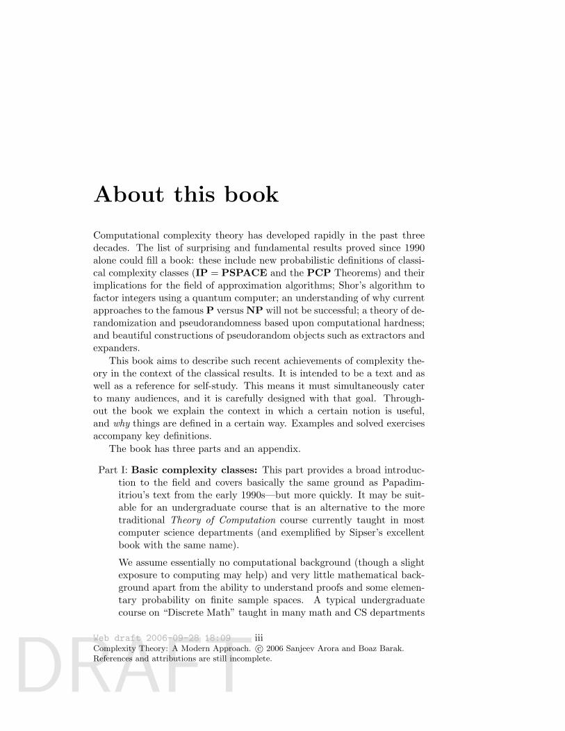
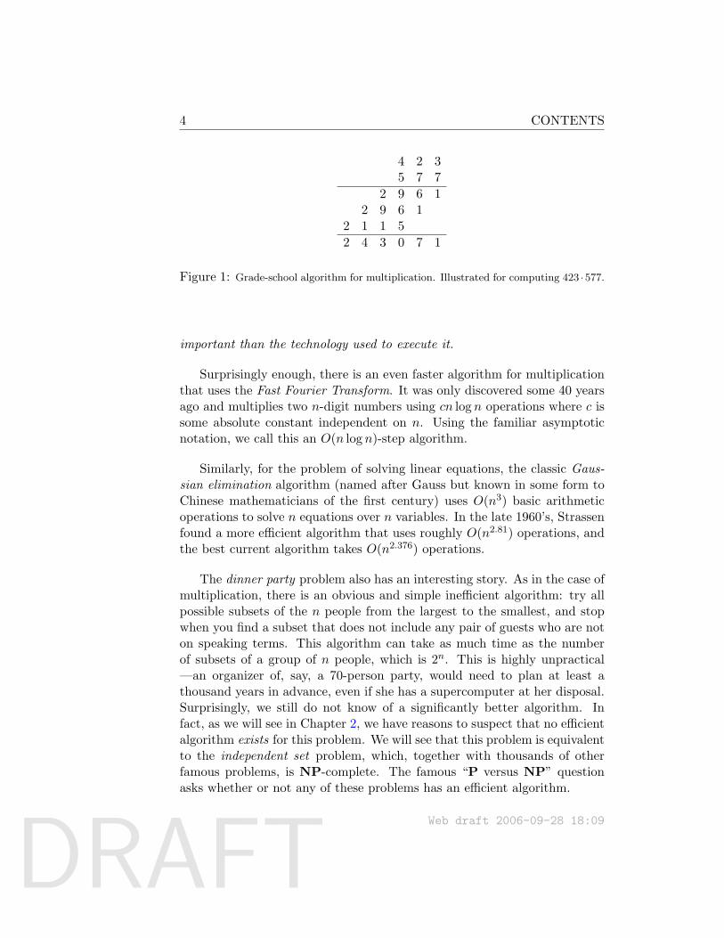
ter, concerns multiplying two integers. Consider two different methods (oralgorithms) for this task. The first is repeated addition: to compute a ·b, justadd a to itself b times. The other is the gradeschool algorithm illustrated inFigure 1. Though the repeated addition algorithm is perhaps simpler thanthe gradeschool algorithm, we somehow feel that the latter is better. Indeed,it is much more efficient. For example, multiplying 577 and 423 by repeatedaddition requires 577 additions, whereas doing it with the gradeschool al-gorithm requires only 3 additions and 3 multiplications of a number by asingle digit.

We will quantify the efficiency of an algorithm by studying the number ofbasic operations it performs as the size of the input increases. Here, the basicoperations are single-digit addition and multiplication. (In other settings,we may wish to throw in division as a basic operation.) The size of the inputis the number of digits in the numbers. The number of basic operations usedto multiply two n-digit numbers (i.e., numbers between 10n−1 and 10n) isat most 2n2 for the gradeschool algorithm and at least n10n−1 for repeatedaddition. Phrased this way, the huge difference between the two algorithmsis apparent: even for 11-digit numbers, a pocket calculator running thegradeschool algorithm would beat the best current supercomputers runningthe repeated addition algorithm. For slightly larger numbers even a fifthgrader with pen and paper would outperform a supercomputer. We seethat the efficiency of an algorithm is to a considerable extent much more

Web draft 2006-09-28 18:09

DRAFT

4 CONTENTS

4 2 35 7 7

2 9 6 12 9 6 1

2 1 1 52 4 3 0 7 1

Figure 1: Grade-school algorithm for multiplication. Illustrated for computing 423 ·577.

important than the technology used to execute it.

Surprisingly enough, there is an even faster algorithm for multiplicationthat uses the Fast Fourier Transform. It was only discovered some 40 yearsago and multiplies two n-digit numbers using cn log n operations where c issome absolute constant independent on n. Using the familiar asymptoticnotation, we call this an O(n log n)-step algorithm.

Similarly, for the problem of solving linear equations, the classic Gaus-sian elimination algorithm (named after Gauss but known in some form toChinese mathematicians of the first century) uses O(n3) basic arithmeticoperations to solve n equations over n variables. In the late 1960’s, Strassenfound a more efficient algorithm that uses roughly O(n2.81) operations, andthe best current algorithm takes O(n2.376) operations.

The dinner party problem also has an interesting story. As in the case ofmultiplication, there is an obvious and simple inefficient algorithm: try allpossible subsets of the n people from the largest to the smallest, and stopwhen you find a subset that does not include any pair of guests who are noton speaking terms. This algorithm can take as much time as the numberof subsets of a group of n people, which is 2n. This is highly unpractical—an organizer of, say, a 70-person party, would need to plan at least athousand years in advance, even if she has a supercomputer at her disposal.Surprisingly, we still do not know of a significantly better algorithm. Infact, as we will see in Chapter 2, we have reasons to suspect that no efficientalgorithm exists for this problem. We will see that this problem is equivalentto the independent set problem, which, together with thousands of otherfamous problems, is NP-complete. The famous “P versus NP” questionasks whether or not any of these problems has an efficient algorithm.

Web draft 2006-09-28 18:09

DRAFT

CONTENTS 5

Proving nonexistence of efficient algorithms

We have seen that sometimes computational problems have nonintuitive al-gorithms, which are quantifiably better (i.e., more efficient) than algorithmsthat were known for thousands of years. It would therefore be really interest-ing to prove for interesting computational tasks that the current algorithm isthe best —in other words, no better algorithms exist. For instance, we couldtry to prove that the O(n log n)-step algorithm for multiplication can neverbe improved (thus implying that multiplication is inherently more difficultthan addition, which does have an O(n)-step algorithm). Or, we could tryto prove that there is no algorithm for the dinner party problem that takesfewer than 2n/10 steps.

It may be possible to mathematically prove such statements, since com-putation is a mathematically precise notion. There are several precedentsfor proving impossibility results in mathematics, such as the independenceof Euclid’s parallel postulate from the other basic axioms of geometry, or theimpossibility of trisecting an arbitrary angle using a compass and straight-edge. Impossibility proofs are among the most interesting, fruitful, andsurprising results in mathematics.

Subsequent chapters of this book identify many interesting questionsabout the inherent computational complexity of tasks, usually with respectto the Turing Machine model. Most such questions are still unanswered, buttremendous progress has been made in the past few decades in showing thatmany of the questions are interrelated, sometimes in unexpected ways. Thisinterrelationship is usually exhibited using a reduction. For an intriguingexample of this, see the last chapter (Chapter 23), which uses computa-tional complexity to explain why we are stuck in resolving the central openquestions concerning computational complexity.

Web draft 2006-09-28 18:09

DRAFT

6 CONTENTS

Web draft 2006-09-28 18:09

DRAFT

CONTENTS 7

Conventions: A whole number is a number in the set Z = 0,±1,±2, . . ..A number denoted by one of the letters i, j, k, `,m, n is always assumed tobe whole. If n ≥ 1, then we denote by [n] the set 1, . . . , n. For a realnumber x, we denote by dx e the smallest n ∈ Z such that n ≥ x and bybx c the largest n ∈ Z such that n ≤ x. Whenever we use a real numberin a context requiring a whole number, the operator d e is implied. Wedenote by log x the logarithm of x to the base 2. We say that a conditionholds for sufficiently large n if it holds for every n ≥ N for some number N(for example, 2n > 100n2 for sufficiently large n). We use expressions suchas∑

i f(i) (as opposed to, say,∑n

i=1 f(i)) when the range of values i takesis obvious from the context. If u is a string or vector, then ui denotes thevalue of the ith symbol/coordinate of u.

Web draft 2006-09-28 18:09

DRAFT

8 CONTENTS

Web draft 2006-09-28 18:09

DRAFT

Part I

Basic Complexity Classes


9

DRAFT

DRAFT

Chapter 1

The computational model—and why it doesn’t matter

“The idea behind digital computers may be explained by sayingthat these machines are intended to carry out any operationswhich could be done by a human computer. The human computeris supposed to be following fixed rules; he has no authority todeviate from them in any detail. We may suppose that theserules are supplied in a book, which is altered whenever he is puton to a new job. He has also an unlimited supply of paper onwhich he does his calculations.”Alan Turing, 1950

The previous chapter gave an informal introduction to computation andefficient computations in context of arithmetic. This chapter gives a morerigorous and general definition. As mentioned earlier, one of the surprisingdiscoveries of the 1930s was that all known computational models are able tosimulate each other. Thus the set of computable problems does not dependupon the computational model.

In this book we are interested in issues of computational efficiency, andtherefore in classes of “efficiently computable” problems. Here, at firstglance, it seems that we have to be very careful about our choice of a compu-tational model, since even a kid knows that whether or not a new video gameprogram is “efficiently computable” depends upon his computer’s hardware.Surprisingly though, we can restrict attention to a single abstract compu-tational model for studying many questions about efficiency—the Turingmachine. The reason is that the Turing Machine seems able to simulate all


11

DRAFT

12 1.1. ENCODINGS AND LANGUAGES: SOME CONVENTIONS

physically realizable computational models with very little loss of efficiency.Thus the set of “efficiently computable” problems is at least as large forthe Turing Machine as for any other model. (One possible exception is thequantum computer model, but we do not currently know if it is physicallyrealizable.)

The Turing machine is a simple embodiment of the age-old intuition thatcomputation consists of applying mechanical rules to manipulate numbers,where the person/machine doing the manipulation is allowed a scratch padon which to write the intermediate results. The Turing Machine can be alsoviewed as the equivalent of any modern programming language — albeitone with no built-in prohibition about memory size1. In fact, this intuitiveunderstanding of computation will suffice for most of the book and mostreaders can skip many details of the model on a first reading, returning tothem later as needed.

The rest of the chapter formally defines the Turing Machine and thenotion of running time, which is one measure of computational effort. Sec-tion 1.4 introduces a class of “efficiently computable” problems called P(which stands for Polynomial time) and discuss its philosophical signifi-cance. The section also points out how throughout the book the definitionof the Turing Machine and the class P will be a starting point for definitionsof many other models, including nondeterministic, probabilistic and quan-tum Turing machines, Boolean circuits, parallel computers, decision trees,and communication games. Some of these models are introduced to studyarguably realizable modes of physical computation, while others are mainlyused to gain insights on Turing machines.

1.1 Encodings and Languages: Some conventions

In general we study the complexity of computing a function whose inputand output are finite strings of bits (i.e., members of the set 0, 1∗, seeAppendix). Note that simple encodings can be used to represent generalmathematical objects—integers, pairs of integers, graphs, vectors, matrices,etc.— as strings of bits. For example, we can represent an integer as a stringusing the binary expansion (e.g., 34 is represented as 100010) and a graphas its adjacency matrix (i.e., an n vertex graph G is represented by an n×n0/1-valued matrix A such that Ai,j = 1 iff the edge (i, j) is present in G).

1Though the assumption of an infinite memory may seem unrealistic at first, in thecomplexity setting it is of no consequence since we will restrict the machine to use a finiteamount of tape cells (the number allowed will depend upon the input size).

Web draft 2006-09-28 18:09

DRAFT

1.1. ENCODINGS AND LANGUAGES: SOME CONVENTIONS 13

We will typically avoid dealing explicitly with such low level issues ofrepresentation, and will use xxy to denote some canonical (and unspecified)binary representation of the object x. Often we will drop the symbols xy andsimply use x to denote both the object and its representation. We use thenotation 〈x, y〉 to denote the ordered pair consisting of x and y. A canonicalrepresentation for 〈x, y〉 can be easily obtained from the representations ofx and y; to reduce notational clutter, instead of x〈x, y〉y we use 〈x, y〉 todenote not only the pair consisting of x and y but also the representation ofthis pair as a binary string.

An important special case of functions mapping strings to strings is thecase of Boolean functions, whose output is a single bit. We identify sucha function f with the set Lf = x : f(x) = 1 and call such sets languagesor decision problems (we use these terms interchangeably). We identify thecomputational problem of computing f (i.e., given x compute f(x)) with theproblem of deciding the language Lf (i.e., given x, decide whether x ∈ Lf ).

By representing the possible invitees to a dinner party with the vertices ofa graph having an edge between any two people that can’t stand one another,the dinner party computational problem from the introduction becomes theproblem of finding a maximum sized independent set (set of vertices notcontaining any edges) in a given graph. The corresponding language is:

INDSET = 〈G, k〉 : ∃S ⊆ V (G) s.t. |S| ≥ k and ∀u, v ∈ S, u v 6∈ E(G)(1)

An algorithm to solve this language will tell us, on input a graph G anda number k, whether there exists a conflict-free set of invitees, called anindependent set, of size at least k. It is not immediately clear that such analgorithm can be used to actually find such a set, but we will see this isthe case in Chapter 2. For now, let’s take it on faith that this is a goodformalization of this problem.

Big-Oh notations. As already hinted, we will often be more interestedin the rate of growth of functions than their precise behavior. The followingwell known set of notations is very convenient for such analysis. If f, g aretwo functions from N to N, then we (1) say that f = O(g) if there exists aconstant c such that f(n) ≤ c · g(n) for every sufficiently large n, (2) saythat f = Ω(g) if g = O(f), (3) say that f = Θ(g) is f = O(g) and g = O(f),(4) say that f = o(g) if for every ε > 0, f(n) ≤ ε · g(n) for every sufficientlylarge n, and (5) say that f = ω(g) if g = o(f). For example, if f(n) =100n log n and g(n) = n2 then we have the relations f = O(g), g = Ω(f), f =Θ(f), f = o(g), g = ω(f). (For more examples and explanations, see any

Web draft 2006-09-28 18:09

DRAFT

14 1.2. MODELING COMPUTATION AND EFFICIENCY

undergraduate algorithms text such as [KT06, CLRS01] or see Section 7.1in Sipser’s book [SIP96].)

1.2 Modeling computation and efficiency

We start with an informal description of computation. Let f be a functionthat takes a string of bits (i.e., a member of the set 0, 1∗) and outputs,say, either 0 or 1. Informally speaking, an algorithm for computing f is aset of mechanical rules, such that by following them we can compute f(x)given any input x ∈ 0, 1∗. The set of rules being followed is finite (i.e.,the same set must work for all infinitely many inputs) though each rule inthis set may be applied arbitrarily many times. Each rule must involve oneof the following “elementary” operations:

1. Read a bit of the input.

2. Read a bit (or possibly a symbol from a slightly larger alphabet, saya digit in the set 0, . . . , 9) from the “scratch pad” or working spacewe allow the algorithm to use.

3. Write a bit/symbol to the scratch pad.

4. Stop and output either 0 or 1.

5. Decide which of the above operations to apply based on the valuesthat were just read.

Finally, the running time is the number of these basic operations per-formed.

Below, we formalize all of these notions.

1.2.1 The Turing Machine

The k-tape Turing machine is a concrete realization of the above informalnotion, as follows (see Figure 1.1).

Scratch Pad: The scratch pad consists of k tapes. A tape is an infiniteone-directional line of cells, each of which can hold a symbol from a finiteset Γ called the alphabet of the machine. Each tape is equipped with a tapehead that can potentially read or write symbols to the tape one cell at atime. The machine’s computation is divided into discrete time steps, andthe head can move left or right one cell in each step. The machine also has

Web draft 2006-09-28 18:09

DRAFT

1.2. MODELING COMPUTATION AND EFFICIENCY 15

a separate tape designated as the input tape of the machine, whose headcan only read symbols, not write them —a so-called read-only head.

The k read-write tapes are called work tapes and the last one of themis designated as the output tape of the machine, on which it writes its finalanswer before halting its computation.

Finite set of operations/rules: The machine has a finite set of states,denoted Q. The machine contains a “register” that can hold a single elementof Q; this is the ”state” of the machine at that instant. This state determinesits action at the next computational step, which consists of the following:(1) read the symbols in the cells directly under the k+1 heads (2) for the kread/write tapes replace each symbol with a new symbol (it has the optionof not changing the tape by writing down the old symbol again), (3) changeits register to contain another state from the finite set Q (it has the optionnot to change its state by choosing the old state again) and (4) move eachhead one cell to the left or to the right.

Inputtape

Worktape

Outputtape

> 0 0 0 1 1 0 1 0 0 0 1 0 0 0 0

> 1 1 0 1 0 1 0 0 0 1

> 0 1

q7Register

read only head

read/write head

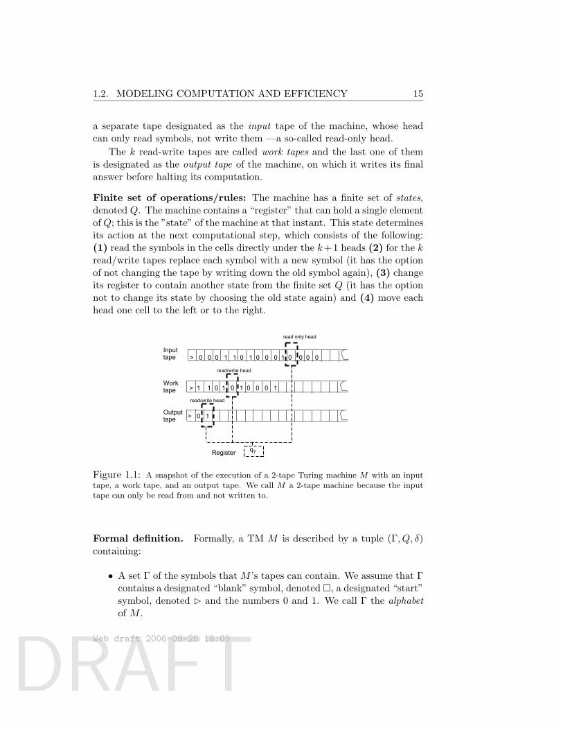
read/write head

Figure 1.1: A snapshot of the execution of a 2-tape Turing machine M with an inputtape, a work tape, and an output tape. We call M a 2-tape machine because the inputtape can only be read from and not written to.

Formal definition. Formally, a TM M is described by a tuple (Γ, Q, δ)containing:

• A set Γ of the symbols that M ’s tapes can contain. We assume that Γcontains a designated “blank” symbol, denoted , a designated “start”symbol, denoted B and the numbers 0 and 1. We call Γ the alphabetof M .

Web draft 2006-09-28 18:09

DRAFT


• A set Q of possible states M ’s register can be in. We assume thatQ contains a designated start state, denoted qstart and a designatedhalting state, denoted qhalt.

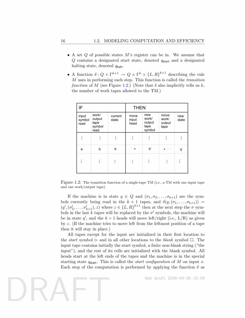
• A function δ : Q × Γk+1 → Q × Γk × L,Rk+1 describing the ruleM uses in performing each step. This function is called the transitionfunction of M (see Figure 1.2.) (Note that δ also implicitly tells us k,the number of work tapes allowed to the TM.)

IF THEN

inputsymbolread

work/outputtapesymbolread

currentstate

moveinputhead

newwork/outputtapesymbol

movework/outputtape

newstate

... ... ... ... ... ... ...

... ... ... ... ... ... ...

a b q b’ q’

Figure 1.2: The transition function of a single-tape TM (i.e., a TM with one input tapeand one work/output tape).

If the machine is in state q ∈ Q and (σ1, σ2, . . . , σk+1) are the sym-bols currently being read in the k + 1 tapes, and δ(q, (σ1, . . . , σk+1)) =(q′, (σ′2, . . . , σ

′k+1), z) where z ∈ L,Rk+1 then at the next step the σ sym-

bols in the last k tapes will be replaced by the σ′ symbols, the machine willbe in state q′, and the k + 1 heads will move left/right (i.e., L/R) as givenby z. (If the machine tries to move left from the leftmost position of a tapethen it will stay in place.)

All tapes except for the input are initialized in their first location tothe start symbol B and in all other locations to the blank symbol . Theinput tape contains initially the start symbol, a finite non-blank string (“theinput”), and the rest of its cells are initialized with the blank symbol. Allheads start at the left ends of the tapes and the machine is in the specialstarting state qstart. This is called the start configuration of M on input x.Each step of the computation is performed by applying the function δ as

Web draft 2006-09-28 18:09

DRAFT

1.2. MODELING COMPUTATION AND EFFICIENCY 17

described above. The special halting state qhalt has the property that oncethe machine is in qhalt, the transition function δ does not allow it to furthermodify the tape or change states. Clearly, if the machine enters qhalt thenit has halted. In complexity theory we are only interested in machines thathalt for every input in a finite number of steps.

Now we formalize the notion of running time. As every non-trivial algo-rithm needs to at least read its entire input, by “quickly” we mean that thenumber of basic steps we use is small when considered as a function of theinput length.

Definition 1.1 (Computing a function and running time)Let f : 0, 1∗ → 0, 1∗ and let T : N → N be some functions. We say that aTM M computes function f if for every x ∈ 0, 1∗, if M is initialized to the startconfiguration on input x, then it halts with f(x) written on its output tape.We say M computes f in T (n)-time2 if for all n and all inputs x of size n, therunning time of M on that input is at most T (n).

Most of the specific details of our definition of Turing machines are quitearbitrary. For example, the following three claims show that restricting thealphabet Γ to be 0, 1,,B, restricting the machine to have a single worktape, or allowing the tapes to be infinite in both directions will not have asignificant effect on the time to compute functions:

Claim 1.2For every f : 0, 1∗ → 0, 1, T : N → N, if f is computable in time T (n)by a TM M using alphabet Γ then it is computable in time 100 log |Γ|T (n)by a TM M using the alphabet 0, 1,,B.

Claim 1.3For every f : 0, 1∗ → 0, 1, T : N → N, if f is computable in time T (n)by a TM M using k work tapes (plus additional input and output tapes)then it is computable in time 100T (n)2 by a TM M using a single work tape(plus additional input and output tapes).

Claim 1.4Define a bidirectional TM to be a TM whose tapes are infinite in bothdirections. For every f : 0, 1∗ → 0, 1∗, T : N → N as above if f is

2Formally we should use T instead of T (n), but we follow the convention of writingT (n) to emphasize that T is applied to the input length.

Web draft 2006-09-28 18:09

DRAFT


computable in time T (n) by a bidirectional TM M then it is computable intime 100T (n) by a standard (unidirectional) TM.

We leave the proofs of these claims as Exercises 2, 3 and 4. The readermight wish to pause at this point and work through the proofs, as this is agood way to obtain intuition for Turing machines and their capabilities.

Other changes that will not have a very significant effect include restrict-ing the number of states to 100, having two or three dimensional tapes,allowing the machine random access to its tape, and making the outputtape write only (see the texts [SIP96, HMU01] for proofs and more exam-ples). In particular none of these modifications will change the class P ofpolynomial-time decision problems defined below in Section 1.4.

1.2.2 The expressive power of Turing machines.

When you encounter Turing machines for the first time, it may not beclear that they do indeed fully encapsulate our intuititive notion of com-putation. It may be useful to work through some simple examples, suchas expressing the standard algorithms for addition and multiplication interms of Turing machines computing the corresponding functions. (See Ex-ercise 7; also, Sipser’s book [SIP96] contains many more such examples.)

Example 1.5(This example assumes some background in computing.) We give a hand-wavy proof that Turing machines can simulate any program written in anyof the familiar programming languages such as C or Java. First, recall thatprograms in these programming languages can be translated (the technicalterm is compiled) into an equivalent machine language program. This is asequence of simple instructions to read from memory into one of a finitenumber of registers, write a register’s contents to memory, perform basicarithmetic operations, such as adding two registers, and control instructionsthat perform actions conditioned on, say, whether a certain register is equalto zero.

All these operations can be easily simulated by a Turing machine. Thememory and register can be implemented using the machine’s tapes, whilethe instructions can be encoded by the machine’s transition function. Forexample, it’s not hard to show TM’s that add or multiply two numbers, ora two-tape TM that, if its first tape contains a number i in binary represen-tation, can move the head of its second tape to the ith location.

Web draft 2006-09-28 18:09

DRAFT

1.3. THE UNIVERSAL TURING MACHINE 19

1.3 The Universal Turing Machine

Underlying the computer revolution of the 20th century is one simple butcrucial observation: programs can be considered as strings of symbols, andhence can be given as input to other programs. The notion goes back to Tur-ing, who described a universal TM that can simulate the execution of everyother TM M given M ’s description as input. This enabled the constructionof general purpose computers that are designed not to achieve one particulartask, but can be loaded with a program for any arbitrary computation.

Of course, since we are so used to having a universal computer on ourdesktops or even in our pockets, we take this notion for granted. But itis good to remember why it was once counterintuitive. The parameters ofthe universal TM are fixed —alphabet size, number of states, and number oftapes. The corresponding parameters for the machine being simulated couldbe much larger. The reason this is not a hurdle is, of course, the ability touse encodings. Even if the universal TM has a very simple alphabet, say0, 1, this is sufficient to allow it to represent the other machine’s state andand transition table on its tapes, and then follow along in the computationstep by step.

Now we state a computationally efficient version of Turing’s constructiondue to Hennie and Stearns [HS66]. To give the essential idea we first provea slightly relaxed variant where the term t log t of Condition 4 below isreplaced with t2. But since the efficient version is needed a few times in thebook, a full proof is also given at the end of the chapter.

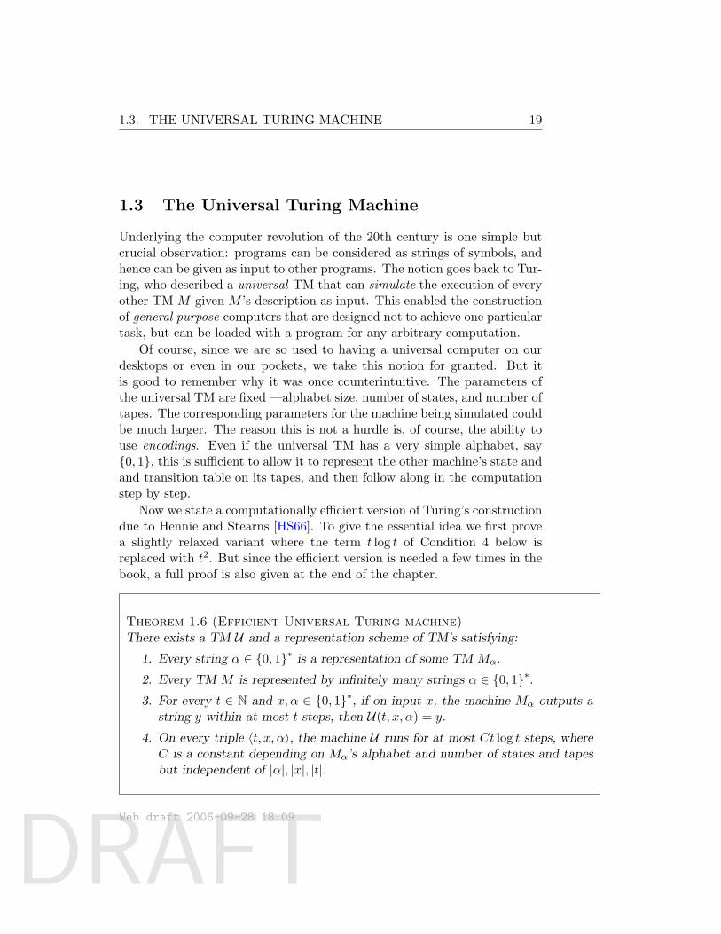
Theorem 1.6 (Efficient Universal Turing machine)There exists a TM U and a representation scheme of TM’s satisfying:

1. Every string α ∈ 0, 1∗ is a representation of some TM Mα.

2. Every TM M is represented by infinitely many strings α ∈ 0, 1∗.3. For every t ∈ N and x, α ∈ 0, 1∗, if on input x, the machine Mα outputs a

string y within at most t steps, then U(t, x, α) = y.

4. On every triple 〈t, x, α〉, the machine U runs for at most Ct log t steps, whereC is a constant depending on Mα’s alphabet and number of states and tapesbut independent of |α|, |x|, |t|.

Web draft 2006-09-28 18:09

DRAFT

20 1.3. THE UNIVERSAL TURING MACHINE

Proof: Represent a TM M in the natural way as the tuple 〈γ, q, δ, z〉 whereγ = |Γ| is the size of M ’s alphabet, q is the size of M ’s state space Q,the transition function δ is described by a table listing all of its inputs andoutputs, and z is a table describing the elements of Γ, Q that correspond tothe special symbols and states (i.e., B,, 0, 1, qstart, qhalt). We also allow thedescription to end with an arbitrary number of 1’s to ensure Condition 2.3

If a string is not a valid representation of a TM according to these rules thenwe consider it a representation of some canonical TM (i.e., a machine thatreads its input and immediately halts and outputs 0) to ensure Condition 1.

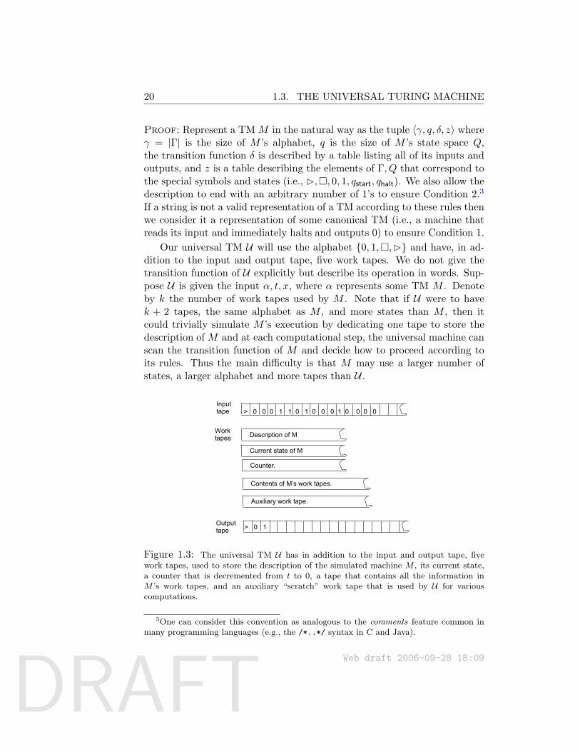
Our universal TM U will use the alphabet 0, 1,,B and have, in ad-dition to the input and output tape, five work tapes. We do not give thetransition function of U explicitly but describe its operation in words. Sup-pose U is given the input α, t, x, where α represents some TM M . Denoteby k the number of work tapes used by M . Note that if U were to havek + 2 tapes, the same alphabet as M , and more states than M , then itcould trivially simulate M ’s execution by dedicating one tape to store thedescription of M and at each computational step, the universal machine canscan the transition function of M and decide how to proceed according toits rules. Thus the main difficulty is that M may use a larger number ofstates, a larger alphabet and more tapes than U .

Inputtape

Worktapes

Outputtape

> 0 0 0 1 1 0 1 0 0 0 1 0 0 0 0

> 0 1

Description of M

Current state of M

Counter.

Contents of M’s work tapes.

Auxiliary work tape.

Figure 1.3: The universal TM U has in addition to the input and output tape, fivework tapes, used to store the description of the simulated machine M , its current state,a counter that is decremented from t to 0, a tape that contains all the information inM ’s work tapes, and an auxiliary “scratch” work tape that is used by U for variouscomputations.

3One can consider this convention as analogous to the comments feature common inmany programming languages (e.g., the /*..*/ syntax in C and Java).

Web draft 2006-09-28 18:09

DRAFT

1.3. THE UNIVERSAL TURING MACHINE 21

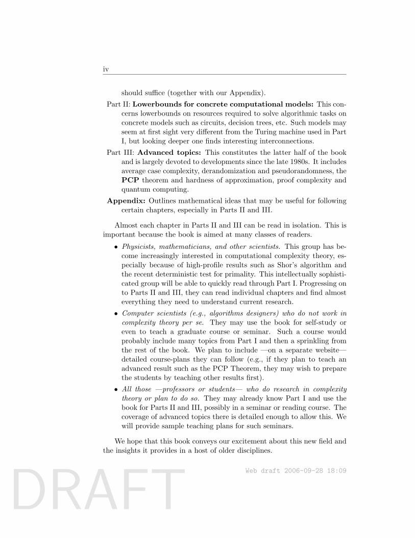
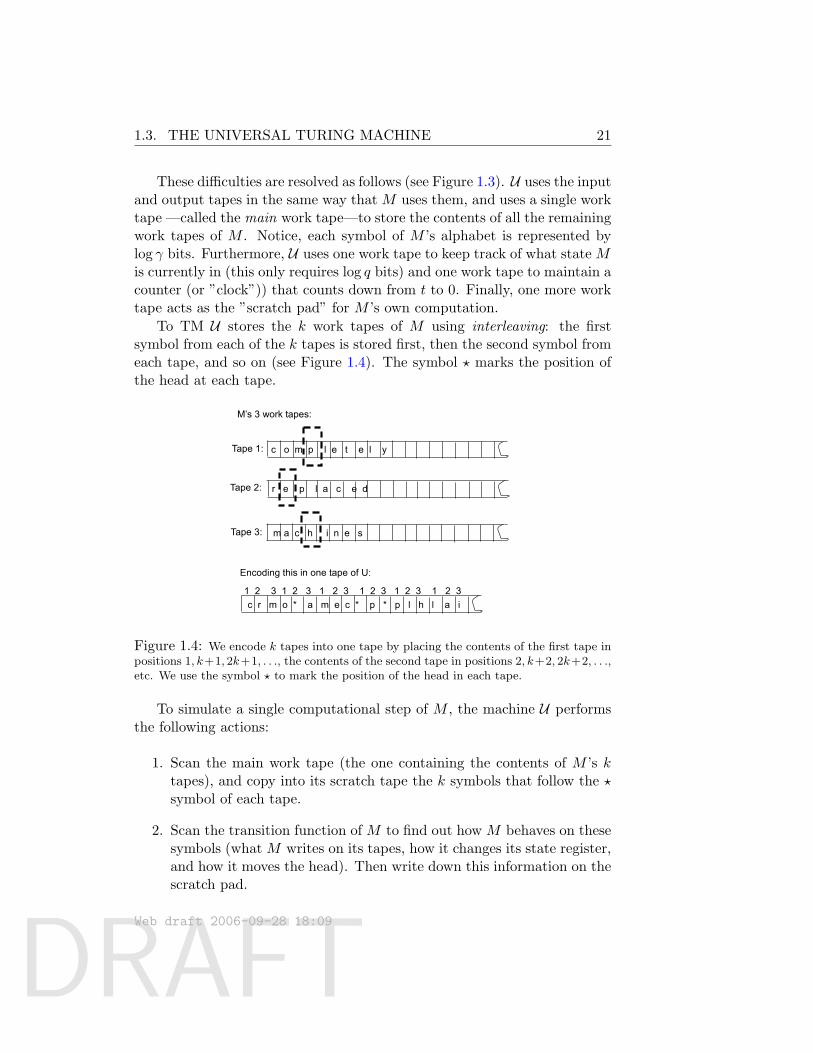
These difficulties are resolved as follows (see Figure 1.3). U uses the inputand output tapes in the same way that M uses them, and uses a single worktape —called the main work tape—to store the contents of all the remainingwork tapes of M . Notice, each symbol of M ’s alphabet is represented bylog γ bits. Furthermore, U uses one work tape to keep track of what state Mis currently in (this only requires log q bits) and one work tape to maintain acounter (or ”clock”)) that counts down from t to 0. Finally, one more worktape acts as the ”scratch pad” for M ’s own computation.

To TM U stores the k work tapes of M using interleaving: the firstsymbol from each of the k tapes is stored first, then the second symbol fromeach tape, and so on (see Figure 1.4). The symbol ? marks the position ofthe head at each tape.

M’s 3 work tapes:

c o m p l e t e l y

r e p l a c e d

m a c h i n e s

Encoding this in one tape of U:

c r m o * a m e c * p * p l h l a i1 2 3 1 2 3 1 2 3 1 2 3 1 2 3 1 2 3

Tape 1:

Tape 2:

Tape 3:

Figure 1.4: We encode k tapes into one tape by placing the contents of the first tape inpositions 1, k+1, 2k+1, . . ., the contents of the second tape in positions 2, k+2, 2k+2, . . .,etc. We use the symbol ? to mark the position of the head in each tape.

To simulate a single computational step of M , the machine U performsthe following actions:

1. Scan the main work tape (the one containing the contents of M ’s ktapes), and copy into its scratch tape the k symbols that follow the ?symbol of each tape.

2. Scan the transition function of M to find out how M behaves on thesesymbols (what M writes on its tapes, how it changes its state register,and how it moves the head). Then write down this information on thescratch pad.

Web draft 2006-09-28 18:09

DRAFT

22 1.4. DETERMINISTIC TIME AND THE CLASS P.

3. Scan the main work tape and update it (both symbols written andhead locations) according to the scratch pad.

4. Update the tape containing M ’s state according to the new state.

5. Use the same head movement and write instructions of M on the inputand output tape.

6. Decrease the counter by 1, check if it has reached 0 and if so halt.

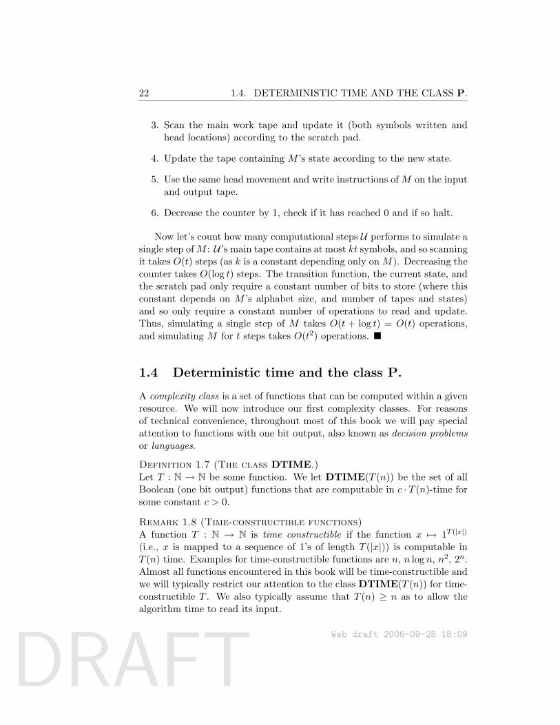
Now let’s count how many computational steps U performs to simulate asingle step ofM : U ’s main tape contains at most kt symbols, and so scanningit takes O(t) steps (as k is a constant depending only on M). Decreasing thecounter takes O(log t) steps. The transition function, the current state, andthe scratch pad only require a constant number of bits to store (where thisconstant depends on M ’s alphabet size, and number of tapes and states)and so only require a constant number of operations to read and update.Thus, simulating a single step of M takes O(t + log t) = O(t) operations,and simulating M for t steps takes O(t2) operations.

1.4 Deterministic time and the class P.

A complexity class is a set of functions that can be computed within a givenresource. We will now introduce our first complexity classes. For reasonsof technical convenience, throughout most of this book we will pay specialattention to functions with one bit output, also known as decision problemsor languages.

Definition 1.7 (The class DTIME.)Let T : N → N be some function. We let DTIME(T (n)) be the set of allBoolean (one bit output) functions that are computable in c · T (n)-time forsome constant c > 0.

Remark 1.8 (Time-constructible functions)A function T : N → N is time constructible if the function x 7→ 1T (|x|)

(i.e., x is mapped to a sequence of 1’s of length T (|x|)) is computable inT (n) time. Examples for time-constructible functions are n, n log n, n2, 2n.Almost all functions encountered in this book will be time-constructible andwe will typically restrict our attention to the class DTIME(T (n)) for time-constructible T . We also typically assume that T (n) ≥ n as to allow thealgorithm time to read its input.

Web draft 2006-09-28 18:09

DRAFT

1.4. DETERMINISTIC TIME AND THE CLASS P. 23

The following class will serve as our rough approximation for the classof decision problems that are efficiently solvable.

Definition 1.9 (The class P)P = ∪c≥1DTIME(nc)

Thus, we can phrase the question from the introduction as to whetherINDSET has an efficient algorithm as follows: “Is INDSET ∈ P?”

1.4.1 On the philosophical importance of P

The class P is felt to capture the notion of decision problems with “feasi-ble” decision procedures. Of course, one may argue whether DTIME(n100)really represents “feasible” computation in the real world. However, in prac-tice, whenever we show that a problem is in P, we usually find an n3 or n5

time algorithm (with reasonable constants), and not an n100 algorithm. (Ithas also happened a few times that the first polynomial-time algorithm fora problem had high complexity, say n20, but soon somebody simplified it tosay an n5 algorithm.)

Note that the class P is useful only in a certain context. Turing machinesare a poor model if one is designing algorithms that must run in a fractionof a second on the latest PC (in which case one must carefully account forfine details about the hardware). However, if the question is whether anysubexponential algorithms exist for say INDSET then even an n20 algorithmon the Turing Machine would be a fantastic breakthrough.

We note that P is also a natural class from the viewpoint of a pro-grammer. Suppose undergraduate programmers are asked to invent thedefinition of an “efficient” computation. Presumably, they would agree thata computation that runs in linear or quadratic time is “efficient.” Next,since programmers often write programs that call other programs (or sub-routines), they might find it natural to consider a program “efficient” if itperforms only “efficient” computations and calls subroutines that are “effi-cient”. The notion of “efficiency” obtained turns out to be exactly the classP (Cobham [Cob64]). Of course, Cobham’s result makes intuitive sensesince composing a polynomial function with another polynomial functiongives a polynomial function (for every c, d > 0, (nc)d = ncd) but the exactproof requires some care.

Web draft 2006-09-28 18:09

DRAFT


1.4.2 Criticisms of P and some efforts to address them

Now we address some possible criticisms of the definition of P, and somerelated complexity classes that address these.

Worst-case exact computation is too strict. The definition of P onlyconsiders algorithms that compute the function exactly on every possi-ble input. However, not all possible inputs arise in practice (althoughit’s not always easy to characterize the inputs that do). Chapter 15gives a theoretical treatment of average-case complexity and defines theanalogue of P in that context. Sometimes, users are willing to settlefor approximate solutions. Chapter 19 contains a rigorous treatmentof the complexity of approximation.

Other physically realizable models. If we were to make contact withan advanced alien civilization, would their class P be any differentfrom the class defined here?

As mentioned earlier, most (but not all) scientists believe the Church-Turing (CT) thesis, which states that every physically realizable com-putation device— whether it’s silicon-based, DNA-based, neuron-basedor using some alien technology— can be simulated by a Turing ma-chine. Thus they believe that the set of computable problems wouldbe the same for aliens as it is for us. (The CT thesis is not a theorem,merely a belief about the nature of the world.)

However, when it comes to efficiently computable problems, the sit-uation is less clear. The strong form of the CT thesis says thatevery physically realizable computation model can be simulated by aTM with polynomial overhead (in other words, t steps on the modelcan be simulated in tc steps on the TM, where c is a constant thatdepends upon the model). If true, it implies that the class P definedby the aliens will be the same as ours. However, several objectionshave been made to this strong form.

(a) Issue of precision: TM’s compute with discrete symbols, whereasphysical quantities may be real numbers in R. Thus TM computationsmay only be able to approximately simulate the real world. Thoughthis issue is not perfectly settled, it seems so far that TMs do not sufferfrom an inherent handicap. After all, real-life devices suffer from noise,and physical quantities can only be measured up to finite precision.Thus a TM could simulate the real-life device using finite precision.

Web draft 2006-09-28 18:09

DRAFT


(Note also that we often only care about the most significant bit of theresult, namely, a 0/1 answer.)

Even so, in Chapter 14 we also consider a modification of the TMmodel that allows computations in R as a basic operation. The re-sulting complexity classes have fascinating connections with the usualcomplexity classes.

(b) Use of randomness: The TM as defined is deterministic. If ran-domness exists in the world, one can conceive of computational modelsthat use a source of random bits (i.e., ”coin tosses”). Chapter 7 consid-ers Turing Machines that are allowed to also toss coins, and studies theclass BPP, that is the analogue of P for those machines. (However,we will see in Chapter 17 the intriguing possibility that randomizedcomputation may be no more powerful than deterministic computa-tion.)

(c) Use of quantum mechanics: A more clever computational modelmight use some of the counterintuitive features of quantum mechanics.In Chapter 21 we define the class BQP, that generalizes P in such away. We will see problems in BQP that may not be in P. However,currently it is unclear whether the quantum model is truly physicallyrealizable. Even if it is realizable it currently seems only able to ef-ficiently solve only very few ”well-structured” problems that are notin P. Hence insights gained from studying P could still be applied toBQP.

(d) Use of other exotic physics, such as string theory. Though anintriguing possibility, it hasn’t yet had the same scrutiny as quantummechanics.

Decision problems are too limited. Some computational problems arenot easily expressed as decision problems. Indeed, we will introduceseveral classes in the book to capture tasks such as computing non-Boolean functions, solving search problems, approximating optimiza-tion problems, interaction, and more. Yet the framework of decisionproblems turn out to be surprisingly expressive, and we will often useit in this book.

1.4.3 Edmonds’ quote

We conclude this section with a quote from Edmonds [Edm65], that inthe paper showing a polynomial-time algorithm for the maximum matching

Web draft 2006-09-28 18:09

DRAFT


problem, explained the meaning of such a result as follows:

For practical purposes computational details are vital. However,my purpose is only to show as attractively as I can that there isan efficient algorithm. According to the dictionary, “efficient”means “adequate in operation or performance.” This is roughlythe meaning I want in the sense that it is conceivable for maxi-mum matching to have no efficient algorithm.

...There is an obvious finite algorithm, but that algorithm in-creases in difficulty exponentially with the size of the graph. Itis by no means obvious whether or not there exists an algorithmwhose difficulty increases only algebraically with the size of thegraph.

...When the measure of problem-size is reasonable and when thesizes assume values arbitrarily large, an asymptotic estimate of... the order of difficulty of an algorithm is theoretically impor-tant. It cannot be rigged by making the algorithm artificiallydifficult for smaller sizes.

...One can find many classes of problems, besides maximum match-ing and its generalizations, which have algorithms of exponentialorder but seemingly none better ... For practical purposes thedifference between algebraic and exponential order is often morecrucial than the difference between finite and non-finite.

...It would be unfortunate for any rigid criterion to inhibit thepractical development of algorithms which are either not knownor known not to conform nicely to the criterion. Many of thebest algorithmic idea known today would suffer by such theoreti-cal pedantry. ... However, if only to motivate the search for good,practical algorithms, it is important to realize that it is mathe-matically sensible even to question their existence. For one thingthe task can then be described in terms of concrete conjectures.

Web draft 2006-09-28 18:09

DRAFT


What have we learned?

• There are many equivalent ways to mathematically model computational pro-cesses; we use the standard Turing machine formalization.

• Turing machines can be represented as strings. There is a universal TM thatcan emulate (with small overhead) any TM given its representation.

• The class P consists of all decision problems that are solvable by Turing ma-chines in polynomial time. We say that problems in P are efficiently solvable.

• Most low-level choices (number of tapes, alphabet size, etc..) in the definitionof Turing machines are immaterial, as they will not change the definition ofP.

Chapter notes and history

The Turing Machine should be thought of as a logical construct, ratherthan as a piece of hardware. Most computers today are implementations of auniversal computer using silicon chips. But many other physical phenomenacan be used to construct universal TMs: amusing examples include bouncingbilliards balls, cellular automata, and Conway’s Game of life. It is alsopossible to study complexity theory axiomatically in a machine-independentfashion. See Cobham [Cob64] and Blum [Blu67] for two approaches.

We omitted a detailed discussion of formal complexity, and in particularthe fact that the class DTIME(f(n)) can be paradoxical if f is not a propercomplexity function (see the standard text [HMU01]). We say f is properif f(n) ≥ f(n − 1) and there is a TM that on input x outputs a string oflength f(|x|) using time O(|x| + f(|x|)) and space O(f(|x|)). This notionwill reappear in Chapter 4.

Exercises

§1 Prove that there exists a function f : 0, 1∗ → 0, 1 that is notcomputable in time T (n) for every function T : N→ N.

Web draft 2006-09-28 18:09

DRAFT


Hint:foranystringα∈0,1∗,letMαbetheTMdescribedby

αanddefinefαsuchthatforeveryx,fα(x)=1ifMαoninputxhaltswithoutput1withinafinitenumberofstepsandfα(x)=0otherwise.Youneedtofindf:0,1

∗→0,1suchthatforevery

αthereexistsxwithf(x)6=fα(x).

§2 Prove Claim 1.2.


Hint:Tostoretheinformationofktapesonasingletape,usepositions1,k+1,2k+1,...tostorethecontentsofthefirsttape,usepositions2,k+2,3k+2,...tostorethecontentsofthesecondtape,andsoon.


Hint:tosimulateabidirectionalTMusingalphabetsizeγuseaunidirectionalTMofalphabetsizeγ

2.

§5 Define a TM M to be oblivious if its head movement does not dependon the input but only on the input length. That is, M is oblivious if forevery input x ∈ 0, 1∗ and i ∈ N, the location of each of M ’s heads atthe ith step of execution on input x is only a function of |x| and i. Showthat for every time-constructible T : N → N, if L ∈ DTIME(T (n))then there is an oblivious TM that decides L in time O(T (n)2).

§6 Show that for every time-constructible T : N→ N, if L ∈ DTIME(T (n))then there is an oblivious TM that decides L in time O(T (n) log T (n)).

Hint:showthattheuniversalTMUobtainedbytheproofofTheorem1.6canbetweakedtobeoblivious.

§7 Define FDTIME and FP to be the generalization of DTIME and Pfor non-Boolean functions (with more than one bit of output). Thatis, f ∈ FDTIME(T (n)) if f is computable in T (n) time and FP =∪c≥1FDTIME(nc).

Prove that the addition and multiplication functions are in FP.

Proof of Theorem 1.6: Universal Simulation in O(t log t)-time

We now show how to prove Theorem 1.6 as stated, with an O(t log t) timesimulation. Our machine U will use the same structure and number of tapes

Web draft 2006-09-28 18:09

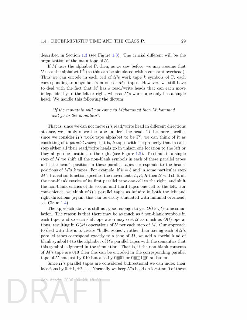
DRAFT


described in Section 1.3 (see Figure 1.3). The crucial different will be theorganization of the main tape of U .

If M uses the alphabet Γ, then, as we saw before, we may assume thatU uses the alphabet Γk (as this can be simulated with a constant overhead).Thus we can encode in each cell of U ’s work tape k symbols of Γ, eachcorresponding to a symbol from one of M ’s tapes. However, we still haveto deal with the fact that M has k read/write heads that can each moveindependently to the left or right, whereas U ’s work tape only has a singlehead. We handle this following the dictum

“If the mountain will not come to Muhammad then Muhammadwill go to the mountain”.

That is, since we can not move U ’s read/write head in different directionsat once, we simply move the tape “under” the head. To be more specific,since we consider U ’s work tape alphabet to be Γk, we can think of it asconsisting of k parallel tapes; that is, k tapes with the property that in eachstep either all their read/write heads go in unison one location to the left orthey all go one location to the right (see Figure 1.5). To simulate a singlestep of M we shift all the non-blank symbols in each of these parallel tapesuntil the head’s position in these parallel tapes corresponds to the heads’positions of M ’s k tapes. For example, if k = 3 and in some particular stepM ’s transition function specifies the movements L,R,R then U will shift allthe non-blank entries of its first parallel tape one cell to the right, and shiftthe non-blank entries of its second and third tapes one cell to the left. Forconvenience, we think of U ’s parallel tapes as infinite in both the left andright directions (again, this can be easily simulated with minimal overhead,see Claim 1.4).

The approach above is still not good enough to get O(t log t)-time simu-lation. The reason is that there may be as much as t non-blank symbols ineach tape, and so each shift operation may cost U as much as O(t) opera-tions, resulting in O(kt) operations of U per each step of M . Our approachto deal with this is to create “buffer zones”: rather than having each of U ’sparallel tapes correspond exactly to a tape of M , we add a special kind ofblank symbol to the alphabet of U ’s parallel tapes with the semantics thatthis symbol is ignored in the simulation. That is, if the non-blank contentsof M ’s tape are 010 then this can be encoded in the corresponding paralleltape of U not just by 010 but also by 0 01 or 0 1 0 and so on.

Since U ’s parallel tapes are considered bidirectional we can index theirlocations by 0,±1,±2, . . .. Normally we keep U ’s head on location 0 of these

Web draft 2006-09-28 18:09

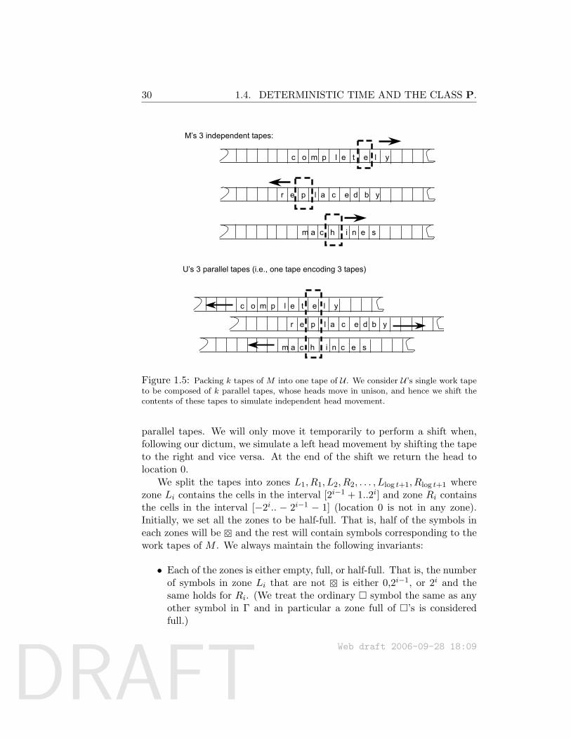
DRAFT


M’s 3 independent tapes:

c o m p l e t e l y

r e p l a c e d b y

m a c h i n e s

U’s 3 parallel tapes (i.e., one tape encoding 3 tapes)

c o m p l e t e l y

r e p l a c e d b y

m a c h i n c e s

Figure 1.5: Packing k tapes of M into one tape of U . We consider U ’s single work tapeto be composed of k parallel tapes, whose heads move in unison, and hence we shift thecontents of these tapes to simulate independent head movement.

parallel tapes. We will only move it temporarily to perform a shift when,following our dictum, we simulate a left head movement by shifting the tapeto the right and vice versa. At the end of the shift we return the head tolocation 0.

We split the tapes into zones L1, R1, L2, R2, . . . , Llog t+1, Rlog t+1 wherezone Li contains the cells in the interval [2i−1 + 1..2i] and zone Ri containsthe cells in the interval [−2i.. − 2i−1 − 1] (location 0 is not in any zone).Initially, we set all the zones to be half-full. That is, half of the symbols ineach zones will be and the rest will contain symbols corresponding to thework tapes of M . We always maintain the following invariants:

• Each of the zones is either empty, full, or half-full. That is, the numberof symbols in zone Li that are not is either 0,2i−1, or 2i and thesame holds for Ri. (We treat the ordinary symbol the same as anyother symbol in Γ and in particular a zone full of ’s is consideredfull.)

Web draft 2006-09-28 18:09

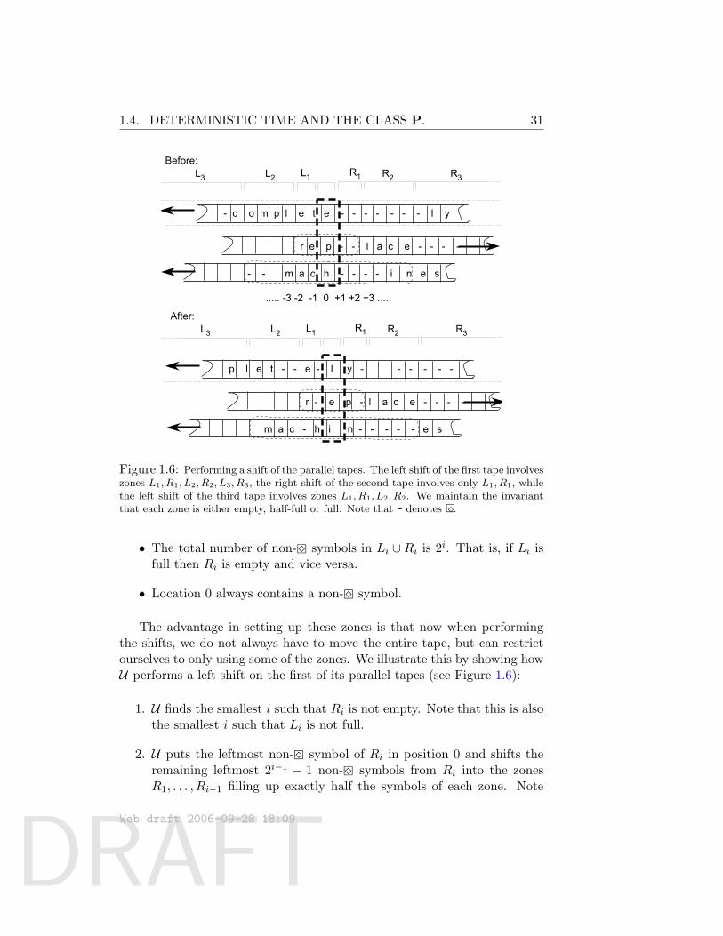
DRAFT


- c o m p l e t e - - - - - - - l y

r e p - - l a c e - - - -

- - m a c h - - - - i n e s

R1 R2 R3L2L3 L1

..... -3 -2 -1 0 +1 +2 +3 .....

Before:

p l e t - - e - l y - - - - - -

r - e p - l a c e - - - -

m a c - h i n - - - - - e s

R1 R2 R3L2L3 L1

After:

Figure 1.6: Performing a shift of the parallel tapes. The left shift of the first tape involveszones L1, R1, L2, R2, L3, R3, the right shift of the second tape involves only L1, R1, whilethe left shift of the third tape involves zones L1, R1, L2, R2. We maintain the invariantthat each zone is either empty, half-full or full. Note that - denotes .

• The total number of non- symbols in Li ∪ Ri is 2i. That is, if Li isfull then Ri is empty and vice versa.

• Location 0 always contains a non- symbol.

The advantage in setting up these zones is that now when performingthe shifts, we do not always have to move the entire tape, but can restrictourselves to only using some of the zones. We illustrate this by showing howU performs a left shift on the first of its parallel tapes (see Figure 1.6):

1. U finds the smallest i such that Ri is not empty. Note that this is alsothe smallest i such that Li is not full.

2. U puts the leftmost non- symbol of Ri in position 0 and shifts theremaining leftmost 2i−1 − 1 non- symbols from Ri into the zonesR1, . . . , Ri−1 filling up exactly half the symbols of each zone. Note

Web draft 2006-09-28 18:09

DRAFT


that there is room to perform this since all the zones R1, . . . , Ri−1

were empty and that indeed 2i−1 =∑i−2

j=0 2j + 1.

3. U performs the symmetric operation to the left of position 0: it shiftsinto Li the 2i−1 leftmost symbols in the zones Li−1, . . . , L1 and reor-ganizes Li−1, . . . , Li such that the remaining

∑i−1j=1 2j−2i−1 = 2i−1−1

symbols, plus the symbol that was originally in position 0 (modifiedappropriately according to M ’s transition function) take up exactlyhalf of each of the zones Li−1, . . . , Li.

4. Note that at the end of the shift, all of the zones L1, R1, . . . , Li−1, Ri−1

are half-full.

Performing such a shift costs O(∑i

j=1 2j) = O(2i) operations. However,once we do this, we will not touch Li again until we perform at least 2i−1

shifts. Thus, we perform a shift involving Li and Ri when simulating atmost a 1

2i−1 of the t steps of M . We perform a shift for every one of thek tapes, but k is a constant, as is the overhead to simulate the alphabet(Γ∪ )k using the alphabet 0, 1,B, and to read the transition functionand state information. Thus total number of operations used by these shiftsis

O(log t+1∑i=1

t

2i−12i) = O(t log t)

where we need an additional O(t log t) operations to maintain the counter.4

4In fact, a more careful analysis shows that only O(t) operations are necessary todecrease a counter from t to 0.

Web draft 2006-09-28 18:09

DRAFT

Chapter 2

NP and NP completeness

“(if φ(n) ≈ Kn2)a then this would have consequences of thegreatest magnitude. That is to say, it would clearly indicate that,despite the unsolvability of the (Hilbert) Entscheidungsproblem,the mental effort of the mathematician in the case of the yes-or-no questions would be completely replaced by machines.... (this)seems to me, however, within the realm of possibility.”Kurt Godel in letter to John von Neumann, 1956; see [Sip92]

aIn modern terminology, if SAT has a quadratic time algorithm

“I conjecture that there is no good algorithm for the travelingsalesman problem. My reasons are the same as for any mathe-matical conjecture: (1) It is a legitimate mathematical possibility,and (2) I do not know.”Jack Edmonds, 1966

“In this paper we give theorems that suggest, but do not im-ply, that these problems, as well as many others, will remainintractable perpetually.”Richard Karp [Kar72], 1972

If you have ever attempted a crossword puzzle, you know that there isoften a big difference between solving a problem from scratch and verifyinga given solution. In the previous chapter we already encountered P, theclass of decision problems that can be efficiently solved. In this chapter,we define the complexity class NP that aims to capture the set of problemswhose solution can be easily verified. The famous P versus NP question asks


33

DRAFT

34 2.1. THE CLASS NP

whether or not the two are the same. The resolution of this conjecture willbe of great practical, scientific and philosophical interest; see Section 2.6.

The chapter also introduces NP-completeness, an important class ofcombinatorial problems that are in P if and only if P = NP. Notions suchas reductions and completeness encountered in this study motivate manyother definitions encountered later in the book.

2.1 The class NP

We will give several equivalent definitions of NP. The first one is as follows:NP contains every language for which membership has a polynomial-timeverifiable certificate (some texts call it a witness). An example is the in-dependent set (INDSET) problem mentioned in Chapter (see Example 2.3below).

Definition 2.1 (The class NP)For every L ⊆ 0, 1∗, we say that L ∈ NP if there exists a polynomial p : N → Nand a polynomial-time TM M such that for every x ∈ 0, 1∗,

x ∈ L⇔ ∃u ∈ 0, 1p(|x|) s.t. M(x, u) = 1

If x ∈ L and u ∈ 0, 1p(|x|) satisfies M(x, u) = 1 then we say that u is a certificatefor x (with respect to the language L and machine M).

We have the following trivial relationship.

Theorem 2.2P ⊆ NP ⊆

⋃c>1 DTIME(2n

c).

Proof: (P ⊆ NP): Suppose L ∈ P is decided in polynomial-time by a TMN . Then L ∈ NP since we can take N as the machine M in Definition 2.1and make p(x) the zero polynomial (in other words, u is an empty string).

(NP ⊆⋃c>1 DTIME(2n

c)): If L ∈ NP and M,p() are as in Defini-

tion 2.1 then we can decide L in time 2O(p(n)) by enumerating all possible uand using M to check whether u is a valid certificate for the input x. Themachine accepts iff such a u is ever found. Since p(n) = O(nc) for somec > 1 then this machine runs in 2O(nc) time. Thus the theorem is proven.

Web draft 2006-09-28 18:09

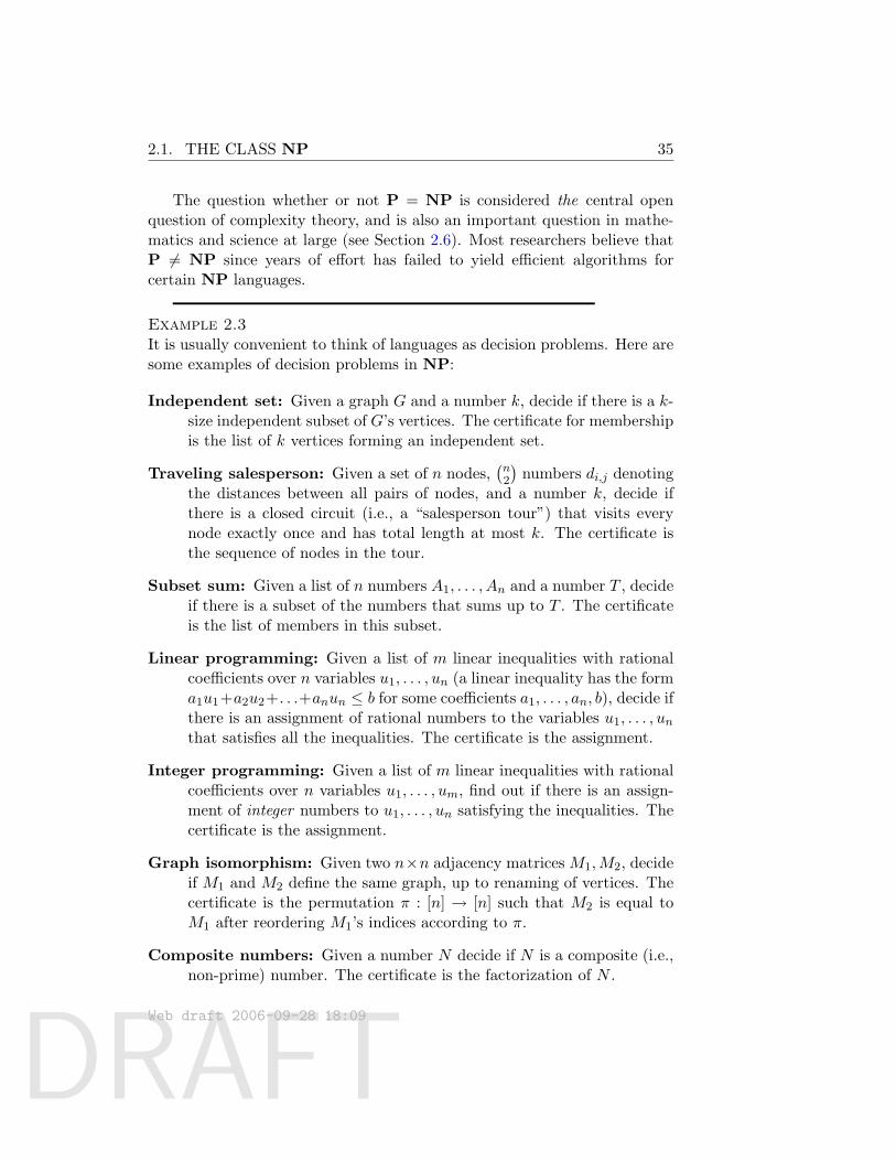
DRAFT

2.1. THE CLASS NP 35

The question whether or not P = NP is considered the central openquestion of complexity theory, and is also an important question in mathe-matics and science at large (see Section 2.6). Most researchers believe thatP 6= NP since years of effort has failed to yield efficient algorithms forcertain NP languages.

Example 2.3It is usually convenient to think of languages as decision problems. Here aresome examples of decision problems in NP:

Independent set: Given a graph G and a number k, decide if there is a k-size independent subset of G’s vertices. The certificate for membershipis the list of k vertices forming an independent set.

Traveling salesperson: Given a set of n nodes,(n2

)numbers di,j denoting

the distances between all pairs of nodes, and a number k, decide ifthere is a closed circuit (i.e., a “salesperson tour”) that visits everynode exactly once and has total length at most k. The certificate isthe sequence of nodes in the tour.

Subset sum: Given a list of n numbers A1, . . . , An and a number T , decideif there is a subset of the numbers that sums up to T . The certificateis the list of members in this subset.

Linear programming: Given a list of m linear inequalities with rationalcoefficients over n variables u1, . . . , un (a linear inequality has the forma1u1+a2u2+. . .+anun ≤ b for some coefficients a1, . . . , an, b), decide ifthere is an assignment of rational numbers to the variables u1, . . . , unthat satisfies all the inequalities. The certificate is the assignment.

Integer programming: Given a list of m linear inequalities with rationalcoefficients over n variables u1, . . . , um, find out if there is an assign-ment of integer numbers to u1, . . . , un satisfying the inequalities. Thecertificate is the assignment.

Graph isomorphism: Given two n×n adjacency matrices M1,M2, decideif M1 and M2 define the same graph, up to renaming of vertices. Thecertificate is the permutation π : [n] → [n] such that M2 is equal toM1 after reordering M1’s indices according to π.

Composite numbers: Given a number N decide if N is a composite (i.e.,non-prime) number. The certificate is the factorization of N .

Web draft 2006-09-28 18:09

DRAFT

36 2.2. NON-DETERMINISTIC TURING MACHINES.

Factoring: Given three numbers N,L,U decide if N has a factor M in theinterval [L,U ]. The certificate is the factor M .

Connectivity: Given a graph G and two vertices s, t in G, decide if s isconnected to t in G. The certificate is the path from s to t.

The Connectivity, Composite Numbers and Linear programming prob-lems are known to be in P. For connectivity this follows from the simpleand well known breadth-first search algorithm (see [?]). The compositenumbers problem was only recently shown to be in P by Agrawal, Kayaland Saxena [?], who gave a beautiful algorithm to solve it. For the lin-ear programming problem this is again highly non-trivial, and follows fromthe Ellipsoid algorithm of Khachiyan [?] (there are also faster algorithms,following Karmarkar’s interior point paradigm [?]).

All the rest of the problems are not known to have a polynomial-timealgorithm, although we have no proof that they are not in P. The Inde-pendent Set, Traveling Salesperson, Subset Sum, and Integer Programmingproblems are known to be NP-complete, which, as we will see in this chap-ter, implies that they are not in P unless P = NP. The Graph Isomorphismand Factoring problems are not known to be either in P nor NP-complete.

2.2 Non-deterministic Turing machines.

The class NP can also be defined using a variant of Turing machines callednon-deterministic Turing machines (abbreviated NDTM). In fact, this wasthe original definition and the reason for the name NP, which stands fornon-deterministic polynomial-time. The only difference between an NDTMand a standard TM is that an NDTM has two transition functions δ0 andδ1. In addition the NDTM has a special state we denote by qaccept. When anNDTM M computes, we envision that at each computational step M makesan arbitrary choice as to which of its two transition functions to apply. Wesay that M outputs 1 on a given input x if there is some sequence of thesechoices (which we call the non-deterministic choices of M) that would makeM reach qaccept on input x. Otherwise— if every sequence of choices makesM halt without reaching qaccept— then we say that M(x) = 0. We say thatM runs in T (n) time if for every input x ∈ 0, 1∗ and every sequence ofnon-deterministic choices, M reaches either a halting state or qaccept withinT (|x|) steps.

Web draft 2006-09-28 18:09

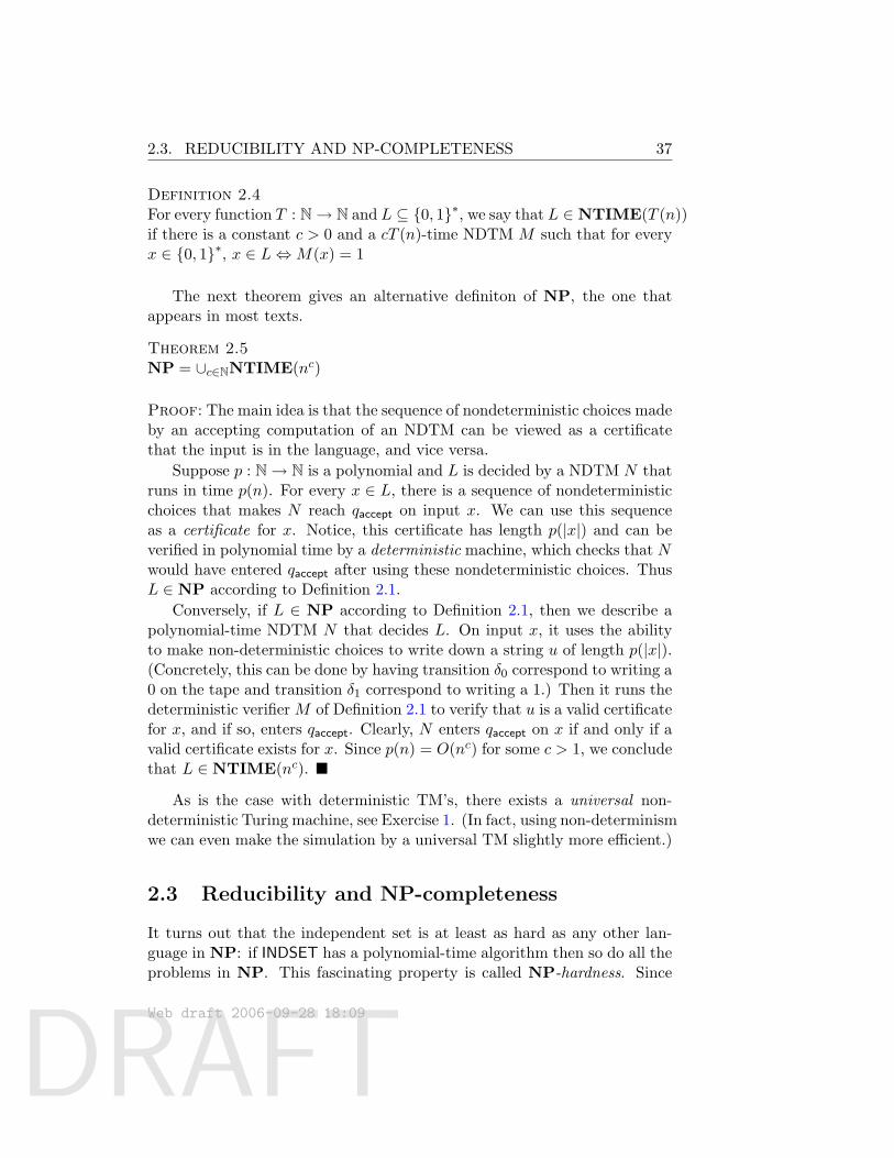
DRAFT

2.3. REDUCIBILITY AND NP-COMPLETENESS 37

Definition 2.4For every function T : N→ N and L ⊆ 0, 1∗, we say that L ∈ NTIME(T (n))if there is a constant c > 0 and a cT (n)-time NDTM M such that for everyx ∈ 0, 1∗, x ∈ L⇔M(x) = 1

The next theorem gives an alternative definiton of NP, the one thatappears in most texts.

Theorem 2.5NP = ∪c∈NNTIME(nc)

Proof: The main idea is that the sequence of nondeterministic choices madeby an accepting computation of an NDTM can be viewed as a certificatethat the input is in the language, and vice versa.

Suppose p : N→ N is a polynomial and L is decided by a NDTM N thatruns in time p(n). For every x ∈ L, there is a sequence of nondeterministicchoices that makes N reach qaccept on input x. We can use this sequenceas a certificate for x. Notice, this certificate has length p(|x|) and can beverified in polynomial time by a deterministic machine, which checks that Nwould have entered qaccept after using these nondeterministic choices. ThusL ∈ NP according to Definition 2.1.

Conversely, if L ∈ NP according to Definition 2.1, then we describe apolynomial-time NDTM N that decides L. On input x, it uses the abilityto make non-deterministic choices to write down a string u of length p(|x|).(Concretely, this can be done by having transition δ0 correspond to writing a0 on the tape and transition δ1 correspond to writing a 1.) Then it runs thedeterministic verifier M of Definition 2.1 to verify that u is a valid certificatefor x, and if so, enters qaccept. Clearly, N enters qaccept on x if and only if avalid certificate exists for x. Since p(n) = O(nc) for some c > 1, we concludethat L ∈ NTIME(nc).

As is the case with deterministic TM’s, there exists a universal non-deterministic Turing machine, see Exercise 1. (In fact, using non-determinismwe can even make the simulation by a universal TM slightly more efficient.)

2.3 Reducibility and NP-completeness

It turns out that the independent set is at least as hard as any other lan-guage in NP: if INDSET has a polynomial-time algorithm then so do all theproblems in NP. This fascinating property is called NP-hardness. Since

Web draft 2006-09-28 18:09

DRAFT

38 2.3. REDUCIBILITY AND NP-COMPLETENESS

most scientists conjecture that NP 6= P, the fact that a language is NP-hard can be viewed as evidence that it cannot be decided in polynomialtime.

How can we prove that a language B is at least as hard as some languageA? The crucial tool we use is the notion of a reduction (see Figure 2.1):

Definition 2.6 (Reductions, NP-hardness and NP-completeness)We say that a language A ⊆ 0, 1∗ is polynomial-time Karp reducible to a languageB ⊆ 0, 1∗ (sometimes shortened to just “polynomial-time reducible”1) denoted byA ≤p B if there is a polynomial-time computable function f : 0, 1∗ → 0, 1∗ suchthat for every x ∈ 0, 1∗, x ∈ A⇔ x ∈ B.We say that B is NP-hard if A ≤p B for every A ∈ NP. We say that B isNP-complete if B is NP-hard and B ∈ NP.

L

L

L’

L’

f(L)

f(L)

Algorithm for L

Algorithm for L’f

Input: x f(x)output:1 iff f(x) in L’

Figure 2.1: A Karp reduction from L to L′ is a polynomial-time function f that mapsstrings in L to strings in L′ and strings in L = 0, 1∗ \L to strings in L′. It can be usedto transform a polynomial-time TM M ′ that decides L into a polynomial-time TM M forL by setting M(x) = M ′(f(x)).

Now we observe some properties of polynomial-time reductions. Part 1shows that this relation is transitive. (Later we will define other notionsof reduction, and all will satisfy transitivity.) Part 2 suggests the reasonfor the term NP-hard —namely, an NP-hard languages is at least as hardas any other NP language. Part 3 similarly suggests the reason for theterm NP-complete: to study the P versus NP question it suffices to studywhether any NP-complete problem can be decided in polynomial time.

1Some texts call this notion “many-to-one reducibility” or “polynomial-time mappingreducibility”.

Web draft 2006-09-28 18:09

DRAFT


Theorem 2.71. (transitivity) A ≤p B and B ≤p C, then A ≤p C.

2. If language A is NP-hard and A ∈ P then P = NP.

3. If language A is NP-complete then A ∈ P if and only if P = NP.

Proof: The main observation is that if p, q are two functions that have poly-nomial growth then their composition p(q(n)) also has polynomial growth.We prove part 1 and leave the others as simple exercises.

If f1 is a polynomial-time reduction from A to B and f2 is a reductionfrom B to C then the mapping x 7→ f2(f1(x)) is a polynomial-time reductionfrom A to C since f2(f1(x)) takes polynomial time to compute given x andf2(f1(x)) ∈ C iff x ∈ A.

Do NP-complete languages exist? It may not be clear that NP shouldpossess a language that is as hard as any other language in the class. How-ever, this does turn out to be the case:

Theorem 2.8The following language is NP-complete:

TMSAT = 〈 xMy, x, 1n, 1t〉 : ∃u ∈ 0, 1n s.t. M outputs 1 on input 〈x, u〉 within t steps

where xMy denotes the representation of the TM M according to the rep-resentation scheme of Theorem 1.6.

Theorem 2.8 is straightforward from the definition of NP and is left tothe reader as Exercise 2. But TMSAT is not a very useful NP-completeproblem since its definition is intimately tied to the notion of the Turingmachine, and hence the fact that it is NP-complete does not provide muchnew insight.

2.3.1 The Cook-Levin Theorem: Computation is Local

Around 1971, Cook and Levin independently discovered the notion of NP-completeness and gave examples of combinatorial NP-complete problemswhose definition seems to have nothing to do with Turing machines. Soonafter, Karp showed that NP-completeness occurs widely and many combi-natorial problems of practical interest are NP-complete. To date, thousandsof computational problems in a variety of disciplines have been found to beNP-complete.

Web draft 2006-09-28 18:09

DRAFT


Some of the simplest examples of NP-complete problems come frompropositional logic. A Boolean formula over the variables u1, . . . , un consistsof the variables and the logical operators AND (∧), NOT (¬) and OR (∨);see Appendix for their definitions. For example, (a ∧ b) ∨ (a ∧ c) ∨ (b ∧ c) isa Boolean formula that is True if and only if the majority of the variablesa, b, c are True. If ϕ is a Boolean formula over variables u1, . . . , un, andz ∈ 0, 1n, then ϕ(z) denotes the value of ϕ when the variables of ϕ areassigned the values z (where we identify 1 with True and 0 with False).The formula is satisfiable if there is an assignment to the variables thatmakes it evaluate to True. Otherwise, we say ϕ is unsatisfiable.

Definition 2.9 (CNF, kCNF)A Boolean formula over variables u1, . . . , un is in CNF form (shorthand forConjunctive Normal Form) if it is an AND of OR’s of variables or theirnegations. It has the form ∧

i

∨j

vij

,

where each vij is a literal of ϕ, in other words either a variable uk or to itsnegation uk. The terms (∨jvij ) are called the clauses. If all clauses containat most k literals, the formula is a kCNF.

For example, the following is a CNF formula that is 3CNF.

(u1 ∨ u2 ∨ u3) ∧ (u2 ∨ u3 ∨ u4) ∧ (u1 ∨ u3 ∨ u4) .

Definition 2.10 (SAT and 3SAT)SAT is the language of all satisfiable CNF formulae and 3SAT is the languageof all satisfiable 3CNF formulae.

Theorem 2.11 (Cook-Levin Theorem [Coo71, Lev73])1. SAT is NP-complete.

2. 3SAT is NP-complete.

Remark 2.12An alternative proof of the Cook-Levin theorem, using the notion of Booleancircuits, is described in Section 6.7.

Web draft 2006-09-28 18:09

DRAFT


Both SAT and 3SAT are clearly in NP, since a satisfying assignment canserve as the certificate that a formula is satisfiable. Thus we only need toprove that they are NP-hard. We do so by first proving that SAT is NP-hard and then showing that SAT is polynomial-time Karp reducible to 3SAT.This implies that 3SAT is NP-hard by the transitivity of polynomial-timereductions. Thus the following lemma is the key to the proof.

Lemma 2.13SAT is NP-hard.

Notice, to prove this we have to show how to reduce every NP languageL to SAT, in other words give a polynomial-time transformation that turnsany x ∈ 0, 1∗ into a CNF formula ϕx such that x ∈ L iff ϕx is satisfiable.Since we know nothing about the language L except that it is in NP, thisreduction has to rely just upon the definition of computation, and expressit in some way using a boolean formula.

Expressiveness of boolean formulae

As a warmup for the proof of Lemma 2.13 we show how to express constraintsusing boolean formulae.

Example 2.14The formula (a ∨ b) ∧ (a ∨ b) is in CNF form. It is satisfied by only thosevalues of a, b that are equal. Thus, the formula

(x1 ∨ y1) ∧ (x1 ∨ y1) ∧ · · · ∧ (xn ∨ yn) ∧ (xn ∨ yn)

is True if and only if the strings x, y ∈ 0, 1n are equal to one another.Thus, though = is not a standard boolean operator like ∨ or ∧, we will

use it as a convenient shorthand since the formula φ1 = φ2 is equivalent to(in other words, has the same satisfying assignments as) (φ1∨φ2)∧(φ1∨φ2).

In fact, CNF formulae of sufficient size can express every Boolean condi-tion, as shown by the following simple claim: (this fact is sometimes knownas universality of the operations AND, OR and NOT)

Claim 2.15For every Boolean function f : 0, 1` → 0, 1 there is an `-variable CNF

formula ϕ of size `2` such that ϕ(u) = f(u) for every u ∈ 0, 1`, where

Web draft 2006-09-28 18:09

DRAFT


the size of a CNF formula is defined to be the number of ∧/∨ symbols itcontains.

Proof: For every v ∈ 0, 1`, there exists a clause Cv such that Cv(v) =0 and Cv(u) = 1 for every u 6= v. For example, if v = 〈1, 1, 0, 1〉, thecorresponding clause is u1 ∨ u2 ∨ u3 ∨ u4. We let S be the set v : f(v) = 1and set ϕ = ∧v∈SCv. Then for every v such that f(v) = 0 it holds thatϕ(v) = 0 and for every u such that f(u) = 1, we have that Cv(u) = 1 forevery v ∈ S and hence ϕ(u) = 1.

In this chapter we will use this claim only when the number of variablesis some fixed constant.

Proof of Lemma 2.13

Let L be an NP language and let M be the polynomial time TM such thatthat for every x ∈ 0, 1∗, x ∈ L ⇔ M(x, u) = 1 for some u ∈ 0, 1p(|x|),where p : N → N is some polynomial. We show L is polynomial-time Karpreducible to SAT by describing a way to transform in polynomial-time everystring x ∈ 0, 1∗ into a CNF formula ϕx such that x ∈ L iff ϕx is satisfiable.

How can we construct such a formula ϕx? By Claim 2.15, the functionthat maps u ∈ 0, 1p(|x|) to M(x, u) can be expressed as a CNF formulaψx (i.e., ψx(u) = M(x, u) for every u ∈ 0, 1p(|x|)). Thus a u such thatM(x, u) = 1 exists if and only if ψx is satisfiable. But this is not usefulfor us, since the size of the formula ψx obtained from Claim 2.15 can beas large as p(|x|)2p(|x|). To get a smaller formula we use the fact that Mruns in polynomial time, and that each basic step of a Turing machine ishighly local (in the sense that it examines and changes only a few bits ofthe machine’s tapes).

We assume for notational simplicity that M only has two tapes: an inputtape and a work/output tape. The proof carries over in the same way forany fixed number of tapes. We also assume that M is an oblivious TM inthe sense that its head movement does not depend on the contents of itsinput tape. In particular, this means that M ’s computation takes the sametime for all inputs of size n and for each time step i the location of M ’sheads at the ith step depends only on i and M ’s input length. We can makethis assumption since every TM can be easily simulated by an oblivious TMincurring only a polynomial overhead (e.g., by replacing each step of thecomputation with a left to right and back sweep of the machine’s tapes; seeExercise 5 of Chapter 1).2

2In fact, with some more effort we even simulate a non-oblivious T (n)-time TM by an

Web draft 2006-09-28 18:09

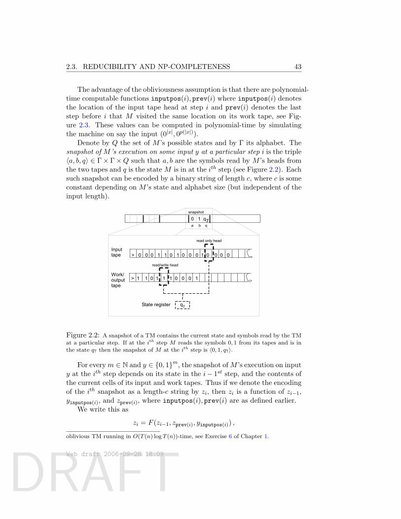
DRAFT


The advantage of the obliviousness assumption is that there are polynomial-time computable functions inputpos(i), prev(i) where inputpos(i) denotesthe location of the input tape head at step i and prev(i) denotes the laststep before i that M visited the same location on its work tape, see Fig-ure 2.3. These values can be computed in polynomial-time by simulatingthe machine on say the input (0|x|, 0p(|x|)).

Denote by Q the set of M ’s possible states and by Γ its alphabet. Thesnapshot of M ’s execution on some input y at a particular step i is the triple〈a, b, q〉 ∈ Γ× Γ×Q such that a, b are the symbols read by M ’s heads fromthe two tapes and q is the state M is in at the ith step (see Figure 2.2). Eachsuch snapshot can be encoded by a binary string of length c, where c is someconstant depending on M ’s state and alphabet size (but independent of theinput length).

Inputtape

Work/outputtape

> 0 0 0 1 1 0 1 0 0 0 1 0 0 0 0

> 1 1 0 1 1 1 0 0 0 1

q7State register

read only head

read/write head

snapshot

0 1 q7a b q

Figure 2.2: A snapshot of a TM contains the current state and symbols read by the TMat a particular step. If at the ith step M reads the symbols 0, 1 from its tapes and is inthe state q7 then the snapshot of M at the ith step is 〈0, 1, q7〉.

For everym ∈ N and y ∈ 0, 1m, the snapshot ofM ’s execution on inputy at the ith step depends on its state in the i− 1st step, and the contents ofthe current cells of its input and work tapes. Thus if we denote the encodingof the ith snapshot as a length-c string by zi, then zi is a function of zi−1,yinputpos(i), and zprev(i), where inputpos(i), prev(i) are as defined earlier.

We write this as

zi = F (zi−1, zprev(i), yinputpos(i)) ,

oblivious TM running in O(T (n) log T (n))-time, see Exercise 6 of Chapter 1.

Web draft 2006-09-28 18:09

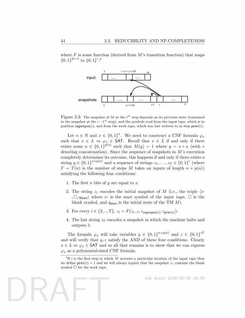
DRAFT


where F is some function (derived from M ’s transition function) that maps0, 12c+1 to 0, 1c.3

1 minputpos(i)

.... ....

............1 prev(i) i-1 i T

input:

snapshots:

Figure 2.3: The snapshot of M at the ith step depends on its previous state (containedin the snapshot at the i− 1st step), and the symbols read from the input tape, which is inposition inputpos(i), and from the work tape, which was last written to in step prev(i).

Let n ∈ N and x ∈ 0, 1n. We need to construct a CNF formula ϕxsuch that x ∈ L ⇔ ϕx ∈ SAT. Recall that x ∈ L if and only if thereexists some u ∈ 0, 1p(n) such that M(y) = 1 where y = x u (with denoting concatenation). Since the sequence of snapshots in M ’s executioncompletely determines its outcome, this happens if and only if there exists astring y ∈ 0, 1n+p(n) and a sequence of strings z1, . . . , zT ∈ 0, 1c (whereT = T (n) is the number of steps M takes on inputs of length n + p(n))satisfying the following four conditions:

1. The first n bits of y are equal to x.

2. The string z1 encodes the initial snapshot of M (i.e., the triple 〈B,, qstart〉 where B is the start symbol of the input tape, is theblank symbol, and qstart is the initial state of the TM M).

3. For every i ∈ 2, .., T, zi = F (zi−1, zinputpos(i), zprev(i)).

4. The last string zT encodes a snapshot in which the machine halts andoutputs 1.

The formula ϕx will take variables y ∈ 0, 1n+p(n) and z ∈ 0, 1cTand will verify that y, z satisfy the AND of these four conditions. Clearlyx ∈ L ⇔ ϕx ∈ SAT and so all that remains is to show that we can expressϕx as a polynomial-sized CNF formula.

3If i is the first step in which M accesses a particular location of the input tape thenwe define prev(i) = 1 and we will always require that the snapshot z1 contains the blanksymbol for the work tape.

Web draft 2006-09-28 18:09

DRAFT


Condition 1 can be expressed as a CNF formula of size 2n (in fact, sucha formula appears in Example 2.14). Conditions 2 and 4 each depend onc variables and hence by Claim 2.15 can be expressed by CNF formulae ofsize c2c. Condition 3, which is an AND of T conditions each depending onat most 3c+ 1 variables, can be expressed as a CNF formula of size at mostT (3c+ 1)23c+1. Hence the AND of all these conditions can be expressed asa CNF formula of size d(n + T ) where d is some constant depending onlyon M . Moreover, this CNF formula can be computed in time polynomial inthe running time of M .

Lemma 2.16SAT ≤p 3SAT.

Proof: We will map a CNF formula ϕ into a 3CNF formula ψ such thatψ is satisfiable if and only if ϕ is. We demonstrate first the case that ϕ isa 4CNF. Let C be a clause of ϕ, say C = u1 ∨ u2 ∨ u3 ∨ u4. We add a newvariable z to the ϕ and replace C with the pair of clauses C1 = u1 ∨ u2 ∨ zand C2 = u3 ∨ u4 ∨ z. Clearly, if u1 ∨ u2 ∨ u3 ∨ u4 is true then there isan assignment to z that satisfies both u1 ∨ u2 ∨ z and u3 ∨ u4 ∨ z and viceversa: if C is false then no matter what value we assign to z either C1 orC2 will be false. The same idea can be applied to a general clause of size 4,and in fact can be used to change every clause C of size k (for k > 3) intoan equivalent pair of clauses C1 of size k − 1 and C2 of size 3 that dependon the k variables of C and an additional auxiliary variable z. Applyingthis transformation repeatedly yields a polynomial-time transformation of aCNF formula ϕ into an equivalent 3CNF formula ψ.

2.3.2 More thoughts on the Cook-Levin theorem

The Cook-Levin theorem is a good example of the power of abstraction.Even though the theorem holds regardless of whether our computationalmodel is the C programming language or the Turing machine, it may havebeen considerably more difficult to discover in the former context.

Also, it is worth pointing out that the proof actually yields a result thatis a bit stronger than the theorem’s statement:

1. If we use the efficient simulation of a standard TM by an oblivious TM(see Exercise 6, Chapter 1) then for every x ∈ 0, 1∗, the size of theformula ϕx (and the time to compute it) is O(T log T ), where T is thenumber of steps the machine M takes on input x (see Exercise 10).

Web draft 2006-09-28 18:09

DRAFT


2. The reduction f from an NP-language L to SAT presented in Lemma 2.13not only satisfied that x ∈ L ⇔ f(x) ∈ SAT but actually the proofyields an efficient way to transform a certificate for x to a satisfyingassignment for f(x) and vice versa. We call a reduction with thisproperty a Levin reduction. One can also verify that the proof sup-plied a one-to-one and onto map between the set of certificates for xand the set of satisfying assignments for f(x), implying that they areof the same size. A reduction with this property is called parsimo-nious. Most of the known NP-complete problems (including all theones mentioned in this chapter) have parsimonious Levin reductionsfrom all the NP languages (see Exercise 11). As we will see in thisbook, this fact is sometimes useful for certain applications.

Why 3SAT? The reader may wonder why is the fact that 3SAT is NP-complete so much more interesting than the fact that, say, the languageTMSAT of Theorem 2.8 is NP-complete. One answer is that 3SAT is usefulfor proving the NP-completeness of other problems: it has very minimalcombinatorial structure and thus easy to use in reductions. Another an-swer has to do with history: propositional logic has had a central role inmathematical logic —in fact it was exclusively the language of classical logic(e.g. in ancient Greece). This historical resonance is one reason why Cookand Levin were interested in 3SAT in the first place. A third answer hasto do with practical importance: it is a simple example of constraint sat-isfaction problems, which are ubiquitous in many fields including artificialintelligence.

2.3.3 The web of reductions

Cook and Levin had to show how every NP language can be reduced toSAT. To prove the NP-completeness of any other language L, we do notneed to work as hard: it suffices to reduce SAT or 3SAT to L. Once weknow that L is NP-complete we can show that an NP-language L′ is in factNP-complete by reducing L to L′. This approach has been used to build a“web of reductions” and show that thousands of interesting languages are infact NP-complete. We now show the NP-completeness of a few problems.More examples appear in the exercises (see Figure 2.4). See the classic bookby Garey and Johnson [?] and the internet site [?] for more.

Theorem 2.17 (Independent set is NP-complete)Let INDSET = 〈G, k〉 : G has independent set of size k. Then INDSET isNP-complete.

Web draft 2006-09-28 18:09

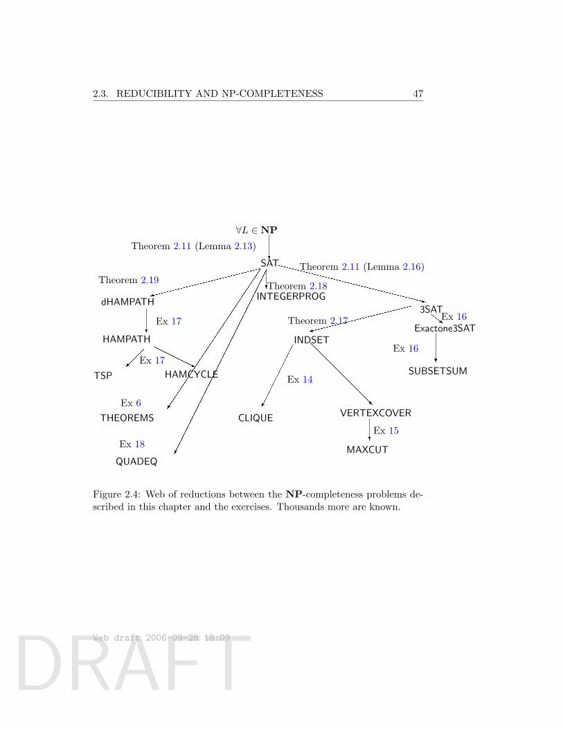
DRAFT


∀L ∈ NP

SAT

Exactone3SAT

?9

dHAMPATH

HAMPATH

TSP HAMCYCLE

?

HHHHHj

Theorem 2.19?

Theorem 2.17Ex 17

Ex 17

Theorem 2.11 (Lemma 2.13)

9

XXXXXXXXXXXXXXXXXz3SATZZ~

?SUBSETSUM

Ex 16INDSET

CLIQUE

Ex 14

@@@@@@@R

?

VERTEXCOVER

Ex 15

MAXCUT

Ex 16

THEOREMS

Ex 6

Ex 18

QUADEQ

Theorem 2.18INTEGERPROG

Theorem 2.11 (Lemma 2.16)

Figure 2.4: Web of reductions between the NP-completeness problems de-scribed in this chapter and the exercises. Thousands more are known.

Web draft 2006-09-28 18:09

DRAFT


Proof: Since INDSET is clearly in NP, we only need to show that it isNP-hard, which we do by reducing 3SAT to INDSET. Let ϕ be a 3CNFformula on n variables with m clauses. We define a graph G of 7m verticesas follows: we associate a cluster of 7 vertices in G with each clause ofϕ. The vertices in cluster associated with a clause C correspond to the7 possible assignments to the three variables C depends on (we call thesepartial assignments, since they only give values for some of the variables).For example, if C is u2∨u5∨u7 then the 7 vertices in the cluster associatedwith C correspond to all partial assignments of the form u1 = a, u2 =b, u3 = c for a binary vector 〈a, b, c〉 6= 〈1, 1, 1〉. (If C depends on less thanthree variables we treat one of them as repeated and then some of the 7vertices will correspond to the same assignment.) We put an edge betweentwo vertices of G if they correspond to inconsistent partial assignments.Two partial assignments are consistent if they give the same value to all thevariables they share. For example, the assignment u1 = 1, u2 = 0, u3 = 0 isinconsistent with the assignment u3 = 1, u5 = 0, u7 = 1 because they sharea variable (u3) to which they give a different value. In addition, we putedges between every two vertices that are in the same cluster.

Clearly transforming ϕ into G can be done in polynomial time. Weclaim that ϕ is satisfiable if and only if G has a clique of size m. Indeed,suppose that ϕ has a satisfying assignment u. Define a set S of m vertices asfollows: for every clause C of ϕ put in S the vertex in the cluster associatedwith C that corresponds to the restriction of u to the variables C dependson. Because we only choose vertices that correspond to restrictions of theassignment u, no two vertices of S correspond to inconsistent assignmentsand hence S is an independent set of size m.

On the other hand, suppose that G has an independent set S of size m.We will use S to construct a satisfying assignment u for ϕ. We define u asfollows: for every i ∈ [n], if there is a vertex in S whose partial assignmentgives a value a to ui, then set ui = a; otherwise set ui = 0. This is welldefined because S is an independent set, and hence each variable ui can getat most a single value by assignments corresponding to vertices in S. On theother hand, because we put all the edges within each cluster, S can containat most a single vertex in each cluster, and hence there is an element of Sin every one of the m clusters. Thus, by our definition of u, it satisfies allof ϕ’s clauses.

We see that, surprisingly, the answer to the famous NP vs. P questiondepends on the seemingly mundane question of whether one can efficientlyplan an optimal dinner party. Here are some more NP-completeness results:

Web draft 2006-09-28 18:09

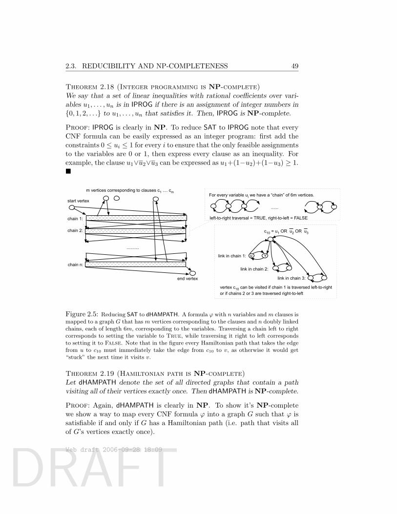
DRAFT


Theorem 2.18 (Integer programming is NP-complete)We say that a set of linear inequalities with rational coefficients over vari-ables u1, . . . , un is in IPROG if there is an assignment of integer numbers in0, 1, 2, . . . to u1, . . . , un that satisfies it. Then, IPROG is NP-complete.

Proof: IPROG is clearly in NP. To reduce SAT to IPROG note that everyCNF formula can be easily expressed as an integer program: first add theconstraints 0 ≤ ui ≤ 1 for every i to ensure that the only feasible assignmentsto the variables are 0 or 1, then express every clause as an inequality. Forexample, the clause u1∨u2∨u3 can be expressed as u1+(1−u2)+(1−u3) ≥ 1.

......

m vertices corresponding to clauses c1 .... cm

start vertex

end vertex

..........

For every variable ui we have a “chain” of 6m vertices.

chain 1:

chain n:

c10 = u1 OR u2 OR u3

link in chain 1:

link in chain 2:

link in chain 3:

left-to-right traversal = TRUE, right-to-left = FALSE

vertex c10 can be visited if chain 1 is traversed left-to-rightor if chains 2 or 3 are traversed right-to-left

u v

chain 2:

Figure 2.5: Reducing SAT to dHAMPATH. A formula ϕ with n variables andm clauses ismapped to a graph G that has m vertices corresponding to the clauses and n doubly linkedchains, each of length 6m, corresponding to the variables. Traversing a chain left to rightcorresponds to setting the variable to True, while traversing it right to left correspondsto setting it to False. Note that in the figure every Hamiltonian path that takes the edgefrom u to c10 must immediately take the edge from c10 to v, as otherwise it would get“stuck” the next time it visits v.

Theorem 2.19 (Hamiltonian path is NP-complete)Let dHAMPATH denote the set of all directed graphs that contain a pathvisiting all of their vertices exactly once. Then dHAMPATH is NP-complete.

Proof: Again, dHAMPATH is clearly in NP. To show it’s NP-completewe show a way to map every CNF formula ϕ into a graph G such that ϕ issatisfiable if and only if G has a Hamiltonian path (i.e. path that visits allof G’s vertices exactly once).

Web draft 2006-09-28 18:09

DRAFT


The reduction is described in Figure 2.5. The graph G has (1)m verticesfor each of ϕ’s clauses c1, . . . , cm, (2) a special starting vertex vstart andending vertex vend and (3) n “chains” of 6m vertices corresponding to then variables of ϕ. A chain is a set of vertices v1, . . . , v6m such that for everyi ∈ [6m− 1], vi and vi+1 are connected by two edges in both directions.

We put edges from the starting vertex vstart to the two extreme points ofthe first chain. We also put edges from the extreme points of the jth chainto the extreme points to the j + 1th chain for every j ∈ [n− 1]. We put anedge from the extreme points of the nth chain to the ending vertex vend.

In addition to these edges, for every clause C of ϕ, we put edges betweenthe chains corresponding to the variables appearing in C and the vertex vCcorresponding to C in the following way: if C contains the literal uj then wetake two neighboring vertices vi, vi+1 in the jth chain and put an edge fromvi to C and from C to vi+1. If C contains the literal uj then we connectthese edges in the opposite direction (i.e., vi+1 to C and C to vi). Whenadding these edges, we never “reuse” a link vi, vi+1 in a particular chain andalways keep an unused link between every two used links. We can do thissince every chain has 5m vertices, which is more than sufficient for this.

ϕ ∈ SAT⇒ G ∈ dHAMPATH. Suppose that ϕ has a satisfying assignmentu1, . . . , un. We will show a path that visits all the vertices of G. The pathwill start at vstart, travel through all the chains in order, and end at vend.For starters, consider the path that travels the jth chain in left-to-right orderif uj = 1 and travels it in right-to-left order if uj = 0. This path visits all thevertices except for those corresponding to clauses. Yet, if u is a satisfyingassignment then the path can be easily modified to visit all the verticescorresponding to clauses: for each clause C there is at least one literal thatis true, and we can use one link on the chain corresponding to that literalto “skip” to the vertex vC and continue on as before.

G ∈ dHAMPATH ⇒ ϕ ∈ SAT. Suppose that G has an Hamiltonian pathP . We first note that the path P must start in vstart (as it has no incomingedges) and end at vend (as it has no outgoing edges). Furthermore, weclaim that P needs to traverse all the chains in order, and within each chaintraverse it either in left-to-right order or right-to-left order. This would beimmediate if the path did not use the edges from a chain to the verticescorresponding to clauses. The claim holds because if a Hamiltonian pathtakes the edge u→ w, where u is on a chain and w corresponds to a clause,then it must at the next step take the edge w → v where v is the vertex

Web draft 2006-09-28 18:09

DRAFT

2.4. DECISION VERSUS SEARCH 51

adjacent to u in the link. Otherwise, the path will get stuck the next timeit visits v (see Figure 2.1). Now, define an assignment u1, . . . , un to ϕas follows: uj = 1 if P traverses the jth chain in left-to-right order, anduj = 0 otherwise. It is not hard to see that because P visits all the verticescorresponding to clauses, u1, . . . , un is a satisfying assignment for ϕ.

In praise of reductions

Though originally invented as part of the theory of NP-completeness, thepolynomial-time reduction (together with its first cousin, the randomizedpolynomial-time reduction defined in Section 7.8) has led to a rich under-standing of complexity above and beyond NP-completeness. Much of com-plexity theory and cryptography today (thus, many chapters of this book)consists of using reductions to make connections between disparate complex-ity theoretic conjectures. Why do complexity theorists excel at reductionsbut not at actually proving lowerbounds on Turing machines? A possibleexplanation is that humans have evolved to excel at problem solving, andhence are more adept at algorithms (after all, a reduction is merely an algo-rithm to transform one problem into another) than at proving lowerboundson Turing machines.

2.4 Decision versus search

We have chosen to define the notion of NP using Yes/No problems (“Isthe given formula satisfiable?”) as opposed to search problems (“Find asatisfying assignment to this formula if one exists”). However, it turns outthat if P = NP then the search versions of NP problems can also be solvedin polynomial time.

Theorem 2.20Suppose that P = NP. Then, for every NP language L there exists apolynomial-time TM B that on input x ∈ L outputs a certificate for x.

That is, if, as per Definition 2.1, x ∈ L iff ∃u ∈ 0, 1p(|x|) s.t. M(x, u) =1 where p is some polynomial and M is a polynomial-time TM, then on inputx ∈ L, B(x) will be a string u ∈ 0, 1p(|x|) satisfying M(x,B(x)) = 1.

Proof: We start by showing the theorem for the case of SAT. In particularwe show that given an algorithm A that decides SAT, we can come up withan algorithm B that on input a satisfiable CNF formula ϕ with n variables,

Web draft 2006-09-28 18:09

DRAFT

52 2.5. CONP, EXP AND NEXP

finds a satisfying assignment for ϕ using 2n+1 calls to A and some additionalpolynomial-time computation.

The algorithm B works as follows: we first use A to check that the inputformula ϕ is satisfiable. If so, we substitute x1 = 0 and x1 = 1 in ϕ (thistransformation, that simplifies and shortens the formula a little, leaving aformula with n − 1 variables, can certainly be done in polynomial time)and then use A to decide which of the two is satisfiable (it is possible thatboth are). Say the first is satisfiable. Then we fix x1 = 0 from now on andcontinue with the simplified formula. Continuing this way we end up fixingall n variables while ensuring that each intermediate formula is satisfiable.Thus the final assignment to the variables satisfies ϕ.

To solve the search problem for an arbitrary NP-language L, we usethe fact that the reduction of Theorem 2.11 from L to SAT is actually aLevin reduction. This means that we have a polynomial-time computablefunction f such that not only x ∈ L⇔ f(x) ∈ SAT but actually we can mapa satisfying assignment of f(x) into a certificate for x. Therefore, we canuse the algorithm above to come up with an assignment for f(x) and thenmap it back into a certificate for x.

Remark 2.21The proof above shows that SAT is downward self-reducible, which meansthat given an algorithm that solves SAT on inputs of length smaller than nwe can solve it on inputs of length n. Using the Cook-Levin reduction, onecan show that all NP-complete problems have a similar property, thoughwe do not make this formal.

2.5 coNP, EXP and NEXP

Now we define some related complexity classes that are very relevant to thestudy of the P versus NP question.

2.5.1 coNP

If L ⊆ 0, 1∗ is a language, then we denote by L the complement of L.That is, L = 0, 1∗ \ L. We make the following definition:

Definition 2.22coNP =

L : L ∈ P

.

It is important to note that coNP is not the complement of the classNP. In fact, they have a non-empty intersection, since every language in P

Web draft 2006-09-28 18:09

DRAFT

2.5. CONP, EXP AND NEXP 53

is in NP∩coNP (see Exercise 19). The following is an example of a coNPlanguage: SAT = ϕ : ϕ is not satisfiable . Students sometimes mistakenlyconvince themselves that SAT is in NP. They have the following polynomialtime NDTM in mind: on input ϕ, the machine guesses an assignment. Ifthis assignment does not satisfy ϕ then it accepts (i.e., goes into qaccept andhalts) and if it does satisfy ϕ then the machine halts without accepting.This NDTM does not do the job: indeed it accepts every unsatisfiable ϕ butin addition it also accepts many satisfiable formulae (i.e., every formula thathas a single unsatisfying assignment). That is why pedagogically we preferthe following definition of coNP (which is easily shown to be equivalent tothe first, see Exercise 20):

Definition 2.23 (coNP, alternative definition)For every L ⊆ 0, 1∗, we say that L ∈ coNP if there exists a polynomialp : N→ N and a polynomial-time TM M such that for every x ∈ 0, 1∗,

x ∈ L⇔ ∀u ∈ 0, 1p(|x|) s.t. M(x, u) = 1

The key fact to note is the use of “∀” in this definition where Defini-tion 2.1 used ∃.

We can define coNP-completeness in analogy to NP-completeness: alanguage is coNP-complete if it is in coNP and every coNP language ispolynomial-time Karp reducible to it.

Example 2.24In classical logic, tautologies are true statements. The following language iscoNP-complete:

TAUTOLOGY = ϕ : ϕ is a boolean formula that is satisfied by every assignment .

It is clearly in coNP by Definition 2.23 and so all we have to show isthat for every L ∈ coNP, L ≤p TAUTOLOGY. But this is easy: just modifythe Cook-Levin reduction from L (which is in NP) to SAT. For every inputx ∈ 0, 1∗ that reduction produces a formula ϕx that is satisfiable iff x ∈ L.Now consider the formula ¬ϕx. It is in TAUTOLOGY iff x ∈ L, and thiscompletes the description of the reduction.

It is a simple exercise to check that if P = NP then NP = coNP = P.Put contrapositively, if we can show that NP 6= coNP then we have shown

Web draft 2006-09-28 18:09

DRAFT

54 2.5. CONP, EXP AND NEXP

P 6= NP. Most researchers believe that NP 6= coNP. The intuition isalmost as strong as for the P versus NP question: it seems hard to believethat there is any short certificate for certifying that a given formula is aTAUTOLOGY, in other words, to certify that every assignment satisfies theformula.

2.5.2 EXP and NEXP

The following two classes are exponential time analogues of P and NP.

Definition 2.25EXP = ∪c≥0DTIME(2n

c).

NEXP = ∪c≥0NTIME(2nc).

Because every problem in NP can be solved in exponential time by abrute force search for the certificate, P ⊆ NP ⊆ EXP ⊆ NEXP. Isthere any point to studying classes involving exponential running times?The following simple result —providing merely a glimpse of the rich web ofrelations we will be establishing between disparate complexity questions—may be a partial answer.

Theorem 2.26If EXP 6= NEXP then P 6= NP.

Proof: We prove the contrapositive: assuming P = NP we show EXP =NEXP. Suppose L ∈ NTIME(2n

c) and NDTM M decides it. We claim

that then the language

Lpad =〈x, 12|x|

c

〉 : x ∈ L

(1)

is in NP. Here is an NDTM for Lpad: given y, first check if there is a stringz such that y = 〈z, 12|z|

c

〉. If not, output REJECT. If y is of this form, thenrun M on z for 2|z|

c

steps and output its answer. Clearly, the running timeis polynomial in |y|, and hence Lpad ∈ NP. Hence if P = NP then Lpad isin P. But if Lpad is in P then L is in EXP: to determine whether an inputx is in L, we just pad the input and decide whether it is in Lpad using thepolynomial-time machine for Lpad.

Remark 2.27The padding technique used in this proof, whereby we transform a languageby “padding” every string in a language with a string of (useless) symbols,is also used in several other results in complexity theory. In many settings it

Web draft 2006-09-28 18:09

DRAFT

2.6. MORE THOUGHTS ABOUT P, NP, AND ALL THAT 55

can be used to show that equalities between complexity classes “scale up”;that is, if two different type of resources solve the same problems withinbound T (n) then this also holds for functions T ′ larger than T . Viewedcontrapositively, padding can be used to show that inequalities betweencomplexity classes involving resurce bound T ′(n) “scale down” to resourcebound T (n).

We note that most of the complexity classes studied later are, like P andNP, also contained in EXP or NEXP.

2.6 More thoughts about P, NP, and all that

2.6.1 The philosophical importance of NP

At a totally abstract level, the P versus NP question may be viewed as aquestion about the power of nondeterminism in the Turing machine model.(Similar questions have been completely answered for simpler models suchas finite automata.)

However, the certificate definition of NP also suggests that the P ver-sus NP question captures a widespread phenomenon of some philosophicalimportance (and a source of great frustration to students): recognizing thecorrectness of an answer is often easier than coming up with the answer. Togive other analogies from life: appreciating a Beethoven sonata is far easierthan composing the sonata; verifying the solidity of a design for a suspensionbridge is easier (to a civil engineer anyway!) than coming up with a gooddesign; verifying the proof of a theorem is easier than coming up with aproof itself (a fact referred to in Godel’s letter mentioned at the start of thechapter), and so forth. In such cases, coming up with the right answer seemsto involve exhaustive search over an exponentially large set. The P versusNP question asks whether exhaustive search can be avoided in general. Itseems obvious to most people —and the basis of many false proofs proposedby amateurs— that exhaustive search cannot be avoided: checking that agiven salesman tour (provided by somebody else) has length at most k oughtto be a lot easier than coming up with such a tour by oneself. Unfortunately,turning this intuition into a proof has proved difficult.

2.6.2 NP and mathematical proofs

By definition, NP is the set of languages where membership has a shortcertificate. This is reminiscent of another familiar notion, that of a mathe-matical proof. As noticed in the past century, in principle all of mathematics

Web draft 2006-09-28 18:09

DRAFT

56 2.6. MORE THOUGHTS ABOUT P, NP, AND ALL THAT

can be axiomatized, so that proofs are merely formal manipulations of ax-ioms. Thus the correctness of a proof is rather easy to verify —just checkthat each line follows from the previous lines by applying the axioms. Infact, for most known axiomatic systems (e.g., Peano arithmetic or Zermelo-Fraenkel Set Theory) this verification runs in time polynomial in the lengthof the proof. Thus the following problem is in NP for any of the usualaxiomatic systems A:

theorems = (ϕ, 1n) : ϕ has a formal proof of length ≤ n in system A .

In fact, the exercises ask you to prove that this problem is NP-complete.Hence the P versus NP question is a rephrasing of Godel’s question (seequote at the beginning of the chapter), which asks whether or not there is aalgorithm that finds mathematical proofs in time polynomial in the lengthof the proof.

Of course, all our students know in their guts that finding correct proofsis far harder than verifying their correctness. So presumably, they believeat an intuitive level that P 6= NP.

2.6.3 What if P = NP?

If P = NP —specifically, if an NP-complete problem like 3SAT had a veryefficient algorithm running in say O(n2) time— then the world would bemostly a Utopia. Mathematicians could be replaced by efficient theorem-discovering programs (a fact pointed out in Kurt Godel’s 1956 letter anddiscovered three decades later). In general for every search problem whoseanswer can be efficiently verified (or has a short certificate of correctness),we will be able to find the correct answer or the short certificate in polyno-mial time. AI software would be perfect since we could easily do exhaustivesearches in a large tree of possibilities. Inventors and engineers would begreatly aided by software packages that can design the perfect part or gizmofor the job at hand. VLSI designers will be able to whip up optimum cir-cuits, with minimum power requirements. Whenever a scientist has someexperimental data, she would be able to automatically obtain the simplesttheory (under any reasonable measure of simplicity we choose) that bestexplains these measurements; by the principle of Occam’s Razor the sim-plest explanation is likely to be the right one. Of course, finding simpletheories sometimes takes scientists centuries to solve. This approach can beused to solve also non-scientific problems: one could find the simplest the-ory that explains, say, the list of books from the New-York Times’ bestseller

Web draft 2006-09-28 18:09

DRAFT


list. (NB: All these applications will be a consequence of our study of thePolynomial Hierarchy in Chapter 5.)

Somewhat intriguingly, this Utopia would have no need for randomness.As we will later see, if P = NP then randomized algorithms would buyessentially no efficiency gains over deterministic algorithms; see Chapter 7.(Philosophers should ponder this one.)

This Utopia would also come at one price: there would be no privacy inthe digital domain. Any encryption scheme would have a trivial decodingalgorithm. There would be no digital cash, no SSL, RSA or PGP (seeChapter 10). We would just have to learn to get along better without these,folks.

This utopian world may seem ridiculous, but the fact that we can’t ruleit out shows how little we know about computation. Taking the half-fullcup point of view, it shows how many wonderful things are still waiting tobe discovered.

2.6.4 What if NP = coNP?

If NP = coNP, the consequences still seem dramatic. Mostly, they haveto do with existence of short certificates for statements that do not seemto have any. To give an example, remember the NP-complete problem offinding whether or not a set of multivariate polynomials has a common root,in other words, deciding whether a system of equations of the following typehas a solution:

f1(x1, . . . , xn) = 0f2(x1, . . . , xn) = 0

...fm(x1, . . . , xn) = 0

where each fi is a quadratic polynomial.If a solution exists, then that solution serves as a certificate to this effect

(of course, we have to also show that the solution can be described usinga polynomial number of bits, which we omit). The problem of decidingthat the system does not have a solution is of course in coNP. Can wegive a certificate to the effect that the system does not have a solution?Hilbert’s Nullstellensatz Theorem seems to do that: it says that the systemis infeasible iff there is a sequence of polynomials g1, g2, . . . , gm such that∑

i figi = 1, where 1 on the right hand side denotes the constant polynomial1.

Web draft 2006-09-28 18:09

DRAFT


What is happening? Does the Nullstellensatz prove coNP = NP? No,because the degrees of the gi’s —and hence the number of bits used torepresent them— could be exponential in n,m. (And it is simple to constructfi’s for which this is necessary.)

However, if NP = coNP then there would be some other notion of ashort certificate to the effect that the system is infeasible. The effect of sucha result on mathematics would probably be even greater than the effect ofHilbert’s Nullstellensatz. Of course, one can replace Nullstellensatz withany other coNP problem in the above discussion.


• The class NP consists of all the languages for which membership can be cer-tified to a polynomial-time algorithm. It contains many important problemsnot known to be in P. NP can also be defined using non-deterministic Turingmachines.

• NP-complete problems are the hardest problems in NP, in the sense thatthey have a polynomial-time algorithm if and only if P =NP. Many naturalproblems that seemingly have nothing to do with Turing machines turn outto be NP-complete. One such example is the language 3SAT of satisfiableBoolean formulae in 3CNF form.

• If P = NP then for every search problem for which one can efficiently verifya given solution, one can also efficiently find such a solution from scratch.


Sipser’s survey [Sip92] succinctly describes the evolution of the conceptsof P, NP in various scholarly articles from the 1950s and 1960s. It alsocontains a translation of Godel’s remarkable letter, which was discoveredamong von Neumann’s papers in the 1980s.

The “TSP book” by Lawler et al. [LLKS85] also has a similar chapter,and it traces interest in the Traveling Salesman Problem back to the 19thcentury. Furthermore, a recently discovered letter by Gauss to Schumachershows that Gauss was thinking about methods to solve the famous EuclideanSteiner Tree problem —today known to be NP-hard— in the early 19thcentury.

Even if NP 6= P, this does not necessarily mean that all of the utopian

Web draft 2006-09-28 18:09

DRAFT


applications mentioned in Section 2.6.3 are gone. It may be that, say, 3SATis hard to solve in the worst case on every input but actually very easyon the average, See Chapter 15 for a more detailed study of average-casecomplexity.

Exercises

§1 Prove the existence of a non-deterministic Universal TM (analogouslyto the deterministic universal TM of Theorem 1.6). That is, prove thatthere exists a representation scheme of NDTMs, and an NDTM NUsuch that for every string α, and input x, if the NDTM Mα representedby α halts on x within at most t steps then NU(α, t, x) = Mα(x).

(a) Prove that there exists such a universal NDTM NU that on in-puts α, t, x runs for at most ct log t steps (where c is a constantdepending only on the machine represented by α).

(b) Prove that there is such a universal NDTM that runs on theseinputs for at most ct steps.

Hint:AsimulationinO(|α|tlogt)timecanbeobtainedbyastraightforwardadaptationoftheproofofTheorem1.6.Todoamoreefficientsimulation,themainideaistofirstrunasimulationofMwithoutactuallyreadingthecontentsoftheworktapes,butrathersimplynon-deterministicallyguessingthesecontents,andwritingthoseguessesdown.Then,goovertapebytapeandverifythatallguesseswereconsistent.Usecanalsousethefactthatdecreasingacounterfromtto0canbedoneusingO(T)steps.

§2 Prove Theorem 2.

§3 Define the language H to consist of all the pairs 〈 xMy, x〉 such thatM(x) does not go into an infinite loop. Show that H is NP-hard. IsH NP-complete?

§4 We have defined a relation ≤p among languages. We noted that it isreflexive (that is, A ≤p A for all languages A) and transitive (that is, ifA ≤p B and B ≤p C then A ≤p C). Show that it is not commutative,namely, A ≤p B need not imply B ≤p A.

§5 Suppose L1, L2 ∈ NP. Then is L1 ∪L2 in NP? What about L1 ∩L2?

Web draft 2006-09-28 18:09

DRAFT


§6 Mathematics can be axiomatized using for example the Zermelo Frankelsystem, which has a finite description. Argue at a high level that thefollowing language is NP-complete.

〈ϕ, 1n〉 : math statement ϕ has a proof of size at most n in the ZF system .

Hint:WhyisthislanguageinNP?Isbooleansatisfiabilityamathmaticalstatement?

The question of whether this language is in P is essentially the questionasked by Godel in the chapter’s initial quote.

§7 Show that NP = coNP iff 3SAT and TAUTOLOGY are polynomial-time reducible to one another.

§8 Can you give a definition of NEXP without using NDTMs, analogousto the definition of NP in Definition 2.1? Why or why not?

§9 We say that a language is NEXP-complete if it is in NEXP andevery language in NEXP is polynomial-time reducible to it. Describea NEXP-complete language.

§10 Show that for every time constructible T : N→ N, if L ∈ NTIME(T (n))then we can give a polynomial-time Karp reduction from L to 3SATthat transforms instances of size n into 3CNF formulae of sizeO(T (n) log T (n)).Can you make this reduction also run in O(T (n) log T (n))?

§11 Recall that a reduction f from an NP-language L to an NP-languagesL′ is parsimonious if the number of certificates of f is equal to thenumber of certificates of f(x).

(a) Prove that the reduction from every NP-language L to SAT pre-sented in the proof of Lemma 2.13 is parsimonious.

(b) Show a parsimonious reduction from SAT to 3SAT.

§12 The notion of polynomial-time reducibility used in Cook’s paper wassomewhat different: a language A is polynomial-time Cook reducibleto a language B if there is a polynomial time TM M that, given anoracle for deciding B, can decide A. (An oracle for B is a magicalextra tape given to M , such that whenever M writes a string on thistape and goes into a special “invocation” state, then the string —in asingle step!—gets overwritten by 1 or 0 depending upon whether thestring is or is not in B, see Section ??)

Web draft 2006-09-28 18:09

DRAFT


Show that the notion of cook reducibility is transitive and that 3SATis Cook-reducible to TAUTOLOGY.

§13 (Berman’s Theorem 1978) A language is called unary if every stringin it is of the form 1i (the string of i ones) for some i > 0. Show thatif a unary language is NP-complete then P = NP. (See Exercise 6 ofChapter 6 for a strengthening of this result.)

Hint:Ifthereisanc

timereductionfrom3SATtoaunarylan-guageL,thenthisreductioncanonlymapsizeninstancesof3SAT

tosomestringoftheform1iwherei≤n

c.Usethisobservationto

obtainapolynomial-timealgorithmforSATusingthedownwardselfreducibilityargumentofTheorem2.20.

§14 In the CLIQUE problem we are given an undirected graph G and aninteger K and have to decide whether there is a subset S of at leastK vertices such that every two distinct vertices u, v ∈ S have anedge between them (such a subset is called a clique). In the VERTEXCOVER problem we are given an undirected graph G and an integer Kand have to decide whether there is a subset S of at most K verticessuch that for every edge i, j of G, at least one of i or j is in S. Provethat both these problems are NP-complete.

Hint:reducefromINDSET.

§15 In the MAX CUT problem we are given an undirected graph G andan integer K and have to decide whether there is a subset of verticesS such that there are at least K edges that have one endpoint in Sand one endpoint in S. Prove that this problem is NP-complete.

§16 In the Exactly One 3SAT problem, we are given a 3CNF formula ϕ andneed to decide if there exists a satisfying assignment u for ϕ such thatevery clause of ϕ has exactly one True literal. In the SUBSET SUMproblem we are given a list of n numbers A1, . . . , An and a number Tand need to decide whether there exists a subset S ⊆ [n] such that∑

i∈S Ai = T (the problem size is the sum of all the bit representationsof all numbers). Prove that both Exactly One3SAT and SUBSET SUMare NP-complete.

Web draft 2006-09-28 18:09

DRAFT


Hint:ForExactlyOne3SATreplaceeachoccurrenceofaliteralviinaclauseCbyanewvariablezi,CandclausesandauxiliaryvariablesensuringthatifviisTruethenzi,CisallowedtobeeitherTrueorFalsebutifviisfalsethenzi,CmustbeFalse.TheapproachforthereductionofExactlyOne3SATtoSUBSETSUM

isthatgivenaformulaϕ,wemapittoaSUBSETSUMinstancebymappingeachpossibleliteraluitothenumber∑j∈Si(2n)

jwhere

Siisthesetofclausesthattheliteraluisatisfies,andsettingthetargetTtobe∑m

j=1(2n)j.Anadditionaltrickisrequiredtoensure

thatthesolutiontothesubsetsuminstancewillnotincludetwoliteralsthatcorrespondtoavariableanditsnegation.

§17 Prove that the language HAMPATH of undirected graphs with Hamil-tonian paths is NP-complete. Prove that the language TSP describedin Example 2.3 is NP-complete. Prove that the language HAMCYCLEof undirected graphs that contain Hamiltonian cycle (a simple cycleinvolving all the vertices) is NP-complete.

§18 Let quadeq be the language of all satisfiable sets of quadratic equationsover 0/1 variables (a quadratic equations over u1, . . . , un has the formform

∑ai,j

uiuj = b), where addition is modulo 2. Show that quadeqis NP-complete.

Hint:ReducefromSAT

§19 Prove that P ⊆ NP ∩ coNP.

§20 Prove that the Definitions 2.22 and 2.23 do indeed define the sameclass coNP.

§21 Suppose L1, L2 ∈ NP ∩ coNP. Then show that L1 ⊕ L2 is in NP ∩coNP, where L1 ⊕ L2 = x : x is in exactly one of L1, L2.

Web draft 2006-09-28 18:09

DRAFT

Chapter 3

Space complexity

“(our) construction... also suggests that what makes “games”harder than “puzzles” (e.g. NP-complete problems) is the factthat the initiative (“the move”) can shift back and forth betweenthe players.”Shimon Even and Robert Tarjan, 1976

In this chapter we will study the memory requirements of computationaltasks. To do this we define space-bounded computation, which has to be per-formed by the TM using a restricted number of tape cells, the number beinga function of the input size. We also study nondeterministic space-boundedTMs. As in the chapter on NP, our goal in introducing a complexity class isto “capture” interesting computational phenomena— in other words, iden-tify an interesting set of computational problems that lie in the complexityclass and are complete for it. One phenomenon we will “capture” this way(see Section 3.3.2) concerns computation of winning strategies in 2-persongames, which seems inherently different from (and possibly more difficultthan) solving NP problems such as SAT, as alluded to in the above quote.The formal definition of deterministic and non-deterministic space boundedcomputation is as follows (see also Figure 3.1):

Definition 3.1 (Space-bounded computation.)Let S : N → N and L ⊆ 0, 1∗. We say that L ∈ SPACE(s(n)) (resp. L ∈NSPACE(s(n))) if there is a constant c and TM (resp. NDTM) M deciding Lsuch that on every input x ∈ 0, 1∗, the total number of locations that are at somepoint non-blank during M ’s execution on x is at most c·s(|x|). (Non-blank locationsin the read-only input tape do not count.)


63

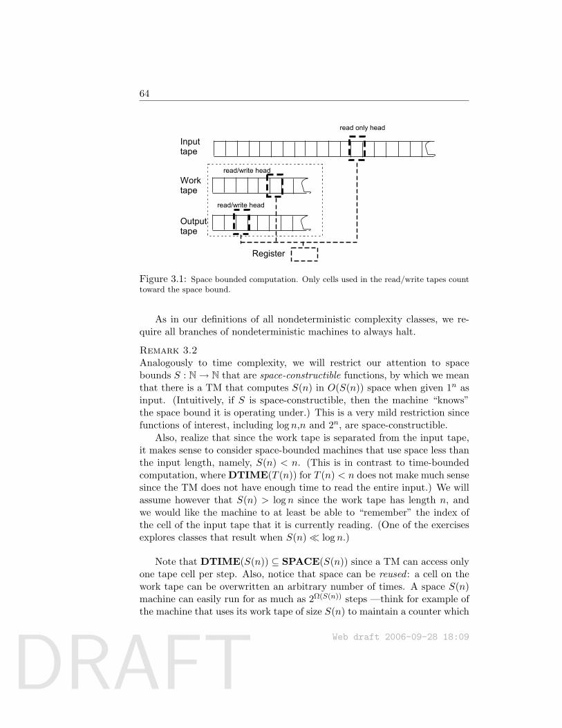
DRAFT

64

Inputtape

Worktape

Outputtape

Register

read only head

read/write head

read/write head

Figure 3.1: Space bounded computation. Only cells used in the read/write tapes counttoward the space bound.

As in our definitions of all nondeterministic complexity classes, we re-quire all branches of nondeterministic machines to always halt.

Remark 3.2Analogously to time complexity, we will restrict our attention to spacebounds S : N→ N that are space-constructible functions, by which we meanthat there is a TM that computes S(n) in O(S(n)) space when given 1n asinput. (Intuitively, if S is space-constructible, then the machine “knows”the space bound it is operating under.) This is a very mild restriction sincefunctions of interest, including log n,n and 2n, are space-constructible.

Also, realize that since the work tape is separated from the input tape,it makes sense to consider space-bounded machines that use space less thanthe input length, namely, S(n) < n. (This is in contrast to time-boundedcomputation, where DTIME(T (n)) for T (n) < n does not make much sensesince the TM does not have enough time to read the entire input.) We willassume however that S(n) > log n since the work tape has length n, andwe would like the machine to at least be able to “remember” the index ofthe cell of the input tape that it is currently reading. (One of the exercisesexplores classes that result when S(n) log n.)

Note that DTIME(S(n)) ⊆ SPACE(S(n)) since a TM can access onlyone tape cell per step. Also, notice that space can be reused : a cell on thework tape can be overwritten an arbitrary number of times. A space S(n)machine can easily run for as much as 2Ω(S(n)) steps —think for example ofthe machine that uses its work tape of size S(n) to maintain a counter which

Web draft 2006-09-28 18:09

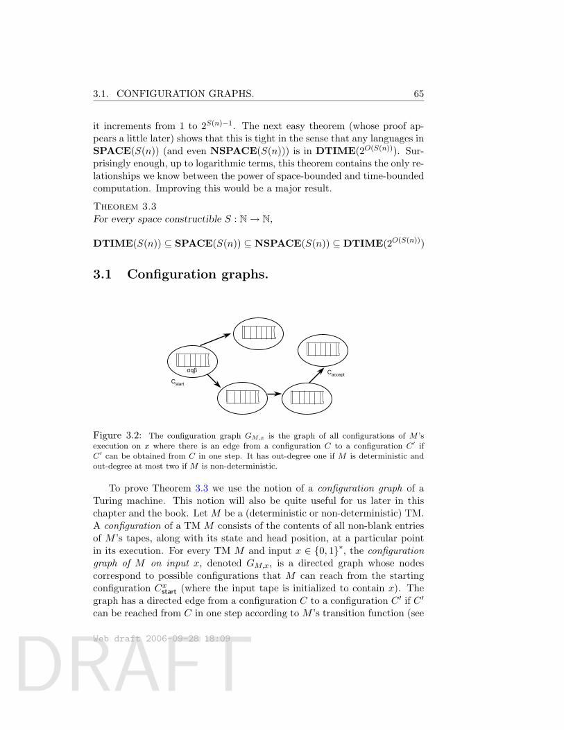
DRAFT

3.1. CONFIGURATION GRAPHS. 65

it increments from 1 to 2S(n)−1. The next easy theorem (whose proof ap-pears a little later) shows that this is tight in the sense that any languages inSPACE(S(n)) (and even NSPACE(S(n))) is in DTIME(2O(S(n))). Sur-prisingly enough, up to logarithmic terms, this theorem contains the only re-lationships we know between the power of space-bounded and time-boundedcomputation. Improving this would be a major result.

Theorem 3.3For every space constructible S : N→ N,

DTIME(S(n)) ⊆ SPACE(S(n)) ⊆ NSPACE(S(n)) ⊆ DTIME(2O(S(n)))

3.1 Configuration graphs.

Cstart

Cacceptαqβ

Figure 3.2: The configuration graph GM,x is the graph of all configurations of M ’sexecution on x where there is an edge from a configuration C to a configuration C′ ifC′ can be obtained from C in one step. It has out-degree one if M is deterministic andout-degree at most two if M is non-deterministic.

To prove Theorem 3.3 we use the notion of a configuration graph of aTuring machine. This notion will also be quite useful for us later in thischapter and the book. Let M be a (deterministic or non-deterministic) TM.A configuration of a TM M consists of the contents of all non-blank entriesof M ’s tapes, along with its state and head position, at a particular pointin its execution. For every TM M and input x ∈ 0, 1∗, the configurationgraph of M on input x, denoted GM,x, is a directed graph whose nodescorrespond to possible configurations that M can reach from the startingconfiguration Cxstart (where the input tape is initialized to contain x). Thegraph has a directed edge from a configuration C to a configuration C ′ if C ′

can be reached from C in one step according to M ’s transition function (see

Web draft 2006-09-28 18:09

DRAFT

66 3.1. CONFIGURATION GRAPHS.

Figure 3.2). Note that if M is deterministic then the graph has out-degreeone, and if M is non-deterministic then it has an out-degree at most two.Also note that we can assume that M ’s computation on x does not repeatthe same configuration twice (as otherwise it will enter into an infinite loop)and hence that the graph is a directed acyclic graph (DAG). By modifyingM to erase all its work tapes before halting, we can assume that there is onlya single configuration Caccept on which M halts and outputs 1. This meansthat M accepts the input x iff there exists a (directed) path in GM,x fromCstart to Caccept. We will use the following simple claim about configurationgraphs:

Claim 3.4Let GM,x be the configuration graph of a space-S(n) machine M on someinput x of length n. Then,

1. Every vertex in GM,x can be described using cS(n) bits for some con-stant c (depending on M ’s alphabet size and number of tapes) and inparticular, GM,x has at most 2cS(n) nodes.

2. There is an O(S(n))-size CNF formula ϕM,x such that for every twostrings C,C ′, ϕM,x(C,C ′) = 1 if and only if C,C ′ encode two neigh-boring configuration in GM,x.

Proof sketch: Part 1 follows from observing that a configuration iscompletely described by giving the contents of all work tapes, the position ofthe head, and the state that the TM is in (see Section 1.2.1). We can encodea configuration by first encoding the snapshot (i.e., state and current symbolread by all tapes) and then encoding in sequence the non-blank contentsof all the work-tape, inserting a special “marker” symbol, to denote thelocations of the heads.

Part 2 follows using similar ideas as in the proof of the Cook-Levintheorem (Theorem 2.11). There we showed that deciding whether two con-figurations are neighboring can be expressed as the AND of many checks,each depending on only a constant number of bits, where such checks canbe expressed by constant-sized CNF formulae by Claim 2.15.

Now we can prove Theorem 3.3.Proof of Theorem 3.3: Clearly SPACE(S(n)) ⊆ NSPACE(S(n))and so we just need to show NSPACE(S(n)) ⊆ DTIME(2O(S(n))). Byenumerating over all possible configurations we can construct the graphGM,x in 2O(S(n))-time and check whether Cstart is connected to Caccept in

Web draft 2006-09-28 18:09

DRAFT

3.2. SOME SPACE COMPLEXITY CLASSES. 67

GM,x using the standard (linear in the size of the graph) breadth-first searchalgorithm for connectivity (e.g., see [?]).

We also note that there exists a universal TM for space bounded com-putation analogously to Theorems 1.6 and ?? for deterministic and non-deterministic time bounded computation, see Section ?? below.

3.2 Some space complexity classes.

Now we define some complexity classes, where PSPACE,NPSPACE areanalogs of P and NP respectively.

Definition 3.5PSPACE = ∪c>0SPACE(nc)NPSPACE = ∪c>0NSPACE(nc)L = SPACE(log n)NL = NSPACE(log n)

Example 3.6We show how 3SAT ∈ PSPACE by describing a TM that decides 3SATin linear space (that is, O(n) space, where n is the size of the 3SAT in-stance). The machine just uses the linear space to cycle through all 2k

assignments in order, where k is the number of variables. Note that oncean assignment has been checked it can be erased from the worktape, andthe worktape then reused to check the next assignment. A similar idea ofcycling through all potential certificates applies to any NP language, so infact NP ⊆ PSPACE.

Example 3.7The reader should check (using the gradeschool method for arithmetic) thatthe following languages are in L:

EVEN = x : x has an even number of 1s .

MULT = ( xny, xmy, xnmy) : n ∈ N .

Web draft 2006-09-28 18:09

DRAFT

68 3.3. PSPACE COMPLETENESS

Its seems difficult to conceive of any complicated computations apartfrom arithmetic that use only O(log n) space. Nevertheless, we cannot cur-rently even rule out that 3SAT ∈ L (in other words —see the exercises—it is open whether NP 6= L). Space-bounded computations with spaceS(n) n seem relevant to computational problems such as web crawling.The world-wide-web may be viewed crudely as a directed graph, whose nodesare webpages and edges are hyperlinks. Webcrawlers seek to explore thisgraph for all kinds of information. The following problem PATH is naturalin this context:

PATH = 〈G, s, t〉 : G is a directed graph in which there is a path from s to t(1)

We claim that PATH ∈ NL. The reason is that a nondeterministic ma-chine can take a “nondeterministic walk” starting at s, always maintainingthe index of the vertex it is at, and using nondeterminism to select a neigh-bor of this vertex to go to next. The machine accepts iff the walk ends at tin at most n steps, where n is the number of nodes. If the nondeterministicwalk has run for n steps already and t has not been encountered, the ma-chine rejects. The work tape only needs to hold O(log n) bits of informationat any step, namely, the number of steps that the walk has run for, and theidentity of the current vertex.

Is PATH in L as well? This is an open problem, which, as we will shortlysee, is equivalent to whether or not L = NL. That is, PATH captures the“essence” of NL just as 3SAT captures the “essence” of NP. (Formally, wewill show that PATH is NL-complete. ) A recent surprising result showsthat the restriction of PATH to undirected graphs is in L; see Chapters 7and 17.

3.3 PSPACE completeness

As already indicated, we do not know if P 6= PSPACE, though we stronglybelieve that the answer is YES. Notice, P = PSPACE implies P = NP.Since complete problems can help capture the essence of a complexity class,we now present some complete problems for PSPACE.

Web draft 2006-09-28 18:09

DRAFT

3.3. PSPACE COMPLETENESS 69

Definition 3.8A language A is PSPACE-hard if for every L ∈ PSPACE, L ≤p A. If inaddition A ∈ PSPACE then A is PSPACE-complete.

Using our observations about polynomial-time reductions from Chapter ??we see that if any PSPACE-complete language is in P then so is every otherlanguage in PSPACE. Viewed contrapostively, if PSPACE 6= P then aPSPACE-complete language is not in P. Intuitively, a PSPACE-completelanguage is the “most difficult” problem of PSPACE. Just as NP triviallycontains NP-complete problems, so does PSPACE. The following is one(Exercise 3):

SPACETM = 〈M,w, 1n〉 : DTM M accepts w in space n . (2)

Now we see some more interesting PSPACE-complete problems. Weuse the notion of a quantified boolean formula, which is a boolean formula inwhich variables are quantified using ∃ and ∀ which have the usual meaning“there exists” and “for all” respectively. It is customary to also specify theuniverse over which these signs should be interpreted, but in our case theuniverse will always be the truth values 0, 1. Thus a quantified booleanformula has the form Q1x1Q2x2 · · ·Qnxnϕ(x1, x2, . . . , xn) where each Qi isone of the two quantifiers ∀ or ∃ and ϕ is an (unquantified) boolean formula1.

If all variables in the formula are quantified (in other words, there areno free variables) then a moment’s thought shows that such a formula iseither true or false —there is no “middle ground”. We illustrate the notionof truth by an example.

Example 3.9Consider the formula ∀x∃y (x ∧ y) ∨ (x ∧ y) where ∀ and ∃ quantify overthe universe 0, 1. Some reflection shows that this is saying “for everyx ∈ 0, 1 there is a y ∈ 0, 1 that is different from it”, which we canalso informally represent as ∀x∃y(x 6= y). This formula is true. (Note: the

1 We are restricting attention to quantified boolean formulae which are in prenex normalform, i.e., all quantifiers appear to the left. However, this is without loss of generalitysince we can transform a general formula into an equivalent formula in prenex form inpolynomial time using identities such as p∨∃xϕ(x) = ∃xp∨ϕ(x) and ¬∀xφ(x) = ∃x¬φ(x).Also note that unlike in the case of the SAT and 3SAT problems, we do not require thatthe inner unquantified formula ϕ is in CNF or 3CNF form. However this choice is also notimportant, since using auxiliary variables in a similar way to the proof of the Cook-Levintheorem, we can in polynomial-time transform a general quantified Boolean formula to anequivalent formula where the inner unquantified formula is in 3CNF form.

Web draft 2006-09-28 18:09

DRAFT


symbols = and 6= are not logical symbols per se, but are used as informalshorthand to make the formula more readable.)

However, switching the second quantifier to ∀ gives ∀x∀y (x∧y)∨(x∧y),which is false.

Example 3.10Recall that the SAT problem is to decide, given a Boolean formula ϕ thathas n free variables x1, . . . , xn, whether or not ϕ has a satisfying assignmentx1, . . . , xn ∈ 0, 1n such that ϕ(x1, . . . , xn) is true. An equivalent wayto phrase this problem is to ask whether the quantified Boolean formulaψ = ∃x1, . . . , xnϕ(x1, . . . , xn) is true.

The reader should also verify that the negation of the formulaQ1x1Q2x2 · · ·Qnxnϕ(x1, x2, . . . , xn) is the same as

Q′1x1Q′2x2 · · ·Q′nxn¬ϕ(x1, x2, . . . , xn),

where Q′i is ∃ if Qi was ∀ and vice versa. The switch of ∃ to ∀ in case of SATgives instances of TAUTOLOGY, the coNP-complete language encounteredin Chapter ??.

We define the language TQBF to be the set of quantified boolean formu-lae that are true.

Theorem 3.11TQBF is PSPACE-complete.

Proof: First we show that TQBF ∈ PSPACE. Let

ψ = Q1x1Q2x2 . . . Qnxnϕ(x1, x2, . . . , xn) (3)

be a quantified Boolean formula with n variables, where we denote the sizeof ϕ bym. We show a simple recursive algorithm A that can decide the truthof ψ in O(n+m) space. We will solve the slightly more general case where, inaddition to variables and their negations, ϕ may also include the constants0 (i.e., “false”) and 1 (i.e., “true”). If n = 0 (there are no variables) thenthe formula contains only constants and can be evaluated in O(m) time and

Web draft 2006-09-28 18:09

DRAFT


space. Let n > 0 and let ψ be as in (3). For b ∈ 0, 1, denote by ψx1=b themodification of ψ where the first quantifier Q1 is dropped and all occurrencesof x1 are replaced with the constant b. Algorithm A will work as follows: ifQ1 = ∃ then output 1 iff at least one of A(ψx1=0) and A(ψx1=1) returns 1.If Q1 = ∀ then output 1 iff both A(ψx1=0) and A(ψx1=1). By the definitionof ∃ and ∀, it is clear that A does indeed return the correct answer on anyformula ψ.

Let sn,m denote the space A uses on formulas with n variables and de-scription size m. The crucial point is —and here we use the fact that spacecan be reused—that both recursive computations A(ψx1=0) and A(ψx1=1)can run in the same space. Specifically, after computing A(ψx1=0), the algo-rithm A needs to retain only the single bit of output from that computation,and can reuse the rest of the space for the computation of A(ψx1=1). Thus,assuming that A uses O(m) space to write ψ x1 = b for its recursive calls,we’ll get that sn,m = sn−1,m +O(m) yielding sn,m = O(n ·m). 2

We now show that L ≤p TQBF for every L ∈ PSPACE. Let M be amachine that decides L in S(n) space and let x ∈ 0, 1n. We show howto construct a quantified Boolean formula ψ of size O(S(n)2) that is trueiff M accepts x. Recall that by Claim 3.4, there is a Boolean formula ϕM,x

such that for every two strings C,C ′ ∈ 0, 1m (where m = O(S(n)) is thenumber of bits require to encode a configuration of M), ϕM (C,C ′) = 1 iffC and C ′ are valid encodings of two adjacent configurations in the config-uration graph GM,x. We will use ϕM,x to come up with a polynomial-sizedquantified Boolean formula ψ′ that has polynomially many Boolean vari-ables bound by quantifiers and additional 2m unquantified Boolean variablesC1, . . . , Cm, C

′1, . . . , C

′m (or, equivalently, two variables C,C ′ over 0, 1m)

such that for every C,C ′ ∈ 0, 1m, ψ(C,C ′) is true iff C has a directedpath to C ′ in GM,x. By plugging in the values Cstart and Caccept to ψ′ weget a quantified Boolean formula ψ that is true iff M accepts x.

We define the formula ψ′ inductively. We let ψi(C,C ′) be true if andonly if there is a path of length at most 2i from C to C ′ in GM,x. Note thatψ′ = ψm and ψ0 = ϕM,x. The crucial observation is that there is a path of

2The above analysis already suffices to show that TQBF is in PSPACE. However, wecan actually show that the algorithm runs in linear space, specifically, O(m + n) space.Note that algorithm always works with restrictions of the same formula ψ. So it can keepa global partial assignment array that for each variable xi will contain either 0, 1 or ’q’

(if it’s quantified and not assigned any value). Algorithm A will use this global space forits operation, where in each call it will find the first quantified variable, set it to 0 andmake the recursive call, then set it to 1 and make the recursive call, and then set it backto ’q’. We see that A’s space usage is given by the equation sn,m = sn−1,m + O(1) andhence it uses O(n+m) space.

Web draft 2006-09-28 18:09

DRAFT


length at most 2i from C to C ′ if and only if there is a configuration C ′′

with such that there are paths of length at most 2i−1 path from C to C ′′

and from C ′′ to C ′. Thus the following formula suggests itself: ψi(C,C ′) =∃C ′′ ψi−1(C,C ′) ∧ ψi−1(C ′′, C).

However, this formula is no good. It implies that ψi’s is twice the size ofψi−1, and a simple induction shows that ψm has size about 2m, which is toolarge. Instead, we use additional quantified variables to save on descriptionsize, using the following more succinct definition for ψi(C,C ′):

∃C ′′∀D1∀D2((D1 = C ∧D2 = C ′)∨ (D1 = C ′ ∧D2 = C ′′)

)⇒ ψi−1(D1, D2)

(Here, as in Example 3.9, = and ⇒ are convenient shorthands, and can bereplaced by appropriate combinations of the standard Boolean operations∧ and ¬.) Note that size(ψi) ≤ size(ψi−1) + O(m) and hence size(ψm) ≤O(m2). We leave it to the reader to verify that the two definitions of ψi areindeed logically equivalent. As noted above we can convert the final formulato prenex form in polynomial time.

3.3.1 Savitch’s theorem.

The astute reader may notice that because the above proof uses the notionof a configuration graph and does not require this graph to have out-degreeone, it actually yields a stronger statement: that TQBF is not just hardfor PSPACE but in fact even for NPSPACE!. Since TQBF ∈ PSPACEthis implies that PSPACE = NSPACE, which is quite surprising sinceour intuition is that the corresponding classes for time (P and NP) aredifferent. In fact, using the ideas of the above proof, one can obtain thefollowing theorem:

Theorem 3.12 (Savitch [Sav70])For any space-constructible S : N→ N with S(n) ≥ logn, NSPACE(S(n)) ⊆SPACE(S(n)2)

We remark that the running time of the algorithm obtained from thistheorem can be as high as 2Ω(s(n)2).Proof: The proof closely follows the proof that TQBF is PSPACE-complete.Let L ∈ NSPACE(S(n)) be a language decided by a TM M such thatfor every x ∈ 0, 1n, the configuration graph G = GM,x has at mostM = 2O(S(n)) vertices. We describe a recursive procedure reach?(u, v, i)that returns “YES” if there is a path from u to v of length at most 2i

and “NO” otherwise. Note that reach?(s, t, d logM e) is “YES” iff t is

Web draft 2006-09-28 18:09

DRAFT


reachable from s. Again, the main observation is that there is a pathfrom u to v of length at most 2i iff there’s a vertex z with paths fromu to z and from z to v of lengths at most 2i−1. Thus, on input u, v, i,reach? will enumerate over all vertices z (at a cost of O(logM) space)and output “YES” if it finds one z such that reach?(u, z, i − 1)=“YES”and reach?(z, v, i− 1)=“YES”. Once again, the crucial observation is thatalthough the algorithm makes n recursive invocations, it can reuse the spacein each of these invocations. Thus, if we let sM,i be the space complexity ofreach?(u, v, i) on an M -vertex graph we get that sM,i = sM,i−1 +O(logM)and thus sM,logM = O(log2M) = O(S(n)2).

3.3.2 The essence of PSPACE: optimum strategies for game-playing.

Recall that the central feature of NP-complete problems is that a yes an-swer has a short certificate. The analogous unifying concept for PSPACE-complete problems seems to be that of a winning strategy for a 2-playergame with perfect information. A good example of such a game is Chess:two players alternately make moves, and the moves are made on a boardvisible to both. Thus moves have no hidden side effects; hence the term“perfect information.” What does it mean for a player to have a “winningstrategy?” The first player has a winning strategy iff there is a 1st movefor player 1 such that for every possible 1st move of player 2 there is a 2ndmove of player 1 such that.... (and so on) such that at the end player 1wins. Thus deciding whether or not the first player has a winning strategyseems to require searching the tree of all possible moves. This is reminiscentof NP, for which we also seem to require exponential search. But the cru-cial difference is the lack of a short “certificate” for the statement “Player1 has a winning strategy,” since the only certificate we can think of is thewinning strategy itself, which as noticed, requires exponentially many bitsto even describe. Thus we seem to be dealing with a fundamentally differentphenomenon than the one captured by NP.

The interplay of existential and universal quantifiers in the descriptionof the the winning strategy motivates us to invent the following game.

Example 3.13 (The QBF game)The “board” for the QBF game is a Boolean formula ϕ whose free variablesare x1, x2, . . . , x2n. The two players alternately make moves, which involvepicking values for x1, x2, . . . , in order. Thus player 1 will pick values for the

Web draft 2006-09-28 18:09

DRAFT


odd-numbered variables x1, x3, x5, . . . (in that order) and player 2 will pickvalues for the even-numbered variables x2, x4, x6, . . . ,. We say player 1 winsiff at the end ϕ becomes true.

Clearly, player 1 has a winning strategy iff

∃x1∀x2∃x3∀x4 · · · ∀x2nϕ(x1, x2, . . . , x2n),

namely, iff this quantified boolean formula is true.Thus deciding whether player 1 has a winning strategy for a given board

in the QBF game is PSPACE-complete.

At this point, the reader is probably thinking of familiar games such asChess, Go, Checkers etc. and wondering whether complexity theory mayhelp differentiate between them—for example, to justify the common intu-ition that Go is more difficult than Chess. Unfortunately, formalizing theseissues in terms of asymptotic complexity is tricky because these are finitegames, and as far as the existence of a winning strategy is concerned, thereare at most three choices: Player 1 has has a winning strategy, Player 2 does,or neither does (they can play to a draw). However, one can study general-izations of these games to an n×n board where n is arbitrarily large —thismay involve stretching the rules of the game since the definition of chessseems tailored to an 8 × 8 board— and then complexity theory can indeedby applied. For most common games, including chess, determining whichplayer has a winning strategy in the n × n version is PSPACE-complete(see [?]or [?]). Note that if NP 6= PSPACE then in general there is noshort certificate for exhibiting that either player in the TQBF game has awinning strategy, which is alluded to in Evens and Tarjan’s quote at thestart of the chapter.

Proving PSPACE-completeness of games may seem like a frivolous pur-suit, but similar ideas lead to PSPACE-completeness of some practicalproblems. Usually, these involve repeated moves that are in turn coun-teracted by an adversary. For instance, many computational problems ofrobotics are PSPACE-complete: the “player” is the robot and the “adver-sary” is the environment. (Treating the environment as an adversary mayappear unduly pessimistic; but unfortunately even assuming a benign or “in-different” environment still leaves us with a PSPACE-complete problem;see the Chapter notes.)

Web draft 2006-09-28 18:09

DRAFT

3.4. NL COMPLETENESS 75

3.4 NL completeness

Now we consider problems that form the “essence” of non-deterministic log-arithmic space computation, in other words, problems that are complete forNL. What kind of reduction should we use? We cannot use the polynomial-time reduction since NL ⊆ P. Thus every language in NL is polynomial-time reducible to the trivial language 1 (reduction: “decide using polyno-mial time whether or not the input is in the NL language, and then mapto 1 or 0 accordingly”). Intuitively, such trivial languages should not be the“hardest” languages of NL.

When choosing the type of reduction to define completeness for a com-plexity class, we must keep in mind the complexity phenomenon we seek tounderstand. In this case, the complexity question is whether or not NL = L.The reduction should not be more powerful than the weaker class, which isL. For this reason we use logspace reductions —for further, justification, seepart (b) of Lemma 3.15 below). To define such reductions we must tackle thetricky issue that a reduction typically maps instances of size n to instancesof size at least n, and so a logspace machine computing such a reductiondoes not have even the memory to write down its output. The way outis to require that the reduction should be able to compute any desired bitof the output in logarithmic space. In other words, if the reduction weregiven a separate output tape, it could in principle write out the entire newinstance by first computing the first bit, then the second bit, and so on.(Many texts define such reductions using a “write-once” output tape.) Theformal definition is as follows.Definition 3.14 (logspace reduction)Let f :0, 1∗ → 0, 1∗ be a polynomially-bounded function (i.e., there’s aconstant c > 0 such that f(x) ≤ |x|c for every x ∈ 0, 1∗). We say that fis implicitly logspace computable, if the languages Lf = 〈x, i〉 | f(x)i = 1and L′f = 〈x, i〉 | i ≤ |f(x)| are in L.

Informally, we can think of a single O(log |x|)-space machine that giveninput (x, i) outputs f(x)|i provided i ≤ |f(x)|.

Language A is logspace reducible to language B, denoted A ≤l B, if thereis a function f :0, 1∗ → 0, 1∗ that is implicitly logspace computable andx ∈ A iff f(x) ∈ B for every x ∈ 0, 1∗.

Logspace reducibility satisfies usual properties one expects.

Lemma 3.15(a) If A ≤l B and B ≤l C then A ≤l C. (b) If A ≤l B and B ∈ L thenA ∈ L.

Web draft 2006-09-28 18:09

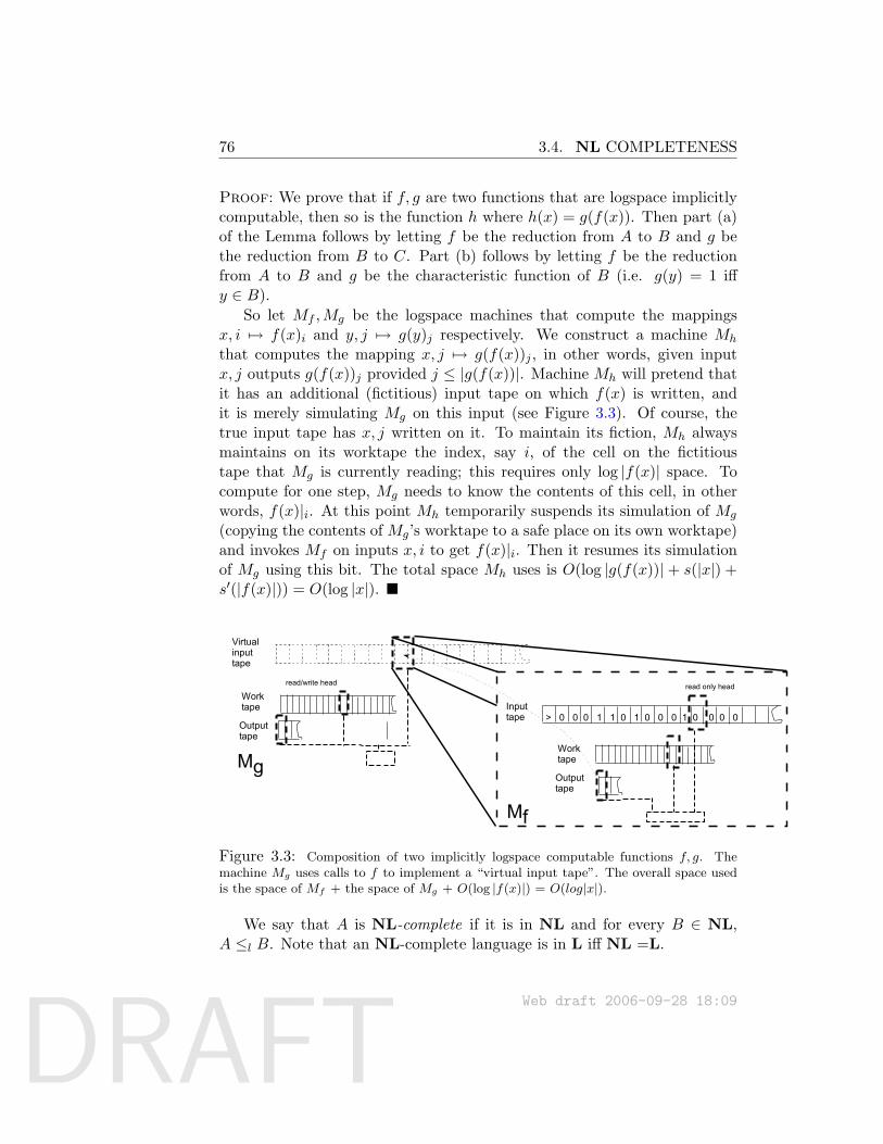
DRAFT

76 3.4. NL COMPLETENESS

Proof: We prove that if f, g are two functions that are logspace implicitlycomputable, then so is the function h where h(x) = g(f(x)). Then part (a)of the Lemma follows by letting f be the reduction from A to B and g bethe reduction from B to C. Part (b) follows by letting f be the reductionfrom A to B and g be the characteristic function of B (i.e. g(y) = 1 iffy ∈ B).

So let Mf ,Mg be the logspace machines that compute the mappingsx, i 7→ f(x)i and y, j 7→ g(y)j respectively. We construct a machine Mh

that computes the mapping x, j 7→ g(f(x))j , in other words, given inputx, j outputs g(f(x))j provided j ≤ |g(f(x))|. Machine Mh will pretend thatit has an additional (fictitious) input tape on which f(x) is written, andit is merely simulating Mg on this input (see Figure 3.3). Of course, thetrue input tape has x, j written on it. To maintain its fiction, Mh alwaysmaintains on its worktape the index, say i, of the cell on the fictitioustape that Mg is currently reading; this requires only log |f(x)| space. Tocompute for one step, Mg needs to know the contents of this cell, in otherwords, f(x)|i. At this point Mh temporarily suspends its simulation of Mg

(copying the contents of Mg’s worktape to a safe place on its own worktape)and invokes Mf on inputs x, i to get f(x)|i. Then it resumes its simulationof Mg using this bit. The total space Mh uses is O(log |g(f(x))| + s(|x|) +s′(|f(x)|)) = O(log |x|).

Inputtape

Worktape

Outputtape

> 0 0 0 1 1 0 1 0 0 0 1 0 0 0 0

read only headread/write head

Mf

Worktape

Outputtape

Virtualinputtape

Mg

Figure 3.3: Composition of two implicitly logspace computable functions f, g. Themachine Mg uses calls to f to implement a “virtual input tape”. The overall space usedis the space of Mf + the space of Mg + O(log |f(x)|) = O(log|x|).

We say that A is NL-complete if it is in NL and for every B ∈ NL,A ≤l B. Note that an NL-complete language is in L iff NL =L.

Web draft 2006-09-28 18:09

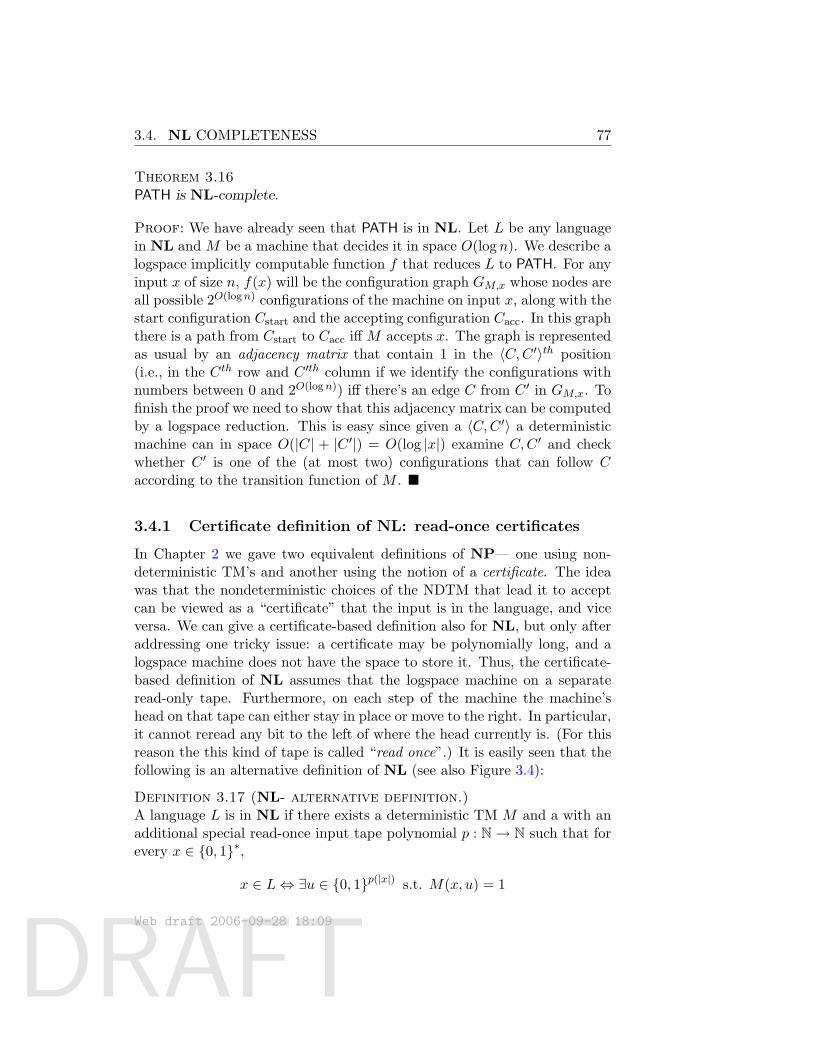
DRAFT


Theorem 3.16PATH is NL-complete.

Proof: We have already seen that PATH is in NL. Let L be any languagein NL and M be a machine that decides it in space O(log n). We describe alogspace implicitly computable function f that reduces L to PATH. For anyinput x of size n, f(x) will be the configuration graph GM,x whose nodes areall possible 2O(logn) configurations of the machine on input x, along with thestart configuration Cstart and the accepting configuration Cacc. In this graphthere is a path from Cstart to Cacc iff M accepts x. The graph is representedas usual by an adjacency matrix that contain 1 in the 〈C,C ′〉th position(i.e., in the Cth row and C ′th column if we identify the configurations withnumbers between 0 and 2O(logn)) iff there’s an edge C from C ′ in GM,x. Tofinish the proof we need to show that this adjacency matrix can be computedby a logspace reduction. This is easy since given a 〈C,C ′〉 a deterministicmachine can in space O(|C| + |C ′|) = O(log |x|) examine C,C ′ and checkwhether C ′ is one of the (at most two) configurations that can follow Caccording to the transition function of M .

3.4.1 Certificate definition of NL: read-once certificates

In Chapter 2 we gave two equivalent definitions of NP— one using non-deterministic TM’s and another using the notion of a certificate. The ideawas that the nondeterministic choices of the NDTM that lead it to acceptcan be viewed as a “certificate” that the input is in the language, and viceversa. We can give a certificate-based definition also for NL, but only afteraddressing one tricky issue: a certificate may be polynomially long, and alogspace machine does not have the space to store it. Thus, the certificate-based definition of NL assumes that the logspace machine on a separateread-only tape. Furthermore, on each step of the machine the machine’shead on that tape can either stay in place or move to the right. In particular,it cannot reread any bit to the left of where the head currently is. (For thisreason the this kind of tape is called “read once”.) It is easily seen that thefollowing is an alternative definition of NL (see also Figure 3.4):

Definition 3.17 (NL- alternative definition.)A language L is in NL if there exists a deterministic TM M and a with anadditional special read-once input tape polynomial p : N→ N such that forevery x ∈ 0, 1∗,

x ∈ L⇔ ∃u ∈ 0, 1p(|x|) s.t. M(x, u) = 1

Web draft 2006-09-28 18:09

DRAFT


Inputtape

Worktape

Outputtape

Register

read only head

read/write head

read/write head

Certificatetape

read once head

Figure 3.4: Certificate view of NL. The certificate for input x is placed on a special“read-once” tape on which the machine’s head can never move to the left.

where by M(x, u) we denote the output of M where x is placed on its inputtape and u is placed on its special read-once tape, and M uses at mostO(log |x|) space on its read/write tapes for every input x.

3.4.2 NL = coNL

Consider the problem PATH, i.e., the complement of PATH. A decisionprocedure for this language must accept when there is no path from s tot in the graph. Unlike in the case of PATH, there is no natural certificatefor the non-existence of a path from s to t and thus it seemed “obvious” toresearchers that PATH 6∈ NL, until the discovery of the following theoremin the 1980s proved them wrong.

Theorem 3.18 (Immerman-Szlepcsenyi)PATH ∈ NL.

Proof: As we saw in Section 3.4.1, we need to show an O(log n)-spacealgorithm A such that for every n-vertex graph G and vertices s and t,there exists a polynomial certificate u such that A(〈G, s, t〉, u) = 1 if andonly if t is not reachable from u in G, where A has only read-once access tou.

What can we certify to an O(log n)-space algorithm? Let Ci be the setof vertices that are reachable from s in G within at most i steps. For everyi ∈ [n] and vertex v, we can easily certify that v is in Ci. The certificatesimply contains the labels v0, v1, . . . , vk of the vertices along the path from

Web draft 2006-09-28 18:09

DRAFT


s to v (we can assume without loss of generality that vertices are labeledby the numbers 1 to n and hence the labels can be described by log n bitstrings). The algorithm can check the certificate using read-once access byverifying that (1) v0 = s, (2) for j > 0, there is an edge from vj−1 to vj ,(3) vk = v and (using a counter) that (4) the path ends within at most isteps. Note that the certificate is indeed of size at most polynomial in n.

Our algorithm uses the following two procedures:

1. Procedure to certify that a vertex v is not in Ci given the size of Ci.

2. Procedure to certify that |Ci| = c for some number c, given the size ofCi−1.

Since C0 = s and Cn contains all the vertices reachable from s, wecan apply the second procedure iteratively to learn the sizes of the setsC1, . . . , Cn, and then use the first procedure to certify that t 6∈ Cn.

Certifying that v is not in Ci, given |Ci|. The certificate is simply thelist of certificates that u is in Ci for every u ∈ Ci sorted in ascending orderof labels (recall that we identify labels with numbers in [n]). The algorithmchecks that (1) each certificate is valid, (2) the label of a vertex u for whicha certificate is given is indeed larger than the label of the previous vertex,(3) no certificate is provided for v, and (4) the total number of certificatesprovided is exactly |Ci|. If v 6∈ Ci then the algorithm will accept the abovecertificate, but if v ∈ Ci there will not exist |Ci| certificates that verticesu1 < u2 < . . . < u|Ci| are in Ci where uj 6= v for every j.

Certifying that v is not in Ci, given |Ci−1|. Before showing how wecertify that |Ci| = c given |Ci−1|, we show how to certify that v 6∈ Ci withthis information. This is very similar to the above procedure: the certificateis the list of |Ci−1| certificates that u ∈ Ci−1 for every u ∈ Ci−1 in ascendingorder. The algorithm checks everything as before except that in step (3) itverifies that no certificate is given for v or for a neighbor of v. Since v ∈ Ciif and only if there exists u ∈ Ci−1 such that u = v or u is a neighbor of vin G, the procedure will not accept a false certificate by the same reasonsas above.

Certifying that |Ci| = c given |Ci−1|. For every vertex v, if v ∈ Ci thenthere is a certificate for this fact, and by the above procedure, given |Ci−1|,if v 6∈ Ci then there is a certificate for this fact as well. The certificatethat |Ci| = c will consist of n certificates for each of the vertices 1 to n inascending order. For every vertex u, there will be an appropriate certificate

Web draft 2006-09-28 18:09

DRAFT


depending on whether u ∈ Ci or not. The algorithm will verify all thecertificate and count the number of certificate that a vertex is in Ci. Itaccepts if this count is equal to c.

Using the notion of the configuration graph we can modify the proof ofTheorem 3.18 to prove the following:

Corollary 3.19For every space constructible S(n) > log n, NSPACE(S(n)) = coNSPACE(S(n)).

Our understanding of space-bounded complexity.The following is our understanding of space-bounded complexity.

DTIME(s(n))⊆SPACE(s(n))⊆NSPACE(s(n))=coNSPACE(s(n))⊆DTIME(2O(s(n))).

None of the inclusions are known to be strict though we believe they all are.


The concept of space complexity had already been explored in the 1960s;in particular, Savitch’s theorem predates the Cook-Levin theorem. Stock-meyer and Meyer proved the PSPACE-completeness of TQBF soon afterCook’s paper appeared. A few years later Even and Tarjan pointed outthe connection to game-playing and proved the PSPACE-completeness ofa game called Generalized Hex. Papadimitriou’s book gives a detailed ac-count of PSPACE-completeness. He also shows PSPACE-completenessof several Games against nature first defined in [Pap85]. Unlike the TQBFgame, where one player is Existential and the other Universal, here thesecond player chooses moves randomly. The intention is to model gamesplayed against nature—where “nature” could mean not just weather for ex-ample, but also large systems such as the stock market that are presumably“indifferent” to the fate of individuals. Papadimitriou gives an alternativecharacterization PSPACE using such games. A stronger result, namely, acharacterization of PSPACE using interactive proofs, is described in Chap-ter 9.

Exercises

§1 Show that SPACE(S(n)) = SPACE(0) when S(n) = log log n.

Web draft 2006-09-28 18:09

DRAFT


§2 Prove the existence of a universal TM for space bounded computation(analogously to the deterministic universal TM of Theorem 1.6). Thatis, prove that there exists a a TM SU such that for every string α, andinput x, if the TM Mα represented by α halts on x before using t cellsof its work tapes then SU(α, t, x) = Mα(x), and moreover, SU usesat most Ct cells of its work tapes, where C is a constant dependingonly on Mα. (Despite the fact that the bound here is better than thebound of Theorem 1.6, the proof of this statement is actually easierthan the proof of Theorem 1.6.)

§3 Prove that the language SPACETM of (2) is PSPACE-complete.

§4 Show that the following language is NL-complete:

xGy : G is a strongly connected digraph .

§5 Show that 2SAT is in NL.

§6 Suppose we define NP-completeness using logspace reductions insteadof polynomial-time reductions. Show (using the proof of the Cook-Levin Theorem) that SAT and 3SAT continue to be NP-complete un-der this new definition. Conclude that SAT ∈ L iff NP = L.

§7 Show that TQBF is complete for PSPACE also under logspace reduc-tions.

§8 Show that in every finite 2-person game with perfect information (byfinite we mean that there is an a priori upperbound n on the numberof moves after which the game is over and one of the two players isdeclared the victor —there are no draws) one of the two players has awinning strategy.

§9 Define polyL to be ∪c>0SPACE(logc n). Steve’s Class SC (named inhonor of Steve Cook) is defined to be the set of languages that can bedecided by deterministic machines that run in polynomial time andlogc n space for some c > 0.

It is an open problem whether PATH ∈ SC. Why does Savitch’s The-orem not resolve this question?

Is SC the same as polyL ∩P?

Web draft 2006-09-28 18:09

DRAFT


Web draft 2006-09-28 18:09

DRAFT

Chapter 4

Diagonalization

“..the relativized P =?NP question has a positive answer forsome oracles and a negative answer for other oracles. We feelthat this is further evidence of the difficulty of the P =?NPquestion.”Baker, Gill, Solovay. [BGS75]

One basic goal in complexity theory is to separate interesting complexityclasses. To separate two complexity classes we need to exhibit a machine inone class that gives a different answer on some input from every machine inthe other class. This chapter describes diagonalization, essentially the onlygeneral technique known for constructing such a machine. The first use ofdiagonalization is to prove hierarchy theorems, according to which givingTuring machines more computational resources (such as time, space, andnon-determinism) allows them to solve a strictly larger number of problems.We will also use it to show that if P 6= NP then there exist problems thatare neither in P nor NP-complete.

Though diagonalization led to some of these early successes of complex-ity theory, researchers realized in the 1970s that diagonalization alone maynot resolve P versus NP and other interesting questions; see Section 4.5.Interestingly, the limits of diagonalization are proved using diagonalization.

This last result caused diagonalization to go out of favor for many years.But some recent results (see Section 17.3 for an example) use diagonalizationas a key component. Thus future complexity theorists should master thissimple idea before going on to anything fancier!


83

DRAFT

84 4.1. TIME HIERARCHY THEOREM

Machines as strings and the universal TM. The one common toolused in all diagonalization proofs is the representation of TMs by strings,such that given a string x a universal TM can simulate the machine Mx

represented by x with a small (i.e. at most logarithmic) overhead, see The-orems 1.6, ?? and ??. Recall that we assume that every string x representssome machine and every machine is represented by infinitely many strings.For i ∈ N, we will also use the notation Mi for the machine represented bythe string that is the binary expansion of the number i.

4.1 Time Hierarchy Theorem

The Time Hierarchy Theorem shows that allowing Turing Machines morecomputation time strictly increases the class of languages that they candecide. Recall that a function f :N → N is a time-constructible function ifthere is a Turing machine that, given the input 1n, writes down 1f(n) on itstape in O(f(n)) time. Usual functions like n log n or n2 satisfy this property,and we will restrict attention to running times that are time-constructible.

Theorem 4.1If f, g are time-constructible functions satisfying f(n) log f(n) = o(g(n)),then

DTIME(f(n)) ( DTIME(g(n)) (1)

Proof: To showcase the essential idea of the proof of Theorem 4.1, we provethe simpler statement DTIME(n) DTIME(n1.5).

Consider the following Turing Machine D: “On input x, run for |x|1.4steps the Universal TM U of Theorem 1.6 to simulate the execution of Mx

on x. If Mx outputs an answer in this time, namely, Mx(x) ∈ 0, 1 thenoutput the opposite answer (i.e., output 1−Mx(x)). Else output 0.” HereMx is the machine represented by the string x.

By definition, D halts within n1.4 steps and hence the language L decidedby D is in DTIME(n1.5). We claim that L 6∈ DTIME(n).

For contradiction’s sake assume that some TM M decides L but runs intime cn on inputs of size n. Then every x ∈ 0, 1∗, M(x) = D(x).

The time to simulate M by the universal Turing machine U on everyinput x is at most c′c|x| log |x| for some constant c′ (depending on the al-phabet size and number of tapes and states of M , but independent of |x|).There exists a number n0 such that for every n ≥ n0, n1.4 > c′cn log n. Letx be a string representing the machine M of length at least n0 (there existssuch a string since M is represented by infinitely many strings). Then, D(x)

Web draft 2006-09-28 18:09

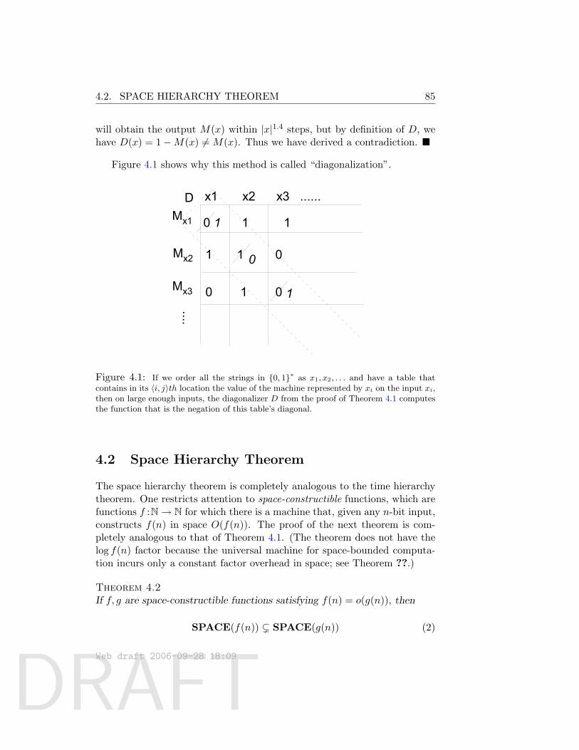
DRAFT

4.2. SPACE HIERARCHY THEOREM 85

will obtain the output M(x) within |x|1.4 steps, but by definition of D, wehave D(x) = 1−M(x) 6= M(x). Thus we have derived a contradiction.

Figure 4.1 shows why this method is called “diagonalization”.

Mx1

x1 x2 x3 ......

Mx2

Mx3

....

0 1 1 1

1 1 0

0 1 0

0

1

D

Figure 4.1: If we order all the strings in 0, 1∗ as x1, x2, . . . and have a table thatcontains in its 〈i, j〉th location the value of the machine represented by xi on the input xi,then on large enough inputs, the diagonalizer D from the proof of Theorem 4.1 computesthe function that is the negation of this table’s diagonal.

4.2 Space Hierarchy Theorem

The space hierarchy theorem is completely analogous to the time hierarchytheorem. One restricts attention to space-constructible functions, which arefunctions f :N→ N for which there is a machine that, given any n-bit input,constructs f(n) in space O(f(n)). The proof of the next theorem is com-pletely analogous to that of Theorem 4.1. (The theorem does not have thelog f(n) factor because the universal machine for space-bounded computa-tion incurs only a constant factor overhead in space; see Theorem ??.)

Theorem 4.2If f, g are space-constructible functions satisfying f(n) = o(g(n)), then

SPACE(f(n)) ( SPACE(g(n)) (2)

Web draft 2006-09-28 18:09

DRAFT

86 4.3. NONDETERMINISTIC TIME HIERARCHY THEOREM

4.3 Nondeterministic Time Hierarchy Theorem

The following is the hierarchy theorem for non-deterministic Turing ma-chines.

Theorem 4.3If f, g are time constructible functions satisfying f(n+ 1) = o(g(n)), then

NTIME(f(n)) NTIME(g(n)) (3)

Proof: Again, we just showcase the main idea by proving NTIME(n) NTIME(n1.5). The technique from the previous section does not directlyapply, since it has to determine the answer of a TM in order to flip it. Todetermine the answer of a nondeterminisitic that runs in O(n) time, wemay need to examine as many as 2Ω(n) possible strings of non-deterministicchoices. So it is unclear that how the “diagonalizer” machine can determinein O(n1.5) (or even O(n100)) time how to flip this answer. Instead we in-troduce a technique called lazy diagonalization, which is only guaranteed toflip the answer on some input in a fairly large range.

For every i ∈ N we denote by Mi the non-deterministic TM representedby i’s binary expansion according to the universal NDTM NU (see The-orem ??). We define the function f : N → N as follows: f(1) = 2 andf(i+ 1) = 2f(i)1.2 . Note that given n, we can can easily find in O(n1.5) timethe number i such that n is sandwiched between f(i) and f(i + 1). Ourdiagonalizing machine D will try to flip the answer of Mi on some input inthe set 1n : f(i) < n ≤ f(i+ 1). It is defined as follows:

“On input x, if x 6∈ 1∗, reject. If x = 1n, then compute i such thatf(i) < n ≤ f(i+ 1) and

1. If f(i) < n < f(i + 1) then simulate Mi on input 1n+1 using nonde-terminism in n1.1 time and output its answer. (If the simulation takesmore than that then halt and accept.)

2. If n = f(i+ 1), accept 1n iff Mi rejects 1f(i)+1 in (f(i) + 1)1.5 time.”

Note that Part 2 requires going through all possible exp((f(i) + 1)1.1)branches of Mi on input 1f(i)+1, but that is fine since the input size f(i+1)is 2f(i)1.2 . We conclude that NDTM D runs in O(n1.5) time. Let L be thelanguage decided by D. We claim that L 6∈ NTIME(n).

Indeed, suppose for the sake of contradiction that L is decided by anNDTM M running in cn steps (for some constant c). Since each NDTM isrepresented by infinitely many strings, we can find i large enough such that

Web draft 2006-09-28 18:09

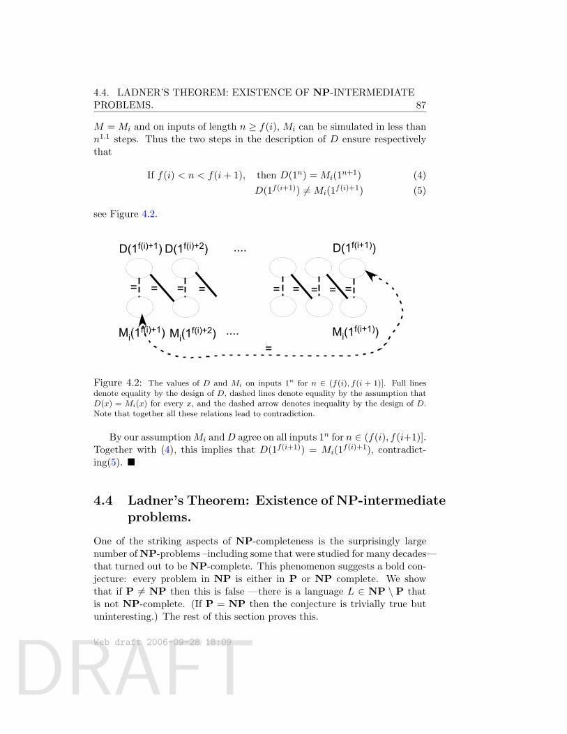
DRAFT

4.4. LADNER’S THEOREM: EXISTENCE OF NP-INTERMEDIATEPROBLEMS. 87

M = Mi and on inputs of length n ≥ f(i), Mi can be simulated in less thann1.1 steps. Thus the two steps in the description of D ensure respectivelythat

If f(i) < n < f(i+ 1), then D(1n) = Mi(1n+1) (4)D(1f(i+1)) 6= Mi(1f(i)+1) (5)

see Figure 4.2.

D(1f(i)+1) D(1f(i)+2) .... D(1f(i+1))

Mi(1f(i)+1) Mi(1

f(i)+2) .... Mi(1f(i+1))

= = = = = = = = =

=

Figure 4.2: The values of D and Mi on inputs 1n for n ∈ (f(i), f(i + 1)]. Full linesdenote equality by the design of D, dashed lines denote equality by the assumption thatD(x) = Mi(x) for every x, and the dashed arrow denotes inequality by the design of D.Note that together all these relations lead to contradiction.

By our assumptionMi andD agree on all inputs 1n for n ∈ (f(i), f(i+1)].Together with (4), this implies that D(1f(i+1)) = Mi(1f(i)+1), contradict-ing(5).

4.4 Ladner’s Theorem: Existence of NP-intermediateproblems.

One of the striking aspects of NP-completeness is the surprisingly largenumber of NP-problems –including some that were studied for many decades—that turned out to be NP-complete. This phenomenon suggests a bold con-jecture: every problem in NP is either in P or NP complete. We showthat if P 6= NP then this is false —there is a language L ∈ NP \ P thatis not NP-complete. (If P = NP then the conjecture is trivially true butuninteresting.) The rest of this section proves this.

Web draft 2006-09-28 18:09

DRAFT

884.4. LADNER’S THEOREM: EXISTENCE OF NP-INTERMEDIATE

PROBLEMS.

Theorem 4.4 (Ladner’s Theorem [?])Suppose that P 6= NP. Then there exists a language L ∈ NP \ P that isnot NP-complete.

Proof: If P 6= NP then we know at least one language in NP\P: namely,the NP-complete language SAT. Consider the language SATH of length nsatisfiable formulae that are padded with nH(n) 1’s for some polynomial-timecomputable functionH : N→ N (i.e., SATH =

ψ01n

H(n): ψ ∈ SAT and n = |ψ|

).

Consider two possibilities:

(a) H(n) is at most some constant c for every n. In this case SATH issimply SAT with a polynomial amount of “padding.” Thus, SATH isalso NP-complete and is not in P if P 6= NP.

(b) H(n) tends to infinity with n, and thus the padding is of superpolyno-mial size. In this case, we claim that SATH cannot be NP-complete.Indeed, if there is a O(ni)-time reduction f from SAT to SATH thensuch a reduction reduces the satisfiability of SAT instances of lengthn to instances of SATH of length O(ni), which must have the formψ01|ψ|

H(|ψ|), where |ψ| + |ψ|H(|ψ|) = O(ni), and hence |ψ| = o(n). In

other words, we have a polynomial-time reduction from SAT instancesof length n to SAT instances of length o(n), which implies SAT canbe solved in polynomial time. (The algorithm consists of applying thereduction again and again, reducing the size of the instances each timeuntil the instance is of size O(1) and can be solved in O(1) time bybrute force) This is a contradiction to the assumption P 6= NP.

The proof of the Theorem uses a language SATH for a function H thatin some senses combines the two cases above. This function tends to infinitywith n, so that SATH is not NP-complete as in Case (b), but grows slowlyenough to assure SATH 6∈ P as in Case (a). Function H is defined as follows:

H(n) is the smallest number i < log log n such that for everyx ∈ 0, 1∗ with |x| ≤ log n,

Mi halts on x within i|x|i steps and Mi outputs 1 iff x ∈ SATH

where Mi is the machine represented by the binary expansion ofi according to the representation scheme of the universal Turingmachine U of Theorem 1.6. If there is no such i then we letH(n) = log log n.

Web draft 2006-09-28 18:09

DRAFT

4.4. LADNER’S THEOREM: EXISTENCE OF NP-INTERMEDIATEPROBLEMS. 89

Notice, this is implicitly a recursive definition since the definition ofH de-pends on SATH , but a moment’s thought shows that H is well-defined sinceH(n) determines membership in SATH of strings whose length is greaterthan n, and the definition of H(n) only relies upon checking the status ofstrings of length at most log n.

There is a trivial algorithm to compute H(n) in O(n3) time. Afterall, we only need to (1) compute H(k) for every k ≤ log n, (2) simu-late at most log log n machines for every input of length at most log n forlog log n(log n)log logn = o(n) steps, and (3) compute SAT on all the inputsof length at most log n.

Now we have the following two claims.

claim 1: SATH is not in P. Suppose, for the sake of contradiction, thatthere is a machine M solving SATH in at most cnc steps. Since M is repre-sented by infinitely many strings, there is a number i > c such that M = Mi.By the definition of H(n) this implies that for n > 22i , H(n) ≤ i. But thismeans that for all sufficiently large input lengths, SATH is simply the lan-guage SAT padded with a polynomial (i.e., ni) number of 1’s, and so cannotbe in P unless P = NP.

claim 2: SATH is not NP-complete. As in Case (b), it suffices to show thatH(n) tends to infinity with n. We prove the equivalent statement that forevery integer i, there are only finitely many n’s such that H(n) = i: sinceSATH 6∈ P, for each i we know that there is an input x such that given i|x|itime, Mi gives the incorrect answer to whether or not x ∈ SATH . Then thedefinition of H ensures that for every n > 2|x|, H(x) 6= i.

Remark 4.5We do not know of a natural decision problem that, assuming NP 6= P, isproven to be in NP \ P but not NP-complete, and there are remarkablyfew candidates for such languages. However, there are a few fascinatingexamples for languages not known to be either in P nor NP-complete. Twosuch examples are the Factoring and Graph isomorphism languages (seeExample 2.3). No polynomial-time algorithm is currently known for theselanguages, and there is some evidence that they are not NP complete (seeChapter 9).

Web draft 2006-09-28 18:09

DRAFT

904.5. ORACLE MACHINES AND THE LIMITS OF

DIAGONALIZATION?

4.5 Oracle machines and the limits of diagonaliza-tion?

Quantifying the limits of “diagonalization” is not easy. Certainly, the di-agonalization in Sections 4.3 and 4.4 seems more clever than the one inSection 4.1 or the one that proves the undecidability of the halting problem.

For concreteness, let us say that “diagonalization” is any technique thatrelies upon the following properties of Turing machines

1. The existence of an effective representation of Turing machines bystrings.

2. The ability of one TM to simulate any another without much overheadin running time or space.

Any argument that only uses these facts is treating machines as black-boxes: the machine’s internal workings do not matter. We show a generalway to define a variant of Turing Machines called oracle Turing Machinesthat still satisfy the above two properties. However, one way of defining thevariants results in TMs for which P = NP, whereas the other way resultsin TMs for which P 6= NP. We conclude that to resolve P versus NP weneed to use some other property besides the above two.

Oracle machines will be used elsewhere in this book in other contexts.These are machines that are given access to an “oracle” that can magicallysolve the decision problem for some language O ⊆ 0, 1∗. The machine hasa special oracle tape on which it can write a string q ∈ 0, 1∗ on a and inone step gets an answer to a query of the form “Is q in O?”. This can berepeated arbitrarily often with different queries. If O is a difficult languagethat cannot be decided in polynomial time then this oracle gives an addedpower to the TM.

Definition 4.6 (Oracle Turing Machines)An oracle Turing machine is a TM M that has a special read/write tape wecall M ’s oracle tape and three special states qquery, qyes, qno. To execute M ,we specify in addition to the input a language O ⊆ 0, 1∗ that is used asthe oracle for M . Whenever during the execution M enters the state qquery,the machine moves into the state qyes if q ∈ O and qno if q 6∈ O, where qdenotes the contents of the special oracle tape. Note that, regardless of thechoice of O, a membership query to O counts only as a single computationalstep. If M is an oracle machine, O ⊆ 0, 1∗ a language, and x ∈ 0, 1∗,then we denote the output of M on input x and with oracle O by MO(x).

Nondeterministic oracle TMs are defined similarly.

Web draft 2006-09-28 18:09

DRAFT

4.5. ORACLE MACHINES AND THE LIMITS OFDIAGONALIZATION? 91

Definition 4.7For every O ⊆ 0, 1∗, PO is the set of languages decided by a polynomial-time deterministic TM with oracle access to O and NPO is the set of lan-guages decided by a polynomial-time non-deterministic TM with oracle ac-cess to O.

To illustrate these definitions we show a few simple claims.

Claim 4.81. Let SAT denote the language of unsatisfiable formulae. Then SAT ∈

PSAT.

2. Let O ∈ P. Then PO = P.

3. Let TQBF be the PSPACE-complete language of true quantifiedBoolean formulae (see Section 3.3). Then PTQBF = NPTQBF = PSPACE.

Proof:

1. Given oracle access to SAT, to decide whether a formula ϕ is in SAT,the machine asks the oracle if ϕ ∈ SAT, and then gives the oppositeanswer as its output.

2. Allowing an oracle can only help compute more languages and so P ⊆PO. If O ∈ P then it is redundant as an oracle, since we can transformany polynomial-time oracle TM using O into a standard (no oracle)by simply replacing each oracle call with the computation of O. ThusPO ⊆ P.

3. Because TQBF is PSPACE-complete, we can decide every language inPSPACE using one oracle call to it, and hence PSPACE ⊆ PTQBF.Note also that clearly PTQBF ⊆ NPTQBF. If M is a non-deterministicpolynomial-time oracle TM, we can simulate its execution with aTQBF oracle in polynomial space: it only requires polynomial space toenumerate all of M ’s non-deterministic choices and to solve the TQBForacle queries. Thus, PSPACE ⊆ PTQBF ⊆ NPTQBF ⊆ PSPACE.

The key fact to note about oracle TMs is the following: Regardless ofwhat oracle O is, the set of all oracle TM’s with access to oracle O satisfyProperties 1 and 2 above. The reason is that we can represent TMs withoracle O as strings, and we have a universal TM OU that, using access

Web draft 2006-09-28 18:09

DRAFT


DIAGONALIZATION?

to O, can simulate every such machine with logarithmic overhead, just asTheorem 1.6 shows for non-oracle machines. Indeed, we can prove this inexactly the same way of Theorem 1.6, except that whenever in the simulationM makes an oracle query, OU forwards the query to its own oracle.

Thus any result about TMs or complexity classes that uses only Prop-erties 1 and 2 above also holds for the set of all TMs with oracle O. Suchresults are called relativizing results.

All of the results on universal Turing machines and the diagonalizationsresults in this chapter are of this type.

The next theorem implies that whichever of P = NP or P 6= NP istrue, it cannot be a relativizing result.

Theorem 4.9 (Baker, Gill, Solovay [BGS75])There exist oracles A,B such that PA = NPA and PB 6= NPB.

Proof: As seen in Claim 4.8, we can use A = TQBF. Now we construct B.For any language B, let UB be the unary language

UB = 1n : some string of length n is in B .

For every oracleB, the language UB is clearly in NPB, since a non-deterministicTM can make a non-deterministic guess for the string x ∈ 0, 1n such thatx ∈ B. Below we construct an oracle B such that UB 6∈ PB, implying thatPB 6= NPB.

Construction of B: For every i, we let Mi be the oracle TM representedby the binary expansion of i. We construct B in stages, where stage i ensuresthat MB

i does not decide UB in 2n/10 time. Initially we let B be empty, andgradually add strings to it. Each stage determines the status (i.e., whetheror not they will ultimately be in B) of a finite number of strings.

Stage i: So far, we have declared for a finite number of strings whetheror not they are in B. Choose n large enough so that it exceeds the lengthof any such string, and run Mi on input 1n for 2n/10 steps. Wheneverit queries the oracle about strings whose status has been determined, weanswer consistently. When it queries strings whose status is undetermined,we declare that the string is not in B. Note that until this point, we havenot declared that B has any string of length n. Now we make sure thatif Mi halts within 2n/10 steps then its answer on 1n is incorrect. If Mi

accepts, we declare that all strings of length n are not in B, thus ensuring1n 6∈ Bu. If Mi rejects, we pick a string of length n that it has not queried(such a string exists because Mi made at most 2n/10 queries) and declare

Web draft 2006-09-28 18:09

DRAFT


that it is in B, thus ensuring 1n ∈ Bu. In either case, the answer of Mi isincorrect. Our construction ensures that UB is not in PB (and in fact notin DTIMEB(f(n)) for every f(n) = o(2n)).

Let us now answer our original question: Can diagonalization or anysimulation method resolve P vs NP? Answer: Possibly, but it has to usesome fact about TMs that does not hold in presence of oracles. Such factsare termed nonrelativizing and we will later see examples of such facts.However, a simple one was already encountered in Chapter ??: the Cook-Levin theorem! It is not true for a general oracle A that every languageL ∈ NPA is polynomial-time reducible to 3SAT (see Exercise 6). Notehowever that nonrelativizing facts are necessary, not sufficient. It is an openquestion how to use known nonrelativizing facts in resolving P vs NP (andmany interesting complexity theoretic conjectures).

Whenever we prove a complexity-theoretic fact, it is useful to checkwhether or not it can be proved using relativizing techniques. The readershould check that Savitch’s theorem (Corollary ??) and Theorem 3.18 dorelativize.

Later in the book we see other attempts to separate complexity classes,and we will also try to quantify —using complexity theory itself!—why theydo not work for the P versus NP question.


• Diagonalization uses the representation of Turing machines as strings to sep-arate complexity classes.

• We can use it to show that giving a TM more of the same type of resource(time, non-determinism, space) allows it to solve more problems, and to showthat, assuming NP 6= P, NP has problems neither in P nor NP-complete.

• Results proven solely using diagonalization relativize in the sense that theyhold also for TM’s with oracle access to O, for every oracle O ⊆ 0, 1∗. Wecan use this to show the limitations of such methods. In particular, relativizingmethods alone cannot resolve the P vs. NP question.


Georg Cantor invented diagonalization in the 19th century to show that theset of real numbers is uncountable. Kurt Godel used a similar technique in

Web draft 2006-09-28 18:09

DRAFT


DIAGONALIZATION?

his proof of the Incompleteness Theorem. Computer science undergraduatesoften encounter diagonalization when they are taught the undecidabilty ofthe Halting Problem.

The time hierarchy theorem is from Hartmanis and Stearns’ pioneeringpaper [HS65]. The space hierarchy theorem is from Stearns, Hartmanis,and Lewis [SHL65]. The nondeterministic time hierarchy theorem is fromCook [Coo73], though the simple proof given here is essentially from [Zak83].A similar proof works for other complexity classes such as the (levels of the)polynomial hierarchy discussed in the next chapter. Ladner’s theorem isfrom [?] but the proof here is due to an unpublished manuscript by Impagli-azzo. The notion of relativizations of the P versus NP question is fromBaker, Gill, and Solovay [BGS75], though the authors of that paper notethat other researchers independently discovered some of their ideas. Thenotion of relativization is related to similar ideas in logic (such as indepen-dence results) and recursive function theory.

The notion of oracle Turing machines can be used to study interrelation-ships of complexity classes. In fact, Cook [Coo71] defined NP-completenessusing oracle machines. A subfield of complexity theory called structuralcomplexity has carried out a detailed study of oracle machines and classesdefined using them; see [].

Whether or not the Cook-Levin theorem is a nonrelativizing fact de-pends upon how you formalize the question. There is a way to allow the3SAT instance to “query” the oracle, and then the Cook-Levin theorem doesrelativize. However, it seems safe to say that any result that uses the localityof computation is looking at the internal workings of the machine and henceis potentially nonrelativizing.

The term superiority introduced in the exercises does not appear in theliterature but the concept does. In particular, ??? have shown the limita-tions of relativizing techniques in resolving certain similar open questions.

Exercises

§1 Show that the following language is undecidable:xMy : M is a machine that runs in 100n2 + 200 time

.

§2 Show that SPACE(n) 6= NP. (Note that we do not know if eitherclass is contained in the other.)

§3 Show that there is a language B ∈ EXP such that NPB 6= PB.

Web draft 2006-09-28 18:09

DRAFT


§4 Say that a class C1 is superior to a class C2 if there is a machine M1

in class C1 such that for every machine M2 in class C2 and every largeenough n, there is an input of size between n and n2 on which M1 andM2 answer differently.

(a) Is DTIME(n1.1) superior to DTIME(n)?

(b) Is NTIME(n1.1) superior to NTIME(n)?

§5 Show that there exists a function that is not time-constructible.

§6 Show that there is an oracle A and a language L ∈ NPA such thatL is not polynomial-time reducible to 3SAT even when the machinecomputing the reduction is allowed access to A.

§7 Suppose we pick a random language B, by deciding for each stringindependently and with probability 1/2 whether or not it is in B.Show that with high probability PB 6= NPB. (To give an answer thatis formally correct you may need to know elementary measure theory.)

Web draft 2006-09-28 18:09

DRAFT


DIAGONALIZATION?

Web draft 2006-09-28 18:09

DRAFT

Chapter 5

The Polynomial Hierarchyand Alternations

“..synthesizing circuits is exceedingly difficulty. It is even moredifficult to show that a circuit found in this way is the mosteconomical one to realize a function. The difficulty springs fromthe large number of essentially different networks available.”Claude Shannon 1949

This chapter discusses the polynomial hierarchy, a generalization of P,NP and coNP that tends to crop up in many complexity theoretic inves-tigations (including several chapters of this book). We will provide threeequivalent definitions for the polynomial hierarchy, using quantified pred-icates, alternating Turing machines, and oracle TMs (a fourth definition,using uniform families of circuits, will be given in Chapter 6). We also usethe hierarchy to show that solving the SAT problem requires either linearspace or super-linear time.

5.1 The classes Σp2 and Πp

2

To understand the need for going beyond nondeterminism, let’s recall an NPproblem, INDSET, for which we do have a short certificate of membership:

INDSET = 〈G, k〉 : graph G has an independent set of size ≥ k .

Consider a slight modification to the above problem, namely, determin-ing the largest independent set in a graph (phrased as a decision problem):

EXACT INDSET = 〈G, k〉 : the largest independent set in G has size exactly k .


97

DRAFT

98 5.1. THE CLASSES ΣP2 AND ΠP

2

Now there seems to be no short certificate for membership: 〈G, k〉 ∈EXACT INDSET iff there exists an independent set of size k in G and everyother independent set has size at most k.

Similarly, consider the language MIN-DNF, the decision version of aproblem in circuit minimization, a topic of interest in electrical engineering(and referred to in Shannon’s paper). We say that two boolean formulae areequivalent if they have the same set of satisfying assignments.

MIN− DNF = xϕy : ϕ is a DNF formula not equivalent to any smaller DNF formula .= xϕy : ∀ψ, |ψ| < |ϕ| ,∃ assignment s such that ϕ(s) 6= ψ(s) .

Again, there is no obvious notion of a certificate of membership. Notethat both the above problems are in PSPACE, but neither is believed tobe PSPACE-complete.

It seems that the way to capture such languages is to allow not only an“exists“ quantifier (as in Definition 2.1 of NP) or only a “for all” quantifier(as Definition 2.23 of coNP) but a combination of both quantifiers. Thismotivates the following definition:

Definition 5.1The class Σp

2 is defined to be the set of all languages L for which there existsa polynomial-time TM M and a polynomial q such that

x ∈ L⇔ ∃u ∈ 0, 1q(|x|) ∀v ∈ 0, 1q(|x|)M(x, u, v) = 1

for every x ∈ 0, 1∗.

Note that Σp2 contains both the classes NP and coNP.

Example 5.2The language EXACT INDSET above is in Σp

2, since as we noted above, apair 〈G, k〉 is in EXACT INDSET iff

∃ S ∀S′ set S is an independent set of size k in G andS′ is not a independent set of size ≥ k + 1.

We define the class Πp2 to be the set

L : L ∈ sigp2

. It is easy to see

that an equivalent definition is that L ∈ Πp2 if there is a polynomial-time

TM M and a polynomial q such that

x ∈ L⇔ ∀u ∈ 0, 1q(|x|) ∃v ∈ 0, 1q(|x|)M(x, u, v) = 1

Web draft 2006-09-28 18:09

DRAFT

5.2. THE POLYNOMIAL HIERARCHY. 99

for every x ∈ 0, 1∗.

Example 5.3The language EXACT INDSET is also in Πp

2 since a pair 〈G, k〉 is in EXACT INDSETif for every S′, if S′ has size at least k+ 1 then it is not an independent set,but there exists an independent set S of size k in G. (Exercise 8 shows afiner placement of EXACT INDSET.)

The reader can similarly check that MIN− DNF is in Πp2. It is conjec-

tured to be complete for Πp2.

5.2 The polynomial hierarchy.

The polynomial hierarchy generalizes the definitions of NP, coNP,Σp2,Π

p2

to consists all the languages that can be defined via a combination of apolynomial-time computable predicate and a constant number of ∀/∃ quan-tifiers:

Definition 5.4 (Polynomial Hierarchy)For every i ≥ 1, a language L is in Σp

i if there exists a polynomial-time TM M anda polynomial q such that

x ∈ L⇔ ∃u1 ∈ 0, 1q(|x|) ∀u2 ∈ 0, 1q(|x|) · · ·Qiui ∈ 0, 1q(|x|)M(x, u1, . . . , ui) = 1,

where Qi denotes ∀ or ∃ depending on whether i is even or odd respectively.

We say that L is in Πpi if there exists a polynomial-time TM M and a polynomial

q such that

x ∈ L⇔ ∀u1 ∈ 0, 1q(|x|) ∃u2 ∈ 0, 1q(|x|) · · ·Qiui ∈ 0, 1q(|x|)M(x, u1, . . . , ui) = 1,

where Qi denotes ∃ or ∀ depending on whether i is even or odd respectively.

The polynomial hierarchy is the set PH = ∪iΣpi .

Remark 5.5Note that Σp

1 = NP and Πp2 = coNP. More generally, for evert i ≥ 1,

Πpi = coΣp

i =L : L ∈ Σp

i

. Note also that that Σp

i ⊆ Πpi+1, and so we can

Web draft 2006-09-28 18:09

DRAFT

100 5.2. THE POLYNOMIAL HIERARCHY.

also define the polynomial hierarchy as ∪i>0Πpi .

5.2.1 Properties of the polynomial hierarchy.

We believe that P 6= NP and NP 6= coNP. An appealing generalization ofthese conjectures is that for every i, Σp

i is strictly contained in Σpi+1. This

is called the conjecture that the polynomial hierarchy does not collapse, andis used often in complexity theory. If the polynomial hierarchy does collapsethis means that there is some i such that Σp

i = ∪jΣpj = PH. In this case we

say that the polynomial hierarchy has collapsed to the ith level. The smalleri is, the weaker, and hence more plausible, is the conjecture that PH doesnot collapse to the ith level.

Theorem 5.61. For every i ≥ 1, if Σp

i = Πpi then PH = Σp

i (i.e., the hierarchy

collapses to the ith level).

2. If P = NP then PH = P (i.e., the hierarchy collapses to P).

Proof: We do the second part; the first part is similar and also easy.Assuming P = NP we prove by induction on i that Σp

i ,Πpi ⊆ P. Clearly

this is true for i = 1 since under our assumption P = NP = coNP. Weassume it is true for i− 1 and prove it for i. Let L ∈ Σp

i , we will show thatL ∈ P. By definition, there is a polynomial-time M and a polynomial qsuch that

x ∈ L⇔ ∃u1 ∈ 0, 1q(|x|) ∀u2 ∈ 0, 1q(|x|) · · ·Qiui ∈ 0, 1q(|x|)M(x, u1, . . . , ui) = 1,

where Qi is ∃/∀ as in Definition 5.4. Define the language L′ as follows:

u ∈ L′ ⇔ ∃∀u2 ∈ 0, 1q(|x|) · · ·Qiui ∈ 0, 1q(|x|)M(u1, u2, . . . , ui) = 1.

Clearly, L′ ∈ Πpi−1 and so under our assumption is in P. This implies that

there is a TM M ′ such that

x ∈ L⇔ ∃u1 ∈ 0, 1q(|x|)M ′(x, u1) = 1 .

But this means L ∈ NP and hence under our assumption L ∈ P. The sameidea shows that if L ∈ Πp

i then L ∈ P.

Web draft 2006-09-28 18:09

DRAFT

5.2. THE POLYNOMIAL HIERARCHY. 101

5.2.2 Complete problems for levels of PH

For every i, we say that a language L is Σpi -complete if L ∈ Σp

i and forevery L′ ∈ Σp

i , L′ ≤p L. We define Πp

i -completeness and PH-completenessin the same way. In this section we show that for every i ∈ N, both Σp

i andΠpi have complete problems. In contrast the polynomial hierarchy itself is

believed not to have a complete problem, as is shown by the following simpleclaim:

Claim 5.7Suppose that there exists a language L that is PH-complete, then there

exists an i such that PH = Σpi (and hence the hierarchy collapses to its ith

level.)

Proof sketch: Since L ∈ PH = ∪iΣpi , there exists i such that L ∈ Σp

i .Since L is PH-complete, we can reduce every language of PH to Σp

i to L,and thus PH ⊆ Σp

i .

Remark 5.8It is not hard to see that PH ⊆ PSPACE. A simple corollary of Claim 5.7is that unless the polynomial hierarchy collapses, PH 6= PSPACE. Indeed,otherwise the problem TQBF would be PH-complete.

Example 5.9The following are some examples for complete problems for individual levelsof the hierarchy:

For every i ≥ 1, the class Σpi has the following complete problem in-

volving quantified boolean expression with limited number of alternations:

ΣiSAT = ∃u1∀u2∃ · · ·Qiui ϕ(u1, u2, . . . , ui) = 1, (1)

where ϕ is a Boolean formula (not necessarily in CNF form, although thisdoes not make much difference), each ui is a vector of boolean variables,and Qi is ∀ or∃ depending on whether i is odd or even. Notice that this isa special case of the TQBF problem defined in Chapter 3. Exercise 1 asksyou to prove that ΣiSAT is indeed Σp

i -complete. One can similarly define aproblem ΠiSAT that is Πp

i -complete.In the SUCCINCT SET COVER problem we are given a collection S =

ϕ1, ϕ2, . . . , ϕm of 3-DNF formulae on n variables, and an integer k. Weneed to determine whether there is a subset S′ ⊆ 1, 2, . . . ,m of size at mostK for which ∨i∈S′ϕi is a tautology (i.e., evaluates to 1 for every assignment to

Web draft 2006-09-28 18:09

DRAFT

102 5.3. ALTERNATING TURING MACHINES

the variables). Umans showed that SUCCINCT SET COVER is Σp2-complete

[Uma01].

5.3 Alternating Turing machines

Alternating Turing Machines (ATM), are generalizations of nondeterminis-tic Turing machines. Recall that even though NDTMs are not a realisticcomputational model, studying them helps us to focus on a natural compu-tational phenomenon, namely, the apparent difference between guessing ananswer and verifying it. ATMs plays a similar role for certain languages forwhich there is no obvious short certificate for membership and hence cannotbe characterized using nondeterminism alone.

Alternating TMs are similar to NDTMs in the sense that they have twotransition functions between which they can choose in each step, but theyalso have the additional feature that every internal state except qaccept andqhalt is labeled with either ∃ or ∀. Similar to the NDTM, an ATM canevolve at every step in two possible ways. Recall that a non-deterministicTM accepts its input if there exists some sequence of choices that leads itto the state qaccept. In an ATM, the exists quantifier over each choice isreplaced with the appropriate quantifier according to the labels.

Definition 5.10Let M be an alternating TM. For a function T : N → N, we say that Mis an T (n)-time ATM if for every input x ∈ 0, 1∗ and for every possiblesequence of transition function choices, M will halt after at most T (|x|)steps.

For every x ∈ 0, 1∗, we let GM,x be the configuration graph of x,whose vertices are the configurations of M on input x and there is an edgefrom configuration C to C ′ if there C ′ can be obtained from C in one stepusing one of the two transition functions (see Section 3.1). Recall that thisis a directed acyclic graph. We label some of the nodes in the graph by“ACCEPT” by repeatedly applying the following rules until they cannot beapplied anymore:

• The configuration Caccept where the machine is in qaccept is labeled“ACCEPT”.

Web draft 2006-09-28 18:09

DRAFT

5.3. ALTERNATING TURING MACHINES 103

• If a configuration C is in a state labeled ∃ and one of the configurationsC ′ reachable from it in one step is labeled “ACCEPT” then we labelC “ACCEPT”.

• If a configuration C is in a state labeled ∀ and both the configurationsC ′, C ′′ reachable from it one step is labeled “ACCEPT” then we labelC “ACCEPT”.

We say that M accepts x if at the end of this process the starting con-figuration Cstart is labeled “ACCEPT”. The language accepted by M is theset of all x’s such that M accepts x. We denote by ATIME(T (n)) the setof all languages accepted by some T (n)-time ATM.

For every i ∈ N, we define ΣiTIME(T (n)) (resp. ΠiTIME(T (n)) tobe the set of languages accepted by a T (n)-time ATM M whose initial stateis labeled “∃” (resp. “∀”) and on which every input and sequence of choicesleads M to change at most i− 1 times from states with one label to stateswith the other label.

The following claim is left as an easy exercise (see Exercise 2):

Claim 5.11For every i ∈ N,

Σpi = ∪cΣiTIME(nc)

Πpi = ∪cΠiTIME(nc)

5.3.1 Unlimited number of alternations?

What if we consider polynomial-time alternating Turing machines with noa priori bound on the number of quantifiers? We define the class AP to be∪cATIME(nc). We have the following theorem:

Theorem 5.12AP = PSPACE.

Proof: PSPACE ⊆ AP follows since TQBF is trivially in AP (just “guess”values for each existentially quantified variable using an ∃ state and for uni-versally quantified variables using a ∀ state) and every PSPACE languagereduces to TQBF.

AP ⊆ PSPACE follows using a recursive procedure similar to the oneused to show that TQBF ∈ PSPACE.

Web draft 2006-09-28 18:09

DRAFT

1045.4. TIME VERSUS ALTERNATIONS: TIME-SPACE TRADEOFFS

FOR SAT.

Similarly, one can consider alternating Turing machines that run in poly-nomial space. The class of languages accepted by such machines is calledAPSPACE, and Exercise 6 asks you to prove that APSPACE = EXP.One can similarly consider alternating logspace machines; the set of lan-guages accepted by them is exactly P.

5.4 Time versus alternations: time-space tradeoffsfor SAT.

Despite the fact that SAT is widely believed to require exponential (or atleast super-polynomial) time to solve, and to require linear (or at least super-logarithmic) space, we currently have no way to prove these conjectures. Infact, as far as we know, SAT may have both a linear time algorithm and alogarithmic space one. Nevertheless, we can prove that SAT does not havean algorithm that runs simultaneously in linear time and logarithmic space.In fact, we can prove the following stronger theorem:

Theorem 5.13 (??)For every two functions S, T : N → N, define TISP(T (n), S(n)) to be theset of languages decided by a TM M that on every input x takes at mostO(T (|x|)) steps and uses at most O(S(|x|)) cells of its read/write tapes.Then, SAT 6∈ TISP(n1.1, n0.1).

Remark 5.14The class TISP(T (n), S(n)) is typically defined with respect to TM’s withRAM memory (i.e., TM’s that have random access to their tapes; suchmachines can be defined in a similar way to the definition of oracle TM’sin Section 4.5). Theorem 5.13 and its proof carries over for that model aswell. We also note that a stronger result is known for both models: forevery c < (

√5 + 1)/2, there exists d > 0 such that SAT 6∈ TISP(nc, nd) and

furthermore, d approaches 1 from below as c approaches 1 from above.

Proof: We will show that

NTIME(n) * TISP(n1.2, n0.2) . (2)

This implies the result for SAT by following the ideas of the proof of theCook-Levin Theorem (Theorem 2.11). A careful analysis of that proof yieldsa reduction from the task of deciding membership in an NTIME(T (n))-language to the task deciding whether an O(T (n) log T (n))-sized formula issatisfiable, such that every output bit of this reduction can be computed in

Web draft 2006-09-28 18:09

DRAFT

5.4. TIME VERSUS ALTERNATIONS: TIME-SPACE TRADEOFFSFOR SAT. 105

polylogarithmic time and space. (See also the proof of Theorem 6.7 for asimilar analysis.) Hence, if SAT ∈ TISP(n1.1, n0.1) then NTIME(n) ⊆TISP(n1.1polylog(n), n0.1polylog(n)). Our main step in proving (2) is thefollowing claim, showing how to replace time with alternations:

Claim 5.14.1TISP(n12, n2) ⊆ Σ2TIME(n8).

Proof: The proof is similar to the proofs of Savitch’s Theorem and thePSPACE-completeness of TQBF (Theorems 3.12 and 3.11). Suppose thatL is decided by a machine M using n12 time and n2 space. For everyx ∈ 0, 1∗, consider the configuration graph GM,x of M on input x. Eachconfiguration in this graph can be described by a string of length O(n2) andx is in L if and only if there is a path of length n12 in this graph from thestarting configuration Cstart to an accepting configuration. There is sucha path if and only if there exist n6 configurations C1, . . . , Cn6 (requiringO(n8) to specify) such that if we let C0 = Cstart then Cn6 is accepting andfor every i ∈ [n6] the configuration Ci is computed from Ci−1 within n6

steps. Because this condition can be verified in n6 time, we can we get anO(n8)-time σ2-TM for deciding membership in L.

Our next step will show that, under the assumption that (2) does nothold (and hence NTIME(n) ⊆ TISP(n1.2, n0.2)), we can replace alterna-tions with time:

Claim 5.14.2Suppose that NTIME(n) ⊆ DTIME(n1.2). Then Σ2TIME(n8) ⊆ NTIME(n9.6).

Proof: Using the characterization of the polynomial hierarchy by alternat-ing machines, L is in Σ2TIME(n8) if and only if there is an O(n8)-timeTM M such that

x ∈ L⇔ ∃u ∈ 0, 1c|x|8

∀v ∈ 0, 1d|x|8

M(x, u, v) = 1 .

for some constants c, d. Yet if NTIME(n) ⊆ DTIME(n1.2) then by asimple padding argument (a la the proof of Theorem 2.26) we have a deter-ministic algorithm D that on inputs x, u with |x| = n and |u| = cn8 runsin time O((n8)1.2) = O(n9.6)-time and returns 1 if and only if there existssome v ∈ 0, 1dn

8

such that M(x, u, v) = 0. Thus,

x ∈ L⇔ ∃u ∈ 0, 1c|x|8

D(x, u) = 0 .

implying that L ∈ NTIME(n9.6).

Web draft 2006-09-28 18:09

DRAFT

106 5.5. DEFINING THE HIERARCHY VIA ORACLE MACHINES.

Claims 5.14.1 and 5.14.2 show that the assumption that NTIME(n) ⊆TISP(n1.2, n0.2) leads to contradiction: by simple padding it implies thatNTIME(n10) ⊆ TISP(n12, n2) which by Claim 5.14.1 implies that NTIME(n10) ⊆Σ2TIME(n8). But together with Claim 5.14.2 this implies that NTIME(n10) ⊆NTIME(n9.6), contradicting the non-deterministic time hierarchy theorem(Theorem 4.3).

5.5 Defining the hierarchy via oracle machines.

Recall the definition of oracle machines from Section 4.5. These are ma-chines that are executed with access to a special tape they can use to makequeries of the form “is q ∈ O” for some language O. For every O ⊆ 0, 1∗,oracle TM M and input x, we denote by MO(x) the output of M on xwith access to O as an oracle. We have the following characterization of thepolynomial hierarchy:

Theorem 5.15For every i ≥ 2, Σp

i = NPΣi−1SAT, where the latter class denotes the setof languages decided by polynomial-time NDTMs with access to the oracleΣi−1SAT.

Proof: We showcase the idea by proving that Σp2 = NPSAT. Suppose that

L ∈ Σp2. Then, there is a polynomial-time TM M and a polynomial q such

that

x ∈ L⇔ ∃u1 ∈ 0, 1q(|x|) ∀u2 ∈ 0, 1q(|x|)M(x, u1, u2) = 1

yet for every fixed u1 and x, the statement “for every u2, M(x, u1, u2) = 1”is the negation of an NP-statement and hence its truth can be determinedusing an oracle for SAT. We get that there is a simple NDTM N that givenoracle access for SAT can decide L: on input x, non-deterministically guessu1 and use the oracle to decide if ∀u2M(x, u1, u2) = 1. We see that x ∈ Liff there exists a choice u1 that makes N accept.

On the other hand, suppose that L is decidable by a polynomial-timeNDTM N with oracle access to SAT. Then, x is in L if and only if thereexists a sequence of non-deterministic choices and correct oracle answers thatmakes N accept x. That is, there is a sequence of choices c1, . . . , cm ∈ 0, 1and answers to oracle queries a1, . . . , ak ∈ 0, 1 such that on input x, if themachine N uses the choices c1, . . . , cm in its execution and receives ai as theanswer to its ith query, then (1) M reaches the accepting state qaccept and

Web draft 2006-09-28 18:09

DRAFT

5.5. DEFINING THE HIERARCHY VIA ORACLE MACHINES. 107

(2) all the answers are correct. Let ϕi denote the ith query that M makesto its oracle when executing on x using choices c1, . . . , xm and receivinganswers a1, . . . , ak. Then, the condition (2) can be phrased as follows: ifai = 1 then there exists an assignment ui such that ϕi(ui) = 1 and if ai = 0then for every assignment vi, ϕi(vi) = 0. Thus, we have that

x ∈ L⇔∃c1, . . . , cm, a1, . . . , ak, u1, . . . , uk∀v1, . . . , vk such thatN accepts x using choices c1, . . . , cm and answers a1, . . . , ak AND∀i ∈ [k] if ai = 1 then ϕi(ui) = 1 AND∀i ∈ [k] if ai = 0 then ϕi(vi) = 0

implying that L ∈ Σp2.

Remark 5.16Because having oracle access to a complete language for a class allows tosolve every language in that class, some texts use the class name insteadof the complete language in the notation for the oracle. Thus, some textsdenote the class Σp

2 = NPSAT by NPNP, the class Σp3 by NPNPNP

and etc.


• The polynomial hierarchy is the set of languages that can be defined via aconstant number of alternating quantifiers. It also has equivalent definitionsvia alternating TMs and oracle TMs. It contains several natural problemsthat are not known (or believed) to be in NP.

• We conjecture that the hierarchy does not collapse in the sense that each ofits levels is distinct from the previous ones.

• We can use the concept of alternations to prove that SAT cannot be solvedsimultaneously in linear time and sublinear space.


The polynomial hierarchy was formally defined by Stockmeyer [Sto77], thoughthe concept appears in the literature even earlier. For instance, Karp [Kar72]notes that “a polynomial-bounded version of Kleene’s Arithmetic Hierar-chy (Rogers 1967) becomes trivial if P = NP.”

Web draft 2006-09-28 18:09

DRAFT


The class DP was defined by Papadimitriou and Yannakakis [PY82],who used it to characterize the complexity of identifying the facets of apolytope.

The class of complete problems for various levels of PH is not as richas it is for NP, but it does contain several interesting ones. See Schaefferand Umans [SU02a, SU02b] for a recent list. The SUCCINCT SET-COVERproblem is from Umans [Uma01], where it is also shown that the followingoptimization version of MIN-DNF is Σp

2-complete:〈ϕ, k〉 : ∃ DNFϕ′ of size at most k, that is equivalent to DNF ϕ

.

Exercises

§1 Show that the language ΣiSAT of (1) is complete for Σpi under poly-

nomial time reductions.

Hint::UsetheNP-completenessofSAT.


§3 Show that if 3SAT is polynomial-time reducible to 3SAT then PH =NP.

§4 Show that PH has a complete language iff it collapses to some finitelevel Σp

i .

§5 Show that the definition of PH using ATMs coincides with our otherdefinitions.

§6 Show that APSPACE = EXP.

Hint:ThenontrivialdirectionEXP⊆APSPACEusesideassimilartothoseintheproofofTheorem5.13.

§7 Show that Σp2 = NPSAT. Generalize your proof to give a characteri-

zation of PH in terms of oracle Turing machines.

§8 The class DP is defined as the set of languages L for which there aretwo languages L1 ∈ NP, L2 ∈ coNP such that L = L1 ∩ L2. (Do notconfuse DP with NP∩ coNP, which may seem superficially similar.)Show that

(a) EXACT INDSET ∈ DP.

Web draft 2006-09-28 18:09

DRAFT

5.5. DEFINING THE HIERARCHY VIA ORACLE MACHINES. 109

(b) Every language in DP is polynomial-time reducible to EXACT INDSET.

§9 Suppose A is some language such that PA = NPA. Then show thatPHA ⊆ PA (in other words, the proof of Theorem ?? relativizes).

§10 Show that SUCCINCT SET-COVER ∈ Σp2.

§11 (Suggested by C. Umans) This problem studies VC-dimension, a con-cept important in machine learning theory. If S = S1, S2, . . . , Smis a collection of subsets of a finite set U , the VC dimension of S,denoted V C(S), is the size of the largest set X ⊆ U such that forevery X ′ ⊆ X, there is an i for which Si ∩X = X ′. (We say that Xis shattered by S.)

A boolean circuit C succinctly represents collection S if Si consists ofexactly those elements x ∈ U for which C(i, x) = 1. Finally,

VC-DIMENSION = 〈C, k〉 : C represents a collection S s.t. V C(S) ≥ k .

(a) Show that VC-DIMENSION ∈ Σp3.

(b) Show that VC-DIMENSION is Σp3-complete.

Hint:ReducefromΣ3-3SAT.Also,thecollectionSproducedbyyourreductioncanusethesamesetmultipletimes.

Web draft 2006-09-28 18:09

DRAFT


Web draft 2006-09-28 18:09

DRAFT

Chapter 6

Circuits

“One might imagine that P 6= NP, but SAT is tractable in thefollowing sense: for every ` there is a very short program thatruns in time `2 and correctly treats all instances of size `. ”Karp and Lipton, 1982

This chapter investigates a model of computation called a Boolean cir-cuit, which is a generalization of Boolean formulae and a rough formalizationof the familiar ”silicon chip.” Here are some motivations for studying it.

First, it is a natural model for nonuniform computation, by which wemean that a different ”algorithm” is allowed for each input size. By contrast,our standard model thus far was uniform computation: the same TuringMachine (or algorithm) solves the problem for inputs of all (infinitely many)sizes. Nonuniform computation crops up often in complexity theory, and alsoin the rest of this book.

Second, in principle one can separate complexity classes such as P andNP by proving lowerbounds on circuit size. This chapter outlines why suchlowerbounds ought to exist. In the 1980s, researchers felt boolean circuits aremathematically simpler than the Turing Machine, and thus proving circuitlowerbounds may be the right approach to separating complexity classes.Chapter 13 describes the partial successes of this effort and Chapter 23describes where it is stuck.

This chapter defines the class P/poly of languages computable by polynomial-sized boolean circuits and explores its relation to NP. We also encountersome interesting subclasses of P/poly, including NC, which tries to capturecomputations that can be efficiently performed on highly parallel comput-ers. Finally, we show a (yet another) characterization of the polynomialhierarchy, this time using exponential-sized circuits of constant depth.


111

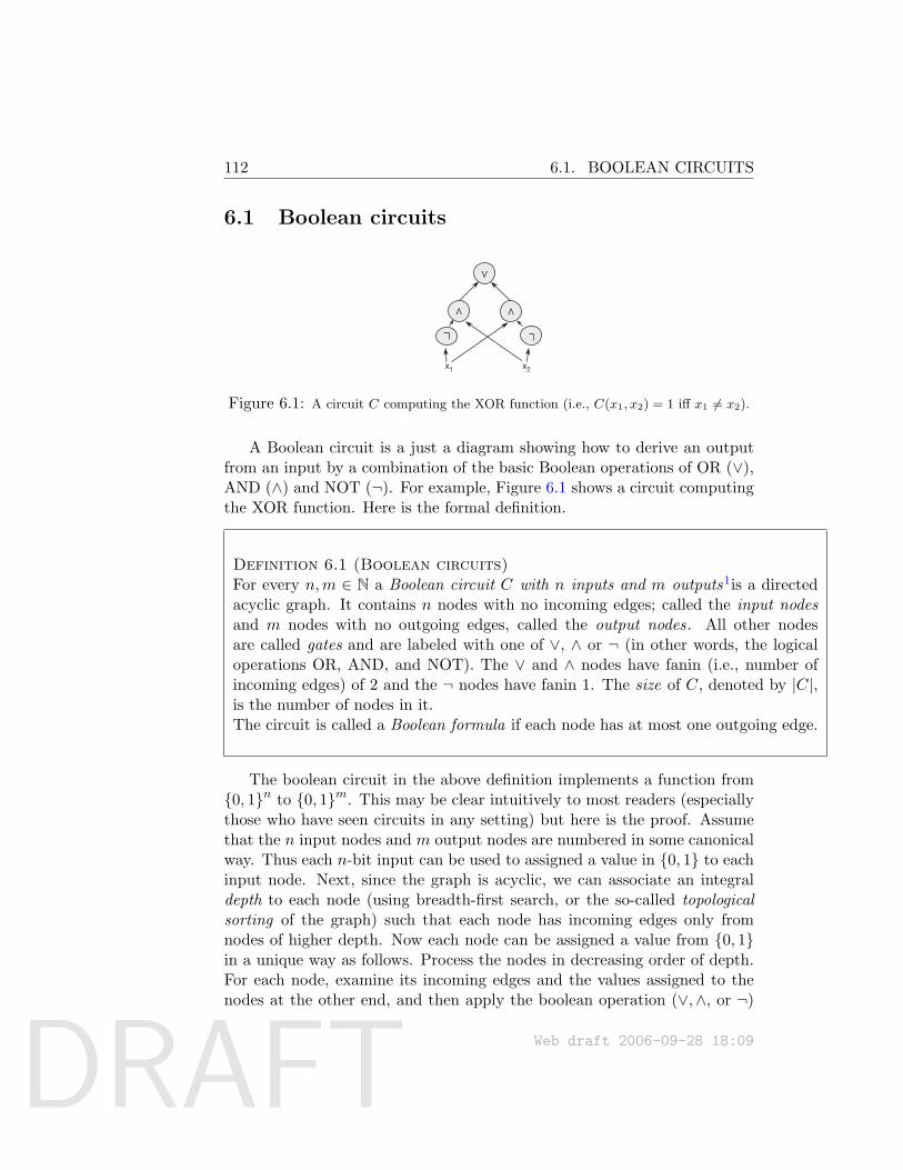
DRAFT

112 6.1. BOOLEAN CIRCUITS

6.1 Boolean circuits

Figure 6.1: A circuit C computing the XOR function (i.e., C(x1, x2) = 1 iff x1 6= x2).

A Boolean circuit is a just a diagram showing how to derive an outputfrom an input by a combination of the basic Boolean operations of OR (∨),AND (∧) and NOT (¬). For example, Figure 6.1 shows a circuit computingthe XOR function. Here is the formal definition.

Definition 6.1 (Boolean circuits)For every n,m ∈ N a Boolean circuit C with n inputs and m outputs1is a directedacyclic graph. It contains n nodes with no incoming edges; called the input nodesand m nodes with no outgoing edges, called the output nodes. All other nodesare called gates and are labeled with one of ∨, ∧ or ¬ (in other words, the logicaloperations OR, AND, and NOT). The ∨ and ∧ nodes have fanin (i.e., number ofincoming edges) of 2 and the ¬ nodes have fanin 1. The size of C, denoted by |C|,is the number of nodes in it.The circuit is called a Boolean formula if each node has at most one outgoing edge.

The boolean circuit in the above definition implements a function from0, 1n to 0, 1m. This may be clear intuitively to most readers (especiallythose who have seen circuits in any setting) but here is the proof. Assumethat the n input nodes and m output nodes are numbered in some canonicalway. Thus each n-bit input can be used to assigned a value in 0, 1 to eachinput node. Next, since the graph is acyclic, we can associate an integraldepth to each node (using breadth-first search, or the so-called topologicalsorting of the graph) such that each node has incoming edges only fromnodes of higher depth. Now each node can be assigned a value from 0, 1in a unique way as follows. Process the nodes in decreasing order of depth.For each node, examine its incoming edges and the values assigned to thenodes at the other end, and then apply the boolean operation (∨,∧, or ¬)

Web draft 2006-09-28 18:09

DRAFT

6.1. BOOLEAN CIRCUITS 113

that this node is labeled with on those values. This gives a value to eachnode; the values assigned to the m output nodes by this process constitutean m-bit output of the circuit.

For every string u ∈ 0, 1n, we denote by C(u) the output of the circuitC on input u.

We recall that the Boolean operations OR, AND, and NOT form a uni-versal basis, by which we mean that every function from 0, 1n to 0, 1mcan be implemented by a boolean circuit (in fact, a boolean formula). SeeClaim 2.15. Furthermore, the “silicon chip” that we all know about is noth-ing but2 an implementation of a boolean circuit using a technology calledVLSI. Thus if we have a small circuit for a computational task, we can im-plement it very efficiently as a silicon chip. Of course, the circuit can onlysolve problems on inputs of a certain size. Nevertheless, this may not be abig restriction in our finite world. For instance, what if a small circuit existsthat solves 3SAT instances of up to say 100, 000 variables? If so, one couldimagine a government-financed project akin to the Manhattan project thatwould try to discover such a small circuit, and then implement it as a siliconchip. This could be used in all kinds of commercial products (recall ourearlier depiction of a world in which P = NP) and in particular would jeop-ardize every encryption scheme that does not use a huge key. This scenariois hinted at in the quote from Karp and Lipton at the start of the chapter.

As usual, we resort to asymptotic analysis to study the complexity ofdeciding a language by circuits.

Definition 6.2 (Circuit families and language recognition)Let T : N → N be a function. A T (n)-sized circuit family is a sequenceCnn∈N of Boolean circuits, where Cn has n inputs and a single output,such that |Cn| ≤ T (n) for every n.

We say that a language L is in SIZE(T (n)) if there exists a T (n)-sizecircuit family Cnn∈N such that for every x ∈ 0, 1n, x ∈ L⇔ C(x) = 1.

As noted in Claim 2.15, every language is decidable by a circuit family ofsize O(n2n), since the circuit for input length n could contain 2n “hardwired”bits indicating which inputs are in the language. Given an input, the circuitlooks up the answer from this table. (The reader may wish to work out animplementation of this circuit.) The following definition formalizes what wecan think of as “small” circuits.

2Actually, the circuits in silicon chips are not acyclic; in fact the cycles in the circuitare crucial for implementing ”memory.” However any computation that runs on a siliconchip of size C and finishes in time T can be performed by a boolean circuit of size O(C ·T ).

Web draft 2006-09-28 18:09

DRAFT


Definition 6.3P/poly is the class of languages that are decidable by polynomial-sized cir-cuit families, in other words, ∪cSIZE(nc).

Of course, one can make the same kind of objections to the practicality ofP/poly as for P: viz., in what sense is a circuit family of size n100 practical,even though it has polynomial size. This was answered to some extentin Section 1.4.1. Another answer is that as complexity theorists we hope(eventually) to show that languages such as SAT are not in P/poly. Thusthe result will only be stronger if we allow even such large circuits in thedefinition of P/poly.

The class P/poly contains P. This is a corollary of Theorem 6.7 that weshow below. Can we give a reasonable upperbound on the computationalpower of P/poly? Unfortunately not, since it contains even undecidablelanguages.

Example 6.4Recall that we say that a language L is unary if it is a subset of 1n : n ∈ N.Every unary language has linear size circuits since the circuit for an inputsize n only needs to have a single “hardwired” bit indicating whether or not1n is in the language. Hence the following unary language has linear sizecircuits, even though it is undecidable:

1n : Mn outputs 1 on input 1n . (1)

where Mn is the machine represented by (the binary expansion of) the num-ber n.

This example suggests that it may be fruitful to consider the restrictionto circuits that can actually be built, say using a fairly efficient Turing ma-chine. It will be most useful to formalize this using logspace computations.

Recall that a function f : 0, 1∗ → 0, 1∗ is implicitly logspace com-putable if the mapping x, i 7→ f(x)i can be computed in logarithmic space(see Definition 3.14).

Definition 6.5 (logspace-uniform circuit families)A circuit family Cn is logspace uniform if there is an implicitly logspacecomputable function mapping 1n to the description of the circuit Cn.

Web draft 2006-09-28 18:09

DRAFT


Actually, to make this concrete we need to fix some representation of thecircuits as strings. We will assume that the circuit of size N is representedby its N ×N adjacency matrix and in addition an array of size N that givesthe labels (gate type and input/output) of each node. This means that Cnis logspace uniform if and only if the following functions are computable inO(log n) space:

• SIZE(n) returns the size m (in binary representation) of the circuitCn.

• TYPE(n, i), where i ∈ [m], returns the label and type of the ith nodeof Cn. That is it returns one of ∨,∧,¬, NONE and in addition〈OUTPUT, j〉 or 〈INPUT, j〉 if i is the jth input or output node ofCn.

• EDGE(n, i, j) returns 1 if there is a directed edge in Cn between the ith

node and the jth node.

Note that both the inputs and the outputs of these functions can beencoded using a logarithmic (in |Cn|) number of bits. The requirement thatthey run in O(log n) space means that we require that log |Cn| = O(log n)or in other words that Cn is of size at most polynomial in n.

Remark 6.6Exercise 7 asks you to prove that the class of languages decided by suchcircuits does not change if we use the adjacency list (as opposed to matrix)representation. We will use the matrix representation from now on.

Polynomial circuits that are logspace-uniform correspond to a familiarcomplexity class:

Theorem 6.7A language has logspace-uniform circuits of polynomial size iff it is in P.

Remark 6.8Note that this implies that P ⊆ P/poly.

Proof sketch: The only if part is trivial. The if part follows the proof ofthe Cook-Levin Theorem (Theorem 2.11). Recall that we can simulate everytime O(T (n)) TM M by an oblivious TM M (whose head movement is in-dependent of its input) running in time O(T (n)2) (or even O(T (n) log T (n))if we are more careful). In fact, we can ensure that the movement of theoblivious TM M do not even depend on the contents of its work tape, and

Web draft 2006-09-28 18:09

DRAFT


so, by simulating Mwhile ignoring its read/write instructions, we can com-pute in O(log T (n)) space for every i the position its heads will be at the ith

step.3

Given this insight, it is fairly straightforward to translate the proof ofTheorem 2.11 to prove that every language in P has a logspace-uniformcircuit family. The idea is that if L ∈ P then it is decided by an obliviousTM M of the form above. We will use that to construct a logspace uniformcircuit family Cnn∈N such that for every x ∈ 0, 1n, Cn(x) = M(x).

Recall that, as we saw in that proof, the transcript of M ’s execution oninput x is the sequence z1, . . . , zT of snapshots (machine’s state and symbolsread by all heads) of the execution at each step in time. Assume that eachsuch zi is encoded by a string (that needs only to be of constant size). Wecan compute the string zi based the previous snapshots zi−1 and zi1 , . . . , zikwhere zij denote the last step that M ’s jth head was in the same positionas it is in the ith step. Because these are only a constant number of stringsof constant length, we can compute zi from these previous snapshot usinga constant-sized circuit. Also note that, under our assumption above, giventhe indices i and i′ < i we can easily check whether zi depends on zi′ .

The composition of all these constant-sized circuits gives rise to a circuitthat computes from the input x, the snapshot zT of the last step of M ’sexecution on x. There is a simple constant-sized circuit that, given zToutputs 1 if and only if zT is an accepting snapshot (in which M outputs1 and halts). Thus, we get a circuit C such that C(x) = M(x) for everyx ∈ 0, 1n.

Because our circuit C is composed of many small (constant-sized) cir-cuits, and determining which small circuit is applied to which nodes can bedone in logarithmic space, it is not hard to see that we can find out everyindividual bit of C’s representation in logarithmic space. (In fact, one canshow that the functions SIZE, TYPE and EDGE above can be computed usingonly logarithmic space and polylogarithmic time.)

6.1.1 Turing machines that take advice

There is a way to define P/poly using Turing machines that ”take advice.”

Definition 6.9Let T, a : N→ N be functions. The class of languages decidable by time-T (n)

3In fact, typically the movement pattern is simple enough (for example a sequenceof T (n) left to right and back sweeps of the tape) that for every i we can compute thisinformation using only O(log T (n)) space and polylogT (n) time.

Web draft 2006-09-28 18:09

DRAFT


TM’s with a(n) advice, denoted DTIME(T (n))/a(n), contains every L suchthat there exists a sequence αnn∈N of strings with αn ∈ 0, 1a(n) and aTM M satisfying

M(x, αn) = 1⇔ x ∈ L

for every x ∈ 0, 1n, where on input (x, αn) the machine M runs for atmost O(T (n)) steps.

Example 6.10Every unary language can be be decided by a polynomial time Turing ma-chine with 1 bit of advice. The advice string for inputs of length n is thesingle bit indicating whether or not 1n is in the language. In particular thisis true of the language of Example 6.4.

This is an example of a more general phenomenon described in the nexttheorem.

Theorem 6.11P/poly = ∪c,dDTIME(nc)/nd

Proof: If L ∈ P/poly, we can provide the polynomial-sized description ofits circuit family as advice to a Turing machine. When faced with an inputof size n, the machine just simulates the circuit for this circuit provided toit.

Conversely, if L is decidable by a polynomial-time Turing machine Mwith access to an advice family αnn∈N of size a(n) for some polynomial a,then we can use the construction of Theorem 6.7 to construct for every n, apolynomial-sized circuit Dn such that on every x ∈ 0, 1n, α ∈ 0, 1a(n),Dn(x, α) = M(x, α). We let the circuit Cn be the polynomial circuit thatmaps x to Dn(x, αn). That is, Cn is equal to the circuit Dn with the stringαn “hardwired” as its second input.

Remark 6.12By “hardwiring” an input into a circuit we mean taking a circuit C withtwo inputs x ∈ 0, 1n , y ∈ 0, 1m and transforming it into the circuit Cythat for every x returns C(x, y). It is easy to do so while ensuring that thesize of Cy is not greater than the size of C. This simple idea is often usedin complexity theory.

Web draft 2006-09-28 18:09

DRAFT

118 6.2. KARP-LIPTON THEOREM

6.2 Karp-Lipton Theorem

Karp and Lipton formalized the question of whether or not SAT has smallcircuits as: Is SAT in P/poly? They showed that the answer is “NO” if thepolynomial hierarchy does not collapse.

Theorem 6.13 (Karp-Lipton, with improvements by Sipser)If NP ⊆ P/poly then PH = Σp

2.

Proof: To show that PH = Σp2 it is enough to show that Πp

2 ⊆ Σp2 and

in particular it suffices to show that Σp2 contains the Πp

2-complete languageΠ2SAT consisting of all true formulae of the form

∀u ∈ 0, 1n ∃v ∈ 0, 1n ϕ(u, v) = 1 . (2)

where ϕ is an unquantified Boolean formula.If NP ⊆ P/poly then there is a polynomial p and a p(n)-sized circuit

family Cnn∈N such that for every Boolean formula ϕ and u ∈ 0, 1n,Cn(ϕ, u) = 1 if and only if there exists v ∈ 0, 1n such that ϕ(u, v) = 1.Yet, using the search to decision reduction of Theorem 2.20, we actuallyknow that there is a q(n)-sized circuit family C ′nn∈N such that for everysuch formula ϕ and u ∈ 0, 1n, if there is a string v ∈ 0, 1n such thatϕ(u, v) = 1 then C ′n(ϕ, u) outputs such a string v. Since C ′n can be describedusing 10q(n)2 bits, this implies that if (2) is true then the following quantifiedformula is also true:

∃w∈ 0, 110q(n)2 ∀u∈ 0, 1nw describes a circuit C ′ s.t. ϕ(u,C ′(ϕ, u)) = 1 .(3)

Yet if (2) is false then certainly (regardless of whether P = NP) theformula (3) is false as well, and hence (3) is actually equivalent to (2)!However, since evaluating a circuit on an input can be done in polynomialtime, evaluating the truth of (3) can be done in Σp

2.

Similarly the following theorem can be proven, though we leave the proofas Exercise 3.

Theorem 6.14 (Karp-Lipton, attributed to A. Meyer)If EXP ⊆ P/poly then EXP = Σp

2.

Combining the time hierarchy theorem (Theorem 4.1) with the previoustheorem implies that if P = NP then EXP 6⊆ P/poly. Thus upperbounds(in this case, NP ⊆ P) can potentially be used to prove circuit lowerbounds.

Web draft 2006-09-28 18:09

DRAFT

6.3. CIRCUIT LOWERBOUNDS 119

6.3 Circuit lowerbounds

Since P ⊆ P/poly, if NP * P/poly then P 6= NP. The Karp-Liptontheorem gives hope that NP 6⊆ P/poly. Can we resolve P versus NP byproving NP * P/poly? There is reason to invest hope in this approach asopposed to proving direct lowerbounds on Turing machines. By representingcomputation using circuits we seem to actually peer into the guts of it ratherthan treating it as a blackbox. Thus we may be able to get around thelimitations of relativizing methods shown in Chapter 4.

Sadly, such hopes have not yet come to pass. After two decades, thebest circuit size lowerbound for an NP language is only 5n. (However, seeExercise 1 for a better lowerbound for a language in PH.) On the positiveside, we have had notable success in proving lowerbounds for more restrictedcircuit models, as we will see in Chapter 13.

By the way, it is easy to show that for large enough n, almost everyboolean function on n variables requires large circuits.

Theorem 6.15For n ≥ 100, almost all boolean functions on n variables require circuits ofsize at least 2n/(10n).

Proof: We use a simple counting argument. There are at most s3s circuitsof size s (just count the number of labeled directed graphs, where each nodehas indegree at most 2). Hence this is an upperbound on the number offunctions on n variables with circuits of size s. For s = 2n/(10n), thisnumber is at most 22n/10, which is miniscule compared 22n , the number ofboolean functions on n variables. Hence most Boolean functions do not havesuch small circuits.

Remark 6.16Another way to present this result is as showing that with high probability, arandom function from 0, 1n to 0, 1 does not have a circuit of size 2n/10n.This kind of proof method, showing the existence of an object with certainproperties by arguing that a random object has these properties with highprobability, is called the probabilistic method, and will be repeatedly used inthis book.

The problem with the above counting argument is of course, that it doesnot yield an explicit Boolean function (say an NP language) that requireslarge circuits.

Web draft 2006-09-28 18:09

DRAFT

120 6.4. NON-UNIFORM HIERARCHY THEOREM

6.4 Non-uniform hierarchy theorem

As in the case of deterministic time, non-deterministic time and space boundedmachines, Boolean circuits also have a hierarchy theorem. That is, largercircuits can compute strictly more functions than smaller ones:

Theorem 6.17For every functions T, T ′ : N→ N with 2n/(100n) > T ′(n) > T (n) > n andT (n) log T (n) = o(T ′(n)),

SIZE(T (n)) ( SIZE(T ′(n))

Proof: The diagonalization methods of Chapter 4 do not seem to work forsuch a function, but nevertheless, we can prove it using the counting argu-ment from above. To show the idea, we prove that SIZE(n) ( SIZE(n2).

For every `, there is a function f : 0, 1` → 0, 1 that is not computableby 2`/(10`)-sized circuits. On the other hand, every function from 0, 1`to 0, 1 is computable by a 2`10`-sized circuit.

Therefore, if we set ` = 1.1 log n and let g : 0, 1n → 0, 1 be thefunction that applies f on the first ` bits of its input, then

g ∈ SIZE(2`10`) = SIZE(11n1.1 log n) ⊆ SIZE(n2)

g 6∈ SIZE(2`/(10`)) = SIZE(n1.1/(11 log n)) ⊇ SIZE(n)

6.5 Finer gradations among circuit classes

There are two reasons why subclasses of P/poly are interesting. First, prov-ing lowerbounds for these subclasses may give insight into how to separateNP from P/poly. Second, these subclasses correspond to interesting com-putational models in their own right.

Perhaps the most interesting connection is to massively parallel comput-ers. In such a computer one uses simple off-the-shelf microprocessors andlinks them using an interconnection network that allows them to send mes-sages to each other. Usual interconnection networks such as the hypercubeallows linking n processors such that interprocessor communication is pos-sible —assuming some upperbounds on the total load on the network—inO(log n) steps. The processors compute in lock-step (for instance, to theticks of a global clock) and are assumed to do a small amount of computa-tion in each step, say an operation on O(log n) bits. Thus each processor

Web draft 2006-09-28 18:09

DRAFT

6.5. FINER GRADATIONS AMONG CIRCUIT CLASSES 121

computers has enough memory to remember its own address in the inter-connection network and to write down the address of any other processor,and thus send messages to it. We are purposely omitting many details ofthe model (Leighton [Lei92] is the standard reference for this topic) sincethe validity of Theorem 6.24 below does not depend upon them. (Of course,we are only aiming for a loose characterization of parallel computation, nota very precise one.)

6.5.1 Parallel computation and NC

Definition 6.18A computational task is said to have efficient parallel algorithms if inputsof size n can be solved using a parallel computer with nO(1) processors andin time logO(1) n.

Example 6.19Given two n bit numbers x, y we wish to compute x+y fast in parallel. Thegradeschool algorithm proceeds from the least significant bit and maintainsa carry bit. The most significant bit is computed only after n steps. Thisalgorithm does not take advantage of parallelism. A better algorithm calledcarry lookahead assigns each bit position to a separate processor and thenuses interprocessor communication to propagate carry bits. It takes O(n)processors and O(log n) time.

There are also efficient parallel algorithms for integer multiplication anddivision (the latter is quite nonintuitive and unlike the gradeschool algo-rithm!).

Example 6.20Many matrix computations can be done efficiently in parallel: these includecomputing the product, rank, determinant, inverse, etc. (See exercises.)

Some graph theoretic algorithms such as shortest paths and minimumspanning tree also have fast parallel implementations.

But many well-known polynomial-time problems such as minimum match-ing, maximum flows, and linear programming are not known to have anygood parallel implementations and are conjectured not to have any; see ourdiscussion of P-completeness below.

Web draft 2006-09-28 18:09

DRAFT

122 6.5. FINER GRADATIONS AMONG CIRCUIT CLASSES

Now we relate parallel computation to circuits. The depth of a circuitis the length of the longest directed path from an input node to the outputnode.

Definition 6.21 (Nick’s class or NC)A language is in NCi if there are constants c, d > 0 such that it can bedecided by a logspace-uniform family of circuits Cn where Cn has sizeO(nc) and depth O(logd n). The class NC is ∪i≥1NCi.

A related class is the following.

Definition 6.22 (AC)The class ACi is defined similarly to NCi except gates are allowed to haveunbounded fanin. The class AC is ∪i≥0ACi.

Since unbounded (but poly(n)) fanin can be simulated using a tree ofORs/ANDs of depth O(log n), we have NCi ⊆ ACi ⊆ NCi+1, and theinclusion is known to be strict for i = 0 as we will see in Chapter 13. (Notice,NC0 is extremely limited since the circuit’s output depends upon a constantnumber of input bits, but AC0 does not suffer from this limitation.)

Example 6.23The language PARITY =x : x has an odd number of 1s is in NC1. Thecircuit computing it has the form of a binary tree. The answer appears atthe root; the left subtree computes the parity of the first |x| /2 bits and theright subtree computes the parity of the remaining bits. The gate at the topcomputes the parity of these two bits. Clearly, unwrapping the recursionimplicit in our description gives a circuit of dept O(log n).

The classes AC, NC are important because of the following.

Theorem 6.24A language has efficient parallel algorithms iff it is in NC.

Proof: Suppose a language L ∈ NC and is decidable by a circuit familyCn where Cn has size N = O(nc) and depth D = O(logd n). Take a gen-eral purpose parallel computer with N nodes and configure it to decide Las follows. Compute a description of Cn and allocate the role of each circuit

Web draft 2006-09-28 18:09

DRAFT

6.5. FINER GRADATIONS AMONG CIRCUIT CLASSES 123

node to a distinct processor. (This is done once, and then the computer isready to compute on any input of length n.) Each processor, after comput-ing the output at its assigned node, sends the resulting bit to every othercircuit node that needs it. Assuming the interconnection network deliversall messages in O(logN) time, the total running time is O(logd+1N).

The reverse direction is similar, with the circuit having N · D nodesarranged in D layers, and the ith node in the tth layer performs the com-putation of processor i at time t. The role of the interconnection network isplayed by the circuit wires.

6.5.2 P-completeness

A major open question in this area is whether P = NC. We believe thatthe answer is NO (though we are currently even unable to separate PHfrom NC1). This motivates the theory of P-completeness, a study of whichproblems are likely to be in NC and which are not.

Definition 6.25A language is P-complete if it is in P and every language in P is logspace-reducible to it (as per Definition 3.14).

The following easy theorem is left for the reader as Exercise 12.

Theorem 6.26If language L is P-complete then

1. L ∈ NC iff P = NC.

2. L ∈ L iff P = L. (Where L is the set languages decidable in logarith-mic space, see Definition 3.5.)

The following is a fairly natural P-complete language:

Theorem 6.27Let CIRCUIT-EVAL denote the language consisting of all pairs 〈C, x〉 suchthat C is an n-inputs single-output circuit and x ∈ 0, 1n satisfies C(x) = 1.Then CIRCUIT-EVAL is P-complete.

Proof: The language is clearly in P. A logspace-reduction from any otherlanguage in P to this language is implicit in the proof of Theorem 6.7.

Web draft 2006-09-28 18:09

DRAFT

124 6.6. CIRCUITS OF EXPONENTIAL SIZE

6.6 Circuits of exponential size

As noted, every language has circuits of size O(n2n). However, actuallyfinding these circuits may be difficult— sometimes even undecidable. If weplace a uniformity condition on the circuits, that is, require them to beefficiently computable then the circuit complexity of some languages couldexceed n2n. In fact it is possible to give alternative definitions of somefamiliar complexity classes, analogous to the definition of P in Theorem 6.7.

Definition 6.28 (DC-Uniform)Let Cnn≥1 be a circuit family. We say that it is a Direct Connect uniform(DC uniform) family if, given 〈n, i〉, we can compute in polynomial time theith but of (the representation of) the circuit Cn. More concretely, we use theadjacency matrix representation and hence a family Cnn∈N is DC uniformiff the functions SIZE, TYPE and EDGE defined in Remark ?? are computablein polynomial time.

Note that the circuits may have exponential size, but they have a suc-cinct representation in terms of a TM which can systematically generate anyrequired node of the circuit in polynomial time.

Now we give a (yet another) characterization of the class PH, this timeas languages computable by uniform circuit families of bounded depth. Weleave it as Exercise 13.

Theorem 6.29L ∈ PH iff L can be computed by a DC uniform circuit family Cn that

• uses AND, OR, NOT gates.

• has size 2nO(1)

and constant depth (i.e., depth O(1)).

• gates can have unbounded (exponential) fanin.

• the NOT gates appear only at the input level.

If we drop the restriction that the circuits have constant depth, then weobtain exactly EXP (see Exercise 14).

6.7 Circuit Satisfiability and an alternative proofof the Cook-Levin Theorem

Boolean circuits can be used to define the following NP-complete language:

Web draft 2006-09-28 18:09

DRAFT

6.7. CIRCUIT SATISFIABILITY AND AN ALTERNATIVE PROOF OFTHE COOK-LEVIN THEOREM 125

Definition 6.30The circuit satisfiability language CKT-SAT consists of all (strings represent-ing) circuits with a single output that have a satisfying assignment. Thatis, a string representing an n-input circuit C is in CKT-SAT iff there existsu ∈ 0, 1n such that C(u) = 1.

CKT-SAT is clearly in NP because the satisfying assignment can serveas the certificate. It is also clearly NP-hard as every CNF formula is inparticular a Boolean circuit. However, CKT-SAT can also be used to give analternative proof (or, more accurately, a different presentation of the sameproof) for the Cook-Levin Theorem by combining the following two lemmas:

Lemma 6.31CKT-SAT is NP-hard.

Proof: Let L be an NP-language and let p be a polynomial and M apolynomial-time TM such that x ∈ L iffM(x, u) = 1 for some u ∈ 0, 1p(|x|).We reduce L to CKT-SAT by mapping (in polynomial-time) x to a circuitCx with p(|x|) inputs and a single output such that Cx(u) = M(x, u) forevery u ∈ 0, 1p(|x|). Clearly, x ∈ L ⇔ Cx ∈ CKT-SAT and so this sufficesto show that L ≤P CKT-SAT.

Yet, it is not hard to come up with such a circuit. Indeed, the proof ofTheorem 6.7 yields a way to map M,x into the circuit Cx in logarithmicspace (which in particular implies polynomial time).

Lemma 6.32CKT-SAT ≤p 3SAT

Proof: As mentioned above this follows from the Cook-Levin theorem butwe give here a direct reduction. If C is a circuit, we map it into a 3CNFformula ϕ as follows:

For every node vi of C we will have a corresponding variable zi in ϕ. Ifthe node vi is an AND of the nodes vj and vk then we add to ϕ clauses thatare equivalent to the condition “zi = (zj ∧ zk)”. That is, we add the clauses

(zi ∨ zj ∨ zk) ∧ (zi ∨ zj ∨ zk) ∧ (zi ∨ zj ∨ zk) ∧ (zi ∨ zj ∨ zk) .

Similarly, if vi is an OR of vj and vk then we add clauses equivalent to “zi =(zj∨zk)”, and if vi is the NOT of vj then we add the clauses (zi∨zj)∧(zi∨zj).

Finally, if vi is the output node of C then we add the clause zi to ϕ. Itis not hard to see that the formula ϕ will be satisfiable if and only if thecircuit C is.

Web draft 2006-09-28 18:09

DRAFT

1266.7. CIRCUIT SATISFIABILITY AND AN ALTERNATIVE PROOF OF

THE COOK-LEVIN THEOREM


• Boolean circuits can be used as an alternative computational model to TMs.The class P/poly of languages decidable by polynomial-sized circuits is a strictsuperset of P but does not contain NP unless the hierarchy collapses.

• Almost every function from 0, 1n to 0, 1 requires exponential-sized circuits.Finding even one function in NP with this property would show that P 6= NP.

• The class NC of languages decidable by (uniformly constructible) circuits withpolylogarithmic depth and polynomial size corresponds to computational tasksthat can be efficiently parallelized.


Karp-Lipton theorem is from [KL82]. Karp and Lipton also gave a moregeneral definition of advice that can be used to define the class C/a(n)for every complexity class C and function a. However, we do not use thisdefinition here since it does not seem to capture the intuitive notion of advicefor classes such as NP ∩ coNP, BPP and others.

The class of NC algorithms as well as many related issues in parallelcomputation are discussed in Leighton [?].

Exercises

§1 [Kannan [Kan82]] Show for every k > 0 that PH contains languageswhose circuit complexity is Ω(nk).

Hint:Keepinmindtheproofoftheexistenceoffunctionswithhighcircuitcomplexity.

§2 Solve the previous question with PH replaced by Σp2.

§3 ([KL82], attributed to A. Meyer) Show that if EXP ⊆ P/poly thenEXP = Σp

2.

§4 Show that if P = NP then there is a language in EXP that requirescircuits of size 2n/n.

Web draft 2006-09-28 18:09

DRAFT

6.7. CIRCUIT SATISFIABILITY AND AN ALTERNATIVE PROOF OFTHE COOK-LEVIN THEOREM 127

§5 A language L ⊆ 0, 1∗ is sparse if there is a polynomial p such that|L∩0, 1n | ≤ p(n) for every n ∈ N. Show that every sparse languageis in P/poly.

§6 (X’s Theorem 19??) Show that if a sparse language is NP-completethen P = NP. (This is a strengthening of Exercise 13 of Chapter 2.)

Hint:Showarecursiveexponential-timealgorithmSthatonin-putan-variableformulaϕandastringv∈0,1

noutputs1iff

ϕhasasatisfyingassignmentvsuchthatv>uwhenbothareinterpretedasthebinaryrepresentationofanumberin[2

n].Use

thereductionfromSATtoLtoprunepossibilitiesintherecursiontreeofS.

§7 Show a logspace implicitly computable function f that maps any n-vertex graph in adjacency matrix representation into the same graphin adjacency list representation. You can think of the adjacency listrepresentation of an n-vertex graph as a sequence of n strings of sizeO(n log n) each, where the ith string contains the list of neighbors ofthe ith vertex in the graph (and is padded with zeros if necessary).

§8 (Open) Suppose we make a stronger assumption than NP ⊆ P/poly:every language in NP has linear size circuits. Can we show somethingstronger than PH = Σp

2?

§9 (a) Describe an NC circuit for the problem of computing the productof two given n× n matrices A,B.

(b) Describe an NC circuit for computing, given an n × n matrix,the matrix An.

Hint:Userepeatedsquaring:A2

k

=(A2

k−1)2.

(c) Conclude that the PATH problem (and hence every NL language)is in NC.

Hint:Whatisthemeaningofthe(i,j)thentryofAn?

§10 A formula is a circuit in which every node (except the input nodes) hasoutdegree 1. Show that a language is computable by polynomial-sizeformulae iff it is in (nonuniform) NC1.

Hint:aformulamaybeviewed—onceweexcludetheinputnodes—asadirectedbinarytree,andinabinarytreeofsizemthereisalwaysanodewhoseremovalleavessubtreesofsizeatmost2m/3each.

Web draft 2006-09-28 18:09

DRAFT

1286.7. CIRCUIT SATISFIABILITY AND AN ALTERNATIVE PROOF OF

THE COOK-LEVIN THEOREM

§11 Show that NC1 = L. Conclude that PSPACE 6= NC1.

§12 Prove Theorem 6.26. That is, prove that if L is P-complete thenL ∈ NC (resp. L) iff P = NC (resp. L).

§13 Prove Theorem 6.29 (that PH is the set of languages with constant-depth DC uniform circuits).

§14 Show that EXP is exactly the set of languages with DC uniform cir-cuits of size 2n

cwhere c is some constant (c may depend upon the

language).

§15 Show that if linear programming has a fast parallel algorithm thenP = NC.

Hint:inyourreduction,expresstheCIRCUIT-EVALproblemasalinearprogramandusethefactthatx∨y=1iffx+y≥1.Becareful;thevariablesinalinearprogramarereal-valuedandnotboolean!

Web draft 2006-09-28 18:09

DRAFT

Chapter 7

Randomized Computation

“We do not assume anything about the distribution of the in-stances of the problem to be solved. Instead we incorporate ran-domization into the algorithm itself... It may seem at first sur-prising that employing randomization leads to efficient algorithm.This claim is substantiated by two examples. The first has to dowith finding the nearest pair in a set of n points in Rk. The sec-ond example is an extremely efficient algorithm for determiningwhether a number is prime.”Michael Rabin, 1976

Thus far our standard model of computation has been the deterministicTuring Machine. But everybody who is even a little familiar with compu-tation knows that that real-life computers need not be deterministic sincethey have built-in ”random number generators.” In fact these generatorsare very useful for computer simulation of ”random” processes such as nu-clear fission or molecular motion in gases or the stock market. This chapterformally studies probablistic computation, and complexity classes associatedwith it.

We should mention right away that it is an open question whether or notthe universe has any randomness in it (though quantum mechanics seemsto guarantee that it does). Indeed, the output of current ”random numbergenerators” is not guaranteed to be truly random, and we will revisit thislimitation in Section 7.4.3. For now, assume that true random number gen-erators exist. Then arguably, a realistic model for a real-life computer isa Turing machine with a random number generator, which we call a Prob-abilistic Turing Machine (PTM). It is natural to wonder whether difficultproblems like 3SAT are efficiently solvable using a PTM.


129

DRAFT

130 7.1. PROBABILISTIC TURING MACHINES

We will formally define the class BPP of languages decidable by polynomial-time PTMs and discuss its relation to previously studied classes such asP/poly and PH. One consequence is that if PH does not collapse, then3SAT does not have efficient probabilistic algorithms.

We also show that probabilistic algorithms can be very practical by pre-senting ways to greatly reduce their error to absolutely minuscule quantities.Thus the class BPP (and its sister classes RP, coRP and ZPP) introducedin this chapter are arguably as important as P in capturing efficient com-putation. We will also introduce some related notions such as probabilisticlogspace algorithms and probabilistic reductions.

Though at first randomization seems merely a tool to allow simulationsof randomized physical processes, the surprising fact is that in the pastthree decades randomization has led to more efficient —and often simpler—algorithms for problems in a host of other fields—such as combinatorialoptimization, algebraic computation, machine learning, and network rout-ing.

In complexity theory too, the role of randomness extends far beyonda study of randomized algorithms and classes such as BPP. Entire areassuch as cryptography and interactive and probabilistically checkable proofsrely on randomness in an essential way, sometimes to prove results whosestatement did not call for randomness at all. The groundwork for studyingthose areas will be laid in this chapter.

In a later chapter, we will learn something intriguing: to some extent,the power of randomness may be a mirage. If a certain plausible complexity-theoretic conjecture is true (see Chapters 17 and 18), then every probabilisticalgorithm can be simulated by a deterministic algorithm (one that does notuse any randomness whatsoever) with only polynomial overhead.

Throughout this chapter and the rest of the book, we will use some no-tions from elementary probability on finite sample spaces; see the appendixfor a quick review.

7.1 Probabilistic Turing machines

We now define probabilistic Turing machines (PTMs). Syntactically, a PTMis no different from a nondeterministic TM: it is a TM with two transitionfunctions δ0, δ1. The difference lies in how we interpret the graph of allpossible computations: instead of asking whether there exists a sequenceof choices that makes the TM accept, we ask how large is the fraction ofchoices for which this happens. More precisely, if M is a PTM, then we

Web draft 2006-09-28 18:09

DRAFT

7.1. PROBABILISTIC TURING MACHINES 131

envision that in every step in the computation, M chooses randomly whichone of its transition functions to apply (with probability half applying δ0and with probability half applying δ1). We say that M decides a languageif it outputs the right answer with probability at least 2/3.

Notice, the ability to pick (with equal probability) one of δ0, δ1 to ap-ply at each step is equivalent to the machine having a ”fair coin”, which,each time it is tossed, comes up ”Heads” or ”Tails” with equal probabilityregardless of the past history of Heads/Tails. As mentioned, whether or notsuch a coin exists is a deep philosophical (or scientific) question.

Definition 7.1 (The classes BPTIME and BPP)For T : N → N and L ⊆ 0, 1∗, we say that a PTM M decides L in time T (n), iffor every x ∈ 0, 1∗, M halts in T (|x|) steps regardless of its random choices, andPr[M(x) = L(x)] ≥ 2/3, where we denote L(x) = 1 if x ∈ L and L(x) = 0 if x 6∈ L.We let BPTIME(T (n)) denote the class of languages decided by PTMs in O(T (n))time and let BPP = ∪cBPTIME(nc).

Remark 7.2We will see in Section 7.4 that this definition is quite robust. For instance,the ”coin” need not be fair. The constant 2/3 is arbitrary in the sense that itcan be replaced with any other constant greater than half without changingthe classes BPTIME(T (n)) and BPP. Instead of requiring the machineto always halt in polynomial time, we could allow it to halt in expectedpolynomial time.

Remark 7.3While Definition 7.1 allows the PTM M , given input x, to output a valuedifferent from L(x) with positive probability, this probability is only over therandom choices that M makes in the computation. In particular for everyinput x, M(x) will output the right value L(x) with probability at least 2/3.Thus BPP, like P, is still a class capturing worst-case computation.

Since a deterministic TM is a special case of a PTM (where both tran-sition functions are equal), the class BPP clearly contains P. As alludedabove, under plausible complexity assumptions it holds that BPP = P.Nonetheless, as far as we know it may even be that BPP = EXP. (Notethat BPP ⊆ EXP, since given a polynomial-time PTM M and inputx ∈ 0, 1n in time 2poly(n) it is possible to enumerate all possible ran-dom choices and compute precisely the probability that M(x) = 1.)

Web draft 2006-09-28 18:09

DRAFT

132 7.2. SOME EXAMPLES OF PTMS

An alternative definition. As we did with NP, we can define BPPusing deterministic TMs where the ”probabilistic choices” to apply at eachstep can be provided to the TM as an additional input:

Definition 7.4 (BPP, alternative definition)BPP contains a language L if there exists a polynomial-time TM M and apolynomial p : N→ N such that for every x ∈ 0, 1∗, Pr

r∈R0,1p(|x|)[M(x, r) =

L(x)] ≥ 2/3.

7.2 Some examples of PTMs

The following examples demonstrate how randomness can be a useful toolin computation. We will see many more examples in the rest of this book.

7.2.1 Probabilistic Primality Testing

In primality testing we are given an integerN and wish to determine whetheror not it is prime. Generations of mathematicians have learnt about primenumbers and —before the advent of computers— needed to do primalitytesting to test various conjectures1. Ideally, we want efficient algorithms,which run in time polynomial in the size of N ’s representation, in otherwords, poly(log n). We knew of no such efficient algorithms2 until the1970s, when an effficient probabilistic algorithm was discovered. This wasone of the first to demonstrate the power of probabilistic algorithms. In arecent breakthrough, Agrawal, Kayal and Saxena [?] gave a deterministicpolynomial-time algorithm for primality testing.

Formally, primality testing consists of checking membership in the lan-guage PRIMES = xNy : N is a prime number. Notice, the correspondingsearch problem of finding the factorization of a given composite number Nseems very different and much more difficult. It is the famous FACTORINGproblem, whose conjectured hardness underlies many current cryptosystems.Chapter 21 describes Shor’s algorithm to factors integers in polynomial timein the model of quantum computers.

We sketch an algorithm showing that PRIMES is in BPP (and in fact in

1Though a very fast human computer himself, Gauss used the help of a human super-computer –an autistic person who excelled at fast calculations—to do primality testing.

2In fact, in his letter to von Neumann quoted in Chapter 2, Godel explicitly men-tioned this problem as an example for an interesting problem in NP but not known to beefficiently solvable.

Web draft 2006-09-28 18:09

DRAFT

7.2. SOME EXAMPLES OF PTMS 133

coRP). For every number N , and A ∈ [N − 1], define

QRN (A) =

0 gcd(A,N) 6= 1

+1A is a quadratic residue modulo NThat is, A = B2 (mod N) for some B with gcd(B,N) = 1

−1 otherwise

We use the following facts that can be proven using elementary numbertheory:

• For every odd prime N and A ∈ [N − 1], QRN (A) = A(N−1)/2

(mod N).

• For every odd N,A define the Jacobi symbol (NA ) as∏ki=1QRPi(A)

where P1, . . . , Pk are all the (not necessarily distinct) prime factors ofN (i.e., N =

∏ki=1 Pi). Then, the Jacobi symbol is computable in time

O(logA · logN).

• For every odd composite N ,∣∣A ∈ [N − 1] : gcd(N,A)=1 and (NA ) =

A(N−1)/2∣∣ ≤ 1

2

∣∣A ∈ [N − 1] : gcd(N,A) = 1∣∣

Together these facts imply a simple algorithm for testing primality of N(which we can assume without loss of generality is odd): choose a random1 ≤ A < N , if gcd(N,A) > 1 or (NA ) 6= A(N−1)/2 (mod N) then output“composite”, otherwise output “prime”. This algorithm will always output“prime” is N is prime, but if N is composite will output “composite” withprobability at least 1/2. (Of course this probability can be amplified byrepeating the test a constant number of times.)

7.2.2 Polynomial identity testing

So far we described probabilistic algorithms solving problems that haveknown deterministic polynomial time algorithms. We now describe a prob-lem for which no such deterministic algorithm is known:

We are given a polynomial with integer coefficients in an implicit form,and we want to decide whether this polynomial is in fact identically zero. Wewill assume we get the polynomial in the form of an arithmetic circuit. Thisis analogous to the notion of a Boolean circuit, but instead of the operators∧,∨ and ¬, we have the operators +,− and ×. Formally, an n-variablearithmetic circuit is a directed acyclic graph with the sources labeled bya variable name from the set x1, . . . , xn, and each non-source node has in-degree two and is labeled by an operator from the set +,−,×. There is a

Web draft 2006-09-28 18:09

DRAFT

134 7.2. SOME EXAMPLES OF PTMS

single sink in the graph which we call the output node. The arithmetic circuitdefines a polynomial from Zn to Z by placing the inputs on the sources andcomputing the value of each node using the appropriate operator. We defineZEROP to be the set of arithmetic circuits that compute the identically zeropolynomial. Determining membership in ZEROP is also called polynomialidentity testing, since we can reduce the problem of deciding whether twocircuits C,C ′ compute the same polynomial to ZEROP by constructing thecircuit D such that D(x1, . . . , xn) = C(x1, . . . , xn)− C ′(x1, . . . , xn).

Since expanding all the terms of a given arithmetic circuit can result ina polynomial with exponentially many monomials, it seems hard to decidemembership in ZEROP. Surprisingly, there is in fact a simple and efficientprobabilistic algorithm for testing membership in ZEROP. At the heart ofthis algorithm is the following fact, typically known as the Schwartz-ZippelLemma, whose proof appears in the appendix (see Lemma A.23):

Lemma 7.5Let p(x1, x2, . . . , xm) be a polynomial of total degree at most d and S isany finite set of integers. When a1, a2, . . . , am are randomly chosen withreplacement from S, then

Pr[p(a1, a2, . . . , am) 6= 0] ≥ 1− d

|S|.

Now it is not hard to see that given a size m circuit C on n variables,it defines a polynomial of degree at most 2m. This suggests the followingsimple probabilistic algorithm: choose n numbers x1, . . . , xn from 1 to 10·2m(this requires O(n ·m) random bits), evaluate the circuit C on x1, . . . , xn toobtain an output y and then accept if y = 0, and reject otherwise. Clearlyif C ∈ ZEROP then we always accept. By the lemma, if C 6∈ ZEROP thenwe will reject with probability at least 9/10.

However, there is a problem with this algorithm. Since the degree of thepolynomial represented by the circuit can be as high as 2m, the output yand other intermediate values arising in the computation may be as large as(10 · 2m)2

m— this is a value that requires exponentially many bits just to

describe!We solve this problem using the technique of fingerprinting. The idea

is to perform the evaluation of C on x1, . . . , xn modulo a number k that ischosen at random in [22m]. Thus, instead of computing y = C(x1, . . . , xn),we compute the value y (mod k). Clearly, if y = 0 then y (mod k) is alsoequal to 0. On the other hand, we claim that if y 6= 0, then with probabilityat least δ = 1

10m , k does not divide y. (This will suffice because we can

Web draft 2006-09-28 18:09

DRAFT

7.2. SOME EXAMPLES OF PTMS 135

repeat this procedure O(1/δ) times to ensure that if y 6= 0 then we findthis out with probability at lest 9/10.) Indeed, assume that y 6= 0 and letS = p1, . . . , p` denote set of the distinct prime factors of y. It is sufficientto show that with probability at δ, the number k will be a prime numbernot in S. Yet, by the prime number theorem, the probability that k is primeis at least 1

5m = 2δ. Also, since y can have at most log y ≤ 5m2m distinctfactors, the probability that k is in S is less than 5m2m

22m 110m = δ. Hence

by the union bound, with probability at least δ, k will not divide y.

7.2.3 Testing for perfect matching in a bipartite graph.

If G = (V1, V2, E) is the bipartite graph where |V1| = |V2| and E ⊆ V1 ×V2 then a perfect matching is some E′ ⊆ E such that every node appearsexactly once among the edges of E′. Alternatively, we may think of it as apermutation σ on the set 1, 2, . . . , n (where n = |V1|) such that for each i ∈1, 2, . . . , n, the pair (i, σ(i)) is an edge. Several deterministic algorithmsare known for detecting if a perfect matching exists. Here we describe avery simple randomized algorithm (due to Lovasz) using the Schwartz-Zippellemma.

Consider the n × n matrix X (where n = |V1| = |V2|) whose (i, j) en-try Xij is the variable xij if (i, j) ∈ E and 0 otherwise. Recall that thedeterminant of matrix det(X) is

det(X) =∑σ∈Sn

(−1)sign(σ)n∏i=1

Xi,σ(i), (1)

where Sn is the set of all permutations of 1, 2, . . . , n. Note that every per-mutation is a potential perfect matching, and the corresponding monomialin det(X) is nonzero iff this perfect matching exists in G. Thus the graphhas a perfect matching iff det(X) 6= 0.

Now observe two things. First, the polynomial in (1) has |E| variablesand total degree at most n. Second, even though this polynomial may beof exponential size, for every setting of values to the Xij variables it canbe efficiently evaluated, since computing the determinant of a matrix withinteger entries is a simple polynomial-time computation (actually, even inNC2).

This leads us to Lovasz’s randomized algorithm: pick random values forXij ’s from [1, . . . , 2n], substitute them in X and compute the determinant.If the determinant is nonzero, output “accept” else output “reject.” Theadvantage of the above algorithm over classical algorithms is that it can be

Web draft 2006-09-28 18:09

DRAFT

136 7.3. ONE-SIDED AND ZERO-SIDED ERROR: RP, CORP, ZPP

implemented by a randomized NC circuit, which means (by the ideas ofSection 6.5.1) that it has a fast implementation on parallel computers.

7.3 One-sided and zero-sided error: RP, coRP,ZPP

The class BPP captured what we call probabilistic algorithms with twosided error. That is, it allows the machine M to output (with some smallprobability) both 0 when x ∈ L and 1 when x 6∈ L. However, many prob-abilistic algorithms have the property of one sided error. For example ifx 6∈ L they will never output 1, although they may output 0 when x ∈ L.This is captured by the definition of RP.Definition 7.6RTIME(t(n)) contains every language L for which there is a is a proba-bilistic TM M running in t(n) time such that

x ∈ L⇒ Pr[M accepts x] ≥ 23

x 6∈ L⇒ Pr[M accepts x] = 0

We define RP = ∪c>0RTIME(nc).

Note that RP ⊆ NP, since every accepting branch is a “certificate” thatthe input is in the language. In contrast, we do not know if BPP ⊆ NP.The class coRP = L | L ∈ RP captures one-sided error algorithms withthe error in the “other direction” (i.e., may output 1 when x 6∈ L but willnever output 0 if x ∈ L).

For a PTM M , and input x, we define the random variable TM,x to bethe running time of M on input x. That is, Pr[TM,x = T ] = p if withprobability p over the random choices of M on input x, it will halt withinT steps. We say that M has expected running time T (n) if the expectationE[TM,x] is at most T (|x|) for every x ∈ 0, 1∗. We now define PTMs thatnever err (also called “zero error” machines):

Definition 7.7The class ZTIME(T (n)) contains all the languages L for which there is anexpected-time O(T (n)) machine that never errs. That is,

x ∈ L⇒ Pr[M accepts x] = 1x 6∈ L⇒ Pr[M halts without accepting on x] = 1

We define ZPP = ∪c>0ZTIME(nc).

Web draft 2006-09-28 18:09

DRAFT

7.4. THE ROBUSTNESS OF OUR DEFINITIONS 137

The next theorem ought to be slightly surprising, since the correspondingstatement for nondeterminism is open; i.e., whether or not P = NP∩coNP.

Theorem 7.8ZPP = RP ∩ coRP.

We leave the proof of this theorem to the reader (see Exercise 4). Tosummarize, we have the following relations between the probabilistic com-plexity classes:

ZPP =RP ∩ coRP

RP ⊆BPP

coRP ⊆BPP

7.4 The robustness of our definitions

When we defined P and NP, we argued that our definitions are robustand were likely to be the same for an alien studying the same concepts in afaraway galaxy. Now we address similar issues for probabilistic computation.

7.4.1 Role of precise constants, error reduction.

The choice of the constant 2/3 seemed pretty arbitrary. We now show thatwe can replace 2/3 with any constant larger than 1/2 and in fact even with1/2 + n−c for a constant c > 0.

Lemma 7.9For c > 0, let BPPn−c denote the class of languages L for which there is apolynomial-time PTM M satisfying Pr[M(x) = L(x)] ≥ 1/2+ |x|−c for everyx ∈ 0, 1∗. Then BPPn−c = BPP.

Since clearly BPP ⊆ BPPn−c , to prove this lemma we need to show thatwe can transform a machine with success probability 1/2+n−c into a machinewith success probability 2/3. We do this by proving a much stronger result:we can transform such a machine into a machine with success probabilityexponentially close to one!

Web draft 2006-09-28 18:09

DRAFT

138 7.4. THE ROBUSTNESS OF OUR DEFINITIONS

Theorem 7.10 (Error reduction)Let L ⊆ 0, 1∗ be a language and suppose that there exists a polynomial-time PTMM such that for every x ∈ 0, 1∗, Pr[M(x) = L(x) ≥ 1

2 + |x|−c.Then for every constant d > 0 there exists a polynomial-time PTM M ′ such thatfor every x ∈ 0, 1∗, Pr[M ′(x) = L(x)] ≥ 1− 2−|x|

d.

Proof: The machine M ′ is quite simple: for every input x ∈ 0, 1∗, runM(x) for k times obtaining k outputs y1, . . . , yk ∈ 0, 1, where k = 8|x|2d+c.If the majority of these values are 1 then accept, otherwise reject.

To analyze this machine, define for every i ∈ [k] the random variable Xi

to equal 1 if yi = L(x) and to equal 0 otherwise. Note that X1, . . . , Xk areindependent Boolean random variables with E[Xi] = Pr[Xi = 1] ≥ 1/2+n−c

(where n = |x|). The Chernoff bound (see Theorem A.16 in the appendix)implies the following corollary:

Corollary 7.11Let X1, . . . , Xk be independent identically distributed Boolean random vari-ables, with Pr[Xi = 1] = p for every 1 ≤ i ≤ k. Let δ ∈ (0, 1). Then,

Pr[∣∣∣∣∣ 1k

k∑i=1

Xi − p

∣∣∣∣∣ > δ]< e−

δ2

4 pk

In our case p = 1/2 + n−c, and plugging in δ = n−c/2, the probabilitywe output a wrong answer is bounded by

Pr[ 1n

k∑i=1

Xi ≤ 1/2 + n−c/2] ≤ e−1

4n−2c128n2c+d

≤ 2−nd

A similar result holds for the class RP. In fact, there we can replace theconstant 2/3 with every positive constant, and even with values as low asn−c. That is, we have the following result:

Theorem 7.12Let L ⊆ 0, 1∗ such that there exists a polynomial-time PTM M satisfyingfor every x ∈ 0, 1∗: (1) If x ∈ L then Pr[M(x) = 1)] ≥ n−c and (2) ifx 6∈ L, then Pr[M(x) = 1] = 0.

Then for every d > 0 there exists a polynomial-time PTM M ′ such thatfor every x ∈ 0, 1∗, (1) if x ∈ L then Pr[M ′(x) = 1] ≥ 1 − 2−n

dand (2)

if x 6∈ L then Pr[M ′(x) = 1] = 0.

Web draft 2006-09-28 18:09

DRAFT

7.4. THE ROBUSTNESS OF OUR DEFINITIONS 139

These results imply that we can take a probabilistic algorithm that suc-ceeds with quite modest probability and transform it into an algorithm thatsucceeds with overwhelming probability. In fact, even for moderate valuesof n an error probability that is of the order of 2−n is so small that for allpractical purposes, probabilistic algorithms are just as good as deterministicalgorithms.

If the original probabilistic algorithm used m coins, then the error re-duction procedure we use (run k independent trials and output the majorityanswer) takes O(m · k) random coins to reduce the error to a value expo-nentially small in k. It is somewhat surprising that we can in fact do better,and reduce the error to the same level using only O(m+k) random bits (seeChapter 16).

7.4.2 Expected running time versus worst-case running time.

When defining RTIME(T (n)) and BPTIME(T (n)) we required the ma-chine to halt in T (n) time regardless of its random choices. We could haveused expected running time instead, as in the definition of ZPP (Defini-tion 7.7). It turns out this yields an equivalent definition: we can add atime counter to a PTM M whose expected running time is T (n) and en-sure it always halts after at most 100T (n) steps. By Markov’s inequality(see Lemma A.8), the probability that M runs for more than this time is atmost 1/100. Thus by halting after 100T (n) steps, the acceptance probabilityis changed by at most 1/100.

7.4.3 Allowing more general random choices than a fair ran-dom coin.

One could conceive of real-life computers that have a “coin” that comes upheads with probability ρ that is not 1/2. We call such a coin a ρ-coin. Indeedit is conceivable that for a random source based upon quantum mechanics,ρ is an irrational number, such as 1/e. Could such a coin give probabilisticalgorithms new power? The following claim shows that it will not.

Lemma 7.14A coin with Pr[Heads] = ρ can be simulated by a PTM in expected timeO(1) provided the ith bit of ρ is computable in poly(i) time.

Proof: Let the binary expansion of ρ be 0.p1p2p3 . . .. The PTM generatesa sequence of random bits b1, b2, . . . , one by one, where bi is generated atstep i. If bi < pi then the machine outputs “heads” and stops; if bi > pi

Web draft 2006-09-28 18:09

DRAFT

140 7.4. THE ROBUSTNESS OF OUR DEFINITIONS

Note 7.13 (The Chernoff Bound)The Chernoff bound is extensively used (sometimes under different names)in many areas of computer science and other sciences. A typical scenario isthe following: there is a universe U of objects, a fraction µ of them have acertain property, and we wish to estimate µ. For example, in the proof ofTheorem 7.10 the universe was the set of 2m possible coin tosses of someprobabilistic algorithm and we wanted to know how many of them cause thealgorithm to accept its input. Another example is that U may be the set ofall the citizens of the United States, and we wish to find out how many ofthem approve of the current president.A natural approach to compute the fraction µ is to sample n members of theuniverse independently at random, find out the number k of the sample’smembers that have the property and to estimate that µ is k/n. Of course,it may be quite possible that 10% of the population supports the president,but in a sample of 1000 we will find 101 and not 100 such people, and sowe set our goal only to estimate µ up to an error of ±ε for some ε > 0.Similarly, even if only 10% of the population have a certain property, wemay be extremely unlucky and select only people having it for our sample,and so we allow a small probability of failure δ that our estimate will beoff by more than ε. The natural question is how many samples do we needto estimate µ up to an error of ±ε with probability at least 1 − δ? TheChernoff bound tells us that (considering µ as a constant) this number isO(log(1/δ)/ε2).This implies that if we sample n elements, then the probability that thenumber k having the property is ρ

√n far from µn decays exponentially with

ρ: that is, this probability has the famous “bell curve” shape:

k

Pr[ ]

0 n0

1

µn µn+ρn1/2µn-ρn1/2

k haveproperty

We will use this exponential decay phenomena several times in this book,starting with the proof of Theorem 7.16, showing that BPP ⊆ P/poly.

Web draft 2006-09-28 18:09

DRAFT

7.5. BPP ⊆ P/POLY 141

the machine outputs “tails” and halts; otherwise the machine goes to stepi+ 1. Clearly, the machine reaches step i+ 1 iff bj = pj for all j ≤ i, whichhappens with probability 1/2i. Thus the probability of “heads” is

∑i pi

12i,

which is exactly ρ. Furthermore, the expected running time is∑

i ic · 1

2i. For

every constant c this infinite sum is upperbounded by another constant (seeExercise 1).

Conversely, probabilistic algorithms that only have access to ρ-coins donot have less power than standard probabilistic algorithms:

Lemma 7.15 (Von-Neumann)A coin with Pr[Heads] = 1/2 can be simulated by a probabilistic TM withaccess to a stream of ρ-biased coins in expected time O( 1

ρ(1−ρ)).

Proof: We construct a TM M that given the ability to toss ρ-coins, outputsa 1/2-coin. The machine M tosses pairs of coins until the first time it getstwo different results one after the other. If these two results were first“heads” and then “tails”, M outputs “heads”. If these two results were first“tails” and then “heads”, M outputs “tails”. For each pair, the probabilitywe get two “heads” is ρ2, the probability we get two “tails” is (1− ρ)2, theprobability we get “head” and then“tails” is ρ(1 − ρ), and the probabilitywe get “tails” and then “head” is (1− ρ)ρ. We see that the probability wehalt and output in each step is 2ρ(1− ρ), and that conditioned on this, wedo indeed output either “heads” or “tails” with the same probability. Notethat we did not need to know ρ to run this simulation.

Weak random sources. Physicists (and philosophers) are still not com-pletely certain that randomness exists in the world, and even if it does, itis not clear that our computers have access to an endless stream of inde-pendent coins. Conceivably, it may be the case that we only have accessto a source of imperfect randomness, that although unpredictable, does notconsist of independent coins. As we will see in Chapter 17, we do knowhow to simulate probabilistic algorithms designed for perfect independent1/2-coins even using such a weak random source.

7.5 BPP ⊆ P/poly

Now we show that all BPP languages have polynomial sized circuits. To-gether with Theorem ?? this implies that if 3SAT ∈ BPP then PH = Σp

2.

Web draft 2006-09-28 18:09

DRAFT

142 7.6. BPP IS IN PH

Theorem 7.16 (Adleman)BPP ⊆ P/poly.

Proof: Suppose L ∈ BPP, then by the alternative definition of BPP andthe error reduction procedure of Theorem 7.10, there exists a TM M thaton inputs of size n uses m random bits and satisfies

x ∈ L⇒ Prr [M(x, r) accepts ] ≥ 1− 2−(n+2)

x 6∈ L⇒ Prr [M(x, r) accepts ] ≤ 2−(n+2)

(Such a machine exists by the error reduction arguments mentioned earlier.)Say that an r ∈ 0, 1m is bad for an input x ∈ 0, 1n if M(x, r) is

an incorrect answer, otherwise we say its good for x. For every x, at most2 · 2m/2(n+2) values of r are bad for x. Adding over all x ∈ 0, 1n, weconclude that at most 2n × 2m/2(n+1) = 2m/2 strings r are bad for some x.In other words, at least 2m−2m/2 choices of r are good for every x ∈ 0, 1n.Given a string r0 that is good for every x ∈ 0, 1n, we can hardwire it toobtain a circuit C (of size at most quadratic in the running time of M) thaton input x outputs M(x, r0). The circuit C will satisfy C(x) = L(x) forevery x ∈ 0, 1n.

7.6 BPP is in PH

At first glance, BPP seems to have nothing to do with the polynomialhierarchy, so the next theorem is somewhat surprising.

Theorem 7.17 (Sipser-Gacs)BPP ⊆ Σp

2 ∩Πp2

Proof: It is enough to prove that BPP ⊆ Σp2 because BPP is closed under

complementation (i.e., BPP = coBPP).Suppose L ∈ BPP. Then by the alternative definition of BPP and the

error reduction procedure of Theorem 7.10 there exists a polynomial-timedeterministic TM M for L that on inputs of length n uses m = poly(n)

Web draft 2006-09-28 18:09

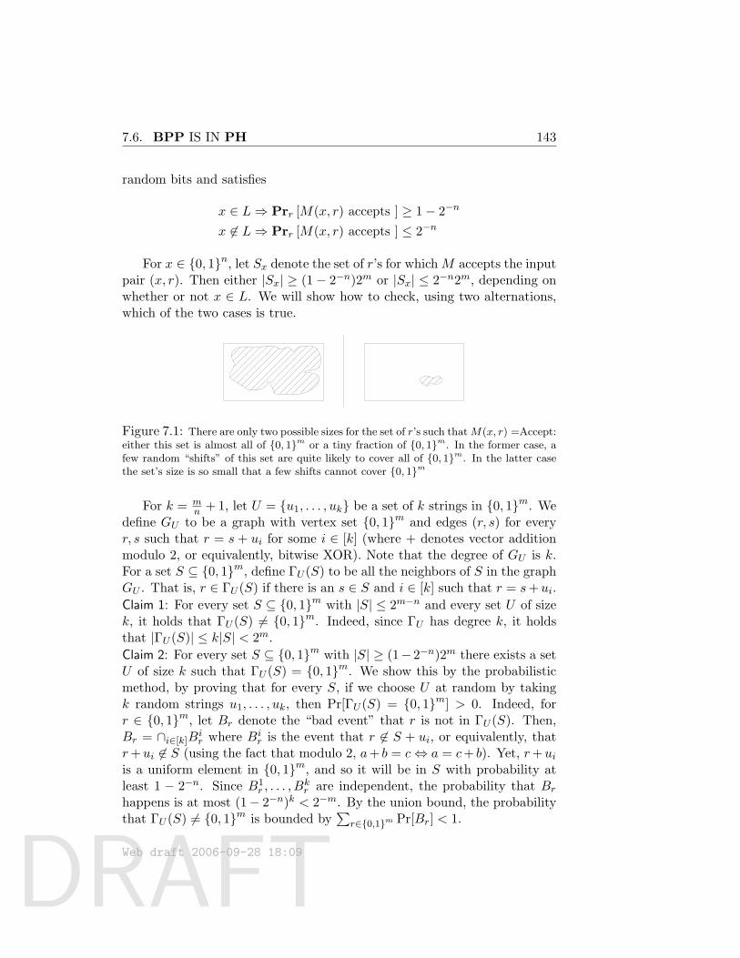
DRAFT

7.6. BPP IS IN PH 143

random bits and satisfies

x ∈ L⇒ Prr [M(x, r) accepts ] ≥ 1− 2−n

x 6∈ L⇒ Prr [M(x, r) accepts ] ≤ 2−n

For x ∈ 0, 1n, let Sx denote the set of r’s for whichM accepts the inputpair (x, r). Then either |Sx| ≥ (1− 2−n)2m or |Sx| ≤ 2−n2m, depending onwhether or not x ∈ L. We will show how to check, using two alternations,which of the two cases is true.

Figure 7.1: There are only two possible sizes for the set of r’s such thatM(x, r) =Accept:either this set is almost all of 0, 1m or a tiny fraction of 0, 1m. In the former case, afew random “shifts” of this set are quite likely to cover all of 0, 1m. In the latter casethe set’s size is so small that a few shifts cannot cover 0, 1m

For k = mn + 1, let U = u1, . . . , uk be a set of k strings in 0, 1m. We

define GU to be a graph with vertex set 0, 1m and edges (r, s) for everyr, s such that r = s + ui for some i ∈ [k] (where + denotes vector additionmodulo 2, or equivalently, bitwise XOR). Note that the degree of GU is k.For a set S ⊆ 0, 1m, define ΓU (S) to be all the neighbors of S in the graphGU . That is, r ∈ ΓU (S) if there is an s ∈ S and i ∈ [k] such that r = s+ui.Claim 1: For every set S ⊆ 0, 1m with |S| ≤ 2m−n and every set U of sizek, it holds that ΓU (S) 6= 0, 1m. Indeed, since ΓU has degree k, it holdsthat |ΓU (S)| ≤ k|S| < 2m.Claim 2: For every set S ⊆ 0, 1m with |S| ≥ (1− 2−n)2m there exists a setU of size k such that ΓU (S) = 0, 1m. We show this by the probabilisticmethod, by proving that for every S, if we choose U at random by takingk random strings u1, . . . , uk, then Pr[ΓU (S) = 0, 1m] > 0. Indeed, forr ∈ 0, 1m, let Br denote the “bad event” that r is not in ΓU (S). Then,Br = ∩i∈[k]B

ir where Bi

r is the event that r 6∈ S + ui, or equivalently, thatr+ui 6∈ S (using the fact that modulo 2, a+ b = c⇔ a = c+ b). Yet, r+uiis a uniform element in 0, 1m, and so it will be in S with probability atleast 1 − 2−n. Since B1

r , . . . , Bkr are independent, the probability that Br

happens is at most (1− 2−n)k < 2−m. By the union bound, the probabilitythat ΓU (S) 6= 0, 1m is bounded by

∑r∈0,1m Pr[Br] < 1.

Web draft 2006-09-28 18:09

DRAFT

144 7.7. STATE OF OUR KNOWLEDGE ABOUT BPP

Together Claims 1 and 2 show x ∈ L if and only if the following statementis true

∃u1, . . . , uk ∈ 0, 1m ∀r ∈ 0, 1mk∨i=1

M(x, r ⊕ ui)accepts

thus showing L ∈ Σ2.

7.7 State of our knowledge about BPP

We know that P ⊆ BPP ⊆ P/poly, and furthermore, that BPP ⊆ Σp2 ∩

Πp2 and so if NP = p then BPP = P. As mentioned above, there are

complexity-theoretic reasons to strongly believe that BPP ⊆ DTIME(2ε)for every ε > 0, and in fact to reasonably suspect that BPP = P (seeChapters 17 and 18). However, currently we are not even able to rule outthat BPP = NEXP!

Complete problems for BPP?

Though a very natural class, BPP behaves differently in some ways fromother classes we have seen. For example, we know of no complete languagesfor it (under deterministic polynomial time reductions). One reason for thisdifficulty is that the defining property of BPTIME machines is semantic,namely, that for every string they either accept with probability at least 2/3or reject with probability at least 1/3. Given the description of a TuringmachineM , testing whether it has this property is undecidable. By contrast,the defining property of an NDTM is syntactic: given a string it is easy todetermine if it is a valid encoding of an NDTM. Completeness seems easierto define for syntactically defined classes than for semantically defined ones.For example, consider the following natural attempt at a BPP-completelanguage: L = 〈M,x〉 : Pr[M(x) = 1] ≥ 2/3. This language is indeedBPP-hard but is not known to be in BPP. In fact, it is not in any levelof the polynomial hierarchy unless the hierarchy collapses. We note that if,as believed, BPP = P, then BPP does have a complete problem. (Onecan sidestep some of the above issues by using promise problems instead oflanguages, but we will not explore this.)

Does BPTIME have a hierarchy theorem?

Is BPTIME(nc) contained in BPTIME(n) for some c > 1? One wouldimagine not, and this seems as the kind of result we should be able to prove

Web draft 2006-09-28 18:09

DRAFT

7.8. RANDOMIZED REDUCTIONS 145

using the tools of Chapter 4. However currently we are even unable to showthat BPTIME(nlog2 n) (say) is not in BPTIME(n). The standard diago-nalization techniques fail, for similar reasons as the ones above. However,recently there has been some progress on obtaining hierarchy theorem forsome closely related classes (see notes).

7.8 Randomized reductions

Since we have defined randomized algorithms, it also makes sense to define anotion of randomized reduction between two languages. This proves usefulin some complexity settings (e.g., see Chapters 8 and 9).

Definition 7.18Language A reduces to language B under a randomized polynomial timereduction, denoted A ≤r B, if there exists a deterministic, polynomial timecomputable function f : 0, 1∗ → 0, 1∗ and a polynomial p() such that

∀x ∈ A Pry∈0,1p(|x|) [f(x, y) ∈ B] ≥ 2/3

∀x 6∈ A Pry∈0,1p(|x|) [f(x, y) ∈ B] ≤ 1/3

We note that if A ≤r B and B ∈ BPP then A ∈ BPP. This alerts us tothe possibility that we could have defined NP-completeness using random-ized reductions instead of deterministic reductions, since arguably BPP isas good as P as a formalization of the notion of efficient computation. Re-call that the Cook-Levin theorem shows that NP may be defined as the setL : L ≤p 3SAT. The following definition is analogous.

Definition 7.19 (BP ·NP)BP ·NP = L : L ≤r 3SAT.

We explore the properties of BP ·NP in the exercises, including whetheror not 3SAT ∈ BP ·NP.

One interesting application of randomized reductions will be shown inChapter 8, where we present a (variant of a) randomized reduction from3SAT to the solving special case of 3SAT where we are guaranteed that theformula is either unsatisfiable or has a single unique satisfying assignment.

7.9 Randomized space-bounded computation

A PTM is said to work in space S(n) if every branch requires space O(S(n))on inputs of size n and terminates in 2O(S(n)) time. Recall that the machine

Web draft 2006-09-28 18:09

DRAFT

146 7.9. RANDOMIZED SPACE-BOUNDED COMPUTATION

has a read-only input tape, and the work space only cell refers only toits read/write work tapes. As a PTM it has two transition functions thatare applied with equal probability. The most interesting case is when theworktape has O(log n) size and the associated complexity classes RL andBPL are defined analogously to RP and BPP. That is, L ∈ BPL ifthere’s a O(log n)-space PTM M such that for every x ∈ 0, 1∗, Pr[M(x) =L(x)] ≥ 2/3, whereas L ∈ RL if there’s a O(log n)-space PTM M such that(1) for every x ∈ L, Pr[M(x) = L(x)] ≥ 2/3 and (2) for every x 6∈ L,Pr[M(x) = L(x)] = 0. The reader can verify that the error reductionprocedure described in Chapter 7 can be implemented with only logarithmicspace overhead, and hence also in these definitions the choice of the preciseconstant is not significant. We note that RL ⊆ NL, and thus RL ⊆ P.The exercises ask you to show that BPL ⊆ P as well.

One famous RL-algorithm is the algorithm to solve UPATH: the re-striction of the NL-complete PATH problem (see Chapter 3) to undirectedgraphs. That is, given an n-vertex undirected graph G and two vertices sand t, determine whether s is connected to t in G. The algorithm is actuallyvery simple: take a random walk of length n3 starting from s. That is,initialize the variable v to the vertex s and in each step choose a randomneighbor u of v, and set v ← u. Accept iff the walk reaches t within n3 steps.Clearly, if s is not connected to t then the algorithm will never accept. Itcan be shown that if s is connected to t then the expected number of stepsit takes for a walk from s to hit t is at most 4

27n3 (see Exercise 9 for a some-

what weaker bound) and hence our algorithm will accept with probabilityat least 3

4 . In Chapter 16 we analyze a variant of this algorithm and alsoshow a recent deterministic logspace algorithm for the same problem.

It is known that BPL (and hence also RL) is contained in SPACE(log3/2 n).In Chapter 17 we will see a somewhat weaker result: a simulation of BPLin log2 n space and polynomial time.

Web draft 2006-09-28 18:09

DRAFT

7.9. RANDOMIZED SPACE-BOUNDED COMPUTATION 147


• The class BPP consists of languages that can be solved by a probabilisticpolynomial-time algorithm. The probability is only over the algorithm’s coinsand not the choice of input. It is arguably a better formalization of efficientcomputation than P.

• RP, coRP and ZPP are subclasses of BPP corresponding to probabilisticalgorithms with one-sided and “zero-sided” error.

• Using repetition, we can considerably amplify the success probability of prob-abilistic algorithms.

• We only know that P ⊆ BPP ⊆ EXP, but we suspect that BPP = P.

• BPP is a subset of both P/poly and PH. In particular, the latter impliesthat if NP = P then BPP = P.

• Randomness is used in complexity theory in many contexts beyond BPP. Twoexamples are randomized reductions and randomized logspace algorithms, butwe will see many more later.


Early researchers realized the power of randomization since their computa-tions —e.g., for design of nuclear weapons— used probabilistic tools such asMonte Carlo simulations. Papers by von Neumann [von61] and de Leeuwet al. [LMSS56] describe probabilistic Turing machines. The definitions ofBPP, RP and ZPP are from Gill [Gil77]. (In an earlier conference pa-per [Gil74], Gill studies similar issues but seems to miss the point that apractical algorithm for deciding a language must feature a gap between theacceptance probability in the two cases.)

The algorithm used to show PRIMES is in coRP is due to Solovay andStrassen [SS77]. Another primality test from the same era is due to Ra-bin [Rab80]. Over the years, better tests were proposed. In a recent break-through, Agrawal, Kayal and Saxena finally proved that PRIMES ∈ P. Boththe probabilistic and deterministic primality testing algorithms are describedin Shoup’s book [?].

Lovasz’s randomized NC algorithm [Lov79] for deciding the existenceof perfect matchings is unsatisfying in the sense that when it outputs “Ac-

Web draft 2006-09-28 18:09

DRAFT


cept,” it gives no clue how to find a matching! Subsequent probabilistic NCalgorithms can find a perfect matching as well; see [KUW86, MVV87].

BPP ⊆ P/poly is from Adelman [Adl78]. BPP ⊆ PH is due toSipser [Sip83], and the stronger form BPP ⊆ Σp

2 ∩Πp2 is due to P. Gacs.

Recent work [] shows that BPP is contained in classes that are seeminglyweaker than Σp

2 ∩Πp2.

Even though a hierarchy theorem for BPP seems beyond our reach,there has been some success in showing hierarchy theorems for the seeminglyrelated class BPP/1 (i.e., BPP with a single bit of nonuniform advice)[Bar02, ?, ?].

Readers interested in randomized algorithms are referred to the excellentbook by Motwani and Raghavan [MR95] from the mid 1990s.

Exercises

§1 Show that for every c > 0, the following infinite sum is finite:∑i≥1

ic

2i.

§2 Show, given input the numbers a, n, p (in binary representation), howto compute an(modp) in polynomial time.

Hint:usethebinaryrepresentationofnandrepeatedsquaring.

§3 Let us study to what extent Claim ?? truly needs the assumption thatρ is efficiently computable. Describe a real number ρ such that givena random coin that comes up “Heads” with probability ρ, a Turingmachine can decide an undecidable language in polynomial time.

Hint:thinkoftherealnumberρasanadvicestring.Howcanitsbitsberecovered?

§4 Show that ZPP = RP ∩ coRP.

§5 A nondeterministic circuit has two inputs x, y. We say that it acceptsx iff there exists y such that C(x, y) = 1. The size of the circuit ismeasured as a function of |x|. Let NP/poly be the languages thatare decided by polynomial size nondeterministic circuits. Show thatBP ·NP ⊆ NP/poly.

Web draft 2006-09-28 18:09

DRAFT

7.9. RANDOMIZED SPACE-BOUNDED COMPUTATION 149

§6 Show using ideas similar to the Karp-Lipton theorem that if 3SAT ∈BP ·NP then PH collapses to Σp

3. (Combined with above, this showsit is unlikely that 3SAT ≤r 3SAT.)

§7 Show that BPL ⊆ P

Hint:trytocomputetheprobabilitythatthemachineendsupintheacceptconfigurationusingeitherdynamicprogrammingormatrixmultiplication.

§8 Show that the random walk idea for solving connectivity does not workfor directed graphs. In other words, describe a directed graph on nvertices and a starting point s such that the expected time to reach tis Ω(2n) even though there is a directed path from s to t.

§9 Let G be an n vertex graph where all vertices have the same degree.

(a) We say that a distribution p over the vertices of G (where pidenotes the probability that vertex i is picked by p) is stable ifwhen we choose a vertex i according to p and take a randomstep from i (i.e., move to a random neighbor j or i) then theresulting distribution is p. Prove that the uniform distributionon G’s vertices is stable.

(b) For p be a distribution over the vertices ofG, let ∆(p) = maxipi−1/n. For every k, denote by pk the distribution obtained bychoosing a vertex i at random from p and taking k random stepson G. Prove that if G is connected then there exists k such that∆(pk) ≤ (1− n−10n)∆(p). Conclude that

i. The uniform distribution is the only stable distribution forG.

ii. For every vertices u, v of G, if we take a sufficiently longrandom walk starting from u, then with high probability thefraction of times we hit the vertex v is roughly 1/n. That is,for every ε > 0, there exists k such that the k-step randomwalk from u hits v between (1− ε)k/n and (1 + ε)k/n timeswith probability at least 1− ε.

(c) For a vertex u in G, denote by Eu the expected number of stepsit takes for a random walk starting from u to reach back u. Showthat Eu ≤ 10n2.

Hint:considertheinfiniterandomwalkstartingfromu.IfEu>

Kthenbystandardtailbounds,uappearsinlessthana2/Kfractionoftheplacesinthiswalk.

Web draft 2006-09-28 18:09

DRAFT


(d) For every two vertices u, v denote by Eu,v the expected numberof steps it takes for a random walk starting from u to reach v.Show that if u and v are connected by a path of length at mostk then Eu,v ≤ 100kn2. Conclude that for every s and t that areconnected in a graph G, the probability that an 1000n3 randomwalk from s does not hit t is at most 1/10.

Hint:Startwiththecasek=1(i.e.,uandvareconnectedbyanedge),thecaseofk>1canbereducedtothisusinglinearityofexpectation.NotethattheexpectationofarandomvariableXoverNisequalto∑m∈NPr[X≥m]andsoitsufficestoshowthattheprobabilitythatan`n

2-steprandomwalkfromudoesnothit

vdecaysexponentiallywith`.

(e) Let G be an n-vertex graph that is not necessarily regular (i.e.,each vertex may have different degree). Let G′ be the graphobtained by adding a sufficient number of parallel self-loops toeach vertex to make G regular. Prove that if a k-step randomwalk in G′ from a vertex s hits a vertex t with probability atleast 0.9, then a 10n2k-step random walk from s will hit t withprobability at least 1/2.

Web draft 2006-09-28 18:09

DRAFT

Chapter 8

Complexity of counting

“It is an empirical fact that for many combinatorial problems thedetection of the existence of a solution is easy, yet no computa-tionally efficient method is known for counting their number....for a variety of problems this phenomenon can be explained.”L. Valiant 1979

The class NP captures the difficulty of finding certificates. However, inmany contexts, one is interested not just in a single certificate, but actuallycounting the number of certificates. This chapter studies #P, (pronounced“sharp p”), a complexity class that captures this notion.

Counting problems arise in diverse fields, often in situations having todo with estimations of probability. Examples include statistical estimation,statistical physics, network design, and more. Counting problems are alsostudied in a field of mathematics called enumerative combinatorics, whichtries to obtain closed-form mathematical expressions for counting problems.To give an example, in the 19th century Kirchoff showed how to count thenumber of spanning trees in a graph using a simple determinant compu-tation. Results in this chapter will show that for many natural countingproblems, such efficiently computable expressions are unlikely to exist.

Here is an example that suggests how counting problems can arise inestimations of probability.

Example 8.1In the GraphReliability problem we are given a directed graph on n nodes.Suppose we are told that each node can fail with probability 1/2 and wantto compute the probability that node 1 has a path to n.


151

DRAFT

152 8.1. THE CLASS #P

A moment’s thought shows that under this simple edge failure model,the remaining graph is uniformly chosen at random from all subgraphs ofthe original graph. Thus the correct answer is

12n

(number of subgraphs in which node 1 has a path to n.)

We can view this as a counting version of the PATH problem.

In the rest of the chapter, we study the complexity class #P, a classcontaining the GraphReliability problem and many other interesting count-ing problems. We will show that it has a natural and important completeproblem, namely the problem of computing the permanent of a given matrix.We also show a surprising connection between PH and #P, called Toda’sTheorem. Along the way we encounter related complexity classes such asPP and ⊕P.

8.1 The class #P

We now define the class #P. Note that it contains functions whose outputis a natural number, and not just 0/1.

Definition 8.2 (#P)A function f : 0, 1∗ → N is in #P if there exists a polynomial p : N → N and apolynomial-time TM M such that for every x ∈ 0, 1∗:

f(x) =∣∣∣y ∈ 0, 1p(|x|) : M(x, y) = 1

∣∣∣ .Remark 8.3As in the case of NP, we can also define #P using non-deterministic TMs.That is, #P consists of all functions f such that f(x) is equal to the numberof paths from the initial configuration to an accepting configuration in theconfiguration graph GM,x of a polynomial-time NDTM M .

The big open question regarding #P, is whether all problems in thisclass are efficiently solvable. In other words, whether #P = FP. (Recall

Web draft 2006-09-28 18:09

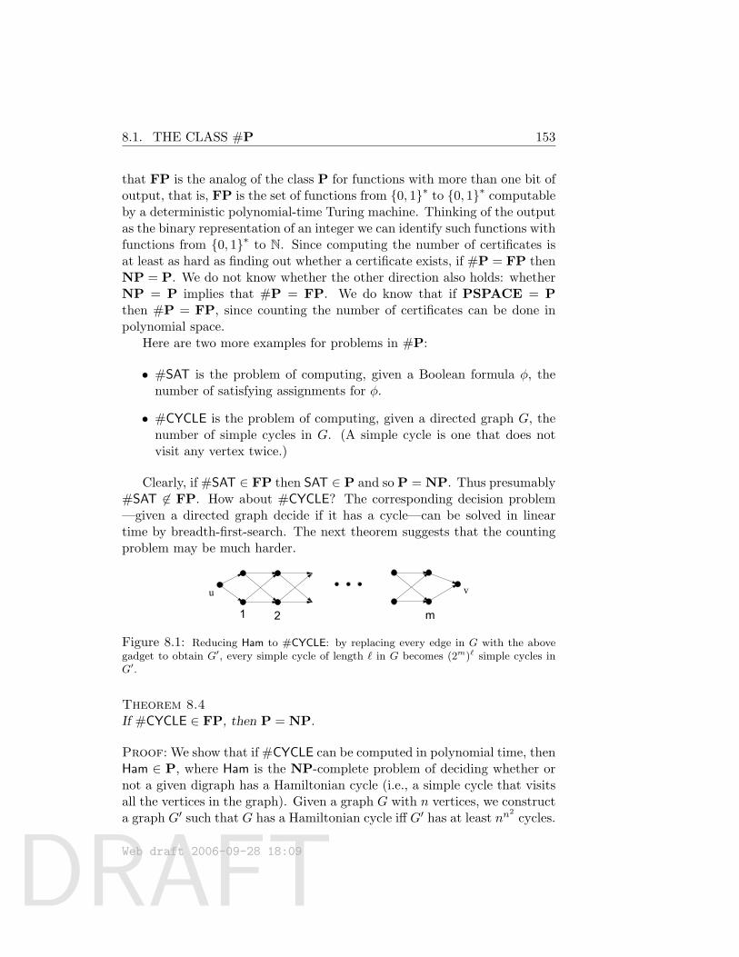
DRAFT

8.1. THE CLASS #P 153

that FP is the analog of the class P for functions with more than one bit ofoutput, that is, FP is the set of functions from 0, 1∗ to 0, 1∗ computableby a deterministic polynomial-time Turing machine. Thinking of the outputas the binary representation of an integer we can identify such functions withfunctions from 0, 1∗ to N. Since computing the number of certificates isat least as hard as finding out whether a certificate exists, if #P = FP thenNP = P. We do not know whether the other direction also holds: whetherNP = P implies that #P = FP. We do know that if PSPACE = Pthen #P = FP, since counting the number of certificates can be done inpolynomial space.

Here are two more examples for problems in #P:

• #SAT is the problem of computing, given a Boolean formula φ, thenumber of satisfying assignments for φ.

• #CYCLE is the problem of computing, given a directed graph G, thenumber of simple cycles in G. (A simple cycle is one that does notvisit any vertex twice.)

Clearly, if #SAT ∈ FP then SAT ∈ P and so P = NP. Thus presumably#SAT 6∈ FP. How about #CYCLE? The corresponding decision problem—given a directed graph decide if it has a cycle—can be solved in lineartime by breadth-first-search. The next theorem suggests that the countingproblem may be much harder.

u v

1 2 m

Figure 8.1: Reducing Ham to #CYCLE: by replacing every edge in G with the abovegadget to obtain G′, every simple cycle of length ` in G becomes (2m)` simple cycles inG′.

Theorem 8.4If #CYCLE ∈ FP, then P = NP.

Proof: We show that if #CYCLE can be computed in polynomial time, thenHam ∈ P, where Ham is the NP-complete problem of deciding whether ornot a given digraph has a Hamiltonian cycle (i.e., a simple cycle that visitsall the vertices in the graph). Given a graph G with n vertices, we constructa graph G′ such that G has a Hamiltonian cycle iff G′ has at least nn

2cycles.

Web draft 2006-09-28 18:09

DRAFT

154 8.2. #P COMPLETENESS.

To obtain G′, replace each edge (u, v) in G by the gadget shown inFigure 8.1. The gadget has m = n log n+ 1 levels. It is an acyclic digraph,so cycles in G′ correspond to cycles in G. Furthermore, there are 2m directedpaths from u to v in the gadget, so a simple cycle of length ` in G yields(2m)` simple cycles in G′.

Notice, if G has a Hamiltonian cycle, then G′ has at least (2m)n > nn2

cycles. If G has no Hamiltonian cycle, then the longest cycle in G has lengthat most n− 1. The number of cycles is bounded above by nn−1. So G′ canhave at most (2m)n−1 × nn−1 < nn

2cycles.

8.1.1 The class PP: decision-problem analog for #P.

Similar to the case of search problems, even when studying counting com-plexity, we can often restrict our attention to decision problems. The reasonis that there exists a class of decision problems PP such that

PP = P⇔ #P = FP (1)

Intuitively, PP corresponds to computing the most significant bit offunctions in #P. That is, L is in PP if there exists a polynomial-time TMM and a polynomial p : N→ N such that for every x ∈ 0, 1∗,

x ∈ L⇔∣∣∣y ∈ 0, 1p(|x|) : M(x, y) = 1

∣∣∣ ≥ 12· 2p(|x|)

You are asked to prove the non-trivial direction of (1) in Exercise 1. Itis instructive to compare the class PP, which we believe contains problemrequiring exponential time to solve, with the class BPP, which althoughit has a seemingly similar definition, can in fact be solved efficiently usingprobabilistic algorithms (and perhaps even also using deterministic algo-rithms, see Chapter 17). Note that we do not know whether this holds alsofor the class of decision problems corresponding to the least significant bitof #P, namely ⊕P (see Definition 8.13 below).

8.2 #P completeness.

Now we define #P-completeness. Loosely speaking, a function f is #P-complete if it is in #P and a polynomial-time algorithm for f implies that#P = FP. To formally define #P-completeness, we use the notion of oracleTMs, as defined in Section 4.5. Recall that a TM M has oracle access to a

Web draft 2006-09-28 18:09

DRAFT

8.2. #P COMPLETENESS. 155

language O ⊆ 0, 1∗ if it can make queries of the form “Is q ∈ O?” in onecomputational step. We generalize this to non-Boolean functions by sayingthat M has oracle access to a function f : 0, 1∗ → 0, 1∗, if it is givenaccess to the language O = 〈x, i〉 : f(x)i = 1. We use the same notationsfor functions mapping 0, 1∗ to N, identifying numbers with their binaryrepresentation as strings. For a function f : 0, 1∗ → 0, 1∗, we defineFPf to be the set of functions that are computable by polynomial-timeTMs that have access to an oracle for f .

Definition 8.5A function f is #P-complete if it is in #P and every g ∈ #P is in FPf

If f ∈ FP then FPf = FP. Thus the following is immediate.

Proposition 8.6If f is #P-complete and f ∈ FP then FP = #P.

Counting versions of many NP-complete languages such as 3SAT,Ham,and CLIQUE naturally lead to #P-complete problems. We demonstrate thiswith #SAT:

Theorem 8.7#SAT is #P-complete

Proof: Consider the Cook-Levin reduction from any L in NP to SATwe saw in Section 2.3.1. This is a polynomial-time computable functionf : 0, 1∗ → 0, 1∗ such that for every x ∈ 0, 1∗, x ∈ L ⇔ f(x) ∈ SAT.However, the proof that the reduction works actually gave us more infor-mation than that. It provided a Levin reduction, by which we mean theproof showed a way to transform a certificate that x is in L into a certificate(i.e., satisfying assignment) showing that f(x) ∈ SAT, and also vice versa(transforming a satisfying assignment for f(x) into a witness that x ∈ L).

In particular, it means that the mapping from the certificates of x to theassignments of f(x) was invertible and hence one-to-one. Thus the numberof satisfying assignments for f(x) is equal to the number of certificates forx.

As shown below, there are #P-complete problems for which the corre-sponding decision problems are in fact in P.

Web draft 2006-09-28 18:09

DRAFT


8.2.1 Permanent and Valiant’s Theorem

Now we study another problem. The permanent of an n × n matrix A isdefined as

perm(A) =∑σ∈Sn

n∏i=1

Ai,σ(i) (2)

where Sn denotes the set of all permutations of n elements. Recall that theexpression for the determinant is similar

det(A) =∑σ∈Sn

(−1)sgn(σ)n∏i=1

Aiσ(i)

except for an additional “sign” term.1 This similarity does not translateinto computational equivalence: the determinant can be computed in poly-nomial time, whereas computing the permanent seems much harder, as wesee below.

The permanent function can also be interpreted combinatorially. First,suppose the matrix A has each entry in 0, 1. It may be viewed as theadjacency matrix of a bipartite graph G(X,Y,E), with X = x1, . . . , xn,Y = y1, . . . , yn and xi, yj ∈ E iff Ai,j = 1. Then the term

∏ni=1Aiσ(i)

is 1 iff σ is a perfect matching (which is a set of n edges such that everynode is in exactly one edge). Thus if A is a 0.1 matrix then perm(A) issimply the number of perfect matchings in the corresponding graph G andin particular computing perm(A) is in #P. If A is a −1, 0, 1 matrix, thenperm(A) =

∣∣σ :∏ni=1Aiσ(i) = 1

∣∣ − ∣∣σ :∏ni=1Aiσ(i) = −1

∣∣, so one canmake two calls to a #SAT oracle to compute perm(A). In fact one can showfor general integer matrices that computing the permanent is in FP#SAT

(see Exercise 2).The next theorem came as a surprise to researchers in the 1970s, since it

implies that if perm ∈ FP then P = NP. Thus, unless P = NP, computingthe permanent is much more difficult then computing the determinant.

1It is known that every permutation σ ∈ Sn can be represented as a composition oftranspositions, where a transposition is a permutation that only switches between twoelements in [n] and leaves the other elements intact (one proof for this statement is theBubblesort algorithm). If τ1, . . . , τm is a sequence of transpositions such that their com-position equals σ, then the sign of σ is equal to +1 if m is even and −1 if m is odd. Itcan be shown that the sign is well-defined in the sense that it does not depend on therepresentation of σ as a composition of transpositions.

Web draft 2006-09-28 18:09

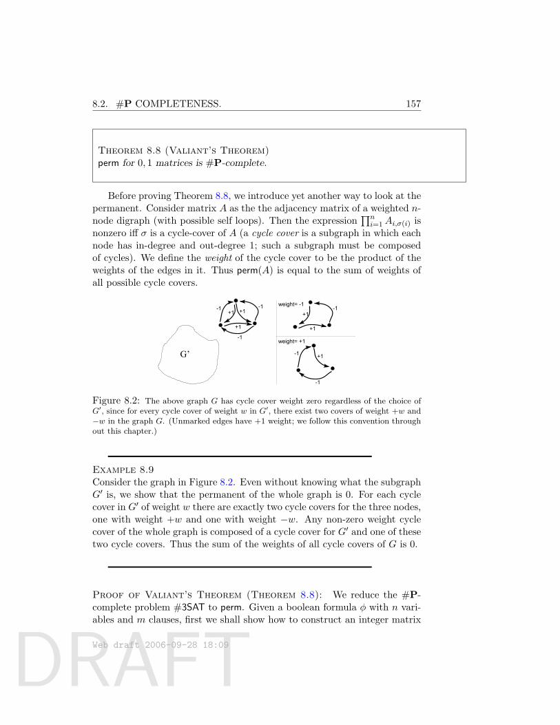
DRAFT


Theorem 8.8 (Valiant’s Theorem)perm for 0, 1 matrices is #P-complete.

Before proving Theorem 8.8, we introduce yet another way to look at thepermanent. Consider matrix A as the the adjacency matrix of a weighted n-node digraph (with possible self loops). Then the expression

∏ni=1Ai,σ(i) is

nonzero iff σ is a cycle-cover of A (a cycle cover is a subgraph in which eachnode has in-degree and out-degree 1; such a subgraph must be composedof cycles). We define the weight of the cycle cover to be the product of theweights of the edges in it. Thus perm(A) is equal to the sum of weights ofall possible cycle covers.

G’

+1

+1

+1-1

-1

-1

+1

+1-1

+1

-1

-1

weight= -1

weight= +1

Figure 8.2: The above graph G has cycle cover weight zero regardless of the choice ofG′, since for every cycle cover of weight w in G′, there exist two covers of weight +w and−w in the graph G. (Unmarked edges have +1 weight; we follow this convention throughout this chapter.)

Example 8.9Consider the graph in Figure 8.2. Even without knowing what the subgraphG′ is, we show that the permanent of the whole graph is 0. For each cyclecover in G′ of weight w there are exactly two cycle covers for the three nodes,one with weight +w and one with weight −w. Any non-zero weight cyclecover of the whole graph is composed of a cycle cover for G′ and one of thesetwo cycle covers. Thus the sum of the weights of all cycle covers of G is 0.

Proof of Valiant’s Theorem (Theorem 8.8): We reduce the #P-complete problem #3SAT to perm. Given a boolean formula φ with n vari-ables and m clauses, first we shall show how to construct an integer matrix

Web draft 2006-09-28 18:09

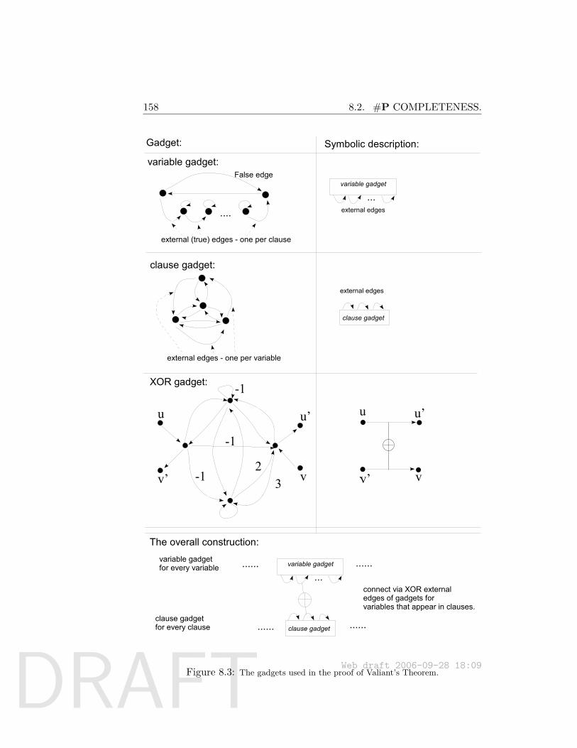
DRAFT


variable gadget:

....

False edge

external (true) edges - one per clause

Symbolic description:

...

Gadget:

clause gadget:

external edges - one per variable

external edges

variable gadget

clause gadget

XOR gadget:

u u’

v’ v

-1

-1

-12

3

u u’

vv’ `

The overall construction:

external edges

...variable gadget

clause gadget

...... ......

............

variable gadgetfor every variable

clause gadgetfor every clause

connect via XOR externaledges of gadgets forvariables that appear in clauses.

Figure 8.3: The gadgets used in the proof of Valiant’s Theorem.Web draft 2006-09-28 18:09

DRAFT


A′ with negative entries such that perm(A′) = 4m · (#φ). (#φ stands for thenumber of satisfying assignments of φ). Later we shall show how to to geta 0-1 matrix A from A′ such that knowing perm(A) allows us to computeperm(A′).

The main idea is that our construction will result in two kinds of cyclecovers in the digraph G′ associated with A′: those that correspond to sat-isfying assignments (we will make this precise) and those that don’t. Wewill use negative weights to ensure that the contribution of the cycle cov-ers that do not correspond to satisfying assignments cancels out. (This issimilar reasoning to the one used in Example 8.9.) On the other hand, wewill show that each satisfying assignment contributes 4m to perm(A′), andso perm(A′) = 4m · (#φ).

To construct G′ from φ, we combine the following three kinds of gadgetsshown in Figure 8.3:

Variable gadget The variable gadget has two possible cycle covers, cor-responding to an assignment of 0 or 1 to that variable. Assigning1 corresponds to a single cycle taking all the external edges (“true-edges”), and assigning 0 correspond to taking all the self-loops andtaking the “false-edge”. Each external edge of a variable is associatedwith a clause in which the variable appears.

Clause gadget The clause gadget is such that the only possible cycle coversexclude at least one external edge. Also for a given (proper) subset ofexternal edges used there is a unique cycle cover (of weight 1). Eachexternal edge is associated with a variable appearing in the clause.

XOR gadget We also use a graph called the XOR gadget whose purposeis to ensure that for some pair of edges

−−→uu′ and

−→v v′, exactly one of

these edges is present in any cycle cover that counts towards the finalsum.

Suppose that we replace a pair of edges−−→uu′ and

−→v v′ in some graph

G with the XOR gadget as described in Figure count:fig:valiantgad toobtain some graph G′. Then, via similar reasoning to Example 8.9,every cycle cover of G of weight w that uses exactly one of the edges−−→uu′ and

−→v v′ is mapped to a set of cycle covers in G′ whose total weight

is 4w (i.e., the set of covers that enter the gadget at u and exit at u′

or enter it at v and exit it at v′), while all the other cycle covers ofG′ have total weight 0 (Exercise 3). For this reason, whenever wereplace edges

−−→uu′ and

−→v v′ with a XOR gadget, we can consider in the

Web draft 2006-09-28 18:09

DRAFT


analysis only cycle covers that use exactly one of these edges, as theother covers do not contribute anything to the total sum.

The XOR gadgets are used to connect the variable gadgets to the corre-sponding clause gadgets so that only cycle covers corresponding to a satis-fying assignment will be counted towards the total number of cycle covers.Consider a clause, and a variable appearing in it. Each has an external edgecorresponding to the other, connected by an XOR gadget. If the externaledge in the clause is not taken then by the analysis of the XOR gadget theexternal edge in the variable must be taken (and hence the variable is true).Since at least one external edge of each clause gadget has to be omitted,each cycle cover that is counted towards the sum corresponds to a satisfy-ing assignment. Conversely, for each satisfying assignment, there is a a setof cycle covers with total weight 43m (since they passes through the XORgadget exactly 3m times). So perm(G′) = 43m#φ.

Reducing to the case 0, 1 matrices. Finally we have to reduce findingperm(G′) to finding perm(G), where G is an unweighted graph (or equiva-lently, its adjacency matrix has only 0, 1 entries). We start by reducing tothe case that all edges have weights in ±1. First, note that replacing anedge of weight k by k parallel edges of weight 1 does not change the per-manent. Parallel edges are not allowed, but we can make edges non-parallelby cutting each edge −→u v in two and inserting a new node w with an edgefrom u to w, w to v and a self loop at w. To get rid of the negative weights,note that the permanent of an n vertex graph with edge weights in ±1 isa number x in [−n!,+n!] and hence this permanent can be computed fromy = x (mod 2m+1) where m is sufficiently large (e.g., m = n2 will do). Butto compute y it is enough to compute the permanent of the graph where allweight −1 edges are replaced with edges of weight 2m. Such edges can beconverted to m edges of weight 2 in series, which again can be transformedto parallel edges of weight +1 as above.

8.2.2 Approximate solutions to #P problems

Since computing exact solutions to #P-complete problems is presumablydifficult, a natural question is whether we can approximate the number ofcertificates in the sense of the following definition.

Definition 8.10Let f :0, 1∗ → N and α < 1. An algorithm A is an α-approximation for fif for every x, αf(x) ≤ A(x) ≤ f(x)/α.

Web draft 2006-09-28 18:09

DRAFT

8.3. TODA’S THEOREM: PH ⊆ P#SAT 161

Not all #P problems behave identically with respect to this notion. Ap-proximating certain problems within any constant factor α > 0 is NP-hard(see Exercise 5). For other problems such as 0/1 permanent, there is a Fullypolynomial randomized approximation scheme (FPRAS), which is an algo-rithm which, for any ε, δ, approximates the function within a factor 1+ε (itsanswer may be incorrect with probability δ) in time poly(n, log 1/δ, log 1/ε).Such approximation of counting problems is sufficient for many applica-tions, in particular those where counting is needed to obtain estimates forthe probabilities of certain events (e.g., see our discussion of the graph reli-ability problem).

The approximation algorithm for the permanent —as well as other sim-ilar algorithms for a host of #P-complete problems—use the Monte CarloMarkov Chain technique. The result that spurred this development is dueto Valiant and Vazirani and it shows that under fairly general conditions,approximately counting the number of elements in a set ( membership inwhich is testable in polynomial time) is equivalent —in the sense that theproblems are interreducible via polynomial-time randomized reductions—to the problem of generating a random sample from the set. We will notdiscuss this interesting area any further.

Interestingly, if P = NP then every #P problem has an FPRAS (and infact an FPTAS: i.e., a deterministic polynomial-time approximation scheme),see Exercise 6.

8.3 Toda’s Theorem: PH ⊆ P#SAT

An important question in the 1980s was the relative power of the polynomial-hierarchy PH and the class of counting problems #P. Both are naturalgeneralizations of NP, but it seemed that their features— alternation andthe ability to count certificates, respectively — are not directly comparableto each other. Thus it came as big surprise when in 1989 Toda showed:

Theorem 8.11 (Toda’s theorem [Tod91])PH ⊆ P#SAT.

That is, we can solve any problem in the polynomial hierarchy given anoracle to a #P-complete problem.

Web draft 2006-09-28 18:09

DRAFT

162 8.3. TODA’S THEOREM: PH ⊆ P#SAT

Remark 8.12Note that we already know, even without Toda’s theorem, that if #P = FPthen NP = P and so PH = P. However, this does not imply that any prob-lem in PH can be computed in polynomial-time using an oracle to #SAT.For example, one implication of Toda’s theorem is that a subexponential(i.e., 2n

o(1)-time) algorithm for #SAT will imply such an algorithm for any

problem in PH. Such an implication is not known to hold from a 2no(1)

-timealgorithm for SAT.

8.3.1 The class ⊕P and hardness of satisfiability with uniquesolutions.

The following complexity class will be used in the proof:

Definition 8.13A language L in the class ⊕P (pronounced “parity P”) iff there exists apolynomial time NTM M such that x ∈ L iff the number of accepting pathsof M on input x is odd.

Thus, ⊕P can be considered as the class of decision problems corre-sponding to the least significant bit of a #P-problem. As in the proofof Theorem 8.7, the fact that the standard NP-completeness reduction isparsimonious implies the following problem ⊕SAT is ⊕P-complete (undermany-to-one Karp reductions):

Definition 8.14Define the quantifier

⊕as follows: for every Boolean formula ϕ on n vari-

ables.⊕

x∈0,1n ϕ(x) is true if the number of x’s such that ϕ(x) is true isodd.2 The language ⊕SAT consists of all the true quantified Boolean for-mula of the form

⊕x∈0,1n ϕ(x) where ϕ is an unquantified Boolean formula

(not necessarily in CNF form).

Unlike the class #P, it is not known that a polynomial-time algorithmfor ⊕P implies that NP = P. However, such an algorithm does imply thatNP = RP since NP can be probabilistically reduced to ⊕SAT:

2Note that if we identify true with 1 and 0 with false then⊕x∈0,1n ϕ(x) =

∑x∈0,1n ϕ(x) (mod 2). Also note that

⊕x∈0,1n ϕ(x) =⊕

x1∈0,1 · · ·⊕

xn∈0,1 ϕ(x1, . . . , xn).

Web draft 2006-09-28 18:09

DRAFT


Theorem 8.15 (Valiant-Vazirani Theorem)There exists a probabilistic polynomial-time algorithm A such that for every n-variable Boolean formula ϕ

ϕ ∈ SAT⇒ Pr[A(ϕ) ∈ ⊕SAT] ≥ 18n

ϕ 6∈ SAT⇒ Pr[A(ϕ) ∈ ⊕SAT] = 0

Tool: Pairwise independent hash functions.

To prove Theorem 8.15 we use the notion of pairwise independent hash func-tions.Definition 8.16 (Pairwise independent hash functions)Let Hn,k be a collection of functions from 0, 1n to 0, 1k. We say thatHn,k is pairwise independent if for every x, x′ ∈ 0, 1n with x 6= x′ and forevery y, y′ ∈ 0, 1k, Prh∈RHn,k [h(x) = y ∧ h(x′) = y′] = 2−2n

Note that an equivalent formulation is that for every two distinct stringsx, x′ ∈ 0, 1n the random variable 〈h(x), h(x′)〉 for h chosen at random fromHn,k is distributed according to the uniform distribution on 0, 1k×0, 1k.

Recall that GF(2n) is the field of 2n elements, whose elements can beidentified with 0, 1n, and whose addition (+) and multiplication (·) opera-tions satisfy the usual commutative and distributive laws, and every elementx has an additive inverse (denoted by −x) and, if nonzero, a multiplicativeinverse (denoted by x−1). The following theorem provides a constructionof an efficiently computable pairwise independent hash functions (see alsoExercise 4 for a different construction):

Theorem 8.17 (Efficient pairwise independent hash functions)For every n define the collection Hn,n to be ha,ba,b∈GF(2n) where for everya, b ∈ GF(2n), the function ha,b : GF(2n)→ GF(2n) maps x to ax+b. Then,Hn,n is a collection of pairwise independent hash functions.

Remark 8.18Theorem 8.17 implies the existence of an efficiently computable pairwiseindependent hash functions Hn,k for every n, k: if k > n we can use thecollection Hk,k and reduce the size of the input to n by padding it withzeros. If k < n then we can use the collection Hn,n and truncate the lastn− k bits of the output.

Web draft 2006-09-28 18:09

DRAFT


Proof: For every x 6= x′ ∈ GF(2n) and y, y′ ∈ GF(2n), ha,b(x) = y andha,b(x′) = y′ iff a, b satisfy the equations:

a · x+ b =ya · x′ + b =y′

These imply a · (x − x′) = y − y′ or a = (y − y′)(x − x′)−1. Since b =y− a · x, the pair 〈a, b〉 is completely determined by these equations, and sothe probability that this happens over the choice of a, b is exactly one overthe number of possible pairs, which indeed equals 1

22n .

Pairwise independent hash functions have several useful properties thatled to numerous applications in theoretical and applied computer science.In this section, we will use the following result:

Lemma 8.19 (Valiant-Vazirani Lemma [?])Let Hn,k be a pairwise independent hash function collection from 0, 1n to

0, 1k and S ⊆ 0, 1n such that 2k−2 ≤ |S| ≤ 2k−1. Then,

Prh∈RHn,k

[∣∣∣x ∈ S : h(x) = 0k

∣∣∣ = 1] ≥ 18

Proof: For every x ∈ S, let p = 2−k be the probability that h(x) = 0k whenh ∈R Hn,k. Note that for every x 6= x′, Pr[h(x)=0k∧h(x′)=0k] = p2. Let Nbe the random variable denoting the number of x ∈ S satisfying h(x) = 0k.Note that E[N ] = |S|p ∈ [14 ,

12 ]. By the inclusion-exclusion principle

Pr[N ≥ 1] ≥∑x∈S

Pr[h(x)=0k]−∑

x<x′∈SPr[h(x)=0k∧h(x′)=0k] = |S|p−

(|S|2

)p2

and by the union bound we get that Pr[N ≥ 2] ≤(|S|

2

)p2. Thus

Pr[N = 1] = Pr[N ≥ 1]−Pr[N ≥ 2] ≥ |S|p− 2(|S|2

)p2 ≥ |S|p− |S|2p2 ≥ 1

8

where the last inequality is obtained using the fact that 14 ≤ |S|p ≤

12 .

Proof of Theorem 8.15

We now use Lemma 8.19 to prove Theorem 8.15. Given a formula ϕ on nvariables, our probabilistic algorithmA chooses k at random from 2, . . . , n+ 1

Web draft 2006-09-28 18:09

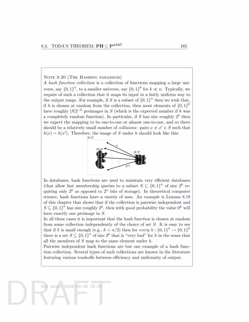
DRAFT


Note 8.20 (The Hashing paradigm)A hash function collection is a collection of functions mapping a large uni-verse, say 0, 1n, to a smaller universe, say 0, 1k for k n. Typically, werequire of such a collection that it maps its input in a fairly uniform way tothe output range. For example, if S is a subset of 0, 1n then we wish that,if h is chosen at random from the collection, then most elements of 0, 1khave roughly |S|2−k preimages in S (which is the expected number if h wasa completely random function). In particular, if S has size roughly 2k thenwe expect the mapping to be one-to-one or almost one-to-one, and so thereshould be a relatively small number of collisions: pairs x 6= x′ ∈ S such thath(x) = h(x′). Therefore, the image of S under h should look like this:

0,1n

0,1k|S|~2k

2n-k

h

......

In databases, hash functions are used to maintain very efficient databases(that allow fast membership queries to a subset S ⊆ 0, 1n of size 2k re-quiring only 2k as opposed to 2n bits of storage). In theoretical computerscience, hash functions have a variety of uses. An example is Lemma 8.19of this chapter that shows that if the collection is pairwise independent andS ⊆ 0, 1n has size roughly 2k, then with good probability the value 0k willhave exactly one preimage in S.In all these cases it is important that the hash function is chosen at randomfrom some collection independently of the choice of set S. It is easy to seethat if k is small enough (e.g., k < n/2) then for every h : 0, 1n → 0, 1kthere is a set S ⊆ 0, 1n of size 2k that is “very bad” for h in the sense thatall the members of S map to the same element under h.Pairwise independent hash functions are but one example of a hash func-tion collection. Several types of such collections are known in the literaturefeaturing various tradeoffs between efficiency and uniformity of output.

Web draft 2006-09-28 18:09

DRAFT


and a random hash function h ∈R Hn,k. It then uses the Cook-Levin re-duction to compute a formula τ on variables x ∈ 0, 1n , y ∈ 0, 1m (form = poly(n)) such that h(x) = 0 if and only if there exists a unique y suchthat τ(x, y) = 1.3 The output of A if the formula

ψ =⊕

x∈0,1n,y∈0,1mϕ(x) ∧ τ(x, y) ,

It is equivalent to the statement⊕x∈0,1n

ϕ(x) ∧ h(x) = 0k ,

If ϕ is unsatisfiable then ψ is false, since we’ll have no x’s satisfyingthe inner formula and zero is an even number. If ϕ is satisfiable, we let Sbe the set of its satisfying assignments. With probability 1/n, k satisfies2k−2 ≤ |S| ≤ 2k, conditioned on which, with probability 1/8, there is aunique x such that ϕ(x) ∧ h(x) = 0n. Since one happens to be an oddnumber, this implies that ψ is true.

Remark 8.21 (Hardness of Unique Satisfiability)The proof of Theorem 8.15 implies the following stronger statement: theexistence of an algorithm to distinguish between an unsatisfiable Booleanformula and a formula with exactly one satisfying assignment implies theexistence of a probabilistic polynomial-time algorithm for all of NP. Thus,the guarantee that a particular search problem has either no solutions or aunique solution does not necessarily make the problem easier to solve.

8.3.2 Step 1: Randomized reduction from PH to ⊕P

We now go beyond NP (that is to say, the Valiant-Vazirani theorem) andshow that we can actually reduce any language in the polynomial hierarchyto ⊕SAT.Lemma 8.22Let c ∈ N be some constant. There exists a probabilistic polynomial-timealgorithm A such that for every ψ a Quantified Boolean formula with c levelsof alternations,

ψ is true⇒Pr[A(ψ) ∈ ⊕SAT] ≥ 23

ψ is false⇒Pr[A(ψ) ∈ ⊕SAT] = 03For some implementations of hash functions, such as the one described in Exercise 4,

one can construct directly (without going through the Cook-Levin reduction) such a for-mula τ that does not use the y variables.

Web draft 2006-09-28 18:09

DRAFT


Before proving the Lemma, let us make a few notations and observations:For a Boolean formula ϕ on n variables, let #(ϕ) denote the number ofsatisfying assignments of ϕ. We consider also formulae ϕ that are partiallyquantified. That is, in addition to the n variables ϕ takes as input it mayalso have other variables that are bound by a ∀,∃ or

⊕quantifiers (for

example ϕ can be of the form ϕ(x1, . . . , xn) = ∀y ∈ 0, 1n τ(x1, . . . , xn, y)where τ is, say, a 3CNF Boolean formula).

Given two (possibly partially quantified) formulae ϕ,ψ on variables x ∈0, 1n , y ∈ 0, 1m we can construct in polynomial-time an n + m vari-able formula ϕ · ψ and a (maxn,m + 1)-variable formula ϕ + ψ suchthat #(ϕ · ψ) = #(ϕ)#(ϕ) and #(ϕ + ψ) = #(ϕ) + #(ψ). Indeed, takeϕ ·ψ(x, y) = ϕ(x)∧ϕ(y) and ϕ+ψ(z) =

((z0 = 0)∧ϕ(z1, . . . , zn)

)∨((z0 =

1)∧ψ(z1, . . . , zm)). For a formula ϕ, we use the notation ϕ+1 to denote the

formula ϕ + ψ where ψ is some canonical formula with a single satisfyingassignment. Since the product of numbers is even iff one of the numbersis even, and since adding one to a number flips the parity, for every twoformulae ϕ,ψ as above(⊕

x

ϕ(x))∧(⊕y

ψ(y))⇔⊕x,y

(ϕ · ψ)(x, y) (3)

¬⊕x

ϕ(x)⇔⊕x,z

(ϕ+ 1)(x, z) (4)

(⊕x

ϕ(x))∨(⊕y

ψ(y))⇔⊕x,y,z

((ϕ+ 1) · (ψ + 1) + 1)(x, y, z) (5)

Proof of Lemma 8.22: Recall that membership in a PH-language canbe reduced to deciding the truth of a quantified Boolean formula with aconstant number of alternating quantifiers. The idea behind the proof is toreplace one-by-one each ∃/∀ quantifiers with a

⊕quantifier.

Let ψ be a formula with c levels of alternating ∃/∀ quantifiers, possiblywith an initial

⊕quantifier. We transform ψ in probabilistic polynomial-

time to a formula ψ′ such that ψ′ has only c − 1 levels of alternating ∃/∀quantifiers, an initial

⊕quantifier, satisfying (1) if ψ is false then so is ψ′,

and (2) if ψ is true then with probability at least 1− 110c , ψ

′ is true as well.The lemma follows by repeating this step c times.

For ease of notations, we demonstrate the proof for the case that ψ hasa single

⊕quantifier and two additional ∃/∀ quantifiers. We can assume

without loss of generality that ψ is of the form

ψ =⊕

z∈0,1`∃x∈0,1n∀w∈0,1kϕ(z, x, w) ,

Web draft 2006-09-28 18:09

DRAFT


as otherwise we can use the identities ∀xP (x) = ¬∃x¬P (x) and (4) to trans-form ψ into this form.

The proof of Theorem 8.15 provides for every n, a probabilistic algorithmthat outputs a formula τ on variables x ∈ 0, 1n and y ∈ 0, 1m such thatfor every nonempty set S ⊆ 0, 1n, Pr[⊕x∈0,1n,y∈0,1mτ(x, y)] ≥ 1/(8n).Run this algorithm t = 100c` log n times to obtain the formulae τ1, . . . , τt.Then, for every nonempty set S ⊆ 0, 1n the probability that there does notexist i ∈ [t] such that⊕x∈0,1n,y∈0,1mτ(x, y) is True is less than 2−`/(10c).We claim that this implies that with probability at least 1 − 1/(10c), thefollowing formula is equivalent to ψ:⊕

z∈0,1`θ(z) , (6)

where

θ(z) = ∨ti=1

⊕x∈0,1n,y∈0,1m

∀w∈0,1kτi(x, y) ∧ ϕ(x, z, w)

Indeed, for every z ∈ 0, 1` define Sz =

x ∈ 0, 1n : ∀w∈0,1kϕ(x, z, w)

.

Then, ψ is equivalent to ⊕z∈0,1` |Sz| is nonempty. But by the union bound,with probability at least 1−1/(10c) it holds that for every z such that Sz isnonempty, there exists τi satisfying ⊕x,yτi(x, y). This means that for everysuch z, θ(z) is true. On the other hand, if Sz is empty then certainly θ(z)is false, implying that indeed ψ is equivalent to (6).

By applying the identity (5), we can transform (6) into an equivalentformula of the desired form ⊕

z,x,y,w

∀wϕ′(x, y, z, w)

for some unquantified polynomial-size formula ϕ′.

8.3.3 Step 2: Making the reduction deterministic

To complete the proof of Toda’s Theorem (Theorem 8.11), we prove thefollowing lemma:

Lemma 8.23There is a (deterministic) polynomial-time transformation T that, for everyformula ψ that is an input for ⊕SAT, T (ψ, 1m) is an unquantified Boolean

Web draft 2006-09-28 18:09

DRAFT


formula and

ψ ∈ ⊕SAT⇒#(ϕ) = −1 (mod 2m+1)

ψ 6∈ ⊕SAT⇒#(ϕ) = 0 (mod 2m+1)

Proof of Theorem 8.11 using Lemmas 8.22 and 8.23.: Let L ∈ PH.We show that we can decide whether an input x ∈ L by asking a singlequestion to a #SAT oracle. For every x ∈ 0, 1n, Lemmas 8.22 and 8.23together imply there exists a polynomial-time TM M such that

x ∈ L⇒ Prr∈R0,1m

[#(M(x, r)) = −1 (mod 2m+1)] ≥ 23

x 6∈ L⇒ ∀r∈R0,1m#(M(x, r)) = 0 (mod 2m+1)

where m is the (polynomial in n) number of random bits used by the proce-dure described in that Lemma. Furthermore, even in the case x ∈ L, we areguaranteed that for every r ∈ 0, 1m, #(M(x, r)) ∈ 0,−1 (mod 2m+1).

Consider the function that maps two strings r, u into the evaluation of theformula M(x, r) on the assignment u. Since this function is computable inpolynomial-time, the Cook-Levin transformation implies that we can obtainin polynomial-time a CNF formula θx on variables r, u, y such that for everyr, u, M(x, r) is satisfied by u if and only if there exist a unique y such thatθx(r, u, y) is true. Let fx(r) be the number of u, y such that θx(r, u, y) istrue, then

#(θx) =∑

r∈0,1mfx(r) ,

But if x 6∈ L then fx(r) = 0 (mod 2m+1) for every r, and hence #(θx) = 0(mod 2m+1). On the other hand, if x ∈ L then fx(r) = −1 (mod 2m+1) forbetween 2

32m and 2m values of r, and is equal to 0 on the other values, andhence #(θx) 6= 0 (mod 2m+1). We see that deciding whether x ∈ L can bedone by computing #(θx).

Proof of Lemma 8.23: For every pair of formulae ϕ,τ recall that wedefined formulas ϕ + τ and ϕ · τ satisfying #(ϕ + τ) = #(ϕ) + #(τ) and#(ϕ · τ) = #(ϕ)#(τ), and note that these formulae are of size at most aconstant factor larger than ϕ, τ . Consider the formula 4τ3 + 3τ4 (where τ3

for example is shorthand for τ · (τ · τ)). One can easily check that

#(τ) = −1 (mod 22i)⇒#(4τ3 + 3τ4) = −1 (mod 22i+1) (7)

#(τ) = 0 (mod 22i)⇒#(4τ3 + 3τ4) = 0 (mod 2)2i+1

(8)

Web draft 2006-09-28 18:09

DRAFT

170 8.4. OPEN PROBLEMS

Let ψ0 = ψ and ψi+1 = 4ψ3i + 3ψ4

i . Let ψ∗ = ψdlog(m+1)e. Repeated use ofequations (7), (8) shows that if #(ψ) is odd, then #(ψ∗) = −1 (mod 2m+1)and if #(ψ) is even, then #(ψ∗) = 0 (mod 2m+1). Also, the size of ψ∗ isonly polynomially larger than size of ψ.


• The class #P consists of functions that count the number of certificates for agiven instance. If P 6= NP then it is not solvable in polynomial time.

• Counting analogs of many natural NP-complete problems are #P-complete,but there are also #P-complete counting problems for which the correspond-ing decision problem is in P. One example for this is the problem perm ofcomputing the permanent.

• Surprisingly, counting is more powerful than alternating quantifiers: we cansolve every problem in the polynomial hierarchy using an oracle to a #P-complete problem.

• The classes PP and ⊕P contain the decision problems that correspond tothe most significant and least significant bits (respectively) of a #P function.The class PP is as powerful as #P itself, in the sense that if PP = P then#P = FP. We do not know if this holds for ⊕P but do know that everylanguage in PH randomly reduces to ⊕P.

8.4 Open Problems

• What is the exact power of ⊕SAT and #SAT ?

• What is the average case complexity of n×n permanent modulo smallprime, say 3 or 5 ? Note that for a prime p > n, random self reducibil-ity of permanent implies that if permanent is hard to compute on atleast one input then it is hard to compute on 1 − O(p/n) fraction ofinputs, i.e. hard to compute on average (see Theorem ??).


The definition of #P as well as several interesting examples of #P problemsappeared in Valiant’s seminal paper [Val79b]. The #P-completeness of the

Web draft 2006-09-28 18:09

DRAFT

8.4. OPEN PROBLEMS 171

permanent is from his other paper [Val79a]. Toda’s Theorem is provedin [Tod91]. The proof given here follows the proof of [KVVY93] (althoughwe use formulas where they used circuits.)

For an introduction to FPRAS’s for computing approximations to manycounting problems, see the relevant chapter in Vazirani [Vaz01] ( an excellentresource on approximation algorithms in general).

.

Exercises

§1 Let f ∈ #P. Show a polynomial-time algorithm to compute f givenaccess to an oracle for some language L ∈ PP (see Remark ??).

Hint:withoutlossofgeneralityyoucanthinkthatf=#CKT−SAT,theproblemofcomputingthenumberofsatisfy-ingassignmentsforagivenBooleancircuitC,andthatyouaregivenanoraclethattellsyouifagivenn-variablecircuit,hasatleast2

n−1satisfyingassignmentsornot.Themainobservationyou

canuseisthatifChasatleast2n−1

satisfyingassignmentsthenitispossibletousetheoracletofindastringxsuchthatChasexactly2

n−1satisfyingassignmentsthatarelargerthanxinthe

naturallexicographicorderingofthestringsin0,1n.

§2 Show that computing the permanent for matrices with integer entriesis in FP#SAT.

§3 Complete the analysis of the XOR gadget in the proof of Theorem 8.8.Let G be any weighted graph containing a pair of edges

−−→uu′ and

−→v v′,

and let G′ be the graph obtained by replacing these edges with theXOR gadget. Prove that every cycle cover of G of weight w that usesexactly one of the edges

−−→uu′ is mapped to a set of cycle covers in G′

whose total weight is 4w, and all the other cycle covers of G′ havetotal weight 0.

§4 Let k ≤ n. Prove that the following family Hn,k is a collection ofpairwise independent functions from 0, 1n to 0, 1k: Identify 0, 1with the field GF(2). For every k×n matrix A with entries in GF(2),and k-length vector b ∈ GF(2)n, Hn,k contains the function hA,b :GF(2)n → GF(2)k defined as follows: hA,b(x) = Ax+ b.

§5 Show that if there is a polynomial-time algorithm that approximates#CYCLE within a factor 1/2, then P = NP.

Web draft 2006-09-28 18:09

DRAFT

172 8.4. OPEN PROBLEMS

§6 Show that if NP = P then for every f ∈ #P and there is a polynomial-time algorithm that approximates f within a factor of 1/2. Can youshow the same for a factor of 1−ε for arbitrarily small constant ε > 0?Can you make these algorithms deterministic?

Note that we do not know whether P = NP implies that exact com-putation of functions in #P can be done in polynomial time.

Hint:UsehashingandideassimilartothoseintheproofofToda’stheorem,wherewealsoneededtoestimatethesizeofasetofstrings.IfyoufindthisquestiondifficultyoumightwanttocomebacktoitafterseeingtheGoldwasser-Sipsersetlowerboundpro-tocolofChapter9.TomakethealgorithmdeterministicusetheideasoftheproofthatBPP⊆PH(Theorem7.17).

§7 Show that every for every language in AC0 there is a depth 3 circuitof npoly(logn) size that decides it on 1 − 1/poly(n) fraction of inputsand looks as follows: it has a single ⊕ gate at the top and the othergates are ∨,∧ of fanin at most poly(log n).

Hint:usetheproofofLemma8.22.

Web draft 2006-09-28 18:09

DRAFT

Chapter 9

Interactive proofs

“What is intuitively required from a theorem-proving procedure?First, that it is possible to “prove” a true theorem. Second, thatit is impossible to “prove” a false theorem. Third, that commu-nicating the proof should be efficient, in the following sense. Itdoes not matter how long must the prover compute during theproving process, but it is essential that the computation requiredfrom the verifier is easy.”Goldwasser, Micali, Rackoff 1985

The standard notion of a mathematical proof follows the certificate def-inition of NP. That is, to prove that a statement is true one provides asequence of symbols that can be written down in a book or on paper, anda valid sequence exists only for true statements. However, people often usemore general ways to convince one another of the validity of statements:they interact with one another, with the person verifying the proof (hence-forth the verifier) asking the person providing it (henceforth the prover) fora series of explanations before he is convinced.

It seems natural to try to understand the power of such interactiveproofs from the complexity-theoretic perspective. For example, can oneprove that a given formula is not satisfiable? (recall that is this problemis coNP-complete, it’s not believed to have a polynomial-sized certificate).The surprising answer is yes. Indeed, interactive proofs turned out to haveunexpected powers and applications. Beyond their philosophical appeal, in-teractive proofs led to fundamental insights in cryptographic protocols, thepower of approximation algorithms, program checking, and the hardness offamous “elusive” problems (i.e., NP-problems not known to be in P nor


173

DRAFT

1749.1. WARMUP: INTERACTIVE PROOFS WITH A DETERMINISTIC

VERIFIER

to be NP-complete) such as graph isomorphism and approximate shortestlattice vector.

9.1 Warmup: Interactive proofs with a determin-istic verifier

Let us consider what happens when we introduce interaction into the NPscenario. That is, we’d have an interrogation-style proof system where ratherthan the prover send a written proof to the verifier, the prover and verifierinteract with the verifier asking questions and the prover responding, whereat the end the verifier decides whether or not to accept the input. Ofcourse, both verifier and prover can keep state during the interaction, orequivalently, the message a party sends at any point in the interaction canbe a function of all messages sent and received so far. Formally, we makethe following definition:

Definition 9.1 (Interaction of deterministic functions)Let f, g : 0, 1∗ → 0, 1∗ be functions. A k-round interaction of f and gon input x ∈ 0, 1∗, denoted by 〈f, g〉(x) is the sequence of the followingstrings a1, . . . , ak ∈ 0, 1∗ defined as follows:

(1)

a1 = f(x)a2 = g(x, a1). . .

a2i+1 = f(x, a1, . . . , a2i)a2i+2 = g(x, a1, . . . , a2i+1)

(Where we consider a suitable encoding of i-tuples of strings to strings.)The output of f (resp. g) at the end of the interaction denoted outf 〈f, g〉(x)

(resp. outg〈f, g〉(x) ) is defined to be f(x, a1, . . . , ak) (resp. g(x, a1, . . . , ak)).

Definition 9.2 (Deterministic proof systems)We say that a language L has a k-round deterministic interactive proofsystem if there’s a deterministic TM V that on input x, a1, . . . , ai runs intime polynomial in |x|, satisfying:

(Completeness)x ∈ L⇒ ∃P : 0, 1∗ → 0, 1∗ outV 〈V, P 〉(x) = 1(Soundness)x 6∈ L⇒ ∀P : 0, 1∗ → 0, 1∗ outV 〈V, P 〉(x) = 1

Web draft 2006-09-28 18:09

DRAFT

9.2. THE CLASS IP 175

The class dIP contains all languages with a k(n)-round deterministicinteractive proof systems with k(n) polynomial in n.

It turns out this actually does not change the class of languages we canprove:

Theorem 9.3dIP = NP.

Proof: Clearly, every NP language has a 1-round proof system. Now weprove that if a L has an interactive proof system of this type then L ∈ NP.The certificate for membership is just the transcript (a1, a2, . . . , ak) causingthe verifier to accept. To verify this transcript, check that indeed V (x) = a1,V (x, a1, a2) = a3, . . ., and V (x, a1, . . . , ak) = 1. If x ∈ L then there indeedexists such a transcript. If there exists such a transcript (a1, . . . , ak) then wecan define a prover function P to satisfy P (x, a1) = a2, P (x, a1, a2, a3) = a4,etc. We see that outV 〈V, P 〉(x) = 1 and hence x ∈ L.

9.2 The class IP

In order to realize the full potential of interaction, we need to let the verifierbe probabilistic. The idea is that, similar to probabilistic algorithms, theverifier will be allowed to come to a wrong conclusion (e.g., accept a prooffor a wrong statement) with some small probability. However, as in the caseof probabilistic algorithms, this probability is over the verifier’s coins andthe verifier will reject proofs for a wrong statement with good probabilityregardless of the strategy the prover uses. It turns out that the combinationof interaction and randomization has a huge effect: as we will see, the setof languages which have interactive proof systems now jumps from NP toPSPACE.

Example 9.4As an example for a probabilistic interactive proof system, consider thefollowing scenario: Marla claims to Arthur that she can distinguish betweenthe taste of Coke (Coca-Cola) and Pepsi. To verify this statement, Marlaand Arthur repeat the following experiment 50 times: Marla turns her backto Arthur, as he places Coke in one unmarked cup and Pepsi in another,choosing randomly whether Coke will be in the cup on the left or on theright. Then Marla tastes both cups and states which one contained whichdrinks. While, regardless of her tasting abilities, Marla can answer correctly

Web draft 2006-09-28 18:09

DRAFT

176 9.2. THE CLASS IP

with probability 12 by a random guess, if she manages to answer correctly

for all the 50 repetitions, Arthur can indeed be convinced that she can tellapart Pepsi and Coke.

To formally define this we extend the notion of interaction to probabilisticfunctions (actually, we only need to do so for the verifier). To model aninteraction between f and g where f is probabilistic, we add an additionalm-bit input r to the function f in (1), that is having a1 = f(x, r), a3 =f(x, r, a1, a2), etc. The interaction 〈f, g〉(x) is now a random variable overr ∈R 0, 1m. Similarly the output outf 〈f, g〉(x) is also a random variable.

Definition 9.5 (IP)Let k : N → N be some function with k(n) computable in poly(n) time. Alanguage L is in IP[k] if there is a Turing machine V such that on inputsx, r, a1, . . . , ai, V runs in time polynomial in |x| and such that

(Completeness) x ∈ L⇒ ∃P Pr[outV 〈V, P 〉(x) = 1] ≥ 2/3 (2)(Soundness) x 6∈ L⇒ ∀P Pr[outV 〈V, P 〉(x) = 1] ≤ 1/3. (3)

We define IP = ∪c≥1IP[nc].

Remark 9.6The following observations on the class IP are left as an exercise (Exercise 1).

1. Allowing the prover to be probabilistic (i.e., the answer function aidepends upon some random string used by the prover) does not changethe class IP. The reason is that for any language L, if a probabilisticprover P results in making verifier V accept with some probability,then averaging implies there is a deterministic prover which makes Vaccept with the same probability.

2. Since the prover can use an arbitrary function, it can in principle useunbounded computational power (or even compute undecidable func-tions). However, one can show that given any verifier V , we can com-pute the optimum prover (which, given x, maximizes the verifier’s ac-ceptance probability) using poly(|x|) space (and hence 2poly(|x|) time).Thus IP ⊆ PSPACE.

3. The probabilities of correctly classifying an input can be made arbi-trarily close to 1 by using the same boosting technique we used for

Web draft 2006-09-28 18:09

DRAFT

9.3. PROVING THAT GRAPHS ARE NOT ISOMORPHIC. 177

BPP (see Section ??): to replace 2/3 by 1 − exp(−m), sequentiallyrepeat the protocol m times and take the majority answer. In fact,using a more complicated proof, it can be shown that we can decreasethe probability without increasing the number of rounds using parallelrepetition (i.e., the prover and verifier will run m executions of theprotocol in parallel). We note that the proof is easier for the case ofpublic coin proofs, which will be defined below.

4. Replacing the constant 2/3 in the completeness requirement (2) by1 does not change the class IP. This is a nontrivial fact. It wasoriginally proved in a complicated way but today can be proved usingour characterization of IP later in Section 9.5.

5. In contrast replacing the constant 2/3 by 1 in the soundness condition(3) is equivalent to having a deterministic verifier and hence reducesthe class IP to NP.

6. We emphasize that the prover functions do not depend upon the ver-ifier’s random strings, but only on the messages/questions the verifiersends. In other words, the verifier’s random string is private. (Oftenthese are called private coin interactive proofs.) Later we will also con-sider the model where all the verifier’s questions are simply obtainedby tossing coins and revealing them to the prover (this is known aspublic coins or Arthur-Merlin proofs).

9.3 Proving that graphs are not isomorphic.

We’ll now see an example of a language in IP that is not known to be inNP. Recall that the usual ways of representing graphs —adjacency lists,adjacency matrices— involve a numbering of the vertices. We say two graphsG1 and G2 are isomorphic if they are the same up to a renumbering ofvertices. In other words, if there is a permutation π of the labels of thenodes of G1 such that π(G1) = G2. The graphs in figure ??, for example,are isomorphic with π = (12)(3654). (That is, 1 and 2 are mapped to eachother, 3 to 6, 6 to 5, 5 to 4 and 4 to 1.) If G1 and G2 are isomorphic, we writeG1 ≡ G2. The GI problem is the following: given two graphs G1, G2 (sayin adjacency matrix representation) decide if they are isomorphic. Notethat clearly GI ∈ NP, since a certificate is simply the description of thepermutation π.

The graph isomorphism problem is important in a variety of fields andhas a rich history (see [?]). Along with the factoring problem, it is the most

Web draft 2006-09-28 18:09

DRAFT

178 9.4. PUBLIC COINS AND AM

Figure unavailable in pdf file.

Figure 9.1: Two isomorphic graphs.

famous NP-problem that is not known to be either in P or NP-complete.The results of this section show that GI is unlikely to be NP-complete, unlessthe polynomial hierarchy collapses. This will follow from the existence ofthe following proof system for the complement of GI: the problem GNI ofdeciding whether two given graphs are not isomorphic.

Protocol: Private-coin Graph Non-isomorphism

V : pick i ∈ 1, 2 uniformly randomly. Randomly permute the ver-tices of Gi to get a new graph H. Send H to P .

P : identify which of G1, G2 was used to produce H. Let Gj be thatgraph. Send j to V .

V : accept if i = j; reject otherwise.

To see that Definition 9.5 is satisfied by the above protocol, note thatif G1 6≡ G2 then there exists a prover such that Pr[V accepts] = 1, becauseif the graphs are non-isomorphic, an all-powerful prover can certainly tellwhich one of the two is isomorphic to H. On the other hand, if G1 ≡ G2 thebest any prover can do is to randomly guess, because a random permutationof G1 looks exactly like a random permutation of G2. Thus in this case forevery prover, Pr[V accepts] ≤ 1/2. This probability can be reduced to 1/3by sequential or parallel repetition.

9.4 Public coins and AM

Allowing the prover full access to the verifier’s random string leads to themodel of interactive proofs with public-coins.

Definition 9.7 (AM, MA)For every k we denote by AM[k] the class of languages that can be decidedby a k round interactive proof in which each verifier’s message consists ofsending a random string of polynomial length, and these messages compriseof all the coins tossed by the verifier. A proof of this form is called a public

Web draft 2006-09-28 18:09

DRAFT

9.4. PUBLIC COINS AND AM 179

coin proof (it is sometimes also known an Arthur Merlin proof).1

We define by AM the class AM[2].2 That is, AM is the class of lan-guages with an interactive proof that consist of the verifier sending a randomstring, the prover responding with a message, and where the decision to ac-cept is obtained by applying a deterministic polynomial-time function tothe transcript. The class MA denotes the class of languages with 2-roundpublic coins interactive proof with the prover sending the first message.That is, L ∈MA if there’s a proof system for L that consists of the proverfirst sending a message, and then the verifier tossing coins and applying apolynomial-time predicate to the input, the prover’s message and the coins.

Note that clearly for every k, AM[k] ⊆ IP[k]. The interactive proof forGNI seemed to crucially depend upon the fact that P cannot see the randombits of V . If P knew those bits, P would know i and so could trivially alwaysguess correctly. Thus it may seem that allowing the verifier to keep its coinsprivate adds significant power to interactive proofs, and so the followingresult should be quite surprising:

Theorem 9.8 ([GS87])For every k : N→ N with k(n) computable in poly(n),

IP[k] ⊆ AM[k + 2]

The central idea of the proof of Theorem 9.8 can be gleaned from theproof for the special case of GNI.

Theorem 9.9GNI ∈ AM[k] for some constant k ≥ 2.

Proof: The key idea is to look at graph nonisomorphism in a different,more quantitative, way. (Aside: This is a good example of how nontrivialinteractive proofs can be designed by recasting the problem.) Consider theset S = H : H ≡ G1 or H ≡ G2. Note that it is easy to prove that a graphH is a member of S, by providing the permutation mapping either G1 orG2 to H. The size of this set depends on whether G1 is isomorphic to G2.

1Arthur was a famous king of medieval England and Merlin was his court magician.Babai named these classes by drawing an analogy between the prover’s infinite power andMerlin’s magic. One “justification” for this model is that while Merlin cannot predict thecoins that Arthur will toss in the future, Arthur has no way of hiding from Merlin’s magicthe results of the coins he tossed in the past.

2Note that AM = AM[2] while IP = IP[poly]. While this is indeed somewhat incon-sistent, this is the standard notations used in the literature. We note that some sourcesdenote the class AM[3] by AMA, the class AM[4] by AMAM etc.

Web draft 2006-09-28 18:09

DRAFT


An n vertex graph G has at most n! equivalent graphs. If G1 and G2 haveeach exactly n! equivalent graphs (this will happen if for i = 1, 2 there’s nonon-identity permutation π such that π(Gi) = Gi) we’ll have that

if G1 6≡ G2 then |S| = 2n! (4)if G1 ≡ G2 then |S| = n! (5)

(To handle the general case that G1 or G2 may have less than n! equiv-alent graphs, we actually change the definition of S to

S = (H,π) : H ≡ G1 or H ≡ G2 and π ∈ aut(H)

where π ∈ aut(H) if π(H) = H. It is clearly easy to prove membership inthe set S and it can be verified that S satisfies (4) and (5).)

Thus to convince the verifier that G1 6≡ G2, the prover has to convincethe verifier that case (4) holds rather than (5). This is done by the followingset lowerbound protocol. The crucial component in this protocol is the useof pairwise independent hash functions (see Definition 8.16).

Protocol: Goldwasser-Sipser Set Lowerbound

Conditions: S ⊆ 0, 1m is a set such that membership in S can becertified. Both parties know a number K. The prover’s goalis to convince the verifier that |S| ≥ K and the verifier shouldreject if |S| ≤ K

2 . Let k be a number such that 2k−2 ≤ K ≤2k−1.

V: Randomly pick a function h : 0, 1m → 0, 1k from a pairwiseindependent hash function collection Hm,k. Pick y ∈R 0, 1k.Send h, y to prover.

P: Try to find an x ∈ S such that h(x) = y. Send such an x to V ,together with a certificate that x ∈ S.

V’s output: If certificate validates that x ∈ S and h(x) = y, ac-cept; otherwise reject.

Let p = K2k

. If |S| ≤ K2 then clearly |h(S)| ≤ p2k

2 and so the verifierwill accept with probability at most p

2 . The main challenge is to show thatif |S| ≥ K then the verifier will accept with probability noticeably largerthan p/2 (the gap between the probabilities can then be amplified usingrepetition). That is, it suffices to prove

Web draft 2006-09-28 18:09

DRAFT

9.4. PUBLIC COINS AND AM 181

Claim 9.9.1Let S ⊆ 0, 1m satisfy |S| ≤ 2k

2 . Then,

Prh∈RHm,k,y∈R0,1k

[∃x∈Sh(x) = y] ≥ 34p

where p = |S|2k

.

Proof: For every y ∈ 0, 1m, we’ll prove the claim by showing that

Prh∈RHm,k

[∃x∈Sh(x) = y] ≥ 34p

. Indeed, for every x ∈ S define the event Ex to hold if h(x) = y. Then,Pr[∃x∈Sh(x) = y] = Pr[∪x∈SEx] but by the inclusion-exclusion principle thisis at least ∑

x∈SPr[Ex]− 1

2

∑x 6=x′∈§

Pr[Ex ∩ E′x]

However, by pairwise independence we have that for x 6= x′, Pr[Ex] = 2−k

and Pr[Ex ∩ E′x] = 2−2k and so this probability is at least

|S|2k− 1

2|S|2

2k=|S|2k

(1− |S|

2k+1

)≥ 3

4p

Given the claim, the proof for GNI consists of the verifier and proverrunning several iterations of the set lower bound protocol for the set Sas defined above, where the verifier accepts iff the fraction of acceptingiterations was at least 0.6p (note that both parties can compute p). Usingthe Chernoff bound (Theorem A.16) it can be easily seen that a constantnumber of iteration will suffices to ensure completeness probability at least23 and soundness error at most 1

3 .

Remark 9.10How does this protocol relate to the private coin protocol of Section 9.3? Theset S roughly corresponds to the set of possible messages sent by the verifierin the protocol, where the verifier’s message is a random element in S. Ifthe two graphs are isomorphic then the verifier’s message completely hidesits choice of a random i ∈R 1, 2, while if they’re not then it completelyreveals it (at least to a prover that has unbounded computation time). Thusroughly speaking in the former case the mapping from the verifier’s coinsto the message is 2-to-1 while in the latter case it is 1-to-1, resulting in

Web draft 2006-09-28 18:09

DRAFT



Figure 9.2: AM[k] looks like∏pk, with the ∀ quantifier replaced by probabilitic choice.

a set that is twice as large. Indeed we can view the prover in the publiccoin protocol as convincing the verifier that its probability of convincing theprivate coin verifier is large. While there are several additional intricaciesto handle, this is the idea behind the generalization of this proof to showthat IP[k] ⊆ AM[k + 2].

Remark 9.11Note that, unlike the private coins protocol, the public coins protocol ofTheorem 9.9 does not enjoy perfect completeness, since the set lowerboundprotocol does not satisfy this property. However, we can construct a per-fectly complete public-coins set lowerbound protocol (see Exercise 3), thusimplying a perfectly complete public coins proof for GNI. Again, this can begeneralized to show that any private-coins proof system (even one not sat-isfying perfect completeness) can be transformed into a perfectly completepublic coins system with a similar number of rounds.

9.4.1 Some properties of IP and AM

We state the following properties of IP and AM without proof:

1. (Exercise 5) AM[2] = BP ·NP where BP ·NP is the class in Defini-tion ??. In particular it follows thatAM[2] ⊆ Σp

3.

2. (Exercise 4) For constants k ≥ 2 we have AM[k] = AM[2]. This“collapse” is somewhat surprising because AM[k] at first glance seemssimilar to PH with the ∀ quantifiers changed to “probabilistic ∀” quan-tifiers, where most of the branches lead to acceptance. See Figure 9.2.

3. It is open whether there is any nice characterization of AM[σ(n)],where σ(n) is a suitably slow growing function of n, such as log log n.

9.4.2 Can GI be NP-complete?

We now prove that if GI is NP-complete then the polynomial hierarchycollapses.

Theorem 9.12 ([?])If GI is NP-complete then Σ2 = Π2.

Web draft 2006-09-28 18:09

DRAFT

9.5. IP = PSPACE 183

Proof: If GI is NP-complete then GNI is coNP-complete which impliesthat there exists a function f such that for every n variable formula ϕ,∀yϕ(y) holds iff f(ϕ) ∈ GNI. Let

ψ = ∃x∈0,1n∀y∈0,1nϕ(x, y)

be a Σ2SAT formula. We have that ψ is equivalent to

∃x∈0,1ng(x) ∈ GNI

where g(x) = f(ϕx).Using Remark 9.11 and the comments of Section 9.4.1, we have that GNI

has a two round AM proof with perfect completeness and (after appropriateamplification) soundness error less than 2−n. Let V be the verifier algorithmfor this proof system, and denote by m the length of the verifier’s randomtape and by m′ the length of the prover’s message and . We claim that ψ isequivalent to

ψ∗ = ∀r∈0,1m′∃x∈0,1n∃a∈0,1mV (g(x), r, a) = 1

Indeed, by perfect completeness if ψ is satisfiable then ψ∗ is satisfiable. If ψis not satisfiable then by the fact that the soundness error is at most 2−n,we have that there exists a single string r ∈ 0, 1m such that for every xwith g(x) 6∈ GNI, there’s no a such that V (g(x), r, a) = 1, and so ψ∗ is notsatisfiable. Since ψ∗ can easily be reduced to a Π2SAT formula, we get thatΣ2 ⊆ Π2, implying (since Σ2 = coΠ2) that Σ2 = Π2.

9.5 IP = PSPACE

In this section we show a surprising characterization of the set of languagesthat have interactive proofs.

Theorem 9.13 (LFKN, Shamir, 1990)IP = PSPACE.

Note that this is indeed quite surprising: we already saw that interactionalone does not increase the languages we can prove beyond NP, and we tendto think of randomization as not adding significant power to computation(e.g., we’ll see in Chapter 17 that under reasonable conjectures, BPP = P).As noted in Section 9.4.1, we even know that languages with constant roundinteractive proofs have a two round public coins proof, and are in particular

Web draft 2006-09-28 18:09

DRAFT

184 9.5. IP = PSPACE

contained in the polynomial hierarchy, which is believed to be a propersubset of PSPACE. Nonetheless, it turns out that the combination ofsufficient interaction and randomness is quite powerful.

By our earlier Remark 9.6 we need only show the direction PSPACE ⊆IP. To do so, we’ll show that TQBF ∈ IP[poly(n)]. This is sufficientbecause every L ∈ PSPACE is polytime reducible to TQBF. We note thatour protocol for TQBF will use public coins and also has the property that ifthe input is in TQBF then there is a prover which makes the verifier acceptwith probability 1.

Rather than tackle the job of designing a protocol for TQBF right away,let us first think about how to design one for 3SAT. How can the prover con-vince the verifier than a given 3CNF formula has no satisfying assignment?We show how to prove something even more general: the prover can proveto the verifier what the number of satisfying assignments is. (In other words,we will design a prover for #SAT.) The idea of arithmetization introducedin this proof will also prove useful in our protocol for TQBF.

9.5.1 Arithmetization

The key idea will be to take an algebraic view of boolean formulae by repre-senting them as polynomials. Note that 0, 1 can be thought of both as truthvalues and as elements of some finite field F. Thus we have the followingcorrespondence between formulas and polynomials when the variables take0/1 values:

x ∧ y ←→ X · Y¬x ←→ 1−X

x ∨ y ←→ 1− (1−X)(1− Y )x ∨ y ∨ ¬z ←→ 1− (1−X)(1− Y )Z

Given any 3CNF formula ϕ(x1, x2, . . . , xn) with m clauses, we can writesuch a degree 3 polynomial for each clause. Multiplying these polynomialswe obtain a degree 3m multivariate polynomial Pϕ(X1, X2, . . . , Xn) thatevaluates to 1 for satisfying assignments and evaluates to 0 for unsatisfyingassignments. (Note: we represent such a polynomial as a multiplication ofall the degree 3 polynomials without “opening up” the parenthesis, and soPϕ(X1, X2, . . . , Xn) has a representation of size O(m).) This conversion ofϕ to Pϕ is called arithmetization. Once we have written such a polynomial,nothing stops us from going ahead and and evaluating the polynomial when

Web draft 2006-09-28 18:09

DRAFT


the variables take arbitrary values from the field F instead of just 0, 1. Aswe will see, this gives the verifier unexpected power over the prover.

9.5.2 Interactive protocol for #SATD

To design a protocol for 3SAT we give a protocol for #SATD, which is adecision version of the counting problem #SAT we saw in Chapter ??:

#SATD = 〈φ,K〉 : K is the number of satisfying assignments of φ .

and φ is a 3CNF formula of n variables and m clauses.

Theorem 9.14#SATD ∈ IP.

Proof: Given input 〈φ,K〉, we construct, by arithmetization, Pφ. Thenumber of satisfying assignments #φ of φ is:

#φ =∑

b1∈0,1

∑b2∈0,1

· · ·∑

bn∈0,1

Pφ(b1, . . . , bn) (6)

To start, the prover sends to the verifier a prime p in the interval (2n, 22n].The verifier can check that p is prime using a probabilistic or deterministicprimality testing algorithm. All computations described below are done inthe field F = Fp of numbers modulo p. Note that since the sum in (6) isbetween 0 and 2n, this equation is true over the integers iff it is true modulop. Thus, from now on we consider (6) as an equation in the field Fp. We’llprove the theorem by showing a general protocol, Sumcheck, for verifyingequations such as (6).

Sumcheck protocol.

Given a degree d polynomial g(X1, . . . , Xn), an integer K, and a prime p,we present an interactive proof for the claim

K =∑

b1∈0,1

∑b2∈0,1

· · ·∑

bn∈0,1

g(X1, . . . , Xn) (7)

(where all computations are modulo p). To execute the protocol V willneed to be able to evaluate the polynomial g for any setting of values to thevariables. Note that this clearly holds in the case g = Pφ.

Web draft 2006-09-28 18:09

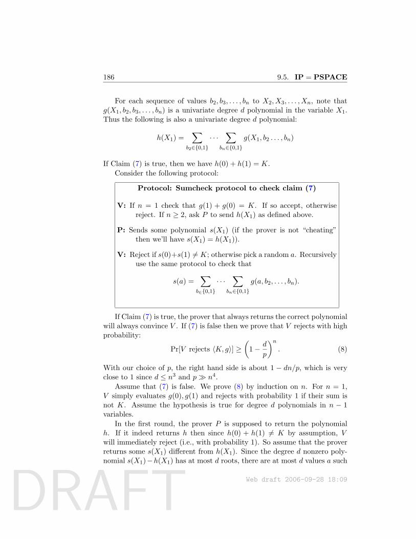
DRAFT

186 9.5. IP = PSPACE

For each sequence of values b2, b3, . . . , bn to X2, X3, . . . , Xn, note thatg(X1, b2, b3, . . . , bn) is a univariate degree d polynomial in the variable X1.Thus the following is also a univariate degree d polynomial:

h(X1) =∑

b2∈0,1

· · ·∑

bn∈0,1

g(X1, b2 . . . , bn)

If Claim (7) is true, then we have h(0) + h(1) = K.Consider the following protocol:

Protocol: Sumcheck protocol to check claim (7)

V: If n = 1 check that g(1) + g(0) = K. If so accept, otherwisereject. If n ≥ 2, ask P to send h(X1) as defined above.

P: Sends some polynomial s(X1) (if the prover is not “cheating”then we’ll have s(X1) = h(X1)).

V: Reject if s(0)+s(1) 6= K; otherwise pick a random a. Recursivelyuse the same protocol to check that

s(a) =∑

b∈0,1

· · ·∑

bn∈0,1

g(a, b2, . . . , bn).

If Claim (7) is true, the prover that always returns the correct polynomialwill always convince V . If (7) is false then we prove that V rejects with highprobability:

Pr[V rejects 〈K, g〉] ≥(

1− d

p

)n. (8)

With our choice of p, the right hand side is about 1 − dn/p, which is veryclose to 1 since d ≤ n3 and p n4.

Assume that (7) is false. We prove (8) by induction on n. For n = 1,V simply evaluates g(0), g(1) and rejects with probability 1 if their sum isnot K. Assume the hypothesis is true for degree d polynomials in n − 1variables.

In the first round, the prover P is supposed to return the polynomialh. If it indeed returns h then since h(0) + h(1) 6= K by assumption, Vwill immediately reject (i.e., with probability 1). So assume that the proverreturns some s(X1) different from h(X1). Since the degree d nonzero poly-nomial s(X1)−h(X1) has at most d roots, there are at most d values a such

Web draft 2006-09-28 18:09

DRAFT


that s(a) = h(a). Thus when V picks a random a,

Pra

[s(a) 6= h(a)] ≥ 1− d

p. (9)

If s(a) 6= h(a) then the prover is left with an incorrect claim to prove in therecursive step. By the induction hypothesis, the prover fails to prove this

false claim with probability at least ≥(1− d

p

)n−1. Thus we have

Pr[V rejects] ≥(

1− d

p

)·(

1− d

p

)n−1

=(

1− d

p

)n(10)

This finishes the induction.

9.5.3 Protocol for TQBF: proof of Theorem 9.13

We use a very similar idea to obtain a protocol for TQBF. Given a quantifiedBoolean formula Ψ = ∃x1∀x2∃x3 · · · ∀xnφ(x1, . . . , xn), we use arithmetiza-tion to construct the polynomial Pφ. We have that Ψ ∈ TQBF if and onlyif

0 <∑

b1∈0,1

∏b2∈0,1

∑b3∈0,1

· · ·∏

bn∈0,1

Pφ(b1, . . . , bn) (11)

A first thought is that we could use the same protocol as in the #SATD

case, except check that s(0) · s(1) = K when you have a∏

. But, alas, mul-tiplication, unlike addition, increases the degree of the polynomial — afterk steps, the degree could be 2k. Such polynomials may have 2k coefficientsand cannot even be transmitted in polynomial time if k log n.

The solution is to look more closely at the polynomials that are aretransmitted and their relation to the original formula. We’ll change Ψ intoa logically equivalent formula whose arithmetization does not cause the de-grees of the polynomials to be so large. The idea is similar to the way circuitsare reduced to formulas in the Cook-Levin theorem: we’ll add auxiliary vari-ables. Specifically, we’ll change ψ to an equivalent formula ψ′ that is notin prenex form in the following way: work from right to left and wheneverencountering a ∀ quantifier on a variable xi — that is, when considering apostfix of the form ∀xiτ(x1, . . . , xi), where τ may contain quantifiers overadditional variables xi+1, . . . , xn — ensure that the variables x1, . . . , xi neverappear to the right of another ∀ quantifier in τ by changing the postfix to∀xi∃x′1, . . . , x′i(x′1 = x1)∧· · ·∧(x′i = xi)∧τ(x1, . . . , xn). Continuing this way

Web draft 2006-09-28 18:09

DRAFT

188 9.6. INTERACTIVE PROOF FOR THE PERMANENT

we’ll obtain the formula ψ′ which will have O(n2) variables and will be atmost O(n2) larger than ψ. It can be seen that the natural arithmetizationfor ψ′ will lead to the polynomials transmitted in the sumcheck protocolnever having degree more than 2.

Note that the prover needs to prove that the arithmetization of Ψ′ leadsto a number K different than 0, but because of the multiplications thisnumber can be as large as 22n . Nevertheless the prover can find a prime pbetween 0 and 2n such that K mod p 6= 0 (in fact as we saw in Chapter 7a random prime will do). This finishes the proof of Theorem 9.13.

Remark 9.15An alternative way to obtain the same result (or, more accurately, an alter-native way to describe the same protocol) is to notice that for x ∈ 0, 1,xk = x for all k ≥ 1. Thus, in principle we can convert any polynomialp(x1, . . . , xn) into a multilinear polynomial q(x1, . . . , xn) (i.e., the degreeof q(·) in any variable xi is at most one) that agrees with p(·) on allx1, . . . , xn ∈ 0, 1. Specifically, for any polynomial p(·) let Li(p) be thepolynomial defined as follows

Li(p)(x1, . . . , xn) = xiP (x1, . . . , xi−1, 1, xi+1, . . . , xn)+(1− xi)P (x1, . . . , xi−1, 0, xi+1, . . . , xn) (12)

then L1(L2(· · · (Ln(p) · · · ) is such a multilinear polynomial agreeing withp(·) on all values in 0, 1. We can thus use O(n2) invocations operator toconvert (11) into an equivalent form where all the intermediate polynomialssent in the sumcheck protocol are multilinear. We’ll use this equivalent formto run the sumcheck protocol, where in addition to having round for a

∑or∏

operator, we’ll also have a round for each application of the operatorL (in such rounds the prover will send a polynomial of degree at most 2).

9.6 Interactive proof for the Permanent

Although the existence of an interactive proof for the Permanent followsfrom that for #SAT and TQBF, we describe a specialized protocol as well.This is both for historical context (this protocol was discovered before theother two protocols) and also because this protocol may be helpful for furtherresearch. (One example will appear in a later chapter.)

Web draft 2006-09-28 18:09

DRAFT

9.6. INTERACTIVE PROOF FOR THE PERMANENT 189

Definition 9.16Let A ∈ Fn×n be a matrix over the field F . The permanent of A is:

perm(A) =∑σ∈Sn

n∏i=1

ai,σ(i)

The problem of calculating the permanent is #P-complete (notice the con-trast with the determinant which is defined by a similar formula but is in factpolynomial time computable). Recall from Chapter ?? that PH ⊆ Pperm

(Toda’s theorem, Theorem 8.11).Observation:

f(x1, x2, ..., xn) := perm

x1,1 x1,2 . . . x1,n

x2,1. . . ... x2,n

......

. . ....

xn,1 xn,2 . . . xn,n

is a degree n polynomial since

f(x1, x2, . . . , xn) =∑σ∈Sn

n∏i=1

xi,σ(i).

We now show two properties of the permanent problem. The first is randomself reducibility, earlier encountered in Section ??:

Theorem 9.17 (Lipton ’88)There is a randomized algorithm that, given an oracle that can compute thepermanent on 1 − 1

3n fraction of the inputs in Fn×n (where the finite fieldF has size > 3n), can compute the permanent on all inputs correctly withhigh probability.

Proof: Let A be some input matrix. Pick a random matrix R ∈R Fn×n

and let B(x) := A+ x ·R for a variable x. Notice that:

• f(x) := perm(B) is a degree n univariate polynomial.

• For any fixed b 6= 0, B(b) is a random matrix, hence the probabilitythat oracle computes perm(B(b)) correctly is at least 1− 1

3n .

Now the algorithm for computing the permanent of A is straightforward:query oracle on all matrices B(i)|1 ≤ i ≤ n + 1. According to the unionbound, with probability of at least 1− n+1

n ≈23 the oracle will compute the

Web draft 2006-09-28 18:09

DRAFT

190 9.6. INTERACTIVE PROOF FOR THE PERMANENT

permanent correctly on all matrices.Recall the fact (see Section ?? in the Appendix) that given n + 1 (point,value) pairs (ai, bi)|i ∈ [n+1], there exists a unique a degree n polynomialp that satisfies ∀i p(ai) = bi. Therefore, given that the values B(i) arecorrect, the algorithm can interpolate the polynomial B(x) and computeB(0) = A.

Note: The above theorem can be strengthened to be based on the assump-tion that the oracle can compute the permanent on a fraction of 1

2 + ε forany constant ε > 0 of the inputs. The observation is that not all values ofthe polynomial must be correct for unique interpolation. See Chapter ??

Another property of the permanent problem is downward self reducibility,encountered earlier in context of SAT:

perm(A) =n∑i=1

a1iperm(A1,i),

where A1,i is a (n−1)×(n−1) sub-matrix of A obtained by removing the 1’strow and i’th column of A (recall the analogous formula for the determinantuses alternating signs).

Definition 9.18Define a (n − 1) × (n − 1) matrix DA(x), such that each entry contains adegree n polynomial. This polynomial is uniquely defined by the values ofthe matrices A1,i|i ∈ [n]. That is:

∀i ∈ [n] . DA(i) = A1,i

Where DA(i) is the matrix DA(x) with i substituted for x. (notice thatthese equalities force n points and values on them for each polynomial ata certain entry of DA(x), and hence according to the previously mentionedfact determine this polynomial uniquely)

Observation: perm(DA(x)) is a degree n(n− 1) polynomial in x.

9.6.1 The protocol

We now show an interactive proof for the permanent (the decision problemis whether perm(A) = k for some value k):

• Round 1: Prover sends to verifier a polynomial g(x) of degree n(n−1),which is supposedly perm(DA(x)).

Web draft 2006-09-28 18:09

DRAFT

9.6. INTERACTIVE PROOF FOR THE PERMANENT 191

• Round 2: Verifier checks whether:

k =m∑i=1

a1,ig(i)

If not, rejects at once. Otherwise, verifier picks a random elementof the field b1 ∈R F and asks the prover to prove that g(b1) =perm(DA(b1)). This reduces the matrix dimension to (n−2)×(n−2).

...

• Round 2(n− 1)− 1: Prover sends to verifier a polynomial of degree 2,which is supposedly the permanent of a 2× 2 matrix.

• Round 2(n− 1): Verifier is left with a 2× 2 matrix and calculates thepermanent of this matrix and decides appropriately.

Claim 9.19The above protocol is indeed an interactive proof for perm.

Proof: If perm(A) = k, then there exists a prover that makes the verifieraccept with probability 1, this prover just returns the correct values of thepolynomials according to definition.On the other hand, suppose that perm(A) 6= k. If on the first round, thepolynomial g(x) sent is the correct polynomial DA(x), then:

k 6=m∑i=1

a1,ig(i) = perm(A)

And the verifier would reject. Hence g(x) 6= DA(x). According to the fact onpolynomials stated above, these polynomials can agree on at most n(n− 1)points. Hence, the probability that they would agree on the randomly chosenpoint b1 is at most n(n−1)

|F | . The same considerations apply to all subsequentrounds if exist, and the overall probability that the verifier will not acceptsis thus (assuming |F | ≥ 10n3 and sufficiently large n):

Pr ≥(

1− n(n− 1)|F |

)·(

1− (n− 1)(n− 2)|F |

)· ...(

1− 3 · 2|F |

)≥

(1− n(n− 1)

|F |

)n−1

≥ 12

Web draft 2006-09-28 18:09

DRAFT

192 9.7. THE POWER OF THE PROVER

9.7 The power of the prover

A curious feature of many known interactive proof systems is that in orderto prove membership in language L, the prover needs to do more powerfulcomputation than just deciding membership in L. We give some examples.

1. The public coin system for graph nonisomorphism in Theorem 9.9 re-quires the prover to produce, for some randomly chosen hash functionh and a random element y in the range of h, a graph H such that h(H)is isomorphic to either G1 or G2 and h(x) = y. This seems harder thanjust solving graph non-isomorphism.

2. The interactive proof for 3SAT, a language in coNP, requires theprover to do #P computations, doing summations of exponentiallymany terms. (Recall that all of PH is in P#P.)

In both cases, it is an open problem whether the protocol can be re-designed to use a weaker prover.

Note that the protocol for TQBF is different in that the prover’s repliescan be computed in PSPACE as well. This observation underlies the follow-ing result, which is in the same spirit as the Karp-Lipton results describedin Chapter ??, except the conclusion is stronger since MA is contained inΣ2 (indeed, a perfectly complete MA-proof system for L trivially impliesthat L ∈ Σ2).

Theorem 9.20If PSPACE ⊆ P/poly then PSPACE = MA.

Proof: If PSPACE ⊆ P/poly then the prover in our TQBF protocol canbe replaced by a circuit of polynomial size. Merlin (the prover) can justgive this circuit to Arthur (the verifier) in Round 1, who then runs theinteractive proof using this “prover.” No more interaction is needed. Notethat there is no need for Arthur to put blind trust in Merlin’s circuit, sincethe correctness proof of the TQBF protocol shows that if the formula is nottrue, then no prover can make Arthur accept with high probability.

In fact, using the Karp-Lipton theorem one can prove a stronger state-ment, see Lemma ?? below.

9.8 Program Checking

The discovery of the interactive protocol for the permanent problem wastriggered by a field called program checking. Blum and Kannan’s motivation

Web draft 2006-09-28 18:09

DRAFT

9.8. PROGRAM CHECKING 193

for introducing this field was the fact that program verification (decidingwhether or not a given program solves a certain computational task) isundecidable. They observed that in many cases we can guarantee a weakerguarantee of the program’s “correctness” on an instance by instance basis.This is encapsulated in the notion of a program checker. A checker C fora program P is itself another program that may run P as a subroutine.Whenever P is run on an input x, C’s job is to detect if P ’s answer isincorrect (“buggy”) on that particular instance x. To do this, the checkermay also compute P ’s answer on some other inputs. Program checking issometimes also called instance checking, perhaps a more accurate name,since the fact that the checker did not detect a bug does not mean that Pis a correct program in general, but only that P ’s answer on x is correct.

Definition 9.21Let P be a claimed program for computational task T . A checker for T isa probabilistic polynomial time TM, C, that, given any x, has the followingbehavior:

1. If P is a correct program for T (i.e., ∀y P (y) = T (y)), then P [CP accepts P (x)] ≥23

2. If P (x) 6= T (x) then P [CP accepts P (x)] < 13

Note that in the case that P is correct on x (i.e., P (x) = C(x)) but theprogram P is not correct everywhere, there is no guarantee on the outputof the checker.

Surprisingly, for many problems, checking seems easier than actuallycomputing the problem. (Blum and Kannan’s suggestion was to build check-ers into the software whenever this is true; the overhead introduced by thechecker would be negligible.)

Example 9.22 (Checker for Graph Non-Isomorphism)The input for the problem of Graph Non-Isomorphism is a pair of labelledgraphs 〈G1, G2〉, and the problem is to decide whether G1 ≡ G2. As noted,we do not know of an efficient algorithm for this problem. But it has anefficient checker.

There are two types of inputs, depending upon whether or not the pro-gram claims G1 ≡ G2. If it claims that G1 ≡ G2 then one can change thegraph little by little and use the program to actually obtain the permutationπ (). We now show how to check the claim that G1 6≡ G2 using our earlierinteractive proof of Graph non-isomorphism.

Recall the IP for Graph Non-Isomorphism:

Web draft 2006-09-28 18:09

DRAFT

194 9.8. PROGRAM CHECKING

• In case prover admits G1 6≡ G2 repeat k times:

• Choose i ∈R 1, 2. Permute Gi randomly into H

• Ask the prover 〈G1,H〉; 〈G2,H〉 and check to see if the prover’s firstanswer is consistent.

Given a computer program that supposedly computes graph isomorphism,P , how would we check its correctness? The program checking approachsuggests to use an IP while regarding the program as the prover. Let C bea program that performs the above protocol with P as the prover, then:

Theorem 9.23If P is a correct program for Graph Non-Isomorphism then C outputs ”cor-rect” always. Otherwise, if P (G1, G2) is incorrect then P [C outputs ”correct” ] ≤2−k. Moreover, C runs in polynomial time.

9.8.1 Languages that have checkers

Whenever a language L has an interactive proof system where the prover canbe implemented using oracle access to L, this implies that L has a checker.Thus, the following theorem is a direct consequence of the interactive proofswe have seen:

Theorem 9.24The problems Graph Isomorphism (GI), Permanent (perm) and True Quan-tified Boolean Formulae (TQBF) have checkers.

Using the fact that P-complete languages are reducible to each other viaNC-reductions, it suffices to show a checker in NC for one P-complete lan-guage (as was shown by Blum & Kannan) to obtain the following interestingfact:

Theorem 9.25For any P-complete language there exists a program checker in NC

Since we believe that P-complete languages cannot be computed in NC, thisprovides additional evidence that checking is easier than actual computation.

Web draft 2006-09-28 18:09

DRAFT

9.9. MULTIPROVER INTERACTIVE PROOFS (MIP) 195

9.9 Multiprover interactive proofs (MIP)

It is also possible to define interactive proofs that involve more than oneprover. The important assumption is that the provers do not communicatewith each other during the protocol. They may communicate before the pro-tocol starts, and in particular, agree upon a shared strategy for answeringquestions. (The analogy often given is that of the police interrogating twosuspects in separate rooms. The suspects may be accomplices who have de-cided upon a common story to tell the police, but since they are interrogatedseparately they may inadvertently reveal an inconsistency in the story.)

The set of languages with multiprover interactive provers is call MIP.The formal definition is analogous to Definition 9.5. We assume there are twoprovers (though one can also study the case of polynomially many provers;see the exercises), and in each round the verifier sends a query to each ofthem —the two queries need not be the same. Each prover sends a responsein each round.

Clearly, IP ⊆ MIP since we can always simply ignore one prover.However,it turns out that MIP is probably strictly larger than IP (unlessPSPACE = NEXP). That is, we have:

Theorem 9.26 ([BFL91])NEXP = MIP

We will outline a proof of this theorem in Chapter ??. One thing thatwe can do using two rounds is to force non-adaptivity. That is, considerthe interactive proof as an “interrogation” where the verifier asks questionsand gets back answers from the prover. If the verifier wants to ensure thatthe answer of a prover to the question q is a function only of q and doesnot depend on the previous questions the prover heard, the prover can askthe second prover the question q and accept only if both answers agree withone another. This technique was used to show that multi-prover interactiveproofs can be used to implement (and in fact are equivalent to) a model ofa “probabilistically checkable proof in the sky”. In this model we go backto an NP-like notion of a proof as a static string, but this string may behuge and so is best thought of as a huge table, consisting of the prover’sanswers to all the possible verifier’s questions. The verifier checks the proofby looking at only a few entries in this table, that are chosen randomlyfrom some distribution. If we let the class PCP[r, q] be the set of languagesthat can be proven using a table of size 2r and q queries to this table thenTheorem 9.26 can be restated as

Web draft 2006-09-28 18:09

DRAFT

196 9.9. MULTIPROVER INTERACTIVE PROOFS (MIP)

Theorem 9.27 (Theorem 9.26, restated)NEXP = PCP[poly,poly] = ∪cPCP[nc, nc]

It turns out Theorem 9.26 can be scaled down to to obtain NP =PCP[polylog,polylog]. In fact (with a lot of work) the following is known:

Theorem 9.28 (The PCP theorem, [AS98, ALM+98])NP = PCP[O(log n), O(1)]

This theorem, which will be proven in Chapter 19, has had many ap-plications in complexity, and in particular establishing that for many NP-complete optimization problems, obtaining an approximately optimal solu-tion is as hard as coming up with the optimal solution itself. Thus, itseems that complexity theory has gone a full circle with interactive proofs:by adding interaction, randomization, and multiple provers, and getting toclasses as high as NEXP, we have gained new and fundamental insightson the class NP the represents static deterministic proofs (or equivalently,efficiently verifiable search problems).


• An interactive proof is a generalization of mathematical proofs in which theprover and polynomial-time probabilistic verifier interact.

• Allowing randomization and interaction seems to add significantly more powerto proof system: the class IP of languages provable by a polynomial-timeinteractive proofs is equal to PSPACE.

• All languages provable by a constant round proof system are in the class AM:that is, they have a proof system consisting of the the verifier sending a singlerandom string to the prover, and the prover responding with a single message.


Interactive proofs were defined in 1985 by Goldwasser, Micali, Rackoff [GMR89]for cryptographic applications and (independently, and using the public coindefinition) by Babai and Moran [BM88]. The private coins interactive prooffor graph non-isomorphism was given by Goldreich, Micali and Wigder-son [GMW87]. Simulations of private coins by public coins we given byGoldwasser and Sipser [GS87]. The general feeling at the time was that

Web draft 2006-09-28 18:09

DRAFT


interactive proofs are only a “slight” extension of NP and that not even3SAT has interactive proofs. The result IP = PSPACE was a big surprise,and the story of its discovery is very interesting.

In the late 1980s, Blum and Kannan [BK95] introduced the notion of pro-gram checking. Around the same time, manuscripts of Beaver and Feigen-baum [BF90] and Lipton [Lip91] appeared. Inspired by some of these de-velopments, Nisan proved in December 1989 that #SAT has multiproverinteractive proofs. He announced his proof in an email to several colleaguesand then left on vacation to South America. This email motivated a flurryof activity in research groups around the world. Lund, Fortnow, Karloffshowed that #SAT is in IP (they added Nisan as a coauthor and the finalpaper is [LFK92]). Then Shamir showed that IP =PSPACE [Sha92] andBabai, Fortnow and Lund [BFL91] showed MIP = NEXP. The entirestory —as well as related developments—are described in Babai’s entertain-ing survey [Bab90].

Vadhan [Vad00] explores some questions related to the power of theprover.

The result that approximating the shortest vector is probably not NP-hard (as mentioned in the introduction) is due to Goldreich and Gold-wasser [GG00].

Exercises

§1 Prove the assertions in Remark 9.6. That is, prove:

(a) Let IP′ denote the class obtained by allowing the prover to beprobabilistic in Definition 9.5. That is, the prover’s strategy canbe chosen at random from some distribution on functions. Provethat IP′ = IP.

(b) Prove that IP ⊆ PSPACE.

(c) Let IP′ denote the class obtained by changing the constant 2/3in (2) and (3) to 1− 2−|x|. Prove that IP′ = IP.

(d) Let IP′ denote the class obtained by changing the constant 2/3in (2) to 1. Prove that IP′ = IP.

(e) Let IP′ denote the class obtained by changing the constant 2/3in (3) to 1. Prove that IP′ = NP.

§2 We say integer y is a quadratic residue modulo m if there is an integerx such that y ≡ x2 (mod m). Show that the following language is in

Web draft 2006-09-28 18:09

DRAFT


IP[2]:

QNR = (y,m) : y is not a quadratic residue modulo m .

§3 Prove that there exists a perfectly complete AM[O(1)] protocol forthe proving a lowerbound on set size.

Hint:Firstnotethatinthecurrentsetlowerboundprotocolwecanhavetheproverchoosethehashfunction.Considertheeas-iercaseofconstructingaprotocoltodistinguishbetweenthecase|S|≥Kand|S|≤

1cKwherec>2canbeevenafunctionof

K.Ifcislargeenoughthewecanallowtheprovertouseseveralhashfunctionsh1,...,hi,anditcanbeproventhatifiislargeenoughwe’llhave∪ihi(S)=0,1

k.Thegapcanbeincreasedby

consideringinsteadofSthesetS`,thatisthe`timesCartesian

productofS.

§4 Prove that for every constant k ≥ 2, AM[k + 1] ⊆ AM[k].

§5 Show that AM[2] = BP ·NP

§6 [BFNW93] Show that if EXP ⊆ P/poly then EXP = MA.

Hint:TheinteractiveproofforTQBFrequiresaproverthatisaPSPACEmachine.

§7 Show that the problem GI is downward self reducible. That is, provethat given two graphs G1,G2 on n vertices and access to a subroutineP that solves the GI problem on graphs with up to n− 1 vertices, wecan decide whether or not G1 and G2 are isomorphic in polynomialtime.

§8 Prove that in the case that G1 and G2 are isomorphic we can obtainthe permutation π mapping G1 to G2 using the procedure of the aboveexercise. Use this to complete the proof in Example 9.22 and showthat graph isomorphism has a checker. Specifically, you have to showthat if the program claims that G1 ≡ G2 then we can do some furtherinvestigation (including calling the programs on other inputs) and withhigh probability conclude that either (a) conclude that the programwas right on this input or (b) the program is wrong on some input andhence is not a correct program for graph isomorphism.

§9 Define a language L to be downward self reducible there’s a polynomial-time algorithm R that for any n and x ∈ 0, 1n, RLn−1(x) = L(x)

Web draft 2006-09-28 18:09

DRAFT


where by Lk we denote an oracle that solves L on inputs of size at mostk. Prove that if L is downward self reducible than L ∈ PSPACE.

§10 Show that MIP ⊆ NEXP.

§11 Show that if we redefine multiprover interactive proofs to allow, insteadof two provers, as many as m(n) = poly(n) provers on inputs of sizen, then the class MIP is unchanged.

Hint:Showhowtosimulatepoly(n)proversusingtwo.Inthissimulation,oneoftheproversplaystheroleofallm(n)provers,andtheotherproverisaskedtosimulateoneoftheprovers,chosenrandomlyfromamongthem(n)provers.Thenrepeatthisafewtimes.

Web draft 2006-09-28 18:09

DRAFT


Web draft 2006-09-28 18:09

DRAFT

Chapter 10

Cryptography

“From times immemorial, humanity has gotten frequent, oftencruel, reminders that many things are easier to do than to re-verse.”L. Levin [Lev]

somewhat rough still

The importance of cryptography in today’s online world needs no intro-duction. Here we focus on the complexity issues that underlie this field. Thetraditional task of cryptography was to allow two parties to encrypt theirmessages so that eavesdroppers gain no information about the message. (SeeFigure 10.1.) Various encryption techniques have been invented throughouthistory with one common characteristic: sooner or later they were broken.


Figure 10.1: People sending messages over a public channel (e.g., the internet) wish touse encryption so that eavesdroppers learn “nothing.”

In the post NP-completeness era, a crucial new idea was presented:the code-breaker should be thought of as a resource-bounded computationaldevice. Hence the security of encryption schemes ought to be proved byreducing the task of breaking the scheme into the task of solving some com-putationally intractable problem (say requiring exponential time complexityor circuit size), thus one could hope to design encryption schemes that areefficient enough to be used in practice, but whose breaking will require, say,millions of years of computation time.


201

DRAFT

202

Early researchers tried to base the security of encyption methods uponthe (presumed) intractability of NP-complete problems. This effort hasnot succeeded to date, seemingly because NP-completeness concerns theintractability of problems in the worst-case whereas cryptography seems toneed problems that are intractable on most instances. After all, when weencrypt email, we require that decryption should be difficult for an eaves-dropper for all (or almost all) messages, not just for a few messages. Thusthe concept most useful in this chapter will be average-case complexity1. Wewill see a class of functions called one-way functions that are easy to com-pute but hard to invert for most inputs —they are alluded to in Levin’s quoteabove. Such functions exist under a variety of assumptions, including thefamous assumption that factoring integers requires time super-polynomialtime in the integer’s bit-length to solve in the average case (e.g., for a prod-uct of two random primes).

Furthermore, in the past two decades, cryptographers have taken ontasks above and beyond the basic task of encryption—from implementingdigital cash to maintaining the privacy of individuals in public databases.(We survey some applications in Section 10.4.) Surprisingly, many of thesetasks can be achieved using the same computational assumptions used forencryption. A crucial ingredient in these developments turns out to be ananswer to the question: “What is a random string and how can we generateone?” The complexity-theoretic answer to this question leads to the notionof a pseudorandom generator, which is a central object; see Section 10.2.This notion is very useful in itself and is also a template for several other keydefinitions in cryptography, including that of encryption (see Section 10.4).

Private key versus public key: Solutions to the encryption problemtoday come in two distinct flavors. In private-key cryptography, one as-sumes that the two (or more) parties participating in the protocol share aprivate “key” —namely, a statistically random string of modest size—thatis not known to the eavesdropper2. In a public-key encryption system (aconcept introduced by Diffie and Hellman in 1976 [DH76]) we drop thisassumption. Instead, a party P picks a pair of keys: an encryption keyand decryption key, both chosen at random from some (correlated) distri-bution. The encryption key will be used to encrypt messages to P and is

1A problem’s average-case and worst-case complexities can differ radically. For in-stance, 3COL is NP-complete on general graphs, but on most n-node graphs is solvable inquadratic time or less. A deeper study of average case complexity appears in Chapter 15.

2Practically, this could be ensured with a face-to-face meeting that might occur longbefore the transmission of messages.

Web draft 2006-09-28 18:09

DRAFT

10.1. HARD-ON-AVERAGE PROBLEMS AND ONE-WAYFUNCTIONS 203

considered public —i.e., published and known to everybody including theeavesdropper. The decryption key is kept secret by P and is used to decryptmessages. A famous public-key encryption scheme is based upon the RSAfunction of Example 10.4. At the moment we do not know how to basepublic key encryption on the sole assumption that one-way functions existand current constructions require the assumption that there exist one-wayfunctions with some special structure (such as RSA, factoring-based, andLattice-based one way functions). Most topics described in this chapter aretraditionally labeled private key cryptography.

10.1 Hard-on-average problems and one-way func-tions

A basic cryptographic primitive is a one-way function. Roughly speaking,this is a function f that is easy to compute but hard to invert. Notice thatif f is not one-to-one, then the inverse f−1(x) may not be unique. In suchcases “inverting” means that given f(x) the algorithm is able to producesome preimage, namely, any element of f−1(f(x))). We say that the functionis one-way function if inversion is difficult for the “average” (or “many”) x.Now we define this formally; a discussion of this definition appears below inSection 10.1.1. A function family (gn) is a family of functions where gn takesn-bit inputs. It is polynomial-time computable if there is a polynomial-timeTM that given an input x computes g|x|(x).

Definition 10.1 (One-way function)A family of functions fn : 0, 1n 7→ 0, 1m(n) is ε(n) one-way withsecurity s(n) if it is polynomial-time computable and furthermore for everyalgorithm A that runs in time s(n),

Prx∈0,1n [A inverts fn(x)] ≤ ε(n). (1)

Now we give a few examples and discuss the evidence that they are hardto invert “on average inputs.”

Example 10.2The first example is motivated by the fact that finding the prime factorsof a given integer is the famous FACTORING problem, for which the bestcurrent algorithm has running time about 2O(n1/3) (and even that boundsrelies on the truth of some unproven conjectures in number theory). The

Web draft 2006-09-28 18:09

DRAFT

20410.1. HARD-ON-AVERAGE PROBLEMS AND ONE-WAY

FUNCTIONS

hardest inputs for current algorithms appear to be of the type x · y, wherex, y are random primes of roughly equal size.

Here is a first attempt to define a one-way function using this observation.Let fn be a family of functions where fn : 0, 1n × 0, 1n → 0, 12n isdefined as fn([x]2, [y]2) = [x · y]2. If x and y are primes —which by thePrime Number Theorem happens with probability Θ(1/n2) when x, y arerandom n-bit integers— then fn seems hard to invert. It is widely believedthat there are c > 1, f > 0 such that family fn is (1 − 1/nc)-one-way withsecurity parameter 2n

f.

An even harder version of the above function is obtained by using theexistence of a randomized polynomial-time algorithm A (which we do notdescribe) that, given 1n, generates a random n-bit prime number. SupposeA uses m random bits, where m = poly(n). Then A may be seen as a(deterministic) mapping fromm-bit strings to n-bit primes. Now let functionfm map (r1, r2) to [A(r1) ·A(r2)]2, where A(r1), A(r2) are the primes outputby A using random strings r1, r2 respectively. This function seems hardto invert for almost all r1, r2. (Note that any inverse (r′1, r

′2) for fm(r1, r2)

allows us to factor the integer A(r1) ·A(r2) since unique factorization impliesthat the prime pair A(r′1), A(r′2) must be the same as A(r1), A(r2).) It iswidely conjecture that there are c > 1, f > 0 such that fn is 1/nc-one-waywith security parameter 2n

f.

The FACTORING problem, a mainstay of modern cryptography, is ofcourse the inverse of multiplication. Who would have thought that the hum-ble multiplication, taught to children in second grade, could be the source ofsuch power? The next two examples also rely on elementary mathematicaloperations such as exponentiation, albeit with modular arithmetic.

Example 10.3Let p1, p2, . . . be a sequence of primes where pi has i bits. Let gi be thegenerator of the group Z∗pi , the set of numbers that are nonzero mod pi.Then for every y ∈ 1, .., pi − 1, there is a unique x ∈ 1, .., p− 1 such that

gxi ≡ y (mod pi).

Then x→ gxi (mod pi) is a permutation on 1, .., pi − 1 and is conjectured tobe one-way. The inversion problem is called the DISCRETE LOG problem.We show below using random self-reducibility that if it is hard on worst-caseinputs, then it is hard on average.

Web draft 2006-09-28 18:09

DRAFT

10.1. HARD-ON-AVERAGE PROBLEMS AND ONE-WAYFUNCTIONS 205

We list some more conjectured one-way functions.

Example 10.4RSA function. Let m = pq where p, q are large random primes and e bea random number coprime to φ(m) = (p − 1)(q − 1). Let Z∗m be the setof integers in [1, . . . ,m] coprime to m. Then the function is defined to befp,q,e(x) = xe (mod m). This function is used in the famous RSA public-keycryptosystem.

Rabin function. For a composite numberm, define fm(x) = x2 (mod m).If we can invert this function on a 1/poly(logm) fraction of inputs then wecan factor m in poly(logm) time (see exercises).

Both the RSA and Rabin functions are useful in public-key cryptography.They are examples of trapdoor one-way functions: if the factors of m (the“trapdoor” information) are given as well then it is easy to invert the abovefunctions. Trapdoor functions are fascinating objects but will not be studiedfurther here.

Random subset sum. Let m = 10n. Let the inputs to f be n positivem-bit integers a1, a2, . . . , an, and a subset S of 1, 2, . . . , n. Its output is(a1, a2, . . . , an,

∑i∈S ai). Note that f maps n(m+ 1)-bit inputs to nm+m

bits.When the inputs are randomly chosen, this function seems hard to invert.

It is conjectured that there is c > 1, d > 0 such that this function is 1/nc-one-way with security 2n

d.

10.1.1 Discussion of the definition of one-way function

We will always assume that the the one-way function under consideration issuch that the security parameter s(n) is superpolynomial, i.e., larger thannk for every k > 0. The functions described earlier are actually believed tobe one-way with a larger security parameter 2n

εfor some fixed ε > 0.

Of greater interest is the error parameter ε(n), since it determines thefraction of inputs for which inversion is easy. Clearly, a continuum of valuesis possible, but two important cases to consider are (i) ε(n) = (1 − 1/nc)for some fixed c > 0, in other words, the function is difficult to invert on at

Web draft 2006-09-28 18:09

DRAFT

20610.1. HARD-ON-AVERAGE PROBLEMS AND ONE-WAY

FUNCTIONS

least 1/nc fraction of inputs. Such a function is often called a weak one-wayfunction. The simple one-way function fn of Example 10.2 is conjectured tobe of this type. (ii) ε(n) < 1/nk for every k > 1. Such a function is called astrong one-way function.

Yao showed that if weak one-way functions exist then so do strong one-way functions. We will prove this surprising theorem (actually, somethingclose to it) in Chapter 18. We will not use it in this chapter, except as ajustification for our intuition that strong one-way functions exist. (Anotherjustification is of course the empirical observation that the candidate one-way functions mentioned above do seem appear difficult to invert on mostinputs.)

10.1.2 Random self-reducibility

Roughly speaking, a problem is random-self-reducible if solving the problemon any input x reduces to solving the problem on a sequence of randominputs y1, y2, . . . , where each yi is uniformly distributed among all inputs.To put it more intuitively, the worst-case can be reduced to the average case.Hence the problem is either easy on all inputs, or hard on most inputs. (Inother words, we can exclude the possibility that problem is easy on almostall the inputs but not all.) If a function is one-way and also randomly self-reducible then it must be a strong one-way function. This is best illustratedwith an example.

Theorem 10.5Suppose A is an algorithm with running time t(n) that, given a prime p,a generator g for Z∗p, and an input gx( mod p), manages to find x for δfraction of x ∈ Z∗p. Then there is a randomized algorithm A′ with running

time O( 1δ log 1/ε(t(n)+poly(n))) that solves DISCRETE LOG on every input

with probability at least 1− ε.

Proof: Suppose we are given y = gx( mod p) and we are trying to findx. Repeat the following trial O(1/(δ log 1/ε)) times: “Randomly pick r ∈0, 1, . . . , p− 2 and use A to try to compute the logarithm of y · gr(modp).Suppose A outputs z. Check if gz−r(modp) is y, and if so, output z −r(mod(p− 1)) as the answer.”

The main observation is that if r is randomly chosen, then y·gr( mod p) israndomly distributed in Z∗p and hence the hypothesis implies that A has a δchance of finding its discrete log. After O(1/(δ log 1/ε) trials, the probabilitythat A failed every time is at most ε.

Web draft 2006-09-28 18:09

DRAFT

10.2. WHAT IS A RANDOM-ENOUGH STRING? 207

Corollary 10.6If for any infinite sequence of primes p1, p2, . . . , DISCRETE LOG mod pi ishard on worst-case x ∈ Z∗pi , then it is hard for almost all x.

Later as part of the proof of Theorem 10.14 we give another example ofrandom self-reducibility: linear functions over GF (2).

10.2 What is a random-enough string?

Cryptography often becomes much easier if we have an abundant supply ofrandom bits. Here is an example.

Example 10.7 (One-time pad)Suppose the message sender and receiver share a long string r of randombits that is not available to eavesdroppers. Then secure communication iseasy. To encode message m ∈ 0, 1n, take the first n bits of r, say thestring s. Interpret both strings as vectors in GF (2)n and encrypt m by thevector m+s. The receiver decrypts this message by adding s to it (note thats+ s = 0 in GF (2)n). If s is statistically random, then so is m+ s. Hencethe eavesdropper provably cannot obtain even a single bit of informationabout m regardless of how much computational power he expends.

Note that reusing s is a strict no-no (hence the name “one-time pad”).If the sender ever reuses s to encrypt another message m′ then the eaves-dropper can add the two vectors to obtain (m + s) + (m′ + s) = m + m′,which is some nontrivial information about the two messages.

Of course, the one-time pad is just a modern version of the old idea ofusing “codebooks” with a new key prescribed for each day.

One-time pads are conceptually simple, but impractical to use, becausethe users need to agree in advance on a secret pad that is large enough to beused for all their future communications. It is also hard to generate becausesources of quality random bits (e.g., those based upon quantum phenomena)are often too slow. Cryptography’s suggested solution to such problems isto use a pseudorandom generator. This is a deterministically computablefunction g : 0, 1n → 0, 1n

c

(for some c > 1) such that if x ∈ 0, 1n israndomly chosen, then g(x) “looks” random. Thus so long as users havebeen provided a common n-bit random string, they can use the generator

Web draft 2006-09-28 18:09

DRAFT

208 10.2. WHAT IS A RANDOM-ENOUGH STRING?

to produce nc “random looking” bits, which can be used to encrypt nc−1

messages of length n. (In cryptography this is called a stream cipher.)Clearly, at this point we need an answer to the question posed in the

Section’s title! Philosophers and statisticians have long struggled with thisquestion.

Example 10.8What is a random-enough string? Here is Kolmogorov’s definition: A stringof length n is random if no Turing machine whose description length is< 0.99n (say) outputs this string when started on an empty tape. Thisdefinition is the “right” definition in some philosophical and technical sense(which we will not get into here) but is not very useful in the complexitysetting because checking if a string is random according to this definition isundecidable.

Statisticians have also attempted definitions which boil down to checkingif the string has the “right number” of patterns that one would expect bythe laws of statistics, e.g. the number of times 11100 appears as a substring.(See Knuth Volume 3 for a comprehensive discussion.) It turns out thatsuch definitions are too weak in the cryptographic setting: one can finda distribution that passes these statistical tests but still will be completelyinsecure if used to generate the pad for the one-time pad encryption scheme.

10.2.1 Blum-Micali and Yao definitions

Now we introduce two complexity-theoretic definitions of pseudorandomnessdue to Blum-Micali and Yao in the early 1980s. For a string y ∈ 0, 1n andS ⊆ [n], we let y|S denote the projection of Y to the coordinates of S. Inparticular, y|[1..i] denotes the first i bits of y.

The Blum-Micali definition is motivated by the observation that oneproperty (in fact, the defining property) of a statistically random sequenceof bits y is that given y|[1..i], we cannot predict yi+1 with odds better than50/50 regardless of the computational power available to us. Thus one coulddefine a “pseudorandom” string by considering predictors that have limitedcomputational resources, and to show that they cannot achieve odds muchbetter than 50/50 in predicting yi+1 from y|[1..i]. Of course, this definitionhas the shortcoming that any single finite string would be predictable for atrivial reason: it could be hardwired into the program of the predictor Turing

Web draft 2006-09-28 18:09

DRAFT


machine. To get around this difficulty the Blum-Micali definition (and alsoYao’s definition below) defines pseudorandomness for distributions of stringsrather than for individual strings. Furthermore, the definition concerns aninfinite sequence of distributions, one for each input size.

Definition 10.9 (Blum-Micali)Let gn be a polynomial-time computable family of functions, where gn :0, 1n → 0, 1m and m = m(n) > n. We say the family is (ε(n), t(n))-unpredictable if for every probabilistic polynomial-time algorithm A thatruns in time t(n) and every large enough input size n,

Pr[A(g(x)[1..i]) = g(x)i+1] ≤12

+ ε(n),

where the probability is over the choice of x ∈ 0, 1n , i ∈ 1, . . . , n , andthe randomness used by A.

If for every fixed k, the family gn is (1/nc, nk)-unpredictable for everyc > 1, then we say in short that it is unpredictable by polynomial-timealgorithms.

Remark 10.10Allowing the tester to be an arbitrary polynomial-time machine makes per-fect sense in a cryptographic setting where we wish to assume nothing aboutthe adversary except an upperbound on her computational power.

Pseudorandom generators proposed in the pre-complexity era, such asthe popular linear or quadtratic congruential generators do not satisfy theBlum-Micali definition because bit-prediction can in fact be done in poly-nomial time.

Yao gave an alternative definition in which the tester machine is givenaccess to the entire string at once. This definition implicitly sets up a testof randomness analogous to the more famous Turing test for intelligence(see Figure 10.2). The tester machine A is given a string y ∈ 0, 1n

c

that isproduced in one of two ways: it is either drawn from the uniform distributionon 0, 1n

c

or generated by taking a random string x ∈ 0, 1n and stretchingit using a deterministic function g : 0, 1n → 0, 1n

c

. The tester is askedto output “1” if the string looks random to it and 0 otherwise. We say thatg is a pseudorandom generator if no polynomial-time tester machine A hasa great chance of being able to determine which of the two distributions thestring came from.

Web draft 2006-09-28 18:09

DRAFT

210 10.2. WHAT IS A RANDOM-ENOUGH STRING?

Definition 10.11 ([Yao82])Let gn be a polynomial-time computable family of functions, where gn :0, 1n → 0, 1m and m = m(n) > n. We say it is a (δ(n), s(n))-pseudorandom generator if for every probabilistic algorithm A running intime s(n) and for all large enough n

|Pry∈0,1nc [A(y) = 1]−Prx∈0,1n [A(gn(x)) = 1]| ≤ δ(n). (2)

We call δ(n) the distinguishing probability and s(n) the security parameter.If for every c′, k > 1, the family is (1/nc

′, nk)-pseudorandom then we say

in short that it is a pseudorandom generator.


Figure 10.2: Yao’s definition: If c > 1 then g : 0, 1n → 0, 1nc

is a pseudorandomgenerator if no polynomial-time tester has a good chance of distinguishing between trulyrandom strings of length nc and strings generated by applying g on random n-bit strings.

10.2.2 Equivalence of the two definitions

Yao showed that the above two definitions are equivalent —up to minorchanges in the security parameter, a family is a pseudorandom generator iffit is (bitwise) unpredictable. The hybrid argument used in this proof hasbecome a central idea of cryptography and complexity theory.

The nontrivial direction of the equivalence is to show that pseudoran-domness of the Blum-Micali type implies pseudorandomness of the Yao type.Not surprisingly, this direction is also more important in a practical sense.Designing pseudorandom generators seems easier for the Blum-Micali defi-nition —as illustrated by the Goldreich-Levin construction below— whereasYao’s definition seems more powerful for applications since it allows the ad-versary unrestricted access to the pseudorandom string. Thus Yao’s theoremprovides a bridge between what we can prove and what we need.

Theorem 10.12 (Prediction vs. Indistinguishability [?])Let Let gn :0, 1n → 0, 1N(n) be a family of functions where N(n) = nk for somek > 1.If gn is ( ε(n)

N(n) , 2t(n))-unpredictable where t(n) ≥ N(n)2 then it is (ε(n), t(n))-pseudorandom.Conversely, if gn is (ε(n), t(n))-pseudorandom, then it is (ε(n), t(n))-unpredictable.

Web draft 2006-09-28 18:09

DRAFT


Proof: The converse part is trivial since a bit-prediction algorithm can inparticular be used to distinguish g(x) from random strings of the samelength. It is left to the reader.

LetN be shorthand forN(n). Suppose g is not (ε(n), t(n))-pseudorandom,and A is a distinguishing algorithm that runs in t(n) time and satisfies:∣∣∣∣∣ Pr

x∈Bn[A(g(x)) = 1]− Pr

y∈0,1N[A(y) = 1]

∣∣∣∣∣ > ε(n). (3)

By considering either A or the algorithm that is A with the answer flipped,we can assume that the |·| can be removed and in fact

Prx∈Bn

[A(g(x)) = 1]− Pry∈0,1N

[A(y) = 1] > ε(n). (4)

Consider B, the following bit-prediction algorithm. Let its input beg(x)|≤i where x ∈ 0, 1n and i ∈ 0, . . . , N − 1 are chosen uniformlyat random. B’s program is: “Pick bits ui+1, ui+2, . . . , uN randomly andrun A on the input g(x)|≤iui+1ui+2 . . . uN . If A outputs 1, output ui+1

else output ui+1.” Clearly, B runs in time less than t(n) + O(N(n)) <2t(n). To complete the proof we show that B predicts g(x)i+1 correctlywith probability at least 1

2 + ε(n)N .

Consider a sequence of N + 1 distributions D0 through DN defined asfollows (in all cases, x ∈ 0, 1n and u1, u2, . . . , uN ∈ 0, 1 are assumed tobe chosen randomly)

D0 = u1u2u3u4 · · ·uND1 = g(x)1u2u3 · · ·uN

......

Di = g(x)≤iui+1 · · ·uN...

...DN = g(x)1g(x)2 · · · g(x)N

Furthermore, we denote by Di the distribution obtained from Di by flippingthe ith bit (i.e., replacing g(x)i by g(x)i). If D is any of these 2(N + 1)distributions then we denote Pry∈D[A(y) = 1] by q(D). With this notationwe rewrite (4) as

q(DN )− q(D0) > ε(n). (5)

Web draft 2006-09-28 18:09

DRAFT

21210.3. ONE-WAY FUNCTIONS AND PSEUDORANDOM NUMBER

GENERATORS

Furthermore, in Di, the (i + 1)th bit is equally likely to be g(x)i+1 andg(x)i+1, so

q(Di) = 12(q(Di+1) + q(Di+1)), (6)

Now we analyze the probability that B predicts g(x)i+1 correctly. Since i ispicked randomly we have

Pri,x

[B is correct] =1N

n−1∑i=0

12

(Prx,u

[B’s guess for g(x)i+1 is correct | ui+1 = g(x)i+1]

+ Prx,u

[B’s guess for g(x)i+1 is correct | ui+1 = g(x)i+1]).

Since B’s guess is ui+1 iff A outputs 1 this is

=1

2N

N−1∑i=0

(q(Di+1) + 1− q(Di+1))

=12

+1

2N

N−1∑i=0

(q(Di+1)− q(Di+1))

From (6), q(Di+1)− q(Di+1) = 2(q(Di+1)− q(Di)), so this becomes

=12

+1

2N

N−1∑i=0

2(q(Di+1)− q(Di))

=12

+1N

(q(DN )− q(D0))

>12

+ε(n)N

.

This finishes our proof.

10.3 One-way functions and pseudorandom num-ber generators

Do pseudorandom generators exist? Surprisingly the answer (though wewill not prove it in full generality) is that they do if and only if one-wayfunctions exist.

Theorem 10.13One-way functions exist iff pseudorandom generators do.

Web draft 2006-09-28 18:09

DRAFT

10.3. ONE-WAY FUNCTIONS AND PSEUDORANDOM NUMBERGENERATORS 213

Since we had several plausible candidates for one-way functions in Sec-tion 10.1, this result helps us design pseudorandom generators using thosecandidate one-way functions. If the pseudorandom generators are everproved to be insecure, then the candidate one-way functions were in factnot one-way, and so we would obtain (among other things) efficient algo-rithms for FACTORING and DISCRETE LOG.

The “if” direction of Theorem 10.13 is trivial: if g is a pseudorandomgenerator then it must also be a one-way function since otherwise the algo-rithm that inverts g would be able to distinguish its outputs from randomstrings. The “only if” direction is more difficult and involves using a one-way function to explicitly construct a pseudorandom generator. We will dothis only for the special case of one-way functions that are permutations,namely, they map 0, 1n to 0, 1n in a one-to-one and onto fashion. Asa first step, we describe the Goldreich-Levin theorem, which gives an easyway to produce one pseudorandom bit, and then describe how to producenc pseudorandom bits.

10.3.1 Goldreich-Levin hardcore bit

Let fn be a one-way permutation where fn :0, 1n → 0, 1n. Clearly, thefunction g :0, 1n×0, 1n → 0, 12n defined as g(x, r) = (f(x), r) is also aone-way permutation. Goldreich and Levin showed that given (f(x), r), it isdifficult for a polynomial-time algorithm to predict xr, the scalar productof x and r (mod 2). Thus even though the string (f(x), r) in principlecontains all the information required to extract (x, r), it is computationallydifficult to extract even the single bit x r. This bit is called a hardcorebit for the permutation. Prior to the Goldreich-Levin result we knew ofhardcore bits for some specific (conjectured) one-way permutations, not all.

Theorem 10.14 (Goldreich-Levin Theorem)Suppose that fn is a family of ε(n))-one-way permutation with security s(n). Let

S(n) = (mins(n), 1

ε(n)

)1/8 Then for all algorithms A running in time S(n)

Prx,r∈0,1n [A(fn(x), r) = x r] ≤ 12

+O(1

S(n)). (7)

Proof: Suppose that some algorithm A can predict x r with probability1/2 + δ in time t(n). We show how to invert fn(x) for O(δ) fraction of theinputs in O(n3t(n)/δ4) time, from which the theorem follows.

Web draft 2006-09-28 18:09

DRAFT


GENERATORS

Claim 10.15Suppose that

Prx,r∈0,1n [A(fn(x), r) = x r] ≥ 12

+ δ. (8)

Then for at least δ fraction of x’s

Prr∈0,1n [A(fn(x), r) = x r] ≥ 12

+δ

2. (9)

Proof: We use an averaging argument. Suppose that p is the fraction ofx’s satisfying (9). We have p · 1 + (1− p)(1/2 + δ/2) ≥ 1/2 + δ. Solving thiswith respect to p, we obtain

p ≥ δ

2(1/2− δ/2)≥ δ.

We design an inversion algorithm that given fn(x), where x ∈R 0, 1n,will try to recover x. It succeeds with high probability if x is such that (9)holds, in other words, for at least δ fraction of x. Note that the algorithmcan always check the correctness of its answer, since it has fn(x) availableto it and it can apply fn to its answer and see if fn(x) is obtained.

Warmup: Reconstruction when the probability in (9) is ≥ 3/4 + δ.

Let P be any program that computes some unknown linear function overGF (2)n but errs on some inputs. Specifically, there is an unknown vectorx ∈ GF (2)n such that

Prr

[P (r) = x · r] = 3/4 + δ. (10)

Then we show to add a simple “correction” procedure to turn P into aprobabilistic program P ′ such that

∀ r Pr[P ′(r) = x · r] ≥ 1− 1n2 . (11)

(Once we know how to compute x · r for every r with high probability, itis easy to recover x bit-by-bit using the observation that if ei is the n-bitvector that is 1 in the ith position and zero elsewhere then x · ei = ai, theith bit of a.)

“On input r, repeat the following trial O(log n/δ2) times. Pick y ran-domly from GF (2)n and compute the bit P (r+y)+P (y). At the end, outputthe majority value.”

Web draft 2006-09-28 18:09

DRAFT

10.3. ONE-WAY FUNCTIONS AND PSEUDORANDOM NUMBERGENERATORS 215

The main observation is that when y is randomly picked from GF (2)n

then r + y and y are both randomly distributed in GF (2)n, and hencethe probability that P (r + y) 6= a · (r + y) or P (y) 6= a · y is at most2 · (1/4− δ) = 1/2− 2δ. Thus with probability at least 1/2 + 2δ, each trialproduces the correct bit. Then Chernoff bounds imply that probability isat least 1− 1/n2 that the final majority is correct.

General Case:

The idea for the general case is very similar, the only difference beingthat this time we want to pick r1, . . . , rm so that we already “know” x ri.The preceding statement may appear ridiculous, since knowing the innerproduct of x with m ≥ n random vectors is, with high probability, enoughto reconstruct x (see exercises). The explanation is that the ri’s will not becompletely random. Instead, they will be pairwise independent. Recall thefollowing construction of a set of pairwise independent vectors: Pick k ran-dom vectors t1, t2, . . . , tk ∈ GF (2)n and for each nonempty S ⊆ 1, . . . , kdefine YS =

∑i∈S ti. This gives 2k − 1 vectors and for S 6= S′ the random

variables YS , YS′ are independent of each other.Now let us describe the observation at the heart of the proof. Suppose

m = 2k − 1 and our random strings r1, . . . , rm are YS’s from the previousparagraph. Then x YS = x (

∑i∈S ti) =

∑i∈S x ti. Hence if we know

x ti for i = 1, . . . , k, we also know x YS . Of course, we don’t actuallyknow x ti for i = 1, . . . , k since x is unknown and the ti’s are randomvectors. But we can just try all 2k possibilities for the vector (x ti)i=1,...,k

and run the rest of the algorithm for each of them. Whenever our “guess”for these innerproducts is correct, the algorithm succeeds in producing xand this answer can be checked by applying fn on it (as already noted).Thus the guessing multiplies the running time by a factor 2k, which is onlym. This is why we can assume that we know x YS for each subset S.

The details of the rest of the algorithm are similar to before. Pick mpairwise independent vectors YS’s such that, as described above, we “know”x YS for all S. For each i = 1, 2, . . . , n, and each S run A on the input(fn(x), YS ⊕ ei) (where YS ⊕ ei is YS with its ith entry flipped). Computethe majority value of A(fn(x), YS ⊕ ei)−xYS among all S’s and use it asyour guess for xi.

Suppose x ∈ GF (2)n satisfies (9). We will show that this algorithmproduces all n bits of x with probability at least 1/2. Fix i. For eachi, the guess for xi is a majority of m bits. The expected number of bitsamong these that agree with xi is m(1/2 + δ/2), so for the majority voteto result in the incorrect answer it must be the case that the number of

Web draft 2006-09-28 18:09

DRAFT


GENERATORS

incorrect values deviates from its expectation by more than mδ/2. Now,we can bound the variance of this random variable and apply Chebyshev’sinequality (Lemma A.14 in the Appendix) to conclude that the probabilityof such a deviation is ≤ 4

mδ2.

Here is the calculation using Chebyshev’s inequality. Let ξS denote theevent that A produces the correct answer on (fn(x), YS⊕ei). Since x satisfies(9) and YS ⊕ ei is randomly distributed over GF (2)n, we have E(ξS) =1/2 + δ/2 and V ar(ξS) = E(ξS)(1−E(ξS)) < 1. Let ξ =

∑S ξS denote the

number of correct answers on a sample of sizem. By linearity of expectation,E[ξ] = m(1/2 + δ/2). Furthermore, the YS ’s are pairwise independent,which implies that the same is true for the outputs ξS ’s produced by thealgorithm A on them. Hence by pairwise independence V ar(ξ) < m. Now,by Chebyshev’s inequality, the probability that the majority vote is incorrectis at most 4V ar(ξ)

m2δ2≤ 4

mδ2.

Finally, setting m > 8/nδ2, the probability of guessing the ith bit incor-rectly is at most 1/2n. By the union bound, the probability of guessing thewhole word incorrectly is at most 1/2. Hence, for every x satisfying (9), wecan find the preimage of f(x) with probability at least 1/2, which makesthe overall probability of inversion at least δ/2. The running time is aboutm2n× (running time of A), which is n3

δ4× t(n), as we had claimed.

10.3.2 Pseudorandom number generation

We saw that if f is a one-way permutation, then g(x, r) = (f(x), r, x r) isa pseudorandom generator that stretches 2n bits to 2n+ 1 bits. Stretchingto even more bits is easy too, as we now show. Let f i(x) denote the i-thiterate of f on x (i.e., f(f(f(· · · (f(x))))) where f is applied i times).

Theorem 10.16If f is a one-way permutation then gN (x, r) = (r, x r, f(x) r, f2(x) r, . . . , fN (x) r) is a pseudorandom generator for N = nc for any constantc > 0.

Proof: Since any distinguishing machine could just reverse the string asa first step, it clearly suffices to show that the string (r, fN (x)r, fN−1(x)r, . . . , f(x)r, xr) looks pseudorandom. By Yao’s theorem (Theorem 10.12),it suffices to show the difficulty of bit-prediction. For contradiction’s sake,assume there is a PPT machine A such that when x, r ∈ 0, 1n andi ∈ 1, . . . , N are randomly chosen,

Pr[A predicts f i(x) r given (r, fN (x) r, fN−1(x) r, . . . , f i+1(x) r)] ≥ 12+ε.

Web draft 2006-09-28 18:09

DRAFT

10.4. APPLICATIONS 217

We describe an algorithm B that given f(z), r where z, r ∈ 0, 1n arerandomly chosen, predicts the hardcore bit zr with reasonable probability,which contradicts Theorem 10.14.

Algorithm B picks i ∈ 1, . . . , N randomly. Let x ∈ 0, 1n be suchthat f i(x) = z. There is of course no efficient way for B to find x, but forany l ≥ 1, B can efficiently compute f i+l(x) = f l−1(f(z))! So it producesthe string r, fN (x) r, fN−1(x) r, . . . , f i+1(x) r and uses it as input toA. By assumption, A predicts f i(x) r = z r with good odds. Thus wehave derived a contradiction to Theorem 10.14.

10.4 Applications

Now we give some applications of the ideas introduced in the chapter.

10.4.1 Pseudorandom functions

Pseudorandom functions are a natural generalization of (and are easily con-structed using) pseudorandom generators. This is a function g : 0, 1m ×0, 1n → 0, 1m. For eachK ∈ 0, 1m we denote by g|K the function from0, 1n to 0, 1m defined by g|K(x) = g(K,x). Thus the family contains2m functions from 0, 1n to 0, 1m, one for each K.

We say g is a pseudorandom function generator if it passes a “Turingtest” of randomness analogous to that in Yao’s definition of a pseudorandomgenerator (Definition 10.11).

Recall that the set of all functions from 0, 1n to 0, 1m, denoted Fn,m ,has cardinality (2m)2

n. The PPT machine is presented with an “oracle” for

a function from 0, 1n to 0, 1n. The function is one of two types: either afunction chosen randomly from Fn,m, or a function f |K where K ∈ 0, 1mis randomly chosen. The PPT machine is allowed to query the oracle in anypoints of its choosing. We say f |K is a pseudorandom function generatorif for all c > 1 the PPT has probability less than n−c of detecting whichof the two cases holds. (A completely formal definition would resembleDefinition 10.1 and talk about a family of generators, one for each n. Thenm is some function of n.)

Now we describe a construction of a pseudorandom function generatorg from a length-doubling pseudorandom generator f : 0, 1m → 0, 12m.For any K ∈ 0, 1m let TK be a complete binary tree of depth n whoseeach node is labelled with an m-bit string. The root is labelled K. If a nodein the tree has label y then its left child is labelled with the first m bits of

Web draft 2006-09-28 18:09

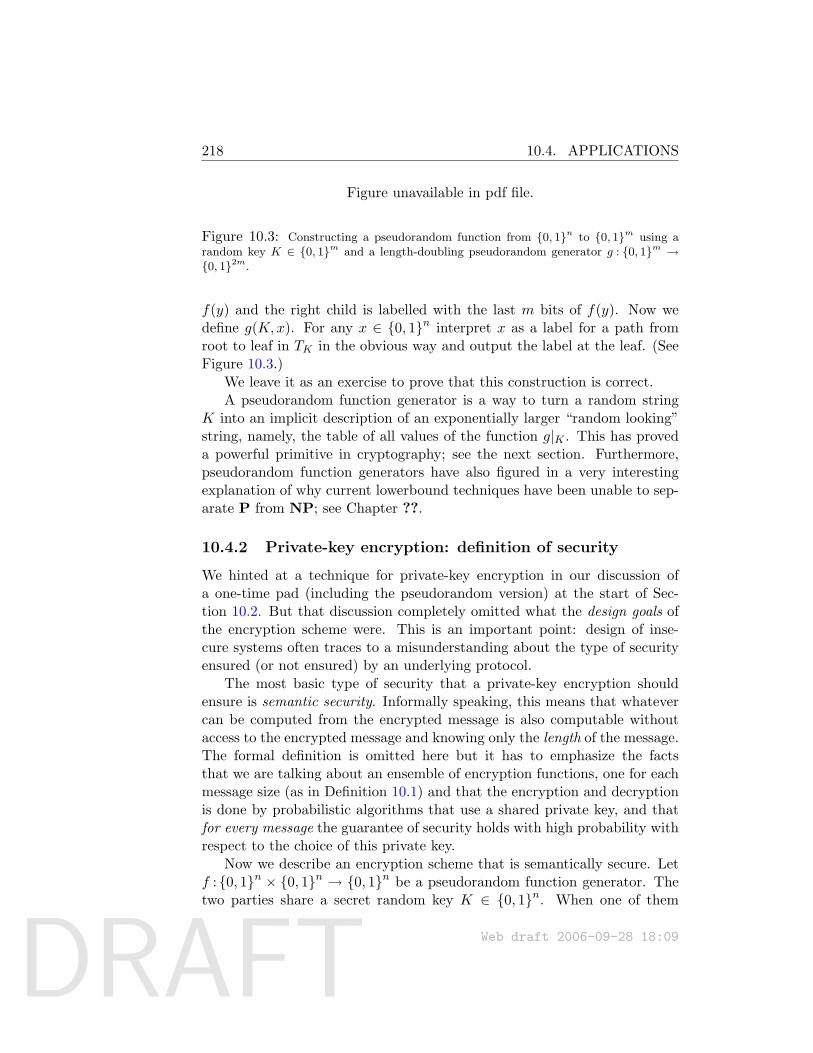
DRAFT

218 10.4. APPLICATIONS


Figure 10.3: Constructing a pseudorandom function from 0, 1n to 0, 1m using arandom key K ∈ 0, 1m and a length-doubling pseudorandom generator g : 0, 1m →0, 12m.

f(y) and the right child is labelled with the last m bits of f(y). Now wedefine g(K,x). For any x ∈ 0, 1n interpret x as a label for a path fromroot to leaf in TK in the obvious way and output the label at the leaf. (SeeFigure 10.3.)

We leave it as an exercise to prove that this construction is correct.A pseudorandom function generator is a way to turn a random string

K into an implicit description of an exponentially larger “random looking”string, namely, the table of all values of the function g|K . This has proveda powerful primitive in cryptography; see the next section. Furthermore,pseudorandom function generators have also figured in a very interestingexplanation of why current lowerbound techniques have been unable to sep-arate P from NP; see Chapter ??.

10.4.2 Private-key encryption: definition of security

We hinted at a technique for private-key encryption in our discussion ofa one-time pad (including the pseudorandom version) at the start of Sec-tion 10.2. But that discussion completely omitted what the design goals ofthe encryption scheme were. This is an important point: design of inse-cure systems often traces to a misunderstanding about the type of securityensured (or not ensured) by an underlying protocol.

The most basic type of security that a private-key encryption shouldensure is semantic security. Informally speaking, this means that whatevercan be computed from the encrypted message is also computable withoutaccess to the encrypted message and knowing only the length of the message.The formal definition is omitted here but it has to emphasize the factsthat we are talking about an ensemble of encryption functions, one for eachmessage size (as in Definition 10.1) and that the encryption and decryptionis done by probabilistic algorithms that use a shared private key, and thatfor every message the guarantee of security holds with high probability withrespect to the choice of this private key.

Now we describe an encryption scheme that is semantically secure. Letf : 0, 1n × 0, 1n → 0, 1n be a pseudorandom function generator. Thetwo parties share a secret random key K ∈ 0, 1n. When one of them

Web draft 2006-09-28 18:09

DRAFT

10.4. APPLICATIONS 219

wishes to send a message x ∈ 0, 1n to the other, she picks a randomstring r ∈ 0, 1n and transmits (r, x⊕ fK(r)). To decrypt the other partycomputes fK(r) and then XORs this string with the last n bits in the receivedtext.

We leave it as an exercise to show that this scheme is semantically secure.

10.4.3 Derandomization

The existence of pseudorandom generators implies subexponential determin-istic algorithms for BPP: this is usually referred to as derandomization ofBPP. (In this case, the derandomization is only partial since it results in asubexponential deterministic algorithm. Stronger complexity assumptionsimply a full derandomization of BPP, as we will see in Chapter 17.)Theorem 10.17If for every c > 1 there is a pseudorandom generator that is secure againstcircuits of size nc, then BPP ⊆ ∩ε>0DTIME(2n

ε).

Proof: Let us fix an ε > 0 and show that BPP ⊆ DTIME(2nε).

Suppose that M is a BPP machine running in nk time. We can buildanother probabilistic machine M ′ that takes nε random bits, streches themto nk bits using the pseudorandom generator and then simulates M usingthis nk bits as a random string. Obviously, M ′ can be simulated by goingover all binary strings nε, running M ′ on each of them, and taking themajority vote.

It remains to prove that M and M ′ accept the same language. Supposeotherwise. Then there exists an infinite sequence of inputs x1, . . . , xn, . . . onwhich M distinguishes a truly random string from a pseudorandom stringwith a high probability, because for M and M ′ to produce different results,the probability of acceptance should drop from 2/3 to below 1/2. Hencewe can build a distinguisher similar to the one described in the previoustheorem by hardwiring these inputs into a circuit family.

The above theorem shows that the existence of hard problems impliesthat we can reduce the randomness requirement of algorithms. This “hard-ness versus randomness” tradeoff is studied more deeply in Chapter 17.Remark 10.18There is an interesting connection to discrepancy theory, a field of math-ematics. Let S be a set of subsets of 0, 1n. Subset A ⊂ 0, 1n hasdiscrepancy ε with respect to S if for every s ∈ S,∣∣∣∣ |s ∩A||S|

− |A|2n

∣∣∣∣ ≤ ε.Web draft 2006-09-28 18:09

DRAFT

220 10.4. APPLICATIONS

Our earlier result that BPP ⊆ P/poly showed the existence of polynomial-size sets A that have low discrepancy for all sets defined by polynomial-timeTuring machines (we only described discrepancy for the universe 0, 1n butone can define it for all input sizes using lim sup). The goal of derandom-ization is to explicitly construct such sets; see Chapter 17.

10.4.4 Tossing coins over the phone and bit commitment

How can two parties A and B toss a fair random coin over the phone? (Manycryptographic protocols require this basic primitive.) If only one of themactually tosses a coin, there is nothing to prevent him from lying about theresult. The following fix suggests itself: both players toss a coin and theytake the XOR as the shared coin. Even if B does not trust A to use a faircoin, he knows that as long as his bit is random, the XOR is also random.Unfortunately, this idea also does not work because the player who revealshis bit first is at a disadvantage: the other player could just “adjust” hisanswer to get the desired final coin toss.

This problem is addressed by the following scheme, which assumes thatA and B are polynomial time turing machines that cannot invert one-waypermutations. The protocol itself is called bit commitment. First, A choosestwo strings xA and rA of length n and sends a message (fn(xA), rA), wherefn is a one-way permutation. This way, A commits the string xA withoutrevealing it. Now B selects a random bit b and conveys it. Then A revealsxA and they agree to use the XOR of b and (xArA) as their coin toss. Notethat B can verify that xA is the same as in the first message by applyingfn, therefore A cannot change her mind after learning B’s bit. On the otherhand, by the Goldreich–Levin theorem, B cannot predict xA rA from A’sfirst message, so this scheme is secure.

10.4.5 Secure multiparty computations

This concerns a vast generalization of the setting in Section 10.4.4. Thereare k parties and the ith party holds a string xi ∈ 0, 1n. They wish tocompute f(x1, x2, . . . , xk) where f : 0, 1nk → 0, 1 is a polynomial-timecomputable function known to all of them. (The setting in Section 10.4.4is a subcase whereby each xi is a bit —randomly chosen as it happens—and f is XOR.) Clearly, the parties can just exchange their inputs (suitablyencrypted if need be so that unauthorized eavesdroppers learn nothing) andthen each of them can compute f on his/her own. However, this leadsto all of them knowing each other’s input, which may not be desirable in

Web draft 2006-09-28 18:09

DRAFT

10.5. RECENT DEVELOPMENTS 221

many situations. For instance, we may wish to compute statistics (such asthe average) on the combination of several medical databases that are heldby different hospitals. Strict privacy and nondisclosure laws may forbidhospitals from sharing information about individual patients. (The originalexample Yao gave in introducing the problem was of k people who wish tocompute the average of their salaries without revealing their salaries to eachother.)

We say that a multiparty protocol for computing f is secure if at the endno party learns anything new apart from the value of f(x1, x2, . . . , xk). Theformal definition is inspired by the definition of a pseudorandom generator,and states that for each i, the bits received by party i during the protocolshould be computationally indistinguishable from completely random bits3.

It is completely nonobvious why such protocols must exist. Yao [Yao86]proved existence for k = 2 and Goldreich, Micali, Wigderson [GMW87]proved existence for general k. We will not describe this protocol in anydetail here except to mention that it involves “scrambling” the circuit thatcomputes f .

10.4.6 Lowerbounds for machine learning

In machine learning the goal is to learn a succinct function f : 0, 1n →0, 1 from a sequence of type (x1, f(x1)), (x2, f(x2)), . . . , where the xi’sare randomly-chosen inputs. Clearly, this is impossible in general since arandom function has no succinct description. But suppose f has a succinctdescription, e.g. as a small circuit. Can we learn f in that case?

The existence of pseudorandom functions implies that even though afunction may be polynomial-time computable, there is no way to learn itfrom examples in polynomial time. In fact it is possible to extend thisimpossibility result (though we do not attempt it) to more restricted functionfamilies such as NC1 (see Kearns and Valiant [KV94]).

10.5 Recent developments

The earliest cryptosystems were designed using the SUBSET SUM problem.They were all shown to be insecure by the early 1980s. In the last few years,

3Returning to our medical database example, we see that the hospitals can indeedcompute statistics on their combined databases without revealing any information to eachother —at least any information that can be extracted feasibly. Nevetheless, it is unclearif current privacy laws allow hospitals to perform such secure multiparty protocols usingpatient data— an example of the law lagging behind scientific progress.

Web draft 2006-09-28 18:09

DRAFT

222 10.5. RECENT DEVELOPMENTS

interest in such problems —and also the related problems of computing ap-proximate solutions to the shortest and nearest lattice vector problems—has revived, thanks to a one-way function described in Ajtai [Ajt96], anda public-key cryptosystem described in Ajtai and Dwork [AD97] (and im-proved on since then by other researchers). These constructions are secureon most instances iff they are secure on worst-case instances. (The idea usedis a variant of random self-reducibility.)

Also, there has been a lot of exploration of the exact notion of secu-rity that one needs for various cryptographic tasks. For instance, the no-tion of semantic security in Section 10.4.2 may seem quite strong, but re-searchers subsequently realized that it leaves open the possibility of someother kinds of attacks, including chosen ciphertext attacks, or attacks basedupon concurrent execution of several copies of the protocol. Achieving se-curity against such exotic attacks calls for many ideas, most notably zeroknowledge (a brief introduction to this concept appears in Section ??).


In the 1940s, Shannon speculated about topics reminiscent of complexity-based cryptography. The first concrete proposal was made by Diffie andHellman [DH76], though their cryptosystem was later broken. The inven-tion of the RSA cryptosystem (named after its inventors Ron Rivest, AdiShamir, and Len Adleman) [RSA78] brought enormous attention to thistopic. In 1981 Shamir [Sha83] suggested the idea of replacing a one-timepad by a pseudorandom string. He also exhibited a weak pseudorandom gen-erator assuming the average-case intractability of the RSA function. Themore famous papers of Blum and Micali [BM84] and then Yao [Yao82] laidthe intellectual foundations of private-key cryptography. (The hybrid ar-gument used by Yao is a stronger version of one in an earlier importantmanuscript of Goldwasser and Micali [GM84] that proposed probabilisticencryption schemes.) The construction of pseudorandom functions in Sec-tion 10.4.1 is due to Goldreich, Goldwasser, and Micali [GGM86]. Thequestion about tossing coins over a telephone was raised in an influentialpaper of Blum [Blu82]. Today complexity-based cryptography is a vast fieldwith several dedicated conferences. Goldreich [Gol04]’s two-volume bookgives a definitive account.

A scholarly exposition of number theoretic algorithms (including gen-erating random primes and factoring integers) appears in Victor Shoup’srecent book [?] and the book of Bach and Shallit [BS96].

Web draft 2006-09-28 18:09

DRAFT

10.5. RECENT DEVELOPMENTS 223

Theorem 10.13 and its very technical proof is in Hastad et al. [HILL99](the relevant conference publications are a decade older).

Our proof of the Goldreich-Levin theorem is usually attributed to Rackoff(unpublished).

Exercises

§1 Show that if P = NP then one-way functions and pseudorandomgenerators do not exist.

§2 (Requires just a little number theory). Prove that if some algorithminverts the Rabin function fm(x) = x2 (mod m) on a 1/poly(logm)fraction of inputs then we can factor m in poly(logm) time.

Hint:Supposem=pqwherep,qareprimenumbers.Thenx2

has4“squareroots”modulom.

§3 Show that if f is a one-way permutation then so is fk (namely, f(f(f(· · · (f(x)))))where f is applied k times) where k = nc for some fixed c > 0.

§4 Assuming one-way functions exist, show that the above fails for one-way functions.

Hint:Youhavetodesignaone-wayfunctionwherefk

isnotone-way.

§5 Suppose a ∈ GF(2)m is an unknown vector. Let r1, r2, . . . , rm ∈GF(2)m be randomly chosen, and a ri revealed to us for all i =1, 2, . . . ,m. Describe a deterministic algorithm to reconstruct a fromthis information, and show that the probability (over the choice of theri’s) is at least 1/4 that it works.

Hint:Youneedtoshowthatacertaindeterminantisnonzero.

This shows that the “trick” in Goldreich-Levin’s proof is necessary.

§6 Suppose somebody holds an unknown n-bit vector a. Whenever youpresent a randomly chosen subset of indices S ⊆ 1, . . . , n, then withprobability at least 1/2+ε, she tells you the parity of the all the bits ina indexed by S. Describe a guessing strategy that allows you to guessa (an n bit string!) with probability at least ( εn)c for some constantc > 0.

Web draft 2006-09-28 18:09

DRAFT

224 10.5. RECENT DEVELOPMENTS

§7 Suppose g :0, 1n → 0, 1n+1 is any pseudorandom generator. Thenuse g to describe a pseudorandom generator that stretches n bits tonk for any constant k > 1.

§8 Show the correctness of the pseudorandom function generator in Sec-tion 10.4.1.

Hint:Useahybridargumentwhichreplacesthelabelsonthefirstklevelsofthetreebycompletelyrandomstrings.Notethattherandomlabelsdonotneedtobeassignedaheadoftime—thiswouldtakeatleast2

ktime—butcanbeassignedonthefly

whenevertheyareneededbythedistinguishingalgorithm.

§9 Formalize the definition of semantic security and show that the en-cryption scheme in Section 10.4.2 is semantically secure.

Hint:Firstshowthatforallmessagepairsx,ytheirencryptionsareindistinguishablebypolynomial-timealgorithms.Whydoesthissuffice?

Web draft 2006-09-28 18:09

DRAFT

Part II

Lowerbounds for ConcreteComputational Models


225

DRAFT

DRAFT

227

In the next few chapters the topic will be concrete complexity, the studyof lowerbounds on models of computation such as decision trees, communi-cation games, circuits, etc. Algorithms or devices considered in this lecturetake inputs of a fixed size n, and we study the complexity of these devicesas a function of n.

Web draft 2006-09-28 18:09

DRAFT

228

Web draft 2006-09-28 18:09

DRAFT

Chapter 11

Decision Trees

A decision tree is a model of computation used to study the number of bitsof an input that need to be examined in order to compute some functionon this input. Consider a function f : 0, 1n → 0, 1. A decision treefor f is a tree for which each node is labelled with some xi, and has twooutgoing edges, labelled 0 and 1. Each tree leaf is labelled with an outputvalue 0 or 1. The computation on input x = x1x2 . . . xn proceeds at eachnode by inspecting the input bit xi indicated by the node’s label. If xi = 1the computation continues in the subtree reached by taking the 1-edge. The0-edge is taken if the bit is 0. Thus input x follows a path through the tree.The output value at the leaf is f(x). An example of a simple decision treefor the majority function is given in Figure 11.1


Figure 11.1: A decision tree for computing the majority function Maj(x1, x2, x3) onthree bits. Outputs 1 if at least two input bits are 1, else outputs 0.

Recall the use of decision trees in the proof of the lower bound forcomparison-based sorting algorithms. That study can be recast in the aboveframework by thinking of the input —which consisted of n numbers — asconsisting of

(n2

)bits, each giving the outcome of a pairwise comparison

between two numbers.We can now define two useful decision tree metrics.

Definition 11.1The cost of tree t on input x, cost(t, x), is the number of bits of x examinedby t.


229

DRAFT

230

Definition 11.2The decision tree complexity of function f , D(f), is defined as follows,where T below refers to the set of decision trees that decide f .

D(f) = mint∈T

maxx∈0,1n

cost(t, x) (1)

The decision tree complexity of a function is the number of bits examinedby the most efficient decision tree on the worst case input to that tree. Weare now ready to consider several examples.

Example 11.3(Graph connectivity) Given a graph G as input, in adjacency matrix form,we would like to know how many bits of the adjacency matrix a decisiontree algorithm might have to inspect in order to determine whether G isconnected. We have the following result.

Theorem 11.4Let f be a function that computes the connectivity of input graphs with mvertices. Then D(f) =

(m2

).

The idea of the proof of this theorem is to imagine an adversary thatconstructs a graph, edge by edge, in response to the queries of a decisiontree. For every decision tree that decides connectivity, the strategy implicitlyproduces an input graph which requires the decision tree to inspect each ofthe

(m2

)possible edges in a graph of m vertices.

Adversary Strategy:Whenever the decision tree algorithm asks about edge ei,answer “no” unless this would force the graph to be disconnected.

After i queries, let Ni be the set of edges for which the adversary hasreplied “no”, Yi the set of edges for which the adversary has replied “yes”.and Ei the set of edges not yet queried. The adversary’s strategy maintainsthe invariant that Yi is a disconnected forest for i <

(m2

)and Yi ∪ Ei is

connected. This ensures that the decision tree will not know whether thegraph is connected until it queries every edge.

Web draft 2006-09-28 18:09

DRAFT

11.1. CERTIFICATE COMPLEXITY 231

Example 11.5(OR Function) Let f(x1, x2, . . . xn) =

∨ni=1 xi. Here we can use an adversary

argument to show that D(f) = n. For any decision tree query of an inputbit xi, the adversary responds that xi equals 0 for the first n − 1 queries.Since f is the OR function, the decision tree will be in suspense until thevalue of the nth bit is revealed. Thus D(f) is n.

Example 11.6Consider the AND-OR function, with n = 2k. We define fk as follows.

fk(x1, . . . , xn) =

fk−1(x1, . . . x2k−1−1) ∧ fk−1(x2k−1 , . . . x2k) if k is evenfk−1(x1, . . . x2k−1−1) ∨ fk−1(x2k−1 , . . . x2k) if k > 1 and is oddxi if k = 1

(2)A diagram of a circuit that computes the AND-OR function is shown inFigure 11.2. It is left as an exercise to prove, using induction, that D(fk) =2k.


Figure 11.2: A circuit showing the computation of the AND-OR function. The circuithas k layers of alternating gates, where n = 2k.

11.1 Certificate Complexity

We now introduce the notion of certificate complexity, which, in a manneranalogous to decision tree complexity above, tells us the minimum amountof information needed to be convinced of the value of a function f on inputx.Definition 11.7Consider a function f : 0, 1n → 0, 1. If f(x) = 0, then a 0-certificatefor x is a sequence of bits in x that proves f(x) = 0. If f(x) = 1, then a1-certificate is a sequence of bits in x that proves f(x) = 1.

Web draft 2006-09-28 18:09

DRAFT

232 11.1. CERTIFICATE COMPLEXITY

Definition 11.8The certificate complexity C(f) of f is defined as follows.

C(f) = maxx:input

number of bits in the smallest 0- or 1- certificate for x

(3)

Example 11.9If f is a function that decides connectivity of a graph, a 0-certificate for aninput must prove that some cut in the graph has no edges, hence it has tocontain all the possible edges of a cut of the graph. When these edges do notexist, the graph is disconnected. Similarly, a 1-certificate is the edges of aspanning tree. Thus for those inputs that represent a connected graph, theminimum size of a 1-certificate is the number of edges in a spanning tree,n − 1. For those that represent a disconnected graph, a 0 certificate is theset of edges in a cut. The size of a 0-certificate is at most (n/2)2 = n2/4,and there are graphs (such as the graph consisting of two disjoint cliques ofsize n/2) in which no smaller 0-certificate exists. Thus C(f) = n2/4.

Example 11.10We show that the certificate complexity of the AND-OR function fk ofExample 11.6 is 2dk/2e. Recall that fk is defined using a circuit of k layers.Each layer contains only OR-gates or only AND-gates, and the layers havealternative gate types. The bottom layer receives the bits of input x asinput and the single top layer gate outputs the answer fk(x). If f(x) = 1,we can construct a 1-certificate as follows. For every AND-gate in the treeof gates we have to prove that both its children evaluate to 1, whereas forevery OR-gate we only need to prove that some child evaluates to 1. Thusthe 1-certificate is a subtree in which the AND-gates have two children butthe OR gates only have one each. Thus the subtree only needs to involve2dk/2e input bits. If f(x) = 0, a similar argument applies, but the role ofOR-gates and AND-gates, and values 1 and 0 are reversed. The result isthat the certificate complexity of fk is 2dk/2e, or about

√n.

Web draft 2006-09-28 18:09

DRAFT

11.1. CERTIFICATE COMPLEXITY 233

The following is a rough way to think about these concepts in analogyto Turing machine complexity as we have studied it.

low decision tree complexity↔ P (4)low 1-certificate complexity↔ NP (5)low 0-certificate complexity↔ coNP (6)

The following result shows, however, that the analogy may not be exactsince in the decision tree world, P = NP ∩ coNP. It should be noted thatthe result is tight, for example for the AND-OR function.

Theorem 11.11For function f , D(f) ≤ C(f)2.

Proof: Let S0, S1 be the set of minimal 0-certificates and 1-certificates,respectively, for f . Let k = C(f), so each certificate has at most k bits.

Remark 11.12Note that every 0-certificate must share a bit position with every 1-certificate,and furthermore, assign this bit differently. If this were not the case, thenit would be possible for both a 0-certificate and 1-certificate to be assertedat the same time, which is impossible.

The following decision tree algorithm then determines the value of f inat most k2 queries.

Algorithm: Repeat until the value of f is determined: Choose a remain-ing 0-certificate from S0 and query all the bits in it. If the bits are thevalues that prove the f to be 0, then stop. Otherwise, we can prune the setof remaining certificates as follows. Since all 1-certificates must intersect thechosen 0-certificate, for any c1 ∈ S1, one bit in c1 must have been queriedhere. Eliminate c1 from consideration if the certifying value of c1 at at lo-cation is different from the actual value found. Otherwise, we only need toconsider the remaining k − 1 bits of c1.

This algorithm can repeat at most k times. For each iteration, theunfixed lengths of the uneliminated 1-certificates decreases by one. This isbecause once some values of the input have been fixed due to queries, forany 0-certificate, it remains true that all 1-certificates must intersect it inat least one location that has not been fixed, otherwise it would be possiblefor both a 0-certificate and a 1-certificate to be asserted. With at most kqueries for at most k iterations, a total of k2 queries is used.

Web draft 2006-09-28 18:09

DRAFT

234 11.2. RANDOMIZED DECISION TREES

11.2 Randomized Decision Trees

There are two equivalent ways to look at randomized decision trees. Wecan consider decision trees in which the branch taken at each node is deter-mined by the query value and by a random coin flip. We can also considerprobability distributions over deterministic decision trees. The analysis thatfollows uses the latter model.

We will call P a probability distribution over a set of decision treesT that compute a particular function. P(t) is then the probability thattree t is chosen from the distribution. For a particular input x, then, wedefine c(P, x) =

∑tinT P(t)cost(t, x). c(P, x) is thus the expected number of

queries a tree chosen from T will make on input x. We can then characterizehow well randomized decision trees can operate on a particular problem.

Definition 11.13The randomized decision tree complexity, R(f), of f , is defined asfollows.

R(f) = minP

maxx

c(P, x) (7)

The randomized decision tree complexity thus expresses how well thebest possible probability distribution of trees will do against the worst pos-sible input for a particular probability distribution of trees. We can observeimmediately that R(f) ≥ C(f). This is because C(f) is a minimum value ofcost(t, x). Since R(f) is just an expected value for a particular probabilitydistribution of these cost values, the minimum such value can be no greaterthan the expected value.

Example 11.14Consider the majority function, f = Maj(x1, x2, x3). It is straightforwardto see that D(f) = 3. We show that R(f) ≤ 8/3. Let P be a uniformdistribution over the (six) ways of ordering the queries of the three inputbits. Now if all three bits are the same, then regardless of the order chosen,the decision tree will produce the correct answer after two queries. For suchx, c(P, x) = 2. If two of the bits are the same and the third is different, thenthere is a 1/3 probability that the chosen decision tree will choose the twosimilar bits to query first, and thus a 1/3 probability that the cost will be2. There thus remains a 2/3 probability that all three bits will need to beinspected. For such x, then, c(P, x) = 8/3. Therefore, R(f) is at most 8/3.

Web draft 2006-09-28 18:09

DRAFT

11.3. LOWERBOUNDS ON RANDOMIZED COMPLEXITY 235

How can we prove lowerbounds on randomized complexity? For this weneed another concept.

11.3 Lowerbounds on Randomized Complexity

needs cleanup nowTo prove lowerbounds on randomized complexity, it suffices by Yao’s

Lemma (see Section 11.6) to prove lowerbounds on distributional complex-ity. Where randomized complexity explores distributions over the space ofdecision trees for a problem, distributional complexity considers probabilitydistributions on inputs. It is under such considerations that we can speakof “average case analysis.”

Let D be a probability distribution over the space of input strings oflength n. Then, if A is a deterministic algorithm, such as a decision tree, fora function, then we define the distributional complexity of A on a functionf with inputs distributed according to D as the expected cost for algorithmA to compute f , where the expectation is over the distribution of inputs.

Definition 11.15The distributional complexity d(A,D) of algorithm A given inputs dis-tributed according to D is defined as:

d(A,D) =∑

x:input

D(x)cost(A, x) = Ex∈D[cost(A, x)] (8)

From this we can characterize distributional complexity as a function ofa single function f itself.

Definition 11.16The distributional decision tree complexity, ∆(f) of function f is definedas:

∆(f) = maxD

minAd(A,D) (9)

Where A above runs over the set of decision trees that are deciders for f .

So the distributional decision tree complexity measures the expectedefficiency of the most efficient decision tree algorithm works given the worstcase distribution of inputs.

The following theorem follows from Yao’s lemma.

Theorem 11.17R(f) = ∆(f).

Web draft 2006-09-28 18:09

DRAFT

23611.4. SOME TECHNIQUES FOR DECISION TREE LOWERBOUNDS

So in order to find a lower bound on some randomized algorithm, itsuffices to find a lower bound on ∆(f). Such a lower bound can be foundby postulating an input distribution D and seeing whether every algorithmhas expected cost at least equal to the desired lower bound.

Example 11.18We return to considering the majority function, and we seek to find a lowerbound on ∆(f). Consider a distribution over inputs such that inputs inwhich all three bits match, namely 000 and 111, occur with probability 0.All other inputs occur with probability 1/6. For any decision tree, that is,for any order in which the three bits are examined, there is exactly a 1/3probability that the first two bits examined will be the same value, and thusthere is a 1/3 probability that the cost is 2. There is then a 2/3 probabilitythat the cost is 3. Thus the overall expected cost for this distribution is8/3. This implies that ∆(f) ≥ 8/3 and in turn that R(f) ≥ 8/3. So∆(f) = R(f) = 8/3.

11.4 Some techniques for decision tree lowerbounds

Definition 11.19 (Sensitivity)If f :0, 1n → 0, 1 is a function and x ∈ 0, 1n then the sensitivity of fon x, denoted sx(f), is the number of bit positions i such that f(x) 6= f(xi),where xi is x with its ith bit flipped. The sensitivity of f , denoted s(f), ismaxx sx(f).

The block sensitivity of f on x, denoted bsx(f), is the maximum numberb such that there are disjoint blocks of bit positions B1,2 , . . . , Bb such thatf(x) 6= f(xBi) where xBi is x with all its bits flipped in block Bi. The blocksensitivity of f denoted bs(f) is maxx bsx(f).

It is conjectured that there is a constant c (as low as 2) such that bs(f) =O(s(f)c) for all f but this is wide open. The following easy observation isleft as an exercise.Lemma 11.20For any function, s(f) ≤ bs(f) ≤ D(f).

Theorem 11.21 (Nisan)C(f) ≤ s(f)bs(f).

Web draft 2006-09-28 18:09

DRAFT

11.4. SOME TECHNIQUES FOR DECISION TREE LOWERBOUNDS237

Proof: For any input x ∈ 0, 1n we describe a certificate for x of sizes(f)bs(f). This certificate is obtained by considering the largest number ofdisjoint blocks of variables B1, B2, . . . , Bb that achieve b = bsx(f) ≤ bs(f).We claim that setting these variables according to x constitutes a certificatefor x.

Suppose not, and let x′ be an input that is consistent with the abovecertificate. Let Bb+1 be a block of variables such that x′ = xBb+1 . ThenBb+1 must be disjoint from B1, B2, . . . Bb, which contradicts b = bsx(f).

Note that each of B1, B2, . . . , Bb has size at most s(f) by definition ofs(f), and hence the size of the certificate we have exhibited is at mosts(f)bs(f).

Recent work on decision tree lowerbounds has used polynomial repre-sentations of boolean functions. Recall that a multilinear polynomial is apolynomial whose degree in each variable is 1.

Definition 11.22An n-variate polynomial p(x1, x2, . . . , xn) represents f : 0, 1n → 0, 1 ifp(x) = f(x) for all x ∈ 0, 1n.

The degree of f , denoted deg(f), is the degree of the multilinear polyno-mial that represents f .

(The exercises ask you to show that the multilinear polynomial representa-tion is unique, so deg(f) is well-defined.)

Example 11.23The AND of n variables x1, x2, . . . , xn is represented by the multilinear poly-nomial

∏ni=1 xi and OR is represented by 1−

∏ni=1(1− xi).

The degree of AND and OR is n, and so is their decision tree complexity.There is a similar connection for other problems too, but it is not as tight.The first part of the next theorem is an easy exercise; the second part isnontrivial.

Theorem 11.241. deg(f) ≤ D(f).

2. (Nisan-Smolensky) D(f) ≤ deg(f)2bs(f) ≤ O(deg(f)4).

Web draft 2006-09-28 18:09

DRAFT

238 11.5. COMPARISON TREES AND SORTING LOWERBOUNDS

11.5 Comparison trees and sorting lowerbounds

to be written

11.6 Yao’s MinMax Lemma

This section presents Yao’s minmax lemma, which is used in a variety of set-tings to prove lowerbounds on randomized algorithms. Therefore we presentit in a very general setting.

Let X be a finite set of inputs and A be a finite set of algorithms thatsolve some computational problem on these inputs. For x ∈ X , a ∈ A,we denote by cost(A, x) the cost incurred by algorithm A on input x. Arandomized algorithm is a probability distribution R on A. The cost ofR on input x, denoted cost(R, x), is EA∈R[cost(A, x)]. The randomizedcomplexity of the problem is

minR

maxx∈X

cost(R, x). (10)

Let D be a distribution on inputs. For any deterministic algorithm A,the cost incurred by it on D, denoted cost(A,D), is Ex∈D[cost(A, x)]. Thedistributional complexity of the problem is

maxD

minA∈A

cost(A,D). (11)

Yao’s Lemma says that these two quantitities are the same. It is easilyderived from von Neumann’s minmax theorem for zero-sum games, or witha little more work, from linear programming duality.

Yao’s lemma is typically used to lowerbound randomized complexity. Todo so, one defines (using some insight and some luck) a suitable distributionD on the inputs. Then one proves that every deterministic algorithm incurshigh cost, say C, on this distribution. By Yao’s Lemma, it follows that therandomized complexity then is at least C.

Exercises

§1 Suppose f is any function that depends on all its bits; in other words,for each bit position i there is an input x such that f(x) 6= f(xi). Showthat s(f) = Ω(log n).

Web draft 2006-09-28 18:09

DRAFT

11.6. YAO’S MINMAX LEMMA 239

§2 Consider an f defined as follows. The n-bit input is partitioned intob√nc blocks of size about

√n. The function is 1 iff there is at least

one block in which two consecutive bits are 1 and the remaining bitsin the block are 0. Estimate s(f), bs(f), C(f), D(f) for this function.

§3 Show that there is a unique multilinear polynomial that representsf :0, 1n → 0, 1. Use this fact to find the multilinear representationof the PARITY of n variables.

§4 Show that deg(f) ≤ D(f).


The result that the decision tree complexity of connectivity and many otherproblems is

(n2

)has motivated the following conjecture (atributed variously

to Anderaa, Karp, Yao):Every monotone graph property has D(·) =

(n2

).

Here “monotone” means that adding edges to the graph cannot make itgo from having the property to not having the property (e.g., connectivity).“Graph property” means that the property does not depend upon the vertexindices (e.g., the property that vertex 1 and vertex 2 have an edge betweenthem). This conjecture is known to be true up to a O(1) factor; the proofuses topology and is excellently described in Du and Ko [DK00]. A moreambitious conjecture is that even the randomized decision tree complexityof monotone graph properties is Ω(n2) but here the best lowerbound is closeto n4/3.

The polynomial method for decision tree lowerbounds is surveyed inBuhrman and de Wolf [BdW02]. The method can be used to lowerboundrandomized decision tree complexity (and more recently, quantum decisiontree complexity) but then one needs to consider polynomials that approxi-mately represent the function.

Web draft 2006-09-28 18:09

DRAFT

240 11.6. YAO’S MINMAX LEMMA

Web draft 2006-09-28 18:09

DRAFT

Chapter 12

Communication Complexity

Communication complexity concerns the following scenario. There are twoplayers with unlimited computational power, each of whom holds an n bitinput, say x and y. Neither knows the other’s input, and they wish tocollaboratively compute f(x, y) where function f :0, 1n×0, 1n → 0, 1is known to both. Furthermore, they had foreseen this situation (e.g., one ofthe parties could be a spacecraft and the other could be the base station onearth), so they had already —before they knew their inputs x, y— agreedupon a protocol for communication1. The cost of this protocol is the numberof bits communicated by the players for the worst-case choice of x, y.

Researchers have studied many modifications of the above basic sce-nario, including randomized protocols, nondeterministic protocols, average-case protocols (where x, y are assumed to come from a distribution), multi-party protocols, etc. Truly, this is a self-contained mini-world within com-plexity theory. Furthermore, lowerbounds on communication complexityhave uses in a variety of areas, including lowerbounds for parallel and VLSIcomputation, circuit lowerbounds, polyhedral theory, data structure lower-bounds, etc. We give a very rudimentary introduction to this area; anexcellent and detailed treatment can be found in the book by Kushilevitzand Nisan [KN97].

1Do not confuse this situation with information theory, where an algorithm is givenmessages that have to be transmitted over a noisy channel, and the goal is to transmit themrobustly while minimizing the amount of communication. In communication complexitythe channel is not noisy and the players determine what messages to send.


241

DRAFT

242 12.1. DEFINITION

12.1 Definition

Now we formalize the informal description of communication complexitygiven above.

A t-round communication protocol for f is a sequence of function pairs(S1, C1), (S2, C2), . . . , (St, Ct), (f1, f2). The input of Si is the communicationpattern of the first i − 1 rounds and the output is from 1, 2, indicatingwhich player will communicate in the ith round. The input of Ci is the inputstring of this selected player as well as the communication pattern of the firsti− 1 rounds. The output of Ci is the bit that this player will communicatein the ith round. Finally, f1, f2 are 0/1-valued functions that the playersapply at the end of the protocol to their inputs as well as the communicationpattern in the t rounds in order to compute the output. These two outputsmust be f(x, y). The communication complexity of f is

C(f) = minprotocols P

maxx,y

Number of bits exchanged by P on x, y.

Notice, C(f) ≤ n + 1 since the trivial protocol is for one player tocommunicate his entire input, whereupon the second player computes f(x, y)and communicates that single bit to the first. Can they manage with lesscommunication?

Example 12.1 (Parity)Suppose the function f(x, y) is the parity of all the bits in x, y. We claimthat C(f) = 2. Clearly, C(f) ≥ 2 since the function depends nontrivially oneach input, so each player must transmit at least one bit. Next, C(f) ≤ 2since it suffices for each player to transmit the parity of all the bits in hispossession; then both know the parity of all the bits.

Remark 12.2Sometimes students ask whether a player can communicate by not sayinganything? (After all, they have three options: send a 0, or 1, or not sayanything in that round.) We can regard such protocols as communicatingwith a ternary, not binary, alphabet, and analyze them analogously.

12.2 Lowerbound methods

Now we discuss methods for proving lowerbounds on communication com-plexity. As a running example in this chapter, we will use the equality

Web draft 2006-09-28 18:09

DRAFT

12.2. LOWERBOUND METHODS 243

function:

EQ(x, y) =

1 if x = y

0 otherwise

We will see that C(EQ) ≥ n.

12.2.1 Fooling set

We show C(EQ) ≥ n. For contradiction’s sake, suppose a protocol existswhose complexity is at most n−1. Then there are only 2n−1 communicationpatterns possible between the players. Consider the set of all 2n pairs (x, x).Using the pigeonhole principle we conclude there exist two pairs (x, x) and(x′, x′) on which the communication pattern is the same. Of course, thus farwe have nothing to object to, since the answers EQ(x, x) and EQ(x′, x′) onboth pairs are 1. However, now imagine giving one player x and the otherplayer x′ as inputs. A moment’s thought shows that the communicationpattern will be the same as the one on (x, x) and (x′, x′). (Formally, thiscan be shown by induction. If player 1 communicates a bit in the first round,then clearly this bit is the same whether his input is x or x′. If player 2communicates in the 2nd round, then his bit must also be the same on bothinputs since he receives the same bit from player 1. And so on.) Hence theplayer’s answer on (x, x) must agree with their answer on (x, x′). But thenthe protocol must be incorrect, since EQ(x, x′) = 0 6= EQ(x, x).

The lowerbound argument above is called a fooling set argument. It isformalized as follows.

Definition 12.3A fooling set for f :0, 1n × 0, 1n → 0, 1 is a set S ⊆ 0, 1n × 0, 1nand a value b ∈ 0, 1 such that:

1. For every (x, y) ∈ S, f(x, y) = b.

2. For every two distinct pairs (x1, y1), (x2, y2) ∈ S, either f(x1, y2) 6= bor f(x2, y1) 6= b.

Lemma 12.4If f has a fooling set with m pairs then C(f) ≥ log2m.

Example 12.5 (Disjointness)Let x, y be interpreted as characteristic vectors of subsets of 1, 2, . . . , n.Let DISJ(x, y) = 1 if these two subsets are disjoint, otherwise DISJ(x, y) =

Web draft 2006-09-28 18:09

DRAFT

244 12.2. LOWERBOUND METHODS

0. Then C(DISJ) ≥ n since the following 2n pairs constitute a fooling set:

S =(A,A) : A ⊆ 1, 2, . . . , n

.

12.2.2 The tiling lowerbound

The tiling lowerbound takes a more global view of f . Consider the matrix off , denoted M(f), which is a 2n× 2n matrix whose (x, y)’th entry is f(x, y).See Figure 12.1. We visualize the communication protocol in terms of this


Figure 12.1: Matrix M(f) for the equality function when the inputs to the players have3 bits. The numbers in the matrix are values of f .

matrix. A combinatorial rectangle (or just rectangle) in the matrix is asubmatrix corresponding to A × B where A ⊆ 0, 1n, B ⊆ 0, 1n. If theprotocol begins with the first player sending a bit, then M(f) partitionsinto two rectangles of the type A0 × 0, 1n, A1 × Bn, where Ab is thesubset of strings for which the first player communicates bit b. Notice,A0 ∪A1 = 0, 1n. If the next bit is sent by the second player, then each ofthe two rectangles above is further partitioned into two smaller rectanglesdepending upon what this bit was. If the protocol continues for k steps, thematrix gets partitioned into 2k rectangles. Note that each rectangle in thepartition corresponds to a subset of input pairs for which the communicationsequence thus far has been identical. (See Figure 12.2 for an example.)


Figure 12.2: Two-way communication matrix after two steps. The large number labelsare the concatenation of the bit sent by the first player with the bit sent by the secondplayer.

If the protocol stops, then the value of f is determined within eachrectangle, and thus must be the same for all pairs x, y in that rectangle.Thus the set of all communication patterns must lead to a partition of thematrix into monochromatic rectangles. (A rectangle A×B is monochromaticif for all x in A and y in B, f(x, y) is the same.)

Web draft 2006-09-28 18:09

DRAFT


Definition 12.6A monochromatic tiling ofM(f) is a partition ofM(f) into disjoint monochro-matic rectangles. We denote by χ(f) the minimum number of rectangles inany monochromatic tiling of M(f).

The following theorem is immediate from our discussion above.Theorem 12.7If f has communication complexity C then it has a monochromatic tilingwith at most 2C rectangles. Consequently, C ≥ log2 χ(f).

The following observation shows that the tiling bound subsumes thefooling set bound.Lemma 12.8If f has a fooling set with m pairs, then χ(f) ≥ m.

Proof: If (x1, y1) and (x2, y2) are two of the pairs in the fooling set, thenthey cannot be in a monochromatic rectangle since not all of (x1, y1), (x2, y2),(x1, y2), (x2, y1) have the same f value.

12.2.3 Rank lowerbound

Now we introduce an algebraic method to lowerbound χ(f) (and hence com-munication complexity). Recall the high school notion of rank of a squarematrix: it is the size of the largest subset of rows/colums that are indepen-dent. The following is another definition.Definition 12.9If a matrix has entries from a field F then the rank of an n × n matrix Mis the minimum value of l such that M can be expressed as

M =l∑

i=1

αiBi,

where αi ∈ F \ 0 and each Bi is an n× n matrix of rank 1.

Note that 0, 1 are elements of every field, so we can compute the rank overany field we like. The choice of field can be crucial; see Problem 5 in theexercises.

The following theorem is trivial, since each monochromatic rectangle canbe viewed (by filling out entries outside the rectangle with 0’s) as a matrixof rank at most 1 .Theorem 12.10For every function f , χ(f) ≥ rank(M(f)).

Web draft 2006-09-28 18:09

DRAFT


12.2.4 Discrepancy

The discrepancy of a rectangle A×B in M(f) is

122n|number of 1’s in A×B − number of 0’s in A×B| . (1)

The discrepancy of the matrix M(f), denote Disc(f), is the largest dis-crepancy among all rectangles. The following Lemma relates it to χ(f).

Lemma 12.11

χ(f) ≥ 1Disc(f)

.

Proof: For a monochromatic rectangle, the discrepancy is its size dividedby 22n. The total number of entries in the matrix is 22n. The bound follows.

Example 12.12Lemma 12.11 can be very loose. For the EQ() function, the discrepancyis at least 1 − 2−n (namely, the discrepancy of the entire matrix), whichwould only give a lowerbound of 2 for χ(f). However, χ(f) is at least 2n, asalready noted.

Now we describe a method to upperbound the discrepancy using eigen-values.Lemma 12.13 (eigenvalue bound)For any matrixM , the discrepancy of a rectangleA×B is at most λmax(M)

√|A| |B|/22n,

where λmax(M) is the magnitude of the largest eigenvalue of M .

Proof: Let 1A, 1B ∈ Rn denote the characteristic vectors of A,B. Then|1A|2 =

√∑i∈A 12 =

√|A|.

The discrepancy of the rectangle A×B is

122n

1TAM1B ≤1

22nλmax(M)

∣∣1TA1B∣∣ ≤ 1

22nλmax(M)

√|A| |B|.

explain this.

Web draft 2006-09-28 18:09

DRAFT


Example 12.14The mod 2 inner product function defined as f(x, y) = (x·y)2 =

∑i xiyi( mod

2) has been encountered a few times in this book. To bound its discrepancy,we consider the matrix 2M(f)− 1. This transformation makes the range ofthe function −1, 1 and will be useful again later. Let this new matrix bedenoted N . It is easily checked that every two distinct rows (columns) ofN are orthogonal, every row has `2 norm 2n/2, and that NT = N . Thus weconclude that N2 = 2nI where I is the unit matrix. Hence every eigenvalueis either +2n/2 or −2n/2, and thus Lemma 12.13 implies that the discrepancyof a rectangle A×B is at most 2n/2

√|A| |B| and the overall discrepancy is

at most 23n/2 (since |A| , |B| ≤ 2n).

A technique for upperbounding the discrepancy

Now we describe an upperbound technique for the discrepancy that will laterbe useful in the multiparty setting (Section 12.3). For ease of notation, inthis section we change the range of f to −1, 1 by replacing 1’s in M(f)with −1’s and replacing 0’s with 1’s. Note that now

Disc(f) = maxA,B

122n

∣∣∣∣∣∣∑

a∈A,b∈Bf(a, b)

∣∣∣∣∣∣ .Definition 12.15E(f) = Ea1,a2,b1,b2

[∏i=1,2

∏j=1,2 f(ai, bj)

].

Note that E(f) can be computed, like the rank, in polynomial time giventhe M(f) as input.

Lemma 12.16

Disc(f) ≤ E(f)1/4.

Proof: The proof follows in two steps.

Claim 1: For every function h : 0, 1n × 0, 1n → 1,−1, E(h) ≥(Ea,b[f(a, b)])4.

Web draft 2006-09-28 18:09

DRAFT


We will use the Cauchy-Schwartz inequality, specifically, the version ac-cording to which E[z2] ≥ (E[z])2 for every random variable z.

E(h) = Ea1,a2

Eb1,b2

∏i=1,2

∏j=1,2

h(ai, bj)

(2)

= Ea1,a2

[(Eb[h(a1, b)h(a2, b)])

2]

(3)

≥ (Ea1,a2 [Eb[h(a1, b)h(a2, b)]])2 (Cauchy Schwartz) (4)

≥ (Ea,b[h(a, b)])4 . (repeating prev. two steps) (5)

Claim 2: For every function f there is a function h such that E(f) = E(h)and Ea,b[h(a, b)] ≥ Disc(f).

First, we note that for every two functions g1, g2 : 0, 1n → −1, 1, ifwe define h = f g1 g2 as

h(a, b) = f(a, b)g1(a)g2(b)

then E(f) = E(h). The reason is that for all a1, a2, b1, b2,∏i=1,2

∏j=1,1

h(ai, bj) = g1(a1)2g1(a2)2g2(b1)2g2(b2)2∏i=1,2

∏j=1,2

f(ai, bj)

and the square of any value of g1, g2 is 1.Now we prove Claim 2 using the probabilistic method. Define two ran-

dom functions g1, g2 :0, 1n → −1, 1 as follows:

g1(a) =

1 if a ∈ Ara ra ∈ −1, 1 is randomly chosen

g2(b) =

1 if b ∈ Bsb sb ∈ −1, 1 is randomly chosen

Let h = f g1 g2, and therefore E(h) = E(f). Furthermore

Eg1,g2 [Ea,b[h(a, b)]] = Ea,b [Eg1,g2 [f(a, b)g1(a)g2(b)]] (6)

=1

22n

∑a∈A,b∈B

f(a, b) (7)

= Disc(f) (8)

where the second line follows from the fact that Eg1 [g1(a)] = Eg2 [g2(b)] = 0for a 6∈ A and b 6∈ B.

Thus in particular there exist g1, g2 such that |Ea,b[h(a, b)]| ≥ Disc(f).

Web draft 2006-09-28 18:09

DRAFT

12.3. MULTIPARTY COMMUNICATION COMPLEXITY 249

12.2.5 Comparison of the lowerbound methods

As already noted, discrepancy upperbounds imply lowerbounds on χ(f).Of the other three methods, the tiling argument is the strongest, since itsubsumes the other two. The rank method is the weakest, since the ranklowerbound always implies a tiling lowerbound and a fooling set lowerbound(the latter follows from Problem 3 in the exercises).

Also, we can separate the power of these lowerbound arguments. Forinstance, we know functions for which there is a significant gap betweenlogχ(f) and log rank(M(f)). However, the following conjecture (we onlystate one form of it) says that all three methods (except discrepancy, whichas already noted can be arbitrarily far from χ(f)) give the same bound upto a polynomial factor.

Conjecture 12.17 (log rank conjecture)There is a constant c > 1 such that C(f) = O(log(rank(M(f)))c) for all fand all input sizes n.

12.3 Multiparty communication complexity

There is more than one way to generalize communication complexity to amultiplayer setting. The most interesting model is the “number on the fore-head” model often encountered in math puzzles that involve people in aroom, each person having a bit on their head which everybody else can seebut they cannot. More formally, there is some function f : (0, 1n)k →0, 1, and the input is (x1, x2, . . . , xk) where each xi ∈ 0, 1n. The ithplayer can see all the xj such that j 6= i. As in the 2-player case, the kplayers have an agreed-upon protocol for communication, and all this com-munication is posted on a “public blackboard”. At the end of the protocolall parties must know f(x1, . . . , xk).

Example 12.18Consider computing the function

f(x1, x2, x3) =n⊕i=1

maj(x1i, x2i, x3i)

in the 3-party model where x1, x2, x3 are n bit strings. The communicationcomplexity of this function is 3: each player counts the number of i’s suchthat she can determine the majority of x1i, x2i, x3i by examining the bits

Web draft 2006-09-28 18:09

DRAFT

250 12.3. MULTIPARTY COMMUNICATION COMPLEXITY

available to her. She writes the parity of this number on the blackboard,and the final answer is the parity of the players’ bits. This protocol is correctbecause the majority for each row is known by either 1 or 3 players, andboth are odd numbers.

Example 12.19 (Generalized Inner Product)The generalized inner product function GIPk,n maps nk bits to 1 bit asfollows

f(x1, . . . , xk) =n⊕i=1

k∧j=1

xij . (9)

Notice, for k = 2 this reduces to the mod 2 inner product of Example 12.14.

In the 2-party model we introduced the notion of a monochromatic rect-angle in order to prove lower bounds. For the k-party case we will use cylin-der intersections. A cylinder in dimension i is a subset S of the inputs suchthat if (x1, . . . , xk) ∈ S then for all x′i we have that (x1, . . . , xi−1, x

′i, xi+1, . . . , xk) ∈

S also. A cylinder intersection is ∩ki=1Ti where Ti is a cylinder in dimensioni.

As noted in the 2-party case, a communication protocol can be viewed asa way of partitioning the matrix M(f). Here M(f) is a k-dimensional cube,and player i’s communication does not depend upon xi. Thus we concludethat if f has a multiparty protocol that communicates c bits, then its matrixhas a tiling using at most 2c monochromatic cylinder intersections.

Lemma 12.20If every partition ofM(f) into monochromatic cylinder intersections requiresat least R cylinder intersections, then the k-party communication complexityisat least log2R.

Discrepancy-based lowerbound

In this section, we will assume as in our earlier discussion of discrepancy thatthe range of the function f is −1, 1. We define the k-party discrepancy of

Web draft 2006-09-28 18:09

DRAFT

12.3. MULTIPARTY COMMUNICATION COMPLEXITY 251

f by analogy to the 2-party case

Disc(f) =1

2nkmaxT

∣∣∣∣∣∣∑

(a1,a2,...,ak)∈T

f(a1, a2, . . . , ak)

∣∣∣∣∣∣ ,where T ranges over all cylinder intersections.

To upperbound the discrepancy we introduce the k-party analogue ofE(f). Let a cube be a set D in 0, 1nk of 2k points of the form a1,1, a2,1×a1,2, a2,2 × · · · × a1,k, a2,k, where each ai,j ∈ 0, 1n.

E(f) = ED

[∏a∈D

f(a)

].

Notice that the definition of E() for the 2-party case is recovered whenk = 2. The next lemma is also an easy generalization.

Lemma 12.21

Disc(f) ≤ (E(f))1/2k.

Proof: The proof is analogous to Lemma 12.16 and left as an exercise.The only difference is that instead of defining 2 random functions we needto define k random functions g1, g2, gk :0, 1nk → −1, 1, where gi dependson every one of the k coordinates except the ith.

Now we can prove a lowerbound for the Generalized Inner Product func-tion. Note that since we changed the range to −1, 1 it is now defined as

GIPk,n(x1, x2, . . . , xk) = (−1)∑i≤n

∏j≤k xij(mod2). (10)

Theorem 12.22The function GIPk,n has k-party communication complexity Ω(n/8k) as ngrows larger.

Proof: We use induction on k. For k ≥ 1 let βk be defined using β1 = 0and βk+1 = 1+βk

2 . We claim that

E(GIPk,n) ≤ βnk .

Web draft 2006-09-28 18:09

DRAFT

252 12.4. PROBABILISTIC COMMUNICATION COMPLEXITY

Assuming truth for k − 1 we prove for k. A random cube D in 0, 1nk ispicked by picking a11, a21 ∈ 0, 1n and then picking a random cube D′ in0, 1(k−1)n.

E(GIPk,n) = Ea11,a21

ED′

∏a∈a11,a21×D′

GIPk,n(a)

(11)

The proof proceeds by considering the number of coordinates where stringsa11 and a21 are identical. Examining the expression for GIPk,n in (10) wesee that these coordinates contribute nothing once we multiply all the termsin the cube, since their contributions get squared and thus become 1. Thecoordinates that contribute are

to be completed

12.4 Probabilistic Communication Complexity

Will define the model, give the protocol for EQ, and describe the discrepancy-based lowerbound.

12.5 Overview of other communication models

We outline some of the alternative settings in which communication com-plexity has been studied.

Nondeterministic protocols: These are defined by analogy to NP. In anondeterministic protocol, the players are both provided an additionalthird input z (“nondeterministic guess”). Apart from this guess, theprotocol is deterministic. The cost incurred on x, y is

minz

|z|+ number of bits exchanged by protocol when guess is z .

The nondeterministic communication complexity of f is the minimumk such that there is a nondeterministic protocol whose cost for allinput pairs is at most k.

In general, one can consider communication protocols analogous toNP, coNP, PH etc.

Randomized protocols: These are defined by analogy to RP,BPP. Theplayers are provided with an additional input r that is chosen uni-formly at random from m-bit strings for some m. Randomization

Web draft 2006-09-28 18:09

DRAFT

12.6. APPLICATIONS OF COMMUNICATION COMPLEXITY 253

can significantly reduce the need for communication. For instance wecan use fingerprinting with random primes (explored in Chapter 7), tocompute the equality function by exchanging O(log n) bits: the playersjust pick a random prime p of O(log n) bits and exchange x (mod p)and y (mod p).

Average case protocols: Just as we can study average-case complexity inthe Turing machine model, we can study communication complexitywhen the inputs are chosen from a distribution D. This is defined as

CD(f) = minprotocols P

∑x,y

Pr[(x, y) ∈ D]×Number of bits exchanged by P on x, y.

Computing a non boolean function: Here the function’s output is notjust 0, 1 but an m-bit number for some m. We discuss one examplein the exercises.

Asymmetric communication: The “cost” of communication is asymmet-ric: there is some B such that it costs the first player B times as muchto transmit a bit than it does the second player. The goal is to mini-mize the total cost.

Multiparty settings: The most obvious generalization to multiparty set-tings is whereby f has k arguments x1, x2, . . . , xk and player i getsxi. At the end all players must know f(x1, x2, . . . , xk). This is notas interesting as the so-called “number of the forehead” where playeri can see all of the input except for xi. We discuss it in Section ??together with some applications.

Computing a relation: There is a relationR ⊆ 0, 1n×0, 1n×1, 2, . . . ,mand given x, y ∈ Bn the players seek to agree on any b ∈ 1, 2, . . . ,msuch that (x, y, b) ∈ R. See section ??.

These and many other settings are discussed in [KN97].

12.6 Applications of communication complexity

We briefly discussed parallel computation in Chapter 6. Yao [Yao79] in-vented communication complexity as a way to lowerbound the running timeof parallel computers for certain tasks. The idea is that the input is dis-tributed among many processors, and if we partition these processors into

Web draft 2006-09-28 18:09

DRAFT

254 12.6. APPLICATIONS OF COMMUNICATION COMPLEXITY

two halves, we may lowerbound the computation time by considering theamount of communication that must necessarily happen between the twohalves. A similar idea is used to prove time/space lowerbounds for VLSIcircuits. For instance, in a VLSI chip that is an m×m grid, if the commu-nication complexity for a function is greater than c, then the time requiredto compute it is at least c/m.

Communication complexity is also useful in time-space lowerbounds forTuring machines (see Problem 1 in exercises), and circuit lowerbounds (seeChapter 13).

Data structures such as heaps, sorted arrays, lists etc. are basic objectsin algorithm design. Often, algorithm designers wish to determine if thedata structure they have designed is the best possible. Communicationcomplexity lowerbounds can be used to establish such results. See [KN97].

Yannakakis [Yan91] has shown how to use communication complexitylowerbounds to prove lowerbounds on the size of polytopes representingNP-complete problems. Solving the open problem mentioned in Problem 8in the exercises would prove a lowerbound for the polytope representingvertex cover.

Exercises

§1 If S(n) ≤ n, show that a space S(n) TM takes at least Ω(n/S(n))steps to decide the language x#x : x ∈ 0, 1∗.

§2 Show that the high school definition of rank (the size of the largestset of independent rows or columns) is equivalent to that in Defini-tion 12.9.

§3 Give a fooling set argument that proves that C(f) ≥ dlog rank(M(f))e.

§4 Show that C(f)rank(M(f) + 1.

§5 Consider x, y as vectors over GF (2)n and let f(x, y) be their innerproduct mod 2. Prove that the communication complexity is n.

Hint:Lowerboundtherankofthematrix2M(f)−JwhereJistheall-1matrix.

What field should you use to compute the rank? Does it matter?

§6 Let f : 0, 1n × 0, 1n → 0, 1 be such that all rows of M(f) aredistinct. Show that C(f) ≥ log n.

Web draft 2006-09-28 18:09

DRAFT

12.6. APPLICATIONS OF COMMUNICATION COMPLEXITY 255

Hint:Lowerboundtherank.

§7 (Aho, Ullman, Yannakakis) Show that C(f) = O(log2 χ(f)).

Hint:Theplayerstrytodeterminewhichofthe|χ(f)|rectanglestheirinput-pairliesin.TheprotocolhasO(logχ(f))phases,andineachphaseO(logχ(f))bitsgetcommunicated.

§8 For any graph G with n vertices, consider the following communicationproblem: Player 1 receives a clique C in G, and Player 2 receives anindependent set I. They have to communicate in order to determine|C ∩ I|. (Note that this number is either 0 or 1.) Prove an O(log2 n)upperbound on the communication complexity.

Can you improve your upperbound or prove a lower bound better thanΩ(log n)? (Open question)

§9 Prove Lemma 12.21 using the hint given there.

§10 (Karchmer-Wigderson) Consider the following problem about comput-ing a relation. Associate the following communication problem withany function f :0, 1n → 0, 1. Player 1 gets any input x such thatf(x) = 0 and player 2 gets any input y such that f(y) = 1. Theyhave to communicate in order to determine a bit position i such thatxi 6= yi.

Show that the communication complexity of this problem is exactlythe minixmum depth of any circuit that computes f . (The maximumfanin of each gate is 2.)

§11 Use the previous question to show that computing the parity of n bitsrequires depth at least 2 log n.

§12 Show that the following computational problem is in EXP: giventhe matrix M(f) of a boolean function, and a number K, decide ifC(f) ≤ K.

(Open since Yao [Yao79]) Can you show this problem is complete forsome complexity class?


Communication complexity was first defined by Yao [Yao79]. Other early pa-pers that founded the field were Papadimitriou and Sipser [PS84], Mehlhorn

Web draft 2006-09-28 18:09

DRAFT

256 12.6. APPLICATIONS OF COMMUNICATION COMPLEXITY

and Schmidt [MS82] (who introduced the rank lowerbound) and Aho, Ull-man and Yannakakis [AUY83].

The original log rank conjecture was that C(f) = O(rank(M(f))) butthis was disproved by Raz and Spieker [RS95].

The book by Nisan and Kushilevitz [KN97] is highly recommended.

Web draft 2006-09-28 18:09

DRAFT

Chapter 13

Circuit lowerbounds

Complexity theory’s Waterloo

We believe that NP does not have polynomial-sized circuits. We’veseen that if true, this implies that NP 6= P. In the 1970s and 1980s, manyresearchers came to believe that the route to resolving P versus NP shouldgo via circuit lowerbounds, since circuits seem easier to reason about thanTuring machines. The success in this endeavor was mixed.

Progress on general circuits has been almost nonexistent: a lowerboundof n is trivial for any function that depends on all its input bits. We areunable to prove even a superlinear circuit lowerbound for any NP problem—the best we can do after years of effort is 4.5n− o(n).

To make life (comparatively) easier, researchers focussed on restrictedcircuit classes, and were successful in proving some decent lowerbounds. Weprove some of the major results of this area and indicate where researchersare currently stuck. In Chapter 23 we’ll explain some of the inherent obsta-cles that need to be overcome to make further progress.

13.1 AC0 and Hastad’s Switching Lemma

As we saw in Chapter 6, AC0 is the class of languages computable bycircuit families of constant depth, polynomial size, and whose gates haveunbounded fanin. (Constant depth circuits with fanin 2 can only computefunctions depending on a constant number of input bits.) The burningquestion in the late 1970s was whether problems like Clique and TSP haveAC0 circuits. However, in 1981, Furst, Saxe and Sipser and independently,Ajtai, proved a lowerbound for a much simpler function:


257

DRAFT

258 13.1. AC0 AND HASTAD’S SWITCHING LEMMA

Theorem 13.1 ([?, ?])Let

⊕be the parity function. That is, for every x ∈ 0, 1n,

⊕(x1, . . . , xn) =∑n

i=1 xi (mod 2). Then⊕6∈ AC0.

Often courses in digital logic design teach students how to do “circuitminimization” using Karnaugh maps. Note that circuits talked about inthose courses are depth 2 circuits, i.e. CNF or DNF. Indeed, it is easyto show (using for example the Karnaugh map technique studied in logicdesign) that the parity function requires exponentially many gates if thedepth is two. However, those simple ideas do not seem to generalize to evendepth 3 circuits.

The main tool in the proof of Theorem 13.1 is the concept of randomrestrictions. Let f be a function computable by a depth d circuit and supposethat we choose at random a vast majority (i.e., n−nε for some constant ε > 0depending on d) of the input variables and assign to each such variable either0 or 1 at random. We’ll prove that with positive probability, the function fsubject to this restriction is constant (i.e., either always zero or always one).Since the parity function cannot be made a constant by fixing values to asubset of the variables, it follows that it cannot be computed by a constantdepth circuit.

13.1.1 The switching lemma

Now we prove the main lemma about how a circuit simplifies under a randomrestriction. A k-DNF (resp. k-CNF) formula is an OR of AND’s (resp. ANDor OR’s) where each AND (resp. OR) involves at most k variables.

Lemma 13.2 (Hastad’s switching lemma [Has86])Suppose f is expressible as a k-DNF, and let ρ denote a random restrictionthat assigns random values to t randomly selected input bits. Then for everys ≥ 2.

Prρ[f |ρ is not expressible as s-CNF ] ≤(

(n− t)k10

n

)s/2(1)

where f |ρ denotes the function f restricted to the partial assignment ρ.

We’ll typically use this lemma with k, s constant and t ≈ n −√n in

which case the guaranteed bound on the probability will be n−c for someconstant c. Note that by applying the lemma to the function ¬f , we canget the same result with the terms DNF and CNF interchanged.

Web draft 2006-09-28 18:09

DRAFT

13.1. AC0 AND HASTAD’S SWITCHING LEMMA 259

Proving Theorem 13.1 from Lemma 13.2. Now we show how Hastad’slemma implies that parity is not in AC0. We start with any AC0 circuit andassume that the circuit has been simplified as follows (the simplifications arestraightforward to do and are left as Exercises 1 and 2): (a) All fanouts are1; the circuit is a tree (b) All not gates to the input level of the circuit;equivalently, the circuit has 2n input wires, with the last n of them beingthe negations of the first n (c) ∨ and ∧ gates alternate —at worst thisassumption doubles the depth of the circuit (d) The bottom level has ∧gates of fanin 1.

We randomly restrict more and more variables, where each step withhigh probability will reduce the depth of the circuit by 1 and will keep thebottom level at a constant fanin. Specifically, letting ni stand for the numberof unrestricted variables after step i, we restrict ni −

√ni variables at step

i + 1. Since n0 = n, we have ni = n1/2i . Let nb denote an upper boundon the number of gates in the circuit and let ki = 10b2i. We’ll show thatwith high probability, after the ith restriction we’re left with a depth-d − icircuit with at most ki fanin in the bottom level. Indeed, suppose that thebottom level contains ∧ gates and the level above it contains ∨ gates. Thefunction each such ∨ gate computes is a ki-DNF and hence by Lemma 13.2,

with probability 1−(

k10i

n1/2i+1

)ki+1/2, which is at least 1− 1/(10nb) for large

enough n, the function such a gate computes will be expressible as a ki+1-CNF. We can then merge this CNF with the ∧-gate above it, reducing thedepth of the circuit by one (see Figures 13.1 and 13.2). The symmetricreasoning applies in the case the bottom level consists of ∨ gates— in thiscase we use the lemma to transform the ki-CNF of the level above it into aki+1-DNF. Note that we apply the lemma at most once per each of the atmost nb gates of the original circuit. By the union bound, with probability9/10, if we continue this process for d−2 steps, we’ll get a depth two circuitwith fanin k = kd−2 at bottom level (i.e., a k-CNF or k-DNF formula). Ifwe then choose to restrict each variable with probability half (i.e., restrictabout half of the variables to a random value), this circuit will be reduced toa constant function with probability at least 2−k. Since the parity functionis not constant under any restriction of less than n variables, this provesTheorem 13.1.


Figure 13.1: Circuit before Hastad switching transformation.

Web draft 2006-09-28 18:09

DRAFT

260 13.1. AC0 AND HASTAD’S SWITCHING LEMMA


Figure 13.2: Circuit after Hastad switching transformation. Notice that the new layerof ∧ gates can be collapsed with the single ∧ parent gate, to reduce the number of levelsby one.

13.1.2 Proof of the switching lemma (Lemma 13.2)

Now we prove the Switching Lemma. The original proof was more com-plicated; this one is due to Razborov. Let f be expressible as a k-DNFon n variables. Let t be as in the lemma and let Rt denote the set of allrestrictions to t variables (note we can assume t > n/2). We have that|Rt| =

(nt

)2t. Let Kt,s denote the set of restrictions ρ such that f |ρ is not a

s-CNF. We need to bound |Kt,s|/|Rt| by the right hand side of (1) to provethe lemma. We’ll do that by showing a one-to-one function mapping Kt,s

into the set Z×S where Z is the set of restrictions of at least t+ s variables(i.e. Z = ∪t′≥t+sRt′) and S is some set of size 32ks. This will prove the

lemma since at he range t′ n/2,(nt′

)≈(

nn−t′

)n−t′and hence Z will be

of size bounded by roughly n2s(n−tn

)s |Rt|. We leave verifying the exactbound as Exercise 3.

Mapping Kt,s into Z × S. Let ρ ∈ Kt,s be a restriction fixing t variablessuch that f |ρ is not an s-CNF. We need to map ρ in a one-to-one way intosome restriction ρ∗ of at least t + s variables, and some additional elementin a set S of size at most 32ks.

Special case: each term has at most one “live” variable. To getsome intuition for the proof, consider first the case that for each term t inthe k-DNF formula for f , ρ either fixed t to the value 0 or left a singleunassigned variable in t, in which case we say that t′s value is ? (ρ can’t fixa term to the value 1 since we assume f |ρ is not constant). We denote byx1, . . . , xs denote the first s such unassigned variables, according to somecanonical ordering of the terms for the k-DNF formula of f (there are morethan s since otherwise f |ρ would be expressible as an s-CNF). For each suchvariable xi, let termi be the ?-valued term in which xi appears. Let Ri bethe operation of setting xi to the value that ensures termi is true. We’llmap ρ to τ1 = R1R2 · · ·Rsρ. That is, apply Rs to ρ, then apply Rk−1 to ρ,· · · , then apply R1 to ρ. The crucial insight is that given τ1, one can deduceterm1: this is the first term that is true in f |τ1 . One might think that the

Web draft 2006-09-28 18:09

DRAFT

13.1. AC0 AND HASTAD’S SWITCHING LEMMA 261

second term that is true in f |τ1 is term2 but that’s not necessarily the case,since the variable x1 may have appeared several times, and so setting it toR1 may have set other terms to true (it could not have set other terms tofalse, since this would imply that f |ρ includes an OR of xi and ¬xi, andhence is the constant one function). We thus supply as part of the mappinga string w1 ∈ 0, 1, ?s that tells us the assignment of the k variables ofterm1 in τ2 = R2 · · ·Rsρ. Given that information we can “undo” R1 andmove from τ1 to τ2. Now in τ2, term2 is the first satisfied term. Continuingon this way we see that from τ1 (which is an assignment of at least t + svariables) and strings w1, . . . , ws that are defined as above, we can recover ρ,implying that we have a one-to-one mapping that takes ρ into an assignmentof at least t+ s variables and a sequence in 0, 1, ?ks.

The general case. We now consider the general case, where some termsmight have more than one unassigned variable in them. We let term1 bethe first ?-valued term in f |ρ and let x1 be the first unassigned variablein term1. Once again, we have an operation R1 that will make term1 true,although this time we think of R1 as assigning to all the k variables in term1

the unique value that makes the term true. We also have an operation L1

assigning a value to x1 such that f |L1ρ cannot be expressed by an s − 1-CNF. Indeed, if for both possible assignments to x1 we get an s − 1-CNFthen f |ρ is an s-CNF. We note that it’s not necessarily the case that x1’svalue under L1ρ is different from its value under R1ρ, but it is the case thatterm1’s value is either ? or False under L1ρ (since otherwise f |L1ρ wouldbe constant). We let term2 be the first ?-valued term in f |L1ρ (note thatterm2 ≥ term1) and let x2 be the first unassigned variable in term2. Onceagain, we have an operation R2 such that term2 is the first true term inf |R2L1ρ and operation L2 such that f |L2L1ρ is not a s− 2-CNF. Continuingin this way we come up with operations L1, . . . , Ls, R1, . . . , Rs such that ifwe let ρi be the assignment Li · · ·L1ρ (with ρ0 = ρ) then for 1 ≤ i ≤ s:

• termi is the first ?-valued term in f |ρi−1 .

• termi is the first true-valued term in f |Riρi−1 .

• Li agrees with ρi−1 on all variables assigned a value by ρi−1.

• Ri agrees with ρi on all variables assigned a value by ρi.

For 1 ≤ i ≤ s, define τi to be RiRi+1 · · ·Rsρs, and define τs+1 = ρs. Wehave that termi is the first true term in f |τi : indeed, all the operations in τi

Web draft 2006-09-28 18:09

DRAFT

262 13.2. CIRCUITS WITH “COUNTERS”:ACC

do not change variables assigned values by ρi−1 and there termi is the first?-valued term. Thus τi cannot make any earlier term true. However, sincethe last operation applied is Ri, termi is true in f |τi .

Let z1, . . . , zs and w1, . . . , ws be 2s strings in 0, 1, ?s defined as follows:zi describes the values assigned to the k variables appearing in termi by ρi−1

and wi describes the value assigned to termi’s variables by τi+1. Clearly,from termi, zi and the assignment ρi one can compute ρi−1 and from termi,wi and the assignment τi one can compute τi+1. We’ll map ρ to τ1 and thesequence z1, . . . , zs, w1, . . . , ws. Note that τ1 does assign values to at leasts variables not assigned by ρ, and that from τ1 we can find term1 (as thisis the first true term in f |τ1) and then using w1 recover τ2 and continue inthis way until we recover the original assignment ρ. Thus this mapping is aone-to-one map from Tt,s to Z × 0, 1, ?2ks.

13.2 Circuits With “Counters”:ACC

One way to extend the AC0 lowerbounds of the previous section was todefine a more general class of circuits. What if we allow more general gates?The simplest example is a parity gate. Clearly, an AC0 circuit providedwith parity gates can can compute the parity function. But are there stillother functions that it cannot compute? Razborov proved the first suchlowerbound using his Method of Approximations. Smolensky later extendedthis work and clarified this method for the circuit class considered here.

Normally we think of a modular computation as working with numbersrather than bit, but it is sufficient to consider modular gates whose outputis always 0/1.

Definition 13.3 (modular gates)For any integer m, the MODm gate outputs 0 if the sum of its inputs is 0modulo m, and 1 otherwise.

Definition 13.4 (ACC)For integersm1,m2, . . . ,mk > 1 we say a language L is in ACC0[m1,m2, . . . ,mk]if there exists a circuit family Cn with constant depth and polynomial size(and unbounded fan-in) consisting of ∧, ∨, ¬ and MODm1 , . . . ,MODmk

gates accepting L.The class ACC0 contains every language that is in ACC0(m1,m2, . . . ,mk)

for some k ≥ 0 and m1,m2, . . . ,mk > 1.

Good lowerbounds are known only when the circuit has one kind ofmodular gate.

Web draft 2006-09-28 18:09

DRAFT

13.2. CIRCUITS WITH “COUNTERS”:ACC 263

Theorem 13.5 (Razborov,Smolensky)For distinct primes p and q, the function MODp is not in ACC0(q).

We exhibit the main idea of this result by proving that the parity functioncannot be computed by an ACC0(3) circuit.Proof: The proof proceeds in two steps.

Step 1. In the first step, we show (using induction on h) that for any depthh MOD3 circuit on n inputs and size S, there is a polynomial of degree(2l)h which agrees with the circuit on 1− S/2l fraction of the inputs.If our circuit C has depth d then we set 2l = n1/2d to obtain a degree√n polynomial that agrees with C on 1−S/2n1/2d/2 fraction of inputs.

Step 2 We show that no polynomial of degree√n agrees with MOD2 on

more than 49/50 fraction of inputs.

Together, the two steps imply that S > 2n1/2d/2/50 for any depth d

circuit computing MOD2, thus proving the theorem. Now we give details.Step 1. Consider a node g in the circuit at a depth h . (The input isassumed to have depth 0.) If g(x1, · · · , xn) is the function computed at thisnode, we desire a polynomial g(x1, · · · , xn) over GF (3) with degree (2l)h,such that g(x1, . . . , xn) = g(x1, . . . , xn) for “most” x1, . . . , xn ∈ 0, 1. Wewill also ensure that on every input in 0, 1n ⊆ GF (3), polynomial g takesa value in 0, 1. This is without loss of generality since we can just squarethe polynomial. (Recall that the elements of GF (3) are 0,−1, 1 and 02 = 0,12 = 1 and (−1)2 = 1.)

We construct the approximator polynomial by induction. When h = 0the “gate” is an input wire xi, which is exactly represented by the degree1 polynomial xi. Suppose we have constructed approximators for all nodesup to height h− 1 and g is a gate at height h.

1. If g is a NOT gate, then g = ¬f1 for some other gate f1 that is atheight h − 1 or less. The inductive hypothesis gives an approximatorf1 for f1. Then we use g = 1− f1 as the approximator polynomial forg; this has the same degree as f1. Whenever f1 = f1 then g = g, sowe introduced no new error.

2. If g is a MOD3 gate with inputs f1, f2, . . . , fk, we use the approxima-tion g = (

∑ki=0 fi)

2. The degree increases to at most 2 × (2l)h−1 <(2l)h. Since 02 = 0 and (−1)2 = 1, we introduced no new error.

Web draft 2006-09-28 18:09

DRAFT

264 13.2. CIRCUITS WITH “COUNTERS”:ACC

3. If g is an AND or an OR gate, we need to be more careful. Suppose g =∧ki=0fi. The naive approach would be to replace g with the polynomialΠi∈I fi. For an OR gate g = ∨ki=0fi De Morgan’s law gives a similarnaive approximator 1 −

∏i∈I(1 − fi). Unfortunately, both of these

multiply the degree by k, the fanin of the gate, which could greatlyexceed 2l.

The correct solution involves introducing some error. We give thesolution for OR; De Morgan’s law allows AND gates to be handledsimilarly.

If g = ∨ki=0fi, then g = 1 if and only if at least one of the fi = 1.Furthermore, by the random subsum principle (see Section ?? in theAppendix) if any of the fi = 1, then the sum (over GF (3)) of a randomsubset of fi is nonzero with probability at least 1/2.

Randomly pick l subsets S1, · · · , Sl of 1, . . . , k. Compute the l poly-nomials (

∑j∈Si fj)

2, each of which has degree at most twice thatof the largest input polynomial. Compute the OR of these l termsusing the naive approach. We get a polynomial of degree at most2l × (2l)h−1 = (2l)h. For any x, the probability over the choice ofsubsets that this polynomial differs from OR(f1, . . . , fk) is at most 1

2l.

So, by the probabilistic method, there exists a choice for the l subsetssuch that the probability over the choice of x that this polynomialdiffers from OR(f1, · · · , fk) is at most 1

2l. We use this choice of the

subsets to construct the approximator.

Applying the above procedure for each gate gives an approximator forthe output gate of degree (2l)d where d is depth of the entire circuit. Eachoperation of replacing the gate by its approximator polynomial introduceserror on at most 1/2l fraction of all inputs, so the overall fraction of erroneousinputs for the approximator is at most S/2l. (Note that errors at differentgates may affect each other. Error introduced at one gate may be cancelledout by errors at another gate higher up. We are being pessimistic in applyingthe union bound to upperbound the probability that any of the approximatorpolynomials anywhere in the circuit miscomputes.)Step 2. Suppose that a polynomial f agrees with the MOD2 function forall inputs in a set G′ ⊆ 0, 1n. If the degree of f is bounded by

√n, then we

show |G′| <(4950

)2n.

Consider the change of variables yi = 1 + xi (mod 3). (Thus 0→ 1 and1→ −1.) Then, G′ becomes some subset G of −1, 1n, and f becomes someother polynomial, say g(y1, y2, . . . , yn), which still has degree

√n. Moreover,

Web draft 2006-09-28 18:09

DRAFT

13.2. CIRCUITS WITH “COUNTERS”:ACC 265

MOD2(x1, x2, . . . , xn) =

1 ⇒ Πn

i=1yi = −10 ⇒ Πn

i=1yi = 1(2)

Thus g(y1, y2, . . . , yn), a degree√n polynomial, agrees with Πn

i=1yi on G.This is decidedly odd, and we show that any such G must be small. Specif-ically, let FG be the set of all functions S : G → 0, 1,−1. Clearly,|FG| = 3|G|, and we will show |FG| ≤ 3(49

50)2n , whence Step 2 follows.

Lemma 13.6For every S ∈ FG, there exists a polynomial gS which is a sum of monomialsaI∏i∈I yi where |I| ≤ n

2 +√n such that gS(x) = S(x) for all x ∈ G.

Proof: Let S :GF (3)n → GF (3) be any function which agrees with S onG. Then S can be written as a polynomial in the variables yi. However, weare only interested in its values on (y1, y2, . . . , yn) ∈ −1, 1n, when y2

i = 1and so every monomial Πi∈Iy

rii has, without loss of generality, ri ≤ 1. Thus

S is a polynomial of degree at most n. Now consider any of its monomialterms Πi∈Iyi of degree |I| > n/2. We can rewrite it as

Πi∈Iyi = Πni=1yiΠi∈Iyi, (3)

which takes the same values as g(y1, y2, . . . , yn)Πi∈Iyi over −1, 1n. Thusevery monomial in S has degree at most n

2 +√n.

To conclude, we bound the number of polynomials whose every monomialwith a degree at most n

2 +√n. Clearly this number is #polynomials ≤

3#monomials, and

#monomials ≤∣∣∣N ⊆ 1 · · ·n| |N | ≤ n

2+√n∣∣∣ (4)

≤∑

i≤n

2+√n

(n

i

)(5)

Using knowledge of the tails of a binomial distribution (or alternatively,direct calculation),

≤ 4950

2n (6)

Web draft 2006-09-28 18:09

DRAFT

266 13.3. LOWERBOUNDS FOR MONOTONE CIRCUITS

13.3 Lowerbounds for monotone circuits

A Boolean circuit is monotone if it contains only AND and OR gates, and noNOT gates. Such a circuit can only compute monotone functions, definedas follows.Definition 13.7For x, y ∈ 0, 1n, we denote x 4 y if every bit that is 1 in x is also 1 in y.A function f :0, 1n → 0, 1 is monotone if f(x) ≤ f(y) for every x 4 y.

Remark 13.8An alternative characterization is that f is monotone if for every input x,changing a bit in x from 0 to 1 cannot change the value of the function from1 to 0.

It is easy to check that every monotone circuit computes a monotonefunction, and every monotone function can be computed by a (sufficientlylarge) monotone circuit. CLIQUE is a monotone function since adding anedge to the graph cannot destroy any clique that existed in it. In this sectionwe show that the CLIQUE function can not be computed by polynomial (andin fact even subexponential) sized monotone circuits:

Theorem 13.9 ([Raz85b, AB87])Denote by CLIQUEk,n : 0, 1(

n2) → 0, 1 be the function that on input an

adjacency matrix of an n-vertex graph G outputs 1 iff G contains a k-vertexclique.

There exists some constant ε > 0 such that for every k ≤ n1/4, there’s

no monotone circuit of size less than 2ε√k that computes CLIQUEk,n.

We believe CLIQUE does not have polynomial-size circuits even allowingNOT gates (i.e., that NP * P/poly). In fact, a seemingly plausible ap-proach to proving this might be to show that for every monotone functionf , the monotone circuit complexity of f is polynomially related to the gen-eral (non-monotone) circuit complexity. Alas, this conjecture was refutedby Razborov ([Raz85a], see also [Tar88]).

13.3.1 Proving Theorem 13.9

Clique Indicators

To get some intuition why this theorem might be true, lets show thatCLIQUEk,n can’t be computed (or even approximated) by subexponentialmonotone circuits of a very special form. For every S ⊆ [n], let CS denote the

Web draft 2006-09-28 18:09

DRAFT

13.3. LOWERBOUNDS FOR MONOTONE CIRCUITS 267

function on 0, 1(n2) that outputs 1 on a graph G iff the set S is a clique in G.

We call CS the clique indicator of S. Note that CLIQUEk,n =∨S⊆[n],|S|=k CS .

We’ll now prove that CLIQUEk,n can’t be computed by an OR of less thann√k/20 clique indicators.Let Y be the following distribution on n-vertex graphs: choose a set

K ⊆ [n] with |K| = k at random, and output the graph that has a cliqueon K and no other edges. Let N be the following distribution on n-vertexgraphs: choose a function c : [n] → [k − 1] at random, and place an edgebetween u and v iff c(u) 6= c(v). With probability one, CLIQUEn,k(Y) = 1and CLIQUEn,k(N ) = 0. The fact that CLIQUEn,k requires an OR of at leastn√k/20 clique indicators follows immediately from the following lemma:

Lemma 13.10Let n be sufficiently large, k ≤ n1/4 and S ⊆ [n]. Then either Pr[CS(N ) =1] ≥ 0.99 or Pr[CS(Y) = 1] ≤ n−

√k/20

Proof: Let ` =√k − 1/10. If |S| ≤ ` then by the birthday bound, we

expect a random f : S → [k − 1] to have less than 0.01 collisions and henceby Markov the probability f is one to one is at least 0.99. This implies thatPr[CS(N ) = 1] ≥ 0.99.

If |S| > ` then Pr[CS(Y) = 1] is equal to the probability that S ⊆ K fora random K ⊆ [n] of size k. This probability is equal to

(n−`k−`)/(nk

)which is

at most(

nk−

√k−1/10

)/(nk

)which, by the formula for the binomial coefficients,

is less than(

2kn

)` ≤ n−0.7` < n−√k/20 (for sufficiently large n).

Approximation by clique indicators.

Together with Lemma 13.10, the following lemma implies Theorem 13.9:

Lemma 13.11Let C be a monotone circuit of size s. Let ` =

√k/10. Then, there exist

sets S1, . . . , Sm with m ≤ n√k/20 such that

PrG∈RY [∨i

CSi(G) ≥ C(G)] >0.9 (7)

PrG∈RN [∨i

CSi(G) ≤ C(G)] >0.9 (8)

(9)

Web draft 2006-09-28 18:09

DRAFT

268 13.3. LOWERBOUNDS FOR MONOTONE CIRCUITS

Proof: Set ` =√k/10, p = 10

√k log n and m = (p − 1)``!. Note that

m n√k/20. We can think of the circuit C as the sequence of s monotone

functions f1, . . . , fs from 0, 1(n2) to 0, 1 where each function fk is either

the AND or OR of two functions fk′ , fk′′ for k′, k′′ < k or is the value ofan input variable xu,v for u, v ∈ [n] (i.e., fk = Cu,v). The function thatC computes is fs. We’ll show a sequence of functions f1, . . . , fs such thateach function fk is (1) an OR of at most m clique indicators CS1 , . . . ,CSmwith |Si| ≤ ` and (2) fk approximates fk in the sense of (7) and (8). Wecall a function fk satisfying (1) an (`,m)-function. The result will follow byconsidering the function fs.

We construct the functions f1, . . . , fs by induction. For 1 ≤ k ≤ s, iffk is an input variable then we let fk = fk. If fk = fk′ ∨ fk′′ then we letfk′ t fk′′ and if fk = fk′ ∧fk′′ then we let fk′ u fk′′ , where the operations t,uwill be defined below. We’ll prove that for every f, g : 0, 1(

n2) → 0, 1

(a) if f and g are (m, `)-functions then so is f t g (resp. f u g) and (b)PrG∈RY [f t g (G) < f ∪ g (G)] < 1/(10S) (resp. PrG∈RY [f u g (G) <f∩g (G)] < 1/(10S)) and PrG∈RN [ftg (G) > f∪g (G)] < 1/(10S) (resp.PrG∈RY [fug (G) < f∩g (G)] < 1/(10S)). The lemma will then follow byshowing using the union bound that with probability ≥ 0.9 the equations ofCondition (b) hold for all f1, . . . , fs. We’ll now describe the two operationst,u. Condition (a) will follow from the definition of the operations, whileCondition (b) will require a proof.

The operation f t g. Let f, g be two (m, `)-functions: that is f =∨mi=1 CSi

and g =∨mj=1 CTj (if f or g is the OR of less than m clique indicators we

can add duplicate sets to make the number m). Consider the functionh = CZ1 ∪ · · · ∪ CZ2m where Zi = Si and Zm+j = Tj for 1 ≤ i, j ≤ m. Thefunction h is not an (m, `)-function since it is the OR of 2m clique indica-tors. We make it into an (m, `)-function in the following way: as long asthere are more than m distinct sets, find p subsets Zi1 , . . . , Zip that are in asunflower formation. That is, there exists a set Z ⊆ [n] such that for every1 ≤ j, j′ ≤ p, Zij ∩ Zi,j′ = Z. Replace the functions CZi1 , . . . ,CZip in thefunction h with the function CZ . Once we obtain an (m, `)-function h′ wedefine f t g to be h′. We won’t get stuck because of the following lemma(whose proof we defer):

Lemma 13.12 (Sunflower lemma [ER60])Let Z be a collection of distinct sets each of cardinality at most `. If |Z| >(p−1)``! then there exist p sets Z1, . . . , Zp ∈ Z and set Z such that Zi∩Zj =Z for every 1 ≤ i, j ≤ p.

Web draft 2006-09-28 18:09

DRAFT

13.3. LOWERBOUNDS FOR MONOTONE CIRCUITS 269

The operation f u g. Let f, g be two (m, `)-functions: that is f =∨mi=1 CSi

and g =∨mj=1 CTj . Let h be the function

∨1≤i,j≤m CSi∪Tj . We perform the

following steps on h: (1) Discard any function CZ for |Z| > `. (2) Reducethe number of functions to m by applying the sunflower lemma as above.

Proving Condition (b). To complete the proof of the lemma, we provethe following four equations:

• PrG∈RY [ftg (G) < f∪g (G)] < 1/(10S).

If Z ⊆ Z1, . . . , Zp then for every i, CZi(G) implies that CZ(G) andhence the operation f t g can’t introduce any “false negatives”.

• PrG∈RN [ftg (G) > f∪g (G)] < 1/(10S).

We can introduce a “false positive” on a graph G only if when wereplace the clique indicators for a sunflower Z1, . . . , Zp with the cliqueindicator for the common intersection Z, it is the case that CZ(G)holds even though CZi(G) is false for every i. Recall that we chooseG ∈R N by choosing a random function c : [n] → [k − 1] and addingan edge for every two vertices u, v with c(u) 6= c(v). Thus, we geta false positive if c is one-to-one on Z (we denote this event by B)but not one-to-one on Zi for every 1 ≤ i ≤ p (we denote these eventsby A1, . . . , Ap). We’ll show that the intersection of B and A1, . . . , Aphappens with probability at most 2−p which (by the choice of p) is lessthan 1/(10m2s). Since we apply the reduction step at most m timesthe equation will follow.

Since ` <√k − 1/10, for every i, Pr[Ai|B] < 1/2 (the probability that

there’ll be a collision on the at most ` elements of Zi \ Z is less thanhalf). Conditioned on B, the events A1, . . . , Ap are independent, sincethey depend on the values of c on disjoint sets, and hence we have thatPr[A1 ∧ · · · ∧Ap ∧B] ≤ Pr[A1 ∧ · · · ∧Ap|B] =

∏pi=1 Pr[Ap|B] ≤ 2−p.

• PrG∈RY [fug (G) < f∩g (G)] < 1/(10S).

By the distributive law f ∩ g =∨i,j(CSi ∩ CTj ). A graph G in the

support of Y consists of a clique over some set K. For such a graphCSi ∩ CTj holds iff Si, Tj ⊆ K and thus CSi ∩ CTj holds iff CSi∪Tjholds. We can introduce a false negative when we discard functionsof the form CZ for |Z| > `, but by Lemma 13.10, for such sets Z,Pr[CZ(Y) = 1] < n−

√k/20 < 1/(10sm2). The equation follows since

we discard at most m2 such sets.

Web draft 2006-09-28 18:09

DRAFT

270 13.4. CIRCUIT COMPLEXITY: THE FRONTIER

• PrG∈RN [fug (G) > f∩g (G)] < 1/(10S).

Since CS∪T implies both CS and CT , we can’t introduce false positivesby moving from f ∩g to

∨i,j CSi∪Tj . We can’t introduce false positives

by discarding functions from the OR. Thus, the only place where wecan introduce false positives is where we replace the clique indicatorsof a sunflower with the clique indicator of the common intersection.We bound this probability in the same way as this was done for the toperator.

Proof of the sunflower lemma (Lemma 13.12). The proof is by in-duction on `. The case ` = 1 is trivial since distinct sets of size 1 mustbe disjoint. For ` > 1 let M be a maximal subcollection of Z containingonly disjoint sets. Because of M’s maximality for every Z ∈ Z there ex-ists x ∈ ∪M = ∪M∈MM such that x ∈ Z. If |M| ≥ p we’re done, sincesuch a collection is already a sunflower. Otherwise, since | ∪M| ≤ (p− 1)`by averaging there’s an x ∈ ∪M that appears in at least a 1

`(p−1) fractionof the sets in Z. Let Z1, . . . , Zk be the sets containing x, and note thatk > (p− 1)`−1(`− 1)!. Thus, by induction there are p sets among the `− 1-sized sets Z1 \ x, · · · , Zk \ x that form a sunflower, adding back x weget the desired sunflower among the original sets. Note that the statement(and proof) assume nothing about the size of the universe the sets in Z livein.

13.4 Circuit complexity: The frontier

Now we sketch the “frontier” of circuit lowerbounds, namely, the dividingline between what we can prove and what we cannot. Along the way wealso define multi-party communication, since it may prove useful for provingsome new circuit lowerbounds.

13.4.1 Circuit lowerbounds using diagonalization

We already mentioned that the best lowerbound on circuit size for an NPproblem is 4.5n− o(n). For PH better lowerbounds are known: one of theexercises in Chapter 6 asked you to show that some for every k > 0, somelanguage in PH (in fact in Σp

2) requires circuits of size Ω(nk). The latter

Web draft 2006-09-28 18:09

DRAFT

13.4. CIRCUIT COMPLEXITY: THE FRONTIER 271

lowerbound uses diagonalization, and one imagines that classes “higher up”than PH should have even harder languages.

Frontier 1: Does NEXP have languages that require super-polynomialsize circuits?

If we go a little above NEXP, we can actually prove a super-polynomiallowerbound: we know that MAEXP * P/poly where MAEXP is the set oflanguages accepted by a one round proof with an all powerful prover andan exponential time probabilistic verifier. This follows from the fact that ifMAEXP ⊆ P/poly then in particular PSPACE ⊆ P/poly. However, byIP = PSPACE (Theorem 9.13) we have that in this case PSPACE = MA(the prover can send in one round the circuit for computing the proverstrategy in the interactive proof). However, by simple padding this impliesthat MAEXP equals the class of languages in exponential space, which can bedirectly shown to not contain P/poly using diagonalization. Interestingly,this lower bound does not relativize (i.e., there’s an oracle under whichMANEXP ⊆ P/poly [BFT98]).

13.4.2 Status of ACC versus P

The result that PARITY is not in AC0 separates NC1 from AC0. The nextlogical step would be to separate ACC0 from NC1. Less ambitiously, wewould like to show even a function in P or NP that is not in ACC0.

The Razborov-Smolenksy method seems to fail when we allow the circuiteven two types of modular gates, say MOD2 and MOD3. In fact if weallow the bounded depth circuit modular gates that do arithmetic mod q,when q is not a prime —a prime power, to be exact— we reach the limitsof our knowledge. (The exercises ask you to figure out why the proof ofTheorem 13.5 does not seem to apply when the modulus is a compositenumber.) To give one example, it it is consistent with current knowledgethat the majority of n bits can be computed by linear size circuits of constantdepth consisting entirely of MOD6 gates. The problem seems to be thatlow-degree polynomials modulo m where m is composite are surprisinglyexpressive [BBR94].

Frontier 2: Show Clique is not in ACC0(6).

Or even less ambitiously:

Frontier 2.1: Exhibit a language in NEXP that is not in ACC0(6).

It is worth noting that thus far we are talking about nonuniform circuits(to which Theorem 13.5 also applies). Stronger lower bounds are known

Web draft 2006-09-28 18:09

DRAFT

272 13.4. CIRCUIT COMPLEXITY: THE FRONTIER


Figure 13.3: The depth 2 circuit with a symmetric output gate from Theorem 13.13.

for uniform circuits: Allender and Gore [AG94] have shown that a decisionversion of the Permanent (and hence the Permanent itself) requires expo-nential size “Dlogtime-uniform” ACC0 circuits. (A circuit family Cn isDlogtime uniform if there exists a deterministic Turing machine M thatgiven a triple (n, g, h) determines in linear time —i.e., O(log n) time wheng, h ≤ poly(n)— what types of gates g and h are and whether g is h’s parentin Cn.)

But going back to nonuniform ACC0, we wish to mention an alternativerepresentation of ACC0 circuits that may be useful in further lowerbounds.Let a symmetric gate be a gate whose output depends only on the numberof inputs that are 1. For example, majority and mod gates are symmetric.Yao has shown that ACC0 circuits can be simplified to give an equivalentdepth 2 circuits with a symmetric gate at the output (figure ??). Beigel andTarui subsequently improved Yao’s result:

Theorem 13.13 (Yao [Yao90], Beigel and Tarui [BT94])If f ∈ ACC0, then f can be computed by a depth 2 circuit C with a

symmetric gate with quasipolynomial (i.e., 2logk n) fan-in at the output leveland ∨ gates with polylogarithmic fan-in at the input level.

We will revisit this theorem below in Section 13.5.1.

13.4.3 Linear Circuits With Logarithmic Depth

When we restrict circuits to have bounded fanin we necessarily need to allowthem to have nonconstant (in fact, Ω(log n)) depth to have any reasonablepower. With this in mind, the simplest interesting circuit class seems to beone of circuits wth linear size and logarithmic depth.

Frontier 3: Find an explicit function that cannot be computed by circuitsof linear size and logarithmic depth.

(Note that by counting one can easily show that some function on n bitsrequires superpolynomial size circuits and hence bounded fan-in circuits withmore than logarithmic depth; see the exercises on the chapter on circuits.Hence we want to show this for an explicit function, e.g. CLIQUE.)

Web draft 2006-09-28 18:09

DRAFT

13.4. CIRCUIT COMPLEXITY: THE FRONTIER 273

Valiant thought about this problem in the ’70s. His initial candidatesfor lowerbounds boiled down to showing that a certain graph called a su-perconcentrator needed to have superlinear size. He failed to prove thisandinstead ended up proving that such superconcentrators do exist!

Another sideproduct of Valiant’s investigations was the following impor-tant lemma concerning depth-reduction for such circuits.

Lemma 13.14 (Valiant)In any circuit with m edges and depth d, there are km/ log d edges whose

removal leaves a circuit with depth at most d/2k−1.

This lemma can be applied as follows. Suppose we have a circuit C ofdepth c log n with n inputs x1, . . . , xn and n outputs y1, . . . , yn, andsuppose 2k ∼ c/ε where ε > 0 is arbitrarily small. Removing O(n/ log log n)edges from C then results in a circuit with depth at most ε log n. But then,since C has bounded fan-in, we must have that each output yi is connected toat most 2ε logn = nε inputs. So each output yi in C is completely determinedby nε inputs and the values of the omitted edges. So we have a “dense”encoding for the function fi(x1, . . . , xn) = yi. We do not expect this to bethe case for any reasonably difficult function.

13.4.4 Branching Programs

Just as circuits are used to investigate time requirements of Turing Machines,branching programs are used to investigate space complexity.

A branching program on n input variables x1, x2, . . . , xn is a directedacyclic graph all of whose nodes of nonzero outdegree are labeled with avariable xi. It has two nodes of outdegree zero that are labeled with anoutput value, ACCEPT or REJECT. The edges are labeled by 0 or 1. Oneof the nodes is designated the start node. A setting of the input variablesdetermines a way to walk on the directed graph from the start node to anoutput node. At any step, if the current node has label xi, then we takean edge going out of the node whose label agrees with the value of xi. Thebranching program is deterministic if every nonoutput node has exactly one0 edge and one 1 edge leaving it. Otherwise it is nondeterministic. Thesize of the branching program is the number of nodes in it. The branch-ing program complexity of a language is defined analogously with circuitcomplexity. Sometimes one may also require the branching program to beleveled, whereby nodes are arranged into a sequence of levels with edges go-ing only from one level to the next. Then the width is the size of the largestlevel.

Web draft 2006-09-28 18:09

DRAFT

274 13.5. APPROACHES USING COMMUNICATION COMPLEXITY


Figure 13.4: If f is computed by the above circuit, then f has a k-party protocol ofcomplexity k logN .

Theorem 13.15If S(n) ≥ log n and L ∈ SPACE(S(n)) then L has branching program

complexity at most cS(n) for some constant c > 1.

Proof: Essentially mimics our proof of Theorem‘?? that SPACE(S(n)) ⊆DTIME(2O(S(n))). The nodes of the branching program correspond to theconfigurations of the space-bounded TM, and it is labeled with variable xiif the configuration shows the TM reading the ith bit in the input.

Of course, a similar theorem is true about NDTMs and nondeterministicbranching program complexity.

Frontier 4: Describe a problem in P (or even NP) that requires branchingprograms of size greater than n1+ε for some constant ε > 0.

There is some evidence that branching programs are more powerful thanone may imagine. For instance, branching programs of constant width (rem-iniscent of a TM with O(1) bits of memory) seem inherently weak. Thusthe next result is unexpected.

Theorem 13.16 (Barrington [?])A language has polynomial size, width 5 branching programs iff it is in NC1.

13.5 Approaches using communication complexity

Here we outline a concrete approach (rather, a setting) in which better lower-bounds may lead to a resolution of some of the questions above. It relatesto generalizations of communication complexity introduced earlier. Mostlywe will use multiparty communication complexity, though Section 13.5.4 willuse communication complexity of a relation.

13.5.1 Connection to ACC0 Circuits

Suppose f(x1, . . . , xk) has a depth-2 circuit with a symmetric gate with fan-in N at the output and ∧ gates with fan-in k−1 at the input level (figure 2).The claim is that f ’s k-party communication complexity is at most k logN .(This observation is due to Razborov and Wigderson [RW93]). To see the

Web draft 2006-09-28 18:09

DRAFT

13.5. APPROACHES USING COMMUNICATION COMPLEXITY 275

claim, first partition the ∧ gates amongst the players. Each bit is not knownto exactly one player, so the input bits of each ∧ gate are known to at leastone player; assign the gate to such a player with the lowest index. Playersthen broadcast how many of their gates output 1. Since this number has atmost logN bits, the claim follows.

Our hope is to employ this connection with communication complexityin conjunction with Theorem 13.13 to obtain lower bounds on ACC0 cir-cuits. For example, note that the function in Example ?? above cannot havek < log n/4. However, this is not enough to obtain a lower bound on ACC0

circuits since we need to show that k is not polylogarithmic to employ The-orem 13.13. Thus a strengthening of the Babai Nisan Szegedy lowerboundto Ω(n/poly(k)) for say the CLIQUE function would close Frontier 2.

13.5.2 Connection to Linear Size Logarithmic Depth Cir-cuits

Suppose that f : 0, 1n × 0, 1logn → 0, 1n has bounded fan-in cir-cuits of linear size and logarithmic depth. If f(x, j, i) denotes the ith bitof f(x, j), then Valiant’s Lemma implies that f(x, j, i) has a simultaneous3-party protocol—that is, a protocol where all parties speak only once andwrite simultaneously on the blackboard (i.e., non-adaptively)—where,

• (x, j) player sends n/ log log n bits;

• (x, i) player sends nε bits; and

• (i, j) player sends O(log n) bits.

So, if we can show that a function does not have such a protocol, then wewould have a lower bound for the function on linear size logarithmic depthcircuits with bounded fan-in.

Conjecture: The function f(x, j, i) = xj⊕i, where j ⊕ i is the bitwise xor,is conjectured to be hard, i.e., f should not have a compact representation.

13.5.3 Connection to branching programs

The notion of multiparty communication complexity (at least the “numberon the forehead” model discussed here) was invented by Chandra Furstand Lipton [?] for proving lowerbounds on branching programs, especiallyconstant-width branching programs discussed in Section ??

Web draft 2006-09-28 18:09

DRAFT


13.5.4 Karchmer-Wigderson communication games and depthlowerbounds

The result that PARITY is not in AC0 separates NC1 from AC0. Thenext step would be to separate NC2 from NC1. (Of course, ignoring for themoment the issue of separating ACC0 from NC1.) Karchmer and Wigder-son [KW90] described how communication complexity can be used to provelowerbounds on the minimum depth required to compute a function. Theyshowed the following result about monotone circuits, which we will not provethis result.Theorem 13.17Detecting whether a graph has a perfect matching is impossible with mono-tone circuits of depth O(log n)

However, we do describe the basic Karchmer-Wigderson game used toprove the above result, since it is relevant for nonmonotone circuits as well.For a function f :0, 1n → 0, 1 this game is defined as follows.

There are two players, ZERO and ONE. Player ZERO receives aninput x such that f(x) = 0 and Player ONE receives an input y such thatf(y) = 1. They communicate bits to each other, until they can agree on ani ∈ 1, 2, . . . , n such that xi 6= yi.

The mechanism of communication is defined similarly as in Chapter 12;there is a protocol that the players agree on in advance before receiving theinput. Note that the key difference from the scenario in Chapter 12 is thatthe final answer is not a single bit, and furthermore, the final answer is notunique (the number of acceptable answers is equal to the number of bitsthat x, y differ on). Sometimes this is described as computing a relation.The relation in this case consists of all triples (x, y, i) such that f(x) = 0,f(y) = 1 and xi 6= yi.

We define CKW (f) as the communication complexity of the above game;namely, the maximum over all x ∈ f−1(0), y ∈ f−1(1) of the number of bitsexchanged in computing an answer for x, y. The next theorem shows thatthis parameter has a suprising alternative characterization. It assumes thatcircuits don’t have NOT gates and instead the NOT gates are pushed downto the inputs using De Morgan’s law. (In other words, the inputs may beviewed as x1, x2, . . . , xn, x1, x2, . . . , xn.) Furthermore, AND and OR gateshave fanin 2. (None of these assumptions is crucial and affects the theoremonly marginally.)

Theorem 13.18 ([KW90])CKW (f) is exactly the minimum depth among all circuits that compute f .

Web draft 2006-09-28 18:09

DRAFT


Proof: First, we show that if there is a circuit C of depth K that computesf then CKW (f) ≤ K. Each player has a copy of C, and evaluates this circuiton the input given to him. Of course, it ealuates to 0 for Player ZERO andto 1 for Player ONE. Suppose the top gate is an OR. Then at least one ofthe two incoming wires to this gate must be 1, and in the first round, PlayerONE sends one bit communicating which of these wires it was. Note thatthis wire is 0 for Player ZERO. In the next round the players focus onthe gate that produced the value on this wire. (If the top gate is an ANDon the other hand, then in the first round Player ZERO speaks, conveyingwhich of the two incoming wires was 0. This wire will be 1 for Player ONE.)This goes on and the players go deeper down the circuit, always maintainingthe invariant that the current gate has value 1 for Player ONE and 0 forPlayer ZERO. Finally, after at most K steps they arrive at an input bit.According to the invariant being maintained, this bit must be 1 for PlayerONE and 0 for Player ZERO. Thus they both know an index i that is avalid answer.

For the reverse direction, we have to show that if CKW (f) = K thenthere is a circuit of depth at most K that computes f . We prove a moregeneral result. For any two disjoint nonempty subsets A ⊆ f−1(0) and B ⊆f−1(1), let CKW (A,B) be the communication complexity of the Karchmer-Wigderson game when x always lies in A and y in B. We show that thereis a circuit of depth CKW (A,B) that outputs 0 on every input from A and1 on every input from B. Such a circuit is called a distinguisher for setsA,B. The proof is by induction on K = CKW (A,B). The base case K = 0is trivial since this means the players do not have to communicate at all toagree on an answer, say i. Hence xi 6= yi for all x ∈ A, y ∈ B, which impliesthat either (a) xi = 0 for every x ∈ A and yi = 0 for every y ∈ B or (b)xi = 1 for every x ∈ A and yi = 1 for every y ∈ B. In case (a) we can usethe depth 0 circuit xi and in case (b) we can use the circuit xi to distinguishA,B.

For the inductive step, suppose CKW (A,B) = K, and at the first roundPlayer ZERO speaks. Then A is the disjoint union of two sets A0, A1

where Ab is the set of inputs in A for which Player ZERO sends bit b.Then CKW (Ab, B) ≤ K − 1 for each b, and the inductive hypothesis givesa circuit Cb of depth at most K − 1 that distinguishes Ab, B. We claimthat C0 ∧ C1 distinguishes A,B (note that it has depth at most K). Thereason is that C0(y) = C1(y) = 1 for every y ∈ B whereas for every x ∈ A,C0(x) ∧ C1(x) = 0 since if x ∈ Ab then Cb(x) = 0.

Thus we have the following frontier.

Web draft 2006-09-28 18:09

DRAFT


Frontier 5: Show that some function f in P (or even NEXP!) hasCKW (f) = Ω(log n log log n).

Karchmer, Raz, and Wigderson [KRW95] describe a candidate functionthat may work. It uses the fact a function on k bits has a truth table ofsize 2k, and that most functions on k bits are hard (e.g., require circuit sizeΩ(2k/k), circuit depth Ω(k), etc.). They define the function by assumingthat part of the n-bit input encodes a very hard function, and this hardfunction is applied to the remaining input in a “tree” fashion.

For any function g : 0, 1k → 0, 1 and s ≥ 1 define gs : 0, 1ks

→0, 1 as follows. If s = 1 then gs = g. Otherwise express the inputx ∈ 0, 1k

s

as x1x2x3 · · ·xk where each xi ∈ 0, 1ks−1

and define

gs(x1x2 · · ·xk) = g(g(s−1)(x1)g(s−1)(x2) · · · g(s−1)(xk)).

Clearly, if g can be computed in depth d then gs can be computed in depthsd. Furthermore, if one fails to see how one could reduce the depth for anarbitrary function.

Now we describe the KRW candidate function f : 0, 1n → 0, 1. Letk = dlog n

2 e and s be the largest integer such that ks ≤ n/2 (thus s =Θ( logn

log logn).) For any n-bit input x, let gx be the function whose truth tableis the first 2k bits of x. Let x|2 be the string of the last ks bits of x. Then

f(x) = gsx (x|2).

According to our earlier intuition, when the first 2k bits of x representa really hard function —as they must for many choices of the input— thengsx (x|2) should require depth Ω(sk) = Ω( log2 n

log logn). Of course, proving thisseems difficult.

This type of complexity questions, whereby we are asking whether sinstances of a problem are s times as hard as a single instance, are calleddirect sum questions. Similar questions have been studied in a variety ofcomputational models, and sometimes counterintuitive results have beenproven for them. One example is that by a counting argument there existsan n × n matrix A over 0, 1, such that the smallest circuit computingthe linear function v 7→ Av for v ∈ 0, 1n is of size Ω(n2). However,computing this function on n instances v1, . . . , vn can be done significantlyfaster than n3 steps using fast matrix multiplication [Str69] (the currentrecord is roughly O(n2.38) [CW90]).

Web draft 2006-09-28 18:09

DRAFT



Shannon defined circuit complexity, including monotone circuit complexity,in 1949. The topic was studied in Russia since the 1950s. (See Trakhten-brot [Tra84] for some references.) Savage [Sav72] was the first to observethe close relationship between time required to decide a language on a TMand its circuit complexity, and to suggest circuit lowerbounds as a way toseparate complexity classes. A burst of results in the 1980s, such as theseparation of P from AC0 [FSS84, Ajt83] and Razborov’s separation ofmonotone NP from monotone P/poly [Raz85b] raised hopes that a resolu-tion of P versus NP might be near. These hopes were dashed by Razborovhimself [Raz89] when he showed that his method of approximations was un-likely to apply to nonmonotone circuits. Later Razborov and Rudich [RR97]formalized what they called natural proofs to show that all lines of attackconsidered up to that point were unlikely to work. (See Chapter 23.)

Our presentation in Sections 13.2 and 13.3 closely follows that in Bop-pana and Sipser’s excellent survey of circuit complexity [BS90], which isstill useful and current 15 years later. (It omits discussion of lowerboundson algebraic circuits; see [Raz04] for a recent result.)

Hastad’s switching lemma [Has86] is a stronger form of results from[FSS84,Ajt83, Yao85]. The Razborov-Smolensky method of using approximatorpolynomials is from [Raz87], strengthened in[Smo87]. Valiant’s observa-tions about superlinear circuit lowerbounds are from a 1975 paper [Val75]and an unpublished manuscript—lack of progress on this basic problem getsmore embarrassing by the day!.

The 4.5n−o(n) lowerbound on general circuits is from Lachish-Raz [LR01].

Exercises

§1 Suppose that f is computable by an AC 0 circuit C of depth d and sizeS. Prove that f is computable by an AC 0 circuit C ′ of size 10S anddepth d that does not contain NOT gates but instead has n additionalinputs that are negations of the original n inputs.

Hint:eachgateintheoldcircuitgetsatwinthatcomputesitsnegation.

§2 Suppose that f is computable by an AC 0 circuit C of depth d andsize S. Prove that f is computable by an AC0 C ′ circuit of size (10S)d

and depth d where each gate has fanout 1.

Web draft 2006-09-28 18:09

DRAFT


§3 Prove that for t > n/2,(nt+k

)≤(nt

) (nn−t

)k. Use this to complete the

proof of Lemma 13.2 (Section 13.1.2).

§4 Show that ACC0 ⊆ NC1.

§5 Identify reasons why the Razborov-Smolensky method does not workwhen the circuit has modm gates, where m is a composite number.

§6 Show that representing the OR of n variables x1, x2, . . . , xn exactlywith a polynomial over GF (q) where q is prime requires degree exactlyn.

§7 The Karchmer-Wigderson game can be used to prove upperbounds,and not just lowerbounds. Show using this game that PARITY andMAJORITY are in NC1.

§8 Show that if a language is computed by a polynomial-size branchingprogram of width 5 then it is in NC1.

§9 Prove Valiant’s Lemma (Lemma 13.14).

Hint:Adirectedacyclicgraphcanbebeturnedintoaleveledgraph,suchthatifu→visanedgethenuoccursatalowerlevelthanv.Labelthisedgebylookingatthenumbersgiventothelevelsofu,vandremovetheedgescorrespondingtotheleastpopularlabel.

Web draft 2006-09-28 18:09

DRAFT

Chapter 14

Algebraic computationmodels

Somewhat rough

We think of numerical algorithms –root-finding, gaussian elimination etc.—as operating over R or C, even though the underlying representation ofthe real or complex numbers involves finite precision. Therefore, it is naturalto ask about the complexity of computations over the real numbers or evencomputations over arbitrary fields. Such an idealized model may not beimplementable, but it provides a useful approximation to the asymptoticbehavior as computers are allowed to use more and more precision in theircomputations. However, coming up with a meaningful, well-behaved modelis not an easy task, as the following example suggests.

Example 14.1 (Pitfalls awaiting designers of such models)A real number can encode infinite amount of information. For example, asingle real number is enough to encode the answer to every instance of SAT(of any language, in general). Thus, a model that can store any real numberwith infinite precision may not be realistic. Shamir has shown how to factorany integer n in poly(log n) time on a computer that can do real arithmeticwith arbitrary precision.

The usual way to avoid this pitfall is to restrict the algorithms’ ability toaccess individual bits (e.g., the machine may require more than polynomialtime to extract a particular digit from a real number).


281

DRAFT

282 14.1. ALGEBRAIC COMPUTATION TREES

In this chapter we define two algebraic computation models: algebraictrees and algebraic Turing Machines. The latter is closely related to thestandard Turing Machine model and allows us to define similar complexityclasses. Then, we refer to the relation of algebraic and boolean classes. Weconclude with a discussion on decidability for the algebraic Turing Machine.

14.1 Algebraic Computation Trees

Recall the comparison based sorting algorithms; they only allow questionsof the type xi > xj , which is the same as asking whether xi − xj > 0.The left hand side term of this last inequality is a linear function. Weexamine the effect of allowing i) the use of any polynomial function and ii)the introduction of new variables together with the ability to ask questionsabout them. These lead to the following definition:

Definition 14.2An Algebraic Computation Tree is a binary tree where each of the nodeshas one of the following types:

• Leaf labelled “Accept” or “Reject”.

• Computation node v labelled with yv, where yv = yu yw and u,ware either inputs or the labels of ancestor nodes and the operator isin +,−,×,÷,√ (Note: this is the standard definition for algebraictrees over fields. We don’t allow division in the case of rings).

• Branch node with out-degree 2. The branch that is taken depends onthe evaluation of some condition, such as yu = 0 or yu ≥ (≤)0, and yuis some designated ancestor.

The path from the root to an accepting or rejecting leaf depends on the inputx1, . . . , xn ∈ R. The complexity of the computation on the path is measuredusing the following costs (which reflect real-life costs to some degree):

• +,− are free.

• ×,÷,√ are charged unit cost.

The depth of the tree is the maximum cost of any path in it.

A fragment of an algebraic decision tree is shown in figure 14.1. The fol-lowing examples illustrate some of the languages (over real numbers) whosecomplexity we want to study.

Web draft 2006-09-28 18:09

DRAFT

14.1. ALGEBRAIC COMPUTATION TREES 283


Figure 14.1: An Algebraic Computation Tree


Figure 14.2: A computation path p of length d defines a set of constraints over the ninput variables xi and d additional variables yj , which correspond to the nodes on p.

Example 14.3[Element Distinctness] Given n numbers x1, x2, . . . , xn we ask whether theyare all distinct. This is equivalent to the question whether

∏i6=j(xi−xj) 6= 0.

Example 14.4[Real number version of subset sum] Given a set of n real numbers X =x1, x2, . . . , xn we ask whether there is a subset S ⊆ X such that

∑i∈S xi =

1.

Remark 14.5If the depth of a path is d and y1, . . . , yd are variables denoting values ofnodes along this path, then the set of inputs (x1, . . . , xn) that follow thispath satisfy a set C of constraints of the type

pi(y1, . . . , yd, x1, . . . , xn) ./ 0,

where pi is a degree 2 polynomial (this is an effect of introducing a newvariable at each node) and ./ is in ≤,≥,=, 6=. For example, yv = yu÷yw ↔yvyw − yu = 0. The set S of points that end up in the same path are thesolution to an algebraic system (see figure 14.2).

By applying the following trick we can replace the “ 6=” constraints fromC. Then, S is defined as a semi-algebraic set and we can apply some knownresults to bound its number of connected components (see Definition 14.8).

Web draft 2006-09-28 18:09

DRAFT

284 14.1. ALGEBRAIC COMPUTATION TREES

Remark 14.6 (Rabinovitch’s Trick)We can change the “ 6=” to “=” in some constraint

pi(y1, . . . , ym) 6= 0,

by introducing a new variable z and asking whether there is a value of zsuch that

qi(y1, . . . , ym, z) ≡ 1− zpi(y1, . . . , ym) = 0.

(This transformation holds for all fields.) Note that we have increased thedegree by 1. Alternatively, one can ask whether

p2i (y1, . . . , ym) > 0,

which doubles the degree and does not hold for all fields (e.g., the complexnumbers).

Note that after this conversion the maximum degree of the constraintsin C remains 2, because the trick is used only for the branch yu 6= 0 which isconverted to 1−zvyu = 0. (We find Rabinovitch’s trick useful also in section14.3.2 where we prove a completeness result for Hilbert’s Nullstellensatz.)

Definition 14.7A set S ⊆ Rn is connected if for all x, y ∈ S there is path p that connects xand y and lies entirely in S.

Definition 14.8For S ⊆ Rn we define #(S) to be the number of connected components ofS.

The main idea for proving lowerbounds for the Algebraic ComputationTree model is to show that #(S) is large. To that end, we will find thefollowing result useful.

Theorem 14.9 (Simple consequence of Milnor-Thom)If S ⊆ Rn is defined by degree d constraints with m equalities and h in-equalities then

#(S) ≤ d(2d− 1)n+h−1

Remark 14.10Note that the above upperbound is independent of m.

Web draft 2006-09-28 18:09

DRAFT

14.1. ALGEBRAIC COMPUTATION TREES 285


Figure 14.3: Projection can merge but not add connected components

Definition 14.11Let W ⊆ Rn. We define the algebraic decision tree complexity of W as

C(W ) = mincomputationtrees C for W

depth of C

Theorem 14.12 (Ben-Or)

C(W ) = Ω(

log (max #(W ),#(Rn −W ))− n)

Proof: Suppose that the depth of a computation tree for W is d, so thatthere are at most 2d leaves. We will use the fact that if S ⊆ Rn and S|k isthe set of points in S with their n − k coordinates removed (projection onthe first k coordinates) then #(S|k) ≤ #(S) (figure 14.3).

For every leaf there is a set of degree 2 constraints. So, consider a leaf `and the corresponding constraints C`, which are in variables x1, . . . , xn, y1, . . . , yd.Let W` ⊆ Rn be the subset of inputs that reach ` and S` ⊆ Rn+d the setof points that satisfy the constraints C`. Note that W` = C`|n i.e., W` isthe projection of C` onto the first n coordinates. So, the number of con-nected components in W` is upperbounded by #(C`). By Theorem 14.9#(C`) ≤ 2 ·3n+d−1 ≤ 3n+d. Therefore the total number of connected compo-nents is at most 2d3n+d, so d ≥ log(#(W ))−O(n). By repeating the sameargument for Rn −W we have that d ≥ log(#(Rn −W ))−O(n).

Now we can apply the previous result to get a Ω(n log n) lowerbound forElement Distinctness.

Theorem 14.13 (Lowerbound for Element Distinctness)Let W = (x1, . . . , xn)|

∏i6=j (xi − xj) 6= 0. Then,

#(W ) ≥ n!

Proof: For each permutation σ let

Wσ = (x1, . . . , xn) | xσ(1) < xσ(2) < . . . < xσ(n).

Web draft 2006-09-28 18:09

DRAFT

286 14.2. ALGEBRAIC CIRCUITS

That is, let Wσ be the set of n-tuples (x1, . . . , xn) to which σ gives order.We claim that for all σ′ 6= σ the sets Wσ and Wσ′ are not connected. Thetheorem follows immediately from this claim.

Now consider two distinct permutations σ and σ′. There exist two dis-tinct i, j with 1 ≤ i, j ≤ n, such that σ−1(i) < σ−1(j) but σ−1(i) > σ−1(j).Thus, in Wσ we have Xj −Xi > 0 while in Wσ′ we have Xi −Xj > 0. Butas we move from the first condition to the second, at some point Xj − Xi

must become 0 (by the intermediate value theorem of calculus). Definition14.7 then implies that Wσ and Wσ′ cannot be connected.

14.2 Algebraic circuits

very sketchy still

An arithmetic circuit over a field F is an acyclic graph whose leaves(nodes of indegree 0) are labeled with a finite set of variables x1, x2, . . . , xnas well as the constant 1 (a member of F ) and whose each nonleaf node islabeled by one of the operations of +, −, × and ÷. For any assignment ofvalues to the input variables, the circuit computes in the obvious way andproduces a value in F as output. The size of an arithmetic circuit is thenumber of gates used by the circuit.

It is easy to check (see exercises) that arithmetic circuits have essentiallythe same power as boolean circuits when field F is finite, so the case ofinterest is when F is infinite.

It is easy to check by simple induction that an algebraic circuit computesa rational function of the input variables, and thus algebraic circuit com-plexity is a useful measure only for functions that are themselves rationalfunctions.

Example 14.14The determinant of an n× n matrix X = (Xij) is

det(X) =∑σ∈Sn

n∏i=1

xiσ(i), (1)

where Sn is the set of all n! permutations on 1, 2, . . . , n. The algebraiccircuit complexity of this is O(n3) (using the obvious circuit correspondingto Gaussian elimination). This is a good illustration how the polynomial

Web draft 2006-09-28 18:09

DRAFT

14.3. THE BLUM-SHUB-SMALE MODEL 287

defining a function may have exponentially many terms —n! in this case—but nevertheless be computable with a polynomial size circuit.

By contrast, no polynomial size algebraic circuit is conjectured to existfor the permanent function, which at first sight seems is very similar to thedeterminant but as we saw in Section ??, is #P-complete.

permanent(X) =∑σ∈Sn

(−1)sgn(σ)n∏i=1

xiσ(i), (2)

The determinant and permanent functions also play a vital role in theworld of algebraic circuits, since they are complete problems for two impor-tant classes.

Definition 14.15 (Algebraic P)To be written.

Definition 14.16 (Algebraic NP)To be written.

Definition 14.17 (Projection reduction)To be written.

Theorem 14.18 (Valiant)Determinant is complete for Algebraic P and Permanent is complete forAlgebraic NP.

14.3 The Blum-Shub-Smale Model

Here we consider a Turing Machine that computes over some arbitrary fieldK (e.g., K = R,C,Z2). This is a generalization of the standard TuringMachine model which operates over the ring Z2. Each cell can hold anelement ofK with a finite number of cells initially not blank. In the standardmodel the computation and branch operations can be executed in the samestep. Here we perform these operations separately. So we divide the set ofstates into the following three categories:

• Shift state: move the head to the left or to the right of the currentposition.

Web draft 2006-09-28 18:09

DRAFT

288 14.3. THE BLUM-SHUB-SMALE MODEL

• Branch state: if the content of the current cell is a then goto state q1else goto state q2.

• Computation state: replace the contents of the current cell with a newvalue. The machine has a hardwired function f and the new contentsof the cell become a ← f(a). In the standard model for rings, f is apolynomial over K, while for fields f is a rational function p/q wherep, q are polynomials in K[x] and q 6= 0. In either case, f can berepresented using a constant number of elements of K.

• The machine has a “register” onto which it can copy the contents ofthe cell currently under the head. This register’s contents can be usedin the computation.

In the next section we define some complexity classes related to the BSSmodel. As usual, the time and space complexity of these Turing Machines isdefined with respect to the input size, which is the number of cells occupiedby the input.

Remark 14.19The following examples show that some modifications of the BSS model canincrease significantly the power of an algebraic Turing Machine.

• If we allow the branch states to check if a > 0, for real a then, themodel becomes unrealistic because it can decide problems that are un-decidable on the normal Turing machine. In particular, such a machinecan compute P/poly in polynomial time. (Recall that we showed thatP/poly contains undecidable languages.) If a language is in P/poly wecan represent its circuit family by a single real number hardwired intothe Turing machine (specifically, as the coefficient of of some polyno-mial p(x) belonging to a state). The individual bits of this coefficientcan be accessed by dividing by 2, so the machine can extract the poly-nomial length encoding of each circuit. Without this ability we canprove that the individual bits cannot be accessed.

• If we allow rounding (computation of bxc) then it is possible to factorin polynomial time, a result due to Shamir.

Even without these modifications, the BSS model is in some sense morepowerful than real-world computers: Consider the execution of the operationx ← x2 for n times. Since we allow each cell to store a real number, theTuring machine can compute and store in one cell (without overflow) thenumber x2n in n steps.

Web draft 2006-09-28 18:09

DRAFT


14.3.1 Complexity Classes over the Complex Numbers

Now we define the corresponding to P and NP complexity classes over C:Definition 14.20 (PC,NPC)PC is the set of languages that can be decided by a Turing Machine over Cin polynomial time. NPC is the set of languages L for which there existsa language L0 in PC, such that an input x is in L iff there exists a string(y1, . . . , ync) in Cnc such that (x, y) is in L0.

The following definition is a restriction on the inputs of a TM over C.These classes are useful because they help us understand the relation be-tween algebraic and binary complexity classes.Definition 14.21 (0-1-NPC)

0-1-NPC = L ∩ 0, 1∗ | L ∈ NPC

Note that the input for an NPC machine is binary but the nondeter-ministic “guess” may consist of complex numbers. Trivially, 3SAT is in0-1-NPC : even though the “guess” consists of a string of complex numbers,the machine first checks if they are all 0 or 1 using equality checks. Havingverified that the guess represents a boolean assignment to the variables, themachine continues as a normal Turing Machine to verify that the assignmentsatisfies the formula.

It is known that 0-1-NPC ⊆ PSPACE. In 1997 Koiran proved that ifone assumes the Riemann hypothesis, then 0-1-NPC ⊆ AM[2]. Recall thatAM[2] is BP ·NP so Koiran’s result suggests that 0-1-NPC may not bemuch bigger than NP.

14.3.2 Hilbert’s Nullstellensatz

The language HNC is defined as the decision version of Hilbert’s Nullstel-lensatz over C. The input consists of m polynomials pi of degree d overx1, . . . , xn. The output is “yes” iff the polynomials have a common roota1, . . . , an. Note that this problem is general enough to include SAT. Weillustrate that by the following example:

x ∨ y ∨ z ↔ (1− x)(1− y)(1− z) = 0.

Next we use this fact to prove that the language 0-1-HNC (where the poly-nomials have 0-1 coefficients) is complete for 0-1-NPC.

Web draft 2006-09-28 18:09

DRAFT



Figure 14.4: Tableau of Turing Machine configurations

Theorem 14.22 (BSS)0-1-HNC is complete for 0-1-NPC.

Proof: (Sketch) It is straightforward to verify that 0-1-HNC is in 0-1-NPC. To prove the hardness part we imitate the proof of the Cook-Levintheorem; we create a computation tableau and show that the verification isin 0-1-HNC.

To that end, consider the usual computation tableau of a Turing Machineover C and as in the case of the standard Turing Machines express the factthat the tableau is valid by verifying all the 2×3 windows, i.e., it is sufficientto perform local checks (Figure 14.4). Reasoning as in the case of algebraiccomputation trees, we can express these local checks with polynomial con-straints of bounded degree. The computation states c ← q(a, b)/r(a, b)are easily handled by setting p(c) ≡ q(a, b)− cr(a, b). For the branch statesp(a, b) 6= 0 we can use Rabinovitch’s trick to convert them to equality checksq(a, b, z) = 0. Thus the degree of our constraints depends upon the de-gree of the polynomials hardwired into the machine. Also, the polynomialconstraints use real coefficients (involving real numbers hardwired into themachine). Converting these polynomial constraints to use only 0 and 1 ascoefficients requires work. The idea is to show that the real numbers hard-wired into the machine have no effect since the input is a binary string. Weomit this mathematical argument here.

14.3.3 Decidability Questions: Mandelbrot Set

Since the Blum-Shub-Smale model is more powerful than the ordinary Tur-ing Machine, it makes sense to revisit decidability questions. In this sectionwe show that some problems do indeed remain undecidable. We study thedecidability of the Mandelbrot set with respect to Turing Machines over C.Roger Penrose had raised this question in his meditation regarding artificialintelligence.

Definition 14.23 (Mandelbrot set decision problem)Let PC(Z) = Z2 + C. Then, the Mandelbrot set is defined as

M = C | the sequence PC(0), PC(PC(0)), PC(PC(PC(0))) . . . is bounded .

Web draft 2006-09-28 18:09

DRAFT


Note that the complement of M is recognizable if we allow inequalityconstraints. This is because the sequence is unbounded iff some numberP kC(0) has complex magnitude greater than 2 for some k (exercise!) and thiscan be detected in finite time. However, detecting that P kC(0) is boundedfor every k seems harder. Indeed, we have:

Theorem 14.24M is undecidable by a machine over C.

Proof: (Sketch) The proof uses the topology of the Mandelbrot set. LetMbe any TM over the complex numbers that supposedly decides this set. Con-sider T steps of the computation of this TM. Reasoning as in Theorem 14.22and in our theorems about algebraic computation trees, we conclude that thesets of inputs accepted in T steps is a finite union of semialgebraic sets (i.e.,sets defined using solutions to a system of polynomial equations). Hence thelanguage accepted by M is a countable union of semi-algebraic sets, whichimplies that its Hausdorft dimension is 1. But it is known Mandelbrot sethas Hausdorff dimension 2, hence M cannot decide it.

Exercises

§1 Show that if field F is finite then arithmetic circuits have exactly thesame power —up to constant factors—as boolean circuits.


needs a lot

Web draft 2006-09-28 18:09

DRAFT


Web draft 2006-09-28 18:09

DRAFT

Part III

Advanced topics


293

DRAFT

DRAFT

Chapter 15

Average Case Complexity:Levin’s Theory

1

needs more work

Our study of complexity —- NP-completeness, #P-completeness etc.—thus far only concerned worst-case complexity. However, algorithms design-ers have tried to design efficient algorithms for NP-hard problems that workfor “many” or “most” instances. This motivates a study of the difficulty ofthe “average” instance. Let us first examine the issues at an intuitive level,so we may be better prepared for the elements of the theory we will develop.

Many average case algorithms are targeted at graph problems in randomgraphs. One can define random graphs in many ways: the simplest onegenerates a graph on n vertices randomly by picking each potential edge withprobability 1/2. (This method ends up assigning equal probability to everyn-vertex graph.) On such rand om graphs, many NP-complete problems areeasy. 3-COLOR can be solved in linear time with high probability (exercise).CLIQUE and INDEPENDENT SET can be solved in n2 logn time (exercise)which is only a little more than polynomial and much less than 2εn, therunning time of the best algorithms on worst-case instances.

However, other NP-complete problems appear to require exponentialtime even on average. One example is SUBSET SUM: we pick n integersa1, a2, . . . , an randomly from [1, 2n], pick a random subset S of 1, . . . , n,and produce b =

∑i∈S ai. We do not know of any efficient average-case al-

gorithm that, given the ai’s and b, finds S. Surprisingly, efficient algorithmsdo exist if the ai’s are picked randomly from the slightly larger interval

1This chapter written with Luca Trevisan


295

DRAFT

296 15.1. DISTRIBUTIONAL PROBLEMS

Note 15.1 (Impagliazzo’s Possible Worlds)At the moment we don’t know if the best algorithm for 3SAT runs in timeO(n) or 2Ω(n) but there are also many other qualitative open questions aboutthe hardness of problems in NP. Russell Impagliazzo characterized a centralgoal of complexity theory as the question of finding out which of the followingpossible worlds is the world we live in:

Algorithmica.

Heuristica.

Pessiland.

Minicrypt.

[1, 2n log2 n]. This illustrates an important point, namely, that average-casecomplexity is sensitive to the choice of the input distribution.

The above discussion suggests that even though NP-complete problemsare essentially equivalent with respect to worst case complexity, they maydiffer vastly in their average case complexity. Can we nevertheless identifysome problems that remain “complete” even for the average case; in otherwords, are at least as hard as every other average-case NP problem?

This chapter covers Levin’s theory of average-case complexity. We willformalize the notion of “distributional problems,” introduce a working def-inition of “algorithms that are efficient on average,” and define a reduc-tion that preserves efficient average-case solvability. We will also exhibitan NP-complete problem that is complete with respect to such reductions.However, we cannot yet prove the completeness of natural distributionalproblems such as SUBSET SUM or one of the number theoretic problemsdescribed in the chapter on cryptography.

15.1 Distributional Problems

In our intuitive discussion of average case problems, we first fixed an inputsize n and then considered the average running time of the algorithm when

Web draft 2006-09-28 18:09

DRAFT

15.1. DISTRIBUTIONAL PROBLEMS 297

inputs of size n are chosen from a distribution. At the back of our mind, weknew that complexity has to be measured asymptotically as a function ofn. To formalize this intuitive discussion, we will define distributions on all(infinitely many) inputs.

Definition 15.2 (Distributional Problem)A distributional problem is a pair 〈L,D〉, where L is a decision problem andD is a distribution over the set 0, 1∗ of possible inputs.

Example 15.3We can define the “uniform distribution” to be one that assigns an inputx ∈ 0, 1∗ the probability

Pr [x] =1

|x| (1 + |x|)2−|x|. (1)

We call this “uniform” because it assigns equal probabilities to all stringswith the same length. It is a valid distribution because the probabilities sumto 1: Is this correct??∑

x∈0,1∗

1|x| (1 + |x|)

2−|x| =∑n≥0

2n2−n

n(n+ 1)= 1. (2)

Here is another distribution; the probabilities sum to 1 since∑

n≥11n2 =

π2/6.

Pr[x] =6π2

2−|x|

|x|2if |x| ≥ 1 (3)

To pick a string from these distributions, we can first an input lengthn with the appropriate probability (for the distribution in (2), we pick nwith probability 6/π2n2) and then pick x uniformly from inputs of length n.This uniform distribution corresponds to the intuitive approach to averagecase complexity discussed in the introduction. However, the full general-ity of Definition 15.2 will be useful later when we study nonuniform inputdistributions.

Web draft 2006-09-28 18:09

DRAFT

298 15.1. DISTRIBUTIONAL PROBLEMS

15.1.1 Formalizations of “real-life distributions.”

Real-life problem instances arise out of the world around us (images thathave to be understood, a building that has to be navigated by a robot, etc.),and the world does not spend a lot of time tailoring instances to be hard forour algorithm —arguably, the world is indifferent to our algorithm. One mayformalize this indifference in terms of computational effort, by hypothesizingthat the instances are produced by an efficient algorithm. We can formalizethis in two ways.

Polynomial time computable distributions. Such distributions have anassociated deterministic polynomial time machine that, given input x,can compute the cumulative probability µD(x), where

µD(x) =∑y≤x

PrD

[y] (4)

Here PrD[y] denotes the probability assigned to string y and y ≤ xmeans y either precedes x in lexicographic order or is equal to x.Denoting the lexicographic predecessor of x by x− 1, we have

PrD

[x] = µD(x)− µD(x− 1), (5)

which shows that if µD is computable in polynomial time, then so isPrD[x]. The uniform distributions in (1) and (1) are polynomial timecomputable, as are many other distributions that are defined usingexplicit formulae.

Polynomial time samplable distributions. These distributions have anassociated probabilistic polynomial time machine that can producesamples from the distribution. In other words, it outputs x with prob-ability PrD[x]. The expected running time is polynomial in the lengthof the output |x|.

Many such samplable distributions are now known, and the samplingalgorithm often uses Monte Carlo Markov Chain (MCMC) techniques.

If a distribution is polynomial time computable then we can efficientlyproduce samples from it. (Exercise.) However, if P 6= P#P there are poly-nomial time samplable distributions (including some very interesting ones)that are not polynomial time computable. (See exercises.)

Web draft 2006-09-28 18:09

DRAFT

15.2. DISTNP AND ITS COMPLETE PROBLEMS 299

In this lecture, we will restrict attention to distributional problems in-volving a polynomial time computable distribution. This may appear to aserious limitation, but with some work the results of this chapter can begeneralized to samplable distributions.

15.2 DistNP and its complete problems

The following complexity class is at the heart of our study of average casecomplexity.

dist NP = 〈L,D〉 : L ∈ NP,D polynomial-time computable . (6)

Since the same NP language may have different complexity behavior withrespect to two different input distributions (SUBSET SUM was cited earlieras an example), the definition wisely treats the two as distinct computationalproblems. Note that every problem mentioned in the introduction to thechapter is in dist NP.

Now we need to define the average-case analogue of P.

15.2.1 Polynomial-Time on Average

Now we define what it means for a deterministic algorithm A to solve adistributional problem 〈L,D〉 in polynomial time on average. The definitionshould be robust to simple changes in model of computation or representa-tion. If we migrate the algorithm to a slower machine that has a quadraticslowdown (so t steps now take t2 time), then polynomial-time algorithmsshould not suddenly turn into exponential-time algorithms. (This migrationto a slower machine is not merely hypothetical, but also one way to look ata reduction.) As we will see, some intuitively appealing definitions do nothave this robustness property.

Denote by t(x) the running time of A on input x. First, note that D is adistribution on all possible inputs. The most intuitive choice of saying thatA is efficient if

E[t(x)] is small

is problematic because the expectation could be infinite even if A runs inworst-case polynomial time.

Web draft 2006-09-28 18:09

DRAFT

300 15.2. DISTNP AND ITS COMPLETE PROBLEMS

Next, we could try to define A to be polynomial provided that for someconstant c and for every sufficiently large n,

E[t(x)| |x| = n] ≤ nc

This has two problems. First, it ignores the possibility that there couldbe input lengths on which A takes a long time, but that are generatedwith very low probability under D. In such cases A may still be regardedas efficient, but the definition ignores this possibility. Second, and moreseriously, the definition is not robust to changes in computational model.To give an example, suppose D is the uniform distribution and t(x0) = 2n

for just one input x0 of size n For every other input of size n, t(x) = n. ThenE[t(x) | |x| = n] ≤ n + 1. However, changing to a model with a quadraticslowdown will square all running times, and E[(t(x))2 | |x| = n] > 2n.

We could try to define A to be polynomial if there is a c > 0 such that

E[t(x)|x|c

]= O(1),

but this is also not robust. (Verify this!)We now come to a satisfying definition.

Definition 15.4 (Polynomial on average and dist P)A problem 〈L,D〉 ∈ dist NP is said to be in dist P if there is an algorithmA for L that satisfies for some constants c, c1

E[t(x)1/c

|x|] = c1, (7)

where t(x) is the running time of A on input x.

Notice that P ⊆ dist P: if a language can be decided deterministicallyin time t(x) = O(|x|c), then t(x)1/c = O(|x|) and the expectation in (7)converges regardless of the distribution. Second, the definition is robust tochanges in computational models: if the running times get squared, we justmultiply c by 2 and the expectation in (7) again converges.

We also point out an additional interesting property of the definition:there is a high probability that the algorithm runs in polynomial time. For,if

E[t (x)1/c

|x|] = c1, (8)

Web draft 2006-09-28 18:09

DRAFT


then we have

Pr[t(x) ≥ k · |x|c] = Pr[t(x)1/c

|x|≥ k1/c] ≤ c1

k1/c(9)

where the last claim follows by Markov’s inequality. Thus by increasing kwe may reduce this probability as much as required.

15.2.2 Reductions

Now we define reductions. Realize that we think of instances as being gen-erated according to a distribution. Defining a mapping on strings (e.g., areduction) gives rise to a new distribution on strings. The next definitionformalizes this observation.

Definition 15.5If f is a function mapping strings to strings and D is a distribution then thedistribution fD is one that assigns to string y the probability

∑x:f(x)=y PrD[x]

Definition 15.6 (Reduction)A distributional problem 〈L1,D1〉 reduces to a distributional problem 〈L2,D2〉(denoted 〈L1,D1〉 ≤ 〈L2,D2〉) if there is a polynomial-time computable func-tion f and an ε > 0 such that:

1. x ∈ L1 iff f (x) ∈ L2.

2. For every x, |f(x)| = Ω(|x|ε).

3. There are constants c, c1 such that for every string y,

PrfD1

(y) ≤ c1 |y|c PrD2

(y). (Domination)

The first condition is standard for many-to-one reductions, ensuring thata decision algorithm for L2 easily converts into a decision algorithm forL1. The second condition is a technical one, needed later. All interestingreductions we know of satisfy this condition. Next, we motivate the thirdcondition, which says that D2 “dominates” (up to a polynomial factor) thedistribution f D1 obtained by applying f on D1.

Web draft 2006-09-28 18:09

DRAFT


Realize that the goal of the definition is to ensure that “if (L1,D1) ishard, then so is (L2,D2)” (or equivalently, the contrapositive “if (L2,D2)is easy, then so is (L1,D1).”) Thus if an algorithm A2 is efficient for prob-lem (L2,D2), then the following algorithm ought to be efficient for problem(L1,D1): on input x obtained from distribution D1, compute f(x) and thenrun algorithm A2 on f(x). A priori, one cannot rule out the possibilitythat that A2 is very slow on some inputs, which are unlikely to be sam-pled according to distribution D2 but which show up with high probabilitywhen we sample x according to D1 and then consider f(x). The dominationcondition helps rule out this possibility.

In fact we have the following result, whose non-trivial proof we omit.Include this proof.

Theorem 15.7If 〈L1,D1〉 ≤ 〈L2,D2〉 and 〈L2,D2〉 has an algorithm that is polynomial onaverage, then 〈L1,D1〉 also has an algorithm that is polynomial on average.

Of course, Theorem 15.7 is useful only if we can find reductions betweeninteresting problems. Now we show that this is the case: we exhibit a prob-lem (albeit an artificial one) that is complete for dist NP. Let the inputshave the form

⟨M,x, 1t, 1l

⟩, where M is an encoding of a Turing machine

and 1t is a sequence of t ones. Then we define the following “universal”problem U .

• Decide whether there exists a string y such that |y| ≤ l and M (x, y)accepts in at most t steps.

Since part of the input is in unary, we need to modify our definition ofa “uniform” distribution to the following.

PrD

(⟨M,x, 1t, 1l

⟩)=

1|M | (|M |+ 1) 2|M | ·

1|x| (|x|+ 1) 2|x|

· 1(t+ l) (t+ l + 1)

.

(10)This distribution is polynomial-time computable (exercise).

Theorem 15.8 (Levin)〈U,D〉 is complete for dist NP, where D is the uniform ditribution.

The proof requires the following lemma, which shows that for polynomial-time computable distributions, we can apply a simple transformation on theinputs such that the resulting distribution has no “peaks” (i.e., no input hastoo high a probability).

Web draft 2006-09-28 18:09

DRAFT


Lemma 15.9 (Peak Elimination)Suppose D is a polynomial-time computable distribution over x. Then thereis a polynomial-time computable function g such that

1. g is injective: g (x) = g (z) iff x = z.

2. |g(x)| ≤ |x|+ 1.

3. For every string y, PrgD(y) ≤ 2−|y|+1.

Proof: For any string x such that PrD(x) > 2−|x|, define h(x) to be thelargest common prefix of binary representations of µD(x), µD(x−1). Then his polynomial-time computatable since µD(x)−µD(x−1) = PrD(x) > 2−|x|,which implies that µD(x) and µD(x−1) must differ in the somewhere in thefirst |x| bits. Thus |h(x)| ≤ log 1/PrD (x) ≤ |x|. Furthermore, h is injectivebecause only two binary strings s1 and s2 can have the longest commonprefix z; a third string s3 sharing z as a prefix must have a longer prefixwith either s1 or s2.

Now define

g(x) =

0x if PrD (x) ≤ 2−|x|

1h(x) otherwise(11)

Clearly, g is injective and satisfies |g(x)| ≤ |x| + 1. We now show thatg D does not give probability more than 2−|y|+1 to any string y. If y is notg(x) for any x, this is trivially true since PrgD(y) = 0.

If y = 0x, where PrD (x) ≤ 2−|x|, then PrgD(y) ≤ 2−|y|+1 and we alsohave nothing to prove.

Finally, if y = g(x) = 1h(x) where PrD (x) > 2−|x|, then as alreadynoted, |h(x)| ≤ log 1/PrD(x) and so PrgD(y) = PrD(x) ≤ 2−|y|+1.

Thus the Lemma has been proved.

Now we are ready to prove Theorem 15.8.

Proof: (Theorem 15.8) At first sight the proof may seem trivial since Uis just the “universal” decision problem for nondeterministic machines, andevery NP language trivially reduces to it. However, we also need to worryabout the input distributions and enforce the domination condition as re-quired by Definition 15.6.

Let 〈L,D1〉 ∈ dist NP. Let M be a proof-checker for language L thatruns in time nc; in other words, x ∈ L iff there is a witness y of length|y| = |x|c such that M(x, y) = Accept. (For notational ease we drop the big-O notation in this proof.) In order to define a reduction from L to U , the first

Web draft 2006-09-28 18:09

DRAFT


idea would be to map input x for L to⟨M,x, 1|x|

c

, 1|x|c⟩. However, this may

violate the domination condition because the uniform distribution assigns aprobability 2−|x|/poly(|x|) to 〈M,x, 1|x|

c

〉 whereas x may have much higherprobability under D1. Clearly, this difficulty arises only if the distributionD1 has a “peak” at x, so we see an opportunity to use Lemma 15.9, whichgives us an injective mapping g such that g D1 has no “peaks” and g iscomputable say in nd time for some fixed constant d.

The reduction is as follows: map x to 〈M ′, g(x), 1|x|c+|x|, 1|x|

c+|x|d〉. HereM ′ is a modification of M that expects as input a string z and a witness(x, y) of length |x| + |x|c. Given (z, x, y) where y = |x|c, M ′ checks in |x|dtime if g(x) = z. If so, it simulates M on (x, y) and outputs its answer. Ifg(x) 6= z then M ′ rejects.

To check the domination condition, note that y = 〈M ′, g(x), 1|x|c+|x|, 1|x|

c+|x|d〉has probability

PrD

(y) =2−|M

′|

|M ′| (|M ′|+ 1)· 2−|g(x)|

|g(x)| (|g(x)|+ 1)· 1

(|x|+ 2 |x|c + |x|d)(|x|+ 2 |x|c + |x|d + 1)

≤ 2−|M′|

|M ′| (|M ′|+ 1)1

|x|2(c+d+1)· 2−g(x) (12)

under the uniform distribution whereas

PrD1

(x) ≤ 2−g(x)+1 ≤ G |x|2(c+d+1) PrD

(y) ,

if we allow the constant G to absorb the term 2|M′| |M ′| (|M ′| + 1). Thus

the domination condition is satisfied.Notice, we rely crucially on the fact that 2|M

′| |M ′| (|M ′|+1) is a constantonce we fix the language L; of course, this constant will usually be quite largefor typical NP languages, and this would be a consideration in practice.

15.2.3 Proofs using the simpler definitions

In the setting of one-way functions and in the study of the average-casecomplexity of the permanent and of problems in EXP (with applicationsto pseudorandomness), we normally interpret “average case hardness” inthe following way: that an algorithm of limited running time will fail tosolve the problem on a noticeable fraction of the input. Conversely, wewould interpret average-case tractability as the existence of an algorithm

Web draft 2006-09-28 18:09

DRAFT


that solves the problem in polynomial time, except on a negligible fractionof inputs. This leads to the following formal definition.

Definition 15.10 (Heuristic polynomial time)We say that an algorithm A is a heuristic polynomial time algorithm for adistributional problem 〈L, µ〉 if A always runs in polynomial time and forevery polynomial p ∑

x:A(x) 6=χL(x)

µ′(x)p(|x|) = O(1)

In other words, a polynomial time algorithm for a distributional problemis a heuristic if the algorithm fails on a negligible fraction of inputs, thatis, a subset of inputs whose probability mass is bounded even if multipliedby a polynomial in the input length. It might also make sense to considera definition in which A is always correct, although it does not necessarilywork in polynomial time, and that A is heuristic polynomial time if there isa polynomial q such that for every polynomial p,

∑x∈Sq µ

′(x)p(|x|) = O(1),where Sq is the set of inputs x such that A(x) takes more than q(|x|) time.Our definition is only more general, because from an algorithm A as beforeone can obtain an algorithm A satisfying Definition 15.10 by adding a clockthat stops the computation after q(|x|) steps.

The definition of heuristic polynomial time is incomparable with the def-inition of average polynomial time. For example, an algorithm could taketime 2n on a fraction 1/nlogn of the inputs of length n, and time n2 on theremaining inputs, and thus be a heuristic polynomial time algorithm withrespect to the uniform distribution, while not beign average polynomial timewith respect to the uniform distribution. On the other hand, consider analgorithm such that for every input length n, and for 1 ≤ k ≤ 2n/2, there isa fraction about 1/k2 of the inputs of length n on which the algorithm takestime Θ(kn). Then this algorithm satisfies the definition of average polyno-mial time under the uniform distribution, but if we impose a polynomialclock there will be an inverse polynomial fraction of inputs of each lengthon which the algorithm fails, and so the definition of heuristic polynomialtime cannot be met.

It is easy to see that heuristic polynomial time is preserved under reduc-tions.

Theorem 15.11If 〈L1, µ1〉 ≤ 〈L2, µ2〉 and 〈L2, µ2〉 admits a heuristic polynomial time algo-rithm, then 〈L1, µ1〉 also admits a heuristic polynomial time algorithm.

Web draft 2006-09-28 18:09

DRAFT

306 15.3. EXISTENCE OF COMPLETE PROBLEMS

Proof: Let A2 be the algorithm for 〈L2, µ2〉, let f be the function realiz-ing the reduction, and let p be the polynomial witnessing the dominationproperty of the reduction. Let c and ε be such that for every x we have|x| ≤ c|f(x)|1/ε.

Then we define the algorithm A1 than on input x outputs A2(f(x)).Clearly this is a polynomial time algorithm, and whenever A2 is correct onf(x), then A1 is correct on x. We need to show that for every polynomial q∑

x:A2(f(x)) 6=χL2(f(x))

µ′1(x)q(|x|) = O(1)

and the left-hand side can be rewritten as∑y:A2(y) 6=χL2

(y)

∑x:f(x)=y

µ′1(x)q(|x|)

≤∑

y:A2(y) 6=χL2(y)

∑x:f(x)=y

µ′1(x)q(c · |y|1/ε))

≤∑

y:A2(y) 6=χL2(y)

µ′2(y)p(|y|)q′(|y|)

= O(1)

where the last step uses the fact that A2 is a polynomial heuristic for 〈L2, µ2〉and in the second-to-last step we introduce the polynomial q′(n) defined asq(c · n1/ε)

15.3 Existence of Complete Problems

We now show that there exists a problem (albeit an artificial one) completefor dist NP. Let the inputs have the form

⟨M,x, 1t, 1l

⟩, where M is an

encoding of a Turing machine and 1t is a sequence of t ones. Then we definethe following “universal” problem U .

• Decide whether there exists a string y such that |y| ≤ l and M (x, y)accepts in at most t steps.

That U is NP-complete follows directly from the definition. Recall thedefinition of NP: we say that L ∈ NP if there exists a machine M running

Web draft 2006-09-28 18:09

DRAFT

15.4. POLYNOMIAL-TIME SAMPLABILITY 307

in t = poly (|x|) steps such that x ∈ L iff there exists a y with y = poly (|x|)such that M (x, y) accepts. Thus, to reduce L to U we need only map xonto R (x) =

⟨M,x, 1t, 1l

⟩where t and l are sufficiently large bounds.

15.4 Polynomial-Time Samplability

Definition 15.12 (Samplable distributions)We say that a distribution µ is polynomial-time samplable if there exists aprobabilistic algorithm A, taking no input, that outputs x with probabilityµ′ (x) and runs in poly (|x|) time.

Any polynomial-time computable distribution is also polynomial-timesamplable, provided that for all x,

µ′ (x) ≥ 2− poly(|x|) or µ′ (x) = 0. (13)

For a polynomial-time computable µ satisfying the above property, we canindeed construct a sampler A that first chooses a real number r uniformlyat random from [0, 1], to poly (|x|) bits of precision, and then uses binarysearch to find the first x such that µ (x) ≥ r.

On the other hand, under reasonable assumptions, there are efficientlysamplable distributios µ that are not efficiently computable.

In addition to dist NP, we can look at the class

〈NP,P-samplable〉 = 〈L, µ〉 : L ∈ NP, µ polynomial-time samplable .(14)

A result due to Impagliazzo and Levin states that if 〈L, µ〉 is dist NP-complete, then 〈L, µ〉 is also complete for the class 〈NP,P-samplable〉.

This means that the completeness result established in the previous sec-tion extends to the class of NP problems with samplable distributions.

Exercises

§1 Describe an algorithm that decides 3-colorability on almost all graphsin linear expected time.

Web draft 2006-09-28 18:09

DRAFT

308 15.4. POLYNOMIAL-TIME SAMPLABILITY

Hint:A3-colorablegraphbetternotcontainacompletegraphon4vertices.

§2 Describe an algorithm that decides CLIQUE on almost all graphs inn2 logn time.

Hint:Thechancethatarandomgraphhasacliqueofsizemorethankisatmost(nk)2−k2/2

.

§3 Show that if a distribution is polynomial-time computable, then it ispolynomial-time sampleable.

Hint:Binarysearch.

§4 Show that if P#P 6= P then there is a polynomial time samplabledistribution that is not polynomial time computable.

§5 Show that the function g defined in Lemma 15.9 (Peak Elimination)is efficiently invertible in the following sense: if y = g(x), then given ywe can reconstruct x in |x|O(1) time.

§6 Show that if one-way functions exist, then dist NP 6⊆ dist P.


Suppose P 6= NP and yet dist NP ⊆ dist P. This would mean that generating hardinstances of NP problems requires superpolynomial computations. Cryptographyis thus impractical. Also, it seems to imply that everyday instances of NP-completeproblems would also be easily solvable. Such instances arise from the world aroundus —we want to understand an image, or removing the obstacles in the path ofa robot— and it is hard to imagine how the inanimate world would do the hugeamounts of computation necessary to generate a hard instance.

Web draft 2006-09-28 18:09

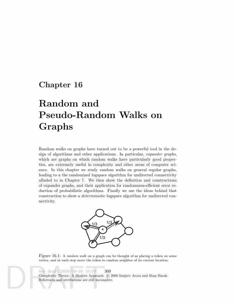
DRAFT

Chapter 16

Random andPseudo-Random Walks onGraphs

Random walks on graphs have turned out to be a powerful tool in the de-sign of algorithms and other applications. In particular, expander graphs,which are graphs on which random walks have particularly good proper-ties, are extremely useful in complexity and other areas of computer sci-ence. In this chapter we study random walks on general regular graphs,leading to a the randomized logspace algorithm for undirected connectivityalluded to in Chapter 7. We then show the definition and constructionsof expander graphs, and their application for randomness-efficient error re-duction of probabilistic algorithms. Finally we use the ideas behind thatconstruction to show a deterministic logspace algorithm for undirected con-nectivity.

*1/31/3

1/3

Figure 16.1: A random walk on a graph can be thought of as placing a token on somevertex, and at each step move the token to random neighbor of its current location.


309

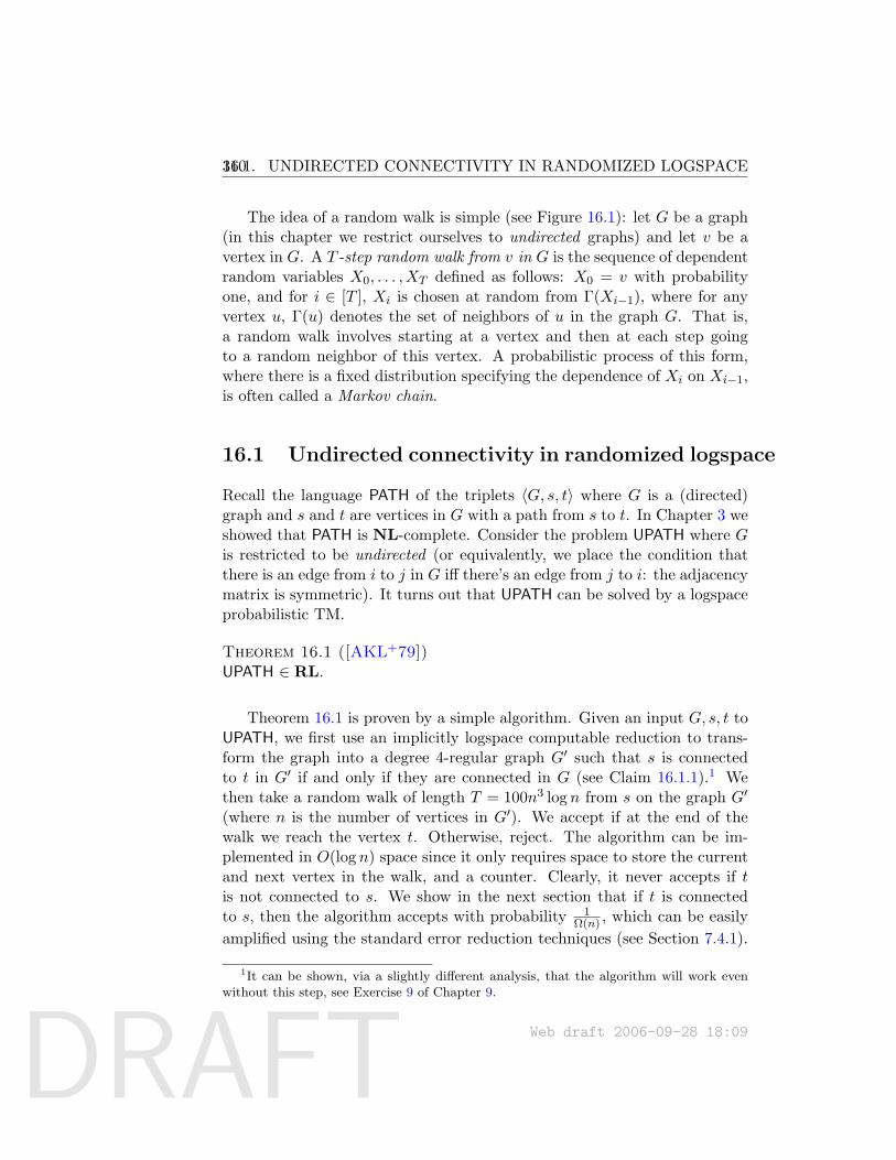
DRAFT

31016.1. UNDIRECTED CONNECTIVITY IN RANDOMIZED LOGSPACE

The idea of a random walk is simple (see Figure 16.1): let G be a graph(in this chapter we restrict ourselves to undirected graphs) and let v be avertex in G. A T -step random walk from v in G is the sequence of dependentrandom variables X0, . . . , XT defined as follows: X0 = v with probabilityone, and for i ∈ [T ], Xi is chosen at random from Γ(Xi−1), where for anyvertex u, Γ(u) denotes the set of neighbors of u in the graph G. That is,a random walk involves starting at a vertex and then at each step goingto a random neighbor of this vertex. A probabilistic process of this form,where there is a fixed distribution specifying the dependence of Xi on Xi−1,is often called a Markov chain.

16.1 Undirected connectivity in randomized logspace

Recall the language PATH of the triplets 〈G, s, t〉 where G is a (directed)graph and s and t are vertices in G with a path from s to t. In Chapter 3 weshowed that PATH is NL-complete. Consider the problem UPATH where Gis restricted to be undirected (or equivalently, we place the condition thatthere is an edge from i to j in G iff there’s an edge from j to i: the adjacencymatrix is symmetric). It turns out that UPATH can be solved by a logspaceprobabilistic TM.

Theorem 16.1 ([AKL+79])UPATH ∈ RL.

Theorem 16.1 is proven by a simple algorithm. Given an input G, s, t toUPATH, we first use an implicitly logspace computable reduction to trans-form the graph into a degree 4-regular graph G′ such that s is connectedto t in G′ if and only if they are connected in G (see Claim 16.1.1).1 Wethen take a random walk of length T = 100n3 log n from s on the graph G′

(where n is the number of vertices in G′). We accept if at the end of thewalk we reach the vertex t. Otherwise, reject. The algorithm can be im-plemented in O(log n) space since it only requires space to store the currentand next vertex in the walk, and a counter. Clearly, it never accepts if tis not connected to s. We show in the next section that if t is connectedto s, then the algorithm accepts with probability 1

Ω(n) , which can be easilyamplified using the standard error reduction techniques (see Section 7.4.1).

1It can be shown, via a slightly different analysis, that the algorithm will work evenwithout this step, see Exercise 9 of Chapter 9.

Web draft 2006-09-28 18:09

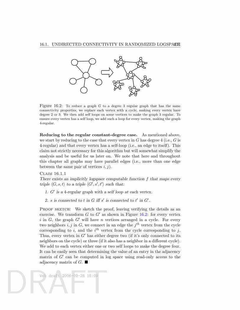
DRAFT

16.1. UNDIRECTED CONNECTIVITY IN RANDOMIZED LOGSPACE311

Figure 16.2: To reduce a graph G to a degree 3 regular graph that has the sameconnectivity properties, we replace each vertex with a cycle, making every vertex havedegree 2 or 3. We then add self loops on some vertices to make the graph 3 regular. Toensure every vertex has a self loop, we add such a loop for every vertex, making the graph4-regular.

Reducing to the regular constant-degree case. As mentioned above,we start by reducing to the case that every vertex in G has degree 4 (i.e., G is4-regular) and that every vertex has a self-loop (i.e., an edge to itself). Thisclaim not strictly necessary for this algorithm but will somewhat simplify theanalysis and be useful for us later on. We note that here and throughoutthis chapter all graphs may have parallel edges (i.e., more than one edgebetween the same pair of vertices i, j).

Claim 16.1.1There exists an implicitly logspace computable function f that maps everytriple 〈G, s, t〉 to a triple 〈G′, s′, t′〉 such that:

1. G′ is a 4-regular graph with a self loop at each vertex.

2. s is connected to t in G iff s′ is connected to t′ in G′.

Proof sketch: We sketch the proof, leaving verifying the details as anexercise. We transform G to G′ as shown in Figure 16.2: for every vertexi in G, the graph G′ will have n vertices arranged in a cycle. For everytwo neighbors i, j in G, we connect in an edge the jth vertex from the cyclecorresponding to i, and the ith vertex from the cycle corresponding to j.Thus, every vertex in G′ has either degree two (if it’s only connected to itsneighbors on the cycle) or three (if it also has a neighbor in a different cycle).We add to each vertex either one or two self loops to make the degree four.It can be easily seen that determining the value of an entry in the adjacencymatrix of G′ can be computed in log space using read-only access to theadjacency matrix of G.

Web draft 2006-09-28 18:09

DRAFT

312 16.2. RANDOM WALK ON GRAPHS

16.2 Random walk on graphs

In this section we study random walks on (undirected regular) graphs. Asa corollary we obtain the proof of correctness for the above algorithm forUPATH. We will see that we can use elementary linear algebra to relateparameters of the graph’s adjacency matrix to the behavior of the randomwalk on that graph. The following definitions and notations will be widelyused in this and later sections of this chapter:

16.2.1 Distributions as vectors and the parameter λ(G).

Let G be a d-regular n-vertex graph. Let p be some probability distributionover the vertices of G. We can think of p as a (column) vector in Rn wherepi is the probability that vertex i is obtained by the distribution. Note thatthe L1-norm of p (see Note 16.2), defined as |p|1 =

∑ni=1 |pi|, is equal to 1.

(In this case the absolute value is redundant since pi is always between 0and 1.)

Now let q represent the distribution of the following random variable:choose a vertex i in G according to p, then take a random neighbor of i inG. We can compute q as a function of p: the probability qj that j is chosenis equal to the sum over all j’s neighbors i of the probability pi that i ischosen times 1/d (where 1/d is the probability that, conditioned on i beingchosen, the walk moves to q). Thus q = Ap, where A = A(G) which is thenormalized adjacency matrix of G. That is, for every two vertices i, j, Ai,jis equal to the number of edges between i and j divided by d. Note that Ais a symmetric matrix,2 where each entry is between 0 and 1, and the sumof entries in each row and column is exactly one (such a matrix is called asymmetric stochastic matrix).

Let eini=1 be the standard basis of Rn (i.e. ei has 1 in the ith coordinateand zero everywhere else). Then, ATes represents the distribution XT oftaking a T -step random walk from the vertex s. This already suggeststhat considering the adjacency matrix of a graph G could be very useful inanalyzing random walks on G.

2A matrix A is symmetric if A = A†, where A† denotes the transpose of A. That is,(A†)i,j = Aj,i for every i, j.

Web draft 2006-09-28 18:09

DRAFT

16.2. RANDOM WALK ON GRAPHS 313

Note 16.2 (Lp Norms)A norm is a function mapping a vector v into a real number ‖v‖ satisfying(1) ‖v‖ ≥ 0 with ‖v‖ = 0 if and only v is the all zero vector, (2) ‖αv‖ =|α| · ‖v‖ for every α ∈ R, and (3) ‖v + u‖ ≤ ‖v‖+ ‖u‖ for every vector u.The third inequality implies that for every norm, if we define the distancebetween two vectors u,v as ‖u−v‖ then this notion of distance satisfies thetriangle inequality.

For every v ∈ Rn and number p ≥ 1, the Lp norm of v, denoted ‖v‖p , is equalto (

∑ni=1 |vi|p)

1/p. One particularly interesting case is p = 2, the so-called

Euclidean norm, in which ‖v‖2 =√∑n

i=1 v2i =

√〈v,v〉. Another interesting

case is p = 1, where we use the single bar notation and denote |v|1 =∑ni=1 |vi|. Another case is p =∞, where we denote ‖v‖∞ = limp→∞ ‖v‖p =

maxi∈[n] |vi|.

The Holder inequality says that for every p, q with 1p + 1

q = 1, ‖u‖p‖v‖q ≥∑ni=1 |uivi|. To prove it, note that by simple scaling, it suffices to con-

sider norm one vectors, and so it enough to show that if ‖u‖p = ‖v‖q = 1then

∑ni=1 |ui||vi| ≤ 1. But

∑ni=1 |ui||vi| =

∑ni=1 |ui|p(1/p)|vi|q(1/q) ≤∑n

i=11p |ui|

p + 1q |vi|

q = 1p + 1

q = 1, where the last inequality uses the factthat for every a, b > 0 and α ∈ [0, 1], aαb1−α ≤ αa + (1 − α)b. This fact isdue to the log function being concave— having negative second derivative,implying that α log a+ (1− α) log b ≤ log(αa+ (1− α)b).Setting p = 1 and q =∞, the Holder inequality implies that

‖v‖2 ≤ |v|1‖v‖∞

Setting p = q = 2, the Holder inequality becomes the Cauchy-Schwartz Inequality stating that

∑ni=1 |uivi| ≤ ‖u‖2‖v‖2 . Setting u =

(1/√n, 1/

√n, . . . , 1/

√n), we get that

|v|1/√n =

n∑i=1

1√n|vi| ≤ ‖v‖2

Web draft 2006-09-28 18:09

DRAFT

314 16.2. RANDOM WALK ON GRAPHS

Definition 16.3 (The parameter λ(G).)Denote by 1 the vector (1/n, 1/n, . . . , 1/n) corresponding to the uniform distri-bution. Denote by 1⊥ the set of vectors perpendicular to 1 (i.e., v ∈ 1⊥ if〈v,1〉 = (1/n)

∑i vi = 0).

The parameter λ(A), denoted also as λ(G), is the maximum value of ‖Av‖2 over allvectors v ∈ 1⊥ with ‖v‖2 = 1.

Remark 16.4The value λ(G) is often called the second largest eigenvalue of G. The reasonis that since A is a symmetric matrix, we can find an orthogonal basis ofeigenvectors v1, . . . ,vn with corresponding eigenvalues λ1, . . . , λn which wecan sort to ensure |λ1| ≥ |λ2| . . . ≥ |λn|. Note that A1 = 1. Indeed, forevery i, (A1)i is equal to the inner product of the ith row of A and thevector 1 which (since the sum of entries in the row is one) is equal to 1/n.Thus, 1 is an eigenvector of A with the corresponding eigenvalue equal to 1.One can show that a symmetric stochastic matrix has all eigenvalues withabsolute value at most 1 (see Exercise 1) and hence we can assume λ1 = 1and v1 = 1. Also, because 1⊥ = Spanv2, . . . ,vn, the value λ above willbe maximized by (the normalized version of) v2, and hence λ(G) = |λ2|.The quantity 1− λ(G) is called the spectral gap of the graph. We note thatsome texts use un-normalized adjacency matrices, in which case λ(G) is anumber between 0 and d and the spectral gap is defined to be d− λ(G).

One reason that λ(G) is an important parameter is the following lemma:

Lemma 16.5For every regular n vertex graph G = (V,E) let p be any probability distri-bution over V , then

‖ATp− 1‖2 ≤ λT

Proof: By the definition of λ(G), ‖Av‖2 ≤ λ‖v‖2 for every v ⊥ 1. Notethat if v ⊥ 1 then Av ⊥ 1 since 〈1, Av〉 = 〈A†1,v〉 = 〈1,v〉 = 0 (as A = A†

and A1 = 1). Thus A maps the space 1⊥ to itself and since it shrinks anymember of this space by at least λ, λ(AT ) ≤ λ(A)T . (In fact, using theeigenvalue definition of λ, it can be shown that λ(AT ) = λ(A).)

Let p be some vector. We can break p into its components in the spacesparallel and orthogonal to 1 and express it as p = α1 + p′ where p′ ⊥ 1

Web draft 2006-09-28 18:09

DRAFT

16.2. RANDOM WALK ON GRAPHS 315

and α is some number. If p is a probability distribution then α = 1 sincethe sum of coordinates in p′ is zero. Therefore,

ATp = AT (1 + p′) = 1 +ATp′

Since 1 and p′ are orthogonal, ‖p‖22

= ‖1‖22

+ ‖p′‖22

and in particular‖p′‖2 ≤ ‖p‖2 . Since p is a probability vector, ‖p‖2 ≤ |p|1 · 1 ≤ 1 (seeNote 16.2). Hence ‖p′‖2 ≤ 1 and

‖ATp− 1‖2 = ‖ATp′‖2 ≤ λT

It turns out that every connected graph has a noticeable spectral gap:Lemma 16.6For every d-regular connected G with self-loops at each vertex, λ(G) ≤1− 1

8dn3 .

Proof: Let u ⊥ 1 be a unit vector and let v = Au. We’ll show that1− ‖v‖2

2≥ 1

d4n3 which implies ‖v‖22≤ 1− 1

d4n3 and hence ‖v‖2 ≤ 1− 1d8n3 .

Since ‖u‖2 = 1, 1− ‖v‖22

= ‖u‖22− ‖v‖2

2. We claim that this is equal to∑

i,j Ai,j(ui − vj)2 where i, j range from 1 to n. Indeed,∑i,j

Ai,j(ui − vj)2 =∑i,j

Ai,ju2i − 2

∑i,j

Ai,juivj +∑i,j

Ai,jv2j =

‖u‖22− 2〈Au,v〉+ ‖v‖2

2= ‖u‖2

2− 2‖v‖2

2+ ‖v‖2

2,

where these equalities are due to the sum of each row and column in Aequalling one, and because ‖v‖2

2= 〈v,v〉 = 〈Au,v〉 =

∑i,j Ai,juivj .

Thus it suffices to show∑

i,j Ai,j(ui−vj)2 ≥ 1d4n3 . This is a sum of non-

negative terms so it suffices to show that for some i, j, Ai,j(ui−vj)2 ≥ 1d4n3 .

First, because we have all the self-loops, Ai,i ≥ 1/d for all i, and so we canassume |ui − vi| < 1

2n1.5 for every i ∈ [n], as otherwise we’d be done.Now sort the coordinates of u from the largest to the smallest, ensuring

that u1 ≥ u2 ≥ · · ·un. Since∑

i ui = 0 it must hold that u1 ≥ 0 ≥ un.In fact, since u is a unit vector, either u1 ≥ 1/

√n or un ≤ 1/

√n and

so u1 − un ≥ 1/√n. One of the n − 1 differences between consecutive

coordinates ui − ui+1 must be at least 1/n1.5 and so there must be an i0such that if we let S = 1, . . . , i0 and S = [n] \ Si, then for every i ∈ Sand j ∈ S, ui − uj ≥ 1/n1.5. Since G is connected there exists an edge(i, j) between S and S. Since |vj − uj | ≤ 1

2n1.5 , for this choice of i, j,|ui − vj | ≥ |ui − uj | − 1

2n1.5 ≥ 12n1.5 . Thus Ai,j(ui − vj)2 ≥ 1

d1

4n3 .

Web draft 2006-09-28 18:09

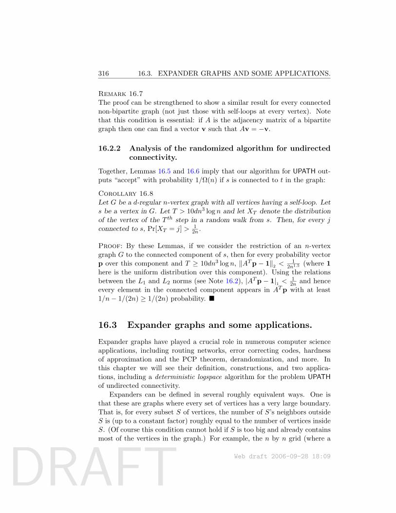
DRAFT

316 16.3. EXPANDER GRAPHS AND SOME APPLICATIONS.

Remark 16.7The proof can be strengthened to show a similar result for every connectednon-bipartite graph (not just those with self-loops at every vertex). Notethat this condition is essential: if A is the adjacency matrix of a bipartitegraph then one can find a vector v such that Av = −v.

16.2.2 Analysis of the randomized algorithm for undirectedconnectivity.

Together, Lemmas 16.5 and 16.6 imply that our algorithm for UPATH out-puts “accept” with probability 1/Ω(n) if s is connected to t in the graph:

Corollary 16.8Let G be a d-regular n-vertex graph with all vertices having a self-loop. Lets be a vertex in G. Let T > 10dn3 log n and let XT denote the distributionof the vertex of the T th step in a random walk from s. Then, for every jconnected to s, Pr[XT = j] > 1

2n .

Proof: By these Lemmas, if we consider the restriction of an n-vertexgraph G to the connected component of s, then for every probability vectorp over this component and T ≥ 10dn3 log n, ‖ATp − 1‖2 < 1

2n1.5 (where 1here is the uniform distribution over this component). Using the relationsbetween the L1 and L2 norms (see Note 16.2), |ATp − 1|1 < 1

2n and henceevery element in the connected component appears in ATp with at least1/n− 1/(2n) ≥ 1/(2n) probability.

16.3 Expander graphs and some applications.

Expander graphs have played a crucial role in numerous computer scienceapplications, including routing networks, error correcting codes, hardnessof approximation and the PCP theorem, derandomization, and more. Inthis chapter we will see their definition, constructions, and two applica-tions, including a deterministic logspace algorithm for the problem UPATHof undirected connectivity.

Expanders can be defined in several roughly equivalent ways. One isthat these are graphs where every set of vertices has a very large boundary.That is, for every subset S of vertices, the number of S’s neighbors outsideS is (up to a constant factor) roughly equal to the number of vertices insideS. (Of course this condition cannot hold if S is too big and already containsmost of the vertices in the graph.) For example, the n by n grid (where a

Web draft 2006-09-28 18:09

DRAFT

16.3. EXPANDER GRAPHS AND SOME APPLICATIONS. 317

vertex is a pair (i, j) and is connected to the four neighbors (i ± 1, j ± 1))is not an expander, as any k by k square (which is a set of size k2) in thisgraph only has a boundary of size O(k) (see Figure 16.3). Another way todefine expanders is as graphs where the random walks rapidly converges tothe uniform distribution. That is, unlike in the general case that (in regulargraphs) the random walk may take a polynomial number of steps to convergeto the uniform distribution, in an n-vertex regular expander this will onlytake O(log n) steps.

Expander: no. of S’s neighbors = Omega(|S|) Grid is not an expander:no. of S’s neighbors = O(|S|1/2)

Figure 16.3: In a combinatorial expander, every subset S of the vertices that is not toobig has at least Ω(|S|) neighbors outside the set. The grid (and every other planar graph)is not a combinatorial expander as a k × k square in the grid has only O(k) neighborsoutside it.

Given the previous section, it is not surprising that we can define ex-panders also in an algebraic way, based on the parameter λ(G) of Defini-tion 16.9. That is, we will say that G is an expander if λ(G) is bounded awayfrom 1. By Lemma 16.5, this does indeed imply that the random walk onG converges to the uniform distribution (in the sense that regardless of thestarting distribution, every vertex will be obtained with probability between12n and 3

2n) within O(log n) steps. We will also see later (Theorem 16.18)the relation between the parameter λ(G) and the combinatorial definitionof set expansion mentioned above.

Definition 16.9 ((n, d, λ)-graphs.)If G is an n-vertex d-regular G with λ(G) ≤ λ for some number λ < 1 then we saythat G is an (n, d, λ)-graph.

Web draft 2006-09-28 18:09

DRAFT


Expander families. For every d and λ < 1 a (d, λ)-expander graph familyis a sequence Gnn∈I of graphs such that Gn is an (n, d, λ)-graph and I isan infinite set. We sometimes drop the qualifiers d, λ and simply call sucha family an expander graph family, referring to a particular graph in thesequence as an expander graph.

Explicit constructions. We say that an expander family Gnn∈I is ex-plicit if (1) the set I is polynomially dense in the sense that there exists apolynomial time algorithm A and a polynomial p such that for every m ∈ N,A(m) outputs a number n ∈ I such that m ≤ n ≤ p(m) and (2) there is apolynomial-time algorithm that on input 1n with n ∈ I outputs the adja-cency matrix of Gn. We say that the family is strongly explicit if (1) I ispolynomially dense and (2) there is a polynomial-time algorithm that forevery n ∈ I on inputs 〈n, v, i〉 where 1 ≤ v ≤ n′ and 1 ≤ i ≤ d outputs theith neighbor of v. (Note that the algorithm runs in time polynomial in theits input length which is polylogarithmic in n.)

As we will see below it is not hard to show that expander families existusing the probabilistic method. But this does not yield explicit (or veryexplicit) constructions of such graphs. In fact, there are also several explicitand strongly explicit constructions of expander graphs known. The smallestλ can be for a d-regular n-vertex graph is Ω( 1√

d)and there are constructions

meeting this bound (specifically the bound is (1 − o(1))2√d−1d where by

o(1) we mean a function that tends to 0 as the number of vertices grows;graphs meeting this bound are called Ramanujan graphs). However, for mostapplications in Computer Science, any family with constant d and λ < 1will suffice (see also Remark 16.10 below). Some of these constructions arevery simple and efficient, but their analysis is highly non-trivial and usesrelatively deep mathematics.3 We show in Section 16.5 a strongly explicitconstruction of expanders with elementary analysis. This construction alsointroduces a tool that is useful to derandomize the algorithm for UPATH.

Remark 16.10One reason that the particular constants of an expander family are notextremely crucial is that we can improve the constant λ (make it arbitrarilysmaller) at the expense of increasing the degree: this follows from the fact,observed above in the proof of Lemma 16.5, that λ(GT ) = λ(G)T , whereGT denotes the graph obtained by taking the adjacency matrix to the T th

3An example for such an expander is the following 3-regular graph: the vertices arethe numbers 1 to p− 1 for some prime p, and each number x is connected to x+ 1,x− 1and x−1 (mod p).

Web draft 2006-09-28 18:09

DRAFT


Note 16.11 (Explicit construction of pseudorandom objects)Expanders are one instance of a recurring theme in complexity theory (andother areas of math and computer science): it is often the case that a ran-dom object can be easily proven to satisfy some nice property, but the ap-plications require an explicit object satisfying this property. In our case,a random d-regular graph is an expander, but to use it for, say, reducingthe error of probabilistic algorithms, we need an explicit construction of anexpander family, with an efficient deterministic algorithm to compute theneighborhood relations. Such explicit constructions can be sometimes hardto come by, but are often surprisingly useful. For example, in our case theexplicit construction of expander graphs turns out to yield a deterministiclogspace algorithm for undirected connectivity.We will see another instance of this theme in Chapter 18, which discusseserror correcting codes.

power, or equivalently, having an edge for every length-T path in G. Thus,we can transform an (n, d, λ) graph into an (n, dT , λT )-graph for every T ≥ 1.Later we will see a different transformation called the replacement productto decrease the degree at the expense of increasing λ somewhat (and alsoincreasing the number of vertices).

16.3.1 Using expanders to reduce error in probabilistic algo-rithms

Before constructing expanders, let us see one application for them in thearea of probabilistic algorithms. Recall that in Section 7.4.1 we saw thatwe can reduce the error of a probabilistic algorithm from, say, 1/3 to 2−Ω(k)

by executing it k times independently and taking the majority value. Ifthe algorithm utilized m random coins, this procedure will use m ·k randomcoins, and intuitively it seems hard to think of a way to save on randomness.Nonetheless, we will show that using expanders we can obtain such errorreduction using only m + O(k) random coins. The idea is simple: take anexpander graph G from a very explicit family that is an (N = 2m, d, 1/10)-graph for some constant d.4 Choose a vertex v1 at random, and take a

4In our definition of an expander family, we did not require that there is an N -vertexgraph in the family for every N , however typical constructions can be tweaked to ensure

Web draft 2006-09-28 18:09

DRAFT


length k− 1 long random walk on G to obtain vertices v2, . . . , vk (note thatchoosing a random neighbor of a vertex requires O(log d) = O(1) randombits). Invoke the algorithm k times using v1, . . . , vk as random coins (weidentify the set [N ] of vertices with the set 0, 1m of possible random coinsfor the algorithm) and output the majority answer.

The analysis is also not too difficult, but to make it even simpler, weanalyze here only the case of algorithms with one-sided error. For example,consider an RP algorithm that will never output “accept” if the input is notin the language, and for inputs in the language will output “accept” withprobability 2/3 (the case of a coRP algorithm is analogous). For such analgorithm the procedure will output “accept” if the algorithm accepts evenon a single set of coins vi. If the input is not in the language, the procedurewill never accept. If the input is in the language, then let B ⊆ [N ] denote the“bad” set of coins on which the algorithms rejects. We know that |B| ≤ N

3 .To show the procedure outputs “reject” with at most 2−Ω(k) probability, weprove the following theorem:

Theorem 16.12 (Expander walks)Let G be an (N, d, λ) graph, and let B ⊆ [N ] be a set with |B| ≤ βN . Let X1, . . . , Xk

be random variables denoting a k−1-step random walk from X1, where X1 is chosenuniformly in [N ]. Then,

Pr[∀1≤i≤kXi ∈ B](∗)

≤ ((1− λ)√β + λ)k−1

Note that if λ and β are both constants smaller than 1 then so is theexpression (1− λ)

√β + λ.

Proof: For 1 ≤ i ≤ k, let Bi be the event that Xi ∈ B. Note that the prob-ability (∗) we’re trying to bound is Pr[B1] Pr[B2|B1] · · ·Pr[Bk|B1, . . . , Bk−1].Let pi ∈ RN be the vector representing the distribution of Xi, conditionedon the events B1, . . . , Bi. Denote by B the following linear transformationfrom Rn to Rn: for every u ∈ RN , and j ∈ [N ], (Bu)j = uj if j ∈ B and(Bu)j = 0 otherwise. It’s not hard to verify that p1 = 1

Pr[B1]B1 (recall that1 = (1/N, . . . , 1/N) is the vector representing the uniform distribution over[N ]). Similarly, p2 = 1

Pr[B2|B1]1

Pr[B1]BAB1 where A = A(G) is the adjacency

this (see Theorem 16.24 below) and so we ignore this issue and assume we have such a2m-vertex graph in the family. Note that we can use powering improve the parameter λof the family to be smaller than 1/10 (see Remark 16.10).

Web draft 2006-09-28 18:09

DRAFT


matrix of G. Since every probability vector p satisfies |p|1 = 1,

(∗) = |(BA)k−1B1|1

We bound this norm by showing that

‖(BA)k−1B1‖2 ≤((1−λ)

√β+λ)k−1

√N

(1)

which suffices since for every v ∈ RN , |v|1 ≤√N‖v‖2 (see Note 16.2).

To prove (1), we use the following definition and lemma:

Definition 16.13 (Matrix Norm)If A is an m by n matrix, then ‖A‖ is the maximum number α such that‖Av‖2 ≤ α‖v‖2 for every v ∈ Rn.

Note that if A is a normalized adjacency matrix then ‖A‖ = 1 (as A1 = 1and ‖Av‖2 ≤ ‖v‖2 for every v). Also note that the matrix norm satisfiesthat for every two n by n matrices A,B, ‖A+B‖ ≤ ‖A‖+‖B‖ and ‖AB‖ ≤‖A‖‖B‖.

Lemma 16.14Let A be a normalized adjacency matrix of an (n, d, λ)-graph G. Let J bethe adjacency matrix of the n-clique with self loops (i.e., Ji,j = 1/n for everyi, j). Then

A = (1− λ)J + λC (2)

where ‖C‖ ≤ 1.

Note that for every probability vector p, Jp is the uniform distribution,and so this lemma tells us that in some sense, we can think of a step on a(n, d, λ)-graph as going to the uniform distribution with probability 1 − λ,and to a different distribution with probability λ. This is of course notcompletely accurate, as a step on a d-regular graph will only go the one ofthe d neighbors of the current vertex, but we’ll see that for the purposes ofour analysis, the condition (2) will be just as good.5

Proof of Lemma 16.14: Indeed, simply define C = 1λ(A− (1−λ)J). We

need to prove ‖Cv‖2 ≤ ‖v‖2 for very v. Decompose v as v = u + w whereu is α1 for some α and w ⊥ 1, and ‖v‖2

2= ‖u‖2

2+ ‖w‖2

2. Since A1 = 1

and J1 = 1 we get that Cu = 1λ(u − (1 − λ)u) = u. Now, let w′ = Aw.

5Algebraically, the reason (2) is not equivalent to going to the uniform distribution ineach step with probability 1− λ is that C is not necessarily a stochastic matrix, and mayhave negative entries.

Web draft 2006-09-28 18:09

DRAFT


Then ‖w′‖2 ≤ λ‖w‖2 and, as we saw in the proof of Lemma 16.5, w′ ⊥ 1.Furthermore, since the sum of the coordinates of w is zero, Jw = 0. We getthat Cw = 1

λw′. Since w′ ⊥ u, ‖Cw‖2

2= ‖u + 1

λw′‖2

2= ‖u‖2

2+ ‖ 1

λw′‖2

2≤

‖u‖22+ ‖w‖2

2= ‖w‖2

2.

Returning to the proof of Theorem 16.12, we can write BA = B((1 −

λ)J + λC), and hence ‖BA‖ ≤ (1 − λ)‖BJ‖ + λ‖BC‖. Since J ’s output

is always a vector of the form α1, ‖BJ‖ ≤√β. Also, because B is an

operation that merely zeros out some parts of its input, ‖B‖ ≤ 1 implying‖BC‖ ≤ 1. Thus, ‖BA‖ ≤ (1−λ)

√β+λ. Since B1 has the value 1/N in |B|

places, ‖B1‖2 =√β√N

, and hence ‖(BA)k−1B1‖2 ≤ ((1 − λ)√β + λ)k−1

√β√N

,establishing (1).

The analysis of the error reduction procedure for algorithms with two-sided errors uses the following theorem, whose proof we omit:

Theorem 16.15 (Expander Chernoff Bound [?])Let G be an (N, d, λ)-graph and B ⊆ [N ] with |B| = βN . Let X1, . . . , Xk be randomvariables denoting a k − 1-step random walk in G (where X1 is chosen uniformly).For every i ∈ [k], define Bi to be 1 if Xi ∈ B and 0 otherwise. Then, for every δ > 0,

Pr[|∑ki=1Bik − β| > δ

]< 2e(1−λ)δ2k/60

16.3.2 Combinatorial expansion and existence of expanders.

We describe now a combinatorial criteria that is roughly equivalent to Def-inition 16.9. One advantage of this criteria is that it makes it easy to provethat a non-explicit expander family exists using the probabilistic method.It is also quite useful in several applications.6

Definition 16.16 (Combinatorial (edge) expansion)An n-vertex d-regular graph G = (V,E) is called an (n, d, ρ)-combinatorialexpander if for every subset S ⊆ V with |S| ≤ n/2, |E(S, S)| ≥ ρd|S|, where

6In our informal discussion above we defined combinatorial expansion by counting thenumber of neighboring vertices of a set S of vertices that are outside the set (this is knownas vertex expansion). In contrast, Definition 16.16 below counts the number of edges thatlie between S and its complement (this is known as edge expansion). However, these twonumbers are clearly related by a factor of up to the degree d, which is not significant forour purposes.

Web draft 2006-09-28 18:09

DRAFT


for subsets S, T of V , E(S, T ) denotes the set of edges (s, t) with s ∈ S andt ∈ T .

Note that in this case the bigger ρ is the better the expander. We’llloosely use the term expander for any (n, d, ρ)-combinatorial expander withc a positive constant. Using the probabilistic method, one can prove thefollowing theorem: (Exercise 3 asks you to prove a slightly weaker version)

Theorem 16.17 (Existence of expanders)Let ε > 0 be some constant. Then there exists d = d(ε) and N ∈ N suchthat for every n > N there exists an (n, d, 1− ε)-combinatorial expander.

The following theorem related combinatorial expansion with our previousDefinition 16.9

Theorem 16.18 (Combinatorial and algebraic expansion)1. If G is an (n, d, λ)-graph then it is an (n, d, (1−λ)/2)-combinatorial expander.

2. If G is an (n, d, ρ)-combinatorial expander then it is an (n, d, 1− ρ2

2 )-graph.

The first part of Theorem 16.18 follows by plugging T = S into thefollowing lemma:

Lemma 16.19 (Expander Mixing Lemma)Let G = (V,E) be an (n, d, λ)-graph. Let S, T ⊆ V , then∣∣∣∣|E(S, T )| − d

n|S||T |

∣∣∣∣ ≤ λd√|S||T |Proof: Let s denote the vector such that si is equal to 1 if i ∈ S andequal to 0 otherwise, and let t denote the corresponding vector for the setS. Thinking of s as a row vector and of t as a column vector, the Lemma’sstatement is equivalent to∣∣∣sAt− |S||T |

n

∣∣∣ ≤ λ√|S||T | , (3)

where A is G’s normalized adjacency matrix. Yet by Lemma 16.14, we canwrite A as (1 − λ)J + λC, where J is the matrix with all entries equal to1/n and C has norm at most one. Hence,

sAt = (1− λ)sJt + λsCt ≤ |S||T |n + λ

√|S||T | ,

Web draft 2006-09-28 18:09

DRAFT


where the last inequality follows from sJt = |S||T |/n and sCt = 〈s, Ct〉 ≤‖s‖2‖t‖2 =

√|S||T |.

Proof of second part of Theorem 16.18.: We prove a slightly relaxedversion, replacing the constant 2 with 8. Let G = (V,E) be an n-vertex d-regular graph such that for every subset S ⊆ V with |S| ≤ n/2, there areρ|S| edges between S and S = V \S, and let A be G’s normalized adjacencymatrix.

Let λ = λ(G). We need to prove that λ ≤ 1 − ρ2/8. Using the factthat λ is the second eigenvalue of A, there exists a vector u ⊥ 1 such thatAu = λu. Write u = v + w where v is equal to u on the coordinates onwhich u is positive and equal to 0 otherwise, and w is equal to u on thecoordinates on which u is negative, and equal to 0 otherwise. Note that,since u ⊥ 1, both v and w are nonzero. We can assume that u is nonzeroon at most n/2 of its coordinates (as otherwise we can take −u instead ofu).

Since Au = λu and 〈v,w〉 = 0,

〈Av,v〉+ 〈Aw,v〉 = 〈A(v + w),v〉 = 〈Au,v〉 = 〈λ(v + w),v〉 = λ‖v‖22.

Since 〈Aw,v〉 is negative, we get that 〈Av,v〉/‖v‖22≥ λ or

1− λ ≥ 1− 〈Av,v〉‖v‖2

2

=‖v‖2

2− 〈Av,v〉‖v‖2

2

=

∑i,j Ai,j(vi − vj)2

2‖v‖22

,

where the last equality is due to∑

i,j Ai,j(vi−vj)2 =∑

i,j Ai,jv2i−2

∑i,j Ai,jvivj+∑

i,j Ai,jv2j = 2‖v‖2

2− 2〈Av,v〉. (We use here the fact that each row and

column of A sums to one.) Multiply both numerator and denominator by∑i,j Ai,j(v

2i + v2

j ). By the Cauchy-Schwartz inequality,7 we can bound thenew numerator as follows:∑

i,j

Ai,j(vi − vj)2

∑i,j

Ai,j(vi + vj)2

≤∑

i,j

Ai,j(vi − vj)(vi + vj)

2

.

7The Cauchy-Schwartz inequality is typically stated as saying that for x,y ∈ Rn,∑i xiyi ≤

√(∑i x

2i )(∑i y

2i ). However, it is easily generalized to show that for every

non-negative µ1, . . . , µn,∑i µixiyi ≤

√(∑i µix

2i )(∑i µiy

2i ) (this can be proven from the

standard Cauchy-Schwartz by multiplying each coordinate of x and y by√µi. It is this

variant that we use here with the Ai,j ’s playing the role of µ1, . . . , µn.

Web draft 2006-09-28 18:09

DRAFT

16.4. GRAPH PRODUCTS AND EXPANSION 325

Hence, using (a− b)(a+ b) = a2 − b2,

1−λ ≥

(∑i,j Ai,j(v

2i − v2

j ))2

2‖v‖22

∑i,j Ai,j(vi + vj)2

=

(∑i,j Ai,j(v

2i − v2

j ))2

2‖v‖22

(∑i,j Ai,jv

2i + 2

∑i,j Ai,jvivj +

∑i,j Ai,jv

2j

) =

(∑i,j Ai,j(v

2i − v2

j ))2

2‖v‖22

(2‖v‖2

2+ 2〈Av,v〉

) ≥(∑

i,j Ai,j(v2i − v2

j ))2

8‖v‖42

,

where the last inequality is due to A having matrix norm at most 1, implying〈Av,v〉 ≤ ‖v‖2

2. We conclude the proof by showing that∑

i,j

Ai,j(v2i − v2

j ) ≥ ρ‖v‖22 , (4)

which indeed implies that 1− λ ≥ ρ2‖v‖42

8‖v‖42

= ρ2

8 .

To prove (4) sort the coordinates of v so that v1 ≥ v2 ≥ · · · ≥ vn (withvi = 0 for i > n/2). Then

∑i,j

Ai,j(v2i − v2

j ) ≥n/2∑i=1

n∑j=i+1

Ai,j(v2i − v2

i+1) =n/2∑i=1

ci(v2i − v2

i+1) ,

where ci denotes∑

j>iAi,j . But ci is equal to the number of edges in G fromthe set k : k ≤ i to its complement, divided by d. Hence, by the expansionof G, ci ≥ ρi, implying (using the fact that vi = 0 for i ≥ n/2):

∑i,j

Ai,j(v2i − v2

j ) ≥n/2∑i=1

ρi(v2i − v2

i+1) =n/2∑i=1

(ρiv2i − ρ · (i− 1)v2

i ) = ρ‖v‖22,

establishing (4).

16.4 Graph products and expansion

A graph product is an operation that takes two graphs G,G′ and outputs agraph H. Typically we’re interested in the relation between properties ofthe graphs G,G′ to the properties of the resulting graph H. In this sectionwe will mainly be interested in three parameters: the number of vertices(denoted n), the degree (denoted d), and the 2nd largest eigenvalue of the

Web draft 2006-09-28 18:09

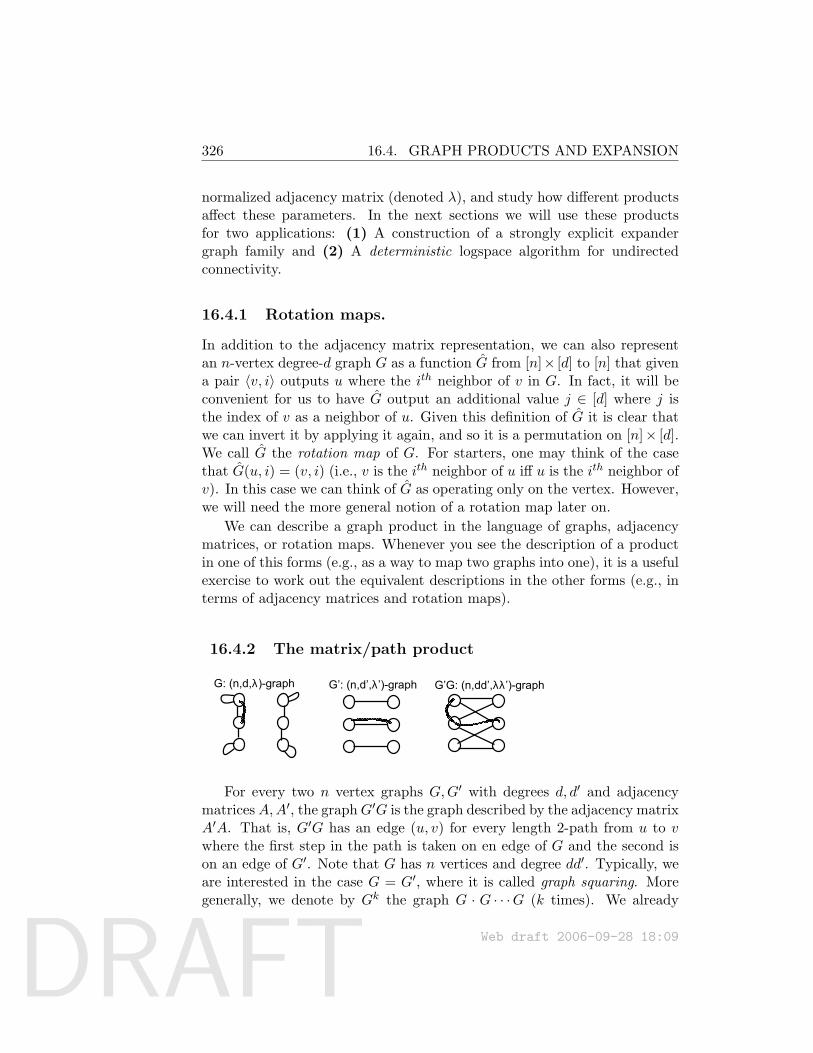
DRAFT

326 16.4. GRAPH PRODUCTS AND EXPANSION

normalized adjacency matrix (denoted λ), and study how different productsaffect these parameters. In the next sections we will use these productsfor two applications: (1) A construction of a strongly explicit expandergraph family and (2) A deterministic logspace algorithm for undirectedconnectivity.

16.4.1 Rotation maps.

In addition to the adjacency matrix representation, we can also representan n-vertex degree-d graph G as a function G from [n]× [d] to [n] that givena pair 〈v, i〉 outputs u where the ith neighbor of v in G. In fact, it will beconvenient for us to have G output an additional value j ∈ [d] where j isthe index of v as a neighbor of u. Given this definition of G it is clear thatwe can invert it by applying it again, and so it is a permutation on [n]× [d].We call G the rotation map of G. For starters, one may think of the casethat G(u, i) = (v, i) (i.e., v is the ith neighbor of u iff u is the ith neighbor ofv). In this case we can think of G as operating only on the vertex. However,we will need the more general notion of a rotation map later on.

We can describe a graph product in the language of graphs, adjacencymatrices, or rotation maps. Whenever you see the description of a productin one of this forms (e.g., as a way to map two graphs into one), it is a usefulexercise to work out the equivalent descriptions in the other forms (e.g., interms of adjacency matrices and rotation maps).

16.4.2 The matrix/path product

G: (n,d,λ)-graph G’: (n,d’,λ’)-graph G’G: (n,dd’,λλ’)-graph

For every two n vertex graphs G,G′ with degrees d, d′ and adjacencymatricesA,A′, the graphG′G is the graph described by the adjacency matrixA′A. That is, G′G has an edge (u, v) for every length 2-path from u to vwhere the first step in the path is taken on en edge of G and the second ison an edge of G′. Note that G has n vertices and degree dd′. Typically, weare interested in the case G = G′, where it is called graph squaring. Moregenerally, we denote by Gk the graph G · G · · ·G (k times). We already

Web draft 2006-09-28 18:09

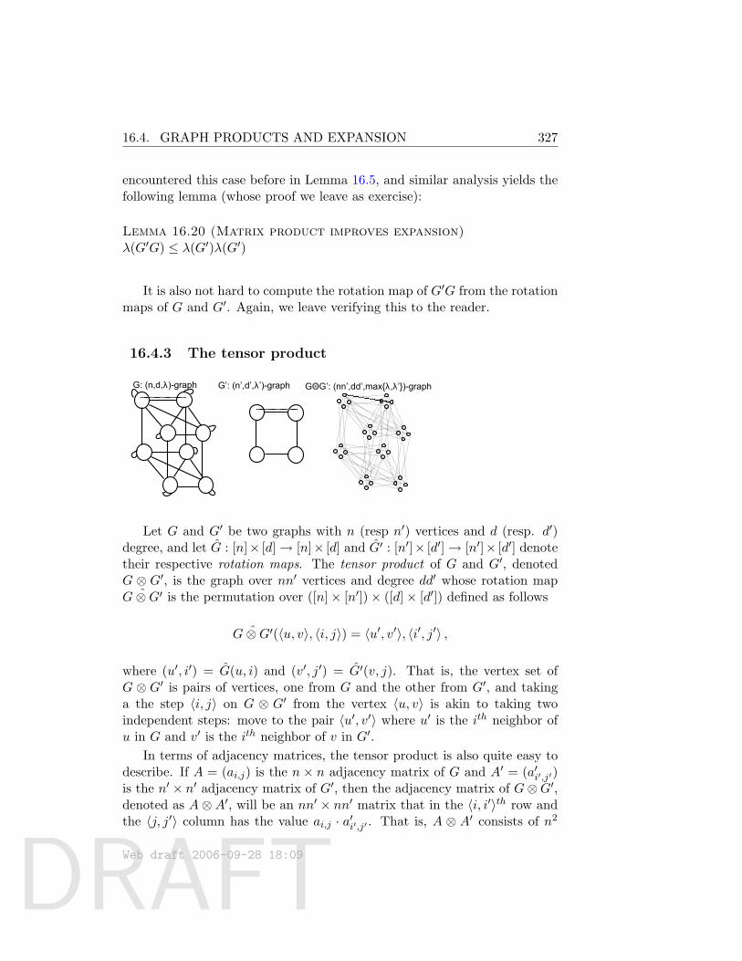
DRAFT


encountered this case before in Lemma 16.5, and similar analysis yields thefollowing lemma (whose proof we leave as exercise):

Lemma 16.20 (Matrix product improves expansion)λ(G′G) ≤ λ(G′)λ(G′)

It is also not hard to compute the rotation map of G′G from the rotationmaps of G and G′. Again, we leave verifying this to the reader.

16.4.3 The tensor product

G: (n,d,λ)-graph G’: (n’,d’,λ’)-graph GOG’: (nn’,dd’,maxλ,λ’)-graphx

Let G and G′ be two graphs with n (resp n′) vertices and d (resp. d′)degree, and let G : [n]× [d]→ [n]× [d] and G′ : [n′]× [d′]→ [n′]× [d′] denotetheir respective rotation maps. The tensor product of G and G′, denotedG ⊗ G′, is the graph over nn′ vertices and degree dd′ whose rotation map

ˆG⊗G′ is the permutation over ([n]× [n′])× ([d]× [d′]) defined as follows

ˆG⊗G′(〈u, v〉, 〈i, j〉) = 〈u′, v′〉, 〈i′, j′〉 ,

where (u′, i′) = G(u, i) and (v′, j′) = G′(v, j). That is, the vertex set ofG ⊗ G′ is pairs of vertices, one from G and the other from G′, and takinga the step 〈i, j〉 on G ⊗ G′ from the vertex 〈u, v〉 is akin to taking twoindependent steps: move to the pair 〈u′, v′〉 where u′ is the ith neighbor ofu in G and v′ is the ith neighbor of v in G′.

In terms of adjacency matrices, the tensor product is also quite easy todescribe. If A = (ai,j) is the n × n adjacency matrix of G and A′ = (a′i′,j′)is the n′ × n′ adjacency matrix of G′, then the adjacency matrix of G⊗G′,denoted as A⊗A′, will be an nn′ × nn′ matrix that in the 〈i, i′〉th row andthe 〈j, j′〉 column has the value ai,j · a′i′,j′ . That is, A ⊗ A′ consists of n2

Web draft 2006-09-28 18:09

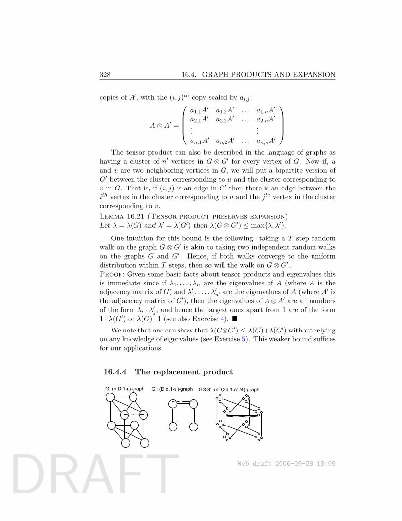
DRAFT


copies of A′, with the (i, j)th copy scaled by ai,j :

A⊗A′ =

a1,1A

′ a1,2A′ . . . a1,nA

′

a2,1A′ a2,2A

′ . . . a2,nA′

......

an,1A′ an,2A

′ . . . an,nA′

The tensor product can also be described in the language of graphs as

having a cluster of n′ vertices in G ⊗ G′ for every vertex of G. Now if, uand v are two neighboring vertices in G, we will put a bipartite version ofG′ between the cluster corresponding to u and the cluster corresponding tov in G. That is, if (i, j) is an edge in G′ then there is an edge between theith vertex in the cluster corresponding to u and the jth vertex in the clustercorresponding to v.Lemma 16.21 (Tensor product preserves expansion)Let λ = λ(G) and λ′ = λ(G′) then λ(G⊗G′) ≤ maxλ, λ′.

One intuition for this bound is the following: taking a T step randomwalk on the graph G⊗G′ is akin to taking two independent random walkson the graphs G and G′. Hence, if both walks converge to the uniformdistribution within T steps, then so will the walk on G⊗G′.Proof: Given some basic facts about tensor products and eigenvalues thisis immediate since if λ1, . . . , λn are the eigenvalues of A (where A is theadjacency matrix of G) and λ′1, . . . , λ

′n′ are the eigenvalues of A (where A′ is

the adjacency matrix of G′), then the eigenvalues of A⊗A′ are all numbersof the form λi · λ′j , and hence the largest ones apart from 1 are of the form1 · λ(G′) or λ(G) · 1 (see also Exercise 4).

We note that one can show that λ(G⊗G′) ≤ λ(G)+λ(G′) without relyingon any knowledge of eigenvalues (see Exercise 5). This weaker bound sufficesfor our applications.

16.4.4 The replacement product

G: (n,D,1-ε)-graph G’: (D,d,1-ε’)-graph GOG’: (nD,2d,1-εε’/4)-graphR

Web draft 2006-09-28 18:09

DRAFT


In both the matric and tensor products, the degree of the resulting graphis larger than the degree of the input graphs. The following product willenable us to reduce the degree of one of the graphs. Let G,G′ be two graphssuch that G has n vertices and degree D, and G′ has D vertices and degree d.The balanced replacement product (below we use simply replacement productfor short) of G and G′ is denoted by G©R G′ is the nn′-vertex 2d-degree graphobtained as follows:

1. For every vertex u of G, the graph G©R G′ has a copy of G′ (includingboth edges and vertices).

2. If u, v are two neighboring vertices in G then we place d parallel edgesbetween the ith vertex in the copy of G′ corresponding to u and thejth vertex in the copy of G′ corresponding to v, where i is the indexof v as a neighbor of u and j is the index of u as a neighbor of v inG. (That is, taking the ith edge out of u leads to v and taking the jth

edge out of v leads to u.)

Note that we essentially already encountered this product in the proofof Claim 16.1.1 (see also Figure 16.2), where we reduced the degree of anarbitrary graph by taking its replacement product with a cycle (althoughthere we did not use parallel edges).8 The replacement product also has asimple description in terms of rotation maps: since G©R G′ has nD verticesand 2d degree, its rotation map ˆG©R G′ is a permutation over ([n]× [D])×([d]× 0, 1) and so can be thought of as taking four inputs u, v, i, b whereu ∈ [n], v ∈ [D], i ∈ [d] and b ∈ 0, 1. If b = 0 then it outputs u, G′(v, i), band if b = 1 then it outputs G(u, v), i, b. That is, depending on whether b isequal to 0 or 1, the rotation map either treats v as a vertex of G′ or as anedge label of G.

In the language of adjacency matrices the replacement product can beeasily seen to be described as follows: A©R A′ = 1/2(A⊗ ID) + 1/2(In ⊗ A′),where A,A′ are the adjacency matrices of the graphs G and G′ respectively,and Ik is the k × k identity matrix.

If D d then the replacement product’s degree will be significantlysmaller than G’s degree. The following Lemma shows that this dramaticdegree reduction does not cause too much of a deterioration in the graph’sexpansion:

8The addition of parallel edges ensures that a random step from a vertex v in G©R G′

will move to a neighbor within the same cluster and a neighbor outside the cluster with thesame probability. For this reason, we call this product the balanced replacement product.

Web draft 2006-09-28 18:09

DRAFT


Lemma 16.22 (Expansion of replacement product)If λ(G) ≤ 1− ε and λ(G′) ≤ 1− ε′ then λ(G©R G′) ≤ 1− εε′/4.

The intuition behind Lemma 16.22 is the following: Think of the inputgraph G as a good expander whose only drawback is that it has a too highdegree D. This means that a k step random walk on G′ requires O(k logD)random bits. However, as we saw in Section 16.3.1, sometimes we can usefewer random bits if we use an expander. So a natural idea is to generate theedge labels for the walk by taking a walk using a smaller expander G′ thathas D vertices and degree d D. The definition of G©R G′ is motivated bythis intuition: a random walk on G©R G′ is roughly equivalent to using anexpander walk on G′ to generate labels for a walk on G. In particular, eachstep a walk over G©R G′ can be thought of as tossing a coin and then, basedon its outcome, either taking a a random step on G′, or using the currentvertex of G′ as an edge label to take a step on G. Another way to gainintuition on the replacement product is to solve Exercise 6, that analyzesthe combinatorial (edge) expansion of the resulting graph as a function ofthe edge expansion of the input graphs.

Proof of Lemma 16.22: Let A (resp. A′) denote the n×n (resp. D×D)adjacency matrix of G (resp. G′) and let λ(A) = 1 − ε and λ(A′) = 1 − ε′.Then by Lemma 16.14, A = (1− ε)C + Jn and A′ = (1− ε′)C ′ + JD, whereJk is the k × k matrix with all entries equal to 1/k.

The adjacency matrix of G©R G′ is equal to

12(A⊗ ID) + 1

2(In⊗A′) = 1−ε2 C ⊗ ID + ε

2Jn⊗ ID + 1−ε′2 In⊗C ′ + ε′

2 In⊗ JD ,

where Ik is the k × k identity matrix.Thus, the adjacency matrix of (G©R G′)2 is equal to(1−ε2 C ⊗ ID + ε

2Jn ⊗ ID + 1−ε′2 In ⊗ C ′ + ε′

2 In ⊗ JD)2

=

εε′

4 (Jn ⊗ ID)(In ⊗ JD) + ε′ε4 (In ⊗ JD)(Jn ⊗ ID) + (1− εε′

2 )F ,

where F is some nD×nD matrix of norm at most 1 (obtained by collectingtogether all the other terms in the expression). But

(Jn ⊗ ID)(In ⊗ JD) = (In ⊗ JD)(Jn ⊗ ID) = Jn ⊗ JD = JnD .

(This can be verified by either direct calculation or by going through thegraphical representation or the rotation map representation of the tensorand matrix products.)

Web draft 2006-09-28 18:09

DRAFT

16.5. EXPLICIT CONSTRUCTION OF EXPANDER GRAPHS. 331

Since every vector v ∈ RnD that is orthogonal to 1 satisfies JnDv = 0,we get that(

λ(G©R G′))2 = λ

((G©R G′)2

)= λ

((1− εε′

2 )F + εε′

2 JnD

)≤ 1− εε′

2 ,

and henceλ(G©R G′) ≤ 1− εε′

4 .

16.5 Explicit construction of expander graphs.

We now use the three graph products of Section 16.4 to show a stronglyexplicit construction of an expander graph family. Recall This is an infinitefamily Gk of graphs (with efficient way to compute neighbors) that hasa constant degree and an expansion parameter λ. The construction is re-cursive: we start by a finite size graph G1 (which we can find using bruteforce search), and construct the graph Gk from the graph Gk−1. On a highlevel the construction is as follows: each of the three product will serve adifferent purpose in the construction. The Tensor product allows us to takeGk−1 and increase its number of vertices, at the expense of increasing thedegree and possibly some deterioration in the expansion. The replacementproduct allows us to dramatically reduce the degree at the expense of ad-ditional deterioration in the expansion. Finally, we use the Matrix/Pathproduct to regain the loss in the expansion at the expense of a mild increasein the degree.

Theorem 16.23 (Explicit construction of expanders)There exists a strongly-explicit λ, d-expander family for some constants d and λ < 1.

Proof: Our expander family will be the following family Gkk∈N of graphs:

• Let H be a (D = d40, d, 0.01)-graph, which we can find using bruteforce search. (We choose d to be a large enough constant that such agraph exists)

• Let G1 be a (D, d20, 1/2)-graph, which we can find using brute forcesearch.

Web draft 2006-09-28 18:09

DRAFT

332 16.5. EXPLICIT CONSTRUCTION OF EXPANDER GRAPHS.

• For k > 1, let Gk = ((Gk−1 ⊗Gk−1)©z H)20.

The proof follows by noting the following points:

1. For every k, Gk has at least 22k vertices.

Indeed, if nk denotes the number of vertices ofGk, then nk = (nk−1)2D.

If nk−1 ≥ 22k−1then nk ≥

(22k−1

)2= 22k .

2. For every k, the degree of Gk is d20.

Indeed, taking a replacement produce with H reduces the degree to d,which is then increased to d20 by taking the 20th power of the graph(using the matrix/path product).

3. There is a 2O(k)-time algorithm that given a label of a vertex u in Gkand an index i ∈ [d20], outputs the ith neighbor of u in Gk. (Note thatthis is polylogarithmic in the number of vertices.)

Indeed, such a recursive algorithm can be directly obtained from thedefinition of Gk. To compute Gk’s neighborhood function, the algo-rithm will make 40 recursive calls to Gk−1’s neighborhood function,resulting in 2O(k) running time.

4. For every k, λ(Gk) ≤ 1/3.

Indeed, by Lemmas 16.20, 16.21, and 16.22 If λ(Gk−1) ≤ 1/3 thenλ(Gk−1 ⊗Gk−1) ≤ 2/3 and hence λ((Gk−1 ⊗Gk−1)©R H) ≤ 1− 0.99

12 ≤1− 1/13. Thus, λ(Gk) ≤ (1− 1/13)20 ∼ e−20/13 ≤ 1/3.

Using graph powering we can obtain such a construction for every con-stant λ ∈ (0, 1), at the expense of a larger degree. There is a variant ofthe above construction supplying a denser family of graphs that containsan n-vertex graph for every n that is a power of c, for some constant c.Since one can transform an (n, d, λ)-graph to an (n′, cd′, λ)-graph for anyn/c ≤ n′ ≤ n by making a single “mega-vertex” out of a set of at most cvertices, the following theorem is also known:

Theorem 16.24There exist constants d ∈ N , λ < 1 and a strongly-explicit graph familyGnn∈N such that Gn is an (n, d, λ)-graph for every n ∈ N.

Web draft 2006-09-28 18:09

DRAFT

16.6. DETERMINISTIC LOGSPACE ALGORITHM FORUNDIRECTED CONNECTIVITY. 333

Remark 16.25As mentioned above, there are known constructions of expanders (typicallybased on number theory) that are more efficient in terms of computationtime and relation between degree and the parameter λ than the product-based construction above. However, the proofs for these constructions aremore complicated and require deeper mathematical tools. Also, the replace-ment product (and its close cousin, the zig-zag product) have found applica-tions beyond the constructions of expander graphs. One such application isthe deterministic logspace algorithm for undirected connectivity describedin the next section. Another application is a construction of combinatorialexpanders with greater expansion that what is implied by the parameterλ. (Note that even for for the impossible to achieve value of λ = 0, Theo-rem 16.1.1 implies combinatorial expansion only 1/2 while it can be shownthat a random graph has combinatorial expansion close to 1.)

16.6 Deterministic logspace algorithm for undirectedconnectivity.

The replacement product has a surprising consequence: a deterministic al-gorithm to determine whether two vertices are connected in a graph usingonly logarithmic space.

Theorem 16.26 (Reingold’s theorem [?])UPATH ∈ L.

The underlying intuition behind the logspace algorithm for UPATH isthat checking connectivity in expander graphs is easy. More accurately, ifevery connected component in G is an expander, then there is a number` = O(log n) such that if s and t are connected then they are connectedwithin a path of length at most `. (Indeed, in this case an `-step randomwalk from s will reach t with reasonable probability.) We can enumerate overall `-step random walks of a d-degree graph in O(d`) space by enumeratingover all sequences of indices i1, . . . , i` ∈ [d]. Thus, in a constant-degree graphwhere all connected components are expanders we can check connectivity inlogarithmic space. The idea behind the algorithm will be to transform thegraph G (in an implicitly computable in logspace way) to a graph G′ suchthat every connected component in G becomes an expander in G′, but twovertices that were not connected will stay unconnected. This transformation

Web draft 2006-09-28 18:09

DRAFT

33416.6. DETERMINISTIC LOGSPACE ALGORITHM FOR

UNDIRECTED CONNECTIVITY.

is reminiscent of the expander construction of the previous section.Proof of Theorem 16.26: Let G be the input graph and s, t two verticesin G. Using the transformation of Claim 16.1.1, we may assume that G isa regular degree-4 graphs with self loops on all vertices. By adding moreself-loops we may assume that the graph is of degree d20 for some constantd that is sufficiently large so that there exists a (d20, d, 0.01)-graph H.

• Let H be a (d20, d, 0.01)-graph, which we can find using brute forcesearch.

• Let G0 = G.

• For k ≥ 1, we define Gk = (Gk−1©R H)20.

Note that these operations do not connect vertices that were discon-nected in G. Thus, we can analyze their effect separately on each connectedcomponent of G. By Lemmas 16.20 and 16.22, for every ε < 1/20 andD-degree graph F , if λ(F ) ≤ 1 − ε then λ(F ©R H) ≤ 1 − ε/5 and henceλ((F©R H)20

)≤ 1− 2ε.

By Lemma 16.6, every connected component of G has expansion param-eter at most 1−1/(8Dn3), where n denotes the number of G’s vertices whichis at least as large as the number of vertices in the connect component. It fol-lows that for k = 10 logD logN , in the graph Gk every connected componenthas expansion parameter at most max1− 1/20, 2k/(8Dn3) = 1− 1/20.

The space required to enumerate over ` length walks from some vertexs in Gk is O(`) bits to store ` indices and the space to compute the rotationmap of Gk. To finish the proof, we will show that we can compute thismap in O(k + log n) space. This map’s input length is O(k + log n) andhence we can assume it is placed on a read/write tape, and will computethe rotation map “in-place” changing the input to the output. Let sk be theadditional space (beyond the input) required to compute the rotation mapof Gk. Note that s0 = O(log n). We show a recursive algorithm to computeGk satisfying the equation sk = sk−1 +O(1). In fact, the algorithm will be apretty straightforward implementation of the definitions of the replacementand matrix products.

The input to Gk is a vertex in (Gk−1©R H) and 20 labels of edges in thisgraph. If we can compute the rotation map of Gk−1©R H in sk−1+O(1) spacethen we can do so for Gk, since we can simply make 20 consecutive calls tothis procedure, each time reusing the space.9 Now, to compute the rotation

9One has to be slightly careful while making recursive calls, since we don’t want to

Web draft 2006-09-28 18:09

DRAFT

16.6. DETERMINISTIC LOGSPACE ALGORITHM FORUNDIRECTED CONNECTIVITY. 335

map of (Gk−1©R H) we simply follow the definition of the replacement prod-uct. Given an input of the form u, v, i, b (which we think of as read/writevariables), if b = 0 then we apply the rotation map of H to (v, i) (can bedone in constant space), while if b = 1 then we apply the rotation map ofGk−1 to (u, v) using a recursive call at the cost of sk−1 space (note that u, vare conveniently located consecutively at the beginning of the input tape).


still a lot missingExpanders were well-studied for a variety of reasons in the 1970s but

their application to pseudorandomness was first described by Ajtai, Komlos,and Szemeredi [AKS87]. Then Cohen-Wigderson [CW89] and Impagliazzo-Zuckerman (1989) showed how to use them to “recycle” random bits as de-scribed in Section 16.3.1. The upcoming book by Hoory, Linial and Wigder-son (draft available from their web pages) provides an excellent introductionto expander graphs and their applications.

The explicit construction of expanders is due to Reingold, Vadhan andWigderson [RVW00], although we chose to present it using the replacementproduct as opposed to the closely related zig-zag product used there. Thedeterministic logspace algorithm for undirected connectivity is due to Rein-gold [?].

Exercises

§1 Let A be a symmetric stochastic matrix: A = A† and every row andcolumn of A has non-negative entries summing up to one. Prove that‖A‖ ≤ 1.

Hint:firstshowthat‖A‖isatmostsayn2.Then,provethatfor

everyk≥1,Ak

isalsostochasticand‖A2k

v‖2≥‖Akv‖

22usingthe

equality〈w,Bz〉=〈B†w,z〉andtheinequality〈w,z〉≤‖w‖2‖z‖2.

§2 Let A,B be two symmetric stochastic matrices. Prove that λ(A+B) ≤λ(A) + λ(B).

lose even the O(log logn) bits of writing down k and keeping an index to the location inthe input we’re working on. However, this can be done by keeping k in global read/writestorage and since storing the identity of the current step among the 50 calls we’re makingonly requires O(1) space.

Web draft 2006-09-28 18:09

DRAFT

33616.6. DETERMINISTIC LOGSPACE ALGORITHM FOR

UNDIRECTED CONNECTIVITY.

§3 Let a n, d random graph be an n-vertex graph chosen as follows: choosed random permutations π1, ldots, πd from [n] to [n]. Let the the graphG contains an edge (u, v) for every pair u, v such that v = πi(u) forsome 1 ≤ i ≤ d. Prove that a random n, d graph is an (n, 2d, 2

3d)combinatorial expander with probability 1− o(1) (i.e., tending to onewith n).

Hint:foreverysetS⊆nwith|S|≤n/2andsetT⊆[n]with|T|≤(1+

23d)|S|,trytoboundtheprobabilitythatπi(S)⊆Tfor

everyi.

§4 Let A be an n×n matrix with eigenvectors u1, . . . ,un and correspond-ing values λ1, . . . , λn. Let B be an m × m matrix with eigenvectorsv1, . . . ,vm and corresponding values α1, . . . , αm. Prove that the ma-trix A⊗B has eigenvectors ui ⊗ vj and corresponding values λi · αj .

§5 Prove that for every two graphs G,G′, λ(G ⊗ G′) ≤ λ(G) + λ(G′)without using the fact that every symmetric matrix is diagonalizable.

Hint:UseLemma16.14.§6 Let G be an n-vertex D-degree graph with ρ combinatorial edge ex-

pansion for some ρ > 0. (That is, for every a subset S of G’s verticesof size at most n/2, the number of edges between S and its comple-ment is at least ρd|S|.) Let G′ be a D-vertex d-degree graph with ρ′

combinatorial edge expansion for some ρ′ > 0. Prove that G©R G′ hasat least ρ2ρ′/1000 edge expansion.

Hint:EverysubsetofG©RG′canbethoughtofasnsubsetsoftheindividualclusters.Treatdifferentlythesubsetsthattakeupmorethan1−ρ/10portionoftheirclustersandthosethattakeuplessthanthat.FortheformerusetheexpansionofG,whileforthelatterusetheexpansionofG′.

Web draft 2006-09-28 18:09

DRAFT

Chapter 17

Derandomization andExtractors

“God does not play dice with the universe”Albert Einstein

“Anyone who considers arithmetical methods of producing ran-dom digits is, of course, in a state of sin.”John von Neumann, quoted by Knuth 1981

“How hard could it be to find hay in a haystack?”Howard Karloff

The concept of a randomized algorithm, though widespread, has both aphilosophical and a practical difficulty associated with it.

The philosophical difficulty is best represented by Einstein’s famousquote above. Do random events (such as the unbiased coin flip assumedin our definition of a randomized turing machine) truly exist in the world,or is the world deterministic? The practical difficulty has to do with actu-ally generating random bits, assuming they exist. A randomized algorithmrunning on a modern computer could need billions of random bits each sec-ond. Even if the world contains some randomness —say, the ups and downsof the stock market — it may not have enough randomness to provide bil-lions of uncorrelated random bits every second in the tiny space inside amicroprocessor. Current computing environments rely on shortcuts such as


337

DRAFT

338

taking a small “fairly random looking” bit sequence—e.g., interval betweenthe programmer’s keystrokes measured in microseconds—and applying a de-terministic generator to turn them into a longer sequence of “sort of randomlooking” bits. Some recent devices try to use quantum phenomena. But forall of them it is unclear how random and uncorrelated those bits really are.

Such philosophical and practical difficulties look deterring; the philo-sophical aspect alone has been on the philosophers’ table for centuries. Theresults in the current chapter may be viewed as complexity theory’s contri-bution to these questions.

The first contribution concerns the place of randomness in our world.We indicated in Chapter 7 that randomization seems to help us design moreefficient algorithms. A surprising conclusion in this chapter is this could be amirage to some extent. If certain plausible complexity-theoretic conjecturesare true (e.g., that certain problems can not be solved by subexponential-sized circuits) then every probabilistic algorithm can be simulated determin-istically with only a polynomial slowdown. In other words, randomized algo-rithms can be derandomized and BPP = P. Nisan and Wigderson [NW94]named this research area Hardness versus Randomness since the existenceof hard problems is shown to imply derandomization. Section 17.3 showsthat the converse is also true to a certain extent: ability to derandomizeimplies circuit lowerbounds (thus, hardness) for concrete problems. Thusthe Hardness ↔ Randomness connection is very real.

Is such a connection of any use at present, given that we have no idea howto prove circuit lowerbounds? Actually, yes. Just as in cryptography, we canuse conjectured hard problems in the derandomization instead of provablehard problems, and end up with a win-win situation: if the conjectured hardproblem is truly hard then the derandomization will be successful; and if thederandomization fails then it will lead us to an algorithm for the conjecturedhard problem.

The second contribution of complexity theory concerns another practicalquestion: how can we run randomized algorithms given only an imperfectsource of randomness? We show the existence of randomness extractors:efficient algorithms to extract (uncorrelated, unbiased) random bits from anyweakly random device.Their analysis is unconditional and uses no unprovenassumptions. Below, we will give a precise definition of the properties thatsuch a weakly random device needs to have. We do not resolve the questionof whether such weakly random devices exist; this is presumably a subjectfor physics (or philosophy).

A central result in both areas is Nisan and Wigderson’s beautiful con-struction of a certain pseudorandom generator. This generator is tailor-made

Web draft 2006-09-28 18:09

DRAFT

17.1. PSEUDORANDOM GENERATORS AND DERANDOMIZATION339

for derandomization and has somewhat different properties than the securepseudorandom generators we encountered in Chapter 10.

Another result in the chapter is a (unconditional) derandomization ofrandomized logspace computations, albeit at the cost of some increase inthe space requirement.

Example 17.1 (Polynomial identity testing)One example for an algorithm that we would like to derandomize is thealgorithm described in Section 7.2.2 for testing if a given polynomial (repre-sented in the form of an arithmetic zero) is the identically zero polynomial.If p is an n-variable nonzero polynomial of total degree d over a large enoughfinite field F (|F| > 10d will do) then most of the vectors u ∈ Fn will satisfyp(u) 6= 0 (see Lemma A.23. Therefore, checking whether p ≡ 0 can be doneby simply choosing a random u ∈R Fn and applying p on u. In fact, it is easyto show that there exists a set of m2-vectors u1, . . . ,um

2such that for every

such nonzero polynomial p that can be computed by a size m arithmeticcircuit, there exists an i ∈ [m2] for which p(ui) 6= 0.

This suggests a natural approach for a deterministic algorithm: show adeterministic algorithm that for every m ∈ N, runs in poly(m) time andoutputs a set u1, . . . ,um

2of vectors satisfying the above property. This

shouldn’t be too difficult— after all the vast majority of the sets of vectorshave this property, so hard can it be to find a single one? (Howard Karloffcalls this task “finding a hay in a haystack”). Surprisingly this turns out tobe quite hard: without using complexity assumptions, we do not know howto obtain such a set, and in Section 17.3 we will see that in fact such analgorithm will imply some nontrivial circuit lowerbounds.1

17.1 Pseudorandom Generators and Derandom-ization

The main tool in derandomization is a pseudorandom generator. This is atwist on the definition of a secure pseudorandom generator we gave in Chap-ter 10, with the difference that here we consider nonuniform distinguishers

1Perhaps it should not be so surprising that “finding a hay in a haystack” is so hard.After all, the hardest open problems of complexity— finding explicit functions with highcircuit complexity— are of this form, since the vast majority of the functions from 0, 1nto 0, 1 have exponential circuit complexity.

Web draft 2006-09-28 18:09

DRAFT

34017.1. PSEUDORANDOM GENERATORS AND DERANDOMIZATION

–in other words, circuits— and allow the generator to run in exponentialtime.

Definition 17.2 (Pseudorandom generators)Let R be a distribution over 0, 1m, S ∈ N and ε > 0. We say that R is an(S, ε)-pseudorandom distribution if for every circuit C of size at most S,

|Pr[C(R) = 1]− Pr[C(Um) = 1]| < ε

where Um denotes the uniform distribution over 0, 1m.

If S : N→ N is a polynomial-time computable monotone function (i.e., S(m) ≥ S(n)for m ≥ n)2 then a function G : 0, 1∗ → 0, 1∗ is called an (S(`)-pseudorandomgenerator (see Figure 17.1) if:

• For every z ∈ 0, 1`, |G(z)| = S(`) and G(z) can be computed in time 2c` forsome constant c. We call the input z the seed of the pseudorandom generator.

• For every ` ∈ N, G(U`) is an (S(`)3, 1/10)-pseudorandom distribution.

Remark 17.3The choices of the constant 3 and 1/10 in the definition of an S(`)-pseudorandomgenerator are arbitrary and made for convenience.

The relation between pseudorandom generators and simulating proba-bilistic algorithm is straightforward:

Lemma 17.4Suppose that there exists an S(`)-pseudorandom generator for some polynomial-time computable monotone S : N → N. Then for every polynomial-timecomputable function ` : N→ N, BPTIME(S(`(n))) ⊆ DTIME(2c`(n)) forsome constant c.

Proof: A language L is in BPTIME(S(`(n))) if there is an algorithm Athat on input x ∈ 0, 1n runs in time cS(`(n)) for some constant c, andsatisfies

Prr∈R0,1m

[A(x, r) = L(x)] ≥ 23

2We place these easily satisfiable requirements on the function S to avoid weird casessuch as generators whose output length is not computable or generators whose outputshrinks as the input grows.

Web draft 2006-09-28 18:09

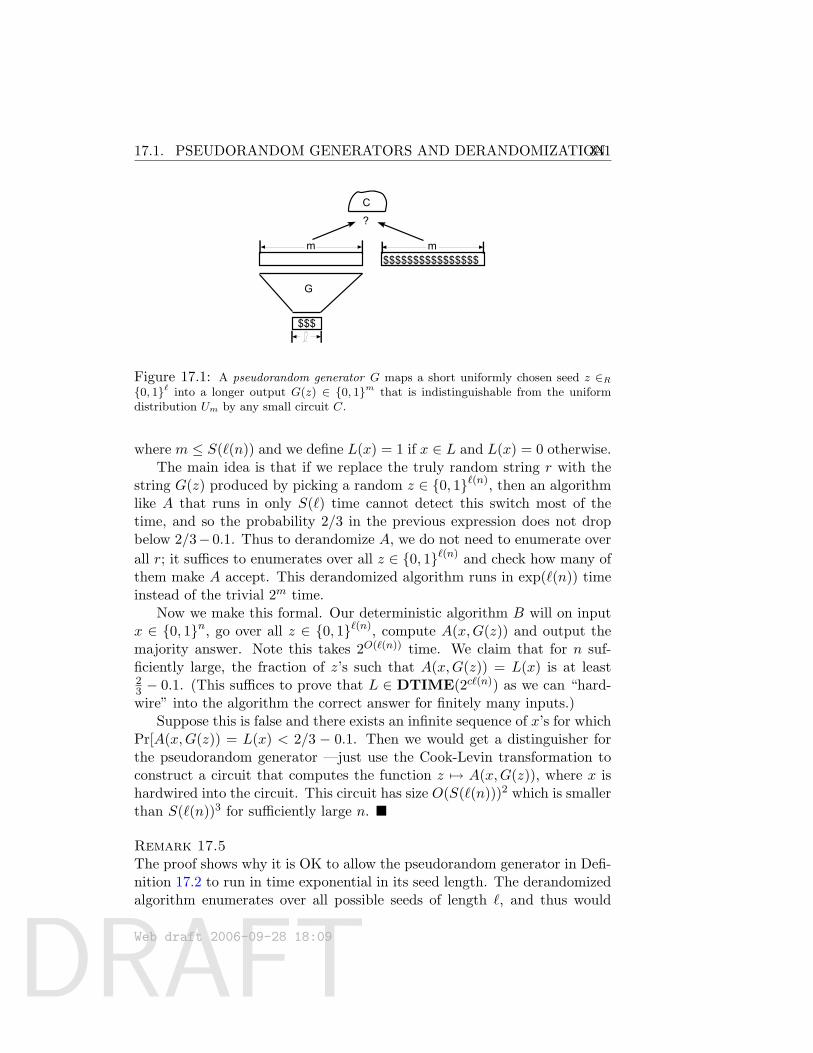
DRAFT


?

C

$$$

$$$$$$$$$$$$$$$$

G

m m

Figure 17.1: A pseudorandom generator G maps a short uniformly chosen seed z ∈R0, 1` into a longer output G(z) ∈ 0, 1m that is indistinguishable from the uniformdistribution Um by any small circuit C.

where m ≤ S(`(n)) and we define L(x) = 1 if x ∈ L and L(x) = 0 otherwise.The main idea is that if we replace the truly random string r with the

string G(z) produced by picking a random z ∈ 0, 1`(n), then an algorithmlike A that runs in only S(`) time cannot detect this switch most of thetime, and so the probability 2/3 in the previous expression does not dropbelow 2/3− 0.1. Thus to derandomize A, we do not need to enumerate overall r; it suffices to enumerates over all z ∈ 0, 1`(n) and check how many ofthem make A accept. This derandomized algorithm runs in exp(`(n)) timeinstead of the trivial 2m time.

Now we make this formal. Our deterministic algorithm B will on inputx ∈ 0, 1n, go over all z ∈ 0, 1`(n), compute A(x,G(z)) and output themajority answer. Note this takes 2O(`(n)) time. We claim that for n suf-ficiently large, the fraction of z’s such that A(x,G(z)) = L(x) is at least23 − 0.1. (This suffices to prove that L ∈ DTIME(2c`(n)) as we can “hard-wire” into the algorithm the correct answer for finitely many inputs.)

Suppose this is false and there exists an infinite sequence of x’s for whichPr[A(x,G(z)) = L(x) < 2/3 − 0.1. Then we would get a distinguisher forthe pseudorandom generator —just use the Cook-Levin transformation toconstruct a circuit that computes the function z 7→ A(x,G(z)), where x ishardwired into the circuit. This circuit has size O(S(`(n)))2 which is smallerthan S(`(n))3 for sufficiently large n.

Remark 17.5The proof shows why it is OK to allow the pseudorandom generator in Defi-nition 17.2 to run in time exponential in its seed length. The derandomizedalgorithm enumerates over all possible seeds of length `, and thus would

Web draft 2006-09-28 18:09

DRAFT


take exponential time (in `) even if the generator itself were to run in lessthan exponential time.

Notice, these generators have to fool distinguishers that run for lesstime than they do. By contrast, the definition of secure pseudorandom gen-erators (Definition 10.11 in Chapter 10) required the generator to run inpolynomial time, and yet have the ability to fool distinguishers that havesuper-polynomial running time. This difference in these definitions stemsfrom the intended usage. In the cryptographic setting the generator is usedby honest users and the distinguisher is the adversary attacking the system— and it is reasonable to assume the attacker can invest more computa-tional resources than those needed for normal/honest use of the system.In derandomization, generator is used by the derandomized algorithm, the”distinguisher” is the probabilistic algorithm that is being derandomized,and it is reasonable to allow the derandomized algorithm higher runningtime than the original probabilistic algorithm.

Of course, allowing the generator to run in exponential time as in thischapter potentially makes it easier to prove their existence compared withsecure pseudorandom generators, and this indeed appears to be the case.(Note that if we place no upperbounds on the generator’s efficiency, we couldprove the existence of generators unconditionally as shown in Exercise 2, butthese do not suffice for derandomization.)

We will construct pseudorandom generators based on complexity as-sumptions, using quantitatively stronger assumptions to obtain quantita-tively stronger pseudorandom generators (i.e., S(`)-pseudorandom gener-ators for larger functions S). The strongest (though still reasonable) as-sumption will yield a 2Ω(`)-pseudorandom generator, thus implying thatBPP = P. These are described in the following easy corollaries of theLemma that are left as Exercise 1.

Corollary 17.61. If there exists a 2ε`-pseudorandom generator for some constant ε > 0

then BPP = P.

2. If there exists a 2`ε-pseudorandom generator for some constant ε > 0

then BPP ⊆ QuasiP = DTIME(2polylog(n)).

3. If there exists an S(`)-pseudorandom generator for some super-polynomialfunction S (i.e., S(`) = `ω(1)) then BPP ⊆ SUBEXP = ∩ε>0DTIME(2n

ε).

Web draft 2006-09-28 18:09

DRAFT


17.1.1 Hardness and Derandomization

We construct pseudorandom generators under the assumptions that cer-tain explicit functions are hard. In this chapter we use assumptions aboutaverage-case hardness, while in the next chapter we will be able to constructpseudorandom generators assuming only worst-case hardness. Both worst-case and average-case hardness refers to the size of the minimum Booleancircuit computing the function:

Definition 17.7 (Hardness)Let f : 0, 1∗ → 0, 1 be a Boolean function. The worst-case hardness of f ,denoted Hwrs(f), is a function from N to N that maps every n ∈ N to the largestnumber S such that every Boolean circuit of size at most S fails to compute f onsome input in 0, 1n.The average-case hardness of f , denoted Havg(f), is a function from N to N that mapsevery n ∈ N, to the largest number S such that Prx∈R0,1n [C(x) = f(x)] < 1

2 + 1S

for every Boolean circuit C on n inputs with size at most S.

Note that for every function f : 0, 1∗ → 0, 1 and n ∈ N, Havg(f)(n) ≤Hwrs(f)(n) ≤ n2n.

Remark 17.8This definition of average-case hardness is tailored to the application ofderandomization, and in particular only deals with the uniform distributionover the inputs. See Chapter 15 for a more general treatment of average-case complexity. We will also sometimes apply the notions of worst-caseand average-case to finite functions from 0, 1n to 0, 1, where Hwrs(f) andHavg(f) are defined in the natural way. (E.g., if f : 0, 1n → 0, 1 thenHwrs(f) is the largest number S for which every Boolean circuit of size atmost S fails to compute f on some input in 0, 1n.)

Example 17.9Here are some examples of functions and their conjectured or proven hard-ness:

1. If f is a random function (i.e., for every x ∈ 0, 1∗ we choose f(x)using an independent unbiased coin) then with high probability, boththe worst-case and average-case hardness of f are exponential (see

Web draft 2006-09-28 18:09

DRAFT


Exercise 3). In particular, with probability tending to 1 with n, bothHwrs(f)(n) and Havg(f)(n) exceed 20.99n. We will often use the shorthandHwrs(f),Havg(f) ≥ 20.99n for such expressions.

2. If f ∈ BPP then, since BPP ⊆ P/poly, both Hwrs(f) and Havg(f) arebounded by some polynomial.

3. It seems reasonable to believe that 3SAT has exponential worst-casehardness; that is, Hwrs(3SAT) ≥ 2Ω(n). It is even more believable thatNP * P/poly, which implies that Hwrs(3SAT) is superpolynomial. Theaverage case complexity of 3SAT is unclear, and in any case dependentupon the way we choose to represent formulas as strings.

4. If we trust the security of current cryptosystems, then we do believethat NP contains functions that are hard on the average. If g is a one-way permutation that cannot be inverted with polynomial probabilityby polynomial-sized circuits, then by Theorem 10.14, the function fthat maps the pair x, r ∈ 0, 1n to g−1(x) r has super-polynomialaverage-case hardness: Havg(f) ≥ nω(1). (Where x r =

∑ni=1 xiri

(mod 2).) More generally there is a polynomial relationship betweenthe size of the minimal circuit that inverts g (on the average) and theaverage-case hardness of f .

The main theorem of this section uses hard-on-the average functions toconstruct pseudorandom generators:

Web draft 2006-09-28 18:09

DRAFT


Theorem 17.10 (Consequences of NW Generator)For every polynomial-time computable monotone S : N → N, if there exists aconstant c and function f ∈ DTIME(2cn) such that Havg(f) ≥ S(n) then thereexists a constant ε > 0 such that an S(ε`)ε-pseudorandom generator exists. Inparticular, the following corollaries hold:

1. If there exists f ∈ E = DTIME(2O(n)) and ε > 0 such that Havg(f) ≥ 2εn thenBPP = P.

2. If there exists f ∈ E = DTIME(2O(n)) and ε > 0 such that Havg(f) ≥ 2nε

thenBPP ⊆ QuasiP.

3. If there exists f ∈ E = DTIME(2O(n)) such that Havg(f) ≥ nω(1) then BPP ⊆SUBEXP.

Remark 17.11We can replace E with EXP = DTIME(2poly(n)) in Corollaries 2 and 3above. Indeed, for every f ∈ DTIME(2n

c), the function g that on input

x ∈ 0, 1∗ outputs the f applies to the first |x|1/c bits of x is in DTIME(2n)and satisfies Havg(g)(n) ≥ Havg(f)(n1/c). Therefore, if there exists f ∈ EXPwith Havg(f) ≥ 2n

εthen there there exists a constant ε′ > 0 and a function

g ∈ E with Havg(g) ≥ 2nε′, and so we can replace E with EXP in Corollary 2.

A similar observation holds for Corollary 3. Note that EXP contains manyclasses we believe to have hard problems, such as NP,PSPACE,⊕P andmore, which is why we believe it does contain hard-on-the-average functions.In the next chapter we will give even stronger evidence to this conjecture,by showing it is implied by the assumption that EXP contains hard-in-the-worst-case functions.

Remark 17.12The original paper of Nisan and Wigderson [NW94] did not prove Theo-rem 17.10 as stated above. It was proven in a sequence of works [?]. Nisanand Wigderson only proved that under the same assumptions there existsan S′(`)-pseudorandom generator, where S′(`) = S

(ε√` log(S(ε

√`))ε

forsome ε > 0. Note that this is still sufficient to derive all three corollariesabove. It is this weaker version we prove in this book.

Web draft 2006-09-28 18:09

DRAFT

34617.2. PROOF OF THEOREM ??: NISAN-WIGDERSON

CONSTRUCTION

17.2 Proof of Theorem 17.10: Nisan-WigdersonConstruction

How can we use a hard function to construct a pseudorandom generator?

17.2.1 Warmup: two toy examples

For starters, we demonstrate this by considering the “toy example” of apseudorandom generator whose output is only one bit longer than its input.Then we show how to extend by two bits. Of course, neither suffices to proveTheorem 17.10 but they do give insight to the connection between hardnessand randomness.

Extending the input by one bit using Yao’s Theorem.

The following Lemma uses a hard function to construct such a “toy” gener-ator:

Lemma 17.13 (One-bit generator)Suppose that there exist f ∈ E with Havg(f) ≥ n4. Then, there exists anS(`)-pseudorandom generator G for S(`) = `+ 1.

Proof: The generator G will be very simple: for every z ∈ 0, 1`, we set

G(z) = z f(z)

(where denotes concatenation). G clearly satisfies the output length andefficiency requirements of an (`+1)-pseudorandom generator. To prove thatits output is 1/10-pseudorandom we use Yao’s Theorem from Chapter 10showing that pseudorandomness is implied by unpredictiability:3

Theorem 17.14 (Theorem 10.12, restated)Let Y be a distribution over 0, 1m. Suppose that there exist S > 10n,ε > 0such that for every circuit C of size at most 2S and i ∈ [m],

Prr∈RY

[C(r1, . . . , ri−1) = ri] ≤12

+ε

m

Then Y is (S, ε)-pseudorandom.

3Although this theorem was stated and proved in Chapter 10 for the case of uniformTuring machines, the proof easily extends to the case of circuits.

Web draft 2006-09-28 18:09

DRAFT

17.2. PROOF OF THEOREM ??: NISAN-WIGDERSONCONSTRUCTION 347

Using Theorem 17.14 it is enough to show that there does not exist acircuit C of size 2(`+ 1)3 < `4 and a number i ∈ [`+ 1] such that

Prr=G(U`)

[C(r1, . . . , ri−1) = ri] > 12 + 1

20(`+1) . (1)

However, for every i ≤ `, the ith bit of G(z) is completely uniform andindependent from the first i − 1 bits, and hence cannot be predicted withprobability larger than 1/2 by a circuit of any size. For i = `+1, Equation (1)becomes,

Prz∈R0,1`

[C(z) = f(z)] >12

+1

20(`+ 1)>

12

+1`4,

which cannot hold under the assumption that Havg(f) ≥ n4.

Extending the input by two bits using the averaging principle.

We now continue to progress in “baby steps” and consider the next naturaltoy problem: constructing a pseudorandom generator that extends its inputby two bits. This is obtained in the following Lemma:

Lemma 17.15 (Two-bit generator)Suppose that there exists f ∈ E with Havg(f) ≥ n4. Then, there exists an(`+2)-pseudorandom generator G.

Proof: The construction is again very natural: for every z ∈ 0, 1`, we set

G(z) = z1 · · · z`/2 f(z1, . . . , z`/2) z`/2+1 · · · z` f(z`/2+1, . . . , z`).

Again, the efficiency and output length requirements are clearly satisfied.To show G(U`) is 1/10-pseudorandom, we again use Theorem 17.14, and

so need to prove that there does not exists a circuit C of size 2(`+ 1)3 andi ∈ [`+ 2] such that

Prr=G(U`)

[C(r1, . . . , ri−1) = ri] >12

+1

20(`+ 2). (2)

Once again, (2) cannot occur for those indices i in which the ith outputof G(z) is truly random, and so the only two cases we need to consider arei = `/2 + 1 and i = `+ 2. Equation (2) cannot hold for i = `/2 + 1 for thesame reason as in Lemma 17.13. For i = `+ 2, Equation (2) becomes:

Prr,r′∈R0,1`/2

[C(r f(r) r′) = f(r′)] >12

+1

20(`+ 2)(3)

Web draft 2006-09-28 18:09

DRAFT


CONSTRUCTION

This may seem somewhat problematic to analyze since the input to Ccontains the bit f(r), which C could not compute on its own (as f is a hardfunction). Couldn’t it be that the input f(r) helps C in predicting the bitf(r′)? The answer is NO, and the reason is that r′ and r are independent.Formally, we use the following principle (see Section A.2.2 in the appendix):

The Averaging Principle: If A is some event depending ontwo independent random variables X,Y , then there exists somex in the range of X such that

PrY

[A(x, Y ) ≥ PrX,Y

[A(X,Y )]

Applying this principle here, if (3) holds then there exists a string r ∈0, 1`/2 such that

Prr′∈R0,1`/2

[C(r, f(r), r′) = f(r′)] >12

+1

20(`+ 2).

(Note that this probability is now only over the choice of r′.) If this is thecase, we can “hardwire” the `/2+1 bits r f(r) to the circuit C and obtaina circuit D of size at most (`+ 2)3 + 2` < (`/2)4 such that

Prr′∈R0,1`/2

[D(r′) = f(r′)] >12

+1

20(`+ 2),

contradicting the hardness of f .

Beyond two bits:

A generator that extends the output by two bits is still useless for our goals.We can generalize the proof Lemma 17.15 to obtain a generator G thatextends the output by k bits setting

G(z1, . . . , z`) = z1 f(z1) z2 f(z2) · · · zk f(zk) , (4)

where zi is the ith block of `/k bits in z. However, no matter how big we setk and no matter how hard the function f is, we cannot get a generator thatexpands its input by a multiplicative factor larger than two. Note that toprove Theorem 17.10 we need a generator that, depending on the hardnesswe assume, has output that can be exponentially larger than the input!Clearly, we need a new idea.

Web draft 2006-09-28 18:09

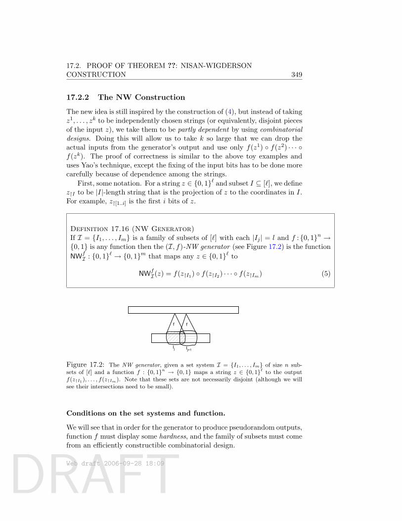
DRAFT


17.2.2 The NW Construction

The new idea is still inspired by the construction of (4), but instead of takingz1, . . . , zk to be independently chosen strings (or equivalently, disjoint piecesof the input z), we take them to be partly dependent by using combinatorialdesigns. Doing this will allow us to take k so large that we can drop theactual inputs from the generator’s output and use only f(z1) f(z2) · · · f(zk). The proof of correctness is similar to the above toy examples anduses Yao’s technique, except the fixing of the input bits has to be done morecarefully because of dependence among the strings.

First, some notation. For a string z ∈ 0, 1` and subset I ⊆ [`], we definezI to be |I|-length string that is the projection of z to the coordinates in I.For example, z[1..i] is the first i bits of z.

Definition 17.16 (NW Generator)If I = I1, . . . , Im is a family of subsets of [`] with each |Ij | = l and f : 0, 1n →0, 1 is any function then the (I, f)-NW generator (see Figure 17.2) is the functionNWf

I : 0, 1` → 0, 1m that maps any z ∈ 0, 1` to

NWfI(z) = f(zI1) f(zI2) · · · f(zIm) (5)

Ij Ij+1

f f

Figure 17.2: The NW generator, given a set system I = I1, . . . , Im of size n sub-sets of [`] and a function f : 0, 1n → 0, 1 maps a string z ∈ 0, 1` to the outputf(zI1), . . . , f(zIm). Note that these sets are not necessarily disjoint (although we willsee their intersections need to be small).

Conditions on the set systems and function.

We will see that in order for the generator to produce pseudorandom outputs,function f must display some hardness, and the family of subsets must comefrom an efficiently constructible combinatorial design.

Web draft 2006-09-28 18:09

DRAFT


CONSTRUCTION

Definition 17.17 (Combinatorial designs)If d, n, ` ∈ N are numbers with ` > n > d then a family I = I1, . . . , Im ofsubsets of [`] is an (`, n, d)-design if |Ij | = n for every j and |Ij ∩ Ik| ≤ d forevery j 6= k.

The next lemma yields efficient constructions of these designs and isproved later.

Lemma 17.18 (Construction of designs)There is an algorithm A such that on input `, d, n ∈ N where n > d and

` > 10n2/d, runs for 2O(`) steps and outputs an (`, n, d)-design I containing2d/10 subsets of [`].

The next lemma shows that if f is a hard function and I is a designwith sufficiently good parameters, than NWf

I(U`) is indeed a pseudorandomdistribution:Lemma 17.19 (Pseudorandomness using the NW generator)If I is an (`, n, d)-design with |I| = 2d/10 and f : 0, 1n → 0, 1 a

function satisfying 2d <√

Havg(f)(n), then the distribution NWfI(U`) is a

(Havg(f)(n)/10, 1/10)-pseudorandom distribution.

Proof: Let S denote Havg(f)(n). By Yao’s Theorem, we need to prove thatfor every i ∈ [2d/10] there does not exist an S/2-sized circuit C such that

PrZ∼U`

R=NWfI(Z)

[C(R1, . . . , Ri−1) = Ri] ≥12

+1

10 · 2d/10. (6)

For contradiction’s sake, assume that (6) holds for some circuit C and somei. Plugging in the definition of NWf

I , Equation (6) becomes:

PrZ∼U`

[C(f(ZI1), · · · , f(ZIi−1)) = f(ZIi)] ≥12

+1

10 · 2d/10. (7)

Letting Z1 and Z2 denote the two independent variables correspondingto the coordinates of Z in Ii and [`] \ Ii respectively, Equation (7) becomes:

PrZ1∼UnZ2∼U`−n

[C(f1(Z1, Z2), . . . , fi−1(Z1, Z2)) = f(Z1)] ≥12

+1

10 · 2d/10, (8)

where for every j ∈ [2d/10], fj applies f to the coordinates of Z1 correspond-ing to Ij ∩ Ii and the coordinates of Z2 corresponding to Ij \ Ii. By the

Web draft 2006-09-28 18:09

DRAFT


averaging principle, if (8) holds then there exists a string z2 ∈ 0, 1`−nsuch that

PrZ1∼Un

[C(f1(Z1, z2), . . . , fi−1(Z1, z2)) = f(Z1)] ≥12

+1

10 · 2d/10. (9)

We may now appear to be in some trouble, since all of fj(Z1, z2) for j ≤ i−1do depend upon Z1, and the fear is that if they together contain enoughinformation about Z1 then a circuit could potentially predict fi(Z1) afterlooking at all of them. To prove that this fear is baseless we use the factthat the circuit C is small and f is a very hard function.

Since |Ij ∩ Ii| ≤ d for j 6= i, the function Z1 7→ fj(Z1, z2) depends atmost d coordinates of z1 and hence can be computed by a d2d-sized circuit.(Recall that z2 is fixed.) Thus if if (8) holds then there exists a circuit B ofsize 2d/10 · d2d + S/2 < S such that

PrZ1∼Un

[B(Z1) = f(Z1)] ≥12

+1

10 · 2d/10>

12

+1S. (10)

But this contradicts the fact that Havg(f)(n) = S.

Remark 17.20 (Black-box proof)Lemma 17.19 shows that if NWf

I(U`) is distinguishable from the uniformdistribution U2d/10 by some circuit D, then there exists a circuit B (of sizepolynomial in the size of D and in 2d) that computes the function f withprobability noticeably larger than 1/2. The construction of this circuit B ac-tually uses the circuit D as a black-box, invoking it on some chosen inputs.This property of the NW generator (and other constructions of pseudoran-dom generators) turned out to be useful in several settings. In particular,Exercise 5 uses it to show that under plausible complexity assumptions,the complexity class AM (containing all languages with a constant roundinteractive proof, see Chapter 9) is equal to NP. We will also use this prop-erty in the construction of randomness extractors based on pseudorandomgenerators.

Putting it all together: Proof of Theorem 17.10 from Lemmas 17.18and 17.19

As noted in Remark 17.12, we do not prove here Theorem 17.10 as statedbut only the weaker statement, that given f ∈ E and S : N → N withHavg(f) ≥ S, we can construct an S′(`)-pseudorandom generator, whereS′(`) = S

(ε√` log(S(ε

√`))ε

for some ε > 0.

Web draft 2006-09-28 18:09

DRAFT


CONSTRUCTION

For such a function f , we denote our pseudorandom generator by NW f .Given input z ∈ 0, 1`, the generator NWf operates as follows:

• Set n to be the largest number such that ` > 100n2/ logS(n). Set d =logS(n)/10. Since S(n) < 2n, we can assume that ` ≤ 300n2/ logS(n).

• Run the algorithm of Lemma 17.18 to obtain an (`, n, d)-design I =I1, . . . , I2d/5.

• Output the first S(n)1/40 bits of NWfI(z).

Clearly, NWf (z) runs in 2O(`) time. Moreover, since 2d ≤ S(n)1/10,Lemma 17.19 implies that the distribution NWf (U`) is (S(n)/10, 1/10)-pseudorandom.Since n ≥

√` logS(n)/300 ≥

√` logS(

√`

300)/300 (with the last inequalityfollowing from the fact that S is monotone), this concludes the proof ofTheorem 17.10.

Construction of combinatorial designs.

All that is left to complete the proof is to show the construction of combi-natorial designs with the required parameters:Proof of Lemma 17.18 (construction of combinatorial designs): Oninputs `, d, n with ` > 10n2/d, our Algorithm A will construct an (`, n, d)-design I with 2d/10 sets using the simple greedy strategy:

Start with I = ∅ and after constructing I = I1, . . . , Im form < 2d/10, search all subsets of [`] and add to I the first n-sizedset I satisfying |I ∩ Ij | ≤ d for every j ∈ [m]. We denote thislatter condition by (*).

Clearly, A runs in poly(m)2` = 2O(`) time and so we only need to proveit never gets stuck. In other words, it suffices to show that if ` = 10n2/dand I1, . . . , Im is a collection of n-sized subsets of [`] for m < 2d/10, thenthere exists an n-sized subset I ⊆ [`] satisfying (*). We do so by showingthat if we pick I at random by choosing independently every element x ∈ [`]to be in I with probability 2n/` then:

Pr[|I| ≥ n] ≥ 0.9 (11)

Pr[|I ∩ Ij | ≥ d] ≤ 0.5 · 2−d/10 (∀j ∈ [m]) (12)

Because the expected size of I is 2n, while the expected size of theintersection I∩Ij is 2n2/` < d/5, both (12) and (11) follow from the Chernoff

Web draft 2006-09-28 18:09

DRAFT

17.3. DERANDOMIZATION REQUIRES CIRCUIT LOWERBOUNDS353

bound. Yet together these two conditions imply that with probability atleast 0.4, the set I will simultaneously satisfy (*) and have size at least n.Since we can always remove elements from I without damaging (*), thiscompletes the proof.

17.3 Derandomization requires circuit lowerbounds

We saw in Section 17.2 that if we can prove certain strong circuit lower-bounds, then we can partially (or fully) derandomize BPP. Now we prove aresult in the reverse direction: derandomizing BPP requires proving circuitlowerbounds. Depending upon whether you are an optimist or a pessimist,you can view this either as evidence that derandomizing BPP is difficult,or, as a reason to double our efforts to derandomize BPP.

We say that a function is in AlgP/poly if it can be computed by a poly-nomial size arithmetic circuit whose gates are labeled by +, −, × and ÷,which are operations over some underlying field or ring. We let perm de-note the problem of computing the permanent of matrices over the integers.(The proof can be extended to permanent computations over finite fields ofcharacteristic > 2.) We prove the following result.

Theorem 17.21 ([?])P = BPP⇒ NEXP * P/poly or perm /∈ AlgP/poly.

Remark 17.22It is possible to replace the “poly” in the conclusion perm /∈ AlgP/poly witha subexponential function by appropriately modifying Lemma 17.25. It isopen whether the conclusion NEXP * P/poly can be similarly strength-ened.

In fact, we will prove the following stronger theorem. Recall the Poly-nomial Identity Testing (ZEROP) problem in which the input consists ofa polynomial represented by an arithmetic circuit computing it (see Sec-tion 7.2.2 and Example 17.1), and we have to decide if it is the identicallyzero polynomial. This problem is in coRP ⊆ BPP and we will show thatif it is in P then the conclusions of Theorem 17.21 hold:

Theorem 17.23 (Derandomization implies lower bounds)If ZEROP ∈ P then either NEXP * P/poly or perm /∈ AlgP/poly.

Web draft 2006-09-28 18:09

DRAFT

35417.3. DERANDOMIZATION REQUIRES CIRCUIT LOWERBOUNDS

The proof relies upon many results described earlier in the book.4 Recallthat MA is the class of languages that can be proven by a one round interac-tive proof between two players Arthur and Merlin (see Definition 9.7). Merlinis an all-powerful prover and Arthur is a polynomial-time verifier that can fliprandom coins. That is, given an input x, Merlin first sends Arthur a “proof”y. Then Arthur with y in hand flips some coins and decides whether or notto accept x. For this to be an MA protocol, Merlin must convince Arthurto accept strings in L with probability one while at the same time Arthurmust not be fooled into accepting strings not in L except with probabilitysmaller than 1/2. We will use the following result regarding MA:

Lemma 17.24 ([BFL91],[BFNW93])EXP ⊆ P/poly ⇒ EXP = MA.

Proof: Suppose EXP ⊆ P/poly. By the Karp-Lipton theorem (Theo-rem 6.14), in this case EXP collapses to the second level Σp

2 of the poly-nomial hierarchy. Hence Σp

2 = PH = PSPACE = IP = EXP ⊆ P/poly.Thus every L ∈ EXP has an interactive proof, and furtheremore, sinceEXP = PSPACE, we can just the use the interactive proof for TQBF, forwhich the prover is a PSPACE machine. Hence the prover can be replacedby a polynomial size circuit family Cn. Now we see that the interactive proofcan actually be carried out in 2 rounds, with Merlin going first. Given aninput x of length n, Merlin gives Arthur a polynomial size circuit C, whichis supposed to be the Cn for L. Then Arthur runs the interactive proof forL, using C as the prover. Note that if the input is not in the language, thenno prover has a decent chance of convincing the verifier, so this is true alsofor prover described by C. Thus we have described an MA protocol for Limplying that EXP ⊆MA and hence that EXP = MA.

Our next ingredient for the proof of Theorem 17.23 is the followinglemma:

Lemma 17.25If ZEROP ∈ P, and perm ∈ AlgP/poly. Then Pperm ⊆ NP.

Proof: Suppose perm has algebraic circuits of size nc, and that ZEROPhas a polynomial-time algorithm. Let L be a language that is decided byan nd-time TM M using queries to a perm-oracle. We construct an NPmachine N for L.

4This is a good example of “third generation” complexity results that use a clevercombination of both “classical” results from the 60’s and 70’s and newer results from the1990’s.

Web draft 2006-09-28 18:09

DRAFT

17.3. DERANDOMIZATION REQUIRES CIRCUIT LOWERBOUNDS355

Suppose x is an input of size n. Clearly, M ’s computation on x makesqueries to perm of size at most m = nd. So N will use nondeterminism asfollows: it guesses a sequence of m algebraic circuits C1, C2, . . . , Cm whereCi has size ic. The hope is that Ci solves perm on i× i matrices, and N willverify this in poly(m) time. The verification starts by verifying C1, which istrivial. Inductively, having verified the correctness of C1, . . . , Ct−1, one canverify that Ct is correct using downward self-reducibility, namely, that for at× t matrix A,

perm(A) =t∑i=1

a1iperm(A1,i),

where A1,i is the (t−1)×(t−1) sub-matrix of A obtained by removing the 1strow and ith column of A. Thus if circuit Ct−1 is known to be correct, thenthe correctness of Ct can be checked by substituting Ct(A) for perm(A) andCt−1(A1,i) for perm(A1,i): this yields an identity involving algebraic circuitswith t2 inputs which can be verified deterministically in poly(t) time usingthe algorithm for ZEROP. Proceeding this way N verifies the correctness ofC1, . . . , Cm and then simulates Mperm on input x using these circuits.

The heart of the proof is the following lemma, which is interesting in itsown right:

Lemma 17.26 ([?])NEXP ⊆ P/poly ⇒ NEXP = EXP.

Proof: We prove the contrapositive. Suppose that NEXP 6= EXP and letL ∈ NEXP \ EXP. Since L ∈ NEXP there exists a constant c > 0 and arelation R such that

x ∈ L⇔ ∃y ∈ 0, 12|x|c

s.t. R(x, y) holds ,

where we can test whether R(x, y) holds in time 2|x|c′

for some constant c′.For every constant d > 0, let Md be the following machine: on input

x ∈ 0, 1n enumerate over all possible Boolean circuits C of size n100d thattake nc inputs and have a single output. For every such circuit let tt(C)be the 2n

c-long string that corresponds to the truth table of the function

computed by C. If R(x, tt(C)) holds then halt and output 1. If this doesnot hold for any of the circuits then output 0.

Since Md runs in time 2n101d+nc , under our assumption that L 6∈ EXP,

for every d there exists an infinite sequence of inputs Xd = xii∈N on whichMd(xi) outputs 0 even though xi ∈ L (note that if Md(x) = 1 then x ∈ L).

Web draft 2006-09-28 18:09

DRAFT

35617.3. DERANDOMIZATION REQUIRES CIRCUIT LOWERBOUNDS

This means that for every string x in the sequence Xd and every y such thatR(x, y) holds, the string y represents the truth table of a function on nc bitsthat cannot be computed by circuits of size n100d, where n = |x|. Using thepseudorandom generator based on worst-case assumptions (Theorem ??),we can use such a string y to obtain an `d-pseudorandom generator.

Now, if NEXP ⊆ P/poly then as noted above NEXP ⊆MA and henceevery language in NEXP has a proof system where Merlin proves that ann-bit string is in the language by sending a proof which Arthur then verifiesusing a probabilistic algorithm of at most nd steps. Yet, if n is the inputlength of some string in the sequence Xd and we are given x ∈ Xd with|x| = n, then we can replace Arthur by non-deterministic poly(nd)2n

ctime

algorithm that does not toss any coins: Arthur will guess a string y such thatR(x, y) holds and then use y as a function for a pseudorandom generator toverify Merlin’s proof.

This means that there is a constant c > 0 such that every language inNEXP can be decided on infinitely many inputs by a non-deterministicalgorithm that runs in poly(2n

c)-time and uses n bits of advice (consisting

of the string x ∈ Xd). Under the assumption that NEXP ⊆ P/poly wecan replace the poly(2n

c) running time with a circuit of size nc

′where c′ is

a constant depending only on c, and so get that there is a constant c′ suchthat every language in NEXP can be decided on infinitely many inputs bya circuit family of size n + nc

′. Yet this can be ruled out using elementary

diagonalization.

Remark 17.27It might seem that Lemma 17.26 should have an easier proof that goes alongthe proof that EXP ⊆ P/poly ⇒ EXP = MA, but instead of using theinteractive proof for TQBF uses the multi-prover interactive proof system forNEXP. However, we do not know how to implement the provers’ strategiesfor this latter system in NEXP. (Intuitively, the problem arises from thefact that a NEXP statement may have several certificates, and it is notclear how we can ensure all provers use the same one.)

We now have all the ingredients for the proof of Theorem 17.23.

Proof of Theorem 17.23: For contradiction’s sake, assume that thefollowing are all true:

ZEROP ∈ P (13)NEXP ⊆ P/poly, (14)

perm ∈ AlgP/poly. (15)

Web draft 2006-09-28 18:09

DRAFT

17.4. WEAK RANDOM SOURCES AND EXTRACTORS 357

Statement (14) together with Lemmas 17.24 and 17.26 imply that NEXP =EXP = MA. Now recall that MA ⊆ PH, and that by Toda’s Theorem(Theorem 8.11) PH ⊆ P#P. Recall also that by Valiant’s Theorem (Theo-rem 8.8) perm is #P-complete. Thus, under our assumptions

NEXP ⊆ Pperm. (16)

Since we assume that ZEROP ∈ P, Lemma 17.25 together with statements(15) and (16) implies that NEXP ⊆ NP, contradicting the Nondeterminis-tic Time Hierarchy Theorem (Theorem 4.3). Thus the three statements atthe beginning of the proof cannot be simultaneously true.

17.4 Weak Random Sources and Extractors

Suppose, that despite the philosophical difficulties, we are happy with prob-abilistic algorithms, and see no need to “derandomize” them, especially atthe expense of some unproven assumptions. We still need to tackle the factthat real world sources of randomness and unpredictability rarely, if ever,behave as a sequence of perfectly uncorrelated and unbiased coin tosses. Canwe still execute probabilistic algorithms using real-world “weakly random”sources?

17.4.1 Min Entropy

For starters, we need to define what we mean by a weakly random source.Definition 17.28Let X be a random variable. The min entropy of X, denoted by H∞(X),is the largest real number k such that Pr[X = x] ≤ 2−k for every x in therange of X.

If X is a distribution over 0, 1n with H∞(X) ≥ k then it is called an(n, k)-source.

It is not hard to see that if X is a random variable over 0, 1n thenH∞(X) ≤ n with H∞(X) = n if and only if X is distributed according tothe uniform distribution Un. Our goal in this section is to be able to executeprobabilistic algorithms given access to a distribution X with H∞(X) assmall as possible. It can be shown that min entropy is a minimal requirementin the sense that in general, to execute a probabilistic algorithm that usesk random bits we need access to a distribution X with H∞(X) ≥ k (seeExercise ??).

Web draft 2006-09-28 18:09

DRAFT

358 17.4. WEAK RANDOM SOURCES AND EXTRACTORS

Example 17.29Here are some examples for distributions X over 0, 1n and their min-entropy:

• (Bit fixing and generalized bit fixing sources) If there is subset S ⊆ [n]with |S| = k such thatX’s projection to the coordinates in S is uniformover 0, 1k, and X’s projection to [n] \S is a fixed string (say the all-zeros string) then H∞(X) = k. The same holds if X’s projection to[n] \ S is a fixed deterministic function of its projection to S. Forexample, if the bits in the odd positions of X are independent anduniform and for every even position 2i, X2i = X2i−1 then H∞(X) =d n2 e. This may model a scenario where we measure some real worlddata at too high a rate (think of measuring every second a physicalevent that changes only every minute).

• (Linear subspaces) If X is the uniform distribution over a linear sub-space of GF(2)n of dimension k, then H∞(X) = k. (In this case X isactually a generalized bit-fixing source— can you see why?)

• (Biased coins) If X is composed of n independent coins, each out-putting 1 with probability δ < 1/2 and 0 with probability 1 − δ, thenas n grows, H∞(X) tends to H(δ)n where H is the Shannon entropyfunction. That is, H(δ) = δ log 1

δ + (1− δ) log 11−δ .

• (Santha-Vazirani sources) If X has the property that for every i ∈ [n],and every string x ∈ 0, 1i−1, conditioned on X1 = x1, . . . , Xi−1 =xi−1 it holds that both Pr[Xi = 0] and Pr[Xi = 1] are between δand 1 − δ then H∞(X) ≥ H(δ)n. This can model sources such asstock market fluctuations, where current measurements do have somelimited dependence on the previous history.

• (Uniform over subset) If X is the uniform distribution over a set S ⊆0, 1n with |S| = 2k then H∞(X) = k. As we will see, this is avery general case that “essentially captures” all distributions X withH∞(X) = k.

We see that min entropy is a pretty general notion, and distributions withsignificant min entropy can model many real-world sources of randomness.

Web draft 2006-09-28 18:09

DRAFT


17.4.2 Statistical distance and Extractors

Now we try to formalize what it means to extract random —more precisely,almost random— bits from an (n, k) source. To do so we will need thefollowing way of quantifying when two distributions are close.Definition 17.30 (statistical distance)For two random variables X and Y with range 0, 1m, their statistical dis-tance (also known as variation distance) is defined as δ(X,Y ) = maxS⊆0,1m|Pr[X ∈S] − Pr[Y ∈ S]|. We say that X,Y are ε-close, denoted X ≈ε Y , ifδ(X,Y ) ≤ ε.

Statistical distance lies in [0, 1] and satisfies triangle inequality, as sug-gested by its name. The next lemma gives some other useful properties; theproof is left as an exercise.Lemma 17.31Let X,Y be any two distributions taking values in 0, 1n.

1. δ(X,Y ) = 12

∑x∈0,1n |Pr[X = x]−Pr[Y = x]| .

2. (Restatement of Definition 17.30) δ(X,Y ) ≥ ε iff there is a booleanfunctionD :0, 1m → 0, 1 such that |Prx∈X [D(x) = 1]− Pry∈Y [D(y) = 1]| ≥ε.

3. If f :0, 1n → 0, 1s is any function, then δ(f(X), f(Y )) ≤ δ(X,Y ).(Here f(X) is a distribution on 0, 1s obtained by taking a sample ofX and applying f .)

Now we define an extractor. This is a (deterministic) function thattransforms an (n, k) source into an almost uniform distribution. It uses asmall number of additional truly random bits, denoted by t in the definitionbelow.Definition 17.32A function Ext : 0, 1n × 0, 1t → 0, 1m is a (k, ε) extractor if for any(n, k)-source X, the distribution Ext(X,Ut) is ε-close to Um. (For every `,U` denotes the uniform distribution over 0, 1`.)

Equivalently, if Ext : 0, 1n × 0, 1t → 0, 1m is a (k, ε) extractor,then for every distribution X ranging over 0, 1n of min-entropy k, and forevery S ⊆ 0, 1m, we have

|Pra∈X,z∈0,1t [Ext(a, z) ∈ S]−Prr∈0,1m [r ∈ S]| ≤ ε

We use this fact to show in Section 17.5.2 how to use extractors and (n, k)-sources to to simulate any probabilistic computation.

Web draft 2006-09-28 18:09

DRAFT


Why an additional input? Our stated motivation for extractors is toexecute probabilistic algorithms without access to perfect unbiased coins.Yet, it seems that an extractor is not sufficient for this task, as we onlyguarantee that its output is close to uniform if it is given an additional in-put that is uniformly distributed. First, we note that the requirement ofan additional input is necessary: for every function Ext : 0, 1n → 0, 1mand every k ≤ n − 1 there exists an (n, k)-source X such that the first bitof Ext(X) is constant (i.e, is equal to some value b ∈ 0, 1 with probability1), and so is at least of statistical distance 1/2 from the uniform distribu-tion (Exercise 7). Second, if the length t of the second input is sufficientlyshort (e.g., t = O(log n)) then, for the purposes of simulating probabilisticalgorithms, we can do without any access to true random coins, by enumer-ating over all the 2t possible inputs (see Section 17.5.2). Clearly, t has to besomewhat short for the extractor to be non-trivial: for t ≥ m, we can havea trivial extractor that ignores its first input and outputs the second input.This second input is called the seed of the extractor.

17.4.3 Extractors based upon hash functions

One can use pairwise independent (and even weaker notions of) hash func-tions to obtain extractors. In this section, H denotes a family of hashfunctions h : 0, 1n → 0, 1k. We say it has collision error δ if for anyx1 6= x2 ∈ 0, 1n, Prh∈H[h(x1) = h(x2)] ≤ (1 + δ)/2k. We assume that onecan choose a random function h ∈ H by picking a string at random from0, 1t. We define the extractor Ext :×0, 1t → 0, 1k+t as follows:

Ext(x, h) = h(x) h, (17)

where denotes concatenation of strings.To prove that this is an extractor, we relate the min-entropy to the

collision probability of a distribution, which is defined as∑

a p2a, where pa

is the probability assigned to string a.

Lemma 17.33If a distribution X has min-entropy at least k then its collision probability

is at most 1/2k.

Proof: For every a in X’s range, let pa be the probability that X = a.Then,

∑a p

2a ≤ maxa pa (

∑a pa) ≤

12k· 1 = 1

2k.

Web draft 2006-09-28 18:09

DRAFT


Lemma 17.34 (Leftover hash lemma)If x is chosen from a distribution on 0, 1n with min-entropy at least k/δ

and H has collision error δ, then h(X) h has distance at most√

2δ to theuniform distribution.

Proof: Left as exercise. (Hint: use the relation between the L2 and L1

norms

17.4.4 Extractors based upon random walks on expanders

This section assumes knowledge of random walks on expanders, as describedin Chapter 16.

Lemma 17.35Let ε > 0. For every n and k ≤ n there exists a (k, ε)-extractor Ext :0, 1n × 0, 1t → 0, 1n where t = O(n− k + log 1/ε).

Proof: Suppose X is an (n, k)-source and we are given a sample a fromit. Let G be a (2n, d, 1/2)-graph for some constant d (see Definition 16.9 andTheorem 16.24).

Let z be a truly random seed of length t = 10 log d(n − k + log 1/ε) =O(n− k + log 1/ε). We interpret z as a random walk in G of length 10(n−k+ log 1/ε) starting from the node whose label is a. (That is, we think of zas 10(n − k + log 1/ε) labels in [d] specifying the steps taken in the walk.)The output Ext(a, z) of the extractor is the label of the final node on thewalk.

We have ‖X − 1‖22 ≤ ‖X‖22 =∑

a Pr[X = a]2, which is at most 2−k byLemma 17.33 since X is an (n, k)-source. Therefore, after a random walk oflength t the distance to the uniform distribution is (by the upperbound in(??)):

‖M tX − 12N

1‖1 ≤ λt2‖X −1

2N1‖2√

2N ≤ λt22(N−k)/2.

When t is a sufficiently large multiple of N − k + log 1/ε, this distance issmaller than ε.

17.4.5 An extractor based upon Nisan-Wigderson

this section is still quite roughNow we describe an elegant construction of extractors due to Trevisan.Suppose we are given a string x obtained from an (N, k)-source. How can

we extract k random bits from it, given O(logN) truly random bits? Let us

Web draft 2006-09-28 18:09

DRAFT


check that the trivial idea fails. Using 2 logN random bits we can computea set of k (where k < N − 1) indices that are uniformly distributed andpairwise independent. Maybe we should just output the corresponding bitsof x? Unfortunately, this does not work: the source is allowed to set N − kbits (deterministically) to 0 so long as the remaining k bits are completelyrandom. In that case the expected number of random bits in our sample isat most k2/N , which is less than even 1 if k <

√N .

This suggests an important idea: we should first apply some transfor-mation on x to “smear out” the randomness, so it is not localized in a fewbit positions. For this, we will use error-correcting codes. Recall that suchcodes are used to introduce error-tolerance when transmitting messages overnoisy channels. Thus intuitively, the code must have the property that it“smears” every bit of the message all over the transmitted message.

Having applied such an encoding to the weakly random string, the con-struction selects bits from it using a better sampling method than pairwiseindependent sampling, namely, the Nisan-Wigderson combinatorial design.

Nisan-Wigderson as a sampling method:

In (??) we defined a function NWf,S(z) using any function f : 0, 1l →0, 1 and a combinatorial design S. Note that the definition works forevery function, not just hard-to-compute functions. Now we observe thatNWf,S(z) is actually a way to sample entries from the truth table of f .

Think of f as a bitstring of length 2l, namely, its truth table. (Like-wise, we can think of any circuit with l-bit inputs and with 0/1 outputsas computing a string of length 2l.) Given any z (“the seed”), NWf,S(z)is just a method to use z to sample a sequence of m bits from f . This iscompletely analogous to pairwise independent sampling considered above;see Figure ??.


Figure 17.3: Nisan-Wigderson as a sampling method: An (l, α)-design (S1, S2, . . . , Sm)where each Si ⊆ [t], |Si| = l can be viewed as a way to use z ∈ 0, 1t to samplem bits fromany string of length 2l, which is viewed as the truth table of a function f :0, 1l → 0, 1.

List-decodable codes

The construction will use the following kind of codes.

Web draft 2006-09-28 18:09

DRAFT


Definition 17.36If δ > 0, a mapping σ :0, 1N → 0, 1N is called an error-correcting code

that is list-decodable up to error 1/2−δ if for every w ∈ 0, 1N , the numberof y ∈ BN such that w, σ(y) disagree in at most 1/2 − δ fraction of bits isat most 1/δ2.

The setσ(x) : x ∈ 0, 1N

is called the set of codewords.

The name “list-decodable” owes to the fact that if we transmit x over a noisychannel after first encoding with σ then even if the channel flips 1/2 − δfraction of bits, there is a small “list” of y that the received message couldbe decoded to. (Unique decoding may not be possible, but this will be of noconsequence in the construction below.) The exercises ask you to prove thatlist-decodable codes exist with N = poly(N, 1/δ), where σ is computable inpolynomial time.

Trevisan’s extractor:

Suppose we are given an (N, k)-source. We fix σ : 0, 1N → 0, 1N , apolynomial-time computable code that is list-decodable upto to error 1/2−ε/m. We assume that N is a power of 2 and let l = log2 N . Now every stringx ∈ 0, 1N may be viewed as a boolean function < x >: 0, 1log N → 0, 1whose truth table is x. Let S = (S1, . . . , Sm) be a (l, logm) design over [t].

The extractor ExtNW : 0, 1N × 0, 1t → 0, 1m is defined as

ExtNWσ,S(x, z) = NW<σ(x)>,S(z) .

That is, ExtNW encodes its first (“weakly random”) input x using an error-correcting code, then uses Nisan-Wigderson sampling on the resulting stringusing the second (“truly random”) input z as a seed.

Lemma 17.37For sufficiently large m and for ε > 2−m

2, ExtNWσ,S is a (m3, 2ε)-extractor.

Proof: Let X be an (N, k) source where the min-entropy k is m3. Toprove that the distribution ExtNW (a, z) where a ∈ X, z ∈ 0, 1t is closeto uniform, it suffices (see our remarks after Definition 17.30) to show foreach function D : 0, 1m → 0, 1 that∣∣∣Prr[D(r) = 1]−Pra∈X,z∈0,1t [D(ExtNW (a, z)) = 1]

∣∣∣ ≤ 2ε. (18)

For the rest of this proof, we fix an arbitrary D and prove that (18) holdsfor it.

Web draft 2006-09-28 18:09

DRAFT


The role played by this test D is somewhat reminiscent of that playedby the distinguisher algorithm in the definition of a pseudorandom genera-tor, except, of course, D is allowed to be arbitrarily inefficient. This is whywe will use the black-box version of the Nisan-Wigderson analysis (Corol-lary ??), which does not care about the complexity of the distinguisher.

Let B be the set of bad a’s for this D, where string a ∈ X is bad for Dif ∣∣∣Pr[D(r) = 1]−Prz∈0,1t [D(ExtNW (a, z)) = 1]

∣∣∣ > ε.

We show that B is small using a counting argument: we exhibit a 1-1mapping from the set of bad a’s to another set G, and prove G is small.Actually, here is G:

G =circuits of size O(m2)

× 0, 12 log(m/ε) × 0, 12 .

The number of circuits of size O(m2) is 2O(m2 logm), so |G| ≤ 2O(m2 logm) ×2(m/ε)2 = 2O(m2 logm).

Let us exhibit a 1-1 mapping from B to G. When a is bad, Corollary ??implies that there is a circuit C of size O(m2) such that either the circuitD(C()) or its negation –XORed with some fixed bit b—agrees with σ(a)on a fraction 1/2 + ε/m of its entries. (The reason we have to allow eitherD(C()) or its complement is the |·| sign in the statement of Corollary ??.)Let w ∈ 0, 1N be the string computed by this circuit. Then σ(a) disagreeswith w in at most 1/2 − ε/m fraction of bits. By the assumed property ofthe code σ, at most (m/ε)2 other codewords have this property. Hence ais completely specified by the following information: (a) circuit C; this isspecified by O(m2 logm) bits (b) whether to use D(C()) or its complementto compute w, and also the value of the unknown bit b; this is specified by2 bits (c) which of the (m/ε)2 codewords around w to pick as σ(a); this isspecified by d2 log(m/ε)e bits assuming the codewords around w are orderedin some canonical way. Thus we have described the mapping from B to G.

We conclude that for any fixed D, there are at most 2O(m2 logm) badstrings. The probability that an element a taken from X is bad for D is (byLemma ??) at most 2−m

3 · 2O(m2 logm) < ε for sufficiently large m. We thenhave ∣∣∣Prr[D(r) = 1]−Pra∈X,z∈0,1t [D(ExtNW (a, z)) = 1]

∣∣∣≤

∑a

Pr[X = a]∣∣∣Pr[D(r) = 1]−Prz∈0,1t [D(ExtNW (a, z)) = 1]

∣∣∣≤ Pr[X ∈ B] + ε ≤ 2ε,

Web draft 2006-09-28 18:09

DRAFT

17.5. APPLICATIONS OF EXTRACTORS 365

where the last line used the fact that if a 6∈ B, then by definition of B,∣∣∣Pr[D(r) = 1]−Prz∈0,1t [D(ExtNW (a, z)) = 1]∣∣∣ ≤ ε.

The following theorem is an immediate consequence of the above lemma.

Theorem 17.38Fix a constant ε; for every N and k = NΩ(1) there is a polynomial-time

computable (k, ε)-extractor Ext : 0, 1N×0, 1t → 0, 1m where m = k1/3

and t = O(logN).

17.5 Applications of Extractors

Extractors are deterministic objects with strong pseudorandom properties.We describe a few important uses for them; many more will undoubtedly befound in future.

17.5.1 Graph constructions

An extractor is essentially a graph-theoretic object; see Figure ??. (In fact,extractors have been used to construct expander graphs.) Think of a (k, ε)extractor Ext : 0, 1N × 0, 1t → 0, 1m as a bipartite graph whose leftside contains one node for each string in 0, 1N and the right side containsa node for each string in 0, 1m. Each node a on the left is incident to 2t

edges, labelled with strings in 0, 1t, with the right endpoint of the edgelabeled with z being Ext(a, z).

An (N, k)-source corresponds to any distribution on the left side withmin-entropy at least k. The extractor’s definition implies that picking a nodeaccording to this distribution and a random outgoing edge gives a node onthe right that is essentially uniformly distributed.


Figure 17.4: An extractor Ext : 0, 1N × 0, 1T → 0, 1m defines a bipartite graphwhere every node on the left has degree 2T .

This implies in particular that for every set X on the left side of sizeexactly 2k —notice, this is a special case of an (N, k)-source— its neighborset Γ(X) on the right satisfies |Γ(X)| ≥ (1− ε)2m.

One can in fact show a converse, that high expansion implies that thegraph is an extractor; see Chapter notes.

Web draft 2006-09-28 18:09

DRAFT

366 17.5. APPLICATIONS OF EXTRACTORS

17.5.2 Running randomized algorithms using weak randomsources

We now describe how to use extractors to simulate probabilistic algorithmsusing weak random sources. Suppose that A(·, ·) is a probabilistic algorithmthat on an input of length n uses m = m(n) random bits, and suppose thatfor every x we have Prr[A(x, r) = right answer ] ≥ 3/4. If A’s answers are0/1, then such algorithms can be viewed as defining a BPP language, buthere we allow a more general scenario. Suppose Ext : 0, 1N × 0, 1t →0, 1m is a (k, 1/4)-extractor.

Consider the following algorithm A′: on input x ∈ 0, 1n and given astring a ∈ 0, 1N from the weakly random source, the algorithm enumeratesall choices for the seed z and computes A(x,Ext(a, z). Let

A′(x, a) = majority value ofA(x,Ext(a, z)) : z ∈ 0, 1t

(19)

The running time of A′ is approximately 2t times that of A. We show that ifa comes from an (n, k + 2) source, then A′ outputs the correct answer withprobability at least 3/4.

Fix the input x. Let R = r ∈ 0, 1m : A(x, r) = right answer , andthus |R| ≥ 3

42m. Let B be the set of strings a ∈ 0, 1N for which themajority answer computed by algorithm A′ is incorrect, namely,

B =a : Prz∈0,1t [A(x,Ext(a, z)) = right answer] < 1/2

=a : Prz∈0,1t [Ext(a, z) ∈ R] < 1/2

claim: |B| ≤ 2k.Let random variable Y correspond to picking an element uniformly at ran-dom from B. Thus Y has min-entropy logB, and may be viewed as a(N, logB)-source. By definition of B,

Pra∈Y,z∈0,1t [Ext(a, z) ∈ R] < 1/2.

But |R| = 342m, so we have∣∣∣Pra∈Y,z∈0,1t [Ext(a, z) ∈ R]−Prr∈0,1m [r ∈ R]

∣∣∣ > 1/4,

which implies that the statistical distance between the uniform distributionand Ext(Y, z) is at least 1/4. Since Ext is a (k, 1/4)-extractor, Y must havemin-entropy less than k. Hence |B| ≤ 2k and the Claim is proved.

Web draft 2006-09-28 18:09

DRAFT


The correctness of the simulation now follows since

Pra∈X [A′(x, a) = right answer ] = 1−Pra∈X [a ∈ B]

≥ 1− 2−(k+2) · |B| ≥ 3/4, (by Lemma ??).

Thus we have shown the following.

Theorem 17.39Suppose A is a probabilistic algorithm running in time TA(n) and using m(n)random bits on inputs of length n. Suppose we have for every m(n) a con-

struction of a (k(n), 1/4)-extractor Extn : 0, 1N × 0, 1t(n) → 0, 1m(n)

running in TE(n) time. Then A can be simulated in time 2t(TA +TE) usingone sample from a (N, k + 2) source.

17.5.3 Recycling random bits

We addressed the issue of recycling random bits in Section ??. An extractorcan also be used to recycle random bits. (Thus it should not be surprisingthat random walks on expanders, which were used to recycle random bits inSection ??, were also used to construct extractors above.)

Suppose A be a randomized algorithm that uses m random bits. LetExt : 0, 1N × 0, 1t) → 0, 1m be any (k, ε)-extractor. Consider thefollowing algorithm. Randomly pick a string a ∈ 0, 1N , and obtain 2t

strings in 0, 1m obtained by computing Ext(a, z) for all z ∈ 0, 1t. Run Afor all these random strings. Note that this manages to run A as many as 2t

times while using only N random bits. (For known extractor constructions,N 2tm, so this is a big saving.)

Now we analyse how well the error goes down. Suppose D ⊆ 0, 1m bethe subset of strings for which A gives the correct answer. Let p = |D| /2m;for a BPP algorithm p ≥ 2/3. Call an a ∈ 0, 1N bad if the above algorithmsees the correct answer for less than p − ε fraction of z’s. If the set of allbad a’s were to have size more than 2k, the (N, k)-source X correspondingto drawing uniformly at random from the bad a’s would satisfy

Pr[Ext(X,Ut) ∈ D]− Pr[Um ∈ D] > ε,

which would contradict the assumption that Ext is a (k, ε)-extractor. Weconclude that the probability that the above algorithm gets an incorrectanswer from A in p− ε fraction of the repeated runs is at most 2k/2N .

Web draft 2006-09-28 18:09

DRAFT


17.5.4 Pseudorandom generators for spacebounded compu-tation

Now we describe Nisan’s pseudo-random generators for space-bounded ran-domized computation, which allows randomized logspace computations tobe run with O(log2 n) random bits.

Throughout this section we represent logspace machines by their config-uration graph, which has size poly(n).Theorem 17.40 (Nisan)For every d there is a c > 0 and a polynomial-time computable function

g : 0, 1c log2 n → 0, 1nd

such that for every space-bounded machine Mthat has a configuration graph of size ≤ nd on inputs of size n:∣∣∣∣∣ Pr

r∈0,1nd[M(x, r) = 1]− Pr

z∈0,1c log2 n[M(x, g(z)) = 1]

∣∣∣∣∣ < 110. (20)

We give a proof due to Impagliazzo, Nisan, and Wigderson [INW94](with further improvements by Raz and Reingold [RR99]) that uses extrac-tors. Nisan’s original paper did not explicitly use extractors —the definitionof extractors came later and was influenced by results such as Nisan’s.

In fact, Nisan’s construction proves a result stronger than Theorem 17.40:there is a polynomial-time simulation of every algorithm in BPL usingO(log2 n) space. (See Exercises.) Note that Savitch’s theorem (Theorem ??)also implies that BPL ⊆ SPACE(log2 n), but the algorithm in Savitch’sproof takes nlogn time. Saks and Zhou [SZ99a] improved Nisan’s ideas toshow that BPL ⊆ SPACE(log1.5 n), which leads many experts to conjec-ture that BPL = L (i.e., randomness does not help logspace computationsat all). (For partial progress, see Section ?? later.)

The main intuition behind Nisan’s construction —and also the conjectureBPL = L— is that the logspace machine has one-way access to the randomstring and only O(log n) bits of memory. So it can only “remember” O(log n)of the random bits it has seen. To exploit this we will use the following simplelemma, which shows how to recycle a random string about which only a littleinformation is known. (Throughout this section, denotes concatenation ofstrings.)Lemma 17.41 (Recycling lemma)Let f :0, 1n → 0, 1s be any function and Ext :0, 1n×0, 1t → 0, 1mbe a (k, ε/2)-extractor, where k = n− (s+ 1)− log 1

ε . When X ∈R 0, 1n,

W ∈R 0, 1m, z ∈R 0, 1t, then

f(X) W ≈ε f(X) Ext(X, z).

Web draft 2006-09-28 18:09

DRAFT


Remark 17.42When the lemma is used, s n and n = m. Thus f(X), which has lengths, contains only a small amount of information about X. The Lemma saysthat using an appropriate extractor (whose random seed can have length assmall as t = O(s+log(1/ε)) if we use Lemma 17.35) we can get a new stringExt(X, z) that looks essentially random, even to somebody who knows f(X).

Proof: For v ∈ 0, 1s we denote by Xv the random variable that is uni-formly distributed over the set f−1(v). Then we can express ‖ (f(X) W −f(X) Ext(X, z) ‖ as

=12

∑v,w

∣∣∣Pr[f(X) = v ∧W = w]− Prz

[f(X) = v ∧ Ext(X, z) = w]∣∣∣

=∑v

Pr[f(X) = v]· ‖W − Ext(Xv, z) ‖ (21)

Let V =v : Pr[f(X) = v] ≥ ε/2s+1

. If v ∈ V , then we can view Xv

as a (n, k)-source, where k ≥ n − (s + 1) − log 1ε . Thus by definition of

an extractor, Ext(Xv, r) ≈ε/2 W and hence the contributions from v ∈ Vsum to at most ε/2. The contributions from v 6∈ V are upperbounded by∑

v 6∈V Pr[f(X) = v] ≤ 2s × ε2s+1 = ε/2. The lemma follows.

Now we describe how the Recycling Lemma is useful in Nisan’s construc-tion. Let M be a logspace machine. Fix an input of size n and view thegraph of all configurations of M on this input as a leveled branching pro-gram. For some d ≥ 1, M has ≤ nd configurations and runs in time L ≤ nd.Assume without loss of generality —since unneeded random bits can alwaysbe ignored— that it uses 1 random bit at each step. Without loss of gen-erality (by giving M a separate worktape that maintains a time counter),we can assume that the configuration graph is leveled: it has L levels, withlevel i containing configurations obtainable at time i. The first level con-tains only the start node and the last level contains two nodes, “accept” and“reject;” every other level has W = nd nodes. Each level i node has twooutgoing edges to level i + 1 nodes and the machine’s computation at thisnode involves using the next bit in the random string to pick one of thesetwo outgoing edges. We sometimes call L the length of the configurationgraph and W the width.

For simplicity we first describe how to reduce the number of randombits by a factor 2. Think of the L steps of the computation as divided intwo halves, each consuming L/2 random bits. Suppose we use some randomstring X of length L/2 to run the first half, and the machine is now at node

Web draft 2006-09-28 18:09

DRAFT



Figure 17.5: Configuration graph for machine M

v in the middle level. The only information known about X at this pointis the index of v, which is a string of length d log n. We may thus viewthe first half of the branching program as a (deterministic) function thatmaps 0, 1L/2 bits to 0, 1d logn bits. The Recycling Lemma allows us touse a random seed of length O(log n) to recycle X to get an almost-randomstring Ext(X, z) of length L/2, which can be used in the second half of thecomputation. Thus we can run L steps of computation using L/2+O(log n)bits, a saving of almost a factor 2. Using a similar idea recursively, Nisan’sgenerator runs L steps using O(log n logL) random bits.

Now we formally define Nisan’s generator.

Definition 17.43 (Nisan’s generator)For some r > 0 let Extk :0, 1kr×0, 1r → 0, 1kr be an extractor functionfor each k ≥ 0. For every integer k ≥ 0 the associated Nisan generator Gk :0, 1kr → 0, 12k is defined recursively as (where |a| = (k − 1)r, |z| = r)

Gk(a z) =

z1 (i.e., first bit of z) k = 1

Gk−1(a) Gk−1(Extk−1(a, z)) k > 1

Now we use this generator to prove Theorem 17.40. We only need toshow that the probability that the machine goes from the start node to the“accept” node is similar for truly random strings and pseudorandom strings.However, we will prove a stronger statement involving intermediate steps aswell.

If nodes u is a node in the configuration graph, and s is a string oflength 2k, then we denote by fu,2k(s) the node that the machine reacheswhen started in u and its random string is s. Thus if s comes from somedistribution D, we can define a distribution fu,2k(D) on nodes that are 2k

levels further from u.Theorem 17.44Let r = O(log n) be such that for each k ≤ d log n, Extk :0, 1kr×0, 1r →0, 1kr is a (kr − 2d log n, ε)-extractor. For every machine of the type de-scribed in the previous paragraphs, and every node u in its configurationgraph:

‖ fu,2k(U2k)− fu,2k(Gk(Ukr)) ‖≤ 3kε, (22)

Web draft 2006-09-28 18:09

DRAFT


where Ul denotes the uniform distribution on 0, 1l.Remark 17.45To prove Theorem 17.40 let u = u0, the start configuration, and 2k = L, thelength of the entire computation. Choose 3kε < 1/10 (say), which meanslog 1/ε = O(logL) = O(log n). Using the extractor of Section 17.4.4 as Extk,we can let r = O(log n) and so the seed length kr = O(r logL) = O(log2 n).

Proof: (Theorem 17.44) Let εk denote the maximum value of the left handside of (22) over all machines. The lemma is proved if we can show induc-tively that εk ≤ 2εk−1 + 2ε. The case k = 1 is trivial. At the inductive step,we need to upperbound the distance between two distributions fu,2k(D1),fu,2k(D4), for which we introduce two distributions D2,D3 and use triangleinequality:

‖ fu,2k(D1)− fu,2k(D4) ‖≤3∑i=1

‖ fu,2k(Di)− fu,2k(Di+1) ‖ . (23)

The distributions will be:

D1 = U2k

D4 = Gk(Ukr)D2 = U2k−1 Gk−1(U(k−1)r)

D3 = Gk−1(U(k−1)r) Gk−1(U ′(k−1)r) (U,U ′ are identical but independent).

We bound the summands in (23) one by one.

Claim 1: ‖ fu,2k(D1)− fu,2k(D2) ‖≤ εk−1.Denote Pr[fu,2k−1(U2k−1) = w] by pu,w and Pr[fu,2k−1(Gk−1(U(k−1)r)) = w]by qu,w. According to the inductive assumption,

12

∑w

|pu,w − qu,w| =‖ fu,2k−1(U2k−1)− fu,2k−1(Gk−1(U(k−1)r)) ‖≤ εk−1.

Since D1 = U2k may be viewed as two independent copies of U2k−1 we have

‖ fu,2k(D1)− fu,2k(D2) ‖ =∑v

12

∣∣∣∣∣∑w

puwpwv −∑w

puwqwv

∣∣∣∣∣where w, v denote nodes 2k−1 and 2k levels respectively from u

=∑w

puw12

∑v

|pwv − qwv|

≤ εk−1 (using inductive hypothesis and∑w

puw = 1)

Web draft 2006-09-28 18:09

DRAFT


Claim 2: ‖ fu,2k(D2)− fu,2k(D3) ‖≤ εk−1.

The proof is similar to the previous case.

Claim 3: ‖ fu,2k(D3)− fu,2k(D4) ‖≤ 2ε.We use the Recycling Lemma. Let gu : 0, 1(k−1)r → [1,W ] be defined asgu(a) = fu,2k−1(Gk−1(a)). (To put it in words, apply the Nisan generatorto the seed a and use the result as a random string for the machine, usingu as the start node. Output the node you reach after 2k−1 steps.) LetX,Y ∈ U(k−1)r and z ∈ Ur. According to the Recycling Lemma,

gu(X) Y ≈ε gu(X) Extk−1(X, z),

and then part 3 of Lemma 17.31 implies that the equivalence continues tohold if we apply a (deterministic) function to the second string on bothsides. Thus

gu(X) gw(Y ) ≈ε gu(X) gw(Extk−1(X, z))

for all nodes w that are 2k−1 levels after u. The left distribution correspondsto fu,2k(D3) (by which we mean that Pr[fu,2k(D3) = v] =

∑w Pr[gu(X) =

w ∧ gw(Y ) = v]) and the right one to fu,2k(D4) and the proof is completed.


The results of this section have not been presented in chronological orderand some important intermediate results have been omitted. Yao [Yao82]first pointed out that cryptographic pseudorandom generators can be usedto derandomize BPP. A short paper of Sipser [Sip88] initiated the studyof “hardness versus randomness,” and pointed out the usefulness of a cer-tain family of highly expanding graphs that are now called dispersers (theyare reminiscent of extractors). This research area received its name as wellas a thorough and brilliant development in a paper of Nisan and Wigder-son [NW94]. missing discussion of followup works to NW94

Weak random sources were first considered in the 1950s by von Neu-mann [von61]. The second volume of Knuth’s seminal work studies real-lifepseudorandom generators and their limitations. The study of weak randomsources as defined here started with Blum [Blu84]. Progressively weakermodels were then defined, culminating in the “correct” definition of an (N, k)source in Zuckerman [Zuc90]. Zuckerman also observed that this definition

Web draft 2006-09-28 18:09

DRAFT


generalizes all models that had been studied to date. (See [SZ99b] for anaccount of various models considered by previous researchers.) He also gavethe first simulation of probabilistic algorithms with such sources assumingk = Ω(N). A succession of papers has improved this result; for some ref-erences, see the paper of Lu, Reingold, Vadhan, and Wigderson [LRVW03],the current champion in this area (though very likely dethroned by the timethis book appears).

The earliest work on extractors —in the guise of leftover hash lemma ofImpagliazzo, Levin, and Luby [ILL89] mentioned in Section 17.4.3— tookplace in context of cryptography, specifically, cryptographically secure pseu-dorandom generators. Nisan [Nis92] then showed that hashing could be usedto define provably good pseudorandom generators for logspace.

The notion of an extractor was first formalized by Nisan and Zucker-man [NZ96]. Trevisan [Tre01] pointed out that any “black-box” construc-tion of a pseudorandom generator gives an extractor, and in particularused the Nisan-Wigderson generator to construct extractors as describedin the chapter. His methodology has been sharpened in many other papers(e.g.,see [LRVW03]).

Our discussion of derandomization has omitted many important papersthat successively improved Nisan-Wigderson and culminated in the resultof Impagliazzo and Wigderson [IW01]that either NEXP = BPP (random-ness is truly powerful!) or BPP has an a subexponential “simulation.” 5

Such results raised hopes that we were getting close to at least a partialderandomization of BPP, but these hopes were dashed by the Impagliazzo-Kabanets [KI03] result of Section 17.3.

Trevisan’s insight about using pseudorandom generators to constructextractors has been greatly extended. It is now understood that three com-binatorial objects studied in three different fields are very similar: pseudo-random generators (cryptography and derandomization), extractors (weakrandom sources) and list-decodable error-correcting codes (coding theoryand information theory). Constructions of any one of these objects oftengives constructions of the other two. For a survey, see Vadhan’s lecturenotes [?].

5The “simulation” is in quotes because it could fail on some instances, but finding suchinstances itself requires exponential computational power, which nature presumably doesnot have.

Web draft 2006-09-28 18:09

DRAFT


Exercises

§1 Verify Corollary 17.6.

§2 Show that there exists a number ε > 0 and a function G : 0, 1∗ →0, 1∗ that satisfies all of the conditions of a 2εn-pseudorandom gener-ator per Definition ??, save for the computational efficiency condition.

Hint:showthatifforeveryn,arandomfunctionmappingnbitsto2

n/10bitswillhavedesiredpropertieswithhighprobabilities.

§3 Show by a counting argument (i.e., probabilistic method) that for everylarge enough n there is a function f : 0, 1n → 0, 1, such thatHavg(f) ≥ 2n/10.

§4 Prove that if there exists f ∈ E and ε > 0 such that Havg(f)(n) ≥ 2εn

for every n ∈ N, then MA = NP.

§5 We define an oracle Boolean circuit to be a Boolean circuit that havespecial gates with unbounded fanin that are marked ORACLE. For aBoolean circuit C and language O ⊆ 0, 1∗, we define by CO(x) theoutput of C on x, where the operation of the oracle gates when fedinput q is to output 1 iff q ∈ O.

(a) Prove that if every f ∈ E can be computed by a polynomial-size circuits with oracle to SAT, then the polynomial hierarchycollapses.

(b) For a function f : 0, 1∗ → 0, 1 and O ⊆ 0, 1∗, defineHavg

O(f) to be the function that maps every n ∈ N to the largestS such that Prx∈R0,1n [C

O(x) = f(x)] ≤ 1/2 + 1/S.

§6 Prove Lemma 17.31.

§7 Prove that for every function Ext : 0, 1n → 0, 1m and there existsan (n, n − 1)-source X and a bit b ∈ 0, 1 such that Pr[Ext(X)1 =b] = 1 (where Ext(X)1 denotes the first bit of Ext(X)). Prove that thisimplies that δ(Ext(X), Um) ≥ 1/2.

§8 Show that there is a constant c > 0 such that if an algorithm runs intime T and requires m random bits, and m > k + c log T , then it isnot possible in general to simulate it in a blackbox fashion using an(N, k) source and O(log n) truly random bits.

Web draft 2006-09-28 18:09

DRAFT


Hint:Foreachsourceshowthatthereisarandomizedalgorithm—itneednotbeefficient,sinceitisbeingusedasa“blackbox”—forwhichthesimulationfails.

§9 A flat (N, k) source is a (N, k) source where for every x ∈ 0, 1N pxis either 0 or exactly 2−k.

Show that a source X is an (N, k)-source iff it is a distribution on flatsources. In other words, there is a set of flat (N, k)-sources X1, X2, . . .and a distribution D on them such that drawing a sample of X corre-sponds to picking one of the Xi’s according to D, and then drawing asample from Xi.

Hint:Youneedtoviewadistributionasapointina2N

-dimensionalspace,andshowthatXisintheconvexhullofthepointsthatrepresentallpossibleflatsources.

§10 Use Nisan’s generator to give an algorithm that produces universaltraversal sequences for n-node graphs (see Definition ??) in nO(logn)-time and O(log2 n) space.

§11 Suppose boolean function f is (S, ε)-hard and let D be the distributionon m-bit strings defined by picking inputs x1, x2, . . . , xm uniformly atrandom and outputting f(x1)f(x2) · · · f(xm). Show that the statisticaldistance between D and the uniform distribution is at most εm.


§13 (Klivans and van Melkebeek 1999) Suppose the conclusion of Lemma ??is true. Then show that MA ⊆ i.o.−[NTIME(2n)/n].

(Slightly harder) Show that if NEXP 6= EXP then AM ⊆ i.o.−[NTIME(2n)/n].

§14 Prove Lemma ??.

Hint:WhataretheeigenvectorsofGl?Youonlyneedtoidentify

nofthem.

§15 Show that if S is any subset of at most half the vertices in a multigraphG = (V,E) then the number of edges

∣∣E(S, S)∣∣ going from S to S is

at least (1− λ(G)) |S| /2.

Hint:UsetheCourant-Fishercharacterization.Youwillneedtopickaparticularvectorthatisorthogonaltothefirsteigenvector,whichis(1,1,...,1).

Web draft 2006-09-28 18:09

DRAFT


Acknowledgements

We thank Luca Trevisan for cowriting an early draft of this chapter. Thanksalso to Valentine Kabanets, Omer Reingold, and Iannis Tourlakis for theirhelp and comments.

Web draft 2006-09-28 18:09

DRAFT

Chapter 18

Hardness Amplification andError Correcting Codes

We pointed out in earlier chapters (e.g., Chapter ?? the distinction betweenworst-case hardness and average-case hardness. For example, the problemof finding the smallest factor of every given integer seems difficult on worst-case instances, and yet is trivial for at least half the integers –namely, theeven ones. We also saw that functions that are average-case hard have manyuses, notably in cryptography and derandomization.

In this chapter we study techniques for amplifying hardness. First, we seeYao’s XOR Lemma, which transforms a “mildly hard” function (i.e., one thatis hard to compute on a small fraction of the instances) to a function that isextremely hard, for which the best algorithm is as bad as the algorithm thatjust randomly guesses the answer. We mentioned Yao’s result in the chapteron cryptography as a means to transform weak one-way functions into strongone-way functions. The second result in this chapter is a technique to useerror-correcting codes to transform worst-case hard functions into average-case hard functions. This transformation unfortunately makes the runningtime exponential, and is thus useful only in derandomization, and not incryptography.

In addition to their applications in complexity theory, the ideas coveredhere have had other uses, including new constructions of error-correctingcodes and new algorithms in machine learning.


377

DRAFT

378 18.1. HARDNESS AND HARDNESS AMPLIFICATION.

18.1 Hardness and Hardness Amplification.

We now define a slightly more refined notion of hardness, that generalizesboth the notions of worst-case and average-case hardness given in Defini-tion 17.7:

Definition 18.1 (Hardness)Let f : 0, 1∗ → 0, 1 and ρ : N → [0, 1]. We define Hρavg(f) to be the func-tion from N to N that maps every number n to the largest number S such thatPrx∈R0,1n [C(x) = f(x)] < ρ(n) for every Boolean circuit C on n inputs with sizeat most S.

Note that, in the notations of Definition 17.7, Hwrs(f) = H1avg(f) and

Havg(f)(n) = maxS : H1/2+1/S

avg (f)(n) ≥ S. In this chapter we show the

following results for every two functions S, S′ : N→ N:

Worst-case to mild hardness. If there is a function f ∈ E = DTIME(2O(n))such that Hwrs(f)(n) = H1

avg(f)(n) ≥ S(n) then there is a function f ′ ∈ Esuch that H0.99

avg (f)(n) ≥ S(εn)ε for some constant ε > 0 and every suf-ficiently large n.

Mild to strong hardness. If f ′ ∈ E satisfies H0.99avg (f ′)(n) ≥ S′(n) then

there is f ′′ ∈ E and ε > 0 such that Havg(f ′′)(n) ≥ S′(nε)ε.

Combining these two results with Theorem 17.10, this implies that ifthere exists a function f ∈ E with Hwrs(f)(n) ≥ S(n) then there exists anS(`ε)ε-pseudorandom generator for some ε > 0, and hence:

Corollary 1 If there exists f ∈ E and ε > 0 such that Hwrs(f) ≥ 2nε

thenBPP ⊆ QuasiP = ∪cDTIME(2lognc).

Corollary 2 If there exists f ∈ E such that Hwrs(f) ≥ nω(1) then BPP ⊆SUBEXP = ∩εDTIME(2n

ε).

To get to BPP = P, we need a stronger transformation. We do thisby showing how to transform in one fell swoop, a function f ∈ E withHwrs(f) ≥ S(n) into a function f ′ ∈ E with Havg(f) ≥ S(εn)ε for some ε > 0.Combined with Theorem 17.10, this implies that BPP = P if there existsf ∈ E with Hwrs(f) ≥ 2Ω(n).

Web draft 2006-09-28 18:09

DRAFT

18.2. MILD TO STRONG HARDNESS: YAO’S XOR LEMMA. 379

18.2 Mild to strong hardness: Yao’s XOR Lemma.

We start with the second result described above: transforming a functionthat has “mild” average-case hardness to a function that has strong average-case hardness. The transformation is actually quite simple and natural, butits analysis is somewhat involved (yet, in our opinion, beautiful).

Theorem 18.2 (Yao’s XOR Lemma)For every f : 0, 1n → 0, 1 and k ∈ N, define f⊕k : 0, 1nk → 0, 1 as follows:

f⊕k(x1, . . . , xk) =∑k

i=1 f(xi) (mod 2).For every δ > 0, S and ε > 2(1− δ/2)k, if H1−δ

avg (f) ≥ S then

H1/2+εavg (f⊕k) ≥ ε2

100 log(1/δε)S

The intuition behind Theorem 18.2 derives from the following fact. Sup-pose we have a biased coin that, whenever it is tossed, comes up heads withprobability 1− δ and tails with probability δ. If δ is small, each coin toss isfairly predictable. But suppose we now toss it k times and define a compos-ite coin toss that is “heads” iff the coin came up heads an odd number oftimes. Then the probability of “heads” in this composite coin toss is at most1/2+(1−2δ)k (see Exercise 1), which tends to 1/2 as k increases. Thus theparity of coin tosses becomes quite unpredictable. The analogy to our caseis that intuitively, for each i, a circuit of size S has chance at most 1− δ of“knowing” f(xi) if xi is random. Thus from its perspective, whether or notit will be able to know f(xi) is like a biased coin toss. Hence its chance ofguessing the parity of the k bits should be roughly like 1/2 + (1− 2δ)k.

We transform this intuition into a proof via an elegant result of Impagli-azzo, that provides some fascinating insight on mildly hard functions.

Definition 18.3 (δ-density distribution)For δ < 1 a δ-density distribution H over 0, 1n is one such that for everyx ∈ 0, 1n, Pr[H = x] ≤ 2−n

δ .

Remark 18.4Note that in Chapter 17 we would have called it a distribution with minentropy n− log 1/δ.

The motivating example for this definition is the distribution that isuniform over some subset of size δ2n and has 0 probability outside this set.

Web draft 2006-09-28 18:09

DRAFT

380 18.2. MILD TO STRONG HARDNESS: YAO’S XOR LEMMA.

A priori, one can think that a function f that is hard to compute bysmall circuits with probability 1− δ could have two possible forms: (a) thehardness is sort of “spread” all over the inputs, and it is roughly 1− δ-hardon every significant set of inputs or (b) there is a subset H of roughly a δfraction of the inputs such that on H the function is extremely hard (cannotbe computed better than 1

2 + ε for some tiny ε) and on the rest of the inputsthe function may be even very easy. Such a set may be thought of as lyingat the core of the hardness of f and is sometimes called the hardcore set.Impagliazzo’s Lemma shows that actually every hard function has the form(b). (While the Lemma talks about distributions and not sets, one caneasily transform it into a result on sets.)

Lemma 18.5 (Impagliazzo’s Hardcore Lemma)For every δ > 0, f : 0, 1n → 0, 1n, and ε > 0, if H1−δ

avg (f) ≥ S then thereexists a distribution H over 0, 1n of density at least δ/2 such that for every

circuit C of size at most ε2S100 log(1/δε) ,

Prx∈RH

[C(x) = f(x)] ≤ 1/2 + ε ,

Proof of Yao’s XOR Lemma using Impagliazzo’s Hardcore Lemma.

We now use Lemma 18.5 to transform the biased-coins intuition discussedabove into a proof of the XOR Lemma. Let f : 0, 1n → 0, 1 be a functionsuch that H1−δ

avg (f) ≥ S, let k ∈ N and suppose, for the sake of contradiction,that there is a circuit C of size ε2

100 log(1/δε)S such that

Pr(x1,...,xk)∈RUkn

[C(x1, . . . , xk) =

k∑i=1

f(xi) (mod 2)

]≥ 1/2 + ε , (1)

where ε > 2(1− δ/2)k.Let H be the hardcore distribution of dens ity at least δ′ = δ/2 that

is obtained from Lemma 18.5, on which every circuit C ′ fails to compute fwith probability better than 1/2+ε/2. Define a distribution G over 0, 1n asfollows: for every x ∈ 0, 1n, Pr[G = x] = (1− δ′ Pr[H = x])/(1− δ′). Notethat G is indeed a well-defined distribution, as H has density at least δ′.Also note that if H was the uniform distribution over some subset of 0, 1nof size δ′2n, then G will be the uniform distribution over the complement ofthis subset.

We can think of the process of picking a uniform element in 0, 1n asfollows: first toss a δ′-biased coin that comes up “heads” with probability δ.

Web draft 2006-09-28 18:09

DRAFT

18.2. MILD TO STRONG HARDNESS: YAO’S XOR LEMMA. 381

Then, if it came up “heads” choose a random element out of H, and withprobability 1 − δ′, and otherwise choose a random element out of G. Weshorthand this and write

Un = (1− δ′)G+ δ′H . (2)

If we consider the distribution (Un)2 of picking two random strings, thenby (2) it can be written as (1−δ′)2G2 +(1−δ′)δ′GH+δ′(1−δ′)HG+δ′2H2.Similarly, for every k

(Un)k = (1− δ′)kGk + (1− δ′)k−1δ′Gk−1H + · · ·+ δ′kHk . (3)

For every distribution D over 0, 1nk let PD be the probability of the eventof the left-hand side of (1) that C(x1, . . . , xk) =

∑ki=1 f(xi) (mod 2) where

x1, . . . , xk are chosen from D. Then, combining (1) and (3),

1/2 + ε ≤ P(Un)k = (1− δ′)kPGk + (1− δ′)k−1δ′PGk−1H + · · ·+ δ′kPHk .

But since δ′ = δ/2 and ε > 2(1− δ/2)k and PGk ≤ 1 we get

1/2 + ε/2 ≤ 1/2 + ε− (1− δ′)k ≤ (1− δ′)k−1δ′PGk−1H + · · ·+ δ′kPHk .

Notice, the coefficients of all distributions on the right hand side sum up toless than one, so there must exist a distribution D that has at least one Hcomponent such that PD ≥ 1/2 + ε/2. Suppose that D = Gk−1H (all othercases are handled in a similar way). Then, we get that

PrX1,...,Xk−1∈RG,Xk∈RH

[C(X1, . . . , Xk−1, Xk) =k∑i=1

f(Xi) (mod 2)] ≥ 1/2+ε/2 .

(4)By the averaging principle, (4) implies that there exist k−1 strings x1, . . . , xk−1

such that if b =∑k−1

i=1 f(xi) (mod 2) then,

PrXk∈RH

[C(x1, . . . , xk−1, Xk) = b+ f(Xk) (mod 2)] ≥ 1/2 + ε/2 . (5)

But by “hardwiring” the values x1, . . . , xk and b into the circuit C, (5) showsa direct contradiction to the fact that H is a hardcore distribution for thefunction f .

Web draft 2006-09-28 18:09

DRAFT

382 18.3. PROOF OF IMPAGLIAZZO’S LEMMA

18.3 Proof of Impagliazzo’s Lemma

Let f be a function with H1−δavg (f) ≥ S. To Prove Lemma 18.5 we need to show

a distribution H over 0, 1n (with no element of weight more than 2·2−n/δ)on which every circuit C of size S′ cannot compute f with probability betterthan 1/2 + ε (where S′,ε are as in the Lemma’s statement).

Let’s think of this task as a game between two players named Russelland Noam. Russell first sends to Noam some distribution H over 0, 1nwith density at least δ. Then Noam sends to Russell some circuit C of sizeat most S′. Russell then pays to Noam Ex∈RH [RightC(x)] dollars, whereRightC(x) is equal to 1 if C(x) = f(x) and equal to 0 otherwise. What weneed to prove is that there is distribution that Russell can choose, such thatno matter what circuit Noam sends, Russell will not have to pay him morethan 1/2 + ε dollars.

An initial observation is that Russell could have easily ensured this if hewas allowed to play second instead of first. Indeed, under our assumptions,for every circuit C of size S (and so, in particular also for circuits of size S′

which is smaller than S), there exists a set SC of at least δ2n ≥ (δ/2)2n in-puts such that C(x) 6= f(x) for every x ∈ SC . Thus, if Noam had to send hiscircuit C, then Russell could have chosen H to be the uniform distributionover SC . Thus H would have density at least δ/2 and Ex∈RH [RightC(x)] = 0,meaning that Russell wouldn’t have to pay Noam a single cent.

Now this game is a zero sum game, since whatever Noam gains Russellloses and vice versa, tempting us to invoke von-Neumann’s famous Min-Max Theorem (see Note 18.7) that says that in a zero-sum game it does notmatter who plays first as long as we allow randomized strategies.1 Whatdoes it mean to allow randomized strategies in our context? It means thatNoam can send a distribution C over circuits instead of a single circuit, andthe amount Russell will pay is EC∈RCEx∈RH [RightC(x)]. (It also means thatRussell is allowed to send a distribution over δ/2-density distributions, butthis is equivalent to sending a single δ/2-density distribution.)

Thus, we only need to show that, when playing second, Russell canstill ensure a payment of at most 1/2 + ε dollars even when Noam sends a

1The careful reader might note that another requirement is that the set of possiblemoves by each player is finite, which does not seem to hold in our case as Russell can sendany one of the infinitely many δ/2-density distributions. However, by either requiringthat the probabilities of the distribution are multiples of ε

100·2n (which won’t make anysignificant difference in the game’s outcome), or using the fact that each such distributionis a convex sum of uniform distributions over sets of size at least (δ/2)2n (see Exercise 9of Chapter 17), we can make this game finite.

Web draft 2006-09-28 18:09

DRAFT

18.3. PROOF OF IMPAGLIAZZO’S LEMMA 383

distribution C of S′-sized circuits. For every distribution C, we say that aninput x ∈ 0, 1n is good for Noam (good for short) with respect to C ifEC∈RC [RightC(x)] ≥ 1/2 + ε. It suffices to show that for every distributionC over circuits of size at most S′, the number of good x’s with respect toC is at most 1 − δ/2. (Indeed, this means that for every C, Russell couldchoose as its distribution H the uniform distribution over the bad inputswith respect to C.)

Suppose otherwise, that there is at least a 1−δ/2 fraction of inputs thatare good for C. We will use this to come up with an S-sized circuit C thatcomputes f on at least a 1−δ fraction of the inputs in 0, 1n, contradictingthe assumption that H1−δ

avg (f) ≥ S. Let t = 10 log(1/δε)/ε2, choose C1, . . . , Ctat random from C and let C = majC1, . . . , Ct be the circuit of size tS′ < Scircuit that on input x outputs the majority value of C1(x), . . . , Ct(x). Ifx is good for C, then by the Chernoff bound we have that C(x) = f(x) withprobability at least 1 − δ/2 over the choice of C1, . . . , Ct. Since we assumeat least 1− δ/2 of the inputs are good for C, we get that

Ex∈R0,1nEC1∈RC,...,Ct∈RC [RightmajC1,...,Ct(x)] ≥ (1− δ2)(1− δ

2) ≥ 1− δ . (6)

But by linearity of expectation, we can switch the order of expectations in(6) obtaining that

EC1∈RC,...,Ct∈RCEx∈R0,1n [RightmajC1,...,Ct(x)] ≥ 1− δ ,

which in particular implies that there exists a circuit C of size at most Ssuch that Ex∈RUn [RightC(x)] ≥ 1 − δ, or in other words, C computes f onat least a 1− δ fraction of the inputs.

Remark 18.6Taken in the contrapositive, Lemma 18.5 implies that if for every significantchunk of the inputs there is some circuit that computes f with on this chunkwith some advantage over 1/2, then there is a single circuit that computesf with good probability over all inputs. In machine learning such a result(transforming a way to weakly predict some function into a way to stronglypredict it) is called Boosting of learning methods. Although the proof wepresented here is non-constructive, Impagliazzo’s original proof was con-structive, and was used to obtain a boosting algorithm yielding some newresults in machine learning, see [?].

Web draft 2006-09-28 18:09

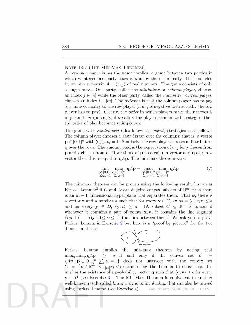
DRAFT

384 18.3. PROOF OF IMPAGLIAZZO’S LEMMA

Note 18.7 (The Min-Max Theorem)A zero sum game is, as the name implies, a game between two parties inwhich whatever one party loses is won by the other party. It is modeledby an m × n matrix A = (ai,j) of real numbers. The game consists of onlya single move. One party, called the minimizer or column player, choosesan index j ∈ [n] while the other party, called the maximizer or row player,chooses an index i ∈ [m]. The outcome is that the column player has to payai,j units of money to the row player (if ai,j is negative then actually the rowplayer has to pay). Clearly, the order in which players make their moves isimportant. Surprisingly, if we allow the players randomized strategies, thenthe order of play becomes unimportant.

The game with randomized (also known as mixed) strategies is as follows.The column player chooses a distribution over the columns; that is, a vectorp ∈ [0, 1]n with

∑ni=1 pi = 1. Similarly, the row player chooses a distribution

q over the rows. The amount paid is the expectation of ai,j for j chosen fromp and i chosen from q. If we think of p as a column vector and q as a rowvector then this is equal to qAp. The min-max theorem says:

minp∈[0,1]n

Σipi=1

maxq∈[0,1]m

Σiqi=1

qAp = maxq∈[0,1]m

Σiqi=1

minp∈[0,1]n

Σipi=1

qAp (7)

The min-max theorem can be proven using the following result, known asFarkas’ Lemma:2 if C and D are disjoint convex subsets of Rm, then thereis an m − 1 dimensional hyperplane that separates them. That is, there isa vector z and a number a such that for every x ∈ C, 〈x, z〉 =

∑i xizi ≤ a

and for every y ∈ D, 〈y, z〉 ≥ a. (A subset C ⊆ Rm is convex ifwhenever it contains a pair of points x,y, it contains the line segmentαx + (1− α)y : 0 ≤ α ≤ 1 that lies between them.) We ask you to proveFarkas’ Lemma in Exercise 2 but here is a “proof by picture” for the twodimensional case:

CD

hyperplane

Farkas’ Lemma implies the min-max theorem by noting thatmaxq minp qAp ≥ c if and only if the convex set D =Ap : p ∈ [0, 1]n

∑i pi = 1 does not intersect with the convex set

C =x ∈ Rm : ∀i∈[m]xi < c

and using the Lemma to show that this

implies the existence of a probability vector q such that 〈q,y〉 ≥ c for everyy ∈ D (see Exercise 3). The Min-Max Theorem is equivalent to anotherwell-known result called linear programming duality, that can also be provedusing Farkas’ Lemma (see Exercise 4). Web draft 2006-09-28 18:09

DRAFT

18.4. ERROR CORRECTING CODES: THE INTUITIVECONNECTION TO HARDNESS AMPLIFICATION 385

18.4 Error correcting codes: the intuitive connec-tion to hardness amplification

Now we construct average-case hard functions using functions that are onlyworst-case hard. To do so, we desire a way to transform any function fto another function g such that if there is a small circuit that computes gapproximately (i.e., correctly outputs g(x) for many x) then there is a smallcircuit that computes f at all points. Taking the contrapositive, we canconclude that if there is no small circuit that computes f then there is nosmall circuit that computes g approximately.

Let us reason abstractly about how to go about the above task.

View a function f : 0, 1n → 0, 1 as its truth table, namely, as astring of length 2n, and view any circuit C for computing this function as adevice that, given any index x ∈ [2n], gives the x’th bit in this string. If thecircuit only computes g on ”average” then this device may be thought of asonly partially correct; it gives the right bit only for many indices x’s, butnot all. Thus we need to show how to turn a partially correct string for ginto a completely correct string for f . This is of course reminiscent of errorcorrecting codes (ECC), but with a distinct twist involving computationalefficiency of decoding, which we will call local decoding.

The classical theory of ECC’s (invented by Shannon in 1949) concerns thefollowing problem. We want to record some data x ∈ 0, 1n on a compactdisk to retrieve at a later date, but that compact disk might scratched andsay 10% of its contents might be corrupted. The idea behind error correctingcodes is to encode x using some redundancy so that such corruptions do notprevent us from recovering x.

The naive idea of redundancy is to introduce repetitions but that doesnot work. For example suppose we repeat each bit three times, in otherwords encode x as the string y = x1x1x1x2x2x2 . . . xnxnxn. But now if thefirst three coordinates of y are corrupted then we cannot recover x1, even ifall other coordinates of y are intact. (Note that the first three coordinatestake only a 1/n 10% fraction of the entire string y.) Clearly, we need asmarter way.

2Many texts use the name Farkas’ Lemma only to denote a special case of the resultstated in Note 18.7. Namely the result that there is a separating hyperplane between anydisjoint sets C,D such that C is a single point and D is a set of the form Ax : ∀ixi > 0for some matrix A.

Web draft 2006-09-28 18:09

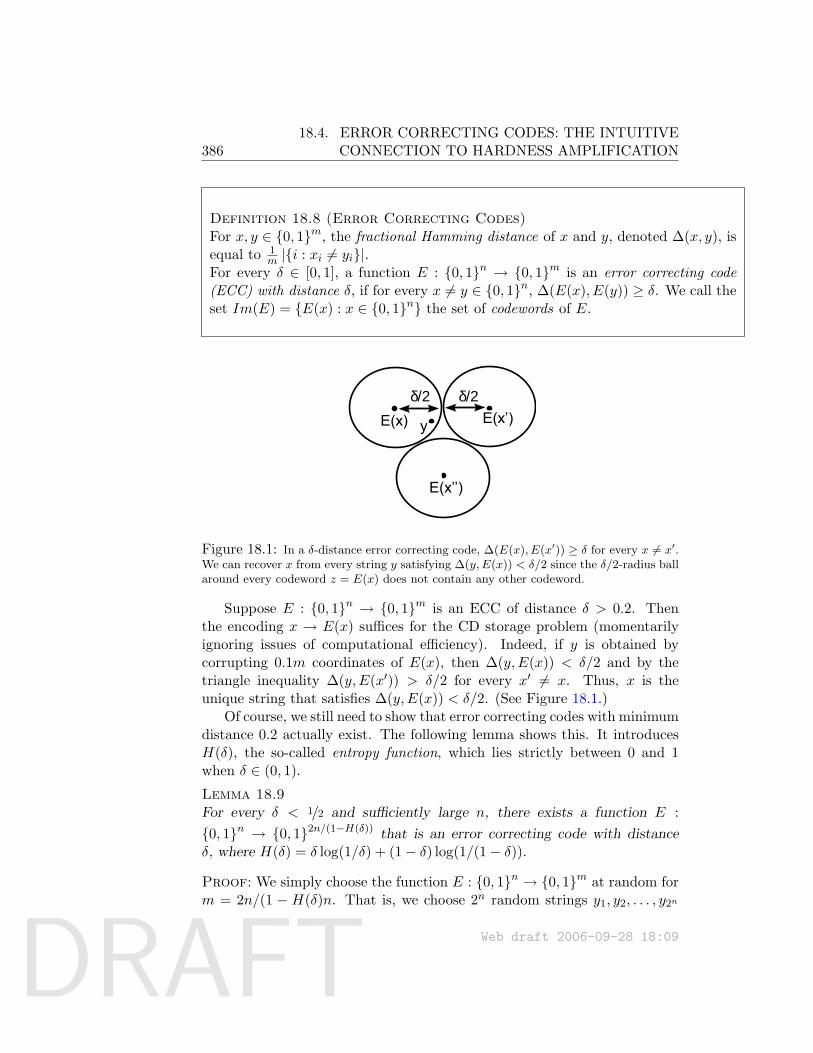
DRAFT

38618.4. ERROR CORRECTING CODES: THE INTUITIVE

CONNECTION TO HARDNESS AMPLIFICATION

Definition 18.8 (Error Correcting Codes)For x, y ∈ 0, 1m, the fractional Hamming distance of x and y, denoted ∆(x, y), isequal to 1

m |i : xi 6= yi|.For every δ ∈ [0, 1], a function E : 0, 1n → 0, 1m is an error correcting code(ECC) with distance δ, if for every x 6= y ∈ 0, 1n, ∆(E(x), E(y)) ≥ δ. We call theset Im(E) = E(x) : x ∈ 0, 1n the set of codewords of E.

δ/2 δ/2E(x) E(x’)

E(x’’)

y

Figure 18.1: In a δ-distance error correcting code, ∆(E(x), E(x′)) ≥ δ for every x 6= x′.We can recover x from every string y satisfying ∆(y,E(x)) < δ/2 since the δ/2-radius ballaround every codeword z = E(x) does not contain any other codeword.

Suppose E : 0, 1n → 0, 1m is an ECC of distance δ > 0.2. Thenthe encoding x → E(x) suffices for the CD storage problem (momentarilyignoring issues of computational efficiency). Indeed, if y is obtained bycorrupting 0.1m coordinates of E(x), then ∆(y,E(x)) < δ/2 and by thetriangle inequality ∆(y,E(x′)) > δ/2 for every x′ 6= x. Thus, x is theunique string that satisfies ∆(y,E(x)) < δ/2. (See Figure 18.1.)

Of course, we still need to show that error correcting codes with minimumdistance 0.2 actually exist. The following lemma shows this. It introducesH(δ), the so-called entropy function, which lies strictly between 0 and 1when δ ∈ (0, 1).

Lemma 18.9For every δ < 1/2 and sufficiently large n, there exists a function E :0, 1n → 0, 12n/(1−H(δ)) that is an error correcting code with distanceδ, where H(δ) = δ log(1/δ) + (1− δ) log(1/(1− δ)).

Proof: We simply choose the function E : 0, 1n → 0, 1m at random form = 2n/(1 − H(δ)n. That is, we choose 2n random strings y1, y2, . . . , y2n

Web draft 2006-09-28 18:09

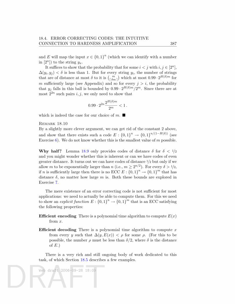
DRAFT


and E will map the input x ∈ 0, 1n (which we can identify with a numberin [2n]) to the string yx.

It suffices to show that the probability that for some i < j with i, j ∈ [2n],∆(yi, yj) < δ is less than 1. But for every string yi, the number of stringsthat are of distance at most δ to it is

(m

d δm e)

which at most 0.99 · 2H(δ)m form sufficiently large (see Appendix) and so for every j > i, the probabilitythat yj falls in this ball is bounded by 0.99 · 2H(δ)m/2m. Since there are atmost 22n such pairs i, j, we only need to show that

0.99 · 22n 2H(δ)m

2m< 1 .

which is indeed the case for our choice of m.

Remark 18.10By a slightly more clever argument, we can get rid of the constant 2 above,and show that there exists such a code E : 0, 1n → 0, 1n/(1−H(δ)) (seeExercise 6). We do not know whether this is the smallest value ofm possible.

Why half? Lemma 18.9 only provides codes of distance δ for δ < 1/2and you might wonder whether this is inherent or can we have codes of evengreater distance. It turns out we can have codes of distance 1/2 but only if weallow m to be exponentially larger than n (i.e., m ≥ 2n/2). For every δ > 1/2,if n is sufficiently large then there is no ECC E : 0, 1n → 0, 1m that hasdistance δ, no matter how large m is. Both these bounds are explored inExercise 7.

The mere existence of an error correcting code is not sufficient for mostapplications: we need to actually be able to compute them. For this we needto show an explicit function E : 0, 1n → 0, 1m that is an ECC satisfyingthe following properties:

Efficient encoding There is a polynomial time algorithm to compute E(x)from x.

Efficient decoding There is a polynomial time algorithm to compute xfrom every y such that ∆(y,E(x)) < ρ for some ρ. (For this to bepossible, the number ρ must be less than δ/2, where δ is the distanceof E.)

There is a very rich and still ongoing body of work dedicated to thistask, of which Section 18.5 describes a few examples.

Web draft 2006-09-28 18:09

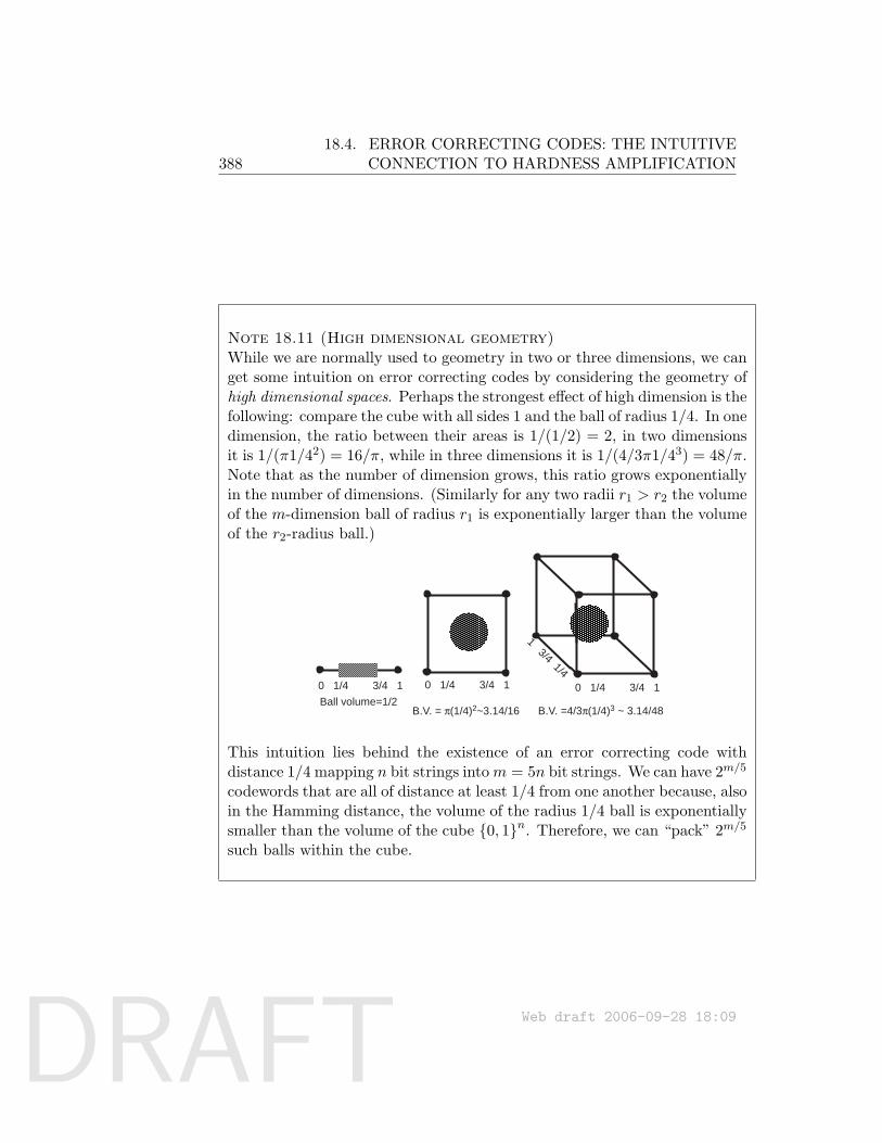
DRAFT



Note 18.11 (High dimensional geometry)While we are normally used to geometry in two or three dimensions, we canget some intuition on error correcting codes by considering the geometry ofhigh dimensional spaces. Perhaps the strongest effect of high dimension is thefollowing: compare the cube with all sides 1 and the ball of radius 1/4. In onedimension, the ratio between their areas is 1/(1/2) = 2, in two dimensionsit is 1/(π1/42) = 16/π, while in three dimensions it is 1/(4/3π1/43) = 48/π.Note that as the number of dimension grows, this ratio grows exponentiallyin the number of dimensions. (Similarly for any two radii r1 > r2 the volumeof the m-dimension ball of radius r1 is exponentially larger than the volumeof the r2-radius ball.)

0 1/4 3/4 1Ball volume=1/2

0 1/4 3/4 1 0 1/4 3/4 1

1 3/4 1/4

B.V. = π(1/4)2~3.14/16 B.V. =4/3π(1/4)3 ~ 3.14/48

This intuition lies behind the existence of an error correcting code withdistance 1/4 mapping n bit strings intom = 5n bit strings. We can have 2m/5

codewords that are all of distance at least 1/4 from one another because, alsoin the Hamming distance, the volume of the radius 1/4 ball is exponentiallysmaller than the volume of the cube 0, 1n. Therefore, we can “pack” 2m/5

such balls within the cube.

Web draft 2006-09-28 18:09

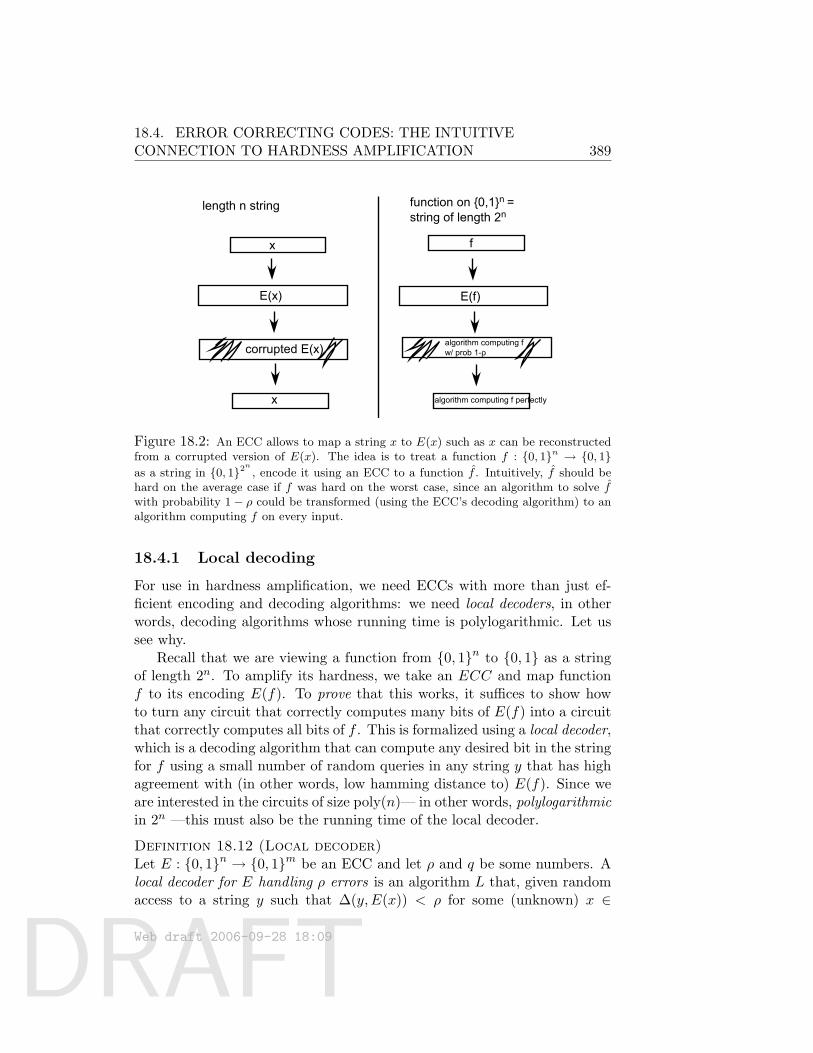
DRAFT


x

E(x)

corrupted E(x)

x

f

E(f)

algorithm computing fw/ prob 1-ρ

length n string function on 0,1n =string of length 2n

algorithm computing f perfectly

Figure 18.2: An ECC allows to map a string x to E(x) such as x can be reconstructedfrom a corrupted version of E(x). The idea is to treat a function f : 0, 1n → 0, 1as a string in 0, 12n

, encode it using an ECC to a function f . Intuitively, f should behard on the average case if f was hard on the worst case, since an algorithm to solve fwith probability 1− ρ could be transformed (using the ECC’s decoding algorithm) to analgorithm computing f on every input.

18.4.1 Local decoding

For use in hardness amplification, we need ECCs with more than just ef-ficient encoding and decoding algorithms: we need local decoders, in otherwords, decoding algorithms whose running time is polylogarithmic. Let ussee why.

Recall that we are viewing a function from 0, 1n to 0, 1 as a stringof length 2n. To amplify its hardness, we take an ECC and map functionf to its encoding E(f). To prove that this works, it suffices to show howto turn any circuit that correctly computes many bits of E(f) into a circuitthat correctly computes all bits of f . This is formalized using a local decoder,which is a decoding algorithm that can compute any desired bit in the stringfor f using a small number of random queries in any string y that has highagreement with (in other words, low hamming distance to) E(f). Since weare interested in the circuits of size poly(n)— in other words, polylogarithmicin 2n —this must also be the running time of the local decoder.

Definition 18.12 (Local decoder)Let E : 0, 1n → 0, 1m be an ECC and let ρ and q be some numbers. Alocal decoder for E handling ρ errors is an algorithm L that, given randomaccess to a string y such that ∆(y,E(x)) < ρ for some (unknown) x ∈

Web draft 2006-09-28 18:09

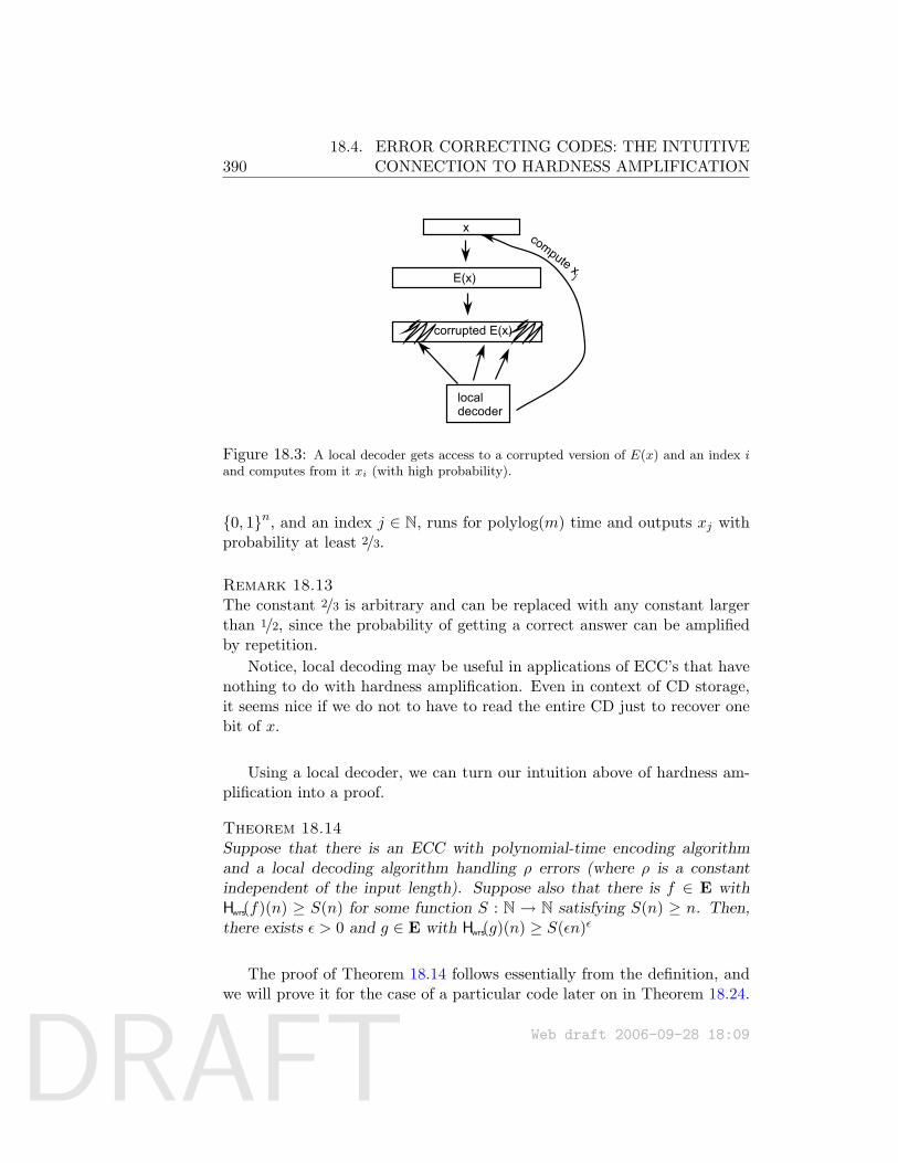
DRAFT



x

E(x)

corrupted E(x)

localdecoder

compute xj

Figure 18.3: A local decoder gets access to a corrupted version of E(x) and an index iand computes from it xi (with high probability).

0, 1n, and an index j ∈ N, runs for polylog(m) time and outputs xj withprobability at least 2/3.

Remark 18.13The constant 2/3 is arbitrary and can be replaced with any constant largerthan 1/2, since the probability of getting a correct answer can be amplifiedby repetition.

Notice, local decoding may be useful in applications of ECC’s that havenothing to do with hardness amplification. Even in context of CD storage,it seems nice if we do not to have to read the entire CD just to recover onebit of x.

Using a local decoder, we can turn our intuition above of hardness am-plification into a proof.

Theorem 18.14Suppose that there is an ECC with polynomial-time encoding algorithmand a local decoding algorithm handling ρ errors (where ρ is a constantindependent of the input length). Suppose also that there is f ∈ E withHwrs(f)(n) ≥ S(n) for some function S : N → N satisfying S(n) ≥ n. Then,there exists ε > 0 and g ∈ E with Hwrs(g)(n) ≥ S(εn)ε

The proof of Theorem 18.14 follows essentially from the definition, andwe will prove it for the case of a particular code later on in Theorem 18.24.

Web draft 2006-09-28 18:09

DRAFT

18.5. CONSTRUCTIONS OF ERROR CORRECTING CODES 391

18.5 Constructions of Error Correcting Codes

We now describe some explicit functions that are error correcting codes,building up to the construction of an explicit ECC of constant distancewith polynomial-time encoding and decoding. Section 18.6 describes localdecoding algorithms for some of these codes.

18.5.1 Walsh-Hadamard Code.

For two strings x, y ∈ 0, 1n, define x y to be the number∑n

i=1 xiyi(mod 2). The Walsh-Hadamard code is the function WH : 0, 1n → 0, 12

n

that maps a string x ∈ 0, 1n into the string z ∈ 0, 12n

where for everyy ∈ 0, 1n, the yth coordinate of z is equal to x y (we identify 0, 1nwith [2n] in the obvious way).

Claim 18.15The function WH is an error correcting code of distance 1/2.

Proof: First, note that WH is a linear function. By this we mean that ifwe take x+ y to be the componentwise addition of x and y modulo 2, thenWH(x+ y) = WH(x)+WH(y). Now, for every x 6= y ∈ 0, 1n we have thatthe number of 1’s in the string WH(x)+WH(y) = WH(x+y) is equal to thenumber of coordinates on which WH(x) and WH(y) differ. Thus, it sufficesto show that for every z 6= 0n, at least half of the coordinates in WH(z) are1. Yet this follows from the random subsum principle (Claim A.3) that saysthat the probability for y ∈R 0, 1n that z y = 1 is exactly 1/2.

18.5.2 Reed-Solomon Code

The Walsh-Hadamard code has a serious drawback: its output size is expo-nential in the input size. By Lemma 18.9 we know that we can do muchbetter (at least if we’re willing to tolerate a distance slightly smaller than1/2). To get towards explicit codes with better output, we need to make adetour to codes with non-binary alphabet.

Definition 18.16For every set Σ and x, y ∈ Σm, we define ∆(x, y) = 1

m |i : xi 6= yi|. We saythat E : Σn → Σm is an error correcting code with distance δ over alphabetΣ if for every x 6= y ∈ Σn, ∆(E(x), E(y)) ≥ δ.

Allowing a larger alphabet makes the problem of constructing codeseasier. For example, every ECC with distance δ over the binary (0, 1)

Web draft 2006-09-28 18:09

DRAFT

392 18.5. CONSTRUCTIONS OF ERROR CORRECTING CODES

alphabet automatically implies an ECC with the same distance over thealphabet 0, 1, 2, 3: just encode strings over 0, 1, 2, 3 as strings over 0, 1in the obvious way. However, the other direction does not work: if we take anECC over 0, 1, 2, 3 and transform it into a code over 0, 1 in the naturalway, the distance might grow from δ to 2δ (Exercise 8).

The Reed-Solomon code is a construction of an error correcting codethat can use as its alphabet any field F:Definition 18.17Let F be a field and n,m numbers satisfying n ≤ m ≤ |F|. The Reed-Solomon code from Fn to Fm is the function RS : Fn → Fm that on inputa0, . . . , an−1 ∈ Fn outputs the string z0, . . . , zm−1 where

zj =n−1∑i=0

aifij

and fj denotes the jth element of F under some ordering.

Lemma 18.18The Reed-Solomon code RS : Fn → Fm has distance 1− n

m .

Proof: As in the case of Walsh-Hadamard code, the function RS is alsolinear in the sense that RS(a+ b) = RS(a) + RS(b) (where addition is takento be componentwise addition in F). Thus, as before we only need to showthat for every a 6= 0n, RS(a) has at most n coordinates that are zero. Butthis immediate from the fact that a nonzero n− 1 degree polynomial has atmost n roots (see appendix).

18.5.3 Concatenated codes

The Walsh-Hadamard code has the drawback of exponential-sized outputand the Reed-Solomon code has the drawback of a non-binary alphabet.We now show we can combine them both to obtain a code without neitherof these drawbacks:Definition 18.19If RS is the Reed-Solomon code mapping Fn to Fm (for some n,m,F) and WH

is the Walsh-Hadamard code mapping 0, 1log |F| to 0, 12log |F|

= 0, 1|F|,then the code WH RS maps 0, 1n log |F| to 0, 1m|F| in the following way:

1. View RS as a code from 0, 1n log |F| to Fm and WH as a code fromF to 0, 1|F| using the canonical representation of elements in F asstrings in 0, 1log |F|.

Web draft 2006-09-28 18:09

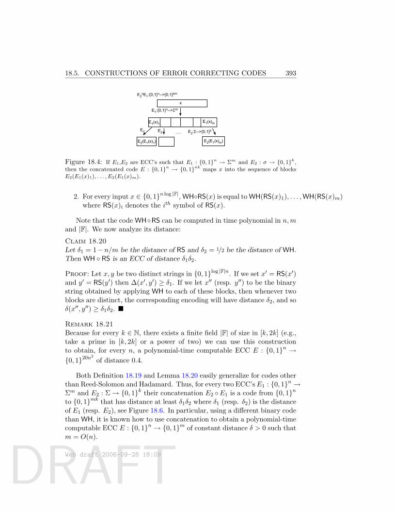
DRAFT


x

E1:0,1n-->Σm

E2 E2 E2:Σ-->0,1k

E2oE1:0,1n-->0,1km

E1(x)1 E1(x)m

.....

E2(E1(x)1) E2(E1(x)m)

Figure 18.4: If E1,E2 are ECC’s such that E1 : 0, 1n → Σm and E2 : σ → 0, 1k,then the concatenated code E : 0, 1n → 0, 1nk maps x into the sequence of blocksE2(E1(x)1), . . . , E2(E1(x)m).

2. For every input x ∈ 0, 1n log |F|, WHRS(x) is equal to WH(RS(x)1), . . . ,WH(RS(x)m)where RS(x)i denotes the ith symbol of RS(x).

Note that the code WHRS can be computed in time polynomial in n,mand |F|. We now analyze its distance:

Claim 18.20Let δ1 = 1−n/m be the distance of RS and δ2 = 1/2 be the distance of WH.Then WH RS is an ECC of distance δ1δ2.

Proof: Let x, y be two distinct strings in 0, 1log |F|n. If we set x′ = RS(x′)and y′ = RS(y′) then ∆(x′, y′) ≥ δ1. If we let x′′ (resp. y′′) to be the binarystring obtained by applying WH to each of these blocks, then whenever twoblocks are distinct, the corresponding encoding will have distance δ2, and soδ(x′′, y′′) ≥ δ1δ2.

Remark 18.21Because for every k ∈ N, there exists a finite field |F| of size in [k, 2k] (e.g.,take a prime in [k, 2k] or a power of two) we can use this constructionto obtain, for every n, a polynomial-time computable ECC E : 0, 1n →0, 120n

2

of distance 0.4.

Both Definition 18.19 and Lemma 18.20 easily generalize for codes otherthan Reed-Solomon and Hadamard. Thus, for every two ECC’s E1 : 0, 1n →Σm and E2 : Σ→ 0, 1k their concatenation E2 E1 is a code from 0, 1nto 0, 1mk that has distance at least δ1δ2 where δ1 (resp. δ2) is the distanceof E1 (resp. E2), see Figure 18.6. In particular, using a different binary codethan WH, it is known how to use concatenation to obtain a polynomial-timecomputable ECC E : 0, 1n → 0, 1m of constant distance δ > 0 such thatm = O(n).

Web draft 2006-09-28 18:09

DRAFT

394 18.5. CONSTRUCTIONS OF ERROR CORRECTING CODES

18.5.4 Reed-Muller Codes.

Both the Walsh-Hadamard and and the Reed-Solomon code are special casesof the following family of codes known as Reed-Muller codes:

Definition 18.22 (Reed-Muller codes)Let F be a finite field, and let `, d be numbers with d < |F|. The Reed Muller

code with parameters F, `, d is the function RM : F(`+dd ) → F|F|` that mapsevery `-variable polynomial P over F of total degree d to the values of P onall the inputs in F`.

That is, the input is a polynomial of the form

g(x1, . . . , x`) =∑

i1+i2+...+i`≤`ci1,...,i`x

i11 x

i22 · · ·x

i``

specified by the vector of(`+dd

)coefficients ci1,...,i` and the output is the

sequence g(x1, . . . , x`) for every x1, . . . , x` ∈ F.

Setting ` = 1 one obtains the Reed-Solomon code (for m = |F|), whilesetting d = 1 and F = GF(2) one obtains a slight variant of the Walsh-Hadamard code. (I.e., the code that maps every x ∈ 0, 1n into the 2 · 2nlong string z such that for every y ∈ 0, 1n,a ∈ 0, 1, zy,a = x y + a(mod 2).)

The Schwartz-Zippel Lemma (Lemma A.23 in the Appendix) shows thatthe Reed-Muller code is an ECC with distance 1 − d/|F|. Note that thisimplies the previously stated bounds for the Walsh-Hadamard and Reed-Solomon codes.

18.5.5 Decoding Reed-Solomon.

To actually use an error correcting code to store and retrieve information,we need a way to efficiently decode a data x from its encoding E(x) even ifE(x) has been corrupted in a fraction ρ of its coordinates. We now show thisfor the Reed-Solomon code, that treats x as a polynomial g, and outputsthe values of this polynomial on m inputs.

We know (see Theorem A.22 in the Appendix) that a univariate degreed polynomial can be interpolated from any d+ 1 values. Here we consider arobust version of this procedure, whereby we wish to recover the polynomialfrom m values of which ρm are “faulty” or “noisy”.

Let (a1, b1), (a2, b2), . . . , (am, bm) be a sequence of (point, value) pairs.We say that a degree d polynomial g(x) describes this (ai, bi) if g(ai) = bi.

Web draft 2006-09-28 18:09

DRAFT


We are interested in determining if there is a degree d polynomial g thatdescribes (1− ρ)m of the pairs. If 2ρm > d then this polynomial is unique(exercise). We desire to recover it, in other words, find a degree d polynomialg such that

g(ai) = bi for at (1− ρ)m least values of i. (8)

The apparent difficulty is in identifying the noisy points; once thosepoints are identified, we can recover the polynomial.

Randomized interpolation: the case of ρ < 1/(d+ 1)

If ρ is very small, say, ρ < 1/(2d) then we can actually use the standardinterpolation technique: just select d + 1 points at random from the set(ai, bi) and use them to interpolate. By the union bound, with probabilityat least 1−ρ(d+1) > 0.4 all these points will be non-corrupted and so we willrecover the correct polynomial. (Because the correct polynomial is unique,we can verify that we have obtained it, and if unsuccessful, try again.)

Berlekamp-Welch Procedure: the case of ρ < (m− d)/(2m)

The Berlekamp-Welch procedure works when the error rate ρ is boundedaway from 1/2; specifically, ρ < (m − d)/(2m). For concreteness, assumem = 4d and ρ = 1/4.

1. We claim that if the polynomial g exists then there is a degree 2dpolynomial c(x) and a degree d nonzero polynomial e(x) such that

c(ai) = bie(ai) for all i. (9)

The reason is that the desired e(x) can be any nonzero degree d poly-nomial whose roots are precisely the ai’s for which g(ai) 6= bi, and thenjust let c(x) = g(x)e(x). (Note that this is just an existence argument;we do not know g yet.))

2. Let c(x) =∑

i≤2d cixi and e(x) =

∑i≤d eix

i. The ei’s and ci’s areour unknowns, and these satisfy 4d linear equations given in (??), onefor each ai. The number of unknowns is 3d + 2, and our existenceargument in part 1 shows that the system is feasible. Solve it usingGaussian elimination to obtain a candidate c, e.

Web draft 2006-09-28 18:09

DRAFT

396 18.6. LOCAL DECODING OF EXPLICIT CODES.

3. Let c, e are any polynomials obtained in part 2. Since they satisfy (9)and bi = g(ai) for at least 3d values of i, we conclude that

c(ai) = g(ai)e(ai) for at least 3d values of i.

Hence c(x) − g(x)e(x) is a degree 2d polynomial that has at least 3droots, and hence is identically zero. Hence e divides c and that in factc(x) = g(x)e(x).

4. Divide c by e to recover g.

18.5.6 Decoding concatenated codes.

Decoding concatenated codes can be achieved through the natural algo-rithm. Recall that if E1 : 0, 1n → Σm and E2 : Σ→ 0, 1k are two ECC’sthen E2E1 maps every string x ∈ 0, 1n to the string E2(E1(x)1) · · ·E2(E1(x)n).Suppose that we have a decoder for E1 (resp. E2) that can handle ρ1 (resp.ρ2) errors. Then, we have a decoder for E2 E1 that can handle ρ2ρ1

errors. The decoder, given a string y ∈ 0, 1mk composed of m blocksy1, . . . , ym ∈ 0, 1k, first decodes each block yi to a symbol zi in Σ, andthen uses the decoder of E1 to decode z1, . . . , zm. The decoder can in-deed handle ρ1ρ2 errors since if ∆(y,E2 E1(x)) ≤ ρ1ρ2 then at most ρ1 ofthe blocks of y are of distance at least ρ2 from the corresponding block ofE2 E1(x).

18.6 Local Decoding of explicit codes.

We now show local decoder algorithm (c.f. Definition 18.12) for severalexplicit codes.

18.6.1 Local decoder for Walsh-Hadamard.

The following is a two-query local decoder for the Walsh-Hadamard codethat handles ρ errors for every ρ < 1/4. This fraction of errors we handle isbest possible, as it can be easily shown that there cannot exist a local (ornon-local) decoder for a binary code handling ρ errors for every ρ ≥ 1/4.

Walsh-Hadamard Local Decoder for ρ < 1/4:

Input: j ∈ [n], random access to a function f : 0, 1n → 0, 1 such thatPry[g(y) 6= x y] ≤ ρ for some ρ < 1/4 and x ∈ 0, 1n.

Web draft 2006-09-28 18:09

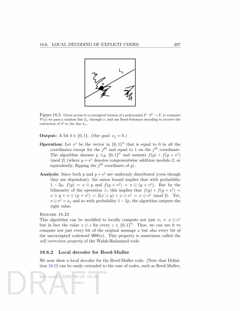
DRAFT

18.6. LOCAL DECODING OF EXPLICIT CODES. 397

Lx

x

Figure 18.5: Given access to a corrupted version of a polynomial P : F` → F, to computeP (x) we pass a random line Lx through x, and use Reed-Solomon decoding to recover therestriction of P to the line Lx.

Output: A bit b ∈ 0, 1. (Our goal: xj = b.)

Operation: Let ej be the vector in 0, 1n that is equal to 0 in all thecoordinates except for the jth and equal to 1 on the jth coordinate.The algorithm chooses y ∈R 0, 1n and outputs f(y) + f(y + ej)(mod 2) (where y + ej denotes componentwise addition modulo 2, orequivalently, flipping the jth coordinate of y).

Analysis: Since both y and y + ej are uniformly distributed (even thoughthey are dependent), the union bound implies that with probability1 − 2ρ, f(y) = x y and f(y + ej) = x (y + ej). But by thebilinearity of the operation , this implies that f(y) + f(y + ej) =x y + x (y + ej) = 2(x y) + x ej = x ej (mod 2). Yet,x ej = xj and so with probability 1− 2ρ, the algorithm outputs theright value.

Remark 18.23This algorithm can be modified to locally compute not just xi = x ej

but in fact the value x z for every z ∈ 0, 1n. Thus, we can use it tocompute not just every bit of the original message x but also every bit ofthe uncorrupted codeword WH(x). This property is sometimes called theself correction property of the Walsh-Hadamard code.

18.6.2 Local decoder for Reed-Muller

We now show a local decoder for the Reed-Muller code. (Note that Defini-tion 18.12 can be easily extended to the case of codes, such as Reed-Muller,

Web draft 2006-09-28 18:09

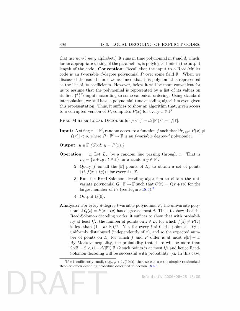
DRAFT


that use non-binary alphabet.) It runs in time polynomial in ` and d, which,for an appropriate setting of the parameters, is polylogarithmic in the outputlength of the code. Convention: Recall that the input to a Reed-Mullercode is an `-variable d-degree polynomial P over some field F. When wediscussed the code before, we assumed that this polynomial is representedas the list of its coefficients. However, below it will be more convenient forus to assume that the polynomial is represented by a list of its values onits first

(d+``

)inputs according to some canonical ordering. Using standard

interpolation, we still have a polynomial-time encoding algorithm even giventhis representation. Thus, it suffices to show an algorithm that, given accessto a corrupted version of P , computes P (x) for every x ∈ F`

Reed-Muller Local Decoder for ρ < (1− d/|F|)/4− 1/|F|.

Input: A string x ∈ F`, random access to a function f such that Prx∈F` [P (x) 6=f(x)] < ρ, where P : F` → F is an `-variable degree-d polynomial.

Output: y ∈ F (Goal: y = P (x).)

Operation: 1. Let Lx, be a random line passing through x. That isLx = x+ ty : t ∈ F for a random y ∈ F`.

2. Query f on all the |F| points of Lx to obtain a set of points(t, f(x+ ty)) for every t ∈ F.

3. Run the Reed-Solomon decoding algorithm to obtain the uni-variate polynomial Q : F→ F such that Q(t) = f(x+ ty) for thelargest number of t’s (see Figure 18.5).3

4. Output Q(0).

Analysis: For every d-degree `-variable polynomial P , the univariate poly-nomial Q(t) = P (x+ ty) has degree at most d. Thus, to show that theReed-Solomon decoding works, it suffices to show that with probabil-ity at least 1/2, the number of points on z ∈ Lx for which f(z) 6= P (z)is less than (1 − d/|F|)/2. Yet, for every t 6= 0, the point x + ty isuniformly distributed (independently of x), and so the expected num-ber of points on Lx for which f and P differ is at most ρ|F| + 1.By Markov inequality, the probability that there will be more than2ρ|F|+2 < (1−d/|F|)|F|/2 such points is at most 1/2 and hence Reed-Solomon decoding will be successful with probability 1/2. In this case,

3If ρ is sufficiently small, (e.g., ρ < 1/(10d)), then we can use the simpler randomizedReed-Solomon decoding procedure described in Section 18.5.5.

Web draft 2006-09-28 18:09

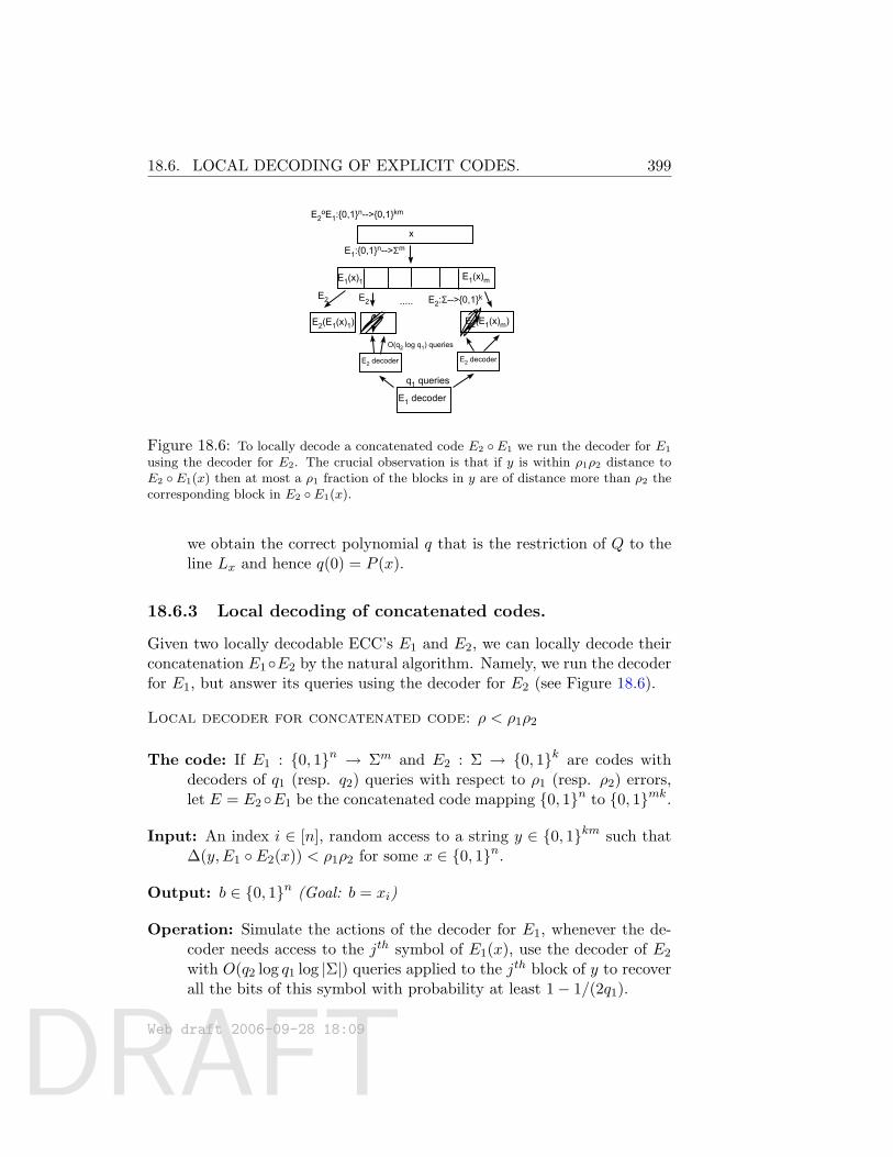
DRAFT


x

E1:0,1n-->Σm

E2 E2 E2:Σ-->0,1k

E2oE1:0,1n-->0,1km

E1(x)1 E1(x)m

.....

E2(E1(x)1) E2(E1(x)m)

E1 decoder

E2 decoder E2 decoder

q1 queries

O(q2 log q1) queries

Figure 18.6: To locally decode a concatenated code E2 E1 we run the decoder for E1

using the decoder for E2. The crucial observation is that if y is within ρ1ρ2 distance toE2 E1(x) then at most a ρ1 fraction of the blocks in y are of distance more than ρ2 thecorresponding block in E2 E1(x).

we obtain the correct polynomial q that is the restriction of Q to theline Lx and hence q(0) = P (x).

18.6.3 Local decoding of concatenated codes.

Given two locally decodable ECC’s E1 and E2, we can locally decode theirconcatenation E1E2 by the natural algorithm. Namely, we run the decoderfor E1, but answer its queries using the decoder for E2 (see Figure 18.6).

Local decoder for concatenated code: ρ < ρ1ρ2

The code: If E1 : 0, 1n → Σm and E2 : Σ → 0, 1k are codes withdecoders of q1 (resp. q2) queries with respect to ρ1 (resp. ρ2) errors,let E = E2E1 be the concatenated code mapping 0, 1n to 0, 1mk.

Input: An index i ∈ [n], random access to a string y ∈ 0, 1km such that∆(y,E1 E2(x)) < ρ1ρ2 for some x ∈ 0, 1n.

Output: b ∈ 0, 1n (Goal: b = xi)

Operation: Simulate the actions of the decoder for E1, whenever the de-coder needs access to the jth symbol of E1(x), use the decoder of E2

with O(q2 log q1 log |Σ|) queries applied to the jth block of y to recoverall the bits of this symbol with probability at least 1− 1/(2q1).

Web draft 2006-09-28 18:09

DRAFT


Analysis: The crucial observation is that at most a ρ1 fraction of the lengthk blocks in y can be of distance more than ρ2 from the correspondingblocks in E2E1(x). Therefore, with probability at least 0.9, all our q1answers to the decoder of E1 are consistent with the answer it wouldreceive when accessing a string that is of distance at most ρ1 from acodeword of E1.

18.6.4 Putting it all together.

We now have the ingredients to prove our second main theorem of thischapter: transformation of a hard-on-the-worst-case function into a functionthat is “mildly” hard on the average case.

Theorem 18.24 (Worst-case hardness to mild hardness)Let S : N→ N and f ∈ E such that Hwrs(f)(n) ≥ S(n) for every n. Then there existsa function g ∈ E and a constant c > 0 such that H0.99

avg (g)(n) ≥ S(n/c)/nc for everysufficiently large n.

Proof: For every n, we treat the restriction of f to 0, 1n as a stringf ′ ∈ 0, 1N where N = 2n. We then encode this string f ′ using a suitableerror correcting code E : 0, 1N → 0, 1N

C

for some constant C > 1. Wewill define the function g on every input x ∈ 0, 1Cn to output the xth

coordinate of E(f ′).4 For the function g to satisfy the conclusion of thetheorem, all we need is for the code E to satisfy the following properties:

1. For every x ∈ 0, 1N , E(x) can be computed in poly(N) time.

2. There is a local decoding algorithm for E that uses polylog(N) runningtime and queries and can handle a 0.01 fraction of errors.

But this can be achieved using a concatenation of a Walsh-Hadamardcode with a Reed-Muller code of appropriate parameters:

1. Let RM denote the Reed-Muller code with the following parameters:

• The field F is of size log5N .

• The number of variables ` is equal to logN/ log logN .4By padding with zeros as necessary, we can assume that all the inputs to g are of

length that is a multiple of C.

Web draft 2006-09-28 18:09

DRAFT


• The degree is equal to log2N .

RM takes an input of length at least (d` )` > N (and so using padding

we can assume its input is 0, 1n). Its output is of size |F|` ≤ poly(n).Its distance is at least 1− 1/ logN .

2. Let WH denote the Walsh-Hadamard code from 0, 1logF = 0, 15 log logN

to 0, 1|F| = 0, 1log5N .

Our code will be WH RM. Combining the local decoders for Walsh-Hadamard and Reed-Muller we get the desired result.

Combining Theorem 18.24 with Yao’s XOR Lemma (Theorem 18.2), weget the following corollary:

Corollary 18.25Let S : N → N and f ∈ E with Hwrs(f)(n) ≥ S(n) for every n. Then, there

exists an S(√`)ε-pseudorandom generator for some constant ε > 0.

Proof: By Theorem 18.24, under this assumption there exists a functiong ∈ E with H0.99

avg (g)(n) ≥ S′(n) = S(n)/poly(n), where we can assumeS′(n) ≥

√S(n) for sufficiently large n (otherwise S is polynomial and the

theorem is trivial). Consider the function g⊕k where k = c logS′(n) for asufficiently small constant c. By Yao’s XOR Lemma, on inputs of lengthkn, it cannot be computed with probability better than 1/2 + 2−cS

′(n)/1000

by circuits of size S′(n). Since S(n) ≤ 2n, kn <√n, and hence we get that

Havg(g⊕k) ≥ Sc/2000.

As already mentioned, this implies the following corollaries:

1. If there exists f ∈ E such that Hwrs(f) ≥ 2nΩ(1)

then BPP ⊆ QuasiP.

2. If there exists f ∈ E such that Hwrs(f) ≥ nω(1) then BPP ⊆ SUBEXP.

However, Corollary 18.25 is still not sufficient to show that BPP = Punder any assumption on the worst-case hardness of some function in E. Itonly yields an S(

√`)Ω(1)-pseudorandom generator, while what we need is an

S(Ω(`))Ω(1)-pseudorandom generator.

Web draft 2006-09-28 18:09

DRAFT

402 18.7. LIST DECODING

18.7 List decoding

Our approach to obtain stronger worst-case to average-case reduction willbe to bypass the XOR Lemma, and use error correcting codes to get di-rectly from worst-case hardness to a function that is hard to compute withprobability slightly better than 1/2. However, this idea seems to run into afundamental difficulty: if f is worst-case hard, then it seems hard to arguethat the encoding of f , under any error correcting code is hard to computewith probability 0.6. The reason is that any error-correcting code has tohave distant at most 1/2, which implies that there is no decoding algorithmthat can recover x from E(x) if the latter was corrupted in more than a1/4 of its locations. Indeed, in this case there is not necessarily a uniquecodeword closest to the corrupted word. For example, if E(x) and E(x′)are two codewords of distance 1/2, let y be the string that is equal to E(x)on the first half of the coordinates and equal to E(x′) on the second half.Given y, how can a decoding algorithm know whether to return x or x′?

This seems like a real obstacle, and indeed was considered as such inmany contexts where ECC’s were used, until the realization of the impor-tance of the following insight: “If y is obtained by corrupting E(x) in, say,a 0.4 fraction of the coordinates (where E is some ECC with good enoughdistance) then, while there may be more than one codeword within distance0.4 to y, there can not be too many such codewords.”

Theorem 18.26 (Johnson Bound)If E : 0, 1n → 0, 1m is an ECC with distance at least 1/2 − ε, then forevery x ∈ 0, 1m, and δ ≥

√ε, there exist at most 1/(2δ2) vectors y1, . . . , y`

such that ∆(x, yi) ≤ 1/2− δ for every i ∈ [`].

Proof: Suppose that x, y1, . . . , y` satisfy this condition, and define ` vectorsz1, . . . , z` in Rm as follows: for every i ∈ [`] and k ∈ [m], set zi,k to equal+1 if yk = xk and set it to equal −1 otherwise. Under our assumptions, forevery i ∈ [`],

m∑k=1

zi,k ≥ 2δm , (10)

since zi agrees with x on an 1/2 + δ fraction of its coordinates. Also, forevery i 6= j ∈ [`],

〈zi, zj〉 =m∑k=1

zi,kzj,k ≤ 2εm ≤ 2δ2m (11)

Web draft 2006-09-28 18:09

DRAFT

18.7. LIST DECODING 403

since E is a code of distance at least 1/2 − ε. We will show that (10) and(11) together imply that ` ≤ 1/(2δ2).

Indeed, set w =∑`

i=1 zi. On one hand, by (11)

〈w,w〉 =∑i=1

〈zi, zi〉+∑i6=j〈zi, zj〉 ≤ `m+ `22δ2m.

On the other hand, by (10),∑

k wk =∑

i,j zi,j ≥ 2δm` and hence

〈w,w〉 ≥ |∑k

wk|2/m ≥ 4δ2m`2 ,

since for every c, the vector w ∈ Rm with minimal two-norm satisfying∑k wk = c is the uniform vector (c/m, c/m, . . . , c/m). Thus 4δ2m`2 ≤

`m+ 2`2δ2m, implying that ` ≤ 1/(2δ2).

18.7.1 List decoding the Reed-Solomon code

In many contexts, obtaining a list of candidate messages from a corruptedcodeword can be just as good as unique decoding. For example, we may havesome outside information on which messages are likely to appear, allowingus to know which of the messages in the list is the correct one. However,to take advantage of this we need an efficient algorithm that computes thislist. Such an algorithm was discovered in 1996 by Sudan for the popularand important Reed-Solomon code. It can recover a polynomial size list ofcandidate codewords given a Reed-Solomon codeword that was corrupted inup to a 1 − 2

√d/|F| fraction of the coordinates. Note that this tends to 1

as |F|/d grows, whereas the Berlekamp-Welch unique decoding algorithm ofSection 18.5.5 gets “stuck” when the fraction of errors surpasses 1/2.

On input a set of data points (ai, bi)mi=1 in F2, Sudan’s algorithm re-turns all degree d polynomials g such that the number of i’s for whichg(ai) = bi is at least 2

√d/|F|m. It relies on the following observation:

Lemma 18.27For every set of m data pairs (a1, b1), . . . , (am, bm), there is a bivariate poly-nomial Q(z, x) of degree at most d

√me+1 in z and x such that Q(bi, ai) = 0

for each i = 1, . . . ,m. Furthermore, there is a polynomial-time algorithm toconstruct such a Q.

Web draft 2006-09-28 18:09

DRAFT

404 18.8. LOCAL LIST DECODING: GETTING TO BPP = P.

Proof: Let k = d√me + 1. Then the unknown bivariate polynomial

Q =∑k

i=0

∑kj=0Qijz

ixj has (k + 1)2 coefficients and these coefficients arerequired to satisfy m linear equations of the form:

k∑i=0

k∑j=0

Qij(bt)i(at)j for t = 1, 2, . . . ,m.

Note that the at’s, bt’s are known and so we can write down these equations.Since the system is homogeneous and the number of unknowns exceeds

the number of constraints, it has a nonzero solution. Furthermore this so-lution can be found in polynomial time.

Lemma 18.28Let d be any integer and k > (d + 1)(d

√me + 1). If p(x) is a degree d

polynomial that describes k of the data pairs, then z − p(x) divides thebivariate polynomial Q(z, x) described in Lemma 18.27.

Proof: By construction, Q(bt, at) = 0 for every data pair (at, bt). If p(x)describes this data pair, then Q(p(at), at) = 0. We conclude that the uni-variate polynomial Q(p(x), x) has at least k roots, whereas its degree isd(d√ne + 1) < k. Hence Q(p(x), x) = 0. By the division algorithm for

polynomials, Q(p(x), x) is exactly the remainder when Q(z, x) is divided by(z − p(x)). We conclude that z − p(x) divides Q(z, x).

Now it is straightforward to describe Sudan’s list decoding algorithm.First, find Q(z, x) by the algorithm of Lemma 18.27. Then, factor it usinga standard algorithm for bivariate factoring (see [VG99]). For every factorof the form (z − p(x)), check by direct substitution whether or not p(x)describes 2

√d/|F|m data pairs. Output all such polynomials.

18.8 Local list decoding: getting to BPP = P.

Analogously to Section 18.4.1, to actually use list decoding for hardnessamplification, we need to provide local list decoding algorithms for the codeswe use. Fortunately, such algorithms are known for the Walsh-Hadamardcode, the Reed-Muller code, and their concatenation.

Definition 18.29 (Local list decoder)Let E : 0, 1n → 0, 1m be an ECC and let ρ > 0 and q be some numbers.An algorithm L is called a local list decoder for E handling ρ errors, if forevery x ∈ 0, 1n and y ∈ 0, 1m satisfying ∆(E(x), y) ≤ ρ, there exists a

Web draft 2006-09-28 18:09

DRAFT

18.8. LOCAL LIST DECODING: GETTING TO BPP = P. 405

number i0 ∈ [poly(n/ε)] such that for every j ∈ [m], on inputs i0, j and withrandom access to y, L runs for poly(log(m)/ε) time and outputs xj withprobability at least 2/3.

Remark 18.30One can think of the number i0 as the index of x in the list of poly(n/ε)candidate messages output by L. Definition 18.29 can be easily generalizedto codes with non-binary alphabet.

18.8.1 Local list decoding of the Walsh-Hadamard code.

It turns out we already encountered a local list decoder for the Walsh-Hadamard code: the proof of the Goldreich-Levin Theorem (Theorem 10.14)provided an an algorithm that given access to a “black box” that computesthe function y 7→ xy (for x, y ∈ 0, 1n) with probability 1/2+ ε, computesa list of values x1, . . . , xpoly(n/ε) such that xi0 = x for some i0. In thecontext of that theorem, we could find the right value of x from that list bychecking it against the value f(x) (where f is a one-way permutation). Thisis a good example for how once we have a list decoding algorithm, we canuse outside information to narrow the list down.

18.8.2 Local list decoding of the Reed-Muller code

We now present an algorithm for local list decoding of the Reed-Muller code.Recall that the codeword of this code is the list of evaluations of a d-degree`-variable polynomial P : F` → F. The local decoder for Reed-Muller getsrandom access to a corrupted version of P and two inputs: an index i andx ∈ F`. Below we describe such a decoder that runs in poly(d, `, |F|) andoutputs P (x) with probability at least 0.9 assuming that i is equal to the“right” index i0. Note: To be a valid local list decoder, given the index i0,the algorithm should output P (x) with high probability for every x ∈ F`.The algorithm described below is only guaranteed to output the right valuefor most (i.e., a 0.9 fraction) of the x’s in F`. We transform this algorithm toa valid local list decoder by combining it with the Reed-Muller local decoderdescribed in Section 18.6.2.

Reed-Muller Local List Decoder for ρ < 1− 10√d/|F|

Inputs: • Random access to a function f such that Prx∈F` [P (x) =f(x)] > 10

√d/|F| where P : F` → F is an `-variable d-degree

polynomial. We assume |F| > d4 and that both d > 1000. (Thiscan always be ensured in our applications.)

Web draft 2006-09-28 18:09

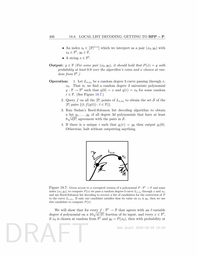
DRAFT


• An index i0 ∈ [|F|`+1] which we interpret as a pair (x0, y0) withx0 ∈ F`, y0 ∈ F,

• A string x ∈ F`.

Output: y ∈ F (For some pair (x0, y0), it should hold that P (x) = y withprobability at least 0.9 over the algorithm’s coins and x chosen at ran-dom from F`.)

Operation: 1. Let Lx,x0 be a random degree 3 curve passing through x,x0. That is, we find a random degree 3 univariate polynomialq : F → F` such that q(0) = x and q(r) = x0 for some randomr ∈ F. (See Figure 18.7.)

2. Query f on all the |F| points of Lx,x0 to obtain the set S of the|F| pairs (t, f(q(t)) : t ∈ F).

3. Run Sudan’s Reed-Solomon list decoding algorithm to obtaina list g1, . . . , gk of all degree 3d polynomials that have at least8√d|F| agreement with the pairs in S.

4. If there is a unique i such that gi(r) = y0 then output gi(0).Otherwise, halt without outputting anything.

Lx,x0

x

x0

Figure 18.7: Given access to a corrupted version of a polynomial P : F` → F and someindex (x0, y0), to compute P (x) we pass a random degree-3 curve Lx,x0 through x and x0,and use Reed-Solomon list decoding to recover a list of candidates for the restriction of Pto the curve Lx,x0 . If only one candidate satisfies that its value on x0 is y0, then we usethis candidate to compute P (x).

We will show that for every f : F` → F that agrees with an `-variabledegree d polynomial on a 10

√d/|F| fraction of its input, and every x ∈ F`,

if x0 is chosen at random from F` and y0 = P (x0), then with probability at

Web draft 2006-09-28 18:09

DRAFT


least 0.9 (over the choice of x0 and the algorithm’s coins) the above decoderwill output P (x). By a standard averaging argument, this implies that thereexist a pair (x0, y0) such that given this pair, the algorithm outputs P (x)for a 0.9 fraction of the x’s in F`.

Let x ∈ F`, if x0 is chosen randomly in F` and y0 = P (x0) then thefollowing

For every x ∈ F`, the following fictitious algorithm can be easily seento have an identical output to the output of our decoder on the inputs x, arandom x0 ∈R F` and y0 = P (x0):

1. Choose a random degree 3 curve L that passes through x. That is,L = q(t) : t ∈ F where q : F → F` is a random degree 3 polynomialsatisfying q(0) = x.

2. Obtain the list g1, . . . , gm of all univariate polynomials over F suchthat for every i, there are at least 6

√d|F| values of t such that gi(t) =

f(q(t)).

3. Choose a random r ∈ F. Assume that you are given the value y0 =P (q(r)).

4. If there exists a unique i such that gi(r) = y0 then output gi(0).Otherwise, halt without an input.

Yet, this fictitious algorithm will output P (x) with probability at least0.9. Indeed, since all the points other than x on a random degree 3 curvepassing through x are pairwise independent, Chebyshev’s inequality impliesthat with probability at least 0.99, the function f will agree with the poly-nomial P on at least 8

√d|F| points on this curve (this uses the fact that√

d/|F| is smaller than 10−6). Thus the list g1, . . . , gm we obtain in Step 2contains the polynomial g : F→ F defined as g(t) = P (q(t)). We leave it asExercise 9 to show that there can not be more than

√|F |/4d polynomials in

this list. Since two 3d-degree polynomials can agree on at most 3d+1 points,

with probability at least (3d+1)√|F |/4d

|F| < 0.01, if we choose a random r ∈ F,then g(r) 6= gi(r) for every gi 6= g in this list. Thus, with this probability,we will identify the polynomial g and output the value g(0) = P (x).

18.8.3 Local list decoding of concatenated codes.

If E1 : 0, 1n → Σm and E2 : Σ → 0, 1k are two codes that are locallylist decodable then so is the concatenated code E2 E1 : 0, 1n → 0, 1mk.

Web draft 2006-09-28 18:09

DRAFT


As in Section 18.6.3, the idea is to simply run the local decoder for E1 whileanswering its queries using the decoder of E2. More concretely, assume thatthe decoder for E1 takes an index in the set I1, uses q1 queries, and canhandle 1 − ε1 errors, and that I2, q2 and ε2 are defined analogously. Ourdecoder for E2 E1 will take a pair of indices i1 ∈ I1 and i2 ∈ I2 and run thedecoder for E1 with the index i1, and whenever this decoder makes a queryanswer it using the decoder E2 with the index i2. (See Section 18.6.3.) Weclaim that this decoder can handle 1/2 − ε1ε2|I2| number of errors. Indeed,if y agrees with some codeword E2 E1(x) on an ε1ε2|I2| fraction of thecoordinates then there are ε1|I2| blocks on which it has at least 1/2 + ε2agreement with the blocks this codeword. Thus, by an averaging argument,there exists an index i2 such that given i2, the output of the E2 decoderagrees with E1(x) on ε1 symbols, implying that there exists an index i1 suchthat given (i1, i2) and every coordinate j, the combined decoder will outputxj with high probability.

18.8.4 Putting it all together.

As promised, we can use local list decoding to transform a function thatis merely worst-case hard into a function that cannot be computed withprobability significantly better than 1/2:

Theorem 18.31 (Worst-case hardness to strong hardness)Let S : N→ N and f ∈ E such that Hwrs(f)(n) ≥ S(n) for every n. Then there exists

a function g ∈ E and a constant c > 0 such that Havg(g)(n) ≥ S(n/c)1/c for everysufficiently large n.

Proof sketch: As in Section 18.6.4, for every n, we treat the restrictionof f to 0, 1n as a string f ′ ∈ 0, 1N where N = 2n and encode it usingthe concatenation of a Reed-Muller code with the Walsh-Hadamard code.For the Reed-Muller code we use the following parameters:

• The field F is of size S(n)1/100. 5

• The degree d is of size log2N .

5We assume here that S(n) > logN1000 and that it can be computed in 2O(n) time.These assumptions can be removed by slightly complicating the construction (namely,executing it while guessing that S(n) = 2k, and concatenating all the results.)

Web draft 2006-09-28 18:09

DRAFT


• The number of variables ` is 2 logN/ logS(n).

The function g is obtained by applying this encoding to f . Given acircuit of size S(n)1/100 that computes g with probability better than 1/2 +1/S(n)1/50, we will be able to transform it, in S(n)O(1) time, to a circuitcomputing f perfectly. We hardwire the index i0 to this circuit as part ofits description.


• Yao’s XOR Lemma allows to amplify hardness by transforming a Booleanfunction with only mild hardness (cannot be computed with say 0.99 success)into a Boolean function with strong hardness (cannot be computed with 0.51success).

• An error correcting code is a function that maps every two strings into a pairof strings that differ on many of their coordinates. An error correcting codewith a local decoding algorithm can be used to transform a function hard inthe worst-case into a function that is mildly hard on the average case.

• A code over the binary alphabet can have distance at most 1/2. A code withdistance δ can be uniquely decoded up to δ/2 errors. List decoding allows toa decoder to handle almost a δ fraction of errors, at the expense of returningnot a single message but a short list of candidate messages.

• We can transform a function that is merely hard in the worst case to a functionthat is strongly hard in the average case using the notion of local list decodingof error correcting codes.


many attributions still missing.

Impagliazzo and Wigderson [IW01] were the first to prove that BPP = Pif there exists f ∈ E such that Hwrs(f) ≥ 2Ω(n) using a derandomized version ofYao’s XOR Lemma. However, the presentation here follows Sudan, Trevisan,and Vadhan [STV], who were the first to point the connection between locallist decoding and hardness amplification, and gave (a variant of) the Reed-Muller local list decoding algorithm described in Section 18.8. They alsoshowed a different approach to achieve the same result, by first showing

Web draft 2006-09-28 18:09

DRAFT


that the NW generator and a mildly hard function can be used to obtainfrom a short random seed a distribution that has high pseudoentropy, whichis then converted to a pseudorandom distribution via a randomness extractor(see Chapter 17).

The question raised in Problem 5 is treated in O’Donnell [O’D04], wherea hardness amplification lemma is given for NP. For a sharper result, seeHealy, Vadhan, and Viola [HVV04].

Exercises

§1 Let X1, . . . , Xn be independent random variables such that Xi is equalto 1 with probability 1 − δ and equal to 0 with probability δ. LetX =

∑ki=1Xi (mod 2). Prove that Pr[X = 1] = 1/2 + (1− 2δ)k.

Hint:DefineYi=(−1)Xi

andY=∏ki=1Yi.Then,usethefact

thattheexpectationofaproductofindependentrandomvariablesistheproductoftheirexpectations.

§2 Prove Farkas’ Lemma: if C,D ⊆ Rm are two convex sets then thereexists a vector z ∈ Rm and a number a ∈ R such that

x ∈ C ⇒ 〈x, z〉 ≥ ay ∈ D ⇒ 〈y, z〉 ≤ a

Hint:StartbyprovingthisinthecasethatCandDareε-separated,whichmeansthatforsomeε>0,‖x−y‖2≥εforeveryx∈Candy∈D.Inthiscaseyoucantakeztobetheshortestvectoroftheformx−yforx∈Candy∈D.

§3 Prove the Min-Max Theorem (see Note 18.7) using Farkas’ Lemma.

§4 Prove the duality theorem for linear programming using Farkas’ Lemma.That is, prove that for every m × n matrix A, and vectors c ∈ Rn,b ∈ Rn,

maxx∈Rns.t.Ax≤bx≥0

〈x, c〉 = miny∈Rms.t.A†y≥cy≥0

〈y,b〉

where A† denotes the transpose of A and for two vectors u,v we saythat u ≥ v if ui ≥ vi for every i.

Web draft 2006-09-28 18:09

DRAFT


§5 Suppose we know that NP contains a function that is weakly hard forall polynomial-size circuits. Can we use the XOR Lemma to infer theexistence of a strongly hard function in NP? Why or why not?

§6 For every δ < 1/2 and sufficiently large n, prove that there exists afunction E : 0, 1n → 0, 1n/(1−H(δ)) that is an error correcting codewith distance δ, where H(δ) = δ log(1/δ) + (1− δ) log(1/(1− δ)).

Hint:Useagreedystrategy,toselectthecodewordsofEonebyone,neveraddingacodewordthatiswithindistanceδtopreviousones.Whenwillyougetstuck?

§7 Show that for every E : 0, 1n → 0, 1m that is an error correctingcode of distance 1/2, 2n < 10

√n. Show if E is an error correcting code

of distance δ > 1/2, then 2n < 10/(δ − 1/2).

§8 Let E : 0, 1n → 0, 1m be a δ-distance ECC. Transform E to a codeE′ : 0, 1, 2, 3n/2 → 0, 1, 2, 3m/2 in the obvious way. Show that E′

has distance δ. Show that the opposite direction is not true: show anexample of a δ-distance ECC E′ : 0, 1, 2, 3n/2 → 0, 1, 2, 3m/2 suchthat the corresponding binary code has distance 2δ.

§9 Let f :F → F be any function. Suppose integer d ≥ 0 and number εsatisfy ε > 2

√d|F| . Prove that there are at most 2/ε degree d polyno-

mials that agree with f on at least an ε fraction of its coordinates.

Hint:ThefirstpolynomialdescribesfinanεfractionofpointssayS1,thesecondpolynomialdescribesfinε−d/|F|fractionofpointsS2whereS1∩S2=∅,etc.

§10 (Linear codes) We say that an ECC E : 0, 1n → 0, 1m is linear iffor every x, x′ ∈ 0, 1n, E(x + x′) = E(x) + E(x′) where + denotescomponentwise addition modulo 2. A linear ECC E can be describedby an m × n matrix A such that (thinking of x as a column vector)E(x) = Ax for every x ∈ 0, 1n.

(a) Prove that the distance of a linear ECC E is equal to the mini-mum over all nonzero x ∈ 0, 1n of the fraction of 1’s in E(x).

(b) Prove that for every δ > 0, there exists a linear ECC E : 0, 1n →0, 11.1n/(1−H(δ)) with distance δ, where H(δ) = δ log(1/δ)+(1−δ) log(1/(1− δ))¿

Web draft 2006-09-28 18:09

DRAFT


Hint:Usetheprobabilisticmethod-showthisholdsforarandommatrix.

(c) Prove that for some δ > 0 there is an ECC E : 0, 1n →0, 1poly(n) of distance δ with polynomial-time encoding and de-coding mechanisms. (You need to know about the field GF(2k)to solve this, see the appendix.)

Hint:UsetheconcatenationofReed-SolomonoverGF(2k)with

theWalsh-Hadamardcode.

(d) We say that a linear code E : 0, 1n → 0, 1m is ε-biased iffor every non-zero x ∈ 0, 1n, the fraction of 1’s in E(x) isbetween 1/2 − ε and 1/2 + ε. Prove that for every ε > 0, thereexists an ε-biased linear code E : 0, 1n → 0, 1poly(n/ε) witha polynomial-time encoding algorithm.

Web draft 2006-09-28 18:09

DRAFT

Chapter 19

PCP and Hardness ofApproximation

“...most problem reductions do not create or preserve suchgaps...To create such a gap in the generic reduction (cf.Cook)...also seems doubtful. The intuitive reason is that compu-tation is an inherently unstable, non-robust mathematical object,in the the sense that it can be turned from non-accepting to ac-cepting by changes that would be insignificant in any reasonablemetric.”Papadimitriou and Yannakakis, 1991 [PY91]

The PCP Theorem provides an interesting new characterization for NP,as the set of languages that have a “locally testable” membership proof. Itis reminiscent of —and was motivated by— results such as IP =PSPACE.Its essence is the following:

Suppose somebody wants to convince you that a Boolean formula issatisfiable. He could present the usual certificate, namely, a satisfying as-signment, which you could then check by substituting back into the formula.However, doing this requires reading the entire certificate. The PCP The-orem shows an interesting alternative: this person can easily rewrite hiscertificate so you can verify it by probabilistically selecting a constant num-ber of locations—as low as 3 bits— to examine in it. Furthermore, thisprobabilistic verification has the following properties: (1) A correct certifi-cate will never fail to convince you (that is, no choice of your random coinswill make you reject it) and (2) If the formula is unsatisfiable, then you areguaranteed to reject every claimed certificate with high probability.


413

DRAFT

414

Of course, since Boolean satisfiability is NP-complete, every other NPlanguage can be deterministically and efficiently reduced to it. Thus thePCP Theorem applies to every NP language. We mention one counterin-tuitive consequence. Let A be any one of the usual axiomatic systems ofmathematics for which proofs can be verified by a deterministic TM in timethat is polynomial in the length of the proof. Recall the following languageis in NP:

L = 〈ϕ, 1n〉 : ϕ has a proof in A of length ≤ n .

The PCP Theorem asserts that L has probabilistically checkable certifi-cates. Such certificate can be viewed as an alternative notion of “proof” formathematical statements that is just as valid as the usual notion. However,unlike standard mathematical proofs, where every line of the proof has tobe checked to verify its validity, this new notion guarantees that proofs areprobabilistically checkable by examining only a constant number of bits inthem1.

This new, “robust” notion of certificate/proof has an important con-sequence: it implies that many optimization problems are NP-hard notonly to solve exactly but even to approximate. As mentioned in Chapter 2,the P versus NP question is practically important —as opposed to “just”philosophically important— because thousands of real-life combinatorial op-timization problems are NP-hard. By showing that even computing approx-imate solutions to many of these problems is NP-hard, the PCP Theoremextends the practical importance of the theory of NP-completeness, as wellas its philosophical significance.

This seemingly mysterious connection between the PCP Theorem —which concerns probabilistic checking of certificates— and the NP-hardnessof computing approximate solutions is actually quite straightforward. AllNP-hardness results ultimately derive from the Cook-Levin theorem (Sec-tion 2.3.1), which expresses accepting computations of a nondeterministicTuring Machine with satisfying assignments to a Boolean formula. Unfor-tunately, the standard representations of computation are quite nonrobust,meaning that they can be incorrect if even one bit is incorrect (see the quoteat the start of this chapter). The PCP Theorem, by giving a robust repre-sentation of the certificate for NP languages, allow new types of reductions;see Section 19.2.3.

Below, we use the term “PCP Theorems” for the body of other resultsof a similar nature to the PCP Theorem that found numerous applications

1One newspaper article about the discovery of the PCP Theorem carried the headline“New shortcut found for long math proofs!”

Web draft 2006-09-28 18:09

DRAFT

19.1. PCP AND LOCALLY TESTABLE PROOFS 415

in complexity theory. Some important ones appear in the next Chapter, in-cluding one that improves the PCP Theorem so that verification is possibleby reading only 3 bits in the proof!

19.1 PCP and Locally Testable Proofs

According to our usual definition, language L is in NP if there is a poly-time Turing machine V (“verifier”) that, given input x, checks certificates(or membership proofs) to the effect that x ∈ L. This means,

x ∈ L⇒ ∃π s.t. V π(x) = 1x /∈ L⇒ ∀π V π(x) = 0,

where V π denotes “a verifier with access to certificate π”.The class PCP (short for “Probabilistically Checkable Proofs”) is a gen-

eralization of this notion, with the following changes. First, the verifier isprobabilistic. Second, the verifier has random access to the proof string Π.This means that each bit of the proof string can be independently queriedby the verifier via a special address tape: if the verifier desires say the ithbit in the proof string, it writes i on the address tape and then receives thebit π[i].2 (This is reminiscent of oracle TMs introduced in Chapter 4.) Thedefinition of PCP treats queries to the proof as a precious resource, to beused sparingly. Note also that since the address size is logarithmic in theproof size, this model in principle allows a polynomial-time verifier to checkmembership proofs of exponential size.

Verifiers can be adaptive or nonadaptive. A nonadaptive verifier selectsits queries based only on its input and random tape, whereas an adaptiveverifier can in addition rely upon bits it has already queried in π to select itsnext queries. We restrict verifiers to be nonadaptive, since most PCP The-orems can be proved using nonadaptive verifiers. (But Exercise 3 exploresthe power of adaptive queries.)

Definition 19.1 ((r, q)-verifier)Let L be a language and q, r : N → N. We say that L has an (r(n), q(n))-verifier if there’s a polynomial-time probabilistic algorithm V satisfying:

Efficiency: On input a string x ∈ 0, 1n and given random access to astring π ∈ 0, 1∗ (which we call the proof ), V uses at most r(n)

2Though widely used, the term “random access” is misleading since it doesn’t involveany notion of randomness per se. “Indexed access” would be more accurate.

Web draft 2006-09-28 18:09

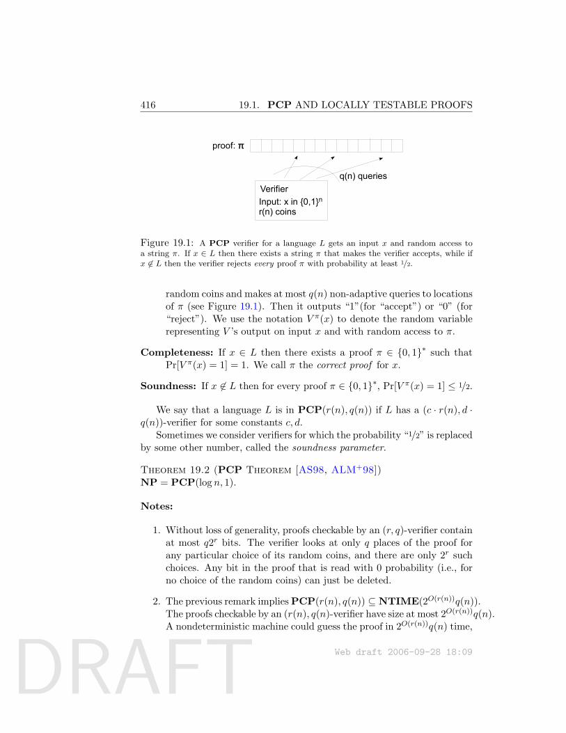
DRAFT

416 19.1. PCP AND LOCALLY TESTABLE PROOFS

VerifierInput: x in 0,1nr(n) coins

q(n) queries

proof: π

Figure 19.1: A PCP verifier for a language L gets an input x and random access toa string π. If x ∈ L then there exists a string π that makes the verifier accepts, while ifx 6∈ L then the verifier rejects every proof π with probability at least 1/2.

random coins and makes at most q(n) non-adaptive queries to locationsof π (see Figure 19.1). Then it outputs “1”(for “accept”) or “0” (for“reject”). We use the notation V π(x) to denote the random variablerepresenting V ’s output on input x and with random access to π.

Completeness: If x ∈ L then there exists a proof π ∈ 0, 1∗ such thatPr[V π(x) = 1] = 1. We call π the correct proof for x.

Soundness: If x 6∈ L then for every proof π ∈ 0, 1∗, Pr[V π(x) = 1] ≤ 1/2.

We say that a language L is in PCP(r(n), q(n)) if L has a (c · r(n), d ·q(n))-verifier for some constants c, d.

Sometimes we consider verifiers for which the probability “1/2” is replacedby some other number, called the soundness parameter.

Theorem 19.2 (PCP Theorem [AS98, ALM+98])NP = PCP(log n, 1).

Notes:

1. Without loss of generality, proofs checkable by an (r, q)-verifier containat most q2r bits. The verifier looks at only q places of the proof forany particular choice of its random coins, and there are only 2r suchchoices. Any bit in the proof that is read with 0 probability (i.e., forno choice of the random coins) can just be deleted.

2. The previous remark implies PCP(r(n), q(n)) ⊆ NTIME(2O(r(n))q(n)).The proofs checkable by an (r(n), q(n)-verifier have size at most 2O(r(n))q(n).A nondeterministic machine could guess the proof in 2O(r(n))q(n) time,

Web draft 2006-09-28 18:09

DRAFT

19.1. PCP AND LOCALLY TESTABLE PROOFS 417

and verify it deterministically by running the verifier for all 2O(r(n))

possible choices of its random coin tosses. If the verifier accepts for allthese possible coin tosses then the nondeterministic machine accepts.

As a special case, PCP(log n, 1) ⊆ NTIME(2O(logn)) = NP: this isthe trivial direction of the PCP Theorem.

3. The constant 1/2 in the soundness requirement of Definition 19.1 isarbitrary, in the sense that changing it to any other positive constantsmaller than 1 will not change the class of languages defined. Indeed, aPCP verifier with soundness 1/2 that uses r coins and makes q queriescan be converted into a PCP verifier using cr coins and cq queries withsoundness 2−c by just repeating its execution c times (see Exercise 1).

Example 19.3To get a better sense for what a PCP proof system looks like, we sketchtwo nontrivial PCP systems:

1. The language GNI of pairs of non-isomorphic graphs is in PCP(poly(n), 1).Say the input for GNI is 〈G0, G1〉, whereG0, G1 have both n nodes. Theverifier expects π to contain, for each labeled graph H with n nodes,a bit π[H] ∈ 0, 1 corresponding to whether H ≡ G0 or H ≡ G1

(π[H] can be arbitrary if neither case holds). In other words, π is an(exponentially long) array of bits indexed by the (adjacency matrixrepresentations of) all possible n-vertex graphs.

The verifier picks b ∈ 0, 1 at random and a random permutation. Sheapplies the permutation to the vertices of Gb to obtain an isomorphicgraph, H. She queries the corresponding bit of π and accepts iff thebit is b.

If G0 6≡ G1, then clearly a proof π can be constructed which makesthe verifier accept with probability 1. If G1 ≡ G2, then the probabilitythat any π makes the verifier accept is at most 1/2.

2. The protocols in Chapter 9 can be used (see Exercise 5) to show thatthe permanent has PCP proof system with polynomial randomnessand queries. Once again, the length of the proof will be exponential.

In fact, both of these results are a special case of the following theorema “scaled-up” version of the PCP Theorem which we will not prove.

Web draft 2006-09-28 18:09

DRAFT

418 19.2. PCP AND HARDNESS OF APPROXIMATION

Theorem 19.4 (Scaled-up PCP, [?, ALM+98, AS98])PCP(poly, 1) = NEXP

19.2 PCP and Hardness of Approximation

The PCP Theorem implies that for many NP optimization problems, com-puting near-optimal solutions is no easier than computing exact solutions.

We illustrate the notion of approximation algorithms with an example.MAX3SAT is the problem of finding, given a 3CNF Boolean formula ϕ asinput, an assignment that maximizes the number of satisfied clauses. Thisproblem is of course NP-hard, because the corresponding decision problem,3SAT, is NP-complete.

Definition 19.5For every 3CNF formula ϕ, define val(ϕ) to be the maximum fraction ofclauses that can be satisfied by any assignment to ϕ’s variables. In partic-ular, if ϕ is satisfiable then val(ϕ) = 1.

Let ρ ≤ 1. An algorithm A is a ρ-approximation algorithm for MAX3SATif for every 3CNF formula ϕ with m clauses, A(ϕ) outputs an assignmentsatisfying at least ρ · val(ϕ)m of ϕ’s clauses.

In many practical settings, obtaining an approximate solution to a prob-lem may be almost as good as solving it exactly. Moreover, for some com-putational problems, approximation is much easier than an exact solution.

Example 19.6 (1/2-approximation for MAX3SAT)We describe a polynomial-time algorithm that computes a 1/2-approximationfor MAX3SAT. The algorithm assigns values to the variables one by one ina greedy fashion, whereby the ith variable is assigned the value that resultsin satisfying at least 1/2 the clauses in which it appears. Any clause that getssatisfied is removed and not considered in assigning values to the remainingvariables. Clearly, the final assignment will satisfy at least 1/2 of all clauses,which is certainly at least half of the maximum that the optimum assignmentcould satisfy.

Using semidefinite programming one can also design a polynomial-time(7/8 − ε)-approximation algorithm for every ε > 0 (see references). (Ob-taining such a ratio is trivial if we restrict ourselves to 3CNF formulae

Web draft 2006-09-28 18:09

DRAFT

19.2. PCP AND HARDNESS OF APPROXIMATION 419

with three distinct variables in each clause. Then a random assignment hasprobability 7/8 to satisfy it, and by linearity of expectation, is expected tosatisfy a 7/8 fraction of the clauses. This observation can be turned into asimple probabilistic or even deterministic 7/8-approximation algorithm.)

For a few problems, one can even design (1−ε)-approximation algorithmsfor every ε > 0. Exercise 10 asks you to show this for the NP-completeknapsack problem.

Researchers are extremely interested in finding the best possible approx-imation algorithms for NP-hard optimization problems. Yet, until the early1990’s most such questions were wide open. In particular, we did not knowwhether MAX3SAT has a polynomial-time ρ-approximation algorithm forevery ρ < 1. The PCP Theorem has the following Corollary.

Corollary 19.7There exists some constant ρ < 1 such that if there is a polynomial-timeρ-approximation algorithm for MAX3SAT then P = NP.

Later, in Chapter 20, we show a stronger PCP Theorem by Hastadwhich implies that for every ε > 0, if there is a polynomial-time (7/8+ε)-approximation algorithm for MAX3SAT then P = NP. Hence the approxi-mation algorithm for this problem mentioned in Example 19.6 is very likelyoptimal. The PCP Theorem (and the other PCP theorems that followed it)imply a host of such hardness of approximation results for many importantproblems, often showing that known approximation algorithms are optimal.

19.2.1 Gap-producing reductions

To prove Corollary 19.7 for some fixed ρ < 1, it suffices to give a polynomial-time reduction f that maps 3CNF formulae to 3CNF formulae such that:

ϕ ∈ 3SAT⇒ val(f(ϕ)) = 1 (1)ϕ 6∈ L⇒ val(f(ϕ)) < ρ (2)

After all, if a ρ-approximation algorithm were to exist for MAX3SAT, thenwe could use it to decide membership of any given formula ϕ in 3SAT byapplying reduction f on ϕ and then running the approximation algorithm onthe resultant 3CNF formula f(ϕ). If val(f(ϕ) = 1, then the approximationalgorithm would return an assignment that satisfies at least ρ fraction of theclauses, which by property (2) tells us that ϕ ∈ 3SAT.

Web draft 2006-09-28 18:09

DRAFT


Later (in Section 19.2) we show that the PCP Theorem is equivalent tothe following Theorem:

Theorem 19.8There exists some ρ < 1 and a polynomial-time reduction f satisfying (1)and (2).

By the discussion above, Theorem 19.8 implies Corollary 19.7 and sorules out a polynomial-time ρ-approximation algorithm for MAX3SAT (un-less P = NP).

Why doesn’t the Cook-Levin reduction suffice to prove Theo-rem 19.8? The first thing one would try is the reduction from any NPlanguage to 3SAT in the Cook-Levin Theorem (Theorem 2.11). Unfortu-nately, it doesn’t give such an f because it does not satisfy property (2): wecan always satisfy almost all of the clauses in the formulae produced by thereduction (see Exercise 9 and also the “non-robustness” quote at the startof this chapter).

19.2.2 Gap problems

The above discussion motivates the definition of gap problems, a notionimplicit in (1) and (2). It is also an important concept in the proof of thePCP Theorem itself.

Definition 19.9 (GAP 3SAT)Let ρ ∈ (0, 1). The ρ-GAP 3SAT problem is to determine, given a 3CNFformula ϕ whether:

• ϕ is satisfiable, in which case we say ϕ is a YES instance of ρ-GAP 3SAT.

• val(ϕ) ≤ ρ, in which case we say ϕ is a NO instance of ρ-GAP 3SAT.

An algorithm A is said to solve ρ-GAP 3SAT if A(ϕ) = 1 if ϕ is a YESinstance of ρ-GAP 3SAT and A(ϕ) = 0 if ϕ is a NO instance. Note thatwe do not make any requirement on A(ϕ) if ϕ is neither a YES nor a NOinstance of ρ-GAP qCSP.

Our earlier discussion of the desired reduction f can be formalized asfollows.

Web draft 2006-09-28 18:09

DRAFT


Definition 19.10Let ρ ∈ (0, 1). We say that ρ-GAP 3SAT is NP-hard if for every language Lthere is a polynomial-time computable function f such that

x ∈ L⇒ f(x) is a YES instance of ρ-GAP 3SAT

x 6∈ L⇒ f(x) is a NO instance of ρ-GAP 3SAT

19.2.3 Constraint Satisfaction Problems

Now we generalize the definition of 3SAT to constraint satisfaction problems(CSP), which allow clauses of arbitrary form (instead of just OR of literals)including those depending upon more than 3 variables. Sometimes the vari-ables are allowed to be non-Boolean. CSPs arise in a variety of applicationdomains and play an important role in the proof of the PCP Theorem.Definition 19.11Let q,W be natural numbers. A qCSPW instance ϕ is a collection of func-tions ϕ1, . . . , ϕm (called constraints) from 0..W−1n to 0, 1 such that eachfunction ϕi depends on at most q of its input locations. That is, for everyi ∈ [m] there exist j1, . . . , jq ∈ [n] and f : 0..W−1q → 0, 1 such thatϕi(u) = f(uj1 , . . . , ujq) for every u ∈ 0..W−1n.

We say that an assignment u ∈ 0..W−1n satisfies constraint ϕi ifϕi(u) = 1. The fraction of constraints satisfied by u is

∑mi=1 ϕi(u)m , and we

let val(ϕ) denote the maximum of this value over all u ∈ 0..W−1n. We saythat ϕ is satisfiable if val(ϕ) = 1.

We call q the arity of ϕ and W the alphabet size. If W = 2 we say that ϕuses a binary alphabet and call ϕ a qCSP-instance (dropping the subscript2).

Example 19.123SAT is the subcase of qCSPW where q = 3, W = 2, and the constraints areOR’s of the involved literals.

Similarly, the NP-complete problem 3COL can be viewed as a subcaseof 2CSP3 instances where for each edge (i, j), there is a constraint on thevariables ui, uj that is satisfied iff ui 6= uj . The graph is 3-colorable iffthere is a way to assign a number in 0, 1, 2 to each variable such that allconstraints are satisfied.

Notes:

Web draft 2006-09-28 18:09

DRAFT


1. We define the size of a qCSPW -instance ϕ to be the number of con-straints m it has. Because variables not used by any constraints areredundant, we always assume n ≤ qm. Note that a qCSPW instanceover n variables with m constraints can be described using O(mnqW q)bits. Usually q,W will be constants (independent of n,m).

2. As in the case of 3SAT, we can define maximization and gap prob-lems for CSP instances. In particular, for any ρ ∈ (0, 1), we defineρ-GAP qCSPW as the problem of distinguishing between a qCSPW -instance ϕ that is satisfiable (called a YES instance) and an instanceϕ with val(ϕ) ≤ ρ (called a NO instance). As before, we will drop thesubscript W in the case of a binary alphabet.

3. The simple greedy approximation algorithm for 3SAT can be general-ized for the MAX qCSP problem of maximizing the number of satisfiedconstraints in a given qCSP instance. That is, for any qCSPW in-stance ϕ with m constraints, the algorithm will output an assignmentsatisfying val(ϕ)

W q m constraints. Thus, unless NP ⊆ P, the problem2−q-GAP qCSP is not NP hard.

19.2.4 An Alternative Formulation of the PCP Theorem

We now show how the PCP Theorem is equivalent to the NP-hardness ofa certain gap version of qCSP. Later, we will refer to this equivalence as the“hardness of approximation viewpoint” of the PCP Theorem.

Theorem 19.13 (PCP Theorem, alternative formulation)There exist constants q ∈ N, ρ ∈ (0, 1) such that ρ-GAP qCSP is NP-hard.

We now show Theorem 19.13 is indeed equivalent to the PCP Theorem:

Theorem 19.2 implies Theorem 19.13. Assume that NP ⊆ PCP(log n, 1).We will show that 1/2-GAP qCSP is NP-hard for some constant q. It isenough to reduce a single NP-complete language such as 3SAT to 1/2-GAP qCSPfor some constant q. Under our assumption, 3SAT has a PCP system inwhich the verifier V makes a constant number of queries, which we denoteby q, and uses c log n random coins for some constant c. Given every inputx and r ∈ 0, 1c logn, define Vx,r to be the function that on input a proof πoutputs 1 if the verifier will accept the proof π on input x and coins r. Notethat Vx,r depends on at most q locations. Thus for every x ∈ 0, 1n, thecollection ϕ = Vx,rr∈0,1c logn is a polynomial-sized qCSP instance. Fur-thermore, since V runs in polynomial-time, the transformation of x to ϕ can

Web draft 2006-09-28 18:09

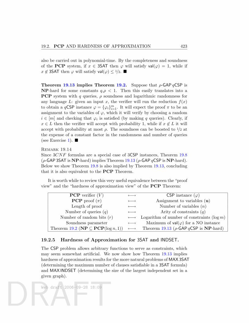
DRAFT


also be carried out in polynomial-time. By the completeness and soundnessof the PCP system, if x ∈ 3SAT then ϕ will satisfy val(ϕ) = 1, while ifx 6∈ 3SAT then ϕ will satisfy val(ϕ) ≤ 1/2.

Theorem 19.13 implies Theorem 19.2. Suppose that ρ-GAP qCSP isNP-hard for some constants q,ρ < 1. Then this easily translates into aPCP system with q queries, ρ soundness and logarithmic randomness forany language L: given an input x, the verifier will run the reduction f(x)to obtain a qCSP instance ϕ = ϕimi=1. It will expect the proof π to be anassignment to the variables of ϕ, which it will verify by choosing a randomi ∈ [m] and checking that ϕi is satisfied (by making q queries). Clearly, ifx ∈ L then the verifier will accept with probability 1, while if x 6∈ L it willaccept with probability at most ρ. The soundness can be boosted to 1/2 atthe expense of a constant factor in the randomness and number of queries(see Exercise 1).

Remark 19.14Since 3CNF formulas are a special case of 3CSP instances, Theorem 19.8(ρ-GAP 3SAT is NP-hard) implies Theorem 19.13 (ρ-GAP qCSP is NP-hard).Below we show Theorem 19.8 is also implied by Theorem 19.13, concludingthat it is also equivalent to the PCP Theorem.

It is worth while to review this very useful equivalence between the “proofview” and the “hardness of approximation view” of the PCP Theorem:

PCP verifier (V ) ←→ CSP instance (ϕ)PCP proof (π) ←→ Assignment to variables (u)Length of proof ←→ Number of variables (n)

Number of queries (q) ←→ Arity of constraints (q)Number of random bits (r) ←→ Logarithm of number of constraints (logm)

Soundness parameter ←→ Maximum of val(ϕ) for a NO instanceTheorem 19.2 (NP ⊆ PCP(log n, 1)) ←→ Theorem 19.13 (ρ-GAP qCSP is NP-hard)

19.2.5 Hardness of Approximation for 3SAT and INDSET.

The CSP problem allows arbitrary functions to serve as constraints, whichmay seem somewhat artificial. We now show how Theorem 19.13 implieshardness of approximation results for the more natural problems of MAX3SAT(determining the maximum number of clauses satisfiable in a 3SAT formula)and MAX INDSET (determining the size of the largest independent set in agiven graph).

Web draft 2006-09-28 18:09

DRAFT


The following two lemmas use the PCP Theorem to show that unlessP = NP, both MAX3SAT and MAX INDSET are hard to approximate withina factor that is a constantless than 1. ( Section 19.3 proves an even strongerhardness of approximation result for INDSET.)

Lemma 19.15 (Theorem 19.8, restated)There exists a constant 0 < ρ < 1 such that ρ-GAP 3SAT is NP-hard.

Lemma 19.16There exist a polynomial-time computable transformation f from 3CNFformulae to graphs such that for every 3CNF formula ϕ, f(ϕ) is an n-vertexgraph whose largest independent set has size val(ϕ)n7 .

Proof of Lemma 19.15: Let ε > 0 and q ∈ N be such that by The-orem 19.13, (1−ε)-GAP qCSP is NP-hard. We show a reduction from (1−ε)-GAP qCSP to (1−ε′)-GAP 3SAT where ε′ > 0 is some constant dependingon ε and q. That is, we will show a polynomial-time function mapping YESinstances of (1−ε)-GAP qCSP to YES instances of (1−ε′)-GAP 3SAT and NOinstances of (1−ε)-GAP qCSP to NO instances of (1−ε′)-GAP 3SAT.

Let ϕ be a qCSP instance over n variables with m constraints. Eachconstraint ϕi of ϕ can be expressed as an AND of at most 2q clauses, whereeach clause is the OR of at most q variables or their negations. Let ϕ′ denotethe collection of at most m2q clauses corresponding to all the constraintsof ϕ. If ϕ is a YES instance of (1−ε)-GAP qCSP (i.e., it is satisfiable) thenthere exists an assignment satisfying all the clauses of ϕ′. if ϕ is a NOinstance of (1−ε)-GAP qCSP then every assignment violates at least an εfraction of the constraints of ϕ and hence violates at least an ε

2q fraction ofthe constraints of ϕ. We can use the Cook-Levin technique of Chapter 2(Theorem 2.11), to transform any clause C on q variables on u1, . . . , uqto a set C1, . . . , Cq of clauses over the variables u1, . . . , uq and additionalauxiliary variables y1, . . . , yq such that (1) each clause Ci is the OR of atmost three variables or their negations, (2) if u1, . . . , uq satisfy C then thereis an assignment to y1, . . . , yq such that u1, . . . , uq, y1, . . . , yq simultaneouslysatisfy C1, . . . , Cq and (3) if u1, . . . , uq does not satisfy C then for everyassignment to y1, . . . , yq, there is some clause Ci that is not satisfies byu1, . . . , uq, y1, . . . , yq.

Let ϕ′′ denote the collection of at most qm2q clauses over the n + qmvariables obtained in this way from ϕ′. Note that ϕ′′ is a 3SAT formula. Ourreduction will map ϕ to ϕ′′. Completeness holds since if ϕ was satisfiablethen so will be ϕ′ and hence ϕ′′. Soundness holds since if every assignment

Web draft 2006-09-28 18:09

DRAFT


violates at least an ε fraction of the constraints of ϕ, then every assign-ment violates at least an ε

2q fraction of the constraints of ϕ′, and so everyassignment violates at least an ε

q2q fraction of the constraints of ϕ′′.

Proof of Lemma 19.16: Let ϕ be a 3CNF formula on n variables withm clauses. We define a graph G of 7m vertices as follows: we associatea cluster of 7 vertices in G with each clause of ϕ. The vertices in clusterassociated with a clause C correspond to the 7 possible assignments to thethree variables C depends on (we call these partial assignments, since theyonly give values for some of the variables). For example, if C is u2 ∨ u5 ∨ u7

then the 7 vertices in the cluster associated with C correspond to all partialassignments of the form u1 = a, u2 = b, u3 = c for a binary vector 〈a, b, c〉 6=〈1, 1, 1〉. (If C depends on less than three variables we treat one of themas repeated and then some of the 7 vertices will correspond to the sameassignment.) We put an edge between two vertices of G if they correspondto inconsistent partial assignments. Two partial assignments are consistentif they give the same value to all the variables they share. For example,the assignment u1 = 1, u2 = 0, u3 = 0 is inconsistent with the assignmentu3 = 1, u5 = 0, u7 = 1 because they share a variable (u3) to which they givea different value. In addition, we put edges between every two vertices thatare in the same cluster.

Clearly transforming ϕ into G can be done in polynomial time. Denoteby α(G) to be the size of the largest independent set in G. We claim thatα(G) = val(ϕ)m. For starters, note that α(G) ≥ val(ϕ)m. Indeed, let u bethe assignment that satisfies val(ϕ)m clauses. Define a set S as follows: foreach clause C satisfied by u, put in S the vertex in the cluster associatedwith C that corresponds to the restriction of u to the variables C dependson. Because we only choose vertices that correspond to restrictions of theassignment u, no two vertices of S correspond to inconsistent assignmentsand hence S is an independent set of size val(ϕ)m.

Suppose that G has an independent set S of size k. We will use Sto construct an assignment u satisfying k clauses of ϕ, thus showing thatval(ϕ)m ≥ α(G). We define u as follows: for every i ∈ [n], if there is a vertexin S whose partial assignment gives a value a to ui, then set ui = a; otherwiseset ui = 0. This is well defined because S is an independent set, and eachvariable ui can get at most a single value by assignments corresponding tovertices in S. On the other hand, because we put all the edges within eachcluster, S can contain at most a single vertex in each cluster, and hencethere are k distinct cluster with members in S. By our definition of u itsatisfies all the clauses associated with these clusters.

Web draft 2006-09-28 18:09

DRAFT

42619.3. N−δ-APPROXIMATION OF INDEPENDENT SET IS NP-HARD.

Remark 19.17In Chapter 2, we defined L′ to be NP-hard if every L ∈ NP reduces toL′. The reduction was a polynomial-time function f such that x ∈ L ⇔f(x) ∈ L′. In all cases, we proved that x ∈ L⇒ f(x) ∈ L′ by showing a wayto map a certificate to the fact that x ∈ L to a certificate to the fact thatx′ ∈ L′. Although the definition of a Karp reduction does not require thatthis mapping is efficient, it often turned out that the proof did provide away to compute this mapping in polynomial time. The way we proved thatf(x) ∈ L′ ⇒ x ∈ L was by showing a way to map a certificate to the factthat x′ ∈ L′ to a certificate to the fact that x ∈ L. Once again, the proofstypically yield an efficient way to compute this mapping.

A similar thing happens in the gap preserving reductions used in theproofs of Lemmas 19.15 and 19.16 and elsewhere in this chapter. Whenreducing from, say, ρ-GAP qCSP to ρ′-GAP 3SAT we show a function f thatmaps a CSP instance ϕ to a 3SAT instance ψ satisfying the following twoproperties:

Completeness We can map a satisfying assignment of ϕ to a satisfyingassignment to ψ

Soundness Given any assignment that satisfies more than a ρ′ fraction ofψ’s clauses, we can map it back into an assignment satisfying morethan a ρ fraction of ϕ’s constraints.

19.3 n−δ-approximation of independent set is NP-hard.

We now show a much stronger hardness of approximation result for theindependent set (INDSET) problem than Lemma 19.16. Namely, we showthat there exists a constant δ ∈ (0, 1) such that unless P = NP, there isno polynomial-time nδ-approximation algorithm for INDSET. That is, weshow that if there is a polynomial-time algorithm A that given an n-vertexgraph G outputs an independent set of size at least opt

nδ(where opt is the

size of the largest independent set in G) then P = NP. We note that aneven stronger result is known: the constant δ can be made arbitrarily closeto 1 [?, ?]. This factor is almost optimal since the independent set problemhas a trivial n-approximation algorithm: output a single vertex.

Our main tool will be the notion of expander graphs (see Note 19.18and Chapter 16). Expander graphs will also be used in the proof of PCPTheorem itself. We use here the following property of expanders:

Web draft 2006-09-28 18:09

DRAFT

19.3. N−δ-APPROXIMATION OF INDEPENDENT SET IS NP-HARD.427

Note 19.18 (Expander graphs)Expander graphs are described in Chapter 16. We define there a parameterλ(G) ∈ [0, 1], for every regular graph G (see Definition 16.3). The mainproperty we need in this chapter is that for every regular graph G = (V,E)and every S ⊆ V with |S| ≤ |V |/2,

Pr(u,v)∈E

[u ∈ S, v ∈ S] ≤ |S||V |

(12

+λ(G)

2

)(3)

Another property we use is that λ(G`) = λ(G)` for every ` ∈ N, where G` isobtained by taking the adjacency matrix of G to the `th power (i.e., an edgein G` corresponds to an (`−1)-step path in G).For every c ∈ (0, 1), we call a regular graph G satisfying λ(G) ≤ c a c-expander graph. If c < 0.9, we drop the prefix c and simply call G anexpander graph. (The choice of the constant 0.9 is arbitrary.) As shownin Chapter 16, for every constant c ∈ (0, 1) there is a constant d and analgorithm that given input n ∈ N , runs in poly(n) time and outputs theadjacency matrix of an n-vertex d-regular c-expander (see Theorem 16.24).

Web draft 2006-09-28 18:09

DRAFT

42819.3. N−δ-APPROXIMATION OF INDEPENDENT SET IS NP-HARD.

Lemma 19.19Let G = (V,E) be a λ-expander graph for some λ ∈ (0, 1). Let S be a subsetof V with |S| = β|V | for some β ∈ (0, 1). Let (X1, . . . , X`) be a tuple ofrandom variables denoting the vertices of a uniformly chosen ( −1)-step pathin G. Then,

(β − 2λ)k ≤ Pr[∀i∈[`]Xi ∈ S] ≤ (β + 2λ)k

The upper bound of Lemma 19.19 is implied by Theorem ??; we omitthe proof of the lower bound.

The hardness result for independent set follows by combining the follow-ing lemma with Lemma 19.16:

Lemma 19.20For every λ > 0 there is a polynomial-time computable reduction f thatmaps every n-vertex graph G into an m-vertex graph H such that

(α(G)− 2λ)logn ≤ α(H) ≤ (α(G) + 2λ)logn

where α(G) is equal to the fractional size of the largest independent set inG.

Recall that Lemma 19.16 shows that there are some constants β, ε ∈(0, 1) such that it is NP-hard to tell whether a given graph G satisfies (1)α(G) ≥ β or (2) α(G) ≤ (1 − ε)β. By applying to G the reduction ofLemma 19.20 with parameter λ = βε/8 we get that in case (1), α(H) ≥(β − βε/4)logn = (β(1 − ε/4))logn, and in case (2), α(H) ≤ ((1 − ε)β +βε/4)logn = (β(1− 0.75ε))logn. We get that the gap between the two casesis equal to clogn for some c > 1 which is equal to mδ for some δ > 0 (wherem = poly(n) is the number of vertices in H).

Proof of Lemma 19.20: Let G, λ be as in the lemma’s statement. Welet K be an n-vertex λ-expander of degree d (we can obtain such a graphin polynomial-time, see Note 19.18). We will map G into a graph H ofndlogn−1 vertices in the following way:

• The vertices of H correspond to all the (log n−1)-step paths in theλ-expander K.

• We put an edge between two vertices u, v of H corresponding to thepaths 〈u1, . . . , ulogn〉 and 〈v1, . . . , vlogn〉 if there exists an edge in Gbetween two vertices in the set u1, . . . , ulogn, v1, . . . , vlogn.

Web draft 2006-09-28 18:09

DRAFT

19.4. NP ⊆ PCP(POLY(N), 1): PCP BASED UPONWALSH-HADAMARD CODE 429

A subset T of H’s vertices corresponds to a subset of log n-tuples ofnumbers in [n], which we can identify as tuples of vertices in G. We letV (T ) denote the set of all the vertices appearing in one of the tuples of T .Note that in this notation, T is an independent set in H if and only if V (T )is an independent set of G. Thus for every independent set T in H, we havethat |V (T )| ≤ α(G)n and hence by the upper bound of Lemma 19.19, Ttakes up less than an (α(H)+2λ)logn fraction of H’s vertices. On the otherhand, if we let S be the independent set of G of size α(G)n then by the lowerbound of Lemma 19.19, an (α− 2λ)logn fraction of H’s vertices correspondto paths fully contained in S, implying that α(H) ≥ (α(G)− 2λ)logn.

19.4 NP ⊆ PCP(poly(n), 1): PCP based upon Walsh-Hadamard code

We now prove a weaker version of the PCP theorem, showing that everyNP statement has an exponentially-long proof that can be locally testedby only looking at a constant number of bits. In addition to giving a tasteof how one proves PCP Theorems, this section builds up to a strongerCorollary 19.26, which will be used in the proof of the PCP theorem.

Theorem 19.21NP ⊆ PCP(poly(n), 1)

We prove this theorem by designing an appropriate verifier for an NP-complete language. The verifier expects the proof to contain an encodedversion of the usual certificate. The verifier checks such an encoded certifi-cate by simple probabilistic tests.

19.4.1 Tool: Linearity Testing and the Walsh-Hadamard Code

We use the Walsh-Hadamard code (see Section 18.5, though the treatmenthere is self-contained). It is a way to encode bit strings of length n by linearfunctions in n variables over GF(2); namely, the function WH : 0, 1∗ →0, 1∗ mapping a string u ∈ 0, 1n to the truth table of the function x 7→u x, where for x,y ∈ 0, 1n we define x y =

∑ni=1 xiyi (mod 2). Note

that this is a very inefficient encoding method: an n-bit string u ∈ 0, 1nis encoded using |WH(u)| = 2n bits. If f ∈ 0, 12

n

is equal to WH(u) forsome u then we say that f is a Walsh-Hadamard codeword. Such a stringf ∈ 0, 12

n

can also be viewed as a function from 0, 1n to 0, 1.

Web draft 2006-09-28 18:09

DRAFT

43019.4. NP ⊆ PCP(POLY(N), 1): PCP BASED UPON

WALSH-HADAMARD CODE

The Walsh-Hadamard code is an error correcting code with minimumdistance 1/2, by which we mean that for every u 6= u′ ∈ 0, 1n, the encodingsWH(u) and WH(u) differ in half the bits. This follows from the familiarrandom subsum principle (Claim A.3) since exactly half of the strings x ∈0, 1n satisfy ux 6= u′x. Now we talk about local tests for the Walsh-Hadamard code (i.e., tests making only O(1) queries).

Local testing of Walsh-Hadamard code. Suppose we are given accessto a function f : 0, 1n → 0, 1 and want to test whether or not f isactually a codeword of Walsh-Hadamard. Since the Walsh-Hadamard code-words are precisely the set of all linear functions from 0, 1n to 0, 1, wecan test f by checking that

f(x + y) = f(x) + f(y) (4)

for all the 22n pairs x,y ∈ 0, 1n (where “+” on the left side of (pcp:eq:lintest)denotes vector addition over GF(2)n and on the right side denotes additionover GF(2)).

But can we test f by querying it in only a constant number of places?Clearly, if f is not linear but very close to being a linear function (e.g., iff is obtained by modifying a linear function on a very small fraction of itsinputs) then such a local test will not be able to distinguish f from a linearfunction. Thus we set our goal on a test that on one hand accepts everylinear function, and on the other hand rejects with high probability everyfunction that is far from linear. It turns out that the natural test of choosingx,y at random and verifying (4) achieves this goal:Definition 19.22Let ρ ∈ [0, 1]. We say that f, g : 0, 1n → 0, 1 are ρ-close if Prx∈R0,1n [f(x) =g(x)] ≥ ρ. We say that f is ρ-close to a linear function if there exists a linearfunction g such that f and g are ρ-close.

Theorem 19.23 (Linearity Testing [?])Let f : 0, 1n → 0, 1 be such that

Prx,y∈R0,1n

[f(x + y) = f(x) + f(y)] ≥ ρ

for some ρ > 1/2. Then f is ρ-close to a linear function.

We defer the proof of Theorem 19.23 to Section 20.3 of the next chap-ter. For every δ ∈ (0, 1/2), we can obtain a linearity test that rejects withprobability at least 1/2 every function that is not (1−δ)-close to a linear func-tion, by testing Condition (4) repeatedly O(1/δ) times with independentrandomness. We call such a test a (1−δ)-linearity test.

Web draft 2006-09-28 18:09

DRAFT


Local decoding of Walsh-Hadamard code. Suppose that for δ < 14

the function f : 0, 1n → 0, 1 is (1−δ)-close to some linear function f .Because every two linear functions differ on half of their inputs, the functionf is uniquely determined by f . Suppose we are given x ∈ 0, 1n and randomaccess to f . Can we obtain the value f(x) using only a constant numberof queries? The naive answer is that since most x’s satisfy f(x) = f(x),we should be able to learn f(x) with good probability by making only thesingle query x to f . The problem is that x could very well be one of theplaces where f and f differ. Fortunately, there is still a simple way to learnf(x) while making only two queries to f :

1. Choose x′ ∈R 0, 1n.

2. Set x′′ = x + x′.

3. Let y′ = f(x′) and y′′ = f(x′′).

4. Output y′ + y′′.

Since both x′ and x′′ are individually uniformly distributed (even thoughthey are dependent), by the union bound with probability at least 1 − 2δwe have y′ = f(x′) and y′′ = f(x′′). Yet by the linearity of f , f(x) =f(x′ + x′′) = f(x′) + f(x′′), and hence with at least 1 − 2δ probabilityf(x) = y′ + y′′.3 This technique is called local decoding of the Walsh-Hadamard code since it allows to recover any bit of the correct codeword (thelinear function f) from a corrupted version (the function f) while makingonly a constant number of queries. It is also known as self correction of theWalsh-Hadamard code.

19.4.2 Proof of Theorem 19.21

We will show a (poly(n), 1)-verifier proof system for a particular NP-completelanguage L. The result that NP ⊆ PCP(poly(n), 1) follows since everyNP language is reducible to L. The NP-complete language L we use isQUADEQ, the language of systems of quadratic equations over GF(2) =0, 1 that are satisfiable.

3We use here the fact that over GF(2), a+ b = a− b.

Web draft 2006-09-28 18:09

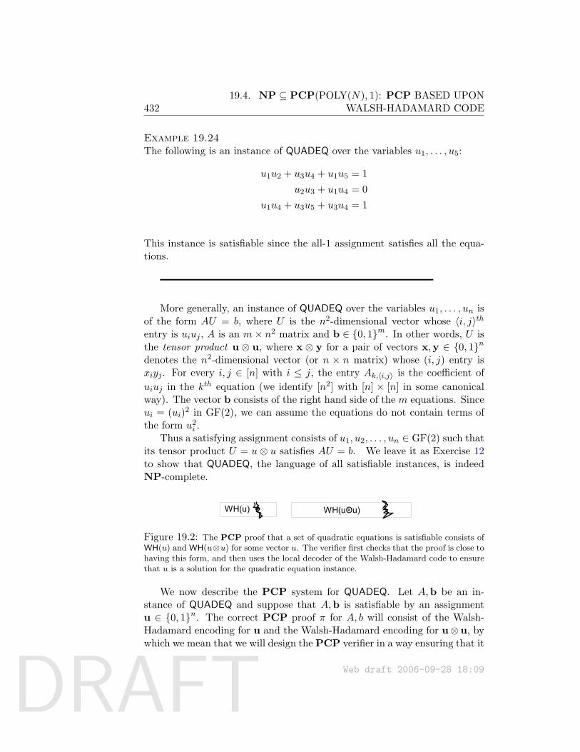
DRAFT


WALSH-HADAMARD CODE

Example 19.24The following is an instance of QUADEQ over the variables u1, . . . , u5:

u1u2 + u3u4 + u1u5 = 1u2u3 + u1u4 = 0

u1u4 + u3u5 + u3u4 = 1

This instance is satisfiable since the all-1 assignment satisfies all the equa-tions.

More generally, an instance of QUADEQ over the variables u1, . . . , un isof the form AU = b, where U is the n2-dimensional vector whose 〈i, j〉thentry is uiuj , A is an m× n2 matrix and b ∈ 0, 1m. In other words, U isthe tensor product u ⊗ u, where x ⊗ y for a pair of vectors x,y ∈ 0, 1ndenotes the n2-dimensional vector (or n × n matrix) whose (i, j) entry isxiyj . For every i, j ∈ [n] with i ≤ j, the entry Ak,〈i,j〉 is the coefficient ofuiuj in the kth equation (we identify [n2] with [n] × [n] in some canonicalway). The vector b consists of the right hand side of the m equations. Sinceui = (ui)2 in GF(2), we can assume the equations do not contain terms ofthe form u2

i .Thus a satisfying assignment consists of u1, u2, . . . , un ∈ GF(2) such that

its tensor product U = u⊗ u satisfies AU = b. We leave it as Exercise 12to show that QUADEQ, the language of all satisfiable instances, is indeedNP-complete.

WH(u) WH(uOu)x

Figure 19.2: The PCP proof that a set of quadratic equations is satisfiable consists ofWH(u) and WH(u⊗u) for some vector u. The verifier first checks that the proof is close tohaving this form, and then uses the local decoder of the Walsh-Hadamard code to ensurethat u is a solution for the quadratic equation instance.

We now describe the PCP system for QUADEQ. Let A,b be an in-stance of QUADEQ and suppose that A,b is satisfiable by an assignmentu ∈ 0, 1n. The correct PCP proof π for A, b will consist of the Walsh-Hadamard encoding for u and the Walsh-Hadamard encoding for u⊗u, bywhich we mean that we will design the PCP verifier in a way ensuring that it

Web draft 2006-09-28 18:09

DRAFT


accepts proofs of this form with probability one, satisfying the completenesscondition. (Note that π is of length 2n + 2n

2.)

Below, we repeatedly use the following fact:

random subsum principle: If u 6= v then for at least 1/2 the choices of x,u x 6= v x. Realize that x can be viewed as a random subset of indicesin [1, . . . , n] and the principle says that with probability 1/2 the sum of theui’s over this index set is different from the corresponding sum of vi’s.

The verifier. The verifier V gets access to a proof π ∈ 0, 12n+2n

2

, whichwe interpret as a pair of functions f : 0, 1n → 0, 1 and g : 0, 1n

2

→0, 1.

Step 1: Check that f , g are linear functions.

As already noted, this isn’t something that the verifier can check per seusing local tests. Instead, the verifier performs a 0.99-linearity test on bothf, g, and rejects the proof at once if either test fails.

Thus, if either of f, g is not 0.99-close to a linear function, then V rejectswith high probability. Therefore for the rest of the procedure we can assumethat there exist two linear functions f : 0, 1n → 0, 1 and g : 0, 1n

2

→0, 1 such that f is 0.99-close to f , and g is 0.99-close to g. (Note: in acorrect proof, the tests succeed with probability 1 and f = f and g = g.)

In fact, we will assume that for Steps 2 and 3, the verifier can query f , gat any desired point. The reason is that local decoding allows the verifierto recover any desired value of f , g with good probability, and Steps 2 and3 will only use a small (less than 15) number of queries to f , g. Thus withhigh probability (say > 0.9) local decoding will succeed on all these queries.

notation: To simplify notation in the rest of the procedure we use f, gfor f , g respectively. Furthermore, we assume both f and g are linear, andthus they must encode some strings u ∈ 0, 1n and w ∈ 0, 1n

2

. In otherwords, f, g are the functions given by f(r) = u r and g(z) = w z.

Step 2: Verify that g encodes u⊗ u, where u ∈ 0, 1n is the stringencoded by f .

Verifier V does the following test 3 times: “Choose r, r′ independentlyat random from 0, 1n, and if f(r)f(r′) 6= g(r⊗ r′) then halt and reject.”

Web draft 2006-09-28 18:09

DRAFT


WALSH-HADAMARD CODE

In a correct proof, w = u⊗ u, so

f(r)f(r′) =

∑i∈[n]

uiri

∑j∈[n]

ujr′j

=

∑i,j∈[n]

uiujrir′j = (u⊗ u) (r⊗ r′),

which in the correct proof is equal to g(r⊗ r′). Thus Step 2 never rejects acorrect proof.

Suppose now that, unlike the case of the correct proof, w 6= u⊗ u. Weclaim that in each of the three trials V will halt and reject with probabilityat least 1

4 . (Thus the probability of rejecting in at least one trial is at least1−(3/4)3 = 37/64.) Indeed, let W be an n×n matrix with the same entriesas w, let U be the n × n matrix such that Ui,j = uiuj and think of r as arow vector and r′ as a column vector. In this notation,

g(r⊗ r′) = w (r⊗ r′) =∑i,j∈[n]

wi,jrir′j = rWr′

f(r)f(r′) = (u r)(u r′) = (n∑i=1

uiri)(n∑j=1

ujr′j) =

∑i,j∈[n]

uiujrirj = rUr′

And V rejects if rWr′ 6= rUr′. The random subsum principle impliesthat if W 6= U then at least 1/2 of all r satisfy rW 6= rU . Applying therandom subsum principle for each such r, we conclude that at least 1/2 ther′ satisfy rWr′ 6= rUr′. We conclude that the test rejects for at least 1/4 ofall pairs r, r′.

Step 3: Verify that f encodes a satisfying assignment.Using all that has been verified about f, g in the previous two steps, it

is easy to check that any particular equation, say the kth equation of theinput, is satisfied by u, namely,∑

i,j

Ak,(i,j)uiuj = bk. (5)

Denoting by z the n2 dimensional vector (Ak,(i,j)) (where i, j vary over[1..n]), we see that the left hand side is nothing but g(z). Since the verifierknows Ak,(i,j) and bk, it simply queries g at z and checks that g(z) = bk.

The drawback of the above idea is that in order to check that u satisfiesthe entire system, the verifier needs to make a query to g for each k =

Web draft 2006-09-28 18:09

DRAFT


1, 2, . . . ,m, whereas the number of queries is required to be independent ofm. Luckily, we can use the random subsum principle again! The verifiertakes a random subset of the equations and computes their sum mod 2. (Inother words, for k = 1, 2, . . . ,m multiply the equation in (5) by a random bitand take the sum.) This sum is a new quadratic equation, and the randomsubsum principle implies that if u does not satisfy even one equation in theoriginal system, then with probability at least 1/2 it will not satisfy thisnew equation. The verifier checks that u satisfies this new equation.

(Actually, the above test has to be repeated twice to ensure that if udoes not satisfy the system, then Step 3 rejects with probability at least3/4.)

19.4.3 PCP’s of proximity

Theorem 19.21 says that (exponential-sized) certificates for NP languagescan be checked by examining only O(1) bits in them. The proof actuallyyields a somewhat stronger result, which will be used in the proof of thePCP Theorem. This concerns the following scenario: we hold a circuit C inour hands that has n input wires. Somebody holds a satisfying assignmentu. He writes down WH(u) as well as another string π for us. We do aprobabilistic test on this by examining O(1) bits in these strings, and at theend we are convinced of this fact.

Concatenation test. First we need to point out a property of Walsh-Hadamard codes and a related concatenation test. In this setting, we aregiven two linear functions f, g that encode strings of lengths n and n + mrespectively. We have to check by examining only O(1) bits in f, g that if uand v are the strings encoded by f, g (that is, f = WH(u) and h = WH(v))then u is the same as the first n bits of v. By the random subsum principle,the following simple test rejects with probability 1/2 if this is not the case.Pick a random x ∈ 0, 1n, and denote by X ∈ GF(2)m+n the string whosefirst n bits are x and the remaining bits are all-0. Verify that f(X) = g(x).

With this test in hand, we can prove the following corollary.

Corollary 19.25 (Exponential-sized PCP of proximity.)There exists a verifier V that given any circuit C of size m and with n inputshas the following property:

1. If u ∈ 0, 1n is a satisfying assignment for circuit C, then there is

a string π2 of size 2poly(m) such that V accepts WH(u) π2 withprobability 1. (Here denotes concatenation.)

Web draft 2006-09-28 18:09

DRAFT


WALSH-HADAMARD CODE

2. For every strings π1, π2 ∈ 0, 1∗, where π1 has 2n bits, if V acceptsπ1 π2 with probability at least 1/2, then π1 is 0.99-close to WH(u)for some u that satisfies C.

3. V uses poly(m) random bits and examines only O(1) bits in the pro-vided strings.

Proof: One looks at the proof of NP-completeness of QUADEQ to realizethat given circuit C with n input wires and size m, it yields an instance ofQUADEQ of size O(m) such that u ∈ 0, 1n satisfies the circuit iff there is astring v of size M = O(m) such that uv satisfies the instance of QUADEQ.(Note that we are thinking of u both as a string of bits that is an input toC and as a string over GF(2)n that is a partial assignment to the variablesin the instance of QUADEQ.)

The verifier expects π2 to contain whatever our verifier of Theorem 19.21expects in the proof for this instance of QUADEQ, namely, a linear functionf that is WH(w), and another linear function g that is WH(w ⊗ w) wherew satisfies the QUADEQ instance. The verifier checks these functions asdescribed in the proof of Theorem 19.21.

However, in the current setting our verifer is also given a string π1 ∈0, 12

n

. Think of this as a function h : GF(2)n → GF(2). The verifierchecks that h is 0.99-close to a linear function, say h. Then to check that fencodes a string whose first n bits are the same as the string encoded by h,the verifier does a concatenation test.

Clearly, the verifier only reads O(1) bits overall.

The following Corollary is also similarly proven and is the one that willactually be used later. It concerns a similar situation as above, except theinputs to the circuit C are thought of as the concatenation of two strings oflengths n1, n2 respectively where n = n1 + n2.

Corollary 19.26 (PCP of proximity when assignment is in two pieces)There exists a verifier V that given any circuit C with n input wires andsize m and also two numbers n1, n2 such that n1 + n2 = n has the followingproperty:

1. If u1 ∈ 0, 1n1 ,u2 ∈ 0, 1n2 is such that u1 u2 is a satisfying

assignment for circuit C, then there is a string π3 of size 2poly(m) suchthat V accepts WH(u1) WH(u2) π3 with probability 1.

2. For every strings π1, π2, π3 ∈ 0, 1∗, where π1 and π2 have 2n1 and 2n2

bits respectively, if V accepts π1 π2 π3 with probability at least 1/2,

Web draft 2006-09-28 18:09

DRAFT

19.5. PROOF OF THE PCP THEOREM. 437

then π1, π2 are 0.99-close to WH(u1), WH(u2) respectively for someu1,u2 such that u1 u2 is a satisfying assignment for circuit C.

3. V uses poly(m) random bits and examines only O(1) bits in the pro-vided strings.

19.5 Proof of the PCP Theorem.

As we have seen, the PCP Theorem is equivalent to Theorem 19.13, statingthat ρ-GAP qCSP is NP-hard for some constants q and ρ < 1. Consider thecase that ρ = 1−ε where ε is not necessarily a constant but can be a functionof m (the number of constraints). Since the number of satisfied constraintsis always a whole number, if ϕ is unsatisfiable then val(ϕ) ≤ 1 − 1/m.Hence, the gap problem (1−1/m)-GAP 3CSP is a generalization of 3SAT andis NP hard. The idea behind the proof is to start with this observation,and iteratively show that (1−ε)-GAP qCSP is NP-hard for larger and largervalues of ε, until ε is as large as some absolute constant independent of m.This is formalized in the following lemma.Definition 19.27Let f be a function mapping CSP instances to CSP instances. We saythat f is a CL-reduction (short for complete linear-blowup reduction) if itis polynomial-time computable and for every CSP instance ϕ with m con-straints, satisfies:

Completeness: If ϕ is satisfiable then so is f(ϕ).

Linear blowup: The new qCSP instance f(ϕ) has at most Cm constraintsand alphabet W , where C and W can depend on the arity and thealphabet size of ϕ (but not on the number of constraints or variables).

Lemma 19.28 (PCP Main Lemma)There exist constants q0 ≥ 3, ε0 > 0, and a CL-reduction f such that forevery q0CSP-instance ϕ with binary alphabet, and every ε < ε0, the instanceψ = f(ϕ) is a q0CSP (over binary alphabet) satisfying

val(ϕ) ≤ 1− ε⇒ val(ψ) ≤ 1− 2ε

Lemma 19.28 can be succinctly described as follows:

Arity Alphabet Constraints ValueOriginal q0 binary m 1− ε

⇓ ⇓ ⇓ ⇓Lemma 19.28 q0 binary Cm 1− 2ε

Web draft 2006-09-28 18:09

DRAFT

438 19.5. PROOF OF THE PCP THEOREM.

This Lemma allows us to easily prove the PCP Theorem.

Proving Theorem 19.2 from Lemma 19.28. Let q0 ≥ 3 be as statedin Lemma 19.28. As already observed, the decision problem q0CSP is NP-hard. To prove the PCP Theorem we give a reduction from this problem toGAP q0CSP. Let ϕ be a q0CSP instance. Let m be the number of constraintsin ϕ. If ϕ is satisfiable then val(ϕ) = 1 and otherwise val(ϕ) ≤ 1 − 1/m.We use Lemma 19.28 to amplify this gap. Specifically, apply the function fobtained by Lemma 19.28 to ϕ a total of logm times. We get an instanceψ such that if ϕ is satisfiable then so is ψ, but if ϕ is not satisfiable (and soval(ϕ) ≤ 1− 1/m) then val(ψ) ≤ 1−min2ε0, 1− 2logm/m = 1− 2ε0. Notethat the size of ψ is at most C logmm, which is polynomial in m. Thus wehave obtained a gap-preserving reduction from L to the (1−2ε0)-GAP q0CSPproblem, and the PCP theorem is proved.

The rest of this section proves Lemma 19.28 by combining two transfor-mations: the first transformation amplifies the gap (i.e., fraction of violatedconstraints) of a given CSP instance, at the expense of increasing the alpha-bet size. The second transformation reduces back the alphabet to binary,at the expense of a modest reduction in the gap. The transformations aredescribed in the next two lemmas.

Lemma 19.29 (Gap Amplification [?])For every ` ∈ N, there exists a CL-reduction g` such that for every CSPinstance ϕ with binary alphabet, the instance ψ = g`(ϕ) has has arity only2 (but over a non-binary alphabet) and satisfies:

val(ϕ) ≤ 1− ε⇒ val(ψ) ≤ 1− `ε

for every ε < ε0 where ε0 > 0 is a number depending only on ` and the arityq of the original instance ϕ.

Lemma 19.30 (Alphabet Reduction)There exists a constant q0 and a CL- reduction h such that for every CSPinstance ϕ, if ϕ had arity two over a (possibly non-binary) alphabet 0..W−1then ψ = h(ϕ) has arity q0 over a binary alphabet and satisfies:

val(ϕ) ≤ 1− ε⇒ val(h(ϕ)) ≤ 1− ε/3

Lemmas 19.29 and 19.30 together imply Lemma 19.28 by setting f(ϕ) =h(g6(ϕ)). Indeed, if ϕ was satisfiable then so will f(ϕ). If val(ϕ) ≤ 1− ε, forε < ε0 (where ε0 the value obtained in Lemma 19.29 for ` = 6, q = q0) then

Web draft 2006-09-28 18:09

DRAFT


val(g6(ϕ)) ≤ 1 − 6ε and hence val(h(g6(ϕ))) ≤ 1 − 2ε. This composition isdescribed in the following table:

Arity Alphabet Constraints ValueOriginal q0 binary m 1− ε

⇓ ⇓ ⇓ ⇓Lemma 19.29 2 W Cm 1− 6ε

⇓ ⇓ ⇓ ⇓Lemma 19.30 q0 binary C ′Cm 1− 2ε

19.5.1 Gap Amplification: Proof of Lemma 19.29

To prove Lemma 19.29, we need to exhibit a function g that maps a qCSPinstance to a 2CSPW instance over a larger alphabet 0..W−1 in a way thatincreases the fraction of violated constraints.

We will show that we may assume without loss of generality that theinstance of qCSP has a specific form. To describe this we need a definition.

We will assume that the instance satisfies the following properties, sincewe can give a simple CL-reduction from qCSP to this special type of qCSP.(See the “Technical Notes” section at the end of the chapter.) We will callsuch instances “nice.”

Property 1: The arity q is 2 (though the alphabet may be nonbinary).

Property 2: Let the constraint graph of ψ be the graph G with vertex set[n] where for every constraint of ϕ depending on the variables ui, uj ,the graph G has the edge (i, j). We allow G to have parallel edges andself-loops. Then G is d-regular for some constant d (independent ofthe alphabet size) and at every node, half the edges incident to it areself-loops.

Property 3: The constraint graph is an expander.

The rest of the proof consists of a “powering” operation for nice 2CSPinstances. This is described in the following Lemma.

Lemma 19.31 (Powering)Let ψ be a 2CSPW instance satisfying Properties 1 through 3. For everynumber t, there is an instance of 2CSP ψt such that:

1. ψt is a 2CSPW ′-instance with alphabet size W ′ < W d5t , where d de-note the degree of ψ’s constraint graph. The instance ψt has dt+

√tn

constraints, where n is the number of variables in ψ.

Web draft 2006-09-28 18:09

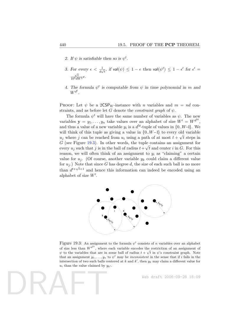
DRAFT


2. If ψ is satisfiable then so is ψt.

3. For every ε < 1d√t, if val(ψ) ≤ 1 − ε then val(ψt) ≤ 1 − ε′ for ε′ =

√t

105dW 4 ε.

4. The formula ψt is computable from ψ in time polynomial in m andW dt .

Proof: Let ψ be a 2CSPW -instance with n variables and m = nd con-straints, and as before let G denote the constraint graph of ψ.

The formula ψt will have the same number of variables as ψ. The newvariables y = y1, . . . , yn take values over an alphabet of size W ′ = W d5t ,and thus a value of a new variable yi is a d5t-tuple of values in 0..W−1. Wewill think of this tuple as giving a value in 0..W−1 to every old variableuj where j can be reached from ui using a path of at most t +

√t steps in

G (see Figure 19.3). In other words, the tuple contains an assignment forevery uj such that j is in the ball of radius t+

√t and center i in G. For this

reason, we will often think of an assignment to yi as “claiming” a certainvalue for uj . (Of course, another variable yk could claim a different valuefor uj .) Note that since G has degree d, the size of each such ball is no morethan dt+

√t+1 and hence this information can indeed be encoded using an

alphabet of size W ′.

k

k’i

t+t 1/2

t+t 1/2t+t 1/2

Figure 19.3: An assignment to the formula ψt consists of n variables over an alphabet

of size less than W d5t

, where each variable encodes the restriction of an assignment ofψ to the variables that are in some ball of radius t +

√t in ψ’s constraint graph. Note

that an assignment y1, . . . , yn to ψt may be inconsistent in the sense that if i falls in theintersection of two such balls centered at k and k′, then yk may claim a different value forui than the value claimed by yk′ .

Web draft 2006-09-28 18:09

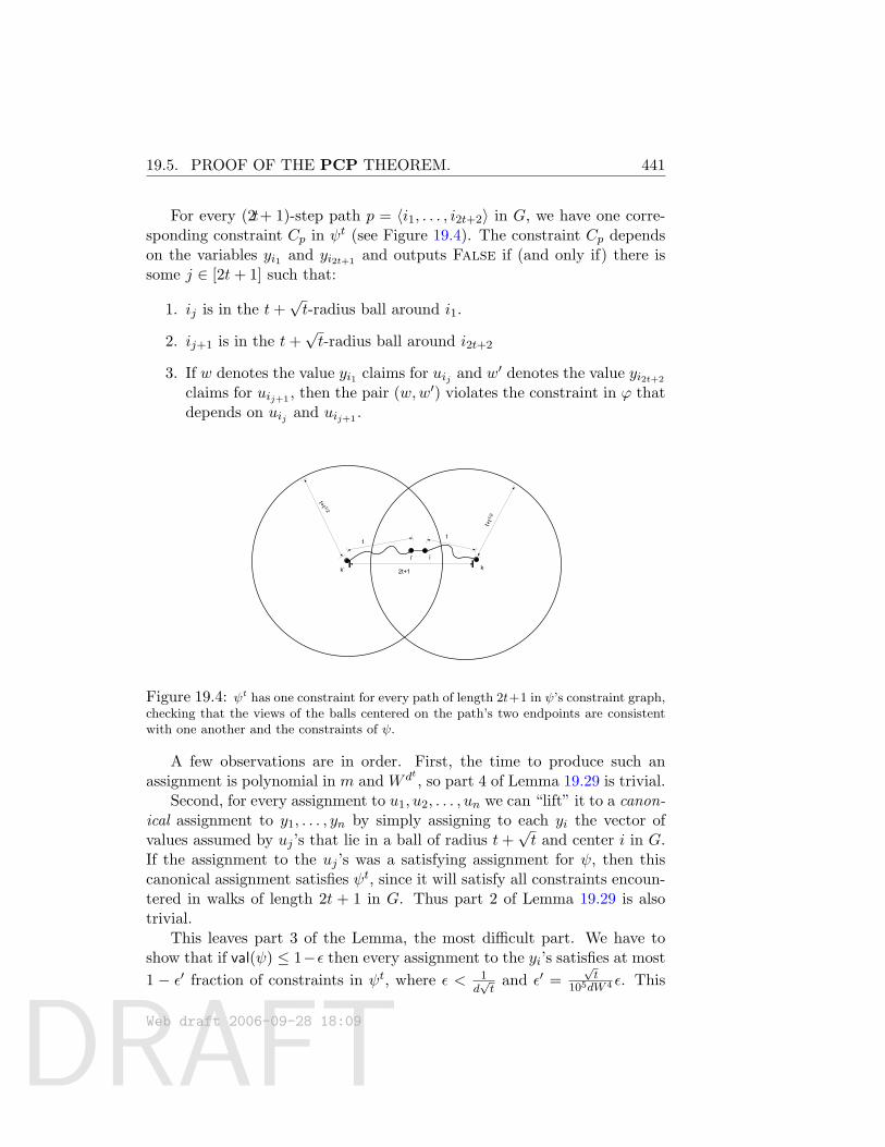
DRAFT


For every (2t+ 1)-step path p = 〈i1, . . . , i2t+2〉 in G, we have one corre-sponding constraint Cp in ψt (see Figure 19.4). The constraint Cp dependson the variables yi1 and yi2t+1 and outputs False if (and only if) there issome j ∈ [2t+ 1] such that:

1. ij is in the t+√t-radius ball around i1.

2. ij+1 is in the t+√t-radius ball around i2t+2

3. If w denotes the value yi1 claims for uij and w′ denotes the value yi2t+2

claims for uij+1 , then the pair (w,w′) violates the constraint in ϕ thatdepends on uij and uij+1 .

t+t1

/2

tt

2t+1t+t 1/2

i

ki’

k’

Figure 19.4: ψt has one constraint for every path of length 2t+1 in ψ’s constraint graph,checking that the views of the balls centered on the path’s two endpoints are consistentwith one another and the constraints of ψ.

A few observations are in order. First, the time to produce such anassignment is polynomial in m and W dt , so part 4 of Lemma 19.29 is trivial.

Second, for every assignment to u1, u2, . . . , un we can “lift” it to a canon-ical assignment to y1, . . . , yn by simply assigning to each yi the vector ofvalues assumed by uj ’s that lie in a ball of radius t+

√t and center i in G.

If the assignment to the uj ’s was a satisfying assignment for ψ, then thiscanonical assignment satisfies ψt, since it will satisfy all constraints encoun-tered in walks of length 2t + 1 in G. Thus part 2 of Lemma 19.29 is alsotrivial.

This leaves part 3 of the Lemma, the most difficult part. We have toshow that if val(ψ) ≤ 1−ε then every assignment to the yi’s satisfies at most1 − ε′ fraction of constraints in ψt, where ε < 1

d√t

and ε′ =√t

105dW 4 ε. This

Web draft 2006-09-28 18:09

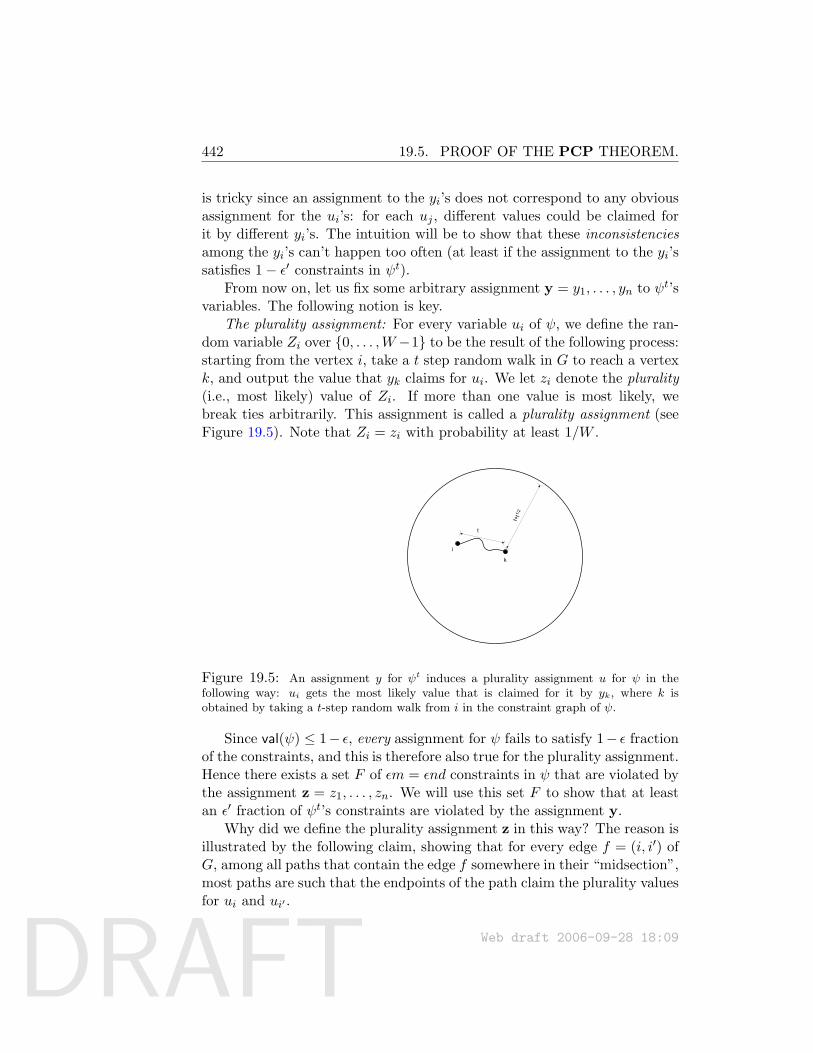
DRAFT


is tricky since an assignment to the yi’s does not correspond to any obviousassignment for the ui’s: for each uj , different values could be claimed forit by different yi’s. The intuition will be to show that these inconsistenciesamong the yi’s can’t happen too often (at least if the assignment to the yi’ssatisfies 1− ε′ constraints in ψt).

From now on, let us fix some arbitrary assignment y = y1, . . . , yn to ψt’svariables. The following notion is key.

The plurality assignment: For every variable ui of ψ, we define the ran-dom variable Zi over 0, . . . ,W−1 to be the result of the following process:starting from the vertex i, take a t step random walk in G to reach a vertexk, and output the value that yk claims for ui. We let zi denote the plurality(i.e., most likely) value of Zi. If more than one value is most likely, webreak ties arbitrarily. This assignment is called a plurality assignment (seeFigure 19.5). Note that Zi = zi with probability at least 1/W .

t+t1

/2

t

i

k

Figure 19.5: An assignment y for ψt induces a plurality assignment u for ψ in thefollowing way: ui gets the most likely value that is claimed for it by yk, where k isobtained by taking a t-step random walk from i in the constraint graph of ψ.

Since val(ψ) ≤ 1− ε, every assignment for ψ fails to satisfy 1− ε fractionof the constraints, and this is therefore also true for the plurality assignment.Hence there exists a set F of εm = εnd constraints in ψ that are violated bythe assignment z = z1, . . . , zn. We will use this set F to show that at leastan ε′ fraction of ψt’s constraints are violated by the assignment y.

Why did we define the plurality assignment z in this way? The reason isillustrated by the following claim, showing that for every edge f = (i, i′) ofG, among all paths that contain the edge f somewhere in their “midsection”,most paths are such that the endpoints of the path claim the plurality valuesfor ui and ui′ .

Web draft 2006-09-28 18:09

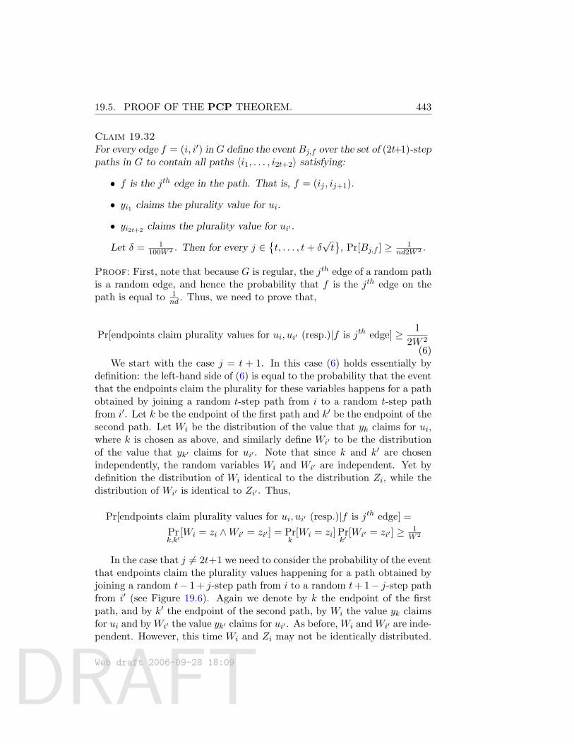
DRAFT


Claim 19.32For every edge f = (i, i′) in G define the event Bj,f over the set of (2t+1)-steppaths in G to contain all paths 〈i1, . . . , i2t+2〉 satisfying:

• f is the jth edge in the path. That is, f = (ij , ij+1).

• yi1 claims the plurality value for ui.

• yi2t+2 claims the plurality value for ui′ .

Let δ = 1100W 2 . Then for every j ∈

t, . . . , t+ δ

√t

, Pr[Bj,f ] ≥ 1nd2W 2 .

Proof: First, note that because G is regular, the jth edge of a random pathis a random edge, and hence the probability that f is the jth edge on thepath is equal to 1

nd . Thus, we need to prove that,

Pr[endpoints claim plurality values for ui, ui′ (resp.)|f is jth edge] ≥ 12W 2

(6)We start with the case j = t + 1. In this case (6) holds essentially by

definition: the left-hand side of (6) is equal to the probability that the eventthat the endpoints claim the plurality for these variables happens for a pathobtained by joining a random t-step path from i to a random t-step pathfrom i′. Let k be the endpoint of the first path and k′ be the endpoint of thesecond path. Let Wi be the distribution of the value that yk claims for ui,where k is chosen as above, and similarly define Wi′ to be the distributionof the value that yk′ claims for ui′ . Note that since k and k′ are chosenindependently, the random variables Wi and Wi′ are independent. Yet bydefinition the distribution of Wi identical to the distribution Zi, while thedistribution of Wi′ is identical to Zi′ . Thus,

Pr[endpoints claim plurality values for ui, ui′ (resp.)|f is jth edge] =Prk,k′

[Wi = zi ∧Wi′ = zi′ ] = Prk

[Wi = zi] Prk′

[Wi′ = zi′ ] ≥ 1W 2

In the case that j 6= 2t+1 we need to consider the probability of the eventthat endpoints claim the plurality values happening for a path obtained byjoining a random t− 1 + j-step path from i to a random t+ 1− j-step pathfrom i′ (see Figure 19.6). Again we denote by k the endpoint of the firstpath, and by k′ the endpoint of the second path, by Wi the value yk claimsfor ui and by Wi′ the value yk′ claims for ui′ . As before, Wi and Wi′ are inde-pendent. However, this time Wi and Zi may not be identically distributed.

Web draft 2006-09-28 18:09

DRAFT


Fortunately, we can show that they are almost identically distributed, inother words, the distributions are statistically close. Specifically, becausehalf of the constraints involving each variable are self loops, we can think ofa t-step random walk from a vertex i as follows: (1) throw t coins and let Stdenote the number of the coins that came up “heads” (2) take St “real” (nonself-loop) steps on the graph. Note that the endpoint of a t-step randomwalk and a t′-step random walk will be identically distributed if in Step (1)the variables St and St′ turn out to be the same number. Thus, the statis-tical distance of the endpoint of a t-step random walk and a t′-step randomwalk is bounded by the statistical distance of St and St′ where S` denotes thebinomial distribution of the sum of ` balanced independent coins. However,the distributions St and St+δ

√t are within statistical distance at most 10δ

for every δ, t (see Exercise 15) and hence in our case Wi and Wi′ are 110W -

close to Zi and Zi′ respectively. Thus |Prk[Wi = zi] − Pr[Zi = zi]| < 110W ,

|Prk[Wi′ = zi′ ] − Pr[Zi′ = zi′ ]| < 110W which proves (6) also for the case

j 6= 2t+ 1.

t+t1

/2

t+εt1/2t-εt1/2

2t+1

t+t 1/2

i

ki’

k’

Figure 19.6: By definition, if we take two t-step random walks from two neighbors i andi′, then the respective endpoints will claim the plurality assignments for ui and uj withprobability more than 1/(2W 2). Because half the edges of every vertex in G have selfloops, this happens even if the walks are not of length t but of length in [t− ε

√t, t+

√t]

for sufficiently small ε.

Recall that F is the set of constraints of ψ (=edges in G) violated bythe plurality assignment z. Therefore, if f ∈ F and j ∈

t, . . . , t+ δ

√t

then all the paths in Bj,f correspond to constraints of ψt that are violatedby the assignment y. Therefore, we might hope that the fraction of vio-lated constraints in ψt is at least the sum of Pr[Bj,f ] for every f ∈ F andj ∈

t, . . . , t+ δ

√t. If this were the case we’d be done since Claim 19.32

Web draft 2006-09-28 18:09

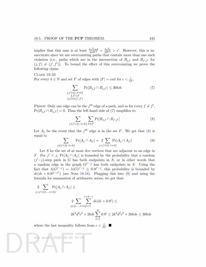
DRAFT


implies that this sum is at least δ√tεnd

2nW 2 = δ√tε

2W 2 > ε′. However, this is in-aaccurate since we are overcounting paths that contain more than one suchviolation (i.e., paths which are in the intersection of Bj,f and Bj′,f ′ for(j, f) 6= (j′, f ′)). To bound the effect of this overcounting we prove thefollowing claim:

Claim 19.33For every k ∈ N and set F of edges with |F | = εnd for ε < 1

kd ,∑j,j′∈t..t+kf,f ′∈F

(j,f) 6=(j′,f ′)

Pr[Bj,f ∩Bj,f ′ ] ≤ 30kdε (7)

Proof: Only one edge can be the jth edge of a path, and so for every f 6= f ′,Pr[Bj,f ∩Bj,f ′ ] = 0. Thus the left-hand side of (7) simplifies to∑

j 6=j′∈t..t+k

∑f 6=f ′

Pr[Bj,f ∩Bj′,f ′ ] (8)

Let Aj be the event that the jth edge is in the set F . We get that (8) isequal to ∑

j 6=j′∈t..t+k

Pr[Aj ∩Aj′ ] = 2∑

j<j′∈t..t+k

Pr[Aj ∩Aj′ ] (9)

Let S be the set of at most dεn vertices that are adjacent to an edge inF . For j′ < j, Pr[Aj ∩ Aj′ ] is bounded by the probability that a random(j′−j)-step path in G has both endpoints in S, or in other words thata random edge in the graph Gj

′−j has both endpoints in S. Using thefact that λ(Gj

′−j) = λ(G)j′−j ≤ 0.9j

′−j , this probability is bounded bydε(dε + 0.9|j−j

′|) (see Note 19.18). Plugging this into (9) and using theformula for summation of arithmetic series, we get that:

2∑

j<j′∈t,...,t+k

Pr[Aj ∩Aj′ ] ≤

2∑

j∈t,...,t+k

t+k−j∑i=1

dε(dε+ 0.9i) ≤

2k2d2ε2 + 2kdε∞∑i=1

0.9i ≤ 2k2d2ε2 + 20kdε ≤ 30kdε

where the last inequality follows from ε < 1kd .

Web draft 2006-09-28 18:09

DRAFT


Wrapping up. Claims 19.32 and 19.33 together imply that

∑j∈t..t+δ√t

f∈F

Pr[Bj,f ] ≥ δ√tε 1

2W 2 (10)

∑j,j′∈t..t+δ√t

f,f ′∈F(j,f) 6=(j′,f ′)

Pr[Bj,f ∩Bj′,f ′ ] ≤ 30δ√tdε (11)

But (10) and (11) together imply that if p is a random constraint of ψt

then

Pr[p violated by y] ≥ Pr[⋃

j∈t..t+δ√tf∈F

Bj,f ] ≥δ√tε

240dW 2

where the last inequality is implied by the following technical claim:

Claim 19.34Let A1, . . . , An be n subsets of some set U satisfying

∑i<j |Ai ∩ Aj | ≤

C∑n

i=1 |Ai| for some number C ∈ N. Then,∣∣∣∣∣n⋃i=1

Ai

∣∣∣∣∣ ≥∑n

i=1 |Ai|4C

Proof: We make 2C copies of every element u ∈ U to obtain a set U with|U | = 2C|U |. Now for every subset Ai ⊆ U , we obtain Ai ⊆ U as follows: forevery u ∈ Ai, we choose at random one of the 2C copies to put in Ai. Notethat |Ai| = |Ai|. For every i, j ∈ [n], u ∈ Ai ∩ Aj , we denote by Ii,j,u theindicator random variable that is equal to 1 if we made the same choice forthe copy of u in Ai and Aj , and equal to 0 otherwise. Since E[Ii,j,u] = 1

2C ,

E[|Ai ∩ Aj |

]=

∑u∈Ai∩Aj

E[Ii,j,u] =|Ai ∩Aj |

2C

and

E

∑i<j

|Ai ∩ Aj |

=

∑i<j |Ai ∩Aj |

2C

Web draft 2006-09-28 18:09

DRAFT


This means that there exists some choice of A1, . . . , Aj such that

n∑i=1

|Ai| =n∑i=1

|Ai| ≥ 2∑i<j

|Ai ∩ Aj |

which by the inclusion-exclusion principle (see Section ??) means that | ∪iAi| ≥ 1/2

∑i |Ai|. But because there is a natural 2C-to-one mapping from

∪iAi to ∪iAi we get that

| ∪ni=1 Ai| ≥| ∪ni=1 Ai|

2C≥∑n

i=1 |Ai|4C

=∑n

i=1 |Ai|4C

Since ε′ < δ√tε

240dW 2 , this proves the lemma.

19.5.2 Alphabet Reduction: Proof of Lemma 19.30

Lemma 19.30 is actually a simple consequence of Corollary 19.26, once werestate it using our “qCSP view” of PCP systems.

Corollary 19.35 (qCSP view of PCP of proximity.)There exists positive integer q0 and an exponential-time transformation thatgiven any circuit C of size m and and n inputs and two numbers n1, n2 such

that n1 + n2 = n produces an instance ψC of q0CSP of size 2poly(m) over abinary alphabet such that:

1. The variables can be thought of as being partitioned into three setsπ1, π2, π3 where π1 has 2n1 variables and π2 has 2n2 variables.

2. If u1 ∈ 0, 1n1 ,u2 ∈ 0, 1n2 is such that u1 u2 is a satisfying

assignment for circuit C, then there is a string π3 of size 2poly(m) suchthat WH(u1) WH(u2) π3 satisfies ψC .

3. For every strings π1, π2, π3 ∈ 0, 1∗, where π1 and π2 have 2n1 and2n2 bits respectively, if π1 π2 π3 satisfy at least 1/2 the constraintsof ψC , then π1, π2 are 0.99-close to WH(u1), WH(u2) respectively forsome u1,u2 such that u1 u2 is a satisfying assignment for circuit C.

Now we are ready to prove Lemma 19.30.

Proof of Lemma 19.30: Suppose the given arity 2 formula ϕ has nvariables u1, u2, . . . , un, alphabet 0..W−1 andN constraints C1, C2, . . . , CN .

Web draft 2006-09-28 18:09

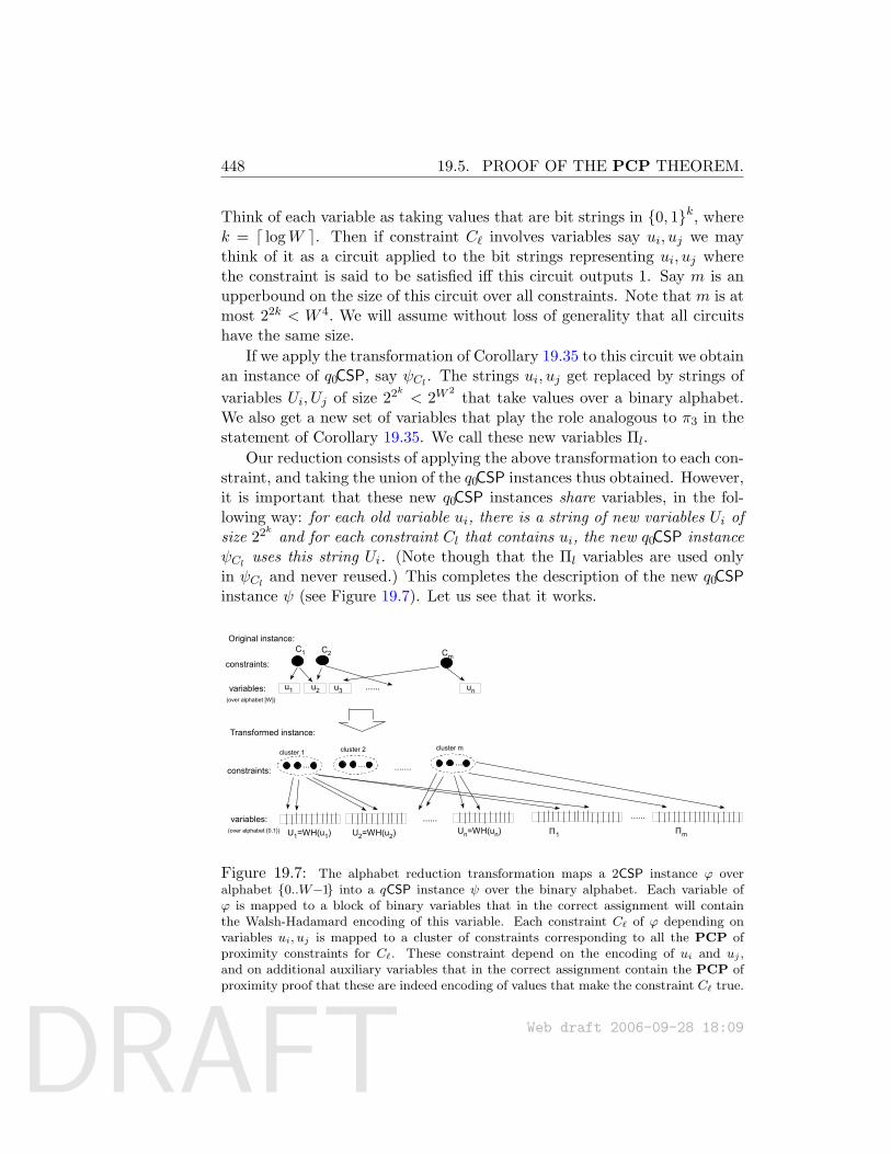
DRAFT


Think of each variable as taking values that are bit strings in 0, 1k, wherek = d logW e. Then if constraint C` involves variables say ui, uj we maythink of it as a circuit applied to the bit strings representing ui, uj wherethe constraint is said to be satisfied iff this circuit outputs 1. Say m is anupperbound on the size of this circuit over all constraints. Note that m is atmost 22k < W 4. We will assume without loss of generality that all circuitshave the same size.

If we apply the transformation of Corollary 19.35 to this circuit we obtainan instance of q0CSP, say ψCl . The strings ui, uj get replaced by strings ofvariables Ui, Uj of size 22k < 2W

2that take values over a binary alphabet.

We also get a new set of variables that play the role analogous to π3 in thestatement of Corollary 19.35. We call these new variables Πl.

Our reduction consists of applying the above transformation to each con-straint, and taking the union of the q0CSP instances thus obtained. However,it is important that these new q0CSP instances share variables, in the fol-lowing way: for each old variable ui, there is a string of new variables Ui ofsize 22k and for each constraint Cl that contains ui, the new q0CSP instanceψCl uses this string Ui. (Note though that the Πl variables are used onlyin ψCl and never reused.) This completes the description of the new q0CSPinstance ψ (see Figure 19.7). Let us see that it works.

Original instance:

constraints:

variables:(over alphabet [W])

u1 u2 u3 ...... un

C1 C2 Cm

Transformed instance:

constraints:

variables:(over alphabet 0.1) U1=WH(u1)

...... ......

U2=WH(u2) Un=WH(un) Π1 Πm

... ... ...cluster 1 cluster 2 cluster m

.......

Figure 19.7: The alphabet reduction transformation maps a 2CSP instance ϕ overalphabet 0..W−1 into a qCSP instance ψ over the binary alphabet. Each variable ofϕ is mapped to a block of binary variables that in the correct assignment will containthe Walsh-Hadamard encoding of this variable. Each constraint C` of ϕ depending onvariables ui, uj is mapped to a cluster of constraints corresponding to all the PCP ofproximity constraints for C`. These constraint depend on the encoding of ui and uj ,and on additional auxiliary variables that in the correct assignment contain the PCP ofproximity proof that these are indeed encoding of values that make the constraint C` true.

Web draft 2006-09-28 18:09

DRAFT

19.6. THE ORIGINAL PROOF OF THE PCP THEOREM. 449

Suppose the original instance ϕ was satisfiable by an assignment u1, . . . ,un.Then we can produce a satisfying assignment for ψ by using part 2 of Corol-lary 19.35, so that for each constraint Cl involving ui, uj , the encodingsWH(ui),WH(ui) act as π1, π2 and then we extend these via a suitable stringπ3 into a satisfying assignment for ψCl .

On the other hand if val(ϕ) < 1− ε then we show that val(ψ) < 1− ε/2.Consider any assignment U1,U2, . . . ,Un,Π1, . . . ,ΠN to the variables of ψ.We “decode” it to an assignment for ϕ as follows. For each i = 1, 2, . . . , n,if the assignment to Ui is 0.99-close to a linear function, let ui be the stringencoded by this linear function, and otherwise let ui be some arbitrarystring. Since val(ϕ) < 1 − ε, this new assignment fails to satisfy at least εfraction of constraints in ϕ. For each constraint Cl of ϕ that is not satisfiedby this assignment, we show that at least 1/2 of the constraints in ψCl arenot satisfied by the original assignment, which leads to the conclusion thatval(ψ) < 1 − ε/2. Indeed, suppose Cl involves ui, uj . Then ui uj is not asatisfying assignment to circuit Cl, so part 3 of Corollary 19.35 implies thatregardless of the value of variables in Πl, the assignment Ui uj Πl musthave failed to satisfy at least 1/2 the constraints of ψCl .

19.6 The original proof of the PCP Theorem.

The original proof of the PCP Theorem, which resisted simplification forover a decade, used algebraic encodings and ideas that are complicated ver-sions of our proof of Theorem 19.21. (Indeed, Theorem 19.21 is the onlypart of the original proof that still survives in our writeup.) Instead of thelinear functions used in Welsh-Hadamard code, they use low degree multi-variate polynomials. These allow procedures analogous to the linearity testand local decoding, though the proofs of correctness are a fair bit harder.The alphabet reduction is also somewhat more complicated. The crucialpart of Dinur’s simpler proof, the one given here, is the gap amplificationlemma (Lemma 19.29) that allows to iteratively improve the soundness pa-rameter of the PCP from very close to 1 to being bounded away from 1by some positive constant. This general strategy is somewhat reminiscentof the zig-zag construction of expander graphs and Reingold’s deterministiclogspace algorithm for undirect connectivity described in Chapter 16.

Web draft 2006-09-28 18:09

DRAFT

450 19.6. THE ORIGINAL PROOF OF THE PCP THEOREM.

Chapter notes

Problems

§1 Prove that for every two functions r, q : N → N and constant s < 1,changing the constant in the soundness condition in Definition 19.1from 1/2 to s will not change the class PCP(r, q).

§2 Prove that for every two functions r, q : N → N and constant c > 1/2,changing the constant in the completeness condition in Definition 19.1from 1 to c will not change the class PCP(r, q).

§3 Prove that any language L that has a PCP-verifier using r coins and qadaptive queries also has a standard (i.e., non-adaptive) verifier usingr coins and 2q queries.

§4 Prove that PCP(0, log n) = P. Prove that PCP(0,poly(n)) = NP.

§5 Let L be the language of matrices A over GF(2) satisfying perm(A) = 1(see Chapters ?? and 9). Prove that L is in PCP(poly(n),poly(n)).

§6 Show that if SAT ∈ PCP(r(n), 1) for r(n) = o(log n) then P = NP.(Thus the PCP Theorem is probably optimal up to constant factors.)

§7 (A simple PCP Theorem using logspace verifiers) Using the fact that acorrect tableau can be verified in logspace, we saw the following exactcharacterization of NP:

NP = L : there is a logspace machine M s.t x ∈ L iff ∃y : M accepts (x, y). .

Note that M has two-way access to y.

Let L-PCP(r(n)) be the class of languages whose membership proofscan be probabilistically checked by a logspace machine that usesO(r(n))random bits but makes only one pass over the proof. (To use the ter-minology from above, it has 2-way access to x but 1-way access to y.)As in the PCP setting, “probabilistic checking of membership proofs”means that for x ∈ L there is a proof y that the machine accepts withprobability 1 and if not, the machine rejects with probability at least1/2. Show that NP = L-PCP(log n). Don’t assume the PCP Theorem!

Web draft 2006-09-28 18:09

DRAFT


Hint:Designaverifierfor3SAT.Thetrivialideawouldbethattheproofcontainsasatisfyingassignmentandtheverifierrandomlypicksaclauseandreadsthecorrespondingthreebitsintheprooftocheckiftheclauseissatisfied.Thisdoesn’twork.Why?Thebetterideaistorequirethe“proof”tocontainmanycopiesofthesatisfyingassignment.Theverifiersusespairwiseindependencetoruntheprevioustestonthesecopies—whichmayormaynotbethesamestring.

(This simple PCP Theorem is implicit in Lipton [Lip90]. The sug-gested proof is due to van Melkebeek.)

§8 Suppose we define J − PCP (r(n)) similarly to L − PCP (r(n)), ex-cept the verifier is only allowed to read O(r(n)) successive bits in themembership proof. (It can decide which bits to read.) Then show thatJ − PCP (log n) ⊆ L.

§9 Prove that there is an NP-language L and x 6∈ L such that f(x) isa 3SAT formula with m constraints having an assignment satisfyingmore than m−m0.9 of them, where f is the reduction from f to 3SATobtained by the proof of the Cook-Levin theorem (Section 2.3.1).

Hint:showthatforanappropriatelanguageL,aslightchangeintheinputfortheCook-Levinreductionwillalsocauseonlyaslightchangeintheoutput,eventhoughthischangemightcauseaYESinstanceofthelanguagetobecomeaNOinstance.

§10 Show a poly(n, 1/ε)-time 1 + ε-approximation algorithm for the knap-sack problem. That is, show an algorithm that given n + 1 numbersa1, . . . , an ∈ N (each represented by at most n bits) and k ∈ [n], findsa set S ⊆ [n] with |S| ≤ k such that

∑i∈S ai ≥

opt1+ε where

opt = maxS⊆[n],|S|≤k

∑i∈S

ai

Hint:firstshowthattheproblemcanbesolvedexactlyusingdy-namicprogrammingintimepoly(n,m)ifallthenumbersinvolvedareintheset[m].Then,showonecanobtainanapproximationalgorithmbykeepingonlytheO(log(1/e)+logn)mostsignificantbitsofeverynumber.

§11 Show a polynomial-time algorithm that given a satisfiable 2CSP-instanceϕ (over binary alphabet) finds a satisfying assignment for ϕ.

Web draft 2006-09-28 18:09

DRAFT


§12 Prove that QUADEQ is NP-complete.

Hint:showyoucanexpresssatisfiabilityforSATformulasusingquadraticequations.

§13 Prove that if Z,U are two n×n matrices over GF(2) such that Z 6= Uthen

Prr,r′∈R0,1n

[rZr′ 6= rUr′] ≥ 14

Hint:usinglinearityreducethistothecasethatUistheallzeromatrix,andthenprovethisusingtwoapplicationsoftherandomsubsumprinciple.

§14 Show a deterministic poly(n, 2q)-time algorithm that given a qCSP-instance ϕ (over binary alphabet) with m clauses outputs an assign-ment satisfying m/2q of these assignment.

Hint:onewaytosolvethisistouseq-wiseindependentfunctions??.

§15 Let St be the binomial distribution over t balanced coins. That is,Pr[St = k] =

(tk

)2−t. Prove that for every δ < 1, the statistical

distance of St and St+δ√t is at most 10ε.

Hint:approximatethebinomialcoefficientusingStirling’sfor-mulaforapproximatingfactorials.

§16 The long-code for a set 0, . . . ,W −1 is the function LC : 0, . . . ,W −1 → 0, 12

W

such that for every i ∈ 0..W−1 and a function f :0..W−1 → 0, 1, (where we identify f with an index in [2w]) the f th

position of LC(i), denoted by LC(i)f , is f(i). We say that a functionL : 0, 12

W

→ 0, 1 is a long-code codeword if L = LC(i) for somei ∈ 0..W−1.

(a) Prove that LC is an error-correcting code with distance half. Thatis, for every i 6= j ∈ 0..W−1, the fractional Hamming distanceof LC(i) and LC(j) is half.

(b) Prove that LC is locally-decodable. That is, show an algorithmthat given random access to a function L : 20,1

W

→ 0, 1 thatis (1−ε)-close to LC(i) and f : 0..W−1 → 0, 1 outputs LC(i)fwith probability at least 0.9 while making at most 2 queries to L.

Web draft 2006-09-28 18:09

DRAFT


(c) Let L = LC(i) for some i ∈ 0..W−1. Prove the for everyf : 0..W−1 → 0, 1, L(f) = 1− L(f), where f is the negationof f (i.e. , f(i) = 1− f(i) for every i ∈ 0..W−1).

(d) Let T be an algorithm that given random access to a functionL : 20,1

W

→ 0, 1, does the following:

i. Choose f to be a random function from 0..W−1 → 0, 1.ii. If L(f) = 1 then output True.iii. Otherwise, choose g : 0..W−1 → 0, 1 as follows: for every

i ∈ 0..W−1, if f(i) = 0 then set g(i) = 0 and otherwise setg(i) to be a random value in 0, 1.

iv. If L(g) = 0 then output True; otherwise output False.

Prove that if L is a long-code codeword (i.e., L = LC(i) for somei) then T outputs True with probability one.Prove that if L is a linear function that is non-zero and nota longcode codeword then T outputs True with probability atmost 0.9.

(e) Prove that LC is locally testable. That is, show an algorithmthat given random access to a function L : 0, 1W → 0, 1outputs True with probability one if L is a long-code codewordand outputs False with probability at least 1/2 if L is not 0.9-close to a long-code codeword, while making at most a constantnumber of queries to L.

Hint:usethetestTabovecombinedwithlinearitytesting,selfcorrection,andasimpletesttoruleouttheconstantzerofunction.

(f) Using the test above, give an alternative proof for the AlphabetReduction Lemma (Lemma 19.30).

Hint:Totransforma2CSPWformulaϕovernvariablesintoaqCSPψoverbinaryalphabet,use2

Wvariablesu

1j,...,u

2W

jforeachvariableujofϕ.Inthecorrectproofthesevariableswillcontainthelongcodeencodingofuj.Then,addasetof2

W2vari-

ablesy1i,...,y

2W2

iforeachconstraintϕiofϕ.Inthecorrectproofthesevariableswillcontainthelongcodeencodingoftheassign-mentfortheconstraintϕi.Foreveryconstraintofϕ,ψwillcontainconstraintsfortestingthelongcodeofboththexandyvariablesinvolvedintheconstraint,testingconsistencybetweenthexvari-ablesandtheyvariables,andtestingthattheyvariablesactuallyencodeasatisfyingassignment.

Web draft 2006-09-28 18:09

DRAFT


Omitted proofs

The preprocessing step transforms a qCSP-instance ϕ into a “nice” 2CSP-instance ψ through the following three claims:

Claim 19.36There is a CL- reduction mapping any qCSP instance ϕ into a 2CSP2q in-stance ψ such that

val(ϕ) ≤ 1− ε⇒ val(ψ) ≤ 1− ε/q

Proof: Given a qCSP-instance ϕ over n variables u1, . . . , un with m con-straints, we construct the following 2CSP2q formula ψ over the variablesu1, . . . , un, y1, . . . , ym. Intuitively, the yi variables will hold the restrictionof the assignment to the q variables used by the ith constraint, and we willadd constraints to check consistency: that is to make sure that if the ith

constraint depends on the variable uj then uj is indeed given a value con-sistent with yi. Specifically, for every ϕi of ϕ that depends on the variablesu1, . . . , uq, we add q constraints ψi,jj∈[q] where ψi,j(yi, uj) is true iff yiencodes an assignment to u1, . . . , uq satisfying ϕi and uj is in 0, 1 andagrees with the assignment yi. Note that the number of constraints in ψ isqm.

Clearly, if ϕ is satisfiable then so is ψ. Suppose that val(ϕ) ≤ 1−ε and letu1, . . . , uk, y1, . . . , ym be any assignment to the variables of ψ. There existsa set S ⊆ [m] of size at least εm such that the constraint ϕi is violated bythe assignment u1, . . . , uk. For any i ∈ S there must be at least one j ∈ [q]such that the constraint ψi,j is violated.

Claim 19.37There is an absolute constant d and a CL- reduction mapping any 2CSPWinstance ϕ into a 2CSPW instance ψ such that

val(ϕ) ≤ 1− ε⇒ val(ψ) ≤ 1− ε/(100Wd).

and the constraint graph of ψ is d-regular. That is, every variable in ψappears in exactly d constraints.

Proof: Let ϕ be a 2CSPW instance, and let Gnn∈N be an explicit familyof d-regular expanders. Our goal is to ensure that each variable appears inϕ at most d + 1 times (if a variable appears less than that, we can alwaysadd artificial constraints that touch only this variable). Suppose that ui isa variable that appears in k constraints for some n > 1. We will change

Web draft 2006-09-28 18:09

DRAFT


ui into k variables y1i , . . . , y

ki , and use a different variable of the form yji in

the place of ui in each constraint ui originally appeared in. We will alsoadd a constraint requiring that yji is equal to yj

′

i for every edge (j, j′) inthe graph Gk. We do this process for every variable in the original instance,until each variable appears in at most d equality constraints and one originalconstraint. We call the resulting 2CSP-instance ψ. Note that if ϕ has mconstraints then ψ will have at most m+ dm constraints.

Clearly, if ϕ is satisfiable then so is ψ. Suppose that val(ϕ) ≤ 1− ε andlet y be any assignment to the variables of ψ. We need to show that yviolates at least εm

100W of the constraints of ψ. Recall that for each variableui that appears k times in ϕ, the assignment y has k variables y1

i , . . . , yki .

We compute an assignment u to ϕ’s variables as follows: ui is assigned theplurality value of y1

i , . . . , yki . We define ti to be the number of yji ’s that

disagree with this plurality value. Note that 0 ≤ ti ≤ k(1−1/W ) (where Wis the alphabet size). If

∑ni=1 ti ≥

ε4m then we are done. Indeed, by (3) (see

Note 19.18), in this case we will have at least∑n

i=1ti

10W ≥ε

40Wm equalityconstraints that are violated.

Suppose now that∑n

i=1 ti <ε4m. Since val(ϕ) ≤ 1 − ε, there is a set S

of at least εm constraints violated in ϕ by the plurality assignment u. All ofthese constraints are also present in ψ and since we assume

∑ni=1 ti <

ε4m,

at most half of them are given a different value by the assignment y than thevalue given by u. Thus the assignment y violates at least ε

2m constraints inψ.

Claim 19.38There is an absolute constant d and a CL-reduction mapping any 2CSPWinstance ϕ with d′-regular constraint graph for d ≥ d′ into a 2CSPW instanceψ such that

val(ϕ) ≤ 1− ε⇒ val(ψ) ≤ 1− ε/(10d)

and the constraint graph of ψ is a 4d-regular expander, with half the edgescoming out of each vertex being self-loops.

Proof: There is a constant d and an explicit family Gnn∈N of graphssuch that for every n, Gn is a d-regular n-vertex 0.1-expander graph (SeeNote 19.18).

Let ϕ be a 2CSP-instance as in the claim’s statement. By adding selfloops, we can assume that the constraint graph has degree d (this can atworst decrease the gap by factor of d). We now add “null” constraints(constraints that always accept) for every edge in the graph Gn. In addition,we add 2d null constraints forming self-loops for each vertex. We denote by

Web draft 2006-09-28 18:09

DRAFT


ψ the resulting instance. Adding these null constraints reduces the fractionof violated constraints by a factor at most four. Moreover, because anyregular graph H satisfies λ(H) ≤ 1 and because of λ’s subadditivity (seeExercise 2, Chapter 16), λ(ψ) ≤ 3

4 + 14λ(Gn) ≤ 0.9 where by λ(ψ) we denote

the parameter λ of ψ’s constraint graph.

Web draft 2006-09-28 18:09

DRAFT

Chapter 20

More PCP Theorems andthe Fourier TransformTechnique

The PCP Theorem has several direct applications in complexity theory,in particular showing that unless P = NP, many NP optimization prob-lems can not be approximated in polynomial-time to within arbitrary preci-sion. However, for some applications, the standard PCP Theorem does notsuffice, and we need stronger (or simply different) “PCP Theorems”. Inthis chapter we survey some of these results and their proofs. The Fouriertransform technique turned out to be especially useful in advanced PCPconstructions, and in other areas in theoretical computer science. We de-scribe the technique and show two of its applications. First, we use Fouriertransforms to prove the correctness of the linearity testing algorithm of Sec-tion 19.4, completing the proof of the PCP Theorem. We then use it toprove a stronger PCP Theorem due to Hastad, showing tight inapproxima-bility results for many important problems, including MAX3SAT.

20.1 Parallel Repetition of PCP’s

Recall that the soundness parameter of a PCP system is the probabilitythat the verifier may accept a false statement. Definition 19.1 specifiedthe soundness parameter to be 1/2, but as we noted, it can be reducedto an arbitrary small constant by increasing the number of queries. Yetfor some applications we need a system with, say, three queries, but anarbitrarily small constant soundness parameter. Raz has shown that this


457

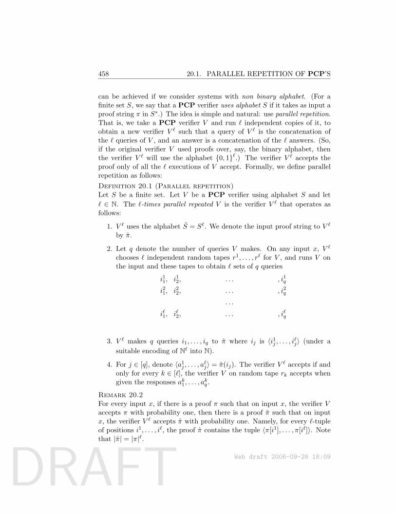
DRAFT

458 20.1. PARALLEL REPETITION OF PCP’S

can be achieved if we consider systems with non binary alphabet. (For afinite set S, we say that a PCP verifier uses alphabet S if it takes as input aproof string π in S∗.) The idea is simple and natural: use parallel repetition.That is, we take a PCP verifier V and run ` independent copies of it, toobtain a new verifier V ` such that a query of V ` is the concatenation ofthe ` queries of V , and an answer is a concatenation of the ` answers. (So,if the original verifier V used proofs over, say, the binary alphabet, thenthe verifier V ` will use the alphabet 0, 1`.) The verifier V ` accepts theproof only of all the ` executions of V accept. Formally, we define parallelrepetition as follows:Definition 20.1 (Parallel repetition)Let S be a finite set. Let V be a PCP verifier using alphabet S and let` ∈ N. The `-times parallel repeated V is the verifier V ` that operates asfollows:

1. V ` uses the alphabet S = S`. We denote the input proof string to V `

by π.

2. Let q denote the number of queries V makes. On any input x, V `

chooses ` independent random tapes r1, . . . , r` for V , and runs V onthe input and these tapes to obtain ` sets of q queries

i11, i12, . . . , i1q

i21, i22, . . . , i2q

. . .

i`1, i`2, . . . , i`q

3. V ` makes q queries i1, . . . , iq to π where ij is 〈i1j , . . . , i`j〉 (under asuitable encoding of N` into N).

4. For j ∈ [q], denote 〈a1j , . . . , a

`j〉 = π(ij). The verifier V ` accepts if and

only for every k ∈ [`], the verifier V on random tape rk accepts whengiven the responses ak1, . . . , a

kq .

Remark 20.2For every input x, if there is a proof π such that on input x, the verifier Vaccepts π with probability one, then there is a proof π such that on inputx, the verifier V ` accepts π with probability one. Namely, for every `-tupleof positions i1, . . . , i`, the proof π contains the tuple 〈π[i1], . . . , π[i`]〉. Notethat |π| = |π|`.

Web draft 2006-09-28 18:09

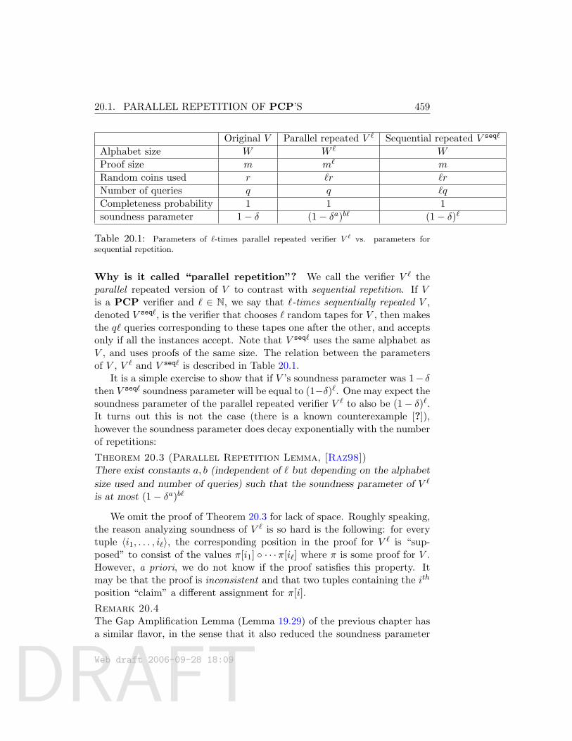
DRAFT

20.1. PARALLEL REPETITION OF PCP’S 459

Original V Parallel repeated V ` Sequential repeated V seq`

Alphabet size W W ` W

Proof size m m` m

Random coins used r `r `r

Number of queries q q `q

Completeness probability 1 1 1soundness parameter 1− δ (1− δa)b` (1− δ)`

Table 20.1: Parameters of `-times parallel repeated verifier V ` vs. parameters forsequential repetition.

Why is it called “parallel repetition”? We call the verifier V ` theparallel repeated version of V to contrast with sequential repetition. If Vis a PCP verifier and ` ∈ N, we say that `-times sequentially repeated V ,denoted V seq`, is the verifier that chooses ` random tapes for V , then makesthe q` queries corresponding to these tapes one after the other, and acceptsonly if all the instances accept. Note that V seq` uses the same alphabet asV , and uses proofs of the same size. The relation between the parametersof V , V ` and V seq` is described in Table 20.1.

It is a simple exercise to show that if V ’s soundness parameter was 1− δthen V seq` soundness parameter will be equal to (1−δ)`. One may expect thesoundness parameter of the parallel repeated verifier V ` to also be (1− δ)`.It turns out this is not the case (there is a known counterexample [?]),however the soundness parameter does decay exponentially with the numberof repetitions:

Theorem 20.3 (Parallel Repetition Lemma, [Raz98])There exist constants a, b (independent of ` but depending on the alphabet

size used and number of queries) such that the soundness parameter of V `

is at most (1− δa)b`

We omit the proof of Theorem 20.3 for lack of space. Roughly speaking,the reason analyzing soundness of V ` is so hard is the following: for everytuple 〈i1, . . . , i`〉, the corresponding position in the proof for V ` is “sup-posed” to consist of the values π[i1] · · ·π[i`] where π is some proof for V .However, a priori, we do not know if the proof satisfies this property. Itmay be that the proof is inconsistent and that two tuples containing the ith

position “claim” a different assignment for π[i].

Remark 20.4The Gap Amplification Lemma (Lemma 19.29) of the previous chapter hasa similar flavor, in the sense that it also reduced the soundness parameter

Web draft 2006-09-28 18:09

DRAFT

460 20.2. HASTAD’S 3-BIT PCP THEOREM

at the expense of an increase in the alphabet size. However, that lemmaassumed that the soundness parameter is very close to 1, and its proof doesnot seem to generalize for soundness parameters smaller than 1/2. We notethat a weaker version of Theorem 20.3, with a somewhat simpler proof, wasobtained by Feige and Kilian [?]. This weaker version is sufficient for manyapplications, including for Hastad’s 3-query PCP theorem (see Section 20.2below).

20.2 Hastad’s 3-bit PCP Theorem

In most cases, the PCP Theorem does not immediately answer the questionof exactly how well can we approximate a given optimization problem (evenassuming P 6= NP). For example, the PCP Theorem implies that if P 6=NP then MAX3SAT cannot be c-approximated in polynomial-time for someconstant ρ < 1. But if one follows closely the proof of Theorem 19.13, thisconstant ρ turns out to be very close to one, and in particular it is larger than0.999. On the other hand, as we saw in Example 19.6, there is a known 7/8-approximation algorithm for MAX3SAT. What is the true “approximationcomplexity” of this problem? In particular, is there a polynomial-time 0.9-approximation algorithm for it? Similar questions are the motivation behindmany stronger PCP theorems. In particular, the following theorem byHastad implies that for every ε > 0 there is no polynomial-time (7/8+ε)-approximation for MAX3SAT unless P = NP:Theorem 20.5 (Hastad’s 3-bit PCP [?])For every ε > 0 and every language L ∈ NP there is a PCP-verifier V for Lmaking three (binary) queries having completeness probability at least 1− εand soundness parameter at most 1/2 + ε.

Moreover, the test used by V are linear. That is, given a proof π ∈0, 1m, V chooses a triple (i1, i2, i3) ∈ [m]3 and b ∈ 0, 1 according tosome distribution and accepts iff πi1 + πi2 + πi3 = b (mod 2).

Theorem 20.5 immediately implies that the problem MAXE3LIN is NP-hard to 1/2+ε-approximate for every ε > 0, where MAXE3LIN is the problemof finding a solution maximizing the number of satisfied equations among agiven system of linear equations over GF(2), with each equation containingat most 3 variables. Note that this hardness of approximation result is tightsince a random assignment is expected to satisfy half of the equations. Alsonote that finding out whether there exists a solution satisfying all of theequations can be done in polynomial-time using Gaussian elimination (andhence the imperfect completeness in Theorem 20.5 is inherent).

Web draft 2006-09-28 18:09

DRAFT

20.3. TOOL: THE FOURIER TRANSFORM TECHNIQUE 461

The result for MAX3SAT is obtained by the following corollary:

Corollary 20.6For every ε > 0, computing (7/8+ε)-approximation to MAX3SAT is NP-hard.

Proof: We reduce MAXE3LIN to MAX3SAT. Take any instance of MAXE3LINwhere we are interested in determining whether (1 − ε) fraction of theequations can be satisfied or at most 1/2 + ε are. Represent each lin-ear constraint by four 3CNF clauses in the obvious way. For example,the linear constraint a + b + c = 0 (mod 2) is equivalent to the clauses(a ∨ b ∨ c), (a ∨ b ∨ c), (a ∨ b ∨ c), (a ∨ b ∨ c). If a, b, c satisfy the linear con-straint, they satisfy all 4 clauses and otherwise they satisfy at most 3 clauses.We conclude that in one case at least (1 − ε) fraction of clauses are simul-taneously satisfiable, and in the other case at most 1− (1

2 − ε)×14 = 7

8 −ε4

fraction are. The ratio between the two cases tends to 7/8 as ε decreases.Since Theorem 20.5 implies that distinguishing between the two cases isNP-hard for every constant ε, the result follows.

20.3 Tool: the Fourier transform technique

The continuous Fourier transform is extremely useful in mathematics andengineering. Likewise, the discrete Fourier transform has found many usesin algorithms and complexity, in particular for constructing and analyzingPCP’s. The Fourier transform technique for PCP’s involves calculatingthe maximum acceptance probability of the verifier using Fourier analysisof the functions presented in the proof string. It is delicate enough to give“tight” inapproximability results for MAX INDSET, MAX3SAT, and manyother problems.

To introduce the technique we start with a simple example: analysisof the linearity test over GF(2) (i.e., proof of Theorem 19.23). We thenintroduce the Long Code and show how to test for membership in it. Theseideas are then used to prove Hastad’s 3-bit PCP Theorem.

20.3.1 Fourier transform over GF(2)n

The Fourier transform over GF(2)n is a tool to study functions on theBoolean hypercube. In this chapter, it will be useful to use the set +1,−1 =±1 instead of 0, 1. To transform 0, 1 to ±1, we use the mappingb 7→ (−1)b (i.e., 0 7→ +1 , 1 7→ −1). Thus we write the hypercube as ±1n

Web draft 2006-09-28 18:09

DRAFT

462 20.3. TOOL: THE FOURIER TRANSFORM TECHNIQUE

instead of the more usual 0, 1n. Note this maps the XOR operation (i.e.,addition in GF(2)) into the multiplication operation.

The set of functions from ±1n to R defines a 2n-dimensional Hilbertspace (see Section ??) as follows. Addition and multiplication by a scalar aredefined in the natural way: (f + g)(x) = f(x) + g(x) and (αf)(x) = αf(x)for every f, g : ±1n → R, α ∈ R. We define the inner product of twofunctions f, g, denoted 〈f, g〉, to be Ex∈±1n [f(x)g(x)].

The standard basis for this space is the set exx∈±1n , where ex(y)is equal to 1 if y = x, and equal to 0 otherwise. This is an orthonormalbasis, and every function f : ±1n → R can be represented in this basis asf =

∑x axex. For every x ∈ ±1n, the coefficient ax is equal to f(x). The

Fourier basis for this space is the set χαα⊆[n] where χα(x) =∏i∈α xi (χ∅

is the constant 1 function). These correspond to the linear functions overGF(2). To see this, note that every linear function of the form b 7→ a b(with a,b ∈ 0, 1n) is mapped by our transformation to the function takingx ∈ ±1n to

∏i s.t. ai=1 xi.

The Fourier basis is indeed an orthonormal basis for the Hilbert space.Indeed, the random subsum principle implies that for every α, β ⊆ [n],〈χα, χβ〉 = δα,β where δα,β is equal to 1 iff α = β and equal to 0 otherwise.This means that every function f : ±1n → R can be represented asf =

∑α⊆[n] fαχα. We call fα the αth Fourier coefficient of f .

We will often use the following simple lemma:

Lemma 20.7Every two functions f, g :±1n → R satisfy

1. 〈f, g〉 =∑

α fαgα.

2. (Parseval’s Identity) 〈f, f〉 =∑

α f2α

Proof: The second property follows from the first. To prove the first weexpand

〈f, g〉 = 〈∑α

fαχα,∑β

gβχβ〉 =

∑α,β

fαgβ〈χα, χβ〉 =∑α,β

fαgβδα,β =∑α

fαgα

Web draft 2006-09-28 18:09

DRAFT


Example 20.8Some examples for the Fourier transform of particular functions:

1. If f(u1, u2, . . . , un) = ui (i.e., f is a coordinate function, a concept wewill see again soon) then f = χi and so fi = 1 and fα = 0 forα 6= i.

2. If f is a random boolean function on n bits, then each fα is a randomvariable that is a sum of 2n binomial variables (equally likely to be1,−1) and hence looks like a normally distributed variable with stan-dard deviation 2n/2 and mean 0. Thus with high probability, all 2n

Fourier coefficients have values in [−poly(n)

2n/2,poly(n)

2n/2].

The connection to PCPs: High level view

In the PCP context we are interested in Boolean-valued functions, i.e., thosefrom GF (2)n to GF (2). Under our transformation these are mapped tofunctions from ±1n to ±1. Thus, we say that : f ±1n → R is Booleanif f(x) ∈ ±1 for every x ∈ ±1n. Note that if f is Boolean then 〈f, f〉 =Ex[f(x)2] = 1.

On a high level, we use the Fourier transform in the soundness proofs forPCP’s to show that if the verifier accepts a proof π with high probability thenπ is “close to” being “well-formed” (where the precise meaning of “close-to”and “well-formed” is context dependent). Technically, we will often be ableto relate the acceptance probability of the verifier to an expectation of theform 〈f, g〉 = Ex[f(x)g(x)], where f and g are Boolean functions arisingfrom the proof. We then use techniques similar to those used to proveLemma 20.7 to relate this acceptance probability to the Fourier coefficientsof f, g, allowing us to argue that if the verifier’s test accepts with highprobability, then f and g have few relatively large Fourier coefficients. Thiswill provide us with some nontrivial useful information about f and g, sincein a “generic” or random function, all the Fourier coefficient are small androughly equal.

20.3.2 Analysis of the linearity test over GF (2)

We will now prove Theorem 19.23, thus completing the proof of the PCPTheorem. Recall that the linearity test is provided a function f :GF(2)n →

Web draft 2006-09-28 18:09

DRAFT


GF(2) and has to determine whether f has significant agreement with alinear function. To do this it picks x,y ∈ GF(2)n randomly and accepts ifff(x + y) = f(x) + f(y).

Now we rephrase this test using ±1 instead of GF(2), so linear func-tions turn into Fourier basis functions. For every two vectors x,y ∈ ±1n,we denote by xy their componentwise multiplication. That is, xy = (x1y1, . . . , xnyn).Note that for every basis function χα(xy) = χα(x)χα(y).

For two Boolean functions f, g, 〈f, g〉 is equal to the fraction of inputson which they agree minus the fraction of inputs on which they disagree.It follows that for every ε ∈ [0, 1] and functions f, g : ±1n → ±1, fhas agreement 1

2 + ε2 with g iff 〈f, g〉 = ε. Thus, if f has a large Fourier

coefficient then it has significant agreement with some Fourier basis function,or in the GF(2) worldview, f is close to some linear function. This meansthat Theorem 19.23 can be rephrased as follows:

Theorem 20.9Suppose that f : ±1n → ±1 satisfies Prx,y[f(xy) = f(x)f(y)] ≥ 1

2 + ε.

Then, there is some α ⊆ [n] such fα ≥ 2ε.

Proof: We can rephrase the hypothesis as Ex,y[f(xy)f(x)f(y)] ≥ (12 +ε)−

(12 − ε) = 2ε. We note that from now on we do not need f to be Boolean,

but merely to satisfy 〈f, f〉 = 1.Expressing f by its Fourier expansion,

2ε ≤ Ex,y[f(xy)f(x)f(y)] = Ex,y[(∑α

fαχα(xy))(∑β

fβχβ(x))(∑γ

fγχγ(y))].

Since χα(xy) = χα(x)χα(y) this becomes

= Ex,y[∑α,β,γ

fαfβ fγχα(x)χα(y)χβ(x)χγ(y)].

Using linearity of expectation:

=∑α,β,γ

fαfβ fγEx,y[χα(x)χα(y)χβ(x)χγ(y)]

=∑α,β,γ

fαfβ fγEx [χα(x)χβ(x)]Ey [χα(y)χγ(y)]

(because x,y are independent).

Web draft 2006-09-28 18:09

DRAFT


By orthonormality Ex[χα(x)χβ(x)] = δα,β, so we simplify to

=∑α

f3α

≤ (maxα

fα)× (∑α

f2α)

Since∑

α f2α = 〈f, f〉 = 1, this expression is at most maxα

fα

. Hence

maxα fα ≥ 2ε and the theorem is proved.

20.3.3 Coordinate functions, Long code and its testing

Let W ∈ N. We say that f : ±1W → ±1 is a coordinate function ifthere is some w ∈ [W ], such that f(x1, x2, . . . , xW ) = xw; in other words,f = χw.

Definition 20.10 (Long Code)The long code for [W ] encodes each w ∈ [W ] by the table of all values of thefunction χw : ±1[W ] → ±1.

Remark 20.11Note that w, normally written using logW bits, is being represented usinga table of 2W bits, a doubly exponential blowup! This inefficiency is thereason for calling the code “long.”

Similar to the test for the Walsh-Hadamard code, when testing the longcode, we are given a function f : ±1W → ±1, and want to find out iff has good agreement with χw for some w, namely, fw is significant.Such a test is described in Exercise 16 of the previous chapter, but it is notsufficient for the proof of Hastad’s Theorem, which requires a test using onlythree queries. Below we show such a three query test albeit at the expenseof achieving the following weaker guarantee: if the test passes with highprobability then f has a good agreement with a function χα with |α| small(but not necessarily equal to 1). This weaker conclusion will be sufficient inthe proof of Theorem 20.5.

Let ρ > 0 be some arbitrarily small constant. The test picks two uni-formly random vectors x,y ∈ ±1W and then a vector z ∈ ±1[W ]according to the following distribution: for every coordinate i ∈ [W ], withprobability 1 − ρ we choose zi = +1 and with probability ρ we choose

Web draft 2006-09-28 18:09

DRAFT


zi = −1. Thus with high probability, about ρ fraction of coordinates in zare −1 and the other 1−ρ fraction are +1. We think of z as a “noise” vector.The test accepts iff f(x)f(y) = f(xyz). Note that the test is similar to thelinearity test except for the use of the noise vector z.

Suppose f = χw. Then

f(x)f(y)f(xyz) = xwyw(xwywzw) = 1 · zw

Hence the test accepts iff zw = 1 which happens with probability 1− ρ. Wenow prove a certain converse:

Lemma 20.12If the test accepts with probability 1/2 + ε then

∑α f

3α(1− 2ρ)|α| ≥ 2ε.

Proof: If the test accepts with probability 1/2+ε then E[f(x)f(y)f(xyz)] =2ε. Replacing f by its Fourier expansion, we have

2ε ≤ Ex,y,z

(∑α

fαχα(x)) · (∑β

fβχβ(y)) · (∑γ

fγχγ(xyz))

= Ex,y,z

∑α,β,γ

fαfβ fγχα(x)χβ(y)χγ(x)χγ(y)χγ(z)

=∑α,β,γ

fαfβ fγEx,y,z [χα(x)χβ(y)χγ(x)χγ(y)χγ(z)] .

Orthonormality implies the expectation is 0 unless α = β = γ, so this is

=∑α

f3αEz[χα(z)]

Now Ez[χα(z)] = Ez

[∏w∈α zw

]which is equal to

∏w∈α E[zw] = (1−2ρ)|α|

because each coordinate of z is chosen independently. Hence we get that

2ε ≤∑α

f3α(1− 2ρ)|α|

The conclusion of Lemma 20.12 is reminiscent of the calculation in theproof of Theorem 20.9, except for the extra factor (1 − 2ρ)|α|. This factordepresses the contribution of fα for large α, allowing us to conclude that thesmall α’s must contribute a lot. This formalized in the following corollary(left as Exercise 2).

Web draft 2006-09-28 18:09

DRAFT

20.4. PROOF OF THEOREM ?? 467

Corollary 20.13If f passes the long code test with probability 1/2 + δ then∑

α:|α|≤k

f3α ≥ 2δ − ε,

where k = 12ρ log 1

ε .

20.4 Proof of Theorem 20.5

Recall that our proof of the PCP Theorem implies that there are constantsγ > 0, s ∈ N such that (1−γ)-GAP 2CSPs is NP-hard (see Claim 19.36). Thismeans that for every NP-language L we have a PCP-verifier for L mak-ing two queries over alphabet 0, . . . , s − 1 with perfect completeness andsoundness parameter 1−γ. Furthermore this PCP system has the propertythat the verifier accepts the answer pair z1, z2 iff z2 = hr(z1) where hr is afunction (depending on the verifier’s randomness r) mapping 0, . . . , s− 1to itself (see Exercise 3). We call this the projection property. Using theRaz’s parallel repetition lemma (Theorem 20.3), we can reduce the sound-ness parameter to an arbitrary small constant at the expense of increasingthe alphabet. Note that parallel repetition preserves the projection property.

Let L be an NP-language and ε > 0 an arbitrarily small constant. Bythe above there exists a constant W and PCP-verifier VRaz (having theprojection property) that makes two queries to a polynomial-sized PCPproof π with alphabet 1, . . . ,W such that for every x, if x ∈ L then thereexists π such that Pr[V π

Raz(x) = 1] = 1 and if x 6∈ L then Pr[V πRaz(x) = 1] < ε

for every π.Now we describe Hastad’s verifier VH . It essentially follows VRaz, but

it expects each entry in the PCP proof π to be encoded using the longcode. It expects these encodings to be bifolded, a technical property we nowdefine and is motivated by the observation that coordinate functions satisfyχw(−u) = −χw(u), where −u is the vector (−u1, . . . ,−uW ).

Definition 20.14A function f : ±1W → ±1 is bifolded if for all u ∈ ±1W , f(−u) =−f(u).

Whenever the PCP proof is supposed to contain a longcode codewordthen we may assume without loss of generality that the function is bifolded.The reason is that the verifier can identify, for each pair of inputs u,−u, onedesignated representative —say the one whose first coordinate is +1— and

Web draft 2006-09-28 18:09

DRAFT

468 20.4. PROOF OF THEOREM ??

just define f(−u) to be −f(u). One benefit —though of no consequence inthe proof— of this convention is that bifolded functions require only half asmany bits to represent. We will use the following fact:

Lemma 20.15If f : ±1W → ±1 is bifolded and fα 6= 0 then |α| must be an oddnumber (and in particular, nonzero).

Proof: By definition,

fα = 〈f, χα〉 = 12n

∑u

f(u)∏i∈α

ui.

If |α| is even then∏i∈α ui =

∏i∈α(−ui). So if f is bifolded, the terms

corresponding to u and −u have opposite signs and the entire sum is 0.

Hastad’s verifier. Recall that VRaz uses its randomness to select a func-tion two entries i, j in the table π and a function h : [W ] → [W ], andaccepts iff π(j) = h(π(i)). Hastad’s verifier, denoted VH , expects the proofπ to consist of (bifolded) longcode encodings of each entry of π. The veri-fier VH emulates VRaz to pick two locations i,j in the table and a functionh : [W ]→ [W ] such that VRaz’s test is to accept iff π[j] = h(π[i]). The proofπ contains in the locations i and j two functions f and g respectively (whichmay or may not be the longcode encoding of π(i) and π(j)). Instead of read-ing the long codes f, g in their entirety, the verifier VH performs a simple testthat is reminiscent of the long code test. For a string y ∈ ±1W we denoteby h−1(y) the string such that for every w ∈ [W ], h−1(y)w = yh(w). In otherwords, for each u ∈ [W ], the bit yu appears in all coordinates of h−1(y) thatare indexed by integers in the subset h−1(u). This is well defined becauseh−1(u) : u ∈ [W ]

is a partition of [W ]. VH chooses uniformly at random

u,y ∈ ±1W and chooses z ∈ ±1W by letting zi = +1 with probability1− ρ and zi = −1 with probability ρ. It then accepts Iff

f(u)g(y) = f(h−1(y)uz) (1)

Translating back from ±1 to 0, 1, note that VH ’s test is indeed linear,as it accepts iff π[i1] + π[i2] + π[i3] = b for some i1, i2, i3 ∈ [m2W ] andb ∈ 0, 1. (The bit b can indeed equal 1 because of the way VH ensures thebifolding property.)

Web draft 2006-09-28 18:09

DRAFT


Completeness of VH . Suppose f, g are long codes of two integers w, u sat-isfying h(w) = u (in other words, Vraz would have accepted the assignmentsrepresented by these integers). Then

f(u)g(y)f(h−1(y)uz) = uwyu(h−1(y)uzw= uwyu(yh(w)uwzw) = zw.

Hence VH accepts iff zw = 1, which happens with probability 1− ρ.

Soundness of VH . We now show that if VH accepts f, g with probabilitysignificantly more than 1/2, then the Fourier transforms of f, g must becorrelated. To formalize this we define for α ⊆ [W ],

h2(α) =u ∈ [W ] :

∣∣h−1(u) ∩ α∣∣ is odd

Notice in particular that for every u ∈ h2(α) there is at least one w ∈ αsuch that h(w) = u.

In the next Lemma δ is allowed to be negative.

Lemma 20.16Let f, g : ±1W → ±1, h : [W ]→ [W ] be bifolded functions passing VH ’stest (1) with probability at least 1/2 + δ. Then∑

α⊆[W ],α 6=∅

f2αgh2(α)(1− 2ρ)|α| ≥ 2δ

Proof: By hypothesis, f, g are such that E[f(u)f(uh−1(y)z)g(y)] ≥ 2δ.Replace f, g by their Fourier expansions. We get that

2δ ≤ = Eu,y,z

(∑α

fαχα(x))(∑β

gβχβ(y))(∑γ

fγχγ(uh−1(y)z))

=∑α,β,γ

fαgβ fγEu,y,z

[χα(u)χβ(y)χγ(u)χγ(h−1(y))χγ(z)

]By orthonormality this simplifies to

=∑α,β

f2αgβEy,z

[χβ(y)χα(h−1(y))χα(z)

]=∑α,β

f2αgβ(1− 2ρ)|α|Ey

[χα(h−1(y)χβ(y)

](2)

Web draft 2006-09-28 18:09

DRAFT

470 20.4. PROOF OF THEOREM ??

since χα(z) = (1−2ρ)|α|, as noted in our analysis of the long code test. Nowwe have

Ey[χα(h−1(y))χβ(y)] = Ey[∏w∈α

h−1(y)w∏u∈β

yu]

= Ey[∏w∈α

yh(w)

∏u∈β

yu],

which is 1 if h2(α) = β and 0 otherwise. Hence (2) simplifies to∑α

f2αgh2(α)(1− 2ρ)|α|.

Finally we note that since the functions are assumed to be bifolded, theFourier coefficients f∅ and g∅ are zero. Thus those terms can be droppedfrom the summation and the Lemma is proved.

The following corollary of Lemma 20.16 completes the proof of Hastad’s3-bit PCP Theorem.Corollary 20.17Let ε be the soundness parameter of VRaz. If ρ, δ satisfy ρδ2 > ε then thesoundness parameter of VH is at most 1/2 + δ.

Proof: Suppose VH accepts a proof π with probability at least 1/2 + δ. Wegive a probabilistic construction of a proof π causing VRaz to accept thesame statement with probability at least ρδ2.

Suppose that VRaz uses proofs π with m entries in [W ]. We can think ofπ as providing, for every i ∈ [m], a function fi : ±1W ±1. We will useπ to construct a proof π for VRaz as follows: we first use fi to come up witha distribution Di over [W ]. We then let π[i] be a random element from Di.

The distribution Di. Let f = fi. The distribution Di is defined by firstselecting α ⊆ [W ] with probability f2

α and then selecting w at random fromα. This is well defined because

∑α f

2α = 1 and (due to bifolding) f∅ = 0.

Recall that VRaz picks using its random tape a pair i, j of locations anda function h : [W ] → [W ] and then verifies that π[j] = h(π[i]). Let r besome possible random tape of VRaz and let i, j, h be the pair of entries inπ and function that are determined by r. We define the indicator randomvariable Ir to be 1 if for w ∈R Di and u ∈R Dj it holds that w = h(u) andto be 0 otherwise. Thus, our goal is to show that

Eπ=D1,...,Dm [Er[Ir]] ≥ ρδ2 (3)

Web draft 2006-09-28 18:09

DRAFT


since that would imply that there exists a table π causing VRaz to acceptwith probability at least ρδ2, proving the corollary.

To prove (3) we first notice that linearity of expectation allows us toexchange the order of the two expectations and so it is enough to boundEr[EDi,Dj [Ir]] where i, j are the entries determined by the random tape r.For every r denote by δr the probability that VH accepts π when it uses ras the random tape for VRaz. The acceptance probability of VH is Er[12 + δr]and hence Er[δr] = δ.

Let i, j, h be the pair and function determined by r and denote by f = fiand g = fj where fi (resp. fj) is the function at the ith (resp. jth) entryof the table π. What is the chance that a pair of assignments w ∈R Di andv ∈R Dj will satisfy the constraint? (i.e., will satisfy v = h(w)?). Recallthat we pick w and u by choosing α with probability f2

α, β with probabilityg2β and choosing w ∈R α, v ∈R β. Now if β = h2(α) then for every v ∈ β

there exists w ∈ α with h(w) = v and hence the probability the constraintis satisfied is at least 1/|α|. Thus, we have that∑

α

1|α|

f2αg

2h2(α) ≤ EDi,Dj [Ir] (4)

This is similar to (but not quite the same as) the expression in Lemma 20.16,according to which

2δr ≤∑α

f2αgh2(α)(1− 2ρ)|α|.

However, since one can easily see that (1− 2ρ)|α| ≤ 2√ρ |α|

we have

2δr ≤∑α

f2α

∣∣gh2(α)

∣∣ 2√ρ |α|

Orδr√ρ ≤

∑α

f2α

∣∣gh2(α)

∣∣ 1√|α|

Applying the Cauchy-Schwartz inequality,∑

i aibi ≤ (∑

i a2i )

1/2(∑

i b2i )

1/2,with fα

∣∣gπ2(α)

∣∣ 1√|α|

playing the role of the ai’s and fα playing that of the

bi’s, we obtain

δr√ρ ≤

∑α

f2α

∣∣gh2(α)

∣∣ 1√|α|≤

(∑α

f2α

)1/2(∑α

fα2g2h2(α)

1|α|

)1/2

(5)

Web draft 2006-09-28 18:09

DRAFT

472 20.5. LEARNING FOURIER COEFFICIENTS

Since∑

α f2α = 1, by squaring (5) and combining it with (4) we get that

for every r,δ2rρ ≤ EDi,Dj [Ir]

taking expectation over r and using E[X]2 ≤ E[X2] we get that

δ2ρ = Er[δr]2ρ ≤ Er[δ2r ]ρ ≤ Er[EDi,Dj [Ir]]

proving (3).

20.5 Learning Fourier Coefficients

Suppose that you are given random access to a Boolean function f : ±1n →±1 and want to find the high Fourier coefficients of f . Of course, we cancompute all of the coefficients in time polynomial in 2n, but is there a fasteralgorithm? By the Parseval equality (Lemma 20.7) we know that there canbe at most 1/ε2 coefficients with absolute value larger than ε, and so we canhope to learn these coefficients in time polynomial in n, and 1/ε. It turnsout we can (almost) achieve this goal:

Theorem 20.18 ([?])There is an algorithm A that given input n ∈ N,ε ∈ (0, 1) and randomaccess to a function f : ±1n → ±1, runs in poly(n, 1/ε) time and withprobability at least 0.9 outputs a set L of size at most O(1/ε2) such that forevery α ⊆ [n], if |fα| > ε then α ∈ L.

Proof: We identify subsets of [n] with strings in 0, 1m in the obviousway. For k ≤ n and α ∈ 0, 1k denote

fα? =∑

β∈0,1n−kf2αβ,

where denotes concatenation. By Parseval (Lemma 20.7) f? = 1. Notealso that for every k < n and α ∈ 0, 1k, fα? = fα0? + fα1?. Therefore, ifwe think of the full depth-n binary labeled by binary strings of length ≤ n(with the root being the empty word and the two children of α are α0 andα1), then at any level of this tree there can be at most 1/ε2 strings α suchthat fα? > ε2 (the kth level of the tree corresponds to all strings of lengthk). Note that if a string α satisfies fα? < ε2 then the same holds for everystring of the form αβ. Our goal will be to find all these strings at all levels,

Web draft 2006-09-28 18:09

DRAFT

20.5. LEARNING FOURIER COEFFICIENTS 473

and then output all the strings that label leaves in the tree (i.e., all n-bitstrings).

The heart of the algorithm is a procedure Estimate that given α andoracle access to f(·), outputs an estimate of fα within ε/4 accuracy withprobability 1 − ε2

100n . Using this procedure we work our way from the rootdown, and whenever Estimate(α) gives a value smaller than ε/2 we “kill”this node and will not deal with it and its subnodes. Note that unless theoutput of Estimate is more than ε/4-far from the real value (which we willensure by the union bound happens with probability less than 0.1 over allthe levels) at most 4/ε nodes will survive at any level. The algorithm willoutput the 4/ε leaves that survive.

The procedure Estimate uses the following claim:Claim 20.19For every α,

fα? = Ex,x′∈R0,1k,y∈R0,1n−k [f(x y)f(x′ y)χα(x)χα(x′)]

Proof: We start with the case that α = 0k. To get some intuition, supposethat f0k? = 1. This means that f can be expressed as a sum of functions ofthe form χ0kβ and hence it does not depend on its first k variables. Thusf(xy) = f(x′y) and we’ll get that E[f(xy)f(x′y)] = E[f(z)2] = 1. Moregenerally, if f0k? is large then that means that in the Fourier representation,the weight of functions not depending on the first k variables is large andhence we expect large correlation between f(x′ y) and f(x y). This isverified by the following calculations:

2−n−k∑

x,x′,y

f(x y)f(x′ y) =basis change

2−n−k∑

x,x′,y

∑γβ

f(γ β)χγβ(x y)

∑γ′β′

f(γ′ β′)χγ′β′(x′ y)

=χγβ(x y) = χγ(x)χβ(y)

2−n−k∑

x,x′,y

∑γβ

f(γ β)χγ(x)χβ(y)

∑γ′β′

f(γ′ β′)χγ′(x′)χβ′(y)

=reordering terms

∑γ,β,γ′,β′

f(γβ)f(γ′β′)2−k(∑

x

χγ′(x)

)2−k

(∑x′

χγ(x′)

)2−(n−k)

(∑y

χβ(y)χβ′(y)

)=

Σχγ(x) = 0 for γ 6= 0k∑β,β′

f(0k β)f(0k β′)δβ,β′ =∑β

f(0k β)2 = f0k?

Web draft 2006-09-28 18:09

DRAFT

474 20.6. OTHER PCP THEOREMS: A SURVEY

For the case α 6= 0k, we essentially add these factors to translate it to thecase α = 0k. Indeed one can verify that if we define g(xy) = f(xy)χα(x)then for every β ∈ 0, 1n−k. g0kβ = fαβ.

By the Chernoff bound, we can estimate the expectation of Claim 20.19(and hence fα?) using repeated sampling, thus obtaining the procedureEstimate and completing the proof.

20.6 Other PCP Theorems: A Survey

The following variants of the PCP Theorem have been obtained and usedfor various applications.

20.6.1 PCP’s with sub-constant soundness parameter.

Because `-times parallel repetition transforms a proof of size m to a proofof size m`, we cannot use it with ` larger than a constant and still have apolynomial-sized proof. Fortunately, there have been direct constructionsof PCP’s achieving low soundness using larger alphabet size, but withoutincreasing the proof’s size. Raz and Safra [?] show that there is an absoluteconstant q such that for every W ≤

√log n, every NP language has a q-

query verifier over alphabet 0, . . . ,W − 1 that uses O(log n) random bits,and has soundness 2−Ω(logW ).

20.6.2 Amortized query complexity.

Some applications require binary-alphabet PCP systems enjoying a tightrelation between the number of queries (that can be an arbitrarily largeconstant) and the soundness parameter. The relevant parameter here turnsout to be the free bit complexity [?, ?]. This parameter is defined as follows.Suppose the number of queries is q. After the verifier has picked its randomstring, and picked a sequence of q addresses, there are 2q possible sequencesof bits that could be contained in those addresses. If the verifier acceptsfor only t of those sequences, then we say that the free bit parameter islog t (note that this number need not be an integer). In fact, for mostapplications it suffices to consider the amortized free bit complexity [?]. Thisparameter is defined as lims→0 fs/ log(1/s), where fs is the number of freebits needed by the verifier to ensure the soundness parameter is at mosts. Hastad constructed systems with amortized free bit complexity tendingto zero [?]. That is, for every ε > 0, he gave a PCP-verifier for NP that

Web draft 2006-09-28 18:09

DRAFT

20.6. OTHER PCP THEOREMS: A SURVEY 475

uses O(log n) random bits and ε amortized free bits. He then used thisPCP system to show (using tools from [?, ?, ?]) that MAX INDSET (andso, equivalently, MAXCLIQUE) is NP-hard to approximate within a factorof n1−ε for arbitrarily small ε > 0.

20.6.3 Unique games.

Exercises

§1 Prove that there is a polynomial-time algorithm that given a satisfi-able 2CSPW instance ϕ over 0..W−1 where all the constraints arepermutations (i.e, ϕi checks that uj′ = h(uj) for some j, j′ ∈ [n] andpermutation h : 0..W−1 → 0..W−1) finds a satisfying assignmentu for ϕ.

§2 Prove Corollary 20.13.

§3 Prove that the PCP system resulting from the proof of Claim 19.36(Chapter 19) satisfies the projection property.

§4 Let f : ±1n → ±1 and let I ⊆ [n]. Let MI be the followingdistribution: we choose z ∈R MI by for i ∈ I, choose zi to be +1 withprobability 1/2 and −1 with probability 1/2 (independently of otherchoices), for i 6∈ I choose zi = +1. We define the variation of f on Ito be Prx∈R±1n,z∈RMI

[f(x) 6= f(xz)].

Suppose that the variation of f on I is less than ε. Prove that thereexists a function g : ±1n → R such that (1) g does not depend onthe coordinates in I and (2) g is 10ε-close to f (i.e., Prx∈R±1n [f(x) 6=g(x)] < 10ε). Can you come up with such a g that outputs values in±1 only?

§5 For f : ±1n → ±1 and x ∈ ±1n we define Nf (x) to be thenumber of coordinates i such that if we let y to be x flipped at the ith

coordinate (i.e., y = xei where ei has −1 in the ith coordinate and +1everywhere else) then f(x) 6= f(y). We define the average sensitivityof f , denoted by as(f) to be the expectation of Nf (x) for x ∈R ±1n.

(a) Prove that for every balanced function f : ±1n → ±1 (i.e.,Pr[f(x) = +1] = 1/2), as(f) ≥ 1.

(b) Let f be balanced function from ±1n to ±1 with as(f) = 1.Prove that f is a coordinate function or its negation (i.e., f(x) =xi or f(x) = −xi for some i ∈ [n] and for every x ∈ ±1n).

Web draft 2006-09-28 18:09

DRAFT

476 20.6. OTHER PCP THEOREMS: A SURVEY

Web draft 2006-09-28 18:09

DRAFT

Chapter 21

Quantum Computation

“Turning to quantum mechanics.... secret, secret, close thedoors! we always have had a great deal of difficulty in under-standing the world view that quantum mechanics represents ...It has not yet become obvious to me that there’s no real problem.I cannot define the real problem, therefore I suspect there’s noreal problem, but I’m not sure there’s no real problem. So that’swhy I like to investigate things.”Richard Feynman 1964

“The only difference between a probabilistic classical world andthe equations of the quantum world is that somehow or other itappears as if the probabilities would have to go negative..”Richard Feynman, in “Simulating physics with computers”, 1982

A quantum computer is a computational model that may be physicallyrealizable and may have an exponential advantage over Turing machinesin solving certain computational problems. In this chapter we survey themodel, its relations to “classical” computational models such as probabilisticand deterministic Turing machines and the most important algorithms forquantum computers.

The strong Church-Turing thesis. As complexity theorists, the mainreason to study quantum computers is that they pose a serious challengeto the strong Church-Turing thesis that stipulates that any physically rea-sonable computation device can be simulated by a Turing machine with


477

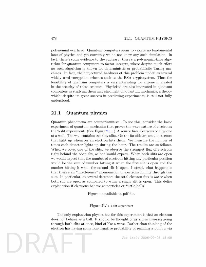
DRAFT

478 21.1. QUANTUM PHYSICS

polynomial overhead. Quantum computers seem to violate no fundamentallaws of physics and yet currently we do not know any such simulation. Infact, there’s some evidence to the contrary: there’s a polynomial-time algo-rithm for quantum computers to factor integers, where despite much effortno such algorithm is known for deterministic or probabilistic Turing ma-chines. In fact, the conjectured hardness of this problem underlies severalwidely used encryption schemes such as the RSA cryptosystem. Thus thefeasibility of quantum computers is very interesting for anyone interestedin the security of these schemes. Physicists are also interested in quantumcomputers as studying them may shed light on quantum mechanics, a theorywhich, despite its great success in predicting experiments, is still not fullyunderstood.

21.1 Quantum physics

Quantum phenomena are counterintuitive. To see this, consider the basicexperiment of quantum mechanics that proves the wave nature of electrons:the 2-slit experiment. (See Figure 21.1.) A source fires electrons one by oneat a wall. The wall contains two tiny slits. On the far side are small detectorsthat light up whenever an electron hits them. We measure the number oftimes each detector lights up during the hour. The results are as follows.When we cover one of the slits, we observe the strongest flux of electronsright behind the open slit, as one would expect. When both slits are openwe would expect that the number of electrons hitting any particular positionwould be the sum of number hitting it when the first slit is open and thenumber hitting it when the second slit is open. Instead, what happens isthat there’s an “interference” phenomenon of electrons coming through twoslits. In particular, at several detectors the total electron flux is lower whenboth slit are open as compared to when a single slit is open. This defiesexplanation if electrons behave as particles or “little balls”.


Figure 21.1: 2-slit experiment

The only explanation physics has for this experiment is that an electrondoes not behave as a ball. It should be thought of as simultaneously goingthrough both slits at once, kind of like a wave. Rather than thinking of theelectron has having some non-negative probability of reaching a point x via

Web draft 2006-09-28 18:09

DRAFT

21.2. QUANTUM SUPERPOSITIONS 479

slit i, we think of it has having some amplitude αx,i, where this amplitude isa complex number (in particular, it can be a negative number). The prob-ability of an electron hitting x when slit i is open is proportional to |αx,i|2and the probability of hitting x when both slits are open is proportional to|αx,1 +αx,2|2. In particular, if, say, αx,1 is positive and αx,2 is negative thenthe electron may hit x with smaller probability when both slits are openthan when only one of them is open.

“Nonsense!” you might say. “I need proof that the electron actuallywent through both slits.” So you propose the following modification to theexperiment. Position two detectors at the slits; these light up whenever anelectron passed through the slit. Now you can test the hypothesis that theelectron went through both slits simultaneously. If you put such detectorsat the slits, you will see that each electron indeed went through only one slit,but now you’ll also see that the interference phenomenon disappears and thegraph of electron hits on the wall becomes a simple sum! The explanationis roughly as follows: the quantum nature of particles “collapses” whenthey are “observed.” More specifically, a quantum system evolves accordingto certain laws, but “observation” from nosy humans and their detectors“collapses” the quantum state and this is a nonreversible operation. (Thismay seem mysterious and it is; see Chapter notes.) One moral to drawfrom this is that quantum computers, if they are ever built, will have tobe carefully isolated from external influences and noise, since noise may beviewed as a “measurement” performed by the environment on the system.Of course, we can never completely isolate the system, which means we haveto make quantum computation tolerant of a little noise. This seems to bepossible under some noise models (see Chapter notes).

21.2 Quantum superpositions

Now we describe a quantum register, a basic component of the quantumcomputer. Recall the classical register, the building block of the memory inyour desktop computer. An n-bit classical register with n bits consists of nparticles. Each of them can be in 2 states: up and down, or 0 and 1. Thusthere are 2n possible configurations, and at any time the register is in oneof these configurations.

The n-bit quantum register is similar, except at any time it can exist in asuperposition of all 2n configurations. (And the “bits” are called “qubits.”)Each configuration S ∈ 0, 1n has an associated amplitude αS ∈ C where

Web draft 2006-09-28 18:09

DRAFT

480 21.2. QUANTUM SUPERPOSITIONS

C is the set of complex numbers.

αS = amplitude of being in configuration S

Physicists like to denote this system state succinctly as∑

S αS |S 〉. Thisis their notation for describing a general vector in the vector space C2n ,expressing the vector as a linear combination of basis vectors. The basiscontains a vector |S 〉 for each configuration S. The choice of the basis usedto represent the configurations is immaterial so long as we fix a basis onceand for all.

At every step, actions of the quantum computer —physically, this mayinvolve shining light of the appropriate frequency on the quantum register,etc.— update αS according to some physics laws. Each computation stepis essentially a linear transformation of the system state. Let α denote thecurrent configuration (i.e., the system is in state

∑S αS |S 〉) and U be the

linear operator. Then the next system state is β = Uα. Physics laws requireU to be unitary, which means UU † = I. (Here U † is the matrix obtainedby transposing U and taking the complex conjugate of each entry.) Note aninteresting consequence of this fact: the effect of applying U can be reversedby applying the operator U †: thus quantum systems are reversible. Thisimposes strict conditions on which kinds of computations are permissibleand which are not.

As already mentioned, during the computation steps, the quantum reg-ister is isolated from the outside world. Suppose we open the system atsome time and observe the state of the register. If the register was in state∑

S αS |S 〉 at that moment, then

Pr[we see configuration S] = |αS |2 (1)

In particular, we have∑

S |αS |2 = 1 at all times. Note that observationis an irreversible operator. We get to see one configuration according to theprobability distribution described in (1) and and the rest of the configura-tions are lost forever.

What if we only observe a few bits of the register —a so-called partialobservation? Then the remaining bits still stay in quantum superposition.We show this by an example.

Example 21.1Suppose an n-bit quantum register is in the state∑

s∈0,1n−1

αs |0〉 |s〉+ βs |1〉 |s〉 (2)

Web draft 2006-09-28 18:09

DRAFT

21.3. CLASSICAL COMPUTATION USING REVERSIBLE GATES 481

(sometimes this is also represented as∑

s∈0,1n−1(αs |0〉 + βs |1〉) |s〉, andwe will use both representations). Now suppose we observe just the first bitof the register and find it to be 0. Then the new state is ∑

s∈0,1n−1

√|αs|2

−1 ∑s∈0,1n−1

αs |0〉 |s〉 (3)

where the first term is a rescaling term that ensures that probabilities infuture observations sum to 1.

21.3 Classical computation using reversible gates

Motivated by the 2nd Law of Thermodynamics, researchers have tried to de-sign computers that expend —at least in principle— zero energy. They haveinvented reversible gates, which can implement all classical computations ina reversible fashion. We will study reversible classical gates as a steppingstone to quantum gates; in fact, they are simple examples of quantum gates.

The Fredkin gate is a popular reversible gate. It has 3 Boolean inputsand on input (a, b, c) it outputs (a, b, c) if a = 1 and (a, c, b) if a = 0. It isreversible, in the sense that F (F (a, b, c)) = (a, b, c). Simple induction showsthat if a circuit is made out of Fredkin gates alone and has m inputs then itmust have m outputs as well. Furthermore, we can recover the inputs fromthe outputs by just applying the circuit in reverse. Hence a Fredkin gatecircuit is reversible.


Figure 21.2: Fredkin gate and how to implement AND with it.

The Fredkin gate is universal, meaning that every circuit of size S thatuses the familiar AND, OR, NOT gates (maximum fanin 2) has an equivalentFredkin gate circuit of size O(S). We prove this by showing that we canimplement AND, OR, and NOT using a Fredkin gate some of whose inputshave been fixed 0 or 1 (these are “control inputs”); see Figure 21.2 for ANDand Figure 21.3 for NOT; we leave OR as exercise. We also need to showhow to copy a value with Fredkin gates, since in a normal circuit, gates can

Web draft 2006-09-28 18:09

DRAFT

482 21.4. QUANTUM GATES

have fanout more than 1. To implement a COPY gate using Fredkin gatesis easy and is the same as for the the NOT gate (see Figure 21.3).

Thus to transform a normal circuit into a reversible circuit, we replaceeach gate with its Fredkin implementation, with some additional “control”inputs arriving at each gate to make it compute as AND/OR/NOT. Theseinputs have to be initialized appropriately.

The transformation appears in Figure 21.4, where we see that the outputcontains some junk bits. With a little more work (see Exercises) we can dothe transformation in such a way that the output has no junk bits, just theoriginal control bits. The reversible circuit starts with some input bits thatare initialized to 0 and these are transformed into output bits.


Figure 21.3: Implementing NOT and COPY with Fredkin Gate


Figure 21.4: Converting a normal circuit C into an equivalent circuit C′ of Fredkingates. Note that we need additional control inputs

21.4 Quantum gates

A 1-input quantum gate is represented by a unitary 2 × 2 matrix U =( U00 U01U10 U11

). When its input bit is 0 the output is the superposition U00 |0〉+U01 |1〉 and when the input is 1 the output is the superposition U10 |0〉 +U11 |1〉. When the input bit is in the superposition α0 |0〉+β0 |1〉 the outputbit is a superposition of the corresponding outputs

(α0U00 + β0U10) |0〉+ (α0U01 + β0U11) |1〉. (4)

More succinctly, if the input state vector is (α0, β0) then the output statevector is (

αβ

)= U

(α0

β0

)If |α|2 + |β|2 = 1 then unitarity of U implies that |α′|2 + |β′|2 = 1.Similarly, a 2-input quantum gate is represented by a unitary 4×4 matrix

R. When the input is the superposition α00 |00〉 + α01 |01〉 + α10 |10〉 +

Web draft 2006-09-28 18:09

DRAFT

21.4. QUANTUM GATES 483

α11 |11〉, the output is β00 |00〉+ β01 |01〉+ β10 |10〉+ β11 |11〉 whereβ00

β01

β10

β11

= R

α00

α01

α10

α11

In general, a quantum gate with k inputs is specified by a unitary 2k×2k

matrix.

Example 21.2A Fredkin gate is also a valid 3-input quantum gate. We represent it by an8× 8 matrix that gives its output on all 23 possible inputs. This matrix is apermutation matrix (i.e., obtainable from the identity matrix by applying apermutation on all the rows) since the output F (a, b, c) is just a permutationof the input (a, b, c). Exercise 3 asks you to verify that this permutationmatrix is unitary.

A quantum circuit on n inputs consists of (a) an n-bit quantum regis-ter (b) a sequence of gates (gj)j=1,2,.... If gj is a k-input gate, then the circuitspecification has to also give a sequence of bit positions (j, 1), (j, 2), . . . , (j, k) ∈[1, n] in the quantum register to which this gate is applied. The circuit com-putes by applying these gate operations to the quantum register one by onein the specified order. The register holds the state of the computation, andonly one gate is applied at any given time.

Example 21.3Suppose we have an n-bit quantum register in the state

∑S∈0,1n αS |S 〉. If

we apply a 1-input quantum gate U to the first wire, the new system stateis computed as follows. First “factor” the initial state by expressing eachn-bit configuration as a concatenation of the first bit with the remainingn− 1 bits: ∑

S′∈0,1n−1

α0,S′∣∣0S′ 〉+ α1,S′

∣∣1S′ 〉. (5)

(Formally we could express everything we are doing in terms of tensor prod-uct of vector spaces but we will not do that.)

Web draft 2006-09-28 18:09

DRAFT

484 21.4. QUANTUM GATES

To obtain the final state apply U on the first bit in each configurationas explained in equation (4). This yields

∑S′∈0,1n−1

(α0,S′U00 + α1,S′U10)∣∣0S′ 〉+ (α0,S′U01 + α1,S′U11)

∣∣1S′ 〉 (6)

We can similarly analyze the effect of applying a k-input quantum gateon any given set of k bits of the quantum register, by first “factoring” thestate vector as above.

21.4.1 Universal quantum gates

You may now be a little troubled by the fact that the set of possible 1-inputquantum gates is the set of all unitary 2 × 2 matrices, an uncountable set.That seems like bad news for the Radio Shacks of the future, who may feelobliged to keep all possible quantum gates in their inventory, to allow theircustomers to build all possible quantum circuits.

Luckily, Radio Shack need not fear. Researchers have shown the exis-tence of a small set of “universal” 2-input quantum gates such that everycircuit composed of S arbitrary k-input quantum gates can be simulatedusing a circuit of size 2poly(k) ·Spoly(logS) composed only of our universalgates. The simulation is not exact and the distribution on outputs is onlyapproximately the same as the one of the original circuit. (All of this as-sumes the absence of any outside noise; simulation in presence of noise is atopic of research and currently seems possible under some noise models.)

In any case, we will not need any fancy quantum gates below; just theFredkin gate and the following 1-input gate called the Hadamard gate:

H =1√2

(1 11 −1

)

Web draft 2006-09-28 18:09

DRAFT

21.5. BQP 485

21.5 BQP

Definition 21.4A language L ⊆ 0, 1∗, is in BQP iff there is a family of quantum circuits(Cn) of size nc s.t. ∀x ∈ 0, 1∗:

x ∈ L⇒ Pr[C(x)1 = 1] ≥ 23

x /∈ L⇒ Pr[C(x)1 = 1] ≤ 13

Here C(x)1 is the first output bit of circuit C, and the probability refers tothe probability of observing that this bit is 1 when we “observe” the outputsat the end of the computation.

The circuit has to be uniform, that is, a deterministic polynomial time(classical) Turing machine must be able to write down its description.

At first the uniformity condition seems problematic because a classicalTuring machine cannot write complex numbers needed to describe quantumgates. However, the machine can just express the circuit approximatelyusing universal quantum gates, which comprise a finite family. The approx-imate circuit computes the same language because of the gap between theprobabilities 2/3 and 1/3 used in the above definition.

Theorem 21.5P ⊆ BQP

Proof: Every language in P has a uniform circuit family of polynomial size.We transform these circuits into reversible circuits using Fredkin gates, thusobtaining a quantum circuit family for the language.

Theorem 21.6BPP ⊆ BQP

Proof: Every language in BPP has a uniform circuit family (Cn) of poly-nomial size, where circuit Cn has n normal input bits and an additionalm = poly(n) input wires that have to be initialized with random bits.

We transform the circuit into a reversible circuit C ′n using Fredkin gates.To produce “random” bits, we feed m zeros into an array of Hadamard gatesand plug their outputs into C ′n; see Figure 21.5.

A simple induction shows that for any N if we start with an N -bitquantum register in the state |0〉 and apply the Hadamard gate one by one

Web draft 2006-09-28 18:09

DRAFT

48621.6. FACTORING INTEGERS USING A QUANTUM COMPUTER


Figure 21.5: Turning a BPP circuit into an equivalent quantum circuit. An array ofHadamard gates turns the all-0 string into a uniform superposition of all m-bit strings.

on all the bits, then we obtain the superposition∑S∈0,1N

12N/2

|S 〉 (7)

(Note: the case N = 1 follows from the definition of the Hadamard gate.)The correctness of the above transformation is now clear since the “ran-

dom” inputs of circuit C ′n receive the output from the array of Hadamardgates, in other words, a uniform quantum superposition of all possible m-bitstrings. Thus the output bit of C ′n is a uniform superposition of the result oneach bit string. If we perform an observation on this output bit at the end,then the the probability that it is observed to be 1 is exactly the probabilitythat Cn accepts when the random gates are fed a truly random string.

21.6 Factoring integers using a quantum computer

This section proves the following famous result.

Theorem 21.7 (Shor [Sho97])There is a polynomial size quantum circuit that factors integers.

We describe Kitaev’s proof of this result since it uses eigenvalues, a morefamiliar and intuitive concept than the Fourier transforms used in Shor’salgorithm.

Definition 21.8 (Eigenvalue)λ is an eigenvalue of matrix M if there is a vector e (called the eigenvector), s.t.:

M · e = λe

Fact: If M is unitary, then |M · x|2 = 1 for each unit vector, so |λ| = 1.In other words there is a θ ∈ [0, 1) such that

λ = e2πιθ = cos(2πθ) + ι sin(2πθ).

Web draft 2006-09-28 18:09

DRAFT

21.6. FACTORING INTEGERS USING A QUANTUM COMPUTER487

Here ι =√−1.

Fact: If M · e = λe then Mk · e = λke. Hence e is still an eigenvector ofMk and λk is the corresponding eigenvalue.

Now we are ready to describe Kitaev’s algorithm and prove Theorem 21.7.Proof: Let N be the number to be factored. As usual, Z∗N is the set ofnumbers mod N that are co-prime to N . Simple number theory shows thatfor every a ∈ Z∗N there is a smallest integer r such that ar ≡ 1 (mod N);this r is called the order of a. The algorithm will try to find the order of arandom element of Z∗N . It is well-known if we can do this then we can factorN with high probability; here’s a sketch. First, note that with probability atleast 1/2, the element a has even order. Now if (ar − 1) ≡ 0 (mod N), then(a

r2 −1)(a

r2 +1) ≡ 0 (mod N). If a is random, with probability ≥ 1

2 , ar2 6= 1

(mod N), ar2 6= −1 (mod N) (this is a simple exercise using the Chinese

remainder theorem). Thus hence gcd(N, ar2 − 1) 6= N, 1. Thus, knowing r

we can compute ar/2 and compute gcd(N, ar2 − 1). Thus with probability at

least 1/4 (over the choice of a) we obtain a factor of N .The factoring algorithm is a mixture of a classical and a quantum al-

gorithm. Using classical random bits it generates a random a ∈ Z∗N andthen constructs a quantum circuit. Observing the output of this quantumcircuit a few times followed by some more classical computation allows it toobtain r, the order of a, with reasonable probability. (Of course, we couldin principle describe the entire algorithm as a quantum algorithm insteadof as a mixture of a classical and a quantum algorithm, but our descriptionisolates exactly where quantum mechanics is crucial.)

Consider a classical reversible circuit of size poly(logN) that acts onnumbers in Z∗N , and computes U(x) = ax (mod N). Then we can viewthis circuit as a quantum circuit operating on a quantum register. If thequantum register is in the superposition1∑

x∈Z∗N

αx |x〉,

then applying U gives the superposition∑x∈Z∗N

αx | ax (mod N)〉.

1Aside: This isn’t quite correct; the cardinality of Z∗N is not a power of 2 so it is not

immediately obvious how to construct a quantum register whose only possible configura-tions correspond to elements of Z∗

N . However, if we use the nearest power of 2, everythingwe are about to do will still be approximately correct. There are also other fixes to thisproblem.

Web draft 2006-09-28 18:09

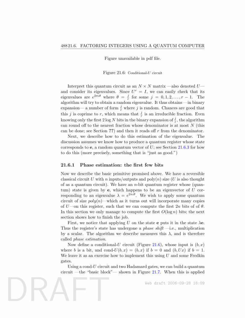
DRAFT



Figure 21.6: Conditional-U circuit

Interpret this quantum circuit as an N ×N matrix —also denoted U—and consider its eigenvalues. Since U r = I, we can easily check that itseigenvalues are e2πιθ where θ = j

r for some j = 0, 1, 2, . . . , r − 1. Thealgorithm will try to obtain a random eigenvalue. It thus obtains —in binaryexpansion— a number of form j

r where j is random. Chances are good thatthis j is coprime to r, which means that j

r is an irreducible fraction. Evenknowing only the first 2 logN bits in the binary expansion of jr , the algorithmcan round off to the nearest fraction whose denominator is at most N (thiscan be done; see Section ??) and then it reads off r from the denominator.

Next, we describe how to do this estimation of the eigenvalue. Thediscussion assumes we know how to produce a quantum register whose statecorresponds to e, a random quantum vector of U ; see Section 21.6.3 for howto do this (more precisely, something that is “just as good.”)

21.6.1 Phase estimation: the first few bits

Now we describe the basic primitive promised above. We have a reversibleclassical circuit U with n inputs/outputs and poly(n) size (U is also thoughtof as a quantum circuit). We have an n-bit quantum register whose (quan-tum) state is given by e, which happens to be an eigenvector of U cor-responding to an eigenvalue λ = e2πιθ. We wish to apply some quantumcircuit of size poly(n)—which as it turns out will incorporate many copiesof U—on this register, such that we can compute the first 2n bits of of θ.In this section we only manage to compute the first O(log n) bits; the nextsection shows how to finish the job.

First, we notice that applying U on the state e puts it in the state λe.Thus the register’s state has undergone a phase shift —i.e., multiplicationby a scalar. The algorithm we describe measures this λ, and is thereforecalled phase estimation.

Now define a conditional-U circuit (Figure 21.6), whose input is (b, x)where b is a bit, and cond-U(b, x) = (b, x) if b = 0 and (b, Ux) if b = 1.We leave it as an exercise how to implement this using U and some Fredkingates.

Using a cond-U circuit and two Hadamard gates, we can build a quantumcircuit —the “basic block”— shown in Figure 21.7. When this is applied

Web draft 2006-09-28 18:09

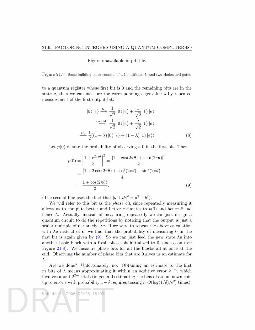
DRAFT



Figure 21.7: Basic building block consists of a Conditional-U and two Hadamard gates.

to a quantum register whose first bit is 0 and the remaining bits are in thestate e, then we can measure the corresponding eigenvalue λ by repeatedmeasurement of the first output bit.

|0〉 |e〉 H1−→ 1√2|0〉 |e〉+ 1√

2|1〉 |e〉

cond-U−→ 1√2|0〉 |e〉+ λ√

2|1〉 |e〉

H2−→ 12((1 + λ) |0〉 |e〉+ (1− λ) |1〉 |e〉) (8)

Let p(0) denote the probability of observing a 0 in the first bit. Then

p(0) =∣∣∣∣1 + e2πιθ

2

∣∣∣∣2 =|1 + cos(2πθ) + ι sin(2πθ)|2

2

=

∣∣1 + 2 cos(2πθ) + cos2(2πθ) + sin2(2πθ)∣∣

4

=1 + cos(2πθ)

2. (9)

(The second line uses the fact that |a+ ιb|2 = a2 + b2).We will refer to this bit as the phase bit, since repeatedly measuring it

allows us to compute better and better estimates to p(0) and hence θ andhence λ. Actually, instead of measuring repeatedly we can just design aquantum circuit to do the repetitions by noticing that the output is just ascalar multiple of e, namely, λe. If we were to repeat the above calculationwith λe instead of e, we find that the probability of measuring 0 in thefirst bit is again given by (9). So we can just feed the new state λe intoanother basic block with a fresh phase bit initialized to 0, and so on (seeFigure 21.8). We measure phase bits for all the blocks all at once at theend. Observing the number of phase bits that are 0 gives us an estimate forλ.

Are we done? Unfortunately, no. Obtaining an estimate to the firstm bits of λ means approximating it within an additive error 2−m, whichinvolves about 22m trials (in general estimating the bias of an unknown coinup to error ε with probability 1−δ requires tossing it O(log(1/δ)/ε2) times).

Web draft 2006-09-28 18:09

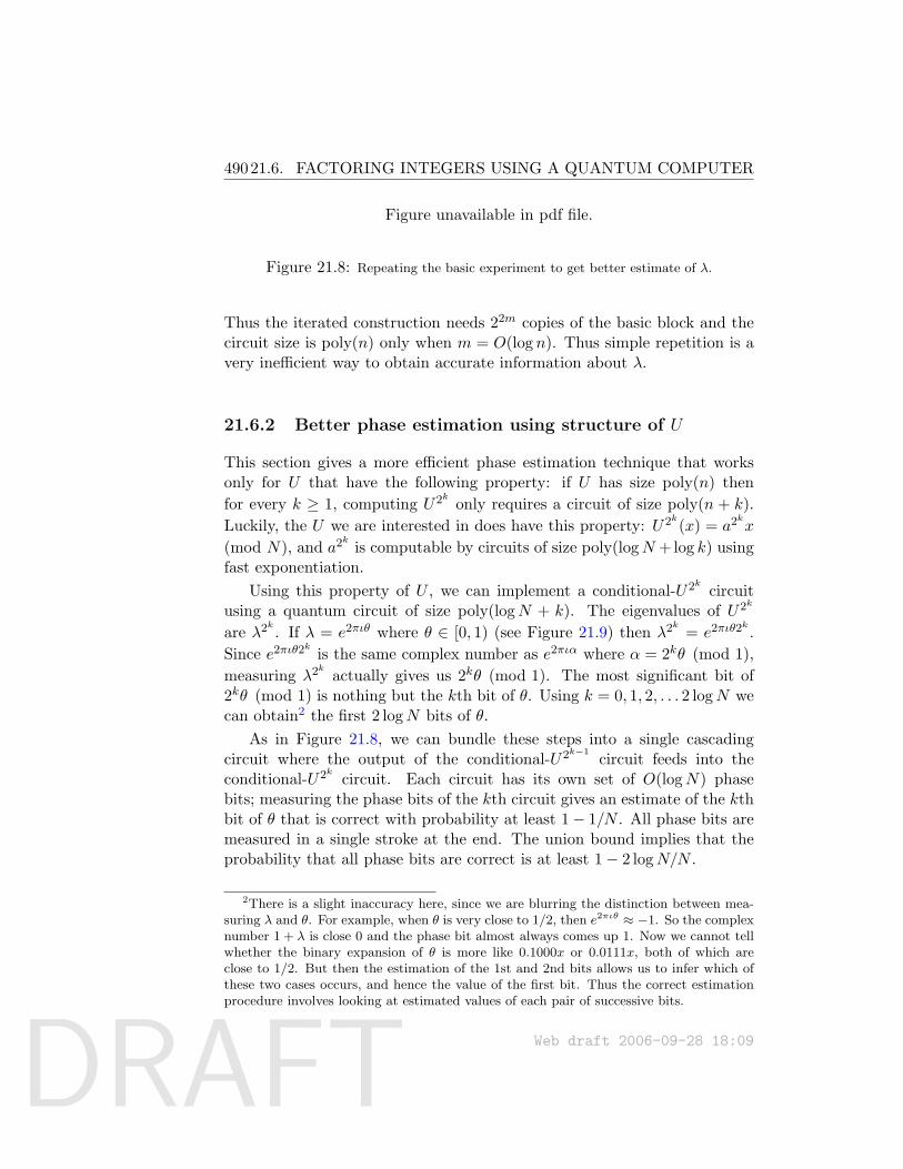
DRAFT



Figure 21.8: Repeating the basic experiment to get better estimate of λ.

Thus the iterated construction needs 22m copies of the basic block and thecircuit size is poly(n) only when m = O(log n). Thus simple repetition is avery inefficient way to obtain accurate information about λ.

21.6.2 Better phase estimation using structure of U

This section gives a more efficient phase estimation technique that worksonly for U that have the following property: if U has size poly(n) thenfor every k ≥ 1, computing U2k only requires a circuit of size poly(n + k).Luckily, the U we are interested in does have this property: U2k(x) = a2kx

(mod N), and a2k is computable by circuits of size poly(logN +log k) usingfast exponentiation.

Using this property of U , we can implement a conditional-U2k circuitusing a quantum circuit of size poly(logN + k). The eigenvalues of U2k

are λ2k . If λ = e2πιθ where θ ∈ [0, 1) (see Figure 21.9) then λ2k = e2πιθ2k.

Since e2πιθ2k

is the same complex number as e2πια where α = 2kθ (mod 1),measuring λ2k actually gives us 2kθ (mod 1). The most significant bit of2kθ (mod 1) is nothing but the kth bit of θ. Using k = 0, 1, 2, . . . 2 logN wecan obtain2 the first 2 logN bits of θ.

As in Figure 21.8, we can bundle these steps into a single cascadingcircuit where the output of the conditional-U2k−1

circuit feeds into theconditional-U2k circuit. Each circuit has its own set of O(logN) phasebits; measuring the phase bits of the kth circuit gives an estimate of the kthbit of θ that is correct with probability at least 1− 1/N . All phase bits aremeasured in a single stroke at the end. The union bound implies that theprobability that all phase bits are correct is at least 1− 2 logN/N .

2There is a slight inaccuracy here, since we are blurring the distinction between mea-suring λ and θ. For example, when θ is very close to 1/2, then e2πιθ ≈ −1. So the complexnumber 1 + λ is close 0 and the phase bit almost always comes up 1. Now we cannot tellwhether the binary expansion of θ is more like 0.1000x or 0.0111x, both of which areclose to 1/2. But then the estimation of the 1st and 2nd bits allows us to infer which ofthese two cases occurs, and hence the value of the first bit. Thus the correct estimationprocedure involves looking at estimated values of each pair of successive bits.

Web draft 2006-09-28 18:09

DRAFT



Figure 21.9: Eigenvalue λ = e2πιθ in the complex plane.

21.6.3 Uniform superpositions of eigenvectors of U

To finish, we need to show how to put a quantum register into a statecorresponding to a random eigenvector. Actually, we only show how to putthe quantum register into a uniform superposition of eigenvectors of U . Thissuffices for our cascading circuit, as we will argue shortly.

First we need to understand what the eigenvectors look like. Recall that1, a, a2, . . . , ar−1

is a subgroup of Z∗N . Let B be a set of representatives

of all cosets of this subgroup. In other words, for each x ∈ Z∗N there is aunique b ∈ B and l ∈ 0, 1, . . . , r − 1 such that x = bal (mod N). It iseasily checked that the following is the complete set of eigenvectors, where

ω = e2πιr :

∀j ∈ 0, 1, . . . , r − 1 ,∀b ∈ B ej,b =r−1∑l=0

ωjl∣∣∣ bal (mod N)〉 (10)

The eigenvalue associated with this eigenvector is ω−j = e−2πιjr .

Fix b and consider the uniform superposition:

1r

r−1∑j=0

ej,b =1r

r−1∑j=0

r−1∑l=0

ωjl∣∣∣ bal (mod N)〉 (11)

=1r

r−1∑l=0

r−1∑j=0

ωjl∣∣∣ bal (mod N)〉. (12)

Separating out the terms for l = 0 and using the formula for sums of geo-metric series:

=1r(r−1∑j=0

|b〉+r−1∑l=1

(ωl)r − 1ωl

∣∣∣ bal (mod N)〉) (13)

since ωr = 1 we obtain

= |b〉 (14)

Web draft 2006-09-28 18:09

DRAFT

492 21.7. QUANTUM COMPUTING: A TOUR DE HORIZON

Thus if we pick an arbitrary b and feed the state |b〉 into the quantumregister, then that can also be viewed as a uniform superposition 1

r

∑j ej,b.

21.6.4 Uniform superposition suffices

Now we argue that in the above phase estimation based algorithm, a uniformsuperposition of eigenvectors is just as good as a single eigenvector.

Fixing b, the initial state of the quantum register is

1r

∑j

|0〉 |ej,b 〉,

where 0 denotes the vector of phase bits that is initialized to 0. Afterapplying the quantum circuit, the final state is

1r

∑j

|cj 〉 |ej,b 〉,

where |cj 〉 is a state vector for the phase bits that, when observed, gives thefirst 2 logN bits of j/r with probability at least 1 − 1/N . Thus observingthe phase bits gives us whp a random eigenvalue.

21.7 Quantum Computing: a Tour de horizon

Will give 1-para intros to quantum information, quantum crypto, the factthat there is an oracle for which NP is not in BQP, grover’s algorithm,models of quantum computation, decoherence and error correction,quantuminteractive proofs.

Exercises

§1 Implement an OR gate using the Fredkin gate.

§2 Verify that the Fredkin gate is a valid quantum gate.

§3 Given any classical circuit computing a function f from n bits to n bits,describe how to compute the same function with a reversible circuitthat is a constant factor bigger and has no “junk” output bits.

Hint:Useourtransformation,thencopytheoutputtoasafeplace,andthenrunthecircuitinreversetoerasethejunkoutputs.

Web draft 2006-09-28 18:09

DRAFT

21.7. QUANTUM COMPUTING: A TOUR DE HORIZON 493

§4 Suppose the description of a quantum circuit U is given to you. De-scribe an implementation of the Conditional-U circuit.

§5 Let N be composite. For a ∈ Z∗N let r = ord(a) be the order of a,i.e. r is the minimal number such that ar = 1 (mod N). Show thatif a ∈ Z∗N is randomly chosen then with probability at least 1/10 (1)ord(a) is even and (2) aord(a)/2 6≡ ±1 (mod N).

Hint:usetheChineseremaindertheoremandthefactthatforaprimepthegroupZp∗iscyclic.


§7 Complete the proof of Lemma 21.10 for the case that r and M arenot coprime. That is, prove that also in this case there exist at leastΩ(r/ log r) values x’s such that 0 ≤ rx (mod M) ≤ r/2 and dM/x eand r are coprime.

Hint:letd=gcd(r,M),r′=r/dandM′=M/d.NowusethesameargumentasinthecasethatMandrarecoprimetoarguethatthereexistΩ(

rdlogr)valuesx∈ZM′satisfyingthiscondition,

andthatifxsatisfiesitthensodoesx+cMforeveryc.§8 (Uses knowledge of continued fractions) Suppose j, r ≤ N are mutually

coprime and unknown to us. Show that if we know the first 2 logNbits of j/r then we can recover j, r in polynomial time.


The “meaning” of quantum theory has eluded (or certainly puzzled) mostscientists. (The physicist Penrose [Pen94] has even sought to link humanconsciousness to the collapse of the quantum wave function, though thisis controversial.) No one doubts that quantum effects exist at microscopicscales. The problem lies in explaining why they do not manifest themselvesat the macrosopic level (or at least not to human consciousness). A ScientificAmerican article by Yam [Yam97] describes various explanations that havebeen advanced over the years. The leading theory is decoherence, whichtries to use quantum theory to explain the absence of macroscopic quantumeffects. Researchers are not completely comfortable with this explanation.

The issue is undoubtedly important to quantum computing, which re-quires hundreds of thousands of particles to stay in quantum superposition

Web draft 2006-09-28 18:09

DRAFT

494 21.8. QUANTUM NOTATIONS

for large-ish periods of time. Thus far it is an open question whether this ispractically achievable. One theoretical idea is to treat decoherence as a formof noise, and to build noise-tolerance into the computation —a nontrivialprocess. For details of this and many other topics, see the books by Kitaev,Shen, and Vyalyi [AA02].

Feynman [Fey82] was the first to suggest the possibility that quantummechanics might allow Turing Machines more computational power thanclassical TMs. In 1985 Deutsch [Deu85] defined a quantum turing ma-chine, though in retrospect his definition is unsatisfactory. Better defini-tions then appeared in Deutsch-Josza [DJ92], Bernstein-Vazirani [BV97] andYao [Yao93], at which point quantum computation was firmly establishedas a field.

The book by Nielsen and Chuang [NC00] gives a comprehensive treat-ment of quantum computation.

Alternative presentation of Shor’s algorithm.

21.8 Quantum Notations

21.9 Simon’s Algorithm

21.10 Integer factorization using quantum com-puters.

21.10.1 Reduction to Order Finding

21.10.2 Quantum Fourier Transform over ZM .

The Fourier transform over an Abelian group G is a linear operation thattransforms a |G|-dimensional vector from representation in the standard ba-sis to a representation in the Fourier basis, which is a different orthonormalbasis. For M = 2m the Fourier over the group ZM (numbers 0, . . . ,M − 1with addition modulo M) can be represented as a 2m × 2m unitary matrix.We’ll now show this matrix can be implemented using O(m2) basic matri-ces. This means that we can transform a quantum system whose registeris in state f to a system whose register is in the state corresponding to theFourier transform f of f . This does not mean that we can compute in O(m2)the Fourier transform over ZM - indeed this is not sufficient time to evenwrite the output! Nonetheless, this transformation still turns out to be very

Web draft 2006-09-28 18:09

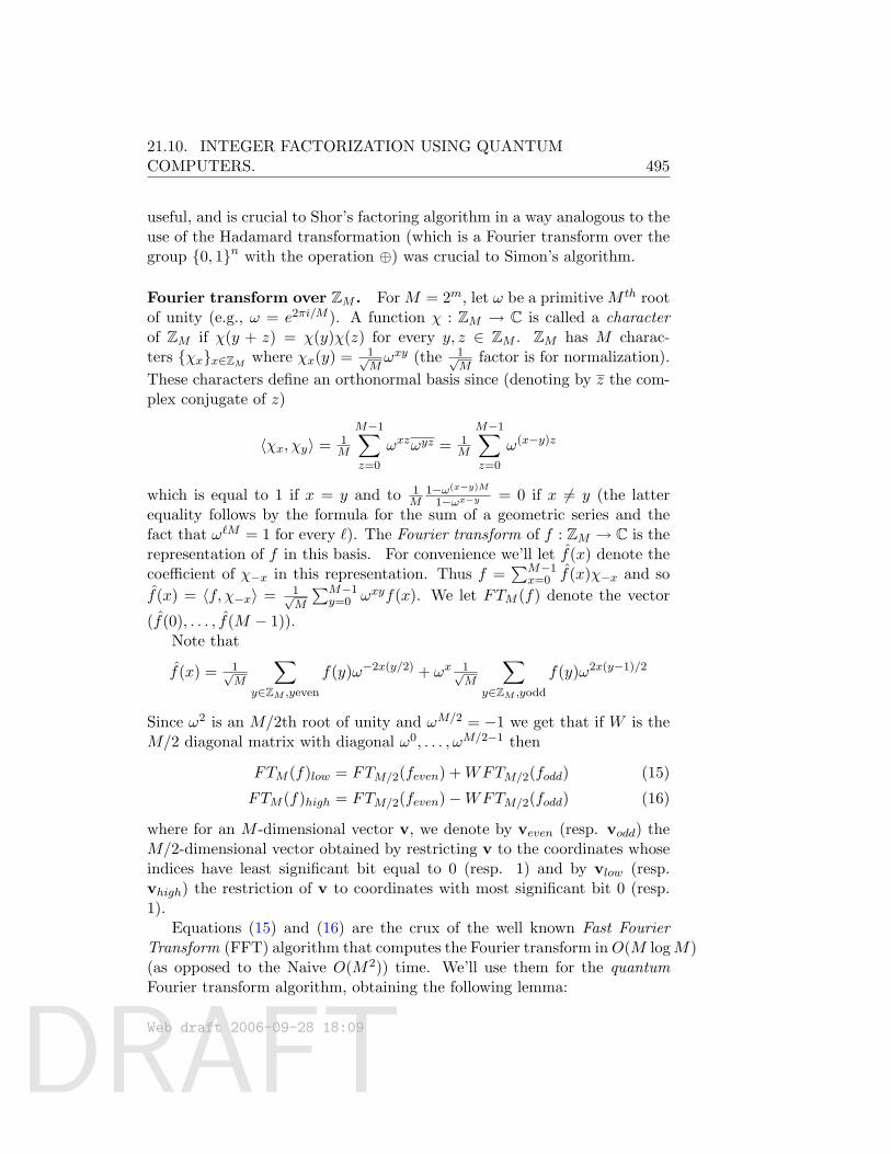
DRAFT

21.10. INTEGER FACTORIZATION USING QUANTUMCOMPUTERS. 495

useful, and is crucial to Shor’s factoring algorithm in a way analogous to theuse of the Hadamard transformation (which is a Fourier transform over thegroup 0, 1n with the operation ⊕) was crucial to Simon’s algorithm.

Fourier transform over ZM . For M = 2m, let ω be a primitive M th rootof unity (e.g., ω = e2πi/M ). A function χ : ZM → C is called a characterof ZM if χ(y + z) = χ(y)χ(z) for every y, z ∈ ZM . ZM has M charac-ters χxx∈ZM where χx(y) = 1√

Mωxy (the 1√

Mfactor is for normalization).

These characters define an orthonormal basis since (denoting by z the com-plex conjugate of z)

〈χx, χy〉 = 1M

M−1∑z=0

ωxzωyz = 1M

M−1∑z=0

ω(x−y)z

which is equal to 1 if x = y and to 1M

1−ω(x−y)M

1−ωx−y = 0 if x 6= y (the latterequality follows by the formula for the sum of a geometric series and thefact that ω`M = 1 for every `). The Fourier transform of f : ZM → C is therepresentation of f in this basis. For convenience we’ll let f(x) denote thecoefficient of χ−x in this representation. Thus f =

∑M−1x=0 f(x)χ−x and so

f(x) = 〈f, χ−x〉 = 1√M

∑M−1y=0 ωxyf(x). We let FTM (f) denote the vector

(f(0), . . . , f(M − 1)).Note that

f(x) = 1√M

∑y∈ZM ,yeven

f(y)ω−2x(y/2) + ωx 1√M

∑y∈ZM ,yodd

f(y)ω2x(y−1)/2

Since ω2 is an M/2th root of unity and ωM/2 = −1 we get that if W is theM/2 diagonal matrix with diagonal ω0, . . . , ωM/2−1 then

FTM (f)low = FTM/2(feven) +WFTM/2(fodd) (15)

FTM (f)high = FTM/2(feven)−WFTM/2(fodd) (16)

where for an M -dimensional vector v, we denote by veven (resp. vodd) theM/2-dimensional vector obtained by restricting v to the coordinates whoseindices have least significant bit equal to 0 (resp. 1) and by vlow (resp.vhigh) the restriction of v to coordinates with most significant bit 0 (resp.1).

Equations (15) and (16) are the crux of the well known Fast FourierTransform (FFT) algorithm that computes the Fourier transform inO(M logM)(as opposed to the Naive O(M2)) time. We’ll use them for the quantumFourier transform algorithm, obtaining the following lemma:

Web draft 2006-09-28 18:09

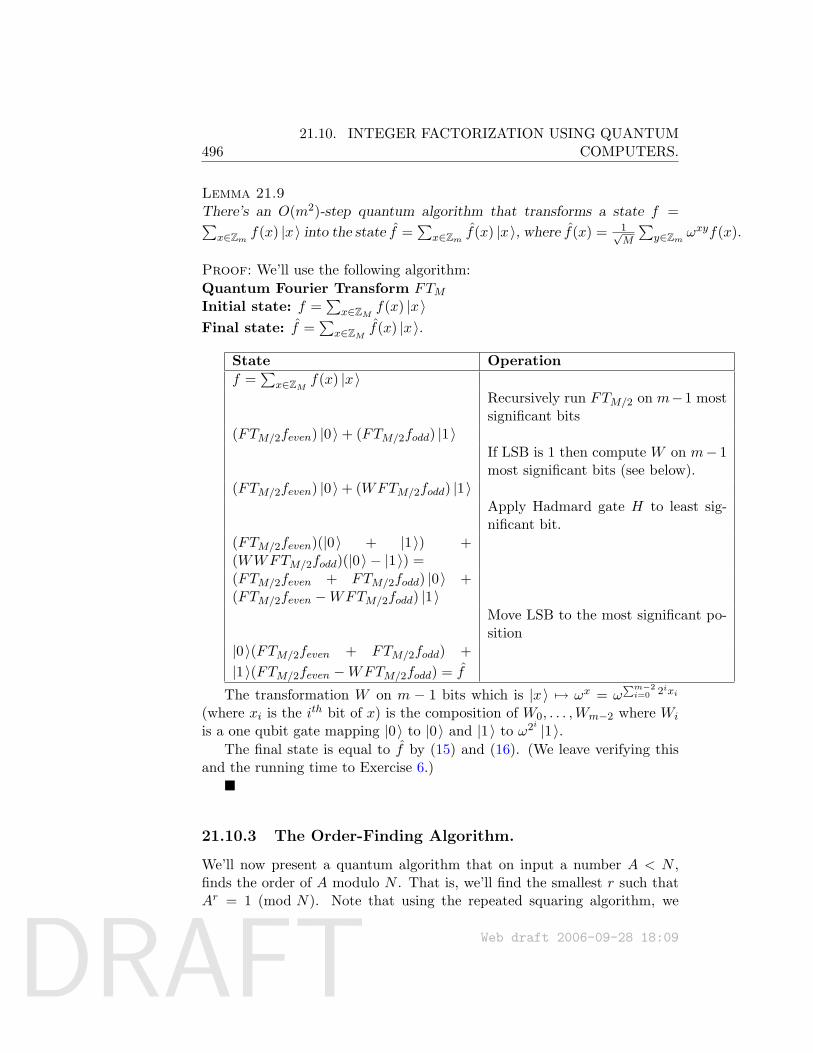
DRAFT

49621.10. INTEGER FACTORIZATION USING QUANTUM

COMPUTERS.

Lemma 21.9There’s an O(m2)-step quantum algorithm that transforms a state f =∑

x∈Zm f(x) |x〉 into the state f =∑

x∈Zm f(x) |x〉, where f(x) = 1√M

∑y∈Zm ω

xyf(x).

Proof: We’ll use the following algorithm:Quantum Fourier Transform FTMInitial state: f =

∑x∈ZM f(x) |x〉

Final state: f =∑

x∈ZM f(x) |x〉.

State Operationf =

∑x∈ZM f(x) |x〉

Recursively run FTM/2 on m−1 mostsignificant bits

(FTM/2feven) |0〉+ (FTM/2fodd) |1〉If LSB is 1 then compute W on m− 1most significant bits (see below).

(FTM/2feven) |0〉+ (WFTM/2fodd) |1〉Apply Hadmard gate H to least sig-nificant bit.

(FTM/2feven)(|0〉 + |1〉) +(WWFTM/2fodd)(|0〉 − |1〉) =(FTM/2feven + FTM/2fodd) |0〉 +(FTM/2feven −WFTM/2fodd) |1〉

Move LSB to the most significant po-sition

|0〉(FTM/2feven + FTM/2fodd) +|1〉(FTM/2feven −WFTM/2fodd) = f

The transformation W on m − 1 bits which is |x〉 7→ ωx = ω∑m−2i=0 2ixi

(where xi is the ith bit of x) is the composition of W0, . . . ,Wm−2 where Wi

is a one qubit gate mapping |0〉 to |0〉 and |1〉 to ω2i |1〉.The final state is equal to f by (15) and (16). (We leave verifying this

and the running time to Exercise 6.)

21.10.3 The Order-Finding Algorithm.

We’ll now present a quantum algorithm that on input a number A < N ,finds the order of A modulo N . That is, we’ll find the smallest r such thatAr = 1 (mod N). Note that using the repeated squaring algorithm, we

Web draft 2006-09-28 18:09

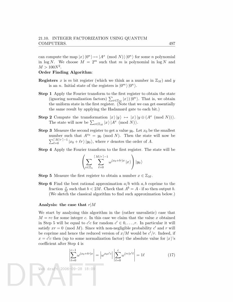
DRAFT


can compute the map |x〉 |0n 〉 7→ |Ax (mod N)〉 |0n 〉 for some n polynomialin logN . We choose M = 2m such that m is polynomial in logN andM > 100N2.Order Finding Algorithm:

Registers x is m bit register (which we think as a number in ZM ) and yis an n. Initial state of the registers is |0m 〉 |0n 〉.

Step 1 Apply the Fourier transform to the first register to obtain the state(ignoring normalization factors)

∑x∈ZM |x〉) |0

n 〉. That is, we obtainthe uniform state in the first register. (Note that we can get essentiallythe same result by applying the Hadamard gate to each bit.)

Step 2 Compute the transformation |x〉 |y 〉 7→ |x〉 |y ⊕ (Ax (mod N))〉.The state will now be

∑x∈ZM |x〉 |A

x (mod N)〉.

Step 3 Measure the second register to get a value y0. Let x0 be the smallestnumber such that Ax0 = y0 (mod N). Then the state will now be∑dM/r e−1

`=0 |x0 + `r 〉 |y0 〉, where r denotes the order of A.

Step 4 Apply the Fourier transform to the first register. The state will be∑x∈Zn

dM/r e−1∑`=0

ω(x0+`r)x |x〉

|y0 〉

Step 5 Measure the first register to obtain a number x ∈ ZM .

Step 6 Find the best rational approximation a/b with a, b coprime to thefraction x

M such that b < 2M . Check that Ab = A - if so then output b.(We sketch the classical algorithm to find such approximation below.)

Analysis: the case that r|M

We start by analyzing this algorithm in the (rather unrealistic) case thatM = rc for some integer c. In this case we claim that the value x obtainedin Step 5 will be equal to c′c for random c′ ∈ 0, . . . , r. In particular it willsatisfy xr = 0 (mod M). Since with non-negligible probability c′ and r willbe coprime and hence the reduced version of x/M would be c′/r. Indeed, ifx = c′c then (up to some normalization factor) the absolute value for |x〉’scoefficient after Step 4 is∣∣∣∣∣

c−1∑`=0

ω(x0+`r)x

∣∣∣∣∣ = ∣∣∣ωx0c′c∣∣∣ ∣∣∣∣∣

c∑`=0

ω(rc)c′`

∣∣∣∣∣ = 1` (17)

Web draft 2006-09-28 18:09

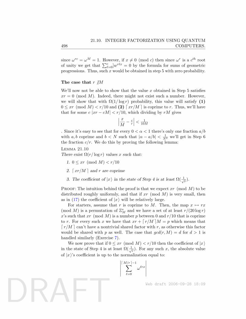
DRAFT


COMPUTERS.

since ωrc = ωM = 1. However, if x 6= 0 (mod c) then since ωr is a cth rootof unity we get that

∑c`=0]w

r`x = 0 by the formula for sums of geometricprogressions. Thus, such x would be obtained in step 5 with zero probability.

The case that r 6 |M

We’ll now not be able to show that the value x obtained in Step 5 satisfiesxr = 0 (mod M). Indeed, there might not exist such a number. However,we will show that with Ω(1/ log r) probability, this value will satisfy (1)0 ≤ xr (mod M) < r/10 and (2) dxr/M e is coprime to r. Thus, we’ll havethat for some c |xr − cM | < r/10, which dividing by rM gives∣∣∣ x

M− c

r

∣∣∣ < 110M

. Since it’s easy to see that for every 0 < α < 1 there’s only one fraction a/bwith a, b coprime and b < N such that |α − a/b| < 1

N2 we’ll get in Step 6the fraction c/r. We do this by proving the following lemma:

Lemma 21.10There exist Ω(r/ log r) values x such that:

1. 0 ≤ xr (mod M) < r/10

2. dxr/M e and r are coprime

3. The coefficient of |x〉 in the state of Step 4 is at least Ω( 1√r).

Proof: The intuition behind the proof is that we expect xr (mod M) to bedistributed roughly uniformly, and that if xr (mod M) is very small, thenas in (17) the coefficient of |x〉 will be relatively large.

For starters, assume that r is coprime to M . Then, the map x 7→ rx(mod M) is a permutation of Z∗M and we have a set of at least r/(20 log r)x’s such that xr (mod M) is a number p between 0 and r/10 that is coprimeto r. For every such x we have that xr + d r/M eM = p which means thatd r/M e can’t have a nontrivial shared factor with r, as otherwise this factorwould be shared with p as well. The case that gcd(r,M) = d for d > 1 ishandled similarly (Exercise 7).

We now prove that if 0 ≤ xr (mod M) < r/10 then the coefficient of |x〉in the state of Step 4 is at least Ω( 1√

r). For any such x, the absolute value

of |x〉’s coefficient is up to the normalization equal to:∣∣∣∣∣∣dM/r e−1∑

`=0

ω`rx

∣∣∣∣∣∣Web draft 2006-09-28 18:09

DRAFT


Let β = ωrx. If β = 1 then this sum is equal to dM/r e and otherwiseit’s equal to

∣∣∣1−βdM/r e1−β

∣∣∣. This is equal to sin(dM/r eθ)sin θ , where θ = rx (mod M)

M

is the angle such that β = eiθ (see Figure ?? ). Since 0 < θ < r10M ,

we get that dM/r eθ ≤ 1/9 and in this range up to a constant we havethat this proportion is again equal to dM/r e. Since the measurement ofStep 3 restricted the space an almost uniform distribution over about M/xof the x’s and the Fourier transform adds another 1√

Mnormalization factor,

it can be shown that the normalization coefficient at this step is at least12

√rM

1√M

=√rM and so we’re done.

Web draft 2006-09-28 18:09

DRAFT


COMPUTERS.

Web draft 2006-09-28 18:09

DRAFT

Chapter 22

Logic in complexity theory

Very sketchy

As mentioned in the book’s introduction, complexity theory (indeed, allof computer science) arose from developments in mathematical logic in thefirst half of the century. Mathematical logic continues to exert an influencetoday, suggesting terminology and choice of problems (e.g., “boolean sat-isfiability”) as well as approaches for attacking complexity’s central openquestions. This chapter is an introduction to the basic concepts.

Mathematical logic has also influenced many other areas of computerscience, such as programming languages, program verification, and modelchecking. We will not touch upon them, except to note that they supplyinteresting examples of hard computational problems —ranging from NP-complete to EXPSPACE-complete to undecidable.

The rest of the chapter assumes only a nodding familiarity with logicterminology, which we now recount informally; for details see a logic text.

A logic usually refers to a set of rules about constructing valid sentences.Here are a few logics we will encounter. Propositional logic concerns sen-tences such as (p∨¬q)∧ (¬p∨ r) where p, q, r are boolean variables. Recallthat the SAT problem consists of determining the satisfiability of such sen-tences. In first order logic, we allow relation and function symbols as wellas quantification symbols ∃ and ∀. For instance, the statement ∀xS(x) 6= xis a first order sentence in which x is quantified universally, S() is a unaryrelation symbol and 6= is a binary relation. Such logics are used in well-known axiomatizations of mathematics, such as Euclidean geometry, PeanoArithmetic or Zermelo Frankel set theory. Finally, second order logic allowssentences in which one is allowed quantification over structures, i.e., func-tions and relations. An example of a second order sentence is ∃S∀xS(x) 6= x,


501

DRAFT

502 22.1. LOGICAL DEFINITIONS OF COMPLEXITY CLASSES

where S is a unary relation symbol.A sentence (or collection of sentences) in a logic has no intrinsic “mean-

ing.” The meaning —including truth or falsehood—can be discussed onlywith reference to a structure, which gives a way of interpreting all symbolsin the sentence. To give an example, Peano arithmetic consists of five sen-tences (“axioms”) in a logic that consists of symbols like S(x), =, + etc. Thestandard structure of these sentences is the set of positive integers, with S()given the intepretation of “successor function,” + given the interpretationof addition, and so on. A structure is said to be a model for a sentence or agroup of sentences if those sentences are true in that structure.

Finally, a proof system consists of a set of sentences Σ called axioms andone or more derivation rules for deriving new sentences from the axioms.We say that sentence σ can be proved from Σ, denoted Σ ` σ, if it can bederived from Σ using a finite number of applications of the derivation rules.A proveable sentence is called a theorem.

Note that a theorem is a result of a mechanical (essentially, algorithmic)process of applying derivation rules to the axioms. There is a related notionof whether or not σ is logically implied by Σ, denoted Σ |= σ, which meansthat every model of Σ is also a model of σ. In other words, there is no“counterexample model” in which the axioms Σ are true but σ is not. Thetwo notions are in general different but Godel in his completeness theoremfor first order theories exhibited a natural set of derivation rules such thatlogically implied sentences are exactly the set of theorems. (This result wasa stepping stone to his even more famous incompleteness theorem.)

Later in this chapter we give a complexity-theoretic definition of a proofsystem, and introduce the area of proof complexity that studies the size ofthe smallest proof of a mathematical statement in a given proof system.

22.1 Logical definitions of complexity classes

Just as Church and others defined computation using logic without refer-ring to any kind of computing machine, it is possible to give “machineless”characterizations of many complexity classes using logic. We describe a fewexamples below.

22.1.1 Fagin’s definition of NP

In 1974, just as the theory of NP-completeness was coming into its own,Fagin showed how to define NP using second-order logic. We describe his

Web draft 2006-09-28 18:09

DRAFT

22.1. LOGICAL DEFINITIONS OF COMPLEXITY CLASSES 503

idea using an example.

Example 22.1(Representing 3-COLOR) We show how to represent the set of 3-colorablegraphs using second order logic.

Let E be a symbol for a binary relation, and C0, C1, C2 be symbolsfor unary relations, and φ(E,C0, C1, C2) be a first order formula that is aconjunction of the following formulae where i + 1, i + 2 are meant to beunderstood modulo 3:

∀u, v E(u, v) = E(v, u) (1)∀u ∧i=1,2,3 (Ci(u)⇒ ¬(Ci+1(u) ∨ Ci+2(u)) (2)∀uCi(u) ∨ Ci+1(u) ∨ Ci+2(u) (3)∀u, v E(u, v)⇒ ∧i=1,2,3(Ci(u)⇒ ¬Ci(v)) (4)

What set of E’s defined on a finite set satisfy ∃C0∃C1∃C2φ(E,C0, C1, C2)?If E is defined on a universe of size n (i.e., u, v take values in this universe)then (1) says that E is symmetric, i.e., it may be viewed as the edge set of anundirected graph on n vertices. Conditions (2) and (3) say that C0, C1, C2

partition the vertices into three classes. Finally, condition (4) says that thepartition is a valid coloring.

Now we can sketch the general result. To represent a general NP prob-lem, there is a unary relation symbol that represents the input (in the abovecase, E). The witness is a tableau (see Chapter 2) of an accepting compu-tation. If the tableau has size nk, the witness can be represented by a k-aryrelation (in the above case the witness is a 3-coloring, which has represen-tation size 3n and hence was represented using 3 unary relations). The firstorder formula uses the Cook-Levin observation that the tableau is correctiff it is correct in all 2× 3 “windows”.

The formal statement of Fagin’s theorem is as follows; the proof is leftas an exercise.

Theorem 22.2 (Fagin)To be written.

Web draft 2006-09-28 18:09

DRAFT

50422.2. PROOF COMPLEXITY AS AN APPROACH TO NP VERSUS

CONP

22.1.2 MAX-SNP

22.2 Proof complexity as an approach to NP ver-sus coNP

Proof complexity tries to study the size of the smallest proof of a statementin a given proof system. First, we need a formal definition of what a proofsystem is. The following definition due to Cook and Reckow focuses atten-tion on the intuitive property that a mathematical proof is “easy to check.”

Definition 22.3A proof system consists of a polynomial-time Turing machine M . A state-ment T is said to be a theorem of this proof system iff there is a stringπ ∈ 0, 1∗ such that M accepts (T, π).

If T is a theorem of proof system M , then the proof complexity of T withrespect to M is the minimun k such that there is some π ∈ 0, 1k for whichM accepts (T, π).

Note that the definition of theoremhood ignores the issue of the lengthof the proof, and insists only that the M ’s running time is polynomial in theinput length |T |+ |π|. The following is an easy consequence of the definitionand the motivation for much of the field of proof complexity.

Theorem 22.4A proof system M in which SAT has polynomial proof complexity exists iffNP = coNP.

Many branches of mathematics, including logic, algebra, geometry, etc.give rise to proof systems. Algorithms for SAT and automated theoremprovers (popular in some areas of computer science) also may be viewed asproof systems.

22.2.1 Resolution

This concerns

22.2.2 Frege Systems

22.2.3 Polynomial calculus

22.3 Is P 6= NP unproveable?

Web draft 2006-09-28 18:09

DRAFT

Chapter 23

Why are circuit lowerboundsso difficult?

Why have we not been able to prove strong lower bounds for circuits? In1994 Razborov and Rudich formalized the notion of a “natural mathematicalproof,” for a circuit lowerbound. They pointed out that current lowerboundarguments involve “natural” mathematical proofs, and show that obtainingstrong lowerbound with such techniques would violate a widely believedcryptographic assumption (namely, that factoring integers requires time 2n

ε

for some fixed ε > 0). Thus presumably we need to develop mathematicalarguments that are not natural. This result may be viewed as a modernanalogue of the Baker, Gill, Solovay result from the 1970s (see Chapter ??)that showed that diagonalization alone cannot resolve P versus NP andother questions.

Basically, a natural technique is one that proves a lowerbound for arandom function and is “constructive.” We formalize “constructive” laterbut first consider why lowerbound proofs may need to work for randomfunctions.

23.1 Formal Complexity Measures

Let us imagine at a high level how one might approach the project of prov-ing circuit lower bounds. For concreteness, focus on formulas, which areboolean circuits where gates have indegree 2 and outdegree 1. It is tempt-ing to use some kind of induction. Suppose we have a function like theone in Figure 23.1 that we believe to be “complicated.” Since the functioncomputed at the output is “complicated”, intuition says that at least one


505

DRAFT

506 23.1. FORMAL COMPLEXITY MEASURES


Figure 23.1: A formula for a hard function.

of the functions on the incoming edges to the output gate should also be“pretty complicated” (after all those two functions can be combined with asingle gate to produce a “complicated” function). Now we try to formalizethis intuition, and point out why one ends up proving a lowerbound on theformula complexity of random functions.

The most obvious way to formalize a “complicatedness” is as a function µthat maps every boolean function on 0, 1n to a nonnegative integer. (Theinput to µ is the truth table of the function.) We say that µ is a formalcomplexity measure if it satisfies the following properties: First, the measureis low for trivial functions: µ(xi) ≤ 1 and µ(xi) ≤ 1 for all i. Second, werequire that

• µ(f ∧ g) ≤ µ(f) + µ(g) for all f, g; and

• µ(f ∨ g) ≤ µ(f) + µ(g) for all f, g.

For instance, the following function ρ is trivially a formal complexity mea-sure

ρ(f) = 1 + the smallest formula size for f. (1)

In fact, it is easy to prove the following by induction.

Theorem 23.1If µ is any formal complexity measure, then µ(f) is a lowerbound on theformula complexity of f .

Thus to formalize the inductive approach outlined earlier, it suffices to de-fine a measure µ such that µ(CLIQUE) is high (say superpolynomial). Forexample, one could try “fraction of inputs for which the function agrees withthe CLIQUE function” or some suitably modified version of this. In general,one imagines that defining a measure that lets us prove a good lowerboundfor CLIQUE would involve some deep observation about the CLIQUE func-tion. The next lemma seems to show, however, that even though all we careabout is the CLIQUE function, our lowerbound necessarily must reasonabout random functions.

Web draft 2006-09-28 18:09

DRAFT

23.2. NATURAL PROPERTIES 507

Lemma 23.2Suppose µ is a formal complexity measure and there exists a function f :0, 1n → 0, 1 such that µ(f) ≥ c for some large number c. Then for atleast 1/4 of all functions g : 0, 1n → 0, 1 we must have µ(g) ≥ c/4.

Proof: Let g : 0, 1n → 0, 1 be any function. Write f as f = h⊕g whereh = f ⊕ g. So f = (h ∧ g) ∨ (h ∧ g) and µ(f) ≤ µ(g) + µ(g) + µ(h) + µ(h).

Now suppose for contradiction’s sake that g : µ(g) < c/4 containsmore than 3/4 of all boolean functions on n-bit inputs. If we pick the abovefunction g randomly, then g, h, h are also random (though not independent).Using the trivial union bound we have Pr[All of h, h, g, g have µ < c/4] > 0.Hence µ(f) < c, which contradicts the assumption. Thus the lemma isproved.

In fact, the following stronger theorem holds:

Theorem 23.3If µ(f) > c then for all ε > 0 and for at least 1− ε of all functions g we havethat,

µ(g) ≥ Ω(

c

(n+ log(1/ε))2

).

The idea behind the proof of the theorem is to write f as the booleancombination of a small number of functions and then proceed similarly asin the proof of the lemma.

23.2 Natural Properties

Moving the above discussion forward, we think of a lowerbound proof asidentifying some property of “hard” functions that is not shared by “easy”functions.Definition 23.4A property Φ is a map from boolean functions to 0, 1. A P-natural propertyuseful against P/poly is a property Φ such that:

1. Φ(f) = 1 for at least a 1/2n fraction of all boolean functions on n bits(recall that there are 22n functions on n bits);

2. Φ(f) = 1 implies that f 6∈ P/poly (or more concretely, that f hascircuit complexity at least nlogn, say); and

3. Φ is computable on n-bit functions in 2O(n) time (i.e., polynomial inthe length of the function’s truth table).

Web draft 2006-09-28 18:09

DRAFT

508 23.2. NATURAL PROPERTIES

The term P-natural refers to requirement (3). The property is useful againstP/poly because of requirement (2). (Note that this requirement also ensuresthat Φ is not trivial, since it must be 0 for functions in P/poly.) Requirement(1) corresponds to our above intuition that circuit lowerbounds should provethe hardness of a random function.

By suitably modifying (2) and (3) we can analogously define, for anycomplexity class C1 and circuit class C2, a C1-natural property that is usefulagainst circuit class C2. We emphasize that when the property is computed,the input is the truth table of a function, whose size is 2n. Thus a P-natural property is computed in time 2cn for some constant c > 1 and aPSPACE-natural property is computed in space 2cn.

Example 23.5The result that PARITY is not computable in AC0 (Section ??) involvedthe following steps. (a) Show that every AC0 circuit can be simplified byrestricting at most n − nε input bits so that it then becomes a constantfunction. (b) Show that the PARITY function does not have this property.

Thus the natural property lurking in this proof is the following: Φ(f) = 1iff for every way of assigning values to at most n−nε input bits the functiondoes not become a constant function. Clearly, if Φ(f) = 1 then f 6∈ AC0, sof is useful against AC0. Furthermore, Φ can be computed in 2O(n) time —just enumerate all possible choices for the subsets of variables and all waysof setting them to 0/1. This running time is polynomial in the length ofthe truth-table, so Φ is P-natural. Finally, requirement (1) is also met sincealmost all boolean functions satisfy Φ(f) = 1 (easy to check using a simpleprobability calculation; left as exercise).

Thinking further, we see that Φ is a AC0-natural property that is usefulagainst AC0.

Example 23.6The lowerbound for ACC0 circuits described in Section ?? is not naturalper se. Razborov and Rudich show how to naturalize the proof, in otherwords change it —while retaining its essence—so that it does use a naturalproperty. Recall that every boolean function on n bits can be represented bya multilinear polynomial over GF (3). The space of all n-variate multilinearpolynomials forms a vector space, whose dimension is N = 2n. Then all

Web draft 2006-09-28 18:09

DRAFT

23.2. NATURAL PROPERTIES 509

multilinear polynomials in n variables of total degree less than n/2 forma subspace of dimension N/2 (this assumes n is even), and we denote thisspace by L. For a boolean function f let f be a multilinear polynomial overGF (3) that represents f . Then define Φ(F ) = 1 iff the dimension of thespace

f l1 + l2 : l1, l2 ∈ L

is at least 3N/4. It can be checked that Φ is 1 for the parity function, aswell as for most random functions. Furthermore, rank computations canbe done in NC2 so it is NC2-natural. The technique of Section ?? can beused to show that if Φ(f) = 1 then f 6∈ ACC0[3]; thus Φ is useful againstACC0[3].

Example 23.7The lowerbound for monotone circuits in Section ?? does use constructivemethods, but it is challenging to show that it applies to a random functionsince a random function is not monotone. Nobody has formulated a gooddefinition of a random monotone function.

In the definition of natural proofs, requirement (3) is the most contro-versial in that there is no inherent reason why mathematical proofs shouldgo hand in hand with efficient algorithms.

Remark 23.8“Constructive mathematics” was a movement within mathematics that re-jected any proofs of existence that did not yield an algorithm for construct-ing the object. Today this viewpoint is considered quaint; nonconstructiveproofs are integral to mathematics.

In our context, “constructive” has a stricter meaning, namely the proofhas to yield a polynomial-time algorithm. Many proofs that would be “con-structive” for a mathematician would be nonconstructive under our defini-tion. Surprisingly, even with this stricter definition, proofs in combinatorialmathematics are usually constructive, and —as Razborov and Rudich arepointing out —the same is true of current circuit lowerbounds as well.

In a few cases, combinatorial results initially proved “nonconstructively”later turned out to have constructive proofs: a famous example is the Lovasz

Web draft 2006-09-28 18:09

DRAFT

510 23.3. LIMITATIONS OF NATURAL PROOFS

Local Lemma (discovered in 1974; algorithmic version is in Beck [Bec91]).The same is true for several circuit lowerbounds—cf. the “naturalized” ver-sion of the Razborov-Smolensky lowerbound for ACC0[q] mentioned earlier,and Raz’s proof [Raz00] of the Babai-Nisan-Szegedy [BNS] lowerbound onmultiparty communication complexity.

23.3 Limitations of Natural Proofs

The following theorem by Razborov and Rudich explains why we have notbeen able to use the same techniques to obtain an upper bound on P/poly:constructing a P-natural property useful against P/poly violates widely be-lieved cryptographic assumptions.

Theorem 23.9 (Razborov, Rudich [RR97])Suppose a P-natural property Φ exists that is useful against P/poly. Thenthere are no strong pseudorandom function generators. In particular, FAC-TORING and DISCRETE LOG can be solved in less than 2n

εtime for all

ε > 0.

Pseudorandom function generators were defined in Section ??. The def-inition used a distinguisher polynomial-time machine that is given oracleaccess to either a truly random function or a function from the pseudoran-dom family. The family is termed pseudorandom if the distinguisher cannotdistinguish between the two oracles. Now we tailor that more general def-inition for our narrow purposes in this section. We allow the distinguisher2O(n) time and even allow it to examine the truth table of the function!This is without loss of generality since in 2O(n) time the distinguisher couldconstruct the truth table using 2n queries to the oracle.

Definition 23.10A pseudorandom function generator is a function f(k, x) computable in poly-nomial time where the input x has n bits and the “key” k has nc bits, wherec > 2 is a fixed constant. Denoting by Fn the function obtained by uniformlyselecting k ∈ 0, 1nc and setting Fn to f(k, ·), we have the property thatthe function ensemble F = Fn∞n=1 is “pseudorandom,” namely, for eachTuring machine M running in time 2O(n), and for all sufficiently large n,

|Pr[M(Fn) = 1]− Pr[M(Hn) = 1]| < 12n2 ,

where Hn is a random function on 0, 1n.We will denote f(k, ·) by fk.

Web draft 2006-09-28 18:09

DRAFT

23.3. LIMITATIONS OF NATURAL PROOFS 511


Figure 23.2: Constructing a pseudorandom function generator from a pseudorandomgenerator.

Intuitively, the above definition says that if f is a pseudorandom functiongenerator, then for a random k, the probability is high that fk “looks like arandom function” to all Turing machines running in time 2O(n). Note thatfk cannot look random to machines that run in 2O(nc) time since they canjust guess the key k. Thus restricting the running time to 2O(n) (or to someother fixed exponential function such as 2O(n2)) is crucial.

Recall that Section ?? described the Goldreich-Goldwasser-Micali con-struction of pseudorandom function generators f(k, x) using a pseudoran-dom generator g that stretches nc random bits to 2nc pseudorandom (alsosee Figure 23.2): Let g0(k) and g1(k) denote, respectively, the first and lastnc bits of g(k). Then the following function is a pseudorandom functiongenerator, where MSB(x) refers to the first bit of a string x:

f(k, x) = MSB(gxn gxn−1 · · · gx2 gx1(k)).

The exercises in Chapter 10 explored the security of this construction asa function of the security parameter of g; basically, the two are essentiallythe same. By the Goldreich-Levin theorem of Section ??, a pseudorandomgenerator with such a high security parameter exists if a oneway permutationexists and some ε > 0, such that every 2n

εtime algorithm has inversion prob-

ability less than 2−nε. The DISCRETE LOG function —a permutation— is

conjectured to satisfy this property. As mentioned in Chapter 10, researchersbelieve that there is a small ε > 0 such that the worst-case complexity ofDISCRETE LOG is 2n

ε, which by random self-reducibility also implies the

hardness of the average case. (One can also obtain pseudorandom generatorsusing FACTORING, versions of which are also believed to be just as hardas DISCRETE LOG.) If this belief is correct, then pseudorandom functiongenerators exist as outlined above. (Exercise.)

Now we can prove the above theorem.

Theorem 23.9: Suppose the property Φ exists, and f is a pseudorandomfunction generator. We show that a Turing machine can use Φ to distinguishfk from a random function. First note that fk ∈ P/poly for every k (justhardwire k into the circuit for fk) so the contrapositive of property (2)implies that Φ(fk) = 0. In addition, property (1) implies that PrHn [Φ(Hn) =

Web draft 2006-09-28 18:09

DRAFT

512 23.4. MY PERSONAL VIEW

1] ≥ 1/2n. Hence,

PrHn

[Φ(Hn)]− Prk∈0,1nc

[Φ(fk)] ≥ 1/2n,

and thus Φ is a distinguisher against f .

23.4 My personal view

Discouraged by the Razborov-Rudich result, researchers (myself included)hardly ever work on circuit lowerbounds. Lately, I have begun to thinkthis reaction was extreme. I still agree that a circuit lowerbound for sayCLIQUE, if and when we prove it, will very likely apply to random functionsas well. Thus the way to get around the Razborov-Rudich observation is todefine properties that are not P-natural; in other words, are nonconstructive.I feel that this need not be such an insurmountable barrier since a host ofmathematical results are nonconstructive.

Concretely, consider the question of separating NEXP from ACC0, oneof the (admittedly not very ambitious) frontiers of circuit complexity out-lined in Chapter 13. As observed there, NEXP 6= ACC0 will follow if wecan improve the Babai-Nisan-Szegedy lowerbound of Ω(n/2k) for k-partycommunication complexity to Ω(n/poly(k)) for some function in NEXP.One line of attack is to lowerbound the discrepancy of all large cylinderintersections in the truth table, as we saw in Raz’s proof of the BNS lower-bound1. (In other words, the “unnatural” property we are defining is Φwhere Φ(f) = 1 iff f has high discrepancy and thus high multiparty com-munication complexity.) For a long time, I found this question intimidatingbecause the problem of computing the discrepancy given the truth tableof the function is coNP-hard (even for k = 2). This seemed to suggestthat a proof that the discrepancy is high for an explicit function (whichpresumably will also show that it is high for random functions) must havea nonconstructive nature, and hence will be very difficult. Lately, I havebegun to suspect this intuition.

A relevant example is Lovasz’s lowerbound of the chromatic number ofthe Kneser graph [Lov78]. Lowerbounding the chromatic number is coNP-complete in general. Lovasz gives a topological proof (using the famousBorsuk-Ulam fixed point theorem) that determines the chromatic number

1Interestingly, Raz discovered this naturalization of the BNS proof after being brieflyhopeful that the original BNS proof—which is not natural— may allow a way around theRazborov-Rudich result.

Web draft 2006-09-28 18:09

DRAFT

23.4. MY PERSONAL VIEW 513

of the Kneser graph exactly. From his proof one can indeed obtain analgorithm for solving chromatic number on all graphs([MZ02]) —but it runsin PSPACE for general graphs! So if this were a circuit lowerbound wecould call it PSPACE-natural, and thus “nonconstructive.” Nevertheless,Lovasz’s reasoning for the particular case of the Kneser graph is not overlycomplicated because the graph is highly symmetrical. This suggests weshould not blindly trust the intuition that “nonconstructive ≡ difficult.”

I fervently hope that the next generation of researchers will view theRazborov-Rudich theorem as a guide rather than as a big obstacle!

Exercises

§1 Prove Theorem 23.3.

§2 Prove that a random function satisfies Φ(f) = 1 with high probability,where Φ is the property defined in Example 23.5.

§3 Show that if the hardness assumption for discrete log is true, thenpseudorandom function generators as defined in this chapter exist.

§4 Prove Wigderson’s observation: P-natural properties cannot provethat DISCRETE LOG requires circuits of 2n

εsize.

Hint:IfDISCRETELOGishardonworst-caseinputsthenitishardonmostinputs,andthenitcanbeusedtoconstructpseudo-randomfunctions.

§5 (Razborov [Raz92]) A submodular complexity measure is a complexitymeasure that satisfies µ(f∨g)+µ(f∧g) ≤ µ(f)+µ(g) for all functionsf, g. Show that for every n-bit function fn, such a measure satisfiesµ(fn) = O(n).

Hint:Itsufficestoprovethiswhenfnisarandomfunction.Useinductiononthenumberofvariables,andthefactthatbothfn

andfnarerandomfunctions.


The observation that circuit lowerbounds may unwittingly end up reasoningabout random functions first appears in Razborov [Raz89]’s result about thelimitations of the method of approximation.

Web draft 2006-09-28 18:09

DRAFT

514 23.4. MY PERSONAL VIEW

We did not cover the full spectrum of ideas in the Razborov-Rudichpaper [RR97], where it is observed that candidate pseudorandom functiongenerators exist even in the class TC0, which lies between ACC0 and NC1.Thus natural proofs will probably not allow us to separate even TC0 fromP.

Razborov’s observation about submodular measures in Problem 5 is im-portant because many existing approaches for formula complexity use sub-modular measures; thus they will fail to even prove superlinear lowerbounds.

In contrast with my limited optimism, Razborov himself expresses (in theintroduction to [Raz03]) a view that the obstacle posed by the natural proofsobservation is very serious. He observes that existing lowerbound approachesuse weak theories of arithmetic such as Bounded Arithmetic. He conjecturesthat any circuit lowerbound attempt in such a logical system must be natural(and hence unlikely to work). But as I mentioned, several theorems even indiscrete mathematics use reasoning (e.g., fixed point theorems like Borsuk-Ulam) that does not seem to be formalizable in Bounded Arithmetic. Thusis my reason for optimism.

However, somen other researchers are far more pessimistic: they fear thatP versus NP may be independent of mathematics (say, of Zermelo-Fraenkelset theory). Razborov says that he has no intuition about this.

Web draft 2006-09-28 18:09

DRAFT

Appendices


515

DRAFT

DRAFT

Appendix A

Mathematical Background.

This appendix reviews the mathematical notions used in this book. However,most of these are only used in few places, and so the reader might want toonly quickly review the section on probability, and come back to the othersections as needed. In particular, apart from probability, the first part of thebook essentially requires only comfort with mathematical proofs and somevery basic notions of discrete math. A gentle introduction to these notionsappears in Chapter 0 of Sipser’s book [SIP96].

The topics described in the appendix are covered in greater depth inmany places. The lecture notes by Lehman and Leighton [LL06] cover themajority of the math topics needed for this book (and some more). Thebooks of Mitzenmacher and Upfal [MU05] and Prabhakar and Raghavan[?] cover both algorithmic reasoning and probability. For more insight ondiscrete probability, see the book by Alon and Spencer [AS00]. A fullercoverage of algorithms appears in the recent book of Kleinberg and Tardos[KT06] or the earlier text of Cormen at al [CLRS01]. This book does notrequire prior knowledge of computability and automata theory, but somebasic familiarity with that theory could be useful: see Sipser’s book [SIP96]for an excellent introduction.

A.1 Sets, Functions, Pairs, Strings, Graphs, Logic.

A set contains a finite or infinite number of elements, without repetitionor respect to order, for example 2, 17, 5, N = 1, 2, 3, . . . (the set ofnatural numbers), [n] = 1, 2, . . . , n (the set of natural numbers from 1 ron), R (the set of real numbers). For a finite set A, we denote by |A| thenumber of elements in A. Some operations on sets are: (1) union: A∪B =


517

DRAFT

518 A.1. SETS, FUNCTIONS, PAIRS, STRINGS, GRAPHS, LOGIC.

x : x ∈ A or x ∈ B, (2) intersection : A ∩ B = x : x ∈ A and x ∈ B,and (3) substraction: A \B = x : x ∈ A and x 6∈ B.

We say that f is a function from a set A to B, denoted by f : A→ B, ifit maps any element of A into an element of B. If B and A are finite, thenthe number of possible functions from A to B is |B||A|. We say that f is oneto one if for every x,w ∈ A with x 6= w, f(x) 6= f(w). If A,B are finite, theexistence of such a function implies that |A| ≤ |B|. We say that f is ontoif for every y ∈ B there exists x ∈ A such that f(x) = y. If A,B are finite,the existence of such a function implies that |A| ≥ |B|. We say that f is apermutation if it is both one-to-one and onto. For finite A,B, the existenceof a permutation from A to B implies that |A| = |B|.

If A,B are sets, then the A×B denotes the set of all ordered pairs 〈a, b〉with a ∈ A, b ∈ B. Note that if A,B are finite then |A×B| = |A| · |B|. Wecan define similarly A×B ×C to be the set of ordered triples 〈a, b, c〉 witha ∈ A, b ∈ B, c ∈ C. For n ∈ N, we denote by An the set A×A× · · · ×A (ntimes). We will often use the set 0, 1n, consisting of all length-n sequencesof bits (i.e., length n strings), and the set 0, 1∗ = ∪n≥0 0, 1n (0, 10 hasa single element: a binary string of length zero, which we call the emptyword and denote by ε).

A graph G consists of a set V of vertices (which we often assume isequal to the set [n] = 1, . . . , n for some n ∈ N) and a set E of edges,which consists of unordered pairs (i.e., size two subsets) of elements in V .We denote the edge u, v of the graph by u v. For v ∈ V , the neighbors ofv are all the vertices u ∈ V such that u v ∈ E. In a directed graph, the edgesconsist of ordered pairs of vertices, to stress this we sometimes denote theedge 〈u, v〉 in a directed graph by −→u v. One can represent an n-vertex graphG by its adjacency matrix which is an n×n matrix A such that Ai,j is equalto 1 if the edge

−→i j is present in G ith and is equal to 0 otherwise. One can

think of an undirected graph as a directed graph G that satisfies that forevery u, v, G contains the edge −→u v if and only if it contains the edge −→v u.Hence, one can represent an undirected graph by an adjecancy matrix thatis symmetric (Ai,j = Aj,i for every i, j ∈ [n]).

A Boolean variable is a variable that can be either True or False(we sometimes identify True with 1 and False with 0). We can com-bine variables via the logical operations AND (∧), OR (∨) and NOT (¬,sometimes also denoted by an overline), to obtain Boolean formulae. Forexample, the following is a Boolean formulae on the variables u1, u2, u3:(u1 ∧ u2) ∨ ¬(u3 ∧ u1). The definitions of the operations are the usual:a ∧ b = True if a = True and b = True and is equal to False oth-

Web draft 2006-09-28 18:09

DRAFT

A.2. PROBABILITY THEORY 519

erwise; a = ¬a = True if a = False and is equal to False otherwise;a ∨ b = ¬(a ∨ b). If ϕ is a formulae in n variables u1, . . . , un, then for anyassignment of values u ∈ False,Truen (or equivalently, 0, 1n), we de-note by ϕ(u) the value of ϕ when its variables are assigned the values in u.We say that ϕ is satisfiable if there exists a u such that ϕ(u) = True.

We will often use the quantifiers ∀ (for all) and ∃ (exists). That is, ifϕ is a condition that can be True or False depending on the value of avariable x, then we write ∀xϕ(x) to denote the statement that ϕ is True forevery possible value that can be assigned to x. If A is a set then we write∀x∈Aϕ(x) to denote the statement that ϕ is True for every assignment forx from the set A. The quantifier ∃ is defined similarly. Formally, we saythat ∃xϕ(x) holds if and only if ¬(∀x¬ϕ(x)) holds.

A.2 Probability theory

A finite probability space is a finite set Ω = ω1, . . . , ωN along with a setof numbers p1, . . . , pN ∈ [0, 1] such that

∑Ni=1 pi = 1. A random element is

selected from this space by choosing ωi with probability pi. If x is chosenfrom the sample space Ω then we denote this by x ∈R Ω. If no distributionis specified then we use the uniform distribution over the elements of Ω (i.e.,pi = 1

N for every i).An event over the space Ω is a subset A ⊆ Ω and the probability that A

occurs, denoted by Pr[A], is equal to∑

i:ωi∈A pi. To give an example, theprobability space could be that of all 2n possible outcomes of n tosses of afair coin (i.e., Ω = 0, 1n and pi = 2−n for every i ∈ [2n]) and the eventA can be that the number of coins that come up “heads” (or, equivalently,1) is even. In this case, Pr[A] = 1/2 (exercise). The following simple bound—called the union bound—is often used in the book. For every set of eventsA1, A2, . . . , An,

Pr[∪ni=1Ai] ≤n∑i=1

Pr[Ai]. (1)

Inclusion exclusion principle. The union bound is a special case of amore general principle. Indeed, note that if the sets A1, . . . , An are not dis-joint then the probability of ∪iAi could be smaller than

∑i Pr[Ai] since we

are overcounting elements that appear in more than one set. We can correctthis by substracting

∑i<j Pr[Ai ∩Aj ] but then we might be undercounting,

since we subtracted elements that appear in at least 3 sets too many times.Continuing this process we get

Web draft 2006-09-28 18:09

DRAFT

520 A.2. PROBABILITY THEORY

Claim A.1 (Inclusion-Exclusion principle)For every A1, . . . , An,

Pr[∪ni=1Ai] =n∑i=1

Pr[Ai]−∑

1≤i<j≤nPr[Ai∩Aj ]+· · ·+(−1)n−1 Pr[A1∩· · ·∩An] .

Moreover, this is an alternating sum which means that if we take only thefirst k summands of the right hand side, then this upperbounds the left-handside if k is odd, and lowerbounds it if k is even.

We sometimes use the following corollary of this claim:Claim A.2For every events A1, . . . , An,

Pr[∪ni=1Ai] ≥n∑i=1

Pr[Ai]−∑

1≤i<j≤nPr[Ai ∩Aj ]

Random subsum principle. The following fact is used often in the book:

Claim A.3 (The random subsum principle)For x, y ∈ 0, 1n, denote x y =

∑ni=1 xiyi (mod 2) (that is, x y is

equal to 1 if the number of i’s such that xi = yi = 1 is odd and equal to 0otherwise). Then for every y 6= 0n,

Prx∈R0,1n

[x y = 1] = 12

Proof: Suppose that yj is nonzero. We can think of choosing x as follows:first choose all the coordinates of x other than the jth and only choose thejth coordinate last. After we choose all the coordinates of x other than thejth, the value

∑i:i6=j xiyi (mod 2) is fixed to be some c ∈ 0, 1. Regardless

of what c is, with probability 1/2 we choose xj = 0, in which case x y = cand with probability 1/2 we choose xj = 1, in which case x y = 1− c. Wesee that in any case x

∏y will be equal to 1 with probability 1/2.

A.2.1 Random variables and expectations.

A random variable is a mapping from a probability space to R. For example,if Ω is as above, the set of all possible outcomes of n tosses of a fair coin,then we can denote by X the number of coins that came up heads.

The expectation of a random variable X, denoted by E[X], is its weightedaverage. That is, E[X] =

∑Ni=1 piX(ωi). The following simple claim follows

from the definition:

Web draft 2006-09-28 18:09

DRAFT


Claim A.4 (Linearity of expectation)For X,Y random variables over a space Ω, denote by X + Y the randomvariable that maps ω to X(ω) + Y (ω). Then,

E[X + Y ] = E[X] + E[Y ]

This claims implies that the random variable X from the example abovehas expectation n/2. Indeed X =

∑ni=1Xi where Xi is equal to 1 if the ith

coins came up heads and is equal to 0 otherwise. But clearly, E[Xi] = 1/2for every i.

For a real number α and a random variable X, we define αX to be therandom variable mapping ω to α ·X(ω). Note that E[αX] = αE[X].

A.2.2 The averaging argument

We list various versions of the “averaging argument.” Sometimes we givetwo versions of the same result, one as a fact about numbers and one as afact about probability spaces.

Lemma A.5If a1, a2, . . . , an are some numbers whose average is c then some ai ≥ c.

Lemma A.6 (“The Probabilistic Method”)If X is a random variable which takes values from a finite set and E[X] = µthen the event “X ≥ µ” has nonzero probability.

Lemma A.7If a1, a2, . . . , an ≥ 0 are numbers whose average is c then the fraction of ai’sthat are greater than (resp., at least) kc is less than (resp, at most) 1/k.

Lemma A.8 (“Markov’s inequality”)Any non-negative random variable X satisfies

Pr (X ≥ kE[X]) ≤ 1k.

Corollary A.9If a1, a2, . . . , an ∈ [0, 1] are numbers whose average is 1 − γ then at least1−√γ fraction of them are at least 1−√γ.

Can we give any meaningful upperbound on Pr[X < c · E[X]] wherec < 1? Yes, if X is bounded.

Web draft 2006-09-28 18:09

DRAFT


Lemma A.10If a1, a2, . . . , an are numbers in the interval [0, 1] whose average is ρ then atleast ρ/2 of the ai’s are at least as large as ρ/2.

Proof: Let γ be the fraction of i’s such that ai ≥ ρ/2. Then γ+(1−γ)ρ/2must be at least ρ/2, so γ ≥ ρ/2. More generally, we have

Lemma A.11If X ∈ [0, 1] and E[X] = µ then for any c < 1 we have

Pr[X ≤ cµ] ≤ 1− µ1− cµ

.

Example A.12Suppose you took a lot of exams, each scored from 1 to 100. If your averagescore was 90 then in at least half the exams you scored at least 80.

A.2.3 Conditional probability and independence

If we already know that an event B happened, this reduces the space fromΩ to Ω∩B, where we need to scale the probabilities by 1/Pr[B] so they willsum up to one. Thus, the probability of an event A conditioned on an eventB, denoted Pr[A|B], is equal to Pr[A ∩B]/Pr[B] (where we always assumethat B has positive probability).

We say that two events A,B are independent if Pr[A∩B] = Pr[A] Pr[B].Note that this implies that Pr[A|B] = Pr[A] and Pr[B|A] = Pr[B]. We saythat a set of events A1, . . . , An are mutually independent if for every subsetS ⊂ [n],

Pr[∩i∈SAi] =∏i∈S

Pr[Ai] . (2)

We say that A1, . . . , An are k-wise independent if (2) holds for every S ⊆ [n]with |S| ≤ k.

We say that two random variables X,Y are independent if for everyx, y ∈ R, the events X = x and Y = y are independent. We generalizesimilarly the definition of mutual independence and k-wise independence tosets of random variables X1, . . . , Xn. We have the following claim:

Web draft 2006-09-28 18:09

DRAFT


Claim A.13If X1, . . . , Xn are mutually independent then

E[X1 · · ·Xn] =n∏i=1

E[Xi]

Proof:

E[X1 · · ·Xn] =∑x

xPr[X1 · · ·Xn = x] =∑x1,...,xn

x1 · · ·xn Pr[X1 = x1 and X2 = x2 · · · and Xn = xn] = (by independence)∑x1,...,xn

x1 · · ·xn Pr[X1 = x1] · · ·Pr[Xn = xn] =

(∑x1

x1 Pr[X1 = x1])(∑x2

x2 Pr[X2 = x2]) · · · (∑xn

xn Pr[Xn = xn]) =n∏i=1

E[Xi]

where the sums above are over all the possible real numbers that can beobtained by applying the random variables or their products to the finiteset Ω.

A.2.4 Deviation upperbounds

Under various conditions, one can give upperbounds on the probability of arandom variable “straying too far” from its expectation. These upperboundsare usually derived by clever use of Markov’s inequality.

The variance of a random variable X is defined to be Var[X] = E[(X −E(X))2]. Note that since it is the expectation of a non-negative randomvariable, Var[X] is always non-negative. Also, using linearity of expectation,we can derive that Var[X] = E[X2] − (E[X])2. The standard deviation of avariable X is defined to be

√Var[X].

The first bound is Chebyshev’s inequality, useful when only the varianceis known.

Lemma A.14 (Chebyshev inequality)If X is a random variable with standard deviation σ, then for every k > 0,

Pr[|X − E[X]| > kσ] ≤ 1/k2

Web draft 2006-09-28 18:09

DRAFT


Proof: Apply Markov’s inequality to the random variable (X − E[X])2,noting that by definition of variance, E[(X − E[X])2] = σ2.

Chebyshev’s inequality is often useful in the case that X is equal to∑ni=1Xi for pairwise independent random variables X1, . . . , Xn. This is

because of the following claim, that is left as an exercise:Claim A.15If X1, . . . , Xn are pairwise independent then

Var(n∑i=1

Xi) =n∑i=1

Var(Xi)

The next inequality has many names, and is widely known in theoreticalcomputer science as the Chernoff bound. It considers scenarios of the fol-lowing type. Suppose we toss a fair coin n times. The expected number ofheads is n/2. How tightly is this number concentrated? Should we be verysurprised if after 1000 tosses we have 625 heads? The bound we present isslightly more general, since it concerns n different coin tosses of possibly dif-ferent expectations (the expectation of a coin is the probability of obtaining“heads”; for a fair coin this is 1/2). These are sometimes known as Poissontrials.Theorem A.16 (“Chernoff” bounds)Let X1, X2, . . . , Xn be mutually independent random variables over 0, 1(i.e., Xi can be either 0 or 1) and let µ =

∑ni=1 E[Xi]. Then for every δ > 0,

Pr[n∑i=1

Xi ≥ (1 + δ)µ] ≤[

eδ

(1 + δ)(1+δ)

]µ. (3)

Pr[n∑i=1

≤ (1− δ)µ] ≤[

e−δ

(1− δ)(1−δ)

]µ. (4)

Often, what we use need is only the corollary that under the aboveconditions, for every c > 0

Pr

[∣∣∣∣∣n∑i=1

Xi − µ

∣∣∣∣∣ ≥ cµ]≤ 2−c

2n/2

Proof: Surprisingly, the Chernoff bound is also proved using the Markovinequality. We only prove the first inequality; a similar proof exists for thesecond. We introduce a positive dummy variable t, and observe that

E[exp(tX)] = E[exp(t∑i

Xi)] = E[∏i

exp(tXi)] =∏i

E[exp(tXi)], (5)

Web draft 2006-09-28 18:09

DRAFT


where exp(z) denotes ez and the last equality holds because the Xi r.v.s areindependent. Now,

E[exp(tXi)] = (1− pi) + piet,

therefore,∏i

E[exp(tXi)] =∏i

[1 + pi(et − 1)] ≤∏i

exp(pi(et − 1))

= exp(∑i

pi(et − 1)) = exp(µ(et − 1)),

(6)

as 1 + x ≤ ex. Finally, apply Markov’s inequality to the random variableexp(tX), viz.

Pr[X ≥ (1+δ)µ] = Pr[exp(tX) ≥ exp(t(1+δ)µ)] ≤ E[exp(tX)]exp(t(1 + δ)µ)

=exp((et − 1)µ)exp(t(1 + δ)µ)

,

using lines (5) and (6) and the fact that t is positive. Since t is a dummyvariable, we can choose any positive value we like for it. Simple calculusshows that the right hand side is minimized for t = ln(1 + δ) and this leadsto the theorem statement.

By the way, if all n coin tosses are fair (Heads has probability 1/2) thenthe the probability of seeing N heads where |N − n/2| > a

√n is at most

e−a2/2. The chance of seeing at least 625 heads in 1000 tosses of an unbiased

coin is less than 5.3× 10−7.

A.2.5 Some other inequalities.

Jensen’s inequality.

The following inequality, generalizing the inequality E[X2] ≥ E[X]2, is alsooften useful:

Claim A.17We say that f : R → R is convex if for every p ∈ [0, 1] and x, y ∈ R,f(px+ (1− p)y) ≤ p · f(x) + (1− p) · f(y). Then, for every random variableX and convex function f , f(E[X]) ≤ E[f(X)].

Web draft 2006-09-28 18:09

DRAFT


Approximating the binomial coefficient

Of special interest is the Binomial random variable Bn denoting the numberof coins that come up “heads” when tossing n fair coins. For every k,Pr[Bn = k] = 2−n

(nk

)where

(nk

)= n!

k!(n−k)! denotes the number of size-k subsets of [n]. Clearly,

(nk

)≤ nk, but sometimes we will need a better

estimate for(nk

)and use the following approximation:

Claim A.18For every n, k < n, (n

k

)k≤(n

k

)≤(nek

)kThe best approximation can be obtained via Stirling’s formula:

Lemma A.19 (Stirling’s formula)For every n,

√2πn

(ne

)ne

112n+1 < n! <

√2πn

(ne

)ne

112n

It can be proven by taking natural logarithms and approximating lnn! =ln(1 ·2 · · ·n) =

∑ni=1 ln i by the integral

∫ n1 lnx dx = n lnn−n+1. It implies

the following corollary:Corollary A.20For every n ∈ N and α ∈ [0, 1],(

n

αn

)= (1±O(n−1)) 1√

2πnα(1−α)2H(α)n

where H(α) = α log(1/α) + (1−α) log(1/(1−α)) and the constants hiddenin the O notation are independent of both n and α.

More useful estimates.

The following inequalities can be obtained via elementary calculus:

• For every x ≥ 1,(1− 1

x

)x ≤ 1e ≤

(1− 1

x+1

)x• For every k,

∑ni=1 i

k = Θ(nk+1

k+1

)• For every k > 1,

∑∞i=1 n

−k < O(1).

• For every c, ε > 0,∑∞

i=1nc

(1+ε)n < O(1).

• For every n,∑n

i=1 = lnn±O(1)

Web draft 2006-09-28 18:09

DRAFT

A.3. FINITE FIELDS AND GROUPS 527

A.3 Finite fields and groups

A field is a set F that has an addition (+) and multiplication (·) opera-tions that behave in the expected way: satisfy associative, commutative anddistributive laws, have both additive and multiplicative inverses, and neu-tral elements 0 and 1 for addition and multiplication respectively. Familiarfields are the real numbers (R), the rational numbers (Q) and the complexnumbers (C), but there are also finite fields.

If q is a prime, then we denote by GF(q) the field consisting of the ele-ments 0, . . . , q − 1 with addition and multiplication performed modulo q.For example, the numbers 0, . . . , 6 yield a field if addition and multipli-cation are performed modulo 7. We leave it to the reader to verify GF(q)is indeed a field for every prime q. The simplest example for such a fieldis the field GF(2) consisting of 0, 1 where multiplication is the AND (∧)operation and addition is the XOR operation.

Every finite field F has a number ` such that for every x ∈ F , x+x+· · ·+x(` times) is equal to the zero element of F (exercise). This number ` is calledthe characteristic of F. For every prime q, the characteristic of GF(q) is equalto q.

A.3.1 Non-prime fields.

One can see that if n is not prime, then the set 0, . . . , n− 1 with additionand multiplication modulo n is not a field, as there exist two non-zero ele-ments x, y in this set such that x · y = n = 0 (mod n). Nevertheless, thereare finite fields of size n for non-prime n. Specifically, for every prime q,and k ≥ 1, there exists a field of qk elements, which we denote by GF(qk).We will very rarely need to use such fields in this book, but still provide anoutline of their construction below.

For every prime q and k there exists an irreducible degree k polynomial Pover the field GF(q) (P is irreducible if it cannot be expressed as the productof two polynomials P ′, P ′′ of lower degree). We then let GF(qk) be the setof all k − 1-degree polynomials over GF(q). Each such polynomial can berepresented as a vector of its k coefficients. We perform both addition andmultiplication modulo the polynomial P . Note that addition correspondsto standard vector addition of k-dimensional vectors over GF(q), and bothaddition and multiplication can be easily done in poly(n, log q) time (we canreduce a polynomial S modulo a polynomial P using a similar algorithm tolong division of numbers). It turns out that no matter how we choose theirreducible polynomial P , we will get the same field, up to renaming of the

Web draft 2006-09-28 18:09

DRAFT

528 A.4. VECTOR SPACES AND HILBERT SPACES

elements. There is a deterministic poly(q, k)-time algorithm to obtain anirreducible polynomial of degree k over GF(q). There are also probabilisticalgorithms (and deterministic algorithms whose analysis relies on unprovenassumptions) that obtain such a polynomial in poly(log q, k) time.

For us, the most important example of a finite field is GF(2k), whichconsists of the set 0, 1k, with addition being component-wise XOR, andmultiplication being polynomial multiplication via some irreducible polyno-mial which we can fine in poly(k) time. In fact, we will mostly not evenbe interested in the multiplicative structure of GF(2k) and only use theaddition operation (i.e., use it as the vector space GF(2)k, see below).

A.3.2 Groups.

A group is a set that only has a single operation, say ?, that is associativeand has an inverse. That is, (G, ?) is a group if

1. For every a, b, c ∈ G , (a ? b) ? c = a ? (b ? c)

2. There exists a special element id ∈ G such that a ? id = a for everya ∈ G, and for every a ∈ G there exists b ∈ G such that a?b = b?a = id.

If G is a finite group, it is known that for every a ∈ G, a ? a ? · · · ? a (|G|times) is equal to the element id. A group is called commutative or Abelianif its operation satisfies a ? b = b ? a for every a, n ∈ G. For every numbern ≥ 2, the set 0, . . . , n− 1 with the operation being addition modulo nis an Abelian group. Also, the set k : k ∈ [n − 1], gcd(k, n) = 1 with theoperation being multiplication modulo n is an Abelian group.

If F is a field and k ≥ 1, then the set of k-dimensional vectors of F(i.e., Fk) together with the operation of componentwise addition, yields anAbelian group. As mentioned above, the most interesting special case for usis the group GF(2)k for some k. Note that in this group the identity elementis the vector 0k and for every x ∈ GF(2)k, x + x = 0k. This group is oftenreferred to as the Boolean cube.

A.4 Vector spaces and Hilbert spaces

A.5 Polynomials

We list some basic facts about univariate polynomials.

Web draft 2006-09-28 18:09

DRAFT

A.5. POLYNOMIALS 529

Theorem A.21A nonzero polynomial of degree d has at most d distinct roots.

Proof: Suppose p(x) =∑d

i=0 cixi has d + 1 distinct roots α1, . . . , αd+1 in

some field F. Thend∑i=0

αij · ci = p(αj) = 0,

for j = 1, . . . , d+ 1. This means that the system Ay = 0 with

A =

1 α1 α2

1 . . . αd11 α2 α2

2 . . . αd2. . . . . . . . . . . . . . . . . . .1 αd+1 α2

d+1 . . . αdd+1

has a solution y = c. The matrix A is a Vandermonde matrix, and it canbe shown that

detA =∏i>j

(αi − αj),

which is nonzero for distinct αi. Hence rankA = d+1. The system Ay = 0has therefore only a trivial solution — a contradiction to c 6= 0.

Theorem A.22For any set of pairs (a1, b1), . . . , (ad+1, bd+1) there exists a unique polynomialg(x) of degree at most d such that g(ai) = bi for all i = 1, 2, . . . , d+ 1.

Proof: The requirements are satisfied by Lagrange Interpolating Polyno-mial:

d+1∑i=1

bi ·∏j 6=i(x− aj)∏j 6=i(ai − aj)

.

If two polynomials g1(x), g2(x) satisfy the requirements then their differencep(x) = g1(x)− g2(x) is of degree at most d, and is zero for x = a1, . . . , ad+1.Thus, from the previous theorem, polynomial p(x) must be zero and poly-nomials g1(x), g2(x) identical.

The following elementary result is usually attributed to Schwartz andZippel in the computer science community, though it was certainly knownearlier (see e.g. DeMillo and Lipton [?]).

Web draft 2006-09-28 18:09

DRAFT

530 A.5. POLYNOMIALS

Lemma A.23If a polynomial p(x1, x2, . . . , xm) over F = GF (q) is nonzero and has totaldegree at most d, then

Pr[p(a1..am) 6= 0] ≥ 1− d

q,

where the probability is over all choices of a1..am ∈ F .

Proof: We use induction on m. If m = 1 the statement follows fromTheorem A.21. Suppose the statement is true when the number of variablesis at most m− 1. Then p can be written as

p(x1, x2, . . . , xm) =d∑i=0

xi1pi(x2, . . . , xm),

where pi has total degree at most d − i. Since p is nonzero, at least one ofpi is nonzero. Let k be the largest i such that pi is nonzero. Then by theinductive hypothesis,

Pra2,a3,...,am

[pi(a2, a3, . . . , am) 6= 0] ≥ 1− d− kq

.

Whenever pi(a2, a3, . . . , am) 6= 0, p(x1, a2, a3, . . . , am) is a nonzero uni-variate polynomial of degree k, and hence becomes 0 only for at most kvalues of x1. Hence

Pr[p(a1..am) 6= 0] ≥ (1− k

q)(1− d− k

q) ≥ 1− d

q,

and the induction is completed.

Web draft 2006-09-28 18:09

DRAFT

Bibliography

[AA02] M.Vyalyi A.Kitaev and A.Shen. Classical and Quantum compu-tation. AMS Press, 2002.

[AB87] Noga Alon and Ravi B. Boppana. The monotone circuit com-plexity of boolean functions. Combinatorica, 7(1):1–22, 1987.

[AD97] M. Ajtai and C. Dwork. A public-key cryptosystem with worst-case/average-case equivalence. In Proceedings of the 29th An-nual ACM Symposium on the Theory of Computing (STOC ’97),pages 284–293, New York, 1997. Association for Computing Ma-chinery.

[Adl78] Leonard Adleman. Two theorems on random polynomial time.In 19th Annual Symposium on Foundations of Computer Sci-ence, pages 75–83, Ann Arbor, Michigan, 1978. IEEE.

[AG94] Eric Allender and Vivek Gore. A uniform circuit lower bound forthe permanent. SIAM Journal on Computing, 23(5):1026–1049,October 1994.

[Ajt83] M. Ajtai. Σ11-formulae on finite structures. Annals of Pure and

Applied Logic, 24:1–48, 1983.

[Ajt96] M. Ajtai. Generating hard instances of lattice problems (ex-tended abstract). In Proceedings of the Twenty-Eighth AnnualACM Symposium on the Theory of Computing, pages 99–108,Philadelphia, Pennsylvania, 1996.

[AKL+79] Romas Aleliunas, Richard M. Karp, Lipton Lipton, LaszloLovasz, and Charles Rackoff. Random walks, universal traver-sal sequences, and the complexity of maze problems. In 20thAnnual Symposium on Foundations of Computer Science, pages218–223, San Juan, Puerto Rico, 29–31 October 1979. IEEE.


531

DRAFT

532 BIBLIOGRAPHY

[AKS87] M. Ajtai, J. Komlos, and E. Szemeredi. Deterministic simulationin LOGSPACE. In ACM, editor, Proceedings of the nineteenthannual ACM Symposium on Theory of Computing, New YorkCity, May 25–27, 1987, pages 132–140, New York, NY, USA,1987. ACM Press.

[ALM+98] Sanjeev Arora, Carsten Lund, Rajeev Motwani, Madhu Sudan,and Mario Szegedy. Proof verification and the hardness of ap-proximation problems. Journal of the ACM, 45(3):501–555, May1998. Prelim version IEEE FOCS 1992.

[AS98] Sanjeev Arora and Shmuel Safra. Probabilistic checking ofproofs: A new characterization of NP. Journal of the ACM,45(1):70–122, January 1998. Prelim version IEEE FOCS 1982.

[AS00] Noga Alon and Joel Spencer. The Probabilistic Method. JohnWiley, 2000.

[AUY83] A.V. Aho, J.D. Ullman, and M. Yannakakis. On notions of infor-mation transfer in VLSI circuits. In Proceedings of the FifteenthAnnual ACM Symposium on Theory of Computing, pages 133–139, 25–27 April 1983.

[Bab90] Laszlo Babai. E-mail and the unexpected power of interaction. InProceedings, Fifth Annual Structure in Complexity Theory Con-ference, pages 30–44, Barcelona, Spain, 8–11 July 1990. IEEEComputer Society Press.

[Bar02] Boaz Barak. A probabilistic-time hierarchy theorem for “SlightlyNon-uniform” algorithms. Lecture Notes in Computer Science,2483:194–??, 2002.

[BBR94] David A. Mix Barrington, Richard Beigel, and Rudich Rudich.Representing Boolean functions as polynomials modulo compos-ite numbers. Computational Complexity, 4(4):367–382, 1994.Prelim. version in ACM STOC 1992.

[BdW02] H. Buhrman and R. de Wolf. Complexity measures and deci-sion tree complexity: A survey. Theoretical Computer Science,288:21–43, 2002.

[Bec91] J. Beck. An algorithmic approach to the lovasz local lemma.Random Structures and Algorithms, 2(4):367–378, 1991.

Web draft 2006-09-28 18:09

DRAFT

BIBLIOGRAPHY 533

[BF90] Donald Beaver and Joan Feigenbaum. Hiding instances in multi-oracle queries. In 7th Annual Symposium on Theoretical Aspectsof Computer Science, volume 415 of lncs, pages 37–48, Rouen,France, 22–24 February 1990. Springer.

[BFL91] Laszlo Babai, Lance Fortnow, and Lund Lund. Non-deterministic exponential time has two-prover interactive pro-tocols. Computational Complexity, 1:3–40, 1991.

[BFNW93] Laszlo Babai, Lance Fortnow, Noam Nisan, and Avi Wigderson.BPP has subexponential time simulations unless EXPTIME haspublishable proofs. Computational Complexity, 3(4):307–318,1993.

[BFT98] H. Buhrman, L. Fortnow, and T. Thierauf. Nonrelativizing sep-arations. In Proceedings of the 13th Annual IEEE Conference onComputational Complexity (CCC-98), pages 8–12, Los Alamitos,June 15–18 1998. IEEE Computer Society.

[BGS75] Theodore Baker, John Gill, and Robert Solovay. Relativiza-tions of the P =? NP question. SIAM Journal on Computing,4(4):431–442, December 1975.

[BK95] M. Blum and S. Kannan. Designing programs that check theirwork. Journal of the ACM, 42(1):269–291, January 1995.

[Blu67] M. Blum. A machine-independent theory of the complexity ofrecursive functions. JACM: Journal of the ACM, 14, 1967.

[Blu82] M. Blum. Coin flipping by telephone. In Proc. 1982 IEEE COM-PCON, High Technology in the Information Age, pages 133–137,1982. See also SIGACT News, Vol 15, No. 1, 1983.

[Blu84] M. Blum. Independent unbiased coin flips from a correlatedbiased source: a finite state Markov chain. In 25th Annual Sym-posium on Foundations of Computer Science, pages 425–433.IEEE, 24–26 October 1984.

[BM84] M. Blum and S. Micali. How to generate cryptographicallystrong sequences of pseudo-random bits. SIAM Journal on Com-puting, 13(4):850–864, Nov 1984.

Web draft 2006-09-28 18:09

DRAFT

534 BIBLIOGRAPHY

[BM88] Laszlo Babai and Shlomo Moran. Arthur-Merlin games: A ran-domized proof system, and a hierarchy of complexity classes.Journal of Computer and System Sciences, 36(2):254–276, April1988.

[BNS] L. Babai, N. Nisan, and M. Szegedy. Multiparty protocols, pseu-dorandom generators for logspace, and time-space trade-offs.

[BS90] R.B. Boppana and M. Sipser. The complexity of finite func-tions. In Handbook of Theoretical Computer Science, Ed. Janvan Leeuwen, Elsevier and MIT Press (Volume A (= “1”): Al-gorithms and Complexity), volume 1. 1990.

[BS96] Eric Bach and Jeffrey Shallit. Algorithmic Number Theory —Efficient Algorithms, volume I. MIT Press, Cambridge, USA,1996.

[BT94] Richard Beigel and Jun Tarui. On ACC. Computational Com-plexity, 4(4):350–366, 1994. Prelim version in IEEE FOCS 1991.

[BV97] E. Bernstein and U. Vazirani. Quantum complexity theory.SIAM Journal on Computing, 26(5):1411–1473, October 1997.Prelim version in STOC 1993.

[CLRS01] T. H. Cormen, C. E. Leiserson, R. L. Rivest, and C. Stein. In-troduction to Algorithms. MIT Press, Cambridge, MA, 2001.

[Cob64] A. Cobham. The intrinsic computational difficulty of functions.In Yehoshua Bar-Hillel, editor, Proceedings of the 1964 Interna-tional Congress for Logic, Methodology, and Philosophy of Sci-ence, pages 24–30. Elsevier/North-Holland, 1964.

[Coo71] S. A. Cook. The complexity of theorem proving procedures. InProc. 3rd Ann. ACM Symp. Theory of Computing, pages 151–158, NY, 1971. ACM.

[Coo73] Stephen A. Cook. A hierarchy for nondeterministic time com-plexity. Journal of Computer and System Sciences, 7(4):343–353,August 1973.

[CW89] Aviad Cohen and Avi Wigderson. Dispersers, deterministic am-plification, and weak random sources (extended abstract). In30th Annual Symposium on Foundations of Computer Science,pages 14–19, 30 October–1 November 1989.

Web draft 2006-09-28 18:09

DRAFT

BIBLIOGRAPHY 535

[CW90] Don Coppersmith and Shmuel Winograd. Matrix multiplicationvia arithmetic progressions. Journal of Symbolic Computation,9(3):251–280, March 1990.

[Deu85] D. Deutsch. Quantum theory, the Church-Turing principle andthe universal quantum computer. Proceedings of the Royal So-ciety of London Ser. A, A400:97–117, 1985.

[DH76] W. Diffie and M. E. Hellman. New directions in cryptogra-phy. IEEE Transactions on Information Theory, 22(5):644–654,November 1976.

[DJ92] D. Deutsch and R. Jozsa. Rapid solution of problems by quan-tum computation. Proc Roy Soc Lond A, 439:553–558, October1992.

[DK00] D.Z. Du and K. I. Ko. Theory of Computational Complexity.Wiley, 2000.

[Edm65] J. Edmonds. Paths, trees, and flowers. Canad. J. Math, 17:449–467, 1965.

[ER60] P. Erdos and R. Rado. Intersection theorems for systems of sets.J. London Math. Soc., 35:85–90, 1960.

[Fey82] R. Feynman. Simulating physics with computers. InternationalJournal of Theoretical Physics, 21(6&7):467–488, 1982.

[FSS84] M. Furst, J. Saxe, and M. Sipser. Parity, circuits, and the poly-nomial time hierarchy. Mathematical Systems Theory, 17:13–27,1984. Prelim version in IEEE FOCS 1981.

[GG00] O. Goldreich and S. Goldwasser. On the limits of nonapprox-imability of lattice problems. JCSS: Journal of Computer andSystem Sciences, 60, 2000.

[GGM86] O. Goldreich, S. Goldwasser, and S. Micali. How to constructrandom functions. Journal of the ACM, 33(4):792–807, October1986. Prelim. version in IEEE FOCS 1984.

[Gil74] John T. Gill. Computational complexity of probabilistic Turingmachines. In ACM, editor, Conference record of sixth annualACM Symposium on Theory of Computing: papers presentedat the symposium, Seattle, Washington, April 30–May 2, 1974,pages 91–95, New York, NY, USA, 1974. ACM Press.

Web draft 2006-09-28 18:09

DRAFT

536 BIBLIOGRAPHY

[Gil77] John Gill. Computational complexity of probabilistic Turing ma-chines. SIAM Journal on Computing, 6(4):675–695, December1977.

[GM84] Shafi Goldwasser and Silvio Micali. Probabilistic encryption.Journal of Computer and System Sciences, 28(2):270–299, April1984.

[GMR89] S. Goldwasser, S. Micali, and C. Rackoff. The knowledge com-plexity of interactive proof systems. SIAM Journal on Com-puting, 18(1):186–208, February 1989. Prelim version in ACMSTOC 1985.

[GMW87] O. Goldreich, S. Micali, and A. Wigderson. How to play anymental game — A completeness theorem for protocols with hon-est majority. In ACM, editor, Proceedings of the nineteenth an-nual ACM Symposium on Theory of Computing, New York City,May 25–27, 1987, pages 218–229, New York, 1987. ACM Press.

[Gol04] Oded Goldreich. Foundations of Cryptography, Volumes 1 and2. Cambridge University Press, 2001,2004.

[GS87] S. Goldwasser and M. Sipser. Private coins versus public coinsin interactive proof systems. In S. Micali, editor, Randomnessand Computation. JAI Press, Greenwich, CT, 1987. ExtendedAbstract in Proc. 18th ACM Symp. on Theory of Computing,1986.

[Has86] Johan Hastad. Almost optimal lower bounds for small depthcircuits. In Proceedings of the Eighteenth Annual ACM Sympo-sium on Theory of Computing, pages 6–20, Berkeley, California,28–30 May 1986.

[HILL99] Johan Hastad, Russell Impagliazzo, Levin Levin, and MichaelLuby. A pseudorandom generator from any one-way function.SIAM Journal on Computing, 28(4):1364–1396, August 1999.

[HMU01] J. E. Hopcroft, R. Motwani, and J. D. Ullman. “Introductionto Automata Theory, Language, and Computation”. Addison–Wesley, 2nd edition edition, 2001.

[HS65] J. Hartmanis and R. E. Stearns. On the computational complex-ity of algorithms. Transactions of the American MathematicalSociety, 117:285–306, 1965.

Web draft 2006-09-28 18:09

DRAFT

BIBLIOGRAPHY 537

[HS66] F. C. Hennie and R. E. Stearns. Two-tape simulation of mul-titape Turing machines. Journal of the ACM, 13(4):533–546,October 1966.

[HVV04] Alexander Healy, Salil Vadhan, and Emanuele Viola. Using non-determinism to amplify hardness. In Proceedings of the thirty-sixth annual ACM Symposium on Theory of Computing (STOC-04), pages 192–201, New York, June 13–15 2004. ACM Press.

[ILL89] Russell Impagliazzo, Leonid A. Levin, and Luby Luby. Pseudo-random generation from one-way functions. In Proceedings ofthe 21st Annual Symposium on Theory of Computing (STOC’89), pages 12–24, New York, May 1989. ACM Association forComputing Machinery.

[INW94] Russell Impagliazzo, Noam Nisan, and Avi Wigderson. Pseu-dorandomness for network algorithms. In Proceedings of theTwenty-Sixth Annual ACM Symposium on the Theory of Com-puting, pages 356–364, 23–25 May 1994.

[IW01] Russell Impagliazzo and Avi Wigderson. Randomness vs time:Derandomization under a uniform assumption. JCSS: Journalof Computer and System Sciences, 63, 2001. Prelim. version inIEEE FOCS 1998.

[Kan82] R. Kannan. Circuit-size lower bounds and non-reducibility tosparse sets. Information and Control, 55(1–3):40–56, 1982. Pre-lim version in IEEE FOCS 1981.

[Kar72] R. M. Karp. Reducibility among combinatorial problems. InR. E. Miller and J. W. Thatcher, editors, Complexity of Com-puter Computations, pages 85–103. Plenum, New York, 1972.

[KI03] Valentine Kabanets and Russell Impagliazzo. Derandomizingpolynomial identity tests means proving circuit lower bounds.In ACM, editor, Proceedings of the Thirty-Fifth ACM Sympo-sium on Theory of Computing, San Diego, CA, USA, June 9–11,2003, pages 355–364, New York, NY, USA, 2003. ACM Press.

[KL82] R. Karp and R. Lipton. Turing machines that take advice. L’Ensignement Mathematique, 28:191–210, 1982.

[KN97] E. Kushilevitz and N. Nisan. Communication Complexity. Cam-bridge University Press, 1997.

Web draft 2006-09-28 18:09

DRAFT

538 BIBLIOGRAPHY

[KRW95] Mauricio Karchmer, Ran Raz, and Avi Wigderson. Super-logarithmic depth lower bounds via the direct sum in communi-cation complexity. Computational Complexity, 5(3/4):191–204,1995.

[KT06] Jon Kleinberg and Eva Tardos. Algorithm Design. PearsonStudium, Boston-San Francisco-New York-London-Toronto-Sydney-Tokyo-Singapore-Madrid-Mexico City-Munich-Paris-Cape Town-Hong Kong-Montreal, 2006.

[KUW86] R.M. Karp, E. Upfal, and A. Wigderson. Constructing a perfectmatching is in random NC. COMBINAT: Combinatorica, 6:35–48, 1986.

[KV94] M. Kearns and L. Valiant. Cryptographic limitations on learningBoolean formulae and finite automata. J. ACM, 41(1):67–95,1994. Prelim. version in 21th STOC, 1989.

[KVVY93] R. Kannan, H. Venkateswaran, V. Vinay, and A. C. Yao. Acircuit-based proof of Toda’s theorem. Information and Compu-tation, 104(2):271–276, 1993.

[KW90] Mauricio Karchmer and Avi Wigderson. Monotone circuits forconnectivity require super-logarithmic depth. SIAM Journal onDiscrete Mathematics, 3(2):255–265, May 1990. Prelim versionin ACM STOC 1988.

[Lei92] F. Thomson Leighton. Introduction to Parallel Algorithms andArchitectures: Arrays • Trees • Hypercubes. Morgan Kaufmann,1992.

[Lev] L. Levin. The tale of one-way functions (english translation).Problemy Peredachi Informatsii, 39(1).

[Lev73] L. Levin. Universal sequential search problems. PINFTRANS:Problems of Information Transmission (translated from Prob-lemy Peredachi Informatsii (Russian)), 9, 1973.

[LFK92] C. Lund, L. Fortnow, and H. Karloff. Algebraic methods forinteractive proof systems. Journal of the ACM, 39(4):859–868,October 1992.

Web draft 2006-09-28 18:09

DRAFT

BIBLIOGRAPHY 539

[Lip90] Richard J. Lipton. Efficient checking of computations. In 7thAnnual Symposium on Theoretical Aspects of Computer Science,volume 415 of lncs, pages 207–215, Rouen, France, 22–24 Febru-ary 1990. Springer.

[Lip91] R. J. Lipton. New directions in testing. In Distributed Comput-ing and Cryptography, volume 2 of DIMACS Series in DiscreteMathematics and Theoretical Computer Science, pages 191–202.American Mathematics Society, 1991.

[LL06] Eric Lehman and Tom Leighton. Mathematics for computerscience. Technical report, 2006. Lecture notes.

[LLKS85] E. L. Lawler, J. K. Lenstra, A. H. G. Rinnooy Kan, and D. B.Shmoys, editors. The Traveling Salesman Problem. John Wiley,New York, 1985.

[LMSS56] K. de Leeuw, E. F. Moore, C. E. Shannon, and N. Shapiro.Computability by probabilistic machines. In C. E. Shannon andJ. McCarthy, editors, Automata Studies, pages 183–212. 1956.

[Lov78] L. Lovasz. Kneser’s conjecture, chromatic number, and homo-topy. J. Combin. Theory Ser. A, 1978.

[Lov79] L. Lovasz. On determinants, matchings, and random algorithms.In L. Budach, editor, Fundamentals of Computation TheoryFCT ’79, pages 565–574, Berlin, 1979. Akademie-Verlag.

[LR01] Oded Lachish and Ran Raz. Explicit lower bound of 4.5n−o(n)for Boolean circuits. In ACM, editor, Proceedings of the 33rdAnnual ACM Symposium on Theory of Computing: Hersonissos,Crete, Greece, July 6–8, 2001, pages 399–408, New York, NY,USA, 2001. ACM Press.

[LRVW03] Chi-Jen Lu, Omer Reingold, Salil Vadhan, and WigdersonWigderson. Extractors: optimal up to constant factors. In ACM,editor, Proceedings of the Thirty-Fifth ACM Symposium on The-ory of Computing, San Diego, CA, USA, June 9–11, 2003, pages602–611, New York, NY, USA, 2003. ACM Press.

[MR95] R. Motwani and P. Raghavan. Randomized algorithms. Cam-bridge University Press, 1995.

Web draft 2006-09-28 18:09

DRAFT

540 BIBLIOGRAPHY

[MS82] K. Mehlhorn and E.M. Schmidt. Las Vegas is better than deter-minism in VLSI and distributed computing (extended abstract).In Proceedings of the Fourteenth Annual ACM Symposium onTheory of Computing, pages 330–337, San Francisco, California,5–7 May 1982.

[MU05] Michael Mitzenmacher and Eli Upfal. Probability and Comput-ing: Randomized Algorithms and Probabilistic Analysis. Cam-bridge University Press, 2005.

[MVV87] K. Mulmuley, U. V. Vazirani, and V. V. Vazirani. Matching isas easy as matrix inversion. Combinatorica, 7:105–113, 1987.

[MZ02] Jiri Matousek and Gunter M. Ziegler. Topological lower boundsfor the chromatic number: A hierarchy, November 24 2002. Com-ment: 16 pages, 1 figure. Jahresbericht der DMV, to appear.

[NC00] M. Nielsen and I. Chuang. Quantum Computation and QuantumInformation. Cambridge University Press, 2000.

[Nis92] N. Nisan. Pseudorandom generators for space-bounded compu-tation. Combinatorica, 12, 1992. Prelim version in ACM STOC1990.

[NW94] Noam Nisan and Avi Wigderson. Hardness vs randomness. Jour-nal of Computer and System Sciences, 49(2):149–167, October1994. Prelim version in IEEE FOCS 1988.

[NZ96] Noam Nisan and David Zuckerman. Randomness is linear inspace. Journal of Computer and System Sciences, 52(1):43–52,1996. Prelim. version in ACM STOC 1993.

[O’D04] O’Donnell. Hardness amplification within NP. JCSS: Journalof Computer and System Sciences, 69, 2004.

[Pap85] Christos H. Papadimitriou. Games against nature. J. Comput.System Sci., 31(2):288–301, 1985.

[Pen94] R. Penrose. Shadows of the Mind: A Search for the MissingScience of Consciousness. Oxford University Press, 1994.

[PS84] Christos H. Papadimitriou and Michael Sipser. Communica-tion complexity. Journal of Computer and System Sciences,28(2):260–269, April 1984. Prelim version in ACM STOC 1982.

Web draft 2006-09-28 18:09

DRAFT

BIBLIOGRAPHY 541

[PY82] C. H. Papadimitriou and M. Yannakakis. The complexity offacets (and some facets of complexity). Journal of Computerand System Sciences, 28(2):244–259, 1982.

[PY91] C. Papadimitriou and M. Yannakakis. Optimization, approxima-tion, and complexity classes. Journal of Computer and SystemSciences, 43(3):425–440, December 1991. Prelim version STOC1988.

[Rab80] M. O. Rabin. A probabilistic algorithm for testing primality.Journal of Number Theory, 12, 1980.

[Raz85a] A lower bound on the monotone network complexity of the log-ical permanent. Matematicheskie Zametki, 37(6):887–900, 1985.In Russian, English translation in Mathematical Notes of theAcademy of Sciences of the USSR 37:6 485-493.

[Raz85b] Alexander A. Razborov. Lowerbounds on the monotone com-plexity of some boolean functions. Doklady Akademii Nauk.SSSR, 281(4):798–801, 1985. Translation in Soviet Math. Dok-lady 31, 354–357.

[Raz87] Alexander A. Razborov. Lower bounds on the size of boundeddepth circuits over a complete basis with logical addition.MATHNASUSSR: Mathematical Notes of the Academy of Sci-ences of the USSR, 41, 1987.

[Raz89] A. A. Razborov. On the method of approximations. In Proceed-ings of the Twenty First Annual ACM Symposium on Theory ofComputing, pages 167–176, 15–17 1989.

[Raz92] A.A. Razborov. On submodular complexity measures. InBoolean Function Complexity, (M. Paterson, Ed.), pages 76–83.London Mathematical Society Lecture Note Series 169, Cam-bridge University Press, 1992.

[Raz98] Ran Raz. A parallel repetition theorem. SIAM Journal onComputing, 27(3):763–803, June 1998. Prelim version in ACMSTOC’95.

[Raz00] R. Raz. The bns-chung criterion for multi-party communicationcomplexity. Computational Complexity, 9(2):113–122, 2000.

Web draft 2006-09-28 18:09

DRAFT

542 BIBLIOGRAPHY

[Raz03] Alexander A. Razborov. Pseudorandom generators hard for k-DNF resolution and polynomial calculus resolution, 2003.

[Raz04] Ran Raz. Multi-linear formulas for permanent and determinantare of super-polynomial size. In Proceedings of ACM Symposiumon Theory of Computing. ACM Press, 2004.

[RR97] Alexander A. Razborov and Steven Rudich. Natural proofs.Journal of Computer and System Sciences, 55(1):24–35, August1997. Prelim version ACM STOC 1994.

[RR99] Ran Raz and Omer Reingold. On recycling the randomnessof states in space bounded computation. In Proceedings of theThirty-First Annual ACM Symposium on Theory of Comput-ing (STOC’99), pages 159–168, New York, 1999. Association forComputing Machinery.

[RS95] R. Raz and B. Spieker. On the “log rank”-conjecture in commu-nication complexity. Combinatorica, 15, 1995. Prelim version inIEEE FOCS 1993.

[RSA78] R. L. Rivest, A. Shamir, and L. Adelman. A method for obtain-ing digital signatures and public-key cryptosystems. Communi-cations of the ACM, 21(2):120–126, 1978.

[RVW00] O. Reingold, S. Vadhan, and A. Wigderson. Entropy waves, thezig-zag graph product, and new constant-degree expanders andextractors. In IEEE, editor, 41st Annual Symposium on Founda-tions of Computer Science: proceedings: 12–14 November, 2000,Redondo Beach, California, pages 3–13. IEEE Computer SocietyPress, 2000.

[RW93] Alexander Razborov and Avi Wigderson. nΩ(logn) Lower boundson the size of depth-3 threshold circuits with AND gates at thebottom. Information Processing Letters, 45(6):303–307, 16 April1993.

[Sav70] W. J. Savitch. Relationships between nondeterministic and de-terministic tape complexities. JCSS: Journal of Computer andSystem Sciences, 4, 1970.

[Sav72] J. E. Savage. Computational work and time on finite machines.Journal of the ACM, 19(4):660–674, October 1972.

Web draft 2006-09-28 18:09

DRAFT

BIBLIOGRAPHY 543

[Sha83] A. Shamir. On the generation of cryptographically strong pseu-dorandom sequences. ACM Trans. on Computer Sys., 1(1):38–44, 1983. Prelim version presented at Crypto’81 and ICALP’81.

[Sha92] Adi Shamir. IP = PSPACE. Journal of the ACM, 39(4):869–877,October 1992.

[SHL65] R. E. Stearns, J. Hartmanis, and P. M. Lewis II. Hierarchies ofmemory limited computations. In Proceedings of the Sixth An-nual Symposium on Switching Circuit Theory and Logical De-sign, pages 179–190. IEEE, 1965.

[Sho97] Peter W. Shor. Polynomial-time algorithms for prime factor-ization and discrete logarithms on a quantum computer. SIAMJournal on Computing, 26(5):1484–1509, October 1997.

[Sip83] Michael Sipser. A complexity theoretic approach to randomness.In Proceedings of the Fifteenth Annual ACM Symposium on The-ory of Computing, pages 330–335, Boston, Massachusetts, 25–27April 1983.

[Sip88] Michael Sipser. Expanders, randomness, or time versus space.Journal of Computer and System Sciences, 36(3):379–383, June1988. Prelim. version in Proc. IEEE Structure in Complexity’86.

[Sip92] M. Sipser. The history and status of the P versus NP ques-tion. In ACM, editor, Proceedings of the twenty-fourth annualACM Symposium on Theory of Computing, Victoria, BritishColumbia, Canada, May 4–6, 1992, pages 603–618, New York,NY, USA, 1992. ACM Press.

[SIP96] M. SIPSER. Introduction to the Theory of Computation. PWS,Boston, MA, 1996.

[Smo87] R. Smolensky. Algebraic methods in the theory of lower boundsfor Boolean circuit complexity. In Proceedings of the nineteenthannual ACM Symposium on Theory of Computing, New YorkCity, May 25–27, 1987, pages 77–82, New York, NY, USA, 1987.ACM Press.

[SS77] R. Solovay and V. Strassen. A fast Monte Carlo test for primal-ity. SIAM Journal on Computing, 6(1):84–85, 1977.

Web draft 2006-09-28 18:09

DRAFT

544 BIBLIOGRAPHY

[Sto77] L. J. Stockmeyer. The polynomial-time hierarchy. TheoreticalComputer Science, 3:1–22, 1977.

[Str69] Volker Strassen. Gaussian elimination is not optimal. Numer.Math., 13:354–356, 1969.

[STV] M. Sudan, L. Trevisan, and S. Vadhan. Pseudorandom genera-tors without the XOR lemma. JCSS: Journal of Computer andSystem Sciences, 62(2).

[SU02a] M. Schaefer and C. Umans. Completeness in the polynomial-time hierarchy: Part I. SIGACTN: SIGACT News (ACM Spe-cial Interest Group on Automata and Computability Theory), 33,September 2002.

[SU02b] M. Schaefer and C. Umans. Completeness in the polynomial-time hierarchy: Part II. SIGACTN: SIGACT News (ACM Spe-cial Interest Group on Automata and Computability Theory), 33,December 2002.

[SZ99a] M. Saks and S. Zhou. BPHSPACE(S) ⊆ DSPACE(S3/2).JCSS: Journal of Computer and System Sciences, 58(2):376–403, 1999.

[SZ99b] Aravind Srinivasan and David Zuckerman. Computing with veryweak random sources. SIAM Journal on Computing, 28(4):1433–1459, August 1999. Prelim. version FOCS 1994.

[Tar88] Eva Tardos. The gap between monotone and non-monotone cir-cuit complexity is exponential. Combinatorica, 8(1):141–142,1988.

[Tod91] S. Toda. PP is as hard as the polynomial-time hierarchy. SIAMJournal on Computing, 20(5):865–877, 1991.

[Tra84] B. A. Trakhtenbrot. A survey of Russian approaches to perebor(brute-force search) algorithms. Annals of the History of Com-puting, 6(4):384–400, October/December 1984. Also contains agood translation of [Lev73].

[Tre01] Luca Trevisan. Extractors and pseudorandom generators. Jour-nal of the ACM, 48(4):860–879, July 2001. Prelim version inACM STOC 1999.

Web draft 2006-09-28 18:09

DRAFT

BIBLIOGRAPHY 545

[Uma01] C. Umans. The minimum equivalent DNF problem and shortestimplicants. JCSS: Journal of Computer and System Sciences,63, 2001.

[Vad00] Salil Vadhan. On transformation of interactive proofs that pre-serve the prover’s complexity. In ACM, editor, Proceedings ofthe thirty second annual ACM Symposium on Theory of Com-puting: Portland, Oregon, May 21–23, [2000], pages 200–207,New York, NY, USA, 2000. ACM Press.

[Val75] Leslie G. Valiant. On non-linear lower bounds in computationalcomplexity. In STOC ’75: Proceedings of seventh annual ACMsymposium on Theory of computing, pages 45–53. ACM Press,1975.

[Val79a] L. G. Valiant. The complexity of computing the permanent.Theoretical Computer Science, 8(2):189–201, 1979.

[Val79b] Leslie G. Valiant. The complexity of enumeration and reliabilityproblems. SIAM Journal on Computing, 8(3):410–421, 1979.

[Vaz01] Vijay V. Vazirani. Approximation Algorithms. Springer-Verlag, Berlin-Heidelberg-New York-Barcelona-Hong Kong-London-Milan-Paris-Singapur-Tokyo, 2001.

[VG99] Joachim Von zur Gathen and Jurgen Gerhard. Modern Com-puter Algebra. Cambridge University Press, New York, NY,USA, 1999.

[von61] J. von Neumann. Probabilistic logics and synthesis of reliable or-ganisms from unreliable components, volume 5. Pergamon Press,1961.

[Yam97] P. Yam. Bringing schroedinger’s cat back to life. Scientific Amer-ican, pages 124–129, June 1997.

[Yan91] M. Yannakakis. Expressing combinatorial optimization problemsby linear programs. Journal of Computer and System Sciences,43(3):441–466, 1991. Prelim version in ACM STOC 1988.

[Yao79] A.C.C. Yao. Some complexity questions related to distributivecomputing(preliminary report). In STOC ’79: Proceedings ofthe 11th ACM STOC, pages 209–213. ACM Press, 1979.

Web draft 2006-09-28 18:09

DRAFT

546 BIBLIOGRAPHY

[Yao82] Andrew C. Yao. Theory and applications of trapdoor functions(extended abstract). In 23rd Annual Symposium on Foundationsof Computer Science, pages 80–91. IEEE, 3–5 November 1982.

[Yao85] A. C.-C. Yao. Separating the polynomial-time hierarchy by or-acles. In 26th Annual Symposium on Foundations of ComputerScience (FOCS ’85), pages 1–10, Los Angeles, Ca., USA, 1985.IEEE Computer Society Press.

[Yao86] Andrew Chi-Chih Yao. How to generate and exchange secrets(extended abstract). In 27th Annual Symposium on Foundationsof Computer Science, pages 162–167. IEEE, 27–29 October 1986.

[Yao90] Andrew Chi-Chih Yao. On ACC and threshold circuits. In31st Annual Symposium on Foundations of Computer Science,volume II, pages 619–627. IEEE, 22–24 October 1990.

[Yao93] A. Yao. Quantum circuit complexity. In 34th Annual Symposiumon Foundations of Computer Science, pages 352–361, Palo Alto,California, 1993. IEEE.

[Zak83] S. Zak. A Turing machine time hierarchy. Theoretical ComputerScience, 26(3):327–333, October 1983.

[Zuc90] David Zuckerman. General weak random sources. In 31st An-nual IEEE Symposium on Foundations of Computer Science,volume II, pages 534–543, 22–24 October 1990.

Web draft 2006-09-28 18:09

Documents

Computational Complexity: A Modern Approach - Computer Science