Embed Size (px)
Citation preview
Vol.:(0123456789)1 3
Journal of Petroleum Exploration and Production Technology (2019) 9:2717–2727 https://doi.org/10.1007/s13202-019-0646-5
ORIGINAL PAPER - EXPLORATION ENGINEERING
Computational fluid dynamics study of yield power law drilling fluid flow through smooth-walled fractures
Faysal Ahammad1 · Shahriar Mahmud1 · Sheikh Zahidul Islam2
Received: 3 July 2018 / Accepted: 19 March 2019 / Published online: 23 March 2019 © The Author(s) 2019
AbstractPresence of natural fractures in sub-surface makes an oil well drilling operation very challenging. As one of the major func-tions of drilling mud is to maintain bottomhole pressure inside a wellbore to avoid any invasion of unwanted high-pressure influx (oil/gas/water), drilling a well through these fractures can cause severe mud loss into the formation and subsequent danger of compromising the wellbore pressure integrity. The aim of this paper is to carry out a Computational Fluid Dynam-ics (CFD) study of drilling fluid flow through natural fractures to improve comprehensive understanding of the flow in fractured media. The study was carried out by creating a three-dimensional steady-state CFD model using ANSYS (Fluent). For simplicity and validation purpose, the model defines fracture as an empty space between two circular disks. Moreover, it is considered that single-phase fluid is flowing through fractures. By solving the flow equations in the model, correlations to determine the fracture width and invasion radius have been developed for specific mud rheological properties. Prior to onset of drilling and at the end of lost circulation, similar correlations can be developed by knowing rheological properties of drilling fluid which will be very much helpful to take an instantaneous action during lost circulation, i.e., determining lost circulation material particle size and also be useful in the well development stage to determine the damaged area to be treated.
Keywords Yield power law · Drilling fluid · Rheology · Natural fractures · Lost circulation materials · Computational fluid dynamics
Introduction
One of the major factors contributing to non-productive time (NPT) in drilling industry is lost circulation. It usually occurs during overbalance drilling operation and is defined as the partial or complete loss of drilling mud into the frac-ture. This phenomenon may trigger issues such as stuck pipe, induced kick, loss of entire wellbore and reduction in drill-ing rate (Feng et al. 2016). From the published data it has been observed that 12% of the NPT in Gulf of Mexico is caused by lost circulation (Wang et al. 2007), and 10–20% of the drilling cost of high-temperature and high-pressure wells is related to lost circulation (Cook et al. 2011). The
principal reason behind lost circulation is the overbalance pressure, i.e., pressure difference between the formation and the bottomhole pressure. When a fracture is encountered during drilling operation, drilling fluid is lost through frac-tures because of overbalance pressure. Lost circulation could be complete or partial depending on the type of fracture. Complete mud loss occurs in heavily fractured formation while partial mud loss occurs in fracture of limited exten-sion. It is essential to understand the underlying physics of fluid flow through fractures because of its importance in production of oil and gas (Mulder et al. 1992; Gauthier et al. 2000; Nair et al. 2005; Li et al. 2009). Preferentially, in a formation with low permeability, more fluid migration occurs though fracture than the surrounding porous medium since it provides lower flow resistance. Significant amount of mud loss occurs through these fractures during overbalance drilling which can have either positive or negative impact on the flow properties of the formation. Large volumes of drilling fluid losses can create severe well control situation as drilling fluid will not be able to do its intended functions. As loss of drilling mud, i.e., lost circulation is a common
* Shahriar Mahmud [email protected]
1 Department of Petroleum and Mineral Resources Engineering, Bangladesh University of Engineering and Technology, Dhaka, Bangladesh
2 School of Engineering, Robert Gordon University, Aberdeen, UK

2718 Journal of Petroleum Exploration and Production Technology (2019) 9:2717–2727
1 3
event in overbalanced drilling; therefore, it is very crucial to have deeper understanding of the behavior and flow pat-tern of the drilling mud inside fracture to facilitate a proper mitigating treatment scheme.
Dyke et al. (1995) conducted the pioneering work to determine the permeability and fracture width of natural fractures based on the analysis of mud loss data. They pro-vided a description of how mud tank volume varies with the change in permeability and fracture width.
Sanfillippo et al. (1997) developed a model based on radial diffusivity equation assuming laminar flow of New-tonian fluid flowing radially into highly conductive circular fractures to estimate width of the fracture and to describe how drilling fluids fill natural fractures during drilling operation. However, as drilling fluids show nonNewtonian behavior, this model is not applicable to common drilling fluids. The rheological behavior, i.e., flow behavior index, consistency index and yield stress of drilling fluid have con-siderable effect on lost circulation. Moreover, assumption of Newtonian mud leads to an unrealistic invasion radius i.e., infinity.
Lietard et al. (1996, 1999) developed a model based on Darcy’s law to describe the flow of Bingham plastic fluid inside fractures. They assumed the flow regime is laminar and drilling mud is flowing radially into a smooth-walled fracture of constant aperture for a constant drilling over-balance pressure. The flow behavior of drilling fluid inside fractures is described by local pressure drop due to laminar flow of Bingham plastic fluid in a slot of constant width (w). They provided type curves describing mud loss volume vs. time to estimate the fracture width. However, assumption of Bingham plastic fluid is not practical as it cannot describe the shear thinning and shear thickening of the drilling fluid.
Considering the drilling mud as power law fluid, Lavrov (2014) and (2014) proposed a model describing the flow of drilling mud flowing into a deformable horizontal fracture of finite length. However, power law model does not incorpo-rate yield stress whereas yield stress has considerable effect on total mud loss volume.
Majidi et al. (2008, 2010 developed a model by charac-terizing the drilling fluid as yield power law (YPL) fluid to more accurately predict the behavior of drilling fluids inside fracture. They provided type curves describing mud loss volume vs. time to determine the fracture width and to predict the maximum volume of mud loss. This model also incorporates the effect of formation fluid.
More recently, assuming drilling fluid as Bingham plastic, Razavi et al. (2017) developed a model incorporating leak-off phenomenon to describe the flow of drilling mud inside fractures. However, it is not realistic to assume the drilling mud as Bingham plastic fluid.
Among all of the non-Newtonian models, yield power law (YPL) model can more accurately predict the behavior
of drilling fluid (Hemphill et al. 1993). Hence, YPL model is selected to study the behavior of drilling mud inside frac-tures. Computational fluid dynamics (CFD) is a useful tech-nique that can help visualize a complex fluid flow problem in a more simplistic way. The purpose of this study is to carry out a CFD study to better comprehend the behavior of drill-ing fluid inside fractures.
Numerical model development
Computational fluid dynamics (CFD) technique was imple-mented in this study to analyze the flow behavior of drill-ing fluid inside fractures because CFD makes it possible to numerically solve flow, mass and energy balances in complex geometries such as fractures. The details of the flow behavior of YPL type drilling mud inside fractures was identified by numerical simulation using a commercial CFD software, ANSYS FLUENT.
Modeling domain and assumptions
To numerically simulate the flow YPL type drilling fluid flow through fractures, a three-dimensional model was solved for different operating conditions. The model shown in Fig. 1 consists of 2-m cross section of a wellbore with a radius of 0.11 m and a circular-shaped smooth-walled frac-ture. The smooth wall fracture was created with a radius of 1 m and a width of 880 µm. The computational domain is the space between wellbore wall and the drilling pipe as shown in, and the space between two circular disks as shown in Fig. 2. The following assumptions were made to develop the CFD model.
• Fracture geometry is the empty space between two paral-lel disks and perpendicular to the wellbore.
Fig. 1 Circular fracture perpendicular to the wellbore

2719Journal of Petroleum Exploration and Production Technology (2019) 9:2717–2727
1 3
• Fracture is smooth walled and the fracture walls are impermeable.
• Fluid is single-phase YPL type fluid and flow pattern is laminar.
Model equations
The governing equations for the steady-state YPL fluid flow model consist of conservation of mass and momentum. The Navier–Stokes equations of conservation of mass and momentum were used to model the steady state, incompress-ible, laminar flow of YPL type of fluid inside fracture. The conservation of mass is given as
and the conservation of momentum is described by
where v is the velocity vector, ρ is the density, µ is the vis-cosity and ∇P is the pressure gradient.
Numerical procedure
The governing equations were solved to investigate the flow of YPL drilling fluid inside a fracture using a finite-volume method. The pressure term in the governing equations has been discretized by second-order and the momentum term by the second-order upwind scheme. The SIMPLE algo-rithm was used for the pressure–velocity coupling. The YPL model was written in C++ user-defined functions (UDFs) which has been interpreted by the CFD solver FLUENT. The convergence criterion for the solution of the governing equations was the residual should be below 10−6.
(1)∇ ⋅ v = 0,
(2)�(v ⋅ ∇)v = −∇P + �∇2v,
Computational domain and physical parameters
The computational domain consists of a section of wellbore and a penny-shaped fracture perpendicular to the wellbore (Fig. 1). As the analytical work by Majidi et al. (2008) was considered as the base case, both the geometry of fracture and the mud properties (Table 1) were taken from the same source. The overbalance pressure was 800 psi mentioned in the field example of BP in Majidi et al. (2008). As the overbalance pressure during drilling operation usually hov-ers around 200–1000 psi (although some exceptions), the overbalance pressure considered here is justified. There is an entrance and an exit region in the computational domain to avoid the effect of inflow and outflow. Symmetrical bound-ary condition at the inlet and outlet regions was consid-ered: constant velocity boundary condition at the inlet and constant pressure boundary condition at the outlet. Physi-cal dimensions of the computational domain and different parameters are given in Table 1.
The computational domain was discretized using the built-in meshing software in ANSYS as shown in Fig. 3.
Fig. 2 Cross section of the wellbore (left) and side view of the fracture (right)
Table 1 Physical parameters and boundary conditions used for simu-lation
Total wellbore length below and above the fracture, L = 2 mWellbore radius, rw = 0.11 mFracture radius, r = 5 mFracture width, w = 880 µmOverbalance pressure, ∆p = 200, 500, 800 and 1000 psiConsistency index, k = 0.04 kg/m sFlow behavior index, m = 0.94Yield stress, τy = 4.022 PaCritical shear rate, γc = 0.01/S

2720 Journal of Petroleum Exploration and Production Technology (2019) 9:2717–2727
1 3
As the computational domain is simple, structured grid was adopted. Generally, smaller grid size in the computational domain will produce more accurate results but requires more computation time. Therefore, to select the proper grid size, a sensitivity analysis of the obtained results to the mesh resolution was carried out to ensure the accuracy of the numerical simulations. Using face meshing option and internally dividing different faces it was found out that for total nodes of 388,241 and total elements of 377,400, the simulation produced more accurate results with less compu-tation time. Based on the results of the analysis, this mesh was used to numerically simulate the YPL type drilling fluid flow through fractures. Simulations were carried out on a Quad Core i3 workstation. Each of the simulation runs took approximately1000 iterations to converge. The time required for each run was approximately 15 min.
CFD results
The study was carried out by considering that YPL type drilling fluid is flowing from the bottom of the wellbore through the smooth-walled annulus to the smooth-walled fracture and there is no loss of fluid through the wall of the fracture as it is considered as impermeable. Values of aver-age velocity of the drilling fluid inside fracture at different fracture radius were obtained by volume integral along the fracture at overbalance pressure of 200 psi, 500 psi, 800 psi and 1000 psi. Drilling fluid velocities obtained from the sim-ulation were then plotted against respective fracture radius. The Cartesian plots in Fig. 6 show the relationship between velocity of drilling fluid in fracture and fracture radius for a particular overbalance pressure. These figures show that velocity of YPL fluid inside fractures is less if the overbal-ance pressure is less. As the overbalance pressure decreases from 1000 to 200 psi the velocity curve shifts toward the bottom. So the lesser the overbalance pressure the lesser will be the loss of drilling fluid inside fractures. Furthermore, it can be seen from the figure that the velocity of the drilling fluid decreases rapidly within 2 m of the fracture and ahead of that region velocity decreases slowly. This occurs due to the sudden disturbance in the flow and because of that disturbance frictional pressure loss is higher in that region (Fig. 4) due to which velocity decreases more rapidly. As the flow pattern becomes developed (Fig. 5) the flow become smooth and the velocity decreases almost linearly with the increasing fracture radius. It can be noted from the figure that the lesser the overbalance pressure the lesser the fric-tional pressure loss in the near-wellbore region, i.e., within 2 m of the wellbore.
The trend line equations for four different lines from top to bottom of Fig. 6 are given by Eqs. (3), (4), (5) and (6), respectively,
It is clear from the equations that power law exponent increases with the increasing overbalance pressure which means that velocity of the drilling fluid at a certain distance from the wellbore will be greater for a higher value of over-balance pressure than to the velocity of the drilling fluid at a lower overbalance pressure. Similarly, the constant term in the equation also increases with the increasing overbal-ance pressure.
In statistics, R2 value defines how well an equation can predict a given data set. The closer the value is to 1, the bet-ter the accuracy. It can be seen from the equations that the R2 value for all the four curves in Fig. 6 is almost 1. There-fore, it is reasonable to conclude that the equations are good enough to predict the values of velocity of drilling fluid at any fracture radius for an overbalance pressure of 200 psi, 500 psi, 800 psi and 1000 psi.
Discussion
As the present study is based on the YPL type drilling fluid, to validate it, a scientifically valid model for flow of YPL type drilling fluid inside fracture is required. Therefore, the model proposed by Majidi et al. (2008) is selected because the model was proved to be correct when implemented dur-ing a drilling operation at a field owned by British Petro-leum (BP). According to the study conducted by Majidi et al. (2008), the velocity of yield power law drilling fluid inside fracture can be calculated by the following equation:
where m is the flow behavior index, w is the fracture width, k is the consistency index, ri is the invasion radius, rw is the wellbore radius, τy is the yield stress and ∆p is the overbal-ance pressure.
The results obtained from the equation above and the simulation results are compared in Fig. 8 for different over-balance pressures. It is visible from the comparison that simulation results are close to the analytical results. As the overbalance pressure increases, the curves generated by
(3)VFracture = 2.056R−1.34i
; R2 = 0.997,
(4)VFracture = 5.069R−1.29i
; R2 = 0.998,
(5)VFracture = 7.804R−1.27i
; R2 = 0.999,
(6)VFracture = 9.458R−1.26i
; R2 = 0.999.
(7)
dri
dt=
(1 − m)1
m
{
m
2m+1
(
w
2
)1+1
m
}
{
ΔP −
(
2m+1
m+1
)(
2�y
w
)
(
ri − rw)
}1
m
ri{
k(
r1−mi
− r1−mw
)}1
m
,

2721Journal of Petroleum Exploration and Production Technology (2019) 9:2717–2727
1 3
the simulation results shift slowly towards left in the near-wellbore region. It is also evident that the velocity of drill-ing fluid decreases rapidly from around 2 m of the fracture radius onwards. This could be due to turbulence of the drill-ing fluid at the beginning of the fracture. Hence, viscous forces among the layer of the drilling fluid cause to lose its energy abruptly, whereas beyond that region, flow is more stable, hence velocity decreases more smoothly with the increasing invasion radius. Eventually, the drilling fluid will cease to flow when the driving energy is unable to overcome the yield stress of the fluid. The velocity of drilling fluid inside fracture is directly related to the overbalance pres-sure. If the overbalance pressure is high, the velocity of the drilling fluid will be higher. On the other hand, if the over-balance pressure is low, the velocity of the drilling fluid will be lower. It can be deduced from the effect of overbalance pressure on the velocity of the drilling fluid that the lower the velocity of drilling fluid, the lower will be loss of drill-ing fluid inside fractures. Therefore, in controlling the lost circulation, the overbalance pressure plays an important role. By decreasing overbalance pressure to an optimal minimum, the lost circulation can be mitigated.
However, as lost circulation is an unwanted phenomenon leading to expensive mud loss and in some cases damag-ing reservoir permeability, it is essential to take mitigation measures as soon as this phenomenon is identified. One uncertainty while preparing for loss treatment is the lost circulation material (LCM) grain size. If the size is not com-patible with fracture opening, then the treatment will not be effective.
Hence, this study focused on finding a way to determine the fracture width as soon as the lost circulation begins so that a proper treatment plan can be facilitated by selecting appropriate particle size of LCM. Prior to onset of drill-ing operation, few simulations like this study can be carried out so that a relation between mud loss rate and fracture width can be developed. Once the correlation is developed, the fracture width can be estimated from the mud loss rate instantaneously.
The mud loss rate at different fracture widths were calcu-lated for 800 psi, respectively. The reason for choosing these two pressures was because Majidi et al. (2008) reported that the overbalance pressure was 800 psi of the BP lost circula-tion field data. The other parameters are stated in Table 1 and then the values are plotted in Fig. 7. The trend line equa-tions obtained after plotting w vs q are
where w and q is fracture width and mud loss rate, respectively.
Majidi et al. (2008) reported that the initial loss rate of the field case was 280 gpm. Additionally, using their analytical work, they calculated the fracture width to be
(8)w = 138.88q0.3169; R2 = 0.9997,
880 µm. As Eq. 8 has been obtained taking parameters from the said field case, if we put the loss rate data on this equation, we get fracture width as 829 µm which is very close to the value obtained by Majidi et al. (2008). Thus, our model is validated with the reference model and indi-rectly with field data.
Therefore, prior to onset of drilling, by knowing mud rheo-logical parameters from the mud report and conducting a few simulations, similar correlations like Eq. 8 can be constructed to estimate the fracture width from the mud loss rate.
Additionally, once the loss is stopped by adding proper LCM, it is necessary to determine the invasion radius of drilling mud so that a proper treatment plan can be facili-tated during well development stage. Similar correlations like Eq. 8 can be developed by analyzing the data. The fracture velocities obtained from Eq. 7 and the simulations are compared in Fig. 8.
The equation of the best fitted line for Fig. 8a–d is given by Eqs. (9), (10), (11) and (12), respectively:
From the VFracture vs Ri plots and the respective trend line equations, it can be seen that the drilling fluid velocity follows power law relation with the invasion radius where the relationship where velocity decreases with radius increases. Additionally, the co-efficient in the right-hand side of the equations is a function of overbalance pressure. As the overbalance pressure increases the value of the co-efficient also increases. Therefore, it is logical to conclude that the velocity of the drilling fluid is a function of both the overbalance pressure and the invasion radius. Denoting the co-efficient as K, it can be generalized that the velocity of drilling fluid inside fracture is
The values of K with corresponding overbalance pres-sure are summarized in the following table (Table 2).
(9)VFracture = 1.9R−1.4i
; R2 = 0.997,
(10)VFracture = 4.9R−1.4i
; R2 = 0.999,
(11)VFracture = 7.9R−1.4i
; R2 = 0.999,
(12)VFracture = 9.9R−1.4i
; R2 = 0.999.
(13)VFracture = KR−1.4i
.
Table 2 Values of co-efficient at different overbalance pressure
Overbalance pres-sure (Δp), psi
Co-efficient, K (analytical)
Co-efficient, K (CFD)
Co-efficient, K (best fitted)
200 1.819 2.056 1.9500 4.82 5.069 4.9800 7.964 7.804 7.91000 10.11 9.458 9.9

2722 Journal of Petroleum Exploration and Production Technology (2019) 9:2717–2727
1 3
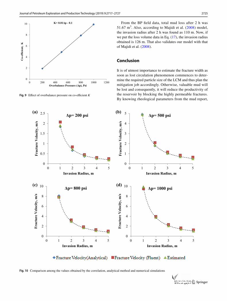
Plotting these values of K against corresponding overbal-ance pressure, it is found that K changes linearly with increas-ing overbalance pressure (Fig. 9). As the value of overbalance pressure increases, value of the co-efficient K also increases.
Therefore, it can be generalized that when consistency index is 0.004 kg/m s, flow behavior index is 0.94, yield stress is 4.022 Pa and the fracture width is 880 µm, the velocity of drilling fluid inside fracture can be calculated using the fol-lowing correlation:
(14)VFracture = (0.01ΔP − 0.1)R−1.4i
.
After completing the study, to validate the correlation, the results produced by the correlation are compared with analytical results obtained from the model developed by Majidi et al. (2008) and CFD simulation results in Fig. 10. This comparison shows that the results obtained by the cor-relation are in close match with the analytical results and the numerical simulation results.
One of the drawbacks in this CFD analysis is that the model over-predicts the value of drilling fluid velocity than the velocity values obtained from the analytical method. However, as the overbalance pressure increased to 800 Psi, model starts to under-predict the drilling fluid velocity when
Fig. 3 Structured mesh of the fracture (left) and structured mesh of the wellbore (right)
Fig. 4 Pressure contour: left (∆p = 200 psi) and right (∆p = 1000 psi)

2723Journal of Petroleum Exploration and Production Technology (2019) 9:2717–2727
1 3
invasion radius is less than 1 m. The percentage of devia-tion of the numerical simulation results and the correla-tion results from the analytical results is plotted in Fig. 11. From Fig. 11 (left), it is clear that the error in the numerical simulation decreases with increasing overbalance pressure. However, the error increases with increasing invasion radius. Therefore, for a high overbalance pressure, the simulation will produce more accurate result in the near-wellbore region. The closer the distance from the wellbore, the more accurate the simulation will be.
In addition, the percentage of deviation of the results obtained using the correlation from the analytical results is plotted in Fig. 11 (right). It can be seen from the figure that
the correlation produces less error than the numerical simula-tion. The error produced in the numerical simulation ranges from − 10 to + 39%, whereas the error produced using the correlation ranges from − 3 to + 10%. The error in the corre-lation results starts to decrease as the overbalance pressure is increased from 200 psi. Among the four overbalance pressures, the correlation produces more accurate results for overbalance pressures of 500 psi, 800 psi and 1000 psi. It is clearly depicted in the figure that in those cases, the error is decreased to ± 3%.
Moreover, results obtained from the equation and the corre-lation is compared in Fig. 12 to find out the deviation between them. The closer the slope of the plot to 1, better the approxi-mation. It is visible from the figure that the slope is almost 1 which proves that the approximation is good enough.
Recalling the basic equations to calculate flow rate and mud loss volume:
Assuming drilling fluid was lost into the fracture at a constant rate, for a fracture width of 880 µm and stated fluid properties given in Table 1, Eqs. (14), (15) and (16) can be combined to determine the invasion radius from the total mud loss volume:
where ∆P is the overbalance pressure (psi), t time (s), and V is the total mud loss volume (m3).
(15)q = 2�RiW × VFracture,
(16)V = q × t.
(17)Ri =
[
5.5292 × 10⁻³(0.01 × ΔP − 0.1)t
V
]2.5
,
Fig. 5 Velocity contour: left (∆p = 200 psi) and Right (∆p = 1000 psi)
0
2
4
6
8
10
0 1 2 3 4 5
Frac
ture
Vel
ocity
, m/s
Fracture Radius, m
Fracture Velocity (∆P=200 Psi) Fracture Velocity (∆P=500 Psi)
Fracture Velocity (∆P=800 Psi) Fracture Velocity (∆P=1000 Psi)
Fig. 6 Results obtained from CFD model

2724 Journal of Petroleum Exploration and Production Technology (2019) 9:2717–2727
1 3
Fig. 7 Relationship between fracture width and mud loss rate (when ∆p = 800 psi)
w = 138.88q0.3169
R² = 0.9997
0
200
400
600
800
1000
1200
1400
1600
0 200 400 600 800 1000 1200 1400 1600 1800 2000
Frac
ture
wid
th, µ
m
Mud Loss Rate, gallon/minute
0
0.5
1
1.5
2
2.5
0 1 2 3 4 5
Frac
ture
Vel
ocity
, m/s
Invasion Radius, m
Δp= 200 psi
0
2
4
6
0 1 2 3 4 5
Frac
ture
Vel
ocity
, m/s
Invasion Radius, m
Δp= 500 psi
0
2
4
6
8
10
0 1 2 3 4 5
Frac
ture
Vel
ocity
, m/s
Invasion Radius, m
Δp= 800 psi
0
2
4
6
8
10
12
0 1 2 3 4 5
Frac
ture
Vel
ocity
, m/s
Invasion Radius, m
Δp= 1000 psi
(a) (b)
(c) (d)
Fig. 8 Comparison between results obtained from analytical method and numerical simulations
2725Journal of Petroleum Exploration and Production Technology (2019) 9:2717–2727
1 3
From the BP field data, total mud loss after 2 h was 51.67 m3. Also, according to Majidi et al. (2008) model, the invasion radius after 2 h was found as 110 m. Now, if we put the loss volume data in Eq. (17), the invasion radius obtained is 126 m. That also validates our model with that of Majidi et al. (2008).
Conclusion
It is of utmost importance to estimate the fracture width as soon as lost circulation phenomenon commences to deter-mine the required particle size of the LCM and thus plan the mitigation job accordingly. Otherwise, valuable mud will be lost and consequently, it will reduce the productivity of the reservoir by blocking the highly permeable fractures. By knowing rheological parameters from the mud report,
K= 0.01Δp - 0.1
0
2
4
6
8
10
0 200 400 600 800 1000 1200
Co-
effic
ient
, K
Overbalance Pressure (Δp), Psi
Fig. 9 Effect of overbalance pressure on co-efficient K
0
0.5
1
1.5
2
2.5
0 1 2 3 4 5
Frac
ture
Vel
ocity
, m/s
Invasion Radius, m
Δp= 200 psi
0
1
2
3
4
5
0 1 2 3 4 5
Frac
ture
Vel
ocity
, m/s
Invasion Radius, m
Δp= 500 psi
0
2
4
6
8
10
0 1 2 3 4 5
Frac
ture
Vel
ocity
, m/s
Invasion Radius, m
Δp= 800 psi
0
2
4
6
8
10
0 1 2 3 4 5
Frac
ture
Vel
ocity
, m/s
Invasion Radius, m
Δp= 1000 psi
(b)(a)
(d)(c)
Fig. 10 Comparison among the values obtained by the correlation, analytical method and numerical simulations

2726 Journal of Petroleum Exploration and Production Technology (2019) 9:2717–2727
1 3
prior to onset of drilling and at the end of lost circulation event, correlations as shown in this study can be developed to determine fracture width and invasion radius, respectively, which will surely be useful to combat lost circulation and to design appropriate well development program more effec-tively. When lost circulation occurs, correlations developed prior to beginning of drilling operation, it is possible to make an estimation of the fracture width from the mud loss rate which will indubitably be helpful in determining the particle size and the type of LCM to be used. Furthermore,
in the well development stage, using the correlation of inva-sion radius, it is possible to determine the area that was dam-aged which will be very much useful to design a proper treatment scheme.
Open Access This article is distributed under the terms of the Crea-tive Commons Attribution 4.0 International License (http://creat iveco mmons .org/licen ses/by/4.0/), which permits unrestricted use, distribu-tion, and reproduction in any medium, provided you give appropriate credit to the original author(s) and the source, provide a link to the Creative Commons license, and indicate if changes were made.
References
Cook J, Growcock F, Guo Q (2011) Stabilizing the wellbore to prevent lost circulation. Oilfield Rev 23:26–35
Dyke CG, Wu B, Tayler DM (1995) Advances in characterizing natu-ral-fracture permeability from mud-log data. SPE 25022 PA. SPE Formation Eval 10:160–166
Feng Y, Jones JF, Gray KE (2016) A review on fracture-initiation and propagation pressures for lost circulation and wellbore strengthen-ing. SPE Drill Completion 17(2):131–144
Gauthier BDM, Franssen RCWM, Drei S (2000) Fracture networks in Rotliegend gas reservoirs of the Dutch offshore: implications for reservoir behavior, geologieen Mijnbouw/Netherlands. J Geosci (Prague) 79(1):45–57
Hemphill T, Campos W, Pilehvari A (1993) Yield-power law model more accurately predicts mud rheology. Oil Gas J 91(34):45–50
Lavrov A (2014) Radial flow of non-newtonian power-law fluid in a rough-walled fracture: effect of fluid rheology. Springer, New York. https ://doi.org/10.1007/s1124 2-014-0384-6
-5
5
15
25
35
45
0 1 2 3 4 5
Err
or, %
Invasion Radius, m-5
0
5
10
15
0 1 2 3 4 5
Err
or, %
Invasion Radius, m
Fig. 11 Deviation of simulation results from analytical method (left) and deviation of correlation results from analytical method (right)
0
2
4
6
8
10
12
0 2 4 6 8 10 12
Frac
ture
Vel
ocity
(Cor
rela
tion)
, m/s
Fracture Velocity (Analytical), m/s
Fig. 12 Comparison between analytical results and correlation results

2727Journal of Petroleum Exploration and Production Technology (2019) 9:2717–2727
1 3
Lavrov A, Tronvoll J (2004) Modeling mud loss in fractured formation. SPE 88700 MS. 11th Abu Dhabi International Petroleum Exhibi-tion and Conference. Abu Dhabi, U.A.E
Li Q, Wang T, Xie X, Shao S, Xia Q (2009) A fracture network model and open fracture analysis of a tight sandstone gas reservoir in Dongpu Depression, Bohaiwan Basin, eastern China. Geophys Prospect 57(2):275–282
Lietard O, Unwin T, Guillot D, Hodder M (1996) Fracture width LWD and drilling Mud/LCM selection guidelines in naturally fractured reservoirs. SPE 36832. European Petroleum Conference. Milan, Italy
Lietard O, Unwin T, Guillot DJ, Hodder MH (1999) Fracture width logging while drilling and drilling mud/loss-circulation-material selection guidelines in naturally fractured reservoirs. SPE Drill Completion 14:168–177
Majidi R, Miska SZ, Yu M, Thompson LG (2008) Modeling of drilling fluid losses in naturally fractured formations. SPE 114630. SPE Annual Technical Conference and Exhibition, Denver, Colorado, USA
Majidi R, Miska S, Thompson LG, Yu M, Zhang J (2010) Quantitative analysis of mud losses in naturally fractured reservoirs: the effect of rheology. SPE 114130. SPE Western Regional and Pacific Sec-tion AAPG Joint Meeting. Bakersfield, California
Mulder G, Busch VP, Reid I, Sleeswijk VTJ, Vanheyst BG (1992) Sole pit: improving performance and increasing reserves by horizontal drilling. Proc. European Petroleum Conf., pp 83–94
Nair R, Abousleiman Y, Zaman M (2005) Modeling fully coupled oil–gas flow in a dual-porosity medium. Int J Geomech. https ://doi.org/10.1061/(ASCE)1532-3641(2005)5:4(326)
Razavi O, Lee HP, Olson JE, Schultz RA (2017) Characterization of naturally fractured reservoirs using drilling mud loss data: the effect of fluid leak-off. ARMA 17-855. 51st US Rock Mechan-ics/Geomechanics Symposium. San Francisco, California, USA
Sanfillippo F, Brignoli M, Santarelli FJ, Bezzola C (1997) Charac-terization of conductive fractures while drilling. SPE 38177. SPE European Formation Damage Conference. The Hague, Netherland
Wang Y, Kang Y, You L (2007) Progresses in mechanism study and control: mud losses to fractured reservoirs. Drill Fluid Completion Fluid 24(4):74–77
Publisher’s Note Springer Nature remains neutral with regard to jurisdictional claims in published maps and institutional affiliations.