Computational Industrial Economics - Engaged Learning · model presented here enables the analysis of interactive dynamics between firms as they compete in a changing ... industry

Computational Industrial Economics A G E N E R A T I V E A P P R O A C H T O D Y N AM I C A N A L Y S I S I N I N D U S T R I A L O R G A N I Z A T I O N

Myong-Hun Chang Department of Economics, Cleveland State University, Cleveland, OH 44115 [email protected]

1

COMPUTATIONAL INDUSTRIAL ECONOMICS A G E N E R A T I V E A P P R O A C H T O D Y N AM I C A N A L Y S I S I N I N D U S T R I A L O R G A N I Z A T I O N

The field of modern industrial economics focuses on the structure and performance of the industry in equilibrium when firms make decisions in an optimizing way, typically with perfect foresight. The patterns that arise in the process of adjustment, induced by persistent external shocks, are often ignored for lack of a proper tool for analysis. This chapter offers a basic agent-based computational model of industry dynamics which allows us to study the evolving industry structure through entry and exit of heterogeneous firms. This approach induces turbulence in market structure through unpredictable shocks to the firms’ technological environment. The base model presented here enables the analysis of interactive dynamics between firms as they compete in a changing environment with limited rationality and foresight. A possible extension of the base model, allowing for R&D by firms, is also discussed.

I propose a computational modeling framework which can form the basis for carrying out dynamic analysis in IO. The main idea is to create an artificial industry within a computational setting, which can then be populated with firms who enter, compete, and exit over the course of the industry’s growth and development. These actions of the firms are driven by pre-specified decision rules, the interactions of which then generate a rich historical record of the industry’s evolution. With this framework, one can study the complex interactive dynamics of heterogeneous firms as well as the evolving structure and performance of the industry. The base model of industry dynamics presented here can be extended and refined to address a variety of standard issues in IO, but it is particularly well-suited for analyzing the dynamic process of adjustment in industries that are subject to persistent external shocks. The empirical significance of such processes is well-reflected in the literature that explores patterns in the turnover dynamics of firms in various industries. The seminal work in this literature is Dunne, Roberts, and Samuelson (1988). They found that the turnovers are significant and persistent over time in a wide variety of industries, though they also noticed substantial cross-industry differences in their rates: “[W]e find substantial and persistent differences in entry and exit rates across industries. Entry and exit rates at a point in time are also highly correlated across

ABSTRACT

1. INTRODUCTION

2

industries so that industries with higher than average entry rates tend to also have higher than average exit rates.” To the extent that firm turnovers are the manifestation of the aforementioned adjustment process, this literature brings to light the empirical significance of the out-of-equilibrium industrial dynamics. Furthermore, it identifies patterns to this adjustment process that the standard equilibrium models (static or dynamic) are simply unable to address. For instance, Caves (2007) states: “Turnover in particular affects entrants, who face high hazard rates in their infancy that drop over time. It is largely because of high infant mortality that rates of entry and exit from industries are positively correlated (compare the obvious theoretical model that implies either entry or exit should occur but not both). The positive entry-exit correlation appears in cross-sections of industries, and even in time series for individual industries, if their life-cycle stages are controlled.” The approach proposed here addresses this uneasy co-existence of equilibrium-theorizing and the non-equilibrium empirical realities in industrial organization. The model entails a population of firms; each of whom endowed with a unique technology that remains fixed over the course of its life. The firms go through a repeated sequence of entry-output-exit decisions. The market competition takes place amid a technological environment that is subject to external shocks, inducing changes in the relative production efficiencies of the firms. Because the firms’ technologies are held fixed, there is no firm-level adaptation to the environmental shifts. However, an industry-level adaptation takes place through the process of firm entry and exit, which is driven by the selective force of the market competition. The implementation of the adjustment process in the proposed model rests on two assumptions. First, the firms in the model are myopic. They do not have the foresight that is frequently assumed in the orthodox industrial organization literature. Instead, their decisions are made on the basis of fixed rules motivated by myopic but maximizing tendencies. Second, the technological environment within which the firms operate is stochastic. How efficient a firm was in one environment does not indicate how efficient it will be in another environment. As such, there is always a possibility that the firms may be re-shuffled when the environment changes. These two assumptions – myopia (or, more broadly, bounded rationality) of firms and stochastic technological environment – lead to persistent firm heterogeneity. It is this heterogeneity that provides the raw materials over which the selective force of market competition can act. Firm myopia drives the entry process; the selective force of market process, acting on the heterogeneous firms, drives the exit process; all the while the stochastic technological environment guarantees the resulting process never settles down, giving us an opportunity to study patterns that may emerge along the process. I offer two sets of results in this chapter. The first set of results is obtained under the assumption of stable market demand; hence the only source of turbulence is the shocks to the technological environment. The results show that the entry and exit dynamics inherent in the process generate patterns that are consistent with empirical observations. Furthermore, the base model enables the analysis of the relationships between the industry-specific demand and technological conditions and the endogenous structure and performance of the industry along the steady-state, thereby generating cross-sectional implications in a fully dynamic setting. The second set of results is generated under the assumption of fluctuating demand; hence, the demand shocks are now superimposed on the technological shocks. The basic relationship between the rate of entry and the rate of exit continues to hold with this extension. In addition, the extension enables a

3

characterization of the way fluctuating demand affects the turnover as well as the structure and performance of the industry. Finally, I discuss a potential extension of the base model, in which the R&D activities of firms can be incorporated.

The base model entails an evolving population of firms which interact with one another through repeated market competition. Figure 2.1 captures the overall structure.

[Figure 2.1 here]

Each period t starts out with a group of surviving incumbents from the previous period, and consists of three decision stages. In stage 1, each potential entrant makes a decision to enter. A new entrant is assumed to enter with a random (but unique) technology and a start-up fund that is common for all entrants. In stage 2, the new entrants and the incumbents, given their endowed technologies, compete in the market. The outcome of the competition in stage 2 generates profits (and losses) for the firms. In stage 3, all firms update their net wealth based on the profits earned (and losses incurred) from the stage-2 competition and decide whether or not to exit the industry. Once the exit decisions are made, the surviving incumbents with their technologies and the updated net wealth move on to period t+1 where the process is repeated. Central to this process are the heterogeneous production technologies held by the firms (which imply cost asymmetry) and the selective force of market competition that leads to entry and exit of firms. The next subsections describe the nature of technology and the market conditions, followed by a detailed description of the multi-stage decision process.

In each period, active firms in the market produce and sell a homogeneous good. The good is produced through a process that consists of N distinct tasks. Each task can be completed using one of two different methods (i.e., ways of doing things). Even though all firms produce a homogeneous good, they may do so using different combinations of methods for the N component tasks. The method used by the firm for a given task is represented by a bit (0 or 1) such that there are two possible methods available for each task and thus 2 variants of the production technology. The base model assumes that a firm enters the industry with a technology that it is endowed. The firm stays with it over the course of its life – i.e., it is committed to using a particular method for a given task at all times.1 A firm’s technology is then fully characterized by a binary vector of N dimensions which captures the complete set of methods it uses to produce the good. Denote it by ∈ 0,1 , where ≡ 1 , 2 , … , and ∈ 0, 1 is firm i’s method in task h.

2. METHODOLOGY

2.1. Modeling Technology

4

In measuring the degree of heterogeneity between any two technologies (i.e., method vectors), and , we use “Hamming Distance,” which is the number of positions for which the corresponding bits differ:

, ) ≡ ∑ . (1)

How efficient a given technology is depends on the environment it operates in. In order to represent the technological environment that prevails in period t, I specify a unique methods vector, ∈ 0, 1 , which is defined as the optimal technology for the industry in t. How well a firm’s technology performs in the current environment then depends on how close it is to the prevailing optimal technology in the technology space. More specifically, the marginal cost of firm i in period t is specified to be a direct function of , , the Hamming distance between the firm’s endowed technology, , and the current optimal technology, . The optimal technology in t is common for all firms – i.e., all firms in a given industry face the same technological environment at a given point in time. As such, once it is defined for a given industry, its technological environment is completely specified for all firms since the efficiency of any technology is well-defined as a function of its distance to this optimal technology.2

In each period, there exist a finite number of firms that operate in the market. In this subsection, I define the static market equilibrium among such operating firms. The technological environment and the endowed technologies for all firms jointly determine the marginal costs of the firms and, hence, the resulting equilibrium. The static market equilibrium defined here is then used to approximate the outcome of market competition in each period. In this sub-section, I temporarily abstract away from the time superscript for ease of exposition. Let m be the number of firms operating in the market. The firms are Cournot oligopolists, who choose production quantities of a homogeneous good. In defining the Cournot equilibrium in this setting, I assume that all m firms produce positive quantities in equilibrium. The inverse market demand function is specified as:

, (2)

where ∑ and s denotes the size of the market. Each operating firm has its production technology, , and faces the following total cost:

; , , ∙ . (3)

For simplicity, the firms are assumed to have identical fixed cost: ⋯ .

2.2. Modeling Market Competition

5

The firm’s marginal cost, , , depends on how different its technology, , is from the optimal technology, :

≡ , 100 ∙,

(4)

Hence, increases in the Hamming distance between the firm’s technology and the optimal technology for the industry. It is at its minimum of zero when = and at its maximum of 100 when all N bits in the two technologies are different from one another.3 The total cost can then be re-written as:

; , 100 ∙, ∙ . (5)

Given the demand and cost functions, firm i’s profit is:

, ∑ ∙ ∙ . (6)

Taking the first-order condition for each i and summing over m firms, we derive the equilibrium industry output rate, which gives us the equilibrium market price, , through equation (2):

∑ . (7)

Given the vector of marginal costs defined by the firms’ technologies and the optimal technology, is uniquely determined and is independent of the market size, s. Furthermore, the equilibrium market price depends only on the sum of the marginal costs and not on the distribution of s. The equilibrium firm output rate is:

∙ ∑ . (8)

A firm’s equilibrium output rate depends on its own marginal cost and the equilibrium market price such that ∙ . Finally, the Cournot equilibrium firm profit is

∙ ∙ . (9)

Note that is a function of and ∑ , where is a function of and for all j. It is then straightforward that the equilibrium firm profit is fully determined, once the vectors of methods are known for all firms. Further note that implies and, hence,

∀ , ∈ 1, … , .

6

In the beginning of any typical period t, the industry opens with two groups of decision makers: 1) a group of incumbent firms surviving from t – 1, each of whom enters t with its endowed technology, , and its net wealth, , carried over from t – 1; 2) a group of potential entrants ready to consider entering the industry in t, each with an endowed technology of and its start-up wealth. All firms face a common technological environment within which his/her technology will be used; this environment is fully represented by the prevailing optimal technology, . Central to the model is the assumption that the production environment is inherently stochastic – that is, the technology which was optimal in one period is not necessarily optimal in the next period. This is captured by allowing the optimal technology, , to vary from one period to the next in a systematic manner. The mechanism that guides this shift dynamic is described next.

Consider a binary vector, ∈ 0, 1 . Define , ⊂ 0, 1 as the set of points that are exactly Hamming distance l from . The set of points that are within Hamming distance l of is then defined as

, ≡ ⋃ , . (10)

The following rule drives the shift dynamic of the optimal technology:

with probability γ

with probability 1‐γ (11)

where ∈ , and and are constant over all t. Hence, with probability the optimal technology shifts to a new one within Hamming distance from the current technology, while with probability 1 it remains unchanged at . The volatility of the technological environment is then captured by and , where is the frequency and is the maximum magnitude of changes in technological environment. The change in technological environment is assumed to take place in the beginning of each period before firms make any decisions. While the firms do not know what the optimal technology is for the new environment, they are assumed to get accurate signals of their own marginal costs based on the new environment when making their decisions to enter. They, however, do not have this information about the existing incumbents. Nevertheless, because they observe and for each j in t-1, they can infer for all firms. As such, in calculating the attractiveness of entry, a potential entrant i relies on and for all j in the set of surviving incumbents from t-1.

2.3. The Base Model of Industry Dynamics

2.3.1. Random Shifts in Technological Environment

7

Denote by the set of surviving firms from 1, where ∅. The set of surviving firms includes those firms which were active in 1 in that their outputs were strictly positive as well as those firms which were inactive with their plants shut down during the previous period. The inactive firms in 1 survive to if and only if they have sufficient net wealth to cover their fixed costs in 1. Each firm ∈ possesses a production technology, , it entered the industry with, which gives rise to its marginal cost in of as defined in equation (4). It also has a current net wealth of it carries over from 1. Let denote the finite set of potential entrants who contemplate entering the industry in the beginning of . I assume that the size of the pool of potential entrants is fixed and constant at throughout the entire horizon. I also assume that this pool of potential entrants is renewed fresh each period. Each potential entrant in is endowed with a technology, , randomly chosen from 0, 1 according to uniform distribution. In addition, each potential entrant has a fixed start-up wealth it enters the market with. Stage 1: Entry Decisions In stage 1 of each period, the potential entrants in first make their decisions to enter. Just as each firm in has its current net wealth of , we will let

for all ∈ where is the fixed “start-up” fund common to all potential entrants. The start-up wealth, , may be viewed as a firm’s available fund that remains after paying for the one-time set-up cost of entry. For example, if one wishes to consider a case where a firm has zero fund available, but must incur a positive entry cost, it would be natural to consider as having a negative value. The entry rule takes the simple form that an outsider will be attracted to enter the industry if and only if it perceives its post-entry net wealth in period t to be strictly above a threshold level representing the opportunity cost to operating in this industry. The entry decision then depends on the profits that it expects to earn in the periods following entry. Realistically, this would be the present discounted value of the profits to be earned over some foreseeable future starting from t. In the base model presented here, I assume the firms to be completely myopic such that the expected profit is simply the static one-period Cournot equilibrium profit based on three things: 1) the marginal cost of the potential entrant accurately reflecting the new technological environment in t; 2) the marginal costs of the active firms from 1; and 3) the potential entrant’s belief that it is the only new entrant in the market.4 In terms of rationality, the extent of myopia assumed here is obviously extreme. The other end of the spectrum is the strategic firm with perfect foresight as typically assumed in Markov Perfect Equilibrium (MPE) models [Pakes and McGuire (1994); Ericson and Pakes (1995)].5 The realistic representation of firm decision making would lie somewhere in between these two extremes. The assumption of myopia is made here to focus on computing the finer details of the interactive dynamics that evolve over the growth and development of an industry. Relaxing this assumption in ways that are consistent with the observations and theories built up in the behavioral literature will be an important agenda for the future.

2.3.2. Three-Stage Decision Making

8

The decision rule of a potential entrant ∈ is then:

,

, , (12)

where is the static Cournot equilibrium profit the entrant expects to make in the period of its entry and is the threshold level of wealth for a firm’s survival (common to all firms). Once every potential entrant in makes its entry decision on the basis of the above criterion, the resulting set of actual entrants, ⊆ , contains only those firms with sufficiently efficient technologies which will guarantee some threshold level of profits given its belief about the market structure and the technological environment. Denote by the set of firms ready to compete in the industry: ≡ ∪ . I will denote by the number of competing firms in period t such that | |. At the end of stage 1 of period t, we then have a well-defined set of competing firms, , with their current net wealth,

∀ ∈ , and their technologies, for all ∈ and for all ∈ . Stage 2: Output Decisions and Market Competition The firms in , with their technologies and current net wealth, engage in Cournot competition in the market, where we “approximate” the outcome with the standard Cournot-Nash equilibrium defined in Section 2.2. The use of Cournot-Nash equilibrium in this context is admittedly inconsistent with the “limited rationality” assumption employed in this model. A more consistent approach would be to explicitly model the process of market experimentation. Instead of modeling this process, which would further complicate the model, I implicitly assume that it is done instantly and without cost. Cournot-Nash equilibrium is then assumed to be a reasonable approximation of the outcome from that process.6 Note that the equilibrium in Section 2.2 was defined for m firms under the assumption that all m firms produce positive quantities. In actuality, given asymmetric costs, there is no reason to think that all firms will produce positive quantities in equilibrium. Some relatively inefficient firms may shut down their plants and stay inactive. What we need is a mechanism for identifying the set of active firms out of such that the Cournot equilibrium among these firms will indeed entail positive quantities only. This is done in the following sequence of steps. Starting from the initial set of active firms, compute the equilibrium outputs for each firm. If the outputs for one or more firms are negative, then de-activate the least efficient firm from the set of currently active firms – i.e., set 0 where i is the least efficient firm. Re-define the set of active firms (as the previous set of active firms minus the de-activated firms) and recompute the equilibrium outputs. Repeat the procedure until all active firms are producing non-negative outputs. Each inactive firm produces zero output and incurs the economic loss equivalent to its fixed cost. Each active firm produces its equilibrium output and earns the corresponding profit. We then have for ∈ . Stage 3: Exit Decisions Given the single-period profits or losses made in stage 2 of the game, the firms in consider exiting the industry in the final stage. Each firm’s net wealth is first updated on the basis of the profit (or loss) made in stage 2:

9

. (13)

The exit decision rule for each firm is then:

, (14)

where is the threshold level of net wealth (as previously defined). Denote by the set of firms that leave the market in t. Once the exit decisions are made by all firms in , the set of surviving firms from period t is then defined as:

≡ ∈ . (15)

The set of surviving firms, , their technologies, ∀ ∈

, and their current net wealth,

∀ ∈ , are then passed on to t+1 as state variables.

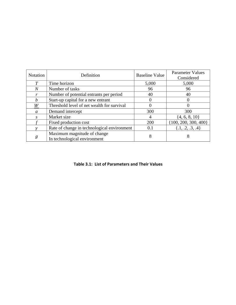
The values of the parameters used here, including those for the baseline simulation, are provided in Table 3.1.

[Table 3.1 here]

I assume that there are 96 separate tasks in the production process, where the method chosen for each task is represented by a single bit. This implies that there are 2 (≅ 8 10 different combinations of methods for the complete production process. In each period, there are exactly 40 potential entrants who consider entering the industry, where a new firm enters with a start-up wealth (b) of 0. An incumbent firm will exit the industry, if his net wealth falls below the threshold rate ( ) of 0. The demand intercept is fixed at 300. The time horizon is over 5,000 periods, where in period 1 the market starts out empty. The focus of my analysis is on the impacts of the market size (s) and the fixed cost (f), as well as of the turbulence parameter, . I consider four different values for each of these parameters: ∈ 4, 6, 8, 10 , ∈ 100, 200, 300, 400 , and ∈ .1, .2, .3, .4 . The maximum magnitude of

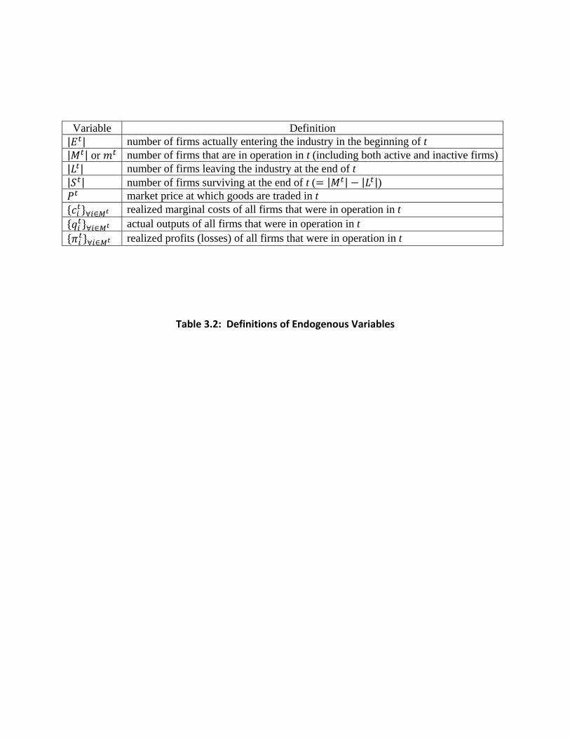
change, , is held fixed at 8. Note that a higher value of reflects more frequent changes in the technological environment. Starting from an empty industry with a given parameter configuration, I evolve the industry and trace its growth and development by keeping track of the endogenous variables listed in Table 3.2.

[Table 3.2 here]

3. DESIGN OF COMPUTATIONAL EXPERIMENTS

10

Using these endogenous variables, I further construct the following variables that are useful for characterizing the behavior of firms in the industry:

: Industry output, such that ∑∀ ∈

: Herfindahl-Hirschmann Index in t, where ∑ ∙ 100∀ ∈

: Industry marginal cost, where ∑ ∙∀ ∈

: Industry price-cost margin, where ∑ ∙∀ ∈

The Herfindahl-Hirschmann index, , captures the concentration of the industry at any given point in time. This is important in this model as firms, in general, have asymmetric market shares which evolve over time due to persistent entries and exits. The industry marginal cost,

, reflects the overall level of production (in)efficiency as it is the weighted sum of the marginal costs of all operating firms, where the weights are the market shares of the individual firms. To the extent that a firm which is inactive – i.e., produces zero output – has zero impact on this measure, the industry marginal cost captures the average degree of production inefficiency of the active firms. Likewise, the industry price-cost margin, , is the market share-weighted sum of the firms’ price-cost margins. It is a measure of the industry’s performance in terms of its allocative inefficiency – i.e., the extent to which the market price deviates from the marginal costs of firms in operation.

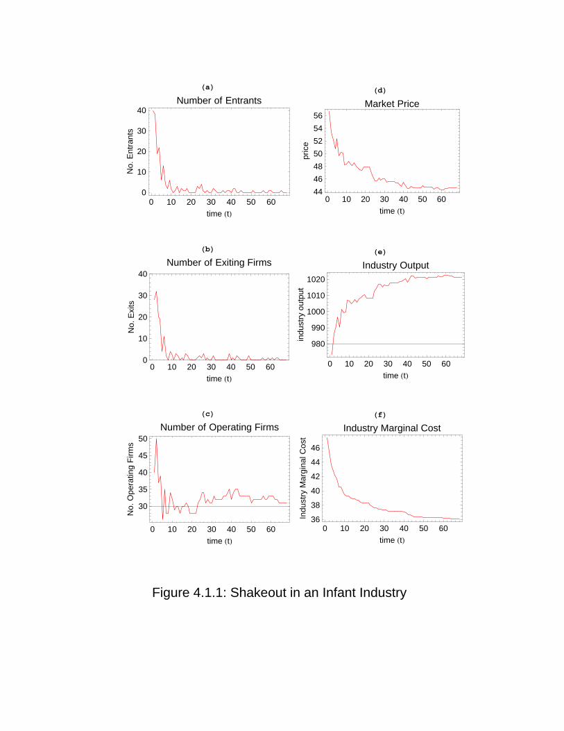
I start by examining the outcomes from a single run of the industry, given the baseline set of parameter values as indicated in Table 3.1. To see the underlying source of the industry dynamics, I first assume an industry which is perfectly protected from external technological shocks – hence an industry with 0 such that its technological environment never changes.

[Figure 4.1.1 here]

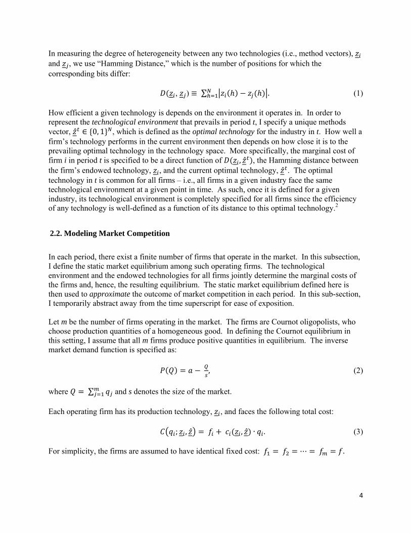
The industry starts out empty in t = 0. A pool of potential entrants considers entry into this industry given their endowed technologies. Figure 4.1.1(a) shows the time series of the number of entries that occur for the first 68 periods of the horizon. The time series data on the number of exits is captured in Figure 4.1.1(b). Clearly, there is a rush to get into the industry in the beginning, followed by a large number of exits. Both moves into and out of the industries quickly slow down and stabilize toward zero. The interaction of entries and exits then generates a time series on the number of operating firms as depicted in Figure 4.1.1(c). It shows the existence of a shakeout, where the initial increase in the number of firms is followed by a severe reduction, ultimately converging toward about 30 firms. These results are in line with the empirical observations made by Gort and Klepper (1982), Klepper and Simons (1997, 2000a,b), Carroll and Hannan (2000), Klepper (2002), and Jovanovic and MacDonald (1994). Also

4. RESULTS I: THE BASE MODEL WITH STABLE MARKET DEMAND

4.1. Firm Behavior over Time: Technological Change and Recurrent Shakeouts

11

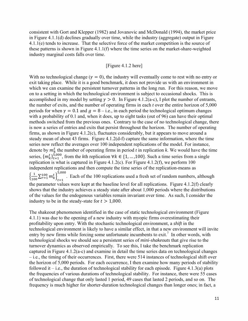
consistent with Gort and Klepper (1982) and Jovanovic and McDonald (1994), the market price in Figure 4.1.1(d) declines gradually over time, while the industry (aggregate) output in Figure 4.1.1(e) tends to increase. That the selective force of the market competition is the source of these patterns is shown in Figure 4.1.1(f) where the time series on the market-share-weighted industry marginal costs falls over time.

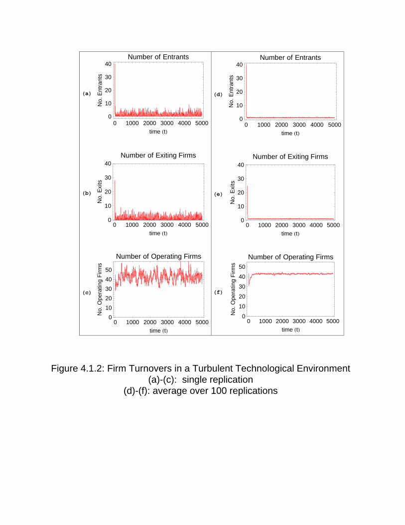
[Figure 4.1.2 here]

With no technological change ( 0), the industry will eventually come to rest with no entry or exit taking place. While it is a good benchmark, it does not provide us with an environment in which we can examine the persistent turnover patterns in the long run. For this reason, we move on to a setting in which the technological environment is subject to occasional shocks. This is accomplished in my model by setting 0. In Figure 4.1.2(a-c), I plot the number of entrants, the number of exits, and the number of operating firms in each t over the entire horizon of 5,000 periods for when 0.1 and 8 – i.e., in each period the technological optimum changes with a probability of 0.1 and, when it does, up to eight tasks (out of 96) can have their optimal methods switched from the previous ones. Contrary to the case of no technological change, there is now a series of entries and exits that persist throughout the horizon. The number of operating firms, as shown in Figure 4.1.2(c), fluctuates considerably, but it appears to move around a steady mean of about 43 firms. Figure 4.1.2(d-f) capture the same information, where the time series now reflect the averages over 100 independent replications of the model. For instance, denote by the number of operating firms in period t in replication k. We would have the time series, , , from the kth replication ∀ ∈ 1,… ,100 . Such a time series from a single replication is what is captured in Figure 4.1.2(c). For Figure 4.1.2(f), we perform 100 independent replications and then compute the time series of the replication-means as

∑,

. Each of the 100 replications used a fresh set of random numbers, although

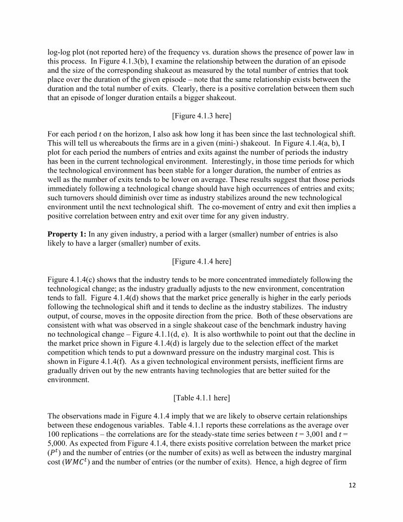
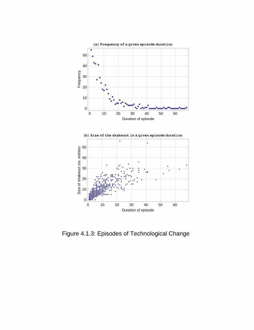
the parameter values were kept at the baseline level for all replications. Figure 4.1.2(f) clearly shows that the industry achieves a steady state after about 1,000 periods where the distributions of the values for the endogenous variables remain invariant over time. As such, I consider the industry to be in the steady-state for 1,000. The shakeout phenomenon identified in the case of static technological environment (Figure 4.1.1) was due to the opening of a new industry with myopic firms overestimating their profitability upon entry. With the stochastic technological environment, a shift in the technological environment is likely to have a similar effect, in that a new environment will invite entry by new firms while forcing some unfortunate incumbents to exit.7 In other words, with technological shocks we should see a persistent series of mini-shakeouts that give rise to the turnover dynamics as observed empirically. To see this, I take the benchmark replication captured in Figure 4.1.2(a-c) and examine in detail the time series data on technological changes – i.e., the timing of their occurrences. First, there were 514 instances of technological shift over the horizon of 5,000 periods. For each occurrence, I then examine how many periods of stability followed it – i.e., the duration of technological stability for each episode. Figure 4.1.3(a) plots the frequencies of various durations of technological stability. For instance, there were 55 cases of technological change that only lasted 1 period, 49 cases that lasted 2 periods, and so on. The frequency is much higher for shorter-duration technological changes than longer ones; in fact, a

12

log-log plot (not reported here) of the frequency vs. duration shows the presence of power law in this process. In Figure 4.1.3(b), I examine the relationship between the duration of an episode and the size of the corresponding shakeout as measured by the total number of entries that took place over the duration of the given episode – note that the same relationship exists between the duration and the total number of exits. Clearly, there is a positive correlation between them such that an episode of longer duration entails a bigger shakeout.

[Figure 4.1.3 here]

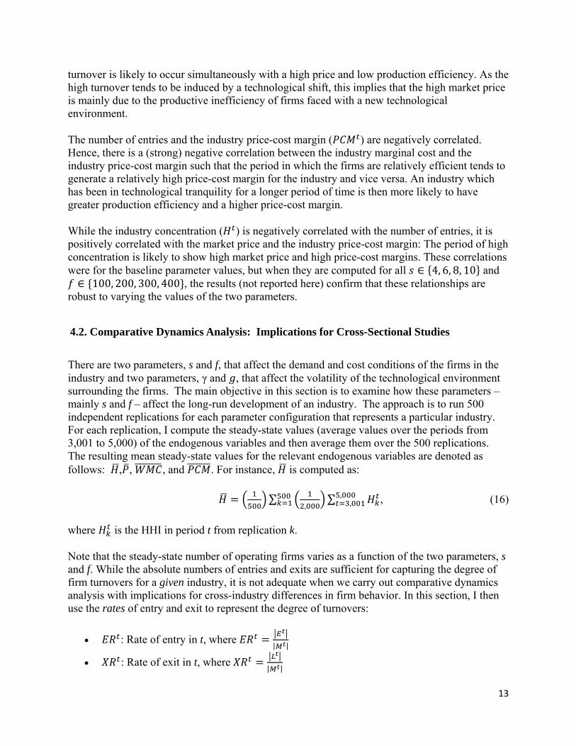
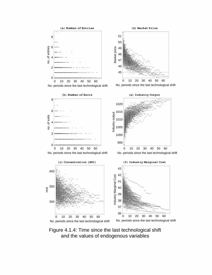
For each period t on the horizon, I also ask how long it has been since the last technological shift. This will tell us whereabouts the firms are in a given (mini-) shakeout. In Figure 4.1.4(a, b), I plot for each period the numbers of entries and exits against the number of periods the industry has been in the current technological environment. Interestingly, in those time periods for which the technological environment has been stable for a longer duration, the number of entries as well as the number of exits tends to be lower on average. These results suggest that those periods immediately following a technological change should have high occurrences of entries and exits; such turnovers should diminish over time as industry stabilizes around the new technological environment until the next technological shift. The co-movement of entry and exit then implies a positive correlation between entry and exit over time for any given industry. Property 1: In any given industry, a period with a larger (smaller) number of entries is also likely to have a larger (smaller) number of exits.

[Figure 4.1.4 here]

Figure 4.1.4(c) shows that the industry tends to be more concentrated immediately following the technological change; as the industry gradually adjusts to the new environment, concentration tends to fall. Figure 4.1.4(d) shows that the market price generally is higher in the early periods following the technological shift and it tends to decline as the industry stabilizes. The industry output, of course, moves in the opposite direction from the price. Both of these observations are consistent with what was observed in a single shakeout case of the benchmark industry having no technological change – Figure 4.1.1(d, e). It is also worthwhile to point out that the decline in the market price shown in Figure 4.1.4(d) is largely due to the selection effect of the market competition which tends to put a downward pressure on the industry marginal cost. This is shown in Figure 4.1.4(f). As a given technological environment persists, inefficient firms are gradually driven out by the new entrants having technologies that are better suited for the environment.

[Table 4.1.1 here] The observations made in Figure 4.1.4 imply that we are likely to observe certain relationships between these endogenous variables. Table 4.1.1 reports these correlations as the average over 100 replications – the correlations are for the steady-state time series between t = 3,001 and t = 5,000. As expected from Figure 4.1.4, there exists positive correlation between the market price ( ) and the number of entries (or the number of exits) as well as between the industry marginal cost ( ) and the number of entries (or the number of exits). Hence, a high degree of firm

13

turnover is likely to occur simultaneously with a high price and low production efficiency. As the high turnover tends to be induced by a technological shift, this implies that the high market price is mainly due to the productive inefficiency of firms faced with a new technological environment. The number of entries and the industry price-cost margin ( ) are negatively correlated. Hence, there is a (strong) negative correlation between the industry marginal cost and the industry price-cost margin such that the period in which the firms are relatively efficient tends to generate a relatively high price-cost margin for the industry and vice versa. An industry which has been in technological tranquility for a longer period of time is then more likely to have greater production efficiency and a higher price-cost margin. While the industry concentration ( ) is negatively correlated with the number of entries, it is positively correlated with the market price and the industry price-cost margin: The period of high concentration is likely to show high market price and high price-cost margins. These correlations were for the baseline parameter values, but when they are computed for all ∈ 4, 6, 8, 10 and ∈ 100, 200, 300, 400 , the results (not reported here) confirm that these relationships are

robust to varying the values of the two parameters.

There are two parameters, s and f, that affect the demand and cost conditions of the firms in the industry and two parameters, γ and , that affect the volatility of the technological environment surrounding the firms. The main objective in this section is to examine how these parameters – mainly s and f – affect the long-run development of an industry. The approach is to run 500 independent replications for each parameter configuration that represents a particular industry. For each replication, I compute the steady-state values (average values over the periods from 3,001 to 5,000) of the endogenous variables and then average them over the 500 replications. The resulting mean steady-state values for the relevant endogenous variables are denoted as follows: , , , and . For instance, is computed as:

∑,

∑ ,, , (16)

where is the HHI in period t from replication k. Note that the steady-state number of operating firms varies as a function of the two parameters, s and f. While the absolute numbers of entries and exits are sufficient for capturing the degree of firm turnovers for a given industry, it is not adequate when we carry out comparative dynamics analysis with implications for cross-industry differences in firm behavior. In this section, I then use the rates of entry and exit to represent the degree of turnovers:

: Rate of entry in t, where | |

: Rate of exit in t, where | |

4.2. Comparative Dynamics Analysis: Implications for Cross-Sectional Studies

14

These time series are again averaged over the 500 independent replications and the resulting mean steady-state values are denoted as and .

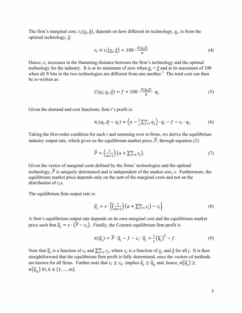
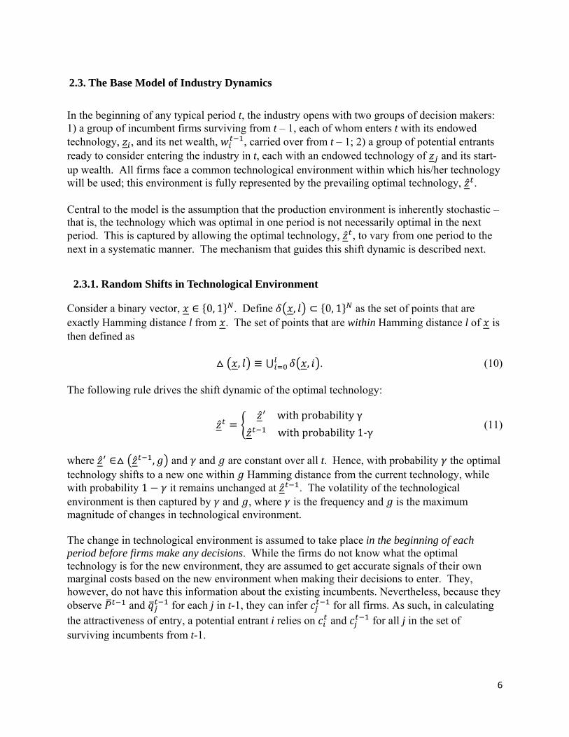
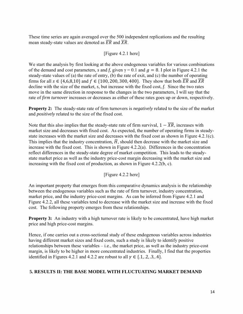
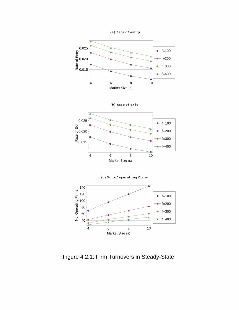
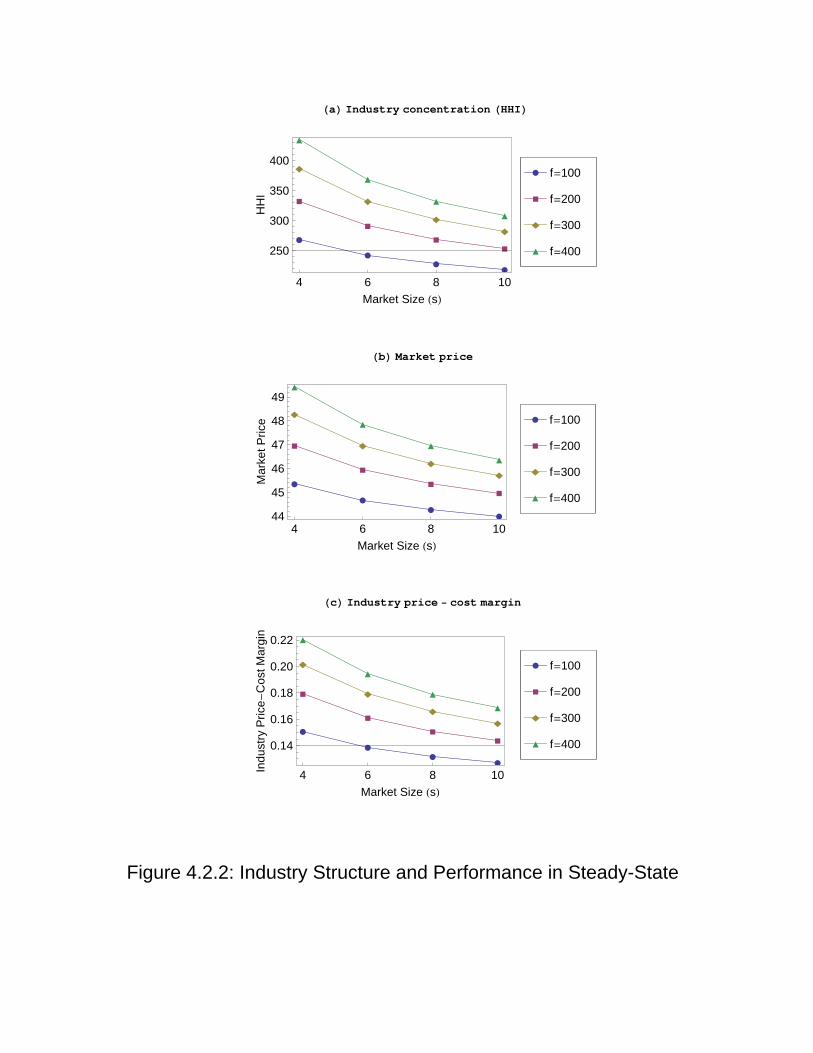
[Figure 4.2.1 here] We start the analysis by first looking at the above endogenous variables for various combinations of the demand and cost parameters, s and f, given γ = 0.1 and 8. I plot in Figure 4.2.1 the steady-state values of (a) the rate of entry, (b) the rate of exit, and (c) the number of operating firms for all ∈ 4,6,8,10 and ∈ 100, 200, 300, 400 . They show that both and decline with the size of the market, s, but increase with the fixed cost, f. Since the two rates move in the same direction in response to the changes in the two parameters, I will say that the rate of firm turnover increases or decreases as either of these rates goes up or down, respectively. Property 2: The steady-state rate of firm turnovers is negatively related to the size of the market and positively related to the size of the fixed cost. Note that this also implies that the steady-state rate of firm survival, 1 , increases with market size and decreases with fixed cost. As expected, the number of operating firms in steady-state increases with the market size and decreases with the fixed cost as shown in Figure 4.2.1(c). This implies that the industry concentration, , should then decrease with the market size and increase with the fixed cost. This is shown in Figure 4.2.2(a). Differences in the concentration reflect differences in the steady-state degree of market competition. This leads to the steady-state market price as well as the industry price-cost margin decreasing with the market size and increasing with the fixed cost of production, as shown in Figure 4.2.2(b, c).

[Figure 4.2.2 here] An important property that emerges from this comparative dynamics analysis is the relationship between the endogenous variables such as the rate of firm turnover, industry concentration, market price, and the industry price-cost margins. As can be inferred from Figure 4.2.1 and Figure 4.2.2, all these variables tend to decrease with the market size and increase with the fixed cost. The following property emerges from these relationships. Property 3: An industry with a high turnover rate is likely to be concentrated, have high market price and high price-cost margins. Hence, if one carries out a cross-sectional study of these endogenous variables across industries having different market sizes and fixed costs, such a study is likely to identify positive relationships between these variables – i.e., the market price, as well as the industry price-cost margin, is likely to be higher in more concentrated industries. Finally, I find that the properties identified in Figures 4.2.1 and 4.2.2 are robust to all ∈ .1, .2, .3, .4 .

5. RESULTS II: THE BASE MODEL WITH FLUCTUATING MARKET DEMAND

15

How do cyclical variations in market demand affect the evolving structure and performance of an industry? Is the market selection of firms more effective (and, hence, firms are more efficient on average) when there are fluctuations in demand? What are the relationships between the movement of demand and those of endogenous variables such as industry concentration, price, aggregate efficiency, and price-cost margins? Are they pro-cyclical or counter-cyclical? The proposed model of industry dynamics can address these issues by computationally generating the time series of these variables in the presence of demand fluctuation. These issues have been explored in the past by researchers from two distinct fields of economics – macroeconomics and industrial organization. A number of stylized facts has been established by the two strands of empirical research. For instance, many papers find procyclical variations in the number of competitors. Chaterjee, Cooper, and Ravikumar (1993) find that both net business formation and new business incorporations are strongly procyclical. Devereux, Head, and Lapham (1996) confirms this finding and further reports that the aggregate number of business failure is countercyclical. Many papers find that markups are countercyclical and negatively correlated with the number of competitors [Bils (1987), Cooley and Ohanian (1991), Rotemberg and Woodford (1990, 1999), Chevalier and Scharfstein (1995), Warner and Barsky (1995), MacDonald (2000), Chevalier, Kashyap, and Rossi (2003), Wilson and Reynolds (2005)].8 Martins, Scapetta, and Pilat (1996) covers different industries in 14 OECD countries and find markups to be countercyclical in 53 of the 56 cases they consider, with statistically significant result in most of these. In addition, these authors conclude that entry rates have a negative and statistically significant correlation with markups. Bresnahan and Reiss (1991) find that increases in the number of producers increases the competitiveness in the markets they analyze. Campbell and Hopenhayn (2005) provide empirical evidence to support the argument that firms’ pricing decisions are affected by the number of competitors they face; they show that markups react negatively to increases in the number of firms. Rotemberg and Saloner (1986) provide empirical evidence of countercyclical price movements and offer a model of collusive pricing when demand is subject to i.i.d. shocks. Their model generates countercyclical collusion and predicts countercyclical pricing.9 The model presented here has the capacity to replicate many of the empirical regularities mentioned above and explain them in terms of the selective forces of market competition in the presence of firm entry and exit. In particular, it can incorporate demand fluctuation by allowing the market size, s, to shift from one period to the next in a systematic fashion. As a starting point, the market size parameter can be shifted according a deterministic cycle such as a sine wave. Section 5.1 investigates the movement of the endogenous variables with this demand dynamic. In Section 5.2, I allow the market size to be randomly drawn from a fixed range according to uniform distribution. By examining the correlations between the time series of the market size and that of various endogenous variables I study the impact that demand fluctuation has on the evolving structure and performance of the industry.

I run 100 independent replications of the base model with the baseline parameter configuration. The only change is in the specification of the market size, s. It is assumed to stay fixed at the

5.1. Cyclical Demand

16

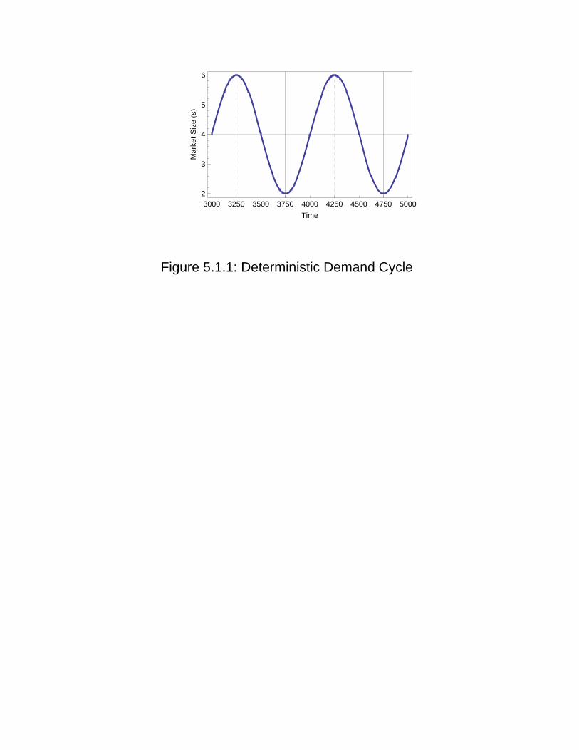
baseline value of 4 up to 2,000 and then follow a deterministic cycle as specified by the following rule:

∙ sin ∙ (16)

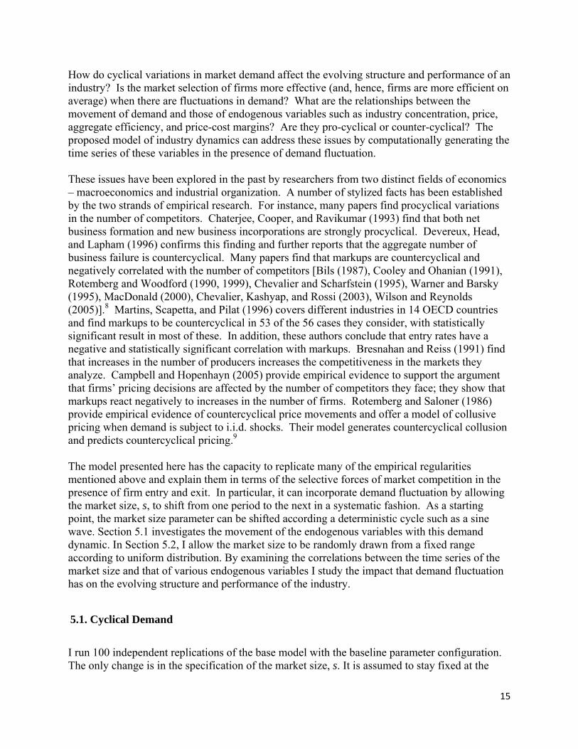
for all 2,001, where is the mean market size (set at 4), is the amplitude of the wave (set at 2), and τ (set at 500) is the period for half-turn (hence, one period is 2τ). Note that the demand fluctuation is not introduced until t = 2,001. This is to ensure that the industry reaches its steady-state before demand fluctuation occurs. Given the assigned values of ( , , τ), the market size then fluctuates between the maximum of 6 and the minimum of 2 with a full cycle of 1,000 periods. In examining the evolution of the industry in the midst of fluctuating demand, I focus on the last 2,000 periods from t = 3,001 to 5,000. The demand cycle over this time period is shown in Figure 5.1.1. The points at which the market size reaches its maximum are indicated by the dotted lines at t = 3,251 and 4,251, while the points at which the market size reaches its minimum are indicated by the solid lines at t = 3,751 and 4,751. I use the same indicator lines when analyzing the movements of the endogenous variables.

[Figure 5.1.1 here] Recall that 100 independent replications were performed. Each replication generates the time series values for the relevant endogenous variables. For each endogenous variable, I then average its time series values over the 100 replications.

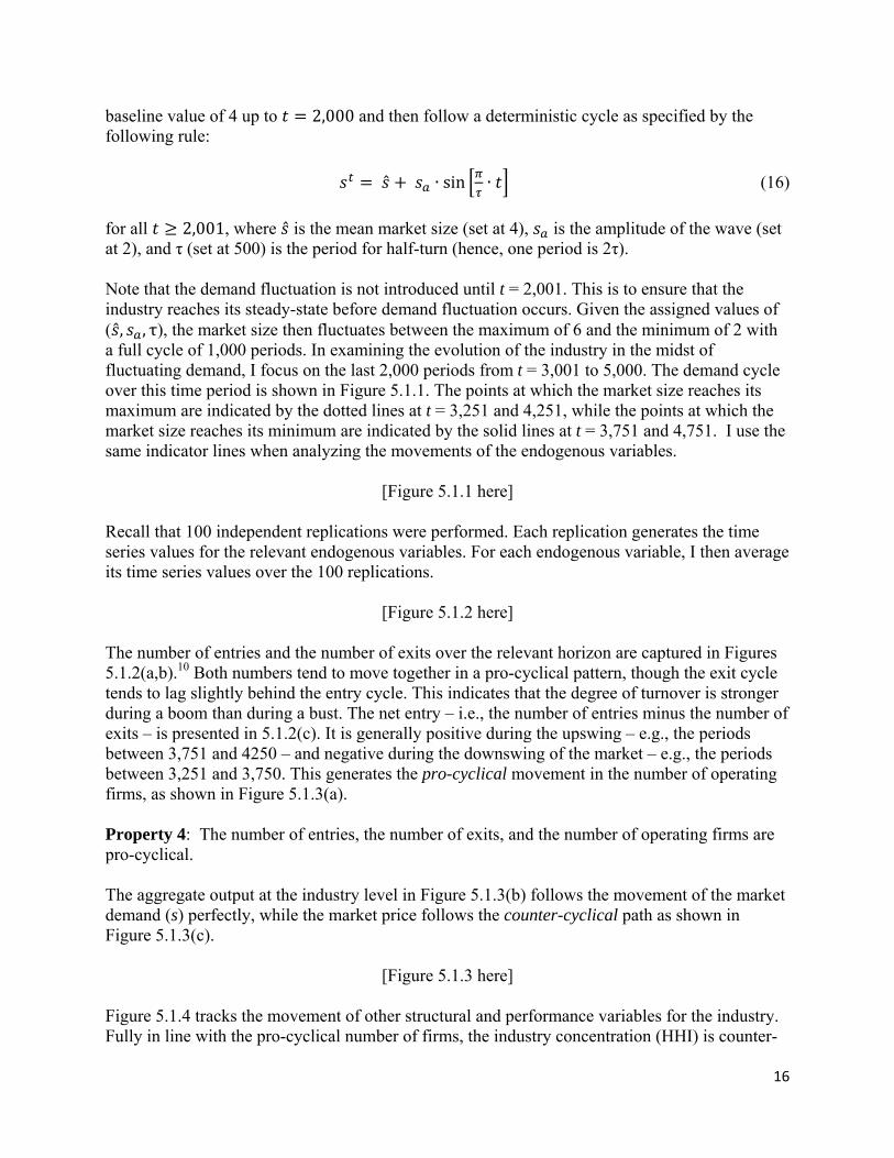
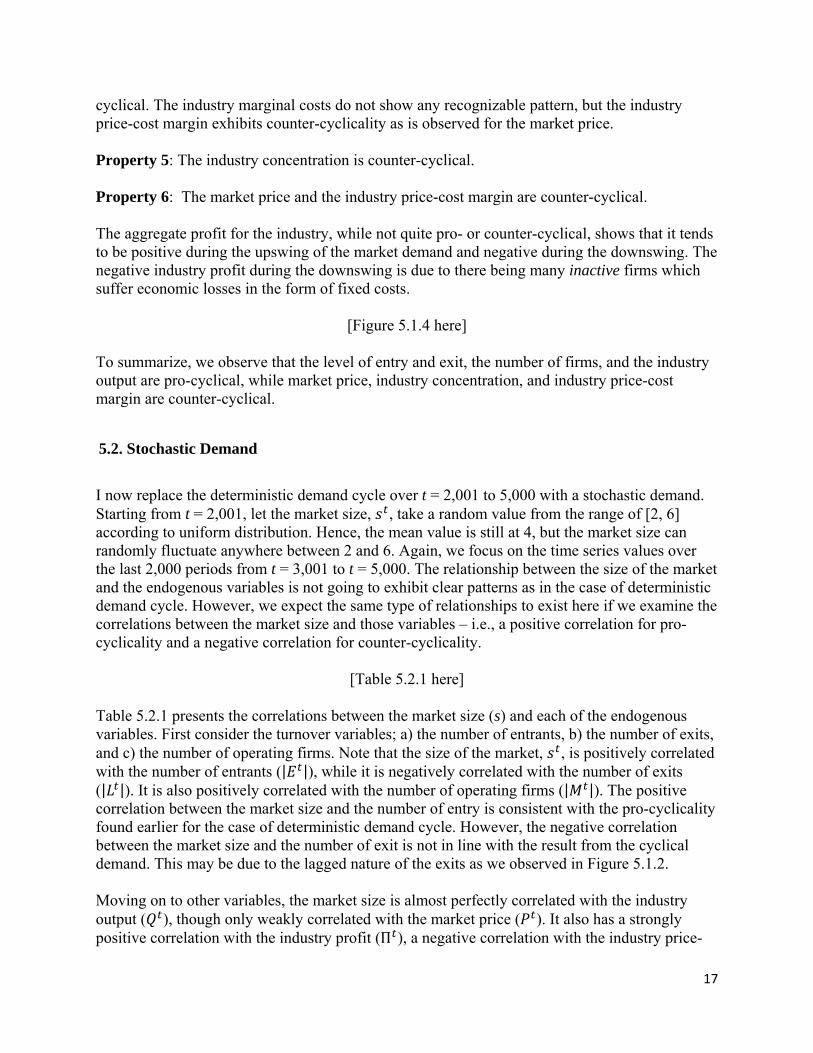
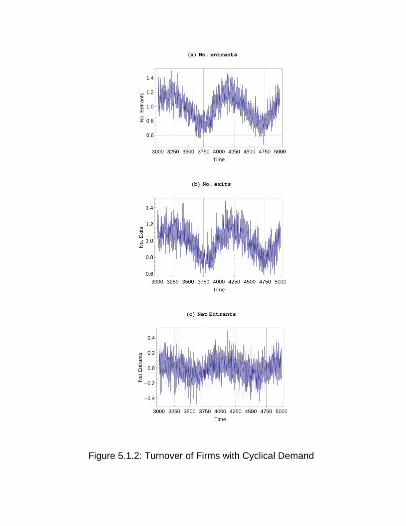
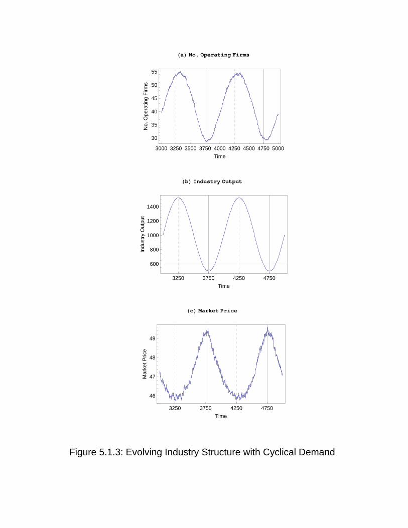
[Figure 5.1.2 here] The number of entries and the number of exits over the relevant horizon are captured in Figures 5.1.2(a,b).10 Both numbers tend to move together in a pro-cyclical pattern, though the exit cycle tends to lag slightly behind the entry cycle. This indicates that the degree of turnover is stronger during a boom than during a bust. The net entry – i.e., the number of entries minus the number of exits – is presented in 5.1.2(c). It is generally positive during the upswing – e.g., the periods between 3,751 and 4250 – and negative during the downswing of the market – e.g., the periods between 3,251 and 3,750. This generates the pro-cyclical movement in the number of operating firms, as shown in Figure 5.1.3(a). Property 4: The number of entries, the number of exits, and the number of operating firms are pro-cyclical. The aggregate output at the industry level in Figure 5.1.3(b) follows the movement of the market demand (s) perfectly, while the market price follows the counter-cyclical path as shown in Figure 5.1.3(c).

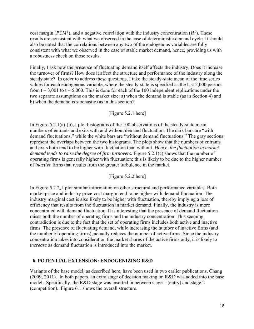
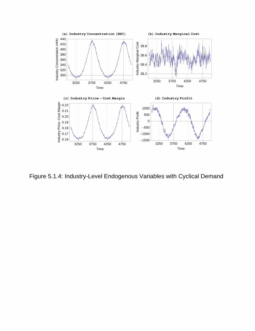
[Figure 5.1.3 here] Figure 5.1.4 tracks the movement of other structural and performance variables for the industry. Fully in line with the pro-cyclical number of firms, the industry concentration (HHI) is counter-

17

cyclical. The industry marginal costs do not show any recognizable pattern, but the industry price-cost margin exhibits counter-cyclicality as is observed for the market price. Property 5: The industry concentration is counter-cyclical. Property 6: The market price and the industry price-cost margin are counter-cyclical. The aggregate profit for the industry, while not quite pro- or counter-cyclical, shows that it tends to be positive during the upswing of the market demand and negative during the downswing. The negative industry profit during the downswing is due to there being many inactive firms which suffer economic losses in the form of fixed costs.

[Figure 5.1.4 here] To summarize, we observe that the level of entry and exit, the number of firms, and the industry output are pro-cyclical, while market price, industry concentration, and industry price-cost margin are counter-cyclical.

I now replace the deterministic demand cycle over t = 2,001 to 5,000 with a stochastic demand. Starting from t = 2,001, let the market size, , take a random value from the range of [2, 6] according to uniform distribution. Hence, the mean value is still at 4, but the market size can randomly fluctuate anywhere between 2 and 6. Again, we focus on the time series values over the last 2,000 periods from t = 3,001 to t = 5,000. The relationship between the size of the market and the endogenous variables is not going to exhibit clear patterns as in the case of deterministic demand cycle. However, we expect the same type of relationships to exist here if we examine the correlations between the market size and those variables – i.e., a positive correlation for pro-cyclicality and a negative correlation for counter-cyclicality.

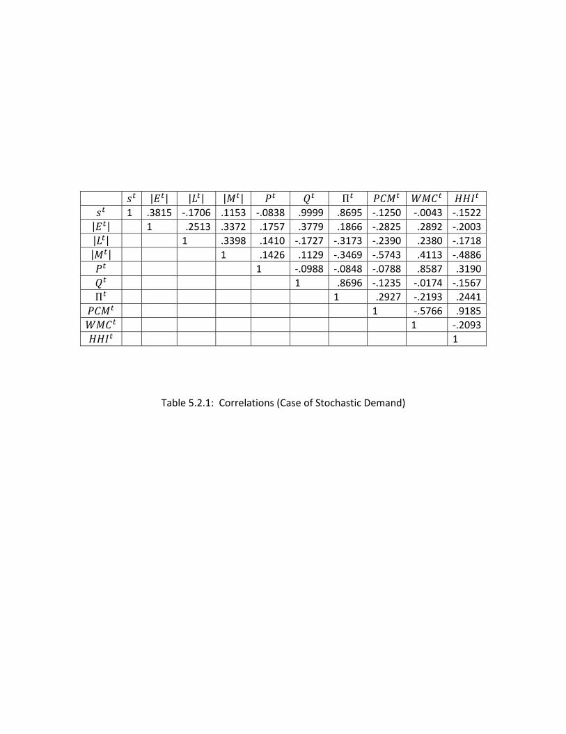
[Table 5.2.1 here] Table 5.2.1 presents the correlations between the market size (s) and each of the endogenous variables. First consider the turnover variables; a) the number of entrants, b) the number of exits, and c) the number of operating firms. Note that the size of the market, , is positively correlated with the number of entrants (| |), while it is negatively correlated with the number of exits (| |). It is also positively correlated with the number of operating firms (| |). The positive correlation between the market size and the number of entry is consistent with the pro-cyclicality found earlier for the case of deterministic demand cycle. However, the negative correlation between the market size and the number of exit is not in line with the result from the cyclical demand. This may be due to the lagged nature of the exits as we observed in Figure 5.1.2. Moving on to other variables, the market size is almost perfectly correlated with the industry output ( ), though only weakly correlated with the market price ( ). It also has a strongly positive correlation with the industry profit (Π ), a negative correlation with the industry price-

5.2. Stochastic Demand

18

cost margin ( ), and a negative correlation with the industry concentration ( ). These results are consistent with what we observed in the case of deterministic demand cycle. It should also be noted that the correlations between any two of the endogenous variables are fully consistent with what we observed in the case of stable market demand, hence, providing us with a robustness check on those results. Finally, I ask how the presence of fluctuating demand itself affects the industry. Does it increase the turnover of firms? How does it affect the structure and performance of the industry along the steady state? In order to address these questions, I take the steady-state mean of the time series values for each endogenous variable, where the steady-state is specified as the last 2,000 periods from t = 3,001 to t = 5,000. This is done for each of the 100 independent replications under the two separate assumptions on the market size: a) when the demand is stable (as in Section 4) and b) when the demand is stochastic (as in this section).

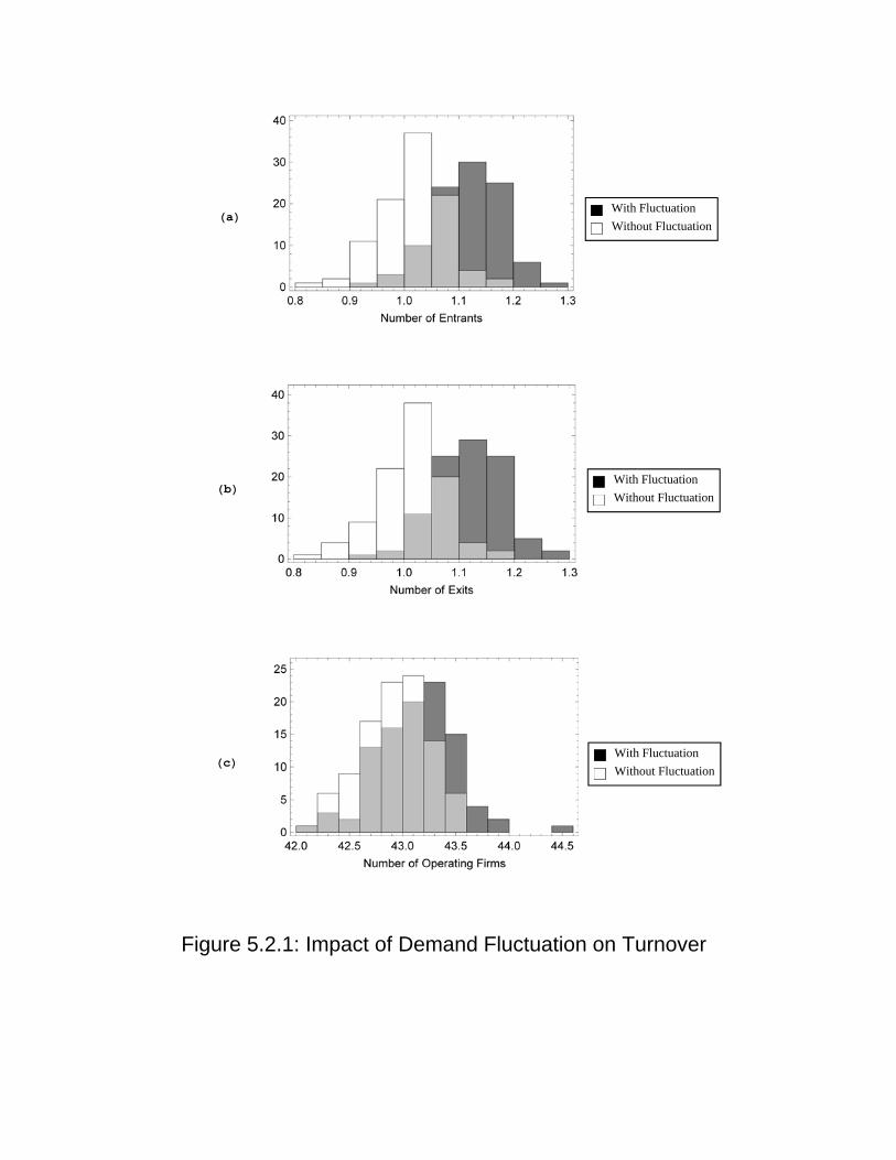
[Figure 5.2.1 here] In Figure 5.2.1(a)-(b), I plot histograms of the 100 observations of the steady-state mean numbers of entrants and exits with and without demand fluctuation. The dark bars are “with demand fluctuations,” while the white bars are “without demand fluctuations.” The gray sections represent the overlaps between the two histograms. The plots show that the numbers of entrants and exits both tend to be higher with fluctuation than without. Hence, the fluctuation in market demand tends to raise the degree of firm turnovers. Figure 5.2.1(c) shows that the number of operating firms is generally higher with fluctuation; this is likely to be due to the higher number of inactive firms that results from the greater turbulence in the market.

[Figure 5.2.2 here] In Figure 5.2.2, I plot similar information on other structural and performance variables. Both market price and industry price-cost margin tend to be higher with demand fluctuation. The industry marginal cost is also likely to be higher with fluctuation, thereby implying a loss of efficiency that results from the fluctuation in market demand. Finally, the industry is more concentrated with demand fluctuation. It is interesting that the presence of demand fluctuation raises both the number of operating firms and the industry concentration. This seeming contradiction is due to the fact that the set of operating firms includes both active and inactive firms. The presence of fluctuating demand, while increasing the number of inactive firms (and the number of operating firms), actually reduces the number of active firms. Since the industry concentration takes into consideration the market shares of the active firms only, it is likely to increase as demand fluctuation is introduced into the market.

Variants of the base model, as described here, have been used in two earlier publications, Chang (2009, 2011). In both papers, an extra stage of decision making on R&D was added into the base model. Specifically, the R&D stage was inserted in between stage 1 (entry) and stage 2 (competition). Figure 6.1 shows the overall structure.

6. POTENTIAL EXTENSION: ENDOGENIZING R&D

19

[Figure 6.1 here]

In both Chang (2009) and Chang (2011), the R&D activity was assumed to be exogenous and costless.11 More specifically, R&D was viewed as serendipitous discovery, in which the methods used in one or more of the tasks were randomly altered for experimentation. Chang (2009) assumed a stable technological environment in which the optimal technology did not change from one period to next – i.e., 0. Instead, the technology itself was assumed to be complex in nature such that there were multiple optima that a firm could converge on. The main focus was on the determinants of the shakeout phase of an industry’s life cycle. Chang (2011) allowed turbulence in technological environment as in this paper – i.e., 0. The focus was on the steady state in which continual series of entries and exits were observed. A more satisfying approach is to endogenize the process of R&D into the base model of industry dynamics. Let me sketch here one possible way to pursue this extension. [A preliminary attempt in this direction is currently in progress.] Suppose we assume that the R&D-related decisions of a firm are driven by a pair of choice probabilities, and , that evolve over time on the basis of reinforcement learning mechanism. Specifically, a firm i chooses to pursue R&D in period t with probability . If it chooses not to pursue R&D (which happens with probability 1 ), its technology stays the same as the previous period’s. If a firm decides to pursue R&D, it can do so through either innovation or imitation. Between these two modes of R&D, the firm chooses innovation mode with probability and imitation mode with 1 . The firm incurs the R&D expenditure, the size of which depends on which of the two modes it chooses. The R&D intensity and the innovation-to-imitation intensity at the firm-level can be inferred from the time paths of these two probabilities. Similar intensities at the industry-level can be inferred from the aggregate expenditure for the overall R&D as well as that for innovation or imitation. The base model with the endogenous R&D opens up a large set of issues. First, it allows us to examine the two Schumpeterian hypotheses: 1) innovation activity is more intense in larger rather than small firms and, hence, firm size matters; 2) innovation activity is more intense in concentrated rather than unconcentrated industries and, hence, industry structure matters. Given the process of creative destruction as envisioned by Schumpeter, both firm size and industry structure coevolve with R&D activities of the firms over the course of the industrial development. The model presented here can explore such evolving relationships in sufficient details so as to test the two hypotheses in a fully dynamic framework. Another issue of interest is to relate the empirical regularities on firm turnovers to the endogenous R&D intensities. The point is that the persistence of entry and exit by firms, as noted in this chapter with the base model, indicates the underlying instability in the cost-positions of the firms. Such instability may be due to the R&D activities of the firms as well as their changing fortunes in the competitive and turbulent environment. What are the theoretical connections between the degree of turnovers, the intensities of R&D activities, and the degree of technological turbulence (as captured by or ) in industries that are differentiated in terms their structural characteristics (e.g., s and f)? For instance, Geroski (1995) states: “High rates of entry are often associated with high rates of innovation and increases in efficiency. … Numerous case studies have suggested that entry is often used as a vehicle for introducing new innovations (frequently because incumbents are more interested in protecting existing rents than in seeking

20

out new profit opportunities), and many show that entry often encourages incumbents to drastically cut slack from their operations.” Lying underneath such a relationship is the unpredictable external shocks to the technological environment surrounding the firm. The base model with endogenous R&D should enable us to perform a detailed analysis of how and affect the endogenous relationship between the turnover rate and the level of aggregate R&D.

I proposed a computational model of industry dynamics, in which a population of firms could interact with one another through the process of market competition. The entry and exit of firms are generated endogenously in this model, thereby giving us an opportunity to study the historical patterns in the turnover dynamics for industries having different demand and technological conditions. The generative approach taken here allows a detailed study of the historical path an industry may take from birth to maturity. The results from the model could be compared to those from the voluminous empirical literature on time series and cross-sectional studies of industrial organization, providing substantive understanding of the evolutionary dynamics of industries. 1 There is, hence, no adaptation at the firm‐level in this model, although adaptation at the industry‐level is possible through the selection of firms via market competition. 2 Given that an entering firm is endowed with a fixed technology that cannot be modified, it does not matter whether the optimal technology is known to the firms or not. In a more general setting where the technology can be modified, any knowledge of the optimal technology, however imperfect, will affect the direction of the firm’s adaptive modification through its R&D decisions. 3 For concreteness, suppose N = 10 and the current technological environment is captured by the optimal vector of

= (1100101100). If a firm i entered the industry with a technology, = (0010011100), then , 5 and the firm’s marginal cost is 50. 4 This requires: 1) a potential entrant (correctly) perceives its own marginal cost from its chosen technology and the prevailing optimal technology; and 2) the market price and the active firms’ production quantities in 1 are common knowledge. Each active incumbent’s marginal cost can be directly inferred from the market price and the

production quantities as . 5 It should be noted that there have been attempts to relax the assumption of perfect foresight within the MPE framework. See Weintraub, Benkard, and Van Roy (2008, 2010). 6 For further justification, I refer the readers to a small body of literature, in which experimental studies are conducted to determine whether firm behavior indeed converges to the Cournot‐Nash equilibrium via best‐reply dynamic: Fouraker and Siegel (1963), Cox and Walker (1998), Theocharis (1960), Huck, Normann, and Oechssler (1999). Also see Armstrong and Huck (2010) for a survey of this literature. 7 This exit can have two causes, one direct and one indirect. The direct cause is the change in the technological environment that negatively affects the firm’s production efficiency. The indirect cause is the new entrants, favored by the new environment, putting competitive pressure on the existing firms. 8 A deviation from this set of papers is Domowitz et al. (1986) who suggested that markups are procyclical. Rotemberg and Woodford (1999) highlight some biases in these results, as they use measures of average variable costs and not marginal costs. 9 See Haltiwanger and Harrington (1991) and Kandori (1991) for further support. In contrast, Green and Porter (1984) develops a model of trigger pricing which predicts positive co‐movements of prices and demand. 10 Because we are focusing on the inter‐temporal movement for a given industry, we again use the numbers (rather than the rates) of entry and exit. 11 It should be noted that some of the results obtained in the base model with the stable demand also hold with these extensions. That they hold in the base model without the R&D activities implies that it is the market

7. CONCLUDING REMARKS

21

selection mechanism, and not the firm‐level adaptation, that is central to the emergent patterns in the non‐equilibrium industry dynamics.

Armstrong, M. and S. Huck, "Behavioral Economics as Applied to Firms: A Primer," Competition Policy International, 6 (2010), 3-45.

Bils, M., "The Cyclical Behavior of Marginal Cost and Price," American Economic Review, 77 (1987), 838-855.

Bresnahan, T. F. and P. C. Reiss, "Entry and Competition in Concentrated Markets," Journal of Political Economy, 99 (1991), 977-1009.

Campbell, J. R. and H. A. Hopenhayn, "Market Size Matters," Journal of Industrial Economics, LIII (2005), 1-25.

Carroll, G. R. and M. T. Hannan, The Demography of Corporations and Industries, Princeton University Press, Princeton, 2000.

Caves, R. E., "In Praise of the Old I.O.," International Journal of Industrial Organization, 25 (2007), 1-12.

Chang, M.-H, "Industry Dynamics with Knowledge-Based Competition: A Computational Study of Entry and Exit Patterns," Journal of Economic Interaction and Coordination, 4 (2009), 73-114.

Chang, M.-H, "Entry, Exit, and the Endogenous Market Structure in Technologically Turbulent Industries," Eastern Economic Journal, 37 (2011), 51-84.

Chatterjee, S., R. Cooper, and B. Ravikumar, "Strategic Complementarity in Business Formation: Aggregate Fluctuations and Sunspot Equilibria," Review of Economic Studies, 60 (1993), 795-811.

Chevalier, J. A., A. K. Kashyap, and P. E. Rossi, "Why Don't Prices Rise During Periods of Peak Demand? Evidence from Scanner Data," American Economic Review, 93 (2003), 15-37.

Chevalier, J. A. and D. S. Scharfstein, "Capital Structure and Product-Market Behavior," American Economic Review: Papers and Proceedings, 82 (1995), 390-396.

Cooley, T. F. and L. E. Ohanian, "The Cyclical Behavior of Prices," Journal of Monetary Economics, 28 (1991), 25-60.

Cox, J. C. and M. Walker, "Learning to Play Cournot Duopoly Strategies," Journal of Economic Behavior & Organization, 36 (1998), 141-161.

Devereux, M. B., A. C. Head, and B. J. Lapham, "Aggregate Fluctuations with Increasing Returns to Specialization and Scale," Journal of Economic Dynamics and Control, 20 (1996), 627-656.

REFERENCES

Domowitz, I., R. G. Hubbard, and B. C. Petersen, "Business Cycles and the Relationship between Concentration and Price-Cost Margins," RAND Journal of Economics, 17 (1986), 1-17.

Dunne, T., M. J. Roberts, and L. Samuelson, "Dynamic Patterns of Firm Entry, Exit, and Growth," RAND Journal of Economics, 19 (1988), 495-515.

Ericson, R. and A. Pakes, "Markov-Perfect Industry Dynamics: A Framework for Empirical Work," Review of Economic Studies, 62 (1995), 53-82.

Fouraker, L. E. and S. Siegel, Bargaining Behavior, McGraw-Hill Book Company, Inc., 1963.

Geroski, P. A., "What Do We Know about Entry?" International Journal of Industrial Organization, 13 (1995), 421-440.

Gort, M. and S. Klepper, "Time Paths in the Diffusion of Product Innovations," Economic Journal, 92 (1982), 630-653.

Green, E. J. and R. H. Porter, "Non-cooperative Collusion under Imperfect Price Information," Econometrica, 52 (1984), 87-100.

Haltiwanger, J. C. and J. E. Harrington, Jr., "The Impact of Cyclical Demand Movements on Collusive Behavior," RAND Journal of Economics, 22 (1991), 89-106.

Huck, S., H.-T. Normann, and J. Oechssler, "Learning in Cournot Oligopoly – An Experiment," Economic Journal, 109 (1999), C80-C95.

Jovanovic, B. and G. M. MacDonald, “The Life Cycle of a Competitive Industry,” Journal of Political Economy, 102 (1994), 322-347.

Kandori, M., "Correlated Demand Shocks and Price Wars during Booms," Review of Economic Studies, 58 (1991), 171-180.

Klepper, S., "Firm Survival and the Evolution of Oligopoly," RAND Journal of Economics, 33 (2002), 37-61.

Klepper, S. and K. L. Simons, "Technological Extinctions of Industrial Firms: An Inquiry into their Nature and Causes," Industrial and Corporate Change, 6 (1997), 379-460.

Klepper, S. and K. L. Simons, “Dominance by Birthright: Entry of Prior Radio Producers and Competitive Ramifications in the US Television Receiver Industry,” Strategic Management Journal, 21 (2000a), 997-1016.

Klepper, S. and K. L. Simons, “The Making of an Oligopoly: Firm Survival and Technological Change in the Evolution of the US Tire Industry,” Journal of Political Economy, 108 (2000b), 728-760.

MacDonald, J. M., "Demand, Information, and Competition: Why Do Food Prices Fall at Seasonal Demand Peaks?" Journal of Industrial Economics, XLVIII (2000), 27-45.

Martins, J. O., S. Scarpetta, and D. Pilat, "Mark-Up Ratios in Manufacturing Industries: Estimates for 14 OECD Countries," OECD Economics Department Working Papers, No. 162 (1996).

Pakes, A. and P. McGuire, "Computing Markov-Perfect Nash Equilibria: Numerical Implications of a Dynamic Differentiated Product Model," RAND Journal of Economics, 25 (1994), 555-589.

Rotemberg, J. J. and G. Saloner, "A Supergame-Theoretic Model of Price Wars During Booms," American Economic Review, 76 (1986), 390-407.

Rotemberg, J. J. and M. Woodford, "Cyclical Markups: Theories and Evidence," NBER Working Paper No. 3534 (1990).

Rotemberg, J. J. and M. Woodford, "The Cyclical Behavior of Prices and Costs," Working Paper (1999).

Theocharis, R., "On the Stability of the Cournot Solution on the Oligopoly Problem," Review of Economic Studies, 73 (1960), 133-134.

Warner, E. J. and R. B. Barsky, "The Timing and Magnitude of Retail Store Markdowns: Evidence from Weekends and Holidays," Quarterly Journal of Economics, 110 (1995), 321-352.

Weintraub, G., L. Benkard, and B. Van Roy, “Markov Perfect Industry Dynamics with Many Firms,” Econometrica, 76 (2008), 1375-1411.

Weintraub, G., L. Benkard, and B. Van Roy, “Computational Methods for Oblivious Equilibrium,” Operations Research, 58 (2010), 1247-1265.

Wilson, B. J. and S. S. Reynolds, "Market Power and Price Movements over the Business Cycle," Journal of Industrial Economics, LIII (2005), 145-174.

Notation Definition Baseline ValueParameter Values

Considered T Time horizon 5,000 5,000 N Number of tasks 96 96 r Number of potential entrants per period 40 40 b Start-up capital for a new entrant 0 0

Threshold level of net wealth for survival 0 0 a Demand intercept 300 300 s Market size 4 {4, 6, 8, 10} f Fixed production cost 200 {100, 200, 300, 400} Rate of change in technological environment 0.1 {.1, .2, .3, .4}

Maximum magnitude of change In technological environment

8 8

Table 3.1: List of Parameters and Their Values

Variable Definition | | number of firms actually entering the industry in the beginning of t | | or number of firms that are in operation in t (including both active and inactive firms)| | number of firms leaving the industry at the end of t | | number of firms surviving at the end of t ( | | | |)

market price at which goods are traded in t

∀ ∈ realized marginal costs of all firms that were in operation in t

∀ ∈ actual outputs of all firms that were in operation in t

∀ ∈ realized profits (losses) of all firms that were in operation in t

Table 3.2: Definitions of Endogenous Variables

| | | | | | 1 .377893 .229091 ‐.146535 ‐.253699 .313877 | | 1 .178438 ‐.123290 ‐.207645 .249140

1 .324510 ‐.094246 .872944

1 .909583 ‐.174888

1 ‐.565350

1

Table 4.1.1: Correlations (Case of Stable Demand)

| | | | | | Π

1 .3815 ‐.1706 .1153 ‐.0838 .9999 .8695 ‐.1250 ‐.0043 ‐.1522| | 1 .2513 .3372 .1757 .3779 .1866 ‐.2825 .2892 ‐.2003| | 1 .3398 .1410 ‐.1727 ‐.3173 ‐.2390 .2380 ‐.1718| | 1 .1426 .1129 ‐.3469 ‐.5743 .4113 ‐.4886

1 ‐.0988 ‐.0848 ‐.0788 .8587 .3190

1 .8696 ‐.1235 ‐.0174 ‐.1567

Π 1 .2927 ‐.2193 .2441

1 ‐.5766 .9185

1 ‐.2093

1

Table 5.2.1: Correlations (Case of Stochastic Demand)

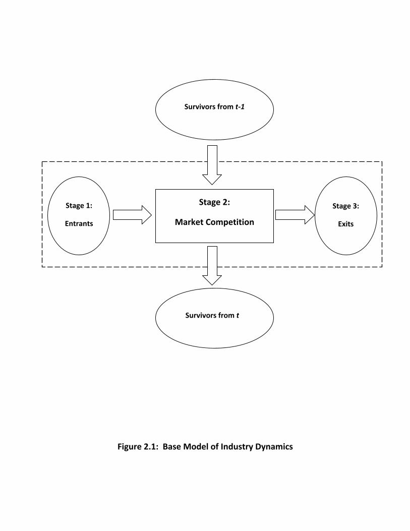
Figure 2.1: Base Model of Industry Dynamics

Stage 2:

Market Competition

Survivors from t‐1

Survivors from t

Stage 1:

Entrants

Stage 3:

Exits

a

0 10 20 30 40 50 600

10

20

30

40

time t

No.

Ent

rant

s

Number of Entrantsd

0 10 20 30 40 50 6044

46

48

50

52

54

56

time t

pric

e

Market Price

b

0 10 20 30 40 50 600

10

20

30

40

time t

No.

Exi

ts

Number of Exiting Firmse

0 10 20 30 40 50 60

980

990

1000

1010

1020

time t

indu

stry

outp

ut

Industry Output

c

0 10 20 30 40 50 60

30

35

40

45

50

time t

No.

Ope

ratin

gF

irms

Number of Operating Firmsf

0 10 20 30 40 50 6036

38

40

42

44

46

time t

Indu

stry

Mar

gina

lCos

t

Industry Marginal Cost

Figure 4.1.1: Shakeout in an Infant Industry

a

0 1000 2000 3000 4000 50000

10

20

30

40

time t

No.

Ent

rant

s

Number of Entrants

b

0 1000 2000 3000 4000 50000

10

20

30

40

time t

No.

Exi

ts

Number of Exiting Firms

c

0 1000 2000 3000 4000 50000

10

20

30

40

50

time t

No.

Ope

ratin

gF

irms

Number of Operating Firms

d

0 1000 2000 3000 4000 50000

10

20

30

40

time t

No.

Ent

rant

s

Number of Entrants

e

0 1000 2000 3000 4000 50000

10

20

30

40

time tN

o.E

xits

Number of Exiting Firms

f

0 1000 2000 3000 4000 50000

10

20

30

40

50

time t

No.

Ope

ratin

gF

irms

Number of Operating Firms

Figure 4.1.2: Firm Turnovers in a Turbulent Technological Environment(a)-(c): single replication

(d)-(f): average over 100 replications

a Frequency of a given episode duration

0 10 20 30 40 50 600

10

20

30

40

50

Duration of episode

Fre

quen

cy

b Size of the shakeout in a given episode duration

0 10 20 30 40 50 600

10

20

30

40

50

Duration of episode

Siz

eo

fsh

ake

ou

tno.

entr

ies

Figure 4.1.3: Episodes of Technological Change

a Number of Entries d Market Price

0 10 20 30 40 50 600

2

4

6

8

No. periods since the last technological shift

no.

ofen

trie

s

0 10 20 30 40 50 60

45

46

47

48

49

50

51


Mar

ket

pric

e

b Number of Exits e Industry Output

0 10 20 30 40 50 600

2

4

6

8


no.o

fex

its

0 10 20 30 40 50 60

995

1000

1005

1010

1015

1020


Indu

stry

outp

ut

c Concentration HHI f Industry Marginal Cost

0 10 20 30 40 50 60

300

350

400


HH

I

0 10 20 30 40 50 6036

37

38

39

40

41

42

43


Indu

stry

Mar

gina

lCos

t

Figure 4.1.4: Time since the last technological shiftand the values of endogenous variables

a Rate of entry

æ

æ

ææ

à

à

àà

ì

ì

ìì

ò

ò

òò

4 6 8 10

0.015

0.020

0.025

Market Size s

Rat

eof

Ent

ryò f=400

ì f=300

à f=200

æ f=100

b Rate of exit

æ

æ

ææ

à

à

àà

ì

ì

ìì

ò

ò

òò

4 6 8 10

0.015

0.020

0.025

Market Size s

Rat

eof

Exi

t

ò f=400

ì f=300

à f=200

æ f=100

c No. of operating firms

æ

æ

æ

æ

à

à

à

à

ìì

ìì

òò

òò

4 6 8 10

40

60

80

100

120

140

Market Size s

No.

Ope

ratin

gF

irms

ò f=400

ì f=300

à f=200

æ f=100

Figure 4.2.1: Firm Turnovers in Steady-State

a Industry concentration HHI

æ

ææ

æ

à

à

àà

ì

ì

ìì

ò

ò

òò

4 6 8 10

250

300

350

400

Market Size s

HH

Iò f=400

ì f=300

à f=200

æ f=100

b Market price

æ

ææ

æ

à

à

àà

ì

ì

ìì

ò

ò

òò

4 6 8 1044

45

46

47

48

49

Market Size s

Mar

ketP

rice

ò f=400

ì f=300

à f=200

æ f=100

c Industry price cost margin

æ

ææ

æ

à

à

àà

ì

ì

ìì

ò

ò

òò

4 6 8 10

0.14

0.16

0.18

0.20

0.22

Market Size s

Indu

stry

Pri

ce-

Cos

tMar

gin

ò f=400

ì f=300

à f=200

æ f=100

Figure 4.2.2: Industry Structure and Performance in Steady-State

3000 3250 3500 3750 4000 4250 4500 4750 50002

3

4

5

6

Time

Mar

ketS

ize

s

Figure 5.1.1: Deterministic Demand Cycle

a No. entrants

3000 3250 3500 3750 4000 4250 4500 4750 5000

0.6

0.8

1.0

1.2

1.4

Time

No.

Ent

rant

s

b No. exits

3000 3250 3500 3750 4000 4250 4500 4750 5000

0.6

0.8

1.0

1.2

1.4

Time

No.

Exi

ts

c Net Entrants

3000 3250 3500 3750 4000 4250 4500 4750 5000

-0.4

-0.2

0.0

0.2

0.4

Time

Net

Ent

rant

s

Figure 5.1.2: Turnover of Firms with Cyclical Demand

a No. Operating Firms

3000 3250 3500 3750 4000 4250 4500 4750 5000

30

35

40

45

50

55

Time

No.

Ope

ratin

gF

irms

b Industry Output

3250 3750 4250 4750

600

800

1000

1200

1400

Time

Indu

stry

Out

put

c Market Price

3250 3750 4250 4750

46

47

48

49

Time

Mar

ketP

rice

Figure 5.1.3: Evolving Industry Structure with Cyclical Demand

a Industry Concentration HHI b Industry Marginal Cost

3250 3750 4250 4750

300

320

340

360

380

400

420

440

Time

Indu

stry

Con

cent

ratio

nH

HI

3250 3750 4250 4750

38.2

38.4

38.6

38.8

Time

Indu

stry

Mar

gina

lCos

t

c Industry Price Cost Margin d Industry Profit

3250 3750 4250 47500.16

0.17

0.18

0.19

0.20

0.21

0.22

Time

Indu

stry

Pric

e-C

ostM

argi

n

3250 3750 4250 4750-1500

-1000

-500

0

500

1000

Time

Indu

stry

Pro

fit

Figure 5.1.4: Industry-Level Endogenous Variables with Cyclical Demand

a With Fluctuation

Without Fluctuation

b With Fluctuation

Without Fluctuation

c With Fluctuation

Without Fluctuation

Figure 5.2.1: Impact of Demand Fluctuation on Turnover

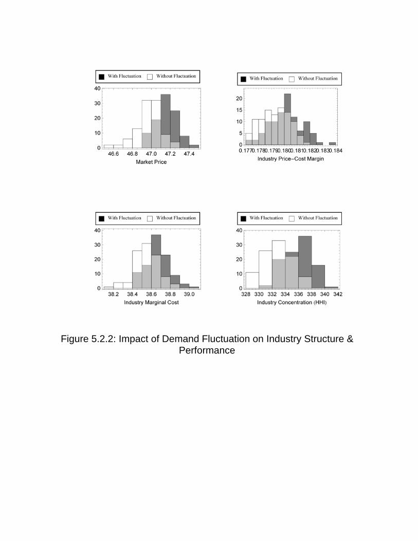
Figure 5.2.2: Impact of Demand Fluctuation on Industry Structure & Performance

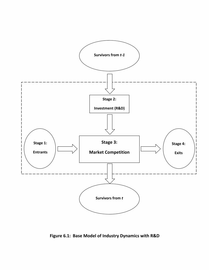
Figure 6.1: Base Model of Industry Dynamics with R&D

Stage 3:

Market Competition

Survivors from t-1

Survivors from t

Stage 1:

Entrants

Stage 4:

Exits

Stage 2:

Investment (R&D)

Documents

Computational Industrial Economics - Engaged Learning · model presented here enables the analysis of interactive dynamics between firms as they compete in a changing ... industry